Investigation of Potential Spudcan Punch-Through Failure on ...
233
Investigation of Potential Spudcan Punch-Through Failure on Sand Overlying Clay Soils By Kok Kuen LEE BEng. This thesis is presented for the degree of Doctor of Philosophy at School of Civil and Resource Engineering Centre for Offshore Foundation Systems April 2009
-
Upload
khangminh22 -
Category
Documents
-
view
4 -
download
0
Transcript of Investigation of Potential Spudcan Punch-Through Failure on ...
Investigation of Potential Spudcan Punch-Through
Failure on Sand Overlying Clay Soils
By
Kok Kuen LEE
BEng.
This thesis is presented for
the degree of Doctor of Philosophy at
School of Civil and Resource Engineering
Centre for Offshore Foundation Systems
April 2009


i
DECLARATION I hereby declare that, except where specific reference is made to the work of others, the contents of this dissertation are original and have not been submitted in whole or in part for consideration for any other degree of qualification at this, or any other, university.
Kok Kuen Lee
April 2009
ii
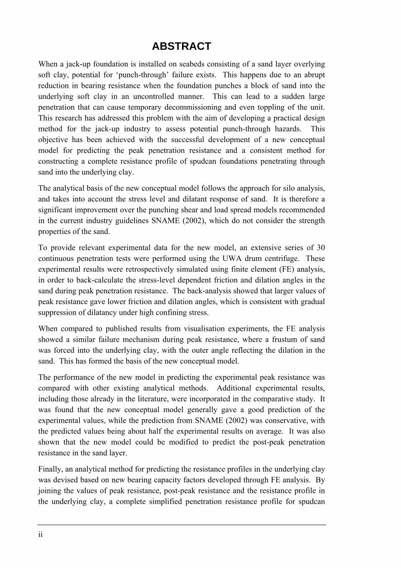
ABSTRACT When a jack-up foundation is installed on seabeds consisting of a sand layer overlying soft clay, potential for ‘punch-through’ failure exists. This happens due to an abrupt reduction in bearing resistance when the foundation punches a block of sand into the underlying soft clay in an uncontrolled manner. This can lead to a sudden large penetration that can cause temporary decommissioning and even toppling of the unit. This research has addressed this problem with the aim of developing a practical design method for the jack-up industry to assess potential punch-through hazards. This objective has been achieved with the successful development of a new conceptual model for predicting the peak penetration resistance and a consistent method for constructing a complete resistance profile of spudcan foundations penetrating through sand into the underlying clay.
The analytical basis of the new conceptual model follows the approach for silo analysis, and takes into account the stress level and dilatant response of sand. It is therefore a significant improvement over the punching shear and load spread models recommended in the current industry guidelines SNAME (2002), which do not consider the strength properties of the sand.
To provide relevant experimental data for the new model, an extensive series of 30 continuous penetration tests were performed using the UWA drum centrifuge. These experimental results were retrospectively simulated using finite element (FE) analysis, in order to back-calculate the stress-level dependent friction and dilation angles in the sand during peak penetration resistance. The back-analysis showed that larger values of peak resistance gave lower friction and dilation angles, which is consistent with gradual suppression of dilatancy under high confining stress.
When compared to published results from visualisation experiments, the FE analysis showed a similar failure mechanism during peak resistance, where a frustum of sand was forced into the underlying clay, with the outer angle reflecting the dilation in the sand. This has formed the basis of the new conceptual model.
The performance of the new model in predicting the experimental peak resistance was compared with other existing analytical methods. Additional experimental results, including those already in the literature, were incorporated in the comparative study. It was found that the new conceptual model generally gave a good prediction of the experimental values, while the prediction from SNAME (2002) was conservative, with the predicted values being about half the experimental results on average. It was also shown that the new model could be modified to predict the post-peak penetration resistance in the sand layer.
Finally, an analytical method for predicting the resistance profiles in the underlying clay was devised based on new bearing capacity factors developed through FE analysis. By joining the values of peak resistance, post-peak resistance and the resistance profile in the underlying clay, a complete simplified penetration resistance profile for spudcan

iii
foundations in sand overlying clay can be generated. The predicted profiles were shown to match the experimental results well.
iv
ACKNOWLEDGEMENTS First and foremost I would like to express my heartfelt gratitude to my supervisors Professor Mark Randolph and Professor Mark Cassidy for their generous guidance. I can recall that when I first started, I was excited but could not help feeling intimidated by their reputation and achievements (MFR – 43rd Rankine Lecturer, MJC – one of the youngest professors and later Physical Scientist of the Year 2007). However, now I realise that my experience with the ‘Mark and Mark’ team was truly a pleasant, inspiring and incredible one. It was pleasant because of their friendly and encouraging attitudes – while they were always able to point out what I had overlooked and corrected my mistakes, they never failed to say ‘well done!’ to keep me going. It was inspiring because of their prompt, in-depth and enlightening replies to my enquiries and doubts, and it was incredible because, despite their busy schedules, I have never had any difficulty to meet them when I needed to.
Secondly, the accomplishment of the centrifuge tests must be credited to Dr Christophe Gaudin, the Centrifuge Manager who arranged for my tests, and his highly efficient centrifuge team: Tuarn Brown, Phil Hortin, Dave Jones, Bart Thompson and Don Herley, who collectively ensured I obtained high quality test data with the shortest possible learning curve. The constructive discussions from Professor Dave White during the tests were also greatly appreciated.
The financial support provided by the ARC Linkage grant (Project LP0561838), University Postgraduate Award and Ad Hoc Scholarships is gratefully acknowledged. I am also grateful for the administrative assistance given by Monica, Lisa, Ivan, Jane, Simone, Inga, Stephanie, Michelle, John, Sharon and the highly capable IT Manager Wenge.
Thanks also to my companions Han Eng, Edmond, An Jui, Hugo, Xiangtao, James, Britta, Marc, Matt, Hisham, Azrul, Jonathan, Shinji, Hongjie, Nick, Nathalie, Gima, Vickie, Fauzan, Long and visitors Kar Lu and Cheng Ti. Without you, this place would not be as enjoyable as it has been. Many other individuals, more than this small page can contain, have brought me much needed encouragement and support. Thank you for making this an excellent place and time for my research.
I would also like to extend my appreciation to Dr S.S.Gue, Y.C.Tan, S.S.Liew and my former colleagues in G&P Geotechnics Sdn. Bhd., for the early guidance and working experience in geotechnical engineering, which inspired me to pursue this research.
Finally, my family, to whom this thesis is dedicated. I am indebted to my parents for their perpetual care, and am also grateful to my sisters and parents-in-law who are ever encouraging. To my wife, Ai Ling, I cannot thank you enough for your unconditional love and support. The arrival of baby Vincent added several sleepless nights, but also brought along bundles of joy and happiness to our family. This fuelled me with much motivation and encouragement. For your love, I am truly overwhelmed with gratitude.
v
CONTENTS Declaration....................................................................................................................... i Abstract........................................................................................................................... ii Acknowledgements........................................................................................................ iv Contents ...........................................................................................................................v Notation............................................................................................................................x Abbreviations .............................................................................................................. xiv Chapter 1. Introduction..................................................................................................1
1.1 Preface................................................................................................................1 1.2 Jack-up unit ........................................................................................................1
1.2.1 The foundations of jack-up units ..........................................................3 1.2.2 Set-up procedures of a jack-up unit ......................................................3
1.3 Punch-through on sand overlying clay...............................................................5 1.3.1 Current best-practice.............................................................................7 1.3.2 Significance of punch-through failures ................................................7
1.4 Motivation of the research .................................................................................8 1.5 Orientation and structure of the thesis ...............................................................9
Chapter 2. Literature review .......................................................................................11 2.1 Introduction......................................................................................................11 2.2 Vertical bearing capacity in homogeneous soil ...............................................11
2.2.1 General................................................................................................11 2.3 Bearing capacity factors...................................................................................13
2.3.1 Bearing capacity factor Nq for strip foundation..................................13 2.3.2 Bearing capacity factor Nc ..................................................................13 2.3.3 Bearing capacity factor Nγ ..................................................................13 2.3.4 Shape factors and depth factors ..........................................................15
2.4 Discussion of the classical bearing capacity equation .....................................18 2.4.1 Non-linearity of friction angle ............................................................18 2.4.2 Dilation angle in classical bearing capacity theory ............................19 2.4.3 Foundation size effect.........................................................................20 2.4.4 Effect of increasing strength with depth for cohesive soils ................21
2.5 Bearing capacity on sand overlying clay soils .................................................22 2.5.1 Projected area method.........................................................................22 2.5.2 Punching shear method.......................................................................24 2.5.3 The method of Okamura et al. (1998) ................................................27 2.5.4 The method of Teh (2007) ..................................................................29

vi
2.6 Numerical analysis for foundation on sand overlying clay .............................32 2.6.1 Limiting sand thickness ......................................................................33 2.6.2 Effect of undrained shear strength of the underlying clay..................34 2.6.3 Effect of foundation roughness...........................................................34 2.6.4 Effect from upper sand layer ..............................................................34
2.7 Current design guidelines ................................................................................35 2.8 Concluding remarks .........................................................................................35
Chapter 3. Experimental apparatus and procedures ................................................37 3.1 Introduction......................................................................................................37 3.2 Centrifuge modelling principles ......................................................................37 3.3 Drum centrifuge facilities at UWA..................................................................38 3.4 Model spudcans and flat-based foundations ....................................................40 3.5 Miniature ball penetrometers made of epoxy ..................................................44
3.5.1 Mechanical behaviour of epoxy Araldite Kit K138 ...........................46 3.5.2 Fabrication of ball penetrometers .......................................................50 3.5.3 Calibration of the miniature ball.........................................................53 3.5.4 Working range of the miniature ball penetrometer.............................54
3.6 Engineeing properties of sand and clay ...........................................................55 3.6.1 Superfine silica sand...........................................................................55 3.6.2 Kaolin clay..........................................................................................56
3.7 Preparation of soil sample................................................................................57 3.7.1 Preparing the lower clay layer ............................................................57 3.7.2 Preparing the upper sand layer ...........................................................58
3.8 Testing programme ..........................................................................................59 3.8.1 Testing layout .....................................................................................62 3.8.2 Testing sequence.................................................................................64 3.8.3 Penetration rate ...................................................................................64 3.8.4 Displacement versus load control mode.............................................66
Chapter 4. Experimental results..................................................................................67 4.1 Introduction......................................................................................................67 4.2 Soil sample examination after test ...................................................................67
4.2.1 Soil profiles after ball and cone penetration tests...............................68 4.2.2 Trapped sand under model spudcan ...................................................70
4.3 Typical flat-based and spudcan foundation penetration profile.......................72 4.4 Experimental results of peak penetration resistance ........................................77 4.5 Miniature ball penetrometer penetration profile ..............................................80 4.6 Characterisation of upper sand layer................................................................84
vii
4.6.1 Measuring sand thickness ...................................................................84 4.6.2 Measuring relative density of the upper sand layer ............................85
4.7 Undrained shear strength profile of the underlying clay..................................86 4.7.1 Background on undrained shear strength profile................................86 4.7.2 Background on field measurement of undrained shear strength ........87 4.7.3 Undrained shear strength profile of the drum centrifuge tests............88
4.8 Concluding remarks .........................................................................................90 Chapter 5. Numerical analysis of bearing capacity on sand overlying clay soils....91
5.1 Introduction......................................................................................................91 5.2 Procedures for modelling of centrifuge tests ...................................................92
5.2.1 General................................................................................................92 5.2.2 Soil models for sand and clay.............................................................93 5.2.3 Boundary conditions...........................................................................94 5.2.4 Finite element mesh size.....................................................................94
5.3 Verification of finite element model ................................................................95 5.3.1 Flat-based foundation on Tresca model (uniform clay) .....................95 5.3.2 Flat-based foundation on Mohr-Coulomb model (homogeneous sand)
............................................................................................................96 5.4 Finite element modelling of the experimental results ......................................99
5.4.1 Typical load-settlement curve and failure load from FE analyses....100 5.4.2 Determining the friction angle and dilation angle in the FE model .102 5.4.3 Examining the failure mechanism from FE results ..........................106 5.4.4 A comparison of FE results with experimentally observed mechanisms
(using PIV)........................................................................................107 5.5 Concluding remarks .......................................................................................108
Chapter 6. Simplified conceptual model for bearing capacity on sand overlying clay soils .......................................................................................................................110
6.1 Introduction....................................................................................................110 6.2 New conceptual model...................................................................................110
6.2.1 General..............................................................................................110 6.2.2 Kinematically admissible failure mechanism...................................110 6.2.3 Bearing capacity of the underlying clay ...........................................112 6.2.4 Analytical treatment of the new conceptual model ..........................113 6.2.5 Normal and shear stresses at slip surfaces ........................................114 6.2.6 Vertical effective stress at slip surfaces............................................116 6.2.7 Vertical force equilibrium on an infinitesimal element ....................117 6.2.8 Integration of vertical force equilibrium equation............................118

viii
6.2.9 Equation for the case of zero dilation angle .....................................119 6.3 Determining strength parameters of sand in the new equation......................120 6.4 Examining various aspects of the new conceptual model .............................121
6.4.1 When sand thickness equals zero .....................................................121 6.4.2 When friction angle equals dilation angle (associated flow rule
material)............................................................................................121 6.5 Back-analysis with experimental results........................................................123
6.5.1 Fitting the distribution factor ............................................................123 6.5.2 Discussion on the back-calculated distribution factor ......................127
6.6 Input parameters for the new equation...........................................................130 6.7 Parametric studies of the new conceptual model ...........................................132
6.7.1 Effects of relative density of sand ....................................................133 6.7.2 Operative friction angle and dilation angle ......................................136 6.7.3 Effects of sand thickness (Hs/D ratio) ..............................................137 6.7.4 Effects of foundation diameter .........................................................139 6.7.5 Effects of bearing capacity of the underlying clay ...........................140
6.8 Limitation of the new conceptual model .......................................................142 6.9 Concluding remarks .......................................................................................143
Chapter 7. Comparison of analytical methods for bearing capacity on sand overlying clay soils ......................................................................................................144
7.1 Introduction....................................................................................................144 7.2 Database.........................................................................................................144 7.3 Analytical methods ........................................................................................147 7.4 Comparison of analytical methods.................................................................148
7.4.1 Punching shear method.....................................................................152 7.4.2 Projected area method ......................................................................153 7.4.3 Okamura et al. (1998) .......................................................................153 7.4.4 Teh (2007) ........................................................................................155 7.4.5 SNAME (2002).................................................................................158 7.4.6 New conceptual method ...................................................................159
7.5 Concluding remarks .......................................................................................161 Chapter 8. Predicting penetration profile on sand overlying clay soils .................164
8.1 Introduction....................................................................................................164 8.2 Predicting penetration resistance profile below the sand-clay interface........164
8.2.1 Finite element model for cylindrical foundation in clay ..................164 8.2.2 Notation for a cylindrical foundation in non-homogenous clay.......167
ix
8.2.3 Cylindrical foundation in non-homogenous clay: Deep failure mechanism ........................................................................................169
8.2.4 Cylindrical foundation in non-homogenous clay: Shallow failure mechanism ........................................................................................177
8.2.5 Predicting penetration resistance profile in the underlying clay involving both shallow and deep failure mechanisms ......................182
8.2.6 Estimating the height of trapped sand ..............................................184 8.3 Predicting the peak penetration resistance .....................................................185 8.4 Predicting the post-peak penetration resistance .............................................186 8.5 Constructing a simplified predicted penetration resistance profile................189 8.6 Comparison of predicted and measured penetration resistance profiles........190 8.7 Concluding remarks .......................................................................................198
Chapter 9. Conclusions and further research ..........................................................199 9.1 Introduction....................................................................................................199 9.2 Conclusions – Main findings .........................................................................199
9.2.1 Development of a new conceptual model for predicting the peak penetration resistance........................................................................199
9.2.2 Predicting a complete penetration profile.........................................202 9.3 Further research..............................................................................................203
9.3.1 Centrifuge tests for refining the empirical distribution factor (DF) ..203 9.3.2 Centrifuge tests using loose sands and compressible sands .............203 9.3.3 Large deformation numerical analyses for foundations on sand
overlying clay ...................................................................................204 9.3.4 Generalisation to foundations founded on multi-layered soils .........205
References ....................................................................................................................206

x
NOTATION Roman
A........... Area of foundation A, A' ..... Constants of the new conceptual model B........... Width of strip foundation c............ Cohesion cv........... Coefficient of consolidation D........... Diameter DF ......... Distribution factor d............ Embedded depth of foundation d50 ......... Mean particle size dc .......... Depth factor for bearing capacity factor Nc
dγ........... Depth factor for bearing capacity factor Nγ dq .......... Depth factor for bearing capacity factor Nq dpeak....... Foundation depth at peak penetration resistance dpost-peak . Foundation depth at post peak penetration resistance E ........... Young’s modulus E, E0 ..... Parameters in the new conceptual model emax ....... Maximum void ratio emin........ Minimum void ratio G........... Shear modulus Gs.......... Specific gravity Hs.......... Thickness of sand layer Hfdn ....... Height of foundation H*......... Critical thickness for upper sand layer where bearing resistance becomes
independent of the strength of the underlying clay when it is exceeded. h............ Embedment depth of foundation ID .......... Relative density IP........... Plasticity index IR .......... Relative dilatancy index Kp ......... Rankine passive earth pressure coefficient Ks.......... Coefficient of punching shear for strip foundation L ........... Length of strip foundation M .......... Critical state frictional constant m .......... Strength increase exponent N........... Resistance factor Nball....... Resistance factor for ball penetrometer NT-bar..... Resistance factor for T-bar penetrometer Nc.......... Bearing capacity factor due to cohesion Nc0 ........ Resistance factor (due to cohesion) at base level of a circular foundation Nγ.......... Bearing capacity factor due to self-weight
xi
Nq ......... Bearing capacity factor due to surcharge p' ........... Mean effective stress Q........... Natural logarithm of the grain crushing strength (in kPa) Q........... Vertical penetration force Qpeak...... Peak penetration force q............ Vertical penetration resistance q0 .......... Effective surcharge at foundation base level qb .......... Bearing resistance of the underlying clay qball........ Ball penetration resistance qclay ....... Bearing capacity of clay qpeak....... Peak penetration resistance (average over entire foundation) qpost-peak....Post-peak penetration resistance (average over entire foundation) qsand....... Bearing capacity of sand qT-bar...... T-bar penetration resistance qu .......... Undrained penetration resistance qult ......... Ultimate penetration resistance R, r........ Radius r ............ Radial coordinate s ............ Undrained strength ratio for normally consolidated clay sc ........... Shape factor for bearing capacity factor Nc sγ ........... Shape factor for bearing capacity factor Nγ sq........... Shape factor for bearing capacity factor Nq ss ........... Shape factor for punching shear coefficient Ks
su........... Undrained shear strength su0 ......... Undrained shear strength at the foundation base level sum......... Undrained shear strength at mudline (or at sand-clay interface for sand
overlying clay soils) V........... Normalised penetration rate (= vD/cv) v............ Penetration velocity z ............ Vertical coordinate (with downward direction as positive) Greek
α ........... Interface friction ratio α ........... Angle of dispersion or projection αa .......... Geometrical parameter representing the extent of mobilisation of clay bearing
capacity in the Method of Teh αc .......... Calculated projection angle in the Method of Okamura δ............ Average mobilised friction angle on the assumed vertical slip plane in the
punching shear method φ' ........... Friction angle φ2 .......... Mobilised friction angle in the Method of Teh

xii
φcv...............Critical state friction angle φ*.......... Reduced friction angle due to non-associative flow rule γ ............ Bulk unit weight γm.......... Material factor in ISO 19901-4 (2003) γ' ........... Effective unit weight γ'c .......... Effective unit weight of clay γ's .......... Effective unit weight of sand κ ........... Dimensionless strength increasing parameter for non-homogeneous cohesive
soils κ ........... Slope of swelling line λ ........... Slope of normal consolidation line λc .......... Normalised bearing capacity of underlying clay in the method of Okamura λp .......... Normalised overburden pressure in the method of Okamura ν............ Poisson's ratio θ............ Skew angle ρ ........... Gradient of linear increment of undrained shear strength with depth σ ........... Standard deviation σmc ........ Mean effective normal stress of clay element just beneath the sand layer in the
method of Okamura σ' .......... Effective stress σ'1 ......... Major principal effective stress σ'3 ......... Minor principal effective stress σ'n ......... Normal effective stress σ'v ......... Vertical effective stress σ'v0........ Effective overburden stress
zσ ........ Mean vertical effective stress (σ'r)slip ... Radial effective stress at slip surface (σ'z)slip... Vertical effective stress at slip surface τ ............ Shear stress ψ ........... Dilation angle ψ ........... Geometrical parameter representing the inclination (to the vertical) of slip
surface in the method of Teh Superscripts
' ............. Effective stress quantity Subscripts
0............ Related to the foundation base level b............ Related to bottom layer ball........ Value related to or measured using ball penetrometer

xiii
c ............ Clay h............ Horizontal n............ Normal s ............ Sand T-bar..... Value related to or measured using T-bar penetrometer u............ Undrained ult ......... Ultimate v............ Vertical

xiv
ABBREVIATIONS 2D........... Two dimensional COV ....... Coefficient of variation CPT ........ Cone penetration test FE........... Finite element LL........... Liquid limit NUS........ National University of Singapore OCR ....... Overconsolidation ratio PIV ......... Particle image velocimetry PL........... Plastic limit RITSS..... Remeshing and Interpolation Technique with Small Strain SFS......... Super fine silica sand SNAME.. The Society of Naval Architects and Marine Engineers UWA ...... The University of Western Australia
Chapter 1: Introduction
1
CHAPTER 1. INTRODUCTION
1.1 PREFACE
Exploration and development of offshore oil and gas fields have extended down continental slopes to water depths of 2000 m or more. However, there is still considerable activity, with development of smaller fields, on the continental shelves in water depths less than 200 m. The majority of offshore operations in water depths up to 120 m are performed from self-elevating mobile units, which are generally referred to as ‘jack-up’ rigs. This is mainly due to their proven flexibility and cost-effectiveness in field development and drilling operation in the offshore industry.
This research was undertaken to study the performance of the foundations of jack-up rigs founded on sand overlying clay soils. Particular attention is given to predicting the maximum bearing resistance for sand overlying clay during installation and to developing a consistent analytical framework to predict the complete resistance profile when the foundation penetrates through the sand into the clay. The research comprised physical modelling of the foundations, supporting numerical analysis and the development of a new conceptual model for practising engineers. A comparison with other data and methods in the literature is also provided.
1.2 JACK-UP UNIT
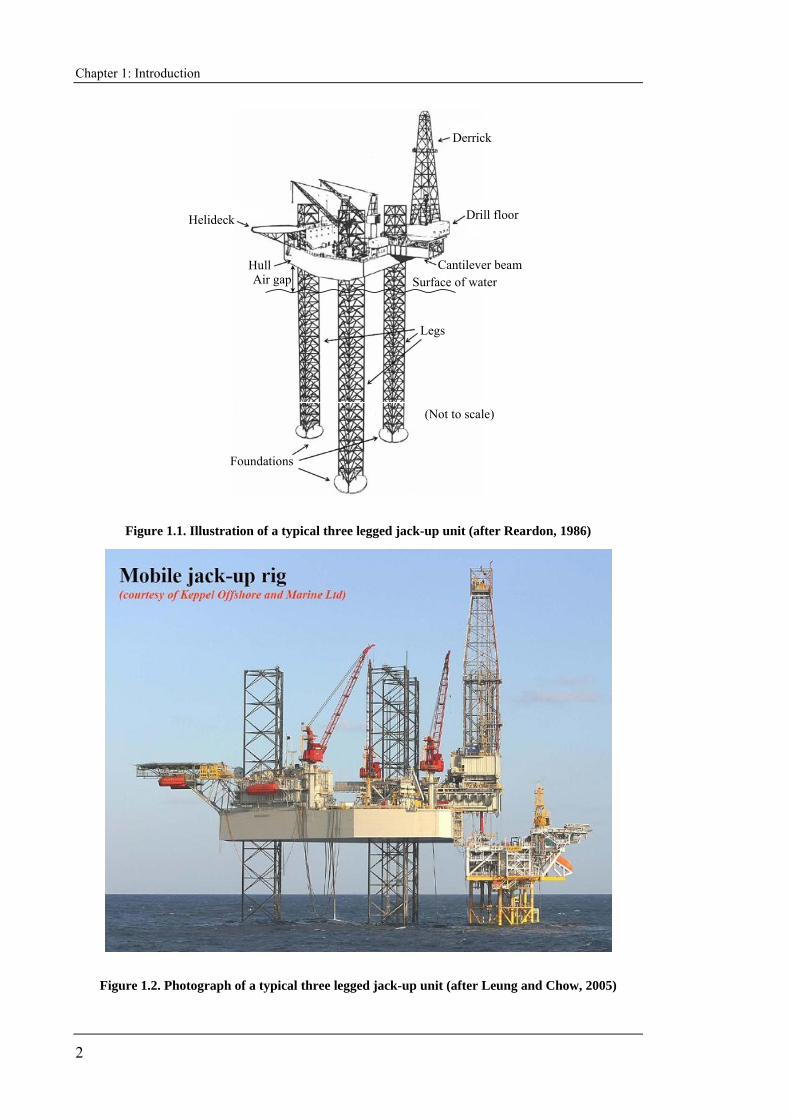
An illustration and a photograph of a typical jack-up unit are shown in Figure 1.1 and Figure 1.2 respectively. A modern jack-up unit usually consists of a triangular platform resting on three independent truss-work legs. Each leg is fitted with a rack and pinion system used to jack the legs up and down through the deck during installation, and to lift the jack-up platform clear of the water during operation.
The cost of a new jack-up unit today exceeds $200 million (Maksoud and Harding, 2007). The water depth capability of jack-ups is increasing following the trend of offshore operations moving into deeper seas. Most new jack-ups are rated for 107 m – 122 m water depth, though some have been rated higher to work in water depths up to 152 m (Maksoud and Harding, 2007).
Chapter 1: Introduction
2
Helideck
Derrick
Drill floor
Cantilever beam
Legs
Foundations
HullAir gap Surface of water
(Not to scale)
Figure 1.1. Illustration of a typical three legged jack-up unit (after Reardon, 1986)
Figure 1.2. Photograph of a typical three legged jack-up unit (after Leung and Chow, 2005)
Chapter 1: Introduction
3
1.2.1 The foundations of jack-up units
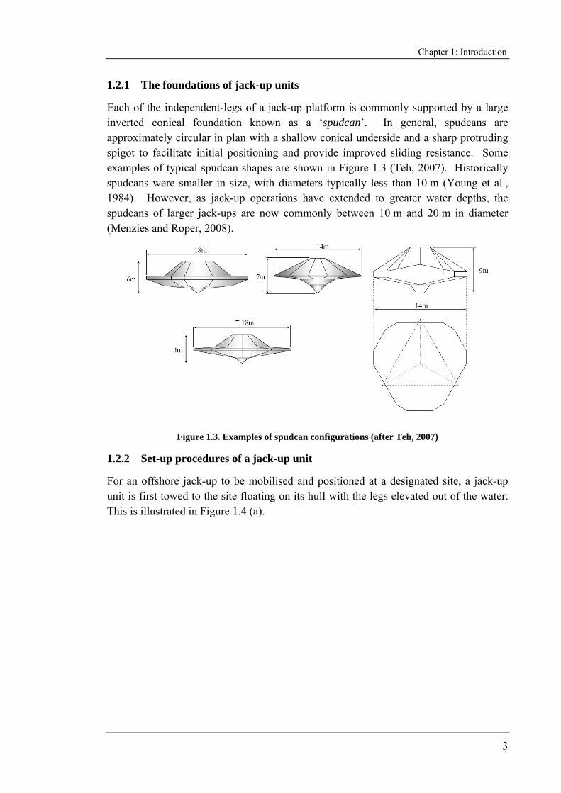
Each of the independent-legs of a jack-up platform is commonly supported by a large inverted conical foundation known as a ‘spudcan’. In general, spudcans are approximately circular in plan with a shallow conical underside and a sharp protruding spigot to facilitate initial positioning and provide improved sliding resistance. Some examples of typical spudcan shapes are shown in Figure 1.3 (Teh, 2007). Historically spudcans were smaller in size, with diameters typically less than 10 m (Young et al., 1984). However, as jack-up operations have extended to greater water depths, the spudcans of larger jack-ups are now commonly between 10 m and 20 m in diameter (Menzies and Roper, 2008).
Figure 1.3. Examples of spudcan configurations (after Teh, 2007)
1.2.2 Set-up procedures of a jack-up unit
For an offshore jack-up to be mobilised and positioned at a designated site, a jack-up unit is first towed to the site floating on its hull with the legs elevated out of the water. This is illustrated in Figure 1.4 (a).
Chapter 1: Introduction
4
Towing to location Preloading Operation (e.g. drilling)
a b c
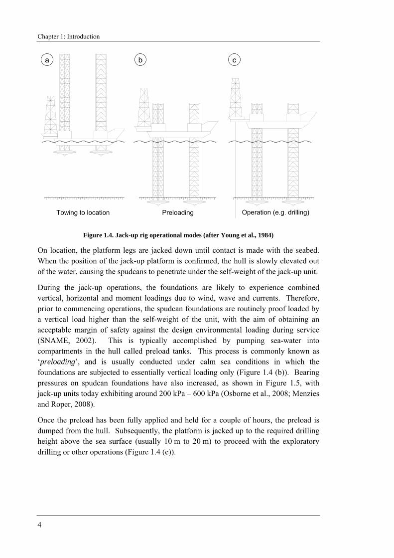
Figure 1.4. Jack-up rig operational modes (after Young et al., 1984)
On location, the platform legs are jacked down until contact is made with the seabed. When the position of the jack-up platform is confirmed, the hull is slowly elevated out of the water, causing the spudcans to penetrate under the self-weight of the jack-up unit.
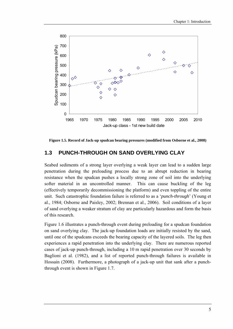
During the jack-up operations, the foundations are likely to experience combined vertical, horizontal and moment loadings due to wind, wave and currents. Therefore, prior to commencing operations, the spudcan foundations are routinely proof loaded by a vertical load higher than the self-weight of the unit, with the aim of obtaining an acceptable margin of safety against the design environmental loading during service (SNAME, 2002). This is typically accomplished by pumping sea-water into compartments in the hull called preload tanks. This process is commonly known as ‘preloading’, and is usually conducted under calm sea conditions in which the foundations are subjected to essentially vertical loading only (Figure 1.4 (b)). Bearing pressures on spudcan foundations have also increased, as shown in Figure 1.5, with jack-up units today exhibiting around 200 kPa – 600 kPa (Osborne et al., 2008; Menzies and Roper, 2008).
Once the preload has been fully applied and held for a couple of hours, the preload is dumped from the hull. Subsequently, the platform is jacked up to the required drilling height above the sea surface (usually 10 m to 20 m) to proceed with the exploratory drilling or other operations (Figure 1.4 (c)).
Chapter 1: Introduction
5
0
100
200
300
400
500
600
700
800
1965 1970 1975 1980 1985 1990 1995 2000 2005 2010Jack-up class - 1st new build date
Spu
dcan
bea
ring
pres
sure
(kP
a)_
Figure 1.5. Record of Jack-up spudcan bearing pressures (modified from Osborne et al., 2008)
1.3 PUNCH-THROUGH ON SAND OVERLYING CLAY
Seabed sediments of a strong layer overlying a weak layer can lead to a sudden large penetration during the preloading process due to an abrupt reduction in bearing resistance when the spudcan pushes a locally strong zone of soil into the underlying softer material in an uncontrolled manner. This can cause buckling of the leg (effectively temporarily decommissioning the platform) and even toppling of the entire unit. Such catastrophic foundation failure is referred to as a ‘punch-through’ (Young et al., 1984; Osborne and Paisley, 2002; Brennan et al., 2006). Soil conditions of a layer of sand overlying a weaker stratum of clay are particularly hazardous and form the basis of this research.
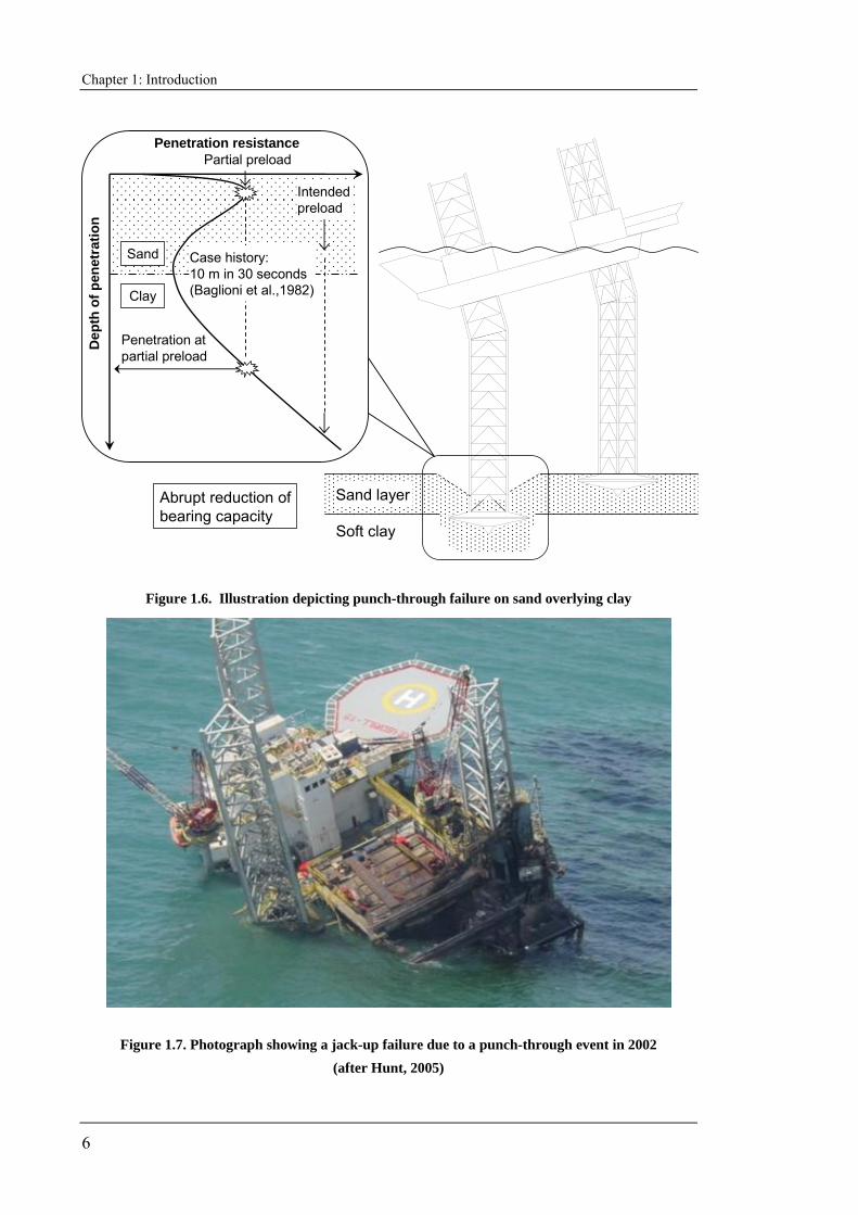
Figure 1.6 illustrates a punch-through event during preloading for a spudcan foundation on sand overlying clay. The jack-up foundation loads are initially resisted by the sand, until one of the spudcans exceeds the bearing capacity of the layered soils. The leg then experiences a rapid penetration into the underlying clay. There are numerous reported cases of jack-up punch-through, including a 10 m rapid penetration over 30 seconds by Baglioni et al. (1982), and a list of reported punch-through failures is available in Hossain (2008). Furthermore, a photograph of a jack-up unit that sank after a punch-through event is shown in Figure 1.7.
Chapter 1: Introduction
6
Abrupt reduction of bearing capacity
Sand layer
Soft clay
Penetration at partial preload
Dep
th o
f pen
etra
tion
Intended preload
Sand
Clay
Case history:10 m in 30 seconds (Baglioni et al.,1982)
Partial preloadPenetration resistance
Figure 1.6. Illustration depicting punch-through failure on sand overlying clay
Figure 1.7. Photograph showing a jack-up failure due to a punch-through event in 2002 (after Hunt, 2005)

Chapter 1: Introduction
7
1.3.1 Current best-practice
Before a jack-up can operate at a given site, an assessment of its ability to be installed and preloaded safely must be performed. ‘Guidelines for the Site Specific Assessment of Mobile Jack-Up Units’ (SNAME, 2002) and a complementary ‘Commentaries’ to the guidelines have been published for this purpose.
The SNAME (2002) guidelines recommend the mechanism developed by Hanna and Meyerhof (1980) for calculating the bearing capacity of foundations on sand overlying clay. For a flat foundation at one particular depth (i.e. wished in place), failure is assumed to be a mechanism of a truncated cone in the upper sand layer being depressed into the underlying clay. However, for calculation purposes, a simpler cylindrical shear surface is used. Visualization experiments reported by Teh (2007) demonstrate that this is a deviation from reality. The ‘projected area’ method is a suggested alternative in the commentaries to SNAME (2002). Here the load is assumed to spread through the upper sand layer to an imaginary foundation of increased size at the sand-clay interface. The assumed angle of spread is critical to this calculation. The commentaries to SNAME (2002) suggests a conservative spread of 1h:5v (horizontal to vertical), although it recognises that higher spread angles were back calculated from actual spudcan penetration data (for example Baglioni et al., 1982). This supports a widely held belief within the jack-up industry that the method under-predicts load capacity and therefore provides an un-conservative assessment of potential punch-through.
The major drawback of the SNAME (2002) guidelines and commentaries is that both recommended calculation procedures do not involve the strength properties of the upper sand layer. This is illogical. It has exacerbated errors and uncertainty in calculating punch-through pressure and therefore accurately predicting the potential for punch-through failure before a jack-up rig goes to site.
1.3.2 Significance of punch-through failures
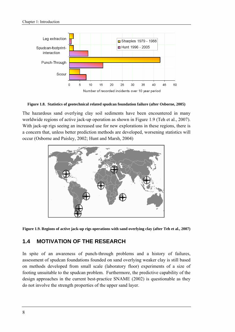
Punch-through failures continue to be a major problem during installation of jack-up platforms, as indicated by the accident statistics shown in Figure 1.8 (Osborne, 2005). Although there has been a reduction in the most recent decade (as reported by Hunt (2005)), there is still one or more failures per year on average.
Osborne and Paisley (2002) reported that rig damage and loss of drilling time resulting from punch-through hazards are typically costing the industry between US$1 million to US$10 million per incident. With these considerations, the loss or temporary lack of serviceability of a rig has major financial implications.
Chapter 1: Introduction
8
Figure 1.8. Statistics of geotechnical related spudcan foundation failure (after Osborne, 2005)
The hazardous sand overlying clay soil sediments have been encountered in many worldwide regions of active jack-up operation as shown in Figure 1.9 (Teh et al., 2007). With jack-up rigs seeing an increased use for new explorations in these regions, there is a concern that, unless better prediction methods are developed, worsening statistics will occur (Osborne and Paisley, 2002; Hunt and Marsh, 2004)
Figure 1.9. Regions of active jack-up rigs operations with sand overlying clay (after Teh et al., 2007)
1.4 MOTIVATION OF THE RESEARCH
In spite of an awareness of punch-through problems and a history of failures, assessment of spudcan foundations founded on sand overlying weaker clay is still based on methods developed from small scale (laboratory floor) experiments of a size of footing unsuitable to the spudcan problem. Furthermore, the predictive capability of the design approaches in the current best-practice SNAME (2002) is questionable as they do not involve the strength properties of the upper sand layer.

Chapter 1: Introduction
9
As the offshore oil and gas industry continues to expand, it is important to ensure safe and economic use of jack-up units. This research was therefore undertaken, with the aim of seeking an improved understanding of the penetration of spudcan foundations in sand overlying clay. Since common engineering design is generally undertaken through simple conceptual models, the ultimate objective is to establish a rational and realistic framework for the jack-up industry to predict spudcan punch-through failure.
1.5 ORIENTATION AND STRUCTURE OF THE THESIS
A new conceptual model based on a rational analytical framework is required to improve the prediction of a potential punch-through before a jack-up unit is installed. In particular, the strength of the sand layer must be incorporated in the conceptual model. The new conceptual model should be calibrated against either field data or an extensive series of centrifuge model tests under stress conditions equivalent in magnitude to those at prototype scale. In addition, finite element modelling should be performed to ensure consistency and eliminate compensating errors within the model. With these considerations, the proposed new model should enable a safer assessment of jack-up units bearing on sand overlying clay soils.
As most of the records for field installation are not available in the public domain (Osborne et al., 2008), centrifuge model tests are an invaluable alternative to produce continual penetration profiles under equivalent stress levels (Murff, 1996). An extensive series of centrifuge tests were carried out in this research to provide relevant experimental data for the new conceptual model.
To assess the failure mechanism, the experimental results were also simulated numerically using small deformation finite element analysis. The failure mechanisms were compared with the results of the visualisation experiments of Teh (2007).
Finally, the prediction capabilities of the new conceptual model were assessed against other experimental data and existing industry guidelines.
The outline of this thesis is listed below.
Chapter 2 initially reviews the methods for predicting the bearing capacity of vertically loaded foundations on single layer soil (sand and clay), before discussing the analytical methods and numerical analyses for predicting the vertical resistance of foundations penetrating sand overlying clay.
Chapter 3 explains the methodology of the centrifuge tests. The preparation of the soil samples is described and the details of the testing programme outlined. To undertake accurate characterisation of the centrifuge samples, miniature ball penetrometer made of epoxy were developed, and these are also discussed.
Chapter 4 reports the results from the centrifuge tests. These include qualitative examination of post-test soil samples and the measured penetration profiles of model
Chapter 1: Introduction
10
foundations and penetrometers. The experiments consisted of various geometrical configurations by using a series of foundations with different diameters penetrating through sand layers with different thicknesses.
Chapter 5 discusses the numerical simulation of the centrifuge tests using finite element (FE) analysis. The aim of the FE modelling was to back-calculate the stress-level dependent friction and dilation angles of the sand during peak penetration resistance. The failure mechanism from the FE analysis is examined and compared with published results of visualisation experiments.
Chapter 6 describes the development of a rational analytical framework to calculate the punch-through load. Importantly, the stress level and dilatant response of the upper sand layer has been taken into account. The calibration of the model using both the centrifuge and FE analysis results is described. A parametric study to evaluate the influence of the input parameters of the model is also presented.
Chapter 7 presents a comparative study of the new analytical model against other published methods, including the industry guidelines in SNAME (2002), in predicting the experimental peak penetration resistance in sand overlying clay soils. Using an experimental database larger than the tests described in Chapters 3 and 4, and including published data of Craig and Chua (1990) and Teh (2007), the predictive capabilities of all analytical methods are examined.
Chapter 8 describes the development of an analytical method to predict the penetration profiles in the underlying clay. A discussion on how to predict the post-peak penetration resistance in the sand layer by modifying the new conceptual model is also presented. By combining all of the analytical methods developed, a complete penetration profile of a circular foundation penetrating sand overlying clay soils can be constructed. The chapter concludes with a comparison between the predicted complete penetration profiles and the centrifuge test results.
Chapter 9 summarises the key conclusions from this research and provides recommendations for future study.
Chapter 2: Literature review
11
CHAPTER 2. LITERATURE REVIEW
2.1 INTRODUCTION
This chapter provides a brief review of methods for predicting the bearing capacity of vertically loaded foundations on single layer soil (sand and clay), as well as on sand overlying clay soils. Bearing capacity involving inclined and horizontal loads is excluded because it is not relevant for potential spudcan punch-through failure during preloading.
The first part of the chapter details the calculation of bearing capacity in single layer sand or clay using the classical bearing capacity approach of Terzaghi (1943). The validity of superposition implied by this approach is discussed, and the development of appropriate bearing capacity factors is summarised. The second part of the chapter presents the development of vertical bearing capacity of circular foundations on sand overlying clay. The discussions focus on the most commonly used prediction methods and on findings from numerical analyses. Finally, the methods from the current design guidelines in SNAME (2002) are presented and discussed.
2.2 VERTICAL BEARING CAPACITY IN HOMOGENEOUS SOIL
2.2.1 General
The bearing capacity of a vertically loaded, shallow strip foundation on a homogeneous soil is traditionally calculated using the conventional bearing capacity theory of Terzaghi (1943), which assumes that the soil is rigid-perfectly plastic with the strength characterised by a cohesion, c, a friction angle φ', and an effective unit weight, γ'1. Following Prandtl (1921), the failure mechanism consists of a rigid triangular wedge beneath the strip foundation, a radial shear zone and an emerging passive wedge, as shown in Figure 2.1.
1 Note that, since the application in this thesis is for offshore foundation, the effective unit weight is considered, rather than the total, or dry, unit weight.
Chapter 2: Literature review
12
Effective surcharge: q0
Foundation width: B
Strip Foundation
45° – φ'/2
Bearing capacity: qult
45° – φ'/2
Cohesion: cFriction angle: φ'Unit weight: γ'
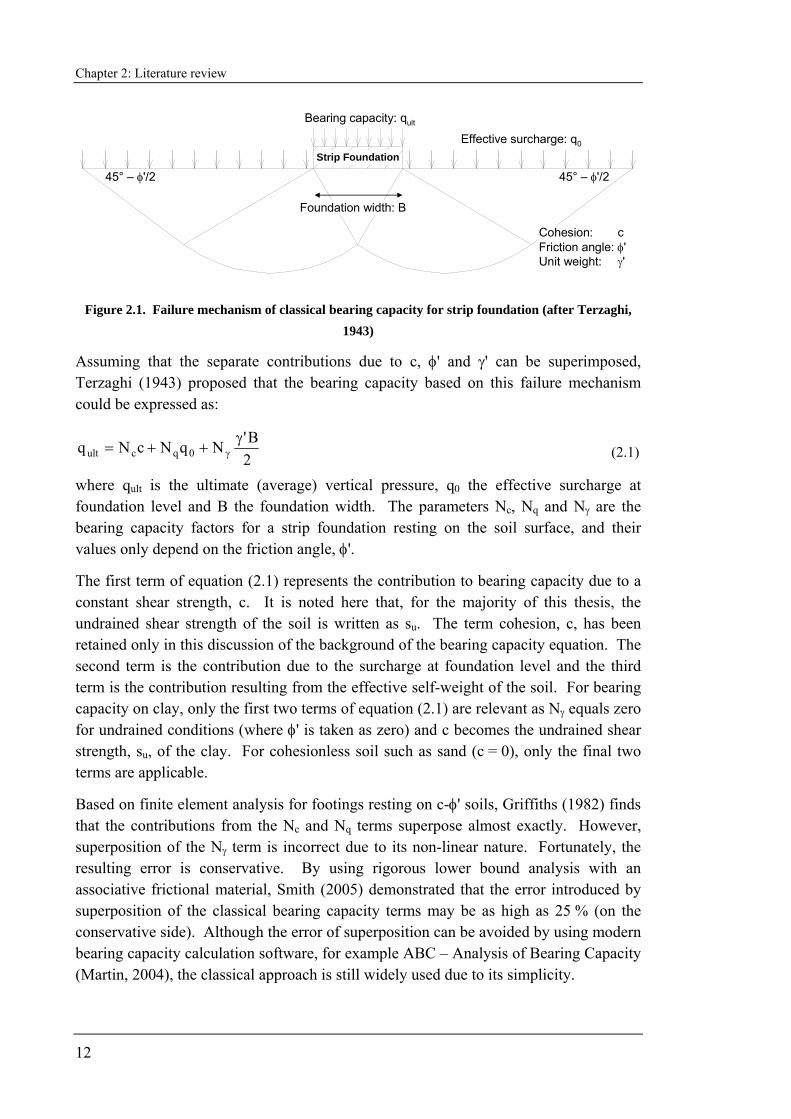
Figure 2.1. Failure mechanism of classical bearing capacity for strip foundation (after Terzaghi, 1943)
Assuming that the separate contributions due to c, φ' and γ' can be superimposed, Terzaghi (1943) proposed that the bearing capacity based on this failure mechanism could be expressed as:
2B'NqNcNq 0qcult
γ++= γ (2.1)
where qult is the ultimate (average) vertical pressure, q0 the effective surcharge at foundation level and B the foundation width. The parameters Nc, Nq and Nγ are the bearing capacity factors for a strip foundation resting on the soil surface, and their values only depend on the friction angle, φ'.
The first term of equation (2.1) represents the contribution to bearing capacity due to a constant shear strength, c. It is noted here that, for the majority of this thesis, the undrained shear strength of the soil is written as su. The term cohesion, c, has been retained only in this discussion of the background of the bearing capacity equation. The second term is the contribution due to the surcharge at foundation level and the third term is the contribution resulting from the effective self-weight of the soil. For bearing capacity on clay, only the first two terms of equation (2.1) are relevant as Nγ equals zero for undrained conditions (where φ' is taken as zero) and c becomes the undrained shear strength, su, of the clay. For cohesionless soil such as sand (c = 0), only the final two terms are applicable.
Based on finite element analysis for footings resting on c-φ' soils, Griffiths (1982) finds that the contributions from the Nc and Nq terms superpose almost exactly. However, superposition of the Nγ term is incorrect due to its non-linear nature. Fortunately, the resulting error is conservative. By using rigorous lower bound analysis with an associative frictional material, Smith (2005) demonstrated that the error introduced by superposition of the classical bearing capacity terms may be as high as 25 % (on the conservative side). Although the error of superposition can be avoided by using modern bearing capacity calculation software, for example ABC – Analysis of Bearing Capacity (Martin, 2004), the classical approach is still widely used due to its simplicity.
Chapter 2: Literature review
13
2.3 BEARING CAPACITY FACTORS
The bearing capacity factors in equation (2.1) are now briefly discussed. It should firstly be highlighted that the bearing capacity factors Nc, Nq and Nγ were originally derived only for surface foundations under plane strain conditions (strip foundations). For foundations with other shapes or embedded within the soil, multiplicative adjustment factors are required, which will be discussed in Section 2.3.4. Secondly, the soil is assumed to follow a linear Mohr-Coulomb yield envelope, where the strength can be characterised by a cohesion, c, and a friction angle, φ', independent of effective stress level. Thirdly, when referring to ‘exact plasticity solutions’ for the bearing capacity factors, there is an implicit assumption that the soil obeys an associated flow rule, where the dilation angle, ψ is equal to the friction angle, φ'. This is because the limit theorems in plasticity theory used to derive the exact solutions can only be proven true for associated materials (Chen, 1975).
2.3.1 Bearing capacity factor Nq for strip foundation
The bearing capacity factor Nq has been obtained by Reissner (1924) from the analysis of weightless soil. This factor was formally established as an exact plasticity solution by Shield (1954), and is expressed as:
⎟⎟⎠
⎞⎜⎜⎝
⎛φ−φ+
=⎟⎠⎞
⎜⎝⎛ φ
+π
= φπφπ
'sin1'sin1e
2'
4taneN tan2'tan
q (2.2)
2.3.2 Bearing capacity factor Nc
The exact theoretical solution for bearing capacity factor Nc was found by Prandtl (1921) using plasticity theory by considering a strip foundation resting on the surface of a weightless soil with constant undrained shear strength, su (or cohesion, c). The exact expression of the Nc factor is given as:
For φ' = 0: 14.52Nc ≈π+=
For a Mohr-Coulomb soil model with values of c and φ': ( ) 'cot1NN qc φ−= (2.3)
It has also been shown that neither bearing capacity factors Nq nor Nc are affected by the base roughness (Chen, 1975).
2.3.3 Bearing capacity factor Nγ
Unlike the factors Nq and Nc, an exact mathematical expression for the factor Nγ has not been found. This is because the varying in-situ effective stresses due to the self-weight of the soil need to be considered in order to evaluate Nγ. In this case, the rigour of the plasticity solution cannot be confirmed due to difficulties in extending the stress field outside the plastic zone (for lower bound solution) and ensuring that the slip mechanisms are kinematically admissible (for upper bound solution) (Frydman and
Chapter 2: Literature review
14
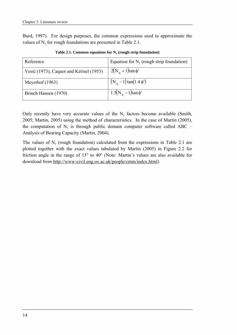
Burd, 1997). For design purposes, the common expressions used to approximate the values of Nγ for rough foundations are presented in Table 2.1.
Table 2.1. Common equations for Nγ (rough strip foundation)
Reference Equation for Nγ (rough strip foundation)
Vesić (1973), Caquot and Kérisel (1953) ( ) 'tan1N2 q φ+
Meyerhof (1963) ( ) ( )'4.1tan1Nq φ−
Brinch Hansen (1970) ( ) 'tan1N5.1 q φ−
Only recently have very accurate values of the Nγ factors become available (Smith, 2005; Martin, 2005) using the method of characteristics. In the case of Martin (2005), the computation of Nγ is through public domain computer software called ABC – Analysis of Bearing Capacity (Martin, 2004).
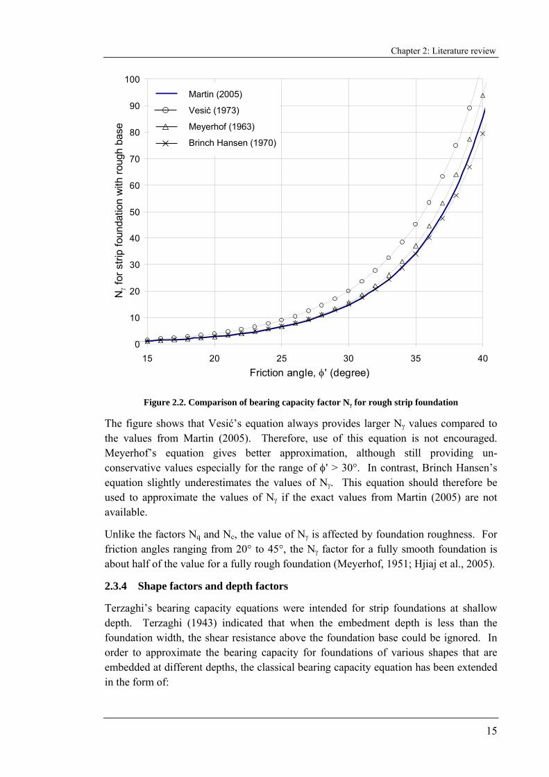
The values of Nγ (rough foundation) calculated from the expressions in Table 2.1 are plotted together with the exact values tabulated by Martin (2005) in Figure 2.2 for friction angle in the range of 15° to 40° (Note: Martin’s values are also available for download from http://www-civil.eng.ox.ac.uk/people/cmm/index.html).
Chapter 2: Literature review
15
0
10
20
30
40
50
60
70
80
90
100
15 20 25 30 35 40Friction angle, φ' (degree)
Nγ f
or s
trip
foun
datio
n w
ith ro
ugh
base
Martin (2005)
Vesić (1973)
Meyerhof (1963)
Brinch Hansen (1970)
Martin (2005)
Vesić (1973)
Meyerhof (1963)
Brinch Hansen (1970)
Figure 2.2. Comparison of bearing capacity factor Nγ for rough strip foundation
The figure shows that Vesić’s equation always provides larger Nγ values compared to the values from Martin (2005). Therefore, use of this equation is not encouraged. Meyerhof’s equation gives better approximation, although still providing un-conservative values especially for the range of φ' > 30°. In contrast, Brinch Hansen’s equation slightly underestimates the values of Nγ. This equation should therefore be used to approximate the values of Nγ if the exact values from Martin (2005) are not available.
Unlike the factors Nq and Nc, the value of Nγ is affected by foundation roughness. For friction angles ranging from 20° to 45°, the Nγ factor for a fully smooth foundation is about half of the value for a fully rough foundation (Meyerhof, 1951; Hjiaj et al., 2005).
2.3.4 Shape factors and depth factors
Terzaghi’s bearing capacity equations were intended for strip foundations at shallow depth. Terzaghi (1943) indicated that when the embedment depth is less than the foundation width, the shear resistance above the foundation base could be ignored. In order to approximate the bearing capacity for foundations of various shapes that are embedded at different depths, the classical bearing capacity equation has been extended in the form of:
Chapter 2: Literature review
16
( ) ( ) ( )2B'NsdqNsdcNsdq 0qqqcccult
γ++= γγγ (2.4)
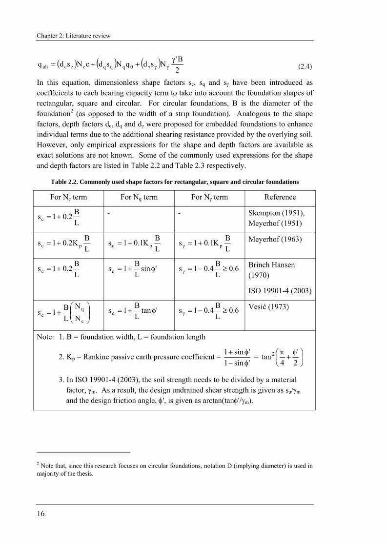
In this equation, dimensionless shape factors sc, sq and sγ have been introduced as coefficients to each bearing capacity term to take into account the foundation shapes of rectangular, square and circular. For circular foundations, B is the diameter of the foundation2 (as opposed to the width of a strip foundation). Analogous to the shape factors, depth factors dc, dq and dγ were proposed for embedded foundations to enhance individual terms due to the additional shearing resistance provided by the overlying soil. However, only empirical expressions for the shape and depth factors are available as exact solutions are not known. Some of the commonly used expressions for the shape and depth factors are listed in Table 2.2 and Table 2.3 respectively.
Table 2.2. Commonly used shape factors for rectangular, square and circular foundations
For Nc term For Nq term For Nγ term Reference
LB2.01sc +=
- - Skempton (1951),
Meyerhof (1951)
LBK2.01s pc +=
LBK1.01s pq +=
LBK1.01s p+=γ Meyerhof (1963)
LB2.01sc +=
'sin
LB1sq φ+= 6.0
LB4.01s ≥−=γ Brinch Hansen
(1970)
ISO 19901-4 (2003)
⎟⎟⎠
⎞⎜⎜⎝
⎛+=
c
qc N
NLB1s 'tan
LB1sq φ+= 6.0
LB4.01s ≥−=γ Vesić (1973)
Note: 1. B = foundation width, L = foundation length
2. Kp = Rankine passive earth pressure coefficient = 'sin1'sin1
φ−φ+ = ⎟
⎠⎞
⎜⎝⎛ φ
+π
2'
4tan 2
3. In ISO 19901-4 (2003), the soil strength needs to be divided by a material factor, γm. As a result, the design undrained shear strength is given as su/γm and the design friction angle, φ', is given as arctan(tanφ'/γm).
2 Note that, since this research focuses on circular foundations, notation D (implying diameter) is used in majority of the thesis.

Chapter 2: Literature review
17
Table 2.3. Commonly used depth factors for embedded foundations
For Nc term For Nq term For Nγ term Reference
BhK2.01d pc += For φ' = 0° : 1dq =
For φ' >10° :
BhK1.01d pq +=
For φ' = 0° : 1d =γ
For φ' >10° :
BhK1.01d p+=γ
Meyerhof (1963)
For 1Bh
≤ :
Bh4.01dc +=
For 1Bh
> :
Bhtan4.01d 1
c−+= ,
where tan-1(h/B) in radian
For 1Bh
≤ : += 1dq
Bh)'sin1('tan2 2φ−φ
For 1Bh
> : += 1dq
Bhtan)'sin1('tan2 12 −φ−φ ,
where tan-1(h/B) in radian
For all φ' : 1d =γ Brinch Hansen (1970) and Vesić (1973)
Bhtan3.01d 1
c−+= ,
where tan-1(h/B) in radian
+= 1dq
Bh)'sin1('tan2.1 2φ−φ
1d =γ ISO 19901-4 (2003)
Note: 1. B = foundation width, h = Depth of foundation embedment
2. Kp = Rankine passive earth pressure coefficient = 'sin1'sin1
φ−φ+ = ⎟
⎠⎞
⎜⎝⎛ φ
+π
2'
4tan 2
3. The expressions for dc and dq given by Brinch Hansen (1970) and Vesić (1973) produce a discontinuity at h/B =1
4. Since the Nγ term reflects the contribution to bearing resistance below the foundation level, the value of dγ = 1 indicates that the effects of the slip mechanism extending above the base are fully captured by the depth factor dq.
Randolph et al. (2004) highlighted that no simple relationship exists for shape factors. Furthermore, it is found that the depth factors and the shape factors are not independent, as is assumed in the classical bearing capacity formula (Salgado et al., 2004; Lyamin et

Chapter 2: Literature review
18
al., 2007). In view of this, the practice of applying shape factors and depth factors should be discouraged.
Instead, rigorous solutions that consider directly both geometry and embedment of a foundation should be used for any foundation engineering design. Exact solutions for a circular foundation for undrained conditions (c = su, φ' taken as zero) weightless soil (Tresca material) have been obtained as shown in Table 2.4. Unlike strip foundations, it is shown that the Nc factor for circular foundations is affected by the base roughness. Following Shield (1955), Cox et al. (1961) obtained a complete solution for the bearing capacity of a smooth circular foundation on c-φ' weightless soil and listed the values of Nc corresponding to friction angles φ' from 0° to 40° at 5° intervals.
Table 2.4. Bearing capacity factors for circular foundations on purely cohesive weightless soil
Bearing capacity factor for circular foundations Reference
Nc = 5.69 (smooth base) Shield (1955)
Nc = 6.05 (rough base) Eason and Shield (1960)
With the advancement of modern computing power, direct bearing capacity factors from rigorous numerical solutions are now available for many more cases. Using modern software such as Martin (2004), closely exact bearing capacity values can be calculated for foundations with various shapes and embedment depths. Some direct bearing capacity factors for circular, square and rectangular foundations embedded at different depths within an associated material (φ' = ψ) are also given in Randolph et al. (2004), Salgado et al. (2004) and Lyamin et al. (2007).
2.4 DISCUSSION OF THE CLASSICAL BEARING CAPACITY EQUATION
The classical bearing capacity equation is the most widely used method for predicting the ultimate vertical load of a shallow foundation. However, several factors that are relevant to spudcan foundation have significant effect on its accuracy. These factors are now briefly discussed.
2.4.1 Non-linearity of friction angle
As presented in Section 2.3, the bearing capacity factors are functions of friction angle, φ', which is commonly assumed as constant. In reality, however, the friction angle is affected by several factors as listed in Table 2.5.
Chapter 2: Literature review
19
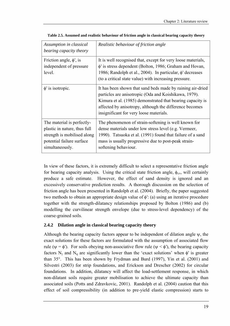
Table 2.5. Assumed and realistic behaviour of friction angle in classical bearing capacity theory
Assumption in classical bearing capacity theory
Realistic behaviour of friction angle
Friction angle, φ', is independent of pressure level.
It is well recognised that, except for very loose materials, φ' is stress dependent (Bolton, 1986; Graham and Hovan, 1986; Randolph et al., 2004). In particular, φ' decreases (to a critical state value) with increasing pressure.
φ' is isotropic. It has been shown that sand beds made by raining air-dried particles are anisotropic (Oda and Koishikawa, 1979). Kimura et al. (1985) demonstrated that bearing capacity is affected by anisotropy, although the difference becomes insignificant for very loose materials.
The material is perfectly-plastic in nature, thus full strength is mobilised along potential failure surface simultaneously.
The phenomenon of strain-softening is well known for dense materials under low stress level (e.g. Vermeer, 1990). Tatsuoka et al. (1991) found that failure of a sand mass is usually progressive due to post-peak strain-softening behaviour.
In view of these factors, it is extremely difficult to select a representative friction angle for bearing capacity analysis. Using the critical state friction angle, φcv, will certainly produce a safe estimate. However, the effect of sand density is ignored and an excessively conservative prediction results. A thorough discussion on the selection of friction angle has been presented in Randolph et al. (2004). Briefly, the paper suggested two methods to obtain an appropriate design value of φ': (a) using an iterative procedure together with the strength-dilatancy relationships proposed by Bolton (1986) and (b) modelling the curvilinear strength envelope (due to stress-level dependency) of the coarse-grained soils.
2.4.2 Dilation angle in classical bearing capacity theory
Although the bearing capacity factors appear to be independent of dilation angle ψ, the exact solutions for these factors are formulated with the assumption of associated flow rule (ψ = φ'). For soils obeying non-associative flow rule (ψ < φ'), the bearing capacity factors Nγ and Nq are significantly lower than the ‘exact solutions’ when φ' is greater than 35°. This has been shown by Frydman and Burd (1997), Yin et al. (2001) and Silvestri (2003) for strip foundations, and Erickson and Drescher (2002) for circular foundations. In addition, dilatancy will affect the load-settlement response, in which non-dilatant soils require greater mobilisation to achieve the ultimate capacity than associated soils (Potts and Zdravkovic, 2001). Randolph et al. (2004) caution that this effect of soil compressibility (in addition to pre-yield elastic compression) starts to

Chapter 2: Literature review
20
dominate for high friction angles, and the exact bearing capacity factors for friction angles in excess of 35° are unlikely to be achievable in practice.
The associated flow rule is a pre-requisite for rigorous limit analysis since both upper bound and lower bound theorems can only be proven true for materials obeying normality (Chen, 1975). However, it has been suggested that these methods can also be extended to include non-associated materials (ψ < φ') if the analysis is carried out as usual but with a reduced friction angle, φ*, defined as (Davis, 1968; Drescher and Detournay, 1993; Michalowski, 1997):
ψφ−ψφ
=φsin'sin1
cos'sin*tan (2.5)
Consideration of equation (2.5) shows that the reduced friction angle, φ* is less than or equal to the initial friction angle φ'. As a result, the actual bearing capacity for sand is always lower than the value calculated using the exact bearing capacity factors. This is because actual sand is a non-associated material with ψ < φ' (Bolton, 1986).
2.4.3 Foundation size effect
The bearing capacity factors are given as functions of friction angle only and are independent of foundation width. In reality, however, the bearing capacity factor Nγ calculated from footing tests on sand is found to reduce with increasing footing size (de Beer, 1963; Kimura et al., 1985; Ueno et al., 1998). It has been explained that the dependence of Nγ on foundation width is largely attributed to the stress-level dependency of friction angle, φ' (Hettler and Gudehus, 1988; Ueno et al., 2001; Zhu et al., 2001).
To investigate the size effect numerically, linear elastic-perfectly plastic soil models, including the widely used Mohr-Coulomb model, cannot be used. Instead, more sophisticated constitutive soil models that can simulate the pressure dependence of φ' must be adopted to determine the changes of Nγ with foundation width (Woodward and Griffiths, 1998). Although the size effects on Nγ are well known, there is no established analytical method to quantify them (Cerato, 2005).
More recently, Yamamoto et al. (2009) performed finite-element analysis to study the effect of foundation size on the response of shallow circular foundations on siliceous and calcareous sands using the MIT-S1 constitutive model (Pestana and Whittle, 1999). This model simulates many facets of real sands including both compression and shear responses. The numerical simulations predicted a smaller Nγ being mobilised as the foundation size increases, consistent with the trends observed in experiments (de Beer, 1963, amongst others).
The numerical study also showed that the compression component of the sand dominates the bearing response as the foundation diameter increases to be more than a certain ‘critical size’. For siliceous sands, this critical size may be range from 20 m to

Chapter 2: Literature review
21
60 m depending on the soil density, but for the more compressible calcareous sands, the critical size of the foundation is estimated to be about 1 m. While the conventional bearing capacity analyses may be applicable to foundations less than the critical size, alternative approaches focusing mainly on the soil compressibility may be required for larger foundations. Yamamoto et al. (2008) propose two semi-analytical formulae for this purpose.
2.4.4 Effect of increasing strength with depth for cohesive soils
Clays often exhibit undrained shear strength profiles that increase with depth. This is particularly important for large foundations such as offshore spudcans. To incorporate this into a calculation procedure, the soil strength is usually taken to vary linearly with depth as shown in Figure 2.3. The strength profile can then be expressed as:
zss umu ρ+= (2.6)
where sum is the undrained shear strength at ground surface (subscript m stands for the mudline or seabed surface in this case), z the depth below surface, and ρ the rate of linear increase of strength with depth.
ρ1
hsum su0 su
z
B or D
Figure 2.3. Linear strength profile (after Randolph et al., 2004)
It is convenient to define the strength at the level of the foundation as su0 = sum + ρh, as shown in Figure 2.3, where h is the depth of the foundation base from the surface. The vertical bearing capacity is then expressed in terms of this strength and a corresponding dimensionless bearing capacity factor, Nc0, as:
0u0cult sNq = (2.7)
The factor Nc0 is a function of tip angle (for conical foundations), base roughness, depth of embedment and a dimensionless rate of increase of strength with depth, κ, which is expressed as (Houlsby and Martin, 2003):
umsDρ
=κ (2.8)
Accurate solutions for soil where the strength varies linearly with depth are available for surface strip and circular foundations (Davis and Booker, 1973; Martin, 2001) and for embedded circular foundations (Houlsby and Martin, 2003). Again, there is no unique
Chapter 2: Literature review
22
relationship for the shape factor, but it has been shown that the shape factor generally decreases as the strength gradient increases (Houlsby and Wroth, 1983, Randolph et al., 2004). A thorough discussion on the development of bearing capacity for clays with strength that increases linearly with depth is given in Randolph et al. (2004).
2.5 BEARING CAPACITY ON SAND OVERLYING CLAY SOILS
While the conventional Terzaghi bearing capacity theory works well for homogeneous soils, it cannot, in general, be used for layered soils. Traditionally, the bearing capacity for sand overlying clay soils has been calculated using simplified conceptual models developed specifically for this purpose. These conceptual models usually assume an imaginary sand block in the shape of a column or a frustum being pushed into the underlying clay. The bearing capacity of the layered soils is obtained from the force equilibrium of the block. Each conceptual model predicts different values of bearing capacity depending on the assumptions adopted during the occurrence of the peak penetration resistance. In general, the determining factors are the shape of the imaginary sand block (usually represented by the projection angle of the block) and the stresses assumed to act on it.
Among others, the projected area method and the punching shear method are the most commonly used methods to calculate the peak penetration resistance on sand overlying clay. Both methods are adopted in the current best-practice for offshore spudcan punch-through hazards (SNAME, 2002). The following sections briefly introduce both models, together with other more recently developed conceptual models for the bearing capacity of foundations on sand overlying clay soils.
2.5.1 Projected area method
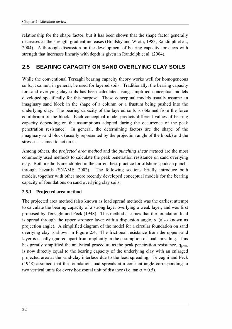
The projected area method (also known as load spread method) was the earliest attempt to calculate the bearing capacity of a strong layer overlying a weak layer, and was first proposed by Terzaghi and Peck (1948). This method assumes that the foundation load is spread through the upper stronger layer with a dispersion angle, α (also known as projection angle). A simplified diagram of the model for a circular foundation on sand overlying clay is shown in Figure 2.4. The frictional resistance from the upper sand layer is usually ignored apart from implicitly in the assumption of load spreading. This has greatly simplified the analytical procedure as the peak penetration resistance, qpeak, is now directly equal to the bearing capacity of the underlying clay with an enlarged projected area at the sand-clay interface due to the load spreading. Terzaghi and Peck (1948) assumed that the foundation load spreads at a constant angle corresponding to two vertical units for every horizontal unit of distance (i.e. tan α = 0.5).
Chapter 2: Literature review
23
Sand: φ', γ's
Clay: su
αHs
scNcsu + q0
q0
Qpeak = qpeak(πD2/4)
D
α
Figure 2.4. Projected area method for circular foundations
Taking the force equilibrium of the imaginary load spreading mechanism shown in Figure 2.4, the peak penetration resistance, qpeak, for a circular foundation can be expressed as:
( )0ucc
2s
peak qsNstanDH
21q +⎟⎠
⎞⎜⎝
⎛ α+= (2.9)
where Hs is the sand thickness, D the foundation diameter, α the projection angle, sc and Nc the shape factor and bearing capacity factor for the cohesion term respectively, su the undrained shear strength of the underlying clay and q0 the effective surcharge.
It is obvious that the angle of projection, α, is crucial in this method. However, there is no consensus on the appropriate value of α. Table 2.6 lists some angles of projection proposed by various researchers (after Craig and Chua, 1990).

Chapter 2: Literature review
24
Table 2.6. Angles of projection advocated by various researchers (after Craig and Chua, 1990)
Reference Angle of projection, α
Terzaghi and Peck (1948) ( )21tan 1−
Yamaguchi (1963) ( )21tan 1− . Note: the frictional resistance between the sand and the passive wedge from the Prandtl mechanism in the clay is taken into account.
Jacobsen et al. (1977)
⎥⎥⎦
⎤
⎢⎢⎣
⎡⎟⎟⎠
⎞⎜⎜⎝
⎛+−
clay
sand1
0344.01125.021tan where qsand and qclay
are the bearing capacities in the two separate layers.
Myslivec and Kysela (1978) (after Kézdi, 1964)
α = 30° when the depth below the foundation base is within a distance equals foundation diameter. Below this depth, the projection line changes to α = 45° until the sand-clay interface.
Young & Focht (1981) ( )31tan 1−
Baglioni et al. (1982) φ'
Dutt and Ingram (1984) ( )21tan 1−
Das & Dallo (1984) φ'
Chiba et al. (1986) ( )31tan30 1−≡°
Tomlinson (1986) 30° or ( )21tan 1−
The range of recommendations may not be too surprising because the projected area method has over-simplified the actual failure mechanism by ignoring the frictional resistance in the sand layer. In addition, the centrifuge tests from Okamura et al. (1997) show that α is not a constant but is affected by the geometry and strength conditions of the layered soils. By using just one predefined angle of projection, the effects of various geometry and strength combinations cannot be accounted for.
2.5.2 Punching shear method
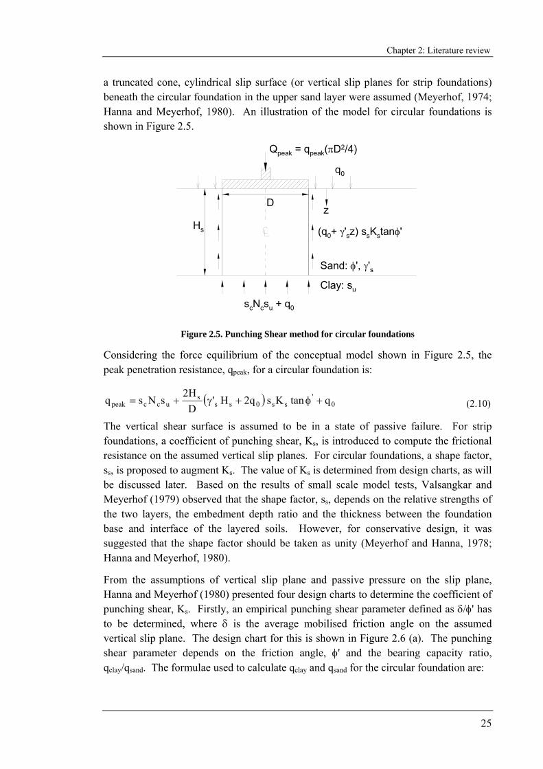
The punching shear method is based on Hanna and Meyerhof (1980), and continues to be advocated, for example by Kraft and Helfrich (1983) and in the SNAME (2002) guidelines. Unlike the projected area method, the frictional resistance of the slip surface is taken into account in the calculation of the bearing capacity for sand overlying clay soils. Although it has been well recognised that the imaginary sand block approximates
Chapter 2: Literature review
25
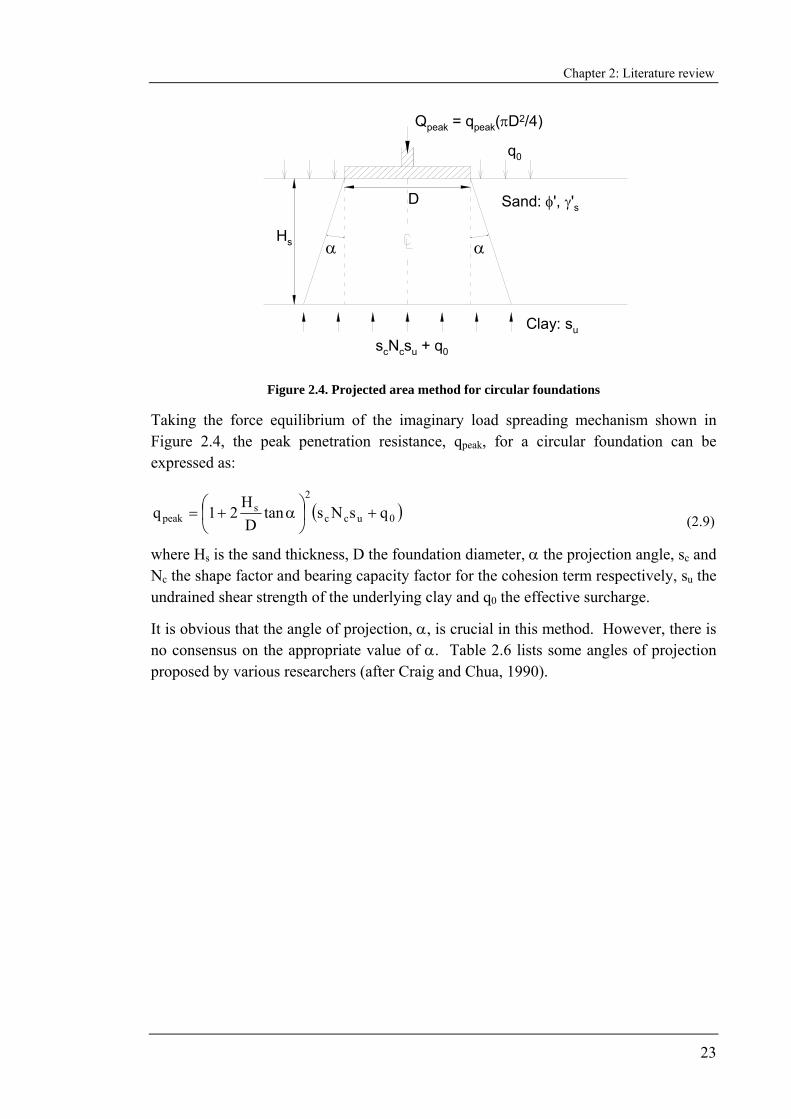
a truncated cone, cylindrical slip surface (or vertical slip planes for strip foundations) beneath the circular foundation in the upper sand layer were assumed (Meyerhof, 1974; Hanna and Meyerhof, 1980). An illustration of the model for circular foundations is shown in Figure 2.5.
(q0+ γ'sz) ssKstanφ'
z
Sand: φ', γ'sClay: su
Hs
scNcsu + q0
q0
D
Qpeak = qpeak(πD2/4)
Figure 2.5. Punching Shear method for circular foundations
Considering the force equilibrium of the conceptual model shown in Figure 2.5, the peak penetration resistance, qpeak, for a circular foundation is:
( ) 0'
ss0sss
uccpeak qtanKsq2H'DH2
sNsq +φ+γ+= (2.10)
The vertical shear surface is assumed to be in a state of passive failure. For strip foundations, a coefficient of punching shear, Ks, is introduced to compute the frictional resistance on the assumed vertical slip planes. For circular foundations, a shape factor, ss, is proposed to augment Ks. The value of Ks is determined from design charts, as will be discussed later. Based on the results of small scale model tests, Valsangkar and Meyerhof (1979) observed that the shape factor, ss, depends on the relative strengths of the two layers, the embedment depth ratio and the thickness between the foundation base and interface of the layered soils. However, for conservative design, it was suggested that the shape factor should be taken as unity (Meyerhof and Hanna, 1978; Hanna and Meyerhof, 1980).
From the assumptions of vertical slip plane and passive pressure on the slip plane, Hanna and Meyerhof (1980) presented four design charts to determine the coefficient of punching shear, Ks. Firstly, an empirical punching shear parameter defined as δ/φ' has to be determined, where δ is the average mobilised friction angle on the assumed vertical slip plane. The design chart for this is shown in Figure 2.6 (a). The punching shear parameter depends on the friction angle, φ' and the bearing capacity ratio, qclay/qsand. The formulae used to calculate qclay and qsand for the circular foundation are:
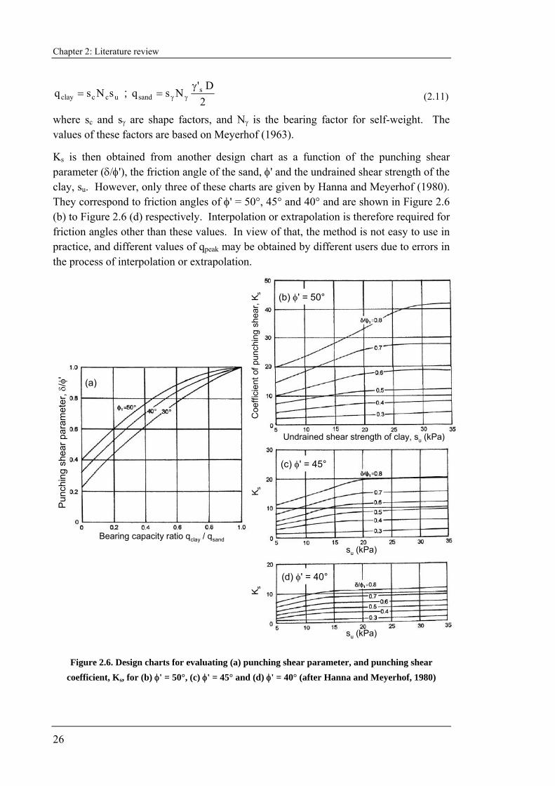
Chapter 2: Literature review
26
uccclay sNsq = ; 2D'
Nsq ssand
γ= γγ (2.11)
where sc and sγ are shape factors, and Nγ is the bearing factor for self-weight. The values of these factors are based on Meyerhof (1963).
Ks is then obtained from another design chart as a function of the punching shear parameter (δ/φ'), the friction angle of the sand, φ' and the undrained shear strength of the clay, su. However, only three of these charts are given by Hanna and Meyerhof (1980). They correspond to friction angles of φ' = 50°, 45° and 40° and are shown in Figure 2.6 (b) to Figure 2.6 (d) respectively. Interpolation or extrapolation is therefore required for friction angles other than these values. In view of that, the method is not easy to use in practice, and different values of qpeak may be obtained by different users due to errors in the process of interpolation or extrapolation.
Pun
chin
g sh
ear p
aram
eter
, δ/φ
'
Coe
ffici
ent o
f pun
chin
g sh
ear,
K s
su (kPa)
Undrained shear strength of clay, su (kPa)
Bearing capacity ratio qclay / qsand
K sK s
su (kPa)
(b) φ' = 50°
(c) φ' = 45°
(d) φ' = 40°
(a)
Figure 2.6. Design charts for evaluating (a) punching shear parameter, and punching shear coefficient, Ks, for (b) φ' = 50°, (c) φ' = 45° and (d) φ' = 40° (after Hanna and Meyerhof, 1980)

Chapter 2: Literature review
27
The centrifuge test results from Okamura et al. (1998) showed that the Hanna and Meyerhof (1980) method gave conservative prediction for foundations without embedment. However, for embedded foundations, overestimation became noticeable as the embedment depth increased. They attributed this to the inappropriate assumption of the horizontal stress acting on the assumed vertical slip surfaces. This suggests that a realistic value of the horizontal stress, which is difficult to determined either experimentally or analytically, is crucial for this method.
2.5.3 The method of Okamura et al. (1998)
Okamura et al. (1988) proposed a new limit equilibrium method with a failure mechanism that combines the concept of the projected area method and the punching shear method (Hanna and Meyerhof, 1980). The simplified diagram for this model is shown in Figure 2.7 (a).
To incorporate the influence of stress level on friction angle, Okamura et al. (1998) suggested adopting an operative friction angle that depends on the initial stress level of the sand layer. The horizontal stress on the slip surface is assumed to correspond to the passive failure state. The mean effective stress at the mid-depth of the conceptual sand frustum, p', is chosen to represent the appropriate stress level, and is expressed as:
⎥⎦
⎤⎢⎣
⎡⎟⎠⎞
⎜⎝⎛ γ
++⎟⎠⎞
⎜⎝⎛ γ
+= pss
0ss
0 K2H'
q2H'
q21'p ( )( )pss0 K1H'q2
41
+γ+=
where Kp = Rankine passive earth pressure coefficient 'sin1'sin1
φ−φ+
= (2.12)
The operative friction angle is then obtained through an iterative procedure with Bolton's (1986) empirical relationships since Kp is also a function of φ'.
Using this approach, however, the stress-level dependency of friction angle cannot be totally accounted for. This is mainly because the effects from the foundation size and the undrained strength of the underlying clay are not incorporated. As discussed in Section 2.4.3, the stress level, and consequently the operative friction angle, is affected by the foundation size. In a similar manner, higher undrained shear strengths cause a larger confining stress and therefore a lower φ'. Furthermore, when peak penetration resistance occurs, it is unclear that the slip surface is at a passive failure state as assumed in the calculation of p'.
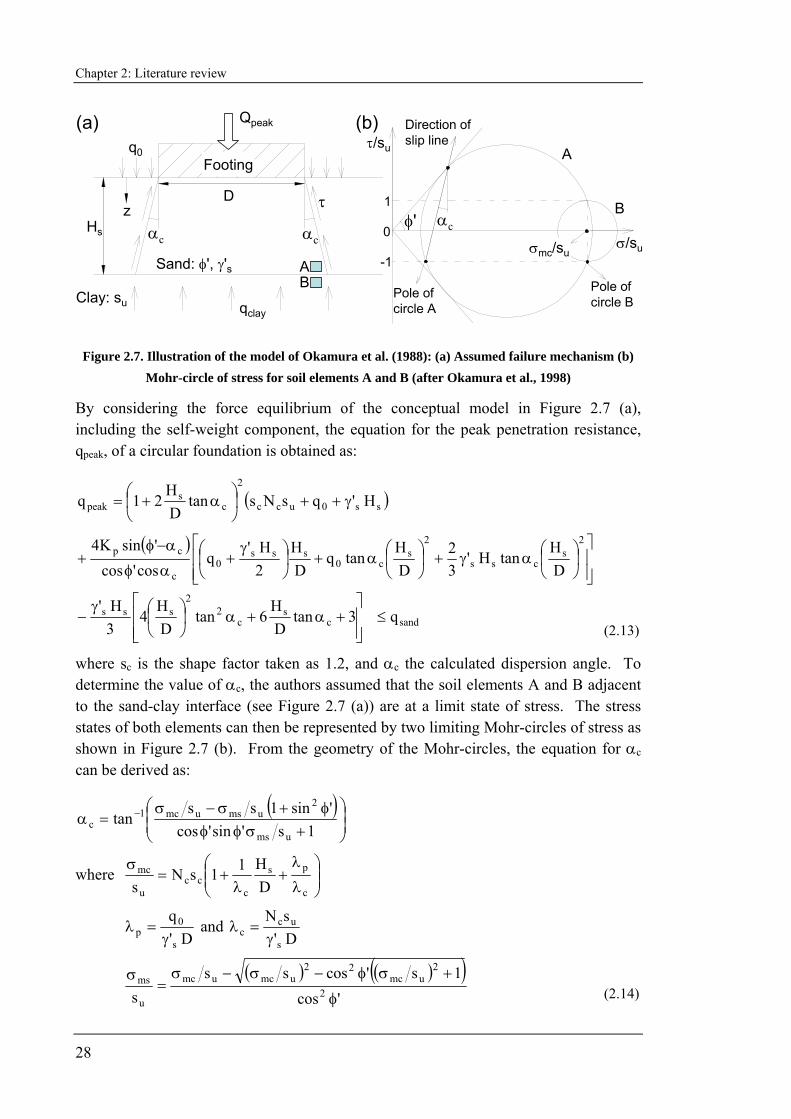
Chapter 2: Literature review
28
qclay
D
BA
q0Footing
Hs
z τ
Sand: φ', γ's
Clay: su
αcαcφ'
σ/su
τ/su
Pole of circle A
Pole of circle B
A
B
Direction of slip line
σmc/su
0
-1
1
(a) (b)
αc
Qpeak
Figure 2.7. Illustration of the model of Okamura et al. (1988): (a) Assumed failure mechanism (b) Mohr-circle of stress for soil elements A and B (after Okamura et al., 1998)
By considering the force equilibrium of the conceptual model in Figure 2.7 (a), including the self-weight component, the equation for the peak penetration resistance, qpeak, of a circular foundation is obtained as:
( )ss0ucc
2
cs
peak H'qsNstanDH
21q γ++⎟⎠
⎞⎜⎝
⎛ α+=
( )⎥⎥⎦
⎤
⎢⎢⎣
⎡⎟⎠⎞
⎜⎝⎛αγ+⎟
⎠⎞
⎜⎝⎛α+⎟
⎠⎞
⎜⎝⎛ γ
+αφ
α−φ+
2s
css
2s
c0sss
0c
cp
DH
tanH'32
DH
tanqDH
2H'
qcos'cos
'sinK4
sandcs
c2
2sss q3tan
DH
6tanDH
43H'
≤⎥⎥⎦
⎤
⎢⎢⎣
⎡+α+α⎟
⎠
⎞⎜⎝
⎛γ−
(2.13)
where sc is the shape factor taken as 1.2, and αc the calculated dispersion angle. To determine the value of αc, the authors assumed that the soil elements A and B adjacent to the sand-clay interface (see Figure 2.7 (a)) are at a limit state of stress. The stress states of both elements can then be represented by two limiting Mohr-circles of stress as shown in Figure 2.7 (b). From the geometry of the Mohr-circles, the equation for αc can be derived as:
( )⎟⎟⎠
⎞⎜⎜⎝
⎛
+σφφφ+σ−σ
=α −
1s'sin'cos'sin1ss
tanums
2umsumc1
c
where ⎟⎟⎠
⎞⎜⎜⎝
⎛λ
λ+
λ+=
σ
c
ps
ccc
u
mc
DH11sN
s
D'
q
s
0p γ
=λ and D'sN
s
ucc γ
=λ
( ) ( )( )
'cos1s'cosss
s 2
2umc
22umcumc
u
ms
φ
+σφ−σ−σ=
σ (2.14)
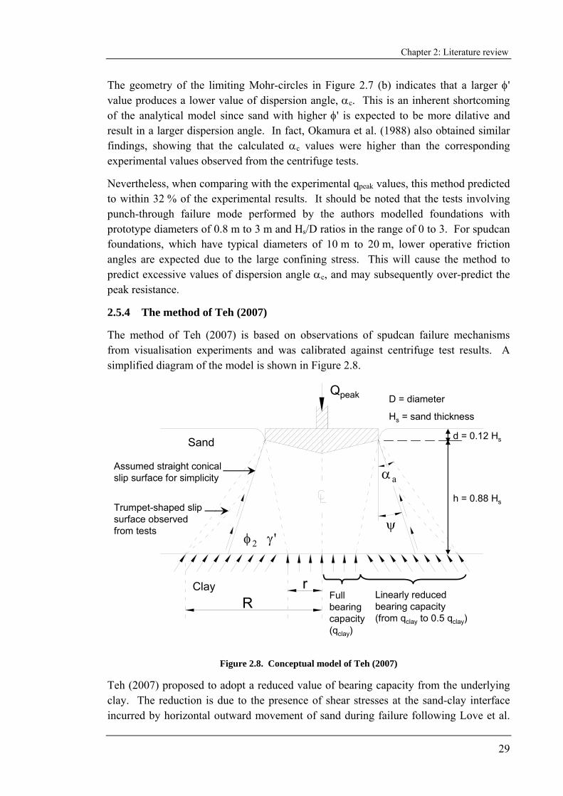
Chapter 2: Literature review
29
The geometry of the limiting Mohr-circles in Figure 2.7 (b) indicates that a larger φ' value produces a lower value of dispersion angle, αc. This is an inherent shortcoming of the analytical model since sand with higher φ' is expected to be more dilative and result in a larger dispersion angle. In fact, Okamura et al. (1988) also obtained similar findings, showing that the calculated αc values were higher than the corresponding experimental values observed from the centrifuge tests.
Nevertheless, when comparing with the experimental qpeak values, this method predicted to within 32 % of the experimental results. It should be noted that the tests involving punch-through failure mode performed by the authors modelled foundations with prototype diameters of 0.8 m to 3 m and Hs/D ratios in the range of 0 to 3. For spudcan foundations, which have typical diameters of 10 m to 20 m, lower operative friction angles are expected due to the large confining stress. This will cause the method to predict excessive values of dispersion angle αc, and may subsequently over-predict the peak resistance.
2.5.4 The method of Teh (2007)
The method of Teh (2007) is based on observations of spudcan failure mechanisms from visualisation experiments and was calibrated against centrifuge test results. A simplified diagram of the model is shown in Figure 2.8.
Assumed straight conical slip surface for simplicity
Rr
Sand
Linearly reduced bearing capacity (from qclay to 0.5 qclay)
Full bearing capacity (qclay)
Qpeak
Clay
'γ
aα
ψ
D = diameter
Hs = sand thickness
2φ
d = 0.12 Hs
h = 0.88 HsTrumpet-shaped slip surface observed from tests
Figure 2.8. Conceptual model of Teh (2007)
Teh (2007) proposed to adopt a reduced value of bearing capacity from the underlying clay. The reduction is due to the presence of shear stresses at the sand-clay interface incurred by horizontal outward movement of sand during failure following Love et al.
Chapter 2: Literature review
30
(1987). The outward movement of sand is negligible at the central region due to symmetry and increases gradually before reducing to zero after passing the foundation edge (Burd and Frydman, 1997). As a result, full bearing capacity, qclay, is assumed to act on a limited region of radius r from the centre line (see Figure 2.8). Beyond the radial distance r, the bearing capacity is assumed to reduce linearly to a minimum value of 0.5 qclay at radial distance R. Both geometrical parameters R and r are empirical factors related to the ratios of Hs/D and qclay/qsand. The values of both parameters are given in two semi-logarithmic design charts proposed by Teh (2007), and are shown in Figure 2.9 (a) and (b) respectively.
To calculate the frictional resistance within the sand layer, it is required to determine the value of ψ, which is defined as the inclination of the shear surface to the vertical as shown in Figure 2.8. It should be noted that ψ is not a dilation angle in this method, but a geometrical parameter used to represent the shear surface inclination. The values of ψ are given in another semi-logarithmic design chart as shown in Figure 2.9 (c). It is noted that these design charts were calibrated based on five experimental data points and were extrapolated to cover a wider range of Hs/D and qclay/qsand (values shown on Figure 2.9).
As indicated in Figure 2.8, the projected area from the shear surfaces in sand (represented by angle ψ) is different from the area at which the bearing capacity of clay is being mobilized (represented by angle αa or radius R). This geometrical inconsistency is due to the assumption of a straight conical slip surface for simplicity while maintaining the clay bearing capacity mobilisation area projected by the actual trumpet-shaped slip surface as illustrated in Figure 2.8.
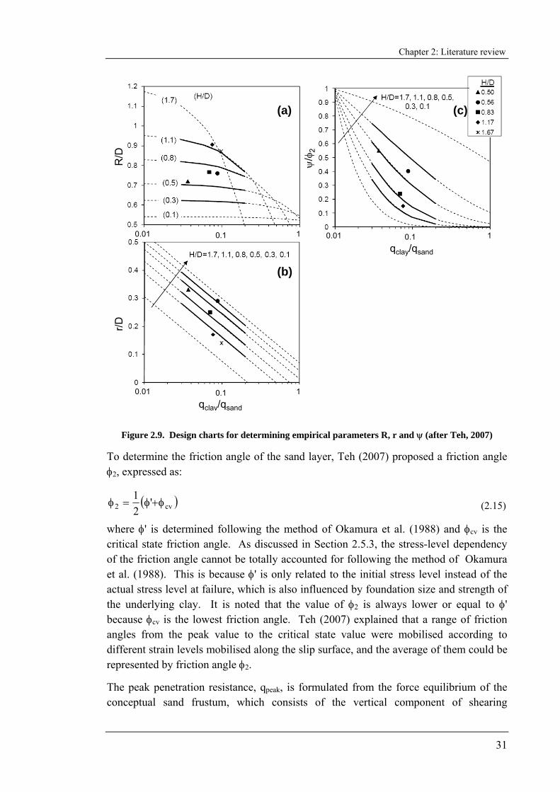
Chapter 2: Literature review
31
qclay/qsand
r/DR
/D
0.01 0.1 1
0.01 0.1 1 0.01 0.1 1
ψ/φ
2
qclay/qsand
(a)
(b)
(c)
Figure 2.9. Design charts for determining empirical parameters R, r and ψ (after Teh, 2007)
To determine the friction angle of the sand layer, Teh (2007) proposed a friction angle φ2, expressed as:
( )cv2 '21
φ+φ=φ (2.15)
where φ' is determined following the method of Okamura et al. (1988) and φcv is the critical state friction angle. As discussed in Section 2.5.3, the stress-level dependency of the friction angle cannot be totally accounted for following the method of Okamura et al. (1988). This is because φ' is only related to the initial stress level instead of the actual stress level at failure, which is also influenced by foundation size and strength of the underlying clay. It is noted that the value of φ2 is always lower or equal to φ' because φcv is the lowest friction angle. Teh (2007) explained that a range of friction angles from the peak value to the critical state value were mobilised according to different strain levels mobilised along the slip surface, and the average of them could be represented by friction angle φ2.
The peak penetration resistance, qpeak, is formulated from the force equilibrium of the conceptual sand frustum, which consists of the vertical component of shearing
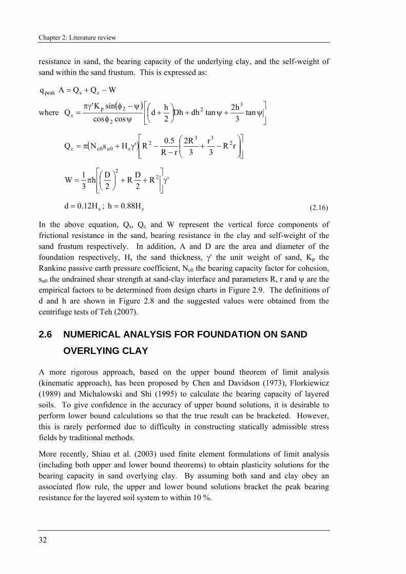
Chapter 2: Literature review
32
resistance in sand, the bearing capacity of the underlying clay, and the self-weight of sand within the sand frustum. This is expressed as:
WQQAq cspeak −+=
where ( )
⎥⎦
⎤⎢⎣
⎡ψ+ψ+⎟
⎠⎞
⎜⎝⎛ +
ψφ
ψ−φπγ= tan
3h2tandhDh
2hd
coscossinK'
Q3
2
2
2ps
( )⎥⎥⎦
⎤
⎢⎢⎣
⎡⎟⎟⎠
⎞⎜⎜⎝
⎛−+
−−γ+π= rR
3r
3R2
rR5.0R'HsNQ 2
332
s0u0cc
'R2DR
2Dh
31W 2
2
γ⎥⎥⎦
⎤
⎢⎢⎣
⎡++⎟
⎠⎞
⎜⎝⎛π=
sH12.0d = ; sH88.0h = (2.16)
In the above equation, Qs, Qc and W represent the vertical force components of frictional resistance in the sand, bearing resistance in the clay and self-weight of the sand frustum respectively. In addition, A and D are the area and diameter of the foundation respectively, Hs the sand thickness, γ' the unit weight of sand, Kp the Rankine passive earth pressure coefficient, Nc0 the bearing capacity factor for cohesion, su0 the undrained shear strength at sand-clay interface and parameters R, r and ψ are the empirical factors to be determined from design charts in Figure 2.9. The definitions of d and h are shown in Figure 2.8 and the suggested values were obtained from the centrifuge tests of Teh (2007).
2.6 NUMERICAL ANALYSIS FOR FOUNDATION ON SAND OVERLYING CLAY
A more rigorous approach, based on the upper bound theorem of limit analysis (kinematic approach), has been proposed by Chen and Davidson (1973), Florkiewicz (1989) and Michalowski and Shi (1995) to calculate the bearing capacity of layered soils. To give confidence in the accuracy of upper bound solutions, it is desirable to perform lower bound calculations so that the true result can be bracketed. However, this is rarely performed due to difficulty in constructing statically admissible stress fields by traditional methods.
More recently, Shiau et al. (2003) used finite element formulations of limit analysis (including both upper and lower bound theorems) to obtain plasticity solutions for the bearing capacity in sand overlying clay. By assuming both sand and clay obey an associated flow rule, the upper and lower bound solutions bracket the peak bearing resistance for the layered soil system to within 10 %.
Chapter 2: Literature review
33
On the other hand, Burd and Frydman (1997) adopted displacement finite element and finite difference analyses to study the peak bearing resistance of sand overlying clay soils. These analyses have the advantage of solving the equations of compatibility and equilibrium together. Shiau et al. (2003) found that the results of Burd and Frydman (1997) lie close to the average of their upper and lower bound estimates.
It should, however, be noted that all these numerical analyses were performed under two dimensional plane strain conditions, simulating strip foundations. The relevance of the results for circular foundations is not known. Furthermore, Tatsuoka et al. (1991) concluded that the results of any numerical analysis would only be close to the experimental results if the true response of the soil can be modelled well, including (1) strength anisotropy, (2) pressure-level dependency of the strength properties of sand, (3) strain-softening effects causing progressive failure, especially for dense sand at low stress levels and (4) the effects of particle size associated with shear banding. By contrast, all soil models used in the aforementioned numerical analyses were based on a simple perfectly-plastic response.
Despite the above, the results from numerical analysis may be useful in providing insights on the failure mechanisms and the effects of each parameter to the punch-through resistance. This can be achieved by examining the failure surface from the numerical analyses and comparing the results from parametric studies. The findings from the numerical analyses are now discussed in the following sections.
2.6.1 Limiting sand thickness
The peak bearing resistance of sand overlying clay, qpeak, is generally lower than the bearing capacity of the upper sand alone, qsand, due to the softening effect of the lower clay layer. However, when the sand thickness, Hs exceeds a certain depth, H*, the failure surface will stay within the sand layer and qpeak becomes independent of the strength of the underlying clay (i.e. qpeak is now equal to qsand). It is generally recognised that the ratio of H*/D is affected by the ratio of bearing capacity for the individual sand and clay layers (qsand/qclay), the friction angle of the sand, the embedment depth and the foundation shape (strip or circular) (Meyerhof, 1974). As a result of these combined effects, a definite value of H*/D is difficult to establish. From centrifuge tests on sand overlying soft clay, Okamura et al. (1997) found that H*/D was around two for a circular foundation without embedment, and the ratio increased with increasing surcharge (embedment) and decreasing strength of the underlying clay. On the effects of foundation shape, Meyerhof (1974) and Valsangkar and Meyerhof (1979) showed that the ratio of H*/D was approximately four for strip foundations and two for circular foundations. This indicates that the stresses induced by strip foundations are distributed to a greater depth than those from circular foundations.
Chapter 2: Literature review
34
2.6.2 Effect of undrained shear strength of the underlying clay
As expected, the peak bearing resistance, qpeak, will increase as the undrained shear strength of the underlying clay, su, increases. However, the rate of increase is not proportional and depends on the Hs/D ratio and the friction angle of the sand layer. Burd and Frydman (1997) found that, for sand layers with high Hs/D ratio and large φ' value, the incremental increase in qpeak for a given increase in su is larger. This is because, as su increases, the failure surface will be gradually pushed back to the sand layer, resulting in larger contribution of resistance from the sand layer. This effect is amplified for sand layers with greater thickness and larger φ' and subsequently reflected as a higher relative incremental increase in qpeak.
It should however be noted that, when su becomes sufficiently large (very stiff clay), qpeak is independent of su as the failure surface is totally confined to within the sand layer.
2.6.3 Effect of foundation roughness
When the failure surface stays within the sand layer, the effects of foundation roughness are obvious – the Nγ factor for fully smooth foundations is about half the value for fully rough foundations (Meyerhof, 1951; Hjiaj et al., 2005). However, Shiau et al. (2003) showed that the effects of base roughness become insignificant when the failure surface extends into the underlying clay. This finding is reasonable since the numerical results show that sand beneath the foundation is moving downward, regardless of the base roughness, when punch-through occurs.
2.6.4 Effect from upper sand layer
Undoubtedly, the value of qpeak will increase when the thickness of the sand layer (or Hs/D ratio) increases. Additionally, Shiau et al. (2003) showed that the value of φ' has greater influence on qpeak for sand layers with larger Hs/D ratios. This is because the majority of the failure surface is within the sand layer for large Hs/D, making the contribution from the frictional resistance in sand more influential.
At a constant Hs/D ratio, it was found that when φ' increases, the failure surface extends more into the underlying clay, thus mobilising a larger extent of the bearing capacity from the underlying clay, on top of the higher frictional resistance from the increased φ' value (Burd and Frydman, 1997). This confirms the intuitive thought that a denser sand layer (which will have a higher φ') is more effective in spreading the load.
It should however be highlighted that φ' is not an intrinsic parameter for sand, since it depends on stress level and strain as discussed in Section 2.4.1. Therefore, sand with similar density and thickness may have different φ' values, depending on the absolute values of foundation diameter and shear strength of the underlying clay.
Chapter 2: Literature review
35
2.7 CURRENT DESIGN GUIDELINES
As discussed in Section 1.3.1, SNAME (2002) provides the current design guidelines for the jack-up industry to predict the peak penetration resistance of a spudcan foundation on sand overlying clay soils. Both of the commonly used approaches, the punching shear method (Hanna and Meyerhof, 1980) and the projected area method, are proposed as the basis for calculation procedures in the guidelines.
In the primary approach, qpeak is calculated following the punching shear method, where the product of the punching shear coefficient, Ks and tan φ' is related to the normalised shear strength of the underlying clay using the following lower bound relationship:
D's
3'tanKs
us γ
=φ (2.17)
where su is the undrained shear strength of the underlying clay, D the equivalent spudcan diameter and γ's the effective unit weight of sand. An alternative design approach is provided in the commentaries to the SNAME (2002) guidelines using the projected area method, with spreading ratios in the range of 1h:5v to 1h:3v (horizontal:vertical).
By ignoring the properties of the upper sand layer (since even in the punching shear approach the frictional resistance through the sand is expressed in terms of the strength of the underlying clay), both methods provide essentially similar and over-simplified approaches whereby the ratio of qpeak to the bearing capacity of the underlying clay increases as a simple quadratic function of Hs/D.
2.8 CONCLUDING REMARKS
A brief review of methods to calculate the bearing capacity of vertically loaded foundations on homogenous sand and clay has been presented. It is evident that many theoretical advances have been achieved in predicting the bearing capacity of a single layer soil since the introduction of Terzaghi's bearing capacity theory. During the early development, semi-empirical correlations or adjustment factors to the classical bearing capacity equation were adopted to allow for variations from the original assumptions. However, more recently, this approach has gradually been replaced with rigorous solutions using modern computing power. Randolph et al. (2004) advocates that this should form the ‘basic’ bearing capacity equation for a simple rigid plastic soil model. Attention should then be focused on the aspects of real soil behaviour that require adjustment of the basic solution, for example strength anisotropy, layered soil profiles, stress-dependent strength and compressibility.
A similar evolution is occurring in the calculation of the bearing capacity on sand overlying clay soils. Initial solutions were based on very simplified methods, namely the punching shear model and the projected area model. Although still commonly used
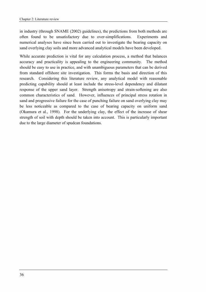
Chapter 2: Literature review
36
in industry (through SNAME (2002) guidelines), the predictions from both methods are often found to be unsatisfactory due to over-simplifications. Experiments and numerical analyses have since been carried out to investigate the bearing capacity on sand overlying clay soils and more advanced analytical models have been developed.
While accurate prediction is vital for any calculation process, a method that balances accuracy and practicality is appealing to the engineering community. The method should be easy to use in practice, and with unambiguous parameters that can be derived from standard offshore site investigation. This forms the basis and direction of this research. Considering this literature review, any analytical model with reasonable predicting capability should at least include the stress-level dependency and dilatant response of the upper sand layer. Strength anisotropy and strain-softening are also common characteristics of sand. However, influences of principal stress rotation in sand and progressive failure for the case of punching failure on sand overlying clay may be less noticeable as compared to the case of bearing capacity on uniform sand (Okamura et al., 1998). For the underlying clay, the effect of the increase of shear strength of soil with depth should be taken into account. This is particularly important due to the large diameter of spudcan foundations.

Chapter 3: Experimental procedures
37
CHAPTER 3. EXPERIMENTAL APPARATUS AND PROCEDURES
3.1 INTRODUCTION
Physical modelling is invaluable in providing the necessary experimental data for the advancement of numerical approaches and the refinement of approximate empirical formulae for foundation response. This vital role of physical modelling is mainly due to the complexity of soil behaviour and the limitations in numerical models of the soil response (Randolph and House, 2001).
Among all physical modelling means, full scale test measurements are most desirable for validation of numerical analyses and calibration of simplified empirical models, which is the primary aim of this research. However, it is difficult to develop analytical models from the field installations of actual spudcans because they are not carried out under controlled environments and, in the case of sand-over-clay punch-through, the ultimate capacity is not reached in a successful operation. To perform dedicated full scale testing of offshore spudcans is prohibitively expensive. Therefore, one option to full scale testing is the geotechnical centrifuge, where the actual field stress levels can be properly simulated at the model scale (Murff, 1996). To study the punch-through phenomenon on sand overlying clay, a series of model spudcan and flat-based foundation tests were carried out using the drum geotechnical centrifuge facility at the University of Western Australia (UWA).
In this chapter, a brief description of the centrifuge modelling principles is initially provided, with further details available in, among others, Schofield (1980), Fuglsang and Ovesen (1988), Ko (1988), Taylor (1995) and more recently Garnier et al. (2007). Following this, the UWA drum centrifuge facility and the experimental apparatus are introduced, as well as a discussion of the test programme, sample preparation and test details. The experimental results will be presented in the next chapter.
3.2 CENTRIFUGE MODELLING PRINCIPLES
Since the behaviour of soil is stress dependent, the confining pressure generated by self-weight of the soil governs the soil behaviour. In order to satisfy the stress similarity conditions in model tests where gravity effects are important, they have to be tested under an increased body force field to properly replicate the full scale prototype behaviour.
In centrifuge modelling where the model dimensions have been reduced by a factor N, the stress similarity between centrifuge model and prototype can be achieved if it is subjected to a centrifugal acceleration of N gravities, effectively increasing the self-

Chapter 3: Experimental procedures
38
weight of the model by the same factor. In this case, the stresses at depth z in the prototype will be identical to those at a depth z/N in the model. If the soil in the model has the same stress-strain response as the soil for the prototype, then strain similarity is also achieved.
Dimensional analysis and analysis of the field equations describing the physical phenomenon are required to allow for the scaling of the centrifuge model dimensions. In geotechnical modelling, the main dimensionless group of interest is usually the ratio of strength to effective stress level, since the soil strength depends on current and past stress level. A brief list of scaling relationships for geotechnical centrifuge tests is presented in Table 3.1.
Table 3.1. Centrifuge model scaling relationships
Quantity Model Prototype
Acceleration level N 1
Length 1 N
Area 1 N2
Volume 1 N3
Density 1 1
Stress 1 1
Strain 1 1
Force 1 N2
Time (dynamic) 1 N
Time (diffusion) 1 N2
Time (creep) 1 1
3.3 DRUM CENTRIFUGE FACILITIES AT UWA
A photograph of the drum centrifuge at the University of Western Australia (UWA) is shown in Figure 3.1 and a schematic cross-sectional diagram in Figure 3.2. The centrifuge has twin concentric shafts that are coupled with a precision servo motor. This allows the central tool table to be rotated differentially to the outer sample containment channel, which is 300 mm in height and 200 mm in radial depth. The radius to the base of the channel is 600 mm. The tool table can also be locked with the channel allowing synchronous rotation during testing. The maximum rotational speed of the channel is 850 rpm which is equivalent to an acceleration of 485 that of earth’s
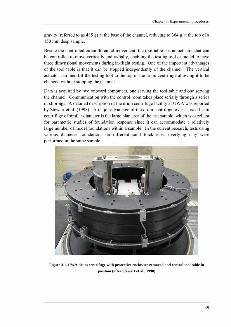
Chapter 3: Experimental procedures
39
gravity (referred to as 485 g) at the base of the channel, reducing to 364 g at the top of a 150 mm deep sample.
Beside the controlled circumferential movement, the tool table has an actuator that can be controlled to move vertically and radially, enabling the testing tool or model to have three dimensional movements during in-flight testing. One of the important advantages of the tool table is that it can be stopped independently of the channel. The vertical actuator can then lift the testing tool to the top of the drum centrifuge allowing it to be changed without stopping the channel.
Data is acquired by two onboard computers, one serving the tool table and one serving the channel. Communication with the control room takes place serially through a series of sliprings. A detailed description of the drum centrifuge facility at UWA was reported by Stewart et al. (1998). A major advantage of the drum centrifuge over a fixed beam centrifuge of similar diameter is the large plan area of the test sample, which is excellent for parametric studies of foundation response since it can accommodate a relatively large number of model foundations within a sample. In the current research, tests using various diameter foundations on different sand thicknesses overlying clay were performed in the same sample.
Figure 3.1. UWA drum centrifuge with protective enclosure removed and central tool table in position (after Stewart et al., 1998)
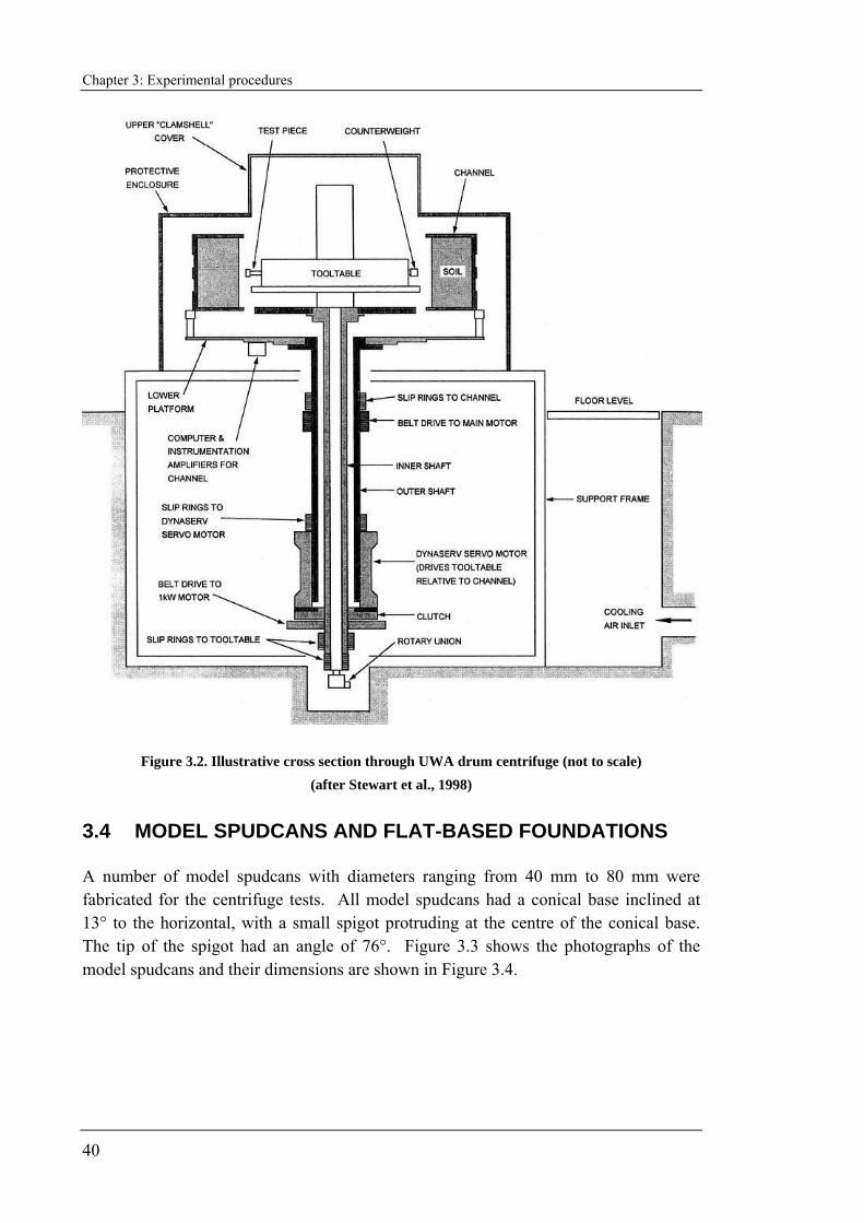
Chapter 3: Experimental procedures
40
Figure 3.2. Illustrative cross section through UWA drum centrifuge (not to scale) (after Stewart et al., 1998)
3.4 MODEL SPUDCANS AND FLAT-BASED FOUNDATIONS
A number of model spudcans with diameters ranging from 40 mm to 80 mm were fabricated for the centrifuge tests. All model spudcans had a conical base inclined at 13° to the horizontal, with a small spigot protruding at the centre of the conical base. The tip of the spigot had an angle of 76°. Figure 3.3 shows the photographs of the model spudcans and their dimensions are shown in Figure 3.4.
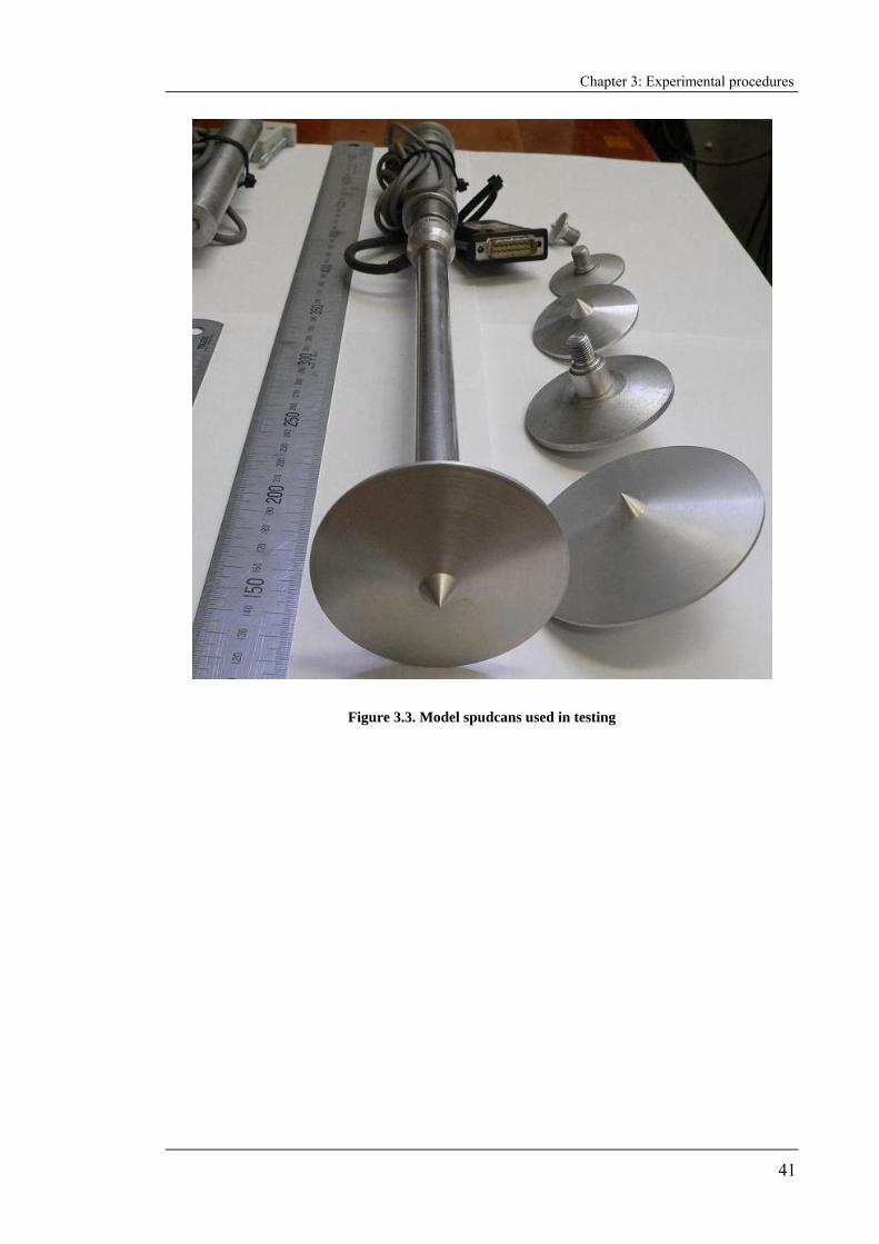
Chapter 3: Experimental procedures
41
Figure 3.3. Model spudcans used in testing
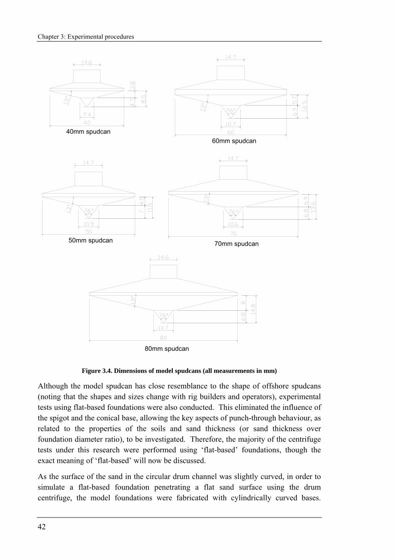
Chapter 3: Experimental procedures
42
50mm spudcan
60mm spudcan
70mm spudcan
40mm spudcan
80mm spudcan
Figure 3.4. Dimensions of model spudcans (all measurements in mm)
Although the model spudcan has close resemblance to the shape of offshore spudcans (noting that the shapes and sizes change with rig builders and operators), experimental tests using flat-based foundations were also conducted. This eliminated the influence of the spigot and the conical base, allowing the key aspects of punch-through behaviour, as related to the properties of the soils and sand thickness (or sand thickness over foundation diameter ratio), to be investigated. Therefore, the majority of the centrifuge tests under this research were performed using ‘flat-based’ foundations, though the exact meaning of ‘flat-based’ will now be discussed.
As the surface of the sand in the circular drum channel was slightly curved, in order to simulate a flat-based foundation penetrating a flat sand surface using the drum centrifuge, the model foundations were fabricated with cylindrically curved bases.
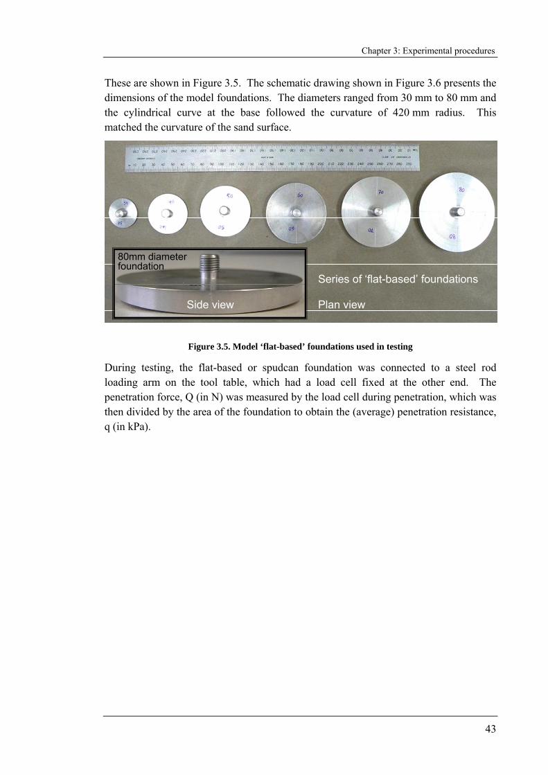
Chapter 3: Experimental procedures
43
These are shown in Figure 3.5. The schematic drawing shown in Figure 3.6 presents the dimensions of the model foundations. The diameters ranged from 30 mm to 80 mm and the cylindrical curve at the base followed the curvature of 420 mm radius. This matched the curvature of the sand surface.
Side view Plan view
80mm diameter foundation
Series of ‘flat-based’ foundations
Figure 3.5. Model ‘flat-based’ foundations used in testing
During testing, the flat-based or spudcan foundation was connected to a steel rod loading arm on the tool table, which had a load cell fixed at the other end. The penetration force, Q (in N) was measured by the load cell during penetration, which was then divided by the area of the foundation to obtain the (average) penetration resistance, q (in kPa).
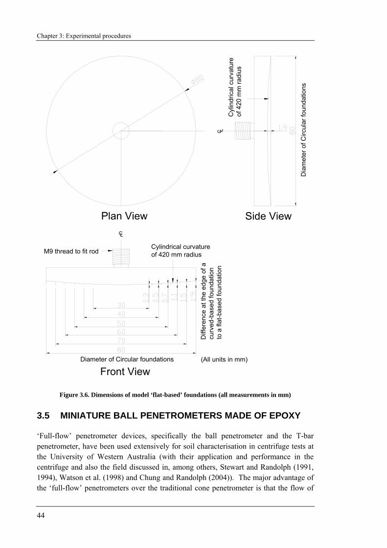
Chapter 3: Experimental procedures
44
Diff
eren
ce a
t the
edg
e of
a
curv
ed-b
ased
foun
datio
n to
a fl
at-b
ased
foun
datio
n
Diameter of Circular foundations (All units in mm)
M9 thread to fit rod
CL
C L
Dia
met
er o
f Circ
ular
foun
datio
ns
Cylindrical curvature of 420 mm radius
Cyl
indr
ical
cur
vatu
re
of 4
20 m
m ra
dius
Plan View
Front View
Side View
Figure 3.6. Dimensions of model ‘flat-based’ foundations (all measurements in mm)
3.5 MINIATURE BALL PENETROMETERS MADE OF EPOXY
‘Full-flow’ penetrometer devices, specifically the ball penetrometer and the T-bar penetrometer, have been used extensively for soil characterisation in centrifuge tests at the University of Western Australia (with their application and performance in the centrifuge and also the field discussed in, among others, Stewart and Randolph (1991, 1994), Watson et al. (1998) and Chung and Randolph (2004)). The major advantage of the ‘full-flow’ penetrometers over the traditional cone penetrometer is that the flow of
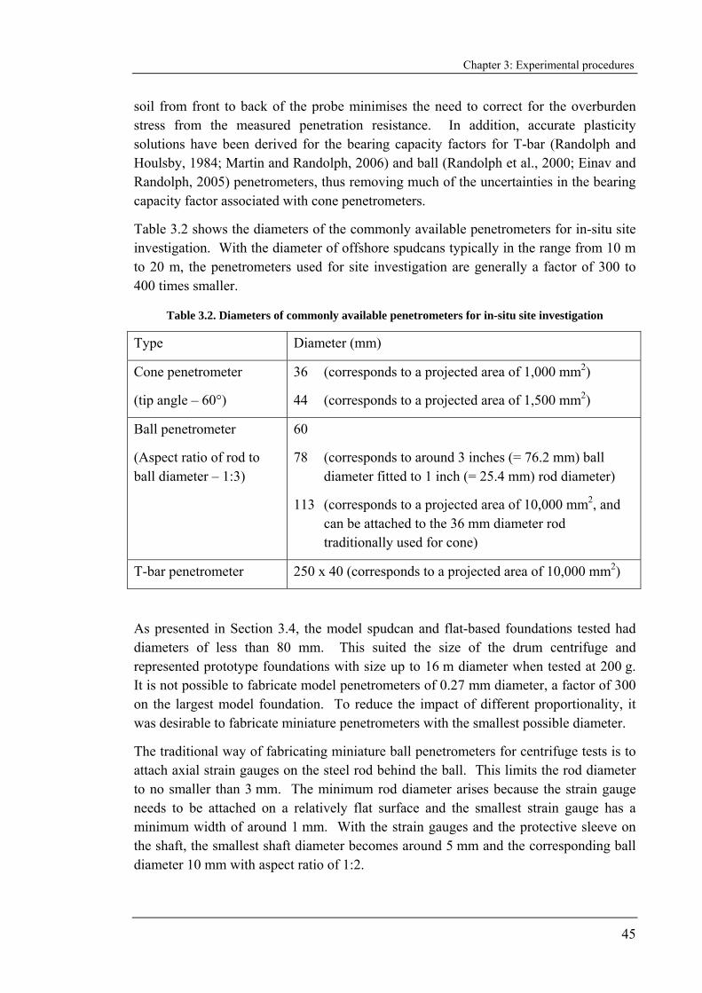
Chapter 3: Experimental procedures
45
soil from front to back of the probe minimises the need to correct for the overburden stress from the measured penetration resistance. In addition, accurate plasticity solutions have been derived for the bearing capacity factors for T-bar (Randolph and Houlsby, 1984; Martin and Randolph, 2006) and ball (Randolph et al., 2000; Einav and Randolph, 2005) penetrometers, thus removing much of the uncertainties in the bearing capacity factor associated with cone penetrometers.
Table 3.2 shows the diameters of the commonly available penetrometers for in-situ site investigation. With the diameter of offshore spudcans typically in the range from 10 m to 20 m, the penetrometers used for site investigation are generally a factor of 300 to 400 times smaller.
Table 3.2. Diameters of commonly available penetrometers for in-situ site investigation
Type Diameter (mm)
Cone penetrometer
(tip angle – 60°)
36 (corresponds to a projected area of 1,000 mm2)
44 (corresponds to a projected area of 1,500 mm2)
Ball penetrometer
(Aspect ratio of rod to ball diameter – 1:3)
60
78 (corresponds to around 3 inches (= 76.2 mm) ball diameter fitted to 1 inch (= 25.4 mm) rod diameter)
113 (corresponds to a projected area of 10,000 mm2, and can be attached to the 36 mm diameter rod traditionally used for cone)
T-bar penetrometer 250 x 40 (corresponds to a projected area of 10,000 mm2)
As presented in Section 3.4, the model spudcan and flat-based foundations tested had diameters of less than 80 mm. This suited the size of the drum centrifuge and represented prototype foundations with size up to 16 m diameter when tested at 200 g. It is not possible to fabricate model penetrometers of 0.27 mm diameter, a factor of 300 on the largest model foundation. To reduce the impact of different proportionality, it was desirable to fabricate miniature penetrometers with the smallest possible diameter.
The traditional way of fabricating miniature ball penetrometers for centrifuge tests is to attach axial strain gauges on the steel rod behind the ball. This limits the rod diameter to no smaller than 3 mm. The minimum rod diameter arises because the strain gauge needs to be attached on a relatively flat surface and the smallest strain gauge has a minimum width of around 1 mm. With the strain gauges and the protective sleeve on the shaft, the smallest shaft diameter becomes around 5 mm and the corresponding ball diameter 10 mm with aspect ratio of 1:2.

Chapter 3: Experimental procedures
46
With these limitations, a paradigm shift in the fabrication method was required and a new method, where the entire ball, shaft and embedded strain gauges were cast in epoxy, was developed. This allowed three miniature ball penetrometers with diameters of 4 mm, 5 mm and 6 mm, all with aspect ratio of 1:2, to be fabricated. The following describes the new fabrication method in detail.
3.5.1 Mechanical behaviour of epoxy Araldite Kit K138
To attain a rigid penetrometer, the epoxy to be used for the casting of the miniature probes should possess high compressive strength and high resistance against the abrasion of sand. As a result, the commercially available high strength epoxy Araldite Kit K138 was chosen. This material, similar to other high strength epoxy, is commonly used for bonding operations where the use of a hot-setting adhesive is not possible. Therefore, the material specifications provided by the manufacturer only included the tensile strength, which was 43 MPa and the tensile bond strength, which was around 12 MPa depending on temperature.
In view of that, additional tests were carried out to determine the epoxy’s compressive strength and its mechanical behaviour under cyclic loads and sustained loads. Figure 3.7 shows the experimental set-up for the uni-axial compression test. A load cell was used to measure the axial force, while the axial deformation was measured by a pair of external deformation gauges (the mechanism and principle of which were discussed by Goto et al., 1991).
Load cell
External deformation gauge
Sample
Load cell
External deformation gauge
Sample
Figure 3.7. Experimental set-up for uni-axial compression test of epoxy K138 sample
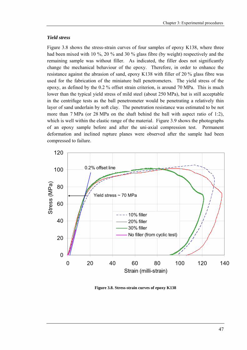
Chapter 3: Experimental procedures
47
Yield stress
Figure 3.8 shows the stress-strain curves of four samples of epoxy K138, where three had been mixed with 10 %, 20 % and 30 % glass fibre (by weight) respectively and the remaining sample was without filler. As indicated, the filler does not significantly change the mechanical behaviour of the epoxy. Therefore, in order to enhance the resistance against the abrasion of sand, epoxy K138 with filler of 20 % glass fibre was used for the fabrication of the miniature ball penetrometers. The yield stress of the epoxy, as defined by the 0.2 % offset strain criterion, is around 70 MPa. This is much lower than the typical yield stress of mild steel (about 250 MPa), but is still acceptable in the centrifuge tests as the ball penetrometer would be penetrating a relatively thin layer of sand underlain by soft clay. The penetration resistance was estimated to be not more than 7 MPa (or 28 MPa on the shaft behind the ball with aspect ratio of 1:2), which is well within the elastic range of the material. Figure 3.9 shows the photographs of an epoxy sample before and after the uni-axial compression test. Permanent deformation and inclined rupture planes were observed after the sample had been compressed to failure.
0
20
40
60
80
100
120
0 20 40 60 80 100 120 140Strain (milli-strain)
Stre
ss (M
Pa)
10% filler20% filler30% fillerNo filler (from cyclic test)
0.2% offset line
Yield stress ~ 70 MPa
Figure 3.8. Stress-strain curves of epoxy K138
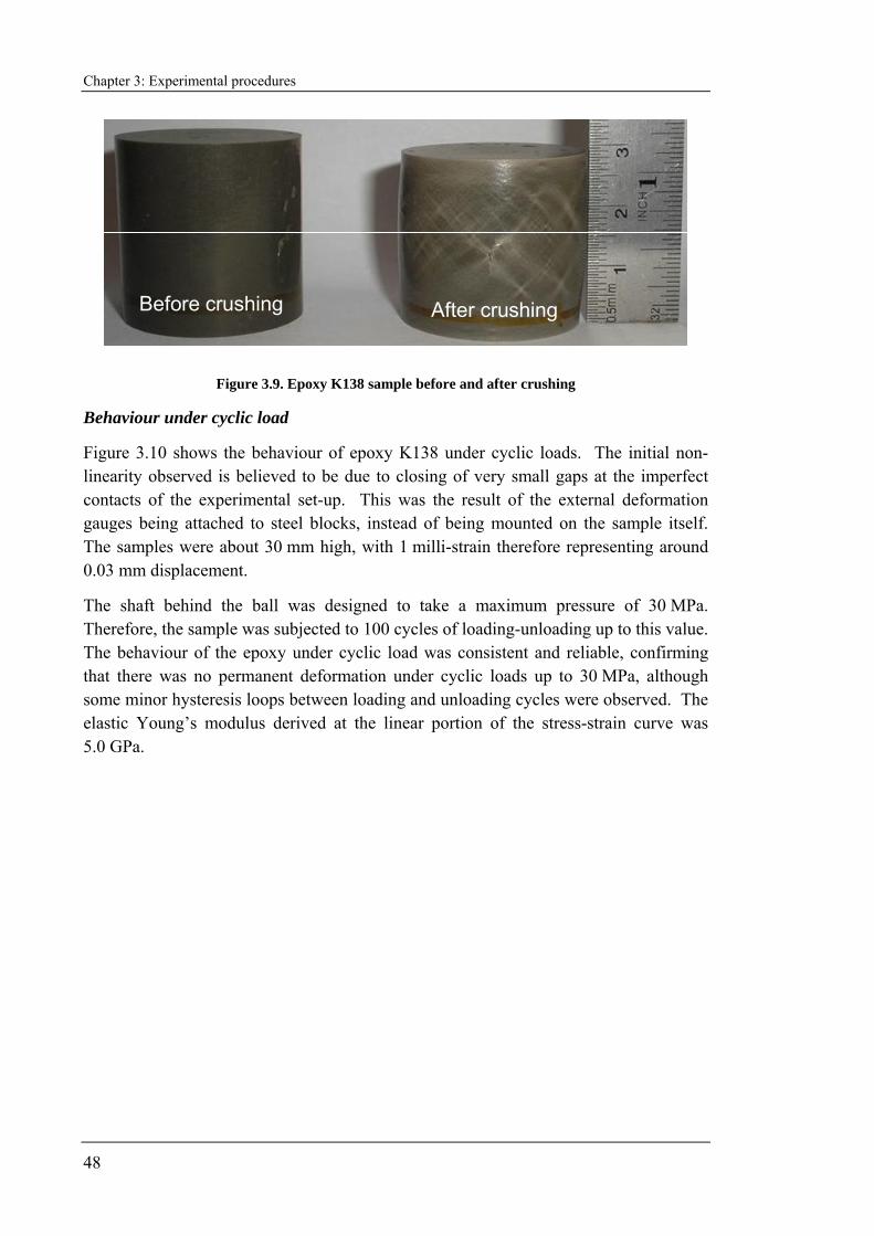
Chapter 3: Experimental procedures
48
Before crushing After crushing
Figure 3.9. Epoxy K138 sample before and after crushing
Behaviour under cyclic load
Figure 3.10 shows the behaviour of epoxy K138 under cyclic loads. The initial non-linearity observed is believed to be due to closing of very small gaps at the imperfect contacts of the experimental set-up. This was the result of the external deformation gauges being attached to steel blocks, instead of being mounted on the sample itself. The samples were about 30 mm high, with 1 milli-strain therefore representing around 0.03 mm displacement.
The shaft behind the ball was designed to take a maximum pressure of 30 MPa. Therefore, the sample was subjected to 100 cycles of loading-unloading up to this value. The behaviour of the epoxy under cyclic load was consistent and reliable, confirming that there was no permanent deformation under cyclic loads up to 30 MPa, although some minor hysteresis loops between loading and unloading cycles were observed. The elastic Young’s modulus derived at the linear portion of the stress-strain curve was 5.0 GPa.

Chapter 3: Experimental procedures
49
0
4
8
12
16
20
24
28
32
0 1 2 3 4 5 6 7 8Strain (milli-strain)
Stre
ss (M
Pa)
100 cycles in 44 minutes
0.007 – 0.003 = 0.004
28 – 8= 20 MPa
E = 20/0.004
= 5.0 GPa
Figure 3.10. Behaviour of epoxy K138 under cyclic loads
Behaviour under maintained load
Another epoxy sample was maintained at a constant axial load of approximately 30 MPa for more than an hour. Figure 3.11 shows the stress and strain responses with time. Less than 2 % creep was recorded after about an hour of maintaining the load at 30 MPa. This was considered negligible as all penetrations took less than 15 minutes at stress levels much lower than 30 MPa on the shaft of the penetrometer. In general, the penetration duration within the sand layer would be around half a minute, whereas for the remaining period the ball would be in the underlying clay with stress levels below 4 MPa on the shaft.
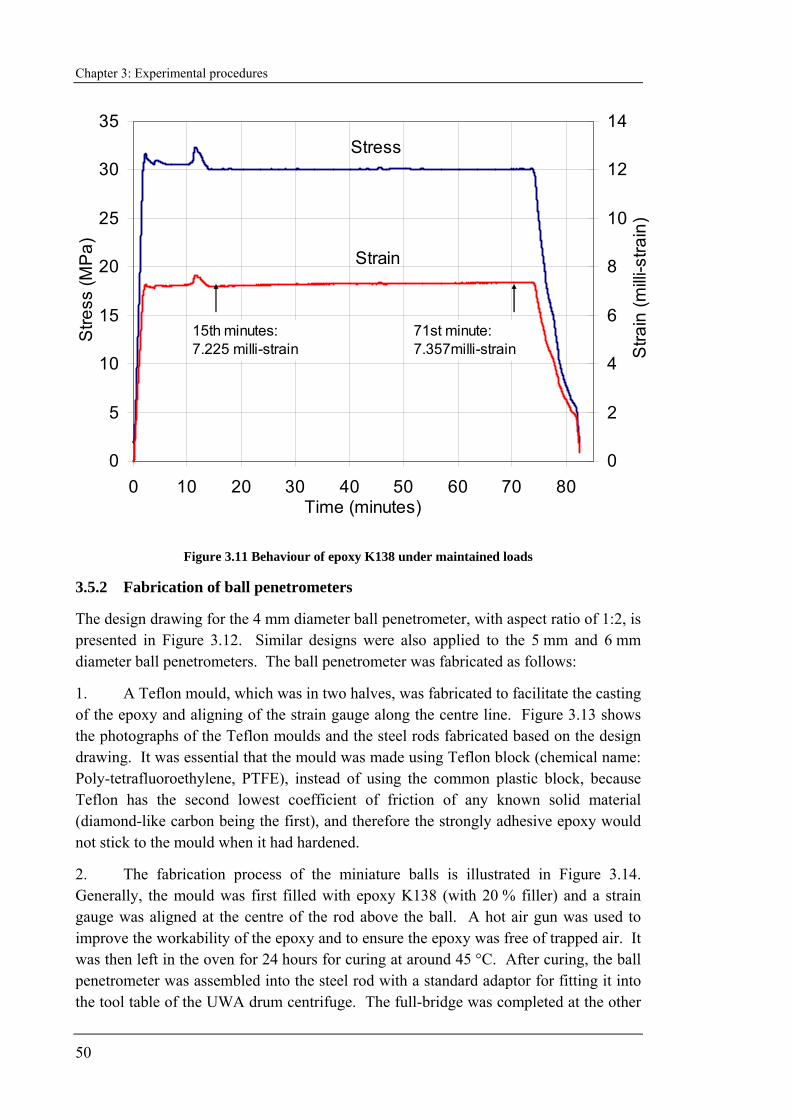
Chapter 3: Experimental procedures
50
0
5
10
15
20
25
30
35
0 10 20 30 40 50 60 70 80Time (minutes)
Stre
ss (M
Pa)
0
2
4
6
8
10
12
14
Stra
in (m
illi-s
train
)
Stress
Strain
15th minutes:7.225 milli-strain
71st minute:7.357milli-strain
Figure 3.11 Behaviour of epoxy K138 under maintained loads
3.5.2 Fabrication of ball penetrometers
The design drawing for the 4 mm diameter ball penetrometer, with aspect ratio of 1:2, is presented in Figure 3.12. Similar designs were also applied to the 5 mm and 6 mm diameter ball penetrometers. The ball penetrometer was fabricated as follows:
1. A Teflon mould, which was in two halves, was fabricated to facilitate the casting of the epoxy and aligning of the strain gauge along the centre line. Figure 3.13 shows the photographs of the Teflon moulds and the steel rods fabricated based on the design drawing. It was essential that the mould was made using Teflon block (chemical name: Poly-tetrafluoroethylene, PTFE), instead of using the common plastic block, because Teflon has the second lowest coefficient of friction of any known solid material (diamond-like carbon being the first), and therefore the strongly adhesive epoxy would not stick to the mould when it had hardened.
2. The fabrication process of the miniature balls is illustrated in Figure 3.14. Generally, the mould was first filled with epoxy K138 (with 20 % filler) and a strain gauge was aligned at the centre of the rod above the ball. A hot air gun was used to improve the workability of the epoxy and to ensure the epoxy was free of trapped air. It was then left in the oven for 24 hours for curing at around 45 °C. After curing, the ball penetrometer was assembled into the steel rod with a standard adaptor for fitting it into the tool table of the UWA drum centrifuge. The full-bridge was completed at the other
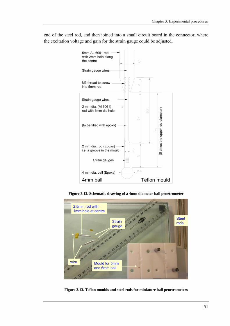
Chapter 3: Experimental procedures
51
end of the steel rod, and then joined into a small circuit board in the connector, where the excitation voltage and gain for the strain gauge could be adjusted.
(5 ti
mes
the
uppe
r rod
dia
met
er)
2 mm dia. rod (Epoxy)i.e. a groove in the mould
Strain gauges
4 mm dia. ball (Epoxy)
Teflon mould
Strain gauge wires
(to be filled with epoxy)
M3 thread to screw into 5mm rod
4mm ball
5mm AL 6061 rod with 2mm hole along the centre
2 mm dia. (Al 6061) rod with 1mm dia hole
Strain gauge wires
Figure 3.12. Schematic drawing of a 4mm diameter ball penetrometer
2.5mm rod with 1mm hole at centre
Strain gauge
wire Mould for 5mm and 6mm ball
Steel rods
Figure 3.13. Teflon moulds and steel rods for miniature ball penetrometers
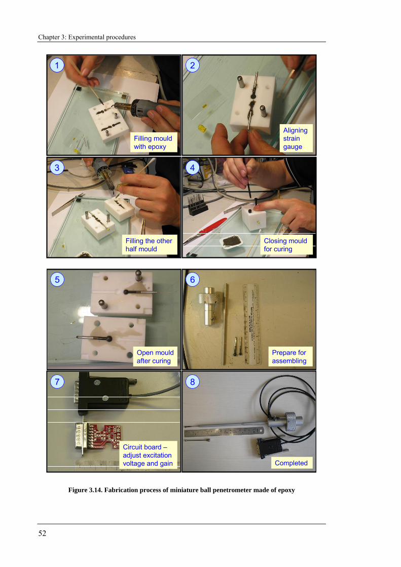
Chapter 3: Experimental procedures
52
Aligning strain gauge
Filling the other half mould
Closing mould for curing
1
3
2
4
Filling mould with epoxy
Prepare for assembling
Circuit board –adjust excitation voltage and gain Completed
5
7
6
8
Open mould after curing
Figure 3.14. Fabrication process of miniature ball penetrometer made of epoxy
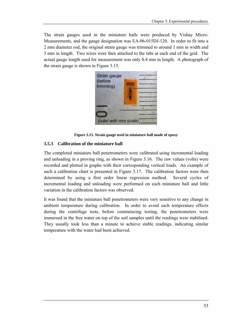
Chapter 3: Experimental procedures
53
The strain gauges used in the miniature balls were produced by Vishay Micro-Measurements, and the gauge designation was EA-06-015DJ-120. In order to fit into a 2 mm diameter rod, the original strain gauge was trimmed to around 1 mm in width and 3 mm in length. Two wires were then attached to the tabs at each end of the grid. The actual gauge length used for measurement was only 0.4 mm in length. A photograph of the strain gauge is shown in Figure 3.15.
Strain gauge (before trimming)
(ruler with mm scale)
Figure 3.15. Strain gauge used in miniature ball made of epoxy
3.5.3 Calibration of the miniature ball
The completed miniature ball penetrometers were calibrated using incremental loading and unloading in a proving ring, as shown in Figure 3.16. The raw values (volts) were recorded and plotted in graphs with their corresponding vertical loads. An example of such a calibration chart is presented in Figure 3.17. The calibration factors were then determined by using a first order linear regression method. Several cycles of incremental loading and unloading were performed on each miniature ball and little variation in the calibration factors was observed.
It was found that the miniature ball penetrometers were very sensitive to any change in ambient temperature during calibration. In order to avoid such temperature effects during the centrifuge tests, before commencing testing, the penetrometers were immersed in the free water on top of the soil samples until the readings were stabilised. They usually took less than a minute to achieve stable readings, indicating similar temperature with the water had been achieved.

Chapter 3: Experimental procedures
54
Proving ring
Miniature ball penetrometer
Figure 3.16. Calibration of miniature ball using proving ring
y = -4.754x - 0.358R2 = 0.999
0
5
10
15
20
25
-5 -4 -3 -2 -1 0Output Voltage (V)
Stre
ss o
n ro
d (M
Pa)
LoadingUnloadinglinear regression line
Figure 3.17. A typical calibration chart of the miniature ball penetrometer
3.5.4 Working range of the miniature ball penetrometer
The following Table 3.3 summarises the working ranges of all three miniature ball penetrometers. The working ranges were generally limited by the buckling mode of failure on the epoxy rod.
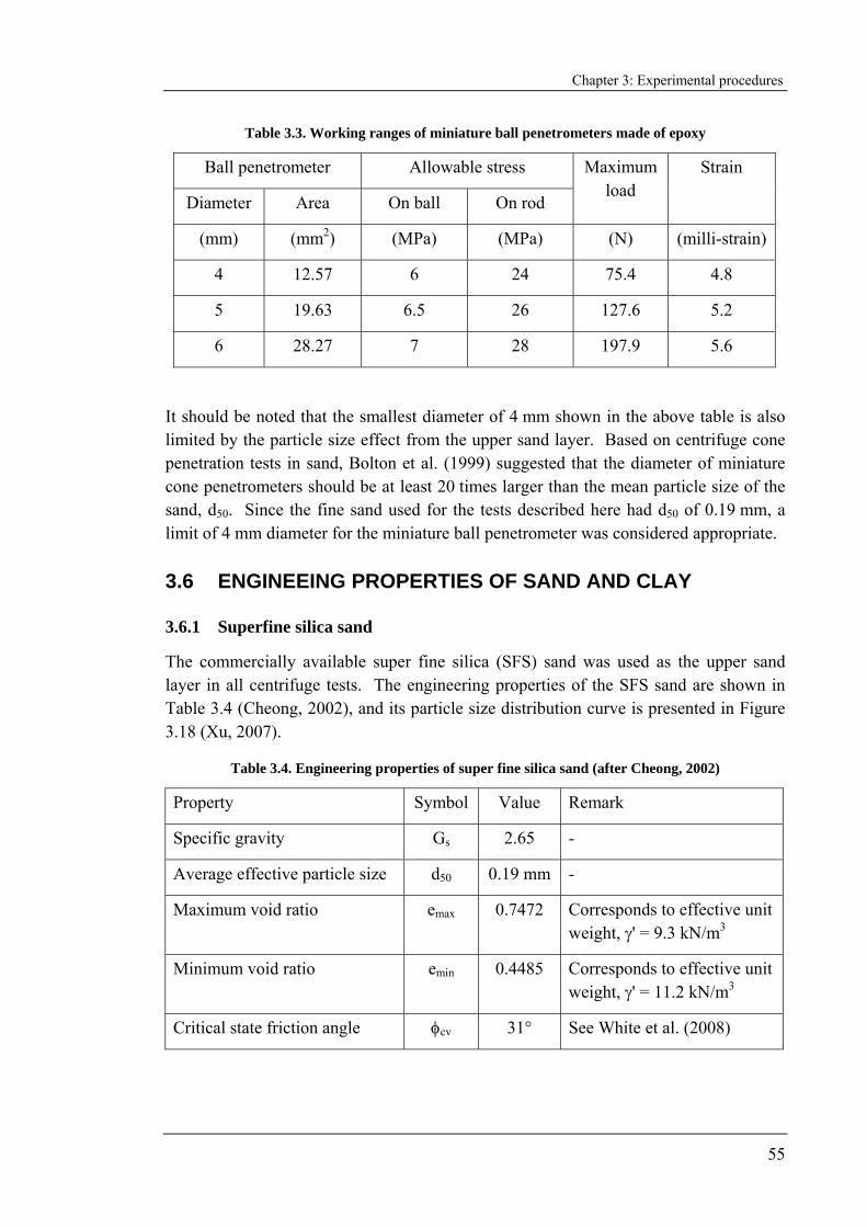
Chapter 3: Experimental procedures
55
Table 3.3. Working ranges of miniature ball penetrometers made of epoxy
Ball penetrometer Allowable stress
Diameter Area On ball On rod
Maximum load
Strain
(mm) (mm2) (MPa) (MPa) (N) (milli-strain)
4 12.57 6 24 75.4 4.8
5 19.63 6.5 26 127.6 5.2
6 28.27 7 28 197.9 5.6
It should be noted that the smallest diameter of 4 mm shown in the above table is also limited by the particle size effect from the upper sand layer. Based on centrifuge cone penetration tests in sand, Bolton et al. (1999) suggested that the diameter of miniature cone penetrometers should be at least 20 times larger than the mean particle size of the sand, d50. Since the fine sand used for the tests described here had d50 of 0.19 mm, a limit of 4 mm diameter for the miniature ball penetrometer was considered appropriate.
3.6 ENGINEEING PROPERTIES OF SAND AND CLAY
3.6.1 Superfine silica sand
The commercially available super fine silica (SFS) sand was used as the upper sand layer in all centrifuge tests. The engineering properties of the SFS sand are shown in Table 3.4 (Cheong, 2002), and its particle size distribution curve is presented in Figure 3.18 (Xu, 2007).
Table 3.4. Engineering properties of super fine silica sand (after Cheong, 2002)
Property Symbol Value Remark
Specific gravity Gs 2.65 -
Average effective particle size d50 0.19 mm -
Maximum void ratio emax 0.7472 Corresponds to effective unit weight, γ' = 9.3 kN/m3
Minimum void ratio emin 0.4485 Corresponds to effective unit weight, γ' = 11.2 kN/m3
Critical state friction angle φcv 31° See White et al. (2008)
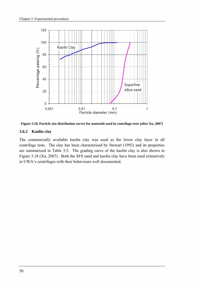
Chapter 3: Experimental procedures
56
Figure 3.18. Particle size distribution curves for materials used in centrifuge tests (after Xu, 2007)
3.6.2 Kaolin clay
The commercially available kaolin clay was used as the lower clay layer in all centrifuge tests. The clay has been characterised by Stewart (1992) and its properties are summarized in Table 3.5. The grading curve of the kaolin clay is also shown in Figure 3.18 (Xu, 2007). Both the SFS sand and kaolin clay have been used extensively in UWA’s centrifuges with their behaviours well documented.
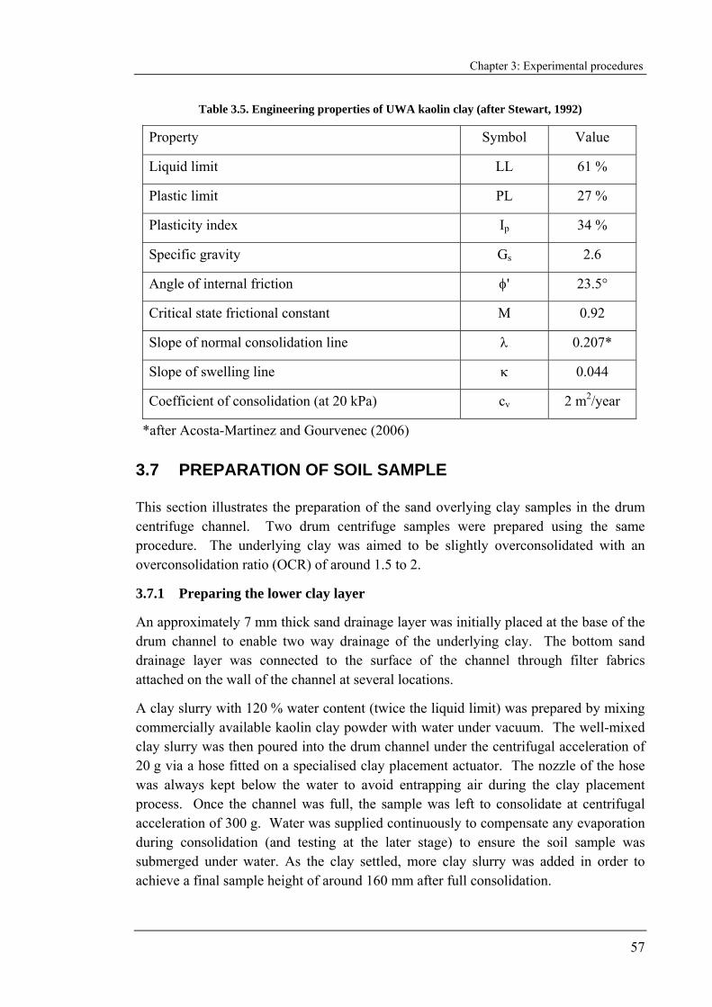
Chapter 3: Experimental procedures
57
Table 3.5. Engineering properties of UWA kaolin clay (after Stewart, 1992)
Property Symbol Value
Liquid limit LL 61 %
Plastic limit PL 27 %
Plasticity index Ip 34 %
Specific gravity Gs 2.6
Angle of internal friction φ' 23.5°
Critical state frictional constant M 0.92
Slope of normal consolidation line λ 0.207*
Slope of swelling line κ 0.044
Coefficient of consolidation (at 20 kPa) cv 2 m2/year
*after Acosta-Martinez and Gourvenec (2006)
3.7 PREPARATION OF SOIL SAMPLE
This section illustrates the preparation of the sand overlying clay samples in the drum centrifuge channel. Two drum centrifuge samples were prepared using the same procedure. The underlying clay was aimed to be slightly overconsolidated with an overconsolidation ratio (OCR) of around 1.5 to 2.
3.7.1 Preparing the lower clay layer
An approximately 7 mm thick sand drainage layer was initially placed at the base of the drum channel to enable two way drainage of the underlying clay. The bottom sand drainage layer was connected to the surface of the channel through filter fabrics attached on the wall of the channel at several locations.
A clay slurry with 120 % water content (twice the liquid limit) was prepared by mixing commercially available kaolin clay powder with water under vacuum. The well-mixed clay slurry was then poured into the drum channel under the centrifugal acceleration of 20 g via a hose fitted on a specialised clay placement actuator. The nozzle of the hose was always kept below the water to avoid entrapping air during the clay placement process. Once the channel was full, the sample was left to consolidate at centrifugal acceleration of 300 g. Water was supplied continuously to compensate any evaporation during consolidation (and testing at the later stage) to ensure the soil sample was submerged under water. As the clay settled, more clay slurry was added in order to achieve a final sample height of around 160 mm after full consolidation.
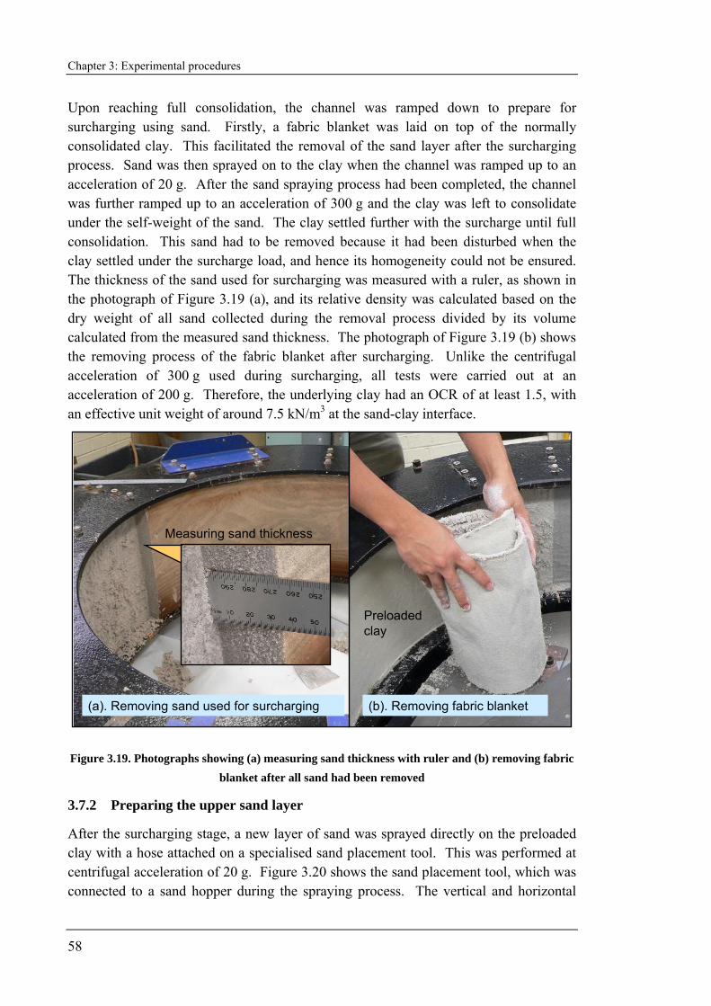
Chapter 3: Experimental procedures
58
Upon reaching full consolidation, the channel was ramped down to prepare for surcharging using sand. Firstly, a fabric blanket was laid on top of the normally consolidated clay. This facilitated the removal of the sand layer after the surcharging process. Sand was then sprayed on to the clay when the channel was ramped up to an acceleration of 20 g. After the sand spraying process had been completed, the channel was further ramped up to an acceleration of 300 g and the clay was left to consolidate under the self-weight of the sand. The clay settled further with the surcharge until full consolidation. This sand had to be removed because it had been disturbed when the clay settled under the surcharge load, and hence its homogeneity could not be ensured. The thickness of the sand used for surcharging was measured with a ruler, as shown in the photograph of Figure 3.19 (a), and its relative density was calculated based on the dry weight of all sand collected during the removal process divided by its volume calculated from the measured sand thickness. The photograph of Figure 3.19 (b) shows the removing process of the fabric blanket after surcharging. Unlike the centrifugal acceleration of 300 g used during surcharging, all tests were carried out at an acceleration of 200 g. Therefore, the underlying clay had an OCR of at least 1.5, with an effective unit weight of around 7.5 kN/m3 at the sand-clay interface.
(b). Removing fabric blanket
Preloaded clay
(a). Removing sand used for surcharging
Measuring sand thickness
Figure 3.19. Photographs showing (a) measuring sand thickness with ruler and (b) removing fabric blanket after all sand had been removed
3.7.2 Preparing the upper sand layer
After the surcharging stage, a new layer of sand was sprayed directly on the preloaded clay with a hose attached on a specialised sand placement tool. This was performed at centrifugal acceleration of 20 g. Figure 3.20 shows the sand placement tool, which was connected to a sand hopper during the spraying process. The vertical and horizontal
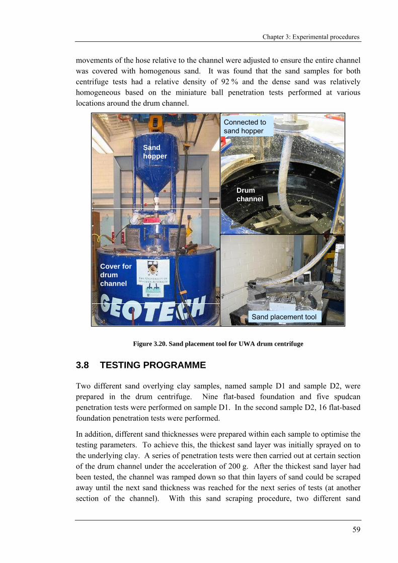
Chapter 3: Experimental procedures
59
movements of the hose relative to the channel were adjusted to ensure the entire channel was covered with homogenous sand. It was found that the sand samples for both centrifuge tests had a relative density of 92 % and the dense sand was relatively homogeneous based on the miniature ball penetration tests performed at various locations around the drum channel.
Sand hopper
Cover for drum channel
Sand placement tool
Connected to sand hopper
Drum channel
Figure 3.20. Sand placement tool for UWA drum centrifuge
3.8 TESTING PROGRAMME
Two different sand overlying clay samples, named sample D1 and sample D2, were prepared in the drum centrifuge. Nine flat-based foundation and five spudcan penetration tests were performed on sample D1. In the second sample D2, 16 flat-based foundation penetration tests were performed.
In addition, different sand thicknesses were prepared within each sample to optimise the testing parameters. To achieve this, the thickest sand layer was initially sprayed on to the underlying clay. A series of penetration tests were then carried out at certain section of the drum channel under the acceleration of 200 g. After the thickest sand layer had been tested, the channel was ramped down so that thin layers of sand could be scraped away until the next sand thickness was reached for the next series of tests (at another section of the channel). With this sand scraping procedure, two different sand

Chapter 3: Experimental procedures
60
thicknesses were created in the first sample D1, whereas sample D2 had four. The sample was left to consolidate under the new sand thickness for one and a half days before the commencement of the penetration tests. Figure 3.21 shows the photograph of the sand scraping process.
Craters from a test series on thicker sand
Hand-dug pocket for measuring sand thickness
Scraping to thinner sand layer
Drum channel
Figure 3.21. Scraping sand after completing a series of tests at thicker sand thickness
Table 3.6 and Table 3.7 present the summary of all flat-based and spudcan foundation penetration tests, and their corresponding sand thicknesses, for test samples D1 and D2 respectively.

Chapter 3: Experimental procedures
61
Table 3.6. Summary of flat-based and spudcan foundation penetration tests for sample D1
Test1 Sand thickness, Hs (mm)2 Foundation diameter, D (mm)2 Hs/D ratio
D1F30a 30 1.03
D1F40a 40 0.78
D1F50a 50 0.62
D1F60a 60 0.52
D1F70a 70 0.44
D1F80a
31
80 0.39
D1F40b 40 0.51
D1F50b 50 0.41
D1F60b
20.5
60 0.34
D1SP40a 40 0.78
D1SP50a 50 0.62
D1SP60a 60 0.52
D1SP70a 70 0.44
D1SP80a
31
80 0.39 1 The test naming system is Sample-Foundation Type (F for flat-based foundation and SP for spudcan)-
Model diameter (in mm)-Alphabet signifying a particular sand thickness 2 Model scale
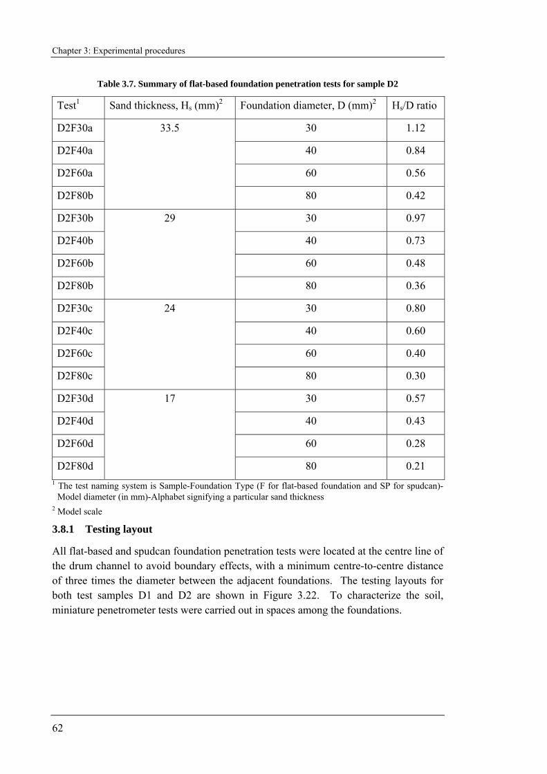
Chapter 3: Experimental procedures
62
Table 3.7. Summary of flat-based foundation penetration tests for sample D2
Test1 Sand thickness, Hs (mm)2 Foundation diameter, D (mm)2 Hs/D ratio
D2F30a 30 1.12
D2F40a 40 0.84
D2F60a 60 0.56
D2F80b
33.5
80 0.42
D2F30b 30 0.97
D2F40b 40 0.73
D2F60b 60 0.48
D2F80b
29
80 0.36
D2F30c 30 0.80
D2F40c 40 0.60
D2F60c 60 0.40
D2F80c
24
80 0.30
D2F30d 30 0.57
D2F40d 40 0.43
D2F60d 60 0.28
D2F80d
17
80 0.21 1 The test naming system is Sample-Foundation Type (F for flat-based foundation and SP for spudcan)-
Model diameter (in mm)-Alphabet signifying a particular sand thickness 2 Model scale
3.8.1 Testing layout
All flat-based and spudcan foundation penetration tests were located at the centre line of the drum channel to avoid boundary effects, with a minimum centre-to-centre distance of three times the diameter between the adjacent foundations. The testing layouts for both test samples D1 and D2 are shown in Figure 3.22. To characterize the soil, miniature penetrometer tests were carried out in spaces among the foundations.
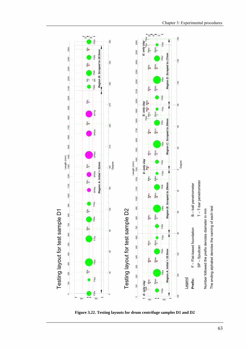
Chapter 3: Experimental procedures
63
150
Deg
ree
180
150
120
9060
300
-30
-60
-120
-90
-150
20
B4d
u
41
F30d
B4d
m
70
2500
2600
E: o
nly
clay
T5ec
T5ea
Reg
ion
D: S
crap
ed to
17m
m
1900
E: o
nly
clay
B4cm
B4cu
B6cu
B5cu
Reg
ion
C: S
crap
ed to
24m
m
F40c
F80c
B5cm
F60c
B6cm
1600
1500
1400
B6e
c
1800
1700
T5eb
B6d
uB
5du
F40d
F30c
B5d
m
F80d
F60d
B6d
m
2000
2100
B6ea
B6e
b
2300
2200
2400
-180
1300
Leng
th (m
m)
E: o
nly
clay
B5a
m
B5a
u
Reg
ion
A: I
nitia
l = 3
3.5m
m
150
F40a
100
0
T5ed
E: o
nly
clay
B4a
uB
6au
F60a
F80a
B6a
m
F30a
F40b
B4a
m
400
300
200
600
500
700
B4b
uB
6bu
B5b
u
B6b
m
Reg
ion
B: S
crap
ed to
29m
m
F80b
B5b
m
F60b
F30b
B4b
m
1000
900
800
1200
1100
330
B4j
B4l
F40b
B5g
F60b
F50b
B6g
360
40
F50a
70
1900
1600
1400
1500
1700
1800
2000
2100
2300
2200
2400
2500
B6h
180
F40a
SP4
0aSP
50a
B5n
010
030
020
040
060
050
070
0
B5k
800
900
1000
1100
1200
Reg
ion
B: S
crap
ed to
20.
5mm
210
240
SP8
0aS
P60
aS
P70a
B6d
270
300
Reg
ion
A: I
nitia
l = 3
1mm
1300
Leng
th (m
m)
Deg
ree
B5d
150
F30a
150
0F50a
F60a
3060
90
F80a
B5a
F70a
B6a
120
150
Test
ing
layo
ut fo
r tes
t sam
ple
D1
Lege
nd
Pref
ix:
F –
Flat
-bas
ed fo
unda
tion
B –
ball
pene
trom
eter
SP
–S
pudc
anT
–T-
bar p
enet
rom
eter
Num
ber f
ollo
wed
the
pref
ix d
enot
es d
iam
eter
in m
m
The
endi
ng a
lpha
bet d
enot
es th
e na
min
g of
eac
h te
st
Test
ing
layo
ut fo
r tes
t sam
ple
D2
Figure 3.22. Testing layouts for drum centrifuge samples D1 and D2
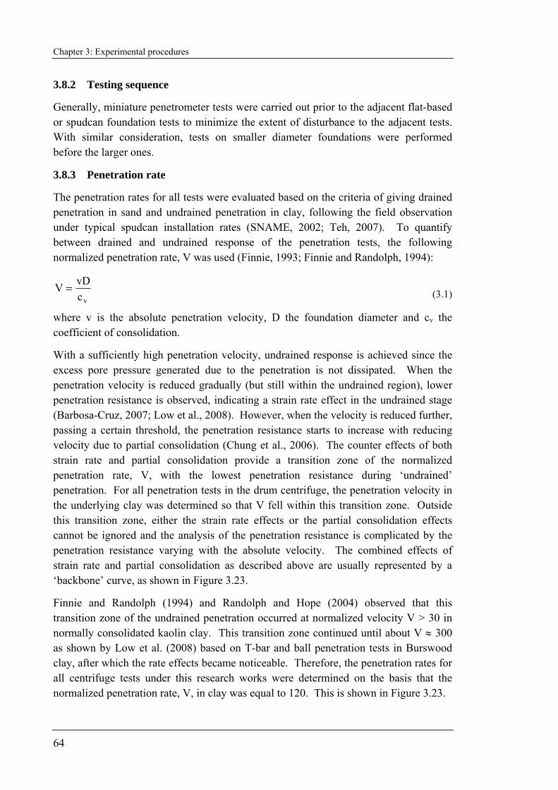
Chapter 3: Experimental procedures
64
3.8.2 Testing sequence
Generally, miniature penetrometer tests were carried out prior to the adjacent flat-based or spudcan foundation tests to minimize the extent of disturbance to the adjacent tests. With similar consideration, tests on smaller diameter foundations were performed before the larger ones.
3.8.3 Penetration rate
The penetration rates for all tests were evaluated based on the criteria of giving drained penetration in sand and undrained penetration in clay, following the field observation under typical spudcan installation rates (SNAME, 2002; Teh, 2007). To quantify between drained and undrained response of the penetration tests, the following normalized penetration rate, V was used (Finnie, 1993; Finnie and Randolph, 1994):
vcvDV = (3.1)
where v is the absolute penetration velocity, D the foundation diameter and cv the coefficient of consolidation.
With a sufficiently high penetration velocity, undrained response is achieved since the excess pore pressure generated due to the penetration is not dissipated. When the penetration velocity is reduced gradually (but still within the undrained region), lower penetration resistance is observed, indicating a strain rate effect in the undrained stage (Barbosa-Cruz, 2007; Low et al., 2008). However, when the velocity is reduced further, passing a certain threshold, the penetration resistance starts to increase with reducing velocity due to partial consolidation (Chung et al., 2006). The counter effects of both strain rate and partial consolidation provide a transition zone of the normalized penetration rate, V, with the lowest penetration resistance during ‘undrained’ penetration. For all penetration tests in the drum centrifuge, the penetration velocity in the underlying clay was determined so that V fell within this transition zone. Outside this transition zone, either the strain rate effects or the partial consolidation effects cannot be ignored and the analysis of the penetration resistance is complicated by the penetration resistance varying with the absolute velocity. The combined effects of strain rate and partial consolidation as described above are usually represented by a ‘backbone’ curve, as shown in Figure 3.23.
Finnie and Randolph (1994) and Randolph and Hope (2004) observed that this transition zone of the undrained penetration occurred at normalized velocity V > 30 in normally consolidated kaolin clay. This transition zone continued until about V ≈ 300 as shown by Low et al. (2008) based on T-bar and ball penetration tests in Burswood clay, after which the rate effects became noticeable. Therefore, the penetration rates for all centrifuge tests under this research works were determined on the basis that the normalized penetration rate, V, in clay was equal to 120. This is shown in Figure 3.23.
Chapter 3: Experimental procedures
65
0.7
0.8
0.9
1
1.1
1.2
1.3
1.4
1 10 100 1000 10000 100000V = vD/cv
q / q
ref
Partial consolidation effects dominate
Strain rate (viscous) effects become noticeable
Adopted V = 120
‘Transition zone’
‘Backbone’curve
Figure 3.23. Effects of strain rate and partial consolidation on values of penetration resistance (after Low et al., 2008)
The absolute penetration rates for various model foundations and penetrometers calculated based on this criterion (V = 120 for the underlying clay) are presented in Table 3.8. A check on these values showed that they were within the working range of the actuator in the UWA drum centrifuge, which had a maximum speed of around 3 mm/s.
Table 3.8. Penetration rates in drum centrifuge tests
Penetration device Diameter, D (mm) Penetration rate, v (mm/s)
30 0.254
40 0.190
50 0.152
60 0.127
70 0.109
Flat-based and spudcan foundations
80 0.095
4 1.903
5 1.522
Ball and T-bar penetrometers
6 1.268

Chapter 3: Experimental procedures
66
Analysis confirmed that the same penetration rates listed in Table 3.8 ensured a drained response in the sand layer. Barbosa-Cruz (2007) observed from spudcan penetration tests that no excess pore pressure was generated when the normalized penetration rate V < 0.1. This indicates fully drained conditions. House et al. (2001) reported the same threshold for drained conditions based on T-bar penetration tests. However, Finnie and Randolph (1994) and Baligh (as presented in Hight and Leroueil, 2003) suggested a lower limit of less than 0.01.
Using the penetration rates listed in Table 3.8, the coefficient of consolidation, cv for sand must be larger than 24,000 m2/year for the normalized penetration rate, V in the upper sand layer to be less than 0.01 and to therefore ensure fully drained conditions.
The thinnest sand layer had a prototype thickness of 3.4 m. Hence, the effective Young’s modulus, E, estimated at the mid depth of this dense sand layer was around 20 MPa (Schanz and Vermeer, 1998). Assuming a typical value of permeability of more than 10-6 m/s (Leroueil and Hight, 2003), the SFS sand used in the centrifuge tests had an estimated cv of at least 60,000 m2/year. Higher cv values would be expected for thicker sand layers due to higher average E values. Hence, the penetration within the sand layer was fully drained with these penetration rates.
3.8.4 Displacement versus load control mode
All penetration tests were carried out under a displacement control mode with the rates outlined in Table 3.8. It is recognised that, in the field, punch-through can cause a rapid penetration, possibly increasing the rate of penetration considerably. However, Teh (2007) found that the difference between displacement controlled and load controlled penetration was negligible in centrifuge tests, provided that the penetration was drained in the upper sand layer and undrained in the underlying clay. Therefore, this minor difference in penetration resistance due to various drainage rates under load control was not considered further in the research presented in this thesis.
Chapter 4: Experimental results
67
CHAPTER 4. EXPERIMENTAL RESULTS
4.1 INTRODUCTION
This chapter presents the drum centrifuge test results of both samples D1 and D2. The first section discusses observation from examination of soil samples collected after the penetration tests on sand overlying clay. The observations are qualitative in nature but they provide some important insights on the penetration mechanism. The penetration profiles of the flat-based and spudcan foundations and miniature ball penetrometers are then presented. There is a focus on the numerical values of the peak penetration resistance of the foundations on different sand thicknesses. These showed consistent trends, indicating the reliability of the centrifuge tests. The latter sections present the soil characterisation of the upper sand layer and the underlying clay of the tests.
4.2 SOIL SAMPLE EXAMINATION AFTER TEST
It is rational to think that some sands will be trapped beneath the foundation when it penetrates from a sand layer into the underlying clay, and this was observed in the particle image velocimetry (PIV) analysis of Teh (2007). Some samples of sand overlying clay were collected from the region around the penetration tests and dissected to examine the post-test soil profiles and the details of the trapped sand left in the clay. The photographs in Figure 4.1 show the processes of extruding, cutting and examining a post-test soil sample.
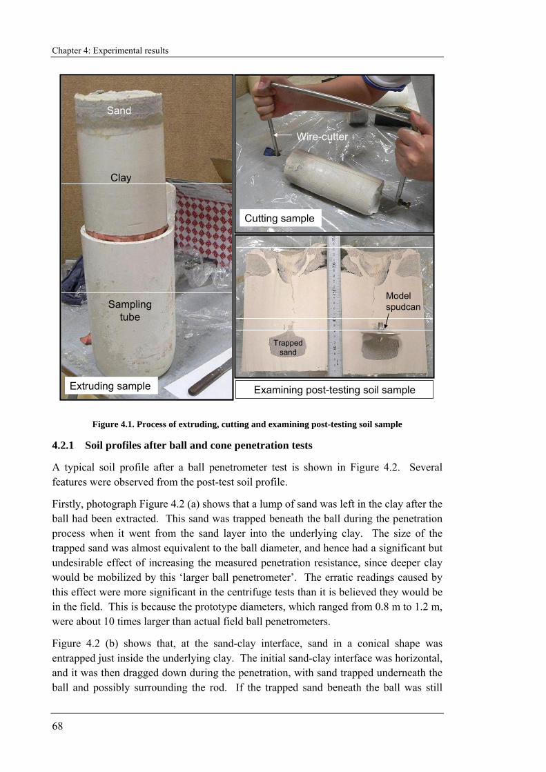
Chapter 4: Experimental results
68
Extruding sample
Cutting sample
Examining post-testing soil sample
Model spudcan
Trapped sand
Wire-cutter
Clay
Sand
Sampling tube
Figure 4.1. Process of extruding, cutting and examining post-testing soil sample
4.2.1 Soil profiles after ball and cone penetration tests
A typical soil profile after a ball penetrometer test is shown in Figure 4.2. Several features were observed from the post-test soil profile.
Firstly, photograph Figure 4.2 (a) shows that a lump of sand was left in the clay after the ball had been extracted. This sand was trapped beneath the ball during the penetration process when it went from the sand layer into the underlying clay. The size of the trapped sand was almost equivalent to the ball diameter, and hence had a significant but undesirable effect of increasing the measured penetration resistance, since deeper clay would be mobilized by this ‘larger ball penetrometer’. The erratic readings caused by this effect were more significant in the centrifuge tests than it is believed they would be in the field. This is because the prototype diameters, which ranged from 0.8 m to 1.2 m, were about 10 times larger than actual field ball penetrometers.
Figure 4.2 (b) shows that, at the sand-clay interface, sand in a conical shape was entrapped just inside the underlying clay. The initial sand-clay interface was horizontal, and it was then dragged down during the penetration, with sand trapped underneath the ball and possibly surrounding the rod. If the trapped sand beneath the ball was still
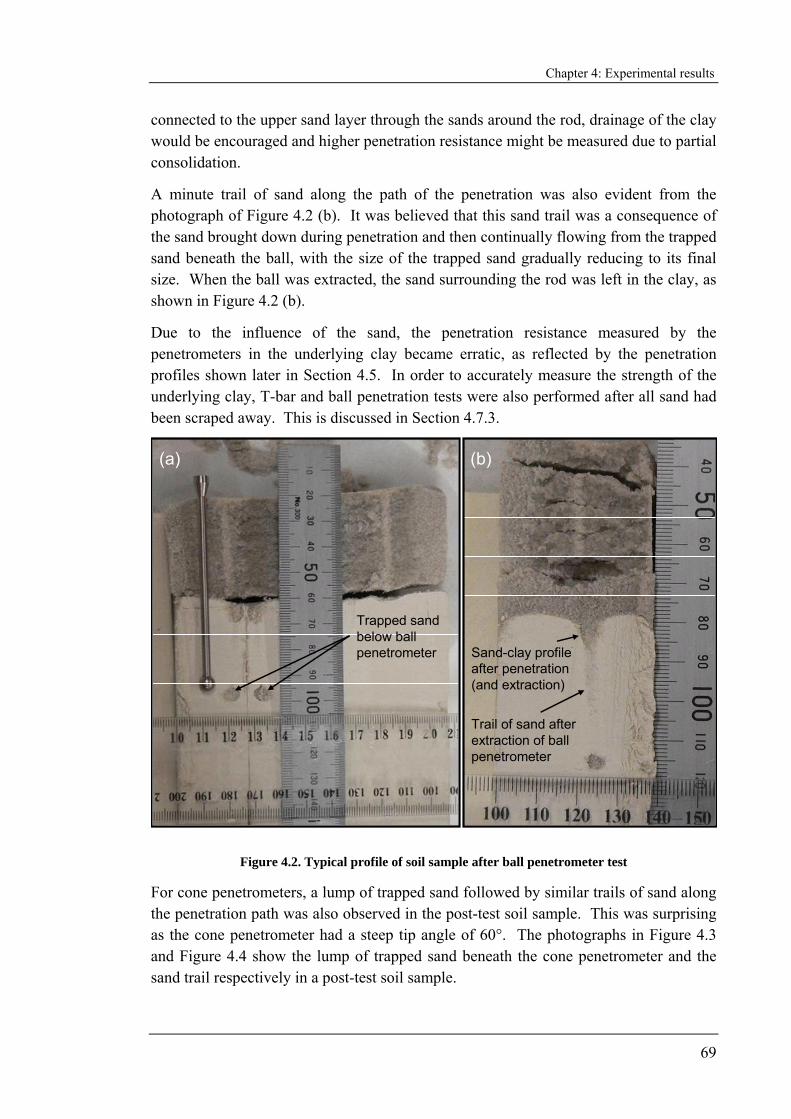
Chapter 4: Experimental results
69
connected to the upper sand layer through the sands around the rod, drainage of the clay would be encouraged and higher penetration resistance might be measured due to partial consolidation.
A minute trail of sand along the path of the penetration was also evident from the photograph of Figure 4.2 (b). It was believed that this sand trail was a consequence of the sand brought down during penetration and then continually flowing from the trapped sand beneath the ball, with the size of the trapped sand gradually reducing to its final size. When the ball was extracted, the sand surrounding the rod was left in the clay, as shown in Figure 4.2 (b).
Due to the influence of the sand, the penetration resistance measured by the penetrometers in the underlying clay became erratic, as reflected by the penetration profiles shown later in Section 4.5. In order to accurately measure the strength of the underlying clay, T-bar and ball penetration tests were also performed after all sand had been scraped away. This is discussed in Section 4.7.3.
Trail of sand after extraction of ball penetrometer
Trapped sand below ball penetrometer Sand-clay profile
after penetration (and extraction)
(a) (b)
Figure 4.2. Typical profile of soil sample after ball penetrometer test
For cone penetrometers, a lump of trapped sand followed by similar trails of sand along the penetration path was also observed in the post-test soil sample. This was surprising as the cone penetrometer had a steep tip angle of 60°. The photographs in Figure 4.3 and Figure 4.4 show the lump of trapped sand beneath the cone penetrometer and the sand trail respectively in a post-test soil sample.

Chapter 4: Experimental results
70
Figure 4.3. Trapped sand beneath cone penetrometer left in the clay after extraction
Figure 4.4. Trail of sand in the underlying clay after cone penetration test
4.2.2 Trapped sand under model spudcan
It was expected that more sand would be brought down into the underlying clay and trapped under the larger size foundations. Figure 4.5 and Figure 4.6 show photographs of a soil sample after a spudcan penetration test. The cylindrical shaped trapped sand had a similar diameter as the spudcan, with a depth approximately 90 % of the thickness of the upper sand layer. It should be noted that the post-test samples investigated were

Chapter 4: Experimental results
71
from cases of Hs/D ratio of less than one. For thicker sand layers, with Hs/D > 1, it is likely that the thickness of the trapped sand will reduce as a ratio of Hs and will ultimately be related more to the diameter of the spudcan, just as for the ball penetrometer.
Trapped sand beneath spudcan
Model spudcan
Clay dropped from the back of spudcan during extraction
Figure 4.5. Soil profile after spudcan penetration
Figure 4.6. Perspective view of the post-testing soil sample
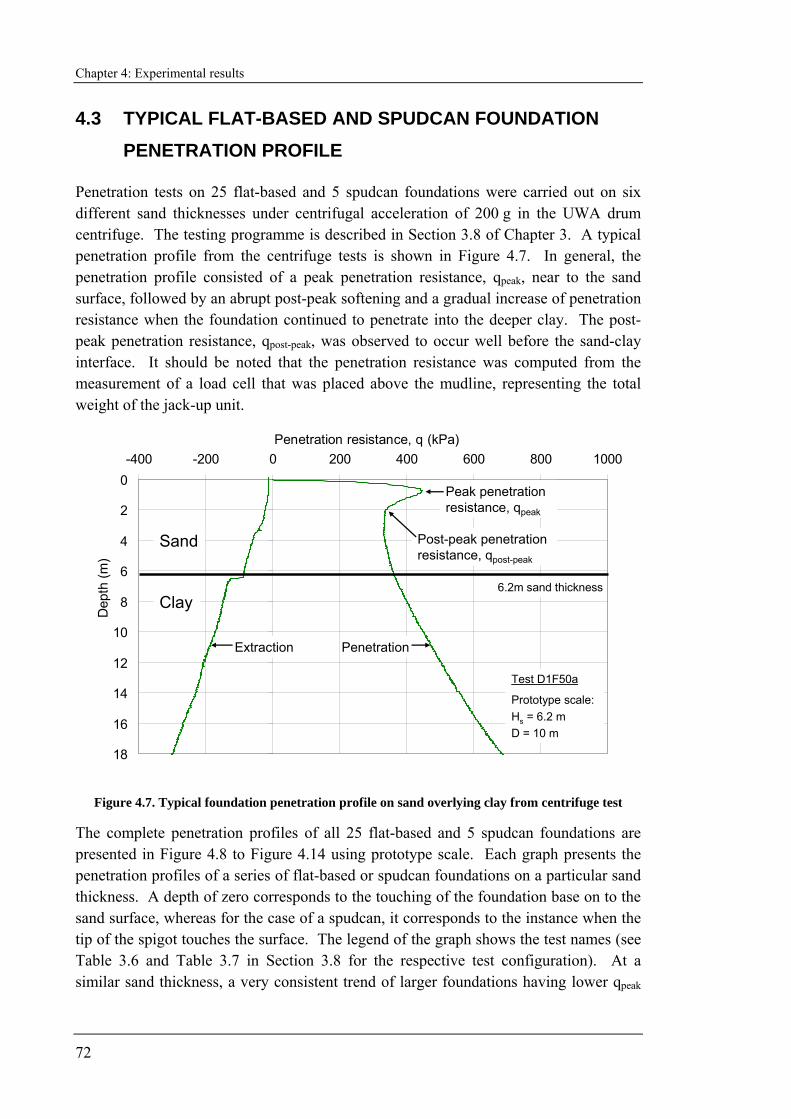
Chapter 4: Experimental results
72
4.3 TYPICAL FLAT-BASED AND SPUDCAN FOUNDATION PENETRATION PROFILE
Penetration tests on 25 flat-based and 5 spudcan foundations were carried out on six different sand thicknesses under centrifugal acceleration of 200 g in the UWA drum centrifuge. The testing programme is described in Section 3.8 of Chapter 3. A typical penetration profile from the centrifuge tests is shown in Figure 4.7. In general, the penetration profile consisted of a peak penetration resistance, qpeak, near to the sand surface, followed by an abrupt post-peak softening and a gradual increase of penetration resistance when the foundation continued to penetrate into the deeper clay. The post-peak penetration resistance, qpost-peak, was observed to occur well before the sand-clay interface. It should be noted that the penetration resistance was computed from the measurement of a load cell that was placed above the mudline, representing the total weight of the jack-up unit.
0
2
4
6
8
10
12
14
16
18
-400 -200 0 200 400 600 800 1000Penetration resistance, q (kPa)
Dep
th (m
)
Peak penetration resistance, qpeak
Post-peak penetration resistance, qpost-peak
Sand
Clay
Extraction
Test D1F50a
Prototype scale:Hs = 6.2 mD = 10 m
Penetration
6.2m sand thickness
Figure 4.7. Typical foundation penetration profile on sand overlying clay from centrifuge test
The complete penetration profiles of all 25 flat-based and 5 spudcan foundations are presented in Figure 4.8 to Figure 4.14 using prototype scale. Each graph presents the penetration profiles of a series of flat-based or spudcan foundations on a particular sand thickness. A depth of zero corresponds to the touching of the foundation base on to the sand surface, whereas for the case of a spudcan, it corresponds to the instance when the tip of the spigot touches the surface. The legend of the graph shows the test names (see Table 3.6 and Table 3.7 in Section 3.8 for the respective test configuration). At a similar sand thickness, a very consistent trend of larger foundations having lower qpeak
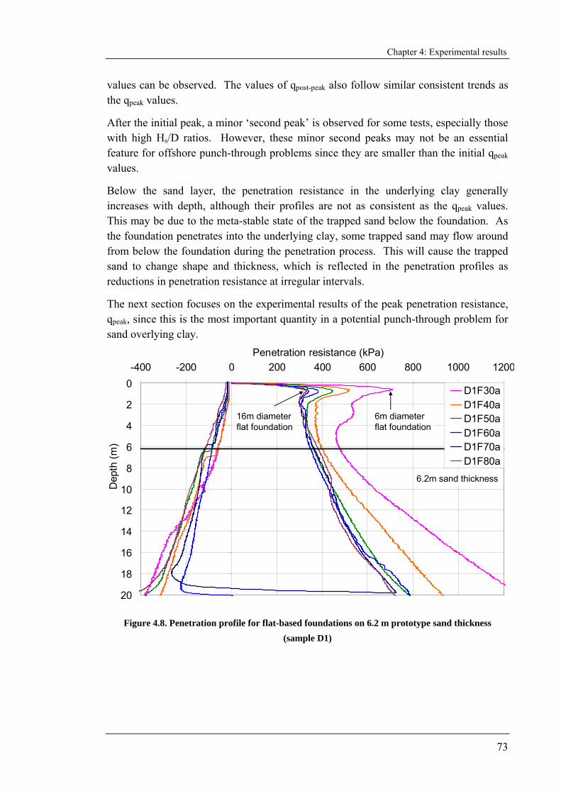
Chapter 4: Experimental results
73
values can be observed. The values of qpost-peak also follow similar consistent trends as the qpeak values.
After the initial peak, a minor ‘second peak’ is observed for some tests, especially those with high Hs/D ratios. However, these minor second peaks may not be an essential feature for offshore punch-through problems since they are smaller than the initial qpeak values.
Below the sand layer, the penetration resistance in the underlying clay generally increases with depth, although their profiles are not as consistent as the qpeak values. This may be due to the meta-stable state of the trapped sand below the foundation. As the foundation penetrates into the underlying clay, some trapped sand may flow around from below the foundation during the penetration process. This will cause the trapped sand to change shape and thickness, which is reflected in the penetration profiles as reductions in penetration resistance at irregular intervals.
The next section focuses on the experimental results of the peak penetration resistance, qpeak, since this is the most important quantity in a potential punch-through problem for sand overlying clay.
0
2
4
6
8
10
12
14
16
18
20
-400 -200 0 200 400 600 800 1000 1200Penetration resistance (kPa)
Dep
th (m
)
D1F30aD1F40aD1F50aD1F60aD1F70aD1F80a
6.2m sand thickness
6m diameter flat foundation
16m diameter flat foundation
Figure 4.8. Penetration profile for flat-based foundations on 6.2 m prototype sand thickness (sample D1)
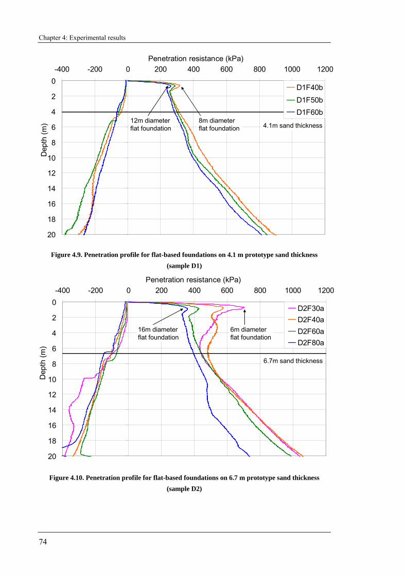
Chapter 4: Experimental results
74
0
2
4
6
8
10
12
14
16
18
20
-400 -200 0 200 400 600 800 1000 1200Penetration resistance (kPa)
Dep
th (m
)
D1F40b
D1F50bD1F60b
4.1m sand thickness8m diameter flat foundation
12m diameter flat foundation
Figure 4.9. Penetration profile for flat-based foundations on 4.1 m prototype sand thickness (sample D1)
0
2
4
6
8
10
12
14
16
18
20
-400 -200 0 200 400 600 800 1000 1200Penetration resistance (kPa)
Dep
th (m
)
D2F30aD2F40aD2F60aD2F80a
6.7m sand thickness
6m diameter flat foundation
16m diameter flat foundation
Figure 4.10. Penetration profile for flat-based foundations on 6.7 m prototype sand thickness (sample D2)
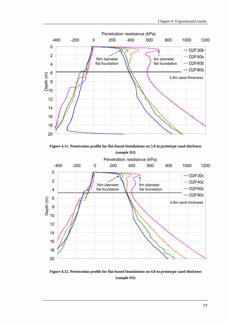
Chapter 4: Experimental results
75
0
2
4
6
8
10
12
14
16
18
20
-400 -200 0 200 400 600 800 1000 1200Penetration resistance (kPa)
Dep
th (m
)D2F30bD2F40bD2F60bD2F80b
5.8m sand thickness
6m diameter flat foundation
16m diameter flat foundation
Figure 4.11. Penetration profile for flat-based foundations on 5.8 m prototype sand thickness (sample D2)
0
2
4
6
8
10
12
14
16
18
20
-400 -200 0 200 400 600 800 1000 1200Penetration resistance (kPa)
Dep
th (m
)
D2F30cD2F40cD2F60cD2F80c
4.8m sand thickness
6m diameter flat foundation
16m diameter flat foundation
Figure 4.12. Penetration profile for flat-based foundations on 4.8 m prototype sand thickness (sample D2)
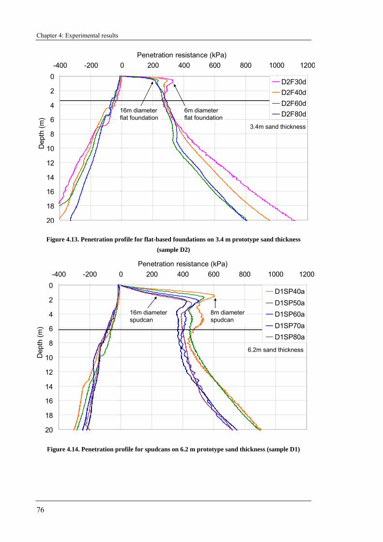
Chapter 4: Experimental results
76
0
2
4
6
8
10
12
14
16
18
20
-400 -200 0 200 400 600 800 1000 1200Penetration resistance (kPa)
Dep
th (m
)
D2F30dD2F40dD2F60dD2F80d
3.4m sand thickness
6m diameter flat foundation
16m diameter flat foundation
Figure 4.13. Penetration profile for flat-based foundations on 3.4 m prototype sand thickness (sample D2)
0
2
4
6
8
10
12
14
16
18
20
-400 -200 0 200 400 600 800 1000 1200Penetration resistance (kPa)
Dep
th (m
)
D1SP40aD1SP50aD1SP60aD1SP70aD1SP80a
6.2m sand thickness
8m diameter spudcan
16m diameter spudcan
Figure 4.14. Penetration profile for spudcans on 6.2 m prototype sand thickness (sample D1)
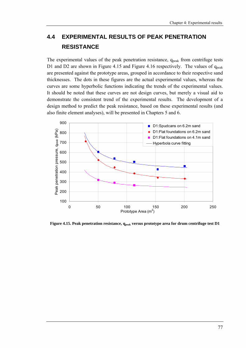
Chapter 4: Experimental results
77
4.4 EXPERIMENTAL RESULTS OF PEAK PENETRATION RESISTANCE
The experimental values of the peak penetration resistance, qpeak from centrifuge tests D1 and D2 are shown in Figure 4.15 and Figure 4.16 respectively. The values of qpeak are presented against the prototype areas, grouped in accordance to their respective sand thicknesses. The dots in these figures are the actual experimental values, whereas the curves are some hyperbolic functions indicating the trends of the experimental values. It should be noted that these curves are not design curves, but merely a visual aid to demonstrate the consistent trend of the experimental results. The development of a design method to predict the peak resistance, based on these experimental results (and also finite element analyses), will be presented in Chapters 5 and 6.
100
200
300
400
500
600
700
800
900
0 50 100 150 200 250Prototype Area (m2)
Pea
k pe
netra
tion
pres
sure
, q pe
ak (k
Pa)
D1:Spudcans on 6.2m sandD1:Flat foundations on 6.2m sandD1:Flat foundations on 4.1m sandHyperbola curve fitting
Figure 4.15. Peak penetration resistance, qpeak versus prototype area for drum centrifuge test D1
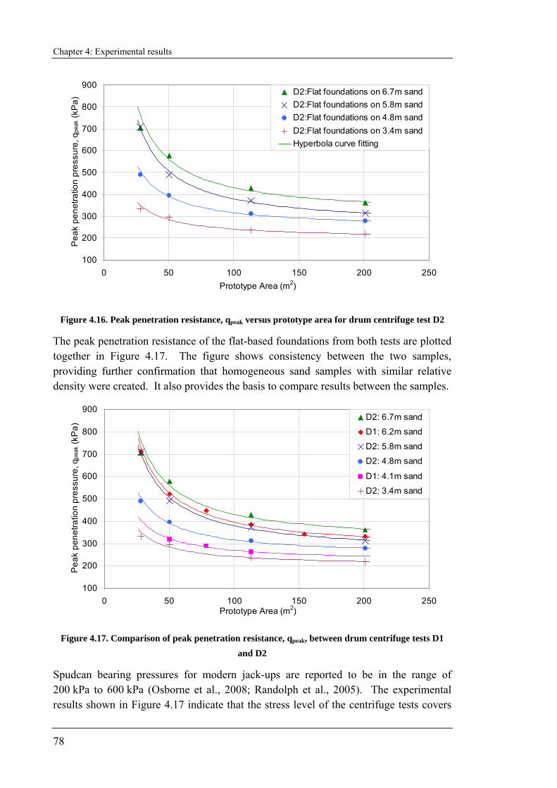
Chapter 4: Experimental results
78
100
200
300
400
500
600
700
800
900
0 50 100 150 200 250Prototype Area (m2)
Pea
k pe
netra
tion
pres
sure
, q pe
ak (k
Pa)
D2:Flat foundations on 6.7m sandD2:Flat foundations on 5.8m sandD2:Flat foundations on 4.8m sandD2:Flat foundations on 3.4m sandHyperbola curve fitting
Figure 4.16. Peak penetration resistance, qpeak versus prototype area for drum centrifuge test D2
The peak penetration resistance of the flat-based foundations from both tests are plotted together in Figure 4.17. The figure shows consistency between the two samples, providing further confirmation that homogeneous sand samples with similar relative density were created. It also provides the basis to compare results between the samples.
100
200
300
400
500
600
700
800
900
0 50 100 150 200 250Prototype Area (m2)
Pea
k pe
netra
tion
pres
sure
, q pe
ak (k
Pa)
D2: 6.7m sand
D1: 6.2m sand
D2: 5.8m sand
D2: 4.8m sand
D1: 4.1m sand
D2: 3.4m sand
Figure 4.17. Comparison of peak penetration resistance, qpeak, between drum centrifuge tests D1 and D2
Spudcan bearing pressures for modern jack-ups are reported to be in the range of 200 kPa to 600 kPa (Osborne et al., 2008; Randolph et al., 2005). The experimental results shown in Figure 4.17 indicate that the stress level of the centrifuge tests covers
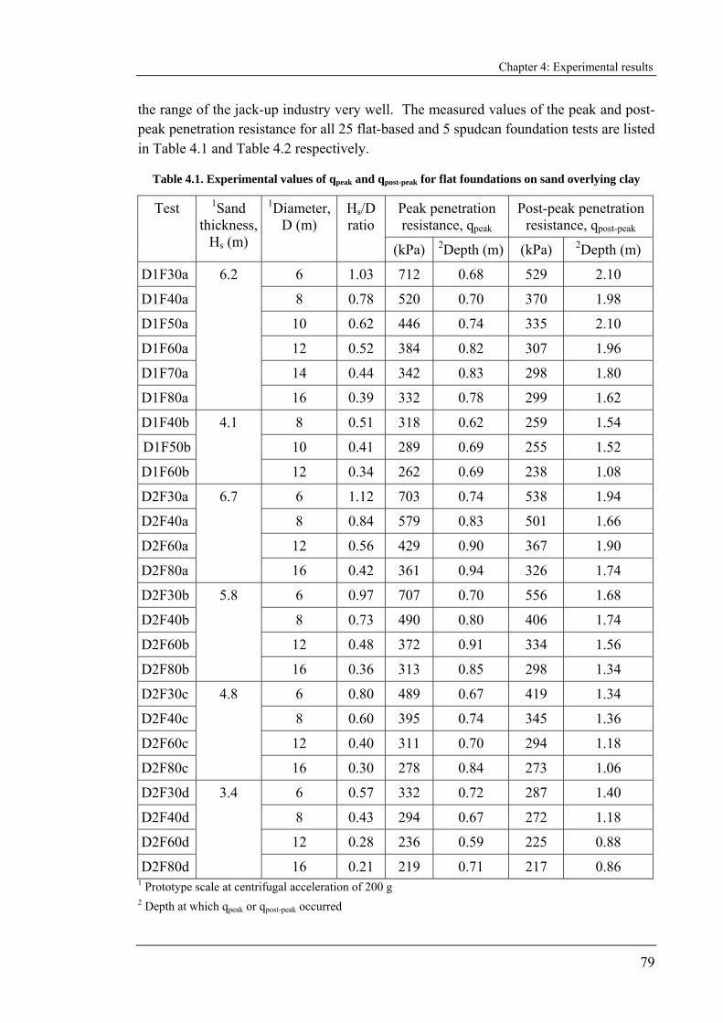
Chapter 4: Experimental results
79
the range of the jack-up industry very well. The measured values of the peak and post-peak penetration resistance for all 25 flat-based and 5 spudcan foundation tests are listed in Table 4.1 and Table 4.2 respectively.
Table 4.1. Experimental values of qpeak and qpost-peak for flat foundations on sand overlying clay
Peak penetration resistance, qpeak
Post-peak penetration resistance, qpost-peak
Test 1Sand thickness,
Hs (m)
1Diameter, D (m)
Hs/D ratio
(kPa) 2Depth (m) (kPa) 2Depth (m)
D1F30a 6 1.03 712 0.68 529 2.10
D1F40a 8 0.78 520 0.70 370 1.98
D1F50a 10 0.62 446 0.74 335 2.10
D1F60a 12 0.52 384 0.82 307 1.96
D1F70a 14 0.44 342 0.83 298 1.80
D1F80a
6.2
16 0.39 332 0.78 299 1.62
D1F40b 8 0.51 318 0.62 259 1.54
D1F50b 10 0.41 289 0.69 255 1.52
D1F60b
4.1
12 0.34 262 0.69 238 1.08
D2F30a 6 1.12 703 0.74 538 1.94
D2F40a 8 0.84 579 0.83 501 1.66
D2F60a 12 0.56 429 0.90 367 1.90
D2F80a
6.7
16 0.42 361 0.94 326 1.74
D2F30b 6 0.97 707 0.70 556 1.68
D2F40b 8 0.73 490 0.80 406 1.74
D2F60b 12 0.48 372 0.91 334 1.56
D2F80b
5.8
16 0.36 313 0.85 298 1.34
D2F30c 6 0.80 489 0.67 419 1.34
D2F40c 8 0.60 395 0.74 345 1.36
D2F60c 12 0.40 311 0.70 294 1.18
D2F80c
4.8
16 0.30 278 0.84 273 1.06
D2F30d 6 0.57 332 0.72 287 1.40
D2F40d 8 0.43 294 0.67 272 1.18
D2F60d 12 0.28 236 0.59 225 0.88
D2F80d
3.4
16 0.21 219 0.71 217 0.86 1 Prototype scale at centrifugal acceleration of 200 g 2 Depth at which qpeak or qpost-peak occurred
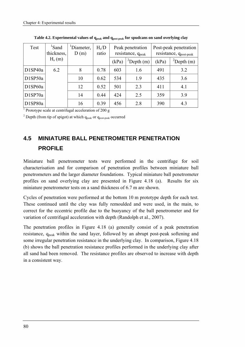
Chapter 4: Experimental results
80
Table 4.2. Experimental values of qpeak and qpost-peak for spudcans on sand overlying clay
Peak penetration resistance, qpeak
Post-peak penetration resistance, qpost-peak
Test 1Sand thickness,
Hs (m)
1Diameter, D (m)
Hs/D ratio
(kPa) 2Depth (m) (kPa) 2Depth (m)
D1SP40a 8 0.78 603 1.6 491 3.2
D1SP50a 10 0.62 534 1.9 435 3.6
D1SP60a 12 0.52 501 2.3 411 4.1
D1SP70a 14 0.44 424 2.5 359 3.9
D1SP80a
6.2
16 0.39 456 2.8 390 4.3 1 Prototype scale at centrifugal acceleration of 200 g 2 Depth (from tip of spigot) at which qpeak or qpost-peak occurred
4.5 MINIATURE BALL PENETROMETER PENETRATION PROFILE
Miniature ball penetrometer tests were performed in the centrifuge for soil characterisation and for comparison of penetration profiles between miniature ball penetrometers and the larger diameter foundations. Typical miniature ball penetrometer profiles on sand overlying clay are presented in Figure 4.18 (a). Results for six miniature penetrometer tests on a sand thickness of 6.7 m are shown.
Cycles of penetration were performed at the bottom 10 m prototype depth for each test. These continued until the clay was fully remoulded and were used, in the main, to correct for the eccentric profile due to the buoyancy of the ball penetrometer and for variation of centrifugal acceleration with depth (Randolph et al., 2007).
The penetration profiles in Figure 4.18 (a) generally consist of a peak penetration resistance, qpeak within the sand layer, followed by an abrupt post-peak softening and some irregular penetration resistance in the underlying clay. In comparison, Figure 4.18 (b) shows the ball penetration resistance profiles performed in the underlying clay after all sand had been removed. The resistance profiles are observed to increase with depth in a consistent way.
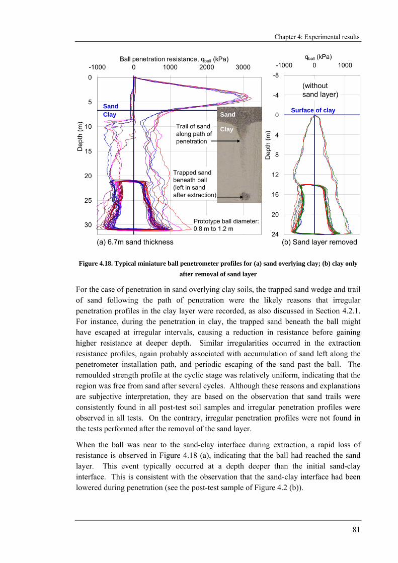
Chapter 4: Experimental results
81
-8
-4
0
4
8
12
16
20
24
-1000 0 1000qball (kPa)
Dep
th (m
)
0
5
10
15
20
25
30
-1000 0 1000 2000 3000Ball penetration resistance, qball (kPa)
Dep
th (m
)
Sand
Clay
(a) 6.7m sand thickness
SandClay
Prototype ball diameter: 0.8 m to 1.2 m
Trail of sand along path of penetration
Trapped sand beneath ball (left in sand after extraction)
(b) Sand layer removed
Surface of clay
(without sand layer)
Figure 4.18. Typical miniature ball penetrometer profiles for (a) sand overlying clay; (b) clay only after removal of sand layer
For the case of penetration in sand overlying clay soils, the trapped sand wedge and trail of sand following the path of penetration were the likely reasons that irregular penetration profiles in the clay layer were recorded, as also discussed in Section 4.2.1. For instance, during the penetration in clay, the trapped sand beneath the ball might have escaped at irregular intervals, causing a reduction in resistance before gaining higher resistance at deeper depth. Similar irregularities occurred in the extraction resistance profiles, again probably associated with accumulation of sand left along the penetrometer installation path, and periodic escaping of the sand past the ball. The remoulded strength profile at the cyclic stage was relatively uniform, indicating that the region was free from sand after several cycles. Although these reasons and explanations are subjective interpretation, they are based on the observation that sand trails were consistently found in all post-test soil samples and irregular penetration profiles were observed in all tests. On the contrary, irregular penetration profiles were not found in the tests performed after the removal of the sand layer.
When the ball was near to the sand-clay interface during extraction, a rapid loss of resistance is observed in Figure 4.18 (a), indicating that the ball had reached the sand layer. This event typically occurred at a depth deeper than the initial sand-clay interface. This is consistent with the observation that the sand-clay interface had been lowered during penetration (see the post-test sample of Figure 4.2 (b)).
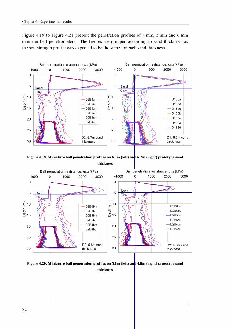
Chapter 4: Experimental results
82
Figure 4.19 to Figure 4.21 present the penetration profiles of 4 mm, 5 mm and 6 mm diameter ball penetrometers. The figures are grouped according to sand thickness, as the soil strength profile was expected to be the same for each sand thickness.
0
5
10
15
20
25
30
-1000 0 1000 2000 3000Ball penetration resistance, qball (kPa)
Dep
th (m
)
D2B6amD2B6auD2B5amD2B5auD2B4amD2B4au
D2: 6.7m sand thickness
SandClay
0
5
10
15
20
25
30
-1000 0 1000 2000 3000Ball penetration resistance, qball (kPa)
Dep
th (m
)
D2B6amD2B6auD2B5amD2B5auD2B4amD2B4au
D2: 6.7m sand thickness
SandClay
0
5
10
15
20
25
30
-1000 0 1000 2000 3000Ball penetration resistance, qball (kPa)
Dep
th (m
)
D1B5aD1B5dD1B5gD1B5kD1B5nD1B6aD1B6d
D1: 6.2m sand thickness
SandClay
0
5
10
15
20
25
30
-1000 0 1000 2000 3000Ball penetration resistance, qball (kPa)
Dep
th (m
)
D1B5aD1B5dD1B5gD1B5kD1B5nD1B6aD1B6d
D1: 6.2m sand thickness
SandClay
Figure 4.19. Miniature ball penetration profiles on 6.7m (left) and 6.2m (right) prototype sand thickness
0
5
10
15
20
25
30
-1000 0 1000 2000 3000Ball penetration resistance, qball (kPa)
Dep
th (m
)
D2B6bmD2B6buD2B5bmD2B5buD2B4bmD2B4bu
D2: 5.8m sand thickness
SandClay
0
5
10
15
20
25
30
-1000 0 1000 2000 3000Ball penetration resistance, qball (kPa)
Dep
th (m
)
D2B6bmD2B6buD2B5bmD2B5buD2B4bmD2B4bu
D2: 5.8m sand thickness
SandClay
0
5
10
15
20
25
30
-1000 0 1000 2000 3000Ball penetration resistance, qball (kPa)
Dep
th (m
)
D2B6cmD2B6cuD2B5cmD2B5cuD2B4cmD2B4cu
D2: 4.8m sand thickness
SandClay
0
5
10
15
20
25
30
-1000 0 1000 2000 3000Ball penetration resistance, qball (kPa)
Dep
th (m
)
D2B6cmD2B6cuD2B5cmD2B5cuD2B4cmD2B4cu
D2: 4.8m sand thickness
SandClay
Figure 4.20. Miniature ball penetration profiles on 5.8m (left) and 4.8m (right) prototype sand thickness
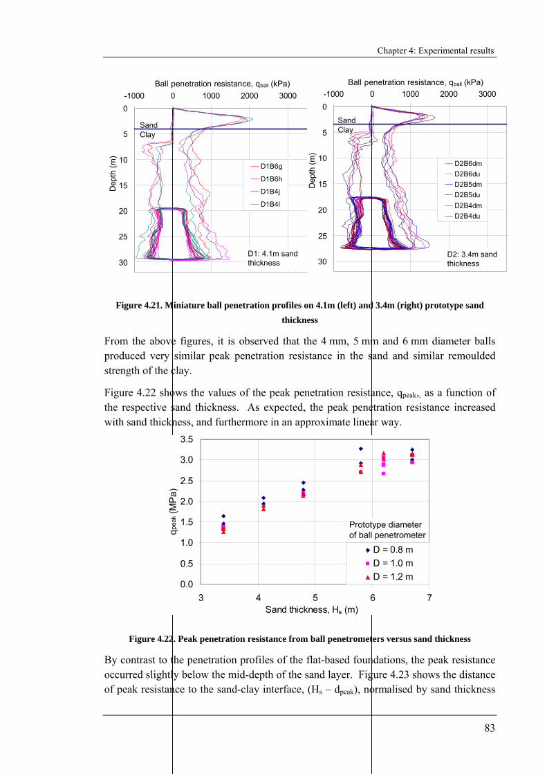
Chapter 4: Experimental results
83
0
5
10
15
20
25
30
-1000 0 1000 2000 3000Ball penetration resistance, qball (kPa)
Dep
th (m
)
D1B6g
D1B6h
D1B4j
D1B4l
D1: 4.1m sand thickness
SandClay
0
5
10
15
20
25
30
-1000 0 1000 2000 3000Ball penetration resistance, qball (kPa)
Dep
th (m
)
D1B6g
D1B6h
D1B4j
D1B4l
D1: 4.1m sand thickness
SandClay
0
5
10
15
20
25
30
-1000 0 1000 2000 3000Ball penetration resistance, qball (kPa)
Dep
th (m
)
D2B6dmD2B6duD2B5dmD2B5duD2B4dmD2B4du
D2: 3.4m sand thickness
SandClay
0
5
10
15
20
25
30
-1000 0 1000 2000 3000Ball penetration resistance, qball (kPa)
Dep
th (m
)
D2B6dmD2B6duD2B5dmD2B5duD2B4dmD2B4du
D2: 3.4m sand thickness
SandClay
Figure 4.21. Miniature ball penetration profiles on 4.1m (left) and 3.4m (right) prototype sand thickness
From the above figures, it is observed that the 4 mm, 5 mm and 6 mm diameter balls produced very similar peak penetration resistance in the sand and similar remoulded strength of the clay.
Figure 4.22 shows the values of the peak penetration resistance, qpeak,, as a function of the respective sand thickness. As expected, the peak penetration resistance increased with sand thickness, and furthermore in an approximate linear way.
0.0
0.5
1.0
1.5
2.0
2.5
3.0
3.5
3 4 5 6 7Sand thickness, Hs (m)
qpea
k (M
Pa)
D = 0.8 mD = 1.0 mD = 1.2 m
Prototype diameter of ball penetrometer
Figure 4.22. Peak penetration resistance from ball penetrometers versus sand thickness
By contrast to the penetration profiles of the flat-based foundations, the peak resistance occurred slightly below the mid-depth of the sand layer. Figure 4.23 shows the distance of peak resistance to the sand-clay interface, (Hs – dpeak), normalised by sand thickness
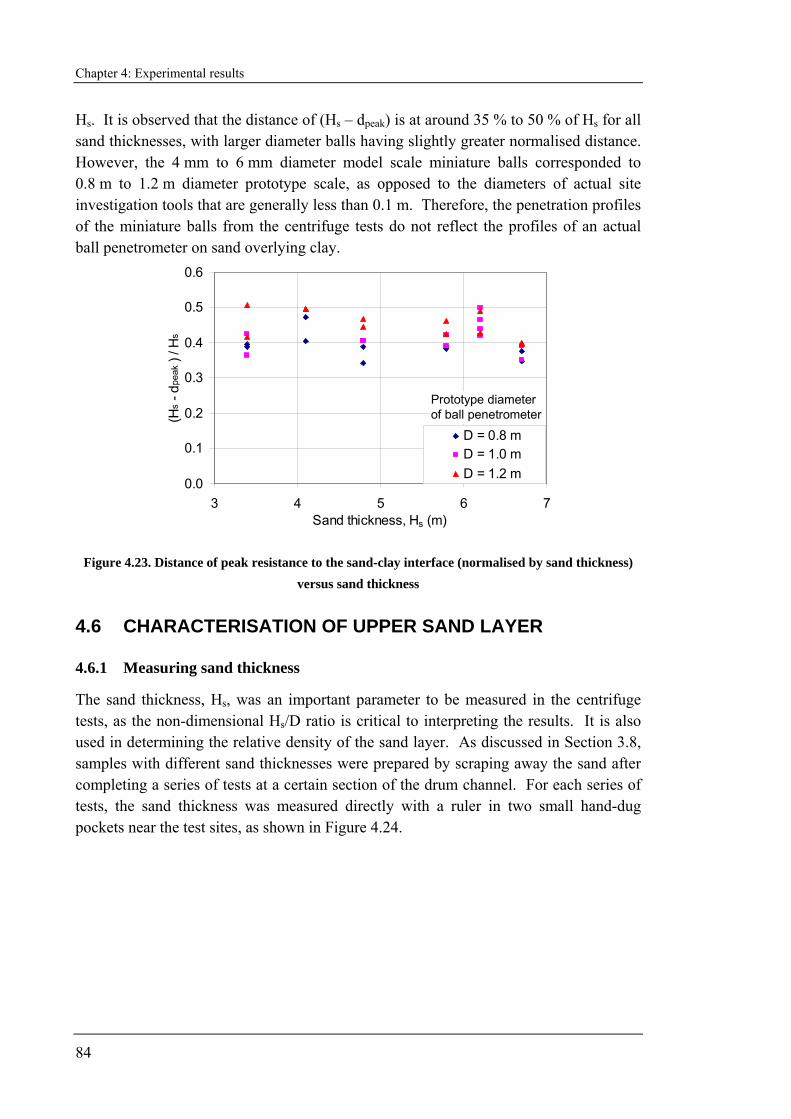
Chapter 4: Experimental results
84
Hs. It is observed that the distance of (Hs – dpeak) is at around 35 % to 50 % of Hs for all sand thicknesses, with larger diameter balls having slightly greater normalised distance. However, the 4 mm to 6 mm diameter model scale miniature balls corresponded to 0.8 m to 1.2 m diameter prototype scale, as opposed to the diameters of actual site investigation tools that are generally less than 0.1 m. Therefore, the penetration profiles of the miniature balls from the centrifuge tests do not reflect the profiles of an actual ball penetrometer on sand overlying clay.
0.0
0.1
0.2
0.3
0.4
0.5
0.6
3 4 5 6 7Sand thickness, Hs (m)
(Hs -
dpe
ak )
/ Hs
D = 0.8 mD = 1.0 mD = 1.2 m
Prototype diameter of ball penetrometer
Figure 4.23. Distance of peak resistance to the sand-clay interface (normalised by sand thickness) versus sand thickness
4.6 CHARACTERISATION OF UPPER SAND LAYER
4.6.1 Measuring sand thickness
The sand thickness, Hs, was an important parameter to be measured in the centrifuge tests, as the non-dimensional Hs/D ratio is critical to interpreting the results. It is also used in determining the relative density of the sand layer. As discussed in Section 3.8, samples with different sand thicknesses were prepared by scraping away the sand after completing a series of tests at a certain section of the drum channel. For each series of tests, the sand thickness was measured directly with a ruler in two small hand-dug pockets near the test sites, as shown in Figure 4.24.
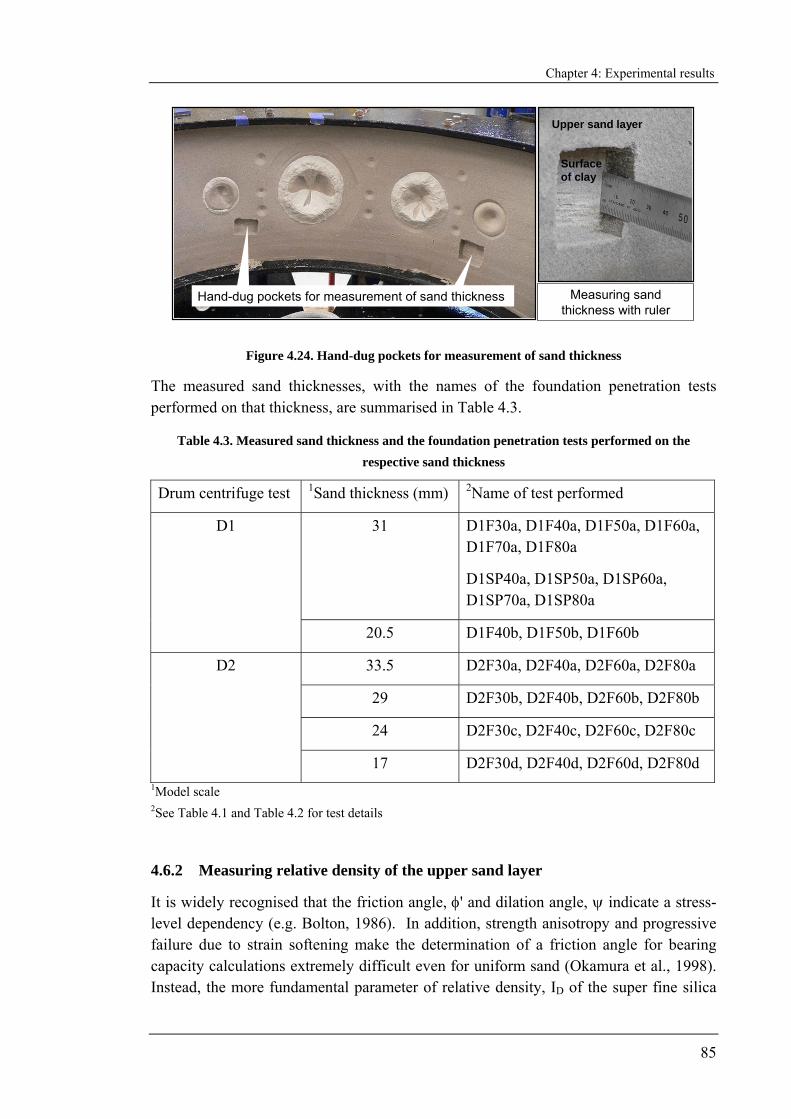
Chapter 4: Experimental results
85
Measuring sand thickness with ruler
Hand-dug pockets for measurement of sand thickness
Surface of clay
Upper sand layer
Figure 4.24. Hand-dug pockets for measurement of sand thickness
The measured sand thicknesses, with the names of the foundation penetration tests performed on that thickness, are summarised in Table 4.3.
Table 4.3. Measured sand thickness and the foundation penetration tests performed on the respective sand thickness
Drum centrifuge test 1Sand thickness (mm) 2Name of test performed
31 D1F30a, D1F40a, D1F50a, D1F60a, D1F70a, D1F80a
D1SP40a, D1SP50a, D1SP60a, D1SP70a, D1SP80a
D1
20.5 D1F40b, D1F50b, D1F60b
33.5 D2F30a, D2F40a, D2F60a, D2F80a
29 D2F30b, D2F40b, D2F60b, D2F80b
24 D2F30c, D2F40c, D2F60c, D2F80c
D2
17 D2F30d, D2F40d, D2F60d, D2F80d 1Model scale 2See Table 4.1 and Table 4.2 for test details
4.6.2 Measuring relative density of the upper sand layer
It is widely recognised that the friction angle, φ' and dilation angle, ψ indicate a stress-level dependency (e.g. Bolton, 1986). In addition, strength anisotropy and progressive failure due to strain softening make the determination of a friction angle for bearing capacity calculations extremely difficult even for uniform sand (Okamura et al., 1998). Instead, the more fundamental parameter of relative density, ID of the super fine silica

Chapter 4: Experimental results
86
(SFS) sand was measured in the experiment to represent the existing state of the sand sample. Finite element analysis, described in Chapter 5, shows that the stress dependent friction angles and dilation angles for different foundation sizes and sand thicknesses can be back-calculated using the experimentally measured relative density.
Based on centrifuge modelling of cone penetration tests (CPTs) in sand, Bolton et al. (1999) found that it was difficult to assess the relative density, ID of the sand at depths of less than 10 diameters as the normalised cone penetration resistance did not reach a steady state but increased with depth ratio in the fashion of shallow foundations. In the present work, the diameters of the available ball and cone penetrometers ranged from 4 mm to 6 mm, but the maximum sand thickness in the centrifuge tests was only 33.5 mm (both in model scale), which was less than 10 diameters of the smallest probe. With further complication from the stratification effect of the underlying clay, it was therefore not possible to assess the relative density of the upper sand layer using miniature probes.
Consequently, an alternate and direct method was pursued. All of the sand was collected to evaluate the relative density. The volume was calculated from the measured sand thickness and the dry weight was determined by weighing the oven dried sand. The relative density, ID of the sand was found to be 92 % for both drum centrifuge tests.
4.7 UNDRAINED SHEAR STRENGTH PROFILE OF THE UNDERLYING CLAY
4.7.1 Background on undrained shear strength profile
When estimating the undrained shear strength of the underlying clay, it is important to consider both the current stress level and the stress history. The following empirical relationship is commonly used to relate the undrained shear strength of clay, su, with its current vertical effective stress, σ'v, and the stress history, represented by the overconsolidation ratio, OCR (Jamiolkowski et al., 1985; Koutsoftas and Ladd,1985):
m
v
u OCRs'
s=
σ (4.1)
where s is the undrained strength ratio for normally consolidated clay (i.e. OCR = 1) and m an exponent describing the strength increase due to overconsolidation. Wroth (1984) presented theoretical evidence to suggest that m = 0.8 is an appropriate estimate for most soils, based on critical state soil mechanics theory and stipulating that m is equivalent to the plastic volumetric strain ratio. Ladd (1991), on the other hand, presented experimental values of 0.74 < m < 1.0, with the range depending on the mode of failure.
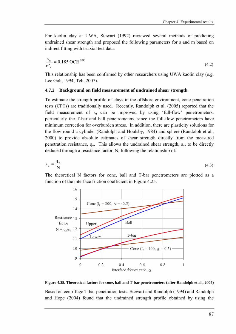
Chapter 4: Experimental results
87
For kaolin clay at UWA, Stewart (1992) reviewed several methods of predicting undrained shear strength and proposed the following parameters for s and m based on indirect fitting with triaxial test data:
85.0
v
u OCR185.0'
s=
σ (4.2)
This relationship has been confirmed by other researchers using UWA kaolin clay (e.g. Lee Goh, 1994; Teh, 2007).
4.7.2 Background on field measurement of undrained shear strength
To estimate the strength profile of clays in the offshore environment, cone penetration tests (CPTs) are traditionally used. Recently, Randolph et al. (2005) reported that the field measurement of su can be improved by using ‘full-flow’ penetrometers, particularly the T-bar and ball penetrometers, since the full-flow penetrometers have minimum correction for overburden stress. In addition, there are plasticity solutions for the flow round a cylinder (Randolph and Houlsby, 1984) and sphere (Randolph et al., 2000) to provide absolute estimates of shear strength directly from the measured penetration resistance, qu. This allows the undrained shear strength, su, to be directly deduced through a resistance factor, N, following the relationship of:
Nq
s uu = (4.3)
The theoretical N factors for cone, ball and T-bar penetrometers are plotted as a function of the interface friction coefficient in Figure 4.25.
Figure 4.25. Theoretical factors for cone, ball and T-bar penetrometers (after Randolph et al., 2005)
Based on centrifuge T-bar penetration tests, Stewart and Randolph (1994) and Randolph and Hope (2004) found that the undrained strength profile obtained by using the
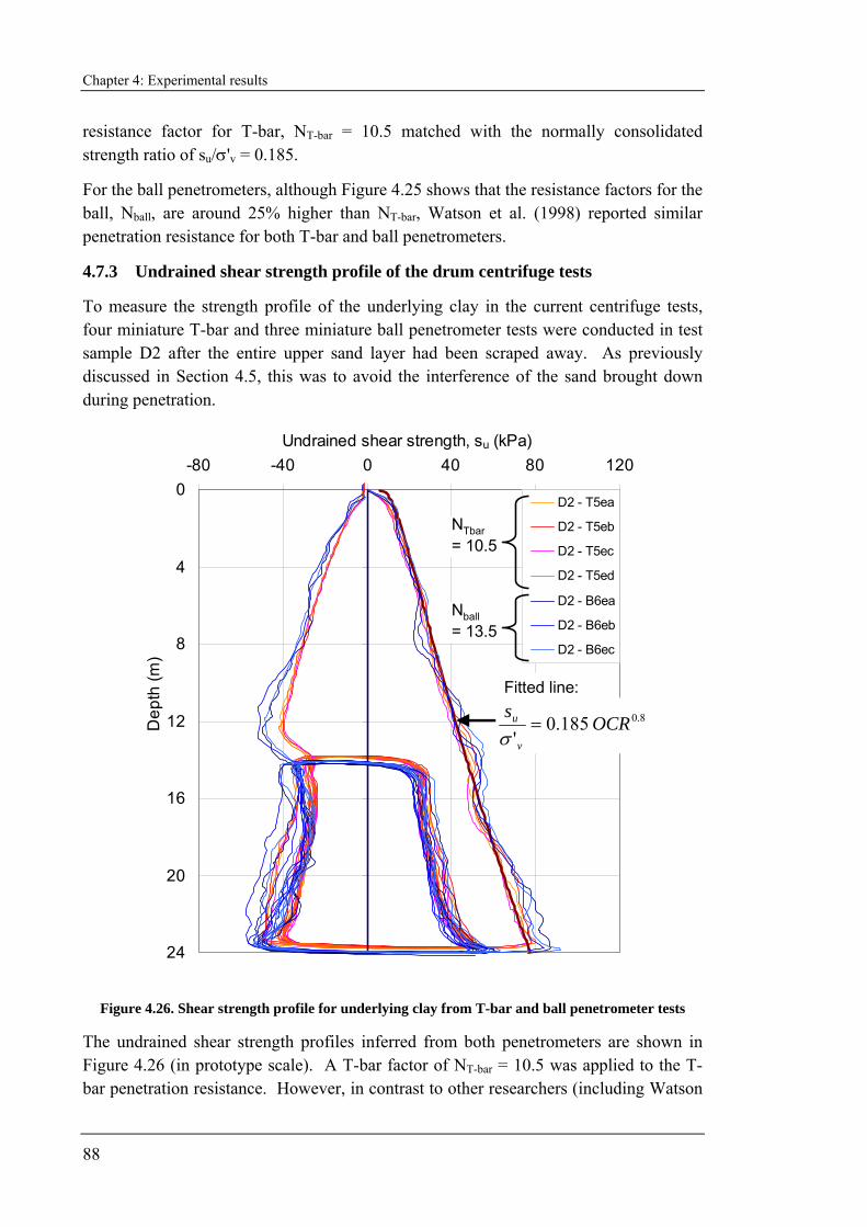
Chapter 4: Experimental results
88
resistance factor for T-bar, NT-bar = 10.5 matched with the normally consolidated strength ratio of su/σ'v = 0.185.
For the ball penetrometers, although Figure 4.25 shows that the resistance factors for the ball, Nball, are around 25% higher than NT-bar, Watson et al. (1998) reported similar penetration resistance for both T-bar and ball penetrometers.
4.7.3 Undrained shear strength profile of the drum centrifuge tests
To measure the strength profile of the underlying clay in the current centrifuge tests, four miniature T-bar and three miniature ball penetrometer tests were conducted in test sample D2 after the entire upper sand layer had been scraped away. As previously discussed in Section 4.5, this was to avoid the interference of the sand brought down during penetration.
0
4
8
12
16
20
24
-80 -40 0 40 80 120Undrained shear strength, su (kPa)
Dep
th (m
)
D2 - T5ea
D2 - T5eb
D2 - T5ec
D2 - T5ed
D2 - B6ea
D2 - B6eb
D2 - B6ec
NTbar= 10.5
Nball= 13.5
8.0185.0'
OCRs
v
u =σ
Fitted line:
Figure 4.26. Shear strength profile for underlying clay from T-bar and ball penetrometer tests
The undrained shear strength profiles inferred from both penetrometers are shown in Figure 4.26 (in prototype scale). A T-bar factor of NT-bar = 10.5 was applied to the T-bar penetration resistance. However, in contrast to other researchers (including Watson
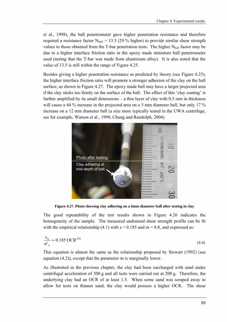
Chapter 4: Experimental results
89
et al., 1998), the ball penetrometer gave higher penetration resistance and therefore required a resistance factor Nball = 13.5 (29 % higher) to provide similar shear strength values to those obtained from the T-bar penetration tests. The higher Nball factor may be due to a higher interface friction ratio in the epoxy made miniature ball penetrometer used (noting that the T-bar was made from aluminium alloy). It is also noted that the value of 13.5 is still within the range of Figure 4.25.
Besides giving a higher penetration resistance as predicted by theory (see Figure 4.25), the higher interface friction ratio will promote a stronger adhesion of the clay on the ball surface, as shown in Figure 4.27. The epoxy made ball may have a larger projected area if the clay sticks too firmly on the surface of the ball. The effect of this ‘clay coating’ is further amplified by its small dimensions – a thin layer of clay with 0.5 mm in thickness will cause a 44 % increase in the projected area on a 5 mm diameter ball, but only 17 % increase on a 12 mm diameter ball (a size more typically tested in the UWA centrifuge, see for example, Watson et al., 1998; Chung and Randolph, 2004).
Photo after testing:
Clay adhering at mid-depth of ball
Figure 4.27. Photo showing clay adhering on a 6mm diameter ball after testing in clay
The good repeatability of the test results shown in Figure 4.26 indicates the homogeneity of the sample. The measured undrained shear strength profile can be fit with the empirical relationship (4.1) with s = 0.185 and m = 0.8, and expressed as:
8.0
v
u OCR185.0'
s=
σ (4.4)
This equation is almost the same as the relationship proposed by Stewart (1992) (see equation (4.2)), except that the parameter m is marginally lower.
As illustrated in the previous chapter, the clay had been surcharged with sand under centrifugal acceleration of 300 g and all tests were carried out at 200 g. Therefore, the underlying clay had an OCR of at least 1.5. When some sand was scraped away to allow for tests on thinner sand, the clay would possess a higher OCR. The shear
Chapter 4: Experimental results
90
strength profile can be conveniently described in prototype scale by the following relationship:
zss umu ρ+= (4.5)
where sum is the shear strength at the sand-clay interface, and ρ is a constant shear strength gradient with depth, z. The shear strength profiles of the underlying clay for each sand thickness are summarized in Table 4.4 below.
Table 4.4. Undrained shear strength of underlying clay at different sand thicknesses
Centrifuge test
1Sand thickness (mm)
Shear strength at sand-clay interface, sum (kPa)
Strength gradient of clay, ρ (kPa/m)
Thickness of sand used as surcharge load for test D1 = 32.5 mm
D1 31 17.7 2.0
D1 20.5 16.3 2.1
Thickness of sand used as surcharge load for test D2 = 35 mm
D2 33.5 19.1 2.0
D2 29 18.6 2.0
D2 24 17.9 2.1
D2 17 16.6 2.1 1 Model scale
4.8 CONCLUDING REMARKS
Extensive centrifuge test results of flat-based and spudcan foundations on sand overlying clay have been presented. The penetration resistance profiles exhibited consistent trends when they were plotted for different sand thicknesses and foundation diameters. These experimental results have provided good quality data for verification of numerical models. This is discussed in the next chapter, along with further development of a conceptual model to predict the peak penetration resistance (or punch-through resistance) on sand overlying clay soils.
Chapter 5: Numerical analysis
91
CHAPTER 5. NUMERICAL ANALYSIS OF BEARING CAPACITY ON SAND OVERLYING CLAY SOILS
5.1 INTRODUCTION
The determination of appropriate bearing resistance on sand overlying clay soils using numerical methods is hampered by (1) the difficulties in modelling all realistic behaviour of sand and clay, and (2) the effects of large deformation during installation. In particular, if any realistic finite element (FE) results are to be achieved, it is essential to incorporate stress-level dependency and strain-softening of the frictional and dilatancy properties of the sand into the FE soil model of the upper sand layer. Even with homogeneous sand of similar relative density, when peak penetration resistance occurs, the sand directly below the foundation has a lower friction angle than the sand outside the edges of the foundation. This is because dilation will be partly suppressed under the large penetration load acting on the foundation (Bolton, 1986). As penetration continues, dense sand dilates to become looser and the friction angle continues to reduce with strain, eventually to the critical state friction angle (Atkinson and Bransby, 1978; Muir Wood, 1990). To correctly model the installation process, and the entrapment of the sand plug below the spudcan, large deformation finite element methods would be required. However, developing such sophisticated soil models and large deformation FE was considered beyond the scope of the current research.
Instead, a small deformation FE analysis with simple soil models was used to simulate the experimental results of the 25 flat-based foundations on sand overlying clay. This was feasible because the high quality of the experimental data (as presented in Chapter 4) provided a means to ‘calibrate’ the small deformation FE, with the primary goal of determining a single ‘operative’ friction angle and dilation angle for each test. This was achieved by matching the FE peak penetration resistance with the experimental results.
The FE analyses were performed using the commercial finite element package PLAXIS, which was specially developed for the analysis of deformation and stability in geotechnical engineering problems (website: http://www.plaxis.nl/). The latest PLAXIS 2D Version 8.4 was used for all numerical simulations. This chapter presents the FE simulation of the centrifuge tests, including the modelling procedures, adopted soil models, verifications and discussion of the FE results.

Chapter 5: Numerical analysis
92
5.2 PROCEDURES FOR MODELLING OF CENTRIFUGE TESTS
5.2.1 General
The FE analyses were carried out using a two dimensional axisymmetry model for the circular flat-based foundation on sand overlying clay, as shown in Figure 5.1. As such, only vertical load and displacement could be simulated, which was consistent with the experimental tests, and reasonably resembles the field conditions as preloading of jack-up spudcans is usually performed in a calm environment.
y
x
Sand
Clay
Foundation
Figure 5.1. Illustration of axisymmetry model of a foundation on sand overlying clay
Two types of elements are available in PLAXIS, namely the 6-node and 15-node triangular elements as shown in Figure 5.2. 15-node triangular elements were used in all analyses. These elements provide more accurate collapse loads and avoids locking of low-order elements modelling incompressible (undrained) or constant dilation conditions (Nagtegaal et al., 1974; Sloan and Randolph, 1982).
6-node triangle 15-node triangle
Stress points
Nodes
Figure 5.2. Position of nodes and stress points in soil elements (after Plaxis Version 8 Reference Manual)
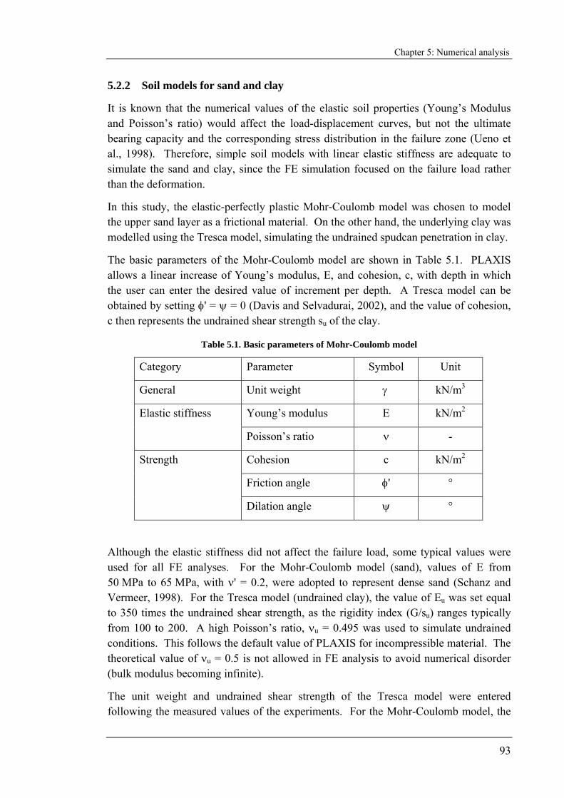
Chapter 5: Numerical analysis
93
5.2.2 Soil models for sand and clay
It is known that the numerical values of the elastic soil properties (Young’s Modulus and Poisson’s ratio) would affect the load-displacement curves, but not the ultimate bearing capacity and the corresponding stress distribution in the failure zone (Ueno et al., 1998). Therefore, simple soil models with linear elastic stiffness are adequate to simulate the sand and clay, since the FE simulation focused on the failure load rather than the deformation.
In this study, the elastic-perfectly plastic Mohr-Coulomb model was chosen to model the upper sand layer as a frictional material. On the other hand, the underlying clay was modelled using the Tresca model, simulating the undrained spudcan penetration in clay.
The basic parameters of the Mohr-Coulomb model are shown in Table 5.1. PLAXIS allows a linear increase of Young’s modulus, E, and cohesion, c, with depth in which the user can enter the desired value of increment per depth. A Tresca model can be obtained by setting φ' = ψ = 0 (Davis and Selvadurai, 2002), and the value of cohesion, c then represents the undrained shear strength su of the clay.
Table 5.1. Basic parameters of Mohr-Coulomb model
Category Parameter Symbol Unit
General Unit weight γ kN/m3
Young’s modulus E kN/m2 Elastic stiffness
Poisson’s ratio ν -
Cohesion c kN/m2
Friction angle φ' °
Strength
Dilation angle ψ °
Although the elastic stiffness did not affect the failure load, some typical values were used for all FE analyses. For the Mohr-Coulomb model (sand), values of E from 50 MPa to 65 MPa, with ν' = 0.2, were adopted to represent dense sand (Schanz and Vermeer, 1998). For the Tresca model (undrained clay), the value of Eu was set equal to 350 times the undrained shear strength, as the rigidity index (G/su) ranges typically from 100 to 200. A high Poisson’s ratio, νu = 0.495 was used to simulate undrained conditions. This follows the default value of PLAXIS for incompressible material. The theoretical value of νu = 0.5 is not allowed in FE analysis to avoid numerical disorder (bulk modulus becoming infinite).
The unit weight and undrained shear strength of the Tresca model were entered following the measured values of the experiments. For the Mohr-Coulomb model, the
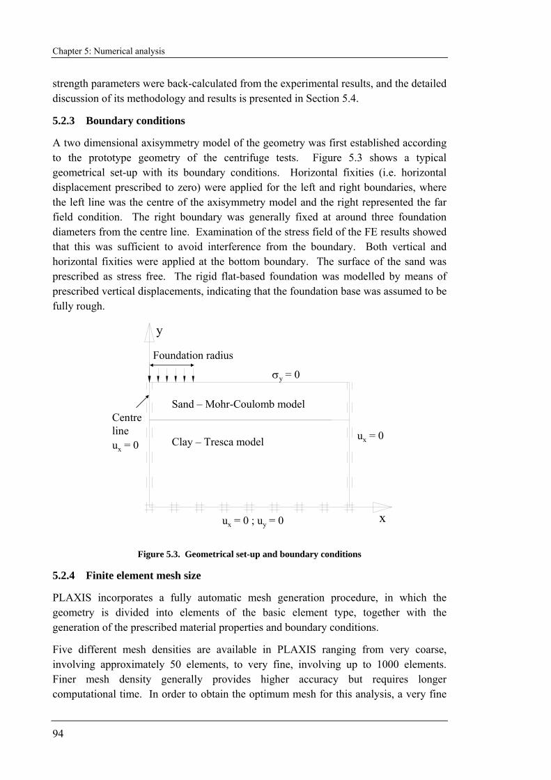
Chapter 5: Numerical analysis
94
strength parameters were back-calculated from the experimental results, and the detailed discussion of its methodology and results is presented in Section 5.4.
5.2.3 Boundary conditions
A two dimensional axisymmetry model of the geometry was first established according to the prototype geometry of the centrifuge tests. Figure 5.3 shows a typical geometrical set-up with its boundary conditions. Horizontal fixities (i.e. horizontal displacement prescribed to zero) were applied for the left and right boundaries, where the left line was the centre of the axisymmetry model and the right represented the far field condition. The right boundary was generally fixed at around three foundation diameters from the centre line. Examination of the stress field of the FE results showed that this was sufficient to avoid interference from the boundary. Both vertical and horizontal fixities were applied at the bottom boundary. The surface of the sand was prescribed as stress free. The rigid flat-based foundation was modelled by means of prescribed vertical displacements, indicating that the foundation base was assumed to be fully rough.
y
x
Sand – Mohr-Coulomb model
Clay – Tresca model
Foundation radius
ux = 0
ux = 0 ; uy = 0
ux = 0
Centre line
σy = 0
Figure 5.3. Geometrical set-up and boundary conditions
5.2.4 Finite element mesh size
PLAXIS incorporates a fully automatic mesh generation procedure, in which the geometry is divided into elements of the basic element type, together with the generation of the prescribed material properties and boundary conditions.
Five different mesh densities are available in PLAXIS ranging from very coarse, involving approximately 50 elements, to very fine, involving up to 1000 elements. Finer mesh density generally provides higher accuracy but requires longer computational time. In order to obtain the optimum mesh for this analysis, a very fine
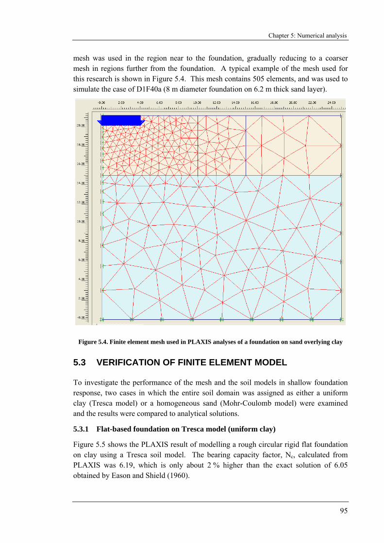
Chapter 5: Numerical analysis
95
mesh was used in the region near to the foundation, gradually reducing to a coarser mesh in regions further from the foundation. A typical example of the mesh used for this research is shown in Figure 5.4. This mesh contains 505 elements, and was used to simulate the case of D1F40a (8 m diameter foundation on 6.2 m thick sand layer).
Figure 5.4. Finite element mesh used in PLAXIS analyses of a foundation on sand overlying clay
5.3 VERIFICATION OF FINITE ELEMENT MODEL
To investigate the performance of the mesh and the soil models in shallow foundation response, two cases in which the entire soil domain was assigned as either a uniform clay (Tresca model) or a homogeneous sand (Mohr-Coulomb model) were examined and the results were compared to analytical solutions.
5.3.1 Flat-based foundation on Tresca model (uniform clay)
Figure 5.5 shows the PLAXIS result of modelling a rough circular rigid flat foundation on clay using a Tresca soil model. The bearing capacity factor, Nc, calculated from PLAXIS was 6.19, which is only about 2 % higher than the exact solution of 6.05 obtained by Eason and Shield (1960).
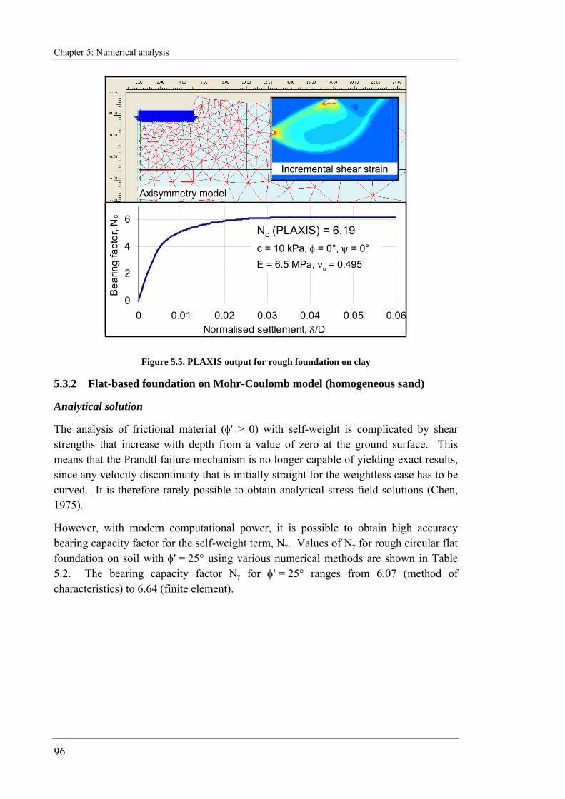
Chapter 5: Numerical analysis
96
0
2
4
6
0 0.01 0.02 0.03 0.04 0.05 0.06Normalised settlement, δ/D
Bea
ring
fact
or, N
c
Incremental shear strain
Nc (PLAXIS) = 6.19c = 10 kPa, φ = 0°, ψ = 0°E = 6.5 MPa, νu = 0.495
Axisymmetry model
Figure 5.5. PLAXIS output for rough foundation on clay
5.3.2 Flat-based foundation on Mohr-Coulomb model (homogeneous sand)
Analytical solution
The analysis of frictional material (φ' > 0) with self-weight is complicated by shear strengths that increase with depth from a value of zero at the ground surface. This means that the Prandtl failure mechanism is no longer capable of yielding exact results, since any velocity discontinuity that is initially straight for the weightless case has to be curved. It is therefore rarely possible to obtain analytical stress field solutions (Chen, 1975).
However, with modern computational power, it is possible to obtain high accuracy bearing capacity factor for the self-weight term, Nγ. Values of Nγ for rough circular flat foundation on soil with φ' = 25° using various numerical methods are shown in Table 5.2. The bearing capacity factor Nγ for φ' = 25° ranges from 6.07 (method of characteristics) to 6.64 (finite element).

Chapter 5: Numerical analysis
97
Table 5.2. Bearing capacity factor Nγ for rough circular foundation on frictional soil with φ' = 25°
Nγ Numerical method Reference
6.07 Method of characteristic implemented numerically in the program ABC (Martin, 2004)
φ' = ψ = 25° (associated soil)
Randolph et al. (2004)
6.22 Weighted average from lower bound (= 5.65) and upper bound (= 8.26) using finite element limit analysis
φ' = ψ = 25° (associated soil)
Lyamin et al. (2007)
6.62 Finite element analysis using the program ICFEP
φ' = 25°, ψ = 0° (non-dilatant soil)
Potts and Zdravkovic (2001)
6.64 Finite element analysis using the program ICFEP
φ' = ψ = 25° (associated soil)
Potts and Zdravkovic (2001)
Current PLAXIS model
Generally, the finite element computation of collapse load for frictional material (φ' > 0) with weight is more complicated and unstable (de Borst and Vermeer, 1984). It was also found during this study that PLAXIS tended to terminate prematurely for circular foundations on sand, particularly when the cohesion in the Mohr-Coulomb model had very small values or was set equal to zero. From experience, it was found that PLAXIS computation of the collapse load can be improved by manually reducing the tolerated error in the iterative procedure to 0.001 from the default value of 0.01. This created very small incremental steps and minimised the drift from the exact solution (reducing global and local equilibrium error). Although much longer computation times were required, the FE results were found to be much more satisfactory.
Two cases of a rough circular flat foundation on cohesionless soil were analysed. Both cases had strength parameters of φ' = 25° and ψ = 0°, but the first case had cohesion, c = 0.1 kPa and the second case had c = 1 kPa. This friction angle was selected in order to compare the results from PLAXIS with existing literature. The effective unit weight was 8 kN/m3. The value of Nγ was then calculated using:
⎟⎠⎞
⎜⎝⎛ −⎟⎟
⎠
⎞⎜⎜⎝
⎛γ
=γ c2 NcrF2
D'2N (5.1)
This equation originates from the classical bearing capacity formula that assumes superposition of different terms, where F is the vertical force from PLAXIS (values
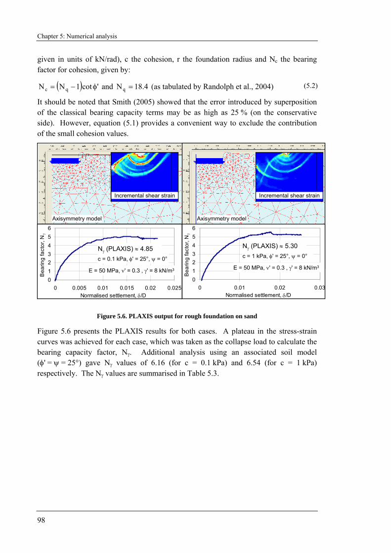
Chapter 5: Numerical analysis
98
given in units of kN/rad), c the cohesion, r the foundation radius and Nc the bearing factor for cohesion, given by:
( ) 'cot1NN qc φ−= and 4.18Nq = (as tabulated by Randolph et al., 2004) (5.2)
It should be noted that Smith (2005) showed that the error introduced by superposition of the classical bearing capacity terms may be as high as 25 % (on the conservative side). However, equation (5.1) provides a convenient way to exclude the contribution of the small cohesion values.
0123456
0 0.005 0.01 0.015 0.02 0.025Normalised settlement, δ/D
Bea
ring
fact
or, N
γ
0123456
0 0.01 0.02 0.03Normalised settlement, δ/D
Bea
ring
fact
or, N
γ
Axisymmetry model
Nγ (PLAXIS) ≈ 5.30c = 1 kPa, φ' = 25°, ψ = 0°
E = 50 MPa, ν' = 0.3 , γ' = 8 kN/m3
Axisymmetry model
Incremental shear strain
Nγ (PLAXIS) ≈ 4.85c = 0.1 kPa, φ' = 25°, ψ = 0°
E = 50 MPa, ν' = 0.3 , γ' = 8 kN/m3
Incremental shear strain
Figure 5.6. PLAXIS output for rough foundation on sand
Figure 5.6 presents the PLAXIS results for both cases. A plateau in the stress-strain curves was achieved for each case, which was taken as the collapse load to calculate the bearing capacity factor, Nγ. Additional analysis using an associated soil model (φ' = ψ = 25°) gave Nγ values of 6.16 (for c = 0.1 kPa) and 6.54 (for c = 1 kPa) respectively. The Nγ values are summarised in Table 5.3.
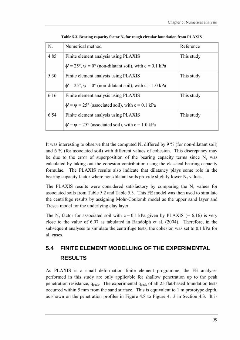
Chapter 5: Numerical analysis
99
Table 5.3. Bearing capacity factor Nγ for rough circular foundation from PLAXIS
Nγ Numerical method Reference
4.85 Finite element analysis using PLAXIS
φ' = 25°, ψ = 0° (non-dilatant soil), with c = 0.1 kPa
This study
5.30 Finite element analysis using PLAXIS
φ' = 25°, ψ = 0° (non-dilatant soil), with c = 1.0 kPa
This study
6.16 Finite element analysis using PLAXIS
φ' = ψ = 25° (associated soil), with c = 0.1 kPa
This study
6.54 Finite element analysis using PLAXIS
φ' = ψ = 25° (associated soil), with c = 1.0 kPa
This study
It was interesting to observe that the computed Nγ differed by 9 % (for non-dilatant soil) and 6 % (for associated soil) with different values of cohesion. This discrepancy may be due to the error of superposition of the bearing capacity terms since Nγ was calculated by taking out the cohesion contribution using the classical bearing capacity formulae. The PLAXIS results also indicate that dilatancy plays some role in the bearing capacity factor where non-dilatant soils provide slightly lower Nγ values.
The PLAXIS results were considered satisfactory by comparing the Nγ values for associated soils from Table 5.2 and Table 5.3. This FE model was then used to simulate the centrifuge results by assigning Mohr-Coulomb model as the upper sand layer and Tresca model for the underlying clay layer.
The Nγ factor for associated soil with c = 0.1 kPa given by PLAXIS (= 6.16) is very close to the value of 6.07 as tabulated in Randolph et al. (2004). Therefore, in the subsequent analyses to simulate the centrifuge tests, the cohesion was set to 0.1 kPa for all cases.
5.4 FINITE ELEMENT MODELLING OF THE EXPERIMENTAL RESULTS
As PLAXIS is a small deformation finite element programme, the FE analyses performed in this study are only applicable for shallow penetration up to the peak penetration resistance, qpeak. The experimental qpeak of all 25 flat-based foundation tests occurred within 5 mm from the sand surface. This is equivalent to 1 m prototype depth, as shown on the penetration profiles in Figure 4.8 to Figure 4.13 in Section 4.3. It is

Chapter 5: Numerical analysis
100
therefore believed that the simulation of peak resistance using small deformation finite element is appropriate and relevant.
The geometry of each FE model was based on the prototype dimensions of the corresponding centrifuge test. The properties of the clay (Tresca model), including the linear strength increment with depth, were based on the strength profile evaluated during the test. These were discussed in Section 4.7.3 and are detailed in Table 4.4. The aim of the FE modelling was to determine a single ‘operative’ friction angle and dilation angle for each test. This was achieved by matching the peak resistance of the FE results with the corresponding experimental qpeak.
5.4.1 Typical load-settlement curve and failure load from FE analyses
A typical load-settlement curve for a flat-based foundation on sand overlying soft clay from PLAXIS analysis is shown in Figure 5.7. It was observed that the load-settlement curve reached a plateau, which has been defined as the failure load. The initial elastic region of the curve was smooth but it gradually became jagged when approaching the plastic region. This is an indication of the numerical instability of the cohesionless sand. In spite of that, all FE models in this study reached a plateau before termination.
0
100
200
300
400
0 0.04 0.08 0.12Normalised settlement, δ/D
Pen
etra
tion
resi
stan
ce, q
(kP
a)
Failure load
Hs = 5.8 m, D = 12 m
Properties of sand layer:
φ' = 38.3°, ψ = 9.1°, γ' = 11 kN/m3
c = 0.1 kPa, E = 50 MPa, ν = 0.2
Properties of underlying clay:
φ' = ψ = 0, γ' = 8 kN/m3
su = 18.6 + 2.0 (z – 5.8 m) kPa
E = 6.5 MPa, ν = 0.495
FE simulation (PLAXIS) of Centrifuge test D2F60b
q peak = 395 kPa
Figure 5.7. Typical load settlement curve for flat foundation on sand overlying clay from PLAXIS
Even though the elastic-perfectly plastic Mohr-Coulomb and Tresca models were used, a peak followed by strain softening was observed in the curve as shown in Figure 5.7.
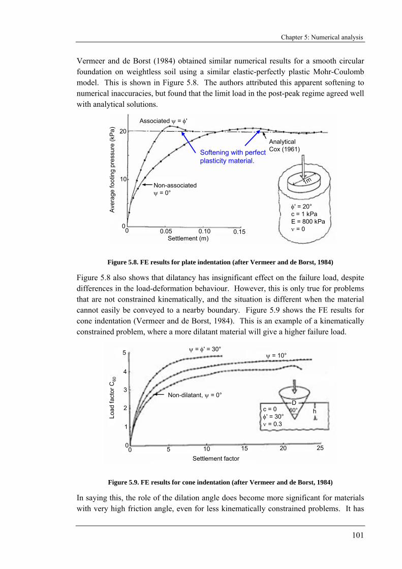
Chapter 5: Numerical analysis
101
Vermeer and de Borst (1984) obtained similar numerical results for a smooth circular foundation on weightless soil using a similar elastic-perfectly plastic Mohr-Coulomb model. This is shown in Figure 5.8. The authors attributed this apparent softening to numerical inaccuracies, but found that the limit load in the post-peak regime agreed well with analytical solutions.
Softening with perfect plasticity material.
Analytical Cox (1961)
Associated ψ = φ'
Non-associated ψ = 0°
φ' = 20°c = 1 kPaE = 800 kPaν = 0
Settlement (m)
Ave
rage
foot
ing
pres
sure
(kPa
)
0
10
20
0 0.05 0.10 0.15
1m
Figure 5.8. FE results for plate indentation (after Vermeer and de Borst, 1984)
Figure 5.8 also shows that dilatancy has insignificant effect on the failure load, despite differences in the load-deformation behaviour. However, this is only true for problems that are not constrained kinematically, and the situation is different when the material cannot easily be conveyed to a nearby boundary. Figure 5.9 shows the FE results for cone indentation (Vermeer and de Borst, 1984). This is an example of a kinematically constrained problem, where a more dilatant material will give a higher failure load.
c = 0φ' = 30°ν = 0.3
60°D
h
ψ = φ' = 30°ψ = 10°
Non-dilatant, ψ = 0°
Settlement factor
Load
fact
or C
60
0 10 20 25155
4
5
3
2
1
0
Figure 5.9. FE results for cone indentation (after Vermeer and de Borst, 1984)
In saying this, the role of the dilation angle does become more significant for materials with very high friction angle, even for less kinematically constrained problems. It has

Chapter 5: Numerical analysis
102
previously been shown that the failure load (or the bearing capacity factor Nγ) increases with dilation angle for surface foundation on cohesionless soils with friction angles, φ' > 35° (see for example Yin et al. (2001) for strip foundations, and Erickson and Drescher (2002) for circular foundations).
Finally, Vermeer and de Borst (1984) presented the extreme case of no volume change (all normal strains kept to zero) in a FE simulation of an isochoric shear test, as shown in Figure 5.10. Despite the use of a non-hardening model, the stress-strain curves show both hardening and softening without definite limit loads.
positive dilation
zero dilation
negative dilation
ψ = 0°
ψ = -3°
ψ = 15°
σxy (kPa)100
50
00 0.01 0.02 γxy
Non-hardening M/C model
σxyγxy
φ' = 43°
E = 45MPa
c = 0 ν = 0.2
σyy = -100σxx = -25kPaσxy = 0
Initially
Figure 5.10. Computed response of sands in an isochoric shear test (after Vermeer and de Borst, 1984)
For the current case of punching shear failure in sand overlying soft clay, the dilation angle of the sand is expected to affect the failure load. This is because the induced dispersion angle of the sand block to be sheared off is related to the dilation angle under the kinematically constraint condition. Furthermore, the dilation angle will also determine the extent of the underlying clay to be mobilised.
5.4.2 Determining the friction angle and dilation angle in the FE model
Following Bolton (1986), the mobilised friction angle consists of two components: (1) the critical state friction angle for shearing at constant volume and (2) the additional friction angle depending on the rate of dilation during shearing of dense sand. A suitable parameter for characterising a dilatant material is the dilation angle, ψ, which has been shown to be directly proportional to the relative density of sand and reduces linearly with the logarithm of stress (Billam, 1972). The critical state friction angle, φcv, is principally a function of mineralogy. By analysing the results of triaxial compression tests performed on 17 siliceous and quartz sands, Bolton (1986) proposed the following empirical strength-dilatancy formulae to reflect the stress-level dependency of the friction angle, φ':
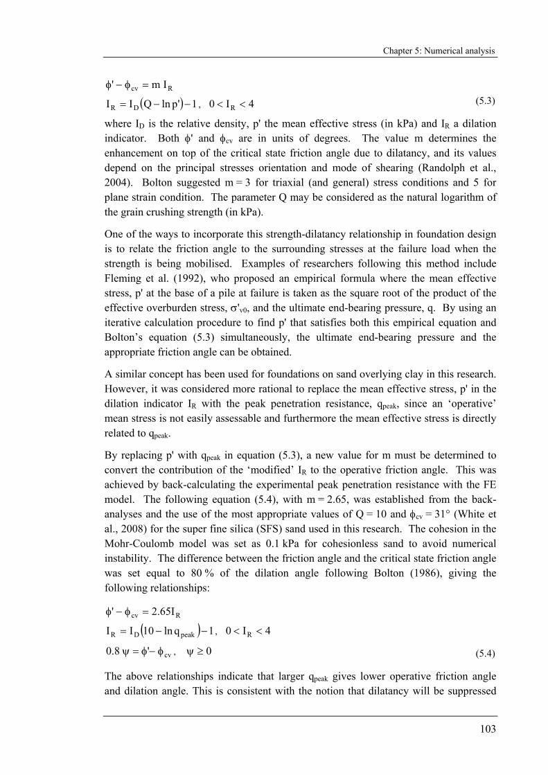
Chapter 5: Numerical analysis
103
Rcv Im' =φ−φ
( ) 1'plnQII DR −−= , 4I0 R << (5.3)
where ID is the relative density, p' the mean effective stress (in kPa) and IR a dilation indicator. Both φ' and φcv are in units of degrees. The value m determines the enhancement on top of the critical state friction angle due to dilatancy, and its values depend on the principal stresses orientation and mode of shearing (Randolph et al., 2004). Bolton suggested m = 3 for triaxial (and general) stress conditions and 5 for plane strain condition. The parameter Q may be considered as the natural logarithm of the grain crushing strength (in kPa).
One of the ways to incorporate this strength-dilatancy relationship in foundation design is to relate the friction angle to the surrounding stresses at the failure load when the strength is being mobilised. Examples of researchers following this method include Fleming et al. (1992), who proposed an empirical formula where the mean effective stress, p' at the base of a pile at failure is taken as the square root of the product of the effective overburden stress, σ'v0, and the ultimate end-bearing pressure, q. By using an iterative calculation procedure to find p' that satisfies both this empirical equation and Bolton’s equation (5.3) simultaneously, the ultimate end-bearing pressure and the appropriate friction angle can be obtained.
A similar concept has been used for foundations on sand overlying clay in this research. However, it was considered more rational to replace the mean effective stress, p' in the dilation indicator IR with the peak penetration resistance, qpeak, since an ‘operative’ mean stress is not easily assessable and furthermore the mean effective stress is directly related to qpeak.
By replacing p' with qpeak in equation (5.3), a new value for m must be determined to convert the contribution of the ‘modified’ IR to the operative friction angle. This was achieved by back-calculating the experimental peak penetration resistance with the FE model. The following equation (5.4), with m = 2.65, was established from the back-analyses and the use of the most appropriate values of Q = 10 and φcv = 31° (White et al., 2008) for the super fine silica (SFS) sand used in this research. The cohesion in the Mohr-Coulomb model was set as 0.1 kPa for cohesionless sand to avoid numerical instability. The difference between the friction angle and the critical state friction angle was set equal to 80 % of the dilation angle following Bolton (1986), giving the following relationships:
Rcv I65.2' =φ−φ
( ) 1qln10II peakDR −−= , 4I0 R <<
cv'8.0 φ−φ=ψ , 0≥ψ (5.4)
The above relationships indicate that larger qpeak gives lower operative friction angle and dilation angle. This is consistent with the notion that dilatancy will be suppressed

Chapter 5: Numerical analysis
104
under high confining stress. Therefore, although the sand samples prepared in the drum centrifuge had similar relative density of 92 % (see Section 4.6.2), different friction angles and dilation angles were mobilized at peak resistance depending on the magnitudes of the failure load caused by various foundation sizes and sand thicknesses.
By using the friction angles and dilation angles calculated from equations (5.4), the qpeak values obtained from FE analyses matched very well with the experimental values. Figure 5.11 shows the comparison between the qpeak from PLAXIS and from the centrifuge tests for all 25 flat-based foundation cases. Differences of less than 10 % were achieved, except for two cases where the differences were 12 % and 18 % respectively. The numerical values of qpeak for all 25 flat-based foundation tests from both centrifuge tests and FE analyses are listed in Table 4.1.
In the next chapter, an equation to calculate qpeak will be developed based on a new conceptual model. Therefore, by using this new equation and equations (5.4), an iterative calculation approach can be devised to determine qpeak and the stress dependent φ' and ψ simultaneously.
0
200
400
600
800
1000
0 200 400 600 800 1000qpeak from centrifuge tests (kPa)
qpea
k fro
m P
LAX
IS (k
Pa)
D2: 6.7m sand D1: 6.2m sandD2: 5.8m sandD2: 4.8m sandD1: 4.1m sandD2: 3.4m sand
+/- 20%
+/- 10%
Line of equility
Figure 5.11. Comparison of peak penetration resistance, qpeak from PLAXIS and centrifuge tests
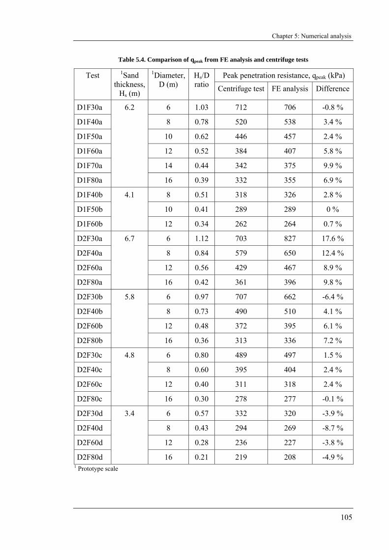
Chapter 5: Numerical analysis
105
Table 5.4. Comparison of qpeak from FE analysis and centrifuge tests
Peak penetration resistance, qpeak (kPa) Test 1Sand thickness,
Hs (m)
1Diameter, D (m)
Hs/D ratio Centrifuge test FE analysis Difference
D1F30a 6 1.03 712 706 -0.8 %
D1F40a 8 0.78 520 538 3.4 %
D1F50a 10 0.62 446 457 2.4 %
D1F60a 12 0.52 384 407 5.8 %
D1F70a 14 0.44 342 375 9.9 %
D1F80a
6.2
16 0.39 332 355 6.9 %
D1F40b 8 0.51 318 326 2.8 %
D1F50b 10 0.41 289 289 0 %
D1F60b
4.1
12 0.34 262 264 0.7 %
D2F30a 6 1.12 703 827 17.6 %
D2F40a 8 0.84 579 650 12.4 %
D2F60a 12 0.56 429 467 8.9 %
D2F80a
6.7
16 0.42 361 396 9.8 %
D2F30b 6 0.97 707 662 -6.4 %
D2F40b 8 0.73 490 510 4.1 %
D2F60b 12 0.48 372 395 6.1 %
D2F80b
5.8
16 0.36 313 336 7.2 %
D2F30c 6 0.80 489 497 1.5 %
D2F40c 8 0.60 395 404 2.4 %
D2F60c 12 0.40 311 318 2.4 %
D2F80c
4.8
16 0.30 278 277 -0.1 %
D2F30d 6 0.57 332 320 -3.9 %
D2F40d 8 0.43 294 269 -8.7 %
D2F60d 12 0.28 236 227 -3.8 %
D2F80d
3.4
16 0.21 219 208 -4.9 % 1 Prototype scale
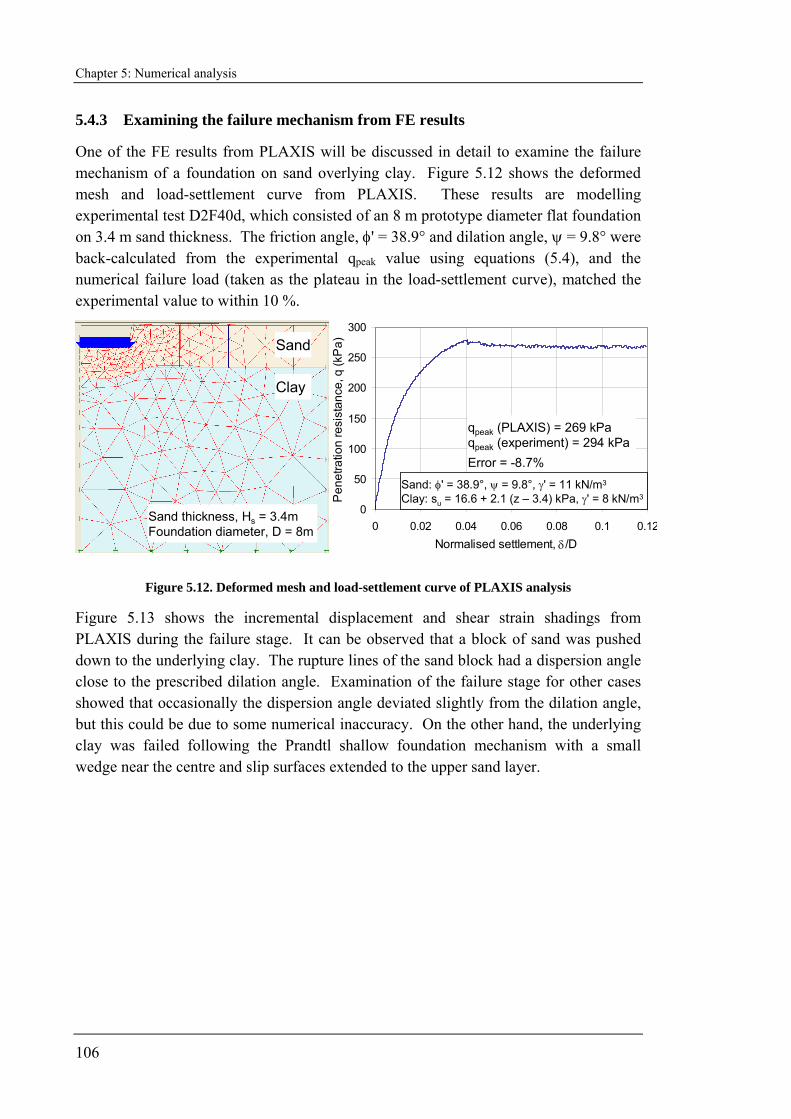
Chapter 5: Numerical analysis
106
5.4.3 Examining the failure mechanism from FE results
One of the FE results from PLAXIS will be discussed in detail to examine the failure mechanism of a foundation on sand overlying clay. Figure 5.12 shows the deformed mesh and load-settlement curve from PLAXIS. These results are modelling experimental test D2F40d, which consisted of an 8 m prototype diameter flat foundation on 3.4 m sand thickness. The friction angle, φ' = 38.9° and dilation angle, ψ = 9.8° were back-calculated from the experimental qpeak value using equations (5.4), and the numerical failure load (taken as the plateau in the load-settlement curve), matched the experimental value to within 10 %.
0
50
100
150
200
250
300
0 0.02 0.04 0.06 0.08 0.1 0.12Normalised settlement, δ/D
Pen
etra
tion
resi
stan
ce, q
(kP
a)
Sand thickness, Hs = 3.4mFoundation diameter, D = 8m
Sand
Clay
qpeak (PLAXIS) = 269 kPaqpeak (experiment) = 294 kPaError = -8.7%
Sand: φ' = 38.9°, ψ = 9.8°, γ' = 11 kN/m3
Clay: su = 16.6 + 2.1 (z – 3.4) kPa, γ' = 8 kN/m3
Figure 5.12. Deformed mesh and load-settlement curve of PLAXIS analysis
Figure 5.13 shows the incremental displacement and shear strain shadings from PLAXIS during the failure stage. It can be observed that a block of sand was pushed down to the underlying clay. The rupture lines of the sand block had a dispersion angle close to the prescribed dilation angle. Examination of the failure stage for other cases showed that occasionally the dispersion angle deviated slightly from the dilation angle, but this could be due to some numerical inaccuracy. On the other hand, the underlying clay was failed following the Prandtl shallow foundation mechanism with a small wedge near the centre and slip surfaces extended to the upper sand layer.

Chapter 5: Numerical analysis
107
Incremental displacement (shading)
Incremental shear strain (shading)9.8° = ψ 9.8° = ψ
Foundation radius
Foundation radius
Sand SandClay Clay
Figure 5.13. Incremental displacement and shear strain shadings from PLAXIS at failure for a foundation on sand overlying clay
Vermeer and Sutjiadi (1985) found a similar failure mechanism for the case of vertical uplift resistance of a shallow embedded anchor in sand from both their FE and scale-model test results. Although the anchor problem was in the inverted direction, it involved approximately straight rupture lines at an inclination corresponding to the dilation angle from the anchor plate to the soil surface.
5.4.4 A comparison of FE results with experimentally observed mechanisms (using PIV)
Teh (2007) carried out a series of half spudcan penetration tests on sand overlying soft clay to study the failure mechanism. In general, the test set-up consisted of a plane strain chamber that had a transparent side wall for viewing. The chamber was subjected to a designated centrifugal acceleration after it had been filled with sand overlying clay soils. A model half spudcan was then placed against the internal side of the transparent wall and penetrated into the soils. During the penetration process, a series of images were captured by a camera fixed at the front of the transparent wall. The deformation fields were then analysed from the images using the method of particle image velocimetry (PIV) and photogrammetry (White et al., 2003).
The details of the test can be found in Teh (2007) and Teh et al. (2008). Although the sand thickness over foundation diameter ratio (Hs/D) in the test was 0.83, which is different from the PLAXIS model of 0.425, their incremental displacement diagrams (represented by arrows) during the occurrence of the peak resistance are compared in Figure 5.14.
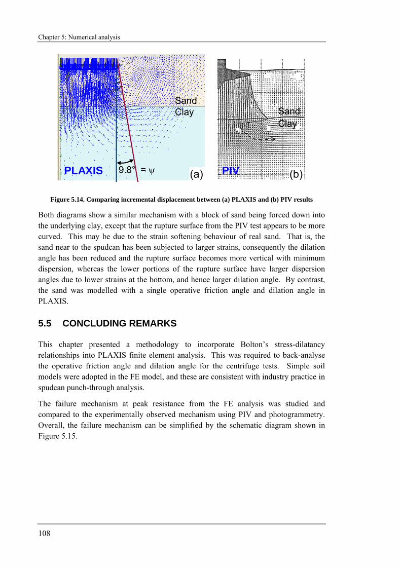
Chapter 5: Numerical analysis
108
9.8°
SandClay
ClaySand
PIVPLAXIS = ψ (a) (b)
Figure 5.14. Comparing incremental displacement between (a) PLAXIS and (b) PIV results
Both diagrams show a similar mechanism with a block of sand being forced down into the underlying clay, except that the rupture surface from the PIV test appears to be more curved. This may be due to the strain softening behaviour of real sand. That is, the sand near to the spudcan has been subjected to larger strains, consequently the dilation angle has been reduced and the rupture surface becomes more vertical with minimum dispersion, whereas the lower portions of the rupture surface have larger dispersion angles due to lower strains at the bottom, and hence larger dilation angle. By contrast, the sand was modelled with a single operative friction angle and dilation angle in PLAXIS.
5.5 CONCLUDING REMARKS
This chapter presented a methodology to incorporate Bolton’s stress-dilatancy relationships into PLAXIS finite element analysis. This was required to back-analyse the operative friction angle and dilation angle for the centrifuge tests. Simple soil models were adopted in the FE model, and these are consistent with industry practice in spudcan punch-through analysis.
The failure mechanism at peak resistance from the FE analysis was studied and compared to the experimentally observed mechanism using PIV and photogrammetry. Overall, the failure mechanism can be simplified by the schematic diagram shown in Figure 5.15.

Chapter 5: Numerical analysis
109
Sand
Clay
ψψ
Frictional resistance from sand
Bearing resistance from clay
Peak penetration resistance, Qpeak
Sand with operative φ' and ψ
Figure 5.15. Schematic diagram for foundation on sand overlying soft clay
The peak penetration resistance occurs when a sand frustum is being sheared off and pushed into the underlying clay. This occurs at a dispersion angle equal to the operative dilation angle. The value of peak pentration resistance consists of the frictional side resistance from sand and the bearing resistance from the underlying clay. This conceptual model will be explained in detail in Chapter 6, with the aim to develop a simplified equation to calculate the peak penetration resistance.
Chapter 6: Simplified conceptual model
110
CHAPTER 6. SIMPLIFIED CONCEPTUAL MODEL FOR BEARING CAPACITY ON SAND OVERLYING CLAY
SOILS
6.1 INTRODUCTION
One of the key motivations for this research was to develop a simple mathematical model to calculate the peak penetration resistance on sand overlying clay soils. For use within the offshore jack-up industry, the analytical model should be relatively simple with straightforward procedures so that it can be easily incorporated into design routines. It must also have well-defined input parameters, and ones that can be derived from standard offshore site investigation.
This chapter describes the development of such a simplified conceptual model for bearing capacity of foundations on sand overlying clay. The model is based on establishing a force equilibrium equation on a conceptual sand frustum with straight rupture surfaces beneath the foundation. A new empirical parameter named the distribution factor (DF) was defined during the derivation of the equation. The peak penetration resistance calculated from the conceptual model shows excellent agreement with the centrifuge test results by adopting a linear variation of the distribution factor with the Hs/D ratio.
6.2 NEW CONCEPTUAL MODEL
6.2.1 General
The new conceptual model has been developed for the specific case of a circular foundation on sand overlying clay. It is only relevant when the load from the foundation is sufficiently large to shear off a block of sand into the underlying clay. The foundation pressure and the weight of the sand block are resisted by the frictional resistance along the sides of the sand block and the bearing capacity of the underlying clay.
For typical spudcan loading rates, it is appropriate to assume that the upper sand layer has drained response whereas the lower clay layer is undrained. Within the current conceptual model, only a homogeneous sand layer is considered, whereas the undrained shear strength of the clay can increase linearly with depth.
6.2.2 Kinematically admissible failure mechanism
The new conceptual model is based on a kinematically admissible failure mechanism that was adopted by Vermeer and Sutjiadi (1985) to develop an analytical method for

Chapter 6: Simplified conceptual model
111
the uplift resistance of anchor plates in sand. They observed from finite element computations and model tests that the failure mechanism for the uplift of an anchor plate in sand involved approximate straight rupture surfaces from the edge of the anchor to the soil surface. In addition, they also found that the inclination of the rupture surfaces corresponded with the dilation angle ψ of the sand. For a circular anchor plate, the rupture surfaces formed an overturned truncated-cone sand block on top of the anchor. Figure 6.1 shows the kinematically admissible failure mechanism for pulling out of an anchor in sand.
ψ
Figure 6.1. Kinematically admissible failure mechanism of an anchor plate in sand (after Vermeer and Sutjiadi, 1985)
The current model assumes a similar failure mechanism, except that the truncated-cone sand block is upside-down (as compared to the anchor problem) and the base of the conceptual sand frustum is resisted by the underlying clay.
Using PIV techniques in centrifuge tests, Teh (2007) showed that the shear surfaces in homogeneous sand were trumpet-shaped when the peak penetration resistance occurred, and gradually reduced to vertical shear surfaces during post-peak penetrations on sand overlying clay (see discussion in Section 5.4.4). This indicates that the dilation angle is not constant even in homogeneous sand, but continues to reduce with strains during the penetration process until it vanishes. The friction angle, which is related to the dilation angle, also varies and reduces to a critical state value accordingly. In addition to the strain-softening behaviour, at any particular instance, the actual friction angle and dilation angle within the vicinity of the foundation are different depending on the surrounding stresses due to their stress-dependent nature. However, the current simplified conceptual model is not able to incorporate such complicated, though realistic, behaviour.
In contrast, a single operative dilation angle and friction angle are used in the current conceptual model. This is acceptable since a relatively simple equation for design
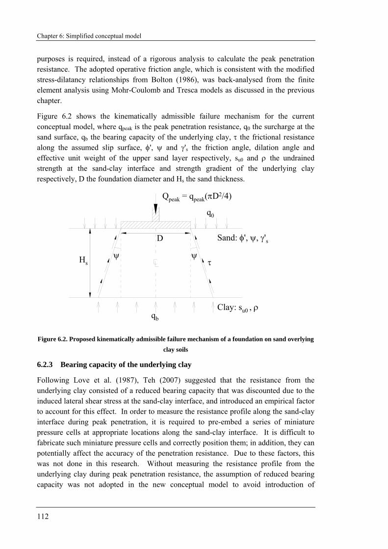
Chapter 6: Simplified conceptual model
112
purposes is required, instead of a rigorous analysis to calculate the peak penetration resistance. The adopted operative friction angle, which is consistent with the modified stress-dilatancy relationships from Bolton (1986), was back-analysed from the finite element analysis using Mohr-Coulomb and Tresca models as discussed in the previous chapter.
Figure 6.2 shows the kinematically admissible failure mechanism for the current conceptual model, where qpeak is the peak penetration resistance, q0 the surcharge at the sand surface, qb the bearing capacity of the underlying clay, τ the frictional resistance along the assumed slip surface, φ', ψ and γ's the friction angle, dilation angle and effective unit weight of the upper sand layer respectively, su0 and ρ the undrained strength at the sand-clay interface and strength gradient of the underlying clay respectively, D the foundation diameter and Hs the sand thickness.
ψψ
qb
q0
τ
Sand: φ', ψ, γ's
Clay: su0 , ρ
Hs
D
Qpeak = qpeak(πD2/4)
Figure 6.2. Proposed kinematically admissible failure mechanism of a foundation on sand overlying clay soils
6.2.3 Bearing capacity of the underlying clay
Following Love et al. (1987), Teh (2007) suggested that the resistance from the underlying clay consisted of a reduced bearing capacity that was discounted due to the induced lateral shear stress at the sand-clay interface, and introduced an empirical factor to account for this effect. In order to measure the resistance profile along the sand-clay interface during peak penetration, it is required to pre-embed a series of miniature pressure cells at appropriate locations along the sand-clay interface. It is difficult to fabricate such miniature pressure cells and correctly position them; in addition, they can potentially affect the accuracy of the penetration resistance. Due to these factors, this was not done in this research. Without measuring the resistance profile from the underlying clay during peak penetration resistance, the assumption of reduced bearing capacity was not adopted in the new conceptual model to avoid introduction of
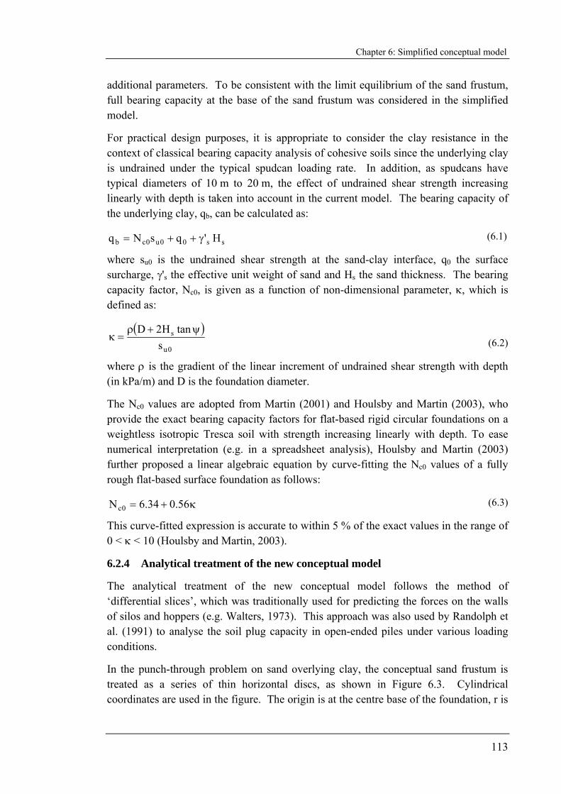
Chapter 6: Simplified conceptual model
113
additional parameters. To be consistent with the limit equilibrium of the sand frustum, full bearing capacity at the base of the sand frustum was considered in the simplified model.
For practical design purposes, it is appropriate to consider the clay resistance in the context of classical bearing capacity analysis of cohesive soils since the underlying clay is undrained under the typical spudcan loading rate. In addition, as spudcans have typical diameters of 10 m to 20 m, the effect of undrained shear strength increasing linearly with depth is taken into account in the current model. The bearing capacity of the underlying clay, qb, can be calculated as:
ss00u0cb H'qsNq γ++= (6.1)
where su0 is the undrained shear strength at the sand-clay interface, q0 the surface surcharge, γ's the effective unit weight of sand and Hs the sand thickness. The bearing capacity factor, Nc0, is given as a function of non-dimensional parameter, κ, which is defined as:
( )0u
s
stanH2D ψ+ρ
=κ (6.2)
where ρ is the gradient of the linear increment of undrained shear strength with depth (in kPa/m) and D is the foundation diameter.
The Nc0 values are adopted from Martin (2001) and Houlsby and Martin (2003), who provide the exact bearing capacity factors for flat-based rigid circular foundations on a weightless isotropic Tresca soil with strength increasing linearly with depth. To ease numerical interpretation (e.g. in a spreadsheet analysis), Houlsby and Martin (2003) further proposed a linear algebraic equation by curve-fitting the Nc0 values of a fully rough flat-based surface foundation as follows:
κ+= 56.034.6N 0c (6.3)
This curve-fitted expression is accurate to within 5 % of the exact values in the range of 0 < κ < 10 (Houlsby and Martin, 2003).
6.2.4 Analytical treatment of the new conceptual model
The analytical treatment of the new conceptual model follows the method of ‘differential slices’, which was traditionally used for predicting the forces on the walls of silos and hoppers (e.g. Walters, 1973). This approach was also used by Randolph et al. (1991) to analyse the soil plug capacity in open-ended piles under various loading conditions.
In the punch-through problem on sand overlying clay, the conceptual sand frustum is treated as a series of thin horizontal discs, as shown in Figure 6.3. Cylindrical coordinates are used in the figure. The origin is at the centre base of the foundation, r is
Chapter 6: Simplified conceptual model
114
the radial coordinate and z is the vertical coordinate with positive downward direction. The equilibrium of the forces outside the conceptual sand frustum is not considered. It is assumed that the outside stresses balance themselves within the interior.
Sand
Clay
Hs
R
z
dz
r
ψ n'σ
(Thin horizontal discs)
qb
q0
τ
ψ
ψ+ tanzR
( )2peakpeak RqQ π=
Figure 6.3. A series of thin horizontal discs in the conceptual sand frustum.
6.2.5 Normal and shear stresses at slip surfaces
Analogous to the problems of calculating skin friction of piles, it is difficult to estimate the horizontal effective stress along the slip surface or its relation with the vertical effective stress. However, for design purposes, it is assumed that the stresses along the slip surfaces of the conceptual model follow the limiting Mohr-circle. This is shown in Figure 6.4, where σ'n is the normal effective stress at the slip surface, (σ'z)slip the vertical effective stress at the slip surface and φ* the reduced friction angle due to a non-associative flow rule.
Drescher and Detournay (1993) showed that for kinematic mechanisms comprised of rigid blocks and velocity discontinuities, the use of a reduced friction angle φ* instead of φ' furnishes reasonable limit load estimates for materials with coaxial non-associated flow rules. They suggested that φ* be viewed as a reduced friction angle that accounts for the softening that may be induced under certain stress conditions by a non-associated flow rule.
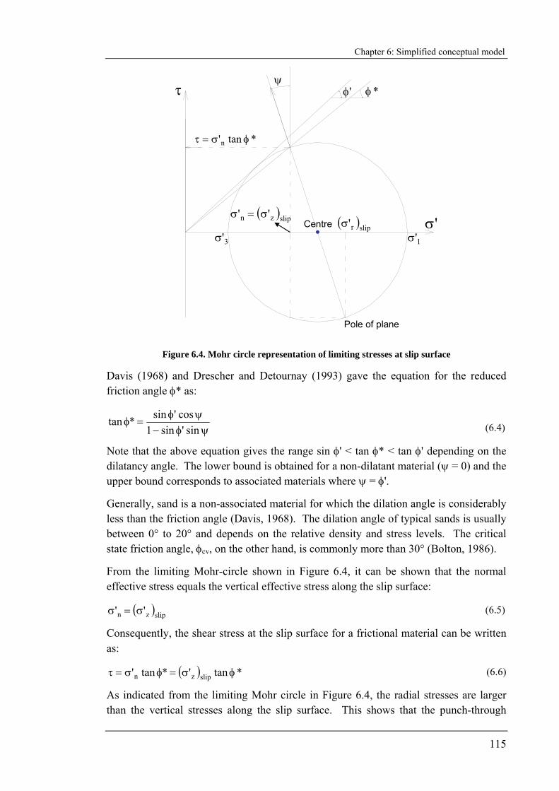
Chapter 6: Simplified conceptual model
115
Pole of plane
Centre ( )slipzn '' σ=σ
3'σ 1'σ
'φ *φ
'σ
*tan'n φσ=τ
ψτ
( )slipr'σ
Figure 6.4. Mohr circle representation of limiting stresses at slip surface
Davis (1968) and Drescher and Detournay (1993) gave the equation for the reduced friction angle φ* as:
ψφ−ψφ
=φsin'sin1
cos'sin*tan (6.4)
Note that the above equation gives the range sin φ' < tan φ* < tan φ' depending on the dilatancy angle. The lower bound is obtained for a non-dilatant material (ψ = 0) and the upper bound corresponds to associated materials where ψ = φ'.
Generally, sand is a non-associated material for which the dilation angle is considerably less than the friction angle (Davis, 1968). The dilation angle of typical sands is usually between 0° to 20° and depends on the relative density and stress levels. The critical state friction angle, φcv, on the other hand, is commonly more than 30° (Bolton, 1986).
From the limiting Mohr-circle shown in Figure 6.4, it can be shown that the normal effective stress equals the vertical effective stress along the slip surface:
( )slipzn '' σ=σ (6.5)
Consequently, the shear stress at the slip surface for a frictional material can be written as:
( ) *tan'*tan' slipzn φσ=φσ=τ (6.6)
As indicated from the limiting Mohr circle in Figure 6.4, the radial stresses are larger than the vertical stresses along the slip surface. This shows that the punch-through
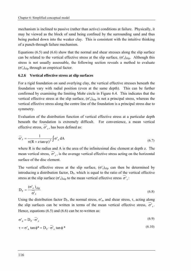
Chapter 6: Simplified conceptual model
116
mechanism is inclined to passive (rather than active) conditions at failure. Physically, it may be viewed as the block of sand being confined by the surrounding sand and thus being pushed down into the weaker clay. This is consistent with the intuitive thinking of a punch-through failure mechanism.
Equations (6.5) and (6.6) show that the normal and shear stresses along the slip surface can be related to the vertical effective stress at the slip surface, (σ'z)slip. Although this stress is not usually assessable, the following section reveals a method to evaluate (σ'z)slip through an empirical factor.
6.2.6 Vertical effective stress at slip surfaces
For a rigid foundation on sand overlying clay, the vertical effective stresses beneath the foundation vary with radial position (even at the same depth). This can be further confirmed by examining the limiting Mohr circle in Figure 6.4. This indicates that the vertical effective stress at the slip surface, (σ'z)slip is not a principal stress, whereas the vertical effective stress along the centre line of the foundation is a principal stress due to symmetry.
Evaluation of the distribution function of vertical effective stress at a particular depth beneath the foundation is extremely difficult. For convenience, a mean vertical effective stress, z'σ , has been defined as:
∫σψ+π
=σ dA')tanzR(
1' z2z (6.7)
where R is the radius and A is the area of the infinitesimal disc element at depth z. The mean vertical stress, z'σ , is the average vertical effective stress acting on the horizontal surface of the disc element.
The vertical effective stress at the slip surface, (σ'z)slip can then be determined by introducing a distribution factor, DF, which is equal to the ratio of the vertical effective stress at the slip surface (σ'z)slip to the mean vertical effective stress z'σ :
z
slipzF '
)'(D
σ
σ= (6.8)
Using the distribution factor DF, the normal stress, σ'n, and shear stress, τ, acting along the slip surfaces can be written in terms of the mean vertical effective stress, z'σ . Hence, equations (6.5) and (6.6) can be re-written as:
zFn 'D' σ⋅=σ (6.9)
*tan'D*tan' zFn φσ⋅=φσ=τ (6.10)
Chapter 6: Simplified conceptual model
117
6.2.7 Vertical force equilibrium on an infinitesimal element
Figure 6.5 shows the stresses on one of the infinitesimal disc elements within the conceptual sand frustum, where each element is acted on by mean vertical stresses z'σ at the top, zz d '' σσ + at the bottom, and normal and shear stresses, σ'n and τ, at the side, which is inclined at the operative dilation angle. The effective unit weight of the horizontal disc element is γ's.
dzds ψ
n'σ
τ
zz 'd' σ+σ
ψ
z'σ
s'γ
Figure 6.5. Stresses on an infinitesimal disc element within the conceptual sand frustum
The vertical force equilibrium equation on the infinitesimal element can be written as:
( ) ( ) ( )[ ] ( )z2
s2
z2 'tandzzR'dztanzR'tanzR σψ++π=γ⋅ψ+π+σψ+π
( )[ ] ( )z2 'dtanzR σψ+π+
( )( )ψ
ψσ−ψτψ+π+cos
dzsin'costanzR2 n (6.11)
With some mathematical manipulations, the above equation can be simplified to the following differential equation:
( ) ( ) ( ) ( ){ } 0dz'tanzRtan'2'tan2'dtanzR snzz =γψ+−ψσ−τ+σψ+σψ+ (6.12)
Following equations (6.9) and (6.10), the normal stress σ'n and shear stress τ in equation (6.12) can be written in term of the mean vertical effective stress, z'σ , which leads to the following differential equation:
( )[ ]( ) 0'
tanzR'tan*tanDtan2
dz'd
szFz =γ−
ψ+σψ−φ+ψ
+σ (6.13)
A new parameter E, which is defined below, is introduced, allowing this differential equation to be simplified to:
Chapter 6: Simplified conceptual model
118
( ) 0'tanzR
'tanEdz
'ds
zz =γ−ψ+
σ⋅ψ+
σ
where ⎥⎦
⎤⎢⎣
⎡⎟⎟⎠
⎞⎜⎜⎝
⎛−
ψφ
+= 1tan
*tanD12E F (6.14)
6.2.8 Integration of vertical force equilibrium equation
If the distribution factor DF is constant with respect to depth z, the differential force equilibrium equation (6.14) can be integrated. However, in reality, DF is likely to vary with depth, and it is very difficult to derive an accurate function of DF in sand overlying clay with various combinations of relative soil strengths and ratios of sand thickness over foundation diameter, Hs/D. In order to obtain a simplified equation for practical design, it is considered appropriate to assume DF as constant. Recall that the distribution factor DF is defined as the ratio of vertical effective stress at the slip surface to the mean vertical effective stress, hence, DF will likely have values of less than unity when the slip surfaces are dispersed outwards from the foundation edge at the dilation angle, ψ. Since there is no rigorous theoretical treatment to determine DF, its values will be derived by calibrating the final equation with the centrifuge results. Details of this will be discussed in Section 6.5.
By assuming DF is a constant with depth, equation (6.14) can be integrated to give:
( ) ( )( ) A
1EtantanzR'
'tanzR1E
sz
E ++ψ
ψ+γ=σ⋅ψ+
+
(6.15)
where A is a constant to be determined from the boundary condition.
Referring to the conceptual model in Figure 6.3, when z equals the sand thickness Hs, the mean vertical effective stress, z'σ equals the bearing capacity of the clay (qb = Nc0su0 + q0 + γ'sHs), and hence A can be evaluated as:
( ) ( ) ( )( ) ⎭
⎬⎫
⎩⎨⎧
+ψψ+γ
−γ++⋅ψ+=1Etan
tanHR'H'qsNtanHRA s
ss00u0cE
s (6.16)
By re-substituting A into equation (6.15), the final equation for the mean vertical effective stress becomes:
( )( )1Etan
tanzR'' sz +ψ
ψ+γ=σ
( )( )
( ) ( )( ) ⎭
⎬⎫
⎩⎨⎧
+ψψ+γ
−γ++⋅ψ+
ψ++
1EtantanHR'
H'qsNtanzRtanHR ss
ss00u0cE
Es
(6.17)
The centrifuge test results showed that the peak penetration resistance of the foundations occurred very near the sand surface, which was less than 1 m prototype scale (or 5 mm model scale). This slight indentation of the foundation into the sand has
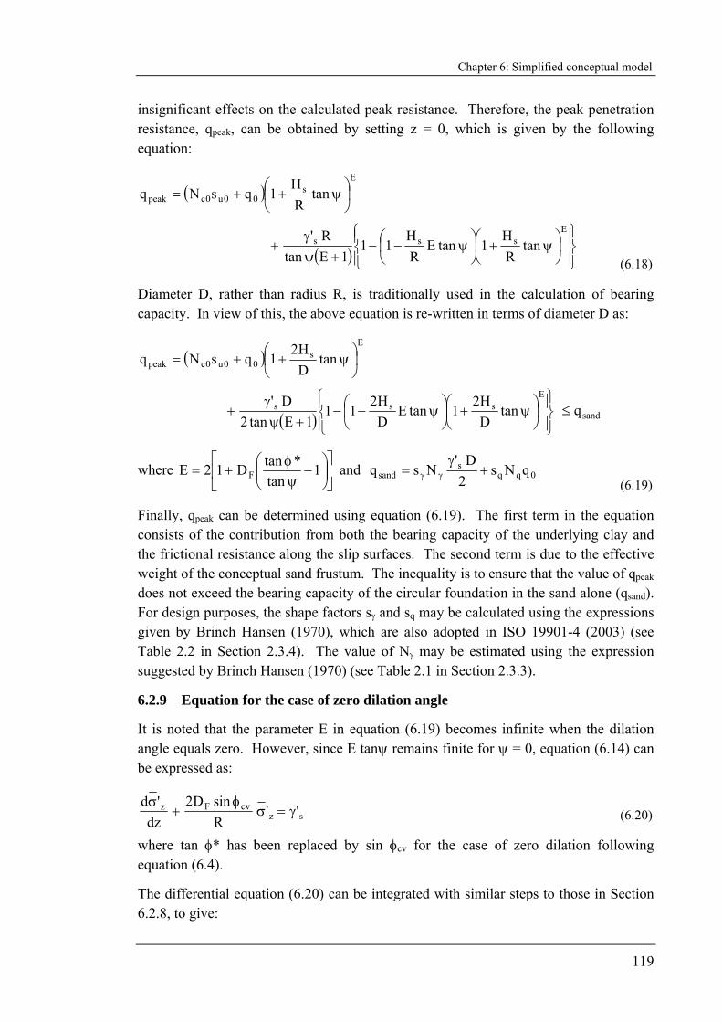
Chapter 6: Simplified conceptual model
119
insignificant effects on the calculated peak resistance. Therefore, the peak penetration resistance, qpeak, can be obtained by setting z = 0, which is given by the following equation:
( )E
s00u0cpeak tan
RH
1qsNq ⎟⎠
⎞⎜⎝
⎛ ψ++=
( ) ⎪⎭
⎪⎬⎫
⎪⎩
⎪⎨⎧
⎟⎠
⎞⎜⎝
⎛ ψ+⎟⎠
⎞⎜⎝
⎛ ψ−−+ψ
γ+
Esss tan
RH
1tanERH
111Etan
R' (6.18)
Diameter D, rather than radius R, is traditionally used in the calculation of bearing capacity. In view of this, the above equation is re-written in terms of diameter D as:
( )E
s00u0cpeak tan
DH2
1qsNq ⎟⎠
⎞⎜⎝
⎛ ψ++=
( ) ⎪⎭
⎪⎬⎫
⎪⎩
⎪⎨⎧
⎟⎠⎞
⎜⎝⎛ ψ+⎟
⎠⎞
⎜⎝⎛ ψ−−
+ψγ
+E
sss tanDH2
1tanEDH2
111Etan2
D' sandq≤
where ⎥⎦
⎤⎢⎣
⎡⎟⎟⎠
⎞⎜⎜⎝
⎛−
ψφ
+= 1tan
*tanD12E F and 0qqs
sand qNs2D'
Nsq +γ
= γγ (6.19)
Finally, qpeak can be determined using equation (6.19). The first term in the equation consists of the contribution from both the bearing capacity of the underlying clay and the frictional resistance along the slip surfaces. The second term is due to the effective weight of the conceptual sand frustum. The inequality is to ensure that the value of qpeak does not exceed the bearing capacity of the circular foundation in the sand alone (qsand). For design purposes, the shape factors sγ and sq may be calculated using the expressions given by Brinch Hansen (1970), which are also adopted in ISO 19901-4 (2003) (see Table 2.2 in Section 2.3.4). The value of Nγ may be estimated using the expression suggested by Brinch Hansen (1970) (see Table 2.1 in Section 2.3.3).
6.2.9 Equation for the case of zero dilation angle
It is noted that the parameter E in equation (6.19) becomes infinite when the dilation angle equals zero. However, since E tanψ remains finite for ψ = 0, equation (6.14) can be expressed as:
szcvFz ''
RsinD2
dz'd
γ=σφ
+σ (6.20)
where tan φ* has been replaced by sin φcv for the case of zero dilation following equation (6.4).
The differential equation (6.20) can be integrated with similar steps to those in Section 6.2.8, to give:
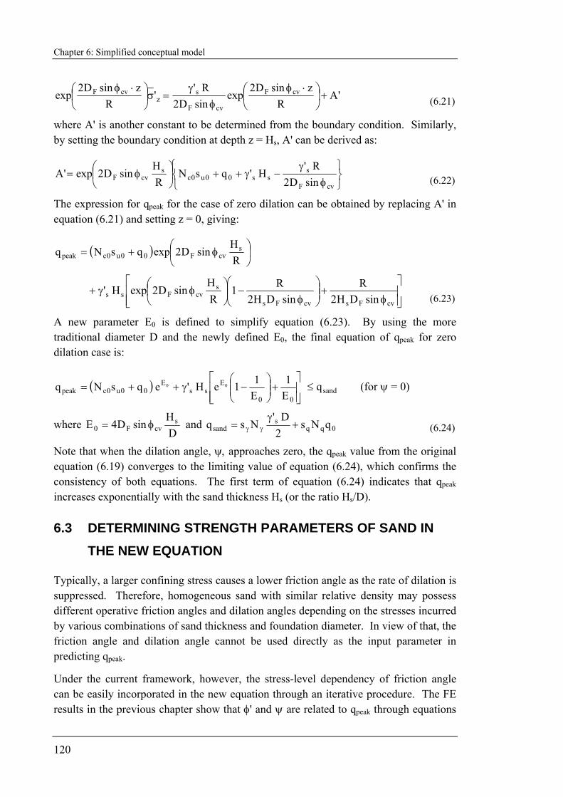
Chapter 6: Simplified conceptual model
120
'AR
zsinD2exp
sinD2R'
'R
zsinD2exp cvF
cvF
sz
cvF +⎟⎠⎞
⎜⎝⎛ ⋅φ
φγ
=σ⎟⎠⎞
⎜⎝⎛ ⋅φ (6.21)
where A' is another constant to be determined from the boundary condition. Similarly, by setting the boundary condition at depth z = Hs, A' can be derived as:
⎭⎬⎫
⎩⎨⎧
φγ
−γ++⎟⎠
⎞⎜⎝
⎛ φ=cvF
sss00u0c
scvF sinD2
R'H'qsN
RH
sinD2exp'A (6.22)
The expression for qpeak for the case of zero dilation can be obtained by replacing A' in equation (6.21) and setting z = 0, giving:
( ) ⎟⎠
⎞⎜⎝
⎛ φ+=RH
sinD2expqsNq scvF00u0cpeak
⎥⎥⎦
⎤
⎢⎢⎣
⎡
φ+⎟⎟
⎠
⎞⎜⎜⎝
⎛φ
−⎟⎠⎞
⎜⎝⎛ φγ+
cvFscvFs
scvFss sinDH2
RsinDH2
R1RH
sinD2expH' (6.23)
A new parameter E0 is defined to simplify equation (6.23). By using the more traditional diameter D and the newly defined E0, the final equation of qpeak for zero dilation case is:
( )⎥⎥⎦
⎤
⎢⎢⎣
⎡+⎟⎟
⎠
⎞⎜⎜⎝
⎛−γ++=
00
Ess
E00u0cpeak E
1E11eH'eqsNq 00 sandq≤ (for ψ = 0)
where DH
sinD4E scvF0 φ= and 0qq
ssand qNs
2D'
Nsq +γ
= γγ (6.24)
Note that when the dilation angle, ψ, approaches zero, the qpeak value from the original equation (6.19) converges to the limiting value of equation (6.24), which confirms the consistency of both equations. The first term of equation (6.24) indicates that qpeak increases exponentially with the sand thickness Hs (or the ratio Hs/D).
6.3 DETERMINING STRENGTH PARAMETERS OF SAND IN THE NEW EQUATION
Typically, a larger confining stress causes a lower friction angle as the rate of dilation is suppressed. Therefore, homogeneous sand with similar relative density may possess different operative friction angles and dilation angles depending on the stresses incurred by various combinations of sand thickness and foundation diameter. In view of that, the friction angle and dilation angle cannot be used directly as the input parameter in predicting qpeak.
Under the current framework, however, the stress-level dependency of friction angle can be easily incorporated in the new equation through an iterative procedure. The FE results in the previous chapter show that φ' and ψ are related to qpeak through equations
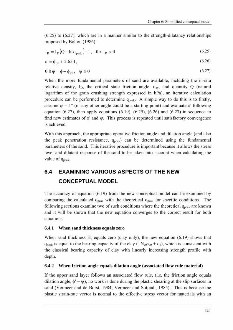
Chapter 6: Simplified conceptual model
121
(6.25) to (6.27), which are in a manner similar to the strength-dilatancy relationships proposed by Bolton (1986):
( ) 1qlnQII peakDR −−= , 4I0 R << (6.25)
Rcv I65.2' +φ=φ (6.26)
cv'8.0 φ−φ=ψ , 0≥ψ (6.27)
When the more fundamental parameters of sand are available, including the in-situ relative density, ID, the critical state friction angle, φcv, and quantity Q (natural logarithm of the grain crushing strength expressed in kPa), an iterative calculation procedure can be performed to determine qpeak. A simple way to do this is to firstly, assume ψ = 1° (or any other angle could be a starting point) and evaluate φ' following equation (6.27), then apply equations (6.19), (6.25), (6.26) and (6.27) in sequence to find new estimates of φ' and ψ. This process is repeated until satisfactory convergence is achieved.
With this approach, the appropriate operative friction angle and dilation angle (and also the peak penetration resistance, qpeak) can be determined using the fundamental parameters of the sand. This iterative procedure is important because it allows the stress level and dilatant response of the sand to be taken into account when calculating the value of qpeak.
6.4 EXAMINING VARIOUS ASPECTS OF THE NEW CONCEPTUAL MODEL
The accuracy of equation (6.19) from the new conceptual model can be examined by comparing the calculated qpeak with the theoretical qpeak for specific conditions. The following sections examine two of such conditions where the theoretical qpeak are known and it will be shown that the new equation converges to the correct result for both situations.
6.4.1 When sand thickness equals zero
When sand thickness Hs equals zero (clay only), the new equation (6.19) shows that qpeak is equal to the bearing capacity of the clay (=Nc0su0 + q0), which is consistent with the classical bearing capacity of clay with linearly increasing strength profile with depth.
6.4.2 When friction angle equals dilation angle (associated flow rule material)
If the upper sand layer follows an associated flow rule, (i.e. the friction angle equals dilation angle, φ' = ψ), no work is done during the plastic shearing at the slip surfaces in sand (Vermeer and de Borst, 1984; Vermeer and Sutjiadi, 1985). This is because the plastic strain-rate vector is normal to the effective stress vector for materials with an
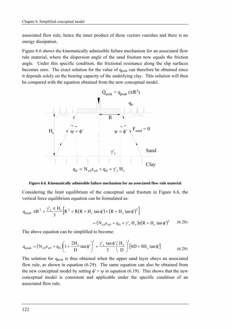
Chapter 6: Simplified conceptual model
122
associated flow rule; hence the inner product of these vectors vanishes and there is no energy dissipation.
Figure 6.6 shows the kinematically admissible failure mechanism for an associated flow rule material, where the dispersion angle of the sand frustum now equals the friction angle. Under this specific condition, the frictional resistance along the slip surfaces becomes zero. The exact solution for the value of qpeak can therefore be obtained since it depends solely on the bearing capacity of the underlying clay. This solution will then be compared with the equation obtained from the new conceptual model.
Qpeak = qpeak (πR2)
q0
Sand
Clay
Fsand = 0Hs 'φ=ψ 'φ=ψ
s'γ
ss00u0cb H'qsNq γ++=
R
Figure 6.6. Kinematically admissible failure mechanism for an associated flow rule material
Considering the limit equilibrium of the conceptual sand frustum in Figure 6.6, the vertical force equilibrium equation can be formulated as:
( ) ( )[ ]2ss
2ss2peak 'tanHR'tanHRRR
3H'
Rq φ++φ++πγ
+π
( ) ( )2sss00u0c 'tanHRH'qsN φ+πγ++= (6.28)
The above equation can be simplified to become:
( ) [ ]'tanH8D6DH
3'tan'
'tanDH2
1qsNq s
2ss
2s
00u0cpeak φ+⎟⎠
⎞⎜⎝
⎛φγ+⎟
⎠
⎞⎜⎝
⎛ φ++= (6.29)
The solution for qpeak is thus obtained when the upper sand layer obeys an associated flow rule, as shown in equation (6.29). The same equation can also be obtained from the new conceptual model by setting φ' = ψ in equation (6.19). This shows that the new conceptual model is consistent and applicable under the specific condition of an associated flow rule.
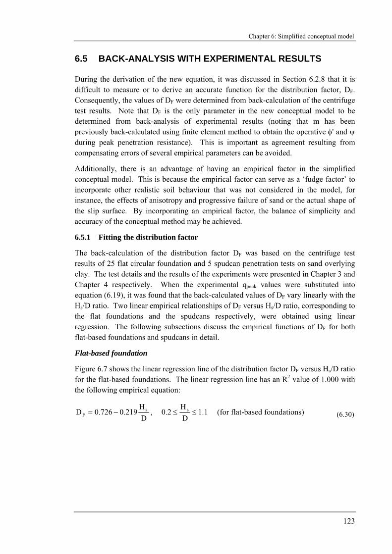
Chapter 6: Simplified conceptual model
123
6.5 BACK-ANALYSIS WITH EXPERIMENTAL RESULTS
During the derivation of the new equation, it was discussed in Section 6.2.8 that it is difficult to measure or to derive an accurate function for the distribution factor, DF. Consequently, the values of DF were determined from back-calculation of the centrifuge test results. Note that DF is the only parameter in the new conceptual model to be determined from back-analysis of experimental results (noting that m has been previously back-calculated using finite element method to obtain the operative φ' and ψ during peak penetration resistance). This is important as agreement resulting from compensating errors of several empirical parameters can be avoided.
Additionally, there is an advantage of having an empirical factor in the simplified conceptual model. This is because the empirical factor can serve as a ‘fudge factor’ to incorporate other realistic soil behaviour that was not considered in the model, for instance, the effects of anisotropy and progressive failure of sand or the actual shape of the slip surface. By incorporating an empirical factor, the balance of simplicity and accuracy of the conceptual method may be achieved.
6.5.1 Fitting the distribution factor
The back-calculation of the distribution factor DF was based on the centrifuge test results of 25 flat circular foundation and 5 spudcan penetration tests on sand overlying clay. The test details and the results of the experiments were presented in Chapter 3 and Chapter 4 respectively. When the experimental qpeak values were substituted into equation (6.19), it was found that the back-calculated values of DF vary linearly with the Hs/D ratio. Two linear empirical relationships of DF versus Hs/D ratio, corresponding to the flat foundations and the spudcans respectively, were obtained using linear regression. The following subsections discuss the empirical functions of DF for both flat-based foundations and spudcans in detail.
Flat-based foundation
Figure 6.7 shows the linear regression line of the distribution factor DF versus Hs/D ratio for the flat-based foundations. The linear regression line has an R2 value of 1.000 with the following empirical equation:
DH
219.0726.0D sF −= , 1.1
DH
2.0 s ≤≤ (for flat-based foundations) (6.30)

Chapter 6: Simplified conceptual model
124
0.45
0.50
0.55
0.60
0.65
0.70
0.75
0 0.2 0.4 0.6 0.8 1 1.2Hs/D ratio
Dis
tribu
tion
fact
or, D
FD2: 6.7m sand
D1: 6.2m sand
D2: 5.8m sandD2: 4.8m sand
D1: 4.1m sand
D2: 3.4m sandy = 0.726 - 0.219xR2 = 1.000
Figure 6.7. Linear regression line of Distribution Factor DF versus Hs/D ratio for flat foundations
By adopting the distribution factor DF from equation (6.30), an excellent match between the calculated qpeak values and the experimental results is obtained. This is shown in Figure 6.8. The differences between the calculated qpeak values and the test results for all 23 penetration tests are within +/- 5 % and the remaining two cases are at around 15 %.
It is likely that both cases with 15 % variation were caused by some errors in the experiments. Figure 6.9 shows the calculated qpeak (lines) and experimental qpeak values (points) versus the prototype area of foundation, with the values of possible experimental errors highlighted. It can be observed that the calculated values (lines) match the experimental values (points) very well (within 5 %), except for two cases where the foundation has 28 m2 prototype area (equivalent to 6 m diameter). The experimental qpeak values for sand layers 5.8 m and 6.2 m thick are almost identical to the qpeak value for a thicker sand layer of 6.7 m (equal to around 700 kPa). This is not rational for sand with similar relative density overlying soft clay. In contrast, the calculated qpeak values are around 15 % lower due to the thinner sand layer.

Chapter 6: Simplified conceptual model
125
0
200
400
600
800
0 200 400 600 800qpeak from centrifuge tests (kPa)
qpea
k fro
m c
once
ptua
l mod
el (k
Pa)
D2: 6.7m sandD1: 6.2m sandD2: 5.8m sandD2: 4.8m sandD1: 4.1m sandD2: 3.4m sand
Line of equility
+/- 20% variation
+/- 10% variation
Figure 6.8. Comparison of calculated and experimental qpeak values for flat foundations
0
100
200
300
400
500
600
700
800
20 70 120 170 220Prototype area (m2)
Pea
k pe
netra
tion
resi
stan
ce, q
pea
k (kP
a) D2: 6.7m sandD1: 6.2m sandD2: 5.8m sandD2: 4.8m sandD1: 4.1m sandD2: 3.4m sand
Possible experimental errors: Similar qpeak for three different sand thicknesses
Points denote test results.Lines denote values calculated from conceptual model.
Figure 6.9. Calculated qpeak and experimental qpeak versus prototype area of flat foundations
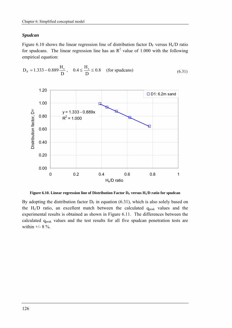
Chapter 6: Simplified conceptual model
126
Spudcan
Figure 6.10 shows the linear regression line of distribution factor DF versus Hs/D ratio for spudcans. The linear regression line has an R2 value of 1.000 with the following empirical equation:
DH
889.0333.1D sF −= , 8.0
DH
4.0 s ≤≤ (for spudcans) (6.31)
0.00
0.20
0.40
0.60
0.80
1.00
1.20
0 0.2 0.4 0.6 0.8 1Hs/D ratio
Dis
tribu
tion
fact
or, D
F
D1: 6.2m sand
y = 1.333 - 0.889xR2 = 1.000
Figure 6.10. Linear regression line of Distribution Factor DF versus Hs/D ratio for spudcan
By adopting the distribution factor DF in equation (6.31), which is also solely based on the Hs/D ratio, an excellent match between the calculated qpeak values and the experimental results is obtained as shown in Figure 6.11. The differences between the calculated qpeak values and the test results for all five spudcan penetration tests are within +/- 8 %.

Chapter 6: Simplified conceptual model
127
0
200
400
600
800
0 200 400 600 800qpeak from centrifuge tests (kPa)
qpea
k fro
m c
once
ptua
l mod
el (k
Pa)
D1: 6.2m sand
Line of equility
+/- 20% variation
+/- 10% variation
Figure 6.11. Comparison of qpeak calculated from current model and the experimental results for spudcan
6.5.2 Discussion on the back-calculated distribution factor
This section discusses the trend of the empirical DF function from the physical perspective of a punch-through phenomenon. It is recalled that DF is defined as the ratio of the vertical effective stress at the slip surface (σ'z)slip to the mean vertical effective stress, z'σ of the conceptual sand frustum. The empirical lines of DF for both flat foundation and spudcan are shown in Figure 6.12.
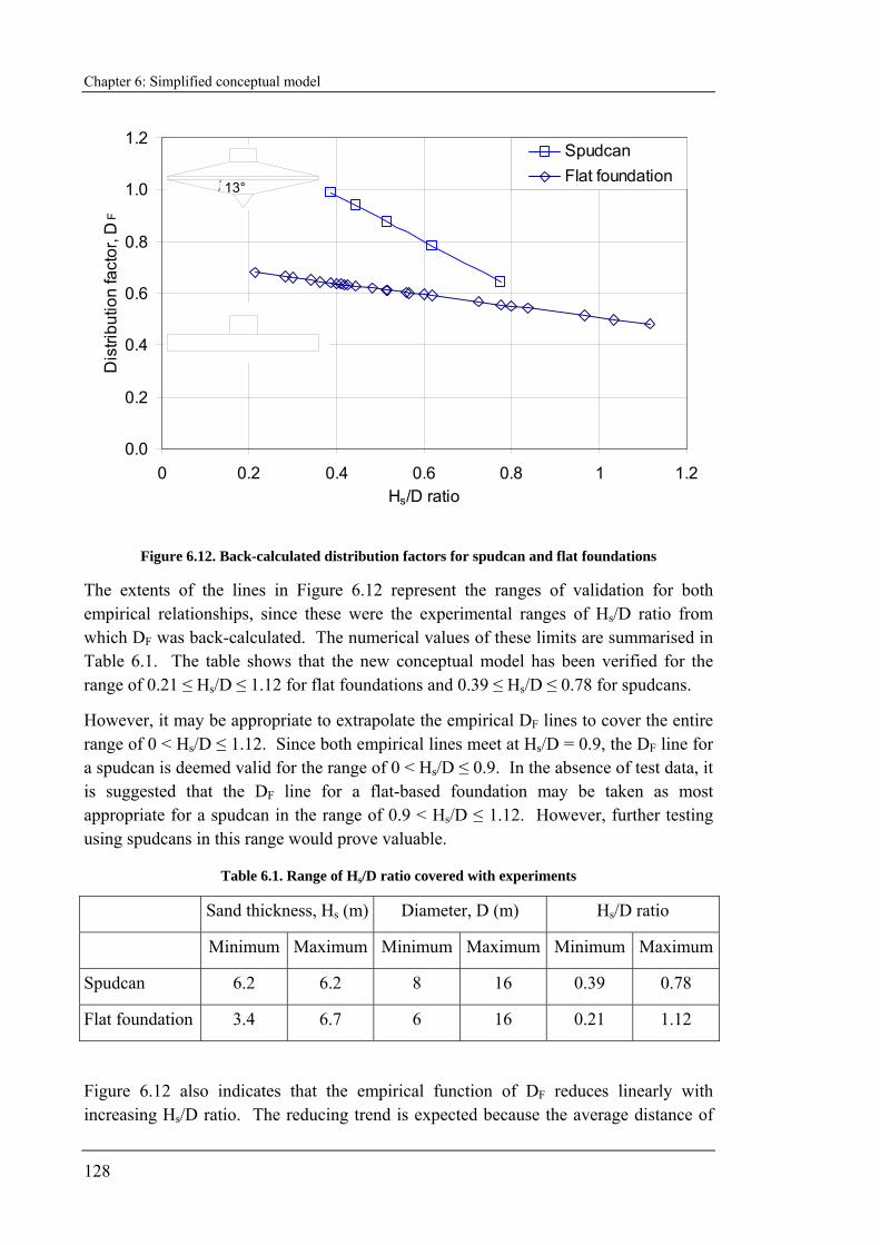
Chapter 6: Simplified conceptual model
128
0.0
0.2
0.4
0.6
0.8
1.0
1.2
0 0.2 0.4 0.6 0.8 1 1.2Hs/D ratio
Dis
tribu
tion
fact
or, D
F
SpudcanFlat foundation
13°
Figure 6.12. Back-calculated distribution factors for spudcan and flat foundations
The extents of the lines in Figure 6.12 represent the ranges of validation for both empirical relationships, since these were the experimental ranges of Hs/D ratio from which DF was back-calculated. The numerical values of these limits are summarised in Table 6.1. The table shows that the new conceptual model has been verified for the range of 0.21 ≤ Hs/D ≤ 1.12 for flat foundations and 0.39 ≤ Hs/D ≤ 0.78 for spudcans.
However, it may be appropriate to extrapolate the empirical DF lines to cover the entire range of 0 < Hs/D ≤ 1.12. Since both empirical lines meet at Hs/D = 0.9, the DF line for a spudcan is deemed valid for the range of 0 < Hs/D ≤ 0.9. In the absence of test data, it is suggested that the DF line for a flat-based foundation may be taken as most appropriate for a spudcan in the range of 0.9 < Hs/D ≤ 1.12. However, further testing using spudcans in this range would prove valuable.
Table 6.1. Range of Hs/D ratio covered with experiments
Sand thickness, Hs (m) Diameter, D (m) Hs/D ratio
Minimum Maximum Minimum Maximum Minimum Maximum
Spudcan 6.2 6.2 8 16 0.39 0.78
Flat foundation 3.4 6.7 6 16 0.21 1.12
Figure 6.12 also indicates that the empirical function of DF reduces linearly with increasing Hs/D ratio. The reducing trend is expected because the average distance of
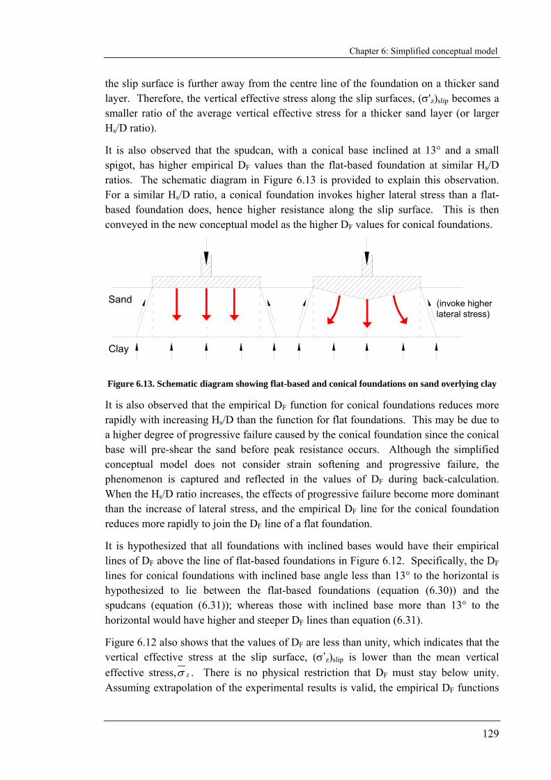
Chapter 6: Simplified conceptual model
129
the slip surface is further away from the centre line of the foundation on a thicker sand layer. Therefore, the vertical effective stress along the slip surfaces, (σ'z)slip becomes a smaller ratio of the average vertical effective stress for a thicker sand layer (or larger Hs/D ratio).
It is also observed that the spudcan, with a conical base inclined at 13° and a small spigot, has higher empirical DF values than the flat-based foundation at similar Hs/D ratios. The schematic diagram in Figure 6.13 is provided to explain this observation. For a similar Hs/D ratio, a conical foundation invokes higher lateral stress than a flat-based foundation does, hence higher resistance along the slip surface. This is then conveyed in the new conceptual model as the higher DF values for conical foundations.
Sand
Clay
(invoke higher lateral stress)
Figure 6.13. Schematic diagram showing flat-based and conical foundations on sand overlying clay
It is also observed that the empirical DF function for conical foundations reduces more rapidly with increasing Hs/D than the function for flat foundations. This may be due to a higher degree of progressive failure caused by the conical foundation since the conical base will pre-shear the sand before peak resistance occurs. Although the simplified conceptual model does not consider strain softening and progressive failure, the phenomenon is captured and reflected in the values of DF during back-calculation. When the Hs/D ratio increases, the effects of progressive failure become more dominant than the increase of lateral stress, and the empirical DF line for the conical foundation reduces more rapidly to join the DF line of a flat foundation.
It is hypothesized that all foundations with inclined bases would have their empirical lines of DF above the line of flat-based foundations in Figure 6.12. Specifically, the DF lines for conical foundations with inclined base angle less than 13° to the horizontal is hypothesized to lie between the flat-based foundations (equation (6.30)) and the spudcans (equation (6.31)); whereas those with inclined base more than 13° to the horizontal would have higher and steeper DF lines than equation (6.31).
Figure 6.12 also shows that the values of DF are less than unity, which indicates that the vertical effective stress at the slip surface, (σ’z)slip is lower than the mean vertical effective stress, zσ . There is no physical restriction that DF must stay below unity. Assuming extrapolation of the experimental results is valid, the empirical DF functions
Chapter 6: Simplified conceptual model
130
in Figure 6.12 suggest that DF may have values larger than unity for conical foundations on sand overlying clay with very low Hs/D ratios. This could be possible as large lateral stresses could be incurred while the degree of progressive failure is small.
It has been noted in the literature that qpeak of a circular foundation on sand overlying clay approaches the bearing capacity of the upper sand for Hs/D > 2 (e.g. Meyerhof, 1974; Okamura et al., 1997). However, since the current conceptual model incorporates an empirical factor, it is suggested that the validated range for both flat foundations and spudcans be kept to Hs/D ≤ 1.12. In any case, the punch-through of an offshore spudcan is rarely a problem for Hs/D > 1 as the peak resistance provided by the layered soils is larger than the typical range of spudcan preloading pressures (see Section 7.2).
6.6 INPUT PARAMETERS FOR THE NEW EQUATION
Table 6.2 summarises all input parameters for the new equation and some remarks on the methods of determining them. The input parameters are well defined and assessable from a proper site investigation scheme. In addition, they are familiar to practising engineers. The new conceptual model essentially involves one equation (i.e. equation (6.19)) and only requires the necessary geometry and soil strength parameters to calculate the peak penetration resistance, qpeak (or punch-through resistance) of a foundation on sand overlying clay. These features enable the new conceptual model to be a potential routine design tool for punch-through on sand overlying clay.

Chapter 6: Simplified conceptual model
131
Table 6.2. Parameters for new conceptual model equation
Category Parameter Method of determining parameter
Foundation diameter, D Known parameter Geometry
Sand thickness, Hs Measured from in-situ tests
Relative density, ID and effective unit weight, γ's
Measured from in-situ or laboratory tests
Critical state friction angle, φcv
Measured from laboratory tests; or estimated based on mineralogy (see Table 6.3)
Parameter Q in Bolton’s (1986) equation
Measured from laboratory tests; or estimated based on mineralogy (see Table 6.3)
Relative dilatancy index, IR Obtained from iterative calculation between equation (6.19) (or equation (6.24) for ψ = 0) and equations (6.25) to (6.27)
Friction angle, φ' and dilation angle, ψ
Obtained from equations (6.26) and (6.27): Rcv I65.2' +φ=φ ; cv'8.0 φ−φ=ψ (φ', φcv
and ψ in degree)
Sand
Reduced friction angle due to non-associated flow rule, φ* ψφ−
ψφ=φ
sin'sin1cos'sin*tan (Drescher and
Detournay, 1993)
Undrained shear strength at sand-clay interface, su0
Measured from in-situ or laboratory tests
Gradient of linear increment of undrained shear strength with depth, ρ and non-dimensional parameter, κ
ρ can be inferred from site investigation, and
κ is given as:( )
0u
s
stanH2D ψ+ρ
=κ
Clay
Bearing capacity factor, Nc0 κ+≈ 56.034.6N 0c or refer to Martin (2001) and Houlsby and Martin (2003)
Empirical factor
Distribution factor, DF Defined as the ratio of the vertical effective stress at the slip surface to the mean vertical effective stress within the sand layer.
For flat-based circular foundation, use
DH
219.0726.0D sF −= , Hs/D ≤ 1.12
For spudcans with conical base inclined at 13° to the horizontal, use
DH
889.0333.1D sF −= , Hs/D ≤ 0.9
DH
219.0726.0D sF −= , 0.9 < Hs/D ≤ 1.12
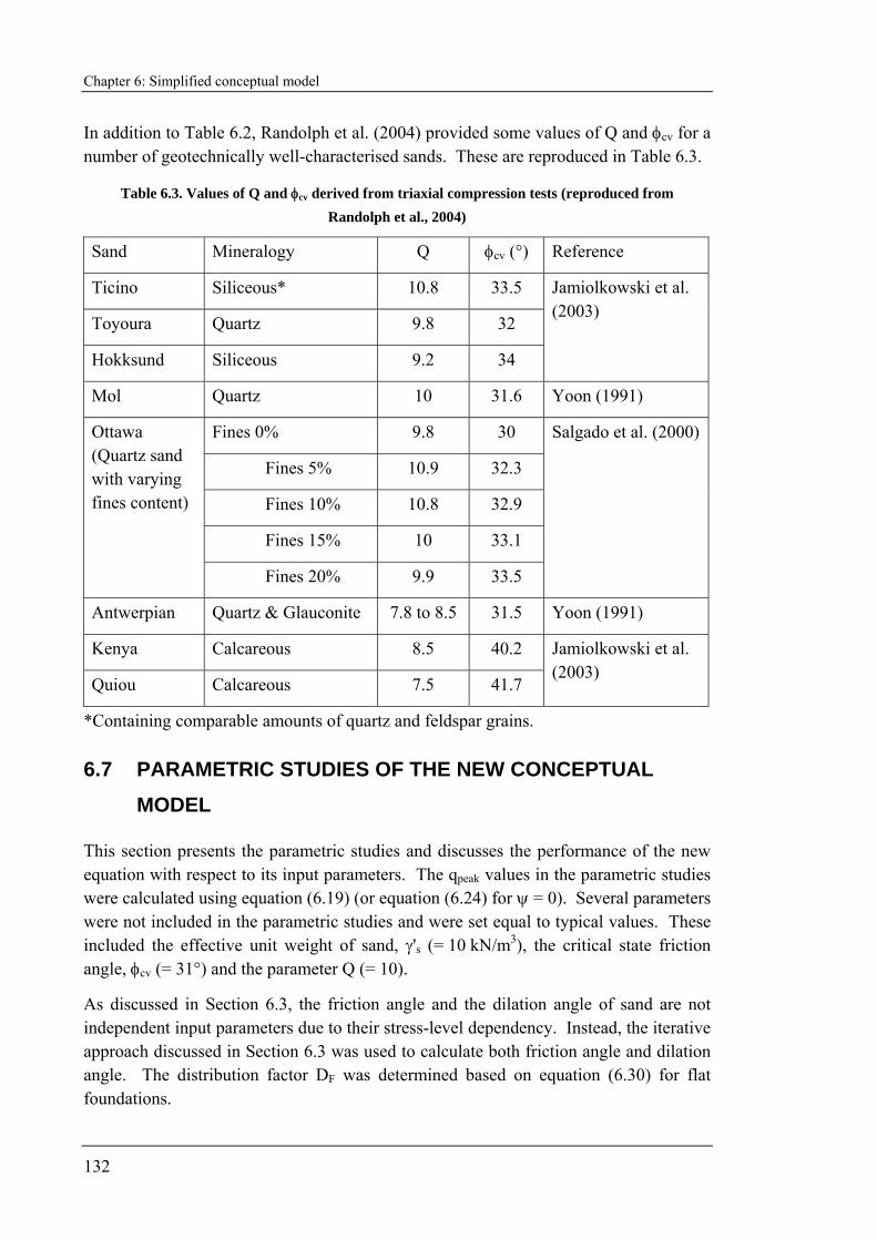
Chapter 6: Simplified conceptual model
132
In addition to Table 6.2, Randolph et al. (2004) provided some values of Q and φcv for a number of geotechnically well-characterised sands. These are reproduced in Table 6.3.
Table 6.3. Values of Q and φcv derived from triaxial compression tests (reproduced from Randolph et al., 2004)
Sand Mineralogy Q φcv (°) Reference
Ticino Siliceous* 10.8 33.5
Toyoura Quartz 9.8 32
Hokksund Siliceous 9.2 34
Jamiolkowski et al. (2003)
Mol Quartz 10 31.6 Yoon (1991)
Fines 0% 9.8 30
Fines 5% 10.9 32.3
Fines 10% 10.8 32.9
Fines 15% 10 33.1
Ottawa (Quartz sand with varying fines content)
Fines 20% 9.9 33.5
Salgado et al. (2000)
Antwerpian Quartz & Glauconite 7.8 to 8.5 31.5 Yoon (1991)
Kenya Calcareous 8.5 40.2
Quiou Calcareous 7.5 41.7
Jamiolkowski et al. (2003)
*Containing comparable amounts of quartz and feldspar grains.
6.7 PARAMETRIC STUDIES OF THE NEW CONCEPTUAL MODEL
This section presents the parametric studies and discusses the performance of the new equation with respect to its input parameters. The qpeak values in the parametric studies were calculated using equation (6.19) (or equation (6.24) for ψ = 0). Several parameters were not included in the parametric studies and were set equal to typical values. These included the effective unit weight of sand, γ's (= 10 kN/m3), the critical state friction angle, φcv (= 31°) and the parameter Q (= 10).
As discussed in Section 6.3, the friction angle and the dilation angle of sand are not independent input parameters due to their stress-level dependency. Instead, the iterative approach discussed in Section 6.3 was used to calculate both friction angle and dilation angle. The distribution factor DF was determined based on equation (6.30) for flat foundations.
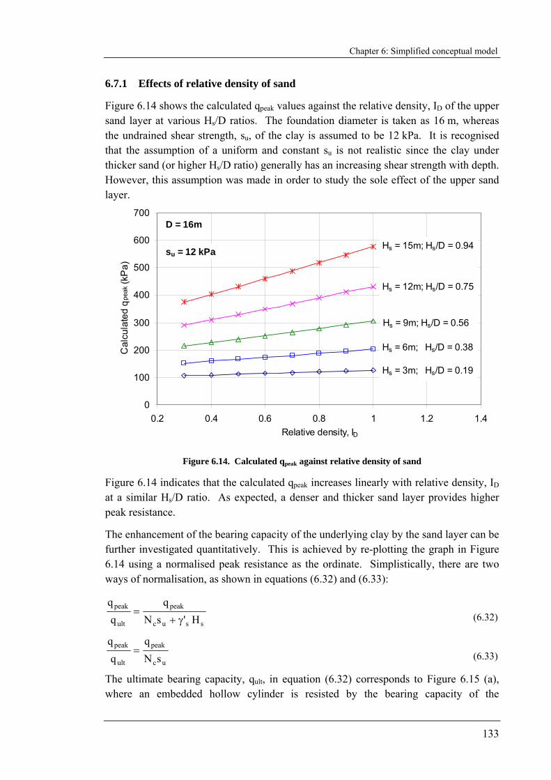
Chapter 6: Simplified conceptual model
133
6.7.1 Effects of relative density of sand
Figure 6.14 shows the calculated qpeak values against the relative density, ID of the upper sand layer at various Hs/D ratios. The foundation diameter is taken as 16 m, whereas the undrained shear strength, su, of the clay is assumed to be 12 kPa. It is recognised that the assumption of a uniform and constant su is not realistic since the clay under thicker sand (or higher Hs/D ratio) generally has an increasing shear strength with depth. However, this assumption was made in order to study the sole effect of the upper sand layer.
0
100
200
300
400
500
600
700
0.2 0.4 0.6 0.8 1 1.2 1.4Relative density, ID
Cal
cula
ted
q pea
k (kP
a)
Hs = 15m; Hs/D = 0.94
Hs = 12m; Hs/D = 0.75
Hs = 9m; Hs/D = 0.56
Hs = 6m; Hs/D = 0.38
Hs = 3m; Hs/D = 0.19
D = 16m
su = 12 kPa
Figure 6.14. Calculated qpeak against relative density of sand
Figure 6.14 indicates that the calculated qpeak increases linearly with relative density, ID at a similar Hs/D ratio. As expected, a denser and thicker sand layer provides higher peak resistance.
The enhancement of the bearing capacity of the underlying clay by the sand layer can be further investigated quantitatively. This is achieved by re-plotting the graph in Figure 6.14 using a normalised peak resistance as the ordinate. Simplistically, there are two ways of normalisation, as shown in equations (6.32) and (6.33):
ssuc
peak
ult
peak
H'sNq
γ+= (6.32)
uc
peak
ult
peak
sNq
= (6.33)
The ultimate bearing capacity, qult, in equation (6.32) corresponds to Figure 6.15 (a), where an embedded hollow cylinder is resisted by the bearing capacity of the
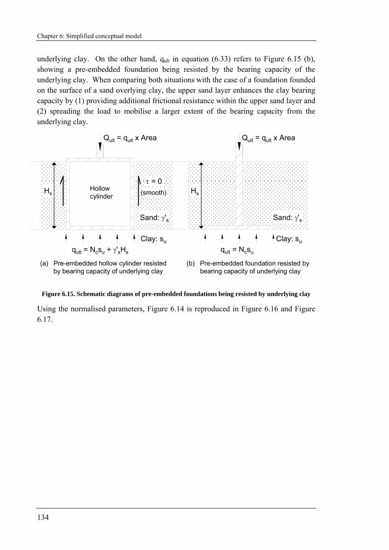
Chapter 6: Simplified conceptual model
134
underlying clay. On the other hand, qult in equation (6.33) refers to Figure 6.15 (b), showing a pre-embedded foundation being resisted by the bearing capacity of the underlying clay. When comparing both situations with the case of a foundation founded on the surface of a sand overlying clay, the upper sand layer enhances the clay bearing capacity by (1) providing additional frictional resistance within the upper sand layer and (2) spreading the load to mobilise a larger extent of the bearing capacity from the underlying clay.
qult = Ncsu
(b) Pre-embedded foundation resisted by bearing capacity of underlying clay
Sand: γ's
Hs
Clay: su
τ = 0(smooth)
qult = Ncsu + γ'sHs
(a) Pre-embedded hollow cylinder resisted by bearing capacity of underlying clay
Hollow cylinder
Sand: γ's
Hs
Clay: su
Qult = qult x Area Qult = qult x Area
Figure 6.15. Schematic diagrams of pre-embedded foundations being resisted by underlying clay
Using the normalised parameters, Figure 6.14 is reproduced in Figure 6.16 and Figure 6.17.
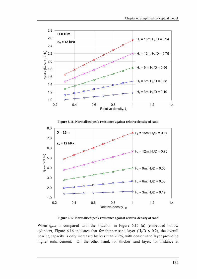
Chapter 6: Simplified conceptual model
135
1.0
1.2
1.4
1.6
1.8
2.0
2.2
2.4
2.6
2.8
0.2 0.4 0.6 0.8 1 1.2 1.4Relative density, ID
qpea
k / (N
c su +
γ's H
s )Hs = 15m; Hs/D = 0.94
Hs = 12m; Hs/D = 0.75
Hs = 9m; Hs/D = 0.56
Hs = 6m; Hs/D = 0.38
Hs = 3m; Hs/D = 0.19
D = 16m
su = 12 kPa
Figure 6.16. Normalised peak resistance against relative density of sand
1.0
2.0
3.0
4.0
5.0
6.0
7.0
8.0
0.2 0.4 0.6 0.8 1 1.2 1.4Relative density, ID
qpea
k / (N
c su )
D = 16m
su = 12 kPa
Hs = 15m; Hs/D = 0.94
Hs = 12m; Hs/D = 0.75
Hs = 9m; Hs/D = 0.56
Hs = 6m; Hs/D = 0.38
Hs = 3m; Hs/D = 0.19
Figure 6.17. Normalised peak resistance against relative density of sand
When qpeak is compared with the situation in Figure 6.15 (a) (embedded hollow cylinder), Figure 6.16 indicates that for thinner sand layer (Hs/D ≈ 0.2), the overall bearing capacity is only increased by less than 20 %, with denser sand layer providing higher enhancement. On the other hand, for thicker sand layer, for instance at
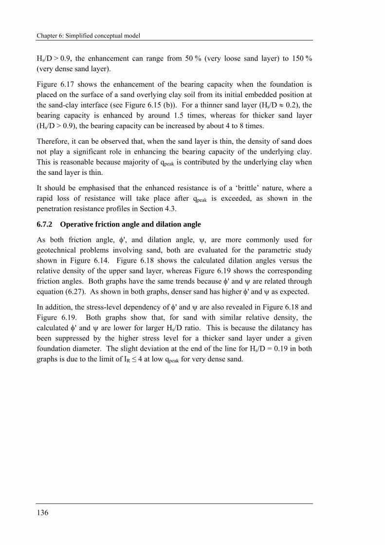
Chapter 6: Simplified conceptual model
136
Hs/D > 0.9, the enhancement can range from 50 % (very loose sand layer) to 150 % (very dense sand layer).
Figure 6.17 shows the enhancement of the bearing capacity when the foundation is placed on the surface of a sand overlying clay soil from its initial embedded position at the sand-clay interface (see Figure 6.15 (b)). For a thinner sand layer (Hs/D ≈ 0.2), the bearing capacity is enhanced by around 1.5 times, whereas for thicker sand layer (Hs/D > 0.9), the bearing capacity can be increased by about 4 to 8 times.
Therefore, it can be observed that, when the sand layer is thin, the density of sand does not play a significant role in enhancing the bearing capacity of the underlying clay. This is reasonable because majority of qpeak is contributed by the underlying clay when the sand layer is thin.
It should be emphasised that the enhanced resistance is of a ‘brittle’ nature, where a rapid loss of resistance will take place after qpeak is exceeded, as shown in the penetration resistance profiles in Section 4.3.
6.7.2 Operative friction angle and dilation angle
As both friction angle, φ', and dilation angle, ψ, are more commonly used for geotechnical problems involving sand, both are evaluated for the parametric study shown in Figure 6.14. Figure 6.18 shows the calculated dilation angles versus the relative density of the upper sand layer, whereas Figure 6.19 shows the corresponding friction angles. Both graphs have the same trends because φ' and ψ are related through equation (6.27). As shown in both graphs, denser sand has higher φ' and ψ as expected.
In addition, the stress-level dependency of φ' and ψ are also revealed in Figure 6.18 and Figure 6.19. Both graphs show that, for sand with similar relative density, the calculated φ' and ψ are lower for larger Hs/D ratio. This is because the dilatancy has been suppressed by the higher stress level for a thicker sand layer under a given foundation diameter. The slight deviation at the end of the line for Hs/D = 0.19 in both graphs is due to the limit of IR ≤ 4 at low qpeak for very dense sand.

Chapter 6: Simplified conceptual model
137
0
2
4
6
8
10
12
14
0.2 0.4 0.6 0.8 1 1.2 1.4Relative density, ID
Dila
tion
angl
e, ψ
(deg
ree)
Hs = 15m; Hs/D = 0.94Hs = 12m; Hs/D = 0.75
Hs = 9m; Hs/D = 0.56
Hs = 6m; Hs/D = 0.38Hs = 3m; Hs/D = 0.19D = 16m
su = 12 kPa
Figure 6.18. Calculated dilation angle against relative density of sand
30
32
34
36
38
40
42
44
0.2 0.4 0.6 0.8 1 1.2 1.4Relative density, ID
Fric
tion
angl
e, φ'
(deg
ree)
D = 16m
su = 12 kPa
φcv = 31°
Hs = 15m; Hs/D = 0.94Hs = 12m; Hs/D = 0.75Hs = 9m; Hs/D = 0.56Hs = 6m; Hs/D = 0.38Hs = 3m; Hs/D = 0.19
Figure 6.19. Calculated friction angle against relative density of sand
6.7.3 Effects of sand thickness (Hs/D ratio)
Figure 6.20 shows the qpeak values of a foundation with 16 m diameter, penetrating on a sand layer with its thickness varying from zero to 15 m. It is observed that the calculated qpeak increases almost exponentially with increasing sand thickness. Furthermore, Figure 6.20 also shows that the rate of increment of qpeak is higher for

Chapter 6: Simplified conceptual model
138
denser sand. This is in line with common sense that a denser sand layer is more effective in enhancing the bearing capacity. This is because (1) a higher friction angle provides a larger frictional resistance and (2) a higher dilation angle causes a larger extent of the underlying clay to be mobilised.
When the sand thickness, Hs becomes zero (clay only profile), all qpeak values converge to a single value that matches with the bearing capacity of the underlying clay. In this parametric study, all lines meet at 76 kPa, which is equal to the product of 12 kPa and a bearing capacity factor of 6.34. This is slightly larger than the exact solution of 6.05 (Eason and Shield, 1960), because the spreadsheet used to produce Figure 6.20 adopted the curve-fitted equation (6.3) in calculating the bearing capacity factor (Houlsby and Martin, 2003).
0
100
200
300
400
500
600
0 5 10 15Sand thickness, Hs (m)
Cal
cula
ted
q pea
k (kP
a)
ID = 0.8D = 16m
su = 12 kPa
ID = 1.0
ID = 0.6
ID = 0.4
ID = 0.2
Figure 6.20. Calculated qpeak against sand thickness
Following a similar discussion in Section 6.7.1, two complementary graphs to Figure 6.20 are produced in Figure 6.21 and Figure 6.22 to examine the enhancement of the underlying bearing capacity by the sand layer. Both figures indicate that the bearing capacity of the underlying clay is enhanced significantly with increasing sand thickness.

Chapter 6: Simplified conceptual model
139
0.8
1.0
1.2
1.4
1.6
1.8
2.0
2.2
2.4
2.6
0 5 10 15Sand thickness, Hs (m)
Cal
cula
ted
q pea
k / (N
c su +
γ's H
s ) ID = 0.8
D = 16m
su = 12 kPa
ID = 1.0
ID = 0.6
ID = 0.4
ID = 0.2
Figure 6.21. Normalised peak resistance against sand thickness
0.0
1.0
2.0
3.0
4.0
5.0
6.0
7.0
8.0
0 5 10 15Sand thickness, Hs (m)
Cal
cula
ted
q pea
k / (N
c su )
ID = 0.8D = 16m
su = 12 kPa
ID = 1.0
ID = 0.6ID = 0.4
ID = 0.2
Figure 6.22. Normalised peak resistance against sand thickness
6.7.4 Effects of foundation diameter
The experimental results in Chapter 4 (see Figure 4.18 and Figure 4.19 in Section 4.4) show that qpeak reduces when a larger foundation is used to penetrate a sand layer with a given thickness. The exact trend is being predicted by the new conceptual model, as shown in Figure 6.23. In this parametric study, the sand thickness and the shear

Chapter 6: Simplified conceptual model
140
strength of the underlying clay were fixed at 8 m and 12 kPa respectively. The calculated qpeak values were then plotted against the foundation diameter. It can be observed that the calculated qpeak reduces with increasing foundation diameter on a given sand layer. Therefore, for a particular field condition of sand overlying clay, a larger spudcan will cause a smaller qpeak. However, it should be noted that the penetration force will actually become larger because qpeak needs to be multiplied with a factor of diameter squared to obtain the penetration force.
0
100
200
300
400
500
600
5 10 15 20Footing diameter, D (m)
Cal
cula
ted
q pea
k (kP
a) ID = 0.8
Hs = 8m
su = 12 kPaID = 1.0
ID = 0.6ID = 0.4
ID = 0.2
Figure 6.23. Calculated qpeak against foundation diameter
6.7.5 Effects of bearing capacity of the underlying clay
Figure 6.24 shows the variation of the calculated qpeak against the bearing capacity of the underlying clay at different Hs/D ratios. For a similar Hs/D ratio, the calculated qpeak increases almost linearly with the shear strength of the underlying clay.
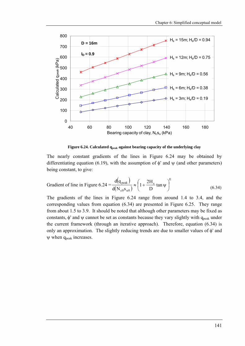
Chapter 6: Simplified conceptual model
141
0
100
200
300
400
500
600
700
800
40 60 80 100 120 140 160 180Bearing capacity of clay, Ncsu (kPa)
Cal
cula
ted
q pea
k (kP
a)
Hs = 15m; Hs/D = 0.94
Hs = 12m; Hs/D = 0.75
Hs = 9m; Hs/D = 0.56
Hs = 6m; Hs/D = 0.38
Hs = 3m; Hs/D = 0.19
D = 16m
ID = 0.9
Figure 6.24. Calculated qpeak against bearing capacity of the underlying clay
The nearly constant gradients of the lines in Figure 6.24 may be obtained by differentiating equation (6.19), with the assumption of φ' and ψ (and other parameters) being constant, to give:
Gradient of line in Figure 6.24 =( )
( )
Es
0u0c
peak tanDH2
1sNd
qd⎟⎠
⎞⎜⎝
⎛ ψ+≈ (6.34)
The gradients of the lines in Figure 6.24 range from around 1.4 to 3.4, and the corresponding values from equation (6.34) are presented in Figure 6.25. They range from about 1.5 to 3.9. It should be noted that although other parameters may be fixed as constants, φ' and ψ cannot be set as constants because they vary slightly with qpeak under the current framework (through an iterative approach). Therefore, equation (6.34) is only an approximation. The slightly reducing trends are due to smaller values of φ' and ψ when qpeak increases.
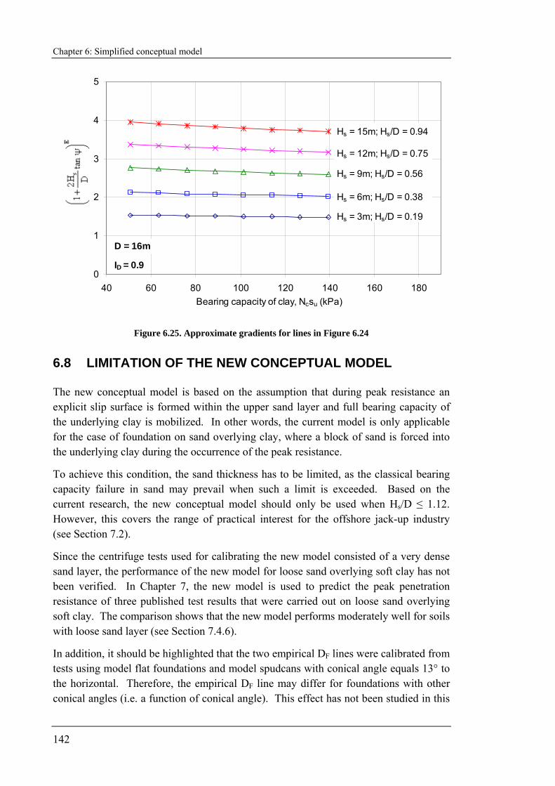
Chapter 6: Simplified conceptual model
142
0
1
2
3
4
5
40 60 80 100 120 140 160 180Bearing capacity of clay, Ncsu (kPa)
"Gra
dien
t"
Hs = 15m; Hs/D = 0.94
Hs = 12m; Hs/D = 0.75
Hs = 9m; Hs/D = 0.56
Hs = 6m; Hs/D = 0.38
Hs = 3m; Hs/D = 0.19
D = 16m
ID = 0.9
Figure 6.25. Approximate gradients for lines in Figure 6.24
6.8 LIMITATION OF THE NEW CONCEPTUAL MODEL
The new conceptual model is based on the assumption that during peak resistance an explicit slip surface is formed within the upper sand layer and full bearing capacity of the underlying clay is mobilized. In other words, the current model is only applicable for the case of foundation on sand overlying clay, where a block of sand is forced into the underlying clay during the occurrence of the peak resistance.
To achieve this condition, the sand thickness has to be limited, as the classical bearing capacity failure in sand may prevail when such a limit is exceeded. Based on the current research, the new conceptual model should only be used when Hs/D ≤ 1.12. However, this covers the range of practical interest for the offshore jack-up industry (see Section 7.2).
Since the centrifuge tests used for calibrating the new model consisted of a very dense sand layer, the performance of the new model for loose sand overlying soft clay has not been verified. In Chapter 7, the new model is used to predict the peak penetration resistance of three published test results that were carried out on loose sand overlying soft clay. The comparison shows that the new model performs moderately well for soils with loose sand layer (see Section 7.4.6).
In addition, it should be highlighted that the two empirical DF lines were calibrated from tests using model flat foundations and model spudcans with conical angle equals 13° to the horizontal. Therefore, the empirical DF line may differ for foundations with other conical angles (i.e. a function of conical angle). This effect has not been studied in this
Chapter 6: Simplified conceptual model
143
research and more experiments using model foundations with various conical angles would prove useful.
6.9 CONCLUDING REMARKS
The development of a new conceptual model to calculate the peak penetration resistance, qpeak of circular foundations on sand overlying clay was presented in this chapter. A new semi-empirical equation has been derived from this conceptual model, with the input parameters listed in Section 6.6. Unlike the traditional analytical methods, the new model takes into account the stress level and dilatant response of the upper sand layer.
The new method involves an iterative approach to determine the stress level dependent friction and dilation angles and the peak penetration resistance consistently. Therefore, in order to use this method effectively, it is best to write the equations into a calculation spreadsheet such as MS Excel for the iterative calculation. This approach has an advantage over producing design charts, since essentially unlimited combinations of input parameters can be entered into the spreadsheet, rather than interpolating among the design charts to calculate the required qpeak.
In addition, sensitivity tests on a particular parameter can be easily performed with the spreadsheet and relevant graphs can be plotted to evaluate the influence of the parameter under studies. This is particularly useful since it is difficult to obtain accurate seabed soil parameters with high confidence for foundation design of mobile jack-ups (Osborne et al., 2006).
The relative simplicity and accuracy of the current conceptual model provides the jack-up industry with an analytical tool for practical routine designs. It will be tested against experimental data outside the database used in its derivations, as well as against current methodologies provided in the jack-up industry guidelines in Chapter 7.
Chapter 7: Comparison of analytical methods
144
CHAPTER 7. COMPARISON OF ANALYTICAL METHODS FOR BEARING CAPACITY ON SAND
OVERLYING CLAY SOILS
7.1 INTRODUCTION
The sensitivity of the new conceptual model to variations of the input parameters has been discussed in Chapter 6. The performance of the new conceptual model in predicting the peak penetration resistance, qpeak, will be further investigated in this chapter through comparative studies with other existing methods and other experimental data.
The new conceptual model was calibrated using the drum centrifuge test results performed in this research. Additional test data, which consist of previously published experimental results and an additional five spudcan penetration tests carried out using the UWA beam centrifuge in this research, will be incorporated in the comparison in this chapter. This allows a fairer comparison of the method.
In addition to the new conceptual model, six published analytical methods, including two from the current design guidelines (SNAME, 2002), are used to calculate the values of qpeak. These are also compared with the experimental results. All of these methods were introduced in Chapter 2, and their performance in predicting the centrifuge test results is discussed in this chapter. Finally, the findings from the comparative studies are summarised at the end of the chapter.
7.2 DATABASE
The database for this comparative study consists of 47 centrifuge tests as summarised in Table 7.1. They are made up of 28 drum centrifuge tests used to derive the model (see Chapters 3 and 4), 14 from previously published results (Teh, 2007; Craig and Chua, 1990) and an additional 5 beam centrifuge tests conducted for this study.
Only test data with Hs/D less than unity have been included in this comparative study. As offshore punch-through cases with Hs/D >1 are rarely reported (Baglioni et al., 1982), this limits the database to a range of practical interest to the jack-up industry. Furthermore, the centrifuge results in this study, and also those carried out by Teh (2007), show that for Hs/D >1 the values of the peak penetration resistance exceed 700 kPa. This is higher than the typical range of spudcan preload of around 400 kPa to 600 kPa (Osborne et al., 2008; Randolph et al., 2005).
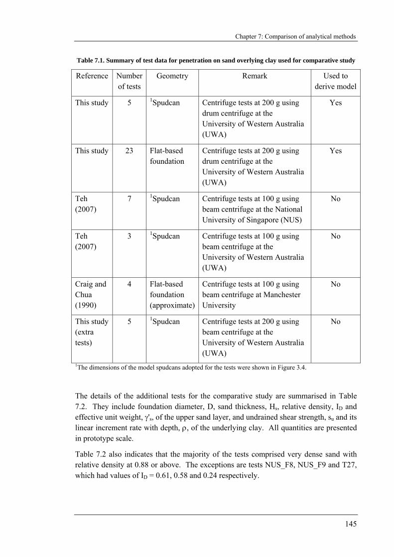
Chapter 7: Comparison of analytical methods
145
Table 7.1. Summary of test data for penetration on sand overlying clay used for comparative study
Reference Number of tests
Geometry Remark Used to derive model
This study 5 1Spudcan Centrifuge tests at 200 g using drum centrifuge at the University of Western Australia (UWA)
Yes
This study 23 Flat-based foundation
Centrifuge tests at 200 g using drum centrifuge at the University of Western Australia (UWA)
Yes
Teh (2007)
7 1Spudcan Centrifuge tests at 100 g using beam centrifuge at the National University of Singapore (NUS)
No
Teh (2007)
3 1Spudcan Centrifuge tests at 100 g using beam centrifuge at the University of Western Australia (UWA)
No
Craig and Chua (1990)
4 Flat-based foundation (approximate)
Centrifuge tests at 100 g using beam centrifuge at Manchester University
No
This study (extra tests)
5 1Spudcan Centrifuge tests at 200 g using beam centrifuge at the University of Western Australia (UWA)
No
1The dimensions of the model spudcans adopted for the tests were shown in Figure 3.4.
The details of the additional tests for the comparative study are summarised in Table 7.2. They include foundation diameter, D, sand thickness, Hs, relative density, ID and effective unit weight, γ's, of the upper sand layer, and undrained shear strength, su and its linear increment rate with depth, ρ, of the underlying clay. All quantities are presented in prototype scale.
Table 7.2 also indicates that the majority of the tests comprised very dense sand with relative density at 0.88 or above. The exceptions are tests NUS_F8, NUS_F9 and T27, which had values of ID = 0.61, 0.58 and 0.24 respectively.
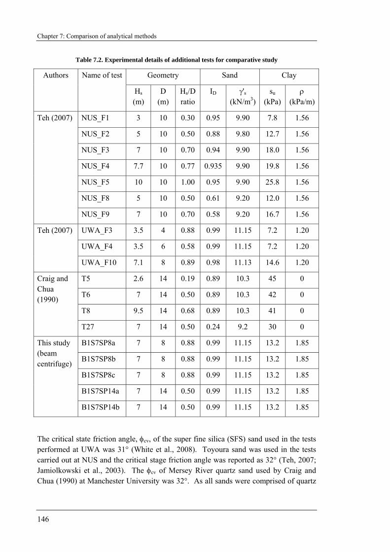
Chapter 7: Comparison of analytical methods
146
Table 7.2. Experimental details of additional tests for comparative study
Geometry Sand Clay Authors Name of test
Hs (m)
D (m)
Hs/D ratio
ID γ's (kN/m3)
su (kPa)
ρ (kPa/m)
NUS_F1 3 10 0.30 0.95 9.90 7.8 1.56
NUS_F2 5 10 0.50 0.88 9.80 12.7 1.56
NUS_F3 7 10 0.70 0.94 9.90 18.0 1.56
NUS_F4 7.7 10 0.77 0.935 9.90 19.8 1.56
NUS_F5 10 10 1.00 0.95 9.90 25.8 1.56
NUS_F8 5 10 0.50 0.61 9.20 12.0 1.56
Teh (2007)
NUS_F9 7 10 0.70 0.58 9.20 16.7 1.56
UWA_F3 3.5 4 0.88 0.99 11.15 7.2 1.20
UWA_F4 3.5 6 0.58 0.99 11.15 7.2 1.20
Teh (2007)
UWA_F10 7.1 8 0.89 0.98 11.13 14.6 1.20
T5 2.6 14 0.19 0.89 10.3 45 0
T6 7 14 0.50 0.89 10.3 42 0
T8 9.5 14 0.68 0.89 10.3 41 0
Craig and Chua (1990)
T27 7 14 0.50 0.24 9.2 30 0
B1S7SP8a 7 8 0.88 0.99 11.15 13.2 1.85
B1S7SP8b 7 8 0.88 0.99 11.15 13.2 1.85
B1S7SP8c 7 8 0.88 0.99 11.15 13.2 1.85
B1S7SP14a 7 14 0.50 0.99 11.15 13.2 1.85
This study (beam centrifuge)
B1S7SP14b 7 14 0.50 0.99 11.15 13.2 1.85
The critical state friction angle, φcv, of the super fine silica (SFS) sand used in the tests performed at UWA was 31° (White et al., 2008). Toyoura sand was used in the tests carried out at NUS and the critical stage friction angle was reported as 32° (Teh, 2007; Jamiolkowski et al., 2003). The φcv of Mersey River quartz sand used by Craig and Chua (1990) at Manchester University was 32°. As all sands were comprised of quartz
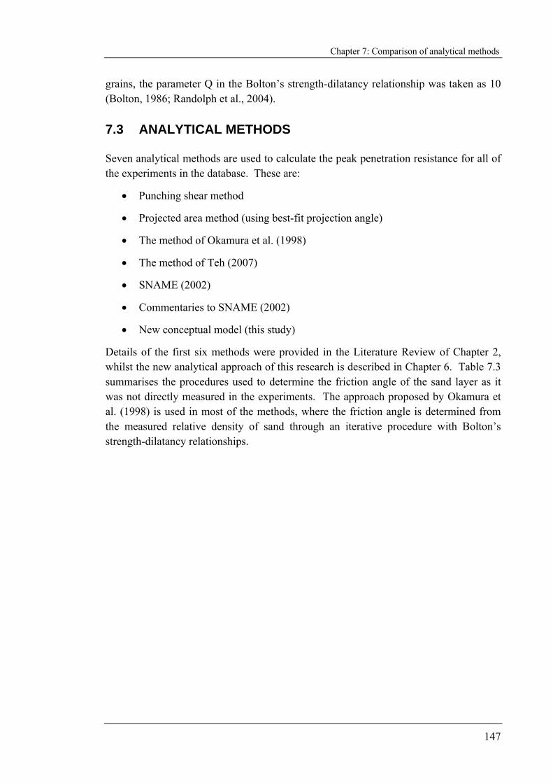
Chapter 7: Comparison of analytical methods
147
grains, the parameter Q in the Bolton’s strength-dilatancy relationship was taken as 10 (Bolton, 1986; Randolph et al., 2004).
7.3 ANALYTICAL METHODS
Seven analytical methods are used to calculate the peak penetration resistance for all of the experiments in the database. These are:
• Punching shear method
• Projected area method (using best-fit projection angle)
• The method of Okamura et al. (1998)
• The method of Teh (2007)
• SNAME (2002)
• Commentaries to SNAME (2002)
• New conceptual model (this study)
Details of the first six methods were provided in the Literature Review of Chapter 2, whilst the new analytical approach of this research is described in Chapter 6. Table 7.3 summarises the procedures used to determine the friction angle of the sand layer as it was not directly measured in the experiments. The approach proposed by Okamura et al. (1998) is used in most of the methods, where the friction angle is determined from the measured relative density of sand through an iterative procedure with Bolton’s strength-dilatancy relationships.
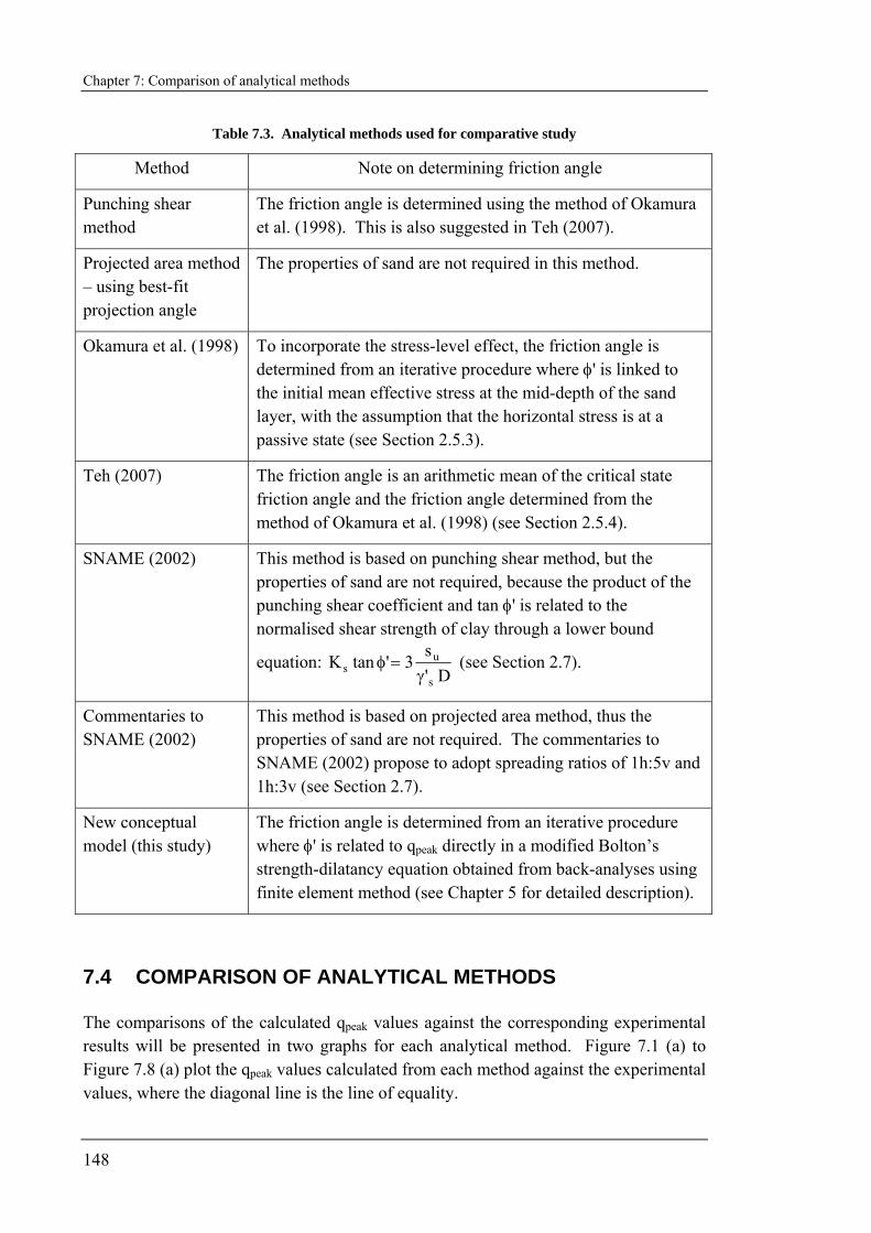
Chapter 7: Comparison of analytical methods
148
Table 7.3. Analytical methods used for comparative study
Method Note on determining friction angle
Punching shear method
The friction angle is determined using the method of Okamura et al. (1998). This is also suggested in Teh (2007).
Projected area method – using best-fit projection angle
The properties of sand are not required in this method.
Okamura et al. (1998) To incorporate the stress-level effect, the friction angle is determined from an iterative procedure where φ' is linked to the initial mean effective stress at the mid-depth of the sand layer, with the assumption that the horizontal stress is at a passive state (see Section 2.5.3).
Teh (2007) The friction angle is an arithmetic mean of the critical state friction angle and the friction angle determined from the method of Okamura et al. (1998) (see Section 2.5.4).
SNAME (2002) This method is based on punching shear method, but the properties of sand are not required, because the product of the punching shear coefficient and tan φ' is related to the normalised shear strength of clay through a lower bound
equation: D'
s3'tanK
s
us γ
=φ (see Section 2.7).
Commentaries to SNAME (2002)
This method is based on projected area method, thus the properties of sand are not required. The commentaries to SNAME (2002) propose to adopt spreading ratios of 1h:5v and 1h:3v (see Section 2.7).
New conceptual model (this study)
The friction angle is determined from an iterative procedure where φ' is related to qpeak directly in a modified Bolton’s strength-dilatancy equation obtained from back-analyses using finite element method (see Chapter 5 for detailed description).
7.4 COMPARISON OF ANALYTICAL METHODS
The comparisons of the calculated qpeak values against the corresponding experimental results will be presented in two graphs for each analytical method. Figure 7.1 (a) to Figure 7.8 (a) plot the qpeak values calculated from each method against the experimental values, where the diagonal line is the line of equality.

Chapter 7: Comparison of analytical methods
149
Additionally, Figure 7.1 (b) to Figure 7.8 (b) present the ratios of calculated to measured qpeak values against the Hs/D ratio. A linear regression line for the data points is also shown in each of these graphs to highlight if the average ratio of calculated to measured qpeak value exhibits any trend with Hs/D.
0.0
0.2
0.4
0.6
0.8
1.0
1.2
1.4
1.6
1.8
2.0
0 0.2 0.4 0.6 0.8 1Hs/D
q pea
k,ca
lcul
ated
/ q p
eak,
mea
sure
d
Teh (2007)_NUS tests Teh (2007)_UWA testsCraig & Chua (1990) This study (beam centrifuge)This study (spudcan) This study (footing)
0
200
400
600
800
1000
0 200 400 600 800 1000qpeak,measured (kPa)
q pea
k,ca
lcul
ated
(kPa
)
(a) (b)
Linear regression line
Figure 7.1. Comparison of calculated and measured qpeak with punching shear method based on
Hanna and Meyerhof (1980)
0.0
0.2
0.4
0.6
0.8
1.0
1.2
1.4
1.6
1.8
2.0
0 0.2 0.4 0.6 0.8 1Hs/D
q pea
k,ca
lcul
ated
/ q p
eak,
mea
sure
d
Teh (2007)_NUS tests Teh (2007)_UWA testsCraig & Chua (1990) This study (beam centrifuge)This study (spudcan) This study (footing)0
200
400
600
800
1000
1200
0 200 400 600 800 1000 1200qpeak,measured (kPa)
q pea
k,ca
lcul
ated
(kP
a)
(a) (b)
Linear regression line
Figure 7.2. Comparison of calculated and measured qpeak with projected area method using best-fit
projection angle, α = 33.5° (spreading ratio of 1h:1.5v)
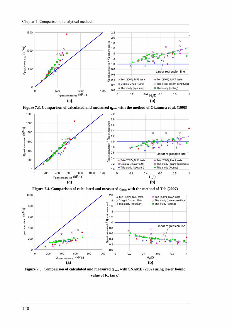
Chapter 7: Comparison of analytical methods
150
0.0
0.2
0.4
0.6
0.8
1.0
1.2
1.4
1.6
1.8
2.0
2.2
0 0.2 0.4 0.6 0.8 1Hs/D
q pea
k,ca
lcul
ated
/ q p
eak,
mea
sure
d
Teh (2007)_NUS tests Teh (2007)_UWA tests
Craig & Chua (1990) This study (beam centrifuge)
This study (spudcan) This study (footing)0
500
1000
1500
0 500 1000 1500qpeak,measured (kPa)
q pea
k,ca
lcul
ated
(kP
a)
(a) (b)
Linear regression line
Figure 7.3. Comparison of calculated and measured qpeak with the method of Okamura et al. (1998)
0.0
0.2
0.4
0.6
0.8
1.0
1.2
1.4
1.6
1.8
2.0
0 0.2 0.4 0.6 0.8 1Hs/D
q pea
k,ca
lcul
ated
/ q p
eak,
mea
sure
d
Teh (2007)_NUS tests Teh (2007)_UWA testsCraig & Chua (1990) This study (beam centrifuge)This study (spudcan) This study (footing)0
200
400
600
800
1000
1200
0 200 400 600 800 1000 1200qpeak,measured (kPa)
q pea
k,ca
lcul
ated
(kPa
)
(a) (b)
Linear regression line
Figure 7.4. Comparison of calculated and measured qpeak with the method of Teh (2007)
0.0
0.2
0.4
0.6
0.8
1.0
1.2
1.4
1.6
1.8
2.0
0 0.2 0.4 0.6 0.8 1Hs/D
q pea
k,ca
lcul
ated
/ q p
eak,
mea
sure
d
Teh (2007)_NUS tests Teh (2007)_UWA testsCraig & Chua (1990) This study (beam centrifuge)This study (spudcan) This study (footing)
0
200
400
600
800
1000
0 200 400 600 800 1000qpeak,measured (kPa)
q pea
k,ca
lcul
ated
(kP
a)
(a) (b)
Linear regression line
Figure 7.5. Comparison of calculated and measured qpeak with SNAME (2002) using lower bound
value of Ks tan φ'
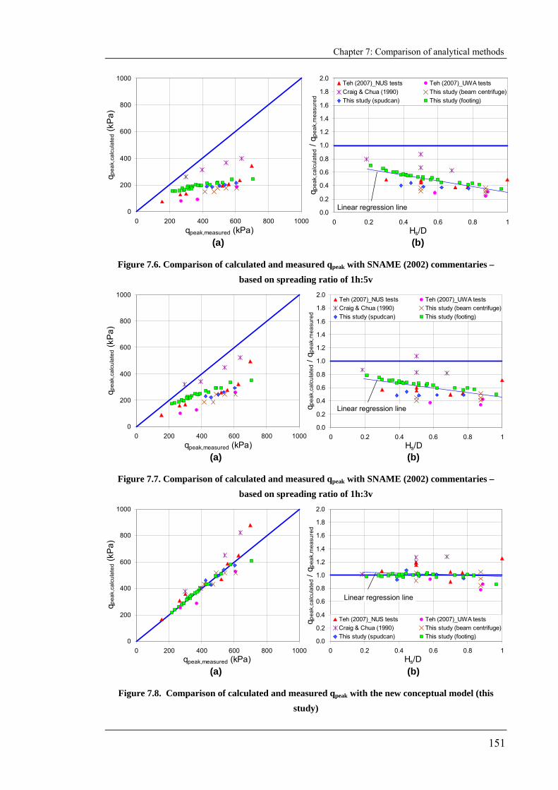
Chapter 7: Comparison of analytical methods
151
0.0
0.2
0.4
0.6
0.8
1.0
1.2
1.4
1.6
1.8
2.0
0 0.2 0.4 0.6 0.8 1Hs/D
q pea
k,ca
lcul
ated
/ q p
eak,
mea
sure
d
Teh (2007)_NUS tests Teh (2007)_UWA testsCraig & Chua (1990) This study (beam centrifuge)This study (spudcan) This study (footing)
0
200
400
600
800
1000
0 200 400 600 800 1000qpeak,measured (kPa)
q pea
k,ca
lcul
ated
(kP
a)
(a) (b)
Linear regression line
Figure 7.6. Comparison of calculated and measured qpeak with SNAME (2002) commentaries – based on spreading ratio of 1h:5v
0.0
0.2
0.4
0.6
0.8
1.0
1.2
1.4
1.6
1.8
2.0
0 0.2 0.4 0.6 0.8 1Hs/D
q pea
k,ca
lcul
ated
/ q p
eak,
mea
sure
d
Teh (2007)_NUS tests Teh (2007)_UWA testsCraig & Chua (1990) This study (beam centrifuge)This study (spudcan) This study (footing)
0
200
400
600
800
1000
0 200 400 600 800 1000qpeak,measured (kPa)
q pea
k,ca
lcul
ated
(kP
a)
(a) (b)
Linear regression line
Figure 7.7. Comparison of calculated and measured qpeak with SNAME (2002) commentaries – based on spreading ratio of 1h:3v
0.0
0.2
0.4
0.6
0.8
1.0
1.2
1.4
1.6
1.8
2.0
0 0.2 0.4 0.6 0.8 1Hs/D
q pea
k,ca
lcul
ated
/ q p
eak,
mea
sure
d
Teh (2007)_NUS tests Teh (2007)_UWA testsCraig & Chua (1990) This study (beam centrifuge)This study (spudcan) This study (footing)
0
200
400
600
800
1000
0 200 400 600 800 1000qpeak,measured (kPa)
q pea
k,ca
lcul
ated
(kPa
)
(a) (b)
Linear regression line
Figure 7.8. Comparison of calculated and measured qpeak with the new conceptual model (this study)

Chapter 7: Comparison of analytical methods
152
By studying the graphs of Figure 7.1 to Figure 7.8, some common attributes of the data sets can be observed. In general, all analytical methods consistently provide higher predicted qpeak values for the tests carried out by Craig and Chua (1990) as compared to other sets of test data. The actual reason for this tendency is not known, but it may be due to certain experimental set-ups that caused lower qpeak values to be measured.
Figure 7.1 (b) to Figure 7.7 (b) show that the ratios of calculated to measured qpeak values (qpeak,calculated/qpeak,measured) for both data sets from Teh (2007), namely the NUS test series (shown as red triangles) and the UWA tests series (shown as pink circles), are generally below the linear regression line. One test from the NUS series is an exception. The test at Hs/D = 1 shows a particularly high predicted value. In comparison, the new conceptual model shown in Figure 7.8 (b) gives good average predictions for both sets of tests.
The large testing area of the drum centrifuge tests in this study has allowed a direct comparison of foundation shape on the same sample. As discussed in Section 3.8, five tests with a spudcan shaped foundation were conducted on the same sample and testing conditions as six flat-based foundation tests. These are shown as blue rhombi and green squares on the plots here respectively. It can be observed that none of the published methods can distinguish the difference between these tests, as highlighted by consistently lower predictions of qpeak for the spudcan shaped data set than for the flat foundations. The new analytical model, on the other hand, has adopted two empirical lines of distribution factor DF to account for differences between a flat foundation and a spudcan shaped foundation (see Section 6.5.2). However, as highlighted in Section 6.8, the empirical DF line for spudcans is obtained using model spudcans with conical angle of 13° to the horizontal. Therefore, the empirical DF line may differ for different conical angles.
Following the observation on general trends of the test data, the specific performance of each analytical method will now be discussed.
7.4.1 Punching shear method
The details of the punching shear method have been discussed in Section 2.5.2. In brief, this method assumes a block of sand with vertical shear surface is pushed into the clay with the frictional resistance calculated from an empirical punching shear coefficient, Ks. The values of Ks are determined from three design charts given in Hanna and Meyerhof (1980), and they are related to the bearing capacity ratio qclay/qsand, friction angle of sand, φ' and the undrained shear strength of clay, su.
Figure 7.1 shows that the punching shear method consistently underestimates the experimental qpeak values. Okamura et al. (1998) commented on a similar finding when comparing the punching shear method to their test results. In that case, the prototype foundation diameters were 0.8 m to 3 m and Hs/D ratios in the range of 0 to 3.
Chapter 7: Comparison of analytical methods
153
Reasons for under-prediction can be found when considering the visualisation experiments from Teh (2007). These show that the actual slip surfaces are curved and inclined outward. Consequently, the bearing capacity of the underlying clay is mobilised over a projected area larger than the foundation size, especially for cases with a dense sand layer. In contrast, the vertical slip surface assumed in this punching shear method has limited the extent of mobilisation of clay bearing capacity. Although the punching shear coefficient is related to passive states, Figure 7.1 suggests that the assumed higher frictional resistance is not sufficient to compensate for the reduced bearing capacity in the underlying clay.
7.4.2 Projected area method
As discussed in Section 2.5.1, the problem of foundations on sand overlying clay is over-simplified by relating the peak bearing resistance to a pre-defined angle of projection, whilst omitting the frictional resistance from the upper sand layer.
As there is no consensus on the value of projection angle, a single best-fit value was used in this comparative study through back-analysis with the entire experimental database. It was found that the average value of qpeak,calculated/qpeak,measured becomes unity when the projection angle α, equals 33.5° (equivalent to load spreading ratio of 1h:1.5v). This value was taken as the best-fit projection angle, and the comparison is shown in Figure 7.2.
This best-fit angle is generally higher than the values proposed by various researchers (see Table 2.6 in Section 2.5.1), with majority of them below 30°. The most frequently reported value of the projection angle, α, is 26.6° (equivalent to spreading ratios of 1h:2v). As the majority of the tests in the database consist of very dense sand, the back-analysed high α value suggests that dense sand is more effective in spreading the foundation load. This is as expected. Meyerhof and Adams (1968) also reported a similar finding that denser sand layer gives higher dispersion angle.
7.4.3 Okamura et al. (1998)
The method of Okamura et al. (1998) generally overestimates the qpeak values as shown in Figure 7.3. The details of this method are discussed in Section 2.5.3. To investigate the underlying factors of the overestimation, the friction angles and dispersion angles calculated with this method are shown in Table 7.4.
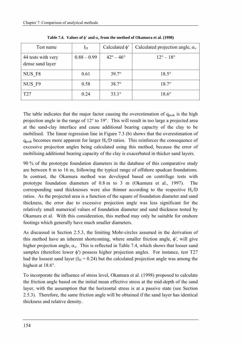
Chapter 7: Comparison of analytical methods
154
Table 7.4. Values of φ' and αc from the method of Okamura et al. (1998)
Test name ID Calculated φ' Calculated projection angle, αc
44 tests with very dense sand layer
0.88 – 0.99 42° – 46° 12° – 18°
NUS_F8 0.61 39.7° 18.5°
NUS_F9 0.58 38.7° 18.7°
T27 0.24 33.1° 18.6°
The table indicates that the major factor causing the overestimation of qpeak is the high projection angle in the range of 12° to 19°. This will result in too large a projected area at the sand-clay interface and cause additional bearing capacity of the clay to be mobilised. The linear regression line in Figure 7.3 (b) shows that the overestimation of qpeak becomes more apparent for larger Hs/D ratios. This reinforces the consequence of excessive projection angles being calculated using this method, because the error of mobilising additional bearing capacity of the clay is exacerbated in thicker sand layers.
90 % of the prototype foundation diameters in the database of this comparative study are between 8 m to 16 m, following the typical range of offshore spudcan foundations. In contrast, the Okamura method was developed based on centrifuge tests with prototype foundation diameters of 0.8 m to 3 m (Okamura et al., 1997). The corresponding sand thicknesses were also thinner according to the respective Hs/D ratios. As the projected area is a function of the square of foundation diameter and sand thickness, the error due to excessive projection angle was less significant for the relatively small numerical values of foundation diameter and sand thickness tested by Okamura et al. With this consideration, this method may only be suitable for onshore footings which generally have much smaller diameters.
As discussed in Section 2.5.3, the limiting Mohr-circles assumed in the derivation of this method have an inherent shortcoming, where smaller friction angle, φ', will give higher projection angle, αc. This is reflected in Table 7.4, which shows that looser sand samples (therefore lower φ') possess higher projection angles. For instance, test T27 had the loosest sand layer (ID = 0.24) but the calculated projection angle was among the highest at 18.6°.
To incorporate the influence of stress level, Okamura et al. (1998) proposed to calculate the friction angle based on the initial mean effective stress at the mid-depth of the sand layer, with the assumption that the horizontal stress is at a passive state (see Section 2.5.3). Therefore, the same friction angle will be obtained if the sand layer has identical thickness and relative density.
Chapter 7: Comparison of analytical methods
155
Unfortunately, this approach assumes that both foundation size and undrained strength of the underlying clay have no effect on the operative friction angle. This contradicts the experimental findings for foundations on sand, where lower bearing resistance is observed when the foundation size increases (de Beer, 1963; Kimura et al., 1985 amongst others). This is because a larger foundation will generate higher confining stress thus invoking a lower operating friction angle (Hettler and Gudehus, 1988; Ueno et al., 2001). For the case of sand overlying clay, such foundation size effect is also observed in the centrifuge tests performed in this study (see Figure 4.15 to Figure 4.17 in Section 4.4). In a similar manner, larger undrained shear strength will invoke a lower friction angle due to a higher confining stress, and consequently affect the peak penetration resistance.
7.4.4 Teh (2007)
Figure 7.4 indicates that this method gives a relatively good prediction on the peak penetration resistance. The details of this method are discussed in Section 2.5.4. The method involves three empirical parameters that need to be determined from separate semi-logarithmic graphs (see Figure 2.9). Since all three empirical parameters are related to the ratios of Hs/D and qclay/qsand, it is difficult to evaluate the influence of each parameter in predicting the value of qpeak. However, the linear regression line in Figure 7.4 (b) indicates that the general trend of calculated to measured qpeak ratios is skewed. As Hs/D increases the relative qpeak prediction compared to the experiments also increases.
A schematic diagram of the model is presented in Figure 7.9. In addition, the values of the calculated friction angle, φ2, and the empirical parameters ψ and αa obtained from this method are given in Table 7.5, where the definitions of the empirical parameters are shown in Figure 7.9 (see Section 2.5.4 for further description). In brief, the inclination of the slip surface is determined by parameter ψ, whereas the extent of the mobilisation of the underlying clay bearing capacity is determined by parameter αa. It can be observed that the values of ψ are generally much lower than the values of αa. This confirms the geometrical inconsistency between the failure mechanisms in the sand layer and the underlying clay as illustrated in the schematic diagram in Figure 7.9.
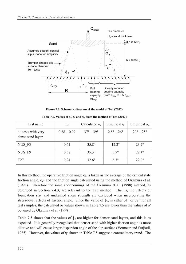
Chapter 7: Comparison of analytical methods
156
Assumed straight conical slip surface for simplicity
Rr
Sand
Linearly reduced bearing capacity (from qclay to 0.5 qclay)
Full bearing capacity (qclay)
Qpeak
Clay
'γ
aα
ψ
D = diameter
Hs = sand thickness
2φ
d = 0.12 Hs
h = 0.88 HsTrumpet-shaped slip surface observed from tests
Figure 7.9. Schematic diagram of the model of Teh (2007)
Table 7.5. Values of φ2, ψ and αa from the method of Teh (2007)
Test name ID Calculated φ2 Empirical ψ Empirical αa
44 tests with very dense sand layer
0.88 – 0.99 37° – 39° 2.5° – 26° 20° – 25°
NUS_F8 0.61 35.8° 12.2° 23.7°
NUS_F9 0.58 35.3° 5.7° 22.4°
T27 0.24 32.6° 6.3° 22.0°
In this method, the operative friction angle φ2 is taken as the average of the critical state friction angle, φcv and the friction angle calculated using the method of Okamura et al. (1998). Therefore the same shortcomings of the Okamura et al. (1998) method, as described in Section 7.4.3, are relevant to the Teh method. That is, the effects of foundation size and undrained shear strength are excluded when incorporating the stress-level effects of friction angle. Since the value of φcv is either 31° or 32° for all test samples, the calculated φ2 values shown in Table 7.5 are lower than the values of φ' obtained by Okamura et al. (1998).
Table 7.5 shows that the values of φ2 are higher for denser sand layers, and this is as expected. It is generally recognised that denser sand with higher friction angle is more dilative and will cause larger dispersion angle of the slip surface (Vermeer and Sutjiadi, 1985). However, the values of ψ shown in Table 7.5 suggest a contradictory trend. The
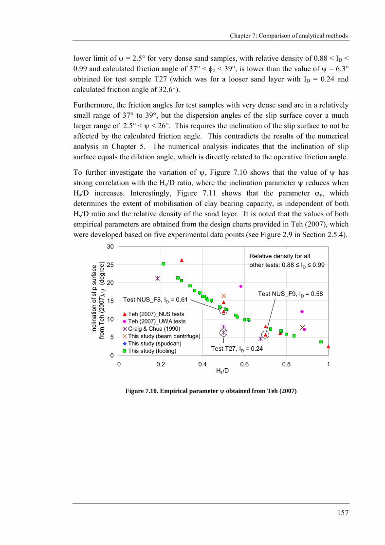
Chapter 7: Comparison of analytical methods
157
lower limit of ψ = 2.5° for very dense sand samples, with relative density of 0.88 < ID < 0.99 and calculated friction angle of 37° < φ2 < 39°, is lower than the value of ψ = 6.3° obtained for test sample T27 (which was for a looser sand layer with ID = 0.24 and calculated friction angle of 32.6°).
Furthermore, the friction angles for test samples with very dense sand are in a relatively small range of 37° to 39°, but the dispersion angles of the slip surface cover a much larger range of 2.5° < ψ < 26°. This requires the inclination of the slip surface to not be affected by the calculated friction angle. This contradicts the results of the numerical analysis in Chapter 5. The numerical analysis indicates that the inclination of slip surface equals the dilation angle, which is directly related to the operative friction angle.
To further investigate the variation of ψ, Figure 7.10 shows that the value of ψ has strong correlation with the Hs/D ratio, where the inclination parameter ψ reduces when Hs/D increases. Interestingly, Figure 7.11 shows that the parameter αa, which determines the extent of mobilisation of clay bearing capacity, is independent of both Hs/D ratio and the relative density of the sand layer. It is noted that the values of both empirical parameters are obtained from the design charts provided in Teh (2007), which were developed based on five experimental data points (see Figure 2.9 in Section 2.5.4).
0
5
10
15
20
25
30
0 0.2 0.4 0.6 0.8 1Hs/D
Incl
inat
ion
of s
lip s
urfa
cefro
m T
eh (2
007)
, ψ (
degr
ee)
Teh (2007)_NUS testsTeh (2007)_UWA testsCraig & Chua (1990)This study (beam centrifuge)This study (spudcan)This study (footing)
Test NUS_F9, ID = 0.58Test NUS_F8, ID = 0.61
Test T27, ID = 0.24
Relative density for all other tests: 0.88 ≤ ID ≤ 0.99
Figure 7.10. Empirical parameter ψ obtained from Teh (2007)

Chapter 7: Comparison of analytical methods
158
0
5
10
15
20
25
30
0 0.2 0.4 0.6 0.8 1Hs/D
Par
amet
er α
a fro
m T
eh (2
007)
(d
egre
e)
Teh (2007)_NUS testsTeh (2007)_UWA testsCraig & Chua (1990)This study (beam centrifuge)This study (spudcan)This study (footing)
Test NUS_F9, ID = 0.58
Test NUS_F8, ID = 0.61
Test T27, ID = 0.24
Relative density for all other tests: 0.88 ≤ ID ≤ 0.99
Figure 7.11. Empirical parameter αa obtained from Teh (2007)
The minimum value of αa being 20° indicates that the projected areas are large. However, the effects of the excessive projected area are mitigated by the reduced bearing capacity proposed in the method (see schematic diagram in Figure 7.9).
In summary, it appears that the individual parameters are not consistent with each other. However, the compensation effects among the empirical parameters and the reduced bearing capacity have worked collectively to produce a set of reasonably calculated qpeak values.
7.4.5 SNAME (2002)
The current industry guidelines SNAME (2002) recommend two approaches for predicting bearing capacity on sand overlying clay. In the primary approach, qpeak is calculated following the punching shear method, where the product of the punching shear coefficient, Ks and tan φ' is related to a normalised shear strength of the underlying clay layer with a lower bound equation. An alternative design approach is provided in the commentaries to the SNAME guidelines using the projected area method, with recommended spreading ratios in the range of 1h:5v to 1h:3v (horizontal:vertical). Both approaches ignore the properties of sand, as even in the punching shear approach the frictional resistance through the sand is expressed in terms of the strength of the underlying clay. Further discussion on the methods of SNAME (2002) was presented in Section 2.7.
As stated in SNAME (2002), the guidelines opt for a conservative prediction of qpeak. This is evident in Figure 7.5 to Figure 7.7. The average qpeak value predicted using the punching shear approach is about 40 % of the average measured value. For the projected area method suggested in the SNAME (2002) commentaries, the average predicted values are around 50 % and 60 % of the experimental values with spreading ratios of 1h:5v and 1h:3v respectively.
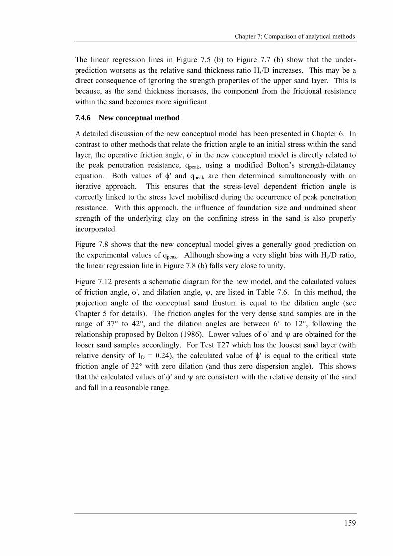
Chapter 7: Comparison of analytical methods
159
The linear regression lines in Figure 7.5 (b) to Figure 7.7 (b) show that the under-prediction worsens as the relative sand thickness ratio Hs/D increases. This may be a direct consequence of ignoring the strength properties of the upper sand layer. This is because, as the sand thickness increases, the component from the frictional resistance within the sand becomes more significant.
7.4.6 New conceptual method
A detailed discussion of the new conceptual model has been presented in Chapter 6. In contrast to other methods that relate the friction angle to an initial stress within the sand layer, the operative friction angle, φ' in the new conceptual model is directly related to the peak penetration resistance, qpeak, using a modified Bolton’s strength-dilatancy equation. Both values of φ' and qpeak are then determined simultaneously with an iterative approach. This ensures that the stress-level dependent friction angle is correctly linked to the stress level mobilised during the occurrence of peak penetration resistance. With this approach, the influence of foundation size and undrained shear strength of the underlying clay on the confining stress in the sand is also properly incorporated.
Figure 7.8 shows that the new conceptual model gives a generally good prediction on the experimental values of qpeak. Although showing a very slight bias with Hs/D ratio, the linear regression line in Figure 7.8 (b) falls very close to unity.
Figure 7.12 presents a schematic diagram for the new model, and the calculated values of friction angle, φ', and dilation angle, ψ, are listed in Table 7.6. In this method, the projection angle of the conceptual sand frustum is equal to the dilation angle (see Chapter 5 for details). The friction angles for the very dense sand samples are in the range of 37° to 42°, and the dilation angles are between 6° to 12°, following the relationship proposed by Bolton (1986). Lower values of φ' and ψ are obtained for the looser sand samples accordingly. For Test T27 which has the loosest sand layer (with relative density of ID = 0.24), the calculated value of φ' is equal to the critical state friction angle of 32° with zero dilation (and thus zero dispersion angle). This shows that the calculated values of φ' and ψ are consistent with the relative density of the sand and fall in a reasonable range.
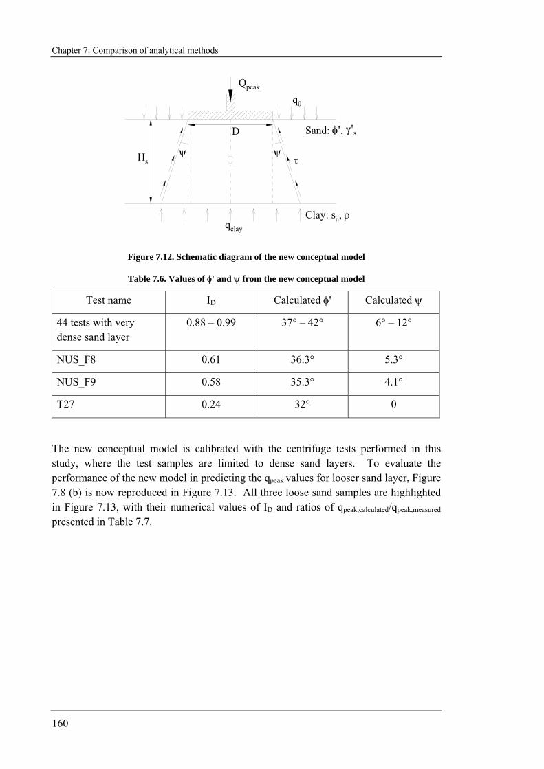
Chapter 7: Comparison of analytical methods
160
ψψ
qclay
Qpeak
q0
τ
Sand: ,
Clay: su, ρ
Hs
'φ s'γD
Figure 7.12. Schematic diagram of the new conceptual model
Table 7.6. Values of φ' and ψ from the new conceptual model
Test name ID Calculated φ' Calculated ψ
44 tests with very dense sand layer
0.88 – 0.99 37° – 42° 6° – 12°
NUS_F8 0.61 36.3° 5.3°
NUS_F9 0.58 35.3° 4.1°
T27 0.24 32° 0
The new conceptual model is calibrated with the centrifuge tests performed in this study, where the test samples are limited to dense sand layers. To evaluate the performance of the new model in predicting the qpeak values for looser sand layer, Figure 7.8 (b) is now reproduced in Figure 7.13. All three loose sand samples are highlighted in Figure 7.13, with their numerical values of ID and ratios of qpeak,calculated/qpeak,measured presented in Table 7.7.
Chapter 7: Comparison of analytical methods
161
0.5
0.6
0.7
0.8
0.9
1.0
1.1
1.2
1.3
1.4
0 0.2 0.4 0.6 0.8 1Hs/D
q pea
k,ca
lcul
ated
/ q p
eak,
mea
sure
d
Teh (2007)_NUS tests Teh (2007)_UWA testsCraig & Chua (1990) This study (beam centrifuge)This study (spudcan) This study (footing)
Test NUS_F9, ID = 0.58
Test NUS_F8, ID = 0.61
Test T27, ID = 0.24
For all other tests: 0.88 ≤ ID ≤ 0.99
Values of qpeak calculated from new conceptual model
Figure 7.13 Effects of relative density to qpeak values calculated using the new conceptual model
Table 7.7. Ratios of qpeak,calculated/qpeak,measured from the new conceptual model
Test name ID Ratio of qpeak,calculated/qpeak,measured
44 tests with very dense sand layer
0.88 – 0.99 0.77 – 1.28
NUS_F8 0.61 1.16
NUS_F9 0.58 0.90
T27 0.24 1.27
As shown in Figure 7.13, the ratios of qpeak,calculated/qpeak,measured for all tests are in the range of 0.77 to 1.28, where the three looser sand samples have ratios of 1.16, 0.90 and 1.27 for ID = 0.61, 0.58 and 0.24 respectively. Although there are only three data points, the new conceptual model still performs moderately well for soils with looser sand layer. However, more experimental data would prove useful.
7.5 CONCLUDING REMARKS
A total of 47 centrifuge tests have been used to perform a comparative study of six existing analytical methods and the new conceptual model. The database consists of 28 tests used to calibrate the model, and an additional 14 tests published by Teh (2007) and Craig and Chua (1990) and another 5 tests conducted using UWA beam centrifuge for this study. To obtain a clearer picture on the performance of various methods in predicting the qpeak values, the above comparisons are summarised in Table 7.8 with
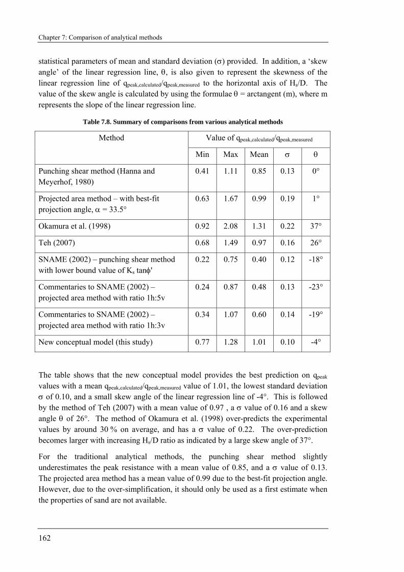
Chapter 7: Comparison of analytical methods
162
statistical parameters of mean and standard deviation (σ) provided. In addition, a ‘skew angle’ of the linear regression line, θ, is also given to represent the skewness of the linear regression line of qpeak,calculated/qpeak,measured to the horizontal axis of Hs/D. The value of the skew angle is calculated by using the formulae θ = arctangent (m), where m represents the slope of the linear regression line.
Table 7.8. Summary of comparisons from various analytical methods
Value of qpeak,calculated/qpeak,measured Method
Min Max Mean σ θ
Punching shear method (Hanna and Meyerhof, 1980)
0.41 1.11 0.85 0.13 0°
Projected area method – with best-fit projection angle, α = 33.5°
0.63 1.67 0.99 0.19 1°
Okamura et al. (1998) 0.92 2.08 1.31 0.22 37°
Teh (2007) 0.68 1.49 0.97 0.16 26°
SNAME (2002) – punching shear method with lower bound value of Ks tanφ'
0.22 0.75 0.40 0.12 -18°
Commentaries to SNAME (2002) – projected area method with ratio 1h:5v
0.24 0.87 0.48 0.13 -23°
Commentaries to SNAME (2002) – projected area method with ratio 1h:3v
0.34 1.07 0.60 0.14 -19°
New conceptual model (this study) 0.77 1.28 1.01 0.10 -4°
The table shows that the new conceptual model provides the best prediction on qpeak values with a mean qpeak,calculated/qpeak,measured value of 1.01, the lowest standard deviation σ of 0.10, and a small skew angle of the linear regression line of -4°. This is followed by the method of Teh (2007) with a mean value of 0.97 , a σ value of 0.16 and a skew angle θ of 26°. The method of Okamura et al. (1998) over-predicts the experimental values by around 30 % on average, and has a σ value of 0.22. The over-prediction becomes larger with increasing Hs/D ratio as indicated by a large skew angle of 37°.
For the traditional analytical methods, the punching shear method slightly underestimates the peak resistance with a mean value of 0.85, and a σ value of 0.13. The projected area method has a mean value of 0.99 due to the best-fit projection angle. However, due to the over-simplification, it should only be used as a first estimate when the properties of sand are not available.

Chapter 7: Comparison of analytical methods
163
Table 7.8 also shows that the methods recommended in the current industry guidelines SNAME (2002) give very conservative prediction, in which the average predicted qpeak values range from 40 % to 60 % of the experimental values. The under-prediction worsens as Hs/D increases as indicated by skew angles of around -20°.
It should be highlighted that this comparative study only focuses on the accuracy of various analytical methods in predicting the peak penetration resistance from centrifuge tests. In order to become an appealing design tool for practising engineers, some other features may also be important. This includes whether the model is based on a logical framework and its convenience to use. The latter refers to its simplicity and unambiguous input parameters. These are not evaluated here, but briefly the new conceptual model can be performed easily from purpose-written calculation spreadsheets, in which the potential punch-through hazards can be evaluated through sensitivity studies. This may offer an advancement over other methods that need to rely on empirical design charts such as the punching shear method and the method of Teh (2007). In addition, the analytical framework of the new model advances the simplified methods such as the SNAME (2002) guidelines that do not consider the strength properties of sand.

Chapter 8: Predicting penetration profile
164
CHAPTER 8. PREDICTING PENETRATION PROFILE ON SAND OVERLYING CLAY SOILS
8.1 INTRODUCTION
This chapter aims to present a consistent framework for constructing a complete simplified penetration resistance profile of a foundation on sand overlying clay. This is important as a complete penetration resistance profile is required to evaluate the impact of a potential punch-through and possibly corresponding mitigation measures.
The first part of the chapter focuses on the development of a design method for predicting the penetration resistance of a foundation below the sand-clay interface. Based on the results of an extensive series of finite element (FE) analyses, two design equations corresponding to shallow and deep failure mechanisms in the underlying clay are established. Two important effects are taken into account in the FE analyses, namely soil strength that increases linearly with depth and the thickness of sand trapped beneath the foundation after punching through the upper sand layer.
The latter portion of the chapter modifies and extends the new conceptual model used to calculate the peak penetration resistance in the upper sand layer. The new model was introduced in Chapter 6. In this chapter, it is shown that the new conceptual model can be modified for the calculation of the post-peak resistance in the upper sand layer.
By adopting these procedures, a complete simplified penetration resistance profile of a foundation in sand overlying clay can be constructed by joining the values of peak resistance, post-peak resistance and the resistance profile in the underlying clay.
Finally, it is shown that the predicted penetration resistance profiles compare reasonably well with the experimental profiles from 25 centrifuge tests performed in this study.
8.2 PREDICTING PENETRATION RESISTANCE PROFILE BELOW THE SAND-CLAY INTERFACE
8.2.1 Finite element model for cylindrical foundation in clay
The commercial finite element package PLAXIS was used to model the penetration of a foundation in the underlying clay after punching through the upper sand layer. Some discussion about the PLAXIS software, including the modelling procedures and verifications, has been presented in Sections 5.2 and 5.3. In general, the modelling procedures adopted for the analysis presented here are similar to that described in Section 5.2.

Chapter 8: Predicting penetration profile
165
The major assumption in using PLAXIS for this application is that it is a small deformation finite element software that is not able to simulate continuous penetration of a foundation in clay. Instead, it can only be used to obtain the bearing capacity of a ‘wished in place’ foundation. Therefore, it is assumed that the penetration resistance from successive failing of the clay during continuous penetration is equal to the ‘wished in place’ bearing capacity at the corresponding depth.
An illustration of the soil displacement trajectory plot from a visualisation experiment of a model spudcan penetrating dense sand overlying soft clay (Teh, 2007) is shown in Figure 8.1 (a). Based on the observation from the visualisation experiment, an idealised FE model is created to evaluate the resistance generated from the undrained shear strength of the underlying clay.
The idealised FE model is shown in Figure 8.1 (b). The visualisation experiment indicates that a crater is formed at the soil surface when the spudcan has penetrated into the underlying clay. However, for simplicity, it is assumed that there is complete backfilling when the foundation reaches the underlying clay, and the upper sand layer is assumed to be a uniform distributed surcharge load on the clay. This uniform surface load is not included in the FE model as it does not affect the penetration resistance from the shear strength of the underlying clay.
Sand
Clay
Trapped sand
(a) Soil displacement trajectory plot from visualisation experiment (after Teh, 2007)
Spudcan and trapped sand are modelled as a single composite foundation in cylindrical shape using a weightless elastic model
(b) Idealised FE model for evaluating the resistance developed from undrained shear strength of the underlying clay
Clay is modelled as a weightless Tresca material
Assume full back-fill in the sand. The sand layer is assumed as a uniform distributed surcharge load
Trapped sand
Spudcan leg is not included in the FE model
0u
ult
0u
ult0c sA
Qsq
N ==
Qult
Figure 8.1. Idealisation of finite element (FE) model for penetration in the underlying clay
The underlying clay is assumed to be weightless because the failure load is independent of the soil unit weight, γ'c (Houlsby and Martin, 2003). Due to the undrained conditions, Tresca yield criterion with undrained shear strength, su, is used to model the clay. The shear strength profile is allowed to increase linearly with depth and the rate is
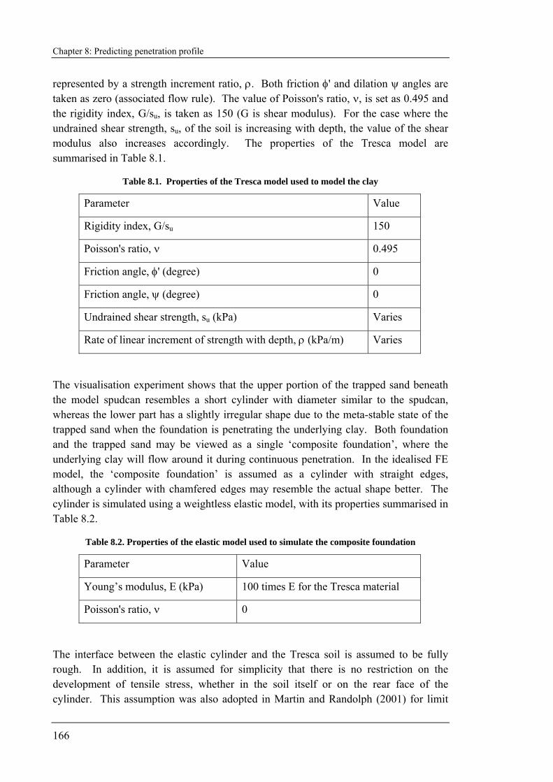
Chapter 8: Predicting penetration profile
166
represented by a strength increment ratio, ρ. Both friction φ' and dilation ψ angles are taken as zero (associated flow rule). The value of Poisson's ratio, ν, is set as 0.495 and the rigidity index, G/su, is taken as 150 (G is shear modulus). For the case where the undrained shear strength, su, of the soil is increasing with depth, the value of the shear modulus also increases accordingly. The properties of the Tresca model are summarised in Table 8.1.
Table 8.1. Properties of the Tresca model used to model the clay
Parameter Value
Rigidity index, G/su 150
Poisson's ratio, ν 0.495
Friction angle, φ' (degree) 0
Friction angle, ψ (degree) 0
Undrained shear strength, su (kPa) Varies
Rate of linear increment of strength with depth, ρ (kPa/m) Varies
The visualisation experiment shows that the upper portion of the trapped sand beneath the model spudcan resembles a short cylinder with diameter similar to the spudcan, whereas the lower part has a slightly irregular shape due to the meta-stable state of the trapped sand when the foundation is penetrating the underlying clay. Both foundation and the trapped sand may be viewed as a single ‘composite foundation’, where the underlying clay will flow around it during continuous penetration. In the idealised FE model, the ‘composite foundation’ is assumed as a cylinder with straight edges, although a cylinder with chamfered edges may resemble the actual shape better. The cylinder is simulated using a weightless elastic model, with its properties summarised in Table 8.2.
Table 8.2. Properties of the elastic model used to simulate the composite foundation
Parameter Value
Young’s modulus, E (kPa) 100 times E for the Tresca material
Poisson's ratio, ν 0
The interface between the elastic cylinder and the Tresca soil is assumed to be fully rough. In addition, it is assumed for simplicity that there is no restriction on the development of tensile stress, whether in the soil itself or on the rear face of the cylinder. This assumption was also adopted in Martin and Randolph (2001) for limit
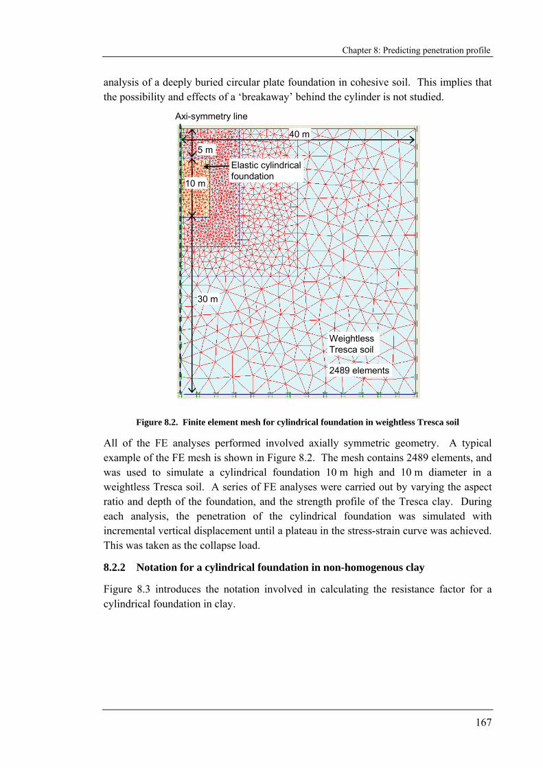
Chapter 8: Predicting penetration profile
167
analysis of a deeply buried circular plate foundation in cohesive soil. This implies that the possibility and effects of a ‘breakaway’ behind the cylinder is not studied.
30 m
5 m
40 m
10 m
2489 elements
Weightless Tresca soil
Elastic cylindrical foundation
Axi-symmetry line
Figure 8.2. Finite element mesh for cylindrical foundation in weightless Tresca soil
All of the FE analyses performed involved axially symmetric geometry. A typical example of the FE mesh is shown in Figure 8.2. The mesh contains 2489 elements, and was used to simulate a cylindrical foundation 10 m high and 10 m diameter in a weightless Tresca soil. A series of FE analyses were carried out by varying the aspect ratio and depth of the foundation, and the strength profile of the Tresca clay. During each analysis, the penetration of the cylindrical foundation was simulated with incremental vertical displacement until a plateau in the stress-strain curve was achieved. This was taken as the collapse load.
8.2.2 Notation for a cylindrical foundation in non-homogenous clay
Figure 8.3 introduces the notation involved in calculating the resistance factor for a cylindrical foundation in clay.
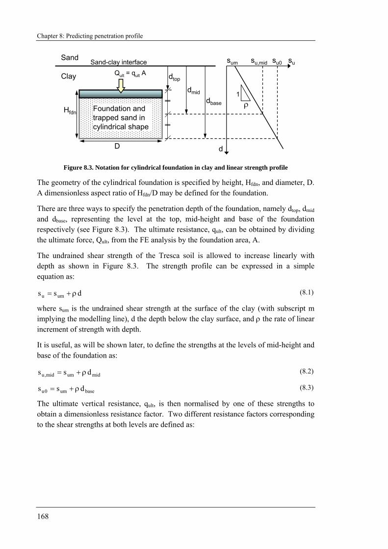
Chapter 8: Predicting penetration profile
168
ρ1
Hfdn
sum su0 su
dD
Foundation and trapped sand in cylindrical shape
Sand-clay interface
Clay
Sand
dtop
dmid
dbase
su,mid
Qult = qult A
Figure 8.3. Notation for cylindrical foundation in clay and linear strength profile
The geometry of the cylindrical foundation is specified by height, Hfdn, and diameter, D. A dimensionless aspect ratio of Hfdn/D may be defined for the foundation.
There are three ways to specify the penetration depth of the foundation, namely dtop, dmid and dbase, representing the level at the top, mid-height and base of the foundation respectively (see Figure 8.3). The ultimate resistance, qult, can be obtained by dividing the ultimate force, Qult, from the FE analysis by the foundation area, A.
The undrained shear strength of the Tresca soil is allowed to increase linearly with depth as shown in Figure 8.3. The strength profile can be expressed in a simple equation as:
dss umu ρ+= (8.1)
where sum is the undrained shear strength at the surface of the clay (with subscript m implying the modelling line), d the depth below the clay surface, and ρ the rate of linear increment of strength with depth.
It is useful, as will be shown later, to define the strengths at the levels of mid-height and base of the foundation as:
midummid,u dss ρ+= (8.2)
baseum0u dss ρ+= (8.3)
The ultimate vertical resistance, qult, is then normalised by one of these strengths to obtain a dimensionless resistance factor. Two different resistance factors corresponding to the shear strengths at both levels are defined as:
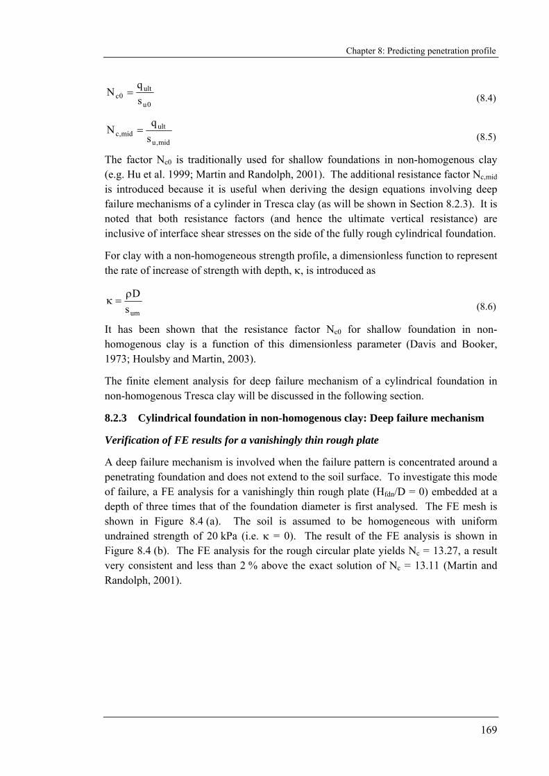
Chapter 8: Predicting penetration profile
169
0u
ult0c s
qN =
(8.4)
mid,u
ultmid,c s
qN =
(8.5)
The factor Nc0 is traditionally used for shallow foundations in non-homogenous clay (e.g. Hu et al. 1999; Martin and Randolph, 2001). The additional resistance factor Nc,mid is introduced because it is useful when deriving the design equations involving deep failure mechanisms of a cylinder in Tresca clay (as will be shown in Section 8.2.3). It is noted that both resistance factors (and hence the ultimate vertical resistance) are inclusive of interface shear stresses on the side of the fully rough cylindrical foundation.
For clay with a non-homogeneous strength profile, a dimensionless function to represent the rate of increase of strength with depth, κ, is introduced as
umsDρ
=κ (8.6)
It has been shown that the resistance factor Nc0 for shallow foundation in non-homogenous clay is a function of this dimensionless parameter (Davis and Booker, 1973; Houlsby and Martin, 2003).
The finite element analysis for deep failure mechanism of a cylindrical foundation in non-homogenous Tresca clay will be discussed in the following section.
8.2.3 Cylindrical foundation in non-homogenous clay: Deep failure mechanism
Verification of FE results for a vanishingly thin rough plate
A deep failure mechanism is involved when the failure pattern is concentrated around a penetrating foundation and does not extend to the soil surface. To investigate this mode of failure, a FE analysis for a vanishingly thin rough plate (Hfdn/D = 0) embedded at a depth of three times that of the foundation diameter is first analysed. The FE mesh is shown in Figure 8.4 (a). The soil is assumed to be homogeneous with uniform undrained strength of 20 kPa (i.e. κ = 0). The result of the FE analysis is shown in Figure 8.4 (b). The FE analysis for the rough circular plate yields Nc = 13.27, a result very consistent and less than 2 % above the exact solution of Nc = 13.11 (Martin and Randolph, 2001).
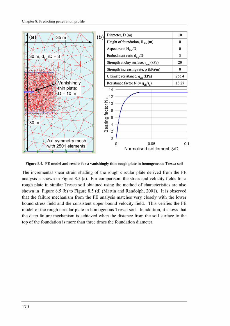
Chapter 8: Predicting penetration profile
170
30 m
30 m, dtop/D = 3
35 m
Vanishingly thin plate:D = 10 m
Axi-symmetry mesh with 2501 elements
13.27Resistance factor N (= qult/su)
265.4Ultimate resistance, qult (kPa)
0Strength increasing rate, ρ (kPa/m)
20Strength at clay surface, sum (kPa)
3Embedment ratio dtop/D
0Aspect ratio Hfdn/D
0Height of foundation, Hfdn (m)
10Diameter, D (m)
13.27Resistance factor N (= qult/su)
265.4Ultimate resistance, qult (kPa)
0Strength increasing rate, ρ (kPa/m)
20Strength at clay surface, sum (kPa)
3Embedment ratio dtop/D
0Aspect ratio Hfdn/D
0Height of foundation, Hfdn (m)
10Diameter, D (m)(a) (b)
0
2
4
6
8
10
12
14
0 0.05 0.1Normalised settlement, δ/D
Bea
ring
fact
or N
c
Figure 8.4. FE model and results for a vanishingly thin rough plate in homogeneous Tresca soil
The incremental shear strain shading of the rough circular plate derived from the FE analysis is shown in Figure 8.5 (a). For comparison, the stress and velocity fields for a rough plate in similar Tresca soil obtained using the method of characteristics are also shown in Figure 8.5 (b) to Figure 8.5 (d) (Martin and Randolph, 2001). It is observed that the failure mechanism from the FE analysis matches very closely with the lower bound stress field and the consistent upper bound velocity field. This verifies the FE model of the rough circular plate in homogenous Tresca soil. In addition, it shows that the deep failure mechanism is achieved when the distance from the soil surface to the top of the foundation is more than three times the foundation diameter.

Chapter 8: Predicting penetration profile
171
Nc (LB) = 13.11
(b) Lower bound stress field
(d) Upper bound velocity field from independent collapse mechanism
Nc (UB) = 13.11 Nc (UB) = 13.31
(c) Upper bound velocity field consistent with lower bound stress field
(a) Incremental shear strain shading from PLAXIS
Nc (FE) = 13.27
Figure 8.5. Comparison of incremental shear strain from PLAXIS and stress and velocity fields for a rough plate in deep homogenous Tresca soil (after Martin and Randolph, 2001)
Investigation of non-dimensional groups for deeply embedded foundations
The FE modelling procedures used for the rough circular plate are repeated for an elastic foundation with aspect ratio of Hfdn/D = 0.8 (Hfdn = 8 m and D = 10 m). The top of the foundation is maintained at three times the foundation diameter from the soil surface to ensure that deep a failure mechanism takes place.
The FE mesh for this configuration is shown in Figure 8.6 (a). Three cases of FE analyses were carried out using this mesh but with different soil strength profiles. The strength profile for each case is shown in Figure 8.6 (b), where Case 1 represents a homogenous clay (uniform su) with κ = 0, and Case 2 and Case 3, with values of κ = 0.5 and 1 respectively.
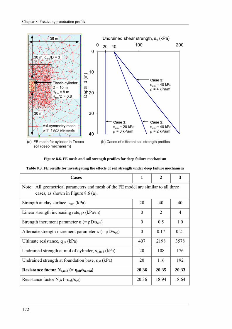
Chapter 8: Predicting penetration profile
172
0
10
20
30
40
0 100 200Undrained shear strength, su (kPa)
Dep
th, d
(m)
30 m
30 m, dtop/D = 3
35 m
Elastic cylinder:D = 10 mHfdn = 8 mHfdn/D = 0.8
Axi-symmetry mesh with 1923 elements
Case 1:sum = 20 kPaρ = 0 kPa/m
Case 2:sum = 40 kPaρ = 2 kPa/m
Case 3:sum = 40 kPaρ = 4 kPa/m
20 40
(a) FE mesh for cylinder in Trescasoil (deep mechanism)
(b) Cases of different soil strength profiles
Figure 8.6. FE mesh and soil strength profiles for deep failure mechanism
Table 8.3. FE results for investigating the effects of soil strength under deep failure mechanism
Cases 1 2 3
Note: All geometrical parameters and mesh of the FE model are similar to all three cases, as shown in Figure 8.6 (a).
Strength at clay surface, sum (kPa) 20 40 40
Linear strength increasing rate, ρ (kPa/m) 0 2 4
Strength increment parameter κ (= ρD/sum) 0 0.5 1.0
Alternate strength increment parameter κ (= ρD/su0) 0 0.17 0.21
Ultimate resistance, qult (kPa) 407 2198 3578
Undrained strength at mid of cylinder, su,mid (kPa) 20 108 176
Undrained strength at foundation base, su0 (kPa) 20 116 192
Resistance factor Nc,mid (= qult/su,mid) 20.36 20.35 20.33
Resistance factor Nc0 (=qult/su0) 20.36 18.94 18.64
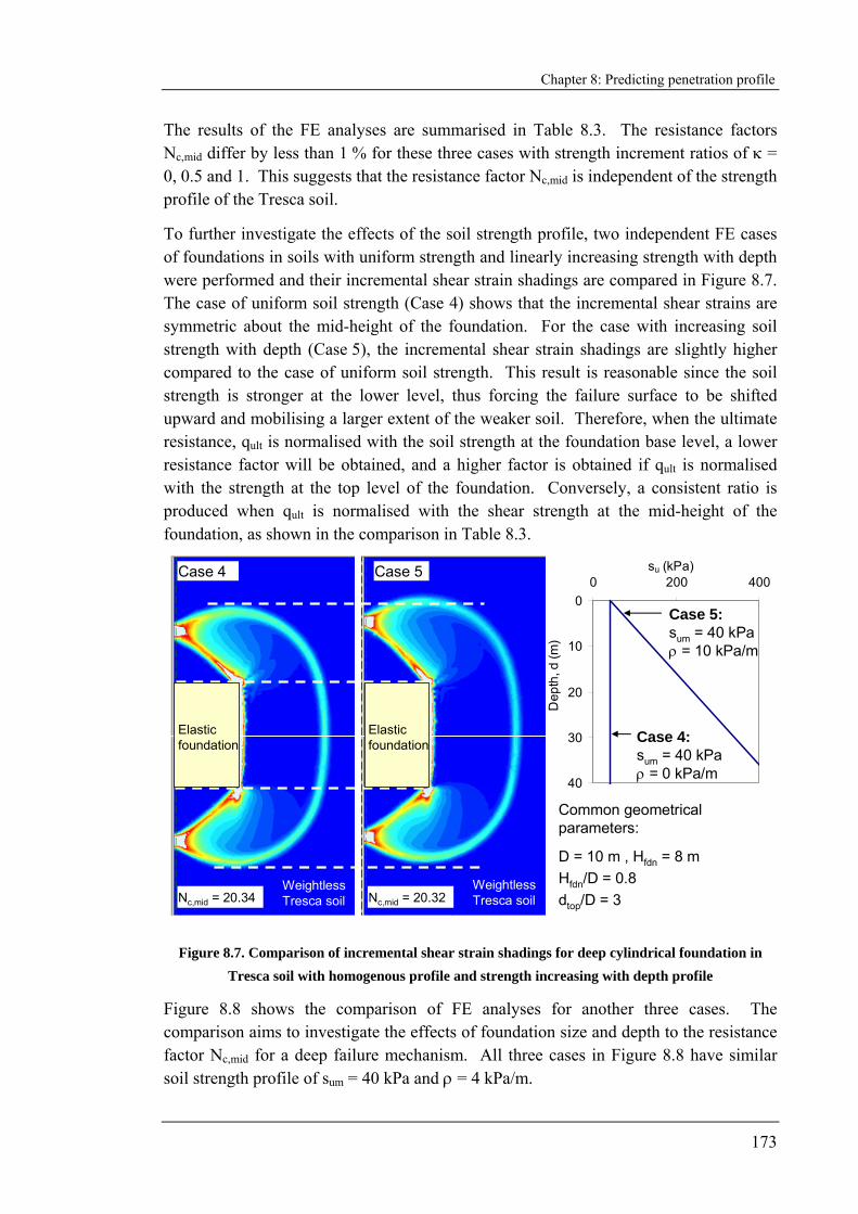
Chapter 8: Predicting penetration profile
173
The results of the FE analyses are summarised in Table 8.3. The resistance factors Nc,mid differ by less than 1 % for these three cases with strength increment ratios of κ = 0, 0.5 and 1. This suggests that the resistance factor Nc,mid is independent of the strength profile of the Tresca soil.
To further investigate the effects of the soil strength profile, two independent FE cases of foundations in soils with uniform strength and linearly increasing strength with depth were performed and their incremental shear strain shadings are compared in Figure 8.7. The case of uniform soil strength (Case 4) shows that the incremental shear strains are symmetric about the mid-height of the foundation. For the case with increasing soil strength with depth (Case 5), the incremental shear strain shadings are slightly higher compared to the case of uniform soil strength. This result is reasonable since the soil strength is stronger at the lower level, thus forcing the failure surface to be shifted upward and mobilising a larger extent of the weaker soil. Therefore, when the ultimate resistance, qult is normalised with the soil strength at the foundation base level, a lower resistance factor will be obtained, and a higher factor is obtained if qult is normalised with the strength at the top level of the foundation. Conversely, a consistent ratio is produced when qult is normalised with the shear strength at the mid-height of the foundation, as shown in the comparison in Table 8.3.
0
10
20
30
40
0 200 400su (kPa)
Dep
th, d
(m)
Case 4 Case 5
D = 10 m , Hfdn = 8 mHfdn/D = 0.8dtop/D = 3
Case 4:sum = 40 kPaρ = 0 kPa/m
Case 5:sum = 40 kPaρ = 10 kPa/m
Common geometrical parameters:
Nc,mid = 20.32Nc,mid = 20.34
Elastic foundation
Elastic foundation
Weightless Tresca soil
Weightless Tresca soil
Figure 8.7. Comparison of incremental shear strain shadings for deep cylindrical foundation in Tresca soil with homogenous profile and strength increasing with depth profile
Figure 8.8 shows the comparison of FE analyses for another three cases. The comparison aims to investigate the effects of foundation size and depth to the resistance factor Nc,mid for a deep failure mechanism. All three cases in Figure 8.8 have similar soil strength profile of sum = 40 kPa and ρ = 4 kPa/m.
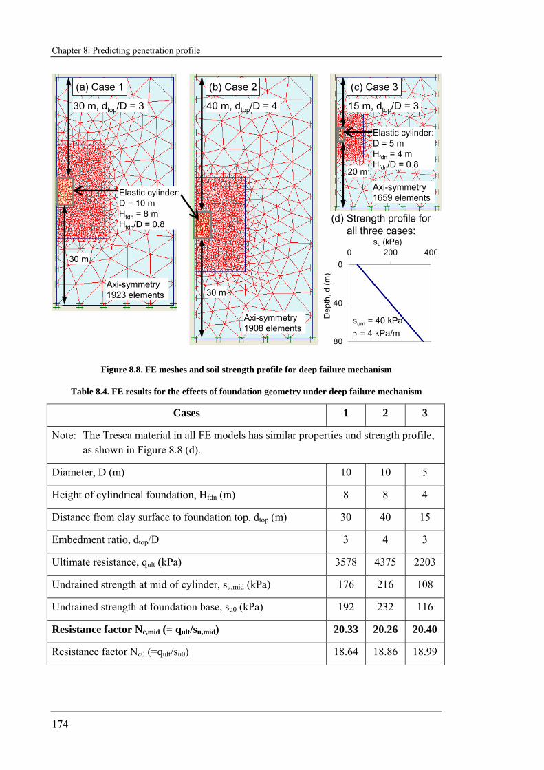
Chapter 8: Predicting penetration profile
174
0
40
80
0 200 400su (kPa)
Dep
th, d
(m)
Elastic cylinder:D = 5 mHfdn = 4 mHfdn/D = 0.8
Axi-symmetry1908 elements
Axi-symmetry 1659 elements
30 m
30 m, dtop/D = 3 40 m, dtop/D = 4 15 m, dtop/D = 3
Elastic cylinder:D = 10 mHfdn = 8 mHfdn/D = 0.8
30 mAxi-symmetry 1923 elements
20 m
(c) Case 3(a) Case 1 (b) Case 2
sum = 40 kPaρ = 4 kPa/m
(d) Strength profile for all three cases:
Figure 8.8. FE meshes and soil strength profile for deep failure mechanism
Table 8.4. FE results for the effects of foundation geometry under deep failure mechanism
Cases 1 2 3
Note: The Tresca material in all FE models has similar properties and strength profile, as shown in Figure 8.8 (d).
Diameter, D (m) 10 10 5
Height of cylindrical foundation, Hfdn (m) 8 8 4
Distance from clay surface to foundation top, dtop (m) 30 40 15
Embedment ratio, dtop/D 3 4 3
Ultimate resistance, qult (kPa) 3578 4375 2203
Undrained strength at mid of cylinder, su,mid (kPa) 176 216 108
Undrained strength at foundation base, su0 (kPa) 192 232 116
Resistance factor Nc,mid (= qult/su,mid) 20.33 20.26 20.40
Resistance factor Nc0 (=qult/su0) 18.64 18.86 18.99
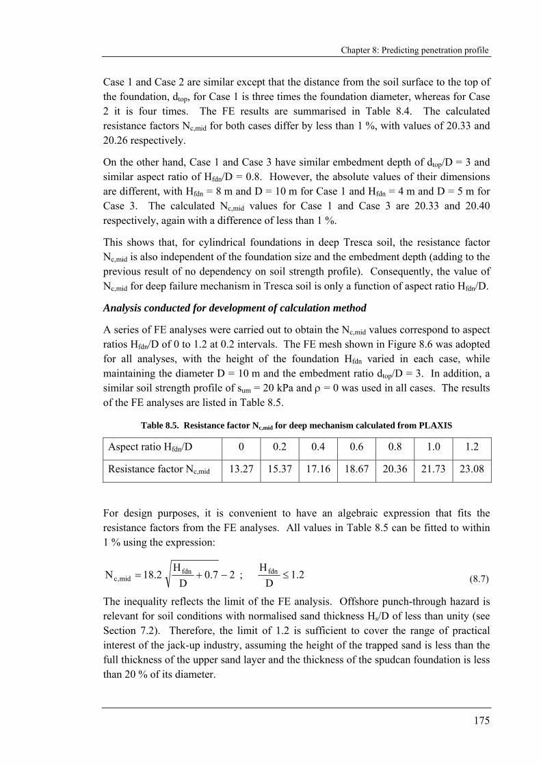
Chapter 8: Predicting penetration profile
175
Case 1 and Case 2 are similar except that the distance from the soil surface to the top of the foundation, dtop, for Case 1 is three times the foundation diameter, whereas for Case 2 it is four times. The FE results are summarised in Table 8.4. The calculated resistance factors Nc,mid for both cases differ by less than 1 %, with values of 20.33 and 20.26 respectively.
On the other hand, Case 1 and Case 3 have similar embedment depth of dtop/D = 3 and similar aspect ratio of Hfdn/D = 0.8. However, the absolute values of their dimensions are different, with Hfdn = 8 m and D = 10 m for Case 1 and Hfdn = 4 m and D = 5 m for Case 3. The calculated Nc,mid values for Case 1 and Case 3 are 20.33 and 20.40 respectively, again with a difference of less than 1 %.
This shows that, for cylindrical foundations in deep Tresca soil, the resistance factor Nc,mid is also independent of the foundation size and the embedment depth (adding to the previous result of no dependency on soil strength profile). Consequently, the value of Nc,mid for deep failure mechanism in Tresca soil is only a function of aspect ratio Hfdn/D.
Analysis conducted for development of calculation method
A series of FE analyses were carried out to obtain the Nc,mid values correspond to aspect ratios Hfdn/D of 0 to 1.2 at 0.2 intervals. The FE mesh shown in Figure 8.6 was adopted for all analyses, with the height of the foundation Hfdn varied in each case, while maintaining the diameter D = 10 m and the embedment ratio dtop/D = 3. In addition, a similar soil strength profile of sum = 20 kPa and ρ = 0 was used in all cases. The results of the FE analyses are listed in Table 8.5.
Table 8.5. Resistance factor Nc,mid for deep mechanism calculated from PLAXIS
Aspect ratio Hfdn/D 0 0.2 0.4 0.6 0.8 1.0 1.2
Resistance factor Nc,mid 13.27 15.37 17.16 18.67 20.36 21.73 23.08
For design purposes, it is convenient to have an algebraic expression that fits the resistance factors from the FE analyses. All values in Table 8.5 can be fitted to within 1 % using the expression:
27.0D
H2.18N fdn
mid,c −+= ; 2.1D
Hfdn ≤ (8.7)
The inequality reflects the limit of the FE analysis. Offshore punch-through hazard is relevant for soil conditions with normalised sand thickness Hs/D of less than unity (see Section 7.2). Therefore, the limit of 1.2 is sufficient to cover the range of practical interest of the jack-up industry, assuming the height of the trapped sand is less than the full thickness of the upper sand layer and the thickness of the spudcan foundation is less than 20 % of its diameter.
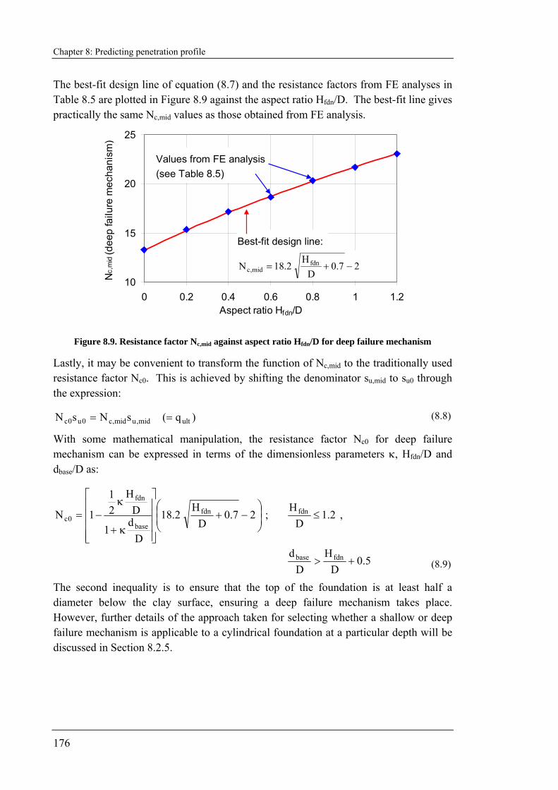
Chapter 8: Predicting penetration profile
176
The best-fit design line of equation (8.7) and the resistance factors from FE analyses in Table 8.5 are plotted in Figure 8.9 against the aspect ratio Hfdn/D. The best-fit line gives practically the same Nc,mid values as those obtained from FE analysis.
10
15
20
25
0 0.2 0.4 0.6 0.8 1 1.2Aspect ratio Hfdn/D
Nc,
mid
(dee
p fa
ilure
mec
hani
sm)_
Values from FE analysis(see Table 8.5)
Best-fit design line:
27.0D
H2.18N fdn
mid,c −+=
Figure 8.9. Resistance factor Nc,mid against aspect ratio Hfdn/D for deep failure mechanism
Lastly, it may be convenient to transform the function of Nc,mid to the traditionally used resistance factor Nc0. This is achieved by shifting the denominator su,mid to su0 through the expression:
)q(sNsN ultmid,umid,c0u0c == (8.8)
With some mathematical manipulation, the resistance factor Nc0 for deep failure mechanism can be expressed in terms of the dimensionless parameters κ, Hfdn/D and dbase/D as:
⎟⎟⎠
⎞⎜⎜⎝
⎛−+
⎥⎥⎥⎥
⎦
⎤
⎢⎢⎢⎢
⎣
⎡
κ+
κ−= 27.0
DH
2.18
Dd
1
DH
21
1N fdn
base
fdn
0c ; 2.1D
Hfdn ≤ ,
5.0D
HD
d fdnbase +> (8.9)
The second inequality is to ensure that the top of the foundation is at least half a diameter below the clay surface, ensuring a deep failure mechanism takes place. However, further details of the approach taken for selecting whether a shallow or deep failure mechanism is applicable to a cylindrical foundation at a particular depth will be discussed in Section 8.2.5.

Chapter 8: Predicting penetration profile
177
8.2.4 Cylindrical foundation in non-homogenous clay: Shallow failure mechanism
When a cylindrical foundation penetrates at shallow depth in clay, the failure surface from the foundation tip level will extend to the soil surface. To investigate this failure mode at shallow depth, FE analyses were again performed using similar procedures as discussed in Section 8.2.3, except that the embedded depths of the cylindrical foundation were limited to dbase/D < 2 following the analyses carried out by Martin (2001) using the upper and lower bound theorems of plasticity.
For soil strength that increases linearly with depth, it has been shown that the resistance factor Nc0 for shallow foundation is a function of the dimensionless rate of increase of strength with depth, κ (see equation (8.6)) (Davis and Booker, 1973; Houlsby and Martin, 2003).
To look into the geometrical effects of the foundation under shallow failure mechanism, three cases of FE analyses were carried out and the comparison is presented in Table 8.6. The same soil strength profile of sum = 20 kPa and ρ = 10 kPa/m was adopted in all three cases. All foundations have a diameter of 10 m and their base level is fixed at the same depth of 15 m from the soil surface. However, the aspect ratio, Hfdn/D, and therefore the embedment depth of the foundation top, dtop/D, are different for each case. The top of the foundation for Case 1 is located at the level of the soil surface with a foundation height of 15 m (corresponds to Hfdn/D = 1.5 and dtop/D = 0). The foundation height for Case 2 is 10 m and the top of foundation is 5 m below soil surface (Hfdn/D = 1.0 and dtop/D = 0.5). For Case 3, the foundation height is 6 m and the top of foundation is 9 m below soil surface (Hfdn/D = 0.6 and dtop/D = 0.9).
The incremental shear strain shadings for these three cases of FE analyses are shown in Figure 8.10. It can be observed that the failure mechanisms are extended to the soil surface.

Chapter 8: Predicting penetration profile
178
Trescamaterial
Elastic material
D/2
D/2
D/2
(c) Case 3(a) Case 1 (b) Case 2
Figure 8.10. Incremental shear strain shadings for cylindrical foundations with similar base level but different aspect ratios Hfdn/D
Table 8.6. Cases of FE analyses for shallow cylindrical foundations
Cases 1 2 3
Note: The Tresca material in all FE models has the same properties and strength profile of sum = 20 kPa and ρ = 10 kPa/m (thus κ = 5).
Diameter, D (m) 10 10 10
Height of cylindrical foundation, Hfdn (m) 15 10 6
Distance from clay surface to foundation top, dtop (m) 0 5 9
Aspect ratio, Hfdn/D 1.5 1.0 0.6
Embedment ratio (referring to top of foundation), dtop/D 0 0.5 0.9
Embedment ratio (referring to base of foundation), dbase/D 1.5 1.5 1.5
Ultimate resistance, qult (kPa) 2412 2409 2412
Undrained strength at mid of cylinder, su,mid (kPa) 95 120 140
Undrained strength at foundation base, su0 (kPa) 170 170 170
Resistance factor Nc,mid (= qult/su,mid) 25.39 20.07 17.23
Resistance factor Nc0 (=qult/su0) 14.19 14.17 14.19
The results of the FE analyses are compared in Table 8.6. The calculated resistance factors Nc0 for all cases are essentially the same from 14.17 to 14.19. This shows that
Chapter 8: Predicting penetration profile
179
the resistance factor Nc0 under shallow failure mechanism only depends on the depth of the foundation base and is not affected by the aspect ratio Hfdn/D of the foundation.
Based on this finding, a parametric study was carried out using the FE mesh shown in Figure 8.11 to obtain the Nc0 values for foundations with various embedment depths and soil strength profiles. In the FE parametric study, the top of the foundation is always fixed at the level of the soil surface. In this case, the embedment ratio of the foundation base, dbase/D, is equal to the aspect ratio Hfdn/D of the foundation.
25 m
Hfdn/D = dbase /D
35 m
Axi-symmetry FE mesh3386 elements
Weightless Tresca soil
Elastic cylindrical foundation:D = 10mHfdn varies
Axi-symmetry line
Figure 8.11. FE mesh for cylindrical foundation at shallow depth in weightless Tresca soil
The parameter study consists of 35 cases with the dimensionless soil strength increment ratio, κ = 0, 1, 2, 5 and 10 and the embedment ratio of the base, dbase/D = 0, 0.1, 0.25, 0.5, 1, 1.5 and 2. The numerical results of the FE analyses are listed in Table 8.7.
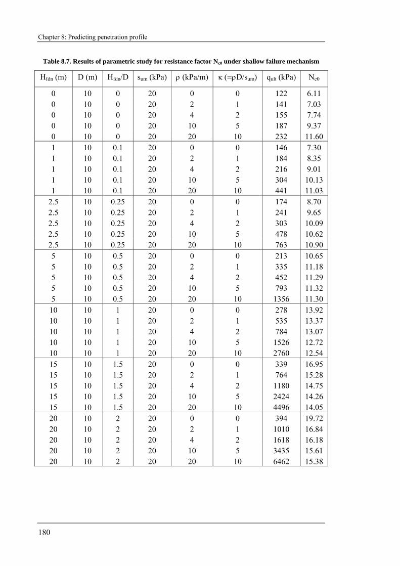
Chapter 8: Predicting penetration profile
180
Table 8.7. Results of parametric study for resistance factor Nc0 under shallow failure mechanism
Hfdn (m) D (m) Hfdn/D sum (kPa) ρ (kPa/m) κ (=ρD/sum) qult (kPa) Nc0
0 10 0 20 0 0 122 6.11 0 10 0 20 2 1 141 7.03 0 10 0 20 4 2 155 7.74 0 10 0 20 10 5 187 9.37 0 10 0 20 20 10 232 11.60 1 10 0.1 20 0 0 146 7.30 1 10 0.1 20 2 1 184 8.35 1 10 0.1 20 4 2 216 9.01 1 10 0.1 20 10 5 304 10.13 1 10 0.1 20 20 10 441 11.03
2.5 10 0.25 20 0 0 174 8.70 2.5 10 0.25 20 2 1 241 9.65 2.5 10 0.25 20 4 2 303 10.09 2.5 10 0.25 20 10 5 478 10.62 2.5 10 0.25 20 20 10 763 10.90 5 10 0.5 20 0 0 213 10.65 5 10 0.5 20 2 1 335 11.18 5 10 0.5 20 4 2 452 11.29 5 10 0.5 20 10 5 793 11.32 5 10 0.5 20 20 10 1356 11.30 10 10 1 20 0 0 278 13.92 10 10 1 20 2 1 535 13.37 10 10 1 20 4 2 784 13.07 10 10 1 20 10 5 1526 12.72 10 10 1 20 20 10 2760 12.54 15 10 1.5 20 0 0 339 16.95 15 10 1.5 20 2 1 764 15.28 15 10 1.5 20 4 2 1180 14.75 15 10 1.5 20 10 5 2424 14.26 15 10 1.5 20 20 10 4496 14.05 20 10 2 20 0 0 394 19.72 20 10 2 20 2 1 1010 16.84 20 10 2 20 4 2 1618 16.18 20 10 2 20 10 5 3435 15.61 20 10 2 20 20 10 6462 15.38
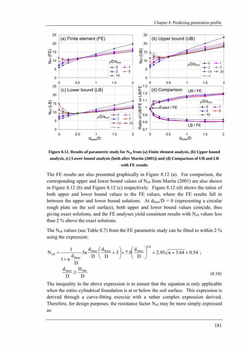
Chapter 8: Predicting penetration profile
181
0
5
10
15
20
25
0 0.5 1 1.5 2dbase/D
Nc0
(FE
)
0 12 510
ρD/sum
0
5
10
15
20
25
0 0.5 1 1.5 2dbase/D
Nc0
(UB
)
0 12 510 20∞
ρD/sum
0
5
10
15
20
25
0 0.5 1 1.5 2dbase/D
Nc0
(LB
)
0 12 510 20∞
ρD/sum
0.7
0.8
0.9
1
1.1
1.2
1.3
0 0.5 1 1.5 2dbase/D
Rat
io o
f UB
/FE
or L
B/F
E
0 12 510
ρD/sum
UB / FE
LB / FE
Exact / FE
(b) Upper bound (UB)
(c) Lower bound (LB)
(a) Finite element (FE)
(d) Comparison
Figure 8.12. Results of parametric study for Nc0 from (a) Finite element analysis, (b) Upper bound analysis, (c) Lower bound analysis (both after Martin (2001)) and (d) Comparison of UB and LB
with FE results
The FE results are also presented graphically in Figure 8.12 (a). For comparison, the corresponding upper and lower bound values of Nc0 from Martin (2001) are also shown in Figure 8.12 (b) and Figure 8.12 (c) respectively. Figure 8.12 (d) shows the ratios of both upper and lower bound values to the FE values, where the FE results fall in between the upper and lower bound solutions. At dbase/D = 0 (representing a circular rough plate on the soil surface), both upper and lower bound values coincide, thus giving exact solutions, and the FE analyses yield consistent results with Nc0 values less than 2 % above the exact solutions.
The Nc0 values (see Table 8.7) from the FE parametric study can be fitted to within 2 % using the expression:
54.064.395.2D
d9.73
Dd
Dd
3
Dd
1
1N8.0
basebasebase
base0c ++κ+⎟
⎠
⎞⎜⎝
⎛+⎟⎠
⎞⎜⎝
⎛ +κκ+
= ;
D
HD
d fdnbase ≥ (8.10)
The inequality in the above expression is to ensure that the equation is only applicable when the entire cylindrical foundation is at or below the soil surface. This expression is derived through a curve-fitting exercise with a rather complex expression derived. Therefore, for design purposes, the resistance factor Nc0 may be more simply expressed as:
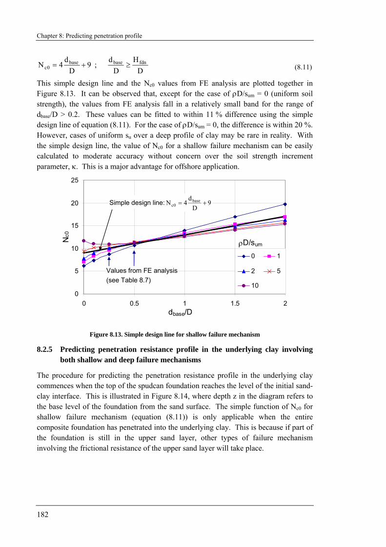
Chapter 8: Predicting penetration profile
182
9D
d4N base
0c += ; D
HD
d fdnbase ≥ (8.11)
This simple design line and the Nc0 values from FE analysis are plotted together in Figure 8.13. It can be observed that, except for the case of ρD/sum = 0 (uniform soil strength), the values from FE analysis fall in a relatively small band for the range of dbase/D > 0.2. These values can be fitted to within 11 % difference using the simple design line of equation (8.11). For the case of ρD/sum = 0, the difference is within 20 %. However, cases of uniform su over a deep profile of clay may be rare in reality. With the simple design line, the value of Nc0 for a shallow failure mechanism can be easily calculated to moderate accuracy without concern over the soil strength increment parameter, κ. This is a major advantage for offshore application.
0
5
10
15
20
25
0 0.5 1 1.5 2dbase/D
Nc0
0 1
2 5
10
ρD/sum
Values from FE analysis(see Table 8.7)
Simple design line:
9D
d4N base
0c +=
Figure 8.13. Simple design line for shallow failure mechanism
8.2.5 Predicting penetration resistance profile in the underlying clay involving both shallow and deep failure mechanisms
The procedure for predicting the penetration resistance profile in the underlying clay commences when the top of the spudcan foundation reaches the level of the initial sand-clay interface. This is illustrated in Figure 8.14, where depth z in the diagram refers to the base level of the foundation from the sand surface. The simple function of Nc0 for shallow failure mechanism (equation (8.11)) is only applicable when the entire composite foundation has penetrated into the underlying clay. This is because if part of the foundation is still in the upper sand layer, other types of failure mechanism involving the frictional resistance of the upper sand layer will take place.
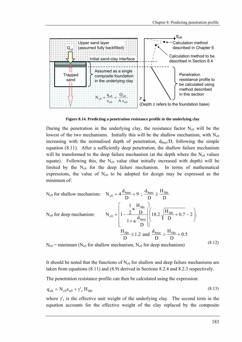
Chapter 8: Predicting penetration profile
183
Upper sand layer (assumed fully backfilled)
0u
ult
0u
ult0c sA
Qsq
N ==
Qult
qult
z
Assumed as a single composite foundation in the underlying clay
Trapped sand
Penetration resistance profile to be calculated using method described in this section
(Depth z refers to the foundation base)
Initial sand-clay interface
Calculation method described in Chapter 6
Calculation method to be described in Section 8.4
Figure 8.14. Predicting a penetration resistance profile in the underlying clay
During the penetration in the underlying clay, the resistance factor Nc0 will be the lowest of the two mechanisms. Initially this will be the shallow mechanism, with Nc0 increasing with the normalised depth of penetration, dbase/D, following the simple equation (8.11). After a sufficiently deep penetration, the shallow failure mechanism will be transformed to the deep failure mechanism (at the depth where the Nc0 values equate). Following this, the Nc0 value (that initially increased with depth) will be limited by the Nc0 for the deep failure mechanism. In terms of mathematical expressions, the value of Nc0 to be adopted for design may be expressed as the minimum of:
Nc0 for shallow mechanism: 9D
d4N base
0c += ; D
HD
d fdnbase ≥
Nc0 for deep mechanism: ⎟⎟⎠
⎞⎜⎜⎝
⎛−+
⎥⎥⎥⎥
⎦
⎤
⎢⎢⎢⎢
⎣
⎡
κ+
κ−= 27.0
DH
2.18
Dd
1
DH
21
1N fdn
base
fdn
0c ;
2.1D
Hfdn ≤ and 5.0D
HD
d fdnbase +>
Nc0 = minimum (Nc0 for shallow mechanism, Nc0 for deep mechanism) (8.12)
It should be noted that the functions of Nc0 for shallow and deep failure mechanisms are taken from equations (8.11) and (8.9) derived in Sections 8.2.4 and 8.2.3 respectively.
The penetration resistance profile can then be calculated using the expression:
fdnc0u0cult H'sNq γ+= (8.13)
where γ'c is the effective unit weight of the underlying clay. The second term in the equation accounts for the effective weight of the clay replaced by the composite
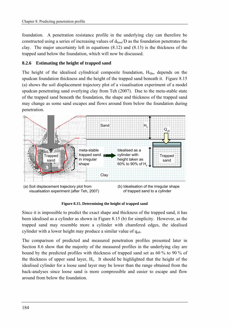
Chapter 8: Predicting penetration profile
184
foundation. A penetration resistance profile in the underlying clay can therefore be constructed using a series of increasing values of dbase/D as the foundation penetrates the clay. The major uncertainty left in equations (8.12) and (8.13) is the thickness of the trapped sand below the foundation, which will now be discussed.
8.2.6 Estimating the height of trapped sand
The height of the idealised cylindrical composite foundation, Hfdn, depends on the spudcan foundation thickness and the height of the trapped sand beneath it. Figure 8.15 (a) shows the soil displacement trajectory plot of a visualisation experiment of a model spudcan penetrating sand overlying clay from Teh (2007). Due to the meta-stable state of the trapped sand beneath the foundation, the shape and thickness of the trapped sand may change as some sand escapes and flows around from below the foundation during penetration.
Idealised as a cylinder with height taken as 60% to 90% of Hs
(a) Soil displacement trajectory plot from visualisation experiment (after Teh, 2007)
Trapped sand
Trapped sand
Qult
meta-stable trapped sand in irregular shape
HsSand
Clay
(b) Idealisation of the irregular shape of trapped sand to a cylinder
Figure 8.15. Determining the height of trapped sand
Since it is impossible to predict the exact shape and thickness of the trapped sand, it has been idealised as a cylinder as shown in Figure 8.15 (b) for simplicity. However, as the trapped sand may resemble more a cylinder with chamfered edges, the idealised cylinder with a lower height may produce a similar value of qult.
The comparison of predicted and measured penetration profiles presented later in Section 8.6 show that the majority of the measured profiles in the underlying clay are bound by the predicted profiles with thickness of trapped sand set as 60 % to 90 % of the thickness of upper sand layer, Hs. It should be highlighted that the height of the idealised cylinder for a loose sand layer may be lower than the range obtained from the back-analyses since loose sand is more compressible and easier to escape and flow around from below the foundation.
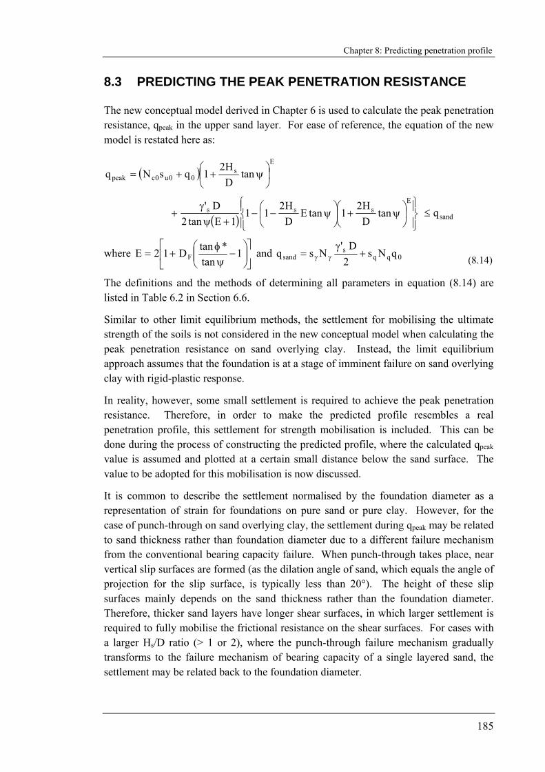
Chapter 8: Predicting penetration profile
185
8.3 PREDICTING THE PEAK PENETRATION RESISTANCE
The new conceptual model derived in Chapter 6 is used to calculate the peak penetration resistance, qpeak in the upper sand layer. For ease of reference, the equation of the new model is restated here as:
( )E
s00u0cpeak tan
DH2
1qsNq ⎟⎠
⎞⎜⎝
⎛ ψ++=
( ) ⎪⎭
⎪⎬⎫
⎪⎩
⎪⎨⎧
⎟⎠⎞
⎜⎝⎛ ψ+⎟
⎠⎞
⎜⎝⎛ ψ−−
+ψγ
+E
sss tanDH2
1tanEDH2
111Etan2
D' sandq≤
where ⎥⎦
⎤⎢⎣
⎡⎟⎟⎠
⎞⎜⎜⎝
⎛−
ψφ
+= 1tan
*tanD12E F and 0qqs
sand qNs2D'
Nsq +γ
= γγ (8.14)
The definitions and the methods of determining all parameters in equation (8.14) are listed in Table 6.2 in Section 6.6.
Similar to other limit equilibrium methods, the settlement for mobilising the ultimate strength of the soils is not considered in the new conceptual model when calculating the peak penetration resistance on sand overlying clay. Instead, the limit equilibrium approach assumes that the foundation is at a stage of imminent failure on sand overlying clay with rigid-plastic response.
In reality, however, some small settlement is required to achieve the peak penetration resistance. Therefore, in order to make the predicted profile resembles a real penetration profile, this settlement for strength mobilisation is included. This can be done during the process of constructing the predicted profile, where the calculated qpeak value is assumed and plotted at a certain small distance below the sand surface. The value to be adopted for this mobilisation is now discussed.
It is common to describe the settlement normalised by the foundation diameter as a representation of strain for foundations on pure sand or pure clay. However, for the case of punch-through on sand overlying clay, the settlement during qpeak may be related to sand thickness rather than foundation diameter due to a different failure mechanism from the conventional bearing capacity failure. When punch-through takes place, near vertical slip surfaces are formed (as the dilation angle of sand, which equals the angle of projection for the slip surface, is typically less than 20°). The height of these slip surfaces mainly depends on the sand thickness rather than the foundation diameter. Therefore, thicker sand layers have longer shear surfaces, in which larger settlement is required to fully mobilise the frictional resistance on the shear surfaces. For cases with a larger Hs/D ratio (> 1 or 2), where the punch-through failure mechanism gradually transforms to the failure mechanism of bearing capacity of a single layered sand, the settlement may be related back to the foundation diameter.
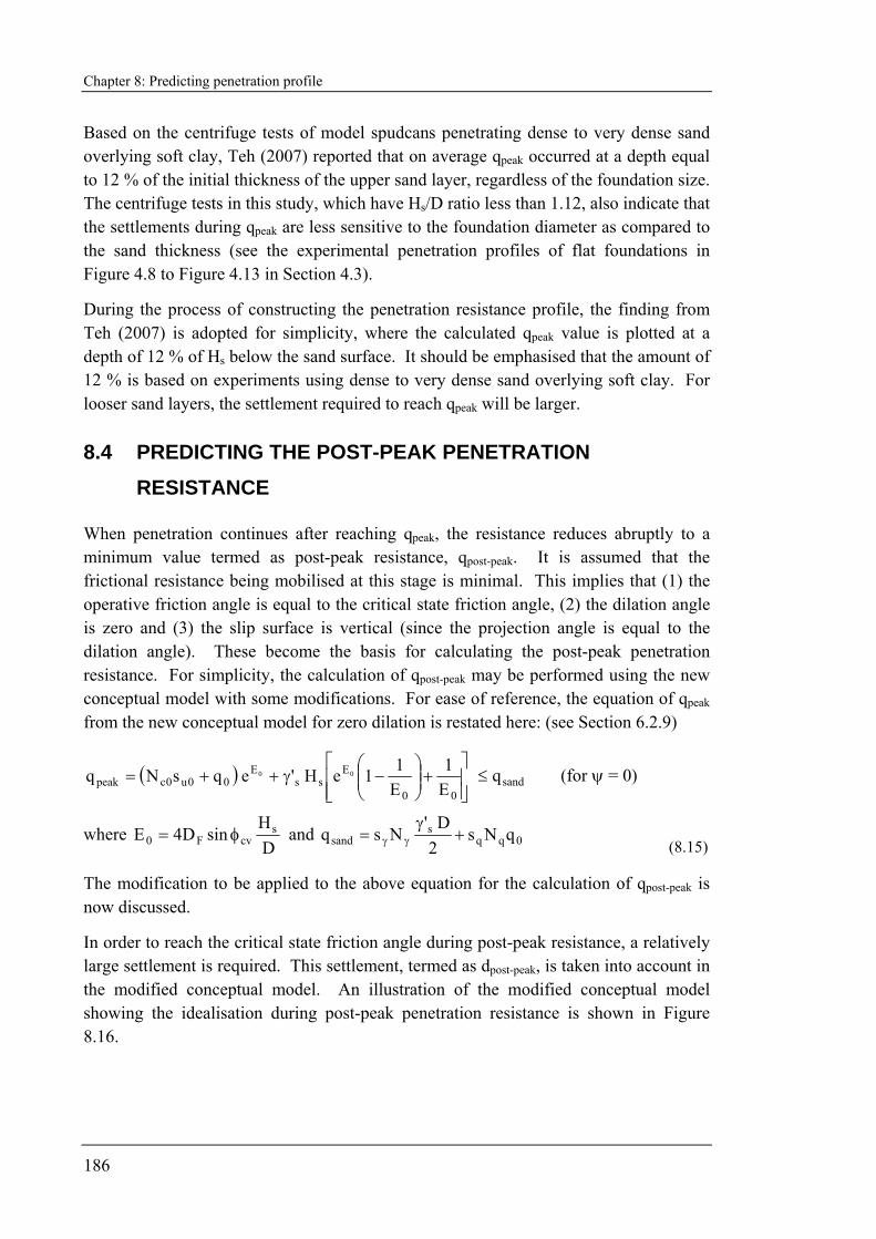
Chapter 8: Predicting penetration profile
186
Based on the centrifuge tests of model spudcans penetrating dense to very dense sand overlying soft clay, Teh (2007) reported that on average qpeak occurred at a depth equal to 12 % of the initial thickness of the upper sand layer, regardless of the foundation size. The centrifuge tests in this study, which have Hs/D ratio less than 1.12, also indicate that the settlements during qpeak are less sensitive to the foundation diameter as compared to the sand thickness (see the experimental penetration profiles of flat foundations in Figure 4.8 to Figure 4.13 in Section 4.3).
During the process of constructing the penetration resistance profile, the finding from Teh (2007) is adopted for simplicity, where the calculated qpeak value is plotted at a depth of 12 % of Hs below the sand surface. It should be emphasised that the amount of 12 % is based on experiments using dense to very dense sand overlying soft clay. For looser sand layers, the settlement required to reach qpeak will be larger.
8.4 PREDICTING THE POST-PEAK PENETRATION RESISTANCE
When penetration continues after reaching qpeak, the resistance reduces abruptly to a minimum value termed as post-peak resistance, qpost-peak. It is assumed that the frictional resistance being mobilised at this stage is minimal. This implies that (1) the operative friction angle is equal to the critical state friction angle, (2) the dilation angle is zero and (3) the slip surface is vertical (since the projection angle is equal to the dilation angle). These become the basis for calculating the post-peak penetration resistance. For simplicity, the calculation of qpost-peak may be performed using the new conceptual model with some modifications. For ease of reference, the equation of qpeak from the new conceptual model for zero dilation is restated here: (see Section 6.2.9)
( )⎥⎥⎦
⎤
⎢⎢⎣
⎡+⎟⎟
⎠
⎞⎜⎜⎝
⎛−γ++=
00
Ess
E00u0cpeak E
1E11eH'eqsNq 00 sandq≤ (for ψ = 0)
where DH
sinD4E scvF0 φ= and 0qq
ssand qNs
2D'
Nsq +γ
= γγ (8.15)
The modification to be applied to the above equation for the calculation of qpost-peak is now discussed.
In order to reach the critical state friction angle during post-peak resistance, a relatively large settlement is required. This settlement, termed as dpost-peak, is taken into account in the modified conceptual model. An illustration of the modified conceptual model showing the idealisation during post-peak penetration resistance is shown in Figure 8.16.
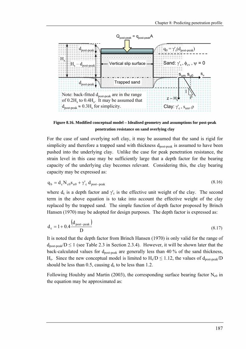
Chapter 8: Predicting penetration profile
187
q0 = γ's(dpost-peak)
Sand: γ's , φcv , ψ = 0
Note: back-fitted dpost-peak are in the range of 0.2Hs to 0.4Hs. It may be assumed that dpost-peak ≈ 0.3Hs for simplicity.
Hs – dpost-peak
Trapped sand
Qpost-peak = qpost-peakA
Hs
dpost-peak
dpost-peak
Clay: γ'c , sum, ρ
1ρ
sum su0
Vertical slip surface
su
z – Hs
Figure 8.16. Modified conceptual model – Idealised geometry and assumptions for post-peak penetration resistance on sand overlying clay
For the case of sand overlying soft clay, it may be assumed that the sand is rigid for simplicity and therefore a trapped sand with thickness dpost-peak is assumed to have been pushed into the underlying clay. Unlike the case for peak penetration resistance, the strain level in this case may be sufficiently large that a depth factor for the bearing capacity of the underlying clay becomes relevant. Considering this, the clay bearing capacity may be expressed as:
peakpostc0u0ccb d'sNdq −γ+= (8.16)
where dc is a depth factor and γ'c is the effective unit weight of the clay. The second term in the above equation is to take into account the effective weight of the clay replaced by the trapped sand. The simple function of depth factor proposed by Brinch Hansen (1970) may be adopted for design purposes. The depth factor is expressed as:
( )D
d4.01d peakpost
c−+= (8.17)
It is noted that the depth factor from Brinch Hansen (1970) is only valid for the range of dpost-peak/D ≤ 1 (see Table 2.3 in Section 2.3.4). However, it will be shown later that the back-calculated values for dpost-peak are generally less than 40 % of the sand thickness, Hs. Since the new conceptual model is limited to Hs/D ≤ 1.12, the values of dpost-peak/D should be less than 0.5, causing dc to be less than 1.2.
Following Houlsby and Martin (2003), the corresponding surface bearing factor Nc0 in the equation may be approximated as:
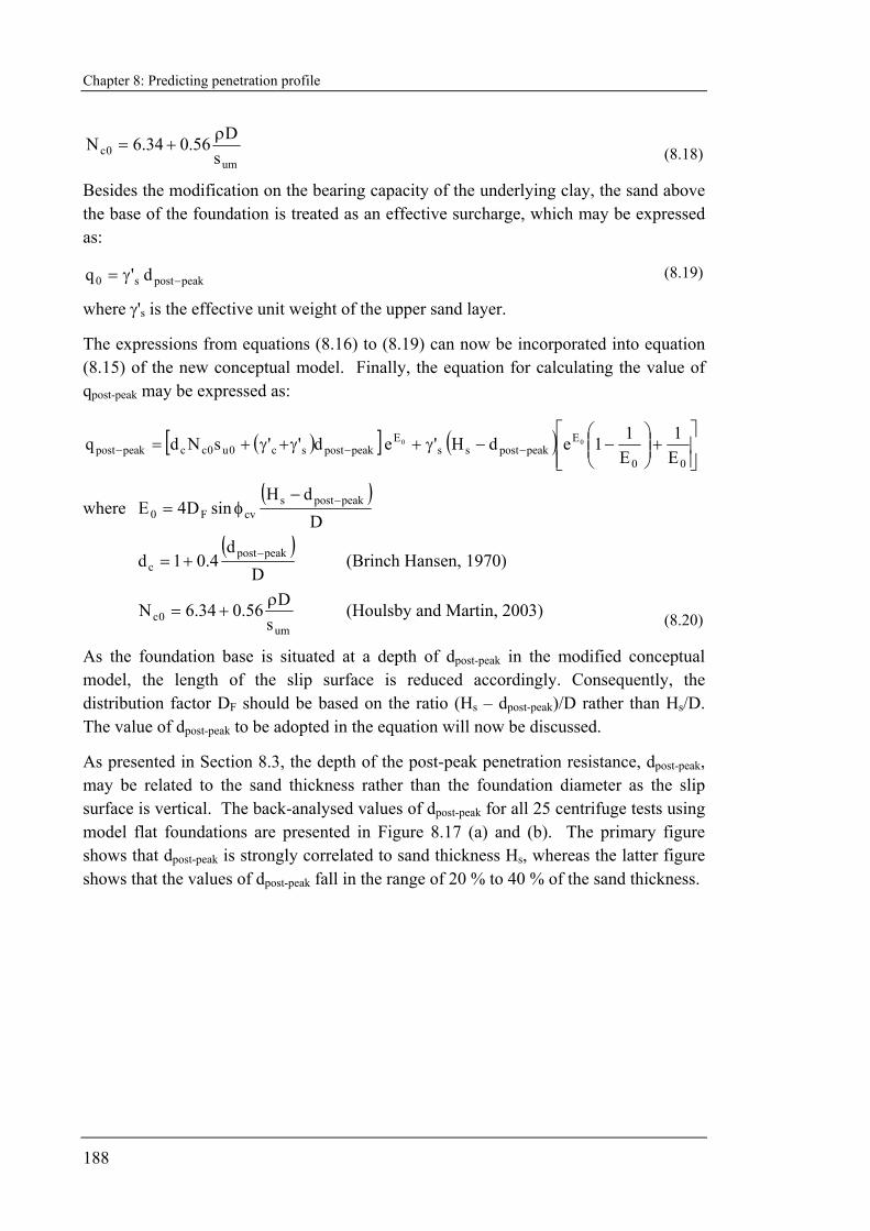
Chapter 8: Predicting penetration profile
188
um0c s
D56.034.6N ρ+= (8.18)
Besides the modification on the bearing capacity of the underlying clay, the sand above the base of the foundation is treated as an effective surcharge, which may be expressed as:
peakposts0 d'q −γ= (8.19)
where γ's is the effective unit weight of the upper sand layer.
The expressions from equations (8.16) to (8.19) can now be incorporated into equation (8.15) of the new conceptual model. Finally, the equation for calculating the value of qpost-peak may be expressed as:
( )[ ] ( )⎥⎥⎦
⎤
⎢⎢⎣
⎡+⎟⎟
⎠
⎞⎜⎜⎝
⎛−−γ+γ+γ+= −−−
00
Epeakpostss
Epeakpostsc0u0ccpeakpost E
1E11edH'ed''sNdq 00
where ( )
DdH
sinD4E peakpostscvF0
−−φ=
( )
Dd
4.01d peakpostc
−+= (Brinch Hansen, 1970)
um
0c sD56.034.6N ρ
+= (Houlsby and Martin, 2003) (8.20)
As the foundation base is situated at a depth of dpost-peak in the modified conceptual model, the length of the slip surface is reduced accordingly. Consequently, the distribution factor DF should be based on the ratio (Hs – dpost-peak)/D rather than Hs/D. The value of dpost-peak to be adopted in the equation will now be discussed.
As presented in Section 8.3, the depth of the post-peak penetration resistance, dpost-peak, may be related to the sand thickness rather than the foundation diameter as the slip surface is vertical. The back-analysed values of dpost-peak for all 25 centrifuge tests using model flat foundations are presented in Figure 8.17 (a) and (b). The primary figure shows that dpost-peak is strongly correlated to sand thickness Hs, whereas the latter figure shows that the values of dpost-peak fall in the range of 20 % to 40 % of the sand thickness.
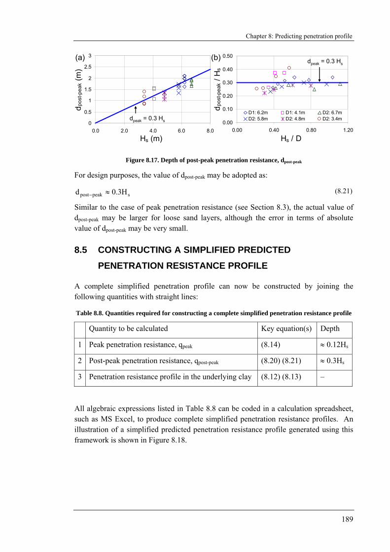
Chapter 8: Predicting penetration profile
189
0.00
0.10
0.20
0.30
0.40
0.50
0.00 0.40 0.80 1.20
Hs / D
d pos
t-pea
k / H
s
D1: 6.2m D1: 4.1m D2: 6.7mD2: 5.8m D2: 4.8m D2: 3.4m
0
0.5
1
1.5
2
2.5
3
0.0 2.0 4.0 6.0 8.0Hs (m)
d pos
t-pea
k (m
)
dpeak = 0.3 Hs
dpeak = 0.3 Hs(a) (b)
Figure 8.17. Depth of post-peak penetration resistance, dpost-peak
For design purposes, the value of dpost-peak may be adopted as:
speakpost H3.0d ≈− (8.21)
Similar to the case of peak penetration resistance (see Section 8.3), the actual value of dpost-peak may be larger for loose sand layers, although the error in terms of absolute value of dpost-peak may be very small.
8.5 CONSTRUCTING A SIMPLIFIED PREDICTED PENETRATION RESISTANCE PROFILE
A complete simplified penetration profile can now be constructed by joining the following quantities with straight lines:
Table 8.8. Quantities required for constructing a complete simplified penetration resistance profile
Quantity to be calculated Key equation(s) Depth
1 Peak penetration resistance, qpeak (8.14) ≈ 0.12Hs
2 Post-peak penetration resistance, qpost-peak (8.20) (8.21) ≈ 0.3Hs
3 Penetration resistance profile in the underlying clay (8.12) (8.13) –
All algebraic expressions listed in Table 8.8 can be coded in a calculation spreadsheet, such as MS Excel, to produce complete simplified penetration resistance profiles. An illustration of a simplified predicted penetration resistance profile generated using this framework is shown in Figure 8.18.
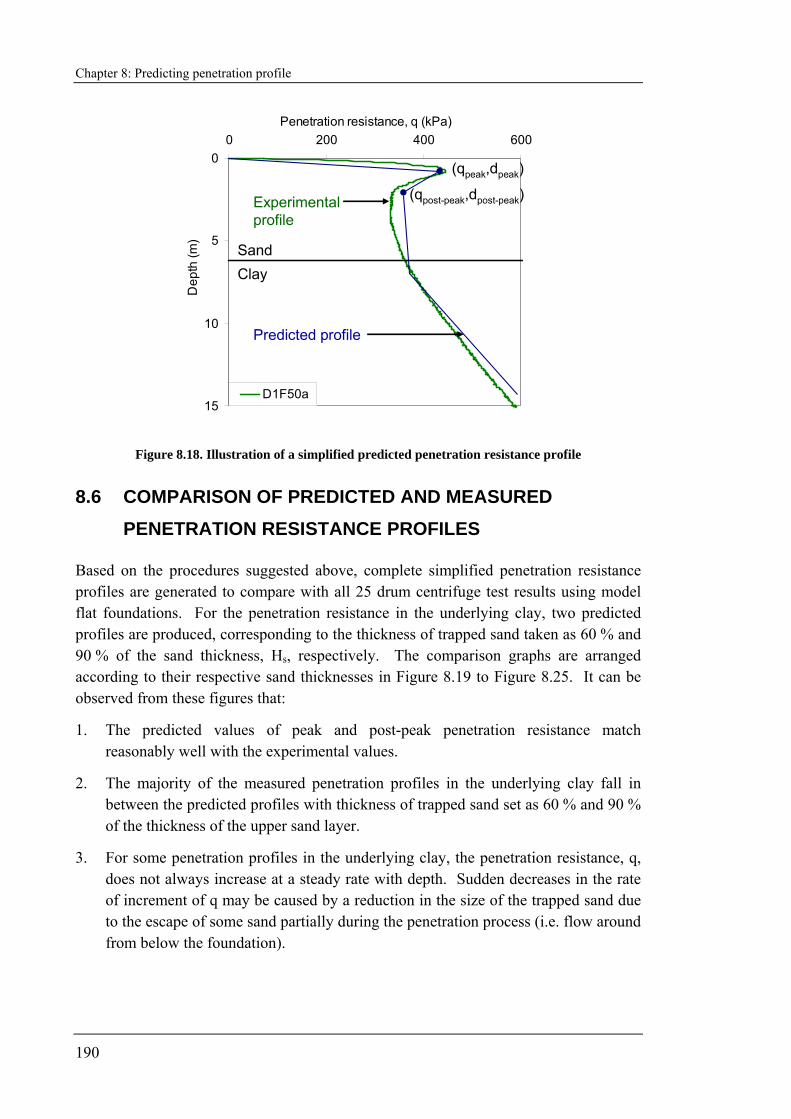
Chapter 8: Predicting penetration profile
190
0
5
10
15
0 200 400 600Penetration resistance, q (kPa)
Dep
th (m
)
D1F50a
(qpeak,dpeak)
ClaySand
Experimental profile
Predicted profile
(qpost-peak,dpost-peak)
Figure 8.18. Illustration of a simplified predicted penetration resistance profile
8.6 COMPARISON OF PREDICTED AND MEASURED PENETRATION RESISTANCE PROFILES
Based on the procedures suggested above, complete simplified penetration resistance profiles are generated to compare with all 25 drum centrifuge test results using model flat foundations. For the penetration resistance in the underlying clay, two predicted profiles are produced, corresponding to the thickness of trapped sand taken as 60 % and 90 % of the sand thickness, Hs, respectively. The comparison graphs are arranged according to their respective sand thicknesses in Figure 8.19 to Figure 8.25. It can be observed from these figures that:
1. The predicted values of peak and post-peak penetration resistance match reasonably well with the experimental values.
2. The majority of the measured penetration profiles in the underlying clay fall in between the predicted profiles with thickness of trapped sand set as 60 % and 90 % of the thickness of the upper sand layer.
3. For some penetration profiles in the underlying clay, the penetration resistance, q, does not always increase at a steady rate with depth. Sudden decreases in the rate of increment of q may be caused by a reduction in the size of the trapped sand due to the escape of some sand partially during the penetration process (i.e. flow around from below the foundation).
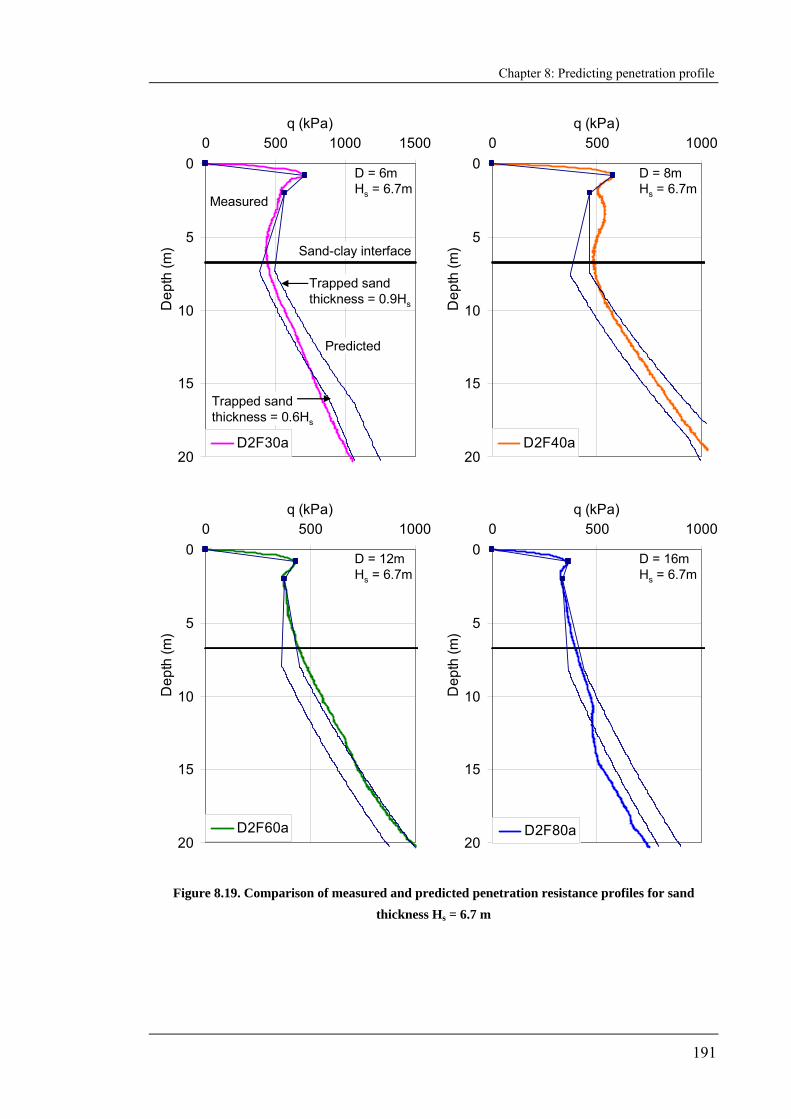
Chapter 8: Predicting penetration profile
191
0
5
10
15
20
0 500 1000 1500q (kPa)
Dep
th (m
)
D2F30a
0
5
10
15
20
0 500 1000q (kPa)
Dep
th (m
)D2F40a
Measured
Trapped sand thickness = 0.6Hs
D = 6mHs = 6.7m
D = 8mHs = 6.7m
Trapped sand thickness = 0.9Hs
Sand-clay interface
Predicted
0
5
10
15
20
0 500 1000q (kPa)
Dep
th (m
)
D2F60a
0
5
10
15
20
0 500 1000q (kPa)
Dep
th (m
)
D2F80a
D = 12mHs = 6.7m
D = 16mHs = 6.7m
Figure 8.19. Comparison of measured and predicted penetration resistance profiles for sand thickness Hs = 6.7 m
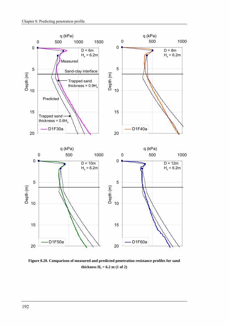
Chapter 8: Predicting penetration profile
192
0
5
10
15
20
0 500 1000 1500q (kPa)
Dep
th (m
)
D1F30a
0
5
10
15
20
0 500 1000q (kPa)
Dep
th (m
)
D1F40a
Trapped sand thickness = 0.6Hs
D = 6mHs = 6.2m
D = 8mHs = 6.2m
Trapped sand thickness = 0.9Hs
Sand-clay interface
Predicted
Measured
0
5
10
15
20
0 500 1000q (kPa)
Dep
th (m
)
D1F50a
0
5
10
15
20
0 500 1000q (kPa)
Dep
th (m
)
D1F60a
D = 10mHs = 6.2m
D = 12mHs = 6.2m
Figure 8.20. Comparison of measured and predicted penetration resistance profiles for sand thickness Hs = 6.2 m (1 of 2)
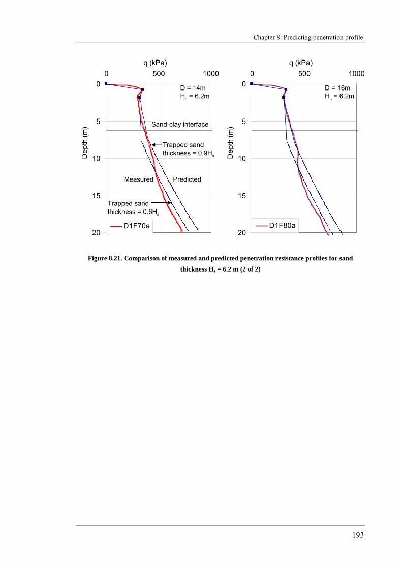
Chapter 8: Predicting penetration profile
193
0
5
10
15
20
0 500 1000q (kPa)
Dep
th (m
)
D1F70a
0
5
10
15
20
0 500 1000q (kPa)
Dep
th (m
)D1F80a
D = 14mHs = 6.2m
D = 16mHs = 6.2m
Sand-clay interface
PredictedMeasured
Trapped sand thickness = 0.6Hs
Trapped sand thickness = 0.9Hs
Figure 8.21. Comparison of measured and predicted penetration resistance profiles for sand thickness Hs = 6.2 m (2 of 2)
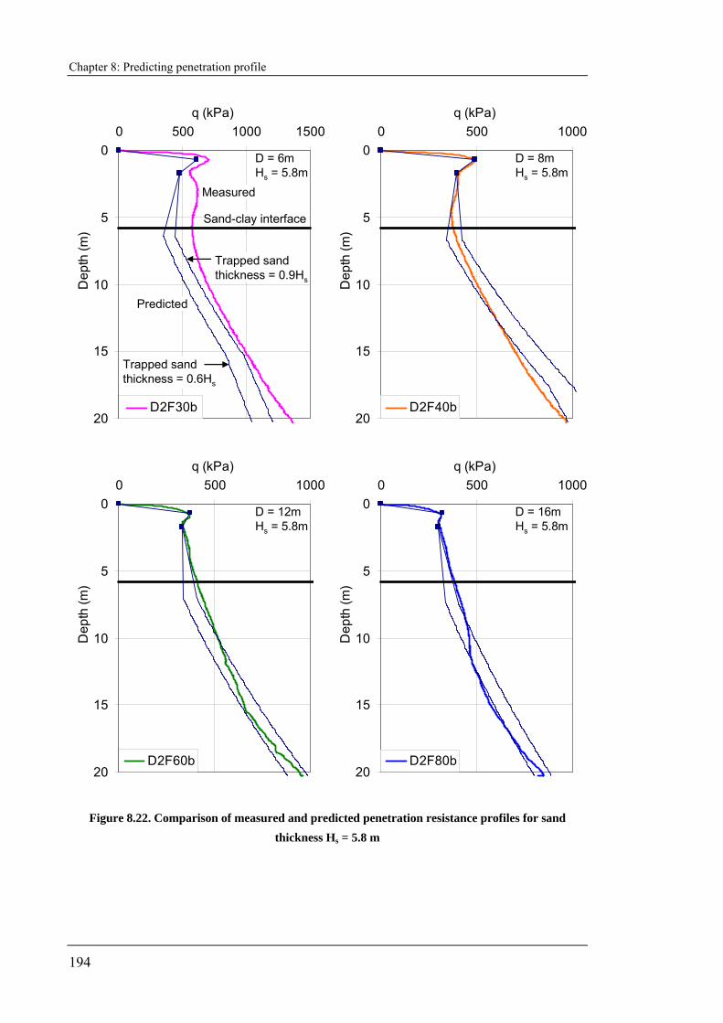
Chapter 8: Predicting penetration profile
194
0
5
10
15
20
0 500 1000 1500q (kPa)
Dep
th (m
)
D2F30b
0
5
10
15
20
0 500 1000q (kPa)
Dep
th (m
)
D2F40b
Measured
Trapped sand thickness = 0.6Hs
D = 6mHs = 5.8m
D = 8mHs = 5.8m
Sand-clay interface
Predicted
Trapped sand thickness = 0.6Hs
Trapped sand thickness = 0.9Hs
0
5
10
15
20
0 500 1000q (kPa)
Dep
th (m
)
D2F60b
0
5
10
15
20
0 500 1000q (kPa)
Dep
th (m
)
D2F80b
D = 12mHs = 5.8m
D = 16mHs = 5.8m
Figure 8.22. Comparison of measured and predicted penetration resistance profiles for sand thickness Hs = 5.8 m
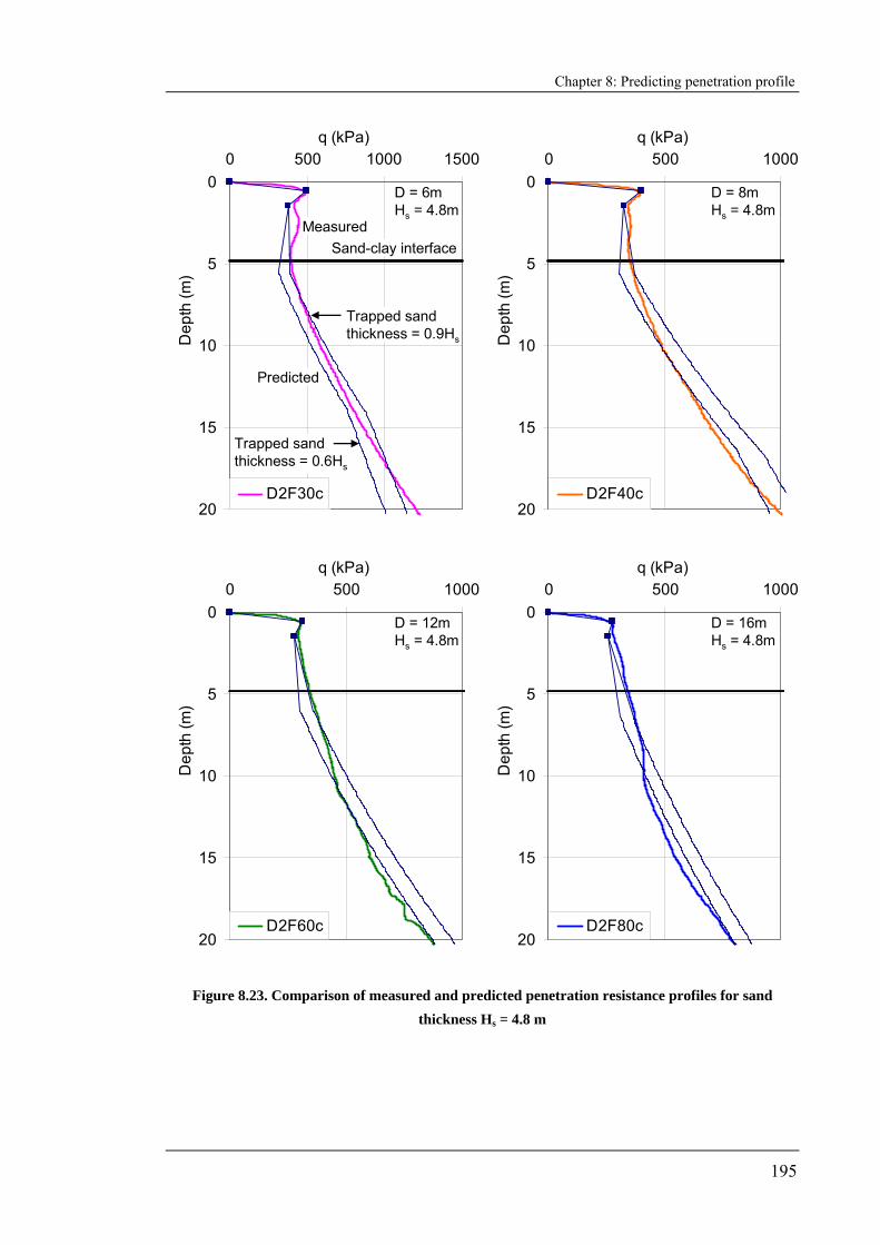
Chapter 8: Predicting penetration profile
195
0
5
10
15
20
0 500 1000 1500q (kPa)
Dep
th (m
)
D2F30c
0
5
10
15
20
0 500 1000q (kPa)
Dep
th (m
)D2F40c
Measured
Trapped sand thickness = 0.6Hs
D = 6mHs = 4.8m
D = 8mHs = 4.8m
Sand-clay interface
Predicted
Trapped sand thickness = 0.6Hs
Trapped sand thickness = 0.9Hs
0
5
10
15
20
0 500 1000q (kPa)
Dep
th (m
)
D2F60c
0
5
10
15
20
0 500 1000q (kPa)
Dep
th (m
)
D2F80c
D = 12mHs = 4.8m
D = 16mHs = 4.8m
Figure 8.23. Comparison of measured and predicted penetration resistance profiles for sand thickness Hs = 4.8 m

Chapter 8: Predicting penetration profile
196
0
5
10
15
20
0 500 1000q (kPa)
Dep
th (m
)
D1F40b
0
5
10
15
20
0 500 1000q (kPa)
Dep
th (m
)
D1F50b
D = 8mHs = 4.1m
D = 10mHs = 4.1m
Sand-clay interface
PredictedMeasured
Trapped sand thickness = 0.6Hs
Trapped sand thickness = 0.9Hs
0
5
10
15
20
0 500 1000q (kPa)
Dep
th (m
)
D1F60b
D = 12mHs = 4.1m
Figure 8.24. Comparison of measured and predicted penetration resistance profiles for sand thickness Hs = 4.1 m
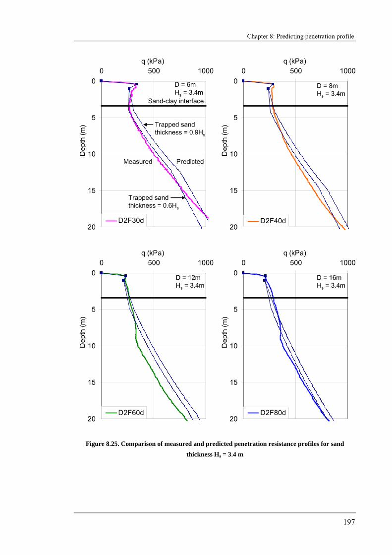
Chapter 8: Predicting penetration profile
197
0
5
10
15
20
0 500 1000q (kPa)
Dep
th (m
)
D2F30d
0
5
10
15
20
0 500 1000q (kPa)
Dep
th (m
)D2F40d
D = 6mHs = 3.4m
D = 8mHs = 3.4m
Sand-clay interface
PredictedMeasured
Trapped sand thickness = 0.6Hs
Trapped sand thickness = 0.9Hs
0
5
10
15
20
0 500 1000q (kPa)
Dep
th (m
)
D2F60d
0
5
10
15
20
0 500 1000q (kPa)
Dep
th (m
)
D2F80d
D = 12mHs = 3.4m
D = 16mHs = 3.4m
Figure 8.25. Comparison of measured and predicted penetration resistance profiles for sand thickness Hs = 3.4 m
Chapter 8: Predicting penetration profile
198
8.7 CONCLUDING REMARKS
A design framework for producing a complete simplified penetration profile for foundations on sand overlying clay has been presented. The framework is established based on simplified conceptual models and design equations that are developed from combinations of physical modelling through centrifuge testing and numerical modelling using finite element analysis.
The design procedures for calculating the penetration resistance are different for the situations where (a) the foundation is in the sand layer and (b) it is in the underlying clay. This reflects the complexity of a penetration problem in sand overlying clay soils. For the penetration resistance in the upper sand layer, the important roles of stress level and dilatant response of sand are taken into account. During penetration in the underlying clay, the proposed design equations incorporate the shear strength increment with depth and the thickness of the trapped sand beneath the foundation. Due to the large diameter of typical spudcan foundations, both effects have significant influence on the penetration resistance.
However, not all aspects of soil behaviour are incorporated in the design framework. Instead, only those aspects of soil behaviour that are considered to be important are included in the design models, together with some idealisations and simplified assumptions. Therefore, great accuracy may not be expected from the design framework, but such an approach is consistent with the objective of developing a relatively simple and practical design procedure for practising engineers.
Straightforward algebraic expressions with clearly defined parameters are given in the design framework for producing a complete simplified penetration profile on sand overlying clay. The equations can therefore be easily implemented into calculation spreadsheets, and the resulting penetration profiles produced and plotted accordingly. In retrospectively calculating the penetration resistance profiles for all 25 centrifuge tests performed in this study, it was shown that the calculated profiles match reasonably well with the experimental profiles.
Chapter 9: Conclusions and further research
199
CHAPTER 9. CONCLUSIONS AND FURTHER RESEARCH
9.1 INTRODUCTION
This research is concerned with the performance of spudcan foundations founded on sand overlying clay soils, where the potential of punch-through failure exists. The major achievements of this research are the development of (1) a new conceptual model for predicting the peak penetration resistance, and (2) a consistent method for constructing a complete penetration resistance profile for foundations on sand overlying clay.
These main findings have been developed through an extensive programme of physical modelling (in the form of centrifuge tests) of foundations on sand overlying clay, and supporting finite element analysis. The new methods have been verified against an experimental database, including those already in the literature. This chapter summarises the key findings of the research. This is followed by a discussion on future research that could build upon this work.
9.2 CONCLUSIONS – MAIN FINDINGS
9.2.1 Development of a new conceptual model for predicting the peak penetration resistance
Following the approach for silo analysis, a new conceptual model has been developed to predict the peak penetration resistance of foundations on sand overlying clay soils. An iterative procedure was devised to take into account the stress-level and dilatant response of the sand layer in the new model. Therefore, it is a significant improvement over the punching shear and load spread models advocated in the current industry guidelines SNAME (2002), in which the strength properties of the sand layer are not considered.
The new model was based on (1) a total of 30 foundation penetration tests conducted on two samples comprising sand overlying clay in the UWA drum centrifuge, and (2) finite element (FE) analysis used to simulate the centrifuge tests.
Physical modelling using drum centrifuge
In the centrifuge tests, the large testing area of the drum centrifuge was advantageously used to produce test results that were able to be compared directly. The experiments included a wide range of sand thickness over diameter (Hs/D) ratios, varying from 0.21 to 1.12. This should well cover the range of practical interest for the offshore jack-up industry. In addition, the measured peak penetration resistance fell in the range of
Chapter 9: Conclusions and further research
200
220 kPa to 710 kPa. These experimental limits are also in the typical range seen offshore, with spudcan preload of around 400 kPa to 600 kPa reported by Osborne et al. (2008) and Randolph et al. (2005).
Qualitative examination of post-test samples showed that trapped sand was left behind in the clay during penetration and extraction of the model foundation. A lump of trapped sand and trails of sand along the penetration path were consistently observed in all post-test soil samples, including those from penetration tests of miniature penetrometers.
It was found that the measured values of the peak penetration resistance followed very consistent trends. This reflects the good quality of the test results, which have provided reliable experimental data for the development of the new conceptual model.
Supporting finite element analysis
The aim of the finite element (FE) analysis was to back-calculate the stress-level dependent friction angle and dilation angle during peak penetration resistance. The upper sand layer was modelled using the Mohr-Coulomb model and the underlying clay as a Tresca material. This is consistent with common industry practice in spudcan punch-through analysis. By matching the peak resistance from the FE analysis with the corresponding experimental value, a single ‘operative’ friction angle and dilation angle was determined for each test.
The FE analyses showed that the back-calculated operative friction and dilation angles varied with the foundation diameter, even on sand layers with the same thickness and relative density. Specifically, the operative friction and dilation angles were found to vary in accordance with a modified form of Bolton’s (1986) empirical strength-dilatancy relationships. This implies that larger values of peak resistance will give lower values of friction and dilation angles, which is consistent with gradual suppression of dilatancy under high confining stress. Therefore, although the sand samples prepared in the centrifuge tests had similar relative density, different values of friction and dilation angles were actually mobilised at peak resistance, since they depended on the magnitudes of the failure load caused by various foundation sizes and sand thicknesses.
When compared to the results of visualisation experiments from Teh (2007) during peak penetration resistance, the FE analysis showed a similar failure mechanism, where a frustum of sand was forced into the underlying clay. In addition, the inclinations of the shear bands to the vertical derived from the FE analyses were found to be consistent with the values of the operative dilation angle mobilised in the sand. This observation has formed the basis of the new simplified conceptual model derived in this study.
Chapter 9: Conclusions and further research
201
New conceptual model
The new model essentially involves one equation (see equation (6.19) in Chapter 6). The input parameters of the model include all necessary geometry and soil strength parameters of a foundation on sand overlying clay and a single empirical factor, which is called the distribution factor, DF. All input parameters (except for DF) are familiar to practising engineers and can be assessed from a proper site investigation scheme.
It was found that the calculated peak resistance values matched the experimental results well by adopting DF values that varied linearly with the Hs/D ratio. Consequently, two linear empirical relationships of DF versus Hs/D ratio, corresponding to the flat-based foundations and the spudcans respectively, were obtained from linear regression. The DF factor calibrates the new conceptual model for other aspects of soil behaviour that were not considered explicitly in formulating the model, such as the effects of anisotropy, progressive failure, actual shape of the slip surface and so forth. By incorporating this empirical factor, a balance of simplicity and accuracy of the conceptual method was achieved. In addition, since there is only one empirical factor, agreement resulting from compensating errors of several empirical parameters could be avoided.
Parametric studies were carried out to examine the influence of the input parameters to the value of the peak penetration resistance. Various trends were correctly predicted in the parametric studies, including the foundation size effect, where the values of peak resistance were shown to decrease with increasing foundation size whilst other input quantities remained unchanged. This was a direct consequence of incorporating the stress level and dilatant response of sand in the new model.
Since the new model involves an iterative procedure, an effective way to execute the calculation is to code the equations into a calculation spreadsheet such as MS Excel. This approach has an advantage over producing design charts, since essentially unlimited combinations of input parameters can be keyed into the spreadsheet for a specific site, rather than interpolating among design charts. Furthermore, sensitivity tests on a given input parameter can be performed easily using the spreadsheet. This is particularly useful since it is difficult to obtain accurate subsea soil parameters with high confidence in foundation assessment for mobile jack-ups (Osborne et al., 2006). This enables the new conceptual model to be a potential routine design tool for punch-through on sand overlying clay.
Limitations
The current model is only applicable for the case of circular foundations on sand overlying clay, where a block of sand is forced into the underlying clay during peak penetration resistance. The new conceptual model should only be used when Hs/D ≤ 1.12, which corresponds to the upper limit verified by experimental data. This range covers that of practical interest for the offshore jack-up industry.
Chapter 9: Conclusions and further research
202
The centrifuge tests used for calibrating the new model incorporated only very dense sand layers. Therefore, the performance of the new model for loose sand overlying clay has not been verified. In addition, it should be emphasised that the two empirical DF lines were calibrated from tests using model flat foundations and model spudcans with conical angle of 13° to the horizontal. Therefore, the empirical DF line may differ for foundations with other conical angles. This effect has not been studied in this work and more experiments using model foundations with various conical angles would prove useful. However, as an initial approach it is suggested that spudcans with conical angles of less than 13° may be analysed by interpolating between the two lines for DF.
The simplified geometry and assumptions on the stresses may limit the accuracy that can be expected from the new model. However, it is a simple model derived from a realistic analytical framework and with input parameters assessable from a proper site investigation scheme. It is therefore believed to provide the jack-up industry with an attractive analytical tool for practical routine designs.
Comparison of the new model with other methods and experimental database
The performance of the new model in predicting the peak penetration resistance was compared with other existing analytical methods, including those recommended in the design guidelines SNAME (2002). In the comparative study, the predicted values calculated using various analytical methods were compared with the experimental results. For a fairer comparison, additional test data were also incorporated. They included previously published experimental results and an additional five spudcan penetration tests carried out for this purpose using the UWA beam centrifuge. The comparative study showed that the new conceptual model provided the best prediction for the peak penetration resistance. The analytical methods from SNAME (2002) gave very conservative prediction, in which the averagely predicted values ranged from 40 % to 60 % of the experimental values.
9.2.2 Predicting a complete penetration profile
A complete penetration resistance profile for foundations on sand overlying clay is important in order to evaluate the severity of a potential punch-through and the appropriate mitigation measures. The ability to predict the entire penetration profile is another major accomplishment of this research. Different calculation methods are used as the spudcan penetrates, accounting for changing failure mechanisms with penetration.
Initially the new conceptual model for calculating the peak penetration is evaluated, with the depth of this peak assumed to occur at 0.12 Hs. Following this, a post-peak resistance is evaluated by modifying the equations from the new conceptual model. The post-peak resistance may be assumed to occur at 0.3 Hs. A design method for calculating the penetration profile in the underlying clay has also been developed. This method is based on new bearing capacity factors developed through FE analysis. By joining the calculated values of peak resistance and post-peak resistance to the predicted
Chapter 9: Conclusions and further research
203
penetration profile in the underlying clay, a complete simplified penetration profile could be constructed.
While a spudcan foundation is penetrating through a sand layer into an underlying clay, the soils are in meta-stable states. During the penetration process, the shape and thickness of the sand trapped beneath the foundation may change as some sand escapes and flows around the foundation. It is therefore impossible to predict the exact geometry of the trapped sand. However, for design purposes, it is recommended that the foundation and the trapped sand may be idealised as a cylindrical composite foundation. With this simplification, FE analysis was carried out to study the penetration resistance of the composite foundation in the underlying clay. The cylindrical composite foundation was modelled using an elastic constitutive model, while the undrained clay was modelled using a Tresca model.
Based on the FE results, two simplified design equations, corresponding to shallow and deep failure mechanisms, were devised to calculate the penetration resistance in the underlying clay. By comparing the calculated penetration profiles with the test results, it was found that the majority of the measured profiles were bracketed in between the predicted profiles with the thickness of trapped sand set as 60 % to 90 % of the thickness of the upper sand layer.
9.3 FURTHER RESEARCH
9.3.1 Centrifuge tests for refining the empirical distribution factor (DF)
Two linear empirical lines for the distribution factor DF, corresponding to flat-based foundations and spudcans with a conical angle of 13° to the horizontal, were back-calculated from the centrifuge tests. For spudcans with different inverted conical angles, it is hypothesized that DF may be a function of the tip angle and the conical shape. In further research, this could be investigated by repeating the centrifuge tests described in Chapter 3 using a series of model conical foundations with different tip angles. As the shallow conical bases of actual spudcans comprise various tip angles, these additional tests would be useful to refine the empirical distribution factor of the new conceptual model.
9.3.2 Centrifuge tests using loose sands and compressible sands
The experiments performed in this study consisted only of very dense silica sands. Hence, the performance of the new conceptual model for foundations on loose sand overlying clay, or with compressible sands such as calcareous sand, has not been verified. Due to the high compressibility of a given (loose) sand layer, it is expected that a lower penetration resistance would be generated before a resistance based on the critical state is reached at a relatively large penetration. Additional centrifuge tests using loose and compressible sand would be valuable to provide experimental evidence for this to allow verification of the new model. If the need arises, some adjustments
Chapter 9: Conclusions and further research
204
may be made to the new model for loose sand layers or where the layer consists of compressible sand (for example a geometry correction factor that accounts for larger settlement in mobilising the strength or a reduction factor that accounts for the compressibility of the sand).
9.3.3 Large deformation numerical analyses for foundations on sand overlying clay
The small deformation finite element (FE) analysis performed in this study was shown to be applicable for shallow penetration up to the peak penetration resistance. For the small deformation FE analysis in the underlying clay, the trapped sand was idealised as an elastic cylinder and the thickness of the trapped sand was back-analysed from the experimental results. An important assumption was that the ‘wished in place’ bearing capacity from the FE analysis equalled the penetration resistance from successive failings of the clay at the corresponding depth during continuous penetration.
In order to utilise numerical simulations to model continuous penetration of a foundation and consequently predict a complete penetration resistance profile for foundations on sand overlying clay, large deformation FE analysis is required. This has been successful for foundations penetrating both homogeneous and layered clays under undrained conditions (e.g. Hossain, 2008) and with consolidation (e.g. Barbosa-Cruz, 2007) using the approach of Remeshing and Interpolation Technique with Small Strain (RITSS) (Hu and Randolph, 1998).
However, such large deformation FE analysis has not been carried out for foundations penetrating sand. This is mainly due to the difficulties in modelling the realistic behaviour of sand (drained conditions) in large deformation numerical analysis. For the case of punch-through in sand overlying clay, it is particularly important to incorporate stress-level dependency and strain-softening of the frictional and dilatancy properties of sand into the constitutive model for the upper sand layer. Visualisation experiments from Teh (2007) indicate that the friction and dilation angles are not constant even in homogeneous sand, but continue to reduce with strains during the penetration process until critical state conditions (with zero dilation) are reached. In addition to the strain-softening behaviour, at any particular instance, the actual friction angle and dilation angle within the vicinity of the foundation change depending on the surrounding stresses due to their stress-dependent nature.
On the other hand, Yamamoto (2005) demonstrated that the MIT-S1 constitutive model (Pestana and Whittle, 1999) has sufficient complexity to simulate both compression and shear responses of real sands using small deformation FE analysis. It may be worth implementing this model in large deformation FE analysis, for example through the RITSS approach.
The consistent and high quality test results obtained in this study could be used to verify and improve the complete penetration profiles produced from a large deformation FE

Chapter 9: Conclusions and further research
205
analysis performed with realistic constitutive models. Consequently, in-depth understanding of the actual underlying mechanisms of punch-through could be achieved, and the influence of all relevant parameters evaluated quantitatively. Both the change in foundation shape and the properties of the soils could also be investigated numerically, if large deformation FE analysis for sand overlying clay was implemented.
It is noted that a smaller second peak was observed in a few of the penetration profiles from the centrifuge tests, especially those with higher values of Hs/D ratio. However, the actual underlying mechanism for this was not evident. Large deformation FE analysis using realistic soil models may also be able to replicate such profiles.
9.3.4 Generalisation to foundations founded on multi-layered soils
This research is limited to the idealised assumption of a single layer sand overlying clay. It is worth exploring whether the new conceptual model could be adapted to multi-layered soils. For this purpose, centrifuge model tests are again an invaluable means to produce continual penetration profiles for foundations on three or more layers of different soils.
The investigation for multi-layered soil could also be carried out in a relatively inexpensive way if the development of large deformation FE analysis with realistic soil models is successful. This is because the numerical simulation could be extended to include a wide combination of multi-layered soils with different geometry and strength properties.
References
206
REFERENCES
Acosta-Martinez, H.E. and Gourvenec, S. (2006). One-dimensional consolidation tests on kaolin clay, Research Report GEO: 06385, University of Western Australia, Geomechanics Group, Perth.
Atkinson, J.H. and Bransby, P.L. (1978). The mechanics of soils: an introduction to critical state soil mechanics. McGraw-Hill Book Company (UK) Limited.
Baglioni, V.P., Chow, G.S. and Endley, S.N. (1982). Jack-up rig foundation stability in stratified soil profiles. Proceedings of Offshore Technology Conference. Houston. 3-6 May 1982, OTC 4409.
Barbosa-Cruz, E.R. (2007). Partial consolidation and breakthrough of shallow foundations in soft soil. PhD thesis, University of Western Australia, Perth.
Billam, J. (1972). Some aspects of the behaviour of granular materials at high pressures. Proceedings of the Roscoe Memorial Symposium: Stress-strain behaviour of soils. Edited by R.H.G. Parry. Cambridge. G.T.Foulis & Co Ltd. pp. 69-80.
Bolton, M.D. (1986). The strength and dilatancy of sands. Géotechnique, 36(1): 65-78.
Bolton, M.D., Gui, M.W., Garnier, J., Corte, J.F., Bagge, G., Laue, J. and Renzi, R. (1999). Centrifuge cone penetration tests in sand. Géotechnique, 49(4): 543-552.
Brennan, R., Diana, H., Stonor, R.W.P., Hoyle, M.J.R., Cheng, C.-P., Martin, D. and Roper, R. (2006). Installing jackups in punch-through-sensitive clays. Proceedings of Offshore Technology Conference. Houston. 1-4 May 2006, OTC 18268.
Brinch Hansen, J., (1970). A revised and extended formula for bearing capacity. Bulletin of the Danish Geotechnical Institute, 28, 5–11.
Burd, H.J. and Frydman, S. (1997). Bearing capacity of plane-strain footings on layered soils. Canadian Geotechnical Journal, 34: 241-253.
Caquot, A. & Kérisel, J. (1953). Sur le terme de surface dans le calcul des fondations en milieu pulvérent. Proc. 3rd Int. Conf. Soil Mech. Found. Engng, Zurich, Switzerland, 1, 336–337.
Cerato, A.B. (2005). Scale effects of shallow foundation bearing capacity on granular material. PhD thesis, University of Massachusetts Amherst.
Chen, W.F. (1975). Limit analysis and soil plasticity. Elsevier, Amsterdam, New York.
Chen, W.F. and Davidson, H.L. (1973). Bearing capacity determination by limit analysis. Journal of the Soil Mechanics and Foundations Division, ASCE, 99(SM6): 433-449.

References
207
Cheong, J. (2002). Physical testing of jack-up footings on sand subjected to torsion. Honours Thesis, University of Western Australia, Perth.
Chiba, S., Onuki, T., and Sao, K. (1986). Static and dynamic measurement of bottom fixity. The Jack-Up Drilling Platform. Edited by L. F. Boswell. Collins, London. pp. 307-327.
Chung, S.F. and Randolph, M.F. (2004). Penetration resistance in soft clay for different shaped penetrometers. Proceedings of ISC-2 on Geotechnical and Geophysical Site Characterization. Edited by A. Viana da Fonseca and P.W. Mayne. Porto, Portugal. Millpress, Rotterdam. pp. 671-677.
Chung, S.F., Randolph, M.F. and Schneider, J.A. (2006). Effect of Penetration Rate on Penetrometer Resistance in Clay. Journal of Geotechnical and Geoenvironmental Engineering, ASCE, 132(9): 1188-1196.
Cox, A.D., Eason, G. and Hopkins, H.G. (1961). Axially Symmetric Plastic Deformations in Soils. Philosophical Transactions of the Royal Society of London. Series A, Mathematical and Physical Sciences, 254(1036): 1-45.
Craig, W.H. and Chua, K. (1990). Deep penetration of spud-can foundations on sand and clay. Géotechnique, 40(4): 541-556.
Das, B. M., and Dallo, K. F. (1984). Bearing capacity of shallow foundations on a strong sand layer. Civil Engineering for Practicing & Design Engineers 3. Pergamon Press, New York. pp. 417-438.
Davis, E.H. (1968). Theories of plasticity and the failure of soil masses. Soil mechanics: selected topics. Butterworth. pp. 341-380.
Davis, E.H. and Booker, J.R. (1973). The effect of increasing strength with depth on the bearing capacity of clays. Géotechnique, 23(4): 551-563.
Davis, R.O. and Selvadurai, A.P.S. (2002). Plasticity and geomechanics. Cambridge University Press.
de Beer, E.E. (1963). The scale effect in the transposition of the results of deep-sounding tests on the ultimate bearing capacity of piles and caisson foundations. Géotechnique, 13(1): 39-75.
de Borst, R. and Vermeer, P.A. (1984). Possibilities and limitations of finite elements for limit analysis. Géotechnique, 34(2): 199-210.
Drescher, A. and Detournay, E. (1993). Limit load in translational failure mechanisms for associative and non-associative materials. Géotechnique, 43(3): 443-456.
Dutt, R.N. and Ingram, W.B. (1984). Jackup rig siting in calcareous soils. Proceedings of Offshore Technology Conference. Houston. 7-9 May 1984. pp. 541-548, OTC 4840.
References
208
Eason, G. and Shield, R.T. (1960). The plastic indentation of a semi-infinite solid by a perfectly rough circular punch. Zeitschrift für Angewandte Mathematik und Physik (ZAMP), 11(1): 33-43.
Einav, I. and Randolph, M.F. (2005). Combining upper bound and strain path methods for evaluating penetration resistance. International Journal for Numerical Methods in Engineering, 63(14): 1991-2016.
Erickson, H.L. and Drescher, A. (2002). Bearing capacity of circular footings. Journal of Geotechnical and Geoenvironmental Engineering, ASCE, 128(1): 38-43.
Finnie, I.M.S. (1993). Performance of shallow foundations in calcareous soil. PhD thesis, University of Western Australia, Perth.
Finnie, I.M.S. and Randolph, M.F. (1994). Punch-through and liquefaction induced failure of shallow foundations on calcareous sediments. Proceedings of International Conference on Behaviour of Offshore Structures. Boston. pp. 217-230.
Fleming, W.G.K., Weltman, A.J., Randolph, M.F. and Elson, W.K. (1992). Piling Engineering. John Wiley & Sons, Inc., New York.
Florkiewicz, A. (1989). Upper bound to bearing capacity of layered soils. Canadian Geotechnical Journal, 26(4): 730-736.
Frydman, S. and Burd, H.J. (1997). Numerical studies of bearing capacity factor Nγ. Journal of Geotechnical and Geoenvironmental Engineering, ASCE, 123(1): 20-29.
Fuglsang, L.D. and Ovesen, N.K. (1988). The applications of the theory of modelling to centrifuge studies. Centrifuges in soil mechanics. A.A. Balkema, Rotterdam. pp. 119-138.
Garnier, J., Gaudin, C., Springman, S.M., Culligan, P.J., Goodings, D., Konig, D., Kutter, B.L., Phillips, R., Randolph, M.F. and Thorel, L. (2007). Catalogue of scaling laws and similitude questions in geotechnical centrifuge modelling. International Journal of Physical Modelling in Geotechnics, 7(3): 1-23.
Goto, S., Tatsuoka, F., Shibuya, S., Kim, Y.-S. and Sato, T. (1991). A simple gauge for local small strain measurements in the laboratory. Soils and Foundations, 31(1): 169-180.
Graham, J. and Hovan, J.M. (1986). Stress characteristics for bearing capacity in sand using a critical state model. Canadian Geotechnical Journal, 23(2): 195-202.
Griffiths, D.V. (1982). Computation of bearing capacity factors using finite elements. Géotechnique, 32(3): 195-202.
References
209
Hanna, A.M. and Meyerhof, G.G. (1980). Design charts for ultimate bearing capacity of foundations on sand overlying soft clay. Canadian Geotechnical Journal, 17: 300-303.
Hettler, A. and Gudehus, G. (1988). Influence of the foundation width on the bearing capacity factor. Soils and Foundations, 28(4): 81-92.
Hight, D.W. and Leroueil, S. (2003). Characterisation of soils for engineering purposes. Characterisation and Engineering properties of Natural Soils. Edited by T.S. Tan, K.K. Phoon, D.W. Hight and S. Leroueil. Singapore. Swets & Zeitlinger, Lisse, Vol.1. pp. 255-360.
Hjiaj, M., Lyamin, A.V. and Sloan, S.W. (2005). Numerical limit analysis solutions for the bearing capacity factor N[gamma]. International Journal of Solids and Structures, 42(5-6): 1681-1704.
Hossain, M.S. (2008). New mechanism-based design approaches for spudcan foundations on clays. PhD thesis, The University of Western Australia, Perth, Australia.
Houlsby, G.T. and Wroth, C.P. (1983). Calculation of Stresses on Shallow Penetrometers and Footings. Proceedings of the International Union of Theoretical and Applied Mechanics (IUTAM)/International Union of Geodesy and Geophysics (IUGG) Symposium on Seabed Mechanics. Newcastle upon Tyne. September 1983. pp. 107-112.
Houlsby, G.T. and Martin, C.M. (2003). Undrained bearing capacity factors for conical footings on clay. Géotechnique, 53(5): 513-520.
House, A.R., Oliveira, J.R.M.S. and Randolph, M.F. (2001). Evaluating the Coefficient of Consolidation using Penetration Tests. International Journal of Physical Modelling in Geotechnics, 1(3): 17-25.
Hu, Y. and Randolph, M.F. (1998). A practical numerical approach for large deformation problems in soil. International Journal for Numerical and Analytical Methods in Geomechanics, 22(5): 327-350.
Hu, Y., Randolph, M.F. and Watson, P.G. (1999). Bearing Response of Skirted Foundation on Nonhomogeneous Soil. Journal of Geotechnical and Geoenvironmental Engineering, ASCE, 125(11): 924-935.
Hunt, R.J. (2005). Opportunities for improvement, contractual, technical and operational. Presentation slides for OGP / CORE Workshop: The Jackup Drilling Option – Ingredients for Success, Singapore.
Hunt, R.J. and Marsh, P.D. (2004). Opportunities to improve the operational and technical management of jack-up deployments. Marine Structures, 17(3-4): 261-273.
References
210
ISO 19901-4 (2003). Petroleum and natural gas industries - Specific requirements for offshore structures - Part 4: Geotechnical and foundation design considerations.
Jacobsen, M., Christensen, K.V., and Sorensen, C.S. (1977). Gennemlokning af tynde sandlag. Vag og Vattenbyggaren 8/9: 23-25.
Jamiolkowski, M.B., Lo Presti, D.C.F. and Manassero, M. (2003). Evaluation of relative density and shear strength of sands from CPT and DMT. Soil Behaviour and Soft Ground Construction (GSP 119). Edited by J.T. Germaine, T.C. Sheahan and R.V. Whitman. Cambridge, Massachusetts. 5-6 October 2001. ASCE. pp. 201-238.
Jamiolkowski, M.B., Ladd, C.C., Germaine, J.T. and Lancellotta, R. (1985). New developments in field and laboratory testing of soils. Proceedings of 11th International Conference on Soil Mechanics and Foundation Engineering. San Francisco. 12-16 August 1985. A.A. Balkema, Vol.1. pp. 57-153.
Kézdi, A (1964). Bodenmechanik. 1st ed. VEB Verlag fürBauwesen and Verlag der Ungarischen Akademie der Wissenschaften Berlin-Budapest, 2 vol.
Kimura, T., Kusakabe, O. and Saitoh, K. (1985). Geotechnical model tests of bearing capacity problems in a centrifuge. Géotechnique, 35(1): 33-45.
Ko, H.Y. (1988). Summary of the state-of-the-art in centrifuge model testing. Centrifuges in soil mechanics. A.A. Balkema, Rotterdam. pp. 11-18.
Koutsoftas, D.C. and Ladd, C.C. (1985). Design Strengths for an Offshore Clay. Journal of Geotechnical Engineering, ASCE, 111(3): 337-355.
Kraft, L.M. and Helfrich, S.C. (1983). Bearing capacity of shallow foundation, sand over clay. Canadian Geotechnical Journal, 20: 182-185.
Ladd, C.C. (1991). Stability evaluation during staged construction. Journal of Geotechnical Engineering Division, ASCE, 117(4): 540-615.
Lee Goh, A.W.H. (1994). A study of measuring in situ the coefficient of consolidation of soft clay using cavity expansion methods. PhD thesis, University of Western Australia, Perth.
Leroueil, S. and Hight, D.W. (2003). Behaviour and properties of natural soils and soft rocks. Characterisation and Engineering properties of Natural Soils. Edited by T.S. Tan, K.K. Phoon, D.W. Hight and S. Leroueil. Singapore. Swets & Zeitlinger, Lisse, Vol.1. pp. 29-254.
Leung, C.F. and Chow, Y.K. (2005). Jackup spudcan studies at NUS. Presentation slides for OGP / CORE Workshop: The Jackup Drilling Option – Ingredients for Success, Singapore.
References
211
Love, J.P., Burd, H.J., Milligan, G.W.E. and Houlsby, G.T. (1987). Analytical and model studies of reinforcement of a layer of granular fill on a soft clay subgrade. Canadian Geotechnical Journal, 24: 611-622.
Low, H.E., Randolph, M.F., DeJong, J.T. and Yafrate, N.J. (2008). Variable rate full-flow penetration tests in intact and remoulded soil. Proceedings of 3rd International Conference on Site Characterization (ISC'3) Geotechnical and Geophysical Site Characterization. Edited by A.-B. Huang and P.W. Mayne. Taipei, Taiwan. 1-4 April 2008. Taylor & Francis. pp. 1087-1092.
Lyamin, A.V., Salgado, R., Sloan, S.W. and Prezzi, M. (2007). Two- and three-dimensional bearing capacity of footings in sand Géotechnique, 57(8): 647-662.
Maksoud, J. and Harding, B. (2007). Deepwater jackup fleet continues to expand. Offshore, July 2007, 67(7): 64.
Martin, C.M. (2001). Vertical bearing capacity of skirted circular foundations on Tresca soil. Proceedings of the 15th International Conference on Soil Mechanics and Geotechnical Engineering. Istanbul. 27-31 August 2001, Vol.1. pp. 743-746.
Martin, C.M. (2004). ABC – Analysis of Bearing Capacity. Available online from www-civil.eng.ox.ac.uk/people/cmm/software/abc.
Martin, C.M. (2005). Exact bearing capacity calculations using the method of characteristics. Proceedings of the 11th International Conference on Computer Methods and Advances in Geomechanics. Edited by G. Barla and M. Barla. Turin, Italy. 19-24 June 2005. pp. 441-450.
Martin, C.M. and Randolph, M.F. (2001). Applications of the lower and upper bound theorems of plasticity to collapse of circular foundations. Proceedings of the 10th International Conference on Computer Methods and Advances in Geomechanics. Tucson, Vol.2. pp. 1417-1428.
Martin, C.M. and Randolph, M.F. (2006). Upper-bound analysis of lateral pile capacity in cohesive soil. Géotechnique, 56(2): 141-145.
Menzies, D. and Roper, R. (2008). Comparison of jackup rig spudcan penetration methods in clay. Proceedings of Offshore Technology Conference. Houston. 5-8 May 2008, OTC 19545.
Meyerhof, G.G. (1951). The ultimate bearing capacity of foundations. Géotechnique, 2(4): 301-332.
Meyerhof, G.G. (1963). Some recent research on bearing capacity of foundations. Canadian Geotechnical Journal, 1(1): 16-26.
Meyerhof, G.G. (1974). Ultimate bearing capacity of footings on sand layer overlying clay. Canadian Geotechnical Journal, 11(2): 223-229.
References
212
Meyerhof, G.G. and Adams, J.I. (1968). The ultimate uplift capacity of foundations. Canadian Geotechnical Journal, 5(4): 225-244.
Meyerhof, G.G. and Hanna, A.M. (1978). Ultimate bearing capacity of foundations on layered soils under inclined load. Canadian Geotechnical Journal, 15(4): 565-572.
Michalowski, R.L. (1997). An estimate of the influence of soil weight on bearing capacity using limit analysis. Soils and Foundations, 37(4): 57-64.
Michalowski, R.L. and Shi, L. (1995). Bearing capacity of footings over two-layer foundation soils. Journal of Geotechnical Engineering Division, ASCE, 121(5): 421-428.
Muir Wood, D. (1990). Soil behaviour and critical state soil mechanics. Cambridge University Press.
Murff, J.D. (1996). The geotechnical centrifuge in offshore engineering. Proceedings of Offshore Technology Conference. Houston, OTC 8265.
Myslivec, A. and Kysela, Z. (1978). The bearing capacity of building foundations. Elsevier Scientific Pub. Co., Amsterdam, New York.
Nagtegaal, J.C., Parks, D.M. and Rice, J.R. (1974). On numerically accurate finite element solutions in the fully plastic range. Computer Methods in Applied Mechanics and Engineering, 4(2): 153-177.
Oda, M. and Koishikawa, I. (1979). Effect of strength anisotropy on bearing capacity of shallow footing in a dense sand. Soils and Foundations, 19(3): 15-28.
Okamura, M., Takemura, J. and Kimura, T. (1997). Centrifuge model tests on bearing capacity and deformation of sand layer overlying clay. Soils and Foundations, 37(1): 73-88.
Okamura, M., Takemura, J. and Kimura, T. (1998). Bearing capacity predictions of sand overlying clay based on limit equilibrium methods. Soils and Foundations, 38(1): 181-194.
Osborne, J.J. (2005). Are we good or are we lucky? Managing the mudline risk. Presentation slides for OGP / CORE Workshop: The Jackup Drilling Option – Ingredients for Success, Singapore.
Osborne, J.J. and Paisley, J.M. (2002). SE Asia jack-up punch-throughs: The way forward? Proceedings of the International Conference on Offshore Site Investigation and Geotechnics - Sustainability and Diversity. London. November 2002. pp. 301-306.
References
213
Osborne, J.J., Pelley, D., Nelson, C. and Hunt, R. (2006). Unpredicted jack-up foundation performance. 1st Jack-up Asia Conference and Exhibition. Singapore. 7-8 December 2006.
Osborne, J.J., Teh, K.L., Leung, C.F., Cassidy, M.J., Houlsby, G.T., Chan, N., Devoy, D., Handidjaja, P. and Foo, K.S. (2008). An introduction to the InSafe JIP. Proceedings of the 2nd Jack-up Asia Conference. Singapore.
Pestana, J.M. and Whittle, A.J. (1999). Formulation of a unified constitutive model for clays and sands. International Journal for Numerical and Analytical Methods in Geomechanics, 23(12): 1215-1243.
Potts, D.M. and Zdravkovic, L. (2001). Finite element analysis in geotechnical engineering: application. Thomas Telford, London, U.K.
Prandtl, L. (1921). Über die Eindringungsfestigkeit (Härte) plastischer Baustoffe und die Festigkeit von Schneiden. Zeit. angew. Math. Mech. 1, 15-20.
Randolph, M.F. and Houlsby, G.T. (1984). The limiting pressure on a circular pile loaded laterally in cohesive soil. Géotechnique, 34(4): 613-623.
Randolph, M.F. and House, A.R. (2001). The complementary roles of physical and computational modelling. International Journal of Physical Modelling in Geotechnics, 1(1): 1-8.
Randolph, M.F. and Hope, S. (2004). Effect of cone velocity on cone resistance and excess pore pressures. Proceeding of International Symposium on Engineering Practice and Performance of Soft Deposits. Osaka, Japan. pp. 147-152
Randolph, M.F., Leong, E.C. and Houlsby, G.T. (1991). One-dimensional analysis of soil plugs in pipe piles. Géotechnique, 41(4): 587-598.
Randolph, M.F., Martin, C.M. and Hu, Y. (2000). Limiting resistance of a spherical penetrometer in cohesive material. Géotechnique, 50(5): 573-582.
Randolph, M.F., Jamiolkowski, M.B. and Zdravkovic, L. (2004). Load carrying capacity of foundations. Proceedings of the Skempton Memorial Conference. London, Vol.1. pp. 207-240.
Randolph, M.F., Low, H.E. and Zhou, H. (2007). In situ testing for design of pipeline and anchoring systems. Proceedings of the 6th International Offshore Site Investigation and Geotechnics Conference: Confronting New Challenges and Sharing Knowledge. London, UK. 11-13 September 2007. The Society for Underwater Technology. pp. 251-262.
Randolph, M.F., Cassidy, M.J., Gourvenec, S. and Erbrich, C.T. (2005). Challenges of offshore geotechnical engineering. Proceedings of the 16th International
References
214
Conference on Soil Mechanics and Geotechnical Engineering (16ICSMGE). Osaka. 12-16 September 2005. Millpress Science, Rotterdam. pp. 123-176.
Reardon, M.J. (1986). Review of the geotechnical aspects of jack-up unit operations. Ground Engineering, 19(7): 21-26.
Reissner, H. (1924). Zum Erddruckproblem. Proc. 1st Int. Conf. Appl. Mech., Delft, 295-311.
Salgado, R., Bandini, P. and Karim, A. (2000). Shear strength and stiffness of silty sand. Journal of Geotechnical and Geoenvironmental Engineering, ASCE, 126(5): 451-462.
Salgado, R., Lyamin, A.V., Sloan, S.W. and Yu, H.S. (2004). Two- and three-dimensional bearing capacity of foundations in clay Géotechnique, 54(5): 297-306.
Schanz, T. and Vermeer, P.A. (1998). On the stiffness of sands. Géotechnique. Special issue on Pre-failure Deformation Behaviour of Geomaterials. Thomas Telford. pp. 383-387.
Schofield, A.N. (1980). Cambridge geotechnical centrifuge operations. Géotechnique, 30(3): 227-268.
Sharples, B.P., Bennett, W.T., Trickey, J.C. (1989). Risk analysis of jack-up rigs. Proceedings of the 2nd International Conference on the Jack-Up Drilling Platform, City University, London.
Shiau, J.S., Lyamin, A.V. and Sloan, S.W. (2003). Bearing capacity of a sand layer on clay by finite element limit analysis. Canadian Geotechnical Journal, 40: 900-915.
Shield, R.T. (1954). Plastic potential theory and Prandtl bearing capacity solution. J. Appl. Mech. 21, 193-194.
Shield, R.T. (1955). On the Plastic Flow of Metals under Conditions of Axial Symmetry. Proceedings of the Royal Society of London. Series A, Mathematical and Physical Sciences, 233(1193): 267-287.
Silvestri, V. (2003). A limit equilibrium solution for bearing capacity of strip foundations on sand. Canadian Geotechnical Journal, 40(2): 351-361.
Skempton, A.W. (1951). The bearing capacity of clays. Building Research Congress. London. pp. 180-189.
Sloan, S.W. and Randolph, M.F. (1982). Numerical prediction of collapse loads using finite element methods. International Journal for Numerical and Analytical Methods in Geomechanics, 6(1): 47-76.
References
215
Smith, C.C. (2005). Complete limiting stress solutions for the bearing capacity of strip footings on a Mohr-Coulomb soil. Géotechnique, 55(8): 607-612.
SNAME (2002). Guidelines for site specific assessment of mobile jackup units, Society of Naval Architects and Marine Engineers, Technical and Research Bulletin 5-5A, New Jersey.
Stewart, D.P. (1992). Lateral loading of piled bridge abutments due to embankment construction. PhD thesis, University of Western Australia, Perth.
Stewart, D.P. and Randolph, M.F. (1991). A new site investigation tool for the centrifuge, Research Report G:1012, University of Western Australia, Geomechanics Group, Perth.
Stewart, D.P. and Randolph, M.F. (1994). T-Bar Penetration Testing in Soft Clay. Journal of Geotechnical Engineering Division, ASCE, 120(12): 2230-2235.
Stewart, D.P., Boyle, R.S. and Randolph, M.F. (1998). Experience with a new drum centrifuge. Proceedings of the International Conference Centrifuge 98. Edited by T. Kimura, O. Kusakabe and J. Takemura. Tokyo, Japan. 23-25 September 1998. A.A.Balkema, Vol.1. pp. 35-40.
Tatsuoka, F., Okahara, M., Tanaka, T., Tani, K., Morimoto, T. and Siddiquee, M.S.A. (1991). Progressive failure and particle size effect in bearing capacity of a footing on sand. Proceedings ASCE Geotechnical Engineering Congress, ASCE Geotechnical Special Publication, Vol.27. Boulder. pp. 788-802.
Taylor, R.N. (1995). Geotechnical centrifuge technology. Blackie Academic & Professional, p. 296.
Teh, K.L. (2007). Punch-through of spudcan foundation in sand overlying clay. PhD thesis, National University of Singapore.
Teh, K.L., Leung, C.F., Chow, Y.K., Cassidy, M.J. and Foo, K.S. (2007). Miniature penetrometers responses in sand overlaying clay. 16th Southeast Asia Geotechnical Conference. Subang Jaya, Malaysia. 8-11 May 2007.
Teh, K.L., Cassidy, M.J., Leung, C.F., Chow, Y.K., Randolph, M.F. and Quah, M. (2008). Revealing the bearing capacity mechanisms of a penetrating spudcan through sand overlying clay. Géotechnique, 58(10): 793-804.
Terzaghi, K. (1943). Theoretical soil mechanics. Chapman and Hall, London.
Terzaghi, K. and Peck, R.B. (1948). Soil Mechanics in engineering practice. John Wiley and Sons, New York.
Tomlinson, M. J. (1986). Foundation design and construction. Longman, London.
References
216
Ueno, K., Miura, K. and Maeda, Y. (1998). Prediction of ultimate bearing capacity of surface footings with regard to size effects. Soils and Foundations, 38(3): 165-178.
Ueno, K., Miura, K., Kusakabe, O. and Nishimura, M. (2001). Reappraisal of Size Effect of Bearing Capacity from Plastic Solution. Journal of Geotechnical and Geoenvironmental Engineering, ASCE, 127(3): 275-281.
Valsangkar, A.J. and Meyerhof, G.G. (1979). Experimental study of punching coefficients and shape factor for two-layered soils. Canadian Geotechnical Journal, 16(4): 802-805.
Vermeer, P.A. (1990). The orientation of shear bands in biaxial tests. Géotechnique, 40(2): 223-236.
Vermeer, P.A. and de Borst, R. (1984). Non-associated plasticity for soils, concrete and rock. Heron, 29(3): 1-64.
Vermeer, P.A. and Sutjiadi, W. (1985). The uplift resistance of shallow embedded anchors. Proceedings of the 11th International Conference on Soil Mechanics and Foundation Engineering. San Francisco. 12-16 August 1985. A.A. Balkema, Vol.3. pp. 1635-1638.
Vesić, A.S. (1973). Analysis of ultimate loads of shallow foundations. Journal of the Soil Mechanics and Foundations Division, ASCE, 99(SM1): 45-73.
Walters, J.K. (1973). A theoretical analysis of stresses in axially-symmetric hoppers and bunkers. Chemical Engineering Science, 28: 779-789.
Watson, P.G., Newson, T.A. and Randolph, M.F. (1998). Strength profiling in soft offshore soils. Proceedings of 1st International Conference on Site Characterization, ISC'98. Atlanta. 19-22 April 1998. Balkema, Vol.2. pp. 1389-1394.
White, D.J., Take, W.A. and Bolton, M.D. (2003). Soil deformation measurement using particle image velocimetry (PIV) and photogrammetry. Géotechnique, 53(7): 619-631.
White, D.J., Teh, K.L., Leung, C.F. and Chow, Y.K. (2008). A comparison of the bearing capacity of flat and conical circular foundations on sand. Géotechnique, 58(10): 781-792.
Woodward, P.K. and Griffiths, D.V. (1998). Observations on the computation of the bearing capacity factor N-gamma by finite elements. Géotechnique, 48(1): 137-141.
Wroth, C.P. (1984). The interpretation of in situ soil tests. Géotechnique, 34(4): 449-489.
References
217
Xu, X. (2007). Investigation of the end bearing performance of displacement piles in sand. PhD thesis, University of Western Australia, Perth.
Yamaguchi, H. (1963). Practical formula of bearing value for two layered ground. Proceeding of 2nd ARCMFE. pp. 176-180.
Yamamoto, N. (2005). Numerical analysis of shallow circular foundations on sands. PhD thesis, University of Western Australia, Perth.
Yamamoto, N., Randolph, M.F. and Einav, I. (2008). Simple formulas for the response of shallow foundations on compressible sands. International Journal of Geomechanics, 8(4): 230-239.
Yamamoto, N., Randolph, M.F. and Einav, I. (2009). Numerical study of the effect of foundation size for a wide range of sands. Journal of Geotechnical and Geoenvironmental Engineering, 134(1): 37-45.
Yin, J.-H., Wang, Y.-J. and Selvadurai, A.P.S. (2001). Influence of nonassociativity on the bearing capacity of a strip footing. Journal of Geotechnical and Geoenvironmental Engineering, ASCE, 127(11): 985-989.
Yoon, Y. (1991). Static and Dynamic Behaviour of Crushable and Non-Crushable Sands. PhD.Thesis, Ghent University.
Young, A. G., and Focht, J. A. (1981). Sub-surface hazards affect mobile jack-up rig operations. Soundings. McClelland Engineers, Houston.
Young, A.G., Remmes, B.D. and Meyer, B.J. (1984). Foundation performance of offshore jack-up drilling rigs. Journal of Geotechnical Engineering Division, ASCE, 110(7): 841-859.
Zhu, F., Clark, J.I. and Phillips, R. (2001). Scale Effect of Strip and Circular Footings Resting on Dense Sand. Journal of Geotechnical and Geoenvironmental Engineering, ASCE, 127(7): 613-621.