1

Investigation of Micro-motion Kinematics ofContinuum Robots for Volumetric OCT and

OCT-guided Visual Servoing

Giuseppe Del Giudice1, Andrew L. Orekhov1,

Jin-Hui Shen2, Karen Joos2, and Nabil Simaan1, Fellow, IEEE

Abstract—Continuum robots (CR) have been recently showncapable of micron-scale motion resolutions. Such motions areachieved through equilibrium modulation using indirect actuationfor altering either internal preload forces or changing thecross-sectional stiffness along the length of a continuum robot.Previously reported, but unexplained, turning point behavioris modeled using two approaches. An energy minimizationapproach is first used to explain the source of this behavior.Subsequently, a kinematic model using internal constraints inmulti-backbone CRs is used to replicate this turning pointbehavior. An approach for modeling the micro-motion differentialkinematics is presented using experimental data based on thesolution of a system of linear matrix equations. This approachprovides a closed-form approximation of the empirical micro-motion kinematics and could be easily used for real-time control.A motivating application of image-based biopsy using 3D opticalcoherence tomography (OCT) is envisioned and demonstrated inthis paper. A system integration for generating OCT volumes bysweeping a custom B-mode OCT probe is presented. Resultsshowing high accuracy in obtaining 3D OCT measurementsare shown using a commercial OCT probe. Qualitative resultsusing a miniature probe integrated within the robot are alsoshown. Finally, closed-loop visual servoing using OCT data isdemonstrated for guiding a needle into an agar channel. Resultsof this paper present what we believe is the first embodiment of acontinuum robot capable of micro and macro motion control for3D OCT imaging. This approach can support the developmentof new technologies for CRs capable of surgical intervention andmicro-motion for ultra-precision tasks.

Index Terms—Surgical robotics, continuum robots, micro mo-tion, multi-scale motion, optical coherence tomography.

I. INTRODUCTION

Continuum robots can navigate deep into human anatomy

for surgical intervention. Such robots have shown their dex-

terous motion capabilities in confined spaces for applications

involving natural orifice surgery [1–5] or single port access

surgery [6], [7]. These applications typically require a large

range of motion and millimeter-level precision. There are,

however, a host of potential applications that require a very

1 Advanced Robotics and Mechanism Applications (ARMA), Departmentof Mechanical Engineering, Vanderbilt University, Nashville, TN, 37235 USA.Email: {giuseppe.del.giudice, andrew.orekhov, nabil.simaan}@vanderbilt.edu.

2 Vanderbilt Eye Institute, VUMC, Nashville, TN, 37232 USA. Email:{jin-hui.shen, karen.joos}@vumc.org.

This research has been supported by NSF Grant #CMMI-1537659. Partialfunding for the authors was also provided by NIH Grant #1R01EY028133,NSF grant #1734461 and by Vanderbilt University internal funds. AndrewOrekhov is also supported by NSF graduate fellowship #1445197.

small micro-motion workspace with micrometer-level preci-

sion. Such applications have been first mentioned in [8] and

they include micro-surgery, cellular-level surgery, and image-

based biopsy which was motivated by the early works of [9] of

optical coherence tomography (OCT). These potential applica-

tions motivate this investigation into the design, modeling and

control of CRs with multi-scale motion capabilities (defined

as macro-motion and micro-motion capabilities).

Most works focusing on multi-scale motion use serial

stacking of a micro-motion and a macro-motion robot. Such

solutions may be difficult to miniaturize or to design in a

manner that respects size, cost, and sterilizability constraints

imposed by the surgical scene. For example, miniature parallel

robots have been designed for surgical applications [10], [11].

Other systems incorporated parallel mechanisms on top of

serial mechanisms for surgery, e.g., [12]. To date, there are no

robotic systems capable of offering macro-scale and micro-

scale motion capabilities in a form factor that can be easily

miniaturized for dexterous surgical intervention.

Works on CRs have focused mostly on several architec-

tures reviewed in [13], [14]. The multi-backbone continuum

robot (MBCR) architecture is a parallel robot architecture

with constrained flexible legs. By extending the length of

these legs, these robots can achieve controllable bending.

Such robots can obtain a large workspace and high precision

approaching the limits of visible motion when operated under

normal endoscope visualization. For example, the insertable

robotic effectors platform (IREP) has been shown to achieve

≈ 300μm precision under telemanipulation and a much higher

motion resolution [6]. Other continuum robot architectures

such as concentric tube robots [15], [16] can offer large

motion. Such robots achieve their motion through changes

in the static equilibrium of antagonistic pre-bent tube pairs.

Althought these robots could theoretically be designed to

achieve micro-motion, they are incapable of providing multi-

scale motion because macro-scale motion requires a large dif-

ference in curvature between their antagonistic tube pairs. This

requirement is contrary to achieving high-motion resolution for

micro-scale motion.

OCT-guided robotics is still also in its infancy. In [17] we

introduced the concept of OCT-guided intervention using a

parallel robot and a custom B-mode OCT probe. Other works

in this domain include [18–20] where a hand-held robot was

introduced for stabilizing the depth of a needle based on an

integrated A-mode OCT probe. Balicki et al. [21] also used

2021 IEEE/ASME International Conference onAdvanced Intelligent Mechatronics (AIM)

978-1-6654-4139-1/21/$31.00 ©2021 IEEE 99

2

depth virtual fixtures with A-mode OCT. OCT-guided needle placement using an external OCT was demonstrated in [22] for deep anterior lamellar keratoplasty. Despite this progress, to date, there are no works that present a deployable B-mode OCT probe that can be integrated within a continuum robot for closed-loop micro-motion control and 3D OCT imaging.

The goal of this work is to address the need for robots capable of multi-scale motion at a form-factor compatible with deployability constraints in surgery. Specifically, we main to establish the feasibility of continuum robot motion with a res-

olution of less than 5μm because we our long term goal is to provide 3D OCT and motions suitable for retinal surgery. We achieve this goal by offering a new design of MBCRs capable of multi-scale motion. These robots achieve macro-motion in the same way MBCRs do through direct actuation of their backbones. They achieve micro-motion through modulation of their static equilibrium as explained in Section II.

Our group has published two papers on the validation of these robots. In [8] we focused on offering a solution for visual tracking with sub-micron precision, validating the micro-motion capabilities of these robots, and demonstrating an early feasibility of integrating OCT into these robots. In [23] we presented a moment coupling model that does not explain why an experimentally observed micro-motion profile occurs, but rather introduces a calibration approach to capture this unexplained phenomenon. In [24] we presented a first validation of feasibility of 3D OCT imaging using these robots.

The contribution of this work relative to prior studies is in offering a solution for a continuum robot that can provide multi-scale motion. Relative to our own prior works, this paper offers new modeling insights that explain the micro-motion of these robots. Specifically, section III presents a first expla-

nation to the turning point phenomenon, originally reported in [23] without an explanation. Section III explains this phe-

nomenon using energy considerations and presents a detailed kinematic model explaining the source of this phenomenon based on internal kinematic constraints in multi-backbone CRs. Section IV presents the micro-motion kinematics first in a way that captures the turning point phenomenon using the internal kinematic constraints, but without accounting for mechanical losses. To overcome this shortcoming, this section also presents a second kinematics modeling approach based on experimental data. Section V presents our system integration to enable 3D OCT and OCT-guided visual servoing. Compared to our validation in [24] where the feasibility of 3D OCT using an external commercial OCT probe was demonstrated, in section VI we use a custom B-mode probe that can be easily integrated into the robot. We also present new validation of 3D OCT volume reconstruction using micro-motion. Section VII presents our feasibility demonstration of OCT-guided micro-

macro motion control for targeted injection in a micro channel.

II. CONTINUUM ROBOTS

WITH EQUILIBRIUM MODULATION

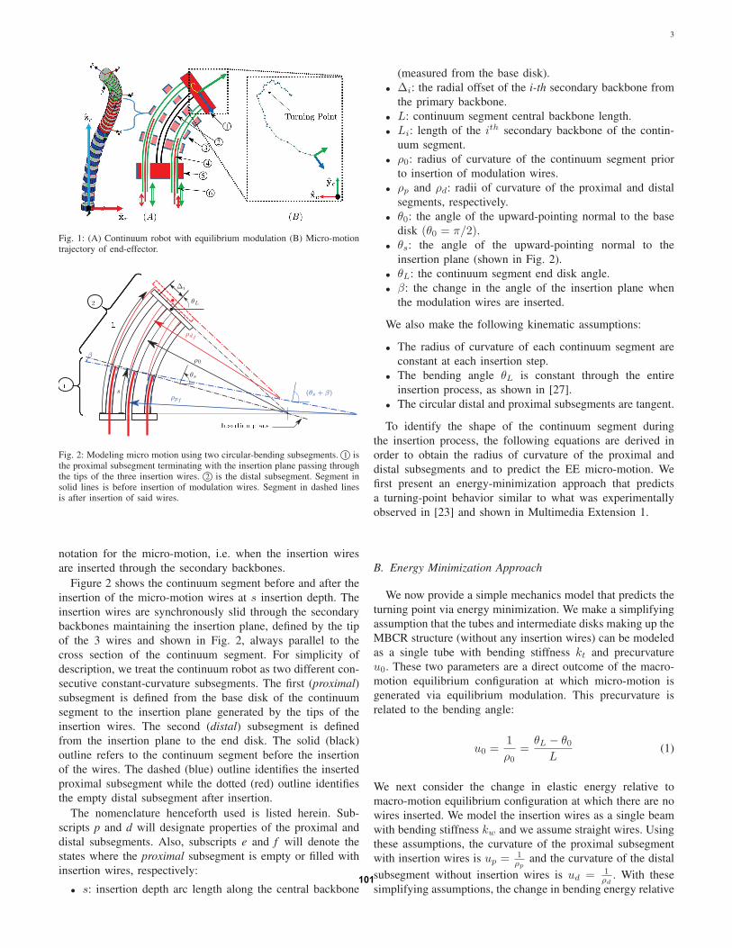
Figure 1 and Multimedia Extension 1 depict the concept of CRs for equilibrium modulation (CREM). This concept was introduced in [8] as a modification of the design proposed

in [25]. A multi-backbone continuum segment includes four

tubular backbones made of superelastic NiTi. These backbones

include a central backbone 2 surrounded by 3 secondary

backbones 6 which are responsible for the macro-motion

actuation. All the backbones slide through a base disk 5 and

spacer disks 3 that maintain a constant radial distance between

them. All the backbones rigidly connect to the end disk 1 .

The (green) double line arrows in Fig. 1A indicate the

direct actuation of the secondary backbones in order to bend

the continuum segment to achieve a desired end-disk orien-

tation in two degrees of freedom. Micro-motion capability is

obtained by controlling the insertion of Niti wires 4 inside

the secondary tubular backbones. This motion is designated

by (red) single line arrows in Fig. 1A. By controlling the

portion of the wires inserted into the secondary backbones,

the flexural rigidity along the length of the continuum robot

is changed. The equilibrium modulation actuation therefore

causes an indirect actuation of the end effector (EE) that

changes its static equilibrium pose to a new pose. In [23]

we presented experimental results that show that the micro-

motion path follows the general shape depicted in Fig. 1B,

but offered no explanation to the source of this phenomenon.

III. MODELING MICRO MOTION KINEMATICS

It was observed in [8], [23] through EE tracking during

experiments that a counterintuitive turning point behavior

occurs during insertion of the insertion wires. An example

of this turning point behavior is shown in Fig. 1B. In this

section, we offer what we believe is the first explanation to

the source of this turning point behavior. This explanation is

presented via an energy-minimization approach and a purely

kinematics-based approach.

The energy minimization approach we present provides

insight into why the turning point behavior occurs and predicts

an ideal turning point behavior, but in experimental data (as

shown in Fig. 1), we observe that the tip position does not

completely return to the starting point after the insertion wires

are fully inserted. We call this the observed turning pointbehavior. We believe this is caused by unmodeled energy

dissipation (e.g. friction, hysteresis), which are nontrivial to

incorporate into a mechanics model. For this reason, we

present a purely kinematics-based model that modifies one

of the kinematic model parameters (the bending angle β) to

replicate the observed turning point behavior.

The analysis in subsections III-B and III-C provides impor-

tant insight into the counterintuitive micro-motion behavior.

Section IV-A provides an empirical derivation of the micro-

motion Jacobian, which accounts for unmodeled effects that

may shift the turning point from its theoretical value.

A. Kinematic Assumptions and Notation

Although our formulation in Section IV-A allows spatial

macro-motion, in this paper we utilize micro-motion within a

single bending plane only. The reader is referred to [26] for a

spatial model of continuum robot kinematics. In this section,

we introduce the planar kinematic modeling assumptions and100

3

Fig. 1: (A) Continuum robot with equilibrium modulation (B) Micro-motiontrajectory of end-effector.

s

θL

ρpf

β

θs

(θs + β)

ρdf

ρ0

Δi

Fig. 2: Modeling micro motion using two circular-bending subsegments. 1 isthe proximal subsegment terminating with the insertion plane passing throughthe tips of the three insertion wires. 2 is the distal subsegment. Segment insolid lines is before insertion of modulation wires. Segment in dashed linesis after insertion of said wires.

notation for the micro-motion, i.e. when the insertion wires

are inserted through the secondary backbones.

Figure 2 shows the continuum segment before and after the

insertion of the micro-motion wires at s insertion depth. The

insertion wires are synchronously slid through the secondary

backbones maintaining the insertion plane, defined by the tip

of the 3 wires and shown in Fig. 2, always parallel to the

cross section of the continuum segment. For simplicity of

description, we treat the continuum robot as two different con-

secutive constant-curvature subsegments. The first (proximal)subsegment is defined from the base disk of the continuum

segment to the insertion plane generated by the tips of the

insertion wires. The second (distal) subsegment is defined

from the insertion plane to the end disk. The solid (black)

outline refers to the continuum segment before the insertion

of the wires. The dashed (blue) outline identifies the inserted

proximal subsegment while the dotted (red) outline identifies

the empty distal subsegment after insertion.

The nomenclature henceforth used is listed herein. Sub-

scripts p and d will designate properties of the proximal and

distal subsegments. Also, subscripts e and f will denote the

states where the proximal subsegment is empty or filled with

insertion wires, respectively:

• s: insertion depth arc length along the central backbone

(measured from the base disk).

• Δi: the radial offset of the i-th secondary backbone from

the primary backbone.

• L: continuum segment central backbone length.

• Li: length of the ith secondary backbone of the contin-

uum segment.

• ρ0: radius of curvature of the continuum segment prior

to insertion of modulation wires.

• ρp and ρd: radii of curvature of the proximal and distal

segments, respectively.

• θ0: the angle of the upward-pointing normal to the base

disk (θ0 = π/2).• θs: the angle of the upward-pointing normal to the

insertion plane (shown in Fig. 2).

• θL: the continuum segment end disk angle.

• β: the change in the angle of the insertion plane when

the modulation wires are inserted.

We also make the following kinematic assumptions:

• The radius of curvature of each continuum segment are

constant at each insertion step.

• The bending angle θL is constant through the entire

insertion process, as shown in [27].

• The circular distal and proximal subsegments are tangent.

To identify the shape of the continuum segment during

the insertion process, the following equations are derived in

order to obtain the radius of curvature of the proximal and

distal subsegments and to predict the EE micro-motion. We

first present an energy-minimization approach that predicts

a turning-point behavior similar to what was experimentally

observed in [23] and shown in Multimedia Extension 1.

B. Energy Minimization Approach

We now provide a simple mechanics model that predicts the

turning point via energy minimization. We make a simplifying

assumption that the tubes and intermediate disks making up the

MBCR structure (without any insertion wires) can be modeled

as a single tube with bending stiffness kt and precurvature

u0. These two parameters are a direct outcome of the macro-

motion equilibrium configuration at which micro-motion is

generated via equilibrium modulation. This precurvature is

related to the bending angle:

u0 =1

ρ0=

θL − θ0L

(1)

We next consider the change in elastic energy relative to

macro-motion equilibrium configuration at which there are no

wires inserted. We model the insertion wires as a single beam

with bending stiffness kw and we assume straight wires. Using

these assumptions, the curvature of the proximal subsegment

with insertion wires is up = 1ρp

and the curvature of the distal

subsegment without insertion wires is ud = 1ρd

. With these

simplifying assumptions, the change in bending energy relative101

4

to the macro-motion equilibrium configuration is given by:

ΔE =1

2

s∫0

�kt (up − u0)

2︸ ︷︷ ︸proximal

+ kw (up)2︸ ︷︷ ︸

wires

�ds+

1

2

L∫s

kt (ud − u0)2︸ ︷︷ ︸

distal

ds

(2)

Integration gives:

ΔE =1

2skt(up−u0)

2+1

2skwu

2p+

1

2(L−s)kt(ud−u0)

2 (3)

We seek the unknown curvatures up and ud that minimize

the energy for a fixed end-disk angle. The rationale for the

fixed end-disk angle stems from the parallel routing of all

the backbones as was shown in [25]. The corresponding

constrained optimization problem is therefore stated as:

minup,ud

ΔE s.t. θL = Lu0 + θ0 (4)

where the constraint is given by solving (1) for θL.

We solve (4) with a Lagrange multiplier , V, using the

following Lagrangian and conditions of optimality:

V = ΔE + λ (θL − Lu0 − θ0) (5)

∂V

∂up= 0,

∂V

∂ud= 0,

∂V

∂λ= 0 (6)

Solving these equations leads to the following result:

up =ktu0 − λ

kt + kw, ud =

ktu0 − λ

kt

λ =−sktkwu0

L(kt + kw)− skt

(7)

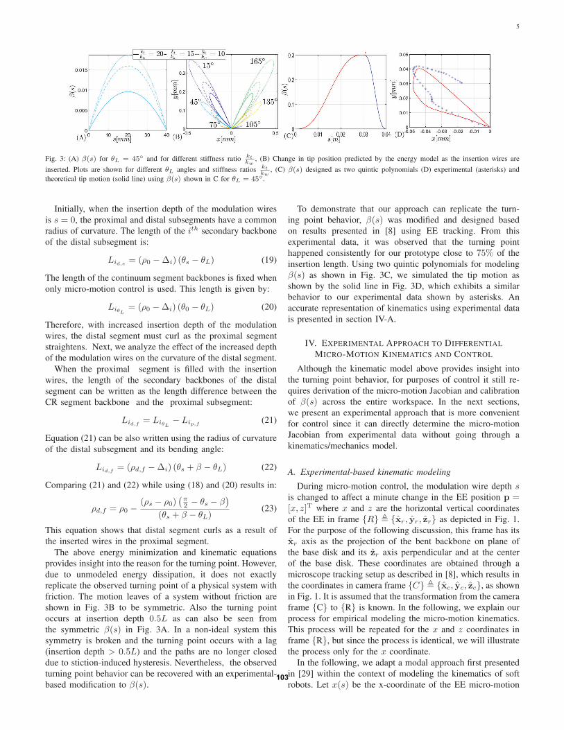
Figure 3B shows the results for the tip motion as the

insertion wires are inserted from s = 0 . . . L. The plot shows

multiple leafs for different θL and different ratios of kt

kw. We

note that each leaves shows a symmetric behavior where the

tip of the continuum segment reverses direction of motion at

a turning point s = L2 . As the wire stiffness is increased, the

amount of tip motion is increased as expected.

In Section III-C we explain this turning point phenomenon

due to a change β(s) in the equilibrium angle θs of the

proximal subsegment. These two angles are shown in Fig. 2.

The angle β(s) may be obtained if either up or ud are given.

Referencing Fig. 2, we have:

θs + β = sup + θ0 (8)

We then substitute θs = θ0 + su0 (the angle θs before

deformation due the inserted wires has occurred) to get:

β(s) = s(up − u0) (9)

Similarly, we can have from Fig. 2:

θL = θs + β + (L− s)ud (10)

Substituting θL = θs + (L − s)u0, (the angle θL prior to

insertion of the wires), we have:

β(s) = (L− s)(u0 − ud) (11)

Figure 3A shows the profiles of β(s) for the tip motion leafs

shown in Fig. 3A. This figure assumes no frictional losses.The following subsection uses this β(s), along with the

kinematic constraints of the continuum robot to explain how

the turning point behavior occurs.

C. Explaining the Source of the Turning Point BehaviorThrough Kinematic Constraints

Subsection III-B explained the source of the turning point

behavior through an energy minimization argument. It resulted

in a predicted change β(s) of the tangent angle at the end

of the proximal segment, but it did not explain internally

what happens from a point of view of kinematic constraints.

This section offers this explanation and also shows how the

observed turning point behavior from experimental results may

be explained by adjusting β(s).When the continuum segment is empty, it assumes a circular

shape as was shown in [28]. The arc length along the central

backbone corresponding with the insertion plane at insertion

depth s is related to the radius of curvature as the following:

s = ρ0

(π2− θs

)(12)

For a given s position of the insertion plane, we can

calculate the length of the ith secondary backbone of the

proximal segment Lip,e when empty as:

Lip,e = (ρ0 −Δi)(π2− θs

)(13)

where the radial offset is given by Δi = r cos ((i− 1)π),i = 1, 2, and r is the pitch circle radius of the spacer disks.

When the micro-motion wires are inserted through the

secondary backbones, the proximal subsegment straightens

and results in a change in the bending angle of the proximal

segment θs. Its radius of curvature changes from the initial ρ0to ρp,f . This change is shown in Fig. 2 by β, ρ0 and ρp,f .

Therefore, equation (12) becomes:

s = ρp,f

(π2− θs − β

)(14)

The new radius of curvature of the proximal segment is:

ρp,f =s

π2 − θs − β

(15)

Recalling (12), ρp,f may also be expressed as:

ρp,f = ρ0 +sβ(

π2 − θs − β

) (π2 − θs

) (16)

which shows that the proximal segment straightens.The lengths of the secondary backbones in the proximal

continuum segment, designated by Lip,f , are given by:

Lip,f = (ρp,f −Δi)(π2− θs − β

)(17)

using ρp,f = ρ0 +Δρ, eq. (17) may be rewritten as:

Lip,f =(ρ0 −Δi)(π2− θs

)︸ ︷︷ ︸

Li

+

Δρ(π2− θs − β

)− (ρ0 −Δi)β =

Li +Δρ(π2− θs − β

)− (ρ0 −Δi)β

(18)

102

5

Fig. 3: (A) β(s) for θL = 45◦ and for different stiffness ratio ktkw

, (B) Change in tip position predicted by the energy model as the insertion wires are

inserted. Plots are shown for different θL angles and stiffness ratios ktkw

, (C) β(s) designed as two quintic polynomials (D) experimental (asterisks) and

theoretical tip motion (solid line) using β(s) shown in C for θL = 45◦.

Initially, when the insertion depth of the modulation wires

is s = 0, the proximal and distal subsegments have a common

radius of curvature. The length of the ith secondary backbone

of the distal subsegment is:

Lid,e = (ρ0 −Δi) (θs − θL) (19)

The length of the continuum segment backbones is fixed when

only micro-motion control is used. This length is given by:

LiθL= (ρ0 −Δi) (θ0 − θL) (20)

Therefore, with increased insertion depth of the modulation

wires, the distal segment must curl as the proximal segment

straightens. Next, we analyze the effect of the increased depth

of the modulation wires on the curvature of the distal segment.

When the proximal segment is filled with the insertion

wires, the length of the secondary backbones of the distal

segment can be written as the length difference between the

CR segment backbone and the proximal subsegment:

Lid,f = LiθL− Lip,f (21)

Equation (21) can be also written using the radius of curvature

of the distal subsegment and its bending angle:

Lid,f = (ρd,f −Δi) (θs + β − θL) (22)

Comparing (21) and (22) while using (18) and (20) results in:

ρd,f = ρ0 −(ρs − ρ0)

(π2 − θs − β

)(θs + β − θL)

(23)

This equation shows that distal segment curls as a result of

the inserted wires in the proximal segment.

The above energy minimization and kinematic equations

provides insight into the reason for the turning point. However,

due to unmodeled energy dissipation, it does not exactly

replicate the observed turning point of a physical system with

friction. The motion leaves of a system without friction are

shown in Fig. 3B to be symmetric. Also the turning point

occurs at insertion depth 0.5L as can also be seen from

the symmetric β(s) in Fig. 3A. In a non-ideal system this

symmetry is broken and the turning point occurs with a lag

(insertion depth > 0.5L) and the paths are no longer closed

due to stiction-induced hysteresis. Nevertheless, the observed

turning point behavior can be recovered with an experimental-

based modification to β(s).

To demonstrate that our approach can replicate the turn-

ing point behavior, β(s) was modified and designed based

on results presented in [8] using EE tracking. From this

experimental data, it was observed that the turning point

happened consistently for our prototype close to 75% of the

insertion length. Using two quintic polynomials for modeling

β(s) as shown in Fig. 3C, we simulated the tip motion as

shown by the solid line in Fig. 3D, which exhibits a similar

behavior to our experimental data shown by asterisks. An

accurate representation of kinematics using experimental data

is presented in section IV-A.

IV. EXPERIMENTAL APPROACH TO DIFFERENTIAL

MICRO-MOTION KINEMATICS AND CONTROL

Although the kinematic model above provides insight into

the turning point behavior, for purposes of control it still re-

quires derivation of the micro-motion Jacobian and calibration

of β(s) across the entire workspace. In the next sections,

we present an experimental approach that is more convenient

for control since it can directly determine the micro-motion

Jacobian from experimental data without going through a

kinematics/mechanics model.

A. Experimental-based kinematic modeling

During micro-motion control, the modulation wire depth sis changed to affect a minute change in the EE position p =[x, z]T where x and z are the horizontal vertical coordinates

of the EE in frame {R} � {xr, yr, zr} as depicted in Fig. 1.

For the purpose of the following discussion, this frame has its

xr axis as the projection of the bent backbone on plane of

the base disk and its zr axis perpendicular and at the center

of the base disk. These coordinates are obtained through a

microscope tracking setup as described in [8], which results in

the coordinates in camera frame {C} � {xc, yc, zc}, as shown

in Fig. 1. It is assumed that the transformation from the camera

frame {C} to {R} is known. In the following, we explain our

process for empirical modeling the micro-motion kinematics.

This process will be repeated for the x and z coordinates in

frame {R}, but since the process is identical, we will illustrate

the process only for the x coordinate.

In the following, we adapt a modal approach first presented

in [29] within the context of modeling the kinematics of soft

robots. Let x(s) be the x-coordinate of the EE micro-motion103

6

path, s ∈ [0 . . . L]. For a given macro motion configuration characterized by θL in the bending plane, the local tangent to the curve c = (s, x(s)) is designated by x′:

x′ =dx

dswhere x′ = x′ (θL, s) (24)

For a fixed θL, a modal representation for x′ (s) may be used

x′ (θL, s) = ψ(s)Ta, a,ψ ∈ IRn (25)

where ψ and a are the modal basis and coefficients. Since

the EE micromotion path is smooth and requires a low order

polynomial to approximate it, we use a monomial basis:

ψ(s) =[1, s, s2, ..., sn−1

]T(26)

To find the modal coefficients a, a data matrix Φ containing

x′(s) for z different CR configurations with r insertion depths

s = s1, s2, . . . sr was constructed. The entries of Φ were

filled based on the finite difference approximation of the local

tangent to the experimental data x(s, θL).

Φ =

⎡⎢⎣x′(s1, θL1

) · · · x′(s1, θLz)

.... . .

...

x′(sr, θL1) · · · x′(sr, θLz

)

⎤⎥⎦ ∈ IRr×z (27)

Since the elements of a depend on θL, we aggregate the modal

approximations of ai such that:

a(θL) = Aη(θL), A ∈ IRn×m, η ∈ IRm (28)

where η (θL) =[1, θL, θL

2, . . . , θLm−1

]T.

The tangent curve c = (s, x(s)) can therefore be obtained

by the following modal approximation:

x′ (θL, s) = ψ(s)TAη(θL) (29)

Assuming z experiments corresponding macro configuration

angles θ1 . . . θz and where the insertion depth is changed with

r values, the ith column of Φ is given by:

Φi =

⎡⎢⎣x′ (θLi

, s1)...

x′ (θLi, sr)

⎤⎥⎦ =

⎡⎢⎣ψT (s1)

...

ψT (sr)

⎤⎥⎦Aη(θLi

) (30)

and the full Φ matrix is given by:

Φ =

⎡⎢⎣ψT (s1)

...

ψT (sr)

⎤⎥⎦

︸ ︷︷ ︸Ω[r×n]

A[n×m]

⎡⎢⎢⎣

......

...

η (θL1) . . . η (θLz

)...

......

⎤⎥⎥⎦

︸ ︷︷ ︸Γ[m×z]

(31)

This is a matrix equation with A as the unknown. It can be

rewritten using Kroneker product as:�ΓT ⊗Ω

�vec (A) = vec (Φ) (32)

where the symbol ⊗ indicates the Kronecker’s matrix product

[30] and vec(A) is a vector sequence of all the columns of

A. Equation (32) is a linear equation with a vector unknown,

which can be solved using the pseudoinverse of�ΓT ⊗Ω

�. Fi-

nally, given the solution to A, one can calculate c = (s, x(s))by substituting θL and s in (29). Finally, the EE coordinate

x(s) may be obtained as:

x(θL, s) =

∫ s

0

x′ (θL, s) =∫ s

0

ψ(s)TAη(θL)ds (33)

Taking the time derivative of (33) using the chain rule:

x (θL, s) =∂

∂s(x(θL, s)) s+

∂

∂θL(x(θL, s)) θL (34)

The first term in the equation above includes micro motion

speed due to the insertion wires and the second term includes

the effect of a change in the macro-motion configuration on the

micro-motion speed. We will next consider the scenario where

the macro-motion configuration is held fixed when one invokes

the micro-motion control. Therefore (34) can be rewritten as:

x (θL, s) = ψ(s)TAη(θL)s = Jμxs (35)

where Jμx is the micro-motion Jacobian matrix for the x

coordinate. Repeating this process for the z coordinate will

also result in similar equations and a Jacobian Jμz.

This method was experimentally validated with our system

described in section V. For each θL ∈ [15◦, 35◦, 45◦, 60◦, 75◦]we moved our robot through 45 EE poses and the EE position

was segmented using our method in [8]. Figure 4 presents

the segmented EE coordinates using asterisk markers. The

numerically integrated curve using (29) is shown with dashed

lines. Table I presents the root mean squared error between the

observed EE micro-motion paths, obtained in [8] and shown as

solid lines. These results suggest that the modeling approach

we presented can represent the robot kinematics well.

θL 15◦ 35◦ 45◦ 60◦ 75◦

x 0.8 (3.3) 0.5 (2.6) 1.1 (3) 1 (2) 0.2 (0.3)y 0.6 (4.4) 0.3 (3.5) 3.7 (3.9) 1.9 (1.2) 0.5 (0.3)

TABLE I: Root mean squared error (maximum error) [μm] between measuredand modeled EE micro-motion paths.

V. EXPERIMENTAL SETUP AND SYSTEM INTEGRATION

Figure 5 and Multimedia Extension 2 show the experimental

setup used to validate our modeling approach, to demonstrate

the feasibility of 3D OCT via CREM micro-motion, and to

validate our approach for OCT-guided micro-motion control.

For our experiments, the continuum robot actuation unit 1 and

the continuum robot segment 2 were used with a commercial

external OCT probe 3 and a custom miniature B-mode OCT

probe 4 that was embedded within the robot. The custom B-

mode OCT probe is a modification of the design presented

in [31] and it uses custom Arduino-based closed-loop control

electronics 5 . The probe was actuated by a voice coil actuator

6 (H2W NCM02-05-005-4JBMC). The external OCT probe

(Thorlabs Telesto-II-1325LR-5P6) has 3.5 to 7mm imaging

depth with 5.5 to 12.0μm axial resolution in air.

The commercial probe was used for proof of concept for

3D volumetric OCT with a calibrated system that can provide104

7

Fig. 4: x and z end effector coordinates over the full insertion length at 5 different CR configurations

quantifiable data about the accuracy of our 3D OCT and micro-

motion resolution and for demonstrating closed-loop visual

servoing in OCT image space. The custom OCT probe was

used for testing the feasibility of embedding a custom B-mode

OCT probe within the robot for generating 3D OCT scans.

In addition to the continuum segment, the setup used a

planar robot 7 comprised of two orthogonally-aligned linear

stages (VELMEX A1506B-S1.5) driven by two DC gearmo-

tors (Maxon combination #351325) and controlled by our

Arduino-based control box 5 . The need for adding this planar

actuation unit is explained in section Section VII.

The control system used four computers depicted in Fig. 5.

The bottom portion of this figure shows how the control

was delineated among these machines. Although this system

may be implemented on a single high-powered computer, we

chose to preserve the modularity of our software environment

to enable rapid-prototyping of our proof-of-concept control

system. The four computers included: a high-level controller

(HLC) 8 for communication and synchronized control, a

low-level controller (LLC) for continuum robot control 9

using Matlab RealTime, a mid-level controller (MLC) 10 for

acquiring EE position data from LLC and for sending the

control-reference signal to the Arduino-based controller of the

OCT and the planar robot 7 , and a computer for OCT image

acquisition and online image segmentation 11 .

Data communication between these computers were carried

out as the following. The HLC computer obtained the EE

position via a microscope camera using MATLAB image

acquisition toolbox. This information is used only for 3D OCT

volume generation. The acquired scans are synchronized with

robot position using time-stamped user datagram protocol

(UDP) messages relayed to the MLC and the MATLAB

Realtime target machine. For visual servoing, the OCT image

segmentation data is relayed to the MLC via UDP commu-

nication. The low-level control frequency on the MATLAB

Realtime target machine for controlling the continuum robot

was 1KhZ. The MLC obtained image segmentation data and

relayed the reference control signal to the Arduino at 30Hz.

In turn, the Arduino-controller using HiLetgo ESP32 micro-

controller implemented its own low-level PID control for the

voice-coil actuator and the planar robot.

VI. MICRO-MOTION FOR VOLUMETRIC OCT IMAGING

This section details the validation of our approach for

achieving volumetric OCT reconstruction via micro-motion.

While the final goal is to obtain a volumetric scan of a vessel

using a custom-made OCT probe integrated inside the CR, we

first validated feasibility using an external commercial OCT

probe. These experiments were first reported in [24] and they

provide an ideal baseline for expected performance where

OCT image aberrations are minimized due to the use of a

commercial OCT probe. This section also details validation

using our own CR with a custom B-mode OCT probe that is

a modification of the design first presented in [32].

A. 3D image reconstruction using commercial OCT probeThe setup used is shown in Fig. 5. We used the external

OCT probe for these experiments. The CR segment was bent

to θL = 60◦ using macro-motion control and the macro motion

joints were held fixed. The CR segment was used to carry an

OCT scanning sample on its tip while the OCT probe was fixed

perpendicularly to the samples. By inserting three equilibrium

modulation wires, micro-motion was used to move the sample

perpendicular to the scanning plane of the probe (we will refer

to the motion as normal motion direction (NMD)). During

micro-motion, every Δs = 0.5mm of insertion depth the

HLC machine ( 8 in Fig. 5) recorded a B-mode OCT scan

image together with the robot configuration joint values. At the

same micro-motion tip tracking was used based on the method

presented in [8] to record the motion profile of the EE and the

CR joint values. At the end of each experiment, MATLAB

image segmentation using Canny filter and/or Hough circles

was used to construct the 3D images.Three samples were used in three experiments to test

feasibility of our method on different materials and shapes.

First, a metric brass screw (0.8mm diameter, 0.2mm pitch)

was scanned, Fig. 6.A. A profile image of the screw was taken

to compare to the known screw pitch geometry (Fig. 6A 1 -

2 ). Micro-motion was initiated to generate a 3D scan which

was reconstructed in Fig. 6A 3 - 5 . The pitch measurement,

based on the profile image (Fig 6A 1 - 2 ) was 209.85μm while

based on the 3D scan reconstruction it was 210.75μm based

on analysis of Figure 6A 4 . This designates an average error

of 0.5%. The micro motion displacement shown in Fig. 6A

3 - 5 corresponded with 92μm motion in NMD and 89 scans.

Therefore, the NMD resolution was 1.03μm.105

8

Fig. 5: Experimental setup: 1 -CREM system 2 -Continuum Segment 3 -OCT Commercial probe 4 -Custom made OCT probe deployed within the CRsegment 5 -OCT/linear-slides Arduino Based control box 6 -Voice coil OCT actuation unit 7 -Planar Robot 8 -High Level Control computer 9 -MatlabRealTime computer 10 -Mid Level Control computer 11 -OCT COmputer 12 -Micro-motion Camera.

Fig. 6: (A)Screw pitch reconstruction: 1 -OCT Image 2 -Screw sample image (OCT camera view) 3 - 5 Different views of the reconstructed profile (B)Multilayer cellophane tape reconstruction 1 -OCT Image 2 -Side view of the multilayer cellophane tape with the double-sided tape added on top 3 -Multilayertape Sample image (OCT camera view) 4 - 6 -Different views of the reconstructed profile (C) Micro Channel reconstruction 1 -OCT Image 2 -NiTi wireused to create the channel still in the agar sample 3 -Channel sample image (OCT camera view) 4 - 6 -different views of the reconstructed profile.

In the second experiment, we used a multilayer cellophane

tape with an additional layer of double-sided tape on top,

Fig. 6.B2-3. The double-sided tape was added to simulate

a thicker layer at the top of the sample. This experiment

was motivated by a future application of 3D retinal layer

reconstruction. Results of the 3D reconstruction are shown in

Figure 6B 4 - 6 . The thickness of the layers measured based on

a single OCT image (Fig. 6B 1 ) had an average of 71.7μmwhile the thickness measured from the reconstructed model

had an average of 67.4μm. The average error is circa 6%.

According to the tape supplier, the tape layer has an average

thickness of 70μm, including the glue layer.

The last experiment aimed to demonstrate reconstruction of

a capillary blood vessel, Fig. 6C. The channel was created

by placing a NiTi wire, 220μm in radius, in Agar. After

solidification, the wire was removed, and the sample scanned

in three experiment sets for (θL = 30◦, 45◦, 60◦). The results

over the 3 experiment sets are shown in Tab II. The average

error between the areas measured using the B-mode OCT

images, as in Fig. 6C 1 , and the cross-sectional area measured

using the 3D reconstructed model is 5%-10%.

θ◦Scan

Lengthμm

Max/Mind μm

STD(d)μm

Segmented /Reconstructed

Area mm2

% Areaerror

30 99.6 3.8/0.6 1.0 0.13/0.12 945 73.8 2.9/0.3 0.7 0.13/0.12 1060 55.8 1.8/0.3 0.4 0.15/0.14 5

TABLE II: Agar channel 3D OCT reconstruction results.

B. 3D reconstruction of an optic nerve blood vessel

This section shows the experimental result for a 3D OCT

reconstruction of an organic tissue. A freshly harvested retinal106

9

optic nerve in a cadaveric swine eye was used as a scanning sample as shown in Fig. 7A.3. Figure 7A.1 shows the first OCT scanned image before that the micro-motion is enabled while Fig. 7A.2 shows the last scanned image after the micro-

motion scanning is completed. It is possible to notice how a vessel branch in Fig. 7A.1 bifurcates by the end of the scanning. The 3D reconstruction, Fig. 7A.4-5, shows the corresponding anatomy in Fig. 7A.1 and Fig. 7A.2 while the branching of the scanned vessel is clearly visible.

C. Volumetric OCT using a miniature OCT probe

After testing the robustness of the 3D OCT reconstruction

using a commercial OCT probe, we established the feasibility

of using the custom-made miniature B-mode OCT probe. As

shown in Fig. 5, the OCT probe 4 was embedded within

the CR segment. An agar sample (Fig. 7B 1 ) was prepared

with a 0.66mm tube embedded in it. Once the agar was

solidified, the tube was removed, a channel remained and was

used as an imaging target for the probe of a mock up vessel.

Using equilibrium modulation, the robot moved the probe

perpendicular to the scan direction of the custom miniature

OCT probe. Results of the 3D reconstruction are shown in

Fig. 7B 3 - 4 . The average area measured using three B-mode

OCT images as in Fig. 7B 2 is 0.32892mm2 while the area

calculated using the 3D reconstruction is 0.31341mm2 which

represents an average deviation of 10%.

VII. OCT-GUIDED VISUAL SERVOING

This section presents the experimental validation of our pro-

posed mixed-feedback control that uses OCT image feedback

and the CR joint-space. The same setup in Fig. 5 and in Multi-

media Extension 3 was used for these experiments. Figure 8.E

depicts the control loop block diagram and the data workflow

between the subsystems involved in theses experiments. We

used the commercial OCT probe for these experiments. The

aim of the experiment was to mimic an automated blood

vessel injection by driving a NiTi needle (0.4mm in diameter),

which was attached to the CR segment, into a mockup vessel

(0.16mm2 cross sectional area) within an agar sample carried

by the planar robot as shown in Fig. 8A. OCT-guided visual

control was achieved by using a custom computer code for

OCT image segmentation. An online (interactive rate ≈ 30Hz)

image segmentation was achieved using a cross-correlation

template matching with manual initialization. At the beginning

of the experiment, the user defined the two templates for the

two tracking targets (vessel and needle tip) by mouse selection

as shown in Fig. 8.B by two red rectangles. The template

matching uses online segmentation and tracking of the mockup

vessel and the NiTi needle as viewed in the OCT system.The

frames definition used for the experiment, shown in Fig. 8B,

follows the standard image frame definition in the MATLAB

environment which place the origin of the picture frame in the

top-left corner of the image with the positive Y-axis pointing

downward and the positive X-axis pointing to the right (frame

{Xc, Yc}) shown by yellow dashed-lines in Fig. 8B. The robot

frames follows the definition used for the continuum segment

EE which place the origin of the frame origin at the center

of the CS end disk with the Y-axis normal to it. Moreover,

as shown in Fig. 8B, the red frame {Xn, Yn} aligns with the

longitudinal axis of the needle that is concentrically mounted

in the primary CS backbone. The relative angle between those

two frames is measured beforehand using Matlab.

A. Experimental Validation of OCT-Guided Visual Servoing

The experiment procedure requires user input for choos-

ing two tracking target templates via mouse selection on a

Matlab2016a window that acquires the OCT image from a

commercial OCT control software. The OCT image in Fig. 8B

shows the result of the tracking method (two red squares)

and the frame definitions. The picture frame is identified by

{xc, yc} while {xn, yn} identifies the needle tip frame. Since

the OCT image was starting to distort when the needle is

piercing the agar sample, the origin of the needle frame was

chosen with a specified offset along the needle axis and is

accounted for in the tracking code. Once the two target points

were chosen, the control code used micro-motion to close the

error in position along the xn direction and consequently along

yn direction using macro-motion. To avoid laceration of the

mockup tissue caused by the sideways motion of the needle,

the HLC first used the micro-motion to converge the needle

laterally and then used macro-motion for needle insertion.

The tracking results of the two red square centers are shown

in Fig. 8C-D. The vector ep indicates the the position of

the target vessel relative to the current needle tip position.

Figure 8C presents the tracking result of the relative angle αbetween ep and xn. Figure 8D presents the tracking results

of the components of ep along xn and yn. The blue shaded

area indicates the portion of the process where only the micro-

motion is enabled. We used two thresholds for position con-

vergence. When using macro-motion we used εpy = 300μmand when using micro-motion we used εpx = 5μm as the

corresponding convergence threshold radii in the depth and

lateral directions. The final position error between the two

centers calculated in the needle frame {xn, yn} is 0.0028mmalong xn and 0.2683mm along yn. The considerable dif-

ference of the magnitude in the error directions came from

the different motion profile associated with each direction.

The first one is completely controlled by micro-motion using

the equilibrium modulation while the piercing direction is

controlled by macro-motion actuation of the linear stage of the

planar robot that has a manufacturer specification of backlash

of 200μm. The need for the linear stage comes from the

missing third degrees of freedom of the single segment CR

which would prevent the straight motion for the injection

process. The data flow and control scheme is summarized in

Fig. 8E.

VIII. CONCLUSION

This work presented a novel approach to solving the prob-

lem of multi-scale manipulation. A new approach for micro-

motion using equilibrium modulation of CRs was presented.

The work was motivated by the potential benefits of using CR107

10

Fig. 7: (A) 3D reconstruction of a branching in an optic nerve of a swine cadaver retina. 1 - 2 -First and last OCT scanned images. 3 -Microscope view ofthe sample showing the B-mode scan direction (red) and micro-motion scan direction (blue). 4 - 5 -Two views of the 3D OCT reconstruction model showingthe corresponding anatomy in 1 and 2 (B) 3D OCT reconstruction using a custom made OCT B-mode probe integrated within the CR. 1 -Mock up vesselgenerated in Agar Sample 2 -Vessel OCT image 3 - 4 -Volumetric reconstruction of the scanned sample

Fig. 8: A) Microscope view of the needle tip and the agar vessel mockup. B) OCT scan image and visual servoing frames definition, C) Gamma angle, D)Components of ep in {xn, yn} frame as shown in (B). Solid line referring to the left y-axis is epx in [mm] and dashed line referring to right y-axis is epyin [mm], E) Visual servoing control block diagram.

for in-situ inspection and image-based biopsy. The source of

the turning point phenomenon was explained from an energy

and internal kinematic constraint standpoints, respectively.

Empirical micro-motion kinematics modeling via modal inter-

polation maps was presented. The feasibility of 3D OCT has

been verified experimentally using both commercial (external)

and a miniature (internal) OCT probes.Results showed that

3D OCT volumes with slice separation of 1μm or 5μm may

be obtained using accurate EE tracking or the closed-form

micro motion kinematics, respectively. Also, closed-loop OCT-

guided servoing for delivering a needle into channel has been

successfully demonstrated. The RMS error using our modeling

approach was less than 1.2 microns, which could be used

for generating a lower-resolution 3D OCT scan that would

still be useful since each image slice still retains its high

resolution. We believe this work is a first key step for future

development of new robotic assistants that can offer multi-

scale manipulation for surgery and for image-based biopsy.

Hysteretic effects due to motions with direction are difficult

to model and solutions using micron-level EE tracking are

needed to overcome this challenge. Nevertheless, applications

such as 3D OCT scanning can be planned and achieved while

avoiding direction reversal.

IX. ACKNOWLEDGEMENT

The authors thank Dr. Rashid Yasin, Mr. Sina Ghandi, Mr.

Emmett Haden and Ms. Zhaoyang Chen for their assistance

in supporting experiments reported in this paper.

REFERENCES

[1] N. Sarli, G. Del Giudice, S. De, M. S. Dietrich, S. D. Herrell, andN. Simaan, “Turbot: A system for robot-assisted transurethral bladdertumor resection,” IEEE/ASME Trans. Mechatronics, vol. 24, no. 4, pp.1452–1463, 2019.

[2] R. E. Goldman, A. Bajo, L. S. MacLachlan, R. Pickens, S. D. Herrell,and N. Simaan, “Design and Performance Evaluation of a MinimallyInvasive Telerobotic Platform for Transurethral Surveillance and Inter-vention,” IEEE TBME, vol. 60, no. 4, pp. 918–925, apr 2013.

[3] R. J. Hendrick, S. D. Herrell, and R. J. Webster, “A multi-arm hand-held robotic system for transurethral laser prostate surgery,” in 2014IEEE ICRA, 2014, pp. 2850–2855.

[4] T. Kato, I. Okumura, H. Kose, K. Takagi, and N. Hata, “Tendon-drivencontinuum robot for neuroendoscopy: validation of extended kinematicmapping for hysteresis operation,” INT J COMPUT ASS RAD, vol. 11,no. 4, pp. 589–602, 2016.

[5] Y. Kim, S. S. Cheng, M. Diakite, R. P. Gullapalli, J. M. Simard, and J. P.Desai, “Toward the development of a flexible mesoscale mri-compatibleneurosurgical continuum robot,” IEEE TRO, vol. 33, no. 6, pp. 1386–1397, 2017.

[6] N. Simaan, A. Bajo, A. Reiter, L. Wang, P. Allen, and D. Fowler,“Lessons learned using the insertable robotic effector platform (IREP)for single port access surgery,” J. Robot. Surg., pp. 1–6, 2013.

[7] J. Ding, R. E. Goldman, K. Xu, P. K. Allen, D. L. Fowler, and N. Simaan,“Design and Coordination Kinematics of an Insertable Robotic EffectorsPlatform for Single-Port Access Surgery.” IEEE/ASME TRO, vol. Inpress., pp. 1612–1624, Oct. 2013.

[8] G. Del Giudice, L. Wang, J. H. Shen, K. Joos, and N. Simaan,“Continuum robots for multi-scale motion: Micro-scale motion throughequilibrium modulation,” in 2017 IEEE/RSJ IROS, Sept 2017, pp. 2537–2542.

108

11

[9] J. G. Fujimoto, “Optical coherence tomography for ultrahigh resolutionin vivo imaging,” Nat. biotech., vol. 21, no. 11, pp. 1361–1367, 2003.

[10] C. Reboulet and S. Durand-Leguay, “Optimal design of redundant paral-lel mechanism for endoscopic surgery,” in Proceedings 1999 IEEE/RSJIROS (Cat. No.99CH36289), vol. 3, 1999, pp. 1432–1437 vol.3.

[11] R. MacLachlan, B. Becker, J. C. Tabares, G. Podnar, L. Lobes, andC. Riviere, “Micron: an actively stabilized handheld tool for micro-surgery,” IEEE TRO, vol. 28, no. 1, pp. 195–212, February 2012.

[12] M. D. Comparetti, A. Vaccarella, I. Dyagilev, M. Shoham, G. Ferrigno,and E. De Momi, “Accurate multi-robot targeting for keyhole neuro-surgery based on external sensor monitoring,” P I MECH ENG H, vol.226, pp. 347–59, 05 2012.

[13] A. L. Orekhov, C. Abah, and N. Simaan, “Snake-like robots forminimally invasive, single port, and intraluminal surgeries,” CoRR, vol.abs/1906.04852, 2019.

[14] N. Simaan, R. M. Yasin, and L. Wang, “Medical technologies andchallenges of robot-assisted minimally invasive intervention and diag-nostics,” Annual Review of Control, Robotics, and Autonomous Systems,vol. 1, no. 1, pp. 465–490, 2018.

[15] P. Sears and P. Dupont, “A steerable needle technology using curvedconcentric tubes,” in 2006 IEEE/RSJ IROS, 2006, pp. 2850–2856.

[16] R. J. Webster, A. M. Okamura, and N. J. Cowan, “Toward activecannulas: Miniature snake-like surgical robots,” in 2006 IEEE/RSJ IROS,2006, pp. 2857–2863.

[17] H. Yu, J.-H. Shen, K. M. Joos, and N. Simaan, “Calibration andintegration of b-mode optical coherence tomography for assistive controlin robotic microsurgery,” IEEE/ASME Trans. Mechatronics, vol. 21,no. 6, pp. 2613–2623, 2016.

[18] Y. Huang, X. Liu, C. Song, and J. U. Kang, “Motion-compensated hand-held common-path fourier-domain optical coherence tomography probefor image-guided intervention,” Biom. opt. express, vol. 3, no. 12, pp.3105–3118, 2012.

[19] C. Song, P. L. Gehlbach, and J. U. Kang, “Active tremor cancellation bya “smart” handheld vitreoretinal microsurgical tool using swept sourceoptical coherence tomography,” Optics express, vol. 20, no. 21, pp.23 414–23 421, 2012.

[20] C. Song, D. Y. Park, P. L. Gehlbach, S. J. Park, and J. U. Kang,“Fiber-optic oct sensor guided “smart” micro-forceps for microsurgery,”Biomedical optics express, vol. 4, no. 7, pp. 1045–1050, 2013.

[21] M. Balicki, J.-H. Han, I. Iordachita, P. Gehlbach, J. Handa, R. Taylor,and J. Kang, “Single fiber optical coherence tomography microsurgicalinstruments for computer and robot-assisted retinal surgery,” in MICCAI.Springer, 2009, pp. 108–115.

[22] M. Draelos, G. Tang, B. Keller, A. Kuo, K. Hauser, and J. A. Izatt,“Optical coherence tomography guided robotic needle insertion for deepanterior lamellar keratoplasty,” IEEE TBME, 2019.

[23] L. Wang, G. Del Giudice, and N. Simaan, “Simplified kinematics ofcontinuum robot equilibrium modulation via moment coupling effectsand model calibration,” ASME JMR, vol. 11, no. 5, 2019.

[24] G. Del Giudice, J. Shen, K. Joos, and N. Simaan, “Feasibility ofvolumetric oct imaging using continuum robots with equilibrium mod-ulation,” in 2019 HSMR, 2019.

[25] N. Simaan, R. Taylor, and P. Flint, “A dexterous system for laryngealsurgery,” in IEEE ICRA, 2004. Proceedings. ICRA ’04. 2004. NewOrleans: IEEE, 2004, pp. 351–357 Vol.1.

[26] N. Simaan, K. Xu, W. Wei, A. Kapoor, P. Kazanzides, P. Flint,and R. Taylor, “Design and Integration of a Telerobotic System forMinimally Invasive Surgery of the Throat,” IJRR, vol. 28, no. 9, pp.1134–1153, 2009.

[27] N. Simaan, “Snake-Like Units Using Flexible Backbones and ActuationRedundancy for Enhanced Miniaturization,” in ICRA 2005. Barcelona,Spain: IEEE ICRA, 2005, pp. 3012–3017.

[28] K. Xu and N. Simaan, “An Investigation of the Intrinsic Force SensingCapabilities of Continuum Robots,” IEEE Transactions on Robotics,vol. 24, no. 3, pp. 576–587, Jun. 2008.

[29] J. Zhang, J. Roland, J. Thomas, S. Manolidis, and N. Simaan, “OptimalPath Planning for Robotic Insertion of Steerable Electrode Arrays inCochlear Implant Surgery,” ASME J. Med. Devices, vol. 3, no. 1, 122008, 011001. [Online]. Available: https://doi.org/10.1115/1.3039513

[30] J. Brewer, “Kronecker products and matrix calculus in system theory,”IEEE Transactions on Circuits and Systems, vol. 25, no. 9, pp. 772–781,1978.

[31] K. Joos, J. Shen, J. Kozub, and M. Hutson, “Apparatus and methodfor real-time imaging and monitoring of an electrosurgical procedure,”Patent U.S. #20 140 163 537, 2014.

[32] J. Shen, J. Kozub, R. Prasad, and K. Joos, “An intraocular OCT probe,”in ARVO, Fort Lauderdale, Florida, 2011.

Giuseppe Del Giudice received his B.S degree inmechanical engineering from University of Rome”La Sapienza”, Rome, Italy, in 2012. He is currentlyworking toward his Ph.D. degree in mechanicalengineering at Vanderbilt University, Nashville, TN.Since 2015 he has been working as a research as-sistant. His research interests include modeling andcalibration of continuum robots, surgical roboticsand robot control exploration.

Andrew L. Orekhov received the B.S. degreein mechanical engineering from the University ofTennessee, Knoxville, TN, USA, in 2016, and iscurrently working toward the Ph.D. in mechanicalengineering at Vanderbilt University, Nashville, TN,USA. His current research interests include design,modeling, and control of continuum manipulators.He received the NSF Graduate Research Fellowshipin 2016.

Jin-Hui Shen received his B.S., and M.S. degreesin Laser Technology and Optical En- gineering fromTianjin University, PRC, in 1984 and 1987, respec-tively, and the Ph.D. degree in Ultrafast OpticalPhenomena from Shanghai Institute of Optics andFine Mechanics, PRC, in 1991. Following a Postdoc-toral Biomedical Engineering Fellowship perform-ing ophthalmic laser research at the University ofMiami, he joined Novatec Laser System, Inc. as anopto-electronic engineer. He then joined VanderbiltUniversity in 1997 as a Research Assistant Professor.

Karen M. Joos received the B.S., M.D. andAnatomy Ph.D. degrees from the University of Iowa,Iowa City, IA, in 1982, 1987, and 1990, respectively.After an ophthalmology residency at the Universityof Iowa, she completed a glaucoma fellowship atthe Bascom Palmer Eye Institute, Miami, FL whereshe engaged in ophthalmic laser research. She thenjoined Vanderbilt University in 1994 as an Assis-tant Professor of Ophthalmology. She is currentlyJoseph and Barbara Ellis Professor of Ophthalmol-ogy, Professor of Biomedical Engineering, Chief of

the Glaucoma Service, a Fellow of the Association for Research in Visionand Ophthalmology (FARVO) and American Society for Lasers in Surgeryand Medicine (ASLMS), and a SPIE Senior Member.

Nabil Simaan (M’04) received his Ph.D. degree inmechanical engineering from the Technion—IsraelInstitute of Technology, Haifa, Israel, in 2002. Dur-ing 2003, he was a Postdoctoral Research Scien-tist at Johns Hopkins University National ScienceFoundation (NSF) ERC-CISST. In 2005, he joinedColumbia University, New York, NY. In 2009 hereceived the NSF Career award for young investi-gators to design new algorithms and robots for safeinteraction with the anatomy. In Fall 2010 he joinedVanderbilt University. In 2020 he was named an

IEEE Fellow for contributions to dexterous continuum robotics. His researchinterests include medical robotics, kinematics, robot modeling and control andhuman-robot interaction.109