Investigation of Interstellar Dust Emission in the Infrared ...
106
Q+£ Investigation of Interstellar Dust Emission in the Infrared-Microwave Range with All-sky Surveys (Q9+HK)=>M™˛’.› (.ı) “2912¿7(Q) 3QQ^Qı£Q+c 9K MS J(5 Bell, Aaron Christopher
-
Upload
khangminh22 -
Category
Documents
-
view
3 -
download
0
Transcript of Investigation of Interstellar Dust Emission in the Infrared ...
学位論文
Investigation of Interstellar Dust Emission in the
Infrared-Microwave Range with All-sky Surveys
(全天サーベイによる赤外線マイクロ波帯での星間
ダスト放射の研究)
平成29年12月博士(理学)申請
東京大学大学院理学系研究科天文学専攻
ベル アーロン クリストファー
Bell, Aaron Christopher
Contents
Abstract vii
1 Introduction 21.1 All-sky Astronomy . . . . . . . . . . . . . . . . . . . . . . . . . . . . . . . . . . 21.2 Infrared astronomy . . . . . . . . . . . . . . . . . . . . . . . . . . . . . . . . . . 21.3 Multi-wavelength investigations . . . . . . . . . . . . . . . . . . . . . . . . . . . 31.4 Interstellar Dust . . . . . . . . . . . . . . . . . . . . . . . . . . . . . . . . . . . . 4
1.4.1 Silicate grains . . . . . . . . . . . . . . . . . . . . . . . . . . . . . . . . . 51.4.2 Carbonaceous grains . . . . . . . . . . . . . . . . . . . . . . . . . . . . . 61.4.3 Polycyclic Aromatic Hydrocarbons and the Unidentified Infrared Bands . 61.4.4 Metrics of Interstellar Dust . . . . . . . . . . . . . . . . . . . . . . . . . 8
1.5 Microwave foregrounds . . . . . . . . . . . . . . . . . . . . . . . . . . . . . . . . 91.6 Anomalous Microwave Emission . . . . . . . . . . . . . . . . . . . . . . . . . . . 10
1.6.1 Correlation with dust . . . . . . . . . . . . . . . . . . . . . . . . . . . . . 131.6.2 Proposed explanations . . . . . . . . . . . . . . . . . . . . . . . . . . . . 131.6.3 Spinning dust . . . . . . . . . . . . . . . . . . . . . . . . . . . . . . . . . 141.6.4 Spinning polycyclic aromatic hydrocarbon (PAH)s? . . . . . . . . . . . . 151.6.5 Excitation factors . . . . . . . . . . . . . . . . . . . . . . . . . . . . . . . 151.6.6 AME vs. IR in the literature . . . . . . . . . . . . . . . . . . . . . . . . . 16
1.7 Statistical Methods . . . . . . . . . . . . . . . . . . . . . . . . . . . . . . . . . . 171.7.1 Correlation tests . . . . . . . . . . . . . . . . . . . . . . . . . . . . . . . 171.7.2 Optimization/Fitting Methods . . . . . . . . . . . . . . . . . . . . . . . . 19
1.8 Scope of this Dissertation . . . . . . . . . . . . . . . . . . . . . . . . . . . . . . 201.8.1 An application of all-sky archival data . . . . . . . . . . . . . . . . . . . 211.8.2 Testing the spinning PAH hypothesis . . . . . . . . . . . . . . . . . . . . 211.8.3 Limitations . . . . . . . . . . . . . . . . . . . . . . . . . . . . . . . . . . 211.8.4 Code availability . . . . . . . . . . . . . . . . . . . . . . . . . . . . . . . 22
2 Data Sources 232.1 A collection of skies . . . . . . . . . . . . . . . . . . . . . . . . . . . . . . . . . . 232.2 AKARI . . . . . . . . . . . . . . . . . . . . . . . . . . . . . . . . . . . . . . . . 25
2.2.1 AKARI/Infrared Camera (IRC) . . . . . . . . . . . . . . . . . . . . . . 252.2.2 The AKARI Far Infrared Surveyor (FIS) . . . . . . . . . . . . . . . . . . 302.2.3 Planck Observatory High Frequency Instrument (HFI) . . . . . . . . . . 30
2.3 Infrared Astronomical Satellite (IRAS) . . . . . . . . . . . . . . . . . . . . . . . 312.4 Planck COMMANDER Parameter Maps . . . . . . . . . . . . . . . . . . . . . . 32
2.4.1 Synchrotron . . . . . . . . . . . . . . . . . . . . . . . . . . . . . . . . . . 322.4.2 Free-free emission . . . . . . . . . . . . . . . . . . . . . . . . . . . . . . . 342.4.3 Thermal dust emission . . . . . . . . . . . . . . . . . . . . . . . . . . . . 342.4.4 AME data . . . . . . . . . . . . . . . . . . . . . . . . . . . . . . . . . . . 34
2.5 All-sky Data Processing . . . . . . . . . . . . . . . . . . . . . . . . . . . . . . . 39
i
CONTENTS
3 Analysis of an interesting AME region: λ Orionis 403.1 An interesting AME region . . . . . . . . . . . . . . . . . . . . . . . . . . . . . . 403.2 Investigative approach . . . . . . . . . . . . . . . . . . . . . . . . . . . . . . . . 413.3 Data preparation . . . . . . . . . . . . . . . . . . . . . . . . . . . . . . . . . . . 44
3.3.1 Point-source and artifact masking . . . . . . . . . . . . . . . . . . . . . . 453.3.2 PSF Smoothing . . . . . . . . . . . . . . . . . . . . . . . . . . . . . . . . 483.3.3 Background subtraction . . . . . . . . . . . . . . . . . . . . . . . . . . . 48
3.4 Multi-wavelength characterization . . . . . . . . . . . . . . . . . . . . . . . . . . 503.4.1 Bootstrap analysis . . . . . . . . . . . . . . . . . . . . . . . . . . . . . . 50
3.5 Comparison with SED Fitting . . . . . . . . . . . . . . . . . . . . . . . . . . . . 523.5.1 Comparing the Correlation Strengths . . . . . . . . . . . . . . . . . . . . 53
3.6 Discussion . . . . . . . . . . . . . . . . . . . . . . . . . . . . . . . . . . . . . . . 603.6.1 Performance of the Hierarchical Bayesian Fitting . . . . . . . . . . . . . 603.6.2 PAH Ionization fraction . . . . . . . . . . . . . . . . . . . . . . . . . . . 63
4 All-sky Analysis 654.1 Resolution matching . . . . . . . . . . . . . . . . . . . . . . . . . . . . . . . . . 654.2 All-sky cross correlations . . . . . . . . . . . . . . . . . . . . . . . . . . . . . . . 664.3 Masked Comparison . . . . . . . . . . . . . . . . . . . . . . . . . . . . . . . . . 70
4.3.1 Pixel mask . . . . . . . . . . . . . . . . . . . . . . . . . . . . . . . . . . . 714.3.2 Effect of mask application . . . . . . . . . . . . . . . . . . . . . . . . . . 72
4.4 Spatial variation of correlations . . . . . . . . . . . . . . . . . . . . . . . . . . . 764.5 Discussion . . . . . . . . . . . . . . . . . . . . . . . . . . . . . . . . . . . . . . . 78
4.5.1 AME and interstellar radiation fields . . . . . . . . . . . . . . . . . . . . 794.5.2 Microwave foreground component separation . . . . . . . . . . . . . . . . 794.5.3 Optical depth . . . . . . . . . . . . . . . . . . . . . . . . . . . . . . . . . 814.5.4 Comparison of λ Orionis vs. All-sky results . . . . . . . . . . . . . . . . 824.5.5 Implications of an absent PAH-AME correlation . . . . . . . . . . . . . . 82
4.6 Future Works . . . . . . . . . . . . . . . . . . . . . . . . . . . . . . . . . . . . . 83
5 Summary 85
Acknowledgements 88
ii
List of Figures
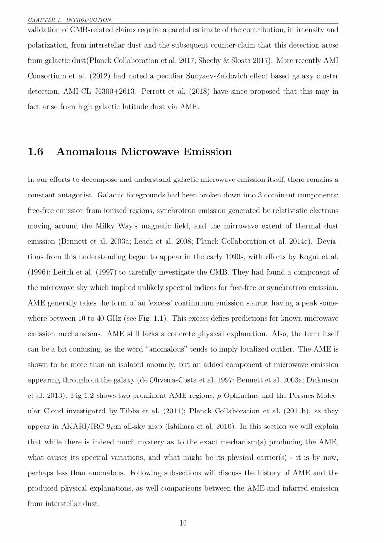
1.1 An example of a potential makeup of microwave emission components. Photometrypoints are extracted from the Planck and WMAP all-sky maps (Planck Collaborationet al. 2014b), for a part of the region well-known for prominant anomalous microwaveemission (AME), ρ Ophiuchus (Planck Collaboration et al. 2011b). The AME curveis produced from a warm neutral medium spinning dust template (Ali-Haïmoud et al.2009), with a frequency-shift applied to approximately fit the microwave data in PlanckCollaboration et al. (2016b) . . . . . . . . . . . . . . . . . . . . . . . . . . . . . . . . . 11
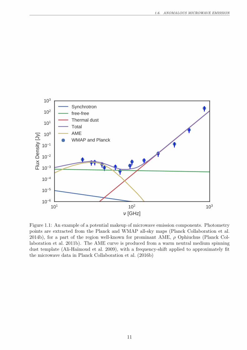
1.2 Two AME prominent regions investigated by Planck Collaboration et al. (2011b); Tibbset al. (2011), ρ Ophiuchus and Perseus, as they appear in the PAH-feature-tracingAKARI/Infrared Camera (IRC) 9µm all-sky data at native resolution (Ishihara et al.2010). White contours show AME at 1◦ resolution, extracted from the map by PlanckCollaboration et al. (2016b). The IRC data shown here is of a much finer resolutionthan the AME data, at around 10”, demonstrating the critical gap in resolvability ofall-sky AME-tracing data itself vs. the IR dust tracers we hope to compare it to. . . 12
2.1 Relative spectral response curves of the bands used in this study. Expected dust emis-sion components, assuming the dust spectral energy distribution (SED) model by (Com-piègne et al. 2011) are also shown. The components are summarized as emission frombig grains (BGs) ( dashed yellow line), emission from very small grains (VSGs) dashedblue line), and emission from PAHs (dashed grey line). . . . . . . . . . . . . . . . . . . 24
2.2 The I12 (orange) and A9 (green) filters coverage of modeled ionized (PAH1, red) andneutral (PAH0, purple)components of PAH features by Compiègne et al. (2011). Thedifference in the PAH feature coverage mainly comes from the 6.2 µm and the 7.7 µmfeature. . . . . . . . . . . . . . . . . . . . . . . . . . . . . . . . . . . . . . . . . . . . . 26
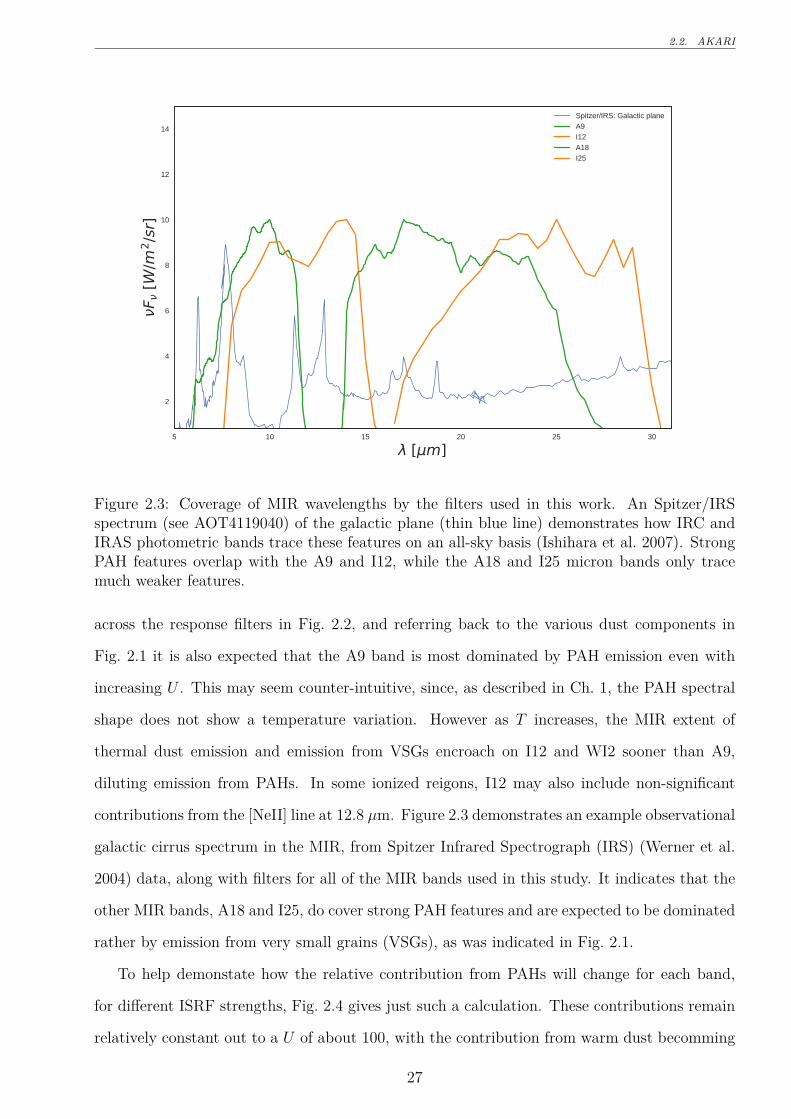
2.3 Coverage of MIR wavelengths by the filters used in this work. An Spitzer/IRS spectrum(see AOT4119040) of the galactic plane (thin blue line) demonstrates how IRC andIRAS photometric bands trace these features on an all-sky basis (Ishihara et al. 2007).Strong PAH features overlap with the A9 and I12, while the A18 and I25 micron bandsonly trace much weaker features. . . . . . . . . . . . . . . . . . . . . . . . . . . . . . . 27
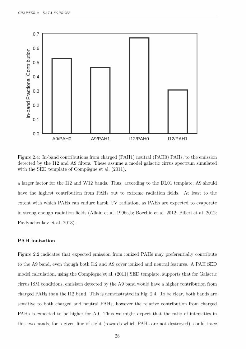
2.4 In-band contributions from charged (PAH1) neutral (PAH0) PAHs, to the emissiondetected by the I12 and A9 filters. These assume a model galactic cirrus spectrumsimulated with the SED template of Compiègne et al. (2011). . . . . . . . . . . . . . 28
2.5 Ionization fraction of PAHs vs. band ratios of I12, I25, to A9, for two ISRF strengths:Top: U = 1, Bottom: U = 10. These ratios are determined by assuming the SEDtemplate of Compiègne et al. (2011) . . . . . . . . . . . . . . . . . . . . . . . . . . . . 29
2.6 AKARI/IRC 9 µm to IRAS 12 µm intensity ratio. . . . . . . . . . . . . . . . . . . . . 302.7 AKARI/IRC 9 µm to IRAS 25 µm intensity ratio. . . . . . . . . . . . . . . . . . . . . 312.8 rs cross correlation matrix of the PCCS maps: temperature T , emissivity index β, and
amplitude at 545 GHz Idust(545) of thermal dust; intensity of free-free emission ff at; intensity of synchrotron emisison at 4 MHz Sync; intensity of the AME var. freq.component AME at 22.8 GHz. . . . . . . . . . . . . . . . . . . . . . . . . . . . . . . . 33
2.9 The peak frequencies of the varying component AMEvar. The pink shaded regionindicates frequencies not covered by either WMAP or Planck The green line at 33.5 GHzindicates the peak frequency of AMEfix. . . . . . . . . . . . . . . . . . . . . . . . . . 35
iii
LIST OF FIGURES
2.10 Histograms of the peak intensity AMEmaps calculated from the original COMMANDER-AME reference frequency maps. The dominant component, AMEvar is indicated inblue, for all pixels in the map, with their spinning dust intensities evaluated their peakfrequencies (see Fig. 2.9.) AMEfix gives the peak intensity of the spatially-constantfrequency component, indicating it is essentially always the weaker component. . . . . 36
2.11 All-sky map of the peak frequencies of the varying component AMEvar, correspondingto Fig. 2.9. Virtually all of the purple regions of the map correspond to pixels flaggedfor point sources in the LFI data. There are very few notable structures in the frequencymap overall, other than the galactic plane itself, ρ Ophiuchus, and Perseus. . . . . . . 37
2.12 Spdust template spinning dust profiles fitted by PC15X when calculating AMEvar. Thereference frequency, 22.8 GHz is indicated by the vertical green line. Each template hasthe same AMEvar amplitude of 100 µK, indicated by the horizontal green line, plottedto highlight the potential deviation between AMEvar and the actual peak intensity. . 38
3.1 λ Orionis as it appears in the AKARI 9 µm data. Contours indicate the AME, as givenby the Planck PR2 AME map. The image is smoothed to a 1◦ PSF (much larger thanthe original 10 arcsec map). The λ Orionis star itself is approximately located at thecenter of the image. . . . . . . . . . . . . . . . . . . . . . . . . . . . . . . . . . . . . . 42
3.2 λ Orionis as it appears in H-alpha emission by Finkbeiner (2003). Contours indicateAME emission, from the variable frequency component. The colorbar indicates Hαemission in Rayleighs. The field of view is slightly larger than that used for the finalprocessed IR comparison (Fig. 3.6). . . . . . . . . . . . . . . . . . . . . . . . . . . . . 43
3.3 The λ Orionis region and its surroundings in AKARI Far Infrared Surveyor (FIS) data,where A65 is blue, A90 is green, and A140 is red. The missing stripe patterns arevisible, and affect all 3 bands shown here as well as the A160 data. . . . . . . . . . . 45
3.4 The λ Orionis region in the A9 band at near-native resolution. This is a mosiac createdfrom the 3x3 degree all-sky survey tiles by Ishirara et al. (in prep.) Missing stripesare less of a problem than with the A18 band (Fig. 3.5), but point sources are morepronounced. Around Betelgeuse, in the lower left of the image, we can see an artifactcaused by scattered light.. . . . . . . . . . . . . . . . . . . . . . . . . . . . . . . . . . 46
3.5 The λ Orionis region in the A18 band at near-native resolution, demonstrating theregions affected by missing stripe errors, but less affected by point-sources than A9(Fig. 3.4). . . . . . . . . . . . . . . . . . . . . . . . . . . . . . . . . . . . . . . . . . . 47
3.6 Processed data at each wavelength for λ Orionis. A flat background has been subtractedfrom each frame based on the mean of pixels within the red rectangle. The pixel widthis 0.25◦, with the data PSF smoothed to 1◦ spatial resolution. Masked pixels (pointsources, stripe errors, convolution artifacts) are shown as white. The frames share thesame FOV and GAL-TAN projection. Colorbars indicate the intensity in MJy/sr. . . . 49
3.7 rs correlation matrix for all of the data used in the λ Orionis analysis, similar to thatpresented for the Planck Commander component maps in Fig. 2.8. The shade andannotation for each cell indicates the rs score, where rs of 1 indicates a monotonicallyincreasing relationship for a given pair of images. The two AME components, as de-scribed in Ch. 2, are listed separately: AMEvar for the frequency-varying component,and AMEfix for the constant frequency component. . . . . . . . . . . . . . . . . . . . 51
3.8 Re-sampled (Bootstrap) correlation tests for IR emission in λ Orionis vs. AME. Eachband’s rs distribution is shown in a different color (the same color scheme for bothplots). The width of the distribution indicates the error for the given data in thecorrelation coefficient. The mean and standard deviation of the scores are given in thelegend of each plot. The plot ranges only show positive values, since no negative scoreswere produced. . . . . . . . . . . . . . . . . . . . . . . . . . . . . . . . . . . . . . . . . 52
3.9 Observed (black circles and errors) and synthetic photometry (gray dots) SED of a pixelwithin λ Orionis, along with the dust SED model fit results. Two SED fits are shown:on for the Bayesian fitting (magenta), and another showing the standard least-squaresresult for comparison (yellow). The fitted interstellar radiation field (ISRF) strengthU , and fraction of mass in PAHs, qPAH are also given. . . . . . . . . . . . . . . . . . . 54
iv
LIST OF FIGURES
3.10 The same as Fig. 3.9, but for a different pixel position. . . . . . . . . . . . . . . . . . . 553.11 Scatter plot with the bivariate error elipses generated through the hierarchical Bayesian
analysis (HB) SED fitting, of total dust mass Mdust vs. IAME scaled by U . Green dotsindicate the results when using a simple least-squares method fit, for comparison withthe HB method. . . . . . . . . . . . . . . . . . . . . . . . . . . . . . . . . . . . . . . . 56
3.12 The same comparison is given by 3.11, but showing total mass of PAHs (MPAH) ratherthan total dust mass on the y-axis. . . . . . . . . . . . . . . . . . . . . . . . . . . . . 57
3.13 The same as in Figs. 3.11 and 3.12, but specifically comparing an estimate of the chargedcomponent of PAH mass MPAH+. This includes anions and cations, since we cannotdistinguish between these two spectroscopically. . . . . . . . . . . . . . . . . . . . . . . 58
3.14 The hierarchical Bayesian correlation probablity distributions of rs) for the three phys-ical parameters vs. the AME intensity: total dust mass, rs(dust) (blue); total PAHmass rs(PAH) (green); and only the ionized PAH mass rs(PAH+) (red). Also givenare the probabilities of either PAH component being better correlated with AME thandust mass, as well as the probability that ionized PAH mass correlates better than totalPAH. . . . . . . . . . . . . . . . . . . . . . . . . . . . . . . . . . . . . . . . . . . . . . . 59
3.15 The hierarchical Bayesian correlation coefficent (rs as shown in PDFs as shown inFig. 3.14, but with the central region of λ Orionis masked, according to Fig. 3.16. . . 61
3.16 The A90 image of λ Orionis shown to demonstrate the mask applied to the centralregion, in order to produce the PDFs in Fig. 3.15. The region showing an apparentdust temperature peak, which was most prominent in the A90 image and the majorpoint of variation accross all the wavelengths, is thus omitted. . . . . . . . . . . . . . . 62
4.1 Distributions of the modal values for each of the 4,737 survey tiles for the A9 band,and for the A18 band. . . . . . . . . . . . . . . . . . . . . . . . . . . . . . . . . . . . . 67
4.2 Point-density distributions of the log AMEvar intensity (Y-axis) vs. log IR bands’intensities. In this case no pixel mask is applied, in order to show overall trend of thefull data-set. However a random sampling is used due to computational contraints. Theplots show a random set of 20% of the full-sky data. Darker shaded regions indicate ahigher density of pixels. . . . . . . . . . . . . . . . . . . . . . . . . . . . . . . . . . . . 68
4.3 ALL-SKY cross-correlation matrix for the 12 infrared bands sampled, as well as the PCcomponent maps described in Ch. 2: the two AME components evaluated at their peakfrequencies AMEvar, AMEfix; Syncrotron, and free-free), and ancilliary maps of NH ,Hα emission, and 408 MHz emission Haslam et al. (1982). The color-scale indicates(rS). Results are based on the unmasked sky, but are split by Galactic latitude: pixelswith |β| > 15◦ (left) and |β| < 15◦ (right). The color and annotations indicate rs as inFig. 3.7. . . . . . . . . . . . . . . . . . . . . . . . . . . . . . . . . . . . . . . . . . . . 69
4.4 All-sky map in A9 emission after applying the combined masks: ecliptic plane, galacticplane, point sources, and pixels with signal-to-noise ratio (S/N) < 3. This mask essen-tially outlines the galaxy, except for the most confused regions. Diffuse galactic emissionis essentially removed by the mask due to low S/N in the mid-infrared (MIR) bands.In the full sky map of ~700,000 pixels, there are ~50,000 unmasked pixels remaining. . 70
4.5 The same comparison as shown for Fig. 4.2, but with the mask applied as in Fig. 4.4. 724.6 Cross-correlation (rs matrix for the IR intensities (unscaled) vs. each other, esssentially
the same comparison as in Fig. 4.3, except that the pixel mask is applied, and we donot perform a split by Galactic latitude— after the mask is applied, over 90% of pixelsare within 10◦ of the galactic plane. . . . . . . . . . . . . . . . . . . . . . . . . . . . . 74
4.7 Cross-correlation (rs matrix for the U -normalized IR intensities vs. each other, andalso against the AME components, other PC products, and ancilliary data. In the leftpanel, only the IR maps are divided by U - other data is unchanged from. In the panelat right, both the the AME and IR intensities are divided by U . Fig. 4.6) . . . . . . . 75
4.8 Cross-correlation (rs matrix for the residual correlations between IR intensities, AME,and other microwave components. All of the maps in this case are normalized by R. ) 75
v
LIST OF FIGURES
4.9 Re-sampled (Bootstrap) correlation tests for IR emission vs. AME, performed on themasked all-sky maps. Each band’s rs distribution is shown in a different color. Thewidth of the distribution indicates the error for the given data in the correlation coef-ficient. The mean and standard deviation of the scores are given in the legend of eachplot. The plot ranges only show positive values, since no negative scores were produced. 76
4.10 Spatial map of rs between the AME:U and A9:U , a tracer of the column density ofPAHs emitting within the A9 filter. rs is calculated for all NSIDE 256 pixels withineach NSIDE 8 pixel-sized bin. The correlation score is calculated with the unmaskedmaps. The colorbar indicates rs, ranging from -1 (negative monotonic relationship) to+1 (positive monotonic relationship). . . . . . . . . . . . . . . . . . . . . . . . . . . . . 77
4.11 Spatial map of rs between the AME:U and I12:U . . . . . . . . . . . . . . . . . . . . . 774.12 Spatial map of rs between the AME:U and A18:U . . . . . . . . . . . . . . . . . . . . 774.13 Spatial map of rs between the AME:U and I25:U . . . . . . . . . . . . . . . . . . . . . 784.14 The ratio of AMEvar and PC dust radiance R, tracing fluctuations in AME per thermal
dust emission. The contours trace the PC synchrotron (black) and free-free (white)components, to highlight various correlations between these components and PC AMEfluctuations. Both free-free and syhncrotron can be seen to correlate and anti-correlatewith the AME to dust ratio. . . . . . . . . . . . . . . . . . . . . . . . . . . . . . . . . . 80
4.15 The same as Fig. 4.14, but with AMEfix/R as the all-sky image. . . . . . . . . . . . . 80
vi
Abstract
The anomalous microwave emission (AME) still lacks a conclusive explanation. This excess of
emission, roughly between 10 and 50 GHz, tends to defy attempts to explain it as synchrotron
or free-free emission. The overlap with frequencies important for cosmic microwae background
explorations, combined with a strong correlation with interstellar dust, drive cross-disciplinary
collaboration between interstellar medium and obervational cosmology. The apparent relation-
ship with dust has prompted a “spinning dust” hypothesis: electric dipole emission by rapidly
rotating, small dust grains. Magnetic dipole emission by grains with magnetic inclusions (“mag-
netic dust”), while less suppported, has not been ruled out. Even assuming a spinning dust
scenario, we are far from concluding which category of dust contributes. The typical peak
frequency range of the AME profile implicates grains on the order of 1nm. This points to
polycyclic aromatic hydrocarbon molecules (PAHs). We use data from the AKARI/Infrared
Camera (IRC; Onaka et al. (2007)), due to its thorough PAH-band coverage, to compare AME
from the Planck Collaboration et al. (2016b). astrophysical component separation product)
with infrared dust emission. We look also at infrared dust emission from other mid IR and far-
IR bands. The results and discussion contained here apply to an angular scale of approximately
1◦. In general, our results support an AME-from-dust hypothesis. We look both at λ Orio-
nis, a region highlighted for strong AME, and find that certainly dust mass correlates with
AME, and that PAH-related emission in the AKARI/IRC 9 µm band may correlate slightly
more strongly. These results are compared to an all-sky analysis, where we find that potential
microwave emission component separation imperfections among other issues, make an all-sky,
delocalized comparsion very challenging. In any case the AME-to-dust correlation persists
even in the all-sky case, but tests of relative variations from different dust SED components
are largely inconclusive. We emphasize that future efforts to understand AME should focus
on individual regions, and a detailed comparsion of the PAH features with the variation of the
AME SED. Further all-sky analyses seem unlikely to help resolve this issue. Non-PAH carriers
vii
LIST OF FIGURES
of the AME, such as nanosilicates, cannot be ruled out either.
viii
LIST OF FIGURES
IRC
1
Chapter 1
Introduction
“It is now plain that about 75% of the data we would like to have can be obtained from
good ground-based sites”
-H. Johnson, 1966
1.1 All-sky Astronomy
All-sky astronomy is not new. Indeed, the notion of capturing a particular “object” or “source”
with a camera and saving it for later investigation would be completely alien to the first as-
tronomers and astronavigators. Absence of telescopes forced us to describe the sky in terms
of its larger patterns, brightest characters. What is new however is the notion of preparing an
archive of the sky itself for not only the research whims of a single investigator, team, institute,
or even a single nation— rather, all-sky surveys tend to be international endeavors in their
production, and even more so in their utilization.
1.2 Infrared astronomy
Infrared astronomy was essentially non-existant as recently as the 1920s, if we judge by the first
IR observations (Pettit & Nicholson 1922, 1928). Mainstream IR astronomy is perhaps much
younger, only really taking off — literally — in the post-war era, via ballon and rocket borne
experiments (Johnson 1966). Compare this to visible wavelengths, a field so old we name it
after the bio-evolutionary advent of sight, itself. Even radio astronomy with its own logistical
and technological challenges, has been around since at least 1932.
Astronomers have not been content to be constrained by atmospheric IR windows, even
2
1.3. MULTI-WAVELENGTH INVESTIGATIONS
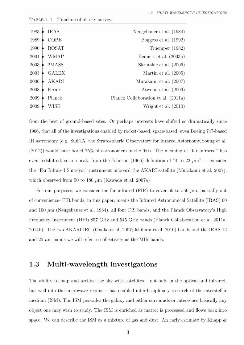
Table 1.1 Timeline of all-sky surveys
1983 • IRAS Neugebauer et al. (1984)1989 • COBE Boggess et al. (1992)1990 • ROSAT Truemper (1982)2001 • WMAP Bennett et al. (2003b)2003 • 2MASS Skrutskie et al. (2006)2003 • GALEX Martin et al. (2005)2006 • AKARI Murakami et al. (2007)2008 • Fermi Atwood et al. (2009)2009 • Planck Planck Collaboration et al. (2011a)2009 • WISE Wright et al. (2010)
from the best of ground-based sites. Or perhaps interests have shifted so dramatically since
1966, that all of the investigations enabled by rocket-based, space-based, even Boeing 747-based
IR astronomy (e.g. SOFIA, the Stratospheric Observatory for Inrared Astornomy,Young et al.
(2012)) would have bored 75% of astronomers in the ’60s. The meaning of “far infrared” has
even redshifted, so to speak, from the Johnson (1966) definition of “4 to 22 µm” — consider
the “Far Infrared Surveyor” instrument onboard the AKARI satellite (Murakami et al. 2007),
which observed from 50 to 180 µm (Kawada et al. 2007a)
For our purposes, we consider the far infrared (FIR) to cover 60 to 550 µm, partially out
of convenience- FIR bands, in this paper, means the Infrared Astronomical Satellite (IRAS) 60
and 100 µm (Neugebauer et al. 1984), all four FIS bands, and the Planck Observatory’s High
Frequency Instrument (HFI) 857 GHz and 545 GHz bands (Planck Collaboration et al. 2011a,
2014b). The two AKARI IRC (Onaka et al. 2007; Ishihara et al. 2010) bands and the IRAS 12
and 25 µm bands we will refer to collectively as the MIR bands.
1.3 Multi-wavelength investigations
The ability to map and archive the sky with satellites – not only in the optical and infrared,
but well into the microwave regime – has enabled interdisciplinary research of the interstellar
medium (ISM). The ISM pervades the galaxy and either surrounds or intervenes basically any
object one may wish to study. The ISM is enriched as matter is processed and flows back into
space. We can describe the ISM as a mixture of gas and dust. An early estimate by Knapp &
3
CHAPTER 1. INTRODUCTION
Kerr (1974) puts the mass of dust in the galaxy at about 1% that of interstellar gas.
A wealth of data is now available not only in the IR, but on into the sub-millimeter range
and the interpretation of this data has become a serious priority. This is especially true for the
last ten years as new, much higher resolution surveys have been carried out such as the Spitzer
Space Telescope (SST) Werner et al. (2004), Herschel Space Observatory (Herschel) (Pilbratt
et al. 2010) by National Aeronautics and Space Administration (NASA) and the European
Space Agency (ESA) respectively, and the AKARI telescope (Murakami et al. 2007), by JAXA.
AKARI especially, produced a wealth of data spanning the entire sky. It was equipped with
IRC (Onaka et al. 2007) to study the MIR, and FIS (Kawada et al. 2007b) to study cooler dust
and gas, and conduct spectroscopy in the FIR via its Fourier Transform Spectrometer (FTS).
In this thesis we use these AKARI surveys in a comparison with other cutting edge all-sky
maps from the Planck Observatory in a multi-wavelength study of yet another part of the ISM
puzzle, the AME and its connection to interstellar dust.
The merits of multiwavelength based investigations arise from the simple fact that the ISM
is very complex— both in terms of the myriad forms of matter present, from plasmas to dust
grains — and in countless physical processes at play. Consider the complex case of a supernova
remnant influencing surrounding ISM: through a combined analysis of radio, mid-far infrared,
and X-ray data, Lau et al. (2015) were able to characterize the history of dust production,
heating, and destruction within the Sgr A East supernova remnant.
1.4 Interstellar Dust
The study of interstellar dust has been connected to mainstream astrophysics research, and
recognized as an integral player in the evolution of the interstellar medium. This has been
shown by early sounding rocket experiments (Wolstencroft & Rose 1967; Soifer et al. 1971),
and balloon experiments (Muehlner & Weiss 1970; Emerson et al. 1973), and dust has been
more profoundly exposed by the advent of all-sky infrared surveys like the Cosmic Background
Explorer (COBE)’s Diffuse Infrared Background Experiment (DIRBE) (Sodroski et al. 1994)
and IRAS (Neugebauer et al. 1984). With space-borne long-term IR mapping finally available
on an all-sky scale, we could move past the interplanetary medium and into the interstellar.
The role of dust in the interstellar medium has expanded beyond simply an intervening,
4
1.4. INTERSTELLAR DUST
stellar light obstructing material. Theoretical models and observations have shown that dust
grains act as a catalyst for the formation of molecular hydrogen and other molecules, providing
a substrate upon which hydrogen and other atoms can meet (Iglesias 1977; Burke & Hollenbach
1983). With infrared observations we are able to study dust directly via its vibrational emission,
rather than relying only on inference from visible reddening and polarization effects (Davis &
Greenstein 1951; Platt 1956; Carrasco et al. 1973). The question of the composition of dust
has grown from a single thread of investigation into a network of questions. Many pieces in
this dusty puzzle are missing. For example, the presence of dust grains containing silicates,
and amorphous carbon is very strongly supported by comparisons of infrared spectroscopy with
laboratory studies (Hagen et al. 1979; Joblin et al. 2009). But many questions remain about
which silicate and carbonaceous species may be present, and in what proportions, and in what
distribution of sizes. The question also remains, is there more to dust than simply carbonaceous
and silicate grains? The exact size distribution of dust grains is also an open question. The
composition of extremely small grains / large molecules is a particularly challenging mystery,
as well as the role of interstellar ices in the evolution dust and gas.
1.4.1 Silicate grains
One of the first materials proposed to exist as interstellar dust were silicates, with the first
evidence being UV absorption features (Knacke et al. 1969). More recently, specific species of
silicates are being identified via absorption spectroscopy (Olofsson et al. 2012). However some
doubt has been cast recently on the structure of the grains. For example, in Jones et al. (2013)
and Jones (2014) an updated model is proposed wherein dust grains may be composed of a
mixture of silicate and amorphous carbon material, such as a silicate core with an amorphous
carbon envelope, representing the first comprehensive model of continuous grain evolution. In
other words, the first model to consider dust grain morphology beyond the descrete categories
of silicate grains, carbonaceous grains, and PAH. An additional feature of this model is that
silicates having iron inclusions are expected, which would be similar to the Fe form of olivine.
This is an update from the conventional “astronomical silicates" assumed in earlier dust SED
models such as Li & Draine (2001) or Compiègne et al. (2011).
5
CHAPTER 1. INTRODUCTION
1.4.2 Carbonaceous grains
As with silicates, the existance well-established that carbonaceous material, primarily amor-
phous carbon, exists in the ISM (Aitken 1981; Tielens & Allamandola 1987). This is material
commonly called “soot" or the fuel we know on earth as coal. Some non-amorphous carbona-
ceous material is also speculated to exist, such as graphite (Zhou et al. 2006) or “buckyonions"
(concentric-shell-graphite) (Li et al. 2008).
1.4.3 Polycyclic Aromatic Hydrocarbons and the Unidentified In-
frared Bands
From the mid-to-near IR however, spectroscopic observations enabled and required the simple
two-populations model of larger and smaller dust (e.g. Mathis et al. (1977)), to be expanded.
“Unidentified IR bands” from 3 to 11 µm (hereafter, UIR bands), demonstrate another diver-
gence from the canonical dust emission story. The UIR bands were first reported at 8 to 13 µm
in planetary nebulae and HII regions by Gillett et al. (1973, 1975) in ground-based observations.
Observations by Merrill et al. (1975) noted another unexplained feature at 3.27 µm, noting:
“there are [...] similarities in the 8-13 µm spectra of NGC 253, NGC 7027, and BD +30◦3639
Gillett et al. (1975)”. Features at 6.2 and 7.7 µm were reported by Russell et al. (1977) using
the first airplane-mounted IR telescope and predecessor to SOFIA, the Kuiper Airborne Ob-
servatory. Sellgren et al. (1983) reported features at 3.3 and 3.4 µm being detected in reflection
nebulae.
Moving into the 1990s, the UIR bands become much less of property of select objects in tar-
geted observations, are seen observed throughout the Milky Way. Balloon-based observation by
Giard et al. (1994) confirmed that the 3.3 µm feature pervades throughout the Galactic plane.
The first-ever airborne IR observatory, Kuiper Several years later, space-based spectroscopy
with the Infrared Telescope in Space (IRTS)(Murakami et al. 1996) and Infrared Space Obser-
vatory (ISO)(Kessler et al. 1996) enabled confirmation by Onaka et al. (1996) and Mattila et al.
(1996) that the mid-infrared UIR features are not limited to a few objects, but are present even
in the diffuse galactic ISM. Dwek et al. (1997) even reported that photometric excess in the
COBE/DIRBE 12 µm band may be caused by the UIR bands, in and suggested they may be
from these UIR features have come to be explained via PAH, a possibility which had been con-
6
1.4. INTERSTELLAR DUST
sidered earlier by Allamandola et al. (1985); Puget et al. (1985). PAHs are a class of molecules
composed primarily of fused carbon rings such as corranulene. PAHs and/or similar amalgems
containing aromatic structures (e.g. quenched carbonaceous composites (QCCs), Sakata et al.
(1984)) have been incorporated into dust mixture SED models over the last two decades (Draine
& Li 2001, 2007a; Hony et al. 2001; Compiègne et al. 2011; Galliano et al. 2011; Jones et al.
2013, 2017).
With the appearance of high powered computers with an ability to perform rigorous calcu-
lations, many attempts have been made to simulate the expected emission from PAHs. Density
functional theory (DFT) (Hohenberg & Kohn 1964) has become available as a tool for simu-
lating molecular emission features using a quantum approach. DFT calculations has become a
subfield of ISM astrophysics. Many attempts are being made to fit particular emission features
of PAHs, and other molecular and grain species, to observed ISM features (Hammonds et al.
2009; Hirata et al. 1999). While it is difficult to reproduce the exact interstellar conditions in
a laboratory setting, DFT simulations have yielded some evidence that the UIR bands can be
explained as PAH vibrational emission features (Pathak & Rastogi 2005; Ricca et al. 2011; Yu
& Nyman 2012).
“PAH” or “UIR”? We should note however that PAHs are not the only proposed expla-
nation for the UIR features, despite being the most widely accepted. Zhang & Kwok (2014)
propsed theoretically that mixtures of non-PAH carbonaceous and silicate spectra could also
fit theoretically calculated PAH emission features. However the PAH-UIR hypothesis is still
widely supported (Tielens 2008; Rastogi et al. 2013). The way that PAHs might be produced
or evolve from other species is not understood however. Though there are efforts underway to
model potential formation pathways. As far as the evolution of larger aromatics form smaller
PAHs, there is one proposed pathway wherein a benzene could grow into a larger aromatic
molecule such as naphthalene (Ghesquière et al. 2014). In any case, the terms “PAH features”
and “UIRs” are too often used interchangably in the literature. In the following sections, we
will define PAHs as the general class of aromatic-ring-containing molecules, and not explicitly
to “pure” PAH species such as benzene, corronene, or corranulene, etc. From this point we will
also abandon the term “UIRs”, and use “PAH features” instead. We do so while acknowledging
that interstellar PAHs is by no means a closed book.
7
CHAPTER 1. INTRODUCTION
1.4.4 Metrics of Interstellar Dust
Carefully describing or parameterizing the SED of interstellar dust emission can be somewhat
involved. Over the years a few conventions have arisen, when referring to dust SED properties.
Interstellar Radiation Field U Throughout this work we will discuss the ISRF in terms
of U , which is a conventional measure normalized to the ISRF of the solar neighborhood. In
otherwords, a U of 1 indicates a “Habing unit”, or 1.6 × 10⁻³ergs−1cm−2, a value given by
Habing (1968). More correctly, U is referring to the integration of the ISRF flux density from
the far-UV to the nearIR, or λ = 0.09 to λ = 0.8 . The ISRF is sometimes indicated in the
literature as G0, instead of U , when integrated only from ~0.09 µm to 0.2µm. As long as we are
assuming a spatially constant SED for the ISRF, it is not so important which one we use, and
does not affect the results or discusison in this thesis. U will be used in the following chapters,
except when referring to previous works which used G0.
Total dust abundance This is the total mass of all dust components contributing to the
observed SED. It is often indicated either as the dust massMdust, in units ofM�, as in Galliano
et al. (2008). The dust abundance can be determined when both the luminosity of the dust,
and the local interstellar radiation field heating the dust, U are known, as in the following
relation:
Mdust ∝ Ldust/U (1.4.1)
Some caution must be excercised, as Mdust may sometimes indicated only the mass of dust
which is emitting thermall, in the FIR, excluding VSGs or PAHs. Throughout this thesis
however, we consider that Mdust includes emisison from both the thermal equilibirum grains,
and small stochastically emitting dust and PAHs.
PAH Fraction qPAH qPAH, sometimes indicated as χPAH , is defined as the fraction of
the total dust mass which is in the form of PAHs, or:
qPAH = MPAH
Mdust
(1.4.2)
8
1.5. MICROWAVE FOREGROUNDS
This parameter can be especially difficult to fit, relative to the total dust mass, for the reason
that there a many more all-sky photometric data points in the far infrared, where thermal
emission from dust grains dominates. In the mid infrared, where PAH features are observed,
we have fewer observational constraints on an all-sky basis. This is discussed further in Ch. 2.
PAH Ionization Fraction fPAH fPAH tells us the fraction of the total PAH mass which
are ionized. Thus:
fPAH = MPAHion
MPAH
(1.4.3)
1.5 Microwave foregrounds
Moving on from the infrared dust SED, into the Rayleigh-Jeans regime of thermal dust emis-
sion, multi-wavelength observations have opened up a new discipline: the disentagnlement of
interstellar dust emission from non-dust emission components. Most notably, separating tem-
perature fluctuations in the cosmic microwae background (CMB) from the microwave extent of
thermal dust emission. Those studying the Milky Way itself, from the far IR into microwave
and radio frequencies, are now collaborating closely with those interested in the precise nature
of the CMB.
Much of the motivation between recent galactic microwave emission research has little to
do with galactic ISM astronomy itself. Rather, our galaxy presents an inconvenience to ob-
servational cosmology in that it ’contaminates’ observations of the CMB. The avereage SED
of the CMB is simple enough to model, with a 2.725 K blackbody function. This tempera-
ture however means that the peak occurs between several microwave foreground components,
from interstellar dust and gas, as displayed in Fig. 1.1. The difficulty of decomposing the mi-
crowave sky into galactic ISM, extragalactic, and CMB temperature fluctuation components
has brought the detailed decomposition of the microwave-radio regime of ISM to the forefront of
Planck Collaboration paper titles (Planck Collaboration et al. 2011a, 2014a, 2016a). Without
extragalactic research, there would be no need for the word “foreground” in describing galactic
microwave emission.
The ISM has intruded into cosmological studies perhaps most prominently with the first
claimed detection of B-mode polarization (Hanson et al. 2013; BICEP2 Collaboration et al.
2014; Flauger et al. 2014), and multiple response papers. The main consensus being that the
9
CHAPTER 1. INTRODUCTION
validation of CMB-related claims require a careful estimate of the contribution, in intensity and
polarization, from interstellar dust and the subsequent counter-claim that this detection arose
from galactic dust(Planck Collaboration et al. 2017; Sheehy & Slosar 2017). More recently AMI
Consortium et al. (2012) had noted a peculiar Sunyaev-Zeldovich effect based galaxy cluster
detection, AMI-CL J0300+2613. Perrott et al. (2018) have since proposed that this may in
fact arise from high galactic latitude dust via AME.
1.6 Anomalous Microwave Emission
In our efforts to decompose and understand galactic microwave emission itself, there remains a
constant antagonist. Galactic foregrounds had been broken down into 3 dominant components:
free-free emission from ionized regions, synchrotron emission generated by relativistic electrons
moving around the Milky Way’s magnetic field, and the microwave extent of thermal dust
emission (Bennett et al. 2003a; Leach et al. 2008; Planck Collaboration et al. 2014c). Devia-
tions from this understanding began to appear in the early 1990s, with efforts by Kogut et al.
(1996); Leitch et al. (1997) to carefully investigate the CMB. They had found a component of
the microwave sky which implied unlikely spectral indices for free-free or synchrotron emission.
AME generally takes the form of an ’excess’ continnuum emission source, having a peak some-
where between 10 to 40 GHz (see Fig. 1.1). This excess defies predictions for known microwave
emission mechansisms. AME still lacks a concrete physical explanation. Also, the term itself
can be a bit confusing, as the word “anomalous” tends to imply localized outlier. The AME is
shown to be more than an isolated anomaly, but an added component of microwave emission
appearing throughout the galaxy (de Oliveira-Costa et al. 1997; Bennett et al. 2003a; Dickinson
et al. 2013). Fig 1.2 shows two prominent AME regions, ρ Ophiuchus and the Persues Molec-
ular Cloud investigated by Tibbs et al. (2011); Planck Collaboration et al. (2011b), as they
appear in AKARI/IRC 9µm all-sky map (Ishihara et al. 2010). In this section we will explain
that while there is indeed much mystery as to the exact mechanism(s) producing the AME,
what causes its spectral variations, and what might be its physical carrier(s) - it is by now,
perhaps less than anomalous. Following subsections will discuss the history of AME and the
produced physical explanations, as well comparisons between the AME and infarred emission
from interstellar dust.
10
1.6. ANOMALOUS MICROWAVE EMISSION
101 102 103
[GHz]
10 6
10 5
10 4
10 3
10 2
10 1
100
101
102
103
Flu
x D
ensi
ty [J
y]
Synchrotronfree-freeThermal dustTotalAMEWMAP and Planck
Figure 1.1: An example of a potential makeup of microwave emission components. Photometrypoints are extracted from the Planck and WMAP all-sky maps (Planck Collaboration et al.2014b), for a part of the region well-known for prominant AME, ρ Ophiuchus (Planck Col-laboration et al. 2011b). The AME curve is produced from a warm neutral medium spinningdust template (Ali-Haïmoud et al. 2009), with a frequency-shift applied to approximately fitthe microwave data in Planck Collaboration et al. (2016b)
11
CHAPTER 1. INTRODUCTION
0 6 24 54
1”
G160.26-18.62 (Perseus) G353.05+16.90 (ρ Ophiuci)
2400
926765620490375
375
275
191
191
122
122
1983
1606
1269
1269
971
971
714
714
495
317
317
178
495
317
1”
96 150
Figure 1.2: Two AME prominent regions investigated by Planck Collaboration et al. (2011b);Tibbs et al. (2011), ρ Ophiuchus and Perseus, as they appear in the PAH-feature-tracingAKARI/IRC 9µm all-sky data at native resolution (Ishihara et al. 2010). White contours showAME at 1◦ resolution, extracted from the map by Planck Collaboration et al. (2016b). The IRCdata shown here is of a much finer resolution than the AME data, at around 10”, demonstratingthe critical gap in resolvability of all-sky AME-tracing data itself vs. the IR dust tracers wehope to compare it to.
12
1.6. ANOMALOUS MICROWAVE EMISSION
1.6.1 Correlation with dust
Since its first detection in early microwave observations, AME has been found to be a widespread
feature of the microwave Milky Way (see the review Dickinson et al. (2013), and an updated
state-of-play of AME research by Dickinson et al. (2018). Kogut et al. (1996); de Oliveira-Costa
et al. (1997) showed that the AME correlates very well with infrared emission from dust, via
COBE/DIRBE and IRAS FIR. Finkbeiner et al. (2002) reported the first detection of a “rising
spectrum source at 8 to 10 GHz” in an observation targeting galactic ISM cloud. de Oliveira-
Costa et al. (2002) furher argued that this emission is in fact “ubiquitous”. The exact mechanism
and carrier/s remain mysterious however. More recent works, employing observations by the
Wilkinson Microwave Anisotropy Probe (WMAP), SST, the latest infrared (IR) to microwave
all-sky maps by Planck, and various ground based radio observations have strongly confirmed a
relationship between interstellar dust emission and AME (Ysard & Verstraete 2010; Tibbs et al.
2011; Hensley et al. 2016). Exactly which physical mechanisms produces the AME however is
still an open question, even if we assume a dusty AME origin. We equally puzzled as to the
chemical composition and morphology of the carrier(s). We also lack an all-sky constraint on
the emissivity of the AME spectrum at frequencies short of the WMAP cut-off, around 23 GHz.
The typical peak frequency of AME, in those cases where it is constrained, does give us a clue.
1.6.2 Proposed explanations
From the observed spatial correlation between AME and dust emerged two prevailing hypothe-
ses:
1) Electric dipole emission by spinning small dust grains, a mechanism proposed in Erickson
(1957) and Hoyle & Wickramasinghe (1970), with further discussion in Ferrara & Dettmar
(1994). Draine & Lazarian (1998b) give the earliest thorough theoretical prediction of a spinning
dust spectrum. A decade later Ali-Haïmoud et al. (2009) contributed substantial updates,
expanded modeling of grain excitation mechanisms and adoption of an updated grain size
distribution by Weingartner & Draine (2001). Ysard & Verstraete (2010) introduced the first
model of a spinning dust spectrum based on rotational emission from PAH, which are implicated
due to their size. Draine & Lazarian (1998b), gives the expected rotational frequency of spinning
13
CHAPTER 1. INTRODUCTION
dust oscillators ω, as follows:
ωT2π = 〈ν2〉1/2 ≈ 5.60× 10⁹a
−5/2−7 ξ−1/2T
1/22 Hz, (1.6.1)
where T is the gas temperature, a is the grain size, and ξ represents the deviation from a
spherical moment of intertia. For example, we can take a typical peak frequency of the AME
of ~20 GHz, a gas temperature of 100 K, roughly spherical grains, and a dipole moment on the
order of 1 debye, and get:
ωT2π = 20 GHz( T
100K )1/2( ρ
3gcm03 )−1/2( a5Å
)−5/2 (1.6.2)
implying an oscillator size of approximately 1 nm. Thus PAHs, as considered by Ysard &
Verstraete (2010), are a primary candidate spinning dust carrier, due to their expected size
range.
2) Magnetic dipole emission, caused by thermal fluctuations in grains with magnetic inclu-
sions, proposed by Draine & Lazarian (1999). More recently, modeled spectra for potential
candidate carriers have appeared in the literature: PAHs, grains with magnetic inclusions
(Draine & Hensley 2013; Ali-Haïmoud 2014; Hoang et al. 2016).
3) Though not widely accepted, another possible explanation for AME is discussed in Jones
(2009). They have suggested that the emissivity of dust, in the spectral range related to AME,
could contain features caused by low temperature solid-state structural transitions.
1.6.3 Spinning dust
Spinning dust need not be the only emission mechanism, a convention as arisen in AME obser-
vational works. The photometric signature of the AME is frequently interepreted via spinning
dust parameters (Ysard et al. 2011; Ali-Haimoud 2010). Archival all-sky AME data products
exclusively assume a spinning dust SED templates. Both WMAP and Planck used a base tem-
plate with 30 GHz peak frequency, and an assumed cold neutral medium environment. Using
the “spdust” spinning dust SED model code to fit excess microwave foreground emission has
become analagous fitting a modified blackbody function to the FIR.
We explore the case that the AME signature arises from spinning dust emission. If the
AME is carried by spinning dust, the carrier should be small enough that it can be rotationally
14
1.6. ANOMALOUS MICROWAVE EMISSION
excited to frequencies in the range of 10-40 GHz, and must have a permanent electric dipole.
Within contemporary dust SED models, only the PAH family of molecules, or nanoscale amor-
phous carbon dust fit these criteria. Those PAHs which have a permanent electric dipole (i.e.
coranulene, but not symmetric molecules like coronene), can emit rotationally. However the
carrier need not be carbon-based.
1.6.4 Spinning PAHs?
Assuming the rotational emission model of Draine & Lazarian (1998b), the AME signature
(consistent with peaked, continuum emission having a peak between 15 and 50 GHz ) implies
very small oscillators (~1 nm).
In any case, the PAH class of molecules are the only spinning dust candidate so far which
show both:
1) Evidence of abundance in the ISM at IR wavelengths, and
2) A predicted range of dipole moments (on order of 1 debye), to produce the observed AME
signature (Draine & Lazarian 1998b; Lovas et al. 2005; Thorwirth et al. 2007).
However, it should be noted that although nanosilicates have not yet been detected in the
ISM, Hensley & Draine (2017) propose that an upper bound on the abundance of nanosilicates
by Li & Draine (2001) (based on Infrared Telescope in Space (IRTS) observations by Onaka
et al. (1996)), allow such small spinning grains to be composed primarily of silicates. This
followed an earlier claim by Hensley et al. (2016) that the absence of a conclusive PAH-AME
link suggested the possibility of AME-from-nanosilicates.
While neither nanosilicates nor any particular species of PAHs have been conclusively iden-
tified in the ISM, there is far more empiracal evidence for PAH-like dust than for nanosilicates.
Mid-infrared features associated with PAH-like aromatic materials have been observed. In fact,
“the PAH features” are ubiquitous in the ISM (Giard et al. 1994; Onaka et al. 1996; Onaka
2000), such that the carriers must be abundant. Andrews et al. (2015) strongly argue for the
existence of a dominant “grandPAH” class, containing 20 to 30 PAH species.
1.6.5 Excitation factors
In the spinning dust model, there are several possible excitation factors for spinning dust.
For the grains to have rotational velocities high enough to create the observed AME, they
15
CHAPTER 1. INTRODUCTION
must be subject to strong excitation mechansisms. The dominant factors that would be giving
grains their spin, are broken down by Draine (2011) into basically two categories: 1) Collisional
excitation. 2) Radiative excitation, the sum of which could lead to sufficient rotational velocities
for sufficiently small grains. However the extent of excitation will depend on environmental
conditions, i.e. there will be more frequent encounters with ions and atoms in denser regions
(so long as the density is not high enough to coagulate the small grains), and more excitation
due to photon emission with increasing ISRF strength (Ali-Haïmoud et al. 2009; Ali-Haïmoud
2014). One of the strongest potential excitation mechansims listed in Draine (2011) is that of
negatively charged grains interacting with ions. Thus not only must we consider environmental
factors, grain composition and size, but also the ionization state of the carriers. (For example,
ionized vs. neutral PAHs.) The dependence of the observed AME on ISM density is modeled
by Ali-Haimoud (2010).
1.6.6 AME vs. IR in the literature
The overall pattern among large-scale studies seems to show that all of the dust-tracing photo-
metric bands correlate with the AME (and each other) to first-order. On an all-sky, pixel-by-
pixel basis, at 1◦ angular resolution, Ysard et al. (2010) find that 12 µm emission, via IRAS,
correlates slightly more strongly with AME (via WMAP) than with 100 µm emission. They
also find that scaling the IR intensity by the ISRF improves both correlations. They interpret
this finding as evidence that AME is related to dust, and more closely related to the small
stochastically emitting dust — predominantly PAHs — that is traced by 12 µm emission. The
improvement of the correlations after scaling by U is expected, as long as the 12 µm band is
dominated by stochastic emisson from PAHs, in other words:
I12 µm ∝ UNPAH , (1.6.3)
where NPAH is the column density of emitting PAHs (Onaka 2000). Such a relationship is
expected, assuming that PAHs are small enough, and their heat capacities low enough, such
that their emission is indeed stochastic– a single UV photon is absorbed, immediately followed
by the emission of many IR photons. Under such conditions, a the radiation field would change
only the intensity of PAH features, and not affect the spectral shape. Thus Ysard et al. (2010)
16
1.7. STATISTICAL METHODS
implies that I12 µm/U is giving us a measure of the column density of spinning dust.
In a similar work however Hensley et al. (2016) report a lack of support for the spinning
PAH hypothesis. Finding that fluctuations in the ratio of PAH-dominated 12 µm emission (via
Wide-field Infrared Survey Explorer (WISE)) to dust radiance, R, (via Planck) do not correlate
with the ratio of AME intensity to R, they conclude that the AME is not likely to come from
PAHs. In terms of emission intensity however, their findings are consistent with Ysard et al.
(2010) in that I12 µm correlates well with IAME. Thus there remains an open question as to
what the actual carrier of the AME is.
The story is no more clear when looking at the average properties of individual regions.
Planck Collaboration et al. (2014d) find that among 22 high-confidence “AME regions” (galactic
clouds such as the ρ Ophiuchus cloud and the Perseus molecular cloud complex) AME vs. 12 µm
shows a marginally weaker correlation than AME vs. 100 µm (via IRAS). Tibbs et al. (2011)
examined the AME-prominent Perseus Molecular Cloud complex, finding that while there is
no clear evidence of a PAH-AME correlation, they do find a slight correlation between AME
and U .
1.7 Statistical Methods
In the following chapters, various IR datasets and analysis comparing the AME to dust emission
will be described, along with a discussion of results testing the “AME from spinning PAHs”
hypothesis. Because this particular hypothesis is challenging to test, due to the first order cor-
relation of different constituents of interstellar matter, we apply variety of statistical techniques
to explore if PAHs show any better correlation with AME than other dust metrics. These meth-
ods range from standard correlation tests to less common techniques, like the bootstrap test,
and even relatively new approaches such as HB. It may be useful to go ahead and introduce
this methods from the outset.
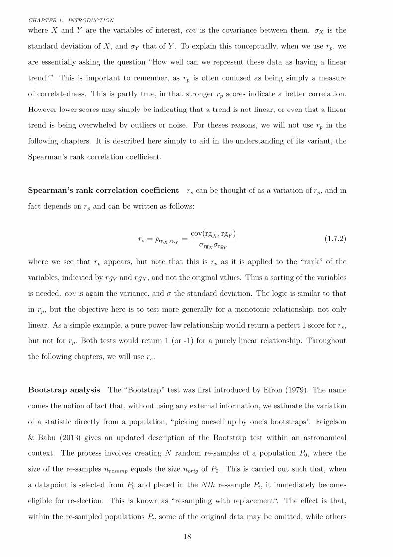
1.7.1 Correlation tests
Pearson correlation coefficient rp is defined as follows:
ρX,Y = cov(X, Y )σXσY
(1.7.1)
17
CHAPTER 1. INTRODUCTION
where X and Y are the variables of interest, cov is the covariance between them. σX is the
standard deviation of X, and σY that of Y . To explain this conceptually, when we use rp, we
are essentially asking the question “How well can we represent these data as having a linear
trend?” This is important to remember, as rp is often confused as being simply a measure
of correlatedness. This is partly true, in that stronger rp scores indicate a better correlation.
However lower scores may simply be indicating that a trend is not linear, or even that a linear
trend is being overwheled by outliers or noise. For theses reasons, we will not use rp in the
following chapters. It is described here simply to aid in the understanding of its variant, the
Spearman’s rank correlation coefficient.
Spearman’s rank correlation coefficient rs can be thought of as a variation of rp, and in
fact depends on rp and can be written as follows:
rs = ρrgX ,rgY= cov(rgX , rgY )
σrgXσrgY
(1.7.2)
where we see that rp appears, but note that this is rp as it is applied to the “rank” of the
variables, indicated by rgY and rgX , and not the original values. Thus a sorting of the variables
is needed. cov is again the variance, and σ the standard deviation. The logic is similar to that
in rp, but the objective here is to test more generally for a monotonic relationship, not only
linear. As a simple example, a pure power-law relationship would return a perfect 1 score for rs,
but not for rp. Both tests would return 1 (or -1) for a purely linear relationship. Throughout
the following chapters, we will use rs.
Bootstrap analysis The “Bootstrap” test was first introduced by Efron (1979). The name
comes the notion of fact that, without using any external information, we estimate the variation
of a statistic directly from a population, “picking oneself up by one’s bootstraps”. Feigelson
& Babu (2013) gives an updated description of the Bootstrap test within an astronomical
context. The process involves creating N random re-samples of a population P0, where the
size of the re-samples nresamp equals the size norig of P0. This is carried out such that, when
a datapoint is selected from P0 and placed in the Nth re-sample Pi, it immediately becomes
eligible for re-slection. This is known as “resampling with replacement“. The effect is that,
within the re-sampled populations Pi, some of the original data may be omitted, while others
18
1.7. STATISTICAL METHODS
may be over-represented. Ideally this process would be repeated for all of the re-sampling
permutations, or N = nPn. This quickly becomes computationally infeasible, and n ∗ log(n)
resamplings has become a conventional compromise, to sufficiently sample the distribution of
your statistic in a reasonable time. Bootstrap tests are often applied to the Spearman and
Pearson correlation tests, described above, to place an error estimate on correlation tests as
well as de-weight outliers. Such an approach is applied in Chs. 3 and 4 to assess the reliability
of Spearman scores between the AME and IR dust emission.
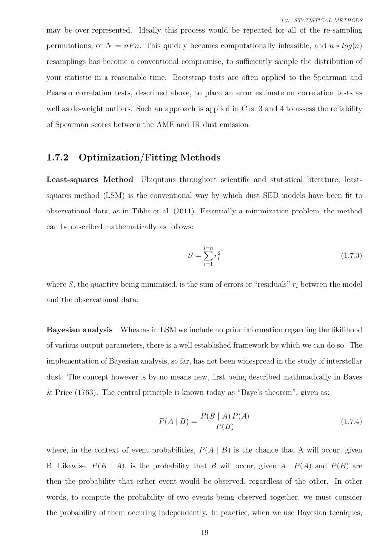
1.7.2 Optimization/Fitting Methods
Least-squares Method Ubiqutous throughout scientific and statistical literature, least-
squares method (LSM) is the conventional way by which dust SED models have been fit to
observational data, as in Tibbs et al. (2011). Essentially a minimization problem, the method
can be described mathematically as follows:
S =i=n∑i=1
r2i (1.7.3)
where S, the quantity being minimized, is the sum of errors or “residuals” ri between the model
and the observational data.
Bayesian analysis Whearas in LSM we include no prior information regarding the likilihood
of various output parameters, there is a well established framework by which we can do so. The
implementation of Bayesian analysis, so far, has not been widespread in the study of interstellar
dust. The concept however is by no means new, first being described mathmatically in Bayes
& Price (1763). The central principle is known today as “Baye’s theorem”, given as:
P (A | B) = P (B | A)P (A)P (B) (1.7.4)
where, in the context of event probabilities, P (A | B) is the chance that A will occur, given
B. Likewise, P (B | A), is the probability that B will occur, given A. P (A) and P (B) are
then the probability that either event would be observed, regardless of the other. In other
words, to compute the probability of two events being observed together, we must consider
the probability of them occuring independently. In practice, when we use Bayesian tecniques,
19

CHAPTER 1. INTRODUCTION
what we are doing is building-in to our model some prior knowledge or expectation about
the distribution of our output parameters. In contrast, when we use LSM, we are implicitly
assuming that any output value is equally likely. In the Bayesian framework, we consider that
we always have some type of prior expectation of the output distribution, and that this must
be stated or selected up-front. This forms the foundation of a method implemented in Ch. 3
to fit the dust SED properties of λ Orionis, called HB.
Hierarchical Bayesian Analysis In Bayesian analysis, we are specifying a prior expectation
for our parameters up-front. The probability distribution that we use can significantly affect
our result. If we instead infer a prior distribution from the data itself, we may be able to
fine-tune the fitting process, and extract patterns that may not be readily revealed by standard
Bayesisn analysis or LSM. This technique is implented in Ch 3, revealing a trend between PAH
emission and the AME, forming the core result of this thesis. We will show also how the result
could not have been demonstrated via LSM. The major advantages of HB are as follows:
• Prior is inferred from the data
• Less vulnerable to local minima
• Avoids noise-induced correlations
• Robust error propagation
The major disadvantage however is that HB is relatively expensive, computationally, compared
to LSM. Also, in the case of only a single data source, we would not be able to build a prior
distribution function from the data.
1.8 Scope of this Dissertation
We attempt to add to the understanding of AME and the possibility of spinning dust emission.
With ample multiwavelength data now available, and a new PAH-focused all-sky survey in
preparation by AKARI, we further test the PAH hypothesis, and assess how the IR to AME
correlation changes as a function of wavelength. This thesis represents the first time that
AKARI IRC data, have been utilized for AME investigation. Moreover, Ch. 3 represents the
first time that AKARI data, and hierarchical Bayesian dust SED fitting respectively, have been
20
1.8. SCOPE OF THIS DISSERTATION
used to investigate the λ Orionis region. The result of Ch. 3 is likewise unique in that it is the
first time a link between AME and PAHs has been demonstrated in λ Orionis, and the first
time that AME in any particular region has been shown to correlate better with PAH mass
than with the total dust mass. Chs. 3 and 4 both utilize a greater number of mid IR to sub-mm
photometric bands, than have ever been used for AME investigations. More specifically, this
work represents the first use of a photometric band covering the 6.2 µm C-C stretching PAH
feature, for a wide-scale galactic investigation.
1.8.1 An application of all-sky archival data
This is an astrophysical data archive based work. The primary goal is to highlight a particular
application of multiwavelength (mid-IR to radio), cross-archive all-sky data analysis. We de-
scribe the interrelatedness between mid to far IR dust emission and possible microwave emission
from dust. This is accomplished through an investigation of photometric all sky maps mainly
from AKARI, IRAS, Planck, and DIRBE.
1.8.2 Testing the spinning PAH hypothesis
For the present work, we consider the spinning PAH hypothesis to have the highest degree of
testability, due to the well-established presence of aromatic emisison features in the ISM. We
do not argue against the physical plausibility of nanosilicates to produce the AME. Indeed,
there is no argument to date that these potential physicalities are mutally exclusive, as long as
both potential carriers are sufficiently abundant. Nor does spinning dust emission theoretically
exclude magnetic dipole emission or microwave thermal dust emissivity fluctuations.
1.8.3 Limitations
We do not explore the modeling of microwave dust emission itself, rather we refer to estimates
of spinning dust emisison provided in the literature (Planck Collaboration et al. 2014c; Bennett
et al. 2003a) in the form of archival data and parameter maps. We consider this problem first
on an all-sky basis, not focusing on any pre-selected object of the sky — in order to assess
if there any general pattern between the IR and the AME, beyond the AME-dust correlation
already described above. We then focus on a region highlighted by the Planck Collaboration
as being especially worthy of further investigation (Planck Collaboration et al. 2016b), and
21
CHAPTER 1. INTRODUCTION
has a resolvable topology even at 1◦ resolution. Essentially all of the analyses and conclusions
presented in this work apply to an angular scale of approximately 1◦, and only for the given
component separation methods (Solar system, galactic, extragalactic) used by each of the data
providers.
1.8.4 Code availability
Because this work is intended to contribute working examples for future students, in addition to
making a research contribution, this thesis is accompanied by a github repository (to be made
available upon acceptance of the thesis.) 1 Most of analyses code are available in that repository,
in the form of Jupyter notebooks. Most of the figures, and code used to generate them, are
also included. The hierarchical Bayes dust SED fitting code used in this work was developed
by Galliano (2018), and its implementation in this work was carried out in collaboration with
their group. The details of the code are described in Galliano (2018), and are not included in
the respository for this thesis.
1Available at: https://github.com/aaroncnb/CosmicDust.
22
Chapter 2
Data Sources
2.1 A collection of skies
This work relies completely on all-sky surveys. All of the maps utilized are photometric-band
infrared maps, except for the AME data, which is an all-sky component separation analysis
product, from the Planck Collaboration’s efforts to separate galactic foregrounds from the
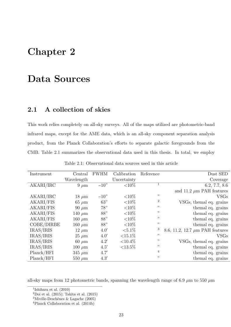
CMB. Table 2.1 summarizes the observational data used in this thesis. In total, we employ
Table 2.1: Observational data sources used in this article
Instrument Central FWHM Calibration Reference Dust SEDWavelength Uncertainty Coverage
AKARI/IRC 9 µm ~10” <10% 1 6.2, 7.7, 8.6and 11.2 µm PAH features
AKARI/IRC 18 µm ~10” <10% ” VSGsAKARI/FIS 65 µm 63” <10% 2 VSGs, themal eq. grainsAKARI/FIS 90 µm 78” <10% ” themal eq. grainsAKARI/FIS 140 µm 88” <10% ” themal eq. grainsAKARI/FIS 160 µm 88” <10% ” themal eq. grainsCOBE/DIRBE 160 µm 88” <10% ” themal eq. grainsIRAS/IRIS 12 µm 4.0′ <5.1% 3 8.6, 11.2, 12.7 µm PAH featuresIRAS/IRIS 25 µm 4.0′ <15.1% ” VSGsIRAS/IRIS 60 µm 4.2′ <10.4% ” VSGs, themal eq. grainsIRAS/IRIS 100 µm 4.5′ <13.5% ” themal eq. grainsPlanck/HFI 345 µm 4.7′ 4 themal eq. grainsPlanck/HFI 550 µm 4.3′ ” themal eq. grains
all-sky maps from 12 photometric bands, spanning the wavelength range of 6.9 µm to 550 µm1Ishihara et al. (2010)2Doi et al. (2015); Takita et al. (2015)3Miville-Deschênes & Lagache (2005)4Planck Collaboration et al. (2014b)
23
CHAPTER 2. DATA SOURCES
101 102 103
[ m]
0.5
1.0
1.5
2.0
2.5
Arb
itrar
y U
nits
VSGsBGsPAHsW12A9A18I12I25I60I100A65A90A140A160PLANCK857PLANCK545
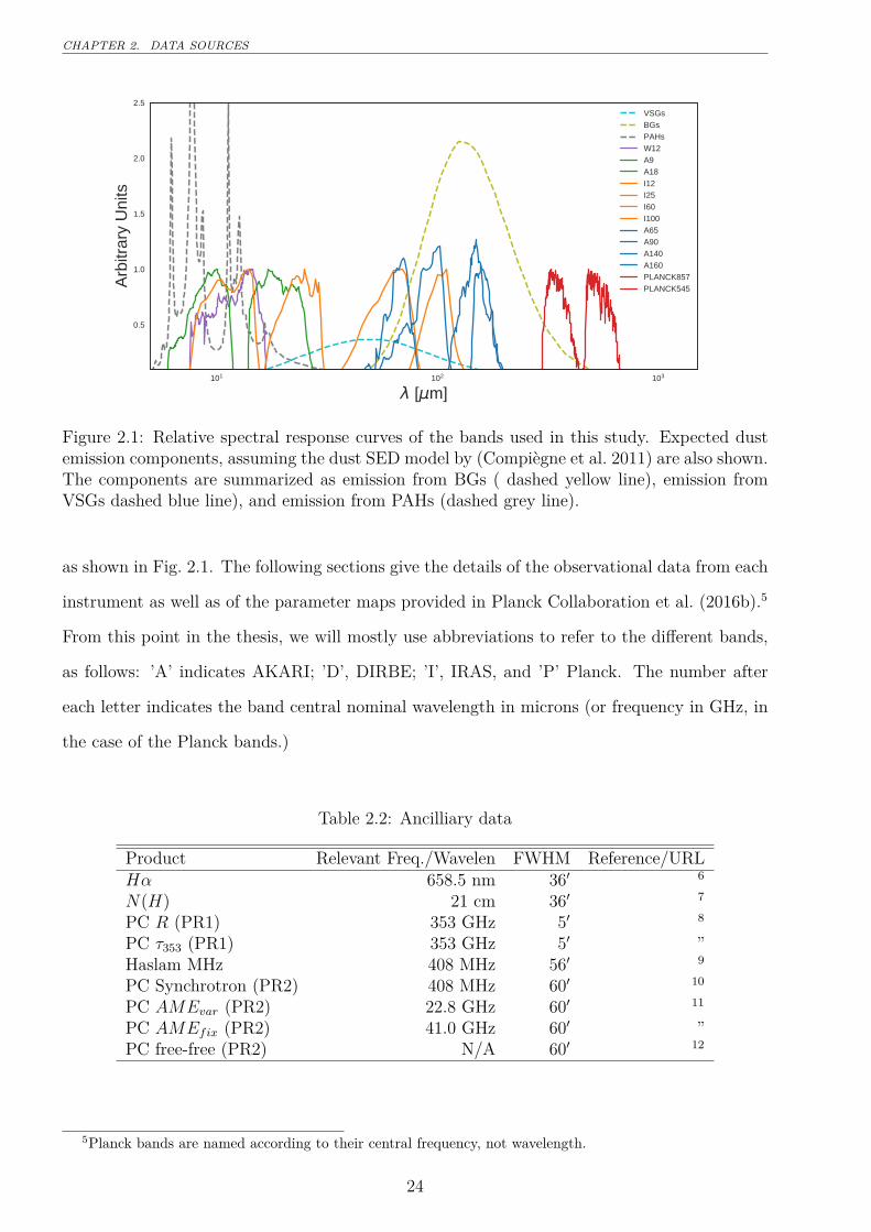
Figure 2.1: Relative spectral response curves of the bands used in this study. Expected dustemission components, assuming the dust SED model by (Compiègne et al. 2011) are also shown.The components are summarized as emission from BGs ( dashed yellow line), emission fromVSGs dashed blue line), and emission from PAHs (dashed grey line).
as shown in Fig. 2.1. The following sections give the details of the observational data from each
instrument as well as of the parameter maps provided in Planck Collaboration et al. (2016b).5
From this point in the thesis, we will mostly use abbreviations to refer to the different bands,
as follows: ’A’ indicates AKARI; ’D’, DIRBE; ’I’, IRAS, and ’P’ Planck. The number after
each letter indicates the band central nominal wavelength in microns (or frequency in GHz, in
the case of the Planck bands.)
Table 2.2: Ancilliary data
Product Relevant Freq./Wavelen FWHM Reference/URLHα 658.5 nm 36′ 6
N(H) 21 cm 36′ 7
PC R (PR1) 353 GHz 5′ 8
PC τ353 (PR1) 353 GHz 5′ ”Haslam MHz 408 MHz 56′ 9
PC Synchrotron (PR2) 408 MHz 60′ 10
PC AMEvar (PR2) 22.8 GHz 60′ 11
PC AMEfix (PR2) 41.0 GHz 60′ ”PC free-free (PR2) N/A 60′ 12
5Planck bands are named according to their central frequency, not wavelength.
24
2.2. AKARI
2.2 AKARI
The AKARI infrared space telescope revealed an entire sky of infrared light, from the mid to
far infrared, via two instruments (Murakami et al. 2007) the IRC (Onaka et al. 2007) and the
FIS (Kawada et al. 2007b). In this section we will discuss the all-sky surveys produced by these
two instruments .
2.2.1 AKARI/Infrared Camera (IRC)
IRC proivded us with both spectroscopic and phometric data from the near to mid-infrared.
In this work, we utilize the all-sky maps centered at 9 and 18 µm, created during the IRC’s
fast-scanning phase. We utilize the most recent version of the IRC data (Ishihara, et al., in
prep.) This version has had an updated model of the Zodiacal light, fitted and subtracted. The
details of the improved Zodi-model, which offers an improvement over that used for the IRAS
all-sky maps, are given in Kondo et al. (2016).
PAH feature coverage
The A9 all-sky map demonstrates the abundance of the PAH bands carrier in the Milky Way
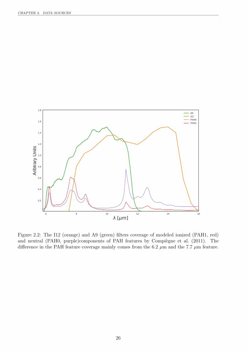
(Ishihara et al. 2010). Figure 2.2 shows the coverage of the PAH features (from both ionized
and neutral PAH components), as they are theoretically determined in Compiègne et al. (2011).
The A9 band uniquely covers major ionized PAH features at 6.2 and 7.7 µm; as well as neutral
PAH features at 8.6 and 11.2 µm across the entire sky (Onaka et al. 2007). The I12 band covers
the 11.2 and 8.6 µm features, and the similarly-shaped W12 band covers primarily the 11.2 µm
feature but do not cover the 7.7 µm completely. According to the distribution of PAH features6Finkbeiner (2003):
https://lambda.gsfc.nasa.gov/product/foreground/halpha_map.cfm7Kalberla, P. M. W. et al. (2005):
https://lambda.gsfc.nasa.gov/product/foreground/fg_LAB_HI_Survey_get.cfm8):
http://irsa.ipac.caltech.edu/data/Planck/release_1/all-sky-maps/previews/HFI_CompMap_ThermalDustModel_2048_R1.20/index.html
9Haslam et al. (1982):
10Planck Collaboration et al. (2016b):http://irsa.ipac.caltech.edu/data/Planck/release_2/all-sky-maps/previews/COM_CompMap_Synchrotron-commander_0256_R2.00/index.html
11http://irsa.ipac.caltech.edu/data/Planck/release_2/all-sky-maps/previews/COM_CompMap_AME-commander_0256_R2.00/index.html
12http://irsa.ipac.caltech.edu/data/Planck/release_2/all-sky-maps/previews/COM_CompMap_freefree-commander_0256_R2.00/index.html
25
CHAPTER 2. DATA SOURCES
6 8 10 12 14 16
[ m]
0.2
0.4
0.6
0.8
1.0
1.2
1.4
1.6
1.8
Arib
trar
y U
nits
A9I12PAH0PAH1
Figure 2.2: The I12 (orange) and A9 (green) filters coverage of modeled ionized (PAH1, red)and neutral (PAH0, purple)components of PAH features by Compiègne et al. (2011). Thedifference in the PAH feature coverage mainly comes from the 6.2 µm and the 7.7 µm feature.
26
2.2. AKARI
5 10 15 20 25 30
[ m]
2
4
6
8
10
12
14
F [W
/m2 /s
r]
Spitzer/IRS: Galactic planeA9I12A18I25
Figure 2.3: Coverage of MIR wavelengths by the filters used in this work. An Spitzer/IRSspectrum (see AOT4119040) of the galactic plane (thin blue line) demonstrates how IRC andIRAS photometric bands trace these features on an all-sky basis (Ishihara et al. 2007). StrongPAH features overlap with the A9 and I12, while the A18 and I25 micron bands only tracemuch weaker features.
across the response filters in Fig. 2.2, and referring back to the various dust components in
Fig. 2.1 it is also expected that the A9 band is most dominated by PAH emission even with
increasing U . This may seem counter-intuitive, since, as described in Ch. 1, the PAH spectral
shape does not show a temperature variation. However as T increases, the MIR extent of
thermal dust emission and emission from VSGs encroach on I12 and WI2 sooner than A9,
diluting emission from PAHs. In some ionized reigons, I12 may also include non-significant
contributions from the [NeII] line at 12.8 µm. Figure 2.3 demonstrates an example observational
galactic cirrus spectrum in the MIR, from Spitzer Infrared Spectrograph (IRS) (Werner et al.
2004) data, along with filters for all of the MIR bands used in this study. It indicates that the
other MIR bands, A18 and I25, do cover strong PAH features and are expected to be dominated
rather by emission from very small grains (VSGs), as was indicated in Fig. 2.1.
To help demonstate how the relative contribution from PAHs will change for each band,
for different ISRF strengths, Fig. 2.4 gives just such a calculation. These contributions remain
relatively constant out to a U of about 100, with the contribution from warm dust becomming
27
CHAPTER 2. DATA SOURCES
A9/PAH0 A9/PAH1 I12/PAH0 I12/PAH10.0
0.1
0.2
0.3
0.4
0.5
0.6
0.7In
-ban
d F
ract
iona
l Con
trib
utio
n
Figure 2.4: In-band contributions from charged (PAH1) neutral (PAH0) PAHs, to the emissiondetected by the I12 and A9 filters. These assume a model galactic cirrus spectrum simulatedwith the SED template of Compiègne et al. (2011).
a larger factor for the I12 and W12 bands. Thus, according to the DL01 template, A9 should
have the highest contribution from PAHs out to extreme radiation fields. At least to the
extent with which PAHs can endure harsh UV radiation, as PAHs are expected to evaporate
in strong enough radiation fields (Allain et al. 1996a,b; Bocchio et al. 2012; Pilleri et al. 2012;
Pavlyuchenkov et al. 2013).
PAH ionization
Figure 2.2 indicates that expected emission from ionized PAHs may preferentially contribute
to the A9 band, even though both I12 and A9 cover ionized and neutral features. A PAH SED
model calculation, using the Compiègne et al. (2011) SED template, supports that for Galactic
cirrus ISM conditions, emisison detected by the A9 band would have a higher contribution from
charged PAHs than the I12 band. This is demonstrated in Fig. 2.4. To be clear, both bands are
sensitive to both charged and neutral PAHs, however the relative contribution from charged
PAHs is expected to be higher for A9. Thus we might expect that the ratio of intensities in
this two bands, for a given line of sight (towards which PAHs are not destroyed), could trace
28
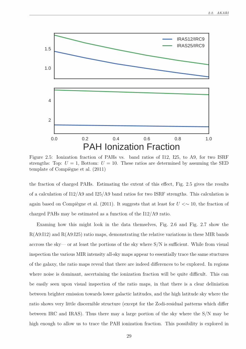
2.2. AKARI
1.0
1.5
IRAS12/IRC9 IRAS25/IRC9
0.0 0.2 0.4 0.6 0.8 1.0
PAH Ionization Fraction
2
4
Figure 2.5: Ionization fraction of PAHs vs. band ratios of I12, I25, to A9, for two ISRFstrengths: Top: U = 1, Bottom: U = 10. These ratios are determined by assuming the SEDtemplate of Compiègne et al. (2011)
the fraction of charged PAHs. Estimating the extent of this effect, Fig. 2.5 gives the results
of a calculation of I12/A9 and I25/A9 band ratios for two ISRF strengths. This calculation is
again based on Compiègne et al. (2011). It suggests that at least for U <∼ 10, the fraction of
charged PAHs may be estimated as a function of the I12/A9 ratio.
Examing how this might look in the data themselves, Fig. 2.6 and Fig. 2.7 show the
R(A9:I12) and R(A9:I25) ratio maps, demonstrating the relative variations in these MIR bands
accross the sky— or at least the portions of the sky where S/N is sufficient. While from visual
inspection the various MIR intensity all-sky maps appear to essentially trace the same stuctures
of the galaxy, the ratio maps reveal that there are indeed differences to be explored. In regions
where noise is dominant, ascertaining the ionization fraction will be quite difficult. This can
be easily seen upon visual inspection of the ratio maps, in that there is a clear deliniation
between brighter emission towards lower galactic latitudes, and the high latitude sky where the
ratio shows very little discernible structure (except for the Zodi-residual patterns which differ
between IRC and IRAS). Thus there may a large portion of the sky where the S/N may be
high enough to allow us to trace the PAH ionization fraction. This possibility is explored in
29
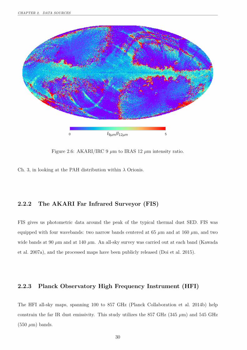
CHAPTER 2. DATA SOURCES
0 5I9 m/I12 m
Figure 2.6: AKARI/IRC 9 µm to IRAS 12 µm intensity ratio.
Ch. 3, in looking at the PAH distribution within λ Orionis.
2.2.2 The AKARI Far Infrared Surveyor (FIS)
FIS gives us photometric data around the peak of the typical thermal dust SED. FIS was
equipped with four wavebands: two narrow bands centered at 65 µm and at 160 µm, and two
wide bands at 90 µm and at 140 µm. An all-sky survey was carried out at each band (Kawada
et al. 2007a), and the processed maps have been publicly released (Doi et al. 2015).
2.2.3 Planck Observatory High Frequency Instrument (HFI)
The HFI all-sky maps, spanning 100 to 857 GHz (Planck Collaboration et al. 2014b) help
constrain the far IR dust emissivity. This study utilizes the 857 GHz (345 µm) and 545 GHz
(550 µm) bands.
30
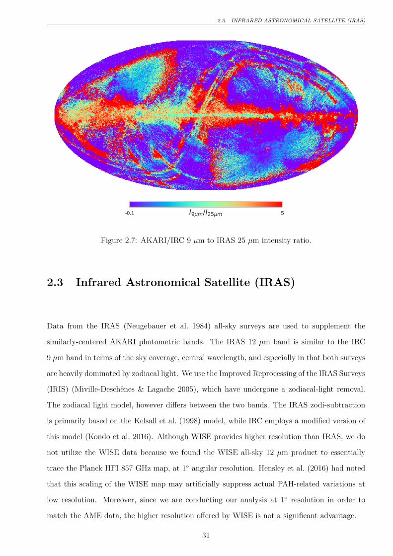
2.3. INFRARED ASTRONOMICAL SATELLITE (IRAS)
-0.1 5I9 m/I25 m
Figure 2.7: AKARI/IRC 9 µm to IRAS 25 µm intensity ratio.
2.3 Infrared Astronomical Satellite (IRAS)
Data from the IRAS (Neugebauer et al. 1984) all-sky surveys are used to supplement the
similarly-centered AKARI photometric bands. The IRAS 12 µm band is similar to the IRC
9 µm band in terms of the sky coverage, central wavelength, and especially in that both surveys
are heavily dominated by zodiacal light. We use the Improved Reprocessing of the IRAS Surveys
(IRIS) (Miville-Deschênes & Lagache 2005), which have undergone a zodiacal-light removal.
The zodiacal light model, however differs between the two bands. The IRAS zodi-subtraction
is primarily based on the Kelsall et al. (1998) model, while IRC employs a modified version of
this model (Kondo et al. 2016). Although WISE provides higher resolution than IRAS, we do
not utilize the WISE data because we found the WISE all-sky 12 µm product to essentially
trace the Planck HFI 857 GHz map, at 1◦ angular resolution. Hensley et al. (2016) had noted
that this scaling of the WISE map may artificially suppress actual PAH-related variations at
low resolution. Moreover, since we are conducting our analysis at 1◦ resolution in order to
match the AME data, the higher resolution offered by WISE is not a significant advantage.
31
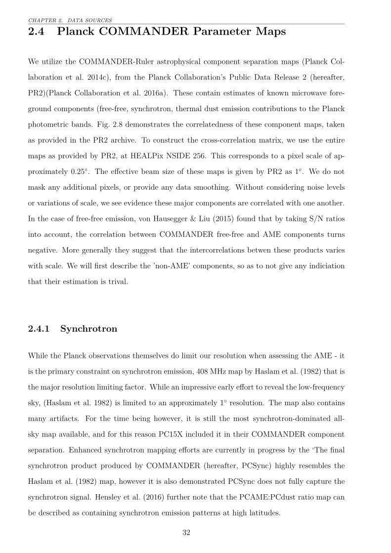
CHAPTER 2. DATA SOURCES
2.4 Planck COMMANDER Parameter Maps
We utilize the COMMANDER-Ruler astrophysical component separation maps (Planck Col-
laboration et al. 2014c), from the Planck Collaboration’s Public Data Release 2 (hereafter,
PR2)(Planck Collaboration et al. 2016a). These contain estimates of known microwave fore-
ground components (free-free, synchrotron, thermal dust emission contributions to the Planck
photometric bands. Fig. 2.8 demonstrates the correlatedness of these component maps, taken
as provided in the PR2 archive. To construct the cross-correlation matrix, we use the entire
maps as provided by PR2, at HEALPix NSIDE 256. This corresponds to a pixel scale of ap-
proximately 0.25◦. The effective beam size of these maps is given by PR2 as 1◦. We do not
mask any additional pixels, or provide any data smoothing. Without considering noise levels
or variations of scale, we see evidence these major components are correlated with one another.
In the case of free-free emission, von Hausegger & Liu (2015) found that by taking S/N ratios
into account, the correlation between COMMANDER free-free and AME components turns
negative. More generally they suggest that the intercorrelations betwen these products varies
with scale. We will first describe the ’non-AME’ components, so as to not give any indiciation
that their estimation is trival.
2.4.1 Synchrotron
While the Planck observations themselves do limit our resolution when assessing the AME - it
is the primary constraint on synchrotron emission, 408 MHz map by Haslam et al. (1982) that is
the major resolution limiting factor. While an impressive early effort to reveal the low-frequency
sky, (Haslam et al. 1982) is limited to an approximately 1◦ resolution. The map also contains
many artifacts. For the time being however, it is still the most synchrotron-dominated all-
sky map available, and for this reason PC15X included it in their COMMANDER component
separation. Enhanced synchrotron mapping efforts are currently in progress by the ‘The final
synchrotron product produced by COMMANDER (hereafter, PCSync) highly resembles the
Haslam et al. (1982) map, however it is also demonstrated PCSync does not fully capture the
synchrotron signal. Hensley et al. (2016) further note that the PCAME:PCdust ratio map can
be described as containing synchrotron emission patterns at high latitudes.
32
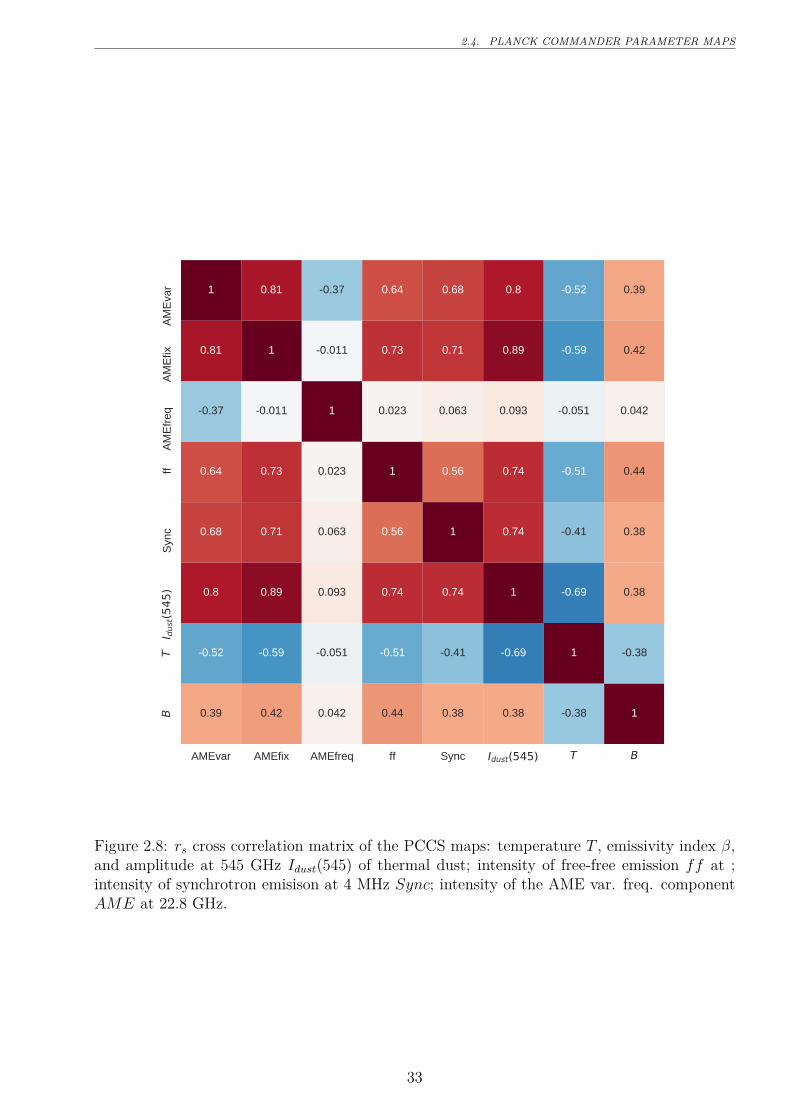
2.4. PLANCK COMMANDER PARAMETER MAPS
AMEvar AMEfix AMEfreq ff Sync Idust(545) T B
BT
I dus
t(545
)S
ync
ffA
ME
freq
AM
Efix
AM
Eva
r
0.39 0.42 0.042 0.44 0.38 0.38 -0.38 1
-0.52 -0.59 -0.051 -0.51 -0.41 -0.69 1 -0.38
0.8 0.89 0.093 0.74 0.74 1 -0.69 0.38
0.68 0.71 0.063 0.56 1 0.74 -0.41 0.38
0.64 0.73 0.023 1 0.56 0.74 -0.51 0.44
-0.37 -0.011 1 0.023 0.063 0.093 -0.051 0.042
0.81 1 -0.011 0.73 0.71 0.89 -0.59 0.42
1 0.81 -0.37 0.64 0.68 0.8 -0.52 0.39
Figure 2.8: rs cross correlation matrix of the PCCS maps: temperature T , emissivity index β,and amplitude at 545 GHz Idust(545) of thermal dust; intensity of free-free emission ff at ;intensity of synchrotron emisison at 4 MHz Sync; intensity of the AME var. freq. componentAME at 22.8 GHz.
33
CHAPTER 2. DATA SOURCES
2.4.2 Free-free emission
Unlike the PCSync component, the fitting of the Planck COMMANDER free-free component
map (hereafter, PCff) does not employ any free-free dominated emisison map, even though an
earlier Planck AME paper (Planck Collaboration et al. 2014d) had employed the Hα map by
Finkbeiner (2003). Uncertainties in this map arise from uncertainties in the gas temperature,
and the Gaunt factor. This emission source is the dominant source of confusion with AME,
especially for HII regions (Planck Collaboration et al. 2014d,c; Paladini et al. 2015).
2.4.3 Thermal dust emission
“Thermal dust emission” in the COMMANDER context refers to dust emission in the Rayleigh
Jeans-regime, as the COMMANDER fitting includes neither photometric constraints on the
thermal emission peak, nor on Wiens-regime emission from small grains. This component
essentially involves the fitting of a modified blackbody curve (Eq. ??.) to the Planck Photome-
try. This approach however results in an apparent anti-correlation between β and T (Fig. 2.8).
Whether or not this anti-correltion is genuine is still unsettled in the literature (Galliano et al.
2011; Juvela & Ysard 2012). In any case, we do not utilize the β and T , only the dust intensity
at 545 GHz (Id) parameter map.
2.4.4 AME data
The COMMANDER map release also provides an “AME component map”, which presumes
that AME originates from spinning dust. While acknowledging that such a decomposition
lacks a strong physical interpretation, Planck Collaboration et al. (2016b) break the AME
into two components: a spatially varying peak frequency component, AMEvar, and a spatially
constant peak frequency component, AMEfix. As seen in Fig. 2.9, virtually all of the fitted
peak frequncies for AMEvar are beyond the reach of WMAP and Planck. Only the fitted global
frequency, 33.5 GHz for the spatially constant component, is covered. However they note that
the combined components, per pixel, would have an average peak at least within the WMAP
coverage range. In any case, we stress that while this is the most careful all-sky attempt to
isolate the AME to date, the constraints of the the frequency peak are still heavily lacking. In
general, AMEvar is the dominant component, accounting for approximately 90% of the total
34
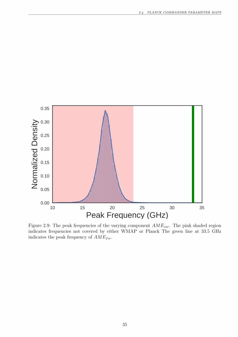
2.4. PLANCK COMMANDER PARAMETER MAPS
10 15 20 25 30 35
Peak Frequency (GHz)
0.00
0.05
0.10
0.15
0.20
0.25
0.30
0.35
Nor
mal
ized
Den
sity
Figure 2.9: The peak frequencies of the varying component AMEvar. The pink shaded regionindicates frequencies not covered by either WMAP or Planck The green line at 33.5 GHzindicates the peak frequency of AMEfix.
35
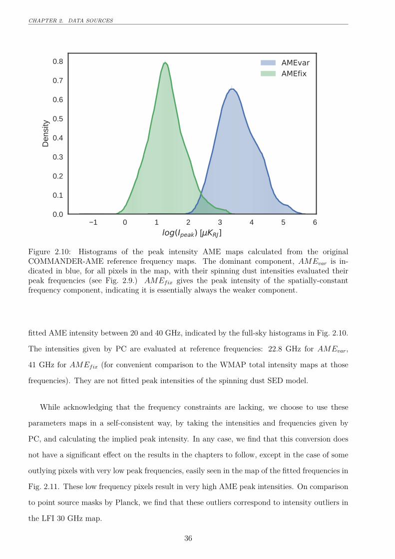
CHAPTER 2. DATA SOURCES
1 0 1 2 3 4 5 6log(Ipeak) [ KRJ]
0.0
0.1
0.2
0.3
0.4
0.5
0.6
0.7
0.8
Den
sity
AMEvarAMEfix
Figure 2.10: Histograms of the peak intensity AME maps calculated from the originalCOMMANDER-AME reference frequency maps. The dominant component, AMEvar is in-dicated in blue, for all pixels in the map, with their spinning dust intensities evaluated theirpeak frequencies (see Fig. 2.9.) AMEfix gives the peak intensity of the spatially-constantfrequency component, indicating it is essentially always the weaker component.
fitted AME intensity between 20 and 40 GHz, indicated by the full-sky histograms in Fig. 2.10.
The intensities given by PC are evaluated at reference frequencies: 22.8 GHz for AMEvar,
41 GHz for AMEfix (for convenient comparison to the WMAP total intensity maps at those
frequencies). They are not fitted peak intensities of the spinning dust SED model.
While acknowledging that the frequency constraints are lacking, we choose to use these
parameters maps in a self-consistent way, by taking the intensities and frequencies given by
PC, and calculating the implied peak intensity. In any case, we find that this conversion does
not have a significant effect on the results in the chapters to follow, except in the case of some
outlying pixels with very low peak frequencies, easily seen in the map of the fitted frequencies in
Fig. 2.11. These low frequency pixels result in very high AME peak intensities. On comparison
to point source masks by Planck, we find that these outliers correspond to intensity outliers in
the LFI 30 GHz map.
36

2.4. PLANCK COMMANDER PARAMETER MAPS
10 40peak(AME) [GHz]
Figure 2.11: All-sky map of the peak frequencies of the varying component AMEvar, corre-sponding to Fig. 2.9. Virtually all of the purple regions of the map correspond to pixels flaggedfor point sources in the LFI data. There are very few notable structures in the frequency mapoverall, other than the galactic plane itself, ρ Ophiuchus, and Perseus.
37
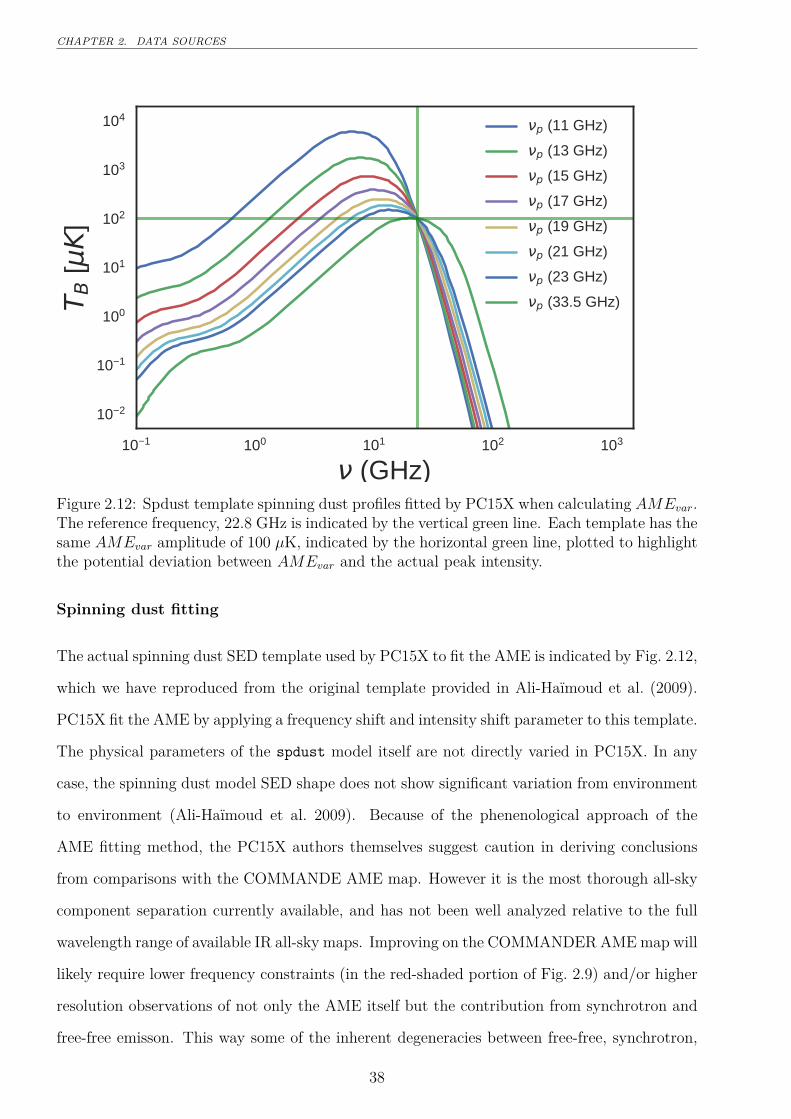
CHAPTER 2. DATA SOURCES
10 1 100 101 102 103
(GHz)
10 2
10 1
100
101
102
103
104
T B [
K]
p (11 GHz)
p (13 GHz)
p (15 GHz)
p (17 GHz)
p (19 GHz)
p (21 GHz)
p (23 GHz)
p (33.5 GHz)
Figure 2.12: Spdust template spinning dust profiles fitted by PC15X when calculating AMEvar.The reference frequency, 22.8 GHz is indicated by the vertical green line. Each template has thesame AMEvar amplitude of 100 µK, indicated by the horizontal green line, plotted to highlightthe potential deviation between AMEvar and the actual peak intensity.
Spinning dust fitting
The actual spinning dust SED template used by PC15X to fit the AME is indicated by Fig. 2.12,
which we have reproduced from the original template provided in Ali-Haïmoud et al. (2009).
PC15X fit the AME by applying a frequency shift and intensity shift parameter to this template.
The physical parameters of the spdust model itself are not directly varied in PC15X. In any
case, the spinning dust model SED shape does not show significant variation from environment
to environment (Ali-Haïmoud et al. 2009). Because of the phenenological approach of the
AME fitting method, the PC15X authors themselves suggest caution in deriving conclusions
from comparisons with the COMMANDE AME map. However it is the most thorough all-sky
component separation currently available, and has not been well analyzed relative to the full
wavelength range of available IR all-sky maps. Improving on the COMMANDER AMEmap will
likely require lower frequency constraints (in the red-shaded portion of Fig. 2.9) and/or higher
resolution observations of not only the AME itself but the contribution from synchrotron and
free-free emisson. This way some of the inherent degeneracies between free-free, synchrotron,
38
2.5. ALL-SKY DATA PROCESSING
thermal dust, and AME parameters may be able to be broken.
2.5 All-sky Data Processing
The HFI, FIS, and IRIS maps used here are downloaded from their respective online repositories,
as all-sky HEALPix13 maps (Górski et al. 2005). NSIDE 2048 maps. In the case of the IRC
maps, we first create HEALPix maps from the 4,857 all-sky survey tiles using the Aladin all-sky
data visualization platform (Bonnarel et al. 2000). NSIDE 2048 implies an average pixel spacing
of 1.7′. The maps are then degraded to NSIDE 1024 before carrying out a Gaussian-beam
smoothing to a 1◦ FWHM. Map smoothing itself is done in spherical harmonic space, before
the maps and transformed back to position space. These steps are handled by the smoothing
function contained in the healpy python package. Following the smoothing process, the maps
are degraded once more to NSIDE 256, or 15′ pixel-width 14. The value of each of the larger
NSIDE 256 pixels, comes from the mean of its parent NSIDE 1024 pixels. The purpose of this
processing is to ensure that all of the maps have the same resolution as the PR2 AME map.
13HEALPix core software is described at http://healpix.sourceforge.net. The HEALPIx python packagehealpy used in this work is available at: https://github.com/healpy/healpy
14HEALPix pixel scale rebinning carried out with healpy.ud_grade
39
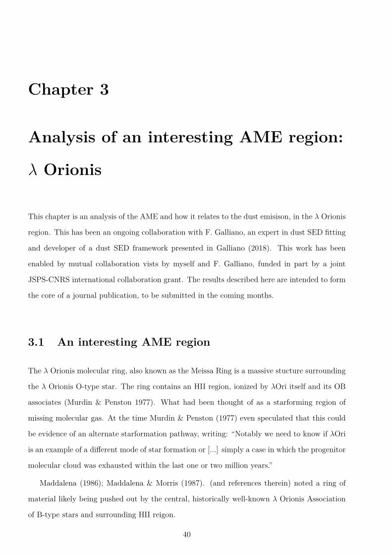
Chapter 3
Analysis of an interesting AME region:
λ Orionis
This chapter is an analysis of the AME and how it relates to the dust emisison, in the λ Orionis
region. This has been an ongoing collaboration with F. Galliano, an expert in dust SED fitting
and developer of a dust SED framework presented in Galliano (2018). This work has been
enabled by mutual collaboration vists by myself and F. Galliano, funded in part by a joint
JSPS-CNRS international collaboration grant. The results described here are intended to form
the core of a journal publication, to be submitted in the coming months.
3.1 An interesting AME region
The λ Orionis molecular ring, also known as the Meissa Ring is a massive stucture surrounding
the λ Orionis O-type star. The ring contains an HII region, ionized by λOri itself and its OB
associates (Murdin & Penston 1977). What had been thought of as a starforming region of
missing molecular gas. At the time Murdin & Penston (1977) even speculated that this could
be evidence of an alternate starformation pathway, writing: “Notably we need to know if λOri
is an example of a different mode of star formation or [...] simply a case in which the progenitor
molecular cloud was exhausted within the last one or two million years.”
Maddalena (1986); Maddalena & Morris (1987). (and references therein) noted a ring of
material likely being pushed out by the central, historically well-known λ Orionis Association
of B-type stars and surrounding HII reigon.
40

3.2. INVESTIGATIVE APPROACH
Cunha & Smith (1996) argued that the ring shape around λ Orionis may have resulted
from a supernova explosion, further speculating that λOri may have been a companion of the
progenitor. λ Orionis is a known binary system, however its current companion is a B-type
star. (Murdin & Penston 1977) . The central region is heated by the λ Orionis star itself, and
the Orion OB association it belongs to (Ochsendorf et al. 2015). The region is known to host
several young stellar and protostellar objects (Koenig et al. 2015).
At approx. 10◦ wide, we can see the outline of the structure even in the low (1◦ FWHM)
resolution PCAME map. The ring shape itself is thought to originate from a supernova, or
perhaps combined effects of the entire star formation history of the λ Orionis Association,
including the formation of its surrounding HII region (Aran 2009).
Although the λ Orionis region has been a popular target for study since approximately the
1980s. Duerr et al. (1982) wrote of the relative lack of work on the overall region: “Surprisingly,
this interesting complex has been little studied”. While this seems surprising given the numbe
of works on the region in the literature now, it is really the advent of all-sky missions that have
driven more recent interest. The large angular size is such that all-sky surveys were a natural
boon for study of such extended structures. WISE especially was a huge source of insight
(Koenig et al. 2015). More recently, Planck Collaboration et al. (2016c) strongly highlighted
the region as a strong candidate for further AME investigation.
3.2 Investigative approach
We have carried out an initial comparison of the AME of this region with its mid to far-IR
dust emission. The region is shown in Fig. 3.1 as it appears in 1◦-smoothed A9 data. The ring
structure itself indicates excess microwave emission attributed to AME, from the dominant
variable frequency component AMEvar (see Ch. 2). The central region is dominated by free-
free emission (Aran 2009; Koenig et al. 2015). Free-free emisison coming from the Hii phase
surrounding the λ Orionis association dominates the region’s morphology in Low Frequency
Instrument (LFI) images. (Planck Collaboration et al. 2016c). Taking the hint from Planck
Collaboration et al. (2016c) that this may be among the more reliably component separated
regions, we evaluate if there is any preferential relationship between any parameter of dust
emission and the AME. Fig. 3.2 shows the expected distribution of free-free emission in the
41
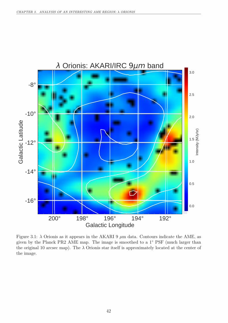
CHAPTER 3. ANALYSIS OF AN INTERESTING AME REGION: λ ORIONIS
192°194°196°198°200°Galactic Longitude
-16°
-14°
-12°
-10°
-8°
Gal
actic
Lat
itude
Orionis: AKARI/IRC 9 m band
0.0
0.5
1.0
1.5
2.0
2.5
3.0
Inte
nsity
(M
Jy/s
r)
Figure 3.1: λ Orionis as it appears in the AKARI 9 µm data. Contours indicate the AME, asgiven by the Planck PR2 AME map. The image is smoothed to a 1◦ PSF (much larger thanthe original 10 arcsec map). The λ Orionis star itself is approximately located at the center ofthe image.
42
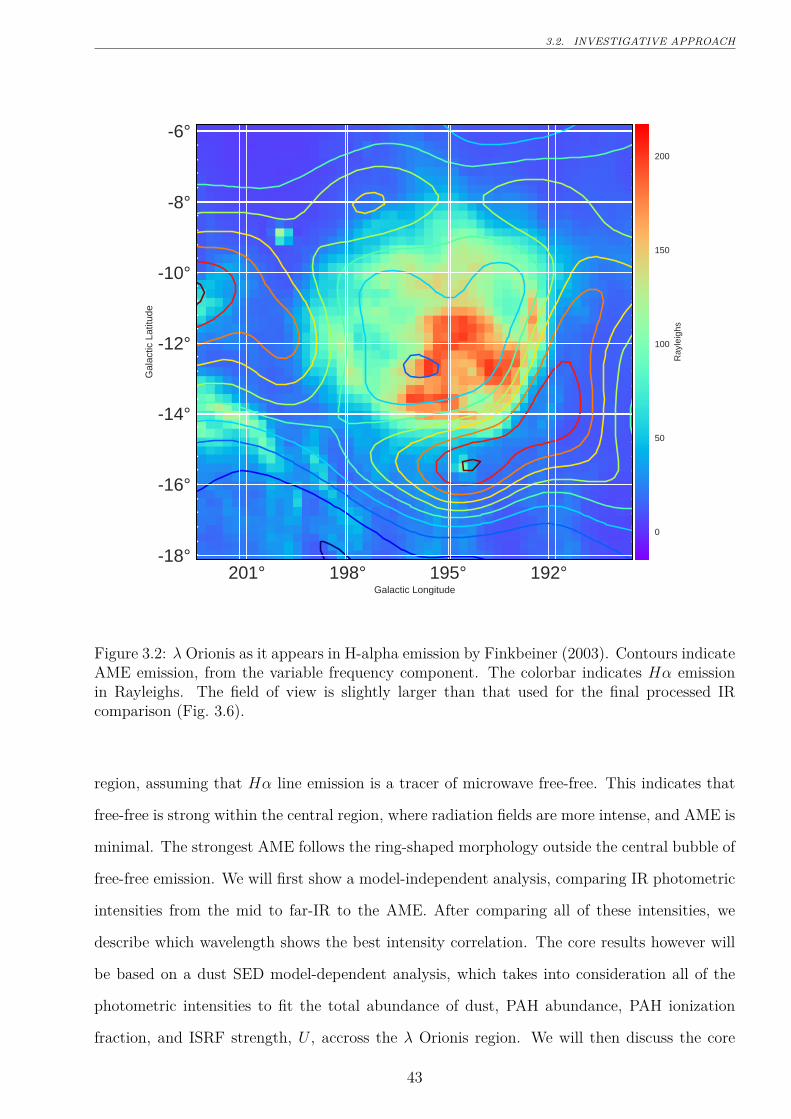
3.2. INVESTIGATIVE APPROACH
192°195°198°201°Galactic Longitude
-18°
-16°
-14°
-12°
-10°
-8°
-6°G
alac
tic L
atitu
de
0
50
100
150
200
Ray
leig
hs
Figure 3.2: λ Orionis as it appears in H-alpha emission by Finkbeiner (2003). Contours indicateAME emission, from the variable frequency component. The colorbar indicates Hα emissionin Rayleighs. The field of view is slightly larger than that used for the final processed IRcomparison (Fig. 3.6).
region, assuming that Hα line emission is a tracer of microwave free-free. This indicates that
free-free is strong within the central region, where radiation fields are more intense, and AME is
minimal. The strongest AME follows the ring-shaped morphology outside the central bubble of
free-free emission. We will first show a model-independent analysis, comparing IR photometric
intensities from the mid to far-IR to the AME. After comparing all of these intensities, we
describe which wavelength shows the best intensity correlation. The core results however will
be based on a dust SED model-dependent analysis, which takes into consideration all of the
photometric intensities to fit the total abundance of dust, PAH abundance, PAH ionization
fraction, and ISRF strength, U , accross the λ Orionis region. We will then discuss the core
43
CHAPTER 3. ANALYSIS OF AN INTERESTING AME REGION: λ ORIONIS
result, suggesting that PAH mass has a stronger relationship with AME than the total dust
mass does, representing the first time such a result has been found for a specific AME-prominent
region.
3.3 Data preparation
As indicated in Ch. 2, we use 12 photometric all-sky maps. For the IRC data (A9 and A18),
we produce mosiacs of λ Orionis from the latest version of the individual tiles provided internal
all-sky archive. A9 and A18 images are produced by regridding the images with the Montage
software by NASA/Infrared Processing and Analysis Center (IPAC). Figs. 3.4 and 3.5 show
high resolution mosaics of the A9 and A18 data before processing. 1 For the other sources,
HEALPix all-sky maps are available publicly, at sufficient resolution relative to their native
resolutions2. 34
Other data were obtained from publically archived HEALPix maps. This includes data
from IRAS, Planck, DIRBE, and AKARI/FIS. For For these data, we employ the healpix2wcs
functionality provided in the gnomdrizz python package56 When the extraction and regridding
are finished, all of the images — those extracted from Hierarchical Equal Area Iso Latitude
Pixelation of the Sphere (HEALPix) maps, as well as the IRC data — share a common FITS
header having a pixel grid spacing equal to the average pixel width in the NSIDE 256 HEALPix
scheme, or about ~0.25◦. After PSF smoothing, described in detail below, the data also have
a common ~1◦ FWHM effective PSF. Although this means that the grid is oversampled, we
choose this approach to preserve as much of the structure of the region as possible, even after
masking bad pixels. Another option would be to interpolate the bad pixels, and degrade the
pixel scale to the PSF size. However we choose the former method due to the relative large
number of bad pixels, especially around the regions affected by missing stripes. This means
that in the analyses that follow, what is important is the relative trends between correlation
coefficients, rather than their absolute values.1IRC all-sky data is still in the proprietary phase at the time of this writing, but should be public by April
2018.2Planck data was retreived from the NASA IPAC online archive at http://irsa.ipac.caltech.edu/data/
Planck/release_2/all-sky-maps/3AKARI/FIS data4IRAS/IRIS data5Available at http://cade.irap.omp.eu/dokuwiki/doku.php?id=software6“drizzlib” 1.2.2 and earlier were not able to correctly access HEALPix files with multiple fields/columns.
See appendix for our recommended workaround.
44

3.3. DATA PREPARATION
Figure 3.3: The λ Orionis region and its surroundings in AKARI FIS data, where A65 is blue,A90 is green, and A140 is red. The missing stripe patterns are visible, and affect all 3 bandsshown here as well as the A160 data.
3.3.1 Point-source and artifact masking
Missing stripes The AKARI all-sky survey suffers from a few missing stripe errors through-
out the IRC and FIS maps (Ishihara et al. 2010; Doi et al. 2015). This is a more serious issue
for FIS. Unfortunately for the present work, some of these stripes pass directly through the
λ Orionis region. Figs. 3.3, 3.4 and 3.5 display the data at near-native resolution, demonstrat-
ing where these patterns occur. Additionally there are some saturated pixels in both IRC and
FIS data.
Point sources A caveat that comes with added ionized PAH feature coverage of the A9
band, is that the shorter central wavelength placement allows more contamination from point
sources. We identify point sources with a moving-window approach provided in the astropy
Python package, flagging pixels which have higher than 5σ intensity among the surrounding
100 pixel window. We then place a mask at the center of the flagged point-sources. The masks
are propogated through the regridding step, such that the low-resolution pixels having more
than 50% of their area masked in the high resolution tiles, also become masked. Such pixels
appear black in Fig. 3.1. The same process is applied to the A18 data. For other maps, which
we extract from HEALPix data, we first regrid from HEALPix to rectangular grids, and then
apply the point-source search and masking as above. For the I12 and I25 images, the rejected
pixels were fewer than with A9, but positions overlapped with those already masked in A9.
45
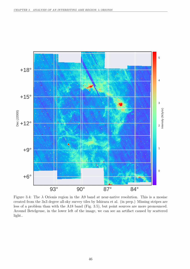
CHAPTER 3. ANALYSIS OF AN INTERESTING AME REGION: λ ORIONIS
84°87°90°93°RA (J2000)
+6°
+9°
+12°
+15°
+18°
Dec
(J2
000)
0
1
2
3
4
5
Inte
nsity
(M
Jy/s
r)
Figure 3.4: The λ Orionis region in the A9 band at near-native resolution. This is a mosiaccreated from the 3x3 degree all-sky survey tiles by Ishirara et al. (in prep.) Missing stripes areless of a problem than with the A18 band (Fig. 3.5), but point sources are more pronounced.Around Betelgeuse, in the lower left of the image, we can see an artifact caused by scatteredlight..
46
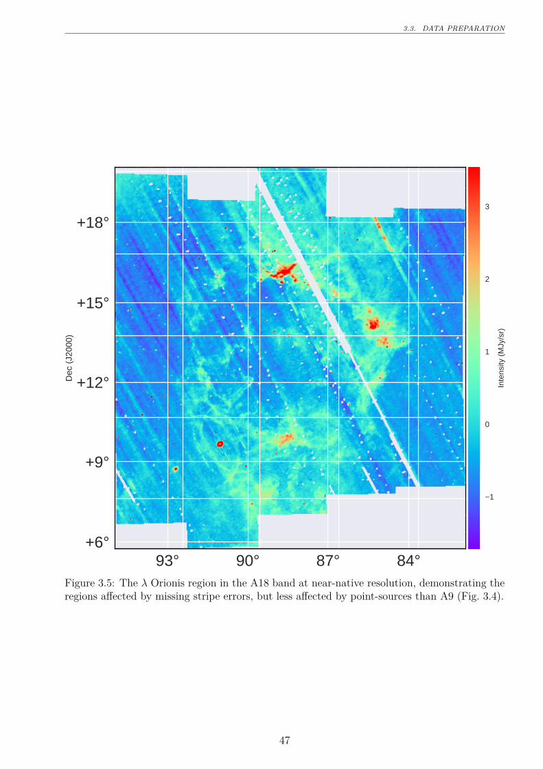
3.3. DATA PREPARATION
84°87°90°93°RA (J2000)
+6°
+9°
+12°
+15°
+18°
Dec
(J2
000)
1
0
1
2
3
Inte
nsity
(M
Jy/s
r)
Figure 3.5: The λ Orionis region in the A18 band at near-native resolution, demonstrating theregions affected by missing stripe errors, but less affected by point-sources than A9 (Fig. 3.4).
47
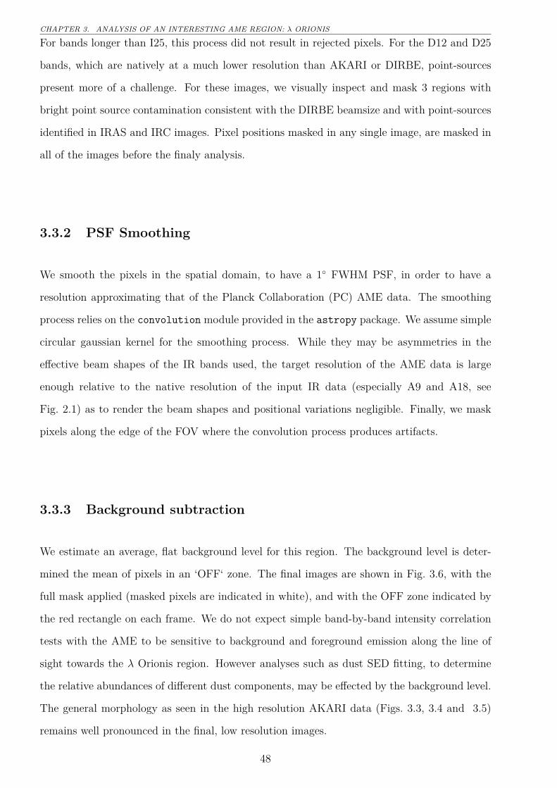
CHAPTER 3. ANALYSIS OF AN INTERESTING AME REGION: λ ORIONIS
For bands longer than I25, this process did not result in rejected pixels. For the D12 and D25
bands, which are natively at a much lower resolution than AKARI or DIRBE, point-sources
present more of a challenge. For these images, we visually inspect and mask 3 regions with
bright point source contamination consistent with the DIRBE beamsize and with point-sources
identified in IRAS and IRC images. Pixel positions masked in any single image, are masked in
all of the images before the finaly analysis.
3.3.2 PSF Smoothing
We smooth the pixels in the spatial domain, to have a 1◦ FWHM PSF, in order to have a
resolution approximating that of the Planck Collaboration (PC) AME data. The smoothing
process relies on the convolution module provided in the astropy package. We assume simple
circular gaussian kernel for the smoothing process. While they may be asymmetries in the
effective beam shapes of the IR bands used, the target resolution of the AME data is large
enough relative to the native resolution of the input IR data (especially A9 and A18, see
Fig. 2.1) as to render the beam shapes and positional variations negligible. Finally, we mask
pixels along the edge of the FOV where the convolution process produces artifacts.
3.3.3 Background subtraction
We estimate an average, flat background level for this region. The background level is deter-
mined the mean of pixels in an ‘OFF‘ zone. The final images are shown in Fig. 3.6, with the
full mask applied (masked pixels are indicated in white), and with the OFF zone indicated by
the red rectangle on each frame. We do not expect simple band-by-band intensity correlation
tests with the AME to be sensitive to background and foreground emission along the line of
sight towards the λ Orionis region. However analyses such as dust SED fitting, to determine
the relative abundances of different dust components, may be effected by the background level.
The general morphology as seen in the high resolution AKARI data (Figs. 3.3, 3.4 and 3.5)
remains well pronounced in the final, low resolution images.
48
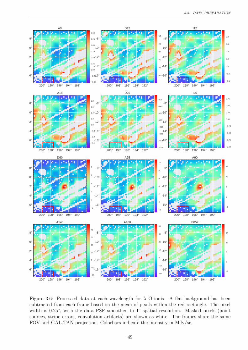
3.3. DATA PREPARATION
192°194°196°198°200°
-16°
-14°
-12°
-10°
-8°
A9
0.50
0.25
0.00
0.25
0.50
0.75
1.00
1.25
1.50
192°194°196°198°200°
-16°
-14°
-12°
-10°
-8°
D12
0.2
0.0
0.2
0.4
0.6
0.8
192°194°196°198°200°
-16°
-14°
-12°
-10°
-8°
I12
0.4
0.2
0.0
0.2
0.4
0.6
0.8
192°194°196°198°200°
-16°
-14°
-12°
-10°
-8°
A18
0.6
0.4
0.2
0.0
0.2
0.4
0.6
0.8
192°194°196°198°200°
-16°
-14°
-12°
-10°
-8°
D25
1.00
0.75
0.50
0.25
0.00
0.25
0.50
0.75
192°194°196°198°200°
-16°
-14°
-12°
-10°
-8°
I25
1.00
0.75
0.50
0.25
0.00
0.25
0.50
0.75
192°194°196°198°200°
-16°
-14°
-12°
-10°
-8°
D60
2
0
2
4
6
8
192°194°196°198°200°
-16°
-14°
-12°
-10°
-8°
A65
2
0
2
4
6
8
10
192°194°196°198°200°
-16°
-14°
-12°
-10°
-8°
A90
5
0
5
10
15
192°194°196°198°200°
-16°
-14°
-12°
-10°
-8°
A140
20
10
0
10
20
30
40
192°194°196°198°200°
-16°
-14°
-12°
-10°
-8°
A160
20
10
0
10
20
30
40
192°194°196°198°200°
-16°
-14°
-12°
-10°
-8°
P857
5
0
5
10
15
Figure 3.6: Processed data at each wavelength for λ Orionis. A flat background has beensubtracted from each frame based on the mean of pixels within the red rectangle. The pixelwidth is 0.25◦, with the data PSF smoothed to 1◦ spatial resolution. Masked pixels (pointsources, stripe errors, convolution artifacts) are shown as white. The frames share the sameFOV and GAL-TAN projection. Colorbars indicate the intensity in MJy/sr.
49
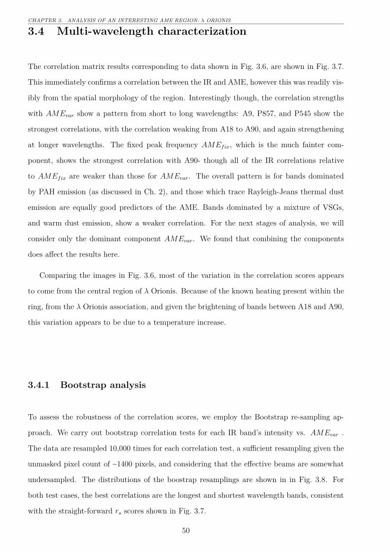
CHAPTER 3. ANALYSIS OF AN INTERESTING AME REGION: λ ORIONIS
3.4 Multi-wavelength characterization
The correlation matrix results corresponding to data shown in Fig. 3.6, are shown in Fig. 3.7.
This immediately confirms a correlation between the IR and AME, however this was readily vis-
ibly from the spatial morphology of the region. Interestingly though, the correlation strengths
with AMEvar show a pattern from short to long wavelengths: A9, P857, and P545 show the
strongest correlations, with the correlation weaking from A18 to A90, and again strengthening
at longer wavelengths. The fixed peak frequency AMEfix, which is the much fainter com-
ponent, shows the strongest correlation with A90- though all of the IR correlations relative
to AMEfix are weaker than those for AMEvar. The overall pattern is for bands dominated
by PAH emission (as discussed in Ch. 2), and those which trace Rayleigh-Jeans thermal dust
emission are equally good predictors of the AME. Bands dominated by a mixture of VSGs,
and warm dust emission, show a weaker correlation. For the next stages of analysis, we will
consider only the dominant component AMEvar. We found that combining the components
does affect the results here.
Comparing the images in Fig. 3.6, most of the variation in the correlation scores appears
to come from the central region of λ Orionis. Because of the known heating present within the
ring, from the λ Orionis association, and given the brightening of bands between A18 and A90,
this variation appears to be due to a temperature increase.
3.4.1 Bootstrap analysis
To assess the robustness of the correlation scores, we employ the Bootstrap re-sampling ap-
proach. We carry out bootstrap correlation tests for each IR band’s intensity vs. AMEvar .
The data are resampled 10,000 times for each correlation test, a sufficient resampling given the
unmasked pixel count of ~1400 pixels, and considering that the effective beams are somewhat
undersampled. The distributions of the boostrap resamplings are shown in in Fig. 3.8. For
both test cases, the best correlations are the longest and shortest wavelength bands, consistent
with the straight-forward rs scores shown in Fig. 3.7.
50
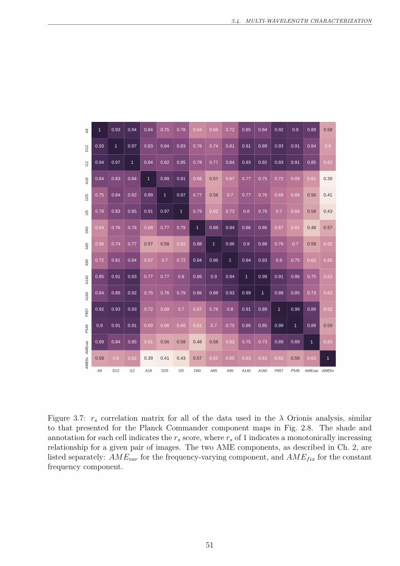
3.4. MULTI-WAVELENGTH CHARACTERIZATION
A9 D12 I12 A18 D25 I25 D60 A65 A90 A140 A160 P857 P545 AMEvar AMEfix
AM
Efix
AM
Eva
rP
545
P85
7A
160
A14
0A
90A
65D
60I2
5D
25A
18I1
2D
12A
9
0.58 0.6 0.62 0.39 0.41 0.43 0.57 0.62 0.65 0.63 0.63 0.62 0.59 0.63 1
0.89 0.84 0.85 0.61 0.56 0.58 0.48 0.58 0.63 0.75 0.73 0.89 0.89 1 0.63
0.9 0.91 0.91 0.69 0.66 0.66 0.61 0.7 0.75 0.86 0.85 0.99 1 0.89 0.59
0.92 0.93 0.93 0.72 0.69 0.7 0.67 0.76 0.8 0.91 0.89 1 0.99 0.89 0.62
0.84 0.89 0.92 0.75 0.76 0.79 0.86 0.88 0.93 0.99 1 0.89 0.85 0.73 0.63
0.85 0.91 0.93 0.77 0.77 0.8 0.86 0.9 0.94 1 0.99 0.91 0.86 0.75 0.63
0.72 0.81 0.84 0.67 0.7 0.73 0.94 0.96 1 0.94 0.93 0.8 0.75 0.63 0.65
0.66 0.74 0.77 0.57 0.58 0.62 0.88 1 0.96 0.9 0.88 0.76 0.7 0.58 0.62
0.64 0.76 0.78 0.68 0.77 0.79 1 0.88 0.94 0.86 0.86 0.67 0.61 0.48 0.57
0.78 0.83 0.85 0.91 0.97 1 0.79 0.62 0.73 0.8 0.79 0.7 0.66 0.58 0.43
0.75 0.84 0.82 0.89 1 0.97 0.77 0.58 0.7 0.77 0.76 0.69 0.66 0.56 0.41
0.84 0.83 0.84 1 0.89 0.91 0.68 0.57 0.67 0.77 0.75 0.72 0.69 0.61 0.39
0.94 0.97 1 0.84 0.82 0.85 0.78 0.77 0.84 0.93 0.92 0.93 0.91 0.85 0.62
0.93 1 0.97 0.83 0.84 0.83 0.76 0.74 0.81 0.91 0.89 0.93 0.91 0.84 0.6
1 0.93 0.94 0.84 0.75 0.78 0.64 0.66 0.72 0.85 0.84 0.92 0.9 0.89 0.58
Figure 3.7: rs correlation matrix for all of the data used in the λ Orionis analysis, similarto that presented for the Planck Commander component maps in Fig. 2.8. The shade andannotation for each cell indicates the rs score, where rs of 1 indicates a monotonically increasingrelationship for a given pair of images. The two AME components, as described in Ch. 2, arelisted separately: AMEvar for the frequency-varying component, and AMEfix for the constantfrequency component.
51
CHAPTER 3. ANALYSIS OF AN INTERESTING AME REGION: λ ORIONIS
0.4 0.5 0.6 0.7 0.8 0.9
rs (10,000 Bootstrap Resamplings)
0
10
20
30
40
50
60
70A9: rs = 0.886 +/- 0.006D12: rs = 0.835 +/- 0.01I12: rs = 0.845 +/- 0.009A18: rs = 0.611 +/- 0.017D25: rs = 0.559 +/- 0.019I25: rs = 0.576 +/- 0.018D60: rs = 0.484 +/- 0.024A65: rs = 0.577 +/- 0.022A90: rs = 0.632 +/- 0.021A140: rs = 0.748 +/- 0.014A160: rs = 0.727 +/- 0.014P857: rs = 0.889 +/- 0.007P545: rs = 0.893 +/- 0.007
Figure 3.8: Re-sampled (Bootstrap) correlation tests for IR emission in λ Orionis vs. AME.Each band’s rs distribution is shown in a different color (the same color scheme for both plots).The width of the distribution indicates the error for the given data in the correlation coefficient.The mean and standard deviation of the scores are given in the legend of each plot. The plotranges only show positive values, since no negative scores were produced.
3.5 Comparison with SED Fitting
We performed a full dust SED fitting on the λ Orionis photometry, according to the dust
model by Galliano et al. (2011), and the hierarchical Bayesian SED fitting framework by Gal-
liano (2018). There are 4 free paremeters: total dust massMdust, fraction of dust mass as PAHs
qPAH , the fraction of PAHs that are ionized, and the average strength of the ISRF U . As indi-
cated in Ch. 1, we implement such an analysis here primarily because it allows a more careful
propgation of the observational errors. We utilize both the HB approach and a least-squares
analysis. The HB approach allows us to accurately propogate errors in the data (including cali-
bration uncertainties) through the SED fitting process, as well as the correlation test thereafter.
Compared to the ubiquitous LSM In traditional SED fitting we often assume only Gaussian
uncorrelated noise. Even if this were a valid assumption for the raw data, processing steps may
induce correlations or skew noise. Induced correlations may also appear in the parameters fit
via standard approaches, when environments are mixed along the line-of-sight (Shetty et al.
2009).
We used a mixture of silicate and carbonaceous dust, silicate dust, the two dominant cate-
52
3.5. COMPARISON WITH SED FITTING
gories of interstellar dust as described in Ch. 1. However, instead of the graphite-based carbon
dust invoked by the canonical Draine & Li (2007b) model (DL07), we assume amorphous car-
bon. This is an attempt to account for an excessive dust-gas-ratio, reported by Israel et al.
(2010); Bot et al. (2010) in the Large Megellanic Cloud (LMC), which was found by Galliano
et al. (2011) to violate elemental depletion constraints. The increased opacity of amorphous
carbon (a factor of 2-3 more than DL07) allows a better fit to Herschel observations of the
LMC (Galliano et al. 2011), and Planck observations of the Milky Way (Planck Collaboration
et al. 2016d). We assume that the radiation field heating this dust mixture takes the profile of
the typical Galactic ISRF in Mathis et al. (1983).
We only carry out the fitting for unmasked pixels. We are primarily interested in which of
the corrleations Mdust vs. IAME or MPAH vs. IAME is stronger.
Two sample SED fitting results are shown in Figs. 3.9, and 3.10. Performing such fits for all
of the pixels, we are able to see how IAME varies with the dust properties of the region. Fig. 3.11
shows the fitted dust mass per pixel, relative to the AME intensity. AME intensity is scaled by
the ISRF intensity U . Although spinning dust emission is not predicted to vary directly with
U , we consider that the ISRF may serve as a diagnostic of environmental conditions in the
ISM. In any case, we find that performing such a scaling improves the correlations with dust
mass. Figs. 3.12 and 3.13 describe the variation with MPAH and MPAH+. Based on the dust
properties derived from these SED fits, we investigate whether any fitted parameter shows a
preferential relation with the AME. Figs. 3.11-3.13 reveal a very similar trend between the AME
and the parametersMPAH ,MPAH+, andMdust. There is a slightly improved correlation between
Mdust and MPAH (0.857 vs 0.867). This is consistent with the intensity cross correlations in
Fig. 3.7. These corrleations are discussed further in Sec. 3.6 and Fig. 3.14.
3.5.1 Comparing the Correlation Strengths
In addition to probability distribution functions of the fitted parameters, HB allows us to
plot the final PDFs of the correlation coefficients themselves. This is a more robust way of
comparing the correlation strengths than simply bootstrapping the correlations. Fig. 3.14
shows the rs PDFs for the 3 major correlations of interest: rs(IAME,Mdust), rs(IAME,MPAH),
and rs(IAME,MPAH+). To assess the effect of the morphology of λ Orionis on these results, we
show the same PDFs but omitting the central region of λ Orionis. This is shown in Fig. 3.15.
53
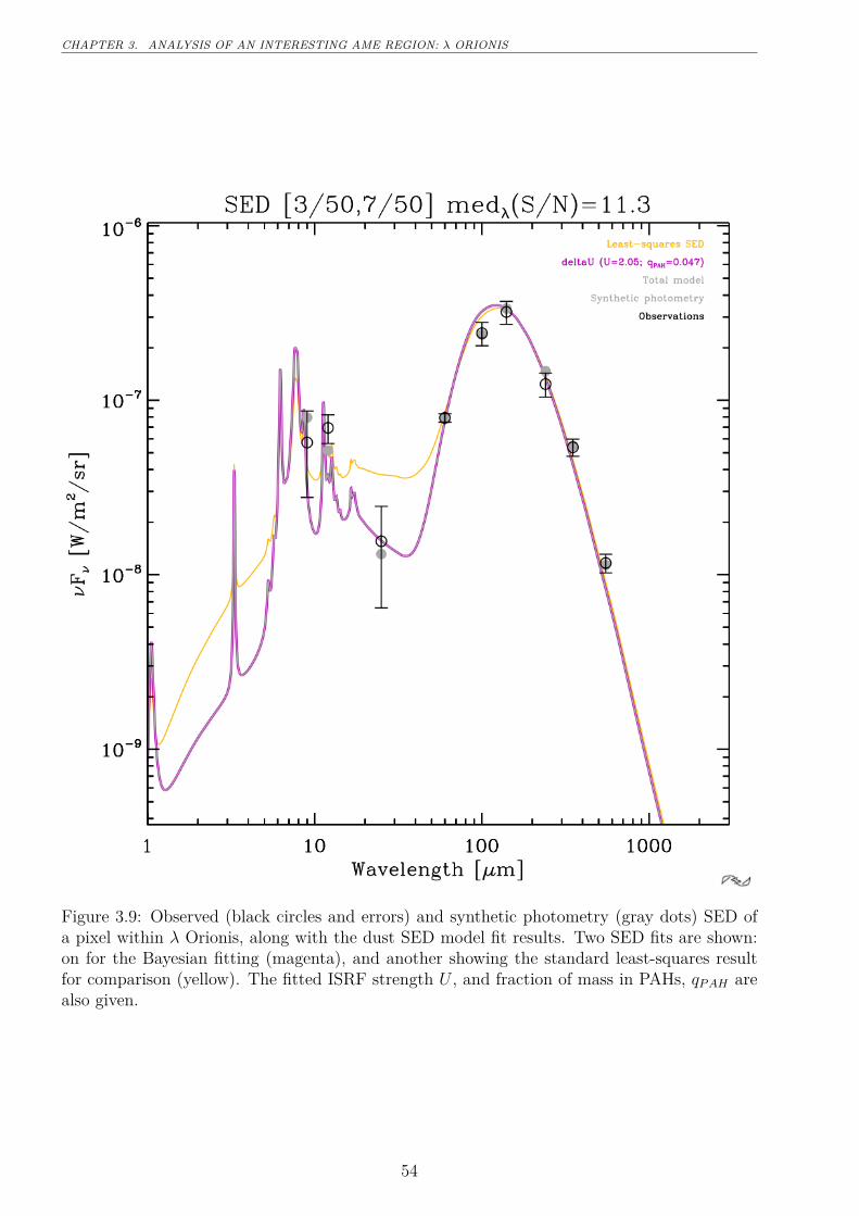
CHAPTER 3. ANALYSIS OF AN INTERESTING AME REGION: λ ORIONIS
Figure 3.9: Observed (black circles and errors) and synthetic photometry (gray dots) SED ofa pixel within λ Orionis, along with the dust SED model fit results. Two SED fits are shown:on for the Bayesian fitting (magenta), and another showing the standard least-squares resultfor comparison (yellow). The fitted ISRF strength U , and fraction of mass in PAHs, qPAH arealso given.
54
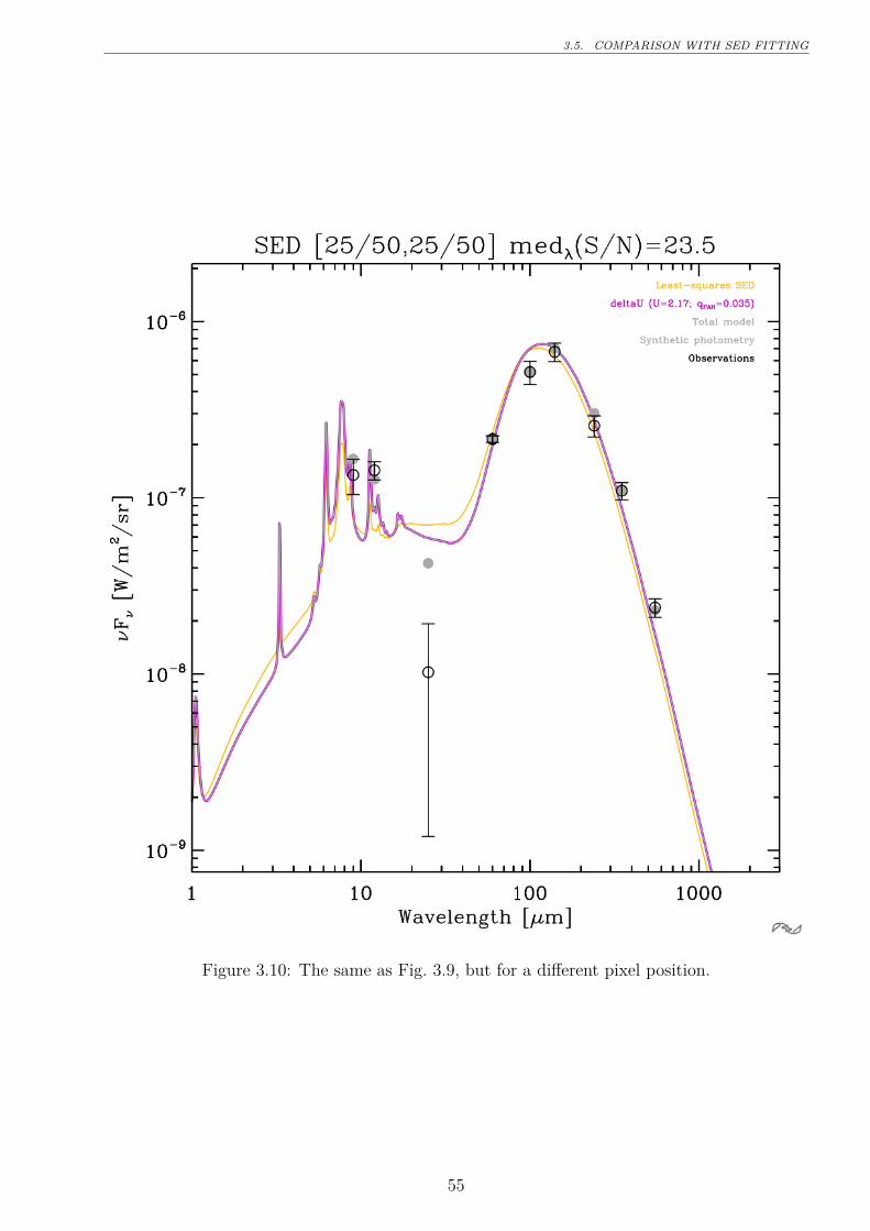
3.5. COMPARISON WITH SED FITTING
Figure 3.10: The same as Fig. 3.9, but for a different pixel position.
55
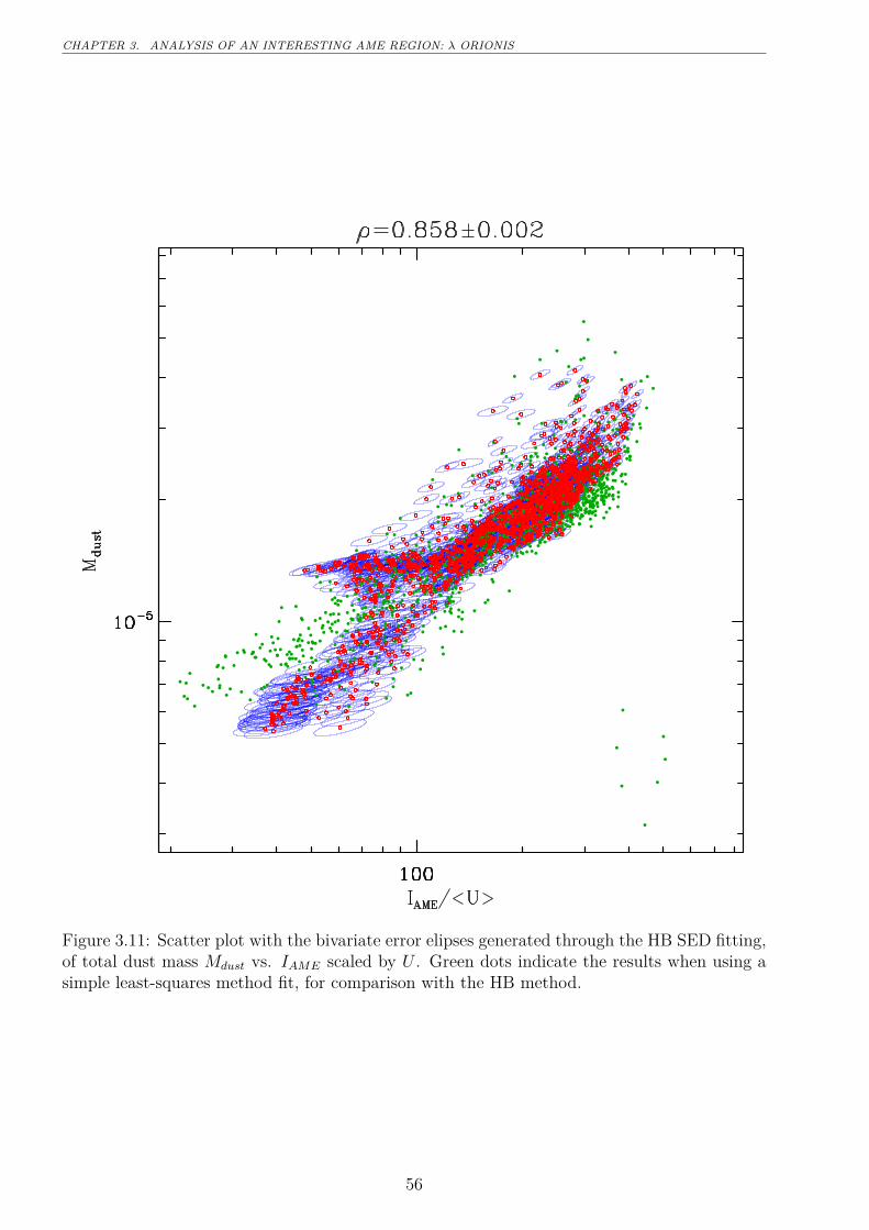
CHAPTER 3. ANALYSIS OF AN INTERESTING AME REGION: λ ORIONIS
Figure 3.11: Scatter plot with the bivariate error elipses generated through the HB SED fitting,of total dust mass Mdust vs. IAME scaled by U . Green dots indicate the results when using asimple least-squares method fit, for comparison with the HB method.
56
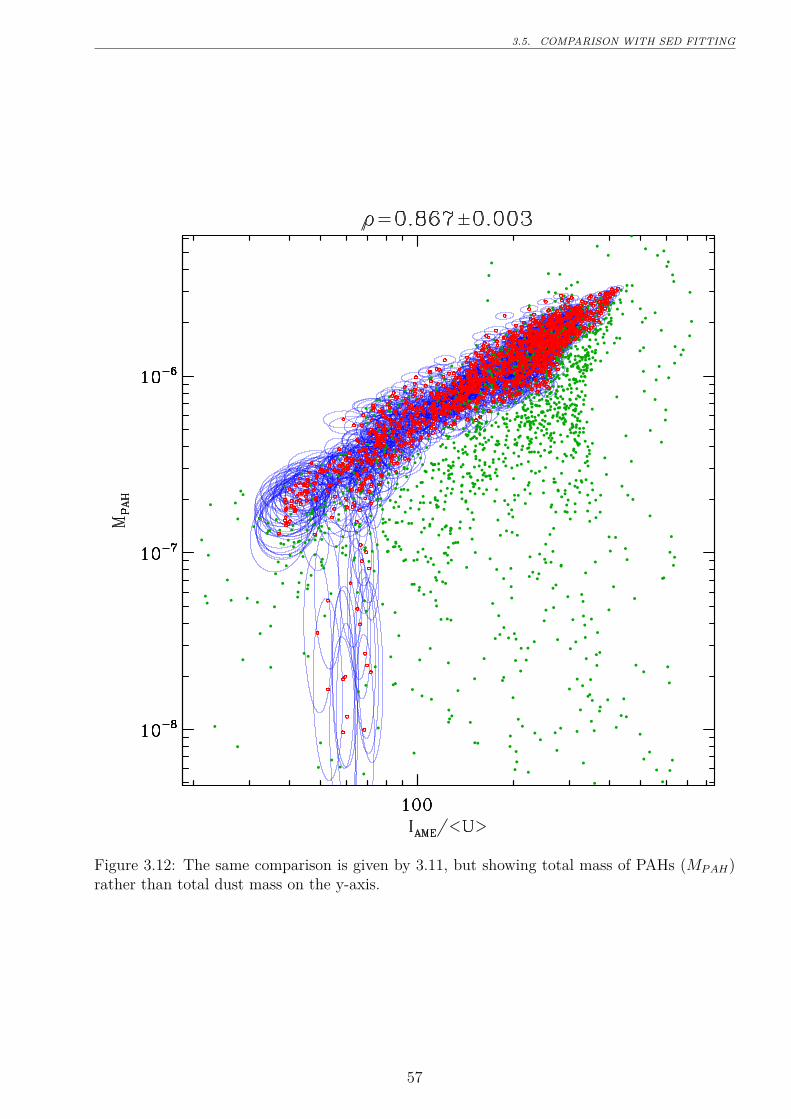
3.5. COMPARISON WITH SED FITTING
Figure 3.12: The same comparison is given by 3.11, but showing total mass of PAHs (MPAH)rather than total dust mass on the y-axis.
57
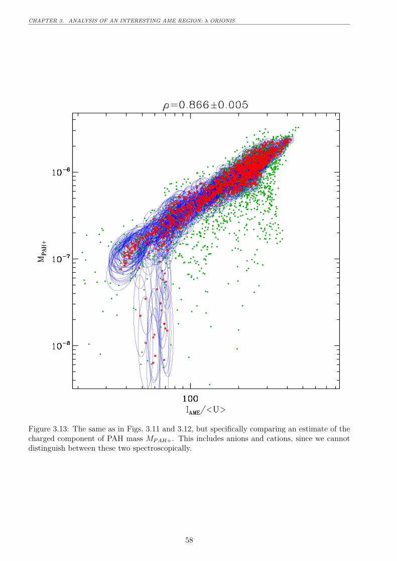
CHAPTER 3. ANALYSIS OF AN INTERESTING AME REGION: λ ORIONIS
Figure 3.13: The same as in Figs. 3.11 and 3.12, but specifically comparing an estimate of thecharged component of PAH mass MPAH+. This includes anions and cations, since we cannotdistinguish between these two spectroscopically.
58
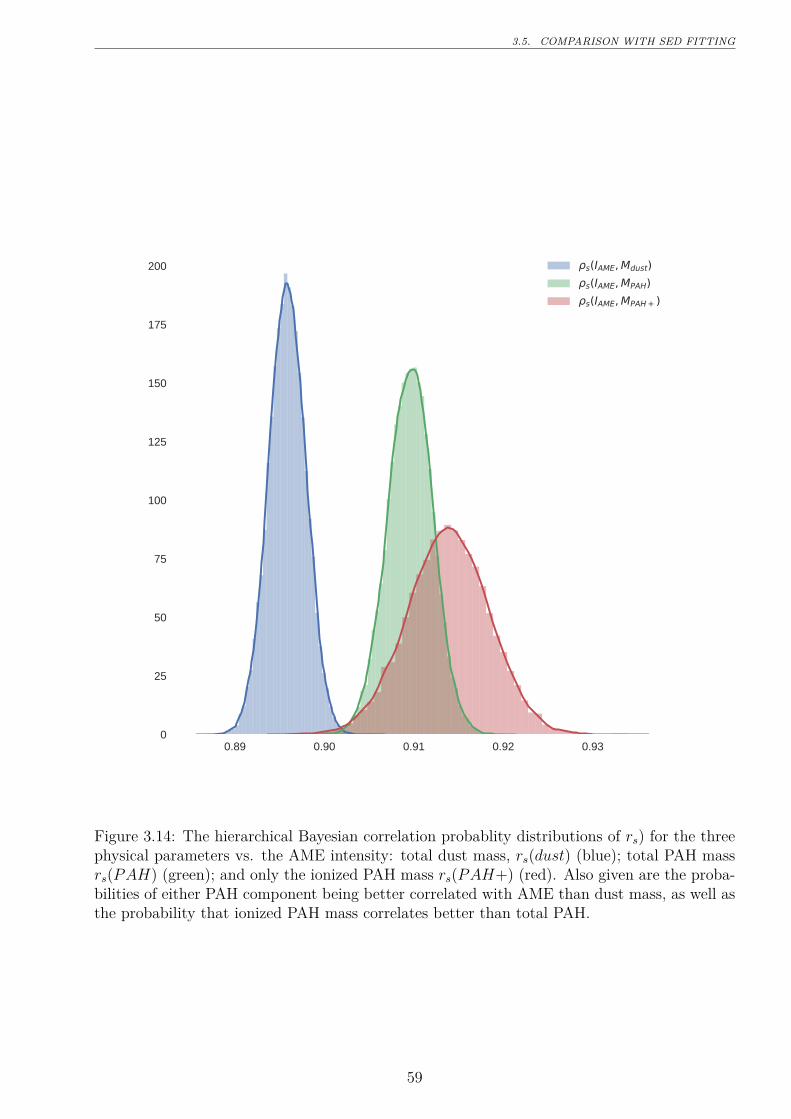
3.5. COMPARISON WITH SED FITTING
0.89 0.90 0.91 0.92 0.930
25
50
75
100
125
150
175
200 s(IAME, Mdust)s(IAME, MPAH)s(IAME, MPAH + )
Figure 3.14: The hierarchical Bayesian correlation probablity distributions of rs) for the threephysical parameters vs. the AME intensity: total dust mass, rs(dust) (blue); total PAH massrs(PAH) (green); and only the ionized PAH mass rs(PAH+) (red). Also given are the proba-bilities of either PAH component being better correlated with AME than dust mass, as well asthe probability that ionized PAH mass correlates better than total PAH.
59
CHAPTER 3. ANALYSIS OF AN INTERESTING AME REGION: λ ORIONIS
The extent of the mask is indicated in Fig 3.16.
3.6 Discussion
In λ Orionis we found that accross the whole region, A9 emission and P545 emission were the
most strongly correlated with AME. This is apparent both in the photometric band analysis,
and in the dust SED fitting. The fact that the correlation strengths of PAH-tracing mission
and sub-mm emission are similar is in-line with what we have seen in Ysard et al. (2010) and
Hensley et al. (2016). In those works, the two relationships (MIR vs. AME and FIR vs. AME)
are very close, although these two papers are odds as to which relationship is stronger, and
thus in their final interpretation. With the present data and analysis of λ Orionis, we fail to
rule out PAHs as carriers of the AME. In fact, our primary result, shown in Fig. 3.14 indicates
that PAH mass is a stronger predictor of the AME, compared to the total dust mass. This is
the first time such a significant result has been found, in support of the PAH hypothesis for a
particular region. This core result is unchanged even when we examine the outer ring structure
separately from the central region, as shown in Fig. 3.15.
The results are consistent with a scenario in which PAH mass, cold dust, and the AME
are tightly correlated. A correlation between cold dust and PAHs is observed in extragalactic
targets (Haas et al. 2002), and may be inferred from the correlation between unidentified
Infrared bands (UIR) and FIR emission reported in diffuse galactic ISM (Onaka et al. 1996).
In the case that AME emanenates from spinning PAHs, it is not surprising that cold dust would
also correlate with the AME. Weaker correlation from 25 to 70 µm may indicate that AME is
weaker in regions of warmer dust and stronger radiation fields. Such an anti-correlation with
harsher radiation are consistent with the carriers of AME being destroyed in the central region
of λ Orionis, thus leading to substantially decreased spinning dust emission.
3.6.1 Performance of the Hierarchical Bayesian Fitting
Indicated in Figs. 3.11, 3.12, and3.13, the trends described in this chapter between dust mass
and PAH mass, and the AME intensity were revealed through the HB analysis. The increased
scatter of best-fit points, produced by the least-squares analysis, obviously obscures the intrin-
sic relationships. With only LSM results, the dust SED fitting comparison would have been
60
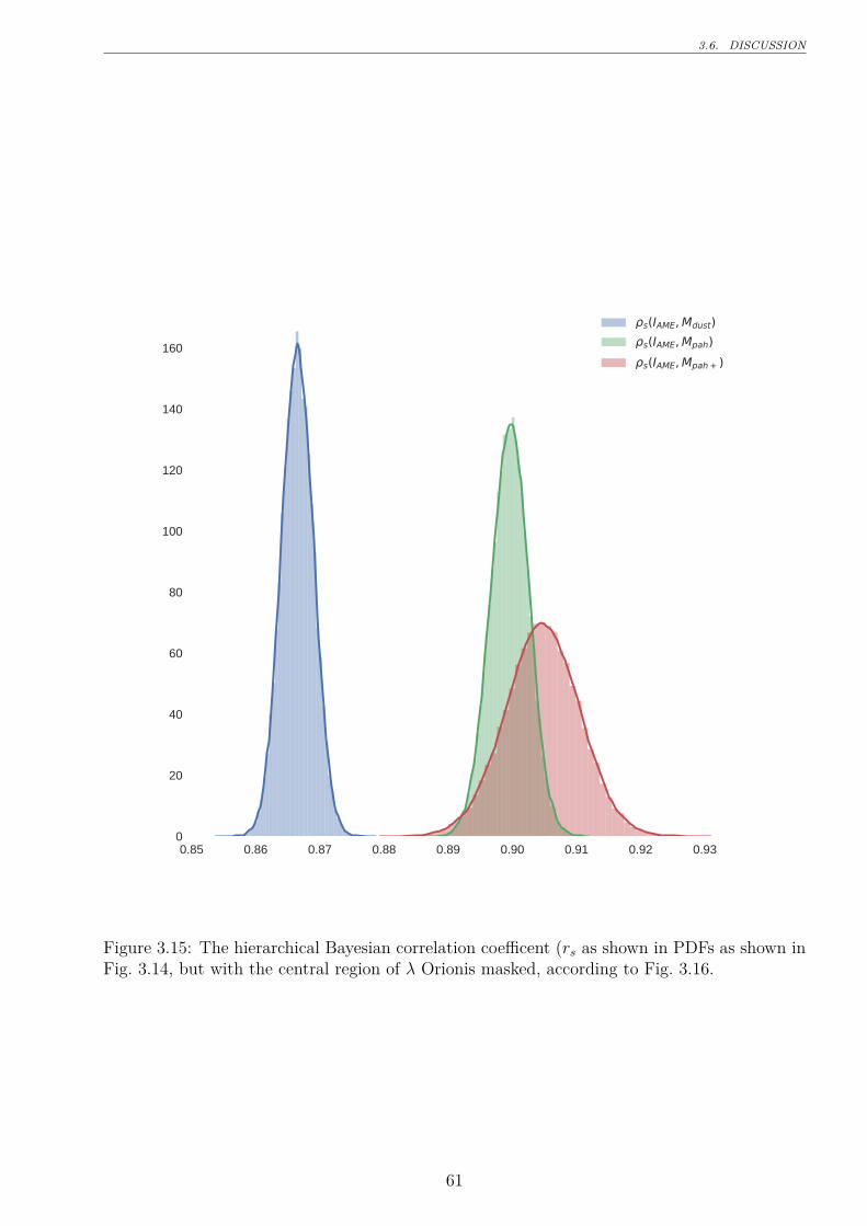
3.6. DISCUSSION
0.85 0.86 0.87 0.88 0.89 0.90 0.91 0.92 0.930
20
40
60
80
100
120
140
160
s(IAME, Mdust)s(IAME, Mpah)s(IAME, Mpah + )
Figure 3.15: The hierarchical Bayesian correlation coefficent (rs as shown in PDFs as shown inFig. 3.14, but with the central region of λ Orionis masked, according to Fig. 3.16.
61
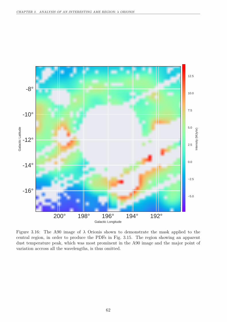
CHAPTER 3. ANALYSIS OF AN INTERESTING AME REGION: λ ORIONIS
192°194°196°198°200°Galactic Longitude
-16°
-14°
-12°
-10°
-8°
Gal
actic
Lat
itude
5.0
2.5
0.0
2.5
5.0
7.5
10.0
12.5
Inte
nsity
(M
Jy/s
r)
Figure 3.16: The A90 image of λ Orionis shown to demonstrate the mask applied to thecentral region, in order to produce the PDFs in Fig. 3.15. The region showing an apparentdust temperature peak, which was most prominent in the A90 image and the major point ofvariation accross all the wavelengths, is thus omitted.
62
3.6. DISCUSSION
inconclusive. To our knowledge, this is the first case of the HB approach being applied to a
localized investigation of AME, and certainly the first time that the dust SED of λ Orionis re-
gion has been investigated in such a way. This raises questions about the future of LSM-based
analysis in dust SED studies, and highlights the potential this HB framework developed by
Galliano (2018).
3.6.2 PAH Ionization fraction
As described in Ch.2 it is expected that relative variations between the A9 and I12 intensities
could be explained by the fraction of PAHs that are charged, fPAH+. Spectroscopically, we
cannot distinguish between PAH anions or cations. However if spinning dust emission arises
from anions, a better correlation with the mass of charged PAHs MPAH+ is expected. However
if the PAHs are positively charged, a stronger correlation with MPAH+ is not expected. This
is due to the rotational excitability of the PAHs: anions are more succeptable to rotational
excitation by H+ and C+ collisions(Ali-Haimoud 2010).
Examining λ Orionis in intensity, we find that the A9 intensity correlates more strongly with
AME than I12 or D12. In the rp case, A9 correlates more strongly with AME than any other
band. This is consistent with the spinning PAH hypothesis, and taken alone may indicate that
the 6.2 µm feature emission from charged PAHs, may be a better predictor of AME intensity.
As shown by the dust SED fitting however, the probability distributions (Fig. 3.14) of
rp(MPAH+ : IAME) do not indicate that ionized PAH mass correlates better with the total
PAH mass. Attempts to estimate the MPAH+ based on the available data appear to only add
noise relative to rp(MPAH : IAME). The means of the two distrubtions rp(MPAH+ : IAME) and
rp(MPAH : IAME) are similar and rp(MPAH+ : IAME) shows a wider distribution. Thus the
question of whether or not AME comes predominantly from charged PAHs remains open.
The fact that A9 correlates more strongly than the 12 µm bands, at least suggests that
this topic is worth further investigation. What is clear from the MIR and AME morphology
however, is that there is a transition from a relatively PAH depleted, warmer, stronger ISRF
in the centerand warm dust in the center to a PAH-supporting region in the ring. Along
this transition, there must be a decreasing radiation field with distance from dimnant heating
sources, in λ Orionis association. Andrews et al. (2016) predict a transition of PAH species
along such a radiation field gradient, from complete PAH destruction in harsh environments,
63
CHAPTER 3. ANALYSIS OF AN INTERESTING AME REGION: λ ORIONIS
to survival of (sufficiently large) PAH anions near the surface of molecular clouds. Thus if our
stronger correlation with A9 indicates charged PAHs, this could be consistent with PAH anions
surviving in the portions of λ Orionis which are emitting the strongest AME. Future wide-
area spectral mapping of the λ Orionis region may be able to conclusively test for increased
fPAH+ in regions with stronger AME. This would also help us to understand the extent to
which [NeII] emission may contribute to the I12 emission, and if this may lead to a relatively
improved correlation between AME and A9. Such studies would be strongly aided by higher
resolution probing of spatial variations the AME spectral profile.
64
Chapter 4
All-sky Analysis
What we present here is a test of the generalizability of results from Ch.3, which focused on a
particular structure on the sky, λ Orionis. We first would like to note that “all-sky analysis” can
be a bit misleading. The term tends to lead readers to the idea of a definitive study, answering
a particular question for any given position on the sky. While a truly all-sky analysis would
be ideal, signal-to-noise constraints (mainly at high galactic latitudes), as well as confusion
along the line of sight (mainly in the galactic plane), make a uniformly powerful study of the
whole sky very challenging. Here we will indeed show results for the entire sky as a benchmark
analysis, but for the core analysis we must mask certain regions dominated by systematic effects
in order to minimize biases for particular wavelenghts.
4.1 Resolution matching
Smoothing
As in Ch. 3, this approach applies to a spatial resolution of approximately ~1◦. The resolution
limimtation is imposed by the PC microwave component maps, which list an effective resolution
of 60′ (Planck Collaboration et al. 2016b). Thus we must apply a smoothing to most of our
input datasets, which have native resolutions of a much finer scale (see Tab. 2.1 and Fig. 1.2).
The data also come in a wide range of beam shapes with their own degrees of uncertainty,
thus we conservatively smooth all of the data in the same way, using a circular Gaussian beam,
to have ~1◦ FWHM resolution. We start with an all-sky AME to IR comparison, looking for
global patterns among all pixels.
65
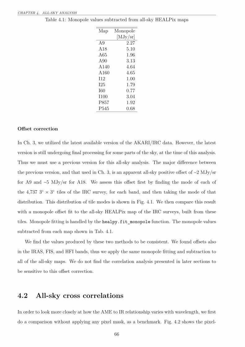
CHAPTER 4. ALL-SKY ANALYSIS
Table 4.1: Monopole values subtracted from all-sky HEALPix maps
Map Monopole[MJy/sr]
A9 2.27A18 5.10A65 1.96A90 3.13A140 4.64A160 4.65I12 1.00I25 1.79I60 0.77I100 3.04P857 1.92P545 0.68
Offset correction
In Ch. 3, we utilized the latest available version of the AKARI/IRC data. However, the latest
version is still undergoing final processing for some parts of the sky, at the time of this analysis.
Thus we must use a previous version for this all-sky analysis. The major difference between
the previous version, and that used in Ch. 3, is an apparent all-sky positive offset of ~2 MJy/sr
for A9 and ~5 MJy/sr for A18. We assess this offset first by finding the mode of each of
the 4,737 3◦ × 3◦ tiles of the IRC survey, for each band, and then taking the mode of that
distribution. This distribution of tile modes is shown in Fig. 4.1. We then compare this result
with a monopole offset fit to the all-sky HEALPix map of the IRC surveys, built from these
tiles. Monopole fitting is handled by the healpy.fit_monopole function. The monopole values
subtracted from each map shown in Tab. 4.1.
We find the values produced by these two methods to be consistent. We found offsets also
in the IRAS, FIS, and HFI bands, thus we apply the same monopole fitting and subtraction to
all of the all-sky maps. We do not find the correlation analysis presented in later sections to
be sensitive to this offset correction.
4.2 All-sky cross correlations
In order to look more closely at how the AME to IR relationship varies with wavelength, we first
do a comparison without applying any pixel mask, as a benchmark. Fig. 4.2 shows the pixel-
66
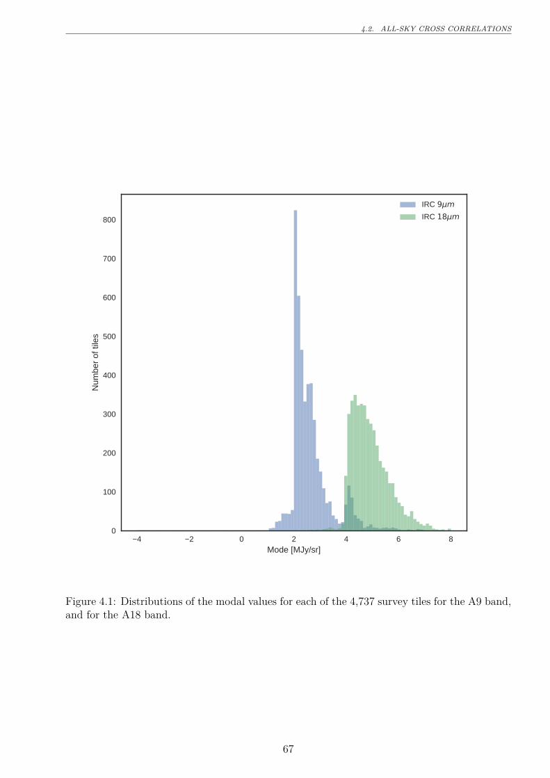
4.2. ALL-SKY CROSS CORRELATIONS
4 2 0 2 4 6 8Mode [MJy/sr]
0
100
200
300
400
500
600
700
800
Num
ber
of ti
les
IRC 9 mIRC 18 m
Figure 4.1: Distributions of the modal values for each of the 4,737 survey tiles for the A9 band,and for the A18 band.
67
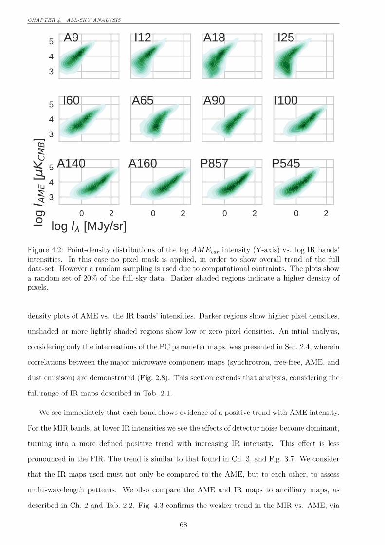
CHAPTER 4. ALL-SKY ANALYSIS
3
4
5 A9 I12 A18 I25
3
4
5 I60 A65 A90 I100
0 2
log I [MJy/sr]
3
4
5
log
I AM
E [
K CM
B]
A140
0 2
A160
0 2
P857
0 2
P545
Figure 4.2: Point-density distributions of the log AMEvar intensity (Y-axis) vs. log IR bands’intensities. In this case no pixel mask is applied, in order to show overall trend of the fulldata-set. However a random sampling is used due to computational contraints. The plots showa random set of 20% of the full-sky data. Darker shaded regions indicate a higher density ofpixels.
density plots of AME vs. the IR bands’ intensities. Darker regions show higher pixel densities,
unshaded or more lightly shaded regions show low or zero pixel densities. An intial analysis,
considering only the interreations of the PC parameter maps, was presented in Sec. 2.4, wherein
correlations between the major microwave component maps (synchrotron, free-free, AME, and
dust emisison) are demonstrated (Fig. 2.8). This section extends that analysis, considering the
full range of IR maps described in Tab. 2.1.
We see immediately that each band shows evidence of a positive trend with AME intensity.
For the MIR bands, at lower IR intensities we see the effects of detector noise become dominant,
turning into a more defined positive trend with increasing IR intensity. This effect is less
pronounced in the FIR. The trend is similar to that found in Ch. 3, and Fig. 3.7. We consider
that the IR maps used must not only be compared to the AME, but to each other, to assess
multi-wavelength patterns. We also compare the AME and IR maps to ancilliary maps, as
described in Ch. 2 and Tab. 2.2. Fig. 4.3 confirms the weaker trend in the MIR vs. AME, via
68
4.2. ALL-SKY CROSS CORRELATIONS
A9
I12
A18 I2
5
I60
A65
A90
I100
A14
0
A16
0
P85
7
P54
5
AM
Eva
r
AM
Efix ff
Syn
c
NH Ha
H40
8
H408
Ha
NH
Sync
ff
AMEfix
AMEvar
P545
P857
A160
A140
I100
A90
A65
I60
I25
A18
I12
A9
0.33 0.38 0.089 0.22 0.51 0.27 0.45 0.57 0.55 0.54 0.53 0.51 0.42 0.46 0.28 0.94 0.53 0.27 1
0.31 0.026-0.062 -0.21 0.69 0.3 0.52 0.72 0.73 0.73 0.72 0.73 0.45 0.68 0.49 0.32 0.7 1 0.27
0.54 0.26 0.052-0.075 0.86 0.4 0.75 0.95 0.95 0.94 0.96 0.96 0.63 0.78 0.51 0.54 1 0.7 0.53
0.31 0.32 0.057 0.16 0.53 0.28 0.46 0.57 0.55 0.54 0.55 0.53 0.45 0.5 0.3 1 0.54 0.32 0.94
0.31 0.12 0.088-0.065 0.49 0.21 0.4 0.53 0.53 0.53 0.53 0.53 0.45 0.58 1 0.3 0.51 0.49 0.28
0.49 0.28 0.032-0.024 0.73 0.43 0.68 0.81 0.81 0.81 0.81 0.81 0.66 1 0.58 0.5 0.78 0.68 0.46
0.52 0.41 0.069 0.13 0.6 0.46 0.64 0.69 0.67 0.67 0.68 0.67 1 0.66 0.45 0.45 0.63 0.45 0.42
0.58 0.33 0.049-0.016 0.88 0.47 0.81 0.97 0.98 0.97 1 1 0.67 0.81 0.53 0.53 0.96 0.73 0.51
0.59 0.34 0.053-0.00570.88 0.47 0.82 0.98 0.98 0.97 1 1 0.68 0.81 0.53 0.55 0.96 0.72 0.53
0.6 0.38 0.051 0.017 0.86 0.54 0.83 0.97 0.99 1 0.97 0.97 0.67 0.81 0.53 0.54 0.94 0.73 0.54
0.59 0.35 0.053-0.00190.88 0.5 0.83 0.98 1 0.99 0.98 0.98 0.67 0.81 0.53 0.55 0.95 0.73 0.55
0.62 0.39 0.067 0.036 0.9 0.52 0.85 1 0.98 0.97 0.98 0.97 0.69 0.81 0.53 0.57 0.95 0.72 0.57
0.64 0.57 0.036 0.16 0.67 0.79 1 0.85 0.83 0.83 0.82 0.81 0.64 0.68 0.4 0.46 0.75 0.52 0.45
0.48 0.62 -0.065 0.28 0.34 1 0.79 0.52 0.5 0.54 0.47 0.47 0.46 0.43 0.21 0.28 0.4 0.3 0.27
0.52 0.32 0.13 0.11 1 0.34 0.67 0.9 0.88 0.86 0.88 0.88 0.6 0.73 0.49 0.53 0.86 0.69 0.51
0.25 0.77 0.18 1 0.11 0.28 0.16 0.036-0.00190.017-0.0057-0.016 0.13 -0.024-0.065 0.16 -0.075 -0.21 0.22
0.5 0.15 1 0.18 0.13 -0.0650.036 0.067 0.053 0.051 0.053 0.049 0.069 0.032 0.088 0.057 0.052-0.0620.089
0.58 1 0.15 0.77 0.32 0.62 0.57 0.39 0.35 0.38 0.34 0.33 0.41 0.28 0.12 0.32 0.26 0.026 0.38
1 0.58 0.5 0.25 0.52 0.48 0.64 0.62 0.59 0.6 0.59 0.58 0.52 0.49 0.31 0.31 0.54 0.31 0.33
A9
I12
A18 I2
5
I60
A65
A90
I100
A14
0
A16
0
P85
7
P54
5
AM
Eva
r
AM
Efix ff
Syn
c
NH Ha
H40
8
H408
Ha
NH
Sync
ff
AMEfix
AMEvar
P545
P857
A160
A140
I100
A90
A65
I60
I25
A18
I12
A9
0.73 0.79 0.65 0.77 0.81 0.77 0.8 0.79 0.74 0.74 0.65 0.62 0.68 0.67 0.5 0.98 0.49 0.19 1
0.42 0.28 0.45 0.24 0.52 0.4 0.49 0.49 0.45 0.43 0.38 0.37 0.31 0.47 0.68 0.11 0.41 1 0.19
0.83 0.78 0.75 0.71 0.75 0.72 0.8 0.82 0.86 0.87 0.91 0.92 0.72 0.8 0.67 0.47 1 0.41 0.49
0.7 0.77 0.59 0.73 0.75 0.76 0.76 0.74 0.7 0.7 0.63 0.6 0.68 0.64 0.43 1 0.47 0.11 0.98
0.74 0.69 0.72 0.64 0.77 0.7 0.77 0.78 0.78 0.77 0.75 0.74 0.55 0.65 1 0.43 0.67 0.68 0.5
0.86 0.83 0.77 0.76 0.85 0.8 0.87 0.88 0.88 0.88 0.86 0.85 0.9 1 0.65 0.64 0.8 0.47 0.67
0.81 0.8 0.72 0.75 0.78 0.74 0.81 0.81 0.83 0.83 0.81 0.8 1 0.9 0.55 0.68 0.72 0.31 0.68
0.93 0.91 0.82 0.84 0.85 0.82 0.9 0.92 0.97 0.97 1 1 0.8 0.85 0.74 0.6 0.92 0.37 0.62
0.94 0.92 0.84 0.85 0.87 0.83 0.92 0.94 0.98 0.98 1 1 0.81 0.86 0.75 0.63 0.91 0.38 0.65
0.96 0.94 0.86 0.87 0.93 0.88 0.97 0.98 1 1 0.98 0.97 0.83 0.88 0.77 0.7 0.87 0.43 0.74
0.96 0.94 0.87 0.87 0.94 0.88 0.97 0.99 1 1 0.98 0.97 0.83 0.88 0.78 0.7 0.86 0.45 0.74
0.95 0.92 0.87 0.87 0.98 0.88 0.99 1 0.99 0.98 0.94 0.92 0.81 0.88 0.78 0.74 0.82 0.49 0.79
0.94 0.92 0.85 0.84 0.98 0.92 1 0.99 0.97 0.97 0.92 0.9 0.81 0.87 0.77 0.76 0.8 0.49 0.8
0.86 0.88 0.71 0.76 0.85 1 0.92 0.88 0.88 0.88 0.83 0.82 0.74 0.8 0.7 0.76 0.72 0.4 0.77
0.91 0.88 0.86 0.86 1 0.85 0.98 0.98 0.94 0.93 0.87 0.85 0.78 0.85 0.77 0.75 0.75 0.52 0.81
0.87 0.93 0.84 1 0.86 0.76 0.84 0.87 0.87 0.87 0.85 0.84 0.75 0.76 0.64 0.73 0.71 0.24 0.77
0.9 0.83 1 0.84 0.86 0.71 0.85 0.87 0.87 0.86 0.84 0.82 0.72 0.77 0.72 0.59 0.75 0.45 0.65
0.94 1 0.83 0.93 0.88 0.88 0.92 0.92 0.94 0.94 0.92 0.91 0.8 0.83 0.69 0.77 0.78 0.28 0.79
1 0.94 0.9 0.87 0.91 0.86 0.94 0.95 0.96 0.96 0.94 0.93 0.81 0.86 0.74 0.7 0.83 0.42 0.73
Figure 4.3: ALL-SKY cross-correlation matrix for the 12 infrared bands sampled, as well asthe PC component maps described in Ch. 2: the two AME components evaluated at theirpeak frequencies AMEvar, AMEfix; Syncrotron, and free-free), and ancilliary maps of NH , Hαemission, and 408 MHz emission Haslam et al. (1982). The color-scale indicates (rS). Resultsare based on the unmasked sky, but are split by Galactic latitude: pixels with |β| > 15◦ (left)and |β| < 15◦ (right). The color and annotations indicate rs as in Fig. 3.7.
a cross-correlation matrix, similar to that used in Ch. 3 and Fig. 3.7. This is reflected in the
comparison between high and low latitude plots: for pixels |β| > 15◦, we see a dramatic effect.
In the most extreme case rs of A18 to AMEvar drops from 0.72 at lower latitudes, to 0.02 at
higher latitudes. rs(A9 : AMEvar) drops from 0.79 to 0.42. Correlations between the MIR
bands and FIR bands also weaken. Only the the interrelations between the FIR bands from
I60 to P545 remain essentially latitude independent (with the exception of A65, which has an
especially high noise level.)
In the lower latitudes, with |β| < 15◦, bright emission in and around the galactic plane
seems to homogenize the bands. We see little change from band to band both in terms of
the relationship with AME or with other IR bands. Thus the increase of S/N with decreasing
brightness at higher latitudes has a strong effect on such intensity correlation tests. Bands
tracing bright thermal dust emission at higher latitudes are more robust against this effect. The
only case where the trend is reversed, is with the maps of N(H) and Hα. Both of these maps
show higher rs when compared to high latitude FIR emission, possibly due to optical effects.
The next section descibes a pixel-masking strategy designed to mitigate both rs suppressing
69
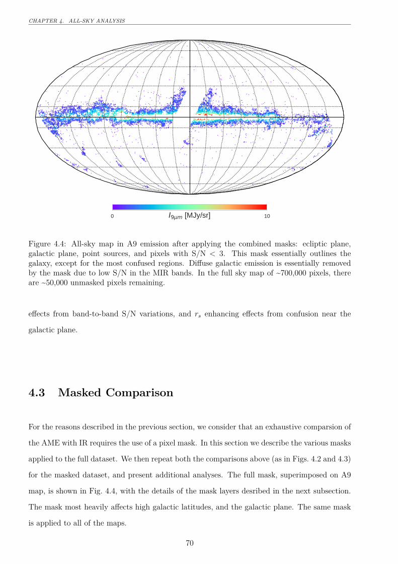
CHAPTER 4. ALL-SKY ANALYSIS
0 10I9 m [MJy/sr]
Figure 4.4: All-sky map in A9 emission after applying the combined masks: ecliptic plane,galactic plane, point sources, and pixels with S/N < 3. This mask essentially outlines thegalaxy, except for the most confused regions. Diffuse galactic emission is essentially removedby the mask due to low S/N in the MIR bands. In the full sky map of ~700,000 pixels, thereare ~50,000 unmasked pixels remaining.
effects from band-to-band S/N variations, and rs enhancing effects from confusion near the
galactic plane.
4.3 Masked Comparison
For the reasons described in the previous section, we consider that an exhaustive comparsion of
the AME with IR requires the use of a pixel mask. In this section we describe the various masks
applied to the full dataset. We then repeat both the comparisons above (as in Figs. 4.2 and 4.3)
for the masked dataset, and present additional analyses. The full mask, superimposed on A9
map, is shown in Fig. 4.4, with the details of the mask layers desribed in the next subsection.
The mask most heavily affects high galactic latitudes, and the galactic plane. The same mask
is applied to all of the maps.
70
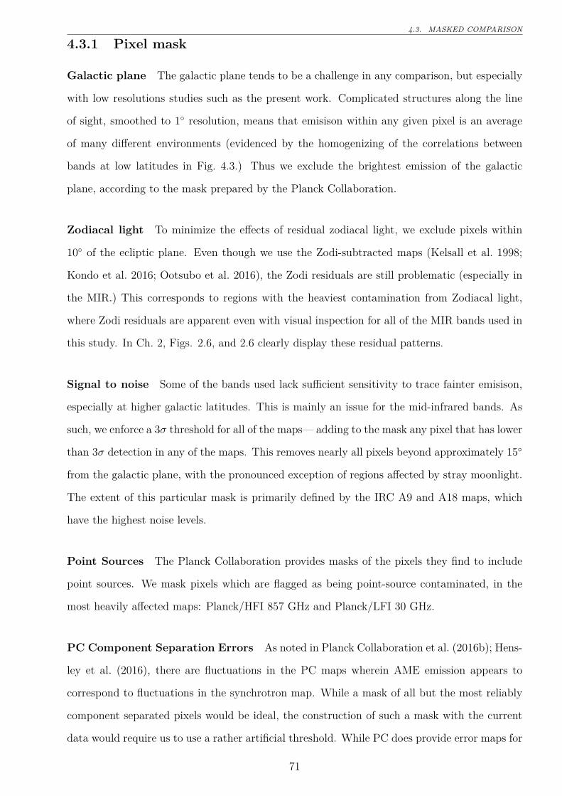
4.3. MASKED COMPARISON
4.3.1 Pixel mask
Galactic plane The galactic plane tends to be a challenge in any comparison, but especially
with low resolutions studies such as the present work. Complicated structures along the line
of sight, smoothed to 1◦ resolution, means that emisison within any given pixel is an average
of many different environments (evidenced by the homogenizing of the correlations between
bands at low latitudes in Fig. 4.3.) Thus we exclude the brightest emission of the galactic
plane, according to the mask prepared by the Planck Collaboration.
Zodiacal light To minimize the effects of residual zodiacal light, we exclude pixels within
10◦ of the ecliptic plane. Even though we use the Zodi-subtracted maps (Kelsall et al. 1998;
Kondo et al. 2016; Ootsubo et al. 2016), the Zodi residuals are still problematic (especially in
the MIR.) This corresponds to regions with the heaviest contamination from Zodiacal light,
where Zodi residuals are apparent even with visual inspection for all of the MIR bands used in
this study. In Ch. 2, Figs. 2.6, and 2.6 clearly display these residual patterns.
Signal to noise Some of the bands used lack sufficient sensitivity to trace fainter emisison,
especially at higher galactic latitudes. This is mainly an issue for the mid-infrared bands. As
such, we enforce a 3σ threshold for all of the maps— adding to the mask any pixel that has lower
than 3σ detection in any of the maps. This removes nearly all pixels beyond approximately 15◦
from the galactic plane, with the pronounced exception of regions affected by stray moonlight.
The extent of this particular mask is primarily defined by the IRC A9 and A18 maps, which
have the highest noise levels.
Point Sources The Planck Collaboration provides masks of the pixels they find to include
point sources. We mask pixels which are flagged as being point-source contaminated, in the
most heavily affected maps: Planck/HFI 857 GHz and Planck/LFI 30 GHz.
PC Component Separation Errors As noted in Planck Collaboration et al. (2016b); Hens-
ley et al. (2016), there are fluctuations in the PC maps wherein AME emission appears to
correspond to fluctuations in the synchrotron map. While a mask of all but the most reliably
component separated pixels would be ideal, the construction of such a mask with the current
data would require us to use a rather artificial threshold. While PC does provide error maps for
71
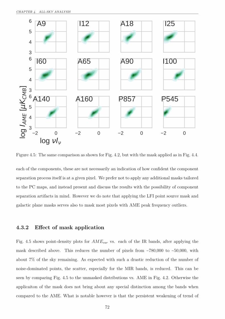
CHAPTER 4. ALL-SKY ANALYSIS
3
4
5
6 A9 I12 A18 I25
3
4
5
6 I60 A65 A90 I100
2 0
log I
3
4
5
6
log
I AM
E [
K CM
B]
A140
2 0
A160
2 0
P857
2 0
P545
Figure 4.5: The same comparison as shown for Fig. 4.2, but with the mask applied as in Fig. 4.4.
each of the components, these are not necessarily an indication of how confident the component
separation process itself is at a given pixel. We prefer not to apply any additional masks tailored
to the PC maps, and instead present and discuss the results with the possibility of component
separation artifacts in mind. However we do note that applying the LFI point source mask and
galactic plane masks serves also to mask most pixels with AME peak frequency outliers.
4.3.2 Effect of mask application
Fig. 4.5 shows point-density plots for AMEvar vs. each of the IR bands, after applying the
mask described above. This reduces the number of pixels from ~780,000 to ~50,000, with
about 7% of the sky remaining. As expected with such a drastic reduction of the number of
noise-dominated points, the scatter, especially for the MIR bands, is reduced. This can be
seen by comparing Fig. 4.5 to the unmasked distributions vs. AME in Fig. 4.2. Otherwise the
applicaiton of the mask does not bring about any special distinction among the bands when
compared to the AME. What is notable however is that the persistent weakening of trend of
72
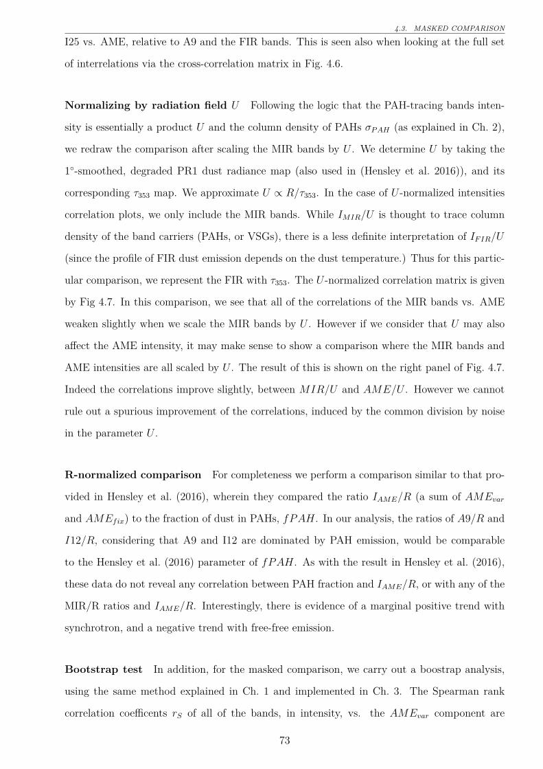
4.3. MASKED COMPARISON
I25 vs. AME, relative to A9 and the FIR bands. This is seen also when looking at the full set
of interrelations via the cross-correlation matrix in Fig. 4.6.
Normalizing by radiation field U Following the logic that the PAH-tracing bands inten-
sity is essentially a product U and the column density of PAHs σPAH (as explained in Ch. 2),
we redraw the comparison after scaling the MIR bands by U . We determine U by taking the
1◦-smoothed, degraded PR1 dust radiance map (also used in (Hensley et al. 2016)), and its
corresponding τ353 map. We approximate U ∝ R/τ353. In the case of U -normalized intensities
correlation plots, we only include the MIR bands. While IMIR/U is thought to trace column
density of the band carriers (PAHs, or VSGs), there is a less definite interpretation of IFIR/U
(since the profile of FIR dust emission depends on the dust temperature.) Thus for this partic-
ular comparison, we represent the FIR with τ353. The U -normalized correlation matrix is given
by Fig 4.7. In this comparison, we see that all of the correlations of the MIR bands vs. AME
weaken slightly when we scale the MIR bands by U . However if we consider that U may also
affect the AME intensity, it may make sense to show a comparison where the MIR bands and
AME intensities are all scaled by U . The result of this is shown on the right panel of Fig. 4.7.
Indeed the correlations improve slightly, between MIR/U and AME/U . However we cannot
rule out a spurious improvement of the correlations, induced by the common division by noise
in the parameter U .
R-normalized comparison For completeness we perform a comparison similar to that pro-
vided in Hensley et al. (2016), wherein they compared the ratio IAME/R (a sum of AMEvar
and AMEfix) to the fraction of dust in PAHs, fPAH. In our analysis, the ratios of A9/R and
I12/R, considering that A9 and I12 are dominated by PAH emission, would be comparable
to the Hensley et al. (2016) parameter of fPAH. As with the result in Hensley et al. (2016),
these data do not reveal any correlation between PAH fraction and IAME/R, or with any of the
MIR/R ratios and IAME/R. Interestingly, there is evidence of a marginal positive trend with
synchrotron, and a negative trend with free-free emission.
Bootstrap test In addition, for the masked comparison, we carry out a boostrap analysis,
using the same method explained in Ch. 1 and implemented in Ch. 3. The Spearman rank
correlation coefficents rS of all of the bands, in intensity, vs. the AMEvar component are
73
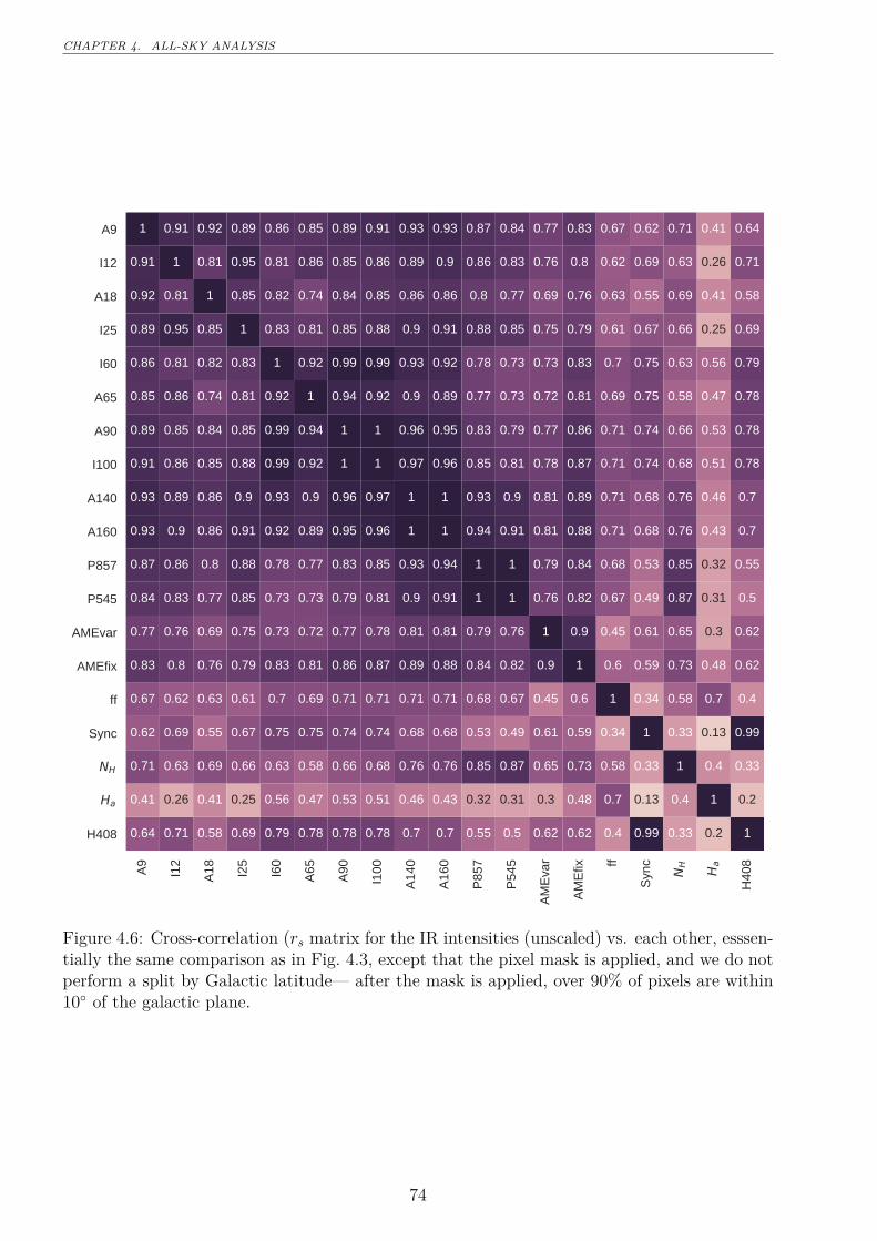
CHAPTER 4. ALL-SKY ANALYSIS
A9
I12
A18 I2
5
I60
A65
A90
I100
A14
0
A16
0
P85
7
P54
5
AM
Eva
r
AM
Efix ff
Syn
c
NH Ha
H40
8
H408
Ha
NH
Sync
ff
AMEfix
AMEvar
P545
P857
A160
A140
I100
A90
A65
I60
I25
A18
I12
A9
0.64 0.71 0.58 0.69 0.79 0.78 0.78 0.78 0.7 0.7 0.55 0.5 0.62 0.62 0.4 0.99 0.33 0.2 1
0.41 0.26 0.41 0.25 0.56 0.47 0.53 0.51 0.46 0.43 0.32 0.31 0.3 0.48 0.7 0.13 0.4 1 0.2
0.71 0.63 0.69 0.66 0.63 0.58 0.66 0.68 0.76 0.76 0.85 0.87 0.65 0.73 0.58 0.33 1 0.4 0.33
0.62 0.69 0.55 0.67 0.75 0.75 0.74 0.74 0.68 0.68 0.53 0.49 0.61 0.59 0.34 1 0.33 0.13 0.99
0.67 0.62 0.63 0.61 0.7 0.69 0.71 0.71 0.71 0.71 0.68 0.67 0.45 0.6 1 0.34 0.58 0.7 0.4
0.83 0.8 0.76 0.79 0.83 0.81 0.86 0.87 0.89 0.88 0.84 0.82 0.9 1 0.6 0.59 0.73 0.48 0.62
0.77 0.76 0.69 0.75 0.73 0.72 0.77 0.78 0.81 0.81 0.79 0.76 1 0.9 0.45 0.61 0.65 0.3 0.62
0.84 0.83 0.77 0.85 0.73 0.73 0.79 0.81 0.9 0.91 1 1 0.76 0.82 0.67 0.49 0.87 0.31 0.5
0.87 0.86 0.8 0.88 0.78 0.77 0.83 0.85 0.93 0.94 1 1 0.79 0.84 0.68 0.53 0.85 0.32 0.55
0.93 0.9 0.86 0.91 0.92 0.89 0.95 0.96 1 1 0.94 0.91 0.81 0.88 0.71 0.68 0.76 0.43 0.7
0.93 0.89 0.86 0.9 0.93 0.9 0.96 0.97 1 1 0.93 0.9 0.81 0.89 0.71 0.68 0.76 0.46 0.7
0.91 0.86 0.85 0.88 0.99 0.92 1 1 0.97 0.96 0.85 0.81 0.78 0.87 0.71 0.74 0.68 0.51 0.78
0.89 0.85 0.84 0.85 0.99 0.94 1 1 0.96 0.95 0.83 0.79 0.77 0.86 0.71 0.74 0.66 0.53 0.78
0.85 0.86 0.74 0.81 0.92 1 0.94 0.92 0.9 0.89 0.77 0.73 0.72 0.81 0.69 0.75 0.58 0.47 0.78
0.86 0.81 0.82 0.83 1 0.92 0.99 0.99 0.93 0.92 0.78 0.73 0.73 0.83 0.7 0.75 0.63 0.56 0.79
0.89 0.95 0.85 1 0.83 0.81 0.85 0.88 0.9 0.91 0.88 0.85 0.75 0.79 0.61 0.67 0.66 0.25 0.69
0.92 0.81 1 0.85 0.82 0.74 0.84 0.85 0.86 0.86 0.8 0.77 0.69 0.76 0.63 0.55 0.69 0.41 0.58
0.91 1 0.81 0.95 0.81 0.86 0.85 0.86 0.89 0.9 0.86 0.83 0.76 0.8 0.62 0.69 0.63 0.26 0.71
1 0.91 0.92 0.89 0.86 0.85 0.89 0.91 0.93 0.93 0.87 0.84 0.77 0.83 0.67 0.62 0.71 0.41 0.64
Figure 4.6: Cross-correlation (rs matrix for the IR intensities (unscaled) vs. each other, esssen-tially the same comparison as in Fig. 4.3, except that the pixel mask is applied, and we do notperform a split by Galactic latitude— after the mask is applied, over 90% of pixels are within10◦ of the galactic plane.
74
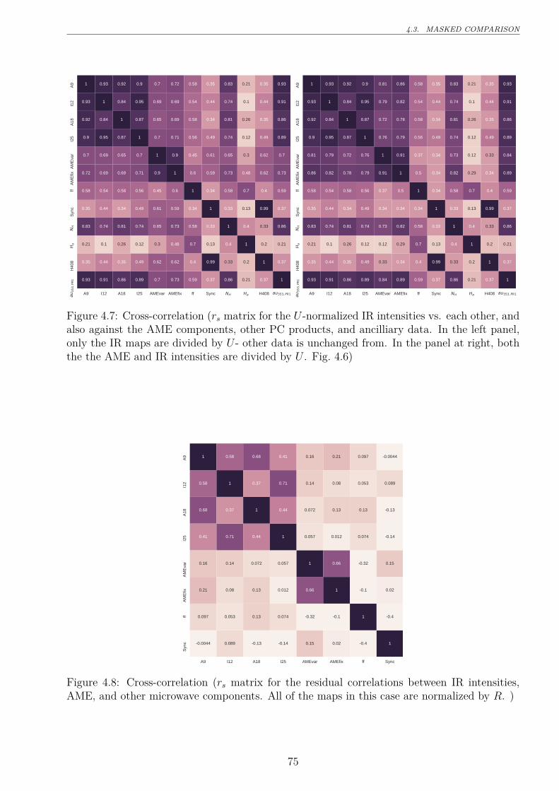
4.3. MASKED COMPARISON
A9 I12 A18 I25 AMEvar AMEfix ff Sync NH Ha H408 au353, PR1au35
3,PR
1H
408
Ha
NH
Syn
cff
AM
Efix
AM
Eva
rI2
5A
18I1
2A
9
0.93 0.91 0.86 0.89 0.7 0.73 0.59 0.37 0.86 0.21 0.37 1
0.35 0.44 0.35 0.49 0.62 0.62 0.4 0.99 0.33 0.2 1 0.37
0.21 0.1 0.26 0.12 0.3 0.48 0.7 0.13 0.4 1 0.2 0.21
0.83 0.74 0.81 0.74 0.65 0.73 0.58 0.33 1 0.4 0.33 0.86
0.35 0.44 0.34 0.49 0.61 0.59 0.34 1 0.33 0.13 0.99 0.37
0.58 0.54 0.58 0.56 0.45 0.6 1 0.34 0.58 0.7 0.4 0.59
0.72 0.69 0.69 0.71 0.9 1 0.6 0.59 0.73 0.48 0.62 0.73
0.7 0.69 0.65 0.7 1 0.9 0.45 0.61 0.65 0.3 0.62 0.7
0.9 0.95 0.87 1 0.7 0.71 0.56 0.49 0.74 0.12 0.49 0.89
0.92 0.84 1 0.87 0.65 0.69 0.58 0.34 0.81 0.26 0.35 0.86
0.93 1 0.84 0.95 0.69 0.69 0.54 0.44 0.74 0.1 0.44 0.91
1 0.93 0.92 0.9 0.7 0.72 0.58 0.35 0.83 0.21 0.35 0.93
A9 I12 A18 I25 AMEvar AMEfix ff Sync NH Ha H408 au353, PR1au35
3,PR
1H
408
Ha
NH
Syn
cff
AM
Efix
AM
Eva
rI2
5A
18I1
2A
9
0.93 0.91 0.86 0.89 0.84 0.89 0.59 0.37 0.86 0.21 0.37 1
0.35 0.44 0.35 0.49 0.33 0.34 0.4 0.99 0.33 0.2 1 0.37
0.21 0.1 0.26 0.12 0.12 0.29 0.7 0.13 0.4 1 0.2 0.21
0.83 0.74 0.81 0.74 0.73 0.82 0.58 0.33 1 0.4 0.33 0.86
0.35 0.44 0.34 0.49 0.34 0.34 0.34 1 0.33 0.13 0.99 0.37
0.58 0.54 0.58 0.56 0.37 0.5 1 0.34 0.58 0.7 0.4 0.59
0.86 0.82 0.78 0.79 0.91 1 0.5 0.34 0.82 0.29 0.34 0.89
0.81 0.79 0.72 0.76 1 0.91 0.37 0.34 0.73 0.12 0.33 0.84
0.9 0.95 0.87 1 0.76 0.79 0.56 0.49 0.74 0.12 0.49 0.89
0.92 0.84 1 0.87 0.72 0.78 0.58 0.34 0.81 0.26 0.35 0.86
0.93 1 0.84 0.95 0.79 0.82 0.54 0.44 0.74 0.1 0.44 0.91
1 0.93 0.92 0.9 0.81 0.86 0.58 0.35 0.83 0.21 0.35 0.93
Figure 4.7: Cross-correlation (rs matrix for the U -normalized IR intensities vs. each other, andalso against the AME components, other PC products, and ancilliary data. In the left panel,only the IR maps are divided by U - other data is unchanged from. In the panel at right, boththe the AME and IR intensities are divided by U . Fig. 4.6)
A9 I12 A18 I25 AMEvar AMEfix ff Sync
Syn
cff
AM
Efix
AM
Eva
rI2
5A
18I1
2A
9
-0.0044 0.089 -0.13 -0.14 0.15 0.02 -0.4 1
0.097 0.053 0.13 0.074 -0.32 -0.1 1 -0.4
0.21 0.08 0.13 0.012 0.66 1 -0.1 0.02
0.16 0.14 0.072 0.057 1 0.66 -0.32 0.15
0.41 0.71 0.44 1 0.057 0.012 0.074 -0.14
0.68 0.37 1 0.44 0.072 0.13 0.13 -0.13
0.58 1 0.37 0.71 0.14 0.08 0.053 0.089
1 0.58 0.68 0.41 0.16 0.21 0.097 -0.0044
Figure 4.8: Cross-correlation (rs matrix for the residual correlations between IR intensities,AME, and other microwave components. All of the maps in this case are normalized by R. )
75
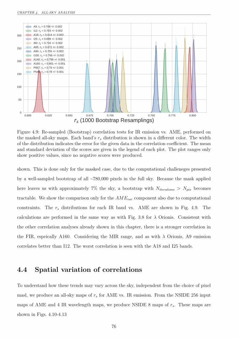
CHAPTER 4. ALL-SKY ANALYSIS
0.600 0.625 0.650 0.675 0.700 0.725 0.750 0.775 0.800
rs (1000 Bootstrap Resamplings)
0
50
100
150
200
250
300
A9: rs = 0.708 +/- 0.002I12: rs = 0.703 +/- 0.002A18: rs = 0.614 +/- 0.002I25: rs = 0.699 +/- 0.002I60: rs = 0.716 +/- 0.002A65: rs = 0.672 +/- 0.002A90: rs = 0.755 +/- 0.002I100: rs = 0.766 +/- 0.002A140: rs = 0.796 +/- 0.001A160: rs = 0.801 +/- 0.001P857: rs = 0.79 +/- 0.001P545: rs = 0.78 +/- 0.001
Figure 4.9: Re-sampled (Bootstrap) correlation tests for IR emission vs. AME, performed onthe masked all-sky maps. Each band’s rs distribution is shown in a different color. The widthof the distribution indicates the error for the given data in the correlation coefficient. The meanand standard deviation of the scores are given in the legend of each plot. The plot ranges onlyshow positive values, since no negative scores were produced.
shown. This is done only for the masked case, due to the computational challeneges presented
by a well-sampled bootstrap of all ~780,000 pixels in the full sky. Because the mask applied
here leaves us with approximately 7% the sky, a bootstrap with Niterations > Npix becomes
tractable. We show the comparison only for the AMEvar component also due to computational
constraints. The rs distributions for each IR band vs. AME are shown in Fig. 4.9. The
calculations are performed in the same way as with Fig. 3.8 for λ Orionis. Consistent with
the other correlation analyses already shown in this chapter, there is a stronger correlation in
the FIR, espeically A160. Considering the MIR range, and as with λ Orionis, A9 emission
correlates better than I12. The worst correlation is seen with the A18 and I25 bands.
4.4 Spatial variation of correlations
To understand how these trends may vary across the sky, independent from the choice of pixel
masl, we produce an all-sky maps of rs for AME vs. IR emission. From the NSIDE 256 input
maps of AME and 4 IR wavelength maps, we produce NSIDE 8 maps of rs. These maps are
shown in Figs. 4.10-4.13
76
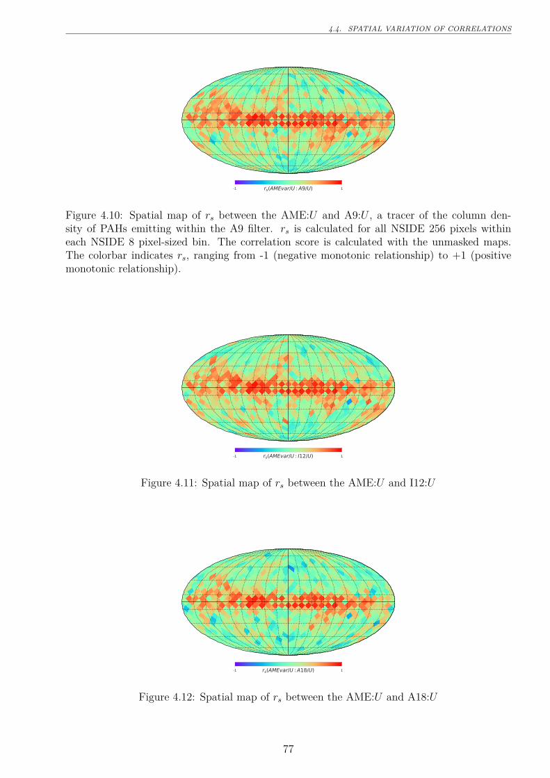
4.4. SPATIAL VARIATION OF CORRELATIONS
-1 1rs(AMEvar/U : A9/U)
Figure 4.10: Spatial map of rs between the AME:U and A9:U , a tracer of the column den-sity of PAHs emitting within the A9 filter. rs is calculated for all NSIDE 256 pixels withineach NSIDE 8 pixel-sized bin. The correlation score is calculated with the unmasked maps.The colorbar indicates rs, ranging from -1 (negative monotonic relationship) to +1 (positivemonotonic relationship).
-1 1rs(AMEvar/U : I12/U)
Figure 4.11: Spatial map of rs between the AME:U and I12:U
-1 1rs(AMEvar/U : A18/U)
Figure 4.12: Spatial map of rs between the AME:U and A18:U
77
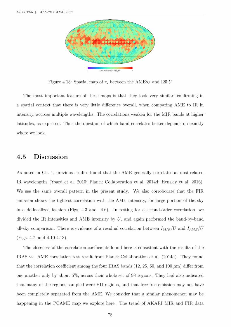
CHAPTER 4. ALL-SKY ANALYSIS
-1 1rs(AMEvar/U : I25/U)
Figure 4.13: Spatial map of rs between the AME:U and I25:U
The most important feature of these maps is that they look very similar, confirming in
a spatial context that there is very little difference overall, when comparing AME to IR in
intensity, accross multiple wavelengths. The correlations weaken for the MIR bands at higher
latitudes, as expected. Thus the question of which band correlates better depends on exactly
where we look.
4.5 Discussion
As noted in Ch. 1, previous studies found that the AME generally correlates at dust-related
IR wavelengths (Ysard et al. 2010; Planck Collaboration et al. 2014d; Hensley et al. 2016).
We see the same overall pattern in the present study. We also corroborate that the FIR
emission shows the tightest correlation with the AME intensity, for large portion of the sky
in a de-localized fashion (Figs. 4.3 and 4.6). In testing for a second-order correlation, we
divided the IR intensities and AME intensity by U , and again performed the band-by-band
all-sky comparison. There is evidence of a residual correlation between IMIR/U and IAME/U
(Figs. 4.7, and 4.10-4.13).
The closeness of the correlation coefficients found here is consistent with the results of the
IRAS vs. AME correlation test result from Planck Collaboration et al. (2014d). They found
that the correlation coefficient among the four IRAS bands (12, 25, 60, and 100 µm) differ from
one another only by about 5%, across their whole set of 98 regions. They had also indicated
that many of the regions sampled were HII regions, and that free-free emission may not have
been completely separated from the AME. We consider that a similar phenomenon may be
happening in the PCAME map we explore here. The trend of AKARI MIR and FIR data
78
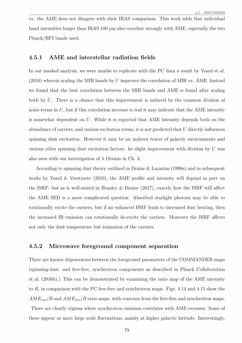
4.5. DISCUSSION
vs. the AME does not disagree with their IRAS comparison. This work adds that individual
band intensities longer than IRAS 100 µm also correlate strongly with AME, especially the two
Planck/HFI bands used.
4.5.1 AME and interstellar radiation fields
In our masked analysis, we were unable to replicate with the PC data a result by Ysard et al.
(2010) wherein scaling the MIR bands by U improves the correlation of MIR vs. AME. Instead
we found that the best correlation between the MIR bands and AME is found after scaling
both by U . There is a chance that this improvement is induced by the common division of
noise-terms in U , but if this correlation increase is real it may indicate that the AME intensity
is somewhat dependent on U . While it is expected that AME intensity depends both on the
abundance of carriers, and various excitation terms, it is not predicted that U directly influences
spinning dust excitation. However it may be an indirect tracer of galactic environments and
various other spinning dust excitation factors. he slight improvement with division by U was
also seen with our investigation of λ Orionis in Ch. 3.
According to spinning dust theory outlined in Draine & Lazarian (1998a) and in subsequent
works by Ysard & Verstraete (2010), the AME profile and intensity will depend in part on
the ISRF- but as is well-stated in Hensley & Draine (2017), exactly how the ISRF will affect
the AME SED is a more complicated question. Absorbed starlight photons may be able to
rotationally excite the carriers, but if an enhanced ISRF leads to increased dust heating, then
the increased IR emission can rotationally de-excite the carriers. Moreover the ISRF affects
not only the dust temperature but ionization of the carriers.
4.5.2 Microwave foreground component separation
There are known degeneracies between the foreground parameters of the COMMANDER maps
(spinning-dust, and free-free, synchrotron components as described in Planck Collaboration
et al. (2016b).) This can be demonstrated by examining the ratio map of the AME intensity
to R, in comparison with the PC free-free and synchrotron maps. Figs. 4.14 and 4.15 show the
AMEvar/R and AMEfix/R ratio maps, with contours from the free-free and synchrotron maps.
There are clearly regions where synchrotron emission correlates with AME excesses. Some of
these appear as more large scale fluctuations, mainly at higher galactic latitude. Interestingly,
79
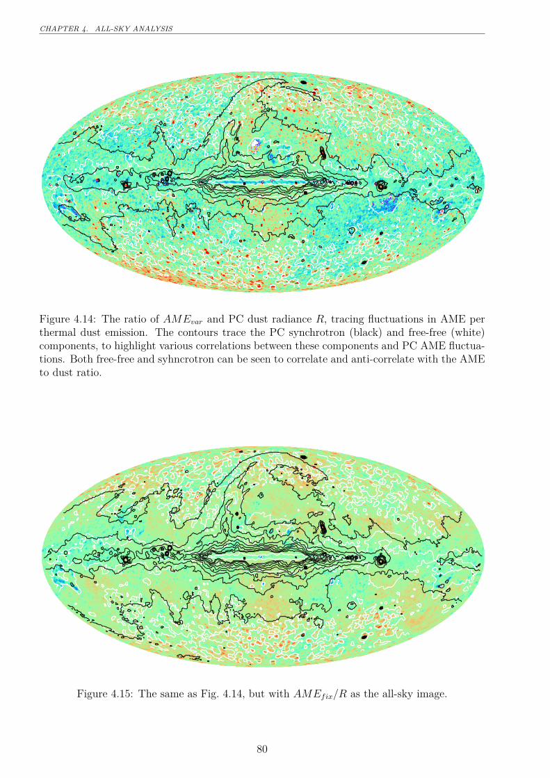
CHAPTER 4. ALL-SKY ANALYSIS
Figure 4.14: The ratio of AMEvar and PC dust radiance R, tracing fluctuations in AME perthermal dust emission. The contours trace the PC synchrotron (black) and free-free (white)components, to highlight various correlations between these components and PC AME fluctua-tions. Both free-free and syhncrotron can be seen to correlate and anti-correlate with the AMEto dust ratio.
Figure 4.15: The same as Fig. 4.14, but with AMEfix/R as the all-sky image.
80
4.5. DISCUSSION
free-free shows agreement with both positive and negative fluctuations in both ratio maps.
At high galactic latitude, free-free tends to be associated with positive fluctuations. This is
supported by the fact that AMEfix shows an improved correlation with both the Hα map
and the PC free-free map, perhaps suggesting confusion between spinning dust and free-free
components. Interestingly, the ring-structure of the λ Orionis region analyzed in Ch. 3, does
not have any apparent conterpart in the AME/R ratio maps in Figs. 4.15 and 4.14.
The results of the R normalized cross-correlation test show that free-free/R shows a negative
correlation with AME/R. This may be furher indication that the AME map, even with the
mask applied from Sec.4.3.1, may suffer from significant MW component confusion in some
regions. It is difficult to quantify potential effects from component separation uncertainties
relative to genuine correlations between microwave emission components, with the present
data. However there remains the potential for such confusion to suppress evidence of any trend
between AME and the actual value of fPAH. The anti-correlation here between free-free/R
and AME/R may be consistent with findings in von Hausegger & Liu (2015) that free-free
emission anti-correlates with AME, if pixels are weighted by S/N.
Even though A9/R and I12/R do not correlate with AME/R in our masked comparison, we
do find some limited regions where these values correlate in our full spatial correlation mapping.
4.5.3 Optical depth
In the interpretation of results here, we have essentially operated under the assumption that
MIR/PAH emisison, FIR emission, and the AME are all in the optically thin domain. This
is supported by the strong agreement in rs, accross all IR bands and the AME, as presented
in the correlation matrices here. (With the exception of the high-latitude, unmasked case in
Fig 4.3.) Conversely, the Hα data — emission known to be absorbed by interstellar dust —
is the only map lacking a correlation with the others at |β| < 5◦. N(H) also shows a weaker
correlation nearer to the galactic plane, likely influenced by saturation and/or self-absorption
effects.
However it has been demonstrated by Sakon et al. (2004) that the optically-thin assumption
for PAH/UIR emission could lead to errors in the estimate of PAH abundance based on these
emision features. Self-absorption for PAHs is another possibility.
We do not expect the analysis presented here to suffer from such effects significantly, as we
81
CHAPTER 4. ALL-SKY ANALYSIS
have masked the most confused lines of sight towards the galactic plane. However we cannot
rule out the possibility that such optical depth effects, not only in PAH emisison but in the FIR
or even AME, may weaken any potential relationship between the IR and microwave emisison
from spinning grains.
4.5.4 Comparison of λ Orionis vs. All-sky results
Results presented here do not necessarily conflict with results from Ch. 3, except in that the
findings from Fig. 3.8, wherein rp of A9 emission correlates better with AME than P545 emis-
sion, do not generalize to the results of this chapter (either the masked or unmasked cases.)
However, in the masked all-sky comparison as well as in λ Orionis, we find a better corrleation
between A9 and AME than between I12 and AME when we subject the correlations to bootstrap
resampling.
The different results between Ch. 3 and Ch. 4 may be explained by variations in the com-
ponent separation reliability. It is apparent that with the presently available data, there are a
very limited number of regions on the sky which do not show strong free-free or synchrotron
emission (relative to AME), while also having enough S/N in the MIR to reliably probe a re-
lationship between PAH abundance fluctuations and AME fluctuations. λ Orionis may be one
of the exceptions, where the S/N is high enough, and we are in fact able to see an improved
correlation between PAHs and AME, relative to the overall dust emission to AME connection.
We also disucssed in Ch. 4 the possibility that the PAH emission may not necessarily be
optically thin. If this were true, it may explain discrepancies for our λ Orionis result and
the results in this chapter. λ Orionis provides us a relatively clean line of sight compared to
delocalized all-sky analysis.
The fact that we do not see a clear preferential relationship between AME and PAHs in the
all-sky analysis, does not rule out a contribution by spinning PAHs to the AME. Likewise the
fact that we do see a better correlation in λ Orionis does not rule out contributions from other
proposals, such as that form non-PAH small grains, or nanosilicates.
4.5.5 Implications of an absent PAH-AME correlation
In the case that we are able to rule PAHs out as the AME carrier with confidence, this may
imply some constraints on the PAH size distribution and dipole moment. As discussed in the
82
4.6. FUTURE WORKS
theoretical work by Draine & Lazarian (1998a); Ali-Haimoud (2010) and others, as well as the
observational work by Hensley et al. (2016), if PAHs exist in the ISM, they are very likely to
be spinning rapidly. Thus if we are able to confirm that they do not produce AME, this could
tell us the morphology of ISM PAHs are not in an appropriate range to produce the observed
AME. Spinning PAHs may be a reality even in the case that the AME comes from something
else, if the PAHs are too large or lack appropriate electric dipoles.
4.6 Future Works
Because of the issues highlighted in previous sections (S/N, component separation, etc.), it is
extremely difficult to draw a conclusion about the carrier of AME based on a general all-sky
analysis such as that shown here. However there may be promise in studies of individual regions,
where an attempt can be made at controlling for local environmental factors, or background/-
foreground contamination. While it is true that previous studies of specific objects have also
not been conclusive, such as the investigation of Perseus by Tibbs et al. (2011), there are still
many other AME prominent regions which have not been probed in-depth, through a combi-
nation of microwave and PAH-range observations. Even the study of λ Orionis in Ch. 3 is not
exhaustive, and this interesting region deserves further attention from targeted observations.
New tests of AME hypotheses should: push limitations in the available data and, focus on
regions well-documented to show a spinning-dust-like AME spectrum. While a simple excess
of microwave emission may be able to be fit by a spinning dust model SED, the spinning
dust explanation is not testable unless the observed SED shows evidence of a low-frequency
downturn.
There are two major boundaries that, based on results presented here, must be pushed.
Spatial resolution and spectral coverage. Spatial resolution constraints are a critical issue in
multiwavelength astornomy, especially in dust-related works. To explain why, simply consider
the description of dust research from Ch. 1, and Tab. 2.1. The spatial resolution of available
data has a wide discrepancy from the MIR to microwave: 10 arcseconds for AKARI 9 micron
to at least a degree FWHM for the “effective resolution” of parameter maps. Likewise, if there
are enivonmental diffrences only visible at sub-degree angular scales, we will have a hard time
controlling for the excitation factors of spinning dust emission. Without separating excitation
83
CHAPTER 4. ALL-SKY ANALYSIS
factors from column density of the carriers. Pairing opportunities for resolution maximizing
ground-based observations of very limited regions of the sky, utilizing facilities such as the
Atacama Large Milimeter Array (ALMA) Band 1 (30-35 GHz, still in production, Huang et al.
(2016).), with detailed assesment of tracers of small dust grains, will be helpful.
Future breakthroughs in the AME may be seen if we are able to increase the number of
regions with a reliable AME estimation. This can be obtained through improved synchrotron
emission constraints, at higher resolutions. C-Band All Sky Survey (CBASS) at 5 GHz will
be helpful in this regard (Irfan et al. 2015). CBASS is expected to provide higher resolution
low frequency constraints for the whole sky (48′ compared to 56′ for H408), with improved
sensitivity (0.1 µK). In terms of localized studies, it may be fruitful to consider the physical
environment of each region (i.e. ionization state, gas temperature and density, other conditions
indicated in Draine & Lazarian (1998a); Ali-Haimoud (2010) to affect the SED shape) rather
than relying of frequency-shifts to a template spectrum. More detailed exploration of PAH
ionization, and other fluctuations between individual PAH features relative to variations in the
AME spectral profile may also help us understand potential roles of PAHs in producing AME.
However, even if we have excellent constraints on PAH emission features, synchrotron emission,
free-free emission, and a powerful spinning dust SED model, the key data will be spectral
coverage of the full AME profile. As noted in Ch. 2, the all-sky maps currently available, do
not give constraints in the 10-20 GHz range. This means that lower frequency spinning dust
peaks and emissivities are not well known. Improved understanding of AME and spinning dust
therefore will require observations such as those being undertaken by the Q-U-I JOint Tenerife
Experiment (QUIJOTE) project, which offers coverage between 10 and 20 GHz (Génova-Santos
et al. 2015).
84
Chapter 5
Summary
In Ch. 1 we demonstrated both the mysteries and potential for answers revealed by all-sky
observation and analysis. A paticular mystery, that of the Anomalous Microwave Emission
(AME), and the popular but yet unproven hypothesis that this AME comes from rapidly
spinning tiny dust grains, perhaps PAHs, was introduced. We explained the merit of testing
a spinning PAH hypothesis, while noting that spinning nanosilicates, or even magnetic dipole
emission from dust have also been put forth in the literature.
In Ch. 2, we overviewed a collection of infrared all-sky surveys that help us prove the dust
SED from the UIR band range to the FIR, and discussed how these could help explore the
AME question. We described also complimentary data and parameter maps from the Planck
Collaboration that can be compared with the IR maps. Particular advantages of the PAH
tracing bands, especially the A9 band, for covering not only neutral but potentially charged
PAHs, were discussed in the context of AME investigation. Limitations were given for all of
these data sets— most of these boiling-down to component separation either of the Zodiacal
light from thermal dust emission, or to the latter from other microwave foregrounds and the
CMB.
In Ch. 3 we combined and processed the data presented in Ch 2 to investigate a particular
region of the sky with relatively high S/N in all of the data, and demonstrating strong AME. We
evaluated the background, noise, and contamination from systematic errors and point sources
in these data, and compared them on a common resolution and grid. All of the analyses from
simple correlation plots, to bootstrap analysis, to dust SED fitting suggest that A9 emisison
correlates with AME better than I12 or D12 — supporting PAH emisison as the source of
AME, and suggesting the role of charged PAHs should be further explored. In addition we
85
CHAPTER 5. SUMMARY
find that the bands near the thermal dust emisison peak show a weaker correlation, perhaps
suggesting that harsh radiation fields may be destroying PAHs, leading to weaker AME. We
also cautioned that although PAH mass correlates better than dust mass, we still see a good
correlation between FIR emisison and AME (P545, P857). This highlights the fact that AME,
PAHs, and cold dust are all correlated.
In Ch. 4 we attempted to find evidence that the result from Ch. 2 applies even when looking
at a less region-specific scale, using an all-sky analysis. However neither the full-sky unmasked
case, or the case employing a mask of low S/N regions (mainly high galactic latitudes), point
sources, and the galactic plane, showed a stronger correlation between PAH related emission
and AME than that seen between FIR emission and the AME. We did however find that as
in Ch. 3, A9 tends to correlate with AME better than I12 or D12. We discussed apparent
systemtic issues with the AME data, such as the possibility for under or over subtraction of
free-free or synchrotron emission, and how these could serve to weaken evidence of any PAH
or small grain correlation wiht the AME. Scaling the infrared intensities by U does not change
this result. We reproduce the result from Hensley et al. (2016) that there is not an overall
correlation between PAH fraction and AME-per-dust-emisison, but expand this calculation
showing that for a few limited regions on the sky there may be evidence of a correlation. We
discuss how a potential variation on the optical thickness between UIR bands, FIR emisison,
among other factors, could lead to a different result between λ Orionis and the all-sky analysis.
We also discuss potential observional advances that could help explore the issue further, such as
improved low frequency constraints,or detailed analysis of the spatial variation of PAH features
paired with high resolution AME observation.
Overall, using the presently available data, it is difficult to isolate the PAH-dust relationship,
from the dust-AME relationship. We find throughout this work that a PAH-emission to AME
correlation is readily demonstable, in intensity. A test of whether a second-order relationship
exists, such that PAH emission is a better predictor of the AME than thermal dust emission,
was shown to be inconclusive. One exception is that of λ Orionis, where our results suggest
that PAH mass correlates better with AME than does the total dust mass. Nevertheless we
emphasize this point cautiously. We were not able to generalize it to a larger scale (all-sky data
with, effectively, a mask on the galactic plane and high latitude emission.) We are not able to
confirm or reject a “spinning PAH” hypothesis for the source of AME. However in λ Orionis,
86
and perhaps other regions yet to be examined in with dust SED fitting, we suggest that there
is still ample reason to continue testing this hypothesis.
87
Acknowledgements
I would like to thank Professor Takashi Onaka firstly for guiding me since I first came to hislaboratory as an undergraduate summer intern, in June 2012. I’m not sure if I’ve worked hardenough for the honor of being his last Ph.D. student, but its been a pleasure. I am extremelyhappy that I to complete my degree here. I wish him the happies of retirements, while sincerelydoubting he will be able to stay away from research for long.
Onaka-sensei and the members of the Onaka-lab have literally helped me to survive here,assisting any time that I have had difficulty adjusting as a foreign student.
Itsuki Sakon has helped me greatly from the moment I arrived in Japan (literally.) It is alsoquite refreshing when his driving skills leave me at my destination much earlier than planned.
I have been very lucky to have helpful co-authors for the various posters and abstracts I havepresented in the course of this thesis: Ho-Gyu Lee, Daisuke Ishihara, Yasuo Doi, Ho-Gyu Lee,Mark Hammonds, Fumihiko Usui, Takafumi Ootsubo, Ryou Ohsawa, Tamami Okada, HidehiroKaneda — especially, my international collaborators kind enough to host me over the years,Ronin Wu, Mridusmita Buragohain, Rupjyoti Gogoi, Frederic Galliano, Amit Pathak, MartinGiard, and Olivier Berne.
My undergraduate advisor, Steven Gibson, deserves a special thanks for continued kindencouragement and research advice even now that I have graduated from WKU.
Most personally, I must thank my mother, Catherine Marie Bell who has supported memore than seems possible for a single human being. The same goes to my younger siblings,Joseph, Emma, Caleb, and Noah who I have too few opportunities to help grow up. I thankalso Deborah and Faithie (“Mama”) Guffy, who have been like aunt and gradnmother to us all.
My day to day life in Japan has been brightened by partner of five years, Yuki Sugisawa(杉澤友紀). His family too, who have been an unofficial host-family over the years, Chikako(千賀子様),Hiromi (宏美様), Takeshi (剛様), and Chiri. Even his grandmother Junko andgrandfather Sadao Masuda (桝田順子と定雄様) have shown me much kindness during myvisits to Osaka.
A special note of thanks is owed to my friends who have inspired me and shared moralsupport, from back in the US, throughout my program: Alexandria Boswell, Hannah Kagan-Moore, Alexander Chen, George Johnson, Nicolas Tarantino, and John Max Wilson; as wellas my classmates at U.Tokyo, Scarlet Elgueta, Jerome de Leon, Ryouta Kawamata, TakahiroSudoh, Taku Okamura, John Livingston, Kyle Mede, Yuta Kato, and others.
This project could not have found its way to any assemblance of completion without kindand insightful discussions with Nathalie Ysard, Alessandra Candian, Chikako Yasui, NoritaKawanaka, Bruce Draine, Chris Tibbs, Francois Boulanger, Brandon Hensley, Clive Dickinson,Yasushi Suto, Othman Benomar, and Anthony Jones.
The staff of GRID, Inc., especially Mehdi Shibahara and Ying-Ming Chen, helped guidemy career choices and advance my knowledge of machine learning besides being the best lunchpals.
I wish the best of luck to my kohais in Onaka-lab: Izumi Endo, Jin Zhang, TomoyukiKimura, Ayato Ikeuchi, and Mingie Jian in their continued studies and careers. I also want toexpress special thanks to the staff of the International Liaison Office, for advising me over thelast five years, even since I was an undergraduate research internship student, in the UTRIPprogram of 2012.
88
This project acknowledges a wide range of authors. I would like also to credit especiallyany of those whose names did not make it into the literature, for whatever reason. Especiallythe many women and minorities who have made direct or indirect contribtuions to science, buthave been systematically overlooked and underrepresented in journals and awards.
My financial support for living and tuition expenses during this time has been generouslyprovided by "MEXT", the Ministry of Education, Culture, Sports, Science and Technology(文部科学省.). This research is based on observations with AKARI, a JAXA project withthe participation of ESA; Planck (http://www.esa.int/Planck), an ESA science mission withinstruments and contributions directly funded by ESA Member States, NASA, and Canada;and IRAS, a joint project of the US, UK and the Netherlands.
This research made use of Montage. It is funded by the National Science Foundation underGrant Number ACI-1440620, and was previously funded by the National Aeronautics and SpaceAdministration’s Earth Science Technology Office, Computation Technologies Project, underCooperative Agreement Number NCC5-626 between NASA and the California Institute ofTechnology
89
References
Aitken, D. K. 1981, in IAU Symposium, Vol. 96, Infrared Astronomy, ed. C. G. Wynn-Williams &D. P. Cruikshank, 207–221
Ali-Haimoud, Y. 2010, SpDust/SpDust.2: Code to Calculate Spinning Dust Spectra, AstrophysicsSource Code Library
Ali-Haïmoud, Y. 2014, MNRAS, 437, 2728
Ali-Haïmoud, Y., Hirata, C. M., & Dickinson, C. 2009, MNRAS, 395, 1055
Allain, T., Leach, S., & Sedlmayr, E. 1996a, A&A, 305, 602
—. 1996b, A&A, 305, 616
Allamandola, L. J., Tielens, A. G. G. M., & Barker, J. R. 1985, ApJ, 290, L25
AMI Consortium et al. 2012, MNRAS, 423, 1463
Andrews, H., Boersma, C., Werner, M. W., Livingston, J., Allamandola, L. J., & Tielens, A. G. G. M.2015, ApJ, 807, 99
Andrews, H., Candian, A., & Tielens, A. G. G. M. 2016, A&A, 595, A23
Aran, A. B. 2009, PhD thesis, UNIVERSIDAD AUTONOMA DE MADRID
Atwood, W. B., et al. 2009, ApJ, 697, 1071
Bayes, M., & Price, M. 1763, Philosophical Transactions of the Royal Society of London Series I, 53,370
Bennett, C. L., et al. 2003a, ApJS, 148, 97
—. 2003b, ApJS, 148, 1
BICEP2 Collaboration et al. 2014, Physical Review Letters, 112, 241101
Bocchio, M., Micelotta, E. R., Gautier, A.-L., & Jones, A. P. 2012, A&A, 545, A124
Boggess, N. W., et al. 1992, ApJ, 397, 420
Bonnarel, F., et al. 2000, A&AS, 143, 33
Bot, C., Ysard, N., Paradis, D., Bernard, J. P., Lagache, G., Israel, F. P., & Wall, W. F. 2010, A&A,523, A20
Burke, J. R., & Hollenbach, D. J. 1983, ApJ, 265, 223
Carrasco, L., Strom, S. E., & Strom, K. M. 1973, ApJ, 182, 95
Compiègne, M., et al. 2011, A&A, 525, A103
Cunha, K., & Smith, V. V. 1996, A&A, 309, 892
90
REFERENCES
Davis, Jr., L., & Greenstein, J. L. 1951, ApJ, 114, 206
de Oliveira-Costa, A., Kogut, A., Devlin, M. J., Netterfield, C. B., Page, L. A., & Wollack, E. J. 1997,ApJ, 482, L17
de Oliveira-Costa, A., et al. 2002, ApJ, 567, 363
Dickinson, C., Paladini, R., & Verstraete, L. 2013, Advances in Astronomy, 2013, 1
Dickinson, C., et al. 2018, ArXiv e-prints
Doi, Y., et al. 2015, PASJ, 67, 50
Draine, B. T. 2011, Physics of the Interstellar and Intergalactic Medium
Draine, B. T., & Hensley, B. 2013, ApJ, 765, 159
Draine, B. T., & Lazarian, A. 1998a, ApJ, 494, L19
—. 1998b, ApJ, 508, 157
—. 1999, ApJ, 512, 740
Draine, B. T., & Li, A. 2001, ApJ, 551, 807
—. 2007a, ApJ, 657, 810
—. 2007b, ApJ, 657, 810
Duerr, R., Imhoff, C. L., & Lada, C. J. 1982, ApJ, 261, 135
Dwek, E., et al. 1997, ApJ, 475, 565
Efron, B. 1979, Ann. Statist., 7, 1
Emerson, J. P., Jennings, R. E., & Moorwood, A. F. M. 1973, ApJ, 184, 401
Erickson, W. C. 1957, ApJ, 126, 480
Feigelson, E. D., & Babu, G. J. 2013, Statistical Methods for Astronomy, ed. T. D. Oswalt & H. E.Bond, 445
Ferrara, A., & Dettmar, R.-J. 1994, ApJ, 427, 155
Finkbeiner, D. P. 2003, ApJS, 146, 407
Finkbeiner, D. P., Schlegel, D. J., Frank, C., & Heiles, C. 2002, ApJ, 566, 898
Flauger, R., Hill, J. C., & Spergel, D. N. 2014, J. Cosmology Astropart. Phys., 8, 039
Galliano, F. 2018, MNRAS
Galliano, F., Dwek, E., & Chanial, P. 2008, ApJ, 672, 214
Galliano, F., et al. 2011, A&A, 536, A88
Génova-Santos, R., et al. 2015, MNRAS, 452, 4169
Ghesquière, P., Talbi, D., & Karton, A. 2014, Chemical Physics Letters, 595, 13
Giard, M., Lamarre, J. M., Pajot, F., & Serra, G. 1994, A&A, 286
Gillett, F. C., Forrest, W. J., & Merrill, K. M. 1973, ApJ, 183, 87
91
REFERENCES
Gillett, F. C., Forrest, W. J., Merrill, K. M., Soifer, B. T., & Capps, R. W. 1975, ApJ, 200, 609
Górski, K. M., Hivon, E., Banday, A. J., Wandelt, B. D., Hansen, F. K., Reinecke, M., & Bartelmann,M. 2005, ApJ, 622, 759
Haas, M., Klaas, U., & Bianchi, S. 2002, A&A, 385, L23
Habing, H. J. 1968, Bull. Astron. Inst. Netherlands, 19, 421
Hagen, W., Allamandola, L. J., & Greenberg, J. M. 1979, Ap&SS, 65, 215
Hammonds, M., Pathak, A., & Sarre, P. J. 2009, Physical Chemistry Chemical Physics (IncorporatingFaraday Transactions), 11, 4458
Hanson, D., et al. 2013, Physical Review Letters, 111, 141301
Haslam, C. G. T., Salter, C. J., Stoffel, H., & Wilson, W. E. 1982, A&AS, 47, 1
Hensley, B. S., & Draine, B. T. 2017, ApJ, 836, 179
Hensley, B. S., Draine, B. T., & Meisner, A. M. 2016, The Astrophysical Journal, 827, 45
Hirata, S., Lee, T. J., & Head-Gordon, M. 1999, J. Chem. Phys., 111, 8904
Hoang, T., Vinh, N.-A., & Quynh Lan, N. 2016, ApJ, 824, 18
Hohenberg, P., & Kohn, W. 1964, Physical Review, 136, 864
Hony, S., Van Kerckhoven, C., Peeters, E., Tielens, A. G. G. M., Hudgins, D. M., & Allamandola,L. J. 2001, A&A, 370, 1030
Hoyle, F., & Wickramasinghe, N. C. 1970, Nature, 227, 473
Huang, Y. D. ., et al. 2016, in Proc. SPIE, Vol. 9911, Modeling, Systems Engineering, and ProjectManagement for Astronomy VI, 99111V
Iglesias, E. 1977, ApJ, 218, 697
Irfan, M. O., et al. 2015, Monthly Notices of the Royal Astronomical Society, 448, 3572
Ishihara, D., et al. 2007, PASJ, 59, S443
—. 2010, A&A, 514, A1
Israel, F. P., Wall, W. F., Raban, D., Reach, W. T., Bot, C., Oonk, J. B. R., Ysard, N., & Bernard,J. P. 2010, A&A, 519, A67
Joblin, C., Berné, O., Simon, A., & Mulas, G. 2009, in Astronomical Society of the Pacific ConferenceSeries, Vol. 414, Cosmic Dust - Near and Far, ed. T. Henning, E. Grün, & J. Steinacker, 383
Johnson, H. L. 1966, ARA&A, 4, 193
Jones, A. 2014, ArXiv e-prints
Jones, A. P. 2009, A&A, 506, 797
Jones, A. P., Fanciullo, L., Köhler, M., Verstraete, L., Guillet, V., Bocchio, M., & Ysard, N. 2013,A&A, 558, A62
Jones, A. P., Köhler, M., Ysard, N., Bocchio, M., & Verstraete, L. 2017, A&A, 602, A46
Juvela, M., & Ysard, N. 2012, A&A, 539, A71
92
REFERENCES
Kalberla, P. M. W., Burton, W. B., Hartmann, Dap, Arnal, E. M., Bajaja, E., Morras, R., & Pöppel,W. G. L. 2005, A&A, 440, 775
Kawada, M., et al. 2007a, PASJ, 59, S389
—. 2007b, PASJ, 59, 389
Kelsall, T., et al. 1998, ApJ, 508, 44
Kessler, M. F., et al. 1996, A&A, 315, L27
Knacke, R. F., Gaustad, J. E., Gillett, F. C., & Stein, W. A. 1969, ApJ, 155, L189
Knapp, G. R., & Kerr, F. J. 1974, A&A, 35, 361
Koenig, X., Hillenbrand, L. A., Padgett, D. L., & DeFelippis, D. 2015, AJ, 150, 100
Kogut, A., Banday, A. J., Bennett, C. L., Gorski, K. M., Hinshaw, G., & Reach, W. T. 1996, ApJ,460, 1
Kondo, T., et al. 2016, AJ, 151, 71
Lau, R. M., Herter, T. L., Morris, M. R., Li, Z., & Adams, J. D. 2015, Science, 348, 413
Leach, S. M., et al. 2008, A&A, 491, 597
Leitch, E. M., Readhead, A. C. S., Pearson, T. J., & Myers, S. T. 1997, ApJ, 486, L23
Li, A., Chen, J. H., Li, M. P., Shi, Q. J., & Wang, Y. J. 2008, MNRAS, 390, L39
Li, A., & Draine, B. T. 2001, ApJ, 554, 778
Lovas, F. J., McMahon, R. J., Grabow, J.-U., Schnell, M., Mack, J., Scott, L. T., & Kuczkowski, R. L.2005, Journal of the American Chemical Society, 127, 4345, pMID: 15783216
Maddalena, R. J. 1986, PhD thesis, National Aeronautics and Space Administration. Goddard Inst. forSpace Studies, New York, NY.
Maddalena, R. J., & Morris, M. 1987, ApJ, 323, 179
Martin, D. C., et al. 2005, ApJ, 619, L1
Mathis, J. S., Mezger, P. G., & Panagia, N. 1983, A&A, 128, 212
Mathis, J. S., Rumpl, W., & Nordsieck, K. H. 1977, ApJ, 217, 425
Mattila, K., Lemke, D., Haikala, L. K., Laureijs, R. J., Leger, A., Lehtinen, K., Leinert, C., & Mezger,P. G. 1996, A&A, 315, L353
Merrill, K. M., Soifer, B. T., & Russell, R. W. 1975, ApJ, 200, L37
Miville-Deschênes, M.-A., & Lagache, G. 2005, ApJS, 157, 302
Muehlner, D., & Weiss, R. 1970, Physical Review Letters, 24, 742
Murakami, H., et al. 1996, PASJ, 48, L41
—. 2007, PASJ, 59, 369
Murdin, P., & Penston, M. V. 1977, MNRAS, 181, 657
Neugebauer, G., et al. 1984, ApJ, 278, L1
93
REFERENCES
Ochsendorf, B. B., Brown, A. G. A., Bally, J., & Tielens, A. G. G. M. 2015, ApJ, 808, 111
Olofsson, J., Juhász, A., Henning, T., Mutschke, H., Tamanai, A., Moór, A., & Ábrahám, P. 2012,A&A, 542, A90
Onaka, T. 2000, Advances in Space Research, 25, 2167
Onaka, T., Yamamura, I., Tanabe, T., Roellig, T. L., & Yuen, L. 1996, PASJ, 48, L59
Onaka, T., et al. 2007, PASJ, 59, 401
Ootsubo, T., et al. 2016, PASJ, 68, 35
Paladini, R., Ingallinera, A., Agliozzo, C., Tibbs, C. T., Noriega-Crespo, A., Umana, G., Dickinson,C., & Trigilio, C. 2015, ApJ, 813, 24
Pathak, A., & Rastogi, S. 2005, in IAU Symposium, Vol. 235, IAU Symposium, 72P
Pavlyuchenkov, Y. N., Kirsanova, M. S., & Wiebe, D. S. 2013, Astronomy Reports, 57, 573
Perrott, Y. C., et al. 2018, MNRAS, 473, 1157
Pettit, E., & Nicholson, S. B. 1922, ApJ, 56, 295
—. 1928, ApJ, 68
Pilbratt, G. L., et al. 2010, A&A, 518, L1
Pilleri, P., Montillaud, J., Berné, O., & Joblin, C. 2012, A&A, 542, A69
Planck Collaboration et al. 2011a, A&A, 536, A1
—. 2011b, A&A, 536, A20
—. 2014a, A&A, 571, A1
—. 2014b, A&A, 571, A8
—. 2014c, A&A, 571, A12
—. 2014d, A&A, 565, A103
—. 2016a, A&A, 594, A1
—. 2016b, A&A, 594, A10
—. 2016c, A&A, 594, A25
—. 2016d, A&A, 586, A132
—. 2017, A&A, 599, A51
Platt, J. R. 1956, ApJ, 123, 486
Puget, J. L., Leger, A., & Boulanger, F. 1985, A&A, 142, L19
Rastogi, S., Pathak, A., & Maurya, A. 2013, in American Institute of Physics Conference Series,Vol. 1543, American Institute of Physics Conference Series, ed. S. K. Chakrabarti, K. Acharyya, &A. Das, 49–63
Ricca, A., Bauschlicher, Jr., C. W., & Allamandola, L. J. 2011, ApJ, 729, 94
Russell, R. W., Soifer, B. T., & Willner, S. P. 1977, ApJ, 217, L149
94
REFERENCES
Sakata, A., Wada, S., Tanabe, T., & Onaka, T. 1984, ApJ, 287, L51
Sakon, I., Onaka, T., Ishihara, D., Ootsubo, T., Yamamura, I., Tanabé, T., & Roellig, T. L. 2004,ApJ, 609, 203
Sellgren, K., Werner, M. W., & Dinerstein, H. L. 1983, ApJ, 271, L13
Sheehy, C., & Slosar, A. 2017, ArXiv e-prints
Shetty, R., Kauffmann, J., Schnee, S., Goodman, A. A., & Ercolano, B. 2009, ApJ, 696, 2234
Skrutskie, M. F., et al. 2006, AJ, 131, 1163
Sodroski, T. J., et al. 1994, ApJ, 428, 638
Soifer, B. T., Houck, J. R., & Harwit, M. 1971, ApJ, 168, L73
Takita, S., et al. 2015, PASJ, 67, 51
Thorwirth, S., Theulé, P., Gottlieb, C. A., McCarthy, M. C., & Thaddeus, P. 2007, ApJ, 662, 1309
Tibbs, C. T., et al. 2011, MNRAS, 418, 1889
Tielens, A. G. G. M. 2008, ARA&A, 46, 289
Tielens, A. G. G. M., & Allamandola, L. J. 1987, in Astrophysics and Space Science Library, Vol. 134,Interstellar Processes, ed. D. J. Hollenbach & H. A. Thronson, Jr., 397–469
Truemper, J. 1982, 2, 241
von Hausegger, S., & Liu, H. 2015, J. Cosmology Astropart. Phys., 8, 029
Weingartner, J. C., & Draine, B. T. 2001, ApJ, 548, 296
Werner, M. W., et al. 2004, ApJS, 154, 1
Wolstencroft, R. D., & Rose, L. J. 1967, ApJ, 147, 271
Wright, E. L., et al. 2010, AJ, 140, 1868
Young, E. T., et al. 2012, ApJ, 749, L17
Ysard, N., Juvela, M., & Verstraete, L. 2011, A&A, 535, A89
Ysard, N., Miville-Deschênes, M. A., & Verstraete, L. 2010, A&A, 509, L1
Ysard, N., & Verstraete, L. 2010, A&A, 509, A12
Yu, H.-G., & Nyman, G. 2012, ApJ, 751, 3
Zhang, Y., & Kwok, S. 2014, ArXiv e-prints
Zhou, Z., Sfeir, M. Y., Zhang, L., Hybertsen, M. S., Steigerwald, M., & Brus, L. 2006, ApJ, 638, L105
95
Acronyms
AME anomalous microwave emission. iii–vi, 4, 10–17, 20, 21, 23, 31–34, 36, 38–44, 48, 50–53, 59,60, 63–66, 68–73, 75–84
BGs big grains. iii, 24
CBASS C-Band All Sky Survey. 84
CMB cosmic microwae background. 9
COBE Cosmic Background Explorer. 4, 6, 13
DIRBE Diffuse Infrared Background Experiment. 4, 6, 13, 21, 44, 48
ESA European Space Agency. 4
FIR far infrared. 3, 4, 13, 14, 60
FIS Far Infrared Surveyor. iv, 25, 45, 66
FTS Fourier Transform Spectrometer. 4
HB hierarchical Bayesian analysis. v, 17, 20, 52, 56, 60, 63
HEALPix Hierarchical Equal Area Iso Latitude Pixelation of the Sphere. 44, 45
Herschel Herschel Space Observatory. 4, 53
HFI High Frequency Instrument. 3, 66
IPAC Infrared Processing and Analysis Center. 44
IR infrared. 13, 66
IRAS Infrared Astronomical Satellite. 3, 4, 13, 16, 17, 21, 44, 66
IRC Infrared Camera. iii, 1, 3, 4, 10, 12, 20, 25, 44, 45, 66
IRTS Infrared Telescope in Space. 15
ISM interstellar medium. 3, 4, 6, 7, 9, 13, 15, 16, 21, 28, 53, 60, 83
ISRF interstellar radiation field. iv, 16, 52–54, 63
LFI Low Frequency Instrument. 41
LMC Large Megellanic Cloud. 53
LSM least-squares method. 19, 20, 52, 60, 63
MIR mid-infrared. v, 3, 60, 63, 68–73, 76, 78, 79, 82, 83
96
Acronyms
NASA National Aeronautics and Space Administration. 4, 44
PAH polycyclic aromatic hydrocarbon. i–vi, 5–7, 12–17, 20, 21, 24–31, 45, 50, 54, 57–60, 63, 64, 73,77, 81–84
PC Planck Collaboration. 48, 65, 68, 79
S/N signal-to-noise ratio. v, 69, 70, 81, 82
SED spectral energy distribution. iii–v, 5, 7–9, 14, 15, 20, 22, 24, 28–30, 36, 38, 40, 48, 52–54, 56,60, 63, 79, 83, 84
SST Spitzer Space Telescope. 4, 13
UIR unidentified Infrared bands. 60
VSGs very small grains. iii, 24
WISE Wide-field Infrared Survey Explorer. 17
WMAP Wilkinson Microwave Anisotropy Probe. 13, 14, 16
97