Journal of Volcanology and Geothermal Research 299 (2015) 68–77

Contents lists available at ScienceDirect

Journal of Volcanology and Geothermal Research

j ourna l homepage: www.e lsev ie r .com/ locate / jvo lgeores

Investigation of hydrothermal activity at Campi Flegrei caldera using 3Dnumerical simulations: Extension to high temperature processes

Andrey Afanasyev a,⁎, Antonio Costa b, Giovanni Chiodini c

a Institute of Mechanics, Moscow State University, Moscow, Russiab Istituto Nazionale di Geofisica e Vulcanologia, Sezione di Bologna, Italyc Istituto Nazionale di Geofisica e Vulcanologia, Sezione di Napoli, Italy

⁎ Corresponding author.

http://dx.doi.org/10.1016/j.jvolgeores.2015.04.0040377-0273/© 2015 Elsevier B.V. All rights reserved.

a b s t r a c t

a r t i c l e i n f o

Article history:Received 13 December 2014Accepted 10 April 2015Available online 30 April 2015

Keywords:Campi FlegreiHydrothermal circulationHydrodynamic reservoir simulationParametric study

Hydrothermal activity at Campi Flegrei caldera is simulated by using the multiphase code MUFITS. We firstprovide a brief description of the simulator covering the mathematical formulation and its applicability atelevated supercritical temperatures. Thenwe apply, for the first time, the code to hydrothermal systems investi-gating the Campi Flegrei caldera case.We consider both shallow subcritical regions and deep supercritical regionsof the hydrothermal system. We impose sophisticated boundary conditions at the surface to provide a betterdescription of the reservoir interactions with the atmosphere and the sea. Finally we carry out a parametricstudy and compare the simulation results with gas temperature and composition, gas and heat fluxes, andtemperature measurements in the wells of that area. Results of the parametric study show that flow rate,composition, and temperature of the hot gas mixture injected at depth, and the initial geothermal gradientstrongly control parameters monitored at Solfatara. The results suggest that the best guesses conditions for thegas mixture injected at 5 km depth correspond to a temperature of ~700 °C, a fluid mass flow rate of about50–100 kg/s, and an initial geothermal gradient of ~120 °C/km.

© 2015 Elsevier B.V. All rights reserved.

Introduction

Modelling of hydrothermal activity often requires application ofrobust numerical techniques. The simulation of the correspondingflows in porous media must be capable of significant pressure andtemperature variations, multiphase flows and phase transitions, aswell as they must account for realistic geological constraints provid-ed in a full-scale (3D) geostatic model of a hydrothermal reservoir. Incase of a deep hydrothermal activity, the numerical algorithms mustalso be robust under near-critical thermodynamic conditions, whenthe density and viscosity of reservoir fluid show rapid nonlinearvariations.

There are several codes that can be applied for scientific investigationsof hydrothermalflows (Pruess et al., 1999; Pruess, 2004; Ingebritsen et al.2010). One of the most popular is TOUGH2 (Pruess et al., 1999; Pruess,2004) and its capability can be assessed through the numerous examplesof its applications (e.g., Todesco, 2009; Petrillo et al., 2013). In this studywe apply the MUFITS software (Afanasyev, 2013b), which we presentto the volcanology community for the first time. A review of other simu-lators discussing their applicability and limitations can be found inIngebritsen et al. (2010).

MUFITS simulator can be used in different applications related tosubsurface exploration, we consider its particular application to model-ling of CO2–H2Omixture convective flows in hydrothermal systems likethat hosted at Campi Flegrei caldera. The CO2–H2Omixture flows can besimulated by TOUGH2 compiled with either EOS2, ECO2N, ECO2M orECO2H properties module. The EOS2 and ECO2H modules (Pruesset al, 1999; Spycher and Pruess, 2011) are usually used in hydrother-mal applications while the ECO2N and ECO2M modules (Pruess andSpycher, 2007; Pruess, 2011) are designed for low temperatures incarbon dioxide sequestration problems. The primary disadvantageof these modules is their incapability to simulate water flows attemperatures above its critical value for H2O and, particularly,under near-critical conditions. Therefore, TOUGH2 (particularlyEOS2 module) cannot be applied to deep hydrothermal flowswhere the pressure and the temperature exceed the critical parametersfor H2O.

In this work, using the MUFITS code, we consider the hydrothermalconvection at Campi Flegrei caldera taking into account both shallowsubcritical and deeper supercritical regions. The proposed method forCO2–H2O mixture properties prediction should be considered as a gen-eralization of EOS2 and ECO2N modules, providing an extension to awider range of pressures and temperatures. The method has alreadybeen applied to underground CO2 storage problems (Afanasyev,2013a, 2013b), whereas, here, we consider its application to hydrother-mal systems. In particular our goals are both to demonstrate the

0 0.25 0.5CO2 mol. fraction CO2 mol. fraction

20

40

60

0 0.4 0.80

50

100

Pres

sure

, MPa

Equation of state

Todheide & Frank (1963)

Takenouchi & Kennedy (1964)

0 0.08 0.16

16

24

32

0 0.4 0.8

0 0.5 1CO2 mol. fraction

CO2 mol. fraction CO2 mol. fraction

CO2 mol. fraction

0

50

100

Pres

sure

, MPa

0

50

100

Pres

sure

, MPa

Pres

sure

, MPa

0

50

100

Pres

sure

, MPa

Pres

sure

, MPa

0 0.3 0.6

T=150 C T=200

T=250 T=275

T=300 T=350

C

CC

C C

Fig. 1. CO2–H2Omixture phase diagram at different temperatures. The highlighted regionis the two-phase state region, C is the critical point, and C(2) is the H2O critical point. Linesare the properties predicted by the cubic equation of state (EoS), points are the laboratorydata.

69A. Afanasyev et al. / Journal of Volcanology and Geothermal Research 299 (2015) 68–77

flexibility and the robustness ofMUFITS and to highlight the parameterscontrolling mass and energy flows in Campi Flegrei hydrothermalsystem.

0 300 600Temperature, C

1

10

100

1000

Den

sity

, kg/

m3

a

Fig. 2. Densities of pure H2O (a) and pure

The numerical model

Governing equations

Formodellingmultiphase flows of CO2–H2Omixturewe use the sys-tem of balance equations for mass (1) and energy (2) together with theDarcy Eq. (3):

∂∂t ϕ

Xpi¼1

ρici jð Þsi

!þ div

Xpi¼1

ρici jð Þwi

!¼ 0; j ¼ 1;2; ð1Þ

∂∂t ϕ

Xpi¼1

ρieisi þ 1−ϕð Þρrer

!þ div

Xpi¼1

ρihiwi−λgradT

!¼ 0; ð2Þ

wi ¼ −Kf iμ i

gradP‐ρigð Þ; i ¼ 1;…;p: ð3Þ

Here,ϕ is the porosity and p is the number of phases. Subscripts i andj refer to the phase and the component of the fluidmixture, whereas thesubscript r refers to the rock. Symbol ci(j) denotes the jth componentmass fraction in the ith phase, si is the ith phase saturation, ρi is the den-sity,wi is the Darcy velocity, ei is the internal energy, hi is the specific en-thalpy, fi is the relative permeability, μi is the viscosity, λ is the effectiveheat conductivity, T is the temperature, K is the absolute permeability ofthe matrix, and P is the pressure.

The maximal number of binary mixture phases in the tempera-ture range of interest is three (p ≤ 3) because we do not considertemperatures at which solid phase appears. The three-phase equilib-ria of CO2–H2O mixture are possible under relatively low tempera-tures and pressures (subcritical for CO2). In this case the threephases are liquid H2O, liquid CO2 and gaseous CO2. Under elevatedtemperatures, only two-phase equilibria, formed by H2O-rich andCO2-rich phase are possible. For the two-phase equilibria, we usethe relative permeabilities as proposed by Brooks and Corey(1964), and the critical saturations of H2O-rich phase and CO2-richphase are set to 0.3 and 0.05 respectively. The extension of therelative permeability model for the case of three-phase equilibria isgiven in Afanasyev (2013a). However, as we mentioned above, thethree-phase equilibria are possible only in regions characterized byrelatively low temperatures and pressures and, actually, they are notobserved in our simulations.

We assume that the parameters of the host rock are given by thefollowing relations:

ρr ¼ const; er ¼ CrT; λr ¼ const;

0 20 40 60Pressure, MPa

0

400

800

Den

sity

, kg/

m3

b

CO2 (b). C(2) is the H2O critical point.

0 0.5 1

CO2 mol. fraction

0

300

600

Den

sity

, kg/

m3

Equation of stateSeitz et al. (1999)

9.94 MPa

24.94 MPa

49.93 MPa

99.93 MPa

Fig. 3. Density of CO2–H2O mixture at T = 400 °C.

70 A. Afanasyev et al. / Journal of Volcanology and Geothermal Research 299 (2015) 68–77

where Cr is the rock heat capacity. For simplicity, we assume that theeffective heat conduction coefficient is described as:

λ ¼ 1−ϕð Þλr :

Mixture properties

The applicability of anymodel for subsurface flows strongly dependson the robustness of method for prediction multiphase properties offluids under reservoir conditions. We use cubic equation of state (EoS)

Fig. 4.Map of the Campi Flegrei caldera (Italy) showing the two caldera rims and some of thecone. Modified after Costa et al. (2009).

for predicting CO2–H2Omixture properties in a wide range of pressuresand temperatures (Afanasyev, 2013a). The coefficients of the equationof state for the mixture are determined by a nonlinear regression to alarge number of laboratory measurements of the mixture properties,which are provided in the literature. In particular, the measurementsunder elevated temperatures, such as those by Todcheide and Franck(1963), Takenouchi and Kennedy (1964), Seitz and Blencoe (1999),and Fenghour et al. (1996), are used.

The accuracy of the equation of state under relatively low tempera-tures (0–100 °C) is estimated in Afanasyev (2013a), whereas, in thiswork, we focus more on elevated temperatures, relevant for hydrother-mal applications. The CO2–H2O mixture pressure–composition phasediagram is shown in Fig. 1 for the range of temperatures from 150 °Cto 350 °C. The green curve, calculated using fitted EoS, bounds thetwo-phase state region (highlighted). The points show the laboratorymeasurements of Todcheide and Franck (1963), and Takenouchi andKennedy (1964), which so far provide the most extensive datasets fortwo-phase equilibria. Actually, only these datasets are used in fittingEoS to two-phase equilibria of CO2–H2Omixture. There is a discrepancybetween the data in terms of the gaseous phase composition, which isobserved under high (N20 MPa) pressures. As it is hard to distinguishthe correct measurements, we use both datasets in EoS fitting. Theregression procedure indicates that the proposed EoS better fits themea-surements of Todcheide and Franck (1963). Indeed, at T=150− 275 °Cthe green curve is much closer to the data of Todcheide and Franck(1963) rather than to the data of Takenouchi and Kennedy (1964). Theshape of the two-phase state region is very sensitive to temperature: asmall variation of the temperature (of about 5 °C) can result in a signifi-cant shift of the two-phase state envelope (see Fig. 1, T = 350 °C, solidand dashed curves). Therefore, we can provide a better fit to differentdatasets by providing a small alteration of the temperature. In fact the

craters associated to the more recent activity, including Solfatara crater and Monte Nuovo

0 0.5 1

MII

4

2

0

Dep

th, k

m

Fig. 6.Multiplying function MII(z) for the porosity distribution in the region II.

71A. Afanasyev et al. / Journal of Volcanology and Geothermal Research 299 (2015) 68–77

EoS can fit each dataset in a small range of pressures and temperaturesbut, as we mentioned above, for a wide range of PT-conditions, the EoSwas calibrated in order to fit the data of Todcheide and Franck (1963).

At relatively low temperatures, T = 150 − 250 °C, the two-phasestate region is not confined at high pressures (yellow region in Fig. 1).The corresponding two-phase states are the equilibria of liquid–liquidtype, where one liquid is the aqueous phase, and the other liquid isthe CO2-rich liquid. At higher temperatures, T= 275− 350 °C, a maxi-mum pressure for the two-phase equilibria exists (yellow region inFig. 1). The corresponding point C is the critical point for the given tem-perature. At higher pressures, there is a continuous transition fromaqueous phase to CO2-rich liquid as CO2 molar fraction increases. Ifthe temperature increases, approaching the H2O critical temperature,then the two-phase state region becomes smaller, and it shrinks to theH2O critical point in the limit (Fig. 1, T = 350 °C).

The accuracy of volumetric properties prediction can be estimatedusing Figs. 2 and 3. The lines represent the EoS results, whereas thepoints are the laboratory data for the density (Altunin, 1975; Rivkinand Alexandrov, 1980; Seitz and Blencoe, 1999). The lines are passingthrough the points ensuring a good accuracy of EoS in prediction themixture density.

It is worth noting, the TOUGH2 code, compiled with ECO2Nmoduleor its extensions, designed for elevated temperatures, can be used onlyunder subcritical pressures and temperatures, that is below the criticalpoint C in Fig. 1. Therefore, it cannot be applied for modelling deep hy-drothermal circulation, particularly in Campi Flegrei region, where aflux of hot CO2-rich mixture from a deep magmatic source occurs(Caliro et al., 2007). The mixture is rising in shallower regions, whereit mixes with meteoric water and cools down, and, therefore, transitionthrough the critical conditions occurs. Our approach can accommodatethis behaviour because we use a thermodynamically consistent EoS-based model of the mixture as well as a good set of primary variables.

MUFITS software

The MUFITS reservoir simulator is non-commercial softwaredeveloped for numerical modelling of different scenarios of subsurfaceexploration (www.mufits.imec.msu.ru). The code is written inFortran-90 and has a module-based internal structure (Afanasyev,2013b). The simulator consists of two primary executables. The firstexecutable – the PVT program – is used for processing of the reservoirfluid properties before the hydrodynamicmodelling, for instance, eitherfor fitting equation of state to laboratory measurements of the

Fig. 5. Computational domain. The number I denotes the region where we used a highresolution topography and computational grid, II indicates the lower resolution peripheralregions, and III shows the clays layer. SV1, SV3, MF1 and AGN are the deep wells in thearea, while SV3s and MF1s indicate the shifted points where temperature profiles werecalculated. (For interpretation of the references to colour in this figure legend, the readeris referred to the web version of this article.)

properties, or for the properties calculation under particular conditions.The second executable – the hydrodynamic simulator – is used for 3Dnumerical modelling of multiphase flows in porous media. The hydro-dynamic module is compiled with the Message Passing Interface(MPI), and, thus, can be used in parallel computations.

The code can load grids in corner-point format developed by petrolengineers to account for complicated geological setting. Therefore,MUFITS can be used to describe reservoirs subjected to faults, layerspinch-out, heterogeneous and anisotropic petro-physical data, etc. Thesimulator can also automatically create Cartesian and radial grids forsimplified studies.

The primary variables are the pressure, the mixture total enthalpy,and the composition. The singularities for the equation system (1)–(3),in the vicinity of critical thermodynamic conditions, are eliminated ifthese variables are used. Therefore, the simulator can avoid dramatictime-step cuts in hydrodynamic simulations under near-criticalconditions.

MUFITS takes a free format input data file, which contains thesimulation schedule description, formulated using keywords syntax.Both the numerical model parameters and computation options canbe specified in the input datafile. The properties in the formof functionsare specified by tables. The simulation results can be visualized andpost-processed using ParaView software (www.paraview.org).

Table 1Physical parameters used in the simulations.

Domain depth (H) 5 kmRadius of region I (R) 6.5 kmRock density (ρr) 2896.5 kg/m3

Rock heat capacity (Cr) 1 kJ/kg/KRock heat conductivity (λr) 1.5 W/m/KRelative permeability Brooks and Corey (1964)Aqueous phase critical saturation 0.3CO2-rich phase critical saturation 0.05Capillary pressure 0Air-rock heat transfer coefficient (αa) 20 W/m2/KWater-rock heat transfer coefficient (αw) 100 W/m2/KPorosity of clays (ϕc) 0.15Permeability of clays (Kc) 0.1 mDParameters of clays layer thickness (ψc; zc) 1.0; 5.0 mReference porosity in region II (ϕII) 0.2

Reference permeability in region II (KII) 1.0 mD

Table 2Simulations carried out for the parametric study.

Geothermalgradient, °C/km

Injectionrate, kg/s

CO2 mol.fraction

Injectiontemperature, °C

Infiltration rate,mm/year

90 100 0.197 700 100100 100 0.197 700 100110 50–500 0.197–0.3294 700 100–200120 50–500 0.197–0.3294 650–750 100–200130 100 0.197 700 100

72 A. Afanasyev et al. / Journal of Volcanology and Geothermal Research 299 (2015) 68–77

Application case: hydrothermal activity at Campi Flegrei

Geological setting and previous simulations

Campi Flegrei (CF, Fig. 4) is a nested caldera resulting from two largecollapses related to the Campanian Ignimbrite (CI) and the NeapolitanYellow Tuff (NYT) eruptions. The CI eruption occurred ~39 ka BP anddispersed 250–300 km3 of tephra covering almost 4 million km2 withmore than 0.5 cm of ash (e.g. Costa et al., 2012 and references therein);the NYT eruption occurred 15 ka BP and emitted ∼40 km3 of pyroclasticdeposits (e.g. Orsi et al., 1992 and references therein). Tuffs originatedby CI and NYT eruptions are by far the most abundant products fillingthe caldera. The most recent volcanic activity consisted of much lowermagnitude intra-calderic eruptions, the last of which, in 1538 A.D.,formed the Monte Nuovo tuff-cone (Fig. 4). More recently, since themiddle of the 20th century, the area is subjected to a long-term crisischaracterized by numerous episodes of ground uplift and correspon-dent seismic swarms (bradyseism, the most significant of which in

0 200 400 600Injection rate, kg/sec

0.1

0.15

0.2

0.25

0.3

CO

2 mol

. fra

ctio

n of

sha

llow

gas

0 200 400 600Injection rate, kg/sec

0

1

2

3

CO

2 flu

x at

Sol

fata

ra, k

g/(d

aym

2 )

a

c

Fig. 7. Shallow gas composition (a) and temperature (b), CO2 flux (c) and heat flux (d) in Solfa3500 years. The yellow colour highlights the ranges of the observed values and dashed lines dlegend, the reader is referred to the web version of this article.)

1950–1953, 1970–1972, and 1982–1984 with a maximum total grounduplift ~4 m; Del Gaudio et al., 2010).

Several studies, aimed to understand these recent dynamics of thesystem and the role of the hydrothermal system hosted in the caldera,were recently carried out applying the TOUGH2 code (e.g. Chiodiniet al., 2003, 2012; Todesco et al., 2003, 2004; Rinaldi et al., 2010;Petrillo et al., 2013 and references therein). The results suggested thatthe occurrence of bradyseisms is at least partially controlled bymagma degassing episodes and by the subsequent perturbation of thehydrothermal system.A significant part of thefluids involved in thepro-cess is released at Solfatara crater (Fig. 4), currently themost active zoneof CF, where the flux of hydrothermal-magmatic CO2 and of thermal en-ergy were estimated to be ~1500 ton/day and ~100 MW, respectively.These values suggest that the release of deep fluids is the main mecha-nism of energy release from the entire caldera (Chiodini et al., 2001).

According to Caliro et al. (2007), the fluids discharged at Solfatara aremixtures of magmatic gases relatively rich in CO2 with a hydrothermalcomponent of meteoric origin.

Previous simulations (e.g. Chiodini et al., 2003, 2012; Todesco et al.,2003, 2004; Petrillo et al., 2013) performed with TOUGH2 code, wereaimed to model the injection at depth, underneath the Solfatara crater,of a hot CO2–H2O mixture, using composition constrained by thegeochemical interpretation (Caliro et al., 2007) and fluxes able toreproduce, at steady state conditions, those measured around theSolfatara crater. Except the study by Petrillo et al. (2013), who consid-ered realistic 3D geometry (and heterogeneity) derived from geophysi-cal data, most of the past simulations were carried out assuming anaxisymmetric cylindrical domain and homogeneous properties of the

0 200 400 600Injection rate, kg/sec

100

150

200

250

Tem

pera

ture

at S

olfa

tara

at d

epth

15

m,

C

0 200 400 600Injection rate, kg/sec

80

120

160

200

240

Hea

t flu

x at

Sol

fata

ra, W

/m2

120 C/km, Xco2=0.197

120 C/km, Xco2=0.291

110 C/km, Xco2=0.291

b

d

tara crater depending on deep source injection rates. Time since the injection beginning isenote mean observed values. (For interpretation of the references to colour in this figure

0.2 0.25 0.3 0.35CO2 mol. fraction of injected mixture

0.1

0.15

0.2

0.25

0.3

CO

2 mol

. fra

ctio

n of

sha

llow

gas

0.2 0.25 0.3 0.35

CO2 mol. fraction of injected mixture

0

1

2

3

CO

2 flu

x at

Sol

fata

ra, k

g/(d

aym

2 )

a b

Fig. 8. Shallow gas composition (a) and CO2 flux at Solfatara (b) depending on deep source composition. The source injection rate is 100 kg/s, geothermal gradient values are indicated inthe inset.

73A. Afanasyev et al. / Journal of Volcanology and Geothermal Research 299 (2015) 68–77

rocks. The computational domain considered in these studies had differ-ent extensions ranging from2.5 km to 6 km in radius and from1.5 km to3 km in depth.

Modelling hydrothermal activity

For this study the computational domain is a cylinder of radius15 km as sketched in Fig. 5. The Solfatara crater is located in the centreof the domain. The top boundary follows the elevation of the terrainboth on-shore and off-shore, whereas the bottom boundary, located atdepth H = 5 km, is flat. We use a high-resolution topographic map ofthe Campi Flegrei caldera in the central area (region I, red zone inFig. 5). In order to reduce effects due to boundary conditions, we ex-tended the domain of Petrillo et al. (2013) by using a lower resolutionperipheral region (region II, green zone in Fig. 5). The horizontal gridsize is 250 m in the region I (r b R = 6.5 km) and gradually increasesup to 1500m in the peripheral region II, as wemove far from the centreof the domain. The vertical grid size is also 250 m and, in order toprovide a better resolution of the phreatic level, gradually decreasesup to 10m in the shallower portion of the domain. The resolution incon-sistency between region I and II was lowered applying a smoothing ofthe data at the boundary between the two regions.

The physical properties of the rocks in the region I are obtained fromPetrillo et al. (2013) who reconstructed the heterogeneous distributionof porosity and permeability by inverting the gravimetric data. Becausethe gravimetric data used by Petrillo et al. (2013) were available up to

650 700 750Injection temperature ( C)

0.13

0.14

0.15

CO

2 mol

. fra

ctio

n of

sha

llow

gas

a

Fig. 9. Shallow gas composition (a) and CO2 flux at Solfatara (b) as function of the deep source inkm. The observed range of shallow gas CO2 molar fraction is 0.19 ± 0.02, whereas the observe

the depth z ≤ 3 km, for the deeper portion of the domain (z N 3 km)we use the same porosity and permeability given at 3 km depth. Theexternal region II is assumed to be filled with low permeable tuffs. Theextension of the domain to cover the region II ismeant to reduce bound-ary condition effects. For the porosity ϕII and permeability KII in theregion II, forwhich similar data are not available, we assumed to dependon depth, z, as:

ϕII zð Þ ¼ ϕIIMII zð Þ; KII zð Þ ¼ KIIMII zð Þ; ð4Þ

where ϕII and KII are the porosity and permeability at depth z = 0 km,andMII(z) is a functionwhich decreases as z increases (Fig. 6). In accordto this parameterization, porosity and permeability decrease with z inorder to account for rock compaction and, as in the region I, the porosityand permeability are constant in the region II if z N 3 km. According toTable 1; Fig. 6, the permeability in region II at depth 3 km is consis-tent with permeability-depth relation derived from geothermal-metamorphic data (Ingebritsen and Manning, 2010). The exactparameterization of porosity and permeability in region II (outsidecaldera) does not significantly affect the distributions in the region I(inside caldera) where permeability is much higher.

As in Petrillo et al. (2013), at the sea base we assume the presence ofa relatively thin layer of low permeable clays (region III, blue zone inFig. 5). The region of the domain filled with clays is identified by the

650 700 750Injection temperature ( C)

1.2

1.3

1.4

1.5

CO

2 flu

x at

Sol

fata

ra, k

g/(d

aym

2 )

b

jection temperature. The source CO2molar fraction is 0.197, geothermal gradient is 120 °C/d range of CO2 flux at Solfatara is 1.85 ± 0.7 kg/(day m2).

90 100 110 120 130

Geothermal gradient, C/km

120

130

140

150

160

170

Tem

pera

ture

at S

olfa

tara

at d

epth

15

m,

C

90 100 110 120 130

Geothermal gradient,

0

1

2

3

CO

2 flu

x at

Sol

fata

ra, k

g/(d

aym

2 )

90 100 110 120 130

Geothermal gradient, C/km

120

160

200

240

Hea

t flu

x at

Sol

fata

ra, W

/m2

a

b

cC/km

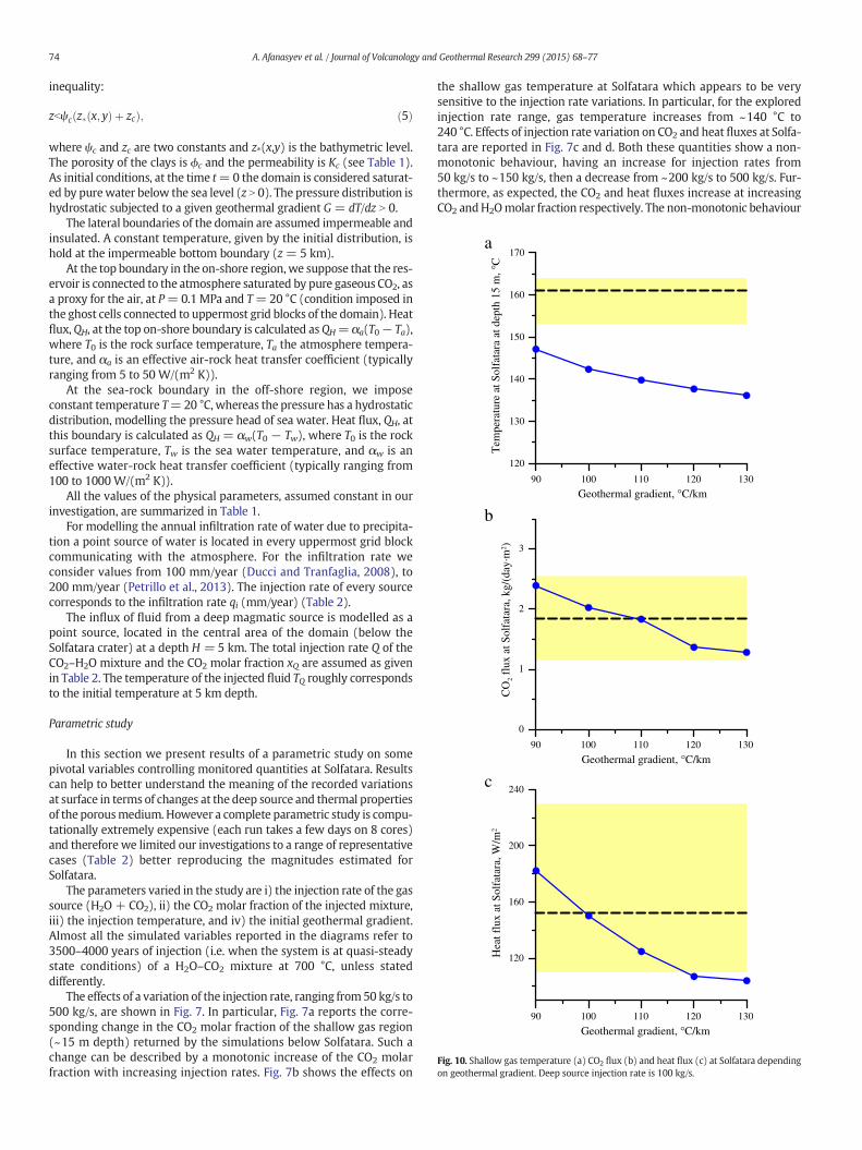
Fig. 10. Shallow gas temperature (a) CO2 flux (b) and heat flux (c) at Solfatara dependingon geothermal gradient. Deep source injection rate is 100 kg/s.

74 A. Afanasyev et al. / Journal of Volcanology and Geothermal Research 299 (2015) 68–77

inequality:

zbψc z� x; yð Þ þ zcð Þ; ð5Þ

where ψc and zc are two constants and z⁎(x,y) is the bathymetric level.The porosity of the clays is ϕc and the permeability is Kc (see Table 1).As initial conditions, at the time t=0 the domain is considered saturat-ed by purewater below the sea level (z N 0). The pressure distribution ishydrostatic subjected to a given geothermal gradient G = dT/dz N 0.

The lateral boundaries of the domain are assumed impermeable andinsulated. A constant temperature, given by the initial distribution, ishold at the impermeable bottom boundary (z = 5 km).

At the top boundary in the on-shore region,we suppose that the res-ervoir is connected to the atmosphere saturated by pure gaseous CO2, asa proxy for the air, at P=0.1MPa and T=20 °C (condition imposed inthe ghost cells connected to uppermost grid blocks of the domain). Heatflux,QH, at the top on-shore boundary is calculated asQH= αa(T0− Ta),where T0 is the rock surface temperature, Ta the atmosphere tempera-ture, and αa is an effective air-rock heat transfer coefficient (typicallyranging from 5 to 50 W/(m2 K)).

At the sea-rock boundary in the off-shore region, we imposeconstant temperature T=20 °C, whereas the pressure has a hydrostaticdistribution, modelling the pressure head of sea water. Heat flux, QH, atthis boundary is calculated as QH = αw(T0 − Tw), where T0 is the rocksurface temperature, Tw is the sea water temperature, and αw is aneffective water-rock heat transfer coefficient (typically ranging from100 to 1000 W/(m2 K)).

All the values of the physical parameters, assumed constant in ourinvestigation, are summarized in Table 1.

For modelling the annual infiltration rate of water due to precipita-tion a point source of water is located in every uppermost grid blockcommunicating with the atmosphere. For the infiltration rate weconsider values from 100 mm/year (Ducci and Tranfaglia, 2008), to200 mm/year (Petrillo et al., 2013). The injection rate of every sourcecorresponds to the infiltration rate qi (mm/year) (Table 2).

The influx of fluid from a deep magmatic source is modelled as apoint source, located in the central area of the domain (below theSolfatara crater) at a depth H = 5 km. The total injection rate Q of theCO2–H2O mixture and the CO2 molar fraction xQ are assumed as givenin Table 2. The temperature of the injected fluid TQ roughly correspondsto the initial temperature at 5 km depth.

Parametric study

In this section we present results of a parametric study on somepivotal variables controlling monitored quantities at Solfatara. Resultscan help to better understand the meaning of the recorded variationsat surface in terms of changes at the deep source and thermal propertiesof the porousmedium. However a complete parametric study is compu-tationally extremely expensive (each run takes a few days on 8 cores)and therefore we limited our investigations to a range of representativecases (Table 2) better reproducing the magnitudes estimated forSolfatara.

The parameters varied in the study are i) the injection rate of the gassource (H2O + CO2), ii) the CO2 molar fraction of the injected mixture,iii) the injection temperature, and iv) the initial geothermal gradient.Almost all the simulated variables reported in the diagrams refer to3500–4000 years of injection (i.e. when the system is at quasi-steadystate conditions) of a H2O–CO2 mixture at 700 °C, unless stateddifferently.

The effects of a variation of the injection rate, ranging from50 kg/s to500 kg/s, are shown in Fig. 7. In particular, Fig. 7a reports the corre-sponding change in the CO2 molar fraction of the shallow gas region(~15 m depth) returned by the simulations below Solfatara. Such achange can be described by a monotonic increase of the CO2 molarfraction with increasing injection rates. Fig. 7b shows the effects on

the shallow gas temperature at Solfatara which appears to be verysensitive to the injection rate variations. In particular, for the exploredinjection rate range, gas temperature increases from ~140 °C to240 °C. Effects of injection rate variation on CO2 and heat fluxes at Solfa-tara are reported in Fig. 7c and d. Both these quantities show a non-monotonic behaviour, having an increase for injection rates from50 kg/s to ~150 kg/s, then a decrease from ~200 kg/s to 500 kg/s. Fur-thermore, as expected, the CO2 and heat fluxes increase at increasingCO2 andH2Omolar fraction respectively. The non-monotonic behaviour

600

800

500 kg/s

75A. Afanasyev et al. / Journal of Volcanology and Geothermal Research 299 (2015) 68–77

of both CO2 and heat fluxes at Solfatara is controlled by the shape anddimension of the gas plume. At low injection rates the plume is narrowand concentrated below Solfatara, while at higher injection rates it en-larges due to more intense convection, and the fluids are dischargedthrough a wider area.

0 2500 5000

Depth below sea level, m

0

200

400

Tem

pera

ture

, C

100 kg/s

50 kg/s

200 kg/s

o

Fig. 12. Temperature profiles along AGN deep well for different injection rates. The mea-sured temperatures in AGN well (Penta, 1954) are shown.

0 2500 5000

Depth below sea level, m

0

200

400

600

800

Tem

pera

ture

, C

0 2500 5000

Depth below sea level, m

0

200

400

600

800

Tem

pera

ture

,

0 2500 5000

Depth below sea level, m

0

200

400

600

800

Tem

pera

ture

,

a

b

c

CC

Fig. 11. Solid lines show calculated temperature profiles for deep wells SV1 (a), SV3(b) and MF1 (c), while dashed lines show profiles for shifted locations SV3s (b) andMF1s (c). Injection rate is 100 kg/s, deep source CO2 molar fraction 0.197, geothermalgradient is 120 °C/km, time since the injection beginning 3500 years.

The control of CO2molar fraction of the injectedmixture is plotted inFig. 8a and b where the total injection rate is maintained constant at100 kg/s for two different initial geothermal gradients. Variations ofthe composition of the injected fluids cause a linear increase of boththe CO2 molar fraction of the shallow gas (Fig. 8a), and the CO2 flux atSolfatara (Fig. 8b). Furthermore both these variables show a negativecorrelation with the initial geothermal gradient (i.e. 110 and 120 °C/

Fig. 13. Temperature distribution at different depths below sea level and differentgeothermal gradients. Injection rate 100 kg/s, deep source CO2 molar fraction is 0.197.

76 A. Afanasyev et al. / Journal of Volcanology and Geothermal Research 299 (2015) 68–77

kmon the same line) that affects the shape and the dimension of the gasplume. The effects on the other variables (heatfluxes at Solfatara and fu-marole temperature) are minor.

We also explored the effects of the temperature of the injectedmixture, from 650 °C to 750 °C, on the checked variables but theseeffects resulted minor (e.g. Fig. 9).

Fig. 10 shows the effect of different initial geothermal gradients onthe temperature of the shallow gas (Fig. 10a), CO2 gas flux (Fig. 10b),and heat flux (Fig. 10c) at Solfatara. An increase of the geothermalgradient from 90 °C/km to 130 °C/km corresponds to a decrease for allthese quantities. Again these effects are caused by the size and theshape of the gas plume which is strongly controlled by the initialgeothermal gradient and, as wementioned before, by the injection rate.

Modelled vs measured

Here we compare simulation results with the available observationsat Solfatara and at the available deep wells (Fig. 5).

Fig. 14. CO2 plume shape for the different geothermal gradients, deep source CO2 molarfractions, and injection rates reported below each figure. Grid blocks, where CO2 molarfraction exceeds 0.05, are rendered in black colour, whereas temperature variations areshown using different colour gradations according to the reported colour scale.

At Solfatara, considering the average data from 2001 to 2008(Chiodini et al., 2010), the maximum fumarole temperature rangedfrom 153 °C to 164 °C (mean 161 ± 2 °C), i.e. the same values roughlysimulated for the 15 m depth gas zone below Solfatara at injectionrates b 200 kg/s and initial geothermal gradient of 120 °C/km (Fig. 7a).During the same period the observed molar fraction was of 0.19 ±0.02 that is consistent with the value simulated for the shallow gaszone when injection rates are ~50–100 kg/s and the CO2 molar fractionof the injected fluids is ~0.2 for an initial geothermal gradientof ~120 °C/km (Fig. 7b). With these flux and compositional ranges ofthe injected mixtures simulations reproduce also the observed CO2

fluxes. The mean CO2 flux measured for the hydrothermal-volcanicsource in 10 campaigns performed during 2003–2008 was in fact of1.85 ± 0.7 kg/(m2 day) roughly in agreement with simulated values(Figs. 7c, 8b, 10b). More difficult is the comparison between thesimulated and the measured heat fluxes because the sporadic andspotted measurements. In spite of these uncertainties, the heat fluxesat Solfatara, measured from 1999 to 2002 by Chiodini et al. (2005),range from 110 W/m2 to 230 W/m2 with the most representativevalue of 152 W/m2, a value of the same order of magnitude of thesimulations (Figs. 7d and 10c).

Another comparison of simulations with observations regarded thethermal profilesmeasured at SV1, SV3 andMF1 (Fig. 5). The simulationsusing an injection rate of 100 kg/s, an initial geothermal gradient of120 °C/km, and a CO2 molar fraction of 0.2 are able to well reproducethe measurements at SV1 (Fig. 11a) while, as in Petrillo et al., 2013,they underestimate the measurements at SV3 and MF1 (Fig. 11b andc). However a better fit is obtained even for these two cases comparingwith the temperature profile simulated in locations close to the wells(points SV3s and MF1s in Fig. 5). This suggests that the model is ableto reproduce the gross features, but not the details, of the CF hydrother-mal system because the developing of convective cells dramaticallyalters the local temperature profiles.

Fig. 12 compares the measured temperature profile of the Agnanowell (AGN in Fig. 5; Penta, 1954) with simulated profiles at an initialgradient of 120 °C/km and different injection rates ranging from50 kg/s to 500 kg/s. As for the other comparisons, measurementsseem consistent with an injection rate of ~100 kg/s.

Discussion and conclusion

With respect to common geothermal simulators, MUFITS can dealwith high temperature processes thus providing an invaluable supportfor the investigation of the phenomena occurring at volcanoes wherefluids originally at magmatic temperatures interact with shallowaquifers.

Herewe applyMUFITS to Campi Flegrei calderawheremany previousstudies point to the input ofmagmaticfluids in the shallower zones of thehydrothermal system as one of the main factors controlling the recentcrisis and affecting chemical and physical variations of themonitored pa-rameters (fumarolic composition and temperature, CO2 and heat fluxes,ground deformation, seismicity; e.g. Caliro et al., 2007; Chiodini et al.,2010 and 2012;D'Auria et al., 2011). Thiswork for thefirst time simulatesmore realistic magmatic fluids considering temperatures (650–750 °C)much higher than those previously adopted (350 °C)whichwere unreal-istically low for a magmatic source.

In order to reduce the effects of boundary conditions, we enlargedand deepened the 3D domain with heterogeneous properties of themedium recently developed by Petrillo et al. (2013).

As in previous studies, the injection of the hot gas mixture from thedeep source produces the development of a gas saturated plumebeneath Solfatara crater.

Our parametric study was firstly aimed to investigate the control ofthe main variables characterizing both the deep source (gas injectionrate, gas mixture composition, temperature) and the medium (initialgeothermal gradient) on the parameters monitored at Solfatara. These

77A. Afanasyev et al. / Journal of Volcanology and Geothermal Research 299 (2015) 68–77

parameters are affected by the size and the shape of the gas plumewhich in turn is strongly controlled by the injection rate and the initialgeothermal gradient. The control of initial geothermal gradients onthe plume beneath Solfatara was here investigated for the first time.High initial gradients tend to enhance the development ofmultiple con-vective cells and the enlargement of the plume, while colder initial con-ditions tend to reduce the plume size and focus the gas flow belowSolfatara (Figs. 13 and 14). Consequently, gas and heat fluxes observedat Solfatara are enhanced by low initial geothermal gradients. Similarconsiderations can be done for injection rate.

Of particular interest resulted the comparison between the simulatedthermal profiles and those measured in geothermal wells. Keeping inmind the uncertainties due to the heterogeneities of the system(Petrillo et al., 2013), the goodmatch obtained for thewells in the easternand north sectors of the caldera (i.e. MF1, SV1 and SV3 located some kmfar from Solfatara) suggests that the model can reproduce the grossfeatures of the CF hydrothermal system and implicitly support the hy-pothesis of a single (or major) deep source of magmatic fluid locatedclose to the centre of the caldera.

Surprising results were also obtained by comparing simulated andobserved (Agnano well) temperature profiles in a zone close to thegas plume: in this case the simulations clearly suggested that themagnitude of the source is of ~100 kg/s.

Finally, this study showed that MUFITS is a powerful tool for investi-gating processes at volcanoes, allowing for coupling deep regions, char-acterized by hot magmatic source, with shallow hydrothermal systems.

Acknowledgements

A. Afanasyev acknowledges financial support by a Grant from thepresident of the Russian Federation for the support of Young Scientists(project No. SP-2222.2012.5). This study has benefited from fundingprovided by the Italian Presidenza del Consiglio deiMinistri Dipartimentodella Protezione Civile (DPC). This paper does not necessarily representDPC official opinion and policies. S. Caliro and C. Cardellini are warmlythanked for the help given in the collection of input data for theCampi Flegrei simulations. The simulations were conducted at theSupercomputing Center of Lomonosov Moscow State University.

References

Afanasyev, A.A., 2013a. Multiphase compositional modelling of CO2 injection undersubcritical conditions: the impact of dissolution and phase transitions between liquidand gaseous CO2 on reservoir temperature. Int. J. Greenhouse Gas Control 19,731–742. http://dx.doi.org/10.1016/j.ijggc.2013.01.042.

Afanasyev, A.A., 2013b. Application of the reservoir simulator MUFITS for 3D modelling ofCO2 storage in geological formations. Energy Procedia 40, 365–374. http://dx.doi.org/10.1016/j.egypro.2013.08.042.

Altunin, V.V., 1975. Thermophysical Properties of Carbon Dioxide. Publishing House ofStandards, Moscow (in Russian).

Brooks, A.N., Corey, A.T., 1964. Hydraulic Properties of Porous Media. Hydrol. Pap.Colorado State University, Fort Collins.

Caliro, S., Chiodini, G., Moretti, R., Avino, R., Granieri, D., Russo, M., Fiebig, J., 2007. The originof the fumaroles of La Solfatara (Campi Flegrei, South Italy). Geochim. Cosmochim. Acta71 (12), 3040–3055. http://dx.doi.org/10.1016/j.gca.2007.04.007.

Chiodini, G., Frondini, F., Cardellini, C., Granieri, D., Marini, L., Ventura, G., 2001. CO2

degassing and energy release at Solfatara volcano, Campi Flegrei, Italy. J. Geophys.Res. 106, 16213–16221. http://dx.doi.org/10.1029/2001JB000246.

Chiodini, G., Todesco, M., Caliro, S., Del Gaudio, C., Macedonio, G., Russo, M., 2003. Magmadegassing as a trigger of bradyseismic events; the case of Phlegrean Fields (Italy).Geophys. Res. Lett. 30, 1434. http://dx.doi.org/10.1029/2002GL016790.

Chiodini, G., Caliro, S., Cardellini, C., Granieri, D., Avino, R., Baldini, A., Donnini, M.,Minopoli, C., 2010. Long-term variations of the Campi Flegrei, Italy, volcanic systemas revealed by the monitoring of hydrothermal activity. J. Geophys. Res. 115,B03205. http://dx.doi.org/10.1029/2008JB006258.

Chiodini, G., Granieri, D., Avino, R., Caliro, S., Costa, A., Werner, C., 2005. Carbon dioxidediffuse degassing: implications on the energetic state of a volcanic hydrothermal sys-tems. J. Geophys. Res Vol. 110, B08204. http://dx.doi.org/10.1029/2004JB003542.

Chiodini, G., Caliro, S., De Martino, P., Avino, R., Gherardi, F., 2012. Early signals of newvolcanic unrest at Campi Flegrei caldera? Insights from geochemical data andphysical simulations. Geology 40, 943–946. http://dx.doi.org/10.1130/G33251.1.

Costa, A., Dell'Erba, F., Di Vito, M.A., Isaia, R., Macedonio, G., Orsi, G., Pfeiffer, T., 2009.Tephra fallout hazard assessment at the Campi Flegrei caldera (Italy), Bull. Volcanol.Vol. 71, 259–273. http://dx.doi.org/10.1007/s00445-008-0220-3.

Costa, A., Folch, A., Macedonio, G., Giaccio, B., Isaia, R., Smith, V.C., 2012. Quantifying vol-canic ash dispersal and impact of the Campanian Ignimbrite super-eruption.Geophys. Res. Lett. 39, L10310. http://dx.doi.org/10.1029/2012GL051605.

D'Auria, L., Giudicepietro, F., Aquino, I., Borriello, G., Del Gaudio, C., Lo Bascio, D., Martini,M., Ricciardi, G.P., Ricciolino, P., Ricco, C., 2011. Repeated fluid-transfer episodes as amechanism for the recent dynamics of Campi Flegrei Caldera (1989–2010).J. Geophys. Res. 116, B04313. http://dx.doi.org/10.1029/2010JB007837.

Del Gaudio, C., Aquino, I., Ricciardi, G.P., Ricco, C., Scandone, R., 2010. Unrest episodes atCampi Flegrei: a reconstruction of vertical ground movements during 1905–2009.J. Volcanol. Geotherm. Res. 195 (1), 48–56. http://dx.doi.org/10.1016/j.jvolgeores.2010.05.014.

Ducci, D., Tranfaglia, G., 2008. The Effect of Climate Change on the Hydrogeological Re-sources in Campania Region (Italy). In: Dragoni, W. (Ed.), Groundwater and climaticchanges. Geological Society 288. Special Publications, London, pp. 25–38. http://dx.doi.org/10.1144/SP288.3.

Fenghour, A., Wakeham,W.A., Watson, J.T.R., 1996. Densities of (water + carbon dioxide)in the temperature range 415 K to 700 K and pressures up to 35 MPa. J. Chem.Thermodyn. 28, 433–446. http://dx.doi.org/10.1006/jcht.1996.0043.

Ingebritsen, S.E., Geiger, S., Hurwitz, S., Driesner, T., 2010. Numerical simulation ofmagmatic hydrothermal systems. Rev. Geophys. 48, RG1002. http://dx.doi.org/10.1029/2009RG000287.

Ingebritsen, S.E., Manning, C.E., 2010. Permeability of the continental crust: dynamicvariations inferred from seismicity and metamorphism. Geofluids 10, 193–205.http://dx.doi.org/10.1111/j.1468-8123.2010.00278.x.

Orsi, G., D'Antonio, M., de Vita, S., Gallo, G., 1992. The Neapolitan Yellow Tuff, alargemagnitude trachytic Phreatoplinian eruption: eruptive dynamics, magmawithdrawal and caldera collapse. J. Volcanol. Geotherm. Res. 53, 275–287. http://dx.doi.org/10.1016/0377-0273(92)90086-S.

Penta, F., 1954. Ricerche e studi sui fenomeni esalativo idrotermali ed il problema delleforze endogene. Ann. Geofis. 8 (3), 1–94.

Petrillo, Z., Chiodini, G., Mangiacapra, A., Caliro, S., Capuano, P., Russo, G., Cardellini, C.,Avino, R., 2013. Defining a 3D physical model for the hydrothermal circulation atCampi Flegrei caldera (Italy). J. Volcanol. Geotherm. Res. 264, 172–182. http://dx.doi.org/10.1016/j.jvolgeores.2013.08.008.

Pruess, K., Oldenburg, C., Moridis, G., 1999. TOUGH2 User's Guide, Version 2. LawrenceBerkley Lab. Report LBNL-43134.

Pruess, K., 2004. The TOUGH codes— a family of simulation tools for multiphase flow andtransport processes in permeable media. Vadose Zone J. 3, 738–746. http://dx.doi.org/10.2113/3.3.738.

Pruess, K., Spycher, N., 2007. ECO2N—a fluid property module for the TOUGH2 code forstudies of CO2 storage in saline aquifers. Energy Convers. Manag. 48 (6),1761–1767. http://dx.doi.org/10.1016/j.enconman.2007.01.016.

Pruess, K., 2011. ECO2M: a TOUGH2 fluid property module for mixtures of water, NaCl,and CO2, including super- and sub-critical conditions, and phase change betweenliquid and gaseous CO2. LBNL-4590E report.

Rinaldi, A.P., Todesco, M., Bonafede, M., 2010. Hydrothermal instability and grounddisplacement at the Campi Flegrei caldera. Phys. Earth Planet. Inter. 178, 155–161.http://dx.doi.org/10.1016/j.pepi.2009.09.005.

Rivkin, S.L., Alexandrov, A.A., 1980. Thermophysical Properties ofWater andWater Vapor.Publishing house “Energiya”, Moscow (in Russian).

Seitz, J.C., Blencoe, J.G., 1999. The CO2–H2O system. I. Experimental determination ofvolumetric properties at 400 °C, 10–100 MPa. Geochim. Cosmochim. Acta 63,1559–1569. http://dx.doi.org/10.1016/S0016-7037(99)00050-2.

Spycher, N., Pruess, K., 2011. A model for thermophysical properties of CO2–brinemixtures at elevated temperatures and pressures. Proceedings Thirty-SixthWorkshop on Geothermal Reservoir Engineering. Stanford University, Stanford, CA(January 31 – February 2, SGP-TR-191).

Takenouchi, S., Kennedy, G.C., 1964. The binary system H2O–CO2 at high temperaturesand pressures. Am. J. Sci. 262, 1055–1074. http://dx.doi.org/10.2475/ajs.262.9.1055.

Todcheide, K., Franck, E.U., 1963. Das zweiphasengebiet und die kritische kurve im systemkohlenchlorid-wasser bis zu drucken von 3500 bar. Z. Phys. Chem. 37, 387–401.

Todesco, M., Chiodini, G., Macedonio, G., 2003. Monitoring and modelling hydrothermalfluid emission at La Solfatara (Phlegrean Fields, Italy); an interdisciplinary approachto the study of diffuse degassing. J. Volcanol. Geotherm. Res. 125, 57–79. http://dx.doi.org/10.1016/S0377-0273(03)00089-1.

Todesco, M., Rutqvist, J., Chiodini, G., Pruess, K., Oldenburg, C.M., 2004. Modeling of recentvolcanic episodes at Phlegrean Fields (Italy); geochemical variations and grounddeformation. Geothermics 33, 531–547. http://dx.doi.org/10.1016/j. geothermics.2003.08.014.

Todesco, M., 2009. Signals from the Campi Flegrei hydrothermal system: role of a“magmatic” source of fluids. J. Geophys. Res. 114, B05201. http://dx.doi.org/10.1029/2008JB006134.