Investigation of a New 3D Intelligent Ray-Tracing Model

Wireless Pers Commun (2014) 77:691–717DOI 10.1007/s11277-013-1532-y

Investigation of a New 3D Intelligent Ray-Tracing Model

Ahmed Wasif Reza · Kamarul Ariffin Noordin · Md. Jakirul Islam ·A. S. M. Zahid Kausar · Harikrishnan Ramiah

Published online: 23 November 2013© Springer Science+Business Media New York 2013

Abstract While characterizing the wireless network, it is critical to predict the exact signalpropagation paths in an efficient way for three dimensional (3D) indoor environment. Inthis paper, a new 3D intelligent ray-tracing (IRT) model based on the modified binary angledivision (MBAD) technique is presented. The MBAD algorithm can launch the minimumamount of rays by identifying the invalid regions, which can skip the processing of the unnec-essary signals. To further accelerate the MBAD algorithm feasible for the 3D environment,virtual surface technique and efficient polygon test are used. Besides, the amount of time forintersection test is reduced by using the surface skipping technique. Moreover, different radiosignal propagation paths, such as reflection, refraction, and diffraction from 3D objects alongwith infinitesimal rays with very small wavefront are considered. The results obtained fromthis study show the superiority of the proposed model in terms of higher prediction accu-racy (29.21 %) and better computational time (58.78 %) than other well-known techniques.Finally, this work also analytically examines the measured and the simulated results for theproposed IRT model and evaluates the effectiveness. The experimental results are comparedwith the simulated results obtained from IRT model and good agreement (accuracy of about97 to >99 %) demonstrated.

Keywords Intelligent ray-tracing · Binary angle division · Virtual surface · Polygon test ·Wireless communication

1 Introduction

The progressive deployment of wireless radio networks has encouraged researchers in thedirection of study of radio propagation and the development of fast and highly accurate radiopropagation prediction models. As various wireless communication services are available for

A. W. Reza (B) · K. A. Noordin · Md. J. Islam · A. S. M. Zahid Kausar · H. RamiahDepartment of Electrical Engineering, Faculty of Engineering,University of Malaya, 50603 Kuala Lumpur, Malaysiae-mail: [email protected]; [email protected]

123

692 A. W. Reza et al.

indoor, the demand for an accurate and efficient radio propagation prediction model rises.Modeling in a three dimensional (3D) environment is more challenging and complex than2D as electromagnetic rays can hit anywhere on a surface of a 3D object. Accurate multipathsignal propagation modeling in 3D complex indoor environments is therefore turned out to bethe primary requirement in designing reliable wireless networks. Basically, radio propagationprediction model, such as 2D ray-tracing (RT) [1] provides less accuracy compared to the 3DRT, therefore, too many investigations on 3D RT are introduced by using commonly knownimage and shooting-and-bouncing ray (SBR) techniques in [2–19]. The image method isaccurate, however, it can only handle simple environment and ray prediction time is increasedrapidly with the number of objects in the 3D environment [16]. On the other hand, the SBRmethod can handle complex environment, but requires more computation time than the imagemethod [17–19]. In order to increase the accuracy of SBR method, a large number of raysneeded to launch from the transmitter. Besides, in KD-tree based SBR technique, the sphericalwavefront is covered by the ray cones and two successive cones overlap each other at theedge. In that case, the receiver located in the overlapping region will receive two rays anddouble ray counting error will occur [14,17].

Another recently developed RT technique, for instance bi-directional path-tracing (BDPT)model [3] failed to reduce the computational time due to the fixed number of launchedrays, dual RT involved, and huge amount of intersection tests. The line search theory (LST)model [5] on the other hand reduces the computation time by reducing the number of theemitted rays based on the power-transporting solid angle concept and by iteratively increasingthe tessellation frequency, which depends on the predefined resolution that degrades theaccuracy. Also in [4], the concept of ray-frustum (RF) is presented, where huge amountof triangles will be generated for the formation of ray frustums in a complex environment.Hence, prior to visibility test, a significant amount of time will be needed to construct a largenumber of triangles. Besides, this model required larger computer memory for the complexenvironments.

The purpose is therefore to develop a new, very fast, and highly accurate intelligent ray-tracing (IRT) model for 3D indoor environment based on the modified binary angle division(MBAD) technique that will eliminate the shortcomings as explained above. The MBADalgorithm will skip all the unnecessary signals by identifying the invalid regions and able tolaunch the exact amount of rays that will make the algorithm faster and provide higher predic-tion accuracy. The proposed 3D IRT model can provide superior accuracy as well as speed upthe RT by introducing new acceleration techniques, such as virtual surface, enhanced polygontest, and surface skipping. Moreover, rays of infinitesimal wavefront are considered in thisstudy to minimize the propagation path error. To prove the superiority, the proposed 3D IRTmodel is compared with the existing 2D IRT [20], BDPT [3], LST [5], RF [4], and SBR [14]techniques. The results obtained show that, the proposed model provides significant perfor-mance in terms of higher number of predicted rays and better computational time. The termsray and signal are used interchangeably with predicted ray and predicted signal in this paper.

However, it should be stressed here that model without verification and validation maynot be efficient and accurate and may not reflect the actual environment. Thus, realizing theimportance of this issue, this paper will investigate the accuracy of the IRT model by theuse of experimental setup. It will determine the differences between the experimental andthe simulated results. The remaining part of this paper is organized as follows. The designdetails of 3D IRT model is described in Sect. 2, followed by simulation results analysis inSect. 3. Section 4 will investigate the accuracy of the IRT model and will determine thematching accuracy between the experimental and the simulated results by performing radiosignal propagation analyses. Finally, Sect. 5 provides the concluding remarks.

123

Investigation of a New 3D Intelligent Ray-Tracing Model 693

2 Proposed 3D IRT Model

To make the proposed 3D IRT model fast and highly efficient, a new algorithm of MBAD isintroduced, followed by acceleration techniques, such as virtual surface technique, efficientpolygon test, and surface skipping.

2.1 MBAD Algorithm

For a single quadrant, let Start and End represent the starting and the ending angles, respec-tively. After launching two rays from the location of Tx at Start and End angles, followthe paths until these becoming weaker or passing away the indoor environment or these arereceived by the receiver (Rx) after reflected, refracted, or diffracted with the objects. If theemanated ray is received by the Rx, then the ray is considered as a significant ray. After-wards, check the paths of the two rays emanated at angles Start and End, if they create a validpolygon. If the polygon is valid and there is no object within the polygon, skip all other rayswithin the angles Start and End. Otherwise, the next ray will be launched by equally dividingthe angles Start and End, which will form two new polygons and repeat this procedure totrace the additional rays. In this way, the MBAD algorithm can identify the invalid regionsto skip all the unnecessary signals and predict the significant signals received by the Rx inan indoor environment.

The RT begins by launching two rays in a particular quadrant with an angle θ such thatStart ≤ θ ≤ End . To build the ray using triangular geometry, suppose a ray R has beenlaunched from the given coordinate T x(x1, y1, z1) at any angle θ with the base line T x B aspresented in Fig. 1. It forms a triangle �T x B N . To compute the end point N (x2, y2, z2) ofR, it is required to calculate the length of normal BN of the triangle �T x B N . The overallformula to calculate the end point N of the ray R has been given in Eqs. (1) to (3).

The length of the base of the triangle �T x B N is,

T x B = W − T x(x1) = W − x value of T x (1)

If the width of the simulation area is W then the length of the normal of that triangle is,

Normal = tan θ × Base = tan θ × (W − T x(x1)) (2)

Using Eqs. (1) and (2), the end point of R can be easily calculated. Therefore, if the simulationarea starts with the coordinate (x, y, z), the following equation can be written,

Fig. 1 Illustration of raybuilding and the closestintersection point (IP ) of theproposed 3D IRT method

123


N (x2, y2, z2) = N (x, Normal + H, 0) (3)

where H = T x(y1) = y value of T x and z to be considered as zero.

2.2 Virtual Surface and Intersection Test

After building a ray, an intersection test will be initiated to find out the origin of the reflected,refracted, or diffracted ray. Basically, it is necessary to find out the origin of those rays,that means, the intersection point of ray-object. For the intersection test, the virtual surfacetechnique is introduced here.

This study considers a 3D space for a typical indoor environment. The 3D objects aremodeled by the cubes or cuboids, as shown in Fig. 2.

Each object has six surfaces, such as left S1(a, b, c, d), right S2(e, f, g, h), topS3(a, b, g, h), bottom S4(c, d, e, f ), front S5(a, d, e, h), and back S6(c, b, g, f ). In a realsituation, the signal emitted from the Tx can hit everywhere on the surface of 3D objects andafter reflection, refraction, or diffraction, it will hit with other objects. However, in case of3D simulation environment, it is quite difficult to determine such kind of random intersectionpoints on the surface of a 3D object. To overcome this type of difficulties, this study uses anew concept of virtual surface. Virtual surface is a rectangle that virtually exists inside theobjects, which will help to easily find out the intersection point on a 3D object. This techniqueis used here to handle the 3D objects and speed up our existing 2D IRT algorithm [20]. Theconstruction process of virtual surface using left and right surfaces of an object is given inFig. 2.

Referring to Fig. 2, let S is the starting coordinate of a virtual surface and H and W arethe width and height of the virtual surface, respectively. Hence, area (virtual surface) of arectangle that starts from S can be calculated by the following equation:

Area = W × H (4)

Fig. 2 Virtual surface marked by black color constructed from left and right surfaces of a 3D object. a Virtualsurface of vertical object. b Virtual surface of horizontal object

123


Algorithm: VIRTUALSURFACE(Object)

Input: 3D object

Output: Return a rectangle as a virtual surface

1. Retrieve left and right surface from a 3D object leftFace Object.GetLeftFace()

rightFace Object.GetRightFace()

2. Calculate the starting location S(x,y) of a virtual surface S.x (leftFace.A.x + leftFace.B.x)/2

S.y (leftFace.A.y + leftFace.B.y)/2

3. Calculate the ending location T(x,y) and U(x) of a virtual surface T.x (leftFace.C.x + leftFace.D.x)/2

T.y (leftFace.C.y + leftFace.D.y)/2

U.x (rightFace.E.x + rightFace.F.x)/2

4. Calculate the width and height of the virtual surface W U.x – T.x

H T.y – S.y

5. Return a rectangle as a virtual surface to the list of objects

return rectangle(S ,W ,H)

Fig. 3 Virtual surface construction algorithm

Fig. 4 Intersection pointbetween ray and virtual surface

In Fig. 2, S is the average value of a and b coordinates of the left surface, T is the averagex-value of c and d coordinates of the right surface, U is the average x-value of e and fcoordinates, H is the difference of y-value between T and S coordinates, and W is thedifference of x-value between U and T coordinates.

The entire construction process of virtual surface is carried out along with the constructionof 3D object that does not effect on the computation time of the proposed 3D IRT technique.The algorithm to construct a virtual surface is given in Fig. 3.

The virtual surface actually helps to find out the intersection point between the ray andobject. In this study, the intersection point is determined from the two lines using the geomet-rical calculation. The emitted ray is considered as “line a” (P1, P2), while “line b” (P3, P4)is made from the virtual surface, as shown in Fig. 4.

Let, “a” and “b” are the two lines and therefore, the equations are as follows:

Xa = P1 + Ua(P2 − P1) (5)

Xb = P3 + Ub(P4 − P3) (6)

The algorithm to determine the ray-object intersection point P(x, y) based on Eqs. (5) and (6)is presented in Fig. 5. If the emitted ray intersects more than one object then it is necessary to

123


Fig. 5 Algorithm to find out the intersection of two lines

calculate the closest ray-object intersection. This calculation is based on the distance from theray emanating point. Suppose, a ray R intersects with the two objects Ip and I ′

p . The distancefrom the origin of the ray to the intersection points are d(Rorigin, Ip) and d(Rorigin, I ′

p). Ifthe distance d(Rorigin, Ip) < d(Rorigin, I ′

p) then Ip is the closest intersection point of theorigin of ray R in Fig. 1.

It should be noted here, the wrong identification of intersection point can change theentire propagation path of the predicted rays, which causes an erroneous ray prediction. Asit is known that, the RT is based on the geometrical optics (GO), which assumes that theelectromagnetic energy can be considered to be radiated through the infinitesimal ray withvery small wavefront as shown in Fig. 6.

Based on the concept of GO, the 3D IRT method considers a ray that lies along thepropagation and travels in a straight line. Hence, the 3D IRT method can perfectly identify

123


Fig. 6 a Infinitesimally ray withvery small wavefront thatincident at a particular object.b Ray with large wavefrontincident at multiple objects

Fig. 7 Finding the closest ray-object intersection point

the exact location of the intersection point during ray-object intersection test and generatesthe accurate propagation path of the emanated ray. As a result, the proposed model yieldsthe exact propagation path. The algorithm of finding the exact closest ray-object intersectionpoint is presented in Fig. 7.

Moreover, while doing the ray-object intersection test, the unnecessary test for the ray-surface intersection can be ignored by using a surface skipping technique as in Fig. 8. Eachobject of the simulation environment has six surfaces, namely, front, back, left, right, top, andbottom. Only two of them are taking part in ray-object intersection test. For example, if anobject is in the first quadrant with respect to the quadrant of the emitted ray, then the possible

123


Fig. 8 Valid intersections between the ray and the surfaces of the objects

Fig. 9 Illustration of a 3D objectwith reflected, refracted, andtransmitted rays by the proposed3D IRT

surface in the intersection test is the left/bottom surface. Again, if an object is in the secondquadrant with respect to the quadrant of the emitted ray, then the surface of the intersectiontest is the right/bottom surface. Similarly, top/right and top/left surfaces are taking part inray-object intersection test in case of third and fourth quadrants, respectively.

Based on this concept, all the valid intersections have been shown in Fig. 8. Here, verticaland horizontal dotted lines drawn from the position of the Tx divide the space into fourquadrants. It is seen from Fig. 8 that there are thirty seven objects in the area (total of37 × 6 = 222 surfaces). However, only 37 × 2 = 74 surfaces of them are taking part inray-object intersection test. Hence, the significant amount of computation time is reduced inray-object intersection test.

However, indoor radio propagation is influenced by the building materials that can changethe entire propagation paths of reflected, refracted, and diffracted rays. Therefore, an accuratecalculation of direction of such rays can achieve the exact path of predicted rays. In this study,the direction of propagated rays can be calculated using vector geometry [21,22], as presentedbelow.

Referring to Fig. 9, let normalized direction vector of incident, reflected, and refractedrays are �Ri , �Rr , and �Rt , respectively, then the normal of these rays is equal to 1, i.e.,

123


| �Ri | = | �Rr | = | �Rt | = | �N | = 1 (7)

where �N is a normalized vector, which is orthogonal to the incident surface and points towardsthe first material η1. If the direction vector �Ri of incident ray splits into two components, suchas orthogonal ( �Ri⊥) and parallel ( �Ri||), then the normal part �Ri⊥ is the orthogonal projection

on �N . Using Eq. (7) and Fig. 9, the following equation can be written,

�Ri⊥ = �Ri · �N| �N |2

�N = ( �Ri · �N ) �N (8)

And, the tangent part �Ri|| is the difference between �Ri and �Ri⊥ , that is,

�Ri|| = �Ri − �Ri⊥ (9)

Similarly, for the case of the reflected ray, �Rr⊥ and �Rr|| are orthogonal and �Rr⊥ is the orthog-

onal projection of �N , that is,

�Rr⊥⊥ �Rr|| (10)

Using the basic geometry as well as Eqs. (7) and (10) of any angle θ ,

cos θ = | �R⊥|| �R| = | �R⊥| (11)

sin θ = | �R|||| �R| = | �R||| (12)

As presented in Fig. 9, the radio signal is reflected by the non-scattering surface of the object.Hence, according to the law of reflection, the angle of the reflected ray is equal to the angleof the incident ray, that is, θi = θr . Using Eqs. (11) and (12), the following equations can beformulated:

| �Rr⊥| = cos θr = cos θi = | �Ri⊥| (13)

| �Rr|| | = sin θr = sin θi = | �Ri|| | (14)

Moreover, all the normal parts of the reflected ray are parallel to each other and also parallelto �n. Therefore, both the parts can be written as follows:

�Rr⊥ = − �Ri⊥ (15)�Rr|| = �Ri|| (16)

Hence, the actual direction of the reflected ray is,

�Rr = �Rr|| + �Rr⊥ = �Ri|| − �Ri⊥ (17)

Equation (17) can be written using Eqs. (8), (9), and (13) as below:

�Rr = �Ri|| − �Ri⊥

=[ �Ri − ( �Ri · �N ) �N

]− ( �Ri · �N ) �N

= �Ri − 2( �Ri · �N ) �N= �i − 2 cos θi �N (18)

123


In this study, the refracted rays are generated when the ray travels through an object made ofglass. Referring to Fig. 9, η1 and η2 are the refractive index of air and glass, respectively. Inthis situation, Snell’s Law describes the resulting deflection of the refracted ray as follows:

η1 sin θi = η2 sin θt => sin θt = η1 sin θi

η2(19)

where θi and θt are the angles between the normal to the interface and the incident andrefracted waves, respectively. The normalized vector of the refracted ray �Rt can be calculatedfrom the triangle of the refracted ray in Fig. 9 as follows:

�Rt = �Rt|| + �Rt⊥ (20)

Using Eqs. (12) and (19), it can be written that,

| �Rt|| | = η1

η2| �Ri|| | (21)

Again, if the values of Eqs. (8) and (9) are put into Eq. (21), the following equation can beobtained,

�Rt|| = η1

η2

[ �Ri − cos θi �N]

(22)

Moreover, the triangle of the refracted ray (Fig. 9) is split in two parts and they are equal toeach other, that is, �Rt⊥ = �Rt|| . Hence, by applying Eq. (7) and commonly known Pythagorasformula, it can be formulated that,

�Rt⊥ = −√

1 − | �Rt|| |2 �N (23)

If the values of Eqs. (22) and (23) are substituted into Eq. (20), then the direction of therefracted ray �Rt becomes,

�Rt = η1

η2�Ri −

(η1

η2cos θi +

√1 − | �Rt|| |2

)�N (24)

=> �Rt = η1

η2�Ri −

(η1

η2cos θi +

√1 − sin2 θt

)�N (25)

Here, the normal of |�t||| = sin θt . Finally, from Eq. (19), it can be written that,

sin2 θt =(

η1

η2

)2

sin2 θi =(

η1

η2

)2 (1 − cos2 θt

)(26)

By substituting the value of Eq. (26) into Eq. (25), the direction of the refracted ray can becalculated. By the same way as explained above, the direction of the transmitted rays canalso be calculated.

In the case of diffracted ray, when an incident ray intersects with the corner of a virtualsurface of any object then the ray originated from that intersection point is treated as thediffracted ray as shown in Fig. 10. Hence, it is efficient to build the path by solving angleconstraints between the edges and the diffracted directions. For a single wedge, the diffractionpoint E on the edge satisfies the following equation [23]:

−→E Ri · −→

V = −→E Rd · −−−→

(−V ) (27)

123


Fig. 10 Illustration of thediffracted ray by the proposed 3DIRT

Fig. 11 Tracing ray using theproposed 3D IRT method

where “·” is a dot product, Ri is the source point of the ray, Rd is the end point of thediffracted ray, and �V is the direction vector. Here, the direction vector �V is oriented such that�V × �W = �N , where �W is a vector that lies in the plane of one of the two polygons of thewedge and �N is the unit vector.

2.3 Ray Prediction Using Polygon Test

The ray prediction algorithm begins by dividing the entire simulation space into four quad-rants at Tx position. The size of each quadrant is 90◦. To trace the rays emitted from theTx, the MBAD algorithm will be applied for each quadrant individually. Figure 11 shows anindoor environment, where the transmitter, the receiver, and the object is represented by Tx,Rx, Obj, respectively. The Rx and Obj are placed in the third quadrant and thus, the MABDalgorithm is applied on the third quadrant. As presented in Fig. 11, two rays R1 and R2 arelaunched from the Tx, a polygon (Zone 1) is formed in the third quadrant using the points R1,Tx, R2, and Q3. Now, it is required to check whether there is any object within this polygonor not. To do this, only the start and end location of each object is needed to be considered.For a given polygon Pmade up of n vertices (xi , yi ) where 0 ≤ i ≤ n − 1, the test pointp(x p, yp) will be determined whether it is inside, outside, or on the edge of the polygon.

In 2D IRT [20], an ordinary point in polygon test algorithm based on the ray-crossingnumber method is used, which takes O(n) time in each point of the polygon test. If the numberof the formed polygons and its corresponding vertices increases, then the computation timealso increases. In that case, the 2D IRT [20] fails to determine the test point p

(x p, yp

)lies

on the edge of a polygon or may coincide with one of the vertices Pi of P , which resultsin lack of accuracy. To overcome these drawbacks, this study uses the new point in polygontest algorithm [24]. This algorithm is developed to efficiently handle the special cases, which

123


Fig. 12 a The ϕ(t) is acontinuous angle for a curve.b The ϕ(t) is a discrete signedangle of a polygon

cannot be solved by the traditional point in the polygon test (as in 2D IRT [20]). This newalgorithm will save a significant amount of ray prediction time. As shown in Fig. 12, thepoint p has a winding number W (p, Cur) about the curve Cc(t) = (xc(t), yc(t))T , t ∈[m, n], Cc(m) = Cc(n).

Actually, this winding number W (p, Cur) is the total number of revolutions around thepoint p while travelling the closed curve Cur [24]. The winding number W (p, Cur) is

undefined if there exists t ∈ [m, n] such that Cc(∼t ) = p. Or else, it can be computed by

integrating differential of the angle ϕ(t) between the edge pCc(t) and the positive horizontalaxis through p (Fig. 12) [24]. Let, the coordinate of p = (0, 0) with the intention that,ϕ(t) = arctan yc(t)

xc(t)[24] and,

W (p, Cur) = 1

2π

n∫

m

dϕ(t) = 1

2π

n∫

m

dϕ

dt(t) dt

= 1

2π

n∫

m

yc(t)xc(t) − yc(t)xc(t)

xc(t)2 + yc(t)2 dt (28)

where xc(t) and yc(t) are the derivatives of xc and yc with respect to time t , respectively.Suppose, a closed polygon Poly has n points and this polygon can be represented as

P0, P1, P2, . . . , Pn = P0, which can be seen as piecewise linear curved t → (xi (t−i), yi (t−i))T , t ∈ [i, i + 1] with (xi (t), yi (t))T = t Pi+1 + (1 − t)Pi .

Therefore, the winding number of a polygon W (p, Poly) can be expressed as follows[24]:

W (p, Poly) = 1

2π

∑0≤i≤n−1

1∫

0

yi (t)xi (t) − yi (t)xi (t)

xi (t)2 + yi (t)2 dt

= 1

2π

∑0≤i≤n−1

arccos〈Pi |Pi+1〉

‖Pi‖ ‖Pi+1‖ · sign{(Pxi × P y

i+1) − (P yi × Px

i+1)}

= 1

2π

∑0≤i≤n−1

ϕi (29)

where ϕi is the angle between the edge pPi and pPi+1. Based on Eq. (29), a new efficientpoint in polygon test algorithm is used for computing the winding number to determine apoint inside, outside, or on the edge of a polygon. The algorithm is illustrated in Fig. 13.

If the proposed polygon test algorithm is applied to the formed polygon as in Fig. 11, itwill be seen that there are six objects exist within the Zone 1. Therefore, the angular distance

123


Fig. 13 Algorithm for new point in polygon test

between R1 and R2 will be divided equally by launching another ray R3 from the Tx. Thiswill produce two new polygons R1T x R3 and R2T x R3, are denoted by Zone 2 and Zone3, respectively. If the polygon test algorithm is applied for Zone 2 and Zone 3, it will beseen that, the objects exist inside both zones. Hence, the R3 is being passed through themiddle of R1 and R2, and intersects with two objects at Ip and I ′

p , as shown in Fig. 11. Ifthe closest object intersection and the intersection of two lines, which are described earlier,

123


are applied for R3, then Ip (marked by the black dot in Fig. 11) will be the closest objectintersection. To this intersection point, a new ray R4 will be built that acts as a reflectedray. Again, the angular distance between R3 and R2 will be divided equally by launchinganother ray R5 from the Tx. This will produce two new polygons R3T x R5 and R2T x R5,represented by Zone 4 and Zone 5, respectively. It will be seen that, nothing exists insidethe Zone 4. Therefore, Zone 4 can be marked as invalid zone and all other signals withinthis zone can be ignored. The signal R5 will be lost because nothing exists along the pathof R5. On the other hand, Zone 5 is a valid zone because two objects and Rx exist withinthat zone. Hence, another ray of R6 is launched by dividing the angle between Zone 5.Here, R6 is received by the receiver. Now, consider another ray R7 that is being passedthrough the middle of the angular distance of the rays R1 and R5 and passes away the indoorarea after diffracted and reflected on the two objects. The path of the signals from Tx toRx is composed of connected line segments, where the first line segment is the emanatedray and the rest of them are either reflected or refracted/diffracted rays. In this way, byapplying the proposed algorithm in all four quadrants, it is possible to identify the invalidregions to skip all the unnecessary signals and predict the significant signals received by thereceivers.

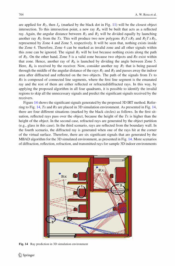
Figure 14 shows the significant signals generated by the proposed 3D IRT method. Refer-ring to Fig. 14, Tx and Rx are placed in 3D simulation environment. As presented in Fig. 14,there are four different situations (marked by the black circles) as follows. In the first sit-uation, reflected rays pass over the object, because the height of the Tx is higher than theheight of the object. In the second case, refracted rays are generated by the object partition(e.g., glass in this case). In the third scenario, rays are reflected from the boundary wall. Inthe fourth scenario, the diffracted ray is generated when one of the rays hit at the cornerof the virtual surface. Therefore, there are six significant signals that are generated by theMBAD algorithm for the 3D simulated environment, as presented in Fig. 14. More scenariosof diffraction, reflection, refraction, and transmitted rays for sample 3D indoor environments

Fig. 14 Ray prediction in 3D simulation environment

123


Fig. 15 Illustration of diffraction where the diffracted corner of the obstacle has been highlighted by the solidcircle

Fig. 16 Illustration of reflected (1), refracted (2), and transmitted (3) rays for a sample 3D indoor environment

Table 1 Specifications of the test environment

Name Material Height (m) Permittivity Refractive index

Wall Brick 2–4.5 5.2 1.7–2.2

Window Glass 1–1.5 3.7 1.50–1.92

Door Wood 1.75–2.75 3.0 2.2

Table Wood 1.1 3.0 2.2

Partition Plastic board 1.83 2.8 1.46–1.55

by the proposed 3D IRT model are illustrated in Figs. 15 and 16. The details of the test envi-ronment (permittivity and refractive index of different materials) corresponding to Figs. 14,15, 16 are given in Table 1. Besides, the experimental settings are provided in Sect. 4. TheMBAD algorithm is demonstrated in Fig. 17.

123


Fig. 17 Representation of MBAD algorithm

3 Results and Discussion

For performance evaluation, 5 different indoor environments are considered in this study. Thesimulation environment has been implemented with Visual Studio 2008 using C# code. Foreach environment, the simulation results have been taken for 10 different scenarios by placing

123


Fig. 18 Simulation environment for performance evaluation

Tx and Rx at different locations in 3D environments (one of which is shown in Fig. 18). Forfair comparison with the existing techniques, all experimental settings are kept analogous.The results show significant improvement obtained by the proposed model after comparingwith the existing 2D IRT [20] and other well-known 3D RT techniques, such as BDPT [3],RF [4], LST [5], and SBR [14]. The results obtained using MBAD algorithm show betterperformance in terms of computation time and the number of predicted rays. The efficientpolygon test algorithm can detect the objects lie within the polygon and launch the minimumamount of rays needed for the RT.

Therefore, none of the objects will be skipped during ray-object intersection test thathelps to keep the accuracy better. Moreover, the proposed model constructs the virtualsurface prior to RT and can ignore the unnecessary objects processing time. In addi-tion, unnecessary surfaces are skipped based on the quadrant of ray while doing ray-object intersection test. Furthermore, infinitesimally rays prevent the occurrence of erro-neous intersection point during ray-object intersecting test. Therefore, the proposed modelable to launch the minimum amount of rays from the T x , which can save a signif-icant amount of computational time. Moreover, the efficient point in the polygon testalgorithm also accelerates the proposed model while testing the objects exist within apolygon.

A comparative study among different RT algorithms in terms of signal prediction isincluded in Fig. 19. It is found that the average predicted rays of the proposed 3D IRTis 46.47 % better than the 2D IRT [20], 28.21 % better than BDPT [3], 36.09 % better thanLST [5], 27.38 % better than RF [4], and 23.65 % better than SBR [14] for 10 different sce-narios as presented in Fig. 18. Hence, the proposed model improves the ray prediction ofabout 32.36 % on average. The obtained computation time of the predicted rays for the abovementioned algorithms that consider 10 different scenarios has been presented in Fig. 20. Theobtained results show that the proposed model takes minimum computation time of about56.46 % on average and obviously, 49.01 % better than 2D IRT [20], 64.69 % better thanBDPT [3], 58.02 % better than LST [5], 48.33 % better than RF [4], and 62.27 % better thanSBR [14] for the given scenarios.

123


1 2 3 4 5 6 7 8 9 105

10

15

20

25

30

35

Number of scenarios

Num

ber o

f pre

dict

ed s

igna

ls

2D IRTLSTBDPTRFSBRProposed

Fig. 19 Comparison among different RT algorithms in terms of signal prediction

1 2 3 4 5 6 7 8 9 10100

200

300

400

500

600

700

800

Number of scenarios

Tim

e (m

s)

2D IRT LST BDPT RF SBR Proposed

Fig. 20 Comparison among different RT techniques in terms of ray prediction time

Due to the fixed number of launched rays and too many intersection tests, the BDPT modelfailed to reduce the computational time, while the LST model reduces the computation timeby reducing the number of the emitted rays based on the power-transporting solid angleconcept and by iteratively increasing the tessellation frequency, which somehow degradesthe accuracy. On the other hand, RF technique performs better as compared to BDPT and LST,though a considerable amount of time is needed to construct a large number of triangles toform ray frustums. The KD-tree based SBR method gives comparatively better ray predictionaccuracy but huge amount of rays are needed to launch from the Tx that increases the rayprediction time.

The comparisons shown in Figs. 19 and 20 were carried out for only 10 different scenar-ios (i.e., different transmitting-receiving antenna locations) of an indoor environment as inFig. 18. However, the results have been further extended for 5 different indoor environments,where each of having 10 different scenarios (distinct Tx–Rx location points). The averagecomputation time and the average number of predicted signals are presented in Table 2,

123


Table 2 Comparison among 2D IRT, existing 3D RT, and proposed 3D IRT algorithms for different indoorenvironments

Environment 1 Environment 2 Environment 3 Environment 4 Environment 5

Time(ms)

Predictedsignals

Time(ms)

Predictedsignals

Time(ms)

Predictedsignals

Time(ms)

Predictedsignals

Time(ms)

Predictedsignals

2D IRT 270.5 29 304.6 17.6 312.4 43.6 412.8 12.9 400.2 20.3

BDPT 633.7 34.9 1130.2 14.9 912 29.1 596.2 17.3 810.1 22.4

SBR 419.2 42.1 730 17.3 636.9 40.5 557.9 18.4 565.1 28.2

RF 302.9 40.9 487.1 19 460.66 40.5 407.4 17.5 419.11 28.2

LST 335.5 38.2 537.4 17.8 496.5 33.9 501.4 15.4 475.8 24.7

Proposed 147.5 51.7 191.7 21.8 218.1 54.9 210.5 24.1 201.3 37

which compares the results obtained using the proposed 3D IRT model with those obtainedby existing 2D IRT and other 3D RT algorithms. It is observed from Table 2 that, the proposed3D IRT model yields better computational time (58.78 % on average) as well as higher rayprediction accuracy (29.21 % on average) compared to the listed techniques as shown belowfor all the measured indoor environments (i.e., 50 different scenarios).

4 Experimental Analysis

In this section, the comparison between the simulated and the experimental data will bedescribed. This section will also analytically examine the measured and the simulated resultsfor the proposed IRT model and evaluate the effectiveness of the proposed IRT technique.To perform a fair comparison between the experimental and the simulated data, similarsimulation environments are designed using 2D IRT [20] and 3D IRT models, where allexperimental settings are kept analogous for both setups.

In order to evaluate the validity of the model, indoor measurements are carried out at2.4 GHz carrier frequency. The transmitter (Tx) used in this study is the R&S®SMU200AVector Signal Generator while the receiver (Rx) is R&S®FSV Signal and Spectrum Analyzer.The transmitter antenna is situated at a height ht of 2 m while the receiver antenna is varying ata height hr of 0 to 1.5 m from the floor plane at various locations. The semi-spherical antennais used for both of Tx and Rx. This is due to capturing the signals from both directions. Theaverage height of the obstacles is just about 1.2 to 1.53 m. The experimental settings are asfollows: the center frequency is 2.4 GHz, the output impendence is 50 �, the output VSWRis 1.5, the sampling rate is 350 MHz, the chip rate is 12 Mcps, the array scan time is 5.26 ms,the samples per chip is 14, and the received signal threshold is −50 dB.

4.1 Path Loss Analysis

Firstly, the most common path loss model, such as free space path loss model [25] is usedfor predicting the average receiver power levels. According to this model, the formula forthe path loss prediction is described as follows [25]:

PL = 32.44 + 20 log f + 20 log(d/1000) (30)

where f is the carrier frequency (MHz) and d is the distance (km) between the transmitter andthe receiver. From the obtained simulated and experimental results (with different receiver

123


Fig. 21 Path loss versus distance

heights and Tx–Rx separation distances) as presented in Fig. 21, it is found that the averagedifference between the measured and the simulated results is about 1.86 % for the 3D IRTmodel, while it is approximately 2.29 % for 2D IRT technique, which indicates that themeasured value and the simulated value are very close to 3D IRT model and yields higheraccuracy of about 98 %. This indicates the high reliability of the experimental results. It isalso found that the path loss increases when the receiver antenna height is decreased.

4.2 Power Delay Profile Analysis

Next, the Power Delay Profile (PDP) is taken into account, which is normalized by the firstray’s power and can be calculated as follows [26,27]:

P D P = α(d) log(1 + i) + 10 log c(i) (31)

where i denotes the excess delay time, normalized by the time resolution 1/B (equivalent tobandwidth B), where i = 0, 1, 2, …

α(d) = −{19.1 + 9.68 log

(ht

H

)}B

{−0.36+0.12 log(

htH

)}d{−0.38+0.21 log(B)} (32)

c(i) =

⎛⎜⎜⎝

1;when(i = 0)

min

⎛⎝

0.63{0.59e−0.0172B + (0.0172 + 0.0004B)H}e−{0.0878e−0.0218B−(0.0014−0.000018B)H}i

⎞⎠ when(i �= 0)

⎞⎟⎟⎠ (33)

where d is the distance (km) from the transmitter to the receiver, B is the chip rate (Mcps)corresponding to bandwidth, ht is the transmitter antenna height (m), and H is the averageobstacle height (m). From the observation as presented in Fig. 22, it is found that the separationdistance between the transmitter and the receiver has an impact on the main signal component.All data for measuring the received signal level are taken when the separation distancebetween Tx and Rx was varied in different locations. At that time, the chip rate was 12 Mcps,the height of the Tx antenna was 2 m, and the average obstacle height was 1.53 m. From

123


Fig. 22 Received signal level versus excess delay time

the measured and the simulated data, it is found that the average difference in terms of PDPis about 0.412 and 0.24 %, respectively for 2D and 3D IRT techniques. The PDP analysisensures that the measured value and the simulated value are almost similar of about 99 %and very close to the 3D IRT model.

4.3 RMS Delay Spread Analysis

Next, the RMS delay spread analysis is considered in this study. The delay spread can bedescribed as the distinction between time of appearance of the initial significant multipathcomponent and time of appearance of the latest multipath component. In this study, the dataare analyzed to show the matching of both the simulation and the measurement results. Asexpressed in [28], the relation between the Level Crossing Rate (LCR) and the RMS delayspread Trms is as follows:

LCR f = Trms × f (K , r, u) (34)

where f is a proportionality factor, which is a function of Rician K-factor K , the thresholdvalue at which LC R f determined is r , and the channel model is expressed by u (the influenceof u is very small, therefore, it can be neglected) [28]. For LC R f at the RMS amplitude valueof the channel transfer function, the factor f (K , r = 1, u = 0) can be approximated by [28]:

f (K , r = 1, u = 0) ={

14 K

32 + 1.3041; K ≤ 1√

K K+1K+0.31 ; K > 1

(35)

From the experimental data, it is found that the obtained mean delay spread is 10.96 ns.From the simulated and experimental data, it is observed that the average difference betweenthe simulated and the experimental results with respect to delay spread is 0.44 and 0.23 %,respectively for 2D and 3D IRT techniques, which indicates that the measured value andthe simulated value are very close (about 99 %) and even closer to the 3D IRT model, aspresented in Fig. 23.

123


Fig. 23 RMS delay spread versus power in LOS

4.4 Power Arrival Angular Profile Analysis

The power arrival angular profile Pa(θ) is essential to precisely evaluate the radio signalpropagation techniques. The power arrival angular profile can be given by a power functionas below [29]:

Pa(θ) = (|θ | + a)−β (36)

where θ = arrival angle and a and β are constants and represented as a function of distanced , transmitter height ht , and average obstacle height H .

a = −0.2d + 2.1

{(H

ht

)0.23}

(37)

β = (−0.015H + 0.63)d − 0.16 + 0.76 log(ht ) (38)

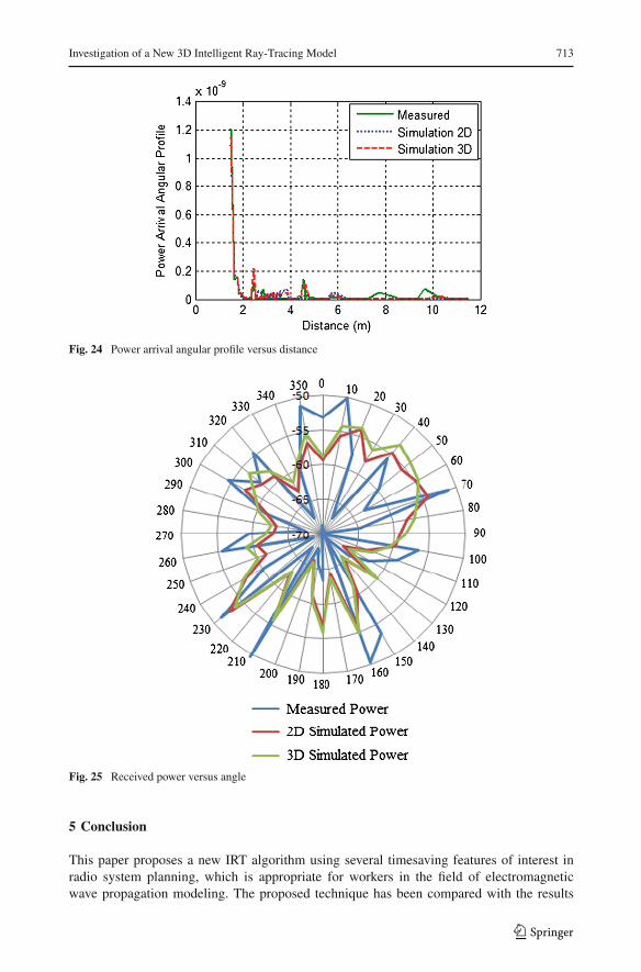
From Fig. 24, it can be seen that the simulated average power arrival angular profile is about3.15 % higher than the experimental results with the 2D IRT model, while it is only 2.87 %using 3D IRT. From the obtained results, it is obvious that after a certain distance, the powerarrival angular profile tends to become zero. It is further observed that when the distance isless than 4.5 m, the average power arrival angular profile is greater than 2.17 × 10−10 andwhen the distance is greater than 4.5 m, it becomes 1.08 × 10−11. The power arrival angularprofile indicates that the 3D IRT model achieves better accuracy as compared to 2D IRTmodel.

Moreover, the received power versus angle is demonstrated in Fig. 25 for better graphicalrepresentation. From the obtained results of Fig. 25, it can be seen that the difference betweenthe experimental results and the simulated results is about 1.28 and 0.9 % for 2D and 3DIRT, respectively, which indicates better accuracy of about 99 % has been achieved with theproposed 3D IRT model. From the Fig. 25, it can be observed that the relative received powerof a receiver is decreasing according to the angle of the arrival of the rays. The maximumarrival angle is 360◦ in this case. It may be less than this value. It depends on the distancebetween the receiver and the transmitter and on the height of the transmitter. When thedistance becomes larger or the height becomes taller, the maximum arrival angle decreasesand vice versa.

123


Fig. 24 Power arrival angular profile versus distance

Fig. 25 Received power versus angle

5 Conclusion

This paper proposes a new IRT algorithm using several timesaving features of interest inradio system planning, which is appropriate for workers in the field of electromagneticwave propagation modeling. The proposed technique has been compared with the results

123


obtained from other state-of-the-art RT algorithms. It is confirmed that the proposed modelcan predict the higher number of rays, able to launch the minimum amount of rays to skipthe processing of the unnecessary signals, reduce the computation time needed for inter-section test, perfectly identify the exact location of the ray-object intersection point, andminimize the propagation path error. Moreover, the performance and accuracy of the pro-posed IRT model are verified by taking comparisons among modeling results and measureddata.

A new 3D IRT model based on the MBAD algorithm is presented. The proposed 3DIRT model includes virtual surface technique as well as efficient polygon test algorithm tominimize the time taken for ray-object intersection test. Besides, infinitesimal rays with verysmall wavefront are considered to minimize the propagation path error. The proposed 3DIRT performs better ray prediction due to following reasons: (i) rays are launched in allpossible directions in the simulation space that considers reflection, refraction, penetration,and diffraction; (ii) the exact and accurate intersection point is determined using the proposedIRT technique; and (iii) no valid object is missed during ray-object intersection test. Theobtained results show that the proposed model predicts the higher number of rays of about29.21 % and provides better computational efficiency of about 58.78 %. The proposed modelcan perfectly identify the exact location of the ray-object intersection point with positioningaccuracy of 100 % and also omit the double ray counting error (that means, each ray is tracedonly once).

The experimental results obtained are compared with the simulation results and it is evidentthat both results are in good agreement. It is observed that the obtained results analysis (bothexperimental and simulation) achieves very high accuracy of about 97 to >99 % in terms ofradio signal propagation analyses, such as path loss analysis, PDP analysis, RMS delay spreadanalysis, and power arrival angular profile analysis. A very slight discrepancy obtained bythe 3D IRT model is due to the better matching of the experimental and simulated platformas the measurement was carried out in realistic environments. It can be concluded that thesimulation results obtained using the 3D IRT model are almost similar to the measurementresults, thus achieving superior accuracy as compared to 2D IRT technique. Basically, theoverall work in this study provides reliable solution, which is supportive for wireless radionetworks, personal communication systems inside buildings, and real system engineering.

Acknowledgments Our sincere thanks go to the University of Malaya for offering extensive financial supportunder the University of Malaya Research Grant (UMRG) scheme (RG098/12ICT).

References

1. Sarker, M. S., Reza, A. W., & Dimyati, K. (2011). A novel ray-tracing technique for indoor radio signalprediction. Journal of Electromagnetic Waves and Applications, 25, 1179–1190.

2. Zhong, J. (2001). Efficient ray-tracing methods for propagation prediction for indoor wireless communi-cations. IEEE Antennas and Propagation Magazine, 43(2), 41–49.

3. Cocheril, Y., & Vauzelle, R. (2007). A new ray-tracing based wave propagation model including roughsurfaces scattering. Progress in Electromagnetics Research, 75, 357–381.

4. Kim, H., & Lee, H.-S. (2009). Accelerated three dimensional ray tracing techniques using ray frustumsfor wireless propagation models. Progress in Electromagnetics Research, 96, 21–36.

5. Mohtashami, V., & Shishegar, A. A. (2010). Accuracy and computational efficiency improvement of raytracing using line search theory. IET Journal on Microwaves, Antennas & Propagation, 4, 1290–1299.

6. Liu, Z.-Y., & Guo, L.-X. (2011). A quasi three-dimensional ray tracing method based on the virtual sourcetree in urban microcellular environments. Progress in Electromagnetics Research, 118, 397–414.

7. Ling, H., Chou, R., & Lee, S. (1989). Shooting and bouncing rays: Calculating the RCS of an arbitrarilyshaped cavity. IEEE Transactions on Antennas Propagation, 37, 194–205.

123


8. Tan, S. Y., & Tan, H. S. (1996). A microcellular communications propagation model based on the uniformtheory of diffraction and multiple image theory. IEEE Transactions on Antennas Propagation, 44, 1317–1326.

9. Chen, S., & Jeng, S. (1997). An SBR/image approach for radio wave propagation in indoor environmentswith metallic furniture. IEEE Transactions on Antennas Propagation, 45, 98–106.

10. Zhuang, L., Zhang, Y., Hu, W., Yu, W., & Zhu, G.-Q. (2008). Automatic incorporation of surface wavepoles in discrete complex image method. Progress in Electromagnetics Research, 80, 161–178.

11. Saeidi, C., Hodjatkashani, F., & Fard, A. (2009). New tube-based shooting and bouncing ray tracingmethod. Proceedings of the International Conference on Advanced Technologies for Communications,Hai Phong, 269–273.

12. Dikmen, F., Ergin, A. A., Sevgili, A. L., & Terzi, B. (2010). Implementation of an efficient shooting andbouncing rays scheme. Microwave and Optical Technology Letters, 52, 2409–2413.

13. Gao, P. C., Tao, Y.-B., & Lin, H. (2010). Fast RCS prediction using multiresolution shooting and bouncingray method on the Gpu. Progress in Electromagnetics Research, 107, 187–202.

14. Tao, Y. B., Lin, H., & Bao, H. J. (2010). GPU-based shooting and bouncing ray method for fast RCSprediction. IEEE Transactions on Antennas and Propagation, 58, 494–502.

15. Lining, Z., Lipo, W., & Weisi, L. (2012). Generalized biased discriminant analysis for content-based imageretrieval. IEEE Transactions on Systems, Man, and Cybernetics, Part B: Cybernetics, 42(1), 282–290.

16. Tiberi, G., Bertini, S., Malik, W. Q., Monorchio, A., Edwards, D. J., & Manara, G. (2009). Analysis ofrealistic ultrawideband indoor communication channels by using an efficient ray-tracing based method.IEEE Antennas and Propagation Magazine, 57(3), 777–785.

17. Tao, Y. B., Lin, H., & Bao, H. J. (2008). KD-tree based fast ray tracing for RCS prediction. Progress inElectromagnetics Research, 81, 329–341.

18. Mohtashami, V., & Shishegar, A. A. (2010). Efficient shooting and bouncing ray tracing using decompo-sition of wavefronts. IET Journal on Microwaves, Antennas & Propagation, 4, 1567–1574.

19. Mohtashami, V., & Shishegar, A. A. (2012). Modified wavefront decomposition method for fast andaccurate ray-tracing simulation. IET Microwaves, Antennas & Propagation, 6(3), 293–304.

20. Reza, A. W., Dimyati, K., Noordin, K. A., & Sarker, M. S. (2011). Intelligent ray-tracing: An efficientindoor ray propagation model. IEICE Electronics Express, 8, 1–7.

21. Glassner, A. (1989). An introduction to ray tracing, The Morgan Kaufmann Series in Computer GraphicsAcademic Press.

22. De Greve, B. (2006). Reflections and refractions in ray tracing. http://www.flipcode.com/archives/reflection_transmission.pdf.

23. Choi, J., Sellen, J., & YAP, C.-K. (1995). Precision-sensitive shortest path in 3-space. In Proceeding of11th ACM symposium on computational geometry, pp. 350–359.

24. Hormann, K., & Agathos, A. (2001). The point in polygon problem for arbitrary polygons. ComputationalGeometry, 20(3), 131–144.

25. Rappaport, T. S. (2002). Wireless communications—Principles and practice (2nd ed.). Upper SaddleRiver, NJ: Prentice Hall.

26. Fujii, T., Ohta, Y., & Omote, H. (2009). Empirical time-spatial propagation model in outdoor NLOS envi-ronments for wideband mobile communication systems. In IEEE 69th vehicular technology conference,pp. 1–5.

27. Molisch, A. F., Cassioli, D., Chia-Chin, C., Emami, S., Fort, A., Kannan, B., et al. (2006). A comprehen-sive standardized model for ultrawideband propagation channels. IEEE Transactions on Antennas andPropagation, 54(11), 3151–3166.

28. Witrisal, K., Yong-Ho, K., & Prasad, R. (2001). A new method to measure parameters of frequency-selective radio channels using power measurements. IEEE Transactions on Communications, 49(10),1788–1800.

29. Omote, H., & Fujii, T. (2007). Empirical arrival angular profile prediction formula for mobile communi-cation systems. In IEEE 65th vehicular technology conference, pp. 599–603.

123

http://www.flipcode.com/archives/reflection_transmission.pdf

http://www.flipcode.com/archives/reflection_transmission.pdf


Author Biographies

Ahmed Wasif Reza received the B.Sc. Engg. (Hons.) degree fromKhulna University, Bangladesh, M.Eng.Sc. degree from MultimediaUniversity, Malaysia, and Ph.D. degree from University of Malaya,Malaysia. He is currently a Senior Lecturer at the Department of Elec-trical Engineering, University of Malaya. His research area includesRFID, radio wave propagation, wireless communications, electromag-netic research and cognitive radio, wireless sensor network, and bio-medical image processing. He has authored and co-authored a num-ber of international journals (Science Citation Index) and conferencepapers.

Kamarul Ariffin Noordin received the B.Eng.(Hons.) and M.Eng.Sc.degrees, both in electrical engineering from the University of Malaya,Kuala Lumpur, Malaysia in 1998 and 2001, respectively. He obtainedhis Ph.D. degree with the specialization in WiMAX system at theDepartment of Communication Systems, Lancaster University, UnitedKingdom in 2009. His research interests are in the areas of wirelesscommunications with emphasis on cross-layer optimization, quality ofservice provisioning, resource allocation, and link adaptation.

Md. Jakirul Islam received B.Sc. degree in Computer Science andEngineering from the Dhaka University of Engineering Technology,Gazipur, Bangladesh. Now, he is doing Master of Engineering Sci-ence in University of Malaya, Faculty of Engineering, Department ofElectrical Engineering, Malaysia. Besides, he is working as a ResearchAssistant (RA). His research interests include wireless communicationand telecommunication systems.

123


A. S. M. Zahid Kausar is a post graduate student in ElectricalEngineering Department of University of Malaya, Malaysia. He hascompleted his Master of Engineering Science (M.Eng.Sc.) from Elec-trical Engineering department of University of Malaya, Malaysia in2013 and Bachelor of Science (B.Sc) degree in Electrical and Elec-tronic Engineering from the Department of Electrical and ElectronicEngineering, Chittagong University of Engineering and Technology(CUET), Bangladesh in 2009. His present research work is opticalantennas for biomedical applications. His research interests includeantenna design, telecommunication, wireless sensor networks, and EMenergy harvesting.

Harikrishnan Ramiah is currently a Senior Lecturer at Departmentof Electrical Engineering, University of Malaya, Malaysia, working inthe area of Analog IC/RFIC design and Electromagnetic Modeling. Hereceived his B.Eng(Hons.), M.Sc and Ph.D. degrees in Electrical andElectronic Engineering, in the field of Analog and Digital IC designfrom University Science Malaysia, Malaysia in 2000, 2003, and 2008,respectively. He was the recipient of Intel Fellowship Grant Award,2000–2008. He received the Best Paper Awards from ICAST (Interna-tional Conference on Advances in Strategic Technologies), 2003 Con-ference. His research work has resulted into various technical publi-cations. His main research interest includes Analog Integrated CircuitDesign, RFIC Design, VLSI system design and Electromagnetic Mod-eling. Dr. Harikrishnan is a Chartered Engineer member of Institute ofElectrical Technology (IET), member of IEEE and IEICE.

123

Investigation of a New 3D Intelligent Ray-Tracing Model

Documents

Transcript of Investigation of a New 3D Intelligent Ray-Tracing Model