Graduate Theses, Dissertations, and Problem Reports

2014

Investigating the Potential of Waste Heat Recovery as a Pathway Investigating the Potential of Waste Heat Recovery as a Pathway

for Heavy-Duty Exhaust Aftertreatment Thermal Management for Heavy-Duty Exhaust Aftertreatment Thermal Management

Saroj Pradhan

Follow this and additional works at: https://researchrepository.wvu.edu/etd

Recommended Citation Recommended Citation Pradhan, Saroj, "Investigating the Potential of Waste Heat Recovery as a Pathway for Heavy-Duty Exhaust Aftertreatment Thermal Management" (2014). Graduate Theses, Dissertations, and Problem Reports. 6445. https://researchrepository.wvu.edu/etd/6445

This Thesis is protected by copyright and/or related rights. It has been brought to you by the The Research Repository @ WVU with permission from the rights-holder(s). You are free to use this Thesis in any way that is permitted by the copyright and related rights legislation that applies to your use. For other uses you must obtain permission from the rights-holder(s) directly, unless additional rights are indicated by a Creative Commons license in the record and/ or on the work itself. This Thesis has been accepted for inclusion in WVU Graduate Theses, Dissertations, and Problem Reports collection by an authorized administrator of The Research Repository @ WVU. For more information, please contact researchrepository@mail.wvu.edu.

Investigating the Potential of Waste Heat Recovery as a Pathway for Heavy-Duty Exhaust

Aftertreatment Thermal Management

Saroj Pradhan

Thesis submitted

to the College of Engineering and Mineral Resources

at West Virginia University

in partial fulfillment of requirements for the degree of

Master of Science in

Mechanical Engineering

Committee Members:

Dr. Arvind Thiruvengadam, Ph.D., Chair

Dr. Gregory Thompson, Ph.D.

Dr. Hailin Li, Ph.D.

Department of Mechanical and Aerospace Engineering

Morgantown, West Virginia, USA

2014

Keywords: Waste Heat Recovery, Heavy-Duty Diesel Engines, SCR, Aftertreatment

Thermal Management

Copyright 2014 Saroj Pradhan

i

ABSTRACT

Investigating the Potential of Waste Heat Recovery as a Pathway for Heavy-Duty Exhaust

Aftertreatment Thermal Management

Saroj Pradhan

Heavy-duty diesel (HDD) engines are the primary propulsion source for most heavy-duty

vehicle freight movement and have been equipped with an array of aftertreatment devices to

comply with more stringent emissions regulations. In light of concerns about the transportation

sector's influence on climate change, legislators are introducing requirements calling for

significant reductions in fuel consumption and thereby, greenhouse gas (GHG) emission over the

coming decades. Advanced engine concepts and technologies will be needed to boost engine

efficiencies. However, increasing the engine’s efficiency may result in a reduction in thermal

energy of the exhaust gas, thus contributing to lower exhaust temperature, potentially affecting

after-treatment activity, and consequently emissions rate of regulated pollutants.

As an aftertreatment thermal management for selective catalytic reduction (SCR) system,

this study investigates the possible utilization of waste heat recovered from a HDD engine as a

means to offset fuel penalty incurred during thermal management of SCR system. Experiments

were aimed at conducting detailed energy audit of a MY 2011 heavy-duty diesel engine equipped

with a DPF and SCR. A MATLAB® based steady-state simulation tool was developed to simulate

a waste heat recovery system (WHRS) based on an Organic Rankine Cycle (ORC), working with

three different organic fluids, and primarily harvesting energy from combinations of the engine’s

heat dissipating circuits. The simulations were based on experimental data obtained through a

comprehensive characterization of engine energy distribution using a heavy-duty engine

dynamometer.

Results obtained from the ORC-WHRS simulation over the engine operating points

showed that the working fluids, R123 and R245fa with utilizing post-SCR exhaust stream, and

exhaust gas recirculation (EGR) cooler as the two heat sources provided the optimum performance.

As the primary goal of this study was to understand the utilization of a WHRS as a strategy for

thermal management of an after-treatment system in reducing NOx levels, the study further

investigates into the dynamic operation of a heavy-duty diesel engine from an actual vehicle

testing. Assessment on magnitude of the energy generated for the transient vehicle operation does

show ORC-WHRS as a feasible application in reaching the desired thermal state of a typical HDD

engine SCR system.

ii

ACKNOWLEDGEMENT

I would like to express my appreciation and thanks to my advisor Dr. Arvind, who has not

only been an excellent mentor but also as a good friend for me. Your support and encouragement

has been a tremendous guidance in this journey of mine. I also thank Dr. Mridul Gautam for giving

me an opportunity to work with CAFEE and giving me your motivational talks to help me grow

my confidence in this challenging and exciting field of study.

Furthermore, a special thanks to Marc and Pragalath for your guidance in this research

work and in all the other projects. I also thank all my CAFEE colleagues for helping me out in the

lab and giving me two years of fun filled moments in CAFEE. I greatly thank Dan for all the

support and inspiration. I thank my committee members, Dr. Gregory Thompson and Dr. Hailin

Li for giving valuable feedbacks.

To my dear mom and dad, thank you for your love, support, and believing in me. I am very

grateful to my sister and Selina for the source of inspiration.

iii

TABLE OF CONTENTS

CHAPTER 1 INTRODUCTION ............................................................................................................................. 1

1.1. INTRODUCTION ............................................................................................................................................. 1 1.2. OBJECTIVE .................................................................................................................................................... 2

CHAPTER 2 LITERATURE REVIEW ................................................................................................................. 3

2.1. NOX REDUCTION TECHNOLOGY USING SCR ............................................................................................... 3 2.1.1. Urea-SCR Catalytic Reactions ............................................................................................................ 3 2.1.2. Urea-SCR Activity Dependency........................................................................................................... 4 2.1.3. Real-World Heavy-Duty Low Exhaust Temperature Activity .............................................................. 8

2.2. THERMAL MANAGEMENT STRATEGIES FOR IMPROVED SCR ACTIVITY ...................................................... 10 2.2.1. Engine Based Measures .................................................................................................................... 10 2.2.2. Electrically Heating the Exhaust Stream ........................................................................................... 10

2.3. WASTE HEAT RECOVERY SYSTEM AS POTENTIAL POWER GENERATOR ..................................................... 11 2.3.1. Waste Heat Recovery Technology Applications ................................................................................ 12 2.3.2. Heavy-Duty Engine Energy Flow ...................................................................................................... 13 2.3.3. Waste Heat Recovery System Design ................................................................................................ 14

CHAPTER 3 EXPERIEMNTAL SET UP ............................................................................................................ 16

3.1. TEST ENGINE SPECIFICATION ...................................................................................................................... 16 3.2. ENGINE DYNAMOMETER AND TEST CELL INTEGRATION ............................................................................ 17 3.3. ENGINE INSTRUMENTATION ........................................................................................................................ 18 3.4. TESTING METHODOLOGY ............................................................................................................................ 19

3.4.1. Engine Mapping Procedure .............................................................................................................. 20 3.4.2. Design of Experiments ....................................................................................................................... 20

3.5. ENERGY AUDIT ........................................................................................................................................... 23

CHAPTER 4 WHRS SIMULATION MODEL .................................................................................................... 28

4.1. INTRODUCTION ........................................................................................................................................... 28 4.2. WHRS DESIGN ........................................................................................................................................... 28 4.3. WHRS MODEL EFFICIENCY ........................................................................................................................ 34 4.4. WHRS MODEL ASSUMPTIONS .................................................................................................................... 35 4.5. WHRS FLUID SELECTION ........................................................................................................................... 35 4.6. ORC-WHRS SIMULATION SETUP ............................................................................................................... 37

CHAPTER 5 RESULTS AND DISCUSSIONS .................................................................................................... 40

5.1. INTRODUCTION ........................................................................................................................................... 40 5.2. DATA ANALYSIS ......................................................................................................................................... 40

5.2.1. Comparison of DoE Methods ............................................................................................................ 40 5.2.2. Analysis of Energy Data .................................................................................................................... 42 5.2.3. Steady-State Temperature Analysis ................................................................................................... 45

5.3. ENERGY AUDIT ........................................................................................................................................... 49 5.4. ORC-WHRS RESULTS ............................................................................................................................... 55

5.4.1. Working Fluid Comparison ............................................................................................................... 55 5.4.2. Heat Source Comparison .................................................................................................................. 59

CHAPTER 6 THERMAL MANAGEMENT POTENTIAL ............................................................................... 62

6.1. INTRODUCTION ........................................................................................................................................... 62 6.2. TRANSIENT DATA SOURCE ......................................................................................................................... 62

iv

6.3. TRANSIENT CYCLE ENERGY ANALYSIS ...................................................................................................... 63 6.4. ORC-WHRS MAPPING ............................................................................................................................... 65 6.5. ORC-WHRS TRANSIENT RESULTS............................................................................................................. 67 6.6. THERMAL MANAGEMENT STRATEGY ......................................................................................................... 70

CHAPTER 7 CONCLUSIONS AND FUTURE WORK ..................................................................................... 72

7.1. CONCLUSIONS ............................................................................................................................................. 72 7.2. FUTURE WORK ........................................................................................................................................... 73

APPENDIX A PUMP CHARACTERISTICS ....................................................................................................... 77

APPENDIX B ORC-WHRS RESPONSE SURFACE RESULTS ........................................................................ 78

v

LIST OF TABLES

TABLE 1. ENERGY FLOW IN TYPICAL MODERN HD DIESEL ENGINE OPERATED AT HIGH LOAD CONDITION .................... 13

TABLE 2. TEST ENGINE SPECIFICATION ........................................................................................................................ 16

TABLE 3. ORC-WHR SYSTEM CHARACTERISTICS ........................................................................................................ 35

TABLE 4. PROPERTIES OF CONSIDERED WORKING FLUIDS ............................................................................................. 37

TABLE 5. ORC-WHRS MODEL HEAT SOURCE AND WORKING FLUID CONFIGURATION ................................................. 39

TABLE 6. SUMMARY OF THE 2ND ORDER CURVE FITTING MODEL FOR THE TWO DESIGN METHODS................................. 40

TABLE 7. SUMMARY OF TEMPERATURE FOR THE SELECT (2 MINUTES) MODES ............................................................. 47

TABLE 8. SUMMARY OF TEMPERATURE FOR THE SELECT (FIRST 20 SECONDS) MODES .................................................. 48

TABLE 10. SUMMARY OF TEMPERATURE FOR THE SELECT (LAST 20 SECONDS) MODES ................................................ 49

TABLE 11. THERMAL CYCLE EFFICIENCY OF ORC-WHRS MODEL ............................................................................... 59

TABLE 12. VEHICLE SPECIFICATION ............................................................................................................................. 62

TABLE B-1. PARAMETER ESTIMATE FOR SECOND ORDER RESPONSE MODEL OF R123 DATA ......................................... 79

TABLE B-2. PARAMETER ESTIMATE FOR SECOND ORDER RESPONSE MODEL OF R245FA DATA ..................................... 80

vi

LIST OF FIGURES

FIGURE 1. NOX CONVERSION FOR VANADIA-BASED AND METAL-EXCHANGED ZEOLITE-BASED SCR ACTIVITY AT

VARYING TEMPERATURES UNDER STANDARD-SCR CONDITIONS ........................................................................... 6

FIGURE 2. NOX CONVERSION OF A STANDARD SCR CATALYST AS FUNCTION OF EXHAUST GAS TEMPERATURE USING

NO:NH3 AND NO:NO2:NH3 FEED ......................................................................................................................... 7

FIGURE 3. INFLUENCE OF THE NO2/NOX FRACTION ON NOX CONVERSION ..................................................................... 7

FIGURE 4. NO2 FRACTION IN NOX AFTER A PT-BASED OXIDATION CATALYST WITH VARYING INLET TEMPERATURE .... 8

FIGURE 5. EXHAUST DEPENDENT CUMULATIVE NOX EMISSION PROFILE FROM A CU-ZEOLITE BASED SCR EQUIPPED

TEST VEHICLE DRIVEN IN A CITY ROUTE ................................................................................................................. 9

FIGURE 6. EMICAT®’S ELECTRICALLY HEATED CATALYST SYSTEM BEFORE SCR CATALYST IN LIGHT DUTY

APPLICATION ....................................................................................................................................................... 11

FIGURE 7. SCHEMATIC OF BASIC RANKINE CYCLE ....................................................................................................... 14

FIGURE 8. MACK MP8 505C TEST CELL SETUP ............................................................................................................. 17

FIGURE 9. SCHEMATIC OF ENGINE INSTRUMENTATION ................................................................................................. 18

FIGURE 10 (A). LATIN HYPERCUBE DESIGN (B). GAUSSIAN PROCESS ISME OPTIMAL DESIGN FOR 25 SPEED/LOAD

NORMALIZED DATA POINTS .................................................................................................................................. 22

FIGURE 11. SPEED AND TORQUE COMBINATION OF 53 TEST POINTS UNDER THE LUG CURVE ........................................ 23

FIGURE 12. SCHEMATIC OF THE ENGINE ENERGY FLOW FOR THE SPECIFIED CONTROL VOLUME ................................... 24

FIGURE 13. CONTROL VOLUME CHOSEN FOR CALCULATING EGR FRACTION AT THE INTAKE MANIFOLD ..................... 27

FIGURE 14. LAYOUT OF PROPOSED RANKINE CYCLE WASTE HEAR RECOVERY SYSTEM WITH ENERGY RECOVERY FROM

TWO HEAT SOURCE .............................................................................................................................................. 29

FIGURE 15. CLASSIFICATION OF WORKING FLUID ON T-S DIAGRAM ............................................................................. 36

FIGURE 16. T-S DIAGRAM SHOWING PROCESS FLOW FOR DRY FLUID ............................................................................ 38

FIGURE 17. T-S DIAGRAM SHOWING PROCESS FLOW FOR WET FLUID ............................................................................ 39

FIGURE 18. COMPARISON OF THE PREDICTED FUEL [G/S] FOR TWO DOE DESIGNS ........................................................ 41

FIGURE 19. PERCENT DIFFERENCE OF THE PREDICTION FUEL [G/S] FOR TWO DOE DESIGNS .......................................... 42

FIGURE 20. DATA ANALYSIS OF EXHAUST ENERGY RATE BY ENGINE POWER DEMAND ............................................... 43

FIGURE 21. DATA ANALYSIS OF COOLANT ENERGY RATE BY ENGINE POWER DEMAND ............................................... 44

FIGURE 22. DATA ANALYSIS OF CAC ENERGY RATE BY ENGINE POWER DEMAND ..................................................... 44

FIGURE 23. CONTINUOUS TEMPERATURE PROFILE FOR SELECT MODES ........................................................................ 46

FIGURE 24. RELATIVE ENERGY DISTRIBUTION WITH RESPECT TO TOTAL FUEL ENERGY ................................................ 50

FIGURE 25. RELATIVE ENERGY DISTRIBUTION WITH RESPECT TO TOTAL FUEL ENERGY FOR SELECT OPERATING POINTS

............................................................................................................................................................................ 51

FIGURE 26. ENERGY DISTRIBUTION OF THE TOTAL ACCOUNTED HEAT LOSS FROM EXHAUST, COOLANT AND CAC ...... 52

FIGURE 27 COMPARISON OF TEMPERATURE PROFILE FOR ALL OPERATING POINTS ....................................................... 53

FIGURE 28. EXHAUST ENERGY POST-TURBO AND POST-SCR ........................................................................................ 54

vii

FIGURE 29. TOTAL COOLANT ENERGY INCLUDING EGR ENERGY ................................................................................. 54

FIGURE 30. HX1 [EXHAUST] – HX2 [EGR] WASTE HEAT RECOVERY FOR DIFFERENT WORKING FLUIDS .................... 55

FIGURE 31. HX1 [EGR] – HX2 [EXHAUST] WASTE HEAT RECOVERY FOR DIFFERENT WORKING FLUIDS .................... 56

FIGURE 32. HX1 [CAC] – HX2 [EXHAUST] WASTE HEAT RECOVERY FOR DIFFERENT WORKING FLUIDS ................... 57

FIGURE 33. HX1 [CAC] – HX2 [EGR] WASTE HEAT RECOVERY FOR DIFFERENT WORKING FLUIDS .......................... 58

FIGURE 34. WHRS CYCLE OUTPUT FOR DIFFERENT HEAT SOURCE CONFIGURATION USING R123 ................................ 60

FIGURE 35. ORC-WHRS CYCLE OUTPUT FOR DIFFERENT HEAT SOURCE CONFIGURATION USING R245FA ................... 60

FIGURE 36. ORC-WHRS CYCLE OUTPUT FOR DIFFERENT HEAT SOURCE CONFIGURATION USING R134A .................... 61

FIGURE 37. PRE-SCR TEMPERATURE PROFILE FROM A COLD-START UDDS CYCLE VEHICLE-CHASSIS TEST RESULTS .. 64

FIGURE 38. PRE-SCR EXHAUST ENERGY THERMAL ANALYSIS ON THE UDDS CYCLE VEHICLE-CHASSIS TEST RESULTS

............................................................................................................................................................................ 64

FIGURE 39. ORC-WHRS CYCLE OUTPUT POWER MAP FOR HX1(EXHAUST POST-SCR) AND HX2(EGR) USING R123 66

FIGURE 40. ORC-WHRS CYCLE OUTPUT POWER MAP FOR HX1(EXHAUST POST-SCR) AND HX2(EGR) USING R245FA

............................................................................................................................................................................ 67

FIGURE 41. TRANSIENT INPUT FACTOR PROFILES ......................................................................................................... 68

FIGURE 42. ORC-WHRS POWER GENERATED FOR HX1 [EXHAUST] - HX2 [EGR] WHRS ON UDDS CYCLE ............. 68

FIGURE 43. CUMULATIVE ENERGY RESULTS USING ORC-WHRS OUTPUT ON UDDS CYCLE ....................................... 69

FIGURE 44. SCHEMATIC OF A THERMAL MANAGEMENT USING ORC-WHRS AS THE POWER SOURCE ........................... 70

FIGURE 45. CATALYST PRE-HEATING STRATEGY BEFORE AND AFTER ENGINE KEY-ON ................................................. 71

FIGURE A-1. PERFORMANCE CURVE FOR THE SELECTED POSITIVE DISPLACEMENT PUMP ............................................. 77

FIGURE B-1. ACTUAL BY PREDICTED PLOT FOR SECOND ORDER RESPONSE MODEL FOR ORC-WHRS (R123) ............. 78

FIGURE B-2. ACTUAL BY PREDICTED PLOT FOR SECOND ORDER RESPONSE MODEL FOR ORC-WHRS (R245FA) ......... 80

1

CHAPTER 1 INTRODUCTION

1.1. Introduction

In recent years, modern heavy-duty (HD) vehicles have demonstrated leading progress in

achieving stringent emission standards put forward by federal emission regulators in US and

Europe. Particularly in the area of reducing vehicle oxides of nitrogen (NOx) emission, the

selective catalytic reduction (SCR) technology has been a viable after-treatment solution.

However, significant challenges are seen in NOx conversion efficiency of a SCR catalyst during

the real world on-road applications (Stanton, 2013).

Implication of lower SCR activity during low exhaust temperature operations such as cold

start, low load/speed, and initial driving phase has shown to result in significantly elevated NOx

emission during such period, and consequently contributing greatly to overall vehicle emission

(Misra et al., 2013). Initiating the NOx conversion reaction in a SCR catalyst system greatly

depends upon the type of catalyst coating used, and the light-off temperature of the catalyst

(Kröcher, 2007). According to studies, catalyst deactivation are seen to occur for temperatures

below 200°C due to decomposition of the reducing agent over the substrate surface and pores

(Koebel et al., 2002).

Engine manufactures have utilized combinations of multiple strategies and mechanisms to

provide thermal management for proper SCR activation and urea injections during cold start and

low load/speed driving operations (Johnson, 2009). Strategically controlling different engine based

parameters to warm-up the exhaust gas stream during low temperature operation has been an

effective approach but at the same time exhibits penalties in fuel consumption, emissions and

system costs (Cavina et al., 2013).

2

An alternative approach is to employ a thermal strategy by means of actively heating the

catalyst substrate or the column of exhaust stream just before the inlet of the SCR system to target

light-off temperatures. Such strategy has been seen in few engine research studies, and commonly

in light–duty diesel vehicle application where the entrance of the SCR catalyst is electrically heated

to target faster light-off time in order to maintain proper temperatures during vehicle warm-up

periods (Wang et al., 2011, Talus et al., 2011).

1.2. Objective

The global objective of this thesis is to investigate potential thermal management strategies

for selective catalytic reduction (SCR) aftertreatment system performance during low exhaust

temperature operations. This study primarily looks into harvesting wasted heat from the HDD

engine, and in order to understand the potential practicality of achieving such strategy this study

splits into three objectives:

1. Conduct an engine dynamometer testing to perform an energy analysis on a modern

HDD engine in order to understand the recoverable wasted energy.

2. Develop a waste heat recovery system (WHRS) model using Organic Rankine Cycle,

and simulate using recoverable heat energy from the same HDD engine to generate

useful mechanical work out from the ORC- turbine.

3. Perform an assessment of the ORC-WHRS generated output work as potential energy

source in electrically heating exhaust stream for SCR thermal management.

3

CHAPTER 2 LITERATURE REVIEW

2.1. NOx Reduction Technology Using SCR

SCR systems have proven to be effective in controlling the NOx emissions over most

operating conditions. This technology has been widely adopted by the heavy duty vehicle industry

along with or without other engine based strategies such as exhaust gas recirculation (EGR), in-

cylinder modifications and more in order to reduce total vehicle-out NOx emissions (Stanton,

2013). As an alternative approach, SCR has aided manufactures in meeting USEPA 2010 NOx

emissions compared to in-cylinder based high EGR strategy. Additionally, use of aqueous urea as

the reducing agent coupled with a SCR catalyst has shown to be an efficient pathway in reducing

NOx under wide range of engine operations. Low exhaust temperature conditions, however, result

in the inactivity of SCR aftertreatment systems. This section addresses on the urea-based SCR

catalyst activity mechanisms and activity dependencies.

2.1.1. Urea-SCR Catalytic Reactions

Oxides of nitrogen in heavy-duty diesel exhaust are composed mostly of NO, which is

typically greater than 90%; the remainder of the NOx is in the form of NO2. Thus, most of the SCR

activity is required in reducing the NO compound (Koebel et al., 2001).

Ammonia (NH3) is used as the primary reducing agent to mitigate NO; the gaseous reaction

with the aid of SCR catalysts is provided by Equation (1). The reaction is interpreted as “standard

SCR” (Koebel et al., 2001), where 4 mole of ammonia reacts with 4 mole of nitrogen monoxide

and only 1 mole of oxygen to produce nitrogen and water. Due to low concentration of oxygen,

the reaction occurs at much slower rate. This standard type of reaction is considered less relevant

to diesel engine application due to lean (high oxygen content) combustion processes where there

is abundance of oxygen in the exhaust stream (Koebel et al., 2000).

4

4NH3 + 4NO + O2 4N2 + 6H2O (1)

Subsequently, a faster known reaction (Bosch and Janssen, 1988) between the reducing

agent NH3, and mixture of NO2 and NO in even ratio of 1:1 is given by the Equation (2). This

reaction is also recognized as “fast SCR” reaction.

4NH3 + 2NO + 2NO2 4N2 + 6H2O (2)

Conversely, the reaction is slower when NO2/NOx ratio exceeds over 50% (Bosch and

Janssen, 1988). Such reaction, solely with NO2 is given by the following Equation (3).

8NH3 + 6NO2 7N2 + 12H2O (3)

Widely used in the heavy-duty SCR application, urea, typically at 32.5% by weight with

water, is considered to be the safest method to obtain NH3 (Sluder et al., 2005). Adequate physical

decomposition is required to convert liquid stored urea to extract NH3 for SCR activity. The three

main processes that undergo this conversion of aqueous urea to obtain NH3 are evaporation,

thermolysis, and hydrolysis, which are provided below by Equation (4), Equation (5) and Equation

(6), respectively (Koebel et al., 2001).

NH2-CO-NH2 (aqueous) NH2-CO-NH2 (solid) + xH2O (gas) (4)

NH2-CO-NH2 (solid) NH3 (gas) + HNCO (gas) (5)

HNCO (gas) + H2O (gas) NH3 (gas) + CO2 (gas) (6)

2.1.2. Urea-SCR Activity Dependency

The main target of the SCR system is the conversion efficiency of NOx, and this efficiency

highly depends upon multiple factors such as type of urea decomposition, catalyst material, NO-

5

to-NO2 ratio, and most importantly the catalyst temperatures at which the reaction takes place

inside the SCR system (Keuper et al., 2011). Additionally, it presents that above mentioned

parameters have interdependency within each other for SCR functionality (Keuper et al., 2011).

As the catalyst temperature is directly related to the exhaust temperatures entering the SCR

system, the SCR activity is predominately linked to the engine operating conditions. According to

a study by Koebel for exhaust stream temperatures below 200°C, the process gets critical in SCR

conversion efficiency between the decomposition of the reducing agent and the catalyst activation

(Koebel et al., 2002). In the same paper, the author mentions at such low temperatures, ammonia

nitrates in solid or liquid form tends to get deposited into the pores of the catalyst, and could

potentially lead to catalyst deactivation. Hence, limiting urea dosing at low temperature conditions

is usually implemented as a control strategy for preventing SCR substrate fouling, and the cut-off

point for urea injection typically ranges between 200-250°C (Majewski, 2014).

As mentioned earlier, the effect of temperature on SCR efficiency also depends on the type

of catalyst coating used. Different catalysts-based material within the SCR system have varying

light-off temperatures along with different temperature ranges for optimum catalyst activity.

Figure 1 compares the catalytic activity of iron-based (Fe), copper-based (Cu) and vanadium-based

(V) coated catalysts given by the symbols (), () and (•), respectively.

6

Figure 1. NOx conversion for vanadia-based and metal-exchanged zeolite-based SCR

activity at varying temperatures under standard-SCR conditions (Kröcher, 2007)

Based on a catalyst performance study (Kröcher, 2007), copper-based catalysts are most

active for SCR NOx conversion in comparison to iron or vanadium-based catalysts for

temperatures below 300°C. Activities characterized by lower and wider temperature ranges seem

to be more suitable for copper-based catalysts. Due to this suitability, copper-based catalysts have

proven to become the common catalyst material in SCR systems for heavy-duty diesel applications

for reducing diesel NOx emissions (Kamasamudram et al., 2010).

Maintaining “fast-SCR” or optimum NO2/NOx ratios has further potential to increase the

SCR performance, even at lower temperatures (Koebel et al., 2002). From a study performed by

Chandler, shows that the control of SCR catalyst activity can be significantly varied by having

NO2 in the exhaust gas, especially at low exhaust temperatures (Chandler et al., 2000). Figure 2,

illustrates such catalyst activities where at lower temperature ranges (175 to 300°C), NOx

conversion efficiency tends to remain above 90% when feeding NO2 as a feed gas than compared

to not having any NO2 at all in the exhaust stream.

7

Figure 2. NOx conversion of a standard SCR catalyst as function of exhaust gas

temperature using NO:NH3 and NO:NO2:NH3 feed (Chandler et al., 2000)

Figure 3, illustrates the influence of percentage of NO2 for the SCR’s ability to reduce

overall NOx. It shows that the optimum conversion efficiency is seen at 50% NO2-to-NOx ratio,

and starts to rapidly decrease as the proportion increases (Koebel et al., 2002).

Figure 3. Influence of the NO2/NOx fraction on NOx conversion (Koebel et al., 2002)

Use of pre-oxidation catalyst located upstream of the SCR have been shown to facilitate

the performance of the SCR catalyst activity. The diesel oxidation catalyst (DOC) systems which

8

are primarily used for controlling carbon monoxide (CO), hydrocarbons (HC), and organic fraction

of diesel particulates (SOF) emissions, are shown to produce representative amount of NO2 during

the oxidation reaction in presence of NO in the exhaust (Majewski, 2014). Likewise, the

performance of the oxidation catalyst also varies with temperature and is shown to be inactive

under certain temperatures ranges. From a relevant DOC performance study (Gieshoff et al.,

2000),on a platinum-based (Pt) oxidation catalyst, the NO2 fraction in NOx peaks (80%) at

temperatures around 250 to 300°C, also depicted in Figure 4. It is also observed that 50% of NO2-

to-NO fraction is seen around 150 to 200°C.

Figure 4. NO2 fraction in NOx after a Pt-based oxidation catalyst with varying inlet

temperature (Gieshoff et al., 2000)

2.1.3. Real-World Heavy-Duty Low Exhaust Temperature Activity

Heavy-duty vehicles are used for wide range of day to day activities. The daily operational

routes can range from low speed/load – stop and go vocational driving schedule to long haul

interstate driving. From a SCR thermal activity study, a typical HDD engine requires about 1 to 2

minutes to obtain a proper SCR activity condition with exhaust temperature reaching above 250°C

(Ettireddy et al., 2014).

9

Similarly, a recent study published by the California Air Resources Board (CARB), have

clearly shown complications of low temperature activity on NOx emissions out of a Class-8 heavy-

duty diesel vehicles equipped with SCR technology. The HDD vehicles for the study were tested

on-road under diverse driving conditions. Figure 5 presents data for a vehicle with EGR and SCR,

illustrating the NOx emissions over the cycle dependent on the vehicle operation leading to

variation in exhaust temperature. The results from this study showed that the SCR aftertreatment

was effective in reducing the NOx emissions typically for highway driving conditions when the

SCR inlet temperatures are shown to be above the proper catalyst activation temperatures, but

exhibits low SCR performance during operations such as cold start, low load/speed, and initial

driving phases (Misra et al., 2013). The study also presents that during the cold start period, when

the SCR inlet temperature are relatively low (considered < 150°C in the study), the rate of vehicle

NOx accumulated tend to rise rapidly, and then begins to gradually slow down as the vehicle

exhaust approaches the optimum SCR activity temperatures.

Figure 5. Exhaust dependent cumulative NOx emission profile from a Cu-zeolite based SCR

equipped test vehicle driven in a city route (Misra et al., 2013)

10

2.2. Thermal Management Strategies for Improved SCR Activity

Engine manufactures have utilized combinations of multiple strategies and mechanisms to

provide thermal management for proper SCR activation along with urea dosing during cold start

and low load/speed driving operation (Johnson, 2009). The desired exhaust thermal conditions at

such vehicle operations can either be reached actively with the assist of engine-based control

measures or by using a medium, for example a heating coil to locally increase the temperature of

the exhaust gas volume entering the SCR substrate. This section reviews two approaches of

thermal management strategies.

2.2.1. Engine Based Measures

Strategically controlling different engine based parameters to warm-up the exhaust gas

stream during cold start and under low load-speed engine conditions has been an effective

approach (Stanton, 2013). Experimental work on thermal management strategies based on engine

control strategies implemented individually or in a combined effort of parameters such as start of

injection (SOI), throttle valve actuation (TVA) system, variable geometry turbocharger (VGT)

actuation, and variable valve train (VVT) have shown to provide faster light-off temperatures of

the catalytic reactions on SCR systems (Cavina et al., 2013). Such studies also show that engine-

based measures tend to negatively affect in producing HC, CO and PM emissions along with fuel

consumption.

2.2.2. Electrically Heating the Exhaust Stream

Another approach for aftertreatment thermal management is directly heating the catalyst

substrate or the volume of exhaust stream just before the inlet of the SCR system. An example

related to similar strategy using electrically heated catalyst (E-SCRTM) provide by EMICAT® has

proven be an effective technology in light-duty diesel application (Ulrich et al., 2012). The device

11

utilizes a heating disc as an integrated part of the SCR system, providing necessary thermal energy

into the exhaust stream passing through the SCR substrate. The heater works on the principle of

resistive heating coil element, and also contains catalyst coating for reducing NOx immediately.

The amount of energy required to raise the exhaust stream to a certain temperature directly depends

on the power supplied to the resistive coil. From the study, the electrically heated catalyst utilizes

energy reclaimed from mechanical work of the engine. Figure 6 shows a schematic of the

EMICAT® electrically heating system before the SCR catalyst.

Figure 6. EMICAT®’s electrically heated catalyst system before SCR catalyst in Light Duty

Application (Ulrich et al., 2012)

2.3. Waste Heat Recovery System as Potential Power Generator

In this proposed context, the most important constraint is the source of energy required in

order to add sufficient energy into the exhaust stream without compromising potential fuel

consumption. This section reviews waste heat recovery as a viable application in extracting wasted

heat from heavy-duty vehicles in the means of achieving thermal energy.

12

2.3.1. Waste Heat Recovery Technology Applications

Utilizing wasted energy converted to electrical energy in automotive applications dates as

early as 1988, when the first exhaust-based Automotive Thermoelectric Electric Generator

(ATEG) was applied on a Porsche 944 exhaust system to produce tens of Watts (Birkholz, 1988).

In 1990, the same ATEG technology with different material design, a diesel truck exhaust system

was capable of producing 1kW. It also shows that TEGs perform well only at higher temperatures

ranges, which would provide disadvantages for temperatures ranges seen in a heavy-duty vehicle

operations (Avadhanula et al., 2013).

Turbochargers are the most known examples of waste heat recovery within heavy-duty and

higher performance light duty engines. Having been around for nearly a century, the use of

conventional turbochargers utilizes exhaust energy to boost intake air and significantly improves

engine efficiency (Arnold et al., 2001). Similar to the concept of turbochargers, mechanical and

electrical turbo-compounding has also been recognized as a potential source to generate useful

work, where the recovered energy from the exhaust is mechanically or electrically added back to

the engine flywheel (Noor et al., 2014). Major heavy-duty truck manufacturers such as Volvo,

Detroit Diesel, Iveco and Scania have already utilized such technology for long-hauled

applications (Noor et al., 2014).

There has been increasing interest and extensive research on recovering waste energy for

heavy-duty diesel vehicles using Rankine Cycle working with environmentally friendly, organic

fluids (Stanton, 2013). Such approach has potentially shown to improve diesel engine’s overall

efficiency just by utilizing wasted energy from different heat sources. The ORC-WHR system with

using two major heat sources, EGR and exhaust stream, have demonstrated beneficial levels of

fuel consumption reduction: for example, providing reduction as high as 6.0% during a highway

13

operation from Class-8 HD vehicle. Other similar analysis have also shown that up to 5% fuel

improvement can be achieved implementing from WHRS utilizing only the EGR (Teng et al.,

2011). In a popular event, the Department of Energy Supertruck Program, major OEMs have

developed and demonstrated WHR system using ORC as a technological pathway in targeting

higher brake thermal efficiency (Gravel, 2013).

2.3.2. Heavy-Duty Engine Energy Flow

In modern on-road heavy-duty vehicles, about 40-42% of the total fuel energy consumed

in the engine is utilized to generate useful work while the rest of the energy is lost in the form of

heat and friction (Talus et al., 2011). For typical heavy-duty diesel engines, experimental results

have shown that most of the input energy from the fuel is discharged in the form of heat to the

ambient air (Latz et al., 2013).

A study aimed specifically in the analysis and development of a waste heat recovery system

for Class-8 diesel vehicles shows that an engine operated at high EGR at B100 steady state point

(mode from the European Stationary Cycle-ESC) rejects about 20% of the total input energy

through the exhaust flow after the turbocharger, while 18% of the engine heat is taken by coolant

(Teng et al., 2011).

Table 1. Energy flow in typical modern HD diesel engine operated at high load condition

(Teng et al., 2011)

Energy Flow Path % of Total Fuel Energy

Brake Power [Shaft-Mechanical Work] 41%

Exhaust Energy [Post-Turbo] 20%

Coolant Energy 18%

Exhaust Gas Recirculation (EGR) 11%

Charge Air Cooler (CAC) 9%

Other [Ambient] 1%

14

2.3.3. Waste Heat Recovery System Design

2.3.3.1. Rankine Power Cycle

Considering the quality (tendency of energy to convert from one form to another) of wasted

energy in a normal engine operation, utilization of a Rankine power cycle are commonly accessed

as a basic approach for waste heat recovery potential (Cozzolini et al., 2012). From the basic

introduction regarding the thermodynamic analysis of power-generating systems, the Rankine

cycle consist of four major components to complete the cycle and generate useful work (Moran

and Shapiro, 2008). Figure 7 illustrates a basic schematic of a Rankine cycle consisting of system

pump, evaporator/boiler (heat exchanger), expander/turbine, and condenser (heat exchanger).

Detailed explanation on individual components and thermodynamic analysis of the processes are

described in Chapter 4.

Figure 7. Schematic of basic Rankine Cycle

From numerous studies and publications it can be noted that manufactures and institutional

researchers have approached WHRS design in multiple paths, taking advantage of different

Evaporator

[Heat Exchanger]

Condenser

[Heat Exchanger]

ExpanderPump

Cooling Stream

Heating Stream

LIQUID PHASEVAPOR PHASE

15

available energy source for gaining the optimum results at different engine operation conditions.

The WHR system built by Cummins Inc. demonstrates the utilization of charge air cooler (CAC),

exhaust gas stream downstream of the aftertreatment and EGR circuit. Similarly, AVL investigates

WHR systems utilizing only the EGR cooler as the primary heat source (Teng and Regner, 2009).

2.3.3.2. WHRS Working Fluids

Considering the system’s component size along with keeping system cost and

environmental aspects in mind, selecting the right working fluid for the Rankine cycle is an

important step in overall performance of the WHR system (Bae et al., 2011). Numerous studies

related to engine waste heat recovery have been investigated with comparing the performance of

different organic fluid types for ORC-WHRS implemented on heavy-duty diesel vehicle

applications (Arunachalam et al., 2012). Selection of the organic fluid for this study are discussed

in the ORC-WHR system design section.

16

CHAPTER 3 EXPERIEMNTAL SET UP

All measurement of the study presented herein were conducted at the Engine and Emissions

Research Laboratory (EERL) at West Virginia University. The EERL is a part of West Virginia

University’s Center for Alternative Fuels, Engines and Emissions (CAFEE) and the transient

engine dynamometer test cell is designed and operated according to recommendations set forth by

Code of Federal Regulations (CFR), Title 40, Part 1065 (USEPA)

3.1. Test Engine Specification

In order to perform a comprehensive energy analysis on a modern, on-road heavy-duty

engine, a 12.8L Mack MP8 505C representing US EPA 2010 emissions compliant engine was

tested on an engine dynamometer test bench. Table 2 summarizes the test engine specifications.

Table 2. Test Engine Specification

Manufacturer Mack

Model year 2011

Model MP8 – 505C

Displacement (L) 12.8

Rated Horsepower (HP) 505

Rated Speed (RPM) 1800

Peak Torque @Speed 1810 ft-lb@1100rpm

After-treatment system DPF-SCR

EGR High pressure cooled EGR

Turbocharger VGT

Fuel Injection Electronic unit injectors (2400 Bar)

Compression Ratio 16:1

Bore and Stroke 131 mm x 158 mm

17

3.2. Engine Dynamometer and Test Cell Integration

The Mack MP8 engine was removed from a Class-8 tractor along with its after-treatment

system. The after-treatment system included the diesel particulate filter (DPF), selective catalytic

reduction (SCR) and a urea tank. The engine with its aftertreatment unit was installed in the WVU

ERC engine test cell as shown in Figure 8. A procured chassis harness was used to link the engine

control unit (ECU) with the aftertreatment ECU, and necessary communication was insured within

the ECU’s and vehicle interface.

Figure 8. Mack MP8 505C test cell setup

A General Electric (GE) 800hp direct current (DC) heavy-duty platform dynamometer,

capable of providing and absorbing power at engine speeds up to 2500 RPM, was used for testing

the Mack MP8 engine rated at 505hp at 1800 RPM. The engine was coupled with the test cell DC

dynamometer via a universal joint dynamometer shaft adapted to the engine flywheel. Throttle

input and speed control were provided using WVU CAFEE’s in-house engine dynamometer test

cell software. CAN bus communication with SAE J1939 protocol was used between the test cell

controller and the engine control unit ECU. Constant monitoring of the engine and aftertreatment

fault codes were made for fault detection to insure proper functionality of the integrated systems.

800 hp DC

dynamometer

Shaft linking

dyno and

engine

Urea tank for

SCR Urea

dosing

MACK MP8

505C engine

SCR

DPF

Exhaust

outlet post-

SCR

18

3.3. Engine Instrumentation

In order to examine and quantify the energy flows on all fluid flows, the test engine was

instrumented for temperature, pressure and flow rates. The intake air, exhaust, coolant, and oil

fluid flow paths were instrumented using ungrounded Omega K-type thermocouples to measure

temperatures. Figure 9 provides a detailed schematic of the temperature instrumentation conducted

on the test engine. The K-type thermocouples have a temperature range of -200 to 1250°C, suitable

for measuring within operating temperatures ranges seen on similar engine models based on a

relevant studies conducted by CAFEE. All thermocouples sensors along with the thermocouple

lines were checked using linearity verification according to 40 CFR Part 1065 Subpart D. For each

thermocouple verification process, an input temperature measure is simulated using a NIST-

traceable thermocouple calibrator, and verified against the response value observed in the data

acquisition monitor.

Figure 9. Schematic of engine instrumentation

The coolant flow rate was measured using a turbine flowmeter from Omega (Model No:

FTB-109). The flowmeter was connected inlet flow of the engine coolant circuit. Intake air flow

Ch

arg

e A

ir

Co

ole

r (C

AC

)

Brake

Work

EG

R C

oo

ler

Co

ola

nt

Hea

t-

Ex

ch

ang

er

Exhaust Gas

OUT

Engine Coolant In

Engine Coolant Out

EGR

Coolant to EGR

Coolant from EGR

Fuel

IN

Cooling

Water

IN

T C

Fuel

OUTT1 Engine Inlet Air (Pre Compressor)

T2 Pre Intercooler (Post Compressor)

T3 Post Intercooler

T4 Engine Intake Manifold

T5 Test Cell

T6 Engine Exhaust Post Turbine

T7 Intercooler Water In

T8 Intercooler Water Out

T9 EGR Gas into EGR-Cooler

T10 EGR Gas out of EGR-Cooler

T11 Coolant into EGR-Cooler

T12 Coolant out of EGR-Cooler

T13 Coolant into Heat-Exchanger

T14 Coolant out of Heat-Exchanger

T15 Water into Heat-Exchanger

T16 Water out of Heat-Exchanger

T17 Intake Cylinder 6

T18 Exhaust Cylinder 6

T19 Fuel Inlet

T20 Fuel Return

T21 Coolant after Thermostat

T22 Engine Oil

T23 Pre-SCR

T24 Post-SCR

Cooling

Water

OUT

T7

T8

T1

T4

T10

T9

T6

T3

T2

T11

T18

T17

T16

T15

T14

T13

T12

T19 T20

T21

T22

Cooling

Water

IN

Cooling

Water

OUT

Thermostat

EGR Valve

ΔP

T Pabs

Intake Air

IN

T5

DOC/

DPFSCR

T23T24

19

rates were measured using the Meriam’s Laminar Flow Element (LFE) (Model No. Z50MC2-6).

The absolute pressure measurements of pre-charge air cooler (CAC), intake manifold, exhaust

manifold, and post-turbine were taken using the pressure transducers from Omega (Model No:

PX613). For depression pressure measurement of the intake air before the turbocharger’s

compressor, a pressure transducer from Validyne (Model No: P55D) was used. All the flowmeter

measurement devices and the pressure transducers were calibrated by the manufactures.

Additional, the fuel outlet line along with the engine oil were also monitored during engine testing

as part of test procedure.

The inlet fuel supply to the engine was installed with an AVL Fuel Mass Flow Meter

(Model No: AVL735) and AVL Fuel Temperature Control (Model No: AVL753C) system

combined for continuous fuel consumption measurement and fuel conditioning, respectively. All

the data channels were recorded at a sampling rate of 10 Hz by the test cell’s data acquisition

system. A WVU CAFEE’s in-house reduction program was used to convert the acquired data by

the data acquisition system from raw data in the form of analog-to-digital code to proper

engineering units.

3.4. Testing Methodology

This section discusses the testing approach and methodologies applied in operating the test

engine in order to collect instrumented data. The primary focus of this work was to understand the

engine’s availability of waste heat energy by characterizing energy flows under maximum

numbers of the engine’s speed and load combinations. The mapped curve was later used for

developing the design of experiments (DOE) for the intent of gathering sufficient information from

the engine.

20

3.4.1. Engine Mapping Procedure

As an initial step, engine mapping was performed to obtain the engine’s operating

boundaries. The process provides in locating the peak torque and peak power curves of the engine

as a function of engine speed. The lug curve, is a common term given to such curve. In engine

dynamometer testing, conducting engine mapping also helps in monitoring proper functionality of

all the engine components under the engine’s operating limits.

Prior to the engine mapping procedure, the engine is warmed up until the engine coolant

and oil temperatures were stabilized. WVU CAFEE’s engine control and monitoring software was

used for carrying out the automated engine mapping process. The control software initiates a

“wide-open-throttle” by demanding a 100% throttle, and then increases the engine speed from idle

to governed speed point, continuously at a rate of 4 rpm per second. Three engine mapping tests

were taken to validate the final torque and power curves. The validation process was based on

comparing the coefficient of determination (r-squared statistics) for the repeatability of the three

obtained lug curves. The mapping curves were also used to verify the maximum torque and power

as per manufacturer’s provided power ratings at specified engine speed, in order to see if the engine

is operating as it’s supposed to be or in a “de-rate” mode where the engine control unit (ECU)

limits in power as a control strategy for various performance and emission reasons.

3.4.2. Design of Experiments

In order to evaluate energy analysis along with the waste heat recovery potential under the

engine operating boundaries, gathering maximum information under the lug curve was important.

To efficiently characterize operating points for a wide area of interest under the operating region,

DoE methodology with space-filling design was used for developing the test matrix. JMP®, a

21

statistical software developed from SAS (Statistical Analysis System) was used for generating and

analyzing the DoE designs.

In the space-filling design, two input parameters (speed and torque) were considered as the

DoE factors which were segmented down into multiple levels. The speed and torque levels were

normalized in creating the DoE design in JMP®. The speed levels are bounded on the lower end

by the engine idle point (650rpm, normalized to 0.3), and on the upper end by the high idle point

(governed speed of 2200 rpm, normalized to 1). When generating the space-filling design, an upper

boundary speed of 0.9 (1980 rpm) was only taken in order avoid the engine control cut-off at the

governed speed. The torque levels at each speed were bounded by 0% of peak torque at that speed

and 100% torque at current speed.

Two different methods known as Latin Hypercube and Gaussian Process IMSE Optimal

were used for the space-filling design for generating the combinations of speed/load test runs for

each design. Due to test cell availability and budget limitations, a total of 25 (speed/load) data

points were chosen for each method. These two methods are described as follows (JMP, 2012):

I) Latin Hypercube Method:

In this method, the specified numbers of combination points are chosen in a way to

maximize the minimum distance between design points while constraining even spacing

throughout the boundaries for the factor levels, as shown in Figure 10 (a). The method also

randomly selects the sequence from the set points, to eliminate potential run order bias.

II) Gaussian Process IMSE Optimal Method:

This method minimizes the integrated mean squared error of the normalized points

on the selected factor’s boundary, shown in Figure 10 (b). The method does not include

22

boundary values from the two factors as compared to a Latin Hypercube design which

could possibly have a boundary value.

In total, 50 speed/load combination points were generated by the two DoE designs under

the engine lug curve obtained from the engine mapping procedure, as shown in Figure 11. Data

capturing for each selected design were performed using a transient ramp-modal cycle, allowing 2

minutes for each steady-state operation at each engine operating point, and 20 seconds for

transitioning between points. Time period of two minute per test point were intently given for

stabilization of the engine’s control parameters and the temperatures. It is to be noted based on

relevant engine studies and CAFEE’s engine testing experiments that two minutes of stabilization

time would not have been sufficient for certain operating points but due limited test cell availability

and budget constraints, such timings were considered for obtaining the entire test matrix. The

effect of stabilization time has been reviewed and discussed in the result section. Three more points

at 100% of the A, B, and C speed from the European Stationary Cycle (ESC) were also used in the

test matrix (symbol ‘X’ in Figure 11) to include conditions at full load operation.

Figure 10 (a). Latin Hypercube Design (b). Gaussian Process ISME Optimal Design for 25

speed/load normalized data points

23

Figure 11. Speed and torque combination of 53 test points under the lug curve

3.5. Energy Audit

The methods for analyzing the energy balances for the test engine are based on basic

thermodynamic principles (Moran and Shapiro, 2008). Defining the control volume in enclosing

the engine subsystems assist in adequately characterizing energies flowing in and out of the

system. Figure 12 displays the control volume surrounding the engine region. For energy balance,

the control volume does not include the aftertreatment system.

Evaluating the first law of thermodynamics for a typical turbo-charged heavy-duty diesel,

a steady-state energy balance performed over a controlled boundary is given by Eq. (7) (Heywood,

1988).

��𝑖𝑛𝑡𝑎𝑘𝑒𝑎𝑖𝑟 + ��𝑓𝑢𝑒𝑙 = ��𝑒𝑥ℎ𝑎𝑢𝑠𝑡 + ��𝑐𝑜𝑜𝑙𝑎𝑛𝑡 + ��𝐶𝐴𝐶 + ��𝑚𝑖𝑠𝑐 + ��𝑠ℎ𝑎𝑓𝑡 (7)

24

Figure 12. Schematic of the engine energy flow for the specified control volume

The total rate of input energy entering the control volume are accounted by the intake air

and the fuel. The input energy carried in by the intake air is calculated using the mass flow rate of

the intake air, ��𝑖𝑛𝑡𝑎𝑘𝑒𝑎𝑖𝑟 and the enthalpy of air at respective intake temperature. The rate of fuel

energy supplied to the engine is calculated based on the mass flow rate of the fuel, ��𝑓𝑢𝑒𝑙, and

energy content of a diesel fuel provided by the lower heating value (LHV) taken as 43MJ/kg

(Giannelli et al., 2005).

��𝑓𝑢𝑒𝑙 = ��𝑓𝑢𝑒𝑙. 𝐿𝐻𝑉 (8)

With depicting the major recoverable waste heat with respect to the rate of input energy

from the fuel, ��𝑒𝑥ℎ𝑎𝑢𝑠𝑡, ��𝑐𝑜𝑜𝑙𝑎𝑛𝑡 and ��𝐶𝐴𝐶 energy terms accounts for the rate of output energy

Char

ge

Air

Coo

ler

(CA

C)

Wshaft

EG

R C

oo

ler

Coo

lan

t

Hea

t-

Exch

anger

Cooling

Water

Exhaust Intake Air

Engine Coolant IN

Engine Coolant Out

EGR

Coolant to EGR

Coolant from EGR

Fuel

Qin

(Fuel)

Qout

(Exhaust)

Qconv

Qout

(Coolant)

Cooling

Water

Qout

(CAC)

Control

Volume

T C

Qin

(Inlet Air)

25

distribution taken by the exhaust gases, engine coolant and compressed charge air cooling,

respectively. The remainder of the unaccounted energy which were not measured for in this study

were lumped into miscellaneous losses, ��𝑚𝑖𝑠𝑐 considered to be such as pumping losses, engine

friction, engine surface heat transfer, auxiliary loadings, etc.

The rate of energy loss carried by the exhaust stream ��𝑒𝑥ℎ𝑎𝑢𝑠𝑡, in Eq. (7) is calculated using

the exhaust mass flow rate, ��𝑒𝑥ℎ𝑎𝑢𝑠𝑡 and enthalpy of exhaust at respective exhaust temperature.

Since, individual exhaust constituents were not measured in this study, the properties of exhaust

flow were evaluated as air (idle air assumption). In order to estimate the energy transported solely

by the exhaust gases, the exhaust energy is also corrected for the energy at intake condition which

is provided by Eq. (9) (Heywood, 1988).

��𝑒𝑥ℎ𝑎𝑢𝑠𝑡 = ��𝑒𝑥ℎ𝑎𝑢𝑠𝑡 ℎ𝑒𝑥ℎ𝑎𝑢𝑠𝑡 − ��𝑖𝑛𝑡𝑎𝑘𝑒𝑎𝑖𝑟 ℎ𝑖𝑛𝑡𝑎𝑘𝑒 (9)

where, ��𝑒𝑥ℎ𝑎𝑢𝑠𝑡 is the exhaust mass flow rate calculated from summing the fuel and intake air

mass flow rates. Enthalpies were calculated at respective exhaust and intake air temperatures and

pressures.

Likewise, the engine coolant fluid carries the heat transferred from the engine’s cylinder

head and walls through the process of thermal conduction. The engine coolant energy also

incorporates the EGR and oil cooling subsystems since it’s an internal fluid circuit included inside

the selected control volume. The rate of thermal energy loss dissipated by the total engine coolant

is calculated as:

��𝑐𝑜𝑜𝑙𝑎𝑛𝑡 = ��𝑐𝑜𝑜𝑙𝑎𝑛𝑡𝑐𝑝 𝑐𝑜𝑜𝑙𝑎𝑛𝑡(𝑇𝑒𝑛𝑔𝑖𝑛𝑒_𝑐𝑜𝑜𝑙𝑎𝑛𝑡_𝑜𝑢𝑡 − 𝑇𝑒𝑛𝑔𝑖𝑛𝑒_𝑐𝑜𝑜𝑙𝑎𝑛𝑡_𝑖𝑛)

(10)

26

where mcoolant is the measured coolant mass flow rate, and 𝑐𝑝_𝑐𝑜𝑜𝑙𝑎𝑛𝑡 is the specific heat of the

coolant. The 𝑐𝑝_𝑐𝑜𝑜𝑙𝑎𝑛𝑡 was calculated for a temperature based on a look up table provided for

ethylene glycol solution of 50% by volume water at (TheEngineeringToolBox). Temperatures are

measured at the inlet and outlet of the engine’s coolant paths.

Eq. (11) gives the rate of energy loss ��𝐶𝐴𝐶 , dissipated through charge air cooler, where

��𝑎𝑖𝑟 the mass flow rate of air, and enthalpies is are calculated for post and pre charge air cooler

at respective temperature and pressure.

��𝐶𝐴𝐶 = ��𝑖𝑛𝑡𝑎𝑘𝑒𝑎𝑖𝑟(ℎ𝑝𝑜𝑠𝑡𝐶𝐴𝐶 − ℎ𝑝𝑟𝑒𝐶𝐴𝐶) (11)

Although the EGR cooler system is considered inside the control volume and combined

within the engine coolant energy, the rate of EGR heat energy provided by Eq. (12) were also

evaluated separately.

��𝐸𝐺𝑅 = ��𝐸𝐺𝑅 𝑐𝑝_𝐸𝐺𝑅 (𝑇𝐸𝐺𝑅_𝑔𝑎𝑠_𝑜𝑢𝑡 − 𝑇𝐸𝐺𝑅_𝑔𝑎𝑠_𝑖𝑛) (12)

where, 𝑐𝑝_𝐸𝐺𝑅 is the specific heat capacity at constant pressure calculated at respective temperature

and pressure. For simplicity, the exhaust gas was assumed as air, since individual exhaust

constituents were not measured as a part of the engine testing and the scope of this study. The

temperatures are measured at inlet and outlet of the EGR cooler’s gas path. The mass flow rate of

the EGR was obtained from performing an energy balance for a control volume underlying the

EGR gas path outlet of the EGR cooler, intake air post CAC, and charge air in intake manifold

(shown in Figure 13).

27

Figure 13. Control volume chosen for calculating EGR fraction at the intake manifold

Assuming adiabatic mixing of the fluids, Eq. (13) provides the calculation of EGR mass

flow rate at respective engine operating point.

��𝐸𝐺𝑅 = ��𝑖𝑛𝑡𝑎𝑘𝑒𝑎𝑖𝑟 (ℎ𝑖𝑛𝑡𝑎𝑘𝑒 𝑐ℎ𝑎𝑟𝑔𝑒 − ℎ𝑝𝑜𝑠𝑡𝐶𝐴𝐶)

ℎ𝐸𝐺𝑅_𝑔𝑎𝑠_𝑜𝑢𝑡 − ℎ𝑖𝑛𝑡𝑎𝑘𝑒 𝑐ℎ𝑎𝑟𝑔𝑒 (13)

where, ��𝑖𝑛𝑡𝑎𝑘𝑒𝑎𝑖𝑟 is the intake mass flow rate. The enthalpy properties, ℎ𝑖𝑛𝑡𝑎𝑘𝑒 𝑐ℎ𝑎𝑟𝑔𝑒 were

calculated for the intake manifold temperature and pressure air condition, ℎ𝑝𝑜𝑠𝑡𝐶𝐴𝐶 using

temperature and pressure outlet of the charge air cooler, and ℎ𝐸𝐺𝑅_𝑔𝑎𝑠_𝑜𝑢𝑡 using temperature and

pressure of the EGR gas outlet of the EGR cooler.

All of the thermodynamic properties for the fluids at respective states were obtained from

Reference Fluid Properties (REFPROP) tool provided by National Institute of Standards (NIST).

A MATLAB® function application provided by the NIST REFPROP program were used to obtain

the properties and evaluate energy analysis at each steady-state engine operating points obtained

from the DoE test matrix.

EGR

Intake Air

[Post CAC]

Charge Air

Control

Volume

28

CHAPTER 4 WHRS SIMULATION MODEL

4.1. Introduction

An approach put forward in designing a waste heat recovery model moreover depends on

the quality of heat source available over defined temperatures ranges during engine operations.

Using Rankine power cycles working on different organic fluids have been widely considered and

studied for extracting useful work from heavy-duty diesel engines (Latz et al., 2012). Therefore,

for this study to lead into estimating possible thermal management strategies as proposed, a

theoretically approached waste heat recovery system was modeled for different cases of heat

sources, and suitable working fluids.

4.2. WHRS Design

The proposed design consists of four major components to complete the standard Rankine

cycle and generate useful work for the cycle working with specific working fluid. Figure 14

illustrates a basic schematic of the Rankine cycle. For this study, in order to achieve maximum

thermal energy recovery from the engine’s different possible paths, the cycle was designed to

extract heat from two different sources. The heat exchangers are identified in the model as HX1

and HX2. The state between any two sub-systems components of the Rankine cycle are evaluated

as pinch-point (steadily operating) condition, meaning the process and the properties does not vary.

The states are labeled from 1 to 5, defining the thermodynamic condition of the working fluid at

specific state as it passes through individual components in the Rankine cycle.

29

Figure 14. Layout of proposed Rankine cycle waste hear recovery system with energy

recovery from two heat source

Detailed processes of proposed components and the methods used in evaluating the

thermodynamic performance in the Rankine cycle are provided in the sections below:

I. Feed Pump

The feed pump is the main circulating mechanism of the Rankine cycle system. The pump

compresses the working fluid from initial pressure of the cycle at state 3 to reach the system

pressure condition at state 4. The working fluid condition outlet of the pump state 4 is evaluated

using Eq. (14)

ℎ4 =(ℎ4𝑠 − ℎ3)

𝜂𝑝𝑢𝑚𝑝+ ℎ3 (14)

where, 𝜂𝑝𝑢𝑚𝑝 is the isentropic pump efficiency. The enthalpy of the working fluid at state 3, ℎ3 is

calculated using condenser outlet temperature and pressure, which is known from the initial system

Heat Source_1

OUT

ẆTURBINE

ẆPUMP

3

4

5

1

2

Heat Source_1

IN

Cooling

Water IN

Cooling

Water OUT

CONDENSER

HX2

HX1

FEED

PUMP

TURBINE

Heat Source_2

OUT

Heat Source_2

IN

30

characteristic assumption. From isentropic assumption, ℎ4𝑠 is evaluated using the relation (s3 =

s4s).

Based on the type of pump selected for the design, the maximum pressure and the mass

flow rate of the system is defined. For this study, a pump having similar characteristics used by

AVL Powertrain Engineering, Inc. (Teng et al., 2011) and Cummins, Inc. (Nelson, 2008) in their

WHR system demonstration for heavy-duty application were considered to make a realistic and

practical model. For defining the system flow rate ranges and maximum pump pressure, pump

performance curve from a Tuthill pump (Model 1L 25.4mm) was used. The performance plot is

attached in APPENDIX A.

The power required by the pump to do work on the fluid passing through is calculated by

performing an energy balance for a control volume enclosing the pump as shown by Eq. (15).

��𝑝𝑢𝑚𝑝 = ��𝑊𝐹(ℎ4 − ℎ3) (15)

where, ��𝑊𝐹 is the mass flow rate of the working fluid.

II. 1st Stage Heat Exchanger

The pressurized working fluid at state 4 was designed to pass through the 1st stage heat

exchanger (HX1). The heat transferred into the working fluid is highly dependent on the heat

exchanger design and the flow rate of the working fluid passing through the heat exchanger. This

heat exchanger acts as the pre-heater in heating the working fluid before it enters the 2nd stage heat

exchanger. The heat exchanger characteristic assumed for this study is a counter-flow shell and

tube heat exchanger. For model simplicity, a negligible pressure drop for the working fluid flowing

through the heat exchanger was assumed.

31

The pre-heater was evaluated based on the outlet properties at state 5 which is calculated

by performing an energy balance for the control volume over the heat exchanger alone with

assuming no heat loss to the surroundings. Eq. (16) shows the method used for obtaining enthalpy

at state 5.

ℎ5 =𝑄 𝐻𝑋1

��𝑊𝐹+ ℎ4 (16)

where, ��𝑊𝐹 is the mass flow rate of the working fluid, and h4 is the enthalpy at state 4 obtained

from Eq. (14). ��𝐻𝑋1 is the total heat transferred into the work fluid, and calculated using the

effectiveness-NTU method. This method is an alternative to log mean temperature difference

(LMTD) method when only the inlet temperatures in the heat exchangers are known and is provide

by Eq. (17) (Incropera et al., 2007).

��𝐻𝑋1 = 𝜀𝐶𝑚𝑖𝑛(𝑇4 − 𝑇𝑆𝑜𝑢𝑟𝑐𝑒𝐼𝑛𝑙𝑒𝑡_𝐻𝑋1) (17)

where, ε is the heat exchanger effectiveness and is assumed a value based on literature. T4 is the

temperature of the working fluid at state 4, and 𝑇𝑆𝑜𝑢𝑟𝑐𝑒𝐼𝑛𝑙𝑒𝑡_𝐻𝑋1 is the temperature of the hot fluid

at the engine source1 entering the 1st stage heat exchanger. 𝐶𝑚𝑖𝑛 represents the heat capacitance

and is calculated by multiplying mass flow rate and specific heat capacity of the respective fluid.

𝐶𝑚𝑖𝑛 is either equal to the heat capacitance of the working fluid or heat source fluid. The criteria

to obtain 𝐶𝑚𝑖𝑛 is given by the following conditions:

if, Ccold (working fluid) < Chot (heat source fluid) then Cmin = Ccold (working fluid)

else if, Ccold (working fluid) > Chot (heat source fluid) then Cmin = Chot (heat source fluid)

32

III. 2nd Stage Heat Exchanger

The pre-heated working fluid at state 5 is then allowed to enter into the 2nd stage heat

exchanger (HX2). The heat transferred into the working fluid is once again dependent on the heat

exchanger design and the flow rate of the working fluid passing through the heat exchanger which

is the same flow rate as was in the HX1. The function of this heat exchanger is to basically extract

enough energy into the working fluid to attain complete vaporization at state 1 before entering the

turbine inlet. The heat exchanger characteristic assumed for this study is a counter-flow shell and

tube heat exchanger. No pressure loss through the heat exchanger was assumed.

The outlet of the 2nd stage heat exchanger is evaluated by performing an energy balance

for the control volume over the heat exchanger alone, and also assuming no heat loss to the

surroundings. Eq. (18) shows the method used for obtaining enthalpy at state 5.

ℎ1 =��𝐻𝑋2

��𝑊𝐹+ ℎ5 (18)

where, mWF is the mass flow of the working fluid. The enthalpy at state 5, h5 is obtained from Eq.

(16). Provided by Eq. (19), ��𝐻𝑋2 is the amount of heat transferred into the work fluid and

calculated using similar method as mentioned in the 1st stage heat exchanger process.

��𝐻𝑋2 = 𝜀𝐶𝑚𝑖𝑛(𝑇5 − 𝑇𝑆𝑜𝑢𝑟𝑐𝑒𝐼𝑛𝑙𝑒𝑡_𝐻𝑋2) (19)

where, ε is the heat exchanger effectiveness which is assumed a constant value. T5 is the

temperature of the working fluid at state 5, and 𝑇𝑆𝑜𝑢𝑟𝑐𝑒𝐼𝑛𝑙𝑒𝑡_𝐻𝑋2 is the temperature of the hot fluid

of the engine source2 entering the 2nd stage heat exchanger. 𝐶𝑚𝑖𝑛 is evaluated the same method as

mentioned in 1st stage heat exchanger.

33

IV. Turbine

The turbine is incorporated in a Rankine cycle to extract mechanical (rotational) work from

the working fluids which is at a higher energy state. The high pressure and temperature fluid is

then allowed to pass through the turbine where the fluid expands through the process and

discharges to a lowered pressure at state 2. The working fluid condition outlet of the turbine at

state 2 is evaluated using Eq. (21).

ℎ2 = ℎ1 + (ℎ1 − ℎ2𝑠). 𝜂𝑡𝑢𝑟𝑏𝑖𝑛𝑒 (20)

where, 𝜂𝑡𝑢𝑟𝑏𝑖𝑛𝑒 is the isentropic turbine efficiency. The enthalpy of the working fluid at state 1, ℎ1

is obtained from Eq. (18). From isentropic assumption, ℎ2𝑠 is evaluated using the relation (s1 =

s2s).

Assuming no heat transfer to the surrounding, performing an energy balance over the

turbine’s control volume gives the work generated by the turbine, and is illustrated by Eq. (21).

��𝑡𝑢𝑟𝑏𝑖𝑛𝑒 = ��𝑊𝐹(ℎ1 − ℎ2) (21)

where, ��𝑊𝐹 is the mass flow rate of the working fluid.

V. Condenser

At the final stage of the Rankine cycle a condenser is a used to condense the working fluid

discharged from the turbine to a liquid phase state and low temperature. The condenser is a heat

exchanger where it aids in dissipating the fluid heat at state 2 to a required state 3 set purposely

for the system. Although condenser physical design was not approached for the study, it was

assumed that the condenser would perform with a characteristic to meet the desired condition

34

before the feed pump. Condenser size and performance characteristics were kept into consideration

in assuming the condenser-out temperature. It was also assumed that there was no pressure loss

through the heat exchanger.

Due to the condenser inlet (State 2) still being at superheated vapor conditions, adding a

recuperator designed to reject heat back to the cycle before the pre-heater at state 4 would help in

cooling down the vapor before the condenser inlet. This would also favor in sizing the condenser

and increase the overall cycle performance. However, introducing a recuperator in the WHR

system model would add complexity to the model and requires advanced level of iterative

approach in solving the thermodynamic cycle problem, and was outside the scope of this study.

For simplicity, hence a recuperator was not considered for this study.

4.3. WHRS Model Efficiency

The overall system efficiency of the Rankine cycle simulated for steady-state engine

operating points are evaluated based on the energy balance over control volume enclosing the

entire system. The efficiency is calculated by taking the ratio of the useful work extracted from

the system to the total input heat energy into the system. The thermal efficiency of the Rankine

cycle is hence represented by the following relation:

𝜂𝑡ℎ𝑒𝑟𝑚𝑎𝑙[%] = (��𝑡𝑢𝑟𝑏𝑖𝑛𝑒 − ��𝑝𝑢𝑚𝑝

��𝐻𝑋1 + ��𝐻𝑋2

) 100% (22)

The system performance obtained from above relation is also compared to the Carnot cycle

efficiency. The Carnot cycle efficiency for the cycle is achieved based on the maximum

temperature, TH and minimum temperature, TL for the Rankine cycle, and is provided by the Eq.

(23).

35

𝜂𝑐𝑎𝑟𝑛𝑜𝑡[%] = 1 −𝑇𝐿

𝑇𝐻 (23)

4.4. WHRS Model Assumptions

In modeling the Rankine cycle waste heat recovery system, key assumptions were

introduced in order to perform steady-state thermodynamic analysis. Based on the scope of the

project, and to estimate a realistic and practical application, standard characteristics of the system

components were obtained from studies demonstrating similar work. Table 3 lists the

characteristics and assumptions applied for simulation.

Table 3. ORC-WHR system characteristics

Working Fluid Flow Rate Range 5 - 35 LPM

Evaporation Pressure 14 bar

Condensation Temperature 36°C

Turbine Efficiency 75%

Pump Efficiency 65%

Heat Exchanger Effectiveness 70%

4.5. WHRS Fluid Selection

Considering the system’s component size along with keeping cost and environmental

aspects in mind, selecting the right working fluid for the Rankine cycle is an important step in

overall performance of the WHR system (Bae et al., 2011). Numerous studies related to engine

waste heat recovery have been investigated with comparing the performance of different organic

fluid types for Rankine cycle waste heat recovery system implemented on heavy-duty diesel

vehicle applications (Arunachalam et al., 2012).

36

The applicability and performance of a working fluid in a Rankine cycle depends highly

on the fluid characteristics. Saturation vapor curve is one of the important fluid characteristics in

selecting an organic fluid. The organic fluids are classified into dry, wet, and isentropic based on

the saturation vapor curve in a T-s diagram. Fluids having dry characteristics exhibit positive

saturation vapor slope where the working fluid would still remain in vapor phase even after the

expansion process, and hence avoiding the possibility of fluid condensation when passing through

the turbine. This would also benefit in designing the system without requiring extra superheating

of the working fluid. In the case of wet fluids, which are characterized by negative saturation vapor

curve, would possibly require excess super heating before the turbine to avoid the fluid

condensation. The T-s diagram showing the characteristics of each working fluid are graphically

illustrated in Figure 15.

Figure 15. Classification of working fluid on T-s diagram

Three common working fluids, R245fa, R123 and R134a were investigated for this study.

Identified as suitable fluids from Cummins, AVL and DOE Supertruck programs. Comparison of

thermodynamic properties along with safety and aspects in terms of environmental are summarized

in Table 4 below.

Liquid Saturation Line

Vapor Saturation Line

[a] Wet Fluid [b] Isentropic Fluid [c] Dry Fluid

1

1 1

37

Table 4. Properties of considered working fluids (Wang et al., 2011, Latz et al., 2012)

R245fa R123 R134a

Fluid Type Dry Dry Wet

Critical Temperature 154°C 183.7°C 101.1°C

Critical Pressure 36.6bar 36.5bar 40.6bar

Flammability None None None

Toxicity Low High High

Global Warming Potential (GWP) 950 120 1300

Ozone Depletion Potential (ODP) 0 0.02 0

4.6. ORC-WHRS Simulation Setup

Standard organic Rankine cycle was developed in MATLAB® using steady state model

analysis. Thermodynamics properties of specific states were called using function applications

inbuilt in MATLAB® provided by the NIST REFPROP program. The model analyzed for each

individual subsystem based on thermodynamic principles of energy balance and applying

assumptions as mentioned earlier. Given below are the simulation steps carried in sequence for

performing the calculations at each states:

STATE 3: The calculation for the model starts at state 3 with a pre-determined cycle

condition set by the condenser temperature (36°C) at liquid state and initially selecting the highest

flow rate of the working fluid i.e. 35LPM based on the selected pump characteristics.

STATE 4: The system pump pressurizes the working fluid from state3 state4 to reach

the evaporation pressure at 14bar. State 4 is known from the two thermodynamic properties,

pressure and entropy (isentropic pump efficiency from assumed value).

STATE 5: Enthalpy at state 5 is calculated based on the amount of heat transferred in the

HX1, mass flow rate of the working fluid and the condition at state 4. A condition was also set

38

where the inlet working fluid temperature does not exceed the inlet temperature of the hot fluid. If

the condition is not met, the simulation goes to the next engine operating point and restarts at state

3.

STATE 1: Similarly, enthalpy at state 1 is calculated based on the amount of heat

transferred in the HX2, mass flow rate of the working fluid and the condition at state 5. At this

state the simulation checks for the fluid thermodynamic condition. Depending on the type of

working fluid selected, two different limiting approaches were set to reach the state 1 condition.

For the dry working fluids (R245fa and R123), state 1 condition was constrained to be at saturated

vapor line, while for the wet fluid (R134a), state 1 was allowed to superheat further to an extent

where sate 2, after the turbine, would fall on the saturation vapor line. If the above conditions are

not met then simulation starts with the next mass flow rate of the working fluid from state 3. Hence,

the maximum cycle temperature is limited to the saturation temperature and pressure at state 1.

The schematics of T-s diagram given by Figure 16 and Figure 17 with respected thermodynamic

states, represents the approach for simulating two different types of working fluid.

Figure 16. T-s diagram showing process flow for dry fluid

T-s diagram

Entropy

Tem

per

atu

re

3

4

5

1

2

Thigh @ 14 bar

Tlow = 36°C

TCR

Liquid Saturation Line

Vapor Saturation Line

39

Figure 17. T-s diagram showing process flow for wet fluid

STATE 2: Once the conditions for state 1 are met, then the process continues in calculating

state 2. As mentioned earlier, the pressure outlet of the turbine is forced to be the same as the

condenser pressure. With the isentropic expansion assumption (s1 = s2), enthalpy at state is

calculated.

The ORC-WHRS simulation model was analyzed for three different organic fluids and four

different engine heat source configuration with two heat exchanger systems placed in series. Table

5 represents the matrix with total of twelve model study configurations.

Table 5. ORC-WHRS model heat source and working fluid configuration

Working Fluids 1st Stage [HX1] 2nd Stage [HX2]

R245fa / R123 /R134a

CAC EGR

CAC Exhaust Post SCR

EGR Exhaust Post SCR

Exhaust Post SCR EGR

Liquid Saturation Line

Vapor Saturation Line

T-s diagram

Entropy

Tem

per

ature

3

4

5

1

2

Thigh @ 14 bar

Tlow = 36°C

TCR

40

CHAPTER 5 RESULTS AND DISCUSSIONS

5.1. Introduction

This chapter illustrates the major results obtained for the study. The chapter is divided into

three sections based on the objective of the evaluation. Preliminary data analysis was made to

ensure confident in the data collected from the experimental work performed for the study. All the

instrumented data were collected in continuous basis, and was averaged over the 2 minute trail

time for each test point operated to achieve steady-state conditions. Analysis and discussion of

averaging the data over the 2 minutes and the uncertainty of this approach are also mentioned

below.

5.2. Data Analysis

5.2.1. Comparison of DoE Methods

As two methodologies were used in designing the test matrix under the engine lug curve,

the raw fuel flow rate data were analyzed in order to understand the difference in operating

behavior of the engine when no repeats were taken. Curve fitting process with a second order fit

was used for the 25 steady state points for fuel mass rate (g/s) data obtained from each of the two

DoE designs, Latin Hyper Cube and Gaussian Process ISME Optimal. Two dependent inputs,

speed in (rpm) and torque in (ft-lbs) were used to obtain the response fuel mass rate in (g/s).

Table 6. Summary of the 2nd order curve fitting model for the two design methods

Coefficient of Determination

(R2)

Root Mean Square Error

(RMSE)

DoE Design 1 0.9966 14.41

DoE Design 2 0.9994 6.2

41

Table 6 provides a summary of the curve fitting, where both the designs showed good

correlation for the response with respect to the two inputs. In order to compare the difference in

the two models, the Design 2 fuel values were predicted using the same (speed and torque) inputs

of Design 1. Figure 18 illustrates a scatter plot of the predicted fuel as a function of engine power,

comparing the two DoE designs. The result obtained once again shows that they correlates well

with respect to the engine power. From the lack of fit test performed, resulted in a P-value<0.001,

shows that there is no significant difference (with significance level of 0.05) between the two

design methods approached for the study. It also shows that most of the fuel variation are seen at

the lower engine power, and tends to gradually decrease as engine power increases, with an

average difference of ~2% as shown in Figure 19. It also shows that DoE 1 consistently has higher

prediction than compared to DoE 2 because of the applied second order fit on DoE 1 results which

had higher overall fueling rates.

Figure 18. Comparison of the predicted fuel [g/s] for two DoE designs

0

5

10

15

20

25

0 50 100 150 200 250 300 350 400

Fuel

Mas

s F

low

rate

[g/s

]

Engine Power [kW]

DoE Design 1 (Predicted)

DoE Design 2 (Predicted)

42

Figure 19. Percent difference of the prediction fuel [g/s] for two DoE designs

5.2.2. Analysis of Energy Data

As the DoE method comparison provided good correlation and no significant difference in

collecting the data with two different ways, all the 50 data points along with the 3 ESC points were

statistically analyzed together for variation in the energy outputs results obtained from experiment

performed. A regression analysis with respect to engine power was applied as the preliminary

analysis to point any unusual trends in the data collected. Following results provides such analysis

for the major energy components:

I. Exhaust Energy

A linear regression applied to the rate of exhaust energy as a function of engine power data

to analyze the trend and variation in the data is given by Figure 20. The regression summary shows

an R2 of 0.969 for the fit with RMSE of 10.58. Rate of exhaust energy at two operating points (@

129.2kW and 279.3kW engine power) indicated by blue cross in the figure were calculated to be

outside the 95% confidence interval of the linearly fitted curve. It is to be noted that any two

combination of speed and torque could provide the same engine power point, and hence variation

-12%

-10%

-8%

-6%

-4%

-2%

0%

2%

4%

6%

0 50 100 150 200 250 300 350 400

Per

cent

Dif

fere

nce

[%

]

Engine Power [kW]

43

in the energy results such as exhaust energy response depends upon engine speed or torque. At

different speed and torque combination to meet the engine power demand, engine control effects

and strategies at different operating points affects pressure, temperature and mass flow rate passing

through the exhaust lines along with the turbocharger. Likewise, strategic events such as EGR,

VGT and combustion could potentially play a significant role in variation in rate of exhaust energy.

Figure 20. Data analysis of Exhaust energy rate by Engine Power Demand

II. Coolant Energy

Similarly, applied linear regression relating to coolant energy to power demand is shown

in Figure 21 where statistical summary show an R2 of 0.8898 for the fit with RMSE of 7.293.

Coolant energy at one operating point (@ 290.8 kW engine power) indicated by blue cross in the

figure were calculated to be outside the 95% confidence interval of the linearly fitted curve.

Variation in rate of coolant energy could potentially come from thermal response of the engine

components where the two minute stabilization time will affect the averaged value of the

measurement. Higher variation of data points at the low power engine operation could also result

44

from thermal history effect mainly when operating a point at lower engine speed and load

consecutively operating after a high engine speed and load combination. For such conditions the

two minute stabilization time may not be sufficient for the temperatures to reach a stable reading.

Further discussion on the steady-state stabilization analysis are provided in next section.

Figure 21. Data analysis of Coolant energy rate by Engine Power Demand

Figure 22. Data analysis of CAC energy rate by Engine Power Demand

45

III. CAC Energy

The rate of charge air cooler energy with respect to engine power showed different

correlation as compared to other energy analysis reviewed earlier. A second order polynomial

curve was fitted through the data to better estimate the relation between the CAC energy rate and

engine power demand. Figure 22 shows the second order fit with shaded area as the confidence

intervals. An R2 of 0.9849 and RMSE of 2.695 was calculated for the fit. It indicates that two points

operated at 64.1kW and 129.2 kW were outside the confidence interval.

5.2.3. Steady-State Temperature Analysis

This section examines the continuous temperature data for select points in order to

understand thermal history effects and influence of data averaging over the steady-state engine

operation. Figure 23 provides the temperature profile for first four modes, where the mode 1 is an

idle (0kW) operation. Each mode represents 120 seconds of steady-state operating with 20 seconds

of transition period in between modes. In the 120 seconds of steady-state operation, the

temperature trend and stabilization period within the modes differ based on the prior operation. In

the initial period of each mode for EGR gas in/out, post-turbo, post/pre CAC, temperature trends

to increase at faster rate, and then gradually levels at mush slower rate of increase. On the other

hand, post-SCR showed a different temperature behavior and the profiles also was not consistent

based on the operating mode. This is due to the nature heat transfer in thermal mass of the

aftertreatment system which includes both DPF/DOC and SCR. Transport delay plays an important

role in heat transfer inside the aftertreatment system, and hence differing in the temperature

behavior.

46

Figure 23. Continuous temperature profile for select modes

Table 7 provides the summary showing the average, standard deviation and coefficient of

variation (COV) for the major temperature parameter for two minute steady-state operation of the

selected modes. Upon observation for the EGR cooler measurement, temperature of EGR gases

entering the cooler showed low COV of ~3.8% (averaged of the four modes) compared to the

temperature of gases leaving the cooler with COV of ~5.8% (averaged of the four modes). Similar

variation trends were also observed for engine coolant leaving and entering the engine or in other

words, engine coolant entering and leaving the coolant heat exchanger. Temperature of the engine

coolant leaving the engine showed significantly low COV of ~ 1.4% while engine coolant entering

the engine showed higher COV of ~6.7% (averaged of four mode). Once again this higher variance

could be from the thermal inertia of the heat exchanger, and hence would require longer time for

a stable temperature reading. The CAC temperature profiles of the air entering and leaving the

CAC heat exchanger shows an opposite trend compared to the EGR and coolant. The post-CAC

temperature which is of the air leaving the CAC heat exchanger showed low COV of ~2.6%

47

(averaged of four modes) compared to the temperature of pre-CAC with a COV ~6.2%. This shows

that the air cooled heat exchanger such as the CAC air stabilizes sooner than the water heat

exchangers (EGR and coolant coolers). The post-turbo temperatures showed on averaged of ~3.4%

COV with mode 1 and 2 having higher averaged COV of ~5.2%, and mode 2 and 3 having a lower

averaged COV of ~1.5%. Overall for all parameters, mode 1 and 2 showed higher variation in the

temperature, meaning at low engine power demands, the modes had higher difference in stabilizing

the temperature within two minutes of the steady-state operation. The effect of thermal history

could be interpreted when moving into mode 2 (105kW) from mode 1 (idle 0kW), where due to

bigger difference in the rise of temperature, it takes longer time for the temperatures to stabilize.

Mode 4 showed the least variation in the temperature for almost all the temperature parameters.

Table 7. Summary of temperature for the select (2 minutes) modes

The two minutes steady-state operation data for the select modes were also analyzed for

two different time periods, first 20 seconds and last 20 seconds of the temperatures data. Table 8,

EGR

Gas IN

EGR

Gas

OUT

Engine

Coolant

Out

Engine

Coolant

In

Post -

Turbo

Post -

SCR

Pre-

CAC

Post-

CAC

Mode1 143.8 72.2 75.7 43.5 162.1 179.2 45.4 25.5

Mode2 403.2 119.7 83.6 38.7 336.5 270.2 77.5 27.0

Mode3 566.1 160.5 84.8 53.5 465.5 311.1 148.5 36.0

Mode4 662.2 175.4 87.9 67.4 506.5 394.6 187.8 39.3

Mode1 6.0 6.9 2.7 2.1 8.8 11.3 1.3 0.1

Mode2 29.6 10.1 1.4 3.3 16.7 13.8 9.5 0.7

Mode3 13.2 7.7 0.3 6.1 7.2 29.3 11.4 2.0

Mode4 9.7 0.9 0.1 1.4 7.7 10.6 3.5 0.7

Mode1 4.2% 9.6% 3.6% 4.8% 5.4% 6.3% 2.9% 0.4%

Mode2 7.4% 8.5% 1.6% 8.5% 5.0% 5.1% 12.2% 2.6%

Mode3 2.3% 4.8% 0.4% 11.4% 1.6% 9.4% 7.7% 5.6%

Mode4 1.5% 0.5% 0.1% 2.1% 1.5% 2.7% 1.9% 1.9%

[degC]

Avergae

Std.Dev

COV

48

and Table 9, provides the summary for the averaged, standard deviation and COV. It is clearly

observed that evaluating the first 20 seconds of the data showed higher variation in the temperature

profiles while evaluating the last 20 seconds of the data showed low variation. The low variation

with COV less than 1% for most of the parameters and modes shows that the temperature change

is small, and therefore be considered has a stable reading.

The goal of the test plan was to achieve steady-state conditions for the 53 operating points

under the lug curve. An analysis of the individual measurements depicted that the temperatures

did not reach a true steady state condition. One of the approach for approximating a steady state

temperature is using appropriate polynomial fits for measured data. As a conservative

approximation of temperatures, the entire two minutes of each modes were averaged instead of

using any trend fits or considering only a certain time period from the mode.

Table 8. Summary of temperature for the select (first 20 seconds) modes

EGR

Gas IN

EGR

Gas

OUT

Engine

Coolant

Out

Engine

Coolant

In

Post -

Turbo

Post -

SCRPre-CAC

Post-

CAC

Mode1 134.9 59.0 71.0 43.8 177.1 158.9 47.1 25.5

Mode2 346.4 102.0 83.2 41.0 304.6 244.9 61.2 26.0

Mode3 542.9 146.3 84.6 42.2 455.4 278.7 126.8 32.4

Mode4 643.9 176.7 87.7 64.7 492.5 377.8 181.2 38.3

Mode1 9.7 6.0 2.2 4.1 3.0 7.5 0.1 0.1

Mode2 26.2 5.2 1.4 0.0 17.7 6.3 6.4 0.2

Mode3 7.7 5.8 0.1 2.6 2.0 0.9 9.7 1.2

Mode4 6.7 1.6 0.1 0.9 6.3 2.5 1.9 0.1

Mode1 7.2% 10.1% 3.0% 9.3% 1.7% 4.7% 0.2% 0.2%

Mode2 7.6% 5.1% 1.7% 0.1% 5.8% 2.6% 10.5% 0.6%

Mode3 1.4% 3.9% 0.2% 6.2% 0.4% 0.3% 7.7% 3.6%

Mode4 1.0% 0.9% 0.1% 1.3% 1.3% 0.7% 1.0% 0.2%

[degC]

Avergae

Std.Dev

COV

49

Table 9. Summary of temperature for the select (last 20 seconds) modes

5.3. Energy Audit

The energy audit results for the data collected from the MY 2011 Mack MP8 engine

dynamometer testing are summarized in terms of individual energy distribution to the input fuel

energy, as based on energy balance applied over steady state operation. Figure 24 gives the percent

energy distribution with respect to the input fuel for all 53 steady-state engine operated points as

a function of engine power. Since, this thesis focuses at major recoverable energy based on relevant

studies, the accounted/measured energies such as the brake work, exhaust, coolant, and CAC

energy values were only considered for the discussion. The remainder of the unaccounted/non-

measured energies which are lumped as other losses are obtained from subtracting the sum of four

accounted losses from the total input fuel energy. The unaccounted losses have shown to include

engine friction (excluding the friction heat taken by the coolant), pumping, convection heat from

engine surface, oil sump, crankcase, and other losses (Heywood, 1988).

EGR

Gas IN

EGR

Gas

OUT

Engine

Coolant

Out

Engine

Coolant

In

Post -

Turbo

Post -

SCR

Pre-

CAC

Post-

CAC

Mode1 142.2 78.0 78.5 41.7 151.7 191.6 43.5 25.4

Mode2 428.0 131.3 83.8 37.5 350.0 278.6 87.8 28.0

Mode3 580.4 167.6 85.1 59.8 475.5 355.2 157.9 38.2

Mode4 671.1 175.2 88.0 68.7 514.1 408.6 191.3 40.4

Mode1 0.5 0.3 0.2 0.2 0.8 1.1 0.2 0.0

Mode2 1.4 0.7 0.0 0.4 1.1 0.9 0.6 0.1

Mode3 1.1 0.5 0.6 0.2 1.1 4.4 0.3 0.1

Mode4 0.4 0.0 0.0 0.2 0.5 1.7 0.2 0.1

Mode1 0.3% 0.4% 0.2% 0.4% 0.6% 0.6% 0.5% 0.0%

Mode2 0.3% 0.6% 0.0% 0.9% 0.3% 0.3% 0.6% 0.5%

Mode3 0.2% 0.3% 0.7% 0.3% 0.2% 1.2% 0.2% 0.3%

Mode4 0.1% 0.0% 0.0% 0.2% 0.1% 0.4% 0.1% 0.3%

[degC]

Avergae

Std.Dev

COV

50

From the energy distribution Figure 24, at lower engine power operation, more variability

in energy distribution per input fuel energy are observed. This could be due to engine stability at

low speed and torque operations (lower power demand), and effects of thermal history as discussed

earlier in the previous section. It also shows that at lower power demand operations, less

percentage of fuel energy are converted to brake work while majority of the fuel energy is shown

to be transported by the exhaust and coolant. At increasing engine power operations, the energy

distribution tends to be stabilizing with engine operating at better work conversion efficiency.

Similarly, less variability are also observed within the individual energy distribution at higher

engine power demand. The “saw” like pattern observed in Figure 24, depicted distinctly at lower

engine power operations, are the result of varying correlation between the engine speed and torque

with respect to energy distribution. It could also be understood that an engine power can be reached

with no one particular combination of speed and torque, hence resulting in different energy flows.

Figure 24. Relative energy distribution with respect to total fuel energy

0%

10%

20%

30%

40%

50%

60%

70%

80%

90%

100%

0.0 52.4 105.2 169.6 251.4 355.2

Per

centa

ge

of

Tota

l F

uel

Ener

gy

Engine Power [kW]

Other

Losses

CAC

Energy

Coolant

Energy

Exhuast

Energy

Brake

Work

51

Figure 25 shows the energy distribution with respect to input fuel energy for a select three

operating points from the collected steady-state data set. Results show that about (~40%) of the

input fuel energy is converted to brake work, while majority of the fuel energy (~25%) is lost

through in terms of engine exhaust heat. Out of the three major energy flow in terms of losses

looked at in this study, part of input energy taken by CAC resulted in lowest, showing on average

6%

Figure 25. Relative energy distribution with respect to total fuel energy for select operating

points

Figure 26 shows the rate of energy for the individual energy distribution: exhaust, coolant

and CAC as a function of engine power. It clearly shows that exhaust energy has the highest

magnitude of recoverable potential as compared to coolant and CAC. It also shows that higher

energy rate could be recovered at higher engine power demand from the exhaust energy. Both

coolant and CAC rate of recoverable energy tends to increase at a same rate as engine power

38% 40% 41%

25% 26% 25%

12% 9% 10%

4% 6% 8%

21% 19% 16%

0%

100%

136kW 227kW 348kW

Per

centa

ge

of

Tota

l F

uel

Ener

gy

Engine Power

Other

Losses

CAC

Energy

Coolant

Energy

Exhaust

Energy

Brake

Work

52

increases. The highest recoverable rate energy from the three engine losses of 363kW was

calculated at the maximum power (369.4kW) among the 53 operating points.

The goal of the energy analysis was to show the potential heat sources which could be used

for ORC-WHR system. But on the other hand, it would not be a probable solution to look at

extracting energy from the exhaust right after the post-turbo as from the very fact that part of the

energy is aimed to provide thermal operation of the after-treatment system located downstream.

However, based on the energy analysis conducted after the post-SCR, it appears that there is still

suitable heat available in the exhaust gas stream relatively at high temperature (300-400°C), as

shown for all operating points in Figure 27.

Figure 26. Energy distribution of the total accounted heat loss from exhaust, coolant and

CAC

53

Figure 27. Comparison of temperature profile for all operating points

Figure 28 shows the magnitude of the rate of exhaust energy after the turbo and after the

SCR, plotted as a function of engine power. It shows that there is still high amount of energy

available after the SCR system. From Figure 27, it also shows that the exhaust energy that could

be recoverable after the post-SCR is considered to be high quality compared to coolant and CAC.

At couple of operating points, especially at lower power demands, the rate of exhaust energy post-

SCR is seen to be higher than the total engine exhaust energy. This could possibly be due to thermal

history effects and thermal inertia of the aftertreatment systems as discussed earlier in the steady-

state data analysis section.

Figure 29 shows the magnitude of the rate of EGR energy as a function of engine power.

Since EGR cooler uses engine coolant for cooling down the recirculated exhaust gases entering

the cooled intake stream, from the result it shows that engine coolant carries a portion of the EGR

heat. However, the coolant is measured to be a low grade heat source due to the availability of heat

at low fluid temperatures, consistently seen at an average temperature of 84°C for most of the

54

operating points as can be observed in Figure 27. While, EGR heat source are considered to be

high quality heat (above 400°C), it could be said that harvesting heat directly at the EGR cooler

could be more beneficial than using the engine coolant alone.

Figure 28. Exhaust energy post-turbo and post-SCR

Figure 29. Total coolant energy including EGR energy

55

5.4. ORC-WHRS Results

5.4.1. Working Fluid Comparison

Figure 30 shows the comparison of total output work generated by different working fluids

for the model configured with two input heat sources; HX1 (exhaust post-SCR) and HX2 (EGR).

It is clearly observed that all three fluids exhibits increasing cycle output with increase in engine

power demand. Similar trend as of the exhaust and EGR energy seen during the energy analysis

earlier. Working fluid, R123 showed the best performance with the maximum cycle power

(24.6kW) generated at the highest engine power operating point (369kW). R245fa showed similar

performance as compared R123. The maximum power (19.9kW) for the fluid was achieved at the

same highest operated engine power. The cycle simulated with R134a fluid generated the lowest

cycle output (6.22kW) at maximum operated power.

Figure 30. HX1 [Exhaust] – HX2 [EGR] Waste Heat Recovery for different working fluids

56

Figure 31. HX1 [EGR] – HX2 [Exhaust] Waste Heat Recovery for different working fluids

Figure 31 shows the working fluid comparison for the cycle output configured with using

HX1 (EGR) and HX2 (exhaust post-SCR) as the two heat sources. Similar trends were observed

for the performance as compared to the previous configuration. Comparing the three working

fluids, the maximum cycle power of 22.7kW for R123, 18.7kW for R245fa, and 6.16kW for R134a

were generated at maximum engine operated power of 369kW.

Figure 32 shows the working fluid comparison for the cycle output configured with using

HX1 (CAC) and HX2 (exhaust post-SCR) as the two heat sources. Once again, similar trends were

observed for the performance as compared to the previous two configurations. The maximum cycle

power of 23.2kW for R123, 19.1kW for R245fa, and 6.3kW for R134a were generated at maximum

engine operated power of 369kW.

Figure 33 shows the working fluid comparison for the cycle output configured with using

HX1 (CAC) and HX2 (EGR) as the two heat sources. For the defined configuration, less number

57

of points are shown in the figure since the cycle was not able to meet the thermodynamic conditions

to generate power, especially at lower engine speed/load conditions. Comparing the three working

fluids, the maximum cycle power of 15kW for R123, 12.3kW for R245fa, and 2.5kW for R134a

were generated at maximum engine operated power of 363.2kW. Since, the availability of the EGR

heat source was higher at 363.2kW than at the maximum engine power operating condition, the

cycle output generated was also observed higher. The cycle was not able to generate turbine work

for majority of the operated points, mostly at lower speed/ load operating points due to insufficient

energy to excite the working fluid to meet the cycle conditions.

Figure 32. HX1 [CAC] – HX2 [Exhaust] Waste Heat Recovery for different working fluids

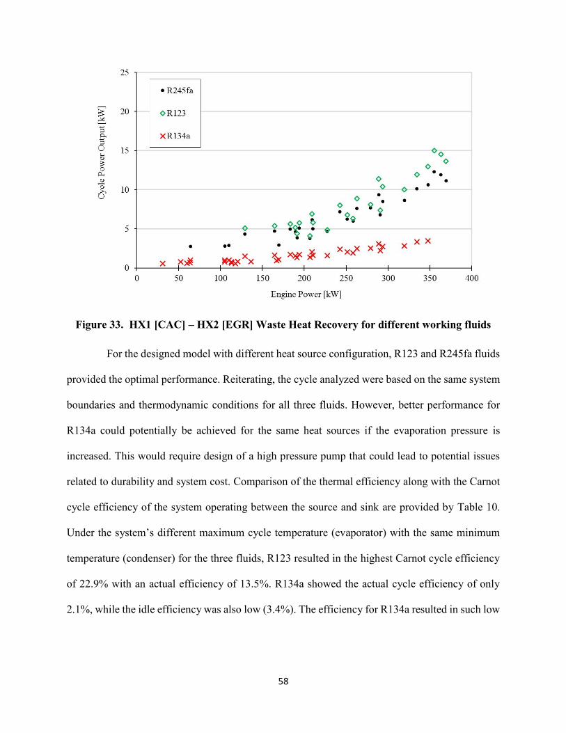
58

Figure 33. HX1 [CAC] – HX2 [EGR] Waste Heat Recovery for different working fluids

For the designed model with different heat source configuration, R123 and R245fa fluids

provided the optimal performance. Reiterating, the cycle analyzed were based on the same system

boundaries and thermodynamic conditions for all three fluids. However, better performance for

R134a could potentially be achieved for the same heat sources if the evaporation pressure is

increased. This would require design of a high pressure pump that could lead to potential issues

related to durability and system cost. Comparison of the thermal efficiency along with the Carnot

cycle efficiency of the system operating between the source and sink are provided by Table 10.

Under the system’s different maximum cycle temperature (evaporator) with the same minimum

temperature (condenser) for the three fluids, R123 resulted in the highest Carnot cycle efficiency

of 22.9% with an actual efficiency of 13.5%. R134a showed the actual cycle efficiency of only

2.1%, while the idle efficiency was also low (3.4%). The efficiency for R134a resulted in such low

59

efficiency values was due to the cycle operating for a small temperature differences between the

condenser (TL) and the evaporator (TH).

Table 10. Thermal cycle efficiency of ORC-WHRS model

R123 R245fa R134a

Carnot Cycle Efficiency 22.9% 18.2% 3.4%

Actual Cycle Efficiency 13.5% 10.8% 2.1%

5.4.2. Heat Source Comparison

Figure 34, Figure 35, and Figure 36 provides comparisons of the system performance based

on four different proposed heat source configuration. With respect to all three fluid types,

configuration with using post-SCR exhaust for the HX1 and EGR for the HX2 showed the best

system performance than compared to other three. While, the configuration with using the two

heat source, charge air cooler (CAC) for the HX1 and EGR for the HX2 showed the lowest system

performance, and the simulation results also had the lowest amounts of points generated (below

150kW engine power) out of the 53 defined points. This shows that at lower engine operating

conditions, CAC and EGR sources would not be able to generate an useful work out of the design

Rankine cycle.

Likewise, the energy recovered from outlet of the SCR assist in pre-heating the working

fluid going through the first stage heat exchanger (HX1), and then utilizes the high quality heat

from the EGR circuit in the second stage heat exchanger (HX2). This results in sufficient energy

for the working fluid to reach the saturated vapor condition, relatively at higher working fluid mass

flow rate which consequently provides better performance from the turbine.

60

Figure 34. WHRS cycle output for different heat source configuration using R123

Figure 35. ORC-WHRS cycle output for different heat source configuration using R245fa

61

Figure 36. ORC-WHRS cycle output for different heat source configuration using R134a

It is to be noted from the above shown results that even though the ORC-WHRS models

were able to simulate cycle power output at lower engine power demands, it would be misleading

to represent ORC-WHRS output potential at lower engine operating conditions, mostly at lower

speed/load points because of the variability observed during the measurement of the energy

distribution. The availability for the Rankine cycles to generate output work was also limited due

to the specified flow rate ranges which was pre-defined for the model based upon the selected

pump characteristics.

62

CHAPTER 6 THERMAL MANAGEMENT POTENTIAL

6.1. Introduction

As the primary goal of this study was to understand the utilization of a WHRS as a strategy

for thermal management of an after-treatment system in reducing NOx levels, the study further

investigates into the dynamic operation of a heavy-duty diesel engine from an actual vehicle testing

results. This chapter details the thermal energy analysis from a similar Class-8 HDD vehicle. It

also provides description of the methodology used in developing ORC-WHRS maps from the

WHRS steady-state basis simulation results, and then used the developed maps to predict the

potential WHRS output for a transient operation.

6.2. Transient Data Source

A similar Class-8 HDD vehicle equipped with standard DOC/DPF and SCR aftertreatment,

tested on a chassis dynamometer testing performed by WVU CAFEE were used for this part of

study. The vehicle specifications are provided in Table 11.

Table 11. Vehicle Specification

Vehicle Manufacturer Mack Trucks Inc.

Vehicle Model CXU613

Vehicle model year 2011

Engine Model MP8 – 445C

Displacement (L) 12.8

After-treatment system DPF-SCR

GVWR 52,000 lbs

Results obtained from a transient test cycle, known as Urban Dynamometer Driving

Schedule (UDDS) with a specific cold-start test was used for the analysis. As the vehicle was not

instrumented for the purpose of performing a complete energy audit, limited parameters were only

63

evaluated. Parameters such as vehicle speed, engine speed, engine load, and post/pre SCR exhaust

temperatures were obtained from the ECU logged channels.

The above mentioned vehicle chassis testing was also performed with using the WVU’s

Heavy Duty Transportable chassis dynamometer lab, capable of performing emission

measurements. A full scaled constant volume sampler (CVS) tunnel designed and maintained as

per CFR 40 Part 1065 were used as the primary method in emission sampling and measurement.

The exhaust mass flow rates needed for the purpose of this study were obtained from the data

reduced as per CFR 40 Part 1065 method.

6.3. Transient Cycle Energy Analysis

A continuous time traced profile of vehicle speed and temperature before the SCR for the

UDDS cycle is presented in Figure 37. On the basis of literature reviews, minimum temperature

of 200°C was considered to be the threshold limit for the SCR inlet condition. It shows that during

initial driving period (from start of the cycle to about 180 seconds) the temperature before the SCR

system are below the threshold temperature which is represented by the red dotted lines in the

figure. It also observed that the temperature falls below 200°C for about 40 seconds after a longer

idle duration. Once the vehicle starts operating at a higher vehicle speed and long driving activity,

the temperature tends to stay well above the threshold limit.

Maintaining the necessary pre-SCR temperatures above 200°C requires additional thermal

energy. The additional required energy for the selected transient cycle to reach the threshold limit

was evaluated using the mass flow rate of the exhaust, and the difference between the enthalpies

at pre-SCR and the threshold temperature. The transient exhaust energy rate traces evaluated

before the SCR and exhaust energy at 200°C for the UDDS cycle are shown in Figure 38. The

64

additional heat required (shown by the green shaded region) to meet the threshold temperature of

200°C is the potential aim to be employed by the thermal management strategy in this study.

Figure 37. Pre-SCR temperature profile from a cold-start UDDS cycle vehicle-chassis test

results

Figure 38. Pre-SCR exhaust energy thermal analysis on the UDDS cycle vehicle-chassis test

results

65

6.4. ORC-WHRS Mapping

In order to quantify the power generated by an ORC-WHRS model for the selected UDDS

cycle, a complete instrumentation would have been required. The data collected from chassis

vehicle testing included post-SCR temperatures and exhaust flow rates but no EGR temperatures.

Hence, simulating the developed ORC-WHRS model in MATLAB® was not possible, but instead

surface maps were generated for predicting the ORC-WHRS power output for the selected UDDS

cycle.

Curve fitting tools were used to predict the ORC-WHR system’s power output for the

transient cycle based on the steady state simulation results. Results from R123 and R245fa fluids

employed with HX1(exhaust post-SCR) and HX2(EGR) configuration were specifically used due

to the optimum performance that were seen from the results obtained for the Mack MP8 engine.

Three influential factors: speed in (rpm), torque in (ft-lbs) and post-SCR exhaust energy in (kW)

were used as model inputs in developing the response surface. JMP® software tool was used for

developing and analyzing the fitting model.

A second-order model over the steady state results for the three input factors provided

reasonable approximation of the response than compared to a linear or higher other polynomials.

The second-order model is represented by Eq. (24) (Montgomery, 2009).

y = β0+β

1x1+β

2x2+β

3x3+β

11x1

2 +β22

x22+β

33x3

2+β12

x1x2+β13

x1x3+β23

x2x3 (24)

Here, y is the model output response which is defined as the ORC-WHRS cycle power

output, and the model input factors x1, x2 and x3 are defined with respect to speed, torque and post-

SCR energy respectively. The β’s represents the partial regression coefficients parameters where

it dictates the weightage of the input factors and the interactions between the input factors in the

66

model. The JMP® software estimates the parameters for the second-order polynomial using the

method of least squares. The summary of the parameter estimates for the two working fluid

response surface models are provided in APPENDIX – B.

From the fit summary for the two models, an R2 of (0.945) for R123 and (0.955) for R245fa

were obtained. It is to be noted that a better prediction of the output response could have been

obtained if a fourth input factor EGR were also used in fitting the second-order model.

Figure 39 and Figure 40 presents the predicted response surface of the ORC-WHR system’s

power output as a contour profile where the horizontal axis represents the engine speed and the

vertical axis represents the engine torque. The boundary of the contour map is defined by the

obtained points resulted from the ORC-WHRS system operated for specific engine speed/load

points.

Figure 39. ORC-WHRS cycle output power map for HX1(exhaust post-SCR) and

HX2(EGR) using R123

67

Figure 40. ORC-WHRS cycle output power map for HX1(exhaust post-SCR) and

HX2(EGR) using R245fa

6.5. ORC-WHRS Transient Results

Respective maps developed for the two working fluids were used to estimate the ORC-

WHRS cycle power output for the transient process. Transient profiles of the three input factors:

engine speed, engine torque and post-SCR energy obtained from the UDDS test data are shown in

Figure 41. As mentioned earlier in this study, generating WHR output at low speed and toque

condition would not be practical, hence for the study, ORC-WHRS cycle power output were set to

zero if the engine operating power was equal to less than 75kW.

Figure 42 provides the results obtained from the ORC-WHRS, comparing the two working

fluids. The estimated cycle output for both R123 and R245fa showed transient correlation with the

three input traces. For the transient cycle, the maximum ORC-WHR cycle power output for R123

and R245fa resulted in 15.1kW and 11.6kW, respectively.

68

Figure 41. Transient input factor profiles

Figure 42. ORC-WHRS power generated for HX1 [Exhaust] - HX2 [EGR] WHRS on

UDDS cycle

0 200 400 600 800 10000

500

1000

1500

2000

Torq

ue [

ft-lbs]

0 200 400 600 800 10000

600

1200

1800

2400

Engin

e S

peed [

rpm

]

0 200 400 600 800 10000

100

200

300

Time [sec]

Rate

of

post-

SC

R E

nerg

y [

kW

]

69

In terms of total energy accumulated for the UDDS cycle, both R123 with 0.987kW-hr and

R245fa with 0.692 kW-hr resulted in exceeding the cumulative energy of 0.432 kW-hr required

by the pre-SCR catalysts to reach the threshold temperature of 200°C as shown in Figure 43. R123

and R245fa were able to produce 56.2% and 37.6% more energy respectively over the entire

UDDS cycle as compared to required thermal energy before the SCR.

Figure 43. Cumulative energy results using ORC-WHRS output on UDDS cycle

The results obtained underlines the magnitude of thermal energy in the exhaust system for

proper SCR activation, and a potential source provided to sufficiently meet the energy requirement,

assuming that all the energy recovered is completely utilized in raising the thermal energy of the

exhaust stream before the SCR catalyst. However, during vehicle start-up period there wouldn’t

be any opportunity in generating power from an ORC-WHRS which could be utilized for thermal

management purposes.

70

6.6. Thermal Management Strategy

This section details the thermal management strategy implementation of an electrically

heated SCR catalyst using the power source obtained from the ORC-WHRS development. Figure

44 shows a simple schematic of a vehicle exhaust system integrated for an electrical heater. As a

probable control technique, using an electrical heater with power usage from a pre-charged

vehicle’s internal battery (secondary source) for pre-heating the SCR catalyst during initial warm-

up period or even before the engine is started, and then utilizing the accumulated energy from the

ORC-WHRS for charging the external battery which would be the primary source for the electrical

heater. The warm-up phase would consist of warming up the pre-SCR air stream in order for the

catalyst to reach its proper operating temperatures.

As control strategy presented in Figure 45 for the first 450 seconds of the UDDS cycle, the

catalyst could be pre-heated before the engine starts (key-on), and since there would be no exhaust

flow before engine key-on, an external air pump would be required at such events. The pump

would also be powered from the same energy source. The duration of the pre-heating time depends

upon the temperature requirement of the SCR system.

Figure 44. Schematic of a thermal management using ORC-WHRS as the power source

ENGINEDOC/DPF SCR

EXTERNAL

ENERGY

STORAGE DEVICE

ORC-

WHRS

AIR

PUMP

T1 T2 T3

T1 Pre-SCR Temperature (before heater)

T2 Pre-SCR Temperature (after heater)

T3 Post-SCR Temperature

Exhaust

Flow

Power Source Path

Electrical

Heater

Primary Source

Secondary Source

Valve

71

Figure 45. Catalyst pre-heating strategy before and after engine key-on

For implementation of such thermal management strategies, monitoring of internal

substrate temperatures would be required as a feedback control: both during pre- and post- engine

key-on phases. In real-time based system controls, due to thermal inertia and transport delay,

physical-based SCR catalyst models are needed to be investigated and developed for implementing

advanced control strategies. Hence, development of system models along with advanced feedback

information from different exhaust sensors could be incorporated for managing the thermal state

of the SCR system during vehicle warm-up and varying driving conditions. Moreover in the light

of this study, the vehicle’s primary battery source would only be utilized for the initial warm-up

period and rest of the power required for employing the proposed thermal management could

solely be consumed from the secondary battery source storing energy obtained from the ORC-

WHR system: harvesting potential energy from different sources that are considered as losses in a

modern heavy-duty diesel engine.

72

CHAPTER 7 CONCLUSIONS AND FUTURE WORK

7.1. Conclusions

In this study, a theoretical waste heat recovery system model was approached based on

experimental data obtained from MY2011 Mack MP8 heavy-duty diesel engine testing. As a

supporting investigation, the preliminary energy analysis applied under wide range of the engine

operating over steady state conditions showed that suitable energy could possibly be extracted

from the EGR loop exhibiting high quality heat. Likewise, post-SCR exhaust stream and charge

air cooler (CAC) circuit also showed potent candidate in heat recovery. This lead to developing an

ORC-WHRS model to include two heat exchangers and evaluating different configuration of heat

sources. The study also evaluated three different types of organic fluids (R123, R245fa, and

R134a) which are seen to be used in relevant works demonstrated in other studies.

Results obtained from a standard ORC-WHRS simulation over the engine operating points

showed that R123 and R245fa gave the optimum performance under the selected characteristics

and assumptions made within the study. The optimum WHRS cycle performance was achieved by

pre-heating the working fluid using the post-SCR exhaust stream, and then using the EGR circuit

to further heat the fluid to reach the saturated vapor conditions.

As the main objective of this study was to identify a thermal management approach for

maintaining proper SCR operating temperatures during dynamic vehicle operation. Hence, testing

results from a vehicle chassis dynamometer study was analyzed in order to estimate the ORC-

WHRS output on a transient basis. Result showed that R123 and R245fa based ORC-WHRS

simulation were able to produce 56.2% and 37.6% more energy respectively over the UDDS cycle

as compared to required thermal energy required to maintain the pre-SCR temperature at 200°C.

73

This study does realizes that extraction of work from the WHR cycle to be immediately

used for thermal management is not possible. However, this study presents a thermal management

scenario wherein utilizing an energy storage system for powering an electrical heater and

replenishing the energy back through the ORC-WHRS when sufficient engine conditions are

achieved.

7.2. Future Work

1. On this basis of future work, this study could further investigate into ORC-WHRS

potential using actual on-road vehicle data operating on diverse operations.

2. Also possibly look into development of ORC-WHR system for conducting actual

experimental work.

3. Research and development into physical-based thermal model of a vehicle exhaust

system equipped with aftertreatment devices

4. Development of control strategies applied for optimization of aftertreatment thermal

activity under different levels of vehicle operation.

74

References

ARNOLD, S., SLUPSKI, K., GROSKREUTZ, M., VRBAS, G., ROB, C. & SHAHED, S. M. 2001.

Advanced Turbocharging Technologies for Heavy-Duty Diesel Engines. SAE, 2001-01-3260.

ARUNACHALAM, P. N., SHEN, M., TUNER, M., TUNESTAL, P. & THERN, M. 2012. Waste Heat

Recovery from Multiple Heat Sources in HD Truck Diesel Engine using a Rankine Cycle - A

Theoretical Evaluation. SAE, 2012-01-1602.

AVADHANULA, V. K., CHUEN-SEN, L. & JOHNSON, T. 2013. Testing a 50kW ORC at Different

Heating and Cooling Source Conditions to Map the Performance Characteristics. SAE, 2013-01-

1649.

BAE, S., HEO, H., LEE, H. & LEE, D. 2011. Performance Charateristics of a Rankine Steam Cycle and

Boiler for Engine Waste Heat Recovery. SAE 2011-28-0055.

BIRKHOLZ, U. Conversion of Waste Exhaust Heat in Automobile using FeSi2 Thermoelements. 7th

International Conference on Thermoelectric Energy Conversion, 1988 Arlington, USA. pp. 124-

128.

BOSCH, H. & JANSSEN, F. 1988. Catalytic Reduction of Nitrogen Oxides. Catalysis Today, vol. 2, pp.

v.

CAVINA, N., MANCUNU, G., CORTI, E., MORO, D., CESARE, M. D. & STOLA, F. 2013. Thermal

Management Strategy for SCR After Treatment Systems. SAE, 2013-24-0153.

CHANDLER, G. R., COOPER, B. J., HARRIS, J. P., THOSS, J. E., UUSIMAKI, A., WALKER, A. P. &

WARREN, J. P. 2000. An Integrated SCR and Continuously Regenerating Trap System to Meet

Future NOx and PM Legislation. SAE, 2000-01-0188.

COZZOLINI, A., BESCH, M. C., KAPPANNA, H., BONSACK, P. & GAUTAM, M. Waste Heat

Recovery in Heavy-Duty Diesel Engines: A Thermodynamic Analysis of Waste Heat

Availability for Implementation of Energy Recovery Systems based upon the Organic Rankine

Cycle. ASME 2012 International Combustion Engine Division Spring Technical Conference,

2012 Torino, Piemonte, Italy.

ETTIREDDY, P. R., KOTRBA, A. & SPINKS, T. 2014. Development of Low Temperature Selective

Catalytic Reduction (SCR) Catalyst for Future Emissions Regulations. SAE, 2014-01-1520, 2.

GIANNELLI, R., NAM, E., HELMER, K., YOUNGLOVE, T., SCORA, G. & BARTH, M. 2005. Heavy-

Duty Diesel Vehicle Fuel Consumption Modeling based on Road Load and Power Train

Parameters. SAE, 2005-01-3549.

GIESHOFF, J., SCHÄFER-SINDLINGER, A., SPURK, P. C. & TILLAART, J. A. A. V. D. 2000.

Improved SCR Systems for Heavy Duty Applications. SAE, 2000-01-0189.

GRAVEL, R. 2013. SuperTruck - An Opportunity to Reduce GHG Emissions while Meeting Service

Demands [Online]. Asilomar Conference. Available:

http://www.its.ucdavis.edu/files/general/pdf/2013-08-21_Asilomar-2013-Gravel.pdf [Accessed

12/02/2014].

75

HEYWOOD, J. B. 1988. Internal Combustion Engine Fundamentals, McGraw Hill.

INCROPERA, F. P., DEWITT, D. P., BERGAN, T. L. & LAVINE, A. A. 2007. Fundamentals of Heat

and Mass Transfer, 6th Edition, John Wiley & Sons, Inc.

JMP 2012. JMP® Design of Experiments Guide.

JOHNSON, T. V. 2009. Diesel Emission Control in Review. SAE, 2012-01-0368.

KAMASAMUDRAM, K., CURRIER, N., SZAILER, T. & YEZERESTS, A. 2010. Why Cu- and Fe-

Zeolite SCR Catalysts Behave Differently at Low Temperature. SAE, 2010-01-1182.

KEUPER, A., UNGER, H.-M. I., HUANG, J., BRESSLER, H. & ALBRECHT, W. 2011. Investigations

to Achieve Highest Efficiencies in Exhaust Gas After-Treatment for Commercial Vehicles

using an SCR system. SAE, 2011-01-2201.

KOEBEL, M., ELSENER, M. & KLEEMANN, M. 2000. Urea-SCR: A Promising Technique to Reduce

NOx Emissions from Automotive Diesel Engines. Catalysis Today, vol. 59, pp. 335-345.

KOEBEL, M., ELSENER, M. & MADIA, G. 2001. Recent Advances in the Development of Urea-SCR

for Automotive Applications. SAE, 2001-01-3625.

KOEBEL, M., MADIA, G. & ELSENER, M. 2002. Selective Catalytic Reduction of NO and NO2 at Low

Temperatures. Catalysis Today, vol. 73, pp. 239-247.

KRÖCHER, O. 2007. Aspects of Catalyst Development for Mobile Urea-SCR Systems - from Vanadia-

Titania Catalysts to Metal-Exchanged Zeolites. Studies in Surface Science and Catalysis, vol.

171, pp. 261-289.

LATZ, G., ANDERSSON, S. & MUNCH, K. 2012. Comparison of Working Fluids in both Subcritical

and Supercritical Rankine Cycles for Waste-Heat Recovery Systems in Heavy-Duty Vehicles.

SAE, 2012-01-1200.

LATZ, G., ANDERSON, S. & MUNCH, K. 2013. Selecting an Expansion Machine for Vehicle Watse-

Heat Recovery Systems based on the Rankine Cycle. SAE, 2013-01-0552.

MAJEWSKI, A. W. 2014. Urea Dosing and Injection Systems [Online]. DieselNet. Available:

http://www.dieselnet.com/tech/cat_scr_mobile_urea_dosing.php [Accessed 12/02/2014].

MISRA, C., COLLINS, J. F., SAX, T., KRISHNAMURTHY, M., SOBIERALSKI, W., BURNTIZKI, M.

& CHERNICH, D. 2013. In-Use NOx Emissions from Model Year 2010 and 2011 Heavy-Duty

Diesel Enigines Eqipped with Aftertreatment Devices. Environmental Science and Technology,

vol. 47, pp. 7892-7898.

MONTGOMERY, D. C. 2009. Design and Analysis of Experiments, 7th Edition, John Wiley & Sons, Inc.

MORAN, M. J. & SHAPIRO, H. N. 2008. Fundamentals of Engineering Thermodynamics, 6th Edition,

John Wiley & Sons, Inc.

NELSON, C. R. 2008. Waste Heat Recovery for Heavy Duty Vehicle. Cummins Inc.: Steam Power.

NOOR, A. M., PUTECH, R. C. & RAJOO, S. 2014. Waste Heat Recovery Technologies in Turbocharged

Automotive Engine - A Review. Journal of Modern Science and Teechnology, vol. 2, pp. 108-

119.

76

SLUDER, C. S., STOREY, J. M. E., LEWIS, S. A. & LEWIS, L. A. 2005. Low Temperature Urea

Decomposition and SCR Performance. SAE, 2005-01-1858.

STANTON, D. W. 2013. Systematic Development of Highly Efficient and Clean Engines to Meet Future

Commerical Vehicle Greenhouse Gas Regulations. SAE, 2013-01-2421.

TALUS, P., TENG, H., HUNTER, G. L., VELDE, B. V. D. & KLAVER, J. 2011. A Rankine Cycle

System for Recovering Watse Heat from HD Diesel Engines - Experimentla Results. SAE 2011-

01-1337.

TENG, H., KLAVER, J., PARK, T., HUNTER, G. L. & VELDE, B. V. D. 2011. A Rankine Cycle

System for Recovering Waste Heat from HD Diesel Engines - WHR System Development.

SAE, 2011-01-0311.

TENG, H. & REGNER, G. 2009. Improving Fuel Economy for HD Diesel Engines with WHR Rankine

Cycle driven by EGR Cooler Heat Rejection. SAE 2009-01-2913.

THEENGINEERINGTOOLBOX. Ethylene Glycol Heat - Transfer Fluid [Online]. Available:

http://www.engineeringtoolbox.com/ethylene-glycol-d_146.html [Accessed 10/08/2014].

TURHILL. 2000. Performance Curves (Metric) L Series. Available:

http://www.tuthillpump.com/dam/2463.pdf [Accessed 09/30/2014].

ULRICH, P., SCHATZ, A. & KONIECZNY, R. 2012. Advanced Exhaust Gas Thermal Management for

Lowest Tailpipe Emissions - Combining Low Emission Engine and Electrically Heated

Catalyst. SAE 2012-01-1090.

USEPA. Engine Testing Regulations [Online]. Available:

http://www.epa.gov/nvfel/testing/regulations.htm [Accessed 05/10/2014].

WANG, E. H., ZHANG, H. G., FAN, B. Y., OUYANG, M. G., ZHAO, Y. & MU, Q. H. 2011. Study of

Working Fluid Selection of Organic Rankine Cycle (ORC) for Engine Waste Heat Recovery.

Energy, 2011-03-041.

77

APPENDIX A Pump Characteristics

Figure A-1. Performance curve for the selected positive displacement pump (Turhill, 2000)

78

APPENDIX B ORC-WHRS Response Surface Results

Following results provided the model fit summary and results used to predict the ORC-

WHRS output map for working fluid R123 and R245fa with HX1(post-SCR exhaust) and

HX2(EGR) combination. Figure B-1, shows the actual versus predicted for R123 model fit. Table

B-1 provides the summary of estimates for the partial regression coefficients parameters in the

second order model. The units for speed, torque and post-SCR are defined in terms of rpm, ft-lbs

and kW. The table also provides p-values for each parameter term and signifies the parameter

significance in the model’s response. A low p-value illustrates a higher influence of the parameter

in the model obtained. It shows that post-SCR has a significant influence in the model with a p-

value of 0.0281 (< p-value of 0.05 at α=5%). Table B-1. Parameter estimate for second order

response model of R123 data.

Figure B-1. Actual by predicted plot for second order response model for ORC-WHRS

(R123)

79

Table B-1. Parameter estimate for second order response model of R123 data

Model Terms β Estimate p-value

Intercept 4.0638 0.5787

Speed [rpm] -0.00207 0.7107

Torque [ft-lbs] -0.00279 0.6041

Post SCR [kW] 0.076893 0.0281*

(Speed [rpm]-1386.18)*(Speed [rpm]-1386.18) -4.18E-06 0.9111

(Speed [rpm]-1386.18)*(Torque [ft-lbs]-1087.79) -3.37E-05 0.6547

(Torque [ft-lbs]-1087.79)*(Torque [ft-lbs]-1087.79) -2.65E-05 0.4773

(Speed [rpm]-1386.18)*(Post SCR [kW]-193.364) 0.000113 0.7982

(Torque [ft-lbs]-1087.79)*(Post SCR [kW]-193.364) 0.000257 0.5593

(Post SCR [kW]-193.364)*(Post SCR [kW]-193.364) -0.00054 0.6735

Figure B-2. Actual by predicted plot for second order response model for ORC-WHRS

(R245fa)

Similarly, Figure B-2 shows the actual versus predicted for R245fa model fit. Table B-2

provides the summary of estimates for the partial regression coefficients parameters in the

second order model. From the p-value results for the obtained model, it shows that post-SCR

has a significant influence in the model with a p-value of 0.0168 (< p-value of 0.05 at α=5%).

80

Figure B-2. Actual by predicted plot for second order response model for ORC-WHRS

(R245fa)

Table B-2. Parameter estimate for second order response model of R245fa data

Model Terms β Estimate p-value

Intercept -0.44265 0.874

Speed [rpm] 0.001481 0.5286

Torque [ft-lbs] 0.000979 0.6773

Post SCR [kW] 0.040951 0.0168*

(Speed [rpm]-1341.78)*(Speed [rpm]-1341.78) 4.36E-06 0.1698

(Speed [rpm]-1341.78)*(Torque [ft-lbs]-839.877) -6.86E-07 0.9308

(Torque [ft-lbs]-839.877)*(Torque [ft-lbs]-839.877) -7E-06 0.1932

(Speed [rpm]-1341.78)*(Post SCR [kW]-152.81) -2.82E-05 0.5779

(Torque [ft-lbs]-839.877)*(Post SCR [kW]-152.81) 5.44E-05 0.427

(Post SCR [kW]-152.81)*(Post SCR [kW]-152.81) -2.57E-05 0.9128