SIAM Journal on Applied Mathematics 1

Inverse Source Problem in Non-homogeneous Background

Media

Anthony J. Devaney∗, Edwin A. Marengo†, and Mei Li‡

March 31, 2007

Abstract

The scalar wave inverse source problem (ISP) of determining an unknown radiating sourcefrom knowledge of the field it generates outside its region of localization is investigated forthe case in which the source is embedded in a non-homogeneous medium with known index ofrefraction profile n(r). It is shown that the solution to the ISP having minimum energy (so-called minimum energy source) can be obtained via a simple method of constrained optimization.This method is applied to the special case when the non-homogeneous background is sphericallysymmetric (n(r) = n(r)) and yields the minimum energy source in terms of a series of sphericalharmonics and radial wave functions that are solutions to a Sturm-Liouville problem. Thespecial case of a source embedded in a spherical region of constant index is treated in detail,and results from computer simulations are presented for this case.

Keywords: Inverse source problem, non-homogeneous media, inhomogeneous media, antenna sub-strate, scattering, reciprocity.

AMS Subject Classifications: 45Q05, 78A46, 78A40, 78A50, 35-02.

Running Title: Inverse Problem in Non-homogeneous Media

∗Department of Electrical and Computer Engineering, Northeastern University, Boston, MA 02115 (Tony-dev@2aol.com).

†Department of Electrical and Computer Engineering, Northeastern University, Boston, MA 02115(emarengo@ece.neu.edu).

‡Department of Electrical and Computer Engineering, Northeastern University, Boston, MA 02115(mli@cdsp.neu.edu).

1

SIAM Journal on Applied Mathematics 2

1 Introduction

We consider in three-dimensional space the fundamental inverse source problem (ISP) of determiningan unknown scalar source ρ to the inhomogeneous Helmholtz equation

[∇2 + k20n

2(r)]U(r) = −ρ(r) (1)

(where ∇2 denotes the Laplacian operator) that radiates a scalar field U which is specified everywhereoutside the support volume τ of the source. In this equation k0 is a constant wavenumber and n(r)is an index of refraction distribution that depends on position r ∈ R3 and that is assumed to go tounity for sufficiently large r. We will assume throughout this paper that the source volume τ is asphere, centered at the origin, and having a radius a. The ISP then consists of computing a sourceρ that generates a prescribed exterior field U , whose value is specified for r /∈ τ .

There are a number of treatments of the scalar ISP of interest in this work as well as of the fullvector electromagnetic inverse problem for the free space case where the index distribution n(r) isconstant (equal to unity) throughout space [1, 2, 3, 4, 5, 6, 7, 8, 9, 10]. Most of these treatmentsmake use of the fact that the source’s radiation pattern (see below) determines, in principle, thefield everywhere outside the source volume [11]. Using this fact the ISP can be cast in terms ofthe radiation pattern: determine a source ρ that generates a prescribed radiation pattern. It isalso well known [12, 13, 14] that there exist an infinity of sources that radiate fields that vanishidentically outside their support volumes so that the ISP does not possess a unique solution; i.e.,an infinity of solutions can be obtained by adding any one of these non-radiating sources to anygiven solution [15, 16]. Thus, in order to obtain a unique solution to the ISP it is necessary to addconstraints that the source must satisfy in addition to yielding a specified radiation pattern. Animportant and tractable choice of constraint is source energy E , defined to be the L2 norm of thesource over the source volume τ :

E =

∫

τ

d3r |ρ(r)|2. (2)

The solution to the ISP that minimizes the source energy as defined in Eq.(2) is usually termedthe minimum energy solution [2, 3, 6, 7, 8, 9, 10]. It is orthogonal to the non-radiating sources [3]and is the pseudo-inverse of the ISP [5, 6]. Physically, this source is also related to the real imagefield generated by a point-reference hologram of the field recorded on a closed surface completelysurrounding the source volume [2, 3, 17].

The source energy as defined in Eq.(2) is an important measure of the realizability of a sourcegenerating a given radiation pattern with the given spatial resource or source volume τ . For the freespace case one finds that the energy of the minimum energy source depends critically on the productx = k0a of the (free space) wavenumber k0 and the source radius a [2, 6]. For a given radiationpattern this energy E(x) is small for x > l0 where l0 is a parameter that characterizes the radiationpattern and that increases with increasing fine detail in the pattern. However, it is found that E(x)increases exponentially with decreasing x below the critical value l0. This exponential increase ofsource energy indicates that the given radiation pattern cannot be physically realized by any sourcehaving that specific k0a product: it is necessary to either decrease the wavelength (increase k0)or increase the source radius. This is analogous to the well known result in antenna theory thatstates that reactive energy and the quality Q of an antenna increase exponentially with decreasingk0a if one attempts to achieve super-directivity [18, 19]. Furthermore, in the associated full vectortreatment the source energy is also a measure of the current levels of the antenna structure whichideally should be small to cope with ohmic losses in realistic lossy antenna material. In particular, theability of a source (antenna) to radiate a prescribed field with reduced source energy or “resources”is an indication of efficiency, so that the constraint of minimizing the source energy for a givenradiation field is of interest not only for the theoretical treatment of the inverse source problem andof the related field realizability question but also for the practical antenna synthesis problem (see,

2

SIAM Journal on Applied Mathematics 3

e.g., the antenna characterizations in [20], the sensitivity factor in [21], and similar factors used in[22, 23, 24]).

As far as the authors of this paper know there are only two treatments of the ISP for the casewhere the background index distribution n(r) in which the source is embedded is non-homogeneous [25,26]. The work in [26] generalizes the main results in [25] to lossy media. Of particular interest tothe present research, which focuses on lossless media, is [25], which shows that the minimum energysolution satisfies an integral equation whose kernel is the imaginary part of the outgoing wave Greenfunction of the inhomogeneous Helmholtz equation (1). Using this fact it is shown in [25] that theminimum energy solution can be expanded into a series of eigenfunctions of this integral equationwith expansion coefficients that can be determined from the radiation pattern. The paper showsthat the formalism reduces to the known theory of the ISP when the index n = 1 (homogeneousmedium case) but does not include any examples of the general theory.

In this paper we consider the case of a source embedded in a known non-homogeneous realbackground index (corresponding to a lossless medium) and solve the minimum energy ISP using asimple method of constrained optimization. Besides providing a simpler formulation of the problemthan the one used in [25] the method yields a solution that is directly implemented without theneed of first computing a Green function for the Helmholtz equation (1) and then computing theeigenfunctions of the imaginary part of this quantity. The special case of a spherically symmetricindex n(r) = n(r) is treated in detail and it is shown that the minimum energy solution to the ISPhas exactly the same mathematical form as the solution for the constant index case but with thespherical Bessel functions employed in the constant index solution replaced by radial wave functionsthat are solutions to a Sturm-Liouville problem. In particular, these radial wave functions arethe radial wave scattering functions obtained in the scattering of an incident plane wave from thespherically symmetric index distribution n(r). This latter problem has been studied extensivelyin both quantum mechanical scattering [27] and optical [28] and electromagnetic [29] scatteringand there exists a number of index distributions for which the scattering wave functions have beencomputed and that can be used to compute the minimum energy solution to the ISP.

Motivation for the research presented in this paper is provided in part by the possibility of op-timally selecting the source region index of refraction distribution n(r) to achieve some specifiedradiation pattern that would otherwise not be realistically possible (due to prohibitive values ofrequired current level, or other engineering constraints) for a source embedded in free space. Thispossibility has attracted research from time to time in the antenna community, being of interest a va-riety of antenna-embedding materials or substrates, including plasmas [30], non-magnetic dielectrics[31, 32, 33, 34, 35, 36], magneto-dielectrics [37, 38, 39, 40], and, more recently, double negative meta-materials which are receiving much recent attention as antenna performance-enhancing substratesby a number of groups [41, 42, 43, 44, 45, 46, 47, 48, 49]. The envisaged property is miniaturiza-tion of antennas by controlling electric size (via larger wavenumber) but other effects are involved,particularly when metamaterials are used.

To arrive from first wave theoretic principles at a non-device specific understanding of the prac-tical possibilities opened by antenna-embedding substrates, we emphasize in the present work thefundamental minimum energy source yielding a given radiation pattern rather than particular de-vices as has been the focus of the aforementioned presentations in this area. Also, the presenttreatment concerns the scalar inverse problem which is a simplification of the full vector electro-magnetic case. Rigorous treatment of the metamaterials which are generally bi-anisotropic mediarequires the full vector formulation [50, 51] and is left for future work. Thus in the present workattention is restricted to the pertinent properties associated to the index of refraction n(r) ≥ 0 ofnatural, “positive” materials whose key aspects can be treated within the scalar formulation, butthe general approach can be extended also to the vector case along the lines of, e.g., [52] where bothsource energy and reactive power constraints have been considered in the formulation of the inverseproblem for sources embedded in free space.

The key observation is that, as outlined earlier and as shown in section 3 of this paper, in the

3

SIAM Journal on Applied Mathematics 4

free space case the minimum energy source energy increases exponentially with decreasing x = k0abelow a critical point that is determined by the fine detail that is desired in the radiation pattern.The question then is whether this limitation can be mitigated by embedding the source in a non-homogeneous background medium. In effect we create a new “effective source” that consists of theactual physical source interacting with the non-homogeneous background. In the simplest case wecan consider a source embedded in a cavity with partially reflecting walls. This cavity will, of course,have a pronounced effect on the radiated field and, possibly, can aid in achieving desired propertiesof the radiation pattern.

In this paper we limit our attention, for the most part, to source regions characterized by a spher-ically symmetric index of refraction distribution n(r) = n(r), although many of our results can begeneralized to sources embedded in cavities and non-spherically symmetric index distributions. Therealizability of a given radiation pattern is investigated in some detail by examining the dependenceof minimum source energy on the index of refraction profile of the source region. It is found thatthis energy depends critically on the (weighted) L2 norm of the radial wavefunctions taken over thesource region. This fact suggests that by proper choice of the index of refraction profile n(r) theenergy can be minimized for any given radiation pattern; i.e., an index distribution can be selectedthat results in a source having minimum energy for a given prescribed radiation pattern.

The L2 norms of the radial wave functions are found to be dependent on “resonant” propertiesof the source index distribution and are also related in a one-to-one fashion with the differentangular modes of the radiation pattern. These facts suggest the interesting possibility of exploitingthe “resonances” of the source index distribution to selectively control the shape and form of theradiation pattern. This possibility is briefly considered in the computer simulation study.

The final section of the paper treats the simple example of a source embedded in a homogeneoussphere whose constant index of refraction differs from that of the background medium. This is thesimplest example of a spherically symmetric index of refraction distribution and the scattering wavefunctions are well known (the so-called Mie scattering problem [28, 29]) and easily computed. Theminimum energy source is computed for this case and results from a computer simulation study thatexamines the dependence of the energy of the minimum energy source on the index of refraction ofthe source region is presented. The source energy depends in a non-linear manner on the value ofthe source region refraction index. The examples considered reveal that, as desired, there are valuesof the index of refraction for which the improvement of the source-embedded case relative to thefree space case is significant for the entire effectively radiating multipole spectrum pertinent to thesame source region in free space.

2 Problem Formulation

We introduce the scattering potential defined according to the equation

V (r) = k20[1 − n2(r)]

and rewrite Eq.(1) in a form that we will use in the development to follow. In particular we findthat

[∇2 + k20 − V (r)]U(r) = −ρ(r), (3)

where here and in the remainder of the paper both the scattering potential V and the source ρ areassumed to vanish outside the source region τ (thus n(r) = 1 for r /∈ τ).

The outgoing wave solution to Eq.(3) is the unique field radiated by the source obeying Sommer-feld’s radiation condition (e.g., see [53], ch. 2; [54], ch. 3), which is the one having the asymptoticbehavior of an outgoing spherical wave

U(rs) = f(s)eik0r

r+O(1/r2) (4)

4

SIAM Journal on Applied Mathematics 5

as k0r → ∞ uniformly in the direction specified by the unit vector s. In the above equation, thequantity f(s) is the source’s far field radiation pattern which is seen to correspond to the limit

f(s) = limr→∞[

re−ik0rU(rs)]

. (5)

In the following, we will bear in mind Eqs.(4,5) but will usually express the associated far fieldasymptotic behavior simply as

U(rs) ∼ f(s)eik0r

r, as k0r → ∞, (6)

with the understanding that throughout the paper all the far field approximations hold to withinO(1/r2). It is well known that the radiation pattern specified for all directions s uniquely determinesthe field U everywhere outside the source region τ [11]; i.e., knowledge of the radiated field everywhereoutside τ is equivalent to knowledge of the radiation pattern f(s) specified for all directions s.

The inverse source problem (ISP) consists of determining a source distribution ρ(r) that radiatesa given field U for r /∈ τ . Because the ISP requires that the field radiated by the source be specifiedonly outside τ the problem does not possess a unique solution because of the possible presence ofnon-radiating sources [12, 13, 14] within τ . A non-radiating source generates a field that vanishesidentically outside τ and, hence, can be added to any given solution to the ISP to yield a differentsolution. Also, because the radiation pattern uniquely determines the field everywhere outside τ ,the ISP is equivalent to the problem of determining a source that generates a prescribed radiationpattern f(s) for all observation directions s.

Most treatments of the ISP cast the problem in terms of the radiation pattern but only requirethat the source generate the radiation pattern to within a given accuracy defined by the integralsquared error

E =

∫

4π

dΩs |f(s) − f(s)|2 (7)

where f is the prescribed radiation pattern and f the radiation pattern actually generated by thesource, while dΩs denotes solid-angular differential element. More precisely, the desired radiationpattern is approximated by a finite series of spherical harmonics Y m

l (s)

f(s) ≈ f(s) =

L∑

l=0

l∑

m=−l

αl,mYml (s) (8)

and the source is required only to generate the approximate radiation pattern f . Here, we have usedthe unit vector s having polar angle θ and azimuthal angle φ to denote the θ, φ arguments of thespherical harmonics. Because the spherical harmonics are orthonormal and complete over the unitsphere the approximated radiation pattern satisfies Eq.(7) with an error E given by

E =∞∑

l=L+1

l∑

m=−l

|αl,m|2

where the expansion coefficients (multipole moments) αl,m, l > L are the higher order (neglected)expansion coefficients of the ideal radiation pattern.

Besides requiring only that the source generate the radiation pattern within a finite error mosttreatments of the ISP also require that the source minimize the source energy defined by (cf., Eq.(2))

E =

∫

τ

d3r |ρ(r)|2. (9)

We will show (see also [3]) that minimizing the source energy leads to a unique solution of the ISP,namely, the minimum energy source, which we designate by ρME . This solution has the distinct

5

SIAM Journal on Applied Mathematics 6

advantage of being the most efficient source that solves the ISP for a given scattering potentialV (r) (corresponding to a given background index of refraction n(r)). Since the minimum energysource and, hence, the minimum source energy, depend on the scattering potential, an interestingquestion arises as to the dependence of the source energy on the background index distribution and,in particular, on which index distributions lead to lowest source energies. This question providesmuch of the motivation for studying the ISP in non-homogeneous backgrounds since it leads to thepossibility of designing very efficient sources (e.g., antennas) that are embedded in such backgrounds.

Our goal in this paper is to develop the formalism for solving the ISP as defined above and toevaluate the formalism in a set of computer simulations. We will first treat the case of a sourceembedded in free space and then extend the free space theory to the general case of a sourceembedded in an inhomogeneous background medium. The free space case is important in that itprovides a benchmark of performance as well as a frame of reference for the general theory.

3 Free Space Case

The minimum energy ISP as defined above has been solved within both the scalar wave formulationunder consideration here [1, 2, 3, 4, 5, 7] and the electromagnetic wave formulation [6, 8, 9, 10] inthe special case where the scattering potential V (r) vanishes; i.e., when the source is embedded infree space. We will review the scalar wave free space case here where, however, we will employ asomewhat different solution methodology to find the minimum energy source than the one adoptedin earlier work. We will use this same procedure for the general case of non-vanishing scatteringpotentials later in the paper.

The outgoing wave solution to Eq.(3) is given in terms of an outgoing wave Green functionG(r, r′) (obeying Eq.(3) for ρ(r) = −δ(r − r

′) and an asymptotic condition of the form Eq.(6)) bythe expression

U(r) = −

∫

τ

d3r′ ρ(r′)G(r, r′), (10)

where (as indicated earlier) the source volume τ is a sphere of radius a centered at the origin. In theparticular free space case where the scattering potential V = 0 the outgoing wave Green function Gis given by

G(r, r′) = −1

4π

eik0|r−r′|

|r − r′|(11)

from which it is easy to show that

G(rs, r′) ∼ −1

4πe−ik0s·r′ e

ik0r

r(12)

as k0r → ∞ in the direction s (which has the required form Eq.(6)). Using the above result weconclude from Eqs.(6,10) that the radiation pattern is given by

f(s) =1

4π

∫

τ

d3r′ ρ(r′)e−ik0s·r′ . (13)

We can obtain an expansion of the radiation pattern in a series of spherical harmonics by usingthe well known expansion

e−ik0s·r′ = 4π

∞∑

l=0

l∑

m=−l

(−i)ljl(k0r′)Y m

l∗(r′)Y m

l (s) (14)

where jl denotes the spherical Bessel function of the first kind of order l, Y ml are the spherical

harmonics of degree l and order m, r′ denotes the unit vector in the r

′ direction, and ∗ denotes

6

SIAM Journal on Applied Mathematics 7

complex conjugate. Upon substituting Eq.(14) into Eq.(13) we find that

f(s) =

∞∑

l=0

l∑

m=−l

αl,mYml (s) (15)

where the expansion coefficients (multipole moments) αl,m are given by

αl,m =

∫

4π

dΩsf(s)Y ml

∗(s)

= (−i)l

∫

τ

d3r′ ρ(r′)jl(k0r′)Y m

l∗(r′). (16)

3.1 Minimum Energy Source

The minimum energy solution to the ISP is required to satisfy Eq.(16) for some given set of multipolemoments αl,m, l = 0, 1, . . . , L and also to minimize the source energy defined according to Eq.(9).Computing the minimum energy source can be cast as a problem of constrained minimization wherethe generalized Lagrangian is given by

L = E +

L∑

l=0

l∑

m=−l

Cl,m[α∗l,m − il

∫

τ

d3r ρ∗(r)jl(k0r)Yml (r)] + c.c.

where E is the source energy defined in Eq.(9) and c.c. stands for the complex conjugate of thesecond term on the r.h.s. of the equation and the Cl,m are a set of Lagrange multipliers to bedetermined. On expressing the source energy in terms of ρ and ρ∗ and taking the first variation ofthe above Lagrangian we obtain

δL =

∫

τ

d3r δρ∗(r)

[

ρ(r) −L

∑

l=0

l∑

m=−l

Cl,miljl(k0r)Y

ml (r)

]

+ c.c.

which, when set equal to zero, yields the solution

ρME(r) =

∑L

l=0

∑l

m=−l Cl,miljl(k0r)Y

ml (r) if r < a

0 if r > a.

The Lagrange multipliers Cl,m are determined from the condition that the source generate themultipole moments according to Eq.(16). We find that

Cl,m =αl,m

σ2l

(17)

where

σ2l =

∫ a

0

r2dr j2l (k0r). (18)

On making use of the above expression for the Lagrange multipliers we finally conclude that theminimum energy solution to the free space ISP is given by

ρME(r) =

∑L

l=0

∑l

m=−l il αl,m

σ2

l

jl(k0r)Yml (r) if r < a

0 if r > a.(19)

7

SIAM Journal on Applied Mathematics 8

3.2 Source Energy

The source energy E is readily computed using the minimum energy source given in Eq.(19). Wefind from Eq.(9) that

EME =

∫

τ

d3r |ρME(r)|2 =

L∑

l=0

l∑

m=−l

|αl,m|2

σ2l

(20)

where we have added the subscript “ME” to denote the energy of the minimum energy source. Now,it is easy to show that the quantities σ2

l depend critically on the product k0a of the free spacewavenumber with the source radius a. In particular these quantities can be shown to be given by

σ2l =

∫ a

0

r2dr |jl(k0r)|2 =

a3

2[jl

2(k0a) − jl−1(k0a)jl+1(k0a)]. (21)

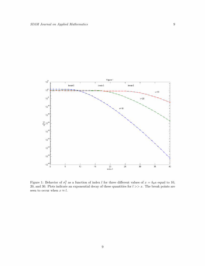
and to decrease exponentially to zero for l > k0a. It then follows that the largest value L of theindex l allowed in the approximation Eq.(8) is L = k0a if we want to maintain low source energy.Values of L >> k0a will lead to extremely high source energy and unstable source distributions.

To illustrate the remarks made above concerning the behavior of the quantities σ2l on the index l

and the product k0a we show in Fig. 1 semilog plots of σ2l as a function the index l for various values

of x = k0a. It is seen from these plots that these quantities decay exponentially to zero for l >> xso that at wavenumber k0 a source of radius a can only efficiently radiate a radiation pattern whosemaximum l value is L = k0a. Similar behavior is exhibited in Fig.2 which shows semilog plots ofσ2

l (x) as a function of x for values of l = 10, 20, and 30.We computed the energy of the minimum energy source for a model radiation pattern f(θ) having

multipole coefficients αl,m given by

αl,m =

1√L+1

if m = 0 and l ≤ L

0 else(22)

This radiation pattern is circularly symmetric about the z axis (is independent of φ since the non-zero multipoles correspond to m = 0), has an effective beam width inversely related to the cut-offvalue L and has unit energy; i.e.,

∫

4π

sin θdθdφ |f(θ)|2 =L

∑

l=0

1

L+ 1= 1.

We show plots of the model radiation pattern as a function of angle θ in Fig. 3 for values of theparameter L equal to L = 10, L = 20 and L = 30. It is clear from these plots that the larger thevalue of L the narrower the radiation pattern and, hence, the higher the directivity of the source.Using the coefficients given in Eq.(22) we computed the source energy using Eq.(20) with the σ2

l

given by Eq.(21) and with three different L values of L = 10, 20 and L = 30. It was found that, asexpected, the source energy becomes extremely large if we try to achieve an L value that exceeds thecritical value L = k0a. This is, of course, due to the fact that the quantities σ2

l become extremelysmall when k0a << l as is indicated in Fig.2.

4 Non-homogeneous Backgrounds

The outgoing wave solution of Eq.(3) for a non-homogeneous index distribution n(r) of support τ ,which behaves as in Eqs.(4,5,6), can be expressed in terms of the outgoing wave Green function for thebackground medium via Eq.(10) where, however, the Green function is no longer the free space Greenfunction defined in Eq.(11) but instead is the total outgoing wave Green function corresponding tothe total medium comprised of free space plus the non-homogeneous index distribution n(r) or its

8

SIAM Journal on Applied Mathematics 9

Figure 1: Behavior of σ2l as a function of index l for three different values of x = k0a equal to 10,

20, and 30. Plots indicate an exponential decay of these quantities for l >> x. The break points areseen to occur when x ≈ l.

9

SIAM Journal on Applied Mathematics 10

Figure 2: σ2l as a function of x = k0a for values of l0 = 10 (.), l0 = 20 (o) and l0 = 30 (x). Plots

indicate an exponential growth of these quantities for x << l0. The break points are seen to occurwhen x ≈ l.

10

SIAM Journal on Applied Mathematics 11

Figure 3: Plots of the model radiation pattern for L = 10 (.), L = 20 (o) and L = 30 (x).

11

SIAM Journal on Applied Mathematics 12

associated scattering potential V (r). In the ISP under consideration in this paper, the field is givenoutside the source region τ only, that is, the field for a source of support τ is given by Eq.(10)where r

′ ∈ τ and r /∈ τ . This particular situation enables us to formulate the forward mappingpertinent here (from a masked source that is confined within τ to an exterior field that is prescribedfor r /∈ τ only) via a conceptually simple and insightful approach which borrows from standardscattering theory and the reciprocity property of the outgoing wave Green function, which can bereadily shown for the formally self-adjoint partial differential operator [∇2+k2

0−V (r)] using standardGreen function theory (e.g., see [55], ch. 9, 10). Two equivalent versions of the general methodologyare outlined next. The main objective is to generalize the statement made in connection with thefree space case in the far field mapping Eq.(13) for the more general case of non-homogeneousbackgrounds. The generalization of the derived expression for the far field mapping will be appliedto the particular spherically symmetric and piecewise constant background cases later in the paper.

The starting point is provided by the familiar Lippmann-Schwinger integral equation (e.g., see[56], Eqs. 8.4, 8.5, 10.12, 10.13; [27], pages 178-179, 263-265; [53], page 5; [57], pages 60-61) whichin the present formulation and notation yields

G(r, r′) = G0(r, r′) +

∫

τ

d3r′′G0(r, r′′)V (r′′)G(r′′, r′) (23)

where here G denotes the total outgoing wave Green function of the total medium comprised offree space plus the generally non-trivial scattering potential V and G0 denotes the free space Greenfunction defined in Eq.(11) (corresponding to V = 0), in particular,

G0(r, r′) = −

1

4π

eik0|r−r′|

|r − r′|

where (see also Eq.(12), where, again, the G in Eq.(12) corresponds to the G0 of the present section)

G0(rs, r′) = −

1

4πe−ik0s·r′ e

ik0r

r+O(1/r2), as k0r → ∞, (24)

in the direction of the unit vector s, so that from the discussion in Eq.(4,5,6) (which holds for ageneral source ρ) one finds that the far field radiation pattern of a point source −δ(r − r

′) in freespace is − 1

4πe−ik0s·r′ . We shall recall this basic result later.

Due to reciprocity, the result Eq.(23) can be rewritten also as

G(r, r′) = G0(r, r′) +

∫

τ

d3r′′G(r, r′′)V (r′′)G0(r′′, r′). (25)

We will borrow from both Eqs.(23,25) in the following.By making use of the asymptotic result Eq.(24) it is not difficult to show from Eq.(23) or its

equivalent, Eq.(25), that the Green function G behaves asymptotically as

G(rs, r′) = −1

4πψ+(r′;−k0s)

eik0r

r+O(1/r2) (26)

as k0r → ∞, where we have introduced the quantity ψ+(r;−k0s) defined by

ψ+(r;−k0s) = e−ik0s·r+

∫

τ

d3r′e−ik0s·r′V (r′)G(r′, r) = e−ik0s·r+

∫

τ

d3r′G(r, r′)V (r′)e−ik0s·r′ . (27)

Note from Eq.(26) that the Green function G(r, r′) does in fact behave as k0r → ∞ as we haverequired in Eqs.(4,5,6). From the same equations one also notes that the far field radiation patternf(s) in Eqs.(4,5,6), corresponding to the field U obeying Eq.(3), applies to the general source ρ,

12

SIAM Journal on Applied Mathematics 13

while, on the other hand, the far field radiation pattern − 1

4πψ+(r′;−k0s) in Eq.(26) corresponds to

that of the total field produced by the particular Dirac-delta, point source at r′ in the same medium.

In other words, the quantity − 1

4πψ+(r′;−k0s) is the far field radiation pattern for the particular

case of a point source at r′. This quantity is seen from Eq.(27) to consist of the sum of two terms:

The first term, − 1

4πe−ik0s·r′ , exists even if V = 0, and is the far field radiation pattern for the point

source in free space (it will account for an incident field in the discussion to follow). This is, infact, what we have discussed before in Eq.(24). On the other hand, the second term, the integral inEq.(27), corresponds to an scattered field contribution, as we shall elaborate further next.

The quantity ψ+(r;−k0s) as defined by the formulation above (Eqs.(26,27)) is customarily termedscattering wave function (e.g., see [56], pages 3, 4, 164, 172). This scattering wave function is theunique total (incident plus scattered) field for the scattering potential V (r) under excitation by theincident plane wave e−ik0s·r in the direction defined by the unit vector −s, under Sommerfeld’sradiation condition for the scattered field, which translates into the requirement that the respectivescattered field, that is, the integral term in Eq.(27), behaves like an outgoing wave at infinity. Thusthe scattering wave function ψ+(r;−k0s) is the solution to the homogeneous Helmholtz equation

[∇2 + k20 − V (r)]ψ+(r;−k0s) = 0, (28)

which obeys an asymptotic condition of the form

ψ+(rr;−k0s) ∼ e−ik0s·r + g(r;−k0s)eik0r

r(29)

as k0r → ∞ where g is the so-called scattering amplitude associated with the scattering potentialV whose role in scattering problems is similar to that of the source radiation pattern f (Eq.(6)) inradiation problems (e.g., see [56], Eq.(10.19); [58]). Note from Eqs.(26,27) that

ψ+(rr;−k0s) ∼ e−ik0s·r−1

4π

eik0r

r

∫

τ

d3r′ψ+(r′;−k0s)V (r′)e−ik0s·r′ as k0r → ∞ (30)

so that from Eq.(29) the scattering amplitude

g(r;−k0s) = −1

4π

∫

τ

d3r′ψ+(r′;−k0s)V (r′)e−ik0s·r′ . (31)

Thus the scattering wave function ψ+(r;−k0s) corresponds to the total (incident plus scattered)field that results when an incident plane wave propagating in the −s direction scatters off theinhomogeneous index of refraction distribution n(r). Note that in the limit when the scatteringpotential vanishes this scattering wave function simply reduces to the incident plane wave.

Now, by substituting the asymptotic result Eq.(26) into Eqs.(4,5,6,10) we find that the radiationpattern f(s) of a general source ρ embedded in the non-homogeneous background characterized byindex of refraction n(r) or, equivalently, scattering potential V (r), is given by

f(s) =1

4π

∫

τ

d3r′ ρ(r′)ψ+(r′;−k0s), (32)

which is simply the free space result Eq.(12) with the plane wave exp(−ik0s · r′) replaced by thescattering wave function ψ+(r′;−k0s). For a given V , this scattering wave function can be ob-tained by solving the scattering problem posed by Eqs.(28,29). The ISP for given non-homogeneousbackground media then reduces to determining a source ρ that satisfies Eq.(32) for all observationdirections s, and where the scattering wave functions ψ+ are to be determined a priori for the per-tinent scattering potential V by addressing the scattering problem in Eqs.(28,29). Clearly, in thespecial case when V = 0 the scattering wave function reduces to the plane wave (refer to Eq.(27))and Eq.(32) reduces to the free space result Eq.(13), as expected.

13

SIAM Journal on Applied Mathematics 14

Previous to engaging in the particular cases of spherically symmetric and piecewise constantbackgrounds, we wish to outline an alternative description of the formulation above based on reci-procity, that is, for the total Green function in the total medium characterized by the scatteringpotential V , G(r, r′) = G(r′, r). Such a description is very insightful in elucidating the connectionbetween radiation and scattering problems (e.g., see [59]), and may thus facilitate application ofthe present inverse source problem research to other areas, such as scattering and inverse scatteringproblems. Without loss of generality, in the rest of this paragraph the point r

′ will be taken to liein the spherical volume τ of radius a centered about the origin (the source region). Also, take r

to be a point in a spherical surface of radius R > a centered about the origin. The idea is thatthe problem of computing the far field produced at the field point Rs (for large k0R, and wheres is a unit vector) by a point source at the point r

′ in the source region τ is, due to reciprocityconsiderations, equivalent to the problem of computing the (near) field produced at point r

′ due toa far zone point source at Rs, in particular, G(Rs, r′) = G(r′, Rs). Conveniently, the latter problemessentially reduces to the familiar scattering problem under plane wave excitation, and this is thebasis of the preceding formulation as well as of the complementary analysis to be given next. Thefield generated by a given point source at r

′ ∈ τ at the field point r = Rs in the far field directiondefined by the unit vector s obeys from Eqs.(4,5,6) the asymptotic form

G(Rs, r′) = f(s; r′)eik0R

R+O(1/R2) (33)

as k0R→ ∞, where the respective radiation pattern f(s; r′) of the total field radiated by the pointsource at r

′ depends on r′ in a way to be clarified in the following (again, note that the radiation

pattern in Eq.(33) is, apart from a factor − 1

4π, the scattering wavefunction ψ+(r′;−k0s) of the

preceding development). On the other hand, the total field produced at the point r′ ∈ τ due

to a point source at Rs can be decomposed into the sum of an incident field, corresponding to theradiation in free space, that is, the free space Green function component G0(r

′, Rs), plus an scatteredfield corresponding to scattering of that incident field by the medium characterized by scatteringpotential V . This can be expressed formally by borrowing from Eqs.(23,25), in particular,

G(r′, Rs) = G0(r′, Rs) +

∫

τ

d3rG0(r′, r)V (r)G(r, Rs)

= G0(r′, Rs) +

∫

τ

d3rG(r′, r)V (r)G0(r, Rs) (34)

where the integrals define the scattered field component, and where from the outgoing wave natureof both G0 and G,

G(r′, Rs) = −1

4πe−ik0s·r′ e

ik0R

R+eik0R

R

∫

τ

d3rG0(r′, r)V (r)f(s; r) +O(1/R2) (35)

as k0R → ∞ (where we have used Eq.(33) and G(r′, Rs) = G(Rs, r′)), or, equivalently (from thesecond of the equations in Eq.(34)), as

G(r′, Rs) = −1

4πe−ik0s·r′ e

ik0R

R−

1

4π

eik0R

R

∫

τ

d3rG(r′, r)V (r)e−ik0s·r +O(1/R2) (36)

as k0R→ ∞; furthermore, using G(r′, Rs) = G(Rs, r′) one recovers from these developments Eq.(33)where f(s; r′) = − 1

4πψ+(r′;−k0s) obeys

f(s; r′) = −1

4πψ+(r′;−k0s) = −

1

4π

[

e−ik0s·r′ +

∫

τ

d3rG0(r′, r)V (r)ψ+(r;−k0s)

]

(37)

14

SIAM Journal on Applied Mathematics 15

or, equivalently,

f(s; r′) = −1

4πψ+(r′;−k0s) = −

1

4π

[

e−ik0s·r′ +

∫

τ

d3rG(r′, r)V (r)e−ik0s·r]

(38)

which agrees with the previous formulation (Eqs.(26,27,28,29)). It follows that, as explained inconnection with those results, the scattering wave function ψ+(r′,−k0s) is the total (incident plusscattered) field at r

′ due to the interaction of an incident plane wave in the direction −s with thescattering potential V . Finally, an alternative way of arriving at these results is via the so-calledmixed reciprocity relation ([57], p. 61-62, in particular, Eq.(2.2.6); see also p. 42) which states thatthe value at s of the far field radiation pattern corresponding to the scattered field component of thefield generated in the non-homogeneous medium due to a point source excitation at r

′ is, apart from amultiplicative factor (− 1

4π), equal to the value at r

′ of the field that is scattered by the same mediumdue to an incident plane wave traveling in the direction −s. In the notation of this paper, the far fieldradiation pattern of the scattered field component of the field generated in the non-homogeneousmedium due to a point source at r

′ is, as has been discussed before (Eqs.(23,24,25,26,27)), preciselythe integration term in Eqs.(27,37,38) which is the field scattered by a plane wave traveling inthe direction −s, as expected. Thus our findings are consistent with this standard relation fromthe literature [57]. Yet, we must point out a difference in notation between [57] and the presentpaper. In our notation (and without loss of generality), the Green function or fundamental solutionapplicable to free space,

G0(r, r′) = −

1

4π

eik0|r−r′|

|r − r′|,

has a negative sign since we define the Green function (or fundamental solution) for a point source−δ(r−r

′) unlike in [57] which considers the fundamental solution for a point source δ(r−r′) (this is

explained in ([57], p. 8); see also [53], p. 16, [54], ch. 3). Our entire formulation incorporates withno loss of generality this particular choice as is obvious in our form of the Green function integralEq.(10). Thus the result Eq.(2.2.6) in ([57], p. 61) involves the factor γ3 = 1

4π(refer to [57], p.

42) which is equivalent, in the present usage for the fundamental solution (with the added negativesign), to our factor − 1

4π, and this completes the picture (the two theories yield the same final result,

as desired). Let us consider special cases next.

4.1 Spherically Symmetric Backgrounds

In the remainder of the paper we will restrict our attention to the case of spherically symmetricindex distributions n(r) = n(r). The scattering wave functions then satisfy (cf., Eq.(28))

[∇2 + k20 − V (r)]ψ+(r;−k0s) = 0, (39)

where the eigenfunctions ψ+ are required to satisfy the boundary condition Eq.(29). Because ofthe spherical symmetry of the scattering potential V , the wavefield ψ+ can only depend on themagnitude r of the field point vector r and the polar angle γ formed between the direction ofpropagation −s of the incident plane wave and r. If we then take the incident wave direction to bethe positive z axis and express the Helmholtz operator in spherical polar coordinates Eq.(39) canbe written in the form

[

1

r2∂

∂r(r2

∂

∂r) +

1

r2 sin γ

∂

∂γ(sin γ

∂

∂γ) − V (r) + k2

0

]

ψ+(r, γ) = 0 (40)

where γ is the polar angle formed between the positive z axis and the field point vector r and wherewe have used the fact that the field must be independent of the azimuthal angle φ. The boundarycondition Eq.(29) becomes

ψ+(r, γ) ∼ eik0r cos γ + g(γ)eik0r

r(41)

15

SIAM Journal on Applied Mathematics 16

where we have set −k0s · r = k0z = k0r cos γ and where g(γ) is the scattering amplitude.We can expand the scattering wave function ψ+(r, γ), the incident plane wave exp(ik0r cos γ)

and the scattering amplitude g(γ) into a series of Legendre polynomials as follows [55, 60]

ψ+(r, γ) =∑

l

il(2l + 1)ψl(r)Pl(cos γ),

eik0r cos γ =∑

l

il(2l + 1)jl(k0r)Pl(cos γ),

g(γ) =∑

l

il(2l + 1)AlPl(cos γ),

where we have introduced the factors il(2l+ 1) into the expansions for the scattering wave functionand the scattering amplitude for later notational convenience. In these equations jl is the sphericalBessel function of the first kind of order l and the Al are expansion coefficients of the scatteringamplitude that depend on the specific form of the scattering potential V (r). On substituting thefirst of these equations into Eq.(40) we find that the radially dependent coefficients ψl(r) satisfy theequation

[

1

r2d

dr(r2

d

dr) −

l(l + 1)

r2− V (r) + k2

0

]

ψl(r) = 0 (42)

where we have used the fact that

1

sin γ

∂

∂γ(sin γ

∂

∂γ)Pl(cos γ) = −l(l + 1)Pl(cos γ).

The asymptotic behavior of the radial functions ψl(r) is obtained by substituting the expansions forthe scattering wave function, the incident plane wave, and the scattering amplitude into Eq.(41).We find that

ψl(r) ∼ jl(k0r) +Al

eik0r

r. (43)

Besides satisfying the boundary condition Eq.(43) we also require that the radial functions be every-where continuous with continuous first derivatives.

Once the radial functions ψl(r) are computed, the scattering wave function ψ+(r, γ) correspond-ing to an incident plane wave propagating along the z axis is given by the expansion in Legendrepolynomials above. However, the defining equation for the radiation pattern Eq.(32) requires thatwe have the scattering wave functions for all directions −s of the incident plane wave. This can beeasily accomplished by using the addition theorem for spherical harmonics [55, 60]

Pl(cos γ) =4π

2l + 1

l∑

m=−l

(−1)lY ml

∗(r)Y ml (s),

where now γ is the angle formed between the arbitrary incident wave direction −s and the fielddirection r. On using the addition theorem we obtain

ψ+(r;−k0s) = 4π

∞∑

l=0

l∑

m=−l

(−i)lψl(r)Yml

∗(r)Y ml (s), (44)

which is the generalization of Eq.(14) to spherically symmetric non-homogeneous index of refractiondistributions.

16

SIAM Journal on Applied Mathematics 17

4.2 Minimum Energy Source

Upon substituting the expansion Eq.(44) into Eq.(32) we obtain Eq.(15) where, however, the mul-tipole moments are now given by

αl,m =

∫

4π

dΩsf(s)Y ml

∗(s)

= (−i)l

∫

τ

d3r ρ(r)ψl(r)Yml

∗(r) (45)

which is the generalization of Eq.(16) to the case where the source is embedded in a non-homogeneousbut spherically symmetric index of refraction profile. The generalized Eq.(45) is seen to result fromEq.(16) under the replacement of the spherical Bessel functions jl by the radial functions ψl. Theminimum energy solution to the ISP is required to satisfy Eq.(45) for some given set of multipolemoments αl,m, l = 0, 1, . . . , L and also to minimize the source energy defined according to Eq.(9).

As in the free space case, the problem of computing the minimum energy source can be cast asone of constrained minimization where the generalized Lagrangian is now given by

L = E +

L∑

l=0

l∑

m=−l

Cl,m[α∗l,m − il

∫

τ

d3r ρ∗(r)ψ∗l (r)Y m

l (r)] + c.c.

where, as before, E is the source energy defined in Eq.(9) and c.c. stands for the complex conjugateof the second term on the r.h.s. of the equation and the Cl,m are a set of Lagrange multipliers tobe determined. On expressing the source energy in terms of ρ and ρ∗ and taking the first variationof the above Lagrangian we obtain

δL =

∫

τ

d3r δρ∗(r)

[

ρ(r) −

L∑

l=0

l∑

m=−l

Cl,milψ∗

l (r)Y ml (r)

]

+ c.c.

which, when set equal to zero, yields the solution

ρME(r) =

∑L

l=0

∑l

m=−l Cl,milψ∗

l (r)Y ml (r) if r < a

0 if r > a.

The Lagrange multipliers Cl,m are determined from the condition that the source generate themultipole moments according to Eq.(45). We find that

Cl,m =αl,m

Σ2l

(46)

where

Σ2l =

∫ a

0

r2dr |ψl(r)|2. (47)

On making use of the above expression for the Lagrange multipliers we finally conclude that theminimum energy solution to the ISP for spherically symmetric background index distributions isgiven by

ρME(r) =

∑L

l=0

∑l

m=−l(i)l αl,m

Σ2

l

ψ∗l (r)Y m

l (r) if r < a

0 if r > a.(48)

The source energy is found to be given by the free space formula Eq.(20) where, however, theσ2

l are replaced by the Σ2l defined in Eq.(47). As in the free space case the source energy is seen

to depend inversely on the Σ2l . Although these quantities are strictly positive they can become

extremely small leading to extremely high source energy and associated instability in the minimum

17

SIAM Journal on Applied Mathematics 18

energy source. Thus, it is of interest to maximize these quantities especially for large values of theindex l which is associated with fine detail (high resolution) in the radiation pattern.

The energy of the minimum energy source is obtained by substituting Eq.(48) into the sourceenergy definition given in Eq.(2). We obtain the same expression as was obtained in the free spacecase Eq.(20) where, however, the σ2

l are replaced by the Σ2l . It is clear that the source energy is

minimized by maximizing the Σ2l which, in turn, is equivalent to maximizing the weighted L2 norm

of the radial functions ψl over the interval [0, a]. Since the radial functions ψl are solutions to aSturm-Liouville problem the energy minimization problem reduces to finding scattering potentialsV (r) whose corresponding Sturm-Liouville problem has solutions with maximum norm over thisinterval. This problem, although simple to state, appears to be non-trivial and the authors offer nosimple recipe for computing optimum potentials at this time. However, in the following section wewill treat a simple class of potentials that illustrates the dependence of source energy on selectionof V .

5 Piecewise Constant Backgrounds

In this section we consider the special case where the scattering potential V (r) is constant throughoutthe source region; i.e.,

V (r) =

k20 − k2 if r < a

0 if r > a,(49)

This is certainly a spherically symmetric scattering potential so that the scattering wave functionscan be expanded in the form of Eq.(44) where the radial functions ψl(r) satisfy Eq.(42) with V (r)given in Eq.(49) above. Thus we find that

[

1

r2d

dr(r2

d

dr) −

l(l + 1)

r2+ k2

]

ψl(r) = 0 if 0 < r < a

[

1

r2d

dr(r2

d

dr) −

l(l + 1)

r2+ k2

0

]

ψl(r) = 0 if a < r <∞

together with the boundary condition from Eq.(43):

ψl(r) ∼ jl(k0r) +Al

eik0r

rif r > a. (50)

We also require that the radial functions be finite and continuous with a continuous first derivative.The set of differential equations together with the boundary and continuity conditions allow us toobtain a unique solution for the radial function.

5.0.1 Radial Function

The radial function has the general form

ψl(r) = Ajl(kr) +Bhl(kr) if 0 < r < a

ψl(r) = Cjl(k0r) +Dhl(k0r) if a < r <∞

where jl is the spherical Bessel function of the first kind and hl the spherical Hankel function of thefirst kind. The requirement that the radial function be finite at the origin r = 0 requires that B = 0while the boundary condition Eq.(50) requires that the constant C = 1. The remaining constantsA and D are determined by the continuity requirements applied at the boundary r = a. Theseconditions are

Ajl(ka) = jl(k0a) +Dhl(k0a)

Ajl′(ka) =

k0

k[jl

′(k0a) +Dhl′(k0a)]

18

SIAM Journal on Applied Mathematics 19

from which we obtain the solution

A =k0

k

jl′(k0a)hl(k0a) − jl(k0a)hl

′(k0a)

jl′(ka)hl(k0a) −

k0

kjl(ka)hl

′(k0a)

D = −jl

′(ka)jl(k0a) −k0

kjl(ka)jl

′(k0a)

jl′(ka)hl(k0a) −

k0

kjl(ka)hl

′(k0a)

The expression for the constant A can be further simplified by using the Wronskian relation forspherical Bessel functions

j′l(k0a)hl(k0a) − jl(k0a)h′l(k0a) =

−i

k20a

2.

We find that

A =−i

k0ka2

jl′(ka)hl(k0a) −

k0

kjl(ka)hl

′(k0a). (51)

5.1 Source Energy

The quantities Σ2l are found using Eq.(47) to be given by

Σl2 =

∫ a

0

r2dr |ψl(r)|2

= |A|2∫ a

0

r2dr |jl(kr)|2

= Tl(k, k0)σ2l (k) (52)

where σ2l (k) is the free space quantity defined in Eq.(21) but with k0 replaced by k and

Tl(k, k0) = |A|2 =1

k20a

4|kj′l(ka)hl(k0a) − k0jl(ka)h′l(k0a)|2. (53)

In the limit when k → k0 we have that

Tl(k, k0) → T (k0, k0) =1

k40a

4|j′l(k0a)hl(k0a) − jl(k0a)h′l(k0a)|2= 1

where we have used the Wronskian between the spherical Bessel and spherical Hankel functions. Itthen follows that Σ2

l → σ2l (k0) in this limit, as required.

The quantities Tl(k, k0) appearing in the expression for the Σ2l have a simple interpretation: they

are the magnitude square of the transmission coefficients relating the amplitudes of the outgoingmultipole fields radiated by the source ρ evaluated on the exterior of the source region to theamplitude of the outgoing wave multipole fields radiated by the source on the interior of the sourceregion. In particular, at the interior of the boundary at r = a we can express the field radiated by thesource in the form of a superposition of outgoing and standing wave solutions to the homogeneousHelmholtz equation with wavenumber k = nk0 while outside this sphere the field is a superpositionof outgoing wave solutions to the Helmholtz equation with wavenumber k0. Because the total fieldand normal derivative must be continuous across the boundary we find that for each multipole modewe require

hl(ka) + rljl(ka) = tlhl(k0a)

h′l(ka) + rlj′l(ka) =

k0

ktlh

′l(k0a)

19

SIAM Journal on Applied Mathematics 20

where rl and tl are reflection and transmission coefficients and the primes denote derivatives. Solvingfor the transmission coefficients tl we find that

tl =j′l(ka)hl(ka) − jl(ka)h

′l(ka)

j′l(ka)hl(k0a) −k0

kjl(ka)h′l(k0a)

=−i

k2a2

j′l(ka)hl(k0a) −k0

kjl(ka)h′l(k0a)

(54)

which is seen to be identical to the coefficient A obtained earlier so that |tl|2 = |A|2 = Tl as indicated.

The interpretation of the quantities Tl as being the magnitude square of the transmission co-efficients from the field modes in the interior of the source region to the field modes outside thisregion makes perfect sense in view of the formula Eq.(52) for the quantities Σ2

l . In particular, tominimize source energy E (i.e., to obtain an efficient source) we wish to maximize the Σ2

l which, inturn, requires us to maximize the Tl or, equivalently, maximize the amount of energy transmittedfrom the source interior to the source exterior. As we will find in our simulations presented belowthe Tl(k, k0) vary inversely with index value n so that low source energy is obtained by selectingn to be small. On the other-hand the Σ2

l and, hence, the source energy also depend on the freespace quantities σ2

l evaluated at the source region wavenumber k and, as is easily confirmed fromthe results presented in section 3, the free space quantities σ2

l (k) increase with k and, hence, indexn, at fixed source radius a. Thus, the two quantities entering into the expression Eq.(52) for Σ2

l

have opposite dependences on source index n and it is necessary to carefully evaluate the relativeimportance of each quantity in order to select an index value that leads to small source energy.

To illustrate, we show in Fig. 4-6 plots of the free space quantities σ2l (k), the modulus square

of the transmission coefficient Tl(k, k0) and, finally, the Σ2l = Tl(k, k0)σ

2l (k) plotted as a function of

the product x = k0a of the free space wavenumber with the source radius a = 10 and for two valuesof the source region index n (n = .5, n = 1.5) and for l values of l = 10, 20 and l = 30. The followingconclusions can be drawn from these plots:

• For fixed a and fixed l the free space quantities σ2l (k = nk0) increase with increasing index n

for any given free space wavenumber k0.

• For fixed a and fixed l the quantities Tl(k = nk0, k0) oscillate with k0. The oscillations indicatethe presence of resonances of the scattering functions within the source volume. The Tl aredecreasing functions of index n at any given free space wavenumber k0.

• The Σ2l = Tlσ

2l oscillate with respect to k0 due to the resonances of the scattering states in the

source region and are also dependent on the source region index n. For k0 values below the

critical point k0a = l, the growth of the free space quantity σ2l (k = nk0) with respect to index n

tends to outweigh the decay of Tl(k = nk0, k0) with respect to n with the result that the product

Σ2l is an increasing function of n.

A more in-depth look at the behavior of the Σ2l as a function of k0, n and l can be obtained from

Figs. 7-9. These figures show composite plots of Σ2l for n = .5, 1 and n = 1.5 for three different l

values (l = 10, 20, 30). It is clear from these plots that by making the source region index n > 1 it ispossible to increase the Σ2

l beyond their free space values σ2l (k0) and thereby obtain sources which

have lower energy than those embedded in free space.We conclude from the above results that like the free space quantities σ2

l (k0), the Σ2l decay

exponentially to zero for l >> k0a. However, by proper selection of the index n of the source regionit is possible to obtain higher values of these quantities around and below the critical point k0a = land, hence, lower source energy than can be obtained in the free space case for the same radiationpattern. This result follows from the fact that the radiation pattern expansion coefficients αl,m are

independent of the source region index distribution so that minimum source energy is obtained bysimply maximizing the Σ2

l .

20

SIAM Journal on Applied Mathematics 21

Figure 4: Plots of σ2l (k = nk0) (dash-dot), Tl(k = nk0, k0) (dotted), and Σ2

l = Tlσ2l (solid) for l = 10

and n = .5 and n = 1.5. It is seen from the plots that the larger n value yields larger Σ2l around

and below the critical point.

21

SIAM Journal on Applied Mathematics 22

Figure 5: Plots of σ2l (k = nk0) (dash-dot), Tl(k = nk0, k0) (dotted), and Σ2

l = Tlσ2l (solid) for l = 20

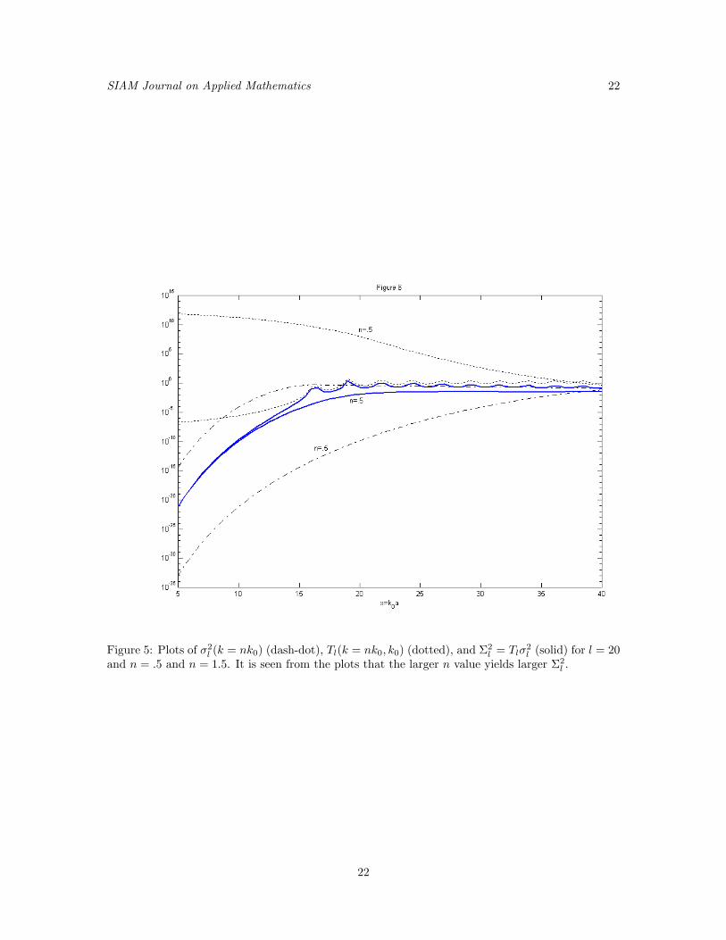
and n = .5 and n = 1.5. It is seen from the plots that the larger n value yields larger Σ2l .

22

SIAM Journal on Applied Mathematics 23

Figure 6: Plots of σ2l (k = nk0) (dash-dot), Tl(k = nk0, k0) (dotted), and Σ2

l = Tlσ2l (solid) for l = 30

and n = .5 and n = 1.5. It is seen from the plots that the larger n value yields larger Σ2l .

23

SIAM Journal on Applied Mathematics 24

Figure 7: Plots of Σ2l = Tlσ

2l for l = 10 and n = .5 (dotted), n = 1 (solid) and n = 1.5 (dashed). It

is seen from the plots that the larger n value yields larger Σ2l around and below the critical point

k0a = l.

24

SIAM Journal on Applied Mathematics 25

Figure 8: Plots of Σ2l = Tlσ

2l for l = 20 and n = .5 (dotted), n = 1 (solid) and n = 1.5 (dashed). It

is seen from the plots that the larger n value yields larger Σ2l around and below the critical point

k0a = l.

25

SIAM Journal on Applied Mathematics 26

Figure 9: Plots of Σ2l = Tlσ

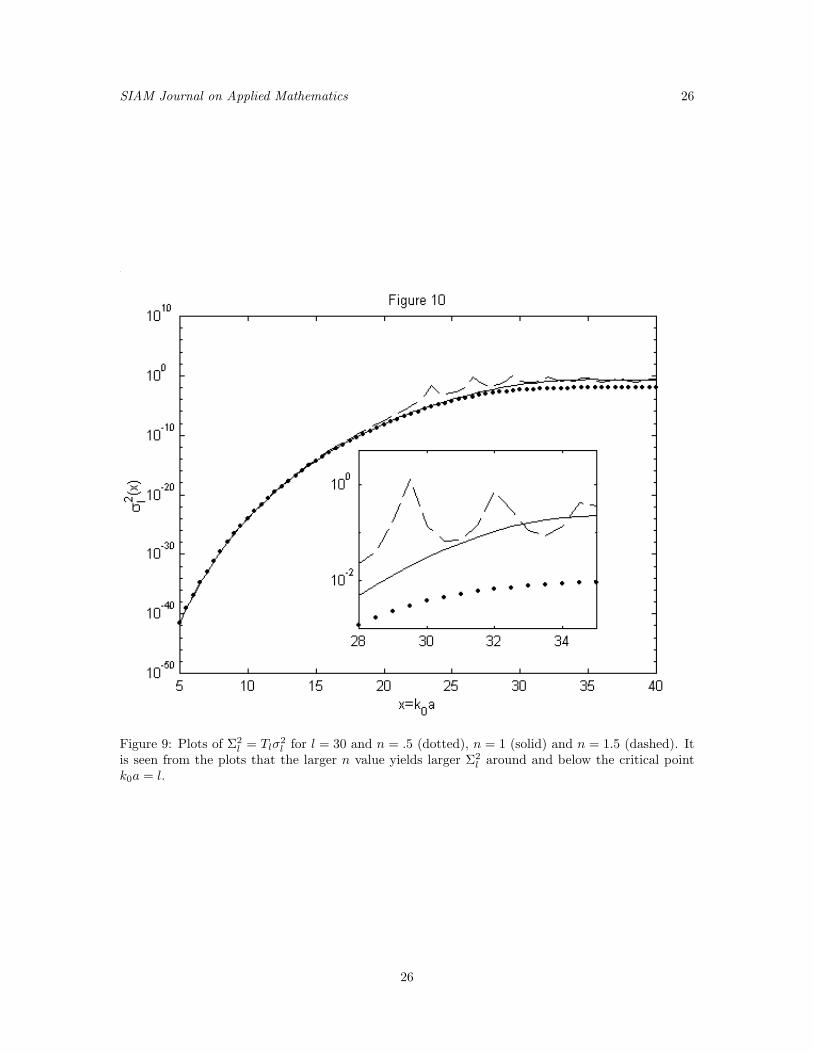
2l for l = 30 and n = .5 (dotted), n = 1 (solid) and n = 1.5 (dashed). It

is seen from the plots that the larger n value yields larger Σ2l around and below the critical point

k0a = l.

26

SIAM Journal on Applied Mathematics 27

Figure 10: Plots of source energy for a = 10, n = 1 (solid) and n = 1.5 (with asterisks) and forL = 10, 20, and L = 30. It is seen from the plots that the larger n value yields smaller energy and,hence, a more efficient source up to the critical point k0a = L.

We computed the source energy for the model radiation pattern employed in the free spaceexamples of section 3.2. Using the coefficients given in Eq.(22) we computed the source energy usingEq.(20) with the Σ2

l given by Eq.(52). We show in Fig. 10 plots of the source energies as a functionof x = k0a for three different values of the cut-off parameter L and for a source radius of a = 10and index value of n = 1.5. We also show for comparison the plots of the source energy for a sourceembedded in free space. It is seen that, as expected, the source energy becomes extremely large ifwe try to achieve an L value that exceeds the critical value L = k0a. This is, of course, due to thefact that the quantities Σ2

l become extremely small when l > k0a.

6 Summary and Conclusions

We have developed the basic theory of the inverse source problem for compactly supported sourcesembedded in an inhomogeneous index profile n(r). Most of our results pertain, in particular, tospherically symmetric index distributions n(r) = n(r) although the underlying formalism is applica-ble to general, non-symmetric distributions. For the class of spherically symmetric index profileswe showed how to construct the so-called minimum energy source that generates a given radiationpattern subject to the constraint that the sources L2 norm over the source region is minimum. It

27

SIAM Journal on Applied Mathematics 28

was found that the energy of the minimum energy source depended on the index profile n(r) andwe examined this dependence using computer simulations for the case of piece-wise constant val-ued profiles that are unity outside the (spherical) source volume and constant within the sourcevolume and for a “model” radiation pattern characterized by a “resolution parameter” L that wasinversely related to the effective angular width of the radiation pattern. The simulations showedthat, in general, the source energy increases exponentially when the wavenumber source radius prod-uct k0a >> L independent of whether or not the source is embedded in a background medium ornot. However, it was found that by embedding the source in a spherical region having constantindex n > 1 the source energy can be made smaller than that obtained for a source in vacuumover moderate ranges of the wavenumber source radius product k0a in the immediate vicinity of thecritical value k0a = L. We conclude that embedding sources in “designer” background distributionsmay lead to significant improvement in source efficiency, particularly for resonant antennas. Thisconclusion has been established here from a new source-inversion point of view which serves as atheoretical framework of reference for ongoing efforts in this direction within the antenna and op-tical communities, particularly in connection with novel magneto-dielectrics and metamaterials forenhanced radiation. Currently we are working on the generalization of the research reported in thiswork to the full vector electromagnetic case including the practical reactive power constraints. Weplan to report this ongoing research elsewhere.

Acknowledgments

This work was supported by the Air Force Office of Scientific Research under grant number FA9550-06-01-0013, and is affiliated with CenSSIS, the Center for Subsurface Sensing and Imaging Systems,under the Engineering Research Centers Program of the National Science Foundation (award numberEEC-9986821). The authors would like to thank Drs. Arje Nachman and Richard Albanese forhelpful comments on the material presented in the paper.

References

[1] N. Bleistein and J.K. Cohen, “Nonuniqueness in the inverse source problem in acoustics andelectromagnetics”, J. Math. Phys., Vol. 18, No. 2, p. 194-201, 1977.

[2] R.P. Porter and A.J. Devaney, “Generalized holography and computational solutions to inversesource problems”, J. Opt. Soc. Am., Vol. 72, p. 1707-1713, 1982.

[3] R.P. Porter and A.J. Devaney, “Holography and the inverse source problem”, J. Opt. Soc. Am.,Vol. 72, No. 3, p. 327-330, 1981.

[4] M. Bertero, C. De Mol and E.R. Pike, “Linear inverse problems with discrete data. I: Generalformulation and singular system analysis”, Inverse Problems, Vol. 1, p. 301-330, 1985.

[5] M. Bertero, “Linear inverse and ill-posed problems”, in Advances in Electronics and Electron

Physics, Academic Press, Vol. 75, p. 1-120, San Diego, 1989.

[6] E.A. Marengo and A.J. Devaney, “The inverse source problem of electromagnetics: Linearinversion formulation and minimum energy solution”, IEEE Trans. Antenn. Propagat., Vol. 47,p. 410-412, 1999.

[7] E.A. Marengo, A.J. Devaney and R.W. Ziolkowski, “Inverse source problem and minimumenergy sources”, J. Opt. Soc. Am. A, Vol. 17, p. 34-45, 2000.

28

SIAM Journal on Applied Mathematics 29

[8] E.A. Marengo and R.W. Ziolkowski, “Nonradiating and minimum energy sources, and theirfields: Generalized source inversion theory and applications”, IEEE Trans. Antennas Propagat.,Vol. 48, p. 1553-1562, 2000.

[9] J.C.-E. Sten, “Reconstruction of electromagnetic minimum energy sources in a prolate spher-oid”, Radio Sci., Vol. 39, RS2020, doi:10.1029/2003RS002973, 2004.

[10] J. C.-E. Sten and E.A. Marengo, “Inverse source problem in an oblate spheroidal geometry”,IEEE Trans. Antennas Propagat., Vol. 54, p. 3418-3428, 2006.

[11] C. Muller, Foundations of the Mathematical Theory of Electromagnetic Waves, Springer Verlag,New York, 1969.

[12] A.J. Devaney and E. Wolf, “Radiating and nonradiating classical current distributions and thefields they generate”, Phys. Rev. D, Vol. 8, No. 4, p. 1044-1047, 1973.

[13] K. Kim and E. Wolf, “Non-radiating monochromatic sources and their fields”, Opt. Comm.,Vol. 59, No. 1, p. 1-6, 1986.

[14] B.J. Hoenders and H.A. Ferwerda, “The non-radiating component of the field generated by afinite monochromatic scalar source distribution”, Pure Appl. Opt.: J. Opt. A, Vol. 7, p. 1201-1211, 1998.

[15] A.J. Devaney and G. Sherman, “Nonuniqueness in inverse source and scattering problems,”IEEE Trans. Ant.and Propag. Vol. 30, p. 1034, 1982.

[16] B.J. Hoenders, “The uniqueness of inverse problems”, in Inverse Source Problems in Optics,H.P. Baltes, ed., Springer, Berlin, 1978, pp. 41-82.

[17] K.J. Langenberg, “Applied inverse problems for acoustic, electromagnetic and elastic wavescattering”, in Basic Methods of Tomography and Inverse Problems, P.C. Sabatier, ed., Bristol,UK: Adam Hilger, 1987, pp. 128-467.

[18] L.J. Chu, “Physical limitations of omni-directional antennas,” J. Appl. Phys. Vol. 19, p. 1163-1175, 1948.

[19] R.F. Harrington, “On the gain and beamwidth of directional antennas”, IRE Trans. Ant. Prop-

agat., Vol. 6, p. 219-225, 1958.

[20] T.S. Angell, A. Kirsch and R.E. Kleinman, “Antenna control and optimization using generalizedcharacteristic modes”, Proc. IEEE, Vol. 79, p. 1559-1568, 1991.

[21] D. Liu, R.J. Garbacz and D.M. Pozar, “Antenna synthesis and solution of inverse problems byregularization methods”, IEEE Trans. Ant. Propagat., Vol. 38, p. 862-868, 1990.

[22] O.M. Bucci, G. D’Elia, G. Mazzarella and G. Panariello, “Antenna pattern synthesis: A newgeneral approach”, Proc. IEEE, Vol. 82, p. 358-371, 1994.

[23] G.A. Deschamps and H.S. Cabayan, “Antenna synthesis and solution of inverse problems byregularization methods”, IEEE Trans. Ant. Propagat., Vol. 20, p. 268-274, 1972.

[24] Y.T. Lo, S.W. Lee and Q.W. Lee, “Optimization of directivity and signal-to-noise ratio of anarbitrary antenna array”, Proc. IEEE, Vol. 54, p. 1033-1045, 1966.

[25] A.J. Devaney and R.P. Porter, “Holography and the inverse source problem. Part II: Inhomo-geneous media”, J. Opt. Soc. Am., Vol. 2, No. 11, p. 2006-2011, 1985.

29

SIAM Journal on Applied Mathematics 30

[26] L. Tsang, A. Ishimaru, R. P. Porter, and D. Rouseff, “Holography and the inverse sourceproblem. III. Inhomogeneous attenuative media”, J. Opt. Soc. Am. A, Vol. 4, 1783-1787, 1987.

[27] R.G. Newton, Scattering Theory of Waves and Particles, Dover Publications, Mineola, NewYork, 2002.

[28] M. Born and E. Wolf, Principles of Optics, 6’th ed., Pergamon Press, New York, 1983.

[29] J.D. Jackson, Classical Electrodynamics, Wiley, New York, 1975.

[30] H.R. Raemer, “Radiation from linear electric or magnetic antennas surrounded by a sphericalplasma shell”, IRE Trans. Ant. Propagat., Vol. 10, p. 69-78, 1962.

[31] D. Lamensdorf, “An experimental investigation of dielectric-coated antennas”, IEEE Trans.

Ant. Propagat., Vol. 15, p. 767-771, 1967.

[32] D. Lamensdorf and C.-Y. Ting, “An experimental and theoretical study of the monopole em-bedded in a cylinder of anisotropic dielectric”, IEEE Trans. Ant. Propagat., Vol. 16, p. 342-349,1968.

[33] S.A. Long, M.W. McAllister, and L.C. Shen, “The resonant cylindrical dielectric cavity an-tenna,” IEEE Trans. Antenn. Propagat., Vol. 31, p. 406-412, May 1983.

[34] K.W. Leung, “Complex resonance and radiation of hemispherical dielectric-resonator antennawith a concentric conductor,” IEEE Trans. Microwave Theory Tech., Vol. 49, p. 524-531, Mar.2001.

[35] J.R. James and J.C. Vardaxoglou, “Investigation of properties of electrically-small sphericalceramic antennas”, Electron. Lett., Vol. 38, p. 1160-1162, 2002.

[36] E.E. Altshuler, “Electrically small genetic antennas immersed in a dielectric”, Proc. IEEE Ant.

Propagat. Soc. Symp., Vol. 3, p. 2317-2320, 2004.

[37] R.C. Hansen and M. Burke, “Antennas with magneto-dielectrics”, Microwave Opt. Tech. Lett.,Vol. 26, p. 75-78, 2000.

[38] K. Buell, H. Mosallaei and K. Sarabandi, “A substrate for small patch antennas providingtunable miniaturization factors”, IEEE Trans. Microwave Theor. Tech., Vol. 54, p. 135-146,2006.

[39] H. Mosallaei and K. Sarabandi, “Magneto-dielectrics in electromagnetics: Concept and appli-cations”, IEEE Trans. Anten. Propagat., Vol. 52, p. 1558-1567, 2004.

[40] Y. Mano and S. Bae, “A small meander antenna by magneto-dielectric material”, Proc. IEEE

Intl. Symp. Micro. Anten. Propagat. and EMC Technol. for Wireless Comm., Vol. 1, p. 63-66,2005.

[41] M. Thevenot, C. Cheype, A. Reineix, and B. Jecko, “Directive photonic-bandgap antennas,”IEEE Trans. Microwave Theory Tech., Vol. 47, p. 2115-2122, Nov. 1999.

[42] B. Temelkuran, M. Bayindir, E. Ozbay, R. Biswas, M.M. Sigalas, G. Tuttle, and K.M. Ho,“Photonic crystal-based resonant antenna with a very high directivity,” J. Appl. Phys., Vol. 87,p. 603-605, 2000.

[43] S. Enoch, G. Tayeb, P. Sabouroux, N. Guerin, and P. Vincent, “A metamaterial for directiveemission,” Phys. Rev. Lett., Vol. 89, p. 213902-1(4), 2002.

30

SIAM Journal on Applied Mathematics 31

[44] A. Alu and N. Engheta, “Radiation from a traveling-wave current sheet at the interface be-tween a conventional material and a metamaterial with negative permittivity and permeability,”Microwave Opt. Technol. Lett., Vol. 35, p. 460-463, 2002.

[45] R.W. Ziolkowski and A. Kipple, “Application of double negative metamaterials to increase thepower radiated by electrically small antennas”, IEEE Trans. Ant. Propagat., Vol. 51, p. 2626-2640, 2003.

[46] D. Tonn and R. Bansal, “Practical considerations for increasing radiated power from an elec-trically small antenna by application of a double negative metamaterial”, IEEE Intl. Anten.

Propagat. Symp., Vol. 2A, p. 602-605, 2005.

[47] A. Erentok, P.L. Luljak and R.W. Ziolkowski, “Characterization of a volumetric metamaterialrealization of an artificial magnetic conductor for antenna applications”, IEEE Trans. Ant.

Propagat., Vol. 53, p. 160-172, 2005.

[48] G. Lovat, P. Burghignoli, F. Capolino, D.R. Jackson and D.R. Wilton, “Analysis of directiveradiation from a line source in a metamaterial slab with low permittivity”, IEEE Trans. Ant.

Propagat., Vol. 54, p. 1017-1030, 2006.

[49] B.-I. Wu, W. Wang, J. Pacheco, X. Chen, T. Grzegorczyk and J.A. Kong, “A study of usingmetamaterials as antenna substrate to enhance gain”, Prog. Electromag. Research, Vol. 51,p. 295-328, 2005.

[50] J.A. Kong, Electromagnetic Wave Theory, EMW Publishing, Cambridge, MA, 2005.

[51] X. Chen, T.M. Grzegorczyk and J.A. Kong, “Optimization approach to the retrieval of theconstitutive parameters of a slab of general bianisotropic medium”, Prog. Electromag. Research,Vol. 60, p. 1-18, 2006.

[52] E.A. Marengo, A.J. Devaney and F.K. Gruber, “Inverse source problem with reactive powerconstraints”, IEEE Trans. Ant. Propagat., Vol. 52, p. 1586-1595, 2004.

[53] D. Colton and R. Kress, Inverse Acoustic and Electromagnetic Scattering Theory, second ed.,Springer, Berlin, 1998.

[54] D. Colton and R. Kress, Integral Equation Methods in Scattering Theory, Wiley, New York,1983.

[55] G. Arfken, Mathematical Methods for Physicists, Academic Press, San Diego, 1985.

[56] J.R. Taylor, Scattering Theory, Wiley, New York, 1972.

[57] R. Potthast, Point Sources and Multipoles in Inverse Scattering Theory, Chapman&Hall, BocaRaton, Florida, 2001.

[58] A.J. Devaney and M.L. Oristaglio, “Inversion procedure for inverse scattering within thedistorted-wave Born approximation”, Phys. Rev. Lett., Vol. 51, p. 237-240, 1983.

[59] R.W. Ziolkowski and A.D. Kipple, “Reciprocity between the effects of resonant scattering andenhanced radiated power by electrically small antennas in the presence of nested metamaterialshells”, Phys. Rev. E, Vol. 72, 036602 (5 pages), 2005.

[60] P.M. Morse and H. Feshbach, Methods of Theoretical Physics, McGraw-Hill, New York, 1953.

31