It

IU

a

ARRAA

JI

KIPPS

1

bastcd21hpdsdav

dl

Ef

0d

Journal of Health Economics 30 (2011) 1280– 1292

Contents lists available at ScienceDirect

Journal of Health Economics

jo u rn al hom epage : www.elsev ier .com/ locate /econbase

nverse probability weighted estimation of social tariffs: An illustration usinghe SF-6D value sets�

ldefonso Méndez ∗, Jose M. Abellán Perpinán, Fernando I. Sánchez Martínez, Jorge E. Martínez Pérezniversity of Murcia, Spain

r t i c l e i n f o

rticle history:eceived 2 April 2010eceived in revised form 18 July 2011ccepted 26 July 2011vailable online 26 August 2011

EL classification:

a b s t r a c t

This paper presents a novel approach to model health state valuations using inverse probability weightingtechniques. Our approach makes no assumption on the distribution of health state values, accommodatescovariates in a flexible way, eschews parametric assumptions on the relationship between the outcomeand the covariates, allows for an undetermined amount of heterogeneity in the estimates and it formallytests and corrects for sample selection biases. The proposed model is semi-parametrically estimated andit is illustrated with health state valuation data collected for Spain using the SF-6D descriptive system.

10

eywords:nverse probability weightingropensity scorereference-based health measureF-6D

Estimation results indicate that the standard regression model underestimates the utility loss that theSpanish general population assigns to departures from full health, particularly so for severe departures.

© 2011 Elsevier B.V. All rights reserved.

idofa

iiiaaasbtfii

. Introduction

Preference-based measures of health status are increasinglyeing used to evaluate the outcomes of health care interventionsnd to inform resource allocation decisions. A number of healthtate descriptive systems have been designed for the characteriza-ion of health states and estimation methods have been applied foralculating a preference-based single index value for every stateefined within some of these systems. The HUI3 (Feeny et al.,002), the EQ-5D (EuroQol Group, 1990) or the SF-6D (Brazier et al.,998) are examples of these systems, and all of them describeealth states by defining a number of dimensions or attributes (e.g.ain, physical functioning, ability for self-care, etc.) each admittingifferent levels of severity or impairment. Since most descriptiveystems define many more health states than it is feasible to elicitirect valuations for in an empirical study, choices have to be madebout how best to estimate values for all states from direct obser-ations on a subset of those states.

The standard approach to model health state values uses a set ofummy indicator variables describing health states in terms of their

evel of severity in different dimensions of health to explain the

∗ Corresponding author at: Departamento de Economía Aplicada, Facultad deconomía y Empresa, 30100, Espinardo, Murcia, Spain. Tel.: +34 868883732;ax: +34 868883745.

oacfm2

c

167-6296/$ – see front matter © 2011 Elsevier B.V. All rights reserved.oi:10.1016/j.jhealeco.2011.07.013

ndividual valuations obtained. Under the assumption of normallyistributed errors, a regression of health state values on the setf dummy variables identifies the valuation effect of departuresrom full health. The estimates are then used to predict the valuessociated to the health states not directly valued.

The main advantadge of the standard approach is its simplic-ty. However, it has some limitations that are likely to underminets benefits. First, the normality assumption is not likely to holdn practice given the skewed, truncated, non-continuous and hier-rchical nature of health state valuation data (Brazier et al., 2002)nd, thus, the estimates are likely to be biased. Second, the standardpproach does not provide any guidance on how to improve thepecification of the regression model by accounting for interactionsetween the severity indicators or for personal characteristics. Onhe one hand, the linear regression model is not the appropriateramework for meaningfully incorporating the large number ofnteractions between the severity indicators that can be definedn any health state descriptive system (Brazier et al., 2002). On thether hand, the traditional way of accommodating personal char-cteristics to the standard model by introducing them additivelyontravenes both the goal of estimating one preference-based tariffor the whole community (Dolan, 1997) and the theoretical require-

ent of the intercept being equal to unity (Brazier et al., 2002,004).

As a result, most articles that use the standard approach do notontrol for personal characteristics nor for severity interactions,

lth Eco

miiiasreatt

iiapctaaseooadd

abibsasd(ws(le

cimtofopimtii

tdboittc

de

bwtumfcratBvdetctd

pstSS

2

Y

wZhoamet(εsse

esFsestimates are likely to be biased.2 Second, the linear regressionmodel is severely limited in the way it controls for interactioneffects and personal characteristics. This model does not provide

1 For the SF-6D descriptive system K = 6 and Wk ranges from 4 to 6. Equivalently,K = 5 and Wk = W = 3 for the EQ-5D.

2 Dolan et al. (1996) find evidence that the distribution of health state valuesobtained using the time trade-off method was non-normal for each health state.Johnson et al. (1998) find departures from normality when estimating US-based

I. Méndez et al. / Journal of Hea

aking misspecification of the regression model more likely. This,n turn, leads to biased estimates. Moreover, these articles implic-tly assume that the valuation impact of a departure from full healths the same for respondents with different personal characteristicsnd is independent of the severity of departures in other dimen-ions of health. This restrictive homogeneity assumption has beenejected by the evidence in Dolan and Roberts (2002) and Kharroubit al. (2007a), among others. They find that some respondents’ char-cteristics impact on the value they give to health states and thathis effect varies with the severity of the health state at examina-ion.

The debate on the valuation effect of personal characteristicss related to that on whose values should count when evaluat-ng health state intervention outcomes and informing resourcellocation decisions. The common recommendation of using thereferences of the whole population (Gold et al., 1996; NICE, 2004)alls for obtaining population valid estimates, that is, to adjust forhe distribution of the covariates in the population. The standardpproach tries to fulfil this requirement by defining samples thatre representative for the population of interest with regard to theex and age interval distributions. The representativeness of thestimates is then analyzed by comparing the descriptive statisticsf a large set of covariates in the sample to those in the populationf interest. Lastly, corrective weights intended to adjust for the agend sex interval population distributions are introduced if relevantiscrepancies are observed between the sample and populationescriptive statistics.

This way of proceeding does not provide the user with theppropriate tools for testing and correcting for sample selectioniases. Non-response issues and the drop of respondents providing

nconsistent responses results in sometimes relevant discrepanciesetween the “representative” sample design and the estimationample. Moreover, there are many personal characteristics thatffect health state values whose sample distribution is not neces-arily that in the population even if age intervals and sex are equallyistributed in both instances. For example, Dolan and Roberts2002) find that marital status and the respondents’ ability to copeith usual activities (i.e. one of the dimensions of their own health

tate) affect health state valuations. Additionally, Kharroubi et al.2007a) find that the individual’s employment status, educationalevel and own physical and social functioning have a significantffect on health state values.

The comparison of the univariate descriptive statistics of theovariates in the estimation sample to those in the population ofnterest is not a formal test of sample selection biases and, thus, it

ight lead to wrong conclusions. In particular, it raises doubts aso in how many covariates we have to find a significant differencef a given magnitude between the sample and population meansor the estimates not to be valid at the population level. More-ver, finding no significant difference between the sample and theopulation means of a continuous variable is not necessarily very

nformative about the presence of relevant discrepancies in otheroments of the distributions. Furthermore, multivariate distribu-

ions can differ significantly even if univariate descriptive statisticsn the estimation sample are close to those in the population ofnterest.

Finally, the corrective weights used to ensure representa-iveness of the regression estimates suffer from the curse ofimensionality problem, that is, its feasibility lowers as the num-er of personal characteristics where relevant discrepancies arebserved between the sample and population descriptive statistics

ncreases. This problem is circumvented in practice by restrictinghe set of personal characteristics used to construct the weightso the respondent’s sex and age group. However, this way of pro-eeding does not remove sample selection biases in other personal

p(oTu

nomics 30 (2011) 1280– 1292 1281

imensions and, thus, it is not likely to produce representativestimates.

This paper presents a new approach to estimating preference-ased measures of health status based on inverse probabilityeighting (IPW) techniques. The IPW approach makes no assump-

ion on the distribution of health state valuations, allows for anndetermined amount of heterogeneity in the estimates, accom-odates covariates in a flexible way, formally tests and corrects

or sample selection biases and uses the distribution of personalharacteristics in the population of interest to guarantee the rep-esentativeness of the estimates. The estimators that we proposere semi-parametrically estimated and their large sample proper-ies are derived. Additionally, and as opposed to the nonparametricayesian approach in Kharroubi et al. (2007a,b), our approach pro-ides the user with a simple table of estimated coefficients thatefines the estimated preference function, which results in relevantfficiency and transparency gains. We illustrate our approach withhe SF-6D descriptive system. Notwithstanding, the IPW approachould be equally applied to other systems (e.g. the EQ-5D) providedhat some requirements regarding the selection of states which areirectly valued in the sample are met, as it will be further discussed.

The paper has four more sections. Section 2 presents theroposed approach and compares its properties to those of thetandard parametric one. Section 3 describes the SF-6D descrip-ive system and the data used to illustrate the proposed estimators.ection 4 presents and discusses the estimation results and, finally,ection 5 concludes.

. Modelling

The standard model of health state valuations can be written as

ij = + ˇ′Zj + εij (1)

here Yij is the utility that individual i assigns to health state j,j is a vector of dummy indicator variables Zkw that equal one ifealth state j reaches level of severity w in dimension k and zerotherwise, for w = 2, 3, . . . , Wk and k = 1, 2, . . ., K, is the interceptnd εij is a zero mean error term.1 Model (1) is the “main effects”odel, as opposed to other specifications that also control for level

ffects, interactions between the elements of Zj or personal charac-eristics. The model is estimated using the Ordinary Least SquaresOLS) or the Random Effects (RE) estimators, that is, assuming that

is normally distributed. Most researchers use the RE estimatorince it takes account that the same individual values several healthtates, increasing the efficiency of the estimates relative to the OLSstimator.

The main advantage of the standard approach is that it can beasily implemented in any statistical package. However, it also hasome relevant limitations that are likely to undermine its benefits.irst, the normality assumption is not likely to hold with healthtate valuation data (Brazier et al., 2002) and, thus, the regression

opulation weights using the EQ-5D questionnaire. Diagnostic tests in Brazier et al.2002) reveal non-normal residuals in the estimation of a preference-based measuref health for the UK general population using the SF-36. Many other studies, likesuchiya et al. (2002) and Lamers et al. (2006), simply provide no formal test of thenderlying distributional assumption.

1 lth Eco

tldto(u

untnscb(teMlmri

atiirttwo

ˇ

wv

ˇ

watmiasi

iplvs1

cf

tv

wtpmcfacmuomn

ptmriow(oip

ttcitedtsuuiti

eudtfistobi

282 I. Méndez et al. / Journal of Hea

he appropriate framework for meaningfully incorporating thearge number of interactions that can be defined in any health stateescriptive system (Brazier et al., 2002). Additionally, the introduc-ion of personal characteristics additively contravenes both the goalf estimating one preference-based tariff for the whole communityDolan, 1997) and the requirement of the intercept being equal tonity (Brazier et al., 2002).3

As a result of the second limitation, the great majority of articlessing the standard approach do not control for interaction termsor for personal characteristics. These articles implicitly assumehat the valuation impact of a departure from full health is the sameo matter the severity of the deviation in the remaining dimen-ions of the health state under evaluation nor the respondents’haracteristics. Such an homogeneity assumption has been rejectedy the evidence in Dolan and Roberts (2002) and Kharroubi et al.2007a), among others, who find that some respondents’ charac-eristics impact on the value they give to health states and that thisffect varies with the severity of the health state at examination.oreover, by reducing the set of feasible specifications the second

imitation increases the risk of misspecification of the regressionodel and, thus, the probability of obtaining biased estimates since

egression models rely heavily on extrapolation when differencesn the covariate distributions for compared respondents are large.

The identification strategy is presented for ˇkw, the coefficientssociated with Zkw that measures the average health state valua-ion impact of moving from level of severity 1 to level of severity wn dimension k. Let Xi be the vector of characteristics of individual

that potentially affect his valuations. The sample is restricted toespondents valuing levels of severity 1 and w in dimension k andhe individual and health state subscripts i and j are dropped outo simplify the notation. The coefficient of interest for the sampleith personal characteristics x that value health states with level

f severity w′ in dimension k′ for k′ /= k and w′ = 2, 3, . . . , Wk′ is4

kw(x, zk′w′ ) = E[Y |Zkw = 1, X = x, Zk′w′ = zk′w′ ]

− E[Y |Zkw = 0, X = x, Zk′w′ = zk′w′ ]

here zk′w′ = {0, 1}. Equivalently, the valuation effect for an indi-idual randomly drawn from the estimation sample is

kw = E[ˇkw(h)] = E[Y |Zkw = 1] − E[Y |Zkw = 0] (2)

here H comprises X and the set of dummy variables Zk′w′ for k′ /= knd w′ = 2, 3, . . . , Wk′ and expectations are defined over the dis-ribution of H in the estimation sample. This way of writing ˇkw

akes it clear that we are not imposing the homogeneous valuationmpact assumption inherent to most applications of the standardpproach. In fact, we allow for the utility loss of moving from level ofeverity 1 to level w in dimension k to vary with any of the elementsn H.

The estimator that we develop for ˇkw can be better interpretedn the context of the treatment effects literature. This literature

rovides answers to questions concerning the efficacy of a particu-

ar programme or policy initiative. In this setting ˇkw is the averagealuation effect of a binary treatment that consists in valuing healthtates where dimension k reaches level of severity w instead of level. The causal interpretation of ˇkw follows from the assumption

3 There are strong theoretical reasons for restricting the intercept to unity since itaptures the utility associated with full health, which equals one on the conventionalull health-death scale used to estimate QALYs.

4 Existence of expectations is assumed throughout.

oeuA

si

e

nomics 30 (2011) 1280– 1292

hat unobserved individual characteristics do not affect health statealuations or their overall average impact is zero.5

Among the broad list of available treatment effect estimators,e opt for the so-called Inverse Probability Weighting estima-

ors for three reasons.6 First, they are easy to implement androvide consistent and in some cases asymptotically efficient esti-ates of the parameter of interest under fairly standard regularity

onditions. Second, they exhibit the best overall finite sample per-ormance among the broad class of treatment effect estimatorsnalyzed in Busso et al. (2009). This is particularly relevant in theurrent context since estimation samples are of modest size inost empirical applications. Finally, weighting estimators can be

sed to assess the effect of changes in the distribution of X on theutcome of interest (DiNardo et al., 1996) and, thus, they allow esti-ation of preference functions for the population of interest from

on-representative samples.Some additional notation is needed at this point. Let

kw(h) = P(Zkw = 1|H = h) be the conditional probability of receivingreatment given H. This variable is the propensity score in the treat-

ent effects literature. The research value of the propensity scoreests on its power to solve the dimensionality problem. Adjust-ng for between-groups differences on a high dimensional vectorf covariates can be either difficult or impossible, as is the casehen using the standard corrective weights. Rosenbaum and Rubin

1983) show that the propensity score captures all of the variancen the covariates relevant for adjusting between-group compar-sons, that is, treated and control units with the same value of theropensity score have the same distribution of the elements in H.

Additionally, the following overlap assumption on the joint dis-ribution of treatments and explanatory variables is necessary forhe estimation problem to be well defined: 0 < P(Zkw = 1|H) < 1. Thisommon support condition requires that for a given value of H theres some fraction of the estimation sample in the treatment and con-rol groups to be compared. That is, a necessary condition for theffect of Zkw to be identified is that no other element of H pre-icts treatment status perfectly. An implication of this condition ishat some respondents valuing levels of severity 1 and w in dimen-ion k will not contribute to the estimation of ˇkw. In particular,nits with propensity scores close to zero or one will be partic-larly influential in the estimation of ˇkw, making the estimation

mprecise. That is the case for respondents whose distributions ofhe elements of H substantially differ from those for respondentsn the other treatment group.

The common support condition is not commonly invoked whenstimating a linear regression model because the regression modelses its functional form to work off the common support in theistribution of the elements of H when estimating ˇkw. However,hat can be highly misleading given the previously discussed speci-cation problems inherent to the standard approach. The commonupport condition ensures that identification does not rest on func-ional form assumptions. This condition has relevant implicationsn the selection of health states valued in the sample for ˇkw toe identified. In particular, it states that there is no level of sever-

ty w′ in dimension k′, for w′ = 1, 2, 3, . . . , Wk′ and k′ /= k, valuednly by respondents of a given treatment status. Otherwise, the

ffect of interest cannot be separately identified from that for Zk′w′nless we rely on extrapolation, like the regression model does.s previously discussed, extrapolation results in biased estimates

5 The assumption is known as selection on observables (Barnow et al., 1981) ortrong ignorable treatment assignment (Rosenbaum and Rubin, 1983) and is alsomplicit in the standard regression model.

6 Imbens (2004) provides an overview of the estimators used in the treatmentffects literature under the selection on observables assumption.

lth Eco

iots

E

cmddscow

g

ttf

E

ˇ

t

ˇcvttbpite(t

cJnoo

prfiic2

tsai

ˇ

weiedsirs

wtssaStrbsHtvui

oRYrYtopoaLoh

I. Méndez et al. / Journal of Hea

f differences between the covariate distributions of respondentsf different treatment status are relevant and the parametric rela-ionship between the outcome and the regressors is not properlypecified.7

The expectations in (2) can be written as

[Y |Zkw = t] = Yf (Y |H)g(H|Zkw = t)dh, for t = {0, 1} (3)

According to the latter expression, each expectation in (2) isalculated using the distribution of H in the corresponding treat-ent group. However, for ˇkw to be identified we need the same

istribution of H in the two expectations. In particular, we use theistribution of H in the sample of respondents valuing levels ofeverity 1 or w in dimension k that satisfy the common supportondition. Formally, let g(H) and g(H|Zkw = t) be the joint densityf H in the estimation sample and in the collective of respondentsith treatment status t, respectively, and observe that by definition

(H) = g(H|Zkw = t)P(Zkw = t)P(Zkw = t|H)

, for t = {0, 1}

That is, the distribution of H in the collective of respondents withreatment status t can be changed for the distribution in the estima-ion sample g (H) by simply introducing the appropriate weightingunction �t in (3)

[Y |Zkw = t] = �tP(Zkw = t)P(Zkw = t|H)︸ ︷︷ ︸Yf (Y |H)g(H|Zkw = t)dh

= Yf (Y |H)g(H)dh, for t = {0, 1}

The effect of interest can now be written as

kw = E[ZkwY

pkw

]− E

[(1 − Zkw)Y

1 − pkw

](4)

This suggests the following estimator of ˇkw which we name ashe IPW1 estimator

kw, IPW1 = n−1∑n

i=1

ZkwiYij

pkwi− n−1

∑n

i=1

(1 − Zkwi)Yij1 − pkwi

(5)

This equation suggests a simple two-step method to estimatekw. First, estimate the propensity score using a binary discretehoice model like the logit or probit models. Second, plug the fittedalues into the sample analog of (5). The IPW1 estimator identifieshe effect of interest if the estimation sample is representative forhe population of interest, that is, if there are no sample selectioniases. However, since we cannot be sure a priori that the sam-le distribution of the elements of X is that in the population, we

mprove on the latter estimator by accounting for the probabilityhat an individual randomly drawn from the population of inter-

st is in the estimation sample.8 We do so by rewriting expression3) so that the two expectations are averaged over the distribu-ion of X in the population of interest. Obviously, the feasibility of

7 Some studies that use the standard approach report evidence of misspecifi-ation of the regression model. A non-exhaustive list includes Dolan (1997) andohnson et al. (1998). Brazier et al. (2002) express their surprise with the result ofo specification problems according to the Ramsey RESET test given the skewnessf their RE estimation residuals. Many other studies simply provide no formal testf misspecification of the regression model.8 On the one hand, deviations from the original sample design due to, for exam-

le, nonresponse issues or to the exclusion of respondents providing inconsistentesponses might result in non-representative samples. On the other hand, it is dif-cult or even impossible to define representative samples for the population of

nterest with regard to the whole set of covariates that have been found to beorrelated with health state valuations (Dolan and Roberts, 2002; Kharroubi et al.,007a).

h

ptc

Fwiw

uHep

nomics 30 (2011) 1280– 1292 1283

his approach rests on whether we have an external representativeample that contains information on X. Conditioned on the avail-bility of the external representative sample, the effect of interests now written as9

kw = E[DsZkwY

pkwps

]− E

[Ds(1 − Zkw)Y(1 − pkw)ps

]here the estimation sample comprises that used for the IPW1

stimate of ˇkw, Ds is a binary indicator variable that equals onef the individual is in the estimation sample and zero if he is in thexternal representative sample and ps(x) = P(Ds = 1|X = x) is the con-itional (on X) probability of being in the estimation sample. Theet of indicator variables Zk′w′ for k′ /= k and w′ = 1, 2, 3, . . . , Wk′s not included in ps(x) since representativeness is analyzed withegard to the distribution of personal characteristics. The internalample analog of expression (6) is the IPW2 estimator of ˇkw

kw, IPW2 = Psn−1

∑n

i=1

ZkwiYij

pkwipsi− Psn

−1∑n

i=1

(1 − Zkwi)Yij(1 − pkwi )psi

(6)

here Ps = P(Ds = 1) is the proportion of individuals in the estima-ion sample. As before, the IPW2 estimate of ˇkw is obtained in twoteps. First, estimate discrete choice models for the two propen-ity scores, compute the fitted values for the estimation samplend ensure the common support condition in the two propensities.econd, plug the fitted values into the sample analog of (7). Underhis scheme, a two-step weighted average of the outcome variableecovers ˇkw in the population of interest. In a first step, the distri-ution of health state values for respondents of a given treatmenttatus is weighted-down (up) for those values of the elements of

that are (under) over-represented among respondents with thatreatment status. In a second step, the distribution of health statealues for sample respondents is weighted-down (up) for those val-es of the elements of X that are (over) under-represented among

ndividuals in the external representative sample.This estimator can also be interpreted in the related framework

f imputation for missing data.10 To appreciate this, we followubin (1974) and define ˇkw in terms of potential outcomes. Lett be the valuation that individual i would have given had heeceived treatment status t. We only observe the realized outcome

= DsZkwY1 + Ds(1 − Zkw)Y0 but want to know about the effect of thereatment for an individual randomly drawn from the populationf interest (ˇkw). In this setting, ˇkw is the difference between theopulation averages of Y1 and Y0, which we label �1 and �0. Wenly observe Y1 for treated individuals in the estimation samplend the probability of a “complete case” i is p = ps(x) × pkw(h). Asunceford and Davidian (2004) point out, weighting by the inversef the product of propensity scores allows observation i to count forimself and (p−1 − 1) other “missing” subjects with like covariates

in estimating �1.

The propensity score ps(x) adjusts for the distribution of

ersonal characteristics in the population of interest. Noticehat this propensity score is a generalization of the traditionalorrective sample weights used to ensure the representativeness

9 The availability of such a sample is not likely to be a problem for most countries.or example, the Census and the European Community Household Panel provide usith the distribution of many sociodemographic, employment and health related

ndividual and household characteristics of the Spanish population. In particular,e use data from the European Community Household Panel for Spain.

10 Each one of the two terms in (7) approximates the average outcome fornits of a given treatment status using a weighted sample mean estimator oforvitz–Thompson type. Horvitz and Thompson (1952) introduced this type ofstimator to analyze samples drawn without replacement with unequal selectionrobabilities from finite universes.

1 lth Eco

oppwscsp

noIttTe

Ieepepremtatosm

cmmcstieeemtwlt

tt

t

ht

wwvmwu(awb

ii

3

MwSdtb1lh

3

uosos(ed

mfasuBnwt

rs

284 I. Méndez et al. / Journal of Hea

f the regression model estimates in the standard approach.11 Inarticular, the corrective weights used in the standard frameworkrovide a nonparametric estimate of the propensity score ps (x)hen X only includes dummy indicator variables. The propensity

core allows us to overcome the dimensionality problem in theonstruction of sample weights and, thus, to account for sampleelection biases in as many discrete and continuously measuredersonal characteristics as necessary.

As discussed in Imbens (2004), the estimator in (7) is notecessarily an attractive estimator for ˇkw since the weights forbservations of a given treatment status t do not add up to unity.ndeed, these weights add up to 1 conditioned on treatment status

in expectation terms, but because the variance of the sum is posi-ive the corresponding sample analog is likely to deviate from one.hus, we normalize the weights to unity and obtain the followingstimator:

kw,IPW2 =(∑n

i=1

Zkwipkwipsi

)−1∑n

i=1

ZkwiYij

pkwipsi

−(∑n

i=1

(1 − Zkwi)(1 − pkwi )psi

)−1∑n

i=1

(1 − Zkwi)Yij(1 − pkwi )psi

(7)

The consistency and large sample properties of the IPW1 andPW2 estimators are derived in Appendix A using the theory of M-stimation.12 The IPW2 estimator can also be non-parametricallystimated by simply producing non-parametric estimates of theropensity scores and plugging the fitted values into (8).13 How-ver, the number of observations required to attain an acceptablerecision for this type of non-parametric estimator increasesapidly with the dimension of X. Moreover, a non-parametricstimate conditioned on particular values of X version of these esti-ators may be difficult to interpret if the dimension of X is larger

han two. Furthermore, the net gains of moving from the standardpproach to an alternative one decrease as the implementation ofhe proposed estimator becomes more challenging. Thus, we focusn semi-parametric approximations to IPW2 where the propensitycores are parametrically estimated using standard discrete choiceodels like the logit or probit models.The IPW2 estimator is member of a class of semi-parametric

onsistent estimators developed in Robins et al. (1994) for generalissing data problems. Robins et al. (1994) show that the esti-ator within the class having the smallest large-sample variance

ombines regression on the explanatory variables and propen-ity score weighting. Contrary to the parametric standard model,he regression model in the semi-parametric efficient estimators incorporated only as a way of gaining efficiency over the IPW2stimator, that will still be consistent. The asymptotically efficientstimator is doubly robust in the sense that it provides consistentstimates of ˇkw if either the propensity score or the regressionodel are correctly specified. Anyway, the double robust estima-

or cannot be implemented in our context because respondents

ith treatment status t do not value any possible combination of

evel of severity w or 1 in dimension k with the levels of severityhat can be defined in the remaining dimensions of health. That is,

11 Tsuchiya et al. (2002) and Kharroubi et al. (2007a) introduce corrective weightso reflect the non-representative age and sex distribution of their respondents inhe standard and the nonparametric Bayesian approaches, respectively.12 A STATA code that implements the IPW1 and IPW2 estimators is available fromhe authors upon request.13 Craig and Busschbach (2009, 2011) develop non-parametric approaches toealth valuation. However, these estimators do not control for personal charac-eristics.

(pc

d(PApwis

nomics 30 (2011) 1280– 1292

e cannot regress health state values on H within each subsampleith treatment status t. Indeed, we can just regress health state

alues on X and some elements of Z for respondents with treat-ent status t, where that subset of elements of Z is likely to varyith treatment status t and also with the estimation subsamplessed to identify each element of ˇ. Anyway, as shown in Busso et al.2009), the small sample properties of the double robust estimatorre close to those for weighting estimator like the IPW2 estimator,ith the former estimator being slightly more variable and more

iased than the one developed in this paper.Finally, the requirement of the intercept being equal to unity

s satisfied by using the transformed outcome variable Y∗ = Y − 1nstead of the original one.

. Data and measurement issues

The data comes from a survey performed in the Spanish region ofurcia over a period of two months in 2007. The sample (n = 1020)as designed using the age interval and sex distributions of the

panish general population. The goal of the survey was to obtainirect valuations for a selection of health states described accordingo the SF-6D classification system. Later on such valuations woulde modeled using our approach in order to predict values for the8,000 health states that the SF-6D system can define. In what fol-

ows we briefly describe the SF-6D instrument, the selection ofealth states valued, and the valuation survey.

.1. The SF-6D

The SF-6D is a preference-based measure of health that attachestility scores to a set of health states by using an algorithm basedn preferences of the general population. A total of 18,000 healthtates are defined by means of a classification system composedf six dimensions: physical functioning (PF), role limitations (RL),ocial functioning (SF), pain (PAIN), mental health (MH), and vitalityVIT). Each dimension has between four to six levels of severity andvery SF-6D health state is defined by selecting one level from eachimension.

Brazier et al. (2002) using a variant of the standard gamble (SG)ethod, elicited preferences for a selection of 249 health states

rom a sample (n = 611) of the UK general population. Next, OLSnd RE models were estimated to predict all 18,000 SF-6D healthtates. The model recommended by the authors for use in cost-tility analysis was an OLS model using mean health state values.razier et al. (2004) improved the previous model by removingon-significant estimates and aggregating those coefficients whichere inconsistent between them. They referred to such a model as

he “parsimonious consistent model”.In contrast to previous algorithms, which relied on paramet-

ic models, Kharroubi et al. (2007b) – using the same UK dataet as Brazier and colleagues – estimated a set of non-parametricBayesian) utility scores for the SF-6D. A drawback of this non-arametric model is that it cannot be defined by a simple table ofoefficients as in parametric models.

New SF-6D algorithms have been estimated by using the stan-ard regression approach for other countries apart from the UKLam et al., 2008; Brazier et al., 2009; Ferrerira et al., 2010; Abellán-erpinán et al., 2011). The Spanish SF-6D value set derived inbellán-Perpinán et al. (2011) uses the same database as in this

aper. The novelty of that value set is that has a minimum (a floor)hich is significantly lower than those estimated in previous stud-

es, making the range of SF-6D values more similar to the EQ-5Dcores range.

lth Economics 30 (2011) 1280– 1292 1285

3

iHmsoiai

wottK(s

bas(wtep

mvsItiDsctt

ias

3

rwsuBv

tcv

6wlTto

Table 1Characteristics of sample respondents and Spanish population.

Sample Populationa

Female 50.0 52.05Age 43.60 (16.64) 46.97 (19.04)MarStat1 59.84 63.59MarStat2 6.53 11.25Mid-educ 34.54 17.56High-educ 31.02 20.55Children (presence) 48.80 25.64Children (number) 1.82 (0.66) 1.41 (0.63)Income2 28.31 17.39Income3 29.82 21.76Income4 18.98 11.47Smoke2 16.57 9.19Smoke3 8.63 13.52Smoke4 1.71 4.74Own2 10.44 22.25Own3 1.20 10.72N 4980 11,515

Notes: The table reports percentages for discrete variables and means and standarderrors (in brackets) for continuous variables.

a The statistics are calculated using the Spanish sample of the European Commu-n

aaw5shs

4

art

4

far(tir

fRdwsfe“cf

I. Méndez et al. / Journal of Hea

.2. Selection of health states and their valuation

Because of the descriptive richness of the SF-6D system, it ismpossible to value all possible permutations of each dimension.ence, a subset of health states has to be identified in order to esti-ate additive or multiplicative specifications. A total of 78 health

tates were selected. Forty-nine were chosen by using the samerthogonal design employed by Brazier et al. (2002) in order todentify the minimum sample of health states required to estimaten additive function. Twenty-nine additional states were includedn order to account for more complex specifications.

A lottery equivalence method (McCord and de Neufville, 1986)as chosen for the valuation of the health states. Such meth-

ds compare two risky prospects or lotteries in such a way thathe potential overvaluation of the sure outcome in comparisono a risky prospect (the well-known certainty effect reported byahneman and Tversky, 1979) leading to biased SG measurements

very high utilities reflecting extreme risk aversion attitude) is pre-umably avoided or, at least, minimized.

Specifically our method asks the respondents to state the proba-ility p* that made them indifferent between prospect (FH, p, Death)nd prospect (FH, 0.5, h), where FH stands for full health and htands for the health state to be valued. Abellán-Perpinán et al.2011), after discussing other possible reasons, concluded that theider range of their SF-6D value set was mainly due to the usage of

his (probability) lottery equivalent method. Both theoretical andmpirical arguments supporting this finding are provided in theiraper.

The procedure used to search for indifference was based on aultiple sequence of choices, in such a way that the interval of

alues from which the indifference probability would be finallyelected became narrower as the respondent made a new choice.nitially, p was fixed as 0.5 to know if the respondent consideredhat the health state was better or worse than death. If for thatnitial probability the respondent preferred the first lottery (FH, p,eath), then the health state h was regarded as worse than death,o the indifference probability should be lower than 0.5. On theontrary, if the respondent preferred the second lottery (FH, 0.5, h)hen h was regarded as better than death and p∗ should be higherhan 0.5.

Utility scores were calculated under expected utility from thendifference values stated by the respondents as U(h) = 2p * − 1,ssuming the conventions of U(FH) = 1 and U(Death) = 0. Utilitycores calculated in such a way range from −1 to 1.

.3. The valuation survey

The total sample was divided into 17 subsamples (n = 60 each)etaining representativeness with respect to age and sex, in such aay that each of the 17 groups of respondents valued a different

ubset of five health states. This between-subject design alloweds to obtain a higher number of valuations per health state thanrazier et al. (2002), in whose study each health state was onlyalued an average of 15 times.

The survey consisted of a computer assisted questionnaire. Allhe interviews were run on notebook computers. Responses wereollected in personal interview sessions. Average time per inter-iew was about 20 min.

Before valuating the health states, a brief explanation of the SF-D classification system was presented to the respondents whoere then asked to rate the five SF-6D health states (anonymously

abeled as V, W, X, Y, Z) by means of a visual analogue scale.he main section of the interview consisted in the valuation ofhose five health states with the lottery equivalence method previ-usly described. In the final part of the questionnaire information

aoit

ity Household Panel for the year 2001.

bout both health status and socioeconomic characteristics (sex,ge, studies, income level, etc.) was collected. Three instrumentsere used to ask the respondents how healthy they felt: the EQ-

D self-report questionnaire, the SF-36 questionnaire and a visualcale similar to that presented previously for the valuation of theypothetical states. Table 1 provides descriptive statistics of theociodemographic variables used in the analysis.

. Estimation results

We first analyze the results of implementing the standardpproach and provide some evidence on the valuation effect of theespondents’ characteristics. Then, we compare the parametric andhe semi-parametric estimates of ˇ.

.1. The standard approach

In Table 2 we present OLS and RE estimates of comingrom the “main effects” model (columns 1 and 2) and fromn expanded regression model that additively incorporates theespondents’ characteristics that were collected in the surveycolumns 3 and 4). In all cases, the Ramsey RESET and Jarque–Beraests reject the null hypothesis that the model is correctly spec-fied and that the estimation residuals are normally distributed,espectively.

Let us first comment on the estimates of ˇ. As is commonlyound in most applications of the standard approach, the OLS andE estimates are quite close in magnitude to each other. No clearirection of change in the magnitude of the estimated is observedhen taking into account that a respondent values several health

tates, that is, when moving from the OLS to the RE estimates. Inact, the only qualitative differences between the OLS and the REstimates concentrate on mild departures from full health in thephysical functioning” and “pain” dimensions. The coefficient asso-iated with these variables is only found to be significantly differentrom zero in the RE estimates.

There are no inconsistencies in the estimated and both the OLS

nd RE estimates indicate that being limited in the kind of work orther activities as a result of physical health (RL2) has no signif-cant effect on health state valuations. An inconsistency occurs ifhe coefficient estimated for Zkw is not strictly higher than that for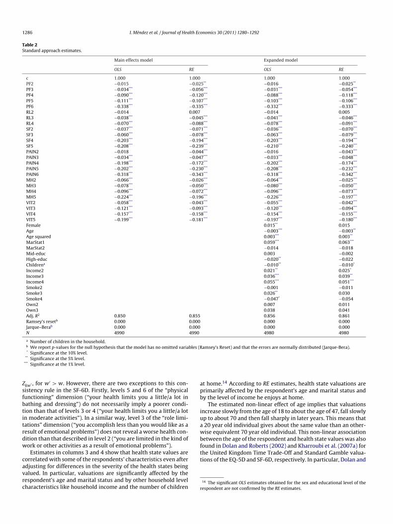

1286 I. Méndez et al. / Journal of Health Economics 30 (2011) 1280– 1292

Table 2Standard approach estimates.

Main effects model Expanded model

OLS RE OLS RE

c 1.000 1.000 1.000 1.000PF2 −0.015 −0.025** −0.016 −0.025**

PF3 −0.034*** −0.056*** −0.031*** −0.054***

PF4 −0.090*** −0.120*** −0.088*** −0.118***

PF5 −0.111*** −0.107*** −0.103*** −0.106***

PF6 −0.338*** −0.335*** −0.332*** −0.333***

RL2 −0.014 0.007 −0.014 0.005RL3 −0.038*** −0.045*** −0.041*** −0.046***

RL4 −0.070*** −0.088*** −0.078*** −0.091***

SF2 −0.037*** −0.071*** −0.036*** −0.070***

SF3 −0.060*** −0.078*** −0.063*** −0.079***

SF4 −0.203*** −0.194*** −0.203*** −0.194***

SF5 −0.208*** −0.239*** −0.210*** −0.240***

PAIN2 −0.018 −0.044*** −0.016 −0.043***

PAIN3 −0.034*** −0.047*** −0.033*** −0.048***

PAIN4 −0.198*** −0.172*** −0.202*** −0.174***

PAIN5 −0.202*** −0.230*** −0.208*** −0.232***

PAIN6 −0.318*** −0.343*** −0.318*** −0.342***

MH2 −0.066*** −0.026*** −0.064*** −0.025***

MH3 −0.078*** −0.050*** −0.080*** −0.050***

MH4 −0.096*** −0.072*** −0.096*** −0.073***

MH5 −0.224*** −0.196*** −0.226*** −0.197***

VIT2 −0.058*** −0.043*** −0.055*** −0.042***

VIT3 −0.121*** −0.093*** −0.120*** −0.094***

VIT4 −0.157*** −0.158*** −0.154*** −0.155***

VIT5 −0.199*** −0.181*** −0.197*** −0.180***

Female 0.015** 0.015Age −0.003*** −0.003**

Age squared 0.003*** 0.003**

MarStat1 0.059*** 0.063***

MarStat2 −0.014 −0.018Mid-educ 0.003 −0.002High-educ −0.020** −0.022Childrena −0.010** −0.010*

Income2 0.021** 0.025*

Income3 0.036*** 0.039**

Income4 0.055*** 0.051***

Smoke2 −0.001 −0.011Smoke3 0.026** 0.030Smoke4 −0.047* −0.054Own2 0.007 0.011Own3 0.038 0.041Adj. R2 0.850 0.855 0.856 0.861Ramsey’s resetb 0.000 0.000 0.000 0.000Jarque–Berab 0.000 0.000 0.000 0.000N 4990 4990 4980 4980

a Number of children in the household.b We report p-values for the null hypothesis that the model has no omitted variables (Ramsey’s Reset) and that the errors are normally distributed (Jarque-Bera).* Significance at the 10% level.

Zsfbtitrdw

cavrc

apb

iuawbfound in Dolan and Roberts (2002) and Kharroubi et al. (2007a) forthe United Kingdom Time Trade-Off and Standard Gamble valua-tions of the EQ-5D and SF-6D, respectively. In particular, Dolan and

** Significance at the 5% level.*** Significance at the 1% level.

kw′ , for w′ > w. However, there are two exceptions to this con-istency rule in the SF-6D. Firstly, levels 5 and 6 of the “physicalunctioning” dimension (“your health limits you a little/a lot inathing and dressing”) do not necessarily imply a poorer condi-ion than that of levels 3 or 4 (“your health limits you a little/a lotn moderate activities”). In a similar way, level 3 of the “role limi-ations” dimension (“you accomplish less than you would like as aesult of emotional problems”) does not reveal a worse health con-ition than that described in level 2 (“you are limited in the kind ofork or other activities as a result of emotional problems”).

Estimates in columns 3 and 4 show that health state values areorrelated with some of the respondents’ characteristics even after

djusting for differences in the severity of the health states beingalued. In particular, valuations are significantly affected by theespondent’s age and marital status and by other household levelharacteristics like household income and the number of children r

t home.14 According to RE estimates, health state valuations arerimarily affected by the respondent’s age and marital status andy the level of income he enjoys at home.

The estimated non-linear effect of age implies that valuationsncrease slowly from the age of 18 to about the age of 47, fall slowlyp to about 70 and then fall sharply in later years. This means that

20 year old individual gives about the same value than an other-ise equivalent 70 year old individual. This non-linear association

etween the age of the respondent and health state values was also

14 The significant OLS estimates obtained for the sex and educational level of theespondent are not confirmed by the RE estimates.

lth Eco

Raa

tiwmwfw

seppibtbipteehu

orrvt

ais1paa

oew

4

mimHfTri

tcdc

ttctwmpo

mrsAa(aswttfhfmatarva

mtftatdwues˛scimilidriˇ

I. Méndez et al. / Journal of Hea

oberts (2002) also find that the age that maximizes valuations isbout 45 years. In contrast, the corresponding age in Kharroubi etl. (2007a) is between 60 and 65 years.

The estimates in Table 2 indicate that there is a positive, mono-onic and quantitatively relevant correlation between householdncome and health state valuations. The values of respondents

hose household income is between 2000 and 3000 euros peronth are, on average, 0.040 higher than those of respondentshose household income is below 1500 euros per month. That dif-

erence amounts to 0.053 if we compare the latter group to thosehose total household income is above 3000 euros per month.

The positive association between household income and healthtate values can be interpreted in the light of the results in Lubetkint al. (2005). They find a positive and relevant association betweenersonal income and health-related quality of life in a large sam-le of the United States general population using the EQ-5D. That

s, ceteris paribus and on average terms, high-income people enjoyetter health than low-income people and, thus, we hypothesizehat they are more likely to assign a low chance to the event of aad health outcome when it is presented to them. Moreover, even

f respondents judge the likelihood of the valued health states inde-endently of their disposable income, the negative consequences ofhe realization of a bad health outcome are likely to be very differ-nt for low- and high-income individuals. The positive coefficientstimated for household income in Table 2 is compatible with theypothesis that respondents value health states according to thetility losses that they expect should that health state be realized.

The estimates in Dolan and Roberts (2002) confirm the presencef systematic differences in the valuations of married and singleespondents. However, while we find that the valuations of mar-ied or cohabiting people are, on average, 0.067 higher than thealuations of single people, they find that the average valuation ofhe latter collective is 0.006 higher than that of the former one.

Regarding children, Kharroubi et al. (2007a) find no significantssociation between the presence of children aged under 16 yearsn the household and the respondents’ valuations. We obtain theame result when we control for whether there is a child aged under2 years in the household or not.15 However, when we allow for theresence and number of children in the household we obtain a neg-tive and significant association between the number of childrent home and the respondent’s valuations.

Although existing studies disagree on the sign and magnitudef the effect of some personal characteristics, they provide robustvidence on the relevance of accounting for personal characteristicshen estimating preference-based value functions.16

.2. The IPW approach

The first two columns of Table 3 present IPW1 and IPW2 esti-ates of calculated using the set of personal characteristics

n Table 2. The external sample necessary to obtain IPW2 esti-ates comes from the Spanish sample of the European Communityousehold Panel for the year 2001, the latest available year. To

acilitate the comparison, the RE main effects model estimates inable 2 are displayed in column 3. We take these numbers as beingepresentative of the standard approach estimates since, as shownn Table 2, they are numerically equivalent to the OLS estimates and

15 These estimates are available upon request to the authors.16 It is beyond the scope of this paper to explain these discrepancies. They mightotally or partially be the result of differences in the elicitation methods, specifi-ations and estimation methods used or they might simply reflect cross-countryifferences in the distribution of personal characteristics or in the effect of thoseharacteristics.

tt

c

rt

s

nomics 30 (2011) 1280– 1292 1287

o those coming from more complex specifications that also con-rol for personal characteristics. The semi-parametric estimates inolumns 4 and 5 are calculated by restricting the elements of X tohe respondents’ sex and age groups and, finally, in the last columne use corrective weights to adjust the RE main effects model esti-ates to the sex and age group distributions of the Spanish adult

opulation, as is frequently done to ensure the representativenessf the standard model estimates.

There are relevant differences between the IPW2 and RE esti-ates of in columns 2 and 3. While just one out of the 25

egression estimates is non-significantly different from zero, theemi-parametric estimates indicate five non-significant estimates.ccording to these estimates, being slightly limited in vigorousctivities (PF2), being limited in social activities most of the timeSF3), having pain that interferes with normal work a little (PAIN3)nd feeling tense or downhearted most of the time (MH4) has noignificant effect. The same holds for being limited in the kind ofork or other activities as a result of physical health (RL2) according

o both the standard and the semi-parametric estimates. Condi-ioning on the estimated coefficients being significantly differentrom zero in both approaches, the semi-parametric estimates areigher in absolute value in 16 out of 20 coefficients and the dif-

erence between the IPW2 and the RE estimates is of much largeragnitude in those cases. On average, while the IPW2 estimates

re 61% higher than the RE ones for the 16 coefficients for whichhe IPW2 estimates are larger in absolute value, the RE estimatesre just 12% higher than the corresponding IPW2 estimates for theemaining 4 coefficients. That is, the IPW approach provides loweraluation impacts of departures from full health than the standardpproach does.

One of the reasons why the standard and the IPW esti-ates differ are the different estimation samples used by the

wo approaches. In particular, while regression models use theirunctional form to extrapolate and overcome lack of overlap inhe covariate distributions between treatment groups, the IPWpproach uses the common support condition to obtain estimateshat are not sensitive to the choice of specification. As previouslyiscussed, the common support condition implies dropping unitsith extreme values of the propensity score. In practice, instead ofsing ad hoc methods for trimming the sample we follow Crumpt al. (2009) and discard observations with estimated propensitycore outside an interval [˛, 1 − ˛], where the optimal cut-off value

is determined by the marginal distribution of the propensitycore. This results in relevant precision gains. In particular, wealculate optimal cut-off values for each of the propensity scoresnvolved in each semi-parametric estimate. In most cases the opti-

al value is close to 0.1.17 The main cost of the approach developedn Crump et al. (2009) is that potentially some external validity isost by focusing on a subset of the original sample. This cost is min-mized in our case since the IPW2 estimator changes the sampleistribution of X to that in the population of interest and, thus, itemoves sample selection biases based on personal characteristicsn X. Moreover, we have analyzed the stability of the estimates of

for different values of ˛. The estimates, available upon request tohe authors, are stable and increase their precision as gets closer

o its optimal value.18

Next, differences between the IPW1 and IPW2 estimates inolumns 1 and 2 indicate that the distribution of personal

17 Crump et al. (2009) find that most of the precision gains are captured by using aule of thumb to discard observations with the estimated propensity score outsidehe range [0.1, 0.9].18 We reach to the same conclusion for the multiple specifications of the propensitycore that have been used in order to improve its balancing power.

1288 I. Méndez et al. / Journal of Health Economics 30 (2011) 1280– 1292

Table 3Standard and semi-parametric estimates of ˇ.

IPW1 IPW2 RE IPW1a IPW2a REb

c 1.000 1.000 1.000 1.000 1.000 1.000PF2 −0.030 −0.011 −0.025** −0.026 −0.028 −0.026***

PF3 −0.050** −0.062* −0.056*** −0.060** −0.063*** −0.057***

PF4 −0.138*** −0.162*** −0.120*** −0.156*** −0.158*** −0.121***

PF5 −0.145*** −0.149*** −0.107*** −0.148*** −0.152*** −0.110***

PF6 −0.392*** −0.451*** −0.335*** −0.396*** −0.398*** −0.334***

RL2 −0.022 −0.027 0.007 −0.027 −0.028 0.009RL3 −0.029** −0.044** −0.045*** −0.041* −0.040* −0.043***

RL4 −0.125*** −0.134*** −0.088*** −0.117*** −0.116*** −0.088***

SF2 −0.043* −0.051* −0.071*** −0.033* −0.035* −0.074***

SF3 −0.022 0.007 −0.078*** −0.030 −0.030 −0.080***

SF4 −0.162*** −0.157*** −0.194*** −0.162*** −0.165*** −0.197***

SF5 −0.221*** −0.219*** −0.239*** −0.233*** −0.232*** −0.238***

PAIN2 −0.054** −0.074** −0.044*** −0.059** −0.062** −0.045***

PAIN3 −0.058** −0.029 −0.047*** −0.081*** −0.078*** −0.042***

PAIN4 −0.194*** −0.209*** −0.172*** −0.193*** −0.194*** −0.172***

PAIN5 −0.247*** −0.274*** −0.230*** −0.244*** −0.244*** −0.228***

PAIN6 −0.320*** −0.326*** −0.343*** −0.300*** −0.303*** −0.343***

MH2 −0.073*** −0.063** −0.026*** −0.102*** −0.103*** −0.024***

MH3 −0.128*** −0.136*** −0.050*** −0.171*** −0.172*** −0.051***

MH4 −0.056* −0.019 −0.072*** −0.062* −0.064** −0.072***

MH5 −0.169*** −0.176*** −0.196*** −0.171*** −0.170*** −0.195***

VIT2 −0.077*** −0.090*** −0.043*** −0.088*** −0.089*** −0.043***

VIT3 −0.162*** −0.165*** −0.093*** −0.189*** −0.185*** −0.089***

VIT4 −0.219*** −0.220*** −0.158*** −0.223*** −0.220*** −0.160***

VIT5 −0.232*** −0.247*** −0.181*** −0.230*** −0.234*** −0.178***

a The elements of X are restricted to the respondents’ sex and age group.b We use corrective weights to adjust to the sex and age groups distribution in the Spanish sample of the ECHP for 2001.*

cStIovS

toKctvsidsmAˇapiittdas

mcS

otbpfaoacteristic but the respondents’ sex significantly differs from that inthe Spanish adult population. This finding that there are relevantcompositional differences between the sample and the population

Table 4Logit estimation of propensity score ps(x) for the coefficient associated to level ofseverity 2 in dimension “personal functioning”.

Variable Coefficient

Constant −2.708***

Female −0.038Age 0.052***

Age sq. −0.013Marstat1 −1.626***

Marstat2 −1.620***

Mid-educ 0.870***

High-educ 0.375***

Children a 1.074***

Income2 1.235***

Income3 0.952***

Income4 1.131***

Smoke1 0.461***

Smoke2 −0.884***

Smoke3 −1.629***

Own2 −0.804***

Own3 −1.950***

Significance at the 10% level.** Significance at the 5% level.

*** Significance at the 1% level.

haracteristics in the sample significantly differs from that in thepanish adult population. These differences are of lower magnitudehan those found when comparing the RE to the IPW2 estimates.n most cases the IPW2 estimate exceed the corresponding IPW1ne. On average, the estimate of ˇkw increases by 13% in absolutealue when using the distributions of personal characteristics in thepanish adult population instead of those in the estimation sample.

The finding that adjusting to the population distribution ofhe covariates results in relevant variations in the magnitudef the semi-parametric estimates contrasts with the evidence inharroubi et al. (2007a) and Dolan and Roberts (2002). These arti-les find that the standard model estimates are almost invarianto the inclusion of corrective weights that adjust to the age inter-al and sex distributions in the population. In fact, we reach theame conclusion when comparing the unweighted RE estimatesn column 3 to those in column 4 where we use corrective weightsefined over the respondents’ sex and age groups. Interestingly, theemi-parametric estimates also lead to the same result once the ele-ents of X are restricted to the respondents’ sex and age groups.s shown in columns 4 and 5, the IPW1 and IPW2 estimates ofkw obtained using the restricted set of personal characteristics arelmost identical for any k and any w. Moreover, the restricted semi-arametric estimates are close in magnitude to the IPW1 estimates

n column 1 but they differ substantially from the IPW2 estimatesn column 2, where we adjust for the population distribution inhe whole list of personal characteristics in Table 2. This suggestshat adjusting to the population distributions of a reduced set ofiscretely measured personal characteristics is not enough to guar-ntee the population validity of the estimates. The propensity scoreeems far more effective in removing sample selection biases.

The estimation of the propensity score ps(x) allows us to for-ally test for sample selection biases, that is, to identify the

haracteristics whose sample distribution differs from that in thepanish adult population. A significant coefficient in the estimation

f the discrete choice model for the propensity score indicates thathe distribution of the corresponding characteristic is not balancedetween the population and the sample. As an illustrative exam-le, in Table 4 we present the results of estimating a logit modelor the propensity score ps(x) in the estimation of the coefficientssociated to dimension “personal functioning” in its second levelf severity (PF2). We find that the sample distribution of any char-

Psedo R2 0.236N 13,509

a Number of children in the household.*** Significance at the 1% level.

I. Méndez et al. / Journal of Health Economics 30 (2011) 1280– 1292 1289

Table 5Standard and semi-parametric consistent estimates.

IPW2 RE

c 1.000 1.000PF2 −0.011 −0.025**

PF3 −0.062* −0.056***

PF4 −0.162*** −0.120***

PF5 −0.149*** −0.107***

PF6 −0.451*** −0.335***

RL2 −0.027 0.007RL3 −0.044** −0.045***

RL4 −0.134*** −0.088***

SF2 −0.051* −0.071***

SF3 −0.078***

SF4 −0.194***

SF34a −0.090***

SF5 −0.219*** −0.239***

PAIN2 −0.074** −0.044***

PAIN3 −0.047***

PAIN4 −0.172***

PAIN34b −0.100***

PAIN5 −0.274*** −0.230***

PAIN6 −0.326*** −0.343***

MH2 −0.063** −0.026***

MH3 −0.136*** −0.050***

MH4 −0.072***

MH5 −0.196***

MH45c −0.138***

VIT2 −0.090*** −0.043***

VIT3 −0.165*** −0.093***

VIT4 −0.220*** −0.158***

VIT5 −0.247*** −0.181***

a Dummy indicator variable that equals one if the “social functioning” dimensionreaches levels of severity 3 or 4, and zero otherwise.

b Dummy indicator variable that equals one if the “pain” dimension reaches levelsof severity 3 or 4, and zero otherwise.

c Dummy indicator variable that equals one if the “mental health” dimensionreaches levels of severity 4 or 5, and zero otherwise.

* Significance at the 10% level.

oe

pdfiftiMfiwstmi

eSmdslT

p

Table 6RE and IPW2 tariffs. Summary statistics of the values predicted for the 18,000 healthstates defined by the SF-6D.

IPW2 RE

Mean 0.354 0.440S.D. 0.249 0.212Minimum −0.553 −0.382Percentiles

10 0.021 0.15625 0.192 0.29950 0.368 0.45275 0.532 0.59490 0.667 0.708

mibut5tpoz3vtttd

ittminoitpsquared error of 0.139 for the RE model, 0.167 for the IPW2 consis-tent model and 0.137 for the IPW1 model associated to the IPW2consistent model. The IPW1 model is included for comparability

.51

1.5

2

** Significance at the 5% level.*** Significance at the 1% level.

f interest is common to the estimation of ps(x) for any of the IPW2stimates in Table 3.19

Following Brazier and Roberts (2004), we estimate a IPW2arsimonious consistent model by aggregating levels of a givenimension when inconsistencies are found, that is, when the coef-cient estimated for Zkw is not higher than that estimated for Zkw′ ,

or w′ > w. Bearing in mind the previously discussed exceptionso this rule, we find three inconsistencies. The estimate for PAIN2s larger in absolute value than that for PAIN3, the coefficient for

H4 is smaller in absolute value than that associated to MH3 and,nally, the estimate for SF3 is not significantly different from zero,hile those for SF2 and SF4 are lower than zero. As opposed to the

tandard model, the IPW approach does not require the estima-ion of the full vector once an inconsistency is detected. The RE

odel estimates are included for comparability purposes, since nonconsistencies are found in these estimates.

The consistent estimates presented in Table 5 allow us tostimate values for the 18,000 health states defined by theF-6D classification system. The resulting RE and IPW2 esti-ated tariffs are summarized in Table 6 and their densities are

epicted in Fig. 1. As expected given the preceding discussion, the

emi-parametrically estimated values tend to be significantlyower than those predicted using the standard regression model.hese discrepancies are observed in any of the distributional

19 These estimates and also those for the first step estimate of the propensity scorekw(x) are available upon request to the authors.

Fpb

Negative values (%) 8.82 2.53

oments and they tend to be higher the lower is the predicted util-ty of a health state, that is, the higher is its severity. The differenceetween the zth percentile of the RE and IPW2 distributions of val-es lowers from 0.135 for z = 10 to 0.041 for z = 90. In relative terms,he 10th and 90th percentiles of the IPW2 distribution are 86.5 and.8% higher than the corresponding percentiles of the RE distribu-ion. A similar picture emerges when looking at the proportion ofredicted negative values. While only 2.5% of the values predictedn the basis of the standard approach estimates are lower thenero, the corresponding number for the semi-parametric values is.5 times higher. In particular, almost 9% of the semi-parametricalues are strictly lower than zero. The densities of the predictedariffs in Fig. 1 confirm that the standard approach underestimateshe utility loss that the Spanish adult population gives to devia-ions from full health, particularly so when dealing with severeeviations.

The IPW and the standard models cannot be directly comparedn terms of their predictive ability since they use different estima-ion samples. While the regression model uses its functional formo work off the common support when estimating ˇkw, the IPW

odel restricts the sample to respondents valuing levels of sever-ty 1 and w in dimension k whose estimated propensity score isot close to zero or one. To get a feeling about the predictive abilityf the models, we restrict the sample to respondents not excludedn the semi-parametric estimation of none of the coefficients usedo predict the value of a particular health state. We find that theredictive performance of the models is similar with a root mean

0

-.5 0 .5 1

RE IPW2

ig. 1. A comparison of the RE and IPW2 tariffs’ predicted values. Note: The graphresents the densities of the values predicted for the 18,000 health states definedy the SF-6D using the RE and IPW2 consistent estimates in Table 5.

1 lth Eco

papI

5

vwOspafaAprasp

tiuohteoidd

Tmfopwtmt

fddglb

tIate

twvdid

Itcdc2oJosima

A

Fs2s

A

t

ovm�∑w�b

wA{sttptT

value �

√n(� − �) −→ N(0, A(�)−1B(�){A(�)−1}T )

290 I. Méndez et al. / Journal of Hea

urposes, since the IPW2 model imposes the distribution of char-cteristics in an external sample and, thus, it is expected to performoorer in terms of within sample predictive ability. The associated

PW1 model performs slightly better than the RE model.

. Conclusions

This paper presents a novel approach to model health statealuations using inverse probability weighting (IPW) techniquesith important advantages over the standard regression model.ur approach makes no assumption on the distribution of health

tate values, accommodates covariates in a flexible way, eschewsarametric assumptions on the relationship between the outcomend the regressors, allows for the valuation impact of departuresrom full health to be heterogeneous in personal characteristicsnd in the severity of departures in other dimensions of health.dditionally, unlike the standard approach, our approach producesopulation valid estimates even if the estimation sample is notepresentative for that population with regard to many discretend continuously measured variables. The proposed estimators areemi-parametrically estimated and we also derive its large sampleroperties.

The standard model estimates are likely to be very sensitiveo differences in the covariate distributions of respondents valu-ng different health states since it applies regression models thatse extrapolation to deal with limited support in the distributionf the covariates. In contrast, our approach calls for selecting theealth states for which direct valuations are obtained for identifica-ion not to rest on extrapolation. That will be the case in the mainffects model if there is common support in the level of severityf the remaining dimensions of health between respondents valu-ng health states with a departure from full health in a particularimension and those valuing health states with full health in thatimension.

We illustrate our approach with the SF-6D descriptive system.he results indicate that the standard and the semi-parametric esti-ates differ to a great extent, with the utility loss of a departure

rom full health being higher in most cases when estimated usingur approach. In fact, when the estimated coefficients are used toredict utilities for the 18,000 health states defined in the SF-6De find that the standard approach systematically underestimates

he valuation impact of departures from full health and that theagnitude of the underestimation increases with the severity of

he health state at examination.Moreover, we also find evidence that the standard approach

ails in its goal of producing population valid estimates by intro-ucing corrective weights that adjust to the sex and age intervalsistribution in the population of interest. We consider continuouseneralizations of the corrective weights that easily overcome theirimitations and allow us to test and correct for sample selectioniases.

The IPW approach is easier to implement and interpret thanhe nonparametric Bayesian approach in Kharroubi et al. (2007b).n particular, and contrary to the nonparametric estimator, ourpproach provides the user with a table of estimated coefficientshat defines the estimated preference function, which results infficiency and transparency gains.

Finally, the IPW approach is suitable for application to any ofhe existing multi-attribute descriptive systems. In particular, itould be of interest to semi-parametrically estimate the EQ-5D

alue sets, since this is the most widely used instrument for theescription and valuation of health states. With reference to this,

t should be stressed the importance of the common support con-ition in the selection of the health states valued in the sample.

ep

nomics 30 (2011) 1280– 1292

f we look at the studies which have derived the EQ-5D tariffs forhe United Kingdom, Spain, the Netherlands and Japan, we con-lude that this overlap requirement in the levels of severity of theimensions of health is met in six out of the 10 estimated coeffi-ients in the case of the UK (Dolan, 1997) and Spain (Badia et al.,001) estimations, whereas the condition is satisfied in just one outf 10 estimated coefficients in the Dutch (Lamers et al., 2006) andapanese (Tsuchiya et al., 2002) tariffs. Consequently, the validityf the Dutch and Japanese estimates rests on whether the corre-ponding regression models were correctly specified or not. Thats, the Dutch and Japanese tariffs are less likely to be robust to the

isspecification of the regression model than those in Dolan (1997)nd Badia et al. (2001).

cknowledgement

José María Abellán Perpinán, Jorge Eduardo Martínez Pérez andernando Ignacio Sánchez Martínez also acknowledge financialupport from Ministerio de Ciencia e Innnovación grant ECO2010-2041-C02-02. This research was supported by the Health and Con-umption Department of the Autonomous Community of Murcia.

ppendix A. Asymptotic properties

We derive the asymptotic properties of kw,IPW2 and present

hose of kw,IPW1 as a particular case. The subscript IPW2 is dropped

ut to reduce the notation. The properties of kw are derived by

iewing it as an M-estimator, that is, as the solution to a set of esti-ating equations.20 In particular, kw is one element of the vector

that solves the vector equation

n

i=1 (Wi, �) = 0

here Wi = [Yi, Zk′w′ , Xi], for k′ /= k and w′ = 2, 3, . . . , Wk′ and = [ı, � , ˇkw]. The vector equation has three equations and cane written as∑n

i=1 1(Wi, �) =

∑n

i=1

Dsi − psi(Xi, ı)psi(Xi, ı)[1 − psi(Xi, ı)]

∂psi(Xi, ı)∂ı

= 0

∑n

i=1 2(Wi, �) =

∑n

i=1

Zkwi − pkwi(Hi, �)pkwi(Hi, �)[1 − pkwi(Hi, �)]

∂pkwi(Hi, �)∂�

= 0

∑n

i=1 3(Wi, �) =

∑n

i=1

{A(1)

ZkwiYipkwipsi

− A(0)(1 − Zkwi)Yi(1 − pkwi )psi

− ˇkw

}= 0

here psi = psi(Xi, ı), pkwi = pkwi(Hi, �), pkwi = (Hi, �), psi = (Xi, ı),(t) = N(

∑ni=1(Zt

kwi(1 − Zkwi)

1−t)/(ptkwi

(1 − pkwi)1−t psi))−1 for t =

0, 1}

and N is the total number of individuals in the estimation

ample. The solutions to equations 1(Wi, �

)and 2

(Wi, �

)are

he maximum likelihood estimates of ı and � , the coefficients ofhe binary response models used to estimate the propensity scoress and pkw, respectively. We estimate the propensity scores usinghe logistic regression model, where p(Q, ϕ) = {1 + exp (− QTϕ)}−1.he solution to equation 3(Wi, �) is the coefficient of interest.

By standard results on M-estimation, under the true parameter

20 Stefanski and Boos (2002) provide an excellent review of the theory of M-stimation. Additionally, Lunceford and Davidian (2004) derive the asymptoticroperties of the IPW1 estimator.

lth Eco

w

A

w

B

w

w

wD

V

wtvmevafata

owte

A

t(E(iwcche3dscArbofvar

R

A

B

B

I. Méndez et al. / Journal of Hea

here

(�) = E[− (W, �)]

ith (W, �) = ∂ (W, �)/∂�T and

(�) = E[ (W, �) (W, �)T ]

To estimate the asymptotic variance use

A = 1n

∑n

i=1− ∂ (Wi, �)

∂�T

B = 1n

∑n

i=1 (Wi, �) (Wi, �)T

here the derivative of can be calculated as

∂ (W, �)∂�T

=

⎛⎜⎜⎜⎜⎜⎜⎜⎝

∂ 1(W, �)∂ıT

∂ 1(W, �)∂�T

∂ 1(W, �)∂ˇT

kw

∂ 2(W, �)∂ıT

∂ 2(W, �)∂�T

∂ 2(W, �)∂ˇT

kw

∂ 3(W, �)∂ıT

∂ 3(W, �)∂�T

∂ 3(W, �)∂ˇT

kw

⎞⎟⎟⎟⎟⎟⎟⎟⎠

here

A11i =∂ 1(W, �)∂ıT

= − 1psi(1 − psi)

PıPTı

A12i =∂ 1(W, �)∂�T

= A13i =∂ 1(W, �)∂ˇT

kw

= 0

A21i =∂ 2(W, �)∂ıT

= A23i =∂ 2(W, �)∂ˇT

kw

= 0

A22i =∂ 2(W, �)∂�T

= − 1pkwi(1 − pkwi)

P�PT�

A31i =∂ 3(W, �)∂ıT

= −[DsiDkwiY

∗i

pkwipsi2− DsiDkwiY

∗i

(1 − pkwi)psi2

]Pı

A32i =∂ 3(W, �)∂�T

= −[DsiDkwiY

∗i

p2kwipsi

+ DsiDkwiY∗i

(1 − pkwi)2psi

]P�

A33i =∂ 3(W, �)∂ˇT

kw

= −1

here Pı = ∂/∂ ı{psi}, P� = ∂/∂ �{pkwi} and Y∗i

= DkwiA(1)Yi + (1 −kwi)A(0)Yi. Equivalently, the elements of B are calculated as

B11i = 1(Wi, �) 1(Wi, �)T = 1psi(1 − psi)

PıPTı

B12i = 1(Wi, �) 2(Wi, �)T = 0

B13i = 1(Wi, �) 3(Wi, �)T =[DsiDkwiY∗

i

pkwipsi2− DsiDkwiY∗

i

(1 − pkwi)psi2

]Pı

B21i = 2(Wi, �) 1(Wi, �)T = 0

B22i = 2(Wi, �) 2(Wi, �)T = 1pkwi(1 − pkwi)

P�PT�

B23i = 2(Wi, �) 3(Wi, �)T =[DsiDkwiY∗

i

p2kwipsi

+ Dsi(1 − Dkwi)Y∗i

(1 − pkwi)2psi

]P�

B31i = 3(Wi, �) 1(Wi, �)T = BT13i

B32i = 3(Wi, �) 2(Wi, �)T = BT23i

B33i = 3(Wi, �) 3(Wi, �)T =(DsiDkwiY∗

i

pkwipsi− Dsi(1 − Dkwi)Y∗

i

(1 − pkwi)psi− ˇkw

)2 B

B

nomics 30 (2011) 1280– 1292 1291

Finally, it can be shown that the large-sample variance of ˇkw is

(ˇkw) = A−133 (B33 − BT23B

−122 B23 − BT13B

−111 B13)(A−1

33 )T

The expression of the large-sample variance of ˇkw in the casehere � and ı are known is A−1

33 B33(A−133 )T . The additional two

erms in the parenthesis are the adjustment in the large-sampleariance of the effect of interest coming from the first step esti-ation of the two propensity scores. Interestingly, it results that

stimation of the propensity scores leads to smaller large-sampleariance for these IPWestimators than using the true values. That is,s Lunceford and Davidian (2004) point out, even if the functionalorm of the propensity score is known exactly, it is beneficial fromn efficiency viewpoint to estimate it. Hirano et al. (2003) explainhis result in the context of the Generalized Method of Momentsnd the Empirical Likelihood estimators.

The expression for the variance of the IPW1 estimator includesnly the first two terms in the parenthesis in the latter expression,here B23 and B33 are now calculated as the sample average of

he following expressions evaluated at the estimated value of thelements of �

B23i =[DkwiY

∗i

p2kwi

+ (1 − Dkwi)Y∗i

(1 − pkwi)2

]P�

B33i =(DkwiY

∗i

pkwi− (1 − Dkwi)Y∗

i

(1 − pkwi)− ˇkw,IPW1

)2

ppendix B. Variable definitions and sources

The variables for the Spanish population are constructed usinghe Spanish sample of the European Community Household PanelECHP) for the year 2001, the latest available year, provided byurostat. In the empirical analysis we control for the sex and agein years) of the respondent, whether he is married or cohabit-ng (MarStat1) or separated, divorced or widow (MarStat2) and

hether the respondent has attained a secondary level of edu-ation (Mid-educ) or an university degree (High-educ). We alsolassify respondents according to whether their monthly totalousehold income is below 1500 euros, between 1500 and 2000uros (Income2), between 2000 and 3000 euros (Income3) or above000 euros (Income4). Regarding their smoking behaviour, weistinguish between non-smokers and respondents who actuallymoke less than 10 cigarettes per day (Smoke2), between 10 and 20igarettes (Smoke3) and more than 20 cigarettes per day (Smoke4).dditionally, we construct two dummy variables that indicate if theespondent thinks that his general health is fair (Own2) or bad/veryad (Own3). The remaining categories in the answer to the questionf how is your health in general are good and very good. We controlor the number of children in the household. However, while theariable constructed using ECHP data refers to children under thege of 16 years, the corresponding variable from the collected dataefers to children aged under the age of 12.

eferences

bellán-Perpinán, J.M., Sánchez-Martínez, F.I., Martínez-Pérez, J.E., Méndez, I., 2011.Lowering the ‘floor’ of the SF-6D scoring algorithm using a lottery equivalentmethod. Health Economics, doi:10.1002/hec.1792.

adia, X., Roset, M., Herdman, M., Kind, P., 2001. A comparison of United Kingdomand Spanish general population time trade-off values for EQ-5D health states.Medical Decision Making 21, 7–16.

arnow, B., Cain, C., Goldberger, A., 1981. Selection on observables. Evaluation Stud-

ies Review Annual 5, 43–59.

razier, J.E., Roberts, J., 2004. The estimation of a preference-based measure of healthfrom the SF-12. Medical Care 42 (9), 851–859.

razier, J.E., Roberts, J., Deverill, M., 2002. The estimation of a preference-basedmeasure of health from the SF-36. Journal of Health Economics 21, 271–292.

1 lth Eco

B

B

B

B

C

C

C

D

D

D

D

E

F

F

G

H

H

I

J

K

K

K

L

L

L

L

M

N

R

R

R

292 I. Méndez et al. / Journal of Hea

razier, J.E., Roberts, J., Tsuchiya, A., Busschbach, J., 2004. A comparison of the EQ-5Dand SF-6D across sever patients groups. Health Economics 13, 873–884.

razier, J.E., Usherwood, T., Harper, R., Thomas, K., 1998. Deriving a preference-basedsingle index from the UK SF-36 health survey. Journal of Clinical Epidemiology51 (11), 1115–1128.

razier, J.E., Fukuhara, S., Roberts, J., Kharroubi, S., Yamamoto, Y., Ikeda, S., Doherty,J., Kurokawa, K., 2009. Estimating a preference-based index form the JapaneseSF-36. Journal of Clinical Epidemiology 62, 1323–1331.

usso, M., DiNardo, J., McCrary, J., 2009. New Evidence on the Finite Sample Proper-ties of Propensity Score Matching and Reweighting Estimators. IZA DiscussionPaper 3998.

raig, B.M., Busschbach, J.J., 2009. The episodic random utility model unifies timetrade-off and discrete choice approaches in health state valuation. PopulationHealth Metrics 7, 16–25.

raig, B.M., Busschbach, J.J., 2011. Toward a more universal approach in healthvaluation. Health Economics 20, 864–875.

rump, R.K., Hotz, V.J., Imbens, G.W., Mitnik, O.A., 2009. Dealing with limited overlapin estimation of average treatment effects. Biometrika 96, 187–199.

iNardo, J., Fortin, N.M., Lemieux, T., 1996. Labor market institutions and the dis-tribution of wages, 1973–1992: a semi-parametric approach. Econometrica 64(5), 1001–1044.

olan, P., 1997. Modelling valuations for Euroqol health states. Medical Care 35,351–363.

olan, P., Gudex, C., Kind, P., Williams, A., 1996. The time trade-off method: resultsfrom a general population study. Health Economics 5, 141–154.

olan, P., Roberts, J., 2002. To what extent can we explain time trade-off values fromother information about respondents? Social Science and Medicine 54, 919–929.

uroQol Group, 1990. EuroQol—a new facility for the measurement of health-relatedquality of life. Health Policy 16, 199–208.

eeny, D., Furlong, W., Torrance, G.W., Goldsmith, C.H., Zenglong, Z., Depauw, S.,Denton, M., Boyle, M., 2002. Multi-attribute and single-attribute utility functionfor the Health Utility Index Mark 3 system. Medical Care 40, 113–128.

erreira, L.N., Ferreira, P.L., Pereira, L.N., Brazier, J.E., Rowen, D., 2010. A PortugueseValue Set for the SF-6D. Value in Health 13 (5), 624–630.

old, M.R., Siegel, J.E., Russell, L.B., Weinstein, M.C., 1996. Cost-Effectiveness inHealth and Medicine. Oxford University Press, Oxford.

irano, K., Imbens, G.W., Ridder, G., 2003. Efficient estimation of average treatmenteffects using the estimated propensity score. Econometrica 71 (4), 1161–1189.

orvitz, D.G., Thompson, D.J., 1952. A generalization of sampling without replace-ment from a finite universe. Journal of the American Statistical Association 47,663–685.

S

T

nomics 30 (2011) 1280– 1292

mbens, G.W., 2004. Nonparametric estimation of average treatment effects underexogeneity: a review. The Review of Economics and Statistics 86 (1), 4–29.

ohnson, J.A., Coons, S.J., Ergo, A., Szava-Kovats, G., 1998. Valuation of EuroQOL (EQ-5D) health state in an adult US sample. Pharmaconomics 13 (4), 421–433.

ahneman, D., Tversky, A., 1979. Prospect theory: An analysis of decision under risk.Econometrica 47, 263–291.

harroubi, S., Brazier, J.E., O’Hagan, A., 2007a. Modelling covariates for the SF-6Dstandard gamble health state preference data using a nonparametric Bayesianmethod. Social Science and Medicine 64, 1242–1252.

harroubi, S., Brazier, J.E., Roberts, J., O’Hagan, A., 2007b. Modelling SF-6D healthstate preference data using a nonparametric Bayesian method. Journal of HealthEconomics 26, 597–612.

am, C.L., Brazier, J.E., McGhee, S.M., 2008. Valuation of the SF-6D health states isfeasible, acceptable, reliable, and valid in a Chinese population. Value in Health11, 295–303.

amers, L.M., McDonnell, J., Stalmeier, F.M., Krabbe, P.F.M., Busschbach, J.J.V., 2006.The Dutch Tariff: results and arguments for an effective design for national EQ-5D valuation studies. Health Economics 15, 1121–1132.

ubetkin, E.I., Jia, H., Franks, P., Gold, M.R., 2005. Relationship among sociodemo-graphic factors, clinical conditions, and health related quality of life: examiningthe EQ-5D in the U.S. general population. Quality of Life Research 14, 2187–2196.

unceford, J.K., Davidian, M., 2004. Stratification and weighting via the propensityscore in estimation of causal treatment effects: a comparative study. Statisticsin Medicine 23, 2937–2960.

cCord, M., de Neufville, R., 1986. Lottery equivalents: reduction of the certaintyeffect problem in utility assessment. Management Science 32 (1), 56–60.

ational Institute for Clinical Excellence (NICE), 2004. Guide to the Methods ofTechnology Appraisal. NICE, London.

obins, J.M., Rotnitzky, A., Zhao, L.P., 1994. Estimation of regression coefficientswhen some regressors are not always observed. Journal of the American Sta-tistical Association 89, 846–866.

osenbaum, P., Rubin, D.B., 1983. The central role of the propensity score in obser-vational studies for causal effects. Biometrika 70, 41–55.

ubin, D.R., 1974. Estimating causal effects of treatments in randomizedand nonrandomized studies. Journal of Educational Psychologies 66, 688–701.

tefanski, L.A., Boos, D.D., 2002. The calculus of M-estimation. The American Statis-tician 56, 29–38.

suchiya, A., Ikeda, S., Ikegami, N., Nishimura, S., Sakai, I., Fukuda, T., Hamashima,C., Hisashige, A., Tamura, M., 2002. Estimating an EQ-5D population value set:the case of Japan. Health Economics 11, 341–353.