Intraspecific diversity in Arctic charr, Salvelinusalpinus, in Iceland: II. Which environmental

factors influence resource polymorphism in lakes?

Pamela J. Woods1,2,3, Skúli Skúlason1, Sigurður S. Snorrason2,Bjarni K. Kristjánsson1, Hilmar J. Malmquist4 and Thomas P. Quinn3

1 Hólar University College, Sauðárkrókur, Iceland, 2 University of Iceland, Reykjavík, Iceland,3 University of Washington, Seattle, Washington, USA and 4 Natural History Museum of

Kópavogur, Kópavogur, Iceland

ABSTRACT

Background: The mechanisms causing resource polymorphism are not well understood,but likely include frequency-dependent selection. However, other selection mechanisms couldalso explain the development of resource polymorphism. Comparative analyses of poly-morphic and monomorphic systems are uncommon, making it difficult to distinguish the effectsof geography, frequency-dependent selection, niche expansion, and species interactions.Detailing ecological conditions associated with the development of resource polymorphism isnecessary to discern demographic and environmental processes that may cause it.

Goal: Test for environmental correlations with (a) the presence of resource polymorphismand (b) the degree of differentiation in polymorphic systems, to evaluate the hypotheses that thedevelopment of resource polymorphism results from (1) frequency dependence, (2) expansionto include a zooplanktivorous niche, or (3) lower survivorship due to predation on intermediatetrait values. Trends in prey consumption, as they related to the presence of polymorphism andlimnetic lake characteristics, were also analysed.

Organism: Arctic charr (Salvelinus alpinus) populations from lakes sampled in 1994–2004across Iceland.

Methods: Random forest and multiple regression models assessing the presence and degreeof resource polymorphism using environmental variables reflecting physical, chemical, and bio-logical conditions. Prey consumption was fitted to the presence of polymorphism and browntrout abundance in negative binomial generalized linear models. The proportion of individualsconsuming zooplankton within monomorphic versus polymorphic populations was also measuredto test the idea that more widespread zooplankton consumption reflects niche expansion.

Results: In Iceland, polymorphic populations tended to occur in cooler lakes with few browntrout (Salmo trutta), a trophic competitor, and in lakes where Arctic charr consumed morezooplankton. Lakes with greater limnetic habitat, fewer nutrients, and greater potential toconsume zooplankton appeared to promote resource polymorphism, thereby supportingthe presence of niche expansion. The overall results supported the frequency dependencehypothesis, as well as the niche expansion hypothesis in most cases. However, morphs that

Correspondence: P.J. Woods, Hólar University College, Háeyri 1, 551 Sauðárkrókur, Iceland. E-mail:pamelajwoods@gmail.comConsult the copyright statement on the inside front cover for non-commercial copying policies.

Evolutionary Ecology Research, 2012, 14: 993–1013

© 2012 Pamela J. Woods

differed in consumption of fish or chironomid pupae rather than zooplankton were also evi-dent, indicating that mechanisms other than niche expansion may also be important. Relativeresource availability and its link with the environment need to be accounted for when trying topredict the occurrence of polymorphism.

Keywords: competition, divergent selection, ecological speciation, individual heterogeneity,limnology, prey availability, resource polymorphism, salmonid.

INTRODUCTION

Resource polymorphism is characterized by the occurrence of discrete forms within apopulation that differ by one or more phenotypic attributes associated with resource use,such as growth rate, age at first maturity, or morphological traits related to feeding (Skúlason

and Smith, 1995). It is most simply observed as bimodality in a population trait. In general,frequency-dependent selection is thought to be the primary evolutionary factor leading tobimodality (van Valen, 1965; Dieckmann et al., 2004). Under frequency-dependent selection, resourcepolymorphism may arise when a single population increases in density, after whichintraspecific competition for a preferable resource increases due to decreasing per capitaavailability of the resource. At some critical point, it becomes beneficial to be efficient atobtaining less preferable but more abundant resources, and selection becomes disruptive onphenotypic attributes associated with foraging. The relative fitness expected of individualspossessing a morphological characteristic therefore depends on its frequency in relation toindividuals with alternative morphological characteristics, resulting in stable frequency-mediated selection (Dieckmann et al., 2004).

Although frequency dependence is difficult to measure, experimental studies haveshown patterns that strongly indicate its presence in polymorphic populations. Geneticcharacteristics have been detected as dependent on their own frequency in a polymorphicsystem (Schluter, 2003), and intraspecific competition can lead to morphological divergence(Schluter, 1994; Bolnick, 2004; Svanbäck and Bolnick, 2007; Bolnick and Lau, 2008). Niche expansioncan also occur alongside mechanisms of frequency dependence; populations at highdensities may consume a wider range of resources (Svanbäck and Persson, 2004). Therefore,divergence is thought to occur under ecological conditions that promote niche expansion,i.e. the greater use of other available resources not used in ancestral populations (Knudsen et al.,

2006).However, frequency dependence is not the only explanation for bimodality in a

population. For example, predation risk can promote differential habitat use, leading todivergent selection (Abrams, 2000; Vamosi and Schluter, 2002; Rundle et al., 2003; Doucette et al., 2004; Langerhans

et al., 2004). Predation has been suggested as a mechanism promoting size divergence ofArctic charr (Salvelinus alpinus), as large forms can escape gape-limited predators andsmall benthic forms can hide among substrate (Snorrason and Skúlason, 2004; Kristjánsson

et al., 2011). On the other hand, cannibalism by Arctic charr can provide an advantage toreaching large sizes (Griffiths, 1994).

In our companion paper (Woods et al., 2012, this issue), we present standard methods fordetecting resource polymorphism and defining the degree of divergence between morphswithin populations of Arctic charr. To understand how such intraspecific diversity arises, anatural question following the detection of polymorphism would be ‘What characteristicsof the environment promote the development of resource polymorphism, and why do

Woods et al.994

populations differ in their degree of polymorphism?’ The goal of this study is to determinewhich characteristics of the lake environment best predict the presence and degree ofpolymorphism in Arctic charr among lakes in Iceland. The availability of biological andlimnological data from a wide diversity of lakes found within the database of the EcologicalSurvey of Icelandic Lakes (ESIL) project (Malmquist et al., 2000; Kristjánsson et al., 2011; Woods

et al., in press) yielded a rare opportunity to test the link between resource polymorphismin Arctic charr and environmental conditions. We tested the hypotheses that resource poly-morphism would be found under environmental conditions that promote (1) frequencydependence (hypothesis 1), (2) niche expansion (hypothesis 2), or (3) greater predation risk(hypothesis 3). To test these relationships, we analysed patterns in (a) the presence ofpolymorphism and (b) the relative degree of differentiation between morphs (restricted tolakes with two morphs) across lakes in Iceland.

As it is difficult to predict which characteristics of the lake environment should reflectthese three phenomena, the present study is a preliminary analysis in which a wide varietyof environmental characteristics were explored. We paid particular attention to environ-mental features used to support the three hypotheses in past studies. Thus, if polymorphismis attributable to frequency-dependent selection (hypothesis 1), then polymorphism anddegree of divergence should be associated with the following patterns:

(1a) High conspecific densities (Griffiths, 1994), indicating greater intraspecific competition,which is thought to influence frequency dependence (Schluter, 1994; Bolnick, 2004; Dieckmann et al., 2004;

Svanbäck and Bolnick, 2007).(1b) Low competitor densities (i.e. the brown trout, Salmo trutta, in Iceland), allowing

for greater niche breadth. Only when these niches are available (i.e. prey populations arenot suppressed by predators other than Arctic charr) is it possible for the frequency ofArctic charr phenotypes specializing on these prey to increase (Griffiths, 1994, 2006; Robinson and

Wilson, 1994; Skúlason and Smith, 1995; Schluter, 1996; Skúlason et al., 1999). This also reducesthe chance of habitat displacement by brown trout, a dominant competitor (Langeland et al.,

1991; Forseth et al., 2003).(1c) High altitudes. High-altitude sites generally have lower species diversity, because they

are more isolated and more recently deglaciated than sites at lower altitude (Griffiths, 2006).However, these regions not only have fewer competitors (see 1b), they also act as a filter:only those species that have the highest colonization potential (i.e. are the most adaptableto new conditions and able to bypass barriers to migration) persist there (Bernatchez and Wilson,

1998; Griffiths, 2006). Perhaps these regions have also promoted adaptation to high environ-mental variability on geological time scales (Bernatchez and Wilson, 1998; Robinson and Schluter, 2000).High adaptability to new environments in these species then more readily initiates theprocess of divergence (Bernatchez and Wilson, 1998; Robinson and Schluter, 2000).

If polymorphism occurs as a result of niche expansion (hypothesis 2), then we would expectthat a greater frequency or degree of polymorphism would be associated with expanded useof available resources relative to an ancestral form (Knudsen et al., 2006). Although this has beenstudied in Arctic charr from other locations as an expansion towards the consumptionof greater profundal benthic resources (Knudsen et al., 2006), we consider expansion towardsthe consumption of limnetic resources, or zooplanktivory. Zooplanktivory is common inEuropean Arctic charr (McCarthy, 2007), but appears to occur as a result of displacement frombenthic zones by co-occurring species, as Arctic charr eat considerably more benthic foods,

Environmental trends with resource polymorphism 995

including fish, when in isolation (Langeland et al., 1991; Halvorsen et al., 1997; Forseth et al., 2003; Klemetsen

et al., 2003). Therefore, an increase in zooplanktivory due to niche expansion may only bedetectable in regions where co-occurring species are few, such as Iceland. This hypothesiswould be supported by an association between a greater or more widespread consumptionof zooplankton and greater incidence of polymorphism or divergence of morphs.

Finally, if polymorphism is based on increased vulnerability to predation rather thanfrequency dependence at intermediate trait values (hypothesis 3), then greater predation onArctic charr should occur in lakes with polymorphism present (Abrams, 2000; Vamosi and Schluter,

2002; Rundle et al., 2003; Doucette et al., 2004; Langerhans et al., 2004). This could be detected as an associ-ation between higher frequencies of polymorphism or greater divergence and higherpredator densities (i.e. brown trout). Predation due to cannibalism could not be tested inthis study, as Icelandic Arctic charr are rarely cannibalistic according to extensive gutcontent data in the ESIL database (<1% of ≈3500 records, unpublished data).

The three expected hypotheses are not mutually exclusive, but one would not expect thefirst and third to apply simultaneously due to their differing expected relationships withbrown trout (i.e. polymorphism should occur with low brown trout density in hypothesis 1versus high brown trout density in hypothesis 3). However, hypothesis 2 is compatible withhypotheses 1 and 3.

MATERIALS AND METHODS

Detection of polymorphism

Data on length-at-age, morphology, maturity, and diet of Arctic charr populations from51 lakes in an Ecological Survey of Icelandic Lakes (August to September in 1992–2004)were used to detect polymorphism in our companion paper (Woods et al., 2012, this issue). (Fordetails on sampling and methods for detecting polymorphism, see the Methods section andTable 1 therein.) Results of that study indicated the presence of resource polymorphism in16 lakes at P = 0.5 when (1) mixture models indicated more than one group, (2) differencesbetween groups were strong enough to be detected in a post-hoc analysis of variance(ANOVA) and could not be attributed to sexual dimorphism, and (3) there were differencesin diet between groups. A measure related to effect size from an ANOVA, termed ‘Dif-ferentiation’, was also used to describe the extent of divergence between morphs forpopulations with only two morphs present.

This three-step confirmation process ensures that the analyses presented in this studyare based on relatively strong polymorphism that is related to resource use, although thenature of this polymorphism may vary among lakes (i.e. differences in morphologicalcharacteristics and resource use may not be consistent among lakes). Analyses in ourcompanion paper also did not control for P-value inflation due to repeating statistical testsacross many lakes. As the final step of the confirmation process involved repeating tests atP = 0.05 across 27 lakes, we can expect that 1–2 of the 16 confirmed lakes may be mis-classified. If a P-value correction were applied to the 27 tests, however, this would likelyinflate our type II error rate to a greater extent than our type I error rate is affected under noP-value correction. Therefore, we decided to use all 16 confirmed lakes for further analyseswith the understanding that the presence of 1–2 misclassified lakes reduces the power offurther tests.

Woods et al.996

Patterns of resource consumption in the presence of polymorphism

To first confirm that niche expansion most likely occurs via zooplankton consumption,rather than the consumption of other resources, consumption of the prey taxa analysedby Woods et al. (2012, this issue) were compared between lakes with monomorphic andpolymorphic Arctic charr. We chose these taxa to represent the most prominent prey in astudy of habitat-related feeding categories (Woods et al., in press) (see also the Appendix). Woodset al. (2012, this issue) analysed the cladocerans Bosmina spp., Daphnia spp., Alona spp.,and Eurycercus spp.; the snail Radix peregra; the tadpole shrimp Lepidurus arcticus;chironomid pupae; chironomid larvae; pea clams Pisidium spp.; and the threespine stickle-back (Gasterosteus aculeatus). In that study, differences between morphs in the consump-tion of chironomid larvae, pea clams, and tadpole shrimp (i.e. axis 2 of the decentralizedcorrespondence analysis) were always associated with differences in other taxa (i.e. axes 1,3, or 4 of the decentralized correspondence analysis). Therefore, these three taxa (i.e.chironomid larvae, pea clams, and tadpole shrimp) were uninformative for distinguishingmorphs and we did not consider them further in this study.

An expansion of the range in food consumed is expected by the niche expansionhypothesis; however, in practice, this increase in range or variance can be difficult to definein multivariate diet data. Therefore, as a simple proxy for range of food consumed withinpopulations, we (1) defined a subset of prey more often consumed within polymorphicpopulations using GLMs, and (2) compared the proportion of individuals that consumedzooplankton within polymorphic populations to the proportion expected from mono-morphic populations. To accomplish the first step, each of the prey taxa considered weresummed across individual gut contents within a lake, and generalized linear models(GLMs) with negative binomial error were used to predict these counts using the presenceof confirmed resource polymorphism as a categorical predictor (K), brown trout abundanceas a continuous variable (BTA), and their interaction (K*BTA). The interaction wasremoved when not significant. Brown trout abundances were included in the model as anattempt to control for the greater consumption of zooplankton via behavioural displace-ment (Langeland et al., 1991; Halvorsen et al., 1997; Forseth et al., 2003; Klemetsen et al., 2003), which wouldconfound support for the niche expansion hypothesis. Model result P-values were thenadjusted for seven tests using a sequential Bonferroni correction.

For the second step, the mean proportion of individuals that consumed zooplanktonin monomorphic populations was then used as the expected probability of succeedingtrials to define a null distribution in a binomial model. The probability of observing theactual number of succeeding trials (i.e. individuals consuming zooplankton) within eachpolymorphic population given this binomial model was then used to calculate a P-value,testing whether this proportion differed significantly in that polymorphic population. Forcomparison with an extremely conservative null hypothesis, the maximum proportionsinstead of the mean proportions were used from the monomorphic populations as theexpected probability, and tests were repeated. Tests were done separately for subsets of lakesthat had brown trout present versus absent, but a sequential Bonferroni correction was usedto adjust P-values across all polymorphic populations.

Environmental trends with resource polymorphism 997

Predicting polymorphism using environmental variables

To examine hypotheses 1–3, we evaluated (1) the presence of polymorphism (categoricalvariable) using random forest models, and (2) the continuous measure of polymorphism(‘Differentiation’) using multiple regression. Environmental data were not available for alllakes, so analyses were restricted to the 41 of 51 lakes that had complete data, including14 lakes with polymorphic Arctic charr. Variables included physical, chemical, and bioticvariables taken or calculated from the ESIL database (Malmquist et al., 2000; Karst-Riddoch et al., 2009;

Kristjánsson et al., 2011; Woods et al., in press). Physical and chemical variables includedaltitude (ALT, m), surface temperature (ST, �C), mean depth (MD, m), pH (PH), con-ductivity (COND, µS ·cm−1), alkalinity (ALK, meq ·L−1), total phosphorus (TP, µg ·L−1),total nitrogen (TN, µg ·L−1), total organic carbon (TOC, mg ·L−1), and silicon dioxide(SiO2, mg ·L−1). Chemical concentrations were obtained from one-litre unfiltered samplestaken from 20 to 40 cm under the lake surface. To correct for skewness, these variables wereall log-transformed, except for SiO2 which was square-root transformed. Biotic variablesincluded Arctic charr abundance (ACA, # per gillnet per hour) and brown trout abundance(BTA, # per gillnet per hour), the presence/absence of threespine stickleback (Gasterosteusaculeatus), detected using minnow traps (SP), and prey abundances listed below (Z, C, S, T,P) as well as a Shannon index of diversity for invertebrates collected from stones (SH). Preyabundances from ESIL invertebrate surveys were calculated within prey categories definedby Woods et al. (in press) (see also the Appendix). Each category was named by its dominantprey items but included a wide variety of taxa (‘zooplankton’ Z, ‘chironomid pupae’ C,‘snails’ S, ‘tadpole shrimp’ T, and ‘pea clams’ P). In the ESIL survey, invertebrateswere collected and counted from the shallow (0.2–0.5 m), rocky, littoral habitat, theoffshore sediment habitat, and the pelagic habitat (for details, see Malmquist et al., 2000; Karst-Riddoch

et al., 2009; Woods et al., in press). Counts within each category were converted to biomass (mg) bymultiplying a weight representative of the order of magnitude for each species and thensumming within categories (for details, see Woods et al., in press) (see also the Appendix). Volumetriczooplankton densities were multiplied by lake mean depth to yield m−2 areal measurescomparable to those of benthic invertebrates, and all were transformed by log(x + 1).Fish abundances (BTA and ACA) were transformed by log(x + 1), but SH was normallydistributed and not transformed. Atlantic salmon (Salmo salar) were rarely caught in lakesso were excluded from analyses. A correlation matrix of all environmental variables is givento aid the interpretation of possible colinearity (Table 1).

To predict the presence of polymorphism, we used random forest categorization models.Random forest models are machine learning methods that compare favourably with othermethods for modelling classification data (Breiman, 2001; Prasad et al., 2006). With this method, arandom forest is ‘grown’ by collecting a number of classification trees formed by fittinga classification tree to a bootstrap sample of the data. For each classification tree, a set ofexplanatory variables are tested to determine which one best splits the data into possibleclasses (i.e. lakes with monomorphic versus polymorphic Arctic charr populations) with theleast number of misclassified data points. Each split leads to two nodes, with data pointspredicted to occur as a certain class within that node. Final classifications for each datapoint are then aggregated across individual trees to yield a collection of votes (1 per tree)for an overall prediction based on the proportion of votes from the forest. We used boot-strapping without replacement to reduce bias in importance measures of explanatoryvariables (Strobl et al., 2007). The overall error rate of the model was calculated by forming

Woods et al.998

Tab

le 1

.P

ears

on c

orre

lati

on c

oeff

icie

nt m

atri

x of

env

iron

men

tal v

aria

bles

use

d in

the

ana

lyse

s

ALT

STM

DP

HC

ON

DA

LK

TP

TN

TO

CSi

O2

AC

AB

TA

ZC

ST

P

ALT

ST−0

.19

MD

0.07

0.23

PH

0.11

−0.2

0−0

.18

CO

ND

−0.

65−

0.16

−0.2

00.

15

AL

K−0

.17

0.12

−0.2

60.

460.

36

TP

0.03

−0.3

3−0

.12

0.07

0.26

0.28

TN

−0.2

7−0

.20

−0.6

10.

240.

500.

460.

53

TO

C−0

.39

−0.0

3−

0.56

0.20

0.54

0.42

0.19

0.85

SiO

20.

140.

400.

400.

03−0

.27

0.11

−0.1

3−0

.46

−0.4

5

AC

A0.

31−0

.24

−0.2

90.

13−0

.08

0.07

0.08

0.08

0.00

0.10

BT

A−0

.24

0.34

−0.1

5−0

.25

−0.0

50.

07−0

.31

−0.0

50.

080.

05−0

.23

Z−0

.28

0.24

0.11

−0.3

00.

170.

07−0

.27

−0.3

5−0

.07

0.32

0.15

0.17

C−0

.07

0.25

0.15

0.04

−0.0

40.

11−0

.04

−0.2

5−0

.11

0.46

0.07

0.02

0.56

S0.

28−0

.10

−0.0

40.

26−0

.13

0.10

0.00

−0.1

6−0

.27

0.41

0.23

−0.1

50.

030.

28

T0.

160.

02−0

.02

−0.2

2−0

.05

0.03

0.00

−0.1

4−0

.05

0.31

0.14

−0.1

60.

470.

440.

18

P0.

060.

18−0

.09

−0.0

50.

020.

22−0

.09

−0.2

2−0

.12

0.40

0.15

−0.0

30.

620.

690.

420.

72

SH−0

.37

0.18

−0.3

20.

070.

310.

14−0

.08

0.31

0.49

0.12

0.05

0.39

0.17

0.32

0.15

0.08

0.20

Not

e: E

nvir

onm

enta

l va

riab

les

incl

uded

alt

itud

e (A

LT),

sur

face

tem

pera

ture

(ST

), m

ean

dept

h (M

D),

pH

(P

H),

con

duct

ivit

y (C

ON

D),

alk

alin

ity

(AL

K),

tot

alph

osph

orus

(T

P),

tot

al n

itro

gen

(TN

), t

otal

org

anic

car

bon

(TO

C),

sili

con

diox

ide

(SiO

2),

Arc

tic

char

r ab

unda

nce

(AC

A),

bro

wn

trou

t ab

unda

nce

(BT

A),

Sha

nnon

inde

x of

sto

ne in

vert

ebra

te d

iver

sity

(SH

), a

nd th

e pr

ey a

bund

ance

cat

egor

ies

zoop

lank

ton

(Z),

chi

rono

mid

pup

ae (C

), s

nails

(S),

tadp

ole

shri

mp

(T),

and

pea

cla

ms

(P).

Cor

rela

tion

s in

bol

d ar

e co

nsid

ered

str

ong

(P>

0.5)

.

predictions for the data that were not collected in the bootstrap sample (i.e. ‘out-of-bag’data), and calculating a misclassification rate over all data points (OOB error rate). Pre-liminary analyses of single classification trees indicated that the maximum number ofexplanatory variables within single trees is not likely to be high. Therefore, the maximumnumber of nodes was set to 8, and the number of trees grown was set to 100,000. Thepackage randomForest v.4.6-2 (Liaw and Wiener, 2002) was used within the statistical software Rv.2.13.0 (R Development Core Team, 2011).

Because random forest models simply detect whether a splitting point in the predictorvariable is adequate to classify groups, they can detect effects of predictor variables even ifthey are non-linear or have complex interactions with other explanatory variables. However,the flexibility of this framework may also lead to the incorporation of improper variables inover-parameterized models (Eustace et al., 2011). Therefore, we used a step-wise model reductionmethod to remove non-significant variables (Diaz-Uriarte and Alvarez de Anderes, 2006; Genuer et al., 2010;

Sethi, 2010). We performed an initial model fit including all explanatory variables, andthen ordered predictors according to importance using the decrease in node impurity asmeasured by the Gini Index, which characterizes the explanatory variable’s ability todistinguish classes at a given split. This index is more stable than the Mean Decrease inAccuracy for small sample sizes (Breiman, 2002; Liaw and Wiener, 2002; Strobl et al., 2007). The leastimportant test variables were then successively deleted if their inclusion in the model did notreduce the OOB error rate.

Because model results may change depending on (1) the number of explanatory variablessubsampled and (2) the threshold proportion of votes for prediction (e.g. default majorityvote, 0.5), these were also varied for each combination of explanatory variables included inthe model. Thresholds were tested at 0.4, 0.5, and 0.6 of votes necessary for classification,whereas the bootstrap subset size of predictor variables ranged from 1 to 8 (or themaximum number of variables included in the model if <8). Our sample of 41 lakes is rathersmall for evaluating the model based on cross-validation methods beyond those providedby OOB, so we instead used a receiver operating characteristic (ROC) curve (Zou et al., 2007) ofthe fitted values as an indicator of model performance with ROCR package v. 1.0-4 (Sing et al.,

2005) in the R statistical software. The area underneath ROC curves (AUC) reflects thetrade-off in model performance between a true-positive and false-positive classification:0.5 reflects a model no better than chance whereas 1.0 reflects perfect correspondencebetween predictions and data. Partial dependence plots were used to show the marginaleffect of successful variables on the classification probability of each variable retained in thereduced model. For example, a high partial dependence value at a high value of a successfulvariable indicates that, after accounting for all other variables in the model, it is more likelyfor polymorphism to occur at high values of that variable.

Multiple regression was used to determine which environmental variables best fitted howdifferent forms were from each other within a population (as indicated by Differentiation).Differentiation values for lakes with two morphs confirmed as exhibiting resourcepolymorphism (see Tables 1 and 2 in Woods et al., 2012, this issue) were log(x + 1) transformed andstandardized to yield standard coefficients in the multiple regression. Only 11 of the 16confirmed lakes had polymorphic populations with only two morphs and sufficient data tobe included. Due to the reduction in sample size, a reduced set of environmental variablesreflecting patterns listed in the Introduction was used in forward and backward selectionby AICc. The model was chosen with the minimum AICc, although all models withAICc values < 4 above the minimum were shown for comparison. The reduced set of

Woods et al.1000

environmental variables included altitude, mean depth, conductivity, surface temperature,total nitrogen concentration, total phosphorus concentration, silicon dioxide concentra-tion, brown trout abundance, Arctic charr abundance, and zooplankton abundance.

RESULTS

Patterns of resource consumption in the presence of polymorphism

Using the 41 lakes with complete data, generalized linear models with negative binomialerror indicated that the presence of polymorphism, brown trout abundance, and theirinteraction had a significant effect on the consumption of Bosmina spp. and Daphnia spp.(Table 2). Eurycercus spp. also showed significance in the main effects only; however, theywere consumed more often in monomorphic rather than polymorphic populations.

Proportions of individuals within lakes consuming either Bosmina or Daphnia spp. werethen used as a proxy for range in zooplankton consumption. The mean proportion ofindividuals observed to consume Bosmina or Daphnia spp. (i.e. succeeding trials) amongmonomorphic populations with brown trout present was 0.15, and the maximum

Table 2. Results of generalized linear models with negative binomial error distribution used to predictthe counts of each of the indicated dietary items summed across individual gut contents within lakes

Est. .. Z P %DE

Bosmina spp. K 2.7729 0.0140 197.3838 <0.0001 26.12BTA 0.3636 0.0110 33.0259 <0.0001K*BTA −0.6872 0.0128 −53.5541 <0.0001

Daphnia spp. K 0.4001 0.0125 32.0704 <0.0001 41.54BTA −0.2753 0.0090 −30.6854 <0.0001K*BTA 1.6672 0.0110 151.8219 <0.0001

Alona spp. K −3.0054 1.2940 −2.3226 0.2222 11.52BTA 2.0919 0.6654 3.1439 0.0167

Eurycercus spp. K −1.1132 0.0182 −61.2193 <0.0001 12.34BTA −0.9180 0.0145 −63.4081 <0.0001

Radix peregra K −0.1413 0.6750 −0.2094 1.0000 4.23BTA 0.4771 0.3472 1.3741 1.0000

Chironomid pupae K −0.3919 0.5771 −0.6791 1.0000 1.79BTA −0.2446 0.2970 −0.8237 1.0000

Gasterosteus aculeatus K −0.0767 0.7874 −0.0974 1.0000 12.24BTA −1.3418 0.4252 −3.1558 0.0144

Note: The coefficient estimates (Est.) and standard errors (..) are for the effect of the presence of polymorphismin the lake as a categorical factor (K), the abundance of brown trout (BTA), and their interaction when significant(K*BTA). Coefficient Z-scores, coefficient P-values, and the percent of deviance explained by the model (%DE)are shown. Forty-one lakes were included in each model. P-values were adjusted using a sequential Bonferronicorrection for the 16 tests shown. P-values in bold are significant (P > 0.5).

Environmental trends with resource polymorphism 1001

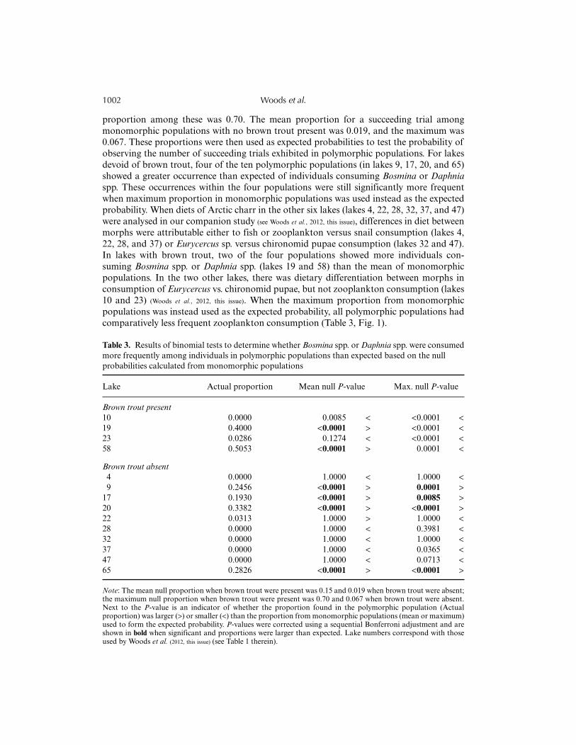
proportion among these was 0.70. The mean proportion for a succeeding trial amongmonomorphic populations with no brown trout present was 0.019, and the maximum was0.067. These proportions were then used as expected probabilities to test the probability ofobserving the number of succeeding trials exhibited in polymorphic populations. For lakesdevoid of brown trout, four of the ten polymorphic populations (in lakes 9, 17, 20, and 65)showed a greater occurrence than expected of individuals consuming Bosmina or Daphniaspp. These occurrences within the four populations were still significantly more frequentwhen maximum proportion in monomorphic populations was used instead as the expectedprobability. When diets of Arctic charr in the other six lakes (lakes 4, 22, 28, 32, 37, and 47)were analysed in our companion study (see Woods et al., 2012, this issue), differences in diet betweenmorphs were attributable either to fish or zooplankton versus snail consumption (lakes 4,22, 28, and 37) or Eurycercus sp. versus chironomid pupae consumption (lakes 32 and 47).In lakes with brown trout, two of the four populations showed more individuals con-suming Bosmina spp. or Daphnia spp. (lakes 19 and 58) than the mean of monomorphicpopulations. In the two other lakes, there was dietary differentiation between morphs inconsumption of Eurycercus vs. chironomid pupae, but not zooplankton consumption (lakes10 and 23) (Woods et al., 2012, this issue). When the maximum proportion from monomorphicpopulations was instead used as the expected probability, all polymorphic populations hadcomparatively less frequent zooplankton consumption (Table 3, Fig. 1).

Table 3. Results of binomial tests to determine whether Bosmina spp. or Daphnia spp. were consumedmore frequently among individuals in polymorphic populations than expected based on the nullprobabilities calculated from monomorphic populations

Lake Actual proportion Mean null P-value Max. null P-value

Brown trout present10 0.0000 0.0085 < <0.0001 <19 0.4000 <0.0001 > <0.0001 <23 0.0286 0.1274 < <0.0001 <58 0.5053 <0.0001 > 0.0001 <

Brown trout absent4 0.0000 1.0000 < 1.0000 <9 0.2456 <0.0001 > 0.0001 >

17 0.1930 <0.0001 > 0.0085 >20 0.3382 <0.0001 > <0.0001 >22 0.0313 1.0000 > 1.0000 <28 0.0000 1.0000 < 0.3981 <32 0.0000 1.0000 < 1.0000 <37 0.0000 1.0000 < 0.0365 <47 0.0000 1.0000 < 0.0713 <65 0.2826 <0.0001 > <0.0001 >

Note: The mean null proportion when brown trout were present was 0.15 and 0.019 when brown trout were absent;the maximum null proportion when brown trout were present was 0.70 and 0.067 when brown trout were absent.Next to the P-value is an indicator of whether the proportion found in the polymorphic population (Actualproportion) was larger (>) or smaller (<) than the proportion from monomorphic populations (mean or maximum)used to form the expected probability. P-values were corrected using a sequential Bonferroni adjustment and areshown in bold when significant and proportions were larger than expected. Lake numbers correspond with thoseused by Woods et al. (2012, this issue) (see Table 1 therein).

Woods et al.1002

Predicting polymorphism using environmental variables

The random forest model performed best when the number of subset explanatory variableswas set to 3, and the best threshold proportion of votes for prediction was 0.5. Sevenexplanatory variables were included according to the stepwise selection procedure in thebest model (Diaz-Uriarte and Alvarez de Andres, 2006; Genuer et al., 2010; Sethi, 2010): Z, SiO2, MD, ST, ACA,BTA, and ALT (in order of Gini index). The OOB error rate was 34.15%, with 22 of 27monomorphic and 5 of 14 polymorphic lakes correctly classified. The model generally had alow AUC of 0.586, indicating moderate to low explanatory ability.

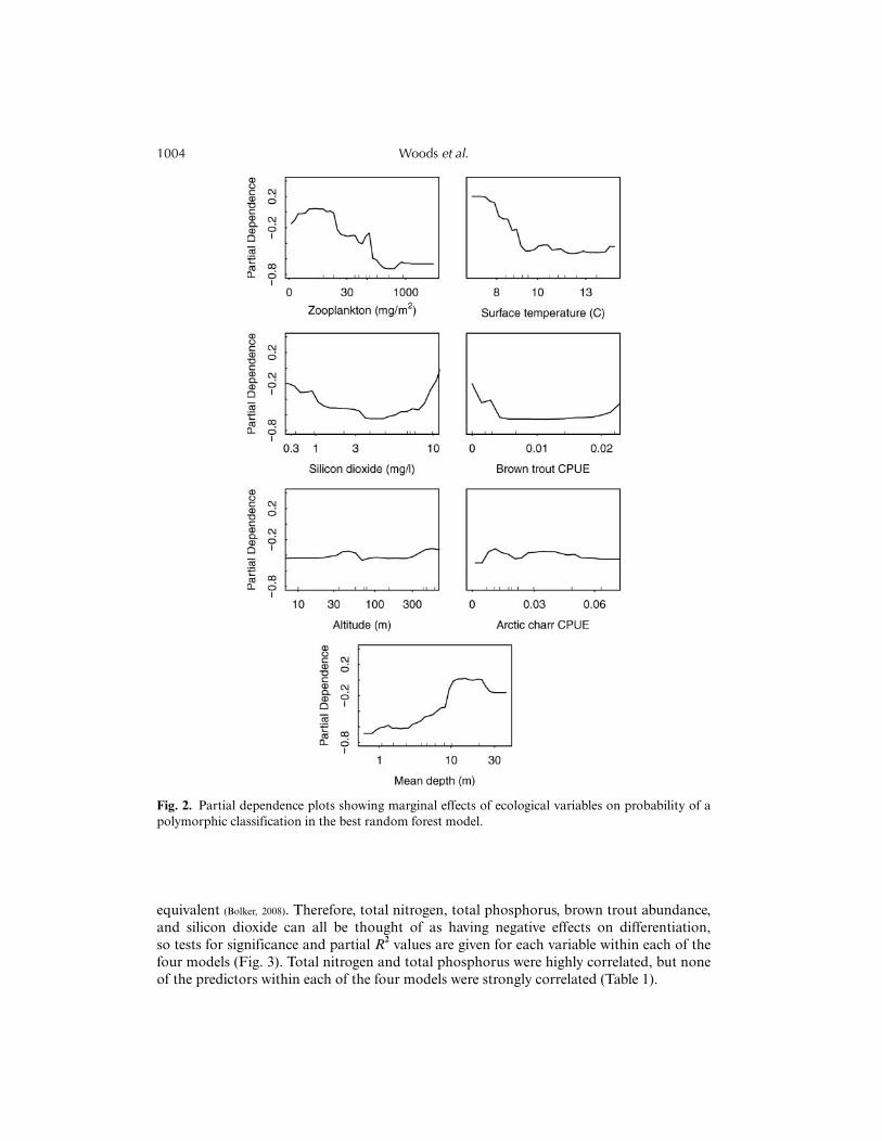
When interpreting partial dependence plots, it is important to note the rug plots along thex-axis. These indicate how well the trends were supported within the data range observed(Fig. 2). The greater partial dependence of resource polymorphism at low values of zoo-plankton abundance and surface temperature was well supported by lakes that span thedata range, indicating that resource polymorphism was more likely to occur in cooler lakeswith low zooplankton abundance. In partial dependence plots, polymorphism was morelikely at low and high values of brown trout abundance and silicon dioxide concentration,but less likely at intermediate values. However, closer inspection showed that the greaterprobability at higher values of these variables depended on only a single lake for each plot;therefore, the right side of these graphs beyond the data range should be disregarded. Theassociation of resource polymorphism with low brown trout abundance contradictshypothesis 3, that greater predator density causes polymorphism, and supports pattern 1b,that polymorphism should be found where there are few interspecific competitors. Thetrends with Arctic charr abundance and altitude were rather weak and variable, so theyare not interpreted further. Deeper lakes were also more likely to contain polymorphicpopulations (Fig. 2).

Multiple regressions by AICc backward and forward selection yielded a set of fourmodels with a change in AICc (δAICc) values < 2 (Table 4). Because the AICc values forthese models differed by less than 2 from the minimum AICc value, they are considered

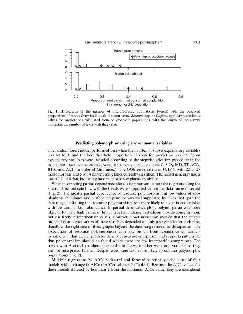
Fig. 1. Histograms of the number of monomorphic populations (y-axis) with the observedproportions of Arctic charr individuals that consumed Bosmina spp. or Daphnia spp. Arrows indicatevalues for proportions calculated from polymorphic populations, with the length of the arrowsindicating the number of lakes with that value.

Environmental trends with resource polymorphism 1003

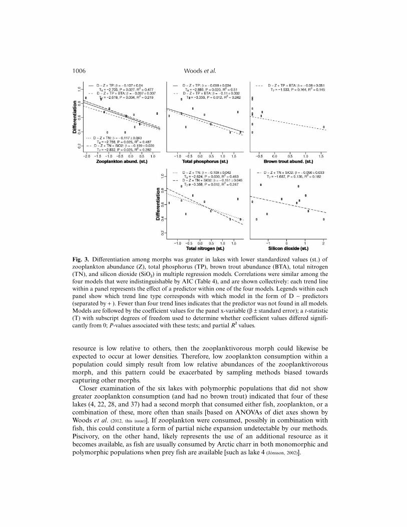
equivalent (Bolker, 2008). Therefore, total nitrogen, total phosphorus, brown trout abundance,and silicon dioxide can all be thought of as having negative effects on differentiation,so tests for significance and partial R2 values are given for each variable within each of thefour models (Fig. 3). Total nitrogen and total phosphorus were highly correlated, but noneof the predictors within each of the four models were strongly correlated (Table 1).

Fig. 2. Partial dependence plots showing marginal effects of ecological variables on probability of apolymorphic classification in the best random forest model.

Woods et al.1004

DISCUSSION

Our results relating Arctic charr polymorphism to lake ecology across Iceland were consist-ent with the first two hypotheses: frequency-dependent selection and niche expansion.These hypotheses are not mutually exclusive, so many of the observed trends may be co-dependent and require experimentation to disentangle. No support was found for the thirdhypothesis, suggesting that polymorphism in Iceland was not related to predation levels onArctic charr.

Support of niche expansion through diet analyses

Niche expansion was detected by two analyses. First, greater total quantities of zoo-plankton were consumed in lakes with polymorphic Arctic charr populations according togeneralized linear models (GLMs). Second, in roughly half the lakes with polymorphicpopulations, individuals consumed zooplankton more frequently, based on binomial tests.Both GLMs and binomial tests also indicated the importance of brown trout abundance inincreased use of zooplankton resources. Therefore, the detection of polymorphism vianiche expansion was confounded whenever brown trout were present. Furthermore, therelative strength of zooplanktivory in Arctic charr likely differs by lake.

We interpret increased consumption of zooplankton in lakes with polymorphicpopulations as niche expansion, but polymorphic lakes lacking detectable increasedzooplankton consumption do not necessarily lack niche expansion. If a morph is highlyefficient at consuming a secondary resource (e.g. zooplankton) or the abundance of that

Table 4. Subset of best multiple regression models topredict Differentiation using the environmental variablesindicated in equation form (separated by +)

Predictor variables AICc δAICc

Z + TP −10.25 0.00Z + TP + BTA −9.58 0.67Z + TN −9.24 1.01Z + TN + SiO2 −9.06 1.19– – – – – – – – – – – – – – – – – – – – – – – – – – – – – – – – – –Z + TP + MD −8.00 2.24Z + TP + BTA + ST −7.75 2.50Z + TP + ST −7.71 2.53Z + TP + ACA −7.14 3.11Z + TP + ALT −6.38 3.87Z + TP + SiO2 −6.33 3.92

Note: Models above the dashed line are those that have a δAICc(i.e. difference between AICc and minimum AICc) < 2, indicatingmodels that are equivalent. All predictors included within thesubset of equivalent models had negative effects (Fig. 3). Modelpredictors include zooplankton abundance (Z), total phosphorusconcentration (TP), brown trout abundance (BTA), total nitrogenconcentration (TN), silicon dioxide concentration (SiO2), meandepth (MD), surface temperature (ST), Arctic charr abundance(ACA), and altitude (ALT).

Environmental trends with resource polymorphism 1005

resource is low relative to others, then the zooplanktivorous morph could likewise beexpected to occur at lower densities. Therefore, low zooplankton consumption within apopulation could simply result from low relative abundances of the zooplanktivorousmorph, and this pattern could be exacerbated by sampling methods biased towardscapturing other morphs.

Closer examination of the six lakes with polymorphic populations that did not showgreater zooplankton consumption (and had no brown trout) indicated that four of theselakes (4, 22, 28, and 37) had a second morph that consumed either fish, zooplankton, or acombination of these, more often than snails [based on ANOVAs of diet axes shown byWoods et al. (2012, this issue)]. If zooplankton were consumed, possibly in combination withfish, this could constitute a form of partial niche expansion undetectable by our methods.Piscivory, on the other hand, likely represents the use of an additional resource as itbecomes available, as fish are usually consumed by Arctic charr in both monomorphic andpolymorphic populations when prey fish are available [such as lake 4 (Jónsson, 2002)].

Fig. 3. Differentiation among morphs was greater in lakes with lower standardized values (st.) ofzooplankton abundance (Z), total phosphorus (TP), brown trout abundance (BTA), total nitrogen(TN), and silicon dioxide (SiO2) in multiple regression models. Correlations were similar among thefour models that were indistinguishable by AIC (Table 4), and are shown collectively: each trend linewithin a panel represents the effect of a predictor within one of the four models. Legends within eachpanel show which trend line type corresponds with which model in the form of D ∼ predictors(separated by + ). Fewer than four trend lines indicates that the predictor was not found in all models.Models are followed by the coefficient values for the panel x-variable (β ± standard error); a t-statistic(T) with subscript degrees of freedom used to determine whether coefficient values differed signifi-cantly from 0; P-values associated with these tests; and partial R2 values.

Woods et al.1006

For all other polymorphic populations that showed low zooplankton consumption (32and 47 with no brown trout present; 10 and 23 with brown trout present), diet differenceswere instead based on chironomid pupae versus Eurycercus spp. consumption (Woods et al.,

2012, this issue). As Eurycercus spp. were consumed less and chironomid pupae were notconsumed more in polymorphic populations (GLMs), our data suggest a partitioning ofthe ancestral morph between these resources, rather than niche expansion. However, thiswas based on few lakes and further comparison of chironomid pupae consumption inmonomorphic versus polymorphic populations is warranted. Perhaps this also constitutes ararer form of niche expansion, as chironomid pupae may be consumed in limnetic zonesas they emerge, and are thought to be an important food source for zooplanktivorousforms during periods of peak chironomid pupae abundance (Malmquist et al., 1992; Woods et al., in

press). In any case, this form of resource segregation is rarely mentioned in the literature, yetappears to be as common in our dataset as the well-known existence of piscivorous Arcticcharr forms.

Environmental characteristics of lakes containing polymorphic populations

In fitting polymorphism to environmental variables, we note that many of the expectedtrends within the three broad hypotheses cannot be separated due to natural correlationsamong landscape features. For example, considering the frequency dependence hypothesis,patterns 1b and 1c (see Introduction) are linked in a manner that would be difficult todisentangle: high altitude and recently deglaciated regions naturally have fewer species(Bernatchez and Wilson, 1998; Robinson and Schluter, 2000; Griffiths, 2006). In addition, monomorphicpopulations in lower elevations may experience more gene flow if there are fewer barriersto migration. Pattern 1a may be further correlated with these conditions because higherconspecific Arctic charr densities are expected under low competitor density, i.e. fewerbrown trout (Langeland et al., 1991; Hesthagen et al., 1997; Jansen et al., 2002; Helland et al., 2011). Therefore, thepatterns presented here should be taken as broadly encompassing many facets, as manyenvironmental variables showed strong correlations among each other (Table 1).

In support of hypothesis 1, lakes were more likely to contain polymorphic Arctic charrpopulations if they were deep, had few competitors, low silicon dioxide concentrations, andlow zooplankton abundance. A similar connection to zooplankton scarcity, low nutrientvalues (i.e. total nitrogen, total phosphorus, and silicon dioxide), and low brown troutabundances was found in multiple regressions to predict greater differentiation (althoughthe effects of silicon dioxide and brown trout abundance were quite low). Upon first glance,the results of GLMs appear contradictory: the negative binomial models indicated thatzooplankton (i.e. Bosmina spp. and Daphnia spp.) were consumed more frequently bypolymorphic populations, but random forest and multiple regression model results suggestthat the presence of polymorphism was associated with low abundances of zooplankton.As low total nutrient levels likely indicated both low dissolved and particulate nutrients(including phytoplankton standing stocks), we offer two explanations for low zooplanktonabundances and low nutrient levels: (1) general productivity and nutrient levels were low, or(2) productivity was high, but biomass turnover rates, via predation and natural mortality,were so fast that biomass levels of all but the top predator (Arctic charr) were low.

For the first explanation for the ‘low nutrient, low zooplankton abundance, high zoo-plankton consumption’ pattern, Arctic charr would be more likely to consume zooplanktonwhen low zooplankton abundance results from low nutrient loading. Low nutrient loading

Environmental trends with resource polymorphism 1007

is not uncommon in Icelandic lakes, as studies of nutrient flux (Jónasson et al., 1992;

Einarsson et al., 2004; Gíslason et al., 2004), diatom assemblages (Dickman et al., 1993; Karst-

Riddoch et al., 2009), experimental nitrogen and phosphorus additions (Friberg et al., 2009;

Guðmundsdóttir et al., 2011), and terrestrial vegetation succession (Cutler, 2011) all suggest thatIcelandic lakes and streams, especially in geologically young volcanic zones, tend to benitrogen-limited, and sometimes phosphorus-limited. Nitrogen limitation is not uncommonfor high-altitude or -latitude lakes due to reduced leaching of limiting nutrients fromterrestrial vegetative areas (Pienitz et al., 1997; Edmundson and Mazumder, 2002; LaPerriere et al., 2003). Ifnutrient loading and productivity are generally low, total food availability is likely limitingand Arctic charr populations may diverge to use alternative resources according to theirrelative availability. This explanation seems likely, given the generalist feeding habits ofArctic charr (Langeland et al., 1991; Halvorsen et al., 1997; Forseth et al., 2003; Klemetsen et al., 2003; McCarthy, 2007).

On the other hand, co-occurring low total phosphorus and nitrogen levels in our datamay indicate that enough nitrogen fixation has occurred to approach co-limitation(Jónasson et al., 1992; Einarsson et al., 2004). This idea is supported by the high correlation betweennitrogen and phosphorus in our data (Table 1). Nutrients would then be limited due to highuptake rates, and phytoplankton and zooplankton production may be higher than our datasuggest. This pattern is supported by exceedingly high estimates of productivity found intwo relatively large oligotrophic Icelandic lakes [Thingvallavatn and Mývatn (Jónasson et al.,

1992)]. This pattern has been interpreted as resulting from high phytoplankton activity perunit biomass due to the dominance of a small-bodied, fast-growing phytoplankton species(Jónasson et al., 1992). In this case, an association of polymorphic populations with low nutrientlevels may signal that the presence of a second morph is facilitated by fast nutrient andenergy cycling in the water column.

Although the mechanism behind the ‘low nutrient, low zooplankton abundance, highzooplankton consumption’ pattern cannot be inferred from our study, this pattern is alsonot uncommon. Siwertsson et al. (2010) found a similar pattern of greater lake whitefishdivergence towards zooplankton consumption in lakes with low nutrient values. Landryet al. (2007) also showed that lake whitefish differentiation towards greater zooplanktonconsumption was positively correlated with an indicator of productivity and low zoo-plankton abundance. Our results also support past studies indicating the importance of lakedepth in the development of polymorphism (Bolnick and Lau, 2008; Vonlanthen et al., 2009). Bolnickand Lau (2008) found that lakes of intermediate depth, rather than shallow or deep lakes,were more likely to contain polymorphic threespine stickleback, potentially indicatingthe importance of evenly balanced resource availability (Bolnick and Lau, 2008). Therefore, aprime area for future research would be to understand how low nutrient levels andlake depths affect relative resource abundances, thereby allowing for the development ofpolymorphism.

Overall, the random forest model used to fit the probability of polymorphism based onenvironmental variables had a relatively low predictive ability, especially for polymorphicpopulations. Such results may occur either because the environmental conditionssurrounding similar polymorphic lakes are highly variable, or because the nature of thepolymorphism defining these lakes is highly variable, or both. For example, perhapspolymorphic lakes should be further categorized by patterns in resource differentiation toobtain clearer links with the environmental variables. The consumption of Daphnia spp.vs. zoobenthos could be analysed separately from the consumption of Bosmina spp. vs.zoobenthos, as the dominance of these taxa may hint at differences in zooplankton

Woods et al.1008

community, possibly as a result of environmental differences. Rarer morphs, such as thosethat consumed mainly fish or chironomid pupae, could also be defined as separatepolymorphism types. Unfortunately, to follow through with this fine-scale categorizationenvironmental analyses would require more data than available even in the extensivedatabase used for this study.

In summary, this study has indicated that patterns in resource polymorphism in Arcticcharr across Icelandic lakes likely result from frequency-dependent selection, not predationrisk. Niche expansion towards the use of zooplankton appears to occur in approximatelyhalf the cases of polymorphism, although less common morphs that consume fish orchironomid pupae were also detected. Polymorphic populations were more likely to occuror become more greatly differentiated in lakes with low nutrient concentrations, lowzooplankton abundances, and greater depths. However, the mechanisms inducingfrequency-dependent selection under these environmental characteristics remain unknown.Future studies should focus on elucidating measures of within-lake relative prey abundancethat better link how frequency dependence and niche expansion develop within specificpolymorphism types, and how this is influenced by nutrient dynamics or lake depth.

ACKNOWLEDGEMENTS

This research was supported by the European Marie Curie Research Training Network FishACE (Fisheries-induced Adaptive Changes in Exploited Stocks), funded through the EuropeanCommunity’s Sixth Framework Programme (Contract MRTN-CT-2004-005578), a research grantprovided by the Icelandic Centre for Research, Leifur Eiríksson Foundation, and the University ofWashington Graduate School Fund for Excellence and Innovation. The ESIL project was fundedwith grants from the Icelandic Research Council, the Ministry of the Environment, the Ministry ofAgriculture, and the Icelandic Fisheries Research Fund. Special thanks are due to those who par-ticipated in the Ecological Survey of Icelandic Lakes, especially the Icelandic Institute of FreshwaterFisheries. We thank Dr. Daniel Schindler and Dr. Michael Kinnison for reviewing earlier versions ofthe manuscript.

REFERENCES

Abrams, P.A. 2000. Character shifts of prey species that share predators. Am. Nat., 156 (suppl.):S45–S61.

Bernatchez, L. and Wilson, C.C. 1998. Comparative phylogeography of Nearctic and Palearcticfishes. Molec. Ecol., 7: 431–452.

Bolker, B.M. 2008. Ecological Models and Data in R. Princeton, NJ: Princeton University Press.Bolnick, D.I. 2004. Can intraspecific competition drive disruptive selection? An experimental test

in natural populations of sticklebacks. Evolution, 58: 608–618.Bolnick, D.I. and Lau, O.L. 2008. Predictable patterns of disruptive selection in sticklebacks of

postglacial lakes. Am. Nat., 172: 1–11.Breiman, L. 2001. Random forests. Machine Learning, 45: 5–32.Breiman, L. 2002. Manual on Setting Up, Using, and Understanding Random Forests v3.1.

http://oz.berkeley.edu/users/breiman/Using_random_forests_V3.1.pdf (last accessed 13 July2011).

Cutler, N. 2011. Nutrient limitation during long-term ecosystem development inferred from amat-forming moss. Bryologist, 114: 204–214.

Diaz-Uriarte, R. and Alvarez de Andres, S. 2006. Gene selection and classification of microarraydata using random forest. BMC Bioinformatics, 7: 3–15.

Environmental trends with resource polymorphism 1009

Dickman, M., Stewart, K. and Servant-Vildary, M. 1993. Spatial heterogeneity of summer phyto-plankton and water chemistry in a large volcanic spring-fed lake in Northern Iceland. ArcticAlpine Res., 25: 228–239.

Dieckmann, U., Metz, J.A.J., Doebeli, M. and Tautz, D. 2004. Adaptive Speciation. Cambridge:Cambridge University Press.

Doucette, L.I., Skúlason, S. and Snorrason, S.S. 2004. Risk of predation as a promoting factor ofspecies divergence in threespine sticklebacks (Gasterosteus aculeatus L.). Biol. J. Linn. Soc., 82:189–203.

Edmundson, J.A. and Mazumder, A. 2002. Regional and hierarchical perspectives of thermalregimes in subarctic, Alaskan lakes. Freshw. Biol., 47: 1–17.

Einarsson, Á., Stefánsdóttir, G., Jóhannesson, H., Ólafsson, J.S., Gíslason, G.M., Wakana, I.et al. 2004. The ecology of Lake Myvatn and the River Laxá: variation in space and time.Aquat. Ecol., 38: 317–348.

Eustace, A.H., Pringle, M.J. and Denham, R.J. 2011. A risk map for gully locations in centralQueensland, Australia. Eur. J. Soil Sci., 62: 431–441.

Forseth, T., Ugedal., O., Jonsson, B. and Fleming, I. 2003. Selection on Arctic charr generated bycompetition from brown trout. Oikos, 101: 467–478.

Friberg, N., Dybkjær, J.B., Ólafsson, J.S., Gíslason, G.M., Larsen, S.E. and Lauridsen,T.L. 2009. Relationships between structure and function in streams contrasting in temperature.Freshw. Biol., 54: 2051–2068.

Genuer, R., Poggi, J.M. and Tuleau-Malot, C. 2010. Variable selection using random forests. Patt.Recog. Lett., 31: 2225–2236.

Gíslason, S.R., Eiríksdóttir, E.S. and Ólafsson, J.S. 2004. Chemical composition of interstitial waterand diffusive fluxes within the diatomaceous sediment in Lake Myvatn, Iceland. Aquat. Ecol.,38: 163–175.

Griffiths, D. 1994. The size structure of lacustrine Arctic charr (Pisces: Salmonidae) populations.Biol. J. Linn. Soc., 51: 337–357.

Griffiths, D. 2006. Pattern and process in the ecological biogeography of European freshwater fish.J. Anim. Ecol., 75: 734–751.

Guðmundsdóttir, R., Ólafsson, J.S., Pálsson, S., Gíslason, G.M. and Moss, B. 2011. How willincreased temperature and nutrient enrichment affect primary producers in sub-Arctic streams?Freshw. Biol., 56: 2045–2058.

Halvorsen, M., Jørgensen, L. and Amundsen, P.-A. 1997. Habitat utilization of juvenile Atlanticsalmon (Salmo salar L.), brown trout (Salmo trutta L.) and Arctic charr (Salvelinus alpinus L.)in two lakes in northern Norway. Ecol. Freshw. Fish, 6: 67–77.

Helland, I.P., Finstad, A.G., Forseth, T., Hesthagen, T. and Ugedal, O. 2011. Ice-cover effects oncompetitive interactions between two fish species. J. Anim. Ecol., 80: 539–547.

Hesthagen, T., Jonsson, B., Ugedal, O. and Forseth, T. 1997. Habitat use and life history of browntrout (Salmo trutta) and Arctic charr (Salvelinus alpinus) in some low acidity lakes in centralNorway. Hydrobiologia, 348: 113–126.

Jansen, P.A., Slettvold, H., Finstad, A.G. and Langeland, A. 2002. Niche segregation between Arcticchar (Salvelinus alpinus) and brown trout (Salmo trutta): an experimental study of mechanisms.Can. J. Fish. Aquat. Sci., 59: 6–11.

Jónasson, P.M., Aðalsteinsson, H. and St. Jónsson, G. 1992. Production and nutrientsupply of phytoplankton in subarctic, dimictic Thingvallavatn, Iceland. Oikos, 64:162–187.

Jónsson, B. 2002. Parallel sympatric segregation in Arctic charr and threespined stickleback in LakeGaltaból, Iceland. Fish. Sci., 68 (supp. 1): 459–460.

Karst-Riddoch, T.L., Malmquist, H.J. and Smol, J.P. 2009. Relationships between freshwater sedi-mentary diatoms and environmental variables in Subarctic Icelandic lakes. Fund. Appl. Limnol.,175: 1–28.

Woods et al.1010

Klemetsen, A., Amundsen, P.-A., Dempson, J.B., Jonsson, B., Jonsson, N., O’Connell, M.F. etal. 2003. Atlantic salmon Salmo salar L., brown trout Salmo trutta L. and Arctic charr Salveli-nus alpinus (L.): a review of aspects of their life histories. Ecol. Freshw. Fish, 12: 1–59.

Knudsen, R., Klemetsen, A., Amundsen, P.-A. and Hermansen, B. 2006. Speciation throughniche expansion: an example from the Arctic charr in a subarctic lake. Proc. R. Soc. Lond. B, 273:2291–2298.

Kristjánsson, B.K., Malmquist, H.J., Ingimarsson, F., Antonsson, T., Snorrason, S.S. and Skúlason,S. 2011. Relationships between lake ecology and morphological characters in Icelandic Arcticcharr, Salvelinus alpinus. Biol. J. Linn. Soc., 103: 761–771.

Landry, L., Vincent, W.F. and Bernatchez, L. 2007. Parallel evolution of lake whitefish dwarfecotypes in association with limnological features of their adaptive landscape. J. Evol. Biol., 20:971–984.

Langeland, A., L’Abée-Lund, J.H., Jonsson, B. and Jonsson, N. 1991. Resource partitioning andniche shift in Arctic charr Salvelinus alpinus and brown trout Salmo trutta. J. Anim. Ecol., 60:895–912.

Langerhans, R.B., Layman, C.A., Shokrollahi, A.M. and DeWitt, T.J. 2004. Predator-drivenphenotypic diversification in Gambusia affinis. Evolution, 58: 2305–2318.

LaPerriere, J.D., Jones, J.R. and Swanson, D.K. 2003. Limnology of lakes in Gates of the ArcticNational Park and Preserve, Alaska. Lake Reservoir Manage., 19: 108–121.

Liaw, A. and Wiener, M. 2002. Classification and regression by randomForest. R News, 2: 18–22.http://www.r-project.org/doc/Rnews/Rnews_2002-3.pdf (last accessed 13 July 2011).

Malmquist, H.J., Snorrason, S.S., Skúlason, S., Jónsson, B., Sandlund, O.T. and Jónasson,P.M. 1992. Diet differentiation in polymorphic Arctic charr in Thingvallavatn, Iceland. J. Anim.Ecol., 61: 21–35.

Malmquist, H.J., Antonsson, T., Guðbergsson, G., Skúlason, S. and Snorrason, S.S. 2000. Bio-diversity of macroinvertebrates on rocky substrate in the surf zone of Icelandic lakes. Verhand.Internat. Limnol., 27: 1–7.

McCarthy, I.D. 2007. The Welsh Torgoch (Salvelinus alpinus): a short review of its distribution andecology. Ecol. Freshw. Fish, 16: 34–40.

Pienitz, R., Smol, J.P. and Lean, D.R.S. 1997. Physical and chemical limnology of 59 lakes locatedbetween the southern Yukon and the Tuktoyaktuk Peninsula, Northwest Territories (Canada).Can. J. Fish. Aquat. Sci., 54: 330–346.

Prasad, A.M., Iverson, L.R. and Liaw, A. 2006. Newer classification and regression tree techniques:bagging and random forests for ecological prediction. Ecosystems, 9: 181–199.

R Development Core Team. 2011. R: A Language and Environment for Statistical Computing.Vienna, Austria: R Foundation for Statistical Computing http://www.R-project.org (last accessed13 July 2011).

Robinson, B.W. and Schluter, D. 2000. Natural selection and the evolution of adaptive geneticradiation in northern freshwater fishes. In Adaptive Genetic Variation (T.A., Mousseau,B. Sinervo and J. Endler, eds.), pp. 65–94. Oxford: Oxford University Press.

Robinson, B.W. and Wilson, D.S. 1994. Character release and displacement in fishes: a neglectedliterature. Am. Nat., 144: 596–627.

Rundle, H.D., Vamosi, S.M. and Schluter, D. 2003. Experimental test of predation’s effect ondivergent selection during character displacement in sticklebacks. Proc. Natl. Acad. Sci. USA,100: 14943–14948.

Schluter, D. 1994. Experimental evidence that competition promotes divergence in adaptiveradiation. Science, 266: 798–801.

Schluter, D. 1996. Ecological speciation in postglacial fishes. Phil. Trans. R. Soc. Lond. B, 351:807–814.

Schluter, D. 2003. Frequency dependent natural selection during character displacement in stickle-backs. Evolution, 57: 1142–1150.

Environmental trends with resource polymorphism 1011

Sethi, S.A. 2010. Fisheries management with people in mind: assessing and managing risk. PhD thesis,University of Washington, Seattle, WA.

Sing, T., Sander, O., Beerenwinkel, N. and Lengauer, T. 2005. ROCR: visualizing classifier per-formance in R. Bioinformatics, 21: 3940–3941.

Siwertsson, A., Knudsen, R., Kahilainen, K.K., Praebel, K., Primicerio, R. and Amundsen,P.A. 2010. Sympatric diversification as influenced by ecological opportunity and historicalcontingency in a young species lineage of whitefish. Evol. Ecol. Res., 12: 929–947.

Skúlason, S. and Smith, T.B. 1995. Resource polymorphisms in vertebrates. Trends Ecol. Evol., 10:366–370.

Skúlason, S., Snorrason, S.S. and Jónsson, B. 1999. Sympatric morphs, populations and speciationin freshwater fish with emphasis on arctic charr. In Evolution of Biological Diversity (A.E.Magurran and R.M. May, eds.), pp. 70–92. Oxford: Oxford University Press.

Snorrason, S.S. and Skúlason, S. 2004. Adaptive speciation in northern freshwater fishes. In AdaptiveSpeciation (U. Dieckmann, M. Doebeli, J.A.J. Metz and D. Tautz, eds.), pp. 210–228. Cambridge:Cambridge University Press.

Strobl, C., Boulesteix, A.L., Zeileis, A. and Hothorn, T. 2007. Bias in random forest variableimportance measures: illustrations, sources and a solution. BMC Bioinformatics, 8: 25–45.

Svanbäck, R. and Bolnick, D.I. 2007. Intraspecific competition drives increased resource usediversity within a natural population. Proc. R. Soc. Lond. B, 274: 839–844.

Svanbäck, R. and Persson, L. 2004. Individual diet specialization, niche width, and populationdynamics: implications for trophic polymorphisms. J. Anim. Ecol., 73: 973–982.

Vamosi, S.M. and Schluter, D. 2002. Impacts of trout predation on fitness of sympatric sticklebacksand their hybrids. Proc. R. Soc. Lond. B, 269: 923–930.

Van Valen, L. 1965. Morphological variation and width of ecological niche. Am. Nat., 99: 277–290.Vonlanthen, P., Roy, D., Hudson, A.G., Larglader, C.R., Bittner, D. and Seehausen, O. 2009.

Divergence along a steep ecological gradient in lake whitefish (Coregonus sp.). J. Evol. Biol.,22: 498–514.

Woods, P.J., Skúlason, S., Snorrason, S.S., Kristjánsson, B.K., Malmquist, H.J. and Quinn, T.P. 2012.Intraspecific diversity in Arctic charr, Salvelinus alpinus, in Iceland: I. Detection using mixturemodels. Evol. Ecol. Res., 14: 973–992.

Woods, P.J., Skúlason, S., Snorrason, S.S., Kristjánsson, B.K., Ingimarsson, F. and Malmquist,H.J. in press. Variability in the functional role of Arctic charr Salvelinus alpinus as it relates tolake ecosystem characteristics. Environ. Biol. Fish.

Zou, K.H., O’Malley, A.J. and Mauri, L. 2007. Receiver-operating characteristic analysis forevaluating diagnostic tests and predictive models. Circulation, 115: 654–657.

APPENDIX

Indicator biomass conversions for prey taxa are given along with the frequency found incapture habitat based on invertebrate surveys. Biomass indicators are based on the order ofmagnitude of dry weights found for individual taxa in the literature (see Woods et al., in press, for

details). Capture habitats include stone (S), fine-grained sediment (from Kajak cores,mud: M), or the water column (from plankton nets, W). Prey categories included snail (S),tadpole shrimp (T), pea clam (P), zooplankton (Z), chironomid pupae (C), and fish (F).Capture habitats are listed in order of importance, with backslashes indicating similarfrequencies (20–80%). Parentheses indicate that expert knowledge was used to fillinformation for taxa absent in invertebrate surveys. Adapted from Woods et al. (in press).

Woods et al.1012

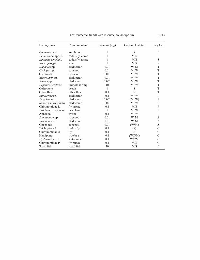
Dietary taxa Common name Biomass (mg) Capture Habitat Prey Cat.

Gammarus sp. amphipod 1 S 0Limnephilus spp. L caddisfly larvae 1 M/S SApatania zonella L caddisfly larvae 1 M/S SRadix peregra snail 1 M/S SDaphnia spp. cladoceran 0.01 W, M TCyclops spp. copepod 0.01 M, W TOstracoda ostracod 0.001 M, W TMacrothrix sp. cladoceran 0.01 M, W TAlona spp. cladoceran 0.001 M, W TLepidurus arcticus tadpole shrimp 10 M, W TColeoptera beetle 1 S TOther flies other flies 0.1 S TEurycercus sp. cladoceran 0.1 M, W PPolyphemus sp. cladoceran 0.001 (M, W) PSimocephalus vetulus cladoceran 0.001 M, W PChironomidae L fly larvae 0.1 M/S PPisidium casertanum pea clam 1 M, W PAnnelida worm 0.1 M, W PDiaptomus spp. copepod 0.01 W, M ZBosmina sp. cladoceran 0.01 W, M ZCopepoda copepod 0.01 (W/M) ZTrichoptera A caddisfly 0.1 (S) CChironomidae A fly 0.1 S CHemiptera true bug 0.1 (WC/M) CHydracarina sp. water mite 0.1 WC/M CChironomidae P fly pupae 0.1 M/S CSmall fish small fish 10 M/S F

Environmental trends with resource polymorphism 1013