Interferometric vs Spectral IASI Radiances: Effective Data-Reduction Approaches for the Satellite...
24
Remote Sensing 2010, 2, 2323-2346; doi:10.3390/rs2102323 OPEN ACCESS Remote Sensing ISSN 2072-4292 www.mdpi.com/journal/remotesensing Article Interferometric vs Spectral IASI Radiances: Effective Data-Reduction Approaches for the Satellite Sounding of Atmospheric Thermodynamical Parameters Giuseppe Grieco, Guido Masiello and Carmine Serio ⋆ DIFA, University of Basilicata, Via Ateneo Lucano 10, Potenza, Italy; E-Mails: [email protected] (G.G.); [email protected] (G.M.) ⋆ Author to whom correspondence should be addressed; E-Mail: [email protected]; Tel.: +39-0971-205-222; Fax +39-0971-205-215. Received: 13 August 2010; in revised form: 29 August 2010 / Accepted: 25 September 2010 / Published: 27 September 2010 Abstract: Two data-reduction approaches for the Infrared Atmospheric Sounder Interferometer satellite instrument are discussed and compared. The approaches are intended for the purpose of devising and implementing fast near real time retrievals of atmospheric thermodynamical parameters. One approach is based on the usual selection of sparse channels or portions of the spectrum. This approach may preserve the spectral resolution, but at the expense of the spectral coverage. The second approach considers a suitable truncation of the interferogram (the Fourier transform of the spectrum) at points below the nominal maximum optical path difference. This second approach is consistent with the Shannon-Whittaker sampling theorem, preserves the full spectral coverage, but at the expense of the spectral resolution. While the first data-reduction acts within the spectral domain, the second can be performed within the interferogram domain and without any specific need to go back to the spectral domain for the purpose of retrieval. To assess the impact of these two different data-reduction strategies on retrieval of atmospheric parameters, we have used a statistical retrieval algorithm for skin temperature, temperature, water vapour and ozone profiles. The use of this retrieval algorithm is mostly intended for illustrative purposes and the user could choose a different inverse strategy. In fact, the interferogram-based data-reduction strategy is generic and independent of any inverse algorithm. It will be also shown that this strategy yields subset of interferometric radiances, which are less sensitive to potential interfering effects such as those possibly introduced
Transcript of Interferometric vs Spectral IASI Radiances: Effective Data-Reduction Approaches for the Satellite...

Remote Sensing 2010, 2, 2323-2346; doi:10.3390/rs2102323OPEN ACCESS
Remote SensingISSN 2072-4292
www.mdpi.com/journal/remotesensing
Article
Interferometric vs Spectral IASI Radiances: EffectiveData-Reduction Approaches for the Satellite Sounding ofAtmospheric Thermodynamical ParametersGiuseppe Grieco, Guido Masiello and Carmine Serio ⋆
DIFA, University of Basilicata, Via Ateneo Lucano 10, Potenza, Italy;E-Mails: [email protected] (G.G.); [email protected] (G.M.)
⋆ Author to whom correspondence should be addressed; E-Mail: [email protected];Tel.: +39-0971-205-222; Fax +39-0971-205-215.
Received: 13 August 2010; in revised form: 29 August 2010 / Accepted: 25 September 2010 /Published: 27 September 2010
Abstract: Two data-reduction approaches for the Infrared Atmospheric SounderInterferometer satellite instrument are discussed and compared. The approaches are intendedfor the purpose of devising and implementing fast near real time retrievals of atmosphericthermodynamical parameters. One approach is based on the usual selection of sparsechannels or portions of the spectrum. This approach may preserve the spectral resolution,but at the expense of the spectral coverage. The second approach considers a suitabletruncation of the interferogram (the Fourier transform of the spectrum) at points belowthe nominal maximum optical path difference. This second approach is consistent withthe Shannon-Whittaker sampling theorem, preserves the full spectral coverage, but at theexpense of the spectral resolution. While the first data-reduction acts within the spectraldomain, the second can be performed within the interferogram domain and without anyspecific need to go back to the spectral domain for the purpose of retrieval. To assessthe impact of these two different data-reduction strategies on retrieval of atmosphericparameters, we have used a statistical retrieval algorithm for skin temperature, temperature,water vapour and ozone profiles. The use of this retrieval algorithm is mostly intendedfor illustrative purposes and the user could choose a different inverse strategy. In fact,the interferogram-based data-reduction strategy is generic and independent of any inversealgorithm. It will be also shown that this strategy yields subset of interferometric radiances,which are less sensitive to potential interfering effects such as those possibly introduced

Remote Sensing 2010, 2 2324
by the day-night cycle (e.g., the solar component, and spectroscopic effect induced by sunenergy) and unknown trace gases variability.
Keywords: infrared; satellites; Fourier transform spectrometers; atmospheric temperature;atmospheric water vapour; atmospheric ozone
1. Introduction
The Infrared Atmospheric Sounding Interferometer (IASI) is providing data of unprecedented spectralquality and accuracy (see e.g., [1]). The assimilation of IASI radiances has produced a significantpositive impact on forecast quality (e.g., [2]) and on the exploitation of trace gases information foratmospheric chemistry.
IASI has been developed in France by the Centre National d’Etudes Spatiales (CNES) and is flyingon board the Metop-A (Meteorological Operational Satellite) platform, the first of three satellites of theEuropean Organization for the Exploitation of Meteorological Satellite (EUMETSAT) European PolarSystem (EPS).
IASI has been primarily put in orbit to work for a meteorological mission, hence its main objective isto provide suitable information on temperature and water vapour profiles. The instrument has a spectralcoverage extending from 645 to 2,760 cm−1, which with a sampling interval ∆σ = 0.25 cm−1 gives8,461 data points or channels for each single spectrum. Data samples are taken at intervals of 25 kmalong and across track, each sample having a minimum diameter of about 12 km. With a swath widthon Earth’s surface of about 2,000 kilometres, global coverage is achieved in 12 hours, during which theinstrument records about 650,000 spectra.
This large amount of data is still now hampering the full exploitation of IASI data at NumericalWeather Prediction (NWP) centers, and in all those situations in which we have the constraint ofprocessing the data in near real time. As an example, to reduce the significant computational burden,of the NIASI = 8461 channels received at the European Centre for Medium Range Weather Forecasts(ECMWF) only N = 366 are routinely monitored [2] and even less (N = 168) are actively assimilated.
However, whatever the methodology or selection rules we apply, any channels reduction directlyperformed in the spectral domain, which yields a sparse sub-set of N radiances with N < NIASI ,violates the Shannon-Whittaker sampling theorem (e.g., [3]) and, therefore, occurs at expense of the fullIASI spectral coverage, and irreversibly destroys that information which is contained in the portion ofthe spectrum or set of channels we do not use.
Conversely, if we first Fourier transform the full IASI spectrum, in order to get the interferogram, andsecond we just truncate the interferogram and retain only the first N out of NIASI samples, we perform achannel interpolation, which is consistent with the Shannon-Whittaker sampling theorem and, therefore,leaves unchanged the full IASI spectral coverage.
Having in mind mainly the retrieval of thermodynamical parameters (temperature and water vapour),the main objective of this study is to demonstrate, with IASI retrieval exercises, the use of theinterferogram-based data reduction approach and compare it to channels selection rules (e.g., [4]), which

Remote Sensing 2010, 2 2325
work directly in the spectral domain. As said, the intercomparison will be performed by performinga series of IASI retrieval exercises for temperature, water vapour and ozone, based on subsets of IASIchannels obtained with both the interferogram-based data reduction truncation approach and the selectionof sparse spectral channels, respectively.
Data-reduction performed directly in the wave number domain by picking up suitable channels savesthe spectral quality of the data (i.e., spectral resolution), but, conversely, it applies no filter to the noise,and destroys the initial full spectral coverage.
On the other hand, truncation in the interferogram domain saves the full spectral coverage, reducesthe noise because we reduce its bandwidth, but degrades the spectral quality.
According to [5] spectral resolution is important to have peaked weighting functions for temperature.However, other authors [6,7] who addressed the problem of vertical spatial resolution in the context of theinterferogram domain found out that the sharpness of weighting functions can even increase consideringinterferogram rather than spectral radiances.
It is fair to say that there is an alternative to the Fourier transform of the spectrum in order to useinformation from all IASI channels. This relies on a different kind of linear transform, which is theEmpirical Orthogonal Functions (EOF) or Principal Component Analysis (PCA) transform (e.g., [8], seealso [9] for a review on the application of EOF to the field of satellite meteorology). Then, instead oftruncating the interferogram radiances, we truncate the PC scores.
The advantage of the EOF transform is that, by truncation, not only we save the full spectral coverageas in the case of the Fourier transform, but we retain most of the spectral quality, because of theeffectiveness of the EOF transform to represent complex but highly redundant signals (as it is the caseof atmospheric spectra) with few PC scores. It might seem that the EOF transform makes the kind ofmagic we need. However, in case we EOF transform the full spectrum, the results is to retain all thosefactors, which may potentially interfere with the temperature and water vapour retrieval process and addbiases to the final products.
Thus, while the EOF approach remains appealing for data compression, it does not solve the problemof alleviating the effect of interfering factors when we use the data for retrieval purposes, unless weremove from the spectral coverage those interfering portions of the spectrum. However, once again thisapproach would sacrifice the full IASI spectral range and make one work with a partial coverage.
The potential interfering factors include minor species (e.g., methane and carbon monoxide), whichare normally not retrieved in the context of meteorological applications, and therefore could add moreuncertainty to the final products of temperature and water vapour. In addition, the IASI spectrum extendsto the side of short wave numbers 2,100 to 2,760 cm−1. At these wave numbers the energy measuredfrom IASI contains a mixture of earth and solar spectra, which may introduce (for daytime spectra)further computational burden and uncertainty in the final products. Moreover, during daytime the coreof the CO2 ν3-band is influenced by non Local Thermodynamic Equilibrium (non LTE), which furthercomplicate the use of the short wave side of the spectrum.
To this respect, the appealing characteristic of the Fourier transform is that it also carries out the taskof transforming very localized and narrow-band spectral features in new ones, which are broadened,distributed and diluted over the entire variability range of the transformed data space, so that theymay become negligible with respect to the strong signal introduced by temperature and water vapour.

Remote Sensing 2010, 2 2326
Thus, even if we want to maintain the machinery of EOF transform within our retrieval scheme, itwould be desirable to first project the data space in a new (orthogonal) one having the characteristicsoutlined above.
It is also important to stress, at this point, that the above projection is what a Fourier transformspectrometer (FTS), such as IASI, automatically provides when it measures the interferogram, which, infact, is the Fourier transform of the spectrum.
Since the spectrum is the linear Fourier transform of the interferogram, and conversely, in general theybring the same information. However, the situation we discuss here is not perfectly symmetric, since forthe spectral domain we use only a partial coverage because of the problem of avoiding interfering effectsand the prohibitive computational effort for real time applications. For the case of the interferogram weuse a truncated version of the interferogram, which has the effect of reducing the number of data points,but still preserving the full spectral coverage. The equivalence between the two spaces is also brokenbecause of noise. In the spectral domain the noise can be correlated because of mathematical apodization,such as that applied to IASI. Conversely even with mathematical apodization in the inteferogram domainthe noise is fairly constant in strength (variance) and is uncorrelated. Finally the signal-to-noise ratio ishigher in the interferogram space than in the spectral domain.
As said before, the use of the interferogram instead of the spectrum for the retrieval of atmosphericparameters is not completely new. It was first suggested and discussed in [6,7] for the case oftemperature. In [6,7] the authors also argued that the interferogram domain could improve the verticalspatial resolution of the retrievals because of weighting functions, which are sharper of those availablein the spectral domain. However, until now the method has non been demonstrated on the basis ofreal observations.
As already outlined before, the main objective of this paper is to illustrate, demonstrate and exemplifythe potential advantages of the interferogram-based data reduction and retrieval over those provided bythe spectrum, through the exploitation of IASI data.
Towards this objective, we have used a retrieval methodology, which is based on a linear regressionalgorithm, in which the data space (spectral radiance domain or interferometric radiance domain) isfurther transformed via EOF in order to reduce the dimensionality of the inverse problem. The EOFregression approach has been used by many authors, among which we refer to [9–13]).
The paper is organized as follows. In Section 2 we describe the basic aspects of ourinterferogram-based data-reduction approach, along with information relevant to forward and inversecalculations. In Section 3 we describe two different subsets of IASI channels for the purpose of near realtime dissemination and retrieval processing of IASI data. A series of retrieval exercises exploiting thereduced data sets of IASI channels will be presented and discussed in Section 4. Conclusions are drawnin Section 5.
2. Methodological Background: Data Reduction Principles, Forward/Inverse Methodology
2.1. The Fourier Pair: Spectrum, R(σ), Interferogram, I(x)
The emission spectrum R(σ), σ being the wave number, of a given source is physically defined in theinterval [0,∞]. However, according to the Shannon Whittaker sampling theorem [3], only bandlimited

Remote Sensing 2010, 2 2327
functions can be effectively sampled without loss of information. In practice, the band-limited propertyis achieved by suitable optical filtering, so that the spectrum R(σ) may be mathematically representedby the band-limited function,
R(σ) =
arbitrary for σ1 ≤ σ ≤ σ2
0 otherwise(1)
where σ2 − σ1 is the bandwidth of the spectrum signal.To cope with the symmetry of the Fourier transform and for a correct application of the convolution
theorem, formal mathematical calculations employ the even function Rt(σ), defined in the interval[−∞, +∞]: Rt(−σ) = Rt(σ), Rt(σ) = R(σ)/2. Note that this definition leaves the total energyunchanged, that is, ∫ +∞
−∞Rt(σ)dσ =
∫ +∞
0R(σ)dσ (2)
The function R(σ) is often referred to as the one-sided spectrum, whereas Rt(σ) is the two-sidedspectrum. The interferogram I(x), which is the function actually measured, e.g., by Fourier TransformSpectrometers, is then the Fourier transform of Rt(σ).
I(x) =∫ +∞
−∞Rt(σ) exp(−2πiσx)dσ (3)
with i the imaginary unit. Note that I(x) is itself an even function, and x is a spatial coordinate,physically related to the optical path difference of the two light beams that travel in the interferometer.If we know, I(x), then Rt(σ) can be recovered by considering the inverse Fourier transform,
Rt(σ) =∫ +∞
−∞I(x) exp(2πiσx)dx (4)
It should be stressed that the a Fourier pair, (R(σ), I(x)) can be defined independently of heinstrument we use to acquire either of R(σ) and I(x). Although, for an interferometer spectrometer,I(x) has a physical meaning, here we are interested in the mathematical properties of the transformitself. Thus, the fact that IASI spectra are, e.g, apodized is of no important concern in the analysis. Wejust consider the Fourier transform of these apodized spectra.
Coming now to the particular case of IASI, Figure 1 exemplifies a couple (R(σ), I(x)) for thisinstrument. According to the Shannon-Whittaker sampling theorem [3], the Fourier transform providesthe right mathematics to sample the band-limited function, R(σ) to, e.g., a sampling rate different fromthe original one. This involves the well-known Nyquist rule about the two sampling rates, ∆σ and ∆x
in the spectral and interferogram domain, respectively,
∆σ =1
2xmax
, ∆x =1
2(σ2 − σ1)(5)
where xmax is the maximum optical depth and, as before, σ2 − σ1 is the spectral bandwidth. For IASIwe have σ1 = 645 cm−1, σ2 = 2760 cm−1 and xmax = 2 cm.
In case we want to re-sample the IASI spectrum at a new rate, say ∆σ∗, the operations involvedconsist in
1. Fourier transform the spectrum to the interferogram domain

Remote Sensing 2010, 2 2328
Figure 1. Example of IASI observed spectrum, R(σ), shown in panel (a), and itsmathematical Fourier transform, I(x), shown in panel (b). The behaviour of I(x) closeto x = 0 is shown in the inset. The interferogram interval [0,0.8] cm has been drawn in redin panel (b).
800 1000 1200 1400 1600 1800 2000 2200 2400 26000
0.05
0.1
wave number, σ (cm−1)
R(σ
), W
−m
−2 −
(cm
−1 )−
1 −sr
−1
a)
0 0.5 1 1.5 2−3
−2
−1
0
1
2
3
optical path difference, x (cm)
I(x)
, W−
m−
2 −sr
−1
b)
0 2 4 6
x 10−3
−200
204060
x (cm)
I(x)
CO2 signature
2. cut the interferogram at a new x∗max = 1/(2∆σ∗)
3. transform back the truncated interferogram to the spectral domain.
An alternative processing approach, which yields the same result, could be to use a suitable cardinalsine (or sinc function) interpolation in the spectral domain. This would avoid the passage through theinterferogram domain. However, we prefer to use the method outlined above, since we want also toshow that the processing chain for the retrieval of atmospheric parameters can be validly performed inthe interferogram domain.
However, either we transform to the interferogram domain or we simply apply a sinc interpolation inthe spectral domain, the operation leaves unchanged the spectral coverage, while it changes the spectralsampling from ∆σ to ∆σ∗.
As anticipated in Figure 1, if we truncate the interferogram at xmax = 0.8 cm−1 and take theinverse Fourier transform back to the spectral domain, we have the spectrum with the new sampling∆σ = 0.625 cm−1, instead of the original one of ∆σ = 0.25 cm−1. Furthermore, the original8,461 spectral data points, would be scaled down by a factor which is equal to the ratio of the twosamplings, so that we are left with 3,385 data points.
An example of these two spectra is shown in Figure 2. Although illustrative, Figure 2 shows that there-sampling from ∆σ = 0.25 cm−1 to ∆σ = 0.625 cm−1 leaves almost unchanged the spectral qualityof the spectrum in the three bands, 645 to 800 cm−1, 900 to 1,000 cm−1, 1,200 to 2,000 cm−1, which areimportant for the sounding of temperature, ozone and water vapour, respectively.

Remote Sensing 2010, 2 2329
Figure 2. Example of IASI spectrum, R(σ), sampled at the nominal rate ∆σ = 0.25 cm−1,shown in panel (a), and ∆σ = 0.625 cm−1, shown in panel (b). The plot in panel (a) alsoshows the main absorption features due to CO2, CH4, H2O and O3.
800 1000 1200 1400 1600 1800 2000 2200 2400 26000
0.05
0.1
wave number (cm−1)
R(σ
), W
−m
−2 −
(cm
−1 )−
1 −sr
−1
a)
800 1000 1200 1400 1600 1800 2000 2200 2400 26000
0.05
0.1
wave number (cm−1)
R(σ
), W
−m
−2 −
(cm
−1 )−
1 −sr
−1
b)
IASI spectrum sampled at a rate ∆ σ=0.25 cm−1
IASI spectrum sampled at a rate ∆ σ=0.625 cm−1
CO2
H2O
CH4
O3
Temperature sounding is mainly performed by exploiting the CO2 longwave band at 15 µm.To improve temperature retrieval, it is important that this band is sampled at a rate better than∆σ = 0.8 cm−1. Doing so, we can see in the ν2 absorption band of CO2 a characteristic periodic pattern,in which relatively transparent channels alternate with more opaque channels. This is a result of the factthat the ν2 fundamental band of CO2 is coupled with rotational transitions, which yield that periodicstructure. This structure allows us to sense also the wings of the lines, which, according to [5], have thesharpest weighting functions for temperature.
The regular spacing of the CO2 lines introduce a very strong signature in the interferogram, as well.The signature can be seen in Figure 1 around x = 0.625 cm and provides a very nice example of the fact,we have mentioned so far, that broad features in one domain, such as periodic behaviour, are transformedin narrow-band, sharp features in the other. Since the line spacing in the ν2 band of CO2 has a regular sizeof about 1.6 cm−1, we have to expect a sharp signature at x = n/1.6 cm, with n = 1, 2, 3, ... an integernumber. For n = 1, we have x = 0.625 cm. This signature is clearly identified in the interferogram ofFigure 1. On passing, it should be noted that the signature for n = 2, that is at 1.25 cm is barely visiblebecause of IASI Gaussian apodization.
The vibration-rotational bands of H2O at 6.7 µm and O3 at 9.6 µm do not yield a regular spacingof the rotational lines, therefore, unlike CO2, for the case of ozone and water vapour there is not aprecise prescription for the sampling rate. Furthermore, neither at 0.25 cm−1 nor at 0.625 cm−1 we caninsulate single lines of ozone or water vapour. In other words, the prescription for a sampling better than0.8 cm−1 is driven by temperature retrieval.
Having in mind the retrieval for temperature, water vapour and ozone, the above discussion lead us toconclude that there is no need to use the 0.25 cm−1 sampled IASI spectrum, since the spectrum sampledat 0.625 cm−1 brings the same spectral information for temperature, water vapour and ozone.
However, it is important to stress that for chemistry studies the sampling at 0.625 cm−1 could benot enough.
Remote Sensing 2010, 2 2330
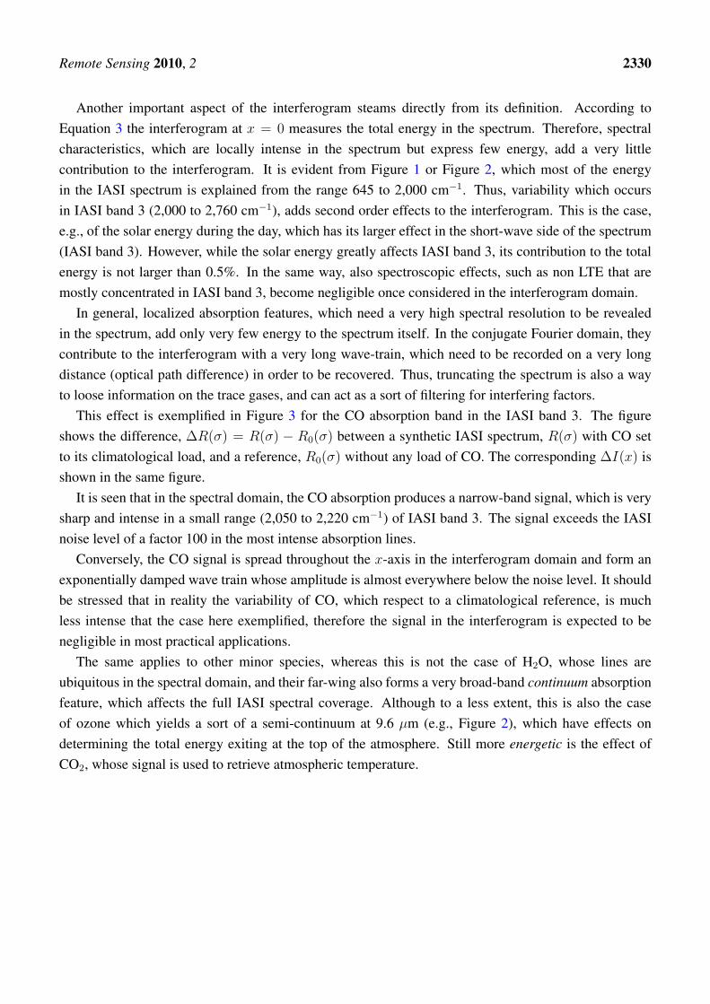
Another important aspect of the interferogram steams directly from its definition. According toEquation 3 the interferogram at x = 0 measures the total energy in the spectrum. Therefore, spectralcharacteristics, which are locally intense in the spectrum but express few energy, add a very littlecontribution to the interferogram. It is evident from Figure 1 or Figure 2, which most of the energyin the IASI spectrum is explained from the range 645 to 2,000 cm−1. Thus, variability which occursin IASI band 3 (2,000 to 2,760 cm−1), adds second order effects to the interferogram. This is the case,e.g., of the solar energy during the day, which has its larger effect in the short-wave side of the spectrum(IASI band 3). However, while the solar energy greatly affects IASI band 3, its contribution to the totalenergy is not larger than 0.5%. In the same way, also spectroscopic effects, such as non LTE that aremostly concentrated in IASI band 3, become negligible once considered in the interferogram domain.
In general, localized absorption features, which need a very high spectral resolution to be revealedin the spectrum, add only very few energy to the spectrum itself. In the conjugate Fourier domain, theycontribute to the interferogram with a very long wave-train, which need to be recorded on a very longdistance (optical path difference) in order to be recovered. Thus, truncating the spectrum is also a wayto loose information on the trace gases, and can act as a sort of filtering for interfering factors.
This effect is exemplified in Figure 3 for the CO absorption band in the IASI band 3. The figureshows the difference, ∆R(σ) = R(σ) − R0(σ) between a synthetic IASI spectrum, R(σ) with CO setto its climatological load, and a reference, R0(σ) without any load of CO. The corresponding ∆I(x) isshown in the same figure.
It is seen that in the spectral domain, the CO absorption produces a narrow-band signal, which is verysharp and intense in a small range (2,050 to 2,220 cm−1) of IASI band 3. The signal exceeds the IASInoise level of a factor 100 in the most intense absorption lines.
Conversely, the CO signal is spread throughout the x-axis in the interferogram domain and form anexponentially damped wave train whose amplitude is almost everywhere below the noise level. It shouldbe stressed that in reality the variability of CO, which respect to a climatological reference, is muchless intense that the case here exemplified, therefore the signal in the interferogram is expected to benegligible in most practical applications.
The same applies to other minor species, whereas this is not the case of H2O, whose lines areubiquitous in the spectral domain, and their far-wing also forms a very broad-band continuum absorptionfeature, which affects the full IASI spectral coverage. Although to a less extent, this is also the caseof ozone which yields a sort of a semi-continuum at 9.6 µm (e.g., Figure 2), which have effects ondetermining the total energy exiting at the top of the atmosphere. Still more energetic is the effect ofCO2, whose signal is used to retrieve atmospheric temperature.

Remote Sensing 2010, 2 2331
Figure 3. Illustrating the property of the Fourier transform to project sharp and narrow-bandspectral features in small-amplitude, broad-band signals. Panel (a) shows the differenceof a synthetic IASI spectrum against a reference with zero load of CO. Panel (b) showsthe corresponding variation in the interferogram, ∆I(x). The noise level (±1σ toleranceinterval) is shown for comparison, as well.
800 1000 1200 1400 1600 1800 2000 2200 2400 2600−2
−1
0
1x 10
−3
wave number, σ (cm−1)
∆ R
(σ),
W−
m−
2 −(c
m−
1 )−1 −
sr−
1
a)
0 0.5 1 1.5 2−0.02
−0.01
0
0.01
0.02
optical path difference, x (cm)
∆ I(
x), W
−m
−2 −
sr−
1
b)
∆ R(σ)
± 1 σ
∆ I(x)
± 1 σ
2.2. Forward and Inverse Modeling
Radiative transfer calculations have been performed with the package ϕ-IASI, which, among manyothers, incorporates a proper forward model, σ-IASI, and a linear regression inverse algorithm, that wecall ε-IASI.
The scheme ϕ-IASI has been variously described in the science literature [9,11,14–16], which thereader is referred to for further details.
The σ-IASI forward module is a monochromatic radiative transfer model, which uses a suitableatmospheric layering method to model the optical depths. This consists of a grid of vertical slabs withconstant pressure. Each layer is defined by the two bounding grid pressure levels (therefore N layersrequire a N + 1 level grid). The discretized version of the radiative transfer equation, which is solvedwithin σ-IASI, uses 63-layer pressure grid which spans the range 1100 − 0.005 hPa.
Of course, monochromatic synthetic radiances are convolved with the appropriate IASI instrumentspectral response function, to yield synthetic IASI spectra.
The retrieval scheme gets estimates of skin temperature, Ts, temperature profile, T , water vapourprofile, w, and ozone profile, q. The profile are obtained on the same pressure grid used for forwardcalculations, therefore, T,w, q are vectors of size 63 each.
The linear retrieval scheme adopts the principle of inverse regression, in which a given parameter,y(p) at a given pressure layer, p is expressed as a linear function of a suitable number, r of PC scores.
y(p) − y(p) = β1c1 + · · · + βrcr (6)
with y(p) the expectation value of y(p), and where βi, i = 1, . . . , r are regression coefficients to bedetermined on the basis of, e.g., a suitable training data set. The PC scores, ci, i = 1, . . . , r can

Remote Sensing 2010, 2 2332
be obtained from the EOF transform of training spectra or interferograms. A detailed account of theEOF retrieval methodology can be found in [9,12]. The methodology has been developed for a genericsignal-noise model and can be applied to any couple of data space and parameter space.
For completeness, we have to say something about the noise in the two data spaces: radiance andinterferogram. For IASI we have a direct knowledge of the noise in the spectral domain, so that we needa suitable model, which transforms the noise between the two data spaces.
If we assume, as usual, a signal-noise model of a pure additive type
Rt(σ) = st(σ) + e(σ) (7)
where st(σ) is the signal, e(σ) a noise term and Rt(σ) the (noisy) observation. Then according to thebasic Equation (3), which defines the interferogram, we have
I(x) =∫ +∞
−∞(st(σ) + n(σ)) exp(−2πiσx)dσ (8)
which says that the noise transforms the same way as the spectrum does.The Fourier transform can be written in terms of a suitable matrix, F so that Equation 8 can be written
in vector form (e.g., see [17]),I = Fst + Fe (9)
where I, st, e are the interferogram signal and noise vectors. Then, if Ce is the covariance matrix ofthe spectral noise term, the corresponding covariance matrix, Cn in the interferogram domain is easilyobtained by the linear transform
Cn = FCeFt (10)
where Ft is the transpose of the matrix F.In the work here shown the noise in the spectral domain is assumed to have variance according to
the level 1C IASI noise, and the corresponding noise strength in the interferogram domain is calculatedaccording to Equation (10).
3. Data Reduction Applied to IASI
Exploiting the methodology outlined in section 2.1, in this section suitable data reductions for IASI areshown and described, which are based on truncating the IASI interferogram at points below its maximumpath difference of 2 cm. The interferogram-based data reduction will be compared to that usuallyperformed in the spectral domain by picking up sparse channels, on the basis, e.g., of minimum-lossinformation criterions (see e.g., [4]).
To avoid possible confusion and misunderstanding, we will henceforth refer to as
• I-method, the method which is based on the truncation of the interferogram at point below the IASImaximum path difference of 2 cm,
• R-method, the method which is based on the selection of sparse spectral channels from the IASIspectrum at its nominal sampling ∆σ = 0.25 cm−1.

Remote Sensing 2010, 2 2333
Figure 4. Example of IASI spectrum, R(σ), with the indication of the 3,385 selected for theR-method.
800 1000 1200 1400 1600 1800 2000 2200 2400 26000
0.05
0.1
0.15
wave number cm−1
R(σ
), W
−m
−2 −
(cm
−1 )−
1 −sr
−1
IASI spectrumChannels used for the EOF regression
We consider two subsets of reduced IASI data. For the first case the 8461 IASI channels are reducedof a factor 2.5, whereas for the second case of a factor ≈ 30.
It should be also stressed that, for the case of the R-method, the reduction of data points completelydestroys the original IASI spectral coverage, whereas in the case of the I-method, the truncation providesa sinc-interpolation of the original data, which leaves unchanged the full IASI spectral coverage.
3.1. Data Reduction of a Factor 2.5
For this first case, the I-method considers a truncation point xt = 0.8 cm, which corresponds toN = 3385 data points. This moderate data-reduction allows us to retain the first CO2 signature in theinterferogram domain (see Figure 1) and is equivalent to work with a spectrum with the full IASI spectralcoverage, but a sampling ∆σ = 0.625 cm−1, instead of the original 0.25 cm−1 (see e.g., Figure 2).
The R-method considers the IASI spectrum at its nominal sampling rate, ∆σ = 0.25 cm−1, thereforewe preserve the original IASI spectral resolution, but we select a set of N = 3385 channels. Thesechannels are exemplified in Figure 4 and belong to spectral ranges which include
1. the ν2 absorption band of CO2 and part of the atmospheric window (range from 645 to 830 cm−1)
2. the ozone band at 9.6 µm
3. the atmospheric window from 1,100 to 1,200 cm−1
4. the core of the ν2 absorption band of H2O at 6.7 µm
5. the portion of the spectrum from 2,000 to 2,230 cm−1, this includes a part of the N2O/CO2
absorption band at 4.3 µm
We stress that the spectral ranges considered yield 3385 spectral channels, therefore, we have exactlythe same data points as those for the I-method. The channels we have selected are a trade-off between
Remote Sensing 2010, 2 2334
the need to limit the data volume and to preserve portions of the spectrum which are mostly sensitivefor the retrieval of temperature, water vapour and ozone. In particular we do not include the spectralsegments
1. 810 to 1,000 cm−1 because of unknown contamination from CFC absorption;
2. 1,200 to 1,450 because of strong contamination by CH4;
3. 2,230 to 2,760, because of spectroscopic issues such as CO2 line and continuum absorptionuncertainty, e.g., [16], non LTE effects and sun contribution during the day.
3.2. Data Reduction of a Factor ≈ 30
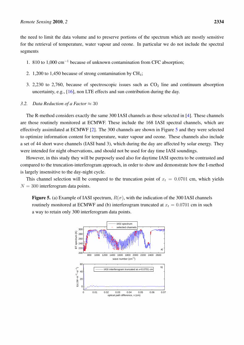
The R-method considers exactly the same 300 IASI channels as those selected in [4]. These channelsare those routinely monitored at ECMWF. These include the 168 IASI spectral channels, which areeffectively assimilated at ECMWF [2]. The 300 channels are shown in Figure 5 and they were selectedto optimize information content for temperature, water vapour and ozone. These channels also includea set of 44 short wave channels (IASI band 3), which during the day are affected by solar energy. Theywere intended for night observations, and should not be used for day time IASI soundings.
However, in this study they will be purposely used also for daytime IASI spectra to be contrasted andcompared to the truncation-interferogram approach, in order to show and demonstrate how the I-methodis largely insensitive to the day-night cycle.
This channel selection will be compared to the truncation point of xt = 0.0701 cm, which yieldsN = 300 interferogram data points.
Figure 5. (a) Example of IASI spectrum, R(σ), with the indication of the 300 IASI channelsroutinely monitored at ECMWF and (b) interferogram truncated at xt = 0.0701 cm in sucha way to retain only 300 interferogram data points.
800 1000 1200 1400 1600 1800 2000 2200 2400 2600200
220
240
260
280
300
wave number (cm−1)
BT
spe
ctru
m (
K)
a)
0 0.01 0.02 0.03 0.04 0.05 0.06 0.07
0
20
40
60
optical path difference, x (cm)
I(x)
(W
−m
−2 −
sr−
1 ) b)
IASI interferogram truncated at x=0.0701 cm
IASI spectrumselected channels
Remote Sensing 2010, 2 2335
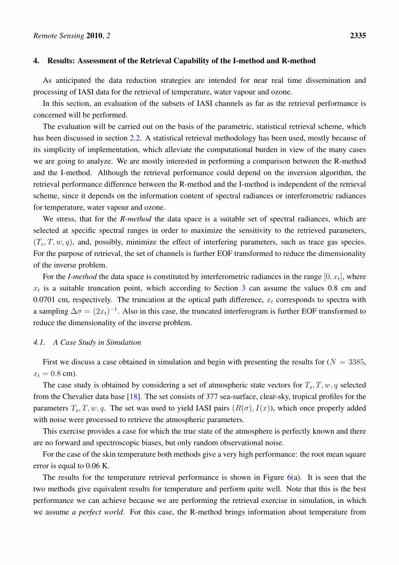
4. Results: Assessment of the Retrieval Capability of the I-method and R-method
As anticipated the data reduction strategies are intended for near real time dissemination andprocessing of IASI data for the retrieval of temperature, water vapour and ozone.
In this section, an evaluation of the subsets of IASI channels as far as the retrieval performance isconcerned will be performed.
The evaluation will be carried out on the basis of the parametric, statistical retrieval scheme, whichhas been discussed in section 2.2. A statistical retrieval methodology has been used, mostly because ofits simplicity of implementation, which alleviate the computational burden in view of the many caseswe are going to analyze. We are mostly interested in performing a comparison between the R-methodand the I-method. Although the retrieval performance could depend on the inversion algorithm, theretrieval performance difference between the R-method and the I-method is independent of the retrievalscheme, since it depends on the information content of spectral radiances or interferometric radiancesfor temperature, water vapour and ozone.
We stress, that for the R-method the data space is a suitable set of spectral radiances, which areselected at specific spectral ranges in order to maximize the sensitivity to the retrieved parameters,(Ts, T, w, q), and, possibly, minimize the effect of interfering parameters, such as trace gas species.For the purpose of retrieval, the set of channels is further EOF transformed to reduce the dimensionalityof the inverse problem.
For the I-method the data space is constituted by interferometric radiances in the range [0, xt], wherext is a suitable truncation point, which according to Section 3 can assume the values 0.8 cm and0.0701 cm, respectively. The truncation at the optical path difference, xt corresponds to spectra witha sampling ∆σ = (2xt)
−1. Also in this case, the truncated interferogram is further EOF transformed toreduce the dimensionality of the inverse problem.
4.1. A Case Study in Simulation
First we discuss a case obtained in simulation and begin with presenting the results for (N = 3385,xt = 0.8 cm).
The case study is obtained by considering a set of atmospheric state vectors for Ts, T, w, q selectedfrom the Chevalier data base [18]. The set consists of 377 sea-surface, clear-sky, tropical profiles for theparameters Ts, T, w, q. The set was used to yield IASI pairs (R(σ), I(x)), which once properly addedwith noise were processed to retrieve the atmospheric parameters.
This exercise provides a case for which the true state of the atmosphere is perfectly known and thereare no forward and spectroscopic biases, but only random observational noise.
For the case of the skin temperature both methods give a very high performance: the root mean squareerror is equal to 0.06 K.
The results for the temperature retrieval performance is shown in Figure 6(a). It is seen that thetwo methods give equivalent results for temperature and perform quite well. Note that this is the bestperformance we can achieve because we are performing the retrieval exercise in simulation, in whichwe assume a perfect world. For this case, the R-method brings information about temperature from

Remote Sensing 2010, 2 2336
the longwave absorption band of CO2 and from the shortwave segment 2,000 to 2,230 cm−1. We aresimulating no biases because of sunlight or non LTE effects.
Figure 6. Results for the case study in simulation and for (N = 3385, xt = 0.8 cm). Thefigure shows the retrieval performance expressed in terms of root mean square error (rmse)for (a) temperature, (b) water vapour and (c) ozone.
0 2 4
0
100
200
300
400
500
600
700
800
900
1000
rmse for Temp. (K)
Pre
ssur
e (h
Pa)
a)
0 1
0
100
200
300
400
500
600
700
800
900
1000
rmse for H2O (g/kg)
Pre
ssur
e (h
Pa)
b)
0 0.2 0.4
10−1
100
101
102
103
rmse for O3 (g/kg)
Pre
ssur
e (h
Pa)
c)
R−methodI−method
R−methodI−method
R−methodI−method
For water vapour the retrieval performance is shown in Figure 6(b). It is seen that now the I-methodprovides a slight but consistent better retrieval in the lower atmosphere, where the water vapour has thelarger variability. We think that this finding can be explained because of the better representation of H2Ocontinuum and line absorption within the I-method than the R-method. In fact, while the R-method doesnot take into account for the full spectral coverage of IASI (see Figure 4), the I-method does.
Finally, for ozone the retrieval performance is shown in Figure 6(c). The ozone band is very wellinsulated in the middle of the spectral coverage (see Figure 4) and adds a sensible contribution to thetotal energy, so that its signature is strong in both domains. As a result the R-method and the I-methodyield almost the same results, with a slight advantage for the R-method.
The results just illustrated says that in case the number of IASI data remains relatively large and of thesame order of NIASI , the two methods are almost equivalent, although the I-method is slightly superiorfor the retrieval of lower atmospheric moisture, which is a primary objective of IASI.
The superiority of the I-method is largely enhanced in case we ask for a larger data-reduction, as wewill show discussing the same exercise as that above, but for the case (N = 300, xt = 0.0701 cm).
The results for the temperature retrieval performance is shown in Figure 7(a). It is seen that theR-method is superior over the I-method in the upper part of the atmosphere. Conversely, in the lowertroposphere, the I-method performs better than the R-method. If we consider the case of water vapour,whose retrieval accuracy is shown in Figure 7(b), we see that the I-method outperforms in the loweratmosphere the R-method. Once again, we think that this finding can be explained because of the bestspectral coverage, and the effect is here much more evident than for the case shown in Figure 6, sincenow the density of the 300 full spectral resolution IASI channels is very low within the ν2 band of H2O(see e.g., Figure 5).
For ozone, the channel density within the band at 9.6 µm is even smaller, and as a result the I-methodyields a better performance than the R-method (see Figure 7(c)).

Remote Sensing 2010, 2 2337
Figure 7. Results for the case study in simulation and for (N = 300, xt = 0.0701 cm). Thefigure shows the retrieval performance expressed in terms of root mean square error (rmse)for (a) temperature, (b) water vapour and (c) ozone.
0 1 2 3 4
0
100
200
300
400
500
600
700
800
900
1000
rmse for Temp. (K)
Pre
ssur
e (h
Pa)
a)
0 1 2
0
100
200
300
400
500
600
700
800
900
1000
rmse for H2O (g/kg)
Pre
ssur
e (h
Pa)
b)
0 0.5
10−1
100
101
102
103
rmse for O3 (ppmv)
Pre
ssur
e (h
Pa)
c)
R−methodI−method
R−methodI−method
R−methodI−method
The superiority of the I-method is confirmed also in case we consider high-latitude, cold air masses.In this respect, since the I-method is expected to have a better signal-to-noise, it should be promisingfor application, especially for processing IASI data at high and/or middle latitude geographic areas inwinter season.
Figure 8 compares the retrieval performance of the I-method to that of the R-method for a case ofhigh-latitude-winter IASI soundings. As for the tropical exercise, this set of soundings was built up byconsidering a suitable ensemble of atmospheric state vectors extracted from the Chevalier data base [18].The ensemble consists of 138 clear-sky, high-latitude-winter profiles for the parameters Ts, T, w, q. Theset was used to yield IASI pairs (R(σ), I(x)), which once properly added with noise were processed toretrieve the atmospheric parameters.
For the sake of brevity the analysis is here limited to the case (N = 300, xt = 0.0701 cm). It isseen from Figure 8 that the comparison of the I-method against the R-method for this case of a coldatmosphere closely parallels the comparison results presented in Figure 7 for a hot, tropical atmosphere.Temperature retrieval performance is nearly the same for the two methods in the troposphere, whereas forwater vapour and ozone the performance provided by the I-method is superior of that of the R-method.
4.2. The JAIVEx Case Study
As for the previous paragraph, we begin with discussing the results for the data-reduction of(N = 3385, xt = 0.8 cm).
The Joint Airborne IASI validation experiment (JAIVEx) [19] was carried over the Gulf of Mexicoduring April and May 2007. We have a series of 6 spectra for the day 29 April 2007, 16 spectra for theday 30 April 2007, and finally 3 spectra for the day 4 May 2007. The total of 25 soundings are time andspace colocated with dropsonde observations. The dropsonde analysis extends from the ground level toabout 400 hPa, therefore the atmospheric profiles have been extended up to 0.1 hPa through the analysisof the ECMWF.

Remote Sensing 2010, 2 2338
Figure 8. Results for the case study in simulation and for (N = 300, xt = 0.0701
cm). The figure shows the retrieval performance expressed in terms of root mean squareerror (rmse) for (a) temperature, (b) water vapour and (c) ozone. The results applies tohigh-latitude-winter IASI soundings.
0 2 4
0
100
200
300
400
500
600
700
800
900
1000
rmse for Temp. (K)
Pre
ssur
e (h
Pa)
a)
0 0.1 0.2 0.3
0
100
200
300
400
500
600
700
800
900
1000
rmse for H2O (g/kg)
Pre
ssur
e (h
Pa)
b)
0 0.5
10−1
100
101
102
103
rmse for O3 (ppmv)
Pre
ssur
e (h
Pa)
c)
R−methodI−method
R−methodI−method
R−methodI−method
The JAIVEx observations were taken during daytime, therefore they also allows us to assess therobustness of the two retrieval methods to the solar contamination in the short wave side of the spectrum.Note that our radiative transfer calculations does not purposely include the solar term to assess itspotential interfering effect over retrievals.
In addition, the real data from the JAIVEx campaign allows us to understand the sensitivity of thetwo methods to the interfering effect of trace gases, which in our radiative calculations are kept constantto their climatological values. Particularly relevant to our analysis are the potential effect due to thevariability of CH4 and CO. Note that the effect of both CH4 and CO have to be expected for the I-method,which uses the full IASI spectral coverage. For the case of the R-method the methane band has beeneliminated form the selected ranges (again see Figure 4), while the CO band has been included.
Keeping this in mind, Figure 9 summarizes the root mean square error for temperature, water vapourand ozone. When comparing the results shown in Figure 9 to those in Figure 6 it has to be consideredthat the findings for the JAIVEx experiment are based only on 25 soundings.
For temperature and ozone the two approaches gives almost the same results, while the I-method issuperior over the R-method for water vapour in the lower part of the atmosphere. It is also important tonote that while for the R-method we selected suitable ranges in order to minimize the interfering effectsof the sun in the short wave and that of CH4 in the left wing of the water vapour band at 6.7 µm, none ofthis precautions were taken for the I-method, which just consider the full spectral coverage.
The results for H2O is important and deserves further analysis to get insight into understandingwhether the improvement involves only the root mean square or the spatial vertical resolution of theprofile itself.
Towards this objective Figure 10 compare the retrieved H2O-profiles to the dropsonde observationsfor the day 29 April 2007. It is interesting to note that the I-method is capable to resolve the double layerstructure which is seen in the lower part of the water vapour profiles. This is done much better than the
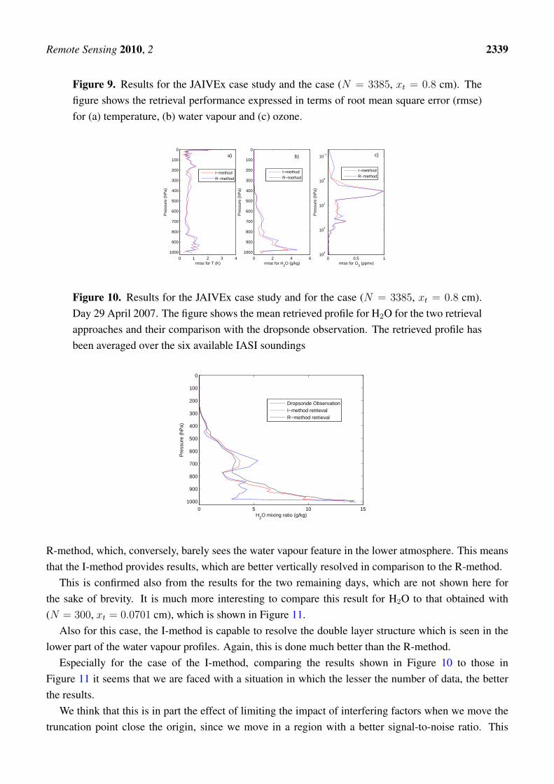
Remote Sensing 2010, 2 2339
Figure 9. Results for the JAIVEx case study and the case (N = 3385, xt = 0.8 cm). Thefigure shows the retrieval performance expressed in terms of root mean square error (rmse)for (a) temperature, (b) water vapour and (c) ozone.
0 1 2 3 4
0
100
200
300
400
500
600
700
800
900
1000
rmse for T (K)
Pre
ssur
e (h
Pa)
a)
0 2 4 6
0
100
200
300
400
500
600
700
800
900
1000
rmse for H2O (g/kg)
Pre
ssur
e (h
Pa)
b)
0 0.5 1
10−1
100
101
102
103
rmse for O3 (ppmv)
Pre
ssur
e (h
Pa)
c)
I−methodR−method
I−methodR−method
I−metrhodR−method
Figure 10. Results for the JAIVEx case study and for the case (N = 3385, xt = 0.8 cm).Day 29 April 2007. The figure shows the mean retrieved profile for H2O for the two retrievalapproaches and their comparison with the dropsonde observation. The retrieved profile hasbeen averaged over the six available IASI soundings
0 5 10 15
0
100
200
300
400
500
600
700
800
900
1000
H2O mixing ratio (g/kg)
Pre
ssur
e (h
Pa)
Dropsonde ObservationI−method retrievalR−method retrieval
R-method, which, conversely, barely sees the water vapour feature in the lower atmosphere. This meansthat the I-method provides results, which are better vertically resolved in comparison to the R-method.
This is confirmed also from the results for the two remaining days, which are not shown here forthe sake of brevity. It is much more interesting to compare this result for H2O to that obtained with(N = 300, xt = 0.0701 cm), which is shown in Figure 11.
Also for this case, the I-method is capable to resolve the double layer structure which is seen in thelower part of the water vapour profiles. Again, this is done much better than the R-method.
Especially for the case of the I-method, comparing the results shown in Figure 10 to those inFigure 11 it seems that we are faced with a situation in which the lesser the number of data, the betterthe results.
We think that this is in part the effect of limiting the impact of interfering factors when we move thetruncation point close the origin, since we move in a region with a better signal-to-noise ratio. This

Remote Sensing 2010, 2 2340
Figure 11. Results for the JAIVEx case study and for the case (N = 300, xt = 0.0701 cm).Day 29 April 2007. The figure shows the mean retrieved profile for H2O for the two retrievalapproaches and their comparison with the dropsonde observation. The retrieved profile hasbeen averaged over the six available IASI soundings.
0 5 10 15
0
100
200
300
400
500
600
700
800
900
1000
H2O mixing ratio (g/kg)
Pre
ssur
e (h
Pa)
DropsondeR−methodI−method
has also the effect that more EOF scores go above the noise level for xt = 0.0701 cm than withxt = 0.8 cm. If we increase the number of EOF scores in the retrieval scheme, we add moredegrees of freedom, hence information to the regression analysis, which improves the spatial verticalresolution. However, this results has to be more carefully assessed on the basis of more extensive set ofIASI soundings.
The results shown in Figure 10 to those in Figure 11 also suggest that there should be an optimaltruncation point, which minimizes the root mean square error for H2O. An issue that we plan toinvestigate in a future study.
Figures 12 and 13 provide a case for temperature, for the two different strategies (N = 3385, xt = 0.8
cm) and (N = 300, xt = 0.0701 cm), respectively, which further deserves to exemplify the bettercapability of the I-method to capture fine structures also in the temperature profile. It is seen from thesetwo figures that the I-method resolves better than the R-method the temperature inversion at about 800hPa, and also the details in the upper troposphere at about 200 hPa are captured much better.
It is also very much interesting to note the bad performance of the R-method for the case of thetemperature retrieval shown in Figure 13. This is due to the sensitivity of 44 out of the 300 IASI channelsto the short-wave side of the spectrum (see Figure 5). These channels were purposely included to showthat the I-method, unlike the R-method, is insensitive to the interfering effects of the solar energy.
When we remove the 44 short-wave IASI channels, the R-method gets comparable results to those ofthe I-method. However, the performance for water vapour remains below that of the I-method.
To sum up we can say that the I-method provides better results for the retrieval of water vapour, andalso for temperature it seems to capture better fine details. Furthermore, the I-method is fairly insensitiveto the potential interfering effects of solar energy and radiatively active trace gases. This simplifies a lotthe radiative transfer calculation and avoids the computational burden of including the solar source inthe computations.

Remote Sensing 2010, 2 2341
Figure 12. Results for the JAIVEx case study and for (N = 3385, xt = 0.8 cm). Day 30April 2007. The figure shows the mean retrieved profile for temperature for the two retrievalapproaches and their comparison with the dropsonde observation. The retrieved profile hasbeen averaged over the 16 available IASI soundings.
200 220 240 260 280 300
0
100
200
300
400
500
600
700
800
900
1000
Temperature (K)
Pre
ssur
e (h
Pa)
a)
285 290 295
750
800
850
900
950
1000
Temperature (K)
Pre
ssur
e (h
Pa)
b)
DropsondeR−methodI−method
4.3. The Tropical Case Study
To boost the results obtained in the previous section with a better statistics we consider a second dataset of IASI spectra, which has been acquired within the tropical belt, during the IASI commissioningphase on 22 July 2007. In total, a number of 647 IASI spectra has been selected. The spectra have beenobserved on sea surface and refer to nadir looking mode and clear sky conditions. Clear sky was checkedusing the cloud detection scheme described in [15]. This second set of data will be referred to as simplythe tropical set.
For the tropical set, in order to develop a consistent set of truth data against which IASI retrievalcould be compared, ECMWF atmospheric analysis fields for temperature, water vapor and ozone wereconsidered. These fields where time and spatially co-located to the 647 IASI soundings. We usedatmospheric analysis fields of 00:00, 06:00, 12:00, 18:00 and 24:00 UTC on 22 July 2007. For moredetails we refer the reader to [16].
The tropical set is made up of 87 daytime IASI spectra, whereas the remaining 560 spectra have beenobserved during the night. To exemplify the robustness of the I-method to the interfering effect of solarenergy, in the following the statistics will be separately shown for day and night conditions.
Figure 14 summarizes the performance of the two approaches for (N = 3385, xt = 0.8 cm). Inthis case the root mean square difference is also influenced by the statistical accuracy of the ECMWFanalysis itself, which in the troposphere is about ±1 K for temperature and ≈ ±0.5 g/kg for watervapour [16]. For this reason we have to expect a relatively larger root mean square difference than thatshown in the two previous sections. The results shown in Figure 14 confirm that the I-method yields aretrieval performance for water vapour that is superior to that obtained with the R-method. In general,the results say that the I-method provides a better accuracy also for the case of temperature, in the lowertroposphere, and almost everywhere for ozone.
In daytime the I-method outperforms the R-method also for the case of temperature, mainly becausethe latter is more sensitive than the former to solar effects in the IASI band 3. Although the R-method,

Remote Sensing 2010, 2 2342
Figure 13. Results for the JAIVEx case study and for (N = 300, xt = 0.0701 cm). Day 30April 2007. The figure shows the mean retrieved profile for temperature for the two retrievalapproaches and their comparison with the dropsonde observation. The retrieved profile hasbeen averaged over the 16 available IASI soundings.
200 220 240 260 280 300
0
100
200
300
400
500
600
700
800
900
1000
Temperature (K)
Pre
ssur
e (h
Pa)
a)
285 290 295
750
800
850
900
950
1000
Temperature (K)
Pre
ssur
e (h
Pa)
b)DropsondeR−methodI−method
for the case (N = 3385, xt = 0.8 cm), has its farer channel at 2230 cm−1, some contamination fromsun energy has to be expected, mostly for the spectral segment 2100 to 2200 cm−1. Another interferingeffect in this band is CO absorption.
In nighttime the two methods yield almost the same results, although the I-method still seems toproduce a better performance in the lower troposphere, both for temperature and water vapour.
Form Figure 14 it appears that the retrieval performance depends on the day/night cycle. We thinkthat this is only an effect of the different statistics, 87 cases for daytime against 560 for nighttime.
Similar results to those we have just discussed and shown in Figure 14 are achieved by considering(see Figure 15) the case (N = 300, xt = 0.0701 cm). Now the negative effect of the solar contaminationis most evident for the R-method, which again gives more evidence to the fact the I-method has a lowsensitivity to the contamination by infrared emission of the sun.
As for the case (N = 3385, xt = 0.8 cm), we see a dependence on the day/night cycle and on overallwe obtain results, which are in agreement with those shown in Figure 14.
Finally, we also stress that if for daytime we do not use the 44 short-wave channels in order tolimit solar contamination, the performance of the R-method improves, but it remains inferior to thatobtained with the I-method. This is exemplified for water vapour in Figure 16. Similar results holds fortemperature and ozone.

Remote Sensing 2010, 2 2343
Figure 14. Results for the tropical case study for (N = 3385, xt = 0.8 cm). The figureshows the retrieval performance expressed in terms of root mean square error (rmse) for (a)temperature, (b) water vapour and (c) ozone.
0 2 4
0
100
200
300
400
500
600
700
800
900
1000
rmse for Temp. (K)
Pre
ssur
e (h
Pa)
a)
0 2 4
0
100
200
300
400
500
600
700
800
900
1000
rmse for H2O (g/kg)
Pre
ssur
e (h
Pa)
b)
0 0.5 1
10−1
100
101
102
103
rmse for O3 (ppmv)
Pre
ssur
e (h
Pa)
c)
R−method dayI−method dayR−method nightI−method night
Figure 15. Results for the tropical case study for (N = 300, xt = 0.0701 cm). The figureshows the retrieval performance expressed in terms of root mean square error (rmse) for(a) temperature, (b) water vapour and (c) ozone.
0 2 4
0
100
200
300
400
500
600
700
800
900
1000
rmse for H2O (g/kg)
Pre
ssur
e (h
Pa)
b)
0 0.5 1
10−1
100
101
102
103
rmse for O3 (ppmv)
Pre
ssur
e (h
Pa)
c)
0 2 4
0
100
200
300
400
500
600
700
800
900
1000
rmse for Temp. (K)
Pre
ssur
e (h
Pa)
a)
R−method dayI−method dayR−method nightI−method night
5. Discussion and Conclusions
The study has been mostly focused on the application to IASI of data reduction strategiescomplemented with a statistical regression methodology, which is able to work indifferently with spectralradiances or interferogram samples. Different data-reduction approaches, yielding a number, N ofspectral radiances, with N in the range N ≤ NIASI and N << NIASI , respectively, have been studiedand inter-compared in order to assess their relative retrieval performance.
Based on a series of retrieval exercises, we have shown that the interferogram-truncation approachprovides a suitable data-reduction methodology in all those cases we are constrained by N << NIASI
and we are interested in the retrieval of temperature and water vapour. In fact, irrespectively of thepoint at which we truncate the interferogram, the I-method preserves the IASI spectral coverage. This isimportant for water vapour, which is radiatevely active across the full IASI spectral coverage.

Remote Sensing 2010, 2 2344
Figure 16. Results for the tropical case study and for daytime IASI soundings. The figureshows the retrieval performance expressed in terms of root mean square error (rmse) forwater vapour and compares the I-method to the R-method with and without solar channels.The results shown in figure applies to the case (N = 300, xt = 0.0701 cm).
0 0.5 1 1.5 2 2.5
0
100
200
300
400
500
600
700
800
900
1000
rmse for H2O (g/kg)
Pre
ssur
e (h
Pa)
R−method without short wave channelsR−method with short wave channelsI−method
It could be argued that in the interferogram domain temperature and water vapour are deeplyconvolved, while in the spectral domain we can achieve a separation of the absorption bands, in suchway to insulate temperature channels from those of water vapour. However, because of the water vapourcontinuum absorption, there is no part of the spectrum which is really not influenced by water vapour,and the effect of H2O becomes increasingly important and convolved with temperature when we considerspectral channels, which peak deeply in the troposphere, which, in turn, is the part of the atmospheremostly relevant to meteorological processes. Thus, in both spaces, there is no way to really insulatetemperature from water vapour. There could be also some constraints, which are determined, e.g., fromthe kind of retrieval process one uses to invert atmospheric parameters from radiances (e.g., the needof well shaped Jacobian and/or averaging kernels). These constraints appear to be of mathematicalnature rather than of physical meaning. However, it is fair to say that the capability of the interferogramapproach has to be confirmed and better assessed also with the use of physical inversion of the radiativetransfer equation performed into the interferogram domain, which means, e.g., the computation ofderivative of I(x) with respect to parameters such as T, w, q.
Having said that, it is important to stress that our results demonstrate that the retrieval capability of theinterferogram domain has been largely under-explored until now, which call for a more comprehensiveanalysis, especially in the quest of suitable methods to reduce the size of IASI data to be transmittedand processed.
In perspective, once we recognize that FTS instruments measure the interferogram, we could thenmake a direct use of interferometric radiances that could allows us to deal with fairly constant-varianceand uncorrelated noise, which would further improve the quality and independency of data and, hence,retrievals, and finally could even simplify the design of future satellite instrumentation.
Remote Sensing 2010, 2 2345
Acknowledgements
IASI has been developed and built under the responsibility of the Centre National d’Etudes Spatiales(CNES, France). It is flown onboard the Metop satellites as part of the EUMETSAT Polar System. TheIASI L1 data are received through the EUMETCast near real time data distribution service. We thankDr Stuart Newman (Met Office) for providing the JAIVEx data. The JAIVEx project has been partiallyfunded under EUMETSAT contract Eum/CO/06/1596/PS. The FAAM BAe 146 is jointly funded by theMet Office and the Natural Environment Research Council. The US JAIVEx team was sponsored bythe National Polar-orbiting Operational Environmental Satellite System (NPOESS) Integrated ProgramOffice (IPO) and NASA.
References and Notes
1. Richter, A.; Wagner, T. The IASI instrument onboard the METOP Satellite: First results.Atmos. Chem. Phys. 2009, Special Issue; Available online: http://www.atmos-chem-phys.net/special issue123.html (accessed on 29 September 2010).
2. Collard, A.D.; McNally, A.P. The assimilation of Infrared Atmospheric Sounding Interferometerradiances at ECMWF. Q. J. R. Meteorol. Soc. 2009, 135, 1044-1058.
3. Robinson, E.A.; Silvia, M.T. Digital Foundation of Time Series Analysis: Wave-EquationSpace-Time Processing; Holden-Day: San Francisco, CA, USA, 1981; Volume 2.
4. Collard, A.D. Selection of IASI channels for use in numerical weather prediction: The assimilationof Infrared Atmospheric Sounding Interferometer radiances at ECMWF. Q. J. R. Meteorol. Soc.2007, 133, 1977-1991.
5. Kaplan, L.D.; Chahine, M.T.; Susskind, J.; Searle, L.E. Spectral band passes for a high precisionsatellite sounder. Appl. Opt. 1977, 16, 322-325.
6. Kyle, T.G. Temperature soundings with partially scanned interferograms. Appl. Opt. 1977, 16,326-333.
7. Smith, W.L.; Howell, H.B.; Woolf, H.M. The use of interferometric radiance measurements for thesounding the atmosphere. Appl. Opt. 1979, 36, 566-575.
8. Huang, H-L; Antonelli, P. Application of principal component analysis to high- resolution infraredmeasurements compression and retrieval. J. Appl. Metereo. 2001, 40, 365-388.
9. Serio, C.; Masiello, G.; Grieco, C. EOF regression analytical model with applications tothe retrieval of atmospheric temperature and gas constituents concentration from high spectralresolution infrared observations. In Environmental Modelling: New Research; Findley, P.N., Ed.;Nova Science Publishers, Inc.: Hauppagauge, NY, USA, 2009; pp. 51-88.
10. Goldberg, M.D.; Qu, Y.; McMillin, L.M.; Wolf, W; Zhou, L.; Divakarla, M. AIRS near-real-timeproducts and algorithms in support of operational numerical weather prediction. IEEE Trans.Geosci. Remote Sens. 2003, 41, 379-389.
11. Masiello, G.; Serio, C. Dimensionality-reduction approach to the thermal radiative transferequation inverse problem. Geophys. Res. Lett. 2004, 31, L11105, doi:10.1029/2004GL019845.

Remote Sensing 2010, 2 2346
12. Serio, C.; Esposito, F.; Masiello, G.; Pavese, G.; Calvello, M.R.; Grieco, G.; Cuomo, V.; Buijs,H.L.; Roy, C.B. Interferometer for ground-based observations of emitted spectral radiance fromthe troposphere: evaluation and retrieval performance. Appl. Opt. 2008, 47, 3909-3919.
13. Zhou, D.K.; Smith, W.L.; Li, J.; Howell, H.B.; Cantwell, G.W.; Larar, A.M.; Knuteson, R.O.;Tobin, D.C.; Revercomb, H.E.; Bingham, G.E.; Tsou, J-.J.; Mango, S.A. Thermodynamic productretrieval methodology and validation for NAST-I. Appl. Opt. 2002, 41, 6957-6970.
14. Amato, U.; Masiello, G.; Serio, C.; Viggiano, M. The σ-IASI code for the calculation of infraredatmospheric radiance and its derivatives. Environ. Model. Software 2002, 17, 651-667.
15. Grieco, G.; Masiello, G.; Matricardi, M.; Serio, C.; Summa, D.; and Cuomo, V. Demonstration andvalidation of the φ-IASI inversion scheme with NAST-I data. Q. J. R. Meteorol. Soc. 2007, 133,217-232.
16. Masiello, G.; Serio, C.; Carissimo, A.; Grieco, G. Application of ϕ-IASI to IASI: retrieval productsevaluation and radiative transfer consistency. Atmos. Chem. Phys. 2009, 9, 8771-8783.
17. Amato, U.; De Canditiis, D.; Serio, C. Effect of apodization on the retrieval of geophysicalparameters from Fourier-Transform Spectrometers. Appl. Opt. 1998, 37, 6537-6543.
18. Chevalier, F. Sampled Database of 60 Levels Atmospheric Profiles from the ECMWF Analysis;Technical Report; ECMWF EUMETSAT SAF programme Research Report 4; ECMWF: ShinfieldPark, Reading, UK, 2001.
19. Taylor, J.P. Joint Airborne IASI Validation Experiment. Available online: http://badc.nerc.ac.uk/data/jaivex/ (accessed on 29 September 2010).
c⃝ 2010 by the authors; licensee MDPI, Basel, Switzerland. This article is an open access articledistributed under the terms and conditions of the Creative Commons Attribution license(http://creativecommons.org/licenses/by/3.0/.)