A novel ensemble method for retrieving propertiesof warm cloud in 3-D using ground-basedscanning radar and zenith radiancesMark D. Fielding1, J. Christine Chiu1, Robin J. Hogan1, and Graham Feingold2

1Department of Meteorology, University of Reading, Reading, UK, 2NOAA Earth System Research Laboratory, Boulder,Colorado, USA

Abstract We present a novel method for retrieving high-resolution, three-dimensional (3-D) nonprecipitatingcloud fields in both overcast and broken-cloud situations. The method uses scanning cloud radar andmultiwavelength zenith radiances to obtain gridded 3-D liquidwater content (LWC) and effective radius (re) and2-D column mean droplet number concentration (Nd). By using an adaption of the ensemble Kalman filter,radiances are used to constrain the optical properties of the clouds using a forward model that employs full 3-Dradiative transfer while also providing full error statistics given the uncertainty in the observations. To evaluatethe new method, we first perform retrievals using synthetic measurements from a challenging cumuluscloud field produced by a large-eddy simulation snapshot. Uncertainty due to measurement error in overheadclouds is estimated at 20% in LWC and 6% in re, but the true error can be greater due to uncertainties in theassumed droplet size distribution and radiative transfer. Over the entire domain, LWC and re are retrievedwith average error 0.05–0.08 gm�3 and ~2μm, respectively, depending on the number of radiance channelsused. The method is then evaluated using real data from the Atmospheric Radiation Measurement programMobile Facility at the Azores. Two case studies are considered, one stratocumulus and one cumulus. Whereavailable, the liquid water path retrieved directly above the observation site was found to be in good agreementwith independent values obtained from microwave radiometer measurements, with an error of 20 gm�2.

1. Introduction

Boundary layer clouds are fundamental to the Earth’s radiation budget, their high reflectance constituting asignificant contribution to the planetary albedo [Hartmann et al., 1992]. Even small changes in theirdistribution or composition can have a significant effect on climate [Oreopoulos and Platnick, 2008]. Theirturbulent, complex structures, coupled with a strong susceptibility to aerosol, mean they remain a key sourceof uncertainty in climate projections [e.g., Randall et al., 2007; Turner et al., 2007b]. To complement advancesin modeling studies, accurate observations of clouds and radiation are vital to improvement in theparameterization schemes of global circulation models (GCMs).

Profiling instruments, such as vertically pointing cloud radar, are invaluable for obtaining long-term time seriesof clouds [e.g., Illingworth et al., 2007] and give good vertical and partial horizontal information on cloudproperties. However, they are less well suited for inferring a whole-sky view. This problem is particularlyapparent when attempting to reproduce observed surface irradiances in radiation closure studies [McFarlaneand Evans, 2004; Wang et al., 2011] or analyzing cloud radiative effects, both of which are sorely needed asobservational constraints for realistic cloud and radiation parameterizations for GCMs [Qian et al., 2012]. Inparticular, the 3-D horizontal transport of photons (henceforth “3-D effects”) is a nonnegligible source of error inthe 1-D radiation schemes of current GCMs [e.g., Cahalan et al., 1994; Hogan and Shonk, 2013], particularlyfor cumulus clouds [Pincus et al., 2005]. The ability to observe cloud structure and cloud microphysicalproperties in 3-D is also a key step to improving our understanding of cloud life cycle and cloud organization.

To address this need for 3-Dmeasurements of clouds, the U.S. Department of Energy’s Atmospheric RadiationMeasurement (ARM) program [Ackerman and Stokes, 2003] has installed scanning polarimetric Doppler cloudradar [Widener et al., 2012] at their Climate Research Facilities. The radars can scan at up to 15° s�1 producingreasonable coverage over a 5min time period, which can then be interpolated to a 3-D gridded domain ofradar reflectivity. However, as radar reflectivity is proportional to both the number and the size of clouddroplets, further information is required to deduce these microphysical properties inside the 3-D domain.

FIELDING ET AL. ©2014. American Geophysical Union. All Rights Reserved. 1

PUBLICATIONSJournal of Geophysical Research: Atmospheres

RESEARCH ARTICLE10.1002/2014JD021742

Key Points:• New method for retrieving 3-Dcloud fields

• Three-dimensional radiative transfer isused as a forward model

• Evaluations against other retrievalsshow good agreement

Correspondence to:M. D. Fielding,m.d.fielding@pgr.reading.ac.uk

Citation:Fielding, M. D., J. C. Chiu, R. J. Hogan,and G. Feingold (2014), A novel ensemblemethod for retrieving properties of warmcloud in 3-D using ground-basedscanning radar and zenith radiances,J. Geophys. Res. Atmos., 119, doi:10.1002/2014JD021742.

Received 12 MAR 2014Accepted 21 AUG 2014Accepted article online 26 AUG 2014

Several existing methods to retrieve cloud microphysical properties using vertically pointing cloud radar andother sources of information could be adapted for a scanning radar retrieval. First, one could add priorknowledge based on in situ observations [e.g.,McFarlane et al., 2002] or based on theory, for example, using asimple model to predict droplet sizes given certain atmospheric conditions [e.g., Rémillard et al., 2013].Second, an additional active sensor could be added to the retrieval. For example, Hogan et al. [2005] andHuang et al. [2009] showed that differential attenuation with dual-wavelength radar could retrieve liquidwater content (LWC). Finally, passive sensors could be added to the retrieval. The most widely used constraintis liquid water path (LWP) measurements from microwave radiometers [e.g., Frisch et al., 1995; Frisch et al.,1998; Lohnert et al., 2001]. Additionally, Dong and Mace [2003] combined radar measurements and cloudoptical depth retrieved from solar irradiances, which works best for relatively overcast, horizontallyhomogeneous clouds due to the hemispheric field of view of radiometers.

In contrast to irradiances, zenith radiances are collected from a narrow field-of-view, which can capture cloudvariability at higher spatial resolution and therefore are a more appealing choice for the retrieval ofheterogeneous cloud. By using a wavelength that is absorbed by liquid water and one that is not absorbed byliquid water, zenith radiance measurements have previously been used to simultaneously constrain dropletsize (using the absorbing wavelength) and cloud optical depth (using the nonabsorbing wavelength) withoutradar measurements [e.g., McBride et al., 2011; Chiu et al., 2012]. These retrievals use a plane parallelapproximation; Marshak et al. [2004] showed that 3-D effects in heterogeneous cloud conditions can lead to“unretrievable” combinations of radiance measurements. The greater the heterogeneity in the cloud field,the greater the 3-D effects, which increases the potential for error in both the retrieved microphysical andradiative properties of the cloud.

As scanning cloud radar provides information on the 3-D cloud structure, it appears possible to utilize theseformerly unwelcome 3-D effects, provided that 3-D radiative transfer is used as a forward model. A potentialstumbling block is that modeling 3-D radiative transfer is a difficult problem and typically their adjoints(models that specify the sensitivity of their output to their input) do not exist, which rules out many standardtechniques for solving inverse problems. By using an ensemble-based method, we will show that we canovercome this issue and use 3-D effects to our advantage.

In this paper, we propose a novel ENsemble ClOud REtrieval method (ENCORE) to retrieve the 3-Dmicrophysicalproperties of clouds using scanning cloud radar and zenith radiances. The method has three key features.First, by using an ensemble-basedmethod, we can use full 3-D radiative transfer as a forwardmodel without theneed for its adjoint. As far as we are aware, the only previous use of a similar method for a meteorological radarretrieval is that described by Grecu and Olson [2008]. Second, while satellite-based radiance-radar retrievalshave been developed for CloudSat and Moderate Resolution Imaging Spectroradiometer (MODIS) [Austinand Stephens, 2001], we are unaware of an equivalent ground-based method. Finally, the retrieval isindependent of microwave-based LWP retrievals, permitting their use for validation.

The paper is organized as follows. We present the methodology of our 3-D retrieval for nonprecipitatingboundary layer clouds in section 2. In section 3 we evaluate the retrieval using synthetic cloud fields fromlarge-eddy simulations. Section 4 contains an analysis of two case study retrievals, one for a cumulus cloudfield and one for a stratocumulus cloud field. A discussion follows in section 5, and the conclusions andsummary are in section 6.

2. Methodology of ENCORE2.1. Overview of Retrieval Method

The method retrieves 2-D fields of cloud droplet number concentration Nd (assumed constant with height)and 3-D LWC and re. Our retrieval is built on a flexible ensemble framework that allows for the easy additionor removal of any observational data set. In this paper, the framework is used to maximize the synergybetween zenith radiances and radar reflectivity from scanning radar.

The required observational data sets are available from colocated instruments at various ARM field sites.Ground-based scanning ARM cloud radars (SACRs) provide radar reflectivity [Widener et al., 2012]. At eachfield site, two radars of different frequency are mounted onto a single pedestal, typically Ka andW band. Boththese radars have very narrow fields of view (~0.3°) making them ideal for cloud studies [Kollias et al., 2014].

Journal of Geophysical Research: Atmospheres 10.1002/2014JD021742

FIELDING ET AL. ©2014. American Geophysical Union. All Rights Reserved. 2

Zenith radiance measurements areavailable from ARM narrow field of viewradiometers (2NFOV) or ARM shortwavearray spectroradiometers (SAS-Ze). Bothof these instruments are ground basedwith 1 s temporal resolution. The 2NFOVhas channels at 673 and 870 nm with a1.2° field of view. The SAS-Ze measuresradiances across the whole shortwavespectrum (350–1700 nm) at a spectralresolution of 2.4 nm in the visible and6 nm in the near infrared with a 1°field-of-view. For clarity, in the rest ofthe paper we will refer to wavelengthsof radiation that are absorbed by liquidwater as “absorbing” (e.g., 1640 nm) andthose that are not as “nonabsorbing”(e.g., 440, 673, and 870 nm). Since thezenith radiances are local column-averaged measurements and do notprovide detailed cloud information forthe full 3-D domain, our retrievalprocedure contains threemajor steps, asillustrated in Figure 1 and outlined next.

The first step is to place all observationson to a common grid. Scanning radarobservations are mapped to a regular3-D grid, using linear interpolation via aDelaunay triangulation [see Fieldinget al., 2013]. Figure 1a illustrates anexample of radar scans made with theCross Wind Range Height Indicator(CWRHI) strategy from a radar located inthe center of the domain. Similarly,zenith radiance observations are alsocollected at the center of the domainand are linearly interpolated to a 1-Dtrack. Both data sets are placed on aspatial grid by assuming the commonlyused frozen turbulence hypothesis,with wind speed and direction obtainedfrom a colocated wind profiler.

Each zenith radiance observation ismainly a function of the overhead cloudproperties due to the narrow field of

view of the radiometers; however, when 3-D effects are not negligible, 1-D radiative transfer calculations areinsufficient to satisfactorily simulate zenith radiances and thus cannot provide proper constraints for ourretrievals. Therefore, 3-D radiative transfer calculations need to be incorporated in our algorithm. Due to thetrade-off between computational cost and the inclusion of 3-D effects, the second step of the retrieval isrestricted to a series of subsets of the full domain; each subset domain, dubbed a “supercolumn,” is selectedalong the aforementioned 1-D “radiance” track. The size of the supercolumn (magenta squares in Figure 1b) ischosen to reduce computational cost while encompassing most 3-D effects. This second step is a keycomponent of our retrieval method and will be detailed in section 2.2.

Figure 1. Diagram showing the main steps of the ENsemble ClOudREtrieval method (ENCORE). (a) Gathering of radiance (red dashed lines)and radar reflectivity (hemispherical slices) observations, (b) retrieveddrop number concentration and effective radius within each supercol-umn (magenta boxes), (c) reflectivity matching of donor columns (solid)to recipient columns (translucent), and (d) completed retrieval.

Journal of Geophysical Research: Atmospheres 10.1002/2014JD021742

FIELDING ET AL. ©2014. American Geophysical Union. All Rights Reserved. 3

Once the retrievals for the supercolumns are complete, the third step, illustrated in Figure 1c, is to retrievecloud properties for the rest of the domain by matching their radar reflectivity with the clouds inside thesupercolumns. Details are given in section 2.3.

2.2. Retrieval for Supercolumns2.2.1. State Vector and Forward ModelsThe state vector, x, which contains the variables we wish to retrieve, is defined as

x ¼ log N i¼1…m; j¼1…nð Þd ; log r i¼1…m; j¼1…n; k¼1…lð Þ

e

� �T; (1)

where i and j are grid indices in the horizontal; k is the vertical index; and n, m, and l define the number ofhorizontal and vertical grid points in the supercolumn, respectively. The variables in x are defined in log spaceto keep their values positive in linear space. Cloud droplet number concentration Nd is forced to be heightinvariant, whereas re is allowed to vary with height. LWC is defined as

LWC ¼ 43πρw Ndr

3e exp �3σ2

� �; (2)

where σ is the shape parameter or geometric standard deviation (standard deviation of the log of dropletradius), and ρw is the density of liquid water. As σ is not retrieved, we choose to keep it constant; we discuss theimpact of this assumption on retrievals in section 3.3. From LWC and re, cloud optical depth, τ, can be given as

τ ¼ 32ρw∫HT

HB

LWC hð Þre hð Þ dh; (3)

where HB is the height of cloud base and HT is the cloud top and the extinction efficiency has been assumedto be 2 (valid in the visible part of the spectrum).

Using Nd, re, and a lognormal cloud droplet distribution, we can also now forwardmodel radar reflectivity andzenith radiance, needed to map the state variables to observation space. We can safely use the Rayleighscattering approximation for cloud droplets since the SACRs operate at Ka or W band, but at these highfrequencies we must account for gas and liquid water attenuation. As a result, radar reflectivity is given as

Z ¼ 64Ndr6e exp 3σ2ð Þ

100:2∫

L

0αfþκf �LWCð Þ dL′

; (4)

where αf (dB km�1) is the one-way specific attenuation coefficient due to atmospheric gases, κf (dB km

�1

(gm�3)�1) is the one-way specific attenuation coefficient of liquid water [Hogan et al., 2005], and L is thedistance to the radar. Note that the assumed unimodal lognormal droplet distribution is only suitable fornonprecipitating clouds. Indeed, the success of the retrieval is strongly dependent on the validity of ourassumed droplet distribution; we are inferring the zeroth, second, and third moments from observations ofthe second and sixth moments.

Zenith radiances are computed using fully 3-D radiative transfer. The effective radius from the state vectorand LWC determined from equation (2) are used to determine cloud extinction, single-scattering albedo, andphase function. To interpret real observations, these need to be combined with similar properties for aerosolsand gases, but since absorption is small at the wavelengths considered, we ignore gaseous attenuation.Aerosol properties are not included in the large-eddy simulations (LES) experiments. Radiative transfer iscomputed using the Spherical Harmonics Discrete Ordinated Method [Evans, 1998]. The surface albedo isspecified using estimates from MODIS operational products [Schaaf et al., 2002].2.2.2. Finding the Best Estimate of the State VectorTo find the best estimate of the state vector, we use an adaption to the ensemble Kalman filter (EnKF, seeEvensen [2003]) similar to Grecu and Olson [2008] and Iglesias et al. [2013]. We outline the theoretical basis firstand then use Figure 2 to explain the practical details.

Let us define an ensemble X of individual state vectors, x, containing N members, i.e.,

X ¼ x1;…; xNð Þ; (5)

where the subscript refers to the particular ensemblemember. Themean of X represents the best estimate ofthe state vector, and the spread of the ensemble members around the mean represents the uncertainty in

Journal of Geophysical Research: Atmospheres 10.1002/2014JD021742

FIELDING ET AL. ©2014. American Geophysical Union. All Rights Reserved. 4

the best estimate. For each set of observations y, the ensemble is updated (subscript “new”) from the currentestimate of the state (subscript “old”) by applying the Extended Kalman Filter update equations [Gelb, 1974],to each ensemble member q, i.e.,

xq;new ¼ xq;old þ K yq � H xq;old� �� �

; and (6)

K ¼ PCT CPCT þ R� ��1

; (7)

where the function H(x) is the forward model; C is the Jacobian of the forward model and is the sensitivity ofthe forward model to its input; P is the error covariance matrix of the current state; R is the observationerror covariance matrix, which represents the uncertainty in the observations; and y represents theobservations perturbed with random noise with variance specified by R. K, known as the Kalman gain matrix,controls how much weight is placed on the observations compared to the current state. As we do not knowC for a 3-D radiative transfer forward model, we approximate K via the ensemble as follows:

Ex ¼ x1 � X;⋯; xN � X� �

(8)

Ey ¼ H x1ð Þ � H xð Þ;⋯;H xNð Þ � H xð Þh i

; (9)

where Ex represents the ensemble spread, Ey represents the spread in predicted observation values, andH xð Þis the mean of the forward modeled observations. We then use

PCT≅1

N � 1Ex Ey� �T

; and (10)

CPCT≅1

N � 1Ey Ey� �T

; (11)

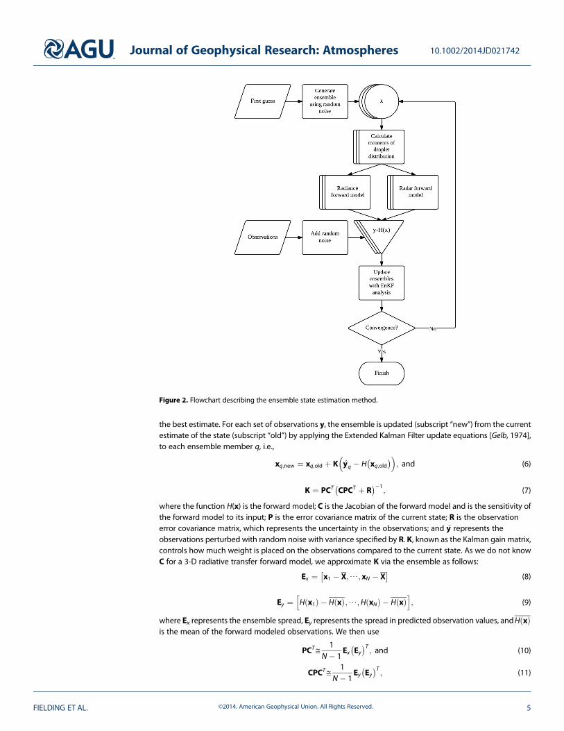
Figure 2. Flowchart describing the ensemble state estimation method.

Journal of Geophysical Research: Atmospheres 10.1002/2014JD021742

FIELDING ET AL. ©2014. American Geophysical Union. All Rights Reserved. 5

so that C is not required (see Gillijns et al. [2006] for a full derivation). Equation (10) can therefore be thoughtof as the covariance between the error in the estimate of the state and the error in the predicted observationsand equation (11) as the covariance of the error in the predicted observations.

In the standard EnKF, equations (6) and (7) would be calculated once per set of observations to provide anestimate of the state that is an error-weighted combination of the current state and observations. In ouradaptation, instead of sequentially updating our state at each set of observations, we iterate equations (6)–(11)using the same observations until the forward modeled values fit the observations to a specified tolerance,effectively losing the information of the state at the start of the iterative process. Note that the reuse ofobservations introduces correlations between the error in the state and the error in the observations,potentially introducing additional error to the retrieval [Ide et al., 1997]. However, in agreement with Yanget al. [2012], we found no significant decrease in error when introducing new, independent observationerrors at every new iteration when testing the method with synthetic data, although there was a tendencyfor an increase in the ensemble spread. We also add a small amount of additional noise after each iterationto help explore the state space, which also helps to reduce any error introduced by reusing observations.Nevertheless, caution should be exercised when using the ensemble spread to estimate the uncertainty inthe retrieval.

The details of the method are outlined in Figure 2. First, an initial ensemble, X, of state variables isgenerated from a first guess by perturbing each member with random noise with their spread representingP. The first guess is chosen from the climatological mean. For a sufficiently large initial uncertainty (P) and alarge number of iterations, the choice of the first guess has little influence on the final solution, becausethe information of the first guess gets lost during iterations as discussed above. Once the ensemble hasbeen set up, the iterative procedure begins. Each ensemble member is forward modeled according to theobservations available. To ensure the correct ensemble spread is maintained, each ensemble member“sees” a slightly different set of observations (i.e., y) by adding random error to each observation accordingto R. The y is generated with a new set of random errors at each iteration. Errors in the forward modelcan also be included in R by adding noise to the appropriate parameter (e.g., surface albedo in theradiance forward model). Next, the EnKF update step is calculated using equations (6)–(11). The procedure isiterated by setting xq,old equal to xq,new until convergence between the observations y and the forward

modeled values, H xð Þ. For each new set of observations, a new ensemble is generated so that each retrievalis independent.

We use the measurement uncertainties of the SACR, 2NFOV, and SAS-Ze to specify the observation errorcovariance matrix R. We assume the errors are unbiased, Gaussian, and uncorrelated between differentradar gates and radiance channels. Random measurement error in radar is caused by the fluctuatingconstructive and destructive interference from the backscatter of the cloud droplets moving relative to eachother inside the target volume. The magnitude of this error is a function of the number of independentsamples and the signal-to-noise ratio, both of which are deducible from SACR measurements. For theexperiments with synthetic measurements, we assume a constant random measurement error of 2 dB. Weassume a 5% measurement uncertainty in zenith radiances [Holben et al., 1998], a 10% uncertainty in surfacealbedo for 440 nm wavelength, and 5% uncertainty for all other wavelengths [Schaaf et al., 2002].

In the experiments here, we make an adaption to the method to save computational cost. Evensen andVanLeeuwen [1996] recommended that the number of ensemble members should equal the size of the state.The computational cost of an ensemble size that matched the number of grid points in a supercolumn wouldbe prohibitively expensive; following Hogan [2007], we therefore reduce the size of the state by assumingthat re is perfectly defined by Z and the column mean Nd (i.e., rearranging equation (4) so re is in terms ofZ and Nd). Random measurement error can still be accounted for in the radar reflectivity by adding theappropriate noise to Zwhen calculating re and LWC for the radiance forward model. This allows us to simplifyequation (1) so that the state vector only contains a 2-D array of column mean Nd.

2.3. Retrieval for the Rest of the Domain (Outside Supercolumns)

Once the supercolumns have been independently retrieved, cloud information for the rest of the domain isretrieved by matching their radar reflectivity factor with those in the supercolumns as follows: We definecolumns inside the supercolumn as donor columns and those outside the supercolumns as recipient

Journal of Geophysical Research: Atmospheres 10.1002/2014JD021742

FIELDING ET AL. ©2014. American Geophysical Union. All Rights Reserved. 6

columns, following a method similar to Barker et al. [2011]. For each recipient column, we choose a donorcolumn with the least sum of the squared differences in radar reflectivity between donor and recipient, i.e.,

argmindBZdonor∈Y

XHT

k¼HB

dBZkrecip � dBZk

donor

� �2; (12)

where Y is a set containing all the columns inside the supercolumns. Then, we assign the Nd of the closest-matching donor column to the recipient column and further retrieve re and LWC using the recipient column’sreflectivity and equations (4) and (2). The process is repeated for all recipient columns.

Note that it would be possible to assign a different moment of the droplet distribution (e.g., re) to thecolumns of similar Z. However, this would likely cause Nd to vary significantly and unrealistically with space.We therefore choose to assign Nd to maintain consistency with the supercolumns.

3. Evaluations Using Synthetic Measurements From Large-Eddy Simulations

We evaluate the retrieval method using a selection of snapshots of shallow trade wind cumulus generatedby a LES model with forcing data collected from the Rain In Cumulus over Ocean campaign [Jiang et al.,2009]. The original domain size is 6.4 × 6.4 × 4 km with grid spacing 25 × 25 × 10m and horizontallyperiodic boundary conditions but is reduced to 50 × 50 × 50m grid spacing to simulate the resolution of agridded scanning radar reflectivity field. To ensure a nonprecipitating cloud field, snapshots are taken froma simulation initialized with 1000 cm�3 hygroscopic aerosol particles, only some fraction of which is activated.The snapshots contain a range of cloud sizes in both area and depth, with cloud average LWP of 37 gm�2

(a maximum of 400gm�2) and re typically less than 10μm. Cloud fraction is on the order of 10%.

Truth cloudmicrophysical properties are calculated directly from the droplet size distributions of the LES, sortedinto 33 size bins. Thus, moments of the droplet size distribution such as Z or τ are calculated without assuminga basis function for the size distribution. However, as Nd is an intensive variable, it is not obvious how tocalculate the truth column average Nd to compare with the retrieved Nd. As our retrieval is constrained withradiances, we use an extinction-weighted effective number concentration, Neff, calculated from the LESsnapshot using the visible extinction, σext, and number concentration calculated at each height level, k:

Neff ¼Xl

k¼1Nd;k �σext; kXl

k¼1σext; k

; (13)

where l is the total number of levels in the snapshot.

3.1. Experiment Setup

Each retrieval uses a snapshot in time of the entire model domain. Synthetic observations of radiances arecalculated using 3-D radiative transfer across the whole domain at 673 and 870 nm to mimic 2NFOVobservations and 440, 870, and 1640 nm to mimic SAS-Ze observations. The radiances are calculated along a1-D track across the domain, collocated with the supercolumns.

Synthetic observations of gridded radar reflectivity are created directly from the LES. The radar reflectivity iscalculated directly from the droplet distributions using a Rayleigh scattering approximation. To limit thesource of errors in the retrieval method, we do not account for errors in gridding the data or errors due togaseous or liquid water attenuation. While we assume an infinitely sensitive radar in the supercolumnretrieval stage, we do restrict the reflectivity in the extrapolation stage to points greater than�50 dBZ so onlycloud grid points are included in the minimization of equation (12).

As mentioned in section 2.2, retrievals are performed for supercolumns first, and the size of the supercolumnsshould be optimized to account for as much as possible of the 3-D effects in radiance measurements whilehaving an acceptable computational time. To find the optimal domain size required to accurately forwardmodel radiances, we compared radiances calculated by 3-D radiative transfer using smaller subdomains to aLES cumulus snapshot “truth” with zenith radiances calculated using the whole domain. As expected, wefound that the root-mean-square error (RMSE) and the bias in the radiances generally decreased withincreasing supercolumn size. To accurately forward model radiances with an RMSE of less than 10%, the

Journal of Geophysical Research: Atmospheres 10.1002/2014JD021742

FIELDING ET AL. ©2014. American Geophysical Union. All Rights Reserved. 7

supercolumn width must be around 1500m for solar zenith angle (SZA) of 30° and 2500m for SZA of 60°(figures not shown).

Ideally, we would simply use a supercolumn with a width of 2500m or larger. However, given a high spatialresolution retrieval, this would create a large state vector such that the retrieval method would require acomputationally prohibitive number of ensemble members. As a compromise, we nest the supercolumn insidea “buffer zone” that is not explicitly retrieved but used in the radiative transfer forwardmodel. We can do this bycalculating LWC and re using Z and the first guess of Nd (again, rearranging equation (4) so re is in terms of Z).

Table 1 lists the key input parameters and settings for the evaluation experiments. We set the supercolumn tocontain 5 × 5 columns, giving a total width of 250m and a total state size of 25. The vertical resolution is 50m.Each supercolumn is nested inside a buffer zone with width 1500m for a 30° SZA. The shape parameter σ waschosen such that it minimized the RMSE between the true LWC from the LES data and the LWC derived fromequation (2) using the true Nd and re from the LES data. This gave a value of 0.3, which is consistent withshape parameters from in situ observations in Miles et al. [2000]. The first guess for each Nd assigned to eachensemble member was chosen to be 100 cm�3, close to the cloud average Nd in the snapshot. Random noisewith standard deviation of ~50 cm�3 is added to each ensemble member in log space.

3.2. Evaluation Results

Figure 3 shows domain retrievals from a single case using synthetic SACR reflectivity and SAS-Ze zenithradiances at 440, 870, and 1640 nm. Qualitatively, the retrievals well capture areas of cloud with higher Nd;the spatial distribution and the magnitude of re are also reasonable. Consequently, the retrieved LWP is verysimilar to the truth except at cloud edges where radar reflectivity is less than �50 dBZ, which excludes themfrom the donor-recipient process of the retrieval (i.e., step 3 in section 2.1).

To focus on quantitative evaluations over cloudy regions only, we define a cloudy column as a region withLWP greater than 5 gm�2 and a cloudy voxel where LWC is greater than 0.01 gm�3. Table 2 shows that thetruth has a domain average LWP of 37 gm�2, re of 6.4μm, and Nd of 196 cm

�3 over cloudy columns. Wholedomain retrievals in Figure 3 have a mean LWP remarkably close to the truth mean, but the correspondingRMSE is 19 gm�2. Not surprisingly, similar error characteristics with a slightly negative bias and a relativelylarge RMSE are also found in LWC retrievals over cloudy voxels. Additionally, retrieved re in cloudy voxels havea negative bias of 19% and RMSE of 2μm, which leads to a positive bias in τ of ~1 over cloudy columns.

We now look more carefully at the errors in the supercolumns where the heart of our retrieval method isperformed. Figure 4 compares retrieved column-averaged properties with the truth along the radiance track.This cross section is a good test for the retrieval—it contains optically thin cumulus clouds with reflectivitiesbelow�40 dBZ to the left of the domain and a much deeper, developed cloud toward the right with a core of�20 dBZ. Retrieved Nd is generally close to the truth except for the very thin clouds at the start of the crosssection. LWP and τ match well and have correlations above 0.9. Effective radius is slightly underestimated,especially where Nd is overestimated at the start of the cross section. The radiance becomes very sensitive toNd in low reflectivity clouds, as shown by the larger uncertainty (blue shading in Figure 4b). Overall, theaverage uncertainty is 77% in Nd, which translates to a 20% uncertainty in LWC and 6% uncertainty in recalculated via equations (2) and (4). If the retrieval were to be used as an operational product, retrievalsassociated with large uncertainty in Nd could be flagged as potentially unreliable to prevent misleadingresults. Also, a very thin cloud might not conform to a lognormal droplet distribution with an assumed shape

Table 1. First Guesses and Uncertainties for Experiments With Synthetic Data

Parameter/Observation Mean Value Standard Deviation

Cloud droplet number concentration Nd (cm�3) 100 50Lognormal shape parameter (unitless) 0.3 0.05Zenith radiance (Wm�2μm�1 nm�1 sr�1) Calculated from 3-D radiative transfer given a cloud field 5%Surface albedo440nm and 673 nm 0.05 10%870nm 0.3 5%1640nm 0.25 5%

Radar Reflectivity (dBZ ) Calculated directly from LES snapshot 2

Journal of Geophysical Research: Atmospheres 10.1002/2014JD021742

FIELDING ET AL. ©2014. American Geophysical Union. All Rights Reserved. 8

parameter of 0.3. Overestimating the shape parameter would lead to an underestimation of re, as discussed insection 3.3.2.

We can also consider individual profiles in the domain. Figure 5 shows the vertical profile of Nd, LWC, and re inthe core of the large cloud at X= 3 km and Y=3 km. Each cloud property matches well with the truth.Above 1400m there is a second layer of cloud with larger re yet smaller Nd than the cloud below. This ispresumably because it is the remnants of a larger cloud where all the smaller droplets have evaporated as aresult of dry air entrained in to the cloud. As the retrieval is constrained to a constant Nd with height, the Nd

in the lower cloud is slightly underestimated, while the upper cloud Nd is overestimated. The nonlinearity

Table 2. Average Cloud Properties in Cloudy Regionsa Across the Full Domain andWithin the Supercolumns Only for theTruth and Retrieval

LWC (gm�3) re (μm) LWP (gm�2) Nd (cm�3)b τ

Full domainTruth 0.113 6.4 37.37 196 8.1Retrieval 0.112 5.2 36.41 258 8.5SupercolumnsTruth 0.165 6.5 72.82 220 15.3Retrieval 0.160 5.7 71.48 262 16.3

aDefined as cloudy voxels greater than 0.01 gm�3 and columns with LWP greater than 5 gm�2.bDroplet number concentration for the truth is calculated using equation (13).

Figure 3. Truth LES snapshot (top row) and retrieved (bottom row) column-averaged (main panels) and vertical cross sec-tions (side panels; bottom, Y=3.1 km, right, X=3.1 km) of number concentration, effective radius, and liquid water path.The retrieval used synthetic radiances at 440, 870, and 1640 nm and synthetic radar measurements, with SZA= 30° andparameters as given in Table 1. The black dashed line indicates the track of radiance measurements. The sun angle is in thepositive Y direction.

Journal of Geophysical Research: Atmospheres 10.1002/2014JD021742

FIELDING ET AL. ©2014. American Geophysical Union. All Rights Reserved. 9

between different parameters causes adifference in the size of the uncertainty,with Nd most uncertain and re the leastuncertain. The true uncertainties arelikely to be greater, as discussed in thenext section.

To summarize, within the supercolumns,re is underestimated by 12% and Nd isoverestimated by 20%, primarily due tothe thin clouds at the start of thesection. Biases in LWC and LWP are less(around 3%) as most of the contributionto the average is from the thickerclouds at the end of the section. Notethat when changing the first guess Nd

between 50 and 500 cm�3, retrievalbiases are similar and vary by only 5%for both LWP and re.

3.3. Sensitivity of Retrieval toRadiance Wavelength andDroplet Distribution

A number of factors potentially affectthe retrieval and its uncertainty,including the choice of wavelength inradiance measurements and thelognormal droplet distributionassumption. Using the same LEScumulus snapshot, the impact of eachfactor on the retrieval is examinedthrough diagrams as shown in Figures 6and 7. Similar to Taylor diagrams [Taylor,2001] that are widely used to evaluatemodel performance and also skill-biasdiagrams [Hogan and Mason, 2011], weexploit a relationship between theRMSE, standard deviation, and bias ofthe retrieval with respect to the truth sothat they can be plotted on the samechart. Given that θ is our retrieval of thetruth, the following holds:

MSE θð Þ ¼ Var θð Þ þ Bias θð Þð Þ2; (14)

where MSE is the mean squared errorand Var is the variance. Therefore, if thebias is plotted against the standarddeviation of the retrieval, usingPythagoras’ rule, lines of equal RMSEemanate from a “perfect retrieval” at theorigin. Importantly, this diagram showshowmuch of the RMSE is attributable tonoise (the standard deviation) ratherthan bias.

Figure 5. The truth (red; from LES in this case) and retrieved (blue) verticalprofiles of (a) cloud droplet number concentration, (b) cloud effectiveradius, and (c) LWC, taken from X=3 km, Y=3 km in Figure 3. Retrievalsare plotted with one standard deviation (shaded light blue) estimatedfrom the spread of the ensembles.

a)

b)

c)

d)

e)

Figure 4. Retrieved cloud properties along the track of radiances atY=3.1 km, using synthetic data shown in Figure 3. (a) Radar reflectivity,(b) cloud droplet number concentration (Nd), (c) liquid water path (LWP),(d) optical depth, and (e) effective radius. Retrieved values are shown indark blue with uncertainty of one standard deviation uncertainty in lightblue shading, while the corresponding truth values are represented bythe dashed red lines.

Journal of Geophysical Research: Atmospheres 10.1002/2014JD021742

FIELDING ET AL. ©2014. American Geophysical Union. All Rights Reserved. 10

3.3.1. Effect of Choice of Radiance WavelengthIdeally, a retrieval that exploits a hyperspectral instrument such as the SAS-Ze would use all the availablewavelengths. This would give the best estimate of the state and minimize the uncertainty from observationalerrors, assuming errors at each wavelength were unbiased and uncorrelated. However, the use of any additionalwavelength increases the computational cost of forward modeling the radiances. Further, radiances atcertain wavelengths may be more susceptible to biases or loss of information—for example, scattering fromaerosols will be greater at shorter wavelengths, so the forward model for radiance at these wavelengths wouldneed to include precise aerosol properties. A careful choice of wavelengths is therefore necessary.

We have examined four different wavelength configurations labeled 1–4 in Figure 6 using the same LESsnapshot as previously described, with the aim of understanding if any particular wavelengths are crucial. Thefirst configuration uses just 870 nm, a nonabsorbing wavelength. The second mimics observations from a2NFOV, which has two nonabsorbing wavelengths at 673 and 870 nm. The third has one nonabsorbing andone absorbing wavelength at 870 and 1640 nm, respectively. Finally, the fourth mimics the SAS-Ze with anadditional 440 nm wavelength (nonabsorbing). As a benchmark, we also test a configuration with noradiances and Nd is kept constant at 100 cm

�3, which has label 5. In this configuration, no ensemble retrievalis performed since Z can be directly converted to LWC and re using equations (2) and (4).

Figure 6 shows retrieval errors in LWC, LWP, re, and τ. The lack of radiance constraints in configuration 5meansthat all supercolumns, and therefore the entire domain, will have the same Nd as the prior guess. This leads to

Figure 6. Markers indicating errors in retrievedmicrophysical properties for different radiance channels, exceptmarker 5 that isfor a fixed cloud droplet number concentration. Standard deviation, bias, RMSE (green contours), and correlation (marker color)of the retrieval with respect to the truth are shown for (a) LWC, (b) effective radius, (c) LWP, and (d) optical depth. Markersfor the supercolumns only and whole domain are plotted as circles and squares, respectively. The plotted circle with label 5for Figure 6a has a bias of �0.065gm�3 and standard deviation 0.082gm�3. Similarly, the plotted circle with label 5 forFigure 6c has bias �16.9gm�2 and standard deviation 30.2gm�2 and Figure 6d has bias �6.6 and standard deviation 4.5.

Journal of Geophysical Research: Atmospheres 10.1002/2014JD021742

FIELDING ET AL. ©2014. American Geophysical Union. All Rights Reserved. 11

a large bias and RMSE for LWC, LWP, and τ, although interestingly it happens to improve the retrieval of re. Theimprovement in re, but a degradation of LWC, suggests that the strong constraint of Z on re (see equation (4))forces the retrieval to compromise between correct LWC and correct re when Nd is constrained by radiances.

The strong constraint of Z on re makes results in Figure 6 somewhat surprising in two aspects. First, comparisonsbetween configurations 1 and 2 suggest the retrievals are insensitive to the additional nonabsorbingwavelength at 673nm. While wavelengths in configuration 2 are necessary to provide a sufficient surfacealbedo contrast for methods that use zenith radiances only to reduce retrieval ambiguity [Chiu et al., 2006], thefinding in Figure 6 suggests that our new method does not require any particular spectral contrast in surfacealbedo. Second, comparisons between configurations 1 and 3 suggest that retrievals are improved by theadditional absorbing wavelength at 1640nm. This additional wavelength reduces the RMSE of LWP and τ by5gm�2 and 1, respectively, and has a negligible impact on re. While 1640nm is the primary wavelength thatprovides information on cloud droplet size formethods that use zenith radiances only, its impact in our retrievalis overwhelmed by the strong constraint from radar reflectivity. However, we did find that it helped to keep theretrieval stable and reduce noise inNd. Similar to the comparison between configurations 1 and 2, configuration4 with the additional 440 nm wavelength has comparable retrieval errors to those in configuration 3.

In short, these findings show that the retrievals are somewhat improved by the inclusion of both anabsorbing and a nonabsorbing wavelength but are insensitive to any further additional wavelengths. Resultsalso indicate that the constraint from zenith radiances is mainly on τ, while the constraint from Z is mainly oncloud droplet size and LWC.3.3.2. Effect of Shape Parameter in Cloud Droplet Size DistributionIn our retrieval we assume that the shape parameter σ of the lognormal droplet distribution is constant. Inreality, σ varies both horizontally and vertically due to variability in cloud condensation nuclei, vertical

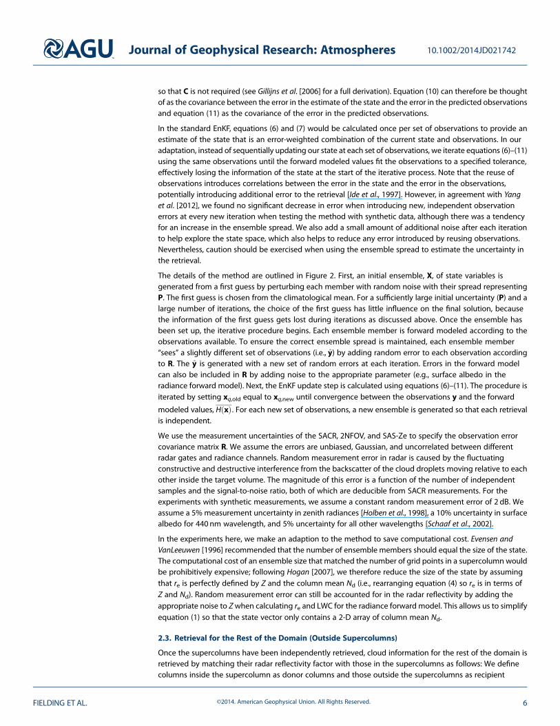
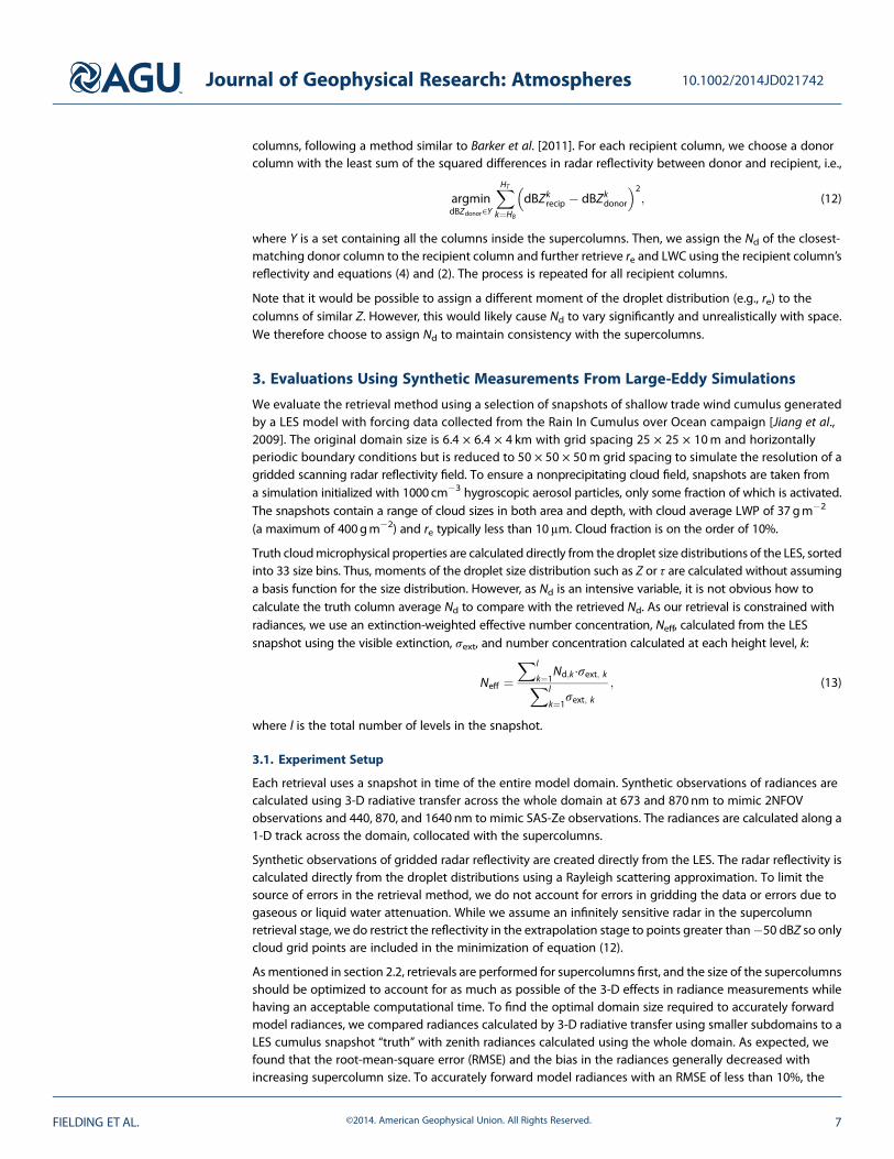
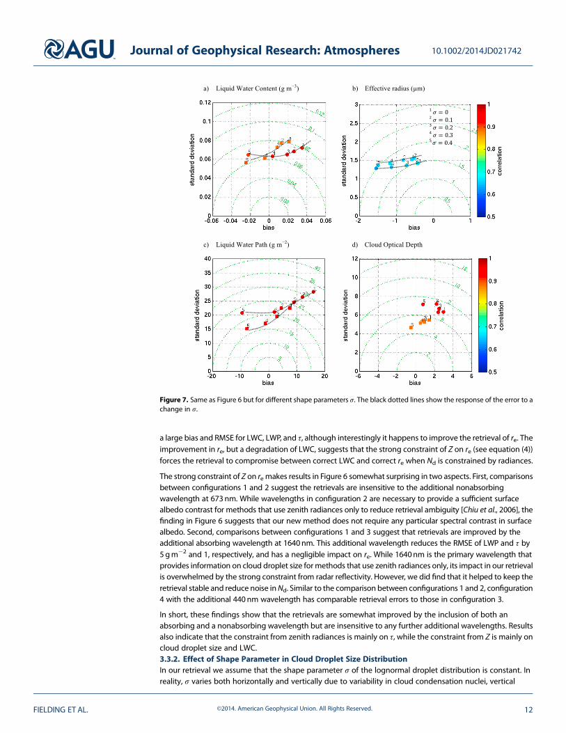
Figure 7. Same as Figure 6 but for different shape parameters σ. The black dotted lines show the response of the error to achange in σ.

Journal of Geophysical Research: Atmospheres 10.1002/2014JD021742

FIELDING ET AL. ©2014. American Geophysical Union. All Rights Reserved. 12

velocity, microphysical processes, and other atmospheric processes such as entrainment-mixing. This sectionassesses the sensitivity of retrieved cloud properties to assuming a constant shape parameter.

Figure 7 shows the retrieval performance for the same LES snapshot but using shape parameters rangingfrom 0 to 0.4. Overall, τ appears less sensitive to the shape parameter (Figure 7d) because radiances directlydepend on optical depth, but increasing σ decreases the retrieved mean re, LWC, and LWP (as shown inFigures 7a–7c), which can be explained as follows. By combining equations (2)–(4) and ignoring the attenuationterm in equation (4) for simplicity, we can rewrite τ as follows:

τ ¼ 2π∫HT

HBZ

13N

23d exp �4σ2

� �dh: (15)

For a given Z and τ, equation (15) indicates that an increase in σ increases Nd, which decreases re based onequation (4). Additionally, equation (3) indicates that if re decreases, LWC also decreases for a given τ, which isconsistent with Figure 7.

Another interesting finding in Figure 7 is that the minimum in bias and RMSE for LWC and LWP occurs whenthe shape parameter is around 0.3, matching the value derived earlier from the truth. We can use thestandard deviation in observed shape parameter of 0.13 found inMiles et al. [2000] to estimate a typical rangeof error for using a shape parameter that differs from the mean. For example, if the shape parameter werechosen in the range 0.17–0.43, Figure 7a suggests that the bias in LWC would be between 0.03 and�0.03 gm�3 (±25% of the domain average; see Table 2) and a maximum RMSE of 0.08 gm�3, whereas theretrieval that used the “true” shape parameter gave a bias < 0.01 gm�3 and < 0.06 gm�3 RMSE.

4. Case Study With Real Data

Two cases were chosen to demonstrate our retrieval method using ARM Mobile Facility data at the Azoresduring November 2009. Potential cases were restricted to daytime, nondrizzling low clouds. At the time,the WSACR (W band SACR) CWRHI scans were performed at a fixed azimuth; to get the best 3-D griddedestimates, we were also restricted to times when the wind direction was approximately perpendicularto these scans. As a result, we selected a relatively homogeneous stratocumulus (Sc) case that latertransitioned to a cumulus (Cu) case on 21 November; both Sc and Cu were analyzed. Surface pressurecharts confirm a northwesterly airflow with a long fetch across the Atlantic Ocean. We used the WSACRas this was the only radar available. As the field site did not have a SAS-Ze, we used radiances fromthe 2NFOV.

4.1. Retrieval Configuration

For both cases, we select the same configuration that was used in the synthetic data experiments given inTable 1, except the first guess for Nd is reduced to 50 cm

�3 as we expect the aerosol loading to be less than thatin the polluted LES case. In spite of this, we found that changing the first guess by a factor of 2 did not affectthe retrieved Nd by more than 5%. Additionally, we use a buffer zone of 2500m to account for the higher ~60°SZA seen in both cases. To match the observed clear-sky radiance, a layer of sulfate aerosol is added toboth cases with particle effective radius of 0.1μm and 10�5 gm�3 density in a 1 km layer from the surface.These values are ad hoc and would ideally use estimates from an independent retrieval; changing the aerosoldensity by a factor of 2 slightly affected the retrieved Nd up to 5%. We make no attempt to model aerosolhygroscopic growth in the vicinity of clouds as in Charlson et al. [2007] or Schmidt et al. [2009] but expect thiseffect to be small in the relatively clean aerosol conditions in the Azores.

For each case we use an average wind speed from cloud base to cloud top obtained from a collocated915MHz wind profiler retrieval, allowing the temporal radiance and radar data to be mapped to the spatialgrid. In both cases, the wind speed was approximately 10m s�1; therefore, to yield a 50m spatial resolution,the 1 s radiance measurements are linearly averaged over a 5 s time period. Corrections for attenuation inthe radar reflectivity in equation (4) are approximated using kl= 4.341 dB km�1 (gm�3)�1, assuming atemperature of 10°C, and the total scattering cross section is small compared to the absorption cross section[Doviak and Zrnic, 1993, pp., 43], and αf= 0.6358 dB km�1, using the line-by-line model of Liebe [1985] withthe same temperature of 10°C and a saturated atmosphere at 1013 hPa.

Journal of Geophysical Research: Atmospheres 10.1002/2014JD021742

FIELDING ET AL. ©2014. American Geophysical Union. All Rights Reserved. 13

4.2. Retrieval Results

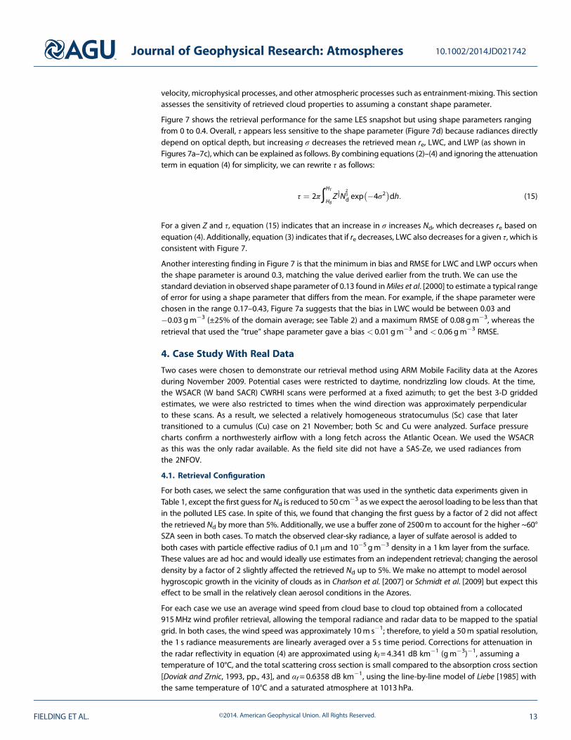
The retrieved 3-Dmicrophysical properties and cloud structure for these two cases are shown in Figure 8, andaverage microphysical properties are summarized in Table 3. The track of radiances for both cases is alongY= 2.5 km, with the clouds passing along the X axis from positive to negative. Overall, the domain average Nd,LWP, and re are higher for the Sc case than the Cu case. The τ is 3 times greater in the Sc case, but thevariability in τ, as a percentage of the mean, is greater in the Cu case.

Figure 9 shows a time series of the observations and retrieved cloud properties for the Sc case directly abovethe site (i.e., the cross section along Y= 2.5 km). The observed radar reflectivity suggests that precipitationis mainly absent and cloud geometric thickness varies between 400m and 800m. Toward the end of the timeseries the stratocumulus is beginning to be coupled with cumulus, as indicated by an area of higherreflectivity underneath the main cloud layer.

Retrieved Nd in Figure 9b generally varies between 50 and 200 cm�3. These values are comfortably in theexpected range for stratocumulus in a maritime airmass [Miles et al., 2000] and within the variability reportedby Wang et al. [2009]. Compared to independent LWP retrievals from microwave radiometer (MWR)measurements (MWRRET [Turner et al., 2007a]), the retrieval shows good agreement (Figure 9c) with a meandifference of 1 gm�2 and root-mean-square difference (RMSD) of 20 gm�2, although the uncertainty ofMWRRET is typically 20–30 gm�2. Additionally, the retrieved τ also shows good agreement with those fromtwo-channel zenith radiances only [Chiu et al., 2006], with a mean difference of 2.6 and RMSD of 6.5. Theobserved radiances in Figure 9e are negatively correlated with retrieved τ in Figure 9d, which is expected

Figure 8. Retrieved cloud fields for (a) stratocumulus case and (b) cumulus case, with 3-D LWC plotted as grey isosurfaces,slices of 3-D effective radius plotted along the Y axis and LWP plotted at the surface. The mean wind (u) direction is shownby the black arrow, while the track of radiances along Y=2.5 km is shown by the red dashed line.

Journal of Geophysical Research: Atmospheres 10.1002/2014JD021742

FIELDING ET AL. ©2014. American Geophysical Union. All Rights Reserved. 14

in an optically thick overcast cloud fieldwhere 3-D effects are less pronounced.Finally, the small differences betweenthe forward modeled radiances and theobserved radiances in Figure 9f give usconfidence in the retrieval.

To understand how much improvementhas been made through the use of theradiances, we compare our retrievals withthose calculated from equations (2)–(4)using a climatological Nd of 50 cm

�3.As shown by black dashed lines inFigure 9, a reasonable agreement withthe MWRRET and radar-only retrieval isfound, but some LWP retrievals notablyfall outside the uncertainty of theMWRRET. The retrieved average LWP is15% less compared to MWRRET (thedifference between our retrieval andMWRRET was 2%), and the averagecloud optical depth is 35% lesscompared to the radiance-only retrieval(the difference between our retrievaland the radiance-only retrieval was20%), suggesting the retrieval from theensemble method has added skill fromthe first guess of 50 cm�3.

Similarly, Figure 10 shows results for theCu case. The low reflectivities andabsence of virga again suggest that thereis no precipitation. The cloud base isgenerally at 800m, but the cloud atX=2 km has a higher cloud base of1200m and is probably the remnants ofthe stratocumulus field from earlier in theday. The domain average Nd is slightlysmaller than the Sc case and with aslightly smaller range of 10–150 cm�3.

Figure 9. Observations and retrieved cloud properties along the track ofradiances (Y=2.5 km) of the stratocumulus case shown in Figure 8. (a)Observed radar reflectivity; (b) retrieved droplet number concentration(dark blue); (c) retrieved liquid water path (dark blue) and MWRRET LWP(red) plotted with ±30 gm�2 error bars; (d) retrieved cloud optical depth(dark blue), 2NFOV retrieved optical depth (red); (e) observed zenithradiance (673 nm blue line; 870 nm red line); and (f ) difference betweenforward modeled radiances and observations (673 nm blue dashed line;870 nm red dashed line). The black dashed line in Figures 9b–9d showsthe retrieval using the first guess of Nd = 50 cm�3.

Table 3. Mean and Standard Deviation (Std) of Retrieved Microphysical Properties Over Cloudy Regionsa for aStratocumulus (Sc) and a Cumulus (Cu) Case From the ARMMobile Facility Deployment at the Azores on 21 November 2009

Scb Cuc

Cloud Property Mean Std Mean Std

Cloud droplet number concentration Nd (cm�3) 69.6 39.2 40.4 32.3Effective radius re (μm) 7.9 3.1 5.8 1.9Liquid water content (gm�3) 0.096 0.070 0.028 0.022Liquid water path (gm�2) 63.0 26.7 13.5 10.9Cloud optical depth 12.2 6.0 4.4 3.0Cloud fraction 1 - 0.24 -

aDefined as cloudy voxels greater than 0.01 gm�3 and columns with LWP greater than 5 gm�2.b11:25–11:35 UTC.c14:10–14:20 UTC.

Journal of Geophysical Research: Atmospheres 10.1002/2014JD021742

FIELDING ET AL. ©2014. American Geophysical Union. All Rights Reserved. 15

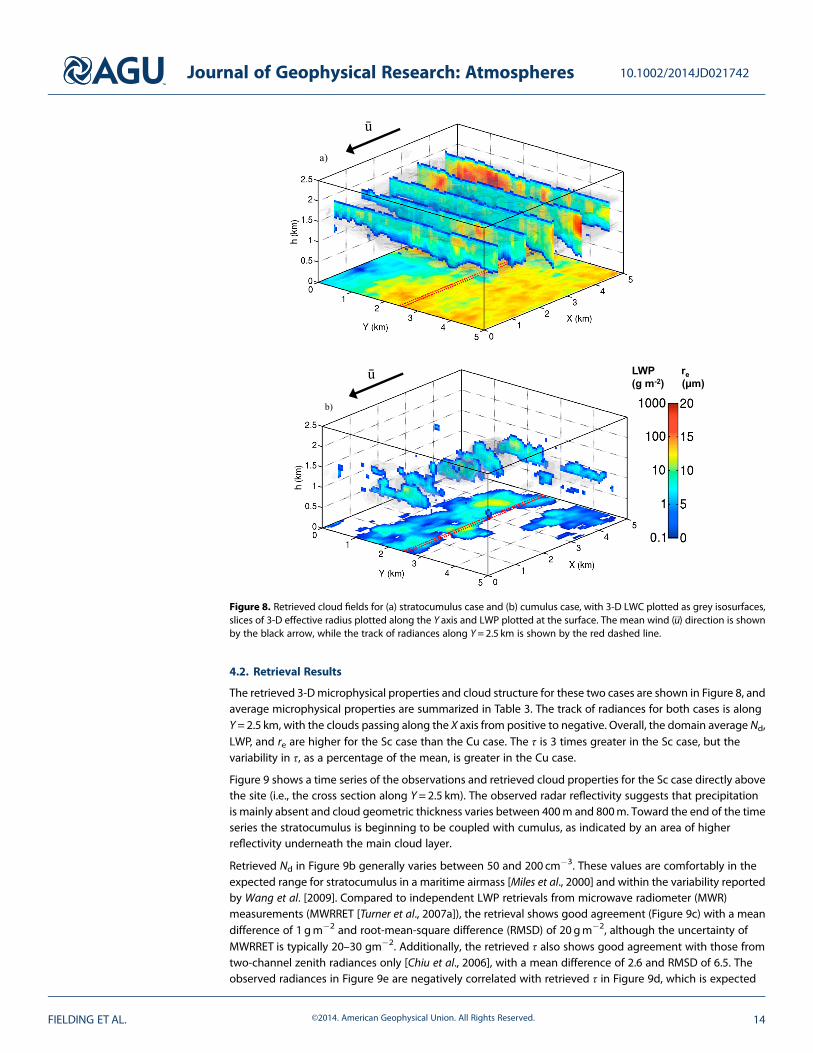
Unfortunately it is difficult to validate thecumulus observations, because retrievalmethods based on measurementsfrom either MWR or 2NFOV struggle withthe low LWP and heterogeneity thatthe cumulus presents. Nevertheless, theretrieved τ and 2NFOV τ for the largercloud in the middle agree in overallmagnitude, whereas the optical depthretrieved using a climatological Nd of50 cm�3 is lower. For the smaller cloudsat the beginning and end of the timeseries the 2NFOV retrieval gives anunphysical retrieval due to the so-called“clear-sky contamination” problem(where the field of view is only partiallyfilled with cloud) identified in Chiu et al.[2006]. By combining radiances withradar reflectivity, our new method helpsresolve this issue. We can also comparethe retrieval with in situ measurementsof similar clouds; the mean LWC of0.03 gm�3 is reasonable fornonprecipitating shallow cumulus. Ataround X=3 km the retrieval has a largeuncertainty in Nd and the forwardmodeled radiances are systematicallyunderestimated. Here the radarreflectivity is very low, and theunderestimation in radiances could bedue to haze particles at cloud edge thatare not detectable by the radar.

5. Discussion

In this section we discuss issues related to radar sensitivity and computational cost for future potentialimprovements. Radar sensitivity limits both the domain size of the retrieval and the ability to detectcloud edges. The current implementation was limited to 5 km × 5km × 5 km because of the sensitivity of theWband scanning cloud radar; a large fraction of cloudwould not be detected beyond this domain. For example,for the scanning radar used here, the minimum detectable reflectivity at 5 km is estimated at �27.5 dBZ.At 10 km this increases to�22.5 dBZ, whichwouldmiss nearly all the clouds in both stratocumulus and cumuluscases described in the previous section. Increasing the sensitivity of the SACRs is an ARM priority and wouldreduce the chance of missing clouds and hence reduce the retrieval uncertainty.

However, cloud edges are likely to be missed even within the limited domain, leading to errors in the retrieval.Examples of the effects of radar sensitivity on retrieved 3-D cloud microphysical properties are given in Fieldinget al. [2013]. Missing a horizontal cloud edge is particularly troublesome as it is likely that no cloud wouldbe retrieved in the whole column. This could then affect the retrieval of neighboring columns where cloudis detected, through knock-on errors in the 3-D radiative transfer modeling of radiances. For example, acloudy pixel neighboring a missed edge might be brighter in the forward model (due to illumination)than in reality. A potential solution could be that when cloud edges are detected in the zenith radiances but notby the radar, artificial observations of radar reflectivity are added to the edges of nearby clouds.

Additionally, using 3-D radiative transfer as a forward model is computationally expensive, driving many ofthe choices for our implementation of the retrieval. For example, when forward modeling radiances, we needto use a buffer zone that surrounds the retrieved supercolumn to ensure that nearby clouds are well

Figure 10. Same as Figure 9 but for the cumulus case shown in Figure 8.Note that the MWR-retrieved LWP is negative and retrievals from two-channel radiances are only physical between 14.24 and 14.26 UTC (hours).

Journal of Geophysical Research: Atmospheres 10.1002/2014JD021742

FIELDING ET AL. ©2014. American Geophysical Union. All Rights Reserved. 16

represented. With unlimited computer resources, one could set the buffer zone to be as large as possible.However, there would be a point where the benefit of increasing the buffer zone further would be limited bythe sensitivity of the radar to observe more distant clouds.

Another adjustable parameter, the supercolumn size (the size of the domain where cloud properties areretrieved directly by the ensemble method), is largely restricted by the influence of the cloud field onzenith radiances. Increasing the supercolumn size beyond a few hundred meters potentially introducesinstability in the retrieval. For a given observed radiance, there could be many different realizations of thecloud field that give the same forward modeled radiance, particularly for lower sun elevation angles. Forlarger supercolumns we often found the retrieved variables would oscillate, creating unrealistic yettechnically correct solutions. One way around this problem is to apply a smoothness constraint to theproblem. This can be implemented in the method by creating correlations between the state variableswhen initializing the ensembles. Subsequent iterations retain the correlation, effectively smoothing thesolution. Also, as this smoothing reduces the degrees of freedom of the problem, the number of ensemblemembers required for an accurate solution is reduced.

6. Summary and Conclusions

Using ground-based observations, we introduced for the first time a new cloud retrieval method thatprovides 2-D fields of Nd and 3-D fields of LWC and re for nonprecipitating warm liquid water clouds. Themethod exploits not only synergetic measurements of scanning cloud radar and shortwave spectralradiances but also a novel ensemble method that incorporates radiance constraints using 3-D radiativetransfer code, which is extremely difficult for other retrieval techniques (e.g., variational methods).Importantly, the constraints from spectral radiances help our retrievals achieve consistency between cloudmicrophysical and optical properties and between shortwave and microwave spectral regions. Since ourretrieval is independent of LWP retrievals from MWR measurements, it greatly enhances ground-based LWCobservations and can serve as an invaluable evaluation data set.

The retrieval performance was first evaluated using synthetic measurements generated from a LES shallowcumulus case, whose small cloud sizes and highly inhomogeneous features pose a great challenge toretrieval methods. In general, the true LWP in this case was an average of 37 gm�2 and did not exceed400 gm�2. The domain size in the horizontal was set around 6.4 km at 50m resolution, based on the scanspeed and the sensitivity of typical cloud radars. Synthetic measurements of radar reflectivity and zenithspectral radiances were generated to mimic ARM SACR and shortwave radiometer observations (e.g., SWS-Zeand 2NFOV), respectively. Given the uncertainty in the observations, the retrieval uncertainty in thesupercolumns (a subdomain directly above the observation site) of LWC is 20% and re 6%. Without theradiance observation at 1640 nm, an absorbing wavelength, the RMSE in LWC increased by 10–20% forretrievals that only use nonabsorbing wavelengths.

The retrieval performance was also evaluated using real data from the ARMMobile Facility deployment at theAzores for stratocumulus and cumulus clouds. In the stratocumulus case, retrieved LWP shows goodagreement with that from independent MWR measurements, with 1 gm�2 bias and RMSD of 20 gm�2.Additionally, the retrieved τ shows good agreement with 2NFOV τ, with a difference of 2.6 and RMSD of 6.5.Unfortunately in the cumulus case, the retrievals are difficult to compare with those from MWR and 2NFOVas they are either unphysical or unavailable for this broken-cloud case with low LWP. Future observationsfrom more scanning radars, SWS-Ze, and a three-channel MWR that has higher sensitivity to low LWPclouds will help make robust evaluations of the retrievals.

The assumed unimodal lognormal droplet distribution in the retrieval is not suitable for drizzling cloud.However, the flexible framework should allow for adaptations to retrieve cloud properties in precipitating cloudif additional information to separate the drizzle and cloud contributions to radar reflectivity is included. Possiblesources of information include lidar, dual-wavelength radar, or Doppler spectra analysis, which is an ongoingarea of research. The framework would also allow the addition of further radiance observations from scanningspectrometers [e.g., Kassianov et al., 2012] or nonscanning multidirectional spectroradiometers [e.g.,Riechelmann et al., 2013] to enhance radiance constraints from more directions, which could potentiallyimprove overall retrievals.

Journal of Geophysical Research: Atmospheres 10.1002/2014JD021742

FIELDING ET AL. ©2014. American Geophysical Union. All Rights Reserved. 17

ReferencesAckerman, T. P., and G. M. Stokes (2003), The Atmospheric Radiation Measurement program, Phys. Today, 56(1), 38–44, doi:10.1063/

1.1554135.Austin, R. T., and G. L. Stephens (2001), Retrieval of stratus cloud microphysical parameters using millimeter-wave radar and visible optical

depth in preparation for CloudSat—1. Algorithm formulation, J. Geophys. Res., 106(D22), 28,233–28,242, doi:10.1029/2000JD000293.Barker, H. W., M. P. Jerg, T. Wehr, S. Kato, D. P. Donovan, and R. J. Hogan (2011), A 3D cloud-construction algorithm for the EarthCARE satellite

mission, Q. J. R. Meteorol. Soc., 137(657), 1042–1058, doi:10.1002/Qj.824.Cahalan, R. F., W. Ridgway, W. J. Wiscombe, S. Gollmer, and Harshvardhan (1994), Independent pixel and Monte-Carlo estimates of

stratocumulus albedo, J. Atmos. Sci., 51(24), 3776–3790, doi:10.1175/1520-0469(1994)051<3776:Ipamce>2.0.Co;2.Charlson, R. J., A. S. Ackerman, F. A. M. Bender, T. L. Anderson, and Z. Liu (2007), On the climate forcing consequences of the albedo

continuum between cloudy and clear air, Tellus B, 59(4), 715–727, doi:10.1111/j.1600-0889.2007.00297.x.Chiu, J. C., A. Marshak, Y. Knyazikhin, W. J. Wiscombe, H. W. Barker, J. C. Barnard, and Y. Luo (2006), Remote sensing of cloud properties using

ground-based measurements of zenith radiance, J. Geophys. Res., 111, D16201, doi:10.1029/2005JD006843.Chiu, J. C., A. Marshak, C. H. Huang, T. Varnai, R. J. Hogan, D. M. Giles, B. N. Holben, E. J. O’Connor, Y. Knyazikhin, and W. J. Wiscombe (2012),

Cloud droplet size and liquid water path retrievals from zenith radiance measurements: Examples from the atmospheric radiationmeasurement program and the aerosol robotic network, Atmos. Chem. Phys., 12(21), 10,313–10,329, doi:10.5194/acp-12-10313-2012.

Dong, X. Q., and G. G. Mace (2003), Profiles of low-level stratus cloud microphysics deduced from ground-based measurements, J. Atmos.Oceanic Technol., 20(1), 42–53, doi:10.1175/1520-0426(2003)020<0042:Pollsc>2.0.Co;2.

Doviak, R. J., and D. S. Zrnic (1993), Doppler Radar and Weather Observations, 2nd ed., Academic Press, San Diego, Calif.Evans, K. F. (1998), The spherical harmonics discrete ordinate method for three-dimensional atmospheric radiative transfer, J. Atmos. Sci.,

55(3), 429–446, doi:10.1175/1520-0469(1998)055<0429:Tshdom>2.0.Co;2.Evensen, G. (2003), The ensemble Kalman filter: Theoretical formulation and practical implementation, Ocean Dyn., 53(4), 343–367.Evensen, G., and P. J. VanLeeuwen (1996), Assimilation of Geosat altimeter data for the Agulhas Current using the ensemble Kalman filter

with a quasigeostrophic model, Mon. Weather Rev., 124(1), 85–96, doi:10.1175/1520-0493(1996)124<0085:Aogadf>2.0.Co;2.Fielding, M. D., J. C. Chiu, R. J. Hogan, and G. Feingold (2013), 3D cloud reconstructions: Evaluation of scanning radar scan strategy with a view

to surface shortwave radiation closure, J. Geophys. Res. Atmos, 118, 9153–9167, doi:10.1002/Jgrd.50614.Frisch, A. S., C. W. Fairall, and J. B. Snider (1995), Measurement of stratus cloud and drizzle parameters in ASTEX with a K-alpha-band Doppler

radar and a microwave radiometer, J. Atmos. Sci., 52(16), 2788–2799, doi:10.1175/1520-0469(1995)052<2788:Moscad>2.0.Co;2.Frisch, A. S., G. Feingold, C. W. Fairall, T. Uttal, and J. B. Snider (1998), On cloud radar and microwave radiometer measurements of stratus

cloud liquid water profiles, J. Geophys. Res., 103(D18), 23,195–23,197, doi:10.1029/98JD01827.Gillijns, S., O. B. Mendoza, J. Chandrasekar, B. L. R. De Moor, D. S. Bernstein, and A. Ridley (2006), What is the ensemble Kalman filter and how

well does it work?, Proc. Am. Control Conf., 1–12, 4448–4453, doi:10.1109/Acc.2006.1657419.Grecu, M., and W. S. Olson (2008), Precipitating snow retrievals from combined airborne cloud radar and millimeter-wave radiometer

observations, J. Appl. Meteorol. Climatol., 47(6), 1634–1650, doi:10.1175/2007jamc1728.1.Hartmann, D. L., M. E. Ockertbell, and M. L. Michelsen (1992), The effect of cloud type on earths energy-balance—Global analysis, J. Clim.,

5(11), 1281–1304, doi:10.1175/1520-0442(1992)005<1281:Teocto>2.0.Co;2.Hogan, R. J. (2007), A variational scheme for retrieving rainfall rate and hail reflectivity fraction from polarization radar, J. Appl. Meteorol.

Climatol., 46(10), 1544–1564, doi:10.1175/Jam2550.1.Hogan, R. J., and I. B. Mason (2011), Deterministic forecasts of binary events, in Forecast Verification: A Practitioner’s Guide in Atmospheric

Science, 2nd ed., edited by I. T. Jolliffe and D. B. Stephenson, John Wiley Ltd., Chichester, U. K., doi:10.1002/9781119960003.ch3.Hogan, R. J., and J. K. P. Shonk (2013), Incorporating the effects of 3D radiative transfer in the presence of clouds into two-stream multilayer

radiation schemes, J. Atmos. Sci., 70(2), 708–724, doi:10.1175/Jas-D-12-041.1.Hogan, R. J., N. Gaussiat, and A. J. Illingworth (2005), Stratocumulus liquid water content from dual-wavelength radar, J. Atmos. Oceanic

Technol., 22(8), 1207–1218, doi:10.1175/Jtech1768.1.Holben, B. N., et al. (1998), AERONET—A federated instrument network and data archive for aerosol characterization, Remote Sens. Environ.,

66(1), 1–16, doi:10.1016/S0034-4257(98)00031-5.Huang, D., K. Johnson, Y. Liu, and W. Wiscombe (2009), High resolution retrieval of liquid water vertical distributions using collocated

Ka-band and W-band cloud radars, Geophys. Res. Lett., 36, L24807, doi:10.1029/2009GL041364.Ide, K., P. Courtier, M. Ghil, and A. C. Lorenc (1997), Unified notation for data assimilation: Operational, sequential and variational, J. Meteorol.

Soc. Jpn., 75(1B), 181–189.Iglesias, M. A., K. J. H. Law, and A. M. Stuart (2013), Ensemble Kalman methods for inverse problems, Inverse Probl., 29(4), doi:10.1088/

0266-5611/29/4/045001.Illingworth, A. J., et al. (2007), Cloudnet—Continuous evaluation of cloud profiles in seven operational models using ground-based

observations, Bull. Am. Meteorol. Soc., 88(6), 883–898, doi:10.1175/Bams-88-6-883.Jiang, H. L., G. Feingold, and I. Koren (2009), Effect of aerosol on trade cumulus cloud morphology, J. Geophys. Res., 114, D11209, doi:10.1029/

2009JD011750.Kassianov, E., C. Flynn, J. Redemann, B. Schmid, P. B. Russell, and A. Sinyuk (2012), Initial assessment of the Spectrometer for Sky-Scanning, Sun-

Tracking Atmospheric Research (4STAR)-based aerosol retrieval: Sensitivity study, Atmos.-Basel, 3(4), 495–521, doi:10.3390/Atmos3040495.Kollias, P., N. Bharadwaj, K. Widener, I. Jo, and K. Johnson (2014), Scanning ARM cloud radars. Part I: Operational sampling strategies, J. Atmos.

Oceanic Technol., 31, 569–582, doi:10.1175/JTECH-D-13-00044.1.Liebe, H. J. (1985), An updated model for millimeter wave-propagation in moist air, Radio Sci., 20(5), 1069–1089, doi:10.1029/RS020i005p01069.Lohnert, U., S. Crewell, C. Simmer, and A. Macke (2001), Profiling cloud liquid water by combining active and passive microwave measurements

with cloud model statistics, J. Atmos. Oceanic Technol., 18(8), 1354–1366, doi:10.1175/1520-0426(2001)018<1354:Pclwbc>2.0.Co;2.Marshak, A., Y. Knyazikhin, K. D. Evans, and W. J. Wiscombe (2004), The “RED versus NIR” plane to retrieve broken-cloud optical depth from

ground-based measurements, J. Atmos. Sci., 61(15), 1911–1925, doi:10.1175/1520-0469(2004)061<1911:Trvnpt>2.0.Co;2.McBride, P. J., K. S. Schmidt, P. Pilewskie, A. S. Kittelman, and D. E. Wolfe (2011), A spectral method for retrieving cloud optical thickness and

effective radius from surface-based transmittance measurements, Atmos. Chem. Phys., 11(14), 7235–7252, doi:10.5194/acp-11-7235-2011.McFarlane, S. A., and K. F. Evans (2004), Clouds and shortwave fluxes at Nauru. Part I: Retrieved cloud properties, J. Atmos. Sci., 61(6), 733–744,

doi:10.1175/1520-0469(2004)061<0733:Casfan>2.0.Co;2.McFarlane, S. A., K. F. Evans, and A. S. Ackerman (2002), A Bayesian algorithm for the retrieval of liquid water cloud properties from

microwave radiometer and millimeter radar data, J. Geophys. Res., 107(D16), 4317, doi:10.1029/2001JD001011.

Journal of Geophysical Research: Atmospheres 10.1002/2014JD021742

FIELDING ET AL. ©2014. American Geophysical Union. All Rights Reserved. 18

AcknowledgmentsARM data is made available onlinethrough the U.S. Department of Energyas part of the Atmospheric RadiationMeasurement Program at http://www.archive.arm.gov. This research wassupported by the Office of Science(BER), U.S. Department of Energy (DOE)under grant DE-SC0007233. G.F.acknowledges DOE’s Office of Science(BER) and NOAA’s Climate Goal forsupport. We would like to thank theDepartment of Meteorology, Universityof Reading, for hosting G.F.’s visit duringsummer 2013, and Javier Amezcua andShuhua Chen for insightful discussionon the ensemble Kalman filter.

Miles, N. L., J. Verlinde, and E. E. Clothiaux (2000), Cloud droplet size distributions in low-level stratiform clouds, J. Atmos. Sci., 57(2), 295–311,doi:10.1175/1520-0469(2000)057<0295:Cdsdil>2.0.Co;2.

Oreopoulos, L., and S. Platnick (2008), Radiative susceptibility of cloudy atmospheres to droplet number perturbations: 2. Global analysisfrom MODIS, J. Geophys. Res., 113, D14S21, doi:10.1029/2007JD009655.

Pincus, R., C. Hannay, and K. F. Evans (2005), The accuracy of determining three-dimensional radiative transfer effects in cumulus cloudsusing ground-based profiling instruments, J. Atmos. Sci., 62(7), 2284–2293, doi:10.1175/Jas3464.1.

Qian, Y., C. N. Long, H. Wang, J. M. Comstock, S. A. McFarlane, and S. Xie (2012), Evaluation of cloud fraction and its radiative effect simulatedby IPCC AR4 global models against ARM surface observations, Atmos. Chem. Phys., 12(4), 1785–1810, doi:10.5194/acp-12-1785-2012.

Randall, D. A., et al. (2007), Climate models and their evaluation, in Climate Change 2007: The Physical Science Basis. Contribution of Working Group I tothe Fourth Assessment Report of the Intergovernmental Panel on Climate Change, edited by S. Solomon et al., pp. 589–662, Cambridge Univ. Press,Cambridge, U. K., and New York.

Rémillard, J., P. Kollias, and W. Szyrmer (2013), Radar-radiometer retrievals of cloud number concentration and dispersion parameter innondrizzling marine stratocumulus, Atmos. Meas. Tech., 6(7), 1817–1828, doi:10.5194/amt-6-1817-2013.

Riechelmann, S., M. Schrempf, and G. Seckmeyer (2013), Simultaneous measurement of spectral sky radiance by a non-scanningmultidirectional spectroradiometer (MUDIS), Meas. Sci. Technol., 24(12), doi:10.1088/0957-0233/24/12/125501.

Schaaf, C. B., et al. (2002), First operational BRDF, albedo nadir reflectance products from MODIS, Remote Sens. Environ., 83(1–2), 135–148,doi:10.1016/S0034-4257(02)00091-3.

Schmidt, K. S., G. Feingold, P. Pilewskie, H. Jiang, O. Coddington, andM. Wendisch (2009), Irradiance in polluted cumulus fields: Measured andmodeled cloud-aerosol effects, Geophys. Res. Lett., 36, L07804, doi:10.1029/2008GL036848.

Taylor, K. E. (2001), Summarizing multiple aspects of model performance in a single diagram, J. Geophys. Res., 106(D7), 7183–7192,doi:10.1029/2000JD900719.

Turner, D. D., S. A. Clough, J. C. Lijegren, E. E. Clothiaux, K. E. Cady-Pereira, and K. L. Gaustad (2007a), Retrieving liquid water path and pre-cipitable water vapor from the atmospheric radiation measurement (ARM) microwave radiometers, IEEE Trans. Geosci. Remote, 45(11),3680–3690, doi:10.1109/Tgrs.2007.903703.

Turner, D. D., et al. (2007b), Thin liquid water clouds—Their importance and our challenge, Bull. Am. Meteorol. Soc., 88(2), 177–374,doi:10.1175/Bams-88-2-177.

Wang, J., P. H. Daum, S. S. Yum, Y. Liu, G. I. Senum, M.-L. Lu, J. H. Seinfeld, and H. Jonsson (2009), Observations of marine stratocumulusmicrophysics and implications for processes controlling droplet spectra: Results from the Marine Stratus/Stratocumulus Experiment,J. Geophys. Res., 114, D18210, doi:10.1029/2008JD011035.

Wang, P., W. H. Knap, and P. Stammes (2011), Cloudy sky shortwave radiative closure for a Baseline Surface Radiation Network site,J. Geophys. Res., 116, D08202, doi:10.1029/2010JD015141.

Widener, K., N. Bharadwaj, and K. Johnson (2012), Scanning ARM Cloud Radar Handbook, doi:10.2172/1043296.Yang, S. C., E. Kalnay, and B. Hunt (2012), Handling nonlinearity in an ensemble Kalman filter: Experiments with the three-variable Lorenz

model, Mon. Weather Rev., 140(8), 2628–2646, doi:10.1175/Mwr-D-11-00313.1.

Journal of Geophysical Research: Atmospheres 10.1002/2014JD021742

FIELDING ET AL. ©2014. American Geophysical Union. All Rights Reserved. 19