Interactions among Soil Physical, Chemical and Biological ...
210
IJERD – International Journal of Environmental and Rural Development (2022)13-1 Ⓒ ISERD 1 Interactions among Soil Physical, Chemical and Biological Properties under Different Farming Systems MARISOL TERASHIMA* Graduate School of Agriculture, Tokyo University of Agriculture, Japan Email: [email protected] MACHITO MIHARA Faculty of Regional Environment Science, Tokyo University of Agriculture, Tokyo, Japan Email: [email protected] Received 14 December 2020 Accepted 9 July 2021 (*Corresponding Author) Abstract The definition of soil quality has always been changing over time within the soil science community. At first, the study focused more on chemical and physical properties and less importance on a sustainable environment. Therefore, the definition of soil quality has changed in the last decade. The importance of biodiversity that exists both on the surface and within the soil began to be understood. These organisms have essential functions such as nutrient cycling, provision of plant nutrients, and modification of physical soil structure, water regimes, and suppression of undesirable organisms on cropland. It has defined soil quality as the function it has within the environment, sustaining productivity, maintaining environmental quality, and promoting health in plants and animals. However, the interaction between some microorganisms is still unknown, or how it could affect the different parameters in the biodiversity of an agro ecosystem. Furthermore, it is unknown what parameters are important in determining soil quality. Therefore, this study analyzed the biological, physical, and chemical properties of the soil of two farms whose practices is different. Water retention capacity, aggregate distribution, organic matter, total nitrogen, NO3, NH4, and biomass of microorganisms were measured. Soils were air dried and sieved to 2mm. They were analyzed after drying in an oven at 105 ° C for 24 h. The biomass of microorganisms was measured by the direct extraction method. The results indicated that there was a significant difference between the microorganisms but could not be found with physical and chemical properties. This result could indicate the importance of biological properties over other parameters to discuss soil quality. In addition, the differences observed could be explained by the different practices carried out on each farm. Keywords soil quality, soil health, biomass of microorganisms, aggregates, total nitrogen INTRODUCTION Soil health is associated with soil biological parameters, such as biodiversity and its stability in the environment. When there are outbreaks of plant diseases, they are indicators of ecosystem instability and poor health. Thus, healthy soil has the ability of the biological community to suppress plant pathogens, the population of plant pathogens in the soil, and control the incidence and severity of diseases (van Bruggen and Grunwald, 1996). Accordingly, Cruz (2004) defines soil quality as dynamic, changing over time within the soil science community. At first, it was focused more on fertility, the yield of crops, and less importance on a sustainable environment. In other words, science has defined soil quality in chemical and physical parameters, such as the quantity or concentration of nutrients, organic matter, and water retention. erd Research article
-
Upload
khangminh22 -
Category
Documents
-
view
0 -
download
0
Transcript of Interactions among Soil Physical, Chemical and Biological ...
IJERD – International Journal of Environmental and Rural Development (2022)13-1
Ⓒ ISERD
1
Interactions among Soil Physical, Chemical and Biological
Properties under Different Farming Systems
MARISOL TERASHIMA* Graduate School of Agriculture, Tokyo University of Agriculture, Japan
Email: [email protected]
MACHITO MIHARA Faculty of Regional Environment Science, Tokyo University of Agriculture, Tokyo, Japan
Email: [email protected]
Received 14 December 2020 Accepted 9 July 2021 (*Corresponding Author)
Abstract The definition of soil quality has always been changing over time within the soil
science community. At first, the study focused more on chemical and physical properties and
less importance on a sustainable environment. Therefore, the definition of soil quality has
changed in the last decade. The importance of biodiversity that exists both on the surface and
within the soil began to be understood. These organisms have essential functions such as
nutrient cycling, provision of plant nutrients, and modification of physical soil structure, water
regimes, and suppression of undesirable organisms on cropland. It has defined soil quality as
the function it has within the environment, sustaining productivity, maintaining environmental
quality, and promoting health in plants and animals. However, the interaction between some
microorganisms is still unknown, or how it could affect the different parameters in the
biodiversity of an agro ecosystem. Furthermore, it is unknown what parameters are important in
determining soil quality. Therefore, this study analyzed the biological, physical, and chemical
properties of the soil of two farms whose practices is different. Water retention capacity,
aggregate distribution, organic matter, total nitrogen, NO3, NH4, and biomass of
microorganisms were measured. Soils were air dried and sieved to 2mm. They were analyzed
after drying in an oven at 105 ° C for 24 h. The biomass of microorganisms was measured by
the direct extraction method. The results indicated that there was a significant difference
between the microorganisms but could not be found with physical and chemical properties. This
result could indicate the importance of biological properties over other parameters to discuss
soil quality. In addition, the differences observed could be explained by the different practices
carried out on each farm.
Keywords soil quality, soil health, biomass of microorganisms, aggregates, total nitrogen
INTRODUCTION
Soil health is associated with soil biological parameters, such as biodiversity and its stability in the
environment. When there are outbreaks of plant diseases, they are indicators of ecosystem instability
and poor health. Thus, healthy soil has the ability of the biological community to suppress plant
pathogens, the population of plant pathogens in the soil, and control the incidence and severity of
diseases (van Bruggen and Grunwald, 1996). Accordingly, Cruz (2004) defines soil quality as dynamic,
changing over time within the soil science community. At first, it was focused more on fertility, the
yield of crops, and less importance on a sustainable environment. In other words, science has defined
soil quality in chemical and physical parameters, such as the quantity or concentration of nutrients,
organic matter, and water retention.
erd
Research article
IJERD – International Journal of Environmental and Rural Development (2022)13-1
Ⓒ ISERD
2
In the last few decades significant efforts have been made to increase agricultural productivity
through increased fertilization and pesticide application, improved irrigation, soil management regimes
and crops, and massive land conversions (Tilman et al., 2002). There is increasing concern, however,
that agricultural intensification is placing tremendous pressure on the soil’s capacity to maintain its
other functions leading to largescale ecosystem degradation and loss of productivity in the long term
(Tilman et al., 2001; Foley et al., 2005; Vitousek et al., 2009). Since microorganisms are involved in
many soil processes, they may also give an integrated measure of soil health, an aspect that cannot be
obtained with physical/chemical measures alone (Nielsen et al., 2002; Kibblewhite et al., 2008;
Mueller et al., 2010; Sharma et al., 2011).
There have been a few reports that have indicated that organic farming practices have positive
effects on soil microbial populations, processes and activities (Clark et al., 1998; Doran et al., 1996;
Drinkwater et al., 1995). Applications of insecticides may promote changes in population biodiversity
and dynamics by inhibiting or killing components of the soil microbial community. Fungicide
application can cause significant changes to the relative sizes of the bacterial and fungal communities
in soil (Sall et al., 2006; Sigler and Turco, 2002). Although most of the research has shown increased
microbial diversity in soils from organic farming systems compared to conventional farming systems,
some studies have found different results. Shannon et al. (2002) studied microbial communities in soils
managed under organic and conventional regimes, and found conflicting evidence that the size,
composition and activity of the soil microbial biomass were attributed to management practice. They
found that differences in microbial communities in soils under different management practices were
subtle rather than dramatic (Liu et al., 2007). Therefore this study focus on analyzing some physical,
chemical, and biological (the microorganism communities) properties as indicator of soil quality / soil
health of two agro ecosystem which have different practices. In addition, the discussion about what
parameters could be important to determine soil health.
MATERIAL AND METHODS
Soils from 2 farms in Kanto Area, Japan, with a history of natural and conventional crop
production were sampled. These were sampled at a depth of the upper 5 cm of the soil. Soils were air
dried and sieved to 2mm. The dry weight of the soil was determined after drying in an oven at 105 ° C
for 24 h.
The biomass of microorganism was measure by direct extraction method. Ten subsamples of 5.00
g of each soil were weighed separately into 50 ml centrifuge tubes and 20 ml of 0.5 M K2SO4 was
added to each. To three subsamples, 0.5 ml of ethanol-free chloroform was added. Both the
chloroform-exposed and the non-fumigated samples were capped and shaken simultaneously for 1 h.
After shaking, the suspensions could settle for 10 min and the supernatants were filtered through
Whatman No. 42 filter. For the sub-samples with chloroform, only the top 15 ml of the supernatant was
filtered to reduce the amount chloroform in the filtrate. Filtrates from soils with and without
chloroform were immediately bubbled with air for 30 min to remove any residual chloroform. Blanks
were treated in the same manner. Dissolved organic carbon in all filtrates was determined after
dichromate digestion by titrating with 0.033 M acidified ferrous ammonium sulphate (Anderson, et al.,
1993). Chloroform labile C was calculated as the difference between the C extracted from the
chloroform fumigated and the non-fumigated sample. All results are expressed on an oven-dry basis.
No conversion factor (kEC) was used to convert chloroform labile C to microbial biomass C because
the range of kEC values (0.41 - 0.58) is used in the literature and it has not been tested which is best
suited for the soils used here (Setia et al., 2012).
In addition, number of culturable bacteria and fungus were quantified. The plate count
methodology by plating is a widely used methodology (Hoben and So-masegaran, 1982), which
IJERD – International Journal of Environmental and Rural Development (2022)13-1
Ⓒ ISERD
3
consists of making 1:10 serial dilutions and spreading 100 µl of each dilution on a plate; plates are
incubated until colonies are countable.
The chemical and physical properties were measured as aggregate size, water retention capacity,
organic matter, total nitrogen, total phosphorus, nitrates, and ammonia. Soil samples analyzed the
aggregate's stability and distribution to observe the resistance in the water. Stability is influenced by
the physical and chemical properties of soils. In addition, the soil samples were evaluated for their
relationship with the organic matter.
For NO3 it was measured by nitration of salicylic acid (Cataldo et al., 1975) and for NH4 with
indophenol blue method described by Searle (1984). Statistical analysis with ANOVA was done for all
the treatments.
RESULTS AND DISCUSSION
Soil Physical and Chemical Properties
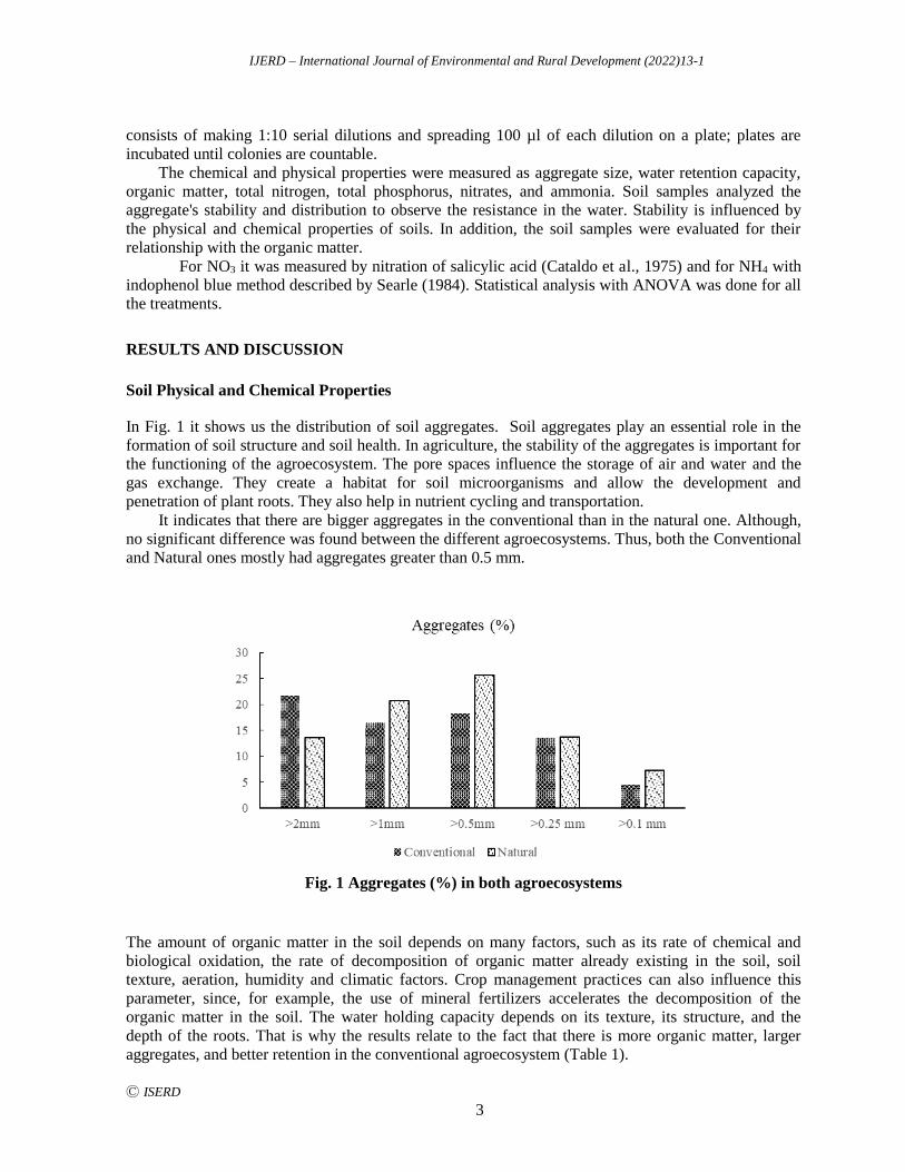
In Fig. 1 it shows us the distribution of soil aggregates. Soil aggregates play an essential role in the
formation of soil structure and soil health. In agriculture, the stability of the aggregates is important for
the functioning of the agroecosystem. The pore spaces influence the storage of air and water and the
gas exchange. They create a habitat for soil microorganisms and allow the development and
penetration of plant roots. They also help in nutrient cycling and transportation.
It indicates that there are bigger aggregates in the conventional than in the natural one. Although,
no significant difference was found between the different agroecosystems. Thus, both the Conventional
and Natural ones mostly had aggregates greater than 0.5 mm.
Fig. 1 Aggregates (%) in both agroecosystems
The amount of organic matter in the soil depends on many factors, such as its rate of chemical and
biological oxidation, the rate of decomposition of organic matter already existing in the soil, soil
texture, aeration, humidity and climatic factors. Crop management practices can also influence this
parameter, since, for example, the use of mineral fertilizers accelerates the decomposition of the
organic matter in the soil. The water holding capacity depends on its texture, its structure, and the
depth of the roots. That is why the results relate to the fact that there is more organic matter, larger
aggregates, and better retention in the conventional agroecosystem (Table 1).
IJERD – International Journal of Environmental and Rural Development (2022)13-1
Ⓒ ISERD
4
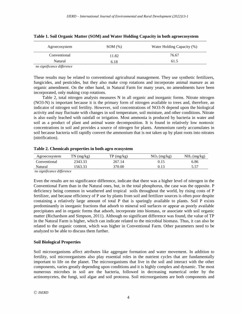
Table 1. Soil Organic Matter (SOM) and Water Holding Capacity in both agroecosystem
Agroecosystem SOM (%) Water Holding Capacity (%)
Conventional 11.82 76.67
Natural 6.18 61.5
no significance difference
These results may be related to conventional agricultural management. They use synthetic fertilizers,
fungicides, and pesticides, but they also make crop rotations and incorporate animal manure as an
organic amendment. On the other hand, in Natural Farm for many years, no amendments have been
incorporated, only making crop rotations.
Table 2, total nitrogen analysis measures N in all organic and inorganic forms. Nitrate nitrogen
(NO3-N) is important because it is the primary form of nitrogen available to trees and, therefore, an
indicator of nitrogen soil fertility. However, soil concentrations of NO3-N depend upon the biological
activity and may fluctuate with changes in soil temperature, soil moisture, and other conditions. Nitrate
is also easily leached with rainfall or irrigation. Most ammonia is produced by bacteria in water and
soil as a product of plant and animal waste decomposition. It is found in relatively low nontoxic
concentrations in soil and provides a source of nitrogen for plants. Ammonium rarely accumulates in
soil because bacteria will rapidly convert the ammonium that is not taken up by plant roots into nitrates
(nitrification).
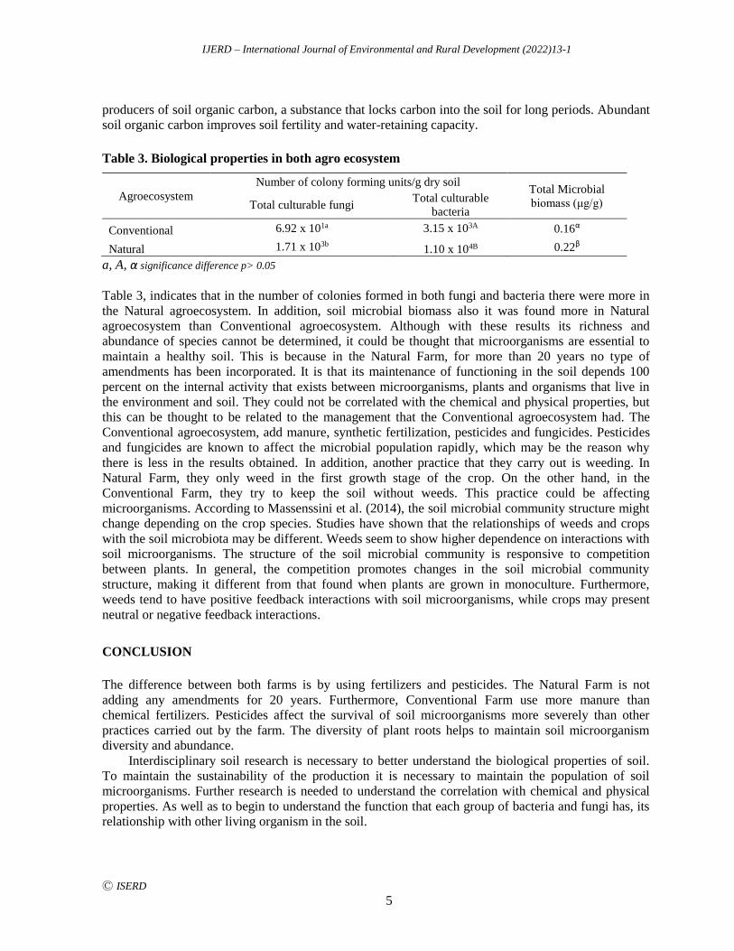
Table 2. Chemicals properties in both agro ecosystem
Agroecosystem TN (mg/kg) TP (mg/kg) NO3 (mg/kg) NH3 (mg/kg)
Conventional 2343.33 267.14 0.15 6.86
Natural 1563.33 370.00 0.13 5.57 no significance difference
Even the results are no significance difference, indicate that there was a higher level of nitrogen in the
Conventional Farm than in the Natural ones, but, in the total phosphorus, the case was the opposite. P
deficiency being common in weathered and tropical soils throughout the world, by rising costs of P
fertilizer, and because efficiency of P use by plants from soil and fertilizer sources is often poor despite
containing a relatively large amount of total P that is sparingly available to plants. Soil P exists
predominantly in inorganic fractions that adsorb to mineral soil surfaces or appear as poorly available
precipitates and in organic forms that adsorb, incorporate into biomass, or associate with soil organic
matter (Richardson and Simpson, 2011). Although no significant difference was found, the value of TP
in the Natural Farm is higher, which can indicate related to the microbial biomass. Thus, it can also be
related to the organic content, which was higher in Conventional Farm. Other parameters need to be
analyzed to be able to discuss them further.
Soil Biological Properties
Soil microorganisms affect attributes like aggregate formation and water movement. In addition to
fertility, soil microorganisms also play essential roles in the nutrient cycles that are fundamentally
important to life on the planet. The microorganisms that live in the soil and interact with the other
components, varies greatly depending upon conditions and it is highly complex and dynamic. The most
numerous microbes in soil are the bacteria, followed in decreasing numerical order by the
actinomycetes, the fungi, soil algae and soil protozoa. Soil microorganisms are both components and
IJERD – International Journal of Environmental and Rural Development (2022)13-1
Ⓒ ISERD
5
producers of soil organic carbon, a substance that locks carbon into the soil for long periods. Abundant
soil organic carbon improves soil fertility and water-retaining capacity.
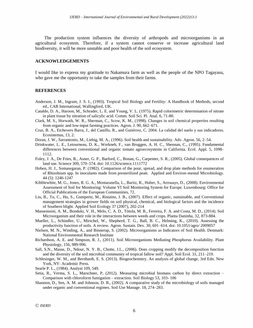
Table 3. Biological properties in both agro ecosystem
Agroecosystem
Number of colony forming units/g dry soil Total Microbial
biomass (μg/g) Total culturable fungi Total culturable
bacteria
Conventional 6.92 x 101a 3.15 x 10³A 0.16α
Natural 1.71 x 10³b 1.10 x 10⁴B 0.22β
a, A, α significance difference p> 0.05
Table 3, indicates that in the number of colonies formed in both fungi and bacteria there were more in
the Natural agroecosystem. In addition, soil microbial biomass also it was found more in Natural
agroecosystem than Conventional agroecosystem. Although with these results its richness and
abundance of species cannot be determined, it could be thought that microorganisms are essential to
maintain a healthy soil. This is because in the Natural Farm, for more than 20 years no type of
amendments has been incorporated. It is that its maintenance of functioning in the soil depends 100
percent on the internal activity that exists between microorganisms, plants and organisms that live in
the environment and soil. They could not be correlated with the chemical and physical properties, but
this can be thought to be related to the management that the Conventional agroecosystem had. The
Conventional agroecosystem, add manure, synthetic fertilization, pesticides and fungicides. Pesticides
and fungicides are known to affect the microbial population rapidly, which may be the reason why
there is less in the results obtained. In addition, another practice that they carry out is weeding. In
Natural Farm, they only weed in the first growth stage of the crop. On the other hand, in the
Conventional Farm, they try to keep the soil without weeds. This practice could be affecting
microorganisms. According to Massenssini et al. (2014), the soil microbial community structure might
change depending on the crop species. Studies have shown that the relationships of weeds and crops
with the soil microbiota may be different. Weeds seem to show higher dependence on interactions with
soil microorganisms. The structure of the soil microbial community is responsive to competition
between plants. In general, the competition promotes changes in the soil microbial community
structure, making it different from that found when plants are grown in monoculture. Furthermore,
weeds tend to have positive feedback interactions with soil microorganisms, while crops may present
neutral or negative feedback interactions.
CONCLUSION
The difference between both farms is by using fertilizers and pesticides. The Natural Farm is not
adding any amendments for 20 years. Furthermore, Conventional Farm use more manure than
chemical fertilizers. Pesticides affect the survival of soil microorganisms more severely than other
practices carried out by the farm. The diversity of plant roots helps to maintain soil microorganism
diversity and abundance.
Interdisciplinary soil research is necessary to better understand the biological properties of soil.
To maintain the sustainability of the production it is necessary to maintain the population of soil
microorganisms. Further research is needed to understand the correlation with chemical and physical
properties. As well as to begin to understand the function that each group of bacteria and fungi has, its
relationship with other living organism in the soil.
IJERD – International Journal of Environmental and Rural Development (2022)13-1
Ⓒ ISERD
6
The production system influences the diversity of arthropods and microorganisms in an
agricultural ecosystem. Therefore, if a system cannot conserve or increase agricultural land
biodiversity, it will be more unstable and poor health of the soil ecosystem.
ACKNOWLEDGEMENTS
I would like to express my gratitude to Nakamura farm as well as the people of the NPO Tagayasu,
who gave me the opportunity to take the samples from their farms.
REFERENCES
Anderson, J. M., Ingram, J. S. I., (1993). Tropical Soil Biology and Fertility: A Handbook of Methods, second
ed., CAB International, Wallingford, UK.
Cataldo, D. A., Haroon, M., Schrader, L. E. and Young, V. L. (1975). Rapid colorimetric determination of nitrate
in plant tissue by nitration of salicylic acid. Comm. Soil Sci. Pl. Anal. 6, 71-80.
Clark, M. S., Horwath, W. R., Sherman, C., Scow, K. M., (1998). Changes in soil chemical properties resulting
from organic and low-input farming practices. Agron. J. 90, 662–671.
Cruz, B. A., Etchevers Barra, J., del Castillo, R., and Gutiérrez, C. 2004. La calidad del suelo y sus indicadores.
Ecosistemas, 13, 2.
Doran, J. W., Sarrantonio, M., Liebig, M. A., (1996). Soil health and sustainability. Adv. Agron. 56, 2–54.
Drinkwater, L. E., Letourneau, D. K., Workneh, F., van Bruggen, A. H. C., Shennan, C., (1995). Fundamental
differences between conventional and organic tomato agroecosystems in California. Ecol. Appl. 5, 1098–
1112.
Foley, J. A., De Fries, R., Asner, G. P., Barford, C., Bonan, G., Carpenter, S. R., (2005). Global consequences of
land use. Science 309, 570–574. doi: 10.1126/science.1111772
Hoben, H. J., Somasegaran, P. (1982). Comparison of the pour, spread, and drop plate methods for enumeration
of Rhizobium spp. In inoculants made from presterilized peatt. Applied and Environ-mental Microbiology.
44 (5): 1246-1247
Kibblewhite, M. G., Jones, R. G. A., Montaranella, L., Baritz, R., Huber, S., Arrouays, D., (2008). Environmental
Assessment of Soil for Monitoring: Volume VI Soil Monitoring System for Europe. Luxembourg: Office for
Official Publications of the European Communities, 72.
Liu, B., Tu, C., Hu, S., Gumpertz, M., Ristaino, J. B., (2007). Effect of organic, sustainable, and Conventional
management strategies in grower fields on soil physical, chemical, and biological factors and the incidence
of Southern blight. Applied Soil Ecology 37 (2007), 202-214
Massenssini, A. M., Bonduki, V. H., Melo, C. A. D., Tótola, M. R., Ferreira, F. A. and Costa, M. D., (2014). Soil
Microorganism and their role in the interactions between weeds and crops. Planta Daninha, 32, 873-884.
Mueller, L., Schindler, U., Mirschel, W., Shepherd, T. G., Ball, B. C., Helming, K., (2010). Assessing the
productivity function of soils. A review. Agron. Sustain. Dev. 30, 601–614. doi: 10.1051/agro/ 2009057
Nielsen, M. N., Winding, A., and Binnerup, S. (2002). Microorganisms as Indicators of Soil Health. Denmark:
National Environmental Research Institute
Richardson, A. E. and Simpson, R. J., (2011). Soil Microorganisms Mediating Phosphorus Availability. Plant
Physiology, 156, 989-996.
Sall, S.N., Masse, D., Ndour, N. Y. B., Chotte, J.L., (2006). Does cropping modify the decomposition function
and the diversity of the soil microbial community of tropical fallow soil? Appl. Soil Ecol. 31, 211–219.
Schlesinger, W. M., and Bernhardt, E. S. (2013). Biogeochemstry. An analysis of global change, 3rd Edn. New
York, NY: Academic Press.
Searle P. L., (1984). Analyst 109, 549.
Setia, R., Verma, S. L., Marschner, P, (2012). Measuring microbial biomass carbon by direct extraction –
Comparison with chloroform fumigation – extraction. Soil Biology 53, 103- 106
Shannon, D., Sen, A. M. and Johnson, D. B., (2002). A comparative study of the microbiology of soils managed
under organic and conventional regimes. Soil Use Manage. 18, 274–283.
IJERD – International Journal of Environmental and Rural Development (2022)13-1
Ⓒ ISERD
7
Sharma, S. K., Ramesh, A., Sharma, M. P., Joshi, O. P., Govaerts, B., Steenwerth, K. L., (2011). “Microbial
community structure and diversity as indicators for evaluating soil quality,” in Biodiversity, Biofuels,
Agroforestry and Conservation Agriculture, ed. E. Lichtfouse (Dordrecht: Springer), 317–358.
Sigler, W.V., Turco, R.F., (2002). The impact of chlorothalonil application on soil bacterial and fungal
populations as assessed by denaturing gradient gel electrophoresis. Appl. Soil Ecol. 21, 107–118
Tilman, D., Cassman, K. G., Matson, P. A., Naylor, R., and Polasky, S. (2002). Agricultural sustainability and
intensive production practices. Nature 418, 671–677. doi: 10.1038/nature01014
Tilman, D., Fargione, J., Wolff, B., D’Antonio, C., Dobson, A., Howarth, R., (2001). Forecasting agriculturally
driven global environmental change. Science 292, 281–284. doi: 10.1126/science.1057544
Trivedi, P., Delgado Baquerizo M., Anderson, I. C., Singh, B., K. (2016). Response of Soil Properties and
Microbial Communities to Agriculture: Implications for Primary Productivity and Soil Health Indicators,
frontiers in Plant Science. doi.org/10.3389/fpls.2016.00990
van Bruggen, A. H. C. and Grunwald, N. J., 1996. Tests for risk assessment of root infection by plant pathogens.
In: Doran, J. W., Jones, A. J. (Eds.), Methods for Assessing Soil Quality. Soil Science Society of America,
Madison, WI, 293-310.
Vitousek, P. M., Naylor, R., Crews, T., David, M. B., Drinkwater, L. E., Holland, E., (2009). Nutrient imbalances
in agricultural development. Science 324:1519. doi: 10.1126/science.1170261
IJERD – International Journal of Environmental and Rural Development (2022)13-1
Ⓒ ISERD
8
Farmers’ Organic and Inorganic Fertilizers Application and its
Effects on Rice Productivity in Prey Chhor District, Kampong
Cham Province
MUY LEANG KIM Graduate School of Agriculture, Tokyo University of Agriculture, Japan
Email: [email protected]
MACHITO MIHARA*
Faculty of Regional Environment Science, Tokyo University of Agriculture, Japan/ Institute of
Environmental Rehabilitation and Conservation, Tokyo, Japan
Email: [email protected]
Received 7 July 2021 Accepted 18 October 2021 (*Corresponding Author)
Abstract Kampong Cham Province is located in plain region of Cambodia. The major activity
of people in the province is agriculture, mainly cultivating rice and vegetables. More than 60%
of farmers in Kampong Cham Province applied chemical fertilizers inappropriately without
understanding on its impacts. The use of high rates of chemical fertilizers continuously for
several years, often lead to unsustainability in production and post harmful to the environment.
Recent years, with the support from the government and non-governmental organization
(NGOs), many farmers realized and look for a better agricultural practice which could
harmonize with natural environment and human health. Several practices were carried to
promote the use of organic fertilizers such as green manures, compost, and bio-liquid fertilizer
in Kampong Cham Province. The use of organic fertilizers it can reduce the input of chemical
fertilizer, improve soil, water, and environment quality. Therefore, the objectives of this study
are to describe farmers’ practices on fertilization and discuss the effect of fertilization
practices on productivity in Samraong and Baray Communes. Ones hundred farmers were
selected for interview with questionnaire surveys on agricultural practices in Samraong and
Baray Communes. The results from the questionnaire surveys showed that more than 70% to
80% of farmers in Samroang and Baray Communes applied organic in combination with
inorgnaic fertilizers and less than 20% use only inorganic fertilizers and 10% only organic
fertilizer. The amount of rice production in each fertilization practices was different, the rice
production in organic fertilizer practices was high compared to other fertilization practices in
Baray Commune, however, in Samraong Commune the rice production was high in chemical
fertilization practices. As farmers in Samraong Commune used more chemical that is why the
production was high compared to other fertilization practices.
Keywords: organic farming, inorganic fertilizers, compost, sustainable agriculture, Kampong
Cham
INTRODUCTION
Plant nutrients are essential for the growth and productivity of crops. Farmers supply nutrients in the
form of organic and inorganic fertilizers. Recently, farmers in Asia have increased the use of inorganic
fertilizers over organic fertilizers, however, integration of both organic and inorganic fertilizers helps
to increase crop productivity, soil fertility and decreases the damage that can be introduced by
inorganic fertilizers. Moreover, farmers in Kampong Cham Province still lake knowledge regarding
the advantages and disadvantages of applying organic and inorganic fertilizers.
erd
Research article
IJERD – International Journal of Environmental and Rural Development (2022)13-1
Ⓒ ISERD
9
Kampong Cham Province is located on the plain region of Cambodia. The province consists of 9
districts and 1 municipality, 109 communes and 916 villages. The total population of this province is
about 1.6 million people in 2013 (JICA, 2013), which accounts for 12.5% of the total population of
Cambodia. The population is comprised of 80% farmers, 1% craftsmen, 14% service providers and 5%
engaged in other businesses. Agriculture activities of people in Kampong Cham Province are changing
from subsistence to commercial monoculture with increased use of inorganic fertilizers.
Organic and inorganic fertilizers are important for achieving an increase in crop productivity
(Tong, 2010), if there is enough supply of nutrients to the soils, crop will grow well and produce high
yields. Application of organic fertilizers, compared to inorganic fertilizers, maintain soil quality by
increasing soil organic matter as well as improve soil physical and chemical properties through
decomposition of its substances (Mader et al., 2002). Additionally, Farmers in Baray Commune, Prey
Chhor District of Kampong Cham Province has been applied organic fertilizers for more than 10 year
which results in better soil properties with organic fertilizer application. Compared to that in Samraong
Commune, farmers applied organic fertilizer for only 5 years in results there was not clearly shown the
influence of organic fertilizer application on soil properties (Kim and Mihara, 2018). Therefore, the
study focused on investigating farmers fertilization practices and the effect of fertilization practices on
n productivity in Samraong and Baray Communes, Prey Chhor District, Kampong Cham Province.
OBJECTIVE
The objectives of this study are to investigate and describe farmers’ fertilization practices and to
discuss the effect of different fertilization practices on rice productivity in Samraong and Baray
Communes.
METHODOLOGY
Study Site
The study is focused in Samraong and Baray Communes in Prey Chhor District, Kampong Cham
Province (Fig.1). Samraong Commune consists of 11 villages and 1,714 households, the farmers in this
commune own cultivation land less than 1 ha. The main crops produced are rice and vegetables with
main soil types being brown hydromorphics, regurs and cultural hydromorphics. The number of
farmers that applied chemical fertilizer or inorganic fertilizers were 1,587 out of 8,123 peoples.
Fig. 1 Map of the study areas and location of Samraong and Baray Communes, Prey Chhor
District, Kampong Cham Province
Baray
Prey Chhor District
Samraong
Kampong Cham Province
Cambodia
IJERD – International Journal of Environmental and Rural Development (2022)13-1
Ⓒ ISERD
10
Baray Commune consists of 13 villages, 2,446 households, with average cultivation land less than
1 ha. The main crops cultivated are rice and vegetables. The soil types are the same in both communes,
In Bary Commune, 1,479 farmers out of 10,637 people used chemical fertilizer (CDB, 2010).
Data Collection and Analysis
Secondary Data Collection
Relevant documents were collected from the research institutions journals and reports of the project
implement and the experts who had studied in the study areas.
Primary Data Collection
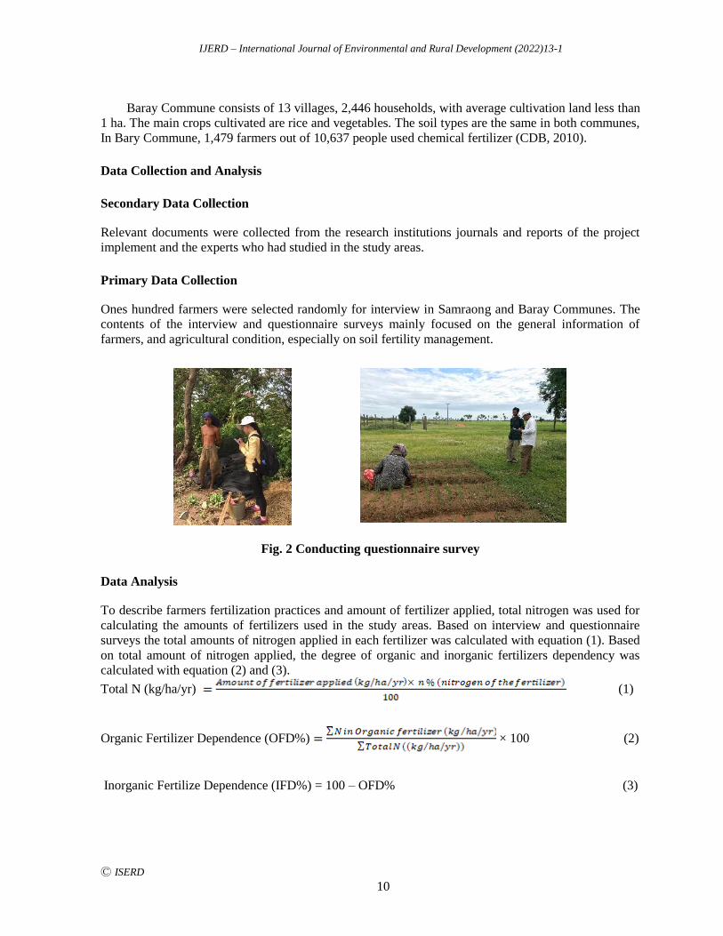
Ones hundred farmers were selected randomly for interview in Samraong and Baray Communes. The
contents of the interview and questionnaire surveys mainly focused on the general information of
farmers, and agricultural condition, especially on soil fertility management.
Fig. 2 Conducting questionnaire survey
Data Analysis
To describe farmers fertilization practices and amount of fertilizer applied, total nitrogen was used for
calculating the amounts of fertilizers used in the study areas. Based on interview and questionnaire
surveys the total amounts of nitrogen applied in each fertilizer was calculated with equation (1). Based
on total amount of nitrogen applied, the degree of organic and inorganic fertilizers dependency was
calculated with equation (2) and (3).
Total N (kg/ha/yr) (1)
Organic Fertilizer Dependence (OFD%) × 100 (2)
Inorganic Fertilize Dependence (IFD%) = 100 – OFD% (3)
IJERD – International Journal of Environmental and Rural Development (2022)13-1
Ⓒ ISERD
11
RESULTS AND DISCUSSION
Types of Fertilizers Uses Among Responded Farmers
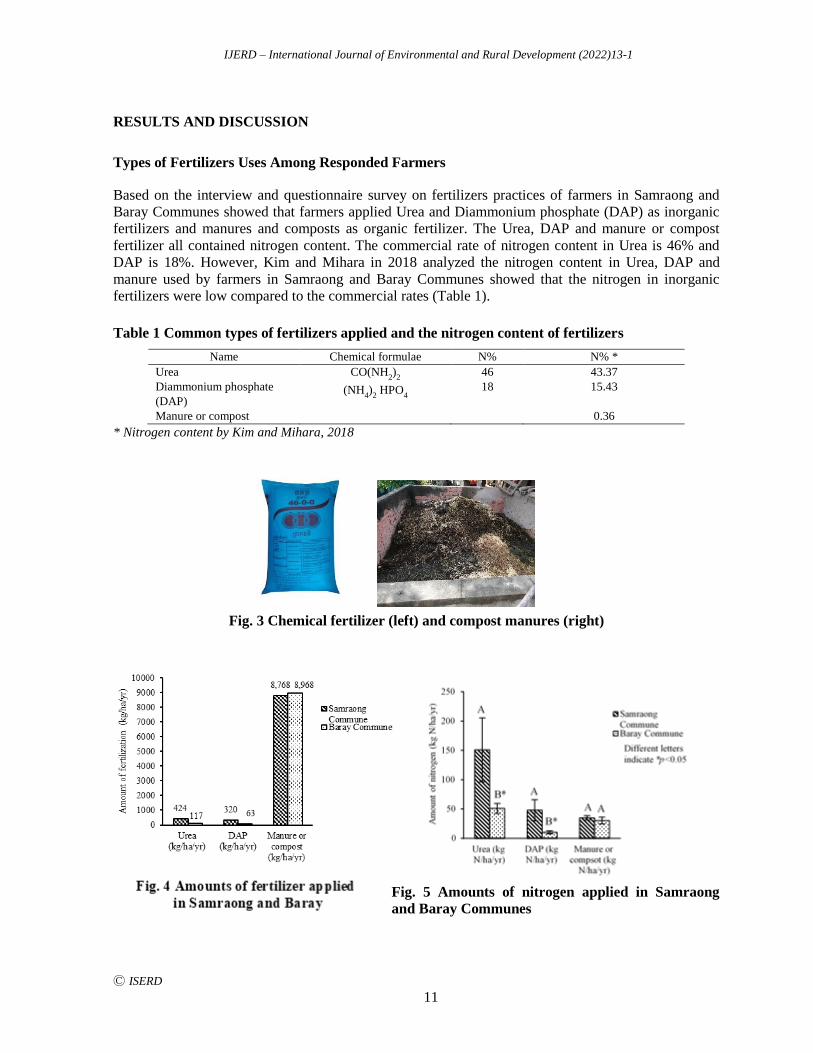
Based on the interview and questionnaire survey on fertilizers practices of farmers in Samraong and
Baray Communes showed that farmers applied Urea and Diammonium phosphate (DAP) as inorganic
fertilizers and manures and composts as organic fertilizer. The Urea, DAP and manure or compost
fertilizer all contained nitrogen content. The commercial rate of nitrogen content in Urea is 46% and
DAP is 18%. However, Kim and Mihara in 2018 analyzed the nitrogen content in Urea, DAP and
manure used by farmers in Samraong and Baray Communes showed that the nitrogen in inorganic
fertilizers were low compared to the commercial rates (Table 1).
Table 1 Common types of fertilizers applied and the nitrogen content of fertilizers
Name Chemical formulae N% N% *
Urea
Diammonium phosphate
(DAP)
Manure or compost
CO(NH2)2
(NH4)2 HPO
4
46
18
43.37
15.43
0.36
* Nitrogen content by Kim and Mihara, 2018
Fig. 3 Chemical fertilizer (left) and compost manures (right)
Fig. 5 Amounts of nitrogen applied in Samraong
and Baray Communes
IJERD – International Journal of Environmental and Rural Development (2022)13-1
Ⓒ ISERD
12
Farmers in Samraong and Baray Communes applied Urea in average is 424 kg/ha/yr and 117 kg/ha/yr,
DAP is 320 kg/ha/yr and 63 kg/year/ha, and manure is 8,768 kg/ha/yr and 8,968 kg/ha/yr, respectively
(Fig. 4). The amounts of fertilizers used in each fertilization were converted to the amounts of nitrogen
contents (Fig. 5). As the results showed fertilizers applied in both Samraong and Baray Commune were
significantly different in 95%, especially in inorganic fertilization practices. Farmers in Samraong
Commune applied higher inorganic fertilizers than farmer in Baray Commune.
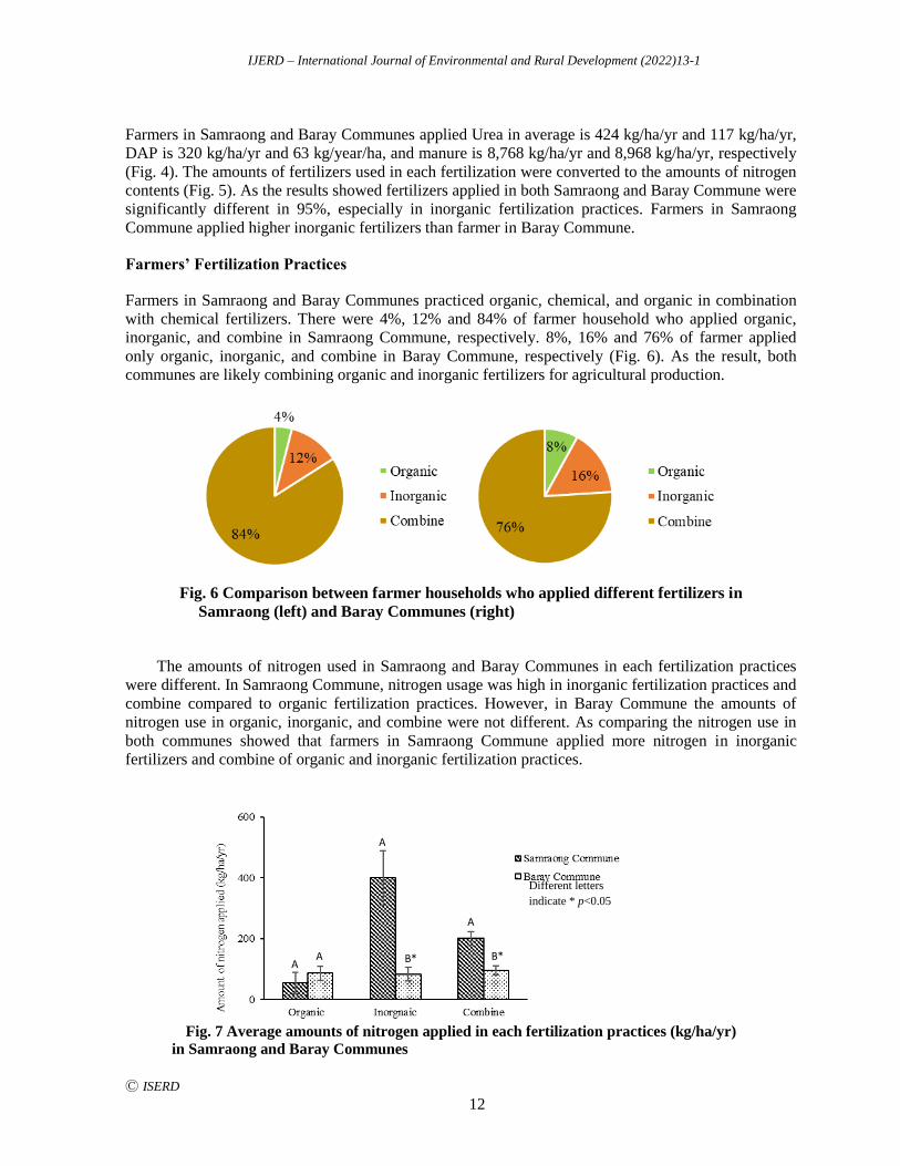
Farmers’ Fertilization Practices
Farmers in Samraong and Baray Communes practiced organic, chemical, and organic in combination
with chemical fertilizers. There were 4%, 12% and 84% of farmer household who applied organic,
inorganic, and combine in Samraong Commune, respectively. 8%, 16% and 76% of farmer applied
only organic, inorganic, and combine in Baray Commune, respectively (Fig. 6). As the result, both
communes are likely combining organic and inorganic fertilizers for agricultural production.
Fig. 6 Comparison between farmer households who applied different fertilizers in
Samraong (left) and Baray Communes (right)
The amounts of nitrogen used in Samraong and Baray Communes in each fertilization practices
were different. In Samraong Commune, nitrogen usage was high in inorganic fertilization practices and
combine compared to organic fertilization practices. However, in Baray Commune the amounts of
nitrogen use in organic, inorganic, and combine were not different. As comparing the nitrogen use in
both communes showed that farmers in Samraong Commune applied more nitrogen in inorganic
fertilizers and combine of organic and inorganic fertilization practices.
Fig. 7 Average amounts of nitrogen applied in each fertilization practices (kg/ha/yr)
in Samraong and Baray Communes
Different letters
indicate * p<0.05
A A
A
B*
A
B*

IJERD – International Journal of Environmental and Rural Development (2022)13-1
Ⓒ ISERD
13
Effect of Different Fertilizer Practices on Rice Productivity
The amounts of rice production were significantly different at 95% interval in each fertilization
practices in Samraong and Baray Communes. Comparing rice production between Samraong and
Baray Communes showed that the rice production shown higher in organic and combine of organic and
inorganic fertilizer practices in Baray Commune (Fig. 8). Also, the rice production was not different in
inorganic fertilization practices in both communes. It was considered that organic fertilizer application
helps to increase the rice productivity in Baray Commune. As farmers in Baray Commune applied less
chemical and more organic fertilizer for long term, when organic fertilizer has been applied for long
time, the production was high indicating on good soil quality
Fig. 8 Amounts of rice production (kg/ha/yr) in Samraong and Baray Communes
Fig. 9 Amounts of rice production (kg/ha/yr) in Samraong (left) and Baray Communes (right)
There was positive ration between organic fertilizer dependence (OFD%) and rice yields per
nitrogen applied at 95% confidence interval in Baray Commune. The combine of organic fertilizer
from 50% to 60 % with inorganic fertilizers showing good results to increase the productivity in Baray
Communes (Fig. 9). However, in Samraong Commune the good rate of organic fertilizer in
combination with inorganic fertilizer was from 30% to 40%. As the results the combined application of
Different letters
indicate * p<0.05
IJERD – International Journal of Environmental and Rural Development (2022)13-1
Ⓒ ISERD
14
organic fertilizers such manures or compost and inorganic fertilizer enhanced tiller number, panicle
length and yield attribute of rice compared to only inorganic fertilizers application (Kakar et al., 2020).
CONCLUSION
Farmers in Samraong and Baray Communes combined organic and inorganic fertilizers, there are also
a few farmers who applied only organic and only inorganic fertilizers. The main sources of nitrogen for
farmers in Samraong Commune are likely from inorganic fertilizer, while in Baray Commune the
sources of nitrogen both from organic and inorganic fertilizers. The use of nitrogen in Samraong
Commune in inorganic fertilization practice and combine was higher, while the rice production was
lower compared to Baray Commune. Farmer in Samraong applied more inorganic fertilizer, but the
rice production was not different compared to Baray Commune when farmers applied fewer inorganic
fertilizers. Organic fertilizer application helps to increase in rice productivity in Baray Commune, as
farmers in Baray has been applied organic fertilizer for more than 10 years and less inorganic fertilizers.
It was considered that when organic fertilizer has been applied for many years like Baray Commune,
the production was high in organic fertilization and combined. Inconclusion of more organic fertilizer
and less inorganic is strongly recommended to farmers in Samraong and Baray as organic fertilizer
contributed to increase the rice productivity.
REFERENCE
Commune Data Base (CDB). 2010. Poverty Reduction by Capital, Province, Municipalities, Districts, Khans and Communes, Sangkats, Cambodia.
Japan International Cooperation (JICA). 2013. Economic Census of Cambodia 2011, Provincial Report 03
Kampong Cham Province, National Institute of Statics, Ministry of Planning, Phnom Penh, Cambodia.
Kakar, K., Xuan, T., Noori, Z., Aryan, S. 2020. Effects of organic and inorganic fertilizer application on growth,
yield, and grain quality of rice. Agriculture 2020. 10, 544.
Mader, P., Nitta, Y., Asagi, N., Komatsuzaki, M., Kokubo, T., 2002. Soil fertility and biodiversity in organic
farming. Science 2002, Vol. 296, 1694-1697.
Muyleang, K., Nakajima, T., Mihara, M. 2018. Comparison of soil properties of farmlands applied with organic
and inorganic fertilizers in Kampong Cham Province, Cambodia. International Journal of Environmental and
Rural Development, 9 - (1), 135-141.
Tong Kimsun. 2010. Agriculture as the Key Source of Growth: A focus on paddy rice production, presentation to
the Cambodia Outlook Conference, 17 March 2010, Phnom Penh, Cambodia.
Theng Vuth. 2012. Fertilizer Value Chains in Cambodia: A case study in Takeo Province, Cambodia
Development Review, Vol. 16 (4), October 2012 (Phnom Penh:CDRI) pp. 5-9.
IJERD – International Journal of Environmental and Rural Development (2022)13-1
Ⓒ ISERD
15
Shedding Light on the Gender Gap in Cambodia’s Agriculture
Sector - A Case of Agricultural Cooperation in Kampong
Cham Province
MARI ARIMITSU* Extension Center, Institute of Environmental Rehabilitation and Conservation, Japan
Email: [email protected]
SHINOBU YAMADA Research Center, Institute of Environmental Rehabilitation and Conservation, Japan
KUMIKO KAWABE Extension Center, Institute of Environmental Rehabilitation and Conservation, Japan
MACHITO MIHARA Faculty of Regional Environment Science, Tokyo University of Agriculture, Japan
Received 21 September 2020 Accepted 26 November 2021 (*Corresponding Author)
Abstract This study deals with the status of women who engage in agricultural practices in
Kampong Cham Province, Cambodia. Specifically, it dissects the selection processes to
determine which gives participant farmers access to training opportunities provided by an
international non-governmental organization. The research was conducted to provide gender-
disaggregated data while elucidating the gender gap that exists in opportunities for equal
participation in and access to training and women’s role within Cambodia’s agricultural sector
based on data analysis for the baseline survey and key informant interviews. This study
concludes that there are specific gender roles, norms and biases, either visible or invisible,
embedded and/or expected in the local community. These traits were manifested by participant
farmers as well as officers who were responsible in selecting farmers. Individual interview
revealed that gender norms regarding men as the head of the house and illiteracy were
mentioned as two possible factors hindering women from participating in agricultural training,
but when leaders who were responsible in selecting farmers were mindful about equal gender
ratio, they could bring equal numbers of female participants. In order to ensure gender equality
in access to skills development opportunities in the agricultural sector, trainings should focus
on building effective program, and optimizing and acknowledging current female farmers’ roles
and contributions in the agricultural and development sector of the rural economy.
Keywords: Gender equality, sustainable agriculture, rural development
INTRODUCTION
A global commitment, Sustainable Development Goal No. 5, is a stand alone goal to end all kinds of
discriminations against women and girls and also to empower them (United Nations). Similarly,
Cambodia’s 5-year strategic plan (Neary Rattanak) is designed to support women to access and claim
their right to fully participate and benefit from economic and social development, and also participate
as decision makers. Agricultural extension services play an essential role in agricultural development,
poverty reduction, and food security (Feder et al., 2011), but women often lack the resources and
opportunities they need, and face more severe constraints than men in accessing productive resources,
erd
Research article
IJERD – International Journal of Environmental and Rural Development (2022)13-1
Ⓒ ISERD
16
markets and services (Raney et al., 2011). Agricultural extension services are particularly needed by
smallholder farmers in developing countries as they usually have low levels of education and limited
access to information and resources to enhance their capacity and level of productivity.
The project on “Promoting Sustainable Agriculture Conditions for Poverty Reduction in
Kampong Cham Province” is currently being implemented by an international organization based in
Japan. The target populations are more than 25 local agriculture extension officers and 1,500 local
farmers in the region where agro-chemical and their improper application is prevalent. According to
FAO statistics, Cambodia’s total fertilizer use increased from 38,693 tons in 2005 to 134,053 in 2018.
The project was designed to alleviate farmers’ poverty and improve their livelihood conditions by
intoroducing and disseminating sustainable agricultural practice. Throughout the project, participant
smallholder farmers have learned the techniques of sustainable agriculture, including composting,
pellet composting, pest and disease management so that they can reduce the use of synthetic products
which economically burden them and are harmful to the human bodies and environment. In the third
year of the project, they will gain techniques on the collecting and shipping process so that they can
sell their safer products with added price. The objective of this study is 1) to elucidate the situation of
the women’s participant to the trainings that are to eradicate the poverty and bring knowledge and
technique on sustainable agricultural practice and analyze the participation rate and the cause of it, and
2) to conduct analysis based on the interview over women’s role and contribution to the agricultural
management, which includes the management of the marketing, and the needs of the training.
METHOLODOGY
This study adopted both quantitative and qualitative approaches. The baseline survey of 500 principal
farmers gathered in 2018 were examined in order to recognize the gender disaggregated data and
elucidate the situation of the women’s participant to the training. Additional key informant interviews
with 40 individual female farmers and ministry officers were conducted in 2019 to complement the
information which was missing from the original baseline survey. The interview was structured in
accordance with the gender analysis, which examines how the roles, rights, and responsibilities of men
and women interact and how that affects outcomes (Doss, 2013). The semi-structured questions were
particularly focused on intersection between gender and recruitment, participation and women’s roles
and their needs in the region: 1) the process of how they were selected, 2) gender roles in agricultural
practice, what are their everyday work in the field and at home, 3) does the training provided by the
organization meets the needs and requests of women. Analysis included looking at the gender norms
and the implications of those relationships on women’s ability to participate in the training on
sustainable agriculture. Interviewees were the participants and beneficiaries of the three-year project
who know what is going on in the field.
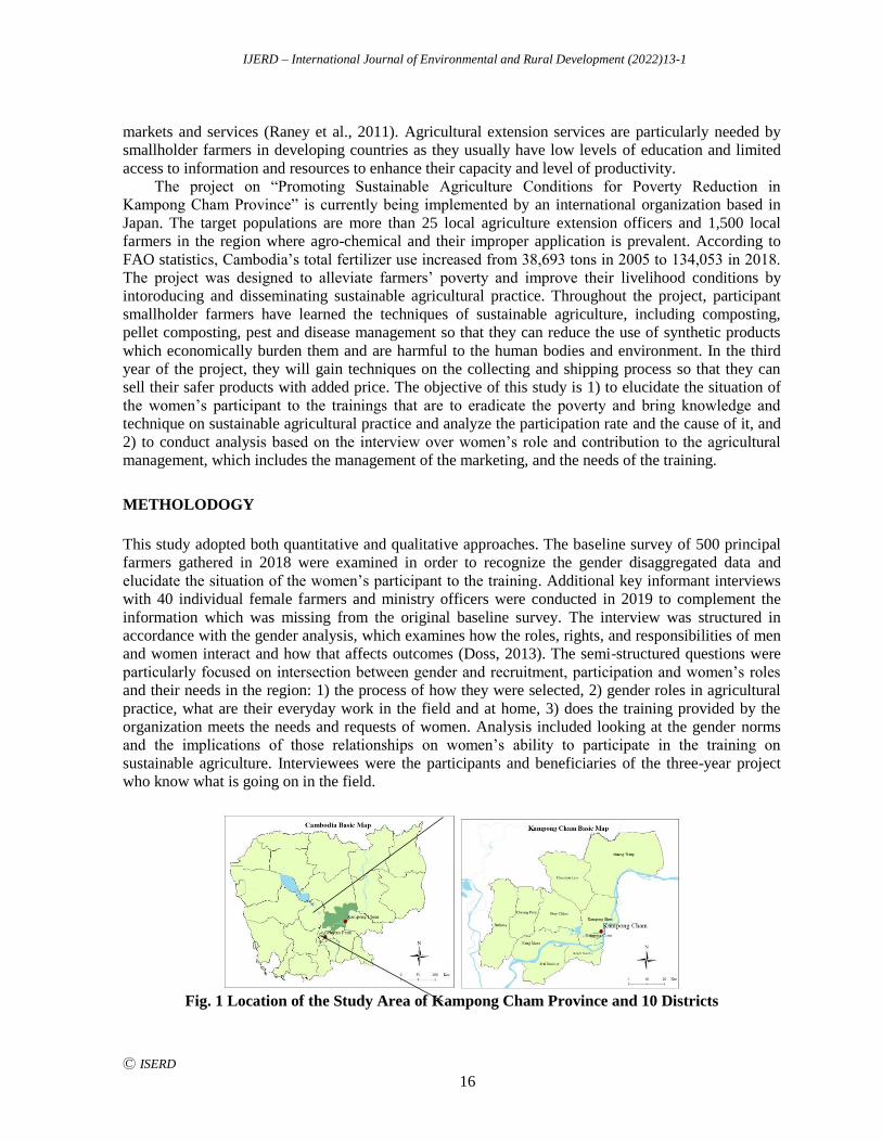
Fig. 1 Location of the Study Area of Kampong Cham Province and 10 Districts
IJERD – International Journal of Environmental and Rural Development (2022)13-1
Ⓒ ISERD
17
The target population was selected across nine districts in Kampong Cham Province that is Prey
Chhor, 8; Batheay, 6; Srei Santhor, 3; Cheung Prey, 8; Kampong Siem, 5; Kang Meas, 2; Kaoh Soutin,
1; Stueng Trang, 5; and Chamkar Leu, 2. Farmers were selected based on availability and willingness
to take part after the training.
RESULTS AND DISCUSSION
The Status of Female Participant’s Rate
After the initiation of the project in 2018, a baseline survey was conducted targeted 500 participating
farmers and was examined as gender segregated data. The baseline survey shows that the principal
farmers consisted of 333 male participants (67%) and 167 female participants (33%). Out of 500
particicpants, 119 male participants (36%) and 59 female participants (35%) answered that they belong
to some agricultural group in their villages. The opportunities provided were geographically varied as
only four female farmers belong to compost and safe vegetable groups in Kampong Cham District,
whereas nine female farmers and 27 male farmers belong to various agricultural groups in Stueng
Trang District. The average size of their agricultural land is 1.07ha. The educational background was
categorized by 1) Never been to school, 2) Primary school, 3) Secondary school, 4) High school, 5)
College, 6) University. For all age groups, on average, men have a slightly higher educational
background (2.43) whereas women’s average is 2.23. According to the age group, both men and
women hold particularly lower educational backgrounds in their 40s and 50s, particularly in their 50s
(Female: 1.86, Male: 2.33). This can be from the fact that they were directly effected by the internal
conflict within Cambodia during the 1970s where people’s educational opportunities were deprived.
Cambodia’s gender gap in adult literacy rate is significantly improved in recent years, but the gap
remains for elderly populations (UNESCO, 2015). The participants’ age varies, but the average age of
male participants is slightly higher than female participants (Female: 45 and Male: 47). The baseline
survey didn’t specify whether the household is either female or male. Hence, the income gap between
male and female participants is not obtained. When they were asked what techniques they need, female
farmers were particularly interested in seeds (48%), organic fertilizers (47%), planting (35%), and
marketing (28%), where as male farmers showed their interests in organic fertilizers (47%), seeds
(44%), planting (30%), and marketing (27%).
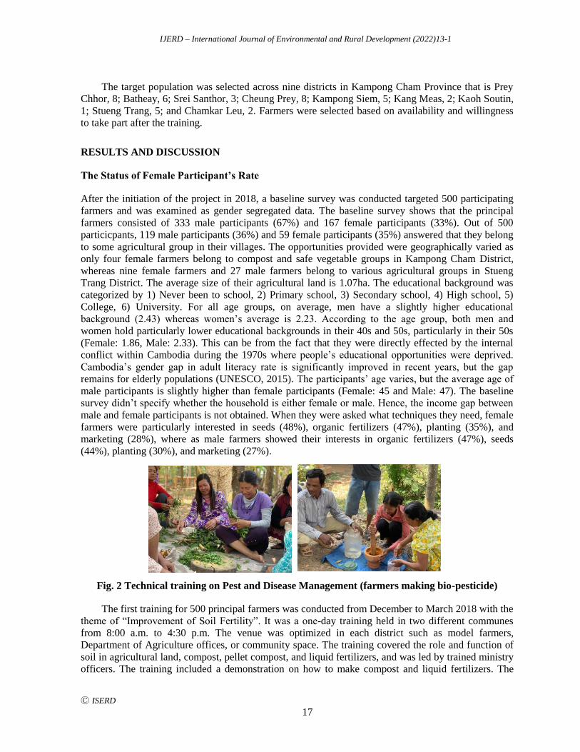
Fig. 2 Technical training on Pest and Disease Management (farmers making bio-pesticide)
The first training for 500 principal farmers was conducted from December to March 2018 with the
theme of “Improvement of Soil Fertility”. It was a one-day training held in two different communes
from 8:00 a.m. to 4:30 p.m. The venue was optimized in each district such as model farmers,
Department of Agriculture offices, or community space. The training covered the role and function of
soil in agricultural land, compost, pellet compost, and liquid fertilizers, and was led by trained ministry
officers. The training included a demonstration on how to make compost and liquid fertilizers. The
IJERD – International Journal of Environmental and Rural Development (2022)13-1
Ⓒ ISERD
18
second training for the same principal farmers was conducted from January to March 2019 with the
theme of “Pest and Disease Management” with adjustment of the time for the morning session to
cocomplete earlier so that female farmers can return back their home for lunch preparation. The
training focused on Integrated Pest Management (IPM), proper use of chemical fertlizers, and technical
and practical knowledge about pest and disease control. The training also included a demonstration on
how to make bio-pesticide (Fig.2).
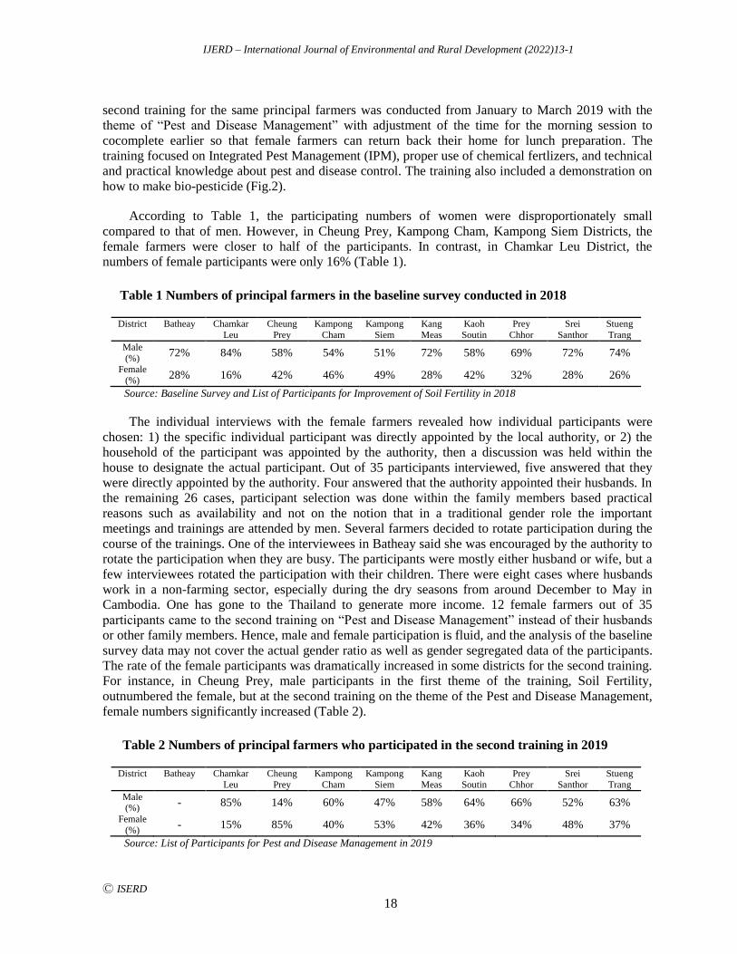
According to Table 1, the participating numbers of women were disproportionately small
compared to that of men. However, in Cheung Prey, Kampong Cham, Kampong Siem Districts, the
female farmers were closer to half of the participants. In contrast, in Chamkar Leu District, the
numbers of female participants were only 16% (Table 1).
Table 1 Numbers of principal farmers in the baseline survey conducted in 2018
District Batheay Chamkar
Leu
Cheung
Prey
Kampong
Cham
Kampong
Siem
Kang
Meas
Kaoh
Soutin
Prey
Chhor
Srei
Santhor
Stueng
Trang
Male
(%) 72% 84% 58% 54% 51% 72% 58% 69% 72% 74%
Female
(%) 28% 16% 42% 46% 49% 28% 42% 32% 28% 26%
Source: Baseline Survey and List of Participants for Improvement of Soil Fertility in 2018
The individual interviews with the female farmers revealed how individual participants were
chosen: 1) the specific individual participant was directly appointed by the local authority, or 2) the
household of the participant was appointed by the authority, then a discussion was held within the
house to designate the actual participant. Out of 35 participants interviewed, five answered that they
were directly appointed by the authority. Four answered that the authority appointed their husbands. In
the remaining 26 cases, participant selection was done within the family members based practical
reasons such as availability and not on the notion that in a traditional gender role the important
meetings and trainings are attended by men. Several farmers decided to rotate participation during the
course of the trainings. One of the interviewees in Batheay said she was encouraged by the authority to
rotate the participation when they are busy. The participants were mostly either husband or wife, but a
few interviewees rotated the participation with their children. There were eight cases where husbands
work in a non-farming sector, especially during the dry seasons from around December to May in
Cambodia. One has gone to the Thailand to generate more income. 12 female farmers out of 35
participants came to the second training on “Pest and Disease Management” instead of their husbands
or other family members. Hence, male and female participation is fluid, and the analysis of the baseline
survey data may not cover the actual gender ratio as well as gender segregated data of the participants.
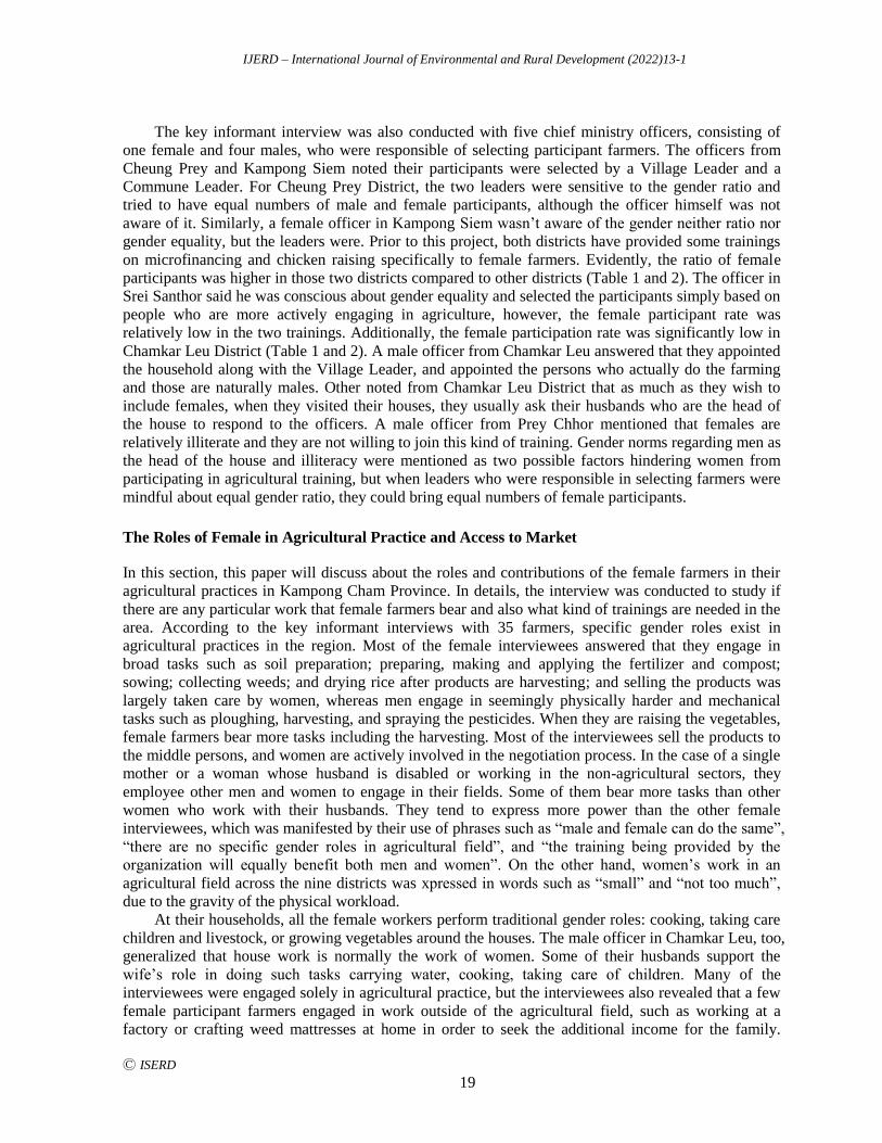
The rate of the female participants was dramatically increased in some districts for the second training.
For instance, in Cheung Prey, male participants in the first theme of the training, Soil Fertility,
outnumbered the female, but at the second training on the theme of the Pest and Disease Management,
female numbers significantly increased (Table 2).
Table 2 Numbers of principal farmers who participated in the second training in 2019
District Batheay Chamkar
Leu
Cheung
Prey
Kampong
Cham
Kampong
Siem
Kang
Meas
Kaoh
Soutin
Prey
Chhor
Srei
Santhor
Stueng
Trang
Male (%)
- 85% 14% 60% 47% 58% 64% 66% 52% 63%
Female
(%) - 15% 85% 40% 53% 42% 36% 34% 48% 37%
Source: List of Participants for Pest and Disease Management in 2019
IJERD – International Journal of Environmental and Rural Development (2022)13-1
Ⓒ ISERD
19
The key informant interview was also conducted with five chief ministry officers, consisting of
one female and four males, who were responsible of selecting participant farmers. The officers from
Cheung Prey and Kampong Siem noted their participants were selected by a Village Leader and a
Commune Leader. For Cheung Prey District, the two leaders were sensitive to the gender ratio and
tried to have equal numbers of male and female participants, although the officer himself was not
aware of it. Similarly, a female officer in Kampong Siem wasn’t aware of the gender neither ratio nor
gender equality, but the leaders were. Prior to this project, both districts have provided some trainings
on microfinancing and chicken raising specifically to female farmers. Evidently, the ratio of female
participants was higher in those two districts compared to other districts (Table 1 and 2). The officer in
Srei Santhor said he was conscious about gender equality and selected the participants simply based on
people who are more actively engaging in agriculture, however, the female participant rate was
relatively low in the two trainings. Additionally, the female participation rate was significantly low in
Chamkar Leu District (Table 1 and 2). A male officer from Chamkar Leu answered that they appointed
the household along with the Village Leader, and appointed the persons who actually do the farming
and those are naturally males. Other noted from Chamkar Leu District that as much as they wish to
include females, when they visited their houses, they usually ask their husbands who are the head of
the house to respond to the officers. A male officer from Prey Chhor mentioned that females are
relatively illiterate and they are not willing to join this kind of training. Gender norms regarding men as
the head of the house and illiteracy were mentioned as two possible factors hindering women from
participating in agricultural training, but when leaders who were responsible in selecting farmers were
mindful about equal gender ratio, they could bring equal numbers of female participants.
The Roles of Female in Agricultural Practice and Access to Market
In this section, this paper will discuss about the roles and contributions of the female farmers in their
agricultural practices in Kampong Cham Province. In details, the interview was conducted to study if
there are any particular work that female farmers bear and also what kind of trainings are needed in the
area. According to the key informant interviews with 35 farmers, specific gender roles exist in
agricultural practices in the region. Most of the female interviewees answered that they engage in
broad tasks such as soil preparation; preparing, making and applying the fertilizer and compost;
sowing; collecting weeds; and drying rice after products are harvesting; and selling the products was
largely taken care by women, whereas men engage in seemingly physically harder and mechanical
tasks such as ploughing, harvesting, and spraying the pesticides. When they are raising the vegetables,
female farmers bear more tasks including the harvesting. Most of the interviewees sell the products to
the middle persons, and women are actively involved in the negotiation process. In the case of a single
mother or a woman whose husband is disabled or working in the non-agricultural sectors, they
employee other men and women to engage in their fields. Some of them bear more tasks than other
women who work with their husbands. They tend to express more power than the other female
interviewees, which was manifested by their use of phrases such as “male and female can do the same”,
“there are no specific gender roles in agricultural field”, and “the training being provided by the
organization will equally benefit both men and women”. On the other hand, women’s work in an
agricultural field across the nine districts was xpressed in words such as “small” and “not too much”,
due to the gravity of the physical workload.
At their households, all the female workers perform traditional gender roles: cooking, taking care
children and livestock, or growing vegetables around the houses. The male officer in Chamkar Leu, too,
generalized that house work is normally the work of women. Some of their husbands support the
wife’s role in doing such tasks carrying water, cooking, taking care of children. Many of the
interviewees were engaged solely in agricultural practice, but the interviewees also revealed that a few
female participant farmers engaged in work outside of the agricultural field, such as working at a
factory or crafting weed mattresses at home in order to seek the additional income for the family.
IJERD – International Journal of Environmental and Rural Development (2022)13-1
Ⓒ ISERD
20
However, according to the participants, women face severe constraints due to lack of knowledge and
skills in a non-agricultural sector or their elderly age as factories or companies favour younger women
as their employees. A study by Gender and Development of Cambodia in 2010 (Ministry of Women
Affairs, 2014) noted that men perceive that they should fulfill the role as the head of the house, and
women perceive normalizing male privilege. Consequently, women tend to see their capacity and
power lower than men in the society. The interview showed that female farmers bear broad range of
agricultural practices as well as domestic work, but some of them seen their ability lower than male
partners, which may be based upon the traditional gender norms prevailing in the country.
Lastly, female farmers expressed concerns about the fixed marking price provided by middle
persons. Some of them noticed that the selling price to the customer is a lot higher than the farmers’
sold price, but they see that there is no way that they can increase the value of it. Out of 35
interviewees, 20 expressed the need of the marketing skills. A female farmer answered that there seems
to be no connection between the producer and the consumer because she sells it to a middle person.
They want to build a strong relationship between the two. Building a relationship between the producer
and customer is a growing trend in agriculture throughout the world, and this can be promoted during
the course of the project. Due to the low price that is given from the middle persons, two female
farmers tried to sell the products in the market, but they faced multiple difficulties ranging from
finding a spot in the market place to selecting a suitable price and attracting regular customers. One of
them expressed the concern over transportation as she uses her own motorbike that she cannot carry
many products at one time. The access to the local market was also depending on the geographical
location of the marketplace versus where they live. The above two female farmers in Kang Meas and
Kampong Siem Districts were able to access the local market because it is accessible from their houses.
The marketing skills will benefit women greatly because majority of sellers in the market consist of
female workers in Kampong Cham Province. Participating female farmers shared the information and
techniques with husbands or other family members, and what they have learned is being practiced at
their farmland. However, they are also seeking other specific trainings such as raising chickens, ducks,
cows, fish, and crafting that they can do while doing the housework at home.
CONCLUSION
The knowledge gained in this study can be summarized as follows. First, regarding the trainings on
promoting sustainable agricultural conditions for poverty reduction, the 2018 baseline survey showed
that participating male farmers significantly outnumbered the female farmers. However, the
participation in the second training revealed that the ratio of male and female participating farmers is
fluid as some of them rotate the participation in accordance with their availability. In two districts,
female farmers outnumbered the male farmers in 2019, where the persons who directly involved in the
selection process were particularly aware of having the equal numbers of men and women. Interviews
also revealed the gender biased selection methods by the officers who were responsible in selecting
farmers at the initial stage. Secondly, female farmers bear broad range of agricultural practices, even
though some of them seen their ability lower than male partners, which is based upon the traditional
gender norms prevailing in the country. Female farmers would come to the training if the content is
related to their regular work that they do in the field, such as soil preparation, pest and disease
management, and the marketing. It is also a key to design the timing, period, and venue of the training
when female farmers can participate, as their reproductive work at home is widely normalized.
Additional training and/or awareness raising may be necessary for the local authorities who are
responsible in selecting farmers in order to disrupt the gender biased selection process. The interview
with the female farmers mentioned the higher needs of the training in marketing in the region, and
some of the challenges they face. Their needs are also varied beyond the basic agricultural techniques.
IJERD – International Journal of Environmental and Rural Development (2022)13-1
Ⓒ ISERD
21
Therefore, in order to reduce the inequality for female farmers in getting agricultural information and
knowledge, building an effective program based on their actual regular agricultural practice is required.
REFERENCES
Doss, C. 2013. Data needs for gender analysis in agriculture. International Food Policy Research Institute, 1-13.
FAO. FAOSTAT Database. Fertilizer indicators. Cambodia. Retrieved from https://www.fao.org/faostat/en/
Feder, G., Birner, R., and Anderson, J. 2011. The private sector’s role in agricultural extension systems: potential
and limitations. Journal of Agribusiness in Developing and Emerging Economies 1 (1).
Ministry of Women’s Affairs. 2014. Attitudes gender relations and attitudes cambodia gender assessment, 1-23.
Ministry of Women’s Affairs. 2014. Neary Rattanak 4. United Nations Development Programme.
Raney, T. and Doss, C. 2011. The role of women in agriculture. ESA Working Paper No. 11-02. Food and
Agriculture Organization, United Nations.
United Nations. Department of Economic and Social Affairs. Sustainable Development. Retrieved from
https://sdgs.un.org/goals/goal5
UNESCO. 2015. Data for sustainable development goals. Cambodia. Retrieved from
http://uis.unesco.org/en/country/kh
IJERD – International Journal of Environmental and Rural Development (2022)13-1
Ⓒ ISERD
22
The Influence of Agricultural Production Information on the
Agricultural Management Scale in Rural Areas of Cambodia
SHINOBU YAMADA* Research Center, Institute of Environmental Rehabilitation and Conservation, Tokyo, Japan
Email: [email protected]
MARI ARIMITSU Extension Center, Institute of Environmental Rehabilitation and Conservation, Tokyo, Japan
MACHITO MIHARA Faculty of Regional Environment Science, Tokyo University of Agriculture, Tokyo, Japan
KUMIKO KAWABE Extension Center, Institute of Environmental Rehabilitation and Conservation, Tokyo, Japan
Received
Received 29 March 2020 Accepted 26 November 2021 (*Corresponding Author)
Abstract The main object of this study was to quantitatively grasp the relevance among local
farmers to analyze the characteristics of local farming and agricultural production information
to build stable and sustainable farming needed by farmers. The research site was ten districts in
Kampong Cham Province, Cambodia. The results of the analysis are summarized as follows: 1)
It was confirmed that the index of agricultural production information varies depending on the
districts; 2) Based on the Canonical Correlation Analysis results, cultivated land and annual
income from agricultural activity, which are regarded to be the results of agricultural
management, have relevance among factors such as attributions, crops, and agricultural
production information was clarified. The cultivated land is affected by the index, which is
aimed at expanding the scale of rice production. In addition, annual income from agricultural
activity is affected by an index aimed at high-quality crop production based on new technology
information, information about organic fertilizer and training. According to the results of the
analysis, agricultural productivity expansions in Cambodia depends on providing information
that can be adaptable to the intention of agricultural management of the local farmers.
Keywords Cambodia, Canonical Correlation Analysis, multiple farming
INTRODUCTION
In Cambodia, per capita income has increased along with economic development. Consequently, a
demand for various agricultural products in addition to rice has increased resulting in increased
production of various agricultural products including vegetables. Currently, in rural areas, many local
farmers intend to produce rice as usual, while many farmers produce vegetables and fruits using
multiple farming. In order to mitigate poverty in rural areas, it is necessary to produce a variety of
crops, centering on rice production, which is expected to expand in the future. The building of stable
and sustainable agricultural management is essential. According to this background, the main object of
this study was to quantitatively grasp the relevance among local farmers in different districts to analyze
the characteristics of local farming and agricultural production information to build stable and
erd
Research article

IJERD – International Journal of Environmental and Rural Development (2022)13-1
Ⓒ ISERD
23
sustainable farming needed by the farmers. In addition, this study focuses on multiple farming in
Cambodia.
OBJECTIVE
The main object of this study was to quantitatively grasp the relevance among local farmers in different
districts to analyze the characteristics of local farming and agricultural production information to build
stable and sustainable farming needed by the farmers. The specific analysis of this study has the
following two issues: 1) The index of agricultural production information required by local farmers per
district; 2) The Canonical Correlation Analysis applies to attributions, crops and agricultural
production information are associated with scale of cultivated land and annual income from
agricultural activity considered to be a result of farm management. The Canonical Correlation Analysis
is used in quantitative analysis of the relation between the agricultural management scale acreage
allotment and regional structure (Ohtake and Aoyagi, 1988, Matsumoto, 1998).
METHODOLOGY
The research site was in Kampong Cham Province. Kampong Cham Province is located northeast of
Phnom Penh, and southeast of Siem Reap. During the French colonial period, in Kampong Cham
Province, the hilly terrain was developed as a rubber plantation zone. The population of Kampong
Cham province is approximately 1.75 million and much of the population is engaged in agriculture.
The target area of the questionnaire survey consisted of the following ten districts: Batheay district: 45
respondents (10.3% of the total respondents); Chamkar Leu district: 50 (11.4%); Chueng Prey district:
36 (8.2%); Kaoh Sotin district: 46 (10.5%); Kampong Siem district: 38 (8.7%); Krong Kampong Cham
district: 48 (11.0%); Kang Meas district: 44 (10.1%); Prey Chhor district: 36 (8.2%); Srei Santhor
district: 50 (11.4%); and Stueng Trang district: 44 (10.1%). The total number of respondents is 471,
and the number of valid respondents is 437. In Kampong Cham Province, vegetables and fruit trees are
widely produced while their main production is rice. As for the vegetables, cabbage and cucumber are
often planted and produced throughout the year. Also, various vegetables and fruits including luffa,
bitter melon, winter melon, Chinese spinach, leaf onion, lemongrass, green beans, papaya, and cashew
etc. are produced. Additionally, at this site, the Institute of Environmental Rehabilitation and
Conservation (ERECON) carries out a project on Promoting Sustainable Agricultural Conditions for
Poverty Reduction in Kampong Cham Province in Cambodia (October/2017-September/2020). This
project aims to promote sustainable farming practices to local farmers based on the cyclic use of
natural resources.
Fig. 1 Location of the study site in Kampong Cham Province
IJERD – International Journal of Environmental and Rural Development (2022)13-1
Ⓒ ISERD
24
RESULTS AND DISCUSSION
The index of agricultural production information required by local farmers per district
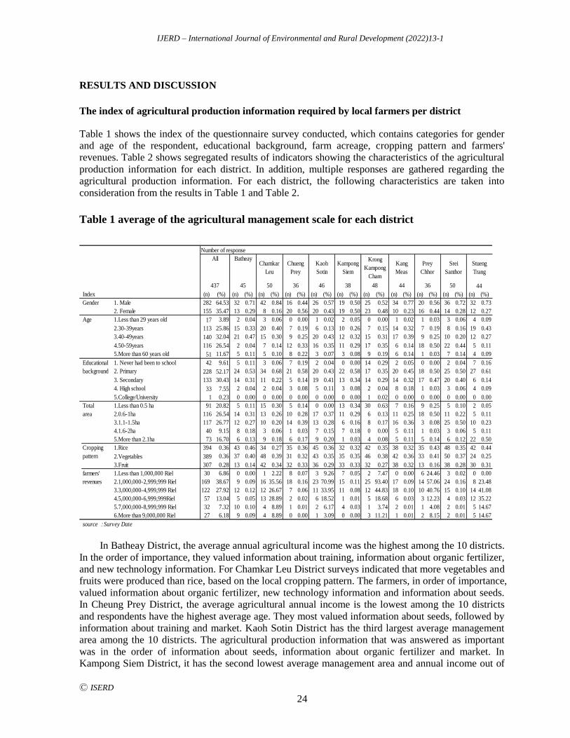
Table 1 shows the index of the questionnaire survey conducted, which contains categories for gender
and age of the respondent, educational background, farm acreage, cropping pattern and farmers'
revenues. Table 2 shows segregated results of indicators showing the characteristics of the agricultural
production information for each district. In addition, multiple responses are gathered regarding the
agricultural production information. For each district, the following characteristics are taken into
consideration from the results in Table 1 and Table 2.
Table 1 average of the agricultural management scale for each district
Number of response
Index (n) (%) (n) (%) (n) (%) (n) (%) (n) (%) (n) (%) (n) (%) (n) (%) (n) (%) (n) (%) (n) (%)
Gender 1. Male 282 64.53 32 0.71 42 0.84 16 0.44 26 0.57 19 0.50 25 0.52 34 0.77 20 0.56 36 0.72 32 0.73
2. Female 155 35.47 13 0.29 8 0.16 20 0.56 20 0.43 19 0.50 23 0.48 10 0.23 16 0.44 14 0.28 12 0.27
Age 1.Less than 29 years old 17 3.89 2 0.04 3 0.06 0 0.00 1 0.02 2 0.05 0 0.00 1 0.02 1 0.03 3 0.06 4 0.09
2.30-39years 113 25.86 15 0.33 20 0.40 7 0.19 6 0.13 10 0.26 7 0.15 14 0.32 7 0.19 8 0.16 19 0.43
3.40-49years 140 32.04 21 0.47 15 0.30 9 0.25 20 0.43 12 0.32 15 0.31 17 0.39 9 0.25 10 0.20 12 0.27
4.50-59years 116 26.54 2 0.04 7 0.14 12 0.33 16 0.35 11 0.29 17 0.35 6 0.14 18 0.50 22 0.44 5 0.11
5.More than 60 years old 51 11.67 5 0.11 5 0.10 8 0.22 3 0.07 3 0.08 9 0.19 6 0.14 1 0.03 7 0.14 4 0.09
Educational 1. Never had been to school 42 9.61 5 0.11 3 0.06 7 0.19 2 0.04 0 0.00 14 0.29 2 0.05 0 0.00 2 0.04 7 0.16
background 2. Primary 228 52.17 24 0.53 34 0.68 21 0.58 20 0.43 22 0.58 17 0.35 20 0.45 18 0.50 25 0.50 27 0.61
3. Secondary 133 30.43 14 0.31 11 0.22 5 0.14 19 0.41 13 0.34 14 0.29 14 0.32 17 0.47 20 0.40 6 0.14
4. High school 33 7.55 2 0.04 2 0.04 3 0.08 5 0.11 3 0.08 2 0.04 8 0.18 1 0.03 3 0.06 4 0.09
5.College/University 1 0.23 0 0.00 0 0.00 0 0.00 0 0.00 0 0.00 1 0.02 0 0.00 0 0.00 0 0.00 0 0.00
Total 1.Less than 0.5 ha 91 20.82 5 0.11 15 0.30 5 0.14 0 0.00 13 0.34 30 0.63 7 0.16 9 0.25 5 0.10 2 0.05
area 2.0.6-1ha 116 26.54 14 0.31 13 0.26 10 0.28 17 0.37 11 0.29 6 0.13 11 0.25 18 0.50 11 0.22 5 0.11
3.1.1-1.5ha 117 26.77 12 0.27 10 0.20 14 0.39 13 0.28 6 0.16 8 0.17 16 0.36 3 0.08 25 0.50 10 0.23
4.1.6-2ha 40 9.15 8 0.18 3 0.06 1 0.03 7 0.15 7 0.18 0 0.00 5 0.11 1 0.03 3 0.06 5 0.11
5.More than 2.1ha 73 16.70 6 0.13 9 0.18 6 0.17 9 0.20 1 0.03 4 0.08 5 0.11 5 0.14 6 0.12 22 0.50
Cropping 1.Rice 394 0.36 43 0.46 34 0.27 35 0.36 45 0.36 32 0.32 42 0.35 38 0.32 35 0.43 48 0.35 42 0.44
pattern 2.Vegetables 389 0.36 37 0.40 48 0.39 31 0.32 43 0.35 35 0.35 46 0.38 42 0.36 33 0.41 50 0.37 24 0.25
3.Fruit 307 0.28 13 0.14 42 0.34 32 0.33 36 0.29 33 0.33 32 0.27 38 0.32 13 0.16 38 0.28 30 0.31
farmers' 1.Less than 1,000,000 Riel 30 6.86 0 0.00 1 2.22 8 0.07 3 9.26 7 0.05 2 7.47 0 0.00 6 24.46 3 0.02 0 0.00
revenues 2.1,000,000-2,999,999 Riel 169 38.67 9 0.09 16 35.56 18 0.16 23 70.99 15 0.11 25 93.40 17 0.09 14 57.06 24 0.16 8 23.48
3.3,000,000-4,999,999 Riel 122 27.92 12 0.12 12 26.67 7 0.06 11 33.95 11 0.08 12 44.83 18 0.10 10 40.76 15 0.10 14 41.08
4.5,000,000-6,999,999Riel 57 13.04 5 0.05 13 28.89 2 0.02 6 18.52 1 0.01 5 18.68 6 0.03 3 12.23 4 0.03 12 35.22
5.7,000,000-8,999,999 Riel 32 7.32 10 0.10 4 8.89 1 0.01 2 6.17 4 0.03 1 3.74 2 0.01 1 4.08 2 0.01 5 14.67
6.More than 9,000,000 Riel 27 6.18 9 0.09 4 8.89 0 0.00 1 3.09 0 0.00 3 11.21 1 0.01 2 8.15 2 0.01 5 14.67
source :Survey Date
38 48 44 36 50 44
Krong
Kampong
Cham
Kang
Meas
Prey
Chhor
Srei
Santhor
Stueng
Trang
437 45 50 36 46
All BatheayChamkar
Leu
Chueng
Prey
Kaoh
Sotin
Kampong
Siem
In Batheay District, the average annual agricultural income was the highest among the 10 districts.
In the order of importance, they valued information about training, information about organic fertilizer,
and new technology information. For Chamkar Leu District surveys indicated that more vegetables and
fruits were produced than rice, based on the local cropping pattern. The farmers, in order of importance,
valued information about organic fertilizer, new technology information and information about seeds.
In Cheung Prey District, the average agricultural annual income is the lowest among the 10 districts
and respondents have the highest average age. They most valued information about seeds, followed by
information about training and market. Kaoh Sotin District has the third largest average management
area among the 10 districts. The agricultural production information that was answered as important
was in the order of information about seeds, information about organic fertilizer and market. In
Kampong Siem District, it has the second lowest average management area and annual income out of
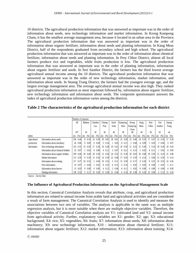
IJERD – International Journal of Environmental and Rural Development (2022)13-1
Ⓒ ISERD
25
10 districts. The agricultural production information that was answered as important was in the order of
information about seeds, new technology information and market information. In Krong Kampong
Cham, it has the smallest average management area, because it located in an urban area in the Province.
The agricultural production information that was answered as important was in the order of
information about organic fertilizer, information about seeds and planting information. In Kang Meas
District, half of the respondents graduated from secondary school and high school. The agricultural
production information that was answered as important was in the order of information about chemical
fertilizer, information about seeds and planting information. In Prey Chhor District, almost all local
farmers produce rice and vegetables, while fruits production is low. The agricultural production
information that was answered as important was in the order of planting information, information
about organic fertilizer and seeds. In Srei Santhor District, the farmers has the third lowest average
agricultural annual income among the 10 districts. The agricultural production information that was
answered as important was in the order of new technology information, market information, and
information about seeds. In Stueng Trang District, the farmers had the youngest average age, and the
largest average management area. The average agricultural annual income was also high. They ranked
agricultural production information as most important followed by, information about organic fertilizer,
new technology information and information about seeds. The composite questionnaire answers the
index of agricultural production information varies among the districts.
Table 2 The characteristics of the agricultural production information for each district
Number of response
Index (n) (%) (n) (%) (n) (%) (n) (%) (n) (%) (n) (%) (n) (%) (n) (%) (n) (%) (n) (%) (n) (%)
Agricultural Information about seeds 194 0.44 8 0.18 14 0.28 29 0.81 28 0.61 22 0.58 22 0.46 24 0.55 17 0.47 13 0.26 17 0.39
production Information about machinery 26 0.06 0 0.00 0 0.00 5 0.14 1 0.02 8 0.21 2 0.04 4 0.09 1 0.03 2 0.04 3 0.07
information New technology information 135 0.31 13 0.29 17 0.34 10 0.28 10 0.22 19 0.50 11 0.23 13 0.30 5 0.14 18 0.36 19 0.43
Information about chemical fertilizer 32 0.07 1 0.02 4 0.08 4 0.11 3 0.07 8 0.21 6 0.13 1 0.02 4 0.11 1 0.02 0 0.00
Information about organic fertilizer 199 0.46 18 0.40 18 0.36 13 0.36 24 0.52 15 0.39 30 0.63 30 0.68 18 0.50 12 0.24 21 0.48
Market information 113 0.26 9 0.20 13 0.26 14 0.39 22 0.48 17 0.45 9 0.19 6 0.14 2 0.06 15 0.30 6 0.14
Information about training 117 0.27 24 0.53 2 0.04 19 0.53 5 0.11 15 0.39 8 0.17 9 0.20 9 0.25 10 0.20 16 0.36
Price information 32 0.07 2 0.04 1 0.02 8 0.22 6 0.13 6 0.16 1 0.02 2 0.05 0 0.00 1 0.02 5 0.11
Information about harvest 15 0.03 0 0.00 0 0.00 4 0.11 2 0.04 4 0.11 1 0.02 0 0.00 0 0.00 0 0.00 4 0.09
Planting information 138 0.32 5 0.11 10 0.20 13 0.36 21 0.46 6 0.16 18 0.38 19 0.43 25 0.69 6 0.12 15 0.34
Source : Survey Date
4838437 46365045
Stueng
Trang
44 36 50 44
Kampong
Siem
Krong
Kampong
Cham
Kang
Meas
Prey
Chhor
Srei
Santhor
All Batheay Chamkar
Leu
Chueng
Prey
Kaoh
Sotin
The Influence of Agricultural Production Information on the Agricultural Management Scale
In this section, Canonical Correlation Analysis reveals that attribute, crop, and agricultural production
information are related to annual income from arable land and agricultural activities and are considered
a result of farm management. The Canonical Correlation Analysis is used to identify and measure the
associations between two sets of variables. The analysis is applicable in the same way as multiple
regression analysis, but it is more suitable when there are multiple objective variables. Therefore, the
objective variables of Canonical Correlation analysis are Y1: cultivated land and Y2: annual income
from agricultural activity. Further, explanatory variables are X1: gender; X2: age; X3: educational
background; X4: rice; X5: vegetables; X6: fruits; X7: information about seeds; X8: information about
machinery; X9: new technology information; X10 : information about chemical fertilizer; X11:
information about organic fertilizer; X12: market information; X13: information about training; X14:
IJERD – International Journal of Environmental and Rural Development (2022)13-1
Ⓒ ISERD
26
price information; X15: information about harvest; and X16: planting information. In Table 3, the
estimation of the Canonical Correlation Analysis results are shown in the research site.
Table 3 Estimation results of the Canonical Correlation Analysis
Iindex CV1 CV2
Cultivated land : Y1 (5 levels) 0.9958 0.3476
Annual income from agricultural activity : Y2 (5 levels) 0.0129 -1.0547
1 Gender : X1 (dummy) 0.0467 0.2559
2 Age : X2 (5 levels) -0.2296 -0.2613
3 Educational background : X3 (5 levels) 0.2534 0.0748
4 Rice : X4 (dummy) 0.698 -0.1882
5 Vegetables : X5 (dummy) -0.259 -0.0244
6 Fruit : X6 (dummy) 0.296 -0.5674
7 Information about seeds : X7 (dummy) -0.3184 -0.3051
8 Information about machinery : X8 (dummy) 0.1119 -0.0629
9 New technology information : X9 (dummy) 0.1061 0.2414
10 Information about chemical fertilizer : X10 (dummy) -0.0442 -0.139
11 Information about organic fertilizer : X11 (dummy) 0.0296 0.2306
12 Market information : X12 (dummy) -0.0133 0.1894
13 Information about training : X13 (dummy) 0.1343 0.2787
14 Price information : X14 (dummy) 0.1084 -0.2773
15 Information about harvest : X15 (dummy) 0.2783 0.0708
16 Planting information : X16 (dummy) 0.0616 -0.1661
Sourse Sarvey date
Note Eigenvalue: CV1; 0.19, CV2; 0.13
Canonical variables
standardized coefficients
According to the results of Canonical Correlation analysis, Canonical variate 1 shows cultivated
land while Canonical variate 2 shows annual income from agricultural activity. Cultivated land:
educational background, rice and fruits are affecting as attributions, and information about harvest is
affecting as agricultural production information. Therefore, the cultivated land is affected by the index
aiming at expanding the scale of rice production. For annual income from agricultural activity: gender
is affecting as attributions, and new technology information, information about organic fertilizer and
training are affecting as agricultural production information. Therefore, annual income from
agricultural activity is affected by an index of new technology information, information about organic
fertilizer and training, all of which are important for high-quality crop production. The results of the
analysis suggest that the development of multiple farming in Cambodia is under the condition of
expanding rice production and increasing the skills of local farmers in agricultural technology.
IJERD – International Journal of Environmental and Rural Development (2022)13-1
Ⓒ ISERD
27
CONCLUSION
The main object of this study was to quantitatively grasp the relevance among local farmers to
analyze the characteristics of local farming and agricultural production information to build stable and
sustainable farming needed by the farmers in Kampong Cham Province, Cambodia. In addition, a
Canonical Correlation Analysis applies to attributions, crops and agricultural production information
are associated with annual income from agricultural activity and cultivated land that are considered as a
result of farm management.
The results of the analysis are summarized as follows:
According to the answers from questionnaire, it was confirmed that the index of agricultural
production information varies depending on the districts. According to the results of Canonical
Correlation analysis, the cultivated land is affected by the index aimed at expanding the scale of rice
production. In addition, annual income from agricultural activity is affected by the index aimed at high-
quality crop production based on new technology information, information about organic fertilizer and
training.
As a result of the analysis, it was suggested that for the development of multiple farming in
Cambodia, in addition to the premise of expanding rice production, it is necessary to improve the skills
necessary for the conversion of high-quality crop production.
ACKNOWLEDGEMENTS
This work was supported by JSPS KAKENHI Grant Number JP18K05857.
REFERENCES
Matsumoto, H. 1998. A Study of Repercussion Effect of Farm Guidance Business in Agricultural Cooperatives.
The Review of Agricultural Economics, 54, 75-85.
Ohtake, H. and Aoyagi, K. 1998. Quantitative Analysis of the Relation between Paddy Field Acreage Allotment
and Regional Structure in the Tohoku District, Japan. Quarterly Journal of Geography, 50,105-108.
Yagura, K. 2008. Poverty and Widening Economic Disparity in Rural Cambodia. Showado, Japan.
Yamada, S, Mihara, M and Kawabe, K. 2016. Characteristics of Transformation of Traditional Upland Farming
System in Cambodia: A Case Study of Snuol Commune, Kratie Province. International Journal of
Environmental and Rural Development 7-2, 81-86.
Yamada, S, Mihara, M and Kawabe, K. 2017. Characteristics of Participants of Non-Formal Education
Contributing to Learning Achievement: A Case Study of Snuol Commune, Kratie Province, Cambodia.
International Journal of Environmental and Rural Development 8-2, 111-116.
IJERD – International Journal of Environmental and Rural Development (2022)13-1
Ⓒ ISERD
28
Moisture Content Prediction of Dried Young Papaya during
Drying and Water Absorption
SOKLY SORM Graduate School of Agriculture, Tokyo University of Agriculture, Tokyo, Japan
YOSHIKI MURAMATSU* Tokyo University of Agriculture, Tokyo, Japan
Email: [email protected]
MASANORI HASHIGUCHI Keisoku Engineering System Co., Ltd., Tokyo, Japan
DAHAI MI
Keisoku Engineering System Co., Ltd., Tokyo, Japan
EIICHIRO SAKAGUCHI Tokyo University of Agriculture, Tokyo, Japan
SHOTARO KAWAKAMI
Tokyo University of Agriculture, Tokyo, Japan
Received 14 January 2021 Accepted 6 December 2021 (*Corresponding Author)
Abstract The effective use of agricultural products and the development of processed foods
with guaranteed safety and quality are needed in Kampong Cham Province, Cambodia. Young
papaya is an important agricultural product in this area. Dried young papaya is one of the
preserved foods. The main objective in this paper was to provide basic information for the
optimization of drying process. Two types of young papaya, raw or fresh papaya and blanched
young papaya, were used in this study to investigate the influence of drying pretreatment, that
is, blanching, on the changes in the moisture content during drying and water absorption. The
hot air-drying characteristics of each sample were measured at three temperatures (30, 50, and
70 °C), three air velocities (1, 2, and 3 m/s), and a relative humidity of 40 %. The examination
of the effects of temperature, air velocity, and blanching on the drying of samples resulted in
the drying characteristics of the raw sample being very similar to that of the blanched sample. A
linear relationship existed in the moisture content range between the initial moisture contents
and 500 % (d.b.). The exponential model was applied to predict the changes in the moisture
contents of samples below 500 % (d.b.) at each drying condition. The drying rate constants in
the period above or below 500 % (d.b.) were increased with increasing air temperature and air
velocity and expressed as a linear function of both temperature and air velocity, respectively.
The water absorption characteristics of the dried young papaya and the dried blanched young
papaya that were dried after blanching were investigated at three temperatures (20, 30, and
40 °C). Blanching before drying of the sample had the effect of slowing the water absorption
rate. The water absorption rate constant tended to increase with increasing soaking temperature.
Keywords young papaya, drying characteristics, water absorption characteristics, blanching,
temperature and air velocity dependency, prediction model of moisture content
erd
Research article
IJERD – International Journal of Environmental and Rural Development (2022)13-1
Ⓒ ISERD
29
INTRODUCTION
The effective use of agricultural products and the development of processed foods with guaranteed
safety and quality are needed in Kampong Cham Province, Cambodia. Young papaya is an important
agricultural product in Kampong Cham. Recently, in Japan, young papaya has been recognized as a
regional biological resource for the diversification of primary producers into processing and
distribution, and it is cultivated in the Kanto region.
Although young papayas can be eaten fresh, they can also be used after drying. Drying is one of
the oldest preservation methods and does not require special machines or devices in almost all cases.
Drying not only increases the shelf life of the product but also increases its food value. Dried young
papaya has been sold as a processed food. Usually, dried young papayas are rehydrated to some degree
before eating. Pretreatments, for example, blanching, are often added to enhance the quality of dried
vegetables. Blanching, a mild thermal treatment similar in temperature-time intensity to pasteurization,
is applied to fruits and vegetables primarily to inactivate enzymes that catalyse degradation reactions
(Park et al., 2014). Lydia et al. (2017) investigated the effects of pretreatments, including soaking in
certain solutions and drying methods, on some qualities of dried mango fruit.
Some researchers (EI-Aouar et al., 2003; Lagunez-Rivera et al., 2007; Fernando et al., 2008;
Lemus-Mondaca et al., 2009; Udomkun et al., 2015) have measured and analysed the drying kinetics
of papaya. Almost all previous papers have reported the drying characteristics of mature papaya.
However, very few studies have measured the hot air-drying characteristics of young papaya with
different air velocities, as performed in this study. In previous references (EI-Aouar et al., 2003;
Lagunez-Rivera et al., 2007; Fernando et al., 2008; Lemus-Mondaca et al., 2009; Muramatsu et al.,
2012; Udomkun et al., 2015), some mathematical models (drying models) were used to describe the
relationship between the moisture content of the sample and drying time. Optimum drying and water
absorption models, including the values of parameters, are particularly useful for easily predicting the
changes in the moisture content of materials. Therefore, determination of the optimum model is
important for practical use.
In this study, we examined the hot air-drying characteristics of two types of young papaya: raw
and blanched young papaya at three different temperatures and air velocities. In addition, the water
absorption (rehydration) characteristics of dried and dried blanched young papaya were also measured
at three different temperatures. The results obtained in this study provide important basic information
and are needed to optimize drying processes and to design dryers.
OBJECTIVE
The objectives of this study were 1) to examine the effects of air temperature, air velocity, and
blanching treatment on the drying characteristics of the sample, 2) to investigate the influence of
blanching treatment and soaking temperature on the water absorption characteristics of the sample, 3)
to derive suitable mathematical drying and water absorption models to describe changes in moisture
content with time, and 4) to obtain empirical equations to express the relationship between the drying
or water absorption rate constants and the measurement conditions.
METHODOLOGY
Sample preparation
Young papaya (Carica papaya) imported from Thailand was purchased at a supermarket in Tokyo,
Japan. Before the test, the young papayas were stored in a refrigerator at approximately 4 °C. After the
peel was removed from the young papaya, the young papaya was cut into a rectangular parallelepiped
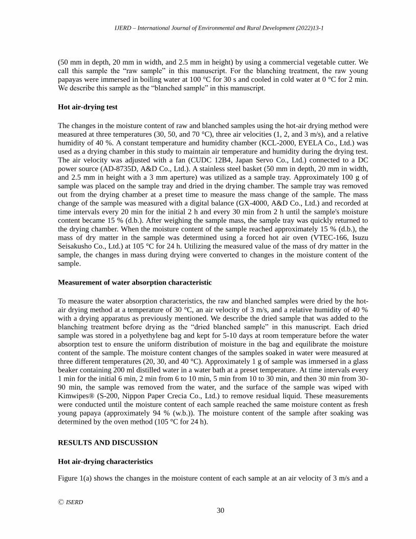
IJERD – International Journal of Environmental and Rural Development (2022)13-1
Ⓒ ISERD
30
(50 mm in depth, 20 mm in width, and 2.5 mm in height) by using a commercial vegetable cutter. We
call this sample the “raw sample” in this manuscript. For the blanching treatment, the raw young
papayas were immersed in boiling water at 100 °C for 30 s and cooled in cold water at 0 °C for 2 min.
We describe this sample as the “blanched sample” in this manuscript.
Hot air-drying test
The changes in the moisture content of raw and blanched samples using the hot-air drying method were
measured at three temperatures (30, 50, and 70 °C), three air velocities (1, 2, and 3 m/s), and a relative
humidity of 40 %. A constant temperature and humidity chamber (KCL-2000, EYELA Co., Ltd.) was
used as a drying chamber in this study to maintain air temperature and humidity during the drying test.
The air velocity was adjusted with a fan (CUDC 12B4, Japan Servo Co., Ltd.) connected to a DC
power source (AD-8735D, A&D Co., Ltd.). A stainless steel basket (50 mm in depth, 20 mm in width,
and 2.5 mm in height with a 3 mm aperture) was utilized as a sample tray. Approximately 100 g of
sample was placed on the sample tray and dried in the drying chamber. The sample tray was removed
out from the drying chamber at a preset time to measure the mass change of the sample. The mass
change of the sample was measured with a digital balance (GX-4000, A&D Co., Ltd.) and recorded at
time intervals every 20 min for the initial 2 h and every 30 min from 2 h until the sample's moisture
content became 15 % (d.b.). After weighing the sample mass, the sample tray was quickly returned to
the drying chamber. When the moisture content of the sample reached approximately 15 % (d.b.), the
mass of dry matter in the sample was determined using a forced hot air oven (VTEC-166, Isuzu
Seisakusho Co., Ltd.) at 105 °C for 24 h. Utilizing the measured value of the mass of dry matter in the
sample, the changes in mass during drying were converted to changes in the moisture content of the
sample.
Measurement of water absorption characteristic
To measure the water absorption characteristics, the raw and blanched samples were dried by the hot-
air drying method at a temperature of 30 °C, an air velocity of 3 m/s, and a relative humidity of 40 %
with a drying apparatus as previously mentioned. We describe the dried sample that was added to the
blanching treatment before drying as the “dried blanched sample” in this manuscript. Each dried
sample was stored in a polyethylene bag and kept for 5-10 days at room temperature before the water
absorption test to ensure the uniform distribution of moisture in the bag and equilibrate the moisture
content of the sample. The moisture content changes of the samples soaked in water were measured at
three different temperatures (20, 30, and 40 °C). Approximately 1 g of sample was immersed in a glass
beaker containing 200 ml distilled water in a water bath at a preset temperature. At time intervals every
1 min for the initial 6 min, 2 min from 6 to 10 min, 5 min from 10 to 30 min, and then 30 min from 30-
90 min, the sample was removed from the water, and the surface of the sample was wiped with
Kimwipes® (S-200, Nippon Paper Crecia Co., Ltd.) to remove residual liquid. These measurements
were conducted until the moisture content of each sample reached the same moisture content as fresh
young papaya (approximately 94 % (w.b.)). The moisture content of the sample after soaking was
determined by the oven method (105 °C for 24 h).
RESULTS AND DISCUSSION
Hot air-drying characteristics
Figure 1(a) shows the changes in the moisture content of each sample at an air velocity of 3 m/s and a
IJERD – International Journal of Environmental and Rural Development (2022)13-1
Ⓒ ISERD
31
temperature of 30 °C. The moisture contents of both samples decreased linearly with elapsed time from
the initial moisture content to approximately 500 % (d.b.) and decreased, exhibiting a gentle downward
curve below 500 % (d.b.). As shown in Fig. 1(b), the slope of the relationship between the drying rate
and moisture content at each sample was changed at approximately 500 % (d.b.). Figure 1 indicates
that the drying characteristics, i.e., changes in the moisture content and drying rate of the raw sample
had almost the same trend as the blanched sample and the hot air-drying process of both samples had
two periods, i.e., the first and second periods. Similar tendencies were obtained for other measurement
conditions not shown in Fig. 1.
In the first period (above 500 % (d.b.)), the moisture contents decreased linearly with an increase
in elapsed time. Therefore, the measured data at each sample and each measurement condition were
fitted to Eq. (1).
1 0M k t M (1)
where M: the moisture content (% (d.b.)), M0: the initial moisture content (% (d.b.)), k1: the drying rate
constant in the first period (1/min), and t: the drying time (min). The measured value of M0 and the
values of k1 determined by using the least squares method and the root mean square error (RMSE) are
shown in Table 1. In the second period (below 500 % (d.b.)), because the drying rate decreased linearly
with decreasing moisture content, the following exponential model (Muramatsu et al., 2012) was used
to analyse the changes in moisture content.
2exp500
ec
e
M Mk t t
M
(2)
where Me: the equilibrium moisture content (% (d.b.)), k2: the drying rate constant in the second period
(1/min), and tc: the drying time at a moisture content of 500 % (d.b.) (min). The value of tc in Eq. (2)
was calculated from Eq. (1). The measured drying data in the second period were fitted to Eq. (2) using
the nonlinear least squares method, and the values of k1 and Me were determined at each sample and
each measurement condition. The values of the parameters and RMSE of Eq. (2) are given in Table 2.
The comparisons of the observed moisture contents with the results calculated from Eqs. (1) and (2) at
an air velocity of 3 m/s for the raw sample are shown in Fig. 2. The solid lines in Fig. 2 show the
results calculated from Eq. (1) or (2). As shown in Fig. 2, the measured results matched well with the
calculated results. Under all measurement conditions, the changes in the moisture content of the sample
caused by hot air-drying could be estimated by Eqs. (1) and (2).
Fig. 1 Drying curve of each sample at an air velocity of 3 m/s and a temperature of 30 °C
(a) Changes in moisture content; (b) drying characteristics curves

IJERD – International Journal of Environmental and Rural Development (2022)13-1
Ⓒ ISERD
32
Fig. 2 Comparisons of observed moisture content changes with the results calculated from
(a): Eq. (1) and (b): Eq. (2) at an air velocity of 3 m/s for the raw sample during drying
As shown in Tables 1 and 2, the drying rate constants varied with temperature and air velocity.
Figure 3 represents the temperature and air velocity dependencies of k1 for the raw sample. Although
the values of k1 for both samples were not much difference between 1 m/s and 2 m/s, the values of k1 at
2 m/s were higher than that at 1 m/s for each temperature. The first period (above 500 % (d.b.)) was
considered as the apparent falling drying rate period including the sample shrinkage, i.e., the constant
drying rate period from the measurement results of changes in the sample surface temperature. In the
constant drying rate period, the drying or water vaporization rate depends on the heat transfer
coefficient, the thicknesses of boundary layers for temperature and air velocity, and so on. Since there
was not much difference in the values of heat transfer coefficient and the thicknesses of boundary
layers between 1 m/s and 2 m/s, the effect of air velocity on the drying rate in the first period might be
weak below 2 m/s. The k1 and k2 of each sample increased almost linearly with the increase in air
velocity at each temperature and the increase in the temperature at each air velocity. Therefore, we
derived the following empirical equation to express the temperature and air velocity dependencies.
1 or 2k aTV bT cV d (3)
where T: temperature (°C), V: air velocity (m/s), a, b, c, d: constant. The regression results for Eq. (3)
are shown in Table 3. The solid lines in Fig. 3 are the results calculated from Eq. (3). The k1 and k2
values of each sample were represented as a function of both temperature and air velocity by Eq. (3).
Fig. 3 Relationships between the drying rate constants in the first period (above a moisture
content of 500 % (d.b.)) of the raw sample and (a): temperature and (b): air velocity
IJERD – International Journal of Environmental and Rural Development (2022)13-1
Ⓒ ISERD
33
Table 1 Initial moisture content (M0), drying rate constant in the first period (above 500 %
(d.b.)) (k1), and root mean square error (RMSE) of Eq. (1) under each set of
measurement conditions
Sample Air velocity
(m/s)
Temperature
(°C)
M0
(% (d.b.))
k1
(1/min)
RMSE
(% (d.b.))
Raw sample 1 30 1525 7.572 19.2
50 1625 12.23 20.9
70 1615 16.03 2.6
2 30 1359 8.909 25.8
50 1253 12.87 14.7
70 1331 17.83 3.0
3 30 1643 13.76 47.0
50 1797 22.63 54.3
70 1800 29.92 20.0
Blanched sample 1 30 1926 9.189 27.8
50 1963 14.35 31.6
70 2008 19.77 10.2
2 30 1807 10.69 63.2
50 1576 15.12 12.9
70 1661 21.51 2.2
3 30 1794 15.31 39.3
50 1896 23.82 47.3
70 2302 37.15 18.1 The values of M0 were measured data. The values of k1 were determined by the least squares method based on the
measured results in the first period (above 500 %(d.b.)). The values of RMSE were calculated from the measured
results and the results calculated from Eq. (1).
Table 2 Drying time at a moisture content of 500 % (d.b.) (tc), drying rate constant in the
second period (below 500 %(d.b.)) (k2), equilibrium moisture content (Me), and root
mean square error (RMSE) of Eq. (2) under each set of measurement conditions
Sample Air velocity
(m/s)
Temperature
(°C)
tc
(min)
k2
(1/min)
Me
(% (d.b.))
RMSE
(% (d.b.))
Raw 1 30 135 1.224×10⁻² 16.09 11.2
50 92 2.058×10⁻² 9.542 14.2
70 70 2.940×10⁻² 5.132 14.0
2 30 96 1.708×10⁻² 14.37 12.8
50 59 2.549×10⁻² 8.183 12.0
70 47 3.649×10⁻² 5.153 16.2
3 30 83 2.052×10⁻² 13.36 16.0
50 57 3.438×10⁻² 8.604 11.8
70 43 5.157×10⁻² 5.226 16.1
Blanched 1 30 155 1.136×10⁻² 13.65 23.0
50 102 1.845×10⁻² 5.345 21.9
70 76 2.785×10⁻² 0.02047 24.5
2 30 122 1.759×10⁻² 14.63 9.9
50 71 2.302×10⁻² 5.895 18.8
70 54 3.315×10⁻² 0.4881 23.6
3 30 85 1.931×10⁻² 11.37 18.4
50 59 3.643×10⁻² 9.005 10.0
70 49 4.249×10⁻² 5.628 26.7 The values of tc were calculated from Eq. (1) by using the values of M0, k1, and M=500. The values of k2 and Me were
determined by the nonlinear least squares method based on the measured results in the second period (below 500 %(d.b.)).
The values of RMSE were calculated from the measured results and the results calculated from Eq. (2).
IJERD – International Journal of Environmental and Rural Development (2022)13-1
Ⓒ ISERD
34
Table 3 Values of the parameters and root mean square error (RMSE) of Eq. (3) for each
drying rate constant and sample
Drying
rate
constant
(1/min)
Sample a
(s/min・°C・m)
b
(1/min・°C)
c
(s/min・m)
d
(1/min)
RMSE
(1/min)
k1 Raw 9.626×10⁻² 8.708×10⁻² 2.687×10⁻¹ 1.238 2.052
Blanched 1.407×10⁻¹ 7.896×10⁻² -1.541 3.613 2.469
k2 Raw 1.736×10⁻⁴ 2.163×10⁻⁴ -1.305×10⁻³ 1.962×10⁻³ 1.438×10⁻³
Blanched 7.535×10⁻⁵ 3.151×10⁻⁴ 2.234×10⁻³ -1.735×10⁻³ 2.251×10⁻³ The values of a, b, c, and d were determined by the least squares method based on the values of k1 and k2 shown in Tables 1
and 2. The values of RMSE were calculated from the values of drying rate constant (k1 or k2) shown in Table 1 or 2 and the
results calculated from Eq. (3).
Water absorption characteristics
The moisture content of dried and dried blanched samples increased with the elapsed time, exhibiting a
gentle upward curve from the beginning of soaking at all three temperatures, as shown in Fig. 4. The
water absorption rate of dried blanched samples was slower than that of dried samples at each
temperature. The dried blanched sample was harder and had a smaller size than the dried sample. The
difference in organizational structure for the samples after drying could be caused by the difference in
water absorption characteristics. The exponential model Eq. (4) (Tagawa et al., 1997) was used to
analyse the changes in moisture content from the initial moisture content of 15 % (d.b.).
3 WAexp15
s
s
M Mk t
M
(4)
where Ms: saturated moisture content (% (d.b.)), k3: water absorption rate constant (1/min), and tWA:
soaking time (min). The solid lines and broken lines in Fig. 4 represent the results calculated from Eq.
(4). The values of k3, Ms, and RMSE of Eq. (4) are shown in Table 4.
The k3 of each sample increased with increasing soaking temperature and was related to soaking
temperature by the following Arrhenius equation.
3 exp 273.15k d E R T (5)
where R: ideal gas constant 8.314 (J/mol・K), d, E: constant. The values of d and E were 6.047×10² and
2.477×10⁵ for the dried sample and 6.444×10³ and 3.278×10⁵ for the dried blanched sample,
respectively.
Table 4 Water absorption rate constant (k3), saturated moisture content (Ms), and root mean
square error (RMSE) of Eq. (4) for each sample
Sample Temperature (°C) k3 (1/min) Ms (% (d.b.)) RMSE (% (d.b.))
Raw 20 2.417×10⁻² 2572 43.8
30 2.994×10⁻² 2748 42.1
40 4.640×10⁻² 2525 37.6
Blanched 20 9.129×10⁻³ 3549 35.0
30 1.499×10⁻² 2999 38.0
40 2.153×10⁻² 2696 59.3 The values of k3 and Ms were determined by the nonlinear least squares method based on the measured results. The
values of RMSE were calculated from the measured results and the results calculated from Eq. (4).
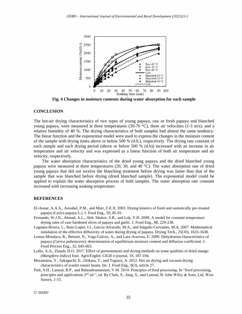
IJERD – International Journal of Environmental and Rural Development (2022)13-1
Ⓒ ISERD
35
Fig. 4 Changes in moisture contents during water absorption for each sample
CONCLUSION
The hot-air drying characteristics of two types of young papaya, raw or fresh papaya and blanched
young papaya, were measured at three temperatures (30-70 °C), three air velocities (1-3 m/s), and a
relative humidity of 40 %. The drying characteristics of both samples had almost the same tendency.
The linear function and the exponential model were used to express the changes in the moisture content
of the sample with drying times above or below 500 % (d.b.), respectively. The drying rate constant of
each sample and each drying period (above or below 500 % (d.b)) increased with an increase in air
temperature and air velocity and was expressed as a linear function of both air temperature and air
velocity, respectively.
The water absorption characteristics of the dried young papaya and the dried blanched young
papaya were measured at three temperatures (20, 30, and 40 °C). The water absorption rate of dried
young papaya that did not receive the blanching treatment before drying was faster than that of the
sample that was blanched before drying (dried blanched sample). The exponential model could be
applied to explain the water absorption process of both samples. The water absorption rate constant
increased with increasing soaking temperature.
REFERENCES
EI-Aouar, A.A.A., Azoubel, P.M., and Murr, F.E.X. 2003. Drying kinetics of fresh and osmotically pre-treated
papaya (Carica papaya L.). J. Food Eng., 59, 85-91.
Fernando, W.J.N., Ahmad, A.L., Abd. Shukor, S.R., and Lok, Y.H. 2008. A model for constant temperature
drying rates of case hardened slices of papaya and garlic. J. Food Eng., 88, 229-238.
Lagunez-Rivera, L., Ruiz-Lopez, I.I., Garcia-Alvarado, M.A., and Salgado-Cervantes, M.A. 2007. Mathematical
simulation of the effective diffusivity of water during drying of papaya. Drying Tech., 25(10), 1633-1638.
Lemus-Mondaca, R., Betoret, N., Vega-Galvez, A., and Lara-Aravena, E. 2009. Dehydration characteristics of
papaya (Carica pubenscens): determination of equilibrium moisture content and diffusion coefficient. J.
Food Process Eng., 32, 645-663.
Lydia, A.A., Zinash, D.O. 2017. Effect of pretreatments and drying methods on some qualities of dried mango
(Mangifera indica) fruit. AgricEngInt: CIGR e-journal, 19, 187-194.
Muramatsu, Y., Sakaguchi, E., Orikasa, T., and Tagawa, A. 2012. Hot air drying and vacuum drying
characteristics of scarlet runner beans. Int. J. Food Eng., 8(3), article 27.
Park, S.H., Lamsal, B.P., and Balasubramaniam, V.M. 2014. Principles of food processing. In “food processing,
principles and applications 2nd ed.”, ed. By Clark, S., Jung, S., and Lamsal, B. John Wiley & Sons, Ltd, West
Sussex, 1-15.

IJERD – International Journal of Environmental and Rural Development (2022)13-1
Ⓒ ISERD
36
Tagawa, A., Muramatsu, Y., Kitamura, Y., and Murata, S. 1997. Water absorption characteristics of soybeans in
soaking. J. Japanese Soc. Agric. Machinery, 59(2), 21-27 (in Japanese).
Udomkun, P., Argyropoulos, D., Nagle, M., Mahayothee, B., Janjai, S., and Muller, J. 2015. Single layer drying
kinetics of papaya amidst vertical and horizontal airflow. LWT-Food Sci. Tech., 64, 67-73.
IJERD – International Journal of Environmental and Rural Development (2022)13-1
Ⓒ ISERD
37
Estimates of Factor Shares for Rice Production in Japan for
the Period of 1922-1944
MITSUHIRO TERAUCHI* Faculty of International Agriculture and Food Studies, Tokyo University of Agriculture, Tokyo,
Japan
Email: [email protected]
SHINOBU YAMADA Research Center, Institute of Environmental Rehabilitation and Conservation, Tokyo, Japan
Received 20 February 2021 Accepted 6 December 2021 (*Corresponding Author)
Abstract The After World War I, the development of the agriculture sector was delayed in
contrast with the rapid growth of the industrial sector. Japanese agriculture accelerated by
innovation after the economic revitalization following World War II. It clarifies the production
structure of the rice production in Japan, and there is this study before the end of World War II
after the First World War end during the analysis period. This study clarifies a change of factor
shares of the rice production sector in this time. The purpose of this study is to elucidate the
characteristics of the production structure of the rice production in Japan from 1922 through
1944, and the agriculture in Japan at this time is considered to be in a developing stage. The
historic change of the rice production in Japan gives a suggestion for agriculture development
in modern Asia. The measurement of factor shares of the rice production in the analysis period
applies "a method to estimate land income as rest." In addition, it measures the Cobb-Douglas's
type amount of production formation function. It clarify the contribution of the production
input. The changes of factor shares are as follows. The change of factor shares is land, labor,
fertilizer, cost of draft animals, agricultural machinery, materials, building for agriculture, seed
in order of the average value from 1922 through 1944. As for the development of production
technological system, it is a technological innovations land-saving and fertilizer-using. The
results of estimate by the amount of production formation function are as follows. In the periods
of 1922-1944, the input of the labor is excess level, the input of the fertilizer is under level and
the input of the land is equilibrium level.
Keywords Japan rice production, factor shares, the amount of production formation
function
INTRODUCTION
World War I, the development of the agriculture sector was delayed in contrast with the rapid growth
of the industrial sector. Japanese agriculture accelerated by innovation after the economic revitalization
following World War II. It clarifies the production structure of the rice production in Japan, and there
is this study before the end of World War II after the First World War end during the analysis period. It
corresponds to the Meiji period and the prewar age of the Showa period, and this period is a stagnation
period of agricultural production. This study clarifies a change of factor shares of the rice production
sector in this time. The purpose of this study is to elucidate the characteristics of the production
structure of the rice production in Japan from 1922 through 1944, and the agriculture in Japan at this
time is considered to be in a developing stage. The historic change of the rice production in Japan gives
a suggestion for agriculture development in modern Asia. The measurement of factor shares of the rice
erd
Research article
IJERD – International Journal of Environmental and Rural Development (2022)13-1
Ⓒ ISERD
38
production in the analysis period applies "a method to estimate land income as rest." In addition, it
measures the Cobb- Douglas's type amount of production formation function. It clarify the contribution
of the production input.
OBJECTIVE
The main object of this study is to analyze the measurement of factor shares of the rice production. In
analysis, the measurement of factor shares of the rice production applies "a method to estimate land
income as rest." In addition, it measures the Cobb-Douglas's type amount of production formation
function. It clarify the contribution of the production input. The data applying to analysis are as follows.
Yukio ISHIBASHI et al,"Teikoku Nokai Kome Seisanhi Cyousa Syusei(Imperial Agricultural
Organization cost of rice production investigation collection)" is from 1922 to 1948(Natl. Res. Inst. of
Agricultural Economics)(Natl. Res. Inst. of Agricultural Economics publication, the 207th). A period
of estimation of factor shares and the amount of production formation function by estimate is 1922
through 1945. Sample data are thyme series data for 24 years.
METHODOLOGY
The estimates of factors share
The measurement of factor shares of the rice production in the analysis period applies "a method to
estimate land income as rest." It is presented by the following:
Factor sharesL=(PL・L)/(P・Q) (1)
Factor sharesK=(PK・L)/(P・Q) (2)
Factor sharesV=(PV・L)/(P・Q) (3)
Factor sharesS=1-(PL・L)/(P・Q)-(PK・L)/(P・Q)-(PV・L)/(P・Q) (4)
where Q is output; P output price; L labor input; K capital input; V fertilizer input; S land input; LP
labor input price; KP capital input price; VP fertilizer input purice and S land input price(Yujiro
Hayami,Y and Ruttan,V.1985).
Amount of production formation function
The function type assumed is the Cobb-Douglas's type production function. The function to estimate is
the next formula (Tsuchiya,K. 1976).
X = A・L^α・V^γ・S^δ (5)
(0 <α, 0 <γ, 0 <δ, α+γ+δ ≒ 1 )
It is presented by the following:
lnX = lnA+αlnL+γlnV+δlnS+ζ (6)
where X is output; L labor input; V fertilizer input; S land input.
IJERD – International Journal of Environmental and Rural Development (2022)13-1
Ⓒ ISERD
39
Examination of the contribution of the production input
The marginal productivity of input X is MPX. P is an output price. PX is X input price. In the case of
①: MPX> (PX/P), the input of X is under. In the case of ②: MPX = (PX/P), the input of the factor of
production is equilibrium. In the case of ③: MPX <(PX/P), the input of the agent of production is
excess. It is represented by the following. ④Value of production elasticity of X>factor shares X. ⑤
Value of production elasticity of X= factor shares X. ⑥Value of production elasticity of X<factor
shares X.
Data collection
As for the data, Miyuki Ishibashi et al,"Imperial Agricultural Organization cost of rice production
investigation collection", the sample data are thyme series data for 24 years. The index to use for
estimation is an unpolished rice yield ("koku"≒140-150kg), product value (Japanese yen), seed costs,
manure costs, wages, material costs, labor force of livestock costs, agricultural machinery costs,
building for agriculture. These variables are numerical value per "tan"(≒10a). The variable data of the
measurement of the amount of production formation function are as follows. Q is the amount of
production. Here, it adopted an unpolished rice yield. L is wages. It adopted the total of family labor
and the employment labor. V is an ordinary input. It adopted seed and sapling costs, manure costs,
agriculture drug costs, and the total of material costs. S is rice paddy area. It is measured using the
variable shown above. The data of the Miyuki Ishibashi great work "Imperial Agricultural
Organization cost of rice production investigation collection" were displayed by a "tan," and therefore
it took advantage, and, on the occasion of a measurement, the numerical value was converted the
planted area around one farmhouse. Therefore the numerical value multiplied the planted area by it and
converted it into numerical value per one farmhouse.
RESULTS AND DISCUSSION
The Development of rice production in Japan: 1881-2012
The analysis object period of this study is 1922-1944. In the history of Japanese agriculture, it confirms
a characteristic of this time. A change of the rice production in Japan from 1881 through 2012 is shown
in the figure. 1881 is standard age (1881 = 1.0). The development of rice production in Japan for the
period of 1881-2012 is shown in Fig. 1.
World War I brought a boom after the war for Japan. By the progress of the industrial division,
the Industrial production value overtook an agricultural production value after the World War I. The
development of the agriculture sector was delayed under the parasitic landlord system in comparison
with the rapid development of the industrial sector (Teruoka,S. 2008). After World War II, the
Japanese economy continued rapid growth during a period from 1955 through 1973(High economic
growth period). In this time, the agriculture sector drastically improved production by the spread of
artificial manure, pesticide, and agricultural machines. However, the consumption of rice was delayed,
so there was overproduction. Therefore, a policy of reducing the rice acreage was started in
1970(Hayami,Y.,Yamada,S.1991).
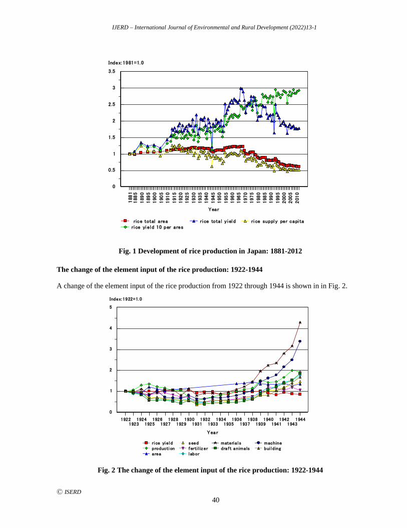
IJERD – International Journal of Environmental and Rural Development (2022)13-1
Ⓒ ISERD
40
1881
1885
1890
1895
1900
1905
1910
1915
1920
1925
1930
1935
1940
1945
1950
1955
1960
1965
1970
1975
1980
1985
1990
1995
2000
2005
2010
Year
0
0.5
1
1.5
2
2.5
3
3.5
Index: 1981=1. 0
rice total areari ce yiel d 10 per ares
ri ce tota l y i el d ri ce supply per capi ta
Fig. 1 Development of rice production in Japan: 1881-2012
The change of the element input of the rice production: 1922-1944
A change of the element input of the rice production from 1922 through 1944 is shown in in Fig. 2.
Fig. 2 The change of the element input of the rice production: 1922-1944
19221923
19241925
19261927
19281929
19301931
19321933
19341935
19361937
19381939
19401941
19421943
1944
Yea r
0
1
2
3
4
5
Index: 1922=1.0
ri ce yieldproductionarea
seedferti l izerl abor
materi a l sdraf t animals
machinebui l ding
IJERD – International Journal of Environmental and Rural Development (2022)13-1
Ⓒ ISERD
41
In this Figure, the change of the input standard of each agent of production is shown in the
standard in 1922(1922 = 1.0).
The change of factor shares of the rice production: 1922-1944
Table 1 shows the change of factor shares is land, labor, fertilizer, cost of draft animals,
agricultural machinery, materials, building for agriculture, seed in order of the average value from
1922 through 1944. The change of these factor shares becomes land, labor, manure, labor force of
livestock, agricultural machinery, materials, a building, the seed in order of a standard level. Factor
share of the capital such as labor force of livestock, agricultural machinery, the building shows a low
value. On the other hand, labor, land and factor share of ordinary input materials such as the manure
shows a high value. The period for the analysis was the time when it could not expect the expansion of
the land area. Under such situations, the change of factor share of the agent of production shows that
the following production engineering system has been developed. As for the development of
production technological system, it is a technological innovations land-saving and fertilizer-using
(Sawada,S.1991).
Table 1 Changes in factor shares for rice production in Japan :1922-1944
The examination of the estimated result of the amount of production formation function
The measurement results of the amount of production formation function are as follows.
lnX= +0.0097 +0.1233lnL +0.3609lnV +0.3627lnS (7)
(0.0051) (0.4687) (1.4125) (0.5920)
R2 = 0.6030
Year seed fertilizer labor materials draft animals machine building land(%) (%) (%) (%) (%) (%) (%) (%)① ② ③ ④ ⑤ ⑥ ⑦ ⑧
1922 0.0147 0.2250 0.4618 0.0199 0.0651 0.0314 0.0341 0.14801923 0.0129 0.2047 0.3835 0.0173 0.0561 0.0286 0.0318 0.26511924 0.0100 0.1611 0.3294 0.0170 0.0419 0.0210 0.0259 0.39361925 0.0081 0.1410 0.2265 0.0129 0.0268 0.0184 0.0159 0.55031926 0.0082 0.1676 0.2392 0.0155 0.0302 0.0261 0.0204 0.49281927 0.0080 0.1787 0.2306 0.0182 0.0333 0.0194 0.0190 0.49281928 0.0081 0.1762 0.2454 0.0200 0.0319 0.0206 0.0200 0.47771929 0.0082 0.1606 0.2421 0.0154 0.0269 0.0202 0.0196 0.50701930 0.0121 0.2416 0.4498 0.0331 0.0548 0.0374 0.0293 0.14201931 0.0103 0.2035 0.4021 0.0291 0.0490 0.0359 0.0312 0.23891932 0.0089 0.1599 0.3420 0.0271 0.0400 0.0296 0.0263 0.36621933 0.0088 0.1740 0.3275 0.0245 0.0390 0.0295 0.0254 0.37121934 0.0081 0.1497 0.2992 0.0212 0.0347 0.0260 0.0232 0.43781935 0.0088 0.1457 0.2974 0.0210 0.0350 0.0255 0.0212 0.44541936 0.0085 0.1451 0.2762 0.0217 0.0315 0.0248 0.0208 0.47141937 0.0095 0.1455 0.2633 0.0223 0.0320 0.0263 0.0204 0.48061938 0.0096 0.1500 0.2819 0.0252 0.0352 0.0283 0.0193 0.45051939 0.0082 0.1355 0.3058 0.0258 0.0386 0.0303 0.0185 0.43741940 0.0109 0.1933 0.3753 0.0312 0.0494 0.0361 0.0198 0.28391941 0.0105 0.1748 0.3872 0.0316 0.0540 0.0377 0.0236 0.28051942 0.0107 0.1417 0.4049 0.0336 0.0543 0.0408 0.0240 0.29001943 0.0095 0.1328 0.3571 0.0315 0.0499 0.0393 0.0241 0.35571944 0.0112 0.1232 0.4231 0.0440 0.0624 0.0549 0.0296 0.2515
Note: ⑧=1-(①+②+③+④+⑤+⑥+⑦)
IJERD – International Journal of Environmental and Rural Development (2022)13-1
Ⓒ ISERD
42
Firstly, the value of A is 0.0097. It is supposed that this suggests the existence of the neutral
technological change. Secondly, the value of α is 0.1233. Thirdly, the value of γ is 0.3609. As for
the fourth, a value of δ is 0.3627. As for the fifth, α+γ+δ is 0.8468, and the values are less than 1.
It is similar to the linear homogeneous production function. This means that the constant returns to
scale. This conclusion supports an original hypothesis. In other words, there are not the economies of
scale in this production stage.
Examination of the contribution of the production input
In a C-D's type production function, a value of the production of agent of production X elasticity and
the distribution diagram of agent of production X have a characteristic to be equal. From it, the
economical analysis of the input standard of the factors of production is possibility. It compares the
value of the factors of production of factor share and the value of the production elasticity by the
estimated result of the C-D's type amount of production formation function. And it adds economical
analysis about the element input standard of each agent of production. As for the labor input standard, an estimate of the labor (α) for 0.1233, as for the factor share of
the labor are 1922-1930:0.3120, 1931-1940:0.3171, 1941-1944:0.3931 and 1922-1944:0.3283.
In all periods, the numerical value of factor share is higher than a value of the production of factors of
production elasticity, it is in this way supposed that the quantity of throwing down standard of factors
of production is an excessive tendency. As for the manure input standard, an estimate of the manure (γ) for 0.3609, as for the factor share of
the labor are 1922-1930:0.1841, 1931-1940:0.1602, 1941-1944:0.1431 and 1922-1944:0.1666. In
all periods, the price of the production of factors of production elasticity is higher than a value of factor
share of factors of production. It is in this way supposed that the quantity of throwing down standard of
factors of production is a too few tendency. As for land input standard, an estimate of the land (δ) for 0.3627, as for the factor share of the labor
are 1922-1930:0.3855, 1931-1940:0.3983, 1941-1944:0.2944 and 1922-1944:0.3752. The period of 1941-1944 years, the price of the production of factors of production elasticity is
higher than a value of factor share of factors of production. It is supposed that the input standard of
factors of production is a too few tendency. However, in other time, as for the value of the production
of factors of production elasticity, the value of factor share of factors of production is almost balanced.
It is supposed that the input standard of factors of production is balanced.
The results of estimate by the amount of production formation function are as follows. In the
periods of 1922-1944, the input of the labor is excess level, the input of the fertilizer is under level and
the input of the land is equilibrium level.
CONCLUSION
The purpose of this study is to elucidate the characteristics of the production structure of the rice
production in Japan from 1922 through 1944. The measurement of factor shares of the rice production
in the analysis period. In addition, it measures the Cobb-Douglas‘s type amount of production
formation function. It clarify the contribution of the production input. The changes of factor shares are
as follows. The change of factor shares is land, labor, fertilizer, cost of draft animals, agricultural
machinery, materials, building for agriculture, seed in order of the average value from 1922 through
1944. As for the development of production technological system, it is a technological innovations
land-saving and fertilizer-using. The results of estimate by the amount of production formation
function are as follows. In the periods of 1922-1944, the input of the labor is excess level, the input of
the fertilizer is under level and the input of the land is equilibrium level.
IJERD – International Journal of Environmental and Rural Development (2022)13-1
Ⓒ ISERD
43
As a result of analysis, for the increase of the agricultural production, it was suggested that the
development of the technique to reduce the limitation of the factor of production was important. The
development of the agriculture section is important in economic development in modern Asia. When it
thinks about a strategy of the agriculture development in modern Asia, it is suggested that it is
necessary to consider the direction of the change of the production technique.
REFERENCES
Tsuchiya, K. 1976. Productivity and Technological Progress in Japanese Agriculture. Univ. of Tokyo Press. 261,
40-70.
Sawada, S.1991. Technological Progress in Japanese Agriculture. Association of Agriculture and Forestry
Staistics. 364, 331-364.
Teruoka S. 2008. Agriculture in the Modernization of Japan 1850-2000. Ajay Kumar Jain for Manohar Publishers
and Distributors. 375,127-154.
Hayami, Y., Yamada, S., Akino,M., Le Thanh Ngiep., Kawagoe, T. and Honma, M. 1991. The Agricultural
Development of Japan: A Century's Perspective. Univ. of Tokyo Press, 276, 13-108.
Hayami, Y and Vernon W. Ruttan. 1985. Agricultural Development: An International Perspective. Johns Hopkins
Univ. Press. 506, 204-205.
IJERD – International Journal of Environmental and Rural Development (2022)13-1
Ⓒ ISERD
44
Perspective on Urban and Peri-Urban Agriculture in
Cambodia’s Capital: Phnom Penh
CHES SOPHY* Researcher, Japan
Email: [email protected]
EIJI YAMAJI Emeritus Professor, University of Tokyo, Japan
THOL DINA Officer, Ministry of Land Management, Urban Planning and Construction, Cambodia
Received 30 January 2022 Accepted 22 April 2022 (*Corresponding Author)
Abstract: Due to population growth and urbanization over two decades, Phnom Penh Capital’s
area has almost doubled from 375 square kilometer in 2001 to 692.46 square kilometer in 2019.
Meanwhile, the number of farmers declined from 36.77% of the population in 2001 to 10% in
2015. Respecting these issues, the government of Cambodia prepared the Land Use Master Plan
of Phnom Penh City 2035. However, no clear implementation of the plan and the fast growth of
construction have become the main concerns of international donors. Moreover, the integration
of Phnom Penh with some areas of neighboring provinces will affect agricultural activities.
Therefore, this research aims to ascertain more details of agricultural land use in Phnom Penh
by responding to the Master Plan and to explain the current activities of urban agriculture or
peri-urban agriculture in the capital. Owing to the pandemic, this research was conducted by
solely reviewing and analyzing legal documents, reports from the government and donors, and
other reliable sources. The Land Use Master Plan clearly indicates the space reserved for the
peri-urban agricultural activities; however, there are no details regarding agricultural policy
dealing with the space reserved for peri-urban agriculture. The involvement of the Ministry of
Agriculture, Forestry and Fisheries is also not explained. Based on the reports from donors and
NGOs, lack of roles and responsibilities, limited capacity and limited finance have become the
main concerns for the government regarding implementation of the Master Plan. Importantly,
current rapid growth of construction does not pay any attention to the development of city plans.
Housing complex projects have increased from 77 in 2011 to 178 projects in 2019. Some
private businesses are practicing peri-urban agriculture on the outskirts of the capital by
growing, selling some vegetables, and providing the space for the relaxation.
Keywords: Urban Agriculture, Peri-Urban Agriculture, Agricultural Policies, Land Use Master
Plan
INTRODUCTION
Phnom Penh, the capital of Cambodia, is located in South-East Asia. All main activities including
economics, politics, culture and diplomacy are centered in the capital which has the highest density of
population 2,143,591 in 2021 based on the World Population Review. Phnom Penh covers the area of
692.46 square kilometer; consisting of 14 districts. Currently, Phnom Penh has expanded by integrating
20 other communes from neighboring province due to rapid population growth and urbanization. Back
in 2001 Phnom Penh covered 375 square kilometers consisting of 70% for human settlement, 21% for
agricultural activities, 8% covered by water, and remaining not in use (Em and Paule, 2005). The
erd
Research article
IJERD – International Journal of Environmental and Rural Development (2022)13-1
Ⓒ ISERD
45
practice of urban agriculture did exist in the capital; however, the number of farmer declined from
36.77% of tge population in the capital in 2001 (Em and Paule, 2005) to only 10% in 2015 based on
the World Bank Group on Urban Development in Phnom Penh (2017). With respect to rapid growth of
urbanization and population, the Government of Cambodia has prepared the Land Use Master Plan of
Phnom Penh City 2035. However, no clear implementation of the plan and the fast growth of construction
have become the main concerns of international donors. Moreover, the integration of Phnom Penh with
some areas of neighboring provinces will affect agricultural activities. Therefore, this research aims to
ascertain more details of agricultural land use in Phnom Penh by responding to the Master Plan; and to
explain the current activities of urban agriculture or peri-urban agriculture in the capital.
METHODOLOGY
Owing to the pandemic, the study was conducted by solely reviewing and analyzing legal documents,
reports from the government and donors, and other reliable sources.
RESULTS AND DISCUSSION
Land Use Pattern in Phnom Penh
Official data on two new integrated districts (Kambo and Boeung Keng Kang) in Phnom Penh is not
available. Fig. 1 shows the administrative boundary of Phnom Penh with only 12 districts. Among the
14 districts, Chraoy Chongvar, Dangkao, Kambo, Mean Chey, Praek Phnov, Pur Senchey and Sensokh
are considered to be the outskirt areas of the capital (Realestate, 2021).
Fig. 1 Phnom Penh Administrative Map
Urban Agriculture in Phnom Penh
Decades ago, according to Srer Khmer (2007), most of people living in Phnom Penh did not practice
agricultural activities even despite of potential agricultural land. At that time, there were only a few
NGOs working on urban and peri-urban agriculture. At the present time, core areas of Phnom Penh
have been occupied by economic activities. Based on the data from Phnom Penh’s Department of

IJERD – International Journal of Environmental and Rural Development (2022)13-1
Ⓒ ISERD
46
Agriculture, Forestry and Fisheries in 2019, some districts on the outskirts of Phnom Penh are used for
growing rice and then for growing vegetables after the rice harvesting season.
Table 1 Agricultural Land in Phnom Penh
District Rice Growing Area (ha) Ownership (ha) Rent (ha)
Praek Pnov 1,409 1,372 37
Chraoy Chongvar 152 75 87
Chbar Ampov 6 6 -
Saen Sokh 247 217 30
Dangkao 3,273 2,247 1,026
Pur Senchey 310 80 230
Kambo 3,048 1,996 1,052 Source: Phnom Penh Department of Agriculture, Forestry and Fisheries (2019)
Land Use Master Plan for Phnom Penh Capital 2035
Because there is no clear land use pattern in Phnom Penh for the current situation and to deal with the
rapid growth of population and urbanization, the government of Cambodia has prepared the Land Use
Master Plan of Phnom Penh Capital 2035. The main objectives of the Master Plan are to develop
Phnom Penh to become a core center for development, an international standard city, a reserve for the
development of necessary physical infrastructure, a metropolitan city and a special area for cultural
heritage. Fig. 2 shows the map of the Land Use Master Plan of Phnom Penh Capital 2035.
Fig. 2 Map of Land Use Master Plan of Phnom Penh Capital 2035
Legend of the map was written in the Khmer language. The English-translated legend was
provided next to the map. The second green symbol in the legend was used to indicate the space
reserved for the peri-urban agriculture in Phnom Penh Capital.
In order to make the Land Use Master Plan realized and vitalized, the Phnom Penh Sustainable
City Plan was designed to support the implementation of the Phnom Penh Master Plan for Land Use
2035. Fig. 3 shows the link between Land Use Master Plan for Phnom Penh 2035 and the Phnom Penh
Sustainable City Plan 2018-2030.
After obtaining the details of both the Land Use Master Plan and the Phnom Penh Sustainable
City plan, the study found that there is no clear explanation nor detail regarding the usage of reserved
spaces for peri-urban agriculture as mentioned clearly in the map (referred to Fig. 2). Noticeably, there
Drainage System
Reserved land for big public buildings
Old ancient buildings
Economic Development Zones
Legend
Areas with high population, buildings along the roads
Areas with much urbanization
Areas with high population density
Reserved Ponds
Waste water (drainage) canal systems needed to be established
Main Drainage systems
Secondary Drainage systems
Pagodas
Waste Water reseviors and biological purification areas
Areas with less urbanization
Building Density
Public Building
Pu
Ps
Pc
Pl
Pla
Pa
Pe
Pb Business Poles
Pr
Pi
Pn
Ld
Ll
Lm
Lf
Lp
Fn
R
60m-Width Belt Roads for traffic diversion
Protected Areas
1. Natural and Agricultural Areas
Areas with low population density
Peri-urban Agriculture Areas
Joint Park Areas and Recreational Buildings
2. Archeological Areas
Archeological Areas
3. Protected River bank Areas
vulnerable river bank areas, urbanization and soft buildings
Road Networks
Ports for tourist ships or boats
To-be-studied Areas
Existing Railways
Administrative borders of Phnom Penh City
30-50m-Width Main Roads
20-30m-Width maind roads in Districts and communes
Main Axis and aligned plants
Transport and Goods
Goods Preparation zones and Warehouses
Train station, airports and ports
Goods
University Poles
Sport Poles
Cultural Poles
Pleasure Poles
Exposure tree planting areas and conservation
Administrative Poles
Environmental and Agricultural Poles
Research Poles
Advanced Industrial Poles
National Identifcation Demonstration Poles
Poles
Bus Station
Landfill
Biological water purification ponds
Wholesale (Lump sum) Markets
Goods Areas
Goods Storing Areas
National Railway Stations
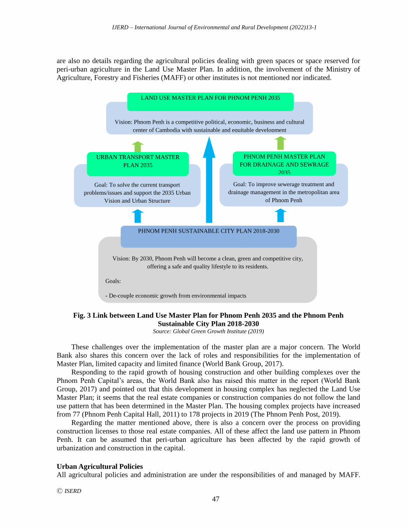
IJERD – International Journal of Environmental and Rural Development (2022)13-1
Ⓒ ISERD
47
are also no details regarding the agricultural policies dealing with green spaces or space reserved for
peri-urban agriculture in the Land Use Master Plan. In addition, the involvement of the Ministry of
Agriculture, Forestry and Fisheries (MAFF) or other institutes is not mentioned nor indicated.
Fig. 3 Link between Land Use Master Plan for Phnom Penh 2035 and the Phnom Penh
Sustainable City Plan 2018-2030 Source: Global Green Growth Institute (2019)
These challenges over the implementation of the master plan are a major concern. The World
Bank also shares this concern over the lack of roles and responsibilities for the implementation of
Master Plan, limited capacity and limited finance (World Bank Group, 2017).
Responding to the rapid growth of housing construction and other building complexes over the
Phnom Penh Capital’s areas, the World Bank also has raised this matter in the report (World Bank
Group, 2017) and pointed out that this development in housing complex has neglected the Land Use
Master Plan; it seems that the real estate companies or construction companies do not follow the land
use pattern that has been determined in the Master Plan. The housing complex projects have increased
from 77 (Phnom Penh Capital Hall, 2011) to 178 projects in 2019 (The Phnom Penh Post, 2019).
Regarding the matter mentioned above, there is also a concern over the process on providing
construction licenses to those real estate companies. All of these affect the land use pattern in Phnom
Penh. It can be assumed that peri-urban agriculture has been affected by the rapid growth of
urbanization and construction in the capital.
Urban Agricultural Policies
All agricultural policies and administration are under the responsibilities of and managed by MAFF.
Vision: Phnom Penh is a competitive political, economic, business and cultural
center of Cambodia with sustainable and equitable development
LAND USE MASTER PLAN FOR PHNOM PENH 2035
Goal: To solve the current transport
problems/issues and support the 2035 Urban
Vision and Urban Structure
URBAN TRANSPORT MASTER
PLAN 2035
Goal: To improve sewerage treatment and
drainage management in the metropolitan area
of Phnom Penh
PHNOM PENH MASTER PLAN
FOR DRAINAGE AND SEWRAGE
2035
Vision: By 2030, Phnom Penh will become a clean, green and competitive city,
offering a safe and quality lifestyle to its residents.
Goals:
- De-couple economic growth from environmental impacts
- Increase social inclusion, reduce poverty levels, and improve urban welfare
- Provide urban resilience for all citizens to natural, climatic and other risks
- Ensure urban competitiveness and attractiveness to businesses
PHNOM PENH SUSTAINABLE CITY PLAN 2018-2030
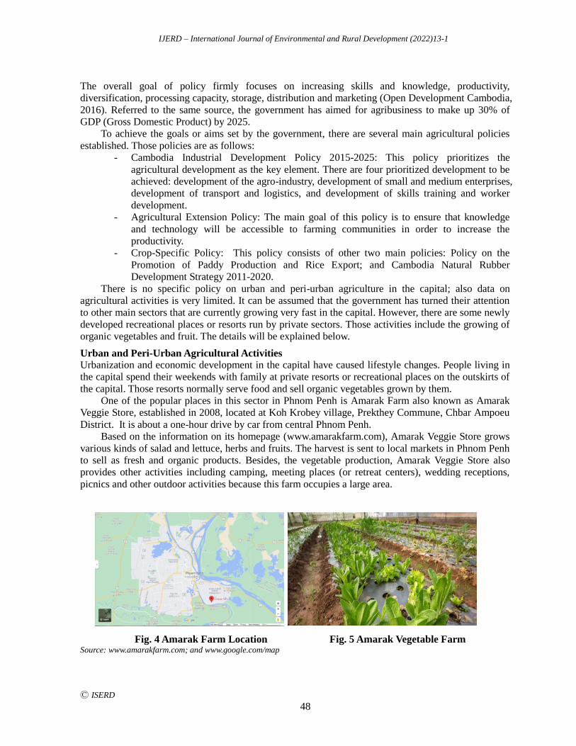
IJERD – International Journal of Environmental and Rural Development (2022)13-1
Ⓒ ISERD
48
The overall goal of policy firmly focuses on increasing skills and knowledge, productivity,
diversification, processing capacity, storage, distribution and marketing (Open Development Cambodia,
2016). Referred to the same source, the government has aimed for agribusiness to make up 30% of
GDP (Gross Domestic Product) by 2025.
To achieve the goals or aims set by the government, there are several main agricultural policies
established. Those policies are as follows:
- Cambodia Industrial Development Policy 2015-2025: This policy prioritizes the
agricultural development as the key element. There are four prioritized development to be
achieved: development of the agro-industry, development of small and medium enterprises,
development of transport and logistics, and development of skills training and worker
development.
- Agricultural Extension Policy: The main goal of this policy is to ensure that knowledge
and technology will be accessible to farming communities in order to increase the
productivity.
- Crop-Specific Policy: This policy consists of other two main policies: Policy on the
Promotion of Paddy Production and Rice Export; and Cambodia Natural Rubber
Development Strategy 2011-2020.
There is no specific policy on urban and peri-urban agriculture in the capital; also data on
agricultural activities is very limited. It can be assumed that the government has turned their attention
to other main sectors that are currently growing very fast in the capital. However, there are some newly
developed recreational places or resorts run by private sectors. Those activities include the growing of
organic vegetables and fruit. The details will be explained below.
Urban and Peri-Urban Agricultural Activities
Urbanization and economic development in the capital have caused lifestyle changes. People living in
the capital spend their weekends with family at private resorts or recreational places on the outskirts of
the capital. Those resorts normally serve food and sell organic vegetables grown by them.
One of the popular places in this sector in Phnom Penh is Amarak Farm also known as Amarak
Veggie Store, established in 2008, located at Koh Krobey village, Prekthey Commune, Chbar Ampoeu
District. It is about a one-hour drive by car from central Phnom Penh.
Based on the information on its homepage (www.amarakfarm.com), Amarak Veggie Store grows
various kinds of salad and lettuce, herbs and fruits. The harvest is sent to local markets in Phnom Penh
to sell as fresh and organic products. Besides, the vegetable production, Amarak Veggie Store also
provides other activities including camping, meeting places (or retreat centers), wedding receptions,
picnics and other outdoor activities because this farm occupies a large area.
Fig. 4 Amarak Farm Location Fig. 5 Amarak Vegetable Farm Source: www.amarakfarm.com; and www.google.com/map
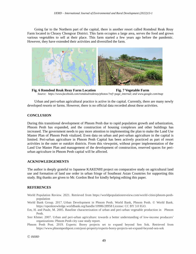
IJERD – International Journal of Environmental and Rural Development (2022)13-1
Ⓒ ISERD
49
Going far to the Northern part of the capital, there is another resort called Romdoul Reak Reay
Farm located in Chraoy Chongvar District. This farm occupies a large area, serves the food and grows
various vegetables to sell at their place. This farm started a few years ago before the pandemic.
However, they have extended their activities and diversified the farm.
Fig. 6 Romdoul Reak Reay Farm Location Fig. 7 Vegetable Farm Source: https://www.facebook.com/romdoulreakreay/photos/?ref=page_internal; and www.google.com/map
Urban and peri-urban agricultural practice is active in the capital. Currently, there are many newly
developed resorts or farms. However, there is no official data recorded about these activities.
CONCLUSION
During this transitional development of Phnom Penh due to rapid population growth and urbanization,
Phnom Penh has expanded, and the construction of housing complexes and other buildings has
increased. The government needs to pay more attention to implementing the plan to make the Land Use
Master Plan of Phnom Penh vitalized. Even data on urban and peri-urban agriculture in the capital is
limited. Peri-urban agriculture in Phnom Penh Capital has been actively practiced as part of resort
activities in the outer or outskirt districts. From this viewpoint, without proper implementation of the
Land Use Master Plan and management of the development of construction, reserved spaces for peri-
urban agriculture in Phnom Penh capital will be affected.
ACKNOWLEDGEMENTS
The author is deeply grateful to Japanese KAKENHI project on comparative study on agricultural land
use and formation of land use order in urban fringe of Southeast Asian Countries for supporting this
study. Big thanks are given to Mr. Gordon Beal for kindly helping editing this paper.
REFERENCES
World Population Review. 2021. Retrieved from https://worldpopulationreveiew.com/world-cities/phnom-penh-
population
World Bank Group. 2017. Urban Development in Phnom Penh. World Bank, Phnom Penh. © World Bank.
https://openknowledge.worldbank.org/handle/10986/28958 License: CC BY 3.0 IGO.
Em, H. and Paule, M. 2005. Baseline characterization of urban and peri-urban vegetable production in Phnom
Penh.
Srer Khmer. 2007. Urban and peri-urban agriculture: towards a better understanding of low-income producers’
organizations: Phnom Penh city case study report.
Phnom Penh Post. 2019. Experts: Borey projects set to expand beyond Sen Sok. Retrieved from
https://www.phnompenhpost.com/post-property/experts-borey-projects-set-expand-beyond-sen-sok

IJERD – International Journal of Environmental and Rural Development (2022)13-1
Ⓒ ISERD
50
Global Green Growth Institute. 2019. Phnom Penh Sustainable City Plan 2018-2030. Retrieved from
https://gggi.org/site/assets/uploads/2019/06/SUBSTAINABLE-CITY-REPORT_EN_FA3.pdf
Phnom Penh Capital Hall. 2011. Notable Data. Retrieved from https://phnompenh.gov.kh/en/phnom-penh-
city/facts/notable-data/
Open Development Cambodia. 2016. Agricultural policy and administration. Retrieved from
https://opendevelopmentcambodia.net/topics/agricutural-policy-and-administration/
Realestate. 2014. Overview of the districts in Phnom Penh. Retrieved from
https://www.realestate.com.kh/guides/overview-of-districts-in-phnom-penh/

IJERD – International Journal of Environmental and Rural Development (2022)13-1
Ⓒ ISERD
51
The Dynamics of Social Interactions of Children Playing
around Rural Rivers in Japan
MASAYUKI NITTA* Department of Civil and Environmental Engineering, Toyo University, Kawagoe, Japan
Email: [email protected]
YOSHIKI KUWABARA Faculty of Agriculture, Yamagata University, Tsuruoka, Japan
MASAHIRO NAKAJIMA Institute of Agriculture, Tokyo University of Agriculture and Technology, Fuchu, Japan
Received 19 February 2022 Accepted 22 April 2022 (*Corresponding Author)
Abstract In Monsoon Asia countries, rivers have intimate bonds with rural communities, which
create diverse social interactions regarding community building such as recreation, education,
and tourism. Especially, children tend to play around rivers, which is considered as one of the
foundations of community building since playing fosters children’s place-attachment to the
local rivers. However, the number of children playing around rivers has been decreasing owing
to expanding urbanization. This study aims to reveal 1) the influences of river use by family
members and neighborhoods on children’s river play, 2) the dynamics of children’s social
interactions in playing around rivers, and 3) the emergence mechanisms of children’s social
interactions in the play places. Questionnaire survey (127 local children from 9 to 11 years old),
participatory observation, and hiring survey (49 local children from 9 to 11 years old) were
conducted in the town of Gujohachiman, the Gifu Prefecture, Japan. Social network analysis
(SNA) was applied to the observation data to examine the dynamics of social interactions in
playing. As a result, river play frequency and preference of children were positively related to
the frequency of daily use of rivers by their family members and neighborhoods. SNA showed
that the interaction density of children playing around the river gradually increased while
repeatedly fluctuating up and down. This dynamical change of interactions was caused by
several leaders. The two factors for the emergence of children’s social interactions were
identified: introducing by the playgroup members and playing with caregivers. These results
imply that rural rivers have the function for children to expand their local interpersonal
relationships through playing, which are supported by local communities. Furthermore,
children’s play places around rivers have the potential to become the social interface for rural
and urban communities.
Keywords rural rivers, children, play places, social interactions, social network analysis,
environmental education
INTRODUCTION
In Monsoon Asia countries, rivers have intimate bonds with rural communities, which create diverse
social interactions regarding community building such as recreation, education, and tourism. Especially,
children tend to play around rivers (Senda, 1982; Kinoshita, 1992). However, children’s water play
around rivers has been decreasing owing to expanding urbanization.
As described in the Convention on the Rights of the Child, an outdoor play of children is essential
for their sound development and it is required that the local communities support children’s outdoor
erd
Research article
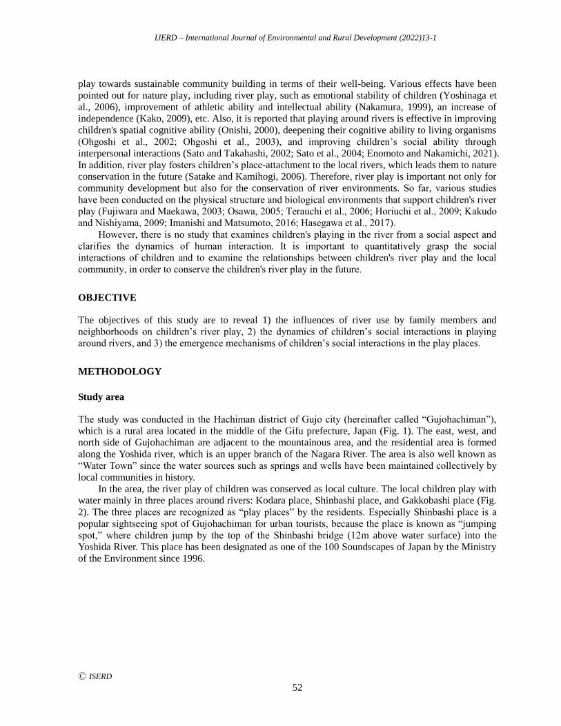
IJERD – International Journal of Environmental and Rural Development (2022)13-1
Ⓒ ISERD
52
play towards sustainable community building in terms of their well-being. Various effects have been
pointed out for nature play, including river play, such as emotional stability of children (Yoshinaga et
al., 2006), improvement of athletic ability and intellectual ability (Nakamura, 1999), an increase of
independence (Kako, 2009), etc. Also, it is reported that playing around rivers is effective in improving
children's spatial cognitive ability (Onishi, 2000), deepening their cognitive ability to living organisms
(Ohgoshi et al., 2002; Ohgoshi et al., 2003), and improving children’s social ability through
interpersonal interactions (Sato and Takahashi, 2002; Sato et al., 2004; Enomoto and Nakamichi, 2021).
In addition, river play fosters children’s place-attachment to the local rivers, which leads them to nature
conservation in the future (Satake and Kamihogi, 2006). Therefore, river play is important not only for
community development but also for the conservation of river environments. So far, various studies
have been conducted on the physical structure and biological environments that support children's river
play (Fujiwara and Maekawa, 2003; Osawa, 2005; Terauchi et al., 2006; Horiuchi et al., 2009; Kakudo
and Nishiyama, 2009; Imanishi and Matsumoto, 2016; Hasegawa et al., 2017).
However, there is no study that examines children's playing in the river from a social aspect and
clarifies the dynamics of human interaction. It is important to quantitatively grasp the social
interactions of children and to examine the relationships between children's river play and the local
community, in order to conserve the children's river play in the future.
OBJECTIVE
The objectives of this study are to reveal 1) the influences of river use by family members and
neighborhoods on children’s river play, 2) the dynamics of children’s social interactions in playing
around rivers, and 3) the emergence mechanisms of children’s social interactions in the play places.
METHODOLOGY
Study area
The study was conducted in the Hachiman district of Gujo city (hereinafter called “Gujohachiman”),
which is a rural area located in the middle of the Gifu prefecture, Japan (Fig. 1). The east, west, and
north side of Gujohachiman are adjacent to the mountainous area, and the residential area is formed
along the Yoshida river, which is an upper branch of the Nagara River. The area is also well known as
“Water Town” since the water sources such as springs and wells have been maintained collectively by
local communities in history.
In the area, the river play of children was conserved as local culture. The local children play with
water mainly in three places around rivers: Kodara place, Shinbashi place, and Gakkobashi place (Fig.
2). The three places are recognized as “play places” by the residents. Especially Shinbashi place is a
popular sightseeing spot of Gujohachiman for urban tourists, because the place is known as “jumping
spot,” where children jump by the top of the Shinbashi bridge (12m above water surface) into the
Yoshida River. This place has been designated as one of the 100 Soundscapes of Japan by the Ministry
of the Environment since 1996.
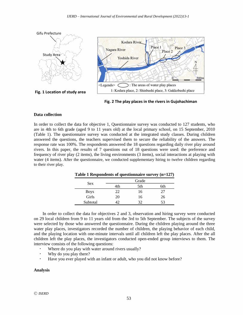
IJERD – International Journal of Environmental and Rural Development (2022)13-1
Ⓒ ISERD
53
Fig. 2 The play places in the rivers in Gujohachiman
Data collection
In order to collect the data for objective 1, Questionnaire survey was conducted to 127 students, who
are in 4th to 6th grade (aged 9 to 11 years old) at the local primary school, on 15 September, 2010
(Table 1). The questionnaire survey was conducted at the integrated study classes. During children
answered the questions, the teachers supervised them to secure the reliability of the answers. The
response rate was 100%. The respondents answered the 18 questions regarding daily river play around
rivers. In this paper, the results of 7 questions out of 18 questions were used: the preference and
frequency of river play (2 items), the living environments (3 items), social interactions at playing with
water (4 items). After the questionnaire, we conducted supplementary hiring to twelve children regarding
to their river play.
Table 1 Respondents of questionnaire survey (n=127)
4th 5th 6th
Boys 22 16 27
Girls 20 16 26
Subtotal 42 32 53
SexGrade
In order to collect the data for objectives 2 and 3, observation and hiring survey were conducted
on 29 local children from 9 to 11 years old from the 3rd to 5th September. The subjects of the survey
were selected by those who answered the questionnaire. During the children playing around the three
water play places, investigators recorded the number of children, the playing behavior of each child,
and the playing location with one-minute intervals until all children left the play places. After the all
children left the play places, the investigators conducted open-ended group interviews to them. The
interview consists of the following questions:
Where do you play with water around rivers usually?
Why do you play there?
Have you ever played with an infant or adult, who you did not know before?
Analysis
Fig. 1 Location of study area
Study Area
Gifu Prefecture
IJERD – International Journal of Environmental and Rural Development (2022)13-1
Ⓒ ISERD
54
In order to analyze the relationships between the preference and the frequency of children’s river play
and their living environments (objective 1), simple tabulation and cross-tabulation were conducted on
the data obtained by questionnaire survey. Secondly, the p-value was calculated using the results of
cross-tabulation. These computations were done using the SPSS program, version 10.0.
As for objective 2, Social Network Analysis (hereinafter called “SNA”) was applied to the
observation data (Freeman, 2004; Nooy et al., 2012). The dynamics of children’s social networks were
analyzed by using density, which is an index of SNA. The density is calculated by using Eq. (1) as
follows:
Where
Di: Density of children’s social networks at the time i
ni: The number of children existing in the play places at the time i
mi: The number of children’s ties at the time i
Density (Di) is an index of how close the social interchange between children playing in the play
places at the time i is. If the density is high, the children make relatively large groups to play together.
If the density is low, children play individually or in small groups.
As for objective 3, how children become acquainted with another child, infant or adult was
analyzed based on the observation data. Focusing on the matter of how the children’s communication
started, the emergence mechanisms of children’s social relationships in the play places were classified
by the acquaintances’ attributes: child, infant, and adult.
RESULTS AND DISCUSSION
Status of river use of children
Table 2 shows the preference and the frequency of river play of the subjects by sex. The ratio of those
who prefer river play was 91.3% in total. As a result of chi-square analysis, the ratio of boys, who
prefer river play (96.9 %) was significantly higher than the ratio of girls (85.5%, p < .05). As for the
frequency of river play, the ratio of those who play with water more than once a week was 50.4% in
total. As a result of chi-square analysis, The ratio of boys, who play with water more than once a week
(67.7%), was significantly higher than the ratio of girls (32.3%, p < .001). Water play around rivers
was generally preferred by many children. In particular, it was found that boys tended to prefer playing
around rivers.
As for the number of members to play with around rivers, all children answered “playing with
someone (friends or caregivers)”, which means no one played alone around rivers. As for the
experiences of children to getting to know new person during river play, 53.6% of the children (n=127)
had experiences to getting to know new person during river play. Table 3 shows the relationship
between the experiences to get to know new persons during river play and the number of members of
river play. As a result of chi-square analysis, the children, who play with more than three members,
tended to have the experiences to get to know new persons during river play, compared to the children,
who play with two or three members (p < .05).
Table 4 shows the relationships between the daily river use of family members and neighbors and
children’s preference and frequency of river play. The children, whose family members and neighbors
used the river in daily life, tended to prefer river play (95.5%), compared to those whose family
members and neighbors did not use the river in daily life (86.9%, p < .05). Further, looking at the
frequency of playing in the river, 63.6% of children, whose family members and neighbors used the
river in daily life, answered that they played around the river for a week or more. On the other hand,
the ratio of children, whose family members and neighbors did not use the river in daily life, was
(1)
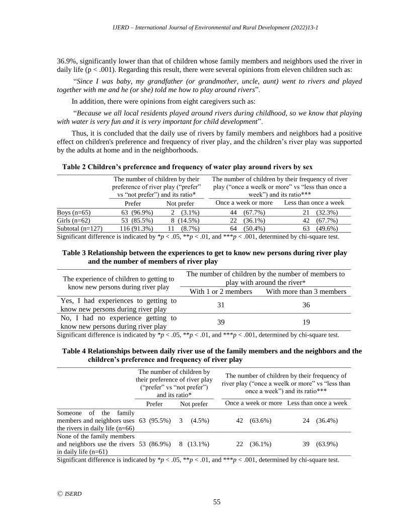
IJERD – International Journal of Environmental and Rural Development (2022)13-1
Ⓒ ISERD
55
36.9%, significantly lower than that of children whose family members and neighbors used the river in
daily life (p < .001). Regarding this result, there were several opinions from eleven children such as:
“Since I was baby, my grandfather (or grandmother, uncle, aunt) went to rivers and played
together with me and he (or she) told me how to play around rivers”.
In addition, there were opinions from eight caregivers such as:
“Because we all local residents played around rivers during childhood, so we know that playing
with water is very fun and it is very important for child development”.
Thus, it is concluded that the daily use of rivers by family members and neighbors had a positive
effect on children's preference and frequency of river play, and the children’s river play was supported
by the adults at home and in the neighborhoods.
Table 2 Children’s preference and frequency of water play around rivers by sex
The number of children by their
preference of river play (“prefer”
vs “not prefer”) and its ratio*
The number of children by their frequency of river
play (“once a weelk or more” vs “less than once a
week”) and its ratio***
Prefer Not prefer Once a week or more Less than once a week
Boys (n=65) 63 (96.9%) 2 (3.1%) 44 (67.7%) 21 (32.3%)
Girls (n=62) 53 (85.5%) 8 (14.5%) 22 (36.1%) 42 (67.7%)
Subtotal (n=127) 116 (91.3%) 11 (8.7%) 64 (50.4%) 63 (49.6%)
Significant difference is indicated by *p < .05, **p < .01, and ***p < .001, determined by chi-square test.
Table 3 Relationship between the experiences to get to know new persons during river play
and the number of members of river play
The experience of children to getting to
know new persons during river play
The number of children by the number of members to
play with around the river*
With 1 or 2 members With more than 3 members
Yes, I had experiences to getting to
know new persons during river play 31 36
No, I had no experience getting to
know new persons during river play 39 19
Significant difference is indicated by *p < .05, **p < .01, and ***p < .001, determined by chi-square test.
Table 4 Relationships between daily river use of the family members and the neighbors and the
children’s preference and frequency of river play
The number of children by
their preference of river play
(“prefer” vs “not prefer”)
and its ratio*
The number of children by their frequency of
river play (“once a weelk or more” vs “less than
once a week”) and its ratio***
Prefer Not prefer Once a week or more Less than once a week
Someone of the family
members and neighbors uses
the rivers in daily life (n=66)
63 (95.5%) 3 (4.5%) 42 (63.6%) 24 (36.4%)
None of the family members
and neighbors use the rivers
in daily life (n=61)
53 (86.9%) 8 (13.1%) 22 (36.1%) 39 (63.9%)
Significant difference is indicated by *p < .05, **p < .01, and ***p < .001, determined by chi-square test.
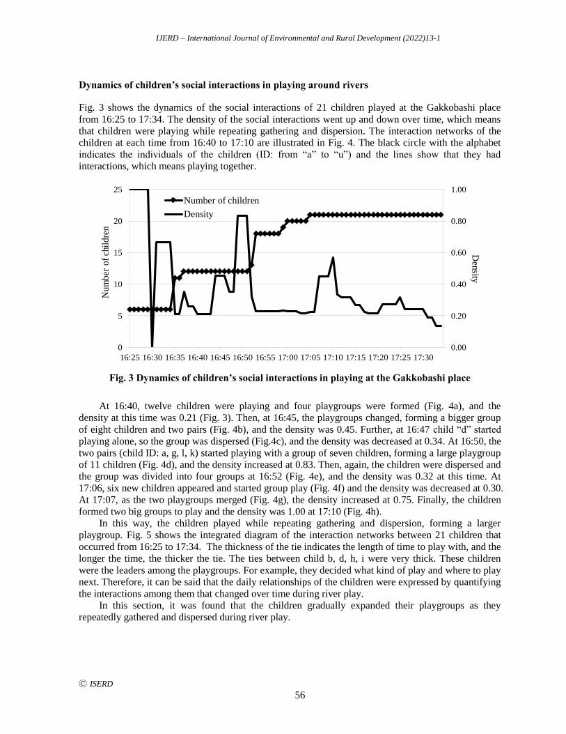
IJERD – International Journal of Environmental and Rural Development (2022)13-1
Ⓒ ISERD
56
Dynamics of children’s social interactions in playing around rivers
Fig. 3 shows the dynamics of the social interactions of 21 children played at the Gakkobashi place
from 16:25 to 17:34. The density of the social interactions went up and down over time, which means
that children were playing while repeating gathering and dispersion. The interaction networks of the
children at each time from 16:40 to 17:10 are illustrated in Fig. 4. The black circle with the alphabet
indicates the individuals of the children (ID: from “a” to “u”) and the lines show that they had
interactions, which means playing together.
0.00
0.20
0.40
0.60
0.80
1.00
0
5
10
15
20
25
16:25 16:30 16:35 16:40 16:45 16:50 16:55 17:00 17:05 17:10 17:15 17:20 17:25 17:30
Number of children
Density
Num
ber
of
chil
dre
n
Density
Fig. 3 Dynamics of children’s social interactions in playing at the Gakkobashi place
At 16:40, twelve children were playing and four playgroups were formed (Fig. 4a), and the
density at this time was 0.21 (Fig. 3). Then, at 16:45, the playgroups changed, forming a bigger group
of eight children and two pairs (Fig. 4b), and the density was 0.45. Further, at 16:47 child “d” started
playing alone, so the group was dispersed (Fig.4c), and the density was decreased at 0.34. At 16:50, the
two pairs (child ID: a, g, l, k) started playing with a group of seven children, forming a large playgroup
of 11 children (Fig. 4d), and the density increased at 0.83. Then, again, the children were dispersed and
the group was divided into four groups at 16:52 (Fig. 4e), and the density was 0.32 at this time. At
17:06, six new children appeared and started group play (Fig. 4f) and the density was decreased at 0.30.
At 17:07, as the two playgroups merged (Fig. 4g), the density increased at 0.75. Finally, the children
formed two big groups to play and the density was 1.00 at 17:10 (Fig. 4h).
In this way, the children played while repeating gathering and dispersion, forming a larger
playgroup. Fig. 5 shows the integrated diagram of the interaction networks between 21 children that
occurred from 16:25 to 17:34. The thickness of the tie indicates the length of time to play with, and the
longer the time, the thicker the tie. The ties between child b, d, h, i were very thick. These children
were the leaders among the playgroups. For example, they decided what kind of play and where to play
next. Therefore, it can be said that the daily relationships of the children were expressed by quantifying
the interactions among them that changed over time during river play.
In this section, it was found that the children gradually expanded their playgroups as they
repeatedly gathered and dispersed during river play.
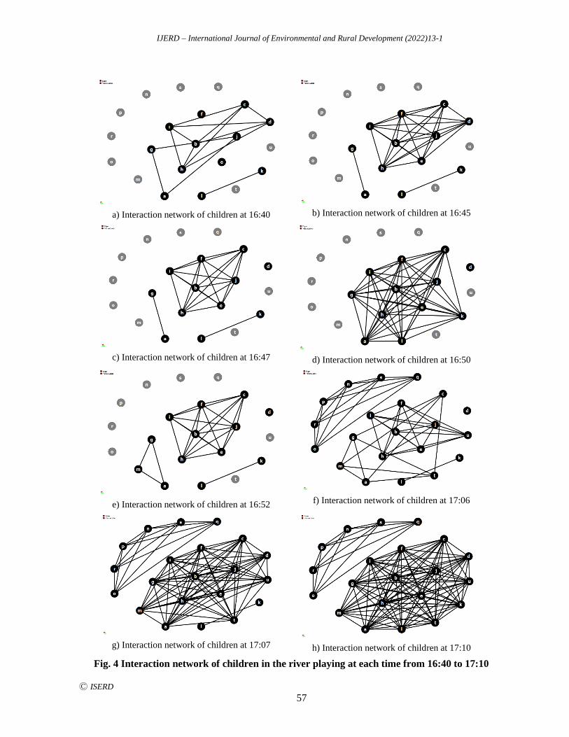
IJERD – International Journal of Environmental and Rural Development (2022)13-1
Ⓒ ISERD
57
a) Interaction network of children at 16:40
b) Interaction network of children at 16:45
c) Interaction network of children at 16:47
d) Interaction network of children at 16:50
e) Interaction network of children at 16:52
f) Interaction network of children at 17:06
g) Interaction network of children at 17:07
h) Interaction network of children at 17:10
Fig. 4 Interaction network of children in the river playing at each time from 16:40 to 17:10

IJERD – International Journal of Environmental and Rural Development (2022)13-1
Ⓒ ISERD
58
Fig. 5 Integrated interaction networks of 21 children observed from 16:25 to 17:34
Factors for the emergence of children’s social interactions
Through the observation survey and hiring survey, two factors for the emergence of children’s social
interactions were identified: (1) introducing by playgroup members and (2) playing with caregivers.
(1) Introducing by playgroup members
From the results in the previous section, it was found that children gradually expanded their playgroups
as they repeatedly gathered and dispersed during river play. Regarding this social interaction processes,
the following opinions were given by the three children who were playing:
“We all (local children) play usually in the three play places (Gakkobashi, Shinbashi, and Kodara
place). So local children playing with water around the rivers have many chances to know each other
very well.”
In addition, the following oral data were obtained from the four children:
“When we find some friends in other playgroups during river play, we play together with all
group members via the friends.”
Therefore, it can be said that there was a social exchange process by introducing to playgroup
members. This process is modeled in Fig. 6. In the Gujohachiman, children's play places in rivers are
fixed, so children's playgroups appeared in close proximity when playing in the river. At this time,
when groups 1 and 2 appeared, if the member “a” and “b” were acquainted, they first left the group and
had a conversation (Fig. 6). This formed a small play subgroup. Then, the children “a” and “b” were
invited to play together in each playgroup, and all of them played together to form a large playgroup.
Then, everyone became friends through river play together.
In this way, the cases that social interactions occurred through an introduction by playgroup
members were observed 17 times during the observation survey. The reason why the children's play
group gradually expanded in the previous section was due to the introduction by playgroup members.

IJERD – International Journal of Environmental and Rural Development (2022)13-1
Ⓒ ISERD
59
a
b
Friends a,bEmerged
new large
group
Group 1
Group 2
Play
together
Form
subgroup
Group 1
Group 2
1st Stage 2nd Stage 3rd Stage
Repeating
Fig. 6 Social interaction process model by introducing by playgroup members
(2) Playing with caregivers
The second is to play with caregivers. In this area, children were often seen playing in the river, so
visitors from outside the area, tourists, often played around the rivers with their family members. From
a viewpoint of the tourists, during the observation survey in the Shinbashi place, social interactions
from the toursts to the children were observed seven times per hour. In addition, the following oral data
were obtained from the ten tourists:
“It looks very fun that the local children play with water dynamically and actively.”
“I (or We) want to play together with them.”
On the other hand, it was also observed that children actively played with adults. When the
children played with an adult, they could play, such as riding on adults’ backs or throwing them on the
water surface, which the children could not do with children. Once the children started to play with an
adult, who is a caregiver of another child, They all played together finally. This process was shown in
Fig. 7. The adult “c” is a caregiver of the child “a”, and once the child “b” started to play with the adult
“c” (the first stage in Fig. 7), the child “a” and “b” played with the adult “c” (the second stage in Fig. 7).
Then The adult “c” introduced the child “b” to child “a” and they played all together finally (the third
stage in Fig. 7). This process was confirmed eleven times during the observation survey.
Child
“a”
Child
“b”
Adult
“c”
Child
“a”
Child
“b”
Adult
“c”
Child
“a”
Child
“b”
Adult
“c”
1st Stage 2nd Stage 3rd Stage
Family
Fig. 7 Social interaction process model of playing with caregivers
CONCLUSION
There were several findings from this study.
Firstly, river play frequency and preference of children were positively related to the frequency of daily
use of rivers by their family members and neighbors. Secondly, the SNA showed that the interaction density
of children playing around the rivers gradually increased while repeatedly fluctuating up and down. Thirdly,
IJERD – International Journal of Environmental and Rural Development (2022)13-1
Ⓒ ISERD
60
the two factors for the emergence of children’s social interactions were identified: introducing by the
playgroup members and playing with caregivers. In addition, although the hiring survey of this study was conducted in 2010, the authors also conducted
supplementary interviews with local children playing around the river in this area in 2016, and have confirmed
that the children yet played around river dynamically and their social interaction was formed through river play
by introducing by playgroup members and caregivers (Nitta et al, 2017).
These results imply that rural rivers have the function for children to expand their local interpersonal
relationships through playing, which are supported by local communities. Furthermore, children’s play
places around rivers have the potential to become the social interface for rural and urban communities, since
the tourists were attracted by the children playing around the rivers dynamically and social interactions have
occurred.
ACKNOWLEDGEMENTS
This study was conducted with the cooperation of the teachers, the students, and the parents of the
Hachiman elementary school in the Gujohachiman. We would like to thank them for collaboration.
Also, this work is supported by the Toyo University Faculty of Science and Technology Policy
Research 2020.
REFERENCES
Enomoto, N. and Nakamichi, N. 2021. The relationship between motor ability, cooperative physical and social
skills in young children. Japan Journal of Human Growth and Development Research, 91, 24-32.
Freeman, C. L. 2004. The development of social network analysis: a study in the sociology of science.
Createspace Independent Pub, 218.
Fujiwara, R. and Maekawa, T. 2003. The changes of playing environment of watersides in the three generations.
Journal of Rural Planning, 22, 253-258.
Hasegawa, Y., Hashimoto, K. and Takenaka, K. 2017. The influence of decision making to benefit of cultural
services by river of urban area. Landscape Research Japan Online, 10, 176-183.
Horiuchi, M., Fukamachi, k., Oku, H. and Okada, K. 2009. Early showa period use of natural resources and
natural space in child play in a rural community in the western part of shiga prefecture, japan. Journal of the
Japanese Institute of Landscape Architecture, 72, 5, 673-678.
Imanishi, A. and Matsumoto, A. 2016. Change of river use by children in Yodo river since 1945. Journal of the
Japanese Society of Revegetation Technology, 42, 1, 220-223.
Kako, S. 2009. What can children obtain from playing. Consultant, 244, 6-7.
Kakudo, H. and Nishiyama, M. 2009. On analysis of flow fields of a river for water activity preferred by children.
Transactions of the Japanese Society of Irrigation, Drainage and Rural Engineering, 77, 1, 1-6.
Kinoshita, I. 1992. A study on children’s contacts to nature in rural areas compared with urban areas: part1
studies on aspects of the function’s for environmental study through children’s play in rural nature spaces.
Journal of Architecture, Planning and Environmental Engineering, 431, 107-118.
Nakamura, K. 1999. The change of children’s play. Physical Education, 49, 25-27.
Nitta, M., Nakajima, M., and Senga, Y. 2017. The regional social system that supports the safety of children’s
diverse water play around rivers. Journal of rural planning association, 36, special issue, 350-355.
Nooy, D. W., Mrvar, A. and Batagelj, V. 2012. Exploratory social network analysis with pajek; expanded edition.
Cambridge University Press, 452.
Ohgoshi, M., Kumagai, Y., Kagawa, T. and Iijima, H. 2002. A study of change in waterside play and cognition of
plants and animals by children. Journal of the Japanese Institute of Landscape Architecture, 66, 5, 733-738.
Ohgoshi, M., Kumagai, Y. and Kagawa, T. 2003. The study of relationship between experiences in satoyama and
recognition of animals and plants. Journal of the Japanese Institute of Landscape Architecture, 67, 5, 647-
652.
Onishi, K. 2000. Children’s geography: perspectives and directions. Japanese Journal of Human Geography, 52,
IJERD – International Journal of Environmental and Rural Development (2022)13-1
Ⓒ ISERD
61
2, 149-172.
Osawa, S. 2005. Comparison of play and wildlife experiences of schoolchildren on waterside between in rural
area and in residential urban area. Journal of Rural Planning, 24, 13-18.
Satake, T. and Kamihogi, A. 2006. Study of the attachment to the local waterfront. Journal of the Japanese
Institute of Landscape Architecture, 70, 5, 663-668.
Sato, M. and Takahashi, T. 2002. A study on the construction of relationships among children and the
coexistence of playgroups: a study on the interaction between children’s ways of becoming members of
society and space part 1. Journal of Architecture and Planning, 67,562, 151-156.
Sato, M., Nishide, K. and Takahashi, T. 2004. A study on children and environment through transition of
playgroups: a study on the interaction between children’s ways of becoming members of society and space
part 2. Journal of Architecture and Planning, 69, 575, 29-35.
Senda, M. 1982. Research on structure of children’s play-spaces by investigating primary scenes in memories
about playing. Architectural Institute of Japan, 322, 108-117.
Terauchi, M., Kaga, H., Shimomura, Y. and Masuda, N. 2005. Study on environmental factors to form children’s
play in the outdoor space in 30s in the showa era. Journal of the Japanese Institute of Landscape Architecture,
69, 659-664.
Yoshinaga, M., Yokoyama, A. and Kinoshita, I. 2009. The play in the town and its psychological impacts on
children’s daily life and health condition. Japanese Journal of School Health, 51, 183-192.

IJERD – International Journal of Environmental and Rural Development (2022)13-1
Ⓒ ISERD
62
Income Generation and Expenditure of Organic Rice Farming
Households: Case Study of Preah Vihear Province, Cambodia
CHANMONY SOK* Graduate School of Agriculture, Tokyo University of Agriculture, Japan
Email: [email protected]
TOMOHIRO UCHIYAMA Faculty of International Agriculture and Food Studies, Tokyo University of Agriculture, Japan
NINA N. SHIMOGUCHI Faculty of International Agriculture and Food Studies, Tokyo University of Agriculture, Japan
Received 31 January 2022 Accepted 22 April 2022 (*Corresponding Author)
Abstract In Cambodia, organic rice farmers commonly engage in integrated farming and off-
farm activities to supplement their income. To identify factors for income optimization, this
study attempted to assess the income and expenditure structure of organic rice farm households
in the Preah Vihear Province, Cambodia. Guided with a structured questionnaire, a total of 90
and 50 randomly selected farmers were interviewed in 2019 and 2021, respectively. This study
utilized both descriptive and multiple regression analyses. Overall, farmers tended to expand
their cultivation area and increase income from off-farm jobs. Particularly, large-scale farmers
(5ha<) significantly expanded their farmland area and increased their livestock and off-farm
activities, while small-scale farmers (5ha>) reduced their farmland area and increased their off-
farm activities. Moreover, the multiple regression analysis revealed that secured spare time
from combine-harvester usage opened opportunities for farmers to engage in off-farm jobs.
These off-farm jobs, particularly by male farmers, boosted their respective annual income. On
the other hand, existing loans gave several farmer respondents negative profit in 2020. Thus,
financial management seemed to be a factor affecting farmers’ incomes in rural areas. For
further study, farm household employment choice behavior, particularly on labor mobility and
off-farm activities, is recommended.
Keywords Expenditure, Income, Off-farm activities, Organic Rice, Rural area
INTRODUCTION
Agricultural development is the most effective way to reduce poverty (World Bank, 2008). Two
effective agricultural development strategies are commonly practiced: engaging organic agriculture and
growing energy crops (Markandya and Setboonsarng, 2015). In Cambodia, agriculture contributed to
poverty reduction from 50% in 2007 to 9.4% in 2017. Moreover, rice is the predominant crop,
occupying 80% of the total crop area, and about 90% of the poor live in rural areas and rely on rice
farming for their primary income sources (NIS, 2013). The agriculture sector still shared around 20%
of GDP in 2019 (MAFF Cambodia, 2020). However, evidence suggests that rural households'
livelihoods draw on various activities in developing countries. From rural development and food
security viewpoints, it is critical to understand the structure of farm households' earnings and income
levels. (Helmers et al.,2004; Tong & Phay, 2013). Located in the Northern part of the country, Preah
Vihear province is one of the main producing area of organic rice in Cambodia. This rural province
produces organic rice once a year. Thus, all farmers have off-farm activities and produce other crop to
erd
Research article
IJERD – International Journal of Environmental and Rural Development (2022)13-1
Ⓒ ISERD
63
support their daily lives. Commonly, farmers produce rice, other crops, and livestock (e.g. cattle,
poultry), and do other off-farm activities as wage-earners and migrants to the city or neighboring
country to do other jobs to maximize their incomes. (Preah Vihear Provincial Department of
Agriculture, 2019). Little research has been performed on organic farm households' expenditure and
income generation, especially in rural areas (Uddin and Takeya, 2006). However, no researcher has
measured the expenditure and income generation of organic rice farm households in integrated farming
based on-farm size and family structures (e.g. gender, age, family member, and off-farm activities) in
Cambodia.
OBJECTIVE
This study aims to assess the income and expenditure structure of organic rice farm households in the
Preah Vihear province, Cambodia, to find the most suitable choice for organic rice farm households to
maximize their income. Specifically, this study aims to identify the characteristic of organic rice farm
households in the study area; clarify the structure of income sources of farm households; and assess
their expenditures.
METHODOLOGY
Study area: Data collection was conducted in Preah Vihear province, the largest organic rice
producing area and largest contract farming area in Cambodia. This region was characterized as a rural
area, with 85% of the population (approximately 60,605 households in 2019) relying on agriculture.
Hence, farmers were the main actors in this rural area. Sample selection: Questionnaire survey and in-
depth interviews were conducted randomly of 50 Organic rice farmers in contract farming during the
fields survey 2021. Collected data were processed and compared with the previous field survey of 90
respondents in 2019 in the same study area. Qualitative data were also collected regarding constraints,
opportunities, and other impact factors, including environmental and social factors. Data
analysis: Descriptive and multi-regression analyses were utilized. The multi-regression model below
was adopted from (Uddin and Takeya, 2006)
RESULTS AND DISCUSSION
Farmer respondents were divided into three groups according to their owned land size, as shown in
table1. Family members and members engaged in agriculture decreased yearly, either overall farmers
or group categories. From 2018 to 2020, farmers seemed to increase their cultivation areas based on
general statistics. However, only farmers who own land more than 5 ha increased their cultivation areas,
and farmers who own land larger than 10ha expanded all their cultivation areas in a fast pace. In
contrast, farmers who own land less than 5 ha seemed to decrease their rice cultivation. From field
Ln AI = ln a + b1X1+ b
2ln X2 + b
3ln X3 + b
4ln X4+ b
5ln X5+ b
6ln X6 + b
7ln X7 + b
8ln X8 +U
i
Ln = Natural logarithm X6 = Family member
Y = Annual income of farm household X7 = Family member engage in Agr
a = Constant or intercept of function X8 = Age of head household
X1 = Total owned land
X2 = Working days per year on farm activities by male b1…b8 = Coefficients of respective
X3 = Working days per year on farm activities by female variables;
X4 = Working days per year off-farm activities by male Ui = Error terms.
X5 = Working days per year off-farm activities by female
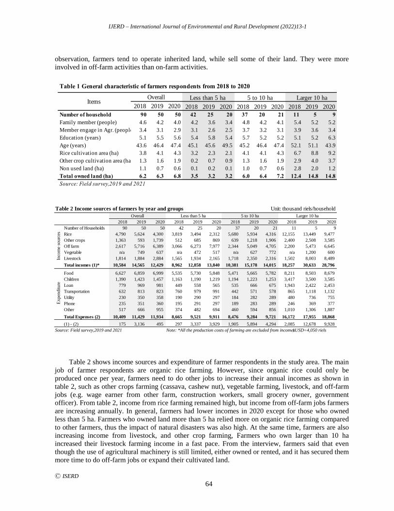
IJERD – International Journal of Environmental and Rural Development (2022)13-1
Ⓒ ISERD
64
observation, farmers tend to operate inherited land, while sell some of their land. They were more
involved in off-farm activities than on-farm activities.
Table 2 shows income sources and expenditure of farmer respondents in the study area. The main
job of farmer respondents are organic rice farming. However, since organic rice could only be
produced once per year, farmers need to do other jobs to increase their annual incomes as shown in
table 2, such as other crops farming (cassava, cashew nut), vegetable farming, livestock, and off-farm
jobs (e.g. wage earner from other farm, construction workers, small grocery owner, government
officer). From table 2, income from rice farming remained high, but income from off-farm jobs farmers
are increasing annually. In general, farmers had lower incomes in 2020 except for those who owned
less than 5 ha. Farmers who owned land more than 5 ha relied more on organic rice farming compared
to other farmers, thus the impact of natural disasters was also high. At the same time, farmers are also
increasing income from livestock, and other crop farming, Farmers who own larger than 10 ha
increased their livestock farming income in a fast pace. From the interview, farmers said that even
though the use of agricultural machinery is still limited, either owned or rented, and it has secured them
more time to do off-farm jobs or expand their cultivated land.
Table 1 General characteristic of farmers respondents from 2018 to 2020
2018 2019 2020 2018 2019 2020 2018 2019 2020 2018 2019 2020
Number of household 90 50 50 42 25 20 37 20 21 11 5 9
Family member (people) 4.6 4.2 4.0 4.2 3.6 3.4 4.8 4.2 4.1 5.4 5.2 5.2
Member engage in Agr. (people) 3.4 3.1 2.9 3.1 2.6 2.5 3.7 3.2 3.1 3.9 3.6 3.4
Education (years) 5.1 5.5 5.6 5.4 5.8 5.4 5.7 5.2 5.2 5.1 5.2 6.3
Age (years) 43.6 46.4 47.4 45.1 45.6 49.5 45.2 46.4 47.4 52.1 51.1 43.9
Rice cultivation area (ha) 3.8 4.1 4.3 3.2 2.3 2.1 4.1 4.1 4.3 6.7 8.8 9.2
Other crop cultivation area (ha) 1.3 1.6 1.9 0.2 0.7 0.9 1.3 1.6 1.9 2.9 4.0 3.7
Non used land (ha) 1.1 0.7 0.6 0.1 0.2 0.1 1.0 0.7 0.6 2.8 2.0 1.2
Total owned land (ha) 6.2 6.3 6.8 3.5 3.2 3.2 6.0 6.4 7.2 12.4 14.8 14.8
Source: Field survey,2019 and 2021
Items Less than 5 ha 5 to 10 haOverall Larger 10 ha
Table 2 Income sources of farmers by year and groups
2018 2019 2020 2018 2019 2020 2018 2019 2020 2018 2019 2020
Number of Households 90 50 50 42 25 20 37 20 21 11 5 9
Rice 4,790 5,624 4,300 3,819 3,494 2,312 5,680 5,934 4,316 12,155 13,449 9,477
Other crops 1,363 593 1,739 512 685 869 639 1,218 1,906 2,400 2,508 3,585
Off farm 2,617 5,716 6,389 3,066 6,273 7,977 2,344 5,049 4,705 2,200 5,473 6,645
Vegetable n/a 749 637 n/a 472 517 n/a 627 772 n/a 1,200 600
Livestock 1,814 1,884 2,884 1,565 1,934 2,165 1,718 2,350 2,316 1,502 8,003 8,489
Total incomes (1)* 10,584 14,565 12,429 8,962 12,858 13,840 10,381 15,178 14,015 18,257 30,633 28,796
Food 6,627 6,859 6,999 5,535 5,730 5,848 5,471 5,665 5,782 8,211 8,503 8,679
Children 1,390 1,423 1,457 1,163 1,190 1,219 1,194 1,223 1,253 3,417 3,500 3,585
Loan 779 969 981 449 558 565 535 666 675 1,943 2,422 2,453
Transportation 632 813 823 760 979 991 442 571 578 865 1,118 1,132
Utility 230 350 358 190 290 297 184 282 289 480 736 755
Phone 235 351 360 195 291 297 189 283 289 246 369 377
Other 517 666 955 374 482 694 460 594 856 1,010 1,306 1,887
Total Expenses (2) 10,409 11,429 11,934 8,665 9,521 9,911 8,476 9,284 9,721 16,172 17,955 18,868
(1) - (2) 175 3,136 495 297 3,337 3,929 1,905 5,894 4,294 2,085 12,678 9,928
Source: Field survey,2019 and 2021 Note: *All the production costs of farming are excluded from incomes 1USD=4,050 riels
Unit: thousand riels/household
Expen
diture
In
com
e so
urc
es
Overall Less than 5 ha 5 to 10 ha Larger 10 ha
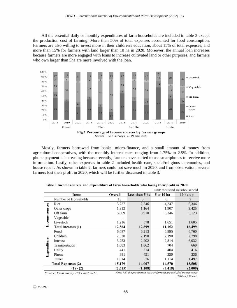
IJERD – International Journal of Environmental and Rural Development (2022)13-1
Ⓒ ISERD
65
All the essential daily or monthly expenditures of farm households are included in table 2 except
the production cost of farming. More than 50% of total expenses accounted for food consumption.
Farmers are also willing to invest more in their children's education, about 15% of total expenses, and
more than 15% for farmers with land larger than 10 ha in 2020. Moreover, the annual loan increases
because farmers are more engaged with loans to increase cultivated land or other purposes, and farmers
who own larger than 5ha are more involved with the loan.
Mostly, farmers borrowed from banks, micro-finance, and a small amount of money from
agricultural cooperatives, with the monthly interest rates ranging from 1.75% to 2.5%. In addition,
phone payment is increasing because recently, farmers have started to use smartphones to receive more
information. Lastly, other expenses in table 2 included health care, social/religious ceremonies, and
house repair. As shown in table 2, farmers could not save much in 2020, and from observation, several
farmers lost their profit in 2020, which will be further discussed in table 3.
Table 3 Income sources and expenditure of farm households who losing their profit in 2020
Unit: thousand riels/household
Items Overall Less than 5 ha 5 to 10 ha 10 ha up
Number of Households 13 5 6 2
Rice 3,727 2,246 4,247 6,346
Other crops 1,812 1,164 1,907 3,425
Off farm 5,809 8,910 3,346 5,123
Vegetable - - - -
Livestock 1,216 578 1,651 1,605
Total incomes (1) 12,564 12,899 11,152 16,499
Food 6,687 6,213 6,995 6,760
Children 2,320 2,190 2,190 2,798
Interest 3,253 2,202 2,814 6,032
Transportation 1,083 1,862 704 669
Utility 441 514 404 416
Phone 381 451 350 336
Other 1,014 576 1,114 1,497
Total Expenses (2) 15,179 14,007 14,570 18,508
(1) - (2) (2,615) (1,108) (3,418) (2,009)
Source: Field survey,2019 and 2021 Note: *All the production costs of farming are excluded from incomes
1USD=4,050 riels
Inco
me
sou
rces
E
xp
end
itu
re
IJERD – International Journal of Environmental and Rural Development (2022)13-1
Ⓒ ISERD
66
Although most farmers reported that the main job is rice farming, Figure 1 clearly shows a natural
shift of farmer income sources to off-farm activities. Moreover, only farmers who own land less than 5
ha rapidly increase off-farm jobs and decrease share income and cultivated rice farming land from
2018 to 2020. This can be attributed to farmers selling of inherited rice cultivated land. In addition,
farmers who own land 5 to 10 ha are increasing off-farm, and other crops farming and farmers who
own land larger than 10 ha are more increasing in livestock because they have larger land and capital.
During the field survey in 2021, some farmers had no profit due to high expenses, as shown in
table 3. All those farmers spent more on paying loan interests, while the income in 2020 decreased.
From field observation, farmers who owned land between 5 to 10 ha engaged more in loans to expand
their land cultivation and other activities. Unfortunately, the rice yield was low, which decreased
income, and farmers could not afford the repayment. In addition, some farmers who owned less than 5
ha needed to sell their lands to afford the repayment to the bank, which made farmers decrease their
owned land, while those who owned land of more than 5ha sold their livestock and other machinery to
repay the loan. Those problems made these farmers further smaller in scale. Therefore, farmers seemed
to need to understand more about financial management to lower risk in the future.
Table 4 Multi-regression on model of farm households’ incomes of groups
<5 ha (2020) (20 respondents) Estimate Std.Error t-value Pr(>|t|)
(Intercept) 11.214 1.483 7.558 0.000 ***
Land size 0.612 0.345 3.724 0.011 *
Working on-farm male 0.139 0.094 1.462 0.171
Working on-farm female -0.073 0.137 -1.534 0.303
Working off-farm male 0.330 0.136 2.422 0.032 *
Working off-farm female 0.292 0.236 2.082 0.064 *
Family members 0.227 0.238 0.942 0.360
Family members engage in farming 0.190 0.272 1.991 0.116
Age 0.145 0.350 0.416 0.580
Signif. codes: 0 ‘***’ 0.001 ‘**’ 0.01 ‘*’ 0.05 ‘.’ 0.1 ‘ ’ 1
Multiple R-squared: 0.6657, Adjusted R-squared: 0.5247
>5ha (2020) (30respondents) Estimate Std.Error t-value Pr(>|t|)
(Intercept) 14.766 3.191 4.627 0.000 ***
Land size 1.324 0.253 5.221 0.000 ***
Working on-farm male 0.554 0.270 2.051 0.053 .
Working on-farm female -0.550 0.281 -1.954 0.064 .
Working off-farm male 0.208 0.073 2.815 0.010 *
Working off-farm female 0.105 0.060 1.739 0.097 .
Family member 0.091 0.230 0.396 0.696
Family member engage in farming 0.140 0.130 1.080 0.292
Age 0.079 0.132 0.603 0.553
Signif. codes: 0 ‘***’ 0.001 ‘**’ 0.01 ‘*’ 0.05 ‘.’ 0.1 ‘ ’ 1
Multiple R-squared: 0.742, Adjusted R-squared: 0.640
Source: Field survey, 2021
Table 4 shows the result of multi-regression on total annual income with working labors, family
members, and age of farm households in 2020 by dividing into two groups: farmers who owned less
than 5ha and a combination of all farmers who owned land larger than 5ha. It should be noted that the
farmers who owned more than 10 ha were not grouped separately due to small sample size of nine
respondents. As a result, besides the land size, off-farm activities significant increased the total annual
income. Working off-farm jobs for male has boosted their annual income, especially farmers who
owned less than 5 ha. On the other hand, working on the farm for females resulted to negative impact
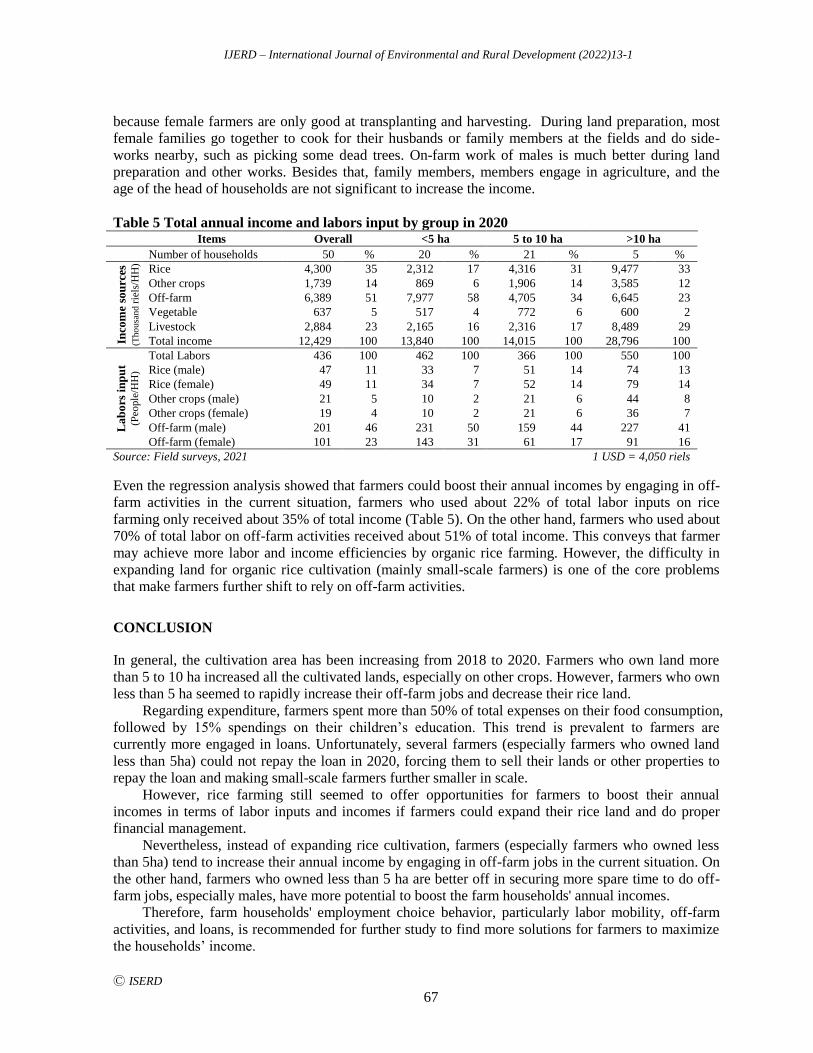
IJERD – International Journal of Environmental and Rural Development (2022)13-1
Ⓒ ISERD
67
because female farmers are only good at transplanting and harvesting. During land preparation, most
female families go together to cook for their husbands or family members at the fields and do side-
works nearby, such as picking some dead trees. On-farm work of males is much better during land
preparation and other works. Besides that, family members, members engage in agriculture, and the
age of the head of households are not significant to increase the income.
Table 5 Total annual income and labors input by group in 2020
Items Overall <5 ha 5 to 10 ha >10 ha
Number of households 50 % 20 % 21 % 5 %
Inco
me
sou
rces
(T
ho
usa
nd r
iels
/HH
)
Rice 4,300 35 2,312 17 4,316 31 9,477 33
Other crops 1,739 14 869 6 1,906 14 3,585 12
Off-farm 6,389 51 7,977 58 4,705 34 6,645 23
Vegetable 637 5 517 4 772 6 600 2
Livestock 2,884 23 2,165 16 2,316 17 8,489 29
Total income 12,429 100 13,840 100 14,015 100 28,796 100
La
bo
rs i
np
ut
(Peo
ple
/HH
)
Total Labors 436 100 462 100 366 100 550 100
Rice (male) 47 11 33 7 51 14 74 13
Rice (female) 49 11 34 7 52 14 79 14
Other crops (male) 21 5 10 2 21 6 44 8
Other crops (female) 19 4 10 2 21 6 36 7
Off-farm (male) 201 46 231 50 159 44 227 41
Off-farm (female) 101 23 143 31 61 17 91 16
Source: Field surveys, 2021
1 USD = 4,050 riels
Even the regression analysis showed that farmers could boost their annual incomes by engaging in off-
farm activities in the current situation, farmers who used about 22% of total labor inputs on rice
farming only received about 35% of total income (Table 5). On the other hand, farmers who used about
70% of total labor on off-farm activities received about 51% of total income. This conveys that farmer
may achieve more labor and income efficiencies by organic rice farming. However, the difficulty in
expanding land for organic rice cultivation (mainly small-scale farmers) is one of the core problems
that make farmers further shift to rely on off-farm activities.
CONCLUSION
In general, the cultivation area has been increasing from 2018 to 2020. Farmers who own land more
than 5 to 10 ha increased all the cultivated lands, especially on other crops. However, farmers who own
less than 5 ha seemed to rapidly increase their off-farm jobs and decrease their rice land.
Regarding expenditure, farmers spent more than 50% of total expenses on their food consumption,
followed by 15% spendings on their children’s education. This trend is prevalent to farmers are
currently more engaged in loans. Unfortunately, several farmers (especially farmers who owned land
less than 5ha) could not repay the loan in 2020, forcing them to sell their lands or other properties to
repay the loan and making small-scale farmers further smaller in scale.
However, rice farming still seemed to offer opportunities for farmers to boost their annual
incomes in terms of labor inputs and incomes if farmers could expand their rice land and do proper
financial management.
Nevertheless, instead of expanding rice cultivation, farmers (especially farmers who owned less
than 5ha) tend to increase their annual income by engaging in off-farm jobs in the current situation. On
the other hand, farmers who owned less than 5 ha are better off in securing more spare time to do off-
farm jobs, especially males, have more potential to boost the farm households' annual incomes.
Therefore, farm households' employment choice behavior, particularly labor mobility, off-farm
activities, and loans, is recommended for further study to find more solutions for farmers to maximize
the households’ income.
IJERD – International Journal of Environmental and Rural Development (2022)13-1
Ⓒ ISERD
68
ACKNOWLEGDE
Apart of this research study was financial supported by RIALS (Research Institute for Agricultural and
Life Sciences)
REFERENCES
Helmers, K., John, G. and Pia, W. 2004. Final report of the rural sources of income and livelihood strategies
study”, memo (World Bank)
MAFF, 2020. Annual report of agriculture, forestry, and fisheries 2019-2020. Ministry of agriculture, forestry and
fisheries, Phnom Penh, Cambodia, 2020.
NIS, 2013. Cambodia socioeconomic survey 2013. National institute of statistic, Cambodia, 23-28.
Uddin, M. T., & Takeya, H. (2006). Employment patterns and income generation of farm households in
integrated farming of Bangladesh. International Journal of Agricultural Research, 1(1), 32-40
Preah Vihear Provincial Department of Agriculture, 2019. Annual report for agriculture, forestry, and fisheries
2018-2019. Provincial department of agriculture, Preah Vihear province, 2019.
Setboonsarng, S. and Markandya, A. 2015. Option for Rural Development in Cambodia and the Lao People's
Democratic Republic, 155-159.
Tong, K. and Phay, S. 2013. The Role of Income Diversification during the Economic and Global Crisis in
Cambodia.
World Bank, 2008. World development report agriculture for development. 2008. 28-29.
https://openknowledge.worldbank.org/handle/10986/5990
IJERD – International Journal of Environmental and Rural Development (2022)13-1
Ⓒ ISERD
69
Economic Assessment of Tea Smallholder Farmers Under
Contract Farming in Rungwe District, Tanzania.
ISSA ABRAHAMAN KACHENJE* Graduate school of Agriculture, Tokyo University of Agriculture, Japan *
Email: [email protected]
NINA N. SHIMOGUCHI Faculty of International Agriculture and Food Studies, Tokyo, Japan
KATSUMORI HATANAKA Faculty of International Agriculture and Food Studies, Tokyo, Japan
RAMADHONA SAVILLE Faculty of International Agriculture and Food Studies, Tokyo, Japan
Received 31 January 2022 Accepted 22 April 2022 (*Corresponding Author)
Abstract In Tanzania, tea is considered as one of the most exported crops. The main
stakeholders of the tea industry are smallholder farmers and estates. Smallholder tea farmers are
required to engage in contract farming, as stipulated in the Tea Regulation of 2010. This study
attempted to assess contract farming and its impact to production and income of tea smallholder
farmers in Rungwe District, Tanzania. A total of 48 randomly selected smallholder farmers
were interviewed using a semi-structured questionnaire in September 2020 and October 2021.
Agribusiness company officials, government officials and extension officers were also
interviewed to clarify the condition and issues of the contract farming scheme. Descriptive
analysis and cost and return analysis were utilized. Results show that yield, income, and
profitability increased from 2016-2019. These can be attributed to steady supply of inputs, easy
access to technical assistance, and early adoption of new technology under contract farming
scheme. Moreover, the price of smallholder green leaf has improved, with farmers receiving a
second payment hence improve their overall revenue returns.
Keywords: Contract farming; smallholder farmers; tea; profitability; Tanzania.
INTRODUCTION
Tea is a globally manufactured and widely consumed beverage (Hicks 2009; Onduru et al. 2012).
Kenya, Malawi, Uganda, Tanzania, Zimbabwe, South Africa, and Rwanda are the principal tea-
producing countries in Africa, with tea contributing considerably to their economy (FAO, 2014). By
the year 2023, the continent's export volume is expected to reach 743,384 metric tons (FAOSTAT,
2015).
Tea is the fifth most exported crop in Tanzania, the tea sector accounts for an average of
approximately USD 50 million every year, when it comes to foreign exchange earnings. Tea industry
also contribute to the huge amount of employment opportunities as it employs more than 50,000
families and indirectly it affects to as many as 2 million Tanzanian citizens (Baffes 2004). Moreover,
the nature of tea production necessitates a significant amount of labor, implying that the sector can
employ a large number of people. It can be harvested all year, making it one of the few crops that can
generate a relatively consistent income when compared to seasonal crops like maize.
erd
Research article
IJERD – International Journal of Environmental and Rural Development (2022)13-1
Ⓒ ISERD
70
Tea cultivation was only done on a large scale under the supervision of several tea estates during
colonial and early post-colonial times, which meant that smallholder farmers were non-existent.
Smallholder tea production legally began only after the independence in 1960s. At that time the
government had actively pushed smallholders’ involvement in the tea sector (Maghimbi et al. 2011;
Gibbon 2011). This marked the starting point for the co-existence and relationship between the
smallholders and estates in the tea sector. The relationship was later on cemented with the introduction
of programs such as contract farming and sales agreements. Further, smallholders are required by law
to have at least a one-year sales agreement in place. This is due to a number of factors: Firstly, the tea
leaves' perishable nature; green leaves can only be stored for around six hours before they must be
processed. Secondly, Tea processing also demands complex and costly machinery, which is why the
majority of tea processing firms are owned by huge corporations. As a result, smallholders are reliant
on tea processing plants owned by large tea companies. This mandates close collaboration between
smallholder farmers and estates that possess processing plants, hence makes sales agreements and
contract farming necessary in Tanzania tea sector.
OBJECTIVE
The main goal of the study was to assess contract farming and its impact to production, income, and
profitability of tea smallholder farmers in Rungwe District, Tanzania.
METHODOLOGY
Study area
This study was conducted in Rungwe district (see Fig. 1) located in the Southern tea growing zone.
Two villages from the Rungwe district namely Katumba and Lugombo village were purposively
selected because these villages large concentration of smallholder farmers operating under a contract
system. A total of 48 randomly selected smallholder farmers were interviewed using a semi-structured
questionnaire in September 2020 and October 2021. Agribusiness company officials, government
officials and extension officers were also interviewed to clarify the condition and issues of the contract
farming scheme.
Fig. 1 Map of the study area Source: Google map
Methods of study
IJERD – International Journal of Environmental and Rural Development (2022)13-1
Ⓒ ISERD
71
For evaluating impact of these Contract Farming schemes on yield, income, and profitability of tea per
unit area, cost and return analysis were utilized. Furthermore, the study compared the yield, income,
and profitability of smallholder tea farmers from the year 2016 to 2019.
Fixed costs, such as family labor and land charges, were separated from variable costs, such as
herbicides, chemical fertilizers, pesticides, and hired labor. The gross return was then obtained by
multiplying the marketable produce by the year's average price per kilogram. The profit was then
calculated by subtracting the total cost from the gross return.
RESULTS AND DISCUSSION
The study estimated the cost of producing green tea leaves for smallholder tea producers in the
Rungwe district of Mbeya, Tanzania, as well as the revenue generated. In the study area, Pesticides,
herbicides, and farm labor both family and hired labor are among the inputs used by smallholder tea
farmers. On the other hand, Chemical fertilizers, such as NPK fertilizers, Glyphosate, UREA, and SA
fertilizer, are also used. Additionally, other farm inputs include safety Goggles, Gloves, Gum Boots,
Raincoat, Mouth Mask, Shears, and Spray Pump are often used by smallholders in the study area. This
section analyzed the production costs and profitability of smallholder farmers participating in Contract
Farming in greater detail. Most of these inputs are provided on credit to smallholder tea farmers in the
study area by their contracting estates. The inputs are distributed according to a well-established
process that is overseen by smallholder association leaders and extension officers. The loaned inputs
are paid for by deducting from the overall earnings that smallholder farmers are expected to gain
without any interest.
Yield of green tea leaves produced by smallholder tea farmers
The yield of a crop is calculated by dividing the amount of crop harvested by the harvested area of that
crop. Mathematically, the yield can be calculated by dividing production data by harvested area data.
According to the findings, the marketable yield for smallholder tea leaves in 2016, 2017, 2018,
and 2019 was 1,093 Kg/ha, 1,175 Kg/ha, 1,247 Kg/ha, and 1,347 Kg/ha, respectively. This is
attributable to a steady supply of inputs, easy access to technical assistance, and the adoption of new
technologies in the study area's contract farming scheme. Similarly, the contracting company has
stepped up its efforts to provide smallholder farmers with inputs such as fertilizers and herbicides at
significantly lower prices than market prices, allowing them to have easy access to supplies at a
reasonable price.
Table 1. Comparison of the between national average yield and study area’s average yield for
smallholder tea farmers.
Items 2016 2027 2028 2029
Country's smallholder average yield 814 1,082 1,203 1,035
Study area's smallholder average yield 1,093 1,175 1,247 1,347
Source: Field survey, 2020
IJERD – International Journal of Environmental and Rural Development (2022)13-1
Ⓒ ISERD
72
The costs of the inputs for green leaf tea production
The overall production cost was estimated, which included not only the cash payment but also the
estimation of the opportunity cost for smallholder farmers. There are two types of costs in agriculture:
variable and fixed. In general, variable costs fluctuate according to the degree of production. Fixed
costs, on the other hand, are expenses that do not change regardless of production level. According to
Mamun et al. (2018), the total cost (TC) can be obtained by adding the total variable cost (TVC) to the
total fixed cost (TFC), as illustrated in the equation below.
TC = TVC +TFC (1)
Where: TC = Total costs
TVC = Total Variable Cost
TFC = Total Fixed Cost
In this study, the total cost was calculated by adding the costs of chemical fertilizers, herbicides,
farm equipment, and labor used by smallholder farmers for producing green tea leaves in the study area.
Moreover, in an effort to improve green tea leaves production volume and quality in the study
area, the amount and frequency of provision of various farm inputs such as herbicides, chemical
fertilizers and other equipment were increased which resulted into the increased cost of production as
shown in the table 6.1. According to the findings, the total production cost of green tea leaves per
hectare was 65.65 TZS/ha, 73.32 TZS/ha, 102.13 TZS/ha, and 112.07 TZS/ha in 2016, 2017, 2018, and
2019 respectively.
Green tea leaves price in the study area
In the study area, for the years 2016, 2017, 2018, and 2019, the contracting company's green tea leaves
price per Kg in the research region was 231 TZS/Kg, 240 TZS/Kg, 315 TZS/Kg, and 320 TZS/Kg,
respectively. These prices offered to smallholders in the study area are higher than the government's
recommended price (basal price), implying that farmers in the study area benefit more than green tea
leaf growers in other tea producing areas, such as the Korogwe district in the northeast zone, where
smallholder tea producers receive no more than the government's recommended price.
Smallholder tea farmers’ Revenue, Income and Profitability in the study area
The gross income (GI), gross revenue (GR) and Gross profit (GP) were estimated using data from the
field survey 2020 and 2021 to better understand the impact of tea leaves production on the
smallholders’ livelihood. The study then simulated the comparative profitability of growing green tea
leaves in various years from 2016 to 2019. This will help to determine the trend of gross income, gross
revenue, and profitability received by smallholder tea farmers each year, as well as ranking the
profitability received over this period of time.
Gross revenue (GR) means the amount received by farmers presumably that their entire volume of
marketable yield is sold at the farm gate price. Dammert and Mohan (2015) support that the concept of
Gross Revenue is calculated as yield multiplied by farm gate price. Further, Gross income (GI) is
computed by subtracting total production costs from Gross Revenue, excluding family labor costs.
Finally, gross profit is derived by subtracting family labor costs from gross income.
The results showed that in 2016, 2017, 2018, and 2019, the gross revenue for smallholder tea
leaves production was 252.48 TZS/ha, 282 TZS/ha, 392 TZS/ha, and 431.04 TZS/ha, respectively.
IJERD – International Journal of Environmental and Rural Development (2022)13-1
Ⓒ ISERD
73
Likewise, the results showed that in 2016, 2017, 2018, and 2019, the gross Income for smallholder tea
leaves production was 215.87 TZS/ha, 241.11 TZS/ha, 335.85 TZS/ha, and 368.54 TZS/ha,
respectively.
Table 6. 4 Total production Cost and Profitability of smallholder tea production (Unit:000’ TZS/ha)
Items 2016 2017 2018 2019
Observed smallholders (n=48) (n=48) (n=48) (n=48)
Average cultivated area (ha) 0.3 0.3 0.3 0.3
Yield (Kg/ha) (AA) 1,093 1,175 1,247 1347
Chemical fertilizer costs (C1) 8.14 9.09 12.66 13.90
Herbicide’s cost (C2) 10.80 12.34 18.10 20.09
Farm Instruments (C3) 2.04 2.28 3.18 3.49
Hired labor cost (C4) 15.62 17.45 24.31 26.67
Total variable cost (TVC)=(C1+C2+C3+C4)
36.61
40.89
56.96
62.50
Family labor cost (C5) 27.77 31.02 43.21 47.42
Total labor cost (C6) = C4+C5 43.39 48.46 67.51 74.08
Total production cost (C7)
=TVC+C5
65.65
73.32
102.13
112.07
Gross revenue (GR) = (AA*Farm gate
price)
252.48
282.00
392.81
431.04
Gross income (GI) = (GR-TVC) 215.87 241.11 335.85 368.54
Gross profit (GP) = (GI-C5) 188.10 210.09 292.64 321.12
Table 6.5. the price of green tea leaves in TZS.
Items 2016 2017 2018 2019
Tea leaves price/Kg. 231 240 315 320
Source: Field survey 2020.
CONCLUSION
Firstly, land ownership of smallholder tea farmers was overwhelmingly male dominated, suggesting
that land ownership for women is a major issue in African traditions and culture as a result of gender
biased traditions. As a result, women's ability to participate in Contract Farming (CF) in Africa is
compromised. Also, low level of education among the smallholder tea farmers was also observed. in
terms of farm size, smallholder tea farms were relatively small (averaging 0.30 hectares). Inadequate
farm size, on the other hand, may limit households' ability to expand their cultivation and fully exploit
the benefits provided by Contract Farming programs in order to maximize productivity while utilizing
the far more advanced technologies. Finally, the findings revealed that farming is the principal
economic activity of the entire sample of respondents in the study area.
IJERD – International Journal of Environmental and Rural Development (2022)13-1
Ⓒ ISERD
74
In the study area, smallholder tea farmers received prices higher than the government's
recommended price, implying that farmers in the study area benefit more than green tea leaf growers in
other tea-producing areas, such as the northeast zone's Korogwe district, where smallholder tea
producers receive no more than the government's recommended price. Furthermore, smallholder
farmers in the study area benefited not only from the higher price than the government recommended,
but also from the introduction of a first and second payment system after the company's sales of the
made tea, based on cost sharing and final market price, which improved their overall revenue returns.
Over the four years for which data were gathered, the trend of Marketable Yield has risen. As a
result, in 2019 the highest marketable yield was obtained, whereas in 2016 the lowest yield was
obtained. Furthermore, data obtained shows that smallholder farmers in the study area produced higher
yields than the country's average yield for each of the four years examined. This is owing to a steady
supply of inputs, easy access to technical assistance, and the adoption of innovative technology in the
study area's contract farming scheme. Similarly, the contracting company has stepped up its efforts to
provide smallholder farmers with inputs such as fertilizers and herbicides at much cheaper prices than
market prices, allowing them to have easy access to supplies at an affordable price. And because of the
higher price and yield, smallholders in the Contract scheme were able to generate more gross revenue,
gross income, and profit compared to national average for smallholder tea farmers. In general, contract
farming in the tea sector appears to be profitable for respondent smallholder tea farmers in the study
area.
However, the need for a higher price for their tea leaves, difficulty adapting to new technologies,
insufficient input supplies, insufficient funds to hire extra farm labor, and insufficient farm equipment
were shown to be the challenges that smallholders experience.
Generally, the contract farming system in the study area has a positive impact on production,
income, and profitability of tea smallholder farmers, despite the existence of some constraints. In light
of the findings and conclusions, the study recommends that the government, agribusiness companies,
smallholder famers association and other stakeholders develop a common strategy and ways for
smallholder tea farmers to have better access to capital in order to boost their adaptability to new
technologies, buy sufficient farm input and farm equipment, and have sufficient funds to hire extra
farm labor to further improve their profitability.
ACKNOWLEDGEMENTS
We are grateful to the Tokyo Nodai Foundation and the More Job Better Life [MJBL] Foundation for
funding this study.
REFERENCES
Baffes, J. (2004). “Tanzania’s tea sector. Constraints and challenges”, Africa Region Working Paper Series 69.
Dammert, A. C., and Mohan, S. (2015). A survey of the economics of fair trade. Journal of Economic Surveys,
29(5), 855-868.
Food and Agriculture Organization Corporate Statistical Database, FAOSTAT (2015). Production quantities by
country. Retrieved from http://faostat3.fao.org
Food and Agriculture Organization, FAO (2014). Supporting sustainable agriculture development for a hunger
free Africa in the next 10 years. Highlights of FAO results in Africa.
Gibbon, P. (2011). “Experiences of plantation and large-scale farming in 20th century Africa”, DIIS Working
Paper No. 2011:20
Hicks. A. (2009). “Current status and future development of global tea production and tea products”, AU Journal
Maghimbi, S., Lokina, R. B., and Senga, M. A. (2011). The agrarian question in Tanzania? a state of the art paper.
Current African Issues 45, Uppsala: Nordiska Afrikainstituttet.
Mamun, A., Rahman, A., and Afrooz, N. (2018). A socio-economic analysis of private plant nursery business in

IJERD – International Journal of Environmental and Rural Development (2022)13-1
Ⓒ ISERD
75
Bangladesh. The Agriculturists, 16(02), 102-114.
Onduru, D., De Jager, A., Hiller, S., and Van den Bosch, R. (2012). “Sustainability of smallholder tea production
in developing countries: Learning experiences from farmer field schools in Kenya”, International Journal of
Development and Sustainability 1(3), 714-742.
IJERD – International Journal of Environmental and Rural Development (2022)13-1
Ⓒ ISERD
76
Performance Assessment of Simple Covered Lagoon Digester
in Large-scale Pig Farm in Cambodia
CHAN MAKARA MEAN Biogas Technology and Information Center, Royal University of Agriculture, Phnom Penh 12401,
Cambodia
Email: [email protected]
LYHOUR HIN* Biogas Technology and Information Center and Faculty of Agricultural Engineering, Royal
University of Agriculture, Phnom Penh 12401, Cambodia
LYTOUR LOR Biogas Technology and Information Center and Faculty of Agricultural Engineering, Royal
University of Agriculture, Phnom Penh 12401, Cambodia
DYNA THENG Biogas Technology and Information Center and Faculty of Agricultural Engineering, Royal
University of Agriculture, Phnom Penh 12401, Cambodia
MAKARA LAY Biogas Technology and Information Center, Royal University of Agriculture, Phnom Penh 12401,
Cambodia; Laboratory of Organic Electronic Department of Science and Technology, Linköping
University, SE-601 74 Norrköping, Sweden
BART FREDERIKS Independent Bioenergy Consultant and Biogas Technology and Information Center, Royal
University of Agriculture, Phnom Penh 12401, Cambodia
Received 31 December 2021 Accepted 22 April 2022 (*Corresponding Author)
Abstract Simple covered lagoons are used to treat wastewater from commercial pig farms in
Cambodia into biogas. The electricity is generated from biogas using a generator. However,
high level of H2S corrodes or breaks down the generator. This study aims to desulfurize biogas
with commercial ferrous oxide pellets (Fe2O3). The effects of desulfurization system on biogas
production, electricity generation, and CO2 reduction are discussed. The results show that H2S
was reduced from 2,000 ppm before treatment to around 50 ppm after treatment. CH4 (57.7 ±
8.76%) and CO2 (24.7 ± 2.67%) contents were not affected by desulfurization. O2 content was
changed from 0.3 to 4.8%. High O2 level was a sign of pipe leakage, lowering CH4 and
eventually electricity production. The increase of O2 level decreased CH4, thus lowering
generator performance. Actual electrical output power produced from biogas was 368.5 ± 29.3
kW, with loading rates of 57.6 ± 4.6% and generator efficiency of 26.8 ± 1.7%. Estimated
amounts of 22,818 tCO2equ were reduced by the biogas system. The desulfurization system
was highly effective in H2S removal without affecting biogas quality. For the long-term biogas
systems in Cambodia, local-made desulfurization systems should be tested and compared with
imported products.
Keywords: Biogas; CO2 reduction; Simple covered lagoon; CH4; Desulfurization; Electricity
generation
I
7
d
e
n
t
4
.
7
2
w
o
r
d
s
erd
Research article
IJERD – International Journal of Environmental and Rural Development (2022)13-1
Ⓒ ISERD
77
INTRODUCTION
Globally, the energy sector that covers electricity, heat, and transport contributes to 73.2% of GHG
emissions, whereas livestock accounts for 14.5% (Quinton, 2019). To produce one kWh of electricity,
0.657 kg CO2 is produced. Meanwhile, a fattening pig ready for slaughter produces 448.3 kg CO2
(Philippe and Nicks, 2015).
To tackle these issues, zero-emissions in all sectors are discussed in the 26th United Nations Climate
Change Conference of the Parties (COP26) held in Glasgow, Scotland, with its intended achievements
to keep global warming below 1.5 oC this century, specifically targeting CH4 reduction (UNEP, 2021).
According to IPCC (2014), CH4 is 28 more potent than CO2 regarding the 100-year global warming
potential, so letting it into the atmosphere is much more harmful to the environment. Climate change
mitigation in livestock production can be done by anaerobic digestion (AD) technology (Achinas et al.,
2017).
In Cambodia, commercial pig farms have increased due to their ability to control the environment
necessary for fast pig growth and effective disease prevention (MAFF, 2019). In those farms,
evaporative cooling systems are used to maintain temperatures of 25 to 27oC inside the barns
(Thanapongtharm et al., 2018). In consequence, electricity consumption is an average of 30 kWh per
head (Putmai et al., 2020). Daily wastewater generated from sows, fatteners, and piglets is 64, 24, and
20 m3 head-1, respectively (Kulpredarat, 2016). It has been reported that the pig farm with fattening
pigs above 3000 heads have a potential to produce biogas through AD technology.
A common AD type used to treat wastewater from commercial pig farms in Cambodia is a simple
covered lagoon digester, with 44 units reported in 2019 (NBP, 2019). They are preferred due to its low-
cost construction, easy operation (Rahman and Borhan, 2012) and its suitability for wastewater that
contains 0.5 - 2% of dry matter (DM). Hin et al. (2021) found that wastewater from pig farms in
Cambodia contains 0.9% DM.
Biogas is a gas mixture that contains CH4 (60 - 70%), CO2 (30 - 40%), and other trace elements
(Okoro and Sun, 2019; Safferman et al., 2007). CH4 is the only source of energy to produce heat and
electricity for farm use. Nevertheless, biogas contains high hydrogen sulfide (H2S) concentration up to
3,500 ppm (Hin et al., 2021; Dumont, 2015). H2S is corrosive to the engine and toxic to humans. H2S
level must be limited to 200-500 ppm for generator operation (Rodrighez et al., 2014). Generally, H2S
removal can be done physically by regulated air injection (Hines et al., 2019), chemically by
application of sodium hydroxide (NaOH), potassium hydroxide (KOH), or Ferrous oxide (Fe2O3)
(Zulkeflia et al., 2016), or biologically by the use of biofilters (Barbusiński and Kalemba, 2016).
However, proper desulfurization techniques are little known in Cambodia, especially for large-scale
biogas systems. The study aims (1) to compare biogas quality before and after being treated with
ferrous oxide (Fe2O3) fed in a Chinese commercial desulfurization system, (2) to determine the
working capacity of the biogas generator, and (3) to evaluate biogas production, electricity production,
the generator efficiency, and CO2 reduction equivalence.
MATERIALS AND METHOD
Materials
The tools used in this study included A biogas 5000 analyser, supplied by Geotech, UK; and Hioki
PW3365-20-01/5000 power logger (Hin et al., 2021).
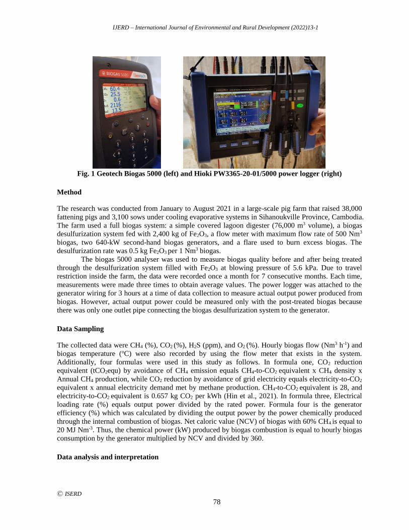
IJERD – International Journal of Environmental and Rural Development (2022)13-1
Ⓒ ISERD
78
Fig. 1 Geotech Biogas 5000 (left) and Hioki PW3365-20-01/5000 power logger (right)
Method
The research was conducted from January to August 2021 in a large-scale pig farm that raised 38,000
fattening pigs and 3,100 sows under cooling evaporative systems in Sihanoukville Province, Cambodia.
The farm used a full biogas system: a simple covered lagoon digester (76,000 m3 volume), a biogas
desulfurization system fed with 2,400 kg of Fe2O3, a flow meter with maximum flow rate of 500 Nm3
biogas, two 640-kW second-hand biogas generators, and a flare used to burn excess biogas. The
desulfurization rate was 0.5 kg Fe2O3 per 1 Nm3 biogas.
The biogas 5000 analyser was used to measure biogas quality before and after being treated
through the desulfurization system filled with Fe2O3 at blowing pressure of 5.6 kPa. Due to travel
restriction inside the farm, the data were recorded once a month for 7 consecutive months. Each time,
measurements were made three times to obtain average values. The power logger was attached to the
generator wiring for 3 hours at a time of data collection to measure actual output power produced from
biogas. However, actual output power could be measured only with the post-treated biogas because
there was only one outlet pipe connecting the biogas desulfurization system to the generator.
Data Sampling
The collected data were CH4 (%), CO2 (%), H2S (ppm), and O2 (%). Hourly biogas flow (Nm3 h-1) and
biogas temperature (oC) were also recorded by using the flow meter that exists in the system.
Additionally, four formulas were used in this study as follows. In formula one, CO2 reduction
equivalent (tCO2equ) by avoidance of CH4 emission equals CH4-to-CO2 equivalent x CH4 density x
Annual CH4 production, while CO2 reduction by avoidance of grid electricity equals electricity-to-CO2
equivalent x annual electricity demand met by methane production. CH4-to-CO2 equivalent is 28, and
electricity-to-CO2 equivalent is 0.657 kg CO2 per kWh (Hin et al., 2021). In formula three, Electrical
loading rate (%) equals output power divided by the rated power. Formula four is the generator
efficiency (%) which was calculated by dividing the output power by the power chemically produced
through the internal combustion of biogas. Net caloric value (NCV) of biogas with 60% CH4 is equal to
20 MJ Nm-3. Thus, the chemical power (kW) produced by biogas combustion is equal to hourly biogas
consumption by the generator multiplied by NCV and divided by 360.
Data analysis and interpretation
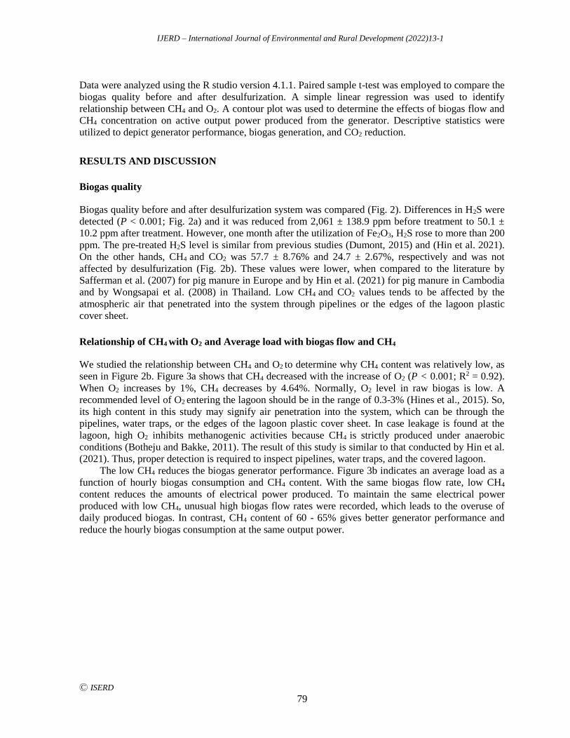
IJERD – International Journal of Environmental and Rural Development (2022)13-1
Ⓒ ISERD
79
Data were analyzed using the R studio version 4.1.1. Paired sample t-test was employed to compare the
biogas quality before and after desulfurization. A simple linear regression was used to identify
relationship between CH4 and O2. A contour plot was used to determine the effects of biogas flow and
CH4 concentration on active output power produced from the generator. Descriptive statistics were
utilized to depict generator performance, biogas generation, and CO2 reduction.
RESULTS AND DISCUSSION
Biogas quality
Biogas quality before and after desulfurization system was compared (Fig. 2). Differences in H2S were
detected (P < 0.001; Fig. 2a) and it was reduced from 2,061 ± 138.9 ppm before treatment to 50.1 ±
10.2 ppm after treatment. However, one month after the utilization of Fe2O3, H2S rose to more than 200
ppm. The pre-treated H2S level is similar from previous studies (Dumont, 2015) and (Hin et al. 2021).
On the other hands, CH4 and CO2 was 57.7 ± 8.76% and 24.7 ± 2.67%, respectively and was not
affected by desulfurization (Fig. 2b). These values were lower, when compared to the literature by
Safferman et al. (2007) for pig manure in Europe and by Hin et al. (2021) for pig manure in Cambodia
and by Wongsapai et al. (2008) in Thailand. Low CH4 and CO2 values tends to be affected by the
atmospheric air that penetrated into the system through pipelines or the edges of the lagoon plastic
cover sheet.
Relationship of CH4 with O2 and Average load with biogas flow and CH4
We studied the relationship between CH4 and O2 to determine why CH4 content was relatively low, as
seen in Figure 2b. Figure 3a shows that CH4 decreased with the increase of O2 (P < 0.001; R2 = 0.92).
When O2 increases by 1%, CH4 decreases by 4.64%. Normally, O2 level in raw biogas is low. A
recommended level of O2 entering the lagoon should be in the range of 0.3-3% (Hines et al., 2015). So,
its high content in this study may signify air penetration into the system, which can be through the
pipelines, water traps, or the edges of the lagoon plastic cover sheet. In case leakage is found at the
lagoon, high O2 inhibits methanogenic activities because CH4 is strictly produced under anaerobic
conditions (Botheju and Bakke, 2011). The result of this study is similar to that conducted by Hin et al.
(2021). Thus, proper detection is required to inspect pipelines, water traps, and the covered lagoon.
The low CH4 reduces the biogas generator performance. Figure 3b indicates an average load as a
function of hourly biogas consumption and CH4 content. With the same biogas flow rate, low CH4
content reduces the amounts of electrical power produced. To maintain the same electrical power
produced with low CH4, unusual high biogas flow rates were recorded, which leads to the overuse of
daily produced biogas. In contrast, CH4 content of 60 - 65% gives better generator performance and
reduce the hourly biogas consumption at the same output power.
IJERD – International Journal of Environmental and Rural Development (2022)13-1
Ⓒ ISERD
80
Fig. 2 Comparison of H2S (a) & CH4 and CO2 (b) before and after desulfurization (Mean ± SD; N
= 21). Paired sample t-test was used for the analysis. Different alphabetic letters denote
significant differences at the error level of 0.05, and NS means non-significance.
Fig. 3 Relationship between CH4 and O2 (a) & Determination of average load as a function of
biogas flow and CH4 (b)
Specific biogas characteristics for the generator operation
Fed into the generator, the biogas was pushed by an electrical blower at 5.6 ± 0.5 kPa. Its temperature
averaged 37.0 ± 5.1oC, rated best for biogas production (Babaei and Shayegan, 2020). Biogas system
produced 4,478 Nm3 day-1, but the actual daily biogas consumption was 4,862 ± 64.6 Nm3 day-1 (Table
2). Therefore, the amount of biogas consumption was 8.6% greater than the biogas production.
In Table 2, the generator was a 640-kW biogas generator, and actual electrical output power
produced from biogas was 368.5 ± 29.3 kW, so the loading rate of the generator was estimated at 57.6
± 4.6% of its full capacity. With the hourly biogas flow rate of 237.6 ± 29.6 Nm3 h-1, the theoretical
electrical power generated from biogas was estimated at 1365.9 ± 174.9 kW. Therefore, the generator
efficiency was 26.8 ± 1.7%, and it was higher than the study by De Souza et al. (2016) and Jeong et al.
(2009). The specific biogas consumption in this study was 0.64 ± 0.08 Nm3 kWh-1, which was lower
than that studied by (De Souza et al., 2016), whose finding was 0.76 m3 kWh-1.
IJERD – International Journal of Environmental and Rural Development (2022)13-1
Ⓒ ISERD
81
Table 1 Biogas production, electricity consumption, and CO2 reduction equivalent
Description Unit Mean ± SD
Biogas temperature oC 37.0 ± 5.1
Estimated daily biogas production Nm3 day-1 4,478
Recorded daily biogas consumption Nm3 day-1 4,862 ± 64.6
Biogas flow rate Nm3 h-1 237.6 ± 29.6
Actual generator power kW 640
Specific biogas consumption Nm3 kWh-1 0.64 ± 0.08
Actual output power kW 368.5 ± 29.3
Chemical power produced by biogas
combustion kW 1365.9 ± 174.9
Loading rate % 57.6 ± 4.6
Genset efficiency % 26.8 ± 1.7
CO2 reduction equivalent tCO2equ yr-1 22,818
CO2 reduction equivalent per head tCO2equ yr-1 head-1 0.56
CO2 Reduction Equivalent
Using the biogas system reduces the enormous amounts of CO2 and CH4 emissions. In this study, the
CO2 reduction equivalent was estimated at 22,818 tCO2equ yr-1, or 0.56 tCO2equ yr-1 head-1. CO2
reduction was lower than that studied by Hin et al. (2021). However, it was higher than Peerapong and
Limmeechokchai (2017), whose founding was 0.47 tCO2eq yr-1 head-1 and for Thai pig farms. The
difference in CO2 emission reduction tends to link with estimated daily manure production.
CONCLUSION
The use of desulfurization system greatly reduced H2S, but did not affect CH4 and CO2 contents.
Biogas quality was undermined by higher O2 levels in it. With low biogas quality, actual electrical
power produced from biogas was also low. However, considerable amounts of CO2 can be cut with this
biogas system. The limitations of this study are that the biogas generator performance could be
evaluated only with already treated biogas because it is the actual farm operation and altering the
system or reconnecting raw biogas pipes to the generator are very costly. Further research will improve
biogas quality with locally made desulfurization systems and prolong the age of iron oxide pellet use to
reduce labor and increase system operation efficiency.
ACKNOWLEDGEMENTS
The study was made possible thanks to the project “Reduction of Greenhouse Gas Emission through
Promotion of Commercial Biogas Plant in Cambodia” implemented by United Nations Industrial
Development Organization (UNIDO) that not only provided funding, but also continuously assisted in
strengthening the research team. Many thanks may also go to the farm owner that allowed for a long-
term experiment.
REFERENCES
Achinas, S., Achinas, V., and Euverink, G. J. W. 2017. A technological overview of biogas production from
biowaste, Engineering, 3: 299-307. http://dx.doi.org/10.1016/J.ENG.2017.03.002.
IJERD – International Journal of Environmental and Rural Development (2022)13-1
Ⓒ ISERD
82
Babaei, A. and Shayegan, J. 2020. Effects of temperature and mixing modes on the performance of municipal
solid waste anaerobic slurry digester. J Environ Health Sci Eng., 17(2): 1077–1084. doi: 10.1007/s40201-
019-00422-6.
Barbusiński, K. and Kalemba, K. 2016. Use of biological methods for removal of h2s from biogas in wastewater
treatment plants – a review. Architecture Civil Engineering Environment, 103-112.
Botheju, D. and Bakke, R. 2011. Oxygen effects in anaerobic digestion – a review. The Open Waste Management
Journal, 4: 1-19.
De Souza, S. N. M., Lenz, A. M., Werncke, I., Nogueira, C. E. C., Antonelli, J., and De Souza, J. 2016. Gas
emission and efficiency of an engine-generator set running on biogas. Journal of the Brazilian Association of
Agricultural Engineering, 1809-4430. Doi:http://dx.doi.org/10.1590/.
Dumont, A. 2015. H2S removal from biogas using bioreactors: a review. International Journal of Energy and
Environnement, International Energy & Environment Fondation, 6 (5), 479-498.
Hin, L., Than, B., Lor, L., Sorn, S., Then, D., Dok, C., Mech, S., Mean, C. M., Yut, S., Lay, M., and Frederiks, B.
2021. Assessment of biogas production potential from commerical pig farms in cambodia. International
Journal of Environmental and Rural Development, 12(1), 172-180. Hines, M. A., Choudhury, A., Felton, G., and Lansing, S. A. 2019. Micro-aeration for hydrogen Sulfide Removal
in Biogas. College Park, MD: University of Maryland Extension.
Intergovernmental Panel on Climate Change (IPCC). 2014. Anthropogenic and Natural Radiative Forcing,
Retrieved from https://www.ipcc.ch/site/assets/uploads/2018/02/WG1AR5_Chapter08_FINAL.pdf.
Jeong, C., Kim, T., Lee, K., Song, S., and Chun, K. M. 2009. Generating efficiency and emissions of a spark-
ignition gas engine generator fuelled with biogas–hydrogen blends. International Journal of Hydrogen
Energy, 34(23), 9620-9627.
Kulpredarat, N. 2016. The impact of pig wastewater to water environment in thailand. Bankork: Department of
Livestock Development, Thailand.
MAFF. 2019. MAFF Annual Report 2018-2019. Phnom Penh: Ministry of Agriculture, Forestry, and Fisheries.
National Biodiester Programme (NBP). 2019. Market Study on Medium-scale and Large-scale Biodigesters.
National Biodiester Programme, General Department of Animal Production and Health.
Okoro, O. V. and Sun, Z. 2019. Desulphurisation of biogas: a systematic qualitative and economic-based
quantitative review of alternative strategies. Chemengineering, 3, 76.
Peerapong, P. and Limmeechokchai, B. 2017. Biogas-based electricity generation in swine farm in thailand:
economic and co2 reduction aspects. Energy Procedia. Elsavier, 657 - 661.
Philippe, F. X. and Nicks, B. 2015. Review on greenhouse gas emissions from pig houses: Production of carbon
dioxide, methane and nitrous oxide by animals and manure. Agriculture, Ecosystems & Environment, 199,
10-25, https://doi.org/10.1016/j.agee.2014.08.015.
Quinton, A. 2019. Cows and Climate Change: Making Cattle More Sustainable.
Rahman, S. and Borhan, M. S. 2012. Typical odor mitigation technologies for swine production facilities - a
review. Civil & Environmental Engineering, 2(4).
Rodriguez, G., Dorado, N. D., Fortuny, M., Gabriel, D., and Gamisans, X. 2014. Biotrickling filters for biogas
sweetening: Oxygen transfer improvement for a reliable operation. Process Safety and Environmental
Protection, 92(3), 261-268.
Safferman, S., Safferman, A., Croskey, H., and Wandersee, W. 2007. Emerging issues in animal agriculture:
swine manure storage covers and economic tools to determine the payback period. Michigan State
University Extension.
Thanapongtharm, W., Linard, C., Chinson, P., Kasemsuwan, S., Visser, M., Gaughan, A. E., Epprech, M.,
Robinson, T. P., and Gilbert, M. 2018. Spatial analysis and characteristics of pig farming in thailand.
Thanapongtharm et al. BMC Veterinary Research, 12:218.
UNEP. 2021. Emissions Gap Report 2021: The Heat Is On – A World of Climate Promises Not Yet Delivered.
Nirobi: United Nations Environment Program.
Wongsapai, W., Thienburanathum, P., and Rerkkriengkrai, P. 2008. Biogas situation and development in thai
swine farm. DOI: 10.24084/repqj06.269
Zulkeflia, N. N., Masdar, M. S., Jahim, J., and Majlan, E. H. 2016. Overview of H2S removal technologies from
biogas production. International Journal of Applied Engineering Research , 11(20): 10060-10066.
IJERD – International Journal of Environmental and Rural Development (2022)13-1
Ⓒ ISERD
83
Migration Characteristics of Communities in the Forestlands
in Ifugao, Philippines
CARMELITO C. VALDEZ* College of Agriculture and Forestry,
Ifugao State University, Potia Campus, Philippines
Email: [email protected]
GEMMA B. DUMANSI Ifugao State University, Potia Campus, Philippines
Received 28 January 2022 Accepted 22 April 2022 (*Corresponding Author)
Abstract. The Ifugao province as a mountainous land of indigenous people, described as a
watershed framework that provides domestic and agricultural services. Greater portion of
the province was declared as Forestland. Due to increase in population, communities tend
to occupy and possess certain part of the forest to provide their basic needs.
Understanding the migration characteristics on the Forestlands in the province of Ifugao
may lead to a solution harmonizing the role of different stakeholders in maintaining the
biological, physical and social aspect of the upland for a sustainable development. The
study employed qualitative method of research and adopted the purposive sampling
technique, in data gathering wherein, respondents are certified migrant in the forestlands
of Ifugao province. It revealed that migration in the Forestlands in Ifugao province is being
influenced by many combined factors and being prompted by poverty and aggravated by
climate change. Socio-economic aspect is the primary reason why people tend occupy
portion of the Forestland. They acquire portions of the Forestland as a source of living as
they are engaged in farming as their main source of livelihood.
Keywords: Indigenous People, Resource Management, Land Use System
INTRODUCTION
Philippines is about 30 million hectares, half of which is classified as forestland, 47 percent is
classified as alienable and disposable land and the remaining three (3) percent is unclassified
forestlands. Alienable and disposable (A&D) lands refer to those areas which may be issued with
permanent title and/or used for varying purposes such as for residential, agricultural, commercial and
other uses. Of the country’s 14.19 million hectares of A & D lands, 9.63 million hectares are already
titled (DENR, 2017). On the other hand, Forestlands are lands belonging to the state and cannot be
alienated unless provided by law. Much of the Forestland are hilly and mountainous with slope of ≥
18 % hence are deemed not suitable for agricultural purposes as legally defined by the Revised
Forestry Code of 1975 (Esplana, M.R & A. Quizon, 2017).
Most of the Forestlands of the country are occupied by indigenous communities. The Philippines
is a culturally diverse country with an estimated 14-17 million indigenous people (IP’s) belonging to
110 ethno-linguistic groups, they are concentrated in Northern Luzon and Mindanao and some in
Visayas (De Vera, 2007 and UNDP, 2010). Indigenous Peoples/Indigenous Cultural Communities
(IP/ICC) refer to a group of people sharing common bonds of language, customs, traditions and other
distinctive cultural traits, and who have, under claims of ownership since time immemorial, occupied,
possessed and utilized a territory (IPRA Law). Thirty three percent (33 %) of the IP population is
erd
Research article
IJERD – International Journal of Environmental and Rural Development (2022)13-1
Ⓒ ISERD
84
located in the Cordillera Administrative region and sixty one percent (61 %) are living in the mountain
ranges of Mindanao (UNDP, 2010). As the population in the uplands continuously increasing, the
demand for a land to cultivate and for housing is becoming more important thus, the widespread
opening of forest for livelihood in the Philippines is pragmatic and natural resources become degraded.
The Cordillera Administrative Region (CAR) is composed of six provinces Abra, Apayao,
Benguet, Ifugao, Kalinga and Mountain Province. It is considered as the watershed cradle of the north
(UNDP, undated) and characterized as rugged, hilly and mountainous in topography. The region has a
total land area of approximately 1.8 million hectares. Almost 1.5 million hectares are classified as
forestlands and 0.3 million hectares is alienable and disposable lands (FMB-DENR, 2013). Cordillera
culture is characterized by its diversity. The major indigenous cultural communities who occupy the
Cordillera are the Ibaloy and southern Kankana-ey in Benguet Province, the Ifugaos of Ifugao Province,
the Bontok and northern Kankana-ey of Mountain Province, the Kalingas of Kalinga, the Isnag of
Apayao, and the Tingguian of Abra. There are numerous smaller distinct ethnic groups and subgroups
within these provinces, such as the Balangao, Kalanguya, and Karao. The groups vary in their political,
kinship, economic, and religious organizations (Mendoza, L. & J. Brett, 2004).
The Ifugao province in particular is a landlocked watershed province bounded by a mountain
range to the north and west that tempers into undulating hills towards the south and the east. The
highest elevation is 2,523 meters above sea level (masl) with the rice terraces lying above 500 masl.
Ifugao province is located at the southern portion of the Cordillera Administrative Region (CAR)
found at the heart of Luzon Island of the Philippines. It is home to the indigenous peoples who call
themselves “Ifugaos” and is host to one of the world-renowned rice terraces clusters that the UNESCO
World Heritage List of cultural and natural properties considered to be of “outstanding universal value.
In the land Classification of The Philippines 2013 as published by the Forest Management Bureau of
the Department of Environment and Natural Resources (FMB-DENR, 2013) Ifugao province has
approximately 251,778 hectares and 90 % (226, 369 has.) of which is declared as forestland only 10 %
(25,409 has.) is considered as Alienable and disposable lands (A & D). The province has growing
population and communities in the forestlands are tremendously increasing.
This study aimed to examine the migration characteristics and identify major drivers of
forestland occupation in the province of Ifugao, Philippines.
METHODOLOGY
Research Design
This study utilized qualitative research. Data where gathered through Focus Group Discussion (FGD)
to the Forestland migrants in Ifugao, Philippines. Moreover, the data were validated through a key
informant interviews (KII). Likewise, actual field visit was conducted to document current scenarios of
upland faming, resource management and practices in the area.
Sampling and Respondents
Purposive sampling technique was employed in this study. Identified Forestland migrants that
represents different sectors of the upland community were interviewed for this purpose, particularly
sectors coming from youth, Barangay officials, elders, upland famers, women’s group and technical
personnel from the Department of Environment and Natural Resources (DENR), and Department of
Agriculture (DA).
Use of Vignette in the study
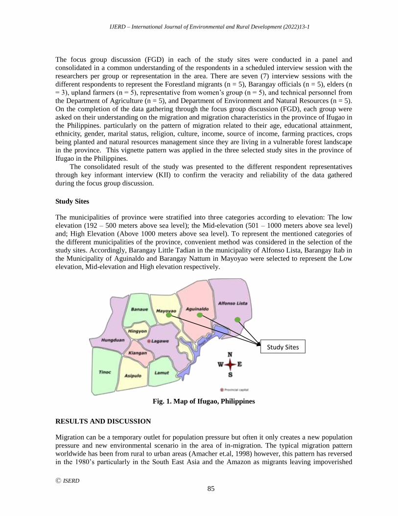
IJERD – International Journal of Environmental and Rural Development (2022)13-1
Ⓒ ISERD
85
The focus group discussion (FGD) in each of the study sites were conducted in a panel and
consolidated in a common understanding of the respondents in a scheduled interview session with the
researchers per group or representation in the area. There are seven (7) interview sessions with the
different respondents to represent the Forestland migrants (n = 5), Barangay officials (n = 5), elders (n
= 3), upland farmers (n = 5), representative from women’s group (n = 5), and technical personnel from
the Department of Agriculture (n = 5), and Department of Environment and Natural Resources (n = 5).
On the completion of the data gathering through the focus group discussion (FGD), each group were
asked on their understanding on the migration and migration characteristics in the province of Ifugao in
the Philippines. particularly on the pattern of migration related to their age, educational attainment,
ethnicity, gender, marital status, religion, culture, income, source of income, farming practices, crops
being planted and natural resources management since they are living in a vulnerable forest landscape
in the province. This vignette pattern was applied in the three selected study sites in the province of
Ifugao in the Philippines.
The consolidated result of the study was presented to the different respondent representatives
through key informant interview (KII) to confirm the veracity and reliability of the data gathered
during the focus group discussion.
Study Sites
The municipalities of province were stratified into three categories according to elevation: The low
elevation (192 – 500 meters above sea level); the Mid-elevation (501 – 1000 meters above sea level)
and; High Elevation (Above 1000 meters above sea level). To represent the mentioned categories of
the different municipalities of the province, convenient method was considered in the selection of the
study sites. Accordingly, Barangay Little Tadian in the municipality of Alfonso Lista, Barangay Itab in
the Municipality of Aguinaldo and Barangay Nattum in Mayoyao were selected to represent the Low
elevation, Mid-elevation and High elevation respectively.
Fig. 1. Map of Ifugao, Philippines
RESULTS AND DISCUSSION
Migration can be a temporary outlet for population pressure but often it only creates a new population
pressure and new environmental scenario in the area of in-migration. The typical migration pattern
worldwide has been from rural to urban areas (Amacher et.al, 1998) however, this pattern has reversed
in the 1980’s particularly in the South East Asia and the Amazon as migrants leaving impoverished
Study Sites
IJERD – International Journal of Environmental and Rural Development (2022)13-1
Ⓒ ISERD
86
cities to settle in sparsely inhabited upland and forest frontiers and Philippines is an example of this
situation (Amacher and Hyde, 1996).
Summary of the Vignette
The study focused on the migration characteristics of communities in the Forestlands in the province of
Ifugao in the Philippines. This study was participated by the different stakeholders of the forestland of
Ifugao in Philippines such as migrants, women’s group, elders, Barangay officials, technical personnel
from the DA and DENR respectively. As a result of the study, migration to the forestland in the
province of Ifugao in the Philippines confirmed three (3) major causes to include cultural, demographic
and socio-economic factors that is consistent with the findings of Li et.al (2014) consequently, there
are factors affecting migration intensions in an ecological area such as demographic factors, socio-
economic factors and other factors (political-economic factors and eco-environmental factors).
The three (3) Major Causes of Migration in the Forestlands in Ifugao, Philippines
A. Cultural Factor
Majority of the Forestland settlers in Ifugao in the Philippines belongs to the Indigenous People
(IP) of the province, some are coming from the neighboring provinces of Nueva Vizcaya, Isabela, and
Mountain Province. Indigenous people in Ifugao has a natural connection to forest resources because it
is their nature to engage in hunting wild animals for food, and sustainable forestry as they acquire
lumber for domestic purposes in their woodlots (Muyong). They also extract wild honey for their
personal consumption and some are for sale as they augment their income. More importantly, it is their
culture to seek for a fertile land for agriculture production or technically known as kaingin.
B. Demographic Factors
Demographic factors are the general indication of a group in the general population in the forestland in
the province of Ifugao such as age, gender, marital status and religion.
Accordingly, migration to the forestlands in the province by the community happens usually
during the young to middle adult ages from 18-38 years old because during this stage individuals are
active explorer, traveler and adventurous as they seek job, belongingness, enjoy the value of nature,
and in the search of partner in life. In addition, people would like to settle in a place wherein they are
going to construct their own houses, established sustainable source of living, invest time and properties
in an area, and this is usually happening in the young adult stage. Consistent with the argument of Abu,
et.al. (2014) that during older age, people may not migrate because their attachment to their community
tends to be stronger than that of younger age. On the other hand, male have higher incidence of
migration in the Forestlands in Ifugao, Philippines because they are usually the once engaged in the
search of livelihood for the family including acquisition of land to be tilled, hunt for wild animals,
harvest wild plants and fruits. Moreover, establishment and settlement in an area is a role of males in
the upland particularly in the province of Ifugao in the Philippines.
Majority of the respondent in the different locations in accordance to the criteria set in this study
pointed that families occupy portion of the forestland in the province of Ifugao with their relatives and
establish a community in the area. Communities in the Forestlands of Ifugao is composed of different
spiritual sectorial belief such as Pentecostal, Roman Catholic, Evangelical, and Baptist Ministry.
Accordingly, their religious belief binds them together and guide them for a peaceful and happy well-
being. The significance of Religion to the migration characteristics of communities is relevant to the
interpretation of Hirschman (2004) that relatives and distant individuals move towards an area of
worship and religious networks of similar belief, supported by the idea of Portes and Rumbaut (2006)
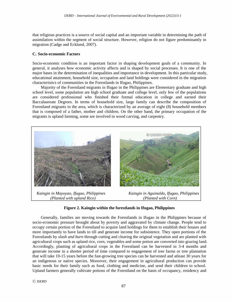
IJERD – International Journal of Environmental and Rural Development (2022)13-1
Ⓒ ISERD
87
that religious practices is a source of social capital and an important variable in determining the path of
assimilation within the segment of social structure. However, religion do not figure predominantly in
migration (Cadge and Ecklund, 2007).
C. Socio-economic Factors
Socio-economic condition is an important factor in shaping development goals of a community. In
general, it analyses how economic activity affects and is shaped by social processes. It is one of the
major bases in the determination of inequalities and importance in development. In this particular study,
educational attainment, household size, occupation and land holdings were considered in the migration
characteristics of communities in the Forestlands in Ifugao, Philippines.
Majority of the Forestland migrants in Ifugao in the Philippines are Elementary graduate and high
school level, some population are high school graduate and college level, only few of the populations
are considered professional who finished their formal education in college and earned their
Baccalaureate Degrees. In terms of household size, large family can describe the composition of
Forestland migrants in the area, which is characterized by an average of eight (8) household members
that is composed of a father, mother and children. On the other hand, the primary occupation of the
migrants is upland farming, some are involved in wood carving, and carpentry.
Kaingin in Mayoyao, Ifugao, Philippines Kaingin in Aguinaldo, Ifugao, Philippines
(Planted with upland Rice) (Planted with Corn)
Figure 2. Kaingin within the forestlands in Ifugao, Philippines
Generally, families are moving towards the Forestlands in Ifugao in the Philippines because of
socio-economic pressure brought about by poverty and aggravated by climate change. People tend to
occupy certain portion of the Forestland to acquire land holdings for them to establish their houses and
more importantly to have lands to till and generate income for subsistence. They open portions of the
Forestlands by slash and burn through cutting and clearing the original vegetation and are planted with
agricultural crops such as upland rice, corn, vegetables and some potion are converted into grazing land.
Accordingly, planting of agricultural crops in the Forestland can be harvested in 3-4 months and
generate income in a shorter period of time compared to engagement of tree farms or tree plantation
that will take 10-15 years before the fast-growing tree species can be harvested and atleast 30 years for
an indigenous or native species. Moreover, their engagement in agricultural production can provide
basic needs for their family such as food, clothing and medicine, and send their children to school.
Upland farmers generally cultivate potions of the Forestland on the basis of occupancy, residency and
IJERD – International Journal of Environmental and Rural Development (2022)13-1
Ⓒ ISERD
88
agricultural engagement in the area. In the absence of any tenure instrument, their cultural rights as the
original tenant over the land is being respected by the community.
The trend of migration to the Forestland in the Ifugao in the Philippines is increasing,
communities are already in place and agricultural production areas are becoming dominant in the area.
The increasing number of populations in the Forestland were observed to have negative impact on the
natural agro-ecological system in the area. As a result of agricultural production in the moderate to
steep slopes areas in the Forestland, there is a significant increase in soil erosion, and siltation in the
water ways. Biodiversity of flora and fauna also are affected since the crops being grown by the
communities are not indigenous particularly the vegetables, and corn that are cultured for a medium to
large scale production. Moreover, the introduction of chemicals in the maintenance of their farms
particularly herbicides, and insecticides brought damages to both micro and macrobiotic diversity of
the area.
CONCLUSION
The migration characteristics of communities in the Forestlands in Ifugao in the Philippines is
characterized by a dynamic and complex cultural, demographic, and socio-economic factor. Nowadays,
the continuous increase in the population in the Forestland is brought about by poverty that cause
families to occupy, posses, and utilize portion of the Forestland for agricultural production for
subsistence and provision of basic needs by the people.
ACKNOWLEDGEMENTS
The authors extend grateful thanks to the Ifugao State University-Research, Development, Extension
and Training (RDET) Department for the funding and continuous support to research endeavors of
faculty members of the institution.
REFERENCES
Abu, M., S. Codjoe & J. Sward. 2014. Climate change and internal migration intentions in the forest-savannah
transition zone of Ghana. Popul. Environ. Vol. 35, 341–364. Retrieved from
https://www.researchgate.net/profile/Mumuni-
Abu/publication/271919675_Climate_change_and_internal_migration_intentions_in_the_forest-
savannah_transition_zone_of_Ghana/links/56447f1d08ae54697fb799a0/Climate-change-and-internal-
migration-intentions-in-the-forest-savannah-transition-zone-of-Ghana.pdf?origin=publication_detail
Amacher, G.S., W. Cruz, D. Grebner & W. F. Hyde. 1998. Land Economics. Vol. 74, No. 1, 92-101
Cadge, W. and Ecklund, E. H. 2007. Immigration and Religion. Annual Review of Sociology. 33:359–379.
Retrieved from https://www.annualreviews.org/doi/pdf/10.1146/annurev.soc.33.040406.131707
De Vera, David. 2007. Indigenous people s in the Philippines: A case study. Presented at the RNIP Regional
assembly in Hanoi, Vietnam. August 20-26, 2007. Retrieved from http://www.iapad.org/wp-
content/uploads/2015/07/devera_ip_phl.pdf
DENR. 2017. Land Resources. Department of Environment and Natural Resources website. Retrieved from
https://www.denr.gov.ph/news-and-features/latest-news/55-land-resources.html
Esplana, M.R & A. Quizon. 2017. Status of reform tenure in the public lands under the comprehensive agrarian
reform program. Asian NGO Coalition for Agrarian Reform and Rural Development. Retrieved from
https://ilc-nes.ph/wp-content/uploads/2017/07/Tenure-Reform-in-Public-Lands-under-CARP_Final_24-
March-2017.pdf
FMB-DENR. 2013. The Philippine Forest Facts and Figures. Department of Environment and Natural Resources.
Quezon City. Philippines. Retrieved from http://forestry.denr.gov.ph/pdf/ref/PF3_2013.pdf
https://aboutphilippines.ph/files/Communal-Land-Management-in-the-Cordillera-Region-chap02.pdf
IJERD – International Journal of Environmental and Rural Development (2022)13-1
Ⓒ ISERD
89
Hirschman, Charles. 2004. The Role of Religion in the Origins and Adaptation of Immigrant Groups in the
United States. International Migration Review. 28:1206–34. Retrieved from
https://journals.sagepub.com/doi/10.1111/j.1747-7379.2004.tb00233.x
IPRA Law. The indigenous peoples rights act of 1997. Retrieved from
http://extwprlegs1.fao.org/docs/pdf/phi13930.pdf
Li, Yongjin & Lopez-Carr, David & Chen, Wenjiang. 2014. Factors Affecting Migration Intentions in Ecological
Restoration Areas and Their Implications for the Sustainability of Ecological Migration Policy in Arid
Northwest China. Sustainability. 6. 8639-8660. 10.3390/su6128639. Retrieved from https://mdpi-
res.com/d_attachment/sustainability/sustainability-06-08639/article_deploy/sustainability-06-
08639.pdf?version=1424779143
Mendoza, L. & J. Brett. 2004. Land and Cultural Survival: The Communal Rights of indigenous people in Asia.
Communal Land Management in the Cordillera Administrative Region of the Philippines. Retrieved from
https://www.adb.org/sites/default/files/publication/27980/land-cultural-survival.pdf
Portes, A, & Rumbaut, R. B. 2006. Immigrant America: A Portrait. 2nd. Berkeley: University California Press.
United Nations Development Program. 2010. Indigenous peoples in the Philippines. Retrieved from
https://www1.undp.org/content/dam/philippines/docs/Governance/fastFacts6%20-
%20Indigenous%20Peoples%20in%20the%20Philippines%20rev%201.5.pdf
IJERD – International Journal of Environmental and Rural Development (2022)13-1
Ⓒ ISERD
90
Discussion about A Model in Operation and Accumulation of
Joint-Use Fund Management by Rice Farmer-groups
YUKI TOYAMA United Graduate School of Agricultural Sciences, Tottori University, Tottori City, Japan
Email: [email protected]
ASRES ELIAS Faculty of Agriculture, Tottori University, Tottori City, Japan
KUMI YASUNOBU Faculty of Agriculture, Tottori University, Tottori City, Japan
PANATDA UTARANAKORN Faculty of Agriculture, Khon Kaen University, Khon Kaen District, Thailand
Received 30 January 2022 Accepted 22 April 2022 (*Corresponding Author)
Abstract Substantial number of rice farmer-groups are established under the promotion of
group farming policies in Thailand. The groups voluntarily form joint-use funds and operate
their business with them. The objective of this study is to make the model of joint-use fund
management by rice farmer-groups with two approaches: 1) observing the characteristics of
successful cases in the rice farmer-groups established by two policies in Northeastern Thailand;
and 2) simulating a fund management on the groups based on one case group in Khon Kaen
province. The case groups established funds using the resources provided by the government.
Through operating the group’s business, members invest in-cash or in-kind input and pay the
service charges into the fund. Then the accumulated capital was used for providing returns to
members’ investments and scaling-up the groups’ business. Based on actual accounting data of
one case group, we simulated revolving joint-use fund by rice farmer-group. The result showed
that the group assumed to accumulate enough amount of assets to provide sufficient service for
all members using the initial fund derived from government support. A conceptual model of
joint-use fund management for the rice farmers group was described. The model will be utilized
to guide rice farmer-groups in developing their business and becoming independent from
government support.
Keywords Group farming, Community, Government support, Northeastern Thailand
INTRODUCTION
Small and family-run farms are evaluated as important agents to achieve a stable and sustainable food
supply (FAO and IFAD, 2019; FAO, 2014). Generally, in the area where small family farms are
dominant, most farmers face challenges to scale-up their business because of land fragmentation and
lack of production resources (HLPE, 2013). On the other hand, group farming is one of the major
means to improve the productivity of small family farms facing resource constraints. It helps to achieve
economies of scale and respond to the external environment. For instance, East Asian countries (e.g.
Japan and South Korea) achieved a dramatic improvement in agricultural productivity through
spreading group farming (Wong, 1977).
In Thailand, the government adopted group farming concept into agricultural development
policies and established many farmer-groups, especially related to rice production. Some studies
erd
Research article
IJERD – International Journal of Environmental and Rural Development (2022)13-1
Ⓒ ISERD
91
mentioned that the rice farmer-groups received in-cash and in-kind resource supports from government
and operated their business through managing and utilizing joint-use funds (Ohara et al., 2021; Tanaka
and Yasunobu, 2019). It is also indicated that a substantial number of groups stopped their operation in
the early years because of the difficulty to continue their business (Uchook, 2018). At present, the
joint-use funds are voluntarily operated by members of the groups. However, to the best of our
knowledge, there is no manual and/or guideline regarding how such kind of activities have been
implemented. Therefore, to suggest a model of handling joint-use fund is supposed to be benefitable
for encouraging farmer-groups to continue/expand their business.
OBJECTIVE
We consider a model of joint-use fund management by rice farmer-groups in Thailand through
achieving the following objectives: 1) To investigate the characteristics of joint-use fund management
among the groups which continuously accumulate the fund; 2) To simulate the cycle of accumulating
joint-use fund and scaling-up the business; and 3) To conceptualize joint-use fund management for
depicting a model based on the above results.
METHODOLOGY
To achieve the objectives of this study, we adopted the following approaches. First, we explored the
actual situation of how rice farmer-groups manage their own business and joint-use fund, with the
cases of rice farmer-groups established by the encouragement of policies. Then, we conducted the
simulation of revolving joint-use fund based on one case which conducted the lending business of
combine harvester and kept its account record, and finally, the conceptual model was induced from the
results.
Survey Site Selection
In this study, we selected cases of rice farmer-groups located in Khon Kaen and Ubon Ratchathani
provinces in, the Northeastern region. The groups were established under the promotion of two
political programs: Community Rice Seed Center (CRSC) and Large Land Plot of Rice (LLPR),
proceeded by the Ministry of Agriculture and Cooperatives (MOAC), Thailand.
Fig. 1 Changes in the distribution of rice production scale among farmers in Thailand Source: Author’s creation with the data opened at the website of Office of Agricultural Economics, Ministry of Agriculture
and Cooperatives, Thailand [https://www.oae.go.th].
Remark) 1 rai = 0.16 ha.
41.3
IJERD – International Journal of Environmental and Rural Development (2022)13-1
Ⓒ ISERD
92
To consider modeling of joint-use fund management, the domain (area and crop) which needs the
model is suitable for the target in this study. In Thailand, Northeastern region and Central region are
the main production areas of rice. The production scale of rice on each farm in Northeastern region is
smaller than Central region and group farming policies aiming at small-scale rice farmers are mainly
extended in Northeastern region. Moreover, in Northeastern region, the ratio of large-scale farmers is
decreasing in total number of rice producers. Fig. 1 shows the changes in production scale of rice
among farmers from 2008 to 2018. At the national level, the ratio of farms operating more than 20 rai
(= 3.2 ha, 1 rai = 0.16 ha) decreased from 29.2 % to 20.0 % and this tendency was especially clear in
Northeastern region; the decrement on the ratio of farms operating more than 20 rai in each region is as
follows: whole country, -31 %; Central, -16 %; Northeast, -44 %. From the above, the model proposed
by this study will be mainly applied to the field in Northeastern Thailand and it is reasonable to adopt
rice farmer-group located in Northeastern Thailand as the cases.
Sampling and Data Collection
Various policies related to group farming have been introduced in Thailand. This study aimed the
groups established under two policies targeting rice farmers: Community Rice Seed Center (CRSC)
and Large Land Plot of Rice (LLPR).
CRSCs have been established since the beginning of 2000s (1,650 CRSCs was existed in
2016/2017) as a local supplier of rice seed (Orachos, 2018). To cope with the shortage of rice seed
certified the quality, Thai government tried to realize the self-supply of rice seed in each rural
communities through establishing the groups of rice farmers for engaging the multiplication of
certified rice seed provided by the government institutions (Moonfoui et al., 2007). LLPRs are also rice
farmer-group targeting to perform the economics of scale on rice production in Thailand. The program
was started from 2016 and 3,759 plots were established until March 2022, and about 60% of them were
in Northeastern region (DOAE, 2022). The activities of LLPRs are jointly procurement and use of
capital, equipment, and materials (e.g., machinery, miller, storage, rice seed, group fund), joint
shipment to the contracted miller and produce GAP certified rice or rice seed. Both two policies are
promoted by the Rice Department, the Ministry of Agriculture and Cooperatives, and certain number
of LLPRs are established based on existing CRSCs.
Surveyed groups were 34 CRSCs (Ubon Ratchathani: 21 in 90 groups, Khon Kaen: 13 in 92
groups), and 4 LLPRs in 48 groups in Khon Kaen province. All groups were sampled randomly.
Regarding the case CRSCs, the data was originally used in Tanaka and Yasunobu (2019). Face-to-face
interview was conducted for group leaders with structured questionnaire in August and September
2015. The data of case LLPRs included both of which deriving from Ohara et. al. (2021) and which
was collected by authors. On our survey, group interview to a few members including leader was
conducted regarding how to manage joint-use fund in August 2018 and July 2019.
RESULTS AND DISCUSSION
Exploring Actual Situation of Joint-Use Funds Management among CRSCs and LLPRs
Table 1 shows how CRSCs accumulated their joint-use funds. All groups accumulating more than
100,000 THB (1 Thai Baht (THB) = 0.031 US$, average in 2021) managed their funds more than 10
years. The larger funds have the tendency that the average amount of fund per member is larger. The
groups which accumulate and enlarge the funds continuously supposed to succuss increasing the
amount of resource which each member can use.
IJERD – International Journal of Environmental and Rural Development (2022)13-1
Ⓒ ISERD
93
Table 1 Accumulation of joint-use funds among CRSCs
Accumulation class
of joint-use fund
Frequency
(N = 19*2)
Average
number of
members
Average term of
accumulating
fund
Average
amount of fund
Average amount of
fund per member
(unit: THB*1)
(unit: years) (unit: THB) (unit: THB/member)
~99,999 5 31.0 05.6 049,547 1,411
100,000~149,999 4 35.5 14.5 130,000 4,040
150,000~199,999 6 41.0 13.2 166,417 5,170
200,000~ 4 42.0 13.8 282,413 7,859
Source: Reorganized by author with the data treated by Tanaka and Yasunobu (2019).
Remarks) *1: THB is an abbreviation of Thai Baht (1 THB = 0.031 US$, average in 2021).
*2: Excluded 8 groups which did not answered amount of fund from 34 surveyed groups.
Table 2 Activities for input and use of joint-use funds among CRSCs (N=27)
Input to fund Frequency Use of fund Frequency
In kind return of rice seed with interest 18 Loan service 18
Share sales 8 Purchasing materials 13
Membership fee 7 Purchasing seeds from members 12
Resales of provided materials 4 Investment for machinery and facility 8
Machinery use charge 4
Source: Reorganized by author with the data treated by Tanaka and Yasunobu (2019).
Remarks) Using the data of 27 groups, excluding 7 groups which did not have joint-use fund from 34 surveyed groups.
The activities for accumulating and using joint-use fund among the case groups are itemized in
Table 2. All case groups received certain amount of free rice seed as government support. Eighteen
groups divided the seed to members and then members return for the dividend in kind with interest
after harvesting. Apart from that, some groups collected membership fee or sold shares to members.
The groups having machinery provided lending service for members. Regarding use of the funds, the
most major use of join-use fund was loan service for supporting members’ livelihood. Other ways of
using the fund were joint procurement of materials, investment for expanding equipment, and
compensation of rice seed sales for members.
On the other hand, in the cases of LLPRs, main income sources were revenue of machinery
lending and investment from members through selling share (Table 3). In terms of the share system, 3
of 4 case groups sold group's share to members. The shareholders could get dividend depending on the
amount of group’s revenue and the number of possessed shares. All case groups provided members
with a lending service of machinery leased by the government. The price of lending charge was lower
than the charge of private contractors in the area. In case non-members rent the machinery, the charge
was higher than the price for members. However, the groups rarely lend machinery to non-members
because they did not possess enough number of machines to provide service for all members. To
prepare enough amount of machinery and equipment, and provide services without competition, groups
need to revolve their initial fund deriving from government support and to accumulate joint-use fund
for capital investment. In contrast to CRSCs, no LLPRs provided loan service to members. Since
LLPRs have operated for a few years, they did not have enough amount of fund to launch financial
business.
IJERD – International Journal of Environmental and Rural Development (2022)13-1
Ⓒ ISERD
94
Table 3 Accumulation and use of joint-use funds among LLPRs
Group A Group B Group C Group D
Number of members 200 67 204 52
Govt. support
Free lending of machinery
1 trailer 2 harvesters
1 tractor 1 harvester 1 trailer 1 drill seeder
1 drill seeder 1 harvester
4 drill seeders
Provision of rice seeds
(2016~2019)
KDML105*1: 15 t RD6*1: 8.6 t
KDML105: 13 t RD6: 2 t
KDML105: 2.25 t RD6: 15 t
KDML105: 30 t RD6: 150 t
Input to fund Share sales Rice sales
Machine use charge
Share sales Rice sales
Machine use charge
Share sales Rice sales
Machine use charge
Seed sales
Machine use charge
Use of fund
Running cost*2 Dividend of share Reward of committee
Running cost Dividend of share Reward of committee
Running cost Dividend of share Reward of committee Community welfare
Running cost
Reward of committee Machinery purchase*3
Source: Reorganized by author with the results of Ohara et al. (2021) and the survey in 2018 and 2019.
Remarks) *1: KDML105 and RD6 are the name of rice variety. KDML105 is non-glutinous variety, and the variety is labeled
“Jasmin rice” in market. RD6 is glutinous variety which is popularly eaten in Northeastern Thailand.
*2: “Running cost” include maintenance of machinery, petrol, wedge for driver and miscellaneous expenses.
*3: Group D purchased 9 drill seeders with their own fund in 2017.
Simulation of Revolving Joint-Use Fund on Lending Combine Harvesters
We simulated revolving joint-use fund with the experience of lending combine harvester in one LLPR
case (group A) and showed the path to accumulate joint-use resource enough to provide services for all
members. The reasons why we choose LLPR as the case of this simulation include: LLPRs focus on
joint-use of production resources, but CRSCs’ main purpose is self-supply of rice seeds and LLPR
program was started later than CRSC, we could collect the detailed information about initiation of
revolving joint-use fund. The information was useful for simulating from the point of receiving
subsidies. Among four cases of LLPRs, we could get detailed account data just from group A; in the
cases of group B, C and D, we could not collect it because of missing some important records of
bookkeeping.
As shown in Table 4, group A had 200 members and 1,000 rai registered paddy field (5 rai for
each member). Each combine harvester assumed to roll 200 rai in one fiscal year and the cost of
purchasing one combine harvester was set 250,000 THB. If the fund accumulated more than 250,000
THB, the group shall purchase an additional combine harvester. The goal of this simulation is to
prepare the number of combine harvesters which is enough to harvest on all registered paddies. Based
on the above assumptions, the group can independently continue its function after the withdrawal of
government supports. The group purchased combine harvester and expanded its business from third
fiscal year. When the number of combine harvester reach to five, the group achieved to prepare enough
number of combine harvesters for providing all members with a lending service.

IJERD – International Journal of Environmental and Rural Development (2022)13-1
Ⓒ ISERD
95
Table 4 Simulation of revolving joint-use fund based on the case of group A
Items (Unit from (1) to (8): THB*1) 1st year*2 2nd year 3rd year 4th year 5th year
Number of operated combine harvesters 2 2 3 4 5 Harvested paddy area by group’s combine harvester*3 Unit: rai (% in 1,000 rai*1 = total registered area)
400 (40%)
400 (40%)
600 (60%)
800 (80%)
1,000 (100%)
(1) Total income 324,550 284,550 386,825 489,100 611,375 Rice sales*4 60,000 40,000 20,000 0 0 Investment from member 20,000 0 0 0 0
Revenue of lending combine harvester*5 244,550 244,550 366,825 489,100 611,375
(2) Total cost 96,728 96,728 133,516 170,305 207,094 Running cost for lending combine harvester*5 73,577 73,577 110,365 147,154 183,943
Reward for committee members 15,400 15,400 15,400 15,400 15,400
Meeting 5,193 5,193 5,193 5,193 5,193
Miscellaneous expenses 2,558 2,558 2,558 2,558 2,558
(3) Dividend for shareholders*6 29,400 29,400 46,662 63,759 80,856 (4) Benefit: (1) – (2) – (3) 198,422 158,422 206,647 255,036 323,425 (5) Amount of fund at the beginning of FY 0 198,422 106,844 63,491 68,527 (6) Amount of fund at the end of operation: (4) + (5) 198,422 356,844 313,491 318,527 391,952 (7) Cost for purchasing combine harvester 0 250,000 250,000 250,000 0 (8) Balance of fund at the end of FY*7: (6) - (7) 198,422 106,844 63,491 68,527 391,952
Source: Reorganized by author with the results of the survey in 2018 and 2019.
Remarks) *1: 1 THB = 0.031 US$ (average in 2021). 1 rai = 0.16 ha.
*2: 1st year’s data is based on the actual account information of group A in 2017/18. The cost-benefit data from 2nd to 5th year
is estimated based on the data of 1st year.
*3: On the simulation, volatility of harvested area caused by disasters or/and crop failures is not considered. Average area of
each registered plot is 5 rai and most of them are a part of each member’s operated paddy. In case member’s total
harvested area is diminished because of disasters or/and crop failures, The area rolled by group’s combine harvesters is
supposed not to be affected since members can use the harvesters for their paddy plots other than registered one.
*4: The government provide LLPRs rice seed for 3 years and the amount is gradually decrease. On the simulation, it is
assumed that the group gets rice for sale from members as the return for providing rice seed provided by the government.
Therefore, the amount of “Rice sales” gradually decreases from 1st to 3rd year and does not account from 4th year.
*5: Regarding “Revenue of lending combine harvester” and “Running cost for lending combine harvester”, the amount is
assumed to change proportionately to “Harvester paddy area by group’s combine harvester” based on the 1st year’s data.
The value rates are as follows; “Revenue of lending combine harvester”: 611 THB/rai, and “Running cost for lending
combine harvester”: 183 THB/rai (including petrol cost, wage for operator, insurance, and maintenance fee). Both of
values were actual data of group A in 2017/18.
*6: “Dividend for shareholders” is estimated based on the following calculation. When the group established, all members
purchased 1 share (100 THB / share) and they receive dividend form the group’s revenue equally. The amount of dividend
was 20 % of the balance between “Revenue of lending combine harvester” and “Total cost” = (2).
*7: “Balance of fund at the end of FY” = (8) is entirely carried forward as “Amount of und at the beginning of FY” = (5).
Conceptual model of Joint-Use Fund Management in Rice Farmers-group
Based on the observation of actual cases and the simulation of revolving joint-use fund, we induced a
conceptual model of joint-use fund accumulation by rice farmer-group (Fig. 2).
This model was formed on the precondition which farmer-group receive an initial provision of
goods (e.g., free lease of machinery, rice seed, fertilizer) from the government. Group members bring
in-cash and in-kind inputs as investments (share purchase or membership fee) and charge of services
(machinery charge or in-kind return for seed provision). Accumulated capital on the fund is used for
providing returns to members (lending machinery, joint procurement of rice seed, dividend for
members who hold shares).Through this input-use cycle, the group keeps enlarging their fund even
after finishing the 3 years provision of materials from the government and success to accumulate
enough amount of fund (including cash and fixed assets) to provide sufficient returns for all members.
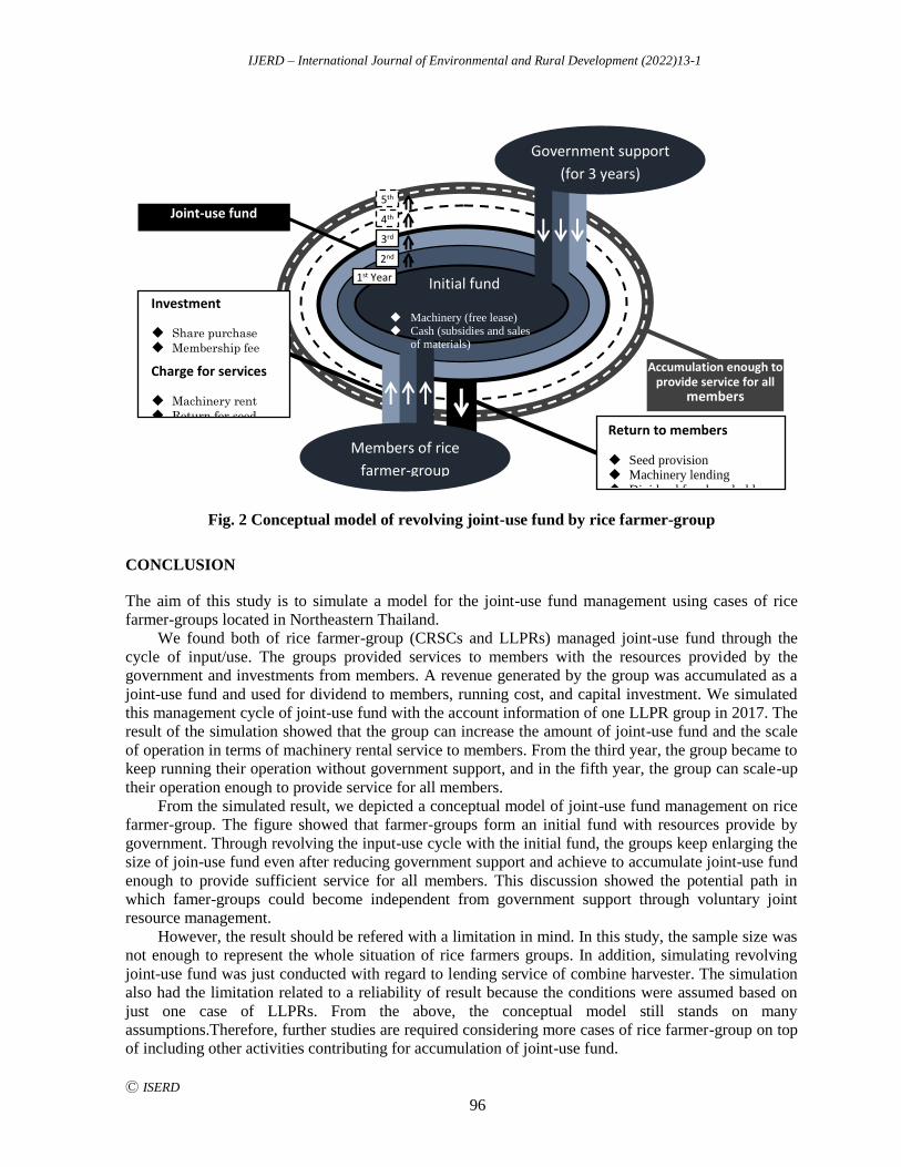
IJERD – International Journal of Environmental and Rural Development (2022)13-1
Ⓒ ISERD
96
Fig. 2 Conceptual model of revolving joint-use fund by rice farmer-group
CONCLUSION
The aim of this study is to simulate a model for the joint-use fund management using cases of rice
farmer-groups located in Northeastern Thailand.
We found both of rice farmer-group (CRSCs and LLPRs) managed joint-use fund through the
cycle of input/use. The groups provided services to members with the resources provided by the
government and investments from members. A revenue generated by the group was accumulated as a
joint-use fund and used for dividend to members, running cost, and capital investment. We simulated
this management cycle of joint-use fund with the account information of one LLPR group in 2017. The
result of the simulation showed that the group can increase the amount of joint-use fund and the scale
of operation in terms of machinery rental service to members. From the third year, the group became to
keep running their operation without government support, and in the fifth year, the group can scale-up
their operation enough to provide service for all members.
From the simulated result, we depicted a conceptual model of joint-use fund management on rice
farmer-group. The figure showed that farmer-groups form an initial fund with resources provide by
government. Through revolving the input-use cycle with the initial fund, the groups keep enlarging the
size of join-use fund even after reducing government support and achieve to accumulate joint-use fund
enough to provide sufficient service for all members. This discussion showed the potential path in
which famer-groups could become independent from government support through voluntary joint
resource management.
However, the result should be refered with a limitation in mind. In this study, the sample size was
not enough to represent the whole situation of rice farmers groups. In addition, simulating revolving
joint-use fund was just conducted with regard to lending service of combine harvester. The simulation
also had the limitation related to a reliability of result because the conditions were assumed based on
just one case of LLPRs. From the above, the conceptual model still stands on many
assumptions.Therefore, further studies are required considering more cases of rice farmer-group on top
of including other activities contributing for accumulation of joint-use fund.
Investment
Share purchase Membership fee
Charge for services
Machinery rent
Return for seed
provision in kind
Joint-use fund
Accumulation enough to provide service for all
members
2nd
3rd
4th
5th
Initial fund
Machinery (free lease) Cash (subsidies and sales
of materials)
Government support
(for 3 years)
Members of rice
farmer-group
Return to members
Seed provision Machinery lending Dividend for share holders
1st Year
IJERD – International Journal of Environmental and Rural Development (2022)13-1
Ⓒ ISERD
97
ACKNOWLEDGEMENT
This research was supported by the Nippon Agricultural Research Institution and JSPS KAKEN Grant
Number JP17H01490.
REFERENCES
Department of Agricultural Extension (DOAE). 2022. Large scale agricultural promotion system, Ministry of
Agriculture and Cooperatives (MOAC), Thailand, Retrieved from https://co-farm.doae.go.th/graph/
Dashboard1dsb
Food and Agriculture Organization (FAO) and International Fund for Agricultural Development (IFAD). 2019.
United nations decade of family farming 2019-2028, Global Action Plan, Rome, Italy, Retrieved from
https://www.fao.org/3/ca4672en/ca4672en
Food and Agriculture Organization (FAO). 2014. The state of food and agriculture report, Innovation in family
farming, Rome, Italy, Retrieved from https://www.fao.org/publications/sofa/2014/en/
Hight Level Panel of Experts (HLPE). 2013. Investing in smallholder agriculture for food and nutrition security:
A report by the high level panel of experts on food security and nutrition, World Food Security, Rome, Italy,
HLPE report 6, Retrieved from https://www.fao.org/3/i2953e/i2953e
Lipton, M. 2005. The family farm in a globalizing world: The role of crop science in alleviating poverty, 2020
Discussion Paper 40, International Food and Policy Research Institution , Washington, D.C., USA, Retrieved
from https://michaellipton.files.wordpress.com/2012/02/thefamilyfarm2005
Moonfoui, J., Radanachaless, T., Gypmantasiri, P. and Utumpan, R. 2007. Potentials of community rice seed
centers in developing towards self-reliance in seed: A case study in Phayao province, Journal of Agriculture,
23(2), 155-164. Retrieved from https://mis.agri.cmu.ac.th/download/publication/2927
Ohara, M., Yasunobu, K., Elias, A., Poungchompu, S. 2021. The effect of large-scale farming policy on rice farm
management in Thailand: A viewpoint of production technology and agricultural gross income (in Japanese),
Journal of Agricultural Development Studies, 31(3), 38-42, ISSN 0918-9432, Japan.
Orachos, N. 2018. Rice seed system in Thailand, Agricultural and Rural Economics Working Paper, Department
of Agricultural and Resource Economics, Faculty of Economics, Kasetsart University, Thailand, Retrieved
from https://ageconsearch.umn.edu/record/284028?ln=en
Tanaka, J. and Yasunobu, K. 2019. Current situation of rice seed production and community rice seed groups in
Northeastern Thailand (in Japanese), Journal of Agricultural Development Studies, 30(l), 33-42, ISSN 0918-
9432, Japan, Retrieved from https://agriknowledge.affrc.go.jp/RN/2010928259
Uchook, D. 2018. Thailand’s large-scale farming model: Problems and concerns, Food and Fertilizer Technology
Center for Asia and Pacific Region, Agricultural Policy Platform, Retrieved from
https://ap.fftc.org.tw/article/1347
Wong, J. 1977. Group farming in Asia: Experience and potentials, Singapore University Press, ISBN 0-821405-
21-7, Singapore.
IJERD – International Journal of Environmental and Rural Development (2022)13-1
Ⓒ ISERD
98
Product and Market Diversification Trends: The Case of
Horticulture Exports in Kenya
JANE GITHIGA Graduate School of Sustainability Science, Tottori University, Tottori City, Japan
Email: [email protected]
ASRES ELIAS Faculty of Agriculture, Tottori University, Tottori City, Japan
KUMI YASUNOBU Faculty of Agriculture, Tottori University, Tottori City, Japan
Received 31 January 2022 Accepted 22 April 2022 (*Corresponding Author)
Abstract One of the major successes of trade liberalization in Kenya was promotion of
horticultural exports. This was aimed at reducing export earnings instability that resulted
from declining commodity prices of tea and coffee. The export promotion programs put in
place in the 90s paid off and horticultural exports was able to record its strongest period of
growth in the 2000s. In this period the major horticulture export product was French beans
in which the EU was the primarily market. However, the global markets have been
changing posing new challenges of increased competition and regulatory standards which
could threaten the survival and sustained participation of Kenyan horticultural exports. At
the same time creating opportunities to increase export products and expand market access
through transfer of knowledge, skills, and technology. For many developing countries
diversification into new products and markets has been encouraged by development
platforms to deal with trade related shocks that emanates from reliance of one market and a
narrow range of products.
Therefore, the objective of this study was to analyze the trends of product and market
diversification of horticulture exports in the periods 2002 to 2019 in Kenya using
UNComtrade data. We employed the Hirschman-Herfindahl index to measure product and
market diversification. The study finds that the horticultural products are less diversified
while the index for the market diversification showed are more diversified markets access.
This shows that horticultural products have not increased instead concentrated into the
same products while widening market access to other regions despite the EU markets
controlling the largest share of exports. The results highlight the need to increase the export
products and take advantage of untapped potential markets.
Key words: Diversification, Horticulture, Exports, Hirschman-Herfindahl index
INTRODUCTION
Dependence on the EU market has been a striking feature for Kenyan horticultural exports sector since
the 1990’s when it became a major supplier of French beans and other Asian vegetables (Jaffee, 2003).
Despite the stiff competition, the exports have continued to grow both in volume and value. In 2019
the sector gained over 1.07 billion USD by exporting over 328.3 thousand metric tonnes of cut flowers,
vegetables, and fruits. It is the second largest foreign exchange earner after tea contributing 19% of
total exports in 2019, and a major employer providing 350,000 jobs directly and supporting over 6
erd
Research article
IJERD – International Journal of Environmental and Rural Development (2022)13-1
Ⓒ ISERD
99
million livelihoods (KNBS, 2020). Horticulture exports are critical for rural development because of
the commercialization of small-scale farming opportunities it provides through contract farming.
(Jaffee, 2003) found that 50% of the vegetables and 85% of fruits total exports were supplied by small
scale farmers while Kazimierczuk, (2018) found that 5% of cut flowers were from small-scale farmers.
From trade-led development perspective, participation in global export markets over a period
often initiate innovation and expansion in terms of market access and products exported. This can
happen in two ways; first, from market related challenges resulting from competition, changes in
consumer needs, instability in the partner markets among others. This manifested in the rapid
transformations of the EU markets in the last two decades resulting to changes in governance of the
supply chain and the way of doing business (Jaffee, 2003). It started with the evolution of Sanitary
and Phyto sanitary (SPS) standards that aimed at enhancing product safety and food quality (Jaffee
and Henson, 2004). This was extensively debated by researchers who raised concern on the market
entry barriers and threatened participation of exporters particularly from developing countries who lack
infrastructure, technology and other trade related costs required to meet these standards (Jaffe &
Masakure, 2005). Consequently, in response to changing regulatory environment, the EU market
supply chain changed from previously wholesale markets to tightly integrated buyer-driven
supermarkets. (Jaffee, 2003). These supermarkets enforced their own standards too, posing further
challenges especially for small-scale farmers. Secondly, there is opportunity by developing countries in participating in high value global
markets. Studies have found that through knowledge and skills transfer farmers develop capacity to
produce and export different varieties and use this knowledge to produce for different markets
therefore increasing market access (Jaffe & Masakure, 2005). Nevertheless, literature tend to agree that
participants of horticultural exports must reorient towards meeting the changing global markets and
embracing opportunities through product and market diversification (Shepherd & Wilson, 2013).
Samen (2010) defines diversification as increasing the number of export products and partner markets.
Through diversifications commodity exporters can navigate through changing market environments
and market externalities resulting from dependence on a single market. The welfare of millions the
sector support depends on its ability to adapt to a highly dynamic market and seek ways of spreading
risks through diversification. Two decades later, Kenyan horticultural exports have been increasing both in volume and value in
a highly dynamic global market. We therefore seek to determine to what extent has the Kenyan
horticultural exports diversification trends changed over time in terms of product exported and market
access.
METHODOLOGY
The data use in the study was obtained from UNComtrade Data, aggregated in World Trade
organisation (WTO) harmonised system (HS). The horticulture products in this study will be defined
as cut flowers, vegetables and fruits categorised by WTO HS codes. HS 06, HS 07, and HS 08
respectively. There are different methods used different studies to measure export diversification.
These methods include the Hirschman- Herfindahl index, entropy index, concentration ratio and the
ogive index (Samen, 2010). For our study based on available data we use the Herfindahl- Hirschman
Index (HHI), a commonly used measure by policy makers to give summary of diversification. The HHI
is the sum of squared export product or markets shares of country at a given time t. HHI index ranges
from 0 to 1 and the closer the index to 0 (=diversified) while the closer the index to 1 (= less
diversified). If the HHI index is 1, it means either a country is exporting only one product or it is the
only exporter in that market.
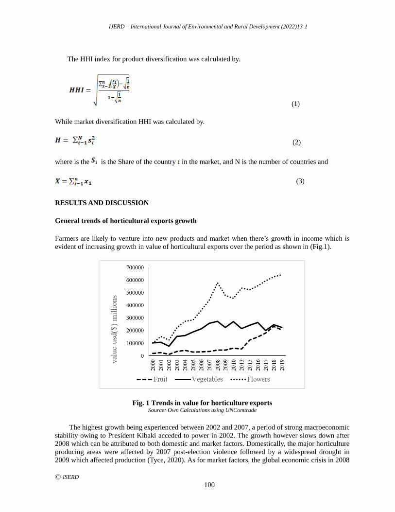
IJERD – International Journal of Environmental and Rural Development (2022)13-1
Ⓒ ISERD
100
The HHI index for product diversification was calculated by.
(1)
While market diversification HHI was calculated by.
(2)
where is the is the Share of the country in the market, and N is the number of countries and
(3)
RESULTS AND DISCUSSION
General trends of horticultural exports growth
Farmers are likely to venture into new products and market when there’s growth in income which is
evident of increasing growth in value of horticultural exports over the period as shown in (Fig.1).
Fig. 1 Trends in value for horticulture exports Source: Own Calculations using UNComtrade
The highest growth being experienced between 2002 and 2007, a period of strong macroeconomic
stability owing to President Kibaki acceded to power in 2002. The growth however slows down after
2008 which can be attributed to both domestic and market factors. Domestically, the major horticulture
producing areas were affected by 2007 post-election violence followed by a widespread drought in
2009 which affected production (Tyce, 2020). As for market factors, the global economic crisis in 2008
IJERD – International Journal of Environmental and Rural Development (2022)13-1
Ⓒ ISERD
101
affected major export markets (Heher & Steenberg, 2021). Further, delays and cancellation of flights to
Europe due to Icelandic ash in April 2010 and heavy snow in December the same year. The exchange
rate volatility especially in 2016 when the Euro/USD exchange rate dropped from 120 to 100, or delays
in the signing of EPA agreement between East African community and EU in 2015. Vegetables exports
have shown more erratic in growth compared to fruits and cut flowers. (Moran, 2018) found that
vegetables are losing popularity due to a stringent market and some exporters are moving to cut
flowers which contributes to the highest share of horticulture exports.
Market access general trends
The EU market still controls the largest share of total horticulture exports although other markets have
showed potential as shown in (Fig.2). The EU controlled over 90% of total exports in 2000 which has
reduced to 71% by 2019. The market with the highest potential is the Middle East which can be
attributed to the proximity it is from Nairobi as found by Irandu (2019) the closer the partner market
the higher the likelihood of trade. Although the EU controls the larger share of the exports, other
markets have experienced higher average growth (Table 1).
Fig. 2 Share of total horticulture exports according to markets Source: Own Calculations using UNComtrade data
Table 1. Average growth in % of major horticulture markets
Market Average growth 2001-2010 Average growth 2010-2019
EU 15% 3%
Middle East 29% 28%
USA 37% 4%
East Asia 21% 155%
Southeast Asia 175% 79%
Sub- Saharan Africa 61% 26% Source: author calculation based on UNComtrade Data.
Average growth was calculated using the average yearly change in percentage of total exports value. The markets were
defined used the United Nations defined regions. The United Kingdom is still included in the EU in this analysis.

IJERD – International Journal of Environmental and Rural Development (2022)13-1
Ⓒ ISERD
102
Product diversification trends
The objective of the study is to determine to what extent have horticultural products have diversified.
This was achieved by the change in the HHI index between 2002 to 2018, If the trend tends towards 1
(=less diversified) if the trend tends towards 0 (= more diversified).
The study found that in all three categories of horticulture exports, the index is less than 1,
meaning that the farmers are already exporting a number of products. As shown in Fig.3 HHI index for
combined horticulture products were 0.28 in 2002 has since rose to 0.31 meaning that the horticultural
products are less diversified and there’s no evidence of increase in additional products in the specified
period. However, if we consider the different products individually, we observed a change of pattern in
vegetable category after 2012. At first the Index rises from 0.34 in 2002 to 0.38 in 2012. Then falls to
0.21 in 2018. The HHI index in the flowers category was 0.71 in 2002 and rose to 0.81 in 2018. The
high index in indicates that there were only a few products exported in this category which have
continued to intensify over time while fruits HHI index rise from 0.31 in 2002 and 0.39 in 2018.
The evolution of SPS standards had a higher impact on vegetable exports compared to fruits and
flowers. This came as a challenge and opportunity, with Global GAP (formally EUREPGAP) being
rolled out in 2007, many farmers were in the process of compliance. However, there was a widespread
product interception and banning of some vegetable products by the EU for failure to meet maximum
residue limits (MRL) in 2012. Farmers took this opportunity to add value to the previously bulk
unprocessed vegetable exports and diversified into semi-processed vegetables prepack Asian
vegetables (karella, chillies, aubergines & okra) (Herher and Steenbergen, 2021). Which could explain
the HHI index for vegetable categories started falling after 2012 as an indication of additional products
in the export baskets.
Fig. 3 Product diversification trends Source: Own Calculations using UNComtrade data
The role of governance of the horticultural supply chain as a possible explanation of less
diversified products. The “buyer -driven” supply chain where supermarkets in the EU dictate what
products to produce, the packaging characteristics and quality of products (Jaffe, 2003) is likely to
affect innovation and addition of new products. Similarly, small scale farmers on contract can only
produce what is provided the contractors. This unbalanced power dynamic observed in the export
business could hinder diversification. The same phenomenon is observed in cut flowers which has the
IJERD – International Journal of Environmental and Rural Development (2022)13-1
Ⓒ ISERD
103
highest HHI index, where breeders and propagators determine what, when and how the planting
materials are distributed (Kazimierczuk et al., 2018; Tyce, 2020).
Finally, an increasing HHI index could be explained by difficulty in access to approved planting
materials especially in cut flowers exports which is associated with high cost of investment that is why
95% of the farms are owned by large scale farmers and multinational companies. High cost of royalty’s
payments for the planting materials, propagating, research, and development of new varieties often
locks out resource poor farmers who only produce low value summer flowers (Kazimierczuk et al.,
2018).
Market diversification trends
HHI index for market diversification in horticulture dropped (Fig. 4) from 0.27 in 2002 to 0.18 in 2019,
with vegetables showing higher market diversification where the index dropped from 0.49 in 2002 to
0.18 in 2019. Fruits HHI index dropped from 0.18 in 2002 to 0.13 in 2019 while flowers index dropped
from 0.37 in 2002 to 0.27 in 2019. The index has a slight increase between 2008 and 2012, which can
be explained by market factors discussed in Fig. 1 above i.e the global economic crisis in 2008, the
flight cancellations in EU markets due to weather.
The EU markets still controls the largest share of exports (Fig. 2) as discussed above which can be
explained. First, the evolution of SPS standards did not deter exporters from the EU markets, instead
most farmers embraced the compliance (Jaffee and Henson, 2004). Second, the presence the foreign
direct investment (FDI) coming from the EU along the supply chain such as exporters, breeders &
propagators and cool chain management and inputs (Irandu, 2019). Third, the established ties in the
EU supermarkets could hinder further market diversification, highly perishable products rely on trusted
relationships and cost of diversion of products from one market to another is high (Dennis & Shepherd,
2007). Fourth, availability of flights to EU that can deliver the highly perishable products in short time.
Fifth, growth and advancement in Kenyan airfreight and tourism has also aided delivery of highly
perishable products in multiple destination within a limited time. Finally Kenyan export’s ability to
meet year-round demand that can supplement their production in winter.
Fig. 4 Market diversification trends Source: Own Calculations using UNComtrade data
IJERD – International Journal of Environmental and Rural Development (2022)13-1
Ⓒ ISERD
104
There is opportunity in participation in the EU market, Kenyan horticultural exports have widened
their market access as indicated by falling HHI index both regionally and beyond (Fig.3). Krishna
(2018) found that emergence of regional value chains has provided exporters a venue to channel excess
spillovers that don’t make it to the main markets. The experience gained from the EU markets has
equipped farmers in supplying horticultural products in multiple markets governed by different regimes.
However, there is still potential in untapped markets.
CONCLUSION
The aim of the study was to determine the diversification trends of Kenyan horticultural exports this
was based on the hypothesis that continued participation of farmers in a highly dynamic global markets
is likely to initiate diversification. Our results confirmed that horticultural exports are more diversified
in terms of markets access as evidenced by a falling HHI index. On the other hand, we found that the
products to be less diversified meaning there is no evidence of any significant change in number of
products exported over time as evidenced by an increasing HHI index. We further found that the EU
still controls the largest share of horticulture exports. Finally, we found that other markets have shown
great potential in terms of growth despite controlling a small share of exports. Trade facilitation by the
government could help farmers tap into those markets and increase new products.
REFERENCES
Dennis, A., and Shepherd, B. (2007). Trade Costs, Barriers to Entry, and Export Diversification in Developing
Countries, Retrieved from http://econ.worldbank.org/projects/trade_costs
Hausmann, R., Hwang, J., and Rodrik, D. (2007). What you export matters. Journal of Economic Growth, 12(1),
1–25. https://doi.org/10.1007/s10887-006-9009-4/
Heher, U., and Steenbergen, V., (2021). Chapter 6, Kenya: Supplying to multinationals exposed local firms to
international horticulture markets in Qiang, Z. C Liu, Y and Steenbergen, V., (2021) An Investment
Perspective on Global Value Chains World Bank, ISBN:978-1-4648-1683-3, Washington DC.
Irandu, E. M. (2019). Factors influencing growth of horticultural exports in Kenya: a gravity model analysis.
GeoJournal, 84(4), 877–887, https://doi.org/10.1007/s10708-018-9888-x
Jaffee, S. (2003). From challenge to opportunity transforming Kenya’s fresh vegetable trade in the context of
emerging food safety and other standards in Europe. Agriculture and Rural Development Working Paper 10,
the IBRD, ARD Department, Washington DC.
Jaffee, S., and Henson, S. (2004). Standards and agro-food exports from developing countries: rebalancing the
debate, World Bank Policy Research Working Paper 3348, Retrieved from https://doi.org/10.1596/1813-
9450-3348
Jaffee, S., and Masakure, O. (2005). Strategic use of private standards to enhance international competitiveness:
Vegetable exports from Kenya and elsewhere. Food Policy, 30(3), 316–333.
https://doi.org/10.1016/j.foodpol.2005.05.009
Kazimierczuk, A., Kamau, P., Kinuthia, B., & Mukoko, C. (2018). Never a rose without a prick: (Dutch)
multinational companies and productive employment in the Kenyan flower sector. Retrieved from
www.ascleiden.nl
Kenya National Bureau of Statistics (KNBS). 2020. Kenya Economic Survey 2020: Retrieved from
https://www.knbs.or.ke/economic-survey-2020/
Krishnan, A. (2018). The origin and expansion of regional value chains: the case of Kenyan horticulture. Global
Networks, 18(2), 238-263. https://doi.org/10.1111/glob.12162
Moran, T. (2018) FDI and supply chains in horticulture (vegetables, fruits, and flowers, raw, packaged, cut, and
processed): diversifying exports and reducing poverty in Africa, Latin America, and other developing
economies Center for Global Development Working Paper No. 475, retrieved from http://dx.doi.org
10.2139/ssrn.3125085
Samen, S. (2010). A primer on export diversification: key concepts, theoretical underpinnings, and empirical
evidence. growth and crisis unit, World Bank, Washington DC.

IJERD – International Journal of Environmental and Rural Development (2022)13-1
Ⓒ ISERD
105
Shepherd, B., & Wilson, N. L. W. (2013). Product standards and developing country agricultural exports: the
case of the European Union. Food Policy, 42, 1–10. https://doi.org/10.1016/j.foodpol.2013.06.003
Tyce, M. (2020). A ‘Private-sector Success Story’? uncovering the role of politics and the state in Kenya’s
horticultural export sector. Journal of Development Studies, 56(10), 1877–1893.
https://doi.org/10.1080/00220388.2020.1715944

IJERD – International Journal of Environmental and Rural Development (2022)13-1
Ⓒ ISERD
106
Impact assessment of System of Rice Intensification Adoption-
Case from Madagascar-
MASATO KISHIMOTO*
Construction and Technology Institution, Tokyo , Japan
Email: [email protected]
EIJI YAMAJI Graduate School of Frontier Science, The University of Tokyo ,Tokyo, Japan
TAKESHI SAKURAI School of Agricultural and Life Sciences, The University of Tokyo , Tokyo, Japan
Received 31 January 2022 Accepted 23 April 2022 (*Corresponding Author)
Abstract The System of Rice Intensification (SRI) is expected to improve rice yield with
minimal impact on harming environment. While many studies have confirmed that the yield
increases with adopting SRI by field surveys, the impact of SRI on household income is still
debatable because SRI is a labor demanding method and may cause labor redistribution within a
household.
This study assesses the impact of SRI on the yield, household income, expenditure and
caloric consumption in Madagascar, taking into account the endogeneity between farmer’s
capacity and adapting technologies. The authors collect the data for small-scale rice producing
households in Alaotra-Mangoro region on Madagascar central highland in 2014 and 2017 by a
face-to-face questionnaire survey.
The authors find that the adoption of at least one component of SRI has no significant impact
on the rice yield, income, expenditure and caloric consumption of households on average
compared with them that adopt none of the SRI components, taking account of the endogeneity
of technology adoption. This study applies Propensity Score Matching (PSM) to take account
of the endogeneity. Then, comparing mean variables with using fertilizer by using PSM, the
authors confirm the positive impact on yield by plot level. However, because households can’t
adopt both SRI and the use of fertilizers for all plots, no significant difference is observed in
household income and expenditure.
The findings suggest that a combination of SRI with fertilizer inputs may increase yield
significantly, if more farmers in the area start using fertilizers in the future. Provision of
technical SRI training alongside sales of fertilizers is crucial. However, it is needed to conduct
further research in our study site to explore the impact on the household adopted all four of the
SRI components which is more effective, and long-term effects of SRI.
Keywords, System of Rice Intensification (SRI), Madagascar, Propensity Score Matching
(PSM), impact assessment, technology adoption, small-scale rice farmers
INTRODUCTION
Sustainable agriculture that reduces environmental load and increases food production has been
attracting attention in recent years. System of Rice Intensification (SRI) is one of such a sustainable
agriculture that has been drawing attention. This study focuses on the impact brought about by the use
of SRI in the Republic of Madagascar, the birthplace of SRI.
erd
Research article
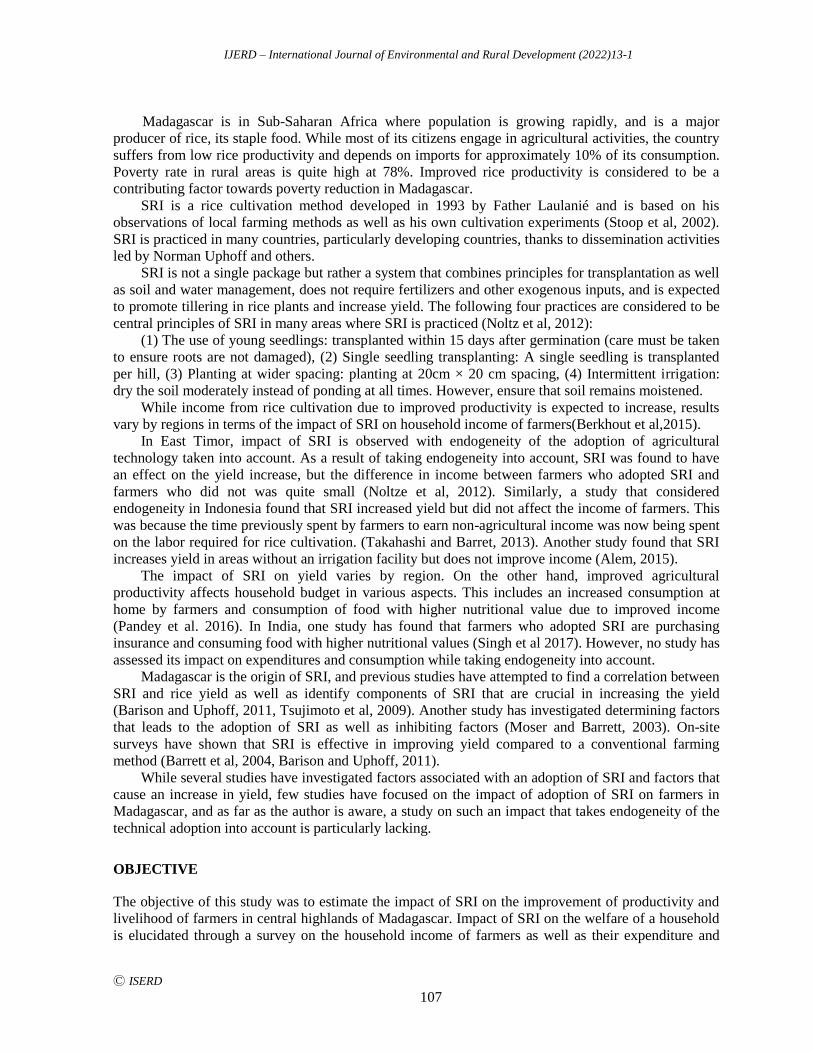
IJERD – International Journal of Environmental and Rural Development (2022)13-1
Ⓒ ISERD
107
Madagascar is in Sub-Saharan Africa where population is growing rapidly, and is a major
producer of rice, its staple food. While most of its citizens engage in agricultural activities, the country
suffers from low rice productivity and depends on imports for approximately 10% of its consumption.
Poverty rate in rural areas is quite high at 78%. Improved rice productivity is considered to be a
contributing factor towards poverty reduction in Madagascar.
SRI is a rice cultivation method developed in 1993 by Father Laulanié and is based on his
observations of local farming methods as well as his own cultivation experiments (Stoop et al, 2002).
SRI is practiced in many countries, particularly developing countries, thanks to dissemination activities
led by Norman Uphoff and others.
SRI is not a single package but rather a system that combines principles for transplantation as well
as soil and water management, does not require fertilizers and other exogenous inputs, and is expected
to promote tillering in rice plants and increase yield. The following four practices are considered to be
central principles of SRI in many areas where SRI is practiced (Noltz et al, 2012):
(1) The use of young seedlings: transplanted within 15 days after germination (care must be taken
to ensure roots are not damaged), (2) Single seedling transplanting: A single seedling is transplanted
per hill, (3) Planting at wider spacing: planting at 20cm × 20 cm spacing, (4) Intermittent irrigation:
dry the soil moderately instead of ponding at all times. However, ensure that soil remains moistened.
While income from rice cultivation due to improved productivity is expected to increase, results
vary by regions in terms of the impact of SRI on household income of farmers(Berkhout et al,2015).
In East Timor, impact of SRI is observed with endogeneity of the adoption of agricultural
technology taken into account. As a result of taking endogeneity into account, SRI was found to have
an effect on the yield increase, but the difference in income between farmers who adopted SRI and
farmers who did not was quite small (Noltze et al, 2012). Similarly, a study that considered
endogeneity in Indonesia found that SRI increased yield but did not affect the income of farmers. This
was because the time previously spent by farmers to earn non-agricultural income was now being spent
on the labor required for rice cultivation. (Takahashi and Barret, 2013). Another study found that SRI
increases yield in areas without an irrigation facility but does not improve income (Alem, 2015).
The impact of SRI on yield varies by region. On the other hand, improved agricultural
productivity affects household budget in various aspects. This includes an increased consumption at
home by farmers and consumption of food with higher nutritional value due to improved income
(Pandey et al. 2016). In India, one study has found that farmers who adopted SRI are purchasing
insurance and consuming food with higher nutritional values (Singh et al 2017). However, no study has
assessed its impact on expenditures and consumption while taking endogeneity into account.
Madagascar is the origin of SRI, and previous studies have attempted to find a correlation between
SRI and rice yield as well as identify components of SRI that are crucial in increasing the yield
(Barison and Uphoff, 2011, Tsujimoto et al, 2009). Another study has investigated determining factors
that leads to the adoption of SRI as well as inhibiting factors (Moser and Barrett, 2003). On-site
surveys have shown that SRI is effective in improving yield compared to a conventional farming
method (Barrett et al, 2004, Barison and Uphoff, 2011).
While several studies have investigated factors associated with an adoption of SRI and factors that
cause an increase in yield, few studies have focused on the impact of adoption of SRI on farmers in
Madagascar, and as far as the author is aware, a study on such an impact that takes endogeneity of the
technical adoption into account is particularly lacking.
OBJECTIVE
The objective of this study was to estimate the impact of SRI on the improvement of productivity and
livelihood of farmers in central highlands of Madagascar. Impact of SRI on the welfare of a household
is elucidated through a survey on the household income of farmers as well as their expenditure and

IJERD – International Journal of Environmental and Rural Development (2022)13-1
Ⓒ ISERD
108
food consumption.
METHODOLOGY
Two communes, Ampitatsimo and Ilafy, located in Ambatondrazaka District in the Alaotra-Mangoro
Region of Madagascar, were chosen as study sites. Irrigated area by Lake Alaotra is located 240km
northeast of the capital Antananarivo at 800m above sea level, and its climate is a tropical highland
climate. Rice cultivation and zebu cattle grazing have been practiced in the region since the 19th
Century(Yokoyama and Sakurai, 2014). Rice production in Lake Alaotra Region is among the largest
in the country and includes District PC15, one of the large-scale irrigated rice cultivation districts from
the French colonial era (Fujiki,2015). Rice cultivation period is long and lasts five to six months, and
rice is usually grown once a year.
Fukuda (2015) investigated characteristics of SRI farmers in Ambatondrazaka District. Farmers in
this area combined technologies per plot with respect to varieties, transplantation, and SRI. SRI was
utilized in combination with the conventional practice. Risk preference also influenced the decision of
technologies. Risk-loving husband were more likely to adopt SRI. On the other hand, more risk-
aversive wives tended to choose conventional varieties and sort seeds.
Survey on an introduction of SRI
A team led by Professor Sakurai of the University of Tokyo conducted a survey of Ambatondrazaka
District in 2014. Survey method is discussed below (Fukuda, 2015). Ampitatsimo consists of eight
villages (fokontany), and Ilafy consists of twelve villages. Average population per village was
calculated by dividing the total population of the commune by the number of villages, and four villages
were selected from Ampitatsimo and six from Ilafy. 40 rice farmer households were randomly selected
from each village (for a total of 400 households), with whom a face-to-face questionnaire survey was
conducted. The survey covered a broad range of topics including socioeconomic attributes, income,
food expenditures of farmers, the use of inputs at a plot level, adoption of the technology, and yield,
and it was conducted twice from May to June in 2014 and again August 2014.
Number of plots managed by farmers totaled 1,337 plots, of which 732 plots were rice paddies
where rice was being cultivated. Surveyed farmers also participated in risk experiment in order to
measure their risk preference.
335 households and 646 plots were used as survey data after removing missing values and outlier
data. Data from farmers who could not respond during the second survey period, farmers whose
responses were insufficient, and farmers whose number of cultivated plots increased between the first
and second survey periods were removed.
Survey on knowledge on SRI and decision on its implementation
Additional survey was conducted in December 2017 to clarify the path of SRI dissemination and the
state of its implementation. A semi-structured interview was conducted with eighteen farmer
households that has partially adopted SRI components, nine households who has not adopted any SRI
components from the previous survey. Additionally, the interview was conducted with two agricultural
bureau staff at the surveyed district, one head of the irrigation association, and one Japanese specialist
staff.
Analysis framework and method
Average treatment effect on the treated (ATT) is used to measure the difference of the average between

IJERD – International Journal of Environmental and Rural Development (2022)13-1
Ⓒ ISERD
109
SRI farmers (i.e. treated group) and non-SRI farmers (non-SRI group) (Wooldridge, 2010).
(1)
yi1 shows the results for treated group, and y0i shows the results for control group. In this study, y
is defined as the income of an SRI farmer or a yield from an SRI plot. Additionally, i is the
identification number assigned to each farmer. Technology is adopted when Di=1 and technology is not
adopted when Di=0.Since yi1 and yi0 cannot be measured at the same time against i-th farmer, E(y0i│Di=1) is replaced with measurable data from a non-SRI farmer. Typically, a difference in farm
management capability and motivation is assumed between SRI farmers and non-SRI farmers, and
such a difference causes bias in the results. Propensity Score Matching (PSM) is used to address the
bias from replacement (Rosenbaum and Rubin, 1983).
PSM assumes that an adoption of SRI is determined by an observable variable. If the adoption is
determined by an observable variable, the following equation can be derived.
(2)
p(xi) shows a probability that SRI is used under observable variable x.
(3)
PSM requires another assumption. Covariance of SRI farmers and non-SRI farmers need to
greatly overlap. In another words, 0<p(xi)<1 needs to be satisfied. The following equation is derived
from equation (1):
(4)
From the above equation, the impact of SRI can be evaluated while taking endogeneity into
account. However, in order to minimize the estimation error of PSM, inclusion of every variable
associated with SRI adoption is recommended. If a variable that is not observed affects the adoption of
SRI, a bias may exist in the ATT result as well. Methods for matching treatment group and control
group includes nearest-neighbor matching, stratification matching, radius matching, and kernel
matching, among others (Wooldridge, 2010). A matching method that minimizes the pseudo-coefficient
of determination and error after estimation was chosen.
Factors that determine SRI adoption were analyzed in order to calculate aforementioned
propensity scores. Farmers presumably combine agricultural technologies independently for each plot.
Therefore, propensity scores were calculated for each plot. Logistic regression was used to calculate
propensity scores.
(5)
y: Adoption of the technology (y=1: SRI plot, y=0: others)
β0: Slices
xk: Variable pertaining to adoption
Hypotheses
This study asks two research questions: "How does SRI technology affect rice yield" and "how does

IJERD – International Journal of Environmental and Rural Development (2022)13-1
Ⓒ ISERD
110
SRI affect farmers?".
A pair of hypotheses are validated. First, fields where SRI is implemented produce greater yields
compared to non-SRI fields. Second, an increase in rice yield leads to an increase in rice income,
resulting in an overall increase in income for the household of the farmer. Over the course of validating
hypotheses, any changes in expenditure and personal caloric consumption are also noted even when the
income of farmers who has adopted SRI has not increased.
RESULTS AND DISCUSSION
Results of introducing SRI
For analysis, an SRI plot is defined as a plot where at least one of the components ((1) Use of young
seedlings within 14 days after sowing, (2) Single seedling transplanting, (3) Transplanting by spacing
of at least 20cm, (4) Intermittent irrigation) is adopted because farmer adapting all component is very
few. A farmer is identified as an SRI farmer if the household practices SRI in at least one of its
cultivated plots.
Table 2 shows the results of a comparison based on whether SRI is adopted or not at a plot level.
Significant differences between SRI plots and non-SRI plots were observed for presence of PC15,
weeding frequency, transplantation, amount of organic fertilizer used, distance from home to plots,
cost of hired labor, and number of labor days worked by non-hired laborers.
Table 2 the results of a comparison based on whether SRI adaptation by plot level Variable SRI Ave. Non-SRI Ave. Total Ave. SRI-Non-SRI Diff.
Cultivated area (ha) 0.60 0.75 0.72 -0.15
Dummy for PC15 0.35 0.14 0.18 0.20***
Presence of an irrigation facility 0.58 0.64 0.63 -0.055
Dummy for land ownership 0.64 0.64 0.64 0.0018
Dummy for land fertility 0.10 0.15 0.14 -0.052
Weeding frequency 1.06 0.86 0.89 0.21***
Dummy for transplantation 0.96 0.61 0.67 0.35***
Dummy for the use of commercial varieties 0.71 0.78 0.77 -0.68
Seed usage (kg/ha) 147 158 156 -12
Total chemical fertilizer usage (kg/ha) 1.20 1.17 1.17 0.033
Total organic fertilizer usage (kg/ha) 1,149 734 810 415*
Distance to the plot (min) 24.1 40.5 37.6 -16.4**
Yield (t/ha) 2.91 2.34 2.44 0.57***
Rice productivity per person (kg/person) 19.3 28.5 26.9 -9.23
Revenue from rice (1,000Ar/ha) …A 2,120 1,703 1,777 417***
Fertilizer cost (1,000Ar/ha) 51.6 36.9 39.5 14.7
Pesticide cost (1,000Ar/ha) 6.01 4.25 4.57 1.76*
Herbicide cost (1,000Ar/ha) 6.677 6.675 6.676 0.002
Seeds cost (1,000Ar/ha) 111 103 104 8.32
Land improvement cost (1,000Ar/ha) 61.4 47.6 50.0 13.8
Hired labor cost (1,000Ar/ha) 272 172 190 100***
# non-hired laborers (man-days/ha) 289 190 207 99**
Cost of rice cultivation (1,000Ar/ha) …B 509 371 395 139***
Cost incl. non-hired labor (1,000Ar/ha) …B’ 1,379 942 1,019 437***
Income from rice (1,000Ar/ha)… (C = A – B) 1,611 1,333 1,382 278*
Profit from rice (1,000Ar/ha) … (D = A - B’) 742 762 758 -20.2
Observed 112 521 633
Note: *** p<0.01, ** p<0.05, * p<0.1
Ratio of transplantation is higher among SRI plots since three of the SRI components (excluding
intermittent irrigation) are techniques related to transplantation. Intermittent irrigation requires an
IJERD – International Journal of Environmental and Rural Development (2022)13-1
Ⓒ ISERD
111
irrigation facility, and the ratio of intermittent irrigation and the ratio of District PC15 was greater for
SRI plots. Weeding work was performed more often in SRI plots due to intermittent irrigation. Greater
number of organic fertilizers used in SRI plots was due to recommendations being made towards the
use of organic fertilizers at the time of SRI adaptation. Greater hired and non-hired labor in SRI plots
was also consistent with previous studies, which confirmed the possibility that SRI is a more labor-
intensive farming method.
Yield increased by 0.57 (t/ha) in SRI plots. At the same time, cost incurred by rice cultivation also
increased. Based on the market price for Alaotra-Mangoro Region from 2014, price per kg of rice was
assumed to be 728 (Ar/kg). Rice income per ha was greater in SRI plots at 10% significance level. Cost
of non-hired labor was calculated by assuming the mode of hired labor cost as the employment wage
within the area. Significant difference was not observed in profit calculated after including a non-hired
labor cost. Significant difference was not observed for rice productivity per person (kg/person), and the
adoption of SRI in the area has not improved labor efficiency. Additionally, farmers who adopted SRI
were accounted for 23% of the total households, and average yield was 2.32(t/ha).
Impact of each variable on the adoption of SRI
The impact of each variable on the adoption of SRI at a plot level, calculated by using a logit model
which can estimates probability to adapt the SRI. Variables that had a negative impact on the adoption
of SRI were cultivated area, number of family members, female family head, distance from home to
the field, and the commune in which the farmer lives. Variables that had a positive impact on the
adoption of SRI were availability of irrigation, PC15 dummy, number of years of education, number of
traders the farmer knows, and knowledge on intermittent irrigation.
Estimated ATT
Table 3 shows the estimated ATT. At a plot level, yield was greater in SRI plots than non-SRI plots
and income, but its difference was not significant. Both hired and non-hired labor were greater in SRI
plots. In particular, non-hired labor was 113 (man-days/ha), which was significantly larger at 10%
significance level and showed a much greater need for labor in SRI plots. No significant differences
were observed for other variables, which show that technologies other than adopted SRI (e.g. fertilizer
inputs) do not make a difference between SRI and non-SRI plots. At a household level, no significant
difference was observed in yield between SRI and non-SRI farmers. Income from rice and income for
the entire household were greater among SRI farmers, but no significant differences were observed.
Income by means other than labor was the only variable where a significant difference was observed
between SRI and non-SRI farmers; SRI farmers were generating a greater amount of income through
remittance and land lease. These results indicate that the adoption of SRI has not had an impact on
yield and income in the area at a household level.
IJERD – International Journal of Environmental and Rural Development (2022)13-1
Ⓒ ISERD
112
Table 3 Estimated results by ATT
plot level
Variable ATT result(SRI plots - non-SRI plots) standard error
Yield (t/ha) 0.37 -0.32
Cost of rice cultivation (1,000Ar/ha) 29.2 -65
Income from rice (1,000Ar/ha) 243 -153
Profit from rice (1,000Ar/ha) -95.4 -212
# non-hired laborers (man-days/ha) 113* -70.0
Hired labor cost (1,000Ar/ha) 44.4 -43
Total chemical fertilizer usage (kg/ha) -2.05 -2.48
Total organic fertilizer usage (kg/ha) 113 -338
Seed usage (kg/ha) -9.59 -17.2
Observed 630 -
household level
Variable ATT result(SRI farmers -non-SRI farmers) standard error
Average yield for a household (t/ha) 0.39 0.39
Household income (1,000Ar) 601 609
Income per person (1,000Ar/person) 77.8 126
Income from rice cultivation (1,000Ar) 244 472
Income from crops excl. rice (1,000Ar) -36.9 104
Income from self-employment (1,000Ar) -14.3 184
Non-agricultural income (1,000Ar) -1.99 122
Income from livestock (1,000Ar) 101 87
Non-labor income (1,000Ar) 309*** 130
Food expenditure (1,000Ar / week) 1.16 2,41
Total expenditure (1,000Ar/ month) 12.4 24,7
Calorie consumption per person (kcal/day) -30.2 173.3
Observed 325 -
Note: *** p<0.01, ** p<0.05, * p<0.1 Plot level uses Kernel matching was used as a matching method. Bandwidth was 0.01, and resampling was iterated 900 times by bootstrap method to obtain a standard error. Household level uses Radius matching was used as a matching method. Radius was 0.06. Observed number is different from Table1 because some date is not suitable due to missing parameter.
Knowledge on SRI and decision on its implementation
Fig 4 shows the timing in which farmers became aware of SRI, and shows components regarded as a
part of SRI technology in the studied area. While there were some differences in terms of the
recognized techniques that constitute SRI, all 27 farmer households interviewed knew about SRI.
Diverse timing in which farmers became aware of SRI and various paths through which SRI
disseminated indicate that the word "SRI" itself is widely known in the studied area. However,
institutions such as JICA and the local agricultural bureau have also disseminated other technologies,
and it is quite possible that farmers confuse these technologies with SRI.
Highest number of farmers that learned about SRI was recorded in 2000, a year in which
extension workers of an NGO have disseminated the SRI technology in several communes. Importance
of water management was recognized in many households. Many farmers also felt the importance of
using relatively innovative technologies, including the use of chemical fertilizers and pesticides and the
use of a rotary weeder. While many farmers said that regular planting and row planting are important,
only three respondents saw increased spacing between rows (a unique feature of SRI) as important,
four saw single seedling transplanting as important, and two saw the use of young seedlings as
important.
Results suggest that farmers in this area may be recognizing new technologies also as "SRI", in
spite of the fact that they are not a part of the four major components that constitute SRI. (N=27)
IJERD – International Journal of Environmental and Rural Development (2022)13-1
Ⓒ ISERD
113
0 5 10 15
Adoption of intermittent irrigation
Organic fertilizers
Use of chemical fertilizers
Liquid fertilizers
Pesticides
Regular planting
Row planting
Interrow spacing at or over 10 cm
Interrow spacing of 20 – 25 cm
Single seedling transplanting
Use of young seedlings
Transplantation with care
Use of a rotary weeder
Leveling
Use of good seeds
Number of responses
SRI Non-SRI
Fig 3 Component techniques of SRI Fig 4 Period in which farmers know about SRI
Impact of fertilizer inputs
Soil fertility in the studied area is low, and phosphorus deficiency is particularly evident (JICA, 2017).
For this reason, widening the spacing between seedlings only widens the space and is likely to reduce
yield. In the farmer’s interview, some farmers indicated that farmers also viewed the relationship
between land fertility and seedling spacing as important. Fertilizer inputs itself is assumed to contribute
greatly to yield improvement. In addition, if seedlings are planted at wider spacing while fertilizers are
applied, merits of SRI such as seed savings and an increase in the number of tillers can be expected.
Therefore, differences in yield and income due to whether fertilizer are applied or not as well as a
combination of fertilizer inputs and SRI were verified using data from 2014.
Table 4 Impact of fertilizer inputs
by plot Estimation by ATT
Variable Fertilizer(Fertilizer = 297) Fertilizer + SRI(Fertilizer + SRI = 61)
Yield (t/ha) 0.37** 0.61***
Cost of rice cultivation (1,000Ar/ha) 130*** 145***
Income from rice (1,000Ar/ha) 138 302**
Profit from rice (1,000Ar/ha) 53.0 66.1
Seed usage (kg/ha) 20.1* 20.1
Cost of hired labor (1,000Ar/ha) 36.7** 86.0***
# non-hired laborers (man-days/ha) 28.4 78.6*
Observed 630 630
per household Estimation by ATT
Variable Fertilizer(Fertilizer = 181) Fertilizer + SRI(Fertilizer + SRI = 50)
Household income (1,000Ar) 82.6 588
Income per person (1,000Ar/capita) 5.29 136
Income from rice cultivation (1,000Ar) 197 416
Average yield for a household (t/ha) 0.26 0.33
Income from crops excl. rice (1,000Ar) 11.0 34.0
Income from self-employment (1,000Ar) -123 -112
Non-agricultural income (1,000Ar) 28.9 47.8
Income from livestock (1,000Ar) 0.875 91.1
Non-labor income (1,000Ar) -31.5 111
Food expenditure (1,000Ar / 1 wk) -0.361 -0.098
Total expenditure (1,000Ar/ month) 16.9 -16.8
Calorie consumption per person (kcal/day) 17 -37
Observed 325 325
Note: *** p<0.01, ** p<0.05, * p<0.1
By plot level uses radius in radius matching for fertilizer use was 0.04, and radius for fertilizer + SRI was 0.01
Per household level uses radius in radius matching for fertilizer use was 0.05, and radius for fertilizer + SRI was 0.06.
(N=27)
IJERD – International Journal of Environmental and Rural Development (2022)13-1
Ⓒ ISERD
114
Table 4 shows the results. Estimation after matching shows an increase in average yield due to
fertilizer inputs. However, a significant difference in income was not observed due to an increase in
fertilizer cost and hired labor cost. When fertilizer inputs were combined with SRI, yield increased by
0.61 (t/ha). While the cost of rice cultivation increased, income per ha also increased due to a
significant increase in yield. However, income did not increase when non-hired labor was converted to
cost due to an increase in the amount of non-hired labor. At a household level, no significant
differences were observed in rice yield and thus income from rice cultivation, and no significant
differences were also observed in other incomes.
As a result, the difference in household income due to fertilizer inputs was not significant. This
result was also the same for a case in which the use of fertilizers and SRI were combined. Lack of
difference in yield and income at the household level may be due to the fact that the technologies were
not being applied across all cultivating plots.
Comparison of average yield difference between years 2016/2017 and 2013/2014 showed a
reduction in average yield for 2017 by 0.68t/ha. This is likely due to a dearth of rainfall in 2016/2017,
which led to a poor harvest for the year with a significant reduction in average yield. Weather
conditions such as rainfall were not controlled, but they suggested that an increase in yield between
2014 and 2017 was unlikely.
CONCLUSION
This study investigated the impact of SRI on yield and living expense among rice farmers in two
communes in Ambatondrazaka District of Madagascar. In the analysis, yield, household income, and
expenditure were compared by using data obtained by on-site surveys. PSM was used to account for
selection bias and compare average yield between SRI and non-SRI plots, which showed that yield was
greater in SRI plots but without a significant difference. Improvement in rice income due to an
adoption of SRI was not observed. While the household income was greater for SRI farmers, there
were no significant differences between two groups. Differences due to SRI adoption were not
observed with regards to a week's worth of food expenditure and expenditure per month by the farmer.
Similarly, consumed calories were calculated based on food consumption by farmers, but no difference
due to the adoption of SRI was observed.
Interview results from 2017 showed that the term "SRI" is widely known among farmers.
However, details of the technology recognized by farmers varied greatly, which implied that SRI is a
technology whose name is well-known, but its details are not accurately known.
Considering low soil fertility of the studied area, wider spacing between seedlings may reduce
yield. On the other hand, high yield may be achieved by improving soil fertility through fertilizer
inputs and adoption of SRI. Survey results from 2014 also confirmed that yield increases when SRI is
combined with fertilizer inputs. In this case, cost incurred to cultivate rice increased at a plot level, but
income also increased, thereby indicating the importance of combining fertilizer inputs with SRI
components. Even in this case however, because households were unable to adopt both SRI and the use
of fertilizers for all plots, no significant difference was observed in income from rice cultivation and
household income.
In the future, a combination of SRI with fertilizer inputs may increase yield significantly, if more
farmers in the area start using fertilizers. Provision of technical SRI training alongside sales of
fertilizers is crucial.
Future Research
Among farmers surveyed in this study, only one household adopted all four of the SRI components. In
the analysis, farmers who have adopted some of the SRI components were defined as farmers who
IJERD – International Journal of Environmental and Rural Development (2022)13-1
Ⓒ ISERD
115
have adopted SRI. SRI is considered to be most effective when all of the components are adopted (J-
SRI, 2011). For this reason, any area nearby the site for this study where SRI is widely practiced may
have adopted all components of SRI and thus increased the yield. In addition, comparison per SRI
component was not possible due to the sample size, and an identification of component(s) that is
important for the study site could not be conducted.
This study did not consider the number of years through which SRI is continually practiced. One
study has suggested that farmers who have continued to practice SRI for a number of years are
accustomed to the technology and thus able to improve their productivity (Moser and Barrett, 2003).
An analysis that accounts for the number of continuously practiced years would be important in
measuring long-term effects of SRI.
REFERENCES
Alem. Y. 2015. Improving Welfare Through Climate-friendly agriculture: the case of the system of rice intensification, Environmental and Resource Economics, 62.2, 243-263.
Barrett C B., Moser M. C, Oloro V. M, Joeli B. 2004. Better technology, better plots, or better farmers? Identifying changes in productivity and risk among Malagasy rice farmers, American Journal of Agricultural Economics, 86.4 869-888.
Barison, J, U, N. 2011. Rice yield and its relation to root growth and nutrient-use efficiency under SRI and conventional cultivation: an evaluation in Madagascar, Paddy and Water Environment, 9(1), 65-78.
Berkhout E, D G, Arie K. 2015. On-farm impact of the System of Rice Intensification (SRI): Evidence and knowledge gaps, Agricultural Systems, 132, 157-166.
Fujiki.K. 2015. The evolution of a rural territory at plot scale: Between hyper-fragmentation and land grabbing (irrigation perimeter PC15 - Marianina Valley, Alaotra-Mangoro, Madagascar), Land use policy, 43, 170-185.
Fukuda, A. 2015. Adoption of an agricultural technology and risk preference of married couples - rice planting technology in Madagascar, Hitotsubashi University Graduate School of Economics, Japan.
J-SRI (Japan Association of the System of Rice Intensification). 2011. Rice Cultivation Revolution: SRI -- Saving the World from Famine, Poverty and Water Scarcity, Nikkei Publishing, Japan.
JICA. Specalist Project Completion Report. 2012 https://www.jica.go.jp/project/madagascar/0700698/materials/ku57pq00001ynw1c-att/soil-analysis_2012_01.pdf (in Japanese)
Moser M, C, Barrett C B. 2003. The disappointing adoption dynamics of a yield-increasing, low external-input technology: the case of SRI in Madagascar, Agricultural Systems, 76.3 1085-1100.
Noltze M, Schwarze S, Qaim M. 2012. Farm Diversity and Heterogeneous Impacts of System Technologies on Yield, Income and Poverty: The System of Rice Intensification in Timor Leste, conference Foz do Iguacu, Brazil. No. 125595, International Association of Agricultural Economists.
Pandey, Vijay L, S. Mahendra D, and Usha J. 2016. Impact of agricultural interventions on the nutritional status in South Asia, A review. Food policy, 62 28-40.
Rosenbaum, P. R. and Rubin, D. 1983. The central role of the propensity score in observational studies for causal effects, Biometrika, 41-55.
Singh, R, Feroze, S. M, Ray, L, I., Singh, K, J, and Muliar, D. 2017. Role of System of Rice Intensification Method in Improving Health and Nutritional Security: A Micro Level Study in Tripura State, Indian Research Journal of Extension Education, 17(2), 1-4.
Stoop, W, A, Uphoff, N, and Kassam, A. 2002. A review of agricultural research issues raised by the system of rice intensification (SRI) from Madagascar: opportunities for improving farming systems for resource-poor farmers, Agricultural systems, 71(3), 249-274.
Takahashi, K, Barrett, C, B. 2013. The system of rice intensification and its impacts on household income and child schooling: evidence from rural Indonesia, American Journal of Agricultural Economics, 96(1), 269-289.
Tsujimoto Y, Horie T, Hamon R, Shiraiwa T, Homma K. 2009. Soil management: The key factors for higher productivity in the fields utilizing the system of rice intensification (SRI) in the central highland of Madagascar, Agricultural Systems, 100.1, 61-71.
Wooldridge, J. M. 2010. Econometric Analysis of Cross Section and Panel Data. 2nd ed. Cambridge, MA: MIT Press.
Yokoyama, S, Sakurai, T. 2014. Participation factors for rice cultivation technology training and its impact - A case of SRI in central highlands in Madagascar, Japanese Journal of Farm Management, 52(3), 83-88.
IJERD – International Journal of Environmental and Rural Development (2022)13-1
Ⓒ ISERD
116
Effects of lead and other metals from historical smelting on
sustainable fruit and vegetable cultivation
BARRY NOLLER* The University of Queensland St Lucia, QLD 4072, Australia
Email: [email protected]
FIONA HENDERSON The University of Queensland St Lucia, QLD 4072, Australia
Received 31 January 2022 Accepted 25 April 2022 (*Corresponding Author)
Abstract Wollongong, located in the Illawarra region of NSW Australia, contains the industrial
complex of Port Kembla. Lead in Port Kembla soils, ~2.5 km from a former copper smelter
(1908-2003), have exceeded soil contamination guidelines for human health (HIL) and
ecological (EIL) investigation levels. Previous studies regarding heavy metal contamination
from the industrial complex, do not include comparisons to HIL and EIL guidelines. This study
re-examines the risk of legacy (historic) heavy metals in urban soils to residents in proximity to
the Port Kembla industrial complex. This was accomplished by reviewing: (i) resolution of
heavy metal dispersion data from the copper smelter, in historic soil concentration data (n=95
top soil samples) collected by Jafari (2009) and reviewed by Noller (2020a); (ii) providing a
new comparison of historic percentile data to current Australian soil contamination guidelines
(NEPC, 2013) and German atmospheric pollutant guidelines; and (iii) re-evaluating treatments
to soil data by Jafari (2009), in the context of bioaccessibility and bioavailability to humans and
plants. At 75th percentile, arsenic, cadmium, copper, lead and zinc concentrations exceeded HIL
Level A guidelines. When detection limit values (52 out of 95) were removed (n=22 samples),
median cadmium concentrations exceeded HIL Level A guidelines. Dietary exposure to
cadmium, lead, zinc and copper is a risk to residents through the consumption of vegetables
grown in urban gardens in proximity to the Port Kembla industrial complex. Copper in
vegetables sampled from soils in the vicinity of the Port Kembla copper smelter was greater in
comparison to sampling completed at other smelter sites. Port Kembla urban garden vegetables
showed exceedance of food guidelines for both cadmium and lead, highlighting the health risks
of growing vegetables in proximity to industrial areas.
Keywords heavy metals, arsenic, smelting, sustainable, fruit and vegetable cultivation
INTRODUCTION
The Wollongong local government area (LAG) is located in the Illawarra region of New South Wales
(NSW), Australia (Fig. 1), 80 km south of Sydney. The Wollongong LAG contains the industrial
complex at Port Kembla; a feature which has remained in place for over 100 years (Chiaradia et al.,
1997; Jafari, 2009). A copper smelter, formerly Southern Copper ERS Ltd (SC in Fig. 1), commenced
operations at Port Kembla from 1908 till 2003 and was subsequently demolished in 2014. A
considerable body of literature exists on the nature, extent and distribution of heavy metals and arsenic
in soils in Wollongong and Port Kembla (Noller, 2020a). The current Australian guidelines for human
health (HIL) and ecological (EIL) investigative levels are risk-based approaches used to examine and
interpret soil, air, water and food environmental data. Existing guidelines (HIL and EIL) had yet to be
implemented at the time of previous data collection and analysis (Noller, 2020a). Previously, lead (Pb)
erd
Research article

IJERD – International Journal of Environmental and Rural Development (2022)13-1
Ⓒ ISERD
117
was the key focus of investigation at Port Kembla, yet cadmium (Cd), zinc (Zn), copper (Cu), and
arsenic (As) were recognized to exceed Australian National soil contamination guidelines (HIL and
EIL) (NEPC, 2013; Noller, 2020b). In the absence of Australian air pollutant guidelines, the
application of German air pollutant controls (TA LUFT standards) for metal fallout were used (TA
LUFT, 1990, 1999; Noller, 2020b).
Fig. 1 Location of the historical Port Kembla industrial complex, including the Southern Copper
smelter (SC) and other sampling sites (Chiaradia et al., 1997)
OBJECTIVE
The objectives of this study are to re-examine and evaluate the human-health risks to residents in the
proximity to the Port Kembla industrial complex, based on historic heavy metal and As concentrations
in soil.
METHODOLOGY
This study aims to follow three methods of re-examination and analysis: (i) to review the resolution of
heavy metal and As dispersion data from the copper smelter, in historic soil concentration data (n=95 top
soil samples) collected by Jafari (2009) and reviewed by Noller (2020a); (ii) to provide a new comparison
of historic percentile data to current Australian soil contamination guidelines (NEPC, 2013) and TA LUFT
(1990, 1999) German atmospheric fallout standards; and (iii) to re-evaluate treatments to soil data by Jafari
(2009), in the context of bioaccessibility and bioavailability to humans and plants.
The Jafari (2009) study measured the total concentration of 37 elements in soil samples (n=95) by
XRF-spectrometry. Soil samples were treated with 0.1M hydrochloric acid extraction and ethylenediamine
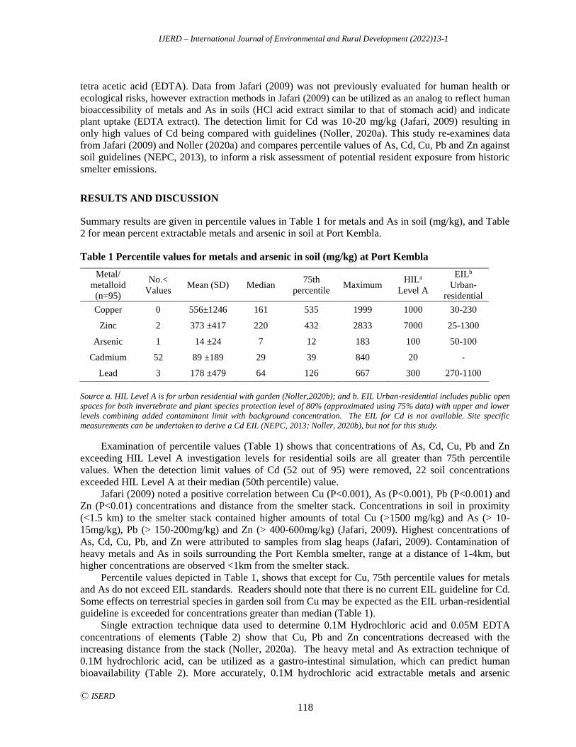
IJERD – International Journal of Environmental and Rural Development (2022)13-1
Ⓒ ISERD
118
tetra acetic acid (EDTA). Data from Jafari (2009) was not previously evaluated for human health or
ecological risks, however extraction methods in Jafari (2009) can be utilized as an analog to reflect human
bioaccessibility of metals and As in soils (HCl acid extract similar to that of stomach acid) and indicate
plant uptake (EDTA extract). The detection limit for Cd was 10-20 mg/kg (Jafari, 2009) resulting in
only high values of Cd being compared with guidelines (Noller, 2020a). This study re-examinese data
from Jafari (2009) and Noller (2020a) and compares percentile values of As, Cd, Cu, Pb and Zn against
soil guidelines (NEPC, 2013), to inform a risk assessment of potential resident exposure from historic
smelter emissions.
RESULTS AND DISCUSSION
Summary results are given in percentile values in Table 1 for metals and As in soil (mg/kg), and Table
2 for mean percent extractable metals and arsenic in soil at Port Kembla.
Table 1 Percentile values for metals and arsenic in soil (mg/kg) at Port Kembla
Metal/
metalloid
(n=95)
No.<
Values Mean (SD) Median
75th
percentile Maximum
HILa
Level A
EILb
Urban-
residential Copper 0 556±1246 161 535 1999 1000 30-230
Zinc 2 373 ±417 220 432 2833 7000 25-1300
Arsenic 1 14 ±24 7 12 183 100 50-100
Cadmium 52 89 ±189 29 39 840 20 -
Lead 3 178 ±479 64 126 667 300 270-1100
Source a. HIL Level A is for urban residential with garden (Noller,2020b); and b. EIL Urban-residential includes public open
spaces for both invertebrate and plant species protection level of 80% (approximated using 75% data) with upper and lower
levels combining added contaminant limit with background concentration. The EIL for Cd is not available. Site specific
measurements can be undertaken to derive a Cd EIL (NEPC, 2013; Noller, 2020b), but not for this study.
Examination of percentile values (Table 1) shows that concentrations of As, Cd, Cu, Pb and Zn
exceeding HIL Level A investigation levels for residential soils are all greater than 75th percentile
values. When the detection limit values of Cd (52 out of 95) were removed, 22 soil concentrations
exceeded HIL Level A at their median (50th percentile) value.
Jafari (2009) noted a positive correlation between Cu (P<0.001), As (P<0.001), Pb (P<0.001) and
Zn (P<0.01) concentrations and distance from the smelter stack. Concentrations in soil in proximity
(<1.5 km) to the smelter stack contained higher amounts of total Cu (>1500 mg/kg) and As (> 10-
15mg/kg), Pb (> 150-200mg/kg) and Zn (> 400-600mg/kg) (Jafari, 2009). Highest concentrations of
As, Cd, Cu, Pb, and Zn were attributed to samples from slag heaps (Jafari, 2009). Contamination of
heavy metals and As in soils surrounding the Port Kembla smelter, range at a distance of 1-4km, but
higher concentrations are observed <1km from the smelter stack.
Percentile values depicted in Table 1, shows that except for Cu, 75th percentile values for metals
and As do not exceed EIL standards. Readers should note that there is no current EIL guideline for Cd.
Some effects on terrestrial species in garden soil from Cu may be expected as the EIL urban-residential
guideline is exceeded for concentrations greater than median (Table 1).
Single extraction technique data used to determine 0.1M Hydrochloric acid and 0.05M EDTA
concentrations of elements (Table 2) show that Cu, Pb and Zn concentrations decreased with the
increasing distance from the stack (Noller, 2020a). The heavy metal and As extraction technique of
0.1M hydrochloric acid, can be utilized as a gastro-intestinal simulation, which can predict human
bioavailability (Table 2). More accurately, 0.1M hydrochloric acid extractable metals and arsenic
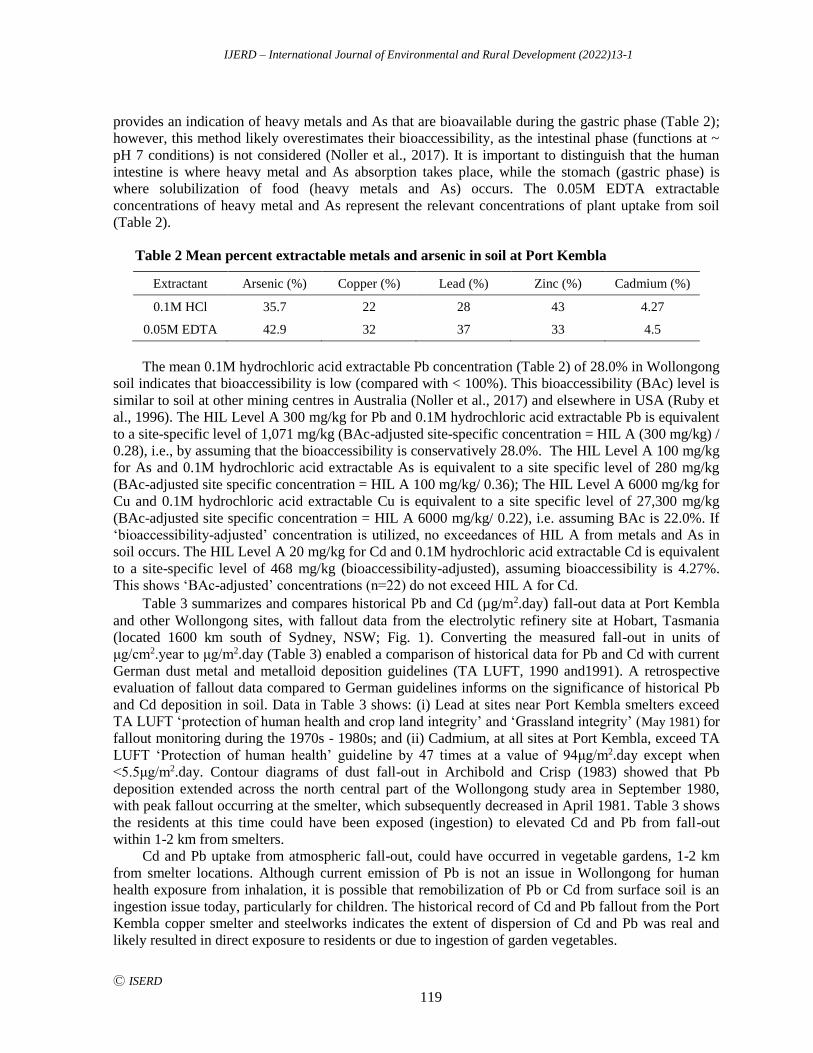
IJERD – International Journal of Environmental and Rural Development (2022)13-1
Ⓒ ISERD
119
provides an indication of heavy metals and As that are bioavailable during the gastric phase (Table 2);
however, this method likely overestimates their bioaccessibility, as the intestinal phase (functions at ~
pH 7 conditions) is not considered (Noller et al., 2017). It is important to distinguish that the human
intestine is where heavy metal and As absorption takes place, while the stomach (gastric phase) is
where solubilization of food (heavy metals and As) occurs. The 0.05M EDTA extractable
concentrations of heavy metal and As represent the relevant concentrations of plant uptake from soil
(Table 2).
Table 2 Mean percent extractable metals and arsenic in soil at Port Kembla
Extractant Arsenic (%) Copper (%) Lead (%) Zinc (%) Cadmium (%)
0.1M HCl 35.7 22 28 43 4.27
0.05M EDTA 42.9 32 37 33 4.5
The mean 0.1M hydrochloric acid extractable Pb concentration (Table 2) of 28.0% in Wollongong
soil indicates that bioaccessibility is low (compared with < 100%). This bioaccessibility (BAc) level is
similar to soil at other mining centres in Australia (Noller et al., 2017) and elsewhere in USA (Ruby et
al., 1996). The HIL Level A 300 mg/kg for Pb and 0.1M hydrochloric acid extractable Pb is equivalent
to a site-specific level of 1,071 mg/kg (BAc-adjusted site-specific concentration = HIL A (300 mg/kg) /
0.28), i.e., by assuming that the bioaccessibility is conservatively 28.0%. The HIL Level A 100 mg/kg
for As and 0.1M hydrochloric acid extractable As is equivalent to a site specific level of 280 mg/kg
(BAc-adjusted site specific concentration = HIL A 100 mg/kg/ 0.36); The HIL Level A 6000 mg/kg for
Cu and 0.1M hydrochloric acid extractable Cu is equivalent to a site specific level of 27,300 mg/kg
(BAc-adjusted site specific concentration = HIL A 6000 mg/kg/ 0.22), i.e. assuming BAc is 22.0%. If
‘bioaccessibility-adjusted’ concentration is utilized, no exceedances of HIL A from metals and As in
soil occurs. The HIL Level A 20 mg/kg for Cd and 0.1M hydrochloric acid extractable Cd is equivalent
to a site-specific level of 468 mg/kg (bioaccessibility-adjusted), assuming bioaccessibility is 4.27%.
This shows ‘BAc-adjusted’ concentrations (n=22) do not exceed HIL A for Cd.
Table 3 summarizes and compares historical Pb and Cd (µg/m2.day) fall-out data at Port Kembla
and other Wollongong sites, with fallout data from the electrolytic refinery site at Hobart, Tasmania
(located 1600 km south of Sydney, NSW; Fig. 1). Converting the measured fall-out in units of
μg/cm2.year to μg/m2.day (Table 3) enabled a comparison of historical data for Pb and Cd with current
German dust metal and metalloid deposition guidelines (TA LUFT, 1990 and1991). A retrospective
evaluation of fallout data compared to German guidelines informs on the significance of historical Pb
and Cd deposition in soil. Data in Table 3 shows: (i) Lead at sites near Port Kembla smelters exceed
TA LUFT ‘protection of human health and crop land integrity’ and ‘Grassland integrity’ (May 1981) for
fallout monitoring during the 1970s - 1980s; and (ii) Cadmium, at all sites at Port Kembla, exceed TA
LUFT ‘Protection of human health’ guideline by 47 times at a value of 94μg/m2.day except when
<5.5μg/m2.day. Contour diagrams of dust fall-out in Archibold and Crisp (1983) showed that Pb
deposition extended across the north central part of the Wollongong study area in September 1980,
with peak fallout occurring at the smelter, which subsequently decreased in April 1981. Table 3 shows
the residents at this time could have been exposed (ingestion) to elevated Cd and Pb from fall-out
within 1-2 km from smelters.
Cd and Pb uptake from atmospheric fall-out, could have occurred in vegetable gardens, 1-2 km
from smelter locations. Although current emission of Pb is not an issue in Wollongong for human
health exposure from inhalation, it is possible that remobilization of Pb or Cd from surface soil is an
ingestion issue today, particularly for children. The historical record of Cd and Pb fallout from the Port
Kembla copper smelter and steelworks indicates the extent of dispersion of Cd and Pb was real and
likely resulted in direct exposure to residents or due to ingestion of garden vegetables.
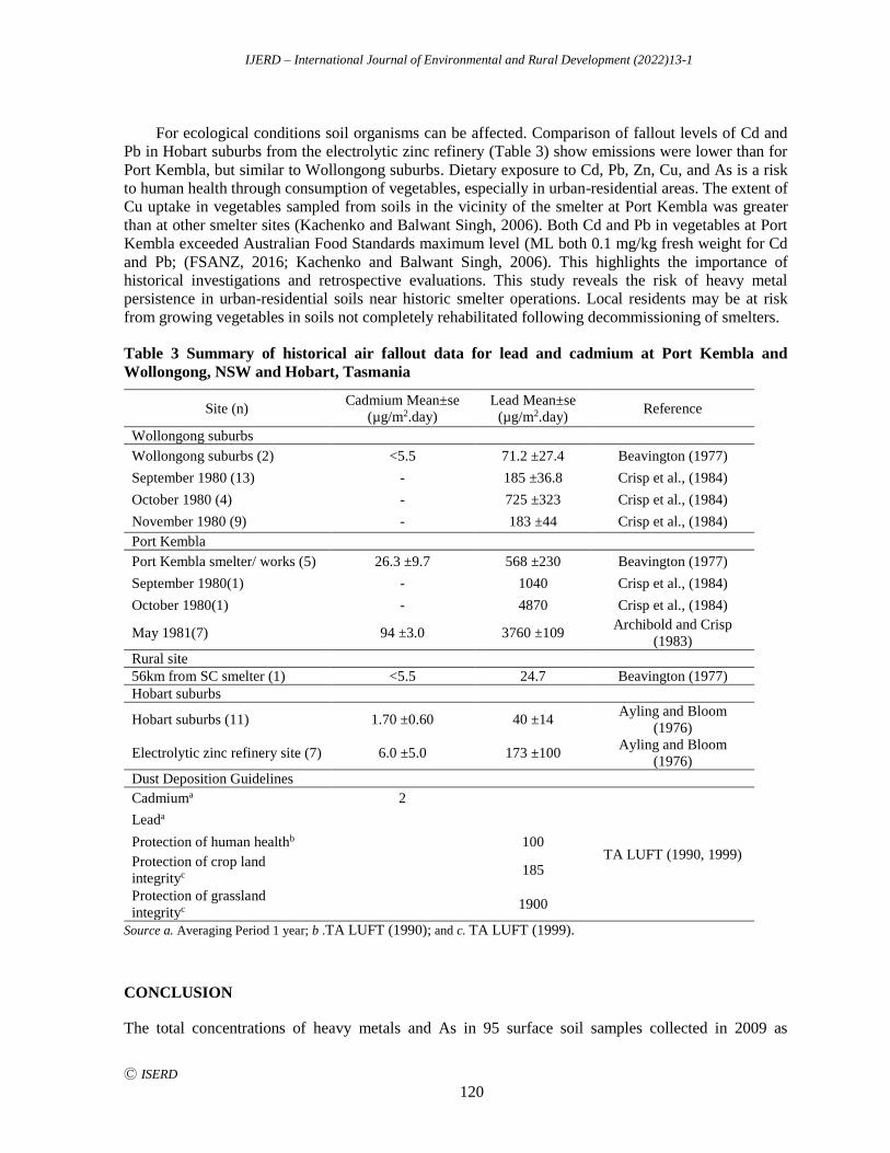
IJERD – International Journal of Environmental and Rural Development (2022)13-1
Ⓒ ISERD
120
For ecological conditions soil organisms can be affected. Comparison of fallout levels of Cd and
Pb in Hobart suburbs from the electrolytic zinc refinery (Table 3) show emissions were lower than for
Port Kembla, but similar to Wollongong suburbs. Dietary exposure to Cd, Pb, Zn, Cu, and As is a risk
to human health through consumption of vegetables, especially in urban-residential areas. The extent of
Cu uptake in vegetables sampled from soils in the vicinity of the smelter at Port Kembla was greater
than at other smelter sites (Kachenko and Balwant Singh, 2006). Both Cd and Pb in vegetables at Port
Kembla exceeded Australian Food Standards maximum level (ML both 0.1 mg/kg fresh weight for Cd
and Pb; (FSANZ, 2016; Kachenko and Balwant Singh, 2006). This highlights the importance of
historical investigations and retrospective evaluations. This study reveals the risk of heavy metal
persistence in urban-residential soils near historic smelter operations. Local residents may be at risk
from growing vegetables in soils not completely rehabilitated following decommissioning of smelters.
Table 3 Summary of historical air fallout data for lead and cadmium at Port Kembla and
Wollongong, NSW and Hobart, Tasmania
Site (n) Cadmium Mean±se
(µg/m2.day)
Lead Mean±se
(µg/m2.day) Reference
Wollongong suburbs
Wollongong suburbs (2) <5.5 71.2 ±27.4 Beavington (1977)
September 1980 (13) - 185 ±36.8 Crisp et al., (1984)
October 1980 (4) - 725 ±323 Crisp et al., (1984)
November 1980 (9) - 183 ±44 Crisp et al., (1984)
Port Kembla
Port Kembla smelter/ works (5) 26.3 ±9.7 568 ±230 Beavington (1977)
September 1980(1) - 1040 Crisp et al., (1984)
October 1980(1) - 4870 Crisp et al., (1984)
May 1981(7) 94 ±3.0 3760 ±109 Archibold and Crisp
(1983)
Rural site
56km from SC smelter (1) <5.5 24.7 Beavington (1977)
Hobart suburbs
Hobart suburbs (11) 1.70 ±0.60 40 ±14 Ayling and Bloom
(1976)
Electrolytic zinc refinery site (7) 6.0 ±5.0 173 ±100 Ayling and Bloom
(1976)
Dust Deposition Guidelines
Cadmiuma 2
TA LUFT (1990, 1999)
Leada
Protection of human healthb 100
Protection of crop land
integrityc 185
Protection of grassland
integrityc 1900
Source a. Averaging Period 1 year; b .TA LUFT (1990); and c. TA LUFT (1999).
CONCLUSION
The total concentrations of heavy metals and As in 95 surface soil samples collected in 2009 as
IJERD – International Journal of Environmental and Rural Development (2022)13-1
Ⓒ ISERD
121
percentile values provided better resolution of dispersion distance from the copper smelter at Port
Kembla. The comprehensive treatment of existing data by comparing historical data against current
guidelines was not previously possible until this study. Historical fallout data compared against current
heavy metal fall-out guidelines predicts past smelter emissions build-up in soil suggesting potential
risks to residents ingesting vegetables grown from contaminated urban soils.
ACKNOWLEDGEMENTS
The NSW EPA, Sydney NSW, Australia funded the literature review of lead and other heavy metals in
soil and roof dust in Wollongong and measures to manage any associated health risks.
REFERENCES
Ayling, G.M. and Bloom, H. 1976. Heavy metals analyses to characterize and estimate distribution of heavy
metals in dust fallout, Atmospheric Environment, 10, 61-64, Retrieved from
https://www.sciencedirect.com/science/article/pii/0004698176902614?via%3Dihub
Archibold, O.W. and Crisp, P.T. 1983. The distribution of airborne metals in the Illawarra region of New South
Wales, Australia. Applied Geography, 3 331-344, Retrieved from
https://www.sciencedirect.com/science/article/pii/0143622883900498
Beavington F. 1977. Trace elements in rainwater and dry deposition around a smelting complex, Environmental
Pollution, 13, 127-131, Retrieved from
https://www.sciencedirect.com/science/article/pii/0013932777900970
Chiaradia, M., Chenhall, B.E., Depers, A.M., Gulson, B.L. and Jones, B.G. 1997. Identification of historical lead
sources in roof dusts and recent lake sediments from an industrialized area: indications from lead isotopes.
Science of the Total Environment, 205, 107–128, Retrieved from
https://www.sciencedirect.com/science/article/pii/S004896979700199X
Crisp, P.T., Archibold, O.W. and Crisp, E.A. 1984. The use of wind direction data to predict pollution dispersal
around the Port Kembla industrial area, New South Wales. Australian Geographical Studies, 22, 243-260,
Retrieved from https://onlinelibrary.wiley.com/doi/epdf/10.1111/j.1467-8470.1984.tb00632.x
Food Standards Australia New Zealand (FSANZ). 2016. Australia New Zealand Food Standards Code –
Schedule 19 – Maximum levels of contaminants and natural toxicants, Australian Government, Canberra,
Australia, Retrieved from https://www.legislation.gov.au/Details/F2017C00333
Jafari, Y. 2009. Trace metal contamination of soils and sediments in the Port Kembla area, New South Wales,
Australia. MSc Dissertation, University of Wollongong, Australia.
Kachenko, A.G. and Singh, B. 2006. Heavy metals contamination in vegetables grown in urban and near smelter
contaminated sites in Australia, Water Air and Soil Pollution, 169, 101-123, Retrieved from
https://link.springer.com/content/pdf/10.1007/s11270-006-2027-1.pdf
National Environment Protection Council (NEPC) 2013. National Environment Protection (Assessment of Site
Contamination) Measure, National Environment Protection Council, Canberra, Australia, Retrieved from
http://www.nepc.gov.au/nepms/assessment-site-contamination
Noller, B.N. 2020a. Literature review of the levels of lead and other heavy metals in soil and roof dust in
Wollongong and measures to manage any associated health risks. NSW Environment Protection Authority,
Sydney, Australia. Retrieved from https://www.epa.nsw.gov.au/-/media/epa/corporate-
site/resources/community/literature-rreview-of-the-levels-of-lead-in-dust-in-
wollongong.pdf?la=en&hash=6161419554B16FD0C6F89CA450ED051DBFB53A4A
Noller, B.N. 2020b. Environmental Effects from Contamination of Agricultural Soils via Spraying and Dust
Application to Crops and Animals, International Journal of Environmental and Rural Development, 11, 69 -
74, Retrieved from https://iserd.net/ijerd111/11-1-11.pdf
Noller, B., Zheng, J., Huynh, T., Ng, J., Diacomanolis, V., Taga, R. and Harris, H. 2017. Lead Pathways Study–
Air. Health Risk Assessment of Contaminants to Mount Isa City. Mount Isa Mines Limited, Mount Isa,
Australia. Retrieved from
http://www.mountisamines.com.au/EN/sustainability/Pages/LEADPATHWAYSSTUDYPORTAL.aspx
Ruby, M. V., Davis, A., Schoof, R., Eberle, S. and Sellstone, C.M. 1996. Estimation of lead and arsenic

IJERD – International Journal of Environmental and Rural Development (2022)13-1
Ⓒ ISERD
122
bioavailability using a physiologically based extraction test, Environmental Science and Technology, 30,
422-430, Retrieved from https://pubs.acs.org/doi/10.1021/es950057z
Technische Anleitung zur Reinhaltung der Luft (TA LUFT) 1990, 1999. Technical Instructions on Air Quality
Control, Bundesministerium für Umwelt, Naturschutz und Reaktorsicherheit (Federal Environment Ministry),
Bonn, Germany, Retrieved from http://www.umweltbundesamt.de
IJERD – International Journal of Environmental and Rural Development (2022)13-1
Ⓒ ISERD
123
Utilizing Lead Isotope Tracing to Investigate Sustainable
Agriculture Practice in the Burdekin Catchment, Australia.
FIONA HENDERSON* The University of Queensland St Lucia, QLD 4072, Australia
Email: [email protected]
BARRY NOLLER The University of Queensland St Lucia, QLD 4072, Australia
TATIANA KOMAROVA Queensland Health Forensic Scientific Services, Brisbane, Australia
Received 31 January 2022 Accepted 25 April 2022 (*Corresponding Author)
Abstract The Burdekin delta is the largest sugarcane producing region in Australia (85,000 ha)
and a major coastal output to the Great Barrier Reef (GBR). Run-off from cultivation areas
contain heavy metals from fertilizers, contributing to elevated Cd, Hg, and Pb in waterways.
Validating the efficacy of sustainable agriculture practice is necessary to determine if current
strategies protect ecosystems and uphold environmental standards. The objective of this study is
to utilize Pb isotope tracing (207/206Pb and 208/206Pb) and elevated trace-elements (Cd, Hg, and
Pb) as a monitoring tool, to detect residual heavy metals from fertilizers and alternative
pollutant sources in the Burdekin catchment. Lead-isotope ratios from dry-season samples of
embankment soils/sediment (n=15, 2016, 2019) and water (n=35, 2016-2020), reveals sources
of natural forest soils, cane soils (fertilizer enriched), ambient dust, and historic coal fly-ash
(Collinsville Power Station). Pb isotope compositions and low levels of heavy metals
(soil/sediment: TCd 0.11 mg/kg, THg 0.03 mg/kg and TPb 11.02 mg/kg; estuary: THg 0.011
μg/L and TPb 4.99 μg/L) indicate that fertilizers applied to soils have minimal impact on
Burdekin waterways during the dry-season, suggesting effective agricultural practice and
sustainable irrigation control.
Keywords agriculture, sustainability, sustainable practice, lead isotope, source-tracing
INTRODUCTION
The GBR is the largest reef ecosystem on the planet (344,400 km2) and a World Heritage site located
off the coast of Queensland (QLD), Australia (Coggan, et al., 2021). Land-runoff from coastal
catchments can adversely impact the GBR (Lewis, et al., 2021). Agricultural mismanagement, (i.e.
fertilizer overuse and uncontrolled irrigation run-off) contributes to water quality risk through the
accumulation of heavy metals in soil and remobilization to waterways (Table 1; Alengebawy, et al.,
2021; Coggan, et al., 2021). In literature, research has conventionally used elevated heavy metals to
establish pollutant presence and Pb-isotopes to trace pollutant source by providing a measure of
geologic age (Table 1; Diaz-somoano et al., 2009; Lottermoser, 2009; Alengebawy et al., 2021).
Following ~10 years of sugarcane cropping, Rayment (2007) noted Cd and Hg were elevated in QLD
cane soils. Davis et al., (2008) detected sugarcane pesticides in Burdekin waterways. Extended
fertilizer use is known to degrade soil fertility and productivity (Ping et al., 2020). Fertilizer overuse
burdens the environment, economic and social value of both the GBR and the sugarcane industry
(DAE, 2017). Sugarcane production is $1.33 billion AUD (gross); the Burdekin represents 31% or
erd
Research article
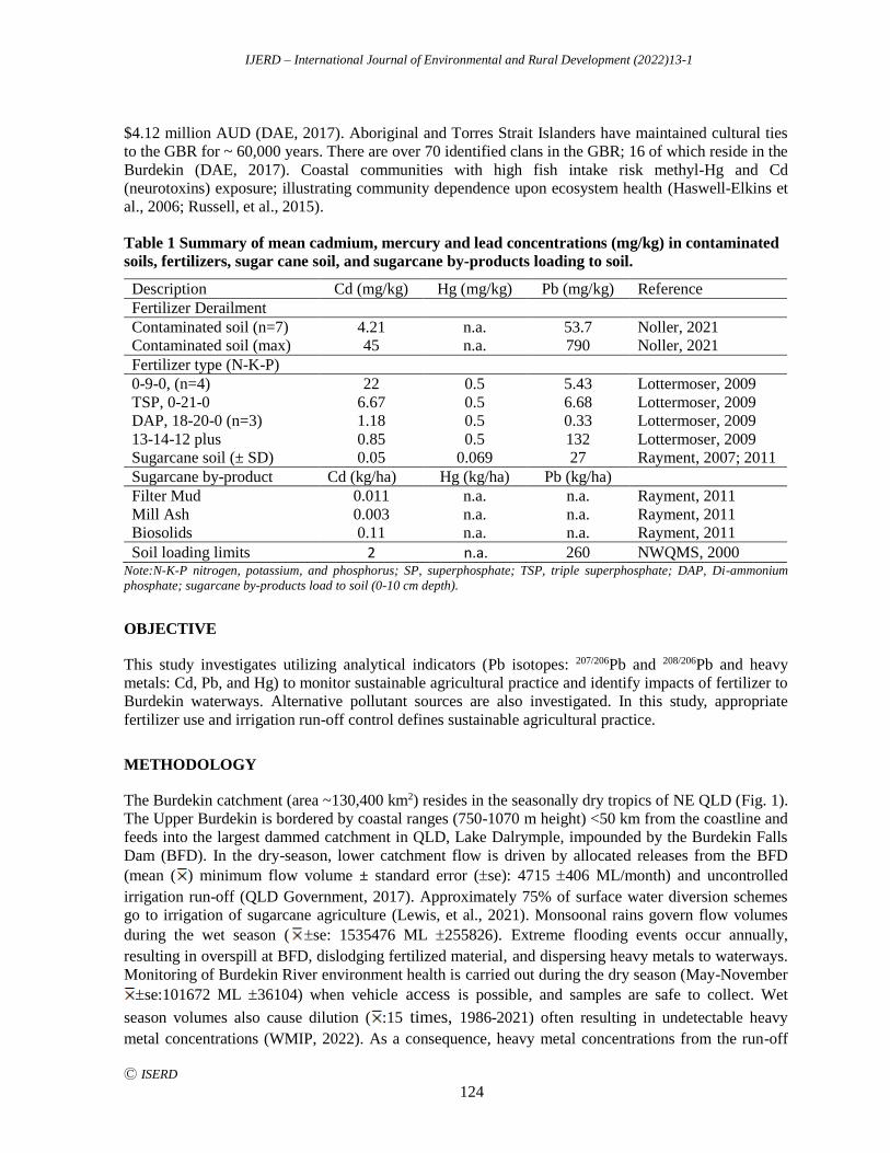
IJERD – International Journal of Environmental and Rural Development (2022)13-1
Ⓒ ISERD
124
$4.12 million AUD (DAE, 2017). Aboriginal and Torres Strait Islanders have maintained cultural ties
to the GBR for ~ 60,000 years. There are over 70 identified clans in the GBR; 16 of which reside in the
Burdekin (DAE, 2017). Coastal communities with high fish intake risk methyl-Hg and Cd
(neurotoxins) exposure; illustrating community dependence upon ecosystem health (Haswell-Elkins et
al., 2006; Russell, et al., 2015).
Table 1 Summary of mean cadmium, mercury and lead concentrations (mg/kg) in contaminated
soils, fertilizers, sugar cane soil, and sugarcane by-products loading to soil.
Description Cd (mg/kg) Hg (mg/kg) Pb (mg/kg) Reference
Fertilizer Derailment
Contaminated soil (n=7) 4.21 n.a. 53.7 Noller, 2021
Contaminated soil (max) 45 n.a. 790 Noller, 2021
Fertilizer type (N-K-P)
0-9-0, (n=4) 22 0.5 5.43 Lottermoser, 2009
TSP, 0-21-0 6.67 0.5 6.68 Lottermoser, 2009
DAP, 18-20-0 (n=3) 1.18 0.5 0.33 Lottermoser, 2009
13-14-12 plus 0.85 0.5 132 Lottermoser, 2009
Sugarcane soil (± SD) 0.05 0.069 27 Rayment, 2007; 2011
Sugarcane by-product Cd (kg/ha) Hg (kg/ha) Pb (kg/ha)
Filter Mud 0.011 n.a. n.a. Rayment, 2011
Mill Ash 0.003 n.a. n.a. Rayment, 2011
Biosolids 0.11 n.a. n.a. Rayment, 2011
Soil loading limits 2 n.a. 260 NWQMS, 2000 Note:N-K-P nitrogen, potassium, and phosphorus; SP, superphosphate; TSP, triple superphosphate; DAP, Di-ammonium
phosphate; sugarcane by-products load to soil (0-10 cm depth).
OBJECTIVE
This study investigates utilizing analytical indicators (Pb isotopes: 207/206Pb and 208/206Pb and heavy
metals: Cd, Pb, and Hg) to monitor sustainable agricultural practice and identify impacts of fertilizer to
Burdekin waterways. Alternative pollutant sources are also investigated. In this study, appropriate
fertilizer use and irrigation run-off control defines sustainable agricultural practice.
METHODOLOGY
The Burdekin catchment (area ~130,400 km2) resides in the seasonally dry tropics of NE QLD (Fig. 1).
The Upper Burdekin is bordered by coastal ranges (750-1070 m height) <50 km from the coastline and
feeds into the largest dammed catchment in QLD, Lake Dalrymple, impounded by the Burdekin Falls
Dam (BFD). In the dry-season, lower catchment flow is driven by allocated releases from the BFD
(mean ( ) minimum flow volume ± standard error (se): 4715 406 ML/month) and uncontrolled
irrigation run-off (QLD Government, 2017). Approximately 75% of surface water diversion schemes
go to irrigation of sugarcane agriculture (Lewis, et al., 2021). Monsoonal rains govern flow volumes
during the wet season ( se: 1535476 ML 255826). Extreme flooding events occur annually,
resulting in overspill at BFD, dislodging fertilized material, and dispersing heavy metals to waterways.
Monitoring of Burdekin River environment health is carried out during the dry season (May-November
se:101672 ML 36104) when vehicle access is possible, and samples are safe to collect. Wet
season volumes also cause dilution ( :15 times, 1986-2021) often resulting in undetectable heavy
metal concentrations (WMIP, 2022). As a consequence, heavy metal concentrations from the run-off

IJERD – International Journal of Environmental and Rural Development (2022)13-1
Ⓒ ISERD
125
events are likely to pose greatest environmental risk during the dry-season, when perennial river
volumes have returned to “steady-state” flows. Embankment soils/sediments (n=15, 0-100 mm depth,
2016, 2019) and water (n=35, unfiltered, 2016, 2018, 2019 and 2020) were sampled in the Upper and
Lower (estuary) sub-catchments of the Burdekin watershed during the dry season. Water and sediment
samples in 2016 and 2018 (Fig. 1) were collected in June and July to demonstrate dry-season sources
of heavy metals, and input of soil seepage, representing concentrations coinciding with fall of the
hydrographic curve. Samples in 2019 and 2020 were collected in late November and early December
(increase in hydrographic curve). Thus, sample collections in 2019 and 2020 (Fig.1) captured first
flush and post run-off heavy metal concentrations from the start of the wet-season, including any input
from agricultural fertilizers.
Fig. 1 Study area and sample site location map.
Water and soil/sediment were analyzed at the NATA accredited laboratory (ISO/IEC 17025,
2017) Inorganic Chemistry, Queensland Health and Forensic Scientific Services, Coopers Plains, QLD
4108, Australia. Agilent 8800 triple quadrupole inductively coupled plasma mass spectrometer (ICP-
QQQ; Agilent Technologies, Santa Clara, CA, USA) measured heavy metal concentrations. Internal
standards, spikes and certified reference materials (CRM, TM-28) were used for quality assurance and
quality control (QA/QC). QC for Hg analysis used 5% Hg (v/v) HNO3 solution (SRM ID 3133, SRM
Lot # 060204; High Purity Standards, Charleston, SC 29423, USA). Pb isotope ratios (207/206Pb and 208/206Pb) in water, soil and sediment digests were determined by Agilent 8800 ICP-QQQ (CRMs:
GXR-1, JG-2, JR-1, JSD-1, JSD-2). Soil/sediment (including CRMs) were prepared following the
standard operating procedure (SOP 18191). Water samples were analyzed directly after addition of 0.2
mL High Purity HNO3 to total 10mL. Pb isotope stock standard solution was used from Choice
Analytical and prepared via serial dilution. Ratios were calculated using instrument software. Blank
corrections were made with 0.5mL High Purity HNO3 in 10mL of deionized water. The ICP-QQQ is
tuned following manufactures recommendations (Ref 11.3) and QIS: 30638 Operational Guidelines –
ICP-MS. Total Hg measurements in soil were analyzed by National Measurement Institute Department
of Industry, Innovation and Science, Sydney, Australia.

IJERD – International Journal of Environmental and Rural Development (2022)13-1
Ⓒ ISERD
126
RESULTS AND DISCUSSION
Mean se of total (T) Hg (0.016 ±0.002 μg/L) and TPb (0.15 ±0.02 μg/L) in freshwater remain below
ANZG (2018) default guideline values (DGVs) (Table 2). Mercury ( se: 0.011 ± 0.001) in the
estuary are below marine DGVs. In one estuary sample, TPb (4.99 μg/L) is above a marine DGV of 4.4
μg/L (Table 2). At < 2 mm size fraction, embankment soil/sediment samples reflect se of TCd (0.11
0.10 mg/kg), THg (0.03 0.004 mg/kg) and TPb (11.02 1.65 mg/kg), all below soil and sediment
DGVs throughout the upper and lower catchments (Table 3). The majority of Burdekin soils/sediments
(80%) and water (72%) samples, reflect isotopic compositions of cane soil (fertilizer enriched) and
natural forest soils (Lottermoser, 2009; Fig. 2A and B). Isotope tracing also suggests TPb Burdekin
soils/sediments and waters are reflective of residual coal fly ash and ambient-background dust (Turull
et al., 2018). NSW coal fly ash signatures (Fig. 2; Diaz-somoana et al., 2009) identified in Burdekin
samples likely reflect historic contributions from a nearby powerplant. A nearby coal-electricity
generation station is the Collinsville Power Plant (Fig. 1). Based on current flow statistics, the
Burdekin River is highly variable, considerably influencing annual sediment and nutrient loads (Brodie
and Bainbridge, 2008). This is apparent in Pb isotope compositions that vary with sample years (Fig.
2B). In 2016, isotope ratios trend toward phosphate-fertilizers and are very similar to ratios found in
fertilizer-enriched cultivation areas of the Tully catchment (QLD; Turull et al., 2018). In 2018 and
2019, ratios in fresh and estuarian waters reflect a mixture of sources: NSW coal fly ash, dust, natural
forest soils and leaded petrol (1996) (Fig. 2 B).
Table 2 Total Hg and Pb (μg/L) in the Burdekin River from 2016, 2018, 2019, and 2020.
Freshwater THg (μg/L) TPb (μg/L) Saltwater THg* (μg/L) TPb (μg/L)
N 24 24 N 11 1
Mean 0.016 0.146 Mean 0.011 4.99
SD 0.01 0.079 SD 0.004 n.a.
SE 0.002 0.018 SEM 0.001 n.a.
Min 0.005 0.053 Min 0.004 n.a.
Median 0.013 0.111 Median 0.011 n.a.
80 percentile 0.022 0.149 80 percentile 0.011 n.a.
95 percentile 0.027 0.204 95 percentile 0.015 n.a.
99 percentile 0.044 0.372 99 percentile 0.018 n.a.
Max 0.048 0.414 Max 0.019 n.a.
Toxicant DGV 0.06a 3.4b Toxicant DGV 0.1a 4.4b Note: N, count; SD, standard deviation; SE, standard error, *Collected in 2019 and 2020 n=11,
a 99% level of protection for Hg. b 95 % level of protection of species for Pb (ANZG-water, 2018)
BFD stores are replenished during the wet-season from moonsoonal rains (cf. Townsville
rainwater se: pH 6 0.1; Na 1 4 mg/L, Cl 17 7 mg/L, from seawater) and released in the dry
season for irrigation (Crosbie et al., 2012). Site 7-19 samples, taken below BFD, captures wet-season
water stores from dam releases. This is evident in 7-19 water characteristics, where pH and electrical
conductivity (EC) are influenced by wet-season rains ( se pH 7.4 0.01, EC: 193 1.1 µS/cm).
Upstream (dry season) waters ( se pH 8.5 0.02, EC: 558 21.1 µS/cm) have higher
alkalinity/hardness and EC demonstrating differences between wet/dry waters. In the dry season, heavy
metal re-mobilization from sugarcane areas has low environmental, economic and social risk; with one
sample, TPb of 4.99 μg/L (2019), above DGVs of 4.4 μg/L (Table 2). Isotope tracing reveals that
fertilizer signals remain low throughout the catchment, suggesting sustainble irrigtion practice and run-
off control. The impact of fertilizer use in this study is likely minimized due to a delayed start to the
IJERD – International Journal of Environmental and Rural Development (2022)13-1
Ⓒ ISERD
127
wet season in 2019 and 2020 resulting in reduced rainfall run-off events. It is recommended that on-
land investigations should be carried out to further inform on fertilizer rates.
Table 3 Total Cd, Hg and Pb (mg/kg), <2mm size fraction soil/sediment from 2016 and 2019.
Summary TCd (mg/kg) THg (mg/kg) TPb (mg/kg)
n 14 15 14
No < values 4 9 0
Mean 0.11 0.03 11.02
SD 0.37 0.01 6.16
SE 0.10 0.004 1.65
Min 0.00 0.02 2.40
Median 0.02 0.03 9.13
80 percentile 0.04 0.04 16.00
95 percentile 0.53 0.05 21.10
99 percentile 1.23 0.05 24.22
Max 1.40 0.05 25.00
Toxicant DGV* 1.5 0.15 50 Note: * No defined level of protection available (ANZG-sediment, 2018)
Fig. 2 Pb isotope ratios, 207Pb/206Pb and 208Pb/206Pb, suggest natural and anthropogenic
sources (A) soil/sediment (2016 and 2019) and (B) water (2016, 2018, and 2019).
A
B
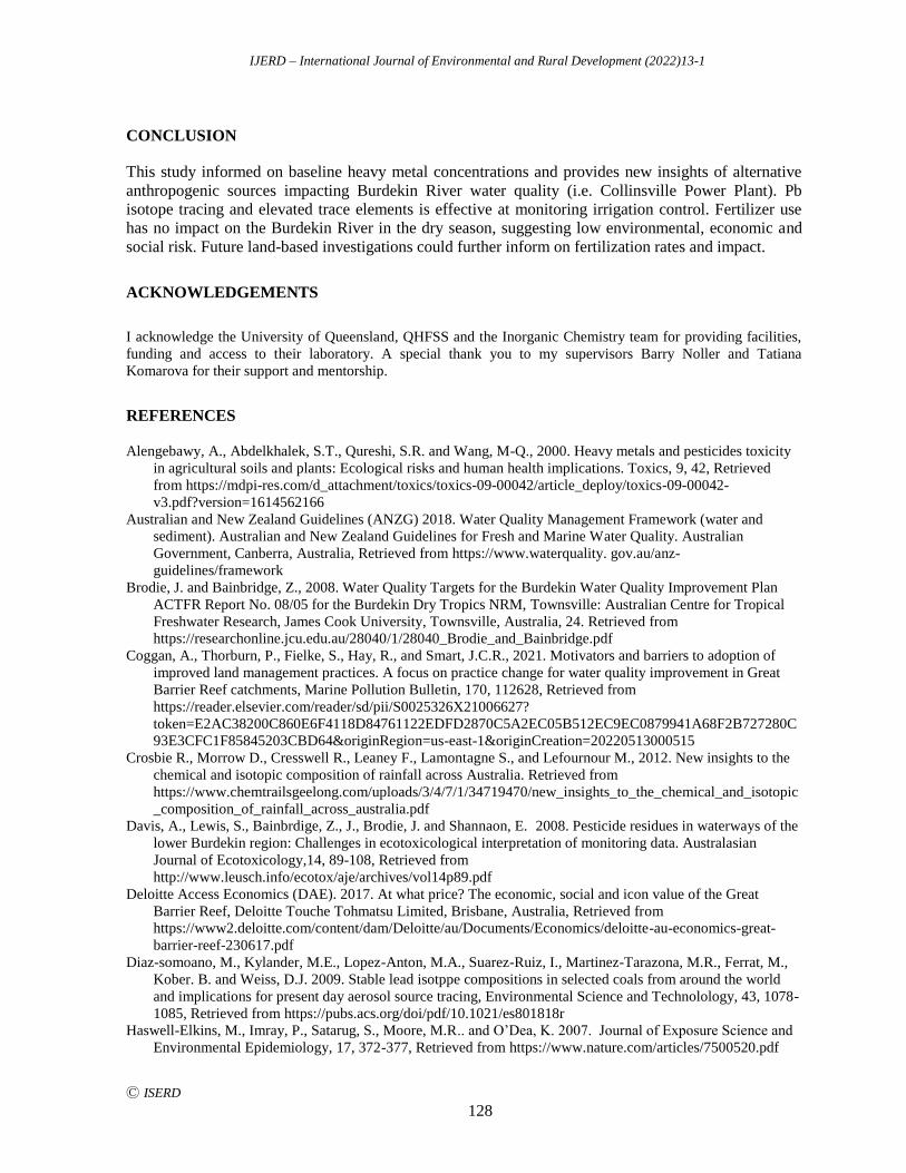
IJERD – International Journal of Environmental and Rural Development (2022)13-1
Ⓒ ISERD
128
CONCLUSION
This study informed on baseline heavy metal concentrations and provides new insights of alternative
anthropogenic sources impacting Burdekin River water quality (i.e. Collinsville Power Plant). Pb
isotope tracing and elevated trace elements is effective at monitoring irrigation control. Fertilizer use
has no impact on the Burdekin River in the dry season, suggesting low environmental, economic and
social risk. Future land-based investigations could further inform on fertilization rates and impact.
ACKNOWLEDGEMENTS
I acknowledge the University of Queensland, QHFSS and the Inorganic Chemistry team for providing facilities,
funding and access to their laboratory. A special thank you to my supervisors Barry Noller and Tatiana
Komarova for their support and mentorship.
REFERENCES
Alengebawy, A., Abdelkhalek, S.T., Qureshi, S.R. and Wang, M-Q., 2000. Heavy metals and pesticides toxicity
in agricultural soils and plants: Ecological risks and human health implications. Toxics, 9, 42, Retrieved
from https://mdpi-res.com/d_attachment/toxics/toxics-09-00042/article_deploy/toxics-09-00042-
v3.pdf?version=1614562166
Australian and New Zealand Guidelines (ANZG) 2018. Water Quality Management Framework (water and
sediment). Australian and New Zealand Guidelines for Fresh and Marine Water Quality. Australian
Government, Canberra, Australia, Retrieved from https://www.waterquality. gov.au/anz-
guidelines/framework
Brodie, J. and Bainbridge, Z., 2008. Water Quality Targets for the Burdekin Water Quality Improvement Plan
ACTFR Report No. 08/05 for the Burdekin Dry Tropics NRM, Townsville: Australian Centre for Tropical
Freshwater Research, James Cook University, Townsville, Australia, 24. Retrieved from
https://researchonline.jcu.edu.au/28040/1/28040_Brodie_and_Bainbridge.pdf
Coggan, A., Thorburn, P., Fielke, S., Hay, R., and Smart, J.C.R., 2021. Motivators and barriers to adoption of
improved land management practices. A focus on practice change for water quality improvement in Great
Barrier Reef catchments, Marine Pollution Bulletin, 170, 112628, Retrieved from
https://reader.elsevier.com/reader/sd/pii/S0025326X21006627?
token=E2AC38200C860E6F4118D84761122EDFD2870C5A2EC05B512EC9EC0879941A68F2B727280C
93E3CFC1F85845203CBD64&originRegion=us-east-1&originCreation=20220513000515
Crosbie R., Morrow D., Cresswell R., Leaney F., Lamontagne S., and Lefournour M., 2012. New insights to the
chemical and isotopic composition of rainfall across Australia. Retrieved from
https://www.chemtrailsgeelong.com/uploads/3/4/7/1/34719470/new_insights_to_the_chemical_and_isotopic
_composition_of_rainfall_across_australia.pdf
Davis, A., Lewis, S., Bainbrdige, Z., J., Brodie, J. and Shannaon, E. 2008. Pesticide residues in waterways of the
lower Burdekin region: Challenges in ecotoxicological interpretation of monitoring data. Australasian
Journal of Ecotoxicology,14, 89-108, Retrieved from
http://www.leusch.info/ecotox/aje/archives/vol14p89.pdf
Deloitte Access Economics (DAE). 2017. At what price? The economic, social and icon value of the Great
Barrier Reef, Deloitte Touche Tohmatsu Limited, Brisbane, Australia, Retrieved from
https://www2.deloitte.com/content/dam/Deloitte/au/Documents/Economics/deloitte-au-economics-great-
barrier-reef-230617.pdf
Diaz-somoano, M., Kylander, M.E., Lopez-Anton, M.A., Suarez-Ruiz, I., Martinez-Tarazona, M.R., Ferrat, M.,
Kober. B. and Weiss, D.J. 2009. Stable lead isotppe compositions in selected coals from around the world
and implications for present day aerosol source tracing, Environmental Science and Technolology, 43, 1078-
1085, Retrieved from https://pubs.acs.org/doi/pdf/10.1021/es801818r
Haswell-Elkins, M., Imray, P., Satarug, S., Moore, M.R.. and O’Dea, K. 2007. Journal of Exposure Science and
Environmental Epidemiology, 17, 372-377, Retrieved from https://www.nature.com/articles/7500520.pdf
IJERD – International Journal of Environmental and Rural Development (2022)13-1
Ⓒ ISERD
129
Lewis, S.E., Bartley, R., Wilkinson, S.N., Bainbridge, Z.T., Henderson, A.E., James, C.S., Irvine S.A., and
Brodie, J.E. 2021. Land use change in the river basins of the Great Barrier Reef, 1860 to 2019: A foundation
for understanding environmental history across the catchment to reef continuum. Marine Pollution Bulletin,
166, 112193, Retrieved by https://reader.elsevier
.com/reader/sd/pii/S0025326X21002277?token=26473E4B2A932AD7546D573A04327A0633E4B68FB02
D5B20B43BBB7A6065C49CDDCEAFB5599531C6A22874838231E498&originRegion=us-east-
1&originCreation=20220513025140
Lottermoser, B.G. 2009. Trace metal enrichment in sugarcane soils due to the long-term application of fertilisers,
North Queensland, Australia: geochemical and Pb, Sr, and U isotopic compositions, Australian Journal of
Soil Research, 47, 311-320, Retrieved from https://www.publish.csiro.au/sr/pdf/SR06178
Noller, B.N. 2020. Environmental Effects from Contamination of Agricultural Soils via Spraying and Dust
Application to Crops and Animals, International Journal of Environmental and Rural Development, 11, 69 -
74, Retrieved from https://iserd.net/ijerd111/11-1-11.pdf
National Water Quality Management Strategy (NWQMS) 2000. National water quality management strategy.
Australian and New Zealand Environment and Conservation Council, Canberra, Australia, Retrieved from
https://www.waterquality.gov.au/anz-guidelines/resources/previous-guidelines/anzecc-armcanz-2000
Ping, A., Jin, K., Alengebawy, A., Elsayed, M., Meng, L., Mengdi, C., and Ran, Y. 2020. Effect of application of
different biogas fertilizer on eggplant production: Analysis of fertilizer value and risk assessment..
Environmental Technology and Innovation, 19, 101019, Retrieved from
https://reader.elsevier.com/reader/sd/pii/S2352186420306088?token=1710864C2AE5E081667A9807A3851
74D24BBEFBD50B6C7AA048F0F367C8FB76B1CD5F9ADC7EB6E5ABE5BDE9BB554FB6E&originRe
gion=us-east-1&originCreation=20220513032114
Queensland Government, 2017. Burdekin Haughton Water Supply Scheme Operations Manual. Retrieved from
https://www.sunwater.com.au/wp-content/uploads/Home/Schemes/Burdekin-Haughton/Burdekin-Haughton-
WSS-Operations-Manual_May_2017.pdf
Rayment, G.E. 2007. Northeast Australian experience in minimizing environmental harm from waste recycling
and potential pollutants of soil and water. Communications in Soil Science and Plant Analysis, 36, 121-131,
Retrieved from https://www.tandfonline.com/doi/pdf/10.1081/CSS-
200043006?casa_token=u5fJaTR3QtUAAAAA:7Qml9jfmSCnGncVZsF3fe0ynr929P-
Q5YxMQB3IdxuE9koClmXMabH597iaiHhQo25egRWRoDBFB
Rayment, G.E. 2011. Cadmium in sugar cane and vegetable systems of Northeast Australia, Communications in
Soil Science and Plant Analysis, 36, 597-608, Retrieved from
https://www.tandfonline.com/doi/pdf/10.1081/CSS-200043296?needAccess=true
Russell, S., Sullivan, C.A. and Reichelt-Brushett, A. J., 2015. Aboriginal consumption of estuarine food
resources and potential implications for health through trace metal exposure; A study in Gumbaynggirr
Country, Australia, PLoS ONE 10, e013068910, Retrieved from
https://journals.plos.org/plosone/article/file?id=10.1371/journal.pone.0130689&type=printable
Turull, M., Komarova, T., Noller, B., Fontàs, C. and Díez, S. 2018. Evaluation of mercury in freshwater
environment impacted by an organomercury fungicide using diffusive gradient in thin films, Science of the
Total Environment, 621, 1475-1484, Retrieved from
https://www.sciencedirect.com/science/article/pii/S0048969717327845?via%3Dihub
Water Monitoring Information Portal (WMIP) 2022. Burdekin River wet season volumes 120006B, Department
of Regional Development, Manufacturing and Water, Queensland Government, Brisbane, Australia,
Retrieved from https://water-monitoring.information.qld.gov.au
IJERD – International Journal of Environmental and Rural Development (2022)13-1
Ⓒ ISERD
130
Enhancement of carbon fiber electrode performance using
lactic acid bacteria and steelmaking slag
NARONG TOUCH* Faculty of Regional Environment Science, Tokyo University of Agriculture, Tokyo, Japan
Email: [email protected]
TADASHI HIBINO Graduate School of Advanced Science and Engineering, Hiroshima University, Hiroshima, Japan
Received 14 January 2022 Accepted 25 April 2022 (*Corresponding Author)
Abstract Microbial fuel cell technology (MFCT) provides many benefits to rural regions, such
as organic waste disposal and renewable energy recovery. However, its performance is low and
must be improved for practical uses. Mixing steelmaking slag (SS) and lactic acid bacteria
(LAB) with sediment can enhance the MFCT performance owing to LAB and iron ions
dissolved from SS attaching to the electrode surface. This study proposes a simple method for
attaching LAB and iron ions on carbon fiber electrode and subsequently evaluating its
performance. A carbon fiber electrode was placed in a bottle containing tap water, SS, LAB,
and bamboo powder (as nutrients for bacteria) for 7 days to allow LAB and iron ions to adhere
to its surface. The electrode was then used as the cathode of MFCT. Results showed a decrease
in the electrode potential and a consequent reduction in MFCT performance owing to the
attached LAB and iron ions. The performance improved after the electrode was oxidized,
suggesting that aeration is required during attachment to prevent the decrease in electrode
potential. After 1 month of electricity generation, the electrode with the attachment produced
high electrical current and exhibited low decrease in MFCT performance owing to electricity
generation. Therefore, attaching LAB and iron ions on the electrode surface can improve the
electrode performance and prevent performance degradation owing to electricity generation.
Keywords Microbial fuel cell, performance, electrode potential, attachment, steelmaking slag,
lactic acid bacteria
INTRODUCTION
Microbial fuel cell technology (MFCT) offers many benefits for rural regions, particularly in
developing countries. For example, this method can be used to treat agricultural wastewater, household
sewage, and organic waste, provide electricity to households, and recycle resources to farmlands
(Touch et al., 2020). However, the performance of MFCT remains low and must be improved for
practical uses. MFCT efficiency depends on the cathode and anode. A low electrode performance will
restrain the overall performance of MFCT. According to Yamasaki et al. (2018), various types of
potential losses occur during electron flow to an electrode. One of which is activation loss that strongly
influences electrode performance. Activation loss should be minimized via pretreating the electrode to
obtain a high MFCT performance. Furthermore, this loss increases during electricity generation owing
to the crystallization of ions present in water on the electrode surface. Thus, a method for minimizing
the performance reduction owing to electricity generation is necessary.
Adsorption of bacteria or metal ions on the electrode surface is a method for improving the
electrode performance. Wang et al. (2009) successfully enhanced electrode performance by activating
the bacteria at the electrode and consequently reducing potential losses. The boosted electrode
erd
Research article
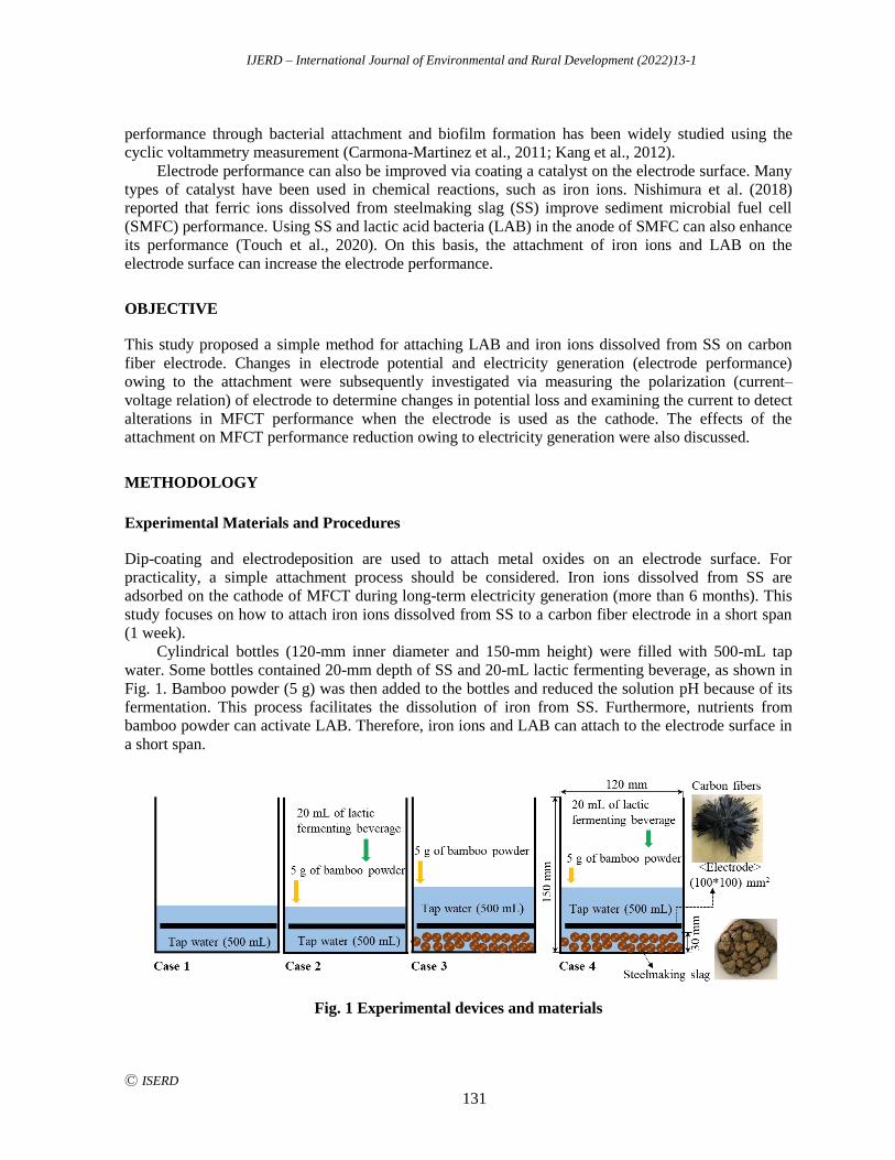
IJERD – International Journal of Environmental and Rural Development (2022)13-1
Ⓒ ISERD
131
performance through bacterial attachment and biofilm formation has been widely studied using the
cyclic voltammetry measurement (Carmona-Martinez et al., 2011; Kang et al., 2012).
Electrode performance can also be improved via coating a catalyst on the electrode surface. Many
types of catalyst have been used in chemical reactions, such as iron ions. Nishimura et al. (2018)
reported that ferric ions dissolved from steelmaking slag (SS) improve sediment microbial fuel cell
(SMFC) performance. Using SS and lactic acid bacteria (LAB) in the anode of SMFC can also enhance
its performance (Touch et al., 2020). On this basis, the attachment of iron ions and LAB on the
electrode surface can increase the electrode performance.
OBJECTIVE
This study proposed a simple method for attaching LAB and iron ions dissolved from SS on carbon
fiber electrode. Changes in electrode potential and electricity generation (electrode performance)
owing to the attachment were subsequently investigated via measuring the polarization (current–
voltage relation) of electrode to determine changes in potential loss and examining the current to detect
alterations in MFCT performance when the electrode is used as the cathode. The effects of the
attachment on MFCT performance reduction owing to electricity generation were also discussed.
METHODOLOGY
Experimental Materials and Procedures
Dip-coating and electrodeposition are used to attach metal oxides on an electrode surface. For
practicality, a simple attachment process should be considered. Iron ions dissolved from SS are
adsorbed on the cathode of MFCT during long-term electricity generation (more than 6 months). This
study focuses on how to attach iron ions dissolved from SS to a carbon fiber electrode in a short span
(1 week).
Cylindrical bottles (120-mm inner diameter and 150-mm height) were filled with 500-mL tap
water. Some bottles contained 20-mm depth of SS and 20-mL lactic fermenting beverage, as shown in
Fig. 1. Bamboo powder (5 g) was then added to the bottles and reduced the solution pH because of its
fermentation. This process facilitates the dissolution of iron from SS. Furthermore, nutrients from
bamboo powder can activate LAB. Therefore, iron ions and LAB can attach to the electrode surface in
a short span.
Fig. 1 Experimental devices and materials
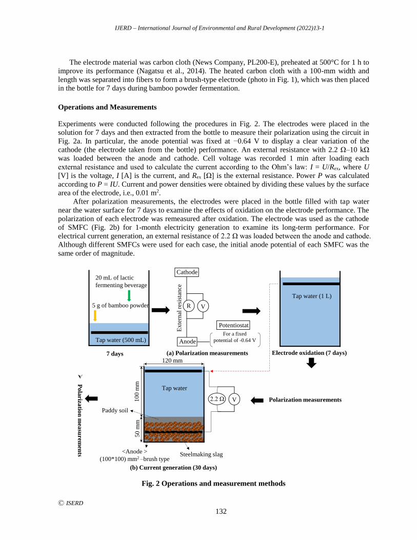
IJERD – International Journal of Environmental and Rural Development (2022)13-1
Ⓒ ISERD
132
The electrode material was carbon cloth (News Company, PL200-E), preheated at 500°C for 1 h to
improve its performance (Nagatsu et al., 2014). The heated carbon cloth with a 100-mm width and
length was separated into fibers to form a brush-type electrode (photo in Fig. 1), which was then placed
in the bottle for 7 days during bamboo powder fermentation.
Operations and Measurements
Experiments were conducted following the procedures in Fig. 2. The electrodes were placed in the
solution for 7 days and then extracted from the bottle to measure their polarization using the circuit in
Fig. 2a. In particular, the anode potential was fixed at −0.64 V to display a clear variation of the
cathode (the electrode taken from the bottle) performance. An external resistance with 2.2 Ω–10 kΩ
was loaded between the anode and cathode. Cell voltage was recorded 1 min after loading each
external resistance and used to calculate the current according to the Ohm’s law: I = U/Rex, where U
[V] is the voltage, I [A] is the current, and Rex [Ω] is the external resistance. Power P was calculated
according to P = IU. Current and power densities were obtained by dividing these values by the surface
area of the electrode, i.e., 0.01 m2.
After polarization measurements, the electrodes were placed in the bottle filled with tap water
near the water surface for 7 days to examine the effects of oxidation on the electrode performance. The
polarization of each electrode was remeasured after oxidation. The electrode was used as the cathode
of SMFC (Fig. 2b) for 1-month electricity generation to examine its long-term performance. For
electrical current generation, an external resistance of 2.2 Ω was loaded between the anode and cathode.
Although different SMFCs were used for each case, the initial anode potential of each SMFC was the
same order of magnitude.
Steelmaking slag
Tap water (500 mL)
5 g of bamboo powder
20 mL of lactic
fermenting beverage
7 days (a) Polarization measurements
Anode
Cathode
R
Ex
tern
al r
esis
tan
ce
V
Potentiostat
For a fixed
potential of -0.64 V
Tap water (1 L)
Electrode oxidation (7 days)
Polarization measurements
(b) Current generation (30 days)
P
ola
rizatio
n m
easu
remen
ts <Anode >
(100*100) mm2 –brush type
Tap water
50
mm
10
0 m
m
120 mm
Paddy soil
2.2 Ω V
Fig. 2 Operations and measurement methods
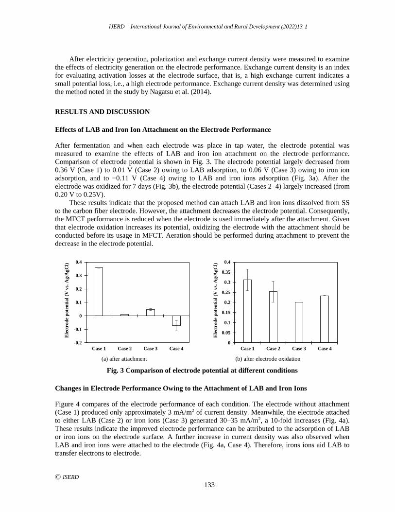
IJERD – International Journal of Environmental and Rural Development (2022)13-1
Ⓒ ISERD
133
After electricity generation, polarization and exchange current density were measured to examine
the effects of electricity generation on the electrode performance. Exchange current density is an index
for evaluating activation losses at the electrode surface, that is, a high exchange current indicates a
small potential loss, i.e., a high electrode performance. Exchange current density was determined using
the method noted in the study by Nagatsu et al. (2014).
RESULTS AND DISCUSSION
Effects of LAB and Iron Ion Attachment on the Electrode Performance
After fermentation and when each electrode was place in tap water, the electrode potential was
measured to examine the effects of LAB and iron ion attachment on the electrode performance.
Comparison of electrode potential is shown in Fig. 3. The electrode potential largely decreased from
0.36 V (Case 1) to 0.01 V (Case 2) owing to LAB adsorption, to 0.06 V (Case 3) owing to iron ion
adsorption, and to −0.11 V (Case 4) owing to LAB and iron ions adsorption (Fig. 3a). After the
electrode was oxidized for 7 days (Fig. 3b), the electrode potential (Cases 2–4) largely increased (from
0.20 V to 0.25V).
These results indicate that the proposed method can attach LAB and iron ions dissolved from SS
to the carbon fiber electrode. However, the attachment decreases the electrode potential. Consequently,
the MFCT performance is reduced when the electrode is used immediately after the attachment. Given
that electrode oxidation increases its potential, oxidizing the electrode with the attachment should be
conducted before its usage in MFCT. Aeration should be performed during attachment to prevent the
decrease in the electrode potential.
-0.2
-0.1
0
0.1
0.2
0.3
0.4
Case 1 Case 2 Case 3 Case 4
Ele
ctro
de
pote
nti
al
(V v
s. A
g/A
gC
l)
0
0.05
0.1
0.15
0.2
0.25
0.3
0.35
0.4
Case 1 Case 2 Case 3 Case 4
Ele
ctro
de
pote
nti
al
(V v
s. A
g/A
gC
l)
(a) after attachment (b) after electrode oxidation
Fig. 3 Comparison of electrode potential at different conditions
Changes in Electrode Performance Owing to the Attachment of LAB and Iron Ions
Figure 4 compares of the electrode performance of each condition. The electrode without attachment
(Case 1) produced only approximately 3 mA/m2 of current density. Meanwhile, the electrode attached
to either LAB (Case 2) or iron ions (Case 3) generated 30–35 mA/m2, a 10-fold increases (Fig. 4a).
These results indicate the improved electrode performance can be attributed to the adsorption of LAB
or iron ions on the electrode surface. A further increase in current density was also observed when
LAB and iron ions were attached to the electrode (Fig. 4a, Case 4). Therefore, irons ions aid LAB to
transfer electrons to electrode.
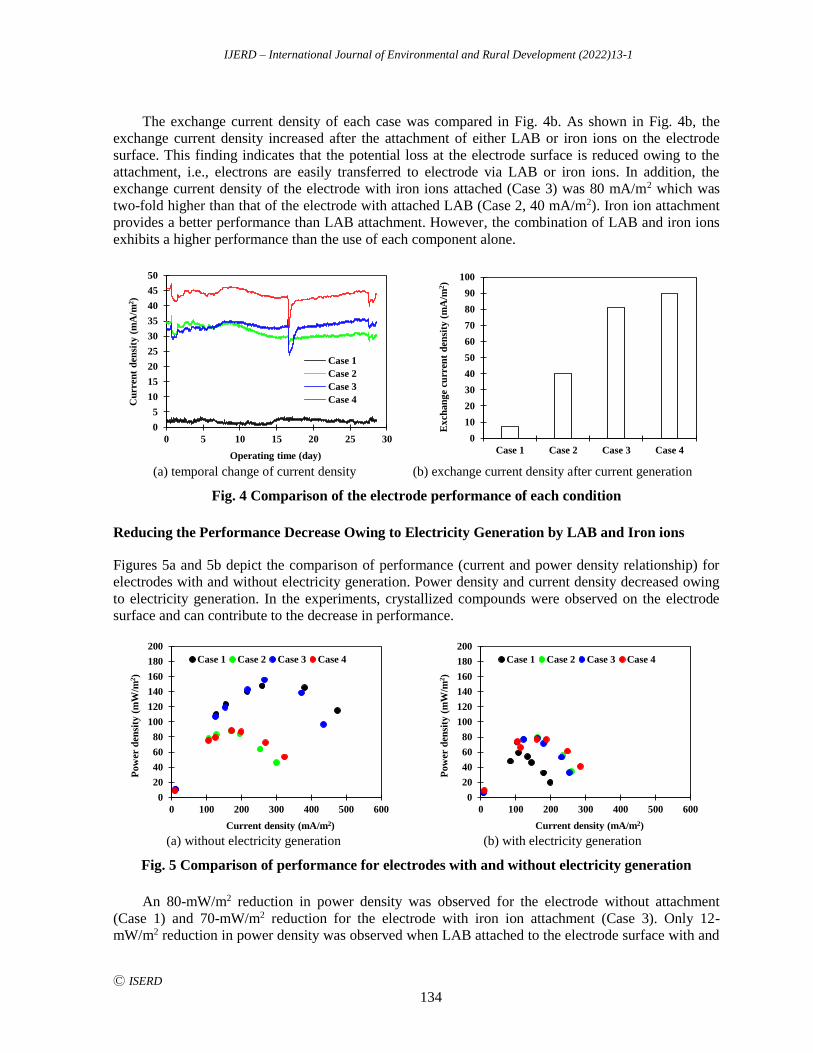
IJERD – International Journal of Environmental and Rural Development (2022)13-1
Ⓒ ISERD
134
The exchange current density of each case was compared in Fig. 4b. As shown in Fig. 4b, the
exchange current density increased after the attachment of either LAB or iron ions on the electrode
surface. This finding indicates that the potential loss at the electrode surface is reduced owing to the
attachment, i.e., electrons are easily transferred to electrode via LAB or iron ions. In addition, the
exchange current density of the electrode with iron ions attached (Case 3) was 80 mA/m2 which was
two-fold higher than that of the electrode with attached LAB (Case 2, 40 mA/m2). Iron ion attachment
provides a better performance than LAB attachment. However, the combination of LAB and iron ions
exhibits a higher performance than the use of each component alone.
0
5
10
15
20
25
30
35
40
45
50
0 5 10 15 20 25 30
Cu
rren
t d
ensi
ty (
mA
/m2)
Operating time (day)
Case 1
Case 2
Case 3
Case 4
0
10
20
30
40
50
60
70
80
90
100
Case 1 Case 2 Case 3 Case 4E
xch
an
ge
curr
ent
den
sity
(m
A/m
2)
(a) temporal change of current density (b) exchange current density after current generation
Fig. 4 Comparison of the electrode performance of each condition
Reducing the Performance Decrease Owing to Electricity Generation by LAB and Iron ions
Figures 5a and 5b depict the comparison of performance (current and power density relationship) for
electrodes with and without electricity generation. Power density and current density decreased owing
to electricity generation. In the experiments, crystallized compounds were observed on the electrode
surface and can contribute to the decrease in performance.
0
20
40
60
80
100
120
140
160
180
200
0 100 200 300 400 500 600
Pow
er d
ensi
ty (
mW
/m2)
Current density (mA/m2)
Case 1 Case 2 Case 3 Case 4
0
20
40
60
80
100
120
140
160
180
200
0 100 200 300 400 500 600
Pow
er d
ensi
ty (
mW
/m2)
Current density (mA/m2)
Case 1 Case 2 Case 3 Case 4
(a) without electricity generation (b) with electricity generation
Fig. 5 Comparison of performance for electrodes with and without electricity generation
An 80-mW/m2 reduction in power density was observed for the electrode without attachment
(Case 1) and 70-mW/m2 reduction for the electrode with iron ion attachment (Case 3). Only 12-
mW/m2 reduction in power density was observed when LAB attached to the electrode surface with and
IJERD – International Journal of Environmental and Rural Development (2022)13-1
Ⓒ ISERD
135
without iron ions (Cases 2&4). Therefore, LAB attachment on electrode surface effectively improves
the reduced performance owing to electricity generation. Crystallization cannot occur on the electrode
surface with LAB.
CONCLUSIONS
Laboratory experiments were conducted to verify the efficiency of the proposed simple method for
attaching LAB and iron ions on a carbon fiber-electrode and to examine the effects of attachment on
the electrode performance. Approximately 300-mV reduction in electrode potential was observed
owing to the attachment. Nevertheless, the electrode potential recovered almost to the initial state after
oxidizing the electrode by placing it in tap water near the water surface for 7 days. Thus, aeration
should be conducted during attachment to prevent the decrease in the electrode potential. A 10-fold
increase in current density was observed for the electrode attached with either LAB or iron ions. A
high increase in current density was obtained when LAB and iron ions were attached to the electrode.
On the basis of the increase in exchange current density owing to the attachment, the potential loss at
the electrode surface is reduced owing to the attachment, i.e., electrons are easily transferred to
electrode via LAB or iron ions. Finally, the performance decrease owing to electricity generation was
largely (88%) reduced for the electrode attached to LAB. Therefore, the attachment of LAB on the
electrode surface can restrain the formation of crystallized compounds.
ACKNOWLEDGMENTS
The authors gratefully acknowledge the partial funding from JSPS: Grant-in-Aid for Scientific
Research (B) (Grant Number: JP-21H01437). The authors would also like to thank the students of the
Rural Environmental Engineering Laboratory, Tokyo University of Agriculture, for their efforts in
collecting data.
REFERENCES
Carmona-Martinez, A.A., Harnisch, F., Fitzgerald, L.A., Biffinger, J.C., Ringeisen, B.R. and Schröder, U. 2021.
Cyclic voltametric analysis of the electron transfer of Shewanella oneidensis MR-1 and nanofilament and
cytochrome knock-out mutants, Bioelectrochemistry, 81, 74–80, Retrieved from
https://doi.org/10.1016/j.bioelechem.2011.02.006
Kang, J., Kim, T., Tak, Y., Lee, J.H. and Yoon, J. 2012. Cyclic voltammetry for monitoring bacterial attachment
and biofilm formation, Journal of Industrial and Engineering Chemistry, 18(2), 800-807, Retrieved from
https://doi.org/10.1016/j.jiec.2011.10.002
Nagatsu, Y., Tachiuchi, K., Touch, N. and Hibino, T. 2014. Factors for improving the performance of sediment
microbial fuel cell, Journal of Japan Society of Civil Engineers Ser B2 (Coastal Engineering), 70(2), 1066-
1070, Retrieved from https://doi.org/10.2208/kaigan.70.I_1066. in Japanese
Nishimura, K., Yamaji, S., Touch, N. and Hibino, T. 2018. Usable output of sediment microbial fuel cell under
the use of steel slag mixed-sediment as a fuel, Journal of Japan Society of Civil Engineers Ser B2 (Coastal
Engineering), 74(2), 1183-1188, Retrieved from https://doi.org/10.2208/kaigan.74.I_1183. in Japanese
Touch, N. and Nakamura, T. 2020. Methods for improving the performance of paddy soil-used sediment
microbial fuel cells, International Journal of Environmental and Rural Development, 11(2), 1-6.
Wang, X., Feng, Y., Ren, N., Wang, H., Lee, H., Li, N. and Zhoa, Q. 2009. Accelerated start-up of two-
chambered microbial fuel cells: Effect of anodic positive poised potential, Electrochimica Acta, 54(3), 1109-
1114, Retrieved from https://doi.org/10.1016/j.electacta.2008.07.085
Yamasaki, R., Maeda T. and Wood, T.K. 2018. Electron carriers increase electricity production in methane
microbial fuel cells that reverse methanogenesis, Biotechnology for Biofuels, 11, 211 (10 pages), Retrieved
from https://doi.org/10.1186/s13068-018-1208-7
IJERD – International Journal of Environmental and Rural Development (2022)13-1
Ⓒ ISERD
136
Characteristics of Ion Components of Clearwater Stream
Watershed in an Agricultural Area with Multivariate Analysis
YURI YAMAZAKI* Tokyo University of Agriculture, Tokyo, Japan
Email: [email protected]
TOSHIMI MUNEOKA Obihiro University of Agriculture and Veterinary Medicine, Hokkaido, Japan
CHIE MATSUDA Zukosha Co., Ltd., Hokkaido, Japan
MASATO KIMURA Obihiro University of Agriculture and Veterinary Medicine, Hokkaido, Japan
OSAMU TSUJI Zukosha Co., Ltd. / Obihiro University of Agriculture and Veterinary Medicine, Hokkaido, Japan
Received 29 January 2022 Accepted 25 April 2022 (*Corresponding Author)
Abstract Restoring the clear-stream environment that once existed in agricultural areas is one
of the major challenges for the development of sustainable agriculture. Therefore, we analyzed
the ionic components of the Rekifune and Satsunai River basins, which are regarded as clear-
water basins in the Tokachi region of Hokkaido, using principal component analysis and cluster
analysis based on surveys conducted in June and September 2014. The results showed that most
of the sampling points in the Rekifune and Satsunai drainages were comparable to the average
values of water quality assessed as clear-streams in Japan. However, in the tributaries of the
Rekifune River, since Cl- and Na+ increased characteristically, the water quality was degraded
by anthropogenic pollution sources such as domestic wastewater. In the Satsunai River, the
water quality of the downstream tributaries was degraded due to agriculture. In addition, in one
of the tributaries, deterioration of water quality was observed only in September, and the water
quality of the main river immediately after the inflow of this tributary was also affected. These
results indicate that the water quality in the two basins in the predominantly agricultural area is
generally good. Still, it is necessary to identify the source of pollution in some areas and take
countermeasures.
Keywords river water quality, agricultural area, principal component analysis, cluster analysis
INTRODUCTION
Historically, rivers flowing through rural areas in Japan had clear water and were home to various
aquatic life. However, modern agricultural land-use changes and river alterations have resulted in the
disappearance of the 'clear water' environment in rural areas. This water pollution caused by modern
agriculture has become a global problem. We now understand the need to conserve intact rivers in
agricultural areas and restore altered river ecosystems to meet the global challenge of more sustainable
agriculture.
The term "clearwater stream" generally refers to uncontaminated rivers—however, no scientific
definition in Japan. For example, the Japanese government publicizes river rankings based on water
erd
Research article
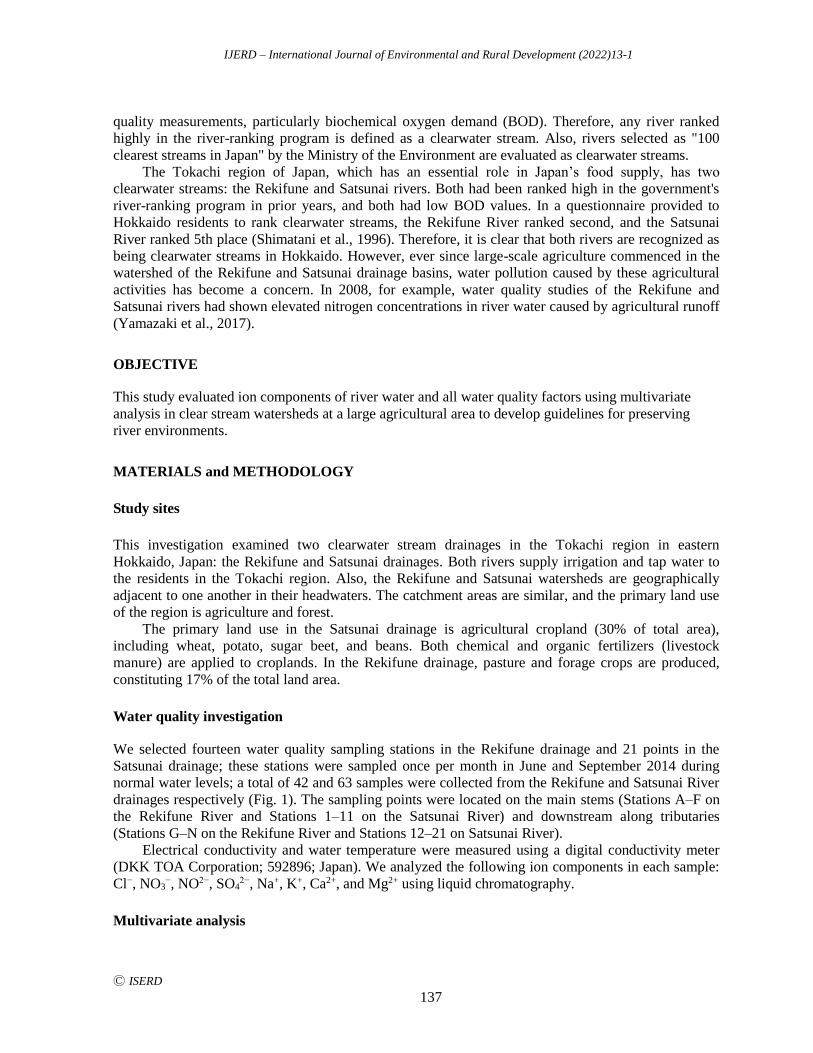
IJERD – International Journal of Environmental and Rural Development (2022)13-1
Ⓒ ISERD
137
quality measurements, particularly biochemical oxygen demand (BOD). Therefore, any river ranked
highly in the river-ranking program is defined as a clearwater stream. Also, rivers selected as "100
clearest streams in Japan" by the Ministry of the Environment are evaluated as clearwater streams.
The Tokachi region of Japan, which has an essential role in Japan’s food supply, has two
clearwater streams: the Rekifune and Satsunai rivers. Both had been ranked high in the government's
river-ranking program in prior years, and both had low BOD values. In a questionnaire provided to
Hokkaido residents to rank clearwater streams, the Rekifune River ranked second, and the Satsunai
River ranked 5th place (Shimatani et al., 1996). Therefore, it is clear that both rivers are recognized as
being clearwater streams in Hokkaido. However, ever since large-scale agriculture commenced in the
watershed of the Rekifune and Satsunai drainage basins, water pollution caused by these agricultural
activities has become a concern. In 2008, for example, water quality studies of the Rekifune and
Satsunai rivers had shown elevated nitrogen concentrations in river water caused by agricultural runoff
(Yamazaki et al., 2017).
OBJECTIVE
This study evaluated ion components of river water and all water quality factors using multivariate
analysis in clear stream watersheds at a large agricultural area to develop guidelines for preserving
river environments.
MATERIALS and METHODOLOGY
Study sites
This investigation examined two clearwater stream drainages in the Tokachi region in eastern
Hokkaido, Japan: the Rekifune and Satsunai drainages. Both rivers supply irrigation and tap water to
the residents in the Tokachi region. Also, the Rekifune and Satsunai watersheds are geographically
adjacent to one another in their headwaters. The catchment areas are similar, and the primary land use
of the region is agriculture and forest.
The primary land use in the Satsunai drainage is agricultural cropland (30% of total area),
including wheat, potato, sugar beet, and beans. Both chemical and organic fertilizers (livestock
manure) are applied to croplands. In the Rekifune drainage, pasture and forage crops are produced,
constituting 17% of the total land area.
Water quality investigation
We selected fourteen water quality sampling stations in the Rekifune drainage and 21 points in the
Satsunai drainage; these stations were sampled once per month in June and September 2014 during
normal water levels; a total of 42 and 63 samples were collected from the Rekifune and Satsunai River
drainages respectively (Fig. 1). The sampling points were located on the main stems (Stations A–F on
the Rekifune River and Stations 1–11 on the Satsunai River) and downstream along tributaries
(Stations G–N on the Rekifune River and Stations 12–21 on Satsunai River).
Electrical conductivity and water temperature were measured using a digital conductivity meter
(DKK TOA Corporation; 592896; Japan). We analyzed the following ion components in each sample:
Cl−, NO3−, NO2−, SO4
2−, Na+, K+, Ca2+, and Mg2+ using liquid chromatography.
Multivariate analysis

IJERD – International Journal of Environmental and Rural Development (2022)13-1
Ⓒ ISERD
138
Fig. 1 Land use and sampling stations of the Rekifune and Satsunai River drainages
We used the R package (R Foundation for Statistical Computing; Ver. 3.0.3; Austria) for cluster and
principal component analyses. The ion components (Cl−, NO3−, SO4
2−, Na+, K+, Ca2+, and Mg2+) were
used as input variables. Cluster analysis and principal component analysis are both types of
multivariate techniques. We applied Ward’s method to the cluster analysis. Principal component
analysis (PCA) was derived using the “princomp” algorithm of the R package.
RESULTS AND DISCUSSION
Cluster analysis and Principal component analysis of the river water quality
Cluster and principal component analysis using correlation matrix were carried out for seven variables:
ion concentrations (Cl−, NO3−, SO4
2−, Na+, K+, Ca2+, and Mg2+) at 35 sampling stations in the Rekifune
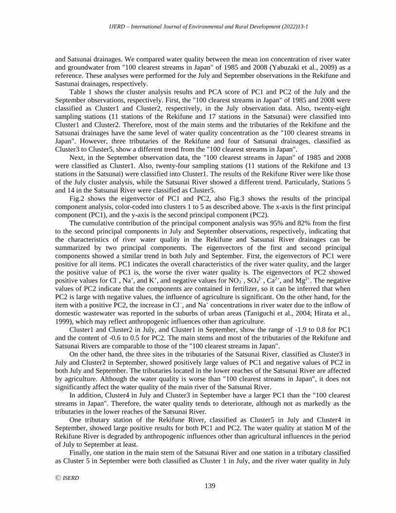
IJERD – International Journal of Environmental and Rural Development (2022)13-1
Ⓒ ISERD
139
and Satsunai drainages. We compared water quality between the mean ion concentration of river water
and groundwater from "100 clearest streams in Japan" of 1985 and 2008 (Yabuzaki et al., 2009) as a
reference. These analyses were performed for the July and September observations in the Rekifune and
Sastunai drainages, respectively.
Table 1 shows the cluster analysis results and PCA score of PC1 and PC2 of the July and the
September observations, respectively. First, the "100 clearest streams in Japan" of 1985 and 2008 were
classified as Cluster1 and Cluster2, respectively, in the July observation data. Also, twenty-eight
sampling stations (11 stations of the Rekifune and 17 stations in the Satsunai) were classified into
Cluster1 and Cluster2. Therefore, most of the main stems and the tributaries of the Rekifune and the
Satsunai drainages have the same level of water quality concentration as the "100 clearest streams in
Japan". However, three tributaries of the Rekifune and four of Satsunai drainages, classified as
Cluster3 to Cluster5, show a different trend from the "100 clearest streams in Japan".
Next, in the September observation data, the "100 clearest streams in Japan" of 1985 and 2008
were classified as Cluster1. Also, twenty-four sampling stations (11 stations of the Rekifune and 13
stations in the Satsunai) were classified into Cluster1. The results of the Rekifune River were like those
of the July cluster analysis, while the Satsunai River showed a different trend. Particularly, Stations 5
and 14 in the Satsunai River were classified as Cluster5.
Fig.2 shows the eigenvector of PC1 and PC2, also Fig.3 shows the results of the principal
component analysis, color-coded into clusters 1 to 5 as described above. The x-axis is the first principal
component (PC1), and the y-axis is the second principal component (PC2).
The cumulative contribution of the principal component analysis was 95% and 82% from the first
to the second principal components in July and September observations, respectively, indicating that
the characteristics of river water quality in the Rekifune and Satsunai River drainages can be
summarized by two principal components. The eigenvectors of the first and second principal
components showed a similar trend in both July and September. First, the eigenvectors of PC1 were
positive for all items. PC1 indicates the overall characteristics of the river water quality, and the larger
the positive value of PC1 is, the worse the river water quality is. The eigenvectors of PC2 showed
positive values for Cl−, Na+, and K+, and negative values for NO3−, SO4
2−, Ca2+, and Mg2+. The negative
values of PC2 indicate that the components are contained in fertilizer, so it can be inferred that when
PC2 is large with negative values, the influence of agriculture is significant. On the other hand, for the
item with a positive PC2, the increase in Cl−, and Na+ concentrations in river water due to the inflow of
domestic wastewater was reported in the suburbs of urban areas (Taniguchi et al., 2004; Hirata et al.,
1999), which may reflect anthropogenic influences other than agriculture.
Cluster1 and Cluster2 in July, and Cluster1 in September, show the range of -1.9 to 0.8 for PC1
and the content of -0.6 to 0.5 for PC2. The main stems and most of the tributaries of the Rekifune and
Satsunai Rivers are comparable to those of the "100 clearest streams in Japan".
On the other hand, the three sites in the tributaries of the Satsunai River, classified as Cluster3 in
July and Cluster2 in September, showed positively large values of PC1 and negative values of PC2 in
both July and September. The tributaries located in the lower reaches of the Satsunai River are affected
by agriculture. Although the water quality is worse than "100 clearest streams in Japan", it does not
significantly affect the water quality of the main river of the Satsunai River. In addition, Cluster4 in July and Cluster3 in September have a larger PC1 than the "100 clearest
streams in Japan". Therefore, the water quality tends to deteriorate, although not as markedly as the
tributaries in the lower reaches of the Satsunai River.
One tributary station of the Rekifune River, classified as Cluster5 in July and Cluster4 in
September, showed large positive results for both PC1 and PC2. The water quality at station M of the
Rekifune River is degraded by anthropogenic influences other than agricultural influences in the period
of July to September at least.
Finally, one station in the main stem of the Satsunai River and one station in a tributary classified
as Cluster 5 in September were both classified as Cluster 1 in July, and the river water quality in July
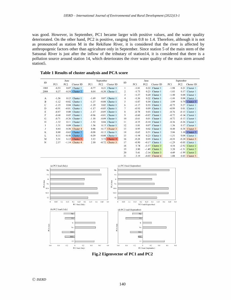
IJERD – International Journal of Environmental and Rural Development (2022)13-1
Ⓒ ISERD
140
was good. However, in September, PC1 became larger with positive values, and the water quality
deteriorated. On the other hand, PC2 is positive, ranging from 0.8 to 1.4. Therefore, although it is not
as pronounced as station M in the Rekifune River, it is considered that the river is affected by
anthropogenic factors other than agriculture only in September. Since station 5 of the main stem of the
Satsunai River is just after the inflow of the tributary of station14, it is considered that there is a
pollution source around station 14, which deteriorates the river water quality of the main stem around
station5.
Table 1 Results of cluster analysis and PCA score
Fig.2 Eigenvector of PC1 and PC2
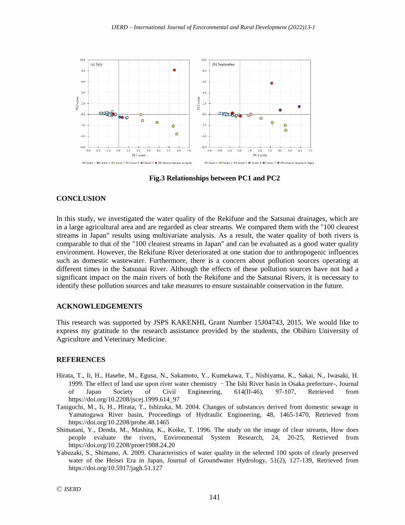
IJERD – International Journal of Environmental and Rural Development (2022)13-1
Ⓒ ISERD
141
Fig.3 Relationships between PC1 and PC2
CONCLUSION
In this study, we investigated the water quality of the Rekifune and the Satsunai drainages, which are
in a large agricultural area and are regarded as clear streams. We compared them with the "100 clearest
streams in Japan" results using multivariate analysis. As a result, the water quality of both rivers is
comparable to that of the "100 clearest streams in Japan" and can be evaluated as a good water quality
environment. However, the Rekifune River deteriorated at one station due to anthropogenic influences
such as domestic wastewater. Furthermore, there is a concern about pollution sources operating at
different times in the Satsunai River. Although the effects of these pollution sources have not had a
significant impact on the main rivers of both the Rekifune and the Satsunai Rivers, it is necessary to
identify these pollution sources and take measures to ensure sustainable conservation in the future.
ACKNOWLEDGEMENTS
This research was supported by JSPS KAKENHI, Grant Number 15J04743, 2015. We would like to
express my gratitude to the research assistance provided by the students, the Obihiro University of
Agriculture and Veterinary Medicine.
REFERENCES
Hirata, T., Ii, H., Hasebe, M., Egusa, N., Sakamoto, Y., Kumekawa, T., Nishiyama, K., Sakai, N., Iwasaki, H.
1999. The effect of land use upon river water chemistry –The Ishi River basin in Osaka prefecture-, Journal
of Japan Society of Civil Engineering, 614(II-46), 97-107, Retrieved from
https://doi.org/10.2208/jscej.1999.614_97
Taniguchi, M., Ii, H., Hirata, T., Ishizuka, M. 2004. Changes of substances derived from domestic sewage in
Yamatogawa River basin, Proceedings of Hydraulic Engineering, 48, 1465-1470, Retrieved from
https://doi.org/10.2208/prohe.48.1465
Shimatani, Y., Denda, M., Mashita, K., Koike, T. 1996. The study on the image of clear streams, How does
people evaluate the rivers, Environmental System Research, 24, 20-25, Retrieved from
https://doi.org/10.2208/proer1988.24.20
Yabuzaki, S., Shimano, A. 2009. Characteristics of water quality in the selected 100 spots of clearly preserved
water of the Heisei Era in Japan, Journal of Groundwater Hydrology, 51(2), 127-139, Retrieved from
https://doi.org/10.5917/jagh.51.127

IJERD – International Journal of Environmental and Rural Development (2022)13-1
Ⓒ ISERD
142
Yamazaki, Y., Muneoka, T., Okazawa, H., Kimura, M., Tsuji, O. 2017. Evaluation of river water quality with
multivariate analysis in clear stream watersheds in agricultural area, Journal of Water and Environment
Technology, 15(3), 86-95, Retrieved from https://doi.org/10.2965/jwet.16-040
IJERD – International Journal of Environmental and Rural Development (2022)13-1
Ⓒ ISERD
143
Evaluating Ion Exchange Capacity of Molten Slag for Hydroponic System
ANTONIO PEREZ FUENTES Graduate School of Agriculture, Tokyo University of Agriculture, Tokyo, Japan
SARVESH MASKEY Faculty of Regional Environment Science, Tokyo University of Agriculture, Tokyo, Japan
HIROMU OKAZAWA * Faculty of Regional Environment Science, Tokyo University of Agriculture, Tokyo, Japan Email: [email protected]
YURI YAMAZAKI Faculty of Agriculture, Tottori University, Tottori, Japan
TOMONORI FUJIKAWA Faculty of Regional Environment Science, Tokyo University of Agriculture, Tokyo, Japan
TOSHIMITSU ASAI Faculty of Regional Environment Science, Tokyo University of Agriculture, Tokyo, Japan
Received 1 February 2022 Accepted 25 April 2022 (*Corresponding Author)
Abstract Hydroponic farming promotes high-efficiency water, fertilizers, and high productivity
under a controlled environment. However, the use of this system needs consistent application of
fertilizers, increasing the cost of operations. Molten Slag (MS), a waste from the Municipal
Solid Waste Incineration has essential nutrients that can be used as fertilizer. The objective of
this study was to clarify the releasing process of nutrients by molten slag to be applied as a
substrate in hydroponic system. For this, anion and cation contents of three varieties of Molten
Slag (MS1, MS2, MS3) were determined in the laboratory by a shaking method. The nutrient
content, P2O5, K2O, MgO and CaO were in MS1, MS3 and MS2. The quantification ion
released was performed at 1, 6, 12 and 24 hours. It was observed that MS3 had performed the
best condition in the releasing process of K+, Mg+, SO4- and Cl-. Although MS1 had higher
nutrient content, MS3 released higher contents of those minerals among the samples. According
to the result of this study, it was confirmed that MS3 has a high potential for hydroponic
farming.
Keywords Molten Slag, Hydroponic system, Ion exchange capacity, Releasing nutrients
INTRODUCTION
Around 200 billion tons of fertilizers are produced annually for agricultural purposes (FAOSTAT,
2021). The use of these fertilizers and water supply tends to increase to provide food safety for 9 million people toward 2050. The benefit of fertilizers in agricultural production is remarkable since it improves yields and keeps fertile soil. On the other hand, the constant use of fertilizers not only increase the costs but hazard the ecological balance with releasing of greenhouse gases and eutrophication to water bodies (Sedlacek et al.,2020).
Molten Slag (MS) is a by-product of the Municipal Solid Waste Incineration -MSWI- process
(Fig.1). The process to generate molten slag starts with the addition of wastes inside a furnace, this
erd
Research article
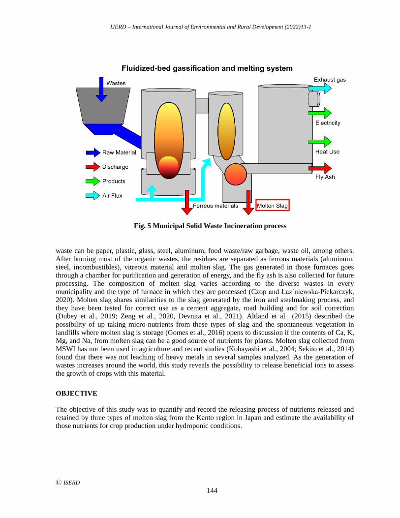
IJERD – International Journal of Environmental and Rural Development (2022)13-1
Ⓒ ISERD
144
waste can be paper, plastic, glass, steel, aluminum, food waste/raw garbage, waste oil, among others. After burning most of the organic wastes, the residues are separated as ferrous materials (aluminum, steel, incombustibles), vitreous material and molten slag. The gas generated in those furnaces goes
through a chamber for purification and generation of energy, and the fly ash is also collected for future processing. The composition of molten slag varies according to the diverse wastes in every municipality and the type of furnace in which they are processed (Czop and Łaz´niewska-Piekarczyk, 2020). Molten slag shares similarities to the slag generated by the iron and steelmaking process, and they have been tested for correct use as a cement aggregate, road building and for soil correction (Dubey et al., 2019; Zeng et al., 2020, Devnita et al., 2021). Altland et al., (2015) described the
possibility of up taking micro-nutrients from these types of slag and the spontaneous vegetation in landfills where molten slag is storage (Gomes et al., 2016) opens to discussion if the contents of Ca, K, Mg, and Na, from molten slag can be a good source of nutrients for plants. Molten slag collected from MSWI has not been used in agriculture and recent studies (Kobayashi et al., 2004; Sekito et al., 2014) found that there was not leaching of heavy metals in several samples analyzed. As the generation of wastes increases around the world, this study reveals the possibility to release beneficial ions to assess
the growth of crops with this material.
OBJECTIVE
The objective of this study was to quantify and record the releasing process of nutrients released and retained by three types of molten slag from the Kanto region in Japan and estimate the availability of those nutrients for crop production under hydroponic conditions.
Fig. 5 Municipal Solid Waste Incineration process
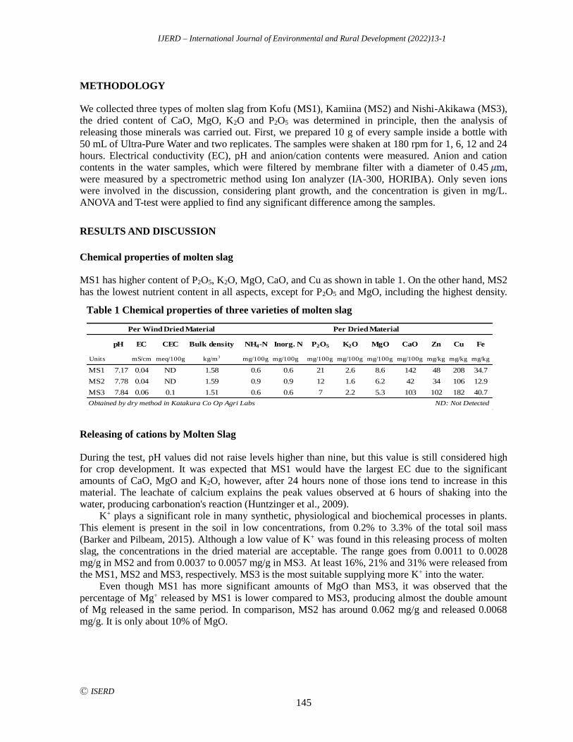
IJERD – International Journal of Environmental and Rural Development (2022)13-1
Ⓒ ISERD
145
METHODOLOGY
We collected three types of molten slag from Kofu (MS1), Kamiina (MS2) and Nishi-Akikawa (MS3), the dried content of CaO, MgO, K2O and P2O5 was determined in principle, then the analysis of releasing those minerals was carried out. First, we prepared 10 g of every sample inside a bottle with
50 mL of Ultra-Pure Water and two replicates. The samples were shaken at 180 rpm for 1, 6, 12 and 24 hours. Electrical conductivity (EC), pH and anion/cation contents were measured. Anion and cation contents in the water samples, which were filtered by membrane filter with a diameter of 0.45 , were measured by a spectrometric method using Ion analyzer (IA-300, HORIBA). Only seven ions were involved in the discussion, considering plant growth, and the concentration is given in mg/L. ANOVA and T-test were applied to find any significant difference among the samples.
RESULTS AND DISCUSSION
Chemical properties of molten slag
MS1 has higher content of P2O5, K2O, MgO, CaO, and Cu as shown in table 1. On the other hand, MS2
has the lowest nutrient content in all aspects, except for P2O5 and MgO, including the highest density.
Releasing of cations by Molten Slag
During the test, pH values did not raise levels higher than nine, but this value is still considered high for crop development. It was expected that MS1 would have the largest EC due to the significant amounts of CaO, MgO and K2O, however, after 24 hours none of those ions tend to increase in this material. The leachate of calcium explains the peak values observed at 6 hours of shaking into the water, producing carbonation's reaction (Huntzinger et al., 2009).
K+ plays a significant role in many synthetic, physiological and biochemical processes in plants.
This element is present in the soil in low concentrations, from 0.2% to 3.3% of the total soil mass (Barker and Pilbeam, 2015). Although a low value of K+ was found in this releasing process of molten slag, the concentrations in the dried material are acceptable. The range goes from 0.0011 to 0.0028 mg/g in MS2 and from 0.0037 to 0.0057 mg/g in MS3. At least 16%, 21% and 31% were released from the MS1, MS2 and MS3, respectively. MS3 is the most suitable supplying more K+ into the water.
Even though MS1 has more significant amounts of MgO than MS3, it was observed that the
percentage of Mg+ released by MS1 is lower compared to MS3, producing almost the double amount of Mg released in the same period. In comparison, MS2 has around 0.062 mg/g and released 0.0068 mg/g. It is only about 10% of MgO.
Table 1 Chemical properties of three varieties of molten slag
Units mS/cm meq/100g kg/m3
mg/100g mg/100g mg/100g mg/100g mg/100g mg/100g mg/kg mg/kg mg/kg
MS1 7.17 0.04 ND 1.58 0.6 0.6 21 2.6 8.6 142 48 208 34.7
MS2 7.78 0.04 ND 1.59 0.9 0.9 12 1.6 6.2 42 34 106 12.9
MS3 7.84 0.06 0.1 1.51 0.6 0.6 7 2.2 5.3 103 102 182 40.7
ND: Not Detected
P2O5 K2O MgO CaO Zn Cu
Obtained by dry method in Katakura Co Op Agri Labs
Per Wind Dried Material Per Dried Material
pH EC CEC Bulk density NH4-N Inorg. N Fe
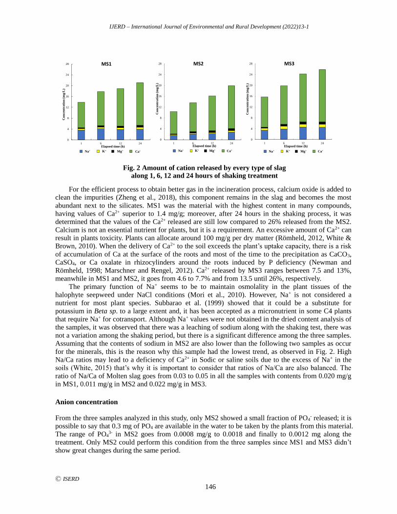
IJERD – International Journal of Environmental and Rural Development (2022)13-1
Ⓒ ISERD
146
For the efficient process to obtain better gas in the incineration process, calcium oxide is added to clean the impurities (Zheng et al., 2018), this component remains in the slag and becomes the most
abundant next to the silicates. MS1 was the material with the highest content in many compounds, having values of Ca2+ superior to 1.4 mg/g; moreover, after 24 hours in the shaking process, it was determined that the values of the Ca2+ released are still low compared to 26% released from the MS2. Calcium is not an essential nutrient for plants, but it is a requirement. An excessive amount of Ca2+ can result in plants toxicity. Plants can allocate around 100 mg/g per dry matter (Römheld, 2012, White & Brown, 2010). When the delivery of Ca2+ to the soil exceeds the plant’s uptake capacity, there is a risk
of accumulation of Ca at the surface of the roots and most of the time to the precipitation as CaCO3, CaSO4, or Ca oxalate in rhizocylinders around the roots induced by P deficiency (Newman and Römheld, 1998; Marschner and Rengel, 2012). Ca2+ released by MS3 ranges between 7.5 and 13%, meanwhile in MS1 and MS2, it goes from 4.6 to 7.7% and from 13.5 until 26%, respectively.
The primary function of Na+ seems to be to maintain osmolality in the plant tissues of the halophyte seepweed under NaCl conditions (Mori et al., 2010). However, Na+ is not considered a
nutrient for most plant species. Subbarao et al. (1999) showed that it could be a substitute for potassium in Beta sp. to a large extent and, it has been accepted as a micronutrient in some C4 plants that require Na+ for cotransport. Although Na+ values were not obtained in the dried content analysis of the samples, it was observed that there was a leaching of sodium along with the shaking test, there was not a variation among the shaking period, but there is a significant difference among the three samples. Assuming that the contents of sodium in MS2 are also lower than the following two samples as occur
for the minerals, this is the reason why this sample had the lowest trend, as observed in Fig. 2. High Na/Ca ratios may lead to a deficiency of Ca2+ in Sodic or saline soils due to the excess of Na+ in the soils (White, 2015) that’s why it is important to consider that ratios of Na/Ca are also balanced. The ratio of Na/Ca of Molten slag goes from 0.03 to 0.05 in all the samples with contents from 0.020 mg/g in MS1, 0.011 mg/g in MS2 and 0.022 mg/g in MS3.
Anion concentration
From the three samples analyzed in this study, only MS2 showed a small fraction of PO4- released; it is
possible to say that 0.3 mg of PO4 are available in the water to be taken by the plants from this material. The range of PO4
3- in MS2 goes from 0.0008 mg/g to 0.0018 and finally to 0.0012 mg along the treatment. Only MS2 could perform this condition from the three samples since MS1 and MS3 didn’t show great changes during the same period.
0
4
8
12
16
20
24
28
1 6 12 24
Con
cen
trati
on
(m
g/L
)
Elapsed time (h)
MS1
Na+ K+ Mg+ Ca+Na+ K+ Mg+ Ca+
0
4
8
12
16
20
24
28
1 6 12 24
Con
cen
trati
on
(m
g/L
)
Elapsed time (h)
MS2
Na+ K+ Mg+ Ca+Na+ K+ Mg+ Ca+
0
4
8
12
16
20
24
28
1 6 12 24
Con
cen
trati
on
(m
g/L
)
Elapsed time (h)
MS3
Na+ K+ Mg+ Ca+Na+ K+ Mg+ Ca+
Fig. 2 Amount of cation released by every type of slag along 1, 6, 12 and 24 hours of shaking treatment
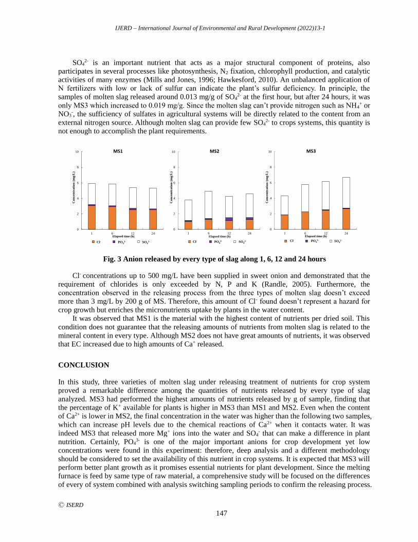
IJERD – International Journal of Environmental and Rural Development (2022)13-1
Ⓒ ISERD
147
SO42- is an important nutrient that acts as a major structural component of proteins, also
participates in several processes like photosynthesis, N2 fixation, chlorophyll production, and catalytic activities of many enzymes (Mills and Jones, 1996; Hawkesford, 2010). An unbalanced application of N fertilizers with low or lack of sulfur can indicate the plant’s sulfur deficiency. In principle, the samples of molten slag released around 0.013 mg/g of SO4
2- at the first hour, but after 24 hours, it was
only MS3 which increased to 0.019 mg/g. Since the molten slag can’t provide nitrogen such as NH4+ or
NO3-, the sufficiency of sulfates in agricultural systems will be directly related to the content from an
external nitrogen source. Although molten slag can provide few SO42- to crops systems, this quantity is
not enough to accomplish the plant requirements.
Cl- concentrations up to 500 mg/L have been supplied in sweet onion and demonstrated that the requirement of chlorides is only exceeded by N, P and K (Randle, 2005). Furthermore, the concentration observed in the releasing process from the three types of molten slag doesn’t exceed more than 3 mg/L by 200 g of MS. Therefore, this amount of Cl- found doesn’t represent a hazard for crop growth but enriches the micronutrients uptake by plants in the water content.
It was observed that MS1 is the material with the highest content of nutrients per dried soil. This
condition does not guarantee that the releasing amounts of nutrients from molten slag is related to the mineral content in every type. Although MS2 does not have great amounts of nutrients, it was observed that EC increased due to high amounts of Ca+ released.
CONCLUSION
In this study, three varieties of molten slag under releasing treatment of nutrients for crop system proved a remarkable difference among the quantities of nutrients released by every type of slag analyzed. MS3 had performed the highest amounts of nutrients released by g of sample, finding that the percentage of K+ available for plants is higher in MS3 than MS1 and MS2. Even when the content of Ca2+ is lower in MS2, the final concentration in the water was higher than the following two samples, which can increase pH levels due to the chemical reactions of Ca2+ when it contacts water. It was
indeed MS3 that released more Mg+ ions into the water and SO4- that can make a difference in plant
nutrition. Certainly, PO43- is one of the major important anions for crop development yet low
concentrations were found in this experiment: therefore, deep analysis and a different methodology should be considered to set the availability of this nutrient in crop systems. It is expected that MS3 will perform better plant growth as it promises essential nutrients for plant development. Since the melting furnace is feed by same type of raw material, a comprehensive study will be focused on the differences
of every of system combined with analysis switching sampling periods to confirm the releasing process.
0
2
4
6
8
10
1 6 12 24
Co
nce
ntr
ati
on
(m
g/L
)
Elapsed time (h)
MS1
Cl- PO4- SO4-Cl- PO43- SO4
2-
0
2
4
6
8
10
1 6 12 24
Con
cen
tra
tio
n (
mg
/L)
Elapsed time (h)
MS2
Cl- PO4- SO4-Cl- PO43- SO4
2-
0
2
4
6
8
10
1 6 12 24
Co
nce
ntr
ati
on
(m
g/L
)
Elapsed time (h)
MS3
Cl- PO4- SO4-Cl- PO43- SO4
2-
Fig. 3 Anion released by every type of slag along 1, 6, 12 and 24 hours
IJERD – International Journal of Environmental and Rural Development (2022)13-1
Ⓒ ISERD
148
ACKNOWLEDGEMENTS
The authors are grateful to KOBELCO ECO-SOLUTION Co., Ltd. for providing us the materials for this study. This research was supported by Tokyo University of Agriculture.
REFERENCES
Altland, J. E., Krause, C., Locke, J. C., and Zellner, W. L. 2015. Micronutrient Availability from Steel Slag
Amendment in Peatmoss Substrates, HortScience, 50(11), 1715-1720,
https://doi.org/10.21273/hortsci.50.11.1715
Barker, A. V., and Pilbeam, D. J. 2015. Handbook of Plant Nutrition. Amsterdam University Press. ISBN 978-1-
4398-8198-9, USA.
Czop, M., and Łaz’niewska-Piekarczyk, B. 2020. Use of slag from the combustion of solid municipal waste as a
partial replacement of cement in mortar and concrete, Materials, 13(7), 1593, Retrieved from
https://doi.org/10.3390/ma13071593
Devnita, R., Sandrawati, A., and Arifin, M. (2021). Utilization of steel slag in agriculture (Review), Soilrens,
19(1), 50. Retrieved from https://doi.org/10.24198/soilrens.v19i1.35090
Dubey, S., Singh, A., and Kushwah, S. S. 2019. Utilization of iron and steel slag in building construction,
Proceedings of the International Conference on Sustainable Materials and Structures for Civil Infrastructures
(SMSCI2019). Retrieved from https://doi.org/10.1063/1.5127156
Food and Agriculture Organization (FAO). 2021. FAOSTAT, Retrieved from
https://www.fao.org/faostat/en/#data/RFB
Gomes, H. I., Mayes, W. M., Rogerson, M., Stewart, D. I., and Burke, I. T. 2016. Alkaline residues and the
environment: a review of impacts, management practices and opportunities, Journal of Cleaner Production,
112, 3571-3582, Retrieved from https://doi.org/10.1016/j.jclepro.2015.09.111
Hawkesford, M. J. 2010. Sulfate transport, The Plant Plasma Membrane, 291-301. Retrieved from
https://doi.org/10.1007/978-3-642-13431-9_13
Huntzinger, D. N., Gierke, J. S., Kawatra, S. K., Eisele, T. C., and Sutter, L. L. 2009. Carbon dioxide
sequestration in cement kiln dust through mineral carbonation, Environmental Science & Technology, 43(6),
1986-1992, Retrieved from https://doi.org/10.1021/es802910z
Jamieson, T. S., Stratton, G. W., Gordon, R., and Madani, A. 2002. Phosphorus adsorption characteristics of a
constructed wetland soil receiving dairy farm wastewater, Canadian Journal of Soil Science, 82(1), 97-104,
Retrieved from https://doi.org/10.4141/s01-042
Kobayashi, J., Kizu, R., and Torii, K. 2004. Physical properties and metal elutions of the thirteen molten slags
produced from incinerated ash, Yakugaku Zasshi, 124(9), 621-625. Retrieved from
https://doi.org/10.1248/yakushi.124.621
Marschner, P., and Rengel, Z. 2012. Nutrient availability in soils, Marschner’s Mineral Nutrition of Higher Plants,
315-330, Retrieved from https://doi.org/10.1016/b978-0-12-384905-2.00012-1
Mills, H.A. and J.B. Jones Jr. 1996. Plant Analysis Handbook II, Micro-Macro Pub. ISBN 1878148052, USA
Mori, S., Akiya, M., Yamamura, K., Murano, H., Arao, T., Kawasaki, A., Higuchi, K., Maeda, Y., Yoshiba, M.,
and Tadano, T. 2010. Physiological role of sodium in the growth of the halophyte suaeda salsa (l.) pall.
under high-sodium conditions, Crop Science, 50(6), 2492-2498. Retrieved from
https://doi.org/10.2135/cropsci2010.02.0119
Neumann, G. and Römheld V. 1998. Root excretion of carboxylic acids and protons in phosphorus-deficient
plants, Plant and Soil, 211, 121-130, Retrieved from https://doi.org/10.1023/a:1004380832118
Randle, W. 2005. Advancements in understanding and manipulating allium flavor: Calcium and Chloride, Acta
Horticulturae, 688, 35-40, Retrieved from https://doi.org/10.17660/actahortic.2005.688.3
Römheld, V. 2012. Diagnosis of deficiency and toxicity of nutrients, Marschner’s Mineral Nutrition of Higher
Plants, 299-312, Retrieved from https://doi.org/10.1016/b978-0-12-384905-2.00011-x
Rondón Quintana, H. A., Muniz De Farías, M., and Reyes Lizcano, F. A. 2018. Uso de escorias de alto horno y
acero en mezclas asfálticas: revisión, Revista Ingenierías Universidad de Medellín, 17(33), 71-97. Retrieved
from https://doi.org/10.22395/rium.v17n33a4
IJERD – International Journal of Environmental and Rural Development (2022)13-1
Ⓒ ISERD
149
Sedlacek, C. J., Giguere, A. T., and Pjevac, P. 2020. Is too much fertilizer a problem? Frontiers for Young Minds,
8, Retrieved from https://doi.org/10.3389/frym.2020.00063
Sekito, T., Onoue, K., Dote, Y., Sakanakura, H., and Nakamura, K. 2014. Variation and correlation of content
and leachability of hazardous metals in MSW molten slag, Environmental Monitoring and Assessment,
187(1), Retrieved from https://doi.org/10.1007/s10661-014-4193-8
Small, H., Stevens, T. S., and Bauman, W. C. 1975. Novel ion exchange chromatographic method using
conductimetric detection, Analytical Chemistry, 47(11), 1801-1809, Retrieved from
https://doi.org/10.1021/ac60361a017
Subbarao, G. V., Wheeler, R. M., Stutte, G. W., and Levine, L. H. 1999. How far can sodium substitute for
potassium in red beet?, Journal of Plant Nutrition, 22(11), 1745-1761, Retrieved from
https://doi.org/10.1080/01904169909365751
White, P. J. 2012. Ion uptake mechanisms of individual cells and roots, Marschner’s Mineral Nutrition of Higher
Plants, 7-47, Retrieved from https://doi.org/10.1016/b978-0-12-384905-2.00002-9
White, P. J., and Brown, P. H. 2010. Plant nutrition for sustainable development and global health, Annals of
Botany, 105(7), 1073-1080, Retrieved from https://doi.org/10.1093/aob/mcq085
Zeng, C., Lyu, Y., Wang, D., Ju, Y., Shang, X., and Li, L. 2020. Application of fly ash and slag generated by
incineration of municipal solid waste in concrete, Advances in Materials Science and Engineering, 2020, 1-7,
Retrieved from http://doi.org/10.1155/2020/7802103
Zheng, X., Ying, Z., Wang, B., and Chen, C. 2018. Effect of calcium oxide addition on tar formation during the
pyrolysis of key municipal solid waste (MSW) components. Waste and Biomass Valorization, 10(8), 2309-
2318, Retrieved from http://doi.org/10.1007/s12649-018-0249-2
IJERD – International Journal of Environmental and Rural Development (2022)13-1
Ⓒ ISERD
150
Some Physico-Chemical Characteristics of Surface Water in
Mining Areas in the Lao PDR
SANTI KONGMANY* Center of Excellence in Environment, Research and Academic Service Office, National University of
Laos, Vientiane Capital, Lao PDR
Email: [email protected]
VANSENG CHOUNLAMANY Faculty of Natural Sciences, National University of Laos, Vientiane Capital, Lao PDR
PHETYASONE XAYPANYA Faculty of Water Resources, National University of Laos, Vientiane Capital, Lao PDR
OULAY PHOUPASONG Faculty of Environmental Sciences, National University of Laos, Vientiane Capital, Lao PDR
BOUNTHOB PRAXAYSOMBATH Faculty of Natural Sciences, National University of Laos, Vientiane Capital, Lao PDR
SINDAVAN PHENGTHAVAN Information Compilation Division, Department of Mines Management, Ministry of Energy and
Mines, Vientiane Capital, Lao PDR
Received 22 February 2022 Accepted 25 April 2022 (*Corresponding Author)
Abstract Lao People’s Democratic Republic (the Lao PDR), is naturally enriched with mineral
resources having been the important potential in the country socio-economic development.
Mining activities for utilizing such resource is expected to bring not only benefit but also
environmental problems such as deforestation due to land opening, surface water quality
decline. The objective of this study was to initially investigate the surface water quality of the
two main rivers (Namkok and NamMo) near two mining areas (Sepon and PhuBia) in
Savannakhet and Xaysomboun provinces, respectively. Water samples from 5 sampling sites on
each river were analyzed for physical (pH, EC, temperature, turbidity, TDS,) and chemical
(alkalinity, DO, COD, inorganic cations and anions, and some heavy metals) characteristics in
two sampling times (May and July) in 2021. The finding results unveiled that the water of the
two rivers had temperature of 23-32oC, DO 8-16 mg/L and COD 1.8-64 mg/L. The water pH,
EC, and alkalinity were found at values of 7-8, 83-576 µS/cm, and 48-174 mg-CaCO3/L ranges,
respectively. In contrast, the amount of TDS in the both rivers were 53-369 mg/L. The detected
dominant cations were Na+, Ca2+ and Mg2+ and their concentration was in a concentration range
of 0.5-34 mg/L, while main anions were F–, Cl– and (3-9 mg/L). The particulate matter
content in the water in the form of TSS (67-372 mg/L) were observed. The presence of both
TDS and TSS might lead to the water turbidity of as low as 5 NTU or as high as 200 NTU. The
investigated heavy metal concentration was typically low. Based on the findings, the water
quality of the two rivers at the time of investigation was not beyond the Lao national
environmental quality criteria.
Keywords Physico-chemical characteristics, surface water, mining areas, the Lao PDR
erd
Research article
IJERD – International Journal of Environmental and Rural Development (2022)13-1
Ⓒ ISERD
151
INTRODUCTION
Lao People’s Democratic Republic (Lao PDR or Laos), a country in Indochina peninsula, has an
outstanding abundance of natural resources such as densely forest for reserving the water resources
and its quality, nutrient-rich abundance for agriculture, streams for agricultural irrigation, human-being
livelihood and water resources for hydropower development, precious minerals, charm and beautiful
tourist sites (Kiprop, 2019). If well managed and used, the natural resources wealth contribute to the
national development and bring benefit to Lao people (Ekaterina Vostroknutova, 2010). Depositing in
many parts of Laos, it has identified that more than 570 mining areas where gold, copper, zinc and lead
covered around 47%, which are the socio-economic development potentials of Laos (Kyophilvong,
2009). Two main mining companies in Laos are Lanxang Mineral Company which have been
operating at Vilabuly district of Savannakhet province since 1993, and PhuBia Mining Company
Limited which have been operating at Anuvong district of Xaysomboun province since 1994 (Yoshiaki
Shibata, 2008).
The environmental impacts from mining is diverse, and various tools are needed for monitoring
and assessing the impacts (Islam et al., 2020). Physical, biological and chemical properties are the
main components of water quality for assessing the mining caused impacts to the water sources
environment (Amin et al., 2016; H. Hirwa, F. X. Nshimiyimana, H. Tuyishime, 2019). The water
quality assessment could provide important information for protecting environment and people living
downstream of the mining areas (Gerhardt et al., 2004). However, the mostly concerned river water
pollution caused by mining is the presence of heavy metals of which their concentration and
distribution in the surface water are dominated by the geochemical situation and the pollution source,
but seriously affected by mining leachate and chemical wastewater discharge (Liang et al., 2011).
Therefore, the inspection of mining companies which must follow the environmental standard criteria
and the participation of the publics in the water quality monitoring (WQM) might have challenges
beyond the environmental responsibility of the authorities: (1) scientific soundness, (2) political
relevance and (3) harmonization in WQM implementation (Mercado-Garcia et al., 2019).
OBJECTIVE
The objective of this study was to investigate the physico-chemical characteristics of the main rivers –
NamKok and NamMo rivers near the two gold-copper mining areas in Vilabuly and Anuvong districts
of Savannakhet and Xaysomboun provinces, respectively.
METHODOLOGY
Sampling sites and times
The physico-chemical characteristics of NamKok and NamMo were investigated in two sampling
times – one in May and another in July as a representative of dry and rainy season in 2021. The typical
maps of the two mining areas where 5 selected sampling sites were marked are shown in Fig. 6. The
selected sampling sites are the same places where the water quality was also monitored by the
companies’ environmental monitoring units.
Sampling and analytical method
The water samples were collected by grabbing method. The collected samples were either preserved or
non-reserved and stored in plastic sample bottles according to the parameters – alkalinity, hardness,
chemical oxygen demand (COD), inorganic cations and anions, and heavy metals for being analyzed in
IJERD – International Journal of Environmental and Rural Development (2022)13-1
Ⓒ ISERD
152
a laboratory. During transportation to the laboratory, the all sample in the bottles were kept in an ice
box with cooling packs. The electrical conductivity (EC), pH, dissolved oxygen (DO), temperature and
turbidity of water samples was measured at the sampling sites using portable multi-parameter water
quality meter and turbidity meter. Total dissolved solids (TDS) was estimated from EC, while total
suspended solid (TSS) was determined by Standard Methods 2540 D (dried at 103–105°C), alkalinity,
hardness by titrimetric method, COD by potassium dichromate method, inorganic cations and anions
by ion chromatographic method, heavy metals (Cu, Pb, Cr, As, Hg, Zn, Cd, Ni, Fe) by atomic
absorption spectrometric method (APHA et al., 2017).
Fig. 6 A typical topographic maps of 5 sampling sites in NamMo (NMo1-5) and NamKok
(NKok1-5) in PhuBia and Sepon Mining Areas.
RESULTS AND DISCUSSION
Temperature, pH, DO and Alkalinity
The comparison of temperature, pH, DO and Alkalinity for the two rivers (NamMo and NamKok) are
shown in Fig. 7. The temperature and pH characteristics of them were similar. In contrast, NamKok’s
DO and alkalinity was somehow higher than those of NamMo. The difference in the river’s alkalinity
in May and July would be due to their seasonal hydrological and geographical characteristics. High
alkalinity of these rivers would be good for high buffering capacity of the water against change in pH
(Weiner & Matthews, 2003), and this would be correlated to the observed pH.
IJERD – International Journal of Environmental and Rural Development (2022)13-1
Ⓒ ISERD
153
Fig. 7 Temperature, pH, DO and Alkalinity of NamMo (NMo1-5) and NamKok (NKok1-5) in
May and July 2021.
TDS, TSS, EC, Turbidity and COD
The analytical results of the two rivers in terms of TDS, TSS, EC, turbidity and COD are shown in Fig.
83. NamKok river showed its TDS and TSS characteristics higher than that of NamMo in May, but not
much different in July, and this would lead to their similar properties on EC. For COD, both rivers
showed high values in opposite month, the reason is still unclear whether by the effect of water nature
dilution or anthropogenic mining activities (Xu et al., 2020).
Fig. 8 TDS, TSS, EC, Turbidity and COD of NamMo (NMo1-5) and NamKok (NKok1-5) in May
and July 2021.
Characteristics of Some Heavy Metals in NamMo and NamKok
The contamination of heavy metals in water resources nearby the mining operation activities is the
most concerned as most of heavy metals are toxic even at very low concentration (Fashola et al., 2016;
Liang et al., 2011; Mahato et al., 2017). In this study, the presence of less toxic metals (Fe, Cu, Zn) and
IJERD – International Journal of Environmental and Rural Development (2022)13-1
Ⓒ ISERD
154
much toxic metals (As, Cr, Cd, Ni, Pb, Hg) in NamMo and NamKok rivers were investigated and the
results are shown in Fig. 9.
The concentrations of heavy metals in NamKok river were mainly higher than those in NamMo,
except Zn and Ni. The Zn concentration in NamMo river was much higher than that in NamKok and it
is expected that Zn metal might be abundant in nature nearby the NamMo area. Concerning As, its
concentration in NamMo river was found similar in all 5 sampling sites indicating that such
presentation would occur naturally (Wurl et al., 2018).
In contrast, the presence of As in NamKok river in July in downstream was somehow higher than
those in upstream, indicating that leaching As from upstream area due to runoff would be expected as
the cause (Dai et al., 2013). Similarly, the concentration of Hg in water sampled at the down-stream in
both rivers was higher than those at upstream. The presence of Hg in the surface water could occur
through soil erosion, surface runoff, and land use in the mining areas (Dai et al., 2013). The presence
of Cr in both NamMo and NamKok rivers is in similar characteristics, while the highest concentration
of Cr peaked at the middle stream. Furthermore, the presence of Cr in such concentration in both rivers
would be due to its natural occurrence (Chrysochoou et al., 2016; Ferronato & Torretta, 2019; Mani
Tripathi & Chaurasia, 2020). The presence of Ni in both rivers was very low indicated by its
concentration below the detection limit.
Fig. 9 Characteristics of Some heavy metals in NamMo (NMo1-5) and NamKok (NKok1-5) in
May and July 2021.
IJERD – International Journal of Environmental and Rural Development (2022)13-1
Ⓒ ISERD
155
CONCLUSION
This study unveiled, even not completely, that the water quality of the two rivers – NamMo and
NamKok in the mining operation areas at the time of our investigation is still not in serious situation
according to their physico-chemical characteristics which were not beyond the limited value in
comparison to the Lao national environmental standard (2017) on surface water quality. The water
quality of the two rivers would be affected by the seasonal (May versus July) and geographical
(upstream versus downstream) difference. The results from this study could be used as a fundamental
scientific data for further study. However, it is recommended that more sampling frequency and sites
should be further taken into account for future investigation so that the water characteristics would be
more realistic.
ACKNOWLEDGEMENTS
The authors would like acknowledge the Second Strengthening Higher Education Project (SSHEP),
Department of Higher Education, Ministry of Education and Sports of Lao PDR for financial support.
Furthermore, Authors would like to thank Lanxang Mineral Mining Limited and PhuBia mining
companies for facilitating our team in site visiting and sample collection.
REFERENCES
Amin, J. K. M., Shekha, Y. A., & Amin, J. K. M. 2016. Environmental Impacts of Sand and Gravel Mining on
Water Quality and Biodiversity in Kalak Sub-District. ZANCO, Journal of Pure and Applied Sciences,
28(5). https://doi.org/10.21271/zjpas.28.5.18
APHA, AWWA, & WEF. 2017. Standard Methods for the Examination of Water and Wastewater. In Standard
Methods. https://doi.org/10.1016/0043-1354(82)90249-4
Chrysochoou, M., Theologou, E., Bompoti, N., Dermatas, D., & Panagiotakis, I. 2016. Occurrence, Origin and
Transformation Processes of Geogenic Chromium in Soils and Sediments, Current Pollution Reports, 2(4),
224–235. https://doi.org/10.1007/s40726-016-0044-2
Dai, Z. H., Feng, X., Zhang, C., Shang, L., & Qiu, G. 2013. Assessment of mercury erosion by surface water in
Wanshan mercury mining area, Environmental Research, 125, 2–11.
https://doi.org/10.1016/j.envres.2013.03.014
Ekaterina Vostroknutova. 2010. Lao PDR Development Report 2010 Natural Resource Management for
Sustainable Development: Hydropower and Mining, In World Bank.
Fashola, M. O., Ngole-Jeme, V. M., & Babalola, O. O. 2016. Heavy metal pollution from gold mines:
Environmental effects and bacterial strategies for resistance, International Journal of Environmental
Research and Public Health, 13(11), Multidisciplinary Digital Publishing Institute (MDPI).
https://doi.org/10.3390/ijerph13111047
Ferronato, N., & Torretta, V. 2019. Waste mismanagement in developing countries: A review of global issues,
International Journal of Environmental Research and Public Health, 16(6).
https://doi.org/10.3390/ijerph16061060
Gerhardt, A., Janssens De Bisthoven, L., & Soares, A. M. V. M. 2004. Macroinvertebrate response to acid mine
drainage: Community metrics and on-line behavioural toxicity bioassay, Environmental Pollution, 130(2),
263–274. https://doi.org/10.1016/j.envpol.2003.11.016
H. Hirwa, F. X. Nshimiyimana, H. Tuyishime, C. S. 2019. Impact of mining activities on water quality status at
Wolfram Mining and Processing (WMP), J. Mater. Environ. Sci, 10(12), 1214–1220.
http://www.jmaterenvironsci.com
Islam, K., Vilaysouk, X., & Murakami, S. 2020. Integrating remote sensing and life cycle assessment to quantify
the environmental impacts of copper-silver-gold mining: A case study from Laos, Resources, Conservation
and Recycling, 154, 104630. https://doi.org/10.1016/j.resconrec.2019.104630
Kiprop, J. 2019. What Are The Major Natural Resources Of South Africa? World Atlas.
IJERD – International Journal of Environmental and Rural Development (2022)13-1
Ⓒ ISERD
156
https://www.worldatlas.com/articles/what-are-the-major-natural-resources-of-laos.html
Kyophilvong, P. 2009. Mining sector in Laos. Ide-Jetro, 17 June 2006, 69–100.
http://www.ide.go.jp/library/English/Publish/Download/Brc/pdf/02_ch3.pdf
Liang, N., Yang, L., Dai, J., & Pang, X. 2011. Heavy metal pollution in surface water of Linglong gold mining
area, China, Procedia Environmental Sciences, 10(PART A), 914–917.
https://doi.org/10.1016/j.proenv.2011.09.146
Mahato, M. K., Singh, G., Singh, P. K., Singh, A. K., & Tiwari, A. K. 2017. Assessment of Mine Water Quality
Using Heavy Metal Pollution Index in a Coal Mining Area of Damodar River Basin, India, Bulletin of
Environmental Contamination and Toxicology, 99(1), 54–61. https://doi.org/10.1007/s00128-017-2097-3
Mani Tripathi, S., & Chaurasia, S. R. 2020. Detection of Chromium in surface and groundwater and its bio-
absorption using bio-wastes and vermiculite, Engineering Science and Technology, an International
Journal, 23(5), 1153–1161. https://doi.org/10.1016/j.jestch.2019.12.002
Mercado-Garcia, D., Beeckman, E., Van Butsel, J., Arroyo, N. D., Peña, M. S., Van Buggendhoudt, C., Saeyer, N.
De, Forio, M. A. E., Schamphelaere, K. A. C. D., Wyseure, G., & Goethals, P. 2019. Assessing the
freshwater quality of a large-scale miningwatershed: The need for integrated approaches. Water
(Switzerland), 11(9), 1–20. https://doi.org/10.3390/w11091797
Weiner, R. F., & Matthews, R. A. (Eds.). 2003. Chapter 5 - Measurement of Water Quality. In Environmental
Engineering, 81–106, Butterworth-Heinemann. https://doi.org/10.1016/b978-075067294-8/50005-1
Wurl, J., Lamadrid, M. I., Mendez-Rodriguez, L., & Vargas, B. A. 2018. Arsenic concentration in the surface
water of a former mining area: The la junta creek, baja california sur, Mexico, International Journal of
Environmental Research and Public Health, 15(3), 437. https://doi.org/10.3390/ijerph15030437
Xu, J., Jin, G., Mo, Y., Tang, H., & Li, L. 2020. Assessing anthropogenic impacts on chemical and biochemical
oxygen demand in different spatial scales with bayesian networks, Water (Switzerland), 12(1), 246.
https://doi.org/10.3390/w12010246
Yoshiaki Shibata. 2008. The Geological Mapping and Mineral Information Service Project for Promotion of
Mining Industry in the Lao PDR, Japan International Cooperation Agency (JICA).

IJERD – International Journal of Environmental and Rural Development (2022)13-1
Ⓒ ISERD
157
Potential use of predatory bug Eocanthecona furcellata for
biological control of Plutella xylostella in chinese kale
production.
JUREEPORN SUKHATIPHUM National. Biological Control Research Center (NBCRC), Upper North eastern Regional Center,
Khon Kaen University, Thailand.
PANIDA KRUAYSAWAT National. Biological Control Research Center (NBCRC), Upper North eastern Regional Center,
Khon Kaen University, Thailand.
NUTCHAREE SIRI National. Biological Control Research Center (NBCRC), Upper North eastern Regional Center,
Khon Kaen University, Thailand.
PRAKAIJAN NIMKINGRAT Department of Entomology and Plant Pathology, Faculty of Agriculture, Khon Kaen University,
Thailand.
UBON TANGKAWANIT * Department of Entomology and Plant Pathology, Faculty of Agriculture, Khon Kaen University,
Thailand.
Email: [email protected]
Received 30 December 2021 Accepted 2 May 2022 (*Corresponding Author)
Abstract Predatory bug Eocanthecona furcellata was investigated for the potential of
biological control agent to Plutella xylostella in the laboratory and greenhouse condition.
Predation rate of 3rd to 4th instar nymphs E. furcellata on 2nd, 3rd and 4th instar larvae P.
xylostella were studied in the laboratory. The results showed that predation rate of 4th and 5th
nymphal instars of E. furcellata were higher than 3rd instar. Feeding rate were greater when
they feed on 2nd and 3rd instar larvae than feed on 4th instar larvae of P. xylostella. The
efficiency of E. furcellata in controlling P. xylostella under greenhouse conditions was
conducted. When P. xylostella population reached to economic threshold (ET), 20 of E.
furcellata were released to chinese kale greenhouse (18 m3), Results showed that pest
population was reduced 10.32% after 5 days of release when compared to control. Additionally,
percentage of plant damage from released predatory bug greenhouse was lower than non-
released greenhouse. Therefore, it is possible to release the predatory bug E. furcellata in
vegetable production as a biological control agent.
Keywords predation, biological control, diamondback moth
INTRODUCTION
Plutella xylostella (L.) is an important pest to Brassicaceae including Chinese kale (Brassica oleracea
var. alboglabra). The first instar larvae feed on mesophyll tissues inside the leaf, whereas, other instar
larvae are surface feeders. They consume leaves, buds, flowers, siliques, and the green outer layer of
erd
Research article
IJERD – International Journal of Environmental and Rural Development (2022)13-1
Ⓒ ISERD
158
stems (Sarfraz et al., 2005). The damage varies, depending on plant growth stage, plant varieties, larval
densities and size. If larvae are numerous, they can consume the entire leaf except the veins. P.
xylostella has been a serious pest of vegetable crops for many decades. The annual cost for its global
control is estimated at US$ 4–5 billion per year (Zalucki et al., 2012). The short generation time, high
fecundity and broad host usage within Brassicaceae host plant of P. xylostella are the important factors
for insecticide resistance for example chlorantraniliprole, Spinosad, chlorfenapyr and lufenuron, an
insect growth regulator (IGR) (Arruda et al., 2020).
A method to delay the evolution of insecticide resistance is to integrate the use of control methods
such as chemical and biological controls (Mccord and Yu, 1987). Eocanthecona furcellata Wolff
(Hemiptera: Pentatomidae) is a common predatory stink bug in Southeast Asia (Tuan et al., 2016). It
has been mass-reared and used as a biological control agent in Thailand (Suasa-ard, 2010). It has been
reported for controlling many caterpillars worm such as Mythimna separata, Helicoverpa armigera,
and Heliothis assulta etc. Predation of E. furcellata gradually increased from the 2nd instar to 5th instar
nymph when fed on Maruca vitrata (Pillai and Agnihotri, 2013) and Spodoptera litura (Tuan et al.,
2016). Even though, there are some studies of feeding efficiency and utilization of E. furcellata for
many insect pests, there are not many studies of E. furcellata fed on P. xylostella. Tuan et al. (2016)
revealed predation rate of each stage and life table of E. furcellata when fed on 4th larval instar but not
all stage. Therefore, this study revealed the predation rate for 3rd -5th nymphal stages of E. furcellata
when fed on 2nd – 4th larval stages of P. xylostella for finding suitable stages for biological control.
Additionally, E. furcellata was evaluated for its efficiency as a biological control agent in the
greenhouse.
OBJECTIVE
The objectives of this study were to examine predation rate of the E. furcellata in predation life stages
and to evaluate its efficiency as a biological control agent in the chinese kale greenhouse.
METHODOLOGY
Insect rearing
P. xylostella was collected from chinese kale production area in Khon Kaen Province, Thailand. Thirty
larvae were transferred in an aluminum cage (90x60x60 cm) with a 15 days old chinese kale in a pot
inside the cage. The larvae were maintained in the cage until they became to pupae. Pupae were
transferred to the mating cage (10 cm in diameter and 10 cm in height). Newly emerged adults were
provided with cotton balls soaked with 20% honey water as food source. Shredded of chinese kale
leaves was used as the substrate for oviposition by the diamondback moth and the F3 was then used in
the experiment. E. furcellata were taken from a colony (10th generation) maintained at NBCRC, Upper
Northeastern Regional Center. The experimental insect was maintained in the laboratory at room
temperature, 28±5°C, relative humidity of 60±10%.
Bioassay
Laboratory: The experiment was examined in the laboratory using Completely Randomized Design
(CRD) with 10 replications. A newly hatched of 3rd, 4th and 5th nymphs of E. furcellata were test for
predation rate. One of each nymph was transferred into a container (7x9x4 cm) with cotton balls
soaked with water, and a chinese kale leaf. Second larval instar of P. xylostella (n=20) were provided
daily as a food until predator change to a new nymphal stage. Then, the experiments were repeated, 3rd
IJERD – International Journal of Environmental and Rural Development (2022)13-1
Ⓒ ISERD
159
and 4th instar larvae of P. xylostella were provided instead as a pray. Predation rate were recorded every
day until E. furcellata change to new nymphal stage. The data were statistically analyzed using
Statistix 10 (Analytical software, 2013) and treatments were compared using Tukey's HSD test
(P<0.05).
Greenhouse: The experiment was examined in the 8 chinese kale greenhouses (18 m3) at NBCRC.
Forty pots of chinese kale were use as the experimental units for each greenhouse. The population of P.
xylostella was artificial infestation by releasing a cluster of eggs/pot when plants were 30 days old.
After eggs hatched to the larvae, the population were recorded. When the population reached to the
economic threshold level (ET) (1 larva/plant), Twenty of E. furcellata were released into the
greenhouse. While, control greenhouse was not released. The experiment was studied with 4
replications. The data were statistically analyzed using Paired sample t-test using Statistix 10
(Analytical software, 2013). Percentage of leaf area damage was recorded in level of injury (0=no
damage, 1=<25% damage, 2=25-50% damage, 3=50-75%, 4=>75%). The percent reduction of P.
xylostella was statistically calculated according to the equation of Henderson and Tilton (1955).
(1)
Where: Ta = population of insect counts after treatment,
Cb = population of untreated insect count before treatment,
Tb = population of insect counts before treatment,
Ca = population of untreated insect count after treatment.
RESULTS AND DISCUSSION
Prey consumption of E. furcellata fed on larvae of P. xylostella was significantly different. The third
nymphal instar of E. furcellata fed on 3rd and 4th instar larvae more than 2nd instar larvae, whereas, 4th
and 5th nymphal instar of E. furcellata fed on younger more than the older prey (Table 1). Predation
rate of E. furcellata may involve with a prey species. Tiwari et al. (2017) revealed that when E.
furcellata fed on S. litura, and M. vitrata, predation rate of prey consumed slightly increased with
increasing prey stage. However, when E. furcellata fed on Spilarctia obliqua and S. frugiperda
predation rate of prey consume decreased with increasing prey size (Kumar et al.,2001; Keerthi et al.,
2020). Rani and Wakamura. (1993) suggested that physical stimuli such as host shape or movement
had no influence on acceptability of the prey to E. furcellata.
Table 1 Prey consumption of different stages of Eocanthecona furcellata fed on larvae of Plutella
xylostella.
Treatment P. xylostella 1/
E. furcellata 2nd instar 3rd instar 4th instar
3rd nymph 28±0.50 B 65±4.50 A 50±1.91 A
4th nymph 71±5.91 A 79±4.72 A 24±0.82 B
5th nymph 71±2.65 A 60±5.35 AB 38±2.08 B
F-test ** ** *
CV (%) 24.33 30.28 26.08
1/Within each column, mean±SD followed by the same capital letter indicate no significantly different (P>0.05)
IJERD – International Journal of Environmental and Rural Development (2022)13-1
Ⓒ ISERD
160
However, Kumar et al. (2001) revealed that visualization of the predator and movement of prey
increases the predation rate. In this case, the active movement of 2nd and 3rd instar larvae of P.
xylostella may be a factor of high predation rate of 4th and 5th nymphal stage of predator. Contrast to 4th
and 5th nymphal stage, 3rd nymphal stage may difficult to handle the active prey movement.
The results of laboratory experiment for predation of E. furcellata lead to a decision to release 3rd
nymphal stage of E. furcellata as a biological control in chinese kale greenhouse. Twenty of 3rd
nymphal stage in a bio-product were released into the greenhouse after diamond back moth reach to 1
larva/plant. The results revealed that the number of P. xylostella was not significant different between
treatment and control (Table 2). However, population of P. xylostella was reduced at 3 days after E.
furcellata released. The percent reduction of P. xylostella at 3-5 day after predator released were 10.32,
21.79 and 18.06%, respectively. During 1-2 days after predator released the population in treatment
was not reduced. At that period, most of P. xylostella was 2nd instar which was not suitable for the
predator stage. Two day later, most of pest population was 3rd instar, and predator was changing
nymphal stage from 3rd to 4th nymph. Then the population was reduced (Percent reduction was higher).
Therefore, in case of a serious outbreak, 4th nymphal stage may use instead. Level of chinese kale leaf
damage in control greenhouse increased from level 1 to level 3, whereas, level of chinese kale leaf
damage in control greenhouse was level 1 and level 2.
However, applying in open field condition may have some factors such as temperature, various
pests, other natural enemies and chemical insecticide which involving the efficiency of predator.
Table 2 Number of Plutella xylostella in chinese kale greenhouse and level of leave damage with
released and non-released Eocanthecona furcellata as a biological control agent, and
percentage reduction.
Plant age
(day)
non-released released Reduction (%)
Insect/plant Level of leave
damage
Insect/plant Level of
leave
damage
362/ 2.32±1.15a 1 1.44±0.15a 1 na
37 2.21±1.12a 1 1.42±0.14a 1 -3.52
38 2.17±1.09a 1 1.40±0.15a 1 -3.94
39 2.12±1.04a 2 1.18±0.18a 1 10.32
40 2.06±1.00a 2 1.00±0.26a 1 21.79
41 1.75±1.00a 3 0.89±0.24a 2 18.06 1/Within each row, mean±SD followed by the same small letter indicate no significantly different (P>0.05), 2/ Eocanthecona furcellata was released into the greenhouse.
CONCLUSION
E. furcellata is an effective predator of P. xylostella, the third nymphal stage consumed 3rd and 4th
larval instar than 2nd instar. In contrast, 4th and 5th nymphal stage consumed 2nd and 3rd instar more than
4th instar. E. furcellata is an alternative biological control agent in chinese kale green house. It can
reduce pest population and level of leaf damage.
ACKNOWLEDGEMENTS
This study was funded by National Research Council of Thailand (NRCT). We are grateful to the
National Biological Control Research Center (NBCRC), Upper North eastern Regional Center,
Thailand for the experimental area and supplying specimen of E. furcellata.
IJERD – International Journal of Environmental and Rural Development (2022)13-1
Ⓒ ISERD
161
REFERENCES
Arruda, L.S., Rodrigues, A.R.S., Bermudez, N.C.B., Ribeiro, L.M.S., Lima Neto, J.E., and Siqueira, H.A.A.
2020. Field resistance of Plutella xylostella (Lepidoptera: Plutellidae) to lufenuron: Inheritance and lack of
cross-resistance to methoxyfenozide, Crop Protection, 136, 105237, Retrieved from
https://doi.org/10.1016/j.cropro.2020.105237
Kumar, V., Morrison, M.N., Rajadurai, S., Babu, A.M., Thiagarajan, V., and Datta, R.K. 2001. Studies on the
Biology and Predatory behaviour of Eocanthecona furcellata (Wolff.) Predating on Spilarctia obliqua
(Walk.) in mulberry plantation, International Journal of Industrial Entomology, 2, 173-180.
Maccord, E., and Yu, S.J. 1987. The mechanisms of carbaryl resistance in the fall armyworm, Spodoptera
frugiperda (J. E. Smith), Pesticide Biochemistry and Physiology, 27 (1), 114–122.
Pillai, A.K., and Agnihotri, M. 2013. Biology and predatory potential of Eocanthecona furcellata (Wolff.) on
Maruca vitrata Geyer, Madras Agricultural Journal, 100, 193-195
Rani, P.U., and Wakamura, S. 1993. Host acceptance behaviour of a predatory pentatomid, Eocanthecona
Furcellata (Wolff) (Heteroptera: Pentatomidae) towards larvae of Spodoptera Litura (Lepidoptera:
Noctuidae). International Journal of Tropical Insect Science, 14, 141–147, Retrieved from
https://doi.org/10.1017/S1742758400014521
Sarfraz, M., Keddie, A.B., and Dosdall, L.M. 2005. Biological control of the diamondback moth, Plutella
xylostella: a review, Biocontrol Science and Technology, 15(8), 763-789, Retrieved from
https://doi.org/10.1080/09583150500136956
Suasa-ard, W. 2010. Natural enemies of important insect pests of field crops and utilization as biological control
agents in Thailand, In Proceedings of International Seminar on Enhancement of Functional Biodiversity
Relevant to Sustainable Food Production in ASPAC, 9-11.
Tiwari, S., Maurya, R.P., and Pandey, A.K. 2017. Effect of different insect hosts on biology and predation
efficiency of Eocanthecona furcellata wolff (hemiptera: pentatomidae), The Bioscan, 12(1), 193-197.
Tuan, S.J., Yeh, C.C., Atlihan, R., and Chi, H. 2016. Linking life table and predation rate for biological control:
A comparative study of Eocanthecona furcellata (Hemiptera: Pentatomidae) fed on Spodoptera litura
(Lepidoptera: Noctuidae) and Plutella xylostella (Lepidoptera: Plutellidae), Journal of Economic
Entomology, 109(1), 13-24, Retrieved from https://doi.org/10.1093/jee/tov265
Zalucki, M.P., Shabbir, A., Silva, R., Adamson, D., Shu-Sheng, L., and Furlong, M.J. 2012. Estimating the
economic cost of one of the world's major insect pests, Plutella xylostella (Lepidoptera: Plutellidae): Just
how long is a piece of string?, Journal of Economic Entomology, 105(4), 1115–1129, Retrieved from
http://dx.doi.org/10.1603/EC12107
IJERD – International Journal of Environmental and Rural Development (2022)13-1
Ⓒ ISERD
162
Improving Water Quality of a University-Managed Biotope
MADOKA KUROTAKI* Graduate school of Agri-enviroment Science, Tokyo University of Agriculture, Tokyo, Japan
Email:[email protected]
MACHITO MIHARA Faculty of Regional Enviroment Science, Tokyo University of Agriculture, Tokyo, Japan
Received 16 January 2022 Accepted 2 May 2022 (*Corresponding Author)
Abstract ”Biotope" was coined in Germany by combining the ancient Greek word "Bios",
which refers to organisms and life, and "Topos", which refers to a place. In Germany, biotopes
have been attracting attention since the 1970s, when environmental problems caused by
industrialization became more serious. Since the end of the 20th century, biotopes have been
created in various parts of Japan, including tidal flats, wetlands, lakes, rivers, and other water
bodies, as well as forests and grasslands. It is still offered as an educational opportunity in
Japan. They are prone to water pollution and need to be improved because biotopes are closed
environmental water bodies. In Japan, there is no set environmental level for the water quality
of biotopes. In this study, we conducted water quality measurement and purification
experiments in the biotope of the University of Agriculture. This study aims to evaluate total
nitrogen in a biotope. The biotope at Tokyo University of Agriculture had not been managed
regularly for a long time. First, the filtration system installed in the biotope was not working so
it was fixed. For measuring water quality, I sampled the biotope at the agricultural university
twice a week in a month. And I measured TN (total nitrogen) by a spectrophotometer. In the
biotope at Tokyo University of Agriculture, total nitrogen ranged from 1.14 to 3.76 mg/L,
which is high compared to the environmental level set by the Ministry of the Environment for
lakes and marshes in Japan. Through a case study approach, this study attempted to improve the
water quality of a university management biotope which has been unmanaged for more than
long years. Water quality measurement and purification experiment revealed that total nitrogen
was improved.
Keywords biotope, water quality, filtration system, total nitrogen
INTRODUCTION
Water pollution is one of the most important environmental problems that have a wide range of effects
such as the reduction of fishery resources, as well as the formation of ecosystems. Water pollution can
be divided into two major categories: first, water pollution caused by toxic substances and pathogens
that threaten human health. The first is water pollution caused by toxic substances and pathogens that
threaten human health, such as heavy metals, cyanide, and contagious pathogens such as dysentery and
cholera. Secondly, water pollution caused by excrement and organic matter discharged by people's
daily activities. In addition, eutrophication caused by the runoff of phosphorus and nitrogen contained
in pesticides and fossil fuels in closed environmental water bodies such as lakes and marshes results in
massive algae blooms that affect many aquatic organisms and cause significant economic losses to
fisheries and other human production activities.
Japan has been taking proactive measures to deal with the water quality environment since the
period of high economic growth in the 1970s. As a result, the non-achievement rate of environmental
erd
Research article
IJERD – International Journal of Environmental and Rural Development (2022)13-1
Ⓒ ISERD
163
standards for substances that affect the human body such as heavy metals, cyanide, organic compounds,
and pesticides (health items) in public water bodies is 0.79%, which can be said to be almost achieved.
On the other hand, however, the rate of achievement of environmental standards for living
environment items such as biochemical oxygen demand (BOD) and chemical oxygen demand (COD)
has not been sufficiently achieved. The percentage of pollution load including domestic wastewater,
waste, livestock wastewater, and small-scale business wastewater generated from people's production
activities is still high.
Since the late 1960s, organic pollution in rivers has been improving, but the status of achievement
of environmental standards for phosphorus and nitrogen in lakes and marshes remains low at around
50%, although there have been signs of improvement in recent years.
As for chemical oxygen demand (COD), one of the representative indicators of organic pollution,
the rate of achievement of environmental standards in lakes and marshes in FY2039 was 50.0%, a
decrease of 4.3 percentage points from the previous year. Looking at the trends since 1979, COD was
almost flat in the upper half of the 3mg/L range before 2002, but has been in the upper half of the
3mg/L range since 2003, and was 3.3mg/L in the first year of 2003.
As for total nitrogen and total phosphorus in lakes, the achievement rate of the environmental
standard was 49.2%. This is an increase of 0.4 percentage points from the previous year. The
achievement rate for total nitrogen was 21.4%, while the achievement rate for total phosphorus was
50.8%.
The environmental standard attainment rate of 50.0% for lakes is still low compared to rivers and
seas. It is said that the achievement rate of closed environmental water bodies is lower than that of
other water bodies due to the fact that closed environmental water bodies have a large pollution load
that flows in and accumulates easily. It can be said that measures to deal with nitrogen and phosphorus
in domestic wastewater, which contribute to this, are a major issue. In particular, lakes and dammed
lakes are often the source of water for water supply, and this causes problems such as moldy odor,
filtration problems caused by blue-green algae, and bad odor.
The main source of pollution in Japan is domestic wastewater from cooking, washing, bathing,
and urination. About 60% of the pollution load flowing into closed environmental water bodies comes
from domestic wastewater, and the load from domestic miscellaneous wastewater (excluding urine) is
particularly large. Domestic wastewater from households, such as cooking, washing, bathing, and
urination, is an important source of water pollution in public water bodies.
However, if we look at the sources of pollution in terms of nitrogen and phosphorus rather than
BOD, manure accounts for a high percentage of 80% and 60%, respectively. This raises the question of
the importance of countermeasures.
On the other hand, measures to deal with the pollution load discharged from a wide range of
sources such as farmland and forests are also considered important. It is said that 20% of the total
pollution load flowing into lakes and marshes comes from this wide area, but the priority of measures
remains low due to the current high pollution load from domestic wastewater.
When we took water samples from the biotope on the university campus and measured them in a
class, they did not meet the total nitrogen and total phosphorus standards of the "Environmental
Standards for the Conservation of the Living Environment for Lakes and Marshes" (Ministry of the
Environment). We was also interested in the water quality of closed environmental water bodies such
as lakes and marshes, so we chose a biotope, which can be considered a closed environmental water
body, as my target site. The term "biotope" was coined in Germany by combining the ancient Greek words "Bios"
meaning organism or life and "Topos" meaning place. In Germany, biotopes have been attracting
attention since the 1970s, when environmental problems caused by industrialization became more
serious. In Japan, too, biotopes have been created in various places since the end of the 20th century,
including water bodies such as tidal flats, wetlands, lakes, and rivers, as well as forests and grasslands.
IJERD – International Journal of Environmental and Rural Development (2022)13-1
Ⓒ ISERD
164
Since biotopes are closed environmental water bodies, they are prone to water pollution and need to be
improved.
OBJECTIVE
Our biotope itself was artificially created. However, because it had been neglected for many years, the
surrounding vegetation had become overgrown and desolate. The filtration system itself had
deteriorated and was not functioning as it should, with pumps and other equipment failing. In addition,
with the construction of the surrounding facilities, the biotope itself was reduced in size, and the flow
of water that should have been there was lost, resulting in the current situation
This study aims to evaluate total nitrogen of this biotope, compare it to the environmental
standard and examine the filtration capacity of the filter.
METHODOLOGY
The biotope in the campus of Tokyo University of Agriculture can be divided into two main areas. The
biotope on the campus of Tokyo University of Agriculture is divided into two main areas: the Chitose
Gate side is called the back and the Ichigokan side is called the front in this study.
The back of the biotope and the front of the biotope are connected by a siphon to keep the water
level constant. The water supply at the back of the biotope brings in new water. In addition, a fully
automatic upward-flow rapid filtration machine is installed near the back of the biotope. It operates
from 8:00 a.m. to 8:00 p.m. and absorbs sludge from the back of the biotope and drains the filtered
water to the back of the biotope.
Since the biotope itself had been neglected for many years and we could not even recognize its
original shape, we decided to clean and repair it.We collected fallen leaves floating on the surface of
the biotope and cut down the surrounding trees.
It was repaired the deteriorated fully automatic upward-flow rapid filtration system. It was
repaired the malfunctioning pump, cleaned the siphon, cleaned the water intake and drainage pipes,
loaded filter media, replaced the filter, and installed a filter on the water intake pipe.The work was
carried out over October 16, October 26, October 30, and November 9. The normal operation of the
pump was confirmed on November 9.
Water samples were taken periodically for about a month at the biotope on the campus of Tokyo
University of Agriculture, the target site. Starting on October 27, water samples were taken in the
morning of October 30, November 3, November 6, November 10, November 13, November 17,
November 20, and November 24, and measurements were taken in the afternoon.
The water samples were placed in containers marked with the date of collection and stored in a
refrigerator. The total nitrogen concentration was measured by absorption spectrophotometry using the
HC-1000 eutrophotometer. The dilution ratio for total nitrogen concentration measurement was 5 times.
In the alkaline potassium peroxodisulfate decomposition and UV absorption method used here, sodium
hydroxide and potassium peroxodisulfate are added to the sample water, and the water is autoclaved
(132℃, 30 min) to oxidize and decompose all nitrogen compounds and replace them with nitrate ions.
Then, the absorbance at the wavelength targeted for nitrate ions is measured and determined as the total
nitrogen concentration. For the total nitrogen concentration, the following formula was used to correct
the reading.
Total nitrogen concentration (mg/L) = reading x dilution factor x 1.2

IJERD – International Journal of Environmental and Rural Development (2022)13-1
Ⓒ ISERD
165
RESULTS AND DISCUSSION
After repairing the biotope by collecting fallen leaves on the surface of the water and cutting down the
surrounding trees, the water area of the biotope became clearly wider than before.
Since the biotope had been neglected for many years, it was confirmed that sludge had
accumulated in the biotope itself and metals had been dissolved.
In addition, shellfish and goldfish were found living in the water of the biotope. Since the biotope
was artificially created, it is unlikely that shellfish and goldfish came from nature to live there.
Therefore, we think it is more likely that they were introduced artificially to improve water quality. We
also saw other aquatic plants that had been planted on the tires. The plastic covers that covered the
pipes were also observed in the water.
0
0.5
1
1.5
2
2.5
3
3.5
4
23-Oct-20 28-Oct-20 2-Nov-20 7-Nov-20 12-Nov-20 17-Nov-20 22-Nov-20
Biotope back(Chitose Gate side)
TN
Fig. 1 Total nitrogen of Biotope back (Chitose Gate side)
0
0.5
1
1.5
2
2.5
3
3.5
4
23-Oct-20 28-Oct-20 2-Nov-20 7-Nov-20 12-Nov-20 17-Nov-20 22-Nov-20
Biotope front(Ichigokan side)
TN
Fig. 2 Total nitrogen of Biotope front (Ichigokan side)
Total nitrogen showed a decreasing trend after the collection of fallen leaves on the 30th of
October. This is thought to be because the fallen leaves that were floating on the water surface were
collected and did not accumulate on the bottom of the water without decomposing in the water. As was
confirmed during the cleanup, the bottom of the biotope was filled with a sludge-like substance where
(mg/L)
(mg/L)
IJERD – International Journal of Environmental and Rural Development (2022)13-1
Ⓒ ISERD
166
fallen leaves had sunk and decomposed. We believe that these had a lot to do with the water quality of
the biotope and also affected the total nitrogen value. The values were on the increase after the
collection of fallen leaves once on October 30. Since it is impossible to completely remove trees and
leaves, we think that fallen leaves accumulated on the water surface again, sinking and turning into
sludge, which affected the values.
On the other hand, the values have been on a downward trend since November 9, when the pump
was confirmed to be in operation. This is thought to be due to the fact that the fully-automatic upward-
flow rapid filtration system works by filtering out mud and pollutants from the water, which lowers the
value of total nitrogen.
The total nitrogen obtained in this study was compared with the "Environmental Standard for the
Conservation of Living Environment (Lakes and Marshes)" of the Ministry of the Environment. The
total nitrogen was less than 1mg/L, which means that the item type is classified as V. In other words, it
can be said that the adaptability of the purpose of use lies in industrial and agricultural water use.
However, the total nitrogen obtained in this study was very high, ranging from 2.0 to 3.0 mg/L,
compared to the standard of 1 mg/L or less. We think that humus and decomposing matter are the
possible causes of the high total nitrogen value in the biotope. The fact that the collection of fallen
leaves on the surface of the water and the cutting down of trees had a great effect on the decrease of the
total nitrogen value, and the fact that rotten fallen leaves were accumulated on the bottom of the
biotope, led us to the above conclusion.
We heard that many people had dealt with the water quality improvement of biotopes as a theme
for their graduation thesis or research in the past. Because of this, there were many shellfish, plants,
and other things left in the biotope that would have been used for research in the past. In addition, the
biotope has been reduced in size due to the construction of neighboring facilities, and the water flow
that should have been there has been lost, which may have affected the water quality. In fact, by
cleaning the biotope and adding new water, the water area has become much wider than before the
repair.
CONCLUSION
Seeing the state of the biotope, which had been neglected to the point of changing its shape, we
strongly considered the importance of maintenance and management. In this study, the fully automatic
upward-flow rapid filtration machine, which had been repaired and was now working properly, can be
said to have fully fulfilled its purification function and contributed to the improvement of water quality.
The filter media, which is considered a consumable item, had not been replaced, and the filtration was
not working because it had not been inspected or repaired. wen the future, it will be important to check
and replace the filter media on a regular basis.
In this study, we thought that the total nitrogen value decreased by collecting fallen leaves. In
order to prevent leaves from falling in the future, it would be a good idea to install a net. However, we
also think that it is necessary to manualize and periodically repair the system, since it could be left for a
long time and deteriorate, causing water pollution.
We also considered that such measures for the maintenance and management of the biotope
should have already been incorporated into the plan when it was artificially created.
If the quality of water and the environment of the biotope is the first priority, it is necessary to
clean and repair the biotope on a regular basis as we did in this study. If it is difficult to do so, we will
have to consider the possibility of removing them.
ACKNOWLEDGEMENTS
We would like to express my sincere gratitude to many people for their support in conducting this
IJERD – International Journal of Environmental and Rural Development (2022)13-1
Ⓒ ISERD
167
research.
We would like to express my sincere gratitude to Professor Machito Mihara and Associate
Professor Toru Nakajima for their guidance, from the conception of the research to the experimental
methods and writing of the paper, despite their busy schedules.
We would also like to express my deepest gratitude to Professor Atsushi Tajima ,Professor Tajima
Seminar of the Biorobotics Laboratory and members of the Social Infrastructure Engineering
Laboratory for their cooperation in repairing the biotope and filter.
REFERENCES
Measures to conserve and improve lake water quality, Ministry of the Environment,
https://www.mlit.go.jp/river/shishin_guideline/kankyo/kankyou/kosyo/tec/pdf/5.pdf, received date 2020-12
Current Status of the Water Environment, Ministry of the Environment,
https://www.env.go.jp/water/confs/fpwq/01/mat03_1.pdf, received date 2020-12
Ministry of the Environment, Ministry of the Environment, https://www.env.go.jp/hourei/add/e018.pdf received
date 2020-12
Environmental Standards for Water Pollution, Ministry of the Environment https://www.env.go.jp/kijun/wt2-1-
2.html, received date 2021-01
Appendix of Environmental Standards for Water Pollution, Ministry of the Environment
https://www.env.go.jp/kijun/mizu.html , received date 2021-01
Administrative response to eutrophication control, Ministry of the Environment
https://www.env.go.jp/earth/coop/coop/document/mle2_j/009.pdf, received date 2021-01
Public water quality measurement results for 2019 Ministry of the Environment
https://www.env.go.jp/water/suiiki/r1/r1-1_r.pdf, received date 2021-01
Environmental standards, items requiring monitoring, and guideline values for water pollution, Ministry of the
Environment, https://www.env.go.jp/water/suiiki/r1/r1-2.pdf, received date 2021-01
Public water quality measurement results for 2019 Ministry of the Environment, Ministry of the Environment,
https://www.env.go.jp/water/suiiki/r1/r1-3.pdf, received date 2021-01
Results of public water testing , Chiba prefecture,
http://www.pref.chiba.lg.jp/suiho/kasentou/koukyouyousui/data/documents/r1_07_lake.pdf, received date
2021-01
IJERD – International Journal of Environmental and Rural Development (2022)13-1
Ⓒ ISERD
168
Design and Experimental Analysis of Atmospheric Water
Generator Based on the Climatic Conditions of Manolo
Fortich, Bukidnon
TAN JERICO D.* Mindanao State University-Iligan Institute of Technology, Iligan City, Philippines
Email: [email protected]
ALBIENTO ELIZABETH EDAN M. Mindanao State University-Iligan Institute of Technology, Iligan City, Philippines
Received 29 January 2022 Accepted 2 May 2022 (*Corresponding Author)
Abstract Most Filipinos living in remote rural and island communities rely on unsafe drinking
water sources due to lack of reliable water supply. With this, an atmospheric water generator
(AWG) can become an alternative water source by condensing and collecting water vapour
present in the air. However, previous researches on the design of AWG devices was conducted
outside the Philippines and most studies did not design the longitudinal profile of the fins and
intake fan component of the device. This study designed the longitudinal fin profile of the fins
and intake fan speed based on the climatic conditions of Manolo Fortich, Bukidnon and
analysed the performance of the device by conducting a field experiment. The study designed
the extended fins and varied the intake fan speed by conducting a parametric analysis using
existing heat and mass transfer equations. The study then conducted the field experiment of the
AWG device by placing the device in a secure open space. Results of the design showed that
the 9 cm fin length were optimal for the device and that higher intake fan speed were more
suitable for high relative humidity (RH) and high air temperature conditions. Results from the
field experiment showed that higher water productivity was observed at higher RH level
compared the lower RH levels. The study concludes that longer length of copper fins and
greater magnitude of intake fan speed does not necessarily translate to higher water productivity
and that higher water production rates was observed during high RH levels.
Keywords: atmospheric water generator, Peltier effect, thermoelectric couple
INTRODUCTION
Potable water is a necessity for us humans to live. However, most of the river systems in the
Philippines face severe problems of pollution, which resulted in the higher cost on the supply of
potable water throughout the country (Rola et al., 2015). One way to obtain water cheaply and
sustainably is to produce water out of air through condensation by using atmospheric water generator
technology (AWG) with the use of thermoelectric couples (TEC).
AWGs are comprised of several components. The TEC is the main cooling unit in which it
consists of cold surface on one side and hot surface on the other side when electric current is passed
thru the device. Copper fins are attached to the cold side to increase the surface area of the cold surface.
A fan is installed to suck in air into the device for air to come in contact with the cold copper surface
making the water vapor condense in these areas. Only around 1% of the carbon dioxide (CO2) present
in the air will dissolve in condensed water vapor to form carbonic acid (H2CO3) making the water
acidic with pH as low as 5.5 (Bauer et.al., 1980) .With this, copper pitting due to carbonic acid is less
likely to occur at lower PH of water (Taxen, C, 2002). The study did not delve deeper on extent of the
erd
Research article
IJERD – International Journal of Environmental and Rural Development (2022)13-1
Ⓒ ISERD
169
effect of the carbonic acid to the copper fins. The hot side is usually installed with aluminum heat sink
to dissipate the heat produced by the TEC. However, little work has been done on the design of two
major components of the AWG namely the cold side copper fins and the intake fan and most of the
studies were designed outside the Philippines. In this study, the length of copper fins was optimized
and the intake fan speed were varied based on Philippine climatic conditions and analyzed its
performance in actual field experiment.
OBJECTIVE
The main objective of this study is to optimize the design of an AWG device based on the climatic
conditions of Manolo Fortich, Bukidnon. Specifically, the study will optimize the length of copper fins,
identify the appropriate intake air velocity considering a maximum air velocity, fabricate the AWG
prototype, and analyze the field test results of the AWG device.
METHODOLOGY
Optimization of Length of Copper Fins
The study initially acquired climatic data for Manolo Fortich, Bukidnon. The average values of the
lowest, median and highest temperature and relative humidity were computed and determined the
dewpoint temperatures using these values. The study then considered four different lengths of copper
fins namely 8cm, 9cm, 10cm and 11cm. To maximize the amount of water generated in the device, all
the surface area along the length of the copper fin should be less than the dewpoint temperature for
maximum water condensation. Hence, the study performed parametric analysis in solving the
temperature distribution along the fins, using Equation 1, by using different fins lengths and different
climatic conditions. The temperature distribution equation was emulated from the study of Shourideh
et.al. (2018) and Kilic & Onat (1981). The lengths of fin among 8cm, 9cm, 10cm and 11cm that has a
temperature distribution below the dewpoint at different climatic conditions were chosen as the
optimized length of copper fins.
(1)
where:
m – fin parameter
T - local fin temperature (K)
Ta - temperature of the surrounding air (K)
hm - mass transfer coefficient (m/s)
hfg* - modified latent heat of vaporization (J/kg)
h - convective heat transfer (W/m2-K)
Rv - ideal gas constant (J/kg-K)
Ta - temperature of the surrounding air (K)
Pv,Ta - partial pressure of water vapour in the surrounding air
Pv,T - partial pressure of water vapour in the fin surface
The boundary conditions for Equation 1 were shown in Equation 2 and Equation 3.
(2)
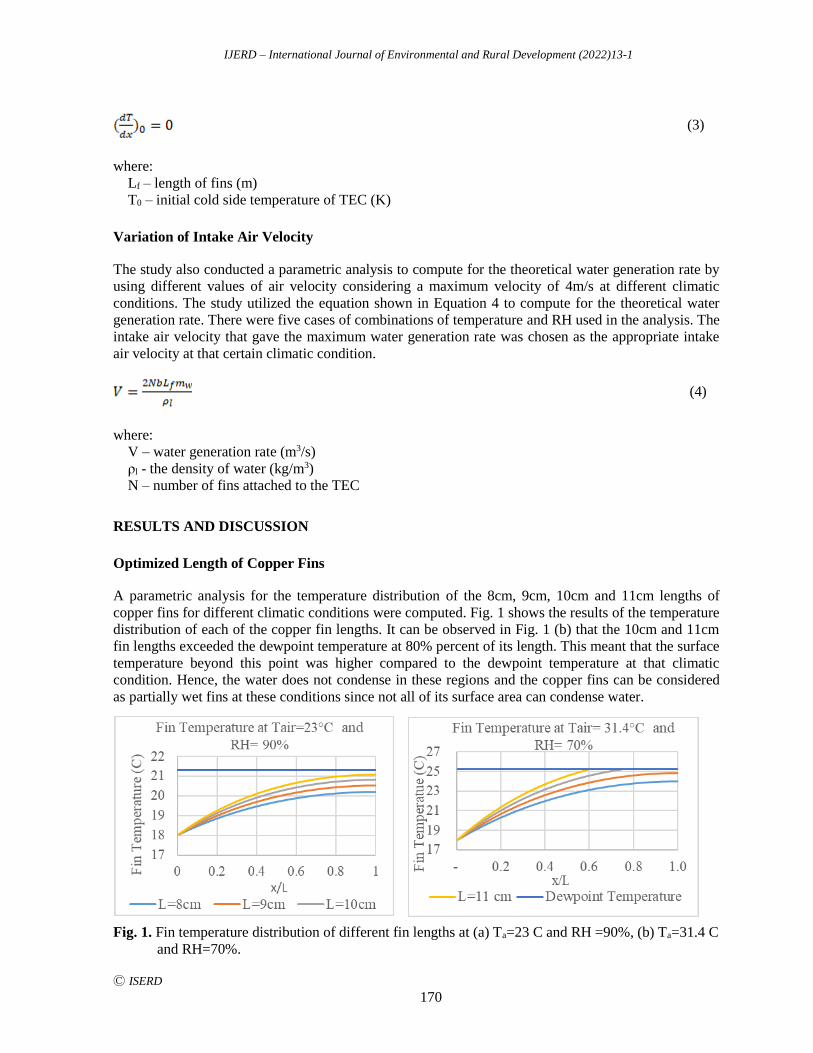
IJERD – International Journal of Environmental and Rural Development (2022)13-1
Ⓒ ISERD
170
(3)
where:
Lf – length of fins (m)
T0 – initial cold side temperature of TEC (K)
Variation of Intake Air Velocity
The study also conducted a parametric analysis to compute for the theoretical water generation rate by
using different values of air velocity considering a maximum velocity of 4m/s at different climatic
conditions. The study utilized the equation shown in Equation 4 to compute for the theoretical water
generation rate. There were five cases of combinations of temperature and RH used in the analysis. The
intake air velocity that gave the maximum water generation rate was chosen as the appropriate intake
air velocity at that certain climatic condition.
(4)
where:
V – water generation rate (m3/s)
ρl - the density of water (kg/m3)
N – number of fins attached to the TEC
RESULTS AND DISCUSSION
Optimized Length of Copper Fins
A parametric analysis for the temperature distribution of the 8cm, 9cm, 10cm and 11cm lengths of
copper fins for different climatic conditions were computed. Fig. 1 shows the results of the temperature
distribution of each of the copper fin lengths. It can be observed in Fig. 1 (b) that the 10cm and 11cm
fin lengths exceeded the dewpoint temperature at 80% percent of its length. This meant that the surface
temperature beyond this point was higher compared to the dewpoint temperature at that climatic
condition. Hence, the water does not condense in these regions and the copper fins can be considered
as partially wet fins at these conditions since not all of its surface area can condense water.
Fig. 1. Fin temperature distribution of different fin lengths at (a) Ta=23 C and RH =90%, (b) Ta=31.4 C
and RH=70%.
IJERD – International Journal of Environmental and Rural Development (2022)13-1
Ⓒ ISERD
171
On the other hand, it can be seen in Fig. 2 that the 9cm fin length did not reached the dewpoint
temperature at all cases of climatic conditions. This meant that all the surface area of the 9cm length
copper fins can condense water vapor. Hence, the optimum length of the copper fins that was also
incorporated in the design of the AWG was the 9cm length.
Variation of Intake Air Velocity
Table 1 presents the cases used in the analysis with different ambient air temperature and variable RH
levels.
Table 1 Summary of Cases of Temperature and RH used in the analysis.
Case No. Ta (oC) RH 1 (%) RH 2 (%) RH 3 (%) RH 4 (%)
1 23.00 80.00 85.00 90.00 -
2 25.00 75.00 80.00 85.00 90.00
3 29.00 75.00 80.00 85.00 90.00
4 31.00 75.00 80.00 85.00 90.00
By applying these cases in the computation along with different variations of intake air velocity
considering a maximum velocity of 4m/s, the theoretical water generation rate was obtained and the
results were shown in Fig. 2. It can be observed from the results that increasing the air velocity
generally increases the water generation rate for most of the cases presented.
Fig. 2. Theoretical Water Generation Rate at different Air Velocities for (a) Case 1, (b) Case 2,
(c) Case 3, (d) Case 4, and (e) Case 5.
For Case 1 and Case 2, there were low ambient air temperature paired with low RH levels. It can
be observed in Fig. 2 (a) and (b) between RH of 75% to 80%, the water generation rate increased
initially when the air velocity was also increased but then decreased at higher magnitudes of air
IJERD – International Journal of Environmental and Rural Development (2022)13-1
Ⓒ ISERD
172
velocity. Hence, the air velocity of the fans can be adjusted at peak water generation rate when the
AWG device is subjected to low relative humidity such as in Case 1 and Case 2.
For Case 3 and Case 4, the increase of air velocity also result in the increase of water generation
rate. For this case, the increase of the value of mass transfer coefficient resulting from the increase in
air velocity outweighed the decrease in the difference between the partial pressure of the surrounding
air and partial pressure at the fin surface.
Based from the results shown in Fig. 2, Table 2 summarizes the appropriate intake air velocity at
different climatic conditions. The values indicated in Table 2 were then incorporated in the design of
the AWG in which the air velocity were varied depending on the climatic conditions.
Table 2 Summary of Appropriate Air Velocity at Different Climatic Conditions.
Relative
Humidity
Intake Air Velocity (m/s)
23°C ≤ 24°C 24°C ≤ 26°C 26°C ≤ 28°C 28°C ≤ Ta
75%<80% 0.00 0.20 2.00 4.00
80%<85% 0.60 2.00 4.00 4.00
85%<90% 2.00 4.00 4.00 4.00
90% < 100% 4.00 4.00 4.00 4.00
Construction and Experimental Analysis of the Device
The study utilized the 9 cm copper fin length and the magnitudes of variable intake air velocity into the
design of the AWG device. Figure 3 shows the blow up figure of the AWG prototype.
The AWG device was continuously operated for 30 days in a secure open space located at Manolo
Fortich, Bukidnon for the experimental analysis. The testing area for the field test was located at the
backyard of a residential lot located at a rural community at Manolo Fortich, Bukidnon. The period of
testing was between the September to October 2021 and the experimental setup is shown in Fig. 3b.
The average hourly RH, ambient air temperature was shown Fig. 4 and the average hourly water
collection was shown in Fig. 5.
Fig. 3 Blow up picture of the AWG Device with its corresponding parts (a) and finished product
and experimental setup (b).
IJERD – International Journal of Environmental and Rural Development (2022)13-1
Ⓒ ISERD
173
Fig. 4 Average hourly ambient air temperature and relative humidity.
Fig. 5 Average Hourly Water Collection for the AWG Device
It can be seen in Figure 5 that the highest water collection rate of the AWG was during nighttime
since there was high RH levels paired with low surrounding temperature. Overall, the highest recorded
amount of water collected in a day was 526mL. Table 3 shows the comparison between the outputs of
this study compared to past literatures.
Table 3. Comparison Water Collected per Day to Past Literatures.
Researcher Location Water Collected(mL/day)
Joshi et.al. (2017) India 480
Liu et.al. (2017) China 525
Present Work Philippines 526
CONCLUSION
The cold side fin length and air velocity are two important features of an AWG device that are needed
to be designed to improve the efficiency and water generation rate. The study observed that while
increasing the length of copper fins increases the cooling surface area, making the fin length
excessively longer does not positively impact the water generation rate of the AWG. Longer fin lengths
will develop dry regions along its length thus becoming inefficient.
Finally, the results in this study showed that there was an ideal air velocity at every climatic
conditions in order to harness the maximum water generation rate for the AWG device. Low air
velocities were assigned to low surrounding temperature with low relative humidity conditions while
high air velocities were designated for high surrounding temperature and high relative humidity
conditions. The highest amount of water collected in a day was 526mL.
IJERD – International Journal of Environmental and Rural Development (2022)13-1
Ⓒ ISERD
174
ACKNOWLEDGEMENTS
The author would like to acknowledge the Engineering Research and Development for Technology
(ERDT) for funding this research Mindanao State University-Iligan Institute of Technology for
supporting this research.
REFERENCES
Joshi, V., Kothari, H., Mahajan, M., Chaudhari, M., & Sant , K. 2017. Experimental investigations on a portable
freshwater generator using a thermoelectric cooler. Energy Procedia, 29, 161-166, Retrieved from http://doi:
10.1016/j.egypro.2017.03.085
Kilic, A., & Onat, K. 1981. The Optimum Shape for Convecting Rectangular Fins when Condensation Occurs.
Warme - und Stoffubetragung, 15, 125–133 (1981). Retrieved from https://doi.org/10.1007/BF01002408
Liu, S., He, W., Hu, D., LV, S., Chen, D., Wu, X., Xu, F & Li, S. 2017. Experimental Analysis of a Portable
Atmospheric Water Generator by Thermoelectric Cooling Method. Energy Procedia, 142, 1609-1614,
Retrieved from https://doi.org/10.1016/j.egypro.2017.12.538
Rola, A. C., Pulhin, J., Guillermo, T., Lizada, J. C., & Dayo, M. F. 2015. Challenges of Water Governance in the
Philippines. Philippine Journal of Science, 144, 197-208, Retrieved from
https://philjournalsci.dost.gov.ph/images/pdf/pjs_pdf/vol144no2/pdf/challenges_of_water_governance_in_th
e_Phils_FinalCopy_05_April_2016.pdf
Hafner, S. 2018. Re: how much CO2/DIC dissolves in water vapor condensate under normal atmospheric
conditions?, Retrieved from: https://www.researchgate.net/post/How-much-CO2-DIC-dissolves-in-water-
vapor-condensate-under-normal-atmospheric-conditions/5a75cecf615e27bab3589949
/citation/download
Shourideh, A., Ajram, W., Lami , J., Haggag, S., & Mansouri, A. 2018. A Comprehensive Study of an
Atmospheric Water Generator using Peltier Effect. Thermal Science and Engineering Progress, 6, 14-26,
Retrived from https://doi.org/10.1016/j.tsep.2018.02.015
IJERD – International Journal of Environmental and Rural Development (2022)13-1
Ⓒ ISERD
175
DNA Fingerprinting of Selected Maize (Zea mays L.)
Genotypes using SSR Markers
SAN KYI* Yezin Agricultural University (YAU), Nay Pyi Taw, Myanmar
Email: [email protected]
KYAW KYAW WIN
Pro-Rector’s Office of (Administration), YAU, Nay Pyi Taw, Myanmar
HLA THAN Pro-Rector’s Office of (Academic), YAU, Nay Pyi Taw, Myanmar
SOE WIN Department of Plant Breeding, Physiology and Ecology, YAU, Nay Pyi Taw, Myanmar
NYO MAR HTWE Advanced Center for Agricultural Research and Education (ACARE), YAU, Nay Pyi Taw, Myanmar
AYE LAE LAE HLAING Plant Molecular Biology Laboratory, Biotechnology Research Section, Department of Agricultural
Research (DAR), Nay Pyi Taw, Myanmar
Received 28 January 2022 Accepted 2 May 2022 (*Corresponding Author)
Abstract Molecular marker has been used for variety identification, genetic diversity of
genotypes and additional using intellectual property protection in DUS testing. DNA
fingerprinting of fourteen maize genotypes had been studied at Plant Biotechnology Laboratory,
DAR, Myanmar during 2020-2021. Nine hybrids and five inbreds were analyzed using 24
polymorphic SSR markers, resulted a total number of 101 alleles with a range from 2 to 9
alleles per locus. Polymorphism has been sufficiently detected with the average of 0.66 per SSR
locus. Cluster analysis separated all the maize genotypes as five major groups and indicated the
existence of genetic variation among the observed inbreds and hybrids. Six SSR primer pairs
(dupssr12, bnlg1940, umc1248, umc1586, bnlg1518 and bnlg1028) were selected as final
marker set for variety identification with the selection criteria such as detection rate of the SSR
fragment, the presence of rare allele, PIC value, and reproducibility and PCR band pattern of
SSR fragments. In this study, all tested genotypes have been fingerprinted with unique profile
identity (ID) to support the DNA fingerprint catalogues of Myanmar Maize Molecular DUS test
guidelines.
Keywords: DNA fingerprinting, Maize SSR markers, Varietal Identification
INTRODUCTION
Maize (Zea mays L.) is the most diverse crop species characterized at both morphological and
molecular levels (Anderson and Cutler, 1942; Buckler et al., 2006; Zheng et al., 2008). Genetic
identification of maize is essential in the process of crop improvement, crop quality estimation and the
finding of parent components and their crosses.
erd
Research article
IJERD – International Journal of Environmental and Rural Development (2022)13-1
Ⓒ ISERD
176
SSR markers were able to discriminate maize genotypes depending upon their hybridization level
and their genetic relationships among the different inbred lines (Kamal et al., 2010). It is the most
powerful biotechnological tool, suitable for detecting of genetic purity status of maize hybrids. SSR
also used in DNA fingerprinting analysis for identification of individuals, populations, inbred lines,
and hybrids, making the description of the species at the molecular level, to protect the breeders’
Rights and its protection.
Plant varietal protection and patents are the most important end products of plant breeding
institutes to get back their research investment by mean of intellectual property protection. DNA
fingerprinting technology is useful for preventing counterfeit and fake varieties in the market and this
fingerprinting information is additional information for DUS characterization (Wang et al., 2013).
UPOV (2010) recommends SSRs for current construction of DNA fingerprint databases that have been
well-defined and tested. In the present study, the SSR primers set were used to differentiate hybrids
and inbreds, and to create the DNA fingerprint catalogues for supporting of Myanmar Maize DUS test
guidelines for identifying maize genotypes in infringement case, and for utilizing as a source of
parental line for future breeding programs.
METHODOLOGY
Plant materials and genomic DNA extraction
Fourteen maize genotypes (Table 1) were used to study molecular characterization at Plant
Biotechnology Laboratory, Department of Agricultural Research (DAR), Myanmar during 2020-2021.
Nine hybrids (imported by private companies) and five inbred lines (developed by DAR) were used.
Genomic DNA extraction, DNA quantification and qualification were carried out according to the
procedure of Hlaing et al., 2017.
Table 1. List of selected maize genotypes for molecular characterization
No. Genotypes Type Source No. Genotypes Type Source
V1 Asia Seed (A.55) Hybrid China V8 NK-621 Hybrid Syngenta
V2 Asia Seed (A.99) Hybrid China V9 TSF-1633 Hybrid Thai
V3 AA-737 Hybrid Thai V10 YZI-10-054 Inbred DAR
V4 GT-722 Hybrid Thai V11 YZI-10-095 Inbred DAR
V5 NK-625 Hybrid Syngenta V12 PAC-999 Inbred Thai
V6 KMHE-3550 Hybrid India V13 C7 Inbred DAR
V7 CP-111 Hybrid Thai V14 YZCI-16-019 Inbred DAR
PCR amplification and gel electrophoresis
Twenty four SSR primer pairs were used to identify the studied maize genotypes. These highly
polymorphic primer sets, PCR amplification and agarose gel electrophoresis were conducted following
the methods reported by previous research findings (Hlaing et al., 2017).
Statistical analysis on marker data
The SSR allele segregation data were used to construct Nei distance dendrogram (Nei, 1972) using
NTSYSpc 2.1 software (Rohlf, 2000). Polymorphism Information Content (PIC) for each SSR was

IJERD – International Journal of Environmental and Rural Development (2022)13-1
Ⓒ ISERD
177
calculated by the formula developed by Ni et al. (2002) where, X2k represents the
frequency of the kth allele, and n represents the number of genotypes.
Development of core SSR marker set for DNA fingerprinting (DUS testing)
Based on their specific discrimination capacity of SSR markers, the core marker set was developed
with the following criteria: (1) PCR banding pattern of SSR fragments (2) the presence of rare allele
(3) PIC values and (4) marker’s reproducibility. Furthermore, the genetic fingerprint map of tested
maize genotypes was constructed using the coding-based system with the original allele size coded by
the assigned numeric values which set in two numeric codes from “01”, “02”, “03”, etc. The
transformation was generated to all cores SSR ID set based on allele size (bp) range. The final SSR
fingerprinting map of maize genotypes was produced to support variety identification and DUS testing
on PVP system.
RESULTS AND DISCUSSION
Amplification profile, SSR polymorphism and Cluster analysis on diversity assessment
SSR markers have been proven to be powerful tools in the assessment of genetic variation within and
among the species. A total of 24 SSR primers were used for identification of maize genotypes through
evaluation of DNA fragment polymorphisms. A total number of 101 alleles were detected with a range
from 2 to 9 alleles per locus. These varied number of alleles indicated that there is a high level of
genetic diversity among tested genotypes. The primer pairs bnlg1028 showed the highest number of 9
alleles per locus, umc1248 showed 8 alleles in all tested genotypes and umc1586, bnlg1940 and
dupssr12 showed 6 alleles in all samples (Table 2).
Table 2. Data on number of allele, total number of allele, and PIC value obtained among 14
maize genotypes for 24 SSR markers
No. SSR
marker
No. of
alleles
Total no.
of alleles
PIC
value No. SSR marker
No. of
alleles
Total no.
of alleles
PIC
value
1. umc1397 4 20 0.63 13. bnlg1617 4 14 0.72
2. umc2234 3 20 0.62 14. umc1520 5 22 0.71
3. dupssr12 6 30 0.77 15. umc1248 8 38 0.85
4. umc1542 3 20 0.62 16. umc1393 3 15 0.66
5. umc2372 4 19 0.70 17. umc1671 5 24 0.59
6. bnlg1940 6 28 0.74 18. umc2395 3 16 0.53
7. bnlg1160 3 23 0.63 19. bnlg1065 3 20 0.65
8. umc1501 4 16 0.73 20. umc1586 6 48 0.80
9. umc2061 4 16 0.72 21. umc2359 2 14 0.41
10. umc1101 3 19 0.61 22. umc1962 5 34 0.77
11. umc1752 2 14 0.50 23. bnlg1518 4 18 0.67
12. umc1792 2 15 0.48 24. bnlg1028 9 36 0.78
The Polymorphism Information Content (PIC) value reflects the evidence of allele diversity and
allele frequency among the tested genotypes (Pervaiz et al., 2009). In present study, PIC value ranged
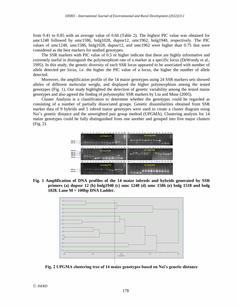
IJERD – International Journal of Environmental and Rural Development (2022)13-1
Ⓒ ISERD
178
from 0.41 to 0.85 with an average value of 0.66 (Table 2). The highest PIC value was obtained for
umc1248 followed by umc1586, bnlg1028, dupssr12, umc1962, bnlg1940, respectively. The PIC
values of umc1248, umc1586, bnlg1028, dupssr12, and umc1962 were higher than 0.75 that were
considered as the best markers for studied genotypes.
The SSR markers with PIC value of 0.5 or higher indicate that these are highly informative and
extremely useful in distinguish the polymorphism rate of a marker at a specific locus (DeWoody et al.,
1995). In this study, the genetic diversity of each SSR locus appeared to be associated with number of
allele detected per locus, i.e. the higher the PIC value of a locus, the higher the number of allele
detected.
Moreover, the amplification profile of the 14 maize genotypes using 24 SSR markers sets showed
alleles of different molecular weight, and displayed the higher polymorphism among the tested
genotypes (Fig. 1). Our study highlighted the detection of genetic variability among the tested maize
genotypes and also agreed the finding of polymorphic SSR markers by Liu and Muse (2005).
Cluster Analysis is a classification to determine whether the genotypes could be regarded as
consisting of a number of partially dissociated groups. Genetic dissimilarities obtained from SSR
marker data of 9 hybrids and 5 inbred maize genotypes were used to create a cluster diagram using
Nei’s genetic distance and the unweighted pair group method (UPGMA). Clustering analysis for 14
maize genotypes could be fully distinguished from one another and grouped into five major clusters
(Fig. 2).
Fig. 1 Amplification of DNA profiles of the 14 maize inbreds and hybrids generated by SSR
primers (a) dupssr 12 (b) bnlg1940 (c) umc 1248 (d) umc 1586 (e) bnlg 1518 and bnlg
1028. Lane M = 100bp DNA Ladder.
Coefficient
0.29 0.44 0.60 0.75 0.91
V10
V1
V4
V2
V3
V5
V12
V14
V6
V8
V7
V9
V10
V11
V13
Fig. 2 UPGMA clustering tree of 14 maize genotypes based on Nei’s genetic distance
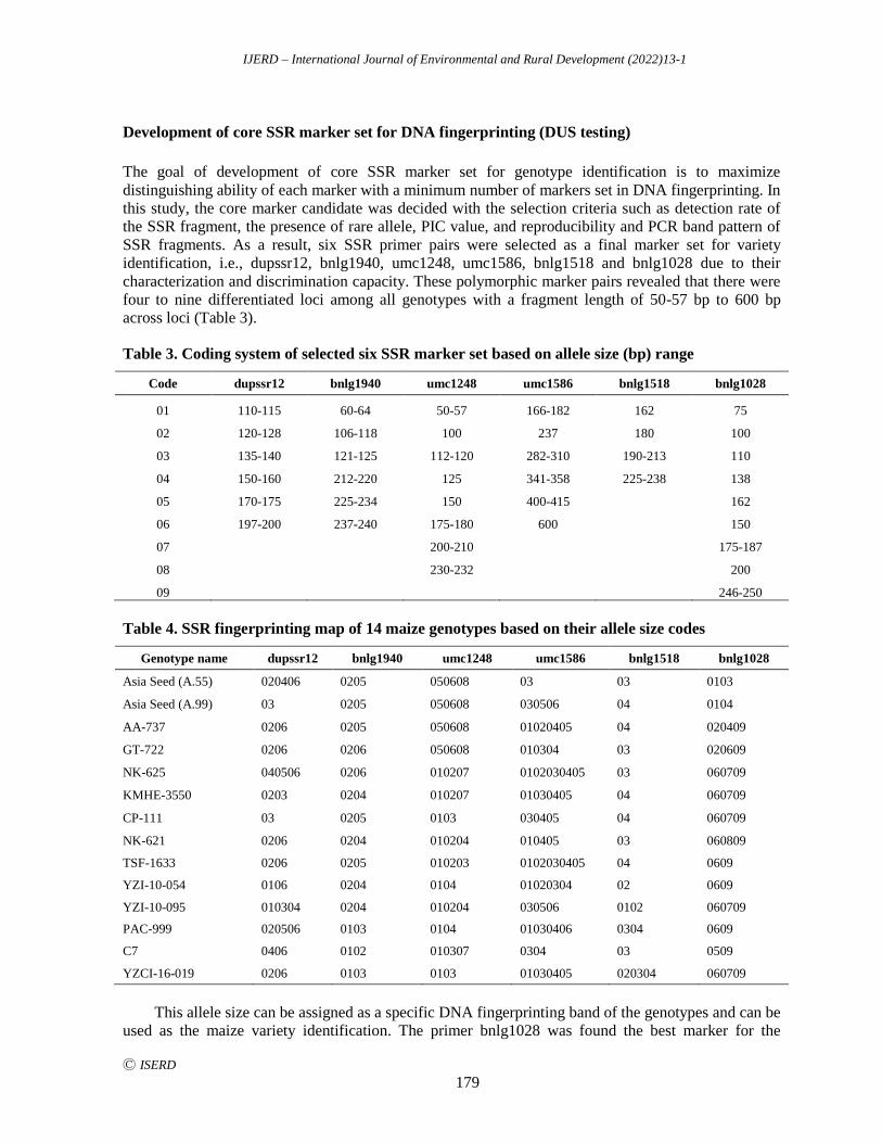
IJERD – International Journal of Environmental and Rural Development (2022)13-1
Ⓒ ISERD
179
Development of core SSR marker set for DNA fingerprinting (DUS testing)
The goal of development of core SSR marker set for genotype identification is to maximize
distinguishing ability of each marker with a minimum number of markers set in DNA fingerprinting. In
this study, the core marker candidate was decided with the selection criteria such as detection rate of
the SSR fragment, the presence of rare allele, PIC value, and reproducibility and PCR band pattern of
SSR fragments. As a result, six SSR primer pairs were selected as a final marker set for variety
identification, i.e., dupssr12, bnlg1940, umc1248, umc1586, bnlg1518 and bnlg1028 due to their
characterization and discrimination capacity. These polymorphic marker pairs revealed that there were
four to nine differentiated loci among all genotypes with a fragment length of 50-57 bp to 600 bp
across loci (Table 3).
Table 3. Coding system of selected six SSR marker set based on allele size (bp) range
Code dupssr12 bnlg1940 umc1248 umc1586 bnlg1518 bnlg1028
01 110-115 60-64 50-57 166-182 162 75
02 120-128 106-118 100 237 180 100
03 135-140 121-125 112-120 282-310 190-213 110
04 150-160 212-220 125 341-358 225-238 138
05 170-175 225-234 150 400-415
162
06 197-200 237-240 175-180 600
150
07
200-210
175-187
08
230-232
200
09
246-250
Table 4. SSR fingerprinting map of 14 maize genotypes based on their allele size codes
Genotype name dupssr12 bnlg1940 umc1248 umc1586 bnlg1518 bnlg1028
Asia Seed (A.55) 020406 0205 050608 03 03 0103
Asia Seed (A.99) 03 0205 050608 030506 04 0104
AA-737 0206 0205 050608 01020405 04 020409
GT-722 0206 0206 050608 010304 03 020609
NK-625 040506 0206 010207 0102030405 03 060709
KMHE-3550 0203 0204 010207 01030405 04 060709
CP-111 03 0205 0103 030405 04 060709
NK-621 0206 0204 010204 010405 03 060809
TSF-1633 0206 0205 010203 0102030405 04 0609
YZI-10-054 0106 0204 0104 01020304 02 0609
YZI-10-095 010304 0204 010204 030506 0102 060709
PAC-999 020506 0103 0104 01030406 0304 0609
C7 0406 0102 010307 0304 03 0509
YZCI-16-019 0206 0103 0103 01030405 020304 060709
This allele size can be assigned as a specific DNA fingerprinting band of the genotypes and can be
used as the maize variety identification. The primer bnlg1028 was found the best marker for the
IJERD – International Journal of Environmental and Rural Development (2022)13-1
Ⓒ ISERD
180
identification of studied genotypes as revealed by higher PIC values and showed the highest
polymorphism. In other study, DNA fingerprinting with SSR set of tested maize genotypes were fully
distinguished from one another compared to the specific SSR markers which differentiated maize
hybrids from their parental inbreds (Jhansi et al., 2015). In this study, the genetic fingerprint map of 14
maize genotypes was constructed using the coding-based method with the original allele size coded by
the assigned numeric values and the specific marker’s allelic fragments were transformed into combine
codes as final identity of the genotype, shown in Table 3 and Table 4. By using the core marker set, the
results of assigning numeric code or ID described a specific identity of the variety (genotype) that can
quantitatively differentiate it from the others. In this study, 14 maize varieties had unique profile ID to
support plant variety protection and breeder right, complementing tools for DUS testing purpose. It is
noted that this findings not only met the requirements for the minimum number of primers but were
also sufficient to fully distinguish the 14 varieties from one another.
CONCLUSION
The goal of this research is to develop DNA fingerprinting catalogue of maize genotypes (both inbreds
and hybrids) using SSR polymorphic information and their genetic variance supporting Myanmar
maize DUS guidelines. In this study, the six pairs SSR sets generate the genetic fingerprint map
(coding system) of typical maize genotypes which can be used in DUS testing for identification of
hybrids and inbreds at any stage of crop growing cycle. Furthermore, molecular based SSR testing
provide a higher degree of detection efficiency in DUS testing than traditional morphological based
DUS method with regard to the verification of new varieties or genotypes.
ACKNOWLEDGEMENTS
The authors are grateful to the responsible persons from DOA, DAR and YAU for their kind
permission and collaborating to conduct this study. We acknowledge all the staffs of Biotechnology
Research Section, DAR for helping us.
REFERENCES
Anderson, E. and Cutler, C.H. 1942. Races of Zea mays: I. Their recognition and classification. Annals of the
Missouri Botanical Garden, 29(2), 69-88. https://doi.org/10.2307/2394331
Buckler, S.E., Gaut, S.B. and McMullen, D.M. 2006. Molecular and functional diversity of maize. Current
Opinion in Plant Biology, 9(2), 172-176. https://doi.org/10.1016/j.pbi.2006.01.013
DeWoody, A.J., Honeycutt, L.R. and Skow, C.L. 1995. Microsatellite markers in white-tailed deer. The Journal
of Heredity, 86(4), 317-319. https://doi.org/10.1093/oxfordjournals.jhered.a111593
Hlaing, L.L.A., Sin, S.E., Chan, N.K., Tint, M.M.A., Yin, T., Yin, N.N. and OO, T.L. 2017. Molecular
characterization of promising maize inbred lines using polymorphic microsatellite markers. Proceedings of
the first agricultural Research Conference. Department of Agricultural Research. Yezin, Nay Pyi Taw. 84-
92.
Jhansi, G., Surender, M., Aparnna., Reddy, S.S. and Sunitha, B. 2015. DNA finger printing of maize hybrids and
development of molecular ID’s using SSR markers. Research Journal of Agricultural Sciences, 6(1), 43-47.
DI:2149-3000-2014-010
Kamal, A., Reddy, S.K., Khan, A.N.M., Shetti, V.R., Ramaiah, J.M., Pushpavalli, L.V.C.N.S., Srinivas, C., Pal-
Bhadra, M., Chourasia, M., Sastry, N.G., Juvekar, A., Zingde, S. and Barkume, M. 2010. Synthesis, DNA-
binding ability and anticancer activity of benzothiazole/benzoxazole–pyrrolo [2, 1-c] [1, 4] benzodiazepine
conjugates. Bioorganic and Medicinal Chemistry, 18(13), 4747-4761.
IJERD – International Journal of Environmental and Rural Development (2022)13-1
Ⓒ ISERD
181
Liu, K. and Muse, V. S. 2005. Power Marker: an integrated analysis environment for genetic marker analysis.
Bioinformatics, 21(9), 2128-2129. https://doi.org/10.1093/bioinformatics/bti282
Nei, M. 1972. Genetic distance between populations. The American Naturalist, 106(949), 283-292.
Ni, J., Colowit, M.P. and Mackill, J.D. 2002. Evaluation of genetic diversity in rice sub species using
microsatellite markers. Crop Science, 42, 601-607. https://doi.org/10.2135/cropsci2002.6010
Pervaiz, H.Z., Rabbani, A.M., Pearce, R.S. and Malik, A.S. 2009. Determination of genetic variability of Asian
rice (Oryza sativa L.) varieties using microsatellite markers. African Journal of Biotechnology, 8(21), 5641-
5651. DOI: 10.5897/AJB09.827
Rohlf, F.J. 2000. NTSYS-pc: Numerical Taxonomy and Multivariate Analysis System Version 2.1 Exeter
Publishing Setauket. New York.
UPOV (International Union for the Protection of New Varieties of Plant). 2010. Guidelines for DNAprofiling:
molecular marker selection and database construction (“BMT guidelines”). UPOV, Geneva, Switzerland.
Wang, Y.P., Shen, Q., Zhang, J.H., Li, H.Y. and Wu, Y. 2013. Genetic diversity analysis and building of DNA
fingerprints of barley standard varieties in DUS testing based on SSR Markers. Journal of Triticeae Crops, 2,
273-278.
Zheng, D-H., Van, K. and Lee, S-H. 2008. Molecular diversity and relationships among elite maize inbreds from
US and CIMMYT populations and current heterotic groups in China. Hereditas, 145(4), 182-193. DOI:
10.1111/j.2008.0018-0661.02048.x
IJERD – International Journal of Environmental and Rural Development (2022)13-1
Ⓒ ISERD
182
Toxicity of plant essential oil from Khok Phutaka Resources
Protection Area, Khon Kaen Province against storage pest,
Sitophilus oryzae
DUANGRAT THONGPHAK* Entomology Section, Faculty of Agriculture, Khon Kaen University, Khon Kaen, 40002, Thailand,
E-mail: [email protected]
PRAPAPORN PIANGSUWAN Entomology Section, Faculty of Agriculture, Khon Kaen University, Khon Kaen, 40002, Thailand
Received 30 January 2022 Accepted 2 May 2022 (*Corresponding Author)
Abstract Botanical insecticides may offer an alternative solution for pest control. The objective
was to test on the repellant, contact, and fumigant effect of the essential oils of 10 indigenous
plants from Khok Phutaka Resources Protection Area, Khon Kaen Province including
Limnophila aromatica, Piper sarmentosum, Clausena harmandiana, Streptocaulon juventas,
Litsea glutinosa, Thunbergia laurifolia, Eupatorium odoratum, Rothmannia wittii, Ficus altissima, Clausena harmandiana and Gymnopetalum integrifolim to control the rice weevil, S.
oryzae. The essential oils of plants were extracted by using hydro-distillation method and then
they were tested against rice grain weevil, S. oryzae for contact, fumigant and repellent
activities in laboratory condition. Adults weevil were different tested oil at the concentrations of
0, 25, 50, 75 and 100 percentage (w/v). The maximum repellency action, 80% when L. glutinosa oil, at the concentrations of 100% (w/v) were applied for after 72 hours follow by L.
aromatica (73.33%) at the concentrations of 25% (w/v) were applied for after 2 hours. The
fumigant and contact test of all 10 essential oils resulted in all lower rate mortality (less than
50%), at all the concentrations.
Keywords: essential oil, Sitophilus oryzae, repellency, fumigant, contact, Khok Phutaka
Resources Protection Area
INTRODUCTION
The rice weevil, Sitophilus oryzae Linnaeus 1763 (Coleoptera: Curculionidae) is a serious and severe
insect pest of stored products (Park I.K., 2003) and one of the most widespread and destructive stored
product pests of rice throughout the world. Treatment of rice with synthetic insecticides is not
recommended because of direct and indirect health hazards to humans. Plants are sources of natural
insecticides that are produced to defend themselves against those insect pests. Many plants are rich in
secondary compounds with insecticidal activities. The several efforts have been focused on the use of
plant derived materials including essential oils as bio insecticides.
OBJECTIVE
The objective of this study was to screen plant oils of 10 indigenous plants from Khok Phutaka
Resources Protection Area, Khon Kaen Province as repellent contact and fumigant against adults of
rice weevil, S. oryzae.
erd
Research article
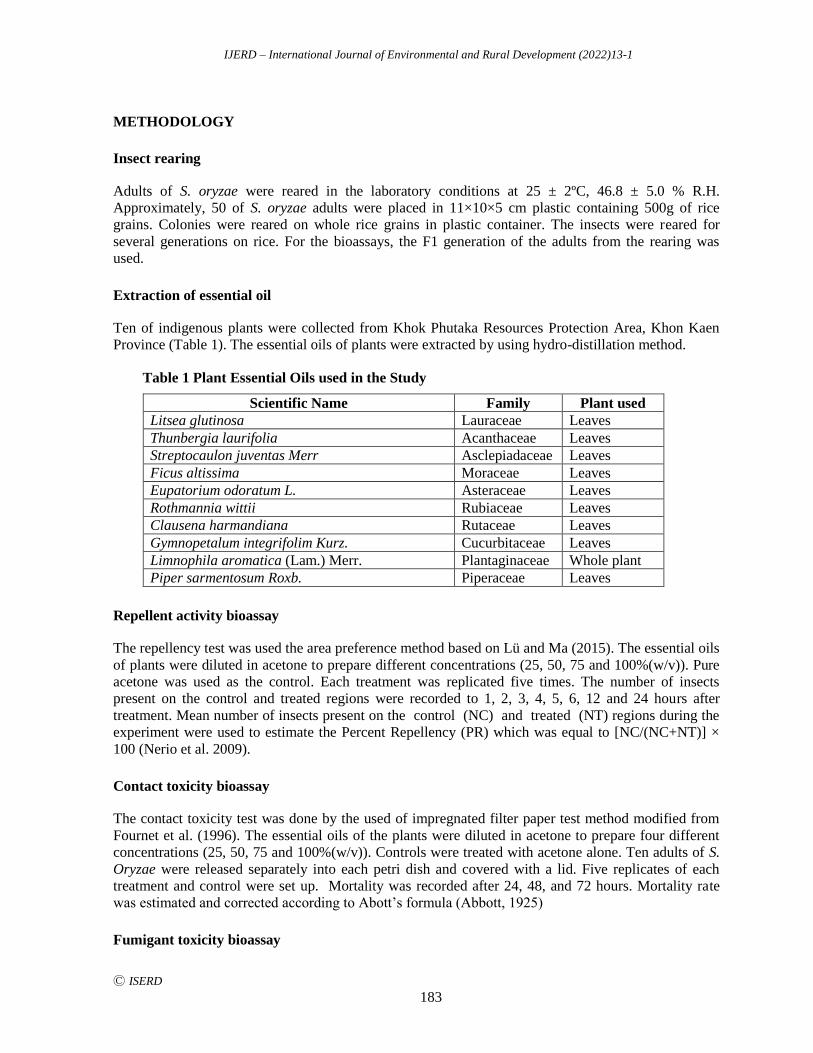
IJERD – International Journal of Environmental and Rural Development (2022)13-1
Ⓒ ISERD
183
METHODOLOGY
Insect rearing
Adults of S. oryzae were reared in the laboratory conditions at 25 ± 2ºC, 46.8 ± 5.0 % R.H.
Approximately, 50 of S. oryzae adults were placed in 11×10×5 cm plastic containing 500g of rice
grains. Colonies were reared on whole rice grains in plastic container. The insects were reared for
several generations on rice. For the bioassays, the F1 generation of the adults from the rearing was
used.
Extraction of essential oil
Ten of indigenous plants were collected from Khok Phutaka Resources Protection Area, Khon Kaen
Province (Table 1). The essential oils of plants were extracted by using hydro-distillation method.
Table 1 Plant Essential Oils used in the Study
Scientific Name Family Plant used
Litsea glutinosa Lauraceae Leaves
Thunbergia laurifolia Acanthaceae Leaves
Streptocaulon juventas Merr Asclepiadaceae Leaves
Ficus altissima Moraceae Leaves
Eupatorium odoratum L. Asteraceae Leaves
Rothmannia wittii Rubiaceae Leaves
Clausena harmandiana Rutaceae Leaves
Gymnopetalum integrifolim Kurz. Cucurbitaceae Leaves
Limnophila aromatica (Lam.) Merr. Plantaginaceae Whole plant Piper sarmentosum Roxb. Piperaceae Leaves
Repellent activity bioassay
The repellency test was used the area preference method based on Lü and Ma (2015). The essential oils
of plants were diluted in acetone to prepare different concentrations (25, 50, 75 and 100%(w/v)). Pure
acetone was used as the control. Each treatment was replicated five times. The number of insects
present on the control and treated regions were recorded to 1, 2, 3, 4, 5, 6, 12 and 24 hours after
treatment. Mean number of insects present on the control (NC) and treated (NT) regions during the
experiment were used to estimate the Percent Repellency (PR) which was equal to [NC/(NC+NT)] ×
100 (Nerio et al. 2009).
Contact toxicity bioassay
The contact toxicity test was done by the used of impregnated filter paper test method modified from
Fournet et al. (1996). The essential oils of the plants were diluted in acetone to prepare four different
concentrations (25, 50, 75 and 100%(w/v)). Controls were treated with acetone alone. Ten adults of S.
Oryzae were released separately into each petri dish and covered with a lid. Five replicates of each
treatment and control were set up. Mortality was recorded after 24, 48, and 72 hours. Mortality rate
was estimated and corrected according to Abott’s formula (Abbott, 1925)
Fumigant toxicity bioassay

IJERD – International Journal of Environmental and Rural Development (2022)13-1
Ⓒ ISERD
184
The fumigant toxicity test was conducted by using space trial test method based on Keita et al. (2001).
Series of dilutions of essential oils were prepared different concentrations (25, 50, 75 and 100% (w/v))
using acetone as a solvent. Five replications of each treatment were set up. Controls were maintained in
the similar way with the solvent only. Mortality was recorded after 24, 48, and 72 hours. Mortality rate
was estimated and corrected according to Abott’s formula (Abbott, 1925)
RESULT AND DISCUSSION
Ten different plant oils were tested against the adults of Sitophilus oryzae at concentrations of 25, 50,
75 and 100%(w/v) for repellent activity, contact toxicity and fumigant toxicity tests.
Repellent activity bioassay
In general, repellency increases with increase in concentration in the treatment. The result indicated
variation among the essential oils tested. The Percent Repellency (PR) ranged from 23.33 to 80.00 %.
The maximum repellency action, 80 % when L. glutinosa oil, at the concentrations of 100 % (w/v)
were applied for after 72 hours follow by L. aromatica (73.33%) at the concentrations of 25 % (w/v)
were applied for after 2 hours (Fig.1). Arshad et al. (2013) that tested the repellents of guava leaf
extracts found 20%(w/v) concentration of P. guajava was the one with the highest repellent effects on
S. oryzae with mean % repellent of 70.3%(class 4) might be attributed to presence of some aromatic
monoterpenoids that are major constituents of family Mytaceae (Isman, 2000) and this substance is a
group of substances found in L. aromatica as well (Vairappan and Nagappan, 2014).
Fig. 1. Comparison percent repellency (PR) of the 10 essential oils with different concentration to
Sitophilus oryzae adults after exposure time using the area preference method
Contact toxicity bioassay
Mortality of S. oryzae varied from 0 to 30% after 24, 48, 72 hrs. of treated of 10 essential oil of plants
at 25,50,75 and 100 concentration (w/v). These results demonstrate (Fig.2) that the efficiency of the
oils was directly related to concentration and exposure time. Oil from R.wittii was the most efficient,
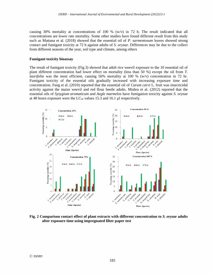
IJERD – International Journal of Environmental and Rural Development (2022)13-1
Ⓒ ISERD
185
causing 30% mortality at concentrations of 100 % (w/v) in 72 h. The result indicated that all
concentrations are lower rate mortality. Some other studies have found different result from this study
such as Mattana et al. (2018) showed that the essential oil of P. sarmentosum leaves showed strong
contact and fumigant toxicity at 72 h against adults of S. oryzae. Differences may be due to the collect
from different seasons of the year, soil type and climate, among others
Fumigant toxicity bioassay
The result of fumigant toxicity (Fig.3) showed that adult rice weevil exposure to the 10 essential oil of
plant different concentration had lower effect on mortality (less than 50 %) except the oil from T.
laurifolia was the most efficient, causing 56% mortality at 100 % (w/v) concentration in 72 hr.
Fumigant toxicity of the essential oils gradually increased with increasing exposure time and
concentration. Fang et al. (2010) reported that the essential oil of Carum carvi L. fruit was insecticidal
activity against the maize weevil and red flour beetle adults. Mishra et al. (2012) reported that the
essential oils of Syzygium aromaticum and Aegle marmelos have fumigation toxicity against S. oryzae
at 48 hours exposure were the LC50 values 15.3 and 16.1 µl respectively.
Fig. 2 Comparison contact effect of plant extracts with different concentration to S. oryzae adults
after exposure time using impregnated filter paper test
IJERD – International Journal of Environmental and Rural Development (2022)13-1
Ⓒ ISERD
186
Fig. 3 Fumigant effect of plant extracts with different concentration to S. oryzae adults after
exposure time using space trial test
CONCLUSION
The results obtained in this study demonstrate that the essential oils tested can be used to control stored
grain pests and to support further studies. The toxic effects of essential oils involve many factors,
among which are the entry point of toxins, and which may have contact, fumigation, and repellent
effects. However, in the present study some of the plant oils did not show any mortality or showed
least mortality which might be due to the presence of weak volatile compounds. However, the results
of this study indicate that the essential oils might be useful for managing the insect pests in storage
especially S. oryzae.
ACKNOWLEDGEMENTS
This research was supported by the Program Management Unit for Human Resources & Institutional
Development, Research and Innovation [grant number B05F630053] and the research was a part of the
Plant Genetic Project under The Royal Initiative of Her Royal Highness Princess Maha Chakri
Sirindhorn, Khon Kaen University [grant number 630000050102]
REFERENCES
Abbott, W.S. 1925. A method of computing the effectiveness insecticides. Journal Economic Entomology 18,
265-267.
Arshad, M.G., A.M. Raza, and N. Iram. 2013. Repellent effects of certain plant extracts against rice weevil,
Sitophilus oryzae L. (ColeopteraP; Curculionidae). International Journal of Applied Agricultural Research.
5(1), 69-73.
Fang, R., C.H. Jiang, X.Y. Wang, H.M. Zhang, Z.L. Liu, L. Zhou, S.S. Du, and Z.W. Deng. 2010. Insecticidal
activity of essential oil of Carum carvi fruits from China and its main components against two grain storage
insects. Molecules. 15, 9391-9402.
IJERD – International Journal of Environmental and Rural Development (2022)13-1
Ⓒ ISERD
187
Fournet, A., A.R. de Ariasb, B. Charlesc, and J. Bruneton. 1996. Chemical constituents of essential oils of Muiia,
Bolivian plants traditionally used as pesticides, and their insecticidal properties against Chagas' disease
vectors. Journal of Ethnophar Macology. 52,145-149.
Isman, M.B. 2000. Plant essential oils for pest and disease management. Crop Protection. 19, 603- 608.
Keita, S.M., C. Vincent, J.P. Schmit, J.T. Arnason, and A. Belanger. 2001. Effecacy of oil of Ocimum basilicum
L. and O. gratissimum L. applied as an insecticidal fumigant and powder to control Callosobruchus
maculates (Fab.) (Coleoptera: Bruchidae). Journal of Stored Products Research. 37, 339-349.
Lü, J. and D. Ma. 2015. Repellent and contact toxicity of Alpinia officinarum rhizome extract against Lasioderma
serricorne adults. PLoS ONE.10(8): e0135631.
Mattana K., Y. Vanichpakorn and P. Vanichpakorn. 2018. Chemical Composition and Toxicity of Essential Oil
from Piper sarmentosum Leaves against Sitophilus oryzae. Khon Kaen Agriculture Journal Vol. 46
SUPPLEMENT 1, 189-194
Mishra, B.B., S.P. Tripathi, and C.P.M. Tripathi. 2012. Bioactivity of two plant derived essential oils against the
rice weevils Sitophilus oryzae (L.) (Coleoptera: Curculionidae). Proceedings of the National Academy of
Sciences India Section B - Biological Sciences. 0369-8211.
Nerio, L., J.O. Verbel, and E. Stashenko. 2009. Repellency activity of essential oils from seven aromatic plants
grown in Colombia against Sitophilus zeamais Motschulsky(Coleoptera). Journal of Stored Products
Research. 45,212-214.
Park, I.K., S.G. Lee, D.H. Choi, J.D. Park, and Y.J. Ahn. 2003. Insecticidal activities of constituents identified in
the essential oil from leaves of Chamaecyparis obtusa against Callosobruchus chinensis (L.) and Sitophilus
oryzae(L.). Journal of Stored Products Research. 39, 375-384.
Vairappan, C.S., and T. Nagappan. 2014. Major volatile hydrocarbons of rice paddy herb, Limnophila aromatica
Lam. Merr as possible chemotaxonomic marker. Journal of Tropical Biology and Conservation 11, 41-48.
IJERD – International Journal of Environmental and Rural Development (2022)13-1
Ⓒ ISERD
188
Microbial Behavior in Cambodian Homemade-style Pickles
SHUKI MURAMATSU* Faculty of Health and Food Sciences, Showa Women’s University, Tokyo, Japan
Email: [email protected]
SOKLY SORM Graduate School of Agriculture, Tokyo University of Agriculture, Tokyo, Japan
MASATAKA UCHINO Faculty of Life Sciences, Tokyo University of Agriculture, Tokyo, Japan
MOTOE SEKIDO
Department of Food and Nutrition, Yamanashi Gakuin Junior College, Tokyo, Japan
YOSHIKI MURAMATSU Faculty of Regional Environment Science, Tokyo University of Agriculture, Tokyo, Japan
DAIKI OKA Faculty of Applied Bioscience, Tokyo University of Agriculture, Tokyo, Japan
YURI TANIKOKA Faculty of International Agriculture and Food Studies, Tokyo University of Agriculture, Tokyo,
Japan
TAKAHIKO NAKAMURA Faculty of Regional Environment Science, Tokyo University of Agriculture, Tokyo, Japan
TORU NAKAJIMA Faculty of Regional Environment Science, Tokyo University of Agriculture, Tokyo, Japan
MARI ARIMITSU Institute of Environmental Rehabilitation and Conservation, Tokyo, Japan
MACHITO MIHARA Faculty of Regional Environment Science, Tokyo University of Agriculture, Tokyo, Japan
Received 26 January 2022 Accepted 2 May 2022 (*Corresponding Author)
Abstract Pickled products made using vegetables are popular in Cambodia. Many types of
homemade pickles are sold at wet markets. Our previous study showed that pickles are
seriously contaminated by microbes, including food poisoning bacteria. Such contamination
may depend on several factors. The objectives of this study were to investigate the levels of
contaminating microbes and their growth patterns in pickles prepared according to traditional
Cambodian recipes and to suggest an improved method to ensure the microbial safety of
homemade pickles. Three kinds of pickles, namely cucumber pickles with or without fish sauce
and bok choy pickles, were prepared following the methods used by local people. Five sample
bottles for each kind of pickle were prepared to observe changes in their characteristics over
time. The Brix values, salt concentrations, and pH of the samples were measured. Next, we
conducted microbiological examination of the samples by testing the presence of total viable
erd
Research article
IJERD – International Journal of Environmental and Rural Development (2022)13-1
Ⓒ ISERD
189
bacteria, coliforms, and fungi. More than 5.00 log10 CFU/g of total bacteria were detected in all
pickle samples at day 0; moreover, the number of bacteria increased until day 4. A similar
concentration of coliforms was observed. Some samples tested positive for fungi. In conclusion,
all samples were contaminated by harmful microorganisms that may cause food spoilage. The
results of this study revealed that microbial growth occurred in all tested pickles, resulting in a
high risk of food spoilage and food poisoning. We suggest that an additional step of
pasteurization would help provide microbiologically safe products. Moreover, use of food
additives that do not alter the taste of pickles may allow maintenance of low levels of
microorganisms.
Keywords pickles, microorganisms, contamination, microbial quality
INTRODUCTION
Pickled products made using vegetables are popular in Cambodia. Many types of homemade pickles
are sold at wet markets. In our previous study, we showed that pickles are seriously contaminated by
microbes, including food poisoning bacteria (Muramatsu, 2020a, b). Despite the seriousness of this
issue for local people in Cambodia, there are few reports on the food safety of homemade products. In
particular, lack of surveys on food poisoning cases in the local population makes it hard to grasp the
current state of food safety in Cambodia.
Food safety is a pivotal issue for all countries. Indeed, food safety and/or food sanitation is
indispensable for human quality of life and promotes not only good health but also economic growth
(Fung, 2018). Nevertheless, the World Health Organization (WHO) reported approximately 600
million cases of foodborne illness and more than 400,000 cases of death from foodborne illness in
2010 (WHO, 2015). Foodborne illness is a serious threat in both developing and developed countries.
Most outbreaks of illnesses associated with food consumed at home have been under-diagnosed and/or
under-reported (Redmond and Griffith, 2003; Keegan, 2009; Vrbova, 2012). In particular, it is
estimated that less than 1% of such cases are reported in developing countries (Satcher, 2000). Especially in developing country, food poisoning incidents are underestimated (Bhaskaran et al., 2020;
Rusnan et al., 2020; Le et al., 2021). Thus, investigating only food poisoning incidents that have been
reported is not sufficient to ensure public health.
Contamination of homemade-style pickles may have several causes. For instance, microbial
behavior during the preparation of pickled products is plausibly associated with food contamination.
Therefore, in this study, we focused on microbial quality of homemade pickles and highlight existing
issues in cooking methods and types of ingredients and seasoning used for their preparation.
In this study, three kinds of pickles, namely cucumber pickles with and without fish sauce, and
bok choy pickles were prepared following the methods used by local people. The samples prepared in
this study showed a highly risk to food poisoning. We aimed to investigate the microbiological quality
of homemade pickles and suggest an improved method to obtain safe homemade products.
OBJECTIVE
The objectives of this study were 1) to determine the microbial quality and nutritional properties of
homemade-style pickles, and 2) to suggest an improved method to obtain safe homemade products.
METHODOLOGY
Materials and pickle production process
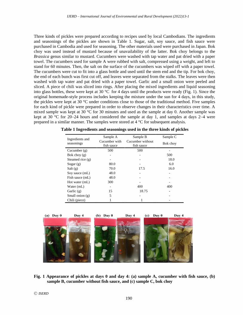
IJERD – International Journal of Environmental and Rural Development (2022)13-1
Ⓒ ISERD
190
Three kinds of pickles were prepared according to recipes used by local Cambodians. The ingredients
and seasonings of the pickles are shown in Table 1. Sugar, salt, soy sauce, and fish sauce were
purchased in Cambodia and used for seasoning. The other materials used were purchased in Japan. Bok
choy was used instead of mustard because of unavailability of the latter. Bok choy belongs to the
Brassica genus similar to mustard. Cucumbers were washed with tap water and pat dried with a paper
towel. The cucumbers used for sample A were rubbed with salt, compressed using a weight, and left to
stand for 60 minutes. Then, the salt on the surface of the cucumbers was wiped off with a paper towel.
The cucumbers were cut to fit into a glass bottle and used until the stem end and the tip. For bok choy,
the end of each bunch was first cut off, and leaves were separated from the stalks. The leaves were then
washed with tap water and pat dried with a paper towel. Garlic and a small onion were peeled and
sliced. A piece of chili was sliced into rings. After placing the mixed ingredients and liquid seasoning
into glass bottles, these were kept at 30 °C for 4 days until the products were ready (Fig. 1). Since the
original homemade-style process includes keeping the mixture under the sun for 4 days, in this study,
the pickles were kept at 30 °C under conditions close to those of the traditional method. Five samples
for each kind of pickle were prepared in order to observe changes in their characteristics over time. A
mixed sample was kept at 30 °C for 30 minutes and used as the sample at day 0. Another sample was
kept at 30 °C for 20–24 hours and considered the sample at day 1, and samples at days 2–4 were
prepared in a similar manner. The samples were stored at 4 °C for subsequent analysis.
Table 1 Ingredients and seasonings used in the three kinds of pickles
Ingredients and
seasonings
Sample A Sample B Sample C
Cucumber with
fish sauce
Cucumber without
fish sauce Bok choy
Cucumber (g) 500 500 -
Bok choy (g) - - 500
Steamed rice (g) - - 18.0
Sugar (g) 80.0 - 6.0
Salt (g) 70.0 17.5 16.0
Soy sauce (mL) 48.0 - -
Fish sauce (mL) 48.0 - -
Hot water (mL) 300 - -
Water (mL) - 400 400
Garlic (g) 15 18.75 -
Small onion (g) 5 - -
Chili (piece) 1 1 -
Fig. 1 Appearance of pickles at days 0 and day 4: (a) sample A, cucumber with fish sauce, (b)
sample B, cucumber without fish sauce, and (c) sample C, bok choy
IJERD – International Journal of Environmental and Rural Development (2022)13-1
Ⓒ ISERD
191
Measurement of food properties
Since the sugar and salt contents and pH of foods affect microbial growth, their values can be good
indicators of the preservability of food. Therefore, we measured the Brix sugar content (soluble solids
content), salt content, and pH of the pickled liquid of the samples using a Brix refractometer (Atago,
Tokyo, Japan), a salt meter (Horiba, Kyoto, Japan), and a pH meter (Horiba), respectively, for all
prepared samples.
Detection of microbes in the samples
After collecting all samples, several microbial detection assays were performed. Ten grams of each
sample containing pickled ingredients and seasoning liquid was mixed with 90 mL of Maximum
Recovery Diluent (Merck KGaA, Darmstadt, Germany) solution in a sterilized storage bag. To obtain
homogeneous suspensions, samples were homogenized using a Stomacher blender. After stomaching,
1 mL of sample suspension was mixed with 9 mL of Maximum Recovery Diluent solution in a sterile
tube. A series of diluted samples was used for the detection of total viable bacteria, coliforms, and
fungi. Standard agar medium (AS ONE, Osaka, Japan) was used for the detection of total viable
bacteria. Desoxycholate agar medium (AS ONE) was used for the detection of coliforms. Solid plates
were incubated at 35 ℃ for 48 hours. For the detection of fungi, plates with Potato Dextrose Agar
medium (AS ONE) were incubated at 30 ℃ for 5 days.
RESULTS AND DISCUSSION
Nutritional properties of pickles prepared according traditional recipes
The nutritional properties of the final pickled products are shown in Table 2. Sample A showed the
highest Brix value and salt concentration. The measured pH values varied slightly among replicates.
The pH value could be affected by the microbes present in the samples; therefore, differences in the
identity of contaminating microorganisms would result in variations in pH.
Table 2 Nutritional properties of final pickled products
Measured
item
Sample A Sample B Sample C
Cucumber with
fish sauce
Cucumber
without fish sauce Bok choy
Brix 11.2 4.4 4.7
pH 4.55 4.5 4.88
Salt (%) 5.1 2.3 2.4
The Brix values of all pickles did not change much from day 0, just after pickling, to day 4, and
were approximately constant (data not shown). The lack of decreasing Brix values indicates that the
microorganisms in samples A and C were unlikely to utilize sugar. During the 4-day storage period, the
salt concentrations in samples B (cucumber without fish sauce) and C (bok choy) decreased slightly,
whereas that in sample A (cucumber with fish sauce) remained almost constant (Fig. 2(a)). All samples
first displayed pH values of approximately 6, but these gradually decreased over time (Fig. 2(b)).
Decreasing pH values indicated that the microbes in the samples produced acids. Clostridium
botulinum, which can trigger deadly diseases, can grow at a minimum pH of 4.6. Improper home
canning of vegetables and improperly fermented and processed foods have caused outbreaks in many
countries (Matthews, 2017). In particular, pickles in sealed containers with pH higher than 4.6 seem to
IJERD – International Journal of Environmental and Rural Development (2022)13-1
Ⓒ ISERD
192
have considerable potential to cause severe food poisoning. Moreover, the Brix value and salt
concentration of pickles are presumably not sufficient to inhibit the growth of most bacteria and yeasts;
therefore, molds grow regularly in pickles (Matthews, 2017).
Fig. 2 Changes in chemical properties of the three kinds of pickles: (a) salt concentration,
and (b) pH
Microbial behavior in homemade pickles
A total of five samples (from day 0 to day 4) for each of the three kinds of pickles were used to observe
changes in microbial composition over time. We tested the presence of total viable bacteria, coliforms,
and fungi (Fig. 3). More than 5.00 log10 CFU/g of total bacteria were detected in all pickle samples at
day 0; also, the number of bacteria increased until day 4 (Fig. 3(a)). Coliforms were detected at a level
similar to that of total viable bacteria. The initial amount of coliforms in samples B and C was almost
5.00 log10, and sample A also tested positive for these bacteria. The concentration of coliforms
increased until day 4 (Fig. 1(b)). Coliforms are considered indicators of fecal contamination; however,
they have been recently acknowledged to be able to grow in non-fecal sites such as food, water, and
waste (Matthews, 2017). Therefore, contamination by coliforms, as shown in Fig. 3(b), does not
directly imply insanitary conditions. Izumi (2010) reported that vegetables dipped in tap water showed
a total bacterial count of approximately 5 log10. This suggests that only washing vegetables with tap
water does not eliminate harmful microorganisms.
Colony observation on agar plates revealed that many samples were contaminated by dangerous
microorganisms that could cause food spoilage. Thus, none of the prepared pickles were safe to eat.
Fungi were not detected on day 0 in sample A, and some samples tested negative or positive for fungi
on days 1–4. Conversely, samples B and C showed fungal contamination on days 0, 1, and 4. We
believe that continuous growth was not observed because each sample for microbial counting was
placed in an independent bottle in order to prevent contamination of the sample once opened for
analysis. The microflora of vegetables is generally composed by 80% bacteria and 20% fungi (Izumi,
2008). This observation suggests that bacteria remained in all samples prepared by washing with tap
water, but fungi were eliminated from some samples. The results of this study suggest that microbial
growth occurred in all three kinds of pickles, resulting in a high risk of food spoilage and food
poisoning. Therefore, the current production process needs to be modified to improve microbial quality.
The addition of a pasteurization step and/or the use of food additives is an effective and practicable
solution. Similar cucumber pickles containing a similar amount of salt, after storage at 30 °C for 2 days,
were reported to carry 8 log10 CFU/g of total viable bacteria and maintain this initial concentration for
8 days at 4 °C (Miyao, 2004). Moreover, some trials of pickle production showed that the products
IJERD – International Journal of Environmental and Rural Development (2022)13-1
Ⓒ ISERD
193
were of uneven quality. This implies that the traditional methods and ingredients used in this study do
not allow spontaneous desirable fermentation into safe products.
Fig. 3 Changes in the amount of microbes in the three kinds of pickles: (a) total viable bacteria,
(b) coliforms, and (c) fungi
In this study, pickles were prepared following homemade-style recipes and analyzed for their
microbial quality. We suggest that pasteurization is required to obtain microbiologically safe products.
Moreover, the use of food additives such as glycine, which does not alter the taste of pickles, sorbic
acid, or alcohol during preparation seems to be effective in controlling the concentration of
microorganisms.
CONCLUSION
In this study, three kinds of pickles were prepared following local traditional methods. To observe
changes over time, five pickle samples were prepared for days 0 to 4. The Brix value, salt
concentration, and pH of the pickling liquids were measured, and microbial detection assays were
performed. More than 5.00 log10 CFU/g of total bacteria was detected in all the samples at day 0; also,
the number of bacteria increased until day 4. Coliforms showed concentrations similar to those of total
viable bacteria. Some samples were positive for fungi. In conclusion, all samples were contaminated
by harmful microorganisms that could cause food spoilage.
The results of this study revealed that microbial growth occurs in all pickles, posing high risk to
food spoilage and food poisoning. We suggest that pasteurization would help obtain microbiologically
IJERD – International Journal of Environmental and Rural Development (2022)13-1
Ⓒ ISERD
194
safe products. Moreover, use of food additives that do not alter the taste of pickles may allow
maintenance of low levels of microorganisms.
REFERENCES
Bhaskaran, S. (Ed) 2020. Zoonoses recent approaches to contain the global zoonotic burden, Indian Veterinary
Association, Kerala, College of Veterinary and Animal Sciences, Mannuthy Unit, Thrissur, Kerala, ISBN
978-93-5437-115-8, India.
Fung, F., Wang, H., and Menon, S. 2018. Food safety in the 21st century, Biomedical Journal, 41, 88-95,
Retrieved from https://doi.org/10.1016/j.bj.2018.03.003
Keegan, V.A., Majowicz, S.E., Pearl, D.L., Marshall, B.J., Sittler,N., Knowles, L. and Wilson, J.B. 2009.
Epidemiology of enteric disease in C-EnterNet’s pilot site – Waterloo region, Ontario, 1990 to 2004.
Canadian Journal of Infectious Disease and Medical Microbiology, 20, 79-87, Retrieved from https://doi.org/10.1155/2009/978784
Izumi, H. 2008. Studies on microbiological safety of fresh-whole and fresh-cut produce, Food Preservation
Science, 34(2), 85-95, Retrieved from https://doi.org/10.5891/jafps.34.85
Izumi, H. 2010. Microbiological safety of fresh produce from the farm-to-table food chain. Memoirs of the
School of BOST of Kinki University, 26, 3-11.
Le, H.H.T., Dalsgaard, A., Andersen, P.S., Nguyen, H.M., Ta, Y.T. and Nguyen, T.T. 2021. Large-scale
Staphylococcus aureus foodborne disease poisoning outbreak among primary school children, Microbiology
Research, 12, 43-52, Retrieved from https://doi.org/10.3390/microbiolres12010005
Matthews, K.R., Knile, K.E., and Montville, T.J. 2017. Food microbiology, Fourth edition, American Society for
Microbiology, ASM Press, ISBN 978-1-555-81938-5, USA. Miyao, S. 2004. Synthetic control of the microorganisms in quality stabilization of pickles, Food Preservation
Science, 30, 29-38, Retrieved from https://doi.org/10.5891/jafps.30.29
Muramatsu, S., Uchino, M., Tanikoka, Y., Sorm, S., Oka, D., Muramatsu, Y., Nakajima, T., Sekido, M.,
Nakamura, T., Chay, C. and Mihara, M. 2020a. Evaluation of bacterial contamination levels in pickles sold
at wet market in Cambodia -part 1- in case of samples from Kampong Cham and Phnom Penh, International
Journal of Environmental and Rural Development, 11(1), 115-120, Retrieved from
https://doi.org/10.32115/ijerd.11.1_115
Muramatsu, S., Uchino, M., Sorm, S., Tanikoka, Y., Oka, D., Muramatsu, Y., Nakajima, T., Sekido, M.,
Nakamura, T., Chay, C. and Mihara, M. 2020b. Evaluation of bacterial contamination levels in pickles sold
at wet market in Cambodia -part 2- detection of several food-poisoning bacteria of 48 samples from Phnom
Penh, International Journal of Environmental and Rural Development, 11(1), 121-126, Retrieved from
https://doi.org/10.32115/ijerd.11.1_121
Redmond, E. C., Griffith, C. J. 2003. Consumer food handling in the home: A review of food safety studies,
Journal of Food Protection, 66, 130-161, Retrieved from https://doi.org/10.4315/0362-028X-66.1.130
Rusnan, A.N., Nordin, N., Radu S. and Abdul-Mutalib, N.A. 2020. Pathogenic Bacillus cereus, an overlooked
food contaminants in Southeast Asia, Tropical Agricultural Science, 43(1), 1-7. Satcher, D. 2000. Food safety: A growing global health problem, 283, 1817, Journal of American Medical
Association, Retrieved from https://doi.org/10.1001/jama.283.14.1817
Vrbova, L., Johnson, K., Whitfield, Y. and Middleton, D. 2012. A descriptive study of reportable gastrointestinal
illnesses in Ontario, Canada, from 2007 to 2009, BMC Public Health, 12, 970, Retrieved from
https://doi.org/10.1186/1471-2458-12-970
World Health Organization (WHO). 2015. Estimates of the global burden of foodborne diseases, Retrieved from
https://apps.who.int/iris/handle/10665/199350
IJERD – International Journal of Environmental and Rural Development (2022)13-1
Ⓒ ISERD
195
Impact Analysis of Population Growth and Fertilizer Use on
Nitrogen Runoff in Nam Ngum Basin, Laos
KOSHI YOSHIDA* Graduate School of Frontier Sciences, The University of Tokyo, Chiba, Japan
Email: [email protected]
ISSAKU AZECHI Graduate School of Bioresources, Mie University, Mie, Japan
TOSHIAKI IIDA Faculty of Agriculture, Iwate University, Iwate, Japan
Received 29 January 2022 Accepted 2 May 2022 (*Corresponding Author)
Abstract Human population growth has led to increased energy and food production, fertilizer
usage and wastewater flows. Increased nitrogen availability is a worldwide cause of
eutrophication of rivers, lakes and estuaries, however, quantitative evaluation the impacts of
nitrogen loads has been insufficient in developing countries because of poor data availability.
The Nam Ngum River basin, Laos, which supplies quality water for domestic use in the
Vientiane Metropolis, was selected as the target area for this study. The Nam Ngum River basin
is 415 km long with a 17,000 km2 catchment area, and the main land uses in 2000 were paddy
(15.6%), forest (32.3%), shrub (40.3%) and urban (0.2%). By UN estimation, population in
Laos is expected to increase 2.1 times from 2000 to 2050, and fertilizer use also will increase to
produce sufficient food. Therefore, future water quality is a main concern in this river basin.
Meteorological and hydrological data from 1995 to 2004, and spatial data such as topography,
land use, and soil properties were collected for model simulation. A conceptual nitrogen
balance model with three nitrogen pools was developed and combined with a rainfall runoff
model. Simulated river discharge and nitrogen loads agreed with the observed data. Then, we
investigated future nitrogen load variations in the basin under different population growth and
agricultural modernization scenarios. As a result, even when population in the basin increased
2.1 times, nitrogen load did not change significantly (11,676 tons/year in 2000 and 11,822
tons/year in 2050). However, the fertilizer increase scenario, from 25 kg/ha/season to 50
kg/ha/season, showed significant increase in nitrogen loading, from 11,676 ton/year to 17,010
ton/year. Our results provide initial insight into the magnitude and spatial distribution of
nitrogen loading in Nam Ngum River Basin, showing that this type of model may be useful for
future impact assessments.
Keywords Nitrogen load, Point sources, Diffuse pollution, Agricultural modernization
INTRODUCTION
As the population increases, especially in developing countries, there is a need to increase food
production. This can be achieved in two ways: by expanding farmland and by increasing the yield per
unit area. The area of agricultural land in the world has already begun to decrease due to soil
degradation and other reasons, thus it is difficult to expect a significant increase in the area of
agricultural land. Therefore, the most realistic approach is to increase the yield per unit area (i.e.
increase the number of crops planted per year by switching to high-yielding varieties and introducing
erd
Research article
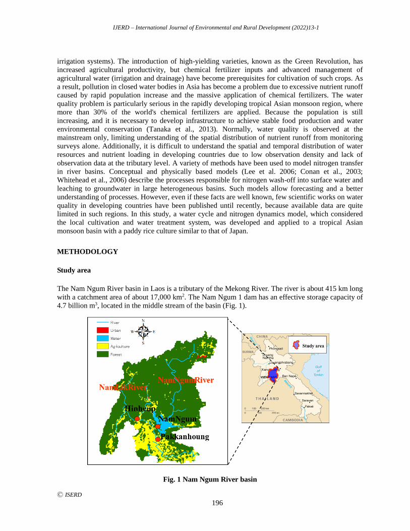
IJERD – International Journal of Environmental and Rural Development (2022)13-1
Ⓒ ISERD
196
irrigation systems). The introduction of high-yielding varieties, known as the Green Revolution, has
increased agricultural productivity, but chemical fertilizer inputs and advanced management of
agricultural water (irrigation and drainage) have become prerequisites for cultivation of such crops. As
a result, pollution in closed water bodies in Asia has become a problem due to excessive nutrient runoff
caused by rapid population increase and the massive application of chemical fertilizers. The water
quality problem is particularly serious in the rapidly developing tropical Asian monsoon region, where
more than 30% of the world's chemical fertilizers are applied. Because the population is still
increasing, and it is necessary to develop infrastructure to achieve stable food production and water
environmental conservation (Tanaka et al., 2013). Normally, water quality is observed at the
mainstream only, limiting understanding of the spatial distribution of nutrient runoff from monitoring
surveys alone. Additionally, it is difficult to understand the spatial and temporal distribution of water
resources and nutrient loading in developing countries due to low observation density and lack of
observation data at the tributary level. A variety of methods have been used to model nitrogen transfer
in river basins. Conceptual and physically based models (Lee et al. 2006; Conan et al., 2003;
Whitehead et al., 2006) describe the processes responsible for nitrogen wash-off into surface water and
leaching to groundwater in large heterogeneous basins. Such models allow forecasting and a better
understanding of processes. However, even if these facts are well known, few scientific works on water
quality in developing countries have been published until recently, because available data are quite
limited in such regions. In this study, a water cycle and nitrogen dynamics model, which considered
the local cultivation and water treatment system, was developed and applied to a tropical Asian
monsoon basin with a paddy rice culture similar to that of Japan.
METHODOLOGY
Study area
The Nam Ngum River basin in Laos is a tributary of the Mekong River. The river is about 415 km long
with a catchment area of about 17,000 km2. The Nam Ngum 1 dam has an effective storage capacity of
4.7 billion m3, located in the middle stream of the basin (Fig. 1).
Fig. 1 Nam Ngum River basin
IJERD – International Journal of Environmental and Rural Development (2022)13-1
Ⓒ ISERD
197
The Nam Ngum 1 dam is dedicated to power generation, and supplies electricity to the Laos
capital, Vientiane, as well as exporting it to Thailand. The estimated basin population is 420 thousand
persons and the average population density of the basin is about 25 people/km2. The basin area
accounts for 7% of the total land area and the basin population accounted for 9% of the total population
of Laos in 2000. The sewerage penetration rate in Laos is estimated to be 19.2%, but this is mainly in
urban areas.
Modernization in the agricultural sector is also lagging, with an irrigation rate of only 11%.
According to interviews in farming villages near Vientiane, the amount of fertilizer applied is still low,
averaging 25 kgN/ha/season, and some farmers do not apply any fertilizer in rainfed paddy fields. The
land use in the basin is paddy fields (16%), forests and bushes (72%), and residential land (only 0.2%).
The Nam Ngum 2 dam (effective storage capacity: 2.6 billion tons, completed in 2011) and the Nam
Ngum 5 dam (effective storage capacity: 250 million tons, completed in 2012) are already in operation
in the basin (Kudo et al., 2013), but this study considered only the Nam Ngum 1 dam, because the
meteorological, hydrological data required for the model simulation, and collected from the hydro
yearbook published by the Mekong River Commission, were only available from 1995–2004. Water
samples were collected monthly at Pakkanhoung station and the total nitrogen concentration was
measured at the National University of Laos in 2003–2004. Additionally, a field survey on water use,
water treatment, irrigation, and cultivation methods was conducted in the KM6 irrigation area in Nam
Ngum basin. The factors affecting the water environment can be broadly classified into point source
loadings from people and livestock and non-point source loadings from forest, farmland and urban
areas. For the point source load, statistical data, such as those on population and number of livestock,
were collected from the Bureau of Statistics, and the units of nitrogen loading in the Mekong river
basin were used (Tanaka et al., 2013). In Laos, households use septic tanks, is the simplest facility in
sewage treatment. The tanks receive domestic wastewater, which is treated by sedimentation and
anaerobic decomposition before the supernatant liquid is discharged into the drainage river. In Laos,
the temperature is high all year round, and the active decomposition of microorganisms is expected to
rapidly decompose excreta, but the treatment efficiency is extremely low due to lack of proper
maintenance. Livestock excrement is directly disposed in farmland and grassland, then discharged into
the ground water system after decomposition and absorption processes in the surface soil.
Rainfall-Runoff model
To evaluate nitrogen transportation according to the river water flow, a distributed water cycling model
was developed and applied to analyze the water balance in the basin. TOPMODEL was employed for
the rainfall-runoff analysis. Such a distributed model can include the spatial distributions of topography,
land use, and soil characteristics. Therefore, TOPMODEL is widely used for hydrological
characteristic analysis, water management, water quality analysis, and future forecasting. TOPMODEL
was proposed by Beven and Kirkby (1979) based on the contributing area concept in hill slope
hydrology. This model is based on the exponential transmissivity assumption, which leads to a
topographic index ln(a/To/tanb), where a is the upstream catchment area draining across a unit length,
To is the lateral transmissivity under saturated conditions, and tanb is the local gradient of the ground
surface. Fig. 2 illustrates the conceptual structure of the water cycle as estimated by TOPMODEL.
Additionally, a dam operation model was combined with TOPMODEL to calculate water storage in the
reservoirs (Hanasaki et al. 2007). For details, please see Yoshida et al., 2017.
Nitrogen balance model
A conceptual nitrogen balance model considering three pools in soil such as organic N, Ammonium N
IJERD – International Journal of Environmental and Rural Development (2022)13-1
Ⓒ ISERD
198
and Nitrate N was developed for this study, as shown in Fig. 3. Soil N, mainly present in organic form,
is almost unavailable to plants.
Fig. 2 TOPMODEL structure
Fig. 3 Structure of the nitrogen balance model in soil
IJERD – International Journal of Environmental and Rural Development (2022)13-1
Ⓒ ISERD
199
The vegetation mainly uses inorganic forms of N, which are made available by organic matter
decomposition. Soil microorganisms convert the N contained in organic matter in a process called
mineralization. Although plants can use both forms of inorganic N, Nitrate is preferred because of its
greater solubility in water. In other words, nitrates quickly dissolve in the pore solution, which is taken
up by plants. On the other hand, this also means that nitrate is easily leached to groundwater.
Ammonium N is less mobile because it strongly adsorbs on clay minerals due to its positive charge.
Denitrification is the anaerobic microbial reduction of N, and is used as an electron acceptor, resulting
in the transfer of soil nitrogen to the atmosphere.
The budget of each pool is expressed in the following equations.
(1)
(2)
(3)
where Norg is organic nitrogen (kg/ha), PSNL is input N from point-sources (kg/ha/day), MinerN is the
mineralization rate (kg/ha/day), RunoffN is the nitrogen loss by surface runoff (kg/ha/day), Nammo is
ammonium nitrogen (kg/ha), DepoN is nitrogen deposition (kg/ha/day), FertiN is fertilized nitrogen
(kg/ha/day), NitriN is the nitrification rate (kg/ha/day), Nnitra is nitrate nitrogen (kg/ha), PupN is the
plant uptake rate (kg/ha/day), DenitN is nitrate nitrogen loss by denitrification (kg/ha/day), and LeachN
is nitrate nitrogen loss by leaching (kg/ha/day). For details on the calculation methods for each nitrogen
flux and denitrification process, please see Yoshida et al., 2017.
Future population growth and fertilizer increase scenarios
According to the United Nations prediction of 2000, the Laos population will increase 2.1 times by
2050. At the same time, chemical fertilizer use will also increase to produce sufficient food by
agricultural modernization. This study evaluated the impacts of such population and fertilizer increases
on nitrogen loading in the Nam Ngum river basin. In 2000, the total population of Nam Ngum basin
was 420 thousand. Therefore, a population increase of 460 thousand people by 2050 was assumed and
used for impact analysis. Additionally, we assumed that fertilizer use would increase from 25
kgN/ha/season to 50 kg/ha/season to check the sensitivity of the model.
RESULTS AND DISCUSSION
Using the proposed model, water and nitrogen balances from 1995 to 2004 in the Nam Ngum Basin
were calculated at a 1 km × 1 km resolution. The first 5 years of data were used for parameter
calibration and the latter 5 years of data were used for validation. Parameters were calibrated by trial
and error method to maximize the Nash-Sutcliffe efficiency (NSE) of discharge and total nitrogen
(TN) concentration at Pakkanhoung (catchment area: 14,300 km2) station. Fig. 4 shows the observed
and calculated river discharge at Pakkanhoung station. The estimated NSE in the calibration and
validation periods were 0.54 and 0.50, respectively.
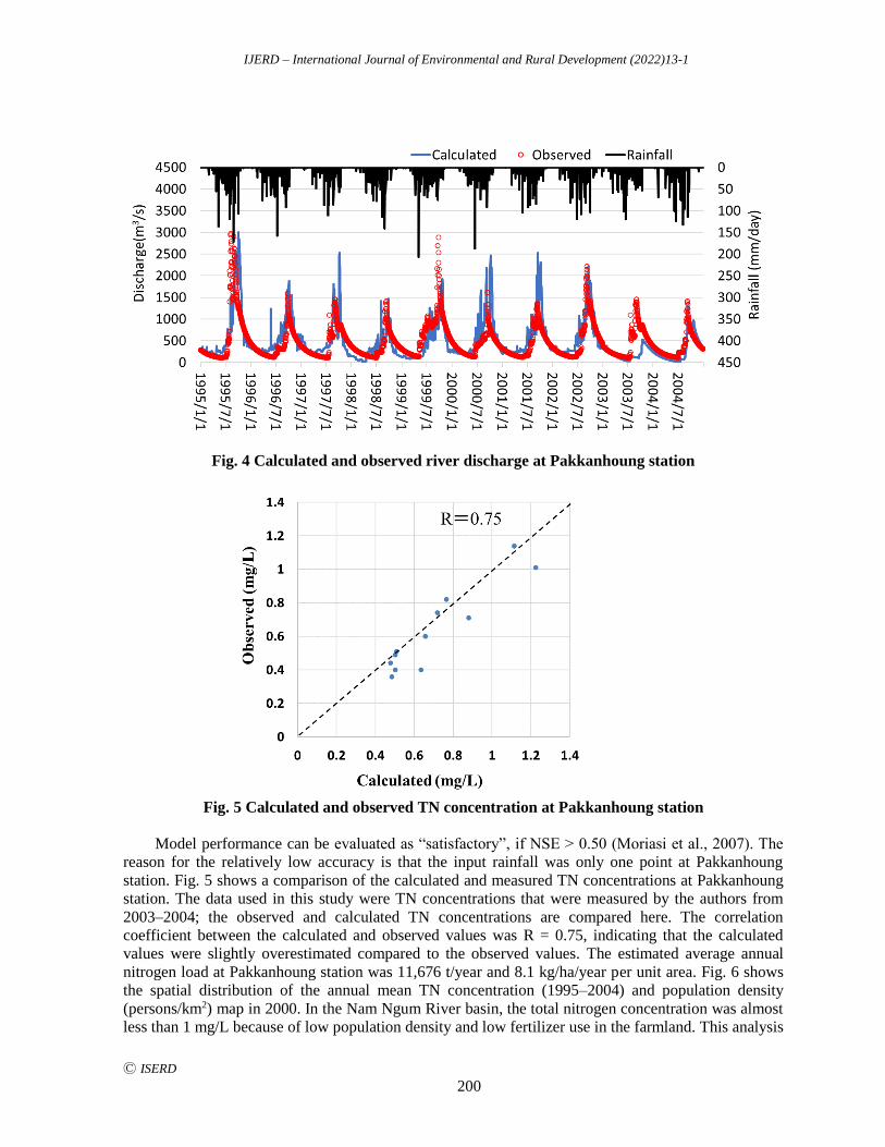
IJERD – International Journal of Environmental and Rural Development (2022)13-1
Ⓒ ISERD
200
Fig. 4 Calculated and observed river discharge at Pakkanhoung station
Fig. 5 Calculated and observed TN concentration at Pakkanhoung station
Model performance can be evaluated as “satisfactory”, if NSE > 0.50 (Moriasi et al., 2007). The
reason for the relatively low accuracy is that the input rainfall was only one point at Pakkanhoung
station. Fig. 5 shows a comparison of the calculated and measured TN concentrations at Pakkanhoung
station. The data used in this study were TN concentrations that were measured by the authors from
2003–2004; the observed and calculated TN concentrations are compared here. The correlation
coefficient between the calculated and observed values was R = 0.75, indicating that the calculated
values were slightly overestimated compared to the observed values. The estimated average annual
nitrogen load at Pakkanhoung station was 11,676 t/year and 8.1 kg/ha/year per unit area. Fig. 6 shows
the spatial distribution of the annual mean TN concentration (1995–2004) and population density
(persons/km2) map in 2000. In the Nam Ngum River basin, the total nitrogen concentration was almost
less than 1 mg/L because of low population density and low fertilizer use in the farmland. This analysis

IJERD – International Journal of Environmental and Rural Development (2022)13-1
Ⓒ ISERD
201
found that the total nitrogen concentration was not affected by the spatial distribution of population
density but was calculated to be relatively high in the farmland during simulation periods.
Fig. 6 Spatial distribution of (a)annual mean total nitrogen concentration and (b) population
density (persons/km2)
Fig. 7 Change in annual mean nitrogen load under the future scenarios.
Fig. 7 shows the change in annual mean nitrogen load under the population growth and fertilizer
increase scenarios. The population of the Nam Ngum River basin was 420 thousand in 2000 and will
increase 2.1 times to 860 thousand in 2050. The nitrogen load did not change significantly (11,676
t/year in 2000 and 11,822 t/year in 2050) as a result of population increase in the basin. The maximum
IJERD – International Journal of Environmental and Rural Development (2022)13-1
Ⓒ ISERD
202
population density in the Nam Ngum River basin in 2000 was about 2,140 persons/km2, with most
people living in rural areas. Even if the population were to increase by 2.1 times, the population density
would remain low; thus, there would be no significant impact on the water quality environment of the
basin. The fertilizer increase scenario, however, from 25 kg/ha/season to 50 kg/ha/season, showed a
significant increase in nitrogen loading, from 11,676 t/year to 17,010 t/year. The current fertilizer
application rate is 25 kgN/ha, which is extremely low. To increase food production in response to
future population growth, it is necessary to increase production per unit area. Therefore, we assumed a
scenario of increasing the amount of applied fertilizer and evaluated the impact on the water quality
environment of the watershed. Doubling the fertilizer application rate to 50 kg/ha resulted in a 46%
increase in the annual nitrogen load at Pakkanhoung station. The nitrogen discharge load per unit area
increased from 8.1 kg/ha/year (equivalent of 0.66 mg/L) to 11.8 kg/ha/year (equivalent of 0.95mg/L)
under this scenario, however, the water quality environment was still favorable.
CONCLUSION
The Nam Ngum River basin, Laos, which supplies high quality domestic water to Vientiane Metropolis,
was selected as the target area for this study. The UN has estimated that the population in Laos will
increase by 2.1 times between 2000 and 2050, and producing sufficient food for the higher population
will require increased fertilizer use. Therefore, changes in future water quality is the main concern for
this river basin. Meteorological and hydrological data from 1995 to 2004, and spatial data such as
topography, land use, and soil properties were collected for model simulation. A conceptual nitrogen
balance model with three nitrogen pools was developed and combined with the rainfall runoff model.
Simulated river discharge and nitrogen loading agreed with the observed data. Next, we investigated
future variations of nitrogen loading in the basin under the population growth and agricultural
modernization scenarios. As a result, even when population in the basin increased by 2.1 times, the
nitrogen load did not change significantly (11,676 t/year in 2000 and 11,822 t/year in 2050). However,
the fertilizer increase scenario, from 25 kg/ha/season to 50 kg/ha/season, showed a significant increase
in nitrogen load from 11,676 t/year to 17,010 t/year. Our results provide a first insight into the
magnitude and spatial distribution of nitrogen loading in Nam Ngum River Basin. This type of model
may be useful for future impact assessments.
ACKNOWLEDGEMENTS
This research was supported by JST SICORP Grant Number JPMJSC20E3, and the MEXT/JSPS
Grant-in-Aid for Scientific Research (KAKENHI) no. 19H03069 and no. 20KK0346.
REFERENCES
Beven, K.J. and Kirkby, M.J. 1979. A physically based, variable contributing area model of hydrology,
Hydrological Sciences Bulletin, 24(1), 43–69, Retrieved from https://doi.org/10.1080/02626667909491834
Conan, C., Bouraoui, F., Turpin, N., de Marsily, G., and Bidglio, G., 2003. Modeling flow and nitrate fate at
catchment scale in Britany (France), Journal of Environmental Quality, 32 (6), 2026–2032, Retrieved from
https://doi.org/10.2134/jeq2003.2026
Hanasaki, N., Utsumi, N., Yamada, T., Shen, Y., Bengtsson, M., Kanae, S., Otaki, M., and Oki, T. 2007.
Development of a global integrated water resources model for water resources assessments under climate
change (in Japanese), Annual Journal of Hydraulic Engineering, JSCE, 51, 229–234, Retrieved from
https://doi.org/10.2208/prohe.51.229
Kudo R., Masumoto T., Horikawa N. and Yoshida T. 2013. Assessment of combined impact of climate change
and water resources development on hydrological cycle in the Nam Ngum river basin (in Japanese),
Transactions of JSIDRE, 81(1), 57-66.
IJERD – International Journal of Environmental and Rural Development (2022)13-1
Ⓒ ISERD
203
Lee M. S., K. K. Lee, Y. Hyuna, T. P. Clement and D. Hamilton 2006. Nitrogen transformation and transport
modeling in groundwater aquifers, Ecological Modelling, 192, 143-159, Retrieved from
https://doi.org/10.1016/j.ecolmodel.2005.07.013
Moriasi, D.N., Arnold, J.G., Van Liew, M.W., Bingner, R.L., Harmel, R.D., and Veith, T.L., 2007. Model
evaluation guidelines for systematic quantification of accuracy in watershed simulations, Transactions of the
American Society of Agricultural and Biological Engineers, 50(3), 885-900.
Tanaka K., Yoshida K., Noda K., Azechi I. and Kuroda H. 2013. Estimation of unit of nitrogen and phosphorous
pollution loading in Mekong River basin (in Japanese), Transactions of JSIDRE, 81(2), 193-199.
Whitehead, P. G., Wilby, R. L., Butterfield, D. and Wade, A. J. 2006. Impacts of climate change on in-stream
nitrogen in a lowland chalk stream: An appraisal of adaptation strategies, Science of The Total Environment,
365, 260–273, Retrieved from https://doi.org/10.1016/j.scitotenv.2006.02.040
Yoshida K., Tanaka K., Noda K., Homma K., Maki M., Hongo C., Shirakawa H., and Oki K. 2017. Quantitative
evaluation of spatial distribution of nitrogen loading in the Citarum River basin, Indonesia. Journal of
Agricultural Meteorology, 73, 31-44, Retrieved from https://doi.org/10.2480/agrmet.D-15-00020
IJERD – International Journal of Environmental and Rural Development (2022)13-1
Ⓒ ISERD
204
Nursery Propagation of Apple Mangrove Sonneratia alba
ARNIE C. TRANGIA* Cebu Technological University, Cebu City, Philippines Email: [email protected]
Received 7 February 2022 Accepted 2 May 2022 (*Corresponding Author)
Abstract Mangrove rehabilitation conducted on the seafront was a failure because of small
survival due to wrong species planted and zonation. Apple mangrove (Sonneratia alba),
"pagatpat," is the most widely distributed mangrove globally, particularly in coastal regions.
The study showed that the Sonneratia species bears plenty of fruits, but seedlings rarely grow in
the wild. The researcher introduced a ninety-day analysis using various soil media and different
watering regimes in a designed concrete tank to determine the survival and growth rates of the
nursery propagated apple mangrove seedlings. He observed that the highest average survival
rate of S alba seedling was in watering regime Treatment 3 and the type of soil medium was
sandy clay. The researcher measured the average survival rate at 23.70% in clay, 52.10% for
sandy clay, 44.32% for sandy soil under a watering regime, 37.41% in clay, and 43.21% in
sandy clay, and 39.41% in sandy soil. Research showed that the seedlings watered under
Treatment 3 observed the highest growth gain (5.41 ± 0.68 cm), while seedlings under
Treatment 1 recorded the lowest growth gain (1.87 ± 0.23 cm) under the watering regime.
Seedlings planted in sandy-clay soil exhibited the highest growth gain (4.15 ± 0.52 cm), while
seedlings planted in clay recorded the lowest growth gain (4.0 ± 0.50 cm) for soil media.
Moreover, the researcher observed that growth showed a significant difference in the different
watering regimes but had no significant difference in the type of soil media.
Keywords apple mangrove, water regimes, soil media, survival rate, growth rate
INTRODUCTION
The Philippines is ranked fourth out of the 180 countries in the 20 years (2000-2019), following Puerto
Rico, Myanmar, and Haiti among the countries most affected by extreme weather according to the
Germanwatch report (Global Climate Index, 2021).
Mangroves are a natural coastal defense against violent storms that bring storm surges and
flooding. It is one of the most effective mitigating measures against climate change. In addition,
mangroves can hold back the sea waves and reduce wave forces with their extensive and dense above-
ground roots by an estimated 70-90% on average (Macintosh, 2010). Furthermore, a study conducted
by Harada et al. (2012) demonstrated that mangroves are as effective as concrete seawall structures in
reducing tsunami-hit house damage behind the forest.
Mangrove systems have contributed significantly to the well-being of coastal communities
through a wide array of ecosystem services classified into regulating, provisioning, cultural, and
supporting (Manual on Community-Based Mangrove Rehabilitation: Box 1, 2012). Fringing
mangroves in the Philippines and the rest of Southeast Asia are naturally lined by a band of Avicennia
marina and Sonneratia alba front-liners with Rhizophora stylosa and R. apiculata immediately behind
(Manual on Community-Based Mangrove Rehabilitation, p. 6, 2012).
Primavera et al. (2014) averred that Sonneratia alba (pagatpat) dominates the eastern Panay
coastline. The species has been proven superior even to the Avicennia marina for the rehabilitation of
sandy fringes. Most of the plantations used Rhizophora species whose propagules are easy to collect
and plant but which cannot withstand wave action. Hence only 10% of these plants survived in open
erd
Research article
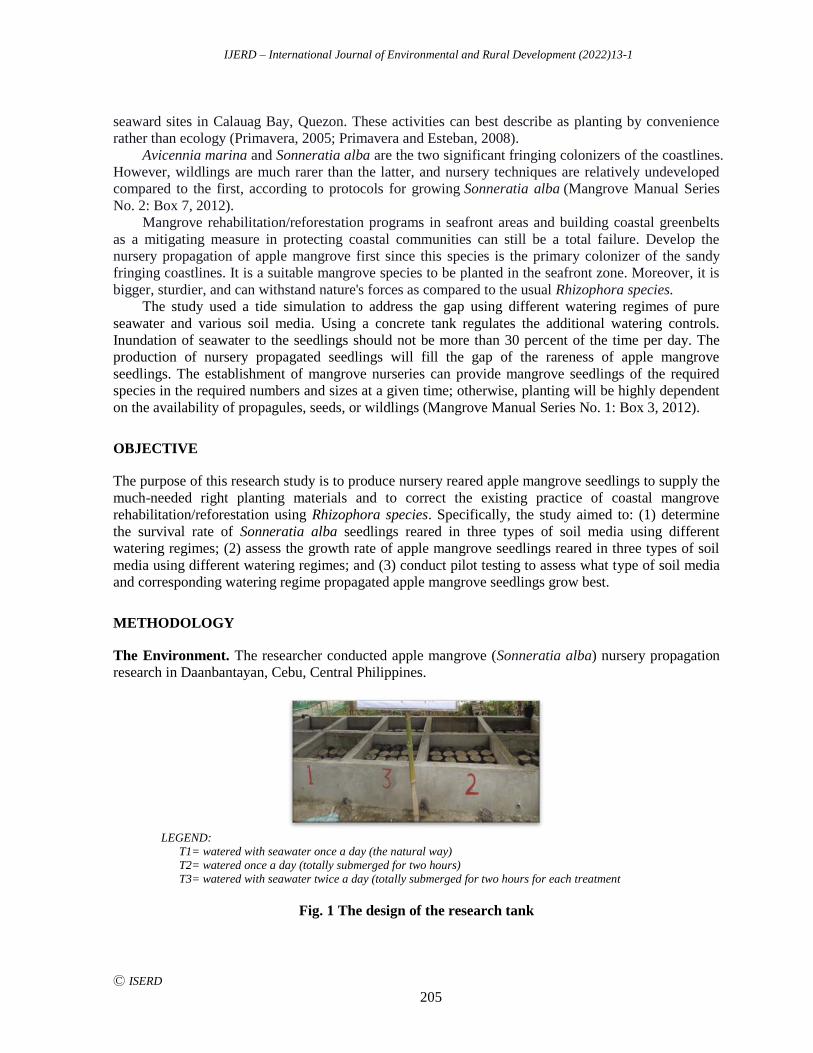
IJERD – International Journal of Environmental and Rural Development (2022)13-1
Ⓒ ISERD
205
seaward sites in Calauag Bay, Quezon. These activities can best describe as planting by convenience
rather than ecology (Primavera, 2005; Primavera and Esteban, 2008).
Avicennia marina and Sonneratia alba are the two significant fringing colonizers of the coastlines.
However, wildlings are much rarer than the latter, and nursery techniques are relatively undeveloped
compared to the first, according to protocols for growing Sonneratia alba (Mangrove Manual Series
No. 2: Box 7, 2012).
Mangrove rehabilitation/reforestation programs in seafront areas and building coastal greenbelts
as a mitigating measure in protecting coastal communities can still be a total failure. Develop the
nursery propagation of apple mangrove first since this species is the primary colonizer of the sandy
fringing coastlines. It is a suitable mangrove species to be planted in the seafront zone. Moreover, it is
bigger, sturdier, and can withstand nature's forces as compared to the usual Rhizophora species.
The study used a tide simulation to address the gap using different watering regimes of pure
seawater and various soil media. Using a concrete tank regulates the additional watering controls.
Inundation of seawater to the seedlings should not be more than 30 percent of the time per day. The
production of nursery propagated seedlings will fill the gap of the rareness of apple mangrove
seedlings. The establishment of mangrove nurseries can provide mangrove seedlings of the required
species in the required numbers and sizes at a given time; otherwise, planting will be highly dependent
on the availability of propagules, seeds, or wildlings (Mangrove Manual Series No. 1: Box 3, 2012).
OBJECTIVE
The purpose of this research study is to produce nursery reared apple mangrove seedlings to supply the
much-needed right planting materials and to correct the existing practice of coastal mangrove
rehabilitation/reforestation using Rhizophora species. Specifically, the study aimed to: (1) determine
the survival rate of Sonneratia alba seedlings reared in three types of soil media using different
watering regimes; (2) assess the growth rate of apple mangrove seedlings reared in three types of soil
media using different watering regimes; and (3) conduct pilot testing to assess what type of soil media
and corresponding watering regime propagated apple mangrove seedlings grow best.
METHODOLOGY
The Environment. The researcher conducted apple mangrove (Sonneratia alba) nursery propagation
research in Daanbantayan, Cebu, Central Philippines.
LEGEND:
T1= watered with seawater once a day (the natural way)
T2= watered once a day (totally submerged for two hours)
T3= watered with seawater twice a day (totally submerged for two hours for each treatment
Fig. 1 The design of the research tank
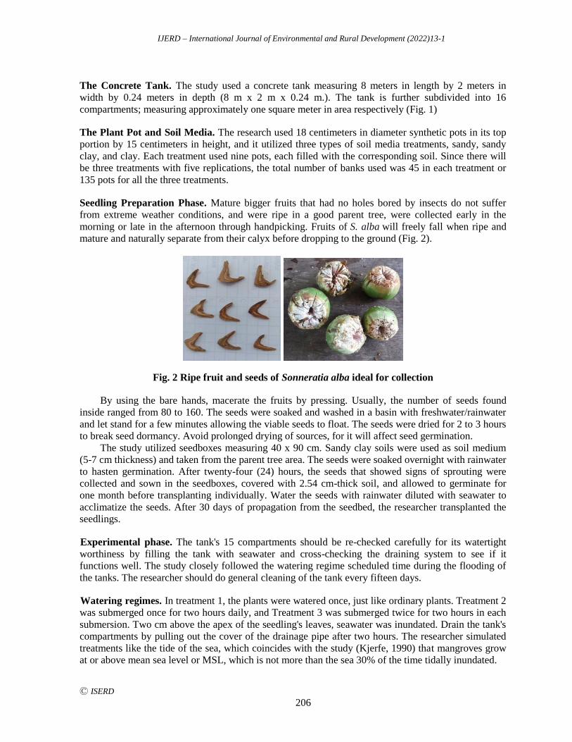
IJERD – International Journal of Environmental and Rural Development (2022)13-1
Ⓒ ISERD
206
The Concrete Tank. The study used a concrete tank measuring 8 meters in length by 2 meters in
width by 0.24 meters in depth (8 m x 2 m x 0.24 m.). The tank is further subdivided into 16
compartments; measuring approximately one square meter in area respectively (Fig. 1)
The Plant Pot and Soil Media. The research used 18 centimeters in diameter synthetic pots in its top
portion by 15 centimeters in height, and it utilized three types of soil media treatments, sandy, sandy
clay, and clay. Each treatment used nine pots, each filled with the corresponding soil. Since there will
be three treatments with five replications, the total number of banks used was 45 in each treatment or
135 pots for all the three treatments.
Seedling Preparation Phase. Mature bigger fruits that had no holes bored by insects do not suffer
from extreme weather conditions, and were ripe in a good parent tree, were collected early in the
morning or late in the afternoon through handpicking. Fruits of S. alba will freely fall when ripe and
mature and naturally separate from their calyx before dropping to the ground (Fig. 2).
Fig. 2 Ripe fruit and seeds of Sonneratia alba ideal for collection
By using the bare hands, macerate the fruits by pressing. Usually, the number of seeds found
inside ranged from 80 to 160. The seeds were soaked and washed in a basin with freshwater/rainwater
and let stand for a few minutes allowing the viable seeds to float. The seeds were dried for 2 to 3 hours
to break seed dormancy. Avoid prolonged drying of sources, for it will affect seed germination.
The study utilized seedboxes measuring 40 x 90 cm. Sandy clay soils were used as soil medium
(5-7 cm thickness) and taken from the parent tree area. The seeds were soaked overnight with rainwater
to hasten germination. After twenty-four (24) hours, the seeds that showed signs of sprouting were
collected and sown in the seedboxes, covered with 2.54 cm-thick soil, and allowed to germinate for
one month before transplanting individually. Water the seeds with rainwater diluted with seawater to
acclimatize the seeds. After 30 days of propagation from the seedbed, the researcher transplanted the
seedlings.
Experimental phase. The tank's 15 compartments should be re-checked carefully for its watertight
worthiness by filling the tank with seawater and cross-checking the draining system to see if it
functions well. The study closely followed the watering regime scheduled time during the flooding of
the tanks. The researcher should do general cleaning of the tank every fifteen days.
Watering regimes. In treatment 1, the plants were watered once, just like ordinary plants. Treatment 2
was submerged once for two hours daily, and Treatment 3 was submerged twice for two hours in each
submersion. Two cm above the apex of the seedling's leaves, seawater was inundated. Drain the tank's
compartments by pulling out the cover of the drainage pipe after two hours. The researcher simulated
treatments like the tide of the sea, which coincides with the study (Kjerfe, 1990) that mangroves grow
at or above mean sea level or MSL, which is not more than the sea 30% of the time tidally inundated.
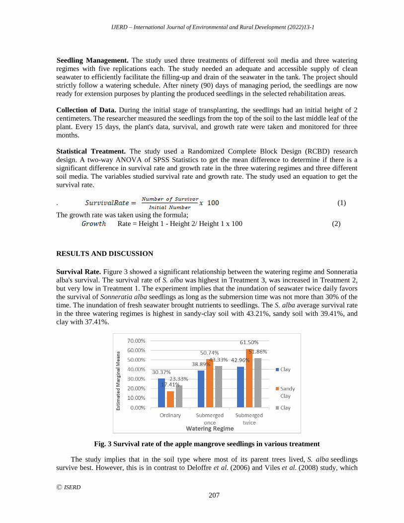
IJERD – International Journal of Environmental and Rural Development (2022)13-1
Ⓒ ISERD
207
Seedling Management. The study used three treatments of different soil media and three watering
regimes with five replications each. The study needed an adequate and accessible supply of clean
seawater to efficiently facilitate the filling-up and drain of the seawater in the tank. The project should
strictly follow a watering schedule. After ninety (90) days of managing period, the seedlings are now
ready for extension purposes by planting the produced seedlings in the selected rehabilitation areas.
Collection of Data. During the initial stage of transplanting, the seedlings had an initial height of 2
centimeters. The researcher measured the seedlings from the top of the soil to the last middle leaf of the
plant. Every 15 days, the plant's data, survival, and growth rate were taken and monitored for three
months.
Statistical Treatment. The study used a Randomized Complete Block Design (RCBD) research
design. A two-way ANOVA of SPSS Statistics to get the mean difference to determine if there is a
significant difference in survival rate and growth rate in the three watering regimes and three different
soil media. The variables studied survival rate and growth rate. The study used an equation to get the
survival rate.
. (1)
The growth rate was taken using the formula;
Rate = Height 1 - Height 2/ Height 1 x 100 (2)
RESULTS AND DISCUSSION
Survival Rate. Figure 3 showed a significant relationship between the watering regime and Sonneratia
alba's survival. The survival rate of S. alba was highest in Treatment 3, was increased in Treatment 2,
but very low in Treatment 1. The experiment implies that the inundation of seawater twice daily favors
the survival of Sonneratia alba seedlings as long as the submersion time was not more than 30% of the
time. The inundation of fresh seawater brought nutrients to seedlings. The S. alba average survival rate
in the three watering regimes is highest in sandy-clay soil with 43.21%, sandy soil with 39.41%, and
clay with 37.41%.
Fig. 3 Survival rate of the apple mangrove seedlings in various treatment
The study implies that in the soil type where most of its parent trees lived, S. alba seedlings
survive best. However, this is in contrast to Deloffre et al. (2006) and Viles et al. (2008) study, which
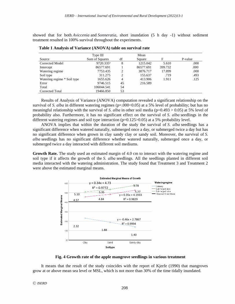
IJERD – International Journal of Environmental and Rural Development (2022)13-1
Ⓒ ISERD
208
showed that for both Aviccenia and Sonneratia, short inundation (5 h day -1) without sediment
treatment resulted in 100% survival throughout the experiments.
Table 1 Analysis of Variance (ANOVA) table on survival rate
Source
Type III
Sum of Squares df
Mean
Square F P-value
Corrected Model 9720.335a 8 1215.042 5.610 .000
Intercept 86577.691 1 86577.691 399.732 .000
Watering regime 7753.435 2 3876.717 17.899 .000
Soil type 311.275 2 155.637 .719 .493
Watering regime * Soil type 1655.626 4 413.906 1.911 .125
Error 9746.515 45 216.589
Total 106044.541 54
Corrected Total 19466.850 53
Results of Analysis of Variance (ANOVA) computation revealed a significant relationship on the
survival of S. alba in different watering regimes (p=.000<0.05) at a 5% level of probability; but has no
meaningful relationship with the survival of S. alba in other soil media (p=0.493 > 0.05) at 5% level of
probability also. Furthermore, it has no significant effect on the survival of S. alba seedlings in the
different watering regimes and soil type interaction (p=0.125>0.05) at a 5% probability level.
ANOVA implies that within the duration of the study the survival of S. alba seedlings has a
significant difference when watered naturally, submerged once a day, or submerged twice a day but has
no significant difference when grown in clay sandy clay or sandy soil. Moreover, the survival of S.
alba seedlings has no significant difference whether watered naturally, submerged once a day, or
submerged twice a day interacted with different soil mediums.
Growth Rate. The study used an estimated margin of 4.0 cm to interact with the watering regime and
soil type if it affects the growth of the S. alba seedlings. All the seedlings planted in different soil
media interacted with the watering administration. The study found that Treatment 3 and Treatment 2
were above the estimated marginal means.
Fig. 4 Growth rate of the apple mangrove seedlings in various treatment
It means that the result of the study coincides with the report of Kjerfe (1990) that mangroves
grow at or above mean sea level or MSL, which is not more than 30% of the time tidally inundated.
1.40
1.88 2.32
5.78
5.35 5.10
4.57 4.84
5.27
y = 0.34x + 4.73
R² = 0.9772
y = -0.46x + 2.7867
R² = 0.9994
y = 0.35x + 4.1933
R² = 0.9829
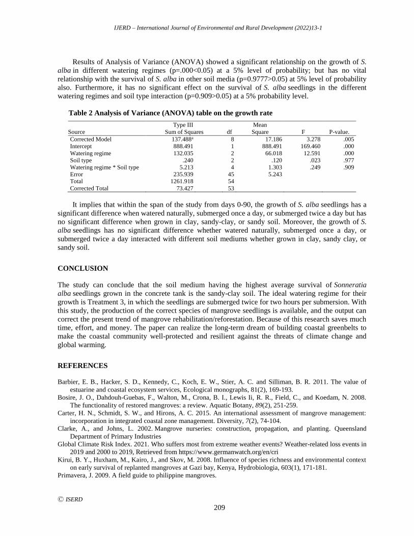
IJERD – International Journal of Environmental and Rural Development (2022)13-1
Ⓒ ISERD
209
Results of Analysis of Variance (ANOVA) showed a significant relationship on the growth of S.
alba in different watering regimes (p=.000<0.05) at a 5% level of probability; but has no vital
relationship with the survival of S. alba in other soil media (p=0.9777>0.05) at 5% level of probability
also. Furthermore, it has no significant effect on the survival of S. alba seedlings in the different
watering regimes and soil type interaction (p=0.909>0.05) at a 5% probability level.
Table 2 Analysis of Variance (ANOVA) table on the growth rate
Source
Type III
Sum of Squares df
Mean
Square F P-value.
Corrected Model 137.488a 8 17.186 3.278 .005
Intercept 888.491 1 888.491 169.460 .000
Watering regime 132.035 2 66.018 12.591 .000
Soil type .240 2 .120 .023 .977
Watering regime * Soil type 5.213 4 1.303 .249 .909
Error 235.939 45 5.243
Total 1261.918 54
Corrected Total 73.427 53
It implies that within the span of the study from days 0-90, the growth of S. alba seedlings has a
significant difference when watered naturally, submerged once a day, or submerged twice a day but has
no significant difference when grown in clay, sandy-clay, or sandy soil. Moreover, the growth of S.
alba seedlings has no significant difference whether watered naturally, submerged once a day, or
submerged twice a day interacted with different soil mediums whether grown in clay, sandy clay, or
sandy soil.
CONCLUSION
The study can conclude that the soil medium having the highest average survival of Sonneratia
alba seedlings grown in the concrete tank is the sandy-clay soil. The ideal watering regime for their
growth is Treatment 3, in which the seedlings are submerged twice for two hours per submersion. With
this study, the production of the correct species of mangrove seedlings is available, and the output can
correct the present trend of mangrove rehabilitation/reforestation. Because of this research saves much
time, effort, and money. The paper can realize the long-term dream of building coastal greenbelts to
make the coastal community well-protected and resilient against the threats of climate change and
global warming.
REFERENCES
Barbier, E. B., Hacker, S. D., Kennedy, C., Koch, E. W., Stier, A. C. and Silliman, B. R. 2011. The value of
estuarine and coastal ecosystem services, Ecological monographs, 81(2), 169-193.
Bosire, J. O., Dahdouh-Guebas, F., Walton, M., Crona, B. I., Lewis Ii, R. R., Field, C., and Koedam, N. 2008.
The functionality of restored mangroves: a review. Aquatic Botany, 89(2), 251-259.
Carter, H. N., Schmidt, S. W., and Hirons, A. C. 2015. An international assessment of mangrove management:
incorporation in integrated coastal zone management. Diversity, 7(2), 74-104.
Clarke, A., and Johns, L. 2002. Mangrove nurseries: construction, propagation, and planting. Queensland
Department of Primary Industries
Global Climate Risk Index. 2021. Who suffers most from extreme weather events? Weather-related loss events in
2019 and 2000 to 2019, Retrieved from https://www.germanwatch.org/en/cri
Kirui, B. Y., Huxham, M., Kairo, J., and Skov, M. 2008. Influence of species richness and environmental context
on early survival of replanted mangroves at Gazi bay, Kenya, Hydrobiologia, 603(1), 171-181.
Primavera, J. 2009. A field guide to philippine mangroves.
IJERD – International Journal of Environmental and Rural Development (2022)13-1
Ⓒ ISERD
210
Primavera, J. H. and Esteban, J. M. A. 2008. A review of mangrove rehabilitation in the Philippines: successes,
failures and future prospects. Wetlands Ecology and Management, 16(5), 345-358.
Primavera, J. H., Rollon, R. N. and Samson, M. S. 2011. The pressing challenges of mangrove rehabilitation:
pond reversion and coastal protection. Biologica, 50, 232.
Primavera, J. H., Sadaba, R. S., Lebata, M. J. H. L., and Altamirano, J. P. 2004. Handbook of mangroves in the
Philippines–Panay SEAFDEC Aquaculture Department. Iloilo, Philippines.
Primavera, J. H., Savaris, J. P., Bajoyo, B. E., Coching, J. D., Curnick, D. J., Golbeque, R., and Koldewey, H. J.
2012. Manual on community-based mangrove rehabilitation. Mangrove Manual Series, 1, 240.
Roldan, R. G. and Mayo-Anda, G. 2004. An assessment of fish sanctuary and mangrove rehabilitation projects
established under the fisheries resource management project. Fisheries Resource Management Project.
Schmitt, K. and Duke, N. C. 2015. Mangrove management, assessment, and monitoring. Tropical forestry
handbook, 1-29.
Viles, H. A., Naylor, L. A., Carter, N. E. A. and Chaput, D. 2008. Biogeomorphological disturbance regimes:
progress in linking ecological and geomorphological systems. Earth Surface Processes and Landforms: The
British Geomorphological Research Group Journal, 33(9), 1419-1435.
Walters, B. B. 2003. People and mangroves in the Philippines: fifty years of coastal environmental
change. Environmental conservation, 30(3), 293-303.