Integrating Aggregational and Probabilistic Approaches to ...

Integrating Aggregational andProbabilistic Approaches

to Dialectology and Language Variation

Inaugural-Dissertationzur

Erlangung der Doktorwürdeder Philologischen Fakultät

der Albert-Ludwigs-UniversitätFreiburg i. Br.

vorgelegt von

Christoph Benedikt Sebastian Wolkaus Freiburg i. Br.

WS 2013/2014

Erstgutachter: Prof. Dr. Benedikt SzmrecsanyiZweitgutachter: Prof. Dr. Bernd Kortmann

Vorsitzender des Promotionsausschussesder Gemeinsamen Kommission derPhilologischen, Philosophischen und Wirtschafts-und Verhaltenswissenschaftlichen Fakultät: Prof. Dr. Bernd Kortmann

Datum der Disputation: 31.03.2014

Contents

List of Maps v

List of Tables vii

List of Figures ix

List of Abbreviations xi

List of County codes xiii

1. Introduction 11.1. Frequency and variation . . . . . . . . . . . . . . . . . . . . . . . . . . . . 11.2. The dialect landscape of Britain . . . . . . . . . . . . . . . . . . . . . . . . 71.3. Outline . . . . . . . . . . . . . . . . . . . . . . . . . . . . . . . . . . . . . 11

2. Aggregation and Language Variation 132.1. Aggregational methodologies: an introduction . . . . . . . . . . . . . . . . 14

2.1.1. Calculating linguistic distance . . . . . . . . . . . . . . . . . . . . . 162.1.2. Fundamental distance analysis methods . . . . . . . . . . . . . . . 20

2.2. Applications of aggregational techniques . . . . . . . . . . . . . . . . . . . 302.2.1. Dialectometry . . . . . . . . . . . . . . . . . . . . . . . . . . . . . . 302.2.2. Aggregational techniques in historical linguistics . . . . . . . . . . 33

2.3. Corpus-based dialectometry . . . . . . . . . . . . . . . . . . . . . . . . . . 36

3. Data and Methods 393.1. Data . . . . . . . . . . . . . . . . . . . . . . . . . . . . . . . . . . . . . . . 39

3.1.1. The Freiburg Corpus of English Dialects . . . . . . . . . . . . . . . 393.1.2. The feature set . . . . . . . . . . . . . . . . . . . . . . . . . . . . . 46

3.2. Methods . . . . . . . . . . . . . . . . . . . . . . . . . . . . . . . . . . . . . 463.2.1. Corpus-based dialectometry . . . . . . . . . . . . . . . . . . . . . . 463.2.2. Extending corpus-based dialectometry . . . . . . . . . . . . . . . . 493.2.3. Automated bottom-up syntactic classification . . . . . . . . . . . . 64

3.3. Chapter summary . . . . . . . . . . . . . . . . . . . . . . . . . . . . . . . 75

4. Feature-based analyses 774.1. Model-based analyses . . . . . . . . . . . . . . . . . . . . . . . . . . . . . . 77

4.1.1. Single feature models . . . . . . . . . . . . . . . . . . . . . . . . . . 774.1.2. On the effect of additional predictors . . . . . . . . . . . . . . . . . 137

i

Contents

4.1.3. Sociolinguistic summary . . . . . . . . . . . . . . . . . . . . . . . . 1484.1.4. Geolinguistic summary . . . . . . . . . . . . . . . . . . . . . . . . . 155

4.2. pos n-gram-based analyses . . . . . . . . . . . . . . . . . . . . . . . . . . 1664.2.1. Geolinguistic results: unigrams . . . . . . . . . . . . . . . . . . . . 1664.2.2. Geolinguistic results: bigrams . . . . . . . . . . . . . . . . . . . . . 1684.2.3. Sociolinguistic results: gender . . . . . . . . . . . . . . . . . . . . . 1804.2.4. Sociolinguistic results: age . . . . . . . . . . . . . . . . . . . . . . . 186

4.3. Chapter summary . . . . . . . . . . . . . . . . . . . . . . . . . . . . . . . 191

5. Aggregational analyses 1935.1. Comparing normalization- and model-based approaches . . . . . . . . . . 1945.2. Dialect areas: hierarchical clustering . . . . . . . . . . . . . . . . . . . . . 197

5.2.1. Normalization-based results . . . . . . . . . . . . . . . . . . . . . . 1985.2.2. lmer-based results . . . . . . . . . . . . . . . . . . . . . . . . . . . 2005.2.3. gam-based results . . . . . . . . . . . . . . . . . . . . . . . . . . . 2035.2.4. Bottom-up analysis: frequency . . . . . . . . . . . . . . . . . . . . 2045.2.5. Bottom up analysis: reliability . . . . . . . . . . . . . . . . . . . . 2055.2.6. Interim summary . . . . . . . . . . . . . . . . . . . . . . . . . . . . 209

5.3. Intersecting dialect areas and continua . . . . . . . . . . . . . . . . . . . . 2105.4. Chapter summary . . . . . . . . . . . . . . . . . . . . . . . . . . . . . . . 217

6. Discussion & Conclusion 2196.1. Summary . . . . . . . . . . . . . . . . . . . . . . . . . . . . . . . . . . . . 2196.2. What do we gain? . . . . . . . . . . . . . . . . . . . . . . . . . . . . . . . 221

6.2.1. On the influence of data availability . . . . . . . . . . . . . . . . . 2226.2.2. On geographic and linguistic distances . . . . . . . . . . . . . . . . 2276.2.3. On non-geographic factors . . . . . . . . . . . . . . . . . . . . . . . 2336.2.4. On bottom-up versus top-down analysis . . . . . . . . . . . . . . . 234

6.3. On the dialect landscape of Britain . . . . . . . . . . . . . . . . . . . . . . 2376.3.1. Revisiting the outliers . . . . . . . . . . . . . . . . . . . . . . . . . 2376.3.2. The North of England . . . . . . . . . . . . . . . . . . . . . . . . . 2406.3.3. The South and Midlands . . . . . . . . . . . . . . . . . . . . . . . . 245

6.4. Outlook and concluding remarks . . . . . . . . . . . . . . . . . . . . . . . 249

Appendices 255

A. CLAWS7 Tag Set 255

B. Technical notes 261B.1. Top-down . . . . . . . . . . . . . . . . . . . . . . . . . . . . . . . . . . . . 261

B.1.1. Data . . . . . . . . . . . . . . . . . . . . . . . . . . . . . . . . . . . 261B.1.2. lmer models . . . . . . . . . . . . . . . . . . . . . . . . . . . . . . . 261B.1.3. gams . . . . . . . . . . . . . . . . . . . . . . . . . . . . . . . . . . 262B.1.4. Aggregation . . . . . . . . . . . . . . . . . . . . . . . . . . . . . . . 262

ii

Contents

B.2. Bottom-up . . . . . . . . . . . . . . . . . . . . . . . . . . . . . . . . . . . . 263B.2.1. Normalization . . . . . . . . . . . . . . . . . . . . . . . . . . . . . . 263B.2.2. Counting and permutation . . . . . . . . . . . . . . . . . . . . . . . 264B.2.3. Analysis . . . . . . . . . . . . . . . . . . . . . . . . . . . . . . . . . 265

Bibliography 269

Deutsche Zusammenfassung 287

iii

List of Maps

1. Dialect area classifications . . . . . . . . . . . . . . . . . . . . . . . . . . . 9

2. fred overview . . . . . . . . . . . . . . . . . . . . . . . . . . . . . . . . . 453. gam map for Feature 5 . . . . . . . . . . . . . . . . . . . . . . . . . . . . 664. Geographic distribution of the bigram PPH1.VBDR, it were . . . . . . . . . 74

5. Single feature models: Features 1–3 . . . . . . . . . . . . . . . . . . . . . . 816. Single feature models: Features 4–5 . . . . . . . . . . . . . . . . . . . . . . 827. Single feature models: Feature 6 . . . . . . . . . . . . . . . . . . . . . . . . 858. Single feature models: Features 7–9 . . . . . . . . . . . . . . . . . . . . . . 869. Single feature models: Features 11 & 12 . . . . . . . . . . . . . . . . . . . 8910. Single feature models: Features 13–14 . . . . . . . . . . . . . . . . . . . . . 9011. Single feature models: Features 15 & 16 . . . . . . . . . . . . . . . . . . . 9312. Single feature models: Features 17–20 . . . . . . . . . . . . . . . . . . . . . 9413. Single feature models: Features 21–23 . . . . . . . . . . . . . . . . . . . . . 9914. Single feature models: Features 24 & 25 . . . . . . . . . . . . . . . . . . . 10015. Single feature models: Feature 26 . . . . . . . . . . . . . . . . . . . . . . . 10316. Single feature models: Features 27 & 28 . . . . . . . . . . . . . . . . . . . 10417. Single feature models: Features 29 & 30 . . . . . . . . . . . . . . . . . . . 10718. Single feature models: Features 31 & 32 . . . . . . . . . . . . . . . . . . . 10819. Single feature models: Features 33–35 . . . . . . . . . . . . . . . . . . . . . 11320. Single feature models: Features 36–38 . . . . . . . . . . . . . . . . . . . . . 11421. Single feature models: Features 39–41 . . . . . . . . . . . . . . . . . . . . . 11922. Single feature models: Features 42 & 43 . . . . . . . . . . . . . . . . . . . 12023. Single feature models: Features 44 & 45 . . . . . . . . . . . . . . . . . . . 12524. Single feature models: Features 46 & 47 . . . . . . . . . . . . . . . . . . . 12625. Single feature models: Feature 48 . . . . . . . . . . . . . . . . . . . . . . . 12926. Single feature models: Features 49 & 50 . . . . . . . . . . . . . . . . . . . 13027. Single feature models: Features 51–54 . . . . . . . . . . . . . . . . . . . . . 13328. Single feature models: Features 55–57 . . . . . . . . . . . . . . . . . . . . . 13429. Case study: contraction in negative contexts . . . . . . . . . . . . . . . . . 14530. Bigrams involving was and were . . . . . . . . . . . . . . . . . . . . . . . 17131. Bigrams: used to . . . . . . . . . . . . . . . . . . . . . . . . . . . . . . . . 17232. Bigrams involving them . . . . . . . . . . . . . . . . . . . . . . . . . . . . 17733. Bigrams: -nae . . . . . . . . . . . . . . . . . . . . . . . . . . . . . . . . . . 17734. Bigrams involving do . . . . . . . . . . . . . . . . . . . . . . . . . . . . . . 178

v

List of Maps

35. Comparison of methods: normalization, lmer and gam modeling . . . . . 19636. Cluster analysis based on normalized feature frequencies . . . . . . . . . . 20137. Cluster analysis based on normalized feature frequencies, fred-s only . . 20138. Cluster analysis based on lmer model predictions . . . . . . . . . . . . . . 20239. Cluster analysis based on gam predictions . . . . . . . . . . . . . . . . . . 20240. Cluster analysis based on unigram frequencies . . . . . . . . . . . . . . . . 20741. Cluster analysis based on bigram frequencies . . . . . . . . . . . . . . . . . 20742. Cluster analysis based on unigram reliability scores . . . . . . . . . . . . . 20843. Cluster analysis based on bigram reliability scores . . . . . . . . . . . . . . 20844. Continuum maps . . . . . . . . . . . . . . . . . . . . . . . . . . . . . . . . 216

vi

List of Tables

2.1. Example data illustrating the Hamming distance measure . . . . . . . . . 182.2. Example data set: data matrix . . . . . . . . . . . . . . . . . . . . . . . . 222.3. Example data set: distance matrix . . . . . . . . . . . . . . . . . . . . . . 222.4. Example data set: distance matrix after first clustering iteration . . . . . . 232.5. Example data set: distance matrix after second clustering iteration . . . . 232.6. Data for the network example . . . . . . . . . . . . . . . . . . . . . . . . . 27

3.1. Feature set used for the model-based analyses . . . . . . . . . . . . . . . . 473.2. Distance matrix calculation . . . . . . . . . . . . . . . . . . . . . . . . . . 493.3. lmer model for Feature 5: us . . . . . . . . . . . . . . . . . . . . . . . . . . 573.4. Comparison of normalization and lmer modeling: simulation results . . . . 613.5. Bottom-up statistics for the bigram PPH1.VBDR, it were . . . . . . . . . . . 73

4.1. Contraction: lmer model results . . . . . . . . . . . . . . . . . . . . . . . . 1424.2. Contraction: gam results . . . . . . . . . . . . . . . . . . . . . . . . . . . 1434.3. Contraction: model predictions compared to reported values . . . . . . . . 1474.4. Summary of the effects of gender across models . . . . . . . . . . . . . . . 1494.5. Summary of the effects of speaker age across models . . . . . . . . . . . . 1524.6. Summary of the interaction of speaker age and gender across models . . . 1544.7. Summary of geographical distribution characteristics . . . . . . . . . . . . 1564.8. Largest lmer county effect variances . . . . . . . . . . . . . . . . . . . . . 1594.9. Largest and smallest significant gam effective degrees of freedom . . . . . 1594.10. Highest significant Moran’s I values for lmer county predictions . . . . . . 1604.11. Highest significant Moran’s I values for gam predictions . . . . . . . . . . 1614.12. Associations of feature bundles to fred regionalizations . . . . . . . . . . 1624.13. Most relevant unigrams . . . . . . . . . . . . . . . . . . . . . . . . . . . . 1674.14. Most relevant was/were related bigrams . . . . . . . . . . . . . . . . . . . 1694.15. Most relevant related bigrams related to used to . . . . . . . . . . . . . . . 1734.16. Most relevant bigrams related to them . . . . . . . . . . . . . . . . . . . . 1744.17. Most relevant bigrams related to -nae . . . . . . . . . . . . . . . . . . . . 1764.18. Most relevant bigrams related to -do . . . . . . . . . . . . . . . . . . . . . 1804.19. Unigrams by gender: nouns and pronouns . . . . . . . . . . . . . . . . . . 1824.20. Bigrams by gender: nouns and pronouns . . . . . . . . . . . . . . . . . . . 1834.21. Unigrams by gender: verbs . . . . . . . . . . . . . . . . . . . . . . . . . . . 1844.22. Bigrams by gender: verbs . . . . . . . . . . . . . . . . . . . . . . . . . . . 1854.23. Unigrams by gender: other . . . . . . . . . . . . . . . . . . . . . . . . . . . 1864.24. Bigrams by gender: other . . . . . . . . . . . . . . . . . . . . . . . . . . . 187

vii

List of Tables

4.25. Unigrams by age: nouns and pronouns . . . . . . . . . . . . . . . . . . . . 1894.26. Bigrams by age: nouns and pronouns . . . . . . . . . . . . . . . . . . . . . 1894.27. Unigrams by age: verbs . . . . . . . . . . . . . . . . . . . . . . . . . . . . 1904.28. Bigrams by age: verbs . . . . . . . . . . . . . . . . . . . . . . . . . . . . . 1904.29. Unigrams by age: other . . . . . . . . . . . . . . . . . . . . . . . . . . . . 1914.30. Bigrams by age: verbs . . . . . . . . . . . . . . . . . . . . . . . . . . . . . 191

6.1. Features associating Northumberland with the Scottish Lowlands or theNorth of England . . . . . . . . . . . . . . . . . . . . . . . . . . . . . . . . 242

6.2. Feature bundles and the North . . . . . . . . . . . . . . . . . . . . . . . . 2426.3. Features associating Lancashire with the North of England or the Midlands2436.4. Distinctively Southwestern Bigrams . . . . . . . . . . . . . . . . . . . . . . 246

viii

List of Figures

2.1. Two-dimensional mds analysis of example data set . . . . . . . . . . . . . 212.2. Clustering result: single linkage . . . . . . . . . . . . . . . . . . . . . . . . 242.3. Clustering solutions using other linking algorithms . . . . . . . . . . . . . 252.4. Phenograms for the example data set . . . . . . . . . . . . . . . . . . . . . 262.5. Splits graph example . . . . . . . . . . . . . . . . . . . . . . . . . . . . . . 28

3.1. Distribution of normalized frequencies: us . . . . . . . . . . . . . . . . . . 503.2. blups (intercept adjustments) by county for Feature 5: us . . . . . . . . . 573.3. Visualization of simulation results . . . . . . . . . . . . . . . . . . . . . . . 623.4. gam perspective plot for us . . . . . . . . . . . . . . . . . . . . . . . . . . 65

4.1. Aggregate view on the feature distribution: Hierarchical cluster plot . . . . 165

5.1. Comparison of methods: normalization vs. lmer . . . . . . . . . . . . . . . 1955.2. Splits graph based on distances derived from lmer model predictions . . . 2115.3. Splits graph based on distances derived from gam predictions . . . . . . . 2125.4. Splits graph based on bigram reliability distances . . . . . . . . . . . . . . 215

6.1. Linguistic distance and corpus size differences . . . . . . . . . . . . . . . . 2236.2. Linguistic distance and minimal corpus size . . . . . . . . . . . . . . . . . 2266.3. Linguistic distance and geographic distance . . . . . . . . . . . . . . . . . 232

ix

List of Abbreviations

blup best linear unbiased predictorcbdm corpus-based dialectometrydm dialectometryedf estimated degrees of freedomfred Freiburg Corpus of English Dialectsfred-s Freiburg Corpus of English Dialects Samplergam generalized additive modelgcv generalized cross validationglmm generalized linear mixed modellmer function name in the statistical package lme4 for R; used here

as a shorthand for glmms created with lmerloess locally weighted scatter-plot smoothingmds multi-dimensional scalingnj Neighbor-Joiningnorm non-mobile older rural manperl a scripting language, sometimes glossed as Practical Extraction

and Report Languagepos part-of-speechpttw per ten thousand wordsrgb red, green, blue color spacesed Survey of English Dialectsupgma unweighted pair group method with averagingvarbrul variable rules analysiswave World Atlas of Variation in English (Kortmann & Lunken-

heimer 2013)wpgma weighted pair group method with averaging

xi

List of County codes

ans Angusban Banffshirecon Cornwallden Denbighshiredev Devondfs Dumfriesshiredur Durhameln East Lothiangla Glamorganshireheb Hebrideskcd Kincardineshireken Kentlan Lancashirelei Leicestershirelnd Londonman Isle of Manmdx Middlesexmln Midlothiannbl Northumberlandntt Nottinghamshireoxf Oxfordshirepee Peebleshireper Perthshireroc Ross and Cromartysal Shropshiresel Selkirkshiresfk Suffolksom Somersetsut Sutherlandwar Warwickshirewes Westmorlandwil Wiltshirewln West Lothianyks Yorkshire

xiii

Acknowledgments

Many have supported me in my work, and I am deeply indebted to them. In particular,I would like to thank:

• Benedikt Szmrecsanyi, my supervisor, for his support, feedback, coaching and kind-ness. Without his help, none of this would have been possible.

• My collaborators on various projects, in particular Bernd Kortmann, Joan Bres-nan, Anette Rosenbach, Lars Konieczny, Katharina Ehret, Peter Baumann, SaschaWolfer, Daniel Müller-Feldmeth and Tobias Streck for many interesting discussionsand for broadening my mind.

• The Freiburg Institute for Advanced Studies (frias) for its generous support anda stimulating environment.

• The Graduiertenkolleg DFG GRK 1624 “Frequenzeffekte in der Sprache”, where Ihad the honor of being an associated member.

• The audiences at the GRK 1624 colloquia, the Freiburg Workshop QuantitativeMethods in Geolinguistics, the Methods in Dialectology XV in Groningen and theISLE3 in Zurich, and in particular John Nerbonne and Joan Bresnan, for theirhelpful comments and questions.

• The authors of the software used in this analysis: to Peter Kleiweg for RuG/L04,Daniel Huson and collaborators for SplitsTree, and the many contributors to R.

• Katharina Ehret for help with proof-reading.

• My friends and family, especially my parents Ingrid and Arnold Wolk, my siblingsSimon, Helena and Clarissa, my grandparents Ottilie and Franz, my aunt Brigitteand my uncle Rolf.

All remaining errors and omissions are my own.

xv

1. Introduction

1.1. Frequency and variation

The present work aims to advance the methodological tool set for the analysis of dialectalvariation; more specifically, it concerns itself with analyses based on naturalistic corpusdata. It is a direct successor of pioneering work by Szmrecsanyi (2008; 2013) in a frameworknamed corpus-based dialectometry (cbdm). The central characteristics of this approach– as I employ it here – can be summarized by the following characteristics:

• centered on morphosyntax

• corpus-based

• frequency-driven

• aggregational

I will discuss these in turn.First, cbdm is centered on morphosyntax. Throughout its history, dialectology has

tended to focus on lexis and pronunciation. Although Kirk (1985: 130) notes a consensusamong several Edinburgh dialectologists “that it is from grammatical material, especiallythe syntactical, that the most interesting results for linguistic variation are to be ex-pected”, most large-scale collections of dialectal data, and the atlases resulting from them,have detailed coverage for lexical and phonetic differences, but are relatively sparse formorphological and syntactic features. There are two major reasons for this (Ihalainen1988: 569). One is theoretical: Szmrecsanyi (2013: 159) notes that some scholars considermorphosyntax less raumbildend than lexicon or phonology and its geographic variationless salient; as examples of this he references, among others, Lass (2004: 374)1 and Wol-fram & Schilling-Estes (1998: 161). Ihalainen (1988) quotes (Wakelin 1977: 125) as aproponent of the similar idea that there is “in general an underlying identity of syntacticalpatternings in all forms of English”.

1Lass does, however, note that there are exceptions to this, such as Scots and the Southwest of England.

1

1. Introduction

Other authors note that grammar is not as easily studied using the survey-basedmethod of traditional dialectology. Consider the three possible realizations of the dativeconstruction in British English dialect grammars - recipient first, recipient second withto, and recipient second without to, as in (1) (see also Section 4.1.1.11.2).

(1) a. I gave him it.b. I gave it to him.c. I gave it him.

Comparing this to lexical variation, Kirk (1985: 133) notes:

Syntax is different. Most speakers could readily produce all three of themapped variants [. . .] whereas no speaker (apart from schooled dialectolo-gists) would be likely to share dolly posh and draidlock in their vernacularvocabularies.

This poses obvious challenges to data collection – simply relying on informants’ individualjudgment is likely to lead to heavily distorted results. Ihalainen (1988) argues that data ofboth a different kind (namely, tape-recorded speech) and different volume (large quantities)will be necessary to properly deal with dialect syntax; finally, new methods for dealing withsuch data will need to be developed. Nevertheless, many traditional surveys include at leastsome morphosyntactic features, and some specialized investigations into morphosyntaxusing such methodology were carried out, such as the Survey of British Dialect Grammar(Cheshire 1989).

Recent years have “[witnessed] on a broad scale an increasing interest in dialect gram-mar” (Kortmann 2004b: 3). This interest stems from several angles, and takes differentforms. One important aspect is the growing body of research into post-colonial En-glishes (Schneider 2007) and their developmental history (Hickey 2004). Especially formorphosyntactic phenomena, features of British English dialects turned out to be quiteunderstudied, making it difficult to trace to what degree a given feature distribution ina “new English” is an influence from a British founding dialect or an independent devel-opment. The question of “[h]ow [. . .] the roots of communities and regions and countriesplay out in the way their dialects are used by contemporary speakers several hundredyears later” (Tagliamonte 2013: xii) led to a large number of studies by Sali Tagliamonte’sresearch group (e.g. Tagliamonte & Lawrence 2000, Tagliamonte & Smith 2002, Taglia-monte et al. 2005, Tagliamonte & Baayen 2012). While these studies generally focus on asmall number of locations, they utilize the full methodological apparatus of modern vari-ationist sociolinguistics to provide detailed accounts of the features under study. Around

2


the same time, typological databases of non-standard varieties of English were compiled,first as part of the Handbook of Varieties of English (Kortmann et al. 2004) includingboth phonology and morphosyntax, and later and specifically for morphosyntax as theWorld Atlas of Variation in English (Kortmann & Lunkenheimer 2013). This allowedthe investigation of the typological distribution of features in Englishes world-wide us-ing a quantitative approach (e.g. Szmrecsanyi & Kortmann 2009, Kortmann & Wolk2013). These studies investigate how different morphosyntactic features pattern acrossthe world and across types of Englishes. Even formal approaches to grammar, a domainwhich previously tended to ignore non-standard structures, have begun to explore “howtheoretical modelling can be enriched by taking variation as a core explanandum” (Adger& Trousdale 2007: 274). This general increase of interest has coincided with a crucialdevelopment: the kind of data that Ihalainen (1988) envisioned has become available, andthis leads us to the next characteristic of the approach presented here.

cbdm is corpus-based. As noted above, the primary data sources for most dialectologicalwork are dialect atlases, typically compiled by fieldworkers using a questionnaire-basedmethod. Szmrecsanyi (2013: 4) therefore considers the atlas signal to be “analytically twiceremoved (via fieldworkers and atlas compilers) from the analyst”. A dialect corpus, i.e. alarge collection of natural dialect speech, is a more direct source of linguistic informationand has several beneficial properties: first, the research questions are not constrained bythe questionnaire design. As long as the feature of interest is frequent enough for theamount of linguistic material available, it can be analyzed by the corpus user, even if thosecollecting the data did not explicitly choose to support that particular feature. Second, asSzmrecsanyi (2013: 4) notes, the data elicited by questionnaires is often “meta-linguistic”in nature, as a response to a fieldworker’s question concerning the informant’s languageuse. It is not guaranteed that this matches the informants’ linguistic behavior in morenatural settings. Corpora, on the other hand, are records of exactly such behavior. Finally,the corpus signal allows a different type of information, which leads us to the third majorcharacteristic of the cbdm approach.

Corpora allow a frequency-driven approach to linguistic analysis. The atlas signal isin essence categorical, answering, for a given location, questions of the type: How is agiven word pronounced? What words do speakers use? Which grammatical constructionsare allowed? These questions can only represent part of the linguistic reality, as theynecessarily hide the gradient properties of variation that may exist. Using a corpus, theanalyst can not only find out what is available, but can, given enough data, preciselydetermine how often it is used and under which circumstances. This can be relevant forall linguistic levels, but is especially so for morphosyntax. As we have seen from Kirk’s

3

1. Introduction

quote above, grammatical features are especially difficult to handle using questionnaires.Frequency information can solve this problem: most speakers can and will produce differentrealizations of a grammatical phenomenon on individual occasions, but the sum of manyobservations yields a more accurate picture of how speakers of a given dialect behave.

Compared to the written material that fills the bulk of modern mega-corpora such as theBritish National Corpus or Davies’s Corpus of Contemporary American English (2008-),spoken corpora are much more labor-intensive to compile. The restriction to dialectalmaterial adds further layers of difficulty. Nevertheless, dialect corpora of respectable sizeshave become available. In English, this includes, among others, the The Helsinki Corpusof British English Dialects (2006) of about 1 million words and the 2.5 million wordsstrong Freiburg Corpus of English Dialects (fred). To add an example for non-Englishdialect corpora: the Nordic Dialect Corpus (Johannessen et al. 2009) is a collection ofsubcorpora containing dialect material from six North Germanic languages, spanningabout 2.8 million words. The availability of such corpora has led to a growing numberof studies doing dialectology with a corpus methodology, including many conducted atthe University of Freiburg on the basis of fred (e.g. Wagner 2002, Herrmann 2003,Anderwald 2003, Schulz 2012).

The final characteristic of cbdm is that it is an aggregational approach. Traditionaldialectology tends to focus on individual features and attempts to abstract their distri-bution into geographically meaningful patterns. The problem is that individual featuresoften do not agree with one another; as in Bloomfield’s famous dictum, “every word hasits own history” (1933: 328). Single-feature analyses fall short when the object of interestis not a single characteristic, but the dialect ‘as a whole’. The dialectometric approachattempts to solve this problem by considering a large number of features holistically.Even if each feature has its own history and distribution, taken together, they constitutethe dialect as a whole. Investigating dozens – or thousands – of characteristics simulta-neously thus leads to a more accurate description of a dialect in its relation to others.Dialectometry as a research project has a considerable tool set of analysis techniquesand visualization types. A more detailed description and explanation follows below asChapter 2. Until the end of the last decade, the frequency-based investigation of regionalvariation in morphosyntax and the dialectometric approach to feature aggregation wereseparate projects, and dialectometric analyses generally tapped classic dialect atlases astheir data source. Since then, various approaches have made considerable progress in mar-rying the “jeweler’s-eye perspective” of quantitative corpus analysis with the “bird’s-eyeperspective” of dialectometry (Szmrecsanyi 2013: 2), of which cbdm is one. Other notableinvestigations are those by Grieve (2009) and Sanders (2010), which will be discussed in

4


Section 2.3.In this dissertation, I attempt to move this union forward. My approach has three

major characteristics in addition to the four discussed so far. It is:

• probabilistic

• both top-down and bottom-up

• incorporating sociological information

First, my approach is probabilistic. The major impetus lies in the following: I fully agreewith Szmrecsanyi (2013: 163) that “frequency noise [is] part of linguistic reality”. Frequencynoise is, however, also part and parcel of frequency-based investigations themselves. It is,in general, not easy to determine whether the observed noise represents true variability inthe signal or is actual noise, i.e. an artifact of the individual data set and its composition.This is especially troubling when the uncertainty is high or unevenly distributed - ameasurement that is based on a small sample will generally be less accurate than onebased on a larger sample, and comparing the two as if they were the same will leadto wrong estimates. I will show, through conceptual arguments, simulations, and finallythrough a reanalysis of Szmrecsanyi’s results, that his method fails to adequately takethis into account. I will also explore ways in which this can be remedied. One involvesbuilding probabilistic models of the feature distributions in such a way that the influenceof some biases can be removed – at the cost of introducing new ones.

Second, I complement the top-down approach with a bottom-up investigation. cbdm isa top-down approach that first defines the features under study, then bases its analysison their frequencies. The bottom-up approach works in the other direction: it startsfrom the corpus in its part-of-speech tagged form and counts the syntagmatic sequencesthat appear. In this way, dialectologically interesting features are not presupposed, butemerge from the data. This also leads to much finer-grained features: Szmrecsanyi, forexample, includes the primary verb to do in his feature list (Feature 13, see Section4.1.1.3.1). The bottom-up approach includes separate counts for all forms of to do withtheir local context, such that the past participle done preceded by the nominative firstperson singular personal pronoun I is measured independently from, say, do precededby a proper name. This approach has two goals: first, more fine-grained features shouldallow finer patterns to emerge. It also makes more of the available data usable, as eachsingle word can enter the analysis, not only those preselected to be relevant. Thus, thebottom-up approach may also help to alleviate the problem of data availability.

Finally, the (top-down) analyses presented here can make use of additional information,which for present purposes pertains mostly to sociological information: speaker age and

5

1. Introduction

gender. Szmrecsanyi’s method effectively treats all speakers as the same. Yet it is aconsistent result in sociolinguistic analysis that female speakers tend to use fewer non-standard forms than male speakers do (Chambers 2003: 116). If one subcorpus containsmore material by female speakers than another, it is not clear whether the resultingfrequency differences stem from dialectal or gender differences. Probabilistic modelingcan estimate the effect that gender and age have on the data as a whole, and thereforereduce such imbalances. The scope of additional information is also not limited to ageand gender. I will present a more elaborate analysis of one feature as a case study, whereseveral language-internal factors are taken into account.

The following research questions summarize the project:

• To what degree does the amount of available data influence the result of the mea-surement? Can the influence of this factor be reduced?

• If we can improve the measurement, how does this influence Szmrecsanyi’s resultsconcerning, for example, the relation between linguistic distance and geographicdistance?

• Do non-geographic factors such as speaker age and gender play a role in the aggre-gational approach?

• How do “top-down” approaches compare with “bottom-up” approaches?

• What do the results from these methods tell us about the structure of morphosyn-tactic variation in the British Isles?

The top-down part reuses the data from Szmrecsanyi (2013), with additional checkingand cleanup. Why do I reanalyze this instead of creating a new data set? There arethree major reasons. Most importantly, it is of exceptional quality. It uses the fred

corpus, which is the largest available dialect corpus for British English, and Szmrecsanyi’sfeature catalog is comprehensive. Most other features are so rare that a quantitativeanalysis is not feasible even on a large corpus like fred (cf. the list of excluded featuresin Szmrecsanyi 2013: 37). Furthermore, one of the explicit goals of the present work is totest the cbdm approach, and this is facilitated by a direct comparison with the flagshipstudy in this paradigm. Finally, the original data set is publicly available2. This allowsfurther methodological refinement, as future progress in cbdm can be directly comparedagainst both Szmrecsanyi’s results and the ones presented here.

The next section will provide some background on the existing reports of the geograph-ical structure of British English dialect variability.

2It can be downloaded from https://sites.google.com/site/bszmrecsanyi/datasets

6

https://sites.google.com/site/bszmrecsanyi/datasets

1.2. The dialect landscape of Britain


Many dialectologists have provided classifications of British English dialects into large-scale areas; a detailed discussion is given by Szmrecsanyi (2013: Chapters 1 and 6). Inthis section, I will provide a concise synthesis of the classifications found there as well asSzmrecsanyi’s results, and add two more recent studies. All schemes detailed here and inSzmrecsanyi (2013) differ by their areal coverage: many do not include Wales or Scotland,or only include parts of these areas. As far as possible, the regions were matched to thecounties included in this work (see Section 3.1.1). Some of the classifications are visualizedin Map 1.

Baugh & Cable (1993) adopt a historical perspective and provide two classifications, oneeach for the dialect areas of Old and Middle English (Maps 1a and 1b). The Old Englishscheme contains four groups and that for Middle English contains five; both cover Englandand part of the Scottish Lowlands. In general, both classifications are quite similar for theareas relevant to this study, although there are points of disagreement between the two.Both distinguish the West Saxon South(west) of England from the Kentish dialects, whichspan Kent, London, and, in OE, also Middlesex. The Mercian Midlands of OE, coveringthe Midlands, East Anglia, and Oxfordshire are divided into western and eastern parts inthe ME classification, with Middlesex falling into the eastern group. The dialects northof the river Humber, including the Scottish dialects that are covered in their analysis,form the Northumbrian group in OE. In the ME scheme, this group is labeled Northernand excludes Lancashire, which here belongs to the West Midlands.

Ellis (1889) provides a classification based on his extensive survey of English dialects,resulting in 42 areas and 6 major groups, 5 of which appear in the data analyzed here (Map1c). Ellis places the Southeast and the Southwest of England together as the Southerngroup, while East Anglia and Middlesex form the Western group. The Midlands, theNorth of England, and the Scottish Lowlands constitute groups of their own. There aremany classifications that draw upon the monumental Survey of English Dialects (sed),conducted by Orton & Dieth (1962), and the various interpretations that were publishedas atlases, such as the Linguistic Atlas of England (Orton et al. 1978) or the StructuralAtlas of the English Dialects (saed, Anderson 1987).

A particularly influential one is Trudgill (1999), who provides both a ‘traditional’ anda ‘modern’ classification. Both are based on pronunciation differences, using a carefulselection of dialectologically relevant features. Similar to Ellis, he finds six groups, whichform two major areas: the South, including the Southeast and the Southwest of Englandas well as the Eastern and Western Midlands, and a northern group containing the North

7

1. Introduction

of England and the Scottish Lowlands. One point of contention between the traditionaland modern schemes concerns Lancashire. As in Baugh & Cable’s ME classification,Trudgill’s traditional scheme includes Lancashire not as part of the North, but of theWestern Midlands. In contrast, in the analysis of modern dialects (Map 1d), Lancashireis grouped with the North.

Goebl (2007a), drawing on the sed for a dialectometric analysis and covering onlyEngland, arrives at 8 distinct groups (Map 1e). His scheme makes a distinction betweenthe Southeast3 and the Southwest of England. Shropshire, part of the Midlands in manyother classifications, here lies in the Northern Southwest. The Midlands themselves aredivided into three groups: the Western Central, Eastern Central and Central East dialects.Finally, in the North, the dialects of Northumberland form their own group separate fromthe other Northern dialects. Again, Lancashire is not part of the North.

Inoue (1996) derives five dialectal areas by means of an experimental study in perceptualdialectology (Map 1f). His study includes Wales and Scotland, and both emerge as separategroups in his classification. England is divided into Southern, Northern and Midlandsdialects; the North includes Lancashire.

Shackleton (2007; 2010) provides an analysis based on phonetic realizations derivedeither directly from the sed material as feature structures of a small selection of individualwords, or from the classifications into phonetic variants in the saed. He finds that themost important split separates the South from the Midlands, followed by a separation ofthe South into eastern and western parts, a separation of the Midlands from the North,and a segmentation of the North into three areas. Overall, his results are similar to thoseof Trudgill; the precise locations of the boundaries differ somewhat.

Szmrecsanyi (2013) provides two different schemes based on a dialectometric analysisusing morphosyntactic data derived from the fred corpus. Both result in geographicallyslightly different and discontinuous groupings. There is a tendency, however, toward havingthree large-scale groups: the South of England (plus Durham and Nottinghamshire asoutliers), a group containing most varieties in the North of England and some of theMidlands, and finally a Scottish group that also contains Northumberland. The Midlandsdo not appear as a group separate from the North, which also includes Lancashire.Szmrecsanyi (127) reports that his results are statistically closest to the categorizationby Ellis (1889).

Kortmann (2013), analyzing the World Atlas of Variation in English data, provides aclassification of the areas of the British Isles based on feature frequency judgments by

3In analogy to Szmrecsanyi (2013: 9), I give the classifications in Goebl (2007a) names according to thescheme by Trudgill (1999).

8


CO

N

DE

N

DE

V

DF

S

DU

R

ELN

GLA

MA

N

KE

N

LA

N

LE

I

LN

DM

DX

MLN

NB

L

NT

T

OX

F

PE

E

SA

L

SE

L

SF

K

SO

M

WA

R

WE

S

WIL

WLN

YK

S

(a)

Bau

gh&

Cab

le(O

E)

CO

N

DE

N

DE

V

DF

S

DU

R

ELN

GLA

MA

N

KE

N

LA

N

LE

I

LN

DM

DX

MLN

NB

L

NT

T

OX

F

PE

E

SA

L

SE

L

SF

K

SO

M

WA

R

WE

S

WIL

WLN

YK

S

(b)

Bau

gh&

Cab

le(M

E)

AN

S

BA

N

CO

N

DE

V

DF

S

DU

R

ELN

MA

N

KC

D

KE

N

LA

N

LE

I

LN

DM

DX

MLN

NB

L

NT

T

OX

F

PE

E

PE

R

SA

L

SE

L

SF

K

SO

M

WA

R

WE

S

WIL

WLN

YK

S

(c)

Elli

s(1

889)

AN

S

BA

N

CO

N

DE

V

DF

S

DU

R

ELN

MA

N

KC

D

KE

N

LA

N

LE

I

LN

DM

DX

MLN

NB

L

NT

T

OX

F

PE

E

PE

R

SA

L

SE

L

SF

K

SO

M

WA

R

WE

S

WIL

WLN

YK

S

(d)

Tru

dgill

(199

9,M

oder

n)

CO

N

DE

V

DU

R

MA

N

KE

N

LA

N

LE

I

LN

DM

DX

NB

L

NT

T

OX

F

SA

L

SF

K

SO

M

WA

R

WE

S

WIL

YK

S

(e)

Goe

bl(2

007)

AN

S

BA

N

CO

N

DE

N

DE

V

DF

S

DU

R

ELN

GLA

HE

B

MA

N

KC

D

KE

N

LA

N

LE

I

LN

DM

DX

MLN

NB

L

NT

T

OX

F

PE

E

PE

R

RO

C

SA

L

SE

L

SF

K

SO

M

SU

T

WA

R

WE

S

WIL

WLN

YK

S

(f)

Inou

e(1

996)

Map

1:O

verv

iew

ofse

vera

ldiff

eren

tdi

alec

tar

eacl

assi

ficat

ions

.

9

1. Introduction

experts. His network-based representation emerges with four major zones: the Southeastand East Anglia are one, Ireland and the Isle of Man another, and Scotland the third. Thefinal group comprises the Southwest, Wales, and the North of England. The position ofthe North here is quite curious and hard to explain. Nevertheless, Kortmann shows thatfor many individual features, broadly Northern and broadly Southern varieties exhibitclearly different patterns, and that the number of features that are characteristic of theNorth is higher than for the South.

In a recent study based on the BBC Voices project, a large-scale investigation intocurrent linguistic variation across all of Great Britain, Wieling et al. (2013) focus on thelexical information gathered from the interactive web site of the project. In contrast totraditional dialectological work, their informants were therefore overall quite young. Theyconsider the ten most frequent lexical variants for each of 38 concepts, and derive dialectareas based on the variant frequencies per British post code using bipartite spectral graphpartitioning. They find that the major split runs between Scotland on the one hand, andEngland, Wales and Northern Ireland on the other. The next split involves the separationof a rather small partition of the far Scottish Northeast from the main Scottish group.For the non-Scottish dialects, the next division separates an area that corresponds to theNorth of England from the other dialects, with the border running south of Lancashireand Yorkshire.

As a summary, all dialect classifications overlap to a considerable degree. Crucially, allof them clearly distinguish the North of England from the South. Furthermore, severalof the lower-level divisions, such as the one between the Southeast and the Southwest ofEngland, are in principle similar between many schemes. Nevertheless, there are notablepoints of disagreement:

• Does Northumberland belong to the North of England, should it be grouped withScotland, or is it a group of its own?

• Does Lancashire group with the North of England or with the Midlands?

• Do the Midlands constitute zero, one or multiple groups?

• How relevant is the distinction between the Southeast and the Southwest of England?

Section 6.3 will revisit these questions in the light of the new data and methods proposedin the present work.

10

1.3. Outline

1.3. Outline

Chapter 2 will introduce the basic ideas behind the aggregational approach to languagevariation. This will include some basic methodological concerns, such as the question ofhow the analyst is to proceed in establishing linguistic distances from different types ofdata. The aggregational analyses used in this work will also be introduced and explainedhere. This section will then continue with a discussion of dialectometry, the field thatapplies this view to dialectological data. Similar approaches in historical linguistics willalso be introduced. A discussion of three approaches that apply dialectometric methodsto corpus-based data will conclude the chapter.

Chapter 3 will first introduce the data set used in the present work: the dialect corpusfred and the part-of-speech tagged version of its subcorpus fred-s. Next, the originalmethodology by Szmrecsanyi will be presented. A discussion of potential problems withthis approach will follow, concentrating on the influences of low data availability at somelocations and on the possibility that factors external to geography may have an influenceon the corpus-based frequencies. Two methods will be proposed that can, to some degree,address these concerns: mixed-effects modeling and generalized additive modeling. Next,innovative new methodology from Nerbonne & Wiersma (2006) and Sanders (2010) willbe extended to the corpus at hand, measuring and evaluating syntactic distances on thebasis of syntagmatic relationships between word classes.

Chapter 4 will apply these methods to a modified version of Szmrecsanyi’s feature setand to the part-of-speech tagged version of fred-s. For the two model-based approaches,each feature will be discussed individually, covering the feature itself, the extractionstrategy, and the major results emerging from the models. This is followed by a casestudy of a single feature, the alternation between negative and auxiliary contraction. Amore complex model will be used to explore how adding information concerning the localcontext of each token influences the results of the modeling process. I will then provide asynopsis of the influence of sociolinguistic factors on each feature, followed by a summarydiscussion of the patterns in geographical distributions. The focus will then switch to thebottom-up analyses and discuss n-grams that were uncovered as reliably different betweencounties. A presentation of the effect of social factors on the part-of-speech patterns willconclude this chapter.

Chapter 5 will leave the analysis of individual features behind and consider the dataas a whole from the bird’s eye perspective. First, the two model types introduced inChapter 3 will be pitted against the normalization-based strategy used by Szmrecsanyi(2013) and against each other, to clarify the effect of each modeling strategy on the

11

1. Introduction

geolinguistic signal. Next, the distances resulting from the models as well as severalbottom-up measures will be analyzed using hierarchical cluster analysis, to determinewhat areal signals can be found in the data. Finally, it will be investigated to which degreethe data is consistent with the assumptions of a hierarchical areal structure. First, a splitsgraph representation using the NeighborNet algorithm will be used, then the structureof British English dialects as a continuum will be explored using a suitable cartographicrepresentation.

The final chapter will begin with a summary of the work presented until then. I willthen return to the research questions outlined in Section 1.1. It will be demonstrated thatdata availability is a significant influence on the results of corpus-based dialectometry,and that both modeling strategies can improve this somewhat, at the cost of introducingadditional assumptions. I will also show that this influences Szmrecsanyi’s results aboutthe relationships between geographic distances, linguistic distances, and linguistic gravity.Finally, the role of sociolinguistic factors as well as the bottom-up oriented approaches inthe corpus-based dialectometric enterprise will be discussed. Then, I will turn my attentionback to the particular application of morphosyntactic variation in British English dialects.I will show that, despite the aforementioned problems, the core of Szmrecsanyi’s analysisis confirmed, and that additional perspectives can highlight individual aspects of themultidimensional forest. I will conclude the work with a brief summary of the majorresults and a discussion of avenues for further development and research.

12

2. Aggregation and Language Variation

This section introduces the aggregational approach to linguistic variation in greaterdetail. Many sub-fields of linguistics deal with complex linguistic objects that may becharacterized along multiple dimensions. Two of them are especially relevant for presentpurposes:

• dialectology concerns itself with dialects, spatially distributed varieties of the samelanguage which vary from one another in a large number of features

• historical linguistics includes the grouping of languages into families based on theirlexical, phonological and morphosyntactic similarities and differences

There are two major ways of dealing with such multi-dimensional objects: One approachesthe object of study along a single dimension, i.e. an individual feature, in great detail,with the goal of achieving deep insights into the characteristics – whether distributionalor developmental – of that specific feature. The other considers a large number of featureswith generally lower levels of detail, then utilizes a synoptic view of all these features toarrive at a holistic representation that makes the large-scale patterns of relations betweenthe varieties or features under study more accessible.

Both of the approaches described above have useful applications, and each has a lotto offer to the other. I will discuss an advanced methodology for single-feature analysis,statistical models such as logistic regression, in the next chapter. The principles behindthe aggregational view are of central importance to this work, and I therefore devotethis chapter to how different sub-fields of linguistics utilize aggregational approaches forfinding and visualizing patterns, with a focus on dialectometry. As there is considerableoverlap, an introduction to aggregation will be given first, together with some generalconsiderations. It will cover both the quantification of linguistic data and the most impor-tant statistical analyses used here. Then, aggregation in dialectology, i.e. dialectometry,will be discussed. While the present work explicitly does not attempt to do historicalanalysis, I will present one visualization technique commonly used in quantitative his-torical classification, splits graph representations, as has proven useful in several fields.Finally, three recent approaches to morphosyntactic dialectometry will be discussed.

13


2.1. Aggregational methodologies: an introduction

Let me begin by describing the key features of aggregational techniques as they are usedin the present work. These methods are used to investigate the relationships betweenthe taxa, the multidimensional objects under study, such as dialects, languages, or texts.The primary goal is not a strict test of previously formulated hypotheses, but ratherexploratory data analysis – summarizing and visualizing the data to identify hiddenpatterns, leading to insights and the formulation of new hypotheses. Each object understudy is evaluated with regard to multiple features, which together are considered tobe representative of the total variability in the data as a whole. Usually, the numberof feature dimensions is rather large, and can range from tens to thousands or more.Then, the individual measurements along these dimensions are viewed holistically, usinga process that is strictly algorithmic and thus suitable for being automatized. While theprocess is fixed, this does not mean that the flow of the analysis strictly and mindlesslygoes from raw data to the end result, nor that the expert knowledge of the researcherperforming the analysis is dispensable. It does mean, however, that any adjustment hasto be made explicit, either by formalizing it into the algorithm, by transformation of theprimary data, or through the interpretation of the result.

Of course, a vast number of different methods exist that fit this description. Newapproaches that are especially adequate for a given application are continuously beingdeveloped, both within the linguistic domain and within other disciplines that employexploratory data analysis – political science, evolutionary biology or community ecologyto name just a few. Thus, a complete description is likely impossible, and certainly beyondthe scope of the present work. The focus here will lie on presenting the characteristicsand core issues that many of them share. The main purpose of this is to introducethe fundamental concepts required for the integration of aggregational and probabilisticanalyses that will be constructed, tested, and applied in the later sections of this work.Background information, such as applications to categorical data, will offer importantcontext and will be helpful in constructing extensions for different applications, even ifthe particulars are not immediately useful for the present purposes,

As defined above, aggregational methods begin with a set of taxa, whose number iscustomarily referred to as N , that are measured along a number of feature dimensions,p. This results in a data matrix N × p, which contains the positions of each taxon in thefeature space. The measurements in this matrix can be of different data types, three ofwhich are particularly relevant for linguistic analysis. The first and simplest of these isthe categorical data type, in which each measurement involves a judgment from a set of

14


categories, i.e. a nominal scale. These categories may differ between feature dimensionsand may range from a simple binary scheme, such as the presence or absence of a givenfeature in a language, to arbitrarily large sets, such as the set of lexical and phoneticrealizations of a certain meaning in the varieties under study. The second data type is thestring data type, linearly ordered sequences of characters using a fixed alphabet, such asLatin script or the International Phonetic alphabet. The advantage of this data type isthat it is a natural representation for data concerning lexical or phonetic information, andthat this allows for a more gradient representation of similarity between measurements– at the cost, however, of a more elaborate algorithmic process in analyzing the data.Finally, the third data type, and the one most relevant to this work, is the numeric datatype, the natural representation for frequency data. These three types do not cover allaspects of linguistic data, and relevant methodologies for other applications continue tobe developed. An example for this are measures for the comparison of syntactic trees(Sanders 2007, Noetzel & Selkow 1999 [1983]).

String and numeric data types can be reduced to the categorical data type, but thisusually results in a loss of information. Trivially, strings can be used as categories, butthis removes the similarity information between realizations that can be calculated fromthe string. For example, such an analysis is able to tell us that eft and eff are differentfrom one another, but could not tell us that they are more similar to one another thanthey are to, say padgetty poll (see also Chambers & Trudgill 1998: 25ff.). A qualitativeapproach could identify categories based on etymology or, where the forms derive fromthe same ancestor, on individual character positions in the string that are consideredinteresting, such as whether the t of eft is present, and use each of these as a categoryin itself. Similarly, frequency could be made discrete by defining frequency categoriesand converting each number to the corresponding class. The benefit of this is that manymethods of the aggregational framework can straightforwardly be applied to categoricaldata. Furthermore, the additional qualitative step allows the researcher to use priorknowledge to put emphasis on relevant features and to reduce noise. These advantagescome at the risk of reduced accuracy.

We can distinguish two main types of aggregational analysis. Both start from the N×p

matrix. One set of methods then explicitly aggregates over the features, resulting in aN × N (dis)similarity that can serve as the input for further analysis. This approachwill be discussed below. The other set of methods eschews this step and begins thestatistical investigation directly from the original input matrix. Character-based analysesof phylogeny inference, which will be discussed in Section 2.2.2, belong to this group.Another group of methods with this characteristic are those related to principle component

15


analysis, such as factor analysis or the correspondence analysis family (e.g. Abdi &Valentin 2007). In these methods, the feature space is rotated with the goal of findingthe configuration in which a small number of dimensions is maximally informative. Inother words, if the data of two or more dimensions are strongly associated with one otherdimension, the feature space is likely to be rotated such that the optimal fit between themconstitutes one dimension of the rotated space. In that case, this dimension now containsinformation about all of the source dimensions that load onto it, and is thus likely to bemore informative about the total structure of the data than any of them individually.

Directly operating on the data matrix usually has beneficial aspects. Crucially, it iscomparatively easier to map the results back to the individual features that they originatefrom – if the aggregation determines a pattern, it is possible to see precisely whichdimensions contribute to that pattern, aiding both interpretation and validation. Suchinformation is much harder to retrieve from methods that require an explicit aggregationalstep. These, however, come with considerable advantages of their own. By abstracting awayfrom the individual measurements, it is possible to find patterns beyond simple correlation,often resulting in a much better representation of the data as a whole. Furthermore,explicit aggregation enables a large variety of powerful methods, allowing the analyst toinvestigate research questions that would be difficult or impossible to tackle otherwise.The next section will detail the particularities of how such a step can be implemented.

2.1.1. Calculating linguistic distance

As noted in the previous section, many aggregational analysis techniques rely on themeasurement of similarity or dissimilarity between taxa. Of these, dissimilarity measuresare used more frequently, as they tend to be easier to determine.

Dissimilarity measures are a subset of distance measures. To qualify as a valid distancemeasure, the calculated values need to satisfy the following conditions, where d(i, j) refersto the distance between taxon i and taxon j:

d(x, y) ≥ 0

d(x, y) = 0 ⇔ x = y

d(x, y) = d(y, x)

d(x, z) ≤ d(x, y) + d(y, z)

These conditions mean that all distances need to be non-negative, that the distancebetween two taxa is zero in exactly those cases when the taxa are equal, that the distance

16


between two points is symmetrical, and that the distance between two points is not largerthan the sum of distances between these two points and a third point. For dissimilaritymeasures, the last restriction is removed. As all methods discussed here satisfy thiscriterion, I will use the terms interchangeably.

Some techniques make use of similarity measures instead. In principle, similarities canbe easily transformed into dissimilarities by using an appropriate function, such as thereciprocal:

similarity(i, j) = 1/d(i, j)

This transformation would satisfy the requirement that the more dissimilar two taxaare in any given measure, the more similar they are in the similarity measure. Thischanges the scale in a non-linear way, however, and similarities and dissimilarities wouldin general only be mildly negatively correlated. It is possible to find a better solutionin those cases where a maximal dissimilarity can be defined in a meaningful way. Thisallows normalization of the distances, i.e. scaling the distances into the interval from 0to 1, and subsequent conversion to similarities as follows:

dnormalized(i, j) =d(i, j)

max(d)where d is the set of all distances

similarity(i, j) = 1− dnormalized(i, j)

Defining a meaningful maximal similarity is usually not problematic for categorical data,but can be difficult on other data types, especially for frequencies. In such cases, theresearcher may choose an arbitrary number as the maximal distance that is at leastas great as the maximal observed distance; the numerical values that result from this,however, do not necessarily have a straightforward interpretation.

One of the simplest categorical distance measures is the Hamming measure (Hamming1950), which operates on strings of equal size. Measurements of taxa along categoricalfeature dimensions can easily be converted to such strings by mapping each categoricallevel per dimension to one character, then joining these in a fixed order. As an example,consider the binary data in Table 2.1. A binary distinction along 5 dimensions for twotaxa has been mapped to 1 and 0 in each case, leading to the strings 00001 for taxonx and 10110 for taxon y. To calculate the distance between these strings, each positionis considered individually, and the distance is increased by 1 if the characters at thatposition are not equal. In other words, Hamming distance counts the number of positionswhere the character needs to be substituted to change one string into the other. In theexample, the only match is in the second of five characters; it follows that the Hamming

17


Dim. 1 Dim. 2 Dim. 3 Dim. 4 Dim. 5Taxon x 0 0 0 0 1Taxon y 1 0 1 1 0Distance 1 0 1 1 1

Table 2.1.: Example data illustrating the Hamming distance measure

distance is 4. Clearly, the maximal distance possible in the example is 5, leading to anormalized Hamming distance of 0.8, and an equivalent similarity of 0.2.

Hamming distance weighs each dimension and feature level equally. In the generalcase, this is a beneficial property. The analyst may nevertheless choose to use a differentmeasure depending on the specific data and research question. For example, for binarydata representing presence or absence of a feature, shared absences may not be consideredinteresting. In such cases, a metric like the Jaccard distance is more appropriate. It isdefined as

1− nshared

nshared + ndifferent

where nshared is the number of shared presences and ndifferent the number of differences. Inother cases, the researcher may wish to place particular emphasis on rare feature values,such that taxa sharing a category in a given dimension are considered more similar whenfewer other taxa share that category. Goebl (1984: I, 83–86) describes such a measure,the Gewichteter Identitätswert1 GIW(x)jk. Categories that can be sensibly mapped tonumbers – such as binary categories which can be mapped to zero and one – may alsobe measured using a numerical distance measure, to which we now turn.

Numerical data matrices can easily be interpreted as a real-valued space Rp. Twodistance measures in such a space are especially natural: the Euclidean and Manhattandistances. Euclidean distance is the length of the straight line connecting two points, andis defined as:

d(x, y) =√

(x1 − y1)2 + (x2 − y2)2 + · · ·+ (xp − yp)2 =

√√√√ p∑i=1

(xi − yi)2

Szmrecsanyi (2011: 54) recommends this measure in the general case, as it is “well-knownand fairly straightforward”. The Manhattan distance, also known as city block distance,

1English publications tend to use Goebl’s original German term, while Goebl (e.g. 2010: 444) himselfuses weighted identity value, WIV(x)jk. The term Gewichtender Identitätswert is also used (e.g. Goebl2007b: 199). The amount of weighting can be controlled through the parameter x, with x = 1 beingthe most common.

18


uses a rectangular line along each individual dimension, and is defined as:

d(x, y) = |x1 − y1|+ |x2 − y2|+ · · ·+ |xp − yp| =p∑

i=1

|xi − yi|

The advantage of this metric is that its interpretation is straightforward: it is the sum ofall individual differences. Furthermore, it is identical to the Hamming distance when thedata comprises only ones and zeros. The Manhattan metric also allows feature dimensionsto be easily weighted, so that the contribution of individual dimensions to the final resultcan be adjusted.

The adequate measurement of the distance between linguistically meaningful strings isnot trivial. While in some cases Hamming distance could be used, this is not satisfactory.I will detail the problems with such an approach using an example from Heeringa (2004:122f.). In Savannah (Georgia), afternoon is realized as ["æ@ft@n0n], and in Lancaster(Pennsylvania) as [æft@r"nun]. In this case, the difference could thus be measured usingHamming distance, resulting in the following when stress is ignored:

æ @ f t @ n 0 næ f t @ r n u n0 1 1 1 1 0 1 0

This approach results in a distance of 5. It is immediately obvious that this is not aninformative result: neither f, t, nor r are actually different, only their relative position inthe string has changed. Furthermore, the distance could not be calculated if the stringswere not of the same length, for example if the two dialects only differed in rhoticity.One way to solve this is through using Levenshtein distance (Kessler 1995). In additionto the substitution operation of Hamming distance, it allows two additional operations:deletion and insertion of characters. The distance is then the shortest sequence of theseoperations that converts one string into the other. The following shows one such solution:

æ@ft@n0n Savannah, GA delete @ 1æft@n0n insert r 1æft@rn0n substitute 0/u 1æft@rnun Lancaster, PA

The Levenshtein distance of these two strings is accordingly 3. This is still a single-featuredistance measure, but an aggregate measure can be derived by combining the distancesof all dimensions, for example by taking the arithmetic mean as in Heeringa (2004).

Measures of linguistic distance can be used with little further processing to tackle anumber of research questions, such as the relation of geographic and linguistic distance,

19


which will be discussed in Section 2.2.1. The next section will introduce two basic tech-niques in analyzing distance matrices, namely multi-dimensional scaling and clustering.

2.1.2. Fundamental distance analysis methods

Once the analyst has derived a distance matrix from the original data set, a wealth ofanalysis and visualization techniques become available. One approach involves finding alower-dimensional arrangement that matches the original distribution of measuring pointsas closely as possible. This can be achieved by using the multi-dimensional scaling (mds)family of procedures. I will illustrate how such an analysis is performed using a small,randomly generated data set.

Table 2.2 contains a randomly generated data set, in which six taxa are measuredalong five dimensions using a numeric scale ranging from 1 to 0. Using the methodoutlined in the previous section with a Euclidean distance measure results in the distancematrix depicted in Table 2.3. Now mds can be used to find a configuration of pointsin a k-dimensional coordinate system that maintains the original distances from thedistance matrix as accurately as possible; n is smaller than the original dimensionalityp, with k = 2 being especially suitable for visualization on paper. Figure 2.1 shows ascatter-plot using metric two-dimensional mds. This analysis reveals that taxa D, B,and F are rather close to one another, and the rest of the taxa are rather far away bothfrom this group and from each other. How good is this representation? To determinethis, the analyst can compute the correlation between the original and the new distancesusing Pearson’s product-moment correlation coefficient r. This coefficient, when squared,indicates the proportion of the variance that the new set of coordinates can account for. Inthe depicted two-dimensional solution, r2 is 0.8, indicating a good, but not perfect match.And indeed, the comparison of the distances in the scatter-plot with those in Table 2.3reveals that, while the general pattern holds, the depicted distances within the D-B-Fgroup are somewhat too small and others are too large. For example, d(B,F) is 0.71 andd(B,E) only slightly larger at 0.85. In the scatter-plot, however, the distance between Band F is clearly much smaller than between B and E. Adding a third dimension increasesthe correlation almost to a perfect match (r2 = 0.995), a considerable improvement. Thisconfirms that a two-dimensional solution is not completely adequate.

Another central technique concerns classification, or more precisely the identificationof groups, subgroups, and their relations. One family of methods suitable for this purposeis cluster analysis. Typically, a cluster analysis builds a hierarchical classification in anagglomerative or bottom-up fashion, but variants exist that divide top-down, or that arenot strictly hierarchical, such as fuzzy clustering or the network-based methods that will

20


−0.6 −0.4 −0.2 0.0 0.2 0.4 0.6

−0.

6−

0.4

−0.

20.

00.

20.

4

Dimension 1

Dim

ensi

on 2

A

B

C

D

E

F

Figure 2.1.: Two-dimensional mds analysis of example data set. Distances in the six-dimensional space are scaled to two dimensions.

be discussed later. The general manner by which a cluster analysis is performed followsthese steps:

1. consider each taxon to be its own cluster

2. identify the two clusters x and y that have the shortest distance between each other

3. replace x and y with a new cluster representing the combination of both andrecalculate the distances

4. repeat from step 2, until there is only one cluster left

5. the history of replacements now constitutes a hierarchical organization of the originaltaxa

To illustrate this, and thus make the interpretation of clustering results more accessible,let us return to the example distance matrix in Table 2.3.

The two taxa with the shortest distance are clearly B and D with a distance of0.48. These taxa are removed from the distance matrix, and a new one containing the(B,D) cluster is inserted. Now, new distances between this cluster and the others need

21


dimension1 dimension2 dimension3 dimension4 dimension5 dimension6A 0.87 0.83 0.48 0.84 0.44 0.14B 0.12 0.79 0.50 0.25 0.31 0.80C 0.09 0.17 0.84 0.87 0.88 0.49D 0.10 0.58 0.84 0.40 0.10 0.89E 0.83 0.91 0.14 0.49 0.16 0.76F 0.11 0.42 0.09 0.21 0.35 0.34

Table 2.2.: Example data set: data matrix. Six objects vary in six numeric dimensions.

A B C D E FA 0.00B 1.17 0.00C 1.22 1.14 0.00D 1.29 0.48 1.08 0.00E 0.84 0.85 1.52 1.08 0.00F 1.16 0.71 1.17 0.99 1.02 0.00

Table 2.3.: Example data set: distance matrix. Euclidean distances between points insix-dimensional space.

to be calculated. The precise manner by which this is accomplished is one of the majorvariables distinguishing different cluster algorithms. For this example, a simple processcalled “single linkage” will be used, in which the new distance between two clusters isthe minimal distance between any point from the first cluster and any from the second.For all distances except that to C, the shortest distance is that involving B. This resultsin the distances shown in Table 2.4. Now, the shortest distance lies between (B,D) andF . The cluster (B,D) is closer to all other points except A, leading to the distances inTable 2.5. Now, the shortest distance is 0.84 between A and E, which are fused next,resulting in the distances d((A,E), ((B,D), F )) = 0.85 and d((A,E), C) = 1.22. In thenext step, (A,E) and ((B,D), F ) are fused, leaving only two taxa which automaticallyhave the shortest distance. The full hierarchy is thus ((((B,D), F ), (A,E)), C), whichcan be depicted as a tree diagram, or dendrogram, as shown in Figure 2.2. The heightindicator at the right side of the plot indicates the distance at which a given cluster ismerged; this is referred to as the cophenetic distance.

Figure 2.3 shows the result of other linking procedures. “Complete linkage”, Figure (a),uses the furthest distance between members of different clusters as their distance. For thisexample, the main difference concerns the position at which taxon C is first merged into

22


A (B, D) C E FA 0.00

(B,D) 1.17 0.00C 1.22 1.08 0.00E 0.84 0.85 1.52 0.00F 1.16 0.71 1.17 1.02 0.00

Table 2.4.: Example data set: distance matrix after the first iteration of the Single linkagehierarchical clustering algorithm.

A ((B, D), F) C EA 0.00

((B,D), F) 1.16 0.00C 1.22 1.08 0.00E 0.84 0.85 1.52 0.00

Table 2.5.: Example data set: distance matrix after the second iteration of the Singlelinkage hierarchical clustering algorithm.

another cluster. In Figures (b) and (c), two ways of using averaged distances are shown.In the first of these, “average linkage” or, especially in bioinformatic contexts, “unweightedpair group method with averaging” (upgma), the average is scaled by the number of taxain each cluster, whereas the second, “McQuitty’s method” or “weighted pair group methodwith averaging” (wpgma) uses the direct average and thus leads to a weighted result. Inthis specific case, both lead to a grouping that is essentially equivalent to single linkage,but with differing cophenetic distances. The final method, “Ward’s method” presented in2.3d, calculates the distance as proportional to the increase in variance that would resultfrom merging those clusters. This method is widely used in dialectometric analyses (e.g.Heeringa & Nerbonne 2001, Szmrecsanyi 2011) and tends to result in “compact, sphericalclusters” (R Development Core Team 2010: hclust).

One final clustering approach will be described here, phenogram construction as im-plemented in the neighbor-joining (nj) algorithm (Saitou & Nei 1987, Studier & Keppler1988), as well as one powerful extension to phenogram trees that removes the restrictionof strict hierarchy. These methods originate in the bioinformatic reconstruction of evolu-tionary history, or phylogenetic inference, that will be discussed in its relation to historicallinguistics in Section 2.2.2. The principles behind the view on clustering employed inthese techniques has found followers beyond the purely historical domain. The first majordifference results from the fact that these methods result in a dendrogram that does not

23


C

F

B D

A E

0.4

0.5

0.6

0.7

0.8

0.9

1.0

1.1

Single Linkage

Hei

ght

Figure 2.2.: Clustering result: single linkage. Dendrogram displays the hierarchical orderin which clusters are fused.

have an explicit root. Rooted trees, by virtue of possessing a special node that repre-sents the origin, have an up-down orientation; in dendrograms resulting from hierarchicalclustering, this root is not always explicit, but is implicitly placed at the final clusteringstep, as evidenced by the evident directionality of the representation. Unrooted trees lacksuch ordering and thus there is no ancestor/descendant relationship. Instead, connectionsbetween nodes are to be understood as splits, bisections of the data into two groups, andtrees are collections of compatible splits2. Rooted trees can be converted into unrootedones by replacing the root and the branches extending from it with a single split, andunrooted trees can be transformed to rooted trees by choosing a split and inserting a rootnode in their middle (Dunn et al. 2008: 723, see also their Figure 1 for a visualization ofthe process). Second, splits may have differing lengths, and the length of the split betweentwo nodes is a representation of their distance. Such trees, called phenograms, can thusbe viewed as accurate a depiction of the underlying distance matrix as is possible in acompatible split system. Many methods use a least-squares estimator (or an equivalent

2A split system Σ is compatible, “if, for any two splits S1 = {A1, A′1}, S2 = {A2, A

′2} in Σ, one of the

four intersectionsA1 ∩A2, A1 ∩A′

2, A′1 ∩A2orA

′1 ∩A′

2

is empty” (Huson 1998: 68)

24


A E

C

F

B D

0.4

0.6

0.8

1.0

1.2

1.4

Complete Linkage

Hei

ght

(a) Complete linkage

C

A E F

B D

0.4

0.6

0.8

1.0

1.2

Average Linkage

Hei

ght

(b) Average linkage

C

A E F

B D

0.4

0.6

0.8

1.0

1.2

McQuitty's method

Hei

ght

(c) McQuitty’s method

A E

C

F

B D

0.4

0.6

0.8

1.0

1.2

1.4

1.6

Ward's method

Hei

ght

(d) Ward’s method

Figure 2.3.: Clustering solutions using other linking algorithms. Dendrograms display thehierarchical order in which clusters are fused.

25


A

E

F

C

B

D

0.1

(a) Neighbor Joining

A

E

F

B

D

C

0.1

(b) NeighborNet

Figure 2.4.: Phenograms for the example data set.

process) to determine branch length (e.g. Saitou & Nei 1987: Appendix 1).

The nj procedure bears similarity to the general clustering procedure outlined above,but is conceptually somewhat different. nj starts out from a star-like constellation, inwhich each taxon is joined to a single central node. Then, for each node pair, it is evaluatedby how much the total sum of branch lengths can be reduced by introducing a new nodebetween these nodes and the central node. This results in a new distance-like matrix,from which the best value is chosen, and the respective node is inserted; let us assumethis node is connected to taxa A and B and is labeled u1. Now, both the branch lengthsfor the connections from A and B to u1 can be identified, and we can replace A and B inthe original distance matrix with u1 by averaging over the remaining differences (i.e. aftersubtracting the already established branch lengths). This process can then iterativelybe applied on the resulting distance matrix, until all branch lengths are determined (seeSaitou & Nei 1987: Figure 3 for a visual example of the process).

Figure 2.4a shows the result of this algorithm on the example data. As with the otherclustering algorithms, the groupings (A, E) and (D, F) are made; the other taxa arerelatively unconnected to either group. This solution has a good Least Squares Fit of99.18, as calculated by the phylogenetic software package SplitsTree (Huson & Bryant2006).

When considering data in terms of splits, it is not difficult to conceive of cases where

26


Feature O&S ScE IrE North[1] them instead of demonstrative those 0 1 1 1[5] Object pronoun forms serving as base for re-

flexives1 0 1 1

[33] after -Perfect 0 0 1 0[61] relative particle what 0 0 0 1[2] me instead of possessive my 0 0 1 1[39] levelling of preterite/ppt verb forms: part. re-

placing the past form0 0 1 1

[7] she/her used for inanimate referents 0 1 0 1

Table 2.6.: Data used for the demonstration of network diagrams. Seven features out ofthe morphosyntactic part of the Handbook of Varieties of English survey, forfour different varieties. From Wolk (2009: Table 2.4).

the splits are not compatible. Consider the following example from Wolk (2009). Thedata set used here is a subset of the morphosyntactic survey of the Handbook of Varietiesof English (Kortmann et al. 2004) and can be found in Table 2.6. It consists of binarypresence information on six morphosyntactic features in four British varieties: Orkney& Shetlands English (O&S), Scottish English (ScE), Irish English (IrE), and the dialectof the North of England (North). Absence is coded as zero and presence as one. As thisis categorical data, the Hamming distance as described in the previous section is anadequate choice.

When only the first four features in Table 2.6 are taken into account, the nj algorithmleads to the simple classification shown in Figure 2.5a. Each variety differs from theothers in exactly one characteristic and no meaningful grouping can be made, yielding astar-like shape. All varieties are equally different from one another. The next two featuresin Table 2.6 change this: both are present only in the North and IrE, which suggests asplit with these dialects on the same side. This is visualized in Figure 2.5b. Both of thesetrees perfectly represent the underlying data.

Adding the final feature from Table 2.6, [7], however, is not straightforward. This featurewould induce a split that groups O&S with IrE and ScE with the North, but this splitis not compatible with the existing grouping of ScE and O&S. Patterns like this can notbe adequately represented as a tree, as the underlying signal is not strictly hierarchical.Forcing it into a dendrogram means that part of the information will be lost.

Methods have been developed that allow the visualization of such non-compatible splitsystems as splits graphs (Dress & Huson 2004). Instead of using simple branches torepresent a split, sets of parallel lines are used, resulting in network diagrams instead of

27


Figure 2.5.: Example nj dendrograms and NeighborNet splits graph using the data fromTable 2.6. a) Features [1], [5], [33], and [61]. b) Features [2] and [39] added.c) Feature [7] added. From Wolk (2009: Figure 2.5).

28


trees. To reduce visual complexity, split systems that can be displayed as planar graphs,i.e. without crossing lines, are especially beneficial. One popular algorithm for findingsuch a system from a distance matrix is an extension of nj called NeighborNet (Bryant &Moulton 2004, Huson & Bryant 2006). It proceeds in a similar fashion and uses the samecriterion, but when a relation between two points is identified, the split is not insertedimmediately. Instead, the two points are just marked, and the procedure is repeated untilthe same point is marked twice. Then, two splits are inserted, each representing the doublymarked point in relation to one of its marked neighbors. This process is repeated untilonly three clusters are left. The fusion sequence can subsequently be used to generate anetwork-like diagram. A beneficial aspect of this procedure is that the results will not beneedlessly complex: for cases where a segment of the data can be adequately representedas a hierarchical tree, the corresponding segment of the network will be tree-shaped.

Figure 2.5c shows the results of using this algorithm on the full data from Table 2.6.The split that groups IrE with the North is still present, but the incompatible split isnow also visible. Together, they form a boxy shape, referred to as a reticulation. Theresulting network diagram can represent the underlying distances perfectly. For datasets with more than four elements and complex signals, this is not necessarily true, asNeighborNet enforces planarity. In general, however, allowing reticulations leads to anotable improvement compared to the corresponding tree.

Let us now return one final time to the data set in Table 2.2. Figure 2.4b shows thesplits graph that the NeighborNet algorithm yields. The least squares fit of this networkis very good (99.85), indicating that it is a very accurate description of the underlyingdistances. This solution is not tree-like, and it has no tree-shaped segments. Instead, wecan find pairwise similarities linking B to A (through D and C). There are also two splitsthat group the taxa into two equally-sized groups, one which contains (B, C, D) and onewith (B, E, F). Interestingly, the (B, D, F) grouping that appeared in the hierarchicalclustering dendrograms in Figures 2.2 and 2.3 does not appear in the network, althoughsuch a split could have been inserted. This indicates that, while these three points areclose together, positing them as a group does not improve the representation, and theirrelation is thus of limited explanatory value. I will return to phenograms and networksin Section 2.2.2.

One final point can be made on the basis of this example. Each technique describedhere focused on another particular aspect of the data. While the results shared manysimilarities, there were also crucial differences. This is true of aggregational approachesin general. Furthermore, individual methods may be very sensitive to small changes inthe data (see e.g. Nerbonne et al. 2008). Thus, any result should be carefully considered

29


in light of the several perspectives that are available, and techniques for testing andincreasing the robustness of the results should be used where feasible.

2.2. Applications of aggregational techniques

2.2.1. Dialectometry

Dialectometry (dm), “the measuring of dialects”, is a research paradigm in dialectology.Its central insight results from the observation that geolinguistic investigation throughsingle features is practically guaranteed to result in a noisy and/or inaccurate pictureof the overall reality. This noisy picture is likely incompatible with both other singlefeatures and with speakers’ perceptions of how the dialects are related to each other.The best way of finding the true geographic signal, then, is not to simplify the data fora single feature through qualitative abstraction, as is done in the interpretative mapsof classical dialectology (Chambers & Trudgill 1998), but to combine a large number offeatures into a single aggregate analysis. A frequently used metaphor is that of findingthe “forest behind the variable trees” (Spruit et al. 2009: 1642); regardless of the precisenature of distortions on a single ‘tree’, aggregation allows the individual noise factors tocancel each other out, and thus leads to greater accuracy in representing the true signalof the multidimensional ‘forest’ (cf. also Szmrecsanyi 2008: Section 2).

The field was pioneered and named by the French geolinguist Jean Séguy, the directorof the Atlas linguistique de la Gascogne project, at the beginning of the 1970s. Whilethe primary result of that project was a traditional dialect atlas containing single-featuremaps, the appendix to the sixth and final volume held the first aggregated maps forthe different linguistic levels contained in the atlas. On these maps, the lines betweenmeasuring points contained a simple measure indicating the percentage of disagreementsbetween the locations (cf. Chambers & Trudgill 1998: 137ff.; Heeringa & Nerbonne 2013).

The manner of aggregation and visual presentation were still quite crude, yet thegeneral idea proved very influential. The first research group that refined these methodswas founded by Hans Goebl (1982, 1984, 2006, 2010) at the end of the 1970s and is nowcommonly referred to as the Salzburg school of dialectometry (Salzburg dm). Goebl’swork formalized the approach used by Séguy and extended both the methodologicalapparatus and the types of visual presentation considerably. The methods of the Salzburgschool are rooted in taxonomy, and are intended to foster a “qualitative geolinguistics viaquantitative means” (Goebl 2010: 436) with the primary goal of uncovering

[t]he effects of the dialectal and basilectal management of geographic space

30


by Homo loquens that is executed according to determinant communicative,social and other similar principles. (ibid.)

The first step of analysis in this paradigm involves the extraction of nominal values fromthe individual maps of a dialect atlas, often splitting the contents of a single source maponto several categories, a process labeled “taxatation”. This selection and classification stepis a thoroughly qualitative one, building on the analyst’s existing knowledge to carefullyidentify and categorize the linguistically interesting features from the raw atlas data.After an aggregation process3 as outlined in Section 2.1.1, many different results can beextracted. As a geolinguistic enterprise, Salzburg dm typically relies on visualizing them ina large number of different maps. Typical applications include the display of the relationsbetween neighboring dialects, group identification, and analysis of the homogeneity withingroups. Many of these visualizations are based on a polygonization of the area understudy using Voronoi tesselation (Goebl 2006: 417 & Figure 3). The resulting polygonscan then be colored to highlight different aspects of the aggregational result, resulting inso-called choropleth maps. There are many types of properties that can be visualized inthis way, including similarities to a reference variety (ibid.: 418 & Maps 3–6), summarystatistics of the distribution of linguistic similarities at each location such as the maximumor the skewness (ibid.: 419f. & Maps 7–8), the results of cluster analyses (ibid.: 420f. &Map 9) or correlations to language-internal or -external characteristics (ibid.: 421f. &Maps 13–16). Beyond choropleth maps, Salzburg dm utilizes interpoint maps, in whicheither the sides of triangles, which are derived from a triangulation of the area understudy, are colored to indicate the similarity (“beam maps”) of a measuring point to itsimmediate neighbors, or the sides of the corresponding polygons are colored to indicatetheir dissimilarity (“honeycomb maps”) (Goebl 2010: 447ff. & Maps 2209–2210). Salzburg-style analyses have focused on romance dialects in France (see e.g. Goebl 2006: referenceson p. 415) and Italy (Goebl 2007b), but were also applied to other languages such asCatalan (Rivadeneira & Casassas 2009) and English (Goebl & Schiltz 1997).

The second influential school in the development of dm, the Groningen-based group ledby John Nerbonne (e.g. Nerbonne 2009, Heeringa 2004), emerged during the later half ofthe 1990s. Much of their work eschews the taxonomic categorization of the primary datathat is characteristic of the Salzburg method. Instead, their methods operate directly onthe character strings that are naturally extracted from lexical or pronunciation data, usingvariants of the Levenshtein algorithm discussed in Section 2.1.1. The Groningen school ischaracterized by a considerable methodological awareness, carefully evaluating the effectof different ways of conducting measurements and analyses. Crucial in their work is the

3Salzburg dm typically relies on similarities instead of distances

31


comparison of aggregational results to external factors for validation, for example viaexperimentally determined perception judgments (Heeringa 2004: chapter 7). They alsouse their results to test external hypotheses, for example the question to which extentsurnames behave like lexical items and the impact of that on using surnames as a proxyfor genetic variation (Manni et al. 2008). A central topic is the precise nature of therelation between geographic and linguistic distance. This relation is used in two ways.First, it is studied in itself (Nerbonne 2013), confirming earlier dialectometric findingsof a sublinear relationship (Séguy 1971, Goebl 2005) and rejecting Trudgill’s linguisticgravity hypothesis (1974) which posits a quadratic relationship (Nerbonne & Heeringa2007). Second, it is proposed as an evaluation criterion, allowing researchers to choosebetween different ways of performing aggregation: per the Fundamental DialectologicalPostulate (Nerbonne & Kleiweg 2007), “[g]eographically proximate varieties tend to bemore similar than distant ones”, and thus a good method of aggregation should generallyresult in greater local coherence than a bad one.

Some visualization methods that the Groningen school of dm uses are similar to thoseof Salzburg dm. For example, choropleth maps are commonly used to depict the resultsof hierarchical clustering and are sometimes referred to as color area maps (e.g. Heeringa2004: 164). The school has also contributed some new methods for cartographic mapping tothe dialectometric apparatus. One is the composite cluster map (Nerbonne et al. 2008: Fig.4). It is related to the honeycomb map, but instead of coloring by the interpoint distance,the thickness of the polygon lines is scaled to their cophenetic distance in a hierarchicalcluster analysis. The composite cluster map thus provides a gradient representation ofdialect areas. The second type of map is named continuum map. It projects the resultsof a three-dimensional mds analysis onto a cartographic representation by linking eachdimension to one axis of the rgb (red, green, blue) color space, and thus generating aunique color for each location (Heeringa 2004: 161ff.). Intermediate points can then beassigned a color through interpolation. Continuum maps yield a direct representation ofthe gradience in a data set.

Within the last few years, two new directions in dialectometric research have emerged.The first is the introduction of explicit models into dialectometry. There are two variantsto this. The first was pioneered by Martijn Wieling and involves using generalized additivemodels to evaluate how much the dialects spoken at individual locations differ from thestandard variety, typically evaluated using Levenshtein distance. This approach has beenused on Dutch pronunciation (Wieling et al. 2011), Catalan pronunciation (Wieling 2012)and Tuscan lexicology (Wieling et al. forthcoming). In contrast to most other approachesin dialectometry, the distances between dialects are not evaluated, only the distance to

32


the standard. The second model-based approach was developed at the universities ofAugsburg and Ulm under the supervision of Werner König and Stephan Elspaß. It movesthe focus from aggregated analyses back to individual features; in their case lexical (lateralso morphological and phonetic) variation in southwestern Bavaria using the Sprachatlasvon Bayerisch-Schwaben (König 1997 – 2009). They use a mathematical technique calledintensity estimation to estimate the probability that a certain lexical variant will beused at a given location. This is intended to account for sampling variance: “a singlerecord at a single site that was uttered by an informant in a specific interview situationmay or may not reflect common usage in the local dialect” (Pickl et al. 2014: 25). Theprobabilities can then be projected onto so-called area class maps, indicating the gradientdominance and competition of variants (Rumpf et al. 2009). The results can then beanalysed using variants of cluster analysis to determine large-scale spatial patterns in thelexical realizations of concepts (Rumpf et al. 2010, Pröll 2013). Recent work has begun tointegrate this with more traditional aggregational metrics such as linguistic distance (Picklet al. 2014), but again centered around improving individual maps. Linguistic distanceis here not the result, but an intermediary step leading to better areal predictions forindividual realizations.

A second recent strand in dialectometric research, the integration of dialectometrictechniques with corpus-based frequency measurements, will be discussed in Section 2.3.

2.2.2. Aggregational techniques in historical linguistics

One of the pillars of historical linguistics is the study of developmental relations betweenlanguages. Its goal is a complete reconstruction of the family history of languages. Insuch a history, each language is linked to the language from which it descended, until alllanguages of one family are connected to their common ancestor genetically, i.e. throughan unbroken series of speakers learning from one another. The major tool of this line ofresearch is the so-called comparative method, which consists of several components that areapplied in an iterative manner. First, connections between languages are established basedon their observed features and the specific differences between them; these then allow theformulation of hypotheses on the rules that govern the changes occurring in that set. Thisknowledge then helps to refine the original observations by eliminating misclassificationsthat result from chance or non-genetic factors. These refinements may result in refinedhypotheses, and finally in the reconstruction of unobserved common ancestor languages.The precise changes from the ancestor to the descendants allows the identification offine-grained subfamilies. In general, this method is applied to lexicophonemic data, wherecognates - words that are genetically related - as well as the sound changes that underlie

33


the differences between realizations of the same cognate are identified.

The investigation of language family histories is an undertaking that requires an ag-gregate view on the data: the words corresponding to a single meaning may have noisyhistories, and the real history will only become apparent when considering many mean-ings at the same time. Early applications, which usually had the Indo-European languagefamily as their subject matter, were very successful, but their data collection methodswere not amenable to quantitative investigation. A crucial development toward moreformalization was the introduction of the lexicostatistical paradigm by Morris Swadesh(1950). Lexicostatistics replaces convenience samples of linguistic features with a carefullyselected, fixed set. This set consists only of basic meanings, whose realizations are bothlikely to be present in each language and unlikely to result from non-genetic change,such as borrowings. Cognancy judgments are then performed on these items, using thestandard tool set of the comparative method. These can then be used to calculate theproportion of shared cognates between two languages, serving as a measure of their re-latedness. On the basis of this information, the branching order of the families can bedetermined. A sister discipline of lexicostatistics named glottochronology then attemptsto place dates on this branching order using estimates of the lexical replacement rate.This method is controversial, and has largely fallen out of favor today (cf. McMahon &McMahon 2005). The general idea behind lexicostatistics, however, has received a surge inpopularity due to the availability of electronic versions of Swadesh-type lists, for examplethe one used by Dyen et al. (1992), and crucially due to the availability of a large andvaried methodological apparatus in another discipline: phylogenetic inference as used inbioinformatics.

Linguists often use evolution as a metaphor for language change. Consider, for example,the concept of genetic language change that was mentioned above, and the notion of “[t]heevolution of Postcolonial Englishes” found in Schneider (2007: title of Chapter 3). Thismetaphor is usually mapped in the following way: languages and language varietiescorrespond to species, speakers (and their linguistic knowledge) correspond to membersof a species, and language features as represented in a speaker’s linguistic knowledgecorrespond to the genetic information that a member of the species carries. Assumingthese correspondences, the task of the historical linguist working on language familiesis very similar to that of the evolutionary biologist trying to determine the branchingorder in the tree of life. The discipline of bioinformatics has developed many methodsfor determining such phylogenies, and several of them have been successfully applied tolinguistic data. The subject of most investigations so far is the Indo-European languagefamily, for example in the work of the cphl project (Computational Phylogenetics in

34


Historical Linguistics, e.g. Ringe et al. 2002), as the good data availability allows robustanalyses, and the large amount of widely accepted prior research provides a backdrop forevaluation of different methodologies. More recent work has begun to extend its focusbeyond Indo-European, such as Michael Dunn’s work (e.g. Dunn et al. 2008) on thelanguages of Island Melanesia, or the Quantitative Historical Linguistics project4 ledby Michael Cysouw, which deals with the indigenous languages of South America. Allthese studies rely on categorical data as input and usually deal with lexical data, oftensupplemented by phonological or morphosyntactic information.

Two types of bioinformatic methods can be distinguished, phylogenetic and phenetic(see also Section 2.1.2) ones. A phylogenetic method leads to a result that constitutes anexact hypothesis about evolutionary history, while a phenetic method “works on the basisof observed similarities and distances between languages at a particular time, and does notexplicitly seek to reconstruct a history for the group” (McMahon & McMahon 2005: 158).Phylogenetic methods often, but not always, directly operate on the observed categoricaldata (“character states”), reconstructing the hypothetical realizations of ancestor nodes.All possible trees are considered, and the ones corresponding best to a relevant criterionare selected. A rather straightforward criterion is Maximum Parsimony, the total amountof character state changes. In other words, when comparing two trees, the history thatinvolves the fewest developments is best. The method used by Ringe et al. (2002: 73) issomewhat related, minimizing the number of characters that are incompatible with thetree, i.e. that do not map to exactly one connected sub-graph. More elaborate character-based methods exist as well, such as Bayesian phylogenetic inference, which is based on aformally specified probabilistic model of evolution that can accommodate prior knowledgeabout the likelihood of certain character state changes. Dunn et al. (2008) use such anapproach. In general, one of the advantages of character-based methods is that it ispossible to identify the exact meaning of each branching in the resulting tree in termsof what exactly the differences in the data between the two descendants are. The costof this is that the methods also require rather clean and historically appropriate data.In contrast, some phenetic methods, and in particular those resulting in a splits graphrepresentation like the NeighborNet algorithm (discussed in Section 2.1.2), have very wideranges of application.

Splits graph representations, as phenetic networks, are an adequate choice when theevolutionary history is mixed through genetic recombination, a process in which strandsof dna or rna exchange genetic material directly (Bryant & Moulton 2004). Such mixedhistories also emerge in linguistic material, when speakers from different languages or

4http://quanthistling.info

35

http://quanthistling.info


dialects exchange characteristics through language contact, for example in the form oflexical borrowing. Thus, such methods are easily and flexibly applied to historical, histor-ically minded dialect-phonological (McMahon et al. 2007) and typological (Albu 2006),as well as purely dialectometric (Szmrecsanyi & Wolk 2011) and typological (Cysouw2007) purposes. Their allure is that they allow patterns in the data to emerge, withoutthe assumption that the data necessarily fall into neat hierarchical groups. Messinessand intersections are allowed. Therefore, as Bickel (2012) notes, “[o]ne method fromphylogenetics, split graphs, is a useful tool for similarity analysis, even without stakesin evolutionary explanations”. In this spirit the NeighborNet algorithm will be used inSection 5.3.

In dialectometric analyses, use of these methods is still rare. This, as Prokić & Nerbonne(2013: 153) argue, is due to the fact that “there is no direct way to link this kind ofrepresentation and geographic data, i.e. to project data onto the map, which is veryimportant element [sic] of the research in traditional dialectology and in dialectometry aswell”. They instead recommend mds-based continuum maps, as introduced in the previoussection. One clear advantage of splits graphs, however, is that the relations are visibledirectly, whereas on continuum maps they have to be inferred from color similarities. Iwill therefore present the two in combination.

2.3. Corpus-based dialectometry

A final, very recent addition to dm is the introduction of corpus-based investigationof dialect features and their frequencies. This line of research tends to focus on mor-phosyntax, although Szmrecsanyi (2013: 4) lists the frequency-based work on phonologyby Hoppenbrouwers & Hoppenbrouwers (2001) as a predecessor in spirit. Three lines ofresearch that are relevant here are Szmrecsanyi’s “corpus-based dialectometry” (cbdm),Grieve’s “multivariate spatial analysis”, and the bottom-up approach by Sanders.

Szmrecsanyi’s cbdm is the direct foundation for all the work presented here, and wewill revisit its methodology and results throughout the following chapters. The discussionhere will be kept high-level and brief. cbdm is, in short, an integration of the corpus-based inquiry of dialectal features (Anderwald & Szmrecsanyi 2009) with dialectometrictechniques. The major motivation for this, in addition to the benefits of aggregationalanalysis in general, is the insight that “compared to linguistic atlas material, corpora yielda more realistic linguistic signal ” (Szmrecsanyi 2013: 4). In contrast to what is essentiallythe judgments of individual informants and fieldworkers as they can be found in dialectatlases, using collections of text that occurred naturally as the primary data source yields

36

2.3. Corpus-based dialectometry

several benefits. Whereas the former is “categorical [and] exhibits a high level of datareduction” (ibid.), investigations of naturalistic frequencies offer a much more gradientsignal. Szmrecsanyi’s method begins by extracting a catalog of features based on theexisting literature on morphosyntactic variation in varieties of English, then conducts acorpus analysis on a suitable dialect corpus, in this case the Freiburg Corpus of EnglishDialects (Hernández 2006), counting occurrences of each feature (Szmrecsanyi 2011: 49ff.).Then, the counts undergo mathematical transformations to make them more suitable forstatistical analysis. This crucially includes a normalization step, in which the frequencydifferences are scaled to a common number to make areas of different text size comparable.Whether this correction is adequate will be one of the central topics of this dissertation.Afterwards, the counts can be transformed into a distance matrix, and finally a varietyof methods from the apparatus of the Salzburg and Groningen schools of dialectometryis applied on the results. Among the many results that are particular to Great Britain,Szmrecsanyi finds one with potentially far-reaching implications: compared to otherresearch, the relation between geographic distance and language variability behaves verydifferently. In contrast to other studies, which largely found a strong correlation and a sub-linear relationship (see Section 2.2.1), Szmrecsanyi only finds a very weak association thatis furthermore linear in nature. Szmrecsanyi argues that the most plausible explanationfor this is that the categorical signal in other analyses is overly reduced, omitting crucialfacts about actual linguistic diversity. This data reduction could be considered “essentiallya form of academic fraud” (168).

Another approach to the combination of corpus investigation and dm is the one pio-neered by Grieve (2009), “multivariate spatial analysis”. It exhibits some similarities toSzmrecsanyi’s method, but also crucial differences. Grieve is interested in studying thegeographic distribution of grammatical variation in written Standard American English,and makes several innovations to this end. Grieve begins by collecting a corpus of lettersto the editor in local American newspapers. As many newspapers have extensive onlinearchives, he was able to collect a large amount of material, comprising in total 25 millionwords spread over 200 cities. He then, like Szmrecsanyi, compiles a feature set. This setcontains 45 grammatical alternations where the probabilities for both realizations canbe determined or approximated automatically using computer-linguistic methods. Grievethen processes the raw probabilities using two techniques. First, he determines bothglobal and local spatial autocorrelation. Global spatial autocorrelation, more specificallyMoran’s I (Cliff & Ord 1973), measures the degree to which higher values tend to becloser to other higher values, and lower values closer to other lower values. All featureswhere this value is not significant are removed from the analysis. Next, Grieve calculates

37


the local spatial autocorrelation for each location and feature via Getis-Ord Gi* (Ord& Getis 1995), a form of hot spot analysis. In this particular application, a 500 mileradius was placed on each location, and all locations in that radius were included as thepoint’s neighbors. Then it is determined to what degree that point and its neighborshave either particularly high or low values. This is a form of geographical smoothing,as each location is pooled with its neighbors to determine the score. These values arethen processed again with a principal components analysis, a technique that can reducethe dimensions of a data set by finding the common elements. The results of this arethen used as the input to a hierarchical cluster analysis; only the six components thatcontribute the most to the overall pattern, which together account for 92 percent of thevariance, are included. Using this method, Grieve is able to identify 12 geographicallycoherent dialect regions. In Szmrecsanyi’s terms, however, Grieve makes use of three datareduction techniques: eliminating features without a spatial distribution, smoothing viaGi*, and removing variation through principle components analysis.

Sanders (2007; 2010) uses a very different approach. He eschews constructed featurelists, as they are “subject to bias from the dialectologist” (2010: 5). Instead, his methodattempts to leverage the automated tagging and syntactic parsing methods available inthe tool set of computational linguistics to derive a measure of syntactic distance fromthe bottom up. To do so, he extends a method for identifying significant differences inpart-of-speech trigram frequencies developed by Nerbonne & Wiersma (2006) to operateon syntactic trees, then develops that into several distance measures based on the derivedcounts and subjects them to dialectometric analysis. Sanders (2007), the first applicationof this method, concerned itself with British dialects using the International Corpus ofEnglish, Great Britain corpus (ice-gb) as the data source. Sanders was able to findthat some dialect areas were significantly different from others and identified a roughnorth/south axis, but did not perform full dialectometric analysis. His later applicationon a Swedish dialect corpus did use dialectometric visualization techniques, and showedthat his approach is able to distinguish the major dialect areas despite a rather smallcorpus. Nevertheless, the match between geographic and linguistic distances is quite low.

In the next chapter, I will present my extensions to these methods. I will argue that thenormalization step in cbdm alone is not enough to make subcorpora comparable, andreplace it with smoothing that takes either the total characteristics of the distribution orthe local and global geographic context into account. Finally, I will present my variant ofSanders’s method, in which I add a method to assess a feature’s distribution throughoutthe corpus by means of permutation.

38

3. Data and Methods

This chapter begins with an introduction of the data source tapped in this work, theFreiburg Corpus of English Dialects. Then, Szmrecsanyi’s corpus-based dialectometrymethodology will be discussed. Potential problems with this method will be demon-strated, and two ways of solving them will be introduced: mixed-effect models using lmerand generalized additive models. Then, I will detail a bottom-up approach that countsand analyzes part-of-speech co-occurrences. A brief summary will conclude this chapter.

3.1. Data

3.1.1. The Freiburg Corpus of English Dialects

All analyses that will be discussed in the later sections tap the Freiburg Corpus of EnglishDialects (fred, cf. Hernández 2006) as their source of data on morphosyntactic variabilityin Britain. fred is a spoken dialect corpus containing orthographic transcriptions of oralhistory interviews with speakers from multiple locations in England, Wales, Scotland andthe Hebrides. In these interviews, the informants were asked about their “life memories”(Hernández 2006: 1). In total, the corpus contains about 2.5 million words spread over372 interviews. Work on fred began at the University of Freiburg in the year 2000 andproceeded as follows:

Tape and mini-disc copies were made of pre-selected original tape recordingsmade available by various fieldworkers, historians, local museums, libraries andarchives from different locations in England, Scotland, Wales, the Hebridesand the Isle of Man. Back at Freiburg University, the tapes were digitised forprotection [. . .] and stored on DVD. The interviews deemed most suitable forour purposes were then transcribed (either from scratch or revised) by Englishnative speakers and linguistically trained staff. (Hernández 2006: 2; footnotesremoved)

Each interview is labeled with an identifier consisting of a three-letter county identifier anda natural number with up to two leading zeros, combined with an underscore. The county

39

3. Data and Methods

identifier is based on the Chapman county codes, “the standard format for genealogicalpurposes”, for the administrative borders as they were structured before 1974 (Hernández2006: 15). As an example, the first text in the Kent subcorpus has the identifier ken_001.

The beginning of one corpus file can be found in (1). The file, labeled ken_004, containsan interview by a single interviewer, IntMW, with a single male informant. This informanthas the identifier KentPB and is a laborer from Tenterden in Kent. The interview wasrecorded in 1976, when KentPB was 87 years old.

(1) { If you could tell me when you were born to start off?} #When I was born? #Well now look, you can get at it perhaps, I’m, well we ’ll say I ’m eighty-six and we ’re nineteen now, seventy-six, idn’t we.#How long would that be, eighteen and eighty-nine...?{ Eighteen eighty-nine, eighteen ninety?} #Ay?{ Eighteen eighty-nine?} #Eighty-nine, yeah, mm. #Well...{ You were going to tell me what you could remember when you werea little boy?} #Ay?{ You were going to tell me what, right back, what you could remem-ber?} #Yeah. #Well now look, I was born at Benenden, Standen Street,in ehh, what ’d we say, eighteen eighty-nine?

The speaker of each utterance is indicated by the speaker tag () preceding it; partscontributed by the interviewers are identified by the presence of curly brackets ({}). Anumber sign (#) indicates the beginning of sentences.

One particularly relevant subset of fred is the fred Sampler (fred-s, Szmrecsanyi& Hernández 2007), which only contains those texts where copyright restrictions do notapply. While fred-s contains a much smaller amount of data – only about one millionwords from 144 dialect speakers – it is available with more extensive annotation, namely asa version including part-of-speech tags from the claws7 tag set. (2) shows the beginningof the ken_004 as it appears in this version of fred-s:

(2) If_CS you_PPY could_VM tell_VVI me_PPIO1 when_CSyou_PPY were_VBDR born_VVN to_TO start_VVI off_RP ?_? </int> When_CS I_PPIS1 was_VBDZ born_VVN ?_? Well_RR

40

3.1. Data

now_RT look_VV0 ,_, you_PPY can_VM get_VVI at_II it_PPH1 per-haps_RR ,_, I_PPIS1 ’m_VBM ,_, well_RR we_PPIS2 ’ll_VM say_VVII_PPIS1 ’m_VBM eighty-six_MC and_CC we_PPIS2 ’re_VBR nineteen_MCnow_RT ,_, seventy-six_MC ,_, id_NN1 n’t_XX we_PPIS2 ._.

Each word is annotated with a part-of-speech tag. For example, KentPB’s first sentencebegins with when, which is classified as CS, the tag for a subordinating conjunction. Thefollowing word, I, is tagged as PPIS1, the first person singular subjective personal pronoun.A list of all tags in the claws7 tag set can be found in Appendix A.

For the analyses presented in the upcoming chapters, only subsets of the completecorpus were suitable. First, there is very little data available in some counties, makingquantitative analysis impossible. Texts and counties were excluded when less than 5,000words of running text were available. Second, the methods that will be discussed in thesecond part of this chapter take advantage of additional information about the informants,namely their gender and age. Speakers where either or both are not available were removedfrom some analyses. Third, a small number of teenagers and children were removed.

About two thirds of the fred informants are older men that have not lived outsidetheir region for a prolonged amount of time (Hernández 2006: 6); in other words, they aremembers of the population group preferred by dialectologists: non-mobile older rural men(norms ). Unfortunately, speaker age and gender are not available for all informants, withage being unknown for 146 speakers and gender missing for 22. Both are necessary for mostanalyses covered in the later chapters. In some cases, the age can be approximated fromthe text, or from additional information such as the combination of birth and interviewyears or decades. For example, informant A109 from Nottinghamshire was born in 1912,but only the interview decade was recorded (the 1980s), not the exact year in which theinterview took place. We can conclude, however, that at the time of the interview A109was at least 68 and at most 77 years old. I therefore place this speaker in the middleof the range, at 73 years of age. Where this was not possible, the whole text had to beremoved from consideration. An exception to this are the bottom-up n-gram analyses.Here, geographic, age-based and gender-based distributions are analyzed separately, andspeakers were only removed from those analyses for which the metadata was missing.

Finally, a small number of very young informants were removed. This usually appliesto family members, children or teenagers, that were present during the interview andcontributed a small amount of spoken material. Including these speakers might lead towrong estimates for the effect of age, as they are clear outliers. The threshold for inclusionwas selected as 40 years younger than the average age, i.e. at an age of about 31.

41

3. Data and Methods

After these exclusions, 273 informants and about 2.1 million words remain. The nextsection gives more information on the geographic and sociological characteristics of thedata set.

3.1.1.1. Areal coverage

The following section details the 38 counties included in fred, and to what extent theyare covered both in the data sets under study.

Angus Chapman code: ans; fred region: Scottish LowlandsFRED 5 speakers with 19900 words in total. 100 percent male speakers, mean age 78.2FRED-S No data available

Banffshire Chapman code: ban; fred region: Scottish LowlandsFRED 1 speakers with 5655 words in total. 0 percent male speakers, mean age 76.0FRED-S No data available

Cornwall Chapman code: con; fred region: Southwest of EnglandFRED 10 speakers with 97766 words in total. 100 percent male speakers, mean age 72.2FRED-S 6 speakers with 27240 words in total. 83 percent male speakers, mean age 80.0

Denbighshire Chapman code: den; fred region: Wales This county is neither included in fred notin fred-s for this study.

Devon Chapman code: dev; fred region: Southwest of EnglandFRED 7 speakers with 61280 words in total. 86 percent male speakers, mean age 83.6FRED-S 11 speakers with 81532 words in total. 64 percent male speakers, mean age 83.0

Dumfriesshire Chapman code: dfs; fred region: Scottish LowlandsFRED 1 speakers with 9997 words in total. 100 percent male speakers, mean age 72.0FRED-S No data available

Durham Chapman code: dur; fred region: North of EnglandFRED 3 speakers with 28069 words in total. 67 percent male speakers, mean age 78.3FRED-S 3 speakers with 27008 words in total. 67 percent male speakers, mean age 78.3

East Lothian Chapman code: eln; fred region: Scottish LowlandsFRED No speakers includedFRED-S 11 speakers with 29403 words in total. 36 percent male speakers, mean age 17.8

Glamorganshire Chapman code: gla; fred region: WalesFRED 6 speakers with 47365 words in total. 100 percent male speakers, mean age 81.7FRED-S No data available

Hebrides Chapman code: heb; fred region: HebridesFRED 13 speakers with 49574 words in total. 46 percent male speakers, mean age 65.4FRED-S No data available

Isle of Man Chapman code: man; fred region: Isle of ManFRED 2 speakers with 10930 words in total. 100 percent male speakers, mean age 81.0FRED-S No data available

Kent Chapman code: ken; fred region: Southeast of EnglandFRED 9 speakers with 176233 words in total. 100 percent male speakers, mean age 84.9FRED-S 9 speakers with 157701 words in total. 89 percent male speakers, mean age 85.1

42

3.1. Data

Kincardineshire Chapman code: kcd; fred region: Scottish LowlandsFRED 1 speakers with 5733 words in total. 100 percent male speakers, mean age 71.0FRED-S No data available

Lancashire Chapman code: lan; fred region: North of EnglandFRED 23 speakers with 205326 words in total. 52 percent male speakers, mean age 67.0FRED-S 13 speakers with 141749 words in total. 38 percent male speakers, mean age 72.4

Leicestershire Chapman code: lei; fred region: English MidlandsFRED 1 speakers with 5864 words in total. 100 percent male speakers, mean age 72.0FRED-S No data available

London Chapman code: lnd; fred region: Southeast of EnglandFRED 6 speakers with 108977 words in total. 50 percent male speakers, mean age 65.2FRED-S 8 speakers with 77277 words in total. 38 percent male speakers, mean age 62.5

Middlesex Chapman code: mdx; fred region: Southeast of EnglandFRED 2 speakers with 31795 words in total. 100 percent male speakers, mean age 74.5FRED-S 2 speakers with 31170 words in total. 100 percent male speakers, mean age 74.5

Midlothian Chapman code: mln; fred region: Scottish LowlandsFRED 2 speakers with 15217 words in total. 100 percent male speakers, mean age 62.0FRED-S 4 speakers with 21358 words in total. 75 percent male speakers, mean age 56.0

Northumberland Chapman code: nbl; fred region: North of EnglandFRED 5 speakers with 30647 words in total. 40 percent male speakers, mean age 81.2FRED-S 5 speakers with 28429 words in total. 20 percent male speakers, mean age 81.5

Nottinghamshire Chapman code: ntt; fred region: English MidlandsFRED 16 speakers with 150816 words in total. 62 percent male speakers, mean age 80.7FRED-S 16 speakers with 136857 words in total. 69 percent male speakers, mean age 80.6

Oxfordshire Chapman code: oxf; fred region: Southwest of EnglandFRED 3 speakers with 14357 words in total. 100 percent male speakers, mean age 85.3FRED-S 4 speakers with 14285 words in total. 75 percent male speakers, mean age 85.3

Peebleshire Chapman code: pee; fred region: Scottish LowlandsFRED 2 speakers with 14956 words in total. 50 percent male speakers, mean age 56.0FRED-S No data available

Perthshire Chapman code: per; fred region: Scottish LowlandsFRED 4 speakers with 17088 words in total. 100 percent male speakers, mean age 82.2FRED-S No data available

Ross and Cromarty Chapman code: roc; fred region: Scottish HighlandsFRED 2 speakers with 10475 words in total. 50 percent male speakers, mean age 80.0FRED-S No data available

Selkirkshire Chapman code: sel; fred region: Scottish LowlandsFRED 3 speakers with 9325 words in total. 100 percent male speakers, mean age 65.0FRED-S No data available

Shropshire Chapman code: sal; fred region: English MidlandsFRED 31 speakers with 149987 words in total. 77 percent male speakers, mean age 81.3FRED-S No data available

Somerset Chapman code: som; fred region: Southwest of EnglandFRED 28 speakers with 176690 words in total. 96 percent male speakers, mean age 80.1

43

3. Data and Methods

FRED-S 13 speakers with 66922 words in total. 92 percent male speakers, mean age 79.0

Suffolk Chapman code: sfk; fred region: Southeast of EnglandFRED 30 speakers with 295339 words in total. 100 percent male speakers, mean age 74.1FRED-S No data available

Sutherland Chapman code: sut; fred region: Scottish HighlandsFRED 4 speakers with 10967 words in total. 100 percent male speakers, mean age 66.5FRED-S No data available

Warwickshire Chapman code: war; fred region: English Midlands This county is not included ineither fred or fred-s for this study.

West Lothian Chapman code: wln; fred region: Scottish LowlandsFRED 3 speakers with 16410 words in total. 67 percent male speakers, mean age 66.7FRED-S 4 speakers with 16520 words in total. 50 percent male speakers, mean age 66.7

Westmorland Chapman code: wes; fred region: North of EnglandFRED 20 speakers with 151806 words in total. 60 percent male speakers, mean age 79.0FRED-S 5 speakers with 21591 words in total. 80 percent male speakers, mean age 78.6

Wiltshire Chapman code: wil; fred region: Southwest of EnglandFRED 21 speakers with 152161 words in total. 57 percent male speakers, mean age 77.0FRED-S 16 speakers with 76499 words in total. 50 percent male speakers, mean age 74.1

Yorkshire Chapman code: yks; fred region: North of EnglandFRED 9 speakers with 79614 words in total. 89 percent male speakers, mean age 81.6FRED-S 11 speakers with 52672 words in total. 64 percent male speakers, mean age 78.8

Map 2a visualizes the distribution of the data in fred. The colors in the backgroundof the map indicate the average number of words per speaker, with blue indicating fewerwords. Clearly, most counties have similar averages of around 6,000-8,000 words. Thegeneral pattern is such that more northern counties have shorter texts, and the southerncounties, especially those in the Southeast, have longer ones. The total number of wordsper county is indicated by the colors of the county marker. The colors match the positionof the county on a scale running from the county with the smallest amount of words(Banffshire) in the deepest blue, to that with the highest amount of words (Suffolk) inred. Intermediate counties exhibit proportional shades of purple. The counties in theEnglish South and Midlands have, with a few exceptions such as Middlesex, relativelygood coverage. For Scotland and the northeastern parts of the English North, on theother hand, only little data is available.

Map 2a similarly visualizes the geographic distribution of the sociological factors. Thebackground coloring of the map represents the average speaker age. Generally, this liesat around 75 years. The southern Scottish Lowlands have particularly young speakers,averaging below 70 years; Lancashire and the area around London have relatively younginformants as well. Northumberland, Kent, and the Southwest of England have the onaverage oldest informants. The colors of the county marker indicate the gender distributionthere: the more reddish that color is, the greater the proportion of female informants.

44

3.1. Data

4000 4000

6000

6000

6000

6000

8000

8000

8000

10000

100

00 1

4000

16000

18000

ANS

BAN

CONDEV

DFS DUR

GLA

HEB

KCD

KEN

LAN

LEI

LNDMDX

MLN

NBL

NTT

OXF

PEE

PER

ROC

SAL

SEL

SFK

SOM

SUT

WES

WIL

WLN

YKS

(a) Distribution of average text size (map coloring, lightercolors indicate larger texts) and total text size (countycoloring, reddish colors indicate higher total text size).

65

65

65

70

70

70

70

70

70

75

75

75

75

75

75

80

80

80

80

80

80

80

85

ANS

BAN

CONDEV

DFS DUR

GLA

HEB

KCD

KEN

LAN

LEI

LNDMDX

MLN

NBL

NTT

OXF

PEE

PER

ROC

SAL

SEL

SFK

SOM

SUT

WES

WIL

WLN

YKS

(b) Distribution of speaker age (map coloring, lighter colorsindicate older average speaker age) and gender (countycoloring, reddish colors indicate more female speakers).

Map 2: Text size, age and gender distribution in fred.

45

3. Data and Methods

The North of England and the Midlands generally have more female speakers, while theSouthwest has mostly male speakers. Scotland presents a mixed picture.

3.1.2. The feature set

Tapping the fred corpus, Szmrecsanyi (2013) derived a feature list containing 57 dialecto-logically relevant features and extracted the relevant feature counts. For the model-basedanalyses in Section 4.1.1, I re-analyze his data. A description of the features involved,together with information on the extraction process and the distributional results, canbe found in that section and in greater detail in Szmrecsanyi (2013: Section 3.4), and,concerning the technicalities, in Szmrecsanyi (2010a).

One crucial difference between Szmrecsanyi’s list and the one used for the presentstudy concerns how binary alternations are treated. In the original study, they werealways included as two separate frequency vectors, one for each realization. Here, theyare combined into a single feature representing the choice between them. The original listcontains 12 such alternations, therefore the data now covers 45 different features. Table3.1 gives the full list.

3.2. Methods

This section discusses the methods used in the present study. It consists of two parts:first, I extend the method proposed by Szmrecsanyi (2013) using two different compo-nents: mixed-effect modeling and generalized additive modeling. Section 3.2.2 will describethese methods and provide a discussion of their validity and feasibility. An expose ofSzmrecsanyi’s method will precede this in Section 3.2.1, to provide the necessary method-ological background. Then, a radically different method will be introduced in Section3.2.3. Instead of starting from a carefully selected feature list, this method proceeds in abottom-up fashion and aims to discover and measure interesting features directly fromthe data itself. The results of both processes will be covered in Chapter 4 and used fordialectometric purposes in Chapter 5.

3.2.1. Corpus-based dialectometry

This section describes the original cbdm methodology, following (Szmrecsanyi 2013:Section 2.2 and 3.2). It can be thought of as a simple step-by-step process, akin to a“cooking recipe” (26). The process starts with a dialect corpus, and as a first step definesa feature catalog. This catalog is constructed by selecting a list of features where the

46

3.2. Methods

1/2 (Non-)standard reflexives3/4 The archaic pronouns thee, thou, thy

4 The archaic pronoun ye5 us6 them7 synthetic adjective comparison

8/9 the genitive alternation10 preposition stranding

11/12 cardinal number + year(s)13 The primary verb to do14 The primary verb to be15 The primary verb to have16 marking of possession: have got

17/18 Future markers be going to and will or shall19/20 habitual past: would or used to

21 progressive verb forms22/23 present perfect: auxiliaries be and have

24 marking of epistemic and deontic modality: must25 marking of epistemic and deontic modality: have to26 marking of epistemic and deontic modality: got to27 a-prefixing on -ing forms28 non-standard weak past tense and past participle forms29 non-standard past tense done30 non-standard past tense come31 the negative suffix -nae32 the negator ain’t33 multiple negation34 contraction in negative contexts36 never as past tense negator

37/38 wasn’t and weren’t39 non-standard verbal -s

40/41 don’t or doesn’t with 3rd person singular subjects42 existential/presentational there is/was with plural subjects43 absence of auxiliary be in progressive constructions44 non-standard was45 non-standard were46 wh-relativization47 the relative particle what48 the relative particle that49 as what or than what in comparative clauses50 unsplit for to

51/52 infinitival or gerundial complementation after begin, start,continue, hate, and love

53/54 zero or that complementation after think, say, and know55 lack of inversion and/or of auxiliaries in wh-questions and in

main clause yes/no questions56/57 the dative alternation following the verb give

Table 3.1.: Feature set used for the model-based analyses.

47

3. Data and Methods

literature suggests a geographic distribution, or where such a distribution is at leastin principle possible. The list can be arbitrarily large; it is only constrained by thefeasibility of corpus investigation. Szmrecsanyi (2013: 35ff.), in constructing his list,drew on the relevant dialectological, variationist and corpus-linguistic literature, witha particular focus on features included in comparative studies across several varieties.Excluded were exceedingly rare phenomena with fewer than 100 observations in fred,as corpus-based methods are unlikely to lead to accurate results here, and features thatrequire a particularly extensive amount of manual annotation, as investigating thesefeatures on such a large scale is not feasible.

Once these prerequisites are in place, the analyst proceeds by creating the frequencymatrix. This involves determining the feature frequencies per location, using the standardmethods available in corpus linguistics. After completion of this step, the researcher thenmakes the data comparable across sites using normalization, i.e. by dividing the numberof attestations per location by the amount of words available at that location, then scalingthat number up to a reference size. This reference size is here always ten thousand words,and the normalized frequencies are therefore average frequencies per ten thousand words(pttw). Szmrecsanyi then recommends a logarithmic transformation (with base 10) “tode-emphasize large frequency differentials and to alleviate the effect of frequency outliers”(25). As the logarithm is not defined for zero, features that do not appear in a givenlocation are set to −1, i.e. 0.1 observations pttw. The individual values for the features arethen compiled into the frequency matrix, in which the rows represent the locations andthe columns contain the log-transformed normalized frequency counts for each feature.

As an example, consider Feature 5, the first person plural object pronoun us. In theLondon subcorpus of fred, which has a total size of 108,977 words, this feature appears67 times. Its normalized frequency is therefore (67/108977) ∗ 10000) ≈ 16.6 pttw. Afterusing the logarithmic transformation, we arrive at a final frequency value of about 1.22.

Repeating this process for all features and locations, one finally arrives at the frequencymatrix. The next step then aggregates over all features, to calculate precisely how thelocations relate to one another with regard to the combination of all of these features.The process for this was already discussed in Section 2.1.2; I will illustrate it here witha small example. Consider Table 3.2a, a subset of the frequency matrix, which showsthe values for London (lnd), Nottinghamshire (ntt) and Northumberland (nbl) forthe following three features: the already mentioned us, the negator ain’t, and multiplenegation (Features 32 and 33). In Northumberland, ain’t is unattested in the corpus,and the final frequency value is set to -1. We can now calculate the distances betweenthe locations by plugging the values into the distance function. For the pair London and

48

3.2. Methods

[6] [32] [33]lnd 1.22 0.10 0.78ntt 1.30 0.20 0.77nbl 1.12 -1 0.41

(a) Subset of data

lnd ntt nbllndntt 0.13nbl 1.16 1.27(b) Resulting distance matrix

Table 3.2.: Distance matrix calculation.

Nottinghamshire, using the Euclidean distance function, this results in the following:

d(LND,NTT ) =√(1.22− 1.30)2 + (0.1− 0.2)2 + (0.78− 0.77)2

=√0.0064 + 0.01 + 0.0001 ≈ 0.13

Applying this process to all pairwise combinations yields the distance matrix in Table3.2b. This matrix can then be used as the input for a wide variety of analysis techniques,such as hierarchical clustering algorithms, NeighborNet, or multidimensional scaling, asdiscussed in Section 2.1.2.

3.2.2. Extending corpus-based dialectometry

Consider again Feature 5, the personal pronoun us. In Banffshire, the county in fred

with the smallest amount of text in running words, there are three tokens in slightly morethan 5,000 words. In Angus, one of its closest neighbors, there are 19 observations in19,000 words. In Lancashire, finally, a county with an excellent textual coverage of over twohundred thousand words, there are 420 instances of us. Let us use the cbdm methodologyon this sample. The normalized value for Banffshire works out to 3/5655 ∗ 10000 ≈ 5.3,for Angus it is 19/19900 ∗ 10, 000 ≈ 9.5 and for Lancashire 420/205326 ≈ 20.5. Afterlogarithmic transformation, we end up with the following values: 0.72 for Banffshire, 0.98for Angus and 1.31 for Lancashire. In other words, as input to the following analysissteps, Angus is considered to be roughly equidistant from both Angus and Lancashire.

Are these distances warranted? The cbdm methodology aggregates over all speakers atone location. Let us thus have a look at within-county variability. Figure 3.1 displays thenormalized frequencies for each individual speaker, ignoring those where fewer than 1,500words are available1. The by-county normalized frequency for Banffshire is highlighted inthe plot by a grey line. Concerning Angus, three of the five speakers exhibit normalizedfrequencies that are virtually indistinguishable from the county mean for Banffshire,

1This removes some speakers from Lancashire that have no attestations for us, and would skew theoverall picture.

49

3. Data and Methods

Banffshire Angus Lancashire

0

1

2

0 10 20 30 40 0 10 20 30 40 0 10 20 30 40normalized frequency of Feature 5, us

num

ber

of s

peak

ers

Figure 3.1.: By-speaker normalized frequencies for us in Angus, Banffshire and Lancashire.Dashed lines indicate overall normalized frequency per county. Dark grey lineshows normalized frequency for Banffshire.

ranging between 4.22 and 6.8. Only two speakers show a much higher rate of usage forthis feature. Furthermore, these two have a relatively small number of running words.In Lancashire, on the other hand, most speakers clearly make use of this feature muchmore frequently. Nevertheless, two of the 19 speakers are clearly below the normalizedfrequency for Banffshire.

Aggregating over all speakers in a county boils this variability down to a neat number,and in general should make the judgment about how prevalent a certain feature is in aregion more accurate. However, this is crucially influenced by how much data we have. If,by some accident in the sampling process of fred, the two speakers from Angus that showparticularly high rates of us had been excluded from the corpus, we would conclude thatthere is very little difference between these counties. The normalized frequency for Anguswould be 6.4, or 0.8 after application of the logarithmic transformation, which is quiteclose to the 0.72 of Banffshire. Thinking about this in another way, how surprised wouldwe be if the speaker from Banffshire actually turned out to be from Angus, as far as thisfeature is concerned? Three of five speakers there show a very similar rate, so the speakerfrom Banffshire would fit in rather neatly. For Lancashire, this is different: while a small

50

3.2. Methods

number of speakers use this feature roughly as often as the informant from Banffshiredoes, most use it much more often. The spread of frequencies across speakers there doesshow, however, that even in counties that clearly behave differently, individual speakersare quite variable. Assuming this is also true for Banffshire, it is quite possible that thisspeaker falls on the lower end of the spectrum, and we again end up with distances thatare over-inflated.

Of course, the purpose of cbdm is not to show, in a statistically reliable way, thatindividual counties are different from one another with regard to a single feature. Rather,it seeks to aggregate the individual measures into a combined value, which smoothsover the differences for individual features. Yet, if this influence of relative sample sizeis a problem, it should be so for many features, and aggregation may well increase theproblem instead of reducing it. When the individual measurements are likely to be ratherinaccurate, it is not necessary that the observed difference is as often smaller as it islarger.

Another potential problem with using normalized values pertains to the influence offactors other than geography. For us, there is a clear gender difference: male speakers,when counted across the whole corpus, use this feature at a rate of about 11.3 pttw, whilefemale speakers exhibit about twice that frequency (22.3 pttw). This difference is highlysignificant according to a simple χ2 test(χ2 = 300, p < 0.001). In other words, we wouldin general expect to find more observations of us when more of a county’s informantsare female. With regard to us, this would confirm the measurement that Banffshire andAngus are quite different, assuming the informant from Banffshire is female whereas allfrom Angus are male. But this is ultimately accidental: if the situations were reversedand Angus had more female speakers than Banffshire does, how would that influence ourjudgment of how similar they are? We would need to conclude that the difference is evenless well-founded. This aspect is especially important for non-standard morphosyntacticfeatures, as female speakers in general tend to use fewer non-standard forms (Chambers2003).

One solution to the first problem is to scale the frequency counts by how well-supportedthey are in the data. In other words (and excluding gender for now), the distances betweenAngus and Banffshire should be smaller than they appear based on normalized featurefrequencies, as the evidence that they actually are different is relatively weak. They shouldstill be considered different, though: after all, the data suggests that they are. Only the sizeof the difference should be reduced, to reflect that, were we to sample different informants,it is quite likely that we would see a less extreme picture.

There are several ways in which one could do this. First, one could look at all the data

51

3. Data and Methods

for one feature and see how it is distributed. One would then assume that overall, thelocations are somewhat similar to each other, and evaluate the data in that light. If onegroup is different from the other groups, and this is based on relatively little data, oneshould conclude that this group is most likely dissimilar to the other groups, but thatthe true difference in absolute numbers is probably lower than what it appears to be onthe surface. Strong claims need strong evidence, but for weaker claims the criteria canbe relaxed.

The advantage of this approach is that, apart from the assignment of speakers togroups (i.e. counties), it is agnostic about geography. Unless explicitly specified, sucha technique would not know anything about how the locations relate to one another,and therefore remain completely neutral. The only thing that would matter is how theindividual observations in their group behave and what the rest of the data looks like.

This advantage, however, is also a disadvantage. Is it the case that individual locationsshould primarily be seen in light of how all data behave, ignoring how they arrangespatially? This seems implausible. When considering the behavior of Scottish dialects,other Scottish dialects are much more likely to be a good base of comparison than, say, theSoutheast of England. The effects of this assumption can influence the analysis negativelyin at least two ways. Consider, first, the case where we have two neighboring locationsthat behave similarly with regard to a certain feature, but one is based on a larger amountof evidence. Taking a perspective that is agnostic about geography, one would scale thecase with weaker evidence more strongly toward the overall behavior; in other words, thedistance between the two neighbors should become larger. And in a certain light, thismakes sense: after all, it is much clearer from the data that the first location is differentin a particular way than it is for the second case. But this seems contrary to, at least, adialectologist’s intuition. Second, if two neighboring locations both have weak evidencein the same direction, they will be both scaled more strongly toward the overall behavior.Again, this is logical, but contrary to intuition; instead it seems more plausible to assumethat close regions, in some way, should count more toward each other than far-awaylocations do. And precisely this is what the second approach entails. Each location is seenin the light of how it relates to points that are close, and to points that are far away.

Both approaches can be implemented using variants of (generalized) linear regressionmodeling. Such models have the advantage that they can also address the effect of otherfactors, such as speaker age and gender. For the first approach, I rely on generalized linearmixed modeling and the so-called partial pooling effect. Here, geography will be includedas a simple categorical factor. For the second approach, I turn to generalized additivemodeling, in which geography will be included directly using smooth functions. Both will

52

3.2. Methods

be discussed in greater detail in the two following sections.

Regardless of the specific model, the same basic steps are involved. I mostly follow therecipe described in Szmrecsanyi (2013) as outlined in the previous section, but replacethe normalization step with one in which a probabilistic model is fit to each feature.These models are then used to predict, for each county, the number of instances thatwe would expect an idealized average male speaker of the overall mean age to producein ten thousand words. These values correspond to the normalized frequencies in theoriginal method and are on the same scale. Analysis can then proceed in the same way,i.e. logarithmic transformation and conversion to a distance matrix using the Euclideandistance metric.

The feature models always include terms for the sociolinguistic effects, speaker age andgender, as well as their interaction. Gender was coded as a binary variable, with the mostfrequent value (male) as the default. Speaker age was centered around the mean. In otherwords, the base model predictions are for a male speaker of average age. Non-significantterms were not removed from the analysis. This is not customary in linguistic models,which usually strive to find the simplest model that can account for the data. Here,model simplicity is not the main goal, but predictive accuracy. Therefore, I follow therecommendations by Gelman & Hill (2007: 69) for removing terms from such models: “Ifa predictor is not statistically significant and has the expected sign, it is generally fineto keep it in. It may not help predictions dramatically but is also probably not hurtingthem.” As for individual features both gender and age may have an effect in any direction,no predictors are removed.

Generalized linear models require an explicit probability distribution that the data areassumed to follow. The choice of this distribution crucially depends on the type of datathat the analyst seeks to model. One of the most commonly used distributions is thebinomial distribution. It is used to model binary outcomes, and the resulting regressionmodels are known as logistic regression models. As many linguistic phenomena can beconsidered binary alternations, this type of analysis has found a large following in linguisticcircles. It first emerged among sociolinguists, where a variant named varbrul (variablerules analysis) is widely popular to this day (Sankoff & Labov 1979, Tagliamonte 2012).In recent years, it has made inroads in corpus- and psycholinguistic research, especiallythat with a focus on syntax (e.g. Bresnan et al. 2007, Szmrecsanyi 2010b, Grafmillerforthcoming). Therefore, where features could conceivably be modeled as alternations,I chose to do so. This is in contrast to the analyses presented in Szmrecsanyi (2013),who only considered absolute feature frequencies. The probability mass function for thebinomial distribution can be found in Equation (3.1), where k represents the number of

53

3. Data and Methods

times one particular outcome happens, p the probability for that outcome, and n thetotal number of tries. The logistic regression estimates this probability, and the influencethat independent factors have on it, from the data.

f(k;n, p) = Pr(K = k) =

(n

k

)pk(1− p)n−k (3.1)

This leaves us with the remaining features, which require count-based models. Thecomputational linguistics literature has covered the question of appropriate probabilitymodels extensively. The most basic and widely used distribution for count data acrossmost scientific disciplines is the Poisson distribution. Equation (3.2) gives its probabilitymass function; k here is the number of times a certain outcome happens in a time unitand λ is the parameter to be estimated, indicating how frequent that outcome is. Byadding the number of words as an offset2 to the corresponding model, it can be used topredict rates of occurrence instead of absolute counts. I will show in the next section thatnormalization is, in essence, a very simple Poisson regression. There is, however, evidencethat words in general do not follow this distribution particularly well, as occurrencestend to be more grouped and “bursty” than the Poisson distribution allows (Altmannet al. 2009, Pierrehumbert 2012). It has already been established in the 1970s, though,that more grammatical items approximately follow this distribution (Bookstein & Kraft1977), and Manning & Schütze (1999: 547) consider it “good for non-content words”.Altmann et al. (2009) recommend the Weibull distribution, where probability decreasesby an additional parameter indicating distance from the last occurrence, but this methodis difficult to implement with the present tools and data set. Manning & Schütze (1999)also suggest the negative binomial distribution as a more adequate choice. Its probabilitymass function can be found in Equation (3.3). It has one additional parameter comparedto the Poisson distribution, which allows the model to account for more variation in howthe data are dispersed.

f(k;λ) = Pr(X = k) =λke−λ

k!(3.2)

f(k; r, p) ≡ Pr(X = k) =

(k + r − 1

k

)(1− p)rpk for k = 0, 1, 2, . . . (3.3)

The choice of the probability distribution in the present study is constrained by whatis available in the statistical packages used here. The binomial distribution is available forboth model types. Concerning the other distributions discussed above, lmer, the method

2An offset is a predictor in the model that does not have its effect estimated, but is fixed to one.

54

3.2. Methods

implementing the first approach, offers the Poisson distribution as the only choice. Forthe second approach, the gam package mgcv allows the Poisson as well as the negativebinomial distribution. I chose to use the negative binomial distribution for these modelsto handle potential overdispersion at least in one set of results.

3.2.2.1. Leveraging the partial pooling effect using lmer

Generalized linear mixed modeling Pinheiro & Bates (2000), also referred to as multilevelmodeling, is an extension of generalized linear modeling. Gelman & Hill (2007: 1) give aconcise definition:

[W]e consider a multilevel model to be a regression (a linear or generalizedlinear model) in which the parameters–the regression coefficients–are givena probability model. This second-level model has parameters of its own–thehyperparameters of the model–which are also estimated from data. [. . .] Thefeature that distinguishes multilevel models from classical regression is in themodeling of the variation between groups.

To understand the effect of this on the results, it is instructive to consider three conceptsthat Gelman & Hill (2007) introduce: complete pooling, no pooling, and partial pooling.Complete pooling refers to analyses that ignore between-group differences completely,and therefore can only give the overall mean as a result. The estimation of this generaltrend, however, is very accurate, since all of the data can be taken into account. Comparethis to no pooling, where a separate model is fit for each group; for present purposes thisis equivalent to including the term as a regular (i.e. fixed effect) predictor in the model.In that case, the estimations for each group are made based only on the observations forthat group, and therefore resemble the available data as closely as possible. Informationabout the other groups and their variability, however, is discarded.

Partial pooling is a hybrid of these two approaches. The influence that the grouping hason the data is included in the analysis, but the effect size of the grouping is constrictedby a probability distribution. For the mixed-effect models used here, this distribution isthe simple normal distribution. In essence, this means that the groups are assumed to bedrawn at random from a larger population, and that the distribution of the variabilityamong that population follows a Gaussian bell curve. The parameters of this curve arethemselves drawn from the distribution of the data. The influence of each group is thenpredicted based on the data and this probability distribution. This leads to what is knownas shrinkage (cf. Baayen 2008: 274ff.): compared to the no pooling estimates, each valueis shrunk toward the overall mean, proportional to the amount of data that is available for

55

3. Data and Methods

that value. Thus, such models “yield more reliable estimates of group-specific properties”(Jaeger et al. 2011: 313). The per-group values are referred to as blups (Best LinearUnbiased Predictors).

Mixed-effect regression models can include both random effects, i.e. predictors usingpartial pooling, and fixed effects that correspond to no pooling. As the fixed effects aresimilar to those in a classical regression model, they can be evaluated for their statisticalsignificance. This characteristic has found many applications in linguistic research, wherefactors abound that may influence the analysis, but by themselves are not crucial to thegoal of the study. For example, in a psycholinguistic experiment on whether a particularpart-of-speech ambiguity of lexical items has an effect on processing time, there are alot of external factors that could influence the results. To name just two, individualparticipants may be faster than others, or individual items may be more difficult thanothers. While possibly influential, these effects are itself not important to the study.Ignoring such variation may make inferences invalid (Clark 1973), but including them asa fixed effect has many problems, such as greatly inflating the complexity of the model andmaking predictions to new data very hard (cf. Baayen 2008: 241). Mixed-effect modelinghas emerged as one of the best solutions to this problem (Baayen et al. 2008, Quené &van den Bergh 2008, Jaeger 2008). Similarly, in grammar-oriented research they havebeen used to account for potential differences between individual speakers, lexemes orregisters (Bresnan & Ford 2010, Wolk et al. 2013). Sociolinguists have also begun to usethem to account for the fact that individual speakers may exhibit idiosyncratic variation(Tagliamonte & Baayen 2012, Johnson 2009).

The cbdm approach using normalization is equivalent to a no pooling estimate. Thiscan be seen as follows: the normalization process uses Equation (3.4), where xi refersto the number of occurrences of a given feature by speaker i in county x, and Xi refersto the number of total observations (i.e. words). The maximum likelihood estimatorfor Poisson-distributed data is given in Equation (3.5), where yi represents the numberof events for one time unit, and N the number of observations. As texts have differentnumbers of words, we cannot use them as the time unit. Instead, let us use words as theunit of time, and identify each instance of a feature use with exactly one word, so that yiequals 1 when word i is an instance of that feature, and 0 if not. Next, we group wordsby speakers in both numerator and denominator, and we end up with exactly Equation(3.4), save for the normalization constant.

norm(x) =x1 + x2 + . . .+ xiX1 +X2 + . . .+Xi

∗ 10000 (3.4)

56

3.2. Methods

AngusBanffshire

CornwallDevon

DumfriesshireDurham

GlamorganshireHebrides

Isle_of_ManKent

KincardineshireLancashire

LeicestershireLondon

MiddlesexMidlothian

NorthumberlandNottinghamshire

OxfordshirePeebleshire

PerthshireRoss_and_Cromarty

SelkirkshireShropshire

SomersetSuffolk

SutherlandWest_LothianWestmorland

WiltshireYorkshire

−1.0 −0.5 0.0 0.5 1.0

●

●

●

●

●

●

●

●

●

●

●

●

●

●

●

●

●

●

●

●

●

●

●

●

●

●

●

●

●

●

●

(Intercept)

Figure 3.2.: blups (intercept adjustments)by county for Feature 5: us

(Intercept) −7.043∗∗∗

(0.094)Sex: female 0.629∗∗∗

(0.053)Age (centered) −0.000

(0.003)Sex × Age 0.011∗∗

(0.004)county (random effect) 0.213

(0.461)

N 273Groups 31

Table 3.3.: lmer model for Feature 5: us.For fixed effects, coefficients andstandard errors (in parentheses)are displayed. Positive coeffi-cients indicate higher frequency.

λ̂ =y1 + y2 + . . .+ yi

N(3.5)

Thus, when performing the normalization step, the analyst is in essence doing a basicPoisson regression. It is, however, using the no pooling approach to variation betweencounties, and in contrast to explicit modeling cannot easily include other predictors.Therefore, the model was made explicit and implemented, for each feature, using thesoftware package lmer. All social predictors were included as fixed effects, and countywas modeled as a random effect.

The result of such modeling for us is shown in Table 3.3. The row labeled (Intercept)gives the natural logarithm of the expected overall rate, −7.043, i.e. for a default speakerwe would expect a rate for us of e−7.034, which works out to 8.81 observations pttw.Unsurprisingly, this value is significantly different from 0, as indicated by the standarderror and the p value in the line below. This means that we can reject the hypothesisthat every word is an instance of us with very high probability. The next value introducesthe first sociolinguistic effect. Female speakers add 0.629 to this intercept; this meansthat overall we would expect women to use us e0.629 = 1.8 times as often as men do,or 16.5 pttw. Again, this value is highly significant, which shows that this frequency

57

3. Data and Methods

difference seems reliable. This is in contrast to the coefficient for age, which is bothvery small and not significant. In other words, for male speakers, age does not affectthe frequency of this feature. The interaction term of both sociolinguistic predictors issignificant again; this means that older female speakers do behave differently from youngerfemale speakers. The coefficient is positive, which means that older women use us moreoften than younger women do. Each year adds the sum of both age terms to the resultingvalue, so female speakers that are ten years older than the average age would producee(−0.000+0.011)∗10 = 1.12 times the number tokens than the female speaker of average age.

Figure 3.1 shows the distribution of blups. Table 3.3 states that this factor has astandard deviation of 0.46, and the values fit the normal distribution quite well, accordingto a Shapiro-Wilk test (p > 0.6). The positions can be treated like the factors above; forexample, Angus is very close to the center of the distribution and shows only slightlyhigher rates for this feature than average: e0.07 times the normal amount, i.e. 7 percentmore. In contrast, the feature is used much more often in Devon, where the model predictse0.863, i.e. 2.37 times the average amount. Oxfordshire on the other hand only exhibitsthis feature very rarely, with a rate of e−0.689, i.e. about half of the overall average.

This, of course, raises a concern: are these values “better” than the ones yielded bysimple normalization, and can we prove this? Furthermore, the models assume that thebetween-group variability is normally distributed. While for many features this seemsto be true, as we have seen for Feature 5 above, in other cases it is obviously not. Atypical example would be Feature 31, the negating suffix -nae, which is almost completelyrestricted to Scotland yet quite frequent there. Therefore, the frequency for most countieswill be zero, but in a few it will be rather high. It follows that the variability cannotbe normally distributed, which violates the assumptions of the model. It will need to betested whether this has adverse effects on the process. Johnson (2009: 380) notes that

[n]ormality of random effects is also an assumption of mixed-model analysis.In practice, the mixed model does not require its random effects to be normallydistributed. If they are not, however, the quality of inference that can be madefrom the model suffers.

In principle, it is not possible to know whether the lmer blups are better for anyspecific feature than the normalized values are. To do so would require knowing how thedialects “actually are” with regard to this feature, and if that was a known quantity, thenno modeling would be necessary: one could simply use the true values as the input forfurther analysis. We can, however, test how likely it is that using this method leads tobetter results, using a simulation-based approach.

58

3.2. Methods

Let us consider that we had a feature where we knew the true values. We could thencompare the two methods by calculating the correlation coefficient between the two. Aswe are primarily interested in the effect on distance measurements, we would correlatethe distances between counties. The better a value is correlated with the true values, themore favorable we would judge that method. Unfortunately, we do not know this for ourreal data. On the other hand, finding possible true values for features is not that difficult:in principle, almost everything is possible (even if some things may be unlikely), andtherefore we can just choose them at random. Now we have the “true values”, but not thedata that result from these values. Both methods assume that the individual observationsare approximately Poisson-distributed. Therefore, we can create the corresponding dataourselves, by drawing them from a Poisson distribution with the true value for thatlocation as the parameter λ. This yields a data set where we know what the best resultshould be, and we can therefore proceed as above.

The advantage of this method is that the effect of several factors on the result can beassessed. In particular, the following conditions will be tested:

base frequency How frequent is the feature overall? This condition has the followingvalues: 0.5, 1, 5, 10 and 15 observations pttw, a range covering almost all featuresin this study.

group variability How much do the groups differ on average? This condition has thefollowing values, in standard deviations: 0.1, 0.2, 0.5 and 1. Again, this covers mostof the variability in the actual data.

aggregation One of the fundamental observations of aggregational analyses is that usingmultiple features at the same time smooths over noise and therefore leads to betterresults. To test this, several features were created with identical distributions. Theconditions were one, three, and five different features with the same distribution.

non-normality: difference What if the variability is not normally distributed? InBritain, a bi-modal distribution seems often quite probable, as both the previ-ous literature and the results reported by Szmrecsanyi (2013) note that much of thevariability is structured around the kernels England and Scotland. To test the effectof this, some of the locations were drawn from another distribution that differed bya certain amount. This amount is either zero, indicating two equal distributions,three or five times the frequency of the lower frequency group.

non-normality: distribution This factor is an addition to the previous one and is con-cerned with the number of locations in the high-frequency group. A location was

59

3. Data and Methods

assigned to this group randomly, with a probability of either 0.1, 0.25 or 0.5.

For each combination of parameters, the simulation was run 25 times, yielding 13,500observations. In each run, a new pseudo-corpus structure was created at random, basedon the group size and text size means and standard deviations from fred. Figure 3.3displays the results graphically. To reduce the visual complexity, some combinationsof conditions were excluded: group variabilities of 1 standard deviation, non-normaldifferences of more than three, and non-normal group effect sizes of 10 percent, andaggregations over three features with the same information. The plots for these are allessentially similar to the closest ones shown. Furthermore, the non-normality distributioncondition is not interesting in the case of equal distributions as both groups are thesame, and therefore only one condition is included. In each cell of the plot, the x-axisrepresents the feature frequency per 10.000 words, and the y-axis shows the correlationbetween the true distances and those based on normalization or lmer modeling. A linearsmoother is included to highlight the general pattern. The horizontal distribution of cellsdisplays the effect of parameter settings for between-group variability, and the verticaldistribution represents the effect of the various parameters for non-normality and foraggregation. Clearly, both methods show improved results across the board as the basefrequency increases, as indicated by the positive slope of the lines. Furthermore, acrossconditions, the lmer model seems to achieve a better fit; this holds in 11,558 runs, or86 percent. Regarding the other predictors, increases in group variability also have anotable effect: overall, the lines in the second and third column are higher than those inthe first. Increases in the difference between the modes (the second row compared to thethird row, and the fifth compared to the sixth) also lead to improved accuracy, as doesan increase in the number of features (rows 4–6 compared to 1–3). These results can betested using regression models. Table 3.4 shows the results for linear regression on thecorrelations for both lmer and normalization results. For each model, terms that wereneither significant by themselves nor in interaction with base frequency were removed.The first two columns show the results of linear regressions for the correlation values forlmer model and normalization values. As the positive coefficients indicate, increases inall predictors improve accuracy for both. For the interactions with base frequency, thesign is negative, indicating that the improvement grows smaller as base frequency growslarger. The third column shows a logistic regression predicting whether the lmer modelsfare better than simple normalization. A similar story holds: all significant parametersimprove the lmer model predictions compared to the normalized values, and this effectdecreases with increasing base frequency.

60

3.2. Methods

Factor lmer normalized lmer better

Intercept 0.41 0.28 0.92log base frequency pttw 0.16 0.17 0.56group variability 0.25 0.28 0.31difference between modes 0.18 0.22 0.00 n.s.proportion of second mode n.s. n.s. 2.07number of features 0.01 0.02 n.s.base frequency:group variability -0.06 -0.05 -0.28base frequency:mode difference -0.05 -0.05 -0.10base frequency:mode proportions n.s. n.s. -0.50base frequency:features -0.00 - 0.00 n.s.

Table 3.4.: Simulation results: effects of parameters on measure accuracy. First column:linear regression model predicting match between lmer model distances andtrue values. Second column: linear regression model predicting match betweennormalized distances and true values. Third column: logistic regression modelpredicting whether the lmer model fares better than the normalized values.Positive values indicate a better fit, or (third column) better odds for the lmermodel. All coefficients significant at p < 0.001 unless marked.

In short then, it is not guaranteed that the lmer modeling process leads to improvedresults for individual features. It is, however, quite likely to do so, and this is most crucialfor features that are infrequent or where the variability between groups is real, but small.Non-normal between-group variability, or at least bi-modal between-group variability, alsodoes not lead to worse results for the lmer model, despite the fact that the assumptionsof the model are violated. The analysis can therefore proceed as planned.

3.2.2.2. Representing geography with generalized additive modeling

The method presented in the last section, mixed-effects modeling with county as a randomeffect, does not include any information about how the counties relate to one anotherspatially. Including such information in a regular or mixed-effects linear model is inprinciple possible. For example, the analyst could include the longitude and latitude ofthe counties as a predictor. The problem with this approach is that it requires the analystto specify the functional form of the geographic effect. If both terms are included directly,the model can only evaluate a linear gradient along the north-south and east-west axes.Geographic language variation, however, is not constrained in such a way, and puttingan a priori shape to this variability is undesirable.

A modeling strategy that is more germane to the particular characteristics of geolinguis-

61

3. Data and Methods

0.1

0.3

0.5

●● ● ●●● ●● ●●●●●●●●●● ●●●

●● ●●●● ● ●●●●● ●● ● ● ●● ●

●● ●● ● ●● ●●● ●● ●● ●●●● ●● ●● ●● ●

● ●● ● ● ●● ● ●●● ●●● ● ● ●●●● ● ●●● ●

● ●● ● ●● ● ● ●● ●● ● ●●● ● ●●● ●● ● ●●

●●●● ● ●●●● ● ●●●●●

● ●● ● ●● ●● ●● ●● ●●

●●● ● ●● ● ●● ●● ●● ●●●● ●● ●● ● ●●

● ●● ●● ●● ● ●●● ● ●● ● ● ● ●●●● ● ●● ●

● ●● ● ●● ●● ●● ●● ●●● ● ●● ●●● ● ●●●

●● ●● ● ● ● ●●●● ●●● ●● ● ●● ●●●●● ●

●● ● ●●●●● ●● ● ●● ●● ●●●● ● ●● ● ●●● ●●● ●● ● ●● ●● ● ●● ●● ●● ● ● ●● ●● ●

●● ●● ● ●● ●● ●● ●● ●●● ●● ●● ●● ●● ●●● ● ●●●● ● ●● ●●● ●●● ● ● ●● ●● ●● ●

●●● ●●● ●● ● ●●● ●● ● ●● ● ● ●● ● ● ● ●●●● ● ●●●● ●● ● ●● ●● ●●● ●● ● ●● ●●

●● ●●●● ● ●●●● ●● ●●● ●● ● ●●● ●● ●● ●●● ● ●● ●● ●● ●● ● ●●● ● ● ●●●● ●●

●● ● ● ● ●● ● ●● ●●● ●●● ● ●●● ●● ●● ●

● ●●●● ● ●● ●● ●● ●● ● ●● ●●● ●●● ● ●

● ● ● ●●● ●● ●● ●● ●● ●● ●● ● ●●● ●● ●

● ●● ● ● ●●● ● ●● ●● ● ●●● ●●● ●● ● ● ●

●● ●●●● ●●●●● ●● ● ●● ● ● ●● ●● ●● ●●● ●● ●● ●● ●● ●● ●● ● ● ●●● ●● ● ●● ●

● ●●●● ● ●●● ●● ● ● ●● ●● ●●● ● ●● ● ●

● ●● ● ●● ●● ●●●● ●●●● ●● ●● ●● ●● ●

● ●● ●●●●● ● ● ●●● ● ●● ● ●● ●● ●● ●●●● ●●●● ●●● ●● ● ●● ●●● ● ●● ●● ●● ●

● ● ●● ●● ●●●● ●● ● ● ●● ●●● ●● ● ●● ●

● ●● ● ●● ●● ●●● ●●●● ● ●●

● ●●● ● ● ●●● ● ●● ●●●● ●● ● ●● ●

●● ●●● ●● ●● ●● ● ●●● ●● ● ● ●● ●●● ●

● ●● ● ● ●●● ● ●●●● ●● ●● ● ●●● ●●● ●

● ●● ● ● ●● ●● ●●● ●●● ●● ●●● ● ●● ●●

● ● ● ●● ●● ●●● ●● ●● ●●● ●

●● ● ● ●●● ●●● ●●● ●● ● ● ●

●● ●●●●● ●● ● ●●● ●●● ●●● ●● ●● ●

● ● ●● ● ●●● ●● ●●● ●● ●● ● ●● ● ●● ●

● ●● ●●●● ● ● ● ●●● ● ● ●●● ● ●● ●●

● ●●● ●● ● ●●●● ●●● ● ●● ●● ●●● ● ●●●● ●● ●●● ● ●● ●● ● ● ●● ●● ●● ●● ●●●

●●● ●● ●● ●●● ●●● ● ●● ●● ●●● ● ● ●●●●● ●●● ● ●●● ● ●●● ●●● ● ●●● ●● ●●

●● ●● ●●● ● ●●● ●● ● ●●● ● ●● ●● ●● ●

●● ●● ●●● ●●● ● ● ● ●●●● ●●● ●● ●● ●

●● ● ●● ●●● ●● ●● ●● ●●●● ● ●● ● ●● ●●●● ●● ●● ●●● ●● ● ●●● ●● ●●●● ● ●●

●●● ●●● ● ●●● ● ●● ● ●●● ● ●●● ●● ●●● ● ●● ●●● ● ●●● ●● ●● ●● ●● ● ●● ●● ●

●●● ●● ●●●● ●●● ●●●● ●●● ●●● ● ●●●● ●●● ●● ● ●●● ● ●●● ●● ●●● ● ●● ●●

● ●●● ● ●● ●● ● ●● ●● ● ●●● ● ●● ●● ●●● ● ● ● ●●●●● ●● ●● ●●●● ●● ●● ●● ●●

●● ●● ● ●● ● ●●● ●● ●●●● ● ●●● ●● ●●

● ● ●●● ●● ● ● ● ●● ●● ● ● ● ● ●●●● ● ●●

●● ●●● ●● ●●●● ●● ●●●● ● ● ● ●● ●●●

● ●● ●●●● ●● ●●● ●● ● ●● ● ● ● ●●●●●● ●●● ● ●●●● ●●●● ●●● ● ●●● ● ●●● ●

●●●● ● ●● ● ●●● ●● ●● ●● ● ●●● ●● ●●

● ●●● ●● ●●●● ●● ●●●●●● ●● ●● ●

●● ●● ●●● ●● ●●● ● ●●●● ●● ●●● ●●●

● ●● ● ●●● ●●● ●● ● ● ●● ● ●● ● ●● ●●●●● ●●● ● ●● ●●●● ● ●●● ●● ●●●● ●● ●

● ●● ● ●●● ●● ●●●● ● ●●● ●●●● ●● ●●

●● ●● ●● ●●●● ●●● ● ●● ●●● ●● ●● ●●

●● ● ●● ●● ●● ●● ● ● ●● ●●● ●● ●● ●● ●

● ●● ● ●●●● ●● ●● ●● ●● ● ●● ● ●● ●●●

● ● ● ●● ● ●● ●●● ●● ●●● ●● ● ●● ● ●● ●

● ●● ● ●● ●●● ● ●●● ● ●●● ●●● ● ●● ●●

● ●● ●● ● ●● ●●● ●● ●●● ●● ●● ●● ● ●●●●● ●●● ●●●●● ● ● ●●● ●●● ● ●● ●● ●

●● ● ●● ●● ●● ●● ●● ●● ● ●● ●● ●● ●●●●● ●●●● ● ●●●● ●● ●●●● ●●●●● ●● ●

● ●●● ● ●● ●●● ● ●● ● ●●●●● ●●●● ● ●

●●● ●●● ●● ●● ● ●● ●● ●●● ●● ● ●● ●●

●●● ●●● ● ●● ●● ● ● ●●● ●●● ●●● ●● ●●● ●●●●● ● ●●● ● ●●● ● ●●●● ●● ●● ●

● ● ●●● ● ● ●●● ● ●● ●● ● ● ●● ● ●●●● ●● ●●● ● ●● ●●●● ●● ● ● ●●●● ●●●● ●●

●●●●● ● ●● ● ●●● ●● ●●● ●● ● ●● ●● ●

●● ●● ● ●● ●● ●● ● ●●● ●● ● ●● ● ● ●● ●

● ●●● ● ●● ●●● ●● ●●● ● ●●● ● ●●● ●●●● ●● ● ●●●● ● ● ●● ● ●●● ●● ● ●● ● ● ●

●● ●● ●● ●● ●● ● ●● ●● ●●●● ●● ●●● ●

●● ●●●● ●● ● ●●● ●● ● ●● ●● ●●● ●●●

● ● ●● ● ●●●●● ● ●●●● ● ●● ●● ●● ●●●●●●● ●●● ●●● ● ● ●●● ● ●●● ● ●●● ●●

●● ●● ●●●●● ●● ●● ●●●● ● ●● ●● ● ●●●●●● ●●●● ● ● ● ●● ●● ●●●● ●● ● ●● ●

● ●●● ●● ●● ● ●● ●● ● ● ● ●● ● ●● ●● ●●

● ● ●● ●● ●● ●●● ●● ● ●● ● ● ●●● ● ●●●

● ●● ●●●● ●●● ● ●● ●● ●● ●● ● ●● ● ● ●●●● ●● ●● ● ● ●●●● ● ●● ●●●● ●● ●●●

● ● ● ●● ●● ●●●● ●●● ●●● ● ● ● ● ●●● ●

● ●● ● ●● ●● ●●●● ● ● ● ● ●●● ● ●● ●●●● ●● ●●● ●● ●●● ●● ● ●●● ● ● ● ●●● ●●

● ●● ●● ●● ●●● ●● ● ● ●● ●●● ● ● ●●● ●

●●● ●● ●● ● ●● ●●● ●●● ● ●●● ●● ●●●

● ● ● ●● ● ●● ●●● ●●● ●●● ●● ● ● ● ●● ●

●● ●●● ● ●●● ● ● ●●● ●●●● ●●● ●●●●●● ●● ● ● ● ●● ●● ●● ● ●●●● ● ●● ●●●●

● ● ● ●● ●● ●● ● ●●● ● ●● ●● ●● ●● ● ●●●● ● ●● ● ●●●● ●● ● ●●●●● ● ●● ●● ●●

●● ●● ●●● ● ● ●●●● ●● ● ● ●● ● ● ● ●● ●● ●●● ●● ● ●● ● ●● ●● ●● ●● ●● ● ● ●● ●

● ●●● ●● ● ●● ●● ● ● ●●●● ●● ●● ●● ●●

● ●● ●● ●● ●● ●●●● ● ●● ●● ●● ●● ●● ●●● ● ●●● ●● ● ●●● ● ●●●●● ● ●● ●● ● ●

●● ●● ● ●● ● ● ● ●●● ●●● ●●●●● ● ●● ●

●●●● ● ●● ●● ● ●●● ●●●● ● ●● ●●● ●●● ● ● ●●●● ●● ●● ●● ●●● ●●● ● ●● ●● ●

● ●● ●● ● ●● ● ● ●● ●● ●●●● ●● ●● ●●●● ● ●● ●● ●● ●●● ● ●● ●● ●●● ●● ●● ●●

● ●● ●● ●● ●● ●● ●● ●● ●●● ● ●● ●● ●●

● ●● ●● ●● ●● ●● ●● ●●●● ● ● ● ●●● ●●

● ● ● ●●●● ●● ● ● ●● ●●●● ●● ● ●● ●●●● ●● ●●● ●● ● ● ●● ●● ●●● ● ●● ●● ●●●

● ● ●● ●● ●● ●●●● ●● ●● ● ●● ●● ●● ●●● ●● ●● ●● ●● ●● ●● ●● ●●●● ● ● ●● ●●

● ●●● ●● ●●● ●● ●●● ●● ●● ●●● ●● ● ●

●● ●●●● ● ●●● ●● ● ●● ●●●● ● ●●● ●●

● ● ●●● ● ●●●● ●●●● ● ●●● ●● ●●● ● ●

● ●● ●● ● ●●●● ● ●● ● ●● ●●● ● ●● ● ●●●● ●● ●● ●● ●● ●● ● ● ●● ●●● ● ● ●●● ●

● ●●● ●● ●●● ●● ●●● ●●●● ●● ● ●● ●●

● ●● ●●● ●●●● ●●● ●●● ●● ● ● ●●● ●●

●● ●● ●● ● ●●● ●● ●● ● ●●● ●● ● ●● ● ●

● ●● ●● ●●●● ●●●● ● ●● ●● ● ●●● ●● ●

●● ●● ●● ●● ● ●● ● ●● ● ● ●● ●● ● ●●● ●

● ●● ● ●●● ● ●● ●● ●● ● ●● ● ● ●● ●●● ●

● ●● ● ● ●● ●● ●● ●● ●● ● ●●●● ● ●● ●●

● ●● ●●● ● ●● ●● ● ●●● ● ● ●●●● ● ●● ●●● ● ●●● ● ● ●●●●● ●●● ●●●●●● ● ●●

●●●● ●● ●● ●● ●● ● ●●● ●● ●●● ●● ●●

● ●● ● ●●● ● ●●●● ● ● ●●● ●● ●● ● ●● ●

● ●●● ● ● ●● ● ●● ●●●● ● ●● ●●● ●●● ●

● ●● ●●● ● ●● ●● ● ●●●● ● ●●●●● ●● ●●●● ●●● ●●● ●● ●●● ● ● ●●●●●● ● ●●

● ● ●● ●●●● ● ● ●● ● ●●● ●● ●●● ●● ●●

● ●●● ● ● ●●●● ●● ● ●● ● ● ●●● ●● ●● ●

● ●●● ●● ●●●● ●● ●● ●● ●● ●● ●● ● ● ●

● ●● ● ●●●● ●●● ● ●● ●● ● ● ● ●● ●● ● ●●●●●●● ● ●●● ●● ●●● ● ● ●● ●● ●● ●●

●● ●●● ● ●● ● ●● ●● ●● ●● ●● ●● ●● ● ●

●● ● ● ● ●● ●●● ● ● ● ●●●● ●● ● ● ●●● ●

●●● ● ●● ●● ● ●●●● ● ●● ● ● ●● ●● ● ●●● ●● ● ●●● ● ● ●● ● ●● ●● ●● ● ● ●●● ● ●

●● ●●● ● ● ●●● ●●● ●● ●● ● ●●● ●● ●●● ● ●●● ● ●● ● ●● ● ●●● ●● ● ●●● ●● ● ●

● ●● ●● ●●●●●● ● ●●●●●● ●●● ● ●● ●

● ●● ●● ●● ● ● ●● ● ●● ●●● ● ●● ● ● ●●●

●● ●● ●● ● ●●● ●● ●● ●● ●●● ●●●● ●●●● ● ●●●● ● ● ●● ●● ●● ●●● ●● ●● ●● ●

●● ●● ● ●● ●● ●● ● ● ●●● ●●●● ● ● ●●●

● ●● ●●● ●●● ● ●● ●●●●● ● ● ●● ●●● ●

● ●● ●● ● ●●● ●● ● ● ● ●● ●● ●● ●● ●●●

●● ●● ● ●● ●●● ●● ● ● ● ●●●● ●●● ●●●

●● ●●● ●● ●● ● ● ●● ●● ●●● ●● ● ●●● ●

●● ●● ●●● ●● ●● ●● ●●● ●●●● ● ● ●●●

●● ●●● ● ●●● ●● ●● ●● ●● ●●● ● ● ●● ●●● ●● ● ● ●● ●● ● ●● ●● ●●●● ● ●●●● ●

● ●●●● ● ●● ●● ●●● ●● ●● ● ●●● ●● ● ●●● ●● ● ●● ●● ● ●● ●● ●● ●● ●●● ●●● ●

● ●● ●● ●● ●● ●●● ● ●● ●● ●● ●●●● ●●

●● ● ●●● ● ●●● ●●●●●● ● ●●● ● ● ●● ●

●● ●● ● ● ●● ●● ●● ●● ● ●●●● ●● ●●● ●● ●● ●●● ●● ●● ●● ●● ● ●● ●●● ● ●●● ●

●● ● ● ● ●● ●● ●●● ●● ●● ●●● ●● ●●● ●● ●●● ● ● ●●● ●●● ● ●● ●● ●● ● ●●●●●

●● ●● ● ● ●● ● ● ●●● ●●● ●●● ●● ● ●●●●●●●● ●●● ●●● ●●● ●● ● ●●●● ● ●● ●

●● ●●● ●● ● ● ●●●● ●● ● ●● ● ●●●● ● ●●●●● ●●● ●● ●● ●● ● ●● ● ●● ●● ●● ● ●

●● ●● ● ●● ● ● ●● ● ● ●● ● ●●● ●●● ●● ●

●● ● ● ● ● ●● ●●●● ● ●● ● ●● ● ●● ● ●●●

● ●● ●● ●●● ●● ● ●● ● ●● ● ●● ●● ● ●● ●●● ●● ●●●● ● ●●●● ●● ● ●● ● ● ●●● ●●

●●●● ●● ● ● ●●● ●● ●●● ●●●● ● ●● ● ●●● ●●● ●●● ● ●● ●● ●●● ●●● ●●●●● ●

0.0

0.5

1.0

0.0

0.5

1.0

0.0

0.5

1.0

0.0

0.5

1.0

0.0

0.5

1.0

0.0

0.5

1.0

one feature one feature one feature five features five features five featuresno difference three times three times no difference three times three times

50% 25% 50% 50% 25% 50%

05

1015

05

1015

05

1015

freq

uenc

y pt

tw

correlation with true value

met

hod

● ●

lmer

norm

.

Figure 3.3.: Visualization of simulation results, plotting the base frequency of the feature(x-axis) against the correlation between results and true values (y-axis).Normalization-based results are shown in blue, lmer-based results in red.Columns display the effect of increases in group variability. Rows 1–3 involvea single feature, rows 4–6 five equivalent features. Rows 1 and 4 show anormally distributed variance, rows 2–3 and 5–6 show the effect of a bi-modaldistribution (3 and 6: equal size, 2 and 5: 3:1 split).

62

3.2. Methods

tics is generalized additive modeling (Wood 2006). It seeks to represent complex patternsas a sum of mathematically well-behaved smooth functions. The shape that emerges fromthis depends, if the functions are chosen correctly, only on the data. Thin plate regressionsplines (Wood 2003) are a good choice for geographic applications, including dialectology(Wieling 2012: 88). The gam process as applied here makes use of a variation of gcv,a form of cross-validation, where measurement points are left out of the analysis, andthe model is re-fit and applied to the excluded data. Then, an error analysis weighs theaccuracy of the model fit of the remaining and excluded points. This way, the result isless likely to overfit the data and more likely to uncover the true signal.

For the gam-based analyses in the present work, thin-plate regression splines wereused, and gcv was the method for evaluating smoothers. gcv can occasionally leadto extreme values in some areas of the plot; an example of this can be seen in Map 9(page 89) for the Hebrides. Other options, such as restricted maximum likelihood, weretested and led to less extreme fits in such cases. Overall they lead to oversmoothing, i.e.they had too little flexibility and abstracted away from the data to such a degree thatvariation between locations mattered too little. The extreme values are not a problemfor the aggregational component, as the they are all negative, i.e. close to zero, and thecbdm method enforces a minimum frequency of 0.1 observations pttw. For these models,the interviews were not aggregated on the county level. Instead, each interview locationwas represented using the actual coordinates; this allows the model to be attentive togeographic effects even within counties. To create per-county values for the aggregationalstep, the predictions were made according to the mean county coordinates.

Figure 3.4 shows the result of this modeling process for Feature 5, us. On the x and y

axes, we see longitude and latitude, while the z-axis gives the frequency adjustments. Inthis case, we see a picture emerge that is quite like a mountain range, with high peaksand deep valleys, but also areas of similar frequencies that bundle together, such as theblue areas in the northern part. Like actual mountain ranges, we can plot these frequencymountains in two dimensions as a topographic map. Map 3 shows the result. We can nowsee clearly that the Scottish Lowlands form a relatively homogeneous region, and thatthere is a relatively steep frequency boundary running through the North of England.The Midlands again form an area of similar frequencies, while the South exhibits a verycomplex pattern, with Devon and the Southeast showing much higher frequencies and asteep frequency boundary forming around Wiltshire, Oxfordshire, and Middlesex.

What is the dialectological explanation of this? Let us turn to the Linguistic Atlas ofEngland (Orton et al. 1978: M75), who found usage of us as a possessive determiner (“withus eyes”) confined to a region in the Midlands, which may account for the area of high

63

3. Data and Methods

frequency of us there. The field-workers’ notebooks for the Survey of English Dialects showa particular density of attestations for us as a subject pronoun in Devon, intermediatenumbers for Cornwall, and low numbers for Somerset and, especially Wiltshire (cf. Wagner2002: Table 1.2). This matches the pattern in the present map. Kortmann & Wagner(2010) provide a summary map of the distribution of pronoun exchange in the materialsin Ellis (1889); for us replacing we, this is largely restricted to the area around Devonand parts of the Midlands. There is also a certain similarity to Map 185 in (Upton et al.1987), comparing the distribution of we two as opposed to us two; the low-frequencyareas in Map 3 correspond quite well to those where we two predominates. Finally, Wales(2006: 186) notes that us for me is a widespread feature in the English Northeast and usfor our appears in Yorkshire.

In short, the geographic distribution as estimated by the gam makes sense linguistically.And importantly, while this method smooths over frequency differences between closepoints, when a difference is well-supported this will still show up as relatively sharpboundaries. This can be seen, for example, in the transition around London and Middlesexfor us – one of the features that contributed most to the outlier status of Middlesex inSzmrecsanyi (2013: 133). This leads to representations with straightforward dialectologicalinterpretations, where level sections represent stable areas and sharp increases or decreasesrepresent frequency boundaries. Therefore, gams seem very suited for dialectologicalanalysis. Pioneering works in this field are Wieling et al. (2011) and Wieling (2012).

3.2.3. Automated bottom-up syntactic classification

A crucial component of dialectometric analysis is the development and application ofmeasures of linguistic diversity, considering both single features and their aggregatedwhole. cbdm is an example of this. Automated measurement that proceeds with as littleintervention by the analyst as possible can be especially enlightening. Doing so providesthe strongest contrast to expert judgments, or at least forces assumptions to be explicitlystated. For measuring phonological and lexical differences, advanced methodologies existthat have proven successful on many data sets; a brief introduction can be found in Section2.1.1. For the profiling of morphosyntactic variation, however, automated measurementis still in its infancy. Dialect corpora seem to be the most promising data source forthis type of analysis. In this section, I present a method for this that is founded on thepermutation-based method developed by Nerbonne & Wiersma (2006) as it was appliedto dialectometry by Sanders (2007; 2010).

The central issue in automatically measuring syntactic differences is the operational-ization of the syntactic dissimilarity inherent in a particular data set. Raw naturalistic

64

3.2. Methods

longitude

latitude

z

Figure 3.4.: gam perspective plot for [5]: us. Frequency adjustments (z-axis) plottedagainst longitude (x-axis) and latitude (y-axis). Yellow colors indicate higherfrequency, blue colors lower frequency.

65

3. Data and Methods

−6 −4 −2 0

5052

5456

58

longitude

latit

ude

1.4

1.4

1.4

1.5 1

.5

1.5

1.5

1.6

1.6

1.6

1.6

1.6

1.6

1.7

1.7

1.7

1.7

1.7

1.7

1.8

1.8

1.8

1

.8

1.8

1.9

1.9

1.9

1.9

2

2

2

2

2.1 2.1

2.1

2.1

2.1

2.1

2.2

2.2

2.2

2.2

2.3 2.3

2.3

2.3

2.4 2.4

2.4

Map 3: Geographic effect in the generalized additive model for Feature 5: us. Yellow colorsindicate higher frequency, blue colors lower frequency.

66

3.2. Methods

corpus material is generally unsuitable for this task, as the surface form is strongly in-fluenced by lexical variation and other incidental differences, such as the topics coveredin individual interviews. It follows that the analysis needs to proceed on a higher levelof syntactic abstraction. While the level of detail for such abstractions may greatly vary,syntactic corpus annotation usually ranges from annotation via part-of-speech (pos) tagsto complex syntactic trees according to various formal grammars. pos tags clearly havethe least amount of syntactic detail, but this leads to high precision; for example, theCLAWS4 tagger3 that annotated the fred-s corpus generally has an accuracy of 96–97percent (Garside & Smith 1997: 120). One way of approximating local syntactic contextsin a pos-tagged corpus is the construction of pos n-grams, i.e. all linear pos sequencesof a certain length n. For linguistic analysis, n usually ranges from 1 (unigrams) to 3(trigrams), as larger values of n result in greatly increased numbers of n-gram types andthus sparse results. As an example, consider sentence (3) for n = 2 (i.e. bigrams). Thesentence consists of the second person plural pronoun (with the pos tag PPIS2), a pasttense lexical verb form (VVD), a preposition (II), a cardinal number (MC), an interjection(UH) and punctuation. For this study, punctuation is ignored to avoid effects resultingfrom transcription differences. Combining these tags pairwise in linear order, we arriveat PPIS2.VVD4., VVD.II, II.MC and MC.UH as the bigrams for this sentence.

(3) WePPIS2 startedVVD atII threeMC ,, yesUH .. [dev_005]

The total distribution of n-grams thus represents a model of syntagmatic relationsbetween different kinds of word classes in a given text. Clearly, this is an incomplete model,as it can only capture adjacent dependencies. Nerbonne & Wiersma (2006) convincinglyargue that this is not necessarily a severe problem, as simple measures often tend tocorrelate with more complex measures. They present a method for comparing two corporabased on the distribution of n-gram patterns. Their data source was a corpus of interviewswith Finnish emigrants to Australia. Some of the informants emigrated as adults and someas children, and the goal of their analysis was to test for the influence of first-languageinterference in their spoken English. Sanders (2007; 2010) extends the general approachto syntactically parsed corpora. He surveys an extensive number of different methods forthis, covering leaf-ancestor paths (Sampson 2000), i.e. the path from the root to eachleaf node in a classic syntactic tree, as well as leaf-head and arc-head paths, a similarmeasure for dependency parses using either part-of-speech or dependency labels. Finally,

3Somewhat confusingly, both versions of the tagger and the corresponding tag set are named claws +number, although the form CLAWS C7 is also used for the tag set CLAWS7. CLAWS4 is the currentversion of the software.

4I use a period as the character linking the individual pos tags in n-grams.

67

3. Data and Methods

he includes two variants of counting the phrase structure rules observed in a particulartree. Comparing the results of these operationalizations, Sanders finds that “trigramsprovide the most reliable results” (70), a fact that he explains by noting that the deepersyntactic measures require an additional parsing step, which increases the probability ofwrong classifications5.

The following is based on the exposition of this method in Nerbonne & Wiersma (2006).

Given a pos-tagged corpus consisting of two subcorpora, the analysis proceeds in thefollowing way:

1. derive the n-grams from the subcorpora and count them

2. normalize the data using two normalization procedures

3. calculate the distance between the subcorpora, both per n-gram and aggregatedover all n-grams

4. repeat the process using permuted versions of the original corpus to determine thereliability of both the per n-gram and total distances

Step 1 proceeds as described above, resulting in two per-subcorpus frequency vectors cy

and co, with the frequency-vector for the total corpus being their sum.

cy =< cy1, cy2, ...c

yn > Ny =

n∑i=1

cyi

co =< co1, co2, ...c

on > No =

n∑i=1

coi

c =< c1, c2, ..., cn > N = Ny +No

In step 2, the raw counts are transformed to correct for differing numbers of n-gramsper subcorpus. This normalization procedure consists of two components. The first ofthese is the actual normalization. First, the raw frequencies are converted to relative

5The fact that part-of-speech tagging and syntactic parsing is usually done by automated, probability-based algorithms is somewhat troubling for further frequency-based analysis, due to a circularity:we want to determine which structures are frequent in a given text, and use frequency informationfrom other texts to identify those structures. Automatic tagging does however lead to results thatare reasonably close to those done by human annotators (cf. Sanders 2010: 71), and should thus beacceptable as a data source.

68

3.2. Methods

frequencies, i.e. each frequency is divided by the total number of n-grams per subcorpus.

fy =< ..., fyi (= cyi /N

y), ... >

fo =< ..., foi (= coi /N

o), ... >

Then, the relative frequencies are converted to per n-gram type proportions, by dividingthe relative frequency of each type in each corpus by the sum of the individual per-typerelative frequencies.

py =< ..., pyi (=fyi

fyi + fo

i

), ... >

po =< ..., poi (=foi

fyi + fo

i

), ... >

These can then be used to scale the original counts:

Cy =< ..., pyi ∗ ci, ... >

Co =< ..., poi ∗ ci, ... >

The end result are normalized frequency vectors that still contain the same amount ofobservations per n-gram type, but where the total amount of n-grams per subcorpus aremore similar to each other than they are in the raw counts. This procedure should beapplied several times, as n-grams that are more frequent in the smaller subcorpus do nothave enough frequency mass. Iterating the process corrects for this. Nerbonne & Wiersma(2006) find that five iterations are enough to reduce the relative size difference to lessthan 0.1%, a result that is confirmed on the data discussed here.

The second normalization procedure is a simple scaling of the normalized frequenciesby the average count of a given n-gram type. Let n be the number of n-gram types andN be the number of n-gram tokens. Then, the scaled, normalized frequency vectors canbe calculated as:

sy = Cy ∗ 2n/N =< ...Cyi ∗ 2n/N >

so = Co ∗ 2n/N =< ...Coi ∗ 2n/N >

The average of these vectors is 1. The reason for this step is to ease interpretation, andas it is a simple linear transformation its result can still be used to calculate linguisticdistances in the next step.

Nerbonne & Wiersma (2006) provide several methods for step 3, the measuring of

69

3. Data and Methods

distances between the frequency vectors that result from the normalization procedure.Vector distance metrics such as the cosine distance frequently used in computationallinguistics can be used, and two metrics based on the Recurrence metric by Kessler(2000) are proposed: R, the absolute difference of each n-gram to the average of bothsubcorpora, and Rsq, the same number squared. An aggregated distance over all n-gramscan be calculated by summing the individual R and Rsq values, leading to the followingformulas:

R =∑i

|ci − c̄i|

Rsq =∑i

(ci − c̄i)2

where c̄i = (ci + c′i)/2

The R metric is equivalent to the Manhattan distance (see Section 2.1.1) divided by two;in the interest of simplicity I employ the regular Manhattan distance here.

The final step is the evaluation of the per n-gram and total distances by means ofpermutation testing. The full original corpus is resampled without replacement into twonew subcorpora, and steps 1 to 3 are applied to the new subcorpora. If the differencebetween subcorpora is meaningful with regard to a certain n-gram, we would expect arandom subdivision to have a smaller distance than the original division. By repeatingthis process many times and counting the number of times where this assumption didnot hold, we get a measure of the reliability both per n-gram and in total. If these countsare divided by the number of iterations, the results can be straightforwardly interpretedas significance values.

For dialectometric work, comparing only two variants is usually not enough. Thus, themethod needs to be extended to work on more than two subcorpora. The simplest wayof doing this is to simply apply the process to all pairwise combinations of subcorpora.As an addition, I propose a method that evaluates reliability by taking all of the corpusinto account. To do this, the formulas given above need to be adapted. In most casesthis is trivial, replacing the vectors for younger and older speakers by vectors for eachsubcorpus, but two steps operate on more than one vector and need to be replaced. Thefirst is the conversion from relative frequencies to proportions, where the frequency needsto be divided by the sum of all frequencies of the n-gram type:

70

3.2. Methods

pg =< ..., pgi (=fgi∑

e∈subcorpora fei

), ... > for each g ∈ subcorpora

Furthermore, in the second normalization, the number of subcorpora needs to replace thefixed number of groups:

sg = Cg ∗ |subcorpora| ∗ n/N =< ..., cgi ∗|subcorpora| ∗ n

N), ... >

Using this method results in a frequency matrix containing n-gram counts that are nor-malized and scaled to the total distribution of n-grams in the complete corpus. Permutingthe whole corpus, I define the per n-gram reliability score qgi of each subcorpus as the sumof runs where the normalized count is higher than the original count, plus the number ofruns where they are equal divided by two6, divided by the number of runs. Calculatingthis for all subcorpora and all n-grams results in the reliability matrix Q. qgi is a directedmeasure: for a given subcorpus and n-gram, it will be close to 0 if that n-gram is reliablyused more in that subcorpus compared to the whole corpus, close to 1 if it is underused,and close to 0.5 if it is used at a similar rate as in the total corpus. It can be translatedinto a unidirectional measure, indicating the extremeness of the distribution by meansof the following formula: pgi = 2 ∗ min(qgi , 1− qgi ). Smaller values indicate more extremedistributions.

Finally, a method for identifying distinctive n-grams is required, both to reduce noisefrom n-grams that do not vary between dialects, and to aid interpretation and qualita-tive validation: a method that identifies known dialect features seems more trustworthyeven on surprising results. I propose two distinctiveness metrics, one based on pairwisecombination, one based on reliability scores. The first, labeled p-distinctiveness, simplycounts the number of pairwise significant comparisons per n-gram; the higher the resultingnumber is, the more distinctive a given n-gram is. The second, labeled r-distinctivenesssums the reliability scores in their unidirectional formulation (i.e. p above); and a lowervalue here is interpreted as greater distinctiveness.

This leaves the question of how exactly to perform the permutation. In Nerbonne &Wiersma (2006), this was done on the basis of sentences: the corpus was divided intosentences, and those sentences were redistributed across subcorpora. Wiersma et al. (2011),however, recommend redistributing based on speakers, as sentences are not independent

6This is mainly relevant for n-grams that occur only rarely and in a small number of subcorpora, andwhere thus the count per subcorpus will be zero in most permutations

71

3. Data and Methods

from one another: if an individual speaker has a preference for a certain pattern, itwill appear in many sentences by that speaker, and thus bias the permutation towardfinding a difference even if that speaker is not representative for the group. The mostextreme difference of this is the case where in the comparison between two groups, acertain pattern appears only in material produced by one speaker, but that speaker usesit in many sentences. When resampling based on sentences, some sentences containinginstances of this pattern will be likely to appear in both groups, and therefore the absolutedifference with regard to that pattern will be less extreme. Resampling based on speakers,however, means that all instances of the pattern are moved as a whole and thus arealways in exactly one group. The total difference is therefore always the same, and thepermutation test would reject the significance of this difference. This, however, requireslarger group sizes to find reliable differences. With low numbers of speakers in somegroups, it is necessary to posit that the speakers are representative for the group; Sanders(2010: 31) therefore permutes his corpus based on sentences. For the geographic partof the analysis, I follow this approach, with the difference that, as sentence boundariesmay be influenced by transcriber differences, whole conversational turns are resampled.For gender and age differences, the speakers per group are larger, and the more strictspeaker-based permutation will be used.

Let me give an example for this process. Consider the case of the pos bigram PPH1.VBDR,it were. Table 3.5 displays the raw counts for this bigram in the column labeled frequency.The next column shows the normalized frequency values, i.e. the relative frequency of thisbigram in the subcorpus compared to all other bigrams. Clearly, the frequency differencesare very large overall. How do these results hold up to normalization across the wholecorpus? The column resampled norm shows the result of an example run. The resultingnumbers end up roughly normally distributed around the overall mean of 4.12. We nowcompare this value to that of the real data, and count it as 1 if the resampled run is largerand 0 if it is smaller. Through many repetitions, we end up with the values shown in thecolumn rel. All values are very close to either one or zero, showing that the distributionsthroughout the whole corpus are rather extreme. Only two counties end up with a differentresult in any of the randomized runs. These are Northumberland and Somerset, whosefrequencies are closest to the overall mean of 4.13. Using the formula above, we candetermine the r-distinctiveness value of this bigram as 0.12; this is the most distinctivebigram in the corpus. Map 4a plots the resulting frequency distributions and Map 4b theinverted reliability score; in both maps, more reddish tones indicate that PPH1.VBDR isused more often.

To determine which individual distances are significant for this bigram, we permute

72

3.2. Methods

county frequency normalized resampled norm. rel. contr. rel

con 2 1.11 4.62 1 1.00dev 4 0.70 4.15 1 1.00dur 2 1.09 3.01 1 1.00eln 0 0.00 5.94 1 1.00ken 5 0.44 4.51 1 1.00lan 143 14.26 4.67 0 0.00lnd 3 0.57 3.81 1 1.00mdx 1 0.47 4.19 1 1.00mln 1 0.69 3.96 1 1.00nbl 4 2.15 4.77 1 0.96ntt 93 9.29 4.09 0 0.00oxf 0 0.00 4.38 1 1.00som 32 6.91 3.27 0 0.02wes 0 0.00 3.07 1 1.00wil 75 14.07 4.16 0 0.00wln 0 0.00 3.95 1 1.00yks 66 18.39 3.61 0 0.00

Table 3.5.: Bottom-up statistics for the bigram PPH1.VBDR, it were. Column frequencyshows raw frequency per county, column normalized the results of the nor-malization process. Columns resampled norm and rel. contr. show the resultsof one permutation run: the normalized counts of a random corpus and thecontribution of that run to the final score. The final column shows the reli-ability: values close to 1 show the original subcorpus is reliably smaller thanexpected based on random distribution, values close to 0 show the subcorpusis reliably larger.

73

3. Data and Methods

CON

DEV

DUR

ELN

KEN

LAN

LNDMDX

MLN

NBL

NTT

OXF

SOM

WES

WIL

WLN

YKS

(a) normalized frequency

CON

DEV

DUR

ELN

KEN

LAN

LNDMDX

MLN

NBL

NTT

OXF

SOM

WES

WIL

WLN

YKS

(b) reliability

CON

DEV

DUR

ELN

KEN

LAN

LNDMDX

MLN

NBL

NTT

OXF

SOM

WES

WIL

WLN

YKS

(c) significant differences

CON

DEV

DUR

ELN

KEN

LAN

LNDMDX

MLN

NBL

NTT

OXF

SOM

WES

WIL

WLN

YKS

(d) non-significant differences

Map 4: Geographic distribution of the bigram PPH1.VBDR, it were, in fred-s. In (a),blue represents low frequency and red high frequency. In (b), blue indicates afrequency reliably smaller than in a random corpus, red indicates one reliablylarger. Bottom plots show lines between all counties that are pairwise significantlydifferent (c) or not significantly different (d).

74

3.3. Chapter summary

only between the two county subcorpora. For Devon and Somerset, as an example, thenormalized values of the original corpus are 0.26 and 2.67. Resampling this, we find, forexample, normalized values of 1.2 and 1.6, a difference that is smaller than the original.As another example, consider Kent and London. We find normalized values of 0.19 and0.25, while an exemplary permuted run leads to normalized values of 0.31 and 0.12. Thedifference in the permuted corpora is larger than the original one, and this run wouldtherefore count against the significance of the difference between these two counties.Repeating this process for all corpus pairs a large number of times, we find that of the136 pairwise combinations, 67 are significant at the α = 0.05 level, or about half. Map 4cshows all combinations that lead to a significant result, while Map 4d shows those thatare not significantly different. The pattern matches that in the frequency and reliability-based maps: pairs involving the high-frequency counties tend to be significant, while thosebetween low-frequency counties usually are not.

In this work, I will restrict myself to uni- and bigrams. Trigrams are difficult to handledue to a large number of low-frequency patterns, and the results from an exploratoryanalysis showed that this measure is strongly affected by idiolectal differences. This isprobably an effect of corpus size: Wiersma et al. (2011), who used trigrams, have a corpusabout one third of the size of fred-s and only compare two groups instead of seventeen.Increasing the amount of data, for example by supplementing fred-s with additionaltexts from fred, may make trigram analysis feasible in the future.


This chapter introduced the data and methods used in the present work. The sourcestapped here are the dialect corpus fred and its part-of-speech tagged subset fred-s.More specifically, the analysis based on fred reuses the feature list of Szmrecsanyi (2013),but includes explicit model-building and represents those features that are intended torepresent binary alternations as such. The analysis is also restricted to cases where therelevant sociolinguistic information about speakers is available. The analysis of fred-s

proceeds in a bottom-up fashion, determining dialectologically relevant features as partof the analysis process.

The discussion of methodology began with a summary of the cbdm methodology as itwas used in Szmrecsanyi (2013). Two critical issues were identified: first, the method islikely to lead to less accurate results where little data is available, and therefore potentially

7The numeric values are different from those in Table 3.5, as there are fewer bigram types when onlycomparing two subcorpora. The ratio between them does not change.

75

3. Data and Methods

overestimates the linguistic distances between groups in such cases. Furthermore, themethod cannot take into account that sociolinguistic variation may matter. If some featurewere to be used less often by younger speakers, for example, the linguistic distances betweencounties with differences in the average age would be inflated. As a solution to theseproblems, two ways of putting explicit probabilistic models were proposed: mixed-effectmodels using lmer and generalized additive models. Both alternatives proposed here allowfor the inclusion of sociolinguistic predictors. It was shown that the normalization processis equivalent to a simple Poisson regression using no pooling, and that lmer modelingreplaces this with partial pooling, where the strength of the evidence influences the valuesfor individual counties. Where the evidence is weak, the per-county adjustments are pulledmore toward the overall mean than where the evidence is strong. Using a simulation-based approach, normalization and mixed modeling were compared. It was shown thatlmer leads, on average, to a better fit between model results and true values. This effectwas most pronounced for rare features and low variability between groups. Generalizedadditive models, on the other hand, make a stronger assumption about geography byfitting a collection of functions to the geographic surface. Where the evidence is strong,abrupt transitions are possible, but where it is weak locations that are close together aremore likely to end up similar to each other.

Finally, the methods of bottom-up analysis based on part-of-speech n-grams wereintroduced. They rely on syntagmatic relationships between word types in the dialectcorpus, and estimate and quantify the difference between counties based on these. Themethods proposed here rely on the permutation-based approaches used by Nerbonne &Wiersma (2006) and Sanders (2010), and are extended by introducing reliability anddistinctiveness measures that compare individual counties to the overall distribution inthe corpus.

The next chapter will discuss the results of this with regard to individual features orn-grams and their geographic and sociolinguistic patterns. The aggregational perspectivecan be found in Chapter 5.

76

4. Feature-based analyses

4.1. Model-based analyses

This chapter presents the results of the methods described in the previous chapter asthey pertain to individual features and uni- or bigrams. First, the modeling results ofboth lmer models and gams will be presented in detail. Next, a case study will be usedto investigate the effect of linguistically more sophisticated analysis. Synopsis sectionswill then survey the effects and distributions of the sociolinguistic factors, speaker ageand gender, followed by a discussion of the most important geolinguistic patterns. I willthen turn my attention to the bottom-up methods and describe a selection of n-gramsthat emerge as geolinguistically distinctive. This will be followed by a short investigationinto the effect of gender and age on the bottom-up measures. A summary of the resultsof the bottom-up analysis will conclude this chapter.

4.1.1. Single feature models

This section proceeds as follows: I will present a brief description of each feature, andsketch the process by which the data was collected. This information is partially based onthe feature descriptions in Szmrecsanyi (2013) and the extraction and coding protocols inSzmrecsanyi (2010a). Each feature will be illustrated with examples from the corpus. I willalso present basic frequency information, including both the total number of observationsand the number of speakers for whom the feature is attested. Here, it is important tonote that this value can only give a lower limit: if 50 percent of all speakers use a certainfeature, we know that it is available to them, but this does not mean that it is not availableto the other half. Then, the results of the modeling process will be presented. For eachfeature, the reliable sociolinguistic predictors in both lmer and gam models will be given,and the geographical results will be both described and projected onto a map. Finally,these results will be compared with the geographic distribution reported in the relevantliterature. Where available, comparisons to the expert judgments in the recently compiledWorld Atlas of Variation in English (Kortmann & Lunkenheimer 2013, henceforth wave)will also be made. To reduce the potential for confusion between the numbering schemes,

77


all wave feature numbers will be prefixed with ‘F’; for example, wave Feature 11 willbe referred to as F11.

The individual maps should be read as follows: The background of the individual mapscontains the topographic display of the gam smoothers, as shown in Section 3.2.2.2;lighter and more red colors indicate higher frequencies while darker and more green colorsindicate lower frequencies. Contour lines indicate the shape of the frequency distributions.In the interest of saving space, the county blups will not be presented as individual tables,as they were in Section 3.2.2.1. Instead, they will be graphically projected onto the map,coloring each county indicator by their position in the range of attested blup values.The county with the lowest frequency adjustment will be colored in blue, and the onewith highest in red. Intermediate points are in different shades of purple, with a rednessthat is proportional to the frequency adjustment.

4.1.1.1. Features 1–6: pronouns and determiners

4.1.1.1.1. Features 1 and 2: (non-)standard reflexives

These two features concern the number of either standard (Feature 1) or non-standard(Feature 2) forms of reflexives. Standard English reflexives follow an irregular paradigm,with myself, yourself/yourselves and ourselves using the possessive determiner + -self/-selves while others use the object form (himself, themselves) or an ambiguous form.Sentence (1a) shows a typical example for a standard reflexive. Some dialects regularizethis pattern by allowing the other form (e.g. hisself, theirselves), as in (1b). Anotherpossibility for forming a non-standard reflexive is a mismatch in number for plural re-flexive pronouns, with speakers using singular -self with a plural pronoun or possessivedeterminer, as in (1c).

(1) a. Well I think it was because he perhaps went to school here himself, at ChurchSchool [. . .] [dev_009]

b. He ’d forgotten you were coming or else he ’s have smartened hisself up.[wil_022]

c. Put a banner across the road what they done theirself, Poor But Loyal.[lnd_004]

According to WAVE (F11), some form of regularization in the reflexive paradigm isavailable in all dialect areas covered here. The feature is rated as rare in Welsh Englishand on the Isle of Man, and as pervasive in East Anglia and in the North. For the otherregions, it is considered to be neither frequent nor rare.

78

The text frequencies for both features were determined automatically using a perl

script searching for the orthographic patterns above. Applying this on the texts in fred

with sufficient metadata yielded in total 1,099 standard reflexives and 146 non-standardreflexives; i.e. 11.7 percent of reflexive usages were non-standard. 73 speakers use anon-standard form at least once.

The two features are modeled in competition using logistic regression. The predictedodds are for non-standard realizations. In neither the lmer model nor the gam do thesociolinguistic predictors or their interaction show a reliable effect.

In both models, the geographic predictors account for some of the variance: in thelmer model, the county random effect has a variance of 0.74; in the gam, the geographicsmoother is significant (p < .001). Map 5a displays the geographic results for both models,with the gam smoothers in the background and the lmer intercept adjustments per countyindicated via colored circles. In both models, the South of England and the Midlandsshow a higher probability of non-Standard reflexives, while Wales, the Scottish Highlands,the Isle of Man, Northumberland and especially the Hebrides have a lower probability.This matches the classifications in fred, especially as far as East Anglia, the Isle of Man,and Wales are concerned. Only the pervasiveness of non-standard reflexives in the Northof England is not apparent from the plot. The gam explains 34.4 percent of the deviance.

4.1.1.1.2. Features 3 and 4: archaic pronouns thee, thou, thy and ye

Another source of variation concerns the archaic forms of the second person pronouns.Feature 3 concerns itself with forms of the archaic second person singular pronoun, thee,thou, and thy, which originally covered all singular uses and later became restricted toinformal address. These forms are no longer in general use in Standard English, where theyare restricted to specific contexts such as religious language. Nevertheless, they are stillavailable in some dialects, especially in the North of England (Evans 1969). Example (2a)shows a typical case. Many instances, however, are direct quotations of past utterances(2b) or of religious material (2c). Feature 4 covers the originally plural nominative formye, which came to be used as the singular form in formal contexts before being replacedby the object form you during the sixteenth century (Raumolin-Brunberg 2005). Likethou, it is still available in some dialects (2d). Wales (2006: 181ff and references therein)notes that thou is still in use in the North of England, and ye in Northumberland.

(2) a. Ah thou ’ll know there ’s never been any trouble [ans_004]b. [. . .] and they used to say, Is thee for hiring lass? [lan_002]c. And a Christian is taught, thou shalt not kill, irrespective. [lan_012]

79

d. [. . .] did ye see her face, she was going to hit us all. [eln_011]

wave covers this variation as part of a broader feature (F35) concerning second personsingular pronouns other than you. This is rated as pervasive in Scottish English, neitherfrequent nor rare in the North and the Southwest of England, and as rare in Wales.

The text frequencies for these features were determined automatically using a perl

script searching for the respective words as lexical strings. Applying this on the texts infred with sufficient metadata yielded in total 172 instances of thee, thou, thy, used atleast once by 42 speakers, and 234 instances of ye, used by 51 speakers.

The archaic pronouns thee, thou, thy (Feature 3) and ye (Feature 4) are analyzed usinga count-based model. The lmer models detect sociolinguistic effects for both features:for Feature 3, gender, age and their interaction influence the frequency of usage. Womenand, surprisingly, older speakers use the archaic form less often. The interaction of bothindicates that the gender difference is less pronounced for older speakers. The effect ofgender is not unexpected: as Wales (2006: 185) reports, in several communities it wasfound that male speakers use thou in more contexts, “as a sign of kinship and paternity,or of camaraderie in the local pub or club”. She also notes an article from the Guardianreporting a spreading use of thou among children in 1983; this should, however, not affectthe data in fred as the included speakers are much older. For Feature 4, only age has areliable effect, such that older speakers use the archaic form more often. The gams aremore conservative and do not detect an effect of any sociolinguistic predictor for Feature3, although there is a non-significant trend for gender (p < .12). With the exception ofage, the numeric values have the same effect direction as in the lmer model. For Feature4, there are again no significant effects, but numeric values have the same effect directionas in the lmer model. Taken together, there is weak evidence for a gender difference inthe use of thee, thou, thy and for an effect of speaker age in the use of ye.

Map 5b displays the geographic distribution of Feature 3 according to the lmer modeland the gam. In both, geography accounts for part of the variance, with the lmer countyrandom effect having a variance of 2 and the geographic smoother in the gam beinghighly reliable (p < .001). Thee, thou, And thy are particularly frequent in the WesternMidlands and North, and particularly infrequent in the Southeast of England, the ScottishHighlands, and the Hebrides. Map 6a shows the geographic distribution of Feature 4.Again, geography has a marked effect, with the lmer county random effect having a varianceof 4.03 and the gam smoother being highly significant (p < .001). ye is especially frequentin the Scottish Lowlands, and infrequent in the very Southeast and rare in Cornwall.

80


−9

−8

−7

−6

−5 −

5

−5

−4

−4

−4

−4

−4

−3

−3

−3

−3

−3

−3

−2

−2

−2

−2

−2

−2

−2

−2

−1

−1

ANS

BAN

CONDEV

DFS DUR

GLA

HEB

MAN

KEN

KCD

LAN

LEI

LNDMDX

MLN

NBL

NTT

OXF

PEE

PER

ROC

SEL

SAL

SOM

SFK

SUT

WLN

WES

WIL

YKS

(a) Features 1 and 2: reflexive pronouns (predicted: non-standard)

−4

−3.

5

−3

−2.

5

−2.5

−2

−2

−2

−2

−2

−1.5

−1.5

−1.5

−1.

5 −

1

−1

−1

−0.

5

−0.5

−0.5

0

0 0

0.5

1

ANS

BAN

CONDEV

DFS DUR

GLA

HEB

MAN

KEN

KCD

LAN

LEI

LNDMDX

MLN

NBL

NTT

OXF

PEE

PER

ROC

SEL

SAL

SOM

SFK

SUT

WLN

WES

WIL

YKS

(b) Feature 3: thee, thou, thy

Map 5: Geographic effects in the lmer models (dot coloring) and gams (area coloring).More red dots and areas indicate higher frequencies (or odds for the predictedrealization), more blue dots and green areas indicate lower frequencies (or odds).

81


−35

−25

−20

−20

−20

−15

−15

−15

−10

−10

−5

−5

−5

−5

−5

−5

−5

0

0

0

0

0

0

ANS

BAN

CONDEV

DFS DUR

GLA

HEB

MAN

KEN

KCD

LAN

LEI

LNDMDX

MLN

NBL

NTT

OXF

PEE

PER

ROC

SEL

SAL

SOM

SFK

SUT

WLN

WES

WIL

YKS

(a) Feature 4: ye

1.4

1.4

1.4

1.5

1.5

1.5

1.5

1.6

1.6

1.6

1.6

1.6

1.6

1.7

1.7

1.7

1.7

1.7

1.7

1.8

1.8

1.8

1.8

1.8

1.9

1.9

1.9

1.9

2

2

2

2

2.1 2.1

2.1

2.1

2.1

2.1

2.2

2.2

2.2

2.2

2.3

2.3

2.3

2.4 2.4

2.4

ANS

BAN

CONDEV

DFS DUR

GLA

HEB

MAN

KEN

KCD

LAN

LEI

LNDMDX

MLN

NBL

NTT

OXF

PEE

PER

ROC

SEL

SAL

SOM

SFK

SUT

WLN

WES

WIL

YKS

(b) Feature 5: us

Map 6: Geographic effects in the lmer models (dot coloring) and gams (area color-ing).More red dots and areas indicate higher frequencies, more blue dots andgreen areas indicate lower frequencies.

82

The gam for Feature 3 explains 40.3 percent of the deviance, and the gam for Feature4 is even better at 67.6 percent.

4.1.1.1.3. Feature 5: us

The first person plural object pronoun form us can be used in several non-standard ways:first, some dialects allow us as the subject form, as in (3a). In wave, this is part of ageneral feature concerning object pronouns in subject function (F31), which is neitherfrequent nor rare in the Southwest, and rare in Wales and the North of England. Farmore dialects allow the use of us + noun phrase as a subject, as in (3b), which is ratedas neither frequent nor rare in Scotland, the North, and the Southwest of England, andfrequent everywhere else. Us can also be used as a possessive determiner, as in (3c). Inwave, this (F27) is considered neither frequent nor rare in the North of England, rare inWales, and absent in all other regions.

(3) a. [. . .] us had to walk there and walk back, winter and summer. [dev_010]b. And us boys used to have to ride ’em, [. . .] [ken_002]c. [. . .] when we got in us teens we used to have to help us mother with her

cleaning [. . .] [ntt_006]

The text frequencies for this feature were determined automatically using a perl scriptsearching for tokens of us. Note that this feature counts all instances of us, includingstandard usages. Applying this on the texts in fred with sufficient metadata yielded intotal 2,907 instances of us, and 249 speakers used it at least once.

Feature 5 was analyzed using a count-based model. The lmer model detects a sociolin-guistic effect for gender, such that female speakers use us more often than male speakersdo. There is also an interaction of gender and age, such that the difference betweenwomen and men is even more pronounced for older speakers. The gam confirms only thegender difference; while all coefficients point into the same direction, neither age nor theinteraction of gender and age emerge as significant in the gam.

Us again shows geographic differences in its frequency distribution, although it is lesspronounced than for the previous features. The lmer county random effect has a varianceof 0.21, and the gam geographic smoother is significant (p < .01). This feature is mostfrequent in the Midlands and the lower part of the North of England, and particularlyrare in Scotland and in the central regions of the English South. Again, the results mostlyfit the wave classifications, complicated by the fact that Feature 5 indirectly maps toseveral wave features: Scotland, which has none of these features, shows very low usageof us, while intermediate regions such as the North and the Southwest of England are

83

rated lower on some wave features and higher on others. The result is also consistentwith other dialectological work, as was discussed in Section 3.2.2.2. The gam explains23.4 percent of the Deviance.

4.1.1.1.4. Feature 6: them

One of the most pervasive dialect features involves usage of the third person plural objectpronoun them as a demonstrative with plural nouns, as in (4a). In wave, where this isF68, it is classified as pervasive in all relevant regions except for Scottish English and theSouthwest, where it is considered neither frequent nor rare.

(4) a. [. . .] they didn’t like you, them blokes what worked there.b. In St. Ives they called them troys. [con_002]

The text frequencies for this feature were determined automatically using a perl scriptsearching for instances of them followed by a word ending in -s1. The count thus presentsan upper boundary for the pervasiveness of this feature, as standard uses of them asin (4b) are also included. Applying this on the texts in fred with sufficient metadatayielded in total 687 instances of them, and 160 speakers used it at least once.

Feature 6 was analyzed using a count-based model. The lmer model detect a significanteffects for gender, with women using the potentially non-standard form significantly lessoften. The gam is again more conservative, and only detects a marginally significanteffect for gender (p < .06) in same direction as the lmer model.

The lmer county random effect has a variance of 0.43, and the geographic smootherin the gam is highly significant (p < .001). Map 7 illustrates these distributions: themis frequent in the Midlands, the North of England, the very Southeast, and parts ofthe Southwest; it is particularly infrequent in Somerset and Scotland. Here, the matchbetween wave classifications and modeled results is particularly nice: the two areas withthe lowest frequency are also ranked lower in wave. The gam explains 23 percent of thedeviance.

4.1.1.2. Features 7–12: the noun phrase

4.1.1.2.1. Feature 7: synthetic adjective comparison

For some adjectives, English allows two variants of the comparative: a synthetic versionconsisting of the adjective suffixed by -er, as in (5a), and an analytic version consisting

1Some high-frequency words ending in -s that are not plural nouns, such as as, were also excluded. SeeSzmrecsanyi (2010a: 10) for the complete list

84

−0.4

−0.

4

−0.

2

−0.2

−0.2

−0.2

0

0

0

0

0

0.2

0.2

0.2

0.4

0.4

0.4

0.4

0.4 0.4

0.6

0.6

0.6

0.6

0.6

0.6

0.8

0.8

0.8 0.8

0.8

0.8

0.8

0.8

1

1

1

1

1

1

1.2 1.2

1.2

1.4

1.4

ANS

BAN

CONDEV

DFS DUR

GLA

HEB

MAN

KEN

KCD

LAN

LEI

LNDMDX

MLN

NBL

NTT

OXF

PEE

PER

ROC

SEL

SAL

SOM

SFK

SUT

WLN

WES

WIL

YKS

Map 7: Geographic effects in the lmer models (dot coloring) and gams (area coloring)for them. More red dots and areas indicate higher frequencies, more blue dots andgreen areas indicate lower frequencies.

of the adjective preceded by more, as in (5b).

(5) a. That was a cheaper way of buying it for them. [wes_001]b. [. . .] and she was more free than us, you see [. . .] [lan_001]

The text frequencies for this feature were determined automatically using a perl scriptsearching for a list of adjectives that can appear with either synthetic or analytic com-parison and were suffixed by -er. the texts in fred with sufficient metadata yielded intotal 96 instances of synthetic adjective comparison, with 57 speakers using it at leastonce.

Feature 7 shows no sociolinguistic effects in either lmer model or gam. The geographicpattern is very weak, with an lmer county random effect variance of 0.12 and only amarginally significant geographic smoother in the gam (p < 0.06). Map 8a displaysthis pattern, with a high frequency in Cornwall and lower values in the other counties,particularly in the North. The model quality here is bad as well, explaining only 4.5percent of the deviance.

85


−1.8

−1.6

−1.6

−1.4

−1.4

−1.2

−1.2

−1.2 −1

−0.8

−0.6

ANS

BAN

CONDEV

DFS DUR

GLA

HEB

MAN

KEN

KCD

LAN

LEI

LNDMDX

MLN

NBL

NTT

OXF

PEE

PER

ROC

SEL

SAL

SOM

SFK

SUT

WLN

WES

WIL

YKS

(a) Feature 7: synthetic adjective comparison

−2.1

−2

−1.9

−1.8 −1.6

−1.

5

−1.5

−1.4

−1.3 −1.2

−1.

2

−1.2

−1.

1

−1.1

−1.

1

−1.1

−1

−1

−1

−1

−0.

9

−0.9

−0.9

−0.8

−0.8

−0.8

−0.8

−0.7

−0.

7

−0.7

−0.7

−0.6

−0.6

−0.

6

−0.

6

−0.

5

−0.5

−0.

5

−0.

5

−0.

4

−0.

4

−0.4

−0.3

−0.3

−0.

3

−0.

2

−0.2

−0.2

−0.1

−0.1

−0.1

0

0

0

0.1 0.2

ANS

BAN

CONDEV

DFS DUR

GLA

HEB

MAN

KEN

KCD

LAN

LEI

LNDMDX

MLN

NBL

NTT

OXF

PEE

PER

ROC

SEL

SAL

SOM

SFK

SUT

WLN

WES

WIL

YKS

(b) Features 8 & 9: genitive alternation (predicted: s-genitive)

Map 8: Geographic effects in the lmer model (dot coloring) and gam (area coloring)More red dots and areas indicate higher frequencies (or odds for the predictedrealization), more blue dots and green areas indicate lower frequencies (or odds).

86

4.1.1.2.2. Features 8 and 9: the genitive alternation

English has two ways of realizing the genitive: the of -genitive, in which the possessor isrealized as a prepositional phrase following the possessum, and the s-genitive, in which thepossessor precedes the possessum and is marked using the clitic ’s. Both forms have existedsince the later stages of Old English, and their prevalence has shifted quite dramaticallyover time (see Wolk et al. 2013: Section 2 for a review). While this variable has notreceived a lot of attention from the dialectological perspective, differences between Britishand American English concerning the determinants of this choice are well-studied (e.g.Szmrecsanyi et al. 2014 and references therein).

Candidates for this alternation were identified automatically using a perl script search-ing for of and ’s, then manually screened to remove instances that were not interchangeablegenitives. Applying this process on the texts in fred with sufficient metadata yielded intotal 1,255 instances of the of -genitive, and 226 speakers used it at least once. For thes-genitive, there are 971 tokens produced by 217 speakers. Overall, 43.6 percent of tokensare s-genitives.

Features 8 and 9 are modeled in competition using logistic regression. The predictedodds are for the s-genitive. Both the lmer model and the gam show similar, very reli-able effects of gender: female speakers are more likely to use the s-genitive than malespeakers (p < .001). Neither age nor its interaction with gender are significant in eithermodel. Concerning geographic effects, the lmer county random effect has a relativelysmall variance of 0.19, but the gam smoother is very reliable at p < .001. Map 8b showsthe pattern: the s-genitive is frequent throughout England and rarer in Wales and inScotland, particularly in the northeast of the Scottish Lowlands. The gam explains 16.6percent of the deviance.

4.1.1.2.3. Feature 10: preposition stranding

English has two options when wh-moving the complement of a preposition: the prepositioncan be moved to the front of the wh-marker as in (6a), a process called pied piping, or itcan be left at its original spot, called preposition stranding, as in (6b). Herrmann (2003:124) finds that dialect speakers in her corpus data clearly prefer preposition strandingover pied piping for relative clauses, both in total by over 90 percent and in those caseswhere pied piping could have easily occurred (i.e. without changing the relative marker)by over 60 percent. Even in sentence (6b) where the preposition is moved, it is reinsertedat it original place and combined with a resumptive pronoun.

The text frequencies for this feature were determined by manually screening a list of

87

instances that fit the general pattern of preposition stranding, which in turn was extractedfrom the corpus automatically using a perl script. Applying this process on the textsin fred with sufficient metadata yielded in total 747 instances of preposition stranding,with 223 speakers using it at least once.

(6) a. You could get over whatever you were preparing, for whichever crop you werepreparing, you could get over it with the agricultural implements. [con_010]

b. The rate of output is about two thousand two hundred pounds of steam perhour, of which we use about three quarters of it to generate our jam pans.[lan_019]

Feature 10 shows neither effects of sociolinguistic predictors nor of geography (lmer countyrandom effect variance = 0, gam geographic smoother significance > 0.34).

4.1.1.2.4. Features 11 and 12: cardinal number + year(s)

In some dialects of English, the plural marking on years in contexts like (7a) and (7b) isoptional. wave subsumes this under a more general feature concerning absence of pluralmarking after quantifiers (F56), which is judged as pervasive in East Anglia, absent inScottish English and the Isle of Man, and neither frequent nor rare in all other relevantregions.

(7) a. Yes, six year, seven year. [dev_002]b. And uh, I took to that, farming, and I stuck it for two years. [dev_002]

The text frequencies for both features were determined automatically using a perl

script searching for the orthographic patterns year and years preceded by a numberword. Applying this on the texts in fred with sufficient metadata yielded in total 1,018instances of years and 351 of year ; i.e. 25.6 percent of the total instances use year. 108speakers use year at least once, compared with 219 for years.

Features 11 and 12 are modeled in competition using logistic regression. The predictedodds are for the version without -s. In the lmer model, the sociolinguistic predictors haveno effects. Here, the gam is less conservative, and finds a gender difference, such thatfemale speakers use the non-standard variant year less often (p < .05).

In both models geography has an effect, with the lmer county random effect having avariance of 1.39, and the gam geographic smoother being highly significant (p < .001).The geographic distribution is quite extreme, as Map 9 shows: year is particularly probablein the east of the North of England and part of the Scottish Lowlands, and very unlikely

88


−50

−45 −40

−25

−20 −15

−15

−15

−10

−10

−5

−5

−5

−5

0

0 0

0

0

0

0

0

0

5 ANS

BAN

CONDEV

DFS DUR

GLA

HEB

MAN

KEN

KCD

LAN

LEI

LNDMDX

MLN

NBL

NTT

OXF

PEE

PER

ROC

SEL

SAL

SOM

SFK

SUT

WLN

WES

WIL

YKS

Map 9: Geographic effects in the lmer models (dot coloring) and gams (area coloring) forcardinal number + year(s) (predicted: year). More red dots and areas indicatehigher odds for the predicted realization, more blue dots and green areas indicatelower odds.

89


3.6

3.7

3.7

3.7

3.8 3

.8

3.9

3.9

3.9

4

4

4

4

4

4.1

4.1

4.1

4.1

4.1

4.2

4.2

4.2

4.2

4.2

4.2

4.2 4.2

4.3 4.3

4.3

4.3

4.3

4.4

4.5

4.6

4.7

ANS

BAN

CONDEV

DFS DUR

GLA

HEB

MAN

KEN

KCD

LAN

LEI

LNDMDX

MLN

NBL

NTT

OXF

PEE

PER

ROC

SEL

SAL

SOM

SFK

SUT

WLN

WES

WIL

YKS

(a) Feature 13: to do

5.2 5.2

5.3 5.3

5.4

5.4

5.5

5.5

5.6

5.6

5.6

5.6

5.6

5.6

5.7

5.7

5.7

5.7

5.7

5.8

5.8

5.9

ANS

BAN

CONDEV

DFS DUR

GLA

HEB

MAN

KEN

KCD

LAN

LEI

LNDMDX

MLN

NBL

NTT

OXF

PEE

PER

ROC

SEL

SAL

SOM

SFK

SUT

WLN

WES

WIL

YKS

(b) Feature 14: to be

Map 10: Geographic effects in the lmer models (dot coloring) and gams (area coloring).More red dots and areas indicate higher frequencies, more blue dots and greenareas indicate lower frequencies.

90

in Shropshire and the western part of the Hebrides. The other counties show intermediateprobabilities. The gam explains 26.2 percent of the deviance.

4.1.1.3. Features 13–16: primary verbs

These three features concern themselves with the primary verbs of English, i.e. the verbsthat can function both as auxiliaries and as main verbs. All of them are involved inseveral dialectal features, and extended usage contexts for these verbs should be reflectedin increased frequencies.


script by searching for the orthographic verb forms of the three verbs, including con-tractions and non-standard forms. Applying this on the texts in fred with sufficientmetadata yielded in total 21,899 instances of to do, 80,701 instances of to be, and 28,519instances of to have. Unsurprisingly, almost all speakers use all three primary verbs: 271speakers use to do, 273 to be, and 270 to have.

4.1.1.3.1. Feature 13: to do

Feature 13, the primary verb to do, is modeled using counts. The lmer model resultsin significant effects for gender and the interaction of gender and age (both p > .001),such that female speakers use to do more often, with this difference decreasing with age.The gam confirms the effect for gender (p > .001) but not the interaction, although thenumeric coefficient points into the same direction.

The lmer county random effect only shows a slight geographic distribution, with thevariance being 0.09. The geographic smoother term in the gam, however, is highlysignificant (p < .001). Map 10a illustrates this distribution. To do is particularly frequentin the Southwest of England, and more rare in Scotland, Wales, and Shropshire. Middlesexand its neighboring county London exhibit very different behavior in lmer and gam

models; the lmer model finds a large difference between the two, while the gam only findssupport for a rather small difference. The gam explains 42.5 percent of the deviance.

4.1.1.3.2. Feature 14: to be

Feature 14, the primary verb to be, was analyzed using a count-based model. Neitherthe lmer model nor the gam find evidence for an influence of sociolinguistic predictors.Geography, however, does seem to have an effect: while the lmer county random effectvariance is very small at 0.02, the geographic smoother term is highly significant (p < .001)Map 10b illustrates this, with the South of England having lower frequencies of to be while

91

the North of England as well as Scotland have higher frequencies. The gam explains 32.3percent of the deviance.

4.1.1.3.3. Feature 15: to have

Feature 15, the primary verb to have, was analyzed using a count-based model. The lmermodel finds significant effects for both sociolinguistic predictors and their interaction,such that female speakers use to have more often while older men have lower frequencies,and for older women the frequency difference is even larger. The gam only supports thegender difference (p < .001) and not the age effect or the interaction, although the effectdirections are the same.

As with to be, to have shows little variance (0.03) as an lmer county random effect, butis highly significant as a geographic smoother in the gam (p < .001). Map 11a shows thedistribution: high frequencies can be found in England, with the exception of Middlesexand London, while Scotland has predominantly low frequencies. The gam explains 23.4percent of the deviance.

4.1.1.3.4. Feature 16: marking of possession: have got

To indicate possession in British English, both the primary verb have (8a) and forms ofhave got (8b) can be used. The latter is a relatively recent form: Denison (1993: 341)places its development in the Modern English period, and Schulz (2012: 120), in herdetailed discussion of the phenomenon and its history, notes a lot of linguistic interest inthe phenomenon since its first appearance in a dictionary in 1773.

(8) a. Oh aye, well she has a good job. [wes_014]b. Louise has got a car. [eln_008]

The text frequencies for this feature were determined automatically using a perl scriptsearching for forms of have followed by got. Instances followed by to, indicating obligationinstead of possession, as well as clear cases of particle verbs involving get were excluded.Applying this on the texts in fred with sufficient metadata yielded in total 366 instancesof have got, and 128 speakers used it at least once.

Feature 16 was analyzed using a count-based model. No sociolinguistic predictors havean effect in any of the models. Geographic variability is somewhat high, with an lmercounty random effect variance of 0.83 and a gam geographic smoother significance at thelevel of .001. Map 11b illustrates this distribution, with the Midlands and Kent havinghigh frequencies and Cornwall, the North of England, the southern Scottish Lowlands,

92


4.15

4.2

4.2

4.2

5 4.25

4.2

5

4.2

5

4.3

4.3

4.3

4.3

4.3

4.3

5

4.35

4.3

5

4.35

4.4

4.4

4.4

5 4.45

4.45

4.45

4.4

5

4.45

4.4

5

4.5

4.5

4.5

4.5

4.5

4.5

4.55

4.55

4.55

4.55

4.5

5

4.55

4.6

4.6

4.6

4.65

4.65

ANS

BAN

CONDEV

DFS DUR

GLA

HEB

MAN

KEN

KCD

LAN

LEI

LNDMDX

MLN

NBL

NTT

OXF

PEE

PER

ROC

SEL

SAL

SOM

SFK

SUT

WLN

WES

WIL

YKS

(a) Feature 15: to have

−2

−1.5

−1.5

−1.

5

−1.

5

−1

−1

−1

−1

−0.5

−0.5

−0.5

−0.

5

−0.5

−0.5

−0.5

−0.5

0

0

0

0

0

0

0.5

0.5

0.5

0.5

0.5

1

1

1

1.5

1.5

ANS

BAN

CONDEV

DFS DUR

GLA

HEB

MAN

KEN

KCD

LAN

LEI

LNDMDX

MLN

NBL

NTT

OXF

PEE

PER

ROC

SEL

SAL

SOM

SFK

SUT

WLN

WES

WIL

YKS

(b) Feature 16: have got


93


−3.5

−3

−3

−2.5

−2.5

−2.5

−2.

5

−2.5

−2.5

−2.5

−2

−2 −2

−2

−2

−2

−2

−2

−2

−2

−1.5

−1.5

−1.

5

−1.

5

−1.5

−1.5

−1.5

−1

−1

−1

−1

−1

−0.5

−0.5

ANS

BAN

CONDEV

DFS DUR

GLA

HEB

MAN

KEN

KCD

LAN

LEI

LNDMDX

MLN

NBL

NTT

OXF

PEE

PER

ROC

SEL

SAL

SOM

SFK

SUT

WLN

WES

WIL

YKS

(a) Features 17 & 18: be going to (predicted) vs. will or shall.

−3.5

−2.5

−2.5 −2

−1.5 −1.5

−1.

5

−1.5

−1

−1

−1

−1

−0.5

−0.

5

−0.5

−0.5

−0.5

0 0

0

0

0

0

0

0

0

0.5

0.5

0.5

0.5

0.5

0.5

0.5

0.5

0.5

1 1

1

1

1

1

1

1.5

1.5

1.5

1.5

2

ANS

BAN

CONDEV

DFS DUR

GLA

HEB

MAN

KEN

KCD

LAN

LEI

LNDMDX

MLN

NBL

NTT

OXF

PEE

PER

ROC

SEL

SAL

SOM

SFK

SUT

WLN

WES

WIL

YKS

(b) Features 19 & 20: would vs. used to (predicted)

Map 12: Geographic effects in the lmer models (dot coloring) and gams (area coloring).More red dots and areas indicate higher odds for the predicted realization, moreblue dots and green areas indicate lower odds.

94

Wales and the Hebrides using have got rarely. The gam explains 43.9 percent of thedeviance.

4.1.1.4. Features 17–23: tense and aspect

4.1.1.4.1. Features 17 and 18: future markers be going to and will or shall

The development of be going to as a future marker is one of the textbook examples ofgrammaticalization (cf. Hopper & Traugott 2003: 88f.). The older future forms will, as in(9b), and shall, as in (9c), emerged during late Old English and became fully productiveand frequent during the Middle English period (Poplack & Tagliamonte 1999: 318). Theyare still in productive use today. Be going to typically carries intentional meaning, as in(9a). Mair (2004: 128) reports a first example of be going to as a future marker in theOxford English Dictionary dating back to 1482 and that the grammaticalization process“was complete by the end of the 17th century”, but also that usage frequencies remainedrelatively low until a major surge at the beginning of the twentieth century.

(9) a. I ’m not going to get rid of any of it. [wil_024]b. [. . .] a furniture sale will be held in the Assembly Rooms tomorrow starting

at eleven a-m. [wes_013]c. I shall be eighty-four in February that is 1876 isn’t it? [wes_001]

Instances of both constructions were selected automatically by searching for orthographicstrings matching the forms of be going to, will, and shall, and in cases where non-futureusages were probable those were manually screened. Applying this process on the textsin fred with sufficient metadata yielded in total 515 instances of be going to and 3627of will or shall, i.e. the overall percentage of be going to is 12.4. 158 speakers use the firstat least once, and 242 speakers the second.

Features 17 and 18 are modeled in competition by means of logistic regression. Thepredicted odds are for be going to. Both the lmer model and the gam show the sameeffect: older speakers use be going to less often to mark the future. For the lmer model,this effect is marginally significant, while the effect in the gam is reliable (p < .01). Thisreplicates Tagliamonte et al. (2014), a recent study of the ongoing grammaticalization ofgoing to in British dialects.

Geographical variation in the choice of future marker is present in both models. Thelmer county random effect has a variance of 0.13, and the gam smoother has a highlysignificant effect (p < .001). As can be seen in Map 12a, be going to is used particularlyoften in the Southwest, particularly in Somerset, while the North of England and the

95

southern Scottish Lowlands prefer will or shall. The gam explains 22.7 percent of thedeviance.

4.1.1.4.2. Features 19 and 20: habitual past: would or used to

There are two ways in English to express past habituality: one consisting of used to +VERB as in (10a), the other of would + VERB. Both are in principle roughly inter-changeable, and researchers often analyze them in competition (Schulz 2012, Tagliamonte& Lawrence 2000)

(10) a. Now we used to do everything for the customer. [wes_023]b. <IntER> Did you do the shopping?

 Oh, I would go on errands, yes, and you go to, you go on errandsfor other people. [lan_003]

Instances matching either marker were extracted automatically, and instances of wouldwere then manually screened to ensure interchangeability with used to. Applying this onthe texts in fred with sufficient metadata yielded in total 1,845 instances of habitualwould and 3,420 of used to, or 35 percent would. 236 speakers use would at least oncecompared with 252 for used to.

Features 19 and 20 are modeled in competition by means of logistic regression. Thelmer model finds significant effects of both gender and age, such that women and olderspeakers are more likely to use used to. The gam confirms this, as both of these effectsare significant and have the same direction.

There is considerable geographic variation: the lmer county random effect has a varianceof 1.11, and the geographic smoother in the gam is highly significant (p < .001). Map12b illustrates these distributions. Used to is most frequent in Middlesex and generallyin England and the south of Scotland. Wales, the Isle of Man, and the north of Scotlanduse would more often. The gam explains 26.2 percent of the deviance.

4.1.1.4.3. Feature 21: progressive verb forms

Forms similar to the modern progressive (as in (11)) have arguably existed in English sincethe Old English period, although their functions were not quite the same (cf. Denison1993: 371, 381). As Hundt (2004: 47) notes, “the rules for the use of this aspectual form aswe know them today only emerge in the course of the seventeenth century”, and frequencyof the progressive begins to increase dramatically during the nineteenth century.

96

(11) [. . .] and poor Milly was sitting there and she stuck her fork in the jam tart [. . .][yks_008]

wave contains two features relevant to progressives, both concerning extensions of theiruse: the first, F88 concerns itself with progressives for stative verbs such as like or want,which is rated as frequent on the Isle of Man and in Scotland, and as neither frequent norrare in the North of England and in Wales. F89 covers the extension to habitual contexts,which is frequent only on the Isle of Man and neither frequent nor rare in Wales. Suchextended uses should, everything else being equal, lead to increased frequencies.

The text frequencies for this feature were determined automatically using a perl

script. Applying this on the texts in fred with sufficient metadata yielded in total 1,280instances of progressive verb forms, and 244 speakers used it at least once.

Feature 21, progressive verb forms, was analyzed using a count-based model. Thelmer model finds a significant effect for gender, age, and their interaction: women useprogressive verb forms less often while older speakers use them more frequently, and thegender difference decreases for older women. The gam does not confirm this, althoughthe coefficients keep their numeric direction.

There is some geographic variability, with the lmer county random effect variancebeing 0.3, and a highly significant (p < .001) geographic smoother in the gam. Map13a visualizes this. Progressive verb forms are particularly frequent in the Hebrides, andshow a combination of east/west and north/south distributions, such that more easternand more southern dialects use fewer progressive verb forms, with the very Southeast ofEngland having the lowest frequency. East Anglia is an outlier, exhibiting intermediatefrequencies despite its very eastern location. These results are somewhat consistent withwave, especially where the Isle of Man and Wales are concerned, with the picture beingless clear for the North and Scotland. The gam explains 34.5 percent of the deviance.

4.1.1.4.4. Features 22 and 23: present perfect: auxiliaries be and have

Be is the original present perfect auxiliary in the Germanic languages, although the perfectwith have was also already available in Old English (Denison 1993: 344, 346). Denisonconsiders the effective complete replacement of be to have happened during the nineteenthcentury (1993: 395), but in some dialects the older form is still available today. While themajority of cases in fred use the standard auxiliary as in (12b), many instances of thepresent perfect with be as in (12a) can be found. wave covers this feature as F102, “beas a perfect auxiliary”. It is rated as neither frequent nor rare on the Isle of Man and inScotland, and as rare in the North and the Southwest of England.

97

(12) a. As you can see, we use it also, we ’re re-roofed it and we use it for packageand storage [. . .] [lan_019]

b. No I haven’t sold the calves yet, I ’ll sell them next month. [heb_019]

The text frequencies for these features were determined using a two-step process: first,all instances of forms of be and have were extracted, ignoring those contexts where apresent perfect can be safely ruled out. The remaining cases were then manually screened.Due to the large number of tokens, for have only the first 1500 words of each text wereincluded. Applying this on the texts in fred with sufficient metadata yielded in total473 instances of the present perfect with be and 1,062 with have (on the restricted dataset), with 53 speakers using it with be at least once compared with 247 for have.

Features 22 and 23 are modeled in competition by means of logistic regression; thepredicted odds are for present perfect realizations using be. As the two features are notcounted over the same data set, the counts for the present perfect using have were scaled upto the full texts. Both models detect a significant effect for age, but with inverse directions:older speakers are more likely to use the non-standard auxiliary be in the lmer model,but less likely to do so in the gam. The gam also detects a marginally significant effectfor gender such that female speakers are less likely to use be; the lmer model only detectsa non-significant trend in the same direction. Where does this disagreement regardingage between the models come from? The overall frequency of the present perfect with bein most regions is very low, and the projection to the full data may well have introducednoise that the models find hard to handle. This makes the results for this feature quitesuspect; for the aggregation this should not matter much, as extreme probabilities arecensored. This leaves almost all counties at the bare minimum for this feature.

There is, however, a geographic distribution: the lmer county random effect has a highvariance of 3.79, and the geographic smoother in the gam is significant (p < .001). Map13b illustrates the pattern: there is little variability in much of the British Isles, onlySuffolk in East Anglia is markedly different and shows a much higher probability forpresent perfect realizations using be. This is somewhat surprising, considering that thefeature is rated as absent in wave for this area. The gam explains 75.6 percent of thedeviance.

4.1.1.5. Features 24–26: modality

English allows several modal verbs as indicators of epistemic or deontic modality. Thefeature set analyzed here covers three markers, namely must as in (13a) to (13c), haveto as in (13d), and got to as in (13e). Variation between these options in Present-day

98


0.6

0.8

1

1

1

1.2

1.2

1.2

1.2

1.2

1.4 1.4

1.4

1.4

1.6

1.6 1.6

1.6

1.8

1.8

1.8

1.8

2

2

2

2.2

2.2

2.2

2.4

2.6

2.8

2.8

ANS

BAN

CONDEV

DFS DUR

GLA

HEB

MAN

KEN

KCD

LAN

LEI

LNDMDX

MLN

NBL

NTT

OXF

PEE

PER

ROC

SEL

SAL

SOM

SFK

SUT

WLN

WES

WIL

YKS

(a) Feature 21: progressive verb forms

−180 −160

−140

−120

−100

−80

−80

−80

−80

−60

−60

−60

−60

−60

−40

−40

−40

−40

−40

−20

−20

−20

−20 −20

−20

0

0

0

0

ANS

BAN

CONDEV

DFS DUR

GLA

HEB

MAN

KEN

KCD

LAN

LEI

LNDMDX

MLN

NBL

NTT

OXF

PEE

PER

ROC

SEL

SAL

SOM

SFK

SUT

WLN

WES

WIL

YKS

(b) Features 22 & 23: present perfect: be (predicted) vs. have


99


0.3

0.4

0.5

0.6 0.6

0.7

0.7 0.7

0.7

0.8

0.8 0.8

0.9

0.9 0.9

0.9

1

1.1

1.1

1.2

ANS

BAN

CONDEV

DFS DUR

GLA

HEB

MAN

KEN

KCD

LAN

LEI

LNDMDX

MLN

NBL

NTT

OXF

PEE

PER

ROC

SEL

SAL

SOM

SFK

SUT

WLN

WES

WIL

YKS

(a) Feature 24: must

2

2.2

2.2

2.4

2.4

2.4

2.4

2.4

2.6

2.6

2.6

2.6

2.6

2.6

2.8

2.8

2.8

2.8

2.8

2.8

2.8

2.8

3

3

3

3

3.2

3.2

3.4

ANS

BAN

CONDEV

DFS DUR

GLA

HEB

MAN

KEN

KCD

LAN

LEI

LNDMDX

MLN

NBL

NTT

OXF

PEE

PER

ROC

SEL

SAL

SOM

SFK

SUT

WLN

WES

WIL

YKS

(b) Feature 25: have to


100

English has received considerable attention (e.g. Jankowski 2004, Close & Aarts 2010,Schulz 2012). One major result is that the frequency of must is on the decline, a fact whichcould be attributed to “a decline in forms expressing strong commitment” (Close & Aarts2010: 178). The benefactor of this development is have to, with have got to remainingrelatively stable in British English (Close & Aarts 2010: 175; Jankowski 2004: 97).

(13) a. [. . .] God has decided that he must go then, [. . .] [lan_012]b. Now what kind of teacher is they going to be in future years? They mustn’t

be as good as they was in the old times [. . .]c. Oh I mustn’t be complaining. [heb_017]d. We had to pick up lots of the little bits ourselves [. . .] [con_007]e. It had to be two buckets a day. One or t’ other had got to go. [sal_033]

Only one of these features can be linked to a feature in wave: F122, epistemic mustn’t asin (13b), should in principle lead to higher usages of Feature 24, and is rated as frequentin the North of England and as neither pervasive nor rare in Scotland and the Southeast.

The text frequencies for these features were determined automatically by means ofperl scripts searching for forms of these markers. Applying this on the texts in fred

with sufficient metadata yielded in total 691 instances of must, 5,869 instances of haveto, and 1,376 of got to. Concerning their spread, 190 speakers use must at least once,compared with 260 for have to and 215 speakers for got to.

4.1.1.5.1. Feature 24: marking of epistemic and deontic modality: must

Feature 24, must as a marker of epistemic or deontic modality, was analyzed using acount-based model. Both models detect the same effects of sociolinguistic predictors:female speakers use must more often, while older speakers have lower frequencies. Thereis a marginally significant trend for the interaction of gender and age in both models,such that the gender gap in must frequency widens with age.

There is slight geographic variability present in the data. The lmer county randomeffect has a somewhat low variance of 0.14, while the geographic smoother in the gam issignificant (p < .01). Map 14a shows that the gam arrives at a simple east/west gradient,with must being more frequent in the east. The values of the lmer model and the gam donot fit together very well here, with many of the highest county-level blups, for examplethe northern Scottish Lowlands or Westmorland, falling into areas the gam identifiesas intermediate frequency. Clearly, the data do not support a more fine-grained patternhere. Neither is particularly harmonious with the prediction from wave. This is alsoillustrated by the low percentage of deviance that the gam explains (8.6).

101

4.1.1.5.2. Feature 25: marking of epistemic and deontic modality: have to

Feature 25, have to as a marker of epistemic or deontic modality, was analyzed using acount-based model. As in Feature 24, must, gender has a significant effect in both models,with female speakers exhibiting greater frequency of have to. There is no effect of age formale speakers in both models, although the lmer model detects a significant interactionof gender and age, indicating that the gender difference increases with age. The gam

identifies the same only as a non-significant trend.

There is some geographic variability, with the lmer county random effect having avariance of 0.17, and the geographic smoother in the gam being highly significant (p <

.01). Map 14b visualizes this: have to is most frequent in the Southwest of Englandand the Isle of Man, and least frequent in the Scottish Highlands and the area spanningOxfordshire, Middlesex, and London. The Scottish Lowlands seem to show an east/westsplit, with frequencies of have to being lower in the east. The gam explains 23.6 percentof the deviance.

4.1.1.5.3. Feature 26: marking of epistemic and deontic modality: got to

Feature 26, got to as a marker of epistemic or deontic modality, was analyzed usinga count-based model. There are no significant effects of the sociolinguistic predictors,although the lmer model detects a marginally significant effect of age such that olderspeakers use got to less often. The gam identifies this as a non-significant trend.

There is considerable geographic variation, with the lmer county random effect variancebeing 0.69 and the geographic smoother in the gam being highly significant (p < .001).Map 15 depicts the distribution: there is a clear north/south split for got to, with thevery Southeast of England and the Midlands exhibiting the highest frequencies, while theNorth of England shows intermediate frequencies. This feature is rare in Scotland. Thegam explains 34.7 percent of the deviance.

4.1.1.6. Features 27–30: verb morphology

4.1.1.6.1. Feature 27: a-prefixing on -ing forms

A-prefixing on -ing forms, as in (14), is a historical variant that is likely related to be +preposition + -ing constructions, which were available from Old English onward (Denison1993: 388f.). Such forms are still available today in some non-standard varieties aroundthe world (Wolfram 2008: 476f.).

102

−1

−0.5

−0.5

0

0

0.5

0.5

0.5

1

1 1

1

1

1.5

1.5

1.5

1.5

2

2

2

ANS

BAN

CONDEV

DFS DUR

GLA

HEB

MAN

KEN

KCD

LAN

LEI

LNDMDX

MLN

NBL

NTT

OXF

PEE

PER

ROC

SEL

SAL

SOM

SFK

SUT

WLN

WES

WIL

YKS

Map 15: Geographic effects in the lmer models (dot coloring) and gams (area coloring):got to. More red dots and areas indicate higher frequencies, more blue dots andgreen areas indicate lower frequencies.

(14) [. . .] and I ’d been a-laughin’ at the times when that picture was taken [. . .][ans_004]

The corresponding feature in wave is F134, also labeled “a-prefixing on ing-forms”. Itis rated as pervasive in East Anglia, as absent in the North and in Scotland, and as rareeverywhere else.

The text frequencies for this feature were determined automatically using a perl

script collecting all instances of words ending in ing/in’ that begin with a-; all formsof a-prefixing in the corpus contain this explicit marking. Applying this on the texts infred with sufficient metadata yielded in total 319 instances of a-prefixing on -ing forms,and 45 speakers used it at least once.

Feature 27 was analyzed using a count-based model. Both models agree on the effect ofage: unsurprisingly, older speakers use this archaic form more often. The gam also findsa non-significant trend such that female speakers have greater frequency of a-prefixing.

The lmer county random effect shows considerable variance (3.57), and the geographicsmoother in the gam is highly significant (p < .001). Map 16a shows that this is mostlyan East Anglian feature, and is also used in other dialects in the Southeast of England andin parts of Scotland. It is rare elsewhere. With the exception of Scotland, this matches

103


−50

0

−500

−45

0

−400

−350

−35

0

−300

−30

0

−300

−25

0

−250

−250

−25

0

−200

−200

−200

−20

0

−150

−150

−15

0 −

150

−100

−100

−10

0

−10

0

−50

−50

−50

−50

−50

−50

0

0

0

0

0

0

0

0

0

0

ANS

BAN

CONDEV

DFS DUR

GLA

HEB

MAN

KEN

KCD

LAN

LEI

LNDMDX

MLN

NBL

NTT

OXF

PEE

PER

ROC

SEL

SAL

SOM

SFK

SUT

WLN

WES

WIL

YKS

(a) Feature 27: a-prefixing

−450

−40

0

−350

−30

0 −

200

−100

−50

0

0

0

0

0

0

0

0

ANS

BAN

CONDEV

DFS DUR

GLA

HEB

MAN

KEN

KCD

LAN

LEI

LNDMDX

MLN

NBL

NTT

OXF

PEE

PER

ROC

SEL

SAL

SOM

SFK

SUT

WLN

WES

WIL

YKS

(b) Feature 28: non-standard weak forms


104

the classifications in wave well. The gam explains 89.9 percent of the deviance.

4.1.1.6.2. Feature 28: non-standard weak past tense and past participle forms

Many highly frequent verbs exhibit ablaut in their past tense and past participle forms(e.g. sell – sold – sold). These verbs are called strong verbs. In non-standard varieties,these verbs are sometimes regularized (sell – selled — selled) as in (15).

(15) And once selled some cattle to some dealing fellow [. . .] [yks_009]

This feature corresponds to F128 in wave, “levelling of past tense/past participle verbforms: regularization of irregular verb paradigms”. It is considered neither pervasive norrare in all relevant areas, with the exception of East Anglia, where it is considered frequent,and the Isle of Man and the Southeast of England, where it is considered rare.

The text frequencies for this feature were determined automatically using a two-stepprocess: first, all forms ending in -ed were identified in the corpus and counted. Thosethat appear more than 10 times in the corpus were screened manually to determinewhether they are unambiguously non-standard forms. This resulted in a list of eightverbs frequently appearing in a non-standard form; the corpus was then searched forthese forms automatically using perl scripts. Applying this on the texts in fred withsufficient metadata yielded in total 240 instances of non-standard weak past tense andpast participle forms, and 74 speakers use them at least once.

Feature 28 was analyzed using a count-based model. Both models show the same effectfor the sociolinguistic predictors: older speakers use significantly more non-standard weakforms. Neither gender nor its interaction with age has an effect in either model.

There is some geographic variability for this feature. The lmer county random effecthas a variance of 0.92; the geographic smoother in the gam, however, is only marginallysignificant (p < 0.09). Map 16b shows that this feature is most frequent in the ScottishLowlands, and does not have a clear pattern in England. The gam values here are a bitsuspect, as the model finds far too extreme values for the Hebrides. Nevertheless, themodel explains 29 percent of the deviance.

4.1.1.6.3. Feature 29: non-standard past tense done

In some English dialects, the standard past tense of to do, did, can replaced by the pastparticiple form done, as in (16).

(16) All you done is sold bootlaces in the trenches, she used to say. [lnd_001]

105

The text frequencies for this feature were determined by automatically processing allinstances of done to remove those that clearly cannot be non-standard past tense usages,then manually selecting valid instances from the resulting list. Applying this on the textsin fred with sufficient metadata yielded in total 571 instances, and 127 speakers used itat least once.

Feature 29 was analyzed using a count-based model. Neither model shows any effect ofthe sociolinguistic predictors.

There is considerable geographic variability though: the lmer county random effecthas a variance of 1.76, and the geographic smoother in the gam is highly significant(p < .001). As can be seen in Map 17a, this is mostly a north/south gradient, withnon-standard done frequent in the South of England and the Isle of Man, and rare in theNorth of England and in Scotland. The Midlands constitute a small transition area, ascan be seen by the bunching of contour lines around Shropshire and Leicestershire. Thegam explains 37.6 percent of the deviance.

4.1.1.6.4. Feature 30: non-standard past tense come

The use of come as the past tense form instead of came is generally very widespread innon-standard English: Anderwald (2009: 149) attests its “enormous geographical spread”.An example in British English dialects can be seen in (17).

(17) And, uh, he, he, in the end he come home on a Saturday afternoon a little bitwiney [. . .] [lnd_006]

The text frequencies for this feature were determined by first automatically selectinginstances of come preceded by a third person singular pronoun or a form likely to be aname. The results were then screened manually to ensure only past tense usages. Applyingthis on the texts in fred with sufficient metadata yielded in total 603 instances of non-standard past tense come, and 147 speakers used it at least once.

Feature 30 was analyzed using a count-based model. Both models agree that olderspeakers use non-standard come more often. The lmer model also finds a marginallysignificant effect of gender, such that women use it less often. The gam agrees with thiseffect only numerically. There is some geographic variability: the lmer county randomeffect has a variance of 0.59, and the geographic smoother in the gam is highly significant(p < .001). Map 17b shows that the feature is overall a little more frequent in the southand generally less frequent the more one moves north, although there are outliers such asDumfriesshire. The Scottish Highlands and the Hebrides show very extreme values in thegam, making the analysis there a little suspect. Nevertheless, it explains 31.3 percent of

106


−2

−1.5

−1.5

−1

−1

−1

−0.5

−0.5

−0.

5

0

0

0

0.5

0.5

0.5

1

1 1

1

ANS

BAN

CONDEV

DFS DUR

GLA

HEB

MAN

KEN

KCD

LAN

LEI

LNDMDX

MLN

NBL

NTT

OXF

PEE

PER

ROC

SEL

SAL

SOM

SFK

SUT

WLN

WES

WIL

YKS

(a) Feature 29: non-standard done

−140 −120

−100

−10

0

−80

−80

−60

−60

−40 −40

−20

0

0

0

0

0

0

0

0

ANS

BAN

CONDEV

DFS DUR

GLA

HEB

MAN

KEN

KCD

LAN

LEI

LNDMDX

MLN

NBL

NTT

OXF

PEE

PER

ROC

SEL

SAL

SOM

SFK

SUT

WLN

WES

WIL

YKS

(b) Feature 30: non-standard come


107


−50

0

−45

0

−40

0

−35

0

−30

0

−250 −250

−250

−25

0

−200

−150

−15

0

−100

−50

−50

−50

−50

0

0

0

0

0

ANS

BAN

CONDEV

DFS DUR

GLA

HEB

MAN

KEN

KCD

LAN

LEI

LNDMDX

MLN

NBL

NTT

OXF

PEE

PER

ROC

SEL

SAL

SOM

SFK

SUT

WLN

WES

WIL

YKS

(a) Feature 31: -nae

−10

−9 −9

−8 −8

−7

−6

−5

−4

−3

−3

−3

−2

−2

−1

−1

−1

0

0

0

0

1

1

ANS

BAN

CONDEV

DFS DUR

GLA

HEB

MAN

KEN

KCD

LAN

LEI

LNDMDX

MLN

NBL

NTT

OXF

PEE

PER

ROC

SEL

SAL

SOM

SFK

SUT

WLN

WES

WIL

YKS

(b) Feature 32: ain’t


108

the deviance.

4.1.1.7. Features 31–38: negation

4.1.1.7.1. Feature 31: the negative suffix -nae

In Scottish English, -nae is a negative suffix alternating with -n’t, which can appear onall modal verbs and do (cf. Miller 2008: 303) and historically also appeared after fullverbs (Anderwald 2003: 54). Examples can be found in (18a) and (18b). This featureis not completely restricted to Scotland, but also appears in the geographically closeNorthumberland, as in (18c), and very rarely in other counties2.

(18) a. [. . .] but they couldnae get them to come to use their canteen [. . .] [wln_006]b. [. . .] we walked out on strike to get him back, we did get him back but we

didnae get the wages. [wln_006]c. [. . .] I cannae remember t’ schoolmaster’s name [. . .] [nbl_003]

The text frequencies for this feature were determined automatically using a perl scriptsearching for word forms ending in -nae. Applying this on the texts in fred with sufficientmetadata yielded in total 347 instances of the negative suffix -nae, and 23 speakers usedit at least once.

Feature 31 was analyzed using a count-based model. The models partially agree onthe effect of the sociolinguistic predictors: the lmer model finds significant effects of age,indicating a decrease in the frequency for older male speakers, and of the interactionof age and gender, indicating an increase in the frequency for older female speakers.The difference between male and female speakers is only marginally significant, butquite large; female speakers use the form less, so the interactions indicate that for olderspeakers the gender difference is smaller. The gam partially confirms this: the effect of ageremains significant, and the interaction achieves marginal significance. The geographicaldistribution of -nae is, however, very extreme, and may cause problems for the models.

Geographic variability is, unsurprisingly, very high: the lmer county random effect hasa huge variance (90.46). The geographic smoother in the gam, on the other hand, isnot significant (p < 0.29). As can be seen in Map 18a, the gam contains very highadjustments in the South of England. While both models correctly identify this to be a

2Due to issues with model fitting, the following token from Wiltshire had to be removed from the dataset:

(i) They couldnae eh keep it all going at once [. . .] [wil_004]

109

feature of the Scottish Lowlands, these high variances and smoother effects indicate thatneither model can cope with the extremeness of the distribution here. Just by model fit,however, the gam appears excellent, explaining 96.1 percent of the deviance.

4.1.1.7.2. Feature 32: the negator ain’t

Ain’t is, as Anderwald (2008: 451f.) attests, “probably the best known indicator of non-standard grammar in North America and the UK”, appearing in most varieties there. Inthe British Isles, ain’t can function as either the negated form of be, as in (19a), or ofhave, as in (19b).

(19) a. Well, draw four-thousand on account, what ain’t there. [ken_003]b. I ain’t got the time. [lnd_007]

wave contains three features relevant to ain’t, including the two that are attested inBritish English dialects: F155 and F156, which correspond to ain’t as the negated form ofbe or have. Neither is attested on the Isle of Man, but F155 is considered frequent in EastAnglia, neither frequent nor rare in the Southeast and the Southwest and rare everywhereelse. Ain’t as the negated form of have follows the same pattern, with the exception ofthe Southwest, where this is now rare, and Scotland, where this feature is not attested.

The text frequencies for this feature were determined automatically using a perl scriptto search for the string ain’t. Applying this on the usable parts of the data set yieldedin total 185 instances of the negator ain’t, and 60 speakers used it at least once.

Feature 32 was analyzed using a count-based model. Here, both models agree thatolder speakers use ain’t significantly more often. In the lmer model, gender also emergesas significant, with female speakers using this negator much less often; in the gam, thesame effect is only a non-significant trend.

There is a clear geographic pattern in the data. The lmer county random effect hasa high variance (2.54), and the geographic smoother in the gam is highly significant(p < .001). Map 18b illustrates the distribution: ain’t is primarily a feature of theSoutheast of England, and also extends into the Southwest of England and the easternMidlands. It is very rare in the North of England and in Scotland. This perfectly matchesthe classifications in wave. The gam explains 48.1 percent of the deviance.

4.1.1.7.3. Feature 33: multiple negation

Multiple negation, also called negative concord, is the “negation of indefinite constituentsin negative contexts” (Chambers 2003: 105); a very frequent feature in varieties of English

110

around the World. Chambers (2003: 226ff.) suggests it as a vernacular primitive witha potentially innate foundation, and Trudgill (2009b: 307) argues that absence of thisfeature should rather be considered a peculiar feature of standard varieties. Anderwald(2005), however, notes a geographical cline in the British Isles, such that southern varietiesare much more likely to use this feature than northern varieties are. Sentences (20a)-(20c)provide some examples.

(20) a. [. . .] course I didn’t see him no more. [wil_008]b. Because they hadn’t no parachutes love they come later all these things come

later. [yks_010]c. We couldn’t see nothing, let go an anchor, and let un go. [som_028]

This feature corresponds to wave feature F154, which is considered neither frequent norrare in all regions except for the Isle of Man, East Anglia, and the Southwest, where it israted as pervasive.

The text frequencies for this feature were determined in two parts: strings were identifiedthat could conceivably constitute instances of multiple negation; these were then manuallyinspected to remove false positives. Strings that are, at least in fred, always instances ofmultiple negation were counted directly using a perl script. Tokens which contain morethan two words between the negators were ignored. Applying this process on the texts infred with sufficient metadata yielded in total 1,085 instances of multiple negation, and169 speakers used it at least once.

Feature 33 was analyzed using a count-based model. Both models find an effect of age,although it is only marginally significant in the gam. Nevertheless, older speakers seemto use multiple negation more often.

There is considerable geographic variability: the lmer county random effect has avariance of 1.03, and the geographic smoother in the gam is highly significant (p < .001).Map 19a illustrates the distribution: multiple negation is a feature of southern England.It is much rarer in Scotland, while the North of England and the western Midlands forma transition area. Again, this is a very good match to the classifications in wave, withonly the minor quibble that the difference between the Southeast and the Southwest ofEngland is not readily apparent from the map. The gam fits the data quite well andexplains 46.9 percent of the deviance.

4.1.1.7.4. Features 34: contraction in negative contexts

Features 34 and 35 concern themselves with contraction when both an auxiliary and anegator are involved. In these cases, the auxiliary can be realized as a full form with the

111

negator as a contracted suffix, as in (21a) and (21b), or the auxiliary can be contractedwith the negator realized as a full form, as in (21c) and (21d). Szmrecsanyi (2013: 58)provides an aggregate of the sizable literature on this topic, noting the consensus thatnegative contraction is more frequent in Southern English dialects, while the reverse istrue for Northern English dialects. Anderwald (2002) reports that forms of present tensebe behave differently from other verbs in that they prefer auxiliary contraction, and thatthere is regional differentiation but no clear geographic cline for either be or other verbs.She does confirm Scotland as an area of highly frequent auxiliary contraction across theboard, and parts of the Midlands as high-frequency areas for auxiliary contraction withverbs other than be.

(21) a. But she isn’t interested in that. [wil_022]b. But you couldn’t use these now because they ’re rusted, you couldn’t use

these. [wil_024]c. [. . .] it ’s not much of a road now, but, er, they did keep what bit there was

open. [sal_027]d. You ’re not going to sing, are you, young man? [sal_013]


script that identifies, for Feature 34, all instances of a word ending in n’t or nae, andfor Feature 35 all auxiliary contractions followed by not. Applying this on the texts infred with sufficient metadata yielded in total 4,625 instances of negative contraction,with 258 speakers using it at least once, and 745 instances of auxiliary contraction, whichis attested for 164 speakers. The overall percentage of negative contraction is 86.1.

Features 34 and 35 were modeled in competition using logistic regression. The predictedodds are for negative contraction. Gender emerges as significant in both models, withfemale speakers using more negative contractions. Neither model finds an effect of age oran interaction of age and gender.

Concerning geography, the lmer county random effect has a intermediate variance of0.5, and the geographic smoother in the gam is highly significant (p < .001). Map 19bvisualizes the distribution. The very South of England emerges as strongly preferringnegative contraction, a preference which decreases as one moves north. Scotland, withthe exception of Banffshire, shows relatively low probabilities of negative contractions,and the same is true for Lancashire and Nottinghamshire. The transition between theNorth of England and Scotland is quite steep, as indicated by the bunching of contourlines near the border. This meshes quite well with the above literature on this topic. Thegam explains 33.3 percent of the deviance.

112


−1.5

−1.5

−1

−1

−1 −0.5

−0.

5

−0.5

0

0

0

0

0

0.5

0.5

0.5 0.5

1

1

1

1

1.5

1.5 1.5

2

2

ANS

BAN

CONDEV

DFS DUR

GLA

HEB

MAN

KEN

KCD

LAN

LEI

LNDMDX

MLN

NBL

NTT

OXF

PEE

PER

ROC

SEL

SAL

SOM

SFK

SUT

WLN

WES

WIL

YKS

(a) Feature 33: multiple negation

1 1

1 1.5

1.5

1.5

1.5

1.5

1.5

2

2

2

2

2

2

2.5

2.5 2.5

3 3

3

ANS

BAN

CONDEV

DFS DUR

GLA

HEB

MAN

KEN

KCD

LAN

LEI

LNDMDX

MLN

NBL

NTT

OXF

PEE

PER

ROC

SEL

SAL

SOM

SFK

SUT

WLN

WES

WIL

YKS

(b) Features 34/35: contraction in negative contexts


113


1.55

1.55

1.6 1

.6

1.6

1.65

1.65

1.7

1.7

1.7

1.7

1.7

1.75

1.75

1.8

1.8

1.8 1.8

1.8

1.85

1.85

1.85

1.8

5

1.9

1.9

1.9

1.9

1.95

1.95

1.95

1.95

2

2

2.05

ANS

BAN

CONDEV

DFS DUR

GLA

HEB

MAN

KEN

KCD

LAN

LEI

LNDMDX

MLN

NBL

NTT

OXF

PEE

PER

ROC

SEL

SAL

SOM

SFK

SUT

WLN

WES

WIL

YKS

(a) Feature 36: never as past tense negator

−3.5

−3

−3

−3

−2.5

−2.5

−2.5

−2

−2

−2

−2

−2

−2

−2

−2

−1.5

−1.

5

−1.

5

−1.5

−1.5

−1.5

−1.

5

−1.5

−1.5

−1

−1

−1

−1

−1

−1

−1

−1

−1

−0.5

−0.5

−0.5

−0.5

0

0

0

0

0

0

0.5

0.5

0.5

1

1

ANS

BAN

CONDEV

DFS DUR

GLA

HEB

MAN

KEN

KCD

LAN

LEI

LNDMDX

MLN

NBL

NTT

OXF

PEE

PER

ROC

SEL

SAL

SOM

SFK

SUT

WLN

WES

WIL

YKS

(b) Features 37 & 38: was/weren’t split (predicted: weren’t)


114

Section 4.1.2 will return to this feature. There, additional predictors will be used totest the robustness of this finding.

4.1.1.7.5. Feature 36: never as past tense negator

The use of never as a past tense negator, as in (22), is generally considered to be one of themost frequent non-standard features in British English dialects (Cheshire et al. 1995: 80)and in Englishes around the world (Kortmann & Szmrecsanyi 2004). The precise historyof this feature is somewhat contentious; Cheshire (1998) sees it in direct continuationof similar forms in Middle English, while Lucas & Willis (2012) argue that it is a morerecent development.

(22) So, way, he generally turned up, I ’ve seen him, know, being up home till eightand half past eight in the morning, but he never turned up. [dfs_001]

wave covers this exact feature as F159. It is considered neither frequent nor rare through-out the British Isles, with the exception of East Anglia and the Isle of Man, where it isconsidered pervasive.

The text frequencies for this feature were determined using a two-step process. First,all instances of never that could not reliably be ruled out as a past tense negator wereidentified automatically using a perl script. The remaining instances were then manuallyscreened to remove instances that were not followed by a past tense verb. Applying thison the texts in fred with sufficient metadata yielded in total 2,023 instances of neveras past tense negator, and 235 speakers used it at least once.

Feature 36 was analyzed using a count-based model. In the lmer model, gender and ageas well as their interaction were found to be significant. Both female and older speakersuse never more often as a past tense negator. For female speakers, the age effect is lesspronounced, leading to a decrease in the gender difference for this feature with increasingage. The gam agrees on the effect directions, but only the effect of gender is significant,while the effect of age is marginally significant and the interaction is a non-significanttrend.

There is little support for an effect of geography: the lmer county random effect has arather low variance of 0.13, and the geographic smoother in the gam is not significant (p <

0.25). Nevertheless, Map 20a depicts the modeling results: there is slight evidence for aeast/west gradient in the North of England and in Scotland, while in the South of Englandand Midlands there is a frequency valley around Somerset, Wiltshire, and Shropshire,with frequencies rising as one moves away from that area. This lack of variability againmostly matches the classifications in wave; even the higher frequency judgment for East

115

Anglia can, with some good will, be seen in the plot. Only the pervasiveness on the Isleof Man is not reflected in the models. The gam explains a very low 8.9 percent of thedeviance.

4.1.1.7.6. Features 37 and 38: wasn’t and weren’t

Features 37 and 38 are the first features that concern themselves with variation betweenwas and were. Cheshire & Fox (2009) note that, across Britain, “the past BE system isreorganising towards the unambiguous expression of polarity, with was levelling favouredin positive polarity contexts and with parallel levelling to weren’t in contexts of negativepolarity.” For areas that are further ahead in this change, we would expect fewer instancesof wasn’t and more of weren’t.

(23) a. [. . .] they wasn’t all that particular about that [. . .] [ken_011]b. But they weren’t all at home. [yks_002]

wave includes this feature as F163, “was – weren’t split”. It is neither frequent nor rarein all regions except for East Anglia, where it is rated as frequent, and Welsh English,where it is absent. Scottish English does not have a classification for this feature. Thetext frequencies for these features were determined automatically using a perl scriptthat searched for instances of was and were followed by n’t/nae. Applying this on thetexts in fred with sufficient metadata yielded in total 2,077 instances of wasn’t and 868of weren’t, or a percentage of 70.5 for wasn’t. 227 speakers use the former at least oncecompared with 186 for the latter.

Features 37 and 38 are not necessarily in competition, but are modeled here as such,in order to approximate the was/weren’t split that occurs in some dialects in the BritishIsles. The predicted odds are for weren’t. No sociolinguistic predictors are statisticallysignificant in either lmer model or gam.

There is evidence for a geographic distribution: the lmer county random effect has avariance of 0.59, and the geographic smoother in the gam is highly significant (p < .001).Map 20b visualizes the distribution: weren’t is particularly probable in East Anglia andthe Isle of Man, and the probability is also higher than normal in the North of Englandand in parts of the English South. This matches the classifications in wave very well, onlythe higher frequency on the Isle of Man is unexpected. The gam explains 35.5 percentof the deviance.

116

4.1.1.8. Features 39–45: agreement

4.1.1.8.1. Feature 39: non-standard verbal -s

Many English dialects extend the third person singular suffix -s to other persons, as in(24). Dawson (2011) provides an extensive review of the literature on this topic and thevarious factors that play a role in the choice of verbal -s in varieties of English.

(24) Like I says, the money, you had to save up for your holidays [. . .] [wil_022]

wave includes this feature as F171, “invariant present tense forms due to generalizationof 3rd person -s to all persons”. For East Anglia, Scotland, and the North of England itis marked as absent, for the Southwest it is considered rare. All other regions are ratedas neither frequent nor rare.

The text frequencies for this feature were determined using a two-step process: first, alltokens ending in s were identified and manually screened to exclude those that are notclearly verbal forms. Then, the corpus was searched for the remaining words preceded bya personal pronoun not in the third person singular. Applying this on the texts in fred

with sufficient metadata yielded in total 3,056 instances of non-standard verbal -s, and189 speakers used it at least once.

Feature 39 was analyzed using a count-based model. In both models, there is a significanteffect of age, such that older speakers use non-standard -s more often, and a significantinteraction of age and gender, such that for women this difference is very close to zero.There is no significant main effect of gender, and the models do not agree on the effectdirection of the trend.

Concerning geography, the lmer county random effect has a high variance of 1.03, andthe geographic smoother in the gam is highly significant (p < .001). Map 21a shows thedistribution: non-standard verbal -s is particularly infrequent in the Scottish Lowlands,and less frequent than elsewhere in the North and the central Southwest of England, aswell as in East Anglia. It is particularly frequent in Nottinghamshire and in the lowerSouthwest of England. Once again, this matches the general pattern in wave, with theexception of Scotland. The gam explains 35.6 percent of the deviance.

4.1.1.8.2. Features 40 and 41: don’t or doesn’t with 3rd person singular sub-jects

Many varieties of English generalize the form don’t of the auxiliary do to the third personsingular, whereas Standard English requires doesn’t.

117

(25) a. He don’t have any flowers on it, it ’s poppies all the year round. [wil_008]b. He doesn’t drink, [. . .] [lnd_002]

wave includes this feature as F158, “invariant don’t for all persons in the present tense”.It is rated as frequent in East Anglia, neither frequent nor rare in Wales, the North andthe Southeast of England, rare in the Southwest, and absent in Scotland.

The text frequencies for doesn’t were determined automatically using a perl script, bysearching for the orthographic string and the corresponding Scottish form doesnae. Thefrequencies for don’t were counted using a two-step process, first automatically selectinginstances that are clearly not in the third person singular, then screening the remaininginstances manually. Applying this on the texts in fred with sufficient metadata yieldedin total 115 instances of don’t and 128 of doesn’t with 3rd person singular subjects, or47.3 percent don’t. Concerning the spread, 67 speakers use the non-standard form at leastonce, whereas the standard form is used by 79 speakers.

Features 40 and 41 are modeled in competition by means of logistic regression. Thepredicted odds are for the non-standard form don’t. In both models, gender has an effect,such that female speakers use the non-standard form less often; neither age nor theinteraction of gender and age has an effect.

There is considerable geographic variation: the lmer county random effect has a verylarge variance (5.26), and the geographic smoother in the gam is highly significant(p < .001). Map 21b depicts the distribution. Invariant don’t is primarily a feature of theEnglish South, particularly of the Southeast. A rather steep transition area runs throughthe Midlands around Shropshire and Leicestershire. Scotland and the western part of theEnglish North form a rather homogeneous area of low probability for invariant don’t, andthe probability further decreases toward the east and particularly the north. Again, thiscaptures the classifications in wave quite well, although the frequencies are somewhathigher in the Southwest than expected. The gam explains 56.7 percent of the deviance.

4.1.1.8.3. Feature 42: existential/presentational there is/was with plural sub-jects

Feature 42 concerns itself with usages of there is/was that have a plural subject, as in(26a). Standard English would require a plural auxiliary here, as in (26b).

(26) a. [. . .] there was rockets, oh yes, we got all such as that, [. . .] [lei_002]b. [. . .] there were thermometers in there. [sal_039]

118


0

0.5

0.5

1

1

1

1

1.5

1.5

1.5

1.5

1.5

1.5

1.5

1.5

1.5 1.5

2

2

2

2

2

2

2

2

2.5

2.5

2.5

2.5

2.5

3

ANS

BAN

CONDEV

DFS DUR

GLA

HEB

MAN

KEN

KCD

LAN

LEI

LNDMDX

MLN

NBL

NTT

OXF

PEE

PER

ROC

SEL

SAL

SOM

SFK

SUT

WLN

WES

WIL

YKS

(a) Feature 39: non-standard verbal -s

−6

−5

−4

−3

−3

−2

−2

−2

−1

0

0

0

1

1

1

1 2

2

ANS

BAN

CONDEV

DFS DUR

GLA

HEB

MAN

KEN

KCD

LAN

LEI

LNDMDX

MLN

NBL

NTT

OXF

PEE

PER

ROC

SEL

SAL

SOM

SFK

SUT

WLN

WES

WIL

YKS

(b) Features 40 & 41: don’t (predicted) vs. doesn’t


119


1

1.2

1.2

1.4

1.4

1.4 1.4

1.6

1.6

1.6

1.6

1.6

1.6

1.8

1.8

1.8

1.8

1.8

2

2

2

2.2

2.2

2.4

2.4

ANS

BAN

CONDEV

DFS DUR

GLA

HEB

MAN

KEN

KCD

LAN

LEI

LNDMDX

MLN

NBL

NTT

OXF

PEE

PER

ROC

SEL

SAL

SOM

SFK

SUT

WLN

WES

WIL

YKS

(a) Feature 42: plural there is/was

−1.4

−1.

2

−1.

2

−1.2

−1

−1

−1

−1

−1

−1

−0.

8

−0.

8

−0.

8

−0.

8

−0.

6

−0.

6

−0.4

−0.4

−0.

4

−0.2

−0.2

ANS

BAN

CONDEV

DFS DUR

GLA

HEB

MAN

KEN

KCD

LAN

LEI

LNDMDX

MLN

NBL

NTT

OXF

PEE

PER

ROC

SEL

SAL

SOM

SFK

SUT

WLN

WES

WIL

YKS

(b) Feature 43: absence of be in progressive constructions


120

This feature is included in wave as F172. It is considered frequent in most regions; theexceptions are the Isle of Man and Wales, where it is judged neither frequent nor rare,and the North, where it is rare.

The text frequencies for this feature were determined using a two-step process, searchingfor all instances of there followed by a singular form of to be that were not in turn followedby a word clearly indicating singular usage. The remaining tokens were manually screenedto remove the singular subjects that were left. Applying this on the texts in fred withsufficient metadata yielded in total 1,663 instances of existential/presentational thereis/was with plural subjects, and 241 speakers used it at least once.

Feature 42 was analyzed using a count-based model. No sociolinguistic predictorsexhibit a significant effect.

Geographically, the lmer county random effect has a rather low variance of 0.15, but thegeographic smoother in the gam is highly significant (p < .001). As can be seen in Map22a, there is/was with plural subjects is primarily a feature of the Scottish Lowlands andparts of the North of England, especially Northumberland. As one moves south or westfrom there, the frequency decreases. Here, the match with the classifications in wave

is less good: while it is rated as rare in the North of England, the map shows it to berather frequent for most counties there. Only Lancashire clearly has lower frequencies.The gam explains a modest 18.4 percent of the deviance.

4.1.1.8.4. Feature 43: absence of auxiliary be in progressive constructions

This feature covers usages of the progressive in which the auxiliary be is deleted, as in(27).

(27) And alright, alright, fair enough, You working? [lnd_007]

This feature is included in wave as F174, and is absent in all regions except for theSouthwest where it is unrated. Many instances of this feature are questions, and thereforefall under F228 and F229, lack of auxiliaries or inversion in wh-questions or main-clauseyes/no questions (see Section 4.1.1.11.1 below). In short, for wh-questions, absence of theauxiliary is unattested in all regions except for the Southwest, while in yes/no questionsit appears neither frequently nor rarely in most areas.

The text frequencies for this feature were determined using a two-step process, searchingfor the subject forms of personal pronouns that were followed by a word ending in ing/in’

that could not be automatically ruled out as instances of this feature. Subsequently, theremaining tokens were screened manually to remove instances that were not progressivesor where the auxiliary was present. Applying this on the texts in fred with sufficient

121

metadata yielded in total 126 instances of the absence of auxiliary be in progressiveconstructions, and 70 speakers used it at least once.

Feature 43 was analyzed using a count-based model. The lmer model and the gam

agree that gender has a significant effect, reducing the frequency of auxiliary deletionfor women. Regarding age, the lmer model finds a significant increase for older speakers,while in the gam this effect is only marginally significant.

The lmer county random effect has a variance of 0.47, but the geographic smoother inthe gam is not significant (p < 0.21). Map 22b depicts this, with frequencies higher inthe central Southeast of England, and relatively low in Suffolk, the western Midlands,the North of England, and the southern Scottish Lowlands. The mismatch with wave isclear, even when F228 and F229 are taken into account: regions where these features aresupposed to be more frequent are not clearly different from the others. Only the Northof England fits the description perfectly. The gam explains 18.8 percent of the deviance.

4.1.1.8.5. Feature 44: non-standard was

Features 44 and 45 continue the spectrum of variation between was and were thatbegan with Features 37 and 38. While those features covered all uses involving negativecontraction, whether standard or not, the present features concern themselves with allnon-standard usages, whether negated or not. In the case of non-standard was, as inthe examples under (28), this can be considered a case of “default singulars”, anothervernacular primitive according to Chambers (2003: 266).

(28) a. Well you was supposed to be, to have a batman’s position [. . .] [lan_020]b. Well I thought that I would finish making that when you was here

see. . .[wil_024]

Both this features and the next are included in the wave feature set as F180, “was/weregeneralization”. It is attested in all regions, usually neither frequent nor rare. The excep-tions to this are East Anglia, where it is frequent, and the Southwest and the Isle of Man,where it is rare.

The text frequencies for this feature were determined using a two-step process, searchingfor all usages of was, including negated forms, not preceded by a word clearly indicatingfirst or third person singular usage. The remaining list was then screened manually toremove false positives. As the number of instances of was is very high, the analysis wasrestricted to the first 1.500 words of each corpus text. Applying this on the texts infred with sufficient metadata yielded in total 396 instances of non-standard was, and147 speakers used it at least once.

122

Feature 44 was analyzed using a count-based model. The lmer model detects an effectof age, such that older speakers use non-standard was more often; in the gam, this effectis only a non-significant trend.

Regarding geography, the lmer county random effect has a variance of 0.3, and thegeographic smoother in the gam is significant (p < 0.03). Map 23a visualizes the distri-bution: non-standard was is particularly frequent in the northern Scottish Lowlands, theSouthwest and Cornwall, and rare in Suffolk, the western North, the Scottish Lowlandsand the Hebrides.

The gam explains 16.3 percent of the deviance.

4.1.1.8.6. Feature 45: non-standard were

Another possibility is the extension of were into context where Standard English wouldrequire was, as in the examples under (29).

(29) a. She were 88 when she died. [wil_011]b. But he were a very nice chap. [ntt_015]

The text frequencies for this feature were determined using a two-step process. First, allinstances of were were identified, including negated forms, unless they were preceded bya second person or plural subject pronoun. A manual screening process then removedall tokens that were not clearly first or third person singular usages. As the number ofinstances of were is very high, the analysis was restricted to the first 1.500 words of eachcorpus text. Applying this on the texts in fred with sufficient metadata yielded in total257 instances of non-standard were, and 77 speakers used it at least once.

Feature 45 was analyzed using a count-based model. No sociolinguistic predictors havean effect in either lmer model or gam.

Regarding geography, the signal is more pronounced than for non-standard was. Thelmer county random effect has a rather high variance of 3.22, and the geographic smootherin the gam is highly significant (p < .001). Map 23b illustrates this distribution. Non-standard were is particularly frequent in the eastern and central Midlands, especially inLeicestershire, in the eastern part of the English North, and in Somerset and Wiltshirein the Southwest of England. The gam explains 43.8 percent of the deviance.

How do the results for Features 44 and 45 compare to the wave feature F180? Overall,we can see several similarities: most regions frequently use at least one non-standardvariant, whether was, were, or both. The feature is marked as rare in the Southwest andon the Isle of Man, of which only the Isle of Man is obvious from the maps. Similarly, it

123


is not apparent that East Anglia shows overall higher frequencies of was/were variationthan the other dialect regions do.

4.1.1.9. Features 46–48: relativization

Features 46–48 cover relativization markers. Feature 46 covers the standard wh-relativization strategy, as in (30a) and (30b), Feature 47 covers the non-standard relativemarker what as in (30c) and (30d), and finally Feature 48 covers the relative marker that,as in (30e) and (30f). Herrmann (2003) provides a detailed study of relative markersin British English dialects; concerning the geographic distribution or relative markers,she finds that overall, that is the most frequent, but comparably rare in the Southwestand East Anglia and more frequent toward the north; what exhibits the inverse pattern.Wh-relativization is most frequent in East Anglia and the Midlands.

(30) a. [. . .] and there was blokes who used to come in front and blow this fire out.[sal_025]

b. [. . .] to say the circumstances under which you was having to live at thetime. [ntt_007]

c. Oh in them days, a pair of boots what we used to wear on the farm, theyused to sell ’em in the shops four and eleven. [ken_011]

d. I can remember a Mr Roberts what used to live down the field, [. . .] [sal_037]e. He worked for a man called Hobbs that lives down there [. . .] [dev_007]f. [. . .] it was something that had to be done. [heb_035]

The relative marker what is included in wave as F190. It is considered frequent for EastAnglia, neither frequent nor rare for the North, the Southeast and Wales, and rare in theSouthwest and on the Isle of Man.

The text frequencies for these features were determined using a two-step process, firstselecting all instances of wh-relativizers (excluding the rare whom), what, and that,ignoring cases that can be automatically ruled out as relative clauses. The remainingtokens were then manually inspected to remove non-relativizer usages of these tokens. Asthe number of instances matching a relativizer is very high, the analysis was restrictedto the first 1.500 words of each corpus text. Applying this on the texts in fred withsufficient metadata yielded in total 611 instances of wh-relativization by 172 speakers,126 instances of the relative particle what by 66 speakers, and 615 of the relative particlethat by 206 speakers.

124


−0.

4

−0.2

−0.

2

−0.2

0

0

0

0

0

0

0.2

0.2

0.2

0.4

0.4

0.4

0.4

0.4

0.6

0.6

0.6

0.6

0.6

0.8

0.8

0.8

0.8

0.8

1

1

1

ANS

BAN

CONDEV

DFS DUR

GLA

HEB

MAN

KEN

KCD

LAN

LEI

LNDMDX

MLN

NBL

NTT

OXF

PEE

PER

ROC

SEL

SAL

SOM

SFK

SUT

WLN

WES

WIL

YKS

(a) Feature 44: non-standard was

−5

−4.5

−4

−3 −2.5

−2.5

−2.

5

−2.

5

−2

−2

−2

−2

−1.5

−1.5

−1.5 −1.5

−1

−1

−1

−1

−1

−1

−1

−0.5

−0.5

−0.5

−0.5

0

0

0

0.5

0.5

0.5

1

1

ANS

BAN

CONDEV

DFS DUR

GLA

HEB

MAN

KEN

KCD

LAN

LEI

LNDMDX

MLN

NBL

NTT

OXF

PEE

PER

ROC

SEL

SAL

SOM

SFK

SUT

WLN

WES

WIL

YKS

(b) Feature 45: non-standard were


125


−0.8

−0.6

−0.4

0 0.2

0.4

0.4

0.4

0.4

0.4

0.6

0.6

0.6 0.6

0.6

0.6

0.8

0.8

0.8

0.8

1

1

1.2

ANS

BAN

CONDEV

DFS DUR

GLA

HEB

MAN

KEN

KCD

LAN

LEI

LNDMDX

MLN

NBL

NTT

OXF

PEE

PER

ROC

SEL

SAL

SOM

SFK

SUT

WLN

WES

WIL

YKS

(a) Feature 46: wh-relativization

−2.5

−2.5

−2.5

−2

−2

−2

−2

−2

−1.5

−1.5

−1.

5

−1.

5

−1

−1

−0.

5

−0.5

0

ANS

BAN

CONDEV

DFS DUR

GLA

HEB

MAN

KEN

KCD

LAN

LEI

LNDMDX

MLN

NBL

NTT

OXF

PEE

PER

ROC

SEL

SAL

SOM

SFK

SUT

WLN

WES

WIL

YKS

(b) Feature 47: relative particle what


126

4.1.1.9.1. Feature 46: wh-relativization

Feature 46, wh-relativization, was analyzed using a count-based model. Both models find asignificant effect of age such that older speakers use fewer wh-relativizers. The interactionof gender and age, which lowers that decrease to close to zero for women, is significant inthe lmer model but not in the gam. Finally, the lmer model detects an effect of gender,with women using fewer wh-relativizers. This coefficient is only marginally significant inthe gam.

The lmer county random effect has a variance of 0.41, and the geographic smoother in thegam is significant (p < 0.03). Map 24a illustrates these distributions. Wh-relativizationis particularly frequent around Shropshire and rare in Scotland and the Hebrides. Thissomewhat matches the results from Herrmann (2003), albeit the Suffolk does not exhibitparticularly high frequency. The gam explains 13.5 percent of the deviance.

4.1.1.9.2. Feature 47: the relative particle what

Feature 47, the relative particle what, was analyzed using a count-based model. In bothmodels, there is only a marginally significant effect of gender, such that women are lesslikely to use this relativizer.

Regarding geography, the lmer county random effect has a rather high variance of0.89, and the geographic smoother in the gam is highly significant (p < .001). Map 24bdepicts this distribution: what is a feature of the English South, particularly the centralSouthwest, and the northern Scottish Lowlands. It is infrequent in the North of England,Cornwall, the Isle of Man, and the Hebrides. This again matches well with the patterndescribed in wave, with the exception of the northeast of the Scottish Lowlands. Theresults also match those by Herrmann (2003) above. The gam explains 35.9 percent ofthe deviance.

4.1.1.9.3. Feature 48: the relative particle that

Feature 48, the relative particle that, was analyzed using a count-based model. No soci-olinguistic predictors have a significant effect.

There is moderate geographic variability, with the lmer county random effect havinga variance of 0.15, and the geographic smoother in the gam being highly significant(p < .001). Map 25 shows that this is mostly a Scottish feature that is much rarer inEngland, with the exception of Cornwall and parts of the North and the Southeast ofEngland. Again, the results are compatible with those presented by Herrmann (2003).The gam explains 14.2 percent of the deviance.

127

4.1.1.10. Features 49–54: complementation

4.1.1.10.1. Feature 49: as what or than what in comparative clauses

Feature 49 concerns itself with either as what (31a) or than what (31b) in comparativeclauses.

(31) a. [. . .] if they were strict to us as what they are today I would be a differentman altogether! [heb_018]

b. [. . .] so I says, Seek a good bit more than what you ’re ever expecting to get.[per_003]

This feature is included in wave as F204. For most regions it is rated as neither frequentnor rare, the exceptions being East Anglia, where it is frequent, Scottish English, whereit is rare, and the Isle of Man, where it is absent.

The text frequencies for this feature were determined automatically using a perl scriptthat searched for all instances of the strings as what and than what. Applying this onthe texts in fred with sufficient metadata yielded in total 225 instances of as what orthan what, and 103 speakers use either at least once.

Feature 49 was analyzed using a count-based model. Both models agree that there is agender difference, with women using this feature considerably less often.

There is only slight support for a geographic distribution of this feature. The lmercounty random effect has a rather low variance of 0.18, and the geographic smoother inthe gam is not significant (p < 0.13). Map 26a illustrates the weak pattern, with highfrequencies in Nottinghamshire and Cornwall, and low frequencies around Wales an inthe northeastern parts of the Scottish Lowlands and the North of England. Nevertheless,the pattern seems compatible with wave, at least with regard to the lower frequency inScotland and the general similarity of most regions. The gam explains 14.3 percent ofthe deviance.

4.1.1.10.2. Feature 50: unsplit for to

In purposive clauses in English dialects, the infinitival marker to can be preceded by for,as is the examples under (32).

(32) a. [. . .] and eh, I was picked for to be on the panel, [. . .] [wln_005]b. And I used to take these loaves of bread down for to make the sausages [. . .]

[wil_005]

128


0.6

0.6

0.6

0.6

0.6

0.8

0.8

0.8

0.8

0.8

0.8

1

1

1

1

1

1

1.2

1.4

1.6

ANS

BAN

CONDEV

DFS DUR

GLA

HEB

MAN

KEN

KCD

LAN

LEI

LNDMDX

MLN

NBL

NTT

OXF

PEE

PER

ROC

SEL

SAL

SOM

SFK

SUT

WLN

WES

WIL

YKS

Map 25: Geographic effects in the lmer model (dot coloring) and gam (area coloring) forthe relative particle that. More red dots and areas indicate higher frequencies,more blue dots and green areas indicate lower frequencies.

129


−0.8

−0.8

−0.6

−0.6

−0.6

−0.6

−0.6

−0.4

−0.4

−0.4

−0.4

−0.

4

−0.4

−0.2

−0.2

−0.2

−0.2

−0.2

0

0

0

0

0.2

0.2

0.4

ANS

BAN

CONDEV

DFS DUR

GLA

HEB

MAN

KEN

KCD

LAN

LEI

LNDMDX

MLN

NBL

NTT

OXF

PEE

PER

ROC

SEL

SAL

SOM

SFK

SUT

WLN

WES

WIL

YKS

(a) Feature 49: as what/than what

−3.5

−3

−3

−2.5

−2

−2

−2

−2

−1.

5

−1.5

−1.5

−1.5

−1.5

−1.5

−1

−1

−1

−1

−1

−1

−1

−1

−0.5

−0.5

−0.5

−0.

5

−0.5

−0.5

−0.5

0 0

0

0

0.5

1

ANS

BAN

CONDEV

DFS DUR

GLA

HEB

MAN

KEN

KCD

LAN

LEI

LNDMDX

MLN

NBL

NTT

OXF

PEE

PER

ROC

SEL

SAL

SOM

SFK

SUT

WLN

WES

WIL

YKS

(b) Feature 50: unsplit for to


130

wave contains this feature as F202, which is classified as neither frequent nor rare inWales, the North and the Southeast of England, and rare in Scotland and the Southwest.

The text frequencies for this feature were determined automatically using a perl scriptthat searched for all instances of the string for to. Applying this on the texts in fred

with sufficient metadata yielded in total 158 instances of unsplit for to, and 61 speakersused it at least once.

Feature 50, was analyzed using a count-based model. Both models find a significanteffect of age such that older speakers use unsplit for to more often than younger speakersdo; in addition, the gam finds a marginally significant trend for gender, indicating lowerfrequencies for female speakers.

The geographic signal in this feature is quite consistent: the lmer county randomeffect has a high variance of 1.7 and the geographic smoother in the gam is significant(p < .001). As can be seen in Map 26b, the gam results in high-frequency clusters aroundthe Scottish-English border, in the Southwest and in Kent. The rest of the Southeast,the North of Scotland and the Midlands show lower frequencies. Unfortunately, this doesnot fit the classifications from wave well, particularly with regard to the Southwest. Thegam explains a respectable 39.4 percent of the deviance.

4.1.1.10.3. Features 51 and 52 : infinitival or gerundial complementation afterbegin, start, continue, hate, and love

In Standard English, some verbs allow complementation either by an infinitival verb form,as in (33a) and (33b), or by the gerund, as in (33c) and (33d).

(33) a. Well mostly women but after a few years we began to introduce a couple ofmen [. . .] [wil_020]

b. I used to love to see all the people coming for dinner at night in this [. . .][wes_006]

c. I ’m not going to start doing that. [wil_024]d. And we used to love going up there [. . .] [wes_006]

The text frequencies for this feature were determined automatically using a perl script.The script searched for all forms of the verbs begin, start, continue, hate and love, thencounted those instances followed by the infinitive marker to for infinitival complementa-tion or a form ending in ing for gerundial complementation. Applying this process onthe texts in fred with sufficient metadata yielded in total 339 instances of infinitivalcomplementation by 139 speakers and 500 instances of gerundial complementation by

131

154 speakers.Features 51 and 52, infinitival or gerundial complementation after begin, start, continue,

hate, and love, are modeled in competition by means of logistic regression. The predictedodds are for infinitival complementation. Both models agree on an effect of gender, suchthat women are more likely to use the infinitive. Age also has a significant effect in thegam, with speakers more likely to use the infinitive the older they are; in the lmer model,this effect is marginally significant.

There is good support for an effect of geography. The lmer county random effecthas a variance of 0.92, and the geographic smoother in the gam is highly significant(p < .001). As Map 27a shows, the distribution is not quite clear. There are areas ofhigher probability for the infinitival complement in Cornwall, Shropshire, and in parts ofthe Scottish Lowlands, with the space in between forming valleys of higher probabilityfor the gerund. The gam explains 28.5 percent of the deviance.

4.1.1.10.4. Features 53 and 54: zero or that complementation after think, say,and know

In Standard English, complement clauses can be prefixed by that, as in (34a), but thecomplementizer may also be left out, as in (34b).

(34) a. I know the coach stayed in the yard at Briery [. . .] [wes_009]b. [. . .] I didn’t know that the ducks didn’t perch anywhere when I went [. . .]

[yks_011]

The text frequencies for this feature were determined automatically using a two-stepprocess. First, all instances of forms of think, say, and know were identified automati-cally, ignoring contexts where complementation is impossible. The remaining tokens werescreened manually. Applying this on the texts in fred with sufficient metadata yieldedin total 4,460 instances of zero and 421 of that complementation, used by 253 and 147speakers. The overall percentage of zero complementation is 91.4.

Features 53 and 54 are modeled in competition by means of logistic regression. Thepredicted odds are for the zero complementation. In both models, we find no significantsociolinguistic effects; the gam finds a marginally significant effect for gender, such thatwomen are more likely to use explicit complementation, while the lmer model detects aninteraction of gender and age, such that older women use the explicit complementationmore often.

There is support for geographic variability in this feature. While the lmer countyrandom effect has a rather low variance of 0.24, the geographic smoother in the gam is

132


−2.5 −2

−1.5

−1.

5

−1

−1

−1

−1

−1

−1

−1

−1

−0.5

−0.5

−0.5

−0.5

−0.5

−0.5

−0.5

−0.

5

0

0

0

0

0

0

0

0

0.5

0.5

0.5

0.5

1

1

1

ANS

BAN

CONDEV

DFS DUR

GLA

HEB

MAN

KEN

KCD

LAN

LEI

LNDMDX

MLN

NBL

NTT

OXF

PEE

PER

ROC

SEL

SAL

SOM

SFK

SUT

WLN

WES

WIL

YKS

(a) Features 51 & 52: infinitival (predicted) vs. gerundial com-plementation

0.8

1

1.2

1.2

1.2

1.4

1.4

1.6

1.6

1.6

1.6

1.6

1.6

1.6

1.6

1.8

1.8

1.8

1.8

1.8

2

2

2

2

2

2

2.2

2.2

2.2

2.2

2.4

2.4

2.4

2.4

2.6

2.6

2.8

2.8

2.8

2.8

3

3.2

ANS

BAN

CONDEV

DFS DUR

GLA

HEB

MAN

KEN

KCD

LAN

LEI

LNDMDX

MLN

NBL

NTT

OXF

PEE

PER

ROC

SEL

SAL

SOM

SFK

SUT

WLN

WES

WIL

YKS

(b) Features 53 & 54: zero (predicted) vs. that complementa-tion

Map 27: Geographic effects in the lmer models (dot coloring) and gams (area coloring).More red dots and areas indicate higher odds for the predicted realization, moreblue dots and green areas indicate lower odds.

133


−1

−0.8

−0.8

−0.6

−0.6 −0.6

−0.6

−0.6

−0.4

−0.4

−0.4

−0.4

−0.2

−0.2

−0.2

−0.2

−0.2

−0.2

−0.

2

0

0

0

0.2

0.2

0.2

0.2

0.4

0.4

0.4

0.6

0.6

0.8

ANS

BAN

CONDEV

DFS DUR

GLA

HEB

MAN

KEN

KCD

LAN

LEI

LNDMDX

MLN

NBL

NTT

OXF

PEE

PER

ROC

SEL

SAL

SOM

SFK

SUT

WLN

WES

WIL

YKS

(a) Feature 55: lack of inversion

1.8

2

2

2

2.2

2.2

2.2

2.2

2.4

2.4

2.4

2.4

2.6

2.6

2.6

2.6

2.8

2.8

2.8

2.8

2.8

3

ANS

BAN

CONDEV

DFS DUR

GLA

HEB

MAN

KEN

KCD

LAN

LEI

LNDMDX

MLN

NBL

NTT

OXF

PEE

PER

ROC

SEL

SAL

SOM

SFK

SUT

WLN

WES

WIL

YKS

(b) Features 56 & 57: dative alternation (predicted: doubleobject dative)


134

highly significant (p < .001). Map 27b visualizes this. Zero complementation is preferredin Suffolk, the Midlands and the lower North. Further to the South, and in the ScottishHighlands and Hebrides, explicit complementation exhibits higher probabilities. The gam

explains 22.8 percent of the deviance.

4.1.1.11. Features 55–57: word order and discourse phenomena

4.1.1.11.1. Feature 55: lack of inversion and/or of auxiliaries in wh-questionsand in main clause yes/no questions

This feature pertains to questions where either the subject and auxiliary are not inverted,as in (35a), or where the auxiliary is completely missing, as in (35b). Kortmann &Szmrecsanyi (2004) list this as one of the most frequent non-standard features aroundthe world.

(35) a. [. . .] a milk can where you used to go and get a pint of milk, you ’ve seenthose cans? [yks_006]

b. [. . .] – but, Where you put the shovel? [con_005]

This feature is split into its components in wave, with F228 concerning itself with wh-questions only, and F229 covering the main clause yes/no questions. F228 is only attestedin the Southwest, where it is neither frequent nor rare. F229, on the other hand, is frequentin East Anglia, neither frequent nor rare in Scotland, Wales, and the Southwest, rare onthe Isle of Man, unattested in the North and not rated in the Southeast.

The text frequencies for this feature were determined using a two-step process. First, allquestions were selected by searching for the question mark character ?, ignoring irrelevantcases such as tag questions. The remaining tokens were then manually inspected to removecases where there was inversion or that were not wh- or main clause yes/no questions.Applying this on the texts in fred with sufficient metadata yielded in total 295 instancesfrom 106 speakers.

Feature 55 was analyzed using a count-based model. There are no sociolinguistic effects,except for a marginally significant effect of gender in the lmer model such that femalespeakers tend to exhibit this feature less often than male speakers do.

There is weak support for a geographic distribution of this feature: while the lmercounty random effect has a comparably high variance of 0.68, the geographic smoother inthe gam is only marginally significant (p < 0.09). As Map 28a illustrates, the Southernparts of England as well as Dumfriesshire have high frequencies, while Shropshire, Suffolk,and the Scottish Northwest have particularly low frequencies. Scotland and the rest of

135


England exhibit intermediate frequencies. Overall, this does not match the judgments inwave well. The Southwest, as the only region where both F228 and F229 are attested,shows higher frequency except for Cornwall, but so do Kent and London. Suffolk doesnot exhibit higher frequencies, but instead is one of the low-frequency areas. The gam

explains 12.1 percent of the deviance.

4.1.1.11.2. Features 56 and 57: the dative alternation following the verb give

English allows realization of the recipient in two major ways: either as an indirect objectfollowing the verb, the double object or ditransitive dative as in (36a), or as a prepositionalphrase following the theme, the prepositional dative as in (36b). In non-standard varieties,the inverted order for the double object dative, as in (36c), is also available (cf. Haddican2010). Similarly, in the case of relativized themes, there is a similar alternation, where therecipient may be marked with the preposition to (36e) or not (36d). Features 56 and 57include these non-standard forms, such that datives including a preposition are includedunder Feature 56 and those without under Feature 57. The double object dative is theoriginal form and allowed variation in the word order in Old English (McFadden 2002).The prepositional dative emerged in the Late Old English period, and grew in frequencyduring Middle English (Fischer & van der Wurff 2006). Throughout the Late ModernEnglish period, the proportions of both variants remained quite stable (Wolk et al. 2013:Section 5). Recent research has shown that the determinants of this alternation differ intheir influence between varieties of English (Bresnan & Hay 2008, Bresnan & Ford 2010,Wolk et al. 2013). As far as variability in the British Isles is concerned, Szmrecsanyi (2013:68) gives an interpretation of the corresponding sed map, noting that the prepositionaldative is especially characteristic of the Southwest and parts of the Southeast and EastAnglia.

(36) a. And they gave it to them. [yks_007]b. aye, you gave me the money for it, you did, you gave me your money for it,

I know I ’ve got to give mum it. [mln_005]c. My dad’s last wage on the Gold Standard, he gave it me when I was kid, I

gave it to my eldest lad twelve months or so ago. [sal_039]d. When mi daughter gave me a birthday party when I was eighty, lovely

birthday party she gave me [. . .] [ntt_006]e. [. . .] the beaded cape as I gave to Heritage Society at Atherton. [lan_016]

The text frequencies for this feature were determined automatically using a two-stepprocess. First, all instances of forms of give were extracted automatically, ignoring clear

136

usages of monotransitive usages. The remaining list was inspected manually to ensurethat only alternating instances remain. Applying this on the texts in fred with sufficientmetadata yielded in total 130 instances of the prepositional and 1,410 of the double objectdative, or a percentage of 8.4 prepositional realizations of the dative. 75 speakers use theprepositional dative, and 222 the double object dative.

Features 56 and 57 are modeled in competition by means of logistic regression. Thepredicted odds are for the double object dative. Again, both models agree on the effects ofsociolinguistic predictors, with age, gender and their interaction emerging as significant.Both women and older males tend to use the prepositional dative more often; the increasewith age is lower for women, indicating a reduction of the gender difference.

There is very little geographic variation: the lmer county random effect has a lowvariance of 0.06, and the geographic smoother in the gam is not significant (p < 0.44).As can be seen in Map 28b, the prepositional dative seems to be less probable in Suffolk,the very Southwest, the Hebrides, and the Scottish Lowlands, and it is more frequentin Kent, Nottinghamshire, the southern Scottish Lowlands and the western parts of theNorth of England. Despite the low reliability, the results seem compatible with the sed

data. The gam explains a rather low 10.3 percent of the deviance.

4.1.2. On the effect of additional predictors

The regression models in the previous section contained only few predictors: geographiclocation, speaker gender and age. Compared to the richness that is characteristic ofsociolinguistic and probabilistic studies of language variation, these models seem overlysimplistic. Furthermore, some features, such as Feature 5, the personal pronoun us, donot measure the phenomenon (the non-standard usages of us) directly, but a super-setof the possible instances of that phenomenon. This approach relies on the intuition that,everything else being equal, frequency differences for that phenomenon will percolateupward to the total frequencies, and that using a large corpus ensures that everything elseis sufficiently equal. As we have seen so far, the results of this approach largely overlapwith the results from more traditional investigation, and therefore seem justified.

In this section, I present a more detailed investigation of one feature, the choice betweennegative and auxiliary contraction. This allows for an investigation of how the simplemodel fares in comparison to a more sophisticated one, and whether simple modelingis an improvement over using normalized values. I will begin by defining the variablecontext in more detail, and by adding some linguistic predictors that have emerged asparticularly relevant in the literature. The major point of reference is Tagliamonte &Smith (2002), who compiled a corpus of sociolinguistic interviews at eight locations in

137


England, Scotland, and Northern Ireland. Their central finding is that there are dialectaldifferences in contraction choice, but the pattern is not as clear as often claimed: neitherthe north/south nor the England/Scotland distinction are adequate descriptions.

4.1.2.1. The variable context

Szmrecsanyi’s feature extraction process here is quite simple: the number of relevantauxiliary contractions is determined by searching for all contracted auxiliaries followedby not, while the number of negative contractions is determined by counting all formsending in a contracted negator.

Tagliamonte & Smith (2002) provide a much more detailed variable context. I applytheir definition, as appropriate, to refine the counts provided by Szmrecsanyi’s method.

Verbs

Three auxiliaries can undergo both auxiliary and negative contraction: be, have, and will(Tagliamonte & Smith 2002: 257f.)3. Of these, be is considered to vary freely, while theothers strongly prefer negative contraction. The new data set only contains forms of theseverbs, with the exception of ain’t which can function as the negative contraction of bothbe and have. Be only allows negative contraction outside the present tense, as there are nocontracted forms of was or were. Therefore, all wasn’t/weren’t tokens were excluded fromthe data set, as well as the non-standard form warn’t. Furthermore, Tagliamonte & Smith(2002: 257f.) report that first person subjects of present tense be behave differently. AsQuirk et al. (1985: 129) note, there is no “completely natural” form of negative contractedI am not, and the common non-standard forms were very rare in Tagliamonte & Smith’sdata, with no observations for amn’t, 7 for aren’t, and 12 for ain’t, a form that onlyappears in two of their sites. Therefore, their variable context excludes first person be. Inthe FRED data set, however, this is not true. There are 15 observations of ain’t with firstperson subjects, spread over 7 of the counties, and 28 of aren’t in 4 counties. Comparedto the 272 instances of I’m not and I’s not, over 13 percent of the first person presenttense forms of be involve auxiliary contraction. Therefore, these cases were not excludedfrom the analysis.

Tagliamonte & Smith (2002: 257f.) do include would, but note that this auxiliary iscommonly considered to not alternate, and they only find a single case where wouldcontracts to ’d not. In fred, there are 9 instances of this, as in the examples in (37).

3shall not and should not can, in principle, also be contracted to ’ll not/shan’t or ’d not/shouldn’t.There were no relevant cases where ’d not clearly means should. Contraction of shall can be difficultto distinguish from will, but is generally considered rare today (Quirk et al. 1985: 122).

138


Compared to over 1000 instances of wouldn’t, their frequency is so low that they do notconvey useful frequency information, and both are excluded from the analysis.

(37) a. Yeah yeah we ’d not be here any more. [ans_004]b. It ’s, it ’s alright he ’d not bother [lan_005]

Interrogatives and tag questions

Tag questions and interrogatives often involve negative contraction, as in the examplesunder (38). In neither case is the alternation with auxiliary contraction available, thereforethese constructions should be excluded from the analysis, as suggested by Tagliamonte& Smith (2002: 263f.).

(38) a. Over east Trevegian, isn’t he? [con_006]b. Isn’t it awful how things disappear ... [wes_008]

An inspection of the data showed that the vast majority of tag questions and interrogativesin this data set involve pronouns, more specifically, they are immediately followed by apronominal form. This led to the following heuristic: a token was marked as potentiallybeing a tag question if that token was immediately followed by a personal pronoun, thereor here. This list also contained those non-standard pronoun forms that appeared after acontraction in the data, such as ’t for it or ’e/ee . These tokens were then removed fromthe data set if they involved a negative contraction.

To evaluate this heuristic a sample of 50 tokens that were included and a sample of 50auxiliary contraction tokens that remained were drawn from the data set. The sample ofremaining tokens contained no interrogatives or tag questions, suggesting that the heuristicleads to few false inclusions. Among the excluded sample, two instances of false exclusionswere found, where a clause boundary intervened between the negative contraction andthe pronoun, as in (39a). Furthermore, this heuristic led to the exclusion of two instancesof disfluencies, as in (39b). Note that the second instance of won’t is included as anothertoken in the data set. The exclusion of these tokens therefore improves the data, as thesetwo instances of won’t are not two independent tokens. There is, however, the problem thatthis might add a bias against negative contractions. Therefore the auxiliary contractionsthat were followed and preceded by a pronominal form were checked, and no comparableinstances were found, suggesting that this particular issue does not usually affect auxiliarycontractions. We therefore end up with two true false exclusions out of 50, a rather lowrate.

139


(39) a. Well no with the seniors we hadn’t we used to turn out of a Saturday andthat was it. [wes_018]

b. no no no he won’t he won’t make them. [wes_003]

Auxiliary deletion and null subjects

Tagliamonte & Smith (2002: 263) also exclude sentences with null subjects, as in (40a),and those where the auxiliary is deleted (40b). As the process employed here searchesfor auxiliaries, deleted ones were never included in the data set. There was no completescreening for null subjects, although cases in which the auxiliary was clearly sentence-initial were removed. This affected 4 interrogatives and only 1 case of a null subject. Thissuggests that overall, null subjects are not particularly common in this data set.

(40) a. Ain’t none. [ntt_013]b. Well, there Ø no many able to dance. (Tagliamonte & Smith 2002: (17a))

Predictors

This section describes the predictors that were used to model this alternation. Two factorsthat Tagliamonte & Smith (2002) code for, complement type as well as usage as auxiliaryor copula in the case of be, are not included here. Both require extensive manual coding,and were found to have no significant effect in their data.

Speaker Age, Gender, and Location

These predictors are as described in Section 3.1.1. Speaker age is centered around themean age to make the default values more easily interpretable and reduce potentialproblems with multi-collinearity. Speaker gender is a binary predictor, with “male” as thedefault level. Location is operationalized using the county labels for the lmer modelsand the interview location’s coordinates for the gams.

Two Scottish locations with relatively little data were removed from the analysis dueto the more restricted variable context: Banffshire and Kincardineshire. Of the originaltokens from these locations, not a single one allowed alternation per the definition above.

Verb

As discussed above, three different auxiliaries are included: be, have, and will. In most cases,the form of the auxiliary can be directly matched to an auxiliary type. The exceptions are

140


’s, which can stand for is or has, ’d which can stand for had or would, and ain’t, whichcan function as the negated form of be, have, and do. These were manually disambiguated.

In total, the data set contains 1016 tokens of be (650 auxiliary contractions), 877 tokensof have (23 auxiliary contractions), and 233 tokens of will (40 auxiliary contractions).

Preceding context

Tagliamonte & Smith (2002: 261) include two predictors concerning the preceding con-text: first, whether the subject type is nominal or pronominal, with pronominal formsappearing more often with auxiliary contraction. Second, they found that the phonologi-cal environment matters; when preceded by a vowel, auxiliary contraction becomes moreprobable.

Both predictors are included in this analysis. The subject type is approximated bylooking at the word immediately preceding the auxiliary. In almost 90 percent of casesthis identified either a personal pronoun, a demonstrative pronoun, or here or there,which Tagliamonte & Smith (2002: 261) include as pronouns. These cases were markedas pronominal subjects, and all others were marked as non-pronominal. This heuristicis not necessarily accurate; nevertheless, a sample showed that the heuristic performsquite well, with only a single case where an immediately preceding pronoun is not thesubject. Finally, first person singular pronouns were labeled as a separate category; thiscan capture some of the variability resulting from the lack of a widespread first personnegative contracted version of be.

Determining the vocality of the previous sound is difficult from written material. It can,however, be approximated using computer-based pronunciation dictionaries. The dictio-nary chosen here is the unisyn dictionary4, provided by the University of Edinburgh.While unisyn is available for several British and international dialects, not all areas inthis sample are covered, and therefore the RP version of the dictionary was used. Oneproblem concerns rhoticity: while most English dialects are non-rhotic, a few of them aswell as the Scottish dialects are. Furthermore, the areas are not stable, as non-rhoticityis spreading eastward in England (Chambers & Trudgill 1998: 95). Upton (2008: 280)lists Scotland and the Southwest of England as the regions in this data set that clearlystill exhibit rhoticity; in these areas, word-final /r/ was kept. For the other regions, threeoptions were explored: keeping every /r/, no /r/, or those where the following word startswith a vowel to simulate linking /r/. The most conservative choice here is to keep none,and this is the default choice for the analyses presented below.

4Available online at www.cstr.ed.ac.uk/projects/unisyn/.

141

www.cstr.ed.ac.uk/projects/unisyn/

Coefficient SE Z p

(Intercept) −2.27 0.38 −6.0 <.0001gender: female 0.16 0.21 0.7 >0.5age (mean 0) 0.02 0.01 2.2 <.05previous word: non-pronominal 3.55 0.41 8.7 <.0001previous word: pronominal 1.04 0.19 5.6 <.0001verb: have 5.61 0.27 20.6 <.0001verb: will 3.32 0.24 13.9 <.0001preceded by vowel −0.35 0.19 −1.9 <0.1gender/age interaction −0.02 0.02 −1.5 >0.1

Table 4.1.: Contraction: coefficients of the lmer model. Predicted odds are for negativecontraction, i.e. positive coefficients indicate increased probability of negativecontraction. Significant predictors highlighted in bold.

4.1.2.2. Results

Let me begin by recapitulating the results obtained from the model with no language-internal predictors. Both lmer model and gam found that the only significant sociolinguis-tic predictor was age. Model quality was acceptable, with the gam explaining 33.3 percentof the deviance, and a geographical distribution was present: the lmer county randomeffect had a variance of 0.5, and the gam smoother was significant. This distribution wassuch that auxiliary contraction was most frequent in England, with the very Southeastand Southwest having particularly high rates. Scotland, and the Lancashire-London axisemerged as hot spots for negative contraction.

Table 4.1 shows the result of the lmer model on this data set. The variability of thecounty random effect is considerably higher than before, at a variance of 2.0 instead of0.5. This suggests that, taking the additional predictors into account, the geographicdifferences increase. The model quality is good: 87.9 percent of tokens are predictedcorrectly. This is a considerable improvement over the baseline of 65.1 percent, whichresults from always predicting the most frequent realization in the data set, negativecontraction. The C value of this model is satisfactory as well: at 0.87 it is comfortablyover the customary threshold of 0.8, suggesting that the model is useful in predicting theresponse (Baayen 2008: 204).

Table 4.2 displays the results of the gam model. Again, the model is quite good, withvirtually the same C score of 0.87, and a slight improvement in predictive accuracy to 88percent (with the same baseline of 65 percent). The geographic effect remains significant.The model explains a considerable amount of the deviance at 56.6 percent, an improvement

142

Coefficient SE Z p

(Intercept) -1.89 0.24 -7.82 <.0001gender: female 0.09 0.21 0.43 >0.5age (mean 0) 0.03 0.01 2.86 <.01previous word: non-pronominal 3.54 0.4 8.82 <.0001previous word: pronominal 1.07 0.18 5.78 <.0001verb: have 5.53 0.27 20.8 <.0001verb: will 3.24 0.23 13.81 <.0001preceded by vowel -0.38 0.19 -2.04 <.05gender/age interaction -0.02 0.02 -1.42 >0.1

Table 4.2.: Contraction: coefficients of the gam. Predicted odds are for negative con-traction, i.e. positive coefficients indicate increased probability of negativecontraction. Significant predictors highlighted in bold.

over the previous gam at 33.3 percent. How much of this can be attributed to geographyversus the other factors? To test this, a model containing no geographic informationwas built. This model fares considerably worse: it only predicts 82.5 percent of tokenscorrectly, has a C value of 0.81 and explains only 44.4 percent of the deviance. Therefore,the geographic distribution is not only statistically significant, but also meaningful inpractice.

Let us now turn to the effects found in the model. In general, both models closelyagree on both effect directions and sizes. Concerning the sociolinguistic predictors, thereis a notable difference between the models presented here and those discussed in Section4.1.1.7.4. Previously, we found a significant effect of speaker gender, but not age. Thispattern is reversed here: there is no significant effect involving gender, but one involvingage. This does not necessarily mean that there is no gender difference, especially as thecoefficients continue to point in the same direction. However, it does suggest that part ofthe previously observed effect of gender was confounded with other factors, such as theinclusion of tag questions. The effect of age found here is such that older speakers aremore likely to use negative contraction.

Concerning the verb, we find that both have and will are more likely to appear withnegative contraction than be, and that this tendency is strongest for have. This result isin lockstep with those reported by Tagliamonte & Smith (2002) and Anderwald (2002:80).

Concerning the preceding context, Tagliamonte & Smith (2002) found, through cross-tabulation, that the effect of pronominality is really one of the phonological environment,and they therefore include only the vocality of the previous sound in their varbrul

143


analysis. In contrast, Bridge (2006) reports that in Derby in the Northern Midlands,pronominality has a stronger effect on alternation choice and that the phonological en-vironment does not have a significant impact. On the present data set, both factorsmatter: for pronominality of the preceding word, the first person pronoun favors auxil-iary contraction most strongly, followed by other pronouns and finally non-pronominalconstituents, which overwhelmingly favor negative contraction. Concerning the precedingsound, the lmer model finds a marginally significant effect, which is significant in thegam. It suggests that, as in Tagliamonte & Smith (2002), a preceding vowel leads to moreauxiliary contraction. This effect is, overall, relatively small, which may be an effect of theconservative coding for rhoticity, as discussed above. Including linking /r/, or countingmore dialect areas as rhotic, would increase the effect of this predictor, yet the fact thatpronominality has a large influence on the result does not change. The fact that thephonological environment does emerge as significant does suggest that both factors havean effect independently from one another.

I now turn to the geographic distribution of contraction choice. The result of the basicmodels can be found in Map 19b, reprinted here for convenience as Map 29a. It was foundthat, in general, the Southern dialects employ more negative contraction, a tendency thatdecreases as one moves north. Scotland, as well as the Lancashire–London axis, exhibitedparticularly high probabilities for auxiliary contraction. This finding largely matches theconsensus in much of the literature, such as Hughes & Trudgill (1979: 20f.)5.

The results of the new models are visually very similar to the previous ones, confirmingthis overall pattern and strengthening it. While the distribution of high and low valuesare similar, the newer model has larger differences, as evidenced by the greater numberof contour lines. Removing non-alternating instances of negative contraction, such astag questions, and removing variation that can be explained by other factors makes theoverall pattern clearer. This is particularly obvious in the case of the northern ScottishLowlands. On the original data set, a particularly high value for negative contractionwas found in Banffshire, leading to a northeast/southwest cline in Scotland. This highvalue resulted from the fact that the data for Banffshire contained no instances where thealternation was truly possible. Removal of these cases led to a clearer clear north/southdistinction in a wide area around the Scottish border.

5Hughes & Trudgill, however, limit their claim to words other than be.

144


1 1

1 1.5

1.5

1.5

1.5

1.5

1.5

2

2

2

2

2

2

2.5

2.5 2.5

3 3

3

ANS

BAN

CONDEV

DFS DUR

GLA

HEB

MAN

KEN

KCD

LAN

LEI

LNDMDX

MLN

NBL

NTT

OXF

PEE

PER

ROC

SEL

SAL

SOM

SFK

SUT

WLN

WES

WIL

YKS

(a) Contraction in negative contexts: previous model

−3

−3

−2.5

−2.5

−2

−2

−2

−2

−2

−2

−2

−1.5

−1.

5

−1.

5

−1

−1

−1

−1

−0.5

−0.

5

0 0

0.5

0.5

1 1

1

1.5

ANS

CONDEV

DFS DUR

GLA

HEB

MAN

KEN

LAN

LEI

LNDMDX

MLN

NBL

NTT

OXF

PEE

PER

ROC

SEL

SAL

SOM

SFK

SUT

WLN

WES

WIL

YKS

(b) Contraction in negative contexts: detailed model

Map 29: Geographic effects in the lmer models (dot coloring) and gams (area coloring).Lighter and more red colors indicate higher odds for negative contraction.

145


4.1.2.3. Discussion

As we have seen the more elaborate model confirms the geographic pattern found inthe simple model. This raises two questions: first, what do the results tell us about thevariation between auxiliary and negative contraction in British English? And second,what are the implications of this for the application of simple modeling to dialectometricanalysis?

To answer the first question: one major result is that three predictors that were foundto have a major influence in previous studies were confirmed here. The type of verb wasfound to have a large influence (Tagliamonte & Smith 2002, Anderwald 2002), as didthe preceding context in terms of pronominality (Bridge 2006) and, to a lesser degree,phonology (Tagliamonte & Smith 2002). The locus of variability resides mostly in presenttense be, with will showing considerably less variation and have being almost categoricallyassociated with negative contraction. This is again in line with previous research on thetopic. However, Anderwald’s finding that throughout Britain the percentage of auxiliarycontraction for present tense be lies above 80 (2002: 76) was not confirmed: both theSouthwest and parts of the Southeast have rates below 50 percent in this sample, withthe Midlands and North being around 80 and Scotland over 90 percent. Concerning thegeographic distribution, the consensus says that negative contraction is more typicalfor the South, while the North and especially Scotland use auxiliary contraction moreoften. Tagliamonte & Smith (2002) reject both the general north/south as well as theEnglish/Scottish distinction, noting that no clear cline is visible from their data, andthat individual locations both in the North and in Scotland behave contrary to thegeneral pattern. The present analysis integrates both: the Southeast and the Southwestuse negative contraction more often, and this decreases toward the North, but there areexceptions to this: the central South and most of the Midlands are closer to the behaviorof the North, while Yorkshire, a locus of frequent negative contractions in Tagliamonte &Smith (2002), is closer to the South with regard to this feature. The Midlands are quiteinteresting here: Shropshire is very different from the dialects toward the East, and hashigher probabilities of negative contraction. This is consistent both with the results fromBridge (2006), who found that Derby has high amounts of auxiliary contraction, and withAnderwald’s reports of statistically significant differences between areas of the Midlands(2002: 77).

Using the gam, we can also predict the probability of auxiliary contractions for locationsthat are not included in fred. This allows us to compare the results of the model withother studies. Tagliamonte & Smith (2002) is a natural fit. I leave out two of their eightlocations – Buckie in the north of Scotland and Culleyback in Northern Ireland – as these

146


tiv hen yrk wht mpt cmn tyn

actual values 0.43 0.83 0.57 0.98 0.51 1.00 0.87model predictions 0.50 0.80 0.82 0.82 0.88 0.93 0.87

Table 4.3.: Reported proportions of auxiliary contraction for the locations in Tagliamonte& Smith (2002) and Beal & Corrigan (2005) compared with the model pre-dictions for these locations.

locations lie far outside the range where data is available to the model. Beal & Corrigan(2005) provide comparable percentages from the tls corpus which contains mostly datafrom Gateshead in Tyneside. I restrict the model predictions to to be as the locus ofgreatest variability. The probabilities in this model of course depend on the linguisticcontext on the level of individual tokens, which is not available in enough detail for theother studies. I therefore only predict the most frequent case, i.e. where the precedingword is pronominal (i.e. neither non-pronominal nor I ) and does not end in a vowel. Theeffect of vocality is small, and non-pronominal preceding words are relatively rare, bothin this corpus and in the examples given in both studies.

Table 4.3 presents the results. For Tiverton (tiv) in the Southwest, Henfield (hen)in the Southwest, Cumrock (cmn) in Scotland and Gateshead/Tyneside (tyn) in theNorth, the predicted values are very close to the observed values. For York (yrk), thedifferences are larger; whereas Tagliamonte & Smith (2002) find auxiliary contraction inonly 57 percent of the tokens, the model predicts 82 percent. It should be noted that thelocations in Yorkshire that are represented in fred are rather far away from York; forthese dialects, the model predict a slightly lower rate of auxiliary contraction at about 75percent. Wheatley Hill (wht) in Durham and Maryport (mpt) in Cumbria exhibit thelargest differences. Nevertheless, the match is quite good. For both predictions and localadjustments, the correlation to the observed values lies at about r = 0.6. This confirmsthe correspondence to the findings of previous research, and strengthens the argumentthat this model is geolinguistically adequate.

To evaluate the implications of this case study on the application of modeling techniquesto dialectometric analysis, we first need to quantify the difference between the differentvalues. To do this, I calculate the contribution of the gam smoother to the final result ateach location for both the simple and the full model. The correlation of both models liesat r = 0.83; in other words, the results of the simple model explain about 70 percent ofthe variability in the results of the full model. Considering the numerous differences thatexist between the two models, namely different numbers of tokens, different definitions

147


of the variable context, and the fact that only one contains linguistic predictors, thisagreement is very high. Furthermore, we can estimate the effect of that last difference bycomparing both models to an intermediate one that operates on the restricted data set,but contains no additional predictors. This model has correlation values of around 0.9 toboth models, suggesting that the effect of additional predictors constitutes about half ofthe difference. For the lmer models6, we find a similar correlation value of 0.77.

The important question, however, is how these values relate to unmodeled values asused in Szmrecsanyi (2013). Concerning proportions, we find that they correlate withboth lmer and gam results on the new data set at r = 0.43 and r = 0.59. Comparingthis to the frequencies of the individual realizations (as they were used in Szmrecsanyi(2013)), we find that auxiliary contraction is slightly negatively correlated (r = −0.3),while negative contraction is positively correlated (r = 0.43). Together, they explainabout as much as the observed proportions. If we assume that either the lmer model orgam presented in this section is the best available representation of the geolinguisticreality in fred with regard to this feature, then other measures should be evaluatedby how close they are to this representation. And while there is a relation between theunmodeled results and the best models, both simple models come much closer to the bestvalues.

In other words, then, using a much more detailed and linguistically appropriate modeland data set leads to results that are different from the simple model, but not overwhelm-ingly so. This ties in nicely with the argument in Section 3.2.2 that modeling should onaverage improve the results. We are therefore justified in proceeding with the analysisbased on the simple models.

4.1.3. Sociolinguistic summary

The previous section uncovered several reliable effects of the two sociolinguistic predictors,gender and age, as well as their interactions. Here, I will summarize these results andprovide some discussion of the patterns. I will only consider predictors that are reliablein both the lmer model and the gam; marginally significant effects, however, will beincluded.

6For the discussion of the lmer models, the two counties not represented in the new data set had to beremoved from consideration, as the model cannot say anything about them. When only gam valuesare considered they remain: they are the most likely to exhibit a difference, and removing them wouldinflate the correlation.

148


Feature lmer coef. gam coef.

47: rel. what −1.27 −1.3440/41: don’t/doesn’t −1.15 −1.18

43: zero aux. progressive −1.41 −1.0849: as what/than what −1.07 −1.04

56/57: dative alternation −0.55 −0.6946: wh-rel. −0.44 −0.396: them −0.50 −0.38

15: to have 0.15 0.1713: to do 0.24 0.25

34/35: contraction with negation 0.30 0.2624: must 0.27 0.3325: have to 0.30 0.3436: never 0.45 0.36

19/20: habituality 0.39 0.4651/52: inf./ger. complementation 0.62 0.64

5: us 0.63 0.668/9: genitive alternation 0.81 0.76

Table 4.4.: Summary of the effects of gender across models, ordered by gam coefficient.Values below zero indicate lower frequency (or odds for the predicted realiza-tion) in female speech.

4.1.3.1. Gender differences

Table 4.4 displays the features where both models found a significant gender differenceas well as the model coefficients for that difference. The default level is “male”, the mostfrequent gender in the corpus; the signs of these coefficients therefore indicate the directionin which the female speakers differ. A negative sign indicates lower frequencies, or fewerrealizations of the predicted variants for alternations. The table is sorted by the effect ofgender in the gams. Both models agree on the effect directions and the effect sizes aregenerally similar, strengthening the confidence in the model results.

These effects can be categorized into several groups. First, there are some core grammat-ical features that female speakers use significantly more often. These include us (Feature5), the primary verbs to do and to have (Features 13 and 15) as well as two of the threemarkers of epistemic or deontic modality, must and have to (Features 24 and 25). Thesephenomena may be related to the content of the texts under investigation. Consider thefirst person plural pronoun us. One could speculate that, in oral history narratives, femalespeakers tend talk more often about groups they are part of, such as their families, which

149


would lead to a higher frequency of first person plural pronouns. This hypothesis can beempirically tested by counting and modeling the other first person plural pronouns weand our ; both gams and lmer models result in a significant positive effect for gender.This makes it less likely that the increased frequency of us for female speakers is theresult of more non-standard usages of us as described in Section 4.1.1.1.3. Furthermore,there is evidence that female speakers generally tend to use pronouns more often. Ina study tapping the conversational component of the British National Corpus, Raysonet al. (1997) compile a list of words that are particularly characteristic for female speech.Of the 25 words covered there, six are personal pronouns; first person plural pronounsare not included in that list, however. Similarly, Hirschman (1994) found that pronounusage differed between the male and the female speakers in her (admittedly rather small)sample, with women employing more first and second person plural pronouns than themen did. We will return to difference in pronoun usages in the bottom-up analyses inSection 4.2.3. Moving to the other features in this group, female speakers exhibit a higherusage frequency of all of the surveyed markers of epistemic and deontic modality, and thisdifference is significant in two out of three cases, must and have to. The greater frequencyof have to could partially explain the higher number of tokens of the primary verb tohave, as one is a subset of the other.

Second, there are many features where female speakers tend to prefer more standardvariants. This is not unexpected, as this is hypothesized to be a general pattern of genderdifferences in language (Chambers 2003). Labov (1990) labels this the Principle I oflinguistic change, and it is widely attested around the world with few counterexamples7.This tendency toward the standard includes greater likelihood of using the standard doesn’twith 3rd person singular subjects instead of invariant don’t (Features 40/41) as well aslower frequencies for the relativizer what (Feature 47), for absence of the auxiliary be inprogressive clauses (Feature 43), for as what/than what in comparative clauses (Feature50) and for them followed by potential plural nouns (Feature 6). The only exception tothis pattern is never as a past tense negator (Feature 36), a non-standard feature that isused more often by women. And this feature can be considered a special case; not onlyis it widely considered to be a supra-regional feature (cf. Cheshire et al. 1995, Britain2010), it can be argued that it is historically a rather new development (Lucas & Willis2012). If this is true and the innovative uses of never are still spreading, a higher ratefor female speakers would be consistent with Labov (1990)’s Principle II, the fact that in

7Auer et al. (2011), for example, show the reverse pattern in their study of southeastern German dialects.They hypothesize that this may be due to female speakers accommodating more to the interviewer’sexpectations, and thus exhibiting more non-standard or older forms.

150


most changes, women use the innovative form at a higher frequency.Then, there are some alternations where both realizations are allowed in Standard

English. Compared to men, female speakers are more likely to use the s-genitive (Features8/9), prefer to use used to to indicate habituality (Features 19/20), are more likelyto contract the negator (Features 34/35), prefer infinitival complementation (Features51/52), and are more likely to use the prepositional dative after give (Feature 56/57). Nopattern readily emerges from this. Concerning both habituality and the dative, femalespeakers tend to prefer the newer variant, while for the genitive and complementationafter begin, start, continue, hate and love they prefer the older form. The gender differencefor contraction is called into question by the results of the more complex model in Section4.1.2, where this difference did not appear. The next section will compare these differencesto the effects of age, where appropriate, to see whether there is a apparent-time drift inthe present data.

4.1.3.2. Effects of age

Table 4.5 displays the features for which both models found a significant effect of speakerage and their model coefficients. The coefficients are much smaller than in the correspond-ing table for the effects of gender. This results from the fact that these values are thechanges per year of difference between the speaker age and the mean age of all speakers,rather than a single change between two groups. Again, the effect directions in bothmodels are the same and the effect sizes are generally similar. There is one exception tothis, the choice of present perfect auxiliary (Feature 22/23). A discussion of this can befound in Section 4.1.1.4.4. It should be kept in mind that an interaction is present in allmodels and therefore these values are the effects for male speakers. In most cases, femalespeakers do not behave significantly different; the small number of features where theydo can be found in the next section.

As with the gender effects, several feature groups with significant effects can be distin-guished. Here interpretation is even more difficult: a given effect can again result fromcontent differences or from actual differences in the grammar, but here these grammaticaldifferences may result from ongoing language change or from performance effects due tothe cognitive effects of aging.

First, there is again a group of core grammatical features, albeit much smaller thanthe corresponding one for gender differences. It again contains a marker of epistemic ordeontic modality, must (Feature 24), which is less frequent for older speakers, but was usedmore frequently by women. These results are incompatible with the literature discussedin Section 4.1.1.5 such as Close & Aarts (2010), who note a decrease of must in real time.

151



22/23: pres. perf. aux. 0.03 −0.0531: -nae −0.04 −0.05

56/57: dative alternation −0.03 −0.0446: wh-rel. −0.03 −0.03

17/18: future marking −0.01 −0.0224: must −0.01 −0.02

19/20: habituality 0.01 0.0136: never 0.01 0.0130: nonst. come 0.02 0.0233: mult. negation 0.02 0.0244: nonst. was 0.02 0.0243: zero aux. progressive 0.03 0.03

51/52: inf./ger. complementation 0.02 0.0339: nonst. verbal -s 0.02 0.0450: for to 0.03 0.0428: nonst. weak forms 0.05 0.0527: a-prefixing 0.07 0.0732: ain’t 0.06 0.07

Table 4.5.: Summary of the effects of speaker age across models, ordered by gam coeffi-cient. Values below zero indicate lower frequency (or odds for the predictedrealization) for each year of speaker age above the average age (75 years).

152


This is, however, a relatively recent change for British English, and the speakers in fred

may be too old to reflect this shift. Another core feature, wh-relativization (46) is usedless often as speaker age increases.

Second, there is a large group containing archaic and non-standard forms; as expected,they are more frequently used by older speakers, or, in the case of alternations, havethe non-standard variant preferred by older speakers. This group comprises a-prefixing(Feature 27), non-standard weak past tense and past participle forms (Feature 28), pasttense come (Feature 30), ain’t (Feature 32), multiple negation (Feature 33), never as apast tense negator (Feature 36), non-standard verbal -s (Feature 39), the absence of theauxiliary be in the progressive (Feature 43), non-standard was (Feature 44) and unsplit forto (Feature 50). There is only one exception to this pattern: the suffix -nae (Feature 31),which is used less often by older speakers. As was mentioned in Section 4.1.1.7.1, thereare some problems with the values for this feature, as the extremeness of the geographicdistribution may have caused modeling problems.

Some of the alternations that exhibited a gender difference again emerge with reliableeffects. This group thus consists of choice of habitual marker (Features 19/20), infinitivaland gerundial complementation (Feature 51/52) and the dative alternation (Feature56/57). For all of these, the effect directions for female speakers and for older men arethe same: both prefer used to, infinitival complementation and the prepositional dative.For older speakers, future marker choice also emerges as significant, with older speakersbeing less likely to choose going to instead of will or shall. This matches the findings thatgoing to as a future marker is still increasing in frequency (Krug 2000, Tagliamonte et al.2014). There is, however, a complication with the dative alternation, as will be discussedin the next section.

4.1.3.3. Interactions between gender and age

Table 4.6 displays the small number of features where female and male speakers differ inhow age affects their linguistic choices. First, there is an interaction such that older womenuse non-standard verbal -s (Feature 39) less often. This contrasts with the effect for oldermen, who exhibit increased frequencies for this feature, indicating that the frequenciesfor female speakers remain rather constant through apparent time. For must (Feature24), women show higher frequencies while older speakers use this marker less often; theinteraction shows that again there is almost no effect of speaker age for female speakers.-nae also reaches statistical significance; see Section 4.1.1.7.1 for the problems with thisfeature. Finally, the dative alternation emerges as significant. The temporal effect forfemale speakers goes in the opposite direction than it does for male speakers, leading to

153



39: nonst. verbal -s −0.02 −0.0524: must 0.01 0.02

56/57: dative alternation 0.06 0.063: -nae 0.31 0.25

Table 4.6.: Summary of the interaction of speaker age and gender across models, orderedby gam coefficient. Values indicate how the effect of age differs for femalespeakers; lower values indicate lower frequencies or odds for the predictedrealization.

a proportional increase of double object datives as speaker age increases. Thus, men andwomen actually become more similar with age, and the symmetry that was observed inthe last section showing that the realization preferred by older speakers is often also theone preferred by female speakers is somewhat broken.

4.1.3.4. Concluding remarks on sociolinguistic results

In summary then, several patterns emerge from the models when looking at the predictorsthat are (at least marginally) significant in either. First, there is a marked differencebetween female speakers and older speakers with regard to clearly non-standard features:as expected, women use these at lower rates than men do, while older speakers usethem more often. This strengthens confidence in the models. Second, in a number ofalternations, women and older speakers prefer the same realization, with older womenreversing the trend in the dative alternation.

These results, while suggestive, should not be over-interpreted. First, fred is not de-signed to explicitly study sociolinguistic variation (Hernández 2006: 1). Then, the modelspresented here do not take into account language-internal variables, which are knownto influence linguistic choices heavily for the alternations discussed above. For example,Tagliamonte & Lawrence (2000) do not report any effect of age or gender in their studyon the determinants of would/used to variation, yet find that many other factors, suchas animacy or the duration of the habit, influence the choice greatly. Thus, it is entirelypossible that differences in frequency or proportions for any feature may not actually besociolinguistic variation in that feature, but differing input frequencies of such determi-nants. To make such large-scale, relatively surface-oriented modeling sociolinguisticallymeaningful, it would need to be supplemented by more careful modeling of at least someof the same data. As in the case study in the previous section, this would require taking

154


other predictors that are known to be relevant into account, to get a sense of whetherhidden variables are present that influence the linguistic choices that speakers make, andthe degree to which they operate. The analysis of negative and auxiliary contraction hasshown that greater care may change the results considerably. Even with that kind ofanalysis, such a big-picture view will tend to be inaccurate and fuzzy, and will be moreuseful for hypothesis generation than for proper sociolinguistic analysis. Nevertheless, it isnoteworthy that age and gender at least appear to have an effect on many of the featuresunder study here. For the purpose of aggregational geolinguistics, however, it is not cru-cially important whether the effect of a non-geographic predictor is a sociolinguisticallymeaningful correlation, or a spurious one resulting from confounding factors. What isimportant is that neither is directly relevant to dialect geography, and thus accountingfor them separately should increase the spatial accuracy of the result.

4.1.4. Geolinguistic summary

4.1.4.1. Feature characteristics

This section presents an overview of the extent to which the distribution of the singlefeatures discussed previously is influenced by geography. Unfortunately, there is no simpleanswer to this question, as various factors play a role. In the single feature discussions,two metrics were provided: first, the variance of the lmer county random effect, indicatinghow much variability there is in the geographic pattern - the larger this value, the moredifference there is between counties. Second, the significance of the gam smoother - thelower this value, the more the gam is convinced that the resulting geographic patternis not just random noise. There are important aspects of the geographic distributionthat these values do not cover. One is the complexity of the geographic signal. Forexample, Feature 24, must as a marker of epistemic and deontic modality (Map 14a),has a significant geographic distribution according to the gam, but the pattern of thatdistribution is a relatively simple east/west gradient, with higher frequencies in the east.In contrast, Feature 25, have to as a marker of epistemic and deontic modality (Map 14b),has a significant distribution as well, but a rather complex pattern: two low-frequencyregions in the Scottish Highlands and the central English Southeast, higher frequenciesin the English Southwest, the Isle of Man, and Kent, and a somewhat complex patternof transition regions. One measure that can be used to operationalize complexity of thepattern are the estimated degrees of freedom (edf) in the gam. This measure basicallyindicates how many different smooth functions the gam needs, and therefore how differentthe geographic pattern is from a flat line. High values can result from an overall hilly

155


shape, as in Features 37/38, the was/weren’t split (Map 20b), or from particularly extremevalues in some parts, as in Feature 22, non-standard past-tense come (Map 13b).

Another criterion that could be used to evaluate the effect of geography is coherence,i.e. how similar each location is to its neighbors, and how different it is from places furtheraway. An appropriate measure for this is Moran’s I (Moran 1950), which consists of anumeric value and a p-value indicating how likely this distribution is to have occurredby chance. These values per feature are provided below for the lmer model, the gam,and for count-based features for the normalization-based values. As there are 45 tests intotal, Bonferroni correction is applied to adjust the customary significance threshold fromα = .05 to α = .05/45 = 0.0011. When the significance value for the feature falls belowthis number, the value is printed in a bold font in the tables below; the same thresholdwas applied to gam smoother significances. Binary weighting was used to determinethese values, with a maximum distance of 250 kilometers. Regarding the interpretation ofthese values, values of I close to zero indicate that the distribution is essentially random,values larger than 0 indicate that closer locations are more similar to each other, andvalues below 0 indicate that closer locations are more dissimilar to each other.

Table 4.7.: Summary of geographical distribution characteristics. Significant values arehighlighted in bold print. Column var displays the county random effectvariance for the lmer models, larger numbers indicate greater geographic vari-ability. Column edf is a measure of gam complexity, where larger numbersrepresent a more complex geographic signal. Remaining columns display spa-tial autocorrelation for lmer models, gams, and normalized values. Numbersabove zero indicate greater local coherence.

Feature var edf Ilmer IGAM Inorm

1/2: (non-)st. reflexives 0.742 18.5 0.06 0.08 NA3: thee, thou, thy 2.002 13 0.03 0.12 0.024: ye 4.029 28.4 0.03 -0.06 0.015: us 0.213 14.6 0.1 0.27 0.036: them 0.427 18.2 0.15 0.44 0.27: synthetic comparison 0.116 2 0.11 0.69 0.04

8/9: genitive alternation 0.192 17.9 0.2 0.41 NA10: prep. stranding 0.000 2 0.04 0.64 0.04

11/12: number + year(s) 1.386 28.6 0.04 0.03 NA13: to do 0.086 18.9 0.11 0.43 0.0614: to be 0.022 22.1 0.39 0.49 0.37

156


Table 4.7.: (continued)


15: to have 0.034 18.8 0.09 0.26 0.0416: have got 0.831 20.6 0.13 0.31 0.21

17/18: future marking 0.132 23.6 0.08 0.07 NA19/20: habituality 1.113 27.4 0.12 0.34 NA

21: progressive 0.305 14.2 0 0.12 0.1122/23: pres. perf. aux. 3.788 27.2 -0.02 -0.06 NA

24: must 0.144 2.2 0.07 0.39 0.0525: have to 0.172 20.1 0.01 0.08 -0.0426: got to 0.694 18 0.4 0.57 0.3827: a-prefixing 3.568 26.5 0.01 -0.01 0.0728: nonst. weak forms 0.915 28.1 -0.04 -0.06 -0.0429: nonst. done 1.764 13.4 0.33 0.65 0.3830: nonst. come 0.591 28 0.09 0.25 0.2831: -nae 90.463 16.1 0.29 0.38 0.2932: ain’t 2.538 13.1 0.43 0.6 0.5133: mult. negation 1.028 18.3 0.4 0.61 0.4

34/35: contraction/negation 0.505 20.8 0.16 0.34 NA36: never 0.130 7.5 -0.05 0.16 -0.06

37/38: wasn’t/weren’t 0.590 27.2 -0.11 -0.08 NA39: nonst. verbal -s 1.031 20.3 -0.04 -0.12 -0.04

40/41: don’t/doesn’t 5.261 11.7 0.36 0.74 NA42: there is 0.151 14.7 0.21 0.45 0.0643: zero aux. progressive 0.473 8.9 -0.08 0.25 -0.0444: nonst. was 0.303 12.3 -0.05 0.04 -0.0845: nonst. were 3.220 18.1 -0.03 0.12 -0.0546: wh-rel. 0.412 11.6 -0.01 0.22 -0.0247: rel. what 0.890 9.8 0.14 0.53 0.0148: rel. that 0.153 11.2 0.02 0.33 0.0149: as what 0.181 9.8 -0.1 -0.03 0.1150: for to 1.703 18.6 0 0.1 -0.07

51/52: inf./ger. compl. 0.924 21.8 -0.11 -0.05 NA53/54: zero/that compl. 0.236 20.6 0.08 0.16 NA

157


Table 4.7.: (continued)


55: lack of inversion 0.679 10.8 -0.06 -0.05 056/57: dative alternation 0.061 8.5 -0.01 0.35 NA

Table 4.7 provides an overview of the above measures for all features.I will now give a brief summary of the results for each measure. Table 4.8 displays the top

10 features according to the lmer county random effect. The list contains several featuresthat are well-known for their strong geographic distribution, for example Features 40/41,don’t as opposed to doesn’t with 3rd person singular subjects, Feature 32, the negatorain’t, and Feature 29, non-standard past tense done, all of which are much more frequentin Southern British English than in Northern and Scottish dialects. The list also containsFeatures that are overall very rare and appear only in certain regions, such as Feature31, the negating suffix -nae, which is mostly restricted to Scotland, as well as Feature 27,a-prefixing on -ing forms, and Features 22/23, the present perfect auxiliary be as opposedto have, which are largely restricted to Suffolk in East Anglia. Of the remaining features,Feature 45, non-standard were, is particularly frequent in parts of the Midlands and theNorth of England and Feature 3, the archaic pronouns thee, thou, thy, shows a partialeast/west split. Features 4, the archaic pronouns ye, and 50, unsplit for to, complete thelist; both appear primarily in Scotland, with Feature 50 also having higher frequencies inthe English south.

Table 4.9 shows the features with the highest and lowest gam smoother estimateddegrees of freedom, restricting our attention to those where the geographic distributionsignificantly adds to the model quality. More than 50 percent of the top six are alternations,suggesting that alternations tend to have rather complex distributions. Most of theseinvolve hilly patterns where areas of high and low frequency may be relatively close toone another, and that therefore eschew easy summarization. The same is true for thenon-alternations on the list, the archaic pronoun ye (Feature 4) and non-standard pasttense come. Regarding the bottom features, we find one of the features from table 4.9,don’t or doesn’t with 3rd person singular subjects (Feature 40/41). While the geographicdifferences here are quite large, they follow a relatively simple north/south pattern. Allfeatures related to relativization are similarly simple and are mostly centered aroundone region, decreasing as one moves away from there. The by far simplest feature, themarking of epistemic and deontic modality using must (Feature 24), is hardly more than

158


Feature varlmer

31: -nae 90.46340/41: don’t/doesn’t 5.261

4: ye 4.02922/23: pres. perf. aux. 3.788

27: a-prefixing 3.56845: nonst. were 3.22032: ain’t 2.5383: thee, thou, thy 2.002

29: nonst. done 1.76450: for to 1.703

Table 4.8.: Largest lmer county effect variances. Larger numbers indicate greater geo-graphic variability.

Feature edfGAM

11/12: number + year(s) 28.64: ye 28.4

30: nonst. come 2819/20: habituality 27.422/23: pres. perf. aux. 27.237/38: wasn’t/weren’t 27.2

44: nonst. was 12.340/41: don’t/doesn’t 11.7

46: wh-rel. 11.648: rel. that 11.247: rel. what 9.824: must 2.2

Table 4.9.: Largest and smallest significant gam effective degrees of freedom. Largernumbers represent a more complex geographic signal.

a linear gradients from the east to the west. While this distribution is significant (withoutBonferroni correction), it should be kept in mind that the corresponding model does notfit the data particularly well.

Let us now move from model characteristics the model predictions, and test for whichfeatures geographically close areas are also linguistically close, using spatial autocorrela-tion. There are quite a few Features where Moran’s I is significant for the lmer models;

159


Feature Ilmer

32: ain’t 0.4326: got to 0.433: mult. negation 0.414: to be 0.39

40/41: don’t/doesn’t 0.3629: nonst. done 0.3331: -nae 0.2942: there is 0.21

8/9: genitive alternation 0.234/35: contraction with negation 0.16

Table 4.10.: Highest significant Moran’s I values for lmer county predictions. Numbersabove zero indicate greater local coherence.

Table 4.10 displays those with the strongest geographical association. First, however,consider the full list in Table 4.7 and compare them to those for the normalization-based values, where possible. There are three cases where the normalized counts reachthe threshold, but the lmer predictions do not. The include them after potential pluralnouns (Feature 6), have got as a marker of possession (Feature 16), and non-standarduses of come (Feature 30). In contrast, one feature is now significant: plural there is/was(Feature 42). The lmer predictions therefore do not reflect geographic signal quite asstrongly. Partially, this is related to the admittedly strict Bonferroni correction. Whennot correcting for multiple comparisons the lmer values fare much better: now the lmervalues reach significance in six cases where the normalized values do not, and only missthree where they do. Let us now turn to the table at hand; there are nine cases where ageographic pattern is apparent. This list contains the already familiar Southern Britishfeatures, as well as three new ones with a similar distribution: multiple negation (Feature33), got to (Feature 26) and to a lesser degree the genitive alternation (Features 8/9).Then, there is a group of features that are more prevalent in Scotland and the North ofEngland: the already familiar features -nae and to be, as well as there is/was with pluralsubjects.

There are many more features where Moran’s I is significant for the predicted smoothergam values. In fact, the gam confirms all features that are significant for the unmodeledvalues, and adds nine new ones. Table 4.11 shows the top ten features with the highestspatial autocorrelation. The list contains mostly features that are familiar from the earlierlists, with three new entries: First, the relative particle what (Feature 47) joins the features

160


Feature IGAM

40/41: don’t/doesn’t 0.747: synthetic comparison 0.69

29: nonst. done 0.6510: prep. stranding 0.6433: mult. negation 0.6132: ain’t 0.626: got to 0.5747: rel. what 0.5314: to be 0.4942: there is 0.45

Table 4.11.: Highest significant Moran’s I values for gam predictions. Numbers abovezero indicate greater local coherence.

that are most common in the south. Then there are two features where the gam smootherdid not reach significance, synthetic adjective comparison (Feature 7) and propositionstranding (Feature 10). Their presence on this list is related to that: as the gam onlyfinds little evidence of a geographic distribution, and that distribution is very linear, closelocations are by necessity similar to one another. As these features are relatively rare,they do not influence the overall result by much.

In summary then, compared to the normalization-based values, the lmer predictions areslightly more conservative, although less so if the restrictive significance thresholds arerelaxed, and the gam predictions seem anti-conservative for features with few attestationsand no clear signals.

4.1.4.2. The geographic relations between features

So far, this section has discussed features individually by the characteristics of their geo-graphic distribution. In this section, I tackle the question of how similar the distributionsbetween the features are. The process here is related to the aggregational analyses thatwill be presented in Chapter 5, but with some crucial differences. First, instead of classi-fying dialects by the features they exhibit, I classify features by their distribution acrossdialects. This necessitates two major modifications to the process. The starting point isthe same: the predictions made by the lmer and gam models after the application ofthe logarithmic transformation and after enforcing minimum frequencies or odds. Whenusing the binary alternations to classify dialects, only the odds for the predicted realiza-tion are included. Here, both the values for the predicted realization as well as those of

161


Cluster Heb MAN Mid N ScH ScL SE SW Wal

light blue −0.99 −0.56 0.27 −0.13 −1.03 0.19 0.46 0.06 −0.37dark blue −0.94 0.39 0.76 0.14 −0.95 −0.70 0.45 0.71 0.40red −0.12 0.02 −0.60 0.14 0.31 0.74 −0.51 −0.74 −0.32dark red 1.62 0.19 −0.35 −0.20 0.80 −0.22 −0.14 0.18 0.27

Table 4.12.: Associations of feature bundles to fred regions. Values close to zero indicatethat features from that bundle are overall distributed in that region as inthe whole corpus; higher and lower values indicate more and less frequentlyused bundles.

the alternative realization are included. The reason for this is as follows: consider, forexample, the alternation between don’t and doesn’t with third person singular subjects.Don’t, the predicted realization, is a feature of the English south, and we would thereforeexpect it to group with other features that are more frequent there. The choice of therealization to predict is, however, arbitrary, and we could have chosen doesn’t just as well.In that case, we would expect the feature to group with things that are rare in the South.By including both variants, each pattern will be apparent. The alternate realizations aremarked by the addition of “non-default” to their label. The second crucial difference tothe classification of dialects is the scaling of values. Some features are very frequent,such as the primary verbs, while others are quite rare. The goal here is to identify thosethat have a similar spatial distribution, but the overall feature frequency obscures this:features that are relatively frequently used everywhere will be similar to each other, evenif their distribution patterns match other features more closely. Therefore, the values arefirst scaled (i.e. divided by their standard deviation) and centered around 0. This putsall features on the same scale. After these adjustments, the aggregation proceeds in theusual fashion, using the Euclidean distance measure.

Figure 4.1 shows the result of hierarchical clustering on the resulting data set. Fourgroups are highlighted in the dendrogram. The major split between groups is the oneseparating the light and dark blue colors from the red ones. We can investigate theassociations between these feature clusters and the regional classifications in fred byaveraging the value of the features in each cluster per region. A value of 0 would thenindicate that, with regard to this cluster of features, the varieties exhibit about averagefrequencies. A value of 1 would indicate that these features are overall one standarddeviation more frequent in that area than they are in the whole corpus.

Table 4.12 displays the result. Let us begin with the blue colors. The dark blue cluster

162


contains the most distinctive features of the English south, especially the Southwest,very closely together, from non-standard done to multiple negation. Also included in thiscluster are several features that a primarily characterized by being rare in Scotland, suchas to have, us or the dative alternation. The light blue cluster, on the other hand, containsfeatures that appear mostly in the Southeast, such as the relativizer what, the doubleobject dative, or non-standard was. The light red group contains features that are eitherdistinctively rare in (especially southern) English English, such as alternate realizationsof features in the blue clusters, and in particular features distinctive for the ScottishLowlands, such as -nae, to be, or there is with plural subjects. The final cluster containsfeatures that are particularly frequent in the Scottish Highlands and the Hebrides, suchas the going to future, the progressive, or explicit plural marking on years after numerals.Note that this cluster, particularly prevalent in comparably young dialects, contains manystandard realizations in alternations, such as standard reflexives and the present perfectusing the auxiliary be. This is consistent with the results from Szmrecsanyi (2013: 84ff.),who finds that these varieties are most similar to both British and American StandardEnglish.

Several comments can be made regarding the feature groups that emerge. First, featuresthat have elements in common tend to group together. For example, the features involvingforms of the primary verb to do, such as non-standard done or invariant don’t, group veryclosely together. The same is true for to have and have to as well as for have got and gotto (all in the dark blue cluster); this dovetails nicely with Schulz (2012)’s hypothesis that

an intraferential process involving HAVEposs , HAVE GOT and HAVETO can be postulated, where the co-presence of the possessive expressionsHAVEposs and HAVE GOT on the one hand and a sharp rise in the frequencyof HAVE TO on the other hand motivate an extension of the subcategorizationframe of HAVE GOT from possessee NP to to-infinitival complements.

Of course there are concerns about circularity between some of these features; for example,all instances of have got and have to also count toward the overall frequency of to have.Similar considerations apply to the forms of to do, and (in the light blue cluster) to non-standard was, which is closely linked to non-standard verbal -s and wasn’t, the alternaterealization of wasn’t/weren’t. Such objections can be ruled out, however, in another case:the distribution closest to those of relativizer that is explicit complementation usingthat. The frequencies for these two features are not included based on the same tokens,and these tokens were manually checked to rule out wrong classifications. This suggestsstructural persistence of the type that Szmrecsanyi (2005; 2006) calls β-persistence,

163


the idea that the linguistic choices of speakers are “affected by non- variable linguisticpatterns that share structural, lexical, or other characteristics with one of the choiceoptions” (2005: 140). A further, albeit less clear example for this involves gerundialcomplementation. Szmrecsanyi (2006) notes that recency of the last -ing form in general(i.e. including progressive forms) increases the probability of a speaker to use gerundialcomplementation. In the dendrogram, this is the alternate realization of Features 51/52,and, while they are not as close to one another as the previous examples, it appears inthe same cluster as the two features counting progressives (Features 21 and 43).

Cluster analyses of this data in the usual direction, i.e. grouping the dialects accordingto their features, will proceed in Chapter 5. The remainder of this chapter will discussthe results of the bottom-up syntactic analysis.

164


[56/57]: dative alternation[17/18]: future marking_non−default

[51/52]: inf./ger. complementation[22/23]: pres. perf. aux.[37/38]: wasn't/weren't

[27]: a−prefixing[1/2]: (non−)st. reflexives

[47]: rel. what[19/20]: habituality[30]: nonst. come

[39]: nonst. verbal s[44]: nonst. was

[28]: nonst. weak forms[37/38]: wasn't/weren't_non−default

[29]: nonst. done[32]: ain't

[40/41]: don't/doesn't[13]: to do

[33]: mult. negation[7]: synthetic comparison

[34/35]: contraction with negation[3]: thee, thou, thy[45]: nonst. were

[46]: wh−rel.[5]: us

[15]: to have[25]: have to

[6]: them[8/9]: genitive alternation

[26]: got to[16]: have got

[53/54]: zero/that complementation[14]: to be

[40/41]: don't/doesn't_non−default[8/9]: genitive alternation_non−default

[19/20]: habituality_non−default[34/35]: contraction with negation_non−default

[10]: prep. stranding[31]: −nae

[42]: there is[4]: ye

[11/12]: number + year(s)[36]: never[50]: for to

[48]: rel. that[53/54]: zero/that complementation_non−default

[11/12]: number + year(s)_non−default[1/2]: (non−)st. reflexives_non−default

[21]: progressive[24]: must

[43]: zero aux. progressive[49]: as what

[55]: lack of inversion[51/52]: inf./ger. complementation_non−default

[22/23]: pres. perf. aux._non−default[17/18]: future marking

[56/57]: dative alternation_non−default

0 20

Figure 4.1.: Aggregate view on the feature distribution: Hierarchical cluster plot

165


4.2. POS n-gram-based analyses

This section discusses the results of the method introduced in Section 3.2.3 on the part-of-speech-tagged fred-s corpus. Only results pertaining to individual n-grams and theirdistribution will be covered here, the results of aggregation and hierarchical clusteringwill be provided in Sections 5.2.4 and 5.2.5. This section will proceed as follows: after abasic overview, a selection of the unigrams and bigrams that have emerged as particularlyrelevant in their geographic distribution will be given. Here, geographic distribution refersto differences across counties; whether geographically close counties are also linguisticallysimilar will not be considered. Then, a similar approach will be used to find which n-gramsvary along the sociolinguistic axes, gender and age.

In total, the corpus consists of 1,008,213 unigrams of 225 types, and 943,541 bigramtokens, spread over 9,035 different types.

Comparing the two distinctiveness measures, p-distinctiveness and r-distinctivenesslead to very similar results, with Spearman’s rank correlation coefficient being ρ = −0.8.Of the two, p-distinctiveness prefers frequent bigrams, with the rank correlation to thebigram frequency being ρ = 0.8 (r-distinctiveness: ρ = 0.55).

The complete list of pos tags can be found in Appendix A.

4.2.1. Geolinguistic results: unigrams

Table 4.13 displays the unigrams that have the highest total r-distinctiveness. Severalof these harbor dialectologically relevant phenomena, and will be discussed in greaterdetail with the bigrams below. The first is was/were variation, represented in the table bywere (VBDR), and, to a certain degree, there (EX), discussed in existential/presentationalcontexts in Section 4.2.2.1. VMK, used in the habitual marker used to, is somewhat loweron the r-distinctiveness scale (rank 25), but is the second-highest on the p-distinctivenessscale; its discussion can be found in Section 4.2.2.2. PPHO2, them, is related to the useof them as a plural determiner, illustrated in Section 4.2.2.3. Plural nouns (NN2) hide,through misclassification, the Scottish negator -nae, as will be shown in Section 4.2.2.4.Several forms of do, including the unmarked form (VD0) that is included in the list of topunigrams, are involved in dialectologically relevant phenomena, which will be the topicof Section 4.2.2.5.

166

4.2. pos n-gram-based analyses

ngram example rel. rank.rel. n.sig. rank.n.sig NPPHS1 he 0.54 1 95 14 18638VBDR were 0.66 2 107 4 6317NNB Mr 0.78 3 91 20 1568RL here 0.88 4 106 5 11408RP over 0.94 5 102 9 21894EX there 0.94 6 89 22 5855RT then 1.06 7 85 30 11964VBZ ’s 1.06 8 98 12 9511NNL1 Street 1.14 9 89 23 1228PPHO2 them 1.38 10 88 25 6740NP1 Tom 1.48 11 102 8 17706VVI instruct 1.52 12 80 37 31465II at 1.64 13 85 29 47539CC and 1.66 14 71 49 43320CST that 1.70 15 73 46 3819CSA as 1.76 16 85 28 2020RR21 sort 1.88 17 93 17 3116RR22 course 1.90 18 93 18 3107VD0 do 1.90 19 81 35 3480PPY you 1.94 20 93 16 24368

Table 4.13.: Most relevant unigrams. Column ngram contains the pos tag, column exam-ple an example. Column rel displays the reliability score (lower is more note-worthy), column n.sig the number of pairwise significant differences (higheris more noteworthy). Rank columns indicate the rank of this unigram in thetotal list when ordered by that metric. Final column shows total unigramfrequency.

167


4.2.2. Geolinguistic results: bigrams

This section provides examples for statistically and geolinguistically relevant bigrams anddiscusses their distribution.

4.2.2.1. was/were variation

Variation between was and were played an important part in the model-based approachto cbdm, most importantly in Features 37/38 (Section 4.1.1.7.6), 44 and 45 (Sections4.1.1.8.5f.). As such, it is reassuring that several bigrams with particularly high relevanceinvolve either was (tag: VDBZ) or were (tag: VBDR). Table 4.14 shows the 20 most relevantbigrams involving either tag; and (41) to (43) show example realizations of the top bigrampatterns. Many or these involve a combination of tags that are either ungrammatical inStandard English (41), or the corresponding standard form (42):

(41) Non-standard was/were:

a. PPH1.VDBR:And that’s how it PPH1 were_VBDR kept going . [lan_003]

b. PPHS1.VDBR:He_PPHS1 were_VBDR a good mam and dad , yeah . [yks_004]

c. PPHS2.VBDZ:They , they_PPHS2 was_VBDZ both born in Preston . [lan_005]

d. PPIS1.VBDR:I_PPIS1 were_VBDR born in 1917 . [ntt_004]

e. NN1.VBDR8:So the eh Manager_NN1 were_VBDR going through and he said [. . .] [wil_001]

(42) Standard was/were

a. PPHS1.VDBZ:He_PPHS1 was_VBDZ a tackler ... [yks_011]

b. PPHS2.VBDR:Aye , they_PPHS2 were_VBDR Tyne Corps . [nbl_007]

Are these bigrams in competition? To test this, we can compare the attested patternswith was to those containing were using Spearman’s rank correlation coefficient. Theoverall mean correlation is 0.03, indicating that in general there is no competition betweenwas and were. Individual bigrams, however, show a strong negative correlation, cruciallyincluding most of the patterns in Table 4.14 and the examples in (41) and (42). The only

8Note that this tag combination is not always non-standard, e.g. What part_NN1 were_VBDR you playing?[Interviewer in eln_011]; I count this bigram as non-standard as most attestations by informantsare clearly non-standard.

168


ngram example rel. rank.rel. n.sig. rank.n.sig NPPH1.VBDR It were 0.10 1 66 127 431PPHS1.VBDR she were 0.28 2 65 133 330PPHS2.VBDZ they was 0.48 3 92 12 779PPHS2.VBDR they were 0.68 6 90 15 1724EX.VBDZ there was 1.24 16 89 17 3110PPIS1.VBDR I were 1.26 17 61 180 300EX.VBDR there were 1.34 19 87 22 633VBDR.AT1 were a 1.70 24 62 176 350PPIS2.VBDZ We was 1.77 26 65 136 353NN1.VBDR War were 1.78 28 58 215 231PPIS2.VBDR we were 1.80 30 99 5 835VBDR.RG were about 1.96 38 67 123 271PPY.VBDZ you was 2.22 57 56 240 298VBDR.JJ were little 2.26 58 62 177 660PPIS1.VBDZ I was 2.30 62 62 169 2662VBDR.RR were always 2.34 65 67 124 471PPHS1.VBDZ he was 2.36 69 87 24 2822VBDR.DB were all 2.49 82 56 241 210PPY.VBDR you were 2.58 88 86 26 462PPH1.VBDZ it was 2.62 94 93 9 4614

Table 4.14.: Most relevant was/were related bigrams. Column ngram contains the posbigram, column example an example. Column rel displays the reliability score(lower is more noteworthy), column n.sig the number of pairwise significantdifferences (higher is more noteworthy). Rank columns indicate the rank ofthis bigram in the total list when ordered by that metric. Final column showstotal bigram frequency.

169


exception to this is PPIS1.VBDZ/VBDR, I was/were, which shows no correlation ( ρ = 0.02).Furthermore, the bigrams listed there tend to be among those with the overall strongestnegative correlation: PPIS2.VBDZ/VBDR (we was/were, ρ = −0.71), PPHS1.VBDZ/VBDR (shewas/were, ρ = 0.58) and PPHS2.VBDZ/VBDR (they was/were, ρ = −0.56) top the list. Maps30a and 30b illustrate this competition for PPIS2.VBDZ/VBDR variation. The non-standardform we was 30b is particularly frequent in the Southeast of England, especially Londonand Kent. The standard form we were is particularly frequent in the North of Englandand especially the Lothians. The Southwest, finally, shows intermediate frequencies forboth. The former clearly shows a similarity to the result of the modeled feature countsin Map 23b (page 125).

(43) Existential there was/there were

a. There_EX were_VBDR three different parts. [lan_003]b. There_EX were_VBDR Roseley Camp and there_EX were_VBDR Brockton Camp .

[yks_010]c. And there_EX was_VBDZ a pump . [yks_009]d. And there_EX was_VBDZ four girls [. . .] [lnd_003]

A special case is existential there followed by either was or were. As the examples in(43) show, both patterns can involve standard or non-standard uses. The special caseof existential there was with a plural subject (as in (43d)) is part of Feature 42 inSzmrecsanyi’s list, and is associated with Scotland (see Map 22a on page 120). We mightexpect that a high prevalence of this feature would lead to more instances of there wasand fewer of there were. Calculating the correlation between usage frequencies showsthat not only is there no competition, both patterns are modestly positively correlated(rho = 0.28). In other words, in counties where speakers use existential sentences involvingwas more often, they also use existential sentences with were more often, and alternationbetween was and were does not seem to have a strong effect on the distribution. Maps30c and 30d illustrate this: many counties end up with similar colors; with there wasand there were both being more frequent in the North of England and Scotland. Thissuggests that Feature 42 is confounded by the frequency of existential or presentationalthere-constructions, which may account for the divergence from the wave results observedin Section 4.1.1.8.3.

4.2.2.2. used to

Another pos tag that appears in patterns high on the distinctiveness scales is VMK (seeTable 4.15), indicating one of the modal catenatives used or ought. In practice, the vast

170


CON

DEV

DUR

ELN

KEN

LAN

LNDMDX

MLN

NBL

NTT

OXF

SOM

WES

WIL

WLN

YKS

(a) PPIS2.VBDR (we were)

CON

DEV

DUR

ELN

KEN

LAN

LNDMDX

MLN

NBL

NTT

OXF

SOM

WES

WIL

WLN

YKS

(b) PPIS2.VBDZ(we was)

CON

DEV

DUR

ELN

KEN

LAN

LNDMDX

MLN

NBL

NTT

OXF

SOM

WES

WIL

WLN

YKS

(c) EX.VBDR (there were)

CON

DEV

DUR

ELN

KEN

LAN

LNDMDX

MLN

NBL

NTT

OXF

SOM

WES

WIL

WLN

YKS

(d) EX.VBDZ (there was)

Map 30: Visualization of geographic variation involving was/were. More reddish colorsindicate greater frequency of the bigram in question.

171


majority of instances involve specifically used to (see examples in (44)).

CON

DEV

DUR

ELN

KEN

LAN

LNDMDX

MLN

NBL

NTT

OXF

SOM

WES

WIL

WLN

YKS

Map 31: Visualization of geographic variation involving used to (VMK.TO). More reddishcolors indicate greater frequency of this bigram.

(44) a. NN1.VMKMy grandmother_NN1 used_VMK to wear one of those . [dev_001]

b. RR.VMKOh it always_RR used_VMK to be Teignmouth . [dev_005]

c. PPIS2.VMKWe_PPIS2 used_VMK to go to church . [ntt_004]

The vast majority of relevant bigrams are different subject types, and a correlation analysisshows that overall, all bigram frequencies involving VMK correlate rather strongly with thefrequency of VMK.TO (mean ρ = 0.25); this holds especially for the most distinctive bigramssuch as NN1.VMK (ρ = 0.90), RR.VMK (ρ = 0.89) or PPIS2.VMK (ρ = 0.69). This stronglysuggests that these bigrams largely measure the same thing, namely the frequency of usedto as a habitual marker. Map 31 displays the geographic distribution of VMK.TO. Thispattern is particularly frequent in Middlesex and Kent in the Southeast and particularlyrare in Scotland. The Southwest and the North of England as well as London show variousdegrees of intermediate frequencies.

Used to as a habitual marker is included in the model-based analysis in alternationwith the habitual marker would as Feature 19/20, and the corresponding Map 12b can

172


ngram example rel. rank.rel. n.sig. rank.n.sig NNN1.VMK man used 0.68 5 88 20 760RR.VMK always used 1.04 13 69 109 368VMK.TO used to 1.74 25 108 1 11223PPIS2.VMK We used 1.78 27 78 58 2187PPHS2.VMK They ought 1.94 35 88 21 2092PPHS1.VMK he used 2.06 43 95 7 1539EX.VMK there used 2.48 79 63 155 396PPY.VMK you used 2.78 112 58 219 481CST.VMK that used 3.12 152 53 267 203NP1.VMK White used 3.55 212 49 310 156

Table 4.15.: Most relevant related bigrams related to used to. Column ngram containsthe pos bigram, column example an example. Column rel displays the relia-bility score (lower is more noteworthy), column n.sig the number of pairwisesignificant differences (higher is more noteworthy). Rank columns indicatethe rank of this bigram in the total list when ordered by that metric. Finalcolumn shows total bigram frequency.

be found on page 94. Here, the match between models and the n-gram methods is a bitworse; while both place a peak of used to frequency in the Southeast, the models do notagree with the feature’s rarity in Scotland.

4.2.2.3. them

Table 4.16 shows the distinctive bigrams related to them (tag: PPHO2). Of these only oneranks particularly high: PPHO.NNT2, i.e. them followed by a temporal plural noun. Almostall of these attestations involve the particular non-standard idiom them days (45a), witha small number of other temporal nouns also attested, namely years (45b), hours andtimes.

(45) bigrams involving them

a. PPHO.NNT2And there was no combines in them_PPHO2 days_NNT2 . [yks_009]

b. PPHO.NNT2With all them_PPHO2 years_NNT2 being out one ? [ntt_013]

c. II.PPHO2And the great bank around_II them_PPHO2. [dev_001]

d. PPHO2.NN2Them_PPHO2 farmers_NN2 was rationed for meat , [. . .] [som_014]

173


ngram example rel. rank.rel. n.sig. rank.n.sig NPPHO2.NNT2 them days 0.94 9 93 10 527II.PPHO2 in them 2.76 107 79 50 1079VVI.PPHO2 pass ’em 3.10 151 61 184 1516VVD.PPHO2 turned them 3.44 192 68 115 694VVN.PPHO2 put them 3.48 199 25 854 147DB.PPHO2 all them 3.57 217 28 729 80PPHO2.II them from 3.78 262 52 283 609PPHO2.CC them and 3.94 306 23 908 401PPHO2.JJ them straight 4.05 327 28 743 148PPHO2.PPHS1 them he 4.37 414 10 1663 39PPHO2.VVI them keep 4.39 420 20 1035 100PPHO2.RR them properly 4.91 600 27 767 174PPHO2.CCB them but 5.19 716 8 1855 69VVG.PPHO2 taking them 5.38 800 18 1156 202PPHO2.RP them up 5.40 804 47 340 770VV0.PPHO2 call them 5.50 862 36 535 988IO.PPHO2 of them 5.62 918 38 486 843VHI.PPHO2 have them 5.71 980 14 1373 68PPHO2.VVD them came 5.72 983 5 2289 75PPHO2.NN2 them berths 5.84 1042 36 532 268

Table 4.16.: Most relevant bigrams related to them. Column ngram contains the posbigram, column example an example. Column rel displays the reliability score(lower is more noteworthy), column n.sig the number of pairwise significantdifferences (higher is more noteworthy). Rank columns indicate the rank ofthis bigram in the total list when ordered by that metric. Final column showstotal bigram frequency.

174


e. PPHO2.NN2We call ’em_PPHO2 Cats_NN2 , see . [som_002]

Other bigrams involving them are less clear in what precise dialectal feature they reflect.For example, it is not immediately clear why the distribution of a preposition (tag: II)followed by them as in (45c) has comparatively strong geographic differences, except thatmany of the PPHO2.NNT2 cases are preceded by a preposition. One pattern with a ratherstraightforward dialectological interpretation, however, is them followed by a general pluralnoun (tag: NN2). Most instances of this pattern involve them in the role of demonstrativethose, as in (45d). It should be noted, however, that the same pattern can also appearin standard syntactic contexts, such as in (45e). The distribution of PPHO2.NN2 is verysimilar to that of PPHO2.NNT2 as measured by Spearman’s rank correlation coefficient(ρ = 0.71). This indicates that the use of them as a demonstrative is, at least in this dataset, especially distinctive in a particular, limited context: temporal nouns such as daysor years.

Maps 32a and 32b display the geographical distribution of them followed by temporaland general plural nouns, respectively. Both patterns are especially rare in Scotland, andrather frequent in the North of England, Kent, and Oxfordshire.

Them, restricted to nouns likely to be plural, is included as Feature 6 in the model-basedanalyses. Map 7 on page 85 shows the result, which is essentially the same as for thebigrams above: higher frequencies in the North and in central England, lower frequenciesin the Southwest and in Scotland,

4.2.2.4. -nae

Some bigrams involving a pronoun, especially the first person singular subject pronounI (tag: PPIS1), followed by a plural noun (tag: NN2) emerge as both significant anddistinctive. Closer inspection shows that these often involve incorrectly tagged words.More specifically, verbs with the suffix -nae, which is used in Scottish dialects to negatemodal auxiliaries and do (cf. Section 4.1.1.7.1), are incorrectly tagged as plural nouns byclaws. Presumably, this is because English words ending in nae are usually plural formsof nouns of Latin origin, for example antennae being the plural of antenna.

(46) -nae related bigrams

a. PPIS1.NN2I_PPIS1 dinnae_NN2 like things like that at all [eln_010]

b. PPIS2.NN2We_PPIS2 coudnae_NN2 do it if [. . .] [eln_008]

175


ngram example rel. rank.rel. n.sig. rank.n.sig NPPIS1.NN2 I havenae 1.0 11 34 582 80PPIS2.NN2 we boys 2.5 84 39 470 65PPHS2.NN2 they cloths 4.4 411 24 870 38PPHS1.NN2 she wouldnae 4.8 562 17 1183 29PPY.NN2 you loads 5.4 793 19 1091 50PPIO2.NN2 us ups 5.7 974 19 1087 79PPHO2.NN2 them berths 5.8 1042 36 532 268PPH1.NN2 it arts 7.0 1779 10 1661 27PPHO1.NN2 him robes 10.5 4292 0 6215 10PPGE.NN2 ours nightfighters 15.2 8065 0 6114 1

Table 4.17.: Most relevant bigrams related to -nae. Column ngram contains the posbigram, column example an example. Column rel displays the reliability score(lower is more noteworthy), column n.sig the number of pairwise significantdifferences (higher is more noteworthy). Rank columns indicate the rank ofthis bigram in the total list when ordered by that metric. Final column showstotal bigram frequency.

176


CON

DEV

DUR

ELN

KEN

LAN

LNDMDX

MLN

NBL

NTT

OXF

SOM

WES

WIL

WLN

YKS

(a) PPHO2.NNT2

CON

DEV

DUR

ELN

KEN

LAN

LNDMDX

MLN

NBL

NTT

OXF

SOM

WES

WIL

WLN

YKS

(b) PPHO2.NN2

Map 32: Visualization of geographic variation involving them + noun. More reddish colorsindicate greater frequency of the bigram in question.

CON

DEV

DUR

ELN

KEN

LAN

LNDMDX

MLN

NBL

NTT

OXF

SOM

WES

WIL

WLN

YKS

Map 33: Geographical variation involving -nae: PPIS1.NN2. More reddish colors indicategreater frequency of this bigram.

177


CON

DEV

DUR

ELN

KEN

LAN

LNDMDX

MLN

NBL

NTT

OXF

SOM

WES

WIL

WLN

YKS

(a) VD0.VVI

CON

DEV

DUR

ELN

KEN

LAN

LNDMDX

MLN

NBL

NTT

OXF

SOM

WES

WIL

WLN

YKS

(b) VDD.VVI

CON

DEV

DUR

ELN

KEN

LAN

LNDMDX

MLN

NBL

NTT

OXF

SOM

WES

WIL

WLN

YKS

(c) VD0.XX

CON

DEV

DUR

ELN

KEN

LAN

LNDMDX

MLN

NBL

NTT

OXF

SOM

WES

WIL

WLN

YKS

(d) PPIS1.VDN

Map 34: Visualization of geographic variation involving do. More reddish colors indicategreater frequency of the bigram in question.

178


c. PPIS2.NN2So were we_PPIS2 boys_NN2 ; [. . .] [som_005]

(46a) and (46b) illustrate the patterns. Note that for plural pronouns, the same patternmay appear in contexts not involving -nae, such as in (46c). It is therefore not surprisingthat the PPIS1.NN2 bigram emerges by far as the most distinctive according to reliabil-ity scores. Map 33 illustrates this: the PPIS1.NN2 pattern occurs almost exclusively inScotland.

This pattern is essentially a misclassification and thus an error. However, it can beconsidered a “happy accident”: first, it captures actual dialectal variation, and second, itserves as an example for the power of this analysis method to identify interesting patterns.

This feature is also included in the model-based analyses, where it proved problematicdue to its extreme geographic distribution. Still, Map 18a on page 108 agrees on theclearly Scottish nature of this feature.

4.2.2.5. do

Table 4.18 shows the top bigrams related to various forms of do. Two of the top patternsinvolve a form of do – either do (tag: VD0) or did (tag: VDD) followed by an infinitival verbform, as in (47a) and (47b). Maps 34a and 34b display their geographical distribution.Both patterns are especially frequent in the Southwest of England. This suggests thatthese bigrams are capturing variation related to do as a habitual or unstressed tensemarker. These are classical dialect features of the Southwest, especially for invariant doas in the most distinctive VD0.VVI pattern (cf. Kortmann 2004c: 2.2 and 2.4)

(47) do related bigrams

a. VD0.VVIWell he do_VD0 make_VVI several different things . [som_009]

b. VDD.VVI[. . .] we did_VDD call_VVI it arts . [som_002]

c. iVD0.XXI do_VD0 n’t_XX suppose that hare saw us . [ken_010]

d. VD0.XX[. . .] where he do_VD0 n’t_XX tread on. [ken_010]

e. PPIS1.VDNI_PPIS1 done_VDN the same thing ! [lnd_003]

Another highly distinctive feature is the frequency of do not or don’t, with the tagpattern VD0.XX, as illustrated by (47c) and (47d). Of course, this is generally a standard

179


ngram example rel. rank.rel. n.sig. rank.n.sig NVD0.VVI do make 2.0 39 46 364 139VD0.XX do n’t 2.2 52 74 74 2362VDD.VVI did spread 2.6 91 49 316 437PPIS1.VDN I done 3.0 132 18 1131 54TO.VDI to do 3.8 258 31 663 1124PPY.VDD you did 3.8 280 59 205 379NN1.VDD mother did 3.9 284 58 216 291PPHS2.VDN they done 3.9 285 27 768 58VBDR.VDG were doing 4.0 323 18 1143 51PPHS1.VDD she did 4.1 334 57 230 511

Table 4.18.: Most relevant bigrams related to -do. Column ngram contains the pos bi-gram, column example an example. Column rel displays the reliability score(lower is more noteworthy), column n.sig the number of pairwise significantdifferences (higher is more noteworthy). Rank columns indicate the rank ofthis bigram in the total list when ordered by that metric. Final column showstotal bigram frequency.

combination. Invariant do as the third person singular word form ((47d), see Features40/41 in Section 4.1.1.8.2) is a dialectal feature that may lead to higher frequencies ofthe VD0.XX pattern. Map 34c displays the geographical distribution of this feature. It isespecially frequent in Cornwall, and has intermediate to lower frequencies elsewhere. Thisdoes not fit the distribution of Features 40/41, which had higher frequencies throughoutthe South.

A final do-related pattern to be discussed here is PPIS1.VDN, the combination of thefirst person singular pronoun and done. This non-standard agreement pattern, illustratedin (47e), is clearly a very southern feature: As Map 34d illustrates, I done appears in alldialects in the Southeast and the Southwest of England except Oxfordshire, but not inany Northern English or Scottish dialect except for Durham. This result is very similarto that for non-standard done, Feature 29 (Section 4.1.1.6.3).

4.2.3. Sociolinguistic results: gender

This section discusses the n-grams where there is a significant gender difference in theirdistribution. As the gender split results in a binary distinction, reliability measures asdiscussed in Section 3.2.3 are not applicable, and the significance of the difference accordingto the method of Nerbonne & Wiersma (2006) will be used instead. A description of thiscan be found in that section as well. The discussion will proceed as follows: First, analysis

180


will be restricted to those n-grams that exhibit a significant gender difference. These willbe grouped by the type of tags they contain. For each n-gram, the normalized frequenciesby male and female speakers will be provided, as well as the p-value resulting from thepermutation test and whether that n-gram is preferred by male or female speakers. Asthere are generally a large number of n-grams belonging to a particular group, the listswill be usually be restricted to the n-grams with the largest absolute differences betweenmale and female speakers. This restriction also removes very infrequent n-grams, which,even if significant, are particularly likely to be accidental.

Of the 221 tag unigrams9, 48 (i.e. 22%) emerge as significant. Similarly, there are8959 tag bigrams, and 643 of them (7%) show a significant gender difference in theirdistribution.

4.2.3.1. Nouns and Pronouns

Table 4.19 lists the tag unigrams related to determiners, nouns and pronouns that exhibita significant gender difference in their distribution. A clear pattern emerges: all significantdifferences for nouns and articles are such that male speakers use them more often.Personal pronouns show the inverse pattern: with the exception of the third person pluralpronoun they (PPHS2) all significantly different pronouns are used more often by femalespeakers. This matches the relevant results from the feature-based data set, where Feature5, us showed a significant gender difference in the same direction. Determiners are, likenouns, consistently more often used by men, with the exception of possessive pronouns,which may function as a determiner and behave like most other pronouns, i.e. are morefrequently used by women.

Based on the results of Feature 6, them, we would expect the unigram PPHO2 to appearin this list. And in fact, the gender difference between these features is about as large asthat for us. However, it fails to achieve significance in the permutation test. This shouldnot necessarily be seen as an indicator that the effect of gender in the model is spurious:there are fewer speakers in this data set, and the missing unigram significance may be theresult of lower power. It is a useful reminder, however, that the modeling results shouldnot be trusted without verification.

Table 4.20 shows bigrams with a significant and large gender difference involving one ofthe tags from Table 4.19 as the first constituent; bigrams where one of the relevant tags isthe second component can be found in Tables 4.22 and 4.24. The patterns evidenced theremostly remain consistent: tag combinations involving articles and nouns are more often

9The number of n-gram types is slightly different from the one in the previous sections, as those textsin which gender information is not available are not included here.

181


ngram example m f p byAPPGE mi 2.08 2.93 0.000 fAT the 9.90 8.37 0.010 mAT1 a 5.69 5.06 0.000 mDD1 that 4.24 3.54 0.000 mDDQ what 1.28 1.09 0.046 mNN1 Bridge 20.68 18.50 0.000 mNNT2 weeks 0.88 0.72 0.028 mNNU1 ha’penny 0.29 0.18 0.017 mPN1 One 1.25 1.48 0.010 fPPHS1 she 3.67 4.54 0.043 fPPHS2 they 4.19 3.44 0.011 mPPIO1 me 0.46 0.65 0.024 fPPIO2 us 0.24 0.49 0.000 fPPIS1 I 5.74 6.92 0.018 fPPIS2 we 2.21 3.03 0.001 f

Table 4.19.: Unigrams relating to nouns and pronouns with a significant gender distri-bution. Column ngram contains the pos tag, column example an example.Columns m and f show the normalized frequencies for male and female speak-ers. Column p displays the permutation-based significance of the difference.Final column indicates the gender for which this unigram is most frequent.

182


ngram example m f p byAPPGE.NN1 my mother 55.1 82.5 0.000 fAPPGE.NN2 your ears 12.6 18.6 0.000 fAT1.NN1 a Terrier 135.1 119.5 0.003 mAT.JJ the following 51.9 38.1 0.002 mAT.NN1 the labour 221.4 186.2 0.018 mDD1.NN1 another thing 39.1 29.9 0.001 mNN1.II rag on 72.9 58.6 0.000 mNN1.IO foot of 66.0 50.0 0.000 mNN1.NN1 sell wash 75.0 65.2 0.041 mNN1.RL message home 15.8 11.0 0.005 mNN1.RP way round 26.2 17.5 0.000 mNN1.VV0 school play 15.8 7.5 0.000 mPPH1.RP it back 13.8 9.4 0.005 mPPH1.VBDZ it was 39.3 48.8 0.027 fPPHO2.RP them up 9.4 5.3 0.000 mPPHS1.VBDZ he was 22.2 31.7 0.013 fPPHS1.VM he would 14.8 20.5 0.006 fPPHS2.VHD they had 17.2 12.0 0.002 mPPHS2.VM they could 25.3 14.8 0.001 mPPHS2.VV0 they work 14.5 10.5 0.003 mPPIS1.RR I often 7.3 12.8 0.000 fPPIS1.VBM I ’m 6.6 10.6 0.022 fPPIS1.VM I ca 25.0 37.3 0.000 fPPIS2.VBDR We were 5.4 10.5 0.006 fPPIS2.VHD we ’d 13.3 18.9 0.028 f

Table 4.20.: Bigrams relating to nouns and pronouns with a significant gender distributionand large gender difference, first component. Column ngram contains the posbigram, column example an example. Columns m and f show the normalizedfrequencies for male and female speakers. Column p displays the permutation-based significance of the difference. Final column indicates the gender forwhich this bigram is most frequent.

183


ngram example m f p byVDD did 0.84 1.12 0.001 fVDI do 0.37 0.48 0.020 f

Table 4.21.: Unigrams relating to verbs with a significant gender distribution. Columnngram contains the pos tag, column example an example. Columns m andf show the normalized frequencies for male and female speakers. Column pdisplays the permutation-based significance of the difference. Final columnindicates the gender for which this unigram is most frequent.

used by male speakers, combinations involving pronouns (including possessive pronouns)are more often used by female speakers. Regarding pronouns, there are few exceptionsto the pattern evidenced in Table 4.19. Combinations involving the third person pluralsubject pronoun are still much more frequent for male speakers, in contrast to to theirgeneral preference for lexical nouns over pronouns. Tag combinations of pronouns andparticles (RP) also tend to be preferably used by men, which is likely to be a side effectof men using these words more.

4.2.3.2. Verbs

Table 4.21 displays the tag unigrams involving verb forms that show a significant genderdistribution and large gender difference. This list is very short, containing only two tokensinvolving to do that are used more frequently by female speakers. Table 4.22, displayingbigrams beginning with a verb form, expands on this: several forms of to be, to do as wellas modal verbs are used more often by women. Lexical verbs, on the other hand, appearmostly in patterns strongly favored by men. This pattern does not hold when consideringthe patterns that have a relatively small gender difference, and thus indicates that thislist may result largely from the other word: the negator (XX) and, as with pronouns,prepositional adverbs and particles RP. For to do, however, the pattern does hold: onlythe finite base form and done appear in a bigram used more by men. This dovetails nicelywith the gender effect found in the models for Feature 13, to do.

However, as with them, we would expect a difference for used to (VMK.TO), whichthe models for Feature 19/20 identified as more characteristic for female speakers. Thedifference is only present in absolute numbers, but it is not significant.

184


ngram example m f p byVBDZ.JJ was late 12.5 18 0.000 fVBDZ.RR was just 13.1 17 0.003 fVBDZ.XX was n’t 9.1 14 0.000 fVDD.XX did n’t 19.4 27 0.001 fVM.XX would n’t 25.5 33 0.002 fVV0.AT know the 17.1 13 0.001 mVV0.RP get up 24.7 17 0.000 mVVD.RP went down 34.1 27 0.006 mVVI.II count to 28.7 36 0.000 fVVN.RP Swollen up 16.2 11 0.001 m

Table 4.22.: Bigrams relating to verbs with a significant gender distribution and largegender difference, first component. Column ngram contains the pos bigram,column example an example. Columns m and f show the normalized frequen-cies for male and female speakers. Column p displays the permutation-basedsignificance of the difference. Final column indicates the gender for whichthis bigram is most frequent.

4.2.3.3. Other

Table 4.23 displays the remaining tag unigrams with a significant and at least somewhatlarge gender difference. As was already noted, female speakers use the negator not/n’t(XX) more often, and the same is true for adverbs (RR) and interjections (UH). Men, onthe other hand, exhibit greater frequencies of prepositions, prepositional adverbs andparticles. Table 4.24, containing bigrams that have one of the tags from Table 4.23 astheir first constituent, and the relevant parts of Tables 4.20 and 4.22 largely confirmthese patterns. One thing emerges that is not clear from the unigram-based table: Severalpatterns with a coordinating conjunction are used more often by women and only one isused more by men. As with lexical verbs, this appears to be an issue of concentration:the patterns with small differences are those used more often by men.

4.2.3.4. Interim summary

To summarize, the bottom-up analysis has uncovered many significant differences betweenmale and female speakers in fred-s. One of the major differences is that, on the whole,female speakers use more pronouns, while male speakers use more lexical nouns; similarlyfemale speakers use more primary verbs – especially to do – interjections, and negators,while male speakers use more base forms of lexical verbs.

185


ngram example m f p byCSA as 0.53 0.36 0.009 mII in 11.15 9.80 0.000 mIO of 2.66 2.05 0.000 mMC two 2.97 2.43 0.007 mRP down 5.57 4.07 0.000 mRR ever 6.31 7.32 0.002 fUH yes 6.88 9.24 0.005 fXX n’t 2.45 3.09 0.002 f

Table 4.23.: Other unigrams with a significant gender distribution and large gender dif-ference. Column ngram contains the pos tag, column example an example.Columns m and f show the normalized frequencies for male and female speak-ers. Column p displays the permutation-based significance of the difference.Final column indicates the gender for which this unigram is most frequent.

Let us now compare these results to those for the model-based analyses in Section4.1.1, especially Table 4.4 (page 149). Some of the significant differences in that list canin some way be found in the bigrams, albeit as relatively rare features that thereforehave an overall low gender difference and may not appear in the tables. Consider Feature49 as what or than what in comparative clauses: the bigram counts for these stringsare captured by CSA.DDQ and CSN.DDQ. Both have a significant or marginally significantgender distribution, with male speakers having about twice the normalized frequency thatfemale speakers do. Feature 5, us, and Feature 13, to do, were already discussed above.

That said, some patterns that were expected did not achieve statistical significance:them (Feature 6) and used to over would (Features 19/20). This could result from missingpower, as the bottom-up analysis is based on a smaller corpus. Nevertheless, it shouldserve as a warning sign against taking either modeling or n-gram results too literally.Where the results are robust and in concord with the existing literature, such as pronounsmatching the results from Rayson et al. (1997) and Hirschman (1994), they can serve asadditional support.

In total then, what models and bottom-up analyses tell us about the effects of genderis partially similar. The next section will test whether the same is true for speaker age.

4.2.4. Sociolinguistic results: age

This section discusses the n-grams where there is a significant age difference in theirdistribution. The method and presentation closely follows the structure outlined in Section

186


ngram example m f p byCC.APPGE and our 4.7 9.6 0.000 fCCB.PPIS1 but I 6.5 11.2 0.000 fCC.MC or six 17.2 10.9 0.000 mCC.PPHS1 and he 22.2 30.9 0.016 fCC.PPIS1 And I 21.2 30.0 0.003 fCC.PPIS2 And we 9.4 15.2 0.009 fCC.RT and then 25.7 35.0 0.031 fCS.PPHS1 ’cause he 10.3 16.9 0.000 fCS.PPIS1 when I 19.6 26.9 0.008 fII21.II22 on to 20.6 15.8 0.032 mII.AT in the 147.8 124.1 0.016 mII.AT1 in a 30.4 25.5 0.026 mII.II about in 10.5 5.2 0.000 mII.RL on there 15.2 10.1 0.010 mIO.AT of the 22.0 13.8 0.000 mJJ.NN1 strong man 105.6 90.0 0.011 mRG.JJ very untidy 17.2 23.1 0.005 fRP.AT up the 10.0 5.2 0.000 mRP.II up through 55.1 35.6 0.000 mRP.RL up there 26.7 17.4 0.011 mRR.PPIS1 So I 18.9 25.9 0.009 fRR.UH well ah 6.3 12.1 0.006 fRR.VVD always said 12.5 20.4 0.000 fUH.PPH1 aye it 7.3 12.0 0.000 fUH.PPHS1 Phew he 10.8 19.4 0.000 fUH.PPIS1 Oh I 18.1 31.6 0.000 fUH.PPIS2 Eh we 7.6 14.5 0.000 fUH.RR Oh definitely 12.9 17.9 0.009 fXX.VVI n’t believe 46.9 62.2 0.001 f

Table 4.24.: Bigrams containing other tags with a significant gender distribution and largegender difference. Column ngram contains the pos bigram, column examplean example. Columns m and f show the normalized frequencies for male andfemale speakers. Column p displays the permutation-based significance ofthe difference. Final column indicates the gender for which this bigram ismost frequent.

187


4.2.3. The speakers were mapped into two age groups, and this mapping attempted tocreate groups that contain similar numbers of speakers while keeping the ratio of male tofemale speakers in both subcorpora as equal as possible. The optimal cut-off point wasdetermined to lie at a speaker age of 80 years. Unfortunately there still remains a genderbias such that younger speakers are more likely to be female than older speakers are.

Of the 221 tag unigrams, 19 (i.e. 9%) emerge as significant. Similarly, there are 8748tag bigrams, and 308 of them (4%) show a significant age difference in their distribution.

4.2.4.1. Nouns and pronouns

Table 4.25 displays the tag unigrams related to determiners, nouns and pronouns thatexhibit a large and significant difference between age groups. There is a clear similarityto the gender effect for the same tags, with younger speakers, like women, tending to usemore pronouns, and older speakers, like men, using more determiners, lexical nouns, andthird person plural pronouns (here including them). Table 4.26 shows the relevant bigramsinvolving one of these tags as the first constituent, with Tables 4.28 and 4.30 containingthe same as the second constituent. As usual, the unigram pattern is largely reflectedin the bigrams, with a few exceptions: singular determiners followed by an adjective(AT1.JJ) are more frequently used by younger speakers, although singular determiners(AT1) and nouns (NN1) are in general more frequently used by older speakers. One bigramthat should be highlighted is they was, PPHS2.VBDZ. Its greater use by older speakersneatly matches the effect of age found in the models for Feature 44, non-standard was.

4.2.4.2. Verbs

Table 4.27 lists the small number of tag unigrams related to verb forms that exhibit alarge and significant difference between age groups. Whereas the previous section founda lot of similarities between gender and age differences, there are none to be found here.We find two forms of present tense to be that are used more by male speakers, the markerof past habituality used to.

Table 4.28 shows the bigrams where a verb form is the first constituent that have asignificant and relevant age-related distribution; bigrams with the verb as the second con-stituent can be found in Tables 4.26 and 4.30. As expected from the unigram distribution,used to (VMK.TO) is used more often by older speakers, and this difference is very largecompared to the other differences between age groups. This confirms the results of themodel-based analyses for Feature 19/20, used to/would (Section 4.1.1.4.2), for age.

188


ngram example old young p byAPPGE his 2.30 2.68 0.000 youngAT the 9.33 8.32 0.000 oldAT1 a 5.39 5.19 0.023 oldDD some 0.66 0.54 0.000 oldNN people 0.64 0.53 0.001 oldNN2 prostitutes 5.59 5.37 0.029 oldNNT1 night 1.91 1.66 0.000 oldPPH1 it 3.87 4.22 0.000 youngPPHO1 him 0.57 0.71 0.000 youngPPHO2 them 1.69 1.27 0.000 oldPPHS1 she 3.67 4.45 0.000 youngPPHS2 they 4.08 3.35 0.000 oldPPIO1 me 0.49 0.63 0.000 youngPPIS1 I 5.92 6.43 0.001 youngPPIS2 we 2.46 2.75 0.000 youngPPY you 4.86 5.61 0.000 young

Table 4.25.: Unigrams relating to nouns and pronouns with a significant age distribution.Column ngram contains the pos tag, column example an example. Columnsyoung and old show the normalized frequencies for younger and older speak-ers. Column p displays the permutation-based significance of the difference.Final column indicates the age group for which this unigram is most frequent.

ngram example young old p byAT1.JJ a gross 45.4 38.7 0.007 youngPPH1.VBZ It ’s 19.9 12.6 0.001 youngPPHS1.VBZ He ’s 7.6 3.4 0.000 youngPPHS2.VBDZ they was 3.9 11.0 0.006 oldPPHS2.VHD they had 12.1 16.4 0.005 oldPPHS2.VMK they used 13.3 26.5 0.001 old

Table 4.26.: Bigrams relating to nouns and pronouns with a significant age distributionand large age difference, first component. Column ngram contains the posbigram, column example an example. Columns young and old show thenormalized frequencies for younger and older speakers. Column p displaysthe permutation-based significance of the difference. Final column indicatesthe age group for which this bigram is most frequent.

189


ngram example young old p byVBR ’re 0.51 0.33 0.002 youngVBZ is 2.28 1.68 0.003 youngVMK used 2.09 3.05 0.036 old

Table 4.27.: Unigrams relating to verbs with a significant age distribution. Column ngramcontains the pos tag, column example an example. Columns young and oldshow the normalized frequencies for younger and older speakers. Column pdisplays the permutation-based significance of the difference. Final columnindicates the age group for which this unigram is most frequent.

ngram example young old p byVBZ.JJ ’s true 13 7.2 0.025 youngVMK.TO used to 88 128.2 0.032 oldVVI.AT pay the 16 20.6 0.036 oldVVI.PPHO2 afford them 11 17.8 0.001 old

Table 4.28.: Bigrams relating to verbs with a significant age distribution and large dif-ference between age groups, first component. Column ngram contains thepos bigram, column example an example. Columns young and old show thenormalized frequencies for younger and older speakers. Column p displaysthe permutation-based significance of the difference. Final column indicatesthe age group for which this bigram is most frequent.

190


ngram example young old p byJJ old 6.56 5.89 0.021 youngTO to 4.22 5.48 0.007 old

Table 4.29.: Other unigrams with a significant age distribution and large age difference.Column ngram contains the pos tag, column example an example. Columnsyoung and old show the normalized frequencies for younger and older speak-ers. Column p displays the permutation-based significance of the difference.Final column indicates the age group for which this unigram is most frequent.

ngram example young old p byCC.VV0 and work 20.5 28 0.022 oldCS.PPHS2 when they 14.1 18 0.023 oldII.PPHO2 in them 8.3 13 0.045 oldTO.VHI to have 12.3 20 0.025 oldTO.VVI to say 127.8 160 0.011 old

Table 4.30.: Bigrams containing other tags with a significant age distribution and largedifference between age groups, first component. Column ngram contains thepos bigram, column example an example. Columns young and old show thenormalized frequencies for younger and older speakers. Column p displaysthe permutation-based significance of the difference. Final column indicatesthe age group for which this bigram is most frequent.

4.2.4.3. Other

Table 4.29 displays the tag unigrams that exhibit a large and significant difference betweenage groups and were not included in Tables 4.25 and 4.27; again this list is very short.The few noteworthy differences have already appeared in the previous discussions, namelythe greater frequency of adjectives in the material from younger speakers or of TO, oftenas part of an infinitive, by older speakers. Table 4.30 does not add a lot, but confirms theused to pattern once again.


This chapter began with the complete results of the lmer models and gams. It was foundthat the features did exhibit a spatial distribution in most cases, and this distributionusually fit together neatly with previous dialectological research on these features. Then acase study explored the effects of more elaborate investigation. This analysis was found to

191


be essentially similar to the simple models, as evidenced by a high correlation coefficientbetween the geographic results. Crucially, the simple models matched the complex modelsbetter than the normalization-based values did. The sociolinguistic summary confirmedthe hypotheses: female speakers use fewer non-standard features and older speakers usethem more frequently. In the geographic summary, features with a noteworthy spatialdistribution were presented, and it was shown that the features can be divided into fourgroups: Southern English features, Southeastern English features, Scottish features andHighlands/Hebrides features.

The bottom-up analysis was able to identify many geolinguistically interesting patterns.Most of them were already included in the feature set used for modeling, yet the bottom-up approach yields frequency information about more narrow contexts, which may add tothe overall result. The sociolinguistic analysis, using speaker-based permutation, resultedin a selection of uni- and bigrams that were significantly different in their gender or agedistribution across the fred-s corpus. These partially reflected the effects observed inthe models, and did not contradict them. On the other hand, some differences that onemight expect on the basis of the previous analyses were not found, or did not achievestatistical significance.

The next chapter will present the results of aggregate analysis on both modeling andbottom-up results. How good these results are will be evaluated in the final chapter, usingdifferent operationalizations of the distance between locations as a yardstick.

192

5. Aggregational analyses

This chapter reports the results of using dialectometric methods on the results of the lmermodels, gams, and n-gram analyses discussed in the previous chapter. A discussion ofhow the three types of top-down analysis compare to one another will be provided first.Then, hierarchical cluster analyses of the results of these three methods will be provided.This will be followed by similar cluster maps for four variants of bottom-up analyses:frequencies and reliability scores for both unigrams and bigrams. Finally, three of thedistance matrices - those based on lmer models, gams and bigram reliability scores - willbe subjected to analysis with NeighborNet and continuum maps.

Let me briefly summarize the methodology used to derive distances from the modelsor n-grams and, ultimately, from feature frequencies. A more detailed description can befound in Chapter 3. The original version of cbdm presented in Szmrecsanyi (2013) canbe summarized with the following ‘cooking recipe’:

• count the frequencies of the features under study in the dialect corpus

• normalize the frequencies to make the areas comparable

• use a logarithmic transformation to de-emphasize the influence of overall frequency,set a lower limit to -1

• derive a distance matrix using an appropriate distance function, here the Euclideandistance

My analysis largely follows the same steps, but replaces the second step with the following:

• create a model for the number of uses of the feature, based on the available soci-olinguistic factors, and one of the following operationalizations of geography:

– a categorical factor, specifying the county that a speaker is from, used as arandom effect. This leverages the partial pooling effect, moving cases towardthe grand mean inversely proportional to the strength of the evidence for thatgroup

193


– as longitude and latitude of individual interview sites, used as a thin plateregression spline in a generalized additive model. This pulls the values for indi-vidual sites, in the absence of strong evidence, toward those of their neighbors

• use that model to predict how many tokens of that feature a speaker from a certaincounty would use in 10.000 words

• proceed as above, using model predictions instead of the normalized values.

For n-grams, normalized frequencies were counted, and the reliability scores were de-termined using a permutation-based process. The corpus was resampled based on conver-sational turns, and the new random subcorpora were compared to the original data setbased on normalized n-gram counts. Particularly low reliability scores indicate reliablyhigh frequencies, particularly high reliability scores indicate reliably low frequencies.

All cluster analyses and maps in this section were created using Peter Kleiweg’s dialec-tometry software package RuG/L04.

5.1. Comparing normalization- and model-based approaches

Let us begin by comparing the two model-based approaches to the normalization-basedmethod and to each other. The reasoning in Section 3.2.2 would lead to the followinghypotheses: compared to normalization, mixed-effect modeling should lead to reduceddistances for counties that do not have a large amount of data available, while the gam-based method should lead to lower distances for counties that are geographically close.

The evaluation of these hypotheses is not quite straightforward, as the absolute dif-ference in distances between methods alone is not necessarily informative. Both modelvariants should, on average, bring extreme values closer to the mean, and therefore thedistances resulting from their predictions should be lower across the board. I thereforeturn to regression modeling of the distances. One distance is used as the predictor, andthe regression model estimates the effect that an increase in that distance has on dis-tances resulting from a different method. Figure 5.1 illustrates this, plotting lmer-deriveddistances (on the y-axis) against normalization-based distances (on the x-axis). The blackline indicates the overall relationship: as one set of distances increases, the other increasesas well. The relationship is not perfect, and individual distances diverge from this patternto varying degrees. The further a pair of distances is from the main trend, the greaterthe difference in how the two methods evaluate the pair of these two counties. The pointsabove the line are distances that the lmer model emphasizes, whereas the points be-low the line are distances that the normalization-based method emphasizes. Overall, the

194

5.1. Comparing normalization- and model-based approaches

●

●

●

●

●

●

●●

●●

● ●

●

●

●

●

●

●

●

●

●

●

●

●

●

●

●

● ●

●

● ●●●

●

●

●●

● ●

●

●

●

●

●

●

●

●●

●●

●●

●

●

●

●

● ●

●

●

●

●

●

●

●

●

●

●●

●●

●

●

●

●

●

●

●

●

●

●

●

●

●

●

●

●

● ●

●

●

●●

●●

●

●

●

●

●

●

●●

●●

●

●●

●

●

●●

●

●

●

●

●

●

●

●●

● ●

●●

●

●

●

●

● ●

●

●

●

●

●

●

●

●

●●

●

●

●

●

●

●

●●

●

●

●

●

●

● ●

●●

●●

●

●

●

●

●

●

●

●

●

●●

●

●●

●●

●●

●

●

●

●

●●

●

●

●

●

●

●

●

●

●

●

●

●●

●

●

●

●●

●

●

●

●

●

●

●

●

●

●

●

●

●

●

●

●

●

●

●

●

●●

●

●

● ●

●

●

●

●

●

●●●

●

●

●

●

●●

●

●

●

●

●

●

●

●●

●

● ●

● ●

●

●

●

●

●

●

●

●

●

●

●

●

●●

●

●

●

●●

●

●

● ●

●

●

●

●

●

●

●

●

●

● ●●

●

●

●

●

●

●

●

●

●

●

●●

●

●

●

●

●

●

●

●

●

●

●

●

●

●

●

●

●

● ●

●

●

●

●●

●

●

●●●

●

●

●

●

●

●

●

●

●

●

●

●

●

●

●

●

●

●

●

●

●

●

●

●

●

●

●

●

●●

●

●

●●

●

●

●

●

●

●

●●

●

●

●

●

●

●

●

●

●

●

●●

●

●●

●

●

●

●

●

●

●●

●

●

●

●

●

●●

●●

●

●

●

●

●●

●

●

●

●

●

●

●

●

●

● ●

●

●

●

●

●

●

●

●●

●

●

2

3

4

5

6

2 4 6 8normalization−based distance

lmer

−ba

sed

dist

ance

Figure 5.1.: Distances resulting from normalization compared to distances resulting fromlmer modeling. The black line indicates the average relation between both dis-tances. Points above the line are distances the lmer model emphasizes, pointsbelow the line are distances the normalization-based method emphasizes.

normalization-based distances explain 32 percent of the variability in the lmer-deriveddistances and 42 percent in the gam-based distances. The mapping between the twomodels is even better at 50 percent of the variance.

Map 35 displays the result for all pairwise combinations of methods as line maps. Forinterpretatory convenience, lines between pairs that are particularly far apart are notshown. In all maps, the more blue a line is, the more the first method considers thedifference between the two points to be larger than the second, while more red linesindicate that the second method considers the difference to be larger than the first. Inother words, the further a given distance is above the line in Figure 5.1, the deeper theshade of red in Map 35a, and the further it is below that line, the deeper the shade ofblue.

For the comparison of normalized results to lmer model results, shown in Map 35a, wefind that most distances in Scotland are colored blue, i.e. the distances resulting from lmermodel predictions are smaller. This is exactly as expected, considering that the coveragein running words for many counties is rather low in Scotland (cf. Map 2a on page 45).On the other hand, distances involving the counties with good coverage, particularlyShropshire and Suffolk, tend to be higher. The same is true for distances between broadareas, such as those between the North of England and the Scottish Lowlands, or between

195


AN

S

BA

N

CO

N

DE

V

DF

S

DU

R

GL

A

HE

B

MA

N

KE

N

KC

D

LA

N

LE

I

LN

DM

DX

ML

N

NB

L

NT

T

OX

F

PE

E

PE

R

RO

C

SE

L

SA

L

SO

M

SF

K

SU

T

WL

N

WE

S

WIL

YK

S

(a)norm

alizedand

lmer

distances(R2=

0.32)

AN

S

BA

N

CO

N

DE

V

DF

S

DU

R

GL

A

HE

B

MA

N

KE

N

KC

D

LA

N

LE

I

LN

DM

DX

ML

N

NB

L

NT

T

OX

F

PE

E

PE

R

RO

C

SE

L

SA

L

SO

M

SF

K

SU

T

WL

N

WE

S

WIL

YK

S

(b)norm

alizedand

gam

distances(R

2=

0.42)

AN

S

BA

N

CO

N

DE

V

DF

S

DU

R

GL

A

HE

B

MA

N

KE

N

KC

D

LA

N

LE

I

LN

DM

DX

ML

N

NB

L

NT

T

OX

F

PE

E

PE

R

RO

C

SE

L

SA

L

SO

M

SF

K

SU

T

WL

N

WE

S

WIL

YK

S

(c)gam

andlm

erdistances

(R2=

0.50)

Map

35:Com

parisonof

methods:differences

between

normalization-based

andlm

erand

gam

deriveddistances

asresulting

froma

linearregression

model.R

edlines

indicatethe

secondm

ethodleads

togreater

distances,bluelines

indicatethe

firstm

ethodleads

togreater

distances.

196

5.2. Dialect areas: hierarchical clustering

the North and the Midlands, with the exception of Leicestershire.The comparison of gam and normalized values in Map 35b leads to a picture with

some crucial differences. First, the gam-based method finds much stronger support forseparating the Scottish Lowlands from the Highlands, which show closer connections toeach other and to the Hebrides than they do in the lmer model predictions. Again, theScottish Lowlands form a more cohesive group. The difference between the Lowlands andthe English North is less pronounced than in the previous map; in general, the gamspredict this difference to be smaller than the normalized frequencies. Exceptions to thisexist, however, in particular the distances between Angus and many other counties inthe Lowlands and the North of England. In England, the strong differences involvingSuffolk and Shropshire that was observed in the previous map almost completely vanishes.Shropshire, however, is still markedly more distant from the Southern dialects than inthe normalized distances. The rest of the South generally forms a more cohesive grouphere, while its distance to the North of England is slightly higher.

Map 35c, finally, compares both model types against one another. Here, red linesindicate smaller distances for gams, and blue lines indicate higher distances for lmermodels. Clearly, the gam method places more emphasis on the difference between theScottish High- and Lowlands as well as generally on higher geographic distances, whereasthe lmer model weighs the differences between the counties with particularly good coveragemore.


This section concerns itself with the classification, more precisely the hierarchical grouping,of dialects. To do so, I use a hierarchical clustering algorithm. In essence, such analysismoves upward from the individual points, finding those with the smallest distance, thenfusing them into a single unit. The distances between the new unit and the other pointsare then recalculated, and the process is iterated on the resulting matrix until only a singlepoint remains. The order in which the elements were merged can then be interpreted asa classification. For example, to divide all the points into two groups, the analyst looksback to the point immediately before the last fusion. At that point, the data set consistedof two points, each of which may represent many points. This splits the set of pointsinto two parts, and both can be considered a group. An example of how such an analysisproceeds can be found in Section 2.1.2.

There are a lot of parameters that the researcher can change while operating a clusteranalysis. First, there are many methods that can be used to choose which points to fuse,

197


and how the distance to the new unit should be calculated. For the following, I always use“Ward’s method”, a common choice in dialectometry (Goebl 2006, Sanders 2010), yet notan uncontroversial one (see Heeringa 2004). The reason is that it is the algorithm chosenby Szmrecsanyi (2011), and one of the two algorithms used in Szmrecsanyi (2013). As oneof the goals of the present investigation is comparability with these studies, introducingadditional variation at this point is unnecessary. The second choice concerns the numberof clusters that are considered for evaluation, especially for plotting. The usual procedureis an inductive and somewhat subjective choice based on how explanatory the clustersare, using a measure called the fusion coefficient and scree plots (see Szmrecsanyi 2013:118). Here, I keep this number fixed at 5, the number of clusters used in Szmrecsanyi(2011). Again this is motivated by the goal of maximizing the comparability to that study.Szmrecsanyi (2013) determines three clusters as the optimal value, but this hides someof the discontinuities in the result. The number of clusters here should be seen mostly asa visual aid; the full classification structure can always be found in the dendrograms thataccompany the maps.

Clustering is a process where small changes to the data can have large effects. Tomitigate this problem, I use a method proposed by Nerbonne et al. (2008), who suggestadding small amounts of random numeric noise to the distance matrix before clustering,then repeating this process a large number of times. The results of this process can thenbe aggregated into a new distance matrix. I use a noise setting of half the standarddeviation of the distances, and repeat the process 10,000 times. The resulting distancematrix should be relatively robust to minor changes in the data.

The rest of this section proceeds as follows: First, I will revisit the original, unmodeleddata used by Szmrecsanyi (2011; 2013). Only subsets of the data are suitable for thevarious analyses presented here; therefore it is necessary to establish first how normalizedcounts fare on these subsets. Then, the results of the models will be presented, first forlmer models and then for gams. Afterward, the distances resulting from unigram andbigram frequencies will be analyzed. Finally, I will present the results of distances basedon a permutation-based measure, again for both unigrams and bigrams.

5.2.1. Normalization-based results

Before discussing the results of the new methodologies presented here, I first present theresults of using Szmrecsanyi’s cbdm on the reduced data sets. Due to the unavailability ofinformation regarding speaker gender and age, only 273 of the 350 speakers (78 percent)in Szmrecsanyi (2013)’s original study are included here; considering the number ofwords, about 90 percent of the original 2,400,000 remain. This reduction also leads to

198


the complete absence of three of the original 34 counties: East Lothian in Scotland,Denbighshire in Wales and Warwickshire in the English Midlands. How do these changesaffect the output of Szmrecsanyi’s method? The new results will serve as a baseline forthe evaluation of the model-based and bottom-up analyses.

Map 36 displays the result of noisy hierarchical clustering using Ward’s method. Themain split in the data is broadly between, on the one hand, England, Wales, and the Isleof Man, which form the light and dark blue groups, and Scotland, represented as pink, redand green groups. Deviations from this larger pattern include Northumberland, which isusually considered to be part of the North of England but is grouped with Scotland here,and the Hebrides, which are part of the (mostly northern) English cluster. In slightlygreater detail, England divides into two clusters, a light and a dark blue one. The firstcomprises all Northern English dialects except Northumberland, as well as Glamorgan-shire in Wales, the Isle of Man, Shropshire and Leicestershire in the English Midlands,Middlesex in the Southeast, and, as noted above, the Hebrides. The remaining Englishdialects, i.e. all Southeastern and Southwestern English dialects except for Middlesex,plus Nottinghamshire in the Midlands, form the second group. The Scottish dialects fallinto three groups, a major one (in red) spanning most dialects in the Scottish Lowlands,a minor one (in green) containing Northumberland in the North of England as well astwo dialects close to the English/Scottish border, Dumfriesshire and Peeblesshire, andfinally, a pink cluster containing Midlothian and the Scottish Highlands.

Comparing these results to the five groups reported in Szmrecsanyi (2011), we can seethat the overall results are quite similar, as was to be expected. The Southern Englishgroup is mostly unchanged here, with the exceptions of Durham in the Northeast, whichjoins that group in Szmrecsanyi (2011). The major Northern English group is similar aswell, but now includes Durham, Middlesex, and the Hebrides. The division in Scotland issomewhat different between the two data sets. The split into a group of dialects close tothe border and a main Lowlands group cannot be found there; instead, all these dialectsform one group with the Lothians as a distinct sub-cluster. The final original clusterspans the Scottish Highlands, the Hebrides, as well as the British and Welsh outliersDenbighshire, Warwickshire and Middlesex. This group is the least similar to any in thereduced data set, presumably due to the fact that this cluster was affected the most bythe removal of speakers. Its closest analogue is the red group comprising the ScottishLowlands and Midlothian.

One customary way to examine how well linguistic and geographic distances fit is tocorrelate them using the Pearson product-moment correlation coefficient; for the reduceddata set using Szmrecsanyi’s method this statistic is 0.22, and geography explains 4.9

199


percent of the variance observed in the data. This is somewhat higher than the correlationfor the full data set (0.21 and 4.4 percent), presumably due to the removal of two atypicalcounties. Furthermore, the groups emerging from the clustering process are geographicallymore contiguous, although outliers still remain.

For the bottom-up analyses, yet another subset of the data was used, as only the textsfrom the fred-s subcorpus were available in a part-of-speech tagged version. Map 37displays the result of Szmrecsanyi’s strategy when analysis is restricted to that subset.The topmost split separates the three Scottish varieties in fred-s (blue) from the Englishdialects. Most of the Southern English varieties group in a single light blue cluster, with theexception of Somerset and Wiltshire, which together with Nottinghamshire form the redcluster. The North of England, finally, falls into two groups: the green group, consisting oftwo English dialects close to the Scottish border (Northumberland and Westmorland), andthe pink one spanning the remaining counties. This grouping seems geographically quitecontiguous, which the correlation between geographic and linguistic distances confirms:r = 0.52, with 27.6 percent of the variance are explained.

5.2.2. lmer-based results

I now turn to the distance matrix resulting from observed frequencies processed using lmermodels with Poisson regression and county as a random effect. Map 38 shows the result ofnoisy hierarchical clustering using Ward’s method. Again, we find that the major split inthe data is between England, represented by the red, light blue and dark blue clusters, andScotland, comprising the pink and green clusters. The cluster boundaries, however, seem tofit the geographic pattern less well than for Szmrecsanyi’s method. The major SouthernEnglish group, in red, now includes both Middlesex, which was part of the Northerncluster in Map 36, but no longer contains Somerset and Wiltshire (as, I note, holds whenconsidering only texts in fred-s). The group containing the British North, in dark blue,includes the Scottish Highlands now, but no longer Lancashire nor Leicestershire. Thefour counties missing from these groups form part of a new, geographically spread outcluster in light blue, which also contains two members of the previous English/Scottishborder group, Dumfriesshire and Peeblesshire. Northumberland again forms part of asmall group away from the Scottish main group, this time together with Midlothian. Thenorthern Scottish Lowlands remain unchanged.

Overall, the picture resulting from the lmer models is similar to the one using nor-malization on a large scale, yet has notable differences in the details. Qualitatively, itis difficult to evaluate them - neither is geographically continuous, nor do the outliersmatch the previous classifications particularly well. Quantitatively, however, we can again

200


AN

S

PE

R

KC

D

BA

N

SE

L

WL

N

DF

S

ML

N

RO

C

SU

T

NB

L

PE

E

CO

N

DE

V

LN

D

KE

N

OX

F

SF

K

NT

T

SO

M

WIL

DU

R

LA

N

YK

S

SA

L

WE

S

GL

A

HE

B

MD

X

LE

I

MA

N

02

04

06

08

0

(a) Dendrogram

ANS

BAN

CON

DEV

DFS

DUR

GLA

HEB

MAN

KCD

KEN

LAN

LEI

LNDMDX

MLN

NBL

NTT

OXF

PEE

PER

ROC

SAL

SEL

SFK

SOM

SUT

WES

WIL

WLN

YKS

(b) Map

Map 36: Cluster analysis based on normalized feature frequencies. Noisy clustering usingWard’s method. Colors indicate group membership in a five-cluster solution.

CO

N

OX

F

DE

V

KE

N

LN

D

MD

X

DU

R

LA

N

YK

S

NT

T

SO

M

WIL

NB

L

WE

S

EL

N

ML

N

WL

N

01

02

03

04

0

(a) Dendrogram

CON

DEV

DUR

ELN

KEN

LAN

LNDMDX

MLN

NBL

NTT

OXF

SOM

WES

WIL

WLN

YKS

(b) Map

Map 37: Cluster analysis based on normalized feature frequencies, only texts in fred-s.Noisy clustering using Ward’s method. Colors indicate group membership in afive-cluster solution.

201


AN

S

BA

N

WL

N

SE

L

KC

D

PE

R

ML

N

NB

L

CO

N

MD

X

DE

V

OX

F

KE

N

LN

D

NT

T

SF

K

DF

S

PE

E

LA

N

LE

I

SO

M

WIL

DU

R

GL

A

MA

N

HE

B

RO

C

SU

T

WE

S

YK

S

SA

L

02

04

06

08

0

(a) Dendrogram

ANS

BAN

CON

DEV

DFS

DUR

GLA

HEB

MAN

KCD

KEN

LAN

LEI

LNDMDX

MLN

NBL

NTT

OXF

PEE

PER

ROC

SAL

SEL

SFK

SOM

SUT

WES

WIL

WLN

YKS

(b) Map

Map 38: Cluster analysis based on lmer model. Noisy clustering using Ward’s method.Colors indicate group membership in a five-cluster solution.

AN

S

KC

D

BA

N

PE

R

WL

N

DU

R

NB

L

ML

N

PE

E

SE

L

DF

S

GL

A

YK

S

LA

N

WE

S

MA

N

SA

L

HE

B

RO

C

SU

T

CO

N

KE

N

LN

D

MD

X

DE

V

LE

I

SF

K

NT

T

OX

F

SO

M

WIL

05

01

00

15

0

(a) Dendrogram

ANS

BAN

CON

DEV

DFS

DUR

GLA

HEB

MAN

KCD

KEN

LAN

LEI

LNDMDX

MLN

NBL

NTT

OXF

PEE

PER

ROC

SAL

SEL

SFK

SOM

SUT

WES

WIL

WLN

YKS

(b) Map

Map 39: Cluster analysis based on gam. Noisy clustering using Ward’s method. Colorsindicate group membership in a five-cluster solution.

202


compare the match between linguistic and geographic distances. Doing so results in a cor-relation coefficient of r = 0.32, explaining 10.1 percent of the variance. Furthermore, therelationship between linguistic and geographic distances seems to be sublinear; comparinglinguistic distances with logarithmically transformed geographic distances, a correlationcoefficient of r = 0.35 is achieved, accounting for 12 percent of the variance. This, incontrast to what was observed for the full data set by Szmrecsanyi and for the reduceddata set above, fits previous dialectometric research, which often found such relationshipsto be sublinear (Nerbonne & Heeringa 2007).

There is, then, some evidence that overall the lmer modeling process has added value:the relation between geographic and linguistic distances is closer to what one wouldexpect from previous research, almost doubling the explanatory power and yielding amore expected distribution. This, however, should not be interpreted as strong evidencefor preferring the clustering in Map 38 over that in Map 36 – even the better of the twofits is still imperfect and quite a bit lower than what is usual in dialectometric research.

5.2.3. GAM-based results

Map 39 displays the results of processing the observed frequencies with negative binomialgams followed by noisy hierarchical clustering using Ward’s method. The major split issomewhat different here: instead of separating England and Scotland (as in the previoustwo maps), Southern England, the dark blue cluster, is split off from all other dialects, withthe dividing line splitting the Midlands into an eastern and a western part. This groupcontains the English South without exceptions. However, looking at the correspondingdendrogram (39a), we can see that the groups that exist within this cluster are much lessgeographically continuous: the next split would separate this large ares into one containingboth the very Southeast and -west, and another one containing East Anglia and the morecentral counties. The Northern English group, in red, spans Wales, the Western Midlands,the North of England and Dumfriesshire in the Southern Scottish Lowlands, but doesnot include Durham or Northumberland in the Northeast. These two form a group atthe English border, together with Selkirkshire, Peeblesshire and Midlothian. The restof Scotland is divided into the Lowlands (in pink) and the Highlands and Hebrides (ingreen).

Overall, then, the gams result in geographically highly contiguous clusters. This wasexpected, as the gam approach assumes that, in the absence of strong evidence to thecontrary, dialects that are geographically close are also similar in how they behave.Unsurprisingly, the relation between linguistic and geographic distance is excellent, witha correlation coefficient of r = 0.61 and 37.7 percent of the variance explained. Again, a

203


sublinear relation leads to a slightly better result, although the difference here is quitesmall (r = 0.62, 38.2 percent of the variance explained).

5.2.4. Bottom-up analysis: frequency

I now turn to the bottom-up measures as discussed in Section 3.2.3.Map 40 displays the result of a noisy clustering process using Ward’s method on the

normalized tag unigram frequencies. Overall, the groupings here are geographically quitediscontinuous, but at least partially similar to the previous results. Again, the topmost splitis separating Scotland, the blue clusters, from the English counties. The exception is thefrequent outlier Middlesex, which groups with Scotland, or more precisely West Lothian.England falls into three groups, only one of which is geographically continuous: the pinkcluster, comprising Devon, Somerset and Wiltshire in the Southwest. The remaining twogroups show no clear pattern, although the green group contains more dialects from theNorth of England, namely Westmorland, Durham and Yorkshire.

Let us now turn to bigrams. Map 41 displays the result of a noisy clustering processusing Ward’s method on the normalized tag bigram frequencies. Once again, we find thatthe major split lies between the South of England in dark blue, and the more northerndialects. There are again some outliers: Middlesex again clusters with West Lothian inScotland, and Oxfordshire and Cornwall (in pink) are also far removed from the otherSouthern dialects. In the north, the remaining two Lothian dialects form the Scottishgroup, in green, and – with the exception of Lancashire – all counties in the Northof England form a single group. In short, there is clearly some heterogeneity in thesegroupings, but traces of the patterns that were established in the previous sections emerge.

The raw correlations between geographical and linguistic distances are quite similar forunigrams and bigrams: for unigrams, there is relatively little correlation of r = 0.27 (7.4percent of variance explained), while the bigrams show a slightly higher score of r = 0.32

(10.2 percent of variance explained).Overall, the results of frequency-based clustering are unsatisfying in that neither version

seems to bear more than a very general resemblance to the dialect areas established eitherby the previous literature or the manually extracted features as in Sections 5.2.1–5.2.3.Furthermore, while the correlations between linguistic and geographic distances for bothuni- and bigrams are higher than the results for the full data set using normalization,they are considerably worse than the corresponding subset of the manual counts (seeSection 5.2.1). Two interpretations seem possible. The first possibility is that the ag-gregate distribution of syntactic features as measured by unigram or bigram frequenciesis not distributed spatially. That individual n-grams seem to be, as was established in

204


Section 4.2, would then be an accidental phenomenon that is not sufficient to influencethe aggregate whole. The second possibility is that while bigram usage may be distributedgeographically, the frequencies themselves are too noisy to appropriately measure this.Other factors may influence direct frequencies too strongly, and the difference in fre-quency may not be proportional to the underlying linguistic differences. Crucially, usingfrequencies directly places heavy emphasis on bigram patterns that are very frequent. Forexample, AT.NN1, an article followed by a singular noun, accounts for about 4.4 percentof the total linguistic difference as measured by bigram frequencies. This pattern actuallydoes exhibit a distinctive distribution, ranking as pattern #21 when ranked according tothe number of individual significant differences, and as pattern #150 when ranked accord-ing to whole-corpus reliability. At 4.4 percent, however, it seems clearly over-representedin the aggregational result.

5.2.5. Bottom up analysis: reliability

I therefore supplement the frequencies with a measure that weighs patterns accordingto the reliability of the differences in distribution, and abstracts away both from totalusage frequencies and the specifics of the potentially noisy relation of individual frequencydifferences. Reliability as defined in Section 3.2.3 fits these criteria: First, the per-patternreliability scores are scaled to the interval between zero and one, limiting the influencethat each feature can have on the total aggregational result. Second, instead of theactually observed normalized frequencies, this measure represents how clear the relationbetween overall usage and subcorpus-specific usage is. Even if a pattern does not havethe same frequency in two counties, if that pattern is reliably more frequent in both thanin the whole corpus, their reliability scores will usually be similar. Frequency does playan important role, though: not only are the reliability scores ultimately based on theobserved frequency patterns, more frequent patterns are more likely to emerge as reliable.This is evidenced by the rank correlation between total frequencies and reliability scoresmentioned in Section 4.2. Furthermore, reliability-derived scores were successfully usedto identify dialectologically interesting n-grams in Section 4.2, and have therefore proventheir usefulness in determining a relevant signal. A final argument for using reliabilityscores is that in contrast to other methods of determining a more robust signal, such asrestricting the analysis to features that are spatially auto-correlated, reliability scoresdo not take geography into account beyond the grouping of corpus texts into counties.Reliability weighs a pattern that has a multi-county areal distribution the same as one inwhich the distribution is discontiguous. Thus, reliability escapes some of the circularityinherent in approaches that place geography first and foremost.

205


There is one issue with using reliability scores for aggregation. As was noted above,they are scaled to the interval between one and zero, and this is generally a good propertyas it limits the influence of individual high-frequency patterns. However, it may also leadto very rare features being too influential. For example, a pattern occurring only oncewill have a reliability of zero for the county in which it appears and a reliability of 0.5plus some small amount of positive, random noise for all others. While the amount thatsuch patterns contribute to the aggregated distances will overall be small, they are notmeaningful and, in large numbers, distract from the pattern inherent in the reliable partof the data. The reliability clustering should therefore be restricted to robust patterns.A simple heuristic is as follows: When establishing pairwise significance values accordingto the method outlined in Section 3.2.3, we perform 136 different significance tests perbigram1. At the customary threshold of α = 0.05, we would thus expect 136 ∗ 0.05 = 6.8

significant differences due to chance. Bigrams that have fewer than 7 significant differencesare thus more likely to result from chance. I thus restrict my analysis to those n-gramswith at least 7 significant differences. This is the case for 149 of the 221 total unigrams (67percent) and for 1,899 of the 9,035 total bigrams (21 percent). By restricting the analysisto these tokens, we can eliminate those patterns that are unlikely to be meaningful.

Map 42 displays the result of a noisy clustering process using Ward’s method on thesignificant tag unigram reliability scores. The top split separates the Southern Englishclusters, in green and pink, from the others; these clusters, however, again are charac-terized by outliers. First, West Lothian now falls into this group, pairing with Wiltshire.Furthermore, London is not in this group, and instead forms the dark blue cluster to-gether with Nottinghamshire and Lancashire. The remaining Northern English varietiesconstitute the light blue cluster, and the remaining Scottish varieties the red one.

Map 43 shows the result of a noisy clustering process using Ward’s method on thesignificant tag bigram reliability scores. Here, we find a very contiguous geographic pattern:As usual, the major split in the data is between the North of England and Scotland on theone hand and the rest of England on the other. The north of Britain falls into three groups:The familiar pair of Midlothian and East Lothian as the pink group, the frequent outlierWest Lothian paired with Northumberland in dark blue, and Durham, Westmorland andYorkshire comprising the red cluster. Only Lancashire falls into the periphery of theEnglish South, together with Nottinghamshire in the Midlands. All of the South forms asingle group.

Regarding the correlation between geographic and linguistic distances, we find a con-

1There are 17 counties in fred-s. Comparing each to all other counties would lead to 17∗16 comparisons.This counts each pair twice, so the number of different comparisons is 17∗16

2= 136.

206


CO

N

OX

F

LN

D

NB

L

LA

N

NT

T

DE

V

SO

M

WIL

DU

R

WE

S

YK

S

KE

N

EL

N

ML

N

MD

X

WL

N

05

01

00

15

02

00

(a) Dendrogram

CON

DEV

DUR

ELN

KEN

LAN

LNDMDX

MLN

NBL

NTT

OXF

SOM

WES

WIL

WLN

YKS

(b) Map

Map 40: Cluster analysis based on unigram frequencies. Noisy clustering using Ward’smethod. Colors indicate group membership in a five-cluster solution.

CO

N

OX

F

MD

X

WL

N

DU

R

NB

L

WE

S

YK

S

EL

N

ML

N

DE

V

KE

N

SO

M

WIL

LA

N

NT

T

LN

D

05

00

01

00

00

(a) Dendrogram

CON

DEV

DUR

ELN

KEN

LAN

LNDMDX

MLN

NBL

NTT

OXF

SOM

WES

WIL

WLN

YKS

(b) Map

Map 41: Cluster analysis based on bigram frequencies. Noisy clustering using Ward’smethod. Colors indicate group membership in a five-cluster solution.

207


CO

N

DE

V

MD

X

KE

N

SO

M

WIL

WL

N

DU

R

NB

L

WE

S

YK

S

OX

F

EL

N

ML

N

LA

N

NT

T

LN

D

01

00

20

03

00

(a) Dendrogram

CON

DEV

DUR

ELN

KEN

LAN

LNDMDX

MLN

NBL

NTT

OXF

SOM

WES

WIL

WLN

YKS

(b) Map

Map 42: Cluster analysis based on unigram reliability scores, unigrams with 7 signifi-cant differences. Noisy clustering using Ward’s method. Colors indicate groupmembership in a five-cluster solution.

CO

N

OX

F

DE

V

MD

X

KE

N

LN

D

SO

M

WIL

LA

N

NT

T

DU

R

YK

S

WE

S

EL

N

ML

N

NB

L

WL

N

01

00

02

00

03

00

04

00

0

(a) Dendrogram

CON

DEV

DUR

ELN

KEN

LAN

LNDMDX

MLN

NBL

NTT

OXF

SOM

WES

WIL

WLN

YKS

(b) Map

Map 43: Cluster analysis based on bigram reliability scores, bigrams with 7 significantdifferences. Noisy clustering using Ward’s method. Colors indicate group mem-bership in a five-cluster solution.

208


siderable improvement over frequencies: for unigrams, the correlation is now r = 0.31

(9.9 percent of variance explained), and for bigrams, r = 0.51 (26.2 percent of varianceexplained). Comparing these results with those for frequencies, we find that the amountof variance explained is considerably higher for unigrams, and more than twice the pre-vious value for bigrams. The bigram reliability scores lead to correlation values that arecomparable to that for manually selected features (cf. Section 5.2.1), although they arestill slightly lower.

5.2.6. Interim summary

So far, we have seen that using different analysis strategies and different data sets leadsto quite large changes in the dialect areas that emerge from the data. Is everything,therefore, just noise? The answer is no: while the specifics may change, global patterns doexist. The most significant, and the one that appeared in virtually all of the Maps, is thatthe South of England is different from the British North. Sometimes, individual dialectsin the South may group with the northern dialects or vice versa, but the overall trendis overwhelming. Secondly, the northern area divides into Scottish (Lowlands) dialectsand those of the English North. This, again, is true for all maps. The precise natureof that split varies, however; interpretation here is complicated by the low number ofScottish varieties in the bottom-up analyses. Nevertheless, in all maps involving the full31 locations, there is some indication of a transition group between the North of Englandand Scotland; this transition usually involves Northumberland. Finally, there is littleevidence of an east/west split in the South of England: In no map does this split appearas one of the five groups, and neither does it in any of the dendrograms as a subdivisionof the Southern English cluster. Variation there is not completely random, however; somepairings appear virtually every time. For example, there is only one map where Somersetdoes not group immediately with Wiltshire, and that map concerns unigram reliabilityscores which are by nature based on relatively little – and potentially under-differentiated– data.

This raises the question whether asking for a hierarchical classification is somethingthat the data are unable to handle, because the linguistic reality is simply too complexto fit such a neat picture. If, for example, the transition between the North of Englandand the South of Scotland is gradual and applies to different features in slightly differentways, we would expect that an analysis that asks to ignore such complications will yieldinconsistent results. Minor fluctuations in the importance that certain methods place onindividual factors may lead to large differences in the overall pattern. In the next section,I will therefore discuss the results on the basis of analysis techniques that do not enforce

209


a strict hierarchy, namely NeighborNet, or no hierarchy at all, namely continuum maps.

5.3. Intersecting dialect areas and continua

This section provides a closer examination of the distances and groupings discussedin the previous section. Here, splits graphs created using the NeighborNet algorithmas introduced in Section 2.1.2 will be used to allow categorization that is not strictlyhierarchical, and thus provides additional gradience in the resulting structures. To alloweasier comparison with the cluster dendrograms found in the previous chapter, the samelabel colors as in the corresponding maps will be used. Furthermore, the networks havebeen oriented such that, where possible, the northern varieties are placed at the top ofthe graph.

Figure 5.2 displays the results of using the NeighborNet algorithm on the results of thelmer-based modeling process. With one exception, the clusters that were found in Map 38emerge as continuous sections in the network; however, as the boxy shapes in the centerof the plot show, the hierarchical assumption is not warranted. Nevertheless, subsectionsof the plot end up comparably compact and tree-like. The members of the red group, allpart of the English South, mostly end up very close together, only Middlesex and Suffolkare slightly removed from the core of the group. The pink group containing most of theScottish Lowlands falls into mainly two parts, with the Kincardineshire-Perthshire pairsomewhat removed from the others. Overall, this group also seems relatively compact.The geographically spread out light and dark blue groups show an interesting pattern:In the center of the Network, a relatively large split is apparent, running roughly fromGlamorganshire to Somerset. If one were to cut the network there, all dialects from theSouth of England would be in one half of the network and all Northern and Scottishvarieties would be in the other. The only exception to this is Durham, which also groupedwith the South of England in Szmrecsanyi (2013). The small green group, consisting onlyof Northumberland and Midlothian, is placed toward the middle between the English andLowland Scottish sections of the network. It is also the only cluster that does not forma continuous part of the network. Northumberland turns out to pattern more stronglywith the northern Scottish Lowlands than Midlothian does.

In summary, the lmer-based network confirms the separation of English and Scottishdialects as the most significant one. The light blue group acts somewhat like a transitionarea. The network thus represents both an areal – though, as in the case of the ScottishHighlands and Hebrides grouping with the English North, not necessarily geographicallycontiguous – signal and a gradient one.

210


ANS

KCD

PER

NBL

PEE

DFS

LAN

SOM

WIL

LEI

MDXCON

KEN

OXF

NTTLND

SFK

DEV

DUR

GLA

HEB

ROC

SUT

YKS

WES

SAL

MLN

SEL

WLN

BAN

MAN

1.0

Figure 5.2.: Splits graph based on distances derived from lmer models. Label colors matchclusters in Map 38.

211


ANS

NBL

DUR

YKS

DEV

CON

LEI

SFK

KENLNDMDX

NTT

OXF

WIL

SOM

GLA

MAN

HEB

ROC

SUT

SAL

WES

LAN

DFS

SEL

PEE

MLN

WLN

PER

BAN

KCD

1.0

Figure 5.3.: Splits graph based on distances derived from gam predictions. Label colorsmatch clusters in Map 39.

212


Figure 5.3 displays the network resulting from using the gam-derived distances. Again,there is a large split separating the North and the South of Britain; here, the EnglishNorth forms an intermediate region on the way to Scotland. The Hebrides and the ScottishLowlands form their own group here, and are removed from the other dialects througha very long split. Still, as in the previous network, this group is placed squarely withinthe (mostly) Northern English section. Regarding the South of England, we find thatthe network placement matches the clustering results. Furthermore, from Somerset untilSuffolk, the order matches the east/west distribution very well; only Devon and Cornwallin the very Southwest do not follow this pattern. Glamorganshire in Wales and the Isleof Man, which formed a cluster with the western North of England, are quite a bit closerto Southern England than the other members of that group. Yorkshire also has a specialplace: It is on the other side of the Network. It shows clear relationships to Durham andNorthumberland toward its north (in light blue), a fact that the hierarchical clusteringcould not detect. It is, however, much less similar to the dialects of the northeasternScottish Lowlands than these two varieties are. The remainder of the light blue group– Selkirkshire, Peeblesshire, and Midlothian – in contrast are rather associated with thewest of the English North and the atypical Scottish dialect Dumfriesshire (cf. Szmrecsanyi2013: Section 7.1.3).

To summarize, the gam-based network finds that the English South is very differentfrom the remaining varieties, and that the North of England and Scotland form a rela-tively clear north-south gradient. There, contiguous areal groups can be found, but theyform interlocking patterns with other geographically close varieties in ways that are notapparent in the hierarchical clustering.

I now turn to the bigrams, restricting attention to the measure that fared best accordingto the fit between linguistic and geographic distances, bigram reliability scores. Figure5.4 displays the resulting network. As with the other networks, the most pronounced splitis clearly that between northern and southern dialects. In the South, the original clustergroups are not clearly demarcated by a split in the network; instead three different groupsseem to emerge. One of them is the Southwest, where four dialects form a group of theirown. London and Kent clearly pattern with the green cluster containing Nottinghamshirein the Midlands and the sole outlier from the North of England, Lancashire. Middlesex andOxfordshire form the periphery of the southern group. Regarding the north, the Englishred group emerges clearly, and so does the pink group comprising East and Midlothian.West Lothian, however, is in a clear reticulation: it is similar to the other Scottish dialectsin a way that Northumberland is not, and similar to Northumberland in a way that theother Scottish dialects are not.

213


This can be seen as a gradient transition from English English to Scottish English, as inthe gam network in the previous section. The network perspective thus adds somethingcrucial to the results of hierarchical clustering. Unfortunately, the projection of suchinterlocking patterns to maps is quite difficult. I therefore turn to continuum maps, atechnique employed in particular by the Groningen school of dialectometry, to visualizethe gradience inherent in the distances. Continuum maps use mds, a statistical techniquefor dimension reduction, to boil the distances in feature space down to a number that iseasier to handle, namely three (see Section 2.1.2). These three dimensions can then bemapped to the rgb (red, green, blue) color space. Locations that end up close together inthe multi-dimensional space therefore have similar colors. RuG/L04 offers three variants ofmulti-dimensional scaling: Classical multi-dimensional scaling (Torgerson 1952), Kruskal’sNon-metric Multidimensional Scaling (Kruskal & Wish 1978), and Sammon’s Non-LinearMapping (Sammon 1969). I follow the recommendation by Heeringa (2004: 160f.) andSzmrecsanyi (2013: 92) to select the method that leads to the best mapping betweenthe mds result and the original distance matrix. This leads to the selection of Kruskal’smethod in all three cases. The two model variants have the best match: the mds basedon the lmer values accounts for 93 percent of the original variance, and that for the gam

results for 95 percent. The bigram reliability scores fare worse and only account for 67percent of the full distance matrix.

Map 44a displays the continuum map for distances based on lmer predictions. Sev-eral geographical close areas exhibit quite similar colors: In the South of England, lightbrown colors dominate. Toward the north, we first find light purple in Leicestershireand Lancashire that grows deeper and more blue. The Scottish Lowlands are mostly ingreen. Shropshire and Suffolk end up with rather unique colors, testament to their uniqueposition in the lmer predictions due to their good textual coverage.

Unsurprisingly, the gam predictions lead to the most geographically continuous result,as can be seen in Map 44b. The South of England is uniformly colored in light pink.Nottinghamshire in the Midlands shares this color, and toward the west we find Leices-tershire in orange and Shropshire in gray. The North of England is in purple; it startsout relatively reddish in Lancashire and grows more blue toward the East and the North.Selkirkshire, in green, is a clear outlier. The Scottish Lowlands are mostly deep blue,while the Highlands and Hebrides are a very light blue.

The bigram reliability scores in Map 44c, finally, exhibit the least coherence. In general,though, Southern England has relatively deep colors. Lancashire has almost exactly thesame green hue as Nottinghamshire in the Midlands. The North of England has lightblue-gray colors, and Scotland is again relatively heterogeneous.

214


CON

DEV

WIL

SOM

DUR

YKS

WES

ELN

MLN

WLN

NBL

MDX

OXF

KEN

NTT

LANLND

100.0

Figure 5.4.: Splits graph based on bigram reliability distances, including only bigramswith at least 7 significant differences. Label colors match clusters in Map 43.

215


AN

S

BA

N

CO

N

DE

V

DF

S

DU

R

GL

A

HE

B

MA

N

KC

D

KE

N

LA

N

LE

I

LN

DM

DX

ML

N

NB

L

NT

T

OX

F

PE

E

PE

R

RO

C

SA

L

SE

L

SF

K

SO

M

SU

T

WE

S

WIL

WL

N

YK

S

(a)lm

erpredictions

AN

S

BA

N

CO

N

DE

V

DF

S

DU

R

GL

A

HE

B

MA

N

KC

D

KE

N

LA

N

LE

I

LN

DM

DX

ML

N

NB

L

NT

T

OX

F

PE

E

PE

R

RO

C

SA

L

SE

L

SF

K

SO

M

SU

T

WE

S

WIL

WL

N

YK

S

(b)gam

predictions

CO

N

DE

V

DU

R

EL

N

KE

N

LA

N

LN

DM

DX

ML

N

NB

L

NT

T

OX

F

SO

M

WE

S

WIL

WL

N

YK

S

(c)bigram

reliabilityscores

Map

44:Continuum

maps.Sim

ilarcolors

indicatesim

ilarpositions

ina

three-dimensional

mds

analysis.

216



This chapter began with a comparison of the effects of the different methods on theindividual distances between counties. The results of both model variants were put inrelation to the normalized distances and to each other. It was shown that both model typesbehave as expected: lmer models reduce the linguistic distances for locations with relativelysparse coverage while emphasizing the distances for those with rather large amounts ofspeakers, while the gams tend to level closer points and place greater importance onlarger geographic trends.

The distances were then subjected to hierarchical cluster analysis. It was found that thenormalization-based measure fares better using only the data where speaker information isavailable (approximately 90 percent of the total corpus in text size) than on the full corpus,presumably due to the exclusion of some outlier counties where the textual coverage isvery low. This improvement can be seen both in the overall fit of geographic distancesto linguistic distances and in the geographic spread of the resulting dialect clusters. Thelmer-based modeling results lead to an increased fit between geography and linguisticdistances, yet the resulting dialect areas were, as in the original study by Szmrecsanyi(2013), often discontinuous. The gam-based distances had the best fit to geography andall dialect clusters were geographically coherent. For unigrams and bigrams, two measureswere explored, one based on normalized frequencies and the other based on reliabilityscores. It was found that reliability scores lead to an increase in geographic cohesion,both based on correlations and on the distribution of dialect areas.

From a qualitative perspective, several patterns emerged: First, all methods agreed thata fundamental split runs through the data set, separating the northern dialects from thesouthern ones. The position of the English North shifts somewhat, grouping more withthe Scottish varieties in the gam clusters as well as for unigram reliability scores and forboth bigram measures, and more with the English South in the remaining analyses. Somedialects, in particular, tend to shift. Northumberland, for example, is part of the Scottishgroup in all feature-based analyses except for the fred-s subset, and part of the Englishdialect group in all n-gram based analyses except for the one based on bigram reliabilityscores. Similarly, Lancashire is part of the English North in most feature-based analyses,but tends to group with the South – with Nottinghamshire in the Midlands in particular– in the bottom-up analyses. The Midlands tend to be split, with Nottinghamshire beingmost similar to the English South and especially the Southeast, while Shropshire tends tofall in with the North of England. Leicestershire, where included, patterns more stronglywith Nottinghamshire than with Shropshire. The Southwest of England rarely forms a

217


single cohesive group, although individual pairs, especially the one containing Somersetand Wiltshire, emerge in most analyses.

Next, it was investigated to what degree the tree-like structure inherent in a hierarchicalcluster analysis is warranted, and whether the differences between methods are reflectedin sub-patterns within the data for a single method. This analysis was performed withsplits graphs, using the NeighborNet algorithm. It showed that for lmer model results,gam results and bigram reliability scores, there was notable non-hierarchical structure inthe distances. In the lmer model, a relatively clear North/South split was hidden, reducingthe geographic incoherence visible in the cluster map. Furthermore, a gradient patternwas apparent, such that Northumberland is in between the main Scottish Lowlands andEnglish groups. Lancashire is placed on the North side of the British North-South split,but also enters a grouping with some dialects from the Southwest and with Leicestershirein the Midlands. In the gam-based distances, Northumberland again is positioned inbetween the English and Scottish group, patterning most strongly with its immediateneighbor Durham. Furthermore, the network uncovers a hidden East-West distributionthat holds in most parts of the South of England as well as in the North. The network basedon bigram reliability scores found Lancashire to group with Nottinghamshire squarelywithin the Southern English group. Furthermore, the Scottish Lowlands dialects show acommon split that excludes Northumberland.

Finally, the same distances were projected to continuum maps. This largely confirmedthe results of the network diagrams. In all maps, Northumberland showed colors thatseem intermediate between the Scottish colors and those of Northern England. Similarly,Lancashire exhibited colors that share properties of both the other Northern dialects andthose of the South, especially parts of the Midlands.

In summary then, the major groups in Britain are the Scottish Lowlands, the EnglishNorth, and the South of England. Parts of the North, however, exhibit more characteristicsof Scotland or of the Midlands and South than the other dialects there do. The EnglishSouthwest is not a clear, cohesive group, although the dialects there are often quite similarin individual pairs.

218

6. Discussion & Conclusion

This section will begin with a summary of the previous sections. Then, the researchquestions that were posed in the introduction will be tackled, beginning with thoseoriented more toward methodology. The structure of dialectal variation in Britain willbe discussed next, focusing on the issues that were raised in Section 1.2. I will concludewith a summary discussion of the major themes and suggestions for follow-up research.

6.1. Summary

Chapter 1 introduced the analysis of dialect morphosyntax and the major purpose of thisdissertation: to expand and improve the corpus-based, statistical approach to evaluatingthe geographical distribution of morphosyntactic features, in particular with regard totheir frequency. The work presented here stands on the shoulders of pioneering work bySzmrecsanyi (2008; 2013), who introduced a principled methodology for doing aggregateanalysis with dialect corpora. Szmrecsanyi’s work focuses on British English dialects, andso does this investigation. Therefore, a summary of the existing large-scale classificationsof dialect variability in Britain was provided.

Chapter 2 introduced the aggregate approach to linguistic variation in greater detail.Starting with a discussion of how to quantify linguistic material of different data types,namely categorical information, strings, and frequencies, it was then shown how the resultsof applying methods to several features can be combined into an aggregate measure ofthe similarities and differences between varieties. A selection of statistical methods thatcan be used to analyze and display the result were presented. Then, two fields in whichthe application of such methods has proven fruitful were detailed. The first of thesewas dialectometry, the statistical investigation of dialect differences. The second was theinference of historical family relations between languages. The chapter concluded witha discussion of three recent approaches for corpus-based analysis of aggregate dialectvariation.

Chapter 3 began with a short overview of the major data sources for the present work,namely the Freiburg Corpus of English Dialects (fred) and its part-of-speech tagged

219


subset fred-s. The remainder of that chapter discussed the methodology applied here,beginning with the formal explication of Szmrecsanyi’s cbdm. Using an example fromthe data, it was shown that data sparsity poses a problem for this type of analysis.Statistical modeling was proposed as a solution to this problem, and two types of modelswere presented. The first of these was mixed effects modeling, which leverages the partialpooling effect to reduce the influence of data points with little support. This methodwas compared with the older normalization-based strategy using simulated data. In thissimulation, many parameters were varied, such as the amount of simulated text andthe feature frequency. On average, the model performed reliably better, and for rarefeatures the effect was particularly clear. The second type of model was the generalizedadditive model (gam). This type of model directly incorporates geography by fittinga two-dimensional functional shape over the coordinates of the locations. To do this,gams take the surrounding locations into account and try to identify both the overallpattern and the degree to which individual locations diverge from it. The final part of thischapter was concerned which bottom-up analysis, in which the features under study arenot pre-selected by the researcher. Instead, part-of-speech combinations that vary by theirgeographic distribution are allowed to emerge through a permutation-based strategy.

Chapter 4 began with a description of the features, the lmer models and gams, andtheir cartographic representations. Overall, the results tend to harmonize with the exist-ing literature on these features. The choice between negative and auxiliary contraction(Features 34/35), was selected as a case study to investigate how integrating more ex-tensive linguistic annotations into the analysis affects the results of simple modeling.Unsurprisingly, more careful analysis led to an improved result, which was furthermorelargely consistent with the existing research on this alternation. Crucially, the results ofthe simple models matched the more elaborate analysis better than the normalization-based values did. Summary sections then discussed the sociolinguistic and geographicfeature distributions. Next, individual part-of-speech patterns that were interesting intheir distribution were identified. It was shown that the bottom-up strategy can captureand identify dialectologically relevant features, such as was/were variation, used to as amarker of habituality, and non-standard done.

Chapter 5 presented the results of aggregational analysis on the output of the modelsand bottom-up measures. First, the effects of model choice were explored. The modelsbehaved as expected: mixed-effects modeling reduced the distances involving locationswith little data, gams those between close locations. Using hierarchical clustering andtheir geographic projection, it was shown that normalization and mixed-effects model-ing result in relatively discontinuous dialect groups, whereas those for gams do not.

220

6.2. What do we gain?

Permutation-based bigram reliability scores also exhibited a notable areal structure. In-tersecting dialect areas and continua were explored using splits graphs and continuummaps. All in all, British English dialects largely fell into three groups: Scottish Englishdialects, Northern English dialects, and Southern English dialects. Within these largergroups, smaller sub-groups exist, as do intersections and continua. Depending on thespecific analysis individual counties may change their position, but the overall results aresimilar.


The present work consisted of two major parts:

1. a reanalysis of the data used in Szmrecsanyi (2013), using two different strategies:

• one based on mixed effects modeling using lme4, in which geography is repre-sented as a random effect, leveraging the partial pooling effect to pull pointstoward the mean

• one based on generalized additive modeling, in which geography is representedusing two-dimensional smoothers

2. a bottom-up analysis of a part-of-speech tagged corpus

The research questions motivating both parts were as follows:

• To what degree does the amount of available data influence the result of the mea-surement? Can the influence of this factor be reduced?

• If we can improve the measurement, how does this influence the relationship oflinguistic distance to external factors such as geographic distance?

• Do non-geographic factors such as speaker age and gender play a role?

• How do top-down approaches, which start with a list of putatively relevant featuresand involve a considerable amount of manual selection and coding, compare withbottom-up approaches, which work directly on the data without manual featureselection?

• What do the results of applying these methods on fred and fred-s tell us aboutthe structure of morphosyntactic variation in the British Isles?

221


The remainder of this section will deal with the first four questions, which are primarilyabout methodology. The dialectologically relevant final question will be discussed inSection 6.3.

6.2.1. On the influence of data availability

Of the six outlier measuring points in Szmrecsanyi (2013)’s original study, five are amongthe 10 regions with the least textual coverage in fred, namely Banffshire, Denbighshire,Dumfriesshire, Leicestershire and Warwickshire. Middlesex alone has relatively goodcoverage in running text, but relies on only two informants. For the model-based analyses,two of these outliers (Denbighshire and Warwickshire) had to be removed completely dueto missing metadata; the other four remain. This allows us to investigate the questionwhether the amount of data available for a given point has any influence on how largethe distance to other points is.

This question is not quite straightforward to investigate, as the distance between twomeasuring points is one that pertains to that specific pair, but the amount of availabledata is a characteristic of a single point. We thus need to operationalize data availabilityin a way that makes sense for pairs of locations. One way to do this is by looking atthe differences in subcorpus sizes – if this difference is large, it should be likely thatthe accuracy of the measurements is different, and thus, if this has an influence on theobserved distances, we should see them grow larger as the size difference increases. Ifthere is no effect, we would expect a scatter plot to show consistent scattering of pointsaround a flat trend line. This is the measure that Szmrecsanyi (2013) uses to investigatethe problem:

A potential problem is that normalization carries with it the danger ofinflating the effect of freak occurrences due to poor sampling, especially ifthe corpus is not entirely balanced and textual coverage for some measuringpoint is comparatively thin. Fortunately, this does not seem, by and large, tobe a major problem in the current dataset. [. . .I]n our dataset large samplesize differentials do not generally have an effect on this study’s morphosyn-tax measurements, because sample size differentials do not predict inflateddialectal distances. (26)

Figure 6.1 displays this for the three feature-based analyses.Let us begin by considering the relationship between subcorpus size differences and

geographic distance, displayed in Figure 6.1a, as this is a potential confounding factor.A small trend can be identified: areas with similar amounts of available data also tend

222


●

●

●

●

●

●

●

●

●

●

●

●

●

●

●

●

●

●

●

●●

●

●

●●

●

●

●

●

●

●

●

● ●

●

●

●

●

●

●

●

●

●

●

●

●

●●

●

●●

●

●

●●

●

●

●

●●

●

●

●

●

●

●

●

●

●

●

●

●

●

●

●

●

●

●

●

●

●

●

●

●

●

●

●

●

●

●

●

●

●

●

●

●

●

●

●

●

●

●

●

●●

●

●

●

●

●

●

●●

●

●

●

●

●●

●

●

●

●

●

●

●●

●

●

●

●

●

●●

●

●

●

●

●

●

●

●

●

●

●

●

●

● ●●

●

●

●●

●

●

●

●

●

●

●

●

●

●

●

●●

●

●

●

●

●

●

●

●

●

●

●

●

●

●

●

●

●●

●

●

●

●

●

●

●

●●

●

●

●

●●

●

●

●

●●

●

●

●

●

●

●

●

●

●

● ●●

●

●

●

●

●

●

●●

●

●

● ●

●

●

●

●

●

●

●

●

●

●

●

●

●

●

●

●●

●

●

●

●

●

●

●

●

●

●

●

● ●

●

●

●

●

●

●

●

● ●

●

●

●

●

●

●

●

●

●

●

●

●

●

●●

●

●

●

●

●

●●●

●

●

●

●

●

●

●

●

●

●

●

●

●●

●

●

●

●●

●

●

●

●●

●

●

●

●

●

●

●

●

●

●

●

●

●

●

●

●●

●

●

●

●

●

●

●●

●

●

●

●

●

●

●

●

●

●●

●

●

●

●

●

●

●

●

●

●

●

●

●

●●

●

●

●

●

●

●

●

●

●

●

●

●

●

●

●

●

●

●

●

●

●

●

●

●

●

●●

●

●

●

●

●●

●

●

●

●●

●

●

●

●

●

●

●

●

●

●

●

●

●

●

●

●●

●

●

●

●

●

●

●

●

●

●

●

●

●

●

●

0

250

500

750

0 100,000 200,000 300,000difference in corpus sizes

as−

the−

crow

−fli

es g

eogr

aphi

c di

stan

ce

(a) geography

●

●

●

●

●

●

●

●

●●

●

●

●

●

●

●

●

●●

●

●

●

●

●

●

●

●

●

●

●●

●

●

●●●

●

●

●

●

●

●●

●

●

●

●

●●

●

●

●●

●

●

●

●

●

●

●

●●

●

●

●

●

●

●

●

●

●

●

●

●

●

●●

●●

●

●●

●

●

●

●

●

●●

●

●

●

●

●●

●

●

●●

●

●

●

●

●●

●

●

●●

●

●

●

●

●

●

●

●

●●● ●

●

●

●

●

●

●

●

●

●●

●

●

●

●

●

●

●

●

●

●

●

●

●

●

●

●

●

●

●

●

●

●

●

●

●●

●

●

●●

●

●

●

●

●

●

●

●

●

●

●

●

●●

●

●

●

●

●●

●

●

●

●●

●

●●

●

●●

●

●

●

●

●

●

●

●

●

●

●

●

●

●

●

●●

●

●

●

●●

●

●

●

●

●

●

●

●

●

●

●●

●

●●

●

●

●●

●

●● ●

●

●

●

●

●

●

●

●●

●

●

●

●●

●

●

●

●

●●

●

●●

●

●

●

●

●

●

●

●●

●

●

●

●

●

●

●

●

●

●

●

●

●

●

●

●

●

●

●

●

●

●

●

●

●

●

●●

●

●

●

●●

●●

●

●

●●

●

●

●

●

●●

●

●

●

●

●

●

●●

●

●

●

●

●

● ●

●

●

●●

●

●

●

●

●

●

●●

●

●

●

●

●

●

●

●

●●

●

●

●

●

●

●

●

●

●

●

●

●

●

●

●

●

●

●

●

●●

●

●

●

●

●

●

●

●●●

●

●

●

●

●

●

●

●

●

●

●

●

●

●

●

●●

●

●

●

●

●

●

●

●

●

●

●

●

●●

●

●

●

●

●

●

●●

●

●

●

●

●

●

●

●

●

●

●

●

●

●

2

4

6

8


norm

aliz

atio

n−ba

sed

lingu

istic

dis

tanc

e

(b) normalized

●

●

●

●

●

●

●●

●●

● ●

●

●

●

●

●

●

●

●

●

●

●

●

●

●

●

● ●

●

●●● ●

●

●

●●

● ●

●

●

●

●

●

●

●

●●

●●

●●

●

●

●

●

●●

●

●

●

●

●

●

●

●

●

●●

●●

●

●

●

●

●

●

●

●

●

●

●

●

●

●

●

●

●●

●

●

●●

●●

●

●

●

●

●

●

● ●

●●

●

●●

●

●

●●

●

●

●

●

●

●

●

●●

● ●

●●

●

●

●

●

● ●

●

●

●

●

●

●

●

●

● ●

●

●

●

●

●

●

●●

●

●

●

●

●

●●

●●

●●

●

●

●

●

●

●

●

●

●

●●

●

●●

●●

●●

●

●

●

●

●●

●

●

●

●

●

●

●

●

●

●

●

●●

●

●

●

● ●

●

●

●

●

●

●

●

●

●

●

●

●

●

●

●

●

●

●

●

●

●●

●

●

●●

●

●

●

●

●

●● ●

●

●

●

●

●●

●

●

●

●

●

●

●

●●

●

● ●

● ●

●

●

●

●

●

●

●

●

●

●

●

●

●●

●

●

●

●●

●

●

● ●

●

●

●

●

●

●

●

●

●

● ●●

●

●

●

●

●

●

●

●

●

●

●●

●

●

●

●

●

●

●

●

●

●

●

●

●

●

●

●

●

●●

●

●

●

●●

●

●

●●●

●

●

●

●

●

●

●

●

●

●

●

●

●

●

●

●

●

●

●

●

●

●

●

●

●

●

●

●

●●

●

●

●●

●

●

●

●

●

●

●●

●

●

●

●

●

●

●

●

●

●

●●

●

●●

●

●

●

●

●

●

●●

●

●

●

●

●

● ●

●●

●

●

●

●

●●

●

●

●

●

●

●

●

●

●

●●

●

●

●

●

●

●

●

●●

●

●

2

3

4

5

6


lmer

−ba

sed

lingu

istic

dis

tanc

e

(c) lmer

●

● ●● ●

●

●

●

●

●

●●

●

●●

●

●

●

●●

●

●

●

●

●

●●

●

●

●

●●

●

●

●

●

● ●

●●

●

●

●

●

●

●

●

●

●

●●●

●

●

●

●●

●

●

● ●

●

●

●

● ●

●●

● ●

●

●

●

●

●

●

●

●

● ●

●●

●

●

●

●

●

●

●

●

●

●

●

●●

●

●

●

●●

●

●

●

●●

●

● ●

●

●

●

●

●

●

●

●

●

●●

●

● ●

●

●

●●

●

●●

●

●

●

●●

●●

●●

●

●

●●

●

●●

●

●

●

●

●

●●

●

●

●

●●

●

●

●

●●

●

●

●

●●

●

●

●●

●

●

●●

●

●

●

●

●

●

●

●

●●

●

●

●●

●

●

●●

●

●

●

●

●

●

●

●

●●

●

●

●

●●

●

●

●

●

●

● ●

●

●

●

●

●

●

●

●●

●

●

●

●●

●

●

●

●

●●

●

●

●

●

●●

●

●

●●

●

●

●●

●

●

●●

●

●

●

●

●●●

●

●

●

●

●●●

●●

●●

●

●

●

●

●

●●

●

●

●

●

●

●

●

● ●

●

● ●

●●

●●

●

●●

●

●

●

●

●

●

●

●

●

●

●

●

●

●

● ●●

●

●

●●

●

●

●

●

●

●

●

●

●

●

●

●

●●

●

●

●

●

●● ●

●

●

●●

●

●

●

●

●●

●

●

● ●

●

●

●

●

●

●●

● ●●●

●

●●

●

●

●

●●

●

●

●

●

●

●

●●

●

●

●

●

●

●

●

●

●

●

●●

●

●

●●

●●

●●

●

●

●

●

●

●●

●

●

●

●

●●

●

●

●

●

●●

●

●● ●●●

●

●

●

●

●

●

●

●

●

●

2

4

6


GA

M−

base

d lin

guis

tic d

ista

nce

(d) gam

Figure 6.1.: Linguistic distance (y-axis) and corpus size differences (x-axis). Smootherlines indicate overall patterns. Top left plot displays geographic distanceagainst corpus size differences for comparison.

223


to be geographically close. As the size difference increases, so does geographical distance,up to a size difference of about 100,000 words. At that point the linguistic distance stayslevel, with a potential uptick for the largest differences. Thus, we would expect that, evenif corpus size does not influence linguistic differences, increasing size disparities may stilllead to some increase in linguistic distance.

How do the three variants of top-down analysis fare under this measure? The normalizeddifferences in Figure 6.1b show a more or less quadratic pattern, with small differencesin size leading to a much larger effect on linguistic distance than slightly larger sizedisparities. With the size differences of 50,000 words, the distance begins to increaseagain. Below that threshold, however, the pattern is exactly the reverse of the pattern forgeographic distance. This indicates that linguistic distances for subcorpora of similar sizemay be overestimated. Figures 6.1c and 6.1d show lmer- and gam-based distances, whichexhibit patterns that are similar to the other two plots. Distances based on lmer modelsbehave slightly more like geographical distances, and the gams more like the normalizedvalues. Both, however, are considerably flatter for corpus-size differences up to around200,000 words. It follows that normalization-based distances are affected by corpus-sizedistances, whereas lmer- and gam-based measures are less so – perhaps even too littlewhen compared to the geographic distances. The overall effect of corpus size differences,however, was not quite as initially predicted: it is small differences in text size that havean effect on normalization-based distances, not large ones.

This raises the question whether corpus size difference is the appropriate measure todetect the influence of potential “freak occurrences”. Let me illustrate the problem witha small thought experiment. If one were to flip a fair coin ten times, getting three headswould not be a very surprising result, nor would seven heads on a second fair coin. Onone hundred flips of two fair coins, however, the same proportions (i.e. 30 and 70 heads)would be much more surprising. With this many trials, the observed counts should bemuch closer to the expected value, 50 of 100. The (normalized) difference is much morelikely to be large for the two coins with fewer flips, as each individual flip contributesmore toward the result. This effect does not, however, result from the difference in thenumber of flips per coin. Within the two sets, the number of flips per coin is the same,and therefore the difference is zero. Comparing coins with unequal numbers of flips, wewould expect differences that are smaller than for coins with equal but small numbersof flips: one of the measurements will have lower variance, and is therefore likely to becloser to the expected value. Going back to the actual corpus data, I furthermore notethat if both sub-corpora are relatively small, their size difference cannot be particularlylarge either. Taking this together, we would expect small differences to have large effects

224


and high variability, intermediate size differences to have smaller effects, and the highestsize differences to again exhibit large effects, as these necessarily involve the corpora withthe smallest total sizes. This is exactly the pattern we see in Figure 6.1b.

Let us thus consider another measure: the size of the smallest corpus. If “freak oc-currences due to poor sampling,” (Szmrecsanyi 2013: 26) are a problem, then pairingsinvolving at least one small corpus should have very large distances, and as minimalcorpus size increases the distances should become smaller. The results are displayed inFigure 6.2.

Again, we begin by considering geographical distance (Figure 6.2a) as a control. Here,we see that when both corpora are rather large, they also tend to be relatively closegeographically, as was shown in Map 2a (page 45). Overall, however, there is almostno correlation (r2 = 0.02). The picture is radically different for normalized distance, asFigure 6.2b shows. When the smallest corpus is particularly small, the linguistic distancesare very large and very variable; as the minimum size increases, the linguistic distancedecreases. For the highest minimum sizes the distance increases again, but that section ofthe plot is based on too few points to properly evaluate this. The correlation is very high,with r2 being 0.61. In other words, over 60 percent of the variability in the normalizeddistances can be explained just by knowing the number of words in the smallest corpusinvolved. The lmer differences, in contrast, are a little wiggly, but exhibit little correlation(r2 = 0.02). Instead, we find a slight trend on a similar measure: distance increases asmaximum text size increases (r2 = 0.08). The gam values, finally, are slightly moresimilar to the normalized values in that they decrease as corpus size increases, but theeffect is much weaker and the r2 value here is only 0.16. The maximum number of wordsdoes not exhibit notable correlation (r2 = 0).

In summary then, Szmrecsanyi (2013)’s claim that “freak occurrences [are] not a majorproblem” (24) seems to be too optimistic: using normalization, the amount of dataavailable for each location does have a notable effect on the linguistic distances it isinvolved in. This is not the case for distances resulting from lmer predictions, and onlyto a much lower degree for those resulting from gam predictions. We can thus considerthe model-based approaches successful in their goal of reducing the influence of oneconfounding factor, although neither removes it completely. The next section will discusswhether this finding has an effect on how geographic and linguistic distances relate toone another.

225


●

●

●

●

●

●

●

●

●

●

●

●

●

●

●

●

●

●

●

● ●

●

●

●●

●

●

●

●

●

●

●

●●

●

●

●

●

●

●

●

●

●

●

●

●

● ●

●

●●

●

●

● ●

●

●

●

●●

●

●

●

●

●

●

●

●

●

●

●

●

●

●

●

●

●

●

●

●

●

●

●

●

●

●

●

●

●

●

●

●

●

●

●

●

●

●

●

●

●

●

●

●●

●

●

●

●

●

●

●●

●

●

●

●

●●

●

●

●

●

●

●

●●

●

●

●

●

●

●●

●

●

●

●

●

●

●

●

●

●

●

●

●

● ●●

●

●

●●

●

●

●

●

●

●

●

●

●

●

●

●●

●

●

●

●

●

●

●

●

●

●

●

●

●

●

●

●

●●

●

●

●

●

●

●

●

●●

●

●

●

●●

●

●

●

●●

●

●

●

●

●

●

●

●

●

●●●

●

●

●

●

●

●

●●

●

●

●●

●

●

●

●

●

●

●

●

●

●

●

●

●

●

●

●●

●

●

●

●

●

●

●

●

●

●

●

●●

●

●

●

●

●

●

●

●●

●

●

●

●

●

●

●

●

●

●

●

●

●

●●

●

●

●

●

●

● ●●

●

●

●

●

●

●

●

●

●

●

●

●

●●

●

●

●

●●

●

●

●

●●

●

●

●

●

●

●

●

●

●

●

●

●

●

●

●

● ●

●

●

●

●

●

●

●●

●

●

●

●

●

●

●

●

●

●●

●

●

●

●

●

●

●

●

●

●

●

●

●

●●

●

●

●

●

●

●

●

●

●

●

●

●

●

●

●

●

●

●

●

●

●

●

●

●

●

●●

●

●

●

●

●●

●

●

●

●●

●

●

●

●

●

●

●

●

●

●

●

●

●

●

●

●●

●

●

●

●

●

●

●

●

●

●

●

●

●

●

●

0

250

500

750

0 50,000 100,000 150,000 200,000smallest corpus size

as−

the−

crow

−fli

es g

eogr

aphi

c di

stan

ce

(a) geography

●

●

●

●

●

●

●

●

●●

●

●

●

●

●

●

●

●●

●

●

●

●

●

●

●

●

●

●

●●●

●

●●●

●

●

●

●

●

●●

●

●

●

●

●●

●

●

●●

●

●

●

●

●

●

●

●●

●

●

●

●

●

●

●

●

●

●

●

●

●

●●

● ●

●

●●

●

●

●

●

●

●●

●

●

●

●

●●

●

●

●●

●

●

●

●

●●

●

●

●●

●

●

●

●

●

●

●

●

●●●●

●

●

●

●

●

●

●

●

●●

●

●

●

●

●

●

●

●

●

●

●

●

●

●

●

●

●

●

●

●

●

●

●

●

●●

●

●

●●

●

●

●

●

●

●

●

●

●

●

●

●

●●

●

●

●

●

●●

●

●

●

●●

●

●●

●

●●

●

●

●

●

●

●

●

●

●

●

●

●

●

●

●

●●

●

●

●

●●

●

●

●

●

●

●

●

●

●

●

● ●

●

●●

●

●

●●

●

●●●

●

●

●

●

●

●

●

●●

●

●

●

●●

●

●

●

●

●●

●

●●

●

●

●

●

●

●

●

●●

●

●

●

●

●

●

●

●

●

●

●

●

●

●

●

●

●

●

●

●

●

●

●

●

●

●

●●

●

●

●

●●

●●

●

●

●●

●

●

●

●

●●

●

●

●

●

●

●

●●

●

●

●

●

●

●●

●

●

●●

●

●

●

●

●

●

● ●

●

●

●

●

●

●

●

●

●●

●

●

●

●

●

●

●

●

●

●

●

●

●

●

●

●

●

●

●

●●

●

●

●

●

●

●

●

●●●

●

●

●

●

●

●

●

●

●

●

●

●

●

●

●

●●

●

●

●

●

●

●

●

●

●

●

●

●

● ●

●

●

●

●

●

●

●●

●

●

●

●

●

●

●

●

●

●

●

●

●

●

2

4

6

8


norm

aliz

atio

n−ba

sed

lingu

istic

dis

tanc

e(b) normalized

●

●

●

●

●

●

●●

●●

●●

●

●

●

●

●

●

●

●

●

●

●

●

●

●

●

●●

●

●●●●

●

●

●●

●●

●

●

●

●

●

●

●

●●

●●

●●

●

●

●

●

●●

●

●

●

●

●

●

●

●

●

●●

● ●

●

●

●

●

●

●

●

●

●

●

●

●

●

●

●

●

●●

●

●

●●●

●

●

●

●

●

●

●

● ●

●●

●

●●

●

●

●●

●

●

●

●

●

●

●

●●

●●

● ●

●

●

●

●

●●

●

●

●

●

●

●

●

●

●●

●

●

●

●

●

●

●●

●

●

●

●

●

●●

●●

●●

●

●

●

●

●

●

●

●

●

●●

●

●●

●●●●

●

●

●

●

●●

●

●

●

●

●

●

●

●

●

●

●

●●

●

●

●

●●

●

●

●

●

●

●

●

●

●

●

●

●

●

●

●

●

●

●

●

●

●●

●

●

●●

●

●

●

●

●

●●●

●

●

●

●

●●

●

●

●

●

●

●

●

●●

●

●●

●●

●

●

●

●

●

●

●

●

●

●

●

●

●●

●

●

●

●●

●

●

●●

●

●

●

●

●

●

●

●

●

●●●

●

●

●

●

●

●

●

●

●

●

●●

●

●

●

●

●

●

●

●

●

●

●

●

●

●

●

●

●

●●

●

●

●

●●

●

●

●●●

●

●

●

●

●

●

●

●

●

●

●

●

●

●

●

●

●

●

●

●

●

●

●

●

●

●

●

●

●●

●

●

●●

●

●

●

●

●

●

●●

●

●

●

●

●

●

●

●

●

●

●●

●

●●

●

●

●

●

●

●

●●

●

●

●

●

●

● ●

●●

●

●

●

●

●●●

●

●

●

●

●

●

●

●

●●

●

●

●

●

●

●

●

●●

●

●

2

3

4

5

6


lmer

−ba

sed

lingu

istic

dis

tanc

e

(c) lmer

●

●●●●

●

●

●

●

●

●●

●

●●

●

●

●

●●

●

●

●

●

●

●●

●

●

●

●●

●

●

●

●

●●

●●

●

●

●

●

●

●

●

●

●

●● ●

●

●

●

●●

●

●

●●

●

●

●

●●

●●

●●

●

●

●

●

●

●

●

●

●●

●●

●

●

●

●

●

●

●

●

●

●

●

●●

●

●

●

●●

●

●

●

●●

●

● ●

●

●

●

●

●

●

●

●

●

●●

●

●●

●

●

●●

●

●●

●

●

●

●●

● ●

●●

●

●

●●

●

●●

●

●

●

●

●

●●

●

●

●

●●

●

●

●

●●

●

●

●

●●

●

●

●●

●

●

●●

●

●

●

●

●

●

●

●

●●

●

●

●●

●

●

●●

●

●

●

●

●

●

●

●

●●●

●

●

●●

●

●

●

●

●

●●

●

●

●

●

●

●

●

●●

●

●

●

●●

●

●

●

●

●●

●

●

●

●

●●

●

●

●●

●

●

●●

●

●

●●

●

●

●

●

● ●●

●

●

●

●

● ●●

●●

●●

●

●

●

●

●

●●

●

●

●

●

●

●

●

●●

●

●●

● ●

●●

●

●●

●

●

●

●

●

●

●

●

●

●

●

●

●

●

● ●●

●

●

●●

●

●

●

●

●

●

●

●

●

●

●

●

● ●

●

●

●

●

● ●●

●

●

●●

●

●

●

●

●●

●

●

●●

●

●

●

●

●

●●

●●● ●●

●●

●

●

●

●●

●

●

●

●

●

●

●●

●

●

●

●

●

●

●

●

●

●

●●

●

●

●●

●●

●●

●

●

●

●

●

●●

●

●

●

●

●●

●

●

●

●

●●

●

● ● ●●●

●

●

●

●

●

●

●

●

●

●

2

4

6


GA

M−

base

d lin

guis

tic d

ista

nce

(d) gam

Figure 6.2.: Linguistic distance (y-axis) and minimal corpus size (x-axis). Smoother linesindicate overall patterns. Top left plot displays geographic distance againstminimal corpus size for comparison.

226


6.2.2. On geographic and linguistic distances

The exact nature of the relationship between geography and linguistic distance hasreceived considerable amount of attention from dialectologists and especially dialec-tometrists. Nerbonne & Kleiweg (2007) formulate the central idea as follows:

Fundamental Dialectological Postulate: Geographically proximate va-rieties tend to be more similar than distant ones.

Of course, this is a statistical generalization; following Saussure (1916 [1983]: 271),“[g]eography alone can have no influence upon a language.” It is only as a proxy forother causal factors that geography appears as a determinant. Yet, the evidence thatthis generalization holds is strong, not only in geolinguistics, but across the geographicalsciences. Tobler (1970), to wide acclaim, formulated this as the first law of geography:“everything is related to everything else, but near things are more related than distantthings”.

Regarding dialectal data alone, the evidence from around the world is overwhelming.Nerbonne (2013) provides an overview of several studies using pronunciation data fromBulgaria, Germany, the Netherlands, the United States and Gabon Bantu. Across thesedata sets, the influence of geography as a predictor of linguistic distance ranges from16 to 37 percent. More related to the topic at hand, Spruit et al. (2009), in a study ofDutch dialects, found that high correlations between linguistic and geographic distancesis not restricted to phonetic data: distances based on pronunciation can be attributedto 47 percent to geography (as measured by the r2 value), for syntactic differences to 45percent, and for lexical variation still to 33 percent. Moreover, the general pattern appliesto British English dialects as well: Shackleton (2010: 167) reports that “roughly half” ofthe variation in British English dialect phonetics can be attributed to geography. Thiscan be increased even further by allowing the precise effect on individual dialect regionsto vary.

Another consideration pertains to the shape of the relation between geography andlanguage. Séguy (1971) first reported a sub-linear relationship, i.e. as geographic distanceincreases, the rate at which the linguistic distance increases becomes smaller. Laterresearch, especially by the Groningen School, has found relationships of this nature inmany different data sets (e.g. Nerbonne & Heeringa 2007, Nerbonne 2009). Anotherwell-known model is Trudgill’s Linguistic Gravity Hypothesis (1974). It seeks to explainthe linguistic relationship between two sites as a function of their distance and of theirpopulation sizes, in analogy to Newton’s gravity. More specifically, the influence of site i

227


on site j is:

Iij = SijPiPj

d2ij∗ Pi

Pi + Pj

where Sij is their preexisting similarity, Pi and Pj are the respective population sizesof i and j, and dij is their distance. This hypothesis is based on the observation thatlarger sites have greater influence, and that innovations first spread across influential sitesakin to “skipping a stone across a pond” (Chambers & Trudgill 1998: 166). The modelhas had considerable success in explaining the distribution of individual features, butits adequacy in the aggregational perspective has largely failed to surface: Nerbonne &Heeringa (2007) note that their data fails to show the quadratic effect of distance thatthe Linguistic Gravity Hypothesis posits.

In contrast, Szmrecsanyi (2012; 2013) reports very different findings for distances basedon corpus frequencies of morphosyntactic features. First, geography explains very littleof the aggregate variation. Three different operationalizations of geographic distancewere tested, including the straightforward as-the-crow-flies distance between sites andestimates of both walking time and modern travel time (i.e. using motorcars and moderninfrastructure). These estimates were derived using the route finder of the British versionof Google Maps (for details, see 2013: 103f.). Neither measure fares particularly well:as-the-crow-flies geographic distance can only explain 4.4 percent of the total variancein linguistic distances, and the travel time estimates only lead to a small improvement,explaining 6.8 percent for walking time and 7.6 percent for driving time. Szmrecsanyi thenrestricts his attention to two subsets of the distances, comparing only English dialectsin the first and only the Scottish Lowlands in the second. For all operationalizations ofdistance, there is no significant correlation within England. For Scotland, however, thegeographic signal is much more informative, explaining 33 percent of the variance usingas-the-crow-flies distances and a full 39.4 percent using travel time by car. The usuallystrong influence of geography thus only held for the Scottish Lowlands, and only to a verylow degree for the total data set. The shape of the relation is, again with the exception ofScotland, also matched better by a simple linear pattern than the expected logarithmicone (Szmrecsanyi 2012).

Then, Szmrecsanyi (2013: 105f.) explores the Linguistic Gravity Hypothesis, drawingon English, Welsh and Scottish census figures from 1901 and the travel time estimatesas above. He finds that linguistic gravity emerges as the best predictor for both the totaldata set and the Scottish Lowlands, explaining 24.1 and 46.5 percent of the variance.This relationship cannot be reduced to the component parts of the gravity values, asboth squared travel time and the population product by themselves can only account for

228


less than ten percent of the variance. Again, this is in stark contrast to other results indialectometry.

Szmrecsanyi (2013: 159f.) considers three possible explanations for this pattern. One isthat the dialects of Britain could be different from those in other areas in that they areless structured in a geographic manner. This claim can be rejected based on the findingsfrom Shackleton (2010) – at least based on pronunciation, Britain seems no differentfrom other regions around the world. Could it be that morphosyntax is distributed lessgeographically? Szmrecsanyi denies this as well, based both on the results of Spruitet al. (2009) and on the fact that theoretical arguments about the lower diffusability ofgrammar have turned out to be at least partially unfounded. His final explanation isa methodological one: the distances that derive from dialect atlases essentially rely on“data reduction” (cf. Wälchli 2009) in that they abstract away the variation that mayexist at individual sites. This argument is corroborated by an experiment in which areduction technique is applied to the data set, replacing the absolute frequency valueswith either frequency rankings or frequency categories, and finds that the influence ofas-the-crow-flies distance increases to about 7 for the first and 9 percent for the second.Similarly, selecting only features that exhibit a geographic distribution by themselvesyields an effect of geography accounting for 14.6 percent of the variance.

As we have seen in the previous section, however, there is another explanation: thelinguistic distances derived from the corpus scores could be too heavily influenced byfactors external to language or geography, namely the low amount of corpus materialat several of the sites. Let us test whether this can account for the results observed bySzmrecsanyi. We will walk through three major results in turn: the effect of linguisticgravity, the differences between England and Scotland, and finally the strength and theshape of the relationship between geography and aggregate linguistic variation.

We established in the previous section that there is no correlation between minimumtext size and geographic distance. Is the same true for linguistic gravity? As it turnsout, it is not: correlating both, we see that the lowest number of words in a pair predictstheir gravity score to about 22.3 percent. Moreover, there is a notable difference betweenEngland and the Scottish Lowlands with regard to this. Considering the Scottish Lowlandsalone, we find a much stronger correlation, accounting for 37.3 percent, while there is nocorrelation for England at all (r2 = 0). This very closely mirrors the relationship betweenthe linguistic distances using normalization. For the modified data set used here theyturn out slightly different from Szmrecsanyi’s original results, with an increased fit forall locations of 30 percent and a small reduction for the Scottish Lowlands to about 31.9percent. In other words, not only is the pattern of correlation to morphosyntactic distance

229


for linguistic gravity similar to that for a crude measure of data availability (60.6 percenttotal and 43.6 percent in Scotland), in absolute numbers it even fares worse.

This relation can also explain the difference between England and Scotland not onlywith regard to the influence of linguistic gravity, but also to that of geography. As we haveseen, overall there is no correlation between minimum text size and geography, and thesame is true when considering only England. For the Scottish Lowlands, however, there isagain a strong signal, accounting for 34.4 percent of the variance. Considering the strongeffect of that factor on the linguistic distances resulting from normalization, it is thusnot surprising that Scotland fares so much better than England does: the distribution oftexts in Scotland simply resembles both geographic distance and linguistic gravity muchbetter.

The distances resulting from lmer modeling do not exhibit such a correlation to min-imum data availability, but a minor one to maximum data availability instead. Thoseresulting from gams exhibit the relation to minimum text size only to a much smallerdegree. Does geographic distance fare better under these circumstances? As it turns out,it does. Concerning all distances resulting from lmer models, as-the-crow-flies distancecan explain 10.1 percent of the variance, a notable increase over the 4.9 percent of theunmodeled variants. England again fares worse with respect to the influence of geography,but shows a similar increase, from zero to 4.6 percent. For Scotland, the strong correlationthat was observed by Szmrecsanyi (2013) is reduced to 8 percent, which is consistentwith the hypothesis that the original finding was an artifact of data availability. Letme now address the shape of the relationship. With the exception of Scotland, thesevalues can be increased further by considering the logarithm of the distance, althoughthe difference is numerically rather small. For the full data set, a sublinear curve explains12 percent for the total data set and 6.5 percent for England. The travel time measuresdo not change these results by much. Both in the total data set and in England only, thelogarithm of driving time improves the values by about one percent. In Scotland it is thelogarithm of walking time that fares best and increases the fit to 12.4 percent. In short,after the lmer models remove the strong influence of corpus size, we achieve a strongereffect of geography, and one that is consistent with the sub-linear relationship reported inthe literature. In absolute numbers, the effect is, however, still much smaller than thosereported in atlas-based studies.

I now turn to the gam-derived distances. On the total data set, as-the-crow-fliesdistance explains 37.7 percent of the variance, a dramatic increase, and a value thatseems more in line with the expectations from other dialectometric research. For Scotlandalone, this value remains essentially unchanged, while England shows a less strong yet still

230


respectable value of 24.8 percent. Once more, however, we can improve on this by assuminga sublinear relationship and by using travel time measures. The most explanatory metricfor the whole data set turns out to be the logarithm of driving time, which can accountfor 44.3 percent of the variance. Similarly, the logarithm of walking time works best forScotland at an explanatory power of 54.2 percent. Only the distances within Englandbest match the (sublinear) as-the-crow-flies distances at 33.4 percent.

Figure 6.3 visualizes these distributions. The black lines are loess smoothers indicatingthe trend in the data. The gam-derived distances (Figures 6.3b, 6.3d and 6.3f) showthe clearest patterns, and all of them are sublinear in nature. The patterns for the lmer-derived distances are less obvious, but still show a sublinear curvature for all distances andfor England. Only the values for the Scottish Lowlands have a notably different pattern:here, for small distances up to about 30 hours of walking time there is no relation betweenlinguistic and geographic distances. For travel times longer than 30 hours, the averagelinguistic distance increases quickly, then levels off at about 40 hours travel time. Thismay be an artifact of data availability – the plots containing only the Scottish Lowlandsare based on the smallest number of distances.

Where does this leave us with respect to the influence of geography? Is the claimby Szmrecsanyi that “[c]ompared to corpus-based and frequency-centered approaches,atlas-based approaches overestimate the importance of geography” (2013: 160) false? Notnecessarily. While the distances derived from lmer-based and gam-based predictions dofit the pattern suggested by the literature much better than Szmrecsanyi’s, in doing sothey effectively use data reduction. The effectiveness of that method in boosting the effectof geography was already confirmed. The precise manner of, and motivation for, datareduction is different in this study, but that does not change the fact that the models are,by nature and design, less sensitive to some types of frequency differences, especially inlow-data situations. The question, then, is whether doing so is warranted; and that is aquestion that cannot be answered easily. From the linguistic perspective, the maps thatresult from the gam process seem meaningful, in that they largely match what is reportedin the literature pertaining to the modeled features. Furthermore, the results of the casestudy presented in Section 4.1.2 suggest that the values resulting from simple models mayreflect those that a linguistically more sophisticated analysis produces much more closelythan the normalized values do. If one accepts the Fundamental Dialectological Postulate,it makes sense to require that good evidence be brought to the table before believingthat two proximate varieties are not similar. Then, however, the results cannot be used toargue for that postulate, as the conclusion is already assumed. The lmer-based method,which makes weaker assumptions – only “everything is related to everything else” and not

231


●

●

●

●

●

●

●●

●●

● ●

●

●

●

●

●

●

●

●

●

●

●

●

●

●

●

●●

●

●●● ●

●

●

●●

●●

●

●

●

●

●

●

●

●●

●●

●●

●

●

●

●

●●

●

●

●

●

●

●

●

●

●

●●

●●

●

●

●

●

●

●

●

●

●

●

●

●

●

●

●

●

●●

●

●

●●

●●

●

●

●

●

●

●

● ●

●●

●

●●

●

●

●●

●

●

●

●

●

●

●

●●

●●

●●

●

●

●

●

●●

●

●

●

●

●

●

●

●

●●

●

●

●

●

●

●

●●

●

●

●

●

●

●●

●●

●●

●

●

●

●

●

●

●

●

●

●●

●

●●

●●

●●

●

●

●

●

●●

●

●

●

●

●

●

●

●

●

●

●

●●

●

●

●

● ●

●

●

●

●

●

●

●

●

●

●

●

●

●

●

●

●

●

●

●

●

●●

●

●

● ●

●

●

●

●

●

●● ●

●

●

●

●

●●

●

●

●

●

●

●

●

●●

●

● ●

●●

●

●

●

●

●

●

●

●

●

●

●

●

●●

●

●

●

●●

●

●

●●

●

●

●

●

●

●

●

●

●

● ●●

●

●

●

●

●

●

●

●

●

●

●●

●

●

●

●

●

●

●

●

●

●

●

●

●

●

●

●

●

●●

●

●

●

●●

●

●

●● ●

●

●

●

●

●

●

●

●

●

●

●

●

●

●

●

●

●

●

●

●

●

●

●

●

●

●

●

●

●●

●

●

●●

●

●

●

●

●

●

●●

●

●

●

●

●

●

●

●

●

●

●●

●

●●

●

●

●

●

●

●

●●

●

●

●

●

●

●●

●●

●

●

●

●

●●

●

●

●

●

●

●

●

●

●

● ●

●

●

●

●

●

●

●

●●

●

●

2

3

4

5

6

0 250 500 750travel time (driving, in minutes)

lmer

−ba

sed

lingu

istic

dis

tanc

e

(a) lmer, all distances, driving time

●

● ●● ●

●

●

●

●

●

●●

●

●●

●

●

●

●●

●

●

●

●

●

●●

●

●

●

●●

●

●

●

●

● ●

●●

●

●

●

●

●

●

●

●

●

●● ●

●

●

●

●●

●

●

●●

●

●

●

●●

●●

●●

●

●

●

●

●

●

●

●

● ●

●●

●

●

●

●

●

●

●

●

●

●

●

●●

●

●

●

●●

●

●

●

●●

●

● ●

●

●

●

●

●

●

●

●

●

●●

●

● ●

●

●

●●

●

●●

●

●

●

●●

●●

●●

●

●

●●

●

●●

●

●

●

●

●

●●

●

●

●

●●

●

●

●

●●

●

●

●

●●

●

●

●●

●

●

●●

●

●

●

●

●

●

●

●

●●

●

●

●●

●

●

●●

●

●

●

●

●

●

●

●

●●

●

●

●

● ●

●

●

●

●

●

● ●

●

●

●

●

●

●

●

●●

●

●

●

●●

●

●

●

●

●●

●

●

●

●

●●

●

●

●●

●

●

●●

●

●

●●

●

●

●

●

●●●

●

●

●

●

●●●

●●

●●

●

●

●

●

●

●●

●

●

●

●

●

●

●

● ●

●

●●

●●

●●

●

● ●

●

●

●

●

●

●

●

●

●

●

●

●

●

●

● ●●

●

●

● ●

●

●

●

●

●

●

●

●

●

●

●

●

● ●

●

●

●

●

● ●●

●

●

●●

●

●

●

●

●●

●

●

● ●

●

●

●

●

●

●●

● ●●●

●

●●

●

●

●

●●

●

●

●

●

●

●

● ●

●

●

●

●

●

●

●

●

●

●

●●

●

●

●●

●●

●●

●

●

●

●

●

●●

●

●

●

●

●●

●

●

●

●

●●

●

●● ●●●

●

●

●

●

●

●

●

●

●

●

2

4

6

0 250 500 750travel time (driving, in minutes)

GA

M−

base

d lin

guis

tic d

ista

nce

(b) gam, all distances, driving time

●

●

●●●

●

●●

●

●

●●

●

●

●

●●

●

●

●

●

●

●

●

●

●●

●

●●

●

●

●

●

●

●

●●

●

●

●●

●

●

●

●

●

●

●

●

●

●●

●

●

●

●

●

●

●

●

●

●

●

●

●

●●

●

●

●

●

●

●

●

●●

●

●● ●●

●

●

●

● ●

●

●

● ●

●

●●

●

●

●

●

●

●

●

●

●

●

●

●

●

●●

●●

●

●

●

●

●

●

●

●

●

●

●

●

●

●

●

●

●

●

●●

●

●

●

●

●

2

3

4

5

100 200 300 400 500travel time (driving, in minutes)

lmer

−ba

sed

lingu

istic

dis

tanc

e

(c) lmer, England only, driving time

●

●

●

●

●

●

●

●

●

●

●

●

●

●●

●●

●

●

●

●

●●

●

●

●

●

●

●

●

●

●

●

●

●●

●

●

●

●

●

●

●

●

●

●

●

●

●

●

●

●

●

●

●

●

●

●●

●

●

●●

●

●

● ●

●

●

●

●

●●●

●

●●

●

●

●

●

● ●

●

●●

●

●

●

●

●●

●

●

●

●

● ●●

●

●●

●

●

●●

●

●

●●

●●

●

●

●

●

●

●

●

●●

●●

●

●

●

●●

● ●

●●

●

●

●

●

1

2

3

4

0 200 400 600as−the−crow−flies geographic distance

GA

M−

base

d lin

guis

tic d

ista

nce

(d) gam, England only, as-the-crow flies distance

●

●

●

●

●

●

●

●●

●●

●

●

●

●

●

●

●

●

●●

●

●

●

●

●

●

●

●

●

●

●

●

●●

●

2

3

4

20 40 60 80travel time (walking, in hours)

lmer

−ba

sed

lingu

istic

dis

tanc

e

(e) lmer, Scottish Lowlands only, walking time

●

●

●

●

●

●

●

●

●

●●

●

●

●

●

●

●

●

●

●

●

●

●●

●

●●

●

● ●

●

●

●

●●

●

0

2

4

100 200 300travel time (walking, in hours)

GA

M−

base

d lin

guis

tic d

ista

nce

(f) gam, Scottish Lowlands only, walking time

Figure 6.3.: Linguistic distance (y-axis)and geographic distance (x-axis). Smoother linesindicate overall patterns. The geographic distance measure chosen is thatwith the overall best correlation.

232


“near things are more related than distant things” in Tobler (1970)’s parlance – finds ageographic signal that lies in between these methods but closer to the unmodeled variant.Yet, the restricted assumptions may well not be enough – why should data from Angusnot give us more information on what Banffshire is like than data from Cornwall does?

Nevertheless, I argue that the influence of corpus size on linguistic distance is a realproblem for the cbdm enterprise, and that, at some level, the researcher will need to paythe “price” (Szmrecsanyi 2013: 165) of abstracting away from variation in her data. Thisabstraction can happen by various means, whether simply by ranking as in Szmrecsanyi’sexperiment, by means of Getis-Ord Gi∗ hotpot analysis as performed by Grieve (2009),or via probabilistic modeling and permutation-based reliability as presented here. If theanalyst is unwilling to do so, she runs the risk of confusing the forest with the branchesof a tree.

6.2.3. On non-geographic factors

Dialectometrists have recently begun to include social variation explicitly (e.g. Wielinget al. 2011, Wieling 2012, Hansen 2011). As Nerbonne & Heeringa (2007) remark:

Finally, and especially given all of the attention which has been paid tosocial factors in language change [. . .] it would be most attractive to analyzedata which has been collected to systematically catalogue variation over arange of extralinguistic variables, including at least geography, class and sex.This would allow a more direct comparison between the roles of geographyand other social factors. (292, references omitted)

fred is, by design, not the corpus required for this investigation. Nevertheless, theanalyses in Chapter 4 have shown that some of the variation in the data can be capturedjust by knowing age and gender of the speakers. Furthermore, this variation is patterned,confirming the wide consensus in sociolinguistics and dialectology that, in general, femalespeakers use more standard variants, and older speakers more non-standard variants. Insome cases, the estimated differences were quite large.

Would these differences strongly affect the linguistic pattern that emerges, though?Let us turn to the models to attempt an answer to that question. When calculatingthe gam predictions, we specified that for each location the predicted data should comefrom a male speaker that had the average speaker age. We can rerun the same process,simulating for variants in speaker age or gender. I repeated this process 100 times eachfor the following variants:

233


• setting (centered) speaker age to a random number drawn from a normal distributionwith the standard deviation equal to that in fred (per county)

• randomly choosing some speakers to be female, with a probability equal to theproportion of female speakers in fred

• the above combined

We can then investigate the correlation between distances derived from default speakers(i.e. male and average age) and what a more varied corpus would look like, according tothe data. If the correlations are high, this is an indication that – at least for the dataset and methodology used in the present work – sociolinguistic factors are not a centralinfluence on the variability in the data, and could in principle have been removed fromthe analysis. If the correlation is low, sociolinguistic factors matter. As it turns out, theformer is mostly true. For age, knowledge of the default speaker explains, on average, 98.8percent of the variance in the randomized data. The effect of gender is more notable, butat 95.0 percent still rather negligible. Their combination does not change much either, asr2 still sits at a comfortable 0.93.

Can we also find this pattern in the normalized linguistic distances? Regressing linguisticdistance on the differences in mean age and gender proportion as well as their interactionleads to a significant, yet very weak signal. Keeping as-the-crow-flies distance as a control,we find that both larger age differences and larger gender proportion differences increasethe average distance while the combination of both reduces it. These predictors accountfor about 2.4 percent of the variance. In other words, variation along social axes has aneffect in this data set, but from an aggregated perspective it does so only to a negligibledegree.

6.2.4. On bottom-up versus top-down analysis

Let us now turn to the results of the bottom-up n-gram analyses. How do they fare,compared to the normalized measure? First, I note that the original cbdm methodologyfares much better when only considering fred-s, at least as far as the relation betweenlinguistic and geographic distance is concerned: knowledge of one explains a full 27.6percent of the variance in the other. Given that many of the counties with particularlythin coverage are not included, this is not surprising: as we have seen, cbdm works bestwhen there is enough data. This sets a high bar for the fully automated analyses. And itis one they fail to pass, particularly as far as n-gram frequencies are concerned.

Perhaps unsurprisingly, unigram frequencies fare relatively badly, with a correlationto geography of 7.4 percent. Bigrams do slightly better at 10.2 percent. These results

234


are consistent with Sanders (2010), who in a survey of different parameter settings foundcorrelations of about r = 0.1 to r = 0.3 for unigrams and trigrams, i.e. r2 values rangingfrom about zero to 10 percent of explained variance. Distances based on reliability show amore encouraging sign of 9.9 percent for unigrams and 26.2 for bigrams. In other words,this again confirms Szmrecsanyi (2013)’s observation that frequency-based measures oftenshow little effect of geography, but that abstractions based on frequency can fare a lotbetter.

How are these distances affected by data availability? First, it should be noted that, aswith the correlation between geographic and linguistic distances, the normalization-basedmetric fares better on fred-s. Nevertheless, with an r2 value of 0.485, there is still a verystrong relationship between the two. For bigram frequencies, the problem is worse, withminimal corpus size explaining 67.2 percent of the variance in the resulting distances.Bigram reliability score distances again are less affected: their r2 value is 0.16, virtuallyidentical to the correlation of gam-based distances and minimum corpus size on thecomplete data set. In short, and at least on this data set, the permutation-based approachcan ameliorate imbalances in the data to a degree.

Pure bottom-up approaches alone seem insufficient for dialectometric purposes. Whatthen is their advantage? Of the cbdm approach, Szmrecsanyi (2013: 165) states that

[i]t can, in principle, just as well be applied to variability in modern dialectsand accents. And this is a desideratum that is high on the agenda. DavidBritain has noted that “there are huge gaps in our knowledge of the present-day grammars of varieties in England” (Britain 2010: 53), and we believethat cbdm is a methodology that advertises itself for addressing these gapsfrom the bird’s-eye perspective, in tandem with more traditional variationistanalysis methods designed to cover the jeweler’s-eye perspective.

If that is the case for a very labor-intensive approach, it should also be true for a linguis-tically much less sophisticated, but faster one. Especially in cases where there are hugegaps, quick methods that yield both a first overview and an automated selection of poten-tially interesting features for further investigation should prove useful. The examples inSection 4.2 have shown that, using the techniques proposed here, bottom-up approachescan achieve that. Furthermore, even if the overall fit to geography is less than one wouldachieve using atlas-based or top-down corpus-based measures, the dialect groupings thatemerge from it seem to be meaningful. This has been shown in Chapter 5, and will bepicked up once again in the next section.

However, the greatest allure of such methods is that they scale well to larger amounts of

235


data. The assignment of part-of-speech tags is a process that can be done automaticallywith a rather high degree of accuracy, and nothing stands in the way of fine-tuning theinvolved algorithms to the specific characteristics of dialectal data. Similarly, determiningsignificant differences and distances based on frequency and reliability can proceed withoutfurther input. If, in the future, appropriate data becomes available on a large scale, suchfully automated techniques may well become very useful, supplementing the bird’s eyeperspective and the jeweler’s eye perspective with satellite imagery.

Let me conclude this comparison of top-down and bottom-up approaches by raisingthe question why I discuss both together in the same work. After all, the two seemquite different in both the precise nature of the data used and in their methodology. Putanother way, both methods are clearly corpus-based and aggregational, but what makes thebottom-up approach probabilistic in the way that the top-down approach is? And, I mustadmit, this question is not easy to dismiss. The two are certainly not so intrinsically linkedthat the connection is automatic or necessary. Nevertheless, I would like to argue that notonly do the two go well together in that they reinforce and complement each other, but theyare also related in meaningful ways, even if this is not immediately obvious. The centralproperty of the top-down methods introduced in this work is that they abstract awayfrom pure observed frequencies into values that remain thoroughly driven by frequencies,but are more robust with regard to the noise inherent in corpus data. Similarly, for thebottom-up approach, we find that reliability scores, which are derived from frequencies,yield better results than frequencies alone, and are less affected by data imbalances. Whilethere are large differences in how the models and the permutation-based approach achievethis, there is also an underlying similarity. The models calculate the probabilities of acertain grammatical feature, or its occurrence rate, which is in essence the probability foreach word to be an instance of this feature. The permutation-based approach yields thereliability measure, which is directly influenced by the probability that a random corpushas a higher feature probability. Whereas the previous applications of permutation-basedtechniques only permuted to evaluate frequency differences in terms of significance, Ireplace the frequencies with, essentially, probabilities. Furthermore, I show that doing sonot only increases the signal, but also reduces the harmful effects of data imbalances. Inother words, the reliability scores perform the same job as the models do, just in radicallydifferent ways. They are not probabilistic in the sense that the top-down methods are,and do not yield anything that can be interpreted as a probabilistic model, but I thinkthe term probabilistic is still appropriate for them. Probabilities as a way of dealing withuncertainty in the face of data sparsity is the central idea that unites the two approaches.

236

6.3. On the dialect landscape of Britain


In the previous section, we have seen that the methods proposed here can reduce externalinfluences compared to a strategy based on normalization; furthermore, this necessitateschanges to the interpretation of some geolinguistically relevant questions. What, then, dothese results tell us about morphosyntactic variation in England, Scotland and Wales?In contrast to the correlates of linguistic distance, the big picture on the geographicstructure of these dialects remains largely unchanged from the results of Szmrecsanyi(2013: 154): “a tripartite division (Scottish English dialects versus Northern EnglishEnglish dialects versus Southern English English dialects)”. This division has emergedacross virtually all cluster analyses and splits graphs in Chapter 5. As in Szmrecsanyi’sanalysis, the general pattern is broken by individual outliers that do not behave quite liketheir geographical neighbors. Two of the original outliers, Denbighshire and Warwickshire,had to be removed from the analysis due to the lack of relevant metadata, but the otherfour remain: Middlesex was found to fit within the general Southern English groupin all model-based cluster analyses, which constitutes a departure from Szmrecsanyi’sresults. A similar case is the Scottish outlier Banffshire, which in general fell within theScottish group when using normalization, but showed quite abrupt color differences in thecorresponding continuum map. Both of the model-based continuum maps, however, showquite smooth color transitions here. In contrast, the Scottish outlier Dumfriesshire, whichdoes not fall into any group in Szmrecsanyi’s wpgma analysis and is part of the mainScottish group using Ward’s method, is now placed away from the Scottish Lowlandsin both models. Instead, it enters either a geographically widespread group (in the lmermodel predictions), or a group of dialects centered in the North of England (in the gam

predictions). The final original outlier, Leicestershire, also emerges as a measuring pointon which the models differ. The next section will discuss these outliers and what featurescontribute to their status. I will then discuss the North of England and the areas ofcontention between different dialect area classifications in the literature in light of thenew analyses. A discussion of the differences within the South of England will concludethis section.

6.3.1. Revisiting the outliers

Szmrecsanyi (2013: Chapter 7) provides a discussion of the features that are significantlydifferent between the outlying measuring points and a geographically close neighbor. Letus consider these differences in light of the geographical distribution as determined by themodeling processes. For Middlesex, which was compared to London, the list consists of

237


the three primary verbs be, have, and do, as well as the pronominal features us and them.The differences in primary verb usage are difficult to explain; the lmer model uncoverssimilar differences (see the county labels in maps 10a to 11a), but reduces their impact inabsolute terms due to both the relatively sparse data from Middlesex and the overall lowvariability of this feature between counties. The gams put the results for these featuresin a broader perspective: to be and to have are involved in larger-scale patterns, such thatto be increases in frequency as one moves north, and to have becomes less frequent as onemoves northwest from Kent (with other high-frequency areas residing in the Southwestand in Yorkshire). Finally, to do is most frequent in the Southwest, and the particularlylow frequency of this feature in Middlesex does not require larger adjustments to thegeneral pattern. From a global perspective, therefore, these differences are not particularlyrelevant, and add little to the final distances. The dialectologically more immediatelyrelevant features them and us are somewhat different. First, neither lmer- nor gam-baseddistances find a particularly strong difference between London and Middlesex for them.Instead, the feature is comparably rare in both1. For us, we do find a notable difference,as a steep frequency cline runs right through the London-Middlesex area. The differencein this individual feature alone, however, is not strong enough to remove Middlesex fromLondon (in the gam) or the general Southern English group (in the lmer-based analyses).

Banffshire, an outlier with particularly low amounts of running text, exhibited a singlesignificant difference to its rather distant neighbor Angus – again the primary verb to be– and two suggestive patterns, namely a low frequency of the negating suffix -nae and theabsence of non-standard was. For to be, both models confirm that Banffshire is an atypicallocation. As mentioned above, the overall influence of this feature is small due to the lowgeographic variability. For -nae, both models attest its overall high frequency in Scotland,and the geographic sub-pattern in that region is of less importance. For non-standardwas, according to Map 23a, it is actually Angus that is the outlier, while Banffshire hassimilar frequencies to the main Scottish group. Szmrecsanyi (2013) concludes that thestatus of Banffshire as an outlier is most likely a statistical aberration due to low samplesize. Both model-based analyses are consistent with this and provide adjusted values.

Dumfriesshire is the other Scottish outlier, and here both models agree on its specialstatus. This measuring point exhibits a large number of significant differences to thegeographically rather close West Lothian in Szmrecsanyi’s analysis, namely absence of-nae as well as increased frequencies of several features: the future marker will or shall,non-standard verbal -s, lack of inversion, used to as a marker of the habitual past, negative

1This discrepancy is due to the removal of some coding errors in the data, bringing them in line withthe descriptions in Szmrecsanyi (2010a).

238


contraction and non-standard past tense come. The models agree that Dumfriesshiredisprefers going to as a future marker compared to the other dialects in the ScottishLowlands; it is more similar to the North of England in that regard (see Map 12a).A similar case holds for used to, which is frequently preferred over would throughoutEngland but less so in Scotland. Map 12b illustrates the pattern. Negative contraction,here modeled in competition with auxiliary contraction, yields a similar picture. Thereis a large difference visible in Map 19b between the Scottish Lowlands and the Northof England, indicated by the bunching of contour lines, and Dumfriesshire falls on theNorthern English side of this. For non-standard verbal -s, it is actually West Lothian thatis the outlier, as this feature is frequent both in the English Southeast and in the ScottishLowlands, with the exception of the Lothians. Similarly for lack of inversion or auxiliariesin questions, a feature which is frequent in the southern Scottish Lowlands, but rare inWest Lothian. For non-standard come, both models agree that the increased frequenciesare particular to Dumfriesshire, although this is not visible in the gam map due to theparticularly extreme local restriction; no measuring point in the area comes even closeto the prevalence of this feature in Dumfriesshire. In short, while Dumfriesshire is oftensimilar to the other dialects in the Scottish Lowlands, for many features it actually behavesmore like the North of England. The models can uncover this, and place it accordingly.

Leicestershire in the Midlands, finally, is a typical case of an outlier with very lowcoverage in running words. It is also a case where the models diverge, with cluster analysisperformed on lmer predictions placing it in the outlier group, and gam predictions placingit toward the Southern Englishes, together with its neighbor Nottinghamshire. Whencomparing it to that dialect, Szmrecsanyi found four significant differences: Leicestershireshows particularly high frequencies for non-standard were and non-standard past tensedone, and particularly low frequencies for them and non-standard verbal -s. For them,the models disagree: while the lmer model predicts rather low frequencies, the gam pullsit much closer to its neighbors Oxfordshire and Nottinghamshire. Overall, the resultsfor this feature are not out of line with the frequencies in other places (thus the lowerrate in the lmer models), but it does not fit the areal pattern there and is supported bylittle evidence. This leads the gam to conclude that these observations are likely to beoutliers. The same story holds for non-standard verbal -s. Considering non-standard were,Leicestershire shows similar frequencies to the dialects of the Southeast, with a frequencyboundary running through the Midlands. There is also evidence of an east-west pattern,such that Leicestershire and Nottinghamshire exhibit higher frequencies than Shropshiretoward the east. For non-standard were, both models find a north-south axis runningthrough the Midlands and connecting the high-frequency areas in Somerset and Wiltshire

239


to those in the southern part of the North of England. It is also worth noting that formany distinctly Southern features, the contour lines and county random effect blupsplace Leicestershire with Nottinghamshire and the South. This includes the s-genitive(Map 4.1.1.2.2 on page 87), ain’t (Map 18b on page 108) and invariant don’t (Map 21bon page 119). For got to, multiple negation, and non-standard was similar circumstancesapply, although the pattern in the lmer models is less clear here.

In short, the outlier status of both Middlesex and Banffshire seems to result from lowtextual coverage and is less pronounced in the modeled analyses, whereas Dumfriesshireis different from its Scottish neighbors in meaningful ways. Leicestershire is difficultto evaluate: the distribution for individual features is, on the whole, not too extreme,but it does not match well with the general geographic pattern in the area. Whether itconstitutes a real outlier depends on how much importance the analyst, or her method,is willing to place on small amounts of data.

6.3.2. The North of England

Let us now switch the focus to the big picture, and address what light these resultsshine on the classification of British English dialects in general. The large-scale divisionthat appears in all results presented here, the tripartite structure Scotland–North ofEngland–South of England, is part of all classifications that were discussed in Section1.2. An area of particular contention between them, however, concerned the positions ofNorthumberland and Lancashire. Northumberland is frequently considered to be separatefrom the other dialects of the North of England, for example by Goebl (2007a). On theother hand, Trudgill (1999) in his classification of modern dialects and Inoue (1996) groupit with the North. Szmrecsanyi (2013) finds Northumberland to consistently fall into theScottish cluster. In the analyses presented here, this is largely corroborated: in most maps,Northumberland joins a group with at least one dialect from the Scottish Lowlands, andusually this group is closer to the other dialects of the Scottish Lowlands than to theNorth of England.

It is the network diagrams in Section 5.3 that especially shed light on this: in all ofthem, Northumberland was found to be in a reticulation with both Scottish and (mostly)Northern English dialects.

What is the linguistic basis for this classification? Table 6.1 shows a comparison ofNorthumberland to the four other varieties from the North of England and to four ge-ographically close dialects in the Scottish Lowlands: Peeblesshire, Selkirkshire and theLothians. All values are based on lmer predictions to avoid the potential oversmooth-ing that may be present in the gam values. The column distance shows the difference

240


between median distances to either group; negative values indicate greater similarity tothe North. Features with an absolute distance of less than 0.1 are ignored here. Theremaining columns show the predicted frequencies or odds for the Scottish Lowlands,Northumberland and the North of England. For several predominantly English features,Northumberland behaves more like the dialects toward its South, these include them (Fea-ture 6), multiple negation (Feature 33), got to (Feature 26) and lack of inversion (Feature55), which is only frequent in one dialect from the Scottish Lowlands, Dumfriesshire. Formany other features, Northumberland is closer to Scotland, especially to its closest neigh-bors Peeblesshire and Selkirkshire. The most important is the Scottish negating suffix-nae (Feature 31), which is very rare in the rest of the North of England, but appearsslightly more often in Northumberland. Similar cases are unsplit for to (Feature 50) andinfinitival complementation (Feature 51/52), which are both relatively rare in the North,but especially frequent in Northumberland and its northern neighbors. Then, there arefeatures that are frequent in the North, but less so in Northumberland and the ScottishLowlands. These include non-standard were (Feature 45), wh-relativization (Feature 46),and explicit complementation using that (Feature 53/54).

Another way to look at this distribution involves the feature clusters that were deter-mined in Section 4.1.4.2. Four clusters were identified: the light blue cluster, which coversmostly features of the English Southeast, the dark blue cluster covering generally Englishfeatures with a bias toward the Southwest, the red cluster with features of the ScottishLowlands and, finally, the dark red cluster that is associated with features of the youngdialects in the Highlands and Hebrides. Table 6.2 displays the lmer-based values for theScottish Lowlands, the North of England, and Northumberland. For all feature clustersexcept the final one, Northumberland shows mean values that are intermediate betweenthose of Scotland and the other varieties of the North. In other words, Northumberland ismore English than the Scottish Lowlands, but less than the North of England; similarlyit is also more Scottish than the North, but less so than Scotland. In addition, bothNorthumberland and Scotland exhibit slightly higher frequencies of the features that areparticularly distinctive for the Southeast of England.

Northumberland is not the only dialect of the North for which the existing classificationsdisagree. Lancashire was found to be part of the Midlands in various schemes, such as theone based on Middle English by Baugh & Cable (1993), the traditional dialect divisionin Trudgill (1999), and the dialectometric analysis by Goebl (2007a). On the other hand,Trudgill’s modern dialect classification considers it to be part of the North, as does Inoue(1996) from the perspective of perceptual dialectometry. Szmrecsanyi (2013) similarlyfinds Yorkshire to consistently cluster with the other varieties of the North, with the

241


Feature distance ScL nbl North6: them −0.36 1.40 3.69 4.11

55: lack of inversion −0.33 0.68 2.51 1.2933: mult. negation −0.27 0.74 2.37 1.8626: got to −0.25 1.55 4.16 2.80

19/20: habitual marking −0.21 1.17 3.74 1.8043: zero aux. progressive −0.14 0.54 0.29 0.394: ye −0.12 0.12 0.68 0.17

24: must −0.10 3.48 2.62 3.0546: wh-rel. 0.11 12.88 11.04 18.52

53/54: zero/that complementation 0.12 10.03 6.84 12.9245: nonst. were 0.15 1.71 3.84 4.3430: nonst. come 0.16 1.34 1.91 1.1839: nonst. verbal s 0.16 6.45 6.24 4.04

11/12: number + year(s) 0.16 0.31 1.64 0.2851/52: inf./ger. complementation 0.31 0.83 1.21 0.31

50: for to 0.42 2.01 2.67 0.3931: -nae 0.82 11.00 3.70 0.10

Table 6.1.: Features associating Northumberland with the Scottish Lowlands or the Northof England, using lmer predictions. Distance shows the median feature dis-tance of Northumberland to the North of England minus the median featuredistance to the Scottish Lowlands. The remaining columns show mean pre-dicted frequencies pttw or odds for the Scottish Lowlands, Northumberlandand the North of England.

.

Cluster ScL nbl N lan Mid

light blue 0.19 0.15 −0.13 0.04 0.27dark blue −0.70 −0.23 0.14 0.38 0.76red 0.74 0.52 0.14 −0.03 −0.60dark red −0.22 −0.24 −0.20 −0.24 −0.35

Table 6.2.: Comparison of average feature bundle values in the Scottish Lowlands, theNorth of England and the Midlands. Lower values indicate that features inthat bundle are rarer than in other varieties. For the classification of featuressee the cluster analysis in section 4.1.4.2

242


Feature distance North lan Midlands

16: have got −0.59 0.749 0.80 4.0351/52: inf./ger. complementation −0.43 0.379 0.23 1.0040/41: don’t/doesn’t −0.30 0.094 0.42 1.68

26: got to −0.23 3.648 2.45 9.2146: wh-rel. −0.19 13.761 20.57 10.27

37/38: wasn’t/weren’t −0.18 0.424 0.61 0.276: them −0.15 3.889 4.82 4.105: us 0.11 9.521 14.65 13.36

33: mult. negation 0.12 2.331 1.43 2.4619/20: habitual marking 0.12 2.141 2.29 2.48

4: ye 0.14 0.168 1.40 0.1842: there is 0.17 11.090 5.57 7.7048: rel. that 0.17 19.606 10.65 13.62

34/35: contraction with negation 0.24 7.788 2.65 6.3830: nonst. come 0.29 1.179 3.51 2.69

Table 6.3.: Features associating Northumberland with the Scottish Lowlands or the Northof England, using lmer predictions. Distance shows the median feature distanceof Lancashire to the Midlands minus the median feature distance to the Northof England. The remaining columns show mean predicted frequencies pttw orodds for the North of England, Lancashire, and the Midlands.

exception of Northumberland as noted above. The clusters based on lmer models andespecially n-gram frequencies or reliability scores, on the other hand, place Lancashireoften together with parts of the Midlands or even the South. The NeighborNet analysesconfirmed this, although a dual membership is only particularly notable for the lmer-basedsplits graph.

Table 6.3 shows a comparison of the features contributing to this, as in the correspondingtable for Northumberland above. Here, Lancashire is compared to the dialects of theNorth and the Midlands. To keep the number of dialects in each group the same, themost centrally north dialect of the English South, Oxfordshire, was included as part ofthe Midlands. We find that Lancashire is more similar to the North for two featuresthat are particularly distinctive for the Midlands. They are have got (Feature 16) andgot to (Feature 26). Similarly, infinitival complementation (Features 51/52) is used moreoften in the Midlands, particularly in the western Midlands, but more rarely in the Northexcept for Northumberland. For the generally southern Feature 40/41, invariant don’tinstead of doesn’t, Lancashire is more similar to the North as well. The same is true for

243


the probability of wasn’t as opposed to weren’t (Features 37/38), which is higher in theNorth, and for them (Feature 6), which is particularly frequent throughout the North,except for Westmorland.

On the other hand, Lancashire is more similar to the Midlands for other very Northernfeatures: the relativizer that (Feature 48) is used less often in the Midlands and Lancashire,but frequent in the North and in Scotland, and similarly for there is/was with pluralsubjects (Feature 42). Some Southern and Midlands features are also relatively frequentin Lancashire, such as us (Feature 5) and used to as a marker of habituality (Feature19/20). There are also two features that are relatively frequent in the Midlands, Scotlandand in Lancashire, but less so in the rest of the North; these are auxiliary contraction(Features 34/35), ye (Feature 4), and non-standard come (Feature 30).

Again, we can also compare the areas using the 4 feature clusters in Table 6.2. For allof them, Lancashire shows values intermediate between the North and the Midlands. Itis more Southern and less Scottish than the North, yet for all clusters it is closer to theNorth than to the Midlands.

The North of England has received considerable linguistic attention in recent years(e.g. Wales 2006, Montgomery 2007). Its opposition to a broad “South” is a culturallyand economically important and salient distinction. That said, Montgomery (2007: 1)notes a “lack of a satisfactory definition” for the concept of the English North, anddifferent authors place the border in very different places. For language variation, thesame is true, as evidenced by the disagreements in expert classifications and in theplacement of boundaries in perceptual dialectology experiments (Montgomery 2007).The investigations here and in Szmrecsanyi (2013) have found that, at least as far asmorphosyntax is concerned, there is a Northern core, comprising Westmorland, Durham,and Yorkshire, with Lancashire and Northumberland somewhat removed toward eitherthe southern dialects or Scotland. Even within that core, however, there is gradience,as the continuum maps in Section 5.3 show. This gradience runs from the North to theSouth, and the dialects become more Scottish as one moves toward the North. The featureclusters confirm this: no distinctively Northern English feature cluster emerges, and theNorth is placed intermediate for both the English and the Scottish features. That said,this is a trend in the aggregate; for individual features, the pattern may well be reversed.Particularly notable are, for instance, the sharp transition between the North and Scotlandfor Feature 6, them or never as a past tense negator, which is more frequent in the Norththan in the southern Scottish Lowlands, but less frequent in the Midlands. Finally, thereare cases where the North forms a buffer zone between frequencies that are more similarin Scotland and in the Midlands. These include future markers, where the North shows a

244


much greater preference for will or shall than either Scotland or the Midlands (Map 12aon page 94), and gerundial complementation (Map 27a on page 133). It is these features,then, that morphosyntactically distinguish the North from its neighbors the strongest.

6.3.3. The South and Midlands

There are two more points of contention between classification schemes that were discussedin Chapter 1.2. The first concerned the status of the Midlands, which were divided intoeither one or several groups in most schemes, but did not emerge as a coherent group inSzmrecsanyi (2013). This result is broadly confirmed here. The general tendency is for theMidlands to be split into one county that groups with Southern English, Nottinghamshire,and one county that is more similar to the North, Shropshire. Leicestershire, the thirdcounty, alternates between these two. Does this mean that the Midlands as a distinctregion do not exist, at least as far as morphosyntax is concerned? The evidence seemsto point in this direction. For many features that are strongly associated with SouthernEnglish, the pattern that was observed for the aggregated data holds well. These includeain’t (Feature 32, Map 18b on page 108), invariant don’t (Features 40/41, Map 21b onpage 119), and to a slightly lower degree multiple negation (Map 19a on page 113), wherethe increased frequency extends to the eastern part of the English North. It should benoted, however, that fred is relatively sparse with regard to the counties of the Midlands,and that one or several definite groups might appear if more counties were included.

Concerning the South of England, no method found a clear split between the Southeastand the Southwest, despite the fact that this division is included in most dialect area clas-sifications. Two explanations seem plausible: first, this distinction may not be warrantedon the basis of morphosyntax alone. This explanation is consistent with survey articlessuch as Anderwald (2008) and Wagner (2008), which note that many of the non-standardfeatures of both the Southeast and the Southwest also appear in other regions, although“quantitative differences may be hiding behind qualitative similarities” (Anderwald 2008:460). Only one sub-area of the Southwest consistently emerges as a group: the centralwestern area around Somerset and Wiltshire. One could therefore conclude that while thequantitative and qualitative distribution of features across Britain does exhibit a clearpattern, it only does so for the South to a very small and localized degree.

The other possibility is that the feature catalog used here does not have sufficientpower to accurately distinguish the Southwest from the Southeast. Wagner (2008: 436f.)lists the following features as uniquely Southwestern: pronoun exchange, “gendered”pronouns, unemphatic periphrastic do as tense carrier, and possibly mass/count distinctionin demonstrative pronouns as well as otiose of. Only pronoun exchange and do are included

245


bigram bigram correlation con dev som wil other

PPHS2.VBM they ’m 0.95 0.44 1.10 1.2 1.03 0.00MD.VVD first started 0.84 0.00 0.22 0.0 0.12 1.24PPHS2.NNT2 they days 0.75 0.85 5.44 1.5 1.42 0.13RP.NP1 down Churchtown 0.75 10.34 4.22 2.0 2.90 0.93CST.VV0 that come 0.70 2.04 1.28 2.7 3.03 0.66VV0.RP come down 0.69 42.42 24.39 35.1 32.31 16.83PPY.VBM you ’m 0.68 0.00 0.42 2.4 0.60 0.00RL.CCB there but 0.65 2.74 2.58 2.4 2.31 1.43DD1.PN1 that one 0.58 6.25 5.66 10.6 4.34 2.45RL.VVG there working 0.58 5.61 2.94 2.5 1.01 0.80

Table 6.4.: Bigrams with the highest correlation between distances in reliability scores anddifferences based on classification as a Southwestern dialect. Higher correlationscores indicate that this bigram is either distinctively frequent or rare in theSouthwest. Remaining columns show normalized bigram frequencies for eachcounty in the Southwest as well as the average normalized frequency in theother counties.

in the feature set, and both are in aggregate features that also cover other phenomena(possessive us for Feature 5, and general frequency of to do for Feature 13). We wouldthen expect to find the Southwest as a more cohesive group if more of these features wereincluded. To a small degree, the bottom-up methods confirm this: for the network basedon bigram reliability scores (Figure 5.4 on page 215) we do find the West Country area asa cohesive subgroup, consisting of Cornwall, Devon, Somerset and Wiltshire. This is alsoconsistent with the result of the bigram analysis, where forms of do followed by a lexicalverb in the infinitive were found to be rather geographically distinctive, with frequenciescentered in the Southwest.

We can test this by considering the bigrams that are most distinctive for the South-west. To do so, the correlation coefficients between distances resulting from individualbigram reliability scores are compared against the classification into a Southwestern core(Cornwall, Devon, Somerset and Wiltshire). In other words, the distances in this matrixare zero for all comparisons either within or completely outside this group, and one forall comparisons between the groups. Again, only bigrams where at least seven pairwisecombinations are significant enter consideration. The ten most distinctively Southwesternfeatures can be found in Table 6.4. First, there are two bigrams involving extensionof first person singular am to other persons, more specifically the third person plural(1a) and the second person (1b). Wagner (2008: 433) lists this as the traditional West

246


Country paradigm for be, noting that it can be considered antiquated and is decreasingin frequency. In the corpus, both are generally rarely used even by speakers that havethis form available, but instances are completely restricted to the Southwest. The thirdpossibility listed by Wagner, we’m, is also attested in the data, but fails to reach therequired number of pairwise significant values as there are only three tokens in total. Allof them are from Somerset, which also has the most tokens for the other two variants,indicating that non-standard am is most alive there. In contrast, Cornwall has the fewesttokens for they’m, and none at all for you’m.

(1) a. And theyPPHS2 ’mVBM still down there now, yeah. [wil_001]b. YouPPY ’mVBM watch what youPPY ’mVBM buying now. [som_005]c. Fortune that was in theyPPHS2 daysNNT2. [dev_005]

Them instead of demonstrative those is Feature 6 in the manually selected feature set.In Section 4.2.2.3, we have seen that this is especially frequent in fred-s after temporalnouns. Wagner (2008: 427) lists they as an alternative demonstrative pronoun in theSouthwest, and we find precisely this combination, they followed by a temporal pluralnoun, as the third-most distinctive bigram. An example is given in (1c). This form ismostly restricted to the Southwest, although a small number of observations in Midlothiancan be found. Two other attestations, from Kent and Nottinghamshire, turned out toresult from disfluencies.

(2) a. And she lived upRP LondonNP1. [wil_008]b. Probably comeVV0 outRP churchyard. [con_001]c. There ’s another picture thereRL butCCB. . .[wil_005]d. Yes , go down thereRL collectingVVG cockles! [dev_008]

Four features involve either prepositional adverbs/particles (RP) or locative adverbs (RL),two unigrams that are also among the ten most distinctive unigrams for the Southwest.Many of the former are actually prepositional usages, as in example (2a). Wagner (2008:431) lists the use of up and down as prepositions indicating an east/west distinction as afrequent feature of the Southwest. The bigram measures agree; when a singular propernoun follows, frequencies in the Southwest are in general at least twice as high as in othercounties. Following an unmarked lexical verb form, most usages occur clearly as part ofparticle verbs, and this is a frequent pos tag sequence in all counties. Nevertheless, itis much more frequent in the Southwest. Non-standard past tense come, as in example(2b) may play a role here, as standard came would be marked as VVD, the past tense of alexical verb. The prepositional usage of up and down is likely to play a role as well. For

247


the bigrams involving locative adverbs, a similar story holds. They are somewhat frequentthroughout Britain, but particularly frequent in the Southwest. The specific bigrams arelocative adverbs followed by either but, as in (2c), or by the -ing form of a lexical verb(2d). The interpretation here is not quite straight-forward, although many of the tokensagain seem to involve the collocates down there and similar.

Two more bigrams that are particularly frequent in the Southwest are that (as aconjunction) followed by an unmarked lexical verb (3a) or a singular determiner (usuallythat, sometimes this or another) followed by an indefinite pronoun (3b). Many instancesof the first pattern involve non-standard verb forms such as come, which either lackexplicit past tense marking or third-person verbal -s. Nevertheless, both combinationsare much more frequent in the Southwest, and other combinations involving that are notparticularly rare there, indicating that a real dialectal difference may exist.2

(3) a. ThatCST comeVV0 from the hill up on the top [. . .] [som_006]b. There look, thatDD1 onePN1 there. [wil_005]c. I firstMD smokedVVD before the War. [wil_008]

Finally, while all bigrams discussed so far are particularly frequent in the Southwest, thesecond-most distinctive bigram is actually an absence. It involves an ordinal number,almost always first, followed by the past tense of a lexical verb, as in (3c). This sequenceis moderately frequent throughout all counties, but very rare in the Southwest, with noattestations in Cornwall and Somerset at all. The absence of this pattern is also restrictedto the informants, as the interviewers did use it.

Other relevant bigrams, such as the aforementioned do-related patterns or cases ofpronoun exchange (e. g. one of they), can be found slightly lower on the list. In otherwords, looking at bigrams, important features of the dialect grammar of the Southwestcan be found. Looking at the lmer or gam model predictions, however, almost no featureshows particular absence or presence in the Southwest. Most features exhibit low corre-lation values and only atypical features score highly, such as the rare and only weaklygeographically distributed Feature 10, synthetic adjective comparison.

Overall, therefore, while there is evidence for an east/west split in the South of England,it is much less important than the larger pattern, contrasting the North and the South.Furthermore, even for those n-grams where a regional pattern is evident, in terms offrequencies the signal is sometimes less clear. For most of the bigrams in Table 6.4,

2Trudgill (2009a: 106) reports that in Norfolk in East Anglia, that can function as the third personsingular neuter personal pronoun. Distinguishing such uses from demonstrative ones can be difficult,and in most instances of the pattern that is used as a relative marker.

248

6.4. Outlook and concluding remarks

one county usually shows a normalized frequency that does not quite fit the others, andfrequencies tend to be rather low. Kortmann & Wagner (2010: 284) note that “high textfrequency is not a necessary prerequisite for salience”, and the results presented hereseem to agree with that. A rather salient distinction in British English dialects, thatbetween the Southeast and the Southwest of England, only emerges when consideringrather rare morphosyntactic features. Emphasizing rare phenomena is, of course, anapproach that has been successfully used in dialectometric analysis. It is the central ideabehind the Gewichtender Identitätswert introduced by Goebl (1984), which has performedadmirably in empirical analysis (Nerbonne & Kleiweg 2007). Szmrecsanyi (2013: 25) alsolists such emphasis as one of the reasons for using a logarithmic transformation onthe normalized frequency counts. This provides a challenge to the cbdm enterprise:rare features are precisely where the corpus-based approach fares worst, as discussed inSzmrecsanyi (2013: 37f.). For them, absence is particularly likely to result from chance,and therefore the results will be subject to high amounts of noise. This was also shown viasimulation in Section 3.2.2. Using n-grams does not solve this problem - absences as wellas comparably high values may still result from chance. The pure amount of features thatenter consideration in the bottom-up analysis, however, appears to remedy such problemsat least partially, and allows finer subgroups to emerge.


Who is the corpus-based dialectometrist to trust? I have argued that there are at leastthree positions she could take.

First, the analyst could place her trust completely in her data. This view has manyadvantages; crucially, it is closest to the actual observations, and keeps all of the noisinessthat is “part of linguistic reality” (Szmrecsanyi 2013: 163). On the other hand, such anapproach is likely to be led astray by this noise. Naturalistic corpus data is influencedby more factors than geography alone, and data sparsity is, at least at present, an issuethat is endemic to dialect corpora. The analyst may therefore end up measuring not thelinguistic diversity, but incidental factors such as subcorpus size.

The next option is to trust reliable data more than less reliable data. The intuition hereis simple: if a certain dialect has extreme frequency distributions that are supported bysmall quantities of data, these distributions should count less than well-supported ones, asthey are subject to higher variance. Only reliable differences should have a strong effecton the result. As was shown in the simulation experiment in Section 3.2.2.1, doing so canincrease the accuracy of the measurements for less frequent features in particular. This,

249


however, requires the analyst to accept two side-effects: first, some of the true variabilityin the data may be lost. Second, this method may overestimate the differences where alot of data is available.

The third option is to let geography guide the analysis. Here, individual observationsare considered in the context of their spatial neighbors and the overall shape of the featuredistribution; if a small number of speakers has an undue influence, they are smoothedtoward the overall pattern. Sharp transitions then require solid support, while gradualtransitions that make sense in the big picture are allowed more freely. The downside tothis is that it is the strongest assumption, and abstracts away the most from the data. Itleads to the most consistent result geolinguistically, but this is hardly surprising as themethod assumes this outcome.

No approach is strictly superior to the others. What does this mean for the cbdm

enterprise? First, the best way to deal with sparsity is, of course, to have data that areplentiful enough. With current dialect corpora, this is unfortunately not an option, be-cause dialectologically suitable texts are not easy to come by. More oral history interviewscould be included in fred, but preparing them for linguistic research is a labor-intensivetask. For modern dialectal variation, deriving data from internet resources is an excitingpossibility (Ruette 2011, Grieve et al. 2013). This, however, largely limits the applicabilityof the methods to dialectal variation that is still in use by modern, computer-literatespeakers, and therefore of questionable use for traditional dialectology. For those purposes,and when compiling larger corpora is not feasible, having a synoptic view of the differentmethods seems to be the best choice. Instead of asking “What is the big picture of mor-phosyntactic variation in Britain?”, the question then becomes “What is morphosyntacticvariation in Britain like given certain, specific assumptions?” The researcher can theninvestigate what remains similar (here, among others, the large-scale split into Scotland,the North and the South of England) versus what is different (here, the details of the splitsand outliers, and the general relation between linguistic distances and operationalizationsof geography).

One area where the model-based variants have a clear advantage, however, is thatthey can cover the full spectrum from the perspective of the jeweler’s eye to that of thebird’s eye. Given the successes of the varbrul approach and its modern descendantsin sociolinguistics and the recent surge of interest in probabilistic grammar, regressionmodeling is likely to be an attractive technique for dialectologists taking a single-featureperspective. Depending on the precise research interests, both lmer models and gamsseem suitable for this task. When several of such studies use the same corpus as theirdata source, they can be combined into a more precise picture using the dialectometric

250


tool set as an additional bonus.

Let me conclude by sketching directions in which the methods proposed here could bedeveloped. For the top-down approach, I see two major areas: including more linguisticdetail into the models, and extending the approach to data with different properties,especially to data from linguistic levels other than morphosyntax. The first involvesannotating the individual tokens for contextual factors, and including them in the modelsas predictors, similar to the case study presented in Section 4.1.2. For example, the genitivetokens collected for Features 8/9 could be annotated for animacy, definiteness and lengthof the constituents using a coding scheme like the one used in Wolk et al. (2013). Notonly could this lead to interesting results regarding the genitive alternation, it shouldalso strengthen the geographic signal, as this process should make the locations morecomparable. An especially interesting possibility involves models that allow the effect ofthese predictors to vary based on geography. For example, in some dialects the genitivechoice might be determined by animacy more strongly than in others, similar to howdifferent varieties of English seem to be influenced by end weight in slightly differentways (Bresnan & Ford 2010, Wolk et al. 2013). Whether current dialect corpora are largeenough to handle such small effects remains to be seen. More extensive models also raisethe question of how to best aggregate over them. Should only one combination of featurescount, as in this study, where only the predictions for the default speaker (male, mean age)are included? How should it be chosen? Or should the aggregation be based on severalpredictors or their combinations? Should they be averaged before aggregating or countas single features? Should this averaging, if any, be weighted by the frequency of thatfeature combination, or should each count the same? While data sparsity and annotationsare likely to be the greatest challenges of this project, the aggregation step is also notcompletely straightforward.

The second direction concerns extensions to different data types. In this work, onlyfrequencies and binary alternations were analyzed, which suffices for many morphosyntac-tic features. However, Szmrecsanyi (2013) argues that the cbdm approach is relevant toall linguistic levels, and especially to the mainstays of dialectometry, lexical and phonet-ic/phonological variation. And here, the limitation to frequencies and binary alternationsis especially troubling. Consider the data set in Streck (2012): a corpus of interviewswith southwest German dialect speakers was searched for 172 lexemes instantiating 38phonological variables. The results of this search were then coded for how the variableswere realized, and Levenshtein distance was applied to them. In some ways, the resultsobtained by Streck (2012) mirror Szmrecsanyi’s: interpretable larger areas with frequentoutliers, and an overall rather low correlation between geographic and linguistic distance.

251


Some lexemes appear frequently while others are only used in few interviews; similarly,the number of observations varies heavily by location. Therefore, it is possible that thedistances are influenced by data sparsity, and the preliminary results of an ongoing col-laboration with Tobias Streck suggest this to be the case. A gam-based strategy couldbe employed to reduce the influence of this factor. However, many of the lexemes havemore than two realizations, with some (such as zwei ‘two’ having over 10). While it wouldbe possible to simply model the frequencies of individual realizations, this is profoundlyunsatisfying: consider a hypothetical case where location L1 has 10 tokens of realization Aand location L2 has 5; neither has any other realization attested in the data set. LocationL3, however, has 10 tokens of A and 5 of C. Going simply by frequencies, L2 and L3seem to be equidistant from L1. However, L1 and L2 have the same observed probabilityof choosing realization A, only the base rate of the lexeme is different. A proper metricshould place L1 much closer to L2 than to L3. Multinomial models are an extension tologistic regression that can represent alternations with more than two realizations, butis computationally difficult and neither lmer nor the gam implementation mgcv provideadequate support. Furthermore, some realizations are very rare and may only appearonce. The model may well assign a very low probability for this realization to occur in anylocation. But we know that it did occur, and it seems important to keep this representedin the data at least to some degree. Both issues necessitate extensions to the methodpresented here.

Finally, let us turn to the bottom-up approach. Here, the opportunities for follow-upresearch are endless. Most urgent is replication of the method on different data sets, as thereliability measure is so new and might, despite its performance on fred-s, not be reliableitself. Replication and development on a large corpus would be best. Unfortunately dialectcorpora larger than fred-s are hard to come by, but there is material for internationalvarieties of English: several components of the International Corpus of English (ice,Greenbaum & Nelson 1996) have recently become available in versions that are pos-annotated using claws7. I have already begun to apply the method on this data set,and the early results look promising. The larger size of the ice components – one millionwords each – will also allow the study of trigrams and possibly even quadgrams. Thiscalls for a method to integrate the different lengths, especially for feature identification.Optimally, patterns only show up where they are most relevant, so that the core patternscan be determined more easily. A way to integrate regional variation with age, gender and(for ice) register variation would also be very welcome. Experimentation with differenttag sets (pos or semantic, e.g. usas (Rayson et al. 2004), also available for ice), untaggeddata (in the spirit of Gries & Mukherjee (2010)), hybrid pos/lexical/semantic n-grams,

252


and different normalization methods may also prove fruitful. If this research confirms theeffectiveness of reliability as a measure, it will be important to find a convincing linguisticor cognitive motivation for this. As it stands, the face validity of this measure is ratherlow – it is certainly not immediately obvious that permuting corpora in this way will leadto meaningful patterns.

As an afterword, let me quote Ihalainen (1988: 581), who in a footnote states:

The problem of obtaining good data for syntactic analysis has worried mesince my first paper on dialectal syntax [. . .], and it still does [. . .]. We are veryfar from the day when one feels comfortable about syntactic data. [referencesomitted]

25 years have passed since the publication of this article, and what he called for in hisarticle is reality now: we have large data sets such as fred, and they exist in taggedversions that make them easy to search. Nevertheless, the availability of good data remainsan issue. We have certainly come a long way, but we should not feel too comfortable yet.

253

A. CLAWS7 Tag Set1

APPGE – possessive pronoun, pre-nominal (e.g. my, your, our)

AT – article (e.g. the, no)

AT1 – singular article (e.g. a, an, every)

BCL – before-clause marker (e.g. in order (that),in order (to))

CC – coordinating conjunction (e.g. and, or)

CCB – adversative coordinating conjunction (but)

CS – subordinating conjunction (e.g. if, because, unless, so, for)

CSA – as (as conjunction)

CSN – than (as conjunction)

CST – that (as conjunction)

CSW – whether (as conjunction)

DA – after-determiner or post-determiner capable of pronominal function (e.g. such,former, same)

DA1 – singular after-determiner (e.g. little, much)

DA2 – plural after-determiner (e.g. few, several, many)

DAR – comparative after-determiner (e.g. more, less, fewer)

DAT – superlative after-determiner (e.g. most, least, fewest)

DB – before determiner or pre-determiner capable of pronominal function (all, half)

DB2 – plural before-determiner (both)

DD – determiner (capable of pronominal function) (e.g. any, some)

DD1 – singular determiner (e.g. this, that, another)1Based on the list available at http://ucrel.lancs.ac.uk/claws7tags.html

255

A. claws7 Tag Set

DD2 – plural determiner (these,those)

DDQ – wh-determiner (which, what)

DDQGE – wh-determiner, genitive (whose)

DDQV – wh-ever determiner, (whichever, whatever)

EX – existential there

FO – formula

FU – unclassified word

FW – foreign word

GE – germanic genitive marker - (’ or ’s)

IF – for (as preposition)

II – general preposition

IO – of (as preposition)

IW – with, without (as prepositions)

JJ – general adjective

JJR – general comparative adjective (e.g. older, better, stronger)

JJT – general superlative adjective (e.g. oldest, best, strongest)

JK – catenative adjective (able in be able to, willing in be willing to)

MC – cardinal number,neutral for number (two, three. . .)

MC1 – singular cardinal number (one)

MC2 – plural cardinal number (e.g. sixes, sevens)

MCGE – genitive cardinal number, neutral for number (two’s, 100’s)

MCMC – hyphenated number (40-50, 1770-1827 )

MD – ordinal number (e.g. first, second, next, last)

MF – fraction,neutral for number (e.g. quarters, two-thirds)

ND1 – singular noun of direction (e.g. north, southeast)

NN – common noun, neutral for number (e.g. sheep, cod, headquarters)

NN1 – singular common noun (e.g. book, girl)

256

NN2 – plural common noun (e.g. books, girls)

NNA – following noun of title (e.g. M.A.)

NNB – preceding noun of title (e.g. Mr., Prof.)

NNL1 – singular locative noun (e.g. Island, Street)

NNL2 – plural locative noun (e.g. Islands, Streets)

NNO – numeral noun, neutral for number (e.g. dozen, hundred)

NNO2 – numeral noun, plural (e.g. hundreds, thousands)

NNT1 – temporal noun, singular (e.g. day, week, year)

NNT2 – temporal noun, plural (e.g. days, weeks, years)

NNU – unit of measurement, neutral for number (e.g. in, cc)

NNU1 – singular unit of measurement (e.g. inch, centimetre)

NNU2 – plural unit of measurement (e.g. ins., feet)

NP – proper noun, neutral for number (e.g. IBM, Andes)

NP1 – singular proper noun (e.g. London, Jane, Frederick)

NP2 – plural proper noun (e.g. Browns, Reagans, Koreas)

NPD1 – singular weekday noun (e.g. Sunday)

NPD2 – plural weekday noun (e.g. Sundays)

NPM1 – singular month noun (e.g. October)

NPM2 – plural month noun (e.g. Octobers)

PN – indefinite pronoun, neutral for number (none)

PN1 – indefinite pronoun, singular (e.g. anyone, everything, nobody, one)

PNQO – objective wh-pronoun (whom)

PNQS – subjective wh-pronoun (who)

PNQV – wh-ever pronoun (whoever)

PNX1 – reflexive indefinite pronoun (oneself )

PPGE – nominal possessive personal pronoun (e.g. mine, yours)

PPH1 – 3rd person sing. neuter personal pronoun (it)

257

A. claws7 Tag Set

PPHO1 – 3rd person sing. objective personal pronoun (him, her)

PPHO2 – 3rd person plural objective personal pronoun (them)

PPHS1 – 3rd person sing. subjective personal pronoun (he, she)

PPHS2 – 3rd person plural subjective personal pronoun (they)

PPIO1 – 1st person sing. objective personal pronoun (me)

PPIO2 – 1st person plural objective personal pronoun (us)

PPIS1 – 1st person sing. subjective personal pronoun (I )

PPIS2 – 1st person plural subjective personal pronoun (we)

PPX1 – singular reflexive personal pronoun (e.g. yourself, itself )

PPX2 – plural reflexive personal pronoun (e.g. yourselves, themselves)

PPY – 2nd person personal pronoun (you)

RA – adverb, after nominal head (e.g. else, galore)

REX – adverb introducing appositional constructions (namely, e.g.)

RG – degree adverb (very, so, too)

RGQ – wh-degree adverb (how)

RGQV – wh-ever degree adverb (however)

RGR – comparative degree adverb (more, less)

RGT – superlative degree adverb (most, least)

RL – locative adverb (e.g. alongside, forward)

RP – prep. adverb, particle (e.g about, in)

RPK – prep. adv., catenative (about in be about to)

RR – general adverb

RRQ – wh-general adverb (where, when, why, how)

RRQV – wh-ever general adverb (wherever, whenever)

RRR – comparative general adverb (e.g. better, longer)

RRT – superlative general adverb (e.g. best, longest)

RT – quasi-nominal adverb of time (e.g. now, tomorrow)

258

TO – infinitive marker (to)

UH – interjection (e.g. oh, yes, um)

VB0 – be, base form (finite i.e. imperative, subjunctive)

VBDR – were

VBDZ – was

VBG – being

VBI – be, infinitive (To be or not. . .It will be ..)

VBM – am

VBN – been

VBR – are

VBZ – is

VD0 – do, base form (finite)

VDD – did

VDG – doing

VDI – do, infinitive (I may do. . .To do. . .)

VDN – done

VDZ – does

VH0 – have, base form (finite)

VHD – had (past tense)

VHG – having

VHI – have, infinitive

VHN – had (past participle)

VHZ – has

VM – modal auxiliary (can, will, would, etc.)

VMK – modal catenative (ought, used)

VV0 – base form of lexical verb (e.g. give, work)

VVD – past tense of lexical verb (e.g. gave, worked)

259

A. claws7 Tag Set

VVG – -ing participle of lexical verb (e.g. giving, working)

VVGK – -ing participle catenative (going in be going to)

VVI – infinitive (e.g. to give. . .It will work. . .)

VVN – past participle of lexical verb (e.g. given, worked)

VVNK – past participle catenative (e.g. bound in be bound to)

VVZ – -s form of lexical verb (e.g. gives, works)

XX – not, n’t

ZZ1 – singular letter of the alphabet (e.g. A,b)

ZZ2 – plural letter of the alphabet (e.g. A’s, b’s)

260

B. Technical notes

The following explains how to implement the analyses described in Section 3.2. Futureimprovements to the material presented here, as well as the data sets or distance matricesused in this analysis, will be made available online at http://wolki.org,

B.1. Top-down

B.1.1. Data

I will assume a data set FRED, which has one row per speaker and the following columns:

• speaker containing the speaker’s unique identifier• county, containing the speaker’s county• cAge, containing the speaker’s age (centered on zero)• Sex, containing the speaker’s gender• latitude, containing the latitude of the interview location• longitude, containing the longitude of the speaker location• feat1–feat57, containing the raw frequency counts for each feature• feat1.no.words–feat57.no.words, containing the number of words examined for

each feature

B.1.2. lmer models

To calculate count-based models, use the number of words as an offset.

feat3.lmer <- glmer(feat3 ~ offset(log(feat3.no.words)) +cAge * Sex + (1| county), data=FRED ,family="poisson")

To fit logistic regression models from the counts for the individual realizations, usecbind. The first argument is the predicted realization.

feat1_2.lmer <- glmer(cbind(feat2 , feat1) ~ cAge * Sex +(1| county), data=FRED ,

family="binomial")

To extract the predicted counts or proportions, use:

261

http://wolki.org

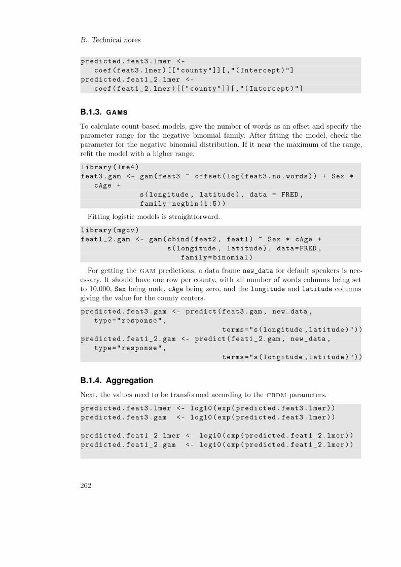
B. Technical notes

predicted.feat3.lmer <-coef(feat3.lmer)[["county"]][,"(Intercept)"]

predicted.feat1_2.lmer <-coef(feat1_2.lmer)[["county"]][,"(Intercept)"]

B.1.3. GAMs

To calculate count-based models, give the number of words as an offset and specify theparameter range for the negative binomial family. After fitting the model, check theparameter for the negative binomial distribution. If it near the maximum of the range,refit the model with a higher range.

library(lme4)feat3.gam <- gam(feat3 ~ offset(log(feat3.no.words)) + Sex *

cAge +s(longitude , latitude), data = FRED ,family=negbin (1:5))

Fitting logistic models is straightforward.

library(mgcv)feat1_2.gam <- gam(cbind(feat2 , feat1) ~ Sex * cAge +

s(longitude , latitude), data=FRED ,family=binomial)

For getting the gam predictions, a data frame new_data for default speakers is nec-essary. It should have one row per county, with all number of words columns being setto 10,000, Sex being male, cAge being zero, and the longitude and latitude columnsgiving the value for the county centers.

predicted.feat3.gam <- predict(feat3.gam , new_data ,type="response",

terms="s(longitude ,latitude)"))predicted.feat1_2.gam <- predict(feat1_2.gam , new_data ,

type="response",terms="s(longitude ,latitude)"))

B.1.4. Aggregation

Next, the values need to be transformed according to the cbdm parameters.

predicted.feat3.lmer <- log10(exp(predicted.feat3.lmer))predicted.feat3.gam <- log10(exp(predicted.feat3.lmer))

predicted.feat1_2.lmer <- log10(exp(predicted.feat1_2.lmer))predicted.feat1_2.gam <- log10(exp(predicted.feat1_2.lmer))

262

B.2. Bottom-up

predicted.feat3.lmer[predicted.feat3.lmer < -1] <- -1predicted.feat3.gam[predicted.feat3.gam < -1] <- -1

For alternations, we constrain the values to the range [−2, 2]

predicted.feat1_2.lmer[predicted.feat1_2.lmer < -2] <- -2predicted.feat1_2.gam [predicted.feat1_2.gam < -2] <- -2

predicted.feat1_2.lmer[predicted.feat1_2.lmer > 2] <- 2predicted.feat1_2.gam [predicted.feat1_2.gam > 2] <- 2

The results can then be combined into matrices predicted.lmer and predicted.gamusing cbind(). The distances can then be calculated using dist(), and be passed toRuG/L04 using its R interface.

B.2. Bottom-up

I am currently reworking the code for the bottom-up analysis. This version is not partic-ularly efficient, but relatively fast and easy to understand.

Two data frames are necessary. One, ngrams, should one row per n-gram token in thecorpus and a unique id for the desired resampling level (here conversational turns); theother countymap, should contain one row per resampling level id (here, the turn id) andthe corresponding analysis level (here, the county). The column names for the resamplinglevel ids must be the same in both data frames.

B.2.1. Normalization

The following code can be used to normalize a matrix with counts, where the rows aren-grams and the columns counties. All other columns have to be removed from the databefore

normalize1 <- function(m) {m <- t(m)mnorm <- m / rowSums(m)result <- t(t(mnorm) * colSums(m) / colSums(mnorm))result[is.nan(result)] <- 0return(t(result))

}

normalize2 <- function(m) {result <- (m * ncol(m) * nrow(m)) / sum(m)return(result)

}

normalize <- function(df, repet =5) {

263

B. Technical notes

df <- df[, colSums(df) > 0]normalized <- normalize1(df)if (repet > 1)

for (i in 1:(repet -1))normalized <- normalize1(normalized)

return(normalize2(normalized))}

B.2.2. Counting and permutation

The following functions can be used to count the ngrams, pairwise (runPair()) or intotal (runAll()). The parameters are as follows:

• base: the data frame containing the ngrams• perm: the data frame mapping the basis of permutation to the groups• which: the name of the column containing the groups• permute: FALSE to get the counts for the original corpus, a number to get a list

containing that many permuted counts.• which2: the column name of the resampling level, only necessary for runPair().

runAll <- function (base , perm , which="county", permute =1) {

doOnce <- function(base ,perm ,which) {left_join(base , perm) %>% function(x)

eval(substitute(group_by(x, which , ngram),list(which = as.name(which)))) %>%

summarize(count=n()) %>%dcast(formula(sprintf("ngram~%s", which)), fill=0,

value.var="count")}

if (permute){lapply (1: permute , function(x){

perm2 <- permperm2[,which] <- sample(perm2[,which])doOnce(base ,perm2 ,which)

})}else

doOnce(base ,perm ,which)}

264

B.2. Bottom-up

runPair <- function(base , perm , a, b, which="county",which2="turn", permute =1) {

perm2 <- perm [ perm[,which] %in% c(a,b),]base2 <- base [ base[,which2] %in% perm2[,which2], ]

runAll(base2 , perm2 , which=which , permute=permute)

}

B.2.3. Analysis

To do a whole-corpus comparison, the following code can be used. Distance matrixcalculation and exporting to Rug/L04 can then happen as usual.

compareRuns <- function(x, original) {

(( normalize(original[, -1]) < normalize(x[,-1])) * 1 +(normalize(original[, -1]) == normalize(x[,-1])) * 0.5)

}

library(dplyr)library(reshape2)library(magrittr)

nruns =1000

relscores <- Reduce("+", lapply(runAll(ngrams , countymap ,permute=nruns),

compareRuns ,runAll(ngrams , countymap ,

permute=FALSE)))/nruns

r.distinct <- 2*pmin(abs(relscores), abs(1 - relscores))

Finally, the following code can be used to run a pairwise analysis. rp is a list ofsignificance matrices, one for each bigram.

runPairwise <- function(repetitions =100, base , perm ,which="county", which2="turn") {

sigmatlist <- list()CORPORA <- unique(perm[,which])pairdiff <- function(a, b) pmax(a,b) - pmin(a,b)

265

B. Technical notes

for (i in levels(ngrams$ngram))sigmatlist [[i]] <- getempty ()

for (i in 1:( length(CORPORA) -1))for (j in (i+1):length(CORPORA)) {

print(paste(CORPORA[i], CORPORA[j]))

base <- runPair(corpbase , map , CORPORA[i],CORPORA[j], permute=FALSE)

rownames(base) <- base[,1]base <- normalize(t(base[,-1]))

rec.base <- pairdiff(base[,1], base [,2])

new.list <- runPair(corpbase , map , CORPORA[i],CORPORA[j], which=which ,

which2=which2 ,permute=repetitions)

new.list <- lapply(new.list , function(new){rownames(new) <- new[,1]new <- normalize(t(new[,-1]))pairdiff(new[,1], new[,2])

})

sigs <- Reduce("+", lapply(new.list , function(x) x >=rec.base))/nrepet

for (bigr in colnames(base)) {sigmatlist [[bigr ]][i,j] <- sigs[bigr]sigmatlist [[bigr ]][j,i] <- sigs[bigr]

}}

sigmatlist

}

rp <- runPairwise(repetitions =1000, base=ngrams ,perm=countymap)

rp <- lapply(rp, function(x) {x[is.na(x)] <- 1; x})

266

B.2. Bottom-up

p.distinct <- sapply(rp, function(x) sum(as.dist(x) < 0.05))

267

Bibliography

Abdi, Hervé & Dominique Valentin. 2007. Multiple correspondence analysis. In N.J.Salkind (ed.), Encyclopedia of measurement and statistics, 651–657. Thousand Oaks(CA): Sage.

Adger, David & Graeme Trousdale. 2007. Variation in English syntax: Theoreticalimplications. English Language and Linguistics 11(2). 261–278.

Albu, Mihai. 2006. Quantitative analyses of typological data. Leipzig: University of Leipzigdissertation.

Altmann, Eduardo G., Janet B. Pierrehumbert & Adilson E. Motter. 2009. Beyond wordfrequency: Bursts, lulls, and scaling in the temporal distributions of words. PLoS One4(11). e7678.

Anderson, Peter M. 1987. A Structural Atlas of the English Dialects. London, New York:Croom Helm.

Anderwald, Lieselotte. 2002. Negation in non-standard British English: Gaps, regulariza-tions, asymmetries (Studies in Germanic Linguistics 8). London, New York: Routledge.

Anderwald, Lieselotte. 2003. Non-standard English and typological principles: The caseof negation. In Günter Rohdenburg & Britta Mondorf (eds.), Determinants of linguisticvariation (Topics in English Linguistics 43), 507–529. Berlin: Mouton de Gruyter.

Anderwald, Lieselotte. 2005. Negative concord in British English dialects. In Iyeiri (2005),113–137.

Anderwald, Lieselotte. 2008. English in the Southeast of England: Morphology andsyntax. In Kortmann & Upton (2008), 440–462.

Anderwald, Lieselotte. 2009. The morphology of English dialects: Verb-formation innon-standard English. Cambridge: Cambridge University Press.

269

Bibliography

Anderwald, Lieselotte & Benedikt Szmrecsanyi. 2009. Corpus linguistics and dialectology.In Anke Lüdeling & Merja Kytö (eds.), Corpus linguistics. An international hand-book, vol. 2 (29 Handbücher zur Sprach- und Kommunikationswissenschaft), 1126–1140.Berlin, New York: Mouton de Gruyter.

Auer, Peter, Peter Baumann & Christian Schwarz. 2011. Vertical vs. horizontal change inthe traditional dialects of southwest Germany: A quantitative approach. taal & tongval63(1). 13–41.

Baayen, R. Harald. 2008. Analyzing linguistic data: A practical introduction to statisticsusing R. Cambridge University Press.

Baayen, R. Harald, Doug J. Davidson & Douglas M. Bates. 2008. Mixed-effects modelingwith crossed random effects for subjects and items. Journal of Memory and Language59(4). 390–412.

Baugh, Albert C. & Thomas Cable. 1993. A history of the English language. EnglewoodCliffs, N.J.: Prentice-Hall 4th edn.

Beal, Joan C. & Karen P. Corrigan. 2005. No, Nay Never : Negation in tyneside English.In Iyeiri (2005), 139–156.

Bickel, Balthasar. 2012. Exploring similarities: p phylogenetic methods beyond phy-logeny. Presented at the workshop "Phylomemetic and phylogenetic approaches in thehumanities", Saturday, Nov. 24th 2012, University of Bern, Switzerland.

Bloomfield, Leonard. 1933. Language. New York: Holt, Rhinehart and Winston.

Bookstein, Abraham & Donald H. Kraft. 1977. Operations research applied to documentindexing and retrieval decisions. Journal of the Association for Computing Machinery24(3). 418–427.

Bresnan, Joan, Anna Cueni, Tatiana Nikitina & R. Harald Baayen. 2007. Predicting thedative alternation. In Gerlof Boume, Irene Kraemer & Joost Zwarts (eds.), Cognitivefoundations of interpretation, 69–94. Amsterdam: Royal Netherlands Academy of Artsand Sciences.

Bresnan, Joan & Marilyn Ford. 2010. Predicting syntax: Processing dative constructionsin American and Australian varieties of English. Language 86(1). 186–213.

Bresnan, Joan & Jennifer Hay. 2008. Gradient grammar: An effect of animacy on thesyntax of give in New Zealand and American English. Lingua 118(2). 245–259.

270

Bibliography

Bridge, Martin. 2006. “It’s not always like this!” - Examining the UK’s negative/auxiliary-contraction strategies. Poster presented at the NWAV 35, Columbus, OH.

Britain, David. 2010. Grammatical variation in the contemporary spoken English ofEngland. In Andy Kirkpatrick (ed.), The handbook of World Englishes, 37–58. London:Routledge.

Bryant, David & Vincent Moulton. 2004. Neighbor-net: an agglomerative method for theconstruction of phylogenetic networks. Molecular Biology and Evolution 21(2). 255–65.

Chambers, J. K. 2003. Sociolinguistic theory: Linguistic variation and its social signifi-cance. Oxford: Blackwell.

Chambers, J. K. & Peter Trudgill. 1998. Dialectology. Cambridge, England: CambridgeUniversity Press 2nd edn.

Cheshire, Jenny. 1989. A survey of dialect grammar in British English. In MichelH. A. Blanc & Josiane F. Hamers (eds.), Problèmes théoriques et méthodologiques dansl’étude des langues/dialectes en contact aux niveaux macrologiques et micrologiques,50–58. Québec: Centre international de recherche sur le bilinguisme.

Cheshire, Jenny. 1998. English negation from an interactional perspective. In IngridTieken-Boon van Ostade, Gunnel Tottie & Wim van der Wurff (eds.), Negation in thehistory of English (Topics in English Linguistics 26), 29–54. Berlin: Mouton de Gruyter.

Cheshire, Jenny, Viv Edwards & Pamela Whittle. 1995. Urban British dialect grammar:The question of dialect levelling. In Iwar Werlen (ed.), Verbale Kommunikation in derStadt, 67–109. Tübingen: Gunter Narr Verlag. Reprinted from English World-Wide 10(2): 185-225.

Cheshire, Jenny & Sue Fox. 2009. Was/were variation: A perspective from London.Language Variation and Change 21(1). 1–38.

Clark, Herbert H. 1973. The language-as-fixed-effect fallacy: A critique of languagestatistics in psychological research. Journal of Verbal Learning and Verbal Behavior12. 335–359.

Cliff, Andrew D. & J. K. Ord. 1973. Spatial autocorrelation. London: Pion.

Close, Joanne & Bas Aarts. 2010. Current change in the modal system of English a casestudy of must, have to and have got to. In Ursula Lenker, Judith Huber & Robert

271

Bibliography

Mailhammer (eds.), English historical linguistics 2008: Selected papers from the fifteenthInternational Conference on English Historical Linguistics (ICEHL 15), Munich, 24-30 August 2008. Volume I: The history of English verbal and nominal constructions,65–182. Amsterdam: John Benjamins.

Cysouw, Michael. 2007. New approaches to cluster analysis of typological indices. InReinhard Köhler & Peter Grzbek (eds.), Exact methods in the study of language andtext, 61–76. Berlin: Mouton de Gruyter.

Davies, Mark. 2008-. The Corpus of Contemporary American English: 450 million words,1990-present. Available online at http://corpus.byu.edu/coca/.

Dawson, Christina. 2011. Shared alternatives to subject-verb agreement: The 3rd singu-lar verb and its uses in English and Brittonic. Freiburg: Albert-Ludwigs-UniversitätFreiburg dissertation.

Denison, David. 1993. English historical syntax: Verbal constructions. London: Longman.

Dress, Andreas W. M. & Daniel H. Huson. 2004. Constructing splits graphs. IEEE/ACMTransactions on Computational Biology and Bioinformatics 1. 109–115.

Dunn, Michael, Stephen C. Levinson, Eva Lindström, Ger Reesink & Angela Terrill. 2008.Structural phylogeny in historical linguistics: Methodological explorations applied inIsland Melanesia. Language 84(4). 710–759.

Dyen, Isidore, Joseph Kruskal & Paul Black. 1992. An Indoeuropean classification: Alexicostatistical experiment. Transactions of the American Philosophical Society 82(5).

Ellis, Alexander J. 1889. The existing phonology of English dialects compared with thatof West Saxon speech (On Early English Pronunciation V). London: Trübner & co.

The Helsinki Corpus of British English Dialects. 2006. Department of Modern Languages,University of Helsinki.

Evans, William. 1969. ‘You’ and ‘thou’ in Northern England. South Atlantic Bulletin34(4). 17–21.

Filppula, Markku, Juhani Klemola & Heli Paulasto (eds.). 2009. Vernacular universalsand language contacts. Abingdon: Routledge.

Fischer, Olga & Wim van der Wurff. 2006. Syntax. In Richard Hogg & David Denison(eds.), A history of the English language, 109–198. Cambridge: Cambridge UniversityPress.

272

http://corpus.byu.edu/coca/

Bibliography

Garside, Roger & Nicholas Smith. 1997. A hybrid grammatical tagger: Claws4. InRoger Garside, Geoffrey Leech & Tony McEnery (eds.), Corpus annotation: Linguisticinformation from computer text corpora., 102–121. London: Longman.

Gelman, Andrew & Jennifer Hill. 2007. Data analysis using regression and multilevel/hier-archical models. Cambridge: Cambridge University Press.

Goebl, Hans. 1982. Dialektometrie. Prinzipien und Methoden des Einsatzes der Nu-merischen Taxonomie im Bereich der Dialektgeographie. Denkschriften der Österre-ichischen Akademie der Wissenschaften, phil.-hist. Klasse, Band 157.

Goebl, Hans. 1984. Dialektometrische Studien anhand italoromanischer, rätoromanischerund galloromanischer Sprachmaterialien aus AIS und ALF. Tübingen: Max Niemeyer.

Goebl, Hans. 2005. Dialektometrie. In Richard Köhler, Gabriel Altmann & Raimund G.Piotrowski (eds.), Quantitative linguistics. An international handbook (Handbücher zurSprach- und Kommunikationswissenschaft 27), 498–531. Berlin, New York: de Gruyter.

Goebl, Hans. 2006. Recent advances in Salzburg dialectometry. Literary and LinguisticComputing 21(4). 411–435.

Goebl, Hans. 2007a. A bunch of dialectometric flowers: a brief introduction to dialectome-try. In Ute Smit, Stefan Dollinger, Julia Hüttner, Günther Kaltenböck & Ursula Lutzky(eds.), Tracing English through time: Explorations in language variation, 133–172. Wien:Braumüller.

Goebl, Hans. 2007b. Dialektometrische Streifzüge durch das Netz des Sprachatlasses AIS.Ladinia XXXI. 187–271.

Goebl, Hans. 2010. Dialectometry and quantitative mapping. In Alfred Lameli, RolandKehrein & Stefan Rabanus (eds.), Language and space. An international handbook oflinguistic variation, vol. 2: Language mapping (Handbücher zur Sprach- und Kommu-nikationswissenschaft 30), 433–464. Berlin: Mouton.

Goebl, Hans & Guillaume Schiltz. 1997. A dialectometrical compilation of CLAE Iand CLAE II. Isoglosses and dialect integration. In Wolfgang Viereck & HeinrichRamisch (eds.), Computer Developed Linguistic Atlas of England (CLAE), vol. 2, 13–21. Tübingen: Niemeyer.

Grafmiller, Jason. forthcoming. Variation in English genitives across modality and genre.English Language & Linguistics.

273

Bibliography

Greenbaum, Sidney & Gerald Nelson. 1996. The International Corpus of English (ICE)project. World Englishes 15(1). 3–15.

Gries, Stefan Th. & Joybrato Mukherjee. 2010. Lexical gravity across varieties of English:an ICE-based study of n-grams in Asian Englishes. International Journal of CorpusLinguistics 15(4). 520–548.

Grieve, Jack. 2009. A corpus-based regional dialect survey of grammatical variation inwritten Standard American English. Flagstaff: Northern Arizona University disserta-tion.

Grieve, Jack, Costanza Asnaghi & Tom Ruette. 2013. Site-restricted web searches fordata collection in regional dialectology. American Speech 88(4). 413–440.

Haddican, William. 2010. Theme–goal ditransitives and theme passivisation in BritishEnglish dialects. Lingua 120(10). 2424–2443.

Hamming, Richard W. 1950. Error detecting and error correcting codes. Bell SystemTechnical Journal 26(2). 147–160.

Hansen, Sandra. 2011. Dialectometrics meets sociolinguistics - an investigation on thephonological dialect shift in southwest Germany. Presented at the International Con-ference on Language Variation in Europe (ICLaVE6). Universität Freiburg, June 2011.

Heeringa, Wilbert. 2004. Measuring dialect pronunciation differences using Levenshteindistance: University of Groningen dissertation.

Heeringa, Wilbert & John Nerbonne. 2001. Dialect areas and dialect continua. LanguageVariation and Change 13, 2001 13(3). 375–400.

Heeringa, Wilbert & John Nerbonne. 2013. Dialectometry. In Frans Hinskens & JohanTaeldeman (eds.), Language and space. An international handbook of linguistic varia-tion, volume III: Dutch (Handbücher zur Sprach- und Kommunikationswissenschaft 30),567–586. Berlin and New York: Walter de Gruyter.

Hernández, Nuria. 2006. User’s guide to FRED: Freiburg Corpus of English Dialects.English Dialect Research Group. Albert-Ludwigs-Universität Freiburg.

Herrmann, Tanja. 2003. Relative clauses in dialects of English: a typological approach.Freiburg: Albert-Ludwigs-Universität Freiburg dissertation.

274

Bibliography

Hickey, Raymond (ed.). 2004. Legacies of colonial English: Studies in transported dialects.Cambridge University Press.

Hirschman, Lynette. 1994. Female–male differences in conversational interaction. Lan-guage in Society 23(3). 427–442.

Hoppenbrouwers, Cor & Geer Hoppenbrouwers. 2001. De indeling van de Nederlandsestreek-talen. Dialecten van 156 steden en dorpen geklasseerd volgens de FFM. Assen:Koninklijke Van Gorcum.

Hopper, Paul & Elizabeth Closs Traugott. 2003. Grammaticalization. Cambridge, UK:Cambridge University Press.

Hughes, Arthur & Peter Trudgill. 1979. English accents and dialects. London: EdwardArnold.

Hundt, Marianne. 2004. Animacy, agency and the spread of the progressive in eighteenth-and nineteenth-century English. English Language and Linguistics 8(1). 47–69.

Huson, Daniel H. 1998. Splitstree: Analyzing and visualizing evolutionary data. Bioin-formatics 14(1). 68–73.

Huson, Daniel H. & David Bryant. 2006. Application of phylogenetic networks in evolu-tionary studies. Molecular Biology And Evolution 23(2). 254–67.

Ihalainen, Ossi. 1988. Creating linguistic databases from machine-readable dialect texts.In Alan R. Thomas (ed.), Methods in Dialectology: Proceedings of the sixth internationalconference held at the University College of North Wales, 3rd-7th August 1987, 569–584.Clevedon: Multilingual Matters.

Inoue, Fumio. 1996. Subjective dialect division in Great Britain. American Speech 71(2).142–161.

Iyeiri, Yoko (ed.). 2005. Aspects of negation. Amsterdam & Philadelphia: John Benjamins.

Jaeger, T. Florian. 2008. Categorical data analysis: Away from ANOVAs (transformationor not) and towards logit mixed models. Journal of Memory and Language 59(4).434–446.

Jaeger, T. Florian, Peter Graff, William Croft & Daniel Pontillo. 2011. Mixed effect modelsfor genetic and areal dependencies in linguistic typology: Commentary on Atkinson.Linguistic Typology 15(2). 281–319.

275

Bibliography

Jankowski, Bridget. 2004. A transatlantic perspective of variation and change in Englishdeontic modality. Toronto Working Papers in Linguistics 23. 85–113.

Johannessen, Janne Bondi, Joel Priestley, Kristin Hagen, Tor Anders Åfarli & ØysteinAlexander Vangsnes. 2009. The Nordic Dialect Corpus - an advanced research tool. InKristiina Jokinen & Eckhard Bick (eds.), Proceedings of the 17th Nordic Conference ofComputational Linguistics NODALIDA 2009 (NEALT Proceedings Series 4), .

Johnson, Daniel Ezra. 2009. Getting off the GoldVarb standard: Introducing Rbrul formixed-effects variable rule analysis. Language and Linguistics Compass 3(1). 359–383.

Kessler, Brett. 1995. Computational dialectology in Irish Gaelic. In Proceedings ofthe seventh conference of the European chapter of the Association for ComputationalLinguistics, 60–66. Morgan Kaufmann Publishers.

Kessler, Brett. 2000. The significance of word lists. Stanford: CSLI Press.

Kirk, John M. 1985. Linguistic atlases and grammar: The investigation and descriptionof regional variation in English syntax. In John M. Kirk, Stewart Sanderson & J. D. A.Widdowson (eds.), Studies in linguistic geography, 130–156. London: Croom Holm.

Kortmann, Bernd. 2004a. Dialectology meets typology: Dialect grammar from a cross-linguistic perspective. Mouton de Gruyter.

Kortmann, Bernd. 2004b. Introduction. In Kortmann (2004a), 1–11.

Kortmann, Bernd. 2004c. Do as a tense and aspect marker in varieties of English. InKortmann (2004a), 245–275.

Kortmann, Bernd. 2013. Regional profile: The British Isles. In Kortmann & Lunkenheimer(2013), 678–703.

Kortmann, Bernd & Kerstin Lunkenheimer (eds.). 2013. The Mouton World Atlas ofVariation in English. Berlin: Mouton de Gruyter.

Kortmann, Bernd, Edgar W. Schneider, Kate Burridge, Rajend Mesthrie & Clive Upton(eds.). 2004. A handbook of varieties of English. Mouton de Gruyter.

Kortmann, Bernd & Benedikt Szmrecsanyi. 2004. Global synopsis: morphological andsyntactic variation in English. In Kortmann et al. (2004), 1142–1202.

Kortmann, Bernd & Clive Upton (eds.). 2008. Varieties of English vol. 1: The BritishIsles. Berlin: Mouton de Gruyter.

276

Bibliography

Kortmann, Bernd & Susanne Wagner. 2010. Changes and continuities in dialect grammar.In Raymond Hickey (ed.), Eighteenth century English. ideology and change, 269–292.Cambridge: Cambridge University Press.

Kortmann, Bernd & Christoph Wolk. 2013. Morphosyntactic variation in the anglophoneworld: A global perspective. In Kortmann & Lunkenheimer (2013), 906–936.

Krug, Manfred. 2000. Emerging English modals: A corpus-based study of grammaticaliza-tion. Berlin/New York: Mouton de Gruyter.

Kruskal, Joseph B. & Myron Wish. 1978. Multidimensional Scaling (Quantitative Applica-tions in the Social Sciences 11). Newbury Park, London, New Delhi: Sage Publications.

König, Werner (ed.). 1997 – 2009. Sprachatlas von Bayerisch-Schwaben (BayerischerSprachatlas Regionalteil 1). Heidelberg: Winter. 14 volumes.

Labov, William. 1990. The intersection of sex and social class in the course of linguisticchange. Language Variation and Change 2. 205–254.

Lass, Roger. 2004. South African English. In Hickey (2004), 363–386.

Lucas, Christopher & David Willis. 2012. Never again: the multiple grammaticalizationof never as a marker of negation in English. English Language and Linguistics 16(3).459–485.

Mair, Christian. 2004. Corpus linguistics and grammaticalisation theory: Beyond statisticsand frequency? In Christian Mair & Hans Lindquist (eds.), Corpus approaches togrammaticalisation in English, 121–150. Amsterdam: Benjamins.

Manni, Franz, Wilbert Heeringa, Bruno Toupance & John Nerbonne. 2008. Do surnamedifferences mirror dialect variation? Human Biology 80(1). 41–64.

Manning, Chris & Hinrich Schütze. 1999. Foundations of statistical natural languageprocessing. Cambridge, MA: MIT Press.

McFadden, Thomas. 2002. The rise of the to-dative in Middle English. In David Lightfoot(ed.), Syntactic Effects of Morphological Change, 107–123. Oxford: Oxford UniversityPress.

McMahon, April, Paul Heggarty, Robert McMahon & Warren Maguire. 2007. The soundpatterns of Englishes: representing phonetic similarity. English Language and Linguis-tics 11(1). 113–142.

277

Bibliography

McMahon, April & Robert McMahon. 2005. Language classification by numbers. Oxford:Oxford University Press.

Miller, Jim. 2008. Scottish English: morphology and syntax. In Kortmann & Upton(2008), 299–327.

Montgomery, Chris. 2007. Northern English dialects: A perceptual approach. Sheffield:University of Sheffield dissertation.

Moran, Patrick A. P. 1950. Notes on continuous stochastic phenomena. Biometrika37(1/2). 17–23.

Nerbonne, John. 2009. Data-driven dialectology. Language and Linguistics Compass3(1). 175–198.

Nerbonne, John. 2013. How much does geography influence language variation? InPeter Auer, Martin Hilpert, Anja Stukenbrock & Benedikt Szmrecsanyi (eds.), Space inlanguage and linguistics. Geographical, interactional, and cognitive perspectives, 220–236. Berlin: Mouton de Gruyter.

Nerbonne, John & Wilbert Heeringa. 2007. Geographic distributions of linguistic variationreflect dynamics of differentiation. In Sam Featherston & Wolfgang Sternefeld (eds.),Roots: Linguistics in search of its evidential base, 267–297. Berlin: Mouton de Gruyter.

Nerbonne, John & Peter Kleiweg. 2007. Toward a dialectological yardstick. Journal ofQuantitative Linguistics 14(2). 148–166.

Nerbonne, John, Peter Kleiweg, Wilbert Heeringa & Franz Manni. 2008. Projecting di-alect differences to geography: Bootstrap clustering vs. noisy clustering. In ChristinePreisach, Lars Schmidt-Thieme, Hans Burkhardt & Reinhold Decker (eds.), Data anal-ysis, machine learning, and applications. Procedings of the 31st annual meeting of theGerman Classification Society, 647–654. Berlin: Springer.

Nerbonne, John & Wybo Wiersma. 2006. A measure of aggregate syntactic distance.In John Nerbonne & Erhard Hinrichs (eds.), Linguistic distances workshop at thejoint conference of the International Committee on Computational Linguistics and theAssociation for Computational Linguistics, 82–90.

Noetzel, Andrew S. & Stanley M. Selkow. 1999 [1983]. An analysis of the general tree-editing problem. In David Sankoff & Joseph Kruskal (eds.), Time warps, string edits andmacromolecules: The theory and practice of sequence comparison, 237–252. Stanford:CSLI.

278

Bibliography

Ord, J. Keith & Arthur Getis. 1995. Local spatial autocorrelation statistics: Distributionalissues and an application. Geographical Analysis 27(4). 286–306.

Orton, Harold & Eugen Dieth. 1962. Survey of English Dialects. Leeds: E. J. Arnold.

Orton, Harold, Stewart Sanderson & John Widdowson. 1978. The Linguistic Atlas ofEngland. London: Croom Helm.

Pickl, Simon, Aaron Spettl, Simon Pröll, Stephan Elspaß, Werner König & Volker Schmidt.2014. Linguistic distances in dialectometric intensity estimation. Journal of LinguisticGeography 2(1). 25–40.

Pierrehumbert, Janet B. 2012. Burstiness of verbs and derived nouns. In Diana Santos,Krister Linden & Wanjiju Ng’ang’a (eds.), Shall we play the festschrift game?: Essayson the occasion of Lauri Carlson’s 60th birthday, Springer Verlag.

Pinheiro, José C. & Douglas M. Bates. 2000. Mixed-effects models in S and S-PLUS.New York: Springer.

Poplack, Shana & Sali Tagliamonte. 1999. The grammaticization of going to in (AfricanAmerican) English. Language Variation and Change 11(3). 315–342.

Prokić, Jelena & John Nerbonne. 2013. Analyzing dialects biologically. In HeinerFangerau, Hans Geisler, Thorsten Halling & William Martin (eds.), Classification andevolution in biology, linguistics and the history of science: Concepts – methods – visu-alization, 147–161. Stuttgart: Steiner.

Pröll, Simon. 2013. Detecting structures in linguistic maps – fuzzy clustering for patternrecognition in geostatistical dialectometry. Literary and Linguistic Computing 28(1).108–118.

Quené, Hugo & Huub van den Bergh. 2008. Examples of mixed-effects modeling withcrossed random effects and with binomial data. Journal of Memory and Language59(4). 413–425.

Quirk, Randolph, Sidney Greenbaum, Geoffrey Leech & Jan Svartvik. 1985. A compre-hensive grammar of the English language. London, New York: Longman.

R Development Core Team. 2010. R: A language and environment for statistical comput-ing. R Foundation for Statistical Computing Vienna, Austria. http://www.R-project.org/.

279

http://www.R-project.org/

http://www.R-project.org/

Bibliography

Raumolin-Brunberg, Helena. 2005. The diffusion of subject you: A case study in historicalsociolinguistics. Language Variation and Change 17(1). 55–73.

Rayson, Paul, Dawn Archer, Scott Piao & Tony McEnery. 2004. The UCREL semanticanalysis system. In Proceedings of the workshop on beyond named entity recognitionsemantic labelling for NLP tasks in association with 4th international conference onLanguage Resources and Evaluation (LREC 2004), 25th May 2004, Lisbon, Portugal,7–12.

Rayson, Paul, Geoffrey Leech & Mary Hodges. 1997. Social differentiation in the useof English vocabulary: Some analyses of the conversational component of the BritishNational Corpus. International Journal of Corpus Linguistics 2(1). 133–152.

Ringe, Don, Tandy Warnow & Ann Taylor. 2002. Indo-European and computationalcladistics. Transactions of the Philological Society 100(1). 59–129.

Rivadeneira, Marcela J. & Xavies Casassas. 2009. New insights into the use of VDM:Some preliminary stages and a revisited case of dialectometry. Dialectologia 2. 23–35.

Ruette, Tom. 2011. Disease inspired expletives in Dutch due to entrenched Calvin-ism. Corpus-based evidence from Twitter. Presented at the workshop on quantitativemethods in geolinguistics, Freiburg, Germany, December 2011.

Rumpf, Jonas, Simon Pickl, Stephan Elspaß, Werner König & Volker Schmidt. 2009.Structural analysis of dialect maps using methods from spatial statistics. Zeitschriftfür Dialektologie und Linguistik 76(3). 280–308.

Rumpf, Jonas, Simon Pickl, Stephan Elspaß, Werner König & Volker Schmidt. 2010.Quantification and statistical analysis of structural similarities in dialectological area-class maps. Dialectologia et Geolinguistica 18. 73–100.

Saitou, Naruya & Masatoshi Nei. 1987. The neighbor-joining method: A new method forreconstructing phylogenetic trees. Molecular Biology and Evolution 4(4). 406–425.

Sammon, J. 1969. A nonlinear mapping for data structure analysis. IEEE Transactionson Computers 18(5). 401–409.

Sampson, Geoffrey. 2000. A proposal for improving the measurement of parse accuracy.International Journal of Corpus Linguistics 5(1). 53–68.

280

Bibliography

Sanders, Nathan C. 2007. Measuring syntactic difference in British English. In ChrisBiemann, Violeta Seretan & Ellen Riloff (eds.), Proceedings of the ACL 2007 Stu-dent Research Workshop, 1–6. Prague, Czech Republic: Association for ComputationalLinguistics.

Sanders, Nathan C. 2010. A statistical method for syntactic dialectometry. Bloomington:Indiana University dissertation.

Sankoff, David & William Labov. 1979. On the uses of variable rules. Language in Society8(2). 189–222.

Saussure, Ferdinand de. 1916 [1983]. Course in general linguistics. Open Court Classics.Translated by Roy Harris.

Schneider, Edgar W. 2007. Postcolonial English. New York: Cambridge University Press.

Schulz, Monika. 2012. Morphosyntactic variation in British English dialects: evidencefrom possession, obligation and past habituality. Freiburg: Albert-Ludwigs-UniversitätFreiburg dissertation.

Shackleton, Robert G. 2007. Phonetic variation in the traditional English dialects: Acomputational analysis. Journal of English Linguistics 35(1). 30–102.

Shackleton, Robert G. 2010. Quantitative assessment of English-American speech rela-tionships. Groningen: University of Groningen dissertation.

Spruit, Marco René, Wilbert Heeringa & John Nerbonne. 2009. Associations amonglinguistic levels. Lingua 119(11). 1624–1642.

Streck, Tobias. 2012. Phonologischer Wandel im Konsonantismus der alemannis-chen Dialekte Baden-Württembergs. Sprachatlasvergleich, Spontansprache und dialek-tometrische Studien (Zeitschrift für Dialektologie und Linguistik – Beihefte 148).Stuttgart: Steiner.

Studier, James A. & Karl J. Keppler. 1988. A note on the neighbor-joining algorithm ofSaitou and Nei. Molecular Biology and Evolution 5(6). 729–731.

Swadesh, Morris. 1950. Salish internal relationships. International Journal of AmericanLinguistics 16(4). 157–167.

Szmrecsanyi, Benedikt. 2005. Language users as creatures of habit: A corpus-linguisticanalysis of persistence in spoken English. Corpus Linguistics and Linguistic Theory1(1). 113–150.

281

Bibliography

Szmrecsanyi, Benedikt. 2006. Morphosyntactic persistence in spoken English. A corpusstudy at the intersection of variationist sociolinguistics, psycholinguistics, and discourseanalysis. Berlin/New York: Mouton de Gruyter.

Szmrecsanyi, Benedikt. 2008. Corpus-based Dialectometry: Aggregate morphosyntacticvariability in British English dialects. International Journal of Humanities and ArtsComputing 2(1-2). 279–296.

Szmrecsanyi, Benedikt. 2010a. The morphosyntax of BrE dialects in a corpus-baseddialectometrical perspective: Feature extraction, coding protocols, projections to ge-ography, summary statistics. Manuscript. http://www.freidok.uni-freiburg.de/

volltexte/7320/.

Szmrecsanyi, Benedikt. 2010b. The English genitive alternation in a cognitive sociolinguis-tics perspective. In Dirk Geeraerts, Gitte Kristiansen & Yves Peirsman (eds.), Advancesin Cognitive Sociolinguistics, 141–166. Berlin, New York: Mouton de Gruyter.

Szmrecsanyi, Benedikt. 2011. Corpus-based dialectometry: A methodological sketch.Corpora 6(1). 45–76.

Szmrecsanyi, Benedikt. 2012. Geography is overrated. In Sandra Hansen, ChristianSchwarz, Philipp Stoeckle & Tobias Streck (eds.), Dialectological and folk dialectologicalconcepts of space, 215–231. Berlin, New York: Walter de Gruyter.

Szmrecsanyi, Benedikt. 2013. Grammatical variation in British English dialects: A studyin corpus-based dialectometry. Cambridge: Cambridge University Press.

Szmrecsanyi, Benedikt & Nuria Hernández. 2007. Manual of information to accompanythe Freiburg Corpus of English Dialects Sampler (FRED-S). English Department,University of Freiburg.

Szmrecsanyi, Benedikt & Bernd Kortmann. 2009. Vernacular universals and angloversalsin a typological perspective. In Filppula et al. (2009), 33–53.

Szmrecsanyi, Benedikt, Anette Rosenbach, Joan Bresnan & Christoph Wolk. 2014. Cul-turally conditioned language change? Genitive constructions in Late Modern English.In Marianne Hundt (ed.), The syntax of Late Modern English, 133–152. Cambridge:Cambridge University Press.

Szmrecsanyi, Benedikt & Christoph Wolk. 2011. Holistic corpus-based dialectology.Brazilian Journal of Applied Linguistics / Revista Brasileira de Linguistica Aplicada11(2). 561–592.

282

http://www.freidok.uni-freiburg.de/volltexte/7320/

http://www.freidok.uni-freiburg.de/volltexte/7320/

Bibliography

Séguy, Jean. 1971. La relation entre la distance spatiale et la distance lexicale. Revue deLinguistique Romane 35. 335–357.

Tagliamonte, Sali A. 2012. Variationist sociolinguistics: Change, observation, interpreta-tion. Hoboken, NJ: Wiley-Blackwell Publishers.

Tagliamonte, Sali A. 2013. Roots of English: Exploring the history of dialects. Cambridge:Cambridge University Press.

Tagliamonte, Sali A. & R. Harald Baayen. 2012. Models, forests and trees of York English:Was/were variation as a case study for statistical practice. Language Variation andChange 24(2). 135–178.

Tagliamonte, Sali A., Mercedes Durham & Jennifer Smith. 2014. Grammaticalization atan early stage: future be going to in conservative British dialects. English Languageand Linguistics 18(1). 75–108.

Tagliamonte, Sali A. & Helen Lawrence. 2000. ‘I used to dance but I don’t dance now’.the habitual past in English. Journal of English Linguistics 28(4). 324–353.

Tagliamonte, Sali A. & Jennifer Smith. 2002. ‘either it isn’t or it’s not’: NEG/AUXcontraction in British dialects. English World Wide 23(2). 251–281.

Tagliamonte, Sali A., Jennifer Smith & Helen Lawrence. 2005. No taming the vernacular!Insights from the relatives in Northern Britain. Language Variation and Change 17(1).75–112.

Tobler, Waldo. 1970. A computer movie simulating urban growth in the Detroit region.Economic Geography 46(2). 234–240.

Torgerson, Warren S. 1952. Multidimensional scaling: I. Theory and method. Psychome-trika 17. 401–419.

Trudgill, Peter. 1974. Linguistic change and diffusion: Description and explanation insociolinguistic dialect geography. Language in Society 3(2). 215–246.

Trudgill, Peter. 1999. The dialects of England. Cambridge, MA, Oxford: Blackwell 2ndedn.

Trudgill, Peter. 2009a. Sociolinguistic typology and complexification. In Geoffrey Samp-son, David Gil & Peter Trudgill (eds.), Language complexity as an evolving variable,98–109. Oxford: Oxford University Press.

283

Bibliography

Trudgill, Peter. 2009b. Vernacular universals and the sociolinguistic typology of Englishdialects. In Filppula et al. (2009), 304–322.

Upton, Clive. 2008. Synopsis: phonological variation in the British Isles. In Kortmann &Upton (2008), 269–282.

Upton, Clive, Stewart Sanderson & J.D.A. Widdowson. 1987. Word maps: A dialect atlasof England. London: Croom Helm.

Wagner, Susanne. 2002. ‘We don’ say she, ’do us?’ Pronoun exchange – a feature ofEnglish dialects? Manuscript, Universität Freiburg.

Wagner, Susanne. 2008. English in the Southwest of England: Morphology and syntax.In Kortmann & Upton (2008), 417–439.

Wakelin, Martyn F. 1977. English dialects: An introduction. London: Athlone Press.

Wales, Katie. 2006. Northern English: A cultural and social history. Cambridge, NewYork: Cambridge University Press.

Wieling, Martijn. 2012. A quantitative approach to social and geographical dialect varia-tion. Groningen: University of Groningen dissertation.

Wieling, Martijn, Simonetta Montemagni, John Nerbonne & R. Harald Baayen. forthcom-ing. Lexical differences between Tuscan dialects and standard Italian: Accounting forgeographic and socio-demographic variation using generalized additive mixed modeling.Language 90(3).

Wieling, Martijn, John Nerbonne & R. Harald Baayen. 2011. Quantitative social dialec-tology: Explaining linguistic variation geographically and socially. PLoS ONE 6(9).e23613.

Wieling, Martijn, Clive Upton & Ann Thompson. 2013. Analyzing the BBC Voices data:Contemporary English dialect areas and their characteristic lexical variants. Literaryand Linguistic Computing 29(1). 107–117.

Wiersma, Wybo, John Nerbonne & Timo Lauttamus. 2011. Automatically extractingtypical syntactic differences from corpora. Literary and Linguistic Computing 26(1).107–124.

Wolfram, Walt. 2008. Rural and ethnic varieties in the Southeast: Morphology and syntax.In Edgar W. Schneider (ed.), Varieties of English: The Americas and the Caribbean,469–492. Berlin: Mouton de Gruyter.

284

Bibliography

Wolfram, Walt & Natalie Schilling-Estes. 1998. American English: Dialects and variation.Malden: Blackwell Publishers.

Wolk, Christoph. 2009. Classifying geographic variation: Morphosyntax and phonology.Freiburg: Albert-Ludwigs-Universität Freiburg Magisterarbeit.

Wolk, Christoph, Joan Bresnan, Anette Rosenbach & Benedikt Szmrecsanyi. 2013. Da-tive and genitive variability in Late Modern English: Exploring cross-constructionalvariation and change. Diachronica 33(3). 382–419.

Wood, Simon N. 2003. Thin-plate regression splines. Journal of the Royal StatisticalSociety (B) 65(1). 95–114.

Wood, Simon N. 2006. Generalized additive models: An introduction with R. Boca Raton,Florida: Chapman & Hall.

Wälchli, Bernhard. 2009. Data reduction typology and the bimodal distribution bias.Linguistic Typology 13(1). 77–94.

285

Deutsche Zusammenfassung

Die vorliegende Arbeit verknüpft zwei moderne Ansätze zur Untersuchung sprachlicherVariation. Auf der einen Seite steht die Dialektometrie, ein Zweig der Geolinguistik, inder mittels Aggregation viele Merkmale gleichzeitig betrachtet werden. Auf der Anderensteht die frequenz- und wahrscheinlichkeitsbasierte Korpuslinguistik. Diese Verknüpfungbesteht aus zwei Komponenten. Einerseits wird die von Szmrecsanyi (u.a. 2013) entwi-ckelte Methode corpus-based dialectometry (cbdm) um eine neue Komponente erweitert.Zur cbdm hinzu kommt die statistische Modellierung der Korpusbeobachtungen mittelszweier Modellierungstechniken – generalized linear mixed-effects modeling (glmm) undgeneralized additive modeling (gam) – um so ein robusteres Bild der geolinguistischenVerteilung zu erhalten. Der zweite Schritt besteht aus einer datengetriebenen Analysemittels Wortart-n-grammen. Mittels dieser kann – anstatt einer relativ geringen Zahlsorgfältig ausgewählter und oft manuell ausgezählter Merkmale – eine sehr große Zahlvon Strukturen vollautomatisch untersucht werden. Mit Hilfe von Permutationstests kannman identifizieren, welche Wortartfolgen eine geographisch verlässliche Frequenzvertei-lung haben, und die Ergebnisse können dann zur aggregativen Auswertung eingesetztwerden. Diese spezifische Anwendung konzentriert sich auf die im Dialektkorpus fred

(Freiburg Corpus of English Dialects, siehe Abschnitt 3.1) enthaltenen DialektregionenGroßbritanniens.

Kapitel 2 stellt Methode und Anwendung aggregativer Analysen vor. In der Dialek-tometrie wird eine Vielzahl einzelner Merkmale kombiniert, um so einen aggregiertenBlick auf die Gesamtstruktur dialektaler Variation zu werfen. Oft wird zur Illustrationder Idee folgende Metapher gebraucht: die detaillierte dialektologische Untersuchung ei-nes Merkmals führt zu einer immer genaueren Beschreibung des einzelnen “Baumes”. Istallerdings der gesamte “Wald” von Interesse, dann verhindert ein zu genauer Blick aufwenige Details wichtige Erkenntnisse; es kann “der Wald vor lauter Bäumen nicht mehrgesehen werden”. Insbesondere sind oft Dialektgruppen in einzelnen Merkmalen nichtklar voneinander getrennt. Durch gleichzeitige Betrachtung vieler Merkmale zeigt sichjedoch dass die Gruppenzugehörigkeit durchaus informativ ist. Auch wenn kein einzelnesMerkmal die Gruppe perfekt abbildet, können sich die Gruppenmitglieder untereinander

287


doch deutlich ähnlicher sein als sie es zu Dialekten außerhalb der Gruppe sind. Zentral isthier im Allgemeinen die Idee der linguistischen Distanz: aus Messungen einzelner Merk-malsdimensionen wird ein gemeinsamer Wert berechnet, der linguistisch aussagekräftigdarüber ist, wie sehr sich die jeweiligen Dialektmesspunkte voneinander unterscheiden.Für alle Dialektpaare berechnet ergeben diese Werte eine Distanzmatrix, auf die verschie-dene statistische Analysen angewendet werden können. Am Ende des Prozesses steht einegeeignete kartographische Repräsentation der Ergebnisse. Zentral sind hier insbesondereClusteranalysen und multi-dimensionale Skalierung. Bei Clusteranalysen werden die Dia-lekte in hierarchische Gruppen eingeteilt, die dann z.B. mit einer Choroplethenkarte (z.B.Karte 36) auf die geographische Ebene projiziert werden können. Multi-dimensionaleSkalierungen reduzieren die Vielzahl linguistischer Dimensionen auf wenige abstrakteDimensionen. Dies ermöglicht die Visualisierung der Ähnlichkeiten zwischen Dialektenmittels gradueller Einfärbungen, bekannt als Kontinuumskarten (z.B. Karte 44b). Auchweit verbreitet sind Korrelationsanalysen, bei denen die linguistischen Dialektabständemit anderen Maßen statistisch verglichen werden. Korrelationsanalysen erlauben es, glo-bale Aussagen zu treffen, beispielsweise über das Verhältnis von linguistischer Diversitätzu geographischer Entfernung. Schließlich sind Splitsgraphen zu erwähnen, eine Technikaus der Bioinformatik, die insbesondere in der historischen Linguistik und der TypologieAnwendung gefunden hat.

In den beiden großen Schulen der modernen Dialektometrie, der Salzburger und derGroninger Schule, werden primär Dialektunterschiede in Lexis und Aussprache unter-sucht. In der Salzburger Schule um Hans Goebl geschieht dies per Taxierung, das heißtdurch linguistisch sinnvolle Klassifizierung der einzelnen Beobachtungen. Die GroningerSchule um John Nerbonne dagegen benutzt üblicherweise Zeichenfolgendistanzmaße wiedie Levenshtein-Distanz, um aus den einzelnen Informantendaten direkt Dialektabständezu generieren. Datenquellen sind jedoch fast immer Dialektatlanten, die letztlich nur Zei-chenfolgen oder kategoriale Daten enthalten. Gerade für morphosyntaktische Merkmalesind jedoch oft graduelle Unterschiede in den Gebrauchsfrequenzen relevant. Szmrecsanyiscbdm (2013) bietet eine Möglichkeit, solche Daten aus Dialektkorpora zu extrahierenund dialektometrisch nutzbar zu machen. Hierzu wird zuerst ein Merkmalskatalog ent-worfen, der ein breites Spektrum morphosyntaktischer Variation aufgreifen soll. Dannwird ein geeignetes Dialektkorpus nach Belegen dieser Merkmale durchsucht. Aus denFundzahlen pro Merkmal können dann durch einen Bearbeitungsprozess Dialektdistan-zen ermittelt werden. Szmrecsanyis Katalog, der hier weiterverwendet wird, enthält 57verschiedene Merkmale. Die originale dialektometrische Analyse zeigt klar, dass Frequen-zen geographisch verteilt sind und dass ein dialektometrischer Ansatz zur Morphosyntax

288

möglich und ergiebig ist (Szmrecsanyi 2013). Einige konfundierende Faktoren erschwerendies jedoch: Erstens sind an den Messpunkten (d.h. Grafschaften) sehr unterschiedlicheMengen an Korpusmaterial verfügbar, was sowohl die Anzahl an Sprechern als auch dieAnzahl an Wörtern betrifft. Messungen, die auf wenig Material basieren, sind allerdingsim Allgemeinen weniger genau, da atypische Textstellen und idiolektale Besonderheitenmehr Gewicht besitzen. Zweitens sind die Informanten soziolinguistisch nicht einheitlich,sondern unterschieden sich sowohl im Geschlecht als auch im Alter voneinander.

Um robustere Ergebnisse zu erzielen, die gegen ungleiche Verteilung der Daten weni-ger empfindlich sind, und um soziologische Faktoren statistisch handhabbar zu machen,kombiniere ich die cbdm mit Regressionsmodellierung. Dabei modelliere ich Frequenzenoder, wenn zwei Merkmale als Alternierung verstanden werden, das Verhältnis der beidenFrequenzen. Die Geographie geht hierbei in zwei Varianten in das Modell ein: Einerseitsverwende ich glmms (vorgestellt in Abschnitt 3.2.2.1), In diesen wird die Zugehörigkeitzu Grafschaften als kategorialer Faktor gesehen, dessen Effekt normalverteilt ist. Hierwird Information zur Verteilung eines Merkmals in anderen Regionen verwendet, um dieAussagekraft einzelner Beobachtungen zu skalieren. In der Literatur wird dies als parti-al pooling bezeichnet. Zur empirischen Validierung werden Simulationstests eingesetzt.Hier ist das den Beobachtungen zugrunde liegende Signal bekannt, und die klassischecbdm kann direkt mit der modellbasierten Variante verglichen werden. Wie erwartetzeigt sich, dass beide Methoden besser werden, je häufiger das Merkmal ist und je größerdie Frequenzunterschiede sind. Im Schnitt ist bei gleichen Bedingungen allerdings dermodellbasierte Ansatz genauer, und damit vorzuziehen.

In der zweiten Modellierungsstrategie, den gams (Abschnitt 3.2.2.2), geht Geographiedirekt mittels der Längen- und Breitengrade der einzelnen Orte in das Modell ein. Dabeiwird eine “Gebirgskarte” erzeugt, die zeigt, in welchen Regionen ein bestimmtes Merkmalhäufiger ist als in anderen. Die Methode ermöglicht eine stärkere lokale Begradigung;in anderen Worten, das Modell nimmt an, dass geographisch nahe Beobachtungspunkteeinander ähnlich sind, und testet dann ob ein stärkerer Unterschied besser zu den Da-ten passt. Dies ist ein zweischneidiges Schwert. Einerseits ist die Ermittlung des lokalenZusammenhanges oft ein Ziel dialektometrischer Untersuchungen. Wird sie als Hypo-these angenommen, besteht die Gefahr einer zirkulären Argumentation. Andererseits istgeolinguistisch gesehen die Annahme, dass Messpunkte, die nahe beieinander liegen, ein-ander auch linguistisch ahnlich sind, eine gute Nullhypothese, die auch als FundamentalDialectological Postulate (Nerbonne & Kleiweg 2007) bezeichnet wird.

In der zweiten Analyse, vorgestellt in Abschnitt 3.2.3, wird eine nach Wortarten ko-dierte Untermenge des fred Korpus datengetrieben untersucht. Aufbauend auf einer

289


von Nerbonne & Wiersma (2006) und Sanders (2010) vorgeschlagenen Methode werdenWortartsfolgen (n-gramme) konstruiert und gezählt. Für n = 2, also Bigramme, ergebensich beispielsweise aus dem Satz

(1) We_PPIS2 started_VVD at_II three_MC ,_, yes_UH ._. [DEV_005]

folgende Kombinationen: PPIS2.VVD, VVD.II, II.MC, MC.UH. Satzzeichen, Disfluenzen undÄhnliches werden ausgelassen, da hier Effekte durch unterschiedliche Transkriptoren zuerwarten sind. Auf alle Sätze und Texte angewendet ergibt sich so ein Profil der lokalensyntaktischen Abfolgen, das durch einen Normalisierungsprozess vergleichbar gemachtwerden kann. Unterschiedliche Dialekte können analysiert werden, indem die Texte aufder Turn-Ebene aufgeteilt und neu vermischt werden. Ist ein gewisses Bigramm in denneu gemischten Texten weniger extrem verteilt als in den originalen Texten, dann wardie originale Verteilung bedeutsam; im Fall von Dialekten bedeutet dies in der Regel einegeographische Verteilung einer gewissen Wortartfolge. Dieser Permutationsprozess kannsowohl auf jeweils zwei Unterkorpora angewendet werden, als auch so erweitert werden,dass das gesamte Korpus verglichen wird. So kann man Abfolgen identifizieren, derengeographische Verteilung besonders stark ist.

Das Ergebnis beider Modellvarianten auf den gesamten Merkmalssatz findet sich inAbschnitt 4.1.1. Es zeigt sich, dass soziolinguistische Faktoren oft in beiden Modellenauftreten. Insbesondere verwenden Frauen, wenn ein geschlechtsspezifischer Unterschiedgefunden wird, bevorzugt Standardrealisierungen (z.B. häufiger doesn’t statt invariantemdon’t mit Subjekten in der dritten Person Singular), während ältere Sprecher häufigerarchaische und Nicht-Standardvarianten verwenden. Überraschend ist allerdings, dassältere Sprecher must weniger häufig verwenden, obwohl in anderen Untersuchungen dieFrequenz von must diachron abnimmt. Aggregiert über den gesamten Merkmalskatalogzeigt sich, dass anhand von zwei Qualitätsmaßen – den Korrelationen zwischen linguisti-schem Abstand und geographischem Abstand oder Datenmenge – modellierte Frequenzenbessere Ergebnisse bringen. Darauf folgt die Analyse mittels Uni- und Bigrammen, inder gezeigt wird dass die vorgestellten Methoden dialektologisch relevante Muster er-kennen können. Beide Permutationsarten kommen zu ähnlichen Ergebnissen, wobei diepaarweise Analyse stärker von der Gesamtfrequenz einzelner n-gramme beeinflusst wird.Viele Merkmale der englischen Dialektgrammatik finden sich wieder, so zum Beispielwas/were-Variation (PPH1.VBDR, it were, ist die markanteste Folge über den gesamtenKorpus), oder periphrastisches do.

Kapitel 5 stellt die Ergebnisse kartographisch dar. Als Dialektkarte dargestellt ergebenglmm-Distanzen kaum erkennbare Verbesserungen. gams dagegen zeigen ein deutlich

290

stärker zusammenhängendes Bild, wobei die oben genannte Zirkularität zu bedenken ist.Beide Karten machen jedoch deutlich, dass der zentrale Dialektunterschied zwischen demNorden und dem Süden liegt. Dabei teilt sich der Norden in eine schottische Gruppeund die Dialekte des englischen Nordens auf, während im Süden eine leichte Trennungin den Südosten und Südwesten (hier primär die Untergruppe Somerset und Wiltshire)auszumachen ist. Die englischen Midlands teilen sich in einen westlichen Teil, der eherdem Norden und Wales ähnelt, und einen östlichen Teil, der eher mit dem Süden eineGruppe bildet. Aggregiert über die normalisierten Frequenzen ergibt sich für Uni- undBigramme, dass benachbarte Grafschaften oft zusammen gruppiert werden. Insgesamtist das Bild jedoch unklar und passt nur begrenzt mit den Ergebnissen der merkmalsba-sierten Analysen zusammen. Nimmt man statt Frequenzen Permutationsergebnisse alsGrundlage der Aggregation, so erhält man insbesondere für Bigramme ein Ergebnis dasbesser harmoniert. Die resultierenden Dialektgruppen sind größtenteils geographisch zu-sammenhängend und zeigen eine deutliche Nord/Süd Trennung. Lancashire, sonst oft Teilder nördlichen Dialekte, fällt hier allerdings mit dem Midlands-Dialekt Nottinghamshirezusammen zur südlichen Gruppe. Dies ist durchaus kompatibel mit der dialektologischenLiteratur, in der Lancashire von einigen Autoren dem Norden Englands zugerechnet wird,von anderen allerdings als Teil der Midlands gesehen wird. Northumberland ist hier denschottischen Dialekten ähnlicher als dem Rest des Nordens. Andere Repräsentationen wiez.B. als Netzwerkdiagramm zeigen eine hybride Klassifizierung, in der Northumberlandsowohl zu Englands Nordens als auch zu Schottland gehört. Auch dies ist konsistent mitder dialektologischen Literatur.

In der Diskussion (Kapitel 6) werden die einzelnen Strände zusammengeführt und mitSzmrecsanyis Studie (2013) verknüpft. Ich zeige, dass Subkorpusgröße in den origina-len Resultaten teils großen Einfluss hat. Dies stellt Szmrecsanyis Ergebnisse teilweise inFrage, insbesondere bezüglich des Zusammenhanges zwischen geographischem und linguis-tischem Abstand und der Schlussfolgerungen daraus. In den modellbasierten Ergebnissenist dieser Einfluss reduziert, und das Verhältnis zwischen geographischem und linguisti-schem Abstand ist anderen dialektometrischen Studien deutlich ähnlicher. Korpus- undFrequenzdaten sind also nicht zwingend fundamental anders als Atlasdaten, und es istnicht klar, zu welchem Grad ein stärker verrauschtes Signal der linguistischen Realitätzuzurechnen ist oder nur ein Artefakt der Datenquelle darstellt. Die soziolinguistischenFaktoren ändern das Resultat des Aggregationsprozesses allerdings nur wenig, wie eineAnalyse der Modelle zeigt. Zum Vergleich des modellbasierten Ansatzes mit dem reindatengetriebenen ist zu sagen, dass letzterer ein weniger überzeugendes Resultat ergiebt,und damit eine linguistisch genaue Analyse sicher nicht ersetzen kann. Als zusätzliches

291


Werkzeug im dialekometrischen Instrumentenkasten bietet diese Methode allerdings deut-liche Vorteile: sie ist mit bedeutend weniger manuellem Aufwand verbunden und kannso schneller eingesetzt werden; zudem kann sie insbesondere seltenere und schwächereMerkmale erfassen.

Auf der dialektologischen Ebene haben sich Szmrecsanyis Ergebnisse größtenteils be-stätigt: die britischen englischen Dialekte fallen auf morphosyntaktischer Ebene in dreigroße Gruppen: Schottland, Nordengland und Südengland. Einige Dialekte, insbesonderein Nordengland, stehen zwischen den Gruppen: Northumberland ähnelt sowohl den süd-schottischen als auch den nordenglischen Dialekten, und Lancashire trägt Züge Nordeng-lands und der Midlands. Im Süden wird aufgrund von lexikalischen und phonologischenDaten oft eine Trennung in einen südwestlichen und einen südöstlichen Teil angenommen.Grammatische Unterschiede zeigen sich jedoch vor allem in seltenen Merkmalen, und dieModelle finden im Aggregat keine klare Trennung. Mittels der Bigramanalyse kann jedochgezeigt werden, dass eine Identifikation aufgrund seltener Muster, z.B. der Verwendungvon am außerhalb der ersten Person, möglich ist.

Zusammenfassend ist zu sagen, dass frequenzbasierte Dialektometrie möglich und ergie-big ist, aber auch, dass Frequenzen verrauscht sind und es schwer ist, ein robustes Signalzu erhalten. Statistische Modellierung und andere Methoden (wie die auf n-grammeangewendeten Permutationsanalysen) können ein klareres Bild ergeben.

292

Integrating Aggregational and Probabilistic Approaches to ...

Documents

Transcript of Integrating Aggregational and Probabilistic Approaches to ...