Edited by

Probabilistic and Fuzzy Approaches for Estimating the Life Cycle Costs of Buildings

Edyta Plebankiewicz

Printed Edition of the Special Issue Published in Applied Sciences

www.mdpi.com/journal/applsci

Probabilistic and Fuzzy Approaches for Estimating the Life Cycle Costs of Buildings

Probabilistic and Fuzzy Approaches for Estimating the Life Cycle Costs of Buildings

Editor

Edyta Plebankiewicz

MDPI • Basel • Beijing • Wuhan • Barcelona • Belgrade • Manchester • Tokyo • Cluj • Tianjin

Editor

Edyta Plebankiewicz

Cracow University of Technology

Poland

Editorial Office

MDPI

St. Alban-Anlage 66

4052 Basel, Switzerland

This is a reprint of articles from the Special Issue published online in the open access journal

Applied Sciences (ISSN 2076-3417) (available at: https://www.mdpi.com/journal/applsci/special

issues/Life Cycle Cost Buildings).

For citation purposes, cite each article independently as indicated on the article page online and as

indicated below:

LastName, A.A.; LastName, B.B.; LastName, C.C. Article Title. Journal Name Year, Volume Number,

Page Range.

ISBN 978-3-0365-2295-1 (Hbk)

ISBN 978-3-0365-2296-8 (PDF)

© 2021 by the authors. Articles in this book are Open Access and distributed under the Creative

Commons Attribution (CC BY) license, which allows users to download, copy and build upon

published articles, as long as the author and publisher are properly credited, which ensures maximum

dissemination and a wider impact of our publications.

The book as a whole is distributed by MDPI under the terms and conditions of the Creative Commons

license CC BY-NC-ND.

Contents

About the Editor . . . . . . . . . . . . . . . . . . . . . . . . . . . . . . . . . . . . . . . . . . . . . . vii

Preface to ”Probabilistic and Fuzzy Approaches for Estimating the Life Cycle Costs of

Buildings” . . . . . . . . . . . . . . . . . . . . . . . . . . . . . . . . . . . . . . . . . . . . . . . . . . ix

Peter Mesaros, Tomas Mandicak, Marcela Spisakova, Annamaria Beh unova and Marcel Beh un

The Implementation Factors of Information and Communication Technology in the Life Cycle Costs of BuildingsReprinted from: Appl. Sci. 2021, 11, 2934, doi:10.3390/app11072934 . . . . . . . . . . . . . . . . . 1

Arturas Kaklauskas, Edmundas Kazimieras Zavadskas, Arune Binkyte-Veliene, Agne Kuzminske, Justas Cerkauskas, Alma Cerkauskiene and Rita Valaitiene

Multiple Criteria Evaluation of the EU Country Sustainable Construction Industry LifecyclesReprinted from: Appl. Sci. 2020, 10, 3733, doi:10.3390/app10113733 . . . . . . . . . . . . . . . . . 19

Jolanta Tamosaitiene, Mojtaba Khosravi, Matteo Cristofaro, Daniel W. M. Chan and Hadi Sarvari

Identification and Prioritization of Critical Risk Factors of Commercial and Recreational Complex Building Projects: A Delphi Study Using the TOPSIS MethodReprinted from: Appl. Sci. 2021, 11, 7906, doi:10.3390/app11177906 . . . . . . . . . . . . . . . . . 47

Anna Sobotka, Kazimierz Linczowski and Aleksandra Radziejowska

Substitution of Material Solutions in the Operating Phase of a BuildingReprinted from: Appl. Sci. 2021, 11, 2812, doi:10.3390/app11062812 . . . . . . . . . . . . . . . . . 71

Jarosław Konior and Tomasz Stachon

Bayes Conditional Probability of Fuzzy Damage and Technical Wear of Residential BuildingsReprinted from: Appl. Sci. 2021, 11, 2518, doi:10.3390/app11062518 . . . . . . . . . . . . . . . . . 87

Jarosław Konior, Marek Sawicki and Mariusz Szostak

Damage and Technical Wear of Tenement Houses in Fuzzy Set CategoriesReprinted from: Appl. Sci. 2021, 11, 1484, doi:10.3390/app11041484 . . . . . . . . . . . . . . . . . 107

Jarosław Konior, Marek Sawicki and Mariusz Szostak

Intensity of the Formation of Defects in Residential Buildings with Regards to Changes inTheir ReliabilityReprinted from: Appl. Sci. 2020, 10, 6651, doi:10.3390/app10196651 . . . . . . . . . . . . . . . . . 121

Jana Korytarova and Vıt Hromadka

Risk Assessment of Large-Scale Infrastructure Projects—Assumptions and ContextReprinted from: Appl. Sci. 2021, 11, 109, doi:10.3390/app11010109 . . . . . . . . . . . . . . . . . . 139

Vıt Hromadka, Jana Korytarova, Eva Vıtkova, Herbert Seelmann and Tomas Funk

New Aspects of Socioeconomic Assessment of the Railway Infrastructure Project Life CycleReprinted from: Appl. Sci. 2020, 10, 7355, doi:10.3390/app10207355 . . . . . . . . . . . . . . . . . 151

Agnieszka Lesniak

Statistical Methods in Bidding Decision Support for Construction CompaniesReprinted from: Appl. Sci. 2021, 11, 5973, doi:10.3390/app11135973 . . . . . . . . . . . . . . . . . 167

v

Masoud Dadkhah, Reza Kamgar, Heisam Heidarzadeh, Anna Jakubczyk-Gałczynska and

Robert Jankowski

Improvement of Performance Level of Steel Moment-Resisting Frames Using TunedMass Damper SystemReprinted from: Appl. Sci. 2020, 10, 3403, doi:10.3390/app10103403 . . . . . . . . . . . . . . . . . 181

vi

About the Editor

Edyta Plebankiewicz is a Professor of Civil Engineering. She is the head of Construction

Management at the Faculty of Civil Engineering at Cracow University of Technology in Poland. Her

research interests include tendering and bidding in construction, planning methods in construction

projects, cost calculation in the investment process, building life cycle costing, and fuzzy logic. She is

the author and coauthor of more than 120 articles in Polish and foreign journals, 2 books, 40 articles

in reviewed conference materials, and 2 textbooks.

vii

Preface to ”Probabilistic and Fuzzy Approaches for

Estimating the Life Cycle Costs of Buildings”

The construction sector is a major consumer of natural resources and incurs high costs. Life cycle

cost (LCC) makes it possible for the whole life performance of buildings and other structures to be

optimized. The introduction of the idea of thinking in terms of a building life cycle resulted in the

need to use appropriate tools and techniques to assess and analyze costs throughout the life cycle of a

building. Traditionally, estimates of LCC have been calculated based on the historical analysis of data

and have used deterministic models. The concepts of probability theory can also be applied to life

cycle costing, treating the costs and timings as a stochastic process. If any subjectivity is introduced

to the estimates, then the uncertainty cannot be handled using probability theory alone. The theory

of fuzzy sets is a valuable tool for handling such uncertainties.

In this Special Issue, a collection of 11 contributions provide an updated overview of the

approaches for estimating the life cycle cost of buildings. In the first paper the importance of

information and communication technology use in life cycle cost management are considered. The

research assumes that the most critical implementation factor is the investment cost. The second

paper uses multiple criteria analysis to define the factors influencing the sustainable construction

industries in the EU member states, the UK and Norway. Construction development of Commercial

and Recreational Complex Building Projects (CRCBPs) is one of the community needs, but the

implementation of these projects is usually very costly. The results and findings of the third

article can be considered by CRCBPs in both the private and public sectors for properly effective

risk identification, evaluation, and mitigation. The next four papers (4–7) consider the broadly

understood maintenance phase of the building, with particular emphasis on the costs incurred at

this stage. The eighth article deals with the partial outputs of large-scale infrastructure project risk

assessment, specifically in the field of road and motorway construction. A partial section of the

research was focused on the analysis of the probability distribution of the input variables, especially

“the investment costs”. The research topic of the ninth article addresses a part of the evaluation of

railway infrastructure project efficiency within its life cycle by using the cost–benefit analysis method.

The contractor selection problem, with emphasis on the life cycle costing method as the criterion

of choosing the most appropriate company, is discussed in the tenth paper. In the last article, the

parameters of tuned mass dampers are optimized to improve the performance level of steel structures

during earthquakes.

Edyta Plebankiewicz

Editor

ix

applied sciences

Article

The Implementation Factors of Information andCommunication Technology in the Life Cycle Costsof Buildings

Peter Mésároš 1, Tomáš Mandicák 1,*, Marcela Spišáková 1, Annamária Behúnová 2 and Marcel Behún 2

���������������

Citation: Mésároš, P.; Mandicák, T.;

Spišáková, M.; Behúnová, A.;

Behún, M. The Implementation

Factors of Information and

Communication Technology in the

Life Cycle Costs of Buildings. Appl.

Sci. 2021, 11, 2934. https://doi.org/

10.3390/app11072934

Academic Editors: Alberto Benato

and Edyta Plebankiewicz

Received: 4 February 2021

Accepted: 23 March 2021

Published: 25 March 2021

Publisher’s Note: MDPI stays neutral

with regard to jurisdictional claims in

published maps and institutional affil-

iations.

Copyright: © 2021 by the authors.

Licensee MDPI, Basel, Switzerland.

This article is an open access article

distributed under the terms and

conditions of the Creative Commons

Attribution (CC BY) license (https://

creativecommons.org/licenses/by/

4.0/).

1 Institute of Technology, Economics and Management in Construction, Faculty of Civil Engineering, TechnicalUniversity of Košice, 042 00 Košice, Slovakia; peter.mesaros@tuke.sk (P.M.); marcela.spisakova@tuke.sk (M.S.)

2 Institute of Earth Sources, Faculty of Mining, Ecology, Process Control and Geotechno-Logy,Technical University of Košice, 040 01 Košice, Slovakia; annamaria.behunova@tuke.sk (A.B.);marcel.behun@tuke.sk (M.B.)

* Correspondence: tomas.mandicak@tuke.sk; Tel.: +421-55-602-4378

Abstract: Life cycle cost management is an integral part of buildings construction. The life cyclecost approach can be considered an objective approach because it considers all life cycles of build-ings. Information and communication technology is one of the critical factors for the success ofconstruction projects. Several studies point to the importance of information and communicationtechnology use in life cycle cost management. Generally, information and communication technologycan be helpful in the cost management process of buildings. However, few implementation factorsof information and communication technology are used in the life cycle cost management of build-ings. The research assumes that the most critical implementation factor is the investment cost forinformation and communication technologies used in cost management during the life cycle. Therelative importance index method was used to evaluate and quantify the final rank of implementationfactors. The Kruskal–Wallis test was used to confirm or reject research results that were statisticallysignificant.

Keywords: implementation factors; information and communication technology; life cycle costs; buildings

1. Introduction

The issue of cost optimization is topical, particularly when participants in construc-tion projects strive to reduce costs from the life cycle cost perspective. The constructionproject should consider cost management approaches from the buildings’ whole life cycleperspective. Life cycle cost management plays an important role that focuses on cost opti-mization [1]. However, this approach has more potential for use than is currently utilized.This is because the relevant databases of information on the expected lifetime of buildings,the time and extent to which they require repairs, and the structures’ maintenance costs arenot available. According to Biolek and Hanák [2], these data should be processed in futurebuilding information modeling (BIM) systems. Several authors have specified the so-calledlife cycle cost (LCC) [3]. This is mainly the sum of costs during the construction project’sindividual stages, such as ownership, implementation, maintenance, and liquidation ofthe building. Budgetary constraints, environmental conditions, lack of communication,and skilled labor availability affect costs and time, even during the maintenance phase.These factors can also significantly affect the cost-effectiveness and efficiency of designmanagement and the construction phase. This means that there is a close link betweenthe maintenance phase and the design and construction phase. Therefore, if the buildingfabric’s maintenance can be related to the initial stage of the design and construction phase,textile maintenance plans can be planned, and compelling predictions of uncertainties canminimize textile maintenance costs [4].

Appl. Sci. 2021, 11, 2934. https://doi.org/10.3390/app11072934 https://www.mdpi.com/journal/applsci

1

Appl. Sci. 2021, 11, 2934

Knezovic et al. [5] noted the application of artificial neural networks, and the specificadvantages and disadvantages that characterize econometric models. Further researchindicates that life cycle management (LCM) is a concept that is often seen as an aggrega-tion of life cycle tools and methods, and focuses on minimizing environmental impactsthroughout their life cycle. Overall, the life cycle costs of a given project have also beenplotted [6–8]. Kambanou notes that this method is still not widespread and has more poten-tial [9]. Perceiving a construction project as a business plan to optimize the life cycle cost isone way to achieve efficiency [10,11]. In addition, cost management has been examined viainformation and communication technology [11]. Other authors agree that the buildingproject should be assessed in terms of its entire life cycle, including the project’s cost [2]. Aconstruction project’s business success depends largely on accurate estimates, such as theinitial investment costs from the design phase to the construction phase, the operating costsrequired for the operation and maintenance phases, and the profits accumulated duringthe operation phase [12]. In many cases, relevant socio-economic benefits and costs alsoaffect the construction project’s economic efficiency; the influence of these factors cannotbe neglected [12]. According to other studies, operating costs exceed implementation [13].This also applies to the assumption of energy utilization [14].

In connection with cost management, several authors have mentioned informationtechnologies used for the needs of cost management. The use of information and digitaltechnologies increases when more cost-effective applications are found [15]. Generally, itcan be said that information technology is gradually expanding in the field of construction.Several scientists have specified the relationship between information and communicationtechnology in the context of successful construction project management or cost manage-ment. Building costs commonly occur under various market and legal conditions, which,unfortunately, often negatively influence construction project aims. Numerous researchresults indicate the scale of this problem. It is possible to define different constructioninvestments that can be specified in various stages of their implementation [16,17]. In-vestment projects are complex and require appropriate management at all stages. Theimportance of procurement is due to the main criteria that affect the project’s success: cost,quality, time, safety, and how the project meets its envisaged purpose. For this reason,one of the crucial success factors of construction projects is to allow bidding for the con-tract only by contractors who are sufficiently qualified for the proper performance of thatcontract [18]. The different life cycles of construction projects can specify various typesof investments. These are characterized by different technological, organizational, andeconomic specifications [19]. There are specific costs associated with repairing defects.Knowledge about implementation factors and defects occurring in residential buildingscan be used to better plan the investment budget [20].

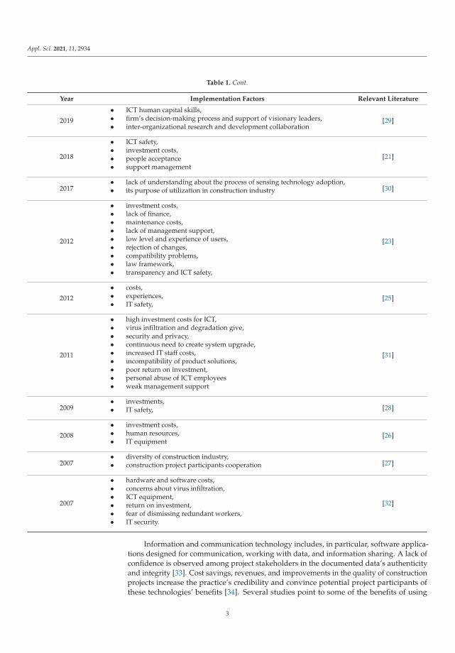
Several studies have already partially addressed factors in implementing informationand communication technology (ICT) for cost management or construction. Several studiessuggest that these are investment costs [21–28]. A detailed overview of studies on thisissue and the identification of factors is given in Table 1.

Table 1. Literature review of information and communication technology (ICT) implementation factors in the constructionindustry [21–32].

Year Implementation Factors Relevant Literature

2020

• mimetic pressure,• strategic value judgment,• behavioral control capability

[24]

2019

• communication and work relationship,• distraction and waste of time,• better information management on-site,• better management of construction defects,• improved work planning

[22]

2

Appl. Sci. 2021, 11, 2934

Table 1. Cont.

Year Implementation Factors Relevant Literature

2019

• ICT human capital skills,• firm’s decision-making process and support of visionary leaders,• inter-organizational research and development collaboration

[29]

2018

• ICT safety,• investment costs,• people acceptance• support management

[21]

2017• lack of understanding about the process of sensing technology adoption,• its purpose of utilization in construction industry [30]

2012

• investment costs,• lack of finance,• maintenance costs,• lack of management support,• low level and experience of users,• rejection of changes,• compatibility problems,• law framework,• transparency and ICT safety,

[23]

2012

• costs,• experiences,• IT safety,

[25]

2011

• high investment costs for ICT,• virus infiltration and degradation give,• security and privacy,• continuous need to create system upgrade,• increased IT staff costs,• incompatibility of product solutions,• poor return on investment,• personal abuse of ICT employees• weak management support

[31]

2009• investments,• IT safety, [28]

2008

• investment costs,• human resources,• IT equipment

[26]

2007• diversity of construction industry,• construction project participants cooperation [27]

2007

• hardware and software costs,• concerns about virus infiltration,• ICT equipment,• return on investment,• fear of dismissing redundant workers,• IT security.

[32]

Information and communication technology includes, in particular, software applica-tions designed for communication, working with data, and information sharing. A lack ofconfidence is observed among project stakeholders in the documented data’s authenticityand integrity [33]. Cost savings, revenues, and improvements in the quality of constructionprojects increase the practice’s credibility and convince potential project participants ofthese technologies’ benefits [34]. Several studies point to some of the benefits of using

3

Appl. Sci. 2021, 11, 2934

information technology in cost management [35]. Cost savings were seen as the most signif-icant benefit by Marsh and Flanagan [36]. Increased efficiency and increased transparency,and greater convenience in the procurement process were determined in the research byKhayyat [37]. ICT functionalities mainly relate to construction management, so it can beargued that the integration of a lean management approach with the technical capabili-ties of ICT will bring benefits to the overall productivity and efficiency of constructionprojects [38]. Another study examined the impact of ICT on the so-called operational bene-fits [39]. In this group of benefits, the authors included flexibility in systems to meet clients’needs; strengthening the relationship with suppliers; competitive advantage in economiesof scale; shortening the production phase; and flexibility of response to the client.

In contrast, information technologies provide little or no benefit according to previousresearch [27]. However, this study argues that there are areas where information technol-ogy implementation can also be beneficial. Improved monitoring and control have alsobeen identified as crucial in implementing ICT in construction due to the impact on costmanagement [40,41]. Other authors discussed the methods of measuring the benefits ofICT and BIM technologies in construction [42,43].

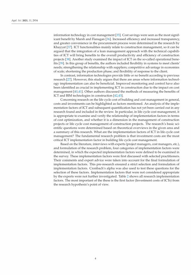
Concerning research on the life cycle cost of building and cost management in general,costs and investments can be highlighted as factors mentioned. An analysis of the imple-mentation factors of ICT and subsequent quantification has not yet been carried out in anyresearch found and included in the review. In particular, in life cycle cost management, itis appropriate to examine and verify the relationship of implementation factors in termsof cost optimization, and whether it is a dimension in the management of constructionprojects or life cycle cost management of construction projects. The research’s basic sci-entific questions were determined based on theoretical overviews in the given area anda summary of this research. What are the implementation factors of ICT in life cycle costmanagement? The fundamental research problem is that investment costs are the mostcritical ICT implementation factor in building life cycle cost management.

Based on the literature, interviews with experts (project managers, cost managers, etc.),and formulation of the research problem, four categories of implementation factors weredetermined, in which the expected implementation factors were defined to be examined inthe survey. These implementation factors were first discussed with selected practitioners.Their comments and expert advice were taken into account for the final formulation ofimplementation factors. This pre-research ensured a strict selection and formulation ofimplementation factors. Cronbach’s alpha was also used to test these questions for theselection of these factors. Implementation factors that were not considered appropriateby the experts were not further investigated. Table 2 shows all research implementationfactors. The most important of the these is the first factor (Investment costs of ICTs) fromthe research hypothesis’s point of view.

4

Appl. Sci. 2021, 11, 2934

Table 2. Research ICT implementation factors in the construction industry (based on literature review and expert statements).

Group of IF Implementation Factors (IF) Description of Factors and Impact on LCC

Economic factors1. Investment costs for ICTs2. System maintenance costs during its lifetime3. The need to recruit IT staff to manage ICT

1. Investment costs represent all costs related to theimplementation of information andcommunication technologies, infrastructuremodification and all installation costs. Theirimpact represents an increased cost of acquiringthe system in the first year, and ICT should have alower cost in the later period.

2. System maintenance costs represent all costs fortechnology maintenance, upgrades, improvements,and additional equipment management andservice costs. The level of these costs should belower than the cost savings resulting from ICTimplementation in each life phase of a constructionproject.

3. Wage-related costs for new staff needed to manageICT. This factor represents the cost burden duringthe entire construction period or each life cyclestage of the construction project.

Technical factors

4. Compatibility of software solutions5. Functional possibilities of the system6. Knowledge of the use of ICT in the field7. System maintenance and service and the need to

upgrade the system (administrative burden,inspections, repairs)

4. Ensuring the compatibility of technologies ischallenging, especially in the construction project’sdesign stage, where it is necessary to combine alltechnologies to ensure a smooth flow of databetween devices. This can have a significantpositive effect on other life cycle costs.

5. The functions and possibilities of technologies canbe a motivation for implementation. It should havea positive impact on costs at each stage, especiallyconcerning increasing productivity.

6. Knowledge is one of the prerequisites for thesuccessful implementation of ICT. Their impact onLCC depends on the value of the people who havethis knowledge and their ability to work with newICTs, which reduces costs at every stage of theproject.

7. The need to deal with service and constantupgrade is associated with increased costs and lossof time and energy of employees, which again hasa negative impact on LCC.

Personnel factors

8. User qualification (training and certificates)9. User experience (practical experience)10. Readiness and disinterest of users11. Ability to embrace innovation and change12. Management support

8. From the LCC’s point of view, the education andtraining of employees is a cost. The highest rate isat the beginning of the project, when this level isthe highest.

9. Practical user experience can have a positiveimpact on LCC. Experience and the necessaryqualifications represent a lower precondition forthe need for training costs at each stage.

10. User lack of interest can have a serious negativeimpact on LCC. Their reluctance to accept changeand innovation can lead to ever-increasing costs.

11. The reluctance to accept changes is equallynegatively transmitted to the LCC.

12. Management support should be one of the keys inmotivating new technologies to be adopted. Theattitude of management can influence the opinionof employees on new technologies. This can have apositive effect on LCC of buildings. Managementsupport can represent a high degree of ICTimplementation and thus lead to cost savings ateach stage.

5

Appl. Sci. 2021, 11, 2934

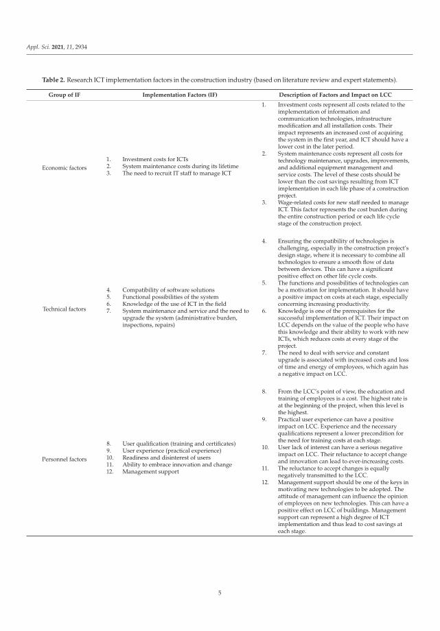
Table 2. Cont.

Group of IF Implementation Factors (IF) Description of Factors and Impact on LCC

Industry factors

13. Fragmentation of the sector and integration amongparticipants in construction projects

14. Legislative framework15. Level of competition in the use of ICT16. Level of use of ICT by other participants in the

construction project.

13. Fragmentation of the sector and integrationbetween participants in construction projectsmeans a hard way of communication betweenparticipants and increases misunderstandings. InLCC, it is reflected as a negative phenomenon, witha large number of sub-suppliers increasing costsand expanding the supply chain. From the LCCpoint of view, it is primarily the risk of increasedcosts in the design and construction stage. On thecontrary, the use phase does not pose this risk.

14. The legislative framework may also affect theimplementation of ICT. If the legislation is simpleand fixed, it can lead to the facilitation of the wholeimplementation process. On the contrary, if thelegislative framework is set incorrectly, a numberof restrictions, etc. this leads to a negative impact.Legislation can also directly affect the regulation ofthe use of specific ICT (such as BIM technology) inthe procurement process and in selected projects.This may delay earlier implementation of ICT. Thiscan have a positive impact on LCC. Thus, costs candecrease over time.

15. The level of use of ICT by competitors may impactthe decision of other construction companies to usetechnology. To minimize LCC and increasecompetitiveness, it also has this impact.

16. Other participants can pressure the use of selectedICTs, which can be a motivator for rapidimplementation. To call other participants canhave a significant positive impact on the LCC.

2. Materials and Methods

2.1. Research Methods and Steps

This research consisted of two phases, the pre-research and the research. The pre-research included determining a basic research question based on a detailed theoreticalanalysis of previous research. This analysis also provided the basis for identifying imple-mentation factors and grouping. These compiled implementation factors were discussed byrelevant experts. Four project managers from large international construction companiesdiscussed the proposed research implementation factors in an interview. Based on theagreement of all, the final implementation factors were determined, and were the subjectof the investigation.

The selection of the research sample was based on the structure of the industry. Therespondents’ selection was from the building industry database (The Statistical Office ofthe Slovak Republic). The total number of entities in the construction industry in Slovakiais 83,560,000. More than 1200 (sample file size) construction companies were approachedto participate in construction projects and final buildings. Respondents were selected as apercentage composition reflecting the number of market participants. The statistical setof respondents included various participants in construction projects. The ratio of realbusiness entities was maintained. Companies were contacted (investors 11.20%, suppliers52%, sub-contractors 16.80%, and designers 20%), and 125 respondents took part in thesurvey. The return rate was 10.42%.

Cronbach’s alpha verified the suitability of the questions. This ensured an adequatedistribution of the research sample. Data processing was based on the relative importanceindex and five critical levels method. Based on this, the ranking was determined, and theKruskal–Wallis test for statistical significance was used to verify the results.

Subsequently, for quantification purposes, the selected group’s arithmetic means andthe specific factor were determined. The Kruskal–Wallis test was also used to verify theinfluence of a given factor. A detailed overview of the research steps and methods used isgiven in Table 3.

6

Appl. Sci. 2021, 11, 2934

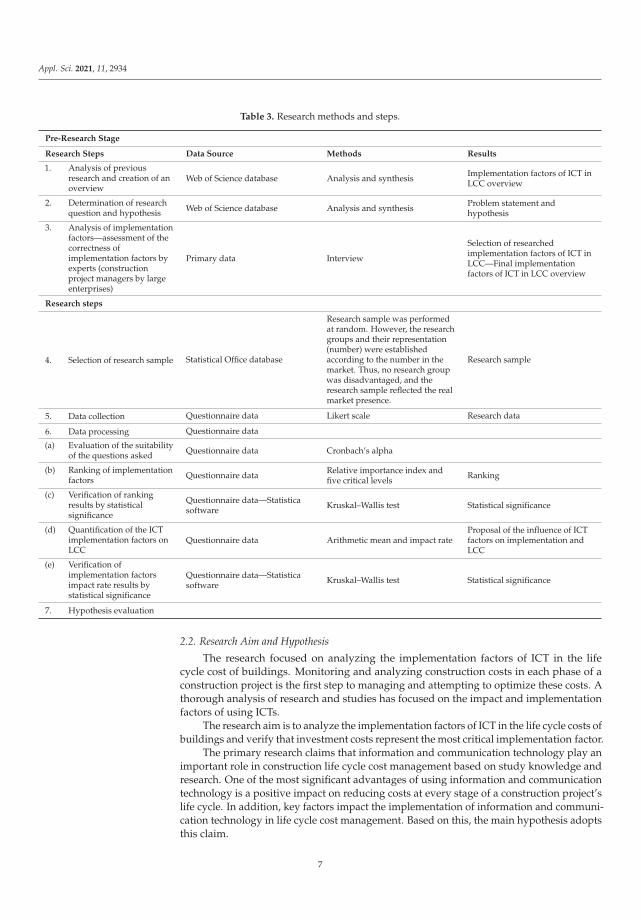
Table 3. Research methods and steps.

Pre-Research Stage

Research Steps Data Source Methods Results

1. Analysis of previousresearch and creation of anoverview

Web of Science database Analysis and synthesis Implementation factors of ICT inLCC overview

2. Determination of researchquestion and hypothesis Web of Science database Analysis and synthesis Problem statement and

hypothesis

3. Analysis of implementationfactors—assessment of thecorrectness ofimplementation factors byexperts (constructionproject managers by largeenterprises)

Primary data Interview

Selection of researchedimplementation factors of ICT inLCC—Final implementationfactors of ICT in LCC overview

Research steps

4. Selection of research sample Statistical Office database

Research sample was performedat random. However, the researchgroups and their representation(number) were establishedaccording to the number in themarket. Thus, no research groupwas disadvantaged, and theresearch sample reflected the realmarket presence.

Research sample

5. Data collection Questionnaire data Likert scale Research data

6. Data processing Questionnaire data

(a) Evaluation of the suitabilityof the questions asked Questionnaire data Cronbach’s alpha

(b) Ranking of implementationfactors Questionnaire data Relative importance index and

five critical levels Ranking

(c) Verification of rankingresults by statisticalsignificance

Questionnaire data—Statisticasoftware Kruskal–Wallis test Statistical significance

(d) Quantification of the ICTimplementation factors onLCC

Questionnaire data Arithmetic mean and impact rateProposal of the influence of ICTfactors on implementation andLCC

(e) Verification ofimplementation factorsimpact rate results bystatistical significance

Questionnaire data—Statisticasoftware Kruskal–Wallis test Statistical significance

7. Hypothesis evaluation

2.2. Research Aim and Hypothesis

The research focused on analyzing the implementation factors of ICT in the lifecycle cost of buildings. Monitoring and analyzing construction costs in each phase of aconstruction project is the first step to managing and attempting to optimize these costs. Athorough analysis of research and studies has focused on the impact and implementationfactors of using ICTs.

The research aim is to analyze the implementation factors of ICT in the life cycle costs ofbuildings and verify that investment costs represent the most critical implementation factor.

The primary research claims that information and communication technology play animportant role in construction life cycle cost management based on study knowledge andresearch. One of the most significant advantages of using information and communicationtechnology is a positive impact on reducing costs at every stage of a construction project’slife cycle. In addition, key factors impact the implementation of information and communi-cation technology in life cycle cost management. Based on this, the main hypothesis adoptsthis claim.

7

Appl. Sci. 2021, 11, 2934

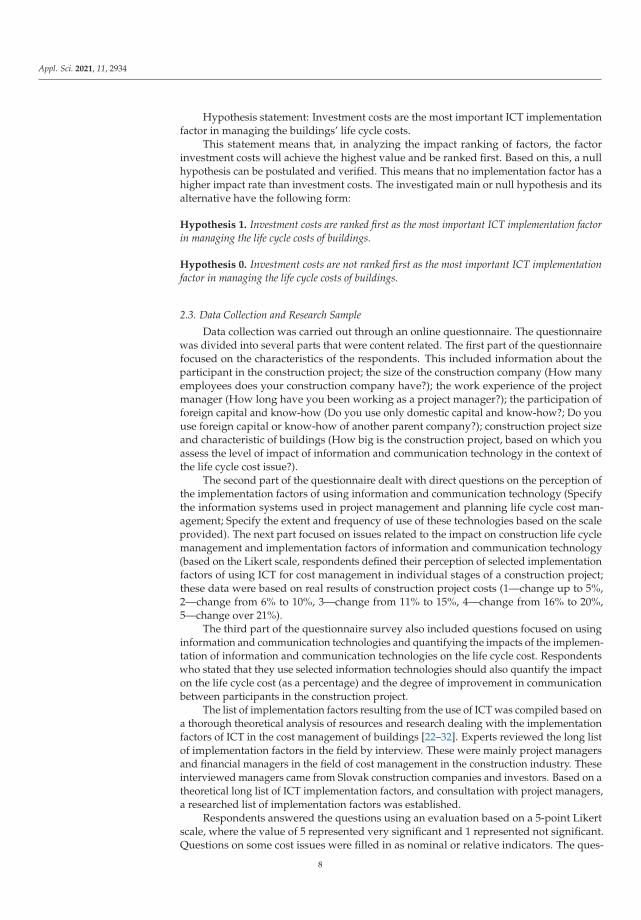
Hypothesis statement: Investment costs are the most important ICT implementationfactor in managing the buildings’ life cycle costs.

This statement means that, in analyzing the impact ranking of factors, the factorinvestment costs will achieve the highest value and be ranked first. Based on this, a nullhypothesis can be postulated and verified. This means that no implementation factor has ahigher impact rate than investment costs. The investigated main or null hypothesis and itsalternative have the following form:

Hypothesis 1. Investment costs are ranked first as the most important ICT implementation factorin managing the life cycle costs of buildings.

Hypothesis 0. Investment costs are not ranked first as the most important ICT implementationfactor in managing the life cycle costs of buildings.

2.3. Data Collection and Research Sample

Data collection was carried out through an online questionnaire. The questionnairewas divided into several parts that were content related. The first part of the questionnairefocused on the characteristics of the respondents. This included information about theparticipant in the construction project; the size of the construction company (How manyemployees does your construction company have?); the work experience of the projectmanager (How long have you been working as a project manager?); the participation offoreign capital and know-how (Do you use only domestic capital and know-how?; Do youuse foreign capital or know-how of another parent company?); construction project sizeand characteristic of buildings (How big is the construction project, based on which youassess the level of impact of information and communication technology in the context ofthe life cycle cost issue?).

The second part of the questionnaire dealt with direct questions on the perception ofthe implementation factors of using information and communication technology (Specifythe information systems used in project management and planning life cycle cost man-agement; Specify the extent and frequency of use of these technologies based on the scaleprovided). The next part focused on issues related to the impact on construction life cyclemanagement and implementation factors of information and communication technology(based on the Likert scale, respondents defined their perception of selected implementationfactors of using ICT for cost management in individual stages of a construction project;these data were based on real results of construction project costs (1—change up to 5%,2—change from 6% to 10%, 3—change from 11% to 15%, 4—change from 16% to 20%,5—change over 21%).

The third part of the questionnaire survey also included questions focused on usinginformation and communication technologies and quantifying the impacts of the implemen-tation of information and communication technologies on the life cycle cost. Respondentswho stated that they use selected information technologies should also quantify the impacton the life cycle cost (as a percentage) and the degree of improvement in communicationbetween participants in the construction project.

The list of implementation factors resulting from the use of ICT was compiled based ona thorough theoretical analysis of resources and research dealing with the implementationfactors of ICT in the cost management of buildings [22–32]. Experts reviewed the long listof implementation factors in the field by interview. These were mainly project managersand financial managers in the field of cost management in the construction industry. Theseinterviewed managers came from Slovak construction companies and investors. Based on atheoretical long list of ICT implementation factors, and consultation with project managers,a researched list of implementation factors was established.

Respondents answered the questions using an evaluation based on a 5-point Likertscale, where the value of 5 represented very significant and 1 represented not significant.Questions on some cost issues were filled in as nominal or relative indicators. The ques-

8

Appl. Sci. 2021, 11, 2934

tionnaire also contained a detailed explanation of the interpretation of the Likert scale’svalues, as mentioned in the previous paragraph.

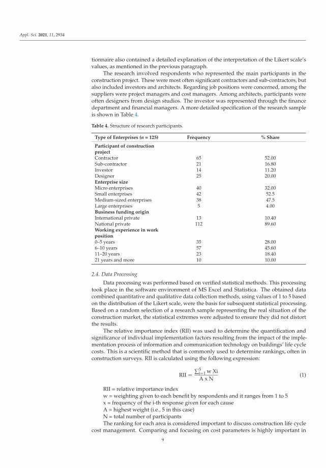
The research involved respondents who represented the main participants in theconstruction project. These were most often significant contractors and sub-contractors, butalso included investors and architects. Regarding job positions were concerned, among thesuppliers were project managers and cost managers. Among architects, participants wereoften designers from design studios. The investor was represented through the financedepartment and financial managers. A more detailed specification of the research sampleis shown in Table 4.

Table 4. Structure of research participants.

Type of Enterprises (n = 125) Frequency % Share

Participant of constructionprojectContractor 65 52.00Sub-contractor 21 16.80Investor 14 11.20Designer 25 20.00Enterprise sizeMicro enterprises 40 32.00Small enterprises 42 52.5Medium-sized enterprises 38 47.5Large enterprises 5 4.00Business funding originInternational private 13 10.40National private 112 89.60Working experience in workposition0–5 years 35 28.006–10 years 57 45.6011–20 years 23 18.4021 years and more 10 10.00

2.4. Data Processing

Data processing was performed based on verified statistical methods. This processingtook place in the software environment of MS Excel and Statistica. The obtained datacombined quantitative and qualitative data collection methods, using values of 1 to 5 basedon the distribution of the Likert scale, were the basis for subsequent statistical processing.Based on a random selection of a research sample representing the real situation of theconstruction market, the statistical extremes were adjusted to ensure they did not distortthe results.

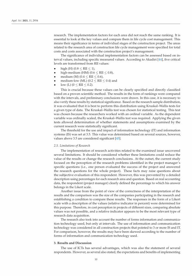
The relative importance index (RII) was used to determine the quantification andsignificance of individual implementation factors resulting from the impact of the imple-mentation process of information and communication technology on buildings’ life cyclecosts. This is a scientific method that is commonly used to determine rankings, often inconstruction surveys. RII is calculated using the following expression:

RII =∑5

i=1 w XiA x N

(1)

RII = relative importance indexw = weighting given to each benefit by respondents and it ranges from 1 to 5x = frequency of the i-th response given for each causeA = highest weight (i.e., 5 in this case)N = total number of participantsThe ranking for each area is considered important to discuss construction life cycle

cost management. Comparing and focusing on cost parameters is highly important in

9

Appl. Sci. 2021, 11, 2934

research. The implementation factors for each area did not reach the same ranking. It isessential to look at the key values and compare them in life cycle cost management. Thismeans their significance in terms of individual stages of the construction project. The areasrelated to the research area of construction life cycle management were specified for totalcosts and costs associated with the construction project’s management.

The significance of individual implementation factors can be assessed based on in-terval values, including specific measured values. According to Akadiri [44], five criticallevels are transformed from RII values:

• high (H) (0.8 ≤ RII ≤ 1),• high-medium (HM) (0.6 ≤ RII ≤ 0.8),• medium (M) (0.4 ≤ RII ≤ 0.6),• medium-low (ML) (0.2 ≤ RII ≤ 0.4) and• low (L) (0 ≤ RII ≤ 0.2).

This is crucial because these values can be clearly specified and directly classifiedbased on a proven scientific method. The results in the form of rankings were comparedwith the intervals, and preliminary conclusions were drawn. In this case, it is necessary toalso verify these results by statistical significance. Based on the research sample distribution,it was evaluated that it is best to perform this distribution using Kruskal–Wallis tests fora given type of data. The Kruskal–Wallis test was chosen for statistical testing. This testwas chosen because the researchers worked with an ordinal variable. As the dependentvariable was ordinally scaled, the Kruskal–Wallis test was required. Applying the giventests allowed determination of whether statements and assumptions examined by thecurrent research were statistically significant.

The threshold for the use and impact of information technology (IT) and informationsystems (IS) was set at 3.5. This value was determined based on several sources, however,values above 3.5 are considered significant [45].

2.5. Limitations of Research

The implementation of research activities related to the examined issue uncoveredseveral limitations. It should be considered whether these limitations could reduce thevalue of the results or change the research conclusions. At the outset, the current studyfocused on the perception of the research problems identified in the project manager’sspecific questions (i.e., one person evaluated the success of the project and answeredthe research questions for the whole project). These facts may raise questions aboutthe subjective evaluation of this respondent. However, this was prevented by a detaileddescription using percentages for each research area and question. Based on real accountingdata, the respondent (project manager) clearly defined the percentage to which his answerbelongs in the Likert scale.

Another issue from the point of view of the correctness of the interpretation of theresults and the comparison was the size of the companies participating in the research andestablishing a condition to compare these results. The responses in the form of a Likertscale with a description of the values (relative indicator in percent) were determined forthis purpose. Therefore, in cost perception in projects of different sizes, comparing absolutevalues was not possible, and a relative indicator appears to be the most relevant type ofresearch data acquisition.

The research also took into account the number of forms information and communica-tion technology used, but only at intervals. The use of information and communicationtechnology was considered in all construction projects that pointed to 3 or more IS and IT.For comparison, however, the results may have been skewed according to the number offorms of information and communication technology used.

3. Results and Discussion

The use of ICTs has several advantages, which was also the statement of severalrespondents. However, as several also stated, the expectations and benefits of implementing

10

Appl. Sci. 2021, 11, 2934

ICTs should be greater than the factors (in many cases, the concerns) that hinder theimplementation of the decision to implement ICT. This research sought to quantify andanalyze these implementation factors focusing on cost optimization throughout the lifecycle of the construction project and a positive impact on cost management during the lifecycle of buildings. Experts in the field answered questions about these implementationfactors. They tried to quantify the impact level of implementation factors on the Likertscale based on managing construction projects.

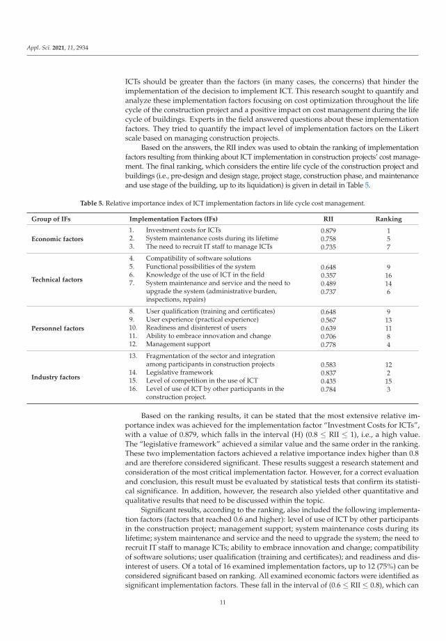
Based on the answers, the RII index was used to obtain the ranking of implementationfactors resulting from thinking about ICT implementation in construction projects’ cost manage-ment. The final ranking, which considers the entire life cycle of the construction project andbuildings (i.e., pre-design and design stage, project stage, construction phase, and maintenanceand use stage of the building, up to its liquidation) is given in detail in Table 5.

Table 5. Relative importance index of ICT implementation factors in life cycle cost management.

Group of IFs Implementation Factors (IFs) RII Ranking

Economic factors

1. Investment costs for ICTs2. System maintenance costs during its lifetime3. The need to recruit IT staff to manage ICTs

0.8790.7580.735

157

Technical factors

4. Compatibility of software solutions5. Functional possibilities of the system6. Knowledge of the use of ICT in the field7. System maintenance and service and the need to

upgrade the system (administrative burden,inspections, repairs)

0.6480.3570.4890.737

916146

Personnel factors

8. User qualification (training and certificates)9. User experience (practical experience)10. Readiness and disinterest of users11. Ability to embrace innovation and change12. Management support

0.6480.5670.6390.7060.778

9131184

Industry factors

13. Fragmentation of the sector and integrationamong participants in construction projects

14. Legislative framework15. Level of competition in the use of ICT16. Level of use of ICT by other participants in the

construction project.

0.5830.8370.4350.784

122

153

Based on the ranking results, it can be stated that the most extensive relative im-portance index was achieved for the implementation factor “Investment Costs for ICTs”,with a value of 0.879, which falls in the interval (H) (0.8 ≤ RII ≤ 1), i.e., a high value.The “legislative framework” achieved a similar value and the same order in the ranking.These two implementation factors achieved a relative importance index higher than 0.8and are therefore considered significant. These results suggest a research statement andconsideration of the most critical implementation factor. However, for a correct evaluationand conclusion, this result must be evaluated by statistical tests that confirm its statisti-cal significance. In addition, however, the research also yielded other quantitative andqualitative results that need to be discussed within the topic.

Significant results, according to the ranking, also included the following implementa-tion factors (factors that reached 0.6 and higher): level of use of ICT by other participantsin the construction project; management support; system maintenance costs during itslifetime; system maintenance and service and the need to upgrade the system; the need torecruit IT staff to manage ICTs; ability to embrace innovation and change; compatibilityof software solutions; user qualification (training and certificates); and readiness and dis-interest of users. Of a total of 16 examined implementation factors, up to 12 (75%) can beconsidered significant based on ranking. All examined economic factors were identified assignificant implementation factors. These fall in the interval of (0.6 ≤ RII ≤ 0.8), which can

11

Appl. Sci. 2021, 11, 2934

be considered as medium–high significance. This again points to the trend that investmentcosts and other types of costs associated with ICT implementation represent a seriousimplementation factor.

It is essential that these findings and the main research hypothesis are confirmed usingthe Kruskal–Wallis test. An overview of groups of factors shows that the most importantare economic factors. Personal factors are also significant. Overall, the setting of people(employees) to accept change, and accept innovation and their skills and knowledge inthe IT field, significantly affect the implementation of ICT in the cycle cost managementof construction and construction projects. Based on the Likert scale and Kruskal–Wallistesting, an infographic was constructed that highlights the importance of individual factorsfor specific groups and provides information about the arithmetic mean for individualimplementation groups (Figure 1).

It is possible to discuss why experts and managers of construction projects havequantified and determined such a ranking of these implementation factors. These resultsshould be compared with the research already carried out in the field of ICT implementationfactors in the context of managing life cycle costs of buildings. The research resultsalso confirm the research conclusions of [22–29], in which the investment cost was asignificant implementation factor. This result and comparison point to one of the phases ofa construction project in the context of cost management. The research results point to arelatively high degree of implementation factors in life cycle cost management.

An important view of the results is presented in Figure 1, in which the degree ofimportance of the implementation factor is quantified. The investment costs reached thehighest value, and the given rate was 4.395, which represents very high importance fromthe point of view of ICT implementation. Regarding the degree of saving resulting from theuse of ICT, which this research investigates, it can be stated that the turning point at whichICT will cover investment costs, should be in the 6th to 10th construction project. Thisclearly depends on other factors such as the size of the projects. However, considerationmust also be given to operating costs, which extend this period. In terms of the mostsignificant impact on implementing ICT for life cycle cost management, it is possible todefine a significant level (3.954) of economic factors. Thus, in addition to the investmentcosts, the operating costs and the costs for the employees who will manage the selectedtechnologies must be included. The research also included questions focused on usinginformation and communication technologies and their impact on LCC. This impact wasmentioned by several respondents, based on which the Kruskal–Wallis test was also carriedout to determine if results were statistically significant. Due to the implementation and useof ICT, the value of cost savings was 10% to 15%.

The use of ICTs can increase efficiency, which has a limited impact on achievingoptimization or a reduction in costs, and costs in terms of the entire life cycle of theconstruction. Monitoring the impacts on life cycle cost management is the more complexsubject of this research. During interviews or in response to additional questions, severalexperts indicated that ICT leads to better cost management if communication and sharingof necessary information is faster. This also proved to be significant at every stage of thelife cycle of a construction project. Here, however, it must be noted that although this ratewas different in the individual phases of the construction cycle, it always reached the levelof at least medium or medium–high based on the empirical method. The details of thesedifferences discussed in more detail later. Based on the RII, the ranking and intervals weredetermined, and indicated the degrees of importance. However, from a statistical pointof view, these values should be verified. Therefore, based on the Likert scale and dataon the frequency of responses with specific values, a table of importance or the so-calledimportance rate (IR), with values from 1 to 5, was constructed. This is the average value ofall respondents values, which is the important frequency of responses. This importanceindex shows the frequency of utilization in similar cases and studies globally. The resultsare mentioned in more detail in Table 6, which shows the value of the Kruskal–Wallis testfor the statistical significance level (Table 5).

12

Appl. Sci. 2021, 11, 2934

Figure 1. Implementation factor groups and impact rates.

13

Appl. Sci. 2021, 11, 2934

Table 6. Hypothesis results and Kruskal–Wallis ANOVA results.

Hypothesis Parameter K-W Anova (p) Rejection

H1: Investment costs are ranked first inthe most important ICT implementationfactors in managing the life cycle costsof buildings.

RII Ranking0.0476

accepted

H0: Investment costs are not ranked firstin the most important ICTimplementation factors in managing thelife cycle costs of buildings

RII Ranking rejected

From the Kruskal–Wallis ANOVA based on ranking, the variable “ICT implementationfactors in life cycle cost management” achieved a p-value of 0.0476, which has significantstatistical significance. The number of valid responses was 125 for each factor (see Table 5).

Table 5 describes the Kruskal–Wallis test to examine the statistical significance ofselected factors’ impact on ICT implementation. Table 5 also describes the decision andevaluation of the scientific hypothesis based on the Kruskal–Wallis ANOVA. Thus, theachieved p-value was 0.0476. This indicates that the statistical implementation factorsconfirmed the statistical significance. That is, at the level of probability α = 0.05, we canreject H0: investment costs are not ranked first in the most important ICT implementa-tion factors in managing the life cycle costs of building, and thus accept the hypothesisH1: investment costs are ranked first in the most important ICT implementation factors inmanaging the life cycle costs of buildings. Thus, it follows that investment costs representthe most important implementation factor influencing the implementation and use of ICTin the life cycle cost management of buildings.

4. Conclusions

It is necessary to examine the issue of implementation factors of ICT adoption in lifecycle cost management and, in particular, to quantify and manage the actual cost of aconstruction project during its entire life cycle. Several studies point to factors that mayinfluence the implementation of ICT in life cycle cost management. This research sought toverify these claims. The assumption was that investment costs represent the most criticalimplementation factor of ICT in life cycle cost management. This statement can be acceptedbased on the empirical methods performed. Based on a selected sample of respondents andprojects, it was determined that investment costs are the most critical implementation factor.Several studies have confirmed the benefits of using ICT in life cycle cost management ofbuildings. Therefore, examining the factors influencing this implementation was highlyimportant, and the research findings are essential for practitioners. Simultaneously, theresearch noted other essential implementation factors of ICT in life cycle cost management.These are the level of use of ICT by other participants in the construction project; man-agement support; system maintenance costs during its lifetime; system maintenance andservice and the need to upgrade the system; the need to recruit IT staff to manage ICTs;ability to embrace innovation and change; compatibility of software solutions; user quali-fications (training and certificates); and readiness and disinterest of users and legislativeframework. The research also highlighted the importance of all economic factors related tothe implementation of ICT in life cycle cost management. Maintenance costs and the costsassociated with recruiting new staff to the IT department greatly influence the decision toimplement ICT for life cycle cost management.

This issue is closely linked to the issue of implementation benefits. This representsanother research gap that this research should address. The extension of this scientificand practical issue should be addressed using the same research sample, which wouldallow a confrontation with the results of this study. The direct benefits of implementingICT in life cycle cost management can contribute to the growth of ICT implementationin construction.

14

Appl. Sci. 2021, 11, 2934

This research confirms the claims of previous studies [12,16]. These previous studiesnote the importance of implementing information and communication technologies for lifecycle cost management. The positive impact on cost financing was also confirmed. As alsomentioned in a previous study [18], one of the main factors is investment costs. Anotherstudy [18] also found that this research has not substantiated that operating costs exceedinvestment costs, and that this is a larger implementation factor.

In contrast, research has also examined the effects of information and communica-tion technologies, and a positive impact of the use of information and communicationtechnologies was found, as stated in the study [20].

The most important research results can be summarized as:

- high investment costs are the most critical implementation factor,- operating costs are also a critical implementation factor for the adoption of ICT, but

this is not the most important, as some studies claim;- the survey showed that the use of information and communication technologies has

the effect of reducing life cycle cost management costs, and this result has also beenquantified at 10% to 15% of costs;

- implementation has improved communication between research participants;- research quantified the importance of specific implementation factors for adopting

ICT in life cycle cost management (this important information for practice has not yetbeen mentioned in any research).

Knowledge of implementation factors in practice also means focusing on specificprocesses that can contribute to better implementation of ICT in construction. It canalso challenge the views and support of management, which can positively affect theindustry’s development.

Author Contributions: Conceptualization, P.M. and T.M.; methodology, T.M.; software, T.M.; val-idation, T.M., A.B. and M.B.; formal analysis, M.S.; investigation, T.M., A.B. and M.B.; resources,T.M., A.B. and M.B.; data curation, T.M., A.B.; writing—original draft preparation, T.M., M.S.,P.M.; writing—review and editing, P.M.; visualization, T.M.; supervision, P.M.; project administra-tion, T.M.; funding acquisition, P.M. All authors have read and agreed to the published version ofthe manuscript.

Funding: This work was supported by the Slovak Research and Development Agency under thecontract no. APVV-17-0549. The paper presents partial research results of project VEGA 1/0828/17“Research and application of knowledge-based systems for modelling cost and economic parametersin Building Information Modelling”. The paper also presents partial research results of project KEGA059TUKE-4/2019 “M-learning tool for intelligent modeling of building site parameters in a mixedreality environment”.

Institutional Review Board Statement: Not applicable.

Informed Consent Statement: Not applicable.

Data Availability Statement: All research activities have been carried out in accordance with theMDPI Ethics and there is no obstacle on our part.

Acknowledgments: This work was supported by the Slovak Research and Development Agencyunder the contract no. APVV-17-0549. Paper presents a partial research results of project VEGA1/0828/17 “Research and application of knowledge-based systems for modelling cost and economicparameters in Building Information Modelling”. The paper presents a partial research results ofproject KEGA 059TUKE-4/2019 “M-learning tool for intelligent modeling of building site parametersin a mixed reality environment”.

Conflicts of Interest: The authors declare no conflict of interest.

References

1. Hromádka, V.; Korytárová, J.; Vítková, E.; Seelman, H.; Funk, T. New aspects of socioeconomic assessment of the railwayinfrastructure project life cycle. Appl. Sci. 2020, 10, 7355. [CrossRef]

2. Biolek, V.; Hanák, T. LCC Estimation Model: A Construction Material Perspective. Buildings 2019, 9, 182. [CrossRef]

15

Appl. Sci. 2021, 11, 2934

3. Zabielski, J.; Zabielska, I. Life Cycle of a Building (LCC) in the Investment Process-Case Study. In Proceedings of the BalticGeodetic Congress, BGC-Geomatics, Olsztyn, Poland, 21–23 June 2018; pp. 254–259.

4. Chen, C.; Tang, L. BIM-based integrated management workflow design for schedule and cost T planning of building fabricmaintenance. Autom. Constr. 2020, 107, 1–12. [CrossRef]

5. Knezevic, M.; Cvetkovska, M.; Hanák, T.; Braganca, L.; Soltesz, A. Artificial Neural Networks and Fuzzy Neural Networks forSolving Civil Engineering Problems. Complexity 2018, 1–2–2. [CrossRef]

6. De Haes, H.A.U.; Rooijen, M.V. Life Cycle Approaches: The Road from Analysis to Practice; UNEP/SETAC Life Cycle Initiative: Paris,France, 2005.

7. Westkämper, E.; Alting, A. Life Cycle Management and Assessment: Approaches and Visions Towards. Sustain. Manuf. Cirp Ann.2009, 49, 501–526. [CrossRef]

8. Bey, N. Life Cycle Management. In Life Cycle Assessment: Theory and Practice; Springer: Berlin/Heidelberg, Germany, 2018.9. Kambanou, M.L. Life Cycle Costing: Understanding How It Is Practised and Its Relationship to Life Cycle Management—A Case

Study. Sustainability 2020, 12, 3252. [CrossRef]10. Grieves, M. CIM data, Product lifecycle management—Empowering the future of business. Technic. Repet. 2002, 2, 1–21.11. Corallo, A.; Latino, M.E.; Lazoi, M.; Verardi, S. Defining Product Lifecycle Management: A Journey across Features, Definitions,

and Concepts. Int. Sch. Res. Not. 2013, 2013, 1–10. [CrossRef]12. Kim, G.T.; KIM, K.T.; Lee, D.H.; Han, C.H.; Kim, H.B.; Jun, J.T. Development of a life cycle cost estimate system for structures of

light rail transit infrastructure. Autom. Constr. 2010, 19, 308–325. [CrossRef]13. Hanák, T.; Marovic, I.; Aigel, P. Perception of Residential Environment in Cities: A Comparative Study. Procedia Eng. 2015, 117,

495–501. [CrossRef]14. Fantozzi, F.; Gargari, C.; Rovai, M.; Salvadori, G. Energy Upgrading of Residential Building Stock: Use of Life Cycle Cost Analysis

to Assess Interventions on Social Housing in Italy. Sustainability 2019, 11, 1452. [CrossRef]15. De Soto, B.G.; Augustí-Juan, I.; Hunhevicz, J.; Joss, S.; Graser, K.; Habert, G.; Adey, B.T. Productivity of digital fabrication in

construction: Cost and time analysis of a robotically built wall. Autom. Constr. 2018, 92, 297–311. [CrossRef]16. Plebankiewicz, E.; Wieczorek, D. Prediction of cost overrun risk in construction projects. Sustanability 2020, 12, 9431. [CrossRef]17. Korytarova, J.; Hromadka, V. Building life cycle economic impacts. In Proceedings of the International Conference on Management

and Service Science, Wuhan, China, 24–26 August 2010.18. Korytárová, J.; Hanák, T.; Kozik, R.; Radziszewska-Zielina, E. Exploring the contractors’ qualification process in public works

contracts. Procedia Eng. 2015, 123, 276–283. [CrossRef]19. Plebankiewicz, E.; Wieczorek, D. Adaptation of a cost overrun risk prediction model to the type of construction facility. Symmetry

2020, 12, 1739. [CrossRef]20. Plebankiewicz, E.; Malara, J. Analysis of defects in residential buildings reported during the warranty period. Appl. Sci. 2020, 10,

6123. [CrossRef]21. Vasista, T.G.; Abone, A. Benefits, Barriers and Applications of Information Communication Technology in Construction Industry:

A Contemporary Study. Int. J. Eng. Technol. 2018, 7, 492–499. [CrossRef]22. Hasan, A.; Ahn, S.; Rameezdeen, R.; Baroudi, B. Empirical Study on Implications of Mobile ICT Use for Construction Project

Management. J. Manag.Eng. 2019, 35, 04019029. [CrossRef]23. Sargent, K.; Hyland, P.; Sawang, S. Factors influencing the adoption of information technology in a construction business.

Australas. J. Constr. Econ. Build. 2012, 12, 72–86. [CrossRef]24. Wang, G.; Lu, H.; Gao, X. Understanding Behavioral Logic of Information and Communication Technology Adoption in Small-

and Medium-Sized Construction Enterprises: Empirical Study from China. J. Manag. Eng. 2020, 36, 1–16. [CrossRef]25. Sekou, A.E. Promoting the Use of ICT in the Construction Industry, Assessing the Factors Hindering Usage by Building

Constractors in Ghana. Ph.D. Thesis, Kwame Nkrumah University, Kumasi, Ghana, September 2012.26. Linderoth, H.C.J.; Jacobsson, M. Understanding adoption and use of ICT in construction projects through the lens of context,

actors and technology. In Proceedings of the International Conference on Information Technology in Construction, CIB W78,Santiago, Chile, 15–17 July 2008.

27. Wigforss, O.; Lofgren, A. Rethinking communication in construction. ITcon 2007, 12, 337–345.28. Woksepp, S.; Olofsson, T. An evaluation model for ICT investments in constriction project. ITconstruction 2009, 13, 343–361.29. Lu, H.; Pishdad-Bozorgi, P.; Wang, G.; Xue, Y.; Tan, D. ICT Implementation of Small- and Medium-Sized Construction Enterprises:

Organizational Characteristics, Driving Forces, and Value Perceptions. Sustainability 2019, 11, 3441. [CrossRef]30. Sepasgozaar, S.M.E.; Shirowzhan, S.; Wang, C. A scanner technology acceptance model for construction projects. Procedia Eng.

2017, 180, 1237–1246. [CrossRef]31. Wang, G.B.; Cao, D.P.; Chong, D. Investigation to factors affecting IT implementation in Chinese construction projects. In

Proceedings of the 4th Conference on Systems Science, Management Science and Systems Dynamics, New York, NY, USA,10–11 April 2011; Volume 3, pp. 1–13.

32. Mahamadu, A.M.; Mahdjoubi, L.; Booth, C.A. Determinants of building information modelling (BIM) acceptance for supplierintegration: A conceptual model. In Proceedings of the 30th Annual ARCOM Conference; Portsmouth, UK, 1–3 September 2014,Association of Researchers in Construction Management; pp. 723–732.

16

Appl. Sci. 2021, 11, 2934

33. Soetanto, R.; Dainty, A.R.J.; Price, A.D.F.; Glass, J. A framework for investigating human issues associated with the implementationof new ICT systems in construction organizations. Innov. Dev. Archit. Eng. Constr. 2003, 2, 121–130.

34. Tetik, M.; Peltokorpi, A.; Seppänen, O.; Holmstrom, J. Direct digital construction: Technology-based operations management Tpractice for continuous improvement of construction industry performance. Autom. Constr. 2019, 107, 1–13. [CrossRef]

35. Love, P.E.D.; Matthews, J. The how of benefits management for digital technology: From engineering to asset management.Autom. Constr. 2019, 107, 1–15. [CrossRef]

36. Flanagan, R.; Marsh, L. Measuring the costs and benefits of information technology in construction. Eng. Constr. Archit. Manag.2000, 7, 423–435. [CrossRef]

37. Khayyat, N.T. Effects of information technology on cost, quality and efficiency in provision of public services. In Information andCommunication Technologies; Nova Science Publishers, Inc.: Hauppauge, NY, USA, 2010.

38. Pérez-López, R.J.; Olguín-Tiznado, J.E.; García-Alcaraz, J.L.; Camargo-Wilson, C.; López-Barreras, J.A. The Role of Planning andImplementation of ICT in Operational Benefits. Sustainability 2018, 10, 2261. [CrossRef]

39. Koskela, L.J.; Kazi, A.S. Information Technology in Construction: How to Realise the Benefits? Information Science Publishing:Manchester, UK, 2003.

40. Lambrecht, J.F.; Vestergaard, F.; Karlshøj, J.; Hauch, P.; Mouritsen, J. Measuring the effects of using ICT/BIM in constructionprojects. In Proceedings of the 33rd CIB W78 Conference 2016, Brisbane, Australia, 31 October–2 November 2016.

41. Sheng, D.; Ding, L.; Zhong, B.; Love, P.E.D.; Luo, H.; Chen, J. Construction quality information management with blockchains.Autom. Constr. 2020, 120, 1–16. [CrossRef]

42. Heigermoser, D.; Garcia de Soto, B.; Sidney Abbott, E.L.; Chua, D.K.H. BIM-based Last Planner System tool for improvingconstruction project management. Autom. Constr. 2019, 104, 246–254. [CrossRef]

43. Chi, C.; Yang, L. Measurement of ICT impact. J. Adv. Commun. Syst. Technol. 2011, 3, 1–11.44. Akadiri, P.O.; Olomolaiye; Chinyio, E.A. Multi-criteria evaluation model for the selection of sustainable materials for building

projects. Autom. Constr. 2013, 30, 113–125. [CrossRef]45. Mutesi, E.T.; Kyakula, M. Application of ICT in the construction industry in Kampala. In Proceedings of the Second International

Conference on Advances in Engineering and Technology, Kampala, Uganda, 31 January–2 February 2011; pp. 263–269.

17

applied sciences

Article

Multiple Criteria Evaluation of the EU CountrySustainable Construction Industry Lifecycles

Arturas Kaklauskas 1,*, Edmundas Kazimieras Zavadskas 2,*, Arune Binkyte-Veliene 2,

Agne Kuzminske 3, Justas Cerkauskas 2, Alma Cerkauskiene 2 and Rita Valaitiene 4

1 Department of Construction Management and Real Estate, Faculty of Civil Engineering, Vilnius GediminasTechnical University, Sauletekio av. 11, LT-10223 Vilnius, Lithuania

2 Institute of Sustainable Construction, Faculty of Civil Engineering, Vilnius Gediminas Technical University,Sauletekio av. 11, LT-10223 Vilnius, Lithuania; arune.binkyte-veliene@vgtu.lt (A.B.-V.);justas.cerkauskas@vgtu.lt (J.C.); alma.cerkauskiene@vgtu.lt (A.C.)

3 Lithuanian Business Support Agency, Savanoriu pr. 28, LT-03116 Vilnius, Lithuania; a.kuzminske@lvpa.lt4 Faculty of Civil Engineering, Vilnius Gediminas Technical University, Sauletekio av. 11, LT-10223 Vilnius,

Lithuania; rita.valaitiene@vgtu.lt* Correspondence: arturas.kaklauskas@vgtu.lt (A.K.); edmundas.zavadskas@vgtu.lt (E.K.Z.);

Tel.: +370-5-274-5234 (A.K.)

Received: 16 April 2020; Accepted: 26 May 2020; Published: 28 May 2020

Abstract: This article looks at the trends and success of the sustainable construction industries inthe EU member states, the UK and Norway. The research, covering the past three decades, revealedthat different quality of life, macroeconomic, human development, construction and well-beingfactors define the sustainable construction industries in the EU member states, the UK and Norway.A multiple criteria decision matrix was created and analysed to look at the EU member countries, theUK and Norway from the perspective of their macro level environment and construction industries.Assessments of the sustainable construction industries were completed by using the COmplexPRoportional Assessment (COPRAS) and Degree of Project Utility and Investment Value Assessments(INVAR), two analysis methods. A look was taken at the dependencies linking the indicators relatedto the construction industries and macro level in the EU member countries, the UK and Norway.Then, the multiple criteria analysis of the construction industry’s utility degree and performanceswere completed, and recommendations were generated. A country’s perceived image and successcan influence the economic behaviour of consumers. By and large, advanced and successful countriesrarely become associated with a negative national image and their products and services rarely suffernegative consequences due to such association. This research, then, offers findings that can assistpotential buyers in more rational decision-making when choosing of products and services based ona country of origin.

Keywords: sustainable construction industry; lifecycles; European Union Member States; complexevaluation; multiple criteria analysis; COPRAS and INVAR methods; success and image of acountry; marketing

1. Introduction

World scientists have studied the construction industry [1–7], energy and buildings [8–11], buildinginformation modelling [12–14] and building and projects lifecycle [15–20]. Each stage of constructionhas certain environmental impacts associated with it and life-cycle assessment (analysis) can be appliedto analyse construction throughout its lifecycle comprising all these stages [21]. Studies suggest thatworking fewer hours could improve sustainability as the scale of economic output would drop alongwith the severity of environmental pressures related to consumption patterns [22].

Appl. Sci. 2020, 10, 3733; doi:10.3390/app10113733 www.mdpi.com/journal/applsci19

Appl. Sci. 2020, 10, 3733

The necessity of having consumption and production systems in synchronisation with societyand the environment first called for identification. The word sustainability was a response; thereby,it has presently been broadly inserted in policy and research aligned with such concepts as “circulareconomy” and “inclusive growth” [23,24]. The amount of construction waste produced annually bythe construction industry in the UK alone is 100 million tonnes, which contain around 13 million tonnesof unused materials. However, the capacity for recycling such waste materials is merely 20% of thevolume. Most of it gets dumped in landfills, which further adds to polluting the biosphere. There arenumerous reasons for such negative impacts, according to the literature in the field. Among others,the reasons probably consist of poor management, embedded cultural values, obsolete technologiesand inappropriate logistics [25]. Previously, environmental quality would be substituted for economicgrowth and vice versa in discussions regarding development. Now, amendments have been includedto such discourses. Currently, talks on growth, environmental sustainability and societal developmentmore and more frequently regard identifying simultaneous targets [26]. The concern of the constructionindustry now more than ever before points to defining needed improvements to sustainability in thespheres of society, the economy and the environment. The foundation of sustainability and building andconstruction improvements consists of applying lifecycle assessment (LCA). These must be understoodby SMEs for their industrial activities. It is a necessity for increasing green construction marketproductivity and competitiveness as well as for satisfying consumers who now call for environmentallyfriendly products [27].

Therefore, only consumption habits require change for sustainability, without reductions in thepresent-day life quality, to foresee continuous development. Being sustainable in this developmentalso relates to universal solidarity and democratic and fair allocations. In other words, via asustainable development model, the suggestion is that a full understanding of development aims toreach environmental management as well as cover social responsibility and economic solutions byabandoning the existence of a consumer society. Thus, it can be stated that sustainable constructionhas three main dimensions/components called environmental, economic and societal. Interactionsbetween ecological protection, economic progression and social fairness are significant parametersof sustainability [28]. Sustainability in the construction industry involves various interest groupswith different demands, awareness, knowledge, communication skills, implementation skills andcommitments. However, all such interest groups orient to the same tasks: climate adaptation,procurement, carbon and energy, environmental management, waste, water, materials, biodiversity,the community and the economy for developing a sustainable construction industry.

LCA enjoys widespread international acceptance as one way to improve environmental processesand services, and this is the reason Ortiz et al. [27] decided to examine it. Additionally, theywanted ways to evade negative environmental impacts, thus they needed to develop appropriateaims. The result was bound to generate a healthy environment for people’s lives and an overallenhancement in the quality of life. The building sector must turn to governmental administrationsalong with environmental agencies to improve sustainability in the industry by generating appropriateconstruction codes and other environmental policies. Meanwhile the construction industry itself mustpay attention to its involved individual players encouraging them to be proactive in developing thesorts of environmental, social and economic guideposts that would achieve sustainability within theindustry [27]. Roads leading to sustainable development must insure an efficient metrics system formeasuring an adequate transition to a greener accomplishment. Such an effort will require inclusionof performances, which distinguish not only recent achievements but also the matters that needimprovement. Thereby, the performance is bound to result in a policy that is better informed [29].The metrics gap is a focal point in the investigation by Doyle et al. [29]. They measured the “globalcompetitiveness” of environmental and social sustainability by estimating the cross-country influenceson economic achievements. The purpose of the research presented here was to develop an effectivesystem consisting of environmental, social and economic criteria as well and to include an instrumentfor analysis, which would support an evolving lifecycle of a sustainable construction industry.

20

Appl. Sci. 2020, 10, 3733

Knight et al. [22] performed a panel analysis of 29 high-income the Organisation for EconomicCo-operation and Development (OECD) countries looking at carbon dioxide emissions, carbonfootprint and ecological footprint, three environmental indicators, to see the effects of working hours.Their research, based on data for 1970–2007, suggests a significant link between working hours andincreased environmental strains; policies intended to boost environmental sustainability, thus, couldtarget this aspect. Hayden and Shandra [30] used the STochastic Impacts by Regression on Population,Affluence and Technology (STIRPAT) design to validate the hypothesis that shows a positive linkbetween hours of work and ecological footprint (EF). Developed countries (Sweden, Australia andothers) have recently started to reduce the number of working hours per week after reaching high levelsof labour productivity per person. Several researchers have analysed the relationship between GrossDomestic Product (GDP) and EF [31–34], EPI [35,36] and environmental quality [37,38]. These andother studies [39] confirm that construction, macroeconomic, quality of life, human development andwell-being factors impact the environment. The United Nations [40] emphasised the need to ensurethe green economy development, when human development, social equity and economic growth goalongside environmental security. In today’s world increasingly concerned about resource draining,both developed and developing countries can improve their construction industries’ sustainability andaddress environmental issues by basing their decisions on lifecycle assessment.

Sustainable development has been an internationally recognised aim since the UN Conference onEnvironment and Development in Rio de Janeiro in 1992. Its central challenges are the maintenance ofsocial security and justice, sustainable economic development and the preservation and creation ofan intact environment [41]. In the 21st century, sustainability has become the most important issueconcerning the construction industry lifecycle [42]. Looking at industrial sectors, the construction sectoris of particular importance. On the one hand, it makes a vital contribution to the social and economicdevelopment of every country by providing housing and infrastructure; on the other hand, this sectoris an important consumer of non-renewable resources, a substantial source of waste, a polluter of airand water and an important contributor to land dereliction [41].

The construction industry is a large and critical sector within the world economy, having asignificant impact on the environment [43]. It is considered one of the main contributors to globalwarming. To mitigate global warming effects, the construction industry has been exploring variousapproaches to mitigate the impacts of carbon dioxide emissions over the entire lifecycle of buildings [1].The need to minimise the negative impacts of construction lifecycle activities is increasing pressure onconstruction organisations to adopt proactive, environmentally sustainable strategies and actions inthe design and construction process [43].

Construction firms are increasingly faced with sustainable development-based requirements thatare influencing many facets of their activities, ranging from proactive environmentally consciousdesign and construction through to sustainable procurement, project efficiency and effectivenessand investment management. A lot of literature suggests that the implementation of sustainableconstruction lifecycle practices is influenced by environmentally sustainable development-basedrequirements in the form of government regulations, as well as stakeholders pressures—from clients,environmental groups, financial institutions and top management commitment [43]. The constructionof buildings brings about a substantial ecological load: about 40% of energy consumption and about25% of material moved by our economy is due to the construction of buildings. New constructionlifecycle technologies and new building components would allow us to reduce the ecological load ofbuildings to a fraction of its present value [44].

Europeans spend over 90% of their time indoors (homes, workplaces, cars and public transportmeans, etc.) and are exposed to a complex mixture of pollutants at concentration levels that are oftenseveral times higher than outdoors [45]. Resource-efficient Europe is an effort to make economicgrowth less dependent on the use of resources, promote the transition to a low carbon economy,increase the share of renewable sources in the energy sector and promote energy efficiency. By 2020,energy efficiency must go up by 20% [46]. The flagship initiative “Innovation union” aims to change

21

Appl. Sci. 2020, 10, 3733

the focus of R&D and innovation policy by shifting it to the challenges facing our society, includingclimate change, energy efficiency and lower resource use.

Kotler and Gertner [47] analysed the influence of established country images on attitudes towardsthe services and products a country offers and the country’s ability to attract tourists, businessesand investment. Kotler and Gertner [47] also investigated strategic marketing management and itsrole in improving a national image, making a country more attractive and its products more popular.A country’s economy highly depends on its brand image and identity. The literature review revealedthe key factors that influence a country’s brand image and its impact on the economy through theintentions of consumers to buy the country’s brands and products [48].

Studies suggest that stereotypes associated with a country can influence the way consumers see abrand irrespective of their intention [49]. Herz and Diamantopoulos [49] carried out three experimentsthat complement each other. They aimed to examine how country cues can lead to various countrystereotypes (emotional vs. functional), which, in turn, make an automatic impact on brand-relatedbehaviour, as well as affective and cognitive brand evaluations by consumers [49].

Saridakis and Baltas [50] examined the impact the country of origin has on new car prices.They applied hedonic price analysis to an extensive dataset. Their models demonstrate that, in additionto implicit prices related to technological characteristics and performance, prices of new cars offeredby a certain brand reflect price distortions stemming from the heterogeneity related to the countryof origin. Universally seen as a source of high-quality products, Japan may have lower demand insome other Eastern Asian countries due to their historical animosity [51]. Less economically developedcountries are usually associated with a negative country image and the products they supply suffer therelated negative effect [52].

Companies apply many different strategies to present their country of origin and make theircustomers more aware of what that country represents [53]. They use flags and symbols of the countryof origin; label their products with the phrase “Made in...”; incorporate imagery of famous buildings ortypical landscapes of their country, as well as famous or stereotypical people; attach origin and qualitylabels; make the country of origin part of the company name; and use the language of the countryof origin.

Pappu et al. [54] applied canonical correlation analysis to examine the relationships that linkthe perception consumers have of a country at the macro-level (the country itself) and micro-level(the products associated with the country), and the equity a brand from that country has in the eyes ofconsumers. They interviewed residents of an Australian state capital city in mall-intercept surveys.The results show a significant impact of both the micro and macro images of the brand’s country oforigin on the equity of a brand perceived by consumers. The two sets of constructs were linked by apositive relationship that depended on the product category. The product category also influencedthe type of contribution each dimension of the brand equity perceived by consumers made to therelationship. The contribution of both macro and micro country image dimensions depended onthe product category as well. An interesting finding is that, among product categories, the countryimage has a bigger impact on cars than on TV sets. The results of this research can give internationalmarketers important direct insights [54].

Roth et al. [55] measure the added value the name of a country can give to a brand or a product inthe eyes of an individual consumer. They applied the construct of brand equity in a country contextand their results suggest that product preferences are influenced by country brand equity in a positiveway [55].

Elliot and Papadopoulos [56] explored the multifaceted nature of the image of a place and how itimpacts buyer behaviour. Their interdisciplinary approach combines tourism, country and productvariables. The authors selected two countries for empirical tests of their integrated model with fourtarget countries analysed in each case. The eight model tests showed the relationships linking thesubcomponents of the image of a place. Affective country image made the biggest impact on destination

22

Appl. Sci. 2020, 10, 3733

evaluations, cognitive country image made the biggest impact on product evaluations and beliefsassociated with a product made an impact on tourism, receptivity [56].

The subject of the current study is the EU sustainable construction industry lifecycle and theconstruction, macroeconomic, quality of life, human development and well-being factors context asa whole.

To achieve the purpose of the research, following objectives were identified:

• Develop integrated numerical and qualitative indicators that define the sustainable constructionindustry and the macro context affecting it.

• Calculate and analyse the correlations linking the sustainable construction industry indicators;• Calculate and analyse the correlations across states.• Create and analyse a decision matrix for the multiple criteria analysis of the macro-level and the

sustainable construction industry in EU countries.• Analyse the dependencies linking the indicators describing the macro level and the sustainable

construction industry.• Make a multiple criteria analysis of the sustainable construction industry in EU countries and

offer recommendations.

An all-encompassing analysis of the EU sustainable construction industry required the applicationof techniques of multiple criteria assessment that allow the user to take a comprehensive look at manyaspects, including the construction, macroeconomic, quality of life, human development and well-being.The variety of investigated factors matches the different forms of data required in multiple criteriadecision making. The analysis makes use of statistical, decision-making and biometric techniques,as well as big data analytics.

The structure of the rest of this paper is as follows. Section 2 presents a multiple criteria assessmentof the sustainable construction industry in the European Union Member States. Section 3 shows acomparison of the sustainable construction industry indicators in the EU countries, the UK and Norwayover the past 29 years. Section 4 presents an analysis of the interdependencies between the macro-levelindicators and the indicators describing the construction industry in the EU member countries, the UKand Norway. Section 5 presents recommendations for EU macro-level and construction sectors.Section 6 concludes the paper and lays the groundwork for future research.

2. Multiple Criteria Assessment of the Sustainable Construction Industry in European UnionMember States

Degree of Project Utility and Investment Value Assessments (INVAR), a new multiple criteriadecision analysis method (Degree of Project Utility and Investment Value Assessment withrecommendations by Kaklauskas [57]) (see Figure 1), applied in this research to analyse countries,shares the first five stages with the COmplex PRoportional Assessment (COPRAS) method [58].The rankings and weights of the countries depend, directly and proportionally, on an appropriatesystem of specific decision criteria, as well as the weights and values of the criteria. At the start, expertsdevelop the system of decision criteria and then determine their weights and values.

The basis for the exhaustive subsystem of criteria describing the sustainable construction industryof the countries considered, which is characterised herein, consists of studies from around theworld [59–70].

The values for the indicators were obtained from the human development index [71], GDP growthdata (annual %) [72–75], GDP per capita in PPP terms [75–77], inflation growth data, consumer prices(annual %) [78], unemployment rates (annual %) [79,80], the ease of doing business ranking [81],the labour productivity per person employed in 1991 USD (converted at Geary Khamis PPPs) [82],public debt (% of GDP) [83–85], the education index [71], the happiness index [86], the social progressindex [87–92], the construction cost index (residential buildings, except for community housing) innational currency (index, 2015 = 100) [93], the building permits index (the amount of new residential

23

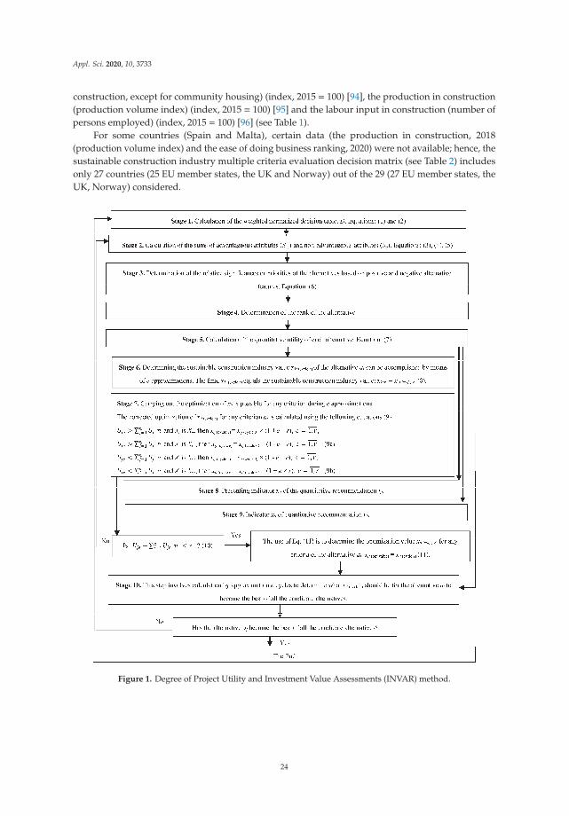
Appl. Sci. 2020, 10, 3733

construction, except for community housing) (index, 2015 = 100) [94], the production in construction(production volume index) (index, 2015 = 100) [95] and the labour input in construction (number ofpersons employed) (index, 2015 = 100) [96] (see Table 1).

For some countries (Spain and Malta), certain data (the production in construction, 2018(production volume index) and the ease of doing business ranking, 2020) were not available; hence, thesustainable construction industry multiple criteria evaluation decision matrix (see Table 2) includesonly 27 countries (25 EU member states, the UK and Norway) out of the 29 (27 EU member states, theUK, Norway) considered.

Figure 1. Degree of Project Utility and Investment Value Assessments (INVAR) method.

24

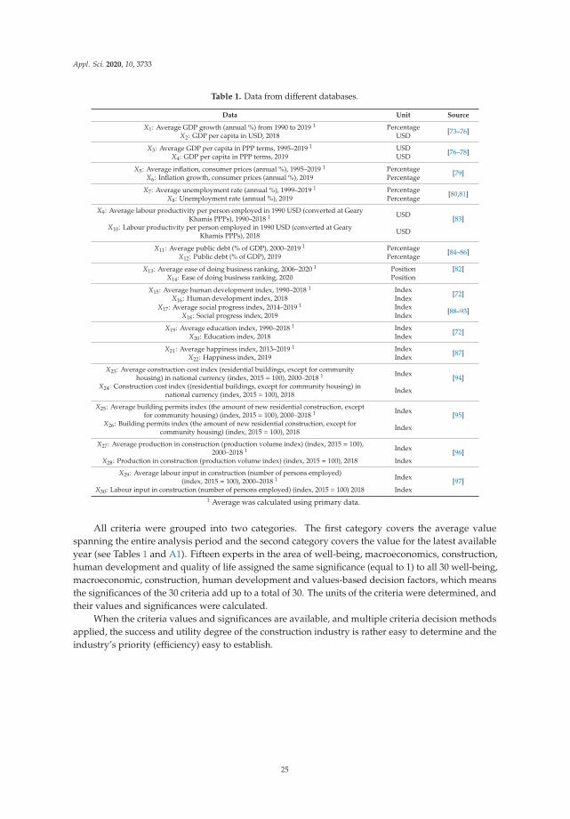
Appl. Sci. 2020, 10, 3733

Table 1. Data from different databases.

Data Unit Source

X1: Average GDP growth (annual %) from 1990 to 2019 1 Percentage [73–76]X2: GDP per capita in USD, 2018 USD

X3: Average GDP per capita in PPP terms, 1995–2019 1 USD [76–78]X4: GDP per capita in PPP terms, 2019 USD

X5: Average inflation, consumer prices (annual %), 1995–2019 1 Percentage [79]X6: Inflation growth, consumer prices (annual %), 2019 Percentage

X7: Average unemployment rate (annual %), 1999–2019 1 Percentage [80,81]X8: Unemployment rate (annual %), 2019 Percentage

X9: Average labour productivity per person employed in 1990 USD (converted at GearyKhamis PPPs), 1990–2018 1 USD [83]

X10: Labour productivity per person employed in 1990 USD (converted at GearyKhamis PPPs), 2018 USD

X11: Average public debt (% of GDP), 2000–2019 1 Percentage [84–86]X12: Public debt (% of GDP), 2019 Percentage

X13: Average ease of doing business ranking, 2006–2020 1 Position [82]X14: Ease of doing business ranking, 2020 Position

X15: Average human development index, 1990–2018 1 Index [72]X16: Human development index, 2018 Index

X17: Average social progress index, 2014–2019 1 Index [88–93]X18: Social progress index, 2019 Index

X19: Average education index, 1990–2018 1 Index [72]X20: Education index, 2018 Index

X21: Average happiness index, 2013–2019 1 Index [87]X22: Happiness index, 2019 Index

X23: Average construction cost index (residential buildings, except for communityhousing) in national currency (index, 2015 = 100), 2000–2018 1 Index [94]

X24: Construction cost index ((residential buildings, except for community housing) innational currency (index, 2015 = 100), 2018 Index

X25: Average building permits index (the amount of new residential construction, exceptfor community housing) (index, 2015 = 100), 2000–2018 1 Index [95]

X26: Building permits index (the amount of new residential construction, except forcommunity housing) (index, 2015 = 100), 2018 Index

X27: Average production in construction (production volume index) (index, 2015 = 100),2000–2018 1 Index [96]

X28: Production in construction (production volume index) (index, 2015 = 100), 2018 Index

X29: Average labour input in construction (number of persons employed)(index, 2015 = 100), 2000–2018 1 Index [97]

X30: Labour input in construction (number of persons employed) (index, 2015 = 100) 2018 Index1 Average was calculated using primary data.

All criteria were grouped into two categories. The first category covers the average valuespanning the entire analysis period and the second category covers the value for the latest availableyear (see Tables 1 and A1). Fifteen experts in the area of well-being, macroeconomics, construction,human development and quality of life assigned the same significance (equal to 1) to all 30 well-being,macroeconomic, construction, human development and values-based decision factors, which meansthe significances of the 30 criteria add up to a total of 30. The units of the criteria were determined, andtheir values and significances were calculated.

When the criteria values and significances are available, and multiple criteria decision methodsapplied, the success and utility degree of the construction industry is rather easy to determine and theindustry’s priority (efficiency) easy to establish.

25

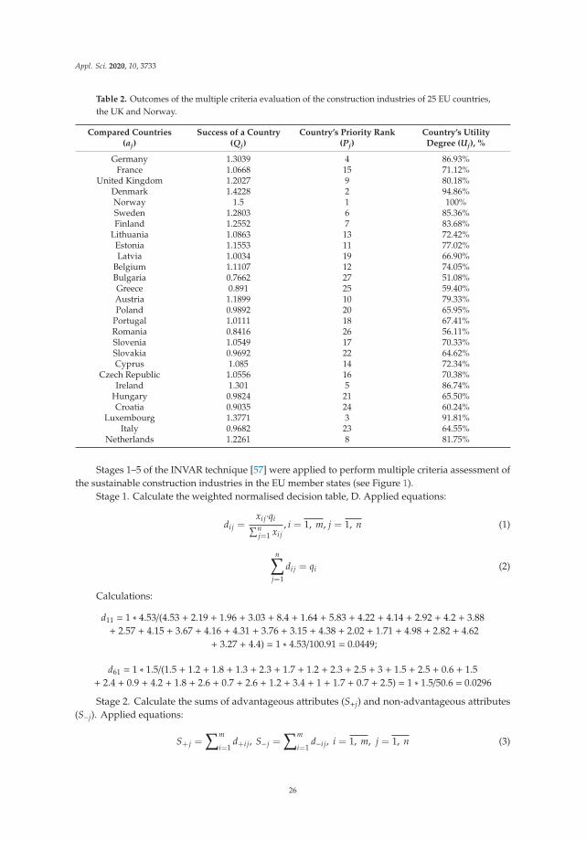
Appl. Sci. 2020, 10, 3733

Table 2. Outcomes of the multiple criteria evaluation of the construction industries of 25 EU countries,the UK and Norway.

Compared Countries(aj)

Success of a Country(Qj)

Country’s Priority Rank(Pj)

Country’s UtilityDegree (Uj), %

Germany 1.3039 4 86.93%France 1.0668 15 71.12%

United Kingdom 1.2027 9 80.18%Denmark 1.4228 2 94.86%Norway 1.5 1 100%Sweden 1.2803 6 85.36%Finland 1.2552 7 83.68%

Lithuania 1.0863 13 72.42%Estonia 1.1553 11 77.02%Latvia 1.0034 19 66.90%

Belgium 1.1107 12 74.05%Bulgaria 0.7662 27 51.08%Greece 0.891 25 59.40%Austria 1.1899 10 79.33%Poland 0.9892 20 65.95%

Portugal 1.0111 18 67.41%Romania 0.8416 26 56.11%Slovenia 1.0549 17 70.33%Slovakia 0.9692 22 64.62%Cyprus 1.085 14 72.34%

Czech Republic 1.0556 16 70.38%Ireland 1.301 5 86.74%

Hungary 0.9824 21 65.50%Croatia 0.9035 24 60.24%

Luxembourg 1.3771 3 91.81%Italy 0.9682 23 64.55%

Netherlands 1.2261 8 81.75%

Stages 1–5 of the INVAR technique [57] were applied to perform multiple criteria assessment ofthe sustainable construction industries in the EU member states (see Figure 1).

Stage 1. Calculate the weighted normalised decision table, D. Applied equations:

dij =xij·qi∑nj=1 xij

, i = 1, m, j = 1, n (1)

n∑j=1

dij = qi (2)

Calculations:

d11 = 1 ∗ 4.53/(4.53 + 2.19 + 1.96 + 3.03 + 8.4 + 1.64 + 5.83 + 4.22 + 4.14 + 2.92 + 4.2 + 3.88+ 2.57 + 4.15 + 3.67 + 4.16 + 4.31 + 3.76 + 3.15 + 4.38 + 2.02 + 1.71 + 4.98 + 2.82 + 4.62

+ 3.27 + 4.4) = 1 ∗ 4.53/100.91 = 0.0449;

d61 = 1 ∗ 1.5/(1.5 + 1.2 + 1.8 + 1.3 + 2.3 + 1.7 + 1.2 + 2.3 + 2.5 + 3 + 1.5 + 2.5 + 0.6 + 1.5+ 2.4 + 0.9 + 4.2 + 1.8 + 2.6 + 0.7 + 2.6 + 1.2 + 3.4 + 1 + 1.7 + 0.7 + 2.5) = 1 ∗ 1.5/50.6 = 0.0296

Stage 2. Calculate the sums of advantageous attributes (S+j) and non-advantageous attributes(S−j). Applied equations:

S+ j =∑m

i=1d+i j, S− j =

∑m

i=1d−i j, i = 1, m, j = 1, n (3)

26

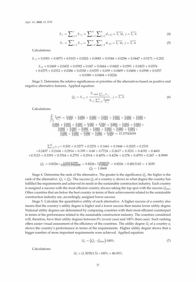
Appl. Sci. 2020, 10, 3733

S+ =∑n

j=1S+ j =

∑m

i=1

∑n

j=1d+i j,= 1, m, j = 1, n (4)

S− =∑n

j=1S− j =

∑m

i=1

∑n

j=1d−i j,= 1, m, j = 1, n (5)

Calculations:

S−1 = 0.0301 + 0.0073 + 0.0103 + 0.0202 + 0.0083 + 0.0344 + 0.0296 + 0.0447 + 0.0171 = 0.202

S+1 = 0.0449 + 0.0432 + 0.0392 + 0.047 + 0.0444 + 0.0402 + 0.0391 + 0.0453 + 0.0376+ 0.0375 + 0.0312 + 0.0286 + 0.0338 + 0.0355 + 0.039 + 0.0409 + 0.0404 + 0.0398 + 0.0357

+ 0.0389 + 0.0404 = 0.8226

Stage 3. Determine the relative significances or priorities of the alternatives based on positive andnegative alternative features. Applied equation:

Qj = S+ j +S−min·∑n

j=1 S− j

S− j·∑nj=1

S−minS− j

, j = 1, n (6)

Calculations:

n∑j=1

S−minS− j

= 0.16610.202 + 0.1661

0.3277 + 0.16610.2251 + 0.1661

0.1661 + 0.16610.1844 + 0.1661

0.2025 + 0.16610.2331+

0.16610.2437 + 0.1661

0.2164 + 0.16610.2914 + 0.1661

0.339 + 0.16610.68 + 0.1661

0.7724 + 0.16610.2617 + 0.1661

0.3231+0.16610.4192 + 0.1661

0.4601 + 0.16610.3123 + 0.1661

0.3393 + 0.16610.3764 + 0.1661

0.2751 + 0.16610.2914+

0.16610.4076 + 0.1661

0.4256 + 0.16610.278 + 0.1661

0.4793 + 0.16610.267 = 15.37543039

∑NJ=1 s−J= 0.202 + 0.3277 + 0.2251 + 0.1661 + 0.1844 + 0.2025 + 0.2331

+0.2437 + 0.2164 + 0.2914 + 0.339 + 0.68 + 0.7724 + 0.2617 + 0.3231 + 0.4192 + 0.4601+0.3123 + 0.3393 + 0.3764 + 0.2751 + 0.2914 + 0.4076 + 0.4256 + 0.278 + 0.4793 + 0.267 = 8.9999

Q1 = 0.8226 ∗ 0.1661∗8.99990.202∗15.37543039 = 0.8226 ∗ 1.49488339

3.105836 = 0.8226 + 0.4813143 = 1.3039Q2 = 1.0668

Stage 4. Determine the rank of the alternative. The greater is the significance Qj, the higher is therank of the alternative: Q1 < Q2. The success Qj of a country aj shows to what degree the country hasfulfilled the requirements and achieved its needs in the sustainable construction industry. Each countryis assigned a success with the most efficient country always taking the top spot with the success Qmax.Other countries that are below the best country in terms of their achievements related to the sustainableconstruction industry are, accordingly, assigned lower success.

Stage 5. Calculate the quantitative utility of each alternative. A higher success of a country alsomeans that the country’s utility degree is higher and a lower success then means lower utility degree.National utility degrees are determined by comparing countries with their most efficient counterpartin terms of the performance related to the sustainable construction industry. The countries consideredwill, therefore, have their utility degrees between 0% (worst case) and 100% (best case). Such rankingoffers easier visual assessment of the efficiency of the countries. The utility degree Uj of a country ajshows the country’s performance in terms of the requirements. Higher utility degree shows that abigger number of more important requirements were achieved. Applied equation:

Uj =(Qj : Qmax

)·100% (7)

Calculations:U1 = (1.3039/1.5) ∗ 100% = 86.93%

27

Appl. Sci. 2020, 10, 3733

U2 = (1.0668/1.5) ∗ 100% = 71.12%

The multiple criteria evaluation outcomes for the countries considered (see Table 2) show thatNorway (a5) scored best (significance Qmax = Q5 = 1.5 and utility degree Umax = U5 = 100%) in terms ofthe criteria considered here.

Lithuania (a8) ranked eleventh with its significance Q8 = 1.0863, well below the top performer.The country’s utility degree was U8 = 72.42% (see Table 2).

Lithuania and Portugal in Table A1 can be examples for discussion. The evaluation of the1990–2019 period shows that, at 4.22%, Lithuania recorded a similar average annual GDP growth toPortugal with 4.16%. The 2019 data show that the GDP per capita in PPP terms was lower in Portugal(30,487.7 USD) than in Lithuania (32,378.6 USD). At 8.81, the average 1999–2019 unemploymentrate in Portugal was about 21% lower than that in Lithuania (10.89), and the 2019 unemploymentrate in Portugal (6.10) was equal to that in Lithuania (6.10). Between 1995 and 2019, the averageinflation growth in Lithuania (3.65%) was 1.825 times as high as in Portugal (2.00%). During 1990–2018,the average labour productivity per person employed was greater in Portugal (58,505.00 USD) than itwas in Lithuania (45,530.00 USD) in 1990 USD terms (converted at Geary Khamis PPPs). However,the average public debt levels between 2000 and 2019 show that Portugal’s debt burden, at 92.42%,was higher than that of Lithuania (29.12%). The conditions of the business environment better inLithuania than in Portugal. Lithuania ranked 11th and Portugal 39th in the 2020 ease of doing businessindex; the average for 2006–2020, meanwhile, shows that Lithuania (21st) offered better conditions interms of the ease of doing business than Portugal (34th) had. The human development index in 2018 issimilar in both countries, in Portugal 0.85 and Lithuania 0.87. The education index in 2018 in Portugal(0.76) is less than in Lithuania (0.89). Conversely, appreciate the social progress index 2019 index isbigger in Portugal (87.12) than in Lithuania (81.30). It is clear from the summary of all 16 indicatorsunder evaluation that, in four instances, Lithuania performed better than Portugal. The remaining13 indicators, however, show Portugal performing better than Lithuania. The combination of thesecomparative data reflects the results of the multiple criteria assessment (see Table 2), showing that,in terms of the criteria considered here, Lithuania (a8) scored better (priority P8 = 13 and utility degreeN8 = 72.42%) [52]. Portugal (a16) ranked 18th with its utility degree N16 = 67.41% (see Table 2).

3. Comparison of the Sustainable Construction Industry Indicators in the EU Countries, the UKand Norway over the Past 29 Years

Over the past 29 years, many EU member countries under evaluation purposed considerableeconomic gains compared with the global level. Next, indicators such as GDP per capita (USD), theease of doing business ranking and a few others are considered as examples (see Table A1 and Figure 2).

The leading countries among EU members, Norway and the UK in terms of GDP per capita (USD)in 2018 were Luxembourg, followed by Norway, Ireland, Denmark, Sweden, Netherlands, Austria,Finland, Germany, Belgium, the UK amd France. Italy is not far behind, followed by Cyprus, Slovenia,Portugal, Czech Republic, Estonia, Greece, Slovakia and Lithuania. The following are countrieswith GDP per capita (USD) 1.9 times or more below Italy’s: Latvia, Hungary, Poland and Croatia.The weakest economies are in Romania and Bulgaria (see Figure 2). Spain (30,523.86 USD) and Malta(30,074.74 USD), which are not included in Table A1, have similar economies to Italy.

28

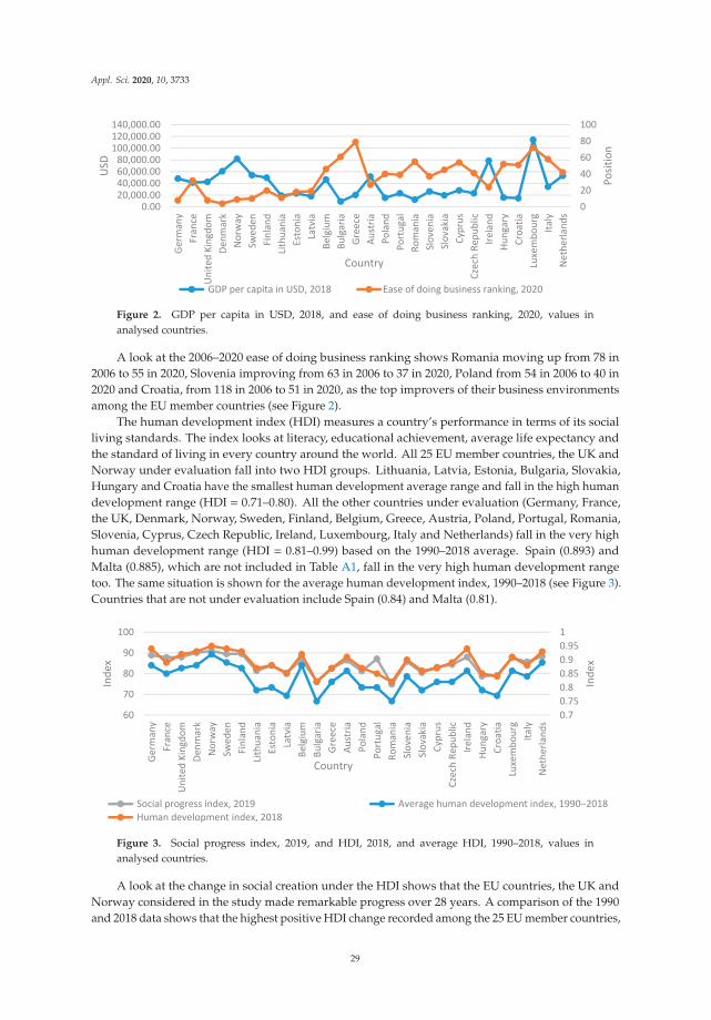
Appl. Sci. 2020, 10, 3733

Figure 2. GDP per capita in USD, 2018, and ease of doing business ranking, 2020, values inanalysed countries.

A look at the 2006–2020 ease of doing business ranking shows Romania moving up from 78 in2006 to 55 in 2020, Slovenia improving from 63 in 2006 to 37 in 2020, Poland from 54 in 2006 to 40 in2020 and Croatia, from 118 in 2006 to 51 in 2020, as the top improvers of their business environmentsamong the EU member countries (see Figure 2).

The human development index (HDI) measures a country’s performance in terms of its socialliving standards. The index looks at literacy, educational achievement, average life expectancy andthe standard of living in every country around the world. All 25 EU member countries, the UK andNorway under evaluation fall into two HDI groups. Lithuania, Latvia, Estonia, Bulgaria, Slovakia,Hungary and Croatia have the smallest human development average range and fall in the high humandevelopment range (HDI = 0.71–0.80). All the other countries under evaluation (Germany, France,the UK, Denmark, Norway, Sweden, Finland, Belgium, Greece, Austria, Poland, Portugal, Romania,Slovenia, Cyprus, Czech Republic, Ireland, Luxembourg, Italy and Netherlands) fall in the very highhuman development range (HDI = 0.81–0.99) based on the 1990–2018 average. Spain (0.893) andMalta (0.885), which are not included in Table A1, fall in the very high human development rangetoo. The same situation is shown for the average human development index, 1990–2018 (see Figure 3).Countries that are not under evaluation include Spain (0.84) and Malta (0.81).

Figure 3. Social progress index, 2019, and HDI, 2018, and average HDI, 1990–2018, values inanalysed countries.

A look at the change in social creation under the HDI shows that the EU countries, the UK andNorway considered in the study made remarkable progress over 28 years. A comparison of the 1990and 2018 data shows that the highest positive HDI change recorded among the 25 EU member countries,

29

Appl. Sci. 2020, 10, 3733

Norway, the UK under evaluation occurred in Ireland (0.18); Croatia (0.17); Czech Republic, Latvia andPoland (0.16); Estonia and the UK (0.15); Germany, Finland, Lithuania, Portugal, Hungary and Cyprus(0.14); Denmark (0.13); Sweden, Luxembourg, Bulgaria, Greece, Austria, Romania and Slovakia (0.12);France, Belgium and Italy (0.11); and Norway and Netherlands (0.10). The smallest recorded, positiveHDI change among the 25 EU member countries, the UK and Norway under evaluation occurredin Slovenia (0.07) (see Figure 3). Countries that are not under evaluation include Spain (0.14) andMalta (0.14).

For the social progress index in 2019, the leading countries are Norway (90.95) and Denmark(90.09), followed by Finland (89.56), Sweden (89.45), Germany (88.84), Netherlands (88.31), the UK(87.98), Ireland (87.97), France (87.79), Luxembourg (87.66), Portugal (87.12), Belgium (86.77), Austria(86.4), Slovenia (85.8), Italy (85.69), Czech Republic (84.36), Estonia (83.98), Cyprus (83.14), Greece(82.48), Lithuania (81.3), Poland (81.25), Slovakia (80.43) and Latvia (80.42). The following are countrieswith social progress index 12.90% or more below that of Norway: Croatia (79.21), Hungary (78.77),Bulgaria (76.17) and Romania (74.81) (see Figure 3). Countries that are not under evaluation includeSpain (87.47) and Malta (82.63), which have similar social progress index values as the UK and Greece.

For the average GDP growth during 1990–2019 (annual %), the leading country is Norway (8.40),followed by Finland (5.83), Hungary (4.98), Luxemburg (4.62), Germany (4.53), Netherlands (4.40),Cyprus (4.38), Romania (4.31) and Lithuania (4.22). The following are countries have average growthduring 1990–2019 (annual %) two times or more below that of Norway: Belgium (4.20), Portugal (4.16),Austria (4.15), Estonia (4.14), Bulgaria (3.88), Slovenia (3.76), Poland (3.67), Italy (3.27), Slovakia (3.15),Denmark (3.03), Latvia (2.92), Croatia (2.82), Greece (2.57), France (2.19) and Czech Republic (2.02).The lowest average GDP growth in 1990–2019 (annual %) is in the UK (1.96), Ireland (1.71) and Sweden(1.64) (see Figure 4). Countries that are not under evaluation include Spain (2.29) and Malta (4.80),which have similar average GDP growth during 1990–2019 (annual %) as France and Hungary.

Figure 4. Average GDP growth, 1990–2019, unemployment rate, 2019, inflation growth, 2019, andpublic debt, 2019, values in analysed countries.

For inflation growth, consumer prices (annual %) in 2019, the leading EU member country isGreece (0.60%), followed by Cyprus (0.70%), Italy (0.70%), Portugal (0.90%) and Croatia (1.00%).The following countries have twice or more inflation growth than Greece: France (1.20%), Finland(1.20%) and Ireland (1.20%), followed by Denmark (1.30%), Germany (1.50%), Belgium (1.50%), Austria(1.50%), Sweden (1.70%), Luxemburg (1.70%), the UK (1.80%), Slovenia (1.80%), Norway (2.30%),Lithuania (2.30%), Poland (2.40%), Estonia (2.50%), Bulgaria (2.50%), Netherlands (2.50%), Slovakia(2.60%) and Czech Republic (2.60%). The highest inflation growth is in Latvia (3.00%), Hungary (3.40%)

30

Appl. Sci. 2020, 10, 3733

and Romania (4.20%) (see Figure 4). Countries that are not under evaluation include Spain—(0.70%),which has the lowest indicator from all comparing countries, and Malta (1.70%), which has the sameinflation growth as in Sweden or Luxemburg.

For unemployment rate (annual %) in 2019, the leading EU member country is the CzechRepublic (2.2%), followed by Germany (3.2%), Netherlands (3.3%), Hungary (3.5%), Norway (3.6%),the UK (3.8%), Poland (3.8%) and Romania (4.3%). The following countries have at least twice theunemployment rate of Czech Republic: Slovenia (4.5%), Estonia (4.7%), Bulgaria (4.9%), Denmark(5.00%), Austria (5.1%), Luxembourg (5.2%), Belgium (5.5%), Ireland (5.5%), Slovakia (6.00%), Portugal(6.1%), Lithuania (6.1%), Sweden (6.5%), Finland (6.5%), Latvia (6.5%) and Cyprus (7.00%). Thefollowing countries have high or very high inflation rates: France (8.6%), Croatia (9.00%), Italy (10.3%)and Greece (17.8%) (see Figure 4). Countries that are not under evaluation include Spain (13.9%),which has a very high unemployment rate, and Malta (3.8%), which has an unemployment rate similarto the UK or Poland.

For public debt (% of GDP) in 2019, the leading EU member country is Estonia (8.2%), followed byBulgaria (19.2%), Luxembourg (21.3%), Czech Republic (31.6%), Lithuania (31.8%), Denmark (33.0%),Latvia (36.3%), Sweden (36.9%), Romania (37.4%), Norway (40.0%), Poland (47.8%), Slovakia (48.4%),Netherlands (49.2%), Germany (58.6%), Finland (58.9%), Ireland (60.9%), Slovenia (67.1%), Hungary(67.5%), Austria (70.7%), Croatia (71.1%), the UK (85.6%), Cyprus (96.1%) and France (99.3%). Four EUmember states have more than 100% public debt: Belgium (101%), Portugal (117.6%), Italy (133.2%)and Greece (176.6%) (see Figure 4). Countries that are not under evaluation include Spain (96.4%) andMalta (42.3%), which have similar public debt as Cyprus and Poland, respectively.

Comparison of indicators in EU member states show that countries that have a high economy, fallin the high human development range, have a high social progress index, have a low unemploymentrate and take a higher position on ease of doing business ranking. However, they have a relatively highinflation rate and public debt. The comparison also showed that lower economy performance countriesduring 29 years boosted their economic, social and environmental performance. In conclusion, it seemsthat economic and social gains encourage boosting the sustainable construction industry performanceof various EU member countries.

4. Analysis of the Interdependencies between the Indicators of the Macro Level and theIndicators Describing the Construction Industry in the EU Countries, the UK and Norway

This study identified correlational relationships among the 25 EU countries, the UK and theNorwegian construction industry (construction cost index, year-over-year change; production inconstruction in terms of the production volume index, year-over-year change; building permits indexin terms of the number of dwellings, year-over-year change; and labour input in construction in termsof the number of persons employed, year-over-year change) and the macro-level indicators of thecountries (GDP annual growth rate, GDP per capita current USD, unemployment rate, public debt,human development index, education index, gender inequality index and life expectancy at birth(total years)).

The outcomes of the correlation analysis are discussed with France taken as an example.The following indicators show strong correlations:

• GDP per capita current USD and construction cost index 2000–2018 (r = 0.86, linear dependence)(Figure 5) and production in construction 2000–2018 (r = 0.81, linear dependence) (Figure 5).

• Construction cost index and public debt 2000–2018 (r = 0.92, linear dependence), humandevelopment index 2000–2018 (r = 0.97, linear dependence), education index 2000–2018 (r = 0.95,linear dependence) and gender inequality index 2000–2018 (r = −0.94, inverse dependence).

• Production in construction and unemployment rate 2000–2018 (r = −0.84, inverse dependence)and public debt 2000–2018 (r = −0.74, inverse dependence).

• Unemployment rate and public debt 2000–2018 (r = 0.76, linear dependence).

31

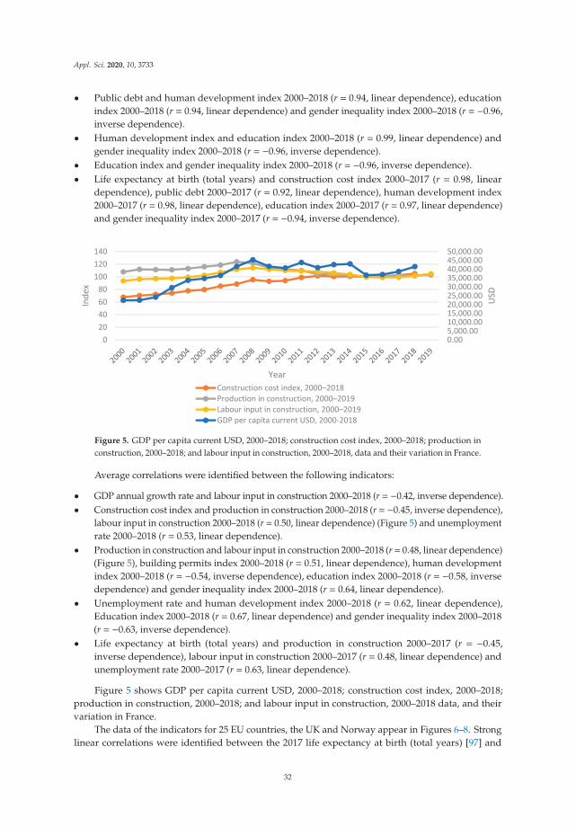
Appl. Sci. 2020, 10, 3733

• Public debt and human development index 2000–2018 (r = 0.94, linear dependence), educationindex 2000–2018 (r = 0.94, linear dependence) and gender inequality index 2000–2018 (r = −0.96,inverse dependence).

• Human development index and education index 2000–2018 (r = 0.99, linear dependence) andgender inequality index 2000–2018 (r = −0.96, inverse dependence).

• Education index and gender inequality index 2000–2018 (r = −0.96, inverse dependence).• Life expectancy at birth (total years) and construction cost index 2000–2017 (r = 0.98, linear

dependence), public debt 2000–2017 (r = 0.92, linear dependence), human development index2000–2017 (r = 0.98, linear dependence), education index 2000–2017 (r = 0.97, linear dependence)and gender inequality index 2000–2017 (r = −0.94, inverse dependence).

Figure 5. GDP per capita current USD, 2000–2018; construction cost index, 2000–2018; production inconstruction, 2000–2018; and labour input in construction, 2000–2018, data and their variation in France.

Average correlations were identified between the following indicators:

• GDP annual growth rate and labour input in construction 2000–2018 (r = −0.42, inverse dependence).• Construction cost index and production in construction 2000–2018 (r = −0.45, inverse dependence),

labour input in construction 2000–2018 (r = 0.50, linear dependence) (Figure 5) and unemploymentrate 2000–2018 (r = 0.53, linear dependence).

• Production in construction and labour input in construction 2000–2018 (r= 0.48, linear dependence)(Figure 5), building permits index 2000–2018 (r = 0.51, linear dependence), human developmentindex 2000–2018 (r = −0.54, inverse dependence), education index 2000–2018 (r = −0.58, inversedependence) and gender inequality index 2000–2018 (r = 0.64, linear dependence).

• Unemployment rate and human development index 2000–2018 (r = 0.62, linear dependence),Education index 2000–2018 (r = 0.67, linear dependence) and gender inequality index 2000–2018(r = −0.63, inverse dependence).

• Life expectancy at birth (total years) and production in construction 2000–2017 (r = −0.45,inverse dependence), labour input in construction 2000–2017 (r = 0.48, linear dependence) andunemployment rate 2000–2017 (r = 0.63, linear dependence).

Figure 5 shows GDP per capita current USD, 2000–2018; construction cost index, 2000–2018;production in construction, 2000–2018; and labour input in construction, 2000–2018 data, and theirvariation in France.

The data of the indicators for 25 EU countries, the UK and Norway appear in Figures 6–8. Stronglinear correlations were identified between the 2017 life expectancy at birth (total years) [97] and

32

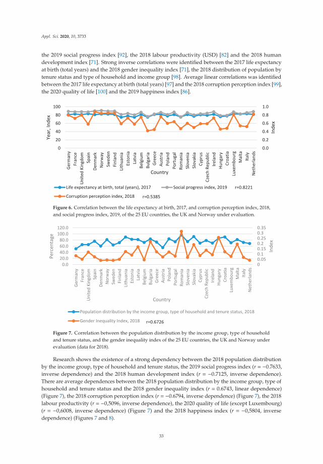
Appl. Sci. 2020, 10, 3733

the 2019 social progress index [92], the 2018 labour productivity (USD) [82] and the 2018 humandevelopment index [71]. Strong inverse correlations were identified between the 2017 life expectancyat birth (total years) and the 2018 gender inequality index [71], the 2018 distribution of population bytenure status and type of household and income group [98]. Average linear correlations was identifiedbetween the 2017 life expectancy at birth (total years) [97] and the 2018 corruption perception index [99],the 2020 quality of life [100] and the 2019 happiness index [86].

Figure 6. Correlation between the life expectancy at birth, 2017, and corruption perception index, 2018,and social progress index, 2019, of the 25 EU countries, the UK and Norway under evaluation.

Figure 7. Correlation between the population distribution by the income group, type of householdand tenure status, and the gender inequality index of the 25 EU countries, the UK and Norway underevaluation (data for 2018).

Research shows the existence of a strong dependency between the 2018 population distributionby the income group, type of household and tenure status, the 2019 social progress index (r = −0.7633,inverse dependence) and the 2018 human development index (r = −0.7125, inverse dependence).There are average dependences between the 2018 population distribution by the income group, type ofhousehold and tenure status and the 2018 gender inequality index (r = 0.6743, linear dependence)(Figure 7), the 2018 corruption perception index (r = −0.6794, inverse dependence) (Figure 7), the 2018labour productivity (r = −0,5096, inverse dependence), the 2020 quality of life (except Luxembourg)(r = −0,6008, inverse dependence) (Figure 7) and the 2018 happiness index (r = −0,5804, inversedependence) (Figures 7 and 8).

33

Appl. Sci. 2020, 10, 3733

Figure 8. Correlation between the population distribution by the income group, type of household andtenure status, 2018, the quality of life, 2019, the happiness index, 2019, and the corruption perceptionindex, 2018, of the 25 EU countries, the UK and Norway under evaluation.

The basis for the assessment of 25 EU members, the UK and Norway is the input data matrixpresented in Table A1. The multiple criteria evaluation ranked 25 EU members, the UK and Norwayby priority and determined their utility degrees.

The same assessments can be used in other cases where a best practice needs to be createdand implemented.

The end of World War II brought communism to the countries in Eastern Europe, and the statetypically promised to provide housing for the people. This meant that the majority of housing stock insuch countries were public rental housing, and the rents, unlike in public housing offered in advancedcapitalist societies, were very low. Everything changed after 1989 when democracy returned toCommunist Europe. The major part of public housing was sold off. The elimination of rent control andprivatisation of public housing encouraged the creation of a significant private renting sector in a fewplaces [101].

A correlation analysis comparing the sustainable construction industry and housing priceindicators of the EU member states, the UK and Norway was performed (see Table 3). The correlationsamong the 2018 real house price index (index, 2015 = 100), the 2018 nominal house price indices(index, 2015 = 100), the 2020 price-to-rent ratio (index, 2010 = 100), the 2018 house price indiceswith the 2018 production in construction (production volume index) (index, 2015 = 100), the 2018construction cost index in national currencies (index, 2015 = 100) and the 2018 building permits indices(the amount of new residential construction, except for community housing) (index 2015 = 100) wereanalysed (Table 3).

34

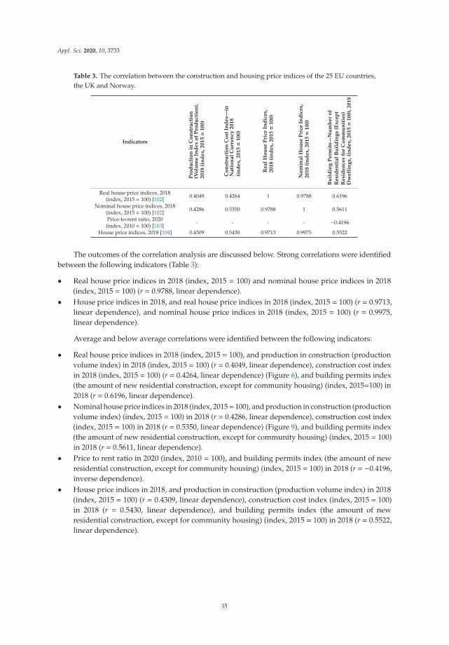
Appl. Sci. 2020, 10, 3733

Table 3. The correlation between the construction and housing price indices of the 25 EU countries,the UK and Norway.

Indicators

Pro

du

ctio

nin

Co

nst

ruct

ion

(Vo

lum

eIn

dex

of

Pro

du

ctio

n),

2018

(in

dex,2015=

100)

Co

nst

ruct

ion

Co

stIn

dex—

inN

ati

on

al

Cu

rren

cy2018

(in

dex,2015=

100)

Real

Ho

use

Pri

ceIn

dic

es,

2018

(in

dex,2015=

100)

No

min

al

Ho

use

Pri

ceIn

dic

es,

2018

(in

dex,2015=

100)

Bu

ild

ing

Perm

its—

Nu

mb

er

of

Resi

den

tial

Bu

ild

ing

s(E

xce

pt

Resi

den

ces

for

Co

mm

un

itie

s)D

well

ing

s,(i

nd

ex,2015=

100),

2018

Real house price indices, 2018(index, 2015 = 100) [102] 0.4049 0.4264 1 0.9788 0.6196

Nominal house price indices, 2018(index, 2015 = 100) [102] 0.4286 0.5350 0.9788 1 0.5611

Price-to-rent ratio, 2020(index, 2010 = 100) [103] - - - - −0.4196

House price indices, 2018 [104] 0.4309 0.5430 0.9713 0.9975 0.5522

The outcomes of the correlation analysis are discussed below. Strong correlations were identifiedbetween the following indicators (Table 3):

• Real house price indices in 2018 (index, 2015 = 100) and nominal house price indices in 2018(index, 2015 = 100) (r = 0.9788, linear dependence).

• House price indices in 2018, and real house price indices in 2018 (index, 2015 = 100) (r = 0.9713,linear dependence), and nominal house price indices in 2018 (index, 2015 = 100) (r = 0.9975,linear dependence).

Average and below average correlations were identified between the following indicators:

• Real house price indices in 2018 (index, 2015 = 100), and production in construction (productionvolume index) in 2018 (index, 2015 = 100) (r = 0.4049, linear dependence), construction cost indexin 2018 (index, 2015 = 100) (r = 0.4264, linear dependence) (Figure 6), and building permits index(the amount of new residential construction, except for community housing) (index, 2015=100) in2018 (r = 0.6196, linear dependence).

• Nominal house price indices in 2018 (index, 2015= 100), and production in construction (productionvolume index) (index, 2015 = 100) in 2018 (r = 0.4286, linear dependence), construction cost index(index, 2015 = 100) in 2018 (r = 0.5350, linear dependence) (Figure 9), and building permits index(the amount of new residential construction, except for community housing) (index, 2015 = 100)in 2018 (r = 0.5611, linear dependence).

• Price to rent ratio in 2020 (index, 2010 = 100), and building permits index (the amount of newresidential construction, except for community housing) (index, 2015 = 100) in 2018 (r = −0.4196,inverse dependence).

• House price indices in 2018, and production in construction (production volume index) in 2018(index, 2015 = 100) (r = 0.4309, linear dependence), construction cost index (index, 2015 = 100)in 2018 (r = 0.5430, linear dependence), and building permits index (the amount of newresidential construction, except for community housing) (index, 2015 = 100) in 2018 (r = 0.5522,linear dependence).

35

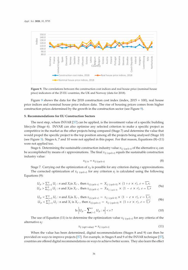
Appl. Sci. 2020, 10, 3733

Figure 9. The correlations between the construction cost indices and real house price (nominal houseprice) indicators of the 25 EU countries, the UK and Norway (data for 2018).

Figure 9 shows the data for the 2018 construction cost index (index, 2015 = 100), real houseprice indices and nominal house price indices data. The rise of housing prices comes from higherconstruction prices determined by the growth in the construction sector (see Figure 9).

5. Recommendations for EU Construction Sectors

The next step, where INVAR [57] can be applied, is the investment value of a specific buildinglifecycle (Stage 6). INVAR can also optimise any selected criterion to make a specific project ascompetitive in the market as the other projects being compared (Stage 7) and determine the value thatwould propel the specific project to the top position among all the projects being analysed (Stage 10)(see Figure 1). Stages 6, 7 and 10 were not applied in this paper. For that reason, Equations (8)–(11)were not applied too.

Stage 6. Determining the sustainable construction industry value x1j (cycle e) of the alternative aj canbe accomplished by means of e approximations. The final x1j (cycle e) equals the sustainable constructionindustry value:

x1j iv = x1j (cycle e) (8)

Stage 7. Carrying out the optimization of xij is possible for any criterion during e approximations.The corrected optimization of xij (cycle e) for any criterion aj is calculated using the following

Equations (9):

Uje >∑n

j=1 Uj : n and Xiis Xi− , then xij(cycle e) = Xij (cycle 0) × (1 + e × r), e = 1, r;

Uje >∑n

j=1 Uj : n and Xiis Xi+ , then xij(cycle e) = XXij (cycle 0)× (1 − e × r), e = 1, r

(9a)

Uje <∑n

j=1 Uj : n and Xiis Xi− , then xij(cycle e) = xij (cycle 0) × (1 − e × r), e = 1, r;

Uje <∑n

j=1 Uj : n and Xi is Xi+ , then xij(cycle e) = xij (cycle 0) × (1 + e × r), e = 1, r(9b)

Is∣∣∣∣∣Uje −

∑n

j=1Uje : n

∣∣∣∣∣ < s ? (10)

The use of Equation (11) is to determine the optimization value xij (cycle e) for any criteria of thealternative aj:

xij (opt value) = xij (cycle e) (11)

When the value has been determined, digital recommendations (Stages 8 and 9) can then beprovided on ways to improve projects [57]. For example, in Stages 8 and 9 of the INVAR technique [57],countries are offered digital recommendations on ways to achieve better scores. They also learn the effect

36

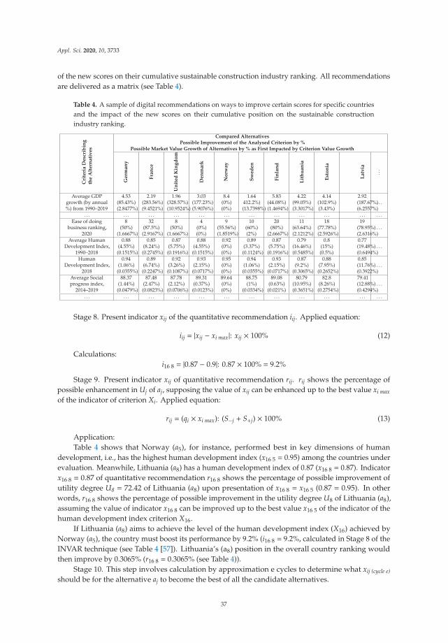
Appl. Sci. 2020, 10, 3733

of the new scores on their cumulative sustainable construction industry ranking. All recommendationsare delivered as a matrix (see Table 4).

Table 4. A sample of digital recommendations on ways to improve certain scores for specific countriesand the impact of the new scores on their cumulative position on the sustainable constructionindustry ranking.

Cri

teri

aD

esc

rib

ing

the

Alt

ern

ati

ves

Compared AlternativesPossible Improvement of the Analysed Criterion by %

Possible Market Value Growth of Alternatives by % as First Impacted by Criterion Value Growth

Germ

an

y

Fra

nce

Un

ited

Kin

gd

om

Den

mark

No

rway

Sw

ed

en

Fin

lan

d

Lit

hu

an

ia

Est

on

ia

Latv

ia

...

Average GDPgrowth (by annual%) from 1990–2019

4.53(85.43%)(2.8477%)

2.19(283.56%)(9.4521%)

1.96(328.57%)(10.9524%)

3.03(177.23%)(5.9076%)

8.4(0%)(0%)

1.64412.2%)(13.7398%)

5.83(44.08%)(1.4694%)

4.22(99.05%)(3.3017%)

4.14(102.9%)(3.43%)

2.92(187.67%)(6.2557%)

. . .

. . . . . . . . . . . . . . . . . . . . . . . . . . . . . . . . . . . .Ease of doing

business ranking,2020

8(50%)

(1.6667%)

32(87.5%)(2.9167%)

8(50%)

(1.6667%)

4(0%)(0%)

9(55.56%)(1.8519%)

10(60%)(2%)

20(80%)

(2.6667%)

11(63.64%)(2.1212%)

18(77.78%)(2.5926%)

19(78.95%)(2.6316%)

. . .

Average HumanDevelopment Index,

1990–2018

0.88(4.55%)(0.1515%)

0.85(8.24%)(0.2745%)

0.87(5.75%)(0.1916%)

0.88(4.55%)(0.1515%)

0.92(0%)(0%)

0.89(3.37%)(0.1124%)

0.87(5.75%)(0.1916%)

0.79(16.46%)(0.5485%)

0.8(15%)(0.5%)

0.77(19.48%)(0.6494%)

. . .

HumanDevelopment Index,

2018

0.94(1.06%)(0.0355%)

0.89(6.74%)(0.2247%)

0.92(3.26%)(0.1087%)

0.93(2.15%)(0.0717%)

0.95(0%)(0%)

0.94(1.06%)(0.0355%)

0.93(2.15%)(0.0717%)

0.87(9.2%)

(0.3065%)

0.88(7.95%)(0.2652%)

0.85(11.76%)(0.3922%)

. . .

Average Socialprogress index,

2014–2019

88.37(1.44%)(0.0479%)

87.48(2.47%)(0.0823%)

87.78(2.12%)(0.0706%)

89.31(0.37%)(0.0123%)

89.64(0%)(0%)

88.75(1%)

(0.0334%)

89.08(0.63%)(0.021%)

80.79(10.95%)(0.3651%)

82.8(8.26%)(0.2754%)

79.41(12.88%)(0.4294%)

. . .

. . . . . . . . . . . . . . . . . . . . . . . . . . . . . . . . . . . .

Stage 8. Present indicator xij of the quantitative recommendation iij. Applied equation:

iij = |xij − xi max|: xij × 100% (12)

Calculations:i16 8 = |0.87 − 0.9|: 0.87 × 100% = 9.2%

Stage 9. Present indicator xij of quantitative recommendation rij. rij shows the percentage ofpossible enhancement in Uj of aj, supposing the value of xij can be enhanced up to the best value xi maxof the indicator of criterion Xi. Applied equation:

rij = (qi × xi max): (S−j + S+j) × 100% (13)

Application:Table 4 shows that Norway (a5), for instance, performed best in key dimensions of human

development, i.e., has the highest human development index (x16 5 = 0.95) among the countries underevaluation. Meanwhile, Lithuania (a8) has a human development index of 0.87 (x16 8 = 0.87). Indicatorx16 8 = 0.87 of quantitative recommendation r16 8 shows the percentage of possible improvement ofutility degree U8 = 72.42 of Lithuania (a8) upon presentation of x16 8 = x16 5 (0.87 = 0.95). In otherwords, r16 8 shows the percentage of possible improvement in the utility degree U8 of Lithuania (a8),assuming the value of indicator x16 8 can be improved up to the best value x16 5 of the indicator of thehuman development index criterion X16.

If Lithuania (a8) aims to achieve the level of the human development index (X16) achieved byNorway (a5), the country must boost its performance by 9.2% (i16 8 = 9.2%, calculated in Stage 8 of theINVAR technique (see Table 4 [57]). Lithuania’s (a8) position in the overall country ranking wouldthen improve by 0.3065% (r16 8 = 0.3065% (see Table 4)).

Stage 10. This step involves calculation by approximation e cycles to determine what xij (cycle e)should be for the alternative aj to become the best of all the candidate alternatives.

37

Appl. Sci. 2020, 10, 3733

Other countries can similarly examine ways to improve their scores on the sustainable constructionindustry ranking.

6. Conclusions

Among the latest available studies on sustainable construction, this research offers three innovativeelements. The first is the use of the INVAR method [57]. This method can be used as the basis for creatingefficient construction, macroeconomic, quality of life, human development and well-being factors toensure improved macro-environments for the lifecycle of sustainable construction. Macro environmentsare important in attempts to make the lifecycle of the sustainable construction industry efficient.The multiple criteria decision matrix makes an integrated assessment of aspects that characterise thesustainable construction industries in the EU member countries, the UK and Norway. The variety ofaspects considered is matched by that of the forms of data required in decision making. The COPRASand INVAR techniques were applied for the evaluation of the sustainable construction industries.

The second innovation is that this research applied INVAR and its capabilities to expand theanalysis of various indicators with extra features. Among them are digital tips for specific constructionindustries analysed against these criteria, deriving rationalised indicators and determining whichvalues of these criteria would push the rating of a specific construction industry up to the expected level.When the INVAR method is applied, a broader look at the contexts such as well-being, macroeconomicfactors, quality of life, construction and human development becomes possible, as well as a morethorough interpretation of the changes and shifts observed in construction industries over recent years.The multiple criteria analysis of the macro environment and construction industries in the EU membercountries, the UK and Norway was performed and recommendations offered.

The third innovation is that we eliminated the need to stick to only construction and othertraditional measures when the indicators for the 27 construction industries analysed in our researchhave to be improved. Corruption, happiness, education and social progress are other, less exploredareas where improvements are possible. The dependencies that link the indicators describing themacro level and construction industry in the EU member countries, the UK and Norway were analysed.

The perceived image and success of a country can influence economic behaviour. Companiesoperate in a macro environment comprising a wide range of technological, ecological, legal, economic,success, image, political, health-related and social aspects, visible on a national level, and thisenvironment is relevant to corporate marketing efforts. Due to its intuitive and cost-conscious nature,the emoticon measure can be a handy marketing tool to discover the sentiments elicited by one nation.Marketing managers then can apply these insights to different export markets [105]. A high developedcountry national image makes a country more attractive and its products more popular, and theimpact such image makes on the economy through the intentions of consumers to buy the country’sbrands and products [48]. The findings of this research, then, can help potential buyers make decisionsregarding the best choice in terms of the country of origin.

The future plans include research on the sustainable construction industries developments inAmerican, African and Asian countries and the supply of recommendations. An innovative integratedevaluation of the sustainable construction industries would allow us in the future to investigate thelifecycle of buildings and its phases, the parties involved in the project and the context as a whole.The current models and intelligent systems available worldwide do not offer these functions.

Author Contributions: Conceptualisation, A.K. (Arturas Kaklauskas) and E.K.Z.; methodology, A.K.(Arturas Kaklauskas), E.K.Z., A.B.-V., A.K. (Agne Kuzminske), J.C., A.C. and R.V.; software, A.K.(Arturas Kaklauskas), A.B.-V., A.K. (Agne Kuzminske), J.C., A.C. and R.V.; validation, A.K. (Arturas Kaklauskas),A.B.-V., A.K. (Agne Kuzminske), J.C., A.C. and R.V.; formal analysis, A.K. (Arturas Kaklauskas), A.B.-V., A.K.(Agne Kuzminske), J.C., A.C. and R.V.; investigation, A.K. (Arturas Kaklauskas), A.B.-V., A.K. (Agne Kuzminske),J.C., A.C. and R.V.; resources, A.K. (Arturas Kaklauskas), A.B.-V., A.K. (Agne Kuzminske), J.C., A.C. and R.V.; datacuration, A.K. (Arturas Kaklauskas), A.B.-V., A.K. (Agne Kuzminske), J.C., A.C. and R.V.; writing—original draftpreparation, A.K. (Arturas Kaklauskas), A.B.-V., A.K. (Agne Kuzminske), J.C., A.C. and R.V.; writing—reviewand editing, A.K. (Arturas Kaklauskas), A.B.-V., A.K. (Agne Kuzminske), J.C., A.C. and R.V.; visualisation, A.K.(Arturas Kaklauskas), A.B.-V., A.K. (Agne Kuzminske), J.C., A.C. and R.V.; supervision, A.K. (Arturas Kaklauskas)

38

Appl. Sci. 2020, 10, 3733

and E.K.Z.; project administration, A.K. (Arturas Kaklauskas) and E.K.Z.; and funding acquisition, A.K. (ArturasKaklauskas) and E.K.Z. All authors have read and agreed to the published version of the manuscript.

Funding: This project received funding from European Regional Development Fund (project No01.2.2-LMT-K-718-01-0073) under grant agreement with the Research Council of Lithuania (LMTLT). The sponsorhad no involvement in the study design, the collection, analysis and interpretation of data, or the preparation ofthe article.

Conflicts of Interest: The authors declare no conflict of interest.

Appendix A

Table A1. The sustainable construction industry multiple criteria evaluation for 25 EU member states,the UK and Norway.

Defining Criteria1 2 3 4 5 6 7 8 9

Germany FranceUnitedKingdom

Denmark Norway Sweden Finland Lithuania Estonia

X1 4.53 2.19 1.96 3.03 8.4 1.64 5.83 4.22 4.14X2 48,195.58 41,463.64 42,491.36 60,726.47 81,807.20 54,111.97 49,648.15 19,089.71 22,927.74X3 36,883.78 33,758.78 32,814.96 37,373.91 55,564.39 36,991.77 33,989.35 17,836.78 19,598.09X4 50,803.60 44,080.70 44,292.20 50,071.50 72,057.60 51,185.00 44,492.20 32,378.60 31,648.80X5 1.45 1.5 2 1.63 2.12 1.46 1.59 3.65 4.61X6 1.5 1.2 1.8 1.3 2.3 1.7 1.2 2.3 2.5X7 6.92 9.17 5.76 5.5 3.73 7.1 8.39 10.89 9.19X8 3.2 8.6 3.8 5 3.6 6.5 6.5 6.1 4.7X9 85,500.00 91,826.00 80,570.00 87,298.00 124,259.00 86,944.00 84,874.00 45,530.00 46,716.00X10 94,634.36 102,188.24 90,454.28 97,713.58 136,315.45 104,569.24 96,093.9 69,218.06 66,790.43X11 68.28 79.89 63.16 40.59 37.66 43.1 48.37 29.12 6.95X12 58.6 99.3 85.6 33 40 36.9 58.9 31.8 8.2X13 7 32 7 5 8 13 13 21 18X14 8 32 8 4 9 10 20 11 18X15 0.88 0.85 0.87 0.88 0.92 0.89 0.87 0.79 0.8X16 0.94 0.89 0.92 0.93 0.95 0.94 0.93 0.87 0.88X17 88.37 87.48 87.78 89.31 89.64 88.75 89.08 80.79 82.8X18 88.84 87.79 87.98 90.09 90.95 89.45 89.56 81.3 83.98X19 0.85 0.75 0.84 0.84 0.88 0.85 0.83 0.79 0.81X20 0.95 0.81 0.92 0.92 0.92 0.91 0.92 0.89 0.88X21 6.89 6.56 6.84 7.57 7.56 7.35 7.51 5.85 5.6X22 6.99 6.59 7.05 7.6 7.55 7.34 7.77 6.15 5.89X23 90.3 89.8 86.4 87.7 82.7 85.7 89.5 86.4 86.5X24 107.9 105 108.3 104.2 108.7 109 103.1 110.2 102.7X25 90.2 115.9 100.6 94.9 100.6 67.5 106.3 81.3 93.2X26 115.4 114.2 110.3 147.2 110.3 111.2 134.7 122.5 125.1X27 98.2 109.8 93.7 97.5 84.7 85.1 87.6 91.2 93.3X28 108.6 102.2 110.2 112.7 111.6 108 113 112.4 149.2X29 99.8 103.5 101.9 102 85.7 85.7 100.2 94.7 95.5X30 105.8 101.5 108.5 111.4 111.2 114.9 116 101.1 110.4

Defining criteria10 11 12 13 14 15 16 17 18

Latvia Belgium Bulgaria Greece Austria Poland Portugal Romania Slovenia

X1 2.92 4.2 3.88 2.57 4.15 3.67 4.16 4.31 3.76X2 18,088.93 46,556.10 9,272.63 20,324.25 51,512.91 15,424.05 23,145.73 12,301.19 26,234.02X3 15,965.26 35,637.57 12,755.57 24,637.00 37.,995.57 17,413.65 23,647.78 14,003.70 24,062.48X4 27,701.60 46,621.30 21,767.60 27,795.90 50,031.00 29,642.20 30,487.30 24,605.30 34,480.00X5 4.39 1.87 53.52 2.5 1.76 4.37 2 20.44 3.91X6 3 1.5 2.5 0.6 1.5 2.4 0.9 4.2 1.8X7 11.51 7.63 10.64 15.52 5.57 11.29 8.81 6.65 6.89X8 6.5 5.5 4.9 17.8 5.1 3.8 6.1 4.3 4.5X9 41,298.00 101,755.00 32,833.00 70,713.00 90,814.00 47,982.00 58,505.00 33,497.00 57,058.00

39

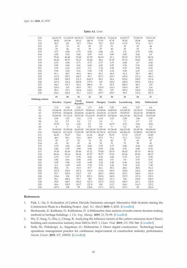
Appl. Sci. 2020, 10, 3733

Table A1. Cont.

X10 62,101.79 111,234.55 44,353.13 71,095.93 99,888.18 71,218.16 65,232.77 57,001.93 72,911.29X11 28.02 101.09 29.12 140.79 73.91 47.97 92.42 29.04 46.65X12 36.3 101 19.2 176.6 70.7 47.8 117.6 37.4 67.1X13 23 33 51 84 27 51 34 55 44X14 19 46 61 79 27 40 39 55 37X15 0.77 0.88 0.75 0.82 0.86 0.8 0.8 0.75 0.84X16 0.85 0.92 0.82 0.87 0.91 0.87 0.85 0.82 0.9X17 79.41 86.48 74.69 81.59 86.43 81.1 85.33 74.33 84.76X18 80.42 86.77 76.17 82.48 86.4 81.25 87.12 74.81 85.8X19 0.76 0.84 0.71 0.73 0.77 0.79 0.68 0.7 0.82X20 0.87 0.89 0.81 0.83 0.87 0.87 0.76 0.76 0.89X21 5.57 6.93 4.51 5.2 7.18 5.95 5.27 5.59 5.92X22 5.94 6.92 5.01 5.29 7.25 6.18 5.69 6.07 6.12X23 81.1 90.7 90.4 96.6 87.3 94.9 91.4 78.7 88.5X24 113.2 105.5 106.3 99.1 107.1 103.7 105.4 121.4 106.3X25 138.8 109.2 131.3 1041.9 89.9 90.4 553.6 104.5 191.4X26 167.6 136.2 205.8 175.9 107 138.2 245.8 109.2 136.2X27 94.9 101.7 83.4 286.5 97 85.5 200.5 84.7 133X28 120.6 103 88.5 74.7 115.9 116.3 100.4 86.7 116X29 96.9 95.3 106.4 134.5 99.7 107 182.3 102.8 120.4X30 104.1 104.9 92.1 131.2 107.7 105.7 99.9 110.6 107.5

Defining criteria19 20 21 22 23 24 25 26 27

Slovakia CyprusCzech

RepublicIreland Hungary Croatia Luxembourg Italy Netherlands

X1 3.15 4.38 2.02 1.71 4.98 2.82 4.62 3.27 4.4X2 19,546.90 28,159.30 23,078.57 78,806.43 15,938.84 14,869.09 114,340.50 34,318.35 53,024.06X3 19,979.43 29,844.96 23,655.00 41,426.35 19,634.74 17,136.39 79,529.57 32,216.30 39,980.96X4 33,069.90 37,172.10 35,537.00 73,214.70 29,558.70 24,748.60 105,147.60 38,233.50 53,933.00X5 4.05 1.87 3.12 1.74 6.35 2.53 2.08 1.88 1.87X6 2.6 0.7 2.6 1.2 3.4 1 1.7 0.7 2.5X7 13.52 7.6 6.22 8.1 7.2 16.73 4.72 9.44 4.94X8 6 7 2.2 5.5 3.5 9 5.2 10.3 3.3X9 53,695.00 72,390.00 54,439.00 103,942.00 53,355.00 51,526.00 140,215.00 92,307.00 90,424.00X10 76,662.91 81,134.22 71,002.58 149,707.06 65,736.31 62,514.81 142,966.76 91,588.91 101,949.93X11 44.03 74.67 32.6 61.02 68.65 56.51 15.15 115.37 54.85X12 48.4 96.1 31.6 60.9 67.5 71.1 21.3 133.2 49.2X13 39 47 52 14 50 80 57 64 29X14 45 54 41 24 52 51 72 58 42X15 0.79 0.82 0.82 0.86 0.79 0.77 0.86 0.84 0.89X16 0.86 0.87 0.89 0.94 0.85 0.84 0.91 0.88 0.93X17 79.59 81.09 83.46 87.21 79.08 78.76 86.02 85.19 88.32X18 80.43 83.14 84.36 87.97 78.77 79.21 87.66 85.69 88.31X19 0.75 0.71 0.78 0.82 0.76 0.68 0.72 0.72 0.84X20 0.82 0.81 0.89 0.92 0.82 0.8 0.8 0.79 0.91X21 6.09 5.86 6.59 6.98 5.24 5.49 6.96 6.02 7.42X22 6.2 6.05 6.85 7.02 5.76 5.43 7.09 6.22 7.49X23 89.4 91 91.9 97.7 82.1 95.5 88.6 89.8 91.2X24 107.8 100.6 107.2 105.4 114.4 100.3 104.8 102.2 106.5X25 92.7 325.6 125.7 371 268.3 226.8 103.1 344.9 122.5X26 116.6 194 127.2 223.1 302.4 168.9 137.3 127.4 129.3X27 94.1 188.2 99.1 183 102.2 131.3 102 134.8 108.3X28 99.8 180.7 106.5 147.2 127.5 110.3 108.7 101.1 125.8X29 99.6 138.5 103.7 127.8 109 113.7 104.1 116.5 123.2X30 107.2 138 99 138.6 117.1 107.6 107.1 98 106.4

References

1. Paik, I.; Na, S. Evaluation of Carbon Dioxide Emissions amongst Alternative Slab Systems during theConstruction Phase in a Building Project. Appl. Sci. (Basel) 2019, 9, 4333. [CrossRef]

2. Morkunaite, Z.; Kalibatas, D.; Kalibatiene, D. A bibliometric data analysis of multi-criteria decision makingmethods in heritage buildings. J. Civ. Eng. Manag. 2019, 25, 76–99. [CrossRef]

3. Wu, P.; Song, Y.; Zhu, J.; Chang, R. Analyzing the influence factors of the carbon emissions from China’sbuilding and construction industry from 2000 to 2015. J. Clean. Prod. 2019, 221, 552–566. [CrossRef]

4. Tetik, M.; Peltokorpi, A.; Seppänen, O.; Holmström, J. Direct digital construction: Technology-basedoperations management practice for continuous improvement of construction industry performance.Autom. Constr. 2019, 107, 102910. [CrossRef]

40

Appl. Sci. 2020, 10, 3733

5. Chowdhury, T.; Adafin, J.; Wilkinson, S. Review of digital technologies to improve productivity of NewZealand construction industry. J. Inf. Technol. Constr. (ITcon) 2019, 24, 569–587.

6. Xu, X.; Wang, Y.; Tao, L. Comprehensive evaluation of sustainable development of regional constructionindustry in China. J. Clean. Prod. 2019, 211, 1078–1087. [CrossRef]

7. Fang, Q.; Chen, L.; Zeng, D.; Zhang, L. Drivers of Professional Service Model Innovation in the ChineseConstruction industry. Sustainability 2019, 11, 941. [CrossRef]

8. Bahramian, M.; Yetilmezsoy, K. Life cycle assessment of the building industry: An overview of two decadesof research (1995–2018). Energy Build. 2020, 219, 109917. [CrossRef]

9. Hong, T.; Wang, Z.; Luo, X.; Zhang, W. State-of-the-art on research and applications of machine learning inthe building life cycle. Energy Build. 2020, 212, 109831. [CrossRef]

10. Mourão, J.; Gomes, R.; Matias, L.; Niza, S. Combining embodied and operational energy in buildingsrefurbishment assessment. Energy Build. 2019, 197, 34–46. [CrossRef]

11. Gluch, P.; Gustafsson, M.; Baumann, H.; Lindahl, G. From tool-making to tool-using and back: Rationales foradoption and use of LCC. Int. J. Strateg. Prop. Manag. 2018, 22, 179–190. [CrossRef]

12. Succar, B.; Poirier, E. Lifecycle information transformation and exchange for delivering and managing digitaland physical assets. Autom. Constr. 2020, 112, 103090. [CrossRef]

13. Ozturk, G.B. Interoperability in building information modeling for AECO/FM industry. Autom. Constr. 2020,113, 103122. [CrossRef]

14. Muller, M.F.; Esmanioto, F.; Huber, N.; Loures, E.R.; Junior, O.C. A systematic literature review ofinteroperability in the green building information modeling lifecycle. J. Clean. Prod. 2019, 223, 397–412.[CrossRef]

15. Santos, R.; Costa, A.A.; Silvestre, J.D.; Vandenbergh, T.; Pyl, L. BIM-based life cycle assessment and life cyclecosting of an office building in Western Europe. Build. Environ. 2020, 169, 106568. [CrossRef]

16. Orgut, R.E.; Batouli, M.; Zhu, J.; Mostafavi, A.; Jaselskis, E.J. Critical Factors for Improving Reliability ofProject Control Metrics throughout Project Life Cycle. J. Manag. Eng. 2020, 36, 04019033. [CrossRef]

17. Kotb, M.H.; Aly, A.S.; Muhammad, E.K.M.A. Risk Assessment of Time and Cost Overrun Factors throughoutConstruction Project Lifecycle. Life Sci. J. 2019, 16, 78–91. [CrossRef]

18. Janjua, S.; Sarker, P.; Biswas, W. Sustainability Assessment of a Residential Building using a Life CycleAssessment Approach. Chem. Eng. Trans. 2019, 72, 19–24.

19. Noktehdan, M.; Shahbazpour, M.; Zare, M.R.; Wilkinson, S. Innovation Management and ConstructionPhases in Infrastructure Projects. J. Constr. Eng. Manag. 2019, 145, 04018135. [CrossRef]

20. Tupenaite, L.; Kaklauskas, A.; Voitov, I.; Trinkunas, V.; Siniak, N.; Gudauskas, R.; Naimaviciene, J.;Kanapeckiene, L. Multiple criteria assessment of apartment building performance for refurbishmentpurposes. Int. J. Strateg. Prop. Manag. 2018, 22, 236–251. [CrossRef]

21. Kaklauskas, A. Analysis of the Life Cycle of a Built Environment: Monograph; Nova Science Publishers, Incorporated:Hauppauge, NY, USA, 2016; Available online: http://iti.vgtu.lt/ceneast/Media/Default/Documents/books/Textbook_Analysis_of_the_life_cycle_of_the_built_environment.pdf (accessed on 15 March 2020).

22. Knight, K.W.; Rosa, E.A.; Schor, J.B. Could working less reduce pressures on the environment? A cross-nationalpanel analysis of OECD countries, 1970–2007. Glob. Environ. Chang. 2013, 23, 691–700. [CrossRef]

23. Corrigan, G.; Crotti, R.; Hanouz, M.D.; Serin, C.; Drzeniek Hanouz, M.; Serin, C. Assessing progresstoward sustainable competitiveness. In The Global Competitiveness Report 2014–2015; World Economic Forum:Cologny, Switzerland, 2014; Chapter 1.2; pp. 53–83.

24. Piketty, T.; Goldhammer, A. Capital in the Twenty-First Century; The Belknap Press of Harvard UniversityPress: Cambridge MA, USA, 2014.

25. Alwan, Z.; Jones, P.; Holgate, P. Strategic sustainable development in the UK construction industry, throughthe framework for strategic sustainable development, using Building Information Modelling. J. Clean. Prod.2017, 140, 349–358. [CrossRef]

26. Ambec, S.; Cohen, M.A.; Elgie, S.; Lanoie, P.; Canada, B.; Chabot, R.; Thornton, G. The porter hypothesis at20: Can environmental regulation enhance innovation and competitiveness? Rev. Environ. Econ. Policy 2013,7, 2–22. [CrossRef]

27. Ortiz, O.; Castells, F.; Sonnemann, G. Sustainability in the construction industry: A review of recentdevelopments based on LCA. Constr. Build. Mater. 2009, 23, 28–39. [CrossRef]

41

Appl. Sci. 2020, 10, 3733

28. Yılmaz, M.; Bakıs, A. Sustainability in Construction Sector. Procedia Soc. Behav. Sci. 2015, 195, 2253–2262.[CrossRef]

29. Doyle, E.; Alaniz, M.P. Dichotomous impacts on social and environmental sustainability: Competitivenessand development levels matter. Compet. Rev. Int. Bus. J. 2020, in press. [CrossRef]

30. Hayden, A.; Shandra, J.M. Hours of work and the ecological footprint of nations: An exploratory analysis.Local Environ. 2009, 14, 575–600. [CrossRef]

31. Liu, L.; Lei, Y. Dynamic changes of the ecological footprint in the Beijing-Tianjin-Hebei region from 1996to 2020. Ecol. Indic. 2020, 112, 106142. [CrossRef]

32. Shujah-ur-Rahman; Chen, S.S.; Saud, S.; Saleem, N.; Bari, M.W. Nexus between financial development,energy consumption, income level, and ecological footprint in CEE countries: Do human capital andbiocapacity matter? Environ. Sci. Pollut. Res. 2019, 26, 31856–31872. [CrossRef]

33. Toth, G.; Szigeti, C. The historical ecological footprint: From over-population to over-consumption. Ecol. Indic.2016, 60, 283–291. [CrossRef]

34. Al-Mulali, U.; Weng-Wai, C.; Sheau-Ting, L.; Mohammed, A.H. Investigating the environmental Kuznetscurve (EKC) hypothesis by utilizing the ecological footprint as an indicator of environmental degradation.Ecol. Indic. 2015, 48, 315–323. [CrossRef]

35. Tektüfekçi, F.; Kutay, N. The Relationship between EPI and GDP Growth: An Examination on Developedand Emerging Countries. J. Mod. Account. Audit. 2016, 12, 268–276. [CrossRef]

36. Hsu, A.; Lloyd, A.; Emerson, J.W. What progress have we made since Rio? Results from the 2012 EnvironmentalPerformance Index (EPI) and Pilot Trend EPI. Environ. Sci. Policy 2013, 33, 171–185. [CrossRef]

37. Sineviciene, L.; Kubatko, O.; Derykolenko, O.; Kubatko, O. The impact of economic performance onenvironmental quality in developing countries. Int. J. Environ. Technol. Manag. 2018, 21, 222–237. [CrossRef]

38. Bernard, J.; Mandal, S.K. The impact of trade openness on environmental quality: An empirical analysis ofemerging and developing economies. WIT Trans. Ecol. Environ. 2016, 203, 195–208.

39. Kaklauskas, A.; Herrera-Viedma, E.; Echenique, V.; Zavadskas, E.K.; Ubarte, I.; Mostert, A.; Podvezko, V.;Binkyte, A.; Podviezko, A. Multiple criteria analysis of environmental sustainability and quality of life inpost-Soviet states. Ecol. Indic. 2018, 89, 781–807. [CrossRef]

40. United Nations. Industry and environment. In Sustainable Building and Construction Initiative: InformationNote; UNEP, Division of Technology, Industry and Economics: Paris, France, 2003; Volume 26, Availableonline: http://www.uneptie.org/pc/pc/SBCI/SBCI_2006_InformationNote.pdf (accessed on 1 April 2020).

41. Wallbaum, H.; Buerkin, C. Concepts and instruments for a sustainable construction sector. Ind. Environ.2003, 26, 53–57.

42. Dobson, D.W.; Sourani, A.; Sertyesilisik, B.; Tunstall, A. Sustainable construction: Analysis of its costsand benefits. Am. J. Civ. Eng. Archit. 2013, 1, 32–38.

43. Akadiri, P.O.; Fadiya, O.O. Empirical analysis of the determinants of environmentally sustainable practicesin the UK construction industry. Constr. Innov. 2013, 13, 352–373. [CrossRef]

44. Rohracher, H. Managing the technological transition to sustainable construction of buildings: A socio-technicalperspective. Technol. Anal. Strateg. Manag. 2001, 13, 137–150. [CrossRef]

45. de Bruin, Y.B.; Koistinen, K.; Kephalopoulos, S.; Geiss, O.; Tirendi, S.; Kotzias, D. Characterisation of urbaninhalation exposures to benzene, formaldehyde and acetaldehyde in the European Union. Environ. Sci.Pollut. Res. 2008, 15, 417–430. [CrossRef] [PubMed]

46. EU 2020 Target for Energy Efficiency. 2014. Available online: https://ec.europa.eu/energy/en/topics/energy-efficiency/targets-directive-and-rules/eu-targets-energy-efficiency (accessed on 5 January 2020).

47. Kotler, P.; Gertner, D. Country as brand, product, and beyond: A place marketing and brand managementperspective. J. Brand Manag. 2002, 9, 249–261. [CrossRef]

48. Saeed, S.A. Creating a country brand identity: A Review of Literature. Pak. Bus. Rev. 2018, 20, 91–98.49. Herz, M.F.; Diamantopoulos, A. Activation of country stereotypes: Automaticity, consonance, and impact.

J. Acad. Mark. Sci. 2013, 41, 400–417. [CrossRef]50. Saridakis, C.; Baltas, G. Modeling price-related consequences of the brand origin cue: An empirical

examination of the automobile market. Mark. Lett. 2016, 27, 77–87. [CrossRef]51. Maheswaran, D.; Chen, C.Y. Nation equity: Country-of-origin effects and globalization. Handb. Int. Mark.

2009, 91–113. [CrossRef]

42

Appl. Sci. 2020, 10, 3733

52. Lumb, R.; Lall, V. Perception of the Quality of Products Made in India by Consumers from the United States:A Longitudinal Analysis. Indian J. Econ. Bus. 2006, 47.

53. Aichner, T. Country-of-origin marketing: A list of typical strategies with examples. J. Brand Manag. 2014, 21,81–93. [CrossRef]

54. Pappu, R.; Quester, P.G.; Cooksey, R.W. Country image and consumer-based brand equity: Relationshipsand implications for international marketing. J. Int. Bus. Stud. 2007, 38, 726–745. [CrossRef]

55. Roth, K.P.Z.; Diamantopoulos, A.; Montesinos, M.Á. Home country image, country brand equity andconsumers’ product preferences: An empirical study. Manag. Int. Rev. 2008, 48, 577–602. [CrossRef]

56. Elliot, S.; Papadopoulos, N. Of products and tourism destinations: An integrative, cross-national study ofplace image. J. Bus. Res. 2016, 69, 1157–1165. [CrossRef]

57. Kaklauskas, A. Degree of Project Utility and Investment Value Assessments. Int. J. Comput. Commun. Control2016, 11, 666–683. [CrossRef]

58. Zavadskas, E.K.; Kaklauskas, A.; Sarka, V. The new method of multicriteria complex proportional assessmentof projects. Technol. Econ. Dev. Econ. 1994, 1, 131–139.

59. Marx, H.J. Outcomes of the 2014 Survey of the CIDB Construction Industry Indicators. 2014. Availableonline: http://www.cidb.org.za/papers/Documents/Construction%20Industry%20Indicators%20-%202014%20Survey%20Outcomes%20-%20Full%20Report.pdf (accessed on 1 April 2020).

60. Zhang, P.; London, K. A Comparative Evaluation of Construction Industry International Performancebetween China and United States Using the International Advanced Index. In Management of Construction:Analysis to Practice, Proceedings of the Joint CIB International Symposium of W055, W065, W089, W118, TG76,TG78, TG81 and TG84 (CIB 2012), Montreal, QC, Canada, 26–29 June 2012; In-House Publishing: Brisbane,Australia, 2012; pp. 25–36.

61. Zhou, Q. Advances in Applied Economics, Business and Creation: International Symposium, Proceedings of the ISAEBD2011, Dalian, China, 6–7 August 2011; Part 2; Springer Science & Business Media: Berlin, Germany, 2011.

62. Meikle, J.L.; Grilli, M.T. Measuring European Construction Output: Problems and Possible Solutions. 1999.Available online: http://citeseerx.ist.psu.edu/viewdoc/download?doi=10.1.1.201.-4682&rep=rep1&type=pdf(accessed on 1 April 2020).

63. Šaparauskas, J. The key aspects of sustainability evaluation in construction. In Proceedings of the 9thInternational Conference on Modern Building Materials, Structures and Techniques, Vilnius, Lithuania,16–18 May 2007.

64. Sultan, B.; Kajewski, S. The behaviour of construction costs and affordability in developing countries:A yemen case study. In Proceedings of the Joint International Symposium on Knowledge Construction ofCIB Working Commissions W55, W65 and W107, Singapore, 22–24 October 2003.

65. Deloitte Real Estate. European Construction Monitor, 2015–2016: PE Firms Aim for European ConstructionMarket. 2016. Available online: https://www2.deloitte.com/content/dam/Deloitte/glo-bal/Documents/About-Deloitte/gx-real-est-construction-monitor.pdf (accessed on 11 March 2020).

66. Building Radar. Construction Industry in Europe. 2016. Available online: https://buildingradar.com/construction-blog/construction-industry-europe/ (accessed on 11 March 2020).

67. European Foundation for the Improvement of Living and Working Conditions. Trends and Drivers of Changein the European Construction Sector: Mapping Report. 2005. Available online: http://www.certificazione.unimore.it/site/home/documento124000637.html (accessed on 1 April 2020).

68. European Commission. European Construction Sector Observatory, Country Profile France; European Commision:Brussels, Belgium, 2018.

69. Olanrewaju, A.L.; Abdul-Aziz, A.R. Building Maintenance Processes, Principles, Procedures, Practices andStrategies. In Building Maintenance Processes and Practices; Springer: Singapore, 2015; pp. 79–129.

70. Nazarko, J.; Chodakowskaa, E. Measuring productivity of construction industry in Europe with DataEnvelopment Evaluation. Procedia Eng. 2015, 122, 204–212. [CrossRef]

71. United Nations Development Programme. Human Development Reports, Education Index, GenderInequeality. 2019. Available online: http://hdr.undp.org/en/data (accessed on 5 January 2020).

72. The World Bank Group. GDP Growth (Annual %). 2019. Available online: https://data.worldbank.org/indicator/ny.gdp.mktp.kd.zg (accessed on 10 February 2020).

73. The World Bank Group. GDP Per Capita (Current US$). 2019. Available online: https://data.worldbank.org/indicator/NY.GDP.PCAP.CD (accessed on 10 February 2020).

43

Appl. Sci. 2020, 10, 3733

74. CountryEconomy.com. Gross Domestic Product. 2020. Available online: https://countryeconomy.com/gdp(accessed on 5 January 2017).

75. Trading Economics. GDP Growth Rate, GDP Per Capita, GDP per Capita PPP. 2020. Available online:https://tradingeconomics.com/ (accessed on 5 January 2020).

76. The World Bank Group. GDP per Capita, PPP (Current International $). 2019. Available online: https://data.worldbank.org/indicator/NY.GDP.PCAP.PP.CD (accessed on 10 February 2020).

77. StatisticsTimes.com. List of Countries by GDP (PPP) per Capita. 2020. Available online: http://statisticstimes.com/economy/countries-by-gdp-capita-ppp.php (accessed on 10 February 2020).

78. The World Bank Group. Inflation, Consumer Prices (Annual %). 2019. Available online: https://data.worldbank.org/indicator/FP.CPI.TOTL.ZG?locations=AT (accessed on 5 March 2020).

79. The World Bank Group. Unemployment, Total. 2019. Available online: https://data.worldbank.org/indicator/sl.uem.totl.zs (accessed on 10 February 2020).

80. Global Economy. Unemployment Rate—Country Rankings. 2020. Available online: http://www.theglobaleconomy.com/rankings/Unemployment_rate/ (accessed on 5 January 2020).

81. The World Bank Group. Doing Business Reports. 2019. Available online: https://www.doingbusiness.org/en/reports/global-reports/doing-business-2020 (accessed on 5 April 2020).

82. Conference Board. The Conference Board Total Economy Database™. November 2018. Available online:https://www.conference-board.org/data/economydatabase/index.cfm?id=30565 (accessed on 5 January 2020).

83. CountryEconomy.com. General Government Gross Debt. 2020. Available online: http://countryeconomy.com/national-debt (accessed on 10 February 2020).

84. IMF. Debt % of GDP. 2019. Available online: https://www.imf.org/external/datamapper/DEBT1@DEBT/OEMDC/ADVEC/WEOWORLD (accessed on 10 February 2020).

85. Central Intelligent Agency. Public Debt. 2020. Available online: https://www.cia.gov/library/publications/the-world-factbook/rankorder/2186rank.html (accessed on 10 February 2020).

86. World Happiness Report. 2020. Available online: https://worldhappiness.report/ (accessed on 5 January2020).

87. Social Progress Index. 2014. Available online: https://www2.deloitte.com/content/dam/Deloitte/cr/Documents/public-sector/2014-Social-Progress-IndexRepIMP.pdf (accessed on 10 February 2020).

88. Social Progress Index. 2015. Available online: https://progresosocial.org.gt/wp-content/uploads/2015/04/2015-Methodology-Report.pdf (accessed on 10 February 2020).

89. Social Progress Index. 2016. Available online: https://www2.deloitte.com/content/dam/Deloitte/mx/Documents/about-deloitte/Social-Progress-Index-2016-Report.pdf (accessed on 10 February 2020).

90. Social Progress Index. 2017. Available online: https://www2.deloitte.com/content/dam/Deloitte/de/Documents/public-sector/Social-Progress-Index-Findings-Report-SPI-2017.pdf (accessed on 10 February 2020).

91. Social Progress Index. 2018. Available online: https://www.socialprogress.org/assets/downloads/resources/2018/2018-Social-Progress-Index-Exec-Summary.pdf (accessed on 10 February 2020).

92. Social Progress Index. 2019. Available online: https://www.socialprogress.org/assets/downloads/resources/2019/2019-Social-Progress-Index-executive-summary-v2.0.pdf (accessed on 10 February 2020).

93. Eurostat.eu. Construction Cost (or Producer Prices), New Residential Buildings—Annual Data. 2020.Available online: http://appsso.eurostat.ec.europa.eu/nui/show.do?dataset=sts_copi_a&lang=en (accessed on5 January 2020).

94. Eurostat.eu. Building Permits—Annual Data. 2020. Available online: http://appsso.eurostat.ec.europa.eu/nui/show.do?dataset=sts_cobp_a&lang=en (accessed on 5 January 2020).

95. Eurostat.eu. Production in Construction—Annual Data. 2020. Available online: https://appsso.eurostat.ec.europa.eu/nui/show.do?dataset=sts_copr_a&lang=en (accessed on 5 January 2020).

96. Eurostat.eu. Labour Input in Construction—Annual Data. 2020. Available online: https://appsso.eurostat.ec.europa.eu/nui/show.do?dataset=sts_colb_a&lang=en (accessed on 5 January 2020).

97. The World Bank Group. Life Expectancy at Birth. 2017. Available online: https://data.worldbank.org/indicator/SP.DYN.LE00.IN?end=2017&start=1990 (accessed on 5 January 2020).

98. Eurostat.eu. Distribution of Population by Tenure Status, Type of Household and Income Group—EU-SILCSurvey. 2018. Available online: https://appsso.eurostat.ec.europa.eu/nui/submitViewTableAction.do(accessed on 5 January 2020).

44

Appl. Sci. 2020, 10, 3733

99. Transparency.org. Corruption Perceptions Index. 2020. Available online: https://www.transparency.org/cpi2019?/news/feature/cpi-2019 (accessed on 5 January 2020).

100. Numbeo.com. Quality of Life. 2019. Available online: https://www.numbeo.com/quality-of-life/rankings_by_country.jsp?title=2019 (accessed on 5 January 2020).

101. Gilbert, A. Rental housing: The international experience. Habitat Int. 2016, 54, 173–181. [CrossRef]102. Oecd.org. Real House Prices, Nominal House Prices. 2019. Available online: https://data.oecd.org/price/

housing-prices.htm (accessed on 5 January 2020).103. Numbeo.com. Price to Rent Ratio. 2020. Available online: https://www.numbeo.com/property-investment/

rankings.jsp (accessed on 5 January 2020).104. Eurostat.eu. House Price Index—Annual Data. 2020. Available online: https://ec.europa.eu/eurostat/

databrowser/view/tipsho20/default/table?lang=en (accessed on 5 January 2020).105. Kock, F.; Josiassen, A.; Assaf, A.G. Toward a Universal Account of Country-Induced Predispositions:

Integrative Framework and Measurement of Country-of-Origin Images and Country Emotions. J. Int. Mark.2019, 27, 43–59. [CrossRef]

© 2020 by the authors. Licensee MDPI, Basel, Switzerland. This article is an open accessarticle distributed under the terms and conditions of the Creative Commons Attribution(CC BY) license (http://creativecommons.org/licenses/by/4.0/).

45

applied sciences

Article

Identification and Prioritization of Critical Risk Factors ofCommercial and Recreational Complex Building Projects:A Delphi Study Using the TOPSIS Method

Jolanta Tamošaitiene 1, Mojtaba Khosravi 2, Matteo Cristofaro 3, Daniel W. M. Chan 4 and Hadi Sarvari 5,*

���������������

Citation: Tamošaitiene, J.; Khosravi,

M.; Cristofaro, M.; Chan, D.W.M.;

Sarvari, H. Identification and

Prioritization of Critical Risk Factors

of Commercial and Recreational

Complex Building Projects: A Delphi

Study Using the TOPSIS Method.

Appl. Sci. 2021, 11, 7906. https://

doi.org/10.3390/app11177906

Academic Editor: Edyta

Plebankiewicz

Received: 12 July 2021

Accepted: 23 August 2021

Published: 27 August 2021

Publisher’s Note: MDPI stays neutral

with regard to jurisdictional claims in

published maps and institutional affil-

iations.

Copyright: © 2021 by the authors.

Licensee MDPI, Basel, Switzerland.

This article is an open access article

distributed under the terms and

conditions of the Creative Commons

Attribution (CC BY) license (https://

creativecommons.org/licenses/by/

4.0/).

1 Faculty of Civil Engineering, Institute of Sustainable Construction, Vilnius Gediminas Technical University,LT-10223 Vilnius, Lithuania; jolanta.tamosaitiene@vilniustech.lt

2 Department of Civil Engineering, Najafabad Branch, Islamic Azad University, Najafabad 8514143131, Iran;m.khosravi@sci.iaun.ac.ir

3 Department of Management and Law, University of Rome “Tor Vergata”, 00133 Rome, Italy;matteo.cristofaro@uniroma2.it

4 Department of Building and Real Estate, The Hong Kong Polytechnic University, Hung Hom, Kowloon,Hong Kong, China; daniel.w.m.chan@polyu.edu.hk

5 Department of Civil Engineering, Isfahan (Khorasgan) Branch, Islamic Azad University,Isfahan 8155139998, Iran

* Correspondence: h.sarvari@khuisf.ac.ir

Abstract: Construction development of Commercial and Recreational Complex Building Projects(CRCBPs) is one of the community needs of many developing countries. Since the implementationof these projects is usually very costly, identifying and evaluating their Critical Risk Factors (CRFs)are of significant importance. Therefore, the current study aims to identify and prioritize CRFs ofCRCBPs in the Iranian context. A descriptive-survey method was used in this research; the statisticalpopulation, selected based on the purposive sampling method, includes 30 construction expertswith hands-on experience in CRCBPs. A questionnaire related to the risk identification stage wasdeveloped based on a detailed study of the research literature and also using the Delphi surveymethod; 82 various risks were finally identified. In order to confirm the opinions of experts inidentifying the potential risks, Kendall’s coefficient of concordance was used. In the first stage ofdata analysis, qualitative evaluation was performed by calculating the severity of risk effect anddetermining the cumulative risk index, based on which 25 CRFs of CRCBPs were identified formore accurate evaluation. At this stage, the identified CRFs were evaluated based on multi-criteriadecision-making techniques and using the TOPSIS technique. Results show that the ten CRFs ofCRCBPs are external threats from international relations, exchange rate changes, bank interest ratefluctuations, traffic licenses, access to skilled labor, changes in regional regulations, the conditionof adjacent buildings, fluctuations and changes in inflation, failure to select a suitable and qualifiedconsultant, and employer’s previous experiences and records. Obviously, the current study’s resultsand findings can be considered by CRCBPs in both the private and public sectors for proper effectiverisk identification, evaluation, and mitigation.

Keywords: risk identification; risk assessment; MCDM; critical risk factors; commercial and recre-ational complex building projects; construction

1. Introduction

“Risk is an uncertain event or conditions that, if it occurs, has a positive or negativeeffect on a project objective” [1]; from that, construction projects are massively pervadedby risks due to the fact that they are planned and managed on the basis of uncertainforecasts [2,3]. These uncertainties come from the ‘variability’ and ‘ambiguity’ in relationto performance measures like cost, duration, or quality and, according to [4], they can begrouped into five areas in relation to construction projects: The variability associated with

Appl. Sci. 2021, 11, 7906. https://doi.org/10.3390/app11177906 https://www.mdpi.com/journal/applsci

47

Appl. Sci. 2021, 11, 7906

estimates of project parameters, the basis of estimates of project parameters, design andlogistics, objectives and priorities, and relationships between project parties. From thecited categories of uncertainty, some risks are inherently related to the project operatingorganizations and only they are responsible for managing them, while others are related tothe economic, social, political, and technological environments [5].

Hence, identifying and evaluating risks in projects is necessary and can play a veryimportant role in achieving project objectives. Project management literature identifiedseveral techniques for identifying and assessing risks involved in the construction industry.For instance, it has been found that the main reference in risk identification is historicaldata, past experience, and judgement [6]. According to Chapman [7], risk identificationmethods can be grouped into three general categories: Identifying the risks by the riskanalyst; risk identification by interviewing key members of the project team; and riskidentification through brainstorming meetings. In this regard, research has shown that thequestionnaire survey is the most frequently used technique for risk identification in theconstruction sector [8,9]. However, despite the literature produced (see also [10–14]), fewcontributions (e.g., Tamošaitiene et al. [12]) have been dedicated to the risks in Commercialand Recreational Complex Building Projects (CRCBPs)—which comprise shops connectedto each other with sidewalks that are designed and built alongside recreational, residential,office, hotel, restaurant, and cinema spaces [15,16]. Among them, it is worth mentioningthe work of Comu et al. [17] that, despite classifying risks for CRCBPs, has the drawback ofdiverging from a very extensive list of risk factors (i.e., 21; much less than the 82 includedin this study). This is the gap addressed in this work and that can be synthesized in thefollowing research question: What are the most severe risks in commercial and recreationalcomplex building projects (CRCBPs)?

To answer the above research question, the Delphi method is used to identify commonrisks of CRCBPs. Then, the qualitative method of probability of occurrence and the effectof risk on project objectives is adopted to identify CRFs of CRCBPs. Finally, a multi-criteriadecision making (MCDM) method is employed, i.e., Technique for Order of Preferenceby Similarity to Ideal Solution (TOPSIS). This is another great advancement with respectto prior works that have been interested in CRFs of CRCBPs (i.e., [5]). As a result, thefindings of this research are an unseen contribution to the original body of CRCBPs andthe construction industry. Such an outcome would enable decision makers to make moreinformed decisions with regard to, for example, proper risk allocation, bid pricing, selectionof the optimum procurement route, and evaluation of different construction projects.

2. Commercial and Recreational Complex Building Projects (CRCBPs)

The increase of the urban population in large metropolises, followed by the increasein demand for better building infrastructure on a global scale, paints a positive outlook forimproving the construction market’s situation in developing countries [18]. Over the pasttwo decades, the construction of CRCBPs, to develop the welfare of citizens and increasesocio-economic development indicators and subsequent sustainable development in Iran,has been greatly increased. Stemming from that, realizing projects faster and cheaper hasbeen prioritized by policymakers and, as a consequence, the amount of construction hasexceeded its quality [19].

Projects are divided into different types depending on the purpose and type of ex-pected operation. In the field of construction projects, we are faced with different typesthat the 2015 United Nations’ product classification (see Section 5) categorizes as Construc-tions Buildings and Civil Engineering Works [20]. A subclass of Construction Buildings isCommercial Buildings and among them there are Commercial and Recreational ComplexBuildings. CRCBPs comprise a series of interconnected sidewalk shops designed andconstructed in conjunction with entertainment, residential, office, hotel, restaurant, andcinema spaces [5]. In order to achieve economic growth, developing countries are forcedto increase investment in infrastructures [21]. In fact, development of an infrastructure,such as construction of CRCBPs, can positively affect economic development [22]. Some

48

Appl. Sci. 2021, 11, 7906

examples of CRCBPs include Siam Paragon in Bangkok, Berjaya Times in Kuala Lumpur,Jewelry in Istanbul, West Edmonton in Edmonton, Canada, Dubai Mall in the UAE, AventraMall in Miami, and Harrods in London.

However, some CRCBPs construction projects have been unsuccessful due to variousmarketing, financial and investment issues. A clear example of such projects is the CRCBPof Arge Jahannam in Isfahan, which has failed due to a lack of detailed market studies andnon-compliance with social rules and conditions [23]. In general, the existence of risk anduncertainty in the project reduces the accuracy and proper estimation of objectives and theefficiency of the project itself; in sum, the need to recognize and manage the risk of fullCRCBPs is being increasingly perceived.

3. Perceived Risks of CRCBPs

Risk is an inherent component of all projects, and it is not possible to eliminate itcompletely. Therefore, identifying and analyzing risks can play an important role in thesuccess of the project. In identifying the critical risk factors (CRFs) of any project, it isnot enough to identify the risks that occur gradually. However, with a well-defined riskstatement, weighing up not only what might happen, but also all the characteristics ofthe time of occurrence, probability of occurrence, and its impacts must also be considered.Determining a process for identifying, evaluating, and responding to CRFs will causeimprovements in the mechanism, increase the accuracy and quality of work, and havea direct impact on time and cost [24]. Marle and Gidel [25] also stated that uncertaintyand risk in projects affect project objectives more than anything else. Therefore, riskmanagement plays an important role in the quality and reliability of decisions duringa project.

The first step of risk management is to identify and record the characteristics of therisks that may affect the project (i.e., listing any potential risk to a project’s cost, schedule, orany other critical success factor [1]). Risk identification is an iterative process, as new risksmay be identified and discovered as the project progresses through its lifespan [16]. In orderto identify the risks, several methods have been proposed, including interviews, hypothesisanalysis, document review, the Delphi technique, brainstorming, graphing methods [26],Artificial Neural Network (ANN) [27], Failure Mode and Effects Analysis (FMEA) [28],Cross Analytical-Machine Learning models [29], and the Integration Definition for FunctionModeling (IDEF0) process [30]. In the risk identification phase, the risks affecting theobjectives should be prioritized and the impact of risks that do not affect the objectivesshould be avoided [12]. In this regard, the methods such as the Delphi technique are usefuldue to their simplicity, flexibility, and ease of access to experts [10,31–34]. With regard toCRCBPs, Chen and Khumpaisal [35] adopted an Analytic Network Process model basedon 29 defined risk assessment criteria associated with commercial real estate development,then classified the data under four risk clusters: Social risks, economic risks, environmentalrisks, and technological risks. However, no prioritization of these risks was offered. Thesame applies for the work by Tamošaitiene et al. [12], who identified 19 types of risks forCRCBPs divided into macro- (i.e., country, industry), meso- (i.e., project, enterprise), andmicro- (i.e., management, organization) categories.

The second step is risk analysis (i.e., the scope of the risk must be determined [1]),considered as a key factor in risk management that greatly aids the process. Risk classifi-cation is an important part of risk management issues with significant effects on the riskmanagement process. General classifications can include cost, financing, demand, andpolitical risks [36]. Risk classification should always be done with regard to the project’sobjectives [37]. There are different classification methods for risks that can be used fordifferent purposes. Based on this, the risks can be divided into main and subsidiary risks [38].They can also be categorized according to their impact on project objectives for projectstatus reporting purposes [39]. However, according to PMI [1], the most appropriate ap-proach for identifying and responding to risks is to determine risk groups based on theirorigin (instead of their impact), e.g., external risks, internal risks, technical risks, and legal

49

Appl. Sci. 2021, 11, 7906

risks [40]. Risk classification is usually done in the form of the Risk Breakdown Structure(RBS), which identifies the groups and subgroups of risks that may occur in a typicalproject, and they are classified based on their origin [41]. Then, the RBS prioritizes theserisks according to their weight—i.e., potential and probable harmful impact [1].

In these cases, where projects deal with a significant set of variables and there is aneed to prioritize decision-making parameters based on their relative importance, usingseveral techniques is a good tool for prioritizing and making more accurate scientificdecisions. In most previous research, risk ranking has been done by applying differentmethods such as the Analytic Hierarchy Process (AHP) [42,43], the Analytic NetworkProcess (ANP) [11,24], the Choosing by Advantages (CBA) method [44], and the Techniquefor Order of Preference by Similarity to Ideal Solution (TOPSIS) [10,45]. Furthermore,more sophisticated techniques have been advanced (e.g., Mata et al. [46]). For example,Liu et al. [47] proposed a model that integrates the Internet of Things (IoT), BuildingInformation Modeling (BIM), a security risk analysis method, the Apriori algorithm, and acomplex network.

In terms of produced results, with a focus on construction project delay, Chengand Darsa [27] found that the most important risk factors in the Ethiopian context are‘change order’, ‘corruption/bribery’, and ‘delay in payment’. Yet, recently, Chattapadhyayet al. [29] while investigating risks in megaprojects—by collecting and prioritizing risksas stated by 70 Indian megaprojects experts—found that the most severe risks are a delayin obtaining traffic regulation orders, inappropriate equipment, political and legal issues,political instability, government intervention, regulatory confirmation and regulation orderdelays, and wrong engineering designs. Comu et al. [17], instead, prioritized these risksfor CRCBPs in the Turkish context by using the ANP model; they found that ‘Exchangerate and inflation rate fluctuations’ ‘Political instability’, and ‘Location selection’ were riskfactors for CRCBPs projects in developing countries.

In terms of categories that can result from the application of the above tools, DrajiJahromi et al.’s [48] study identified twelve criteria for assessing risks, which are vulnerabil-ity, threat, consequence, uniqueness, risk uncertainty, proximity of risk, interaction of eachrisk, risk identification, response to risk occurrence, risk manageability, risk occurrence,and risk forecasting. In another study, Mohammadi Talvar and Panahi [49] also intro-duced various criteria for risk assessment, including technical dimensions, experimental,management, good track record and credibility, competence, and proposed price.

Failure to manage risks in CRCBPs usually leads to excessive costs and prolongationof the project [50] and considering the implementation of a risk management process inCRCBPs is necessary in order to try to countervail these failures.

4. Research Methodology

The present study seeks to provide clear guidance for the stakeholders to properlyidentify and classify the risks of CRCBPs. For this purpose, both qualitative and quanti-tative approaches were used for the current research. There are three main stages in thisstudy, as displayed in the following flowchart (Figure 1).

In situations where the prioritization of decision-making units, based on their rela-tive importance and according to various criteria, is considered, the use of multi-criteriadecision-making techniques is suitable for ranking and making rational decisions. Amongthese techniques, we can mention the multi-criteria decision-making methods that havebeen used according to the advantages and results as well as the characteristics of theTOPSIS method as a priority of risk prioritization [1].

50

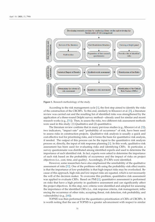
Appl. Sci. 2021, 11, 7906

Figure 1. Research methodology of the study.

According to the risk management cycle [1], the first step aimed to identify the risksof the construction of the CRCBPs. To this end, similarly to Khosravi et al. [5], a literaturereview was carried out and the resulting list of identified risks was strengthened by theapplication of a three-round Delphi survey method—already used for similar and recentresearch works (e.g., [51]). Then, to assess the risks, two different risk assessment methodswere used in this study: (1) Qualitative and (2) quantitative.

The literature review confirms that in many previous studies (e.g., Khosravi et al. [5]),two indicators, “impact rate” and “probability of occurrence” of risk, have been usedto assess risks in construction projects. Qualitative risk analysis is usually a quick andcost-effective tool for prioritizing risks, and it forms the basis for quantitative risk analysis,if needed. The output of this process can be the input to the quantitative risk analysisprocess or, directly, the input of risk response planning [1]. In this work, qualitative riskassessment has been used for evaluating risks and identifying CRFs. In particular, asurvey questionnaire was distributed among identified experts and used to determine theimportance of each identified risk. In fact, experts were asked to determine the importanceof each risk based on the probability of occurrence and the impact of risks on projectobjectives (i.e., cost, time, and quality). Accordingly, 25 CRFs were identified.

However, some researchers have also emphasized the unreliability of the qualitativeassessment of risks [52]. One of the problems with using the probability–risk effect matrixis that the importance of low-probability is that high-impact risks may be overlooked. Be-cause of this approach, high-risk and low-impact risks are equated, which is not necessarilythe will of the decision maker. To overcome this problem, quantitative risk assessmentwas applied to evaluate CRFs. Based on PMI [1], quantitative assessment is performedon risks that have a high priority in qualitative assessment and can significantly affectthe project objectives. In this step, new criteria were identified and adopted for assessingthe importance of the identified CRFs (i.e., risk response criteria, risk management, influ-encing the occurrence of other risks, accepting threat, risk detection, risk probability, andvulnerability) (e.g., [48]).

TOPSIS was then performed for the quantitative prioritization of CRFs of CRCBPs. Itis worth noting that the use of TOPSIS is a greater advancement with respect to similar

51

Appl. Sci. 2021, 11, 7906

works [5,53] because it has been proved to work satisfactorily across different applicationareas and industrial sectors with varying terms and subjects [54], and “although severaltechniques have been combined or integrated with the classical TOPSIS, many other tech-niques have not been investigated. These techniques make the classical TOPSIS morerepresentative and workable in handling practical and theoretical problems”. Stemmingfrom that recognized value of the TOPSIS method, in a series of studies. it has been empiri-cally found to be better performing than other techniques, such as the Analytical HierarchyProcess (e.g., [55]), under some contextual circumstances. With regard to the proposedapplication, TOPSIS has been successfully used in works concerning the assessment of risksin construction projects and it is the preferred method, rather than simple/probit/logitregressions in risk analysis works [54]; this is due to its ability to fully use attribute informa-tion, providing a cardinal ranking of alternatives, and not requiring attribute preferencesto be independent. Indeed, Gebrehiwet and Luo [56] recently adopted it for risk levelevaluation on a construction project lifecycle and found that the construction stage is themost influenced by risk factors. Yet, Dandage et al. [57] used TOPSIS for reviewing the riskcategories that are predominant in international projects and ranked them according totheir effect on project success; they found political risks, technical risks, and design-relatedrisks as the most important.

Investing in construction projects in Iran is one of the most lucrative decisions, butthe lack of regular supervision in this sector has caused the people in the community to beexposed to human and financial damage due to the quality of construction of buildings [58].Iran’s economic problems, along with the country’s situation in the international arena, areissues that foster project-related risks. In fact, political issues related to nuclear energy andsubsequent sanctions against Iran have led to an increase in Iran’s economic risk index inrecent years [11]. The growth of the economic risk index has undoubtedly reduced Iran’seconomic interactions with other parts of the world, which can increase the likelihoodof occurrence and severity of the impact of various other internal and external risks ofprojects [59]. At the same time, building construction is one of the main problems indeveloping countries today and because of rapid population growth, lack of financialresources, land problems, lack of skilled manpower, and, most importantly, lack of properpolicy and planning, this issue has become critical [60]. In light of the above, constructionprojects in Iran, as a developing country, are always associated with many risks anduncertainties. Therefore, Iran was selected for this study to identify and evaluate the CRFsof large and complex CRCBPs.

4.1. Delphi Survey Technique

The Delphi technique is often used for risk determination and screening before theapplication of a MCDM method. The Delphi technique’s main goal is to obtain the mostreliable experts’ opinions through a series of structured questionnaires with controlledfeedback. For the selection of experts that were asked to respond to the Delphi question-naires, one important rule is to prioritize the quality of experts over their quantity [50].From that, participants of the Delphi survey are experts with solid knowledge and ex-perience in the same subject, with time to participate in the research, and with effectivecommunication skills [61,62]. Regarding the number of involved experts, this is usuallyless than 50, and often from 10 to 20 [62,63]. The survey also depends on a series of factors,such as desired sample homogeneity, the Delphi goal, difficulty range, quality of decision,ability of the research team, internal and external validity, time of data collection, availableresources, and the scope of the problem under study [63]. The study adopted a purposivesampling technique in the selection of respondents, as done by other scholars for similarresearch [51,62]. In this regard, 30 experts were selected among practitioners of CRCBPsin Iran based on their level of knowledge and expertise in the field. In this regard, allthe experts in this study have experience in the construction of CRCBPs. The surveywas launched in May and June 2019. Table 1 shows the demographic data of the expertsparticipating in the Delphi process.

52

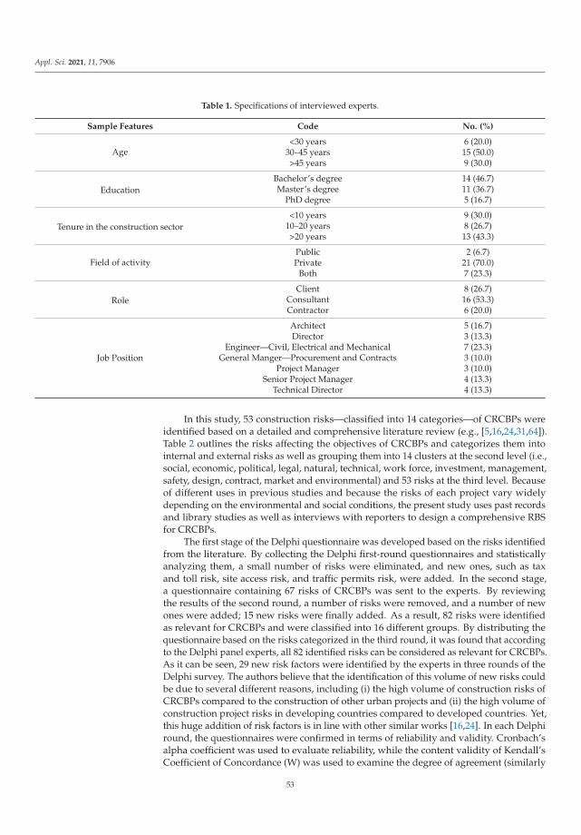
Appl. Sci. 2021, 11, 7906

Table 1. Specifications of interviewed experts.

Sample Features Code No. (%)

Age<30 years 6 (20.0)

30–45 years 15 (50.0)>45 years 9 (30.0)

EducationBachelor’s degree 14 (46.7)Master’s degree 11 (36.7)

PhD degree 5 (16.7)

Tenure in the construction sector<10 years 9 (30.0)

10–20 years 8 (26.7)>20 years 13 (43.3)

Field of activityPublic 2 (6.7)Private 21 (70.0)

Both 7 (23.3)

RoleClient 8 (26.7)

Consultant 16 (53.3)Contractor 6 (20.0)

Job Position

Architect 5 (16.7)Director 3 (13.3)

Engineer—Civil, Electrical and Mechanical 7 (23.3)General Manger—Procurement and Contracts 3 (10.0)

Project Manager 3 (10.0)Senior Project Manager 4 (13.3)

Technical Director 4 (13.3)

In this study, 53 construction risks—classified into 14 categories—of CRCBPs wereidentified based on a detailed and comprehensive literature review (e.g., [5,16,24,31,64]).Table 2 outlines the risks affecting the objectives of CRCBPs and categorizes them intointernal and external risks as well as grouping them into 14 clusters at the second level (i.e.,social, economic, political, legal, natural, technical, work force, investment, management,safety, design, contract, market and environmental) and 53 risks at the third level. Becauseof different uses in previous studies and because the risks of each project vary widelydepending on the environmental and social conditions, the present study uses past recordsand library studies as well as interviews with reporters to design a comprehensive RBSfor CRCBPs.

The first stage of the Delphi questionnaire was developed based on the risks identifiedfrom the literature. By collecting the Delphi first-round questionnaires and statisticallyanalyzing them, a small number of risks were eliminated, and new ones, such as taxand toll risk, site access risk, and traffic permits risk, were added. In the second stage,a questionnaire containing 67 risks of CRCBPs was sent to the experts. By reviewingthe results of the second round, a number of risks were removed, and a number of newones were added; 15 new risks were finally added. As a result, 82 risks were identifiedas relevant for CRCBPs and were classified into 16 different groups. By distributing thequestionnaire based on the risks categorized in the third round, it was found that accordingto the Delphi panel experts, all 82 identified risks can be considered as relevant for CRCBPs.As it can be seen, 29 new risk factors were identified by the experts in three rounds of theDelphi survey. The authors believe that the identification of this volume of new risks couldbe due to several different reasons, including (i) the high volume of construction risks ofCRCBPs compared to the construction of other urban projects and (ii) the high volume ofconstruction project risks in developing countries compared to developed countries. Yet,this huge addition of risk factors is in line with other similar works [16,24]. In each Delphiround, the questionnaires were confirmed in terms of reliability and validity. Cronbach’salpha coefficient was used to evaluate reliability, while the content validity of Kendall’sCoefficient of Concordance (W) was used to examine the degree of agreement (similarly

53

Appl. Sci. 2021, 11, 7906

to Sarvari et al. [51] and Khosravi et al. [5]). Kendall’s coefficient of concordance shows(i) whether people who sorted items according to their importance used similar criteriafor their judgment with regard to these items and (ii) whether these people agree witheach other [65,66]. Kendall’s coefficient of concordance is calculated using the followingFormula (1).

W =S

112 k2

(N3 − N

) , (1)

Within this formula, K is the sum of all rankers (number of judges); N is the numberof ranked items; 1

12 k2(

N3 − N)

is the maximum value of the sum of squares of variationsfrom average Rj (which is equal to S in case of complete agreement between K judges);S is the sum of squares of Rj variations minus the mean Rj (i.e., all ranks for an item).

From that, S is, therefore, calculated as follows: S = ∑[

Rj − ∑ RjN

]2. However, due to the

complexity and time-consuming calculations of the value of S, Kendall’s coefficient ofconcordance is computed by the Statistical Packages for Social Sciences (SPSS) computersoftware (similarly to other scholars [67–69]).

Table 2. Identified risks affecting the objectives of CRCBPs based on the review of the literature.

No.Chapter RBS

Level 1Group RBS

Level 2Risk RBS

Level 3References

R1

External

SocialDissatisfaction [2,24,70]

R2 Sabotage [2,24,37,70,71]

R3

Economical

Exchange rate fluctuation [10,35,36,70]

R4 Inflation [8,37,56,64,70]

R5 Government economic policies [11,70,72]

R6

Political

Government policies [37,41,70,73]

R7 Foreign threats [8,11,49,70,74]

R8 Political events [12,70,71]

R9

Legal

Changes in law [8,11,70]

R10 Standards and requirements [3,35,48,70,71]

R11 Regional standards [10,33,64,70]

R12 Changing point view of government organization [12,36,70,72]

R13

Natural

Earthquake [12,33,64,70]

R14 Storm [11,35,49,70]

R15 Flood [8,36,70]

R16 Fire [37,41,70,73]

R17Technical

Lack of documentation on the changes in project [3,36,70–72]

R18 Lack of acceptance changes control [11,24,56,70,74]

54

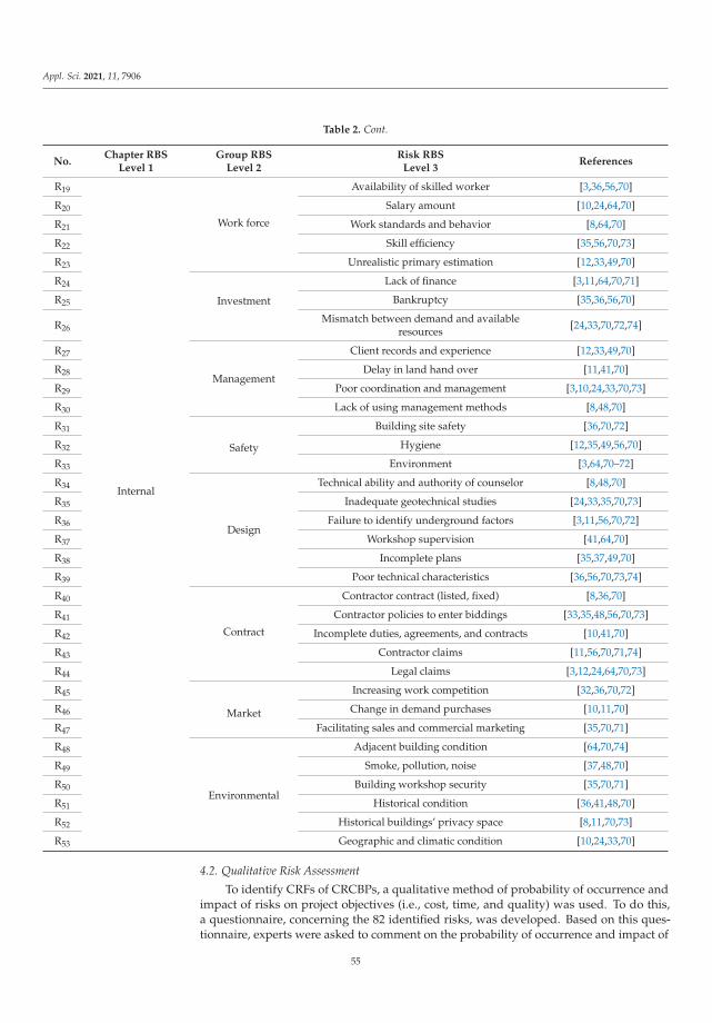
Appl. Sci. 2021, 11, 7906

Table 2. Cont.

No.Chapter RBS

Level 1Group RBS

Level 2Risk RBS

Level 3References

R19

Internal

Work force

Availability of skilled worker [3,36,56,70]

R20 Salary amount [10,24,64,70]

R21 Work standards and behavior [8,64,70]

R22 Skill efficiency [35,56,70,73]

R23 Unrealistic primary estimation [12,33,49,70]

R24

Investment

Lack of finance [3,11,64,70,71]

R25 Bankruptcy [35,36,56,70]

R26Mismatch between demand and available

resources [24,33,70,72,74]

R27

Management

Client records and experience [12,33,49,70]

R28 Delay in land hand over [11,41,70]

R29 Poor coordination and management [3,10,24,33,70,73]

R30 Lack of using management methods [8,48,70]

R31

Safety

Building site safety [36,70,72]

R32 Hygiene [12,35,49,56,70]

R33 Environment [3,64,70–72]

R34

Design

Technical ability and authority of counselor [8,48,70]

R35 Inadequate geotechnical studies [24,33,35,70,73]

R36 Failure to identify underground factors [3,11,56,70,72]

R37 Workshop supervision [41,64,70]

R38 Incomplete plans [35,37,49,70]

R39 Poor technical characteristics [36,56,70,73,74]

R40

Contract

Contractor contract (listed, fixed) [8,36,70]

R41 Contractor policies to enter biddings [33,35,48,56,70,73]

R42 Incomplete duties, agreements, and contracts [10,41,70]

R43 Contractor claims [11,56,70,71,74]

R44 Legal claims [3,12,24,64,70,73]

R45

Market

Increasing work competition [32,36,70,72]

R46 Change in demand purchases [10,11,70]

R47 Facilitating sales and commercial marketing [35,70,71]

R48

Environmental

Adjacent building condition [64,70,74]

R49 Smoke, pollution, noise [37,48,70]

R50 Building workshop security [35,70,71]

R51 Historical condition [36,41,48,70]

R52 Historical buildings’ privacy space [8,11,70,73]

R53 Geographic and climatic condition [10,24,33,70]

4.2. Qualitative Risk Assessment

To identify CRFs of CRCBPs, a qualitative method of probability of occurrence andimpact of risks on project objectives (i.e., cost, time, and quality) was used. To do this,a questionnaire, concerning the 82 identified risks, was developed. Based on this ques-tionnaire, experts were asked to comment on the probability of occurrence and impact of

55

Appl. Sci. 2021, 11, 7906

each of the risks of CRCBPs based on a 5-point Likert scale measurement (very low, low,medium, high and very high). The questionnaire used at this stage, like the Delphi stage,was evaluated and approved in terms of content reliability and validity. Risk refers to thenumber of expectations for that event to occur; in cases where the probability of occurrenceis random, it is only possible to rely on the opinion of experts [12]. The magnitude ofthe impact of risk and the probability of occurrence are expressed by using descriptiveor numerical expressions. Unlike the probability of occurrence, which is one, the impactof risk can have more than one effect; that is, it affects more than one project goal. Inpreparing the questionnaire, an attempt was made to obtain more valid results by insertingthe structure of risk failure and determining the group of internal and external originsof the risks. Yet, with the aim of prioritizing risks by using the risk failure structure andcalculating the effect of each risk, the score of each risk in the set of risk failure structurecan be determined. The intensity of the impact of each risk is obtained by multiplyingthe probability of occurrence of each risk by the impact of the same risk on the projectobjectives. Thus, at first an initial risk index is defined based on the criteria of probabilityof occurrence and the effect of risk on project time, cost, and quality (Formula (2)).

PIR = ∑ (PIt) + (PIc) + (PIq), (2)

In this equation, PIR represents the initial risk index for each risk. Furthermore, ‘P’ isthe probability of occurrence of risk; ‘It’ is the impact of risk on project time; ‘Ic’ is the impactof risk on project cost; and ‘Iq’ is the impact of risk on project quality. These indicators areseparately measured based on each expert’s opinion. To this end, according to Formula (3),the arithmetic mean method is used to aggregate indicators and the aggregated initial riskindex is calculated for each of the risks.

APIR =∑30

i=1(PIRi)

N(3)

In this formula, the APIR represents the cumulative primary risk index for each of therisks. ‘PIRi’ means initial risk index per risk for each specialist and ‘N’ is the total numberof experts; in this study, there are 30. Finally, by using this index, it is possible to rank therisks qualitatively based on the severity of the impact of each risk.

4.3. Quantitative Risk Assessment

After evaluating and qualitatively prioritizing the risks, a quantitative evaluation isperformed for CRFs of CRCBPs. To do this, the TOPSIS technique was used as one of theMCDM methods (Taylan et al., 2014). There are eight steps of the TOPSIS technique, basedon Hwang and Yoon [75]: (i) setting risk assessment criteria; (ii) adjusting the decisionmatrix based on the prepared questionnaires; (iii) converting the decision matrix intoa scaleless matrix; (iv) creating a weightless scale matrix; (v) identifying positive andnegative ideal solutions; (vi) calculating the relative distance through the ideal positiveand negative solutions; (vii) determining the relative proximity to each alternative; and(viii) determining the most important and least significant risks based on the proximityobtained. In this study, quantitative evaluation of CRFs has been done based on the samesteps. In addition, the calculations related to the TOPSIS method were done using MicrosoftExcel Office software.

In particular, to identify the risk assessment criteria, the results of the research of DrajiJahromi et al. [48]—which was performed to evaluate the risk assessment criteria—wereused. Thus, seven risk assessment criteria were selected to evaluate CRFs of CRCBPs.These criteria are (i) risk response criteria, (ii) risk management, (iii) influencing theoccurrence of other risks, (iv) accepting threat, (v) risk detection, (vi) risk probability, and(vii) vulnerability. Risks iii, iv, and vii were considered as criteria with a negative effect onrisk assessment, while risks i, ii, v, and vi were considered as criteria with a positive effecton risk assessment.

56

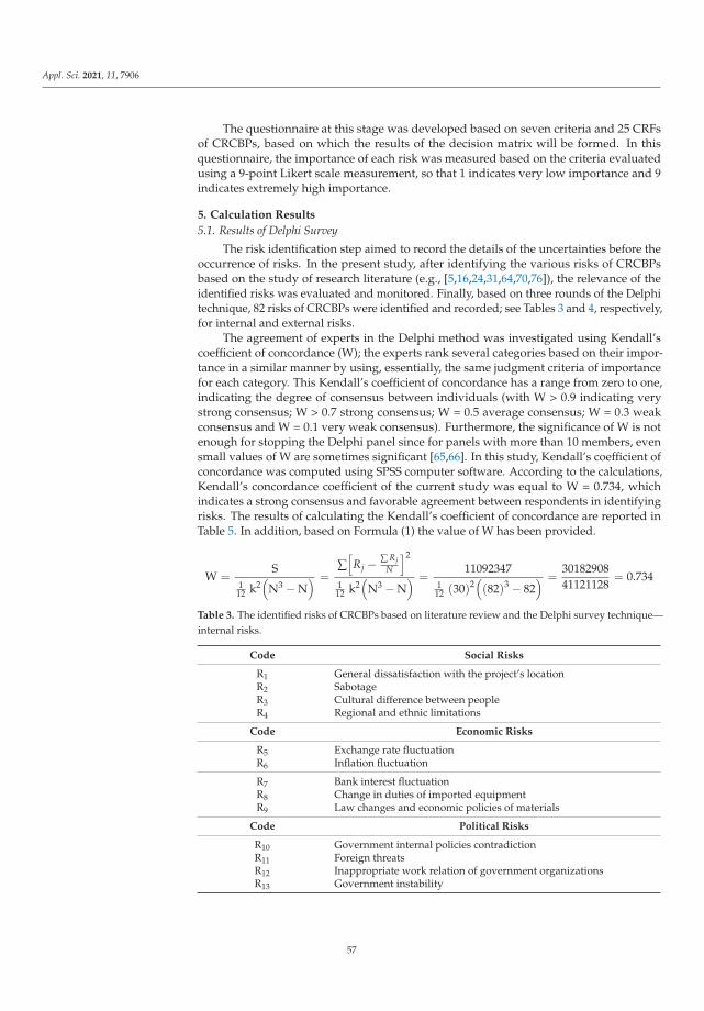
Appl. Sci. 2021, 11, 7906

The questionnaire at this stage was developed based on seven criteria and 25 CRFsof CRCBPs, based on which the results of the decision matrix will be formed. In thisquestionnaire, the importance of each risk was measured based on the criteria evaluatedusing a 9-point Likert scale measurement, so that 1 indicates very low importance and 9indicates extremely high importance.

5. Calculation Results

5.1. Results of Delphi Survey

The risk identification step aimed to record the details of the uncertainties before theoccurrence of risks. In the present study, after identifying the various risks of CRCBPsbased on the study of research literature (e.g., [5,16,24,31,64,70,76]), the relevance of theidentified risks was evaluated and monitored. Finally, based on three rounds of the Delphitechnique, 82 risks of CRCBPs were identified and recorded; see Tables 3 and 4, respectively,for internal and external risks.

The agreement of experts in the Delphi method was investigated using Kendall’scoefficient of concordance (W); the experts rank several categories based on their impor-tance in a similar manner by using, essentially, the same judgment criteria of importancefor each category. This Kendall’s coefficient of concordance has a range from zero to one,indicating the degree of consensus between individuals (with W > 0.9 indicating verystrong consensus; W > 0.7 strong consensus; W = 0.5 average consensus; W = 0.3 weakconsensus and W = 0.1 very weak consensus). Furthermore, the significance of W is notenough for stopping the Delphi panel since for panels with more than 10 members, evensmall values of W are sometimes significant [65,66]. In this study, Kendall’s coefficient ofconcordance was computed using SPSS computer software. According to the calculations,Kendall’s concordance coefficient of the current study was equal to W = 0.734, whichindicates a strong consensus and favorable agreement between respondents in identifyingrisks. The results of calculating the Kendall’s coefficient of concordance are reported inTable 5. In addition, based on Formula (1) the value of W has been provided.

W =S

112 k2

(N3 − N

) =∑[

Rj − ∑ RjN

]2

112 k2

(N3 − N

) =11092347

112 (30)2

((82)3 − 82

) =3018290841121128

= 0.734

Table 3. The identified risks of CRCBPs based on literature review and the Delphi survey technique—internal risks.

Code Social Risks

R1 General dissatisfaction with the project’s locationR2 SabotageR3 Cultural difference between peopleR4 Regional and ethnic limitations

Code Economic Risks

R5 Exchange rate fluctuationR6 Inflation fluctuation

R7 Bank interest fluctuationR8 Change in duties of imported equipmentR9 Law changes and economic policies of materials

Code Political Risks

R10 Government internal policies contradictionR11 Foreign threatsR12 Inappropriate work relation of government organizationsR13 Government instability

57

Appl. Sci. 2021, 11, 7906

Table 3. Cont.

Code Legal Risks

R14 Changes in lawR15 Changes in binding legal obligations in contractsR16 Regional standard changes (firefighting-master plans, etc.)

Code Accident Risks

R17 Natural disasters (flood—earthquake, etc.)R18 Sewage and water network unexpected accidentsR19 Annual change in weatherR20 Electrical distribution network unexpected accident

Code Market Risks

R21 Mismatching spaces with customer needsR22 Public’s lack of interestR23 Increased work competition around project areaR24 Changes in demand for the purchase of spaces with different usesR25 Facilitate sales and marketing conditions for specific user spaces

Code Work force Risks

R26 Access to skilled workerR27 Changes in the legal obligations of contractsR28 Behaviour, standards, work commitmentR29 Mismatch of job referrals to personnel with related specialized skills

Code Investment Risks

R30 Unrealistic primary estimationR31 Inappropriate financeR32 Lack of on time financeR33 BankruptcyR34 Mismatch between demand and available resources

Table 4. The identified risks of CRCBPs based on literature review and the Delphi survey technique—external risks.

Code Management Risks

R35 Previous employer-related experience and backgroundR36 Site unavailability and delay in delivery of land to the presenterR37 Unauthorized allocation of funds at various stagesR38 Lack of realistic goalsR39 Poor coordination and management

Code Project communication Risks

R40 Lack of using appropriate methods in workshop managementR41 Lack of proper organizational coordinationR42 Project staff crisis in different unitsR43 Assigning responsibility of units to a third partyR44 Lack of qualified consultantR45 Incomplete plan

Code Design Risks

R46 Poor technical specificationsR47 Mismatch of layout with site locationR48 Inaccuracies in realistic calculations and estimatesR49 Non-compliance with design codesR50 Lack of maintenance period in designing processR51 Lack of a specific contract with contractorsR52 Contractor’s claimR53 Lack of coordination between the design process and manufacturing technology

58

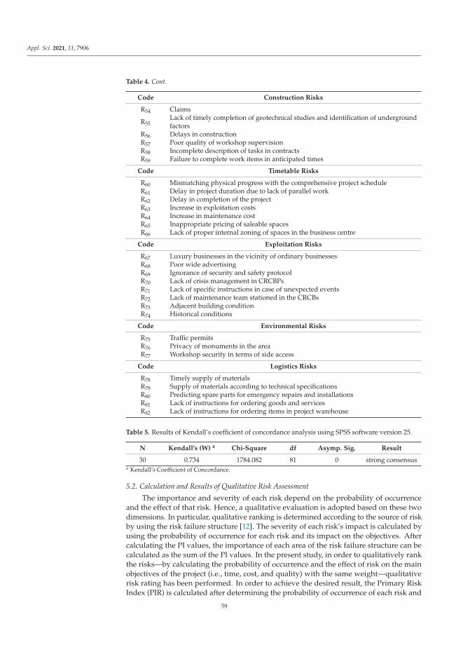
Appl. Sci. 2021, 11, 7906

Table 4. Cont.

Code Construction Risks

R54 Claims

R55Lack of timely completion of geotechnical studies and identification of undergroundfactors

R56 Delays in constructionR57 Poor quality of workshop supervisionR58 Incomplete description of tasks in contractsR59 Failure to complete work items in anticipated times

Code Timetable Risks

R60 Mismatching physical progress with the comprehensive project scheduleR61 Delay in project duration due to lack of parallel workR62 Delay in completion of the projectR63 Increase in exploitation costsR64 Increase in maintenance costR65 Inappropriate pricing of saleable spacesR66 Lack of proper internal zoning of spaces in the business centre

Code Exploitation Risks

R67 Luxury businesses in the vicinity of ordinary businessesR68 Poor wide advertisingR69 Ignorance of security and safety protocolR70 Lack of crisis management in CRCBPsR71 Lack of specific instructions in case of unexpected eventsR72 Lack of maintenance team stationed in the CRCBsR73 Adjacent building conditionR74 Historical conditions

Code Environmental Risks

R75 Traffic permitsR76 Privacy of monuments in the areaR77 Workshop security in terms of side access

Code Logistics Risks

R78 Timely supply of materialsR79 Supply of materials according to technical specificationsR80 Predicting spare parts for emergency repairs and installationsR81 Lack of instructions for ordering goods and servicesR82 Lack of instructions for ordering items in project warehouse

Table 5. Results of Kendall’s coefficient of concordance analysis using SPSS software version 25.

N Kendall’s (W) a Chi-Square df Asymp. Sig. Result

30 0.734 1784.082 81 0 strong consensusa Kendall’s Coefficient of Concordance.

5.2. Calculation and Results of Qualitative Risk Assessment

The importance and severity of each risk depend on the probability of occurrenceand the effect of that risk. Hence, a qualitative evaluation is adopted based on these twodimensions. In particular, qualitative ranking is determined according to the source of riskby using the risk failure structure [12]. The severity of each risk’s impact is calculated byusing the probability of occurrence for each risk and its impact on the objectives. Aftercalculating the PI values, the importance of each area of the risk failure structure can becalculated as the sum of the PI values. In the present study, in order to qualitatively rankthe risks—by calculating the probability of occurrence and the effect of risk on the mainobjectives of the project (i.e., time, cost, and quality) with the same weight—qualitativerisk rating has been performed. In order to achieve the desired result, the Primary RiskIndex (PIR) is calculated after determining the probability of occurrence of each risk and

59

Appl. Sci. 2021, 11, 7906

each risk’s impact on the time, cost, and quality of the project. It is worth mentioning thatthe above index is calculated separately based on the presentation of each expert. PIR1to PIR30 is then determined for each of the 82 risks. The aggregated risk index will thenbe calculated for each of the risks. By calculating the PIR of all risks, the APIR value iscalculated, and the final ranking is provided. Table 6 shows the overall PIR and APIRresults of the risks and the degree of rating of each risk based on the probability and effectmethod. According to the results of the qualitative evaluation stage, risks with an APIRvalue of 0.6 and above were identified as CRFs. Thus, a total of 25 risks were identified asCRFs of CRCBPs that will be quantitatively analyzed.

Table 6. PRI and APRI results of qualitative risk evaluation.

Code ∑PRI Sample Size APRI Risk Ranking Code ∑PRI Sample Size APRI Risk Ranking

R1 6.30 28 0.225 67 R42 10.22 28 0.365 49R2 8.26 28 0.295 58 R43 8.32 28 0.297 55R3 3.48 28 0.124 81 R44 23 44 28 0.837 7R4 4.18 28 0.149 79 R45 17.22 28 0.611 23R5 46.36 28 1.655 1 R46 17.04 28 0.608 24R6 25.23 28 1.615 2 R47 12.62 28 0.455 39R7 14.44 28 0.872 6 R48 14.90 28 0.532 30R8 18.92 28 0.675 18 R49 7.84 28 0.280 60R9 17.76 28 0.634 21 R50 8.64 28 0.308 53R10 13.67 28 0.488 35 R51 15.14 28 0.540 29R11 24.49 28 0.874 5 R52 24.98 28 0.892 4R12 11.68 28 0.417 46 R53 13.44 28 0.480 37R13 10.20 28 0.346 50 R54 12.50 28 0.446 42R14 12.38 28 0.442 43 R55 11.02 28 0.393 48R15 8.28 28 0.295 57 R56 20.26 28 0.723 13R16 19.58 28 0.699 14 R57 16.36 28 0.580 26R17 13.50 28 0.482 36 R58 9.10 28 0.325 52R18 2.28 28 0.081 82 R59 16.90 28 0.603 25R19 7.86 28 0.280 59 R60 13.14 28 0.469 38R20 3.80 28 0.135 80 R61 13.54 28 0.447 41R21 6.74 28 0.240 65 R62 16.24 28 0.580 27R22 6.57 28 0.234 66 R63 4.58 28 0.163 75R23 7.42 28 0.265 62 R64 5.42 28 0.193 71R24 4.52 28 0.161 77 R65 5.34 28 0.190 72R25 4.56 28 0.162 76 R66 5.61 28 0.200 70R26 25.02 28 0.893 3 R67 4.58 28 0.163 75R27 19.54 28 0.697 15 R68 4.24 28 0.151 78R28 14.01 28 0.500 33 R69 5.24 28 0.187 73R29 20.72 28 0.740 11 R70 5.98 28 0.213 68R30 22.66 28 0.809 9 R71 7.00 28 0.253 63R31 18.21 28 0.647 20 R72 7.02 28 0.250 64R32 18.72 28 0.668 19 R73 21.84 28 0.780 10R33 17.36 28 0.620 22 R74 8.52 28 0.304 54R34 19.44 28 0.694 16 R75 22.82 28 0.815 8R35 20.72 28 0.694 16 R76 5.80 28 0.207 69R36 13.72 28 0.490 34 R77 12.80 28 0.431 45R37 11.04 28 0.390 47 R78 15.36 28 0.548 28R38 7.47 28 0.266 61 R79 12.34 28 0.440 44R39 14.10 28 0.503 32 R80 8.32 28 0.297 56R40 19.08 28 0.681 17 R81 9.47 28 0.338 51R41 12.62 28 0.450 40 R82 14.20 28 0.507 31

60

Appl. Sci. 2021, 11, 7906

5.3. Calculation and Results of Quantitative Risk Assessment

To determine the final priority of the identified CRFs, first the decision matrix shouldbe formed based on the evaluation criteria and using the TOPSIS technique. Then, thenormal matrix is extracted and the relative proximity of each option to the solutionis determined.

The first step in the TOPSIS technique is the formation of a decision matrix, which isprepared by gathering the opinions of experts through a decision matrix questionnaire.This matrix is needed for evaluating the importance of risks based on criteria. Table A1(Appendix A) shows the results of the questionnaires collected from 30 experts. Normal-ization is the second step in solving all MCDM techniques based on the decision matrix.In the present study, normalization is performed by the vector method, which results innormalization according to Table A2. In the TOPSIS method, to create a normal matrix, theweight of each criterion is multiplied by all the numbers below each of the same criteria.Accordingly, the weight of the proposed criteria is according to Table A3. After applying inthe normal matrix, the normal matrix will be in accordance with Table A4.

In order to determine the risk rating, the relative proximity of each option to the idealsolution must be extracted. The Euclidean distance of each option from the positive andnegative ideals was calculated, and the positive and negative ideals of each criterion werecalculated according to Table A5. Formula (6) is also used to calculate the relative proximityof each option to the ideal solution. Finally, the rating of each risk is determined based onConfidence Interval (CL), which is a number between one and zero. The closer this value isto one, the higher the risk priority; conversely, the closer the value is to zero, the lower therisk significance. Table 7 shows the final results of the CRFs ranking of CRCBPs using theTOPSIS method.

d+i =

√∑n

j=1

(vij − v+

j

)2(4)

d−i =

√∑n

j=1

(vij − v−

j

)2(5)

CL+1 =

d−1

d−i + d+

i(6)

Table 7. Prioritization of CRFs of CRCBPs using the TOPSIS method.

Code d+ d− CL Final Rank Code d+ d− CL Final Rank

CRF1 008/0 047/0 852/0 2 CRF14 019/0 036/0 657/0 6CRF2 020/0 035/0 640/0 8 CRF15 039/0 016/0 286/0 22CRF3 018/0 038/0 678/0 5 CRF16 032/0 022/0 416/0 18CRF4 026/0 028/0 519/0 12 CRF17 042/0 014/0 256/0 23CRF5 006/0 050/0 895/0 1 CRF18 028/0 026/0 483/0 15CRF6 011/0 044/0 795/0 3 CRF19 027/0 027/0 495/0 14CRF7 025/0 030/0 549/0 9 CRF20 027/0 027/0 502/0 13CRF8 018/0 038/0 681/0 4 CRF21 037/0 018/0 331/0 21CRF9 029/0 025/0 457/0 17 CRF22 028/0 031/0 528/0 11CRF10 019/0 036/0 650/0 7 CRF23 047/0 007/0 128/0 24CRF11 036/0 021/0 346/0 20 CRF24 053/0 000/0 000/0 25CRF12 025/0 030/0 548/0 10 CRF25 032/0 022/0 407/0 19CRF13 030/0 025/0 459/0 16

Results shown in Table 7 highlight that the five CRFs with the highest importancefor CRCBPs are (1) the risk of external threats due to international factors (with a relativedistance of 0.895), (2) exchange rate fluctuations and changes (with a relative distanceof 0.852), (3) bank interest rate fluctuations (with a relative distance of 0.795), (4) trafficlicenses (with a relative distance of 0.681), and (5) access to skilled labor (with a relativedistance of 0.678).

61

Appl. Sci. 2021, 11, 7906

6. Discussions and Conclusions

What are the most severe risks in commercial and recreational complex building projects(CRCBPs)? This is the question at the center of the presented study, and results of thequantitative step (see Table 7) showed that the 10 most important CRFs of CRCBPsare (i) threats from international relations, (ii) exchange rate fluctuations and changes,(iii) bank interest rate fluctuations, (iv) traffic licenses, (v) access to skilled labor,(vi) changes in regional regulations, (vii) the condition of adjacent buildings, (viii) fluctua-tions and changes in inflation rates, (ix) failure to select a suitable and qualified advisor,and (x) previous experiences and records related to the employer.

The results of the current study are partly aligned with those of some previous scholarsinterested in identifying and ranking CRFs in construction projects, even if not specificallyconsidering CRCBPs. For example, [10] reported that construction project risk indicatorsare mainly related to changes in domestic and international situations and the efficiency of acountry’s economics/workforce/construction characteristics/consultative and contractualservices. Yet, Hatefi and Mohseni [73] also ranked the CRFs as high in relation to initial pricefluctuations, rising inflation, exchange rate fluctuations, bank interest rate fluctuations,tax increases, and the uncertainty of fiscal policies. Results are slightly in contrast toDey [74] who, by evaluating project risks using a MCDM method, identified that also risksconnected with government bonds and equipment suppliers and technology selection havea high priority in construction projects (not ranked high in the proposed study).

With regard to CRCBPs, the produced results extend the contributions by Chen andKhumpaisal [35] and by Tamošaitiene et al. [12], who identified risks for CRCBPs without,however, providing their prioritization. Yet, when considering prior studies that identifiedand prioritized CRFs of CRCBPs, results of the proposed work are partly in accord; indeed,with regard to Comu et al. [17], this is despite ‘exchange rate and inflation rate fluctuations’and ‘political instability’ not being included with other CRFs ranked as important in theproposed work (e.g., traffic licenses, access to skilled labor, changes in regional regulations,etc.). Differences in these findings can come from the different economic, social, andcultural contexts, as well as from the different features of the samples involved. Indeed,respondents for the proposed contribution are more experienced, they come from distinctstakeholders’ categories (clients and consultants have been included), and they are moreheterogeneous in terms of field of specialty. These individual differences, according tothe literature [77], can lead to different perceptions and, as a consequence, to distinctprioritization of categories. Yet, project risks can also vary from time to time depending onthe progress level of the project [78], and this is more important for financial risks, such asthe exchange rate instabilities, which can occur suddenly due to unforeseen factors [79],most of which are often external ones.

If looking at risks identified and prioritized for megaprojects that have some paral-lelism with CRCBPs [80], results are slightly in contrast. Indeed, Cheng and Darsa [27]found that the most important risk factors in the Ethiopian context are ‘change order’,‘corruption/bribery’, and ‘delay in payment’, while Chattapadhyay et al. [29] found that themost severe risks are delay in obtaining traffic regulation orders, inappropriate equipment,political and legal issues, political instability, government intervention, regulatory confir-mation and regulation order delays, and wrong engineering designs. Obviously, thesedifferences can be associated to the usual distinct nature of megaprojects and CRCBPS,mainly public and private, respectively [81].

Among the ten identified risks, some were external risks of CRCBPs while otherswere internal risks. However, all the identified risks have significant effects on projectdevelopment in the setting of developed or developing countries. As expected, given thetiming of the investigation into sanctions and severe economic problems in Iran, the mostimportant CRFs were in the economic risk group. Sanctions imposed on Iran have reducedliquidity and increased inflation, which is reflected on the price of equipment and materials.Therefore, factors, such as exchange rate fluctuations and inflation, followed by changes inbank interest rates, certainly cause serious uncertainties in CRCBPs projects. The reason

62

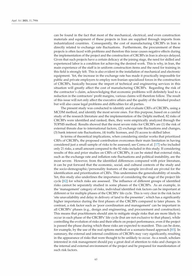
Appl. Sci. 2021, 11, 7906

can be found in the fact that most of the mechanical, electrical, and even constructionmaterials and equipment of these projects in Iran are supplied through imports fromindustrialized countries. Consequently, the cost of manufacturing CRCBPs in Iran isdirectly related to exchange rate fluctuations. Furthermore, the procurement of theseprojects is often faced with problems and therefore this issue causes negative effects duringthe implementation of the project and the construction of CRCBPs in Iran is always delayed.Given that such projects have a certain delicacy at the joining stage, the need for skilled andexperienced labor is a condition for achieving the desired work. This is why, in Iran, themain experience of the staff is in uniform construction items and the need for training inthis field is strongly felt. This is also evident in the installation of mechanical and electronicequipment. Yet, the increase in the exchange rate has made it practically impossible forpublic and private employers to employ non-Iranian specialized forces in the constructionof CRCBPs, basically because the import of technical and engineering services in thissituation will greatly affect the cost of manufacturing CRCBPs. Regarding the risk ofthe contractor’s claim, acknowledging that economic problems will definitely lead to areduction in the contractors’ profit margins, various claims will therefore follow. The resultof this issue will not only affect the executive affairs and the quality of the finished productbut will also cause legal problems and difficulties for all parties.

The present study was conducted to identify and evaluate CRFs of CRCBPs, using aMCDM method, and identify the most severe ones. For this purpose, based on a carefulstudy of the research literature and the implementation of the Delphi method, 82 risks ofCRCBPs were identified and ranked; then, they were empirically analyzed through theTOPSIS method. Results showed that the most severe risks for CRCBPs are (1) the risk ofexternal threats due to international factors, (2) exchange rate fluctuations and changes,(3) bank interest rate fluctuations, (4) traffic licenses, and (5) access to skilled labor.

In terms of theoretical implications, when considering similar works that prioritizedCRFs of CRCBPs, the proposed contribution overcomes their main limitation in havingconsidered just a small sample of risks to be assessed; see Comu et al. [17] who includedonly 21 risks, a small amount compared to the 82 risks included in this study. If consideringresults of this and prior studies on CRFs of CRCBPs, it can be stated that external risks,such as the exchange rate and inflation rate fluctuations and political instability, are themost severe. However, from the identified differences compared with prior literature,it can be put forward that the economic, social, and cultural contexts of the study andthe socio-demographic/personality features of the sample involved are pivotal for theidentification and prioritization of CRFs. This undermines the generalizability of results.Yet, this study also underlines the importance of considering the stage of the project lifecycle [82] for which risks are assessed. The influence of different groups of identifiedrisks cannot be separately studied in some phases of the CRCBPs. As an example, inthe ‘management’ category of risks, individual identified risk factors can be important atdifferent or for multiple phases of the CRCBPs’ life cycle. This is very clear in the risk factor‘site unavailability and delay in delivery of land to the presenter’, which has a significantlyhigher importance during the first phases of the CRCBPs compared to later phases. Incontrast, a risk factor such as ‘poor coordination and management’ can be important inall CRCBPs’ phases (e.g., design and engineering, and procurement and construction).This means that practitioners should aim to mitigate single risks that are more likely tooccur in each phase of the CRCBPs’ life cycle (but are not exclusive to that phase), whilecontrolling the evolution of risks and their effects on project performance, even if the projectis passed the phase during which these risks are expected to manifest. This can be done,for example, by the use of the real options method or a scenario-based approach [83]. Insummary, the external and internal conditions of CRCBPs may vary significantly, resultingin the appearance of risks that were thought to be unlikely to occur. As a result, scholarsinterested in risk management should pay a great deal of attention to risks and changes inthe internal and external environment of the project and be prepared for manifestation ofsuch risk factors.

63

Appl. Sci. 2021, 11, 7906

In terms of practical implications, it is worth noting that a number of external risks,such as fluctuations in currency exchange rates, changes in inflation rate, foreign threatsdue to international relations, and fluctuations of banking interest rates, are outside ofthe power of CRCBPs’ managers while also having a large impact—especially on theproject’s conceptual planning and feasibility study’s life cycle. Indeed, the presence ofthese economic and financial risks during the initial phases of the project can result inCRCBPs’ decision makers abandoning the project before significant investments are made.Alternatively, decision makers can try implementing projects in countries and/or duringperiods of stable exchange rates that can facilitate the fulfillment of project objectives.Another practical strategy to reduce these risks is to insure CRCBPs’ against possibleeconomic and financial risks. The cost of such insurance is even more financially acceptableif investors in CRCBPs also have significant investments in other projects. The increasein the number of projects in the investors’ portfolio allows them to control investmentswith different levels of risk manifestation and can reduce the risk of overall failure inpractice. However, insurance protection is not possible for risks such as traffic permitsand the condition of adjacent buildings, which are always outside a project managementteam’s control. If such risks are verified, they can result in significant delays in CRCBPs (orundermine their fruition), and therefore decrease the overall value of the CRCBPs. In sucha case, CRCBPs’ decision makers must choose to either continue with the project whileattempting to maintain economic and financial equilibrium or liquidate the project if thecost of these risks can reach or exceed the planned return on investments.

Finally, the risks of lack of access to skilled labor, lack of qualified consultants, andunrealistic preliminary estimation can also have significant effects, similar to the previouslydiscussed risks, by delaying the execution of the CRCBPs while also undermining risk man-agement and coordination efforts. However, since these risks are related to processes activelycontrolled by CRCBPs’ management, their direct control is possible. For instance, the lack ofaccess to resources or qualified consultants can often be resolved through human resourceagencies, headhunters, or other qualified players capable of identifying and delivering suit-able employees and consultants for participation in CRCBPs. Similarly, simple solutions arepossible for unrealistic primary estimation, including conducting suitable feasibility studieson the CRCBPs. Furthermore, using skilled labor and qualified consultants can help minimizethe forecasted mistakes and problems in the project’s progress.

There are few limitations to this study. Despite the fact that the categories of identifiedrisks overlap with the ones identified in the extensive and recent review on constructionrisks by Siraj et al. [70], all the risks identified by these scholars (i.e., 571) have not beenincluded in our survey due to the: (i) Lack of a complete list of these risks (authors just pro-pose a sample of 10 risks for each category), and (ii) methodological difficulty in proposinga related lengthy questionnaire for the ranking of risks. Always with regard to the methodadopted, i.e., the Delphi technique, it has inner reliability and validity limits. In particular,considering the reliability problem of the Delphi study (i.e., two or more different groupsof experts can lead to different results even if facing the same questions/phenomena);and the criteria for qualitative studies—i.e., truthfulness, applicability, consistency andconfirmability—were followed to ensure that credible interpretations of the findings areproduced [84]. These criteria are based on the following issues; however, as Keeneyet al. [85] stated, following these criteria cannot totally limit the involvement of differentpanels that may lead to obtaining the same results. Despite that, results emerging fromthe Delphi study can be considered reliable, in as much as the best (in terms of knowledgeand expertise) possible panelists are involved. With regard to the validity problem (i.e.,whether the produced results are the right expression of the investigated phenomena), theinvolvement of a respondent with great knowledge in the field is the most used approachwithin the technique [85] and this solves also the problem of convergence of opinionsthat can occur over three rounds of the Delphi technique. However, it is true that thisstudy involved a small number of experts, even though their expertise was in line with thestudy’s aims and that this number is similar to works in the same field adopting the Delphi

64

Appl. Sci. 2021, 11, 7906

method [15]. Future studies should increase the validity of the results through interviewinga larger group of experts, at least around 50, or expanding their scope to that of otherdeveloping countries. Additionally, comparing the results of similar studies conductedin developed countries to that of developing countries could lead to interesting results.Furthermore, the socio-demographic characteristics of the experts participating in the initialphase of identifying risks of CRCBPs can play a role through their opinions regardingthe existence and/or importance of certain risk factors. Therefore, an interesting futureprospect will be to carry out future quantitative studies based on Upper Echelons Theoryliterature [77,86], regarding the effects of socio-demographic characteristics and/or otherpsychological variables on definition and evaluation of CRCBPs’ risks at the individualand group levels. Another main limitation of this study is the adoption of the TOPSISmethod. Indeed, as well accounted by Madi et al. [87], TOPSIS uses crisp information thatis impractical in many real-world situations (e.g., human judgements are often vague andcannot estimate preferences in exact numerical form). Yet, TOPSIS suffers from the rankreversal problem that is related to the change in the ranking of alternatives when a criterionor an alternative is added or dropped; yet, since TOPSIS uses Euclidean distance (that doesnot consider correlations), results are affected due to information overlap [88]. To try toovercome this limitation, future research is encouraged to combine MCDM techniques [89].Another solution is to adopt established developments of the TOPSIS method, such asfuzzy TOPSIS; the sets can be used to express preferences using linguistic variables [90].The adoption of this more sophisticated technique can help also to overcome the limitationof this study having been based on a MCDM approach; indeed, the fuzzy set theory hasled to a new decision theory, known today as fuzzy MCDM where decision-maker modelsare able to deal with incomplete and uncertain knowledge and information [91].

Author Contributions: Conceptualization, H.S. and J.T.; methodology, H.S. and M.K.; formal anal-ysis, H.S. and M.K.; investigation, J.T., H.S., and D.W.M.C.; data curation, H.S. and D.W.M.C.;writing—original draft preparation, H.S. and J.T.; writing—review and editing, M.C. and H.S.; vi-sualization, H.S. and M.C.; supervision, H.S.; project administration, J.T. All authors have read andagreed to the published version of the manuscript.

Funding: This research received no external funding.

Institutional Review Board Statement: Not applicable.

Informed Consent Statement: Not applicable.

Data Availability Statement: Not applicable.

Conflicts of Interest: The authors declare no conflict of interest.

Appendix A

Table A1. Decision matrix based on the results of the collected questionnaires.

Code Risks

Vulnerability(−)

Probability ofOccurrence of

Risk(−)

RiskDetection

(+)

AcceptingThreat

(−)

Impact on theOccurrence ofOther Risks

(−)

Risk Manage-ability

(+)

RiskResponse

(+)

C1 C2 C3 C4 C5 C6 C7

CRF1 Exchange rate fluctuation 1/333 1/625 6/375 2/25 2/5 4/625 4/25CRF2 Inflation fluctuation 2/667 2/375 6 4 3/625 4 3/875CRF3 Access to skilled worker 4/167 3/875 4/625 2/25 4/875 4/5 4CRF4 Contractor’s claim 4/5 3/625 4/75 4/125 4/875 3/5 3/625CRF5 Foreign threats 2/667 2/25 5/375 1/375 2/625 5/625 5CRF6 Bank interest fluctuation 2/167 3/5 4/875 2/25 2/25 5 5/375

CRF7Lack of qualified

consultant 1/833 3/375 5/125 4/125 5/25 3/375 3/25

CRF8 Traffic permits 2/333 1/375 4/625 3/75 3 4/125 3/625

CRF9Unrealistic primary

estimation 4/167 4/75 3/875 4/625 4/875 3/75 3/625

CRF10Adjacent building

condition 3/333 3 5 3/375 5/375 4/625 4/375

65

Appl. Sci. 2021, 11, 7906

Table A1. Cont.

Code Risks

Vulnerability(−)

Probability ofOccurrence of

Risk(−)

RiskDetection

(+)

AcceptingThreat

(−)

Impact on theOccurrence ofOther Risks

(−)

Risk Manage-ability

(+)

RiskResponse

(+)

C1 C2 C3 C4 C5 C6 C7

CRF11

Mismatch of job referralsto personnel with related

specialized skills5/833 5/625 4/25 5/5 5/75 4 4/125

CRF12

Previous employer-relatedexperience and

background4/667 4/625 5 4 4/25 4/25 4/5

CRF13 Delays in construction 5 4/375 4/125 4/75 4/25 4/125 3/75

CRF14

Regional standardchanges

(firefighting-masterplans, etc.)

4/5 3/5 5/25 3/25 4 4/625 4/625

CRF15Changes in the legal

obligations of contracts 5/633 5/5 3/375 5/75 6 3 3/625

CRF16

Mismatch betweendemand and

available resources5/167 4/625 4 4/875 4/375 3/375 3

CRF17

Lack of using appropriatemethods in workshop

management6/167 5/865 3/375 6/125 6/75 3/25 3/625

CRF18Change in duties of

imported equipment 4/5 4/125 4/625 4/5 4/625 3/5 3/875

CRF19 Lack of on time finance 4/167 4 5/25 4/25 5 3/25 3/5CRF20 Inappropriate finance 4/167 4 4/625 4 5/625 3/375 3/5

CRF21

Law changes andeconomic policies

of materials5/633 5/5 3/5 4/875 6/25 2/75 3/125

CRF22 Bankruptcy 4/833 5/875 3 3/875 3/5 4/875 4CRF23 Incomplete plan 6/333 6/125 2 6/375 6/625 2/125 1/625

CRF24Poor technicalspecifications 6/5 6/375 1/75 7/25 7 1/375 1/125

CRF25Failure to complete workitems in anticipated times 5 4/75 4/25 5 5 3/625 3

Table A2. Normalized decision matrix based on the results of the collected questionnaires.

Risks− − + − − + +

C1 C2 C3 C4 C5 C6 C7

CRF1 0/0590 0/074 0/284 0/101 0/101 0/238 0/225CRF2 0/118 0/108 0/267 0/179 0/147 0/205 0/205CRF3 0/184 0/176 0/206 0/101 0/197 0/231 0/211CRF4 0/199 0/165 0/212 0/185 0/197 0/180 0/192CRF5 0/118 0/102 0/239 0/062 0/106 0/289 0/264CRF6 0/096 0/159 0/217 0/101 0/091 0/257 0/284CRF7 0/081 0/153 0/228 0/185 0/212 0/173 0/172CRF8 0/103 0/063 0/206 0/168 0/121 0/212 0/192CRF9 0/184 0/216 0/173 0/207 0/197 0/193 0/192CRF10 0/148 0/136 0/223 0/151 0/217 0/228 0/231CRF11 0/258 0/256 0/189 0/246 0/233 0/205 0/218CRF12 0/207 0/210 0/223 0/179 0/172 0/218 0/238CRF13 0/221 0/199 0/184 0/213 0/212 0/212 0/198CRF14 0/199 0/159 0/234 0/145 0/162 0/238 0/244CRF15 0/249 0/250 0/150 0/257 0/243 0/154 0/192CRF16 0/229 0/210 0/178 0/218 0/177 0/173 0/158CRF17 0/273 0/267 0/150 0/274 0/273 0/167 0/192CRF18 0/199 0/188 0/206 0/201 0/187 0/180 0/205CRF19 0/184 0/182 0/234 0/190 0/202 0/167 0/185CRF20 0/184 0/182 0/206 0/179 0/228 0/173 0/185CRF21 0/249 0/25 0/156 0/218 0/253 0/141 0/165CRF22 0/214 0/267 0/134 0/173 0/142 1/250 0/211CRF23 0/280 0/279 0/089 0/285 0/268 0/109 0/086CRF24 0/288 0/290 0/078 0/325 0/283 0/071 0/059CRF25 0/221 0/216 0/189 0/224 0/202 0/186 0/158

66

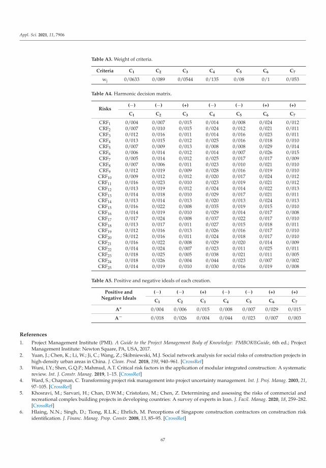
Appl. Sci. 2021, 11, 7906

Table A3. Weight of criteria.

Criteria C1 C2 C3 C4 C5 C6 C7

wj 0/0633 0/089 0/0544 0/135 0/08 0/1 0/053

Table A4. Harmonic decision matrix.

Risks(−) (−) (+) (−) (−) (+) (+)

C1 C2 C3 C4 C5 C6 C7

CRF1 0/004 0/007 0/015 0/014 0/008 0/024 0/012CRF2 0/007 0/010 0/015 0/024 0/012 0/021 0/011CRF3 0/012 0/016 0/011 0/014 0/016 0/023 0/011CRF4 0/013 0/015 0/012 0/025 0/016 0/018 0/010CRF5 0/007 0/009 0/013 0/008 0/008 0/029 0/014CRF6 0/006 0/014 0/012 0/014 0/007 0/026 0/015CRF7 0/005 0/014 0/012 0/025 0/017 0/017 0/009CRF8 0/007 0/006 0/011 0/023 0/010 0/021 0/010CRF9 0/012 0/019 0/009 0/028 0/016 0/019 0/010CRF10 0/009 0/012 0/012 0/020 0/017 0/024 0/012CRF11 0/016 0/023 0/010 0/023 0/019 0/021 0/012CRF12 0/013 0/019 0/012 0/024 0/014 0/022 0/013CRF13 0/014 0/018 0/010 0/029 0/017 0/021 0/011CRF14 0/013 0/014 0/013 0/020 0/013 0/024 0/013CRF15 0/016 0/022 0/008 0/035 0/019 0/015 0/010CRF16 0/014 0/019 0/010 0/029 0/014 0/017 0/008CRF17 0/017 0/024 0/008 0/037 0/022 0/017 0/010CRF18 0/013 0/017 0/011 0/027 0/015 0/018 0/011CRF19 0/012 0/016 0/013 0/026 0/016 0/017 0/010CRF20 0/012 0/016 0/011 0/024 0/018 0/017 0/010CRF21 0/016 0/022 0/008 0/029 0/020 0/014 0/009CRF22 0/014 0/024 0/007 0/023 0/011 0/025 0/011CRF23 0/018 0/025 0/005 0/038 0/021 0/011 0/005CRF24 0/018 0/026 0/004 0/044 0/023 0/007 0/002CRF25 0/014 0/019 0/010 0/030 0/016 0/019 0/008

Table A5. Positive and negative ideals of each creation.

Positive andNegative Ideals

(−) (−) (+) (−) (−) (+) (+)

C1 C2 C3 C4 C5 C6 C7

A+ 0/004 0/006 0/015 0/008 0/007 0/029 0/015

A− 0/018 0/026 0/004 0/044 0/023 0/007 0/003

References

1. Project Management Institute (PMI). A Guide to the Project Management Body of Knowledge: PMBOK®Guide, 6th ed.; ProjectManagement Institute: Newton Square, PA, USA, 2017.

2. Yuan, J.; Chen, K.; Li, W.; Ji, C.; Wang, Z.; Skibniewski, M.J. Social network analysis for social risks of construction projects inhigh-density urban areas in China. J. Clean. Prod. 2018, 198, 940–961. [CrossRef]

3. Wuni, I.Y.; Shen, G.Q.P.; Mahmud, A.T. Critical risk factors in the application of modular integrated construction: A systematicreview. Int. J. Constr. Manag. 2019, 1–15. [CrossRef]

4. Ward, S.; Chapman, C. Transforming project risk management into project uncertainty management. Int. J. Proj. Manag. 2003, 21,97–105. [CrossRef]

5. Khosravi, M.; Sarvari, H.; Chan, D.W.M.; Cristofaro, M.; Chen, Z. Determining and assessing the risks of commercial andrecreational complex building projects in developing countries: A survey of experts in Iran. J. Facil. Manag. 2020, 18, 259–282.[CrossRef]

6. Hlaing, N.N.; Singh, D.; Tiong, R.L.K.; Ehrlich, M. Perceptions of Singapore construction contractors on construction riskidentification. J. Financ. Manag. Prop. Constr. 2008, 13, 85–95. [CrossRef]

67

Appl. Sci. 2021, 11, 7906

7. Chapman, R.J. The effectiveness of working group risk identification and assessment techniques. Int. J. Proj. Manag. 1998, 16,333–343. [CrossRef]

8. Goh, C.S.; Abdul-Rahman, H.; Abdul Samad, Z. Applying risk management workshop for a public construction project: Casestudy. J. Constr. Eng. Manag. 2013, 139, 572–580. [CrossRef]

9. Marcelino-Sádaba, S.; Pérez-Ezcurdia, A.; Lazcano, A.M.E.; Villanueva, P. Project risk management methodology for small firms.Int. J. Proj. Manag. 2014, 32, 327–340. [CrossRef]

10. Zavadskas, E.K.; Turskis, Z.; Tamošaitiene, J. Risk assessment of construction projects. J. Civ. Eng. Manag. 2010, 16, 33–46.[CrossRef]

11. Valipour, A.; Yahaya, N.; Md Noor, N.; Kildiene, S.; Sarvari, H.; Mardani, A. A fuzzy analytic network process method for riskprioritization in freeway PPP projects: An Iranian case study. J. Civ. Eng. Manag. 2015, 21, 933–947. [CrossRef]

12. Tamošaitiene, J.; Zavadskas, E.K.; Turskis, Z. Multi-criteria risk assessment of a construction project. Procedia Comput. Sci. 2013,17, 129–133. [CrossRef]

13. Tamošaitiene, J.; Sarvari, H.; Chan, D.W.M.; Cristofaro, M. Assessing the Barriers and Risks to Private Sector Participation inInfrastructure Construction Projects in Developing Countries of Middle East. Sustainability 2021, 13, 153. [CrossRef]

14. Tamošaitiene, J.; Yousefi, V.; Tabasi, H. Project Portfolio Construction Using Extreme Value Theory. Sustainability 2021, 13, 855.[CrossRef]

15. Tamošaitiene, J.; Sarvari, H.; Cristofaro, M.; Chan, D.W.M. Identifying and prioritizing the selection criteria of appropriate repairand maintenance methods for commercial buildings. Int. J. Strateg. Prop. Manag. 2021, 25, 413–431. [CrossRef]

16. Sarvari, H.; Valipour, A.; Yahya, N.; Noor, N.; Beer, M.; Banaitiene, N. Approaches to Risk Identification in Public–PrivatePartnership Projects: Malaysian Private Partners’ Overview. Adm. Sci. 2019, 9, 17. [CrossRef]

17. Comu, S.; Elibol, A.Y.; Yucel, B. A risk assessment model of commercial real estate development projects in developing countries.J. Constr. Eng. 2021, 4, 52–67. [CrossRef]

18. Sarvari, H.; Chan, D.W.M.; Alaeos, A.K.F.; Olawumi, T.O.; Abdalridah Aldaud, A.A. Critical success factors for managingconstruction small and medium-sized enterprises in developing countries of Middle East: Evidence from Iranian constructionenterprises. J. Build. Eng. 2021, 43, 103152. [CrossRef]

19. Mirkatouli, J.; Samadi, R.; Hosseini, A. Evaluating and analysis of socio-economic variables on land and housing prices inMashhad, Iran. Sustain. Cities Soc. 2018, 41, 695–705. [CrossRef]

20. United Nations. Central Product Classification; United Nations Statistics Division: New York, NY, USA, 2015.21. Sarvari, H.; Mehrabi, A.; Chan, D.W.M.; Cristofaro, M. Evaluating urban housing development patterns in developing countries:

Case study of Worn-out Urban Fabrics in Iran. Sustain. Cities Soc. 2021, 70, 102941. [CrossRef]22. Kumaraswamy, M.M.; Zhang, X.Q. Governmental role in BOT-led infrastructure development. Int. J. Proj. Manag. 2001, 19,

195–205. [CrossRef]23. Ghaed Rahmati, S.; Daneshmandi, N. Analysis of urban tourism spatial pattern (case study: Urban tourism space of Isfahan city).

Hum. Geogr. Res. 2018, 50, 945–961.24. Sarvari, H.; Rakhshanifar, M.; Tamošaitiene, J.; Chan, D.W.M.; Beer, M. A risk based approach to evaluating the impacts of

Zayanderood drought on sustainable development indicators of riverside urban in Isfahan-Iran. Sustainability 2019, 11, 6797.[CrossRef]

25. Marle, F.; Gidel, T. A multi-criteria decision-making process for project risk management method selection. Int. J. MulticriteriaDecis. Mak. 2012, 2, 189–223. [CrossRef]

26. Yatsalo, B.; Gritsyuk, S.; Sullivan, T.; Trump, B.; Linkov, I. Multi-criteria risk management with the use of DecernsMCDA: Methodsand case studies. Environ. Syst. Decis. 2016, 36, 266–276. [CrossRef]

27. Cheng, M.Y.; Darsa, M.H. Construction Schedule Risk Assessment and Management Strategy for Foreign General ContractorsWorking in the Ethiopian Construction Industry. Sustainability 2021, 13, 7830. [CrossRef]

28. Czajkowska, A.; Ingaldi, M. Structural Failures Risk Analysis as a Tool Supporting Corporate Responsibility. J. Risk Financ. Manag.2021, 14, 187. [CrossRef]

29. Chattapadhyay, D.B.; Putta, J.; Paneem, R.M. Risk Identification, Assessments, and Prediction for Mega Construction Projects: ARisk Prediction Paradigm Based on Cross Analytical-Machine Learning Model. Buildings 2021, 11, 172. [CrossRef]

30. Tserng, H.P.; Cho, I.; Chen, C.H.; Liu, Y.F. Developing a Risk Management Process for Infrastructure Projects Using IDEF0.Sustainability 2021, 13, 6958. [CrossRef]

31. Chan, D.W.M.; Chan, J.H.L.; Ma, T. Developing a fuzzy risk assessment model for guaranteed maximum price and target costcontracts in South Australia. Facilities 2014, 32, 624–646. [CrossRef]

32. Siu, F.M.F.; Leung, J.W.Y.; Chan, D.W.M. A Data-driven approach to identify-quantify-analyse construction risk for Hong KongNEC projects. J. Civ. Eng. Manag. 2018, 24, 592–606. [CrossRef]

33. Chatterjee, K.; Zavadskas, E.K.; Tamošaitiene, J.; Adhikary, K.; Kar, S. A hybrid MCDM technique for risk management inconstruction projects. Symmetry 2018, 10, 46. [CrossRef]

34. Zhou, H.; Zhao, Y.; Shen, Q.; Yang, L.; Cai, H. Risk assessment and management via multi-source information fusion for underseatunnel construction. Autom. Constr. 2020, 111, 103050. [CrossRef]

35. Chen, Z.; Khumpaisal, S. An analytic network process for risks assessment in commercial real estate development. J. Prop. Invest.Financ. 2009, 27, 238–258. [CrossRef]

68

Appl. Sci. 2021, 11, 7906

36. Irimia Diéguez, A.I.; Sánchez Cazorla, Á.; Alfalla Luque, R. Risk management in megaprojects. Procedia Soc. Behav. Sci. 2014, 119,407–416. [CrossRef]

37. Krane, H.P.; Rolstadås, A.; Olsson, N.O. Categorizing risks in seven large projects—Which risks do the projects focus on? Proj.Manag. J. 2010, 41, 81–86. [CrossRef]

38. Wang, H.; Tong, Y. Algorithm Study on Models of Multiple Objective Risk Decision under Principal and Subordinate HierarchDecision-making. Oper. Res. Manag. Sci. 2007, 16, 1–8.

39. Wideman, R.M. A Guide to Managing Project Risks and Opportunities; Project Management Institute: Newtown Square, PA, USA,1992.

40. Sigmund, Z.; Radujkovic, M. Risk breakdown structure for construction projects on existing buildings. Procedia-Soc. Behav. Sci.2014, 119, 894–901. [CrossRef]

41. Hillson, D.; Grimaldi, S.; Rafele, C. Managing project risks using a cross risk breakdown matrix. Risk Manag. 2006, 8, 61–76.[CrossRef]

42. Dabiri, M.; Oghabi, M.; Sarvari, H.; Sabeti, M.; Kashefi, H. A combination risk-based approach to post-earthquake temporaryaccommodation site selection: A case study in Iran. Iran. J. Fuzzy Syst. 2020, 17, 54–74. [CrossRef]

43. Lyu, H.M.; Sun, W.J.; Shen, S.L.; Zhou, A.N. Risk assessment using a new consulting process in fuzzy AHP. J. Constr. Eng. Manag.2020, 146, 04019112. [CrossRef]

44. Milion, R.N.; Alves, T.D.C.; Paliari, J.C.; Liboni, L.H. CBA-Based Evaluation Method of the Impact of Defects in ResidentialBuildings: Assessing Risks towards Making Sustainable Decisions on Continuous Improvement Activities. Sustainability 2021, 13,6597. [CrossRef]

45. Taylan, O.; Bafail, A.O.; Abdulaal, R.M.; Kabli, M.R. Construction projects selection and risk assessment by fuzzy AHP and fuzzyTOPSIS methodologies. Appl. Soft Comput. 2014, 17, 105–116. [CrossRef]

46. Mata, P.; Silva, P.F.; Pinho, F.F. Risk Management of Bored Piling Construction on Sandy Soils with Real-Time Cost Control.Infrastructures 2021, 6, 77. [CrossRef]

47. Liu, Z.; Meng, X.; Xing, Z.; Jiang, A. Digital Twin-Based Safety Risk Coupling of Prefabricated Building Hoisting. Sensors 2021, 21,3583. [CrossRef] [PubMed]

48. Draji Jahromi, A.; Valipour, A.; Pakdel, A. Ranking of risk assessment criteria in construction projects using network analysis. InProceedings of the 4th International Congress on Civil Engineering, Architecture & Urban Development, Tehran, Iran, 27–29December 2016.

49. Mohammadi Talvar, Z.; Panahi, J. Identifying effective criteria in assessing and ranking the risk management of constructionprojects. In Proceedings of the Conference on Civil Engineering, Architecture and Urbanism of the Islamic Countries, Tabriz, Iran,10 May 2018.

50. Muriana, C.; Vizzini, G. Project risk management: A deterministic quantitative technique for assessment and mitigation. Int. J.Proj. Manag. 2017, 35, 320–340. [CrossRef]

51. Sarvari, H.; Cristofaro, M.; Chan, D.W.M.; Noor, N.M.; Amini, M. Completing abandoned public facility projects by the privatesector: Results of a Delphi survey in the Iranian Water and Wastewater Company. J. Facil. Manag. 2020, 18, 547–566. [CrossRef]

52. Cox, L.A., Jr.; Babayev, D.; Huber, W. Some limitations of qualitative risk rating systems. Risk Anal. Int. J. 2005, 25, 651–662.[CrossRef]

53. Zou, P.X.; Zhang, G.; Wang, J. Understanding the key risks in construction projects in China. Int. J. Proj. Manag. 2007, 25, 601–614.[CrossRef]

54. Behzadian, M.; Otaghsara, S.K.; Yazdani, M.; Ignatius, J. A state-of the-art survey of TOPSIS applications. Expert Syst. Appl. 2012,39, 13051–13069. [CrossRef]

55. Jozaghi, A.; Alizadeh, B.; Hatami, M.; Flood, I.; Khorrami, M.; Khodaei, N.; Ghasemi Tousi, E.A. Comparative Study of the AHPand TOPSIS Techniques for Dam Site Selection Using GIS: A Case Study of Sistan and Baluchestan Province, Iran. Geosciences2018, 8, 494. [CrossRef]

56. Gebrehiwet, T.; Luo, H. Risk level evaluation on construction project lifecycle using fuzzy comprehensive evaluation and TOPSIS.Symmetry 2019, 11, 12. [CrossRef]

57. Dandage, R.; Mantha, S.S.; Rane, S.B. Ranking the risk categories in international projects using the TOPSIS method. Int. J. Manag.Proj. Bus. 2018, 11, 317–331. [CrossRef]

58. Jalal, M.P.; Shoar, S. A hybrid framework to model factors affecting construction labour productivity: Case study of Iran. J. Financ.Manag. Prop. Constr. 2019, 24, 630–654. [CrossRef]

59. Ghasseminejad, S.; Jahan-Parvar, M.R. The impact of financial sanctions: Case Iran. J. Policy Modeling 2021, 43, 601–621. [CrossRef]60. Arnott, R. Housing policy in developing countries: The importance of the informal economy. In Urbanization and Growth; Spence,

M., Annez, P.C., Buckley, R.M., Eds.; The World Bank: Washington, DC, USA, 2008; pp. 167–196.61. Yeung, J.F.Y.; Chan, A.P.C.; Chan, D.W.M.; Li, L.K. Development of a partnering performance index (PPI) for construction projects

in Hong Kong: A Delphi study. Constr. Manag. Econ. 2007, 25, 1219–1237. [CrossRef]62. Chan, D.W.M.; Chan, J.H.L. Developing a Performance Measurement Index (PMI) for target cost contracts in construction: A

Delphi study. Constr. Law J. 2012, 28, 590–613.63. Olawumi, T.O.; Chan, D.W.M. Critical success factors for implementing building information modeling and sustainability

practices in construction projects: A Delphi survey. Sustain. Dev. 2019, 27, 587–602. [CrossRef]

69

Appl. Sci. 2021, 11, 7906

64. Ezeldin, S.; Ibrahim, H.H. Risk analysis for mega shopping mall projects in Egypt. J. Civ. Eng. Archit. 2015, 9, 444–651.65. Schmidt, R.C. Managing Delphi surveys using nonparametric statistical techniques. Decis. Sci. 1997, 28, 763–774. [CrossRef]66. Chan, D.W.M.; Chan, A.P.C.; Lam, P.T.I.; Wong, J.M.W. An empirical survey of the motives and benefits of adopting guaranteed

maximum price and target cost contracts in construction. Int. J. Proj. Manag. 2011, 29, 577–590. [CrossRef]67. Yeung, J.F.Y.; Chan, A.P.C.; Chan, D.W.M. Developing a performance index for relationship-based construction projects in

Australia: Delphi study. J. Manag. Eng. 2009, 25, 59–68. [CrossRef]68. Chan, A.P.C.; Lam, P.T.I.; Chan, D.W.M.; Cheung, E.; Ke, Y. Potential obstacles to successful implementation of public-private

partnerships in Beijing and the Hong Kong special administrative region. J. Manag. Eng. 2010, 26, 30–40. [CrossRef]69. Durdyev, S.; Mbachu, J.; Thurnell, D.; Zhao, L.; Hosseini, M.R. BIM Adoption in the Cambodian Construction Industry: Key

Drivers and Barriers. ISPRS Int. J. Geo-Inf. 2021, 10, 215. [CrossRef]70. Siraj, N.B.; Fayek, A.R. Risk identification and common risks in construction: Literature review and content analysis. J. Constr.

Eng. Manag. 2019, 145, 03119004. [CrossRef]71. Shin, D.W.; Shin, Y.; Kim, G.H. Comparison of risk assessment for a nuclear power plant construction project based on analytic

hierarchy process and fuzzy analytic hierarchy process. J. Build. Constr. Plan. Res. 2016, 4, 157–171. [CrossRef]72. Tian, J.; Yan, Z.F. Fuzzy analytic hierarchy process for risk assessment to general-assembling of satellite. J. Appl. Res. Technol. 2013,

11, 568–577. [CrossRef]73. Hatefi, S.; Mohseni, H. Evaluating and prioritizing the risks of BOT projects using structural equations and integrated model of

fuzzy AHP and fuzzy TOPSIS. J. Struct. Constr. Eng. 2019, 6, 111–130. [CrossRef]74. Dey, P.K. Project risk management using multiple criteria decision-making technique and decision tree analysis: A case study of

Indian oil refinery. Prod. Plan. Control 2012, 23, 903–921. [CrossRef]75. Hwang, C.L.; Yoon, K. Methods for multiple attribute decision making. In Multiple Attribute Decision Making; Springer:

Berlin/Heidelberg, Germany, 1981; pp. 58–191. [CrossRef]76. Taroun, A. Towards a better modelling and assessment of construction risk: Insights from a literature review. Int. J. Proj. Manag.

2014, 32, 101–115. [CrossRef]77. Abatecola, G.; Cristofaro, M. Upper echelons and executive profiles in the construction value chain: Evidence from Italy. Proj.

Manag. J. 2016, 47, 13–26. [CrossRef]78. Perroni, M.; Dalazen, L.L.; Da Silva, W.V.; Gouv, S.; Da Veiga, C.P. Evolution of risks for energy companies from the energy

efficiency perspective: The Brazilian case. Int. J. Energy Econ. Policy 2015, 5, 612–623.79. Froot, K.A. The intermediation of financial risks: Evolution in the catastrophe reinsurance market. Risk Manag. Insur. Rev. 2008,

11, 281–294. [CrossRef]80. Shatkin, G. The city and the bottom line: Urban megaprojects and the privatization of planning in Southeast Asia. Environ. Plan.

A 2008, 40, 383–401. [CrossRef]81. Brunet, M. Making sense of a governance framework for megaprojects: The challenge of finding equilibrium. Int. J. Proj. Manag.

2021, 39, 406–416. [CrossRef]82. Wetzel, E.M.; Thabet, W.Y. The use of a BIM-based framework to support safe facility management processes. Autom. Constr.

2015, 60, 12–24. [CrossRef]83. Chen, T.; Zhang, J.; Lai, K.K. An integrated real options evaluating model for information technology projects under multiple

risks. Int. J. Proj. Manag. 2009, 27, 776–786. [CrossRef]84. Lincoln, Y.S.; Guba, E.G. Naturalistic Inquiry; Sage: London, UK, 1985.85. Keeney, S.; McKenna, H.; Hasson, F. The Delphi Technique in Nursing and Health Research; John Wiley and Sons: London, UK, 2011.86. Abatecola, G.; Cristofaro, M. Hambrick and Mason’s “Upper Echelons Theory”: Evolution and open avenues. J. Manag. Hist.

2020, 26, 116–136. [CrossRef]87. Madi, E.N.; Garibaldi, J.M.; Wagner, C. An exploration of issues and limitations in current methods of TOPSIS and fuzzy TOPSIS.

In Proceedings of the 2016 IEEE International Conference on Fuzzy Systems (FUZZ-IEEE), Vancouver, BC, Canada, 24–29 July2016; pp. 2098–2105. [CrossRef]

88. Çelikbilek, Y.; Tüysüz, F. An in-depth review of theory of the TOPSIS method: An experimental analysis. J. Manag. Anal. 2020, 7,281–300. [CrossRef]

89. Yadav, S.K.; Joseph, D.; Jigeesh, N. A review on industrial applications of TOPSIS approach. Int. J. Serv. Oper. Manag. 2018, 30,23–28. [CrossRef]

90. Nădăban, S.; Dzitac, S.; Dzitac, I. Fuzzy TOPSIS: A general view. Procedia Comput. Sci. 2016, 91, 823–831. [CrossRef]91. Sun, C.C. A performance evaluation model by integrating fuzzy AHP and fuzzy TOPSIS methods. Expert Syst. Appl. 2010, 37,

7745–7754. [CrossRef]

70

applied sciences

Article

Substitution of Material Solutions in the Operating Phase ofa Building

Anna Sobotka, Kazimierz Linczowski and Aleksandra Radziejowska *

���������������

Citation: Sobotka, A.; Linczowski,

K.; Radziejowska, A. Substitution of

Material Solutions in the Operating

Phase of a Building. Appl. Sci. 2021,

11, 2812. https://doi.org/10.3390/

app11062812

Academic Editor: Francesco Colangelo

Received: 8 January 2021

Accepted: 17 March 2021

Published: 22 March 2021

Publisher’s Note: MDPI stays neutral

with regard to jurisdictional claims in

published maps and institutional affil-

iations.

Copyright: © 2021 by the authors.

Licensee MDPI, Basel, Switzerland.

This article is an open access article

distributed under the terms and

conditions of the Creative Commons

Attribution (CC BY) license (https://

creativecommons.org/licenses/by/

4.0/).

Department of Geomechanics, Civil Engineering and Geotechnics, Faculty of Mining and Geoengineering,AGH University of Science and Technology in Cracow, Al. Mickiewicza 30, 30-059 Cracow, Poland;sobotka@agh.edu.pl (A.S.); klinczowski@gmail.com (K.L.)* Correspondence: aradziej@agh.edu.pl

Abstract: During the operation of buildings, repairs, modernizations, adaptations, renovations, andreconstructions of parts of historic objects are performed. There is often the problem of using adifferent material or construction technology than was originally used, for a variety of reasons. Forexample, these are materials not currently manufactured, with necessary higher performance values(insulation, strength). The aim of the article was to analyze and evaluate the possibility of materialsubstitution in repair works and to analyze the cause and effect analysis of its application in thecontext of different conditions. The article analyzes the causes and conditions of the substitution ofmaterials in various stages of the exploitation phase of buildings, including historic buildings. ASWOT (Strengths, Weaknesses, Opportunities, Threats) matrix was developed for the phenomenon ofmaterial substitution during the operational phase. With aid from the DEMATEL (Decision MakingTrial and Evaluation Laboratory) method, identification of cause–effect relationships regarding theissue of the possibility of applying the substitution of material solutions in building objects wascarried out. The analysis carried out by the authors allows us to conclude that the use of substitutionin the construction sector is justified and shows great opportunities in its implementation anddevelopment.

Keywords: substitution; operation and maintenance phase; cause–effect relationships; histori-cal buildings

1. Introduction

The phenomenon of substitution is common in various fields of social and economicactivity [1–4]. In the case of material economic activity, it is the mutual substitutability ofgoods with similar properties. The subject of the article is the substitution of constructionaland material solutions in the implementation of construction projects, understood as aphenomenon consisting of replacing the designed object structure (element) with anotherone that meets the same or similar technical and functional requirements, as well asaesthetic requirements [5].

In construction, the application of substitution occurs throughout the life cycle of anobject and addresses various issues. Both in the preparation phase, e.g., during choosing thelocation of a construction investment, variants of functions and/or construction, technology,as well as during the implementation of facilities and construction works, especially whenthe contractor is left with the choice of construction products. The selection and supplyof construction sites with resources is related to the phenomenon of the substitution ofsuppliers and entire supply chains.

The exploitation phase of a building object is the longest period of its life cycle.However, the scope of construction works, at this stage, is not too large compared to theconstruction of the facility. Decisions related to undertaking repairs, including reconstruc-tion, changes in the functions of rooms and facilities, and the choice of material solutions

Appl. Sci. 2021, 11, 2812. https://doi.org/10.3390/app11062812 https://www.mdpi.com/journal/applsci

71

Appl. Sci. 2021, 11, 2812

of the structure, their repair, replacement, or renovation of finishing elements, etc., aredifficult and require many aspects to be taken into account.

Despite the phenomenon of substitution that has been present in construction projectsfor years, there is a need to develop theoretical foundations and methods and tools tosupport decision-making in construction practice. Analysis and selection of substitutematerials should consider the full life cycle of the object. They should also refer to currentsocio-economic concepts such as sustainable development and the circular economy.

Substitution can significantly affect the quality, cost, and time of individual construc-tion projects. It also has a broader multi-faceted impact on the delivery of construction inenvironmental, economic, and social contexts. For example, the use of material substitutionmay make it possible to meet a construction completion date in the event of a marketcollapse or to purchase equally suitable but less expensive products. This may resultin improved user comfort or use of products whose manufacture and use do not resultin harmful emissions. This last example has a very large contribution to environmentalprotection—the implementation of sustainable development principles.

In the presented article, the authors focus on the application of the possibility ofsubstituting construction products. It may be caused by the desire to use materials thatraise the standard of the facility and cost conditions, as well as limitations due to theunavailability of original materials used during construction. The last aspect concerns, inparticular, the refurbishment of buildings entered in the register of monuments. The useof replacement construction products in these types of buildings is a challenge, not onlybecause of the difficulty in selecting an appropriate substitute, but also because of meetingthe procedural requirements approved by the restorer. Thus, many factors and conditionsof different natures influence the selection of the best substitute under given conditions,taking into account the consequences in terms of durability, strength, etc. during theirfurther use [6], and, therefore, on the life cycle costs of the facility.

The purpose of this paper is to analyze and evaluate the possibility of material substi-tution in repair works and to analyze the cause and effect analysis of its application in thecontext of various conditions. A division of the service life of a building was made in thecontext of the execution of construction works, their contractors, and investors. Conditionsand factors occurring in the decision-making process of maintenance of the object in thedeteriorated condition, selection of works, and building materials were analyzed. Attentionis drawn to the possibility and necessity of material substitution in relation to historicalbuildings. The developed SWOT matrix and its analysis allowed us to systematize factors(conditions and limitations) of substitution in the exploitation phase and its influence onthe life cycle of buildings. The factors covering various substitution determinants, includedin the SWOT matrix, were used for identification of cause–effect relationships in the issueof possibility to apply the substitution of material solutions in building objects. For thispurpose, the DEMATEL method was used.

2. Substitution of Construction Products in the Exploitation Phase of a Building Object

One of the activities aimed at caring for the environment is striving to extend thelife cycle. The products of the construction industry are one of the elements that allowus to take care of this trend. Existing buildings are designed for many years, and thanksto appropriate maintenance and refurbishment measures, they can survive many timeslonger. One of the ways of extending the life cycle of building objects is to carry out arefurbishment policy, during which it is necessary to take care of the proper selection ofmaterial solutions.

Depending on the stage of exploitation under consideration, the participant of theinvestment process, which may be the user, owner/investor, or property manager, willmake decisions in which sooner or later will meet the need, or even the necessity, to use thesubstitution of construction products. Considering the wide market offer of constructionproducts, the decision-maker will have to consider many criteria before deciding to use aproduct other than the originally built-in product.

72

Appl. Sci. 2021, 11, 2812

Due to many different conditions, it is proposed in the research that the substitutionof construction products in the operation phase should be considered by distinguishing itsthree stages/periods:

Substitution of construction products during the life of a building object is strictlyconnected with the division presented in Figure 1.

Substitution of construction products

in operation phase

Operation during the warranty and

guarantee period of the building object put into

use

Operation after the warranty and

guarantee period has expired

Operation of buildings entered in

the register of monuments

Figure 1. Division of substitution during the lifetime of a building structure.

During the warranty and guarantee period in a newly commissioned building, allnecessary repairs should be carried out by the contractor who carried out this investment.Consequently, all costs associated with the construction work under consideration arenot financially chargeable to the property owner. In the situation described above, due tothe short period of time from putting the facility into use, construction products used forrepairs and troubleshooting should still be available on the market.

The substitution of construction products during the warranty and guarantee periodshould result from a possible lack of availability of the original product at the moment ofrepairing the defect resulting from e.g., the necessity to wait too long for the constructionproduct originally used in the facility, change of the manufacturer’s brand, completion ofproduction of a specific construction product, a clear wish of the facility owner, or a changeof e.g., fire safety regulations.

However, during the warranty and guarantee period, construction work may alreadyoccur that does not merely involve the removal and repair of faults. The owner of theproperty may decide to reconstruct, expand, or even change the use of a building that hasjust been put into use. In such a situation, the guarantee and warranty for the currentscope of construction works is lost, and as a result, substitutes for the construction productsoriginally used may be introduced.

The next stage of the operation of a building object, after the warranty period, whichwill usually last for several or even several dozen years, is a natural period during whichsubstitution of construction products is a common phenomenon. It results from the naturalwear and tear of a given element and the desire to replace it with other products thatraise the standard of use, e.g., safety, convenience, aesthetics, comfort, and even fashion.After the expiry of the warranty and guarantee period, the construction products used forrepairs are the responsibility of the property owners and to a large extent their choice isalso dependent on the purchase price. In this phase of building operation, all factors thataffect the price of the construction service (refurbishment, reconstruction, etc.) are crucial.It can be stated that the investor, when determining the scope of planned works, in mostcases initiates a tender procedure, which differs from the one used during the constructionof a new facility only in the scope of planned works. The very stage of collecting offers,their consideration, and selection of a potential contractor is analogous to that of any newconstruction project under construction.

It is important to note that the selection of construction products during this phaseis critical in terms of the life cycle of the facility [7]. The proper selection of these for

73

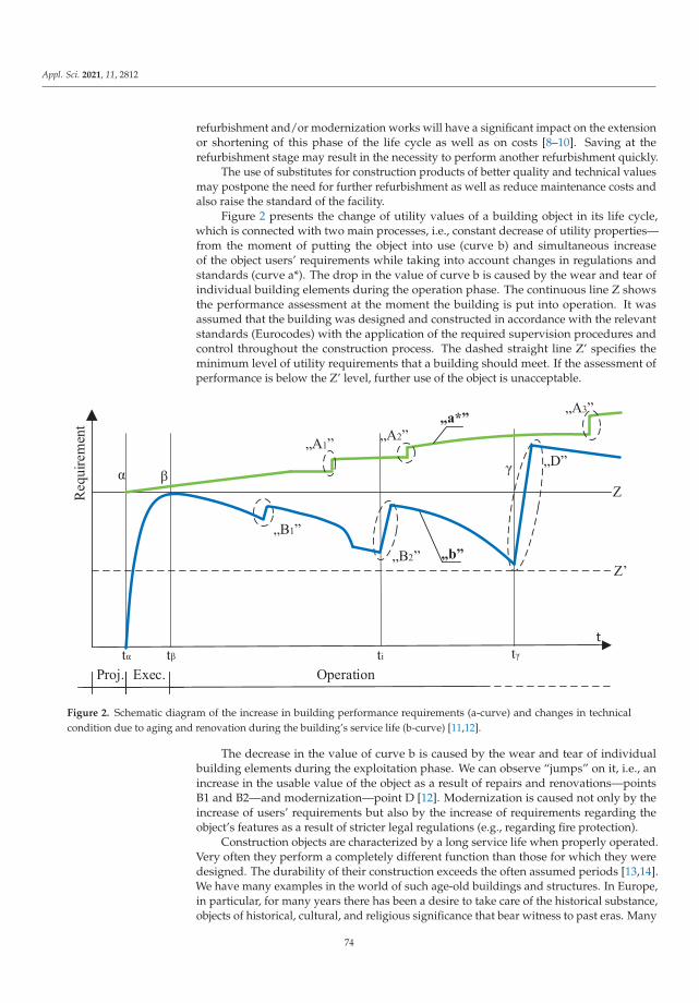
Appl. Sci. 2021, 11, 2812

refurbishment and/or modernization works will have a significant impact on the extensionor shortening of this phase of the life cycle as well as on costs [8–10]. Saving at therefurbishment stage may result in the necessity to perform another refurbishment quickly.

The use of substitutes for construction products of better quality and technical valuesmay postpone the need for further refurbishment as well as reduce maintenance costs andalso raise the standard of the facility.

Figure 2 presents the change of utility values of a building object in its life cycle,which is connected with two main processes, i.e., constant decrease of utility properties—from the moment of putting the object into use (curve b) and simultaneous increaseof the object users’ requirements while taking into account changes in regulations andstandards (curve a*). The drop in the value of curve b is caused by the wear and tear ofindividual building elements during the operation phase. The continuous line Z showsthe performance assessment at the moment the building is put into operation. It wasassumed that the building was designed and constructed in accordance with the relevantstandards (Eurocodes) with the application of the required supervision procedures andcontrol throughout the construction process. The dashed straight line Z’ specifies theminimum level of utility requirements that a building should meet. If the assessment ofperformance is below the Z’ level, further use of the object is unacceptable.

Proj. OperationExec.

Requ

irem

ent

„D”„A1”

„b”

„a*”

Z

Z’

t t ti

t

t

„A2”

„A3”

„B21”

„B1”

Figure 2. Schematic diagram of the increase in building performance requirements (a-curve) and changes in technicalcondition due to aging and renovation during the building’s service life (b-curve) [11,12].

The decrease in the value of curve b is caused by the wear and tear of individualbuilding elements during the exploitation phase. We can observe “jumps” on it, i.e., anincrease in the usable value of the object as a result of repairs and renovations—pointsB1 and B2—and modernization—point D [12]. Modernization is caused not only by theincrease of users’ requirements but also by the increase of requirements regarding theobject’s features as a result of stricter legal regulations (e.g., regarding fire protection).

Construction objects are characterized by a long service life when properly operated.Very often they perform a completely different function than those for which they weredesigned. The durability of their construction exceeds the often assumed periods [13,14].We have many examples in the world of such age-old buildings and structures. In Europe,in particular, for many years there has been a desire to take care of the historical substance,objects of historical, cultural, and religious significance that bear witness to past eras. Many

74

Appl. Sci. 2021, 11, 2812

of the objects among those existing in the building stock, that due to their exceptional value,are entered in the register of monuments kept by the relevant governmental administrationbodies. There is no specific time after which the building is considered a monument.The Act on the Protection and Care of Historical Monuments states that any buildingwhich is important for history and science can become a monument, and thus should bepreserved [15]. It can also be a building built in the 1950s or 1960s if it presents featurescharacteristic for the architecture of a given period and can be important for its history.Buildings entered in the register of monuments are subject to the Act on the Protection andCare of Historical Monuments [16] and all activities related to the use and in particular theirmaintenance in a proper technical condition and standard are subject to the supervisionof the conservator. Thus, in the phase of exploitation of buildings, the period of theirfunctioning as a monument should be distinguished for a group of exceptional objects.

Substitution starts to appear much more often in the case of buildings already in usefor a longer period of time [17–21]. Among the exploited properties, we can observe acertain phenomenon, in which the trend is manifested by the growing deficiencies in thedocumentation of the exploitation of the building with its age. For example, the documen-tation of mass-produced buildings built in the 1970s and 1980s in large panel technology isoften incomplete and inconsistent. Therefore, owners often look for construction productssimilar to the original ones while carrying out renovation works, usually guided by thecriterion of aesthetics and price. In this case, someone else is also responsible for financingthe work on the facility. In cooperative buildings or those owned by housing communities,the costs of all repairs and renovations is borne by the property owners. Most often this isdone through the so-called “renovation fund”. Such works are very often performed in theorder of “from the most urgent”, unfortunately in many cases without taking into accountthe durability of the construction products used for this purpose.

Moreover, one of the major problems of substitution is the choice of substitute material.During the design phase, the architect is almost free to choose a replacement material. Incontrast, there are many more factors to consider during the renovation phase. Thanksto advances in material engineering, manufacturers offer a large selection of substitutionproducts with different properties. There is a need to select criteria to evaluate possiblealternate materials and make a decision. This is done by multi-criteria analysis usingdifferent methods [22]. Among the adopted criteria, the important ones are those that takeinto account the principles of sustainable development. Therefore, ecological materials,modern technologies or modernization of traditional ones with addition of raw materialsfrom different branches of economy (tea to brick) are being sought.

Two types of approach to substitution can be observed. The first, in a more generalsense, is an attempt to:

− produce new materials and building elements capable of performing the appropri-ate function in the construction of a building. Improve their physical, chemical, etc.properties and usability (durability, aesthetics, usability, operation, etc.), thanks tothe development of materials engineering, using the achievements of science, nan-otechnology, etc. [23–26]. They can be used interchangeably with traditional materials(instead of clay bricks, e.g., cellular concrete).

The second, however, related to the idea of sustainable development through:

− development and use of materials and elements of the structure of a building andits equipment in building installations which minimize energy consumption (energyefficient) [27–29];

− production of raw and building materials using wastes (as additives e.g., to cementand aggregates or entirely made from waste) [30–33].

The second approach to substitution is a partial restriction on the choice of a substituteby, for example, an architect, developer, or user by placing a condition (of an aesthetic, lo-gistical, etc. nature). This situation relates to a specific building or material solution [34,35].Here also the selection can be made in terms of one or more optimization criteria [36]. The

75

Appl. Sci. 2021, 11, 2812

criteria are based on the individual requirements of the user, the investor or on currentsocial and economic concepts: sustainable development, circular economy [37]. Applyingmaterial substitution, it is useful to have knowledge about the determinants of its use, thecause–effect relationships of the factors that have an impact on its use. Such research andresults are presented in Section 4 of the article.

3. Substitution in Historical Buildings

It should be noted that in most European countries it is obligatory to replace thematerials used in historic buildings with the same ones that were used originally. In Poland,however, the law allows the use of substitutes [16] depending on various conditions.

Factors that affect the possibility of using construction product substitutes are definedin the so-called conservation program, which is developed for each renovation of an objectentered in the register of monuments. Each proposed substitute for a construction productmust be prepared in the form of a sample and accepted by the Conservator.

Positive aspects of the application of construction product substitution in the reno-vation of buildings entered in the register of monuments are the factors that primarilyenable the refurbishment. Historic sites were built in different construction realities, ata time when available building products were based on natural resources (e.g., stone,rock, clay) and the technology to produce them was simpler. It was common practiceto import construction products from other areas of Europe. Even today it is costly andenvironmentally unfriendly and, due to the environmental protection of certain areas,exploitation is prohibited. However, it is worth considering the use of a substitute materialand conducting an analysis of the impact of using such a solution on social, environmental,and economic factors [38–41].

Ownership of the most valuable objects entered in the register of monuments ismostly in the hands of the State or various institutions such as the churches. It should beremembered that the number of facilities under consideration is large and the possibilitiesof financing renovations are limited, hence the price will always be an important componentof planning a refurbishment. The use of original construction products in one object maylead to abandonment or postponement of the renovation in other objects. Such a situationmay lead to degradation of the remaining buildings and, consequently, increase the costsof renovations that are planned in them. Therefore, the introduction of substitutes forconstruction products in historic buildings, which give positive aesthetic and visual valuesand are less of a financial burden, gives the opportunity to conduct a more effective andlarger-scale renovation policy.

In the case of the described refurbishments, a significant price-creating factor is alsothe time of completion. It is obvious that a longer period of renovation of one object canpostpone the start of renovation in another object, which also requires this renovation.Substitution of construction products may increase the pace of renovation works in connec-tion with, among others, less complicated technology of conducting works, faster pace ofassembly of built-in elements, and the possibility of conducting works in less favorableweather conditions. Reducing the duration of the renovation gives further savings, thanksto which it is possible to predict that the renovation of a monumental object (the processof renovation of an object entered in the register of monuments takes a very long timebecause not all the necessary construction works can be predicted at the stage of designingthe renovation) will be completed within the assumed time.

Construction products used in historic buildings have often survived years or evencenturies. Thus, these are durable products that have been subject to gradual degradationover the years due to lack of refurbishment or minor damage, which has increased theimpact zone from year to year [42,43]. The weakness of the construction product substitutesmay be their durability and resistance to weather conditions in comparison with primaryproducts and other influences e.g., related to the intensity of car exhaust or air pollution [44].Renovations of buildings included in the register of monuments should be carried out bycompanies specializing in this type of construction works. Due to the specific nature of

76

Appl. Sci. 2021, 11, 2812

renovation work in historic buildings, the contractor may encounter problems at each stageof the work that are unusual for newly erected buildings.

Substitutes of construction products used in the renovation of historic buildings give awide range of possibilities. Substitutes can be manufactured from recycled, environmentally-friendly materials and produced by local entrepreneurs [7,45]. The current technology ofconducting construction works and the variety of construction products makes it possibleto carry out a renovation of basically any building, including historic buildings.

In the current market situation, the cost and time of implementation are critical inany type of construction project. In the case of renovations of objects entered in theregister of monuments, the specificity of the conducted construction works and a certainunpredictability of additional construction works, which may appear at each stage of therenovation, are still imposed.

The authors met with an opinion that a historic object that has undergone renovationwith the use of construction product substitutes loses its historical value and should nolonger be treated as a monument. The basic issue to consider in such a situation is thepossibility of renovation.

In old, historic buildings, especially those protected by law (in Poland the register ofhistoric monuments), the use of substitution of materials has a long history. There is anextensive literature in this area, including concepts of substitution principles, developedand proven methodologies for design, testing, analysis, and selection of substitutes [46–48].

4. Evaluation of the Possibility of Using Material Substitution in the Maintenanceof Buildings

Preceding the decision to use substitution, the authors suggest performing an as-sessment and identifying key factors that influence the effectiveness of its use. On thebasis of the presented conditions and factors influencing the application of substitutionin construction objects in the exploitation phase, a SWOT (Strengths, Weaknesses, Oppor-tunities, Threats) matrix was developed (see Table 1). It contains factors that constitutestrengths and weaknesses of the substitution phenomenon and opportunities and threatsin its application.

Table 1. SWOT (Strengths, Weaknesses, Opportunities, Threats) analysis of the application of material substitution inrenovation works during the operation of buildings.

Inside

Positive Negative

Strenghts Weaknesses

1.1. possibility of refurbishment,1.2. lower price of the renovation,1.3. faster pace of construction works

(less complicated technology),1.4. to achieve the desired visual effect,1.5. replacement of products that are no longer found

in the market,1.6. shortening of supply chains

2.1. faster degradation of the object’s substance byinappropriate selection of built products,

2.2. involvement in the work of specialized companies,2.3. conducting works by experienced supervision,2.4. investment revaluation,2.5. possible lack of a proposed substitute in a

previously approved solution

Outside

Opportunities Threats

3.1. market (access and development) of modernconstruction products

3.2. recycled products,3.3. products more environmentally friendly,3.4. establishing cooperation with local entrepreneurs,3.5. revitalization of degraded areas under

conservation care

4.1. loss of authenticity and historical value and object4.2. specific requirements for carrying out works,

especially renovations during adverseweather conditions,

4.3. lack of competent professionals,inspectors, conservators,

4.4. lack of legal regulations concerning theapplied solutions

77

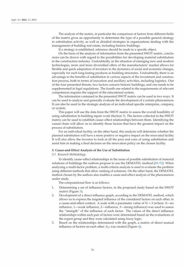
Appl. Sci. 2021, 11, 2812

The analysis of the matrix, in particular the comparison of factors from different fieldsof the matrix gives an opportunity to determine the type of a possible general strategyin substitution activity, as well as detailed strategies in organizations dealing with themanagement of building real estate, including historic buildings.

If a strategy is established, reference should be made to a specific object.On the basis of the analysis of information from the presented SWOT matrix, conclu-

sions can be drawn with regard to the possibilities for developing material substitutionin the construction industry. Undoubtedly, in the situation of emerging new and moderntechnologies, more and more diversified offers of the manufacturers’ market allows forflexible and quick adaptation of investors to the dynamics of social and economic changes,especially for such long-lasting products as building structures. Undoubtedly, there is anadvantage to the benefits of substitution in various aspects of the investment and construc-tion process, both in terms of execution and ancillary activities, including logistics. Outof the four presented threats, two factors concern historic buildings, and one needs to besupplemented in legal regulations. The fourth one related to the requirements of relevantcompetences requires the support of the educational system.

The information contained in the presented SWOT matrix can be used in two ways. Itcan be used to analyze and generally evaluate the development of a certain phenomenon.It can also be used in the strategic analysis of an individual specific enterprise, company,or system.

This paper will use the data from the SWOT matrix to assess the overall feasibility ofusing substitution in building repair work (Section 5). The factors collected in the SWOTmatrix can be used to establish cause–effect relationships between them. Identifying thecausal chain will allow us to identify those factors that have the greatest impact on theprocess of substitution.

For an individual facility, on the other hand, this analysis will determine whether theplanned substitution will have a more positive or negative impact on the renovated facility.It will also allow the investor to look at all the pros and cons of using substitution andassist him in making a final decision on the renovation policy on the chosen facility.

5. Cause-and-Effect Analysis of the Use of Substitution

5.1. Research Methodology

To identify cause–effect relationships in the issue of possible substitution of materialsolutions of buildings the authors propose to use the DEMATEL method [49–52]. Whenanalyzing a multi-factor problem, a multi-criteria analysis is used to evaluate the problemusing different methods that allow ranking of solutions. On the other hand, the DEMATELmethod chosen by the authors also enables a cause-and-effect analysis of the phenomenonunder study.

The computational flow is as follows:

1. Determining a set of influence factors, in the proposed study based on the SWOTmatrix (Figure 3);

2. Development of a direct influence graph, according to the DEMATEL method, whichallows us to express the targeted influence of the considered factors on each other, ina cause-and-effect context. A scale with a parameter value of N = 3 (where: 0—noinfluence, 1—weak influence, 2—influence, 3—strong influence) was used to assessthe “strength” of the influence of each factor. The values of the direct influencerelationships within each pair of factors were determined based on the evaluations ofthe expert group and they were calculated using fuzzy logic;

3. Based on the relationships determined with the graph, a matrix of direct mutualinfluence of factors on each other AD was created (Figure 4);

78

Appl. Sci. 2021, 11, 2812

4. Determination of the normalized direct influence matrix A′D, which contains all

parameters that take values that are in the range [0, 1] (Table 2). The normalizingnumber (n) is taken as the largest of the sum of the rows or columns of the matrix AD:

A′D =

ADn

, (1)

n = max{

∑ni=1aij; ∑n

j=1aij;}

, (2)

5. It is also possible to develop an indirect impact matrix ΔT:

ΔT = A′2D·(

I − A′D), (3)

6. Determination of the total influence matrix T (Table 3):

T = A′D·(

I − A′D), (4)

7. On the basis of the above matrices, the determination of the indices of position andrelationship, respectively, which express in turn: s+—tells about the role of a givenfactor in the process of determining the structure of links between objects, whiles−—expresses the total influence of a given factor on the others. These values aredetermined according to the formulas (Table 4):

s+ =n

∑j=1

tij +n

∑j=1

tji = RTi + CTi , (5)

s− =n

∑j=1

tij −n

∑j=1

tji = RTi − CTi , (6)

When these values are plotted on a graphical representation, it is easy to see whichfactors have the greatest influence on the others and to determine which are the causesand which are the effects of the actions taken (Figure 5).

8. Finally, the net impact value is also determined, which tells the factor that has thegreatest impact on the others considering both the causal and effect nature (Table 4):

netto = s+ + s− (7)

Table 2. The fragment of normalized direct influence matrix A′D.

1.1 1.2 1.3 1.4 1.5 1.6 2.1 . . . . . .

1.1 −0.0156 −0.0017 0.0000 0.0313 0.0000 0.0000 −0.0035 . . . . . .1.2 0.1250 0.0000 0.0000 −0.0052 0.0000 0.0000 0.0833 . . . . . .1.3 0.0729 0.0833 0.0000 −0.0035 0.0000 0.0000 −0.0069 . . . . . .1.4 0.0000 0.0000 0.0000 0.0000 0.0000 0.0000 0.0000 . . . . . .1.5 0.1128 0.0330 0.0816 0.0781 −0.0017 −0.0035 −0.0052 . . . . . .

. . . . . . . . . . . . . . . . . . . . . . . . . . . . . . . . . . . . . . . . . . . . . . . . . . .

79

Appl. Sci. 2021, 11, 2812

Table 3. Total influence matrix T (fragment).

1.1 1.2 1.3 1.4 1.5 1.6 2.1 . . . . . .

1.1 0.0000 0.0000 0.0000 0.0417 0.0000 0.0000 0.0000 . . . . . .1.2 0.1250 0.0000 0.0000 0.0000 0.0000 0.0000 0.0833 . . . . . .1.3 0.0833 0.0833 0.0000 0.0000 0.0000 0.0000 0.0000 . . . . . .1.4 0.0000 0.0000 0.0000 0.0000 0.0000 0.0000 0.0000 . . . . . .1.5 0.1250 0.0417 0.0833 0.0833 0.0000 0.0000 0.0000 . . . . . .

. . . . . . . . . . . . . . . . . . . . . . . . . . . . . . . . . . . . . . . . . . . . . . . . . . . . . .

Table 4. Summary of DEMATEL analysis results.

Criterion i RTi CTi s+ s− Netto

1.1 0.2830 0.6042 0.8872 −0.3212 0.56601.2 0.2396 0.4288 0.6684 −0.1892 0.47921.3 0.1146 0.1198 0.2344 −0.0052 0.22921.4 0.1198 0.2899 0.4097 −0.1701 0.23961.5 0.5243 0.0399 0.5642 0.4844 1.04861.6 0.0590 0.1493 0.2083 −0.0903 0.11812.1 0.0799 0.2708 0.3507 −0.1910 0.15972.2 0.1181 0.1632 0.2813 −0.0451 0.23612.3 0.1198 0.0330 0.1528 0.0868 0.23962.4 0.0000 0.0660 0.0660 −0.0660 0.00002.5 0.0000 0.1163 0.1163 −0.1163 0.00003.1 0.4757 0.0000 0.4757 0.4757 0.95143.2 0.2865 0.0122 0.2986 0.2743 0.57293.3 0.3038 0.0399 0.3438 0.2639 0.60763.4 0.0347 0.0399 0.0747 −0.0052 0.06943.5 0.1563 0.0365 0.1927 0.1198 0.31254.1 0.0365 0.7743 0.8108 −0.7378 0.07294.2 0.1927 0.1632 0.3559 0.0295 0.38544.3 0.1094 0.0000 0.1094 0.1094 0.21884.4 0.2153 0.1215 0.3368 0.0938 0.4306

1.1 1.2

1.3

1.4

1.5

1.6

2.2

2.1

2.3

2.4

2.5

3.1 3.2

3.3

3.4

3.5

4.14.2

4.3

4.4

Strong influence

Influence

Weak influence

Figure 3. Direct influence graph—expert evaluation results.

80

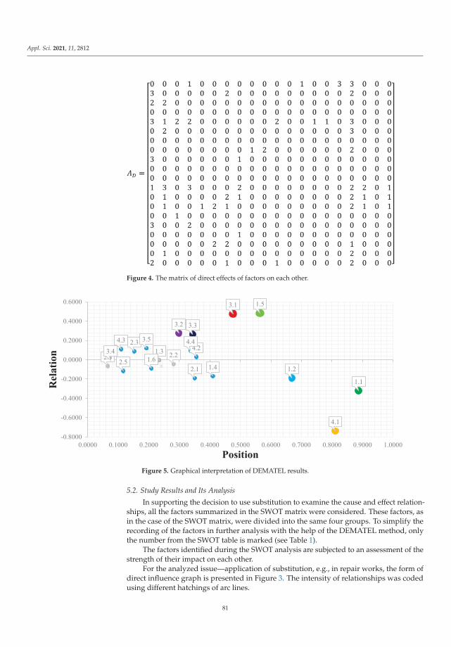
Appl. Sci. 2021, 11, 2812

Figure 4. The matrix of direct effects of factors on each other.

1.1

1.2

1.3

1.4

1.5

1.62.1

2.2

2.3

2.42.5

3.1

3.2 3.3

3.4

3.5

4.1

4.24.3 4.4

-0.8000

-0.6000

-0.4000

-0.2000

0.0000

0.2000

0.4000

0.6000

0.0000 0.1000 0.2000 0.3000 0.4000 0.5000 0.6000 0.7000 0.8000 0.9000 1.0000

Rel

atio

n

PositionFigure 5. Graphical interpretation of DEMATEL results.

5.2. Study Results and Its Analysis

In supporting the decision to use substitution to examine the cause and effect relation-ships, all the factors summarized in the SWOT matrix were considered. These factors, asin the case of the SWOT matrix, were divided into the same four groups. To simplify therecording of the factors in further analysis with the help of the DEMATEL method, onlythe number from the SWOT table is marked (see Table 1).

The factors identified during the SWOT analysis are subjected to an assessment of thestrength of their impact on each other.

For the analyzed issue—application of substitution, e.g., in repair works, the form ofdirect influence graph is presented in Figure 3. The intensity of relationships was codedusing different hatchings of arc lines.

81

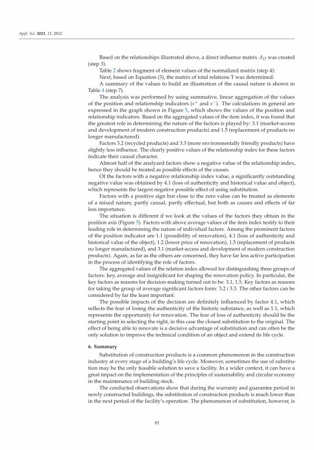
Appl. Sci. 2021, 11, 2812

Based on the relationships illustrated above, a direct influence matrix AD was created(step 3).

Table 2 shows fragment of element values of the normalized matrix (step 4):Next, based on Equation (3), the matrix of total relations T was determined:A summary of the values to build an illustration of the causal nature is shown in

Table 4 (step 7).The analysis was performed by using summative, linear aggregation of the values

of the position and relationship indicators (s+ and s−). The calculations in general areexpressed in the graph shown in Figure 5, which shows the values of the position andrelationship indicators. Based on the aggregated values of the item index, it was found thatthe greatest role in determining the nature of the factors is played by: 3.1 (market-accessand development of modern construction products) and 1.5 (replacement of products nolonger manufactured).

Factors 3.2 (recycled products) and 3.3 (more environmentally friendly products) haveslightly less influence. The clearly positive values of the relationship index for these factorsindicate their causal character.

Almost half of the analyzed factors show a negative value of the relationship index,hence they should be treated as possible effects of the causes.

Of the factors with a negative relationship index value, a significantly outstandingnegative value was obtained by 4.1 (loss of authenticity and historical value and object),which represents the largest negative possible effect of using substitution.

Factors with a positive sign but close to the zero value can be treated as elementsof a mixed nature, partly causal, partly effectual, but both as causes and effects of farless importance.

The situation is different if we look at the values of the factors they obtain in theposition axis (Figure 5). Factors with above average values of the item index testify to theirleading role in determining the nature of individual factors. Among the prominent factorsof the position indicator are 1.1 (possibility of renovation), 4.1 (loss of authenticity andhistorical value of the object), 1.2 (lower price of renovation), 1.5 (replacement of productsno longer manufactured), and 3.1 (market-access and development of modern constructionproducts). Again, as far as the others are concerned, they have far less active participationin the process of identifying the role of factors.

The aggregated values of the relation index allowed for distinguishing three groups offactors: key, average and insignificant for shaping the renovation policy. In particular, thekey factors as reasons for decision-making turned out to be: 3.1, 1.5. Key factors as reasonsfor taking the group of average significant factors form: 3.2 i 3.3. The other factors can beconsidered by far the least important.

The possible impacts of the decision are definitely influenced by factor 4.1, whichreflects the fear of losing the authenticity of the historic substance, as well as 1.1, whichrepresents the opportunity for renovation. The fear of loss of authenticity should be thestarting point in selecting the right, in this case the closest substitution to the original. Theeffect of being able to renovate is a decisive advantage of substitution and can often be theonly solution to improve the technical condition of an object and extend its life cycle.

6. Summary

Substitution of construction products is a common phenomenon in the constructionindustry at every stage of a building’s life cycle. Moreover, sometimes the use of substitu-tion may be the only feasible solution to save a facility. In a wider context, it can have agreat impact on the implementation of the principles of sustainability and circular economyin the maintenance of building stock.

The conducted observations show that during the warranty and guarantee period innewly constructed buildings, the substitution of construction products is much lower thanin the next period of the facility’s operation. The phenomenon of substitution, however, is

82

Appl. Sci. 2021, 11, 2812

often encountered in the long-term perspective of facility operation, especially during allrepair and overhaul works.

One of the ways of extending the life cycle of buildings is a proper renovation policy,which through proper selection of material solutions will ensure longer durability ofcomponents and the entire facility.

A special case is the substitution in the renovation works of objects entered in theregister of monuments, which gives the possibility to protect the historic substance whilemaintaining the structural and aesthetic values.

Product substitution, which is often cheaper than the original, may also allow fora wider range of renovations, which directly contributes to improving the technical andfunctional condition of the object and thus allows for extending its life cycle.

The SWOT analysis conducted by the authors allows us to conclude that substitutionin the construction industry is justified and that there are great opportunities for its imple-mentation and development. A detailed analysis of the SWOT matrix factors, using theDEMATEL method, allowed for an overall assessment of substitution possibilities with thedetermination of the cause–effect relationship of factors from particular groups characteriz-ing the strengths and weaknesses of substitution as well as the opportunities and threats.Undoubtedly, the use of substitute materials, especially in historic buildings, will result ina decrease in their authenticity, but will ultimately restore them to safe operation and inother buildings allow for an extended life cycle.

Despite the possibility of product substitution thanks to materials engineering andtechnology development, the use of substitution should not be approached uncritically.The authors recommend a case-by-case approach, conducting a comprehensive analysisand making decisions based on, among other things, the tools proposed in the article andevaluating the cause-and-effect relationships that will occur when substitution is applied.

The above comment also applies to using a different approach to material substitutionin historic buildings. The decision whether or not to use substitution and the freedomto choose substitution solutions are influenced by the conservation concepts and legalregulations of the respective country or type of object.

Author Contributions: Conceptualization, A.S., K.L. and A.R.; methodology, A.S., K.L. and A.R.;validation, A.S., K.L. and A.R.; formal analysis, A.S., K.L. and A.R.; investigation, A.S., K.L. and A.R.;resources, K.L. and A.R.; writing—original draft preparation, A.S., K.L. and A.R.; writing—reviewand editing, A.S. and A.R.; visualization, K.L. and A.R.; supervision, A.S. All authors have read andagreed to the published version of the manuscript.

Funding: This research received no external funding.

Institutional Review Board Statement: Not applicable.

Informed Consent Statement: Not applicable.

Data Availability Statement: Data sharing not applicable.

Acknowledgments: The work was carried out as part of statutory research no. 11.11.100.197 inthe Department of Geomechanics, Civil Engineering and Geotechnics of Faculty of Mining andGeoengineering, AGH University of Science and Technology in Cracow.

Conflicts of Interest: The authors declare no conflict of interest.

References

1. Linczowski, K.; Sobotka, A. Relations between substitution in technological processes and construction supply logistics. Logistics2014, 6, 9816–9825.

2. Gustavsson, L.; Pingoud, K.; Sathre, R. Carbon dioxide balance of wood substitution: Comparing concreto- and wood-framedbuildings. Mitig. Adapt. Strateg. Glob. Chang. 2006, 11, 667–691. [CrossRef]

3. Wadr, H.J. The Use of Substitute Materials on Historic Building Exteriors. 1988. Available online: http://www.nps.gov/tps/how-to-preserve/briefs/16-substitute-materials.htm#top (accessed on 14 February 2021).

4. New Zealand Government, Ministry of Business Innovation & Employment. Quick Guide to Product Substitution; New ZealandGovernment: Wellington, New Zealand, 2004.

83

Appl. Sci. 2021, 11, 2812

5. Linczowski, K.; Sobotka, A. Analysis of logistics for construction site supply with reinforcing steel. Tech. Trans. Civ. Eng. 2014, 6,225–232.

6. Arendalski, J. Durability and Reliability of Residential Buildings; Arkady: Warsaw, Poland, 1978.7. Petersen, A.K.; Solberg, B. Environmental and economic impacts of substitution between wood products and alternative materials:

A review of micro-level analyses from Norway and Sweden. For. Policy Econ. 2005, 3, 249–259. [CrossRef]8. Fregonara, E.; Patono, S. A sustainability indicator for building projects in presence of risk/uncertainty over time: A research

experience. AESTIMUM 2018, 19, 173–205.9. Grzyl, B.; Apollo, M.; Miszewska-Urbanska, E.; Kristowskim, A. Object operation management in terms of life cycle costs. Acta

Sci. Pol. 2017, 16, 85–89.10. Plebankiewicz, E.; Meszek, W.; Zima, K.; Wieczorek, D. Probabilistic and fuzzy approaches for estimating the life cycle costs of

buildings under conditions of exposure to risk. Sustainability 2020, 12, 2504. [CrossRef]11. Orłowski, Z.; Szklennik, N. Analysis of the building value in use as a function of time. Tech. Trans. 2010, 6, 303–312.12. Radziejowska, A. The Method of Assessing the Social Performance of Residential Buildings in the Aspect of Sustainable

Construction. Ph.D. Thesis, AGH, Cracow, Poland, 2018.13. Economakis, R. Durability in Construction: Traditions and Sustainability in 21st Century Architecture; Papadakis Publisher: Winter-

bourne, Berkshire, UK, 2015; ISBN-13: 978-1906506551.14. Bai, J. Durability of sustainable construction materials. Sustain. Constr. Mater. 2016, 38, 397–414.15. Gmiter, M. Guide to the Investment Process in Historic Buildings; Presscom Sp. Z.o.o.: Poland, Wrocław, 2018.16. Act on the Protection and Care of Historical Monuments, Old Monuments Law (Ustawa, o Ochronie Zabytków; Opiece Nad

Zabytkami) of 23 July 2003, with Later Changes; Journal of Laws: 2014; pos. 1446. Available online: https://isap.sejm.gov.pl/isap.nsf/download.xsp/WDU20031621568/U/D20031568Lj.pdf (accessed on 16 February 2021).

17. Technical Preservation Services. Evaluating Substitute Materials in Historic Buildings; Historic Preservation Tax Incentives Pro-gramme: Washington, DC, USA, 2007.

18. Cluver, J.H. No Substitute: Inexpensive and Maintenance Free or Short Sighted and Maintenance Proof: How Do Substitute Materials StackUp in the Long Run? Labine’s Period Homes: Boulder, CO, USA, 2005; pp. 12–16.

19. Dierickx, M.B. Substitute materials for wooden buildings: The system or the artifact? APT Bull. 1986, 18, 4–5. [CrossRef]20. Capen, J. Using substitute materials in a historic district. Hill Rag 2008, 5, 134–135.21. S & D Design Guidelines for Landmark. Guidelines for Preserving Historic Buildings—Alterations to Landmark Structures and

Contributing Structures in Historic Districts; S & D Design Guidelines for Landmark: Denver, CO, USA, 2016.22. Zavadskas, E.K.; Turkis, Z.; Tamosaitiene, J. Selection of construction enterprises management strategy based on the SWOT and

multi-criteria analysis. Arch. Civ. Mech. Eng. 2011, 11, 1063–1082. [CrossRef]23. Nawar, A.H. Nano-technologies and nano-materials for civil engineering construction works applications. Mater. Today Proc.

2020. [CrossRef]24. Razakhanova, F.M. Issues concerning import substitution of building materials in the construction market. Vestn. Dagest. Gos.

Teh. Univ. Teh. Nauk. 2018, 44, 223–233. [CrossRef]25. Li, H.; Xu, B. Advanced Building Materials and Structural Engineering; Advanced Materials Research; Trans Tech Publications Ltd.:

Zurich, Switzerland, 2012; Volume 461.26. Enríquez, E.; Torres-Carrasco, M.; Cabrera, M.; Muñoz, D.; Fernández, J. Towards more sustainable building based on modified

Portland cements through partial substitution by engineered feldspars. Constr. Build. Mater. 2020. [CrossRef]27. Piccardo, C.; Dodoo, A.; Gustavsson, L.; Tettey, U. Retrofitting with different building materials: Life-cycle primary energy

implications. Energy 2020, 19, 5–10. [CrossRef]28. Blomqvist, S.; La Fleur, L.; Amiri, S.; Rohdin, P.; Ödlund, L. The impact on system performance when renovating a multifamily

building stock in a district heated region. Sustainability 2019, 11, 2199. [CrossRef]29. Rubio-Cintas, M.D.; Parron-Rubio, M.E.; Perez-Garcia, F.; Ribeiro, A.B.; Oliveira, M.J. Influence of steel slag type on concrete

shrinkage. Sustainability 2021, 13, 214.30. Bouasria, M.; Khadraoui, F.; Benzaama, M.-H.; Touati, K.; Chateigner, D.; Gascoin, S.; Pralong, V.; Orberger, B.; Babouri, L.; El

Mendili, Y. Partial substitution of cement by the association of Ferronickel slags and Crepidula fornicata shells. J. Build. Eng. 2021,4, 103. [CrossRef]

31. Chen, W.; Li, Y.; Chen, S.; Zheng, C. Properties and economics evaluation of utilization of oil shale waste as an alternativeenvironmentally-friendly building materials in pavement engineering. Constr. Build. Mater. 2020. [CrossRef]

32. Patel, D.; Shrivastava, R.; Tiwari, R.; Yadav, R. Properties of cement mortar in substitution with waste fine glass powder andenvironmental impact study. J. Build. Eng. 2020. [CrossRef]

33. Raheem, A.A.; Ikotun, B.D. Incorporation of agricultural residues as partial substitution for cement in concrete and mortar. J.Build. Eng. 2020. [CrossRef]

34. Hafner, A.; Schäfer, S. Comparative LCA study of different timber and mineral buildings and calculation method for substitutionfactors on building level. J. Clean. Prod. 2017, 167, 630–642. [CrossRef]

35. D’Amico, B.; Pomponi, F.; Hart, J. Global potential for material substitution in building construction: The case of cross laminatedtimber. J. Clean. Prod. 2021, 7, 279. [CrossRef]

84

Appl. Sci. 2021, 11, 2812

36. Vachris, J. Asbestos substitution serviceability of new materials. In Proceedings of the Electrical Insulation Conference andElectrical Manufacturing & Coil Winding Conference, Cincinnati, OH, USA, 26–28 October 1999.

37. Omer, M.A.; Noguchi, T. A conceptual framework for understanding the contribution of building materials in the achievement ofSustainable Development Goals (SDGs). Elsevier Sustain. Cities Soc. 2020, 52, 244–302. [CrossRef]

38. Van Domelen, S.K. The Choice Is Yours: Considerations & Methods for the Evaluation & Selection of Substitute Materialsfor Historic Preservation. Ph.D. Thesis, University of Pennsylvania, Philadelphia, PA, USA, 2009. Available online: http://repository.upenn.edu/hp_theses (accessed on 14 February 2021).

39. Liu, L.; Li, H.; Lazzaretto, A.; Manente, G.; Tong, C.; Liu, Q.; Li, N. The development history and prospects of biomass-basedinsulation materials for buildings. Renew. Sustain. Energy Rev. 2017, 69, 912–932. [CrossRef]

40. Iucolano, F.; Boccarusso, L.; Langella, A. Hemp as eco-friendly substitute of glass fibres for gypsum reinforcement: Impact andflexural behaviour. Compos. Part B Eng. 2019, 175, 25. [CrossRef]

41. Mathur, V. Composite materials from local resources. Constr. Build. Mater. 2006, 20, 470–477. [CrossRef]42. Myers, J.; Aluminum and Vinyl Siding on Historic Buildings. The Appropriateness of Substitute Materials for Resurfacing

Historic Wood Frame Buildings. 1984. Available online: https://www.nps.gov/TPS/how-to-preserve/briefs/8-aluminum-vinyl-siding.htm (accessed on 14 February 2021).

43. Nowogonska, B. Value of technical wear and costs of restoring performance characteristics to residential buildings. Buildings2020, 10, 9. [CrossRef]

44. Demir, I. An investigation on the production of construction brick with processed waste tea. Build. Environ. 2006, 9, 1274–1278.[CrossRef]

45. Teha, S.H.; Wiedmann, T.; Schinabeck, J.; Moorea, S. Replacement scenarios for construction materials based on economy-widehybrid LCA. Procedia Eng. 2017, 180, 179–189. [CrossRef]

46. Friedman, D. Historical Building Construction: Design, Materials, and Technology; W.W. Norton & Company: New York, NY, USA,1995.

47. Fisher, T. The sincerest form of flattery. Progress. Archit. 1985, 85, 118–123.48. Brownell, B. Transmaterial: A Catalog of Materials that Redefine our Physical Environment; Princeton Architectural: New York, NY,

USA, 2006; Volume 6.49. Dytczak, M.; Ginda, G.; Gotowała, B.; Szklennik, N. Application potential of Dematel method and its extensions for analysis of

decision problems in civil engineering. Bud. Inzynieria Sr. 2011, 2, 235–240.50. Sheng-Li, S.; Xiao-Yue, Y.; Hu-Chen, L.; Ping, Z. Dematel technique: A systematic review of the state-of-the-art literature on

methodologies and applications. Math. Probl. Eng. 2018, 23, 1–33.51. Jiunn, I.S.; Hsin-Hung, W.; Kuan-Kai, H. A Dematel method in identifying key success factors of hospital service quality. Knowl.

Based Syst. 2010, 23, 277–282.52. Kijewska, K.; Torbacki, W.; Iwan, S. Application of AHP and Dematel methods in choosing and analysing the measures for the

distribution of goods in Szczecin region. Sustainability 2018, 10, 2365. [CrossRef]

85

applied sciences

Article

Bayes Conditional Probability of Fuzzy Damage and TechnicalWear of Residential Buildings

Jarosław Konior * and Tomasz Stachon

���������������

Citation: Konior, J.; Stachon, T. Bayes

Conditional Probability of Fuzzy

Damage and Technical Wear of

Residential Buildings. Appl. Sci. 2021,

11, 2518. https://doi.org/10.3390/

app11062518

Academic Editor: Marco Vona

Received: 17 February 2021

Accepted: 8 March 2021

Published: 11 March 2021

Publisher’s Note: MDPI stays neutral

with regard to jurisdictional claims in

published maps and institutional affil-

iations.

Copyright: © 2021 by the authors.

Licensee MDPI, Basel, Switzerland.

This article is an open access article

distributed under the terms and

conditions of the Creative Commons

Attribution (CC BY) license (https://

creativecommons.org/licenses/by/

4.0/).

Department of Building Engineering, Faculty of Civil Engineering, Wroclaw University of Science andTechnology, 50-370 Wrocław, Poland; tomasz.stachon@pwr.edu.pl* Correspondence: jaroslaw.konior@pwr.edu.pl; Tel.: +48-71-320-23-69

Abstract: The purpose of the research presented in the article is to identify the impact of the processesassociated with the broadly understood maintenance of old residential buildings with a traditionalconstruction on the size and intensity of the wear of their elements. The goal was achieved by analyzingthe symptoms of the technical wear process, which involved the understanding of the mechanismof the occurrence of the phenomenon of damage, and the identification of the size and intensity ofthe damage to the elements of the evaluated buildings. The consequence of systematizing the mostimportant processes that influence the loss of functional properties of residential buildings was thecreation of the authors’ own qualitative model and its transformation into a quantitative model. This,in turn, enabled a multi-criteria quantitative analysis of the cause and effect phenomena—“damage-technical wear”—of the most important elements of downtown tenement buildings to be carried outin fuzzy conditions, i.e., uncertainty concerning the occurrence of damage and the wear process. Thefollowing key question was answered in the subjective expert assessment of the technical conditionof an evaluated residential building: what is the probability of the wear of an element, which maybe more or less correlated with its average maintenance conditions, or more simply, what is theprobability that the element is more or less (approximately) worn? It has been proven that theconditional probability of the technical wear of an element in relation to its damage increases withthe deterioration of the maintenance conditions of the building, and this increase is very regular,even in the case of different building elements. This probability is characterized by a low standarddeviation and a narrow range of the dispersion of results in the case of various elements with regardsto each of the considered building maintenance conditions.

Keywords: residential buildings; technical wear; damage; Bayes conditional probability; fuzzy sets

1. Introduction

1.1. Literature Survey

The literature survey was based on the theory of decision-making in the conditions ofuncertainty and fuzziness, which is given by Kacprzyk [1], and which defines the followingdecision situations [2]:

• Certainty: all the information that describes the issue of decision-making is deter-ministic, i.e., options for choosing a decision, and what each choice gives in terms ofcertain usefulness (e.g., value analysis) etc., is known. In this case, making decisionscomes down to the direct maximization of the utility function;

• Risk: information that describes the decision-making issue is probabilistic, i.e., appro-priate probability distributions are provided. In this case, making decisions comesdown to maximizing the expected value of the utility function;

• Indeterminacy: even probabilities are not known. Decision-making usually comesdown to applying a minimax strategy in order to ensure the highest utility valueunder the most unfavorable conditions;

Appl. Sci. 2021, 11, 2518. https://doi.org/10.3390/app11062518 https://www.mdpi.com/journal/applsci

87

Appl. Sci. 2021, 11, 2518

• Fuzziness: indeterminacy not only relates to the occurrence of an event, but also to itsmeaning in general, which can no longer be described using probabilistic methods.Of course, further extensions are possible here, such as adding risk to fuzziness.

When assessing the degree of the technical wear of building elements, apart from mea-surable (quantitative) criteria, non-measurable (qualitative) criteria are also used. They areexpressed in the analysis of symptoms by, i.e., damage that reduces the technical conditionand utility value of building elements. Only some of these criteria can be roughly quantified.However, most of these criteria are qualitative. Their value is determined verbally by usingterms such as “significant”, “poor”, “strong”, “almost not at all”, “partial”, or “complete”,and always appears in the description of damage phenomena. The interpretation of theeffects of these phenomena, which is performed according to subjective and qualitativepremises, leads to the indiscriminate categorization of the technical maintenance conditionsfor buildings and their elements, i.e., good, satisfactory, average, poor, or bad. Striving fora quantification of criteria that are inherently qualitative and immeasurable, and trying todetermine the relations between them, led to the use of the category of fuzzy sets (the basisof which were formulated by Zadeh [3,4] and Yager [5,6]) with regards to this issue. Theirproperties enable damage to building elements, as well as the conditions of their technicalmaintenance, to be described within an unambiguous measurable quantitative aspect.

In the methodical approach to the technical assessment of residential buildings, re-search by Nowogonska [7–11] was used, which provides methods and models for theestimation of the degree of the technical wear of buildings. However, it should be remem-bered that the presented methodical approach of Nowogonska is exclusively deterministic,and therefore simplified and also practical. This approach is confirmed by the researchof Lee and Kim [12], who indicated the degree of risk that is associated with damageto a building element. The assessment of the entire service life of a building structureincludes a fuzzy calculation, which was presented in the publications of Plebankiewicz,Wieczorek, and Zima [13–16] in order to determine the impact and significance of the riskof the emergency operation of a building. The works by Ibadov [17–20] concerning thebuilding investment process with a fuzzy phase allowed for the practical application ofuncertain and subjective events when determining the degree of damage to the testedtenement houses. The assessment of the risk and costs of maintaining construction facil-ities, and also the conducting of the construction process in fuzzy conditions, were alsopresented by Kamal and Jain [21], Andric, Wang, Zou and Zhang [22], J. Marzouk andAmin [23], Knight, Robinson, and Fayek [24], Sharma and Goyal [25], Al-Humaidi andHadipriono [26], Ammar, Zayed and Moselhi [27], Chan, Kwong, Dillon and Fung [28],and Naszrzadeh, Afshar, Khanzadi, and Howick [29].

Methods, models, and methodological tools for the assessment of the technical condi-tion of buildings, which are considered in the article with regards to the research sample,were described and summarized by Konior in papers [30–34] with co-authors [35–37] andin a collective study under the supervision of Kaplinski, which is entitled “Methods andModels in the Engineering of Building Processes” [38].

1.2. Research Sample

The research sample, which included 102 technically assessed residential buildingsfrom the “Srodmiescie” district of Wroclaw, was selected from a group of 160 examinedobjects [39]. The overriding criterion for sampling involved the obtaining of a comparablegroup of objects. Mutual comparability of the downtown tenement houses meant:

• age coherence, i.e., a similar period of erection, maintenance, and use with regards tohistorical and social aspects;

• compactness of the building development in the urban layout that remained un-changed for years;

• similar location along downtown street routes with an urban, but not representative, character;• construction and material homogeneity, especially with regards to the load-bearing

structure of buildings;

88

Appl. Sci. 2021, 11, 2518

• identical functional solutions, understood as the standard of apartment amenities andfurnishings (for that time), and a defined standard of living for residents.

The method of selecting the research sample at the level of greater detail was basedon the mutual similarity of all the technical solutions of the downtown tenement houses.The selected research sample, according to the criteria presented above, is a representativesample with regards to the concept of representativeness that is specific to the adoptedpurpose of the study [40,41]. It contains all the values of the variables that could berecreated from the research carried out earlier using a different objective function than theone adopted in the study.

These values and variables were then compiled and processed in such a way that itwas possible to make conclusions about the cause–effect relationships between them in thegeneral population.

Therefore, it can be considered as a typologically representative sample that includesthe desired types of homogeneous variables. Due to the fact that the structure of thepopulation and its properties were previously well recognized, such a selection of theresearch sample can also be seen as a deliberate selection. It should be noted that the samplemay not be representative in terms of the distributions of the studied variables, whichmay—for the adopted level of significance—not correspond to analogous distributionsin the general population. It is also not known—at this stage of the research—whetherthe selected sample is representative due to the relationship between its variables and theidentically defined variables in the entire set of downtown residential buildings. Therefore,at the very beginning of the research, it was assumed that a specific research sample occursin the existing population with the fuzzy phase.

Tested buildings have been classified into classes, determined by the degree of thetechnical wear. The technical wear 0–15% has been classified to the class I, 16–30% to theclass II, 31–50% to the class III, 51–70% to the class IV, 71–100% to the class V. Owing to thefact that all considering apartment houses belong to the same group of their age it is possibleto assume that the class of the technical wear corresponds to the conditions of buildingmaintenance. Therefore, the equivalence has been defined: a poor maintenance—the classIV, V, an average maintenance—the class III, an above than an average maintenance—theclass II, a very well cared maintenance—the class I.

2. Research Method

2.1. Problem Identification

The research methodology at a level of greater detail was prepared in such a way thatallowed the previously prepared qualitative model to be transformed into a quantitativemodel. Therefore, the diagnosis of the impact of the maintenance of the residential build-ings on the amount of their technical wear was carried out using quantitative methodsin fuzzy set categories, and also by using the authors’ own model that was created inthe conditions of fuzziness. The model allowed for the determination of the conditionalprobabilities of the process of technical wear, and also the set of damage according to bothBayes formulas [40–42] and the combined approach of Zadeh [3,4] and Yager [5,6];

As mentioned in the introduction, when visually assessing the technical wear ofbuilding elements, the symptoms of their destruction are taken into account, i.e., individualdamage that can be categorized into the following groups (groups) of damage:

• UM—mechanical damage to the structure and texture of building elements;• UW—damage to building elements caused by water penetration and moisture penetration;• UD—damage resulting from the loss of the original shape of wooden elements;• UP—damage to wooden elements attacked by biological pests.

The purpose of such a conceptual and technical systematization of damage is a com-prehensive diagnosis of the extent to which a building element is worn. This assessment, inturn, leads to the implication of stating under what technical conditions—good, satisfactory,average, poor, or bad—the building element was (is) maintained. It is difficult to definea fuzzy set with such a broad meaning as “average technical condition of maintenance”

89

Appl. Sci. 2021, 11, 2518

using one membership function. In this case, a semantic analysis of the term “technicalwear of a building element” was used, which was denoted with the symbol of a fuzzyset “Z”. Let the technical wear of building element Z consist of: mechanical wear of itsstructure and texture (fuzzy set ZM), its technical wear caused by water penetration andmoisture penetration (fuzzy set ZW), technical wear resulting from the loss of its originalshape (fuzzy set ZD), and technical wear caused by the attack of biological pests (fuzzy ZPharvest). This sum can then be expressed as follows:

Z = ZM∪ZW∪ZD∪ZP (1)

and when assuming the identity of the degree of technical wear and its visual symptom(Z ⇔ U)—damage to a building element that is integrated into the above-described damagesets—this expression takes the following form:

U = UM∪UW∪UD∪UP (2)

If technical wear was assumed in the observed states with its measure—the degree ofwear as a fuzzy set with no crisp membership boundary of {z} = Z—then the visual image ofthis wear—global damage to a building element—should be treated as a fuzzy set, the fuzzyevents of which are arguments—distinguished types of damage {u} = U. Therefore, fuzzyrandom events are fuzzy sets that express the degree of technical wear, for which there isno complete (measurable) certainty of membership to the II, III or IV class of the technicalmaintenance of an element. The question then arises: what is the probability of an elementbeing worn, which will more or less represent its average maintenance conditions. To put itsimply, what is the probability that an element is more or less (approximately) worn?

The approach of Zadeh [3,4], who defined the probabilities of fuzzy events in the formof real numbers from interval [0, 1], was used in the research. Therefore, the probabilityof a fuzzy event, which is the technical wear of a building element, which corresponds tosatisfactory, average, and poor maintenance conditions, was defined as:

P(Z)II, III, IV =n

∑i=1

p(zi)μzi(zi), if Z = {zi} = {z1, z2, . . . , zn} (3)

For the global damage of a structural element, which is assumed equivalently to theevent of technical wear, the probability of its occurrence is expressed by the followinganalogous relationship:

P(U)II, III, IV =m

∑j=1

p(uj) μuj(uj), gdy U = {uj} = {u1, u2, . . . , um} (4)

The probabilities p(ui) of the occurrence of elementary damage ui in sets II, III, IVwere calculated and then presented in Table 1.

90

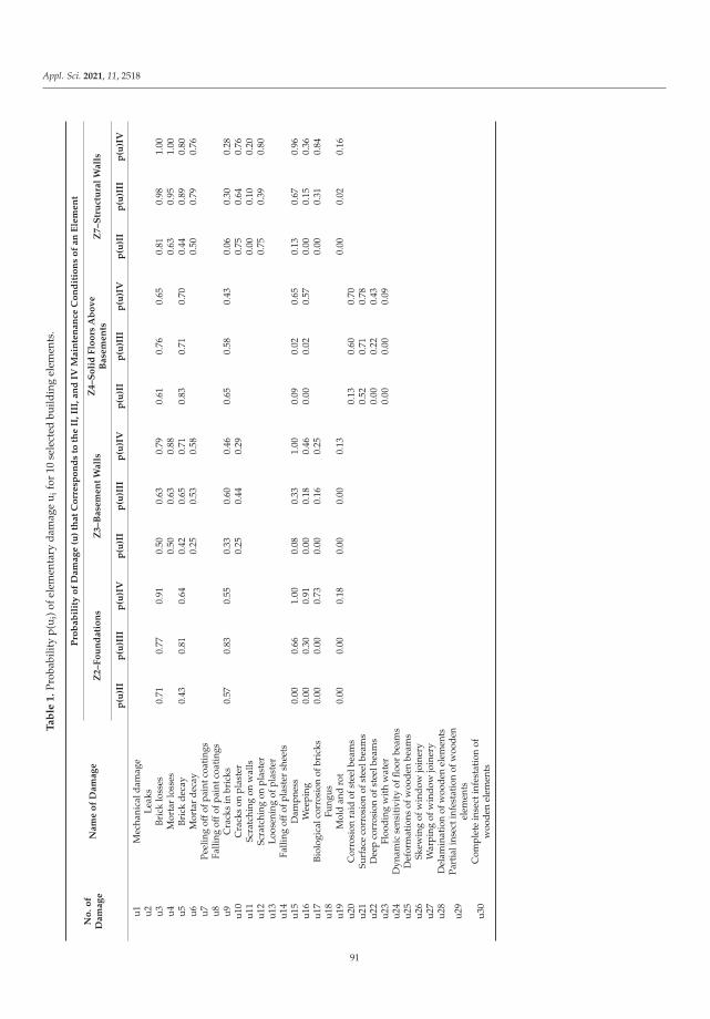
Appl. Sci. 2021, 11, 2518

Ta

ble

1.

Prob

abili

typ(

u i)o

fele

men

tary

dam

age

u ifo

r10

sele

cted

build

ing

elem

ents

.

No

.o

fD

am

ag

eN

am

eo

fD

am

ag

e

Pro

ba

bil

ity

of

Da

ma

ge

(u)

tha

tC

orr

esp

on

ds

toth

eII

,II

I,a

nd

IVM

ain

ten

an

ceC

on

dit

ion

so

fa

nE

lem

en

t

Z2

–F

ou

nd

ati

on

sZ

3–

Ba

sem

en

tW

all

sZ

4–

So

lid

Flo

ors

Ab

ov

eB

ase

me

nts

Z7

–S

tru

ctu

ral

Wa

lls

p(u

)II

p(u

)III

p(u

)IV

p(u

)II

p(u

)III

p(u

)IV

p(u

)II

p(u

)III

p(u

)IV

p(u

)II

p(u

)III

p(u

)IV

u1M

echa

nica

ldam

age

u2Le

aks

u3Br

ick

loss

es0.

710.

770.

910.

500.

630.

790.

610.

760.

650.

810.

981.

00u4

Mor

tar

loss

es0.

500.

630.

880.

630.

951.

00u5

Bric

kde

cay

0.43

0.81

0.64

0.42

0.65

0.71

0.83

0.71

0.70

0.44

0.89

0.80

u6M

orta

rde

cay

0.25

0.53

0.58

0.50

0.79

0.76

u7Pe

elin

gof

fofp

aint

coat

ings

u8Fa

lling

offo

fpai

ntco

atin

gsu9

Cra

cks

inbr

icks

0.57

0.83

0.55

0.33

0.60

0.46

0.65

0.58

0.43

0.06

0.30

0.28

u10

Cra

cks

onpl

aste

r0.

250.

440.

290.

750.

640.

76u1

1Sc

ratc

hing

onw

alls

0.00

0.10

0.20

u12

Scra

tchi

ngon

plas

ter

0.75

0.39

0.80

u13

Loos

enin

gof

plas

ter

u14

Falli

ngof

fofp

last

ersh

eets

u15

Dam

pnes

s0.

000.

661.

000.

080.

331.

000.

090.

020.

650.

130.

670.

96u1

6W

eepi

ng0.

000.

300.

910.

000.

180.

460.

000.

020.

570.

000.

150.

36u1

7Bi

olog

ical

corr

osio

nof

bric

ks0.

000.

000.

730.

000.

160.

250.

000.

310.

84u1

8Fu

ngus

u19

Mol

dan

dro

t0.

000.

000.

180.

000.

000.

130.

000.

020.

16u2

0C

orro

sion

raid

ofst

eelb

eam

s0.

130.

600.

70u2

1Su

rfac

eco

rros

ion

ofst

eelb

eam

s0.

520.

710.

78u2

2D

eep

corr

osio

nof

stee

lbea

ms

0.00

0.22

0.43

u23

Floo

ding

wit

hw

ater

0.00

0.00

0.09

u24

Dyn

amic

sens

itiv

ity

offlo

orbe

ams

u25

Def

orm

atio

nsof

woo

den

beam

su2

6Sk

ewin

gof

win

dow

join

ery

u27

War

ping

ofw

indo

wjo

iner

yu2

8D

elam

inat

ion

ofw

oode

nel

emen

ts

u29

Part

iali

nsec

tinf

esta

tion

ofw

oode

nel

emen

ts

u30

Com

plet

ein

sect

infe

stat

ion

ofw

oode

nel

emen

ts

91

Appl. Sci. 2021, 11, 2518

Ta

ble

1.

Con

t.

No

.o

fD

am

ag

eN

am

eo

fD

am

ag

e

Pro

ba

bil

ity

of

Da

ma

ge

(u)

tha

tC

orr

esp

on

ds

toth

eII

,II

I,a

nd

IVM

ain

ten

an

ceC

on

dit

ion

so

fa

nE

lem

en

t

Z8

–In

ter-

Sto

ryW

oo

de

nF

loo

rsZ

9–

Sta

irs

Z1

0–

Ro

of

Co

nst

ruct

ion

Z1

3–

Win

do

wJo

ine

ry

p(u

)II

p(u

)III

p(u

)IV

p(u

)II

p(u

)III

p(u

)IV

p(u

)II

p(u

)III

p(u

)IV

p(u

)II

p(u

)III

p(u

)IV

u1M

echa

nica

ldam

age

0.82

0.88

0.84

0.88

0.85

1.00

u2Le

aks

0.88

0.92

1.00

u3Br

ick

loss

es0.

650.

860.

75u4

Mor

tar

loss

esu5

Bric

kde

cay

u6M

orta

rde

cay

u7Pe

elin

gof

fofp

aint

coat

ings

u8Fa

lling

offo

fpai

ntco

atin

gsu9

Cra

cks

inbr

icks

u10

Cra

cks

onpl

aste

ru1

1Sc

ratc

hing

onw

alls

u12

Scra

tchi

ngon

plas

ter

0.74

0.92

0.75

u13

Loos

enin

gof

plas

ter

0.44

0.57

0.63

u14

Falli

ngof

fofp

last

ersh

eets

u15

Dam

pnes

s0.

780.

950.

750.

080.

600.

790.

000.

350.

96u1

6W

eepi

ng0.

390.

760.

630.

000.

570.

880.

170.

290.

630.

000.

120.

74u1

7Bi

olog

ical

corr

osio

nof

bric

ksu1

8Fu

ngus

0.00

0.08

0.63

u19

Mol

dan

dro

t0.

000.

040.

22u2

0C

orro

sion

raid

ofst

eelb

eam

s0.

060.

820.

91u2

1Su

rfac

eco

rros

ion

ofst

eelb

eam

s0.

060.

450.

88u2

2D

eep

corr

osio

nof

stee

lbea

ms

0.00

0.06

0.28

u23

Floo

ding

wit

hw

ater

u24

Dyn

amic

sens

itiv

ity

offlo

orbe

ams

0.59

0.70

0.50

u25

Def

orm

atio

nsof

woo

den

beam

s0.

300.

430.

38u2

6Sk

ewin

gof

win

dow

join

ery

0.41

0.81

0.93

u27

War

ping

ofw

indo

wjo

iner

y0.

350.

690.

56u2

8D

elam

inat

ion

ofw

oode

nel

emen

ts0.

670.

330.

63

u29

Part

iali

nsec

tinf

esta

tion

ofw

oode

nel

emen

ts0.

000.

020.

090.

080.

100.

190.

000.

020.

19

u30

Com

plet

ein

sect

infe

stat

ion

ofw

oode

nel

emen

ts0.

070.

430.

630,

000.

330.

770.

000.

000.

00

92

Appl. Sci. 2021, 11, 2518

Ta

ble

1.

Con

t.

No

.o

fD

am

ag

eN

am

eo

fD

am

ag

e

Pro

ba

bil

ity

of

Da

ma

ge

(u)

tha

tC

orr

esp

on

ds

toth

eII

,II

I,a

nd

IVM

ain

ten

an

ceC

on

dit

ion

so

fa

nE

lem

en

t

Z1

5–

Inn

er

Pla

ste

rsZ

20

–F

aca

de

s

p(u

)II

p(u

)III

p(u

)IV

p(u

)II

p(u

)III

p(u

)IV

u1M

echa

nica

ldam

age

0.80

0.69

0.68

0.65

0.73

0.78

u2Le

aks

u3Br

ick

loss

esu4

Mor

tar

loss

esu5

Bric

kde

cay

u6M

orta

rde

cay

0.40

0.81

0.95

0.59

0.86

0.96

u7Pe

elin

gof

fofp

aint

coat

ings

0.90

0.76

0.86

0.59

0.91

0.96

u8Fa

lling

offo

fpai

ntco

atin

gs0.

200.

310.

230.

000.

230.

30u9

Cra

cks

inbr

icks

u10

Cra

cks

onpl

aste

r0.

500.

780.

910.

410.

861.

00u1

1Sc

ratc

hing

onw

alls

u12

Scra

tchi

ngon

plas

ter

0.30

0.78

0.86

0.35

0.59

1.00

u13

Loos

enin

gof

plas

ter

0.00

0.29

0.95

0.00

0.14

0.89

u14

Falli

ngof

fofp

last

ersh

eets

0.00

0.00

0.36

0.00

0.05

0.22

u15

Dam

pnes

s0.

000.

000.

230.

000.

000.

93u1

6W

eepi

ng0.

000.

000.

140.

000.

000.

41u1

7Bi

olog

ical

corr

osio

nof

bric

ksu1

8Fu

ngus

0.00

0.00

0.00

0.00

0.00

0.04

u19

Mol

dan

dro

t0.

000.

000.

000.

000.

000.

00u2

0C

orro

sion

raid

ofst

eelb

eam

su2

1Su

rfac

eco

rros

ion

ofst

eelb

eam

su2

2D

eep

corr

osio

nof

stee

lbea

ms

u23

Floo

ding

wit

hw

ater

u24

Dyn

amic

sens

itiv

ity

offlo

orbe

ams

u25

Def

orm

atio

nsof

woo

den

beam

su2

6Sk

ewin

gof

win

dow

join

ery

u27

War

ping

ofw

indo

wjo

iner

yu2

8D

elam

inat

ion

ofw

oode

nel

emen

ts

u29

Part

iali

nsec

tinf

esta

tion

ofw

oode

nel

emen

ts

u30

Com

plet

ein

sect

infe

stat

ion

ofw

oode

nel

emen

ts

93

Appl. Sci. 2021, 11, 2518

It should be noted that a slightly simplified approach, in which a fuzzy number isassigned to the probability of fuzzy events, was used here. This is opposed to the Yagerapproach [5,6], in which the probabilities are fuzzy events. It is important that the studydid not consider the differences between the concepts of fuzziness and randomness. It wasonly assumed, although these phenomena are different and described differently, that theymay nevertheless occur together as two types of uncertainty.

2.2. Model of Determining the Conditional Probabilities of the Process of Technical Wear inRelation to the Occurrence of Damage

The preliminary assumption: the process of technical wear of building elements occurswhen there is identifiable damage: {ZII, ZIII, ZIV} = Z ⇔ U.

The technical wear of building elements, determined by a group of experts in the II,III, and IV state of their technical maintenance, takes the following argument values:

• ZII = {20, 25, 30}% = {z1, z2, z3}, moreover, z4 = 0;• ZIII = {35, 40, 45, 50}% = {z1, z2, z3, z4};• ZIV = {55, 60, 65, 70}% = {z1, z2, z3, z4}.

Technical inspections of the residential buildings were executed by a team of expertsconsisted of:

• 1 architect;• 1 structural engineer;• 1 mechanical/sanitary engineer;• 1 electrical engineer;• 2 quantity surveyors;• 1 technician/administrator.

In order to simplify the calculations, it was assumed that the domain of sets definedas fuzzy (ZII, ZIII, and ZIV) is interval [0.2, 0.7], and each of the sets contains a sum of Narguments of z1, z2, z3, z4. Each of these arguments occurs n times in the set. Withoutcomplicating the method with operations performed on fuzzy sets, it can be assumed thatthe degree to which arguments z1, z2, z3, z4 belong to fuzzy sets ZII, ZIII, ZIV is equal tothe frequency of their occurrence in the sets:

μzi = ni/Nk, where i = 1, 2, 3, 4, and k = 1,2,3 ⇔ II, III, IV (5)

Each of the fuzzy sets ZII, ZIII, ZIV can be written with the use of the membershipfunction as follows:

ZII = (μz1/z1 + μz2/z2 + μz3/z3)II (6)

ZIII = (μz1/z1 + μz2/z2 + μz3/z3 + μz4/z4)III (7)

ZIV = (μz1/z1 + μz2/z2 + μz3/z3 + μz4/z4)IV (8)

and when supplementing the output data with the values of their intersections:

ZII•ZIII = (μz1μz1/z1 + μz2μz2/z2 + μz3μz3/z3)II, III (9)

ZII•ZIV = (μz1μz1/z1 + μz2μz2/z2 + μz3μz3/z3)II, IV (10)

ZIII•ZIV = (μz1μz1/z1 + μz2μz2/z2 + μz3μz3/z3 + μz4μz4/z4)III, IV (11)

ZII•ZIII•ZIV = (μz1μz1μz1/z1 + μz2μz2μz2/z2 + μz3μz3μz3/z3)II, III, IV (12)

The probabilities of the occurrence of individual arguments in sets ZII, ZIII, ZIV areas follows:

p(z1)II = 1/3; p(z2)II = 1/3; p(z3)II = 1/3; p(z4)II = 0 (13)

p(z1)III = 1/4; p(z2)III = 1/4; p(z3)III = 1/4; p(z4)III = 1/4 (14)

p(z1)IV = 1/4; p(z2)IV = 1/4; p(z3)IV = 1/4; p(z4)IV = 1/4 (15)

94

Appl. Sci. 2021, 11, 2518

When using dependence (3), the degrees of membership of arguments z1, z2, z3, andz4 (6–12), and the probabilities of the occurrence of particular arguments in sets ZII, ZIII,ZIV (13–15), the partial probabilities of the occurrence of technical wear processes werecalculated as fuzzy events in the satisfactory, average, and poor technical maintenanceconditions of the analyzed residential buildings:

P(ZII) = (3

∑i=1

p(zi) μzi(zi))II (16)

P(ZIII) = (4

∑i=1

p(zi) μzi(zi))III (17)

P(ZIV) = (4

∑i=1

p(zi) μzi(zi))IV (18)

and their products:

P(ZII•ZIII) =3

∑i=1

[(p(zi) μzi(zi))II•(p(zi) μzi(zi))III] (19)

P(ZII•ZIV) =3

∑i=1

[(p(zi) μzi(zi))II•(p(zi) μzi(zi))IV] (20)

P(ZIII•ZIV) =4

∑i=1

[(p(zi) μzi(zi))III•(p(zi) μzi(zi))IV] (21)

P(ZII•ZIII•ZIV) =3

∑i=1

[(p(zi) μzi(zi))II•(p(zi) μzi(zi))III•(p(zi) μzi(zi))IV] (22)

abilities of the occurrence of a set of damage to residential building elements in relationto the processes of their wear. It was assumed that the conditional probabilities, definedin such a way, correspond to the frequency of the occurrence of all elementary damagerelated to a single element in the following building maintenance conditions:

• satisfactory—P(U/ZII);• average—P(U/ZIII);• poor—P(U/ZIV);• satisfactory and average—P(U/ZII•ZIII);• satisfactory and poor—P(U/ZII•ZIV);• average and poor—P(U/ZIII•ZIV);• satisfactory, average and poor—P(U/ZII•ZIII•ZIV).

The above calculations of conditional and partial probabilities (16—22) allowed theprobability of the occurrence of a group of damage to be determined in the middle, non-acute technical maintenance states of the analyzed residential buildings:

P(U) = P(U/ZII)•P(ZII) + P(U/ZIII)•P(ZIII) + P(U/ZIV)•P(ZIV) − P(U/ZII•ZIII)•P(ZII•ZIII)

− P(U/ZII•ZIV)•P(ZII•ZIV) − P(U/ZIII•ZIV)•P(ZIII•ZIV)

+ P(U/ZII•ZIII•ZIV)•P(ZII•ZIII•ZIV)

(23)

In the last stage of the developed model, the Bayes formula [37–39] for a posterioriprobabilities was used. It determines the conditional probabilities of fuzzy events (i.e., theprocesses of the technical wear of building elements) in relation to another fuzzy event, i.e.,the occurrence of their damage. The Bayes formula under satisfactory, average, and poorfuzziness conditions is as follows:

P(ZII/U) =P(U/ZII)•P(ZII)

P(U)(24)

95

Appl. Sci. 2021, 11, 2518

P(ZIII/U) =P(U/ZIII)•P(ZIII)

P(U)(25)

P(ZIV/U) =P(U/ZIV)•P(ZIV)

P(U)(26)

The defined conditional probabilities of fuzzy event Z = {z1, z2, z3, z4} were sup-plemented, using the relationships (3) and (13)–(15), with the calculations of its meanvalue in relation to the probabilistic measure P(Z) in classes II, III, and IV of the technicalmaintenance of building elements:

mp(Z)II, III, IV = 1/P(Z)II, III, IV •4

∑i=1

p(zi) μzi(zi)zi (27)

The values of the conditional probabilities of the technical wear processes Z, whichcorrespond to the II, III, and IV maintenance conditions of 10 selected elements of theanalyzed buildings, in relation to the occurrence of their damage U, and with their meanvalues in relation to the probabilistic measure P(Z), are given in Table 2.

96

Appl. Sci. 2021, 11, 2518

Ta

ble

2.

Fuzz

yco

ndit

iona

lpro

babi

litie

sof

the

tech

nica

lwea

rp

roce

ssin

rela

tion

toth

ep

roba

bilis

tic

mea

sure

and

the

occu

rren

ceof

dam

age,

asw

ella

sth

efu

zzy

cond

itio

nalp

roba

bilit

ies

ofth

eoc

curr

ence

ofa

grou

pof

dam

age

inre

lati

onto

the

tech

nica

lwea

rpr

oces

s.

Gro

up

Nu

mb

er

Bu

ild

ing

Ele

me

nt

No

.o

fD

am

ag

eN

am

eo

fD

am

ag

e

Co

nd

itio

na

lP

rob

ab

ilit

ies

of

Fu

zz

yE

ve

nts

Acc

ord

ing

toth

eB

ay

es

Fo

rmu

lafo

r:

the

Pro

cess

of

Te

chn

ica

lw

ea

r(Z

)th

at

Co

rre

spo

nd

sto

the

II,

III

an

dIV

Co

nd

itio

ns

of

the

Ma

inte

na

nce

of

an

Ele

me

nt

inR

ela

tio

nto

its

Da

ma

ge

(U)

/A

ve

rag

eV

alu

eo

fth

eF

uz

zy

Ev

en

t(Z

)in

Re

lati

on

toth

eP

rob

ab

ilis

tic

Me

asu

reP

(Z)

the

Occ

urr

en

ceo

fth

eG

rou

po

fD

am

ag

e(U

)th

at

Co

rre

spo

nd

sto

the

II,

III

an

dIV

Co

nd

itio

ns

of

Ma

inte

na

nce

of

an

Ele

me

nt

inR

ela

tio

nto

the

We

ar

Pro

cess

(Z)

P(Z

II/U

)/m

p(Z

II)

P(Z

III/

U)/

mp

(ZII

I)P

(ZIV

/U)/

mp

(ZIV

)P

(UII

/Z)

P(U

III/

Z)

P(U

IV/Z

)

Z2

Foun

datio

ns

u3Br

ick

loss

esu5

Bric

kde

cay

u9C

rack

sin

bric

ksu1

5D

ampn

ess

0.26

55/0

.300

0.39

57/0

.441

0.57

55/0

.600

0.00

000.

2702

0.95

86u1

6W

eepi

ngu1

7Bi

olog

ical

corr

osio

nof

bric

ksu1

9M

old

and

rot

Z3

Base

men

tw

alls

u3Br

ick

loss

esu4

Mor

tar

loss

esu5

Bric

kde

cay

u6M

orta

rde

cay

u9C

rack

sin

bric

ks0.

2879

/0.3

000.

3915

/0.4

290.

5187

/0.6

070.

0000

0.55

430.

8494

u10

Cra

cks

onpl

aste

ru1

5D

ampn

ess

u16

Wee

ping

u17

Biol

ogic

alco

rros

ion

ofbr

icks

u19

Mol

dan

dro

t

Z4

Solid

floor

sab

ove

base

-m

ents

u3Br

ick

loss

esu5

Bric

kde

cay

u9C

rack

sin

bric

ksu1

5D

ampn

ess

0.38

46/0

.270

0.37

78/0

.406

0.51

73/0

.613

0.23

710.

4577

0.63

30u1

6W

eepi

ngu2

0C

orro

sion

raid

ofst

eelb

eam

s

u21

Surf

ace

corr

osio

nof

stee

lbe

ams

u22

Dee

pco

rros

ion

ofst

eelb

eam

su2

3Fl

oodi

ngw

ith

wat

er

97

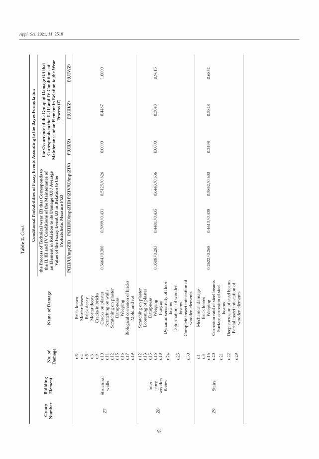
Appl. Sci. 2021, 11, 2518

Ta

ble

2.

Con

t.

Gro

up

Nu

mb

er

Bu

ild

ing

Ele

me

nt

No

.o

fD

am

ag

eN

am

eo

fD

am

ag

e

Co

nd

itio

na

lP

rob

ab

ilit

ies

of

Fu

zz

yE

ve

nts

Acc

ord

ing

toth

eB

ay

es

Fo

rmu

lafo

r:

the

Pro

cess

of

Te

chn

ica

lw

ea

r(Z

)th

at

Co

rre

spo

nd

sto

the

II,

III

an

dIV

Co

nd

itio

ns

of

the

Ma

inte

na

nce

of

an

Ele

me

nt

inR

ela

tio

nto

its

Da

ma

ge

(U)

/A

ve

rag

eV

alu

eo

fth

eF

uz

zy

Ev

en

t(Z

)in

Re

lati

on

toth

eP

rob

ab

ilis

tic

Me

asu

reP

(Z)

the

Occ

urr

en

ceo

fth

eG

rou

po

fD

am

ag

e(U

)th

at

Co

rre

spo

nd

sto

the

II,

III

an

dIV

Co

nd

itio

ns

of

Ma

inte

na

nce

of

an

Ele

me

nt

inR

ela

tio

nto

the

We

ar

Pro

cess

(Z)

P(Z

II/U

)/m

p(Z

II)

P(Z

III/

U)/

mp

(ZII

I)P

(ZIV

/U)/

mp

(ZIV

)P

(UII

/Z)

P(U

III/

Z)

P(U

IV/Z

)

Z7

Stru

ctur

alw

alls

u3Br

ick

loss

esu4

Mor

tar

loss

esu5

Bric

kde

cay

u6M

orta

rde

cay

u9C

rack

sin

bric

ksu1

0C

rack

son

plas

ter

0.34

64/0

.300

0.39

99/0

.431

0.51

25/0

.626

0.00

000.

4487

1.00

00u1

1Sc

ratc

hing

onw

alls

u12

Scra

tchi

ngon

plas

ter

u15

Dam

pnes

su1

6W

eepi

ngu1

7Bi

olog

ical

corr

osio

nof

bric

ksu1

9M

old

and

rot

Z8

Inte

r-st

ory

woo

den

floor

s

u12

Scra

tchi

ngon

plas

ter

u13

Loos

enin

gof

plas

ter

u15

Dam

pnes

su1

6W

eepi

ng0.

3508

/0.2

830.

4401

/0.4

350.

6443

/0.6

360.

0000

0.30

480.

9615

u18

Fung

us

u24

Dyn

amic

sens

itiv

ity

offlo

orbe

ams

u25

Def

orm

atio

nsof

woo

den

beam

s

u30

Com

plet

ein

sect

infe

stat

ion

ofw

oode

nel

emen

ts

Z9

Stai

rs

u1M

echa

nica

ldam

age

u3Br

ick

loss

esu1

6W

eepi

ng0.

2622

/0.2

680.

4613

/0.4

380.

5842

/0.6

000.

2498

0.58

280.

6852

u20

Cor

rosi

onra

idof

stee

lbea

ms

u21

Surf

ace

corr

osio

nof

stee

lbe

ams

u22

Dee

pco

rros

ion

ofst

eelb

eam

s

u29

Part

iali

nsec

tinf

esta

tion

ofw

oode

nel

emen

ts

98

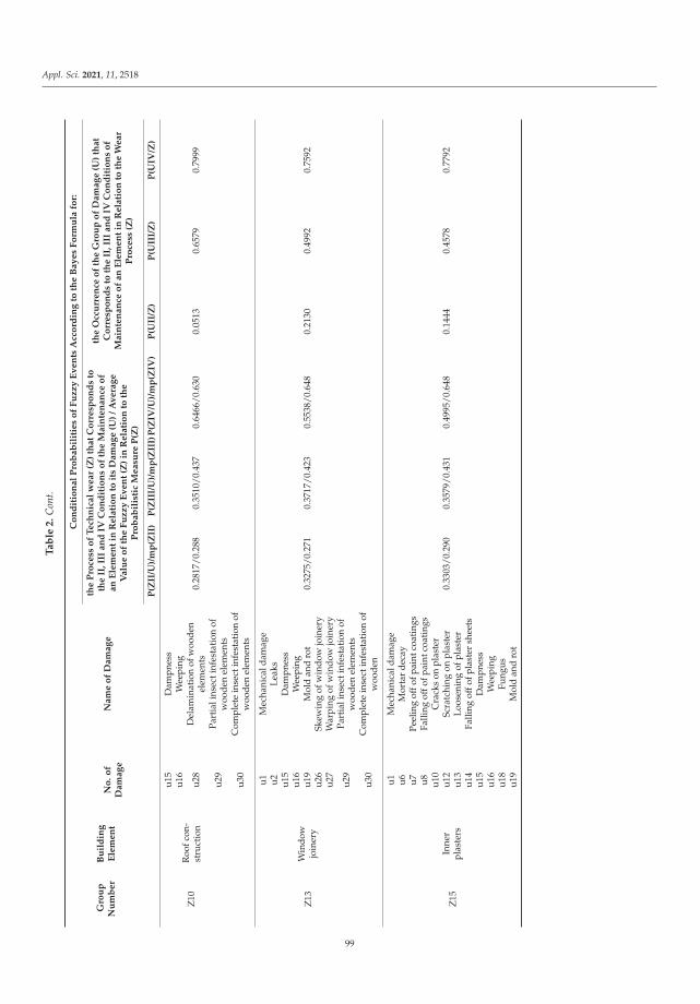
Appl. Sci. 2021, 11, 2518

Ta

ble

2.

Con

t.

Gro

up

Nu

mb

er

Bu

ild

ing

Ele

me

nt

No

.o

fD

am

ag

eN

am

eo

fD

am

ag

e

Co

nd

itio

na

lP

rob

ab

ilit

ies

of

Fu

zz

yE

ve

nts

Acc

ord

ing

toth

eB

ay

es

Fo

rmu

lafo

r:

the

Pro

cess

of

Te

chn

ica

lw

ea

r(Z

)th

at

Co

rre

spo

nd

sto

the

II,

III

an

dIV

Co

nd

itio

ns

of

the

Ma

inte

na

nce

of

an

Ele

me

nt

inR

ela

tio

nto

its

Da

ma

ge

(U)

/A

ve

rag

eV

alu

eo

fth

eF

uz

zy

Ev

en

t(Z

)in

Re

lati

on

toth

eP

rob

ab

ilis

tic

Me

asu

reP

(Z)

the

Occ

urr

en

ceo

fth

eG

rou

po

fD

am

ag

e(U

)th

at

Co

rre

spo

nd

sto

the

II,

III

an

dIV

Co

nd

itio

ns

of

Ma

inte

na

nce

of

an

Ele

me

nt

inR

ela

tio

nto

the

We

ar

Pro

cess

(Z)

P(Z

II/U

)/m

p(Z

II)

P(Z

III/

U)/

mp

(ZII

I)P

(ZIV

/U)/

mp

(ZIV

)P

(UII

/Z)

P(U

III/

Z)

P(U

IV/Z

)

Z10

Roo

fcon

-st

ruct

ion

u15

Dam

pnes

su1

6W

eepi

ng

u28

Del

amin

atio

nof

woo

den

elem

ents

0.28

17/0

.288

0.35

10/0

.437

0.64

66/0

.630

0.05

130.

6579

0.79

99

u29

Part

iali

nsec

tinf

esta

tion

ofw

oode

nel

emen

ts

u30

Com

plet

ein

sect

infe

stat

ion

ofw

oode

nel

emen

ts

Z13

Win

dow

join

ery

u1M

echa

nica

ldam

age

u2Le

aks

u15

Dam

pnes

su1

6W

eepi

ngu1

9M

old

and

rot

0.32

75/0

.271

0.37

17/0

.423

0.55

38/0

.648

0.21

300.

4992

0.75

92u2

6Sk

ewin

gof

win

dow

join

ery

u27

War

ping

ofw

indo

wjo

iner

y

u29

Part

iali

nsec

tinf

esta

tion

ofw

oode

nel

emen

ts

u30

Com

plet

ein

sect

infe

stat

ion

ofw

oode

n

Z15

Inne

rpl

aste

rs

u1M

echa

nica

ldam

age

u6M

orta

rde

cay

u7Pe

elin

gof

fofp

aint

coat

ings

u8Fa

lling

offo

fpai

ntco

atin

gsu1

0C

rack

son

plas

ter

u12

Scra

tchi

ngon

plas

ter

0.33

03/0

.290

0.35

79/0

.431

0.49

95/0

.648

0.14

440.

4578

0.77

92u1

3Lo

osen

ing

ofpl

aste

ru1

4Fa

lling

offo

fpla

ster

shee

tsu1

5D

ampn

ess

u16

Wee

ping

u18

Fung

usu1

9M

old

and

rot

99

Appl. Sci. 2021, 11, 2518

Ta

ble

2.

Con

t.

Gro

up

Nu

mb

er

Bu

ild

ing

Ele

me

nt

No

.o

fD

am

ag

eN

am

eo

fD

am

ag

e

Co

nd

itio

na

lP

rob

ab

ilit

ies

of

Fu

zz

yE

ve

nts

Acc

ord

ing

toth

eB

ay

es

Fo

rmu

lafo

r:

the

Pro

cess

of

Te

chn

ica

lw

ea

r(Z

)th

at

Co

rre

spo

nd

sto

the

II,

III

an

dIV

Co

nd

itio

ns

of

the

Ma

inte

na

nce

of

an

Ele

me

nt

inR

ela

tio

nto

its

Da

ma

ge

(U)

/A

ve

rag

eV

alu

eo

fth

eF

uz

zy

Ev

en

t(Z

)in

Re

lati

on

toth

eP

rob

ab

ilis

tic

Me

asu

reP

(Z)

the

Occ

urr

en

ceo

fth

eG

rou

po

fD

am

ag

e(U

)th

at

Co

rre

spo

nd

sto

the

II,

III

an

dIV

Co

nd

itio

ns

of

Ma

inte

na

nce

of

an

Ele

me

nt

inR

ela

tio

nto

the

We

ar

Pro

cess

(Z)

P(Z

II/U

)/m

p(Z

II)

P(Z

III/

U)/

mp

(ZII

I)P

(ZIV

/U)/

mp

(ZIV

)P

(UII

/Z)

P(U

III/

Z)

P(U

IV/Z

)

Z20

Faca

des

u1M

echa

nica

ldam

age

u6M

orta

rde

cay

u7Pe

elin

gof

fofp

aint

coat

ings

u8Fa

lling

offo

fpai

ntco

atin

gsu1

0C

rack

son

plas

ter

u12

Scra

tchi

ngon

plas

ter

0.28

54/0

.253

0.36

70/0

.450

0.62

99/0

.641

0.12

500.

3623

0.90

12u1

3Lo

osen

ing

ofpl

aste

ru1

4Fa

lling

offo

fpla

ster

shee

tsu1

5D

ampn

ess

u16

Wee

ping

u18

Fung

usu1

9M

old

and

rot

100

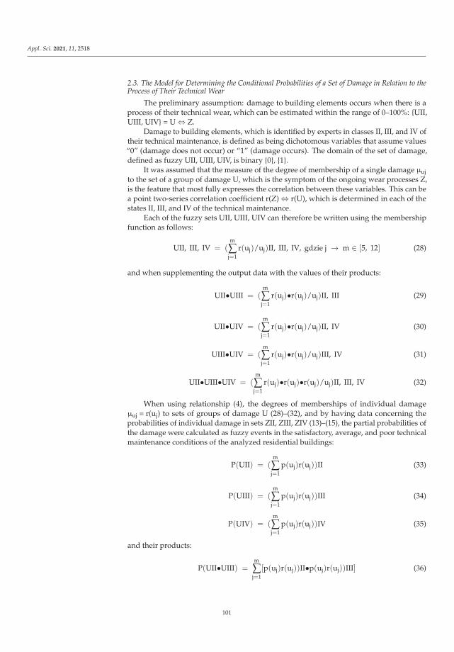
Appl. Sci. 2021, 11, 2518

2.3. The Model for Determining the Conditional Probabilities of a Set of Damage in Relation to theProcess of Their Technical Wear

The preliminary assumption: damage to building elements occurs when there is aprocess of their technical wear, which can be estimated within the range of 0–100%: {UII,UIII, UIV} = U ⇔ Z.

Damage to building elements, which is identified by experts in classes II, III, and IV oftheir technical maintenance, is defined as being dichotomous variables that assume values“0” (damage does not occur) or “1” (damage occurs). The domain of the set of damage,defined as fuzzy UII, UIII, UIV, is binary {0}, {1}.

It was assumed that the measure of the degree of membership of a single damage μujto the set of a group of damage U, which is the symptom of the ongoing wear processes Z,is the feature that most fully expresses the correlation between these variables. This can bea point two-series correlation coefficient r(Z) ⇔ r(U), which is determined in each of thestates II, III, and IV of the technical maintenance.

Each of the fuzzy sets UII, UIII, UIV can therefore be written using the membershipfunction as follows:

UII, III, IV = (m

∑j=1

r(uj)/uj)II, III, IV, gdzie j → m ∈ [5, 12] (28)

and when supplementing the output data with the values of their products:

UII•UIII = (m

∑j=1

r(uj)•r(uj)/uj)II, III (29)

UII•UIV = (m

∑j=1

r(uj)•r(uj)/uj)II, IV (30)

UIII•UIV = (m

∑j=1

r(uj)•r(uj)/uj)III, IV (31)

UII•UIII•UIV = (m

∑j=1

r(uj)•r(uj)•r(uj)/uj)II, III, IV (32)

When using relationship (4), the degrees of memberships of individual damageμuj = r(uj) to sets of groups of damage U (28)–(32), and by having data concerning theprobabilities of individual damage in sets ZII, ZIII, ZIV (13)–(15), the partial probabilities ofthe damage were calculated as fuzzy events in the satisfactory, average, and poor technicalmaintenance conditions of the analyzed residential buildings:

P(UII) = (m

∑j=1

p(uj)r(uj))II (33)

P(UIII) = (m

∑j=1

p(uj)r(uj))III (34)

P(UIV) = (m

∑j=1

p(uj)r(uj))IV (35)

and their products:

P(UII•UIII) =m

∑j=1

[p(uj)r(uj))II•p(uj)r(uj))III] (36)

101

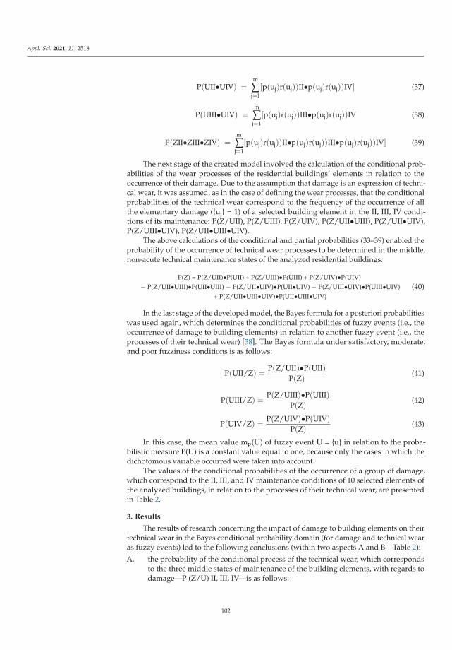
Appl. Sci. 2021, 11, 2518

P(UII•UIV) =m

∑j=1

[p(uj)r(uj))II•p(uj)r(uj))IV] (37)

P(UIII•UIV) =m

∑j=1

[p(uj)r(uj))III•p(uj)r(uj))IV (38)

P(ZII•ZIII•ZIV) =m

∑j=1

[p(uj)r(uj))II•p(uj)r(uj))III•p(uj)r(uj))IV] (39)

The next stage of the created model involved the calculation of the conditional prob-abilities of the wear processes of the residential buildings’ elements in relation to theoccurrence of their damage. Due to the assumption that damage is an expression of techni-cal wear, it was assumed, as in the case of defining the wear processes, that the conditionalprobabilities of the technical wear correspond to the frequency of the occurrence of allthe elementary damage ({uj} = 1) of a selected building element in the II, III, IV condi-tions of its maintenance: P(Z/UII), P(Z/UIII), P(Z/UIV), P(Z/UII•UIII), P(Z/UII•UIV),P(Z/UIII•UIV), P(Z/UII•UIII•UIV).

The above calculations of the conditional and partial probabilities (33–39) enabled theprobability of the occurrence of technical wear processes to be determined in the middle,non-acute technical maintenance states of the analyzed residential buildings:

P(Z) = P(Z/UII)•P(UII) + P(Z/UIII)•P(UIII) + P(Z/UIV)•P(UIV)− P(Z/UII•UIII)•P(UII•UIII) − P(Z/UII•UIV)•P(UII•UIV) − P(Z/UIII•UIV)•P(UIII•UIV)

+ P(Z/UII•UIII•UIV)•P(UII•UIII•UIV)(40)

In the last stage of the developed model, the Bayes formula for a posteriori probabilitieswas used again, which determines the conditional probabilities of fuzzy events (i.e., theoccurrence of damage to building elements) in relation to another fuzzy event (i.e., theprocesses of their technical wear) [38]. The Bayes formula under satisfactory, moderate,and poor fuzziness conditions is as follows:

P(UII/Z) =P(Z/UII)•P(UII)

P(Z)(41)

P(UIII/Z) =P(Z/UIII)•P(UIII)

P(Z)(42)

P(UIV/Z) =P(Z/UIV)•P(UIV)

P(Z)(43)

In this case, the mean value mp(U) of fuzzy event U = {u} in relation to the proba-bilistic measure P(U) is a constant value equal to one, because only the cases in which thedichotomous variable occurred were taken into account.

The values of the conditional probabilities of the occurrence of a group of damage,which correspond to the II, III, and IV maintenance conditions of 10 selected elements ofthe analyzed buildings, in relation to the processes of their technical wear, are presentedin Table 2.

3. Results

The results of research concerning the impact of damage to building elements on theirtechnical wear in the Bayes conditional probability domain (for damage and technical wearas fuzzy events) led to the following conclusions (within two aspects A and B—Table 2):

A. the probability of the conditional process of the technical wear, which correspondsto the three middle states of maintenance of the building elements, with regards todamage—P (Z/U) II, III, IV—is as follows:

102

Appl. Sci. 2021, 11, 2518

• the conditional probability of the technical wear of an element in relation to itsdamage increases with the deterioration of the maintenance conditions of thebuilding (this is an exceptionally steady increase, even in the case of differentbuilding elements);

• the probability of such a conditionally defined fuzzy event indicates the state ofthe technical wear for which the fuzzy damage occurs with the highest intensity,and it amounts, for the following elements of the tested residential buildings intheir average maintenance condition P(ZIII/U), to:

◦ for foundations: dampness of foundations 0.40◦ for basement walls: crack in bricks 0.39◦ for solid floors above basements: dampness of floors 0.38◦ for structural walls: cracks of plaster 0.40◦ for wooden inter-storey floors: weeping on floors 0.44◦ for internal stairs: weeping on stairs 0.46◦ for roof constructions: delamination of beams 0.35◦ for window joinery: mold and rot on windows 0.37◦ for inner plasters: scratches on plaster 0.36◦ for facades: scratches on plaster 0.37

The above values are therefore a fuzzy value of the probability of the degree of thetechnical wear, which was determined as an average degree, i.e., within the range of35–50%—in the case of the occurrence of a fuzzy damage to the building element;

• this probability is characterized by a low standard deviation and a narrowrange of the results of various elements within each of the considered buildingmaintenance conditions—satisfactory (0.2622–0.3846), average (0.3510–0.4613)and poor (0.4995–0.6466). A similar remark concerns the mean value of thisprobability in relation to its probabilistic measure;

B. the conditional probability of a group of damage, which corresponds to the threemiddle states of maintenance of building elements, in relation to the process of theirtechnical wear—P(U/Z) II, III, IV—is as follows:

• the conditional probability of damage to the element in relation to its technicalwear increases with the deterioration of the building maintenance conditions;

• the probability of such a conditionally defined fuzzy event is indicated by thedamage that most intensely affects the technical wear of the following elementsof the tested residential buildings, and it amounts in their average maintenancecondition P(UIII/Z) to:

◦ for foundations: dampness of foundations 0.27◦ for basement walls: crack in bricks 0.55◦ for solid floors above basements: dampness of floors 0.46◦ for structural walls: cracks of plaster 0.45◦ for wooden inter-storey floors: weeping on floors 0.31◦ for internal stairs: weeping on stairs 0.58◦ for roof constructions: delamination of beams 0.66◦ for window joinery: mold and rot on windows 0.50◦ for inner plasters: scratches on plaster 0.46◦ for facades: scratches on plaster 0.36

The above values are therefore a fuzzy value of the probability of damage to abuilding element, but only in the case that its fuzzy technical wear is determined tobe an average degree, i.e., within the range of 35–50%;

• the irregularity of this increase and the too-high coefficients of variation indicateonly a partial identity of the fuzzy event defined within aspect B with thereverse event; the fuzzy event determined within aspect A is characterized by amuch greater consistency of the obtained results.

103

Appl. Sci. 2021, 11, 2518

4. Discussion and Conclusions

Quantitative damage analysis, which was carried out using empirical methods ofassessing the technical condition of a building, indicates the type and size of damage to thebuilding’s elements, which are characteristic of the appropriate maintenance conditions.Research concerning the cause–effect relationships (“damage-technical wear”) in fuzzycalculus allowed for a numerical approach to the impact of building maintenance condi-tions on the degree of technical wear of its elements. The analysis of fuzzy cause–effectrelationships (“damage-technical wear”) created the possibility of determining conditionalprobabilities of these dependencies that are treated as fuzzy events. The fuzzy conditionalprobabilities of the technical wear process in relation to the occurrence of damage (with aprobabilistic measure), as well as conditional probabilities of the occurrence of a group ofdamage in relation to the process of technical wear, were determined.

The research methodology has been prepared in such a way that allowed the previ-ously prepared qualitative model to be transformed into a quantitative model. Therefore,the diagnosis of the impact of the maintenance of the residential buildings on the amountof their technical wear was executed using quantitative methods in fuzzy set categories,and also by using the authors’ own model that was created in the conditions of fuzziness.The model allowed for the determination of the conditional probabilities of the process oftechnical wear, and also the set of damage according to both Bayes formulas applied tofuzzy sets operations.

The research procedure was developed in a way that allowed for the transition ofa previously prepared qualitative model into a quantitative model. The diagnosis of theimpact of the maintenance of residential buildings on the amount of their technical wearwas carried out using quantitative methods in the categories of fuzzy sets, and also byusing the authors’ own model of determining the mutually dependent probabilities createdin the conditions of fuzziness. The model enabled the conditional probabilities of theprocess of the technical wear, as well as the set of damage, to be determined according toprobabilistic Bayes formulas. Moreover, it also allowed the fuzzy approach of Zadeh to becombined with the Yager approach. In such a multi-criteria fuzzy technical assessment ofresidential buildings, a simplified approach was used. In this approach, the probabilityof fuzzy events was assigned to a fuzzy measure, as opposed to the Yager approach, inwhich the probabilities are fuzzy events. The differences between the concepts of fuzzinessand randomness were not considered in the study. It was assumed that these phenomenaare different and described differently, however, they may—as two types of uncertainty—occur together.

The methods and results of the research presented in the article indicated a way thatallows for the transition of the previously prepared qualitative model into a quantitativemodel. The diagnosis of the impact of the maintenance of residential buildings on the amountof their technical wear was carried out using quantitative methods in the categories of fuzzysets, and also using the authors’ own models created in fuzzy conditions. The key questionfrom the subjective expert assessment of the technical condition of the evaluated residentialbuildings was answered: what is the probability of the wear of an element that may be moreor less represented by its average maintenance conditions? Therefore, the probability that theelement is more or less worn was determined. It was proven that the conditional probabilityof the technical wear of an element in relation to its failure increases with the deterioration ofthe maintenance conditions of the building, and this increase is extremely regular, even inthe case of different building elements. This probability is characterized by a low standarddeviation and a narrow range of the dispersion of the results in the case of various elementswithin each of the considered building maintenance conditions.

Author Contributions: Conceptualization, J.K., T.S.; methodology, J.K.; software, T.S.; validation,J.K.; formal analysis, J.K., T.S.; investigation, J.K., T.S.; resources, J.K., T.S.; writing—original draftpreparation, J.K.; writing—review and editing, J.K., T.S.; supervision, J.K. All authors have read andagreed to the published version of the manuscript.

104

Appl. Sci. 2021, 11, 2518

Funding: This research received no external funding.

Institutional Review Board Statement: Not applicable.

Informed Consent Statement: Not applicable.

Data Availability Statement: No new data were created or analyzed in this study. Data sharing isnot applicable to this article.

Conflicts of Interest: The authors declare no conflict of interest.

References

1. Kacprzyk, J. Fuzzy Sets in the System Analysis; PWN: Warsaw, Poland, 1986.2. Konior, J. Decision assumptions on building maintenance management. Probabilistic methods. Arch. Civ. Eng. 2007, 53, 403–423.3. Zadeh, L.A. Fuzzy sets. Inf. Control. 1965, 8, 338–353. [CrossRef]4. Zadeh, L.; Aliev, R. Fuzzy Logic Theory and Applications; World Scientific Publishing Co Pte Ltd.: Singapore, 2018.5. Yager, R.R. A note on probabilities of fuzzy events. Inf. Sci. 1979, 18, 113–129. [CrossRef]6. Yager, R.R. On the fuzzy cardinality of a fuzzy set. Int. J. Gen. Syst. 2006, 35, 191–206. [CrossRef]7. Nowogonska, B. Diagnoses in the aging process of residential buildings constructed using traditional technology. Buildings 2019,

9, 126. [CrossRef]8. Nowogonska, B. Intensity of damage in the aging process of buildings. Arch. Civ. Eng. 2020, 66, 19–31. [CrossRef]9. Nowogonska, B.; Korentz, J. Value of technical wear and costs of restoring performance characteristics to residential buildings.

Buildings 2020, 10, 9. [CrossRef]10. Nowogonska, B. The Method of Predicting the Extent of Changes in the Performance Characteristics of Residential Buildings.

Arch. Civ. Eng. 2019, 65, 81–89. [CrossRef]11. Nowogonska, B. Proposal for determing the scale of renovation needs of residential buildings. Civ. Environ. Eng. Rep. 2016, 22,

137–144. [CrossRef]12. Lee, S.; Lee, S.; Kim, J. Evaluating the Impact of Defect Risks in Residential Buildings at the Occupancy Phase. Sustainability 2018,

10, 4466. [CrossRef]13. Plebankiewicz, E.; Wieczorek, D.; Zima, K. Life cycle cost modelling of buildings with consideration of the risk. Arch. Civ. Eng.

LXII 2016, 62, 149–166. [CrossRef]14. Plebankiewicz, E.; Wieczorek, D.; Zima, K. Quantification of the risk addition in life cycle cost of a building object. Tech. Trans.

2017, 5, 35–45.15. Plebankiewicz, E.; Wieczorek, D.; Zima, K. Model estimation of the whole life cost of a building with respect to risk factors.

Technol. Econ. Dev. Econ. 2019, 25, 20–38.16. Wieczorek, D. Fuzzy risk assessment in the life cycle of building object—Selection of the right defuzzification method. In AIP

Conference Proceedings; AIP Publishing: Melville, NY, USA, 2018; Volume 1978, p. 240005.17. Ibadov, N. Fuzzy Estimation of Activities Duration in Construction Projects. Arch. Civ. Eng. LXI 2015, 61, 23–34. [CrossRef]18. Ibadov, N.; Kulejewski, J. Construction projects planning using network model with the fuzzy decision node. Int. J. Environ. Sci.

Technol. 2019, 16, 4347–4354. [CrossRef]19. Ibadov, N.; Kulejewski, J. The assessment of construction project risks with the use of fuzzy sets theory. Tech. Trans. 2014, 1,

175–182.20. Ibadov, N. The alternative net model with the fuzzy decision node for the construction projects planning. Arch. Civ. Eng. 2018, 64,

3–20. [CrossRef]21. Jain, K.K.; Bhattacharjee, B. Application of Fuzzy Concepts to the Visual Assessment of Deteriorating Reinforced Concrete

Structures. J. Constr. Eng. Manag. 2012, 138, 399–408. [CrossRef]22. Andric, J.M.; Wang, J.; Zou, P.X.; Zhang, J.; Zhong, R. Fuzzy Logic–Based Method for Risk Assessment of Belt and Road

Infrastructure Projects. J. Constr. Eng. Manag. 2019, 145, 238–262. [CrossRef]23. Marzouk, M.; Amin, A. Predicting Construction materials prices using fuzzy logic and neural networks. J. Constr. Eng. Manag.

2013, 139, 1190–1198. [CrossRef]24. Knight, K.; Robinson, R.; Fayek, A. Use of fuzzy logic of predicting design cost overruns on building projects. J. Constr. Eng.

Manag. 2002, 128, 503–512. [CrossRef]25. Sharma, S.; Goyal, P.K. Fuzzy assessment of the risk factors causing cost overrun in construction industry. Evol. Intell. 2019, 1–13.

[CrossRef]26. Al-Humaidi, H.M.; Hadipriono, T.F. Fuzzy logic approach to model delays in construction projects using rotational fuzzy fault

tree models. Civ. Eng. Environ. Syst. 2010, 27, 329–351. [CrossRef]27. Ammar, M.; Zayed, T.; Moselhi, O. Fuzzy-based life-cycle cost model for decision making under subjectivity. J. Constr. Eng.

Manag. 2012, 139, 556–563. [CrossRef]28. Chan, K.Y.; Kwong, C.K.; Dillon, T.S.; Fung, K.Y. An intelligent fuzzy regression approach for affective product design that

captures nonlinearity and fuzziness. J. Eng. Des. 2011, 22, 523–542. [CrossRef]

105

Appl. Sci. 2021, 11, 2518

29. Nasirzadeh, F.; Afshar, A.; Khanzadi, M.; Howick, S. Integrating system dynamics and fuzzy logic modelling for construction riskmanagement. Constr. Manag. Econ. 2008, 26, 1197–1212. [CrossRef]

30. Konior, J. Technical assessment of old buildings by fuzzy approach. Arch. Civ. Eng. 2019, 65, 129–142. [CrossRef]31. Konior, J. Technical Assessment of old buildings by probabilistic approach. Arch. Civ. Eng. 2020, 66, 443–466. [CrossRef]32. Konior, J. Maintenance of apartment buildings and their measurable deterioration. Tech. Trans. Czas. Tech. 2017, 6, 101–107.

[CrossRef]33. Konior, K. Bi-serial correlation of civil engineering building elements under constant technical deterioration. J. Sci. Gen. Tadeusz

Kosiuszko Mil. Acad. L. Forces 2016, 179, 142–150.34. Konior, J. Intensity of defects in residential buildings and their technical wear. Tech. Trans. Civ. Eng. 2014, 111, 137–146.35. Konior, J.; Sawicki, M.; Szóstak, M. Intensity of the Formation of Defects in Residential Buildings with Regards to Changes in

Their Reliability. Appl. Sci. 2020, 10, 6651. [CrossRef]36. Konior, J.; Sawicki, M.; Szóstak, M. Influence of Age on the Technical Wear of Tenement Houses. Appl. Sci. 2020, 10, 6651.

[CrossRef]37. Konior, J.; Sawicki, M.; Szóstak, M. Damage and Technical Wear of Tenement Houses in Fuzzy Set Categories. Appl. Sci. 2021, 11,

1484. [CrossRef]38. Multi-Author Work under Kaplinski, O. lead. Research Models and Methods in Construction Projects Engineering; PAN KILiW:

Warsaw, Poland, 2007.39. Multi-Author Work under Czaplinski, K. lead. Assessment of Wroclaw Downtown Apartment Houses’ Technical Conditions.

Reports series “U”; Building Engineering Institute at Wroclaw University of Science and Technology: Wroclaw, Poland, 1984-96.40. Hellwig, Z. Elements of Probability Calculus and Mathematical Statistics; PWN: Warsaw, Poland, 2001. (In Polish)41. Morrison, D. Multivariate Statistical Methods, 4th ed.; Duxbury Press: London, UK, 2004.42. Witte, R.; Witte, J. Statistics, 11th ed.; Wiley: New York, NY, USA, 2017.

106

applied sciences

Article

Damage and Technical Wear of Tenement Houses in FuzzySet Categories

Jarosław Konior *, Marek Sawicki and Mariusz Szóstak

���������������

Citation: Konior, J.; Sawicki, M.;

Szóstak, M. Damage and Technical

Wear of Tenement Houses in Fuzzy

Set Categories. Appl. Sci. 2021, 11,

1484. https://doi.org/10.3390/

app11041484

Academic Editor: Asterios Bakolas

Received: 18 January 2021

Accepted: 4 February 2021

Published: 6 February 2021

Publisher’s Note: MDPI stays neutral

with regard to jurisdictional claims in

published maps and institutional affil-

iations.

Copyright: © 2021 by the authors.

Licensee MDPI, Basel, Switzerland.

This article is an open access article

distributed under the terms and

conditions of the Creative Commons

Attribution (CC BY) license (https://

creativecommons.org/licenses/by/

4.0/).

Department of Building Engineering, Faculty of Civil Engineering, Wroclaw University of Science andTechnology, 50-370 Wrocław, Poland; marek.sawicki@pwr.edu.pl (M.S.); mariusz.szostak@pwr.edu.pl (M.S.)* Correspondence: jaroslaw.konior@pwr.edu.pl; Tel.: +48-71-320-23-69

Abstract: The results and conclusions of the research presented in the article concern the topic of thetechnical maintenance and wear of traditionally erected residential buildings. The cause and effectrelations between the occurrence of damage to the elements of tenement houses, which are treated asan expression of their maintenance conditions, and the size of the technical wear of these elementswere determined in a representative and purposefully selected sample of 102 apartment houses builtin the second half of the 19th and early 20th centuries in the Wroclaw, Poland downtown district“Srodmiescie”. Recognition of the impact of the maintenance of residential buildings on the levelof their technical wear was carried out using quantitative methods from fuzzy set categories, andalso with the use of the authors’ own model. The created model, based on the Zadeh function, wascreated in fuzzy conditions for the purpose of assessing the degree of damage to selected buildingelements. The treatment of the problem with regard to fuzzy criteria allowed for the synthesisof elementary criteria, which give the greatest approximations at the technical research stage of aresidential building, into a global assessment of the degree of the wear of its elements. Moreover, italso significantly reduced the subjective factor of this assessment, which had a significant impact onthe results of the research obtained in the case of good, medium and poor conditions of tenementhouses. It was proven that the conditions of maintenance and use of buildings determine the amountof technical wear of their elements. The state of exploitation of the examined tenement houses isreflected in the mechanical damage to the internal structure of the elements (determined in fuzzycategories). This damage has a significant frequency and cumulative effects, and is characteristic forbuildings with satisfactory and average maintenance.

Keywords: tenement houses; technical wear; damage; maintenance; fuzzy sets

1. Introduction

1.1. Source Literature

The aim of the research was to identify the impact of the processes associated withthe broadly understood maintenance of old residential buildings with a traditional con-struction on the size and intensity of the wear of their elements. The degree of technicalwear of residential building elements is a parameter of fundamental importance in thecomprehensive assessment of their technical condition, regardless of the approach thatwas used in the test method. The aim of the research was achieved through the analysisof the symptoms of the technical wear process—understanding the mechanism of thephenomenon of damage and identifying the size and intensity of damage to the elementsof the evaluated buildings.

Essential research of tenement houses aims to undertake a qualitative analysis ofdetected defects and identify all particular defects of their elements. Therefore, the “reason–effect” model is applied as follows:

[ REASONS] → [observed SYMPTOMS←−−−−−→ measured] → [EFFECTS ]

Appl. Sci. 2021, 11, 1484. https://doi.org/10.3390/app11041484 https://www.mdpi.com/journal/applsci

107

Appl. Sci. 2021, 11, 1484

Commonly used mathematical methods and the broadly understood system analysisdeal with real tasks in which the basic goal is the possibility of including all the typesof indeterminacy among modeled quantities and the relationships between them. Everyindeterminacy has traditionally been equated with the uncertainty of a random type, whichhas enabled known probabilistic and statistical tools to be used. In practice, however, thereare many cases in which the indeterminacy of the type of inaccuracy, ambiguity and impre-cision of meanings can be found. However, these situations are not of a random nature, andtherefore traditional probabilistic models may not be adequate [1–7]. When assessing thepossibility of random and/or fuzzy events occurring in construction investment projects,apart from immeasurable (qualitative) criteria, measurable (quantitative) criteria are alsoused. These quantitative criteria are expressed in a mathematical model that describesmultiple phenomena of construction engineering processes. Only some of these criteria arestrictly defined concepts—boundary, extreme. Most of these criteria are approximate. Theirvalue is determined using descriptive methods, e.g., “good quality”, “short term”, “lowbudget”. Therefore, concepts of this type cannot be adequately represented as a conven-tional set. To overcome this difficulty, in 1965, Lotfi A. Zadeh of the University of Californiain Berkeley introduced the concept of a fuzzy set with its membership function [8–10].

Zadeh [8,9], when developing the foundations of fuzzy set theory, formulated thefollowing principle: “in general, complexity and precision are inversely related to eachother in the sense that if the complexity of the problem under consideration increases,the possibility of its precise analysis decreases”. Yager [11,12] independently came to asimilar conclusion when examining the uncertainty in probability. However, people cancope with situations in which all attempts at the mathematical formalization of a task andits solutions are unsuccessful due to the fact that, e.g., it is impossible to build an exactmathematical model, or it would take too long to solve it. Zadeh saw the reasons for this inthe ability of the human mind to think in approximate categories, which microprocessorsdo not have. Due to this, a person can process approximate and ambiguous data, createmodels of the most complex processes, determine approximate solutions, etc. Fuzzy settheory, according to Zadeh and Yager, is therefore a tool used to formalize this approximatereasoning in vague and ambiguous terms.

For a long time, “uncertainty” and “ambiguity” have been used as synonyms for a lackof knowledge, which is decreasing as research progresses. Relatively recently, starting fromthe 1970s, these terms began to be treated as a reflection of reality, without the previousclearly negative meaning. It was then that the first major works in the field of multipleapplications of fuzzy sets occurred, including Zadeh [8,9], Yager [11,12] and Sanchez [13].Summing up, among the formal apparatuses that led to the development of fuzzy settheory, the first place is occupied by multi-valued logics. Previously, since ancient times,almost the entire development of logic could have been equated with two-valued logic,in which a statement can only be either true or false. The fact of such a polarization oftruth and falsehood was considered as an essential feature of any “logical” reasoning.Many logicians, represented especially by Lukaszewicz (a co-founder of the Polish School ofLogic), were already aware of the mismatch between such “rigid” logic and reality. Theexplosion of interest in multi-valued logics also aroused a significant increase in the interestof fuzziness and its origins, which was widely described in the later works of Zadeh [9],Yager [12], Sanchez [13] and Kasprzyk [14].

The stage preceding the main scope of the work was the conducting of a qualitativeanalysis of damage to the elements of the tested residential buildings [1,15]. The technicalcharacteristics and typological ordering of this damage, understood as an expression of thequality of maintenance of residential buildings, enabled the exploitation conditions of theconsidered objects to be identified.

A number of works by Nowogonska [16–20] were used in the methodical approachto the technical assessment of tenement houses, and the fuzzy calculus presented in thepublications of Plebankiewicz, Wieczorek and Zima [21–26] was used in the assessment of thewhole service life of a building object. The works of Ibadov [27–30] and other authors [31–39],

108

Appl. Sci. 2021, 11, 1484

which concerned the construction investment process with the fuzzy phase, allowed forthe practical application of uncertain and subjective events when determining the degreeof damage to the tested tenement houses.

1.2. Subject of Study

A group of old tenement houses (that is, those erected before the First World War)takes an important place in Polish building resources. This group includes about 10.1% ofthe whole number of urban flats. What is more, the importance of this type of buildingrelies on the fact that it takes part in creating an urban environment. At present, an actionneeds to be directed to the repair of the old land development. Doubtless, cultural aspectsmotivate all this action. To estimate its technical and economic justification, the degree ofthe technical wear of the old land development must be recognized and calculated.

This paper is a result of technical research and analyses on the old apartment housesin Wrocław, Poland [40]. The aim of the analysis is to provide information, which shouldhelp to direct an action, connected with this group of residential buildings. They are theapartment houses which were built at the turn of the nineteenth and twentieth centuries.The buildings are situated in the part of the city which (as a district from very few ones)was not completely destroyed by the war activities. The apartment houses are three- orfour-storey buildings, made of bricks, erected in longitudinal, usually three-row, structuralsystems. Apart from the floors over the basement, which are solid ones, all the inter-storeyfloors represent typical wooden floors. All the buildings are covered with wooden rafterframing, usually a purlin–collar one. The staircases are composed of wooden or steelstructural elements with wooden flights of steps.

1.3. Research Problem

While appraising building elements’ technical wear—apart from applying the measur-able (qualitative) criteria—the immeasurable (quantitative) criteria representing symptoms(pinpointed defects) of their deterioration have been taken into account. Only very few ofthese criteria can be classified at a high level of probability. There are symptoms of extremecharacters, described by extreme dichotomic divisions. It is, however, agreed that between,e.g., a total pest attack to wooden elements and a lack of pests, the mid-states appear. Theirvalue is often appreciated in a verbal way, e.g., “substantially”, considerably”, “signifi-cantly”, “partially”, “hardly” and it is always used in a description of detected defects as aresult of a building object’s technical inspections.

When assessing the degree of technical wear of building elements, apart from mea-surable (quantitative) criteria, immeasurable (qualitative) criteria are also used. They areexpressed in the analysis of symptoms, i.e., damage, which lowers the technical conditionand utility value of building elements. Only some of these criteria can be quantified witha big approximation. These are the symptoms with an extreme character, e.g., inter-storyceilings that are replaced with new elements that are not damp. It can then be assumedthat the damage, and the technical wear it causes, take a value of zero.

In turn, flooding of the floors above basements does not raise doubts regarding theoccurrence of the total dampness, and therefore the degrees of damage and technical wearcaused by moisture take values equal to one within the variability interval of [0, 1]. Mostof these criteria, however, are qualitative. Their value is determined verbally, e.g., as“significant”, “poor”, “strong”, “almost not at all”, “partial” or “complete”, and it alwaysappears in the description of damage phenomena. The interpretation of the effects of thesephenomena, which is performed according to qualitative (i.e., subjective) premises, leadsto the indiscriminate categorization of the technical maintenance conditions for buildingsand their elements, i.e., good, satisfactory, average, poor or bad. Therefore, can a buildingelement with a degree of technical wear of, e.g., 15%, be considered good or satisfactoryfrom the point of view of the technical maintenance quality? Does significant biologicalcontamination of wooden floor beams determine their 100% wear?

109

Appl. Sci. 2021, 11, 1484

Striving for a quantification of criteria that are inherently qualitative (and thereforeimmeasurable), and trying to determine the relations between them, led to the use of thecategory of fuzzy sets with regard to this issue. Their properties enable damage to buildingelements, as well as the conditions of their technical maintenance, to be described withinan unambiguous quantitative (measurable) aspect.

Therefore, the research led towards looking at the problem from this angle, whichallowed the description of naturally qualitative (immeasurable) variables and the determi-nation of existing relations between them in fuzzy set categories [15,25–39]. The advantagesof fuzzy theory made it possible to describe the defects, representing three middle states(II, III, IV) of conditions of the building elements’ maintenance, in a clear quantitative(measurable) aspect. Doubtless, fuzzy conditions are fully represented in these mid-states.

2. Research Methodology

2.1. Fuzzy Set Theory

The basic concept of the theory that was used in this paper is the concept of a fuzzyset [8,9,11–14]. The definition of a fuzzy set can be formulated as follows: a fuzzy set is setA, the x elements of which are characterized by the lack of a clear boundary between themembership and non-membership of x to A. The degree of the membership of element x tofuzzy set A is described by function μA(x), which is called the membership function. TheμA(x) function takes values from the interval of [0, 1], where:

μA(x) = 0, which means that x is not a member of A;

μA(x) = 1, which means that x is a full member of A.

Fuzzy set A in a certain space (in this paper, it is the area of considerations concerningthe observed states) X = {x}, which is written as A ⊆ X, is called the set of pairs:

A = {(μA(x), x)}, ∀ x ∈ X.

Therefore, two basic fuzzy sets can be distinguished in a problem (each one is de-scribed in the three following observed states—II, III, IV):

• a fuzzy set of the technical wear of building elements A ⊆ Ze ⇔ Z (to simplify thedesignations): Z = {(μZ(z), z)}, ∀ z ∈ Z;

• a fuzzy set of damage to building elements B ⊆ U:

U = {(μU(u), u)}, ∀ u ∈ U.

The basic operations performed on the fuzzy sets defined in the article are pre-sented below:

• the absolute complement of the fuzzy set A ⊆ X, denoted as −A:

μ−A(x) = 1− μA(x), ∀ x ∈ X (1)

• the multiple sum of fuzzy sets A,B ⊆ X, denoted as A ∪ B:

μA∪B(x) = μA(x) ∨ μB(x), ∀ x ∈ X (symbol ∨ denotes „max”) (2)

• the intersection of fuzzy sets A,B ⊆ X, denoted as A∩B:

μA∩B(x) = μA(x) ∧ μB(x), ∀ x ∈ X (symbol ∧ denotes „min”) (3)

• the k-th power (k > 0) of fuzzy set A ⊆ X, denoted as Ak:

μAk(x) = (μ(x))k, ∀ x ∈ X (4)

Special cases of exponentiation include:

110

Appl. Sci. 2021, 11, 1484

• the concentration of fuzzy set A ⊆ X, denoted as CON (A):

μCON(A)(x) = (μA(x))2, ∀ x ∈ X (5)

• the dilution of fuzzy set A ⊆ X, denoted as DIL (A):

μDIL(A)(x) = (μA(x))0.5, ∀ x ∈ X (6)

All these operations, which are of great importance in linguistic semantics, are inter-preted as:

• −A ⇔ “not A”;• A ∪ B ⇔ “A or B”;• A ∩ B ⇔ “A and B”;• CON (A) ⇔ “strong A” (crispens the fuzzy set);• DIL (A) ⇔ “more or less, likely A” (flattens the fuzzy set).

When visually assessing the technical wear of building elements that inspected tene-ment houses consist of, the symptoms of their damage are taken into account, i.e., individualdamage that can be categorized into the following groups of damage:

• UM—mechanical damage to the structure and texture of building elements;• UW—damage to building elements caused by water penetration and moisture pene-

tration;• UD—damage resulting from the loss of the original shape of wooden elements;• UP—damage to wooden elements attacked by biological pests.

The purpose of such a conceptual and technical systematization of damage is a com-prehensive diagnosis of the extent to which a building element is worn. This assessment,in turn, leads to the implication of stating under what technical conditions—good, satisfac-tory, average, poor or bad—the building element was (is) maintained. The terms “goodtechnical condition of maintenance”, “satisfactory technical condition of maintenance”,etc., can be considered as fuzzy sets with regard to semantic (qualitative) and technical(quantitative) aspects.

It is difficult to define a fuzzy set with such a broad meaning as “average technicalcondition of maintenance” using one membership function. In this case, a semantic analysisof the term “technical wear of a building element” was used, which was denoted withthe symbol of a fuzzy set “Z”. Let the technical wear of building element Z consist of:mechanical wear of its structure and texture (fuzzy set ZM), its technical wear caused bywater penetration and moisture penetration (fuzzy set ZW), technical wear resulting fromthe loss of its original shape (fuzzy set ZD) and technical wear caused by the attack ofbiological pests (fuzzy ZP harvest). This sum can then be expressed as follows:

Z = ZM ∪ ZW ∪ ZD ∪ ZP (7)

and when assuming the identity of the degree of technical wear and its visual symptom(Z ⇔ U)—damage to a building element that is integrated into the above-described damagesets (Expression (7))—it takes the following form:

U = UM ∪ UW ∪ UD ∪ UP (8)

2.2. Research Model

The aim of the proposed model is to assess the technical wear of a building elementwith regard to the overriding criterion, i.e., “slightly worn, worn, significantly worn”. Theconcepts defined in this way at the basic level best describe the behavior of a buildingelement in its three middle maintenance states. It is in them, after rejecting the extremestates (i.e., good and bad) that have the most reliable evaluation principles from thetechnical point of view, that the fuzzy conditions are most fully represented. The basic

111

Appl. Sci. 2021, 11, 1484

principles of fuzzy logic and approximate reasoning were applied [8,9,11–15], and thefuzzy state was described as follows: its damage means that it can be classified as being ina satisfactory (II), average (III) and poor (IV) technical condition of maintenance. Therefore,in each maintenance state, the total damage to a building element is a multiplicity sum ofthe sets of damage, and it is expressed by Formula (9):

U(II, III, IV) = UM(II, III, IV) ∪ UW(II, III, IV) ∪ UD(II, III, IV) ∪ UP(II, III, IV) (9)

where each set of damage, in each of the three maintenance states (II, III, IV), is a set ofbasic damage uj, which represents elementary lower order criteria:

• UM = {u1, u2, . . . ,u14};• UW = {u15, u16, . . . ,u23};• UD = {u24, u25, . . . ,u28};• UP = {u29, u30}.

Multiplication sum (9) can be written in each of the three maintenance states (II, III,IV) using the membership function:

μU = μUM ∨ μUW ∨ μUD ∨ μUP (10)

There is an intermediate stage between identifying damage at the elementary level,which occurs in everyday construction practice, and merging it into sets of damage interms of their similarity regarding the wear processes. This stage involves the selection ofdamage of the same type but of different intensity (e.g., pitting corrosion, surface corrosion,deep corrosion of steel beams), or damage occurring to complex elements (e.g., structuralwalls—decay of brick or mortar). This method of combining elementary damage was usedin the research, which led to the obtaining of greater possibilities of using operations ofsystem analysis in fuzzy sets. In the considered sample of downtown tenement houses,this division is as follows:

• {u1, u2} = U1 ⇔ mechanical damage and leaks;• {u3, u4} = U2 ⇔ brick and mortar losses;• {u5, u6} = U3 ⇔ brick and mortar decay;• {u7, u8} = U4 ⇔ peeling off and decomposing of the paint coatings;• {u9, u10} = U5 ⇔ cracks in brick and plaster;• {u11, u12} = U6 ⇔ scratching on walls and plaster;• {u13, u14} = U7 ⇔ loosening and falling off of plaster sheets;• {u15, u16, u23} = U8 ⇔ dampness, weeping and flooding with water;• {u17, u18, u19} = U9 ⇔ brick corrosion, fungus and mold;• {u20, u21, u22} = U10 ⇔ pitting corrosion, surface corrosion and deep corrosion of steel

beams;• {u24, u25} = U12 ⇔ dynamic sensitivity and deformation of floor beams;• {u26, u27, u28} = U13 ⇔ torsional buckling and distortion of window joinery and wood

elements;• {u29, u30} = U14 ⇔ touchwood and biological infestation of wooden elements.

In each of the damage types distinguished in this way, there is an intersection of twoor three elementary fuzzy sets. Between them, as is the case between sets of damage, thereis a multiple sum of the fuzzy sets that are defined above. All these dependencies can bedescribed by the general formula for assessing the degree of damage to the elements of theanalyzed residential buildings in their middle maintenance states which, when using themembership function, is as follows:

μU = (μu1 ∧ μu2) ∨ (μu3 ∧ μu4) ∨ (μu5 ∧ μu6) ∨ (μu7 ∧ μu8) ∨ (μu9 ∧ μu10) ∨∨ (μu11 ∧ μu12) ∨ (μu13 ∧ μu14) ∨ (μu15 ∧ μu16∧ μu23) ∨ (μu17 ∧ μu18 ∧μu19) ∨∨ (μu20 ∧ μu21 ∧ μu22) ∨ (μu24 ∧ μu25) ∨ (μu26 ∧ μu27∧ μu28) ∨ (μu29 ∧ μu30)

(11)

112

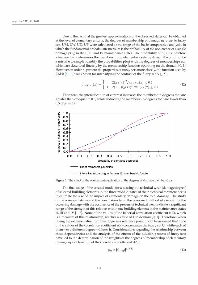
Appl. Sci. 2021, 11, 1484

Due to the fact that the greatest approximations of the observed states can be obtainedat the level of elementary criteria, the degrees of membership of damage u1 ÷ u30 to fuzzysets UM, UW, UD, UP were calculated at the stage of the basic comparative analysis, inwhich the fundamental probabilistic measure is the probability of the occurrence of a singledamage p(uj) in the II, III and IV maintenance states. The probability of p(uj) is thereforea feature that determines the membership to elementary sets u1 ÷ u30. It would not bea mistake to simply identify the probabilities p(uj) with the degrees of memberships μuj,which are described linearly by the membership function operating on the domain [0, 1].However, in order to present the properties of fuzzy sets more closely, the function used byZadeh [8–10] was chosen for intensifying the contrast of the fuzzy set A ⊆ X:

μINT(A)(x) =

{2(μA(x))2, ∀x : μA(x) < 0.5

1 − 2(1 − μA(x))2, ∀x : μA(x) ≥ 0.5(12)

Therefore, the intensification of contrast increases the membership degrees that aregreater than or equal to 0.5, while reducing the membership degrees that are lower than0.5 (Figure 1).

Figure 1. The effect of the contrast intensification of the degrees of damage memberships.

The final stage of the created model for assessing the technical wear (damage degree)of selected building elements in the three middle states of their technical maintenance isto estimate the size of the impact of elementary damage on the total damage. The studyof the observed states and the conclusions from the proposed method of associating theoccurring damage with the occurrence of the process of technical wear indicate a significantrange of the strength of this relation within one building element in the maintenance statesII, III and IV [1–7]. None of the values of the bi-serial correlation coefficient r(Z), whichis a measure of this relationship, reaches a value of 1 in domain [0, 1]. Therefore, whentaking the extreme value from this range as a reference point, it can be assumed that noneof the values of the correlation coefficient r(Z) concentrates the fuzzy set U, while each ofthem—to a different degree—dilutes it. Considerations regarding the relationship betweenthese dependencies and the analysis of the effects of the dilution process of fuzzy setshave led to the determination of the weights of the degrees of membership of elementarydamage uj as a function of the correlation coefficient r(Z):

μuj = [f(μuj)]1/r(Z) (13)

113

Appl. Sci. 2021, 11, 1484

The result of the proposed Formula (13) is the following change in the membershipfunction:

• r(Z) → 0 ⇒ μuj → 0;• r(Z) → 1 ⇒ μuj → μuj.

The application of the original procedures of the intensification and dilution of mem-bership functions, according to Formulas (12) and (13), to the general Formula (11) ofthe model for assessing the degree of damage to the elements of the analyzed tenementhouses in terms of fuzzy sets allowed for the transition from the data recorded usingnon-measurable variables to results defined by measurable values. The proposed modelgives a numerical answer to the question of to what extent is a building element damaged.The total degrees of damage to the ten selected elements of the analyzed buildings S(U) inthe maintenance states II, III and IV are presented in Table 1.

Table 1. The degree of fuzzy damage to building elements in their middle maintenance states. (grey backgroud is necessaryto distinguish extreme values)

Group Number BuildingElement

Damage Number Damage Description

Degree of Fuzzy Damage Set S(U) Corresponding tothe Maintenance States II, III and IV

S(U)II S(U)III S(U)IV

Z2 Foundations

u3 brick losses 0.24 0 0

u5 brick decay 0 0.59 0

u9 brick cracks 0 0 0

u15dampness offoundations 0 0 0

u16 weeping on foundations 0 0 0.97

u17biological corrosion of

bricks 0 0 0

u19mold and rot on

foundations 0 0 0

Z3 Basement walls

u3 brick losses 0.05 0.25 0.67

u4 mortar losses 0 0 0

u5 brick decay 0 0 0

u6 mortar decay 0 0 0

u9 cracks in bricks 0 0 0

u10 cracks in mortar 0 0 0

u15 dampness of walls 0 0 0

u16 weeping on walls 0 0 0

u17biological corrosion of

bricks 0 0 0

u19 mold and rot on walls 0 0 0

Z4 Solid floors abovebasements

u3 brick losses 0.01 0.22 0

u5 brick decay 0 0 0

u9 cracks in bricks 0 0 0

u15 dampness of floors 0 0 0

u16 weeping on floors 0 0 0.50

u20corrosion raid on steel

beams 0 0 0

u21surface corrosion of

steel beams 0 0 0

u22deep corrosion of steel

beams 0 0 0

u23flooding of floors with

water 0 0 0

114

Appl. Sci. 2021, 11, 1484

Table 1. Cont.

Group Number BuildingElement

Damage Number Damage Description

Degree of Fuzzy Damage Set S(U) Corresponding tothe Maintenance States II, III and IV

S(U)II S(U)III S(U)IV

Z7 Structural walls

u3 brick losses 0 0 1.00

u4 mortar losses 0.34 0.93 0

u5 brick decay 0 0 0

u6 mortar decay 0 0 0

u9 cracks in bricks 0 0 0

u10 cracks on plaster 0 0 0

u11 scratching on walls 0 0 0

u12 scratching on plaster 0 0 0

u15 dampness of walls 0 0 0

u16 weeping on walls 0 0 0

u17biological corrosion of

bricks 0 0 0

u19 mold and rot on walls 0 0 0

Z8 Inter-storywooden floors

u12scratching on the plaster

of the ceiling 0 0 0

u13peeling of ceiling

plaster 0 0 0

u15 dampness of floors 0 0 0

u16 weeping on floors 0.01 0.64 0

u18 fungus on floors 0 0 0.49

u24dynamic sensitivity of

floor beams 0 0 0

u25deformations ofwooden beams 0 0 0

u30

complete insectinfestation of wooden

beams0 0 0

Z9 Stairs

u1 mechanical damage 0.26 0.56 0

u3 brick losses 0 0 0

u16 weeping on stairs 0 0 0.95

u20corrosion raid on steel

beams 0 0 0

u21surface corrosion of

steel beams 0 0 0

u22deep corrosion of steel

beams 0 0 0

u29partial insect infestation

of wooden elements 0 0 0

Z10 Roof construction

u15 dampness of truss 0 0 0

u16weeping on wooden

elements 0 0.43 0.53

u28 delamination of beams 0.03 0 0

u29partial insect infestation

of wooden elements 0 0 0

u30

complete insectinfestation of wooden

beams0 0 0

115

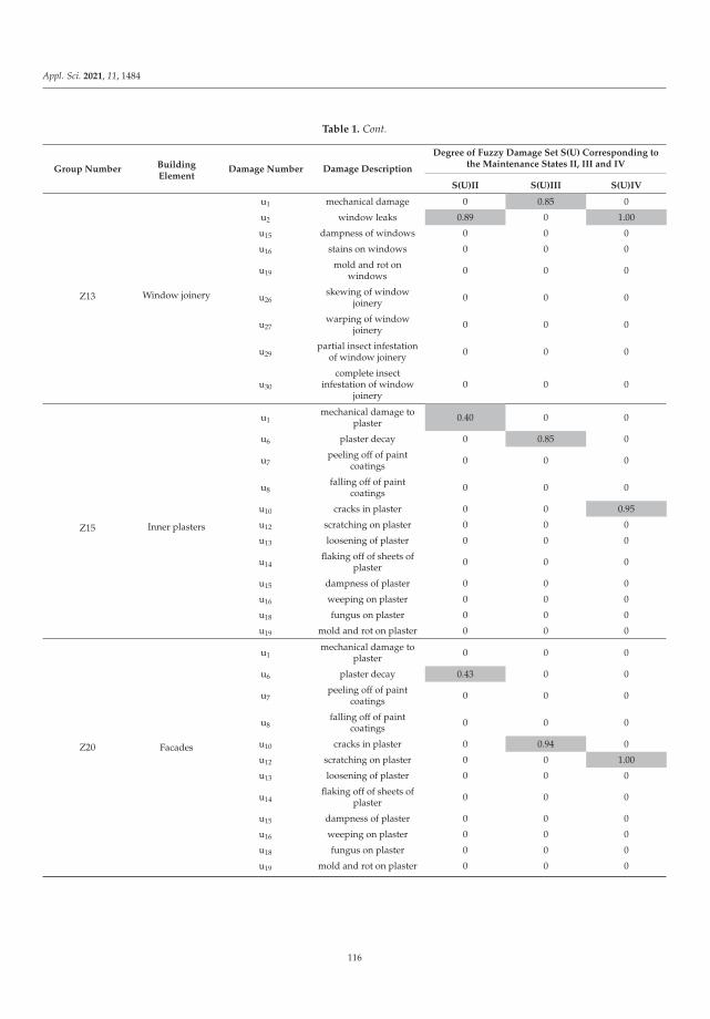
Appl. Sci. 2021, 11, 1484

Table 1. Cont.

Group Number BuildingElement

Damage Number Damage Description

Degree of Fuzzy Damage Set S(U) Corresponding tothe Maintenance States II, III and IV

S(U)II S(U)III S(U)IV

Z13 Window joinery

u1 mechanical damage 0 0.85 0

u2 window leaks 0.89 0 1.00

u15 dampness of windows 0 0 0

u16 stains on windows 0 0 0

u19mold and rot on

windows 0 0 0

u26skewing of window

joinery 0 0 0

u27warping of window

joinery 0 0 0

u29partial insect infestation

of window joinery 0 0 0

u30

complete insectinfestation of window

joinery0 0 0

Z15 Inner plasters

u1mechanical damage to

plaster 0.40 0 0

u6 plaster decay 0 0.85 0

u7peeling off of paint

coatings 0 0 0

u8falling off of paint

coatings 0 0 0

u10 cracks in plaster 0 0 0.95

u12 scratching on plaster 0 0 0

u13 loosening of plaster 0 0 0

u14flaking off of sheets of

plaster 0 0 0

u15 dampness of plaster 0 0 0

u16 weeping on plaster 0 0 0

u18 fungus on plaster 0 0 0

u19 mold and rot on plaster 0 0 0

Z20 Facades

u1mechanical damage to

plaster 0 0 0

u6 plaster decay 0.43 0 0

u7peeling off of paint

coatings 0 0 0

u8falling off of paint

coatings 0 0 0

u10 cracks in plaster 0 0.94 0

u12 scratching on plaster 0 0 1.00

u13 loosening of plaster 0 0 0

u14flaking off of sheets of

plaster 0 0 0

u15 dampness of plaster 0 0 0

u16 weeping on plaster 0 0 0

u18 fungus on plaster 0 0 0

u19 mold and rot on plaster 0 0 0

116

Appl. Sci. 2021, 11, 1484

3. Results

The analysis of the results of the research concerning the impact of damage to buildingelements on their technical wear with regard to fuzzy sets leads to the following conclusions(Table 1):

a. in the field of assessing the degree of fuzzy damage to elements of downtowntenement houses—S(U) II, III, IV:

• the development of the model presented in the article allowed the fundamentalquestion of to what extent a building element is worn (damaged), when knowingthat it is (more or less) satisfactorily, moderately or poorly maintained, tobe answered;

• the use of simple operations in the fuzzy set calculus enabled the influence ofboth elementary damage that occurs with a specific frequency (probability) andthe measure of its interdependence (correlation) on the observed technical wearof building elements to be considered;

• as a result of the proposed model, which is based on fuzzy set theory, it waspossible to identify the elementary damage that determines the degree of de-struction of the building’s elements;

b. when determining the degree of damage of 10 selected building elements accordingto fuzzy criteria, it was indicated that there is a need for an individual approachto each of the elements (especially structural) during the process of their technicalassessment. However, several regularities can be identified:

• the degree of damage to the element increases with the deterioration of its main-tenance conditions (although not proportionally to the maintenance conditionsand not equally for different types of elements). For instance, degrees of fuzzydamage set S(U) corresponding to the maintenance states II, III and IV grow inthe following way: Z3—basement walls—u3—brick losses: 0.05; 0.25; 0.67. Itmost often differs from the observed values of the degree of the technical wearthat was determined using the probabilistic approach [1]—in particular, in poorconditions of building maintenance, the degree of damage exceeds 70% of itstechnical wear threshold;

• elementary damage that determines the degree of destruction of an elementcomes much more often from group I (mechanical damage to the structure andtexture of elements) than was the case in the analysis of the observed states.Only under poor conditions of building maintenance does the analysis of theobserved random [1] and fuzzy [15] phenomena show a great similarity—thedecisive damage is the destruction of the element caused by water penetrationand moisture penetration (group II);

• at the level of the greatest detail, the type of damage and the degrees of fuzzydamage to the elements of the downtown tenement houses were determined. Inthe most representative, i.e., average/satisfactory condition of maintenance—S(U) III—the degrees were as follows:

� for foundations: brick decay 0.59� for basement walls: brick decrements 0.25� for solid floors above basements: brick decrements 0.22� for structural walls: mortar decrements 0.93� for wooden inter-storey floors: weeping 0.64� for internal stairs: mechanical damage 0.56� for roof constructions: weeping on wooden elements 0.43� for window joinery: mechanical damage 0.85� for inner plasters: plaster decay 0.85� for facades: cracks on plaster 0.94

117

Appl. Sci. 2021, 11, 1484

4. Summary and Discussion

At the beginning, general methodological conclusions were formulated. They re-sulted from the modeling of the impact of the maintenance of tenement houses on thetechnical wear of their elements in fuzzy conditions. Such an approach gives much greaterpossibilities of studying cause and effect relationships than the probabilistic analysis [1]:

a. the use of simple operations in the fuzzy set calculus enables the simultaneousrecognition of the impact of elementary damage that occurs with a specific frequency(probability), and also the measure of its interdependence (correlation) on the ob-served technical wear of building elements;

b. in the effect of fuzzy transformations, it is possible to identify the elementary damagethat determines the degree of destruction of the building element. The result of thecumulative effects of frequently occurring mechanical damage to the structure andtexture of elements indicates that this type of damage is no less important in theprocess of the technical wear of elements of downtown tenement houses;

c. consideration of the problem with regard to fuzzy phenomena allows for the syn-thesis of elementary criteria. This gives the greatest approximations (at the stage ofthe technical investigation of a residential building) for the global assessment of thedegree of wear of the building’s elements. In addition, it significantly reduces thesubjective factor of this assessment, which has the greatest impact on the result ofresearch conducted for the middle maintenance states of buildings.

The consequence of systematizing the most important processes that influence theloss of functional properties of residential buildings was the creation of the authors; ownqualitative model and its transformation into a quantitative model. This, in turn, enabled amulti-criteria quantitative analysis of the cause–effect phenomena—“damage–technicalwear”—of the most important elements of downtown residential buildings to be conductedin the so-called conventional and fuzzy sets. In conventional sets, in which attempts weremade to describe the observed (empirical) states with the use of theoretical formulas, theprobabilistic side of the problem and its random nature were considered [1]. In turn, infuzzy sets, the observed states of cause–effect phenomena in the fuzzy conditions [15] (i.e.,uncertainty as to the very fact of their occurrence) were analyzed.

The fact that the membership function of a fuzzy set assumes values from interval[0, 1] leads to the hasty conclusion that fuzziness is a hidden form of randomness, andtherefore fuzzy set theory is basically nothing new in relation to probability. The differencesbetween fuzziness and randomness, however, concern both their nature and the formaldifferences between probabilistic calculus and fuzzy sets. The nature of these phenomenalies in the problem of the uncertainty of the type of randomness and fuzziness. In the caseof randomness, the event is strictly defined, while its occurrence is uncertain. Therefore,randomness can be equated with the uncertainty regarding an element’s membership ornon-membership. This is not the case with fuzziness, which concerns the very degree ofmembership of an element to a set, and therefore an event is no longer strictly defined. Suchevents are the ones analyzed in the paper—the occurring damage of building elements andthe processes of their technical wear. Their nature, in the authors’ opinion, is more fuzzythan random.

The differences between randomness and fuzziness can be presented with regard tothe following three points of view:

• level of uncertainty;• number of decision makers;• number of steps in the decision process.

Regarding “the degree of uncertainty”, the following decision-making situations, withan increasing degree of uncertainty, can be distinguished:

• Certainty: all the information that describes the issue of decision making is deterministic;• Risk: information that describes the decision-making issue is probabilistic, i.e., the

data have appropriate probability distributions;

118

Appl. Sci. 2021, 11, 1484

• Uncertainty: even the probabilities are not known. Making decisions is usuallyreduced to using a minimax strategy;

• Fuzziness: uncertainty not only relates to the occurrence of an event, but also to itsmeaning in general, and this can no longer be considered using probabilistic methods.Of course, further extensions, such as adding risk to fuzziness, are also possible.

The sense of a fuzzy set can therefore be used to formally determine and quantitativelyexpress ambiguous concepts that are always present in the programming and analysis of aconstruction process. Thus, fuzzy set theory is a theory of classes in which the transitionfrom membership to non-membership does not have a jumping character, as is the case ina conventional set, but instead it is gradual. Striving for a quantification of criteria that areinherently qualitative (and therefore immeasurable), and trying to determine the relationsbetween them, led to the use of the category of fuzzy sets with regard to this issue. Theirproperties enable elementary construction processes to be mathematically described asfuzzy events within an unambiguous quantitative (measurable) aspect.

To sum up, the approach of the creator of fuzzy set theory [8–10] (Lofti Zadeh, who,unlike Yager and Kaufmann [11,12], assumed the fuzzy set as a random event) was con-sciously used by the authors. This enabled the question of what is the probability thata building element is more or less (approximately) worn to be answered. Therefore, thedifferences between the concepts of fuzziness and randomness were not considered. It wasonly assumed that although these phenomena are different and described differently, theymay nevertheless occur together as two types of uncertainty.

Author Contributions: Conceptualization, J.K., M.S. (Marek Sawicki) and M.S. (Mariusz Szóstak);methodology, J.K.; software, J.K. and M.S. (Mariusz Szóstak); validation, J.K., M.S. (Marek Sawicki)and M.S. (Mariusz Szóstak); formal analysis, J.K., M.S. (Marek Sawicki) and M.S. (Mariusz Szóstak); in-vestigation, J.K. and M.S. (Marek Sawicki); resources, J.K. and M.S. (Marek Sawicki); writing—originaldraft preparation, J.K.; writing—review and editing, J.K. and M.S. (Mariusz Szóstak); supervision,M.S. (Marek Sawicki). All authors have read and agreed to the published version of the manuscript.

Funding: This research received no external funding.

Institutional Review Board Statement: Not applicable.

Informed Consent Statement: Not applicable.

Data Availability Statement: No new data were created or analyzed in this study. Data sharing isnot applicable to this article.

Conflicts of Interest: The authors declare no conflict of interest.

References

1. Konior, J. Technical Assessment of old buildings by probabilistic approach. Arch. Civ. Eng. 2020, 66, 443–466. [CrossRef]2. Konior, J. Decision assumptions on building maintenance management. Probabilistic methods. Arch. Civ. Eng. 2007, 53, 403–423.3. Konior, J. Maintenance of apartment buildings and their measurable deterioration. Tech. Trans. Czas. Tech. 2017, 6, 101–107.

[CrossRef]4. Konior, K. Bi-serial correlation of civil engineering building elements under constant technical deterioration. J. Sci. Gen. Tadeusz

Kosiuszko Mil. Acad. Land Forces 2016, 179, 142–150.5. Konior, J. Intensity of defects in residential buildings and their technical wear. Tech. Trans. Civ. Eng. 2014, 111, 137–146.6. Konior, J.; Sawicki, M.; Szóstak, M. Intensity of the Formation of Defects in Residential Buildings with Regards to Changes in

Their Reliability. Appl. Sci. 2020, 10, 6651. [CrossRef]7. Konior, J.; Sawicki, M.; Szóstak, M. Influence of Age on the Technical Wear of Tenement Houses. Appl. Sci. 2020, 11, 297.

[CrossRef]8. Zadeh, L. Fuzzy sets. Inf. Control 1965, 8, 338–353. [CrossRef]9. Zadeh, L. Fuzzy sets and systems. Int. J. Gen. Syst. 1990, 17, 129–138. [CrossRef]10. Zadeh, L.; Aliev, R. Fuzzy Logic Theory and Applications; World Scientific Publishing Co Pte Ltd.: Singapore, 2018.11. Yager, R.R. A Note on Probabilities of Fuzzy Events Information and Science; Iona College: New Rochelle, NY, USA, 1979; Volume 18.12. Yager, R.R. On the fuzzy cardinality of a fuzzy set. Int. J. Gen. Syst. 2006, 35, 191–206. [CrossRef]13. Sanchez, E. Resolution of composite fuzzy relation equations. Inf. Control 1976, 30, 38–48. [CrossRef]14. Kacprzyk, J. Fuzzy Sets in the System Analysis; PWN: Warsaw, Poland, 1986.

119

Appl. Sci. 2021, 11, 1484

15. Konior, J. Technical assessment of old buildings by fuzzy approach. Arch. Civ. Eng. 2019, 65, 129–142. [CrossRef]16. Nowogonska, B. Diagnoses in the aging process of residential buildings constructed using traditional technology. Buildings 2019,

9, 126. [CrossRef]17. Nowogonska, B. Intensity of damage in the aging process of buildings. Arch. Civ. Eng. 2020, 66, 19–31. [CrossRef]18. Nowogonska, B.; Korentz, J. Value of technical wear and costs of restoring performance characteristics to residential buildings.

Buildings 2020, 10, 9. [CrossRef]19. Nowogonska, B. The Method of Predicting the Extent of Changes in the Performance Characteristics of Residential Buildings.

Arch. Civ. Eng. 2019, 65, 81–89. [CrossRef]20. Nowogonska, B. Proposal for determing the scale of renovation needs of residential buildings. Civ. Environ. Eng. Rep. 2016,

22, 137–144. [CrossRef]21. Plebankiewicz, E.; Karcinska, P. Creating a Construction Schedule Specifying Fuzzy Norms and the Number of Workers. Arch.

Civ. Eng. 2016, 62, 149–166.22. Plebankiewicz, E.; Wieczorek, D.; Zima, K. Life cycle cost modelling of buildings with consideration of the risk. Arch. Civ. Eng.

2016, 62, 149–166. [CrossRef]23. Plebankiewicz, E.; Wieczorek, D.; Zima, K. Quantification of the risk addition in life cycle cost of a building object. Tech. Trans.

2017, 5, 35–45.24. Plebankiewicz, E.; Wieczorek, D.; Zima, K. Model estimation of the whole life cost of a building with respect to risk factors.

Technol. Econ. Dev. Econ. 2019, 25, 20–38.25. Plebankiewicz, E.; Wieczorek, D. Fuzzy risk assessment in the service life of building objects. Mater. Bud. 2016, 6, 59–61.26. Wieczorek, D. Fuzzy risk assessment in the life cycle of building object—Selection of the right defuzzification method. In

Proceedings of the AIP Conference Proceedings, Maharashtra, India, 5–6 July 2018; AIP Publishing: Melville, NY, USA, 2018;Volume 1978, p. 240005.

27. Ibadov, N. Fuzzy Estimation of Activities Duration in Construction Projects. Arch. Civ. Eng. 2015, LXI, 23–34. [CrossRef]28. Ibadov, N.; Kulejewski, J. Construction projects planning using network model with the fuzzy decision node. Int. J. Environ. Sci.

Technol. 2019, 16, 4347–4354. [CrossRef]29. Ibadov, N.; Kulejewski, J. The assessment of construction project risks with the use of fuzzy sets theory. Tech. Trans. 2014, 1, 175–182.30. Ibadov, N. The alternative net model with the fuzzy decision node for the construction projects planning. Arch. Civ. Eng.

2018, 64, 3–20. [CrossRef]31. Kamal, K.J.; Jain, B.B. Application of Fuzzy Concepts to the Visual Assessment of Deteriorating Reinforced Concrete Structures.

J. Constr. Eng. Manag. 2012, 138, 399–408.32. Andric, J.M.; Wang, J.X.W.; Zou, P.; Zhang, J. Fuzzy Logic–Based Method for Risk Assessment of Belt and Road Infrastructure

Projects. J. Constr. Eng. Manag. 2019, 145, 238–262. [CrossRef]33. Marzouk, M.; Amin, A. Predicting Construction materials prices using fuzzy logic and neural networks. J. Constr. Eng. Manag.

2013, 139, 1190–1198. [CrossRef]34. Knight, K.; Robinson, R.; Fayek, A. Use of fuzzy logic of predicting design cost overruns on building projects. J. Constr. Eng.

Manag. 2002, 128, 503–512. [CrossRef]35. Sharma, S.; Goyal, P.K. Fuzzy assessment of the risk factors causing cost overrun in construction industry. Evol. Intell. 2019, 1–13.

[CrossRef]36. Al-Humaidi, H.M.; Hadipriono, T.F. Fuzzy logic approach to model delays in construction projects using rotational fuzzy fault

tree models. Civ. Eng. Environ. Syst. 2010, 27, 329–351. [CrossRef]37. Ammar, M.T.; Zayed, T.; Moselhi, O. Fuzzy-based life-cycle cost model for decision making under subjectivity. J. Constr. Eng.

Manag. 2012, 139, 556–563. [CrossRef]38. Chan, K.Y.; Kwong, C.K.; Dillon, T.S.; Fung, K.Y. An intelligent fuzzy regression approach for affective product design that

captures nonlinearity and fuzziness. J. Eng. 2011, 22, 523–542. [CrossRef]39. Nasirzadeh, F.; Afshar, A.; Khanzadi, M.; Howick, S. Integrating system dynamics and fuzzy logic modelling for construction risk

management. Constr. Manag. Econ. 2008, 26, 1197–1212. [CrossRef]40. Czaplinski, K. Assessment of Wroclaw Downtown Apartment Houses’ Technical Conditions; Reports series “U” of Building Engineering

Institute; Wroclaw University of Science and Technology: Wroclaw, Poland, 1984.

120

applied sciences

Article

Intensity of the Formation of Defects in ResidentialBuildings with Regards to Changes inTheir Reliability

Jarosław Konior, Marek Sawicki and Mariusz Szóstak *

Department of Building Engineering, Faculty of Civil Engineering, Wroclaw University of Science and Technology,50-370 Wrocław, Poland; jaroslaw.konior@pwr.edu.pl (J.K.); marek.sawicki@pwr.edu.pl (M.S.)* Correspondence: mariusz.szostak@pwr.edu.pl; Tel.: +48-71-320-23-69

Received: 27 August 2020; Accepted: 19 September 2020; Published: 23 September 2020

Abstract: Defining the basic determinants of the level of reliability with regards to the use of residentialbuildings and determining the function of the intensity of their characteristic defects are importantissues concerning renovation strategy. The distribution of the exploitation time of residential buildings,the function of their reliability, and the distribution of the defect intensity of examined buildingsare interdependent terms. Therefore, it can be assumed that the defect intensity of an object willbe higher with an increase in its exploitation time. However, it is neither an increase reflecting thelength of the building’s service life nor the value directly proportional to its age. The article presentsa model and method of testing the defects and reliability of a representative group of traditionaldowntown residential buildings, which were erected in Wroclaw, Poland at the turn of the 19th and20th centuries. A basic conclusion was drawn regarding the mechanism of damage of residentialbuildings: for the period of using the facility, in which the time of correct operation until failure hasan exponential distribution, the average remaining time of failure-free operation is unchanged atany time. It was confirmed that the tested residential buildings, after a certain period of failure-freeoperation, fulfil their functions, just like new buildings. The optimal moment of renovation occursafter the end of the second period of operation, before the period of rapid wear. The study of thecourse of the damage intensity function over time reflects the wear process of a residential buildingin a representative sample of downtown residential buildings that were erected using traditionalmethods. Defining the average duration of the correct failure-free operation of an object by thereliability function, which determines the probability with which the correct operation time of anobject will be longer than its age, has a practical application in the exploitation of a residential buildingand its components.

Keywords: residential buildings; defects; intensity; reliability; technical wear

1. Introduction

1.1. Damage to Building Objects

Damage is an event that involves the loss of serviceability of an element or building [1–10]. It isrelated to them reaching their limit state. The exceeding of the limit state that is appropriate for thesubsequent utility functions of individual elements of a residential building reduces their exploitationpotential [11]. An element loses various utility functions when it reaches the serviceability limit stateand enters the state that is defined in reliability theory as being defective (but fit for use). This state lastsuntil all of its functions exceed this limit state. The element then becomes unusable. The serviceabilitylimit state is a contractual value, which depends on the adopted criteria.

The stimuli that cause the limit states to be exceeded by successive element functions may besudden (random damage), gradual (aging damage), or have a nature of relaxation extortion (gradual

Appl. Sci. 2020, 10, 6651; doi:10.3390/app10196651 www.mdpi.com/journal/applsci121

Appl. Sci. 2020, 10, 6651

aging of an element and its sudden transition to a state of being unfit for use occur together) [12].Aging processes, which gradually occur, are usually caused by damage of a deterministic nature(predictable in a given time) [13]. Random damage occurs suddenly (breakdowns, catastrophes), orit is caused by accelerated wear (sporadic defects and technological defects) [14]. Defects (sporadicdefects) are typical damage that result from the poor performance of executive works, the poor qualityof the used construction materials, or they are caused by both of these causes simultaneously [15].On the other hand, erroneous design assumptions and defective design and material solutions causetechnological (chronic) defects are damage. Poor workmanship and the low-quality of built-in materialsonly exacerbate this problem [16].

If a technical element contains a sporadic or chronic defect, the limit state of its individualfunctions is reached faster. Subsequently, there is a clear reduction in the resistance of the materialto external stimuli. Sudden damage causes unexpected changes in the essential physical parametersthat determine the performance of the element’s basic operational tasks. During a failure, the limitvalues of the safety functions of the element’s structure are not exceeded, while, during a disaster,the parameters change beyond the values that are permissible by the requirements. Gradual damage isthe result of aging activities. Aging processes are associated with irreversible structural changes in thematerials that are used in building components. They result from physicochemical reactions that occurover time due to the operation of destructive stimuli on a macro and micro scale.

The rate of aging of materials depends on:

• the resistance of material to destructive stimuli; and,• the intensity of the impact of destructive stimuli [17–21].

The accumulation of the effects of these interactions causes structural changes in material. The resultof these external and internal destructive processes is the reduction of the material’s resistance todamage that occurs during various periods of operation [22]. Consequently, there is a gradual increasein wear and a loss of functional properties of the element, which leads to its inoperability, and later toit being unfit for use. Exceeding the serviceability limit state by the individual operational functionsof an element does not mean its full, physical destruction. Full physical destruction (and, at thesame time, complete technical, social, and economic wear) occurs when the technical features offundamental importance for the appropriate performance of the element’s operational functions donot meet the parameters that guarantee safe operation [23]. The issue of safety is defined here byappropriate standards, technological guidelines, conditions of admission to use, approvals, and technicalcertifications [24]. Therefore, the criterion of safe operation is absolutely essential in the exploitationprocess, regardless of the nature of the causes of damage to a building’s elements [25].

The so-called Lorenz curve illustrates the typical course of the wear process of building elementsduring their operation [26–28]. In this process, we can distinguish the following three basic intervals ofa building’s age t and the corresponding intervals of technical wear Zt—Figure 1:

• a warranty and post-warranty period of up to about 0.15 of a building’s age t, in which the object“adjusts” and shows technical wear Zt at a level of 0.2,

• a period of normal exploitation of up to around 0.75 of a building’s age t, in which the facility isproperly maintained and shows technical wear Zt at a level of 0.5, and

• a period of planned exploitation of up to 1.0 of a building’s age t, which is equal to its expecteddurability T, and in which the object should be renovated/modernized until it reaches a level oftechnical wear of 1.0.

The last period of planned exploitation and the period of unplanned use of residential buildings,the age of which exceeds their literature service life [29], is the subject of research and analysis regardingthe intensity of damage and the change in the reliability state of buildings that qualified for the targetedresearch sample that is described below.

122

Appl. Sci. 2020, 10, 6651

Figure 1. A typical course of the wear process of residential buildings during their exploitation.

1.2. Literature Review

During exploitation, construction objects are subjected to continuous destructive processes ofvarious courses. With the passage of time, their functional properties decrease, and their partialrestoration occurs as a result of repairs [30]. Therefore, during the use of buildings, it becomes necessaryto carry out renovation works [31], which, according to the principle of sustainable development,should be included in the life cycle costs of construction objects [32–34].

Deciding which repair solutions to choose is a difficult and complex task. To this end, many modelsand methods have been developed in order to support policymakers and building administrators.They include the computer decision model for selecting repair options [35]; a simplified methodof estimating technical degradation, which uses artificial neural networks [36]; and, the feasibilityassessment of works using fuzzy stochastic networks [37].

In the proposed models and methods, an important element is the correct assessment of the sizeand intensity of defects to structural elements. A significant problem in the discussed issue is anincrease of damage and partial defects [38], which is, the change in the building’s reliability state duringits operation. The analysis of the technical condition and intensity of damage requires appropriatemodelling. The Rayleigh distribution [39,40] or Weilbull distribution [41,42] can be used for modelingthis phenomenon.

The Weilbull exponential distribution is often used to evaluate the distribution of normal operationtime [43], because it assumes that failures are only caused by external random events. However,in reality, there is no such exponential model of reliability distribution. Significant approximations,in which a negligible influence of wear processes is assumed, are made in the exponential distribution.A special example of the Weibull distribution is the Rayleigh distribution. This distribution, in turn,occurs when the wear of an element increases over time, i.e., it is the main cause of failure over time.The appropriate modelling of exploitation scenarios helps to select the optimal planning of renovationworks for a building.

The aim of the research was to determine, while using the example of over 102 tested residentialbuildings, how the intensity of damage affects the reliability of construction objects.

2. Research Method

2.1. Research Sample

The subject of the research [44–48] involves tenement houses in a separate part of the downtowndistrict in Wroclaw, Poland. The buildings are situated along downtown streets of secondary importance

123

Appl. Sci. 2020, 10, 6651

in an urban layout that has remained unchanged for years. They are front buildings, and alsooutbuildings with a modest architectural design and economical functional standard. The facilities werebuilt of brick in longitudinal, usually three-bay, structural systems.

102 tenement houses were mainly erected in the second half of the nineteenth century, until theoutbreak of World War I. However, three of them are 170 years old. It is difficult to determine withcertainty the type of building development due to the enormous scale of war damage that took placein this region in 1945; it can be assumed that, at the time of the examination, almost 2/3 of the buildingswere built in compact developments, 1/5 in semi-compact developments, and 1/6 as free-standingbuildings. The number of storeys varies from 2 to 5: 9% are two-story buildings, 10% are three-storybuildings, 39% are four-story buildings, and 42% are five-story buildings. The vast majority of tenementhouses (84%) have a basement under the entire building, 9% under a part of the building, and 7% haveno basement at all. With the exception of three buildings, all of them have a usable attic. 83% of theattics are used as a drying room and 17% have been converted into apartments.

The apartments were designed without sanitary installations. Water intake points, as well assinks and toilets (c.c.), were later installed on the staircase landings and even in the kitchens of theapartments. Furnaces heat most of the apartments, and only a few have central heating made bythe residents themselves. Electrical installations, originally designed as surface-mounted, after theunprofessional modifications of tenants, are placed under the plaster. Gas installations were graduallyintroduced, with the development of the city network, to almost all apartments.

The term “tenement houses” defines the above-described downtown residential buildings withconstruction and material solutions that are typical for the turn of the 19th and 20th centuries, similarfunctions and standards, and a specific form of ownership (the so-called pre-war “tenement houses”)in all parts of this article.

The research sample, covering 102 technically assessed residential buildings from Wroclaw’sSrodmiescie district, was selected from a group of 160 examined buildings. The overriding criterion forthe selection of the sample was the obtaining of a comparable group of objects. Mutual comparabilityof downtown tenement houses meant:

• age coherence, i.e., a similar period of erection, maintenance and exploitation with regards tohistorical and social aspects;

• compact development in the urban layout that has remained unchanged for years;• similar location along downtown street routes with an urban, but not representative, character;• construction and material homogeneity, especially regarding the load-bearing structure of

buildings; and,• identical functional solutions, which are understood as the standard of apartment amenities and

furnishings in force at that time, and also a specific standard of living of residents.

A method of selecting the research sample at the level of greater detail was based on the mutualsimilarity of all technical solutions of downtown tenement houses.

The selected research sample, according to the criteria presented above, is representative withregards to one of the concepts (specific for the adopted purpose of the study) of representativeness [49,50].It contains all the values of the variables, which could be recreated from previous research that had adifferent objective function than the one that was adopted in this study. However, these values werecompiled and processed in such a way that it is possible to make conclusions about the cause–effectrelationships between them in the general population. Thus, the typological representativeness ofthe sample into which the desired types of homogeneous variables are classified can be assumed.Because of the fact that the structure of the population and its properties were well recognized earlier,such a selection of the research sample can also be considered to be deliberate. It should be notedthat the sample may not be representative in terms of the distributions of the examined variables,which may—for the adopted significance level—not correspond to the analogous distributions in thegeneral population. It is also not known—at this stage of the research—whether the selected sample is

124

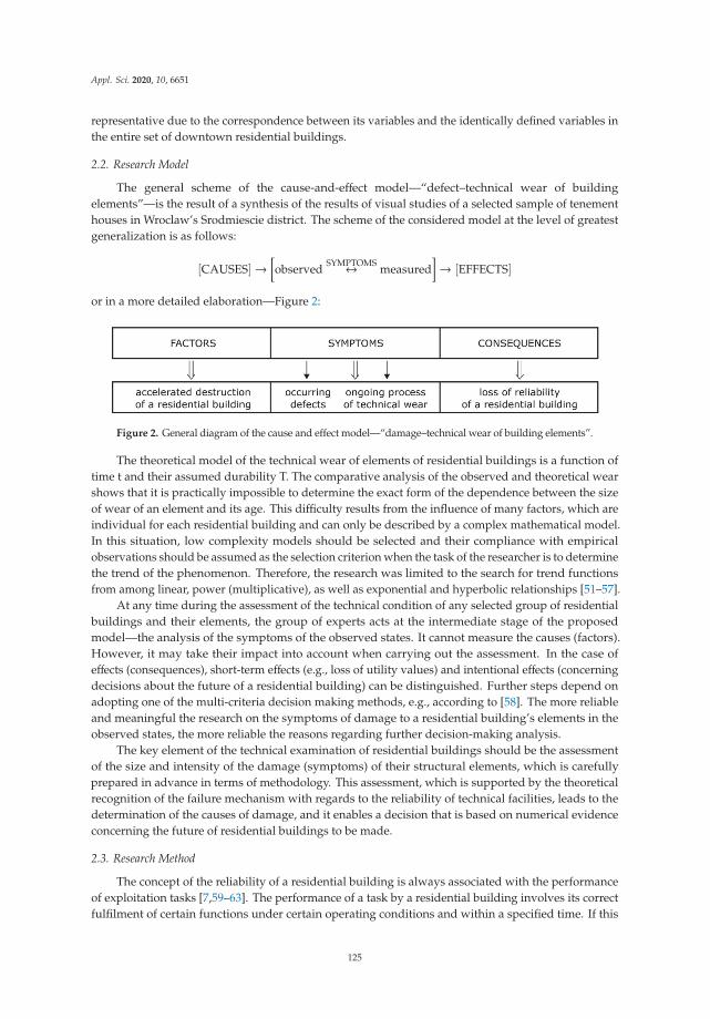
Appl. Sci. 2020, 10, 6651

representative due to the correspondence between its variables and the identically defined variables inthe entire set of downtown residential buildings.

2.2. Research Model

The general scheme of the cause-and-effect model—“defect–technical wear of buildingelements”—is the result of a synthesis of the results of visual studies of a selected sample of tenementhouses in Wroclaw’s Srodmiescie district. The scheme of the considered model at the level of greatestgeneralization is as follows:

[CAUSES]→[observed SYMPTOMS↔ measured

]→ [EFFECTS]

or in a more detailed elaboration—Figure 2:

Figure 2. General diagram of the cause and effect model—“damage–technical wear of building elements”.

The theoretical model of the technical wear of elements of residential buildings is a function oftime t and their assumed durability T. The comparative analysis of the observed and theoretical wearshows that it is practically impossible to determine the exact form of the dependence between the sizeof wear of an element and its age. This difficulty results from the influence of many factors, which areindividual for each residential building and can only be described by a complex mathematical model.In this situation, low complexity models should be selected and their compliance with empiricalobservations should be assumed as the selection criterion when the task of the researcher is to determinethe trend of the phenomenon. Therefore, the research was limited to the search for trend functionsfrom among linear, power (multiplicative), as well as exponential and hyperbolic relationships [51–57].

At any time during the assessment of the technical condition of any selected group of residentialbuildings and their elements, the group of experts acts at the intermediate stage of the proposedmodel—the analysis of the symptoms of the observed states. It cannot measure the causes (factors).However, it may take their impact into account when carrying out the assessment. In the case ofeffects (consequences), short-term effects (e.g., loss of utility values) and intentional effects (concerningdecisions about the future of a residential building) can be distinguished. Further steps depend onadopting one of the multi-criteria decision making methods, e.g., according to [58]. The more reliableand meaningful the research on the symptoms of damage to a residential building’s elements in theobserved states, the more reliable the reasons regarding further decision-making analysis.

The key element of the technical examination of residential buildings should be the assessmentof the size and intensity of the damage (symptoms) of their structural elements, which is carefullyprepared in advance in terms of methodology. This assessment, which is supported by the theoreticalrecognition of the failure mechanism with regards to the reliability of technical facilities, leads to thedetermination of the causes of damage, and it enables a decision that is based on numerical evidenceconcerning the future of residential buildings to be made.

2.3. Research Method

The concept of the reliability of a residential building is always associated with the performanceof exploitation tasks [7,59–63]. The performance of a task by a residential building involves its correctfulfilment of certain functions under certain operating conditions and within a specified time. If this

125

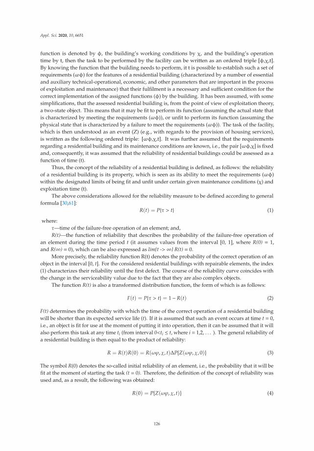
Appl. Sci. 2020, 10, 6651

function is denoted by φ, the building’s working conditions by χ, and the building’s operationtime by t, then the task to be performed by the facility can be written as an ordered triple [φ,χ,t].By knowing the function that the building needs to perform, it t is possible to establish such a set ofrequirements (ωφ) for the features of a residential building (characterized by a number of essentialand auxiliary technical-operational, economic, and other parameters that are important in the processof exploitation and maintenance) that their fulfilment is a necessary and sufficient condition for thecorrect implementation of the assigned functions (φ) by the building. It has been assumed, with somesimplifications, that the assessed residential building is, from the point of view of exploitation theory,a two-state object. This means that it may be fit to perform its function (assuming the actual state thatis characterized by meeting the requirements (ωφ)), or unfit to perform its function (assuming thephysical state that is characterized by a failure to meet the requirements (ωφ)). The task of the facility,which is then understood as an event (Z) (e.g., with regards to the provision of housing services),is written as the following ordered triple: [ωφ,χ,t]. It was further assumed that the requirementsregarding a residential building and its maintenance conditions are known, i.e., the pair [ωφ,χ] is fixedand, consequently, it was assumed that the reliability of residential buildings could be assessed as afunction of time (t).

Thus, the concept of the reliability of a residential building is defined, as follows: the reliabilityof a residential building is its property, which is seen as its ability to meet the requirements (ωφ)within the designated limits of being fit and unfit under certain given maintenance conditions (χ) andexploitation time (t).

The above considerations allowed for the reliability measure to be defined according to generalformula [30,61]:

R(t) = P{τ > t} (1)

where:τ—time of the failure-free operation of an element; and,R(t)—the function of reliability that describes the probability of the failure-free operation of

an element during the time period t (it assumes values from the interval [0, 1], where R(0) = 1,and R(∞) = 0), which can be also expressed as lim{t ->∞} R(t) = 0.

More precisely, the reliability function R(t) denotes the probability of the correct operation of anobject in the interval [0, t]. For the considered residential buildings with repairable elements, the index(1) characterizes their reliability until the first defect. The course of the reliability curve coincides withthe change in the serviceability value due to the fact that they are also complex objects.

The function R(t) is also a transformed distribution function, the form of which is as follows:

F(t) = P{τ > t} = 1−R(t) (2)

F(t) determines the probability with which the time of the correct operation of a residential buildingwill be shorter than its expected service life (t). If it is assumed that such an event occurs at time t = 0,i.e., an object is fit for use at the moment of putting it into operation, then it can be assumed that it willalso perform this task at any time ti (from interval 0<ti ≤ t, where i = 1,2, . . . ). The general reliability ofa residential building is then equal to the product of reliability:

R = R(t)R(0) = R(ωϕ,χ, t)ΔP{Z(ωϕ,χ, 0)

}(3)

The symbol R(0) denotes the so-called initial reliability of an element, i.e., the probability that it will befit at the moment of starting the task (t = 0). Therefore, the definition of the concept of reliability wasused and, as a result, the following was obtained:

R(0) = P{Z(ωϕ,χ, t)

}(4)

126

Appl. Sci. 2020, 10, 6651

and then:R(t) = P

{Z(ωϕ,χ, ti)

}, 0 < ti < t/Z(ωϕ,χ, 0) (5)

It was further assumed that event Z(ωφ, χ, 0) is certain, i.e., it is certain that, if a residentialbuilding adopted from the investment process to the exploitation process meets all the specifiedfunctions, then it will fulfil all the operational tasks assigned to it and it can also be inhabited byresidents. In this case, R(0) = 1, and expression (5) takes the following form:

R(t) = P{Z(ωϕ,χ, ti)

}, 0 < ti ≤ t (6)

Ultimately, the overall reliability of a residential building can be expressed by the R(t) function,which may have different distributions in different periods of the building’s operation. Most often,variable (t) can be treated as a random variable of the continuous type and then the density function isa derivative of the distribution function F(t):

f (t) = F′(t) = −R′(t) (7)

and then:

F(t) =

∞∫0

f (t)dt =

∞∫0

(−R

′(t)dt)

(8)

These are important relationships in the process of analysing building structures.Note that the reliability function is a decreasing function. This means that e.g., R(ti)<R(ti−1),

and, in extreme cases for ti = 0 and ti =∞, the reliability function takes the values R(0) = 1 and R(∞) = 0.This is contrary to the distribution function F(t), also called the unreliability function, for whichti: F(0) = 0 and F(∞) = 1 for the same values.

Further considerations were based on the definition of durability (T), which can be formalizedas a function of the following quantities [61,64]: the reliability of a residential building R(t), which isconsidered to be an event of randomly reaching the limit state by its element; the flux of physical agingextortions of a building and its elements W(t) (sometimes in the form of step stimuli); and, the level ofresistance of elements to the effects of extortions D(t). When presenting the problem with regards toreliability, it can be defined as the functional:

R(t) = Ψ{T(t), W(t), D(t)

}(9)

in which reliability is expressed by the durability and flux of changes in the level of aging and,thus, the processes of physical wear (if the problem is simplified by not taking the processes of socialwear into account). The wear processes are manifested by damage to a residential building andits elements, as a result of which the building is unfit for use (loses its serviceability value) andrequires renovation (if it is technically possible and economically justified). With exploitation time,a residential building becomes unfit for use more often, as it is subjected to increasingly frequentdamage (aging processes). For the sake of simplifying the considerations, distinguishing betweenthe state of operability and inoperability was omitted. However, the subsequent state of being fit foruse, after renovation, already represents a level of serviceability that is lower than the previous one.Therefore, it is possible to talk about a greater intensity of damage to the object with an increase in itsoperation time, although this is neither an increase reflecting the length of the building’s service lifenor an increase directly proportional to its age.

An important issue in renovation strategy is to define the basic determinants of the level ofreliability concerning the use of residential buildings. The basic element of these studies is thedetermination of the defect intensity function, which is itself an important issue with regards to theassessment of renovation decisions regarding residential buildings.

127

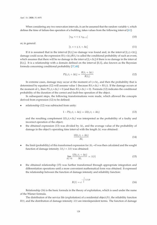
Appl. Sci. 2020, 10, 6651

When considering any two renovation intervals, it can be assumed that the random variable τ, whichdefines the time of failure-free operation of a building, takes values from the following interval [61]:

[τRi < τ ≤ τRi+1] (10)

or, in general:[ti < τ ≤ ti + Δti] (11)

If it is assumed that in the interval [0,ti] no damage was found and, in the interval [ti,ti+Δti],damage could occur, the expression R(ti+Δti)/R(ti) is called the conditional probability of such an event,which assumes that there will be no damage in the interval [ti+Δti] if there is no damage in the interval[0,ti]. It is a relationship with a domain defined on the interval [0,1], also known as the Bayesianformula concerning conditional probability [37,48]:

P{ti; ti + Δti} = R(ti + Δti)

R(ti)(12)

In extreme cases, damage may occur at the moment of ti+Δti, and then the probability that isdetermined by equation (12) will assume value 1 (because R(ti+Δti) = R(ti)). If the damage occurs atthe moment of ti, then P{ti;ti+Δti} = 0 (and then R(ti+Δti) = 0). Formula (12) indicates the conditionalprobability of the duration of the correct and fault-free operation of the object.

In subsequent steps, the following transformations were made, which allowed the conceptsderived from expression (12) to be defined:

• relationship (12) was subtracted from unity:

1− P{ti; ti + Δti} = U{ti; ti + Δti} (13)

and the resulting complement U{ti;ti+Δti} was interpreted as the probability of a faulty andincorrect operation of the object;

• the obtained expression (13) was divided by Δti, and the average value of the probability ofdamage in the object’s operating time interval with the length Δti was obtained:

U{ti; ti + Δti}Δti

(14)

• the limit (probability) of this transformed expression for Δti→0 was then calculated and the soughtfunction of damage intensity λ(ti) = λ(t) was obtained:

limΔti→0

U{ti; ti + Δti}Δti

= λ(t) (15)

• the obtained relationship (15) was further transformed through appropriate integration anddifferentiation operations until a more convenient mathematical form was obtained. It expressedthe relationship between the function of damage intensity and reliability function:

R(t) = e−

t∫0λ(t)dt

(16)

Relationship (16) is the basic formula in the theory of exploitation, which is used under the nameof the Wiener formula.

The distribution of the service life (exploitation) of a residential object f(t), the reliability functionR(t), and the distribution of damage intensity λ(t) are interdependent terms. The function of damage

128

Appl. Sci. 2020, 10, 6651

intensity itself depends—just like the reliability function (because it is a set of its arguments)—on manyfactors. These include the physical and chemical properties of the elements of residential buildings,the aging and wear processes W(t), the requirements for these objects (ωφ), and the maintenanceconditions of these objects (χ). The damage intensity function λ(t) can take various forms. It may bemonotonically increasing or decreasing (possibly with a few extreme points) or it may be constant overtime. The time course of the damage intensity function λ(t) reflects the course of the wear processesof a residential building throughout its service life. Table 1 shows the average values of the damageintensity function λ(t) for the ten most important elements of the examined downtown tenementhouses, as well as the indication of the lack of damage intensity λ(t) < 0.12, the damage tendency0.12 < λ(t) < 0.20, and a strong damage intensity λ(t) > 0.20.

The statistical form of this reliability measure is also used apart from the probabilistic (based on theprobability calculus) approach for determining the failure intensity function in the exploitation theory [61]:

λ(t) =n(t + Δt) − n(t)

N(t)Δt(17)

where:N(t)—the number of objects fit for use until time t;N(t + Δt)—the number of damaged objects until time t + Δt; and,λ(t)—a statistical measure of damage intensity.λ(t) is therefore the share of the number of defects in the analysed time unit (Δt) in interval

[t,t+Δt] and in the number of objects fit for use at the beginning of this interval, i.e., at time t.For the renovation strategy of a residential building, an important issue is to find—with the

assumed reliability level—a rational moment of renovation τR, i.e., to determine the most technicallyand economically advantageous average time of exploitation of the object τ0 from one renovation tothe next one. The measure of the average inter-repair time (or the value of the average random variableτ, i.e., the variable that determines the time of the correct operation of the facility) is:

τ0 = E(τ) =

τR∫0

R(t)dt (18)

It should be assumed that, in the period of building adaptation, i.e., for objects damaged duringthis period, the distribution of the damage intensity function is usually explained by various functionsthat have a monotonic and decreasing character of their course (more or less, depending on the natureof the damage intensity). The processes of the adaptation period are associated with the loss ofserviceability, which is caused by the exceeding of the limit states. After a fairly long-term effect ofloads, when they are continuously distributed and cyclically repeated in the process of exploitation,the Weibull function can be used, the density of which has the form of:

f (t) =β

αtβ−1e

tβα (19)

where: β—shape parameter, α—scale parameter.Because the damage intensity function can be written using the parameters α and β in the form:

λ(t) =β

αtβ−1 (20)

then:

R(t) = e−∞∫0

βα tβ−1dt

(21)

129

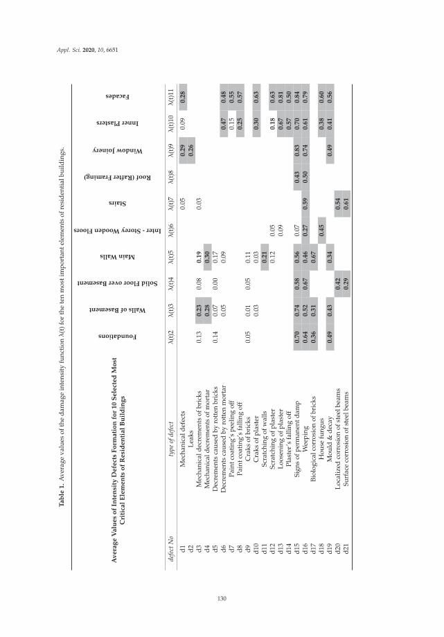
Appl. Sci. 2020, 10, 6651

Ta

ble

1.

Ave

rage

valu

esof

the

dam

age

inte

nsit

yfu

ncti

onλ

(t)f

orth

ete

nm

osti

mpo

rtan

tele

men

tsof

resi

dent

ialb

uild

ings

.

Av

era

ge

Va

lue

so

fIn

ten

sity

De

fect

sF

orm

ati

on

for

10

Se

lect

ed

Mo

stC

riti

cal

Ele

me

nts

of

Re

sid

en

tia

lB

uil

din

gs

Foundations

WallsofBasement

SolidFlooroverBasement

MainWalls

Inter-StoreyWoodenFloors

Stairs

Roof(RafterFraming)

WindowJoinery

InnerPlasters

Facades

defe

ctN

oty

peof

defe

ctλ

(t)2

λ(t

)3λ

(t)4

λ(t

)5λ

(t)6

λ(t

)7λ

(t)8

λ(t

)9λ

(t)1

0λ

(t)1

1

d1M

echa

nica

ldef

ects

0.05

0.2

90.

090

.28

d2Le

aks

0.2

6d3

Mec

hani

cald

ecre

men

tsof

bric

ks0.

130

.23

0.08

0.1

90.

03d4

Mec

hani

cald

ecre

men

tsof

mor

tar

0.2

80

.30

d5D

ecre

men

tsca

used

byro

tten

bric

ks0.

140.

070.

000.

17d6

Dec

rem

ents

caus

edby

rott

enm

orta

r0.

050.

090

.47

0.4

8d7

Pain

tcoa

ting

’spe

elin

goff

0.15

0.5

5d8

Pain

tcoa

ting

’sfa

lling

off0

.25

0.5

7d9

Cra

ksof

bric

ks0.

050.

010.

050.

11d1

0C

raks

ofpl

aste

r0.

030.

030

.30

0.6

3d1

1Sc

ratc

hing

ofw

alls

0.2

1d1

2Sc

ratc

hing

ofpl

aste

r0.

120.

050

.18

0.6

3d1

3Lo

osen

ing

ofpl

aste

r0.

090

.67

0.8

1d1

4Pl

aste

r’s

falli

ngoff

0.5

70

.50

d15

Sign

sof

perm

anen

tdam

p0

.70

0.7

40

.58

0.5

60.

070

.43

0.8

30

.70

0.8

4d1

6W

eepi

ng0

.64

0.5

20

.67

0.4

60

.27

0.5

90

.50

0.7

40

.61

0.7

9d1

7Bi

olog

ical

corr

osio

nof

bric

ks0

.36

0.3

10

.67

d18

Hou

sefu

ngus

0.4

50

.38

0.6

0d1

9M

ould

&de

cay

0.4

90

.43

0.3

40

.49

0.4

10

.56

d20

Loca

lized

corr

osio

nof

stee

lbea

ms

0.4

20

.54

d21

Surf

ace

corr

osio

nof

stee

lbea

ms

0.2

90

.61

130

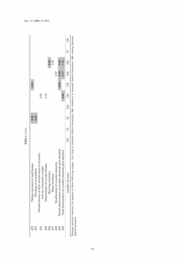
Appl. Sci. 2020, 10, 6651

Ta

ble

1.

Con

t.

d22

Pitt

ing

corr

osio

nof

stee

lbea

ms

0.5

50

.53

d23

Floo

ding

offo

unda

tion

0.4

5

d24

Woo

den

beam

sof

floor

sens

itiv

enes

sto

dyna

mic

acti

vity

ofhu

man

’sw

eigh

t0.

00

d25

Def

orm

atio

nof

woo

den

beam

s0.

12d2

6Sk

ewin

gof

join

ery

0.4

2d2

7W

arp

ofjo

iner

y0.

04d2

8St

rati

ficat

ion

ofw

oode

nel

emen

ts0.

07d2

9Pa

rtia

ldet

erio

rati

onof

woo

den

elem

ents

pest

atta

cked

0.3

80

.28

0.4

5d3

0To

tald

eter

iora

tion

ofw

oode

nel

emen

tspe

stat

tack

ed0

,43

0.57

0.42

num

ber

ofca

ses:

100

9393

100

100

100

100

100

9710

0

Dam

age

inte

nsit

yfu

ncti

onλ

(t)

app

ears

inth

ree

follo

win

gra

nges

:λ

(t)—

lack

ofin

tens

ity

def

ects

form

atio

n;λ

(t)—

tend

ency

toin

tens

ity

def

ects

form

atio

n;λ

(t)—

stro

ngin

tens

ity

defe

cts

form

atio

n.

131

Appl. Sci. 2020, 10, 6651

A typical distribution for objects subjected to damage in the first period of exploitation may bethe gamma distribution in the form:

f (t) =λ(λ(t))β−1e−λ(t)∫ ∞

0 e−ttβ−1dt(22)

in which the denominator is the so-called Euler’s integral. This distribution represents the processes ofloss of serviceability well, which are based on the cumulative effects of external factors. Ultimately,as a result of the elimination of all the defects and faults covered by the warranty, it is assumedthat gradual and sudden defects (the latter ones that result from the step operation of stimuli inthe conditions of accumulation of wear) are completely eliminated. This characterizes the end ofthe adaptation period of a residential building and the beginning of its normal operation period.The shape of the intensity function becomes “smooth”. Hence, value 1 for the shape parameter (β) canbe assumed for both the Weibull distribution and gamma distribution. It is a very characteristic periodof a residential building’s service life, in which the risk function takes a constant value (λ(t) = λ).This results from the following transformations of the mentioned functions:

• for the Weibull function:

λ(t) =β

αtβ−1 =

1α

t1−1 =1α= λ (23)

• for the gamma function (using a shortcut for long calculations):

λ(t) =f (t)R(t)

(24)

f (t) = λe−λt (25)

F(t) = 1− e−λt (26)

and using dependence (2):R(t) = e−λt (27)

ultimately:

λ(t) =λe−λt

e−λt = λ(= const) (28)

If the risk function has a domain defined by segment ti of the exploitation time (0 < ti ≤ t),then λ(t) = const (for λ > 0 and t > 0) and the time of correct operation of a residential building hasan exponential distribution. Finally, after several mathematical transformations of Equation (18), it ispossible to determine the most technically and economically advantageous average service life of theobject τ0 from the end of the warranty period:

τ0 =1λ

(29)

The last dependence leads to an extremely important conclusion for the mechanism of theoccurrence of defects in residential buildings: for the period of using a facility, in which the time ofcorrect operation to damage has an exponential distribution, the average remaining time of failure-freeoperation is unchanged at any time. Therefore, after a certain time of failure-free operation, residentialbuildings fulfil their functions, just like new ones, and after exceeding the planned exploitation timebeyond the assumed service life (t > T), they show “over-durability”—Figure 3:

132

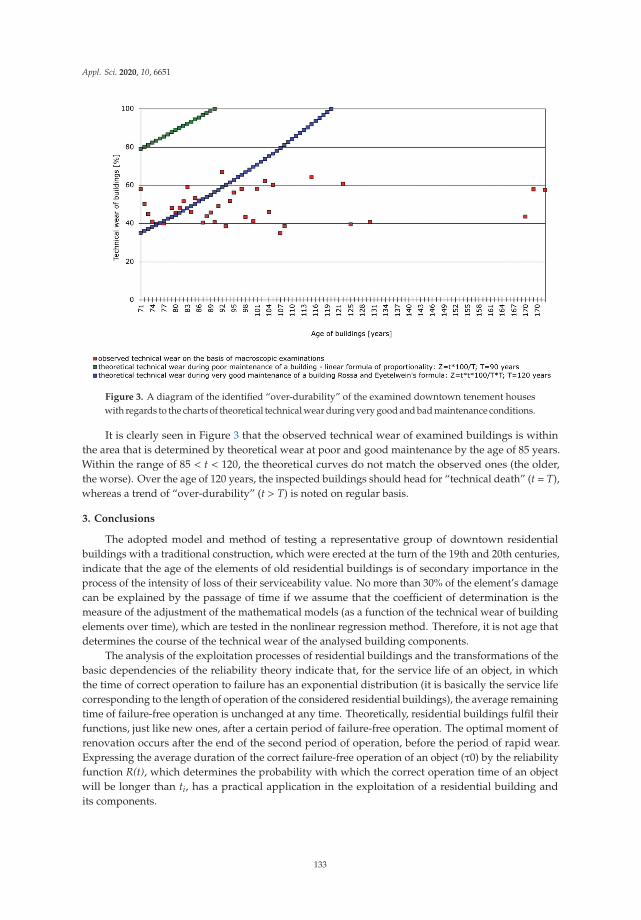
Appl. Sci. 2020, 10, 6651

Figure 3. A diagram of the identified “over-durability” of the examined downtown tenement houseswith regards to the charts of theoretical technical wear during very good and bad maintenance conditions.

It is clearly seen in Figure 3 that the observed technical wear of examined buildings is withinthe area that is determined by theoretical wear at poor and good maintenance by the age of 85 years.Within the range of 85 < t < 120, the theoretical curves do not match the observed ones (the older,the worse). Over the age of 120 years, the inspected buildings should head for “technical death” (t = T),whereas a trend of “over-durability” (t > T) is noted on regular basis.

3. Conclusions

The adopted model and method of testing a representative group of downtown residentialbuildings with a traditional construction, which were erected at the turn of the 19th and 20th centuries,indicate that the age of the elements of old residential buildings is of secondary importance in theprocess of the intensity of loss of their serviceability value. No more than 30% of the element’s damagecan be explained by the passage of time if we assume that the coefficient of determination is themeasure of the adjustment of the mathematical models (as a function of the technical wear of buildingelements over time), which are tested in the nonlinear regression method. Therefore, it is not age thatdetermines the course of the technical wear of the analysed building components.

The analysis of the exploitation processes of residential buildings and the transformations of thebasic dependencies of the reliability theory indicate that, for the service life of an object, in whichthe time of correct operation to failure has an exponential distribution (it is basically the service lifecorresponding to the length of operation of the considered residential buildings), the average remainingtime of failure-free operation is unchanged at any time. Theoretically, residential buildings fulfil theirfunctions, just like new ones, after a certain period of failure-free operation. The optimal moment ofrenovation occurs after the end of the second period of operation, before the period of rapid wear.Expressing the average duration of the correct failure-free operation of an object (τ0) by the reliabilityfunction R(t), which determines the probability with which the correct operation time of an objectwill be longer than ti, has a practical application in the exploitation of a residential building andits components.

133

Appl. Sci. 2020, 10, 6651

The study of the course of the damage intensity function λ(t) over time reflects the wear processof a residential building in a representative sample of downtown residential buildings erected whileusing traditional methods. It authorizes the formulation of the following conclusions—Table 1:

• there is measurable the damage intensity function in interval [0, t] for all 10 tested buildingelements, but the damage intensity force shows a significant span (from 0.00 to 0.84);

• as a rule, damage that is caused by water penetration and moisture penetration is of the highestintensity -0.54 on average;

• the technical condition of each of the tested elements also shows the intensity of defects that arecharacteristic for their design and material solutions, e.g.,:

� damage to wooden parts of elements (ceiling beams, stair treads, roof trusses, windowjoinery), which are attacked by biological pests;

� mechanical damage to the structure and texture, the intensity of which applies only to thoseelements in which the damage may cause the intensification of the impact of subsequent(cumulative) defects, e.g., construction walls underground and aboveground, as well asinternal and external plasters (but not foundations or massive cellar ceilings); and,

• damage that is manifested by the loss of the original shape of wooden elements can be consideredas not very intense; an exception is the torsion of window joinery (with an intensity of 0.42),for which this damage determines a significant decrease in its serviceability value.

4. Summary and Discussion

The practical approach to the problem of the intensity of the formation of defects in the testedresidential buildings with regards to the change in their reliability condition enables summing up thefollowing findings:

• generally used normative definitions of the reliability of buildings facilitate the study andinterpretation of the course of exploitation processes of residential buildings;

• for the purpose of a comprehensive assessment of changes in the reliability level of residentialbuildings, various reliability characteristics should be used, in which the damage intensity functionis of key importance, as it enables the construction of other reliability indicators; and,

• using the characteristics of the reliability of a residential building in renovation decisions allowsfor a rational renovation strategy to be determined by e.g., the determination of maintenanceintervals on the basis of established damage intensity distributions.

The methodological approach to the technical assessment of buildings, and their durability andreliability, has been known and presented in the literature for many years, especially in the papers ofArendarski [5], Zaleski [8,9], Thierry [21], and Tyminski [61]. Their works are used as manuals formanagers and administrators regarding the use of buildings. Nowogonska [11,18,28,30,31,39,40] dealswith the study of the impact of the maintenance of residential buildings on both the degree of damageand the reliability function. The reliable results of these studies are presented with a division intobuilding elements with the greatest share and significance for the proper functioning of the examinedbuildings. Such a division is particularly important in the last period of the building’s “service life”,when its operation time is approaching its expected durability.

A similar approach, as presented in previous publications, was adopted by the authors ofthis article, who conducted the technical assessment of tenement houses under the supervision ofMarcinkowska and Czaplinski [44–48,58]. This methodology of diagnosing residential buildings hasbeen presented for many years by the researchers of the so-called “German school”—Deutschmann [6]and Zimmermann [10]. They indicated the methods of measuring technical wear, damage sizeand the aging process of the load-bearing structure of engineering objects. Plebankiewicz, Zima,and Wieczorek [32,33] deal with the life cycle of a building object with regards to the risk and cost

134

Appl. Sci. 2020, 10, 6651

of its restoration as a result of renovation activities, which—in the opinion of the authors of thispublication—should be a secondary feature: cost versus technical. After all, increasing cultural,historical, and humanistic aspects prevail over material ones when making decisions about theso-called “technical death” of facilities that are located in the centres and suburbs of many cities.Therefore, the priority seems to be to study the damage intensity of residential buildings in the contextof changes in their reliability state.

It is worth noting that the discussed quantitative data can provide the basis for programmingthe size and structure of specialized construction companies that are involved in the maintenanceand renovation of residential buildings. These data are included in the technical information thatis necessary for managing buildings and designing the organization of these maintenance activitiesfor residential buildings, which, in turn, determines the quality of broadly understood housingmaintenance conditions.

Finally, attention should be paid to the individual nature of the results of the study, which wasbased on research on a homogeneous coherent group of downtown tenement houses. The transferof the results of the technical assessment to a different population of residential buildings with atraditional construction should be conducted with great caution and with the necessity to performsurveys. Undoubtedly, such studies should be preceded by the careful, purposeful selection of atypological sample that is representative for the general population. Such a sample may contain amuch smaller number of objects, but it is extremely important that the decisive selection criterionfor the technical assessment involves the elements (or only parts of them) that are essential for thestructure (load-bearing structure) of the building. This division is especially important when examiningcomposite and complex elements. It can then be assumed that, from the point of view of the ultimatelimit states of elements, the degree of their technical wear (while maintaining the safe and reliableoperating conditions of the object) is equal to 75%.

The methodological aspects of the reliability of the quantitative results of the technical assessmentshould also aim to minimize the subjectivity of expert judgment in the process of technical examinationsof residential buildings by specifying the type of the predicted random impacts, and by determiningthe variability of at least some of them. It should also be remembered that the issue of technicaltests of buildings (especially residential buildings) needs to be updated with full recognition ofthe forms of their immaterial wear—social and economic. It is a sign of recent times that it is thepsychological aspects of the perception of the process of decline in the serviceability value of flats bytheir users, being supported by the analysis of the profitability of replacing entire buildings, which playa fundamental role when making decisions regarding the future of downtown housing developments.

Therefore, the results of the research should be treated as an exploratory study, the main aim ofwhich was to model the solution of cause–effect relationships. These dependencies indicate the typeand size of damage that shows the impact of the maintenance conditions of downtown residentialbuildings on the technical wear of their components. Like any exploratory solution, it should betreated as a multi-criteria recognition of the mechanism of the occurrence and effects of phenomenathat are encountered by an adjudicator at each stage of the technical assessment of an engineeringobject. However, this assessment, in its nature, includes an unmeasurable (partly subjective) aspect.The construction of a new model of the technical inspection of residential buildings, which is basedon the assumptions and conclusions resulting from the study, will allow the burden of the results ofthe technical assessment to be considered as more quantitative than qualitative. The intention of theauthors is that further work related to the broadly understood diagnosis of technical objects should goin this direction.

Author Contributions: Conceptualization, J.K., M.S. (Marek Sawicki) and M.S. (Mariusz Szóstak); methodology,J.K.; software, J.K. and M.S. (Mariusz Szóstak); validation, J.K., M.S. (Marek Sawicki) and M.S. (Mariusz Szóstak);formal analysis, J.K., M.S. (Marek Sawicki) and M.S. (Mariusz Szóstak); investigation, J.K. and M.S. (Marek Sawicki);resources, J.K. and M.S. (Marek Sawicki); writing—original draft preparation, J.K.; writing—review and editing,J.K. and M.S. (Mariusz Szóstak); supervision, M.S. (Marek Sawicki). All authors have read and agreed to thepublished version of the manuscript.

135

Appl. Sci. 2020, 10, 6651

Funding: This research received no external funding.

Conflicts of Interest: The authors declare no conflict of interest.

References

1. Kim, B.; Ahn, Y.; Lee, S. LDA-based model for defect management in residential buildings. Sustainability2019, 11, 7201. [CrossRef]

2. Rotimi, F.; Tookey, J.; Rotimi, J. Evaluating defect reporting in new residential buildings in New Zealand.Buildings 2015, 5, 39–55. [CrossRef]

3. Sandeford, P. Planning for durability and life cycle maintenance of buildings during design. In Proceedingsof the International Conference on Performance-based and Life-cycle Structural Engineering, Brisbane, QLD,Australia, 9–11 December 2015; University of Queensland Library: Brisbane, Australia, 2016; pp. 1094–1103.

4. Šnıdere, L.; Geipele, I.; Stamure, I. Case study of standard multi-storey residential building owners and tenants’perception of building technical conditions and renovation issues. Balt. J. Real Estate Econ. Constr. Manag.2017, 5, 6–22. [CrossRef]

5. Arendarski, J. Durability and Reliability of Residential Buildings Erected Using Industrialized Methods; Arkady:Warsaw, Poland, 1978. (In Polish)

6. Deutschmann, E. Development of Measuring Techniques In Situ for Residential Buildings; WissenschaftlicheZeitschrift der Technischen Universitaet: Dresden, Germany, 1987.

7. Merminod, P. Investigation of Wear and Damages of Old Buildings; Chantiers Revue du Batiment du Genie civilet de la Securite: France, 1984.

8. Zaleski, J. Renovations and Modernizations of Residential Buildings; Arkady: Warsaw, Poland, 1995. (In Polish)9. Zaleski, J. Renovation of Residential Buildings, Guide; Arkady: Warsaw, Poland, 1995. (In Polish)10. Zimmermann, G. Impairment of Structures-Building Failure, Damages, Wear and Tear and Aging; Deutsches

Architektenblatt, Ausgabe Baden: Wuerttemberg, Germany, 1976.11. Nowogonska, B. Prognosis of the technical condition of masonry walls in residential buildings. Bud. Archit.

2014, 13, 27–32. [CrossRef]12. Macarulla, M.; Forcada, N.; Casals, M.; Gangolells, M.; Fuertes, A.; Roca, X. Standardizing housing defects:

Classification, validation, and benefits. J. Constr. Eng. Manag. 2013, 139, 968–976. [CrossRef]13. Chen, C.; Juan, Y.; Hsu, Y. Developing a systematic approach to evaluate and predict building service life.

J. Civil Eng. Manag. 2017, 23, 890–901. [CrossRef]14. Chong, W.; Low, S. Assessment of defects at construction and occupancy stages. J. Perform. Constr. Facil.

2005, 19, 283–289. [CrossRef]15. Pan, W.; Thomas, R. Defects and their influencing factors of posthandover new-build homes. J. Perform.

Constr. Facil. 2015, 29, 04014119. [CrossRef]16. Kim, Y.; Oh, S.; Cho, Y.; Seo, J. A PDA and wireless web-integrated system for quality inspection and defect

management of apartment housing projects. Autom. Constr. 2008, 17, 163–179. [CrossRef]17. Jernberg, P.; Lacasse, M.; Haagenrud, S.; Sjöström, C. Guide and Bibliography to Service Life and Durability

Research for Buildings and Components; Joint CIB W80/RILEM TC 140–TSL Committee on Service Life ofBuilding Materials and Components CIB Report, Publication 295; CIB: Rotterdam, The Netherlands, 2004.

18. Nowogonska, B. Diagnoses in the aging process of residential buildings constructed using traditionaltechnology. Buildings 2019, 9, 126.

19. van Breugel, K.; Koleva, D.; van Beek, T. The Ageing of Materials and Structures; Springer InternationalPublishing: Delft, The Netherlands, 2018.

20. Thier, H. Cases of Damage and Their Analysis; Deutscher Verlag fuer Schweisstechnik: Duesseldorf, Germany,1985.

21. Thierry, J.; Zaleski, J. Renovation of Buildings and Strengthening of Structures; Arkady: Warsaw, Poland, 1982.(In Polish)

22. Silva, A.; de Brito, J.; Gaspar, P. Methodologies for Service Life Prediction of Buildings with a Focus on FacadeClaadings; Springer International Publishing: Lisbon, Portugal, 2016.

23. Thomsen, A.; van Der Flier, K. Understanding obsolescence: A conceptual model for buildings. Build. Res. Inf.2011, 39, 352–362. [CrossRef]

136

Appl. Sci. 2020, 10, 6651

24. Hoła, B.; Nowobilski, T. Analysis of the influence of socio-economic factors on occupational safety in theconstruction industry. Sustainability 2019, 11, 4469. [CrossRef]

25. Grzyl, B.; Apollo, M.; Miszewska-Urbanska, E.; Kristowski, A. Management of exploitation in terms of lifecycle costs of built structures. Acta Sci. Pol. Archit. 2017, 16, 85–89.

26. Forster, A.; Kayan, B. Maintenance for historic buildings: A current perspective. Struct. Surv. 2009, 27,210–229. [CrossRef]

27. Sugier, J.; Anders, G. Modelling and evaluation of deterioration process with maintenance activities.Maint. Reliab. 2013, 15, 305–311.

28. Nowogonska, B.; Korentz, J. Value of technical wear and costs of restoring performance characteristics toresidential buildings. Buildings 2020, 10, 9. [CrossRef]

29. Ramuhalli, P.; Henager, C.; Griffin, J.; Meyer, R.; Coble, J.; Pitman, S.; Bond, L. Material aging and degradationdetection and remaining life assessment for plant life management, Third International Conference onNuclear Power Plant Life Management. In Proceedings of the International Conference, Salt Lake City, UT,USA, 14–18 May 2012.

30. Nowogonska, B. Intensity of damage in the aging process of buildings. Arch. Civil Eng. 2020, 66, 19–31.31. Nowogonska, B. Proposal for determing the scale of renovation needs of residential buildings. Civil Environ.

Eng. Rep. 2016, 22, 137–144. [CrossRef]32. Plebankiewicz, E.; Zima, K.; Wieczorek, D. Original model for estimating the whole life costs of buildings

and its verification. Arch. Civil Eng. 2019, 65, 163–179. [CrossRef]33. Plebankiewicz, E.; Zima, K.; Wieczorek, D. Life cycle cost modelling of buildings with consideration of the

risk. Arch. Civil Eng. 2016, 65, 149–166. [CrossRef]34. Grant, A.; Ries, R. Impact of building service life models on life cycle assessment. Build. Res. Inf. 2013, 41,

168–186. [CrossRef]35. Bucon, R.; Sobotka, A. Decision-making model for choosing residential building repair variants. J. Civil Eng. Manag.

2015, 21, 893–901. [CrossRef]36. Knyziak, P. Estimating the technical deterioration of large-panel residential buildings using artificial neural

networks. Procedia Eng. 2014, 91, 394–399. [CrossRef]37. Radziszewska-Zielina, E.; Sladowski, G. Proposal of the use of a fuzzy stochastic network for the preliminary

evaluation of the feasibility of the process of the adaptation of a historical building to a particular form ofuse. Iop. Conf. Ser. Mater. Sci. Eng. 2017, 245, 1–11. [CrossRef]

38. Gradzki, R.; Lindstedt, P. Method of assessment of technical object aptitude in environment of exploitationand service conditions. Maint. Reliab. 2015, 17, 54–63. [CrossRef]

39. Nowogonska, B. Preventive services of residential buildings according to the Pareto principle. Iop. Conf. Ser.Mater. Sci. Eng. 2019, 471, 112034. [CrossRef]

40. Nowogonska, B. The life cycle of a building as a technical object. Period. Polytech. Civil Eng. 2016, 60, 331–336.[CrossRef]

41. Zaidi, A.; Bouamama, B.; Tagina, M. Bayesian reliability models of weibull systems: State of the art. Int. J.Appl. Math. Comput. Sci. 2012, 22, 585–600. [CrossRef]

42. Cordeiro, G.; Ortega, E.; Lemonte, A. The exponential-Weibull lifetime distribution. J. Stat. Comput. Simul.2014, 84, 2592–2606. [CrossRef]

43. Khelassi, A.; Theilliol, D.; Weber, P. Reconfigurability analysis for reliable fault-tolerant control design. Int. J.Appl. Math. Comput. Sci. 2011, 21, 431–439. [CrossRef]

44. Konior, J. Technical assessment of old buildings by fuzzy approach. Arch. Civil Eng. 2019, 65, 129–142.[CrossRef]

45. Marcinkowska, E. Technical and functional requirements of building deterioration estimation. Arch. Civil Eng.2002, 48, 125–134.

46. Marcinkowska, E.; Gawron, K. Down-town tenement-houses in Wroclaw as a subject of real estate sales.Pr. Nauk. Inst. Budownictwa Politech. Wrocławskiej. Studia I Mater. 2006, 87, 315–324. (In Polish)

47. Marcinkowska, E. Analyses of techical and functional requirements of building modernization. Arch. CivilEng. 2003, 49, 53–62.

48. Multi-Author Work under K. Czaplinski Lead, Assessment of Wrocław Downtown Apartment Houses’ TechnicalConditions; Reports Series “U” of Building Engineering Institute; Wrocław University of Technology: Wrocław,Poland, 1984; Volume 96.

137

Appl. Sci. 2020, 10, 6651

49. Govindarajulu, Z. Elements of Sampling Theory and Methods; Pearson: Upper Saddle River, NJ, USA, 1999.50. Barnett, V. Elements of Sampling Theory; PWN: Warsaw, Poland, 1982. (In Polish)51. Baer, D. An Introduction to Latent Variable Models in the Social Sciences; University of Western Ontario: London,

ON, Canada, 1993.52. Gerstenkorn, T.; Sródka, T. Combinatorics and Probability Calculus; PWN: Warsaw, Poland, 1980. (In Polish)53. Gren, J. Models and Tasks of Mathematical Statistics; PWN: Warsaw, Poland, 1978. (In Polish)54. Hellwig, Z. Elements of Probability Calculus and Mathematical Statistics; PWN: Warsaw, Poland, 1993. (In Polish)55. Stuart, A. Rank Correlation Methods. By M. G. Kendall. Br. J. Stat. Psychol. 1956, 9, 68. [CrossRef]56. Morrison, D. Multivariate Statistical Methods, 4th ed.; Thomson Brooks/Cole: New York, NY, USA, 2004.57. Zajac, K. Outline of Statistical Methods; PWE: Warsaw, Poland, 1994. (In Polish)58. Marcinkowska, E. Decision-Making Problems in the Design of Buildings and Construction Processes; Monograph

of the Wroclaw University of Science and Technology: Wroclaw, Poland, 1986.59. Sognen, O. The Scandinavian approach to maintenance and modernization, International Symposium on

Management, Maintenance and Modernisation of Building Facilities. In Proceedings of the Strategies andTechnologies for Maintenance and Modernisation of Building, Tokyo, Japan, 26–28 October 1994.

60. Torregrossa, J. Liquidated Damages: Three Myths Exposed; Construction-Specifier: London, UK, 1987.61. Tyminski, J. Elements of the Theory of Reliability of Residential Buildings; Wydawnictwo WSGK w Kutnie: Kutno,

Poland, 2001. (In Polish)62. Weil, G. Detecting the Defects; Civil Engineering ASCE: London, UK, 1989.63. Pihlajavaara, S. Background and Principles of Long-Term Performance of Building Materials, Durability of Building

Materials and Components; Sereda, P., Litvan, G., Eds.; ASTM International: West Conshohocken, PA, USA,1980; pp. 5–16.

64. Wolff, R.; Dicke, P. Maintenance and Modernisation; Beton: Germany, 1988.

© 2020 by the authors. Licensee MDPI, Basel, Switzerland. This article is an open accessarticle distributed under the terms and conditions of the Creative Commons Attribution(CC BY) license (http://creativecommons.org/licenses/by/4.0/).

138

applied sciences

Article

Risk Assessment of Large-Scale InfrastructureProjects—Assumptions and Context

Jana Korytárová * and Vít Hromádka

���������������

Citation: Korytárová, J.; Hromádka,

V. Risk Assessment of Large-Scale

Infrastructure Projects—Assumptions

and Context. Appl. Sci. 2021, 11, 109.

https://dx.doi.org/10.3390/app1101

0109

Received: 1 December 2020

Accepted: 22 December 2020

Published: 24 December 2020

Publisher’s Note: MDPI stays neu-

tral with regard to jurisdictional claims

in published maps and institutional

affiliations.

Copyright: © 2020 by the authors. Li-

censee MDPI, Basel, Switzerland. This

article is an open access article distributed

under the terms and conditions of the

Creative Commons Attribution (CC BY)

license (https://creativecommons.org/

licenses/by/4.0/).

Faculty of Civil Engineering, Brno University of Technology, 60200 Brno, Czech Republic;hromadka.v@fce.vutbr.cz* Correspondence: korytarova.j@fce.vutbr.cz; Tel.: +420-733-164-369

Featured Application: The results of the presented research extend the methodology of economic

analysis and risk assessment of large infrastructure projects.

Abstract: This article deals with the partial outputs of large-scale infrastructure project risk assess-ment, specifically in the field of road and motorway construction. The Department of Transportspends a large amount of funds on project preparation and implementation, which however, mustbe allocated effectively, and with knowledge of the risks that may accompany them. Therefore,documentation for decision-making on project financing also includes their analysis. This articlemonitors the frequency of occurrence of individual risk factors within the qualitative risk analysis,with the support of the national risk register, and identifies dependent variables that represent part ofthe economic cash flows for determining project economic efficiency. At the same time, it comparesthese dependent variables identified by sensitivity analysis with critical variables, followed by testingthe interaction of the critical variables’ effect on the project efficiency using the Monte Carlo method.A partial section of the research was focused on the analysis of the probability distribution of inputvariables, especially “the investment costs” and “time savings of infrastructure users” variables. Theresearch findings conclude that it is necessary to pay attention to the setting of statistical characteris-tics of variables entering the economic efficiency indicator calculations, as the decision of whether ornot to accept projects for funding is based on them.

Keywords: CBA; investment project; probability distribution; sensitivity analyses; risk assessment

1. Introduction

Transport infrastructure projects are important carriers and supporters of economicgrowth for national economies. Implementation of investment projects, in addition to thedirect benefits for which they are implemented, brings growth potential for the nationaleconomy; they reduce unemployment, increase the sales of design and implementationcompanies, and thus create revenue capacity on the demand side for purchases of goodsand services. Implementation of investment projects will also be a key factor in alleviatingthe current COVID-19 pandemic effect in all national economies; e.g., the draft of the statebudget of the Czech Republic brings record investments for the future, which have beenincreased by CZK 178 billion for 2021 (€6.7 billion). Even so, the supply of funds for projectimplementation is limited. Therefore, it is always necessary to choose for financing onlythose projects that are efficient. The efficiency of projects to be implemented is assessed inthe ex-ante period, on the basis of feasibility study data, which is addressed in the form ofa cost–benefit analysis (CBA).

The authors of this article have been carrying out research into development in eco-nomic efficiency assessment of public transport infrastructure projects for a long time. Inthe present article they focused on the analysis of the economic outputs of road infras-tructure projects, motorways, and class I roads via CBA. CBA has the largest explanatorypower [1–4], which is based on the determination of cost-effectiveness against the total

Appl. Sci. 2021, 11, 109. https://dx.doi.org/10.3390/app11010109 https://www.mdpi.com/journal/applsci

139

Appl. Sci. 2021, 11, 109

societal benefits. Generally, four criteria are solved and monetized in large-scale transportinfrastructure project appraisals: travel time savings, travel and operational costs, safety,and environmental cost, from different perspectives. In ref. [5] based on the modelingof economic cash flows determined by these variables, the following economic efficiencyindicators were established: economic net present value (ENPV), economic internal rateof return (ERR), and benefit cost ratio (BCR) [6,7]. The values of the economic indicatorswere tested for critical variables and the switching values of indicators (threshold valueof the indicator in terms of efficiency, e.g., ENPV = 0, ERR = discount rate) were deter-mined. In the following step, a quantitative risk analysis using the Monte Carlo methodwas performed for the identified critical variables. At the same time, a qualitative riskanalysis, which considered potential risk factors using a risk register [7], was performed.It monitored the project risk impact, the occurrence probability, and deduced the riskrelevance for the implementation and operation of the project. Individual projects thatdemonstrated a positive evaluation from all perspectives examined are ready for funding,and further phases of their life cycle can be launched for them. The research questionaddressed by the implemented research team was which variables are risky, how strongis their influence on economic efficiency, and whether and how the projects are resilient;robust to the potential risk interaction. This concerns questions of the connection of thequalitative and quantitative risk analysis, which dependant variables are resulting from thequalitative analysis, and if they are also considered in the quantitative analysis. In the caseof the important critical variable it was the objective to test the changes of the efficiency ofprojects while using different probability distributions.

Investors aim, not only to prevent project failure, but also to select the best alternativesamong the available investment projects, so as to gain more benefits and achieve betterresults [8]. In the investment decision-making process of large-scale projects, many riskfactors can cause decision failure [9]. This is also why decision-support systems are of highimportance for investors in the construction industry [10].

2. Materials and Methods

The aim of the research described in this paper was to find the relations betweenthe outputs of the qualitative risk analysis, sensitivity analysis, and quantitative riskanalysis, which were performed in the evaluation of the economic efficiency of transportinfrastructure projects, as part of the modeling of economic Cash Flow (CF) of their life cycle.For the case study, a set of projects being prepared for realization in the Czech Republicwas chosen. The authors of the paper have many years of experiences in the evaluation ofprojects in Czech transport infrastructure, and during these years they were able to collecta large amount of input data. However, the authors would like to emphasize that for thepresented procedures, and partly also for the results, it is possible, respecting individualspecifics of economic evaluation in other countries, to relate them to projects carried outabroad. The research sample consisted of 20 large-scale transport infrastructure projectsfrom the Czech Republic, which were the pre-investment phase in the 2018–2020 period,and with proven economic efficiency. Only those projects that could be compared witheach other due to the fact that they were processed according to the same methodologicalprocedure, e.g., according to the Departmental Methodology valid since 2017 [7], wereincluded in the research sample.

Net cash flow (NCF) for the calculation of economic ratios consisted of the savingsin the costs of the suggested (investment) variant related to the zero variant (withoutinvestment). The calculation formula consists of four types of particular benefits; socio-economic savings. They are savings in travel and operating costs, savings in travel timecosts, reduction in accident costs, and savings in exogenous costs. The time value of moneydetermining the amount of the discount rate for the calculation of the ENPV indicator wasset at 5% for the Czech Republic in the EU programming period 2014–2020.

The research presented in this article examined project risk frequency, and the impacton their economic efficiency and robustness of economic efficiency indicators, using sen-

140

Appl. Sci. 2021, 11, 109

sitivity analysis, and finally involved confirmation or refusing the robustness of projectsaccording to the previous step by determining the cumulative probability of achievingproject economic efficiency using the Monte Carlo method. To assess the real risk of failureassociated with the investment, changes in the values of economic performance indicatorsderiving from the simultaneous change of several project variables had to be identified [11].As stated by [12], one of the risk assessment tools is the Monte Carlo method, whichcombines and develops both sensitivity analysis, and scenario analysis, methods. In theresource material, Ref. [13] focused on the Monte Carlo method used in the case of theearned value management methodology. Bowers also provided a broader view of the issueof project risk assessment [14].

2.1. Data

Table 1 presents the research sample projects with their basic characteristics. It statesthe undiscounted economic investment costs (i.e., investment costs excluding VAT reducedby a conversion coefficient 0.807), economic internal rate of return (ERR), economic netpresent value (ENPV), and cost benefit ratio (BCR), which was calculated according to thefollowing relation:

BC

= 1 +ENPV

IC(1)

where:

BCR: Cost Benefit RatioENPV: Economic Net Present ValueIC: Discounted Investment Costs

Table 1. Basic economic data on research sample projects.

No. Name of the ProjectIC€

ERR%

ENPV€

BCR

P1 Vestec connection 73,655,517 13.15% 134,141,506 2.90P2 I/22 Draženov-Horažd’ovice 253,477,033 5.67% 25,929,610 1.11P3 I/27 Kaznejov, bypass 91,192,128 9.50% 74,002,422 1.83

P4 I/13 Ostrov-Smilov,right bank 141,082,434 5.88% 19,811,383 1.15

P5 I/13 Ostrov-Smilov,left bank 116,820,770 7.52% 50,193,343 2.01

P6 I/26 Horšovský Týn 50,375,269 5.60% 4,578,849 1.09P7 D0 Brezineves-Satalice var. 1 371,886,072 39.45% 2,576,573,157 8.28P8 D0 Brezineves-Satalice var. 2 434,933,917 30.46% 2,395,820,591 6.92P9 D0 Brezineves-Satalice var. 3 757,919,450 17.89% 1,934,644,942 3.81P10 I11– Hradec Králové, tangent 111,776,135 17.24% 336,621,090 4.15P11 I/18 Príbram-bypass var. 1 28,417,453 14.20% 54,410,634 2.96P12 I/18 Príbram-bypass var. 2 49,497,029 13.21% 74,973,161 2.61P13 I/50 Bucovice 78,579,450 7.56% 32,937,152 1.44P14 I/36 Trnová-Fablovka-Dubina 53,652,370 19.20% 190,286,624 4.73P15 I/11 Nové Sedlice-Opava Komárov 91,436,523 5.52% 7,834,232 1.09P16 I/26 Holysov, bypass 56,624,471 9.19% 42,452,457 1.80P17 D10 Praha-Kosmonosy 361,367,050 5.72% 35,994,616 1.11P18 I/67 Bohumín-Karviná 83,937,876 5.33% 4,067,671 1.05P19 D43 Boritov-Staré Mesto 56,624,471 9.19% 42,452,457 1.80P20 D27 Preštice-Klatovy 128,638,259 5.12% 22,333,326 1.02

Source: Feasibility Studies of Investment projects, The State Fund for Transport Infrastructure SFDI, authors’ own processing.

Qualitative risk analysis is generally based on expert opinions on the risks that threatena particular investment project. Lists of risks are usually created, based on the knowledge

141

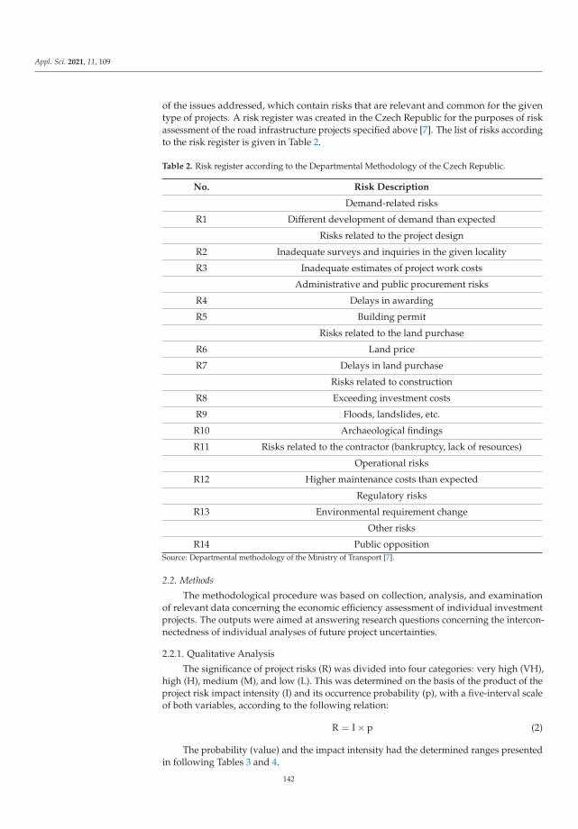
Appl. Sci. 2021, 11, 109

of the issues addressed, which contain risks that are relevant and common for the giventype of projects. A risk register was created in the Czech Republic for the purposes of riskassessment of the road infrastructure projects specified above [7]. The list of risks accordingto the risk register is given in Table 2.

Table 2. Risk register according to the Departmental Methodology of the Czech Republic.

No. Risk Description

Demand-related risks

R1 Different development of demand than expected

Risks related to the project design

R2 Inadequate surveys and inquiries in the given locality

R3 Inadequate estimates of project work costs

Administrative and public procurement risks

R4 Delays in awarding

R5 Building permit

Risks related to the land purchase

R6 Land price

R7 Delays in land purchase

Risks related to construction

R8 Exceeding investment costs

R9 Floods, landslides, etc.

R10 Archaeological findings

R11 Risks related to the contractor (bankruptcy, lack of resources)

Operational risks

R12 Higher maintenance costs than expected

Regulatory risks

R13 Environmental requirement change

Other risks

R14 Public oppositionSource: Departmental methodology of the Ministry of Transport [7].

2.2. Methods

The methodological procedure was based on collection, analysis, and examinationof relevant data concerning the economic efficiency assessment of individual investmentprojects. The outputs were aimed at answering research questions concerning the intercon-nectedness of individual analyses of future project uncertainties.

2.2.1. Qualitative Analysis

The significance of project risks (R) was divided into four categories: very high (VH),high (H), medium (M), and low (L). This was determined on the basis of the product of theproject risk impact intensity (I) and its occurrence probability (p), with a five-interval scaleof both variables, according to the following relation:

R = I × p (2)

The probability (value) and the impact intensity had the determined ranges presentedin following Tables 3 and 4.

142

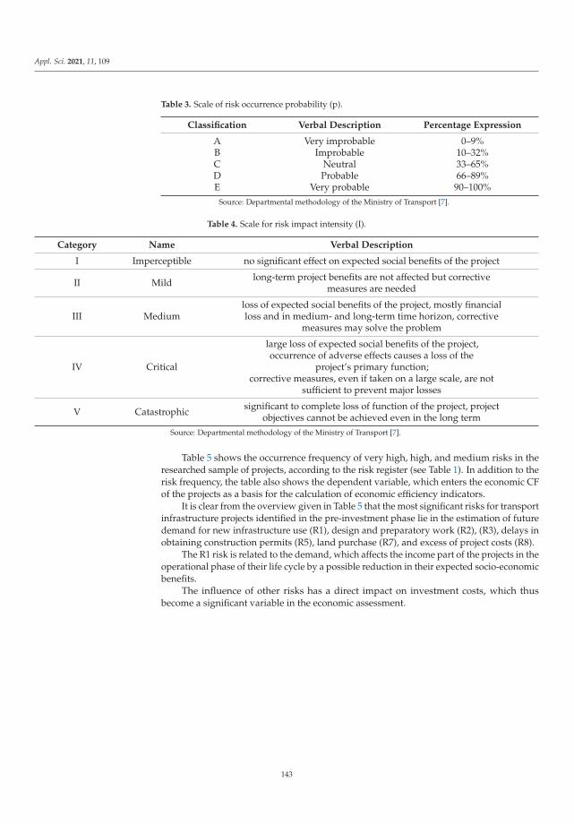
Appl. Sci. 2021, 11, 109

Table 3. Scale of risk occurrence probability (p).

Classification Verbal Description Percentage Expression

A Very improbable 0–9%B Improbable 10–32%C Neutral 33–65%D Probable 66–89%E Very probable 90–100%

Source: Departmental methodology of the Ministry of Transport [7].

Table 4. Scale for risk impact intensity (I).

Category Name Verbal Description

I Imperceptible no significant effect on expected social benefits of the project

II Mild long-term project benefits are not affected but correctivemeasures are needed

III Mediumloss of expected social benefits of the project, mostly financialloss and in medium- and long-term time horizon, corrective

measures may solve the problem

IV Critical

large loss of expected social benefits of the project,occurrence of adverse effects causes a loss of the

project’s primary function;corrective measures, even if taken on a large scale, are not

sufficient to prevent major losses

V Catastrophic significant to complete loss of function of the project, projectobjectives cannot be achieved even in the long term

Source: Departmental methodology of the Ministry of Transport [7].

Table 5 shows the occurrence frequency of very high, high, and medium risks in theresearched sample of projects, according to the risk register (see Table 1). In addition to therisk frequency, the table also shows the dependent variable, which enters the economic CFof the projects as a basis for the calculation of economic efficiency indicators.

It is clear from the overview given in Table 5 that the most significant risks for transportinfrastructure projects identified in the pre-investment phase lie in the estimation of futuredemand for new infrastructure use (R1), design and preparatory work (R2), (R3), delays inobtaining construction permits (R5), land purchase (R7), and excess of project costs (R8).

The R1 risk is related to the demand, which affects the income part of the projects in theoperational phase of their life cycle by a possible reduction in their expected socio-economicbenefits.

The influence of other risks has a direct impact on investment costs, which thusbecome a significant variable in the economic assessment.

143

Appl. Sci. 2021, 11, 109

Table 5. Risk frequency according to their significance, including the dependent variable identification.

Risk No.VH and H

RisksM

RiskTotal Dependent Variable

R1 3 5 8 Revenues alias operating phase savingsR2 5 8 12 Investment costs, beginning of the constructionR3 4 6 10 Investment costsR4 0 5 5 Beginning of the constructionR5 0 9 9 Beginning of the constructionR6 0 2 2 Investment costsR7 12 2 14 Beginning of the constructionR8 8 5 13 Investment costs

R9 0 1 1 Investment costs, extension of construction, delay/shortening of theoperational phase for evaluation

R10 0 1 1 Investment costs, extension of construction, delay/shortening of theoperational phase for evaluation

R11 0 2 2 Investment costs, extension of construction, delay/shortening of theoperational phase for evaluation

R12 0 0 0 Operating costs, reduction of benefits under “Infrastructureoperating costs” item

R13 0 0 0 Changes in benefits under “Externalities” itemR14 0 0 0 Influence on the beginning of construction

Source: Feasibility Studies of Investment projects, SFDI, authors’ own processing.

2.2.2. Sensitivity Analysis

The outputs of the sensitivity analysis (elasticity coefficients and switching values ofeconomic efficiency indicators) were investigated for individual projects in the followingphase of the research in order to determine project resilience to changes in variablespotentially affected by risks. The elasticity coefficients were determined both for investmentcosts and for all relevant socio-economic benefits, which as a total amount, form the incomepart of the economic CF (following the R1 risk).

It can be seen from the data in Table 6 that variables such as accident rate, externalities,and/or total operating costs generally have low elasticity coefficients, and are not in mostcases identified as critical variables. Investment costs and the time savings of infrastructureusers already showed that they very often become critical variables (EC > 1). For thisreason, occurrences of switching values (i.e., ENPV = 0), which show the influence of thesecritical variables, were investigated in the following phase of the research. Outputs weredivided into the interval of changes up to 10%, up to 30%, and over 30%. It can be clearlyseen from Table 7 that the projects showed a relatively high efficiency robustness; about70% of projects met a limit of efficiency when changing one of these critical variables up to30%.

Table 6. Frequency of elasticity coefficient (EC) values.

Variable 0 ≤ EC < 0.5 0.5 ≤ EC < 1 1 ≤ EC < 1.5 EC ≥ 1.5

Total investment costs 5 4 4 5Vehicle operating costs 16 1 1 0

User time costs 1 7 5 5Accident rate 13 3 0 2

Other externalities 13 2 0 3

144

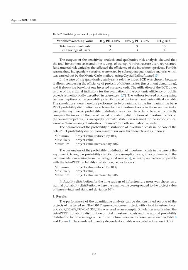
Appl. Sci. 2021, 11, 109

Table 7. Switching values of project efficiency.

Variable/Switching Value 0 ≤ PH < 10% 10% ≤ PH < 30% PH ≥ 30%

Total investment costs 3 3 13Time savings of users 2 3 14

The outputs of the sensitivity analysis and qualitative risk analysis showed thatthe total investment costs and time savings of transport infrastructure users representedfundamental risk variables that affected the efficiency of the investment projects. For thisreason, these independent variables were tested by subsequent quantitative analysis, whichwas carried out by the Monte Carlo method, using Crystal Ball software [15].

In the case of the quantitative analysis, a relative index BCR was chosen, becauseit allows comparing the efficiency of projects of different sizes (investment demanding),and it shows the benefit of one invested currency unit. The utilization of the BCR indexas one of the criterial indicators for the evaluation of the economic efficiency of publicprojects is methodically described in references [6,7]. The authors focused on comparingtwo assumptions of the probability distribution of the investment costs critical variable.The simulations were therefore performed in two variants, in the first variant the beta-PERT probability distribution was chosen for the investment costs, in the second variant atriangular asymmetric probability distribution was used. In order to be able to correctlycompare the impact of the use of partial probability distributions of investment costs onthe overall project results, an equally normal distribution was used for the second criticalvariable “time savings of infrastructure users” for both simulation variants.

The parameters of the probability distribution of investment costs in the case of thebeta-PERT probability distribution assumption were therefore chosen as follows:

Minimum project value reduced by 10%,Most likely project value,Maximum project value increased by 50%.

The parameters of the probability distribution of investment costs in the case of theasymmetric triangular probability distribution assumption were, in accordance with therecommendations arising from the background source [9], set with parameters comparablewith the beta-PERT probability distribution, i.e., as follows:

Minimum project value reduced by 10%,Most likely project value,Maximum project value increased by 50%.

Probability distribution for the time savings of infrastructure users was chosen as anormal probability distribution, where the mean value corresponded to the project valueof time savings and standard deviation 10%.

3. Results

The performance of the quantitative analysis can be demonstrated on one of theprojects of the tested set. The D10 Prague-Kosmonosy project, with a total investment costof CZK 9,272,678,497 (€361,367,050), was used as an example. Simulation results when thebeta-PERT probability distribution of total investment costs and the normal probabilitydistribution for time savings of the infrastructure users were chosen, are shown in Table 8and Figure 1. The simulated quantity dependent variable was cost-effectiveness (BCR).

145

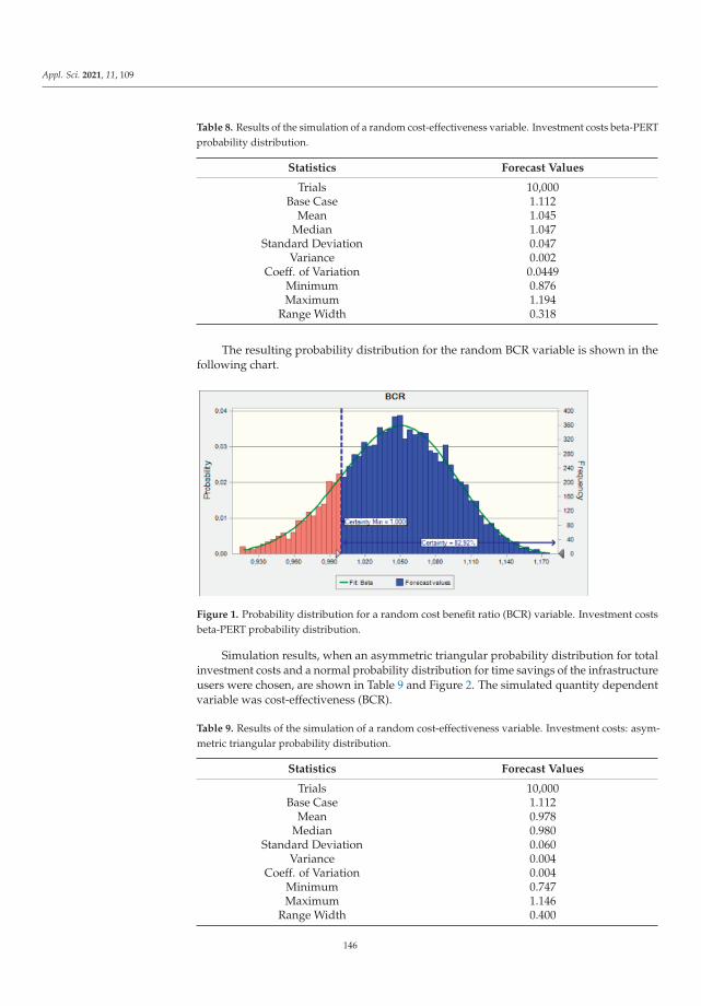
Appl. Sci. 2021, 11, 109

Table 8. Results of the simulation of a random cost-effectiveness variable. Investment costs beta-PERTprobability distribution.

Statistics Forecast Values

Trials 10,000Base Case 1.112

Mean 1.045Median 1.047

Standard Deviation 0.047Variance 0.002

Coeff. of Variation 0.0449Minimum 0.876Maximum 1.194

Range Width 0.318

The resulting probability distribution for the random BCR variable is shown in thefollowing chart.

Figure 1. Probability distribution for a random cost benefit ratio (BCR) variable. Investment costsbeta-PERT probability distribution.

Simulation results, when an asymmetric triangular probability distribution for totalinvestment costs and a normal probability distribution for time savings of the infrastructureusers were chosen, are shown in Table 9 and Figure 2. The simulated quantity dependentvariable was cost-effectiveness (BCR).

Table 9. Results of the simulation of a random cost-effectiveness variable. Investment costs: asym-metric triangular probability distribution.

Statistics Forecast Values

Trials 10,000Base Case 1.112

Mean 0.978Median 0.980

Standard Deviation 0.060Variance 0.004

Coeff. of Variation 0.004Minimum 0.747Maximum 1.146

Range Width 0.400

146

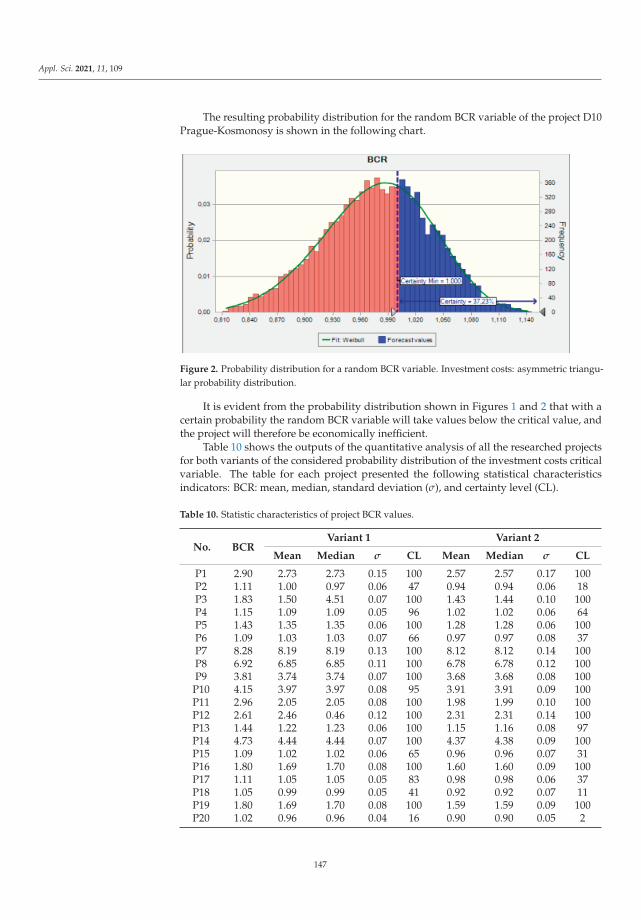
Appl. Sci. 2021, 11, 109

The resulting probability distribution for the random BCR variable of the project D10Prague-Kosmonosy is shown in the following chart.

Figure 2. Probability distribution for a random BCR variable. Investment costs: asymmetric triangu-lar probability distribution.

It is evident from the probability distribution shown in Figures 1 and 2 that with acertain probability the random BCR variable will take values below the critical value, andthe project will therefore be economically inefficient.

Table 10 shows the outputs of the quantitative analysis of all the researched projectsfor both variants of the considered probability distribution of the investment costs criticalvariable. The table for each project presented the following statistical characteristicsindicators: BCR: mean, median, standard deviation (σ), and certainty level (CL).

Table 10. Statistic characteristics of project BCR values.

No. BCRVariant 1 Variant 2

Mean Median σ CL Mean Median σ CL

P1 2.90 2.73 2.73 0.15 100 2.57 2.57 0.17 100P2 1.11 1.00 0.97 0.06 47 0.94 0.94 0.06 18P3 1.83 1.50 4.51 0.07 100 1.43 1.44 0.10 100P4 1.15 1.09 1.09 0.05 96 1.02 1.02 0.06 64P5 1.43 1.35 1.35 0.06 100 1.28 1.28 0.06 100P6 1.09 1.03 1.03 0.07 66 0.97 0.97 0.08 37P7 8.28 8.19 8.19 0.13 100 8.12 8.12 0.14 100P8 6.92 6.85 6.85 0.11 100 6.78 6.78 0.12 100P9 3.81 3.74 3.74 0.07 100 3.68 3.68 0.08 100

P10 4.15 3.97 3.97 0.08 95 3.91 3.91 0.09 100P11 2.96 2.05 2.05 0.08 100 1.98 1.99 0.10 100P12 2.61 2.46 0.46 0.12 100 2.31 2.31 0.14 100P13 1.44 1.22 1.23 0.06 100 1.15 1.16 0.08 97P14 4.73 4.44 4.44 0.07 100 4.37 4.38 0.09 100P15 1.09 1.02 1.02 0.06 65 0.96 0.96 0.07 31P16 1.80 1.69 1.70 0.08 100 1.60 1.60 0.09 100P17 1.11 1.05 1.05 0.05 83 0.98 0.98 0.06 37P18 1.05 0.99 0.99 0.05 41 0.92 0.92 0.07 11P19 1.80 1.69 1.70 0.08 100 1.59 1.59 0.09 100P20 1.02 0.96 0.96 0.04 16 0.90 0.90 0.05 2

147

Appl. Sci. 2021, 11, 109

The outputs of all projects showed a normal distribution of the BCR indicator. Theresearch in [11] came to the same results, where an experiment which was identified as apseudo-random number sequence as normally distributed was carried out.

In the interpretation of results it is necessary to respect certain limits connected withthe elaborated analysis. As mentioned above, in this paper is presented the case studyelaborated using projects being prepared for realization in the Czech Republic. Even if theoriginal methodical steps used in this paper are generally accepted and used, it is necessaryto respect certain national specificities in the evaluation of public investment projects. Thenext limit, which it is necessary to consider, is the definition of probability distributionsfor the simulation. In the presented analysis it was for the random variable “investmentcosts”, and the triangle and beta-PERT probability distributions were alternatively used,which is in harmony with the present state in the references, and opinions of other experts.However, it is not possible to exclude that the real probability distribution of investmentcosts of partial projects will be different. However, for the correct evaluation, and theidentification of the influence of the selected probability distribution on the results of theevaluated projects it was necessary to uniformly use the chosen probability distributions. Ina similar limitation, it is necessary to also note the probability distributions of the randomvariable “time savings of infrastructure users“. In this case it was uniformly selected forboth variants of the simulation normal probability distribution, even if the real probabilitydistribution of this variable can be, for partial projects, slightly different.

4. Discussion

It can be concluded from the above-stated calculations that one of the importantsettings of the input variables is their assumed probability distribution. From the avail-able literature research and the authors’ own expert opinion, it can be assumed that theinvestment costs variable tends to have a rather asymmetric probability distribution. Thiswas also confirmed by the CBA guide [6], which considers an asymmetric triangular proba-bility distribution in the range −5% to 20%. Makovšek [16], who dealt with a long-termanalysis of cost over-runs of road constructions in Slovenia, addressed this issue in detail.Two fundamental conclusions emerged from his analysis: the fact that cost over-runsare systematic (not randomly distributed around zero) and that cost over-runs appearconstantly over a time period of several decades and do not decrease (and thus do notshow signs of improved forecasting tools and methods). A conclusion can also be drawnfrom these deductions, that the probability distribution of investment costs tends to berather asymmetric.

An interesting comparison was published by Emhjellen [17], who dealt with the dif-ference of values when setting different limits of normal distribution and their effect onthe resulting values. Kumar [18] noted that the concessionaire aims to bear minimal cost,so maximum probability occurs at lower cost values, and hence it followed a lognormalprobability distribution. Jakiukevicius [19,20] worked with normal and triangular distribu-tions, for which he set theoretical parameters which he, based on simulations, convertedto log logistics parameters. Kumar [18] adhered to a lognormal distribution of projectcosts. Gorecki [21] used a triangular distribution. The Czech author Hnilica [22] workedwith the beta-PERT distribution, which he considered to be smoother, with possible valuesmore concentrated around the most probable value, and the probability decreases towardsthe limit values faster than linearly. The authors of this article believe that the beta-PERTdistribution best fits an expert estimate of the investment costs behaviour in comparingtheir values in the ex-ante and ex-post phases. The authors of this article carried out projectsimulations as mentioned above, assuming both a probability distribution of beta-PERT,and an asymmetric triangular one, and state that the results of the outputs in the expectedvalue of “BCR-mean” ranged up to 7% for all of the projects. The outputs of all projectsin both variants of solutions proved the normal distribution of the BCR indicator. Theauthors of the background research [4] reached the same results, where they stated that anexperiment which identifies a pseudo-random number sequence as normally distributed

148

Appl. Sci. 2021, 11, 109

was carried out. The reading of the frequency distribution of the evaluation indicatorprovides information of extreme importance, as regards the riskiness of the investmentproject [23].

5. Conclusions

It is clear from the above-stated findings that attention must be paid to the setting ofstatistical characteristics of variables which enter into the calculations of economic efficiencyindicators, and on the basis of which it is decided whether or not to accept projects forfinancing. At present, data on post-audits of major transport infrastructure projects arebeginning to be collected and analysed in the Czech Republic, and it is expected that theanalyses will make possible, among other things, reaching more precise assumptions.

Although the projects proved efficient, a combination of negative changes to bothvariables can already bring projects with a certain value of probability into negative results.Based on the analysis of the research sample, it is clear that it cannot be clearly establishedfor projects that a certain value of the BCR ratio predicts 100% stability of the projectunder the action of several critical variables. It is obvious from the mean value simulationsdetermining the expected BCR value that projects with BCR < 1.1 show, at a certainpercentage of probability, and at the critical variable limits specified above, that they shallnot be 100% effective. However, the variance of the results obtained was large. ProjectP10 also showed an interesting result; a relatively high mean BCR ratio showed with a 5%probability that it will not be effective.

The results of the research point to the fact that it is always necessary to performa quantitative analysis, since the results of the combination of the interaction of criticalvariables cannot be derived from the partial results of the sensitivity and qualitativeanalyses. The result will always depend on the absolute values of the critical variables ofeach unique project.

Author Contributions: Conceptualization. J.K. and V.H.; methodology. J.K. and V.H.; validation.J.K. and V.H.; formal analysis. J.K. and V.H.; investigation. J.K. and V.H.; resources. J.K. and V.H.;data curation. J.K. and V.H.; writing—original draft preparation. J.K. and V.H.; writing—review andediting. J.K. and V.H.; visualization. J.K.; supervision. J.K.; project administration. J.K.; fundingacquisition. J.K. Both authors have read and agreed to the published version of the manuscript.

Funding: This research was funded by project Brno University of Technology No. FAST-S-20-6383Selected Economic and Managerial Aspects in Construction Engineering.

Acknowledgments: This paper has been worked out under the project of Brno University of Tech-nology no. FAST-S-20-6383 Selected Economic and Managerial Aspects in Construction Engineering.

Conflicts of Interest: The authors declare no conflict of interest.

References

1. Demart, S.; Roy, B. The uses of cost-benefit analysis in public transportation decision-making in France. Transp. Policy 2009, 16,200–212. [CrossRef]

2. Hyard, A. Cost-benefit analysis according to Sen: An application in the evaluation of transport infrastructures in France. Transp.Res. Part A Policy Pract. 2012, 46, 707–719. [CrossRef]

3. Jones, H.; Moura, F.; Domingos, T. Transport Infrastructure Project Evaluation Using Cost-Benefit Analysis. Procedia Soc. Behav.Sci. 2014, 111, 400–409. [CrossRef]

4. Mackie, P.; Worsley, T.; Eliasson, J. Transport Appraisal Revisited. Res. Transp. Econ. 2014, 47, 3–18. [CrossRef]5. Korytárová, J.; Papežíková, P. Assessment of Large-Scale Projects Based on CBA. Procedia Comput. Sci. 2015, 64, 736–743.

[CrossRef]6. Sartori, D. Guide to Cost-benefit Analysis of Investment Projects. Economic appraisal tool for Cohesion Policy 2014–2020. In

Directorate-General for Regional and Urban Policy; European Commission: Brussels, Belgium, 2014; ISBN 978-92-79-34796-2.7. Ministry of Transport of the Czech Republic (MoT CZ). Departmental Guideline for the Evaluation of Economic Effectiveness of

Transport Construction Projects. 2017. Available online: https://www.sfdi.cz/soubory/obrazky-clanky/metodiky/2017_03_departmental-methodology-full.pdf (accessed on 25 August 2020).

8. Mokhtari, H.; Kiani, K.; Tahmasebpoor, S. Economic evaluation of investment projects under uncertainty: A probability theoryperspective. Sci. Iran. 2020, 27, 448–468. [CrossRef]

149

Appl. Sci. 2021, 11, 109

9. Liu, Y.; Ting-Hua, Y.; Cui-Qin, W. Investment decision support for engineering projects based on risk correlation analysis. Math.Probl. Eng. 2012, 2012. [CrossRef]

10. Marovic, I.; Androjic, I.; Jajac, N.; Hanák, T. Urban road infrastructure maintenance planning with application of neural networks.Complexity 2018. [CrossRef]

11. Nesticò, A.; He, S.; De Mare, G.; Benintendi, R.; Maselli, G. The ALARP Principle in the Cost-Benefit Analysis for the Acceptabilityof Investment Risk. Sustainability 2018, 10, 4668. [CrossRef]

12. Bilenko, D.; Lavrov, R.; Onyshchuk, N.; Poliakov, B.; Kabenok, Y. The Normal Distribution Formalization for Investment EconomicProject Evaluation Using the Monte Carlo Method. Montenegrin J. Econ. 2019, 15, 161–171. [CrossRef]

13. Acebes, F.; Pajares, J.; Galán, J.M.; López-Paredes, A. A new approach for project control under uncertainty. Going back to thebasics. Int. J. Proj. Manag. 2014, 32, 423–434. [CrossRef]

14. Bowers, J.; Khorakian, A. Integrating risk management in the innovation project. Eur. J. Innov. Manag. 2014, 17, 25–40. [CrossRef]15. Software Oracle Crystal Ball, Perpetual Licencs, 2020–2021. Available online: https://www.oracle.com/cz/applications/

crystalball/ (accessed on 25 August 2020).16. Makovšek, D. Systematic construction risk cost estimation mechanism and unit price movements. Transp. Policy 2014, 35, 135–145.

[CrossRef]17. Emhjellen, K.; Emhjellen, M.; Osmundsen, P. Investment cost estimates and investment decisions. Energy Policy 2002, 30, 91–96.

[CrossRef]18. Kumar, L.; Apurva, J.; Velaga, N.R. Financial risk assessment and modelling of PPP based Indian highway infrastructure projects.

Transp. Policy 2018, 62, 2–11. [CrossRef]19. Jasiukevicius, L.; Vasiliauskaite, A. Risk Assessment in Public Investment Projects: Impact of Empirically-grounded Methodology

on Measured Values of Intangible Obligations in Lithuania. Procedia Soc. Behav. Sci. 2015, 213, 370–375. [CrossRef]20. Jasiukevicius, L.; Vasiliauskaite, A. Cost Overrun Risk Assessment in the Public Investment Projects: An Empirically-Grounded

Research. Inz. Ekon. Eng. Econ. 2015, 26, 245–254. [CrossRef]21. Gorecki, J.; Diaz-Madronero, M. Who Risks and Wins?—Simulated Cost Variance in Sustainable Construction Projects.

Sustainability 2020, 12, 3370. [CrossRef]22. Hnilica, J.; Fotr, J. Aplikovaná Analýza Rizika ve Financním Management a Investicním Rozhodování; Grada Publishing: Prague,

Czech Republic, 2009; ISBN 978-80-247-2560-4.23. De Mare, G.; Nesticò, A.; Benintendi, R.; Maselli, G. ALARP approach for risk assessment of civil engineering projects. In Lecture

Notes in Computer Science (Including Subseries Lecture Notes in Artificial Intelligence and Lecture Notes in Bioinformatics); Springer:Berlin/Heidelberg, Germany, 2018; pp. 75–86, ISBN 978-3-319-95174-4. [CrossRef]

150

applied sciences

Article

New Aspects of Socioeconomic Assessment of theRailway Infrastructure Project Life Cycle

Vít Hromádka *, Jana Korytárová, Eva Vítková, Herbert Seelmann and Tomáš Funk

Faculty of Civil Engineering, Brno University of Technology, 602 00 Brno, Czech Republic;korytarova.j@fce.vutbr.cz (J.K.); vitkova.e@fce.vutbr.cz (E.V.); seelmann.h@fce.vutbr.cz (H.S.);tomas.funk@email.cz (T.F.)* Correspondence: hromadka.v@fce.vutbr.cz; Tel.: +420-541-148-641

Received: 25 September 2020; Accepted: 19 October 2020; Published: 21 October 2020

Featured Application: The results of the presented research will become part of the methodological

material for the economic analysis of railway infrastructure projects after the completion of a broader

research task.

Abstract: The paper deals with the issue of evaluation of socioeconomic impacts of occurrencesemerging from railway infrastructure. The presented research results form part of a broader researchsubject focusing on the evaluation of the socioeconomic benefits of projects for the implementationof measures aimed at increasing the safety and reliability of railway infrastructure. The researchtopic addresses a part of the evaluation of railway infrastructure project efficiency within its lifecycle using the cost–benefit analysis method. The methodology is based on the description anddefinition of input variables that are essential for the process of evaluating socioeconomic impacts.It is followed by another important step, which is the analysis of the categories and the number ofoccurrences, separately, for regional and national lines, and, further, the data is sorted according towhether occurrences emerge at stations or on a wide line. The result of the presented research isan overview of the calculated values of the expected socioeconomic impacts of partial occurrencesaccording to the categories related to the year of operation on the railway infrastructure and the unitof measure. The research team carried out an inquiry into the annual impacts of the subcategoriesof occurrences related to one railway station and one kilometer of wide line, e.g., for national lines,the impacts of €2922.72/station/year and €41.67/km of wide line/year were determined. The results ofthe presented research represent important and necessary inputs for the next phase of the researchtopic, i.e., the evaluation of the socioeconomic benefits of projects increasing the safety and reliabilityof railway infrastructure.

Keywords: railway infrastructure; occurrences; socioeconomic impact; economic evaluation; CBA;life cycle

1. Introduction

The research, the results of which are presented in the paper, is focused on the issue of thesocioeconomic evaluation of projects in the field of transport, especially railway infrastructure.The issue of the economic evaluation of public projects is very broad; however, the basic principleshave been known for many years. Unlike commercial projects, where profit or profit-derived cash-flowplays a key role in the economic evaluation, the evaluation of public projects is usually based on theuse of cost–output methods. The most important and widely used method is the cost–benefit analysis(CBA). CBA is thoroughly described in a number of guidelines and publications (e.g., [1]). In the caseof transport infrastructure projects, there is a detailed methodological guide for its elaboration [2].However, none of these documents are detailed enough to include methodologies for evaluating all

Appl. Sci. 2020, 10, 7355; doi:10.3390/app10207355 www.mdpi.com/journal/applsci151

Appl. Sci. 2020, 10, 7355

relevant costs and benefits that arise in connection with transport (and especially railway) infrastructure.The paper presents the results of applied research aimed at incorporating the benefits associated withincreasing the safety and reliability of railway infrastructure as a result of the implementation ofprojects for the installation of new and improved security equipment. The importance of researchlies mainly in the fact that, currently, the benefits associated with increasing the safety and reliabilityof railways are not incorporated into the socioeconomic evaluation carried out in accordance withthe methodology (in the case of the Czech Republic, it is departmental methodology [2]) using CBA,although it is clear that these benefits arise from railway infrastructure project implementation. As aresult, railway infrastructure projects show worse results in economic efficiency evaluation and seemto be less economically efficient. The presented paper focuses on the evaluation of the socioeconomicimpacts of occurrences that emerge from railway infrastructure. The aim of the paper is to methodicallydescribe and verify the procedure for determining the socioeconomic impacts of occurrences thatemerge from railway infrastructure in a case study. The Database of Occurrences [3], which containsdetailed information on occurrences emerging from the railway in the Czech Republic, managed byemployees of the Railway Administration, was used for the purposes of analysis and subsequentsynthesis of the obtained data into methodological steps. Occurrences from the 2011–2018 period wereused for the purposes of the research. The output of the research presented in the article is to determinethe values of the expected annual socioeconomic impacts of occurrences according to the categoriesrelated to railway stations or one kilometer of the track segment. The outputs of the presentedresearch will be used in follow-up research for the purpose of determining potential savings on railwayinfrastructure arising from the reduction of the number of occurrences, characterized by their potentialsocioeconomic impact. The reduction in the number of occurrences will be achieved by implementingappropriate security measures. Their economic efficiency shall be assessed by these steps.

2. Materials and Methods

The subject of the paper is the analysis and subsequent synthesis of relevant data in order to identifythe methodology for evaluating the socioeconomic impacts of occurrences emerging from railwayinfrastructure. The purpose of the evaluation of these socioeconomic impacts is their subsequent usein the analysis of project costs and benefits in the field of transport infrastructure. This article, from ageneral point of view, can be included in the issue of socioeconomic evaluation of public investmentprojects in the field of transport infrastructure. The principles and procedures applied in the processof cost–benefit analysis are methodically described in the Guide to CBA of Investment Projects [1],where the general rules are defined and the specifics for the process of CBA for individual types ofpublic projects are described. The issue of public projects in the field of transport infrastructure is dealtwith in detail by the Departmental Guideline of the Ministry of Transport of the Czech Republic [2],which addresses the economic evaluation of transport infrastructure projects, both in general and witha focus on individual modes of transport, i.e., projects of roads and highways, projects of railwayline construction and projects in the field of transport-important waterways. The abovementionedmethodology provides some procedures for evaluating the socioeconomic impacts of transport projects(e.g., user savings, transport time savings, traffic accident savings, or impact on externalities). However,some key impacts, such as the impact on transport network safety and reliability, dealt with in theresearch presented here, are not addressed in more detail in the methodology. One of the aims ofthe paper is to explore the possibilities for supplementing the methodology for the socioeconomicevaluation of investment projects in the field of railway infrastructure by assessing its impact on thesafety and reliability of railway infrastructure.

Based on research into the available scientific literature, it has not been found that any of thescientific teams were directly involved in assessing the impacts associated with increasing the safety ofrailway infrastructure. However, the research included texts dealing with the issue of occurrencesemerging from railway infrastructure and their causes, as well as technical impacts (material damage,train delays). The basic input task was the identification of occurrences emerging from railway

152

Appl. Sci. 2020, 10, 7355

infrastructure, their impact, prevention, and classification. Santos-Reyes [4] dealt with a generalanalysis of the occurrence of traffic accidents on the railway [4] and presented basic study points to beaddressed in order to subsequently prevent occurrences from railway infrastructure. The methodologydeveloped within the Dnipro National University of Railways [5] presented the definition of thecategories of occurrences from railway infrastructure in relation to the amount of material damagecaused. Occurrences were classified according to the severity of the consequences, which wereexpressed in physical quantities. The paper provides an overview of financial losses associated withsubcategories of occurrences, which represent a suitable data set for its comparison with the partialoutputs of the presented results.

Klockner and Toft dealt with the modeling of occurrences on the railway in their study [6].A second significant part of the publication deals with the factors influencing the occurrence emergencefrom railway infrastructure. In their study, Iridiastadi and Ikatrinasari [7] presented a classificationsystem, including subfactors, with the potential to influence the occurrence emergence. Zhou and Leialso addressed the causes of occurrences on the railway in their article [8]. In their paper, Baysari et al. [9]presented a detailed analysis of errors leading to railway occurrences. Their work was based on a setof forty reports on the investigation of occurrences in railway infrastructure in Australia. The studyconcluded that up to half of the occurrences were caused by equipment failure due to insufficientmaintenance. The conclusions of the paper [9] are important in relation to the presented researchresults. The subject of a detailed examination within the presented research is mainly occurrencesemerging as a result of human factor failure, not due to a technical defect. Consequently, the nextscientific papers also directly focus on the influence of the human factor on occurrence emergencefrom railway infrastructure. The paper by Hani Tabai et al. [10], which focused on the evaluationof the relationship between engine driver demography, cognitive performance, and the risk of anoccurrence emergence, where the need to pay continuous attention had been identified as one of themost important reasons for an occurrence emergence due to an engine driver’s error, can serve as oneof the examples. The study of Zhan [11] elicits a qualitative and quantitative analysis method to detectthe human- and organization-related causes of railway accidents. The HFACS-RAs framework, basedon the incident and accident data of the railway industry, is proposed in this study. Evans [12], in hispaper, dealt with the influence of the speed of trains on railway infrastructure and the number andseverity of occurrences and extended his own previous statistics by the influence of train speed on theseverity of the occurrences. This represents an important aspect of occurrences emerging from railwayinfrastructure; however, this dimension was not considered within the presented research.

An important (albeit rather marginal) issue within the presented research is the causes ofoccurrences emerging at railway crossings [13] and as a result of suicides [14,15]. These are veryimportant occurrences emerging from all railway infrastructure, which represent a significant partof occurrences recorded in the database used. However, they are not considered in more detail inthe analysis presented in this paper. Occurrences emerging at railway crossings are the subject ofa separate methodology, according to which they are further assessed, so the development of thismethodology is not the subject of the presented research either. Occurrences emerging as a result ofsuicides represent types of occurrences that cannot be effectively prevented by the implementation ofappropriate measures and, therefore, also do not fall within the scope of the research.

The last important area relevant to the scope of the presented paper is the issue of occurrenceprevention in railway infrastructure. Kim et al., in their article [16], presented results of a factualanalysis of the railway occurrence rate and subsequently proposed preventive care systems focusedmainly on the development of a training program for railway safety and railway safety training centers.Edkins and Pollock addressed the issue of the analysis of occurrences in railway infrastructure andthe subsequent proposal of preventive measures aimed at reducing the number of occurrences [17].It comprised a retrospective analysis of 112 railway occurrences in Australia, which revealed a tendencyto human error and subsequently led to the development of a railway safety checklist. Evans presentedan overview of the development of statistics on rail occurrences in Europe and a proposal for preventive

153

Appl. Sci. 2020, 10, 7355

measures to reduce the number of occurrences [18]. Authors Cheng and Tsai dealt, in their article [19],with the issue of competencies in the case of occurrence management and the restoration of normaloperations after the occurrence emergence and its resolution. The abovementioned research revealsfindings explaining the emergence of occurrences and the possibilities for reducing their number,which corresponds to the findings of the research team on the Czech conditions. The conclusions ofthe research confirm the topicality of the issue. The presented research builds on these basic buildingblocks and proceeds to the further step, i.e., the quantification of impacts from the socioeconomic pointof view. These are very important and inspiring findings that explain the emergence of occurrencesand the possibilities for reducing their number. The conclusions of the articles confirm the need toaddress the issue of occurrences and to identify and quantify their impacts.

The authors of the article, following the above-listed research of foreign resources, use othersurveys and analyses based on the issues in the national environment and focus on the usability oftechnical data for socioeconomic analysis (evaluation of economic efficiency), which can be used as abasis for the decision-making process in investment projects for the security devices. The main goalof the research is to develop and present methodological steps for the evaluation of socioeconomicimpacts of occurrences emerging from railway infrastructure and to verify the methodology on theoccurrences emerging from railway infrastructure in the Czech Republic. The main result of the appliedresearch presented in this paper is the determination of the value of the annual socioeconomic impactof occurrences emerging from railway infrastructure in the Czech Republic per one kilometer of thetrack segment and one railway station, divided into both national and regional lines.

2.1. Data

The basic background for the research of the issue dealt with is the creation of a database ofoccurrences in the researched region/national economy/territorial unit. The Database of Occurrences,managed by the employees of the Railway Administration of the Czech Republic, is the key source ofdata for the creation of the methodology and the elaboration of the case study, where all occurrencesarising in railway infrastructure of the Czech Republic in the 2009–2018 period were registered [3].The Database of Occurrences is not a publicly accessible source of information; the database wasprovided to the research team by the Railway Administration of the Czech Republic, upon request,exclusively for the purpose of conducting the presented research. This represents a very large documentthat contains more than 500,000 items of information.

2.2. Methods

The proposed methodology is based on the collection, analysis, and use of relevant data to evaluatethe societal benefits arising from the establishment of security measures. The outputs are bound forthe later use of the “opportunity cost” valuation approach.

The subject of the paper is to develop and present a methodology for the quantification andevaluation of the socioeconomic impacts of occurrences emerging from railway infrastructure, dividedinto relevant subcategories, following the scientific literature research and basic principles of economicanalysis of public investment projects.

Development of the methodology for the evaluation of the socioeconomic impacts of occurrencesemerging from railway infrastructure consists of the following steps:

• Analyzing the Database of Occurrences, defining the categories, and selecting the data forfurther use.

• Defining the key characteristics of occurrences, including health and delay impacts on passengerand freight trains and their economic evaluation.

• Determining the expected impact of occurrences by category.

154

Appl. Sci. 2020, 10, 7355

The calculation of the amount of the expected socioeconomic impacts of occurrences by thecategories of per kilometer of railway line and station is performed in Section 3. The partial steps aredescribed in detail in the following sections.

2.2.1. Analysing the Database of Occurrences, Defining the Categories, and Selecting the Data forFurther Use

Occurrences emerging within the railway infrastructure can be classified into three basic groups:

• A—Serious accidents (A1–A4),• B—Accidents (B1–B10),• C—Incidents (C1–C21).

Subcategories of occurrences were defined within the mentioned groups of occurrences, whichdiffer mainly in the causes of the occurrences and their impacts. For the purposes of the presentedresearch, the following variables, which are relevant to the methodological procedure, were selectedfrom the Database of Occurrences:

• Impact on health,

� Death,� Serious injury,� Minor injury,

• Material damage,• Costs,• Number of delayed passenger trains,• Total delay of passenger trains,• Number of delayed freight trains,• Total delay of freight trains, and• The cause of the occurrence,

� Technical,� Human factor,� Others.

These variables are listed in the Database of Occurrences for each specific occurrence.The Database of Occurrences [3] could not be used for further research purposes in its original

version without modifications as the recorded variables were developed year-on-year and the datastructure was not consistent. The researchers, therefore, made the necessary adjustments for thepurposes of its further use. The analysis of the Database of Occurrences was elaborated in orderto address the research question of the average, minimum, and maximum annual impact values(number of occurrences, deaths, number of serious/minor injuries, material damage, and costs) ofoccurrences, with their possible deviation, which was monitored based on the standard deviation.It was subsequently decided, following the results of the analysis, that the follow-up research wouldnot include occurrences due to suicides and those emerging at railway crossings. Detailed results ofthe above-defined analysis of the Database of Occurrences and conclusions and recommendationsresulting from the analysis were published in [20].

2.2.2. Defining the Key Characteristics of Occurrences and Their Economic Evaluation

The research team defined the information and characteristics of partial occurrences within theDatabase of Occurrences that provided data on the partial socioeconomic impacts of the occurrenceson society. An overview of this information and characteristics is presented in the previous section.

155

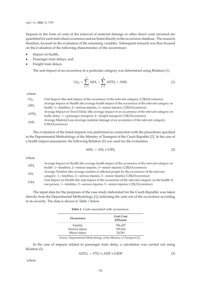
Appl. Sci. 2020, 10, 7355

Impacts in the form of costs of the removal of material damage or other direct costs incurred arequantified for each individual occurrence and are listed directly in the occurrence database. The research,therefore, focused on the evaluation of the remaining variables. Subsequent research was thus focusedon the evaluation of the following characteristics of the occurrences:

• Impact on health,• Passenger train delays, and• Freight train delays.

The unit impact of an occurrence in a particular category was determined using Relation (1).

UIO =3∑

i=1

AIHi +2∑

j=1

AITDj + AML (1)

where

UIO Unit Impact (the unit impact of the occurrence of the relevant category; CZK/Occurrence)

AIHiAverage Impact on Health (the average health impact of the occurrence of the relevant category onhealth: 1—fatalities, 2—serious injuries, 3—minor injuries; CZK/Occurrence)

AITDjAverage Impact on Travel Delay (the average impact of an occurrence of the relevant category ontraffic delay: 1—passenger transport, 2—freight transport; CZK/Occurrence)

AMLAverage Material Loss (average material damage of an occurrence of the relevant category;CZK/Occurrence)

The evaluation of the listed impacts was performed in connection with the procedures specifiedin the Departmental Methodology of the Ministry of Transport of the Czech Republic [2]. In the case ofa health impact assessment, the following Relation (2) was used for the evaluation.

AIHi = AHi ×UIHi (2)

where

AIHiAverage Impact on Health (the average health impact of the occurrence of the relevant category onhealth: 1—fatalities, 2—serious injuries, 3—minor injuries; CZK/Occurrence)

AHiAverage Number (the average number of affected people by the occurrence of the relevantcategory: 1—fatalities, 2—serious injuries, 3—minor injuries; CZK/Occurrence)

UIHiUnit Impact on Health (the unit impact of the occurrence of the relevant category on the health ofone person, 1—fatalities, 2—serious injuries, 3—minor injuries; CZK/Occurrence)

The input data for the purposes of the case study elaborated for the Czech Republic was takendirectly from the Departmental Methodology [2], indicating the unit cost of the occurrence accordingto its severity. The data is shown in Table 1 below.

Table 1. Costs associated with occurrences.

OccurrenceUnit Cost€/Person

Fatality 786,457Serious injury 190,414Minor injury 24,581

Source: Departmental Methodology of the Ministry of Transport [2].

In the case of impacts related to passenger train delay, a calculation was carried out usingRelation (3).

AITD1 = PTU×ADP×UIDP (3)

where

156

Appl. Sci. 2020, 10, 7355

PTU Personal Train Utilization (average passenger train occupancy; Persons/Train)

ADPAverage Delay of Personal Trains (the average total delay of passenger trains due to the occurrenceof the relevant category; Train*Hour/Occurrence)

UIDP Unit Impact of Personal Train Delay (unit cost of passenger time; CZK/Hour*Person)

The data presented in the Departmental Methodology [2] and statistical data from the StatisticalYearbook of the Czech Railways Group [21] were used for the purposes of the case study performedfor the Czech Republic. Based on these sources, the expected occupancy of one passenger train wasdetermined at 66.55 people/train and the average value of passenger time at 10.63 €/person-hour.

In the case of the evaluation of the impacts associated with the delay of freight trains, the followingRelation (4) was used for the calculation:

AITD2 = CTU×ADC×UIDC (4)

where

CTU Cargo Train Utilization (average freight weight of a freight train; Tons/Train)

ADCAverage Delay of Cargo Trains (the average total delay of freight trains due to an occurrence of arelevant category; Trains*Hour/Occurrence)

UIDC Unit Impact of Cargo Train Delay (unit time cost of transported cargo; CZK/Hour)

The average freight weight of a freight train was determined at 455 t/train using statistical data [21]as part of a case study elaborated for the territory of the Czech Republic. The average value of freighttransport time was subsequently determined at 0.23 €/ton using the values of freight transport timeaccording to commodities taken from the Departmental Methodology [2] and the percentage rate ofindividual commodities in freight transport.

The values of the input quantities used for the calculation of Relations (1)–(4) within the casestudy were taken from the national sources of the Czech Republic. These sources were used in the formof official methodological documents for the socioeconomic evaluation of public projects and are basedon long-term statistical data. The key methodological basis was the Departmental Methodology of theMinistry of Transport, which defines some input variables (e.g., unit impacts on health or unit cost ofpassenger time or cargo). The already mentioned occurrence database or statistical yearbooks of carriersor the administrator of railway infrastructure fall within the documents containing statistical data.

The quantities UIHi (Unit Impact on Health), UIDP (Unit Impact of Personal Train Delay),and UIDC (Unit Impact of Cargo Train Delay) were taken from the Departmental Guideline [2] forthe purposes of the presented research. The quantities AML (Average Material Loss), AHi (AverageNumber), ADP (Average Delay of Personal Trains), and ADC (Average Delay of Cargo Trains)were determined using data recorded in the Database of Occurrences [18], and PTU (Personal TrainUtilization) and CTU (Cargo Train Utilization) values were derived from statistical data presented inthe Statistical Yearbook of Czech Railways [21].

A detailed calculation of these unit impacts of railway occurrences in railway infrastructure,including a case study to verify the functionality of the evaluation algorithm, is provided in [22].

2.2.3. Determining the Expected Impact of Occurrences by Category

Only those occurrences that emerged due to human error were considered for the calculation ofthe average impacts of occurrences following the conclusions of [22]. The categories of occurrenceslisted in Table 2 are, therefore, considered for the current research.

157

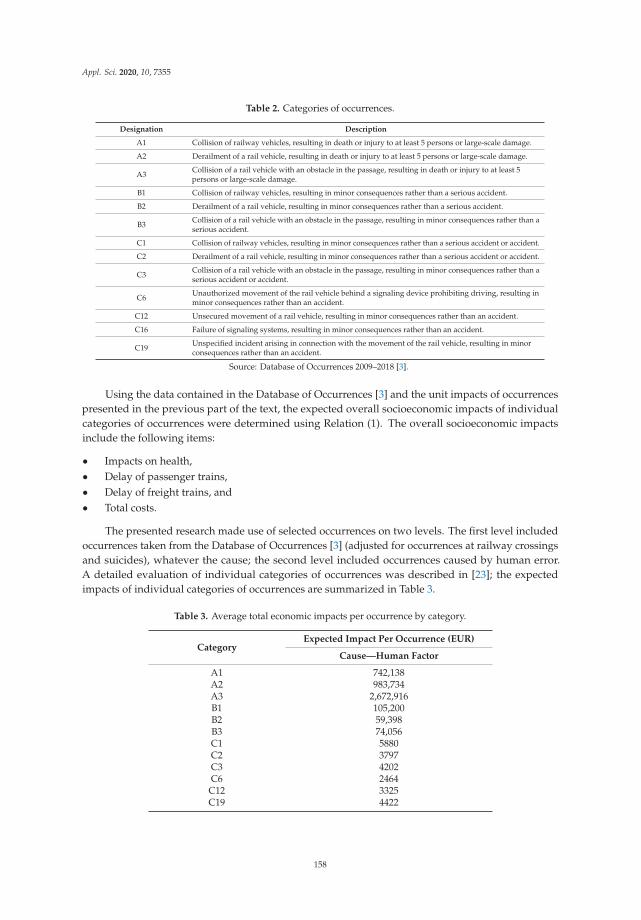
Appl. Sci. 2020, 10, 7355

Table 2. Categories of occurrences.

Designation Description

A1 Collision of railway vehicles, resulting in death or injury to at least 5 persons or large-scale damage.

A2 Derailment of a rail vehicle, resulting in death or injury to at least 5 persons or large-scale damage.

A3 Collision of a rail vehicle with an obstacle in the passage, resulting in death or injury to at least 5persons or large-scale damage.

B1 Collision of railway vehicles, resulting in minor consequences rather than a serious accident.

B2 Derailment of a rail vehicle, resulting in minor consequences rather than a serious accident.

B3 Collision of a rail vehicle with an obstacle in the passage, resulting in minor consequences rather than aserious accident.

C1 Collision of railway vehicles, resulting in minor consequences rather than a serious accident or accident.

C2 Derailment of a rail vehicle, resulting in minor consequences rather than a serious accident or accident.

C3 Collision of a rail vehicle with an obstacle in the passage, resulting in minor consequences rather than aserious accident or accident.

C6 Unauthorized movement of the rail vehicle behind a signaling device prohibiting driving, resulting inminor consequences rather than an accident.

C12 Unsecured movement of a rail vehicle, resulting in minor consequences rather than an accident.

C16 Failure of signaling systems, resulting in minor consequences rather than an accident.

C19 Unspecified incident arising in connection with the movement of the rail vehicle, resulting in minorconsequences rather than an accident.

Source: Database of Occurrences 2009–2018 [3].

Using the data contained in the Database of Occurrences [3] and the unit impacts of occurrencespresented in the previous part of the text, the expected overall socioeconomic impacts of individualcategories of occurrences were determined using Relation (1). The overall socioeconomic impactsinclude the following items:

• Impacts on health,• Delay of passenger trains,• Delay of freight trains, and• Total costs.

The presented research made use of selected occurrences on two levels. The first level includedoccurrences taken from the Database of Occurrences [3] (adjusted for occurrences at railway crossingsand suicides), whatever the cause; the second level included occurrences caused by human error.A detailed evaluation of individual categories of occurrences was described in [23]; the expectedimpacts of individual categories of occurrences are summarized in Table 3.

Table 3. Average total economic impacts per occurrence by category.

CategoryExpected Impact Per Occurrence (EUR)

Cause—Human Factor

A1 742,138A2 983,734A3 2,672,916B1 105,200B2 59,398B3 74,056C1 5880C2 3797C3 4202C6 2464

C12 3325C19 4422

158

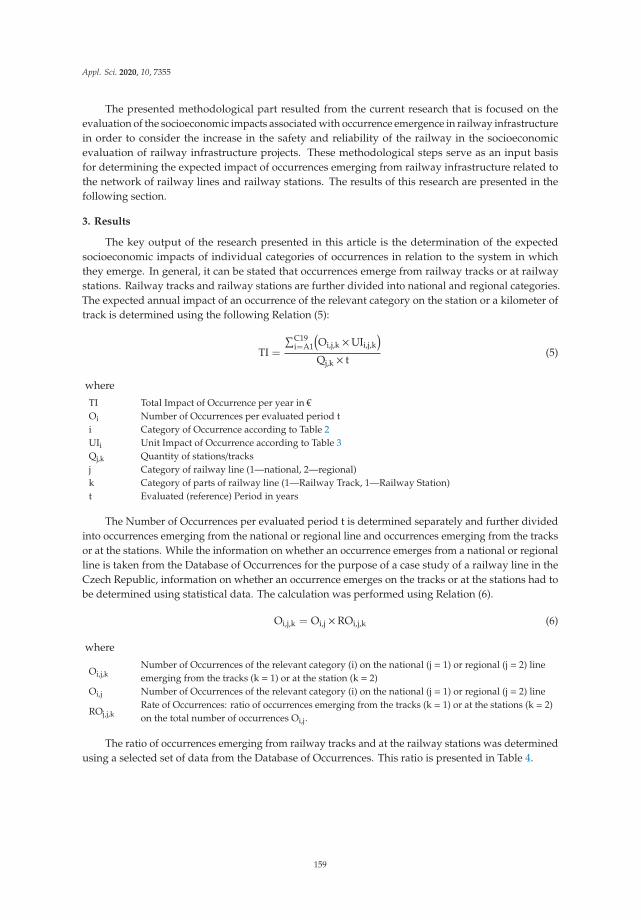
Appl. Sci. 2020, 10, 7355

The presented methodological part resulted from the current research that is focused on theevaluation of the socioeconomic impacts associated with occurrence emergence in railway infrastructurein order to consider the increase in the safety and reliability of the railway in the socioeconomicevaluation of railway infrastructure projects. These methodological steps serve as an input basisfor determining the expected impact of occurrences emerging from railway infrastructure related tothe network of railway lines and railway stations. The results of this research are presented in thefollowing section.

3. Results

The key output of the research presented in this article is the determination of the expectedsocioeconomic impacts of individual categories of occurrences in relation to the system in whichthey emerge. In general, it can be stated that occurrences emerge from railway tracks or at railwaystations. Railway tracks and railway stations are further divided into national and regional categories.The expected annual impact of an occurrence of the relevant category on the station or a kilometer oftrack is determined using the following Relation (5):

TI =

∑C19i=A1

(Oi,j,k ×UIi,j,k

)Qj,k × t

(5)

where

TI Total Impact of Occurrence per year in €Oi Number of Occurrences per evaluated period ti Category of Occurrence according to Table 2UIi Unit Impact of Occurrence according to Table 3Qj,k Quantity of stations/tracksj Category of railway line (1—national, 2—regional)k Category of parts of railway line (1—Railway Track, 1—Railway Station)t Evaluated (reference) Period in years

The Number of Occurrences per evaluated period t is determined separately and further dividedinto occurrences emerging from the national or regional line and occurrences emerging from the tracksor at the stations. While the information on whether an occurrence emerges from a national or regionalline is taken from the Database of Occurrences for the purpose of a case study of a railway line in theCzech Republic, information on whether an occurrence emerges on the tracks or at the stations had tobe determined using statistical data. The calculation was performed using Relation (6).

Oi,j,k = Oi,j ×ROi,j,k (6)

where

Oi,j,kNumber of Occurrences of the relevant category (i) on the national (j = 1) or regional (j = 2) lineemerging from the tracks (k = 1) or at the station (k = 2)

Oi,j Number of Occurrences of the relevant category (i) on the national (j = 1) or regional (j = 2) line

ROj,j,kRate of Occurrences: ratio of occurrences emerging from the tracks (k = 1) or at the stations (k = 2)on the total number of occurrences Oi,j.

The ratio of occurrences emerging from railway tracks and at the railway stations was determinedusing a selected set of data from the Database of Occurrences. This ratio is presented in Table 4.

159

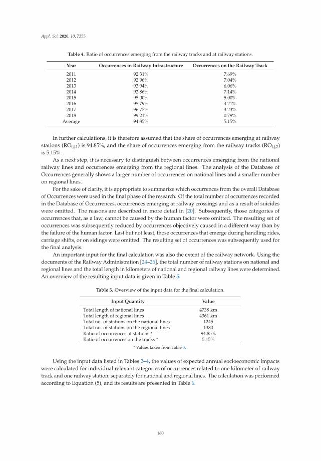
Appl. Sci. 2020, 10, 7355

Table 4. Ratio of occurrences emerging from the railway tracks and at railway stations.

Year Occurrences in Railway Infrastructure Occurrences on the Railway Track

2011 92.31% 7.69%2012 92.96% 7.04%2013 93.94% 6.06%2014 92.86% 7.14%2015 95.00% 5.00%2016 95.79% 4.21%2017 96.77% 3.23%2018 99.21% 0.79%

Average 94.85% 5.15%

In further calculations, it is therefore assumed that the share of occurrences emerging at railwaystations (ROi,j,1) is 94.85%, and the share of occurrences emerging from the railway tracks (ROi,j,2)is 5.15%.

As a next step, it is necessary to distinguish between occurrences emerging from the nationalrailway lines and occurrences emerging from the regional lines. The analysis of the Database ofOccurrences generally shows a larger number of occurrences on national lines and a smaller numberon regional lines.

For the sake of clarity, it is appropriate to summarize which occurrences from the overall Databaseof Occurrences were used in the final phase of the research. Of the total number of occurrences recordedin the Database of Occurrences, occurrences emerging at railway crossings and as a result of suicideswere omitted. The reasons are described in more detail in [20]. Subsequently, those categories ofoccurrences that, as a law, cannot be caused by the human factor were omitted. The resulting set ofoccurrences was subsequently reduced by occurrences objectively caused in a different way than bythe failure of the human factor. Last but not least, those occurrences that emerge during handling rides,carriage shifts, or on sidings were omitted. The resulting set of occurrences was subsequently used forthe final analysis.

An important input for the final calculation was also the extent of the railway network. Using thedocuments of the Railway Administration [24–26], the total number of railway stations on national andregional lines and the total length in kilometers of national and regional railway lines were determined.An overview of the resulting input data is given in Table 5.

Table 5. Overview of the input data for the final calculation.

Input Quantity Value

Total length of national lines 4738 kmTotal length of regional lines 4361 kmTotal no. of stations on the national lines 1245Total no. of stations on the regional lines 1380Ratio of occurrences at stations * 94.85%Ratio of occurrences on the tracks * 5.15%

* Values taken from Table 3.

Using the input data listed in Tables 2–4, the values of expected annual socioeconomic impactswere calculated for individual relevant categories of occurrences related to one kilometer of railwaytrack and one railway station, separately for national and regional lines. The calculation was performedaccording to Equation (5), and its results are presented in Table 6.

160

Appl. Sci. 2020, 10, 7355

Ta

ble

6.

Cal

cula

tion

ofth

eex

pect

edan

nual

impa

ctof

subc

ateg

orie

sof

occu

rren

ces

per

stat

ion

and

per

kmof

trac

k.

Occ

urr

en

ceC

ate

go

ryN

ati

on

al/

Re

gio

na

lT

ota

lN

um

be

ro

fO

ccu

rre

nce

s2

01

1–

20

18

Nu

mb

er

of

Occ

urr

en

ces

Sta

tio

nN

um

be

ro

fO

ccu

rre

nce

sT

rack

Un

itIm

pa

cto

fO

ccu

rre

nce

in€

Ex

pe

cte

dA

nn

ua

lIm

pa

ctin€

Pe

rS

tati

on

Ex

pe

cte

dA

nn

ua

lIm

pa

ctin€

Pe

rk

mo

fT

rack

A1

nati

onal

1211

.38

0.62

757,

756.

4786

5.98

12.3

5re

gion

al2

1.90

0.10

757,

756.

4713

0.21

2.24

A2

nati

onal

32.

850.

151,

004,

436.

3628

6.97

4.09

regi

onal

10.

950.

051,

004,

436.

3686

.30

1.48

A3

nati

onal

21.

900.

102,

729,

166.

4551

9.82

7.41

regi

onal

00.

000.

002,

729,

166.

450.

000.

00B1

nati

onal

3735

.10

1.90

107,

414.

1737

8.49

5.40

regi

onal

76.

640.

3610

7,41

4.17

64.6

01.

11B2

nati

onal

3432

.25

1.75

60,6

47.5

719

6.38

2.80

regi

onal

76.

640.

3660

,647

.57

36.4

80.

63B3

nati

onal

1413

.28

0.72

75,6

14.3

710

0.82

1.44

regi

onal

32.

850.

1575

,614

.37

19.4

90.

33C

1na

tion

al75

71.1

43.

8660

03.7

342

.88

0.61

regi

onal

43.

790.

2160

03.7

32.

060.

04C

2na

tion

al39

537

4.67

20.3

338

77.3

914

5.86

2.08

regi

onal

8277

.78

4.22

3877

.39

27.3

20.

47C

3na

tion

al25

424

0.93

13.0

742

90.5

310

3.79

1.48

regi

onal

8075

.88

4.12

4290

.53

29.4

90.

51C

6na

tion

al63

760

4.22

32.7

825

16.1

315

2.64

2.18

regi

onal

8681

.57

4.43

2516

.13

18.5

90.

32C

12na

tion

al10

498

.65

5.35

3394

.95

33.6

30.

48re

gion

al37

35.1

01.

9033

94.9

510

.79

0.19

C19

nati

onal

222

210.

5811

.42

4515

.41

95.4

71.

36re

gion

al14

13.2

80.

7245

15.4

16.

020.

09

161

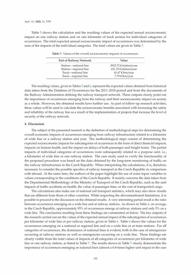
Appl. Sci. 2020, 10, 7355

Table 5 shows the calculation and the resulting values of the expected annual socioeconomicimpact on one railway station and on one kilometer of track section for individual categories ofoccurrences. The total expected annual socioeconomic impact of occurrences was determined by thesum of the impacts of the individual categories. The total values are given in Table 7.

Table 7. Values of the overall socioeconomic impacts of occurrences.

Part of Railway Network Value

Station—national line 2922.72 €/station/yearStation—regional line 431.35 €/station/yearTrack—national line 41.67 €/km/yearTrack—regional line 7.39 €/km/year

The resulting values, given in Tables 5 and 6, represent the expected values obtained from historicaldata taken from the Database of Occurrences for the 2011–2018 period and from the documents ofthe Railway Administration defining the railway transport network. These outputs clearly point outthe importance of occurrences emerging from the railway and their socioeconomic impact on societyas a whole. However, the obtained results have further use. As part of follow-up research activities,these values will be used to calculate the socioeconomic benefits associated with increasing the safetyand reliability of the railway line as a result of the implementation of projects that increase the level ofsecurity of the railway network.

4. Discussion

The subject of the presented research is the definition of methodological steps for determining theoverall economic impacts of occurrences emerging from railway infrastructure related to a kilometerof wide line or a railway station and year. The methodological steps consist of determining theexpected socioeconomic impacts for subcategories of occurrences in the form of direct financial impacts,impacts on human health, and the impact on delays of both passenger and freight trains. The partialimpacts of individual categories of occurrences were subsequently related to a purpose unit, i.e.,a kilometer of wide line or one railway station. The case study used to verify the functionality ofthe proposed procedure was based on the data obtained by the long-term monitoring of traffic onthe railway infrastructure in the Czech Republic. When interpreting the calculations, it is, therefore,necessary to consider the possible specifics of railway transport in the Czech Republic in comparisonwith abroad. At the same time, the authors of the paper highlight the use of some input variables invalues corresponding to the conditions of the Czech Republic. It mainly concerns the data taken fromthe Departmental Methodology of the Ministry of Transport of the Czech Republic, such as the unitimpacts of traffic accidents on health, the value of passenger time, or the cost of transported cargo.

The calculations also make use of national rail transport statistics, which may also show resultsthat are different from those of other countries. While respecting the abovementioned limitations, it ispossible to proceed to the discussion on the obtained results. A very interesting partial result is the ratiobetween occurrences emerging on a wide line and at railway stations. As shown in Table 4, on average,in the Czech Republic, approximately 95% of occurrences emerge at railway stations and only 5% on awide line. The conclusions resulting from these findings are commented on below. The key outputs ofthe research carried out are the values of the expected annual impact of the subcategories of occurrencesper kilometer of wide line or per railway station, given in Table 6. Table 6 shows the values for theoccurrences emerging on a national or regional line and on a wide line or at train stations. For allcategories of occurrences, the dominance of national lines is evident, both in the case of emergenciesoccurring at railway stations as well as emergencies occurring on a wide line. These findings areclearly visible from the total values of impacts of all categories of occurrences per kilometer of wideline or one railway station, as listed in Table 7. The results shown in Table 7 clearly demonstrate theimportance of occurrences emerging on national lines (almost a 6.8-times higher unit impact in the case

162

Appl. Sci. 2020, 10, 7355

of railway stations and a 5.6 times higher impact in the case of a wide line) compared to regional lines.Considering the above-listed results, it can be stated that while respecting the restrictions arising fromthe data used, as well as inputs related solely to the Czech Republic area, it is generally recommendedto pay attention and use resources to eliminate occurrence emergence risk at railway stations on thenational line, as, in this sector, there is a high damage occurrence risk caused by occurrence emergencefrom railway infrastructure. This conclusion can be useful in both planning new projects in the field ofconstruction and the modernization of the railway infrastructure, as well as in the decision-makingprocess on the allocation of investment funds.

Authors of the results presented in [5] arrived at methodologically similar partial results.This text provides information on the average losses associated with the occurrences in Ukraine.The categorization of occurrences used in this article is slightly different from the categories used in thepresented research; a certain comparison of both is possible. However, this is not a comparison of thefinal results of the presented research, but a comparison of the processing of partial results listed inTable 3, i.e., the expected impacts of subcategories of occurrences. In the case of the results publishedin [5], the following results can be given as an example:

• Financial loss related to the occurrence (accident with serious consequences)—€38,041,• Accident—€16,988,• Collision of passenger or freight trains with other trains or rolling stock or the approximation of

rolling stock in trains at companies and stations, which, due to their consequences, do not belongamong occurrences—€11,446.

It is evident that the results presented in this paper present other values when compared with thecorresponding results given in Table 3 of this article. Absolute values of quantities due to differentlevels of purchasing power cannot be directly compared without further adjustments. However, in part,the reason can also be seen in the fact that the overall impact, including socioeconomic damage, wasdetermined for the purposes of the presented research results, while in the case of [5], financial losswas exclusively considered. Another reason may result from the fact that only occurrences associatedwith human factor failure were considered in the case of the presented research results. A slightlydifferent classification of occurrences may also play a role. The authors also stated that while financialloss is the result of the research in [5], in the case of the presented research, this is a value obtainedfrom long-term relevant statistics administered by a state authority.

The findings resulting from the presented research have a significant impact on the processof socioeconomic evaluation of projects of transport infrastructure, which forms an integral part ofthe life cycle of a public investment project. The long-term experience of the research team showsthat despite the quality methodological data used to perform a socioeconomic evaluation of railwayinfrastructure projects, it is not possible to perform a comprehensive socioeconomic evaluation of therailway infrastructure project as the current methodological documents lack a procedure for takinginto account the increase in the safety and reliability of the railway line, although, in connection withmost of the evaluated projects, the increase in the safety and reliability of the railway line is veryclosely related to them. The presented results provide important information on the values of thesocioeconomic impacts of subcategories of occurrences, and, when considering the frequency of theiremergence, as derived from a detailed database of occurrences, the socioeconomic impacts related tospecial-purpose units are determined, in this case, for one railway station or one kilometer of railwaytrack. In addition, all this is carried out separately for the national and regional lines, as during theresearch, there were significant differences in the number and severity of occurrences with regard towhether it was a regional or national line.

Follow-up research will focus on the use of the obtained data for the development of a methodologyfor the evaluation of benefits associated with increasing the safety and reliability of the railway.The authors assume that the results of the research will be incorporated into the existing Departmental

163

Appl. Sci. 2020, 10, 7355

Methodology, which addresses the course of the socioeconomic evaluation of projects in the field oftransport infrastructure in the Czech Republic.

5. Conclusions

The paper presents the results of applied research aimed at refining the evaluation of socioeconomicbenefits associated with increasing the safety and reliability of the railway line as a result of theimplementation of investment projects in the field of railway infrastructure within a CBA analysis.The aim of the paper was to methodically describe and verify a case study on the procedure fordetermining the socioeconomic impacts of occurrences that emerge from railway infrastructure.The article presents partial methodological steps that have been developed for these purposes.The research is based on a detailed Database of Occurrences emerging from the railway line inthe Czech Republic, using data for the 2011–2018 period, which originally included a total of 8455occurrences divided into subcategories. After the elimination of the occurrences connected withsuicides and accidents at railway crossings, a total of 5378 occurrences was used for a more detailedanalysis. The first step was to define the methodological steps for determining the socioeconomicimpact of an occurrence emerging on a railway line. The overall socioeconomic impact includesmaterial damage and costs, evaluated costs associated with health impacts, and evaluated impactsassociated with delays of both passenger and freight trains. Using these documents and the entireDatabase of Occurrences, the expected value of the impact of an occurrence of a relevant categorywas subsequently determined. Combining it with additional information on the railway transportnetwork and the ratio of occurrences emerging on the national or regional line, the expected annualimpacts of occurrences of individual categories on a railway station or one kilometer of track werederived in the final phase of the research. The main goal of the paper was to present methodologicalsteps for evaluating the socioeconomic impacts of occurrences emerging from railway infrastructureand to verify the methodology in the case of occurrences emerging from railway infrastructure in theCzech Republic area. The research presented in the paper assessed new aspects of the socioeconomicevaluation of railway projects and subsequently proposed new procedures aimed at quantifyingthe socioeconomic impacts of occurrences emerging from railway infrastructure. In the follow-upresearch, the existing process of evaluating the economic efficiency of railway infrastructure projectswill be supplemented by a new dimension, i.e., considering the increase in the reliability and safety ofrailway infrastructure.

When interpreting the results obtained, it is necessary to accept certain limitations associated withthe research carried out, as well as the data used. While the proposed methodological steps are generallyapplicable for the purposes defined in the research goal, the results of the case study are influenced bythe fact that they were determined using data specific to the Czech Republic area. For the purposes ofthe case study, data from the occurrence database emerging exclusively from the Czech Republic areawere used, and other input information was also taken from national methodological documents andstatistics. In this regard, follow-up research on the topic is also proposed for other countries for thepossibility of assessing the international applicability of the methodological steps and for comparingthe situation in the field of occurrence impacts on railway infrastructure.

Follow-up research will focus on projecting the results achieved in the presented research intothe final methodology to consider the benefits associated with increasing the safety and reliability ofthe railway network in the socioeconomic evaluation of investment projects of railway infrastructure.The aim of the authors is to incorporate the resulting methodology into the process of economicefficiency assessment of investment projects in the field of railway infrastructure in the form ofan annex to the Departmental Methodology of the Ministry of Transport and the State Fund forTransport Infrastructure.

164

Appl. Sci. 2020, 10, 7355

Author Contributions: Conceptualization, V.H., J.K. and E.V.; methodology, V.H., J.K., E.V., H.S. and T.F.;validation, V.H., H.S. and T.F.; formal analysis, V.H., J.K. and E.V.; investigation, V.H., J.K., E.V., H.S. and T.F.;resources, E.V., J.K., H.S. and V.H.; data curation, V.H., H.S. and T.F.; writing—original draft preparation,V.H. and J.K.; writing—review and editing, V.H., E.V., H.S. and T.F.; visualization, V.H.; supervision, J.K.;project administration, V.H.; funding acquisition, V.H. All authors have read and agreed to the published versionof the manuscript.

Funding: This research was funded by the Technology Agency of the Czech Republic, grant number TL02000278.

Acknowledgments: This paper comes under the project of the Technology Agency of the Czech Republic“TL02000278 Evaluation of increased safety and reliability of railway infrastructure after its modernization orreconstruction”.

Conflicts of Interest: The authors declare no conflict of interest.

References

1. Sartori, D. Guide to Cost-Benefit Analysis of Investment Projects, Economic Appraisal Tool for Cohesion Policy2014–2020; European Commission, Directorate-General for Regional and Urban Policy: Brussels, Belgium,2014; ISBN 978-92-79-34796-2.

2. Ministry of Transport of the Czech Republic (MoT CZ). Departmental Guideline for the Evaluation ofEconomic Effectiveness of Transport Construction Projects. 2017. Available online: http://www.sfdi.cz/pravidla-metodiky-a-ceniky/metodiky/ (accessed on 3 July 2020).

3. Czech Railway Infrastructure Administration (SŽDC). Statistika Mimorádných Událostí, Databáze 2009–2018(Database of Occurrences 2009–2018). Transp. Res. Procedia 2020, 44, 47–52.

4. Santos-Reyes, J.; Beard, A.N.; Smith, R.A. A systemic analysis of railway accidents. In Proceedings of theInstitution of Mechanical Engineers, Part F: Journal of Rail and Rapid Transit; SAGE Publications: London, UK,2005; Volume 219, pp. 47–65. [CrossRef]

5. Ohar, O.M.; Rozsocha, O.V.; Shapoval, G.V.; Smachylo, Y.V. Transport Accidents Distribution at UkrainianRailways According to Categories Depending on Severity of Consequences. Nauka ta Progres Transportu;Dnipro National University of Railway Transport Named after Academician V. Lazaryan: Kyiv, Ukraine,2018; Volume 75, pp. 7–19. Available online: https://doaj.org/article/fedc1e6ccf164b6b94cbc363f5d990b4(accessed on 7 July 2020). [CrossRef]

6. Klockner, K.; Toft, Y. Railway accidents and incidents: Complex socio-technical system accident modellingcomes of age. Saf. Sci. 2018, 110, 59–66. [CrossRef]

7. Iridiastadi, H.; Ikatrinasari, Z.F. Indonesian Railway Accidents—Utilizing Human Factors Analysis andClassification System in Determining Potential Contributing Factors. Work 2012, 41, 4246–4249. [CrossRef][PubMed]

8. Zhou, J.-L.; Lei, Y. Paths between latent and active errors: Analysis of 407 railway accidents/incidents’ causesin China. Saf. Sci. 2018, 110, 47–58. [CrossRef]

9. Baysari, M.T.; McIntosh, A.S.; Wilson, J.R. Understanding the human factors contribution to railway accidentsand incidents in Australia. Accid. Anal. Prev. 2008, 40, 1750–1757. [CrossRef] [PubMed]

10. Hani Tabai, B.; Bagheri, M.; Sadeghi-Firoozabadi, V.; Sze, N.N. Evaluating the impact of train drivers’cognitive and demographic characteristics on railway accidents. Saf. Sci. 2018, 110, 162–167. [CrossRef]

11. Zhan, Q.; Zheng, W.; Zhao, B.; Zhan, Q. A hybrid human and organizational analysis method for railwayaccidents based on HFACS-Railway Accidents (HFACS-RAs). Saf. Sci. 2017, 91, 232–250. [CrossRef]

12. Evans, A.W. Speed and rolling stock of trains in fatal accidents on Britain’s main line railways: 1967–2000.In Proceedings of the Institution of Mechanical Engineers, Part F: Journal of Rail and Rapid Transit; SAGEPublications: London, UK, 2002; Volume 216, pp. 81–95. [CrossRef]

13. Dina, A.; Akanni, C.; Badejo, B. Evaluation of Railway Level Crossing Attributes on Accident Causation inLagos, Nigeria. Indones. J. Geogr. 2017, 48, 108–117. [CrossRef]

14. Havarneanu, G.M.; Burkhardt, J.-M.; Paran, F. A systematic review of the literature on safety measures toprevent railway suicides and trespassing accidents. Accid. Anal. Prev. 2015, 81, 30. [CrossRef] [PubMed]

15. Ueda, M.; Sawada, Y.; Matsubayashi, T. The effectiveness of installing physical barriers for preventing railwaysuicides and accidents: Evidence from Japan. J. Affect. Disord. 2015, 178, 1–4. [CrossRef] [PubMed]

16. Kim, H.J.; Jeong, J.Y.; Kim, J.W.; Oh, J.K. A Factor Analysis of Urban Railway Casualty Accidents andEstablishment of Preventive Response Systems. Procedia Soc. Behav. Sci. 2016, 218, 131–140. [CrossRef]

165

Appl. Sci. 2020, 10, 7355

17. Edkins, G.D.; Pollock, C.M. The influence of sustained attention on Railway accidents. Accid. Anal. Prev.1997, 29, 533–539. [CrossRef]

18. Evans, A.W. Fatal train accidents on Europe’s railways: 1980–2009. Accid. Anal. Prev. 2011, 43, 391–401.[CrossRef] [PubMed]

19. Cheng, Y.-H.; Tsai, Y.-C. Railway-controller-perceived competence in incidents and accidents. Ergonomics2011, 54, 1130–1146. Available online: http://www.tandfonline.com/doi/abs/10.1080/00140139.2011.622795(accessed on 8 July 2020). [CrossRef] [PubMed]

20. Funk, T.; Hromádka, V.; Korytárová, J.; Vítková, E.; Seelmann, H. Statistic evaluation of occurrences onrailways in the Czech Republic. In Proceedings of the Economic and Social Development, 45th InternationalScientific Conference on Economic and Social Development–XIX International Social Congress (ISC 2019), Book ofProceedings, International Scientific Conference on Economic and Social Development, Varazdin, Croatia, Moscow,Russia, 17–18 October 2019; Varazdin Development and Entrepreneurship Agency: Varazdin, Croatia, 2019;pp. 1–8.

21. Czech Railway Group. Statistical Yearbook of the Czech; Czech Railway Group: Prague, Czech Republic, 2018.22. Hromádka, V.; Korytárová, J.; Vítková, E.; Seelmann, H.; Funk, T. Evaluation of Socio-economic Impacts of

Incidents on the Railway Infrastructure. In Proceedings of the XV International Conference on Durability ofBuilding Materials and Components (DBMC), Barcelona, Spain, 20–23 October 2020.

23. Hromádka, V.; Korytárová, J.; Vítková, E.; Seelmann, H.; Funk, T. Economic impact of occurrenceson railways. In Proceedings of the CENTERIS—International Conference on Enterprise InformationSystems/ProjMAN—International Conference on Project MANagement/HCist—International Conferenceon Health and Social Care Information Systems and Technologies, Vilamoura, Algarve, Portugal,21–23 October 2020.

24. Czech Railway Infrastructure Administration (SŽDC). Prohlášení o Dráze Celostátní a Regionální (Nationaland Regional Railway Declaration); Czech Railway Infrastructure Administration (SŽDC): Prague,Czech Republic, 2015.

25. Czech Railway Infrastructure Administration (SŽDC). Jízdní rád (Timetable). Available online: https://www.spravazeleznic.cz/cestujici/jizdni-rad (accessed on 21 July 2020).

26. Czech Railway Infrastructure Administration (SŽDC). Abecední Seznam Stanic a Zastávek (AlphabeticalList of Stations and Stops). Available online: https://www.spravazeleznic.cz/documents/50004227/50157161/seznam-stanic.pdf (accessed on 20 July 2020).

Publisher’s Note: MDPI stays neutral with regard to jurisdictional claims in published maps and institutionalaffiliations.

© 2020 by the authors. Licensee MDPI, Basel, Switzerland. This article is an open accessarticle distributed under the terms and conditions of the Creative Commons Attribution(CC BY) license (http://creativecommons.org/licenses/by/4.0/).

166

applied sciences

Article

Statistical Methods in Bidding Decision Support forConstruction Companies

Agnieszka Lesniak

���������������

Citation: Lesniak, A. Statistical

Methods in Bidding Decision Support

for Construction Companies. Appl.

Sci. 2021, 11, 5973. https://doi.org/

10.3390/app11135973

Academic Editor: Igal M. Shohet

Received: 26 May 2021

Accepted: 24 June 2021

Published: 27 June 2021

Publisher’s Note: MDPI stays neutral

with regard to jurisdictional claims in

published maps and institutional affil-

iations.

Copyright: © 2021 by the author.

Licensee MDPI, Basel, Switzerland.

This article is an open access article

distributed under the terms and

conditions of the Creative Commons

Attribution (CC BY) license (https://

creativecommons.org/licenses/by/

4.0/).

Faculty of Civil Engineering, Cracow University of Technology, 31-155 Krakow, Poland; alesniak@l7.pk.edu.pl

Abstract: On the border of two phases of a building life cycle (LC), the programming phase (concep-tion and design) and the execution phase, a contractor is selected. A particularly appropriate methodof selecting a contractor for the construction market is the tendering system. It is usually based onquality and price criteria. The latter may involve the price (namely, direct costs connected with worksrealization as well as mark-ups, mainly overhead costs and profit) or cost (based on the life cyclecosting (LCC) method of cost efficiency). A contractor’s decision to participate in a tender and tocalculate a tender requires an investment of time and company resources. As this decision is oftenmade in a limited time frame and based on the experience and subjective judgement of the contractor,a number of models have been proposed in the literature to support this process. The present paperproposes the use of statistical classification methods. The response obtained from the classificationmodel is a recommendation to participate or not. A database consisting of historical data was usedfor the analyses. Two models were proposed: the LOG model—using logit regression and the LDAmodel—using linear discriminant analysis, which obtain better results. In the construction of theLDA model, the equation of the discriminant function was sought by indicating the statisticallysignificant variables. For this purpose, the backward stepwise method was applied, where initiallyall input variables were introduced, namely, 15 identified bidding factors, and then in subsequentsteps, the least statistically significant variables were removed. Finally, six variables (factors) wereidentified that significantly discriminate between groups: type of works, contractual conditions,project value, need for work, possible participation of subcontractors, and the degree of difficulty ofthe works. The model proposed in this paper using a discriminant analysis with six input variablesachieved good performance. The results obtained prove that it can be used in practice. It shouldbe emphasized, however, that mathematical models cannot replace the decision-maker’s thoughtprocess, but they can increase the effectiveness of the bidding decision.

Keywords: bidding decision; LCC criterion; price criterion; construction; statistical method; classifi-cation; probability of winning

1. Introduction

With the development of new technologies and advanced building materials, anincreasing number of demands are placed on the construction industry. Modern buildingsshould have as little impact as possible on the environment [1–3] using sustainable materials(such as natural or recycled materials) [4–6] and environmentally friendly constructiontechnologies [7–9]. They should have low energy consumption [10,11], demonstrate theability to perform repairs resulting from wear and tear [12–14], as well as from possiblebreakdowns [15,16]. Preferably, they should allow the recycling or disposal [17,18] ofthe resulting construction waste. These aspects are considered by the participants in theinvestment process, both the investor, the contractor, and the user against the backgroundof the different stages of the building life cycle. Phases identified in the literature includethe following: the programming phase (study and conceptual analysis, as well as design),the execution phase (construction of the facility), the operation phase (operation, use, andmaintenance of the facility) and the decommissioning phase (demolition of the facility). In

Appl. Sci. 2021, 11, 5973. https://doi.org/10.3390/app11135973 https://www.mdpi.com/journal/applsci

167

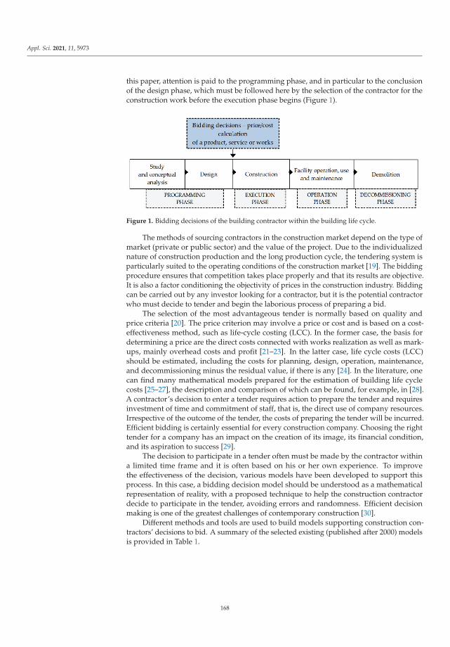
Appl. Sci. 2021, 11, 5973

this paper, attention is paid to the programming phase, and in particular to the conclusionof the design phase, which must be followed here by the selection of the contractor for theconstruction work before the execution phase begins (Figure 1).

Figure 1. Bidding decisions of the building contractor within the building life cycle.

The methods of sourcing contractors in the construction market depend on the type ofmarket (private or public sector) and the value of the project. Due to the individualizednature of construction production and the long production cycle, the tendering system isparticularly suited to the operating conditions of the construction market [19]. The biddingprocedure ensures that competition takes place properly and that its results are objective.It is also a factor conditioning the objectivity of prices in the construction industry. Biddingcan be carried out by any investor looking for a contractor, but it is the potential contractorwho must decide to tender and begin the laborious process of preparing a bid.

The selection of the most advantageous tender is normally based on quality andprice criteria [20]. The price criterion may involve a price or cost and is based on a cost-effectiveness method, such as life-cycle costing (LCC). In the former case, the basis fordetermining a price are the direct costs connected with works realization as well as mark-ups, mainly overhead costs and profit [21–23]. In the latter case, life cycle costs (LCC)should be estimated, including the costs for planning, design, operation, maintenance,and decommissioning minus the residual value, if there is any [24]. In the literature, onecan find many mathematical models prepared for the estimation of building life cyclecosts [25–27], the description and comparison of which can be found, for example, in [28].A contractor’s decision to enter a tender requires action to prepare the tender and requiresinvestment of time and commitment of staff, that is, the direct use of company resources.Irrespective of the outcome of the tender, the costs of preparing the tender will be incurred.Efficient bidding is certainly essential for every construction company. Choosing the righttender for a company has an impact on the creation of its image, its financial condition,and its aspiration to success [29].

The decision to participate in a tender often must be made by the contractor withina limited time frame and it is often based on his or her own experience. To improvethe effectiveness of the decision, various models have been developed to support thisprocess. In this case, a bidding decision model should be understood as a mathematicalrepresentation of reality, with a proposed technique to help the construction contractordecide to participate in the tender, avoiding errors and randomness. Efficient decisionmaking is one of the greatest challenges of contemporary construction [30].

Different methods and tools are used to build models supporting construction con-tractors’ decisions to bid. A summary of the selected existing (published after 2000) modelsis provided in Table 1.

168

Appl. Sci. 2021, 11, 5973

Table 1. Examples of models supporting tender decisions presented in the literature after 2000.

Bidding Decision Model Authors Source Year of Publication

Model based on Case-based reasoning approach Chua D.K.H, Li D.Z, Chan W.T. [31] 2001

Model based on the Analytical Hierarchy Process(AHP) method Cagno E., Caron F., Perego A. [32] 2001

Model based on artificial neural network Wanous M., Boussabaine A. H., Lewis J. [33] 2003

Model based on fuzzy linguistic approach Lin Ch.-T., Chen Y.-T. [34] 2004

Model based on logistic regression Drew D., Lo H.P. [35] 2007

Model based on a knowledge system Egemen M., Mohamed A. [36] 2008

Model based on data envelopment analysis (DEA) El-Mashaleh M. S. [37] 2010

Model based on a multi-criteria analysis and fuzzy settheory

Cheng M.-Y., Hsiang C. Ch., Tsai H.-Ch,Do H.-L. [38] 2011

Model based on an ant colony optimisation algorithmand artificial neural network Shi, H. [39] 2012

Model based on fuzzy Analytical Hierarchy Processand regression-based simulation Chou, J. S., Pham, A. D., Wang, H. [40] 2013

Model based on a fuzzy set theory Lesniak, A., Plebankiewicz, E. [41] 2016

Model based on RBF neural networks Lesniak, A. [42] 2016

Model based on the simple additive weighted scoring Chisala, M. L. [43] 2017

Model based on the fuzzy AHP Lesniak, A., Kubek, D., Plebankiewicz,E., Zima, K., Belniak, S. [44] 2018

Model based on the game theory Arya, A., Sisodia, S., Mehroliya, S.,Rajeshwari, C. S. [45] 2020

Model based on structural equation Ojelabi, R. A., Oyeyipo, O. O., Afolabi,A. O., Omuh, I. O. [46] 2020

Model Based on Projection Pursuit Learning Method Zhang, X., Yu, Y., He, W., Chen, Y. [47] 2021

It is worth noting that the indicated models differ in the methods used. Differentmethods, techniques, and approaches are sought and applied to obtain the most effectivemodels. What is important, continuously for at least 20 years, modeling of a tender decisionis still an object of research and interest of researchers.

The models proposed in the literature are generally based on factors, also calledcriteria, affecting the decision, and using them as input parameters. The number ofpublications on the identification of factors is considerable, as each country and regionhas a certain characteristic group of factors that will not be found in other markets [48–50].It can therefore be concluded that the factors influencing tender decisions depend notonly on the project to be tendered but also on the environment and market in which thecontractor operates.

Bidding problems are also known in procurement auctions [51,52]. This paper [53]presents the analysis of the relation between the award price and the bidding price inthe case of public procurement in Spain. An award price estimator was proposed as it isbelieved to be particularly useful for companies and public procurement agencies. Procure-ment auctions have long been employed in the logistics and transportation industry [54].In combinatorial auctions, each carrier must determine the set of profitable contracts tobid on and the associated ask prices. This is known as the bid construction problem(BCP) [55]. Different approaches for the bid construction problem (BCP) in transportationprocurement auctions are proposed in literature. One of them can be found in [56] whereauthors proposed solving the BCP problem for heterogeneous truckload using exact andheuristic methods.

169

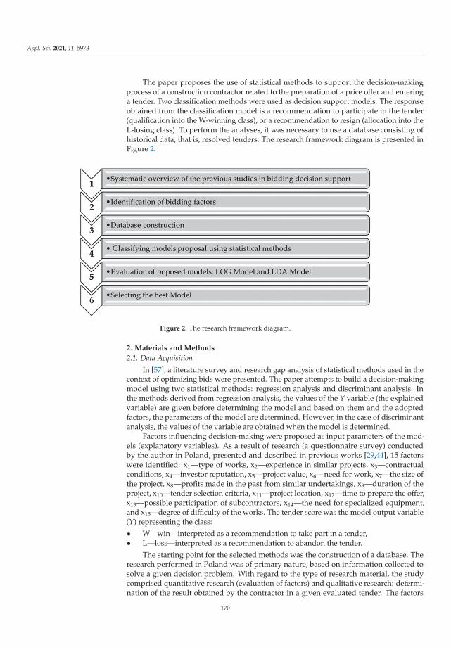
Appl. Sci. 2021, 11, 5973

The paper proposes the use of statistical methods to support the decision-makingprocess of a construction contractor related to the preparation of a price offer and enteringa tender. Two classification methods were used as decision support models. The responseobtained from the classification model is a recommendation to participate in the tender(qualification into the W-winning class), or a recommendation to resign (allocation into theL-losing class). To perform the analyses, it was necessary to use a database consisting ofhistorical data, that is, resolved tenders. The research framework diagram is presented inFigure 2.

Figure 2. The research framework diagram.

2. Materials and Methods

2.1. Data Acquisition

In [57], a literature survey and research gap analysis of statistical methods used in thecontext of optimizing bids were presented. The paper attempts to build a decision-makingmodel using two statistical methods: regression analysis and discriminant analysis. Inthe methods derived from regression analysis, the values of the Y variable (the explainedvariable) are given before determining the model and based on them and the adoptedfactors, the parameters of the model are determined. However, in the case of discriminantanalysis, the values of the variable are obtained when the model is determined.

Factors influencing decision-making were proposed as input parameters of the mod-els (explanatory variables). As a result of research (a questionnaire survey) conductedby the author in Poland, presented and described in previous works [29,44], 15 factorswere identified: x1—type of works, x2—experience in similar projects, x3—contractualconditions, x4—investor reputation, x5—project value, x6—need for work, x7—the size ofthe project, x8—profits made in the past from similar undertakings, x9—duration of theproject, x10—tender selection criteria, x11—project location, x12—time to prepare the offer,x13—possible participation of subcontractors, x14—the need for specialized equipment,and x15—degree of difficulty of the works. The tender score was the model output variable(Y) representing the class:

• W—win—interpreted as a recommendation to take part in a tender,• L—loss—interpreted as a recommendation to abandon the tender.

The starting point for the selected methods was the construction of a database. Theresearch performed in Poland was of primary nature, based on information collected tosolve a given decision problem. With regard to the type of research material, the studycomprised quantitative research (evaluation of factors) and qualitative research: determi-nation of the result obtained by the contractor in a given evaluated tender. The factors

170

Appl. Sci. 2021, 11, 5973

identified were used to evaluate the tenders entered into by the contractors participatingin the research. Each factor, from x1 to x15, was rated on a scale from 1 to 7, where thenumbers meant 1—very unfavorable, and 7—very favorable influence of the factor onthe decision to participate in the tender. This scale has already been used successfully inprevious works [44]. The result for each tender evaluated was then recorded (W—win,L—loss). In the end, the database contained 88 evaluated tenders, of which 64 were lostcases (L) and 24 won cases (W). Selected database records of evaluated tenders includingfactor evaluations with the corresponding result obtained in the tender (W—win, L—loss,)are presented in Table 2.

Table 2. Selected database records.

Record(Evaluated

Tender)Factors Result

i x1 x2 x3 x4 x5 x6 x7 x8 x9 x10 x11 x12 x13 x14 x154 6 7 5 5 3 6 3 4 5 3 6 5 2 6 7 L12 4 6 5 6 1 6 1 4 6 5 6 6 7 3 5 W62 7 7 4 4 4 5 3 4 5 3 5 5 4 6 6 L

2.2. Regression Analysis Model

The main task of the qualitative decision-making model will be to determine theprobability of the contractor’s success in the tender (winning) and to identify variables thatsignificantly affect the outcome of the tender. A binomial (dichotomous) model is sought inwhich the explanatory variable Y is quantified by a zero-one variable. It takes two possiblevariants described by the codes “1”—W (win) and “0”—L (loss). If pi is the probability ofthe event Yi = 1, then 1 − pi is the probability of the event Yi = 0. The expected value of thevariable Yi is [58,59]:

E(Yi) = 1·pi + 0·(1 − pi) = pi (1)

In binomial models, it is assumed that pi is a function of the vector of values of theexplanatory variables xi for the i-th object and the parameter vector β [58,59]:

Pi = P(yi = 1) = F(

xTi β

)(2)

Depending on the type of F-function, different types of models are distinguished [60]: alinear probability model, logit model, and probit model. Using the simplest of the binomialmodels—the linear probability model—has many negative consequences described inthe literature [58,61]. Probit and logit models, on the other hand, as indicated by someauthors [60], are similar to each other and in practice one of them is used. Therefore, thesearch for a binomial model for the phenomenon in question was limited to a logisticregression model. The general form of the logit model is as follows [58,59]:

Y∗i = ln

pi1 − pi

= β0α0 + β1X1i + β2xX2i + · · ·+ βkXki + ui (3)

where:

β j—structural model parameters,ui—random component,ln pi

1−pi—logit,

Y∗i —unobservable qualitative variable,

Xji—the values of the explanatory variables of the model,pi—the probability of taking the value “1” by the dependent variable Yi calculated fromthe logistic distribution density function.

171

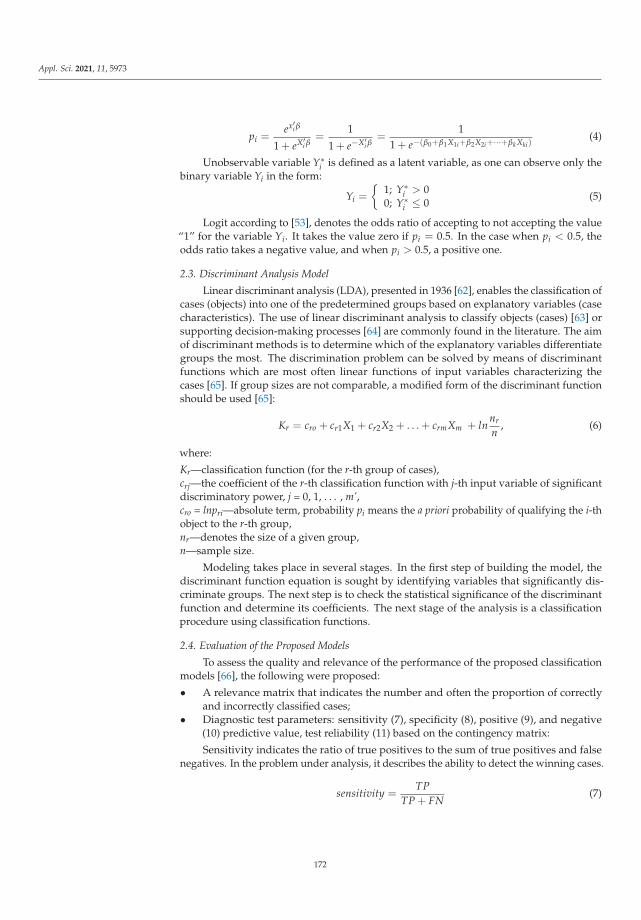
Appl. Sci. 2021, 11, 5973

pi =ex′i β

1 + eX′i β

=1

1 + e−X′i β

=1

1 + e−(β0+β1X1i+β2X2i+···+βkXki)(4)

Unobservable variable Y∗i is defined as a latent variable, as one can observe only the

binary variable Yi in the form:

Yi =

{1; Y∗

i > 00; Y∗

i ≤ 0(5)

Logit according to [53], denotes the odds ratio of accepting to not accepting the value“1” for the variable Yi. It takes the value zero if pi = 0.5. In the case when pi < 0.5, theodds ratio takes a negative value, and when pi > 0.5, a positive one.

2.3. Discriminant Analysis Model

Linear discriminant analysis (LDA), presented in 1936 [62], enables the classification ofcases (objects) into one of the predetermined groups based on explanatory variables (casecharacteristics). The use of linear discriminant analysis to classify objects (cases) [63] orsupporting decision-making processes [64] are commonly found in the literature. The aimof discriminant methods is to determine which of the explanatory variables differentiategroups the most. The discrimination problem can be solved by means of discriminantfunctions which are most often linear functions of input variables characterizing thecases [65]. If group sizes are not comparable, a modified form of the discriminant functionshould be used [65]:

Kr = cro + cr1X1 + cr2X2 + . . . + crmXm + lnnr

n, (6)

where:

Kr—classification function (for the r-th group of cases),crj—the coefficient of the r-th classification function with j-th input variable of significantdiscriminatory power, j = 0, 1, . . . , m’,cro = lnpri—absolute term, probability pi means the a priori probability of qualifying the i-thobject to the r-th group,nr—denotes the size of a given group,n—sample size.

Modeling takes place in several stages. In the first step of building the model, thediscriminant function equation is sought by identifying variables that significantly dis-criminate groups. The next step is to check the statistical significance of the discriminantfunction and determine its coefficients. The next stage of the analysis is a classificationprocedure using classification functions.

2.4. Evaluation of the Proposed Models

To assess the quality and relevance of the performance of the proposed classificationmodels [66], the following were proposed:

• A relevance matrix that indicates the number and often the proportion of correctlyand incorrectly classified cases;

• Diagnostic test parameters: sensitivity (7), specificity (8), positive (9), and negative(10) predictive value, test reliability (11) based on the contingency matrix:

Sensitivity indicates the ratio of true positives to the sum of true positives and falsenegatives. In the problem under analysis, it describes the ability to detect the winning cases.

sensitivity =TP

TP + FN(7)

172

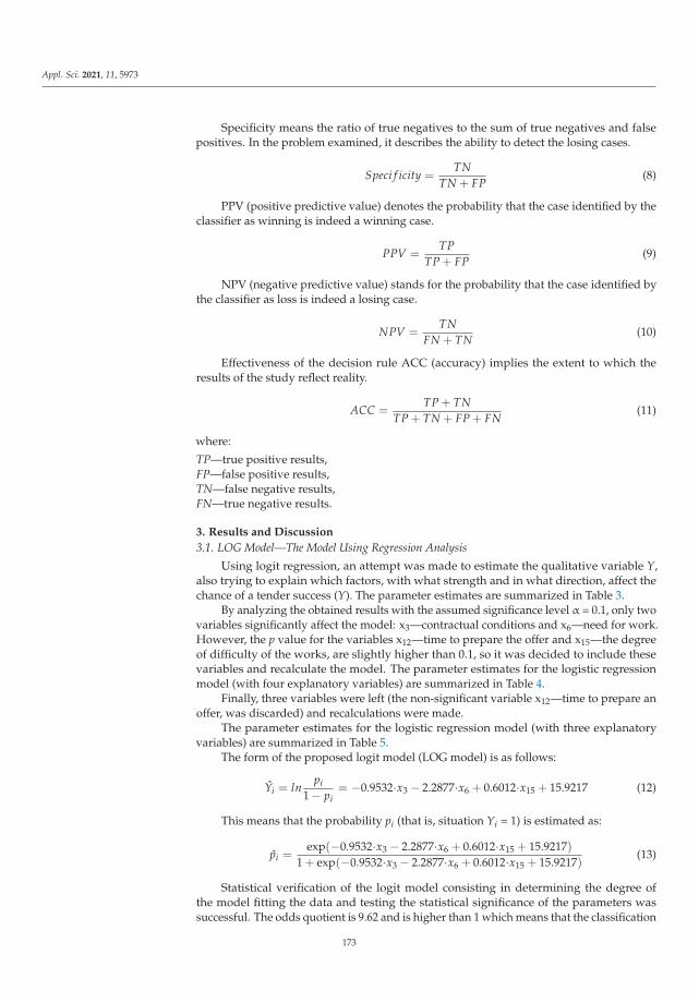
Appl. Sci. 2021, 11, 5973

Specificity means the ratio of true negatives to the sum of true negatives and falsepositives. In the problem examined, it describes the ability to detect the losing cases.

Speci f icity =TN

TN + FP(8)

PPV (positive predictive value) denotes the probability that the case identified by theclassifier as winning is indeed a winning case.

PPV =TP

TP + FP(9)

NPV (negative predictive value) stands for the probability that the case identified bythe classifier as loss is indeed a losing case.

NPV =TN

FN + TN(10)

Effectiveness of the decision rule ACC (accuracy) implies the extent to which theresults of the study reflect reality.

ACC =TP + TN

TP + TN + FP + FN(11)

where:

TP—true positive results,FP—false positive results,TN—false negative results,FN—true negative results.

3. Results and Discussion

3.1. LOG Model—The Model Using Regression Analysis

Using logit regression, an attempt was made to estimate the qualitative variable Y,also trying to explain which factors, with what strength and in what direction, affect thechance of a tender success (Y). The parameter estimates are summarized in Table 3.

By analyzing the obtained results with the assumed significance level α = 0.1, only twovariables significantly affect the model: x3—contractual conditions and x6—need for work.However, the p value for the variables x12—time to prepare the offer and x15—the degreeof difficulty of the works, are slightly higher than 0.1, so it was decided to include thesevariables and recalculate the model. The parameter estimates for the logistic regressionmodel (with four explanatory variables) are summarized in Table 4.

Finally, three variables were left (the non-significant variable x12—time to prepare anoffer, was discarded) and recalculations were made.

The parameter estimates for the logistic regression model (with three explanatoryvariables) are summarized in Table 5.

The form of the proposed logit model (LOG model) is as follows:

Yi = lnpi

1 − pi= −0.9532·x3 − 2.2877·x6 + 0.6012·x15 + 15.9217 (12)

This means that the probability pi (that is, situation Yi = 1) is estimated as:

pi =exp(−0.9532·x3 − 2.2877·x6 + 0.6012·x15 + 15.9217)

1 + exp(−0.9532·x3 − 2.2877·x6 + 0.6012·x15 + 15.9217)(13)

Statistical verification of the logit model consisting in determining the degree ofthe model fitting the data and testing the statistical significance of the parameters wassuccessful. The odds quotient is 9.62 and is higher than 1 which means that the classification

173

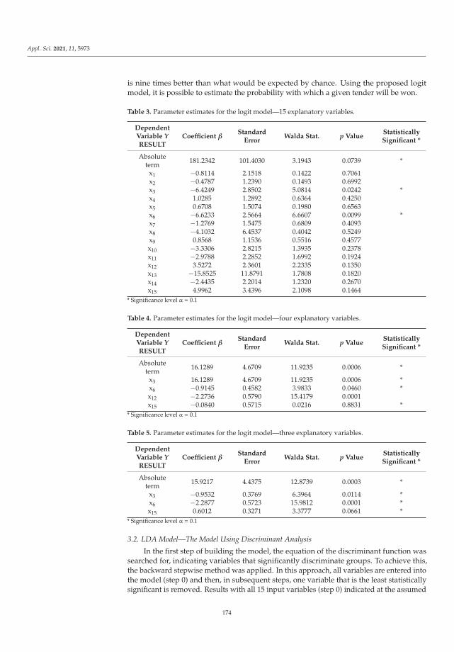
Appl. Sci. 2021, 11, 5973

is nine times better than what would be expected by chance. Using the proposed logitmodel, it is possible to estimate the probability with which a given tender will be won.

Table 3. Parameter estimates for the logit model—15 explanatory variables.

DependentVariable YRESULT

Coefficient βStandard

ErrorWalda Stat. p Value

StatisticallySignificant *

Absoluteterm 181.2342 101.4030 3.1943 0.0739 *

x1 −0.8114 2.1518 0.1422 0.7061x2 −0.4787 1.2390 0.1493 0.6992x3 −6.4249 2.8502 5.0814 0.0242 *x4 1.0285 1.2892 0.6364 0.4250x5 0.6708 1.5074 0.1980 0.6563x6 −6.6233 2.5664 6.6607 0.0099 *x7 −1.2769 1.5475 0.6809 0.4093x8 −4.1032 6.4537 0.4042 0.5249x9 0.8568 1.1536 0.5516 0.4577x10 −3.3306 2.8215 1.3935 0.2378x11 −2.9788 2.2852 1.6992 0.1924x12 3.5272 2.3601 2.2335 0.1350x13 −15.8525 11.8791 1.7808 0.1820x14 −2.4435 2.2014 1.2320 0.2670x15 4.9962 3.4396 2.1098 0.1464

* Significance level α = 0.1

Table 4. Parameter estimates for the logit model—four explanatory variables.

DependentVariable YRESULT

Coefficient βStandard

ErrorWalda Stat. p Value

StatisticallySignificant *

Absoluteterm 16.1289 4.6709 11.9235 0.0006 *

x3 16.1289 4.6709 11.9235 0.0006 *x6 −0.9145 0.4582 3.9833 0.0460 *x12 −2.2736 0.5790 15.4179 0.0001x15 −0.0840 0.5715 0.0216 0.8831 *

* Significance level α = 0.1

Table 5. Parameter estimates for the logit model—three explanatory variables.

DependentVariable YRESULT

Coefficient βStandard

ErrorWalda Stat. p Value

StatisticallySignificant *

Absoluteterm 15.9217 4.4375 12.8739 0.0003 *

x3 −0.9532 0.3769 6.3964 0.0114 *x6 −2.2877 0.5723 15.9812 0.0001 *x15 0.6012 0.3271 3.3777 0.0661 *

* Significance level α = 0.1

3.2. LDA Model—The Model Using Discriminant Analysis

In the first step of building the model, the equation of the discriminant function wassearched for, indicating variables that significantly discriminate groups. To achieve this,the backward stepwise method was applied. In this approach, all variables are entered intothe model (step 0) and then, in subsequent steps, one variable that is the least statisticallysignificant is removed. Results with all 15 input variables (step 0) indicated at the assumed

174

Appl. Sci. 2021, 11, 5973

significance level α = 0.1, that only four variables significantly discriminate between groups(x3, x5, x6, x13).

The results for the model and the evaluation of all 15 input variables (step 0) are givenin Table 6.

Table 6. Evaluation of the parameters of the discriminant function—15 explanatory variables.

VariablesWilks’

LambdaPartial Lambda

WilksThe Value of the F

Statisticp Value Tolerance 1-Tolerance

StatisticallySignificant *

x1 0.430141 0.961162 2.90937 0.092377 0.377706 0.622294x2 0.413447 0.999971 0.00207 0.963850 0.370875 0.629125x3 0.449346 0.920082 6.25390 0.014669 0.376703 0.623297 *x4 0.421275 0.981391 1.36523 0.246487 0.522505 0.477495x5 0.454559 0.909531 7.16170 0.009215 0.109267 0.890733 *x6 0.609746 0.678045 34.18763 0.000000 0.643071 0.356929 *x7 0.419668 0.985148 1.08548 0.300962 0.096009 0.903991x8 0.434939 0.950558 3.74495 0.056895 0.577896 0.422104x9 0.414878 0.996522 0.25127 0.617712 0.757040 0.242960x10 0.417598 0.990032 0.72491 0.397361 0.672704 0.327296x11 0.424018 0.975042 1.84297 0.178843 0.633470 0.366531x12 0.430727 0.959854 3.01140 0.086960 0.512083 0.487917x13 0.444633 0.929835 5.43308 0.022563 0.513878 0.486123 *x14 0.414026 0.998573 0.10292 0.749283 0.580513 0.419487x15 0.434007 0.952600 3.58258 0.062408 0.391804 0.608196

* Significance level α = 0.05.

By analyzing the obtained results with the assumed significance level α = 0.1, only fourvariables (x3; x5; x6; x13) discriminated significantly between groups. The model parametersare as follows: Wilks’ Lambda = 0.41344, the corresponding F statistic (15.72) = 6.8100, andp < 0.0000.

During the first step of the analysis, the variable x2 was removed—the least signifi-cantly discriminating group. Subsequent steps (k = 2, . . . , 15) made it possible to select themost significant variables (Table 7).

Table 7. Evaluation of the discriminant function parameters—final model (six input variables).

Variables Wilks’ Lambda Partial Lambda Wilks The Value of the F Statistic p Value Tolerance Wilks’ Lambda

x1 0.570048 0.825309 17.14504 0.000084 0.694765 *x3 0.495679 0.949133 4.341000 0.040358 0.771227 *x5 0.557289 0.844204 14.94840 0.000222 0.541454 *x6 0.740919 0.634977 46.56377 0.000000 0.776650 *x13 0.532386 0.883694 10.66070 0.001605 0.803942 *x15 0.500913 0.939217 5.242020 0.024650 0.789131 *

* Significance level α = 0.05.

Finally, six input variables, x1—type of works, x3—contractual conditions, x5—projectvalue, x6—need for work, x13—possible participation of subcontractors, x15—the degree ofdifficulty of the works, discriminate significantly between groups. The model parametersare as follows: Wilks’ Lambda = 0.47047; the corresponding statistic F (6.81) = 15.195;p < 0.0000. It is worth noting that the smaller the value of Wilks’ Lambda (from therange <0, 1>) the better the discriminating power the model has. In the analyzed example(0.47047), it is acceptable. Tolerance coefficient Tk determines the proportion of the varianceof the variable xk that is not explained by the variables in the model. If Tk coefficient takesa value smaller than the default 0.01, the variable is more than 99% redundant with othervariables in the model. Entering variables with low tolerance coefficients into the modelmay cause its large inaccuracy. In the model under consideration, the Tk coefficients for theassumed variables exceed the value of 0.5.

175

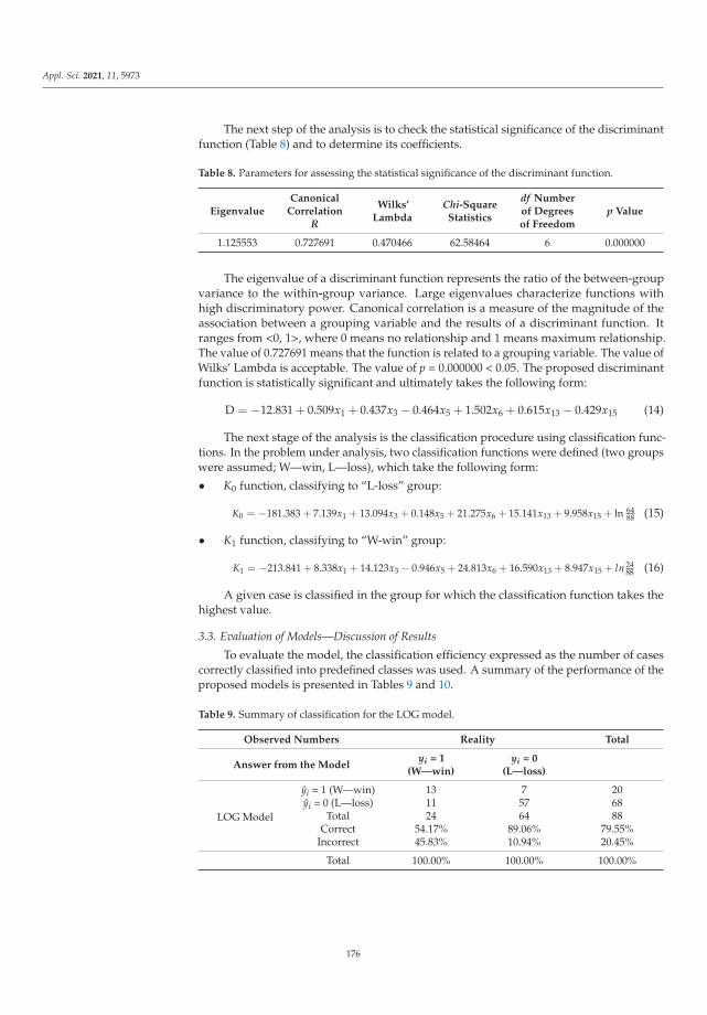
Appl. Sci. 2021, 11, 5973

The next step of the analysis is to check the statistical significance of the discriminantfunction (Table 8) and to determine its coefficients.

Table 8. Parameters for assessing the statistical significance of the discriminant function.

EigenvalueCanonical

CorrelationR

Wilks’Lambda

Chi-SquareStatistics

df Numberof Degreesof Freedom

p Value

1.125553 0.727691 0.470466 62.58464 6 0.000000

The eigenvalue of a discriminant function represents the ratio of the between-groupvariance to the within-group variance. Large eigenvalues characterize functions withhigh discriminatory power. Canonical correlation is a measure of the magnitude of theassociation between a grouping variable and the results of a discriminant function. Itranges from <0, 1>, where 0 means no relationship and 1 means maximum relationship.The value of 0.727691 means that the function is related to a grouping variable. The value ofWilks’ Lambda is acceptable. The value of p = 0.000000 < 0.05. The proposed discriminantfunction is statistically significant and ultimately takes the following form:

D = −12.831 + 0.509x1 + 0.437x3 − 0.464x5 + 1.502x6 + 0.615x13 − 0.429x15 (14)

The next stage of the analysis is the classification procedure using classification func-tions. In the problem under analysis, two classification functions were defined (two groupswere assumed; W—win, L—loss), which take the following form:

• K0 function, classifying to “L-loss” group:

K0 = −181.383 + 7.139x1 + 13.094x3 + 0.148x5 + 21.275x6 + 15.141x13 + 9.958x15 + ln 6488 (15)

• K1 function, classifying to “W-win” group:

K1 = −213.841 + 8.338x1 + 14.123x3 − 0.946x5 + 24.813x6 + 16.590x13 + 8.947x15 + ln 2488 (16)

A given case is classified in the group for which the classification function takes thehighest value.

3.3. Evaluation of Models—Discussion of Results

To evaluate the model, the classification efficiency expressed as the number of casescorrectly classified into predefined classes was used. A summary of the performance of theproposed models is presented in Tables 9 and 10.

Table 9. Summary of classification for the LOG model.

Observed Numbers Reality Total

Answer from the Modelyi = 1

(W—win)yi = 0

(L—loss)

LOG Model

yi = 1 (W—win) 13 7 20yi = 0 (L—loss) 11 57 68

Total 24 64 88Correct 54.17% 89.06% 79.55%

Incorrect 45.83% 10.94% 20.45%

Total 100.00% 100.00% 100.00%

176

Appl. Sci. 2021, 11, 5973

Table 10. Summary of classification for the LDA model.

Observed Numbers Reality Total

Answer from the Modelyi = 1

(W—win)yi = 0

(L—loss)

LDA Model

yi = 1(W—win) 15 3 18yi = 0 (L—loss) 9 61 70

Total 24 64 88Correct 62.50% 95.31% 86.36%

Incorrect 37.50% 4.69% 13.64%

Total 100.00% 100.00% 100.00%

The data in Tables 8 and 9 enable the basic parameters of the classification model to bedetermined. The results are given in Table 11.

Table 11. Basic parameters of LOG and LDA models as a classifier.

Model Sensitivity SpecificityPositive

PredictiveValue (PPV)

NegativePredictive

Value (NPV)

Effectiveness(ACC)

LOG Model 54.17% 89.06% 65.00% 83.82% 79.55%LDA Model 62.50% 95.31% 83.33% 87.14% 86.36%

From the values in Table 10, the LOG model correctly classified 79.55% of the cases,more correctly predicting tender failure (83.82%). The values obtained show a good fitof the model, but it is worrying that the model indicated only three tender factors asstatistically significant: x3—contractual conditions, x6—need for work, and x15—degree ofdifficulty of the works. In the case of the LDA model, classification into the set L—87.14%means that the model (analogous to the LOG model) more accurately predicts tender failurethan winning (83.33%). The results obtained by the LDA model are better as it rendered 86%of correctly classified cases. The discriminant analysis, apart from the variables x3, x6, x15indicated also x1—type of works, x5—value of the project, and x13—possible participationof subcontractors, as significant variables for the model, where the greatest independentinfluence on the result of the discriminant function is exerted by the variable x6—the needfor work, while the least x3—contractual conditions. The following is an extract from theLDA model results sheet with the values of the classification functions in relation to theobserved (actual) values shown in Table 12.

Table 12. Classification function values for selected cases.

Case Number

GroupMembership:

GroupMembership:

Function Value

Observed Model K0—win K1—loss

10 W W 208.994 211.74728 L L 189.970 186.249

* 29 W L 207.961 206.83230 L L 199.490 196.887

* 35 L W 220.759 222.847* Cases misclassified.

The analyses presented in this paper do not exhaust the issue of modeling contractors’decisions to participate in tenders for construction works. They can become a supplementof the models proposed so far in the literature. It should be noted that the constructionof classification models requires having an appropriate database, which is built based ontender factors selected by the author of each model.

177

Appl. Sci. 2021, 11, 5973

It is also worth emphasizing that in the face of fierce competition on the constructionmarket, contractors are looking for solutions to maximize their chances of winning tenders.It is worth noting the observations of the authors of the study [67], who noted that the bidpreparation process, which is time-consuming and requires a lot of effort, may create theneed to have appropriate specialists. Typically, large companies are more able to employsuch specialists, while small and medium-sized companies are definitely more likely tofeel the need for tools to support the proper selection of orders and the decision to tender.It therefore appears that the proposal to build and use mathematical models is appropriate.

In further research, using the author’s constructed database, the author of the paperintends to apply methods of artificial intelligence. The same database, model input and out-put parameters will allow to objectively compare the effectiveness of these two approaches.

4. Conclusions

The construction company at each stage of its activity has to make a number of impor-tant decisions related to the functioning of the company. One of them is the decision toenter a tender. Although it involves company finances and resources, the decision is usuallytaken quickly and based on subjectively perceived information. A number of models andmathematical methods have been proposed in the literature to assist the decision makerand to increase the effectiveness of the decisions taken. In this paper, two statistical classifi-cation methods are used for modeling: linear regression and linear discriminant analysis.The response obtained from the classification model is a recommendation to participatein the tender (qualification into class W—win), or a recommendation to resign (allocationinto class L—loss). To perform the analyses, it was necessary to use a database consistingof historical data, that is, resolved tenders. The comparison of the classification modelsshows that the model using linear discriminant analysis performed well (86% correctlyclassified cases). The backward stepwise method was used to eliminate the least statisticallysignificant variables. Finally, from a set of 15 identified factors, six input variables (factors)were identified that significantly discriminate between groups: x1—type of works, x3—contractual conditions, x5—project value, x6—need for work, x13—possible participation ofsubcontractors, x15—the degree of difficulty of the works. With these variables, the modelachieved good performance. The paper by [44] presents the results of a survey in whichthe works contractors selected the following as the most important factors influencing thedecision to enter a tender: type of works, contractual conditions, experience in similarprojects, project value, need for work. As can be seen, they mostly coincide with the resultsobtained from statistical methods. The obtained results (effectiveness of classification andvalues of model evaluation parameters) testify to the possibility of using the LDA modelin practice.

Funding: This research received no external funding.

Institutional Review Board Statement: Not applicable.

Informed Consent Statement: Not applicable.

Data Availability Statement: Data sharing not applicable.

Conflicts of Interest: The author declares no conflict of interest.

References

1. Bernardi, E.; Carlucci, S.; Cornaro, C.; Bohne, R.A. An Analysis of the Most Adopted Rating Systems for Assessing theEnvironmental Impact of Buildings. Sustainability 2017, 9, 1226. [CrossRef]

2. Sztubecka, M.; Skiba, M.; Mrówczynska, M.; Mathias, M. Noise as a Factor of Green Areas Soundscape Creation. Sustainability2020, 12, 999. [CrossRef]

3. Wałach, D. Analysis of Factors Affecting the Environmental Impact of Concrete Structures. Sustainability 2021, 13, 204. [CrossRef]4. Antico, F.C.; Ibáñez, U.A.; Wiener, M.J.; Araya-Letelier, G.; Retamal, R.G. Eco-bricks: A sustainable substitute for construction

materials. Revista Construcción 2017, 16, 518–526. [CrossRef]5. Govindan, K.; Shankar, M.; Kannan, D. Sustainable material selection for construction industry—A hybrid multi criteria decision

making approach. Renew. Sustain. Energy Rev. 2016, 55, 1274–1288. [CrossRef]

178

Appl. Sci. 2021, 11, 5973

6. Reddy, B.V. Sustainable materials for low carbon buildings. Int. J. Low Carbon Technol. 2009, 4, 175–181. [CrossRef]7. Lesniak, A.; Zima, K. Comparison of traditional and ecological wall systems using the AHP method. In Proceedings of the

International Multidisciplinary Scientific GeoConference Surveying Geology and Mining Ecology Management, SGEM, Albena,Bulgaria, 18–24 June 2015; Volume 3, pp. 157–164.

8. Zavadskas, E.K.; Antucheviciene, J.; Vilutiene, T.; Adeli, H. Sustainable Decision-Making in Civil Engineering, Construction andBuilding Technology. Sustainability 2018, 10, 14. [CrossRef]

9. Apollo, M.; Siemaszko, A.; Miszewska, E. The selected roof covering technologies in the aspect of their life cycle costs. Open Eng.2018, 8, 478–483. [CrossRef]

10. Sztubecka, M.; Skiba, M.; Mrówczynska, M.; Bazan-Krzywoszanska, A. An Innovative Decision Support System to Improve theEnergy Efficiency of Buildings in Urban Areas. Remote Sens. 2020, 12, 259. [CrossRef]

11. Chen, S.; Zhang, G.; Xia, X.; Setunge, S.; Shi, L. A review of internal and external influencing factors on energy efficiency designof buildings. Energy Build. 2020, 216, 109944. [CrossRef]

12. Nowogonska, B. A Methodology for Determining the Rehabilitation Needs of Buildings. Appl. Sci. 2020, 10, 3873. [CrossRef]13. Słowik, M.; Skrzypczak, I.; Kotynia, R.; Kaszubska, M. The Application of a Probabilistic Method to the Reliability Analysis of

Longitudinally Reinforced Concrete Beams. Procedia Eng. 2017, 193, 273–280. [CrossRef]14. Konior, J.; Sawicki, M.; Szóstak, M. Damage and Technical Wear of Tenement Houses in Fuzzy Set Categories. Appl. Sci. 2021,

11, 1484. [CrossRef]15. Ahn, S.; Kim, T.; Kim, J.-M. Sustainable Risk Assessment through the Analysis of Financial Losses from Third-Party Damage in

Bridge Construction. Sustainability 2020, 12, 3435. [CrossRef]16. Bednarz, L.; Bajno, D.; Matkowski, Z.; Skrzypczak, I.; Lesniak, A. Elements of Pathway for Quick and Reliable Health Monitoring

of Concrete Behavior in Cable Post-Tensioned Concrete Girders. Materials 2021, 14, 1503. [CrossRef] [PubMed]17. Spišáková, M.; Mésároš, P.; Mandicák, T. Construction Waste Audit in the Framework of Sustainable Waste Management in

Construction Projects—Case Study. Buildings 2021, 11, 61. [CrossRef]18. Tang, Z.; Li, W.; Tam, V.W.; Xue, C. Advanced progress in recycling municipal and construction solid wastes for manufacturing

sustainable construction materials. Resour. Conserv. Recycl. 2020, 6, 100036. [CrossRef]19. Smith, A.J. Estimating, Tendering and Bidding for Construction Work; Macmillan International Higher Education: London, UK, 2017.20. Waara, F.; Bröchner, J. Price and Nonprice Criteria for Contractor Selection. J. Constr. Eng. Manag. 2006, 132, 797–804. [CrossRef]21. Plebankiewicz, E.; Lesniak, A. Overhead costs and profit calculation by Polish contractors. Technol. Econ. Dev. Econ. 2013, 19,

141–161. [CrossRef]22. Hegazy, T.; Moselhi, O. Elements of cost estimation: A survey in Canada and United States. Cost Eng. 1995, 37, 27–33.23. Doloi, H.K. Understanding stakeholders’ perspective of cost estimation in project management. Int. J. Proj. Manag. 2011, 29,

622–636. [CrossRef]24. Boussabaine, A.; Kirkham, R. Whole Life-Cycle Costing: Risk and Risk Responses; Blackwell Publishing, Ltd.: Oxford, UK, 2008.25. Plebankiewicz, E.; Meszek, W.; Zima, K.; Wieczorek, D. Probabilistic and Fuzzy Approaches for Estimating the Life Cycle Costs

of Buildings under Conditions of Exposure to Risk. Sustainability 2020, 12, 226. [CrossRef]26. Hromádka, V.; Korytárová, J.; Vítková, E.; Seelmann, H.; Funk, T. New Aspects of Socioeconomic Assessment of the Railway

Infrastructure Project Life Cycle. Appl. Sci. 2020, 10, 7355. [CrossRef]27. Biolek, V.; Hanák, T. LCC Estimation Model: A Construction Material Perspective. Buildings 2019, 9, 182. [CrossRef]28. Plebankiewicz, E.; Zima, K.; Wieczorek, D. Review of methods of determining the life cycle cost of buildings. In Proceedings

of the Creative Construction Conference, Kraków, Poland, 21–24 June 2015; Hajdu, M., Ed.; Elsevier B.V.: Amsterdam, TheNetherlands, 2015; pp. 309–316.

29. Lesniak, A. Classification of the Bid/No Bid Criteria—Factor Analysis. Arch. Civ. Eng. 2015, 61, 79–90. [CrossRef]30. Kaplinski, O.; Tupenaite, L. Review of the multiple criteria decision making methods, intelligent and biometric systems applied

in modern construction economics. Transform. Bus. Econ. 2011, 10, 166–181.31. Chua, D.K.H.; Li, D.Z.; Chan, W.T. Case-Based Reasoning Approach in Bid Decision Making. J. Constr. Eng. Manag. 2001, 127,

35–45. [CrossRef]32. Cagno, E.; Caron, F.; Perego, A. Multi-criteria assessment of the probability of winning in the competitive bidding process. Int. J.

Proj. Manag. 2001, 19, 313–324. [CrossRef]33. Wanous, M.; Boussabaine, A.H.; Lewis, J. A neural network bid/no bid model: The case for contractors in Syria. Constr. Manag.

Econ. 2003, 21, 737–744. [CrossRef]34. Lin, C.-T.; Chen, Y.-T. Bid/no bid decision-making—A fuzzy linguistic approach. Int. J. Proj. Manag. 2004, 22, 585–593. [CrossRef]35. Oo, B.; Drew, D.S.; Lo, H.P. Applying a random coefficients logistic model to contractors’ decision to bid. Constr. Manag. Econ.

2007, 25, 387–398. [CrossRef]36. Egemen, M.; Mohamed, A. SCBMD: A knowledge-based system software for strategically correct bid/no bid and mark-up size

decisions. Autom. Constr. 2008, 17, 864–872. [CrossRef]37. El-Mashaleh, M.S. Decision to bid or not to bid: A data envelopment analysis approach. Can. J. Civ. Eng. 2010, 37, 37–44.

[CrossRef]38. Cheng, M.-Y.; Hsiang, C.-C.; Tsai, H.-C.; Do, H.-L. Bidding decision making for construction company using a multi-criteria

prospect model. J. Civ. Eng. Manag. 2011, 17, 424–436. [CrossRef]

179

Appl. Sci. 2021, 11, 5973

39. Shi, H. ACO trained ANN-based bid/no-bid decision-making. Int. J. Model. Identif. Control 2012, 15, 290–296. [CrossRef]40. Chou, J.-S.; Pham, A.-D.; Wang, H. Bidding strategy to support decision-making by integrating fuzzy AHP and regression-based

simulation. Autom. Constr. 2013, 35, 517–527. [CrossRef]41. Lesniak, A.; Plebankiewicz, E. Modeling the Decision-Making Process Concerning Participation in Construction Bidding. J.

Manag. Eng. 2015, 31, 04014032. [CrossRef]42. Lesniak, A. Supporting contractors’ bidding decision: RBF neural networks application. AIP Conf. Proc. 2016, 1738, 200002.

[CrossRef]43. Chisala, M.L. Quantitative Bid or No-Bid Decision-Support Model for Contractors. J. Constr. Eng. Manag. 2017, 143, 04017088.

[CrossRef]44. Lesniak, A.; Kubek, D.; Plebankiewicz, E.; Zima, K.; Belniak, S. Fuzzy AHP Application for Supporting Contractors’ Bidding

Decision. Symmetry 2018, 10, 642. [CrossRef]45. Arya, A.; Sisodia, S.; Mehroliya, S.; Rajeshwari, C. A novel approach to Optimize Bidding Strategy for Restructured Power Market

using Game Theory. In Proceedings of the 2020 IEEE International Symposium on Sustainable Energy, Signal Processing andCyber Security (iSSSC), Gunupur Odisha, India, 16–17 December 2020; pp. 1–6.

46. Ojelabi, R.A.; Oyeyipo, O.O.; Afolabi, A.O.; Omuh, I.O. Evaluating barriers inhibiting investors participation in Public-PrivatePartnership project bidding process using structural equation model. Int. J. Constr. Manag. 2020. [CrossRef]

47. Zhang, X.; Yu, Y.; He, W.; Chen, Y. Bidding Decision-Support Model for Construction Projects Based on Projection PursuitLearning Method. J. Constr. Eng. Manag. 2021, 147, 04021054. [CrossRef]

48. Shokri-Ghasabeh, M.; Chileshe, N. Critical factors influencing the bid/no bid decision in the Australian construction industry.Constr. Innov. 2016, 16, 127–157. [CrossRef]

49. Jarkas, A.M.; Mubarak, S.A.; Kadri, C.Y. Critical Factors Determining Bid/No Bid Decisions of Contractors in Qatar. J. Manag.Eng. 2014, 30, 05014007. [CrossRef]

50. Li, G.; Chen, C.; Zhang, G.K.; Martek, I. Bid/no-bid decision factors for Chinese international contractors in internationalconstruction projects. Eng. Constr. Arch. Manag. 2020, 27, 1619–1643. [CrossRef]

51. Song, J.; Regan, A. Approximation algorithms for the bid construction problem in combinatorial auctions for the procurement offreight transportation contracts. Transp. Res. Methodol. 2005, 39, 914–933. [CrossRef]

52. Hanák, T.; Serrat, C. Analysis of construction auctions data in Slovak public procurement. Adv. Civ. Eng. 2018, 2018, 9036340.[CrossRef]

53. Rodríguez, M.J.G.; Montequín, V.R.; Fernández, F.O.; Balsera, J.M.V. Public Procurement Announcements in Spain: Regulations,Data Analysis, and Award Price Estimator Using Machine Learning. Complexity 2019, 2019, 2360610. [CrossRef]

54. Kuyzu, G.; Akyol, Ç.G.; Ergun, Ö.; Savelsbergh, M. Bid price optimization for truckload carriers in simultaneous transportationprocurement auctions. Transp. Res. Methodol. 2015, 73, 34–58. [CrossRef]

55. Hammami, F.; Rekik, M.; Coelho, L.C. Exact and hybrid heuristic methods to solve the combinatorial bid construction problemwith stochastic prices in truckload transportation services procurement auctions. Transp. Res. Methodol. 2021, 149, 204–229.[CrossRef]

56. Hammami, F.; Rekik, M.; Coelho, L.C. Exact and heuristic solution approaches for the bid construction problem in transportationprocurement auctions with a heterogeneous fleet. Transp. Res. Logist. Transp. Rev. 2019, 127, 150–177. [CrossRef]

57. Aasgård, E.K.; Fleten, S.-E.; Kaut, M.; Midthun, K.; Perez-Valdes, G.A. Hydropower bidding in a multi-market setting. EnergySyst. 2019, 10, 543–565. [CrossRef]

58. Maddala, G.S.; Lahiri, K. Introduction to Econometrics; Macmillan: New York, NY, USA, 1992.59. Larose, D.T. Data Mining Methods and Models; Wiley-Interscience: Hoboken, NJ, USA, 2006.60. Judge, G.G.; Hill, C.; Griffiths, W.E.; Lütkepohl, H.; Lee, T. The Theory and Practice of Econometrics; John Wiley & Sons: New York,

NY, USA, 1985.61. Gatnar, E. Symbolic Methods of Data Classification; Polish Scientific Publishers PWN: Warsaw, Poland, 1998. (In Polish)62. Fisher, R. Has Mendel’s work been rediscovered? Ann. Sci. 1936, 1, 115–137. [CrossRef]63. Steiniger, S.; Langenegger, T.; Burghardt, D.; Weibel, R. An Approach for the Classification of Urban Building Structures Based on

Discriminant Analysis Techniques. Trans. GIS 2008, 12, 31–59. [CrossRef]64. Fernandez, G.C. Discriminant analysis: A powerful classification technique in data mining. In Proceedings of the SAS Users

International Conference, Orlando, FL, USA, 14–17 April 2002; pp. 247–256.65. Huberty, C.J.; Barton, R.M. An Introduction to Discriminant Analysis. Meas. Eval. Couns. Dev. 1989, 22, 158–168. [CrossRef]66. Panek, T.; Zwierzchowski, J. Statistical Methods of Multivariate Comparative Analysis. Theory and Applications; SGH Publishing

House: Warsaw, Poland, 2013. (In Polish)67. Bageis, A.S.; Fortune, C. Factors affecting the bid/no bid decision in the Saudi Arabian construction contractors. Constr. Manag.

Econ. 2009, 27, 53–71. [CrossRef]

180

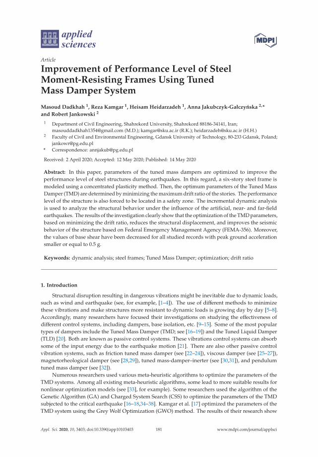
applied sciences

Article

Improvement of Performance Level of SteelMoment-Resisting Frames Using TunedMass Damper System

Masoud Dadkhah 1, Reza Kamgar 1, Heisam Heidarzadeh 1, Anna Jakubczyk-Gałczynska 2,*

and Robert Jankowski 2

1 Department of Civil Engineering, Shahrekord University, Shahrekord 88186-34141, Iran;masouddadkhah1354@gmail.com (M.D.); kamgar@sku.ac.ir (R.K.); heidarzadeh@sku.ac.ir (H.H.)

2 Faculty of Civil and Environmental Engineering, Gdansk University of Technology, 80-233 Gdansk, Poland;jankowr@pg.edu.pl

* Correspondence: annjakub@pg.edu.pl

Received: 2 April 2020; Accepted: 12 May 2020; Published: 14 May 2020

Abstract: In this paper, parameters of the tuned mass dampers are optimized to improve theperformance level of steel structures during earthquakes. In this regard, a six-story steel frame ismodeled using a concentrated plasticity method. Then, the optimum parameters of the Tuned MassDamper (TMD) are determined by minimizing the maximum drift ratio of the stories. The performancelevel of the structure is also forced to be located in a safety zone. The incremental dynamic analysisis used to analyze the structural behavior under the influence of the artificial, near- and far-fieldearthquakes. The results of the investigation clearly show that the optimization of the TMD parameters,based on minimizing the drift ratio, reduces the structural displacement, and improves the seismicbehavior of the structure based on Federal Emergency Management Agency (FEMA-356). Moreover,the values of base shear have been decreased for all studied records with peak ground accelerationsmaller or equal to 0.5 g.

Keywords: dynamic analysis; steel frames; Tuned Mass Damper; optimization; drift ratio

1. Introduction

Structural disruption resulting in dangerous vibrations might be inevitable due to dynamic loads,such as wind and earthquake (see, for example, [1–4]). The use of different methods to minimizethese vibrations and make structures more resistant to dynamic loads is growing day by day [5–8].Accordingly, many researchers have focused their investigations on studying the effectiveness ofdifferent control systems, including dampers, base isolation, etc. [9–15]. Some of the most populartypes of dampers include the Tuned Mass Damper (TMD; see [16–19]) and the Tuned Liquid Damper(TLD) [20]. Both are known as passive control systems. These vibrations control systems can absorbsome of the input energy due to the earthquake motion [21]. There are also other passive controlvibration systems, such as friction tuned mass damper (see [22–24]), viscous damper (see [25–27]),magnetorheological damper (see [28,29]), tuned mass-damper–inerter (see [30,31]), and pendulumtuned mass damper (see [32]).

Numerous researchers used various meta-heuristic algorithms to optimize the parameters of theTMD systems. Among all existing meta-heuristic algorithms, some lead to more suitable results fornonlinear optimization models (see [33], for example). Some researchers used the algorithm of theGenetic Algorithm (GA) and Charged System Search (CSS) to optimize the parameters of the TMDsubjected to the critical earthquake [16–18,34–38]. Kamgar et al. [17] optimized the parameters of theTMD system using the Grey Wolf Optimization (GWO) method. The results of their research show

Appl. Sci. 2020, 10, 3403; doi:10.3390/app10103403 www.mdpi.com/journal/applsci181

Appl. Sci. 2020, 10, 3403

that the maximum structural responses (i.e., roof displacement and stroke ratio) may be reduced byoptimizing parameters of the TMD system and the dynamic behavior of the structure in terms ofminimizing the input, and kinematic energies can be improved. Khatibinia et al. [19] investigated theoptimum parameters of the TMD system intending to minimize the sum of the root-mean-square ofdrifts in the frequency domain under the critical earthquake for a 10-story shear building. Wong [39]evaluated the problem of the input energy dissipation for non-elastic structures equipped with theTMD. The author demonstrated the effectiveness of the TMD system in reducing the dynamic responsesof the structures and concluded that the control of the structure using the TMD system could absorbmore input energy, and subsequently, could damp the absorbed energy. This damping energy improvesthe dynamic performance of the structure. Nigdeli et al. [40] optimized the parameters of the TMDsystem based on the minimization of the acceleration transfer function. The results of their researchindicate that the use of meta-heuristic algorithms to optimize the TMD parameters is more effectivethan classical methods. Kamgar et al. [16] calculated the optimum parameters of the TMD system,taking into account the soil-structure interaction effect adapting the whale optimization algorithm.They showed that the soil type and the objective function were very effective in the optimal parametersobtained for the TMD system.

An accurate estimation of the dynamic capacity of structures is one of the most critical challengesfor researchers. The use of the Incremental Dynamic Analysis (IDA) is essential to evaluate accuratelythe dynamic performance of structures subjected to earthquake loads. For the first time, Berteroin [41] presented the IDA’s time history analysis by scaling the earthquake records step by step andincrementally. Vamvatsikos and Cornell [42] introduced the IDA analysis as a method often used today.The most important advantage of the IDA analysis, in comparison with other methods, is the highability of this type of analysis to show the actual attitude of the structure from the elastic state to theinelastic one. Additionally, this method can consider structural instability due to entering the structurefrom the elastic state into the inelastic one [43]. The optimization algorithm has also been utilized todesign semi-rigid steel frames and reinforced concrete sections (see [44,45]).

In the present paper, a moment-resisting steel frame equipped with the TMD system is selected(see [39,46]). The nonlinear behavior of the joints is modeled using zero-length spring elements androtational springs at the end of the beam-column elements [47]. Additionally, OpenSees software isused to simulate the dynamic structural behavior. Herein, the parameters of the TMD system areoptimized to minimize the maximum drift ratio of structures subjected to earthquakes. Then, the effectof an optimal TMD on the development of the nonlinear seismic efficiency of steel moment-resistingframes is investigated. The main aim of the paper is to investigate a system that, in addition tolower cost, can improve the performance of the structure in comparison with the other vibrationcontrol systems.

The authors of previously published papers focused on the optimization of the parameters of theTMD system by calculating the optimal values of the TMD system numerically using the optimizationalgorithms [16–19,34–40]. The most important question is whether these optimal values can still controlthe dynamic responses of structures by changing the characteristics of the earthquake. Therefore,in this paper, the controlled structure is subjected to several incremental dynamics analyses usingthe optimal values for the TMD system to answer this question. The answer to the question that thecontrolled structure can withstand large earthquakes is vital in this regard. Additionally, the otherquestion is whether the controlled structure can minimize the structural responses in other ranges ofthe peak ground acceleration (PGA) rather than the studied earthquakes? In fact, the structure is firstdesigned to an earthquake with the PGA equal to 1 g (g is the acceleration of gravity) using a TMDsystem. Then the responses of the controlled structure are examined using the incremental dynamicanalyses by changing the PGA from 0.1 g to 1 g. Additionally, in this paper, for the first time, the LifeSafety constraint is introduced to keep the structure in a safe zone based on FEMA-356 [48].

182

Appl. Sci. 2020, 10, 3403

2. Optimal Design of the TMD System

The paper is focused on an optimization method of the parameters of the TMD system (includingdamping, stiffness, and mass). The optimization is conducted according to a reduction in the maximumdrift ratio of structures exposed to earthquakes. This criterion is upon the limitation proposed byFEMA-356 [48] for the maximum allowable drift ratio of the steel moment-resisting frame. Therefore,the optimal design of the TMD system for a steel moment-resisting frame can be formulated as:

Find : Md, Kd, Cd

Minimize : max(

max|dri f ti|with TMDmax|dri f ti|without TMD

)× 100, i = 1, 2, 3, . . . , n

Subjected to : Mmind ≤Md ≤Mmax

d

Kmind ≤ Kd ≤ Kmax

d (1)

Cmind ≤ Cd ≤ Cmax

d

max(∣∣∣ud(t) − xroo f (t)

∣∣∣) ≤ 1000 (mm)

max∣∣∣dri f ti

∣∣∣with TMD ≤ 0.025, i = 1, 2, 3, . . . , n

where Md, Kd and Cd indicate the mass, stiffness, and damping coefficient for the TMD system,respectively. Mmin

d , Mmaxd , Kmin

d , Kmaxd , Cmin

d and Cmaxd are the lower and upper bounds of the TMD

mass, stiffness and damping constants, respectively. These lower and upper bounds have been selectedbased on the work [46].

3. Passive Control Systems

Currently, the control of the seismic response of the structures subjected to dynamic loads isa method that can help engineers to design structures. Among various methods of seismic control,the passive control method is one of the most popular, due to the lower cost of construction andmaintenance. One of the passive control systems is the application of TMD. This system, consistingof a mass, damping, and linear spring, is typically installed on the roof of the structure. The systemreduces the dynamic response of the structure by affecting its dominant mode. The mass of the TMDsystem moves with a different phase relative to the structure, and it improves the seismic structuralresponse by the dissipation of energy [49–51]. The efficiency of the TMD system is highly dependent onits parameters. Therefore, the optimization of these parameters for the seismic control of tall structuresagainst dynamic loads is one of the crucial issues.

A schematic view of the TMD system is exhibited in Figure 1. In this study, the Water CycleAlgorithm (WCA) has been used to reduce the relative displacement of the considered frame by theLS performance level presented in FEMA-356 [48] (i.e., the maximum allowable drift ratio for thesteel moment-resisting frame is 2.5%). Therefore, the dynamic capacity and the performance of thecontrolled structure have been investigated using the IDA analysis.

183

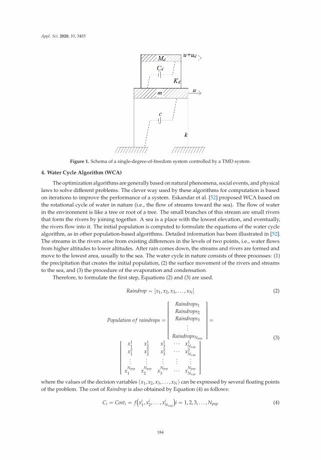
Appl. Sci. 2020, 10, 3403

Figure 1. Schema of a single-degree-of-freedom system controlled by a TMD system.

4. Water Cycle Algorithm (WCA)

The optimization algorithms are generally based on natural phenomena, social events, and physicallaws to solve different problems. The clever way used by these algorithms for computation is basedon iterations to improve the performance of a system. Eskandar et al. [52] proposed WCA based onthe rotational cycle of water in nature (i.e., the flow of streams toward the sea). The flow of waterin the environment is like a tree or root of a tree. The small branches of this stream are small riversthat form the rivers by joining together. A sea is a place with the lowest elevation, and eventually,the rivers flow into it. The initial population is computed to formulate the equations of the water cyclealgorithm, as in other population-based algorithms. Detailed information has been illustrated in [52].The streams in the rivers arise from existing differences in the levels of two points, i.e., water flowsfrom higher altitudes to lower altitudes. After rain comes down, the streams and rivers are formed andmove to the lowest area, usually to the sea. The water cycle in nature consists of three processes: (1)the precipitation that creates the initial population, (2) the surface movement of the rivers and streamsto the sea, and (3) the procedure of the evaporation and condensation.

Therefore, to formulate the first step, Equations (2) and (3) are used.

Raindrop = [x1, x2, x3, . . . , xN] (2)

Population o f raindrops =

⎡⎢⎢⎢⎢⎢⎢⎢⎢⎢⎢⎢⎢⎢⎢⎢⎢⎢⎢⎢⎣

Raindrops1

Raindrops2

Raindrops3...

RaindropsNpop

⎤⎥⎥⎥⎥⎥⎥⎥⎥⎥⎥⎥⎥⎥⎥⎥⎥⎥⎥⎥⎦=

⎡⎢⎢⎢⎢⎢⎢⎢⎢⎢⎢⎢⎢⎢⎢⎢⎢⎣

x11 x1

2 x13 · · · x1

Nvar

x21 x2

2 x23 · · · x2

Nvar...

......

......

xNpop

1 xNpop2 x

Npop3 · · · x

NpopNvar

⎤⎥⎥⎥⎥⎥⎥⎥⎥⎥⎥⎥⎥⎥⎥⎥⎥⎦

(3)

where the values of the decision variables (x1, x2, x3, . . . , xN) can be expressed by several floating pointsof the problem. The cost of Raindrop is also obtained by Equation (4) as follows:

Ci = Costi = f(xi

1, xi2, . . . , xi

Nvar

)i = 1, 2, 3, . . . , Npop (4)

184

Appl. Sci. 2020, 10, 3403

in which Npop and Nvar represent the stream population as the initial population and some designvariables, respectively. Costi shows the cost estimation function of the variables, see for example [53].Firstly, the parameter Npop is generated, and a number is selected for the Nsr parameter as the bestvalue (minimum values) for the rivers and sea in the first step. The number of rivers and the sea iscalculated as a variable Nsr as follows:

Nsr = Number o f Rivers + 1︸︷︷︸Sea

(5)

NRaindrop = Npop −Nsr (6)

The parameter NRaindrop is the rest of the population that make up possible routes to the sea or therivers. Equation (7) is used depending on the intensity of the flow to determine and assign raindropsin rivers and sea:

NSn = Round

⎧⎪⎪⎨⎪⎪⎩∣∣∣∣∣∣∣

Costn∑Nsri=1 Costi

∣∣∣∣∣∣∣×NRaindrops

⎫⎪⎪⎬⎪⎪⎭, n = 1, 2, . . . , NSR (7)

in which NSn is a number of streams that flow into some specific rivers or the sea. Besides, the newpositions of the streams and rivers are also expressed as follows:

→X

t+1

Stream =→X

t

Stream + rand×C×(→X

t

River −→X

t

Stream

)(8)

→X

t+1

River =→X

t

River + rand×C×(→X

t

Sea −→X

t

River

)(9)

in which rand is a uniformly distributed random number from the interval 〈0, 1〉. Additionally,the parameter C has a number between 1 and 2, and it is usually close to 2. If the evaporation conditionsare taken into account, it can help the algorithm to prevent premature convergence:

I f ‖→XSea(t) −→X

i

River(t)‖ < dmax(t)orrand ∈ 〈0, 1〉,n = 1, 2, 3, . . . , Nsr − 1

(10)

where dmax is a small number (close to zero). It indicates that the river is connected to the sea whenthe river is away from the sea less than the value of dmax. The parameter dmax can control the optimalsolution, and its value is updated as follows:

dmax(t + 1) = dmax(t) − dmax(t)MaxIteration

(11)

Additionally, after considering the evaporation conditions for the algorithm, the new streams arerandomly generated in the search space as follows:

→X

New

Stream = LB + rand · (UB− LB) (12)

in which the parameters UB, LB are the minimum and maximum boundary conditions, respectively.Then, the river flowing to the sea is selected from the best new raindrops, and the other remainingnew raindrops create streams that can flow to the river or sea. Equation (13) is utilized for the streamsthat have flowed to the sea to check the computational performance and convergence rate of theoptimization problem:

→X

New

Stream = Xsea +√μ× randn(1, Nvar) (13)

where μ is a coefficient, and the value of 0.1 has been proposed for it in [52].

185

Appl. Sci. 2020, 10, 3403

5. Incremental Dynamic Analysis (IDA)

IDA is an accurate analysis method that is capable of estimating the seismic behavior of structuressubjected to different earthquakes. One of the principles of the functional design of structures is theuse of the nonlinear dynamic capacity of load-bearing members in the design of structures.

The stiffness values of the structural elements decrease when a severe dynamic load is applied tothe structure. As a result, the stiffness matrix of the structure will decrease when the plastic joints areformed in the members. Finally, it results in the redistribution of the forces among the members of thestructure. Finally, the structure experiences more deformation because of yielding in some elements,and it leads to more significant energy absorption and damping.

In IDA, a structure is subjected to a mapping acceleration. The mapping acceleration is selectedfrom an earthquake. Then, the earthquake is scaled so that its maximum acceleration is equal to 1 g.Hence, the structure is subjected to the scaled earthquake record. Next, the maximum acceleration isadded to the value of 0.2 g, and the structure is re-analyzed. This process continues until the maximumacceleration of the earthquake is equal to 1 g. Finally, the IDA curve is plotted for the frame andearthquake. The IDA shows the nonlinear dynamic response of the structure against the intensity ofthe seismic excitation.

6. Modeling and Verification

A six-story steel frame is selected in this study (see Figure 2). The frame has already been studiedby several researchers (see [39,46]). A finite element software named OpenSees [47] is used to modelthe frame. Additionally, the modified Ibarra–Krawinkler (IMK) deterioration model (see [54–56]) isutilized to simulate the nonlinear behavior of the plastic joints. According to this constitutive model,the zero-length elements are considered as concentrated plasticity at the beam-column connections.The IMK model takes into account the cyclic response of the springs, which shows the nonlinearbehavior of the frame. Due to the presence of the gravitational loads, as well as the TMD mass,the P-delta effect must be taken into account to consider the enhanced structural responses. For thispurpose, a virtual column with truss elements attached to the base of the structure is analyzed.Additionally, all columns are considered to be fixed at the base of the structure. Since the rotationalsprings and frame elements are connected in series, the stiffness of the rotational elements must bemodified in such a way that the stiffness value of elements and the actual stiffness of the frame arethe same. For this purpose, the stiffness of the rotational springs is considered to be n = 10 timeshigher than the rotational stiffness of the elastic elements. The stiffness and also the moment of inertiaof the elastic element are multiplied into the (n + 1)/n. Finally, to match the nonlinear behavior ofthe elements and the actual behavior of the frame, the strain coefficient of the plastic joint should bemodified according to Equation (14)—see [54–57].

αs,spring = αs,mem/(1 + n · (1− αs,mem)) (14)

where αs,mem shows the real strain coefficient of the frame, and αs,spring is the strain hardening coefficientof the rotational spring. All beam elements are subjected to the uniformly distributed load equal to21.89 kN/m. Additionally, the following relations (Equations (15)–(22)) are used to determine theparameters required in the definition of the behavioral curve of the rotational springs [54–57]:

θp = 0.318(

htw

)−0.55(

b f2tw

)−0.345(Lbry

)−0.023(Ld

)0.09(

c1unit·d533

)−0.33( c2unit·Fy355

)−0.13

d ≥ 21in(15)

θpc = 5.63(

htw

)−0.565(

b f2tw

)−0.8( c1unit·d533

)−0.28( c2unit·Fy355

)−0.43

d ≥ 21in(16)

186

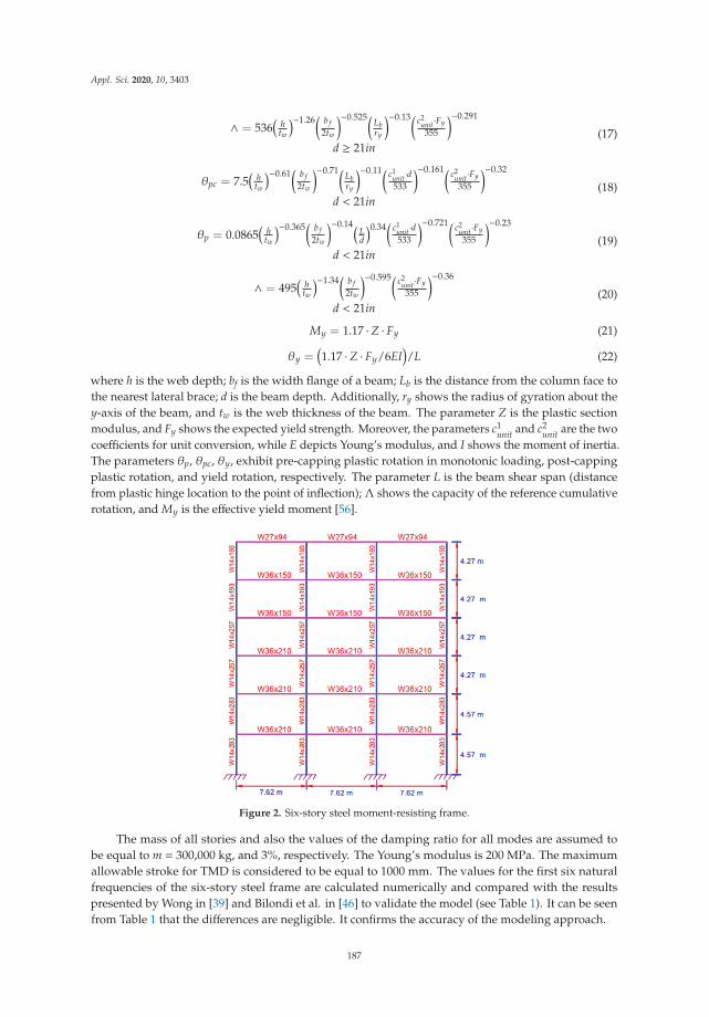
Appl. Sci. 2020, 10, 3403

∧ = 536(

htw

)−1.26(

b f2tw

)−0.525(Lbry

)−0.13( c2unit·Fy355

)−0.291

d ≥ 21in(17)

θpc = 7.5(

htw

)−0.61(

b f2tw

)−0.71(Lbry

)−0.11( c1unit·d533

)−0.161( c2unit·Fy355

)−0.32

d < 21in(18)

θp = 0.0865(

htw

)−0.365(

b f2tw

)−0.14(Ld

)0.34(

c1unit·d533

)−0.721( c2unit·Fy355

)−0.23

d < 21in(19)

∧ = 495(

htw

)−1.34(

b f2tw

)−0.595( c2unit·Fy355

)−0.36

d < 21in(20)

My = 1.17 ·Z · Fy (21)

θy =(1.17 ·Z · Fy/6EI

)/L (22)

where h is the web depth; bf is the width flange of a beam; Lb is the distance from the column face tothe nearest lateral brace; d is the beam depth. Additionally, ry shows the radius of gyration about they-axis of the beam, and tw is the web thickness of the beam. The parameter Z is the plastic sectionmodulus, and Fy shows the expected yield strength. Moreover, the parameters c1

unit and c2unit are the two

coefficients for unit conversion, while E depicts Young’s modulus, and I shows the moment of inertia.The parameters θp, θpc, θy, exhibit pre-capping plastic rotation in monotonic loading, post-cappingplastic rotation, and yield rotation, respectively. The parameter L is the beam shear span (distancefrom plastic hinge location to the point of inflection); Λ shows the capacity of the reference cumulativerotation, and My is the effective yield moment [56].

Figure 2. Six-story steel moment-resisting frame.

The mass of all stories and also the values of the damping ratio for all modes are assumed tobe equal to m = 300,000 kg, and 3%, respectively. The Young’s modulus is 200 MPa. The maximumallowable stroke for TMD is considered to be equal to 1000 mm. The values for the first six naturalfrequencies of the six-story steel frame are calculated numerically and compared with the resultspresented by Wong in [39] and Bilondi et al. in [46] to validate the model (see Table 1). It can be seenfrom Table 1 that the differences are negligible. It confirms the accuracy of the modeling approach.

187

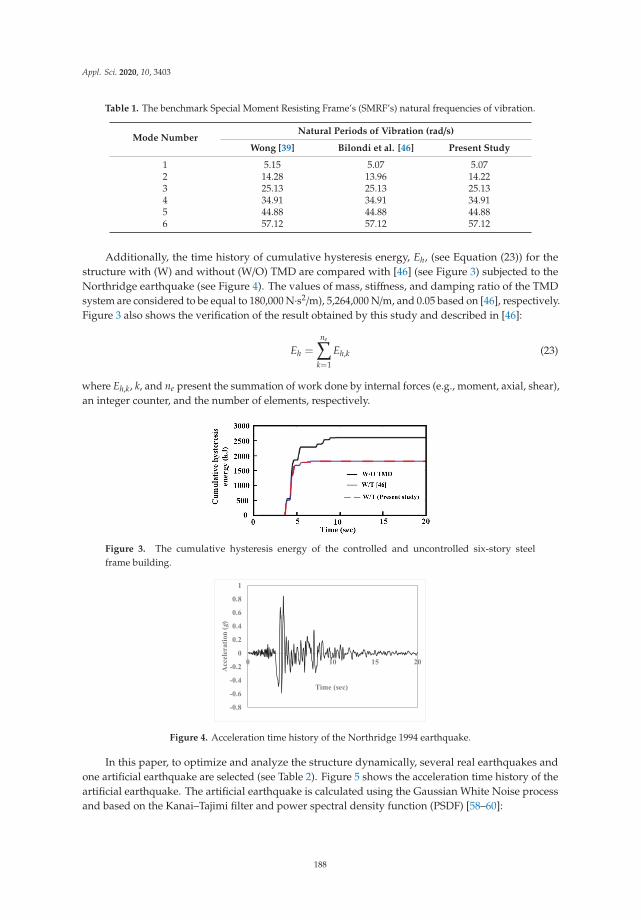
Appl. Sci. 2020, 10, 3403

Table 1. The benchmark Special Moment Resisting Frame’s (SMRF’s) natural frequencies of vibration.

Mode NumberNatural Periods of Vibration (rad/s)

Wong [39] Bilondi et al. [46] Present Study

1 5.15 5.07 5.072 14.28 13.96 14.223 25.13 25.13 25.134 34.91 34.91 34.915 44.88 44.88 44.886 57.12 57.12 57.12

Additionally, the time history of cumulative hysteresis energy, Eh, (see Equation (23)) for thestructure with (W) and without (W/O) TMD are compared with [46] (see Figure 3) subjected to theNorthridge earthquake (see Figure 4). The values of mass, stiffness, and damping ratio of the TMDsystem are considered to be equal to 180,000 N·s2/m), 5,264,000 N/m, and 0.05 based on [46], respectively.Figure 3 also shows the verification of the result obtained by this study and described in [46]:

Eh =

ne∑k=1

Eh,k (23)

where Eh,k, k, and ne present the summation of work done by internal forces (e.g., moment, axial, shear),an integer counter, and the number of elements, respectively.

Figure 3. The cumulative hysteresis energy of the controlled and uncontrolled six-story steelframe building.

Figure 4. Acceleration time history of the Northridge 1994 earthquake.

In this paper, to optimize and analyze the structure dynamically, several real earthquakes andone artificial earthquake are selected (see Table 2). Figure 5 shows the acceleration time history of theartificial earthquake. The artificial earthquake is calculated using the Gaussian White Noise processand based on the Kanai–Tajimi filter and power spectral density function (PSDF) [58–60]:

188

Appl. Sci. 2020, 10, 3403

SKanai−Tajimi(ω) = S0[ω4

g+(2×ωg×ξg×ω)2

(ω2−ω2g)

2+(2×ωg×ξg×ω)2 ]

S0 =0.03×ξg

π×ωg×(4×ξ2g+1)

(24)

where S0, ωg, and ξg are the intensity of the PSDF, frequency, and damping of the soil, respectively.In this paper,ωg and ξg are considered to be equal to 25.13 rad/s and 0.8 rad/s, respectively, based on [61],which indicates that the structure has been located on the stiff soil. The strong ground motion of theartificial earthquake is big enough, and it can be used in the dynamic analysis of the structures basedon Uniform Building Code 97 [62].

It should be noted that Chandler’s classification has been considered in the selection of theearthquake to cover all existing categories for the earthquakes (see [8,63]).

Figure 5. Acceleration time history of an artificial earthquake.

Table 2. Characteristics of the selected scaled earthquakes.

Abbreviation AE NE3 NE2 NE1 FE3 FE2 FE1

EarthquakeAn

artificialearthquake

KocaeliTurkey

GazliUSSR

Chi-ChiTaiwan

SuperstitionHills-02 San Fernando Duzce

Turkey

Station — Arcelik Karakyr CHY101El CentroImp. Co.

Cent

LA—HollywoodStor FF Bolu

PGA(g) 1 1 1 1 1 1 1

PGA/PGV (g·s/m) 0.206 0.601 1.277 0.630 0.743 1.035 1.32

Strong ground motionduration (s) 18 13.265 6.956 28.55 27.99 13.15 8.55

Predominant Period (s) 0.2 0.28 0.14 1.08 0.22 0.24 0.32

Total time duration (s) 19.98 29.995 13.0878 88.995 59.99 79.44 55.89

Arias Intensity (m/s) 33.311 15.370 7.599 12.291 8.646 13.396 6.806

PGA—Peak Ground Acceleration; PGV—Peak Ground Velocity.

189

Appl. Sci. 2020, 10, 3403

7. Results and Discussion

7.1. Optimization of the Parameters of the TMD System

In this paper, a six-story steel frame equipped with the TMD system is studied. One of the mostcritical issues with the TMD systems is to determine their optimal parameters. Therefore, differentmethods are used to optimize these parameters. Among them, the meta-heuristic algorithms arecommonly used due to the current uncertainty of the mathematical problem as well as differentscenarios used for the objective function. In general, all meta-heuristic algorithms start from a localsearch and eventually reach the desired values. In this paper, a WCA (see Section 4) meta-heuristicalgorithm has been selected because of its ability to solve constraint problems. Therefore, the optimumparameters for the TMD system are calculated by WCA to minimize the relative displacement of thestories adapted to the LS performance level presented by FEMA-356 [48]. The optimum parameters ofthe TMD system exposed to the near- and far-field earthquakes, as well as to the artificial earthquake,have been presented in Table 3.

In fact, the water cycle algorithm has been used to optimize the parameters of the TMD systemsubjected to the far-, near-field, and artificial earthquakes. Equations (2)–(13) are utilized to perform anoptimization problem using Matlab software. Additionally, Equation (1) is used to make an optimizationproblem with an upper and lower boundary for the optimization variables. Table 3 shows the optimumparameters of the TMD system subjected to different studied earthquakes.

Table 3. Optimum parameters achieved for TMD subjected to the drift ratio constraint.

Earthquake Ktmd (N/mm) Ctmd (N·s/mm) Mtmd (N·s2/mm)

FE1 404.94 770.18 180FE2 543.76 304.28 180FE3 490.1 942.89 180NE1 421.67 1753.1 180NE2 315.87 972.87 141NE3 405.02 500.0 180AE 405.47 935.66 180

7.2. The Structural Seismic Performance

The results for the structure controlled with the TMD system are shown in Table 4. As it isobserved from the table, the reduction in the base shear is less than 3.49% under different earthquakes,even though the base shear has increased slightly during the earthquakes NE1 and AE. Hence, due tothe insignificant reduction in the base shear under different earthquakes, it might be concluded thatthe optimization of the TMD parameters focused on reducing the drift will not have a significant effecton the base shear of structures. Table 4 shows that the average acceleration of the structure equippedwith the TMD system has increased under the FE2 and AE earthquakes by about 5% but, for the restof earthquakes, the parameters of TMD optimized based on drift can reduce the acceleration of thestructure. Similar results have been obtained for the average displacement of the structure controlledwith the TMD system. In fact, for the FE2, NE3 earthquakes, the average displacement of the controlledstructure has increased while this parameter has decreased for other earthquakes. It should be notedthat the negative and positive signs in Table 4 show the decrease and increase in the average reduction,respectively. In other words, the positive value shows that the parameter is reduced, and the negativevalue shows that it is increased.

The maximum drift ratio of all stories and the roof displacement time history of the structure aredepicted in Figures 6 and 7 with and without the TMD system subjected to the near- and far-fieldearthquakes. It is clear from the table that the maximum drift ratio of the stories has been reduced forall earthquakes. It is also observed that the roof displacement has increased for some earthquakes(e.g., FE2, and NE3). The controlled structure has been vibrated about a new plastic axis subjected to

190

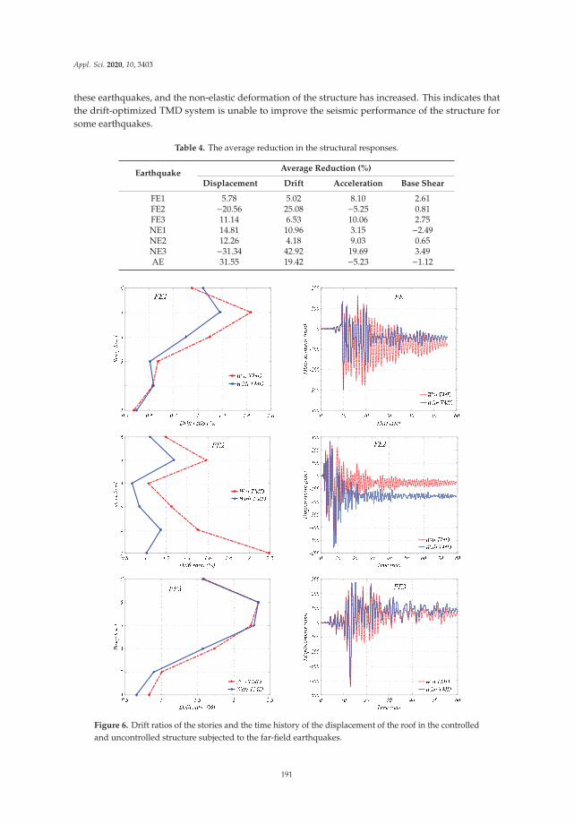
Appl. Sci. 2020, 10, 3403

these earthquakes, and the non-elastic deformation of the structure has increased. This indicates thatthe drift-optimized TMD system is unable to improve the seismic performance of the structure forsome earthquakes.

Table 4. The average reduction in the structural responses.

EarthquakeAverage Reduction (%)

Displacement Drift Acceleration Base Shear

FE1 5.78 5.02 8.10 2.61FE2 −20.56 25.08 −5.25 0.81FE3 11.14 6.53 10.06 2.75NE1 14.81 10.96 3.15 −2.49NE2 12.26 4.18 9.03 0.65NE3 −31.34 42.92 19.69 3.49AE 31.55 19.42 −5.23 −1.12

Figure 6. Drift ratios of the stories and the time history of the displacement of the roof in the controlledand uncontrolled structure subjected to the far-field earthquakes.

191

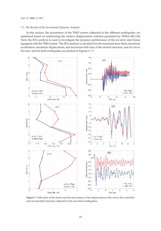
Appl. Sci. 2020, 10, 3403

7.3. The Results of the Incremental Dynamic Analysis

In this section, the parameters of the TMD system subjected to the different earthquakes areoptimized based on minimizing the relative displacement criterion presented by FEMA-356 [48].Next, the IDA analysis is used to investigate the dynamic performance of the six-story steel frameequipped with the TMD system. The IDA analysis is calculated for the maximum base shear, maximumacceleration, maximum displacement, and maximum drift ratio of the desired structure, and its curvesfor near- and far-field earthquakes are plotted in Figures 8–11.

Figure 7. Drift ratios of the stories and the time history of the displacement of the roof in the controlledand uncontrolled structure subjected to the near-field earthquakes.

192

Appl. Sci. 2020, 10, 3403

7.3.1. The Results of IDA for the Drift Ratio

The drift ratio of the structures with and without the TMD system is shown in Figure 8. It can beconcluded that the maximum drift ratio of all stories has been decreased for the structure controlledwith the TMD system subjected to the FE1, NE1, and NE2 earthquakes. The drift ratio has increasedfor the FE2 earthquake with PGA equal to 0.9 g and 1 g. Additionally, the maximum drift ratio of thestructure has increased under the FE3 earthquake in the range of 0.6g ≤ PGA ≤ 0.9g. A disturbancehas taken place for the NE3 earthquake in the range of 0.7g ≤ PGA ≤ 0.9g. Therefore, it might beconcluded that the TMD parameters should be evaluated for PGA values larger than 0.5 g in controllingthe drift ratio.

Figure 8. Maximum drift ratio of the frame subjected to different far- and near-field earthquakes.

193

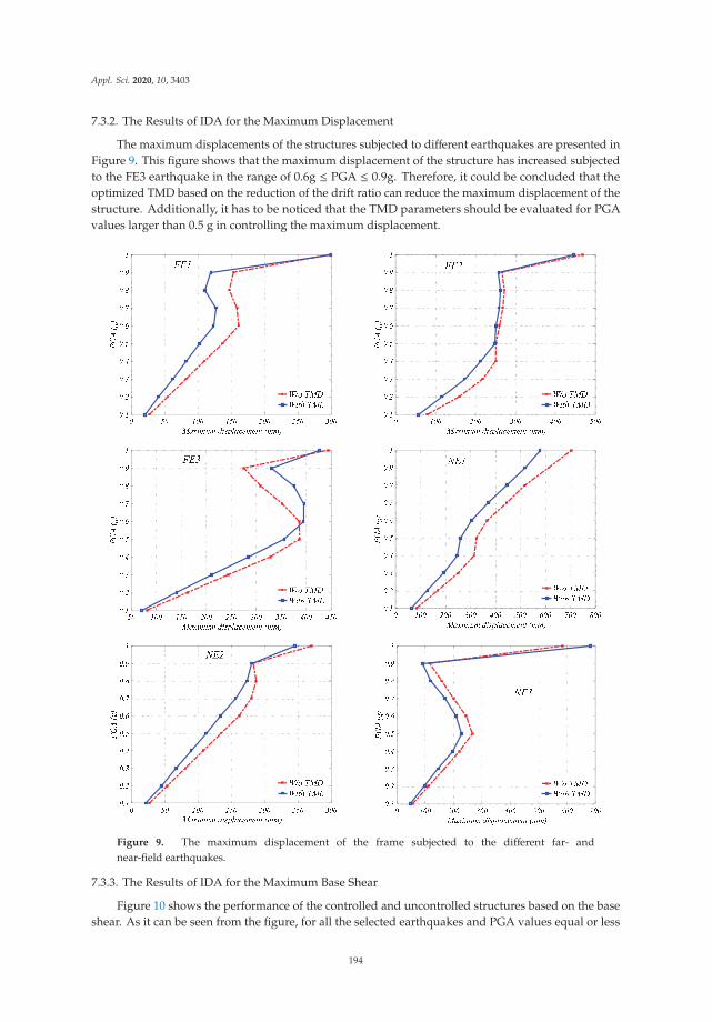
Appl. Sci. 2020, 10, 3403

7.3.2. The Results of IDA for the Maximum Displacement

The maximum displacements of the structures subjected to different earthquakes are presented inFigure 9. This figure shows that the maximum displacement of the structure has increased subjectedto the FE3 earthquake in the range of 0.6g ≤ PGA ≤ 0.9g. Therefore, it could be concluded that theoptimized TMD based on the reduction of the drift ratio can reduce the maximum displacement of thestructure. Additionally, it has to be noticed that the TMD parameters should be evaluated for PGAvalues larger than 0.5 g in controlling the maximum displacement.

Figure 9. The maximum displacement of the frame subjected to the different far- andnear-field earthquakes.

7.3.3. The Results of IDA for the Maximum Base Shear

Figure 10 shows the performance of the controlled and uncontrolled structures based on the baseshear. As it can be seen from the figure, for all the selected earthquakes and PGA values equal or less

194

Appl. Sci. 2020, 10, 3403

than 0.5 g, the maximum base shear of the controlled structure has decreased. Additionally, the baseshear has not changed for PGA larger than 0.5 g. Therefore, it could be concluded that the optimizedTMD system based on minimizing the drift ratio does not have any particular effect on the base shearfor PGA values larger than 0.5 g.

Figure 10. Maximum base shear of the frame subjected to different far- and near-field earthquakes.

7.3.4. The Results of IDA for the Maximum Acceleration of the Structure

A comparison between the results for the maximum acceleration is shown in Figure 11. It canbe concluded that the performance of the structure equipped with the optimized TMD system hasbeen improved in minimizing the maximum acceleration of the structure subjected to the FE1, NE1,and NE2 earthquakes. The maximum acceleration of the structure has increased in the range of0.8g ≤ PGA ≤ 1.0g under the FE2 earthquake. Besides, an increase in the acceleration response has

195

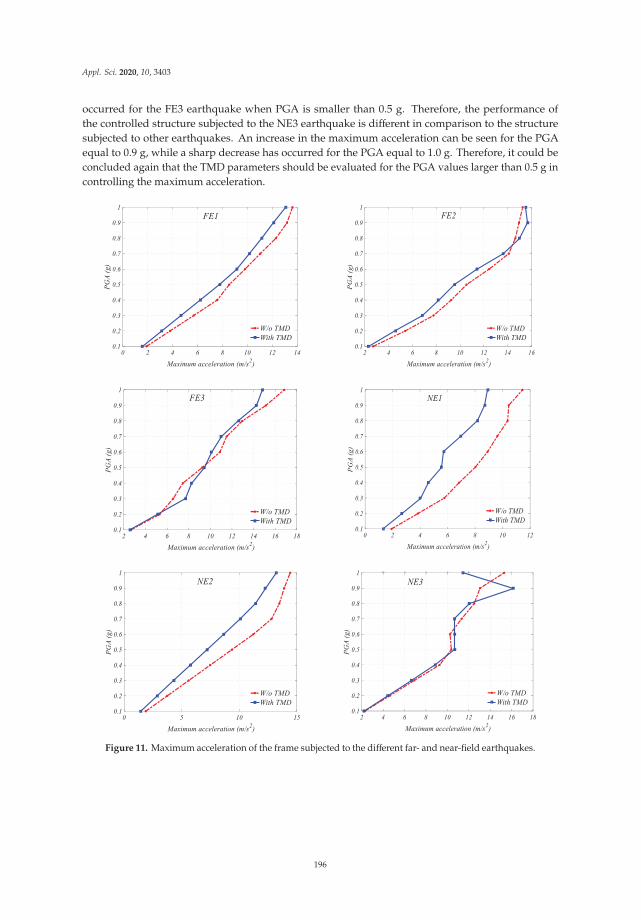
Appl. Sci. 2020, 10, 3403

occurred for the FE3 earthquake when PGA is smaller than 0.5 g. Therefore, the performance ofthe controlled structure subjected to the NE3 earthquake is different in comparison to the structuresubjected to other earthquakes. An increase in the maximum acceleration can be seen for the PGAequal to 0.9 g, while a sharp decrease has occurred for the PGA equal to 1.0 g. Therefore, it could beconcluded again that the TMD parameters should be evaluated for the PGA values larger than 0.5 g incontrolling the maximum acceleration.

Figure 11. Maximum acceleration of the frame subjected to the different far- and near-field earthquakes.

196

Appl. Sci. 2020, 10, 3403

7.4. The Results for the Artificial Earthquake

7.4.1. Seismic Performance of the Controlled and Uncontrolled Structures Exposed to theArtificial Earthquake

Figure 12 presents the responses of the controlled and uncontrolled structures (i.e., drift ratio,maximum displacement, maximum base shear, and the maximum acceleration) exposed to the artificialearthquake. The figure indicates that the TMD system optimized based on the drift ratio can reduceall structural responses, except for the maximum acceleration of the structure. The optimized TMDsystem has also controlled the maximum acceleration of the fifth and sixth stories, but it has increasedthis value for the lower stories.

Figure 12. Maximum drift ratio, displacement, base shear, and acceleration of the frame subjected tothe artificial earthquake.

7.4.2. IDA for the Dynamic Performance of the Controlled and Uncontrolled Structures Exposed to theArtificial Earthquake

The results of IDA for the structure subjected to artificial earthquakes are shown in Figure 13.The performance of the controlled structure shows an increase in the maximum acceleration values inthe range of 0.7g ≤ PGA ≤ 0.8g. The maximum acceleration of the structure has decreased for otherPGA values. Moreover, the value of base shear has decreased for PGA smaller than 0.5 g and remainedconstant for PGA larger than 0.5 g. Additionally, the results show that the performance of the structurehas improved for the maximum displacement and drift ratio.

197

Appl. Sci. 2020, 10, 3403

Figure 13. Results of Incremental Dynamic Analysis (IDA) analysis for the frame subjected to theartificial earthquake.

7.4.3. Investigation of the Performance Level of the Structure Subjected to the Artificial Earthquake

The performance levels of the structure subjected to the artificial earthquake, based on theFEMA-356 [48], are presented in Figure 14. Based on FEMA-356, the maximum drift ratios of thecontrolled and uncontrolled structures have been categorized in the figure as:

1. Immediate Occupancy ≤ 0.7%;2. 0.7% ≤ Life Safety ≤ 2.5%;3. 2.5% ≤ Collapse Prevention ≤ 5%.

As it can be observed from Figure 14, the six-story steel moment-resisting frame without TMDsystem has entered into the collapse prevention level for PGA larger than 0.8 g, but the performancelevel of the structure controlled with the TMD system has remained in the life safety range. Therefore,results indicate that the optimization of the TMD parameters to minimize the maximum drift ratiosmaller than 2.5% substantially improve the seismic performance of the structure subjected to theartificial earthquake. It leads to a delay in the fracture of the bending connections (see FEMA-356 [48]),and it can help the beams and columns to sustain distortion.

198

Appl. Sci. 2020, 10, 3403

PGA

(g)

Figure 14. The performance level of the frame subjected to the artificial earthquake.

Besides, to evaluate the capability of the method presented in this paper, the six-story steelmoment-resisting frame structure is considered. For this purpose, two other objective functions (seeEquation (25)) are considered, and the optimal values of the TMD system are computed under theartificial earthquake. Table 5 shows the optimal values of the TMD system for different objectivefunctions. It should be noted that the constraints and upper and lower bounds are considered as inEquation (1) and Ref. [46].

Find : Md, Kd, Cd

Minimize : max(

max|dri f ti|with TMDmax|dri f ti|without TMD

)× 100, i = 1, 2, 3, . . . , n (O .F 1)

Minimize : max(

max∣∣∣Accroo f

∣∣∣with TMD

max∣∣∣Accroo f

∣∣∣without TMD

)× 100, i = 1, 2, 3, . . . , n (O .F 2) (25)

Minimize : max(

max∣∣∣Disproo f

∣∣∣with TMD

max∣∣∣Disproo f

∣∣∣without TMD

)× 100, i = 1, 2, 3, . . . , n (O .F 3)

where O.F., Accroof, and Disproof show the objective function, roof acceleration, and displacement,respectively. The last-second objective functions are usually used by researchers to optimize theparameters of vibration control systems [18,34,37,40]. Additionally, the computational workload, in theform of required running time, for each objective function is presented in Table 5. The calculationshave been run on a computer with a 64-bit operating system and CPU Intel(R) Core(TM) i3-4170 CPU3.70 GHz with 4 GB RAM.

Table 5. Optimum parameters and required running time achieved for the TMD subjected the artificialearthquake for different objective functions.

O.F Ktmd (N/mm) Ctmd (N·s/mm) Mtmd (N·s2/mm)Required Running Time

(s)

O.F 1 405.47 935.66 180 997.854O.F. 2 211.021 1130.6 122.87 865.528O.F. 3 250.025 749.317 163.156 1114.548

199

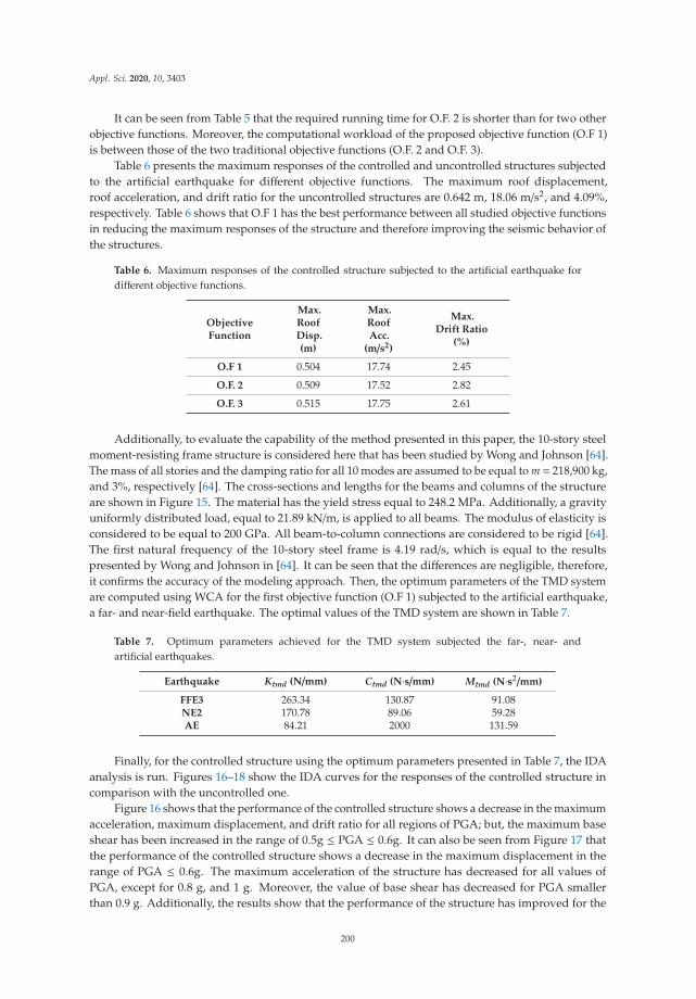
Appl. Sci. 2020, 10, 3403

It can be seen from Table 5 that the required running time for O.F. 2 is shorter than for two otherobjective functions. Moreover, the computational workload of the proposed objective function (O.F 1)is between those of the two traditional objective functions (O.F. 2 and O.F. 3).

Table 6 presents the maximum responses of the controlled and uncontrolled structures subjectedto the artificial earthquake for different objective functions. The maximum roof displacement,roof acceleration, and drift ratio for the uncontrolled structures are 0.642 m, 18.06 m/s2, and 4.09%,respectively. Table 6 shows that O.F 1 has the best performance between all studied objective functionsin reducing the maximum responses of the structure and therefore improving the seismic behavior ofthe structures.

Table 6. Maximum responses of the controlled structure subjected to the artificial earthquake fordifferent objective functions.

ObjectiveFunction

Max.RoofDisp.(m)

Max.RoofAcc.

(m/s2)

Max.Drift Ratio

(%)

O.F 1 0.504 17.74 2.45

O.F. 2 0.509 17.52 2.82

O.F. 3 0.515 17.75 2.61

Additionally, to evaluate the capability of the method presented in this paper, the 10-story steelmoment-resisting frame structure is considered here that has been studied by Wong and Johnson [64].The mass of all stories and the damping ratio for all 10 modes are assumed to be equal to m = 218,900 kg,and 3%, respectively [64]. The cross-sections and lengths for the beams and columns of the structureare shown in Figure 15. The material has the yield stress equal to 248.2 MPa. Additionally, a gravityuniformly distributed load, equal to 21.89 kN/m, is applied to all beams. The modulus of elasticity isconsidered to be equal to 200 GPa. All beam-to-column connections are considered to be rigid [64].The first natural frequency of the 10-story steel frame is 4.19 rad/s, which is equal to the resultspresented by Wong and Johnson in [64]. It can be seen that the differences are negligible, therefore,it confirms the accuracy of the modeling approach. Then, the optimum parameters of the TMD systemare computed using WCA for the first objective function (O.F 1) subjected to the artificial earthquake,a far- and near-field earthquake. The optimal values of the TMD system are shown in Table 7.

Table 7. Optimum parameters achieved for the TMD system subjected the far-, near- andartificial earthquakes.

Earthquake Ktmd (N/mm) Ctmd (N·s/mm) Mtmd (N·s2/mm)

FFE3 263.34 130.87 91.08NE2 170.78 89.06 59.28AE 84.21 2000 131.59

Finally, for the controlled structure using the optimum parameters presented in Table 7, the IDAanalysis is run. Figures 16–18 show the IDA curves for the responses of the controlled structure incomparison with the uncontrolled one.

Figure 16 shows that the performance of the controlled structure shows a decrease in the maximumacceleration, maximum displacement, and drift ratio for all regions of PGA; but, the maximum baseshear has been increased in the range of 0.5g ≤ PGA ≤ 0.6g. It can also be seen from Figure 17 thatthe performance of the controlled structure shows a decrease in the maximum displacement in therange of PGA ≤ 0.6g. The maximum acceleration of the structure has decreased for all values ofPGA, except for 0.8 g, and 1 g. Moreover, the value of base shear has decreased for PGA smallerthan 0.9 g. Additionally, the results show that the performance of the structure has improved for the

200

Appl. Sci. 2020, 10, 3403

maximum drift ratio for the PGA smaller than 0.5 g. Figure 18 indicates that the performance of thecontrolled structure shows a decrease in all regions of PGA for the maximum drift ratio, acceleration,and base shear. The maximum displacement of the structure has decreased for all values of PGAin the range of PGA ≤ 0.8g. Therefore, the results show that the performance of the structure hasimproved significantly.

Figure 15. Ten-story steel moment-resisting frame.

201

Appl. Sci. 2020, 10, 3403

50 150 250 350 450

0.1

0.2

0.3

0.4

0.5

0.6

0.7

0.8

0.9

1

PGA

(g)

Maximum displacement (mm)

W/o TMDWith TMD

NE2

0.2 0.6 1 1.4 1.8

0.1

0.2

0.3

0.4

0.5

0.6

0.7

0.8

0.9

1

Maximum drift ratio (%)

PGA

(g)

W/o TMDWith TMD

NE2

0 5 10 15

0.1

0.2

0.3

0.4

0.5

0.6

0.7

0.8

0.9

1

Maximum acceleration (m/s2)

PGA

(g)

W/o TMDWith TMD

NE2

1 3 5 7 9x 106

0.1

0.2

0.3

0.4

0.5

0.6

0.7

0.8

0.9

1

Maximum base shear (N)

PGA

(g)

W/o TMDWith TMD NE2

Figure 16. Results of IDA analysis for the frame subjected to a near-field earthquake (Gazli earthquake).

50 150 250 350 450

0.1

0.2

0.3

0.4

0.5

0.6

0.7

0.8

0.9

1

PGA

(g)

Maximum displacement (mm)

W/o TMDWith TMD

FE3

0 0.5 1 1.5 2 2.5

0.1

0.2

0.3

0.4

0.5

0.6

0.7

0.8

0.9

1

Maximum drift ratio (%)

PGA

(g)

W/o TMDWith TMD

FE3

2 6 10 14 18

0.1

0.2

0.3

0.4

0.5

0.6

0.7

0.8

0.9

1

PGA

(g)

Maximum acceleration (m/s2)

W/o TMDWith TMD

FE3

1 3 5 7 9x 106

0.1

0.2

0.3

0.4

0.5

0.6

0.7

0.8

0.9

1

Maximum base shear (N)

PGA

(g)

W/o TMDWith TMD FE3

Figure 17. Results of IDA analysis for the frame subjected to a far-field earthquake(Superstition earthquake).

202

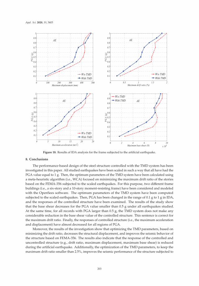
Appl. Sci. 2020, 10, 3403

0 100 200 300 400 500

0.1

0.2

0.3

0.4

0.5

0.6

0.7

0.8

0.9

1PG

A (g

)

Maximum displacement (mm)

W/o TMDWith TMD

AE

0 0.5 1 1.5 2

0.1

0.2

0.3

0.4

0.5

0.6

0.7

0.8

0.9

1

Maximum drift ratio (%)

PGA

(g)

W/o TMDWith TMD

AE

0 5 10 15 20 20

0.1

0.2

0.3

0.4

0.5

0.6

0.7

0.8

0.9

1

PGA

(g)

Maximum acceleration (m/s2)

W/o TMDWith TMD

AE

0 2 4 6 8 10x 106

0.1

0.2

0.3

0.4

0.5

0.6

0.7

0.8

0.9

1

Maximum base shear (N)

PGA

(g)

W/o TMDWith TMD AE

Figure 18. Results of IDA analysis for the frame subjected to the artificial earthquake.

8. Conclusions

The performance-based design of the steel structure controlled with the TMD system has beeninvestigated in this paper. All studied earthquakes have been scaled in such a way that all have had thePGA value equal to 1 g. Then, the optimum parameters of the TMD system have been calculated usinga meta-heuristic algorithm (i.e., WCA) focused on minimizing the maximum drift ratio of the storiesbased on the FEMA-356 subjected to the scaled earthquakes. For this purpose, two different framebuildings (i.e., a six-story and a 10-story moment-resisting frame) have been considered and modeledwith the OpenSees software. The optimum parameters of the TMD system have been computedsubjected to the scaled earthquakes. Then, PGA has been changed in the range of 0.1 g to 1 g in IDA,and the responses of the controlled structure have been examined. The results of the study showthat the base shear decreases for the PGA value smaller than 0.5 g under all earthquakes studied.At the same time, for all records with PGA larger than 0.5 g, the TMD system does not make anyconsiderable reduction in the base shear value of the controlled structure. This sentence is correct forthe maximum drift ratio. Finally, the responses of controlled structure (i.e., the maximum accelerationand displacement) have almost decreased for all regions of PGA.

Moreover, the results of the investigation show that optimizing the TMD parameters, based onminimizing the drift ratio, decreases the structural displacement, and improves the seismic behavior ofthe structure based on FEMA-356. The results also indicate that the response of the controlled anduncontrolled structure (e.g., drift ratio, maximum displacement, maximum base shear) is reducedduring the artificial earthquake. Additionally, the optimization of the TMD parameters, to keep themaximum drift ratio smaller than 2.5%, improves the seismic performance of the structure subjected to

203

Appl. Sci. 2020, 10, 3403

the artificial earthquake. It leads to a delay in the fracture of the bending connections, and it can helpthe beams and columns to sustain distortion.

Finally, a comparison between the traditional objective functions and the proposed objectivefunction (i.e., the maximum drift ratio of less than 2.5%) has been presented. The results show thatthe optimum parameters of the TMD system based on the proposed objective function have a betterperformance in reducing the structural responses in comparison with the other previously usedobjective functions.

Author Contributions: Conceptualization, M.D., R.K., and H.H.; methodology, M.D., R.K., H.H., A.J.-G., and R.J.;software, M.D., R.K., and H.H.; validation, M.D., R.K., H.H., A.J.-G., and R.J.; formal analysis, M.D., R.K., and H.H.;investigation, M.D. and R.K.; writing—original draft preparation, M.D., R.K., and H.H.; writing—review andediting, A.J.-G. and R.J. All authors have read and agreed to the published version of the manuscript.

Funding: This research received no external funding.

Conflicts of Interest: The authors declare no conflicts of interest.

References

1. Elwardany, H.; Seleemah, A.; Jankowski, R. Seismic pounding behavior of multi-story buildings in seriesconsidering the effect of infill panels. Eng. Struct. 2017, 144, 139–150. [CrossRef]

2. Elwardany, H.; Seleemah, A.; Jankowski, R.; El-Khoriby, S. Influence of soil-structure interaction on seismicpounding between steel frame buildings considering the effect of infill panels. Bull. Earthq. Eng. 2019, 17,6165–6202. [CrossRef]

3. Jankowski, R. Pounding between superstructure segments in multi-supported elevated bridge with three-spancontinuous deck under 3D non-uniform earthquake excitation. J. Earthq. Tsunami 2015, 9, 1550012. [CrossRef]

4. Sołtysik, B.; Jankowski, R. Non-linear strain rate analysis of earthquake-induced pounding between steelbuildings. Int. J. Earth Sci. Eng. 2013, 6, 429–433.

5. Kamgar, R.; Rahgozar, R. Determination of optimum location for flexible outrigger systems in non-uniformtall buildings using energy method. Int. J. Optim. Civ. Eng. 2015, 5, 433–444.

6. Tavakoli, R.; Kamgar, R.; Rahgozar, R. The best location of belt truss system in tall buildings using multiplecriteria subjected to blast loading. Civ. Eng. J. 2018, 5, 1338–1353. [CrossRef]

7. Tavakoli, R.; Kamgar, R.; Rahgozar, R. Seismic performance of outrigger–belt truss system consideringsoil–structure interaction. Int. J. Adv. Struc. Eng. 2019, 11, 45–54. [CrossRef]

8. Kamgar, R.; Shojaee, S.; Rahgozar, R. Rehabilitation of tall buildings by active control system subjected tocritical seismic excitation. Asi. J. Civ. Eng. 2015, 16, 819–833.

9. Chung, L.L.; Wu, L.Y.; Huang, H.H.; Chang, C.H.; Lien, K.H. Optimal design theories of tuned mass damperswith nonlinear viscous damping. Earthq. Eng. Eng. Vib. 2009, 8, 547–560. [CrossRef]

10. Fei, Z.; Jinting, W.; Feng, J.; Liqiao, L. Control performance comparison between tuned liquid damper andtuned liquid column damper using real-time hybrid simulation. Earthq. Eng. Eng. Vib. 2019, 18, 695–701.[CrossRef]

11. Housner, G.W.; Bergman, L.A.; Caughey, T.K.; Chassiakos, A.G.; Claus, R.O.; Masri, S.F.; Skelton, R.E.;Soong, T.T.; Spencer, B.F.; Yao, J.T.P. Structural control: Past, present, and future. J. Eng. Mech. 1997, 123,897–971. [CrossRef]

12. Kamgar, R.; Askari Dolatabad, Y.; Babadaei Samani, M.R. Seismic optimization of steel shear wall usingshape memory alloy. Int. J. Optim. Civ. Eng. 2019, 9, 671–687.

13. Lasowicz, N.; Kwiecien, A.; Jankowski, R. Experimental study on the effectiveness of polymer damper indamage reduction of temporary steel grandstand. J. Phys. Conf. Ser. 2015, 628, 012051. [CrossRef]

14. Falborski, T.; Jankowski, R. Experimental study on effectiveness of a prototype seismic isolation systemmade of polymeric bearings. Appl. Sci. 2017, 7, 808. [CrossRef]

15. Miari, M.; Choong, K.K.; Jankowski, R. Seismic pounding between adjacent buildings: Identification ofparameters, soil interaction issues and mitigation measures. Soil Dyn. Earthq. Eng. 2019, 121, 135–150.[CrossRef]

16. Kamgar, R.; Khatibinia, M.; Khatibinia, M. Optimization criteria for design of tuned mass dampers includingsoil–structure interaction effect. Int. J. Optim. Civ. Eng. 2019, 9, 213–232.

204

Appl. Sci. 2020, 10, 3403

17. Kamgar, R.; Samea, P.; Khatibinia, M. Optimizing parameters of tuned mass damper subjected to criticalearthquake. Struct. Des. Tall Spec. Build. 2018, 27, 1460. [CrossRef]

18. Kaveh, A.; Mohammadi, S.; Hosseini, O.K.; Keyhani, A.; Kalatjari, V.R. Optimum parameters of tuned massdampers for seismic applications using charged system search. Iran. J. Sci. Technol. Trans. Civil Eng. 2015, 39,21.

19. Khatibinia, M.; Gholami, H.; Kamgar, R. Optimal design of tuned mass dampers subjected to continuousstationary critical excitation. Int. J. Dyn. Control 2018, 6, 1094–1104. [CrossRef]

20. Kamgar, R.; Gholami, F.; Zarif Sanayei, H.R.; Heidarzadeh, H. Modified tuned liquid dampers for seismicprotection of buildings considering soil-structure interaction effects. Iran. J. Sci. Technol. Trans. Civ. Eng.2020, 44, 339–354. [CrossRef]

21. Soong, T.T.; Dargush, G.F. Passive Energy Dissipation Systems in Structural Engineering; Wiley: Hoboken, NJ,USA, 1997.

22. Mualla, I.H.; Belev, B. Performance of steel frames with a new friction damper device under earthquakeexcitation. Eng. Struc. 2002, 24, 365–371. [CrossRef]

23. Jarrahi, H.; Asadi, A.; Khatibinia, M.; Etedali, S. Optimal design of rotational friction dampers for improvingseismic performance of inelastic structures. J. Buil. Eng. 2020, 27, 100960. [CrossRef]

24. Miguel, L.F.F.; Miguel, L.F.F.; Lopea, R.H. Simultaneous optimization of force and placement of frictiondampers under seismic loading. Eng. Opt. 2016, 48, 1–21. [CrossRef]

25. Shen, H.; Zhang, R.; Weng, D.; Ge, Q.; Wang, C.; Islam, M.M. Design method of structural retrofitting usingviscous dampers based on elastic-plastic response reduction curve. Eng. Struc. 2020, 208, 109917. [CrossRef]

26. Akehashi, H.; Takewaki, I. Comparative investigation on optimal viscous damper placement for elastic-plasticMDOF structures: Transfer function amplitude for double impulse. Soil Dyn. Earth. Eng. 2020, 130105987.[CrossRef]

27. Naeem, A.; Kim, J. Seismic performance evaluation of spring viscous damper cable system. Eng. Struc. 2018,176, 455–467. [CrossRef]

28. Wei, M.; Rui, X.; Zhu, W.; Yang, F.; Gu, L.; Zhu, H. Design, modelling and testing of a novel high-torquemagnetorheological damper. Smart Mat. Struc. 2020, 29, 025024. [CrossRef]

29. Farahmand Azar, B.; Veladi, H.; Talatahari, S.; Raeesi, F. Optimal design of magnetorheological damperbased on tuning Bouc-Wen model parameters using hybrid algorithm. Struc. Eng. 2020, 24, 867–878.

30. Petrini, F.; Giaralis, A.; Wang, Z. Optimal tuned mass-damper-inerter (TMDI) design in wind-excited tallbuildings for occupants’ comfort serviceability performance and energy harvesting. Eng. Struc. 2020, 204,109904. [CrossRef]

31. Masnata, C.; Matteo, A.D.; Adam, C.; Pirrotta, A. Smart structures through nontraditional design of tunedmass damper inerter for higher control of base isolated systems. Mech. Res. Comm. 2020, 105, 103513.[CrossRef]

32. Love, J.S.; McNamara, K.P.; Tiat, M.J.; Haskett, T.C. Series-type pendulum tuned mass damper-tuned sloshingdamper. J. Vib. Ac. 2020, 142, 011003. [CrossRef]

33. Gandomi, A.H.; Yang, X.S.; Talatahari, S.; Alavi, A.H. Metaheuristic algorithms in modeling and optimization.Metaheuristic Appl. Struct. Infrastruct. 2013, 1–24.

34. Kaveh, A.; Pirgholizadeh, S.; Khadem, H.O. Semi-active tuned mass damper performance with optimizedfuzzy controller using CSS algorithm. Asian J. Civil Eng. 2015, 16, 587–606.

35. Lee, C.L.; Chen, Y.T.; Chung, L.L.; Wang, Y.P. Optimal design theories and applications of tuned massdampers. Eng. Struct. 2006, 28, 43–53. [CrossRef]

36. Marano, G.C.; Greco, R.; Trentadue, F.; Chiaia, B. Constrained reliability-based optimization of linear tunedmass dampers for seismic control. Int. J. Solids Struct. 2007, 44, 7370–7388. [CrossRef]

37. Salvi, J.; Rizzi, E. Optimum tuning of Tuned Mass Dampers for frame structures under earthquake excitation.Struct. Control Health Monit. 2015, 22, 707–725. [CrossRef]

38. Tigli, O.F. Optimum vibration absorber (tuned mass damper) design for linear damped systems subjected torandom loads. J. Sound Vib. 2012, 331, 3035–3049. [CrossRef]

39. Wong, K.K. Seismic energy dissipation of inelastic structures with tuned mass dampers. J. Eng. Mech. 2018,134, 163–172. [CrossRef]

205

Appl. Sci. 2020, 10, 3403

40. Nigdeli, S.M.; Bekdas, G.; Sayin, B. Optimum tuned mass damper design using harmony search withcomparison of classical methods. AIP Conf. Proc. 2017, 1863, 540004.

41. Bertero, V.V. Strength and Deformation Capacities of Buildings under Extreme Environments; Prentice-Hall:Upper Saddle River, NJ, USA, 1980.

42. Vamvatsikos, D.; Cornell, C.A. Incremental dynamic analysis. Earthq. Eng. Struct. Dyn. 2002, 31, 491–514.[CrossRef]

43. Han, S.W.; Chopra, A.K. Approximate incremental dynamic analysis using the modal pushover analysisprocedure. Earthq. Eng. Struct. Dyn. 2006, 35, 1853–1873. [CrossRef]

44. Sánchez-Olivares, G.; Tomás Espín, A. Design of planar semi-rigid steel frames using genetic algorithms andcomponent method. J. Cons. Steel Res. 2013, 88, 267–278. [CrossRef]

45. Sánchez-Olivares, G.; Tomás Espín, A. Improvements in meta-heuristic algorithms for minimum cost designof reinforced concrete rectangular sections under compression and biaxial bending. Eng. Struc. 2017, 130,162–179. [CrossRef]

46. Bilondi, M.R.S.; Yazdani, H.; Khatibinia, M. Seismic energy dissipation-based optimum design of tuned massdampers. Struct. Multidiscip. Optim. 2018, 58, 2517–2531. [CrossRef]

47. Mazzoni, S.; McKenna, F.; Scott, M.H.; Fenves, G.L. The Open System for Earthquake Engineering Simulation(OpenSEES) User Command-Language Manual; Pennsylvania State University: University Park, PA, USA, 2006.

48. FEMA-356. Prestandard and Commentary for the Seismic Rehabilitation of Buildings; American Society of CivilEngineers: Reston, VA, USA, 2000.

49. Connor, J.J.; Laflamme, S. Applications of Active Control. In Structural Motion Engineering; Springer:New York, NY, USA, 2014; pp. 347–386.

50. Naderpour, H.; Naji, N.; Burkacki, D.; Jankowski, R. Seismic response of high-rise buildings equipped withbase isolation and non-traditional tuned mass dampers. Appl. Sci. 2019, 9, 1201. [CrossRef]

51. Khatami, S.M.; Naderpour, H.; Razavi, S.M.N.; Barros, R.C.; Jakubczyk-Gałczynska, A.; Jankowski, R.Study on methods to control interstory deflections. Geosciences 2020, 10, 75. [CrossRef]

52. Eskandar, H.; Sadollah, A.; Bahreininejad, A.; Hamdi, M. Water cycle algorithm–A novel metaheuristicoptimization method for solving constrained engineering optimization problems. Comput. Struct. 2012, 110,151–166. [CrossRef]

53. Siemaszko, A.; Jakubczyk-Gałczynska, A.; Jankowski, R. The idea of using Bayesian networks in forecastingimpact of traffic-induced vibrations transmitted through the ground on residential buildings. Geosciences2019, 9, 339. [CrossRef]

54. Ibarra, L.F.; Krawinkler, H. Global Collapse of Frame Structures under Seismic Excitations; Pacific EarthquakeEngineering Research Center: Berkeley, CA, USA, 2005; pp. 29–51.

55. Ibarra, L.F.; Medina, R.A.; Krawinkler, H. Hysteretic models that incorporate strength and stiffnessdeterioration. Earthq. Eng. Struct. Dyn. 2005, 34, 1489–1511. [CrossRef]

56. Lignos, D.G.; Krawinkler, H. Deterioration modeling of steel components in support of collapse predictionof steel moment frames under earthquake loading. J. Struct. Eng. 2011, 137, 1291–1302. [CrossRef]

57. Krawinkler, H.; Zareian, F.; Lignos, D.G.; Ibarra, L.F. Prediction of collapse of structures under earthquakeexcitations. In Proceedings of the 2nd International Conference on Computational Methods in StructuralDynamics and Earthquake Engineering COMPDYN 2009, Rhodes, Greece, 22–24 June 2009; paper no. CD449.

58. Kanai, K. An empirical formula for the spectrum of strong earthquake motions. Bull. Earthq. Res. Inst. 1961,39, 85–95. (In Japanese)

59. Mohebbi, M.; Shakeri, K.; Ghanbarpour, Y.; Majzoub, H. Designing optimal multiple tuned mass dampersusing genetic algorithms (GAs) for mitigating the seismic response of structures. J. Vib. Control 2013, 19,605–625. [CrossRef]

60. Tajimi, H. A statistical method of determining the maximum response of a building structure during anearthquake. In Proceedings of the 2nd World Conference on Earthquake Engineering, Tokyo and Kyoto,Japan, 11–18 July 1960; pp. 781–797.

61. Wu, J.; Chen, G.; Lou, M. Seismic effectiveness of tuned mass dampers considering soil–structure interaction.Eart. Eng. Struc. Dyn. 1999, 28, 1219–1233. [CrossRef]

62. UBC-97, Uniform Building Code; International Conference of Building Officials: Whittier, CA, USA, 1997.

206

Appl. Sci. 2020, 10, 3403

63. Kamgar, R.; Rahgozar, R. Determination of critical excitation in seismic analysis of structures. Earth. Struc.2015, 9, 875–891. [CrossRef]

64. Wong, K.K.; Johnson, J. Seismic energy dissipation of inelastic structures with multiple tuned mass dampers.J. Eng. Mech. 2009, 135, 265–275. [CrossRef]

© 2020 by the authors. Licensee MDPI, Basel, Switzerland. This article is an open accessarticle distributed under the terms and conditions of the Creative Commons Attribution(CC BY) license (http://creativecommons.org/licenses/by/4.0/).

207

MDPISt. Alban-Anlage 66

4052 BaselSwitzerland

Tel. +41 61 683 77 34Fax +41 61 302 89 18

www.mdpi.com

Applied Sciences Editorial OfficeE-mail: applsci@mdpi.com

www.mdpi.com/journal/applsci

MDPI

St. Alban-Anlage 66

4052 Basel

Switzerland

Tel: +41 61 683 77 34

Fax: +41 61 302 89 18

www.mdpi.com ISBN 978-3-0365-2296-8