Honors Program

Honors Program Theses

University of Puget Sound Year

Insights into the evolution of the Great

Plains grassland ecosystem over the last

5 million years from paleotemperature

and paleovegetation records

Anne FetrowUniversity of Puget Sound, afetrow@pugetsound.edu

This paper is posted at Sound Ideas.

http://soundideas.pugetsound.edu/honors program theses/13

UNIVERSITY OF PUGET SOUND

Insights into the evolution of the Great Plains grassland ecosystem over the last 5 million

years from paleotemperature and paleovegetation records

Anne Fetrow

Coolidge Otis Chapman Honors Senior Thesis

April 20th

, 2015

Fetrow 1

Table of Contents

Abstract ………………………………………………………………………………….. 2

Introduction ……………………………………………………………….……………... 3

Methods and Materials ……………………………………………..……………………. 6

Results ………………………………………………………………………………..… 11

Discussion ………………………………………………………………...………......... 13

Conclusions …………………………………...…………………………………...….... 16

Acknowledgements …………………………………………………………..……...…. 17

References …………………………………………………………………………...…. 18

Appendix I: Figures ……………………………………………………...……….......... 22

Appendix II: Summary Table …………………………………………...………......... 29

Fetrow 2

Abstract

Over the last 10 million years, the Great Plains transitioned to the modern C4 grass

dominated ecosystem. Well-preserved late Miocene to Holocene fossils and paleosols make the

Meade Basin in southwest Kansas, USA a unique place to determine how paleoenvironmental

conditions changed during C4 grassland evolution. δ18O values of paleosol carbonates (δ18Ocarb)

in the Meade Basin decreased from the Miocene to Holocene while δ13C values increased; these

trends were interpreted as an increase in temperature and/or in aridity coincident with an increase

of C4 grass biomass on the landscape. Estimating temperature from δ18Ocarb is complicated,

however, by the role of source water δ18O (δ18Owater) values in δ18Ocarb values. Thus, we used

carbonate clumped isotope (∆47) thermometry of paleosol carbonate nodules to develop

independent paleotemperature estimates and estimated δ18Owater by combining temperature and

δ18Ocarb values.

Preliminary temperature estimates (5-1.8 Ma) in the Meade Basin range from 17°C to

24°C with no systematic change through time, when compared to the modern mean annual

(14°C) and warm season (24°C) temperatures. In contrast, δ18Owater values increased through

time. We preliminarily suggest that local/regional temperature change was not the primary factor

that drove grassland ecosystem evolution in the Meade Basin, while increasing δ18Owater values

suggest increased aridity may have been a bigger influence on C4 biomass and faunal changes,

although we cannot rule out atmospheric CO2 (pCO2) changes. In addition, ∆47 temperatures and

δ18Owater values may reflect numerous factors besides air temperature and aridity changes,

respectively, including depositional environment differences, soil type/depth, and source water

changes. Additional analyses and detailed organic biomarker records currently underway will

help further constrain the roles of paleoenvironmental factors in C4 grassland expansion.

Fetrow 3

Introduction

Over the last 10 million years (m.y.), the Great Plains ecosystem in North America has

evolved into the modern grassland ecosystem characterized by an understory dominated by C4

grasses (Fox et al., 2011a; Edwards et al., 2010; Still et al., 2010; van Fischer et al., 2008; Sage

et al., 2004; Cerling et al., 1997; Ehleringer et al., 1997; Ehleringer et al., 1991). C4 dominated

grassland ecosystems are pervasive across the globe and constitute approximately 25% of gross

primary productivity on Earth today while comprising less than 4% of all terrestrial plant species

(Edwards et al., 2011; Strӧmberg et al., 2011; Edwards et al., 2010; Cowling et al., 2007; Still et

al., 2003). In general, modern C4 grass biomass varies latitudinally across the Great Plains, with

the highest C4 biomass in Texas (>90%) and lowest in North Dakota (<10%). These grassland

ecosystems have received considerable attention in the past several decades because of their

important ecological, geochemical, and evolutionary influence on the geologic record, and their

economic significance today. Determining the reason for the development of a C4 dominated

grassland ecosystem will provide critical information to better understand environmental

interactions that occurred over the last 10 m.y. in the Great Plains ecosystem.

Stable isotope analyses of ungulate tooth enamel, soil carbonates, carbonate cements,

plant lipids, and phytolith assemblages provide insight into the evolution of the Great Plains

grasslands. These datasets suggest the region evolved from a C3 grass dominated landscape to an

ecosystem dominated by C4 grasses along with distinct shifts in mammalian morphology and

community assemblage (Fox et al., 2011a; McInerney et al., 2011; Passey et al., 2010; Martin et

al., 2008; Fox and Koch, 2004; Fox and Koch, 2003; Passey et al., 2002; Martin et al., 2000;

Cerling et al., 1997). For example, the tooth crown height of grazers, such as horses, increased in

response to C4 forage availability (Passey et al., 2002), and there were distinct episodes of

Fetrow 4

resorting within the small mammal community (Martin et al., 2008). The exact timing of the

evolution of the C4 photosynthetic pathway remains uncertain in part because of the complex

evolution of the clade of grasses, Poaceae, of which C4 grasses are a part (Fox et al., 2011a). The

clade of Poaceae evolved during the Late Cretaceous according to molecular clock (Janssen and

Bremer, 2004; Bremer, 2002) and fossil phytolith analyzes (Prasad et al., 2005), however, it is

suggested that the timing of the evolution varied across continents because of differing

environmental conditions (Fox et al., 2011a). On the North American continent, C4 grasses are

thought to have evolved during the Oligocene (33.9 – 23 m.y.) (Christin et al., 2008; Tipple and

Pagani, 2007; Sage, 2004) while the rise in C4 grasses’ ecological dominance did not occur until

approximately the Miocene (10-8 Ma) (Fox et al., 2011b; Passey et al., 2002).

The disparity between the timing of the evolution of the C4 photosynthetic pathway and

its dominance within open, grass-dominated ecosystems raises the perplexing question of why C4

grasses took approximately 20 million years to become ecologically relevant after evolving. The

Meade Basin in southwestern Kansas preserves a sequence of fossil-bearing paleosols that

capture the past 10 million years of grassland evolution. By 9 Ma, the ecosystem of Meade

County was a mixture of C3 (~80%) and C4 (~20%) grasses (Fox et al., 2011a). Between 5 m.y.

and 2.5 m.y., the ecosystem evolved into the modern state with approximately 78% C4 grasses

biomass (Fox et al., 2011a). Different environmental factors facilitated the C4 grass expansion,

including global temperature change, changes in atmospheric pCO2, and global and/or local

aridification (Fox et al., 2011a/b; Beerling and Royer, 2011; Breecker at al., 2010; Tipple et al.,

2010; Cerling et al., 1997; Latorre et al., 1996; Cerling and Quade, 1993). More complete

paleoenvironmental records are needed to gain a detailed understanding of the dynamics of C4

grassland evolution at the local scale.

Fetrow 5

In order to begin to answer this large paleoenvironmental question, we have developed

new paleoclimate records that span the Great Plains C4 grassland evolution over the past 10

million years. The Meade Basin is a particularly high-quality location to establish this context

because of its biostratigraphy, geochronology, sedimentology, and stratigraphy that have been

determined from numerous, well-preserved, and accessible outcrops (Fox et al., 2011a/b; Martin

et al., 2008; Honey et al., 2005; Martin et al., 2000; Izett and Honey, 1995; Zakrezewski, 1975;

Hibbard and Taylor, 1960). In this study, we use stable carbon, oxygen, and “clumped” isotope

analysis of paleosol carbonate nodules to reconstruct paleotemperature, paleohydrology, and

paleovegetation for the Meade Basin. Within this study, we aim to address the question: do

variations in the paleotemperature record correlate with changes in paleovegetation and/or

intervals of small mammal change?

Fetrow 6

Methods and Materials

Meade Basin Field Location

Field sites for this project are located in the Meade Basin, which is a northeast-southwest

trending depositional basin located in southwest Kansas in Meade County (Fox et al., 2011a/b;

Izett and Honey, 1995). Meade Basin contains late Miocene to Holocene deposits and is

approximately 50km in length, extending across the Kansas-Oklahoma border (Figure 1). The

Cimarron River and its tributaries downcut the Meade Basin and are the primary cause for

extensive exposure of the Meade Basin sedimentary rocks. Deposits are mostly fluvial silts and

sands which contain pedogenic carbonate nodules and calcrete zones, small mammal fossils, and

are interbedded by generally well-preserved paleosols (Figure 2) (Fox et al., 2011a/b; Martin et

al., 2008; Izett and Honey, 1995). The well-understood mammalian biostratigraphy and the

presence of the Huckleberry Ridge ash layer (2.06Ma), Cerro Toledo B ashes (1.47-1.23Ma), and

Lava Creek B ash (0.64Ma) provide well-resolved ages for the Meade Basin strata (Martin et al.,

2003; Fox et al., 2011a).

Sample Collection

Carbonates nodule were collected from paleosols throughout seven sections (Figure 1).

Nodules were taken at vertical intervals that ranged from 3 to 277cm and averaged ~35 ± 4.8cm.

Each nodule was collected in-situ and the stratigraphic height was measured from the base of the

section for each. Paleosol sections were trenched using shovels and pick-axes in order to expose

fresh surfaces from which to collect samples. Some sections overlapped stratigraphically. For

example, the section NNT1 is located at the same geographic location of Raptor 1 (RP1) and is

considered to have formed during a portion of the same time period (Figure 2). NNT1 is a thick

and carbonate-rich section that was sampled more exhaustively at ~10cm intervals in order to

Fetrow 7

provide a higher resolution record to distinguish effects of soil depth on different paleoclimate

datasets.

Stable Isotope Geochemistry

Carbonate Clumped Isotope (∆47) Thermometry

Carbonate forms naturally in a variety of settings, and is part of many common minerals,

including calcite, dolomite, aragonite, and siderite. During the precipitation process, ‘clumping”

of heavy isotopes, 18O-13C, in carbonate ions, becomes more pronounced as the temperature

decreases during mineral formation (Quade et al., 2013; Huntington et al., 2009; Eiler, 2007;

Eiler and Ghosh et al., 2006; Schauble, 2004). This preferential ‘clumping’ of the heavier and

rarer isotopes into the same molecule is thermodynamically favored at cooler temperatures,

rather than a random distribution of isotopes (Ghosh et al., 2006; Eiler and Schauble, 2004;

Wang et al., 2004). A measurable form of these isotopologues can be produced by digestion of

carbonate powder in phosphoric acid to produce CO2 (Swart et al. 1991). The “clumped”

isotopologue of this evolved CO2 (18O-13C-16O) has a molecular mass of 47 (Ghosh et al., 2006),

and is the most abundant of the heavy-substituted isotopologues (Eiler, 2007; Eiler and Schauble,

2004). The inverse relationship between ‘clumping’ and temperature of carbonate formation is

described by Ghosh et al. (2006) and can be used as a paleothermometer. The abundance of

mass-47 is expressed as the ratio of measured mass-47 to measured mass-44 (R47sample =

M47sample/ M

44sample) compared to the expected R47 value for a stochastic distribution of 13C and

18O isotopes among CO2 molecules (Eiler, 2007; Eiler and Schauble, 2004): ��� � � ����� �

����������� � �

1� � 1000 (1).

Along with ∆47 temperature estimates, carbon (δ13C) and oxygen (δ18O) isotope values

were determined for each carbonate sample. δ18O of the water (δ18Ow) from which the mineral

Fetrow 8

precipitated was calculated from the ∆47 temperature estimate and the δ18O of the carbonate

(δ18Oc). Carbon and oxygen stable isotope ratios are reported using delta notation, � �

� �������������� � 1� � 1000 where R is the molar ratio of the heavy to light isotope of the sample or

standard ( � !"#$%&'(!) ) and expressed on a permil scale (‰), relative to the Vienna Peedee

Belemnite standard composition and Standard Mean Ocean Water (SMOW), respectively.

Sample preparation for isotope analysis

We cut carbonate nodules along the longest axis using a rock saw and polished the cut

surfaces using a combination of polishing wheel, sand paper, and polishing glass with varying

sizes of grit. From these polished faces, we drilled small areas to create a fine powder using a

dental drill under a binocular microscope to a maximum of 1-2mm in depth. This powder was

then ground with a mortar and pestle to homogenize the sample. The vast majority for samples

appeared homogenous, with no evidence for diagenesis, such as secondary mineral precipitation

or recrystallized sections (e.g. large crystals or veins). We carefully drilled powder only from

nodule regions with no diagenetic indicators. A selection of samples is shown in figure 7 to

demonstrate drilling technique, and the range in nodule mineralogy.

Analytical Procedure

Approximately 10-12mg of the powdered samples was weighed into silver capsules and

loaded into a sample carousel fitted to a semi-automated CO2 gas generation and cleaning system

(Passey et al., 2010; Huntington et al., 2009). In this system, carbonate samples and carbonate

standards are digested in a bath of phosphoric acid held at 90ӧC, yielding CO2 gas. These CO2

gases, as well as heated gas standards that are prepared beforehand, are cryogenically purified by

passing through traps at approximately -60°C to remove water and a poropak-filled gas

chromatograph column held at -20°C to remove possible contaminants that have the same

Fetrow 9

molecular masses as the CO2 isotopologues of interest (masses 44, 45, 46, 47). Carbonate δ18O

values (δ18OC) were calculated using the acid digestion fractionation factor of 1.000821 (Swart et

al., 1991). Thirteen samples out of 44 show excess mass-48, which is often the result of

incomplete cleaning of hydrocarbons or halocarbons which produce potential interference with

the ∆47 values (Huntington et al., 2009; Ghosh et al., 2006).

Analytical Error and Temperature Estimations

Each CO2 gas sample was analyzed 5-8 times on the mass spectrometer; each of these

acquisitions included 7-10 cycles of sample and reference gas peak determinations with 8-second

peak integration times. The average isotope ratios from the 5-8 acquisitions were used to

determine the uncorrected ∆47 values (∆47, unc) and associated δ13C and δ18O values. ∆47, unc values

were corrected (∆47,corr) for non-linearity effects in the mass spectrometer using a heated gas line

generated from CO2 gases heated to 1000°C. Changes in the heated gas line were corrected to

instrument conditions during the determination of the original ∆47-temperature calibration using

a stretching factor, following the procedure discussed in Huntington et al. (2009) and Passey et

al. (2010). For individual gas ∆47, unc values analytical precision ranges from 0.0049‰ to

0.0163‰ (one standard error of the mean (1 s.e.)). Uncertainties for ∆47,corr values in our data set

range from 0.0077‰ to 0.0284‰, which includes error associated with the heated gas line, in

addition to the analytical uncertainties of the sample. Heated gases and gases held at 25ӧC

equilibration with deionized water were used to create a transfer function that converted the “in-

house” ∆47, unc values to the Absolute Reference Frame (ARF). Two carbonate standards, CIT

Carrara marble and TV03, were also analyzed to monitor instrument accuracy and precision

during analysis. From the converted ∆47 values, temperatures are calculated using the calibration

from Ghosh et al. (2006).

Fetrow 10

Statistical Analyses

Statistical tests were conducted using JMP® v11 (SAS Institute Inc., 2013). We used

Levene's test of unequal variance to identify differences in variability of ∆47 temperature

estimates, δ18O values, and δ13C values between sections. Both the temperature estimate and

δ18O value variances were significantly unequal (p<0.05) so for these factors we used the

nonparametric Welch’s ANOVA test to analyze differences among sections. The result of the

Levene’s test for the δ13C values was not significant, indicating variances are equal among

sections, so we used a parameteric one-way ANOVA to analyze differences in δ13C values

among sections.

Fetrow 11

Results

Preliminary Temperature Estimates and Variability

The modern mean annual and warm season temperatures for Meade are 14°C and 24°C,

respectively (Fox et al., 2011a) (Table 1). Our preliminary temperature estimates for 5 to 1.8 Ma

in the Meade Basin range from 17°C to 24°C with no systematic change through time. The

average temperature, using the estimates from all of the sections, is 21°C ± 5°C (Figure 3). The

Welch’s ANOVA test found no significant difference in ∆47 temperature estimates between

sections. The Levene’s test showed significantly different variances among sections (F5,36=3.025,

p=0.0222), however. The standard deviation of the temperature estimates within a section ranged

from 1.338ӧC to 2.561ӧC.

δ18

Owater values

In contrast to the temperatures, δ18Ow values increase through time. δ18Ow values range

from -9.1‰ to 2.3‰ across sections (Figure 4). Values steadily increase throughout all sections,

except for a dramatic spike to more positive values at the top of Borcher’s 3 and near the bottom

of the section Borcher’s 4. The Levene’s test for unequal variances in the δ18Ow values among

sections (F6, 35= 4.1196, p=0.0031). Both the Welch’s nonparametric test and one-way ANOVA

(F6, 12.146=25.328, P<0.001) were highly significant and in agreement, so we used the Tukey-

Kramer post-hoc pairwise comparison test to interpret differences in mean δ18Ow values among

section (Table 1).

δ13

C values

Overall, there is a trend towards higher δ13C values through time (Figure 5). δ13C values

range between -6.68‰ to 1.97‰ with an average standard error of 0.099‰ (Table 1). The

Levene’s test for δ13C values across sections was not significant, but the one-way ANOVA was

Fetrow 12

highly significant (F6, 12.2=29.09, P<0.0001). The Tukey-Kramer’s post-hoc pairwise comparison

separates the Meade Basin sections into three groups of sections. The NNT1 section has the

highest variation with includes several distinct oscillations. Additionally, δ13C values for the

Wiens section are all outside the range of values for other sections.

Percent C4 Calculations

δ13C values were used to estimate the percent of the biomass that utilized the C4

photosynthetic pathway (%C4) using the linear mixing model described by Fox et al. (2011b).

The percent of C4 biomass on the landscape increased from approximately 28% at ~5 m.y. to

~60% at 1.7 m.y. (Figure 6). The modern percent C4 values for Meade Basin is 78% ± 10.8%

(Fox et al., 2011a).

Weight Percent Carbonate

Weight percent carbonate (wt%carb) of the samples ranged between 36.1% and 90.9%

(mean ~72%) (Table 1). Wt%carb values were plotted against ∆47 temperature estimates, δ13C

values, and δ18Owater values. No discernible relationships between these paleoenvironmental

proxies and wt%carb were observed (Figure 7).

Fetrow 13

Discussion

The last 65 million years has been a complex time for the Earth’s climate (Beerling and

Royer, 2011; Zachos et al., 2001), and high-resolution paleoenvironmental records from sites

like the Meade Basin provide an unique opportunity to investigate the relative influences of

local, regional, and global temperature and aridity patterns that are recorded in a well-preserved

terrestrial record. By quantifying abiotic factors and biotic changes in the same record from the

Meade Basin, we can gain novel insight into the interactions and dynamics that have shaped the

development of the modern Great Plains grassland ecosystem. Here we show that ∆47

temperature estimates do not vary through time, and therefore, suggest that temperature may not

have been the primary factor responsible for changes in vegetation and fauna between ~5 m.y.

and ~2.5 m.y. Our results suggest that temperature was decoupled from changes in paleo-

hydrology in the Meade Basin.

We used weight percent carbonate calculations to help to assess the likelihood that our

temperature values reflects soil temperature, and not carbonate formed in other settings or after

soil formation. The majority of the samples analysed have high weight percent carbonate values

and morphologies consistent with soil carbonate nodules, which indicate that the carbonate

formed from soil processes (Snell et al., 2013). Our visual assessment of bivariate scatterplots of

weight percent carbonate values versus δ18Ow and δ13C values found no correlation (Figure 7).

This suggests that the lower weight percent carbonate samples, which are less reliably derived

from soil processes than the higher weight percent carbonate samples, were derived from a

similar fluid source as the more reliable, higher weight percent carbonate samples.

Samples with ∆48-excess have been plotted separately in order to assess if there is a

relationship between ∆48-excess and the paleoenvironmental proxies (Figure 7). For all the plots,

Fetrow 14

data with ∆48-excess are consistently the outliers of the general data cluster. This indicates that

upon further sample and replicate analysis, data with ∆48-excess could potentially be winnowed

out of the overall data set in an attempt to provide a cleaner signal for δ18Ow, δ13C, and ∆47

temperature values.

Although ∆47 temperature estimates do not vary among sections, they do vary within

sections. This variability may result from a number of factors. First, temperature estimates

derived from soil carbonate nodules often show a warm-season bias in formation timing (Hough

et al., 2014; Quade et al., 2012; Passey et al., 2010; Breecker et al., 2009). Based on these

studies, we infer that our temperature estimates reflect summer temperatures. Second, clumped

isotope temperature estimates that are derived from soil carbonate nodules may produce

temperatures estimates that are higher than mean summer air temperatures, due in part to solar

heating at the surface when ground cover is low (Hough et al., 2014). Third, as discussed in

Quade et al. (2012), the depth of formation may also have a significant impact on the ∆47

temperature estimates, if samples have been collected from various depths in a soil horizon. At

deeper depths in the soil profile, temperatures are less affected by seasonal and diurnal cycles,

and therefore, nodules that form during the summer will be cooler at greater depths in the soil

profile. Ground surface heating and potential site shading must be considered when examining

temperature estimates. Much of the variation in temperature estimates is attributed to a

combination of these phenomena. In section NNT1, we believe that more detailed sampling has

captured a record that demonstrates the variation in temperature that occurs due to carbonate

burial depth. There appears to be two distinct soil horizons within NNT1, as shown by two

obvious oscillations from cooler to warmer temperatures (Figure 3).

Fetrow 15

δ18Ow values do vary among sections and further analyses and replicates are needed to

understand in-section trends and potential outliers. The enrichment of δ18Owater values suggests

increased evaporation, possibly as a product of increased aridity. In addition, an increase in δ18O

values may reflect the effects of the onset of continental glaciation, which increases δ18O values

of the starting moisture source (Fox et al., 2011b).

This study provides an additional data set to examine the evolution of C4 grasses in the

Meade Basin, complementing previous work conducted by Fox et al. (2011a). Statistical analysis

finds that δ13C values change through time, which may reflect a change in the percent of C4

biomass on the landscape. The steady increase in the percent of C4 biomass on the landscape is in

agreement with previously reported percent C4 estimates by Fox et al (2011a). Fox et al. (2011a)

report that the first appearance of an ecosystem like that of the modern Great Plains, in regards to

the abundance of C4 grasses, occurred between 1.47-1.23 Ma. Variations in section, particularly

for section Wiens, could reflect local paleoenvironmental differences, such as heterogeneity of

vegetation or potential diagenesis. We have shown that temperature does not change over time

and so temperature and temporal changes in paleovegetation do not correlate.

Fetrow 16

Conclusions

The Meade Basin is an ideal example of a Great Plains grassland ecosystem, and the basin

has also provided well-preserved and well-understood paleoenvironmental records. Using

“clumped” isotope paleothermometry and stable isotope geochemistry, we have begun to unveil

the complex interactions between abiotic and biotic factors across this landscape. Throughout the

5 to 2.5 m.y. record that was analysed for this project, temperature estimates do not vary

systematically through time, but do have unequal variances within individual sections. δ18Ow

values increase overtime suggesting that aridification may have played a role in the evolution of

the Meade Basin ecosystem. δ13C values also increase temporally indicating a steady increase in

the percent of the biomass on the landscape that is C4 grasses. The results of this study indicate

that temperature is not likely the driving factor that has caused the rapid expansion of this C4

dominated ecosystem in the Meade Basin. To further understand the effect of temperature on the

evolution of the modern Great Plains grassland ecosystem, more samples and replicates need to

be analysed in order to produce a more comprehensive and robust paleotemperature and

paleovegetation record.

Based on our current results, we are unable to attribute this massive ecosystem shift to

changes in paleotemperature; therefore, other factors must also be examined in order to develop

a comprehensive picture of this ecosystem through time. Several partner projects are currently

underway and aim to assess the roles of mean annual precipitation and organic biomarker records

in the paleoenvironment. As we face rapid climate change across the globe, understanding the

evolution of the Great Plains ecosystem in greater detail may provide insight into other complex

ecosystems and future environmental shifts and changes.

Fetrow 17

Acknowledgements

First and foremost, I would like to thank Professor Kena Fox-Dobbs of the Geology

Department for the thoughtful and enthusiastic guidance and mentorship that she has given me

during my time at the University of Puget Sound. She sparked my interest in biogeochemistry,

has provided me with amazing opportunities, and has consistently motivated me to strive for new

and diverse academic achievements. I would like to also thank Professor Kathryn Snell for her

expertise and patient guidance as she introduced me to clumped isotope paleothermometry at the

California Institute of Technology and coached me through data analysis and interpretation.

Additionally, I would like to thank the other primary investigators associated with this project:

Professor David Fox, Dr. Pratigya Polissar, and Dr. Kevin Uno for their input and expertise.

Thank you to all of those who we involved in the field team in Meade Basin. In particular, thank

you to Elizabeth Roepke and Brenden Femal for their partnership and being on ‘Team Rat’ with

me. Finally, I would like to the thank the University of Puget Sound, the Geology Department,

and the Coolidge Otis Chapman Honors Scholar Program for the many opportunities for

academic and personal growth that have been afforded me over my four incredible years at Puget

Sound and my wonderful family for supporting me along the way.

Fetrow 18

References

Beerling, D.J. and Royer, D.L. 2011. Convergent Cenozoic CO2 history. Nature Geoscience. 4, 418-420.

Bowen G. J. and Revenaugh J. 2003. Interpolating the isotopic composition of modern meteoric precipitation. Water Resources Research 39(10), 1299.

Bremer, K. 2002. Gondwanan evolution of the grass alliance of families (Poales): Evolution; International Journal of Organic Evolution. 121, 630-640.

Breecker, D.O., Sharp, Z.D., and McFadden, L.D.. 2010. Atmospheric CO2 concentrations during ancient greenhouse climates were similar to those predicted for A.D. 2100. Proceedings of the National Academy of Science, USA. 107, 576-580.

Breecker, D.O., Sharp, Z.D., and McFadden, L.D. 2010. Seasonal bias in the formation and stable isotopic composition of pedogenic carbonate in modern soils from central New Mexico. Geological Society of America Bulletin. 121 (3/4), 630-640.

Cerling, T.E., Wynn, J.G., Andanje, S.A., Bird, M.I., Korir, D.k>, Levin, N.E., Mace, W., Macharia, A.N., Quade, J., and Remien, C.H. 2011. Woody cover and hominin environments in the past 6-million years. Nature, 475, 51-56.

Cerling, T.E. and Quade, J. 1993. Stable Isotopes in Soil Carbonates. Climate Change in American Geophysical Union, Geophysical Monograph 78, 217-231.

Cerling, T.E., Harris, J.M., MacFadden, B.J., Leakey, M.G., Quade, J., Eisenmann, V., Ehleringer, J.R. 1997. Global vegetation change through the Miocene/Pliocene boundary. Nature. 389, 153-158.

Christin, P.A., Besnard, G., Samaritani, E., Duvall, M.R., Hodkinson, T.R., Savolainen, V., and Salamin, N. 2008. Oligocene CO2 decline promoted C4 photosynthesis in grasses. Current Biology. 18. 37-43.

Cowling, S.A., Jones, C.D., and Cox, P.M. 2007. Consequences of the evolution of the C4 photosynthesis for surface energy and water exchange. Journal of Geophysical Research. 112, G01020.

Edwards, G.R., Osborne, C.P., Strӧmberg, C.A.E., Smith, S.A., and the C4 Grasses Consortium. 2010. The origins of C4 grasslands: Integrating evolutionary and ecosystem science. Science. 328, 587-591.

Edwards, E.J. and Smith, S.A. 2010. Phylogenetic analyses reveal the shady history of C4

grasses. Proceedings of the National Academy of Sciences USA. 107, 2532-2537.

Eiler, J.M., 2007. “Clumped-isotope” geochemistry – The study of naturally-occurring, multiply-substituted isotopologues. Earth and Planetary Science Letters. 262, 309–327.

Fetrow 19

Eiler, J.M., Schauble,E., 2004. (OCO)–O18–C13–O16 in Earth’s atmosphere. Geochim. Cosmochim. Acta 68, 4767–4777.

Ehleringer, J.R., Cerling, T.E., Helliker, B.R. 1997. C4 photosynthesis, atmospheric CO2, and climate. Oecologia. 112, 285-299.

Ehleringer, J.R., Sage, R.F., Flanagan, L.B., and Pearcy, R.W. 1991. Climate change and the evolution of C4 photosynthesis: Trends in Ecology & Evolution, 6, 95-99.

Fox, D.L., Honey, J.G., Martin, R.A., and Peláez-Campomanes, P., 2012b, Pedogenic carbonate stable isotope record of environmental change during the Neogene in the southern Great Plains, southwest Kansas, USA: Carbon isotopes and the evolution of C4-dominated grasslands. Bulletin Geological Society of America. 124, 444-462.

Fox, D.L., Honey, J.G., Martin, R.A., Peláez-Campomanes, P., 2012. Pedogenic carbonate stable isotope record of environmental change during the Neogene in the southern Great Plains, southwest Kansas, USA: Oxygen isotopes and paleoclimate during the evolution of C4-dominated grasslands. Bulletin Geological Society of America. 124, 431-443.

Fox, D.L., and Koch, P.L. 2003. Carbon and oxygen isotopic variability in Neogene paleosol carbonates: Constraints on the evolution of the C4-dominated grasslands of the Great Plains, USA. Paleogeography, Palaeoclimatology, Palaeoecology, 207, 305-329.

Fox, D.L. and Koch, P.L. 2003. Tertiary history of C4 biomass in the Great Plains, USA. Geology, 31, 809-812.

Ghosh, P., Adkins, J., Affek, H., Balta, B., Guo, W.F., Schauble, E.A., Schrag, D., Eiler, J.M., 2006. C13–O18bonds in carbonate minerals: A new kind of paleothermometer. Geochim. Cosmochim. Acta70, 1439–1456.

Hibbard, C.W. and Taylor, D.W., 1960. Two late Pleistocene faunas from southwestern Kansas. Contributions Museum of Palaeontology, University of Michigan, 56, 1-223.

Hough, B.G., Fan, M., Passey, B.H., 2014.Calibration of the clumped isotope geothermometer in soil carbonate in Wyoming and Nebraska, USA: Implication for paleoelevation and paleoclimate reconstruction. Earth and Planetary Science Letters, 391, 110-120.

Huntington, K.W., Eiler, J.M., Affek, H.P., Guo, W., Bonifacie, M., Yeung, L.Y., Thiagarajan, N., Passey, B., Tripati, A., Daeron, M., and Came, R. 2009. Methods and limitations of ‘clumped’ CO2 isotope ∆47 analysis by gas-source isotope ratio mass spectrometry. Journal of Mass Spectrometry. 44, 1318-1329.

Izett, G.A. and Honey, J.G., 1995. Geologic map of the Irish Flats NE quadrangle, Meade Country, Kansas, United States Geologic Survey Miscellaneous Investigations Series Map I-2498.

Janssen, T., and Bremer, K., 2004. The age of major mococot groups inferred from 800+ rbcL sequences. Botanical Journal of the Linnean Society. 146, 385-398.

Fetrow 20

Latorre, C., Quade, J., McIntosh, W.C., 1996. The expansion of C4 grasses and global change in the late Miocene: Stable isotope evidence from the Americas, Earth and Planetary Science Letters, 146, 83-96.

Martin, R.A., Honey, J.G., and Peláez-Campomanes, P., 2000, The Meade Basin rodent project: A progress report: Paludicola. 3, 1–32.

Martin, R.A., Peláez-Campomanes, P., Honey, J.G., Fox, D.L., Zakrzewski, R.J., Albright, L.B., Lindsay, E.H., Opdyke, N.D., and Goodwin, H.T., 2008. Rodent community change at the Pliocene-Pleistocene transition in south western Kansas and identification of the Microtus immigration event on the Central Great Plains. Palaeogeography, Palaeoclimatology, Palaeoecology. 267, 196–207.

McInerney, F.A., Strӧmberg, C.A.E., and White, J.W.C., 2011. The Neogene transition from C3

to C4 grasslands in North America: stable carbon isotope ratios for fossil phytoliths. Paleobiology. 37(1), 23-49.

Passey, B.H., Levin, N.E., Cerling, T.E., Brown, F.H., Eiler, J.M., 2010. High-temperature environments of human evolution in East Africa based on bond ordering in paleosol carbonates. Proc. Natl. Acad. Sci. USA 107, 11245–11249.

Passey, B.H., Cerling, T.E., Perkins, M.E., Voorhies, M.R., Harris, J.M., and Tucker, S.T. 2002. Environmental change in the Great Plains: An isotopic record from fossil horses. Journal of Geology. 110, 123-140.

Prasad, V., Strӧmberg, C.A.E., Alimohammadian, H., and Sahni, A., 2005. Dinosaur coprolites and the early evolution of grasses and grazers. Science. 30, 1177-1180.

Quade, J., Eiler, J., Daëron, M., Achyuthan, H., 2013. The clumped isotope geothermometer in soil and paleosol carbonate. Geochim. Cosmochim. Acta 105, 92.

Sage, R.F. 2004. The evolution of C4 photosynthesis. The New Phytologist. 161. 341-370.

Still, C.J., Berry, J.A., Collatz, G.J., and DeFries, R.S. 2003. Global distribution of C-3 and C-4 vegetation: Carbon cycle implications. Global Biogeochemical Cycles. 17, 1-14.

Snell, K.E., Thrasher, B.L., Eiler, J.M., Koch, P.L., Sloan, L.C., and Tabor, N.J. 2013. Hot summers in the Bighorn Basin during the early Paleogene. Geology. 41, 55-58.

Strӧmberg, C.A.E. and McInerney, F.A. 2011. The Neogene transition from C3 to C4 grasslands in North America: Assemblage analysis fossil phytoliths. Paleobiology. 37, 50-71.

Swart, P.K., Burns, S.J., Leder, J.J., 1991. Fractionation of the stable isotopes of oxygen and carbon in carbon-dioxide during the reaction of calcite with phosphoric-acid as a function of temperature and technique. Chemical Geology. 86, 89–96.

Fetrow 21

Tipple, B.J., Meyers, S.R., and Pagani, M. 2010. Carbon isotope ratio of Cenozoic CO2: A comparative evaluation of available geochemical proxies. Paleooceanography. 25, PA3202.

Tipple, B.J., and Pagani, M. 2007. The early origins of terrestrial C4 photosynthesis. Annual Review of Earth and Planetary Sciences. 35. 435-461.

von Fischer, J.C., Tieszen, L.L., and Schimel, D.S. 2008. Climate controls on C3 vs. C4 productivity in North American grasslands from carbon isotope composition of soil organic matter. Global Change Biology. 14, 1141-1155.

Wang, Z.G., Schauble, E.A., Eiler, J.M., 2004. Equilibrium thermodynamics of multi-ply substituted isotopologues of molecular gases. Geochim. Cosmochim. Acta 68, 4779–4797.

Zakrzewski, R.J. 1975. Pleistocene stratigraphy and paleontology in western Kansas: the state of the art. Studies on Cenozoic Paleoontology and stratigraphy in honor of Claude W. Hibbard. University of Michigan. Papers on Paleoontology, 12.

Appendix I: Figures

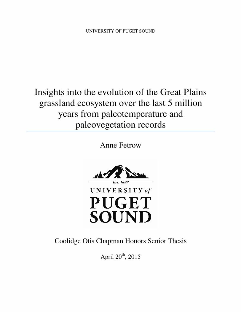
Figure 1: Site map of Meade Basin, Kansalocations are marked individually. have very similar geographic locations and so distances between sites have been slightly exaggerated.

: Site map of Meade Basin, Kansas modified from Fox et al. (2011a/b). Section locations are marked individually. On the north side of the Cimarron River, site locations have very similar geographic locations and so in order to distinguish sites visually

between sites have been slightly exaggerated.

Fetrow 22

. Section On the north side of the Cimarron River, site locations

in order to distinguish sites visually

Fetrow 23

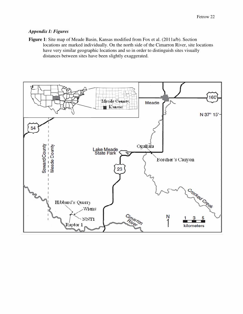
Figure 2. Composite stratigraphic summary of the seven sections analyzed in this study from the

Meade Basin. Original stratigraphic column has been modified from Fox et al. (2011a).

NALMA: North American Land Mammal Age.

BR

3

BR

1

H

Q

Wi

ens

R

P1

N

N

T

B

R

4

Fetrow 24

Figure 3: Estimated temperature (ӧC) calculated from ∆47 values of paleosol carbonate nodules.

The dashed vertical line indicates the average temperature, 21.4°C, and the light grey shaded box

includes ± 1 standard deviation (5°C). Modern mean annual (MAT, 14ӧC) and mean warm

season (MWST, 24ӧC) temperatures are indicated with labelled dotted lines. Two ages are

based upon marker beds; Huckleberry Ridge Ash (2.06 Ma) and CC1 (3.6 Ma), indicated by the

horizontal, long dashed lines (Fox et al., 2011a; Martin et al., 2003).

10 15 20 25 30 35

400

200

0

400

200

0

400

200

0

400

200

0

400

200

0

400

0

200

600

800

1000

B

R4

B

R3

W

ie

ns

B

R1

NN

T1

RP

1

HQ

Hei

ght

in

sect

ion

(cm

abo

ve

loca

l

dat

um)

∆47 Temperature Estimates (ᵒC)

MAT (14ӧC) MWST (24ӧC)

CC1

(3.6 Ma)

Huckleberry Ridge

Ash (2.06 Ma)

Average

(21.4ӧC)

Fetrow 25

Figure 4: δ18O values of water (SMOW) of paleosol carbonate nodules plotted relative to in-

section stratigraphic height. Two ages are based upon marker beds; Huckleberry Ridge Ash (2.06

Ma) and CC1 (3.6 Ma), indicated by the horizontal, long dashed lines (Fox et al., 2011a; Martin

et al., 2003). The estimated modern warm season δ18Owater value (-6.675‰) for precipitation in

Meade Basin is shown using a vertical dotted line and was calculated using the Online Isotopes

in Precipitation Calculator (version 7.2008) (Lat: 37.28, Long: 100.339, Alt: 762m, avg. of May-

Aug) (Bowen and Revenaugh, 2003).

-10 -8 -6 -4 -2 0 2

400

200

0

400

200

0

400

200

0

400

200

0

400

200

0

400

0

200

600

800

1000

B

R4

B

R3

W

ie

ns

B

R1

NN

T1

RP

1

HQ

Hei

ght

in

sect

ion

(cm

abo

ve

loca

l

dat

um)

δ18

Owater (‰)

Huckleberry Ridge

Ash (2.06 Ma)

CC1

(3.6 Ma) (-

6.675‰

)

Fetrow 26

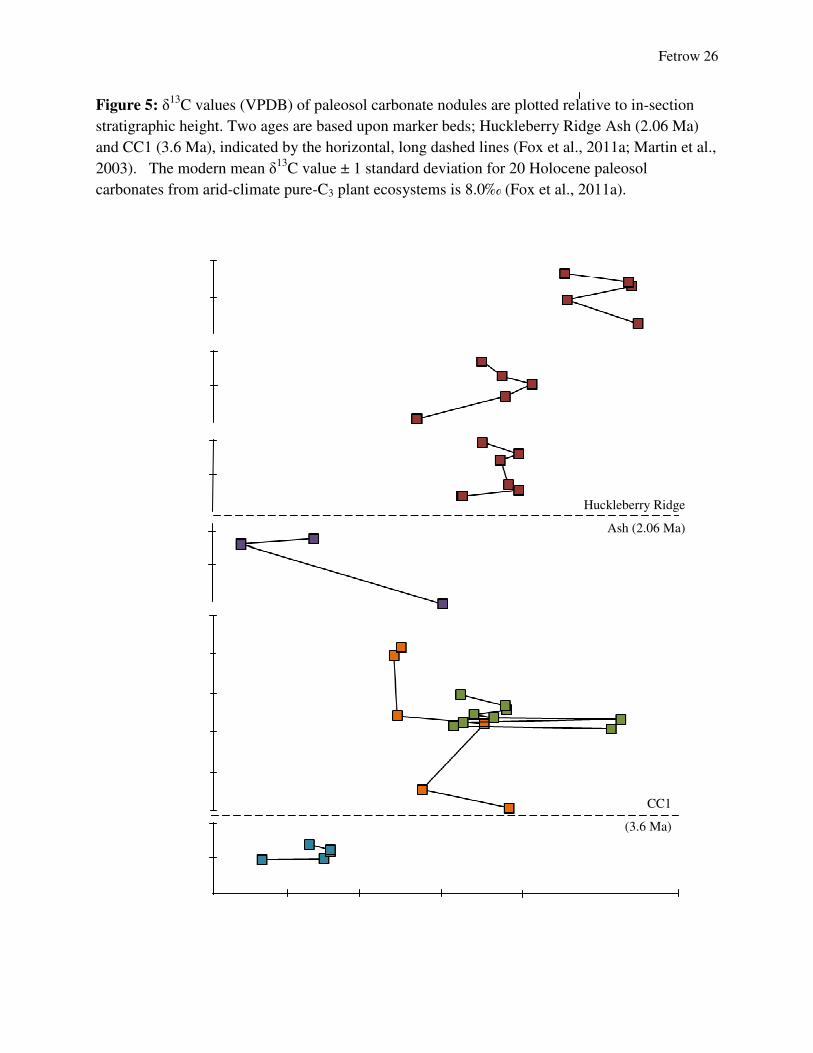
Figure 5: δ13C values (VPDB) of paleosol carbonate nodules are plotted relative to in-section

stratigraphic height. Two ages are based upon marker beds; Huckleberry Ridge Ash (2.06 Ma)

and CC1 (3.6 Ma), indicated by the horizontal, long dashed lines (Fox et al., 2011a; Martin et al.,

2003). The modern mean δ13C value ± 1 standard deviation for 20 Holocene paleosol

carbonates from arid-climate pure-C3 plant ecosystems is 8.0‰ (Fox et al., 2011a).

-7 -6 -5 -4 -3 -2 -1

400

200

0

400

200

0

400

200

0

400

200

0

400

200

0

400

0

200

600

800

1000

B

R4

B

R3

W

ie

ns

B

R1

NN

T1

RP

1

HQ

Hei

ght

in

sect

ion

(cm

abo

ve

loca

l

dat

um)

δ13

C (‰)

Huckleberry Ridge

Ash (2.06 Ma)

CC1

(3.6 Ma)

Fetrow 27

Figure 6: Percent C4 biomass on the landscape calculated from paleosol carbonate nodule δ13C

values following Fox et al. (2011a). Dashed line and light grey box indicate mean modern

abundance of C4 biomass in the Meade Basin region ± 1 standard deviation. Data is plotted

relative to in-section stratigraphic height. Two ages are based upon marker beds; Huckleberry

Ridge Ash (2.06 Ma) and CC1 (3.6 Ma), indicated by the horizontal, long dashed lines (Fox et

al., 2011a; Martin et al., 2003).

Huckleberry Ridge

Ash (2.06 Ma)

0 20 40 60 80 100

400

200

0

400

200

0

400

200

0

400

200

0

400

200

0

400

0

200

600

800

1000

Meade

Basin, KS

78 ±

10.8%

B

R4

B

R3

W

ie

ns

B

R1

NN

T1

RP

1

HQ

Hei

ght

in

sect

ion

(cm

abo

ve

loca

l

dat

um)

C4 Biomass (%)

CC1

(3.6 Ma)

Fetrow 28

a. ∆48 excess b. ∆48 excess

c. no ∆48 excess d. no ∆48 excess

BR3.240.07.CN RP1.115.04.CN

BR1.265.04.CN NNT1.023.01.CN

I. II.

III. IV.

Figure 7: Weight percent carbonate in paleosol carbonate nodules was calculated in reference to 100% carbonate standards and is shown against I.)

temperature estimates (ӧC), III.) δ18Owater values, and IV.) δ13C values. The black diamonds indicate samples that do not have excess mass-48 (∆48

excess), while small red circles indicate samples that have ∆48 excess, as determined by Caltech inter-lab standards. Quadrant II demonstrates the

variety of carbonate nodules sampled throughout the sections and each sample letter correlates to the data point in the plots in I, III, and IV. Drill sites

on each sample demonstrate to what extent and to what depth each sample was drilled.

Weight Percent Carbonate (%)

Fetrow 29

Appendix II: Tables Table 1. Summary of ∆47, temperature estimates, δ18Ow, weight percent carbonate, and percent C4 biomass. Stratigraphic height is measured for each section from the local datum.

Sections means are given for temperature estimates, δ13C, and δ18O, and statistically-derived group distinctions are indicated with a subscripted letter to demonstrate significant

differences between sites. Sample ID Strat.

Height

(cm)

∆47

(avg)

∆47

(1 s.e.)

Section

Mean

T (ᵒC)

T

(ᵒC)

T (ᵒC)

(1 s.e.)

Section

Mean

δ13C (‰)

δ13Cc

(‰,PDB)

δ13Cc

(1s.e.)

Section

Mean

δ18Ow (‰)

δ18Ow

(‰,

SMOW)

δ18Ow

(1 s.e.)

Weight

%Carb

%

C4

Borcher's 4

BR4.070.03.CN 70 0.721 0.001 19.640 22.9 2.4 -2.148A -1.75 0.008 -5.100A, B, C 2.3 0.5 90.2 61.4

BR4.190.05.CN 190 0.745 NA

18.1 NA

-2.63 Inf

-6.8 NA 73.3 55.5

BR4.260.07.CN 260 0.743 NA

18.5 NA

-1.83 NA

-7.1 NA NA 60.9

BR4.280.08.CN 280 0.727 Inf

21.7 Inf

-1.87 NA

-6.5 NA NA 60.6

BR4.325.10.CN 325 0.751 NA

17 NA

-2.66 NA

-7.4 NA NA 55.3

Borcher's 3

BR3.025.01.CN 25 0.725 0.022 20.033 22.1 5.4 -3.775A, B -4.5 0.001 -3.350A -4.2 1.1 78.2 41.6

BR3.025.01.CN 25 0.747 0.003

17.7 2.7

-4.51 0.077

-5.1 0.6 NA 41.5

BR3.140.04.CN 140 0.738 0.009

19.5 3.2

-3.41 0.004

-5.3 0.7 65.8 48.9

BR3.200.06.CN 200 0.736 NA

19.9 NA

-3.08 NA

-5.3 NA NA 51.1

BR3.240.07.CN 240 0.757 NA

15.8 NA

-3.45 NA

-1 NA 52.5 48.7

BR3.315.10.CN 315 0.71 NA

25.2 NA

-3.7 NA

0.8 NA NA 47.0

Borcher's 1

BR1.080.10.CN 80 0.727 NA 21.857 21.7 NA -3.567A, B -3.96 NA -4.157A, B -4.2 NA 71.7 45.2

BR1.080.10.CN 80 0.725 NA

22.1 NA

-3.95 NA

-4.1 NA NA 45.3

BR1.110.09.CN 110 0.735 NA

20.1 NA

-3.25 NA

-4.3 NA NA 50.0

BR1.140.08.CN 140 0.75 NA

17.1 NA

-3.38 NA

-5.1 NA NA 49.1

BR1.265.04.CN 265 0.718 0.019

23.5 4.8

-3.48 0.011

-3.7 1 75.7 48.5

BR1.295.03.CN 295 0.705 NA

26.2 NA

-3.25 NA

-3.3 NA 90.9 50.0

BR1.355.01.CN 355 0.724 0.011

22.3 3.4

-3.7 0.008

-4.4 0.7 NA 47.0

Wiens 1

WI1.000.01.CN 0 0.696 0.025 21.933 28.1 6.2 -5.540B, C -4.17 0.013 -7.500A, B, C -6 1.2 65.3 43.2

WI1.300.03.CN 300 0.732 NA

20.7 NA

-6.68 NA

-7.8 NA NA 26.3

WI1.325.05.CN 325 0.751 NA

17 NA

-5.77 NA

-8.7 NA 87.5 32.4

NNT1

NNT1.023.01.CN 23 0.759 0.004 24.156 15.4 2.9 -3.350A -2.09 0.346 -7.200B, C -7.7 0.6 82.3 57.1

NNT1.038.03.CN 38 0.709 NA

25.4 NA

-4.05 NA

-6.5 NA NA 44.0

NNT1.056.05.CN 56 0.692 0.041

29 9.8

-3.93 0.151

-6.5 1.9 69.8 44.8

NNT1.073.07.CN 73 0.677 NA

32.3 NA

-1.97 NA

-4.7 NA NA 57.9

NNT1.080.08.CN 80 0.755 NA

16.2 NA

-3.55 Inf

-9 NA 69.8 47.3

NNT1.097.10.CN 97 0.743 0.013

18.5 3.8

-3.8 0

-8.9 0.8 72.8 45.6

NNT1.119.12.CN 119 0.727 NA

21.7 NA

-3.39 NA

-8.8 NA NA 48.4

NNT1.142.14.CN 142 0.698 NA

27.7 NA

-3.41 Inf

-6.7 NA NA 48.3

NNT1.197.19.CN 197 0.682 NA

31.2 NA

-3.96 NA

-6 NA 81.1 44.6

Fetrow 30

Raptor 1

RP1.000.01.CN 0 0.75 Inf 22.557 17.1 Inf -3.673A, B 0 NA -7.057B, C -9 NA NA 71.1

RP1.020.02.CN 20 0.677 0.051

32.3 12.5

-3.36 0.004

-4.8 2.4 NA 48.6

RP1.115.04.CN 115 0.751 0.016

17 4.3

-4.44 0.03

-7.7 0.9 36.1 41.3

RP1.450.09.CN 450 0.723 0.017

22.5 4.5

-3.67 0.95

-6.9 0.9 78.9 46.5

RP1.490.13.CN 490 0.725 0.031

22.1 7.2

-4.75 0.003

-7 1.5 79.6 39.3

RP1.795.16.CN 795 0.71 NA

25.2 NA

-4.79 NA

-6.6 NA NA 39.0

RP1.840.18.CN 840 0.727 NA

21.7 NA

-4.7 NA

-7.4 NA NA 39.6

Hibbard's Quarry

HQ1.185.15.CN 185 0.737 NA -5.774 19.7 NA -5.774C -6.4 NA -8.560C -8.7 NA 68.2 28.2

HQ1.190.16.CN 190 0.732 0.026

20.7 6.1

-5.61 0.011

-8.3 1.3 84.1 33.5

HQ1.230.20.CN 230 0.719 0.031

23.3 7.3

-5.53 0.03

-7.7 1.5 NA 34.0

HQ1.240.21.CN 240 0.744 NA

18.3 NA

-5.53 NA

-9.1 NA NA 34.0

HQ1.270.04.CN 270 0.749 NA

17.3 NA

-5.8 NA

-9 NA NA 32.2