AVHRR estimates of surface temperature during the Southern Great Plains 1997 Experiment

AVHRR estimates of surface temperature during the SouthernGreat Plains 1997 Experiment

Amy L. Kaleita and Praveen KumarEnvironmental Hydrology and Hydraulic Engineering, Department of Civil Engineering, University of Illinois, Urbana

Abstract. In this study we aim to (1) explore the differences in the accuracy of satellite-derived land-surface skin temperature for day and nighttime observations, (2) assess theeffects of large solar zenith angles, and (3) develop an understanding of the spatialvariability of the observed temperatures. Land-surface skin temperatures are obtainedusing the split-window technique from observations of the AVHRR instrument aboard theNOAA-12 and NOAA-14 satellites for the SGP97 (Southern Great Plains 1997) hydrologyexperiment. From the study of several days of observations we find that observed biaseswith respect to the ground temperature, both during day and night, are small. However,except for one rainy day measurement, there consistently was a warm bias during the dayand cold bias during the night. Contrary to the hypothesis that at large solar zenith anglesthe observed temperatures are representative of the shelter height air temperature, wefind that the observed temperatures are still closer to the ground temperatures than theair temperature. The spatial correlation is nearly isotropic and has an exponential decay.The correlation lengths demonstrate tremendous spread both during the day and duringthe night with the mean during the day being about 50% larger than that during the night.The average correlation length of 8.63 km during the day is much smaller than the gridsizes typically used in short-time hydrology/mesoscale forecasts. This suggests that formodeling purposes the temperatures in each grid box may be treated as uncorrelated.However, the variance captured can be significantly smaller than the true value.

1. Introduction

The availability of satellite-based measurements of land-surface characteristics is providing a powerful avenue for in-vestigating large-scale dynamics of hydrologic processes, espe-cially those related to the land-atmosphere interaction. Theseobservations not only are providing data for initializing andvalidating hydrologic models [Jin et al., 1997] for large-scalestudies but are also increasingly being utilized in data-assimilation mode for improving the model forecast/predic-tion. Among the several parameters involved in such studies,surface temperature plays a crucial role in determining thepartitioning of incoming radiant energy into the ground, sen-sible, and latent heat fluxes, and the determination of outgoinglongwave flux. Recent studies [Lakshmi, 1998] have shown thatassimilation of surface temperature can be used to improve theprediction of near-surface soil moisture. In order to guaranteethat such studies are successful, it is important to understandthe accuracy of the estimation techniques for the satellite-derived skin temperature, its relationship with the observedsoil and air temperatures, and its spatial variation. This work istargeted toward this objective with the aim that an improvedunderstanding of these factors will enable us to better utilizethe data in modeling and simulation studies.

Given the numerous applications of surface temperature, itsestimation using satellite observations [Price, 1984] has beenthe subject of several investigations for testing and improve-ment of retrieval algorithms, and understanding of factors in-fluencing its variability. The most popular estimation method

for land-surface temperature is a variant of the split-windowtechnique developed for sea surface temperature [Price, 1984].To apply this technique to land surface, corrections are appliedto adjust for emissivities for different surface types. Severalvalidation studies over different terrain types have indicateddiscrepancies ranging from 1 to 3 K. Price [1984] reported thatwith an emissivity correction the split-window technique usedon an area of land in the south central United States gave anoverall error of 2–3 K. Vidal [1991] found that the global errorof the split-window technique combined with an emissivitycorrection over an area in Morocco was about 3 K with a 2 Kdifference from blackbody temperature estimation and a 1 Kdifference from emissivity errors of ;1%. Similarly, Ottle andVidal-Madjar [1992] reported that an error of 2% on the meansurface emissivity values yielded a difference of 1 K of theestimated surface temperature for a region in southwesternFrance. Schmugge and Schmidt [1998] reported a bias of 5 to 6K in NOAA-9 advanced very high resolution radiometer(AVHRR) derived temperature estimates, as compared to in-frared measurements at the ground, using a split-window tech-nique, over the FIFE (First International Satellite Land Sur-face Climatology Project (ISLSCP) Field Experiment) site. Inall the above studies, the satellite estimates were generallyhigher than the ground measurements.

This study examines the accuracy and spatial variability ofskin surface temperatures derived from the AVHRR instru-ment aboard the NOAA-12 and NOAA-14 satellites for theSGP97 (Southern Great Plains 1997) hydrology experiment[Jackson, 1997] study site, with particular emphasis on under-standing the differences between the day and nighttime esti-mates. SGP97 was a field experiment carried out in the sub-humid environment of Oklahoma from June 18 to July 17,1997, to primarily investigate if retrieval algorithms for near-

Copyright 2000 by the American Geophysical Union.

Paper number 2000JD900202.0148-0227/00/2000JD900202$09.00

JOURNAL OF GEOPHYSICAL RESEARCH, VOL. 105, NO. D16, PAGES 20,791–20,801, AUGUST 27, 2000

20,791

surface soil-moisture developed earlier [Jackson et al., 1995]using an L-band electronically scanned thinned array radiom-eter (ESTAR) instrument aboard an aircraft can be extendedto coarser resolutions expected from satellite platforms. Addi-tional objectives of the experiment were to retrieve verticalprofiles of soil-moisture and temperature using in situ andremote sensing data, along with modeling techniques, and tostudy their influence on the development of the boundarylayer. Although the soil-moisture mapping domain consisted ofan area of ;10,000 km2, we consider an area of about 5000km2 centered over the Little Washita basin which was denselyinstrumented for in situ measurements. Land cover in theLittle Washita watershed is primarily shrub, grassland, andcropland, and did not change significantly over the course ofthe experiment. We use the micronet data (http://grl.ars.usda.gov/micronet/) of ground and air temperature measure-ments for validation. The daytime observations from the sat-ellites are for late afternoon hours, giving us an opportunity toexamine the effect of large solar zenith angles on the temper-ature estimates. We also study the spatial variability of thetemperature estimates and discuss their implications for hy-drologic data assimilation.

In section 2 we describe the details of the data used in thestudy. In section 3 we review the estimation algorithm for thesurface temperature estimation from the AVHRR data. Theresults of the analysis are described in section 4 and conclu-sions are given in section 5.

2. Data Description2.1. AVHRR Data

The AVHRR instruments aboard the NOAA satellites weredesigned for meteorological observations but provide data thathave subsequently been successfully used in a variety of appli-cations [Campbell, 1996]. AVHRR is a scanning radiometer,making calibrated measurements of upwelling radiation frompixels scanned across the satellite track. The instrument col-lects data at roughly 1100 m resolution in five channels (twovisible and three infrared) from an altitude of 833 km. Thesatellites have a 102 min period and a swath width of 2400 km,allowing for data collection for the entire globe twice daily.Data obtained directly from the satellite scans is called high-resolution picture transmission (HRPT). Alternatively, an on-board computer aggregates data from one visible and oneinfrared channel of the 1 km data to 4 km resolution, providingbroader geographic coverage in the same volume of data. Thisis called automatic picture transmission (APT). One full orbitof APT data is called global area coverage (GAC) data, while10 min of full resolution HRPT data is called local area cov-erage (LAC) data, covering approximately a 2320 pixel by 780pixel area where each pixel is 1.1 by 1.1 km.

The data used in this study were collected by the AVHRRinstruments aboard the NOAA-12 and NOAA-14 satellites,the only AVHRR satellites operational during the SGP97study. The spectral characteristics of the sensors in differentchannels is given in Table 1. LAC data for 34 dates duringJune, July, and August 1997 were obtained for the SGP97 sitefrom the Satellite Active Archive operated by NOAA. Theimages were then calibrated, converting radiances in the visiblebands (channels 1 and 2) to spectral albedo values and radi-ances in the thermal bands (channels 3, 4, and 5) to blackbodytemperatures [Di and Rundquist, 1994]. This calibration did notinclude the nonlinear corrections in the thermal bands recom-mended by NOAA; however, the errors introduced by neglect-ing these corrections are relatively small, less than 0.2 K forNOAA 14 and similar for NOAA 12. Earth location datasupplied within the raw AVHRR data allow for mapping ontoa latitude-longitude grid. The images, converted to a UTMzone-14 projection, were subsequently clipped to a 64 3 64pixel size (to facilitate statistical analysis of the images), cor-responding to a 70.4 3 70.4 km2 area surrounding the LittleWashita watershed.

2.2. Micronet Data

Air and soil temperature measurements were obtained from42 Agricultural Research Service (ARS) micronet stations inthe Little Washita River watershed. The locations of thesemicronet sites are listed in Table 2. Plate 1 shows the locationsof the micronet sites within a digital elevation model (DEM)grid with approximately the same limits as the 64 3 64 satelliteimages. The soil temperature data from site 147 was deter-mined to be unreliable, often reporting temperatures 208 to 308above average. Therefore all data from this site were discardedin our study.

Air temperature was measured at a height of 1.5 m using asensor housed in a standard pie-plate shield. Ground temper-ature was measured by thermistor probes physically embeddedin the ground at ;5 cm depths. Air temperature measurementswere made every 5 min, while ground temperature measure-ments were made every 15 min. Although air temperaturemeasurements occurred with greater frequency, for the sake of

Table 1. AVHRR Spectral Channels for NOAA-12 and-14 Satellites

AVHRR SpectralChannels (mm) NOAA 12 NOAA 14

1 0.58–0.68 0.58–0.682 0.72–1.10 0.72–1.103 3.55–3.93 3.55–3.934 10.50–11.50 10.30–11.305 11.50–12.50 11.50–12.50

Table 2. Coordinates of the Little Washita Micronet Sites

SiteID

Latitude(UTM)

Longitude(UTM)

SiteID

Latitude(UTM)

Longitude(UTM)

110 590731 3874885 150 568422 3862687111 595639 3875111 151 564606 3863449121 600878 3868352 152 568459 3857703122 595378 3870552 153 573127 3857084123 590978 3870552 154 578889 3857131124 585992 3870235 155 589586 3855643125 579587 3871608 156 595229 3855924130 565313 3868252 157 599469 3853961131 569983 3867601 158 597649 3849364132 575034 3866684 159 592099 3850757133 579613 3867546 160 588093 3851121134 584450 3866202 161 583196 3850740135 589523 3865223 162 578504 3852481136 594479 3865315 163 573622 3852903137 598354 3867282 164 565943 3853302144 598966 3859960 165 578186 3849087147 584438 3862910 168 593592 3846065148 579658 3862010 181 563855 3858621149 574841 3861889 182 584736 3856043

See Plate 1.

KALEITA AND KUMAR: AVHRR ESTIMATES OF SURFACE TEMPERATURE20,792

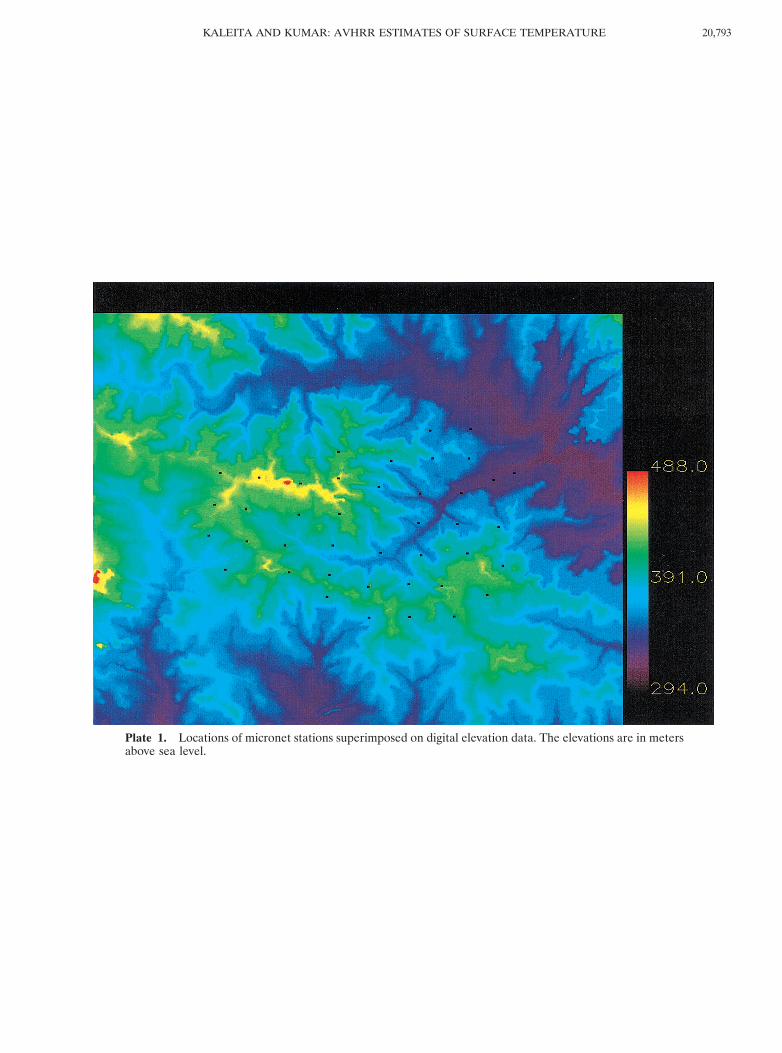
Plate 1. Locations of micronet stations superimposed on digital elevation data. The elevations are in metersabove sea level.

20,793KALEITA AND KUMAR: AVHRR ESTIMATES OF SURFACE TEMPERATURE

consistency we used only data from time steps for whichground temperature was also available.

3. Review of Estimation Algorithms3.1. Estimation of Surface Temperature

The most widely accepted and validated method for surfacetemperature estimation is the split-window technique, so calledbecause it uses data from two or more satellite channels inatmospheric windows. Thermal radiances as observed by thesatellite can be converted, through inversion of the Planckfunction, to blackbody temperatures. By assuming that for twochannels relatively close together, the atmospheric contribu-tion to the measured radiances is the same and that transmit-tance differences in the two channels are due solely to differ-ences in the absorption of atmospheric water vapor, the use oftwo channels allows for estimation of the temperature of thesurface observed by the satellite. The resulting equation is[Price, 1984]

TS 5 TB1 11

b2

b12 1

~TB1 2 TB2! , (1)

where TS is the temperature of the surface as seen by thesatellite, TB1 and TB2 are the respective blackbody temperaturessensed in the two channels, and b1 and b2 are the water vaporabsorption coefficients in the two thermal channels, respectively.

AVHRR channels 4 and 5 are particularly suited to thisanalysis. However, since the ratio R 5 b2/b1 is a somewhatabstract parameter, most studies using the split window tech-nique have used regression methods to determine this value.Both Price [1984] and Vidal [1991] found that R ' 1.33 gaveresults accurate to about 2 K.

A difficulty with the split-window technique for surface tem-perature derivation is in specifying the emissivity. In the deri-vation of (1) it was assumed that the emissivity in each bandwas the same. The split-window method was originally derivedfor sea surface, which has a relatively uniform unit emissivity,thus this assumption is a good one. However, over the landsurface the emissivity in each band may vary slightly, althoughthe value is quite close to 0.96 [Vidal, 1991]. Becker [1987]showed that

T9S 2 TS 5 501 2 «#

«#, (2)

where T9S is the actual surface temperature, TS is the surfacetemperature calculated via the split-window method (equation(1)) and «# is the mean emissivity in AVHRR channels 4 and 5.

It has been recommended [Prata, 1993] that pixels with largeview angles be excluded from analysis due to uncertaintiesintroduced by longer atmospheric paths. In this analysis, be-cause the study area was in the center of the LAC data, zenithangles were small and therefore no data were excluded.

Using (1) with R 5 1.33, surface temperature images weregenerated from the calibrated AVHRR images. Surface tem-perature images were then corrected for surface emissivity byemploying the adjustment described by (2) using a mean emis-sivity of 0.96.

3.2. Identification of Cloud-Contaminated Pixels

Finally, images were processed to determine cloud-contaminated pixels to exclude them from further analysis.

Methods for determining contaminated pixels were basedupon the TeraScan software algorithms developed by theSpace Oceanography Group at the Johns Hopkins UniversityApplied Physics Laboratory [Monaldo, 1996]. The TeraScanprocedures are consistent with other recommendations, suchas those used to process TOVS soundings [McMillin and Dean,1982]. The sequence of steps to identify cloudy pixels involvesseveral filters. The criteria are as follows:

3.2.1. Channel 4 difference. The presence of clouds in apixel will change the apparent brightness temperature. If weassume that the land surface temperature is not extremelyvariant, it would follow that a large difference in temperaturein a local region may indicate the presence of clouds. There-fore if the difference between the maximum and the minimumchannel 4 brightness temperatures in a 3 3 3 region is above acutoff value, the center pixel is considered contaminated. Thevalues used for this analysis are 2.5 K for daytime images and1 K for nighttime images.

3.2.2. Channel 2 difference. A large variation in localchannel 2 albedo can be indicative of cloud contamination. Ifthe difference between the maximum and the minimum chan-nel 2 albedo values in a 3 3 3 region is greater than 2%, thecenter pixel is considered contaminated. This test is only usedfor nighttime images.

3.2.3. Channels 3 and 4 difference. Because channels 3and 4 absorb different proportions of water vapor, a largedifference (more than 5 K) in the brightness temperatures inthese two channels is an indication of cloud contamination.Since channel 3 may contain reflected sunlight, this test is notused for daytime images.

3.2.4. Maximum channel 2 albedo. A large channel 2 al-bedo is an indicator of cloud contamination. Therefore a pixelwith a channel 2 albedo of 8% for a daytime image or 2% fora nighttime image is considered contaminated.

3.2.5. Minimum channel 4 temperature. A channel 4brightness temperature that is very low could indicate that thesatellite is seeing cloud-top temperatures. Thus if the temper-ature in a pixel is less than 283 K, the pixel is consideredcontaminated.

To be considered clear, a pixel had to fail all five of theabove criteria. This analysis eliminated 23 of the original im-ages, as they were deemed significantly cloudy, having a totalcloud cover greater than ;30% over our study area. The datesand timing of the remaining 12 images are given in Table 3.

4. Results and Discussion4.1. Comparison of Ground and Satellite Data

The spatial distribution of the estimated temperatures foreach image are shown in Plates 2 and 3. The pixels identifiedas cloudy are set to a value of 0 K and appear dark in thefigures. The day and nighttime images are grouped separately.Many images show several pixels with relatively cold temper-atures (for example, see images for June 11, June 30, and July9). We believe that these pixels represent partially cloudy areasthat are not excluded by the cloud detection algorithm de-scribed earlier. Figure 1 shows the timing of all images super-imposed on daily precipitation logs obtained from the micro-net data. July 4 and August 14 had rainfall during the earlymorning hours (see Figure 6).

To facilitate comparison of the surface meteorological mea-surements and satellite estimates, those pixels correspondingto the micronet sites were identified by matching the latitude


and longitude of the micronet sites to individual pixel coordi-nates within the images. It should be noted at this point, how-ever, that while the surface measurements are point measure-ments and therefore represent highly localized temperaturevalues, the satellite estimates are averages over 1.1 km 3 1.1km pixels; thus the satellite and surface data have significantlydifferent scales. Furthermore, the surface measurements usedin this comparison are at the nearest quarter hour after thetime the satellite image was begun. This means that the surfacedata used can be 5 to 10 min displaced from the time that thesatellite data for the study region was obtained, as the studyregion is in the middle of the LAC data. Inspection of the datarecords of the ground and air temperatures showed that themaximum error introduced by this discrepancy was ;0.2 K,occurring during the daytime observations. Therefore no in-terpolation was used. There is virtually no error associatedwith this approximation for the nighttime data.

Figures 2 and 3 show the box plots of satellite estimates andair and ground temperature measurements for each image.Figure 2 represents daytime images, while Figure 3 representsnighttime images. The box indicates the interquartile range, orthe range of values falling between the 25th and 75th percen-tile of the data. The middle white strip indicates the median.The whiskers are drawn at 1.53 (interquartile range). Valuesbeyond this range are drawn individually. Comparison of tem-perature range for an entire scene and those corresponding tothe micronet site (compare s1 and s2 in Figures 2 and 3) showsthat the subset of pixels corresponding to the micronet sitesexhibit the same distribution as that of the entire image (exceptfor the outliers) and will therefore be regarded as representa-tive of the entire scene.

On several days the distribution of the satellite estimatesshow a large negative skew (June 11, 25, and 30; see also Table4) due to the problem of partial cloud contamination discussedearlier. Also, the ground temperature measurements duringboth the daytime and the nighttime show much higher spreadin the interquartile range than either the satellite estimates orthe air temperature measurements. This is attributed to theissue of scale. The satellite pixels represent averages over 1.21km2, whereas the ground data are a point measurement andare thus highly localized. This would cause the ground mea-surements to show higher variability. In the case of the airtemperature, however, because the air is subjected to somedegree to mixing due to winds, air temperature measurementstend to be more representative of large areas than groundtemperature measurements. Because of this issue of scale, it isappropriate to compare the mean surface measurement datawith the mean satellite data for the same pixels. Table 4 com-pares the mean satellite data for pixels corresponding to mi-cronet sites with the mean surface measurement data. Figures4 and 5 show the mean satellite estimates for the entire scenecompared with the mean surface data. In general, the satelliteestimates are slightly higher than the 5 cm ground temperaturemeasurements for the daytime data, i.e., exhibit a warm bias(1.28 K mean bias) but lower than the ground temperaturemeasurements for the nighttime data, i.e., show a cold bias(21.25 K mean bias).

The biases are within the 2 to 3 K error range reported inprevious studies and may be due to the issue of scale and thefact that the in situ measurements are at a depth of 5 cm.During the daytime the soil temperature is generally lowerthan the surface temperature, so measurements at the surfacewould report higher temperatures than at a 5 cm depth. The

reverse is true during the night, when the soil temperature ishigher than the surface temperature. The satellite estimatescalculated in this study are measurements of surface temper-ature, and thus the observed biases of the surface with respectto the ground at 5 cm are much as would be expected. It istherefore reasonable to assume that the biases found in thisstudy are at least in part related to the above.

No discernible pattern is found for days with rainfall events.Figure 6 shows the time of satellite observation superimposedon rainfall rate over a 24 hour period for two such cases (July4 and August 14; see also Figure 1). From Table 4 and Figure2 we see that the satellite underestimates the temperature onJuly 4 but overestimates on August 14.

Some studies have used an expanded technique to computeair temperature estimates from daytime AVHRR data [Pri-hodko and Goward, 1997; Czajkowksi et al., 1997]. The tem-perature-vegetation index (TVX) method used in these studiesextrapolates air temperature from the relationship betweensatellite-estimated surface temperature and a spectral vegeta-tion index such as normalized difference vegetation index(NDVI), based upon the idea that air temperature can beestimated from the skin temperature of a full canopy. How-ever, as pointed out by Czajkowski et al. [1997], for large solarzenith angles, such as during the morning and late afternoonhours, shelter height air temperature is the same as the averagesatellite-estimated surface temperature, evidenced by anNDVI versus temperature slope of close to zero degrees. Asindicated in Table 3, all of the daytime images used in thisstudy were taken around 1930 or 0830 LST, consequently solarzenith angles are quite large, of the order of 708 deg. Further-more, brief analysis of NDVI for the scenes confirmed a gen-erally flat TVX slope. In this case, then, it is reasonable tocompare satellite estimates with air temperature measure-ments for the daytime measurements. Comparison to night-time measurements is included for the sake of completeness.

The satellite estimates are considerably greater than the airtemperature measurements for both daytime and nighttimeobservations. In fact, we see from Table 4 that the biases androot-mean-square error are greater with respect to air temper-ature than the ground temperature.

4.2. Spatial Variability

To use the satellite estimates for improving hydrologicmodel forecasts, we need to get an assessment of its spatialvariability, typically measured through the correlation length.

Table 3. Dates of Cloud-Free Satellite Images Used in theAnalysis

Date Julian Day Local Time Satellite

06/11/97 162 0410 NOAA 1406/11/97 162 1930 NOAA 1206/25/97 176 1923 NOAA 1206/30/97 181 0403 NOAA 1407/04/97 185 1925 NOAA 1207/09/97 190 0406 NOAA 1407/13/97 194 1929 NOAA 1208/05/97 217 0410 NOAA 1408/05/97 217 1925 NOAA 1208/09/97 221 0816 NOAA 1208/14/97 226 1927 NOAA 1208/23/97 235 0415 NOAA 12

The local time represents daylight savings time.


Plate 2. Daytime satellite temperature estimates for entire scene. Dates horizontally from top left: June 11and 25, 1997; July 4 and 13, 1997; August 5, 9 and 14, 1997. Black areas represent cloud-contaminated regions.


Plate 3. Same as Plate 2 but for nighttime observations. Dates horizontally from top left: June 11 and 30,1997; July 9, August 5, and August 23, 1997.


A longer correlation length indicates greater homogeneity andvice versa. Table 4 shows that the correlation length for thetemperature estimates during the daytime are on an averagesignificantly larger than that of the nighttime with a mean of8.6 and 5.4 km, respectively. The correlations were computedby considering only the noncloudy pixels. They are nearly iso-tropic and typically have an exponential decay with respect tothe radial lag t 5 =tx

2 1 ty2 (Figures 7 and 8); that is,

r~t! 5 e2utu/b, (3)

where b is the correlation length, and tx and ty are lags in thex and y directions. The range «, i.e., the distance beyond whichany two values may be considered uncorrelated, is given by « 53b for the above exponential model [Christakos, 1996]. Thissuggests that the average range is about 25 and 16 km for theday and nighttime observations, respectively. However, be-cause of the wide spread in the correlation length (see Table4), the individual values of « can be quite different.

The variance of a random field, such as the skin tempera-ture, decreases with increase in the averaging interval. Thisrelationship is given as [Vanmarcke, 1988]

sT2 5 g~T!s2, (4)

where s2 and sT2 are the variances of the random field and that

obtained after averaging over a window of length T , respec-tively. The variance function g(T) measures the reduction ofthe point variance s2 under local averaging. For the exponen-tial correlation model (3) it is given as [Vanmarcke, 1988]

g~T! 5 2S bTD

2STb 2 1 1 e2T/bD . (5)

Alternatively, writing the averaging length T as a multiple ofthe correlation length b , i.e., T 5 ab , we can obtain

g~T! 5 2S 1aD

2

~a 2 1 1 «2a! . (6)

This result indicates that for a 5 3, the average process cap-tures only about 45% of the point variance.

The following implications can be drawn from these resultsfor the assimilation of skin temperatures in hydrologic models:

1. By choosing the model grid size of the order of theobserved range ('25 km for the SGP site), we can treat thetemperature observations for each grid box as essentially spa-tially uncorrelated.

2. The trade-off, however, is that we capture only abouthalf the true spatial variability. For smaller grid sizes, whichwill enable us to capture better the point variability, spatialcorrelation will need to be accounted for.

Both of the results are a consequence of the heterogeneity ofthe temperature distribution. The shorter the correlationlength, the larger the loss of variance information due to av-eraging with increasing window size, and vice versa.

5. ConclusionsThe aim of the study was to (1) explore the differences in the

accuracy of satellite-derived land-surface skin temperature forday and nighttime observation; (2) assess the effects of largesolar zenith angles; and (3) develop an understanding of thespatial variability of the observed temperatures.

We find that observed biases with respect to the groundtemperature, both during day and night, are small. However,except for one rainy day measurement, there consistently wasa warm bias during the day and a cold bias during the night.

Figure 1. Timing of satellite images (*) superimposed onprecipitation logs.

Figure 2. Box plots for daytime data; s1, satellite tempera-ture estimates for entire scene (excluding cloudy pixels); s2,satellite temperature estimates for only pixels that include mi-cronet sites; a, air, and g, ground temperatures for micronetsites. Dates in 1997 are indicated along the top of the graph. Itshould be noted that due to discarded cloudy pixels, all datesdo not contain the same number of data points.

Figure 3. Same as Figure 2 but for nighttime observations.


The lack of any large bias in the satellite estimates is a depar-ture from the results of some other researchers, particularlyover the FIFE site [Schmugge and Schmidt, 1998], who reportthat the split-window technique overestimates the surface tem-perature by as much as 48 deg. Other authors, however, did notfind any systematic bias [Vidal, 1991]. Schmugge and Schmidt[1998] explain that a potential reason for the overestimationfound for the FIFE site is that the surface measurement sta-tions in the that study were enclosed and thus were preferen-tially making measurements over a shaded surface. That wasnot the case in the SGP97 study, which may explain why thesame bias was not found.

Contrary to the hypothesis that at large solar zenith anglesthe observed temperatures are representative of the shelterheight air temperature, we find that the observed temperatures

are still closer to the ground temperatures than the air tem-perature. The results for air temperature comparison havesome implications for the usefulness of the TVX technique.NDVI is a strong function of solar angle, and therefore theTVX slope is dependent not only on the surface characteristicsbut also on the time of day. A correlation between satelliteestimates and daytime air temperature measurements is notapparent in this study, because the mean biases were quitelarge (3.05 K), as shown in Table 4. This is presumably due tothe large solar angles for images in this study. Further researchtherefore may be needed to define a range of solar angles forwhich the method is applicable.

The correlation is nearly isotropic and has an exponentialdecay. The correlation lengths demonstrated tremendousspread both during the day and night with the mean during theday being 50% larger than that during the night. The averagecorrelation length of 8.63 km during the day is much smaller

Table 4. Statistics of Satellite-Derived Temperature Estimates in Relation to Ground-Based Surface and Air Temperature Estimates for Several Days in 1997 for the SGPExperimental Site

Mean(K) s.d. Skewness

Correl.Length(km)

*Bias wrtAir Temp.

*rms wrtAir Temp.

*Bias wrtgd. Temp.

*rms wrtgd. Temp.

Day06/11 300.29 1.971 22.995 11.30 1.62 2.03 1.52 2.4806/25 304.79 0.827 0.341 6.41 4.31 4.45 1.69 2.7307/04 300.27 0.803 0.254 8.76 4.54 4.66 21.37 2.1607/13 306.99 1.159 0.348 20.62 2.47 2.65 2.33 3.1108/05 307.07 1.557 24.320 2.22 4.79 5.05 0.84 3.7408/09 295.77 0.537 2.586 2.21 0.48 0.75 0.92 1.2308/14 305.54 0.793 22.010 8.90 3.15 3.28 3.13 3.43Mean 8.63 3.05 3.27 1.28 2.70

Night06/11 293.59 0.829 20.070 3.24 3.47 3.70 20.18 1.1206/30 298.33 1.085 25.199 1.44 4.60 4.72 20.87 1.4207/09 298.44 0.861 21.420 3.14 3.39 3.64 21.10 1.6308/05 300.48 0.995 0.131 4.52 4.08 4.28 21.48 2.2208/23 294.93 1.026 0.130 14.72 2.65 2.87 22.68 3.01Mean 5.4 3.11 3.85 21.25 1.88

*Note that the mean biases and root mean square (rms) error report the results of the satellite estimatesfor individual pixels over the micronet sites with respect to the corresponding micronet surface data; gd.,ground. Read 06/11 as June 11.

Figure 4. Daytime mean surface measurements versus meansatellite-estimated temperatures for entire scene; plus, groundtemperature; triangle, air temperature. Figure 5. Same as Figure 4 but for nighttime images.


than the grid sizes typically used in short-time hydrology/mesoscale forecasts. This suggests that for modeling purposesthe temperatures in each grid box may be treated as uncorre-lated. However, the variance captured can be significantlysmaller than the true value.

Acknowledgments. This research was partially funded by NASAgrants NAGW-5247, NAG5-7170, NSF grant EAR97-06121, and theNSF Graduate Student Fellowship program. We would also like tothank the Agricultural Research Service, United States Department ofAgriculture for providing the micronet data and NOAA for makingavailable the AVHRR data through their Satellite Active Archive website.

ReferencesBecker, F., The impact of spectral emissivity on the measurement of

land surface temperature from a satellite, Int. J. Remote Sens., 8,1509–1522, 1987.

Campbell, J., Introduction to Remote Sensing, Academic, 474 pp., SanDiego, Calif., 1996.

Christakos, G., Random Field Models in Earth Sciences, 622 pp., Guil-ford, New York, 1996.

Czajkowski, K. P., T. Mulhern, S. N. Goward, J. Cihlar, R. O.Dubayah, and S. D. Prince, Biospheric environmental monitoring atBOREAS with AVHRR observations, J. Geophys. Res., 102, 29,651–29,662, 1997.

Di, L., and D. C. Rundquist, A one-step algorithm for correction andcalibration of AVHRR Level 1b data, Photogramm. Eng. RemoteSens., 60, 165–177, 1994.

Jackson, T. J., Southern Great Plains 1997 (SGP97) Hydrology Experi-ment Plan, U.S. Dep. of Agric., Washington, D. C., 1997.

Jackson, T. J., D. M. LeVine, C. T. Swift, and T. Schmugge, Large areamapping of soil moisture using the ESTAR passive microwave ra-diometer, Remote Sens. Environ., 54, 27–37, 1995.

Jin, M., R. E. Dickinson, and A. M. Vogelmann, A comparison ofCCM2-BATS skin temperature and surface-air temperature withsatellite and surface observations, J. Clim., 10, 1505–1524, 1997.

Lakshmi, V., Surface temperature assimilation in a hydrologicalmodel, Eos Trans. AGU, 79(17), S40–S41, 1998.

McMillin, L. M., and C. Dean, Evaluation of a new operation tech-nique for producing clear radiances, J. Appl. Meteorol., 21, 1005–1014, 1982.

Monaldo, F., Primer on the estimation of sea surface temperatureusing TeraScan processing of NOAA AVHRR satellite data, version2.0, S1R-96M-03, 1996. (Available as http://fermi.jhuapl.edu/avhrr/primer/primer_html.html).

Ottle, C., and D. Vidal-Madjar, Estimation of land surface tempera-ture with NOAA9 data, Remote Sens. Environ., 40, 27–41, 1992.

Prata, A. J., Land surface temperatures derived from the AdvancedVery High Resolution Radiometer and the Along-Track ScanningRadiometer, J. Geophys. Res., 98, 16,689–16,702, 1993.

Price, J. C., Land surface temperature measurements from the splitwindow channels of the NOAA 7 Advanced Very High ResolutionRadiometer, J. Geophys. Res., 89, 7231–7237, 1984.

Prihodko, L., and S. N. Goward, Estimation of air temperature fromremotely sensed surface observations, Remote Sens. Environ., 60,335–346, 1997.

Figure 6. Distribution of rainfall with respect to satellite ob-servation time on July 4 and August 14, 1997. The asteriskshows the time of satellite overpass.

Figure 7. Omnidirectional correlation function r(t) for day-time observations.

Figure 8. Same as Figure 7 but for nighttime observations.


Schmugge, T. J., and G. M. Schmidt, Surface temperature observationsfrom AVHRR in FIFE, J. Atmos. Sci., 55(4), 1239–1246, 1998.

Vanmarcke, E., Random Fields: Analysis and Synthesis, 382 pp., MITPress, Cambridge, Mass., 1988.

Vidal, A., Atmospheric and emissivity correction of land surface tem-perature measured from satellite using ground measurements orsatellite data, Int. J. Remote Sens., 12(12), 2449–2460, 1991.

A. L. Kaleita and P. Kumar, Environmental Hydrology and Hydrau-lic Engineering, Department of Civil and Environmental Engineering,University of Illinois, Urbana, IL 61801. ([email protected])

(Received May 28, 1999; revised March 24, 2000;accepted March 25, 2000.)


20,802

AVHRR estimates of surface temperature during the Southern Great Plains 1997 Experiment

Documents

Transcript of AVHRR estimates of surface temperature during the Southern Great Plains 1997 Experiment