Astronomy & Astrophysics manuscript no. pol_elais c©ESO 2014July 9, 2014

Initial LOFAR observations of epoch of reionization windows:II. Diffuse polarized emission in the ELAIS-N1 field

V. Jelic1, 2?, A. G. de Bruyn1, 2, M. Mevius1, F. B. Abdalla3, K. M. B. Asad1, G. Bernardi4, M. A. Brentjens2, S. Bus1,E. Chapman3, B. Ciardi5, S. Daiboo1 E. R. Fernandez1, A. Ghosh1, G. Harker6, H. Jensen7, S. Kazemi1, L. V. E.

Koopmans1, P. Labropoulos1, O. Martinez-Rubi1, G. Mellema7, A. R. Offringa8, 9, V. N. Pandey2, A. H. Patil1, R. M.Thomas1, H. K. Vedantham1, V. Veligatla1, S. Yatawatta2, S. Zaroubi1, A. Alexov10, J. Anderson11, I. M. Avruch1, 12,

R. Beck13, M. E. Bell9, M. J. Bentum2, P. Best14, A. Bonafede15, J. Bregman2, F. Breitling11, J. Broderick16,W. N. Brouw1, 2, M. Brüggen15, H. R. Butcher8, J. E. Conway17, F. de Gasperin15, E. de Geus2, A. Deller2,

R.-J. Dettmar18, S. Duscha2, J. Eislöffel19, D. Engels20, H. Falcke2, 21, R. A. Fallows2, R. Fender22, C. Ferrari23,W. Frieswijk2, M. A. Garrett2, 24, J. Grießmeier25, 26, A. W. Gunst2, J. P. Hamaker2, T. E. Hassall16, 27, M.

Haverkorn21, 24, G. Heald2, J. W. T. Hessels2, 28, M. Hoeft19, J. Hörandel21, A. Horneffer13, A. van der Horst28,M. Iacobelli24, E. Juette18, A. Karastergiou22, V. I. Kondratiev2, 29, M. Kramer13, 27, M. Kuniyoshi13, G. Kuper2, J. vanLeeuwen2, 28, P. Maat2, G. Mann11, D. McKay-Bukowski30, 31, J. P. McKean2, H. Munk2, A. Nelles21, M. J. Norden2,

H. Paas32, M. Pandey-Pommier33, G. Pietka22, R. Pizzo2, A. G. Polatidis2, W. Reich13, H. Röttgering24,A. Rowlinson28, A. M. M. Scaife16, D. Schwarz34, M. Serylak22, O. Smirnov4, 35, M. Steinmetz11, A. Stewart22,

M. Tagger25, Y. Tang2, C. Tasse36, S. ter Veen21, S. Thoudam21, C. Toribio2, R. Vermeulen2, C. Vocks11, R. J. vanWeeren37, R. A. M. J. Wijers28, S. J. Wijnholds2, O. Wucknitz13, 38, and P. Zarka36

(Affiliations can be found after the references)

Received 15/04/2014 / Accepted 07/07/2014

ABSTRACT

Aims. This study aims to characterise the polarized foreground emission in the ELAIS-N1 field and to address its possible implicationsfor extracting of the cosmological 21-cm signal from the LOw-Frequency ARray - Epoch of Reionization (LOFAR-EoR) data.Methods. We used the high band antennas of LOFAR to image this region and RM-synthesis to unravel structures of polarizedemission at high Galactic latitudes.Results. The brightness temperature of the detected Galactic emission is on average ∼ 4 K in polarized intensity and covers the rangefrom −10 to +13 rad m−2 in Faraday depth. The total polarized intensity and polarization angle show a wide range of morphologicalfeatures. We have also used the Westerbork Synthesis Radio Telescope (WSRT) at 350 MHz to image the same region. The LOFARand WSRT images show a similar complex morphology at comparable brightness levels, but their spatial correlation is very low. Thefractional polarization at 150 MHz, expressed as a percentage of the total intensity, amounts to ≈ 1.5%. There is no indication ofdiffuse emission in total intensity in the interferometric data, in line with results at higher frequenciesConclusions. The wide frequency range, high angular resolution, and high sensitivity make LOFAR an exquisite instrument forstudying Galactic polarized emission at a resolution of ∼ 1 − 2 rad m−2 in Faraday depth. The different polarized patterns observedat 150 MHz and 350 MHz are consistent with different source distributions along the line of sight wring in a variety of Faradaythin regions of emission. The presence of polarized foregrounds is a serious complication for epoch of reionization experiments. Toavoid the leakage of polarized emission into total intensity, which can depend on frequency, we need to calibrate the instrumentalpolarization across the field of view to a small fraction of 1%.

Key words. radio continuum: ISM - techniques: interferometric, polarimetric - cosmology: observations, diffuse radiation, reioniza-tion

1. Introduction

The LOw-Frequency ARray - Epoch of Reionization (LOFAR-EoR) key science project will use the LOFAR radio telescopeto study the epoch of reionization (van Haarlem et al. 2013).The EoR is a pivotal period in the history of the Universe duringwhich the all-pervasive cosmic gas was transformed from a neu-tral to an ionized state. It holds the key to structure formation and

? E-mail:vjelic@astro.rug.nl

the evolution of the Universe as we know it today, and touchesupon fundamental questions in cosmology.

The LOFAR-EoR project plans to probe the EoR in up to fiveobserving fields (de Bruyn et al, in prep.). Three of these fieldshave been observed during the commissioning phase of LOFAR.The first field is centred on the North Celestial Pole (NCP). Thesecond field coincides with the ELAIS-N1 field, while the thirdcontains a very bright source, 3C196. The choice of these threefields was motivated by the desire to address most of the prob-lems and challenges that will affect much longer LOFAR-EoRobservations.

Article number, page 1 of 12

arX

iv:1

407.

2093

v1 [

astr

o-ph

.GA

] 8

Jul

201

4

A&A proofs: manuscript no. pol_elais

The results of our commissioning observations are presentedin two papers. In the first paper (Yatawatta et al. 2013) we testedvarious calibration approaches and conducted a thorough anal-ysis of the noise by analysing the NCP observations. The NCPfield only has a few bright sources, and the diffuse linearly po-larized emission from our Galaxy is relatively faint. In the NCPdata we reached a noise level of about 100 µJy PSF−1 (PSF: pointspread function) with then still poorly calibrated LOFAR array.

In this paper we present LOFAR observations of the ELAIS-N1 field, which was found to have bright polarized emissioncoming from the Galactic foreground. The ELAIS-N1 field isone of the northern fields of the European Large Area InfraredSpace Observatory (ISO) Survey. It is a field with no radiosources brighter than 3 Jy at 325 MHz (WENSS survey; Ren-gelink et al. 1997). Given its location in the Galactic halo, wedo not expect high levels of emission from our Galaxy in totalintensity. However, linear polarization at surface brightness lev-els of a few K has been detected at 350 MHz (PI: V. Jelic) usingthe Westerbork Synthesis Radio Telescope (WSRT). The emis-sion is confined to Faraday depths varying from −10 rad m−2 to+10 rad m−2, and they show large-scale spatial Faraday depthgradients of a few rad m−2 deg−1. This field is therefore suitablefor polarimetric studies of Galactic foreground emission and ofits possible contaminating effects on the feeble cosmological sig-nals coming from the EoR.

The ELAIS-N1 field will also be targeted with Subaru HyperSuprime-Cam (Miyazaki et al. 2002) to search for high-redshiftLyα emitters (LAEs). With a significant number of detectedLAEs one could in principle study reionization using both theshape and normalization of the cross-power spectrum betweenthe galaxies and EoR (e.g. Wiersma et al. 2013). Thus, the multi-wavelength aspect of this field will play an important role in thedetection of the cosmological signal by providing further insightinto physical processes during the EoR.

This paper is organised as follows. In Section 2 we givean overview of the observational setup and the data reduction.The initial widefield images of the ELAIS-N1 field in total in-tensity and polarization are presented in Section 3, where wealso present the effect of correction for Faraday rotation in theEarth’s ionosphere. In Section 4 we discuss the properties of thedetected polarized emission and importance to understand it fora proper extraction of the cosmological signal from the LOFAR-EoR data. We summarise and conclude in Section 5.

2. Observation and data reduction

The ELAIS-N1 field was observed on 2 and 3 July 2011 with55 LOFAR High Band Antenna (HBA) stations in the Nether-lands. The observation was part of an initial suite of LOFARcommissioning observations. The array configuration consistedof 46 core stations (CS) and nine remote stations (RS). The phasecentre was set at RA 16h 14m and Dec +54d 30m (J2000). Datawere recorded in the frequency range from 138 MHz to 185 MHzdistributed over 240 sub-bands. Each sub-band has a width of195 kHz covered by 64 channels. The total integration time was7 h (mostly night time) with a correlator integration time of 2 s.The uv coverage was fully sampled up to baselines of 2 km. Werefer to van Haarlem et al. (2013) for a detailed overview of theLOFAR radio telescope and its frequency characteristics.

The initial pre-processing was done on the CEP2 clusterby the Radio Observatory of ASTRON (the Netherlands Insti-tute of Radio Astronomy). All other processing was done on a

Fig. 1. Rotation measure spread function (RMSF) for the ELAIS-N1observation. A resolution in Faraday depth space is δΦ = 1.75 rad m−2,while the largest Faraday structure that can be reliably detected has awidth of ∆Φscale = 1.15 rad m−2.

CPU/GPU1 cluster dedicated to the LOFAR-EoR project, at theUniversity of Groningen, the Netherlands. During the processingwe used the LOFAR-EoR Diagnostic Database (LEDDB) that isused for the storage, management, processing, and analysis ofthe LOFAR-EoR observations (Martinez-Rubi et al. 2013).

2.1. Initial pre-processing (flagging and averaging)

The LOFAR observing frequencies are affected by man-made ra-dio frequency interference (RFI; Offringa et al. 2013). RFI miti-gation works best on data with a very fine resolution in time andfrequency. Therefore, the first step in our initial pre-processing isflagging of the data using the aoflagger (Offringa et al. 2010,2012). On average about 3% − 4% of our data were flagged.However, around three frequencies (170 MHz, 178 MHz, and182 MHz) the percentage of RFIs is much higher (> 30%). Thesecond frequency corresponds to the ∼ 1.5 MHz wide DigitalAudio Broadcasting (DAB) band C allocated in the Netherlands.A total of six stations were not delivering good data at the timeof our observation and were not included in the subsequent pro-cessing. The 4 edge channels of the 64 channel sub-band areflagged to remove edge effects from the polyphase filter. Afterflagging, the data are averaged to 15 channels per sub-band toreduce the data volume for further processing.

2.2. Sky model

The sky model used for the initial calibration of the ELAIS-N1field contains approximately 30 of the brightest discrete sources.The flux and spectral index of these sources are determined fromthe WENSS2 (Rengelink et al. 1997) and VLSS3 (Cohen et al.2007) radio source catalogues at 325 MHz and 74 MHz.

1 CPU: Central Processing Unit; GPU: Graphics Processing Unit2 The Westerbork Northern Sky Survey, http://www.astron.nl/wow/3 The VLA Low-Frequency Sky Survey, http://lwa.nrl.navy.mil/VLSS/

Article number, page 2 of 12

V. Jelic et al.: Initial LOFAR-EoR observations - diffuse polarized emission in the ELAIS-N1 field

Fig. 2. Frequency-averaged Stokes I image of the ELAIS-N1 region. The image is 6.6◦ × 6.6◦ in size, with a PSF of 16.0′′ × 8.8′′, and the noiselevel is 1.0 mJy PSF−1. We are a factor of ∼ 2 above the thermal noise.

After the initial calibration and imaging, we update the skymodel by extracting the source information from the LOFARimages themselves. For this we use Duchamp (v. 1.1.11; Whit-ing 2012), a source finder that creates masks around potentialsources, then we used buildsky (v. 0.0.5; Yatawatta et al. 2013)to create a model with the minimum number of required sourcecomponents. Our updated sky model has ∼ 200 sources and as-sumes that all sources are unpolarized. This assumption has noeffect on the calibration. The diffuse polarized emission is notpart of the sky model.

2.3. Calibration and source subtraction

The main steps in the calibration and source subtraction are verysimilar to the steps presented in our first paper (Yatawatta et al.2013). Therefore we limit ourselves here to a brief overview.

We begin with a direction-independent calibration to correctfor clock errors and ionospheric errors effecting the brightestsources in the image. This is done separately on each sub-bandusing the Black Board Selfcal (BBS) package (Pandey et al.2009). Each sub-band has 15 channels of 12 kHz at 2 s integra-tion but we determine calibration solutions per sub-band for ev-ery 10 s. The data are also corrected for the element and stationbeam gains for the centre of the image.

After performing direction-independent calibration, the cor-rected data are flagged for bad solutions and averaged to onechannel per 180 kHz sub-band and 10 s integration time.

Direction-dependent station beam and ionospheric correctionsfor the brightest sources were determined using SAGECal, whichis based on Expectation Maximization (Yatawatta et al. 2008;Kazemi et al. 2011; Yatawatta 2013; Kazemi et al. 2013). Wesubtract around 200 sources within the image, clustered in ∼50different directions within the main field of view. The very brightA-team sources (CasA and CygA) and a few bright 3C-sourceslocated near to the ELAIS-N1 field (e.g. 3C295) were among the50 clusters.

For the purpose of this work we use data calibrated withSAGECal to build and update our sky model. The analysis of dif-fuse polarized emission uses the data calibrated only with BBS.SAGECal calibration will suppress large scale diffuse emission,because this emission is not part of the sky model. Since our skymodel only contains discrete sources, we do not use SAGECalcalibration for polarimetric study of diffuse emission. The dy-namic range in the polarized emission also does not require so-phisticated calibration.

2.4. Imaging

For imaging we use AWimager. AWimager is a fast imager de-veloped and optimized for LOFAR (Tasse et al. 2013). It is basedon full-polarization A-projection that can deal with non-coplanararrays, arbitrary station beams, and non-diagonal Mueller ma-trices. The algorithm is designed to correct for all direction-dependent effects varying in time and frequency, including in-

Article number, page 3 of 12

A&A proofs: manuscript no. pol_elais

dividual station and dipole beams, the projection of the dipoleson the sky and the beam forming, as well as ionospheric refrac-tion effects.

To update the sky model, we make images in total intensityof calibrated and source-subtracted data. In order to create ac-curate source models, these images have the highest resolutionavailable at the time the data were taken (∼ 20′′). We use uniformweighting and the subtracted sources are restored onto these im-ages, after convolving with the nominal Gaussian PSF. We alsomade very large images with low angular resolution to iden-tify bright radio sources surrounding the ELAIS-N1 field, whosesidelobes contaminate the emission in the inner area. To analysethe polarization of the diffuse Galactic emission, which mostlyappears on spatial scales greater than a few arcmin, we make alower resolution images in all Stokes parameters (IQUV). Theseimages are produced using only baselines smaller than 1000wavelengths, providing a frequency independent resolution ofabout 3 arc min. We used robust (Briggs) weighting with robust-ness parameter equal to 0.

The beam pattern of a LOFAR-HBA station can be describedas the product of an antenna beam pattern and the array beampattern of the station (van Haarlem et al. 2013). To first order (i.e.excluding mutual coupling) the station (array) beam is scalar, hasno polarizing characteristics itself and depends mainly on thegeometry of the tile distribution. The element beam pattern isstrongly polarized (Hamaker 2006). Its polarization response isrelated to the projection of the beam patterns of two orthogonaldipoles on the sky and the changing parallactic angle. During along synthesis observation, spurious polarization is produced bythe field rotation relative to the dipoles as well as by the move-ment of the station beam through the polarized pattern of the av-eraged beam of the element antennas (for a detailed discussionwe refer to Bregman 2012).

We correct the data for the beam pattern in two steps. Thefirst correction is applied during the calibration, using BBS. Thedata are corrected for both the array and the element beam gainat the centre of the image. The relative variation of the elementbeam pattern across the field of view, as well as the temporalchanges are taken into account during the imaging step, usingthe AWimager.

2.5. Rotation Measure synthesis

The technique of Rotation Measure (RM) synthesis (Brentjens &de Bruyn 2005) is used to unravel the linearly polarized emissionas a function of Faraday depth (Φ). The Faraday depth is definedas:

Φ

[rad m−2]= 0.81

∫ observer

source

ne

[cm−3]B‖

[µG]dl

[pc], (1)

where ne is electron density; B‖ is the magnetic field componentparallel to the line of sight dl and the integral is taken over theentire path from the source to the observer. A positive Faradaydepth implies a magnetic field component pointing towards theobserver and a negative Faraday depth implies a magnetic fieldcomponent pointing away from the observer.

The RM synthesis technique takes advantage of the relation-ship, which exists between the measured complex polarizationP(λ2) = Q(λ2) + iU(λ2) in λ2-space and Faraday depth:

F(Φ) =1

W(λ2)

∫ +∞

−∞

P(λ2)e−i2Φλ2dλ2, (2)

where W(λ2) is the sampling function, also known as the rotationmeasure spread function (RMSF). Note that we can only sample

Fig. 3. Ionospheric RM values for different LOFAR-HBA stationsduring the ELAIS-N1 observation estimated from Global IonosphericMaps (GIMs). Note that GIMs have an error of 1 TEC unit, which trans-lates to an RM error of 0.1 rad m−2.

a finite positive range of wavelengths, resulting in an incompleteF(Φ). The RM synthesis method is constrained by the spectralbandwidth (∆λ2), the spectral resolution (δλ2), and the minimum(λ2

min) of the measured λ2 distribution. These observational pa-rameters are also directly linked to three physical quantities inFaraday depth space: (i) the maximum detectable Faraday depth,Φmax ≈

√3/δλ2; (ii) the largest structure that can be resolved in

Faraday depth, ∆Φscale ≈ π/λ2min; and (iii) the resolution in Fara-

day depth space, δΦ ≈ 2√

3/∆λ2, which defines the minimumseparation between two different structures that are detectable.

For this work we are using the RM synthesis code writtenby M. Brentjens and we apply it to ∼ 200 sub-bands, whichhave comparable noise level. We first synthesized a low res-olution Faraday cube over a wide range in Faraday depth todetermine where polarized emission could be detected. The fi-nal cube covers a Faraday depth range from −30 rad m−2 to+30 rad m−2 with 0.25 rad m−2 step. The absolute value of theRMSF corresponding to the frequency coverage of the observa-tion is given in Fig. 1. The resolution in Faraday depth spaceis δΦ = 1.75 rad m−2, while the largest Faraday structure thatcan be resolved is ∆Φscale = 1.15 rad m−2. Since the resolutionis higher than the maximum detectable scale, we can only detectFaraday thin structures. A structure is Faraday thin if λ2∆Φ � 1,where ∆Φ denotes the extent of the structure in Faraday depth.If λ2∆Φ � 1, then the structure is called Faraday thick.

3. Results

3.1. Widefield image in total intensity

The frequency-averaged Stokes I widefield image of the ELAIS-N1 region is presented in Fig. 2. The image is obtained after cal-ibration as described in Sect. 2.3 and it is 6.6◦ × 6.6◦ in size witha PSF of 16.0′′ × 8.8′′. The noise level is 1.0 mJy PSF−1. Thereis no indication of diffuse emission in total intensity. A circlemarks a region around the giant radio galaxy J162740+514012(see Schoenmakers et al. 2001), which contains two lobes that

Article number, page 4 of 12

V. Jelic et al.: Initial LOFAR-EoR observations - diffuse polarized emission in the ELAIS-N1 field

Fig. 4. Effect of the ionospheric RM variation. Bottom plot shows the Faraday spectrum centred at the SW lobe of the giant radio galaxyJ162740+514012, before (dashed line) and after (solid line) applying the ionospheric RM correction. As expected, there is (i) a shift in Fara-day spectrum that corresponds to an average of the ionospheric rotation measure; and (ii) an increase in the peak flux by 20%. The ionospheric RMvariation also has an effect on the diffuse polarized emission as shown in the two images in the upper part of the figure. Note that these images aregiven at Faraday depths separated by an average of the ionospheric rotation measure to correct for a shift due to Faraday rotation in the ionosphere.

were found to be highly polarized at 325 MHz. The source isfound to be polarized in the LOFAR band as well, although atmuch lower levels. The RMs of the two lobes have been deter-mined at both frequency regimes. For each lobe, the two deter-minations at two different frequency regimes agree to within themeasurement accuracy. Small calibration errors due to variationof the station beams and rapid ionospheric phase fluctuations arestill visible around some bright sources. These errors can be sup-pressed by direction dependent calibration using SageCal. Forthe purpose of this paper we are mainly interested in polariza-tion, and we will leave the analysis of the total intensity emissionfor future work.

3.2. Correcting for Faraday rotation in the Earth’s ionosphere

An electromagnetic wavefront passing through an ionizedmedium with a variable index of refraction experiences time de-lays in different parts of the wavefront. These delays are propor-

tional to the total electron content (TEC)4 and are inversely pro-portional to the square of the observing frequency (e.g. Thomp-son et al. 2007). Indeed, at LOFAR frequencies the Earth’s iono-sphere is the dominant source of phase errors. A linear spatialionospheric TEC gradient causes a position shift of the source.Higher-order variations in the index of refraction cause a moreserious distortion producing defocusing and even scintillationsin extreme cases.

In polarimetric studies there is an additional ionospheric ef-fect that one needs to correct for. Faraday rotation in the Earth’sionosphere changes the polarization angle of the incoming polar-ized emission. This happens on a timescale that is much smallerthan the total integration time of an observation. As a result ofthis, the observed polarized emission will be shifted in Faradaydepth space and be partially decorrelated. The average shift isproportional to the ionospheric RM averaged over the observ-ing time. If the variation during the synthesis time is longer

4 Total electron content (TEC) is the integrated electron density alongthe line of sight through Earth’s ionosphere, with units of electrons persquare meter (1016 electrons/m2 = 1 TEC unit).

Article number, page 5 of 12

A&A proofs: manuscript no. pol_elais

Fig. 5. Widefield images of the ELAIS-N1 region in polarized intensity (PI), Stokes Q, and Stokes U given at Faraday depths of -5.5, -2.5, -1.5,-0.5, +0.5, +1.5 rad m−2. Images are 5.7◦ × 5.7◦ in size with a PSF of 3.4′ × 3.1′. The noise level is 0.3 mJy PSF−1 RMSF−1 in polarized intensityand 0.5 mJy PSF−1 RMSF−1 in Stokes Q,U. The images in polarized intensity have not been corrected for polarization noise bias.

than ≈ 1 rad the emission will be depolarized and the dynamic range in the image will be reduced. Thus, one needs to esti-

Article number, page 6 of 12

V. Jelic et al.: Initial LOFAR-EoR observations - diffuse polarized emission in the ELAIS-N1 field

Fig. 5. Continued.

Fig. 6. Faraday depth spectra of a few interesting lines of sight throughthe RM cube of polarized intensity. The typical width of the detectedstructures is a few rad m−2.

mate the amount of ionospheric RM as a function of time andthen “derotate” the observed polarization angle by that amount.Large TEC-gradients across the array can cause differential Fara-day rotation, making unpolarized sources appear circularly po-larized. These were not present in the current data. To esti-

mate the ionospheric RM during our observation, we use theGlobal Ionospheric Maps (GIMs) of the vertical total electroncontent (VTEC) and the Earth’s magnetic field model (Interna-tional Geomagnetic Reference Field; Maus et al. 2005) fromthe casacore5 library. The GIMs are generated by the RoyalObservatory of Belgium using near real time data taken every15 min by more than 100 Global Positioning System (GPS) sitesspread across Europe (Bergeot et al. 2009, http://gnss.be). Theresolution of these maps is 0.5◦ × 0.5◦ in longitude and latitude.

The estimated ionospheric RM values for the ELAIS-N1 ob-servation are plotted in Fig. 3. The difference between the RMvalues across the LOFAR array (presented with different lines inFig. 3) is very small for this particular observation. The degree ofionization in the ionosphere depends essentially on the amountof radiation received from the Sun. Hence, the RM values arehigher at the beginning of the observation (∼ 2.5h before sunset)than at the end of it (∼ 4.5h after sunset). During our observa-tion the ionosphere shows typical behaviour and the estimatedionospheric RM corrections are not unusual.

We have corrected our data for the time-variable ionosphericRM using RMWriter code written by M. Mevius. Figure 4 showsthe Faraday spectrum centred at the SW (Southwest) lobe of thegiant radio galaxy J162740+514012. This lobe is polarized andits emission appears around Φ = +22 rad m−2 before applyingthe ionospheric RM correction (dashed line in Figure 4). Af-ter we apply the ionospheric RM correction (solid line in Fig-ure 4), its emission is centred around Φ = +21 rad m−2. A shiftof |∆Φ| = 1 rad m−2 corresponds to the average of the iono-spheric rotation measure 〈RMion〉 = 1.2 rad m−2. There is alsoan increase in the peak flux by 20%.

5 http://casacore.googlecode.com

Article number, page 7 of 12

A&A proofs: manuscript no. pol_elais

Fig. 7. Image on the left shows the distribution of peak intensities in the Faraday depth spectra at every spatial pixel. Image on the right gives thecorresponding RM value for each pixel

Correcting the data for the time-dependent ionospheric RMvariation also has an effect on the images of the diffuse polarizedemission. An example is shown in Figure 4. For the predictedRM variation we would expect this effect to be about 15-20%.Indeed, the diffuse emission is brighter, the morphological fea-tures are sharper and the edge of the station primary beam ismore clearly visible in the corrected image, as compared to theuncorrected image.

3.3. Diffuse polarized emission

A series of widefield images of the ELAIS-N1 region in bothpolarized intensity and Stokes Q,U are presented in Fig. 5.Given the observed rather uniform levels of the polarized in-tensity the polarity of Stokes Q,U is a good indicator of thespatial variations of the plane of polarization. The imagesare 5.7◦ × 5.7◦ in size with a PSF of 3.4′ × 3.1′ and thenoise level is 0.3 mJy PSF−1 RMSF−1 in polarized intensity and0.5 mJy PSF−1 RMSF−1 in Stokes Q,U. Images are given atFaraday depths of -5.5, -2.5, -1.5, -0.5, +0.5, +1.5 rad m−2 toemphasise the various detected structures in linear polarization.Note that all images are produced using the RM cubes correctedfor Faraday rotation in the ionosphere.

We detect faint polarized emission (.1 mJy PSF−1 RMSF−1) over a range of Faraday depthsfrom −10 to +13 rad m−2. The brightest and most prominentfeatures are detected in a smaller range of Faraday depth. From−10 to −4 rad m−2 there is a northwest to southeast gradient ofemission, which starts as a small-scale feature and builds up toan extended northeast-southwest structure. The mean surfacebrightness of this emission is 1.8 mJy PSF−1 RMSF−1. From −4to −0.5 rad m−2 there is diffuse emission with patchy morphol-ogy and a mean surface brightness of 5.4 mJy PSF−1 RMSF−1,and it shows a gradient in the same direction as the feature atmore negative Faraday depth but is less prominent. Around+0.5 rad m−2, polarized emission is detected over the fullprimary beam. At more positive values it becomes patchy andfades away towards +10 rad m−2. We note a conspicuous, stripymorphological pattern of diffuse emission oriented North-Southin the Eastern part of the image. This structure is visible from

0 to +4 rad m−2. A few representative Faraday spectra of thesefeatures are shown in Fig. 6. Following Schnitzeler et al. (2009)we show a map of the highest peak of Faraday depth spectra ateach spatial pixel in Fig. 7. On the same figure we also show amap of the RM value of each peak.

In contrast to polarized intensity, which reflects the ampli-tude of polarized emission, Stokes Q,U reflects the morphol-ogy of both its amplitude and its polarization angle. Therefore,Stokes Q,U images show even more striking morphological pat-terns and structures in polarization (Fig. 5). Particularly note-worthy are the faint linear features at Faraday depths around+1 rad m−2 that are visible on the Eastern side of the Stokes Q,Uimages. They point to large gradients in the polarization positionangle in the direction orthogonal to the long axes.

We also compute the total polarized intensity at each pixelby integrating the polarized intensity RM cube along Faradaydepth. The integral is given by (Brentjens 2011):

PI =1B

n∑i=0

(|PI(Φi)| − nPI) , (3)

where B is the area under the restoring beam of RMCLEAN(Heald et al. 2009) divided by ∆Φ = |Φi+1 − Φi| and nPI is themean value of the polarized intensity in the RM cube in regionswhere no signal is present. Assuming that the noise distributionsof Q,U RM cubes have equal σ and zero mean, and are uncorre-lated, then the mean value of the PI is nPI = σ

√π2 .

We have not attempted to deconvolve our RM cubes for theeffects of the side lobes of the RMSF (see Fig. 1). The sidelobesare small and the S/N is generally so low that this would havehad very little effect on the images. Moreover, deconvolution inFaraday space is a nontrivial operation with many uncertaintiesdue to missing structure in λ2-space (see (Brentjens & de Bruyn2005).

To calculate parameter B we use the area under the RMSF in-stead of the restoring beam of the RM-CLEAN. Fig. 9 shows animage of the integrated polarized intensity. Most of the sourcesvisible in the image are instrumentally polarized and appeararound Φ = −1 rad m−2, which corresponds to Φ = 0 rad m−2

in RM cubes not corrected for ionospheric Faraday rotation. We

Article number, page 8 of 12

V. Jelic et al.: Initial LOFAR-EoR observations - diffuse polarized emission in the ELAIS-N1 field

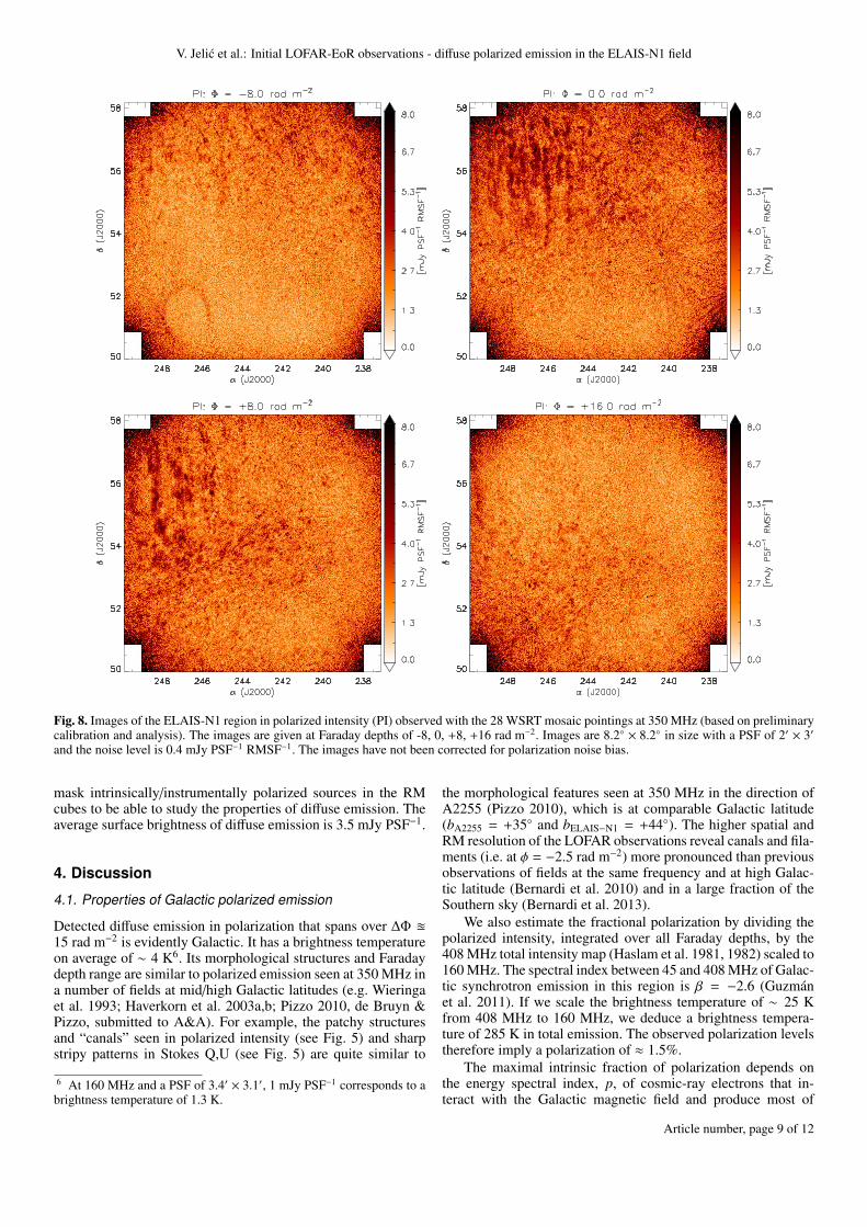
Fig. 8. Images of the ELAIS-N1 region in polarized intensity (PI) observed with the 28 WSRT mosaic pointings at 350 MHz (based on preliminarycalibration and analysis). The images are given at Faraday depths of -8, 0, +8, +16 rad m−2. Images are 8.2◦ × 8.2◦ in size with a PSF of 2′ × 3′and the noise level is 0.4 mJy PSF−1 RMSF−1. The images have not been corrected for polarization noise bias.

mask intrinsically/instrumentally polarized sources in the RMcubes to be able to study the properties of diffuse emission. Theaverage surface brightness of diffuse emission is 3.5 mJy PSF−1.

4. Discussion

4.1. Properties of Galactic polarized emission

Detected diffuse emission in polarization that spans over ∆Φ u15 rad m−2 is evidently Galactic. It has a brightness temperatureon average of ∼ 4 K6. Its morphological structures and Faradaydepth range are similar to polarized emission seen at 350 MHz ina number of fields at mid/high Galactic latitudes (e.g. Wieringaet al. 1993; Haverkorn et al. 2003a,b; Pizzo 2010, de Bruyn &Pizzo, submitted to A&A). For example, the patchy structuresand “canals” seen in polarized intensity (see Fig. 5) and sharpstripy patterns in Stokes Q,U (see Fig. 5) are quite similar to

6 At 160 MHz and a PSF of 3.4′ × 3.1′, 1 mJy PSF−1 corresponds to abrightness temperature of 1.3 K.

the morphological features seen at 350 MHz in the direction ofA2255 (Pizzo 2010), which is at comparable Galactic latitude(bA2255 = +35◦ and bELAIS−N1 = +44◦). The higher spatial andRM resolution of the LOFAR observations reveal canals and fila-ments (i.e. at φ = −2.5 rad m−2) more pronounced than previousobservations of fields at the same frequency and at high Galac-tic latitude (Bernardi et al. 2010) and in a large fraction of theSouthern sky (Bernardi et al. 2013).

We also estimate the fractional polarization by dividing thepolarized intensity, integrated over all Faraday depths, by the408 MHz total intensity map (Haslam et al. 1981, 1982) scaled to160 MHz. The spectral index between 45 and 408 MHz of Galac-tic synchrotron emission in this region is β = −2.6 (Guzmánet al. 2011). If we scale the brightness temperature of ∼ 25 Kfrom 408 MHz to 160 MHz, we deduce a brightness tempera-ture of 285 K in total emission. The observed polarization levelstherefore imply a polarization of ≈ 1.5%.

The maximal intrinsic fraction of polarization depends onthe energy spectral index, p, of cosmic-ray electrons that in-teract with the Galactic magnetic field and produce most of

Article number, page 9 of 12

A&A proofs: manuscript no. pol_elais

Fig. 9. Total polarized intensity image of the ELAIS-N1 region integrated along Faraday depth at 160 MHz (observed with a single LOFARpointing; left panel) and at 350 MHz (observed with the 28 WSRT mosaic pointings; right panel). A region observed with the LOFAR is smallerthan a region observed with the WSRT. Hence, the image at 160 MHz measures 5.7◦ × 5.7◦ in size and the image at 350 MHz measures 8.2◦ × 8.2◦in size. The white box marks a common region of the two images. A middle panel shows a part of the WSRT image within the white box. A PSF is3.4′ × 3.1′ at 160 MHz and 2′ × 3′ at 350 MHz. A flux of 1 mJy PSF−1 corresponds to a brightness temperature of 0.46 K at 350 MHz, respectively1.3 K at 160 MHz. The strongest emission in the WSRT 350 MHz image occurs in the North-Eastern part. Unfortunately the size of the LOFARstation beam at 160 MHz prevents us from detecting any corresponding emission at 150 MHz.

the synchrotron emission in our Galaxy. The expected intrin-sic fraction of Galactic polarization is at most Π(p = −2.1) =(|p| + 1)/(|p| + 7/3) = 69.9% (e.g. Sun et al. 2008). This value ismuch higher than what we observe. To reach this maximum per-centage however requires a uniform magnetic field in the emit-ting region, a situation that is rarely achieved in a physically deepemitting region. In addition, the emitting region may not be Fara-day thin, leading to a sharp, frequency-dependent reduction inthe emerging polarized flux, which can not be recovered usingRM synthesis.

As mentioned in Sect. 1, the ELAIS-N1 region was also ob-served at 350 MHz as a part of a WSRT continuum legacy sur-vey. In that survey we observed an area of 64 deg2 with a 28-pointing mosaic. A preliminary calibration and analysis of partof the 350 MHz data show large-scale emission, located mostlyin the North-East part of the mosaic at Faraday depths rangingfrom −10 rad m−2 to +10 rad m−2 (see Fig. 8). Fig. 9 showsthis emission in total polarized intensity integrated along Fara-day depth. In the North-East region where the most prominentfeatures were detected at 350 MHz, we do not have enough sen-sitivity in the current LOFAR data to make a meaningful com-parison. We can only see that these features have the same orien-tation as features detected at Φ = +0.5 − 1.5 radm−2 in the Eastpart of the LOFAR images (see Fig. 5). However, there are noclear traces of the prominent morphological features detected atthe LOFAR frequencies in the central part of the WSRT mosaic(see Fig. fig:intP).

The difference in observed emission between two frequen-cies can be attributed to many instrumental and astrophysicaleffects: (i) lower sensitivity and poorer resolution in Faradayspace at 350 MHz; (ii) a complex distribution of emitting andFaraday rotating structures along the line of sight with variableFaraday depths; and (iii) depolarization that is more prominentat lower radio frequencies than at higher frequencies. If we wereto scale the observed polarized emission at LOFAR frequenciesto 350 MHz we would expect to see emission levels of at least0.9 K or higher, assuming a spectral index of β = −2.6. Thenoise in our preliminary RM cubes at 350 MHz is ∼ 0.46 K.Thus at 350 MHz, we are able to detect just the brightest peaksof emission observed at LOFAR frequencies.

We also note that the resolution in Faraday depth at 350 MHzis an order of magnitude worse than that at LOFAR frequen-cies. It is possible that multiple Faraday thin structures (∆Φ <δΦ350 MHz) detected in the LOFAR low-frequency images willdecorrelate when we observe them with a much broader RMSF.To test this we have also generated RM cubes at LOFAR fre-quencies using an RMSF that has a resolution of δΦ350 MHz. Anew image of total polarized intensity integrated along Faradayspace shows only 45% correlation with the image in Fig. 9. Thismeans that ∼ 55% of the polarized emission detected with thefull range of LOFAR frequencies will remain undetectable at350 MHz.

The underlying distribution of synchrotron-emitting andFaraday rotating structures is known to be very complex. Fora detailed discussion we refer to de Bruyn & Pizzo (submitted toA&A), who carried out a detailed analysis of the Galactic fore-ground structures in the direction of the cluster Abell 2255. Toincorporate the LOFAR and WSRT RM cubes, taken in two widebut discontinuous frequency ranges, into one physical picturewill probably require a 3D-model and a full radiative transferanalysis. This is beyond the scope of this preliminary analysisand we will leave it for future work once we have fully anal-ysed the WSRT 350 MHz data and incorporated deeper LOFARobservations of the ELAIS-N1 field. To perform such modellingwill probably require data over the full frequency range.

4.2. Foreground emission in the LOFAR-EoR experiment

One of the major astrophysical challenges for the EoR experi-ments is the extraction of the cosmological 21-cm signal fromthe prominent astrophysical foregrounds (e.g. Jelic 2010, andreferences therein). The extraction is usually done in total in-tensity along frequency. The cosmological 21 cm signal is es-sentially unpolarized and fluctuates along frequency. The fore-grounds are smooth along frequency in total intensity and mightshow fluctuations in polarized intensity. Therefore, the EoR sig-nal can be extracted from the foreground emission by fitting outthe smooth component of the foregrounds along frequency, asshown for the LOFAR case by Jelic et al. (2008); Harker et al.(2009); Chapman et al. (2012, 2013).

Article number, page 10 of 12

V. Jelic et al.: Initial LOFAR-EoR observations - diffuse polarized emission in the ELAIS-N1 field

The LOFAR radio telescope has an instrumentally polarizedresponse (van Haarlem et al. 2013), which needs to be calibrated.If calibration of the instrument and modelling of and correctionfor the beam polarization is not accurate, the Stokes Q,U sig-nals can leak to Stokes I and vice versa. Leaked polarized emis-sion can introduce frequency dependent signals that can mimicas cosmological 21-cm signal, making extraction and analysismore demanding. This was addressed for the first time throughsimulations by Jelic et al. (2010). Geil et al. (2011) showed, inthe case of a simple foreground model and a single thin Fara-day screen, how RM synthesis may be used to separate the cos-mological signal from the leaked polarized foregrounds. How todeal with spatially varying instrumental polarization leakage andcomplex Faraday spectra has not yet been addressed.

The ELAIS-N1 region shows very complex Galactic polar-ized emission of ∼ 4 K. Assuming a residual leakage of 0.1–0.2%, constrained by current data analysis tools, we may stillexpect error signals of ∼ 4−8 mK in Stokes I. Current noise lev-els in Stokes I images are still higher than this. Stokes I imagesare also confusion limited and dominated by point sources. Weneed to subtract as many sources as possible, using SAGEcal, tolower the noise in the images and hence be able to analyse theleakage of polarized diffuse emission and to test RM synthesis asa potential method for dealing with the leakages. We also needto model the LOFAR beam to high accuracy. All of this goesbeyond the main purpose of this paper but we will address it infuture work.

5. Summary and Conclusions

We have presented results from a LOFAR HBA observation ofthe ELAIS-N1 region, taken as a part of commissioning activi-ties to characterise the foregrounds in the LOFAR-EoR observ-ing fields and the LOFAR performance. We have detected polar-ized diffuse emission over a wide range of Faraday depths, rang-ing from −10 to +13 rad m−2. The average brightness tempera-ture of this polarized emission is ∼ 4 K. This is much more thanit was anticipated on the basis of earlier WSRT (e.g. Bernardiet al. 2009, 2010; Pizzo et al. 2011) and GMRT observations(e.g. Pen et al. 2009) in the same frequency band. First resultsfrom MWA were ambiguous in the observed intensity and mor-phology (Bernardi et al. 2013). The wide range of morphologicalfeatures detected in ELAIS-N1 field at LOFAR frequencies arereminiscent of those observed in the Galactic polarized emissionat 350 MHz (e.g. in the direction of A2255, Pizzo 2010).

The ELAIS-N1 region was also observed at 350 MHz withthe WSRT. A preliminary analysis of these data reveal a large-scale gradient of Galactic polarized emission, in the upperleft part of the mosaic and at Faraday depths ranging from−10 rad m−2 to +10 rad m−2. A detailed comparison between thesignals observed with LOFAR and the WSRT is not yet possible.The most significant correlation between the patterns observedin the two frequency bands are the vertical stripy patterns seenon the East and North-Eastern side of the images. However, theS/N in the WSRT data is too low, and the region where the mostprominent signals are seen at 350 MHz falls outside the primarybeam of the current LOFAR observations, to speculate about thenature of this correlation.

The presence of intrinsic polarization signals at levels of sev-eral K with complicated structure over a wide range of Faradaydepths will seriously effect epoch of reionization experiments.The instrumental polarization of LOFAR will have to be cali-brated to a small fraction of a percent to limit leakage of po-larization signals to levels of a few mK. We will return to this

problem when more sensitive observations obtained in LOFARCycle 0 will be analysed.

Even though the presented results have a preliminary nature,they show the potential of low frequency polarimetry with LO-FAR to study the ISM at high Galactic latitudes. Iacobelli et al.(2013) showed how it is possible with LOFAR to study interstel-lar turbulence through fluctuations in synchrotron emission in aspecial low Galactic latitude region, known as the Fan, whichhas long been known for its exceptionally bright polarized emis-sion. Combining these two results, we can conclude that the widefrequency coverage and high angular resolution make LOFARan exquisite instrument for studying Galactic polarized emissionat a resolution of ∼ 1 − 2 rad m−2 in Faraday depth. In com-bination with detailed simulations they will permit us to studythe underlying 3D distribution of synchrotron emitting and Fara-day rotating structures and constrain the properties of interstellarmedium, turbulence and magnetic fields.Acknowledgements. We thank an anonymous referee for useful comments thatimproved the manuscript. VJ would like to thank the Netherlands Foundationfor Scientific Research for financial support through VENI grant 639.041.336.CF acknowledges financial support by the “Agence Nationale de la Recherche”through grant ANR-09-JCJC-0001-01. The Low-Frequency Array (LOFAR) wasdesigned and constructed by ASTRON, the Netherlands Institute for Radio As-tronomy, and has facilities in several countries, which are owned by various par-ties (each with their own funding sources), and that are collectively operatedby the International LOFAR Telescope (ILT) foundation under a joint scientificpolicy. The WSRT is operated by ASTRON/NWO.

ReferencesBergeot, N., Bruyninx, C., Pireaux, S., et al. 2009, in EGU General Assem-

bly Conference Abstracts, Vol. 11, EGU General Assembly Conference Ab-stracts, ed. D. N. Arabelos & C. C. Tscherning, 5654

Bernardi, G., de Bruyn, A. G., Brentjens, M. A., et al. 2009, A&A, 500, 965Bernardi, G., de Bruyn, A. G., Harker, G., et al. 2010, A&A, 522, A67Bernardi, G., Greenhill, L. J., Mitchell, D. A., et al. 2013, ApJ, 771, 105Bregman, J. D. 2012, PhD thesis, University of GroningenBrentjens, M. A. 2011, A&A, 526, A9Brentjens, M. A. & de Bruyn, A. G. 2005, A&A, 441, 1217Chapman, E., Abdalla, F. B., Bobin, J., et al. 2013, MNRAS, 429, 165Chapman, E., Abdalla, F. B., Harker, G., et al. 2012, MNRAS, 423, 2518Cohen, A. S., Lane, W. M., Cotton, W. D., et al. 2007, AJ, 134, 1245Geil, P. M., Gaensler, B. M., & Wyithe, J. S. B. 2011, MNRAS, 418, 516Guzmán, A. E., May, J., Alvarez, H., & Maeda, K. 2011, A&A, 525, A138Hamaker, J. P. 2006, A&A, 456, 395Harker, G., Zaroubi, S., Bernardi, G., et al. 2009, MNRAS, 397, 1138Haslam, C. G. T., Klein, U., Salter, C. J., et al. 1981, A&A, 100, 209Haslam, C. G. T., Salter, C. J., Stoffel, H., & Wilson, W. E. 1982, A&AS, 47, 1Haverkorn, M., Katgert, P., & de Bruyn, A. G. 2003a, A&A, 403, 1031Haverkorn, M., Katgert, P., & de Bruyn, A. G. 2003b, A&A, 404, 233Heald, G., Braun, R., & Edmonds, R. 2009, A&A, 503, 409Iacobelli, M., Haverkorn, M., Orrú, E., et al. 2013, A&A, 558, A72Jelic, V. 2010, PhD thesis, University of GroningenJelic, V., Zaroubi, S., Labropoulos, P., et al. 2010, MNRAS, 409, 1647Jelic, V., Zaroubi, S., Labropoulos, P., et al. 2008, MNRAS, 389, 1319Kazemi, S., Yatawatta, S., & Zaroubi, S. 2013, MNRAS, 430, 1457Kazemi, S., Yatawatta, S., Zaroubi, S., et al. 2011, MNRAS, 414, 1656Martinez-Rubi, O., Veligatla, V. K., de Bruyn, A. G., et al. 2013, in Astronom-

ical Society of the Pacific Conference Series, Vol. 475, Astronomical DataAnalysis Software and Systems XXII, ed. D. N. Friedel, 377

Maus, S., Macmillan, S., Chernova, T., et al. 2005, Physics of the Earth andPlanetary Interiors, 151, 320

Miyazaki, S., Komiyama, Y., Sekiguchi, M., et al. 2002, PASJ, 54, 833Offringa, A. R., de Bruyn, A. G., Biehl, M., et al. 2010, MNRAS, 405, 155Offringa, A. R., de Bruyn, A. G., Zaroubi, S., et al. 2013, A&A, 549, A11Offringa, A. R., van de Gronde, J. J., & Roerdink, J. B. T. M. 2012, A&A, 539,

A95Pandey, V. N., van Zwieten, J. E., de Bruyn, A. G., & Nijboer, R. 2009, in

Astronomical Society of the Pacific Conference Series, Vol. 407, The Low-Frequency Radio Universe, ed. D. J. Saikia, D. A. Green, Y. Gupta, & T. Ven-turi, 384

Pen, U.-L., Chang, T.-C., Hirata, C. M., et al. 2009, MNRAS, 399, 181Pizzo, R. F. 2010, PhD thesis, University of Groningen

Article number, page 11 of 12

A&A proofs: manuscript no. pol_elais

Pizzo, R. F., de Bruyn, A. G., Bernardi, G., & Brentjens, M. A. 2011, A&A, 525,A104

Rengelink, R. B., Tang, Y., de Bruyn, A. G., et al. 1997, A&AS, 124, 259

Schnitzeler, D. H. F. M., Katgert, P., & de Bruyn, A. G. 2009, A&A, 494, 611

Schoenmakers, A. P., de Bruyn, A. G., Röttgering, H. J. A., & van der Laan, H.2001, A&A, 374, 861

Sun, X. H., Reich, W., Waelkens, A., & Enßlin, T. A. 2008, A&A, 477, 573

Tasse, C., van der Tol, S., van Zwieten, J., van Diepen, G., & Bhatnagar, S. 2013,A&A, 553, A105

Thompson, A. R., Moran, J. M., & Swenson, G. W. 2007, Interferometry andSynthesis in Radio Astronomy, John Wiley & Sons, 2007. (Wiley & Sons)

van Haarlem, M. P., Wise, M. W., Gunst, A. W., et al. 2013, A&A, 556, A2

Whiting, M. T. 2012, MNRAS, 421, 3242

Wieringa, M. H., de Bruyn, A. G., Jansen, D., Brouw, W. N., & Katgert, P. 1993,A&A, 268, 215

Wiersma, R. P. C., Ciardi, B., Thomas, R. M., et al. 2013, MNRAS, 432, 2615

Yatawatta, S. 2013, MNRAS, 428, 828

Yatawatta, S., de Bruyn, A. G., Brentjens, M. A., et al. 2013, A&A, 550, A136

Yatawatta, S., Zaroubi, S., de Bruyn, G., Koopmans, L., & Noordam, J. 2008,ArXiv e-prints

1 Kapteyn Astronomical Institute, University of Groningen, PO Box800, 9700 AV Groningen, the Netherlands

2 ASTRON - the Netherlands Institute for Radio Astronomy, PO Box2, 7990 AA Dwingeloo, the Netherlands

3 Department of Physics & Astronomy, University College London,Gower Street, London WC1E 6BT, UK

4 SKA SA, 3rd Floor, The Park, Park Road, Pinelands, 7405, SouthAfrica

5 Max-Planck Institute for Astrophysics, Karl-Schwarzschild-Strasse1, D-85748 Garching bei München, Germany

6 Center for Astrophysics and Space Astronomy, 389 University ofColorado Boulder, CO 80309, USA

7 Department of Astronomy and Oskar Klein Centre, Stockholm Uni-versity, AlbaNova, SE-10691 Stockholm, Sweden

8 RSAA, Australian National University, Mt Stromlo Observatory, viaCotter Road, Weston, ACT 2611, Australia

9 ARC Centre of Excellence for All-sky Astrophysics (CAASTRO)10 Space Telescope Science Institute, 3700 San Martin Drive, Balti-

more, MD 21218, USA11 Leibniz-Institut für Astrophysik Potsdam (AIP), An der Sternwarte

16, 14482 Potsdam, Germany12 SRON Netherlands Insitute for Space Research, PO Box 800, 9700

AV Groningen, The Netherlands13 Max-Planck-Institut für Radioastronomie, Auf dem Hügel 69,

53121 Bonn, Germany14 Institute for Astronomy, University of Edinburgh, Royal Observa-

tory of Edinburgh, Blackford Hill, Edinburgh EH9 3HJ, UK15 University of Hamburg, Gojenbergsweg 112, 21029 Hamburg, Ger-

many16 School of Physics and Astronomy, University of Southampton,

Southampton, SO17 1BJ, UK17 Onsala Space Observatory, Dept. of Earth and Space Sciences,

Chalmers University of Technology, SE-43992 Onsala, Sweden18 Astronomisches Institut der Ruhr-Universität Bochum, Universi-

taetsstrasse 150, 44780 Bochum, Germany19 Thüringer Landessternwarte, Sternwarte 5, D-07778 Tautenburg,

Germany20 Hamburger Sternwarte, Gojenbergsweg 112, D-21029 Hamburg21 Department of Astrophysics/IMAPP, Radboud University Ni-

jmegen, P.O. Box 9010, 6500 GL Nijmegen, The Netherlands22 Astrophysics, University of Oxford, Denys Wilkinson Building, Ke-

ble Road, Oxford OX1 3RH23 Laboratoire Lagrange, UMR7293, Université de Nice Sophia-

Antipolis, CNRS, Observatoire de la Cóte dÁzur, 06300 Nice,France

24 Leiden Observatory, Leiden University, PO Box 9513, 2300 RA Lei-den, The Netherlands

25 LPC2E - Universite d’Orleans/CNRS26 Station de Radioastronomie de Nancay, Observatoire de Paris -

CNRS/INSU, USR 704 - Univ. Orleans, OSUC , route de Souesmes,18330 Nancay, France

27 Jodrell Bank Center for Astrophysics, School of Physics and As-tronomy, The University of Manchester, Manchester M13 9PL,UK

28 Astronomical Institute “Anton Pannekoek”, University of Amster-dam, Postbus 94249, 1090 GE Amsterdam, The Netherlands

29 Astro Space Center of the Lebedev Physical Institute, Profsoyuz-naya str. 84/32, Moscow 117997, Russia

30 Sodankylä Geophysical Observatory, University of Oulu, Tähtelän-tie 62, 99600 Sodankylä, Finland

31 STFC Rutherford Appleton Laboratory, Harwell Science and Inno-vation Campus, Didcot OX11 0QX, UK

32 Center for Information Technology (CIT), University of Groningen,The Netherlands

33 Centre de Recherche Astrophysique de Lyon, Observatoire de Lyon,9 av Charles André, 69561 Saint Genis Laval Cedex, France

34 Fakultät für Physik, Universität Bielefeld, Postfach 100131, D-33501, Bielefeld, Germany

35 Department of Physics and Elelctronics, Rhodes University, PO Box94, Grahamstown 6140, South Africa

36 LESIA, UMR CNRS 8109, Observatoire de Paris, 92195 Meudon,France

37 Harvard-Smithsonian Center for Astrophysics, 60 Garden Street,Cambridge, MA 02138, USA

38 Argelander-Institut für Astronomie, University of Bonn, Auf demHügel 71, 53121, Bonn, Germany

Article number, page 12 of 12