Influence that interannual variations in Siberian river discharge have on redistribution of...

ISSN 0001�4338, Izvestiya, Atmospheric and Oceanic Physics, 2010, Vol. 46, No. 6, pp. 770–783. © Pleiades Publishing, Ltd., 2010.Original Russian Text © V.I. Kuzin, G.A. Platov, E.N. Golubeva, 2010, published in Izvestiya AN. Fizika Atmosfery i Okeana, 2010, Vol. 46, No. 6, pp. 831–845.

770

INTRODUCTION

The global hydrologic cycle in the atmosphere andocean is one of the key factors in the earth’s climatesystem. The Arctic plays an important role in the cli�mate system, which explains the notable growth ofinterest in the hydrologic processes of the ArcticOcean in recent decades. Accounting for 5%(14.2 million km2) [1] of the total area of the WorldOcean and 1% of its total volume, the Arctic Oceancontributes 11% of all freshwater to the World Ocean[2]. The data of [3–7] suggest that the total amount offreshwater in the Arctic Ocean, which was estimatedwith respect to the mean value of 34.93‰, is 80 thou�sand km3. This freshwater is lost through the FramStrait and straits of the Canadian Archipelago (Fig. 1).Estimates of freshwater loss rates contain many still�unresolved uncertainties. However, [7] suggests thatthe freshwater is lost mainly through the Fram Strait inice removed by East Greenland current, which is esti�

mated at 2790 km3 per year. The liquid�phase fluxes offreshwater through the Fram Strait and the straits ofthe Canadian Archipelago are estimated at 820 and920 km3, respectively.

This water, transported from the Arctic Ocean toGreenland, Iceland, and the Labrador Seas in theform of ice or low�salinity water flow, is an essentialcontrol regulating the thermohaline structure ofNorth Atlantic and World Ocean [8, 9]. In cycloniccycles of these seas, it influences the formation pro�cesses of deep Atlantic waters [7]. One example of thisinfluence may be the appearance of Great SalinityAnomaly (GSA) of the 1960s and 1970s [10], which isassociated with an increase in the supply of freshwaterfrom the Arctic Ocean to North Atlantic. Therefore,studies of the propagation of freshwater in the ArcticOcean–North Atlantic system is of great interest.

The inflow of freshwater to the Arctic Ocean isdriven by the following processes: an excess of precip�

Influence that Interannual Variations in Siberian River Discharge have on Redistribution of Freshwater Fluxes

in Arctic Ocean and North AtlanticV. I. Kuzin, G. A. Platov, and E. N. Golubeva

Institute of Computational Mathematics and Mathematical Geophysics, Siberian Branch, Russian Academy of Sciences,pr. Akademika Lavrentyeva 6, Novosibirsk, 630090 Russia

e�mail: [email protected] April 19, 2010; in final form May 7, 2010

Abstract—A numerical simulation with a coupled sea�ice model of the Arctic and North Atlantic oceans isused to study the influence that the interannual variations in the Siberian river discharge have on the distri�bution and propagation of freshwater in this region. In numerical experiments we compared simulations withthe use of observational data on the discharge of the most significant Siberian rivers (Ob, Yenisei, and Lena)against the results of climatic seasonally average variations of their discharges. This comparison showed thatthe interannual variations may have significant consequences despite their smallness when compared withoceanic�scale water transport. These consequences include (1) the intensification of either cyclonic or anti�cyclonic components of motion of the subsurface Arctic Ocean waters and, as a result, the redistribution offreshwater fluxes from Arctic regions between the Fram Strait and the straits of the Canadian Archipelago. Achange in the store of fresh Arctic Ocean waters due to interannual variations in the Ob, Yenisei, and Lenadischarges is approximately ±400 km3, whereas the volume of water redirected in this regard, which forms alink between some straits, reaches 15 thousand km3. On the other hand, (2) insignificant changes in the prop�agation direction of freshwaters are multiply enhanced in the process of their motion in the North Atlantic aspart of the subpolar gyre because of their smaller or larger involvement in the processes of vertical mixing. Asa result of this, anomalies of freshwater develop considerably far from the river mouths, like in the region ofthe Azores islands, and are 5–6 times larger than the maximum values of the accumulated variability volumesof the river discharge.

Keywords: Arctic Ocean, North Atlantic, numerical simulation, river discharge, oceanic circulation, interan�nual variations.

DOI: 10.1134/S0001433810060083

IZVESTIYA, ATMOSPHERIC AND OCEANIC PHYSICS Vol. 46 No. 6 2010

INFLUENCE THAT INTERANNUAL VARIATIONS IN SIBERIAN RIVER 771

itation over evaporation, an influx of Pacific watersthrough the Bering Strait, an inflow of freshwater as aresult of the shrinking area of Arctic ice, and river dis�charge. This paper studies how the discharge of Sibe�rian rivers influences the distribution of freshwaterfluxes in the Arctic and North Atlantic.

According to the data of [4, 13], the total river dis�charge is estimated currently to be 3300 km3 per year.Large Siberian rivers yield about 2240 km3 per year,i.e., about 70% of the total river discharge. Theremaining rivers, including the Mackenzie (340 km3

per year) and small rivers (720 km3 per year) supply therest of the freshwater [7]. The largest contributors arerivers such as the Yenisei, Ob, and Lena, dischargingannually 603, 530, and 520 km3 respectively, i.e., 46%of the total freshwater supply to Arctic Ocean [14].This explains why many researchers concentrated onthe study of the hydrologic regime of these rivers [14–

18]. Work [19] provides statistical estimates togetherwith standard deviations equaling 577 ± 42, 526 ± 63,and 397 ± 61 km3 for the Yenisei, Lena, and Ob respec�tively.

These annual totals of discharges of the Siberianrivers have substantial variations in the intra�annualhydrograph. The principle point is the considerableflood�caused supply of freshwater to the shelf zone ofocean, which creates zones of freshwater in compactforms on the shelf that propagate further into the Arc�tic Ocean [20, 21] in the system of surface currents.

The above values of the annual discharges for theYenisei, Lena, and Ob are just certain averages over theperiod of a few decades. The Hydrometeorologic ser�vice data suggest [22, 23] that the total annual dis�charges of the Yenisei, Lena, and Ob show consider�able interannual variations over the considered timeperiod from 1936 to 1990 in the range of from 25 to

Mouths of Siberian rivers:Ob, Yenisei, and Lena

RU

SSIA

GR

EE

NL

AN

D

Canadianbasin

C

D

B

CAN

ADA

CanadianStraits

Azores islands

DenmarkStrait

FramStrait

Fig. 1. Geographic locations of the studied objects and events. Arrows in the Arctic Ocean schematically show the trajectory ofthe river discharge anomaly in 1958–1962; this anomaly arose due to the difference between the observed and climatic river dis�charges. Bold arrows in the North Atlantic show the approximate pathway of the GSA. A, B, C, and D denote certain regionsalong the propagation path of the GSA.

772


KUZIN et al.

30%. The interannual climatic variations of the atmo�spheric circulation and surface characteristics play animportant role in this [24, 25]. The main mechanismbehind these processes in the Arctic region is the Arc�tic Oscillation (AO) or, more specifically, the North�ern Hemisphere (NH) annular mode [26, 27]. At thesame time, the correlation between variations in theclimatic characteristics and river discharge is not asstrong as expected. For the annual discharge, only 31–55% of the variations are explained by the surface andatmospheric conditions [28].

In addition to the interannual variations, thehydrologic characteristics of the Siberian rivers exhibitstable trends. They reflect the trends in the general cli�matic system; may produce feedbacks; and, as such,attract the elevated interest of researchers. Forinstance, the river discharge into the Arctic Ocean hasbeen observed to increase in recent decades in the Arc�tic [18, 20, 29, 30]. The river discharge had increasedby 128 km3 from 1936 to 1999 [18], or by 10 km3 peryear, throughout Eurasia [31].

The existing hypotheses explaining the observedtrend differ and, moreover, none have been completelyconfirmed [18, 28, 30]. In [28], the presence of trendsin recent decades is attributed to an increase in theindices of the North Atlantic Oscillation (NAO) andNH annular mode. The relation between the Siberianriver discharge and the characteristics of atmosphericcirculation is analyzed in [32] with the use of empiricaland model data.

The influence that variations in the river dischargehave on the climate system may be significant andrequires study with the use of climate models [33],because the method of mathematical simulation ispresently one of the most efficient tools of studying theearth’s climate system [34, 35]. Coupled models of thelarge�scale circulation of the ocean and sea ice wereused to calculate the propagation pathways of riverwaters in the Arctic basin [36–39]. The trajectory ofwater motion was determined usually through solvingthe problem of tracer propagation from point sourceslocated at the mouths of large rivers feeding into theArctic Ocean. Those works, like many other studiesperformed as part of the international Arctic OceanIntercomparison Project (AOMIP, http://www.whoi.edu/page.do?pid=29900) use numerical modelsof the ocean dynamics which specify the boundaryconditions for supplying the river freshwater accordingto the available data on the climatic seasonally aver�aged variations of discharge of the main 13 rivers of theArctic region. This work is aimed at studying the influ�ence that the interannual variations of the Siberianriver discharge have on the distribution of freshwaterinputs from the Arctic to the North Atlantic. Thenumerical simulations are used to explore the sensitiv�ity of the modeled distribution to small changes in

external effects caused by the variations in the dis�charge of the main Siberian rivers.

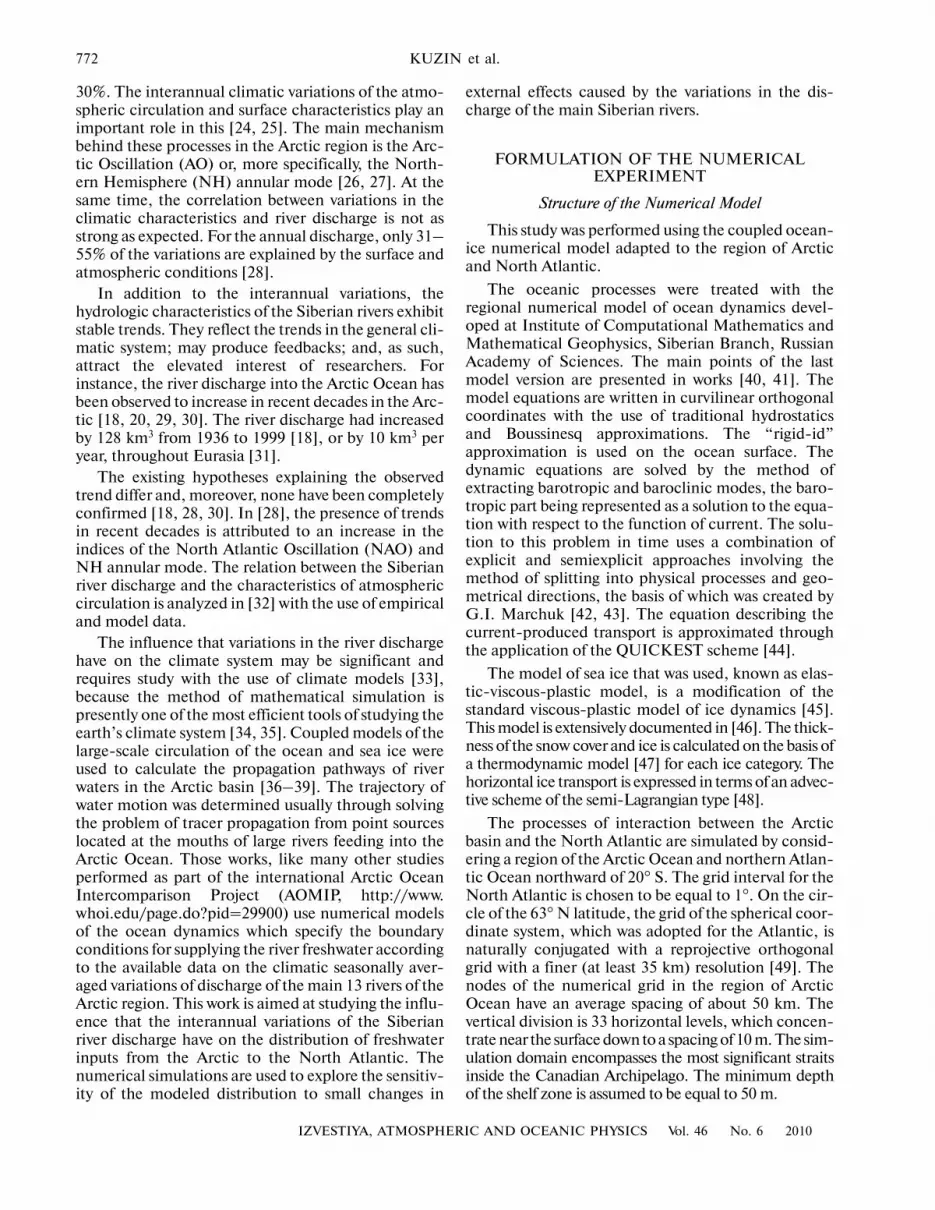
FORMULATION OF THE NUMERICAL EXPERIMENT

Structure of the Numerical Model

This study was performed using the coupled ocean�ice numerical model adapted to the region of Arcticand North Atlantic.

The oceanic processes were treated with theregional numerical model of ocean dynamics devel�oped at Institute of Computational Mathematics andMathematical Geophysics, Siberian Branch, RussianAcademy of Sciences. The main points of the lastmodel version are presented in works [40, 41]. Themodel equations are written in curvilinear orthogonalcoordinates with the use of traditional hydrostaticsand Boussinesq approximations. The “rigid�id”approximation is used on the ocean surface. Thedynamic equations are solved by the method ofextracting barotropic and baroclinic modes, the baro�tropic part being represented as a solution to the equa�tion with respect to the function of current. The solu�tion to this problem in time uses a combination ofexplicit and semiexplicit approaches involving themethod of splitting into physical processes and geo�metrical directions, the basis of which was created byG.I. Marchuk [42, 43]. The equation describing thecurrent�produced transport is approximated throughthe application of the QUICKEST scheme [44].

The model of sea ice that was used, known as elas�tic�viscous�plastic model, is a modification of thestandard viscous�plastic model of ice dynamics [45].This model is extensively documented in [46]. The thick�ness of the snow cover and ice is calculated on the basis ofa thermodynamic model [47] for each ice category. Thehorizontal ice transport is expressed in terms of an advec�tive scheme of the semi�Lagrangian type [48].

The processes of interaction between the Arcticbasin and the North Atlantic are simulated by consid�ering a region of the Arctic Ocean and northern Atlan�tic Ocean northward of 20° S. The grid interval for theNorth Atlantic is chosen to be equal to 1°. On the cir�cle of the 63° N latitude, the grid of the spherical coor�dinate system, which was adopted for the Atlantic, isnaturally conjugated with a reprojective orthogonalgrid with a finer (at least 35 km) resolution [49]. Thenodes of the numerical grid in the region of ArcticOcean have an average spacing of about 50 km. Thevertical division is 33 horizontal levels, which concen�trate near the surface down to a spacing of 10 m. The sim�ulation domain encompasses the most significant straitsinside the Canadian Archipelago. The minimum depthof the shelf zone is assumed to be equal to 50 m.



Initial and Boundary Conditions

The initial distributions of temperature and salinityare derived from a combination of Levitus data and anumber of oceanographic data collected during sensorstudies of Arctic and adjoining regions. The Polar Sci�ence Center Hydrographic Climatology (РНС) data[50] were obtained in exactly the same way and consti�tute a 3D monthly distribution of temperature andsalinity in the layer down to a 1�km depth, as well asseasonal (winter and summer) and annually averagedata for the entire depth range. In particular, the win�tertime distribution was used as the initial distribution,because the numerical simulation starts precisely dur�ing the winter (on January 1, 1948). The absolutewater temperature, which is shown in the data, wasrecalculated to get the potential�temperature distribu�tion, which is required in order to correctly accountfor the vertical heat fluxes.

The ice field changes stronger than the thermoha�line structure of the deep ocean; therefore, it can bereconstructed faster with the help of the model itself.In conformity with AOMIP recommendations, a pre�liminary numerical experiment was performed from1948 to 1954 in order to reconstruct the initial icefield; it is noteworthy that the starting distribution issuch that the ice thickness is 2 m where the surfacetemperatures is less than 0°C and no ice is presentelsewhere. Distributions of the thickness and com�pactness for all ice categories obtained during this pre�liminary experiment are used to specify the initial con�ditions of the main experiment from 1948 to 2009.

The initial velocity components of water and ice arealso obtained as a result of the preliminary experiment.The starting conditions for this preliminary experi�ment are assumed to be zero for velocity componentsof both ice and water.

The boundary conditions at the bottom and at thesolid�state lateral boundaries do not admit heat or saltfluxes across these boundaries; the current undergoesa local friction against bottom, which is proportionalto the square of the near�bottom speed. The southernboundary, which connects the simulation domain withthe South Atlantic, is liquid�state. The conditions atthis boundary admit a free advection beyond the sim�ulation domain when the velocity is in that same direc�tion. Otherwise, the values drawn from the initial РНСdistribution for the temperature and salinity serve tospecify the advective fluxes into the domain. Barotro�pic water loss is specified to correspond to the removalof part of the waters through this boundary. This loss islinearly distributed across the width of the Atlantic atthe latitude of the southern boundary of the domainand compensates for the total river discharge andwater delivery via the Bering Strait. No lateral condi�tions for the liquid�phase ice boundaries are pre�

sumed, because the southern boundary is inaccessibleto ice and the Bering Strait is assumed to be closed forthe ice drift.

The river discharge is specified simultaneously withthe presetting of the supply of freshwater by using thefollowing boundary condition for salinity:

where is a normal to the boundary through which thewater is supplied, is the velocity in thisdirection, Tr is the river discharge, and is the area ofthe lateral surface equaling the product of the length

of segment of the boundary times the depth ofthe basin on this segment. The water flow on the sec�tion of the Bering Strait is specified in the same wayand only differs in that the salinity of the inflowingwater is taken from the PHC data. Thus,

The necessary conditions on the surface of theocean�ice system include the heat fluxes: latent andsensible heat, incoming solar and longwave radiation;longwave surface emission; wind drag; and a flux offreshwater associated with precipitation in the form ofrain and snow.

Calculating these characteristics requires not onlyknowledge of the intrinsic system parameters, namely,the surface temperature and the compactness of iceand of its categories, but also data on the parameters ofthe lower atmosphere and intensity of the radiationbalance terms. The required atmospheric data includenear�surface wind speed and direction, potential andabsolute temperature of the lower atmospheric layer,specific humidity, sea level pressure and air density,total downward solar and infrared radiation, and theprecipitation (snowfall and rainfall) rate.

The precipitation is not explicitly separated intofractions in the initial data; therefore, it is additionallyassumed that the falling precipitation is snow if thenear�ground temperature is negative and that it is rainotherwise.

The numerical experiments used the characteris�tics of the lower atmosphere obtained from the archiveof NCEP/NCAR and CIAF reanalysis data [51].

Numerical Experiments and Results of the Study

To solve this problem, we performed two numericalexperiments for the time period from 1948 to 2009; theexperiments differed in the assumed boundary condi�tions characterizing the river discharge.

( )sdSA S Qd

− + ⋅ =u nn

,

Tr,

SQ

A= −

n( )nu = ⋅u n

A

lΔ H

( )PHC Tr.

S SQ

A

−

=

774


KUZIN et al.

Experiment 1. The lateral boundaries for the suppliedfresh river water are specified according to the availabledata on the climatic average seasonal variations of dis�charges of the 13 main rivers of the Arctic region takenfrom the AOMIP project. The total discharge is8.6 km3/day. In addition, the discharges of 23 rivers of theNorth Atlantic and equatorial Atlantic are taken intoaccount, the losses of which average 29.7 km3/day,according to River Discharge Database [52].

A study of the variations in the Arctic Ocean watercirculation and drift in the period from 1948 to 2007based on a numerical model and on the scenario ofexperiment 1 was carefully documented in [53]. Inaccordance with the atmospheric circulation pattern,the trajectory of the Arctic Ocean surface waters iscyclonic or anticyclonic, which determines the propa�gation direction of the fresh river waters. Generally,the freshwaters are accumulated in the Canadian basinin the period of the anticyclonic circulation and theyare transported through the Fram strait and straits ofthe Canadian Archipelago in the period of cycloniccirculation. At the same time, in separate years of pro�nounced anticyclonic regime, the ice and river waters

are directionally carried into the Fram Strait (Fig. 2),thus favoring the appearance of salinity anomalies inthe North Atlantic.

In late 1960s, an anomalously large amount of iceand freshwater was carried from the Arctic basin to theeast of Greenland by the East Greenland current. Sub�sequent ice melt had led to the appearance of a salinityanomaly on the order of 0.1‰, which traversed theDenmark Strait, spread in the system of currents of thesubpolar North Atlantic gyre, and returned back to theGreenland Sea in the early 1980s [10]. This phenomenonwas the GSA. Salinity anomalies were also recorded inthe North Atlantic in the 1980s and 1990s [54].

Simulations suggest that the transport of icethrough the Fram Strait increases by a factor of 2.5 inthe period from 1965 to 1967 (Fig. 3). One conse�quence of this had been that a vast region of anoma�lously low salinity formed near the east coast ofGreenland and in the region of the Denmark Strait inthe late 1960s. In Fig. 4, this anomaly is distinctly seenin the period corresponding to 1968. The salinityanomaly propagated further in accordance with thesystem of currents of the Atlantic subpolar gyre, as well

5

29303

30

27

28

2728

29

29

29

31

30

2830

30

33

30

3029

3029

30

29

33

3030

28

33

33

30

31

31

31

33

3130

35

29

29

Fig. 2. Distribution of salinity and speeds of currents on the ocean surface in 1961. Experiment 1. Propagation of freshwater inthe direction of the Fram Strait. The length of the arrow in the legend corresponds to a speed of 5 cm/s.



as with the currents of the Norwegian Sea. The salinitydistribution of the surface layer of the ocean in the1970s shows that the model�derived exit of the anom�aly through the Denmark Strait to the Labrador Sea,the inclusion in the Atlantic subpolar gyre, the partialtransition to the subtropical gyre, and the exit to theNorwegian Sea coincide well with observations of theGSA trajectory of propagation.

Experiment 2. In contrast to experiment 1, thebasins of the three main rivers, namely, the Ob,Yenisei, and Lena, are now described using themonthly average data of discharges for the time periodfrom 1948 to 1992 [22, 23].

From the viewpoint of the numerical simulationwith the use of the real Siberian river discharge (exper�iment 2), the most interesting task would be to con�sider the deviations of the obtained fields from thesimulations employing the climatic behavior of theriver discharge (experiment 1).

It is convenient to show the proper data on the riverdischarge in the form of a time�integrated differenceof discharge rates between experiments 2 and 1. Thisoperation will help determine how more river water isdischarged by a given time in measurements whencompared with the climatic norm. The pattern of theriver discharge difference, which has accumulatedsince 1948, is presented in Fig. 5. The mouths of theOb and Yenisei rivers are closely (from the simulationviewpoint) located; therefore, data on the river dis�charge are shown separately for Ob–Yenisei and Lena.The total discharge is also shown. As can be seen inthis figure, the total discharge depends most stronglyon the Ob–Yenisei discharge. However, the differenceaccumulated by 1992 (the last data year) owes the mostto the Lena river discharge. The most characteristic

features pertain to periods of accumulation and deficitof the river discharge. On the whole, we can note thata general deficit of the river discharge in comparisonwith the climatic norm had been observed for a ratherlong time (from 1955 to 1974). Exceptions are 1958–1962, when the accumulated deficit was totally com�pensated for, and even a certain excess of about150 km3 of river discharge appeared by 1962. Overall,the growth during these years stems from the jointincrease of discharge of all the considered rivers. Overthe period from 1958 to 1962, 600 km3 more (com�pared with climatic norm) freshwater was discharged,of which the Lena and Ob–Yenisei contributedapproximately same amount of 300 km3.

We analyzed the discharge of the freshwaterthrough the main straits connecting the Arctic Oceanand the North Atlantic (Fig. 6a) and can note that, onthe average, about 10–20 thousand m3/s of freshwateris transported into the North Atlantic. Dischargethrough the Canadian Straits was about 10 thousandm3/s in the late 1940s, and it decreased to 2–5 thou�sand m3/s by the early 1960s. By this time, the rate thefreshwater discharge through the Fram Strait substan�tially increased, from 2 thousand m3/s in 1949 to 10–15 thousand m3/s after 1960. The difference in dis�charges, which accumulated since 1948, between theexperiment using the real river discharge and theexperiment using climatic data is shown in Fig. 6b. Itcan be seen that the total discharge of freshwater dif�fers little between the experiments until 1962. In 1961the discharge through the Canadian Straits decreasesless in experiment 2; and up to 1963, increasinglymore freshwater is discharged through the Fram Strait.By 1963, 150 km3 more freshwater is transportedthrough the Fram Strait to the Atlantic than in the cli�

6000

4000

2000

0 1950 1960 1970 1980 1990 2000 2010

(а)

(b)600

400

200

0 1950 1960 1970 1980 1990 2000 2010

Fig. 3. Ice loss (km3/yr) in the numerical experiment through (a) the Fram Strait and (b) the Canadian Archipelago Straits. Asharp maximum is characteristic for the late 1960s. Elevated ice transport is obtained for the early and late 1980s and for the mid�1990s.

776


KUZIN et al.

matic experiment. Interestingly, the excess of the riverdischarge formed by this time reached exactly thesame amount, as was already noted above.

The behaviors of the responses of dischargesthrough the straits are also demonstrated in the table,which presents the correlation coefficients of theaccumulated anomaly of the river discharge and dis�charges through the straits with an indication of thetime of the strongest response. For instance, the lossesthrough the Canadian Straits decrease in the same

year as the anomaly of the river discharge forms; thelosses through the Fram Strait change in the oppositedirections of the river discharge with a 4 to 6�yeardelay. Following the increase of the river discharge,approximately four years later, the flow of the Atlanticwaters through the Barents Sea decreases; 8 years later,the weakening of the loss through the Canadian Straitsis repeated.

An analysis of the pattern of the surface currentsshows that the anticyclonic mode of the wind circula�tion prevailed in late 1950s and early 1960s; therefore,the freshwater anomaly, which formed due to the dif�ference in the river discharge of freshwater in the twoexperiments, drifts along with the surface currentimmediately from the river mouths to the Fram Straitwith no marked effect on the properties of the ArcticOcean waters. In other words, we can claim that (1) noexcess of freshwater in the Arctic should be observedfrom almost 1955 to 1974 because of the increase of itsloss through the Fram Strait and (2) the GSA, whichstarted to form in the early 1960s, was fueled by anextra 150 km3 of freshwater when compared to exper�iment 1. However, starting from 1963, the lossesthrough the Fram Strait had equalized in both experi�ments and the loss through the Canadian Straits con�tinued to decrease in experiment 2. On the whole, by1970, these straits under�delivered about 600 km3 offreshwater to the North Atlantic when compared tothe climatic experiment. The pattern of the accumu�lated difference of the Arctic (and not only fresh)water losses through the main straits presented in Fig.6c shows that, in experiment 2, the decrease of the lossin the late 1950s through the Canadian Straits isaccompanied by an increase in loss through the FramStrait. The loss of freshwater through the Fram Straitincreases only in the early 1960s, indicating that theincrease in the total discharge in the late 1950s iscaused by the weakening of a current adding saline andwarm waters from the North Atlantic. It should bestressed that, despite the fact that the difference in dis�charges through the straits is due to the difference inthe river discharge in experiments 1 and 2, the ampli�tude of these variations is 1–2 orders of magnitudelarger than the difference in the river dischargebetween these experiments. For instance, the maxi�mum accumulated excess–deficit of the river dischargeover the period of model integration is ±400 km3,whereas the excess–deficit of the losses through thestraits is more than 15 thousand km3; i.e., the responseis found to be many times larger than the magnitude ofthe initial disturbance. This requires a clarificationand explanation. Specifically, we should see how thesesmall changes in the store of freshwater affect theredistribution of direction of fluxes through the mainstraits connecting the Arctic Ocean and the NorthAtlantic.

1968

1972

1975

35 3434.5 35.536

33

33.5

33

33.5

34

36

34.5

3535.5

34.534.534

34

35

3433.532.5

33.5

34

35 34.5 35.53636.5

3635.5

3434

Fig. 4. The salinity distribution of the surface layer of theArctic Ocean subpolar gyre and northern seas shows thepropagation of the salinity anomaly of the 1970s accordingto the results of numerical experiment 1.



A store of freshwater in the Arctic Ocean favors theformation of a low�salinity water lens in the region ofthe Canadian basin. The presence of the fresh (lighter)water lens by itself in the region of the Canadian basinand Beaufort Sea produces a cyclonic motion in thesubsurface layer. The greater (lower) the freshwaterloading of the lens is, the stronger (weaker) the lenscyclonicity is. If we trace the difference in the averagevorticity between the two experiments in the interme�diate layer of the Canadian basin, which is equivalentto calculating the difference in the velocity circula�tions along the boundary of this basin (Fig. 1), we cansee (Fig. 7) a large resemblance between the time vari�ations of this quantity and the accumulated differenceof the river discharge, which is presented in Fig. 5. Thecorrelation coefficient of these two quantities will be54%; whereas, for the 45 years covered by observa�tions, a correlation in excess of 45% will be significant.This suggests that, between the river discharge andwater circulation in the Arctic, there is a direct relationcorresponding to the linear regression. A result of thisrelation in experiment 2 is a general weakening of thecyclonic water motion in the Arctic in the period from1955 to 1974, which is primarily due to the deficit ofthe river discharge in this long time period. The weak�ening of cyclonicity also leads to the above�mentioneddeceleration of the water motion through the Cana�dian Straits and to the smaller supply of Atlantic

waters through the Fram Strait, because they are com�ponents of the cyclonic water motion in the ArcticOcean basin. This acts to increase the relative role ofthe components of the anticyclonic motion and, morespecifically, the role of Pacific waters supplied throughthe Bering Strait (though their supply rate remainsconstant for each year, the contribution of the watersto the total balance increases) and to increase the out�flow of Arctic waters through the Fram Strait.

An analysis of the ice volume transported to theNorth Atlantic shows that the associated flux of fresh�water is an order of magnitude larger than the volumeof freshwater carried by the oceanic currents. None�theless, the differences in the ice fields between exper�iments 1 and 2 were found to be negligibly small.Toward the end of 1980, the maximum difference hadbeen about 100 km3, i.e., even smaller than the varia�tions caused by the difference in the river discharge.Therefore, the difference in the flux of freshwater,which was caused by the ice outflow, between theexperiments had little effect on the balance of freshwa�ter in the region.

As to the coupled Arctic Ocean–North Atlanticsystem, the volume of freshwater generally increasedfrom 170 thousand km3 to 205 thousand km3 over theperiod from 1948 to 1973; i.e., the increase was about35 thousand km3 (Fig. 8а), which led to the formation

1200

1000

800

600

400

200

0

–200

–400

1995199019851980197519701945 1965196019551950

–600

–800

LenaOb and YeniseiTotal

km3

Fig. 5. Difference in the volumes between the observed and climatic discharges of Siberian rivers accumulated since 1948.

778


KUZIN et al.

and further development of GSA [10]. At the sametime, we note (Fig. 8b) that the difference between theexperiment assuming the real discharge of the Siberianrivers and the experiment with climatic discharge

showed up most appreciably only after this timeperiod, in 1972–1975, when the volume in one exper�iment exceeded that in the other by 3 thousand km3.Such a substantial (a factor of 5–6) difference exceedsthe available growth of the Siberian river discharge inthe period from 1958 to 1962 as compared to climaticnorm; this cannot be explained by the conventionaltransport of freshwaters by the existing currents.

However, the dynamics of the motion of the anom�aly which occurred in these years is very important forexplaining these substantial consequences. As wasalready noted above, by virtue of the circulation estab�lished in the Arctic Ocean in these years, the anomalymoved immediately from the mouths of the Ob,Yenisei, and Lena rivers toward the Fram Strait; thepassage of these waters through the strait can be seenin Fig. 6b, where, in the period of 1960–1963, the vol�ume of freshwater removed from the Arctic exceedsthe climatic value. The further propagation of thisfreshwater anomaly over the regions of the NorthAtlantic is demonstrated in Fig. 9, which presents thedifference in the volumes of freshwater between thetwo experiments in the regions (a) between the FarmStrait and the Denmark Strait, (b) near Newfound�land island, (c) to the west of Great Britain, and (d) inthe region of Azores islands. The first three regions arelocated along the line of the current as part of the sub�polar gyre. The fourth region corresponds to thesouthern branch of the subpolar front. From this figureit can be seen that the freshwater anomaly in the firstregion reaches its maximum in 1964, when the differencein the volumes of freshwater is approximately 300 km3,i.e., two times larger than the volume supplied throughthe Fram Strait. The next region near NewfoundlandIsland is reached by the anomaly in 1970. The ampli�tude of the disturbance at the initial stage correspondsto the volume of the anomaly in the first region; how�ever, in subsequent years it increased manifold, so thatin 1979 the difference in the volumes of freshwaterbetween the experiments was 800 km3. During the sub�sequent eastward motion of the anomaly, it splits intonorth and south branches. It is noteworthy that theregion of the north branch westward of Great Britain isreached by the anomaly in 1975, and the volume offreshwater composing it is only about 100 km3. Also in1975, the anomaly reaches the region of the Azoresislands, where the southern branch of propagation offreshwaters is located. The difference in the volumes offreshwaters between the experiments increases there to1200 km3, i.e., almost ten times larger than the initialexcess of the freshwater that passed through the FramStrait. The thickness of the layer of freshwater, deter�mined with respect to the average salinity of the ArcticOcean S0 = 34.8‰, may change only as a result of themixing of waters of differing types. If a layer withthickness h and salinity S1 < S0 is located above a layer

20

15

10

5

0

19801995

199019851975

1970

–51965

19601955

19501945

800

600

0

–200

–400

19801995

199019851975

1970

–10001965

19601955

19501945

20

15

10

5

0

19801995

199019851975

1970

–201965

19601955

19501945

–5

–10

–15

400200

–600–800

Canadian StraitsFram StraitBarents SeaTotal

thou

san

d m

3 /skm

3th

ousa

nd

km3

(а)

(b)

(c)

Fig. 6. Loss characteristics through the main straits con�necting the Arctic Ocean and North Atlantic: (a) loss offreshwaters with respect to the average salinity of 34.8‰(positive values correspond to water transport from theArctic Ocean to the North Atlantic); (b) difference, accu�mulated since 1948, between experiments 2 and 1 in thefreshwater volumes transported from the Arctic Ocean tothe North Atlantic; and (c) difference between experi�ments 2 and 1 in water volumes transported from the ArcticOcean to the North Atlantic since 1948.



with the same thickness and with salinity S2 > S0, thethickness of the layer of freshwater, recalculated for thereference value S0, will be

As a result of mixing, the salinity of the mixed layerwith thickness 2h will be (S1 + S2)/2. If this is largerthan S0, the thickness of the layer of freshwater willvanish. Otherwise, if the resulting salinity is less than

, the thickness of the layer after mixing will be

Thus, the change of the thickness of the freshwaterlayer will be negative

that is, the volume of the freshwater will decrease as aresult of mixing in any case.

Consequently, the fact that the volume of freshwa�ter in experiment 2 is so much larger than it is in exper�iment 1 is not because of an increase in the amount ofthis water in experiment 2, but rather because of its

init0 1 1

0 0

1 0.S S SH h hS S

⎛ ⎞−= = − >⎜ ⎟⎝ ⎠

0S

h

init

1 20

0

1 2 2

0 0 0

22

2 1 .

S SSH h

S

S S Sh H hS S S

+−=

⎛ ⎞ ⎛ ⎞= − − = − −⎜ ⎟ ⎜ ⎟

⎝ ⎠ ⎝ ⎠

h init2

0

1 0,SH H H hS

⎛ ⎞Δ = − = − − <⎜ ⎟

⎝ ⎠ drastic decrease in experiment 1 as a result of convec�tive and/or shearing mixing or due to lateral diffusion.The excess freshwater, which is present in experiment 2,ensures the more stable stratification of waters in theupper layer; as a result, the vertical mixing is moreprobable under the impact of external factors: the den�sity (heat and salinity) flux on the surface of the ocean;

Coefficients of correlation of accumulated river dischargewith the total loss through the main straits, as well as with loss�es of freshwater though these straits

Straits 1 2 3

Total loss through the straits

Fram Strait –0.78 4 1.30

Canadian Archipelago 0.59 (0.71) 0 (12) 1.06 (0.98)

Barents Sea 0.74 4 1.23

Freshwater discharge

Fram Strait –0.75 6 1.20

Canadian Archipelago 0.57 (0.71) 0 (12) 1.03 (0.98)

Barents Sea 0.40 7 0.62

Note: (heading 1) Correlation coefficient at the maximum levelwith respect to the significance level, (heading 2) time lagprior to the maximum response (in years) to the river dis�charge anomaly, and (heading 3) ratio of the correlation coef�ficient to the significance level. For the Canadian ArchipelagoStraits, there is a subsequent second maximum; however, it isless than the significance level because the time seriesbecomes shorter as the time lag increases.

0.15

0.10

0.05

0

–0.05

–0.10

–0.15

–0.201945 1950 1955 1960 1965 1970 1975 1980 1985 1990 1995

m/s

Fig. 7. Difference in the circulation of the velocity of the current at a depth of 100 m between experiments 2 and 1 around theCanadian basin, represented in terms of the average velocity directed along the contour counterclockwise.

780


KUZIN et al.

the wind shear of velocity; and in the case of the hori�zontal advection of other types of water in the frontalzone, which disturbs the vertical stability.

A confirmation of this may be the difference in thewater volumes mixed in the upper layer in region А(Fig. 10) in experiments 2 and 1. In total agreementwith our understanding of the mechanism, the vol�umes of the mixed waters strongly differed betweenexperiments 1 and 2 in 1965, when the volume of themixed waters in experiment 1 exceeded that in experi�ment 2 by 25 thousand km3. Other than this disagree�ment, we can also note another less significant dis�crepancy in the opposite direction in 1960. This isbecause 1960 is the final year of the preceding period,when the flux of the freshwater was less in experiment 2than in experiment 1.

As can be seen, the most substantial differencetakes place during the development of the situationnear the Azores islands, where the southern propagationbranch of the waters of the GSA develops (Fig. 10).These waters move in the southern direction more rap�idly in the case using the real Siberian river discharge.Analysis shows that, as was expected, the deficit offreshwater in the experiment using climatic river dis�charge weakens the vertical salinity stratification in theregion of the southern branch of the GSA, thus creat�ing the situation of convective or shear instability andwater mixing in the vertical. In this case, the situationof the vertical instability (a) is caused by an advance ofsaline and warm waters from the direction of the Gutof Gibraltar and (b) is a consequence of the fact thatthis region is characterized by the presence of strongtrade winds. Therefore, even a slight weakening of thedensity stratification may substantially activate thevertical mixing, which we ultimately see in the resultsof experiment 1.

19451950

19551960

19651970

19751980

19851990

1995

210

205

200

195

190

185

180

175

170

165

thou

san

d km

3th

ousa

nd

km3

19451950

19551960

19651970

19751980

19851990

1995

3.5

3.0

2.5

2.0

1.5

1.0

0.5

0

–0.5

(a)

(b)

Experiment 1

Experiment 2

Fig. 8. Change in the store of freshwater in the ArcticOcean and North Atlantic with respect to the averagesalinity of the Arctic Ocean of 34.8‰: (a) change in thetotal store of freshwater in experiments 1 and 2 and (b) dif�ference in the store of freshwater between experiments 2and 1 (the positive value corresponds to the larger store inexperiment 2 than in experiment 1).

(а)

(b)

(c)

(d)

0.5

0

thou

san

d km

3

–0.5

1.0

0.5

0

–0.5

0.2

0

–0.2

2

1

0

–11950 1960 1970 1980 1990

thou

san

d km

3th

ousa

nd

km3

thou

san

d km

3

Fig. 9. Time behavior of the difference in the volumes offreshwater between experiments 2 and 1 in differentregions of the North Atlantic along the propagation path ofthe GSA (see notations in Fig. 1): (a) region A eastward ofGreenland between the Denmark Strait and Fram Strait,(b) region B eastward of the Newfoundland island, (c)region C westward of Great Britain, and (d) region D west�ward of Spain in the region the Azores islands.



CONCLUSIONS

A numerical simulation with the coupled ocean�icemodel of the region of the Arctic Ocean and NorthAtlantic was performed to study the effect that theinterannual variations in the Siberian river dischargehave on the distribution and spread of the freshwater inthis region. For this, we compared two experimentswith and without accounting for the interannual vari�ations in the discharge of three Siberian rivers: Yenisei,Lena, and Ob.

The variations in the discharge of the three riversover 45 years (from 1948 to 1992) had yielded up to600�km3 differences in the accumulated volume of thedelivered freshwater when compared with the climaticvariations. Despite the fact that the interannual varia�tions of the river discharge are small compared withthe rate of the main currents, we can indicate a num�ber of cases when the after effect of these small varia�tions had been much stronger than the initial distur�bance.

First, it was shown that the excess or deficit of theriver discharge appropriately favors the intensificationor weakening of the circulation cyclonicity of the sub�surface Arctic Ocean waters. The cyclonicity intensifi�cation is accompanied by an increase in the loss of therelatively fresh and cold Arctic waters through theCanadian Straits with the pertinent increase of the vol�umes of the saline and warm waters supplied from theAtlantic. On the other hand, the weakening of thecyclonicity of the air mass motion in the Arctic resultsin a reduction of the transport of Arctic waters throughCanadian Straits with a simultaneous decrease in thesupply of saline and warm waters from the Atlantic.Simultaneously, the flux of Arctic waters through

Fram Strait increases and, against the background of aweakening in the supply of Atlantic waters, the frac�tion of inflow of relatively fresh Pacific waters throughthe Bering Strait becomes more significant.

Thus, the excess or deficit of freshwater in the Arc�tic, which accumulated due to the interannual varia�tions, favors the redistribution of the direction oflosses of Arctic waters through the main straits.

Secondly, it was found that even small changes inthe abundance of freshwater, which developed againstthe background of the GSA, lead to considerable devi�ations of the thermohaline structure in the upperocean layer from the climatic norm. Changes in thecontent of freshwater in the anomaly under the condi�tions of identical atmospheric impacts may happenonly in the negative direction as a result of the verticalmixing or lateral diffusion exchange. In this situation,even small salinity variations may cause substantialchanges in the stratification of the upper ocean layer,leading to appreciable changes in the volumes of waterinvolved in the vertical mixing. Therefore, the excessof the freshwater in the upper ocean layer diminishesthe volume of the mixed waters and keeps a certainpart of the existing amount of freshwater of the GSAunmixed, although it is quite large compared with theinitial disturbance. In other words, a small excessivecontent of freshwater may prevent a large amount ofrelatively fresh waters from mixing, thereby increasingthe deviation of the volume of freshwater from the vol�ume in the experiment with climatic discharge distri�bution. This means that the difference in the volumesof the GSA between the two experiments considerablyincreases along the GSA trajectory. This growth con�tinues until the GSA itself exists.

ACKNOWLEDGMENTS

This work was supported by the Russian Fund forBasic Research (grants nos. 08�05�00708 and 08�05�00457), by the Presidium of Russian Academy of Sci�ences (project 17.2), and by the Department of Math�ematical Sciences of the Russian Academy of Sciences(project 1.3.6).

REFERENCES

1. V. V. Ivanov, “Water Balance and Water Resources ofthe Arctic Region,” Trudy AANII 323, 4–24 (1976).

2. G. P. Kalinin and I. A. Shiklomanov, “The Use of WaterResources of the Earth,” in The World Water Balanceand Water Resources of the Earth (Gidrometizdat, Len�ingrad, 1974), pp. 575–606 [in Russian].

3. The World Ocean Atlas, Ed. by S. G. Gorshkov (Perga�mon, New York, 1983), Vol. 3.

4. The Arctic Atlas, Ed. by A. F. Treshnikov (AANII, Mos�cow, 1985) [in Russian].

15

10

5

0

–5

–10

–15

–20

–25

–301945

19501955

19601965

19701975

thou

san

d km

3

19801985

19901995

Fig. 10. Time behavior of the difference in the volumes ofwater between experiments 2 and 1, which were verticallymixed for a year in region A eastward of Greenlandbetween the Denmark Strait and the Fram Strait.

782


KUZIN et al.

5. D. J. Hanzlik and K. Agaard, “Fresh and Atlantic Waterin the Kara Sea,” J. Geophys. Res. 85 (C9), 4937–4942(1980).

6. R. W. McDonald, C. S. Wong, and P. E. Erickson, “TheDistribution of Nutrience in the Southeastern BeaufortSea: Implications for Water Circulation and PrimaryProduction,” J.Geophys. Res. 92 (C3), 2939–2952(1987).

7. K. Aagaard and E. C. Carmack, “The Role of Sea Iceand Other Fresh Water in the Arctic Circulation,”J. Geophys. Res. 94 (C10), 14485–14498 (1989).

8. S. S. Lappo, “The Causes of Heat Advection to theNorth across the Equator in the Atlantic Ocean,” inStudies of Processes of Interaction between the Ocean andthe Atmosphere (Moscow, 1984), pp. 125–129 [in Rus�sian].

9. W. S. Broecker, “Thermohaline Circulation, the Achil�les Heel of Our Climate System: Will Man�Made CO2Upset the Current Balance?,” Science 278 (5343),1582–1588 (1997).

10. R. R. Dickson, J. Meincke, S.�A. Malmberg, et al.,“The "Great Salinity Anomaly” in the Northern NorthAtlantic 1968–1982," Progr. Oceanogr. 20 (2), 103–151 (1988).

11. L. K. Coachman and K. Agaard, “Transport throughBering Strait: Annual and Interannual Variability,”J.Geophys. Res. 93 (15), 535–539 (1988).

12. R. A. Woodgate, K. Aagaard, and T. Weingartner, “Intran�nual Changes in the Bering Strait Fluxes of Volume, Heat,and Freshwater between 1991 and 2004,” Geophys. Rev.Lett. 33, L15609, doi: 1029/2006GL026931 (2006).

13. J. D. Milliman and R. H. Meade, “World Wide of RiverDelivery Sediment to the Oceans,” J. Geol. 91, 1–21(1983).

14. World Water Balance and Water Resources of the Earth,Ed. by I. Sh. Korzun, A. A. Sokolov, M. I. Budyko, et al.(Gidrometeoizdat, Leningrad, 1974) [in Russian].

15. D. Yang, D. Kane, L. Hinzman, et al., “Major SiberianRiver Discharge Regime and Change,” J. Geophys.Res. 107 doi: 10.1029/2002JD002542 (2002).

16. D. Yang, B. Ye, and A. Shiklomanov, “Discharge Char�acteristics and Changes Over the Ob River Watershed inSiberia,” J. Hydromet. 5 (4), 595–608 (2004).

17. B. Ye, D. Yang, and D. Kane, “Changes in Lena RiverStreamflow Hydrology: Human Impacts versus NaturalVariations,” Water Resour. Res. 39, 1200,doi: 10.1029/2003WR001991 (2003).

18. J. W. McClelland, R. M. Holmes, B. J. Peterson, et al.,“Increasing River Discharge in the Eurasian Arctic:Consideration of Dams, Permafrost Thaw, and Fires asPotential Agents of Change,” J. Geophys. Res. 109,D18102, doi: 10.1029/2004JD004583 (2004).

19. A. Dai and K. Trenberth, “Estimates of FreshwaterDischarge from Continents: Latitudinal and SeasonalVariations,” J. Hydrometeor. 3, 660–687 (2002).

20. S. Berezovskaya, D. Yang, and D. Kane, “Compatibil�ity Analysis of Precipitation and Runoff Trends over theLarge Siberian Watersheds,” Geoph. Res. Lett. 31 doi:10.1029/2004GL121277 (2004).

21. I. P. Semiletov, N. I. Savelieva, G. E. Weller, et al., “TheDispersion of Siberian River Flows into Coastal Waters:Meteorological, Hydrological and Hydrochemical

Aspects,” in The Freshwater Budget of the Arctic Ocean,Ed. by E. Lewis et al. (Kluwer, Norwell, London,2000), pp. 323–366.

22. Multiannual Data on the Regimen and Resources of Sur�face Waters of Land (Gidrometeoizdat, Leningrad,1985), Vol. 1, nos. 10, 12, 16 [in Russian].

23. State Water Cadastre, Section 1: Surface Waters, Ser. 2:Annual Data on the Regimen and Resources of SurfaceInland Waters in 1981–1990, Parts 1 and 2, Vol. 1,nos. 10, 12, 16.

24. A. Proshutinksy, I. Polyakov, and M. Johnson, “Cli�mate States and Variability of Arctic Ice and WaterDynamics during 1946–1997,” Polar Res. 18 (2), 135–142 (1999).

25. J. E. Walsh, “Global Atmospheric Circulation Patternsand Relationships to Arctic Freshwater Fluxes, in TheFreshwater Budget of the Arctic Ocean, Ed. by E. Lewiset al. (Kluwer Acad. Publ., Norwell, London, 2000),pp. 21–41.

26. D. W. J. Thompson and J. M. Wallace, “Annular Modesin Extratropical Circulation. Pt I: Month�to�MonthVariability,” J. Clim. 13 (5), 1000–1016 (2000).

27. D. W. J. Thompson, J. M. Wallace, and G. C. Hegerl,“Annular Modes in Extratropical Circulation. Part II:Trends,” J. Clim. 13 1018–1036 (2000).

28. Y. Ye, D. Yang, T. Zhang, et al., “The Impact of Cli�matic Conditions of Seasonal River Discharges in Sibe�ria,” J. Hydromet. 5 (2), 286–295 (2004).

29. R. Lammers, A. Shiklomanov, C. Vorosmarty, et al.,“Assessment of Contemporary Arctic River RunoffBased on Observational Discharge Records,” J. Geo�phys. Res. 106 (D4), 3321–3334 (2001).

30. B. J. Peterson, R. M. Holmes, J. W. McClelland, et al.,“Increasing River Discharge to the Arctic Ocean,” Sci�ence 298 (5601), 2171–2173 (2002).

31. A. I. Shiklomanov and R. B. Lamers, “Record RussianRiver Discharge in 2007 and the Limits of Analysis,” Envi�ron. Res. Lett. 4 doi: 10.1088/1748–9326/4/4/045015(2009).

32. I. I. Mokhov, V. A. Semenov, and V. Ch. Khon, “Esti�mates of Possible Regional Hydrologic RegimeChanges in the 21st Century Based on Global ClimateModels,” Izv. Akad. Nauk, Fiz. Atmos. Okeana 39 (2),150–162 (2003) [Izv., Atmos. Ocean. Phys. 39 (2),130–144 (2003)].

33. Intergovernmental Panel on Climate Change (IPCC). Cli�mate Change 2001: The Scientific Basis; Contribution ofWorking Group I to the Third Assessment Report of theIPCC, Ed. by J. C. Houghton et al. (Cambridge Univ.Press, Cambridge, 2001).

34. G. I. Marchuk and A. S. Sarkisyan, Mathematical Sim�ulation of Ocean Circulation (Nauka, Moscow, 1988) [inRussian].

35. V. P. Dymnikov, V. N. Lykosov, and E. M. Volodin,“Problems of Modeling Climate and Climate Change,”Izv. Akad. Nauk, Fiz. Atm. Okeana 42 (5), 618–636(2006) [Izv., Atmos. Ocean. Phys. 42 (5), 568–585(2006)].

36. W. Maslowski, B. Newton, P. Schlosser, et al., “Model�ing Recent Climate Variability in the Arctic Ocean,”Geophys. Rev. Lett. 27 (22), 3743–3746, doi:10.1029/1999GL011227 (2000).



37. V. A. Ryabchenko, G. V. Alekseev, I. A. Neelov, et al.,“Distribution of River Waters in the Arctic Ocean,”Meteorol. Gidrol., No. 9, 61–69 (2001).

38. V. I. Kuzin, E. N. Golubeva, and G. A. Platov, “Mod�eling of Hydrophysical Characteristics of the ArcticOcean–Northern Atlantics System,” in Basic Studies ofOceans and Seas, Book 1, Ed. by N. P. Laverov (Nauka,Moscow, 2006) [in Russian].

39. A. S. Sarkisyan and J. E. Sundermann, Modelling OceanClimate Variability (Sringer, Berlin, 2009).

40. E. N. Golubeva and G. A. Platov, “On Improving theSimulation of Atlantic Water Circulation in the ArcticOcean,” J. Geophys. Res. 112, C04S05, doi:10.1029/2006JC003734 (2007).

41. E. N. Golubeva, “Numerical Modeling of AtlanticWater Dynamics in the Arctic Basin using theQUISKEST Scheme,” Vychislit. Tekhnol. 13 (5), 11–24 (2008).

42. G. I. Marchuk, Numerical Solution of Problems of Atmo�sphere and Ocean Dynamics (Gidrometeoizdat, Lenin�grad, 1974) [in Russian].

43. G. I. Marchuk, Splitting Methods (Nauka, Moscow,1988) [in Russian].

44. B. P. Leonard, “A Stable and Accurate ConvectiveModeling Procedure Based on Quadratic UpstreamInterpolation,” Comp. Meth. Appl. Mechan. Engin.19, 59–98 (1979).

45. W. D. Hibler, “A Dynamic Thermodynamic Sea IceModel,” J. Phys. Oceanogr. 9 (4), 815–846 (1979).

46. E. C. Hunke and J. K. Dukowicz, “An Elastic�Viscous�Plastic Model for Ice Dynamics,” J. Phys. Oceanogr.27 (9), 1849–1867 (1997).

47. C. M. Bitz and W. H. Lipscomb, “An Energy�Conserv�ing Thermodynamic Model of Sea Ice,” J. Geophys.Res. 104 (C7), 15669–15677 (1999).

48. W. H. Lipscomb and E. C. Hunke, “Modeling Sea IceTransport using Incremental Remapping,” Mon. Wea.Rev. 132 (6), 1341–1354 (2004).

49. R. J. Murray, “Explicit Generation of OrthogonalGrids for Ocean Models,” J. Comput. Phys. 126, 251–273 (1996).

50. M. Steele, R. Morley, and W. Ermold, “PHC: A GlobalHydrography with a High Quality Arctic Ocean,”J. Clim. 14 (9), 2079–2087 (2000).

51. W. G. Large and S. G. Yeager, “Diurnal to DecadalGlobal Forcing for Ocean and Sea�Ice Models: TheData Sets and Flux Climatologies,” Technical Report2004, TN�460+STR, NCAR (2004).

52. C. J. Volosmarty, B. Fekete, and B. A. Tucker, RiverDischarge Database. Version 1.1 (RivDIS v1.0 supple�ment) (University of New Hampshire, Durham, NH,USA, 1998).

53. E. N. Golubeva and G. A. Platov, “Numerical Model�ing of the Arctic Ocean Ice System Response to Varia�tions in the Atmospheric Circulation from 1948 to2007,” Izv. Akad. Nauk, Fiz. Atmos. Okeana 45 (1),145–160 (2009) [Izv., Atmos. Ocean. Phys. 45 (1),137–152 (2009)].

54. I. Belkin, S. Levitus, J. Antonov, et al., “Great SalinityAnomalies” in the North Atlantic,” Prog. Oceanogr.41 (1), 1–68 (1998).

Influence that interannual variations in Siberian river discharge have on redistribution of...

Documents

Transcript of Influence that interannual variations in Siberian river discharge have on redistribution of...