Influence of the convection electric field models on predicted

plasmapause positions during magnetic storms

V. Pierrard,1,3 G. V. Khazanov,2 J. Cabrera,3 and J. Lemaire1,3

Received 27 June 2007; revised 28 August 2007; accepted 7 March 2008; published 9 August 2008.

[1] In the present work, we determine how three well documented models of themagnetospheric electric field, and two different mechanisms proposed for the formation ofthe plasmapause influence the radial distance, the shape and the evolution of theplasmapause during the geomagnetic storms of 28 October 2001 and of 17 April 2002.The convection electric field models considered are: McIlwain’s E5D electric field model,Volland-Stern’s model, and Weimer’s statistical model compiled from low-Earth orbitsatellite data. The mechanisms for the formation of the plasmapause to be tested are: (1) theMHD theory where the plasmapause should correspond to the last-closed-equipotential(LCE) or last-closed-streamline (LCS), if the E-field distribution is stationary or time-dependent respectively; (2) the interchange mechanism where the plasmapausecorresponds to streamlines tangent to a Zero-Parallel-Force surface where the field-alignedplasma distribution becomes convectively unstable during enhancements of the E-fieldintensity in the nightside local time sector. The results of the different time dependentsimulations are compared with concomitant EUV/IMAGE observations when available.The plasmatails or plumes observed after both selected geomagnetic storms are predictedin all simulations and for all E-field models. However, their shapes are quite differentdepending on the E-field models and the mechanisms that are used. Despite the partialsuccess of the simulations to reproduce plumes during magnetic storms and substorms,there remains a long way to go before the detailed structures observed in the EUVobservations during periods of geomagnetic activity can be accounted for very preciselyby the existing E-field models. Furthermore, it cannot be excluded that the mechanismscurrently identified to explain the formation of ‘‘Carpenter’s knee’’ during substormevents, will have to be revised or complemented in the cases of geomagnetic storms.

Citation: Pierrard, V., G. V. Khazanov, J. Cabrera, and J. Lemaire (2008), Influence of the convection electric field models on

predicted plasmapause positions during magnetic storms, J. Geophys. Res., 113, A08212, doi:10.1029/2007JA012612.

1. Introduction

[2] The plasmapause position prediction is very importantfor the scientific community because the plasmasphereinteracts with the other regions of the magnetosphere andwith the ionosphere. The location of the plasmapause deter-mines for instance where wave-particle interaction processeschange the pitch angle and energy spectra of radiation belts(RB) electrons. Cornwall et al. [1971] noted that maximuminstability of ElectroMagnetic Ion Cyclotron (EMIC) wavesgenerated by ring current (RC) anisotropy should occur justwithin the plasmapause. They also suggested that pitch anglediffusion of RC ions resonant with the EMIC waves gener-ated within the plasmapause should be important loss processfor the RC. Recent global self-consistent RC/EMIC waves

modeling by Khazanov et al. [2006] conforms this initialstudy. It was found that global EMIC wave distribution has ahighly plasmapause organized structure during the May,1998 storm period that has been presented in this study.Khazanov et al. [2007] also found that plasmaspheric energydeposition to the thermal electrons via Landau EMIC wavedamping is very critical to position of plasmapause.[3] During magnetic storms, under certain conditions,

relativistic electrons with energies �1 MeV can be removedfrom the outer RB by EMIC wave scattering. Recentcalculations suggest that pitch angle scattering via EMICwaves can compete with Dst effect as a mechanism fordepleting relativistic electrons from the outer RB zoneduring the initial and main phases of a magnetic storm[Summers and Thorne, 2003; Albert, 2003]. So, it becomesmore and more obvious that RC and RB populations arevery sensitive to the core plasmasphere distribution andspecifically to the position of the plasmapause [Spasojevicet al., 2004; Baker et al., 2004].[4] The position of the plasmapause is determined by the

interplay between the corotation and convection electricfields. This statement is very general but it does not reallyidentify and grasp the specific physical mechanism that is

JOURNAL OF GEOPHYSICAL RESEARCH, VOL. 113, A08212, doi:10.1029/2007JA012612, 2008ClickHere

for

FullArticle

1Belgian Institute for Space Aeronomy, Brussels, Belgium.2National Space Science and Technology Center, NASA Marshall

Space Flight Center, Huntsville, Alabama, USA.3Center for Space Radiations, Universite Catholique de Louvain,

Louvain-La-Neuve, Belgium.

Copyright 2008 by the American Geophysical Union.0148-0227/08/2007JA012612$09.00

A08212 1 of 21

underlying the formation of the plasmapause. The magne-tospheric convection electric field, controlled by the solarwind conditions and the level of geomagnetic activity, is akey factor in all existing theories for the formation of theplasmapause. Therefore it is important to have first areliable magnetospheric electric field model. Since there isno way to determine directly, at each instant of time, theglobal electric field distribution in the whole magneto-sphere, various empirical and mathematical models havebeen built, tentatively, with various degrees of sophistica-tion. The E-field models used in the present paper are(1) the VSMC model introduced by Volland and Stern[Volland, 1973; Stern, 1975] and adapted by Maynard andChen [1975], (2) the E5D model derived by McIlwain[1986] from ATS5 and ATS6 observations at geosynchro-nous orbit, and (3) the model of Weimer [1996] determinedfrom ionospheric measurements; these empirical electricfield models are respectively associated with (1) a centereddipole magnetic field, (2) the M2 magnetic field determinedfrom geosynchroneous measurements, and (3) Tsyganenkoand Stern’s [1996] magnetic field model determined fromvarious statistical magnetometric in situ measurements.These models will be briefly described in the next section.[5] In addition to a reliable magnetospheric electric field

model, one needs also to have a correct physical theory forthe formation of the plasmapause, i.e., a specific physicalmechanism that accounts for the observations. Several suchmechanisms have been proposed in the past and can besimulated numerically once an E-field model has beenadopted.[6] In the following sections, we use the three E-field

models mentioned above, and compare their influence onthe dynamics of the plasmasphere during the geomagneticstorm on 28 October 2001. Moreover, for the E5D model,the dynamical evolution of the cold plasma is tracked byusing two different categories of simulations to predict thepositions of the plasmapause and its deformations at differ-ent times precisely when EUV observations are available.[7] There are other sophisticated models for the magne-

tospheric electric field distribution: for instance, AMIEdeveloped by Richmond and Kamide [1988]. This popularE-field model was obtained from ground-based (magnetom-eter and radar) and ionospheric (DMSP satellite) data.Although it might be of some interest to use this additionalmodel, it is not completely clear that ionospheric electricfield distribution can be directly mapped up into theequatorial region of the magnetosphere where plasmapauseknee start to form. Not only is the actual 3D distribution ofmagnetic field lines not completely guaranteed, but theexistence of field-aligned electric potential drops is likelyto jeopardize such a field-aligned mapping of ionosphericE-field into the magnetosphere.[8] In several studies, different convection electric field

models have already been compared with observations[Jordanova et al., 2001; Boonsiriseth et al., 2001; Khazanovet al., 2004]. Their influence on the ring current wasanalyzed in detail by Chen et al. [2003]. However, theireffects on particles of lower energies (<10 eV) populatingthe plasmasphere was less well studied, except by Liemohnet al. [2004] who compared some electric field models, andtheir effects on plasmaspheric morphologies; he used (1) amodified McIlwain electric field model, (2) the Weimer

model, and (3) as well as another self-consistent electricpotential model for the time span of the recovery phase ofthe 17 April 2002 magnetic storm. These authors found thatall these models have certain strengths but also someweaknesses in predicting the observed plasmapause positionduring this storm. They found especially that the electricfield intensity of Weimer’s model was a bit too strong in theinner magnetosphere, leading to a too small plasmasphere.Liemohn’s modifiedMcIlwain model (which differs from theoriginal E5Dmodel, and was not used with the associatedM2magnetic field model) has a too small electric field intensityaround noon, leading to a plasmapause position that does notcorrespond to the EUVobservations on the dayside althougha good fit was obtained in the nightside.[9] In the present work, we also present the results

obtained during this magnetic storm of 17 April 2002, butwe have focused our attention on another clean and isolatedgeomagnetic storm: that observed on 28 October 2001. TheVSMC, unmodified E5D and Weimer E-field models havebeen used with the hope to determine which of them mightbe the most appropriate for this magnetic storm.[10] It is commonly assumed that the topologies of both

the electric field and magnetic field determine the positionwhere the plasmapause is formed at the time of geomagneticstorms and substorms. Postulating that the plasmapausecoincides with the last closed equipotential of the magneto-spheric electrostatic field distribution as proposed by Brice[1967], this led authors to derive an electric field topologyfrom observed plasmapause positions: e.g., Maynard andChen [1975]. This led also Goldstein et al. [2002] to add anelectric field component penetrating into the plasmasphere toobtain plasmaspheric shapes and positions fitting thoseobserved on 24 May 2000, when a plasmaspheric shoulderwas found in the EUV observations. In a subsequent study,Goldstein et al. [2003] included an additional E-field distri-bution related to subauroral polarization stream to obtain abetter fit with plasmapause positions observed by EUV/IMAGE on 2 June 2001. The MHD simulations are essen-tially based on the postulate that the plasmapause coincideswith the Last Closed Equipotential (LCE) of a stationaryglobal magnetospheric electric field. When the magneto-spheric electric field is not stationary, the plasmapause cannotbe identified with the LCE of the time-dependent E-field, butmay be assumed to correspond to a Last Closed Streamline(LCS). This is what will be assumed in the MHD simulationspresented below. The second mechanism used below topredict the plasmapause positions and shapes is based onthe mechanism of interchange reported in the book byLemaire and Gringauz [1998]. These mechanisms arerecalled and described in section 3.[11] In section 4, we illustrate the plasmapause positions

simulated for all three different electric fields models andwith both kinds of mechanisms. The results are thencompared with observations of EUV/IMAGE. Discussionand conclusion are given in the last section.

2. Models of Electric and Magnetic Fields

2.1. Volland-Stern’s and Maynard-Chen’s ConvectionElectric Field (VSMC)

[12] The Volland-Stern model [Volland, 1973; Stern,1975] is a simple mathematical model where a uniform

A08212 PIERRARD ET AL.: PLASMAPAUSE POSITIONS

2 of 21

A08212

dawn-dusk convection electric potential distribution is ap-plied across the magnetosphere. It has become very popularbecause of its simplicity and portability. In this model, thereis no induced electric field resulting from time dependentmagnetic field variations as can be envisaged during stronggeomagnetic storms; the magnetospheric electric fieldderives from a scalar potential which, in a corotating frameof reference, is given by

F ¼ AR2 sinf

where R is the equatorial radial distance, f is the azimuthalangle from noon and the Kp dependent factor A =

0:0451�0:159Kp þ 0:0093Kp2ð Þ3

kVR2E

h idetermines the convection electric

field intensity.[13] The Kp dependence of this empirical model was

obtained by Maynard and Chen [1975] by adjusting the lastclosed equipotential (LCE) of the total E-field with plasma-pause positions determined by OGO3 and OGO5 satelliteobservations; this is why this model has been given theacronym VSMC in the following. The Kp dependence isvery sensitive especially at small values of Kp; the value ofA varies from A = 45 V/RE

2 for Kp = 0 to over 800 V/RE2 for

Kp = 6.

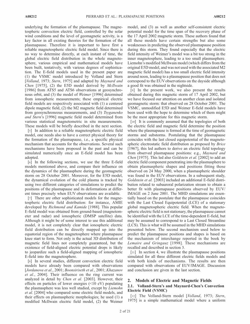
[14] Figure 1 illustrates the equatorial contour maps of theequipotentials for the VSMC convection electric field every2 h from 0:00 UT to 10:00 UT during the geomagneticstorm of 28 October 2001. To limit the effects of theartificial discontinuity appearing every 3 h in Kp indexvariation, we assume that a Kp increase (decrease)appears during the first hour (last half hour) of the 3 hrange. A linear interpolated value of Kp is used duringthis variation. This evolution of Kp is illustrated by theblacked region in the top panels of the simulation figures(Figures 9 to 15). Because of this ‘‘smoothed or fileddown Kp variation’’, the electric field varies moresmoothly in our simulations. Figure 1 shows how thedawn-dusk electric field component is shielded close tothe Earth and how it is assumed to change over this 10 hperiod. During this period of time, Kp increased from 1�

at 0:00 UT to 7� at 05:00 UT, as illustrated in the toppanels of Figure 9.[15] In our simulations, this convection electric field is

used with a centered dipolar magnetic field B. Indeed, thiswas the magnetic field assumed by Maynard and Chen[1975] to compute theMHD convection velocity: (~E�~B)/B2.

2.2. McIlwain’s E5D Convection Electric Field

[16] Another analytical representation of the magneto-spheric convection electric potential was derived byMcIlwain [1986] from electron and proton dynamical

Figure 1. Equipotential contours of the convection electric field Volland-Stern on 28 October 2001(without corotation electric field). The values of the potential (in kV) are given on the equipotentialcontours, which are drawn every 4 kV.

A08212 PIERRARD ET AL.: PLASMAPAUSE POSITIONS

3 of 21

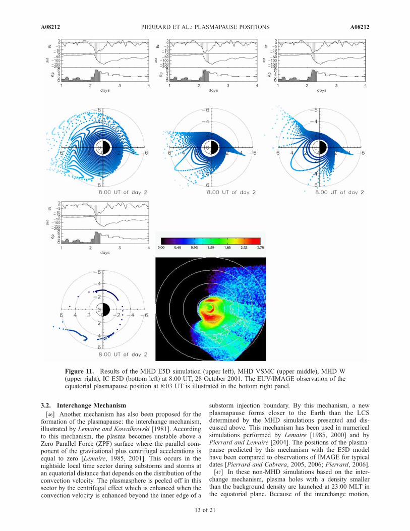
A08212

spectra measured at geosynchronous orbit during the ATS-5and ATS-6 missions:

F ¼ R 0:8 sinfþ 0:2 cosfð Þ þ 3f g 1þ 0:3Kp

1þ 0:1Kp

� �

� 1

1þ 0:8* Rar

R

� �8 !

with Rar = 9.8 � 1.4cos f + (�0.9 � 0.3cos f) Kp1þ0:1Kp.

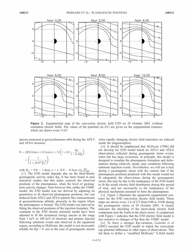
[17] The E5D model depends also on the three-hourlygeomagnetic activity index Kp. It has been found in paststatistical studies that this index controls the observedpositions of the plasmapause, when the level of geomag-netic activity changes. Note however that, unlike the VSMCmodel, the E5D model was not derived by adjusting itsparameters to fit observed plasmapause positions, but wasdeduced from ATS-5 and ATS-6 particle flux measurementsat geosynchronous altitude, precisely in the region wherethe plasmapause is formed. The E5D model was derived byfitting the observed positions of the injection boundary. Theconstants in the E5D electric potential model have beenadjusted to fit the dynamical energy spectra in the rangefrom 1 keV to 100 keV of electrons and protons injectedfollowing substorm events and observed in the equatorialregion; according to McIlwain, this model is not necessarilyreliable for Kp > 6, nor in the case of geomagnetic storms

when rapidly changing electric field intensities are inducedinside the magnetosphere.[18] It should be emphasized that McIlwain [1986] did

not develop his E5D model based on ATS-5 and ATS-6observations collected during geomagnetic storm events,when Dst has large excursions. In principle, this model isdesigned to simulate the plasmapause formation and defor-mations during relatively steady state conditions followingsubstorm injection events. Nevertheless, we will use it hereduring a geomagnetic storm with the caution that if theplasmapause positions predicted with this model would notfit adequately the observations during the geomagneticstorm, this may be due to the inadequacy of the E5D modelto fit the actual electric field distribution during this periodof time, and not necessarily to the inadequacy of thephysical mechanism assumed to form the plasmapause.[19] Figure 2 illustrates the equatorial equipotential con-

tours for the E5D convection electric field model. Thesemaps are shown every 2 h of UT from 0:00 to 10:00 duringthe geomagnetic storm of 28 October 2001. It clearlyindicates the shielding of the dawn-dusk electric fieldcomponent near the Earth in the dawn sector. A comparisonwith Figure 1 indicates that the E5D electric field model isless sensitive to changes of Kp than the VSMC model.[20] To force a stronger Kp-variation, Liemohn et al

[2001] rescaled the E5D model to match the cross-polarcap potential difference to other types of observations. Thisled them to define a ‘‘modified McIlwain’’ E-field model

Figure 2. Equipotential map of the convection electric field E5D on 28 October 2001 (withoutcorotation electric field). The values of the potential (in kV) are given on the equipotential contours,which are drawn every 4 kV.

A08212 PIERRARD ET AL.: PLASMAPAUSE POSITIONS

4 of 21

A08212

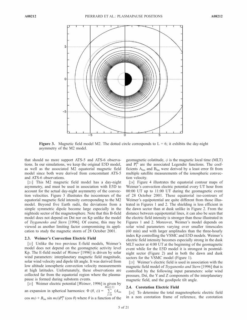
that should no more support ATS-5 and ATS-6 observa-tions. In our simulations, we keep the original E5D model,as well as the associated M2 equatorial magnetic fieldmodel since both were derived from concomitant ATS-5and ATS-6 observations.[21] This M2 magnetic field model has a day-night

asymmetry, and must be used in association with E5D toaccount for the actual day-night asymmetry of the convec-tion velocities. Figure 3 illustrates the isocontours of theequatorial magnetic field intensity corresponding to the M2model. Beyond five Earth radii, the deviations from asimple symmetric dipole become large especially in thenightside sector of the magnetosphere. Note that this B-fieldmodel does not depend on Dst nor on Kp unlike the modelof Tsyganenko and Stern [1996]. Of course, this may beviewed as another limiting factor compromising its appli-cation to study the magnetic storm of 28 October 2001.

2.3. Weimer’s Convection Electric Field

[22] Unlike the two previous E-field models, Weimer’smodel does not depend on the geomagnetic activity levelKp. The E-field model of Weimer [1996] is driven by solarwind parameters: interplanetary magnetic field magnitude,solar wind velocity and dipole tilt angle. It was derived fromlow altitude ionospheric convection velocity measurementsat high latitudes. Unfortunately, these observations arecollected far from the equatorial region where the plasma-pause is formed during substorm events.[23] Weimer electric potential [Weimer, 1996] is given by

an expansion in spherical harmonics: F (q, f) =PMin l;3ð Þ

l¼0

(Alm

cos mf + Blm sin mf)Plm (cos q) where q is a function of the

geomagnetic colatitude, f is the magnetic local time (MLT)and Pl

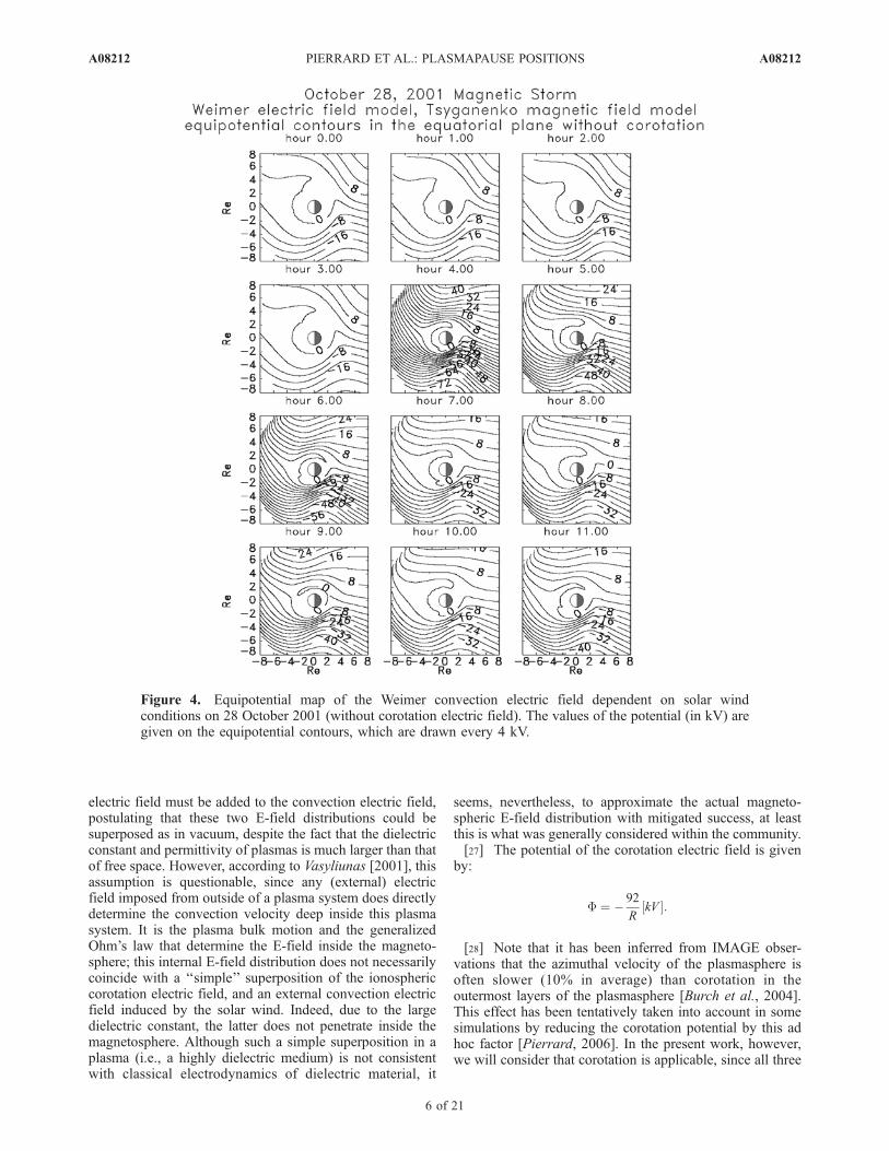
m are the associated Legendre functions. The coef-ficients Alm and Blm were derived by a least error fit frommultiple satellite measurements of the ionospheric convec-tion velocity.[24] Figure 4 illustrates the equatorial contour maps of

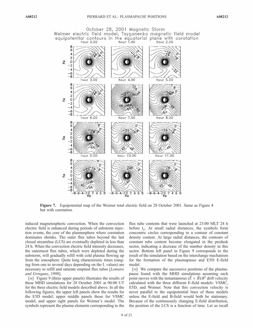
Weimer’s convection electric potential every UT hour from00:00 UT up to 11:00 UT during the geomagnetic eventof 28 October 2001. These equatorial iso-contours ofWeimer’s equipotential are quite different from those illus-trated in Figures 1 and 2. The shielding is less efficient inthe dawn sector than at dusk unlike in Figure 2. From thedistance between equipotential lines, it can also be seen thatthe electric field intensity is stronger than those illustrated inFigures 1 and 2. Moreover, Weimer’s model depends onsolar wind parameters varying over smaller timescales(60 min) and with larger amplitudes than the three-hourlyindex Kp controlling the VSMC and E5D models. Weimer’selectric field intensity becomes especially strong in the duskMLT sector at 4:00 UT at the beginning of the geomagneticevent while for the E5D model it is strongest in postmid-night sector (Figure 2) and in both the dawn and dusksectors for the VSMC model (Figure 1).[25] Weimer’s electric field is used in association with the

magnetic field model of Tsyganenko and Stern [1996] that iscontrolled by the following input parameters: solar windpressure, Dst, the Y and Z components of the interplanetarymagnetic field, and the geodipole tilt angle.

2.4. Corotation Electric Field

[26] To determine the total magnetospheric electric fieldin a non corotation frame of reference, the corotation

Figure 3. Magnetic field model M2. The dotted circle corresponds to L = 6; it exhibits the day-nightasymmetry of the M2 model.

A08212 PIERRARD ET AL.: PLASMAPAUSE POSITIONS

5 of 21

A08212

electric field must be added to the convection electric field,postulating that these two E-field distributions could besuperposed as in vacuum, despite the fact that the dielectricconstant and permittivity of plasmas is much larger than thatof free space. However, according to Vasyliunas [2001], thisassumption is questionable, since any (external) electricfield imposed from outside of a plasma system does directlydetermine the convection velocity deep inside this plasmasystem. It is the plasma bulk motion and the generalizedOhm’s law that determine the E-field inside the magneto-sphere; this internal E-field distribution does not necessarilycoincide with a ‘‘simple’’ superposition of the ionosphericcorotation electric field, and an external convection electricfield induced by the solar wind. Indeed, due to the largedielectric constant, the latter does not penetrate inside themagnetosphere. Although such a simple superposition in aplasma (i.e., a highly dielectric medium) is not consistentwith classical electrodynamics of dielectric material, it

seems, nevertheless, to approximate the actual magneto-spheric E-field distribution with mitigated success, at leastthis is what was generally considered within the community.[27] The potential of the corotation electric field is given

by:

F ¼ � 92

RkV½ �:

[28] Note that it has been inferred from IMAGE obser-vations that the azimuthal velocity of the plasmasphere isoften slower (10% in average) than corotation in theoutermost layers of the plasmasphere [Burch et al., 2004].This effect has been tentatively taken into account in somesimulations by reducing the corotation potential by this adhoc factor [Pierrard, 2006]. In the present work, however,we will consider that corotation is applicable, since all three

Figure 4. Equipotential map of the Weimer convection electric field dependent on solar windconditions on 28 October 2001 (without corotation electric field). The values of the potential (in kV) aregiven on the equipotential contours, which are drawn every 4 kV.

A08212 PIERRARD ET AL.: PLASMAPAUSE POSITIONS

6 of 21

A08212

E-field models have been derived, originally, under such anassumption.[29] In any case, the corotation electric field dominates

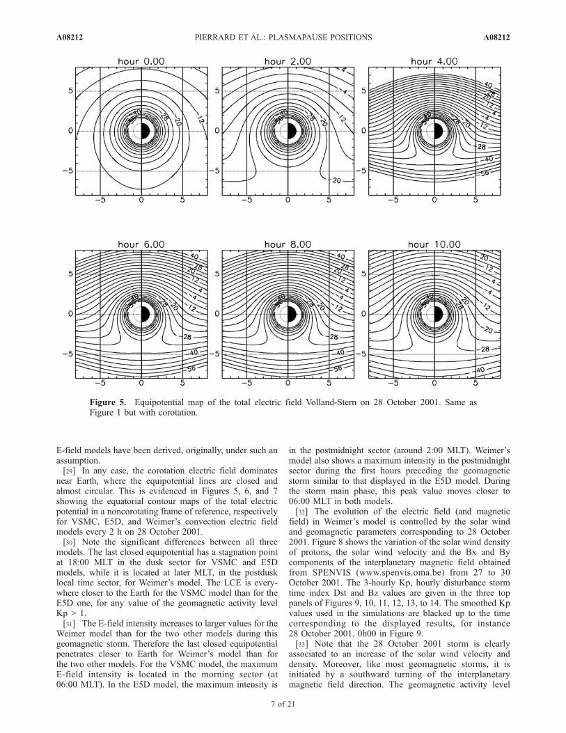
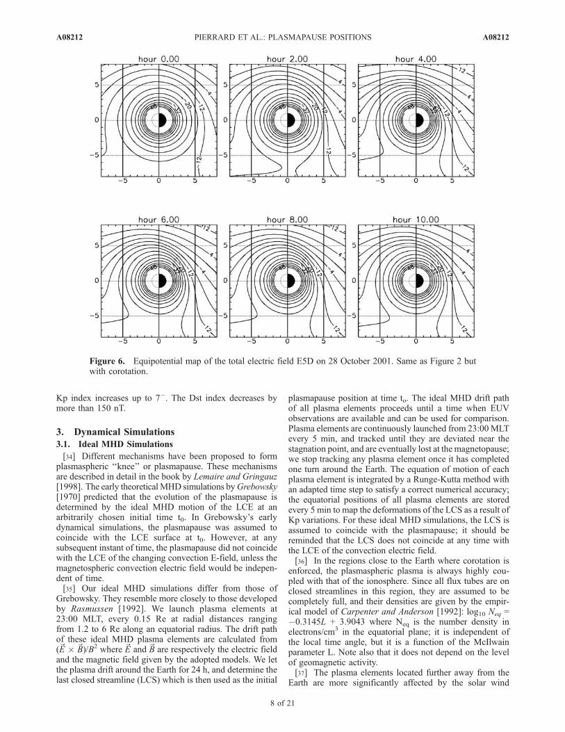
near Earth, where the equipotential lines are closed andalmost circular. This is evidenced in Figures 5, 6, and 7showing the equatorial contour maps of the total electricpotential in a noncorotating frame of reference, respectivelyfor VSMC, E5D, and Weimer’s convection electric fieldmodels every 2 h on 28 October 2001.[30] Note the significant differences between all three

models. The last closed equipotential has a stagnation pointat 18:00 MLT in the dusk sector for VSMC and E5Dmodels, while it is located at later MLT, in the postdusklocal time sector, for Weimer’s model. The LCE is every-where closer to the Earth for the VSMC model than for theE5D one, for any value of the geomagnetic activity levelKp > 1.[31] The E-field intensity increases to larger values for the

Weimer model than for the two other models during thisgeomagnetic storm. Therefore the last closed equipotentialpenetrates closer to Earth for Weimer’s model than forthe two other models. For the VSMC model, the maximumE-field intensity is located in the morning sector (at06:00 MLT). In the E5D model, the maximum intensity is

in the postmidnight sector (around 2:00 MLT). Weimer’smodel also shows a maximum intensity in the postmidnightsector during the first hours preceding the geomagneticstorm similar to that displayed in the E5D model. Duringthe storm main phase, this peak value moves closer to06:00 MLT in both models.[32] The evolution of the electric field (and magnetic

field) in Weimer’s model is controlled by the solar windand geomagnetic parameters corresponding to 28 October2001. Figure 8 shows the variation of the solar wind densityof protons, the solar wind velocity and the Bx and Bycomponents of the interplanetary magnetic field obtainedfrom SPENVIS (www.spenvis.oma.be) from 27 to 30October 2001. The 3-hourly Kp, hourly disturbance stormtime index Dst and Bz values are given in the three toppanels of Figures 9, 10, 11, 12, 13, to 14. The smoothed Kpvalues used in the simulations are blacked up to the timecorresponding to the displayed results, for instance28 October 2001, 0h00 in Figure 9.[33] Note that the 28 October 2001 storm is clearly

associated to an increase of the solar wind velocity anddensity. Moreover, like most geomagnetic storms, it isinitiated by a southward turning of the interplanetarymagnetic field direction. The geomagnetic activity level

Figure 5. Equipotential map of the total electric field Volland-Stern on 28 October 2001. Same asFigure 1 but with corotation.

A08212 PIERRARD ET AL.: PLASMAPAUSE POSITIONS

7 of 21

A08212

Kp index increases up to 7�. The Dst index decreases bymore than 150 nT.

3. Dynamical Simulations

3.1. Ideal MHD Simulations

[34] Different mechanisms have been proposed to formplasmaspheric ‘‘knee’’ or plasmapause. These mechanismsare described in detail in the book by Lemaire and Gringauz[1998]. The early theoretical MHD simulations byGrebowsky[1970] predicted that the evolution of the plasmapause isdetermined by the ideal MHD motion of the LCE at anarbitrarily chosen initial time t0. In Grebowsky’s earlydynamical simulations, the plasmapause was assumed tocoincide with the LCE surface at t0. However, at anysubsequent instant of time, the plasmapause did not coincidewith the LCE of the changing convection E-field, unless themagnetospheric convection electric field would be indepen-dent of time.[35] Our ideal MHD simulations differ from those of

Grebowsky. They resemble more closely to those developedby Rasmussen [1992]. We launch plasma elements at23:00 MLT, every 0.15 Re at radial distances rangingfrom 1.2 to 6 Re along an equatorial radius. The drift pathof these ideal MHD plasma elements are calculated from(~E � ~B)/B2 where ~E and ~B are respectively the electric fieldand the magnetic field given by the adopted models. We letthe plasma drift around the Earth for 24 h, and determine thelast closed streamline (LCS) which is then used as the initial

plasmapause position at time to. The ideal MHD drift pathof all plasma elements proceeds until a time when EUVobservations are available and can be used for comparison.Plasma elements are continuously launched from 23:00MLTevery 5 min, and tracked until they are deviated near thestagnation point, and are eventually lost at the magnetopause;we stop tracking any plasma element once it has completedone turn around the Earth. The equation of motion of eachplasma element is integrated by a Runge-Kutta method withan adapted time step to satisfy a correct numerical accuracy;the equatorial positions of all plasma elements are storedevery 5 min to map the deformations of the LCS as a result ofKp variations. For these ideal MHD simulations, the LCS isassumed to coincide with the plasmapause; it should bereminded that the LCS does not coincide at any time withthe LCE of the convection electric field.[36] In the regions close to the Earth where corotation is

enforced, the plasmaspheric plasma is always highly cou-pled with that of the ionosphere. Since all flux tubes are onclosed streamlines in this region, they are assumed to becompletely full, and their densities are given by the empir-ical model of Carpenter and Anderson [1992]: log10 Neq =�0.3145L + 3.9043 where Neq is the number density inelectrons/cm3 in the equatorial plane; it is independent ofthe local time angle, but it is a function of the McIlwainparameter L. Note also that it does not depend on the levelof geomagnetic activity.[37] The plasma elements located further away from the

Earth are more significantly affected by the solar wind

Figure 6. Equipotential map of the total electric field E5D on 28 October 2001. Same as Figure 2 butwith corotation.

A08212 PIERRARD ET AL.: PLASMAPAUSE POSITIONS

8 of 21

A08212

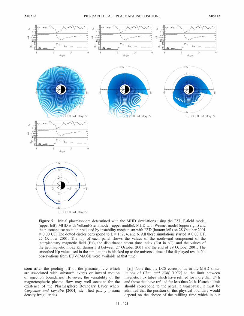
induced magnetospheric convection. When the convectionelectric field is enhanced during periods of substorm injec-tion events, the core of the plasmasphere where corotationdominates shrinks. The outer flux tubes beyond the lastclosed streamline (LCS) are eventually depleted in less than24 h. When the convection electric field intensity decreases,the outermost flux tubes, which were depleted during thesubstorm, will gradually refill with cold plasma flowing upfrom the ionosphere. Quite long characteristic times (rang-ing from one to several days depending on the L values) arenecessary to refill and saturate emptied flux tubes [Lemaireand Gringauz, 1998].[38] Figure 9 (three upper panels) illustrates the results of

these MHD simulations for 28 October 2001 at 00:00 UTfor the three electric field models described above. In all thefollowing figures, the upper left panels show the results forthe E5D model; upper middle panels those for VSMCmodel, and upper right panels for Weimer’s model. Thesymbols represent the plasma elements corresponding to the

flux tube contents that were launched at 23:00 MLT 24 hbefore to. At small radial distances, the symbols formconcentric circles corresponding to a contour of constantdensity content. At large radial distances, the contours ofconstant tube content become elongated in the predusksector, indicating a decrease of the number density in thissector. Bottom left panel in Figure 9 corresponds to theresult of the simulation based on the interchange mechanismfor the formation of the plasmapause and E5D E-fieldmodel.[39] We compare the successive positions of the plasma-

pause found with the MHD simulations assuming eachpoint moves with the instantaneous (~E �~B)/B2 drift velocitycalculated with the three different E-field models: VSMC,E5D, and Weimer. Note that this convection velocity isnever parallel to the equipotential lines of these modelsunless the E-field and B-field would both be stationary.Because of the continuously changing E-field distribution,the position of the LCS is a function of time. Let us recall

Figure 7. Equipotential map of the Weimer total electric field on 28 October 2001. Same as Figure 4but with corotation.

A08212 PIERRARD ET AL.: PLASMAPAUSE POSITIONS

9 of 21

A08212

that the LCS corresponds to the envelope of all drift pathsthat have not reached the magnetopause boundary duringthe previous 24 h. This is why it should be denoted LCS-24h. A different LCS could have been obtained if theclosure time would have been 25 h, 2 d, 3d or 6 d as inthe MHD simulations of Chen and Wolf [1972].[40] The position of the LCS-24h found with our MHD

simulations corresponds to the boundary where the numberof plasma elements per unit area decreases sharply inFigures 9 to 15 (except at 23:00 MLT and beyond wherenew plasma elements are continuously launched every5 min). If the plasmapause is identified with one of the lastclosed streamlines, it should be specified what is the closuretime that has been adopted in the MHD simulations. Thismeans that the location of the plasmapause, a physicalboundary, would depend on the arbitrary choice of a closuretime in any MHD simulation. This is clearly a conceptuallimitation of the plasmapause with the LCS and even worsewith the LCE.[41] Figures 9 to 14 show that a plume is produced in the

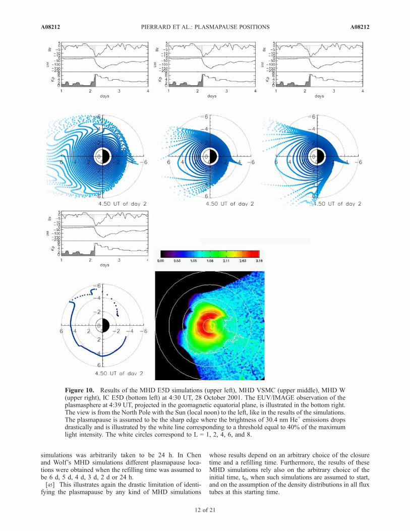
dusk sector during the magnetic storm in all three MHDsimulations. This plume in the LCS-24h is similar to thatobserved by EUV/IMAGE after 18:00 UT.[42] Figure 10 shows that at 04:30 UT, the LCS-24h has

been pushed inward in the nightside region. Although theEUV observations show also an inward shift of the plasma-

pause near midnight, the overall shape of the plasmasphereis however very different from that of the LCS-24h obtainedwith the MHD simulations. While the LCS has rathersmooth and regular shape, the actual plasmapause is muchmore indented and irregular. This can be a consequence ofthe rather poor time resolution of the Kp index controllingthe E-field distributions. Since the magnetospheric E-field ischanging over smaller timescale, the actual MLT variationof the LCS is expected to be more irregular than illustratedin Figures 10 to 14.[43] Another important consequence of the shorter time

variation of the E-field distribution, and of the associatedplasma flow which must be quite variable, was pointed outby Dungey [1967] soon after the discovery of the sharpnessof ‘‘Carpenter’s knee’’. He wrote: ‘‘Some tubes of highdensity (i.e., from inside the plasmasphere) should some-times be swept out on the day side, and some tubes, afterentering from the tail, should enter the inner region and,after a few days, should have intermediate values of density.It then seems rather surprising that the knee should be sosharp, but the variable model would predict a patchy densityin the region near the knee and this could be the true state’’(sic). We share Dungey’s early concern about the sharpnessof a knee along the LCS. The short timescale variability ofthe magnetospheric plasma flow does not support theformation of sharp density gradients like those observed

Figure 8. Variation of the solar wind density of protons, the solar wind velocity and the Bx and Bycomponent of the magnetic field from 27 to 30 October 2001.

A08212 PIERRARD ET AL.: PLASMAPAUSE POSITIONS

10 of 21

A08212

soon after the peeling off of the plasmasphere whichare associated with substorm events or inward motionof injection boundaries. However, the variability of themagnetospheric plasma flow may well account for theexistence of the Plasmasphere Boundary Layer whereCarpenter and Lemaire [2004] identified patchy plasmadensity irregularities.

[44] Note that the LCS corresponds in the MHD simu-lations of Chen and Wolf [1972] to the limit betweenmagnetic flux tubes which have refilled for more than 24 hand those that have refilled for less than 24 h. If such a limitshould correspond to the actual plasmapause, it must beadmitted that the position of this physical boundary woulddepend on the choice of the refilling time which in our

Figure 9. Initial plasmasphere determined with the MHD simulations using the E5D E-field model(upper left), MHD with Volland-Stern model (upper middle), MHD with Weimer model (upper right) andthe plasmapause position predicted by instability mechanism with E5D (bottom left) on 28 October 2001at 0:00 UT. The dotted circles correspond to L = 1, 2, 4, and 6. All these simulations started at 0:00 UT,27 October 2001. The top of each panel shows the values of the northward component of theinterplanetary magnetic field (Bz), the disturbance storm time index (Dst in nT), and the values ofthe geomagnetic index Kp during 3 d between 27 October 2001 and the end of 29 October 2001. Thesmoothed Kp value used in the simulations is blacked up to the universal time of the displayed result. Noobservations from EUV/IMAGE were available at that time.

A08212 PIERRARD ET AL.: PLASMAPAUSE POSITIONS

11 of 21

A08212

simulations was arbitrarily taken to be 24 h. In Chenand Wolf’s MHD simulations different plasmapause loca-tions were obtained when the refilling time was assumed tobe 6 d, 5 d, 4 d, 3 d, 2 d or 24 h.[45] This illustrates again the drastic limitation of identi-

fying the plasmapause by any kind of MHD simulations

whose results depend on an arbitrary choice of the closuretime and a refilling time. Furthermore, the results of theseMHD simulations rely also on the arbitrary choice of theinitial time, t0, when such simulations are assumed to start,and on the assumption of the density distributions in all fluxtubes at this starting time.

Figure 10. Results of the MHD E5D simulations (upper left), MHD VSMC (upper middle), MHD W(upper right), IC E5D (bottom left) at 4:30 UT, 28 October 2001. The EUV/IMAGE observation of theplasmasphere at 4:39 UT, projected in the geomagnetic equatorial plane, is illustrated in the bottom right.The view is from the North Pole with the Sun (local noon) to the left, like in the results of the simulations.The plasmapause is assumed to be the sharp edge where the brightness of 30.4 nm He+ emissions dropsdrastically and is illustrated by the white line corresponding to a threshold equal to 40% of the maximumlight intensity. The white circles correspond to L = 1, 2, 4, 6, and 8.

A08212 PIERRARD ET AL.: PLASMAPAUSE POSITIONS

12 of 21

A08212

3.2. Interchange Mechanism

[46] Another mechanism has also been proposed for theformation of the plasmapause: the interchange mechanism,illustrated by Lemaire and Kowalkowski [1981]. Accordingto this mechanism, the plasma becomes unstable above aZero Parallel Force (ZPF) surface where the parallel com-ponent of the gravitational plus centrifugal accelerations isequal to zero [Lemaire, 1985, 2001]. This occurs in thenightside local time sector during substorms and storms atan equatorial distance that depends on the distribution of theconvection velocity. The plasmasphere is peeled off in thissector by the centrifugal effect which is enhanced when theconvection velocity is enhanced beyond the inner edge of a

substorm injection boundary. By this mechanism, a newplasmapause forms closer to the Earth than the LCSdetermined by the MHD simulations presented and dis-cussed above. This mechanism has been used in numericalsimulations performed by Lemaire [1985, 2000] and byPierrard and Lemaire [2004]. The positions of the plasma-pause predicted by this mechanism with the E5D modelhave been compared to observations of IMAGE for typicaldates [Pierrard and Cabrera, 2005, 2006; Pierrard, 2006].[47] In these non-MHD simulations based on the inter-

change mechanism, plasma holes with a density smallerthan the background density are launched at 23:00 MLT inthe equatorial plane. Because of the interchange motion,

Figure 11. Results of the MHD E5D simulation (upper left), MHD VSMC (upper middle), MHD W(upper right), IC E5D (bottom left) at 8:00 UT, 28 October 2001. The EUV/IMAGE observation of theequatorial plasmapause position at 8:03 UT is illustrated in the bottom right panel.

A08212 PIERRARD ET AL.: PLASMAPAUSE POSITIONS

13 of 21

A08212

these holes drift ultimately toward an asymptotic trajectorywhere the radial component of the gravitational force andcentrifugal force balance each other. This corresponds to theZero Radial Force (ZRF) surface. However, the parallelcomponents of these forces balance each other closer to theEarth along a virtual surface that Lemaire [1985] has calledthe Zero Parallel Force (ZPF) surface. It is assumed that thefield aligned plasma distribution becomes convectivelyunstable along all flux tubes that traverse or are tangent tothis virtual ZPF surface. In these flux tubes field alignedflow velocity is enhanced, and the plasma density is reduceddue to its upward expansion. For a dipole magnetic fielddistribution the equatorial distance of the ZPF is 32/3 time

smaller than that of the ZRF surface. We assume that for theM2 magnetic field model the minimum equatorial distanceof the ZPF surface is also approximately 32/3 times smallerthan that of the ZRF surface, as it is for a dipole B-field.[48] To determine the plasmapause shape at t = 0 h on

28 October 2001, we run the interchange simulationbetween t = �24 h and t = 0 h. By this way, the positionof the plasmapause obtained at t = 0 h is determined at allMLT angles by the interchange mechanism and by thehistory of the geomagnetic activity level during the previous24 h. Note that the simulations could also be started byusing an observed plasmapause position at the time t0 like inthe study of Goldstein et al. [2003]. This procedure would

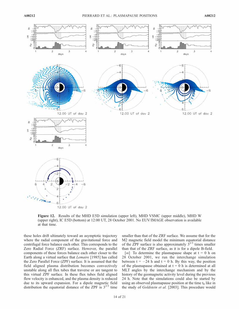
Figure 12. Results of the MHD E5D simulation (upper left), MHD VSMC (upper middle), MHD W(upper right), IC E5D (bottom) at 12:00 UT, 28 October 2001. No EUV/IMAGE observation is availableat that time.

A08212 PIERRARD ET AL.: PLASMAPAUSE POSITIONS

14 of 21

A08212

of course favor the agreement between the results of thesimulation and the observations at any subsequent times.Unfortunately, this procedure does not tell us about thephysical mechanism that has formed this initial plasma-pause; it may only be useful to test the appropriateness ofthe E-field models chosen in simulations, after the plasma-pause had already formed.[49] In the next section, we describe and compare the

results obtained with the following series of simulations:MHD with the E5D model (MHD E5D), MHD with the

Volland-Stern-Maynard-Chen model (MHD VSMC), MHDwith the Weimer model (MHD W), and interchange withE5D model (IC E5D).

4. Discussion of the Results

4.1. Magnetic Storm of 28 October 2001

[50] Figures 9 to 14 illustrate the equatorial position ofthe plasmapause obtained with two different mechanismsfor the formation of the plasmapause and three different

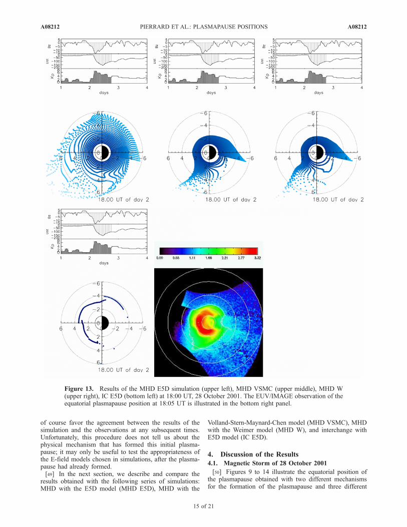
Figure 13. Results of the MHD E5D simulation (upper left), MHD VSMC (upper middle), MHD W(upper right), IC E5D (bottom left) at 18:00 UT, 28 October 2001. The EUV/IMAGE observation of theequatorial plasmapause position at 18:05 UT is illustrated in the bottom right panel.

A08212 PIERRARD ET AL.: PLASMAPAUSE POSITIONS

15 of 21

A08212

electric field models, respectively at 0:00, 4:30, 8:00, 12:00,18:00, and 20:00 UT. The simulations correspond to MHDE5D (left upper panels), MHD VSMC (middle upperpanels) and MHD W (right upper panels). The resultsobtained with the interchange mechanism and the E5Dmodel are also presented in the left bottom panel of thesegraphs. The plasmapause found with the interchange mech-anism is closer to Earth than with MHD simulations when asame E-field model is used. We do not provide simulationswith interchange mechanism for the other electric field

models since this would prohibitively increase the size ofthis paper without improving significantly its main results.Note also that the use of the interchange mechanism wouldnot be physically significant in association with an E-fieldlike the VSMC model which has been fitted in order tomatch the LCE with observed plasmapause positions.[51] The top of each panel in Figures 9 to 14 illustrate the

Kp and Dst indices and the northward component of theinterplanetary magnetic field (Bz) from the beginning of27 October 2001 to the end of 29 October 2001. At

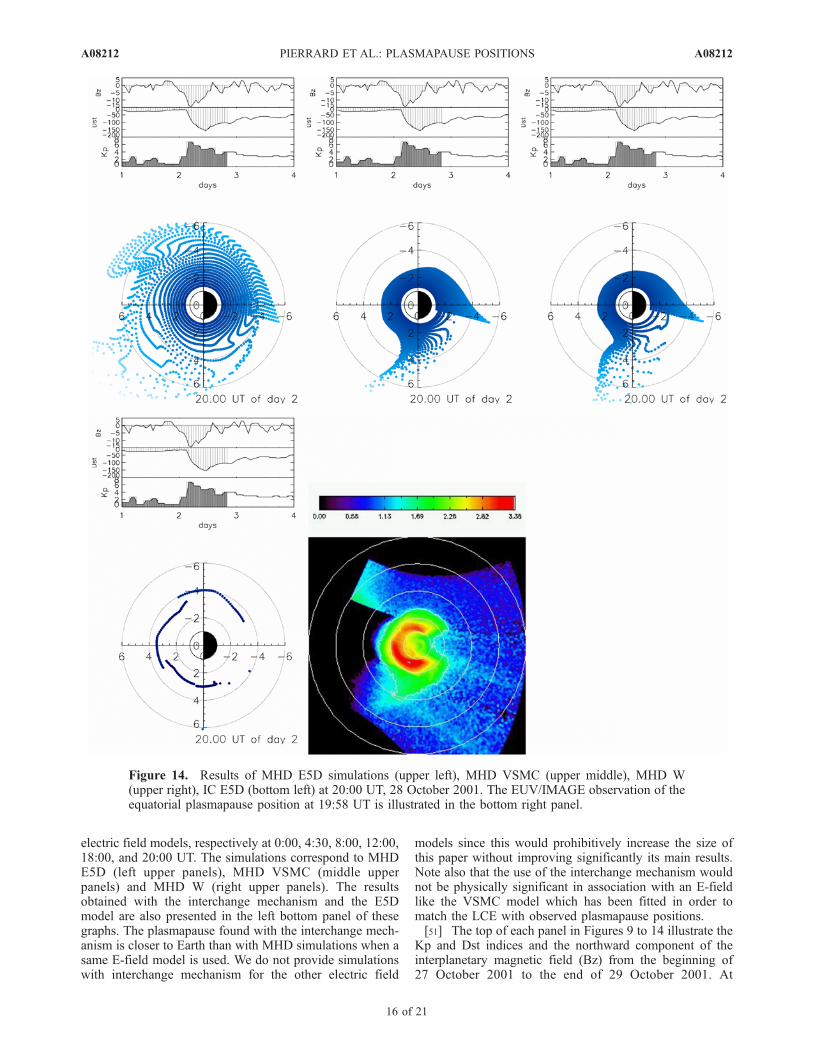
Figure 14. Results of MHD E5D simulations (upper left), MHD VSMC (upper middle), MHD W(upper right), IC E5D (bottom left) at 20:00 UT, 28 October 2001. The EUV/IMAGE observation of theequatorial plasmapause position at 19:58 UT is illustrated in the bottom right panel.

A08212 PIERRARD ET AL.: PLASMAPAUSE POSITIONS

16 of 21

A08212

00:00 UT, the level of geomagnetic activity is very low(Kp = 1�) and increases to 7� over the next 3 h when themain phase of the geomagnetic storm starts, i.e., when Dstbegins a gradual drop, as shown on Figure 9.[52] At 04:39, 08:03, 18:05, and 19:58 UT, there are

exploitable observations from the EUV instrument sincethe orbit of the satellite IMAGE is close to its apogee.These images are presented in the bottom right panels ofFigures 10, 11, 13, and 14, respectively. These observationsare intensity maps of the 30.4 nm emissions of Helium ions

integrated along the line of sight. They are projected in thegeomagnetic equatorial plane in the SM coordinate systemwith the program XForm available at (ftp://euv.lpl.arizona.edu/pub/bavaro/unsupported/). This software tool enables toview the plasmapause cross section from over the NorthPole like in our simulations. The bright arc close to theEarth is due to airglow of 58.4 nm neutral helium andoxygen ions. Its drop in intensity behind the Earth is causedby the Earth’s shadow.

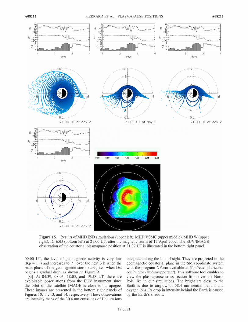
Figure 15. Results of MHD E5D simulations (upper left), MHD VSMC (upper middle), MHDW (upperright), IC E5D (bottom left) at 21:00 UT, after the magnetic storm of 17 April 2002. The EUV/IMAGEobservation of the equatorial plasmapause position at 21:07 UT is illustrated in the bottom right panel.

A08212 PIERRARD ET AL.: PLASMAPAUSE POSITIONS

17 of 21

A08212

[53] The plasmasphere corresponds to the region sur-rounding the Earth and shown up mainly in green on thefigures. The plasmapause is assumed to be the sharp edgewhere the brightness of 30.4 nm He+ emissions dropsdrastically. This boundary is illustrated by a white linecorresponding to a threshold equal to 40% of the maximumlight intensity.[54] Just before the storm, the MHD E5D simulation

predicts at 00:00 UT a plasmasphere extending up to 6 Re.Since the dawn-dusk component of the two other convec-tion electric fields (VMSC and Weimer) are stronger thanthat of the E5D model, the LCS is located closer to the Earthfor these two other models: i.e., around 4 Re for the MHDVSMC, and even closer for the MHD W simulation. Whenthe interchange mechanism is assumed to peel off theplasmasphere, the plasmapause at midnight LT is locatedaround 4.5 Re with the E5D model; this is closer to Earththan the LCS simulation for this same E-field model.However, the plasmapause predicted by the IC E5D simu-lation is located at larger equatorial distances than theLCS for the two other E-field models. However, for a sameE-field model, the minimum equatorial distance of the ZPFsurface is generally smaller than that of the LCS.[55] Note that the plasmasphere is almost circular at that

time. Although the level of geomagnetic activity has beennearly constant and quite low during the previous 24 h, abulge is present at 00:00 UT in the dusk sector in the MHDVSMC simulation. However, according to the EUV obser-vations the plasmasphere is usually circular after prolongedquiet periods. Plasma tails or plumes are formed only duringdisturbed periods [Pierrard and Cabrera, 2005]. Unfortu-nately, no observations of EUV/IMAGE are available at00:00 UT 28 October 2001, since the satellite was not closeto its apogee at that time.[56] At 04:30 UT as illustrated in Figure 10, the geomag-

netic activity level Kp increases significantly and reaches amaximum Kp = 7�. This increase of Kp is associated to asouthward turning of the interplanetary magnetic field Bz,as well as a decrease of Dst index. The latter reaches aminimum of �157 nT at 11:00 UT. By that time, theconvection electric field intensity has increased in all modelsso that the corresponding LCS-24h are less extended. Onlythe innermost flux tubes have a circular trajectory, while themore distant closed streamlines are highly skewed with amaximum radial distance in the postnoon sector. Beyond theLCS, the plasma elements are lost to the magnetosheath andare not any longer tracked in our MHD simulations.According to this MHD theory for the formation of theplasmapause, a more or less sharp knee is formed along theLCS-24h, wherein the streamlines have remained closed forat least 24 h.[57] The LCS shrinks to about 3 Re in the night sector for

all MHD simulations. A bulge is formed in the afternoonsector for all the simulations as a result of the enhancementof the dawn-dusk E-field component. Indeed, this enhance-ment of E-field in the dusk sector produces a sunward surgeof plasma in this MLT sector. Note, however, the quitedifferent shapes of the equatorial cross section of the LCSpredicted by the various E-field models. The bulge in theLCS is the precursor of the plume that usually developsduring geomagnetic storms and substorms.

[58] The interchange mechanism shown in the fourthpanels produces much more irregular plasmapause shapesthan the MHD simulations. From the fourth panel in Figure10, it can be seen that the ZPF surface where the plasma-sphere is peeled off in the postmidnight sector correspondsto an equatorial distance slightly beyond 2 Re. Despite therather limited quality of the observations of IMAGE at thetime of 04:30 UT, it can be seen that the plasmapause islocated close to the Earth during this storm.[59] At 08:00 UT, the Kp index is still high: Kp = 6�. As

illustrated in Figure 11, a plume is now clearly developed inall the simulations, with and without interchange. Theplumes are located in the afternoon sector but have ratherdifferent shapes and experience quite different developmentdepending on the adopted E-field model. The observation ofEUV/IMAGE at 08:03 UT is very contaminated, but aplume can clearly be identified in the afternoon sector.[60] With MHD VSMC and Weimer simulations, the

plasmasphere is still smaller than with MHD E5D, due totheir stronger dawn-dusk E-field intensity which implies astagnation point rather close to Earth. The simulation ofinterchange with the E5D model, gives a position of theplasmapause which is rather close to that of the LCS ofMHD E5D simulation.[61] By 12:00 UT, the plume observed in the simulations

has slightly rotated eastward as can be seen in Figure 12. NoEUV observations are unfortunately available at that time.At 18:05 and 19:58 UT, EUV/IMAGE provides nice obser-vations, and a plume is clearly visible in the afternoon/duskregion as illustrated in Figures 13 and 14. The results of thesimulations are also shown for 18:00 and 20:00 UT. Thelongitudinal extent and MLT position of the plume is againslightly different in the different models. Note that byreducing arbitrarily the corotation velocity, a better agree-ment would be obtained. This kind of forcing has beenavoided in the present work in order not to distort theoriginal E-field models which have been derived withoutreducing the corotation electric field intensity. Note never-theless that the velocity of the plasmasphere is observed tobe generally slower than corotation [Burch et al., 2004],which explains the faster rotation of the plume in thedifferent simulations compared to the EUV observations.[62] Similar plumes are often observed by EUV/IMAGE

and CLUSTER after a significant increase of the geomag-netic activity level [Darrouzet et al., 2006a, 2006b]. Theyare formed in the afternoon sector and then rotate eastwardwith the core of the plasmasphere. Other examples ofIMAGE observations during quiet and disturbed periodsthat have been compared to results of simulations based onthe interchange mechanism (IC E5D) have been presentedby Pierrard and Cabrera [2005, 2006] and Pierrard [2006].

4.2. Magnetic Storm of 17 April 2002

[63] Figure 15 shows the results of similar simulationsobtained during the geomagnetic storm of 17 April 2002.This case is particularly interesting since a global observa-tional study of the dynamics of the plasmasphere, aurora,ring current and subauroral ionosphere was provided duringthis storm by Goldstein et al. [2005]. This is also the singleevent for which the effect of several electric field models onthe position of the plasmapause has been also determined byLiemohn et al. [2004]. The E-field models tested in this

A08212 PIERRARD ET AL.: PLASMAPAUSE POSITIONS

18 of 21

A08212

paper were (1) their modified E5D model rescaled to have alarger intensity than McIlwain’s original version, (2) theWeimer model, and (3) a self consistent E-field determinedby the authors. Thus it is interesting to compare the resultsof the present MHD simulations based on VSMC as well ason the original E5D model version with the results found byLiemohn et al. [2004] for the same event on 17 April 2002with other E-fields models. Moreover, we also show theeffect of the interchange mechanism on the positions, shapeand evolution of the plasmapause during this magneticstorm.[64] Figure 15 shows the results at 21:00 UT on 17-4-

2002 obtained with the MHD simulations respectively forE5D, VSMC and Weimer models (three upper panels), aswell as with interchange mechanism based on the E5Dmodel (left bottom panel). A plume is again formed with allthe electric field models. Its development is associated tothe increase of the geomagnetic activity level up to Kp = 7+.This increase of Kp is also associated with a southwardturning of the interplanetary magnetic field, like during allgeomagnetic storms. During the main phase, Dst decreasesreaching a minimum of �105 nT on 17 April 2002 and evena lower value the day after. The plume is located approx-imately in the same MLT sector as in the observations ofEUV. The MHD E5D simulation shows a plasmapause quitesimilar to that obtained with the rescaled E5D model usedby Liemohn et al. The position of the plasmapause found byLiemohn et al. MHD simulation was in good agreementwith the observations of EUV in the nightside, but it was toofar from the Earth on the dayside. We obtain the samecharacteristics with the MHD E5D simulation.[65] The MHD VSMC simulation corresponds better to

the plasmapause observations on the dayside, but on thenightside, it is too close to the Earth. TheMHDW simulationbased on Weimer model gives also a plasmapause closer tothe Earth than what is observed, especially on the nightsideand on the morningside; these results are in agreement withthe simulation published by Liemohn et al. where theWeimerconvection E-field is also used.[66] The simulation of the interchange mechanism with

the E5D model gives results closer to the EUVobservationsthan the MHD simulations with this same E5D electric fieldmodel. This does not imply, of course, that there is no needfor better E-field model than E5D, nor is it a pleading forthe mechanism of interchange, since any physical theory isnecessarily an approximation and is therefore perfectible.[67] While in general, interchange simulations with E5D

model predict results that are in good agreement with theEUV observations during substorm events [Pierrard andCabrera, 2005], we have seen here that such an agreementis more precarious during the geomagnetic storms examinedin this paper. We attribute the lack of satisfactory resultsduring geomagnetic storms to the lack of characterization ofthe E5D electric field model under this sort of geomagneticdisturbances. Indeed, this empirical E-field model wasnot designed to reproduce the magnetospheric convectionelectric field during geomagnetic storms, but only to modelthe dispersion of electrons and protons accelerated orinjected into the magnetosphere following substorm events[McIlwain, 1986]. This lays the need to update and improvecurrently available empirical electric field models not onlyat ionospheric level but also at high altitudes in the Earth

magnetosphere. Furthermore, nobody can argue that futurealternative theories for the formation of the plasmapausewill not be able to simulate the dynamics of the plasma-sphere more accurately and offer predictions in closeragreement with observational reality.

5. Conclusions

[68] After brief descriptions of different electric fieldsmodels (the Volland-Stern-Maynard-Chen model VSMC,McIlwain’s E5D model and the Weimer model), we firstdetermined how the distribution of the equatorial equipo-tentials corresponding to these magnetospheric convectionE-field models change during the geomagnetic storm of28 October 2001. Their equipotentials in corotating andnoncorotating frames of reference depend on the levelgeomagnetic activity; they are thus changing as a functionof universal time since the geomagnetic activity indexes Kpand Dst are varying hour after hour.[69] The radial and local time distributions of these

equipotential contours have been displayed in Figures 1,2, 4, 5, 6, and 7 for a set of times for which EUVobservations are sometimes available. The E-field modelsare used in association with magnetic field models (VSMC/dipole, E5D/M2 model, and Weimer/Tsyganenko respec-tively), to calculate the convection velocity of cold plasmaor the drift velocity of zero energy charged particles. Thedipolar and M2 magnetic field models had been employedto design, respectively, the VSMC and E5D models from insitu satellite observations. In addition to their portability,these simple quasi-stationary E-field models have an expe-dient advantage: they depend only on one single parameter,the 3-hourly Kp geomagnetic activity index. This makesthem user friendly and easy to implement in any numericalcodes. Weimer E-field is more sophisticated: it depends onseveral solar wind parameters and varies with a higher timeresolution. Nevertheless, it is based on low altitudes andhigh latitudes observations collected far from the equatorialregion where the plasmapause is formed.[70] Although all these empirical electric field models are

based on observations (respectively, on OGO-3 & 5 satel-lites for VSMC, AST-5 & 6 satellites for E5D, and lowaltitude ionospheric convection velocity measurements athigh latitudes for Weimer), they occur to be quite differentfrom each other. Note that these models are averages andapproximations of the actual field distributions at anyparticular instant of time, and at any particular place inthe magnetosphere. Some of them were not designed tomodel magnetospheric electric fields in cases of rapidlychanging magnetic field intensities: e.g., during geomag-netic storms when induction electric fields are generatedon top of the electrostatic component approximated by theseE-field models. For instance, the E5D model was essentiallybuilt to represent the E-field distribution immediately after asubstorm injection event; furthermore, it was developed torepresent the E-field in the region of geosynchronous orbit,only when the level of geomagnetic activity, denoted by thevalue of Kp, remains nearly constant and smaller than 6.McIlwain’s electric field E5D was not developed under suchcircumstances as geomagnetic storms. However, taking intoaccount these warnings and restrictions, it is interesting tonote that the plasmapause position obtained with this E-field

A08212 PIERRARD ET AL.: PLASMAPAUSE POSITIONS

19 of 21

A08212

model and the IC mechanism is in better agreement with theEUVobservations during the geomagnetic storm of 17 April2002 than the positions obtained with the other E-fieldsmodels and MHD simulations.[71] Two mechanisms of plasmapause formation were

also compared and confirm that the last-closed-streamline(LCS) of the MHD simulation is located beyond theplasmapause predicted by the interchange mechanism forthe geomagnetic storm of 28 October 2001: the latter beingthus generally closer to the Earth. A similar comparisonwith results obtained for the geomagnetic storm of 17 April2002 leads to the same conclusions.[72] The choice of the E-field model is crucial in the results

of the simulations. Plumes develop during geomagneticstorms and substorms with all the various E-field models,but quite different shapes of the equatorial cross section of theLCS are predicted. It is quite clear that more detailedmagnetospheric E-field models with higher time resolutionsshould be developed. In such future E-field models, thedistribution of the equipotential surfaces should possibly bedesynchronized: their evolution in the night side should notnecessarily be synchronized with that in the dayside or at anyother MLTs. Finally, it would be useful to model also theinductive electric field component in order to model moreproperly what happens during geomagnetic storms.[73] Despite the better scores of the E5D electric field

model and of the interchange scenario for the formation ofthe plasmapause found in many case studies, it must beadmitted, however, that the equatorial cross section of theplasmapause as determined from the EUV observationsduring both geomagnetic storms, are not very well repro-duced by none of the simulations presented above, not evenwhen the Weimer electric field model is used instead ofthe E5D model. This leads us to conclude that none of theelectrostatic field models is fully adapted to model theactual magnetospheric E-field distribution during geomag-netic storms (at least for those selected in the present study).[74] Since previous simulations by Pierrard and Lemaire

[2004] as well as by Pierrard and Cabrera [2005] based onthe interchange mechanism and the E5D electric field modelhave shown that overall shapes of the plasmapause and itsevolution does rather well explain the formation of plasma-tails or plumes as well as shoulders following to substormevents, it may be speculated that during geomagnetic stormscharacterized by larger Dst variations, the time dependentelectric field distribution has an induced component asso-ciated to the increase of southward magnetic field which isgenerated by the Ring Current during the main phase. Atoroidal induced electric field of smaller intensity and ofopposite direction is also expected during the recoveryphase of geomagnetic storms. These toroidal induced elec-tric fields cannot be represented as the gradient of a scalarelectrostatic potential as most empirical magnetosphericE-field models used above. The effect of such additional timedependent and non curlfree electric field distribution on theplasmasphere and on the formation of the plasmapause,should be evaluated in detail.[75] It is suggested here that such induced electric fields

generated during geomagnetic storms are responsible for thelack of satisfactory agreement between the simulationspresented in this study based on curlfree electric fieldmodels. We suggest that this effect should be examined in

the future and included in forthcoming and more compre-hensive theories for the formation of the plasmapause notonly during substorm events but also even during geomag-netic storms with large Dst variations.[76] Therefore this study points out the need to develop

higher time resolution empirical models for the magneto-spheric electrostatic field distribution like those developedfor the geomagnetic field. It urges to take into account theeffect of induced electric fields generated in the magneto-sphere during geomagnetic storms with large Dst variations.An induced electric field model in the inner magnetospherehas to depend on Dst and on the Dst change rate (dDst/dt).Since it cannot be derived from the gradient of an electro-static potential, this adds mathematical complexity to anyfuture induced electric field model. However, it is onlywhen such more detailed and comprehensive E-field modelswill be available in association with the time dependentempirical B-field models, that one might expect to testquantitatively and more definitely any of the existing andfuture theories for the formation of the plasmapause bycomparing their theoretical predictions to observations likethose of EUV.

[77] Acknowledgments. The authors thank the Belgian Science Pol-icy office (SPP) for supporting this study. Support for George Khazanovwas provided by the NASA LWS Program.[78] Zuyin Pu thanks Iannis Dandouras and another reviewer for their

assistance in evaluating this paper.

ReferencesAlbert, J. M. (2003), Evaluation of quasi-linear diffusion coefficients forEMIC waves in a multispecies plasma, J. Geophys. Res., 108(A6), 1249,doi:10.1029/2002JA009792.

Baker, D. N., S. G. Kanekal, X. Li, S. P. Monk, J. Goldstein, and J. L. Burch(2004), An extreme distortion of the Van Allen belt arising from the‘‘Halloween’’ storm in 2003, Nature, 432, 878, doi:10.1038/nature03116.

Boonsiriseth, A., R. M. Thorne, G. Lu, V. K. Jordanova, M. F. Thomsen,D. M. Thomsen, D. M. Ober, and A. J. Ridley (2001), A semiempiricalequatorial mapping of AMIE convection electric potentials (MACEP)for the January 10, 1997, magnetic storm, J. Geophys. Res., 106,12,903–12,917.

Brice, N. M. (1967), Bulk motion of the magnetosphere, J. Geophys. Res.,72, 5193–5211.

Burch, J. L., J. Goldstein, and B. R. Sandel (2004), Cause of plasmaspherecorotation lag, Geophys. Res. Lett., 31, L05802, doi:10.1029/2003GL019164.

Carpenter, D. L., and R. R. Anderson (1992), An ISEE/whistler model ofequatorial electron density in the magnetosphere, J. Geophys. Res.,97(A2), 1097–1108.

Carpenter, D. L., and J. Lemaire (2004), The plasmasphere boundary layer,Ann. Geophys., 22, 4291–4298.

Chen, A. J., and R. A. Wolf (1972), Effects on the plasmasphere of time-varying convection electric field, Planet. Space Sci., 20, 483–509.

Chen, M. W., M. Schulz, G. Lu, and L. R. Lyons (2003), Quasi-steady driftpaths in a model magnetosphere with AMIE electric field: Implicationsfor ring current formation, J. Geophys. Res., 108(A5), 1180, doi:10.1029/2002JA009584.

Cornwall, J. M., H. H. Hilton, and P. F. Mizera (1971), Observations ofprecipitating protons in the energy range 2.5 keV < E < 200 keV,J. Geophys. Res., 76, 5220.

Darrouzet, F., et al. (2006a), Plasmaspheric plumes: CLUSTER, IMAGEand simulations, in Proceedings of the Cluster and Double StarSymposium, 5th Anniversary of Cluster in Space, pp. 1–6, ESA SP-598, ESTEC, Noordwijk, Netherlands.

Darrouzet, F., et al. (2006b), Analysis of plasmaspheric plumes: CLUSTERand IMAGE observations, Ann. Geophys., 24, 1737–1758.

Dungey, J.W. (1967), The theory of the quiet magnetosphere, in Proceedingsof the 1966 Symposium on Solar-Terrestrial Physics, Belgrade, edited byJ. W. King andW. S. Newman, pp. 91–106, Academic Press Inc., London.

Goldstein, J., R. W. Spiro, P. H. Reiff, R. A. Wolf, B. R. Sandel, J. W.Freeman, and R. L. Lambour (2002), IMF-driven overshielding electricfield and the origin of the plasmaspheric shoulder of May 24, 2000,Geophys. Res. Lett., 29(16), 1819, doi:10.1029/2001GL014534.

A08212 PIERRARD ET AL.: PLASMAPAUSE POSITIONS

20 of 21

A08212

Goldstein, J., B. R. Sandel, M. R. Hairston, and P. H. Reiff (2003), Controlof plasmaspheric dynamics by both convection and subauroral polarizationstream, Geophys. Res. Lett., 30(24), 2243, doi:10.1029/2003GL018390.

Goldstein, J., J. L. Burch, B. R. Sandel, S. B. Mende, P. C. son Brandt, andM. R. Hairston (2005), Coupled response of the inner magnetosphere andionosphere on 17 April 2002, J. Geophys. Res., 110, A03205, doi:10.1029/2004JA010712.

Grebowsky, J. M. (1970), Model study of plasmapause motion, J. Geophys.Res., 75, 4329–4333.

Jordanova, V. K., L. M. Kistler, C. J. Farrugia, and R. B. Torbert (2001),Effects of inner magnetospheric convection on ring current dynamics,March 10–12, 1998, J. Geophys. Res., 106, 29,705–29,720.

Khazanov, G. V., M. W. Liemohn, T. S. Newman, M.-C. Fok, and A. J.Ridley (2004), Magnetospheric convection electric field dynamics andstormtime particle energization: Case study of the magnetic storm of4 May 1998, Ann. Geophys., 22, 497–510.

Khazanov, G. V., K. Gamayunov, D. L. Gallagher, and J. U. Kozyra (2006),Self-consistent model of magnetospheric ring current and propagatingelectromagnetic ion cyclotron waves: Waves in multi-ion magnetosphere,J. Geophys. Res., 111, A10202, doi:10.1029/2006JA011833.

Khazanov, G. V., K. Gamayunov, D. L. Gallagher, J. U. Kozyra, and M. W.Liemohn (2007), Self-consistent ring current modeling with propagatingelectromagnetic ion cyclotron waves in the presence of heavy ions:2. Ring current ion precipitation and wave induced thermal fluxes,J. Geophys. Res., 112, A04209, doi:10.1029/2006JA012033.

Lemaire, J. (1985), Frontiers of the plasmasphere, These d’agregationde l’Enseignement Superieur, Jezierski ed., Aeronomica Acta A, No. 298,Cabay, Louvain-la-Neuve.

Lemaire, J. (2000), The formation of plasmaspheric tails, Phys. Chem.Earth, 25, 9–17.

Lemaire, J. F. (2001), The formation of the light-ion trough and peeling offthe plasmasphere, J. Atmos. Sol. Terr. Phys., 63, 1285–1291.

Lemaire, J. F., and K. I. Gringauz, with contributions from D. L. Carpenterand V. Bassolo (1998), The Earth’s Plasmasphere, 350 pp., CambridgeUniv. Press, New York.

Lemaire, J., and L. Kowalkowski (1981), The role of plasma interchangemotion for the formation of a plasmapause, Planet. Space Sci., 29(4),469–478.

Liemohn, M. W., J. U. Kozyra, M. F. Thomsen, J. L. Roeder, G. Lu, J. E.Borovsky, and T. E. Cayton (2001), Dominant role of the asymmetric ringcurrent in producing the stormtime Dst, J. Geophys. Res., 106(A6),10,883–10,904.

Liemohn, M. W., A. J. Ridley, D. L. Gallagher, D. M. Ober, and J. U.Kozyra (2004), Dependence of plasmaspheric morphology on the electricfield description during the recovery phase of the 17 April 2002 magneticstorm, J. Geophys. Res., 109, A03209, doi:10.1029/2003JA010304.

Maynard, N. C., and A. J. Chen (1975), Isolated cold plasma regions:Observations and their relation to possible production mechanisms,J. Geophys. Res., 80, 1009–1013.

McIlwain, C. E. (1986), A Kp dependent equatorial electric field model:The physics of thermal plasma in the magnetosphere, Adv. Space Res.,6(3), 187–197.

Pierrard, V. (2006), The dynamics of the plasmasphere, in Space Science:New Research, edited by N. S. Maravell, pp. 83–96, Nova Sci.Publ., New York.

Pierrard, V., and J. Cabrera (2005), Comparisons between EUV/IMAGEobservations and numerical simulations of the plasmapause formation,Ann. Geophys., 23, 7, 2635–2646, SRef-ID: 1432-0576/ag/2005-23-2635.

Pierrard, V., and J. Cabrera (2006), Dynamical simulations of plasmapausedeformations, Space Sci. Rev., 122, 1–4, 119–126, doi:10.1007/s11214-005-5670-8.

Pierrard, V., and J. Lemaire (2004), Development of shoulders and plumes inthe frame of the interchange instability mechanism for plasmapause forma-tion, Geophys. Res. Lett., 31, L05809, doi:10.1029/2003GL018919.

Rasmussen, C. E. (1992), The plasmasphere, in Physics of Space Plasmas,edited by T. Chang and J. R. Jasperse, pp. 279–302, Sci. Publ., Inc.Cambridge, Massachusetts.

Richmond, A. D., and Y. Kamide (1988), Mapping electrodynamic featuresof the high-latitude ionosphere from localized observations: 1. Technique,J. Geophys. Res., 93, 5741–5759.

Spasojevic, M., H. U. Frey, M. F. Thomsen, S. A. Fuselier, S. P. Gary, B. R.Sandel, and U. S. Inan (2004), The link between a detached subauroralprotons arcs and a plasmaspheric plume, Geophys. Res. Lett., 31, L04803,doi:10.1029/2003GL018389.

Stern, D. P. (1975), The motion of a proton in the equatorial magneto-sphere, J. Geophys. Res., 80, 595–599.

Summers, D., and R. M. Thorne (2003), Relativistic electron pitch-anglescattering by electromagnetic ion cyclotron waves during geomagneticstorms, J. Geophys. Res., 108(A4), 1143, doi:10.1029/2002JA009489.

Tsyganenko, N. A., and D. P. Stern (1996), Modeling the global magneticfield of the large-scale Birkeland current systems, J. Geophys. Res., 101,27,187–27,198.

Vasyliunas, V. M. (2001), Electric field and plasma flow: What driveswhat?, Geophys. Res. Lett., 28, 2177–2180.

Volland, H. (1973), A semiempirical model of large-scale magnetosphericelectric fields, J. Geophys. Res., 78, 171–180.

Weimer, D. R. (1996), A flexible, IMF dependent model of high-latitudeelectric potentials having ‘‘space weather’’ applications, Geophys. Res.Lett., 23, 2549–2552.

�����������������������J. Cabrera, Center for Space Radiations, Universite Catholique de

Louvain, 2 chemin du cyclotron, 1348 Louvain-La-Neuve, Belgium.G. V. Khazanov, NASA Marshall Space Flight Center, Science and

Exploration Office, VP62, National Space Science and Technology Center,320 Sparkman Drive, Huntsville, AL 35805, USA.J. Lemaire and V. Pierrard, Belgian Institute for Space Aeronomy, 3

avenue Circulaire, B-1180 Brussels, Belgium. (viviane.pierrard@oma.be)

A08212 PIERRARD ET AL.: PLASMAPAUSE POSITIONS

21 of 21

A08212