Predicted Speed Control based on Fuzzy Logic for Belt ...

Predicted Speed Control based on Fuzzy Logic for Belt Conveyors

Fuzzy logikbaserad predicerade hastighetskontroll för bandtransportörsystem

Agha Rehmat Ali

Faculty of Health, Science and Technology

Master’s Program in Electrical Engineering

Degree Project of 15 credit points

Dr.ir. Yusong Pang, 3ME Delft University of Technology, The Netherlands

Assistant Professor Magnus Mossberg, Karlstad University, Sweden

2018-11-12

Summary

In order to achieve energy savings for belt conveyor system, speed control providesone of the best solutions. Most of the traditional belt conveyors used in the indus-tries are based on constant speed for all operational times. Due to the need andadvancements in technology, Variable Frequency Drives (VFD) are employed in in-dustries for a number of processes. Passive Speed Control was previously suggestedfor the proper utilization of VFD to make belt conveyor systems more power e�-cient with increased life expectancy and reduced environmental e�ects including thenoise reduction caused by constant speed of operation. Due to certain conditionsand nature of operation of belt conveyor systems, it is not desirable to use PassiveSpeed control where feeding rate is random. Due to the extreme non-linearity of therandom feeding rate, an Active speed control for VFD is desired which adjusts beltspeed according to the material loading. In this thesis an Active Speed control forVFD is proposed that can achieve energy and cost e�cient solutions for belt conveyorsystems as well as avoiding half-�lled belt operations.

The aim of this thesis work is primarily to determine reliability and validity of ActiveSpeed Control in terms of power savings. Besides achieving power savings, it is alsonecessary to check the economic feasibility. A detailed study is performed on thefeasibility of Active Speed Control for random feeding rate according to industrialrequirements. Due to the random and non-linearity of the material loading on thebelt conveyor systems, a fuzzy logic algorithm is developed using the DIN 22101model. The developed model achieves Active Speed Control based on the feedingrate and thereby optimizes the belt speed as required. This model also overcomes therisks of material spillage, overloading and sudden jerks caused due to unpredictedrise and fall during loading. The model conserves 20- 23% of the total power utilizedcompared to the conventional conveyor systems in use. However it is noticed thatthe peak power of conventional conveyor belt systems is up to 16% less compared tothe proposed model. If implemented in di�erent industries, based on the operationaltime and total consumption of electricity, the proposed Active speed control systemis expected to achieve economic savings up to 10-12 % .

i

Acknowledgements

This thesis research work is done as �nal assignment towards completion of my Mas-ter of Electrical Engineering. I would like to thank my external supervisor Prof.Yusong Pang of Delft University of Technology for providing me this opportunitywhich gives more insight in �eld of belt conveyor system and providing his valuablesuggestion, guidelines and help in understanding the concepts of research. The re-search carried out is proposed for energy savings, which is of vital importance when itcomes to bulk material handling in envoirnmental friendly way. My sincere and deep-est thanks to Mr. Daijie He, my daily supervisor at Delft University of Technologyfor his continuous support, guidance and help in understanding the concepts of bulkmaterial handling and operation. Due to his continuous support and guidelines, Imade it possible to achieve this goal. I would also like to thank Mr. Stef.W.Lommenfor suggesting me to use Lyx and also in solving the problems related to it.

I would also like to thank my internal Supervisor Prof. Magnus Mossberg and Exam-iner Prof. Jorge Solis at Karlstad University for providing guidelines and suggestionstowards the completion of this thesis work. Besides that I am also obliged to all peo-ple including study supervisor, friends and colleagues for their support, advice andco-operation both in Sweden and Netherlands.

I dedicate my work to my family for their continuous support, encouragement andwell wishes throughout my life especially my mother, who is a continuous source ofinspiration for me.

iii

List of Symbols

FH = Feeding Hopper

Qvth = Conveying Capacity [m3h−1]

Qmth = Conveying Capacity [th−1]

T2 = Tension due to gravity [N ]

mT = Mass of gravity take up device [kg]

C = Length Coe�cient [-]

f = Friction Coe�cient [-]

g = Acceleration due to gravity [ms−2]

L = Length of belt conveyor [m]

B = Width of the belt [m]

Lp = Length of primary belt conveyor [m]

Ls = Length of secondary belt conveyor [m]

m′idler,c = Mass of idler on carrying side per meter [kgm−1]

m′idler,r = Mass of idler on return side per meter [kgm−1]

m′belt = Mass of belt per meter [kgm−1]

m′bulk = Mass of bulk material per meter [kgm−1]

m′motor = Inertial mass of Motor [kg]

m′gear = Inertial mass of Gear [kg]

ρ = Density of loading material [kgm−3]

δ = Gradient resistance (neglected if <18 ) [-]

H = Height between belt conveyors [m]

v = Speed of Belt conveyor [ms−1]

v

vi List of Symbols

a = Acceleration of the belt [ms−2]

η = E�ciency of the system [-]

ηm = Mechanical e�ciency [-]

ηd = Electric drive e�ciency [-]

ηf = Frequency drive e�ciency [-]

t = Current time [sec]

t0 = Starting time [sec]

Vb,0 = Velocity at time t equals 0 [ms−1]

Ta = Acceleration time [sec]

µ = Frictional coe�cient between drive pulley and belt conveyor [-]

α = Wrap of the belt around the pulley [# ]

kN = Nominal rupture force of the belt [N ]

SA,min = Minimum safety factor [-]

FdA = Peripheral driving force on drive pulley [N ]

Fd = Motional resistance [N ]

Fda,max = Maximum Peripheral driving force on drive pulley [N ]

T1 = Tight-side tension at pulley [N ]

T2 = Slack-side tension at pulley [N ]

Fac = Force caused by acceleration [N ]

Ff = Motional resistance [N ]

Fc = Motional resistance at the carrying side [N ]

Fr = Motional resistance at the return side [N ]

ηsplice = Belt splicing e�ciency [-]

Cw = Wrap Factor [-]

isf = Motor service factor [-]

Tmax,motor = Motor maximum torque [Nm]

Tnom,motor = Motor rated torque [Nm]

Tmax,pulley = Torque due to drive pulley [Nm]

irf = Inertia due to gearbox [kg.m−2]

Rd = Radius of drive pully [m]

List of Symbols vii

Acronyms

BCS Belt Conveyor SystemTBCS Troughed Belt Conveyor SystemFLC Fuzzy logic ControllerASC Active Speed ControlFIS Fuzzy Interface SystemPLC Programmable Logic ControlSCADA Supervisory control and data acquisition

Contents

Summary i

Acknowledgements iii

List of Symbols v

Contents ix

List of Figures xi

List of Tables xiii

1 Introduction 1

1.1 Problem Statement . . . . . . . . . . . . . . . . . . . . . . . . . . . . 2

1.2 Research Scope . . . . . . . . . . . . . . . . . . . . . . . . . . . . . . 3

1.3 Aim and Objectives . . . . . . . . . . . . . . . . . . . . . . . . . . . 4

1.4 Thesis Outline . . . . . . . . . . . . . . . . . . . . . . . . . . . . . . 5

2 Belt Conveyor Systems, Types and Feed Scenarios 7

2.1 Types . . . . . . . . . . . . . . . . . . . . . . . . . . . . . . . . . . . 7

2.2 Troughed Belt Conveyor . . . . . . . . . . . . . . . . . . . . . . . . . 8

2.3 Recent Developments in Troughed Belt Conveyor Drive System . . . 9

2.4 Material loading on Troughed Belt Conveyor . . . . . . . . . . . . . 10

2.5 Feeding Scenario . . . . . . . . . . . . . . . . . . . . . . . . . . . . . 12

ix

x Contents

2.5.1 Constant Feed . . . . . . . . . . . . . . . . . . . . . . . . . . 12

2.5.2 Feed Varying between Operations . . . . . . . . . . . . . . . . 13

2.5.3 Random Feed . . . . . . . . . . . . . . . . . . . . . . . . . . . 13

3 Speed Control, Types and Constraints 15

3.1 Speed Control . . . . . . . . . . . . . . . . . . . . . . . . . . . . . . . 15

3.1.1 Speed Control for Constant Feed . . . . . . . . . . . . . . . . 16

3.1.2 Speed Control for Varying Feed . . . . . . . . . . . . . . . . . 16

3.1.3 Speed Control for Random Feed . . . . . . . . . . . . . . . . 16

3.2 Feasibility of Implementing Speed Control based on feeding scenario 17

3.3 Types of Speed Control . . . . . . . . . . . . . . . . . . . . . . . . . 17

3.3.1 Passive Speed Control . . . . . . . . . . . . . . . . . . . . . . 18

3.3.2 Active Speed Control . . . . . . . . . . . . . . . . . . . . . . . 19

3.4 Scenario under consideration . . . . . . . . . . . . . . . . . . . . . . 19

3.5 Constraints to Speed Control . . . . . . . . . . . . . . . . . . . . . . 20

3.5.1 Transient operation model . . . . . . . . . . . . . . . . . . . . 23

3.5.2 Risk of belt over tension . . . . . . . . . . . . . . . . . . . . . 23

3.5.3 Risk of belt slippage . . . . . . . . . . . . . . . . . . . . . . . 24

3.5.4 Induction motor and torque rating . . . . . . . . . . . . . . . 25

3.5.5 Acceleration Pro�le . . . . . . . . . . . . . . . . . . . . . . . . 26

4 Speed Controller 29

4.1 Control Strategies . . . . . . . . . . . . . . . . . . . . . . . . . . . . 29

4.2 Fuzzy Logic . . . . . . . . . . . . . . . . . . . . . . . . . . . . . . . . 31

4.3 Control method . . . . . . . . . . . . . . . . . . . . . . . . . . . . . . 32

4.4 Predicted Control . . . . . . . . . . . . . . . . . . . . . . . . . . . . . 36

4.4.1 Prediction towards acceleration procedure . . . . . . . . . . . 37

4.4.2 Predictions towards deceleration procedure . . . . . . . . . . 38

5 Simulations & Results 41

5.1 Calculations towards Speed Control . . . . . . . . . . . . . . . . . . . 41

5.2 Simulation of speed control . . . . . . . . . . . . . . . . . . . . . . . 42

5.3 Power Consumption . . . . . . . . . . . . . . . . . . . . . . . . . . . 47

5.4 Work done . . . . . . . . . . . . . . . . . . . . . . . . . . . . . . . . 49

6 Conclusions & Recommendation 51

References 53

List of Figures

1.1 System of cascaded belt conveyors . . . . . . . . . . . . . . . . . . . 3

2.1 Belt conveyor deployed in mining industry (courtesy Dunlop ConveyorBelting). . . . . . . . . . . . . . . . . . . . . . . . . . . . . . . . . . 9

2.2 Cross Section of troughed belt conveyor (courtesy Transmission Products,Inc). . . . . . . . . . . . . . . . . . . . . . . . . . . . . . . . . . . . . 10

2.3 General pro�le of Belt conveyor (Zhang, 2002) . . . . . . . . . . . . . 11

2.4 Constant Feed Scenario . . . . . . . . . . . . . . . . . . . . . . . . . 12

2.5 Overview of material loading rate changes (Pang, 2011) . . . . . . . 13

2.6 Loading rate mean value (Daus et al., 1998) . . . . . . . . . . . . . . 14

3.1 Operation dependent feeding . . . . . . . . . . . . . . . . . . . . . . 18

3.2 Random Feed Rate . . . . . . . . . . . . . . . . . . . . . . . . . . . . 20

3.3 Belt tension in steady state operation (courtesy Daijie He). . . . . . 21

3.4 Exploded view of induction motor (Courtesy Baldor Electric Company). 25

3.5 Desired acceleration and velocity pro�le . . . . . . . . . . . . . . . . 27

4.1 Block Diagram of Controller . . . . . . . . . . . . . . . . . . . . . . . 32

4.2 Membership functions feed �ow . . . . . . . . . . . . . . . . . . . . . 34

4.3 Membership functions speed . . . . . . . . . . . . . . . . . . . . . . . 34

4.4 Curve of controlled function V ref . . . . . . . . . . . . . . . . . . . 36

5.1 Feed Flow vs Active Speed . . . . . . . . . . . . . . . . . . . . . . . . 43

5.2 Feed �ow vs Predicted Active Speed . . . . . . . . . . . . . . . . . . 44

xi

xii List of Figures

5.3 Material Feeding vs Active Speed vs Predicted Active Speed . . . . . 45

5.4 Material loading on belt conveyors . . . . . . . . . . . . . . . . . . . 46

5.5 Material unloading from belt conveyors . . . . . . . . . . . . . . . . . 47

5.6 Power consumed by active speed operation . . . . . . . . . . . . . . 48

5.7 Power consumed by constant speed operation . . . . . . . . . . . . . 49

5.8 Work done by controlled and constant speed operation . . . . . . . . 49

List of Tables

1.1 Belt Conveyor Parameters . . . . . . . . . . . . . . . . . . . . . . . . 3

3.1 Transition times vs feed �ow rate . . . . . . . . . . . . . . . . . . . . 20

3.2 Length coe�cient C dependent on belt conveyor length L [31] . . . . 22

5.1 Belt conveyor parameters . . . . . . . . . . . . . . . . . . . . . . . . 42

5.2 Comparison of predicted reference speed and non-predicted speed . 45

5.3 Feed �ow vs controlled speed . . . . . . . . . . . . . . . . . . . . . . 46

5.4 Comparison of Power Savings . . . . . . . . . . . . . . . . . . . . . . 50

6.1 Energy Savings between Constant and Speed Control operation . . . 52

xiii

Chapter 1

Introduction

Throughout the history, humans have been in pursuit of making things easier forthem. Because of their unrelenting nature for getting things easily done, they havealways invested their time, energy and capital into developing simpler and easierthings that can serve them better. Belt conveyors are one of such inventions in-tended for the tranportation of raw and bulk material. With the advancement intechnology-the usage of belt conveyors which were limited for industrial materialtransfer, also became a common transporation system at airports and shopping mallscarrying people from one point to another. Likewise, every other modernised indus-trial equipment, belt conveyors are also operated by electric power-high power ratedelectric drives are needed to operate them. Induction motors are used to providethat high amount of power and torque needed by belt conveyor system (BCS) forvarious operations[14].

Most of the large scale belt conveyors are run by induction motors whose power rat-ings normally fall in the range of 10′s of kilowatts to 100′s of kilowatts and normallythey operate at constant speed. In large industrial units, belt conveyors are used fortransporation of raw material and �nished goods back and forth from the storagerooms. Generally, these units are in working condition for at least 8 hours a day.If the total amount of yearly working hours are calculated, according to the hourlyrate, a huge amount of money is paid to the utility companies by these industrialunit for using high amount of electric power. In cases where the BCS, operated at aconstant speed regardless of the amount of load on the belt, has to carry certain loadfor longer distances and when running on an empty system, the energy consumptionis greatly reduced. According to [36], more than 60% of the industrial power con-sumption is caused by high rated electric power drives. In order to overcome thesementioned isssues, smart control of the BCS is required.

To overcome these problems as well as to reduce noise pollution caused by constantspeed of operation, Variable Frequency drives (VFD) which have an ability to controltorque and speed of induction motors were developed [1]. Most of BCSs are pow-ered by electric drives controlled by VFD. VFD's are employed in conjunction with

1

2 Introduction

induction motor to provide possibilty of controlled start and stop procedure for BCS[19]. VFD provides a solution towards energy savings and to avoid empty or half�lled operation of belt conveyors in certain conditions. Moreover, a recent study [14]proposes that VFD can provide more energy savings if a proper control algorithmis developed according to the system distrubances. In [22] a detailed study of thetwo di�erent control algorithms, Passive and Active Speed Control, are explained.Passive speed control refers to control technique when speed of belt is adjusted priorto material loading based on known feeding scenario. Whereas active speed control

refers to the control method which adjusts belt speed to follows the material loadingin running time.

1.1 Problem Statement

According to [14, 18, 29], speed control of a BCS can increase the energy e�ciency,e�ective material transportation as well as reduce the envoirnmental e�ects causedby constant speed operation of BCS. Also [14, 41] explains the use of passive speedcontrol technique to obtain energy e�cient solutions based on the known amount offeed �ow prior to loading. In passive speed control, di�erent speed limits are pre-de�ned based on the amount of material to be loaded on belt conveyor and therebyadjusting the belt speed accordingly for known amount of material loads for �xedtime intervals. Then by calculating the di�erence between the energy consumed byconstant speed and controlled speed of operation, total energy savings are calculated.Passive speed control which is widely implemented in many existing BCS that arein use, does not take into account the mechanical jerks, material spillage and beltslippage in transition stage of belt speed thereby resulting in system malfunction.In order to overcome the problems of passive speed control, active speed control isproposed [22] . The control technique which actively changes the belt speed accord-ing to the material loading, in real time, is known as active speed control. Beforediscussing active speed control operation, it is important that one has to understandterms such as feeding scenario, transition stage and varied speed control. Thesethree constraints, as they are interrelated, will be explained in detail in Sections 2.5,3.3.2and3.5.1 .

Due to the lack of a standard mathematical model for active speed controlled BCS,the industires using Active Speed control algorithms in their BCS experience issuesrelated to belt slippage on drive pulleys, material spillage and soft speed transitionsresulting in system malfunctions thereby halting the process. Avoiding belt slippageand material spillage during speed transitions are the most important factors whichmust be avoided to achieve active speed control. In order to overcome these fac-tors a control technique which deals with all three constraints (mentioned above) isrequired.

[29] and [32] state that, implementing a fuzzy logic control for optimal speed adjust-ment to actively control a BCS helps achieve an energy e�cient solution during theoperation with reduced environmental impact and cost of operation. In [32] imple-menting a FLC and sequential quadratic programming for speed determination ofthe BCS resulted in minumum energy savings but the results were similar comparedto the energy savings achieved using the DIN22101 method.

1.2 Research Scope 3

Figure 1.1: System of cascaded belt conveyors

Belt Conveyor Parameters Symbols Units

Feeding Hopper FH (-)

Length of primary belt conveyor Lp m

Speed of the primary belt conveyor Vp m/s

Average bulk mass per unit length m'bulk kg/m

Mass of idler per unit length carrying side m'idler,c kg/m

Mass of idler per unit length return side m'idler,r kg/m

Feed Sensor S (-)

Length of secondary belt conveyor Ls m

Speed of the secondary belt conveyor Vs m/s

Table 1.1: Belt Conveyor Parameters

All the above mentioned studies state the feasibility of using ASC for a BCS withoutconsidering the issues related to varations in feed, transition and speed of BCS.Research needs to be done on the time implementation of ASC in BCS consideringthese constraints.

In this Master Thesis research, an algorithm describing a soft and gentle approachtowards speed adjustment of the belt conveyor based on the material loading isexplained. Also, a mathematical model is developed and implemented that overcomesthe problems due to the above mentioned issues.

The proposed controlled algorithm is investigated and implemented for a system ofcascaded conveyors belts as given in Fig.1.1 considering the parameters as shown inthe Table 1.1

The algorithm, which actively tracks the amount of material loading on the primarybelt, controls the speed of the secondary belt thereby avoiding risks involved duringfeeding scenario, transition stages and varied speed.

1.2 Research Scope

To achieve energy e�ciency by implementing Active speed control, feeding charac-teristics such as volume of the material and time of feed are important factors to

4 Introduction

be considered. Moreover, implementing speed control of a BCS cannot always bean energy e�cient solution. In certain conditions, when the material being fed ontothe belt conveyor is not variable and the time of operation of the belt is known, thespeed of the belt is set to a constant where implementing ASC is ine�cient. Also,in cases where the amount of time is known for which the feeding material will notbe varied, using active speed control will be neither cost-e�ective nor energy e�-cient. Moreover, in cases where the rise and fall of material feed varies but not sorandomly in a known time period, using ASC will only result in extra installationand maintainance costs.

In particular scenarios, such as at dryports and mining industries, where cascadedBCS are used with a random material feed, for every 60 seconds or more, imple-menting ASC provides maximum energy e�ciency and optimal material �ow. Thespeci�c senario of a cascaded BCS in an underground coal mine is considered in thisThesis. By gathering the information of material feed from the loading sensors andconsidering the distance and speed of operation of the primary converyor belt, amathematical model is designed. The model predicts the feed of the material �owon the primary BCS and thus controls the speed of secondary BCS.

1.3 Aim and Objectives

The aim of the thesis is to answer the following research question within the researchscope as presented.

�Can implementing active speed control in cascaded belt conveyor system result inmore enery savings and overcome the issues related to belt slippage, material spillageduring speed transistions? �

The research question further requires the investigation of the following objectives:

� Understand and de�ne the minumum requirements, such as - the strengthof troughed belt mateiral, minimum power rating of the induction motor toovercome the frictional forces and rating of the VFD, that must be present ina BCS for a sucessful implementation of ASC.

� Study the Randomness in weight of feed �ow and the amount of time for whichthe randomness in weight exists.

� Study the dynamics of the BCS and how they e�ect the implementation ofASC.

� Develop a mathematical model that provides information towards minimumand maximum optimised speed of the BCS.

� Implement the created mathematical model by considering all the above men-tioned factors and perfrom simulations for a system of belt conveyors in anunderground coal mine. Thereby, determine the energy e�ciency achieved andthe probablity of system malfunctioning during feeding scenario, transitionstages and varied speed.

1.4 Thesis Outline 5

1.4 Thesis Outline

This thesis report comprises of 6 chapter. In Chapter 2 brief history of belt conveyor,types with emphasis on Troughed Belt Conveyors (which is considered in this thesisproject) is described. Di�erent terms related to belt capacity and feeding is also dis-cussed. Various feeding scenarios are presented and explained with their feasibility ofspeed control. Chapter 3 deals with de�ning the speed controller, parameters whichare to be considered and analyzed while implementing speed control. Explanationof electric drive control, recommended techniques used for the speed control are alsodiscussed in Chapter 3. A detailed discussion about Fuzzy Logic Speed Controllerand method adopted to implement is discussed in Chapter 4. Chapter 5 discussesthe �ndings and simulations done to implement speed control operation. Resultsbased on constant speed operation and controlled speed operation are described andin the last section a comparison is made to describe the energy saving and amountof money which can be saved yearly by using controlled speed operation. The com-parison includes linearity of the system, speed limitation and percentage savings forboth techniques. Last chapter of this thesis report gives conclusion while gather-ing all the information discussed in chapter 4 and chapter 5 and proposes featurerecommendations.

Chapter 2

Belt Conveyor Systems, Types

and Feed Scenarios

Man started using belt conveyors in the later half of 17th century. In 1795, beltconveyors became a popular means for transporting bulk materials. The very �rstbelt conveyor was used for tranporting grain sacks over short distances. Early con-veyors were simple, made of wooden rollers and a belt made of leather or canvas ranover them with a hand driven pulley [27]. In year 1892 Thomas Robins, developeda belt conveyor for carrying coal, ore and other raw material [37]. First, steel beltconveyors were developed in 1901 by the Swedish company Sandvik [27]. Britishmining engineer, Richard Sutcli�e in year 1905 made world's �rst belt conveyor forunderground mining [38]. After his invention, the belt conveyors revolutionized themining industry. The longest BCS is deployed in Western Sahara and it stretchesover 100 km. It is used to transport phosphate with a capacity of 2000 metric tonsfrom the mines of Bou Craa to the port city of El-Aaiun from where it is transportedto rest of the world using cargo ships [27].

2.1 Types

Based on the functionality and providing the best possible solution of material trans-portation in beverage, postal, shipping, food processing and automotive industryleads to di�erent types of belt conveyors systems. The three basic types of beltconveyor systems are as

� Flat belt or troughed belt conveyor

� Gravity Roller Conveyor

� Live Roller Conveyors

7

8 Belt Conveyor Systems, Types and Feed Scenarios

Flat and troughed belt conveyors are widely used in industry where the material sizeand shape is small and prone to fall o� from conveyor. An ordinary �at belt conveyorcan be seen in grocery stores, where the rubber belt is moved over certain rollers.Troughed belt conveyors are employed for the safe transporation of granualor orrocky material from one place to another. Troughed belts provide best transporationsolution for mining industry where large amount of raw material is to be transportedwith safe and easy handling.

Other type of belt conveyor is gravity roller conveyor which comprise of metal rollerswhich rolls on �xed inclined or declined shaft. Normally a certain angle of de-clination is provided and distance between rollers is equal to the width of roller itselfto provide less friction among them. As their name suggested these conveyors workon the principle of gravity and found in beverage, automotive industry and for thebaggage transfer at airports.

The last type of belt conveyor - live roller conveyor is found in industries whereproducts are to be merged or sorted in a certain fashion. The product lying on theroller is tranported via mechanically powered rollers.

In current thesis projected troughed belt conveyor system is discussed and used forthe research purposes. A detailed study on its structure, loading and related termsare discussed in next sections.

2.2 Troughed Belt Conveyor

A troughed belt conveyor consists of two or more pulleys, supported by a set ofrollers, and a belt made up of rubbber which is rolled over them. A typical troughedbelt conveyor is shown in Fig. 2.1. The pulley which is powered by the motor isknown as drive pulley and other is tail pulley. The rollers generally known as idlers,are present on carrying as well as return side to maintain a proper shape and toavoid sag in belt.

The belt consists of two layers, upper layer known as cover which is made up of rubberor plastic based on nature of transporting material. Layer underneath cover is carcasswhich provides linear strength and shape to the belt. A wrap and weft structure isgenerally used to make carcass, in order to provide strength and durability to thebelt. Polyester, nylon and steel cords are employed to retain wrap and weft structureof belt [35]. Steel cords are used to provide maximum strength for increased amountof feed �ow.

2.3 Recent Developments in Troughed Belt Conveyor Drive System 9

Figure 2.1: Belt conveyor deployed in mining industry (courtesy Dunlop ConveyorBelting).

2.3 Recent Developments in Troughed Belt Conveyor Drive

System

After the Second World War, BCS were widely researched with the development ofhigh strength rubber. The research led to implementing BCS for in-plant as well asfor long overland distances, with high loading capacities. After Second World War,high capacity, lift, speed and start/stop procedures for BCS were primarily focussed.In last tewenty years, advancements in drive technology modernized belt conveyoroperations, providing possibility to control start/stop procedure of BCS [10].

The development of design tool for BCS which incorporates the e�ects of dynamicsof BCS is divided into three main time periods; �rst one is from 1955 to 1975, secondone is from 1975 to 1995 and last one which revolutionized BCS is from 1995 tilldate. During the period from 1955 to 1975, research was done towards de�ning apractical mathematical model which can de�ne relevant parameters for BCS. Themathematical model developed by Funke [9], in that period was useful and helpfultowards future developments. In that model belt was divided into two homogeneousand continuous elements, i-e; carrying and return strand of belt. From 1975 to1995, BCS was studied and researched for developing a more practical, advancemodel, which can de�ne stress in belt with respect to material, inclination, motionalresistance between drive pulley and belt which gives estimation towards power ofelectric drive required for speci�c operation. Model developed by Lodewijks [24, 26],in last period, is based on �nite element model which gives more insight to multibodydynamics of BCS.

BCS implemented over longer distances increases the capcity of load being trans-ported but also gives rise to issues related to material handling, functionality andstability of the system. The scaling of the BCS is nonlinear in nature and only onedimensional model was considered for the predictions of BCS [10, 12, 22]. Accordingto Lodewijk [10], as the computational capacity increased over the time, one dimen-sional models were improved to two dimensional models and are used for the purpose


of scaling BCS.

Due to the fact that demand of belt conveyors increased over time, it became therequirement of industry to have faster, energy e�cient belt conveyors which have lessenvironmental impact [10]. Previously �uid couplings were used in drive system, toovercome the problem of environmental impact and for controlled start/stop proce-dures. Fluid couplings were introduced to provide a smooth start/stop procedure forinduction motors used to drive BCS. Fluid couplings help in getting a desired equi-librium condition after sudden start and stop of electric drive. However, for speedcontrolled operation, �uid couplings cannot be used for continuous adjustment ofspeed [22]. For speed controlled operation, a much advanced technique was requiredwhich can control driving torque in running condition. Variable frequency drives(VFD), having ability to change frequency and drive torque provide better solutiontowards speed controlled operation.

2.4 Material loading on Troughed Belt Conveyor

Troughed belt conveyors are used for tranporting free �owing dry bulk material atdry ports, under ground mining industry and where a certain amount of raw materialis desired to transport by avoiding spilling out of belt [13]. Troughed belt conveyorconsists of three idlers which are of equal length. The two side idlers are inclined atcertain angle, known as trough angle (≤ 40) to hold the designed nominal amount ofmaterial.

Figure 2.2: Cross Section of troughed belt conveyor (courtesy Transmission Products,Inc).

Fig.2.2 shows the cross section of a troughed belt conveyor with certain amount offeed on it. The amount of bulk material loaded on a toughed belt conveyor dependsupon the density of material, speed and area of belt conveyor [14].The idlers areplaced in a set and distance between consecutive set ranges from 0.8 to 2.5 metersfor carrying side, whereas this distance increase for return idlers. Generally, returnidlers are separated by twice as much of the distance between carrying idlers basedon nature of operation [14, 35]. Fig.2.3, shows a side view of belt conveyor system,which can be used to describe a general pro�le of a BCS.

2.4 Material loading on Troughed Belt Conveyor 11

Figure 2.3: General pro�le of Belt conveyor (Zhang, 2002)

The carrying idlers help in preventing the sag for a certain limit. To measure feedrate on belt conveyor, di�erent sensors are used to calculate the amount of materialin conjunction with conveyor speed [20].

Feed rate = Belt speed×Belt load

Belt speed v is expressed in meter per second and belt load in kilogram per meter.Feed rate is also referred as nominal capacity expressed in kilogram per second andbelt load is referred asm′bulk in Chapter (3) and (4). Another term which is importantto de�ne is conveying capacity. Conveying mass capacity Qvth having units of (m

3/s)is product of is the cross-sectional area A of material and speed of belt conveyor v,where A has unit of (m2) and speed has unit of (m/s), mathematically mass capacityis

Qvth = Av (2.1)

Whereas the volumetric capacity Qmth is de�ned as follows and has units (t/h)

Qmth = 3.6ρAv (2.2)

In above equation ρ is the density of the material (kg/m3). The amount of materialthat is transported over belt conveyor over a certain period of time is the feed rateand according to DIN 22101 [7], its unit is tonnes per hour (tph). It is importantto note that conveying capacity of belt conveyor is dependent upon the density ofmaterial which is to be transported. For instance at equal volume �ows, belt conveyorwill transport less mass of the material which is more dense [14].

In order to check the feasibility of speed control, feeding scenario is most importantfactor and necessary to understand for implementation of speed control . Feedingscenario is considered as input for the speed control operation. According to Yusong[30], nature of feeding scenario is key factor for designing a speed controlled beltconveyor system.


2.5 Feeding Scenario

The term feeding scenario refers to the way belt conveyor is loaded under normalconditions. Feeding scenario is a key factor which determines the feasibility of speedcontrol towards the speci�c scenario. In simple words these are di�erent patterns ofthe material loading on BCS. Feeding scenarios can be of di�erent types dependingupon type and nature of operation. In most cases, the feeding scenario remains uni-form for all operating conditions, however there are some scenarios where the feedingscenario is not uniform and either changes over di�erent operational conditions orremain random through out the operation.

2.5.1 Constant Feed

The most common feeding sceanrio is that of constant feed. It is one of the mostcommon feeding scenarios employed for BCS. It is considered that the average ma-terial feeding remains the same over whole operational time. The scenario can befound at dry bulk terminal where the dry bulk is transported to or from the shipvessel to the storage container present at dry port [2]. The feed rate remains almostconstant, having small variation which are in limit of nominal capacity and thus anominal belt speed proposed provides a realiable and satisfactory operation for thesystem.

Figure 2.4: Constant Feed Scenario

Fig.2.5.1, shows a scenario, where feeding rate is considered uniform over operationaltime and a pre-de�ned nominal speed is set for average value of feeding rate. Thereare numerous di�erent situations and industries where feed rate remain constantand speed control is not considered feasible solution, for example riped grains from�elds are tranported to a storage place or warehouse is considered as constant feed�ow when a grain excavator excavates a certain amount of grains or corns on thetroughed belt. This scenario is common in food processing units where raw productis transported via several belt conveyors and packed into storage container for furthertransportation.

2.5 Feeding Scenario 13

2.5.2 Feed Varying between Operations

This kind of scenario can be found at dry bulk ports where the feeding remain almostconstant for a certain period of time, then it changes again for a di�erent operation.For instance at EMO, Rotterdam a dry bulk port where deep sea vessels are unloadedon to belt conveyors with the help of cranes [14, 23]. There are three cranes employedwhich unload a vessel on the same BCS.

Figure 2.5: Overview of material loading rate changes (Pang, 2011)

Amount of material every crane load on the belt conveyor is almost the same. Fora small vessel or for di�erent operation, there might be a single crane employed tounload the bulk material. In this case the load on the BCS remains uniform for aspeci�c time period. For instance when a vessel is unloaded with number of cranesthe load will be di�erent as compared to the speci�c time when only a single craneis employed. There can be some delays in the operating conditions depending upondi�erent circumstances, e.g; operator, time delay between the unloading of one cranewith the other. This type of feeding scenario is discussed by Pang [29], and shownin Fig.2.5.

2.5.3 Random Feed

This can be the loading condition in underground coal, iron or copper mines wherethe raw material is extracted from the underground mines, then crused and processedfor the further transporation of the material to the land. For instance, Nochtenopencast mine, Germany [6], where raw coal is transported to coal handling plant.Fig.2.6, shows loading of belt conveyor with coal for a time span of 8 hours. It isdue to complexity of the system, which involves number of excavators undergroundmining equipment drillers, bores and shearers to drill at the proper place to getmaximum quantity of raw material to provide a constant feed all the time.


Figure 2.6: Loading rate mean value (Daus et al., 1998)

It can be a rare scenarios where nature of the feed �ow is absolutely random howevermostly found in underground mining. It can be considered for implementation of anactive speed controller due to the random nature of material loading. Terms relatedto de�ne and implement ASC are discussed in next chapters.

Chapter 3

Speed Control, Types and

Constraints

In the last chapter di�erent types of feeding scenarios are discussed in detail toprovide an understanding for the speed controlled operation. Primarily speed controlis de�ned in general then speed controlled operation for belt conveyors system isexplained in detail alongwith di�erent types and feeding scenarios.

A step wise (steady state and transient operation) approach for calculation of dif-ferent forces acting on BCS, di�erent terms related to implement a speed control,especially the driving and resistive forces are de�ned and discussed. Factors (Failurerisks) which play a vital role in acceleration and de-acceleration procedure of speedcontrol are also discussed in this chapter.

3.1 Speed Control

Generally, speed control is referred as adopting speed limit according to surroundingand limit. In case of BCS, it is adjustment of speed of driving force, electric driveto follow the material loading. Belt conveyor can be speed controlled to su�cenominal material feed rate, in order to decrease the amount of electrical energyconsumed during an operation. It is proposed by industry to reduce operationalcosts of BCS by controlling the belt speed [30]. Generally, belt conveyor operatesat a nominal speed which can transport a nominal material �ow. However, beltconveyor operates at a nominal speed regardless of the amount of material loading.Practically, belt conveyor run as partially �lled when actual material �ow is less thannominal material �ow [33]. According to DIN [7], by adjusting belt speed accordingto material feeding, it decreases electrical energy consumption and increases amountof material �ow within the nominal range. Adjusting belt speed according to material�ow also prevents excessive running of belt conveyor with less than nominal capacity.The idea behind a speed control is to adjust the belt speed to achieve the maximum

15

16 Speed Control, Types and Constraints

nominal loading and preventing the half or less than half �lled belt operation. Speedcontrol, when applied to BCS not only achieve nominal capacity of material feedingbut also save energy, system becomes more economical and has less envoirnmentale�ects.

Research into the topic suggested that peak power required by speed control op-eration is higher than that of constant speed operation, it is also proved from thecurrent research, results to this can be found in Chapter 5. However, total powerconsumed for whole operational period, is far more less than that of constant speedoperation. It is also important to note that speed control on BCS does not imply thata perfect uniform loading of material will be achieved [14]. Research towards speedcontrolled operation [11], proposes that in certain cases it is also not necessary toachieve energy savings through speed control operation, as implementing the speedcontrol increases the overall power consumption.

3.1.1 Speed Control for Constant Feed

For constant feed, as discussed in Section 2.5.1, average amount of material feedingremains constant over operational time and to implement a speed controller for thisspeci�c scenario will not help in achieving a handsome amount of energy savings.The price of installing sensors, controllers and electric drive will be much higher ascompared to the savings that can be achieved in a speci�c time period. It is becauseof the fact that feeding rate remains constant during all operations for a pre-de�nedbelt speeed and there is no need to change the speed any time during the operation.

3.1.2 Speed Control for Varying Feed

The speed controller can be applied to the varying feed as discussed in Section 2.5.2,it is due to the fact that the feed remains constant over a certain period of time andonly changes for a speci�c operation. Speed controller can be realized for that timeperiod when the feed changes from a certain level to another. Speed controller hasanother advantage over this scenario as the feed �ow remains almost constant fora speci�c operation and it does not require a lot of changes in the mechanical partof the belt conveyor. Inertial forces considered to be remain constant for a certaintime period and speed controller will not a�ect the system equilibrium. The smallchanges in the feed �ow will also not a�ect the system parameters and not cause thebelt slipping or material spillage. According to economical point of view, it helpsin achieving energy savings if the feed �ow remains in the nominal limit. In designand installation process of belt conveyors, there is a range de�ned for the maximum,nominal load for the conveyor system and a speed controller can be realized withinthat limit.

3.1.3 Speed Control for Random Feed

An active speed controller is best realized for a feeding scenario which is random innature as described in Section 2.5.3. To achieve handsome amount of energy saving,

3.2 Feasibility of Implementing Speed Control based on feeding scenario 17

it is necessary to realize or predict the loading on the BCS. This can be done byusing a precise load sensor or laser sensor which measures the amount of materialloaded after every second in order to give a precise and reliable signal to controllerto adjust the speed accordingly. It is also necessary to have a robust BCS which canbear di�erent speed ranges and time response of the system is in accordance withthat of feed change. In this thesis project main concern is the controller design forthe speed of belt conveyor which takes into account mechanical disturbances causedby adjusting the speed. The mechanical parameters of belt conveyor which are ofvital importance in controller design are jerk, material spillage and slippage of motorrotor.

3.2 Feasibility of Implementing Speed Control based on

feeding scenario

Implementing speed control for every type feeding scenario is neither feasible nor eco-nomical [14, 39]. Certain parameters are need to be considered for speed controlledoperation of the BCS. They are as stated below:

� Is feeding scenario changing over regular interval of time?

� Is VFD installed with electric drive system?

� Does mechanical system support speed regulation after regular interval of time?

� installation cost of precise and intelligent sensors?

All these parameters plays a signi�cant role in implementing a speed control. Whereas,most important parameter to consider is the feeding rate. There are two di�erentapproaches de�ned in [32], �rst aproach is to decrease the cross-sectional area ofmaterial and increasing speed within nominal range to transport same amount ofmaterial. And other is to reduce speed and increase the cross-sectional area ofmaterial. According to Eq.2.1, conveying capacity Qvthremains the same either byincreasing the area of material and decreasing the speed or by decreasing area ofmaterial and increasing the speed. However, increasing speed of the system requiresmore energy, which does not comply with energy saving criteria. Moreover in DIN22101 model, decreasing the nominal speed of belt to match nominal capacity offeed �ow decreases the amount of power required to operate the belt at decreasednominal speed.

3.3 Types of Speed Control

There are two types of speed control which are proposed when implementing a speedcontrol for BCS. They are Passive speed control and Acitve speed control, Section(3.3.1), (3.3.2) discuss Passive and Active speed control in detail. Since its not along ago that Variable Frequency Drives (VFD) are physcially employed in industryfor operation of speed control. Fluid couplings is one of the methods which was used


in the past to control driving torque of the electric drive. However, research into �eldof electric drives proposes and proofs that Variable frequency drives serve the bestsolution for the purpose of controlling drive torque[1, 28, 25]. VFD are employed tocontrol torque of induction motor which is the driving source for BCS. E�ciency,reliability and robustness of VFD makes it a better alternate as compared to �uidcouplings when a variable speed is desired.

3.3.1 Passive Speed Control

The technique which adjusts the conveyor speed prior to material loading is PassiveSpeed Control [14]. In Passive speed control the material feed rate is assumed to beknown before loading on BCS and according to known limit of material, the speed isadjusted accordingly. For a certain period of time the belt speed remains constantand then if the material loading changes, then speed is adjusted according to newmaterial loading rate. Speed of the belt should be kept higher than nominal in orderto handle sudden peaks of material loading. This type of control is used in industryfor the application of speed control [14]. The fact behind that is neither feed �owchanges abruptly nor speed of the BCS which cause the disturbance in the equilibriumof the system. The savings, both in terms of energy and cost are less than that ofactive speed control. The savings achieved by Passive speed control are howevermore than that of constant speed operation. More energy savings are achieved ifoptimal belt speed is chosen according to the material feed rate [22]. Passive speedis physically employed for a small BCS for providing maximum nominal capacity andfor energy savings [14].

Figure 3.1: Operation dependent feeding

Passive speed control �nd its application where feed �ow remains almost constantover a certain period of time and then it changes to a certain level within the nominalcapacity of system. It can be due to nature of operation where BCS is used. For

3.4 Scenario under consideration 19

this, speci�c type of control technique, speed can be adjusted by controller whichdetermines amount of feed �ow and according to that it adjusts the speed. This typeof control is well suit for a feed �ow as described by Zhang and Pang [41, 29]. Fig.3.1,shows feed scenario considered by Zhang, which describes case of coal �red powerplant. Boilers are fed with coal from saved bins, which are fed at a rated capacity of1500 tph at a speed of 2.5m/s. Passive speed control can be realized for such typeof feed �ow and proposed energy savings too.

3.3.2 Active Speed Control

The adjustment of belt speed according to material feed rate in running time is Activespeed control. In simple word active speed control follows the material loading. Inactive speed control feed �ow is continuously monitored and belt speed is adjustedthrough the closed loop control to load maximum amount of material within nominalcapacity. This kind of speed control is not yet implemented in the industry, becauseof di�erent risks involved (which are explained as failure risks later in the chapter).To achive a certain speed for a certain amount of load needs a proper accelerationpro�le which avoids sudden mechanical jerks and it is necessary that time reponse ofsystem is in accordance with material feed rate [14]. Active speed control requires arobust system, which can bear constant changing of speed and also requires a propercooling method for electric drive which avoids overheating in drive system. Thesavings achieved by active speed control considered to be higher than passive speedcontrol [22]. Active speed control is researched and proposed for this thesis work.

3.4 Scenario under consideration

For this thesis project a random feed scenario is considered as discussed in Section2.5.3, to implement the speed controller. However, it is also assumed that applying aproposed controller based on fuzzy logic could help in saving more energy for varyingfeed scenario. It is well de�ned and suited for active speed control, which keeps trackof the feeding rate and regulates speed accordingly. The material feeding range isaccording to nominal speed v of 5.2m/s, for a troughed belt having width B of1200mm which can support a nominal capacity of 2500 tph. The minimum amountof material transported is 0 tph, maximum is 2500 tph whereas average feeding rateis about 1372 tph. It is assumed that time repsonse of the primary belt conveyorsystem su�ces the speed control of secondary belt.


Figure 3.2: Random Feed Rate

Fig.(3.2) shows the feed rate of 2500 tonnes per hour (tph) over a time span of 10500seconds (approx 2.91 hours) which is typically found in the underground mining [6,34]. To better realize a speed controller, the feed rate starts from the minimum levelof 0, goes upto the nominal capacity of 2500 tph and then it decreases to minimumlevel. For the implementation of speed controller for this specifc scenario a randomdata is generated in MATLAB. Table. 3.1, gives shows percentage feed �ow on BCSafter a time window of approximately 1000 seconds.

Table 3.1: Transition times vs feed �ow rate

Time [sec] Feed Flow [% of 2500 tph]

0 0

1039 0.399

2044 0.322

3003 0.514

4028 0.783

5001 0.684

6063 0.221

7001 0.192

8024 0.083

9057 0.347

10246 0.062

3.5 Constraints to Speed Control

For the implementation of the speed control it is necessary to understand di�erentforces acting on BCS and their e�ect on electric drive. There are di�erent stan-dards employed for calculating these resistive forces which a�ect speed of system.However, most widely used standards for the design and installation of BCS areDIN 22101[8], ISO 5048[16] and Conveyor Equipment Manufacturers Association(CEMA) [3]. Mathematical model for belt conveyors system can be well described

3.5 Constraints to Speed Control 21

by using the DIN 22101 standard. However, there are some discrepancies in thatmodel and Zhang [40] presented a modi�ed energy model which can be consideredfor both achieving energy saving and to implement a speed control. The methodadopted to calculate the resistive forces in [40]is same as DIN 22101. According toDIN 22101[7], the driving forces exerted on the drive pulley is sum of four resistiveforces namely primary resistance (FH), secondary resistance (FN ), gradient resis-tance (FST ) and special resistance (FS), which a�ect the e�ciency of the electricdirve. In this thesis work, work done by Daijie [5], (is used which is in pressing stateand will be published in next year). According to his research, motional resistancemodel based on belt tension in steady state is shown in Fig.3.3 and can be de�nedas

T2 =1

2mT g (3.1)

In the above equation, T2 is slack-side tension at pulley which is caused by the gravitytake-up device. In steady state operation, belt tension is distributed as shown in Fig.3.3, where T1 is the tension at the tight side of pulley,T3 is tension due to secondarypulley,mT is the mass of gravity take up device, Fd is braking force at the belt, Fc andFr stands for the motional resistance at the carrying side and return side respectively.In order to derive motional resistance model for BCS, motional resistance Fr of thetail pulley is ignored due to the fact that it is small as compared to the total lengthof belt conveyor and it is assumed that the belt tension before the tail pulley is equalto the belt tension after the tail pulley, mathematically, it can be written as

T3 = T2 + Fr

T1 = T3 + Fc

Fd = T1 − T2

Then driving force exerted on drive pulley will be

Fd = Ff = Fc + Fr (3.2)

Figure 3.3: Belt tension in steady state operation (courtesy Daijie He).


Ff is the total motional resistance of belt conveyor. If belt on the carrying side isassumed to be fully loaded, then according to DIN 22101, motional resistance Fc oncarrying side is given as follows, for a BCS which is inclined at some angle δ and His the height due to inclination.

Fc = CfgL(m′idler, c + (m′belt +m′bulk) cos δ) +m′bulkgH (3.3)

Similarly, motional resistance Fr on the return side can be written as

Fr = CfgL(m′idler,r +m′belt cos δ) (3.4)

In above equation C is the length coe�cient, f is frictional coe�cient, g is theconstant of gravity and L is the length of belt conveyor, H is the lifting height ofthe belt conveyor,δ is the angle of inclination or declination of conveyor (is neglectedif ≤15°). m′idler,c is the mass of the idler on the carrying side and m′idler,r is mass ofidler on the return side, m′belt is the mass of the belt per unit length and m'bulk isthe mass of the bulk material per unit length. Substituting equation (3.3) and (3.4)in (3.2), will get

Fd = Ff = CfgL(m′idler + (2m′belt +m′bulk) cos δ) +m′bulkgH (3.5)

In current research, system of belt conveyor is assumed to be horizontal and heightH as well as angle of inclinationδ are neglected. Then, equation (3.5) can be writtenas

Fd = Ff = CfgL(m′idler + 2m′belt +m′bulk) (3.6)

Length coe�cient C varies with the length of belt conveyor and have speci�c valuefor speci�c length of belt conveyor as de�ned by Alles [31] and given in Table 3.2

Table 3.2: Length coe�cient C dependent on belt conveyor length L [31]

L in m C L in m C L in m C L in m C

3 9.0 50 2.2 200 1.45 700 1.144 7.6 63 2.0 250 1.38 800 1.126 5.9 80 1.92 300 1.31 900 1.1010 4.5 90 1.86 350 1.27 1000 1.0916 3.6 100 1.78 400 1.25 1500 1.0620 3.2 120 1.70 450 1.22 2000 1.0525 2.9 140 1.63 500 1.20 2500 1.0432 2.6 160 1.56 550 1.18 5000 1.0340 2.4 180 1.50 600 1.17

The value of f friction coe�cient ranges from 0.012 to 0.035, and dependent onoperation and installation condition [8].


3.5.1 Transient operation model

In implementing a speed control, usually dynamics of the system in running opera-tion are considered and di�erent risks involved in the adjusting the belt speed areneglected. The process of achieving a certain speed limit according to the material�ow is transient operation of BCS. Transient operation involves both accelerationand de-acceleration process. However, in current research only acceleration processis considered. To achieve a certain speed, a suitable acceleration pro�le is consideredwhich avoids di�erent risks involved in speed control including, belt rupture, materialspillage and belt slippage at the drive pulley. Optimized acceleration time is calcu-lated while considering all of these failure risks. For acceleration and de-accelerationprocess, a sinusoid pro�le is preferred over the rectangular and triangular pro�les. Si-nusoid pro�le provide soft acceleration, de-acceleration, avoids the drive over heatingand decreases the probability of material spillage. Mechanical jerk to the belt con-veyor is also minimized with the help of sinusoid acceleration pro�le [5]. Accelerationpro�le suitable for active speed control is further discussed in Section 3.5.2.

3.5.2 Risk of belt over tension

During the transient operation, the peripheral driving forces Fda on the drive pulleyequal the forces required to overcome the motional resistances Ff adding the extraforces Fac caused by acceleration.

Fda = Ff + Fac (3.7)

Fac can be written as follow, while considering the Newton's second law of motion

Fac = ma

Acceleration can be calculated as follows by considering total mass of belt, idlers andmaterial.

a =Facm

=Fac

L(m′idler + 2m′belt +m′bulk)(3.8)

=Fac

L(m′idler + 2m′belt +m′bulk)− Cfg (3.9)

Fda can be written as follows by combining equation (3.6) and (3.9)

Fda = Ff + Fac = (CfgL+ a)(m′idler + 2m′belt +m′bulk) (3.10)

The tension forces acting at the drive pulley in transient operation can be written as

T1 = T2 + Fda =1

2mT g + (CfgL+ a)(m′idler + 2m′belt +m′bulk) (3.11)


For transient operation, acceleration can be written as

a =T1 − 1

2mT g − CfgL(m′idler + 2m′belt +m′bulk)


The failure risk of belt rupture at slicing area, in transient operation must be pre-vented. To prevent belt rupture, DIN 22101 [7] suggests that safety factor of thebelt conveyor SA satisfy the following condition.

SA =kNBηsplice

T1≥ SA,min (3.13)

In the above equation kN is the nominal belt tension per unit width, B is the widthof the belt conveyor, ηsplice is the belt splicing e�ciency and SA,min is the minimumdemanded safety factor in the transient operation. The maximum belt tension T1,maxcan be mathematically de�ned as

T1,max =kNBηspliceSA,min

(3.14)

The permitted acceleration amax,rupture is the maximum acceleration which belt con-veyor can bear within the permissible range of belt rupture.

amax,rupture =

kNBηspliceSA,min

− 12mT g − CfgL(m′idler + 2m′belt +m′bulk)


3.5.3 Risk of belt slippage

The risk of belt slippage is also an important factor, which must be considered inorder to optimize speed of BCS. The belt slippage occurs at point of contact betweendrive pulley and belt itself. If belt slippage occurs for certain time period, then itwill cause belt overheating and might cause belt to get �re. Material spillage frombelt is also caused by the belt slippage. To overcome this phenomena it is suggestedthat coe�cient of friction µ between the drive pulley and belt must be greater than0.33. To minimize this e�ect wrap factor Cw is introduced which is dependent oncoe�cient of frictionµ between belt and drive pulley and wrap angle α around drivepulley. Wrap factor Cw is de�ned mathematically as

Cw = eµα − 1 (3.16)

According to G. Kunhert [21], the ratio between the driving forces exerted on thedrive pulley and belt tension after drive pulley is equal to wrap factor Cw. Thenwrap factor can be de�ned in terms of drive force exerted and tension after drivepulley as follows by combining equations (3.1)and (3.16).

Cw =Fda,maxT2

(3.17)


Fda,max = T2Cw =1

2mT g(eµα − 1) (3.18)

Substituting the above equation in (3.9) gives the maximum acceleration, whichcaters for the slippage.

amax,slippage =12mT g(eµα − 1)

L(m′idler + 2m′belt +m′bulk)− Cfg (3.19)

3.5.4 Induction motor and torque rating

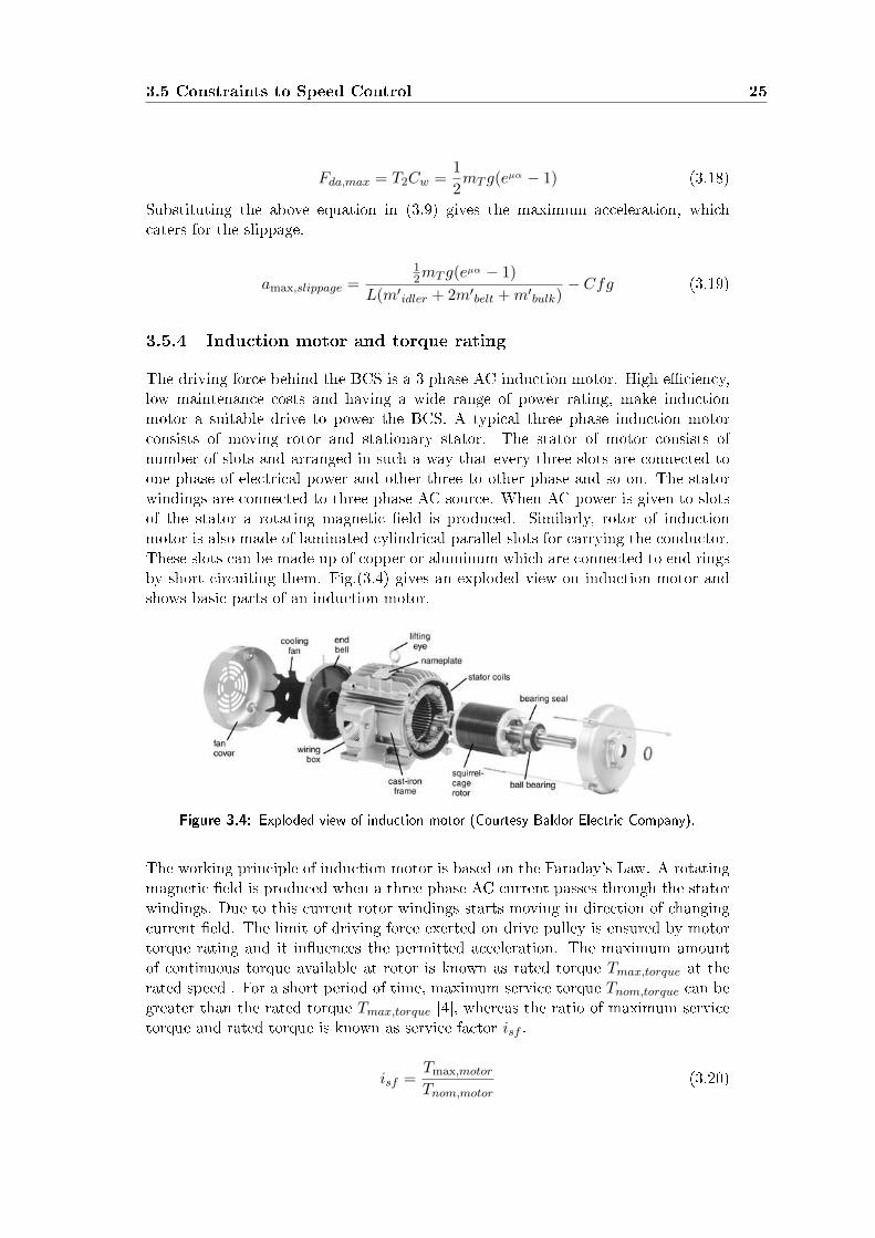
The driving force behind the BCS is a 3 phase AC induction motor. High e�ciency,low maintenance costs and having a wide range of power rating, make inductionmotor a suitable drive to power the BCS. A typical three phase induction motorconsists of moving rotor and stationary stator. The stator of motor consists ofnumber of slots and arranged in such a way that every three slots are connected toone phase of electrical power and other three to other phase and so on. The statorwindings are connected to three phase AC source. When AC power is given to slotsof the stator a rotating magnetic �eld is produced. Similarly, rotor of inductionmotor is also made of laminated cylindrical parallel slots for carrying the conductor.These slots can be made up of copper or aluminum which are connected to end ringsby short circuiting them. Fig.(3.4) gives an exploded view on induction motor andshows basic parts of an induction motor.

Figure 3.4: Exploded view of induction motor (Courtesy Baldor Electric Company).

The working principle of induction motor is based on the Faraday's Law. A rotatingmagnetic �eld is produced when a three phase AC current passes through the statorwindings. Due to this current rotor windings starts moving in direction of changingcurrent �eld. The limit of driving force exerted on drive pulley is ensured by motortorque rating and it in�uences the permitted acceleration. The maximum amountof continuous torque available at rotor is known as rated torque Tmax,torque at therated speed . For a short period of time, maximum service torque Tnom,torque can begreater than the rated torque Tmax,torque [4], whereas the ratio of maximum servicetorque and rated torque is known as service factor isf .

isf =Tmax,motor

Tnom,motor(3.20)


Service factor isf proposes motor's ability of tolerating overloading condition withoutthe phenomena of overheating. For active speed control, during acceleration, it isnecessary that service factor isf of electric motor is in permissible range in order tominimize the e�ect of overheating. The maximum instantaneous drive torque can becalculated by ignoring in�uence of gearbox inertia.

Tmax,pulley = irfTmax,motor = irf isfTnom,motor (3.21)

In above equation, isf is the reduction factor of gearbox. The permitted drivingforce Fda,max exerted on the drive pulley can be written as

Fda,max =Tmax,pulley

Rd=irf isfTnom,motor

Rd(3.22)

Where Rd represents the radius of the drive pulley. To get the permitted accelerationwhile considering the in�uence of motor and gear box inertia, Equation (3.22) issubstituted in equation (3.9)

amax,heat =irf isfTnom,motor −RdCfgL(m′idler + 2m′belt +m′bulk)

(RdL(m′idler + 2m′belt +m′bulk) +m′rotor +m′gear)(3.23)

In above equation m′motor and m′gear represent the inertial mass of motor and gear

which is deduced to the the drive pulley. Permitted acceleration for speed controloperation is minimum of the acceleration de�ned by equation (3.23), (3.19) and(3.15);

amax = min(amax,rupture, amax,slippage, amax,heat)

3.5.5 Acceleration Pro�le

A suitable acceleration pro�le is needed to be followed for speed control operation,which can bear sudden jerks of the speed control. Previously �uid couplings areused to change the speed of the induction motor. Fluid couplings helps to attainthe equilibrium for the induction motor in the start and stop procedures. Whenthe induction motor is switched on and o�, large acceleration, variations in volt-ages are experienced and �uid coupling helps to overcome these large variations.However, �uid couplings are helpful in the start and stop procedure of the electricmotor but cannot handle e�ciently sudden speed changes. To overcome these sud-den jerks, variable frequency drives (VFD) were introduced. Variable frequency driveovercomes the issue of sudden speed changes in speed controlled operation. The fre-quency of the induction motor is controlled by the variable frequency drives whichin turn controls speed of the induction motor and the torque available at the rotor.Daijie He [4], suggests that a sinusoid acceleration is a better choice to minimizee�ects of jerks and belt rupture during acceleration. In Fig.3.5 a suitable sinusoidacceleration pro�le in accordance with a sinusoid velocity pro�le is shown.


Figure 3.5: Desired acceleration and velocity pro�le

Sinusoid acceleration pro�le can be described mathematically as

a(t) =π

2

Vb − Vb,0Ta

sinπ(t− t0)

Ta, 0 ≤ t ≤ Ta

Vba(t) =Vb − Vb,0

2

(1− cos

(π(t− t0Ta

))+ Vb,0

Where t0is the starting time, t is the current time, Vb is desired speed, Vb,o is speedbefore acceleration, Ta is required acceleration time. Optimized acceleration timecan be calculated by knowing the desired speed and speed before the acceleration.

Ta,min =π(Vb − Vb,0)

2amax

Desired acceleration time and speed are calculated if wrap factor, belt safety factor,rated tension and motor torque is previously known or calculated. To get the opti-mized acceleration time, acceleration pro�le is considered accordingly and possiblerisks will be minimized too, which cause system to stop working or block feed �owfrom hopper or loading chute. Proper calculations for the acceleration time andde-acceleration time are explained in the next chapter.

Chapter 4

Speed Controller

An overview of di�erent control strategies are de�ned and discussed in this chaptertowards the speed control operation of BCS. Motivation towards the implementedcontrol technique and Fuzzy logic controller is discussed in detail for speed controlledoperation based on material feeding rate.

4.1 Control Strategies

The task of optimizing the belt speed in the running process when belt is randomlyloaded is a di�cult task. Due to extreme randomness and to avoid system con-straints, limits the choice of control to be considered. Optimizing the belt speedwith minimal overshoot, undershoot and quicker response according to feed �owrequire a very sophisticated controller. From a very simple Proportional (P) to Pro-portional Integral Derivative (PID) control which are most widely used controllersin industrial applications neither provide a competent control to random nature offeed nor have the ability to bear system constraints. Passive speed control can beimplemented by considering a simple proportional controller for belt conveyor sys-tem when feed �ow on belt is known and task is to optimize belt speed for certainperiod of time. The focus of this thesis work is to de�ne a controller for randomfeeding which bears extreme overshoots in material feeding and provides a quickerresponse to system disturbances with minimal overshoot and undershoot. In currnetscenario adding special features to a PID controller does not provide proper speedadjustments, makes controller more complex and resulting into system instability.

Active speed control for belt conveyors requires quick and precise system response insuch a case implementing PID control is not a suitable option when auto-tuning ofPID is required for acquiring optimal PID constants. However, a controller similar toa simple proportional control which has a quick system response, has better systemstability, requires less computational power and easy to implement can be consideredan appropriate option. Such a control can be considered by using fuzzy logic control,where material feeding is used as principle for fuzzy set of rules. Other reason for

29

30 Speed Controller

using fuzzy logic for current research is lack of a proper system model which de�nesall system parameters and constraints to control the system [32, 29].

Fuzzy logic is a form of a manual mimicing process. In fuzzy control technique entireprocess is governed by sense of physical behavior of system and knowledge of humangoverning the process. The very intelligent however, simple trait of human natureis guessing and forecasting certain conditions helps in devising controllers which aredi�cult to be controlled. Fuzzy controllers are a better and robust substitute toPID control when system have multiple constraints, requires quick system responseand provides better system stability. Fuzzy control is most oftenly described byifelse-then rules for integrating with human expertise. This criteria is translated forde�ning fuzzy sets, by using some reference input and constraints of the system tobe controlled. This method is of particular importance of fuzzy model based control,which follows model predictive control.

Nowadays, Model Predictive Control (MPC) is considered one of most desired andproposed control strategy for controlling a system having multiple inputs and con-straints. Due to ability to predict future inputs and proposing a controller based onthese prediction, it is assumed that MPC have better controllability and optimizedoutput. In predicted control strategy, e�ects of input onto the output are linearizedand this information will help to get proposed output of system. However, widelyused control techniques, require the system to operate in same operational envirorn-mental conditions and require a pre-de�ned system model, which helps in proposing,designing and implementing a controller. In case of current research, neither thesystem under consideration work under same environmental conditions nor a pre-de�ned system model is available, which tightens the selection of a proper controltechnique.

MPC's are widely considered nowadays due to strong ability to predit, which letMPC outstand among other control strategies. According to control point of view,any system which possess a proper mathematical model and helps in predicting itsfuture states will be of great interest. In predicted control, usually system inputsare predicted based on previous system data and environmental conditions, helpingsystem future output to react according to predictions used. These predictions areeither based on model of the system or human predictions. Humans are good inforecasting certain parameters and they try to control di�erent systems based onthis unique trait. In case of BCS, which is considered to be model free system, acontroller is proposed which acts like human brain, makes certain assumptions andpredictions to achieve desired output.

Due to ever increasing demand of BCS which makes system more complex in means ofnatural operating condititons and having numerous constraints, leads scientists andresearchers to propose controller which do not really require a system model but o�ersbetter controlability towards system. For such systems, system inputs and di�erentparameters are considered to propose a knowledge based controller. A controllerbased on fuzzy values of the system can be a better choice in such scenarios, wherehuman knowledge based on fuzzy input of system and general system paremeters areconsidered to propose a controlller.

A fuzzy control algorithm is developed to optimize belt speed to avoid potentialrisks including material spillage, belt slippage and material overloading caused by

4.2 Fuzzy Logic 31

short-term material loading peaks. A controller based on Fuzzy logic which can alsobe realized as Proportional (P) controller is discussed in next section while taking inaccount acceleration pro�le, acceleration time and other constrains related to speedcontrol of BCS.

4.2 Fuzzy Logic

Fuzzy logic was �rst introduced in 1965 by an Iranian Professor Lot� Zadeh workingat University of California [15]. He proposed it to use for process imprecise data.Fuzzy control technique is robust and have ability to overcome strong non-linearity ofsystem. It can be used for a number of inputs, outputs and can be easily modi�ed bychanging fuzzy limits. It is much simpler, quick and easier to implement for a numberof control problems. Due to all these properties of FLC, towards non-linear system,it is employed to control �ight control of war planes, stabilization of camcorders andin Anti-Lock Braking system in cars [15].

Fuzzy set theory is used for modeling of systems. The modeling task is done by usingfuzzy interface system (FIS). By using FIS, input data is converted into linguisticvariables by means of fuzzi�cation process, this process is re-processed by using arule base and generates a set of numerical results from conclusion of re-processingwhich is known as defuzzi�cation process. FIS performs a universal approximations,which means that any continuous function is approximated to a compact domainwithin a certain level of accuracy. Fuzzy models provides an extra output whichis the linguistic description of processesed model. Most common types of fuzzymodels are based on Mamdani model. Mamdani model is based on antecedents andconsquences of the fuzzy prepostions. Takagi-Sugeno fuzzy model is another typeof fuzzy models, which uses precise and crisp functions of antecedents. Di�erentmodels can be developed by using available empirical knowledge. In many casesthese models gives better results based on empirical knowledge and applying a moreprecise guess. Most often these functions provide better parameter tuning and alsoincrease system stability [17].

As word fuzzy means indistinct and unclear, likewise the way it is used is based oncertain assumptions known as fuzzy values. These values are based on certain infor-mation obtained by system characteristcs and based on these characteristics di�erentfuzzy values are described, which considered to cater for information provided by thesystem. The degree of trueness and falseness is based on the fuzzy subsets whichis a function of U→ [0, 1]. To work with fuzzy logic, a set of membership functionis need to be de�ned, which gives an idea about the value of membership function.Generally, there are two notations for fuzzy sets, U and A, where A is known as�linguistic label� and denoted by µA. The set A gives information about the systeminput values and µA gives degree of trueness of A. For a fuzzy set A : U → [0, 1],the value A(u) is known as degree of membership of u in the fuzzy set A. The valueof A is context and scenario dependent [15].

Powerful control strategies are designed by using fuzzy logic in many di�erent areas.Basically there are two main types of fuzzy controller, one is based on a propermathematical model, if its available, known as model based fuzzy controller and other

32 Speed Controller

one is model free controller, which refers to unavailability of a proper mathematicalmodel. Model based fuzzy control require a proper mathematical model in order tobe implemented, however model free controller based on fuzzy logic can be designedand implemeted if there is no de�ned mathematical model available. In that caserecorded system input, output data from previous operating times is considered alongwith other parameters to propose a fuzzy controller. [17].

A fuzzy controller is proposed and implemented for current research having twoinputs and a single output. In next section fuzzy controller is discussed in detail.

4.3 Control method

In current research, Fuzzy Logic is used to design a controller which provides refer-ence speed for belt conveyor based on feeding rate and fuzzy values for speed. Theinput to Fuzzy Logic controller is the material feeding rate which is in form of ratio ofmaterial feeding and proposed speed values for di�erent proportions of material feed-ing. A proper acceleration time and pro�le is considered to implement the controller.Output of Fuzzy logic controller gives a reference speed vref , this reference speedis fed into Induction motor control based on either Direct Torque Control or FieldOriented Control to get the desired torque for speci�c reference speed. Fig.4.1, givesan overview of the desired controller based on Fuzzy Logic to get uniform loading,optimized reference speed and also helps in energy savings. Main task of research isto design a controller, based on material feeding rate, which follows material feedingand gives reference speed accordingly, which is used to control the output torque ofdriving force, i-e; induction motor.

��

��

��

��

��

��

��

��

��

��

Figure 4.1: Block Diagram of Controller

Speed control operation is best realized based on material loading. In order todesign and implement a speed control, fuzzy membership function are de�ned basedon material loading. This fuzzy set of material loading and desired speed can beobtained by setting percentage limits to material loading. In order to design acontroller based on fuzzy logic, input and output of controller must be identi�ed.The input of system is feeding rate q and output is reference speed vref . Then thesystem will be of the form.

Zt = {v(1), q(1), ...., v(t), q(t)} (4.1)

After de�ning the system input and output, a predictor model is required which isthe result of previous data set Zt−1to the next output, i-e v(t) and mathematically

4.3 Control method 33

de�ned as

v(t) = f(Zt−1) (4.2)

In above equation v(t) is the estimated speed. The purpose of identi�ying systeminput and output is to design the function f by means of a fuzzy model. Equation 4.2,which de�nes the fuzzy system can be described as follows by applying paramterizablemapping.

v(t|θ) = f(Zt−1|θ) (4.3)

where θ=

amax,heat

a(t)Vba(t)Ta,min

In above equation θ de�nes parameters, i-e; acceleration pro�le, acceleration timeand minimum reference speed. Due to the non-linear nature of material feeding, andto de�ne all the parameters which are de�ned in earlier chapters, a more detailedform of equation 4.2, is required. To de�ne all these parameters another vector ϕ(t)is introduced in equation 4.2, then

v(t|θ) = f(ϕ(t)|θ) (4.4)

In above equation, ϕis vector containing the regressors and known as regressionvector. Mathematically ϕis de�ned as

ϕ(t) = [v(t− 1), ..., v(t− n), q(t− 1), ...., q(t−m)] (4.5)

For de�ning a fuzzy system, di�erent parameters need to be de�ned which include,membership functions, AND, OR operation, defuzzi�cation method and sub type offuzzy model (Mamdani or Takagi-Sugeno).

A fuzzy controller based on Takagi-Sugeno model and guassian membeship functionis used to implement the controller while using Fuzzy Logic Toolbox. The mem-bership functions of input feed �ow and speed are given in Fig4.2 and Fig.4.3. Forfuzzi�cation of input, feed �ow and speed is mapped between [0,1] interval, anddivided into fuzzy sets: zero(ZE), positive small (PS), positive medium (PM) andpositive big (PB), where Min-Max method is used for processing of fuzzy rules valeswhereas defuzzi�cation is done by weighted sum.

34 Speed Controller

0 0.1 0.2 0.3 0.4 0.5 0.6 0.7 0.8 0.9 1

0

0.2

0.4

0.6

0.8

1ZE PS PM PB

Figure 4.2: Membership functions feed �ow

According to membership functions as feed �ow increases speed of belt also increasesafter calculating the amount of change in feed �ow. If amount of feed �ow is changed,then controller calculates the amount of change from the previous value, either it isincreased or decrease. If its increase from the previous value, then is it falling intothe same limit of feed �ow or the change is big enough to also change reference speedaccordingly. Otherwise, if the amount of feed �ow remains the same, then there isno change in reference speed.

0 0.1 0.2 0.3 0.4 0.5 0.6 0.7 0.8 0.9 1

0

0.2

0.4

0.6

0.8

1ZE PS PM PB

Figure 4.3: Membership functions speed

Based on Takagi-Sugeno model, the equation which gives the input and output pa-rameters of fuzzy system is of the form,

f(x) =

L∑l=1

Alqµl(q)∑Ll=1 µl(q)

(4.6)

where Al is row vector which includes ϕ(t) and µl(q) is membership functions of therule l and l =4 for current control method. Structure of regressor is based on NARX

4.3 Control method 35

model, due to the ability to include the past input and output values, which helpsin achieving proposed results in less time.

ϕ(t) = [v(t− 1), ..., v(t− n), q(t− 1), ...., q(t−m)]

NARX model is widely used due to nonrecursive structure of regressor and easetowards the future forcasting for one or few steps. The state-space model for thecase of stochastic case is de�ned as follows

x(t+ 1) = f(x(t), u(t))

y(t) = g(x(t), u(t))

Due to the linear relationship of feed �ow and speed Takagi-Sugeno models is used.Takagi-Sugeno models are more preferable than Mamdani models when fuzzy rulesresults act as linear functions.

These models use the structure of stochastic state-space model mentioned above andtheir functionality is based on the inference system mechnanism, which is guidedby inputs or outputs. However, in most of the cases these variables are consideredbeing acquired from previous knowledge of system. Initial distribution of membershipfunctions is done using the NARX structure, since it updates the previous values ofinput and output. In order to get more better results gradient descent method canbe used. After selection of state-space model, quadratic cost function should beminimized in for �ne tuning of controller.

VN =1

2N

N∑t=1

|y(t)− |y(t|θ)|2 (4.7)

Again θ is vector containing parameters of membership functions and y(t),y(t) areproposed and desired values of reference velocity. Proposed performance, i-e desiredreference speed of system is accomplished with four fuzzy set for each input, howeverincreasing the fuzzy set values, will make controller more complex and takes consid-erable amount of time for tuning. The shape of generated control function is shownin Fig.4.4.

36 Speed Controller

10.8

Speed

0.60.4

0.201

0.80.6

Feed Flow

0.40.2

0.9

0.5

0.4

0.3

0.2

0.1

0.8

0.7

0.6

0

Vre

f

Figure 4.4: Curve of controlled function V ref

4.4 Predicted Control

Predicted control refers to the fact, that any of system input is predicted, helping toachieve more desired and optimized output. Predictions can be made on any systeminput, having more in�uence to output as compared to rest of inputs which is feedingrate in current case. In current research the basic goal is to estimate feeding rateand based on that estimation a controller is designed which is discussed in previoussection. The controller designed based on fuzzy logic is used to get a referencespeed based on a soft acceleration pro�le and time which follow the material feedingrate. After the successful implementation of fuzzy logic controller, based on materialfeeding it is observed that controller gives a reference speed within the nominal speedrange of belt, however it can be optimized to a certain extent. For that reason, timedi�erence is calculated between the material feeding and resulted reference speed. Itis noticed from output of fuzzy logic controller Fig.5.2 that reference belt speed canbe optimized to a certain level while avoiding di�erent constraints to system whichare discussed in Section 3.5.2 and Section ??. The prediction horizon is kept largeenough for system to get to the desired state while avoiding di�erent risks involvedin speed control operation. Prediction de�ned, provide soft and gentle accelerationto maintain system stability. For every sudden rise and fall in material feeding,same prediction is applied which optimizes belt speed as much possible while beingfollowing basic system design and avoiding di�erent risks.

In order to de�ne a prediction towards the output of fuzzy logic controller, timeis measured which is taken to follow the material feeding. A prediction is madetowards that time and then according to that a delay is introduced which gives moreoptimized reference belt speed for both acceleration, de-acceleration procedures andhelps in saving more energy.

In order to calculate the prediction, infromation from previous section is used toestimate di�erent parameter towards prediction. The prediction can be de�ned as

minu(k),......,u(k+nc)

J(u(k), y(k), w(k)) =∑k+Np

t=k (w(t)−y(t))TQ((w(t)−y(t))+δ(u(t)tRδu(t))

4.4 Predicted Control 37

Where u(k) is the input, i-e; reference speed V ref , y(k) is the output, i-e; optimizedreference speed, w(k) is the future reference signal, δu(t) = u(t)−u(t−1), Np is theprediction horizon equals to 30 after calculating the time di�erence between materialfeeding and reference speed and by analyzing output of the optimized reference speed,Q is a positive de�nite matrix of input that is reference speed and R is positivesemide�nite containing values of reference signal. The approximation of the predictedfuture output is

y(t+ k|t) = yforced(t+ k|t) + yfree(t+ k|t) (4.8)

In above equation yforced(t + k|t) is dependent on future increments on the feedingrate and yfree(t + k|t) depends on previous material feeding and reference speedvalues. In order to predict time taken by the fuzzy controller to achieve a certainlevel of material feeding, it is important to know what is acceleration time andmaximum acceleration which is suppose to be safe and belt conveyor keeps workingin a normal condition. The maximum acceleration time used is about 20s, since it isassumed that secondary belt conveyor is running on minimum designed speed whichis 2m/s and time needed by secondary belt to accelerate from minimum speed to acertain level is approximately 10s to 20s depending on steepness of material feedingwhere maximum permissible acceleration is 0.085 m/s2.

4.4.1 Prediction towards acceleration procedure

The MATLAB code used to predict the time delay for acceleration procedure isgiven below which is according to equation ??. According to MATLAB code, �rst itis checked whether the reference speed of secondary belt is greater than temporaryspeed (minimum speed), if its true, �ag sets to 0 and so is the delay, till the �agremain 0, a delay keeps updating and continue calculating time di�erence. It keepschecking how much time it need to accelerate from a certain value of reference speedand accelerate the belt at t = minimumspeed+delay. The delay introduced ensuresthat belt is accelerated just before material starts loading on the secondary belt.The increment for reference speed is calculated and being updated to the predictionpath. In the acceleration procedure, prediction follows the last value of referencespeed. The whole procedure is divided into the following steps.

1. Determine the speed change from previous to new measured values.

2. Calculate optimized time for acceleration if it is changed from previous step.

3. Achieving the proposed acceleration while following the prediction and referencespeed.

38 Speed Controller

if belt2.reference_speed>temp_speed�ag=0;delay=0;while �ag == 0;delay=delay+1;error=belt1.import(t-sample_interval-T_acc+delay+1:t-sample_interval+delay);if min((SPEED'/5.2)-belt1.import(t-sample_interval-T_acc+delay+1:t-sample_interval+delay))<0;�ag =1;if delay<30delay=delay-1;end

First the material feeding on the secondary belt is read and processed by de�nig thelength of primary belt and number of blocks it is divided. For every time unit themass on primary is calculated and processed with the nominal speed of 5.2 m/s. Byknowing the length of primary belt, time taken by it to unload material on secondaryis calculated and bulk mass per unit length. By using simple relation s = vt, wheres is length of primary belt, v is speed of primary and t is calculated to acceleratesecondary belt. Prediction for reference speed is done by using the sample timewhich is obtained by feed sensor data placed at primary belt. The last value whichis obtained from the delay till prediction horizon is used at end of prediction path.

4.4.2 Predictions towards deceleration procedure

Similar to acceleration procedure the deceleration procedure is also implemented byusing equation ??. It will start checking if reference speed is less than temporaryspeed and needs to be decreased. In this case the value of delay is t = −delay, wheredelay is set to a value of -1. This is due to the face that amount of maximum materialin particular time frame is already loaded on to secondary belt and incoming materialvalue is less than previous value. And belt needs to be slow down to certain speedbefore that certain amount of material is loaded to secondary belt. The decelerationprocedure is followed by the following MATLAB code.

4.4 Predicted Control 39

elseif belt2.reference_speed<temp_speedde�ag=-1;dedelay=-1;while de�ag ==-1;dedelay=dedelay-1;error=belt1.import(t-sample_interval+1+dedelay:t-sample_interval+T_acc+dedelay);if min((SPEED'/5.2)-belt1.import(t-sample_interval+1+dedelay:t-sample_interval+T_acc+dedelay))<0;de�ag =0;if dedelay<-30dedelay=dedelay+1;endendif dedelay<-30de�ag=0;endend

The deceleration path continue calculating the refernce speed and material feeding.Reduction in speed follows prediction path de�ned for deceleration. The resultsobtained from these prediction is discussed in the next chapter.

Chapter 5

Simulations & Results

In this chapter �ndings of implementation and simulation results are presented anddiscussed with reference to previous chapters. Random feeding scenarios are appliedto speed controller to check stability and working of proposed control speed strategy.Simulation results based on random feed rate and active speed control based on fuzzylogic controller are discussed. At the end of chapter a comparison is made betweenamount of energy savings.

5.1 Calculations towards Speed Control

To realize and implement a speed control, calculated values are desired which are inaccordance with DIN 22101 standard and well suited for a FLC. First, amount ofmaterial that is loaded on belt conveyor according to nominal capacity and nominalspeed is calculated. Nominal capacity of system is 2500 tph and nominal speedis5.2m/s.

m′bulk =QnomVb

= 133.54kg/m

The amount of material per unit belt lenght is 133.54kg/m. Next, step is to calculatethe combined mass of idlers both on carrying and return side. The mass of idlerson carrying side is14.28 kg/mand that on return side is 7.72 kg/m, and total massof idlers is

m′idler, c +m′idler,r = 22.59kg/m

According to DIN 22101 the safety factor SA,min of belt ranges from 5.4 to 8.0based on length of belt conveyor system and nominal capacity. The coe�cient ofsecondary resistance C has a value of 1.09 for a belt length of 1000m. Then by usingthe equation ((3.15)) , the maximum acceleration time is calculated while taking intoaccount the rupture strenght.

41

42 Simulations & Results

amax,rupture =

kNBηspliceSA,min

− 12mT g − CfgL(m′idler + 2m′belt +m′bulk)

L(m′idler + 2m′belt +m′bulk)= 0.156m/s2

The permitted acceleration around the drive pulley is calculated by using equation(3.19) while considering the risk of belt slippage.

amax,slippage =12mT g(eµα − 1)

L(m′idler + 2m′belt +m′bulk)− Cfg = 0.078m/s2

Based on these calculations, an active speed control based on Fuzzy Logic is imple-mented in MATLAB. Table. 5.1 gives information to di�erent parameters of beltconveyor which are used for simulation purposes. These parameters are taken fromthe case study of Daijie.He [4]. The simulation results are discussed in the nextchapter.

Table 5.1: Belt conveyor parameters

Parameter Symbol Unit Value

Conveyor length L [m] 1000

Nominal Capacity Qm [th−1] 2500

Nominal Speed Vb [ms−1] 5.2

Belt Width B [m] 1.2

Height of BCS H [m] 0

Mass of belt per unit length m′belt [kgm−1] 14.28

Mass of idler per unit length on thecarrying side

m′idler,c [kgm−1] 14.87

Mass of idler per unit length on thereturn side

m′idler,r [kgm−1] 7.72

Mass of gravity take-up device mT [kg] 5060

Length Coe�cient C [−] 1.09

Gravitational acceleration g [ms−2] 9.8

Arti�cial frictional coe�cient f [−] 0.018

Minimum safety factor SA,min [-] 5.4

Density of material ρ [kgm−3] 850

Nominal rupture force of the belt kN [N ] 500

Frictional coe�cient between drivepulley and belt conveyor

µ [-] 0.35

Wrap of the belt around the pulley α [# ] 180

5.2 Simulation of speed control

In this section simulation results based on fuzzy logic and predictions as describedin Section 4.4.1 and 4.4.2 are presented and explained. For simulation purposesdi�erent feeding scenario are considered to check the functionality of implemented

5.2 Simulation of speed control 43

speed control. Speed control is checked by changing di�erent parameter, speci�callysample interval time to observe the behavior of controller towards extended sampletime. The proposed acceleration and de-acceleration time are in range of 10 − 20sec, based on steepness of material feeding curve. For simulation purposes feed �owof 2.91 hours is considered.

Time t [s]0 2000 4000 6000 8000 10000 12000

Con

trol

led

Spe

ed v

[m/s

]

2

2.5

3

3.5

4

4.5

Fee

d flo

w T

onne

s/ho

ur

0

0.2

0.4

0.6

0.8

1Active SpeedFeeding Rate

Figure 5.1: Feed Flow vs Active Speed

For simulation purposes, belt conveyor is divided in to a number of blocks, to getthe total amount of feed on belt conveyor and also reference speed de�ned on baseof percentage feed �ow. Fig. 5.1 shows the output of active speed control based onfuzzy logic applied to secondary belt. The red curve represents feed �ow onto beltconveyor and blue curve is active controlled speed. Minimum speed of controller isset at 2m/s. Controlled speed is achieved by providing a soft, gentle acceleration andde-acceleration using the sinusoidal acceleration pro�le as discussed in Section3.5.5.Fig.5.2, shows the active speed control without using any prediction.

A prediction is made towards time taken by the belt speed to achieve desired speedand a delay is initialized based on reference speed as discussed in Section 4.4.1 and4.4.2. If the reference speed is greater than minimum nominal speed, then it checksthe di�erence between reference speed of two adjacent blocks of belt. If the di�erenceis greater than half of sample time, then belt speed is adjusted with that amount ofdelay. This delay helps in achieving a more optimized belt speed.


Time t (s)0 2000 4000 6000 8000 10000 12000

Spe

ed (

m/s

)

2

2.5

3

3.5

4

4.5

Fee

d flo

w (

% T

onne

s/ho

ur)

0

0.2

0.4

0.6

0.8

1Active SpeedFeeding Rate

Figure 5.2: Feed �ow vs Predicted Active Speed

Similary, based on di�erent speed limits de�ned for percentage value of feed �ow,if the feed �ow is decreased, then based on the same time prediction belt speed isadjusted for a less amount of feed �ow. Control algorithm is implemented to followfeed �ow on the belt and speed rises to a certain limit according to range of nominalcapacity of feed �ow. It is important to note that nominal capacity of material is2500 tph, however in above Fig.5.2 maximum speed is 4.5m/s which is 86 percent ofnominal speed which is in accordance to 86 percent of nominal capacity of feed �ow.To handle sudden peaks of feed �ow, a greater value of nominal speed is assigned forpreventing material spillage. Table 5.2, gives a comparison of simple active speedcontrol and that of predicted active speed. It is noticed that at same time, value ofreference speed obtained from simple active speed is quite big as that of predictedspeed.

5.2 Simulation of speed control 45

Table 5.2: Comparison of predicted reference speed and non-predicted speed

Time (s) Non Predicted Speed (m/s) Predicted Speed(m/s)

525 4.5 2.9

675 4.5 3.9

1875 2.4 2

2477 3.89 2.4

3970 4 3.4

4200 3.7 3.2

4630 3.2 2.9

4744 3.7 2.9

5488 3.3 2

5696 4.07 3.4

7800 3.9 2.09

8000 2.9 2.6

8700 4.2 3.9

10000 3.1 2

10225 2 2

Comparing predicted and simple control one can �nd that predicted speed controlgives a more precise following of feed �ow, however, simple control technique hasa time delay in between which makes it less desired when more energy savings aredesired. Table 5.4, shows the di�erence between control and predicted control powersavings. In order to better understand the di�erence between active speed andpredicted speed, both control techniques are plotted in Fig. 5.3 along with the feed�ow rate. Simple active speed is shown as blue curve following feed �ow rate inred color, where predicted speed is drawn in green color which shows that predictedspeed is more optimized than active speed.

Time t (s)0 2000 4000 6000 8000 10000 12000

Spe

ed m

/s

0

5

Fee

d flo

w (

% T

onne

s/ho

ur)

0

0.2

0.4

0.6

0.8

1Predicted Active SpeedActive SpeedFeeding Rate

Fee

d flo

w T

onne

s/ho

ur

0

0.5

1

Figure 5.3: Material Feeding vs Active Speed vs Predicted Active Speed


Table 5.3: Feed �ow vs controlled speed

Time [sec] Feed Flow [% of 2500 tph] Speed [m/s]

0 0 01039 0.399 2.7212044 0.322 2.63003 0.514 2.94028 0.783 4.25001 0.684 3.96063 0.221 27001 0.192 28024 0.083 29057 0.347 210246 0.062 2

Table 5.3, gives an overview of reference speed according to percentage loading offeed �ow. Minimum speed is set at 2m/s for a 40 percent feed �ow rate and thevalue of reference speed increases to 5.2m/s for 96 percent of nominal capacity.

Time t [s]0 2000 4000 6000 8000 10000 12000

Feed

Flo

w m

g [%

250

0 tp

h]

0

0.2

0.4

0.6

0.8

1

belt1.importbelt2.import

0

0.2

0.4

0.6

0.8

1

Figure 5.4: Material loading on belt conveyors

Fig.5.4 presents material loading of primary and secondary belt conveyors. Bluecurve represents the loading of primary belt and red curve is unloading of materialfrom primary to secondary. It is noticed that there is a time delay between loadingof primary and secondary belt which is calculated by dividing length of primary bynominal speed. The time delay is approximately 140 seconds.

5.3 Power Consumption 47

Time t [s]0 2000 4000 6000 8000 10000 12000

Feed

Fee

d Fl

ow [%

250

0 tp

h]

0

0.2

0.4

0.6

0.8

1

belt1.exportbelt2.export

0

0.2

0.4

0.6

0.8

1

Figure 5.5: Material unloading from belt conveyors

Fig. 5.5, presents the unloading of primary and secondary belts, where red curve isthe result of unloading of secondary belt due to speed controlled operation. Due tospeed controlled operation on secondary belt, feed �ow seems to get uniform for aspeci�c time when material loading is within certain limits and belt speed adjustsaccording to feed �ow. It is one of the goals to implement a speed control to getapproximately uniform material loading on secondary belt conveyors. In current casefeed �ow is random and variations are higher, however it is assumed that there willmore uniform export of feed �ow on secondary belt by means of speed controlledoperation, if material feeding is less random. The time delay between emptying ofprimary and seconday belt is 290 seconds which is twice as much as that of materialloading.

5.3 Power Consumption

The basic goal to apply a speed control is to save energy. Total power consumedby secondary belt is calculated by simulating, controlled speed with respect to feed�ow. To calculate the total amount of material which is transported from primarybelt to secondary is calculated by dividing the secondary belt into small segments,calculating the material on each small segment and integrating it over time gives totalmass tranported in speci�c time. To calculate the power consumption by secondarybelt, it is necessary to include mass of idlers, belt and of material. The total powerconsumed is calculated by using the relation provided in Chapter 3.

It is obvious that peak power required by controlled speed operation is larger as com-pared to constant speed operation. Whereas, the total power consumed by controlledspeed operation is less than constant speed operation. To calculate the amount ofpower being saved is based on a theoretical model presented in [13]. Based on that,


power saving by decreasing the nominal speed vnom for actual material �ow Qmisgiven as

4P (Qm) = P (Qm, vnom)− P (Qm, vact) (5.1)

Amount of power P which is required to transport a certain feed �ow depends ontotal motional resistance F (m′L), belt speed v and e�ciencies of electric drive ηd ,frequency converter ηf and also mechanical e�ciency of drive ηm, where is given asfollows

P =F (m′L)v

ηdηfηm(5.2)

Time t [s]0 2000 4000 6000 8000 10000 12000

Pow

er [k

W]

0

20

40

60

80

100

120

140

160

180

200

Controlled Power

Figure 5.6: Power consumed by active speed operation

Fig. 5.6 presents power consumed by controlled speed operation and Fig. 5.7 presentspower consumption of constant speed operation . It is noticable that minimum powerrequied by controlled speed operation is 20 kWatts and 50kWatts for constant speedopeation. The maximum power reaches 182 kWatts for controlled speed operationand 154 kWatt for constant speed operation to transport same amount of materialbut with optimized speed. This gives another considerable result towards the size ofelectric drive required for both types of operation.

5.4 Work done 49

Time t [sec]0 2000 4000 6000 8000 10000 12000

Pow

er

[kW

]

0

20

40

60

80

100

120

140

160

Constant Power

Figure 5.7: Power consumed by constant speed operation

5.4 Work done

Amount of work done by both methods is also simulated to support the �ndings ofActive Speed control and to check whether work done by the speed control is alsoless than that of constant speed. Simulation results of work done by both operationsare shown in Fig.5.8 below.

Time t [s]0 2000 4000 6000 8000 10000 12000

Wo

rk [

kJo

ule

s]

0

50

100

150

200

250

300

Controlled Work

Time t [s]0 2000 4000 6000 8000 10000 12000

Work

[kJ

oule

s]

0

50

100

150

200

250

300

350

Constant Work

Figure 5.8: Work done by controlled and constant speed operation

Table.5.4 gives information about the power savings achieved by controlled speedoperation and predicted speed operation. For constant speed operation, belt speed ofboth primary and secondary is set at5.2m/s as per normal operational conditions. Byimplementing a controlled speed operation, average speed of secondary remains2.91


m/s for total simulation time, however by using predicted technique, average speeddecreases to 2.75 m/s. The decrease in speed of predicted speed operation also helpsin achieving more energy savings as simple controlled operation. The maximumpowered required by constant speed operation is however less than both contolledand predicted controlled speed.

Table 5.4: Comparison of Power Savings

ParametersConstantspeed

Controlledspeed

PredictedCon-trolledspeed

Avg. belt speed 5.2 m/s 2.91 m/s 2.75 m/sTotal Power 338 kWh 260.8 kWh 260.2 kWhPeak Power 154 kWatt 191 kWatt 182 kWattEst.YearlyConsumption

1.05 GWh 0.542 GWh 0.541 GWh

Power Saving % (-) 22.4 23.23

Chapter 6

Conclusions & Recommendation

Conclusions and �ndings of Active speed control in regard with all the constraintsdescribed in previous chapters are discussed in this chapter. Conclusions based on ofFuzzy logic control to achieve energy savings are discussed primarily and afterwardssome recommendations to future research are provided.

1. Speed control operation is a feasible solution towards energy savings dependenton the feed �ow.

2. Active speed control can be used to achieve energy savings for random feed �ow.Fuzzy logic provides soft and gentle acceleration and de-acceleration towardsspeed control and avoids event of material spillage and belt slippage. Researchtowards Active speed control proposes that reducing the belt speed to a certainlevel will save energy by providing a more uniform material loading on beltsas compared to constant speed operation. Less amount of power is required todrive the belt at lower speed, whereas a more powerful drive system is requiredto apply active speed control. It is found out through simulation that peakpower increases for active speed operation.

3. A robust, intelligent and soft control is desired for speed control, which canavoid mechanical jerks to the system in transition stage of adjusting the speed.It helps to increase the life expectancy of system too for controlled speed oper-ation. Prediction towards material feeding increases energy savings. Amountof energy savings increases as the length of belt conveyor increases.

4. To implemented active speed control a digital controller is a feasible optionwhich is based on discrete system parameters. If the feed �ow is less random,then modern control algorithms can be used for more energy savings.

5. For a passive control, simple control techniques can also be used by proposinga speed greater than nominal speed for certain amount of load.

51

52 Conclusions & Recommendation

Table 6.1: Energy Savings between Constant and Speed Control operation

TimeSpan

ConstantSpeed

SpeedControl

PredictedSpeedControl

Simulatedtime

33.61 Euro 26.60 Euro 26.28 Euro

YearlySaving

34,954.4Euro

27,664 Euro27,331.2Euro

6. Amount of power savings is dependent upon the feed scenario. However, activespeed controls requires complex closed loop control to match feed �ow, whereasan active speed control is simple and easier to implement. Active speed controlis proposed for new BCS which are to be installed in future.

7. Current research proposes that speed control operation is economically feasibleoption, if existing system is powered by VFD and belt tensions are within thelimits of belt constraints.

8. By speed controlled operation a handsome amount of money is saved by re-ducing the amount of power consumption, amount of taxes are also reducedby less amount of carbon dioxide emission. It also helps in reducing the noisepollution by reducing the speed of system.

Table.6.1 gives an overview of estimated yearly savings by applying controlled speedoperation. The calculations are based on a power tari� of 0.102 Euro per kWh and forestimation of year savings, it is assumed that BCS is working 12 hours a day, 5 daysa week and 52 weeks a year. The di�erence of savings is higher between constant andspeed controlled operation, however there is not much di�erence between a simplespeed controlled operationa and predicted speed controlled operation.

For future research it is recommended to consider the DIN 22101 and IS0 5048model for the calculation of resistive forces. A more detailed and dynamic model isrequired which incorporates mechanical jerks and constraints towards speed controloperation. Speed controlled operation is presented and supported by simulationsdone on MATLAB/SIMULINK. It is recommended to implement physically to doreal time analysis of speed control operation. It is suggested to make a laboratorymodel which can be used to implement a speed control.

Active speed control operation for belt conveyor can be best explained and described,if a suitbale acceleration is de�ned and proposed based on constraints described inChapter 3. Based on the value of acceleration a suitable control technique can bedesribed for drive control. For future research it is highly recommended to pro-pose a control technique for electric drive based on acceleration which avoids theseconstraints.

References

[1] ABB Technical Guide No 1 REVC.

[2] Alain de Visscher, Commercial Manager, Vigan Engineering SA, Nivelles, Bel-gium. Analysing performance of agribulk unloading systems. pages 147�150.

[3] Conveyor Equipment Manufacturers Association Engineering Conference. Beltconveyors for bulk materials. Conveyor Equipment Manufacturers Association,1997.

[4] Daijie He, Yusong Pang, and Gabriel Lodewijks. Determination of Accelerationfor Belt Conveyor Speed Control in Transient Operation. IACSIT International

Journal of Engineering and Technology, 8(3):206�211.

[5] Daijie He, Yusong Pang, and Gabriel Lodewijks. Speed Control of Belt Convey-ors during Transient Operation. Powder Technology.

[6] W. Daus, S. Koerber, and N. Becker. Raw coal loading and belt conveyor systemat Nochten Opencast Mine- a new conveying and loading system based on drivescontrolled and adjusted by frequency converter[Die Rohkohleverladung undBandanlage im Tagebau Nochten- Ein neues Foerder- und Verladesystem aufder Grundlage umrichtergesteuerter und geregelter Antriebe]. BRAUNKOHLE,50(2):117�130, 1998.

[7] DIN 22101. GurtfördererfürSchüttgut � Grundlagenfür die Berechnung undAuslegung (Belt conveyor for bulk materials � fundamentals for calculation anddesign). Berlin: DeutschesInstitutfürNormung, 2002. Technical report.

[8] DIN 22101. GurtfördererfürSchüttgut � Grundlagenfür die Berechnung undAuslegung (Belt conveyor for bulk materials � fundamentals for calculation anddesign). Berlin: DeutschesInstitutfürNormung, 2002. Technical report, 2002.

[9] H. Funke. Zum dynamischen Verhalten von Gurtförderanlagen beim Anfahrenund Stillsetzen unter Berücksichtigung der Bewegungswiderstände. Diss. TU

Hannover, pages 64�73, 1973.

53

54 References

[10] G. Lodewijks. Two Decades Dynamics of Belt Conveyor Systems. 22(2):124�132,2002.

[11] H. Lauho�. Speed Control on Belt Conveyors - Does it Really Save Energy?Bulk Solild Handling, 25(6):368�377, 2005.

[12] A. Harrison. FLEXURAL BEHAVIOUR OF TENSIONED CONVEYORBELTS. pages 79�83, 1983.

[13] J. Hiltermann, G. Lodewijks, D. L. Schott, J. C. Rijsenbrij, J. a. J. M. Dek-kers, and Y. Pang. A Methodology to Predict Power Savings of Troughed BeltConveyors by Speed Control. Particulate Science And Technology, 29(1):14�27,January 2011.

[14] Jan Hiltermann, Gabriel Lodewijks, Joan C. Rijsenbrij, Dingena L. Schott,Jan AJM Dekkers, and Yusong Pang. Reducing the power consumption oftroughed belt conveyors by speed control. 6th International Conference for

Conveying and Handling of Particulate Solids: 3-7 August 2009, Brisbane Con-

vention & Exhibition Centre, Queensland, Australia, page 306, 2009.

[15] Hung T. Nguyen and Elbert A. Walker. A First Course in Fuzzy Logic, Third

Edition.

[16] International Standard (ISO 5048). Continuous mechanical handling equipment- Belt conveyors with carrying idlers - Calculation of operating power and tensileforces. ISO ISO 5048, September 1989.

[17] Jairo Espinosa, Joos Vandewalle, and Vincent Wertz. Fuzzy Logic, Identi�ca-

tion and Predictive Control. Advances in Industrial Control. Springer-Verlag,London, 2005.

[18] B. Jeftenic, M. Bebic, M. Gvozdenovic, N. Rasic, L. Ristic, D. Jevtic, P. Lucic,and D. Slavkovic. Load equalization for high-power induction motors by speedcontrol in limited range. In International Symposium on Power Electronics,

Electrical Drives, Automation and Motion, 2008. SPEEDAM 2008, pages 842�847, June 2008.

[19] B. Jeftenic, L. Risti¢, M. Bebi¢, and S. Statkic. Controlled induction motordrives supplied by frequency converters on belt conveyors #x2014; modelingand commissioning. In 35th Annual Conference of IEEE Industrial Electronics,

2009. IECON '09, pages 1063�1068, November 2009.

[20] K. KRISHNASWAMY and M. PONNI BALA. POWER PLANT INSTRU-

MENTATION. PHI Learning Pvt. Ltd., August 2013.

[21] Kuhnert, G. and Schulz, G. The Origins of the "Rope Friction Equation. BULKSOLIDS HANDLING, 15(2):261�264, 1995.

[22] Lange, L.R. de. Active speed control for energy saving purposes on belt con-veyor systems. Master thesis report, Delft University of Technology, Delft, TheNetherlands.

References 55

[23] Lange, L.R. de. View entry 28286: Digital Library. Master thesis, Delft Uni-versity of Technology, Delft, The Netherlands.

[24] G. Lodewijks. On the Application of Beam Elements in Finite Element Modelsof Belt Conveyors-Part 1. Bulk Solids Handling, 14(4):729�738, 1994.

[25] G. Lodewijks, D. L. Schott, and Y. Pang. Energy saving at belt conveyors byspeed control. In Proceedings of the BeltCon 16 conference, pages 2�3.

[26] Gabriël Lodewijks. Dynamics of belt systems. PhD thesis, TU Delft, DelftUniversity of Technology, 1996.

[27] Neven Lovrin and Draºen Debeli¢. ABOUT THE HISTORY OF BELT CON-VEYORS. Engineering Review, 28(2):111, 111�118, 118, December 2008.

[28] Jia Luo, Weijian Huang, and Shirong Zhang. Energy cost optimal operation ofbelt conveyors using model predictive control methodology. Journal of CleanerProduction, 105:196�205, October 2015.

[29] Y. Pang and G. Lodewijks. Improving energy e�ciency in material transportsystems by fuzzy speed control. pages 159�164. IEEE, August 2011.

[30] Yusong Pang, Gabriel Lodewijks, and Dingena L. Schott. Fuzzy ControlledEnergy Saving Solution for Large-Scale Belt Conveying Systems. Applied Mech-

anics and Materials, 260-261:59�64, December 2012.

[31] R. Alles,. Conveyor belt system design, continental ag, 3,�. (Revised Edition),1998.

[32] L.B. Ristic, M.Z. Bebic, D.S. Jevtic, I.D. Mihailovic, S.Z. Statkic, N.T. Rasic,and B.I. Jeftenic. Fuzzy speed control of belt conveyor system to improve energye�ciency. pages DS2a.9�1�DS2a.9�7. IEEE, September 2012.

[33] Leposava B. Ristic and Borislav I. Jeftenic. Implementation of Fuzzy Controlto Improve Energy E�ciency of Variable Speed Bulk Material Transportation.IEEE Transactions on Industrial Electronics, 59(7):2959�2969, July 2012.

[34] Sandvik. Advanced conveying in one of the world's most e�cient mines. Tech-nical report.

[35] Shalom Akhai and Harpreet Singh. DESIGN OPTIMIZATION FOR MODI-FICATION OF TROUGH BELT CONVEYOR TO REDUCE MATERIALSPILLAGE USED IN CLINKER TRANSPORT IN CEMENT PLANT. In-

ternational Journal of Research in Advent Tech nology, 1(4):27�37, November2013.

[36] W. A. Günthner, Ch. Tilke, and S. Rakitsch. Energy e�ciency in bulk materialshandling. bulk solids handling, 30(3):138�142.

[37] S. C. Walker. Mine Winding and Transport. Elsevier, December 2012.

[38] E. D. Yardley and L. R. Stace. Belt Conveying of Minerals. Elsevier, February2008.

56 References

[39] Yusong Pang. Intelligent Belt Conveyor Modelling and Control. Doctoral Re-search.

[40] Shirong Zhang and Xiaohua Xia. A new energy calculation model of belt con-veyor. In AFRICON, 2009. AFRICON '09., pages 1�6, September 2009.

[41] Shirong Zhang and Xiaohua Xia. Optimal control of operation e�ciency of beltconveyor systems. Applied Energy, 87(6):1929�1937, June 2010.

Predicted Speed Control based on Fuzzy Logic for Belt ...

Documents

Transcript of Predicted Speed Control based on Fuzzy Logic for Belt ...