INFLUENCE OF STRESS, UNDERCUTTING, BLASTING AND ...
303
INFLUENCE OF STRESS, UNDERCUTTING, BLASTING AND TIME ON OPEN STOPE STABILITY AND DILUTION A Thesis Submitted to the College of Graduate Studies and Research in Partial Fulfillment of the Requirements for the Degree of Doctor of Philosophy in the Department of Civil and Geological Engineering University of Saskatchewan Saskatoon By Jucheng Wang © Copyright Jucheng Wang, August 2004. All rights reserved.
-
Upload
khangminh22 -
Category
Documents
-
view
1 -
download
0
Transcript of INFLUENCE OF STRESS, UNDERCUTTING, BLASTING AND ...

INFLUENCE OF STRESS, UNDERCUTTING, BLASTING ANDTIME ON OPEN STOPE STABILITY AND DILUTION
A Thesis Submitted to the College of
Graduate Studies and Research
in Partial Fulfillment of the Requirements for the Degree of
Doctor of Philosophy
in the Department of Civil and Geological Engineering
University of Saskatchewan
Saskatoon
By
Jucheng Wang
© Copyright Jucheng Wang, August 2004. All rights reserved.

i
PERMISSION TO USE
In presenting this thesis in partial fulfillment of the requirements for a Postgraduate
degree from the University of Saskatchewan, I agree that the Libraries of this University
may make it freely available for inspection. I further agree that permission for copying
of this thesis in any manner, in whole or in part, for scholarly purposes may be granted
by the professor or professors who supervised my thesis work or, in their absence, by
the Head of the Department or the Dean of the College in which my thesis work was
done. It is understood that any copying or publication or use of this thesis or parts
thereof for financial gain shall not be allowed without my written permission. It is also
understood that due recognition shall be given to me and to the University of
Saskatchewan in any scholarly use which may be made of any material in my thesis.
Requests for permission to copy or to make other use of material in this thesis in whole
or part should be addressed to:
Head of the Department of Civil and Geological Engineering
University of Saskatchewan
Saskatoon Saskatchewan, Canada
S7N5A9

ii
ABSTRACT
This thesis presents the results of open stope stability and dilution research which
focused on evaluating and quantifying stress, undercutting, blasting and exposure time
and their effect on open stope stability and dilution.
Open stope mining is the most common method of underground mining in Canada.
Unplanned stope dilution is a major cost factor for many mining operations. Significant
advances in empirical stability and dilution design methods have improved our ability to
predict probable dilution from open stoping operations. However, some of the factors
that influence hanging wall dilution are either ignored or assessed in purely subjective
terms in existing designs. This thesis attempts to quantify these factors, from a
geomechanics perspective, to assist in predicting and minimizing dilution.
A comprehensive database was established for this study based on two summers of field
work. Site geomechanics rock mass mapping and classification were conducted and
case histories were collected from Cavity Monitoring System (CMS) surveyed stopes
from Hudson Bay Mining and Smelting Co. Ltd. (HBMS) operations.
The stope hanging wall (HW) zone of stress relaxation was quantified based on
extensive 2D and 3D numerical modelling. Stress relaxation was linked to the stope
geometry and the degree of adjacent mining activity.
The influence of undercutting on stope HW stability and dilution was analysed using the
case histories collected from HBMS mines. An undercutting factor (UF) was developed
to account for the undercutting influence on stope HW dilution. Numerical simulations
were conducted to provide a theoretical basis for the undercutting factor. A relationship

iii
was observed between the degree of undercutting, expressed by the UF term and the
measured dilution.
Many factors can significantly and simultaneously affect a blast performance, which
may result in blast damage to stope walls. Major blasting factors which influence stope
HW stability were identified. The influence of blasting on stope HW stability and
dilution was evaluated based on the established database.
The HBMS database, Bieniawski’s stand-up time graph, as well as Geco mine case
histories were used to evaluate the influence of exposure time on stope stability and
dilution. Relating increased mining time to increased dilution allows the mining
engineer to equate mining delays to dilution costs.
Each of the factors assessed in this study was studied independently to assess its
influence on stope dilution, based on the HBMS database. The factors influencing
dilution often work together, so a multiple parameter regression model was used to
analyze the available parameters in the HBMS database.
The findings of this research greatly improve an engineer’s ability to understand and to
predict the influence of mining activities and stoping plans on hanging wall dilution.

iv
ACKNOWLEDGEMENTS
I would like to thank my supervisors Dr. D. Milne, Dr. M. Reeves and my Ph.D.
supervision committee members for their continuous invaluable guidance during my
research and the completion of the thesis.
I also would like to thank the Callinan Mine, Ruttan Mine and Trout Lake Mine of
Hudson Bay Mining and Smelting Co. Ltd. who allowed me to collect data and
provided me with valuable assistance for the study. Special thanks go to Mr. G. Allen,
M. Yao, K. Pawliuk and M. Willet for their assistance with my field work.
The following organizations deserve thanks for their much appreciated financial
support:
• Hudson Bay Mining & Smelting Co. Ltd.,
• The Natural Sciences and Engineering Research Council of Canada (NSERC),
• The University of Saskatchewan,
• The Department of Civil and Geological Engineering at the University of
Saskatchewan,
• The Department of Geological Sciences at the University of Saskatchewan.
Appreciation is extended to all the people who gave me precious assistance and
suggestions, and to my proofreaders.
Finally, I would like to thank my wife Wei Gu for her patience and encouragement
throughout the research. Thanks to my two daughters Tina and Nita for making me
enjoy my lovely family.

v
TABLE OF CONTENTS
PERMISSION TO USE . ..................................................................................................... i
ABSTRACT .......................................................................................................................... ii
ACKNOWLEDGEMENTS .............................................................................................. iv
TABLE OF CONTENTS . .................................................................................................. v
LIST OF TABLES . ...........................................................................................................xii
LIST OF FIGURES . ........................................................................................................xiv
LIST OF PHOTOS ........................................................................................................xxiii
CHAPTER 1. INTRODUCTION . .................................................................................... 1
1.1 Background ............................................................................................................. 1
1.2 Objective of the Research ..................................................................................... 4
1.3 Thesis Overview ..................................................................................................... 7
CHAPTER 2. OPEN STOPE STABILITY AND DILUTION DESIGN
METHODS ............................................................................................... 10
2.1 Introduction .......................................................................................................... 10
2.2 Analytical Methods for Excavation Design ...................................................... 11
2.2.1 Stress Driven Failure .................................................................................. 11
a). Kirsch’s Equation – A 2D Analytical Method for Estimating Stress........ 11
b). Mohr-Coulomb Failure Criterion .............................................................. 13
c). Hoek and Brown Failure Criterion ............................................................ 15
2.2.2 Gravity Driven Failure ............................................................................... 16
a). Kinematic Failure. ........................................................................................ 17
b). Beam Failure. ............................................................................................... 17
c). Plate Failure ................................................................................................. 21
d). Voussoir Beam Failure . .............................................................................. 22

vi
2.2.3 Gravity Derived Stress Relaxation Failure ................................................ 30
2.3 Empirical Open Stope Stability and Dilution Design Methods ..................... 30
2.3.1 NGI Classification System, Q and Modified Q, Q’. .................................. 31
2.3.2 Stability Number, N and Modified Stability Number, N’.......................... 37
2.3.3 Shape Factor, Hydraulic Radius and Radius Factor................................... 39
2.3.4 Empirical Stability Graph Design Methods .............................................. 40
2.3.5 Empirical Dilution Design Methods .......................................................... 44
2.4 Numerical Design Methods ................................................................................ 44
2.4.1 Finite Element Methods (FEM).................................................................. 47
2.4.2 Boundary Element Methods (BEM)........................................................... 48
2.5 Summary ............................................................................................................... 49
CHPATER 3. BACKGROUND ON FIELD SITE DATA .......................................... 51
3.1 Introduction .......................................................................................................... 51
3.2 General Mine Information ................................................................................. 52
3.2.1 Trout Lake Mine ......................................................................................... 52
3.2.2 Callinan Mine . ............................................................................................ 53
3.2.3 Ruttan Mine . ............................................................................................... 53
3.3 Mine Geology ........................................................................................................ 53
3.3.1 Regional Geology ....................................................................................... 53
3.3.2 Mine Geology ............................................................................................. 56
a). Callinan Mine . ............................................................................................ 56
b). Trout Lake Mine . ....................................................................................... 58
c). Ruttan Mine . ............................................................................................... 60
3.4 Rock Mass Classification .................................................................................... 60
3.4.1 Methodology................................................................................................ 60
3.4.2 Joint Sets Information ................................................................................ 62
3.4.3 RQD Estimating ......................................................................................... 63
3.4.4 Joint Quantification Parameters, Jn, Jr, Ja, Jw, and SRF ............................. 63
3.4.5 NGI Q system rock Mass Classification ................................................... 65

vii
3.5 Quantifying Dilution with the Cavity Monitoring System . ............................ 68
3.5.1 Cavity Monitoring System Survey and Data Manipulating ...................... 68
3.6 Summary ............................................................................................................... 70
CHAPTER 4. EMPIRICAL DATABASE AND DESCRIPTION ............................ 71
4.1 Empirical Database . ............................................................................................ 71
4.2 Database Descriptions . ........................................................................................ 74
4.2.1 General ........................................................................................................ 74
4.2.2 Stope Geometry .......................................................................................... 74
4.2.3 Stope HW Modified Stability Number N’ . ............................................... 78
4.2.4 Undercutting of Stope Hanging Walls ....................................................... 79
4.2.5 Drilling and Blasting . ................................................................................. 80
4.2.6 Stope Stress Situation before Mining . ....................................................... 85
4.2.7 CMS Surveyed HW Dilution ..................................................................... 85
4.2.8 Open Stope Exposure Time ....................................................................... 87
4.3 Summary ............................................................................................................... 88
CHAPTER 5. DILUTION FACTOR AND DILUTION PREDICTION ERROR . 90
5.1 Dilution Design Graph . ...................................................................................... 90
5.2 Dilution Factor . ................................................................................................... 92
5.3 Dilution Prediction Error . ................................................................................. 93
5.4 Summary .............................................................................................................. 95
CHAPTER 6. INFLUENCE OF STRESS ON OPEN STOPE HANGING WALL
STABILITY AND DILUTION ............................................................... 96
6.1 Introduction .......................................................................................................... 96
6.1.1 Stress Related Failure ................................................................................. 97
6.1.2 Empirical Assessment of Hanging wall Stress Conditions ....................... 98

viii
6.2 Stress Relaxation ................................................................................................. 99
6.3 Assessment of Opening Geometry and Relaxation Extent ........................... 101
6.3.1 Hydraulic Radius and Radius Factor ....................................................... 101
6.3.2 Quantifying the Relaxation Zone ............................................................. 102
6.4 Previous Modelling Studies .............................................................................. 103
6.5 Current Modelling Studies ............................................................................... 105
6.5.1 Modelling Geometries and Input Parameters ......................................... 105
6.5.2 Modelling Study of rectangular Hanging Wall Geometries ................... 107
6.5.2.1 Comparison with Previous Modelling Studies ................................. 115
6.5.3 Relationship between Radius Factor, Stress Ratio K and the Depth of
Relaxation for 2D Tunnel Geometries ..................................................... 116
6.5.4 Modelling Study of Disc Shaped Geometries ......................................... 119
6.5.5 Discussion of the Modelling Results ....................................................... 123
6.5.6 Proposed Application of the ELRD to RF Relationships ....................... 129
6.6 Relating Mining Activity, Stress State and Dilution ..................................... 132
6.7 Summary ............................................................................................................. 141
CHAPTER 7. INFLUENCE OF UNDERCUTTING ON STOPE STABILITY AND
DILUTION .............................................................................................. 143
7.1 Introduction ........................................................................................................ 143
7.2 Quantifying Hanging Wall Undercutting ....................................................... 146
7.3 Interaction of Undercutting and Stress............................................................ 148
7.4 General Interaction of Undercutting on Stability and Dilution.................... 158
7.5 Case History Assessment .................................................................................. 159
7.5.1 Stress Influence ......................................................................................... 159
7.5.2 Abutment Loss Influence ......................................................................... 161
7.5.3 Case History Example .............................................................................. 163
7.6 Summary ............................................................................................................ 166

ix
CHAPTER 8. INFLUENCE OF BLASTING ON STOPE HANGING WALL
STABILITY AND DILUTION ............................................................. 167
8.1 Introduction ........................................................................................................ 167
8.2 Blasting Background ......................................................................................... 168
8.3 Methods of Assessing Blast Damage ............................................................... 171
8.3.1 Peak Particle Velocity Method ................................................................ 171
8.3.2 Blast Damage Consideration in Hoek and Brown Failure Criterion ...... 173
8.3.3 Visual Inspection and CMS Survey Methods ......................................... 174
8.4 Factors Influencing HW Blast Damage and Dilution ................................... 174
8.4.1 Rock Mass Properties ............................................................................... 176
8.4.2 Drillhole Design ....................................................................................... 177
8.4.3 Explosive Type ......................................................................................... 179
8.4.4 Wall Control Methods .............................................................................. 179
8.4.5 Explosive Distribution ............................................................................. 180
8.4.6 Initiation Sequence, Explosive Per Delay and Availability of Free
Surface ...................................................................................................... 181
8.4.7 Drillhole Deviation ................................................................................... 181
8.5 Database Assessment of Blast Parameters and Dilution .............................. 183
8.5.1 Drillhole Pattern versus Stope HW Dilution ........................................... 184
8.6 Summary ............................................................................................................. 192
CHAPTER 9. INFLUENCE OF STOPE EXPOSURE TIME ON HANGING
WALL STABILITY AND DILUTION ............................................... 194
9.1 Introduction ......................................................................................................... 194
9.2 Mechanism of Time Influence on Stability and Dilution ............................... 196
9.3 Influence of Exposure Time on the HBMS Database ..................................... 199
9.4 Complementary Data on the Influence of Exposure Time ............................ 203
9.4.1 Stand-up Time Graph Analysis .................................................................... 203
9.4.2 Geco Mine Case History Study .................................................................... 206

x
9.5 Summary .............................................................................................................. 206
CHAPTER 10. STATISTICAL ANALYSIS OF EMPIRICAL DATA . ................ 208
10.1 Introduction ...................................................................................................... 208
10.2 Parameters in the Statistical Analysis ........................................................... 208
10.3 Multiple Parameter Statistical Analysis . ...................................................... 209
10.4 Stepwise Multiple Parameter Regression Analysis ..................................... 215
10.5 Graphical Presentation of the Statistical Analysis Results ......................... 221
10.6 Comparison of the Empirical and Statistical Analysis of the HBMS
Database ............................................................................................................. 224
10.7 Summary ............................................................................................................ 226
CHAPTER 11. CONCLUSION AND RECOMMENDATIONS ............................. 229
11.1 Establishment of a Comprehensive Database .............................................. 229
11.2 Quantifying Stress Relaxation as a Factor Influencing HW Dilution ....... 230
11.3 Influence of Undercutting, Blasting and Exposure Time on Open Stope
HW Dilution ....................................................................................................... 232
11.3.1 Influence of Undercutting on Open Stope HW Dilution ........................ 233
11.3.2 Influence of Blasting on Open Stope HW Stability and Dilution ........... 234
11.3.3 Influence of Stope Exposure Time on Open Stope HW Stability and
Dilution ..................................................................................................... 235
11.4 Statistical Evaluation of the Factors Influencing Open Stope Stability and
Dilution ................................................................................................................ 236
11.5 Summary and Assessment of Findings ......................................................... 238
11.6 Recommendations for Future Research ....................................................... 239
REFERENCES ................................................................................................................ 240

xi
APPENDIX I. BRIEF DESCRIPTION OF INDIRECT BOUNDARY ELEMENT
METHOD (BEM) -FICTITIOUS STRESS METHODS................. 248
1. Introduction ............................................................................................................ 248
2. Assumptions for the Application of the Method ................................................ 248
3. The Principle of Indirect BEM ............................................................................. 250
APPENDIX II. HBMS DATABASE ............................................................................. 255
APPENDIX III. VARIATION OF THE DEPTH OF THE RELAXATION ZONE
WITH LOCATION ON THE SURFACE EXPRESSED AS THE
EFFECTIVE RADIUS FACTOR ........................................................ 273

xii
LIST OF TABLES
Table 2.1 Classifications of rock mass quality based on Q .......................................... 33
Table 2.2 Classification of individual parameters used in the NGI Q
classification system ..................................................................................... 34
Table 3.1 Rock Mass Classification at Callinan, Trout and Ruttan Mines .................. 67
Table 4.1. Example stope summary sheet .................................................................... 73
Table 4.2. Stope location category................................................................................. 85
Table 4.3. Summary of the database parameters........................................................... 84
Table 6.1. Modelling geometry (HW) configurations ................................................. 112
Table 6.2. Modelled results showing the depth of relaxation at the centre of a
stope HW for rectangular shaped HWs....................................................... 107
Table 6.3. Modelled results of ELRD for rectangular shaped HW ............................ 115
Table 6.4. Examine 2D geometries modelled .............................................................. 117
Table 6.5. Maximum relaxation depth and ELRD for tunnel span geometries .......... 117
Table 6.6. Modelling geometries for disc shaped openings......................................... 119
Table 6.7. Relaxation depth at the centre of HW ......................................................... 123
Table 6.8. ELRD for disc shaped stope HW modelling results................................... 123
Table 6.9. Stress situation modelled results ................................................................. 135
Table 7.1. Calculated UF for test case Examine 3D model stope ............................... 152
Table 7.2. ELRDuc modelled results for test case Examine 3D model stope ............. 156
Table 8.1. Peak Particle Velocity threshold damage levels ....................................... 172
Table 8.2. Hoek and Brown failure criterion m and s constants values .................... 175

xiii
Table 9.1. Influence of stand-up time on stability and effective classification
values (10m span) based on the RMR Stand-up Time Graph ................... 205
Table 10.1. Parameters included in analysis and descriptive statistics ...................... 209
Table 10.2 Correlations between parameters ............................................................ 212
Table 10.3. Multiple parameter regression coefficients ............................................. 214
Table 10.4. Variables Entered/Removed .................................................................... 217
Table 10.5. Stepwise multiple parameter regression coefficients ............................. 218
Table 10.6. Comparison between empirical and statistical analysis (stepwise
results) ......................................................................................................... 226

xiv
LIST OF FIGURES
Figure 1.1. Dilution definition ........................................................................................ 3
Figure 1.2. Factors affecting open stope stability and dilution...................................... 5
Figure 2.1. Definition of stresses in polar coordinates used in Kirsch’s equations
. ....................................................................................................................... 13
Figure 2.2 Mohr Coulomb failure criterion.................................................................... 14
Figure 2.3. Hoek and Brown failure criterion ................................................................ 16
Figure 2.4. Deflection of a simple beam ....................................................................... 19
Figure 2.5. Illustration of parameters.............................................................................. 19
Figure 2.6. Voussoir block theory . ................................................................................ 23
Figure 2.7. Voussoir arch failure modes ........................................................................ 26
Figure 2.8. General solutions for beam (infinite depth) and square plate . ................... 28
Figure 2.9. Stress factor A for stability graph analysis ................................................. 38
Figure 2.10. Determination of joint orientation factor B for stability graph
analysis ........................................................................................................... 38
Figure 2.11. Determination of gravity adjustment factor C for stability graph
analysis ........................................................................................................... 39
Figure 2.12. Mathews Stability Graph........................................................................... 41
Figure 2.13. Modified stability graph............................................................................ 42
Figure 2.14. Modified stability graph with support ...................................................... 43
Figure 2.15. Empirical dilution approach...................................................................... 45
Figure 2.16. ELOS dilution design method.................................................................... 46
Figure 3.1. Mines location map . ................................................................................... 52
Figure 3.2. Generalized regional geology of the Flin Flon area .................................. 55
Figure 3.3. Longitudinal view of Callinan Mine orebody ........................................... 57
Figure 3.4. Longitudinal view of Trout Lake Mine orebody........................................ 59

xv
Figure 3.5. Longitudinal view of Ruttan Mine orebody .............................................. 61
Figure 3.6 Illustration of joint set orientation mapping ................................................ 62
Figure 3.7 Trout Lake Mine major joints planes stereonet plot.................................... 64
Figure 3.8 Callinan Mine major joints planes strreonet plot......................................... 64
Figure 3.9 Example rock mass classification recording sheet ....................................... 66
Figure 3.10. Schematic illustration of the typical CMS set-up..................................... 69
Figure 4.1. Rock mechanics database structure ........................................................... 72
Figure 4.2. Isometric of a typical open stope ................................................................ 75
Figure 4.3. Stope strike length distribution .................................................................. 75
Figure 4.4. Stope height distribution ............................................................................ 76
Figure 4.5. Stope hanging wall hydraulic radius (HR) distribution ............................. 76
Figure 4.6. Stope hanging wall dip distribution ........................................................... 77
Figure 4.7. Stope width distribution ............................................................................. 77
Figure 4.8. Distribution of modified stability number N’............................................. 79
Figure 4.9. Distribution of overcut drifts undercutting ................................................ 81
Figure 4.10. Distribution of undercut drifts undercutting ............................................ 82
Figure 4.11. Drillhole size distribution ......................................................................... 83
Figure 4.12. Drillhole pattern distribution .................................................................... 84
Figure 4.13. Distribution of powder factor.................................................................... 84
Figure 4.14. Distribution of stope location categories ................................................. 86
Figure 4.15. Stope HW ELOS distribution .................................................................. 86
Figure 4.16. Stope exposure time distribution ............................................................. 87
Figure 5.1. Dilution design graph ................................................................................. 91
Figure 5.2. Illustration of obtaining dilution factor ...................................................... 92
Figure 5.3. Illustration of accuracy of current dilution design on Callinan Mine
and Trout Lake Mine case histories............................................................... 94
Figure 5.4. Comparison between actual ELOS and Dilution Graph predicted
ELOS for the HBMS database ...................................................................... 95

xvi
Figure 6.1. Rock fractures forming rock blocks within the rock mass with a 1 m
long scale........................................................................................................ 98
Figure 6.2. Deflection of streamlines around a cylindrical obstruction .................... 100
Figure 6.3. Schematic illustrating of model geometries modeled by Clark (1998) ... 104
Figure 6.4. ELOS vs. HR ............................................................................................ 104
Figure 6.5. Schematic illustration of the numerical modelling geometry ................. 106
Figure 6.6. σ1 predicted using Examine3D; example plot for a 40x40x10m stope
with K=2.0.................................................................................................... 109
Figure 6.7. σ2 predicted using Examine3D; example plot for a 40x40x10m stope
with K=2.0.................................................................................................... 110
Figure 6.8. σ3 predicted using Examine3D; example plot for a 40x40x10m stope
with K=2.0.................................................................................................... 111
Figure 6.9. The depth of relaxation at the centre of the stope HW vs. radius
factor for different stress ratios for rectangular shaped stope HWs ........... 112
Figure 6.10. The depth of relaxation at the centre of the stope HW vs. hydraulic
radius for different stress ratios for rectangular shaped stope HWs........... 113
Figure 6.11. ELRD vs. radius factor for different stress ratios for rectangular
shaped stope hanging walls ......................................................................... 114
Figure 6.12. ELRD vs. HR for different stress ratios for rectangular shaped
stope hanging walls...................................................................................... 114
Figure 6.13. Relaxation depth at middle height of side-walls vs. RF for K=1.5,
2.0 and 2.5 ................................................................................................... 118
Figure 6.14. Variation of ELRD with radius factor for tunnel side walls .................. 118
Figure 6.15. σ1 predicted using Examine3D; example plot for a 20 m diameter
disc shaped stope with K=2.0 ...................................................................... 120
Figure 6.16. σ2 predicted using Examine3D; example plot for a 20 m diameter
disc shaped stope with K=2.0 ...................................................................... 121
Figure 6.17. σ3 predicted using Examine3D; example plot for a 20 m diameter
disc shaped stope with K=2.0 ...................................................................... 122

xvii
Figure 6.18. The depth of relaxation at centre of the stope vs. radius factor for
different stress ratios for disc shaped stope hanging walls ......................... 124
Figure 6.19. ELRD vs. radius factor plot with three stress regimes for circular
shaped surfaces............................................................................................. 124
Figure 6.20. Overall comparison of depth of relaxation at the centre of stope
HW versus RF for different shaped models for three stress regimes......... 125
Figure 6.21. Overall comparison of depth of relaxation at the centre of stope HW
versus HR for different shaped models for three stress regimes ................ 125
Figure 6.22. Overall comparison of ELRD vs. RF for different shaped models
for three stress regimes ................................................................................ 126
Figure 6.23. Overall comparison of ELRD vs. HR for different shaped models
for three stress regimes ................................................................................ 126
Figure 6.24. Variation in hydraulic radius and radius factor for a constant 100
metre span and increasing length ................................................................ 128
Figure 6.25. Design graph of depth of relaxation at the centre of stope HW
surface based on RF .................................................................................... 129
Figure 6.26. Design graph of depth of relaxation at the centre of stope HW
surface based on HR ................................................................................... 130
Figure 6.27. ELRD design graph based on RF ........................................................... 130
Figure 6.28. ELRD design graph based on HR ........................................................... 131
Figure 6.29. Comparison of modelled values of ELRD with ELOS on Clark’s
dilution graph for K=2.0 .............................................................................. 133
Figure 6.30. Stope categories showing adjacent mining configurations .................... 134
Figure 6.31. Modelled stress ratio change for the stope categories (K initial =
1.3)................................................................................................................ 136
Figure 6.32. ELRD estimate for stope stress categories (solid lines are modelled
and dashed lines are inferred from the modelled results) .......................... 136
Figure 6.33. CMS measured ELOS versus stope categories plot ............................... 137
Figure 6.34. Actual ELOS minus dilution factor against stope stress category
case history plot ........................................................................................... 138

xviii
Figure 6.35. Actual ELOS minus dilution factor against stope stress category for
the cases with N’ < 10 (31 cases) ............................................................... 139
Figure 6.36. Actual ELOS minus dilution factor versus the stope stress category
for the cases with DF > 1.0 (37 cases) ....................................................... 139
Figure 6.37. Dilution prediction error (ELOSact. – DF) against the estimated
ELRD cases history plots (88 cases) .......................................................... 140
Figure 6.38. Dilution prediction error (ELOSact. – DF) against the estimated
ELRD cases history plots for the cases with the N’ < 10 (29 cases) ......... 141
Figure 7.1. Percentage of undercutting (UC) and the undercutting depth from the
HBMS database............................................................................................ 144
Figure 7.2. Schematic illustration of instability caused by undercutting ................... 145
Figure 7.3. Stope isometric showing the undercutting parameters ............................ 148
Figure 7.4. Distribution of the calculated UF values for the HBMS database (150
cases) ........................................................................................................... 149
Figure 7.5. Schematic showing influence of undercutting on stope relaxation ......... 149
Figure 7.6. Stress relaxation zone (shaded) around a stope with no undercutting ..... 150
Figure 7.7. Stress relaxation zone (shaded) around a stope with 5 metres of
undercutting ................................................................................................. 151
Figure 7.8. Effect of undercutting on stress relaxation modelling model .................. 151
Figure 7.9. Examine 3D σ3 plot for the stope geometry without undercutting
with K = 2..................................................................................................... 153
Figure 7.10. Examine 3D σ3 plot for the stope geometry with 1.5m average
undercutting with K = 2 .............................................................................. 154
Figure 7.11. Examine 3D σ3 plot for the stope geometry with 3m average
undercutting with K = 2 .............................................................................. 155
Figure 7.12. Example plots of ELRD versus average depth of undercutting (for a
40x30x5 m stope) ........................................................................................ 157
Figure 7.13. Example plots of additional ELRD due to undercutting versus
average depth of undercutting (for a 40x30x5m stope) ............................. 157

xix
Figure 7.14. Schematic cross section showing the zones of undercutting
influence ...................................................................................................... 158
Figure 7.15. Additional ELRD due to undercutting that can be expected for the 6
stope stress categories (for a typical HBMS stope geometry with a HR
of 8.6m) ....................................................................................................... 160
Figure 7.16. ELRDtotal versus the actual dilution minus the dilution factor case
history plots (88 cases) ................................................................................ 160
Figure 7.17. ELRDtotal versus the actual dilution minus the dilution factor case
history plots for the cases with N’ < 10 (29 cases) .................................... 161
Figure 7.18. Comparison between UF and dilution in excess of predicted values ... 162
Figure 7.19. UF versus average dilution in excess of predicted values ..................... 162
Figure 7.20. UF/N’ versus ELOS prediction error case history plot .......................... 163
Figure 7.21. Plane view of stope drifts layout and undercutting (shaded areas) ....... 164
Figure 7.22. Drilling cross section showing CMS surveyed overbreak profiles
and undercutting .......................................................................................... 165
Figure 8.1. First stage of explosive /rock interaction ................................................. 169
Figure 8.2. Later stages of explosive/rock interaction ............................................... 170
Figure 8.3. Schematic illustration of the effect of burden on explosives fired in
rock .............................................................................................................. 178
Figure 8.4. Cross section showing the drillhole deviation orientations....................... 182
Figure 8.5. Plane view showing surveyed drillhole deviation along strike ................ 183
Figure 8.6. Drillhole size versus actual ELOS case history plots............................... 184
Figure 8.7. Drillhole size versus actual ELOS minus DF case history plots............... 185
Figure 8.8. Powder factor versus actual ELOS case history plots............................... 185
Figure 8.9. Powder factor versus actual ELOS minus DF case history plots.............. 186
Figure 8.10. Definition of parallel drillhole pattern ..................................................... 187
Figure 8.11. Definition of fanned drillhole pattern ..................................................... 187
Figure 8.12. Schematic Illustration of drillhole deviation .......................................... 188
Figure 8.13. Histograms showing the influence of parallel and fanned drillhole
pattern on stope dilution .............................................................................. 189

xx
Figure 8.14. Individual cases showing the influence of parallel and fanned
drillhole patterns on stope dilution ............................................................. 189
Figure 8.15. Comparison between two drillhole patterns on HW dilution for
Callinan Mine .............................................................................................. 191
Figure 8.16. Comparison between two drillhole patterns on HW dilution for
Trout Lake Mine ......................................................................................... 191
Figure 8.17. Drillhole pattern versus undercutting factor ............................................ 192
Figure 9.1. CMS surveyed progressive caving with time ........................................... 195
Figure 9.2. Stand-up time guidelines........................................................................... 195
Figure 9.3. Schematic illustration of time dependent stress redistribution ................ 198
Figure 9.4. Stope exposure time case histories............................................................. 200
Figure 9.5. CMS measured ELOS versus exposure time case history plots .............. 201
Figure 9.6. Histogram plot of average ELOS prediction error versus stope
exposure time ............................................................................................... 201
Figure 9.7. Stope exposure time versus ELOS prediction error case history plots .... 202
Figure 9.8. Stope exposure time divided by N’ versus ELOS prediction error
case history plots ......................................................................................... 203
Figure 9.9. Manipulating the N’ change for the ELOS increase on Clark’s (1998)
dilution graph .............................................................................................. 205
Figure 10.1. Histogram of regression standardized residual....................................... 215
Figure 10.2. Comparison between CMS measured ELOS and multiple
parameter regression model calculated ELOS............................................ 216
Figure 10.3. Histogram of standardized residual for stepwise analysis ..................... 219
Figure 10.4. Comparison between CMS measured ELOS and the most influence
parameter regression model calculated ELOS............................................ 220
Figure 10.5. Comparison between the models shown in Figure 2 and Figure 4 ....... 220
Figure 10.6. The model design lines for the average T and UF values with case
histories plots................................................................................................ 222

xxi
Figure 10.7. Illustration of the influence of stope exposed time (T) on hanging
wall ELOS (ELOS=1.0m) ........................................................................... 223
Figure 10.8. Illustration of the influence of undercutting factor (UF) on stope
hanging wall ELOS (ELOS=1.0m) ............................................................. 223
Figure 10.9. Example interpretation of dilution graph (dilution graph with the
HBMS data plotted) ..................................................................................... 225
Figure 10.10. The model design lines for the average T and UF values with case
history data and Clark’s dilution design lines ............................................ 227
Figure I-1. Idealized diagram showing the transition from intact rock to a heavily
jointed rock mass with increasing sample size .......................................... 249
Figure I-2. The problem to be solved ......................................................................... 251
Figure I-3. Tractions on potential boundary before excavation .................................. 251
Figure I-4. Negative tractions representing effects of excavation .............................. 252
Figure I-5. The approach of solving of the problem – superposition ......................... 252
Figure I-6. Illustration of numerical model ................................................................. 254
Figure III-1. An irregular stope back showing the calculated ERF value and RF
value ............................................................................................................ 274
Figure III-2. Effective Radius Factor (ERF) values along centre lines of a 40m x
40m surface ................................................................................................. 276
Figure III-3. Effective radius factor changes with the distance change along axes
for a 40m x 40m rectangular surface .......................................................... 276
Figure III-4. Depth of relaxation along axes of a 40m x 40m square shaped
surface corresponding to distance (from centre of the surface) and
ERF .............................................................................................................. 277
Figure III-5. ERF values along two mutual perpendicular axes, measured at 5
meters intervals, for a 40m x 100m rectangular surface ............................ 277
Figure III-6. ERF changes with the distance from the surface center along two
axes for a 40m x 100 m rectangular surface ............................................... 278

xxii
Figure III-7. Depth of relaxation along the long axis of a 40 x100m2 rectangular
shaped surface corresponding to distance from the centre or ERF ........... 278
Figure III-8. Depth of relaxation along the short axis of a 40x100m2 rectangular
shaped surface corresponding to distance from the centre or ERF ........... 278

xxiii
LIST OF PHOTOS
Photo 9.1. Illustration of instability caused by stress redistribution process............... 197

1
CHAPTER 1
INTRODUCTION
1.1 Background
This thesis focuses on the influence of stress, undercutting, blasting and exposure time
on open stope hanging wall stability and dilution (in this thesis, dilution refers to the
unplanned dilution from a stope hanging wall). Open stope mining is a non-entry mass-
production mining method and the most commonly practiced mining method in Canada.
Open stope instability and ore dilution are important factors which can create significant
additional operating expenses for underground mines. Dilution is defined as waste rock
which mixes with ore, reducing or diluting the grade. Dilution directly increases the
costs of production (i.e., cost per unit weight of metal mined). Understanding and
controlling dilution are important factors for reducing mining costs. The costs of
dilution are significant and increase the cost of both the mining and milling operations.
The direct costs associated with dilution are primarily due to physically handling
additional waste materials. These costs consist of mucking, tramming, crushing,
hoisting and milling of waste rock, as well as the additional demands for backfilling.
Anderson and Grebence (1995) and Dunne et. al (1996) reported that the typical costs
for mining, milling and administration to handle the waste materials are approximately
$30-40/tonne. In 2000, Hudson Bay Mining & Smelting Co. Ltd. reported that their
direct cost of dilution was about $20/tonne (Yao et al., 1999). Anderson et al. (1995)
reported that the cost of dilution at the Golden Giant Mine (Hemlo Gold Mines Inc) is
approximately $5.4 million per year ($38/tonne at a mining rate of 3000 tonnes/day,
14% dilution). These per tonne dilution costs can amount to a very high annual expense.

2
The indirect costs are harder to quantify, but are typically associated with instability.
Oversized waste rock caused by dilution can result in significant indirect cost. Oversize
may cause plugged drawpoints, secondary blasting, lost access to ore and lost ore
resource, lengthy mucking time and equipment damage. However, the most serious cost
of dilution is the cost resulting from ore being displaced by waste within the mine/mill
circuit. Open stope instability and dilution can seriously increase expenses for a mining
operation.
Scoble and Moss (1994) defined the total dilution as the sum of the planned dilution and
unplanned dilution. Figure 1.1 shows this definition of dilution. Planned dilution is the
non-ore material (below cutoff grade) that lies within the designed stope boundaries
(mining lines). Unplanned dilution is additional non-ore material, which is derived from
rock or backfill outside the stope boundaries (mining lines). Unplanned dilution is
predominately due to blast overbreak and sloughing of unstable walls. Unplanned open
stope dilution is a measure of stope instability. Planned dilution can be controlled by
optimizing the mining method and mining design, while unplanned dilution can create
excessive mining costs.
Many factors, such as rock mass condition, stope geometry, in-situ stress condition,
blasting, stope exposure time and geological structures influence stope stability and
dilution. Experience based empirical methods (Mathews et al., 1981; Pakalnis, 1986;
Potvin et al., 1988; Milne 1997; Clark, 1998) and computer based numerical methods
(e.g., Finite element methods, boundary element methods) exist for predicting stope
stability and dilution. Both general design approaches ignore some important factors
that influence hanging wall dilution. Empirical methods do not adequately account for
stope hanging wall geometry, blasting, exposure time and stresses. Numerical methods
can adequately assess opening geometry and stresses. However the influence of blasting,

3
Extraction
Geological Mining
Planned Dilution
Mining Line
Unplanned Dilution
Ore Body
Figure 1.1. Dilution definition (after Scoble & Moss, 1994)
exposure time and the overall rock mass strength properties are not easily assessed due
to the difficulty of obtaining realistic input data. These factors may have a significant
effect on stope instability and dilution.
This research project is mainly based on the collection and analysis of a large number of
case histories from field-collected data at Hudson Bay Mining and Smelting (HBMS)
operations. The analysis of this large number of case histories could not practically be
undertaken by computer modelling of each case. The complex opening geometry would
be very time consuming to model and many of the factors influencing stability and
dilution, such as exposure time and blasting influences, cannot be easily modelled. An
empirical approach, coupled with selective numerical modelling, has been followed to
take advantage of the strong points of both general approaches to analysis. An existing
empirical method of estimating stope dilution (Clark, 1998) has formed the initial basis
of the empirical approach for data analysis. Figure 1.2 shows the general factors

4
influencing open stope dilution, as well as those factors that form a key part of this
research.
1.2 Objectives of the Research
The overall objectives of this research project are to:
• Improve the understanding of factors which control open stope stability and
dilution
• Quantify the factors, which are poorly accounted for or ignored by existing
empirical design methods, and
• Provide better guidelines for designing stable open stopes with minimum dilution
The general approach taken for this research was to collect a large number of case
histories documenting hanging wall dilution. Information on the rock properties and
mining conditions were related to measured hanging wall dilution to determine
guidelines for estimating dilution. The Cavity Monitoring System (CMS) instrument
was used to measure the excavated stope geometry. This instrument is described in
detail in Section 3.5.
Two full summers of fieldwork were conducted at the Callinan, Trout Lake and Ruttan
Mines of Hudson Bay Mining and Smelting Co. Ltd. The main goal of the fieldwork
was to collect field data pertaining to dilution. Systematic underground site mapping
and rock mass classification were conducted at the mines. A comprehensive database
was established for the study based on stope mining data, rock mass mapping and
classification data as well as survey data on the open stope geometry. Based on the
database and site observations, it has been recognized that stress, undercutting and
blasting, as well as stope exposure time, have a significant effect on stope stability and
ore dilution, in addition to the factors that had been incorporated by existing empirical
design methods. These factors are ignored (e.g., undercutting, blasting and exposure
time factors) or not adequately accounted for (e.g., stress factor) in current design
approaches. The proposed research is directed toward quantifying the

5
Figure 1.2. Factors affecting open stope stability and dilution
Rock M
ass Quality
• R
ock type•
Strength of intact rock•
Rock joint density
• R
ock joint orientation•
Bedding and foliation
Opening C
haracteristics•
Dim
ension•
Shape•
Inclination
Open Stope
Stability &D
ilution
Stress Conditions
• Initial stress state
• M
ining induced stress•
High stress
concentration•
Stress relaxation
Blasting
• B
last design•
Drilling accuracy
• Explosive loading
• Tim
ing•
Wall controls
Undercutting
• H
anging wall undercutting
-overcut drift undercutting-undercut drift undercutting
• Footw
all undercutting-overcut drift undercutting-undercut drift undercutting
Other Factors
• Stope design
• G
eological structures•
Water conditions
• Etc.
1
3
2
1. The factorsaccounted for byexisting em
piricalopen stope stabilityand dilution designs
2. The factors to bequantified in thestudy
3. The factors thatneed to beconsidered in thefuture
Exposure T
ime
• Size of stope
• M
ucking rate•
Etc.
5

6
influence of these factors. More specifically, the objectives of this research are
described as follows:
a) Quantify the influence of stress on open stope stability and dilution
Stress can have a significant effect on stope stability and dilution. Open stope hanging
wall (HW) instability is influenced by the size of the stress relaxation zone on the stope
HW. Without clamping (confining) stresses, the jointed rock mass may fall towards the
excavated stope void due to gravitational force. The size of the relaxation zone on a
stope hanging wall is directly related to the in-situ stress conditions. This can have a
significant influence on stope stability and dilution. Some stopes may lie in a stress
shadow zone that has a lower stress state, while other stopes may lie in an area of higher
stresses. Typical stope configurations have been numerically modelled in this project to
analyze stress effects. The effect of the pre-mining stress state on stope stability and
dilution has been assessed.
b) Quantify the influence of undercutting on open stope stability and dilution
Undercutting in this study is defined as the stope overcut and the undercut drifts that are
cut into the stope hanging wall. Undercutting also has a significant effect on stope
stability and dilution. Undercutting the stope hanging wall on both overcut and undercut
drifts is a well recognized factor which contributes to hanging wall instability and
dilution. In many mines, undercutting the hanging wall degrades the integrity of the
rock mass, as it breaks along continuous foliation or bedding planes parallel to the stope
hanging wall contact, reducing stability. This undercutting also increases the zone of
destressed or relaxed rock that may potentially fall into the open stope as dilution. The
effect of undercutting on stope stability and dilution has been quantified in this project
using case history analysis, as well as 2D and 3D numerical modelling.
c) Evaluate the effect of blasting on open stope stability and dilution
There are many factors that may affect blast performance. In general, a good blast is

7
one that will maximize ore recovery and fragmentation, and minimize waste dilution
into the ore. Attempts have been made by researchers to quantify the effect of blasting
on stope stability and dilution. Success has been limited due to the complexity of the
problem. Factors influencing stope hanging wall blast damage include the properties of
the rock mass (ore) being blasted and the hanging wall rock mass, explosive properties,
drillhole design, drilling accuracy, explosive distribution, and initiation sequence. The
effect of blasting on stope stability and dilution is complicated and is assessed based on
the collected empirical data.
d) Evaluate the influence of stope exposure time on open stope stability and dilution
The length of an opening exposure time has been recognized as a factor influencing
open stope stability and dilution. When an open stope is made in a pre-stressed rock, the
stress field is disturbed. The magnitude and orientation of stresses in the vicinity of the
stope will change to reach a new state of equilibrium. At the stope abutments, high stress
concentrations occur. Stress relaxation or tensile stresses will be induced in the stope
hanging wall and footwall. In the high compressive stress concentration abutments, the
rock mass will undergo deformation and shearing. This will cause stress shedding
farther away from the opening which will in turn increase the hanging wall and footwall
zone of relaxation. The deformation will not stop until a new equilibrium is reached.
During this new equilibrium formation process, the accumulated deformation increases
with the exposure time. The HBMS mines’ database and the complementary data from
stand-up time graph (Bieniawski 1976) and Geco Mine have been used in this project to
analyse the effect of exposure time on stope stability and dilution.
1.3 Thesis Overview
The thesis, organized into 11 chapters, is focused on assessing the influence of stress,
undercutting, blasting and exposure time on open stope hanging wall stability and
dilution. The following is an overview of the thesis:

8
Chapter 1 provides background information on the research, the objectives and the scope
of the study.
Chapter 2 briefly reviews open stope stability and dilution related literature. The review
includes theoretical rock/rockmass failure (stress driven failure, gravity driven failure)
along with open stope stability and dilution design methods (analytical design methods,
empirical design methods and numerical design methods).
Chapter 3 introduces the mines from which the case histories were collected. The case
histories were collected from Trout Lake Mine, Callinan Mine and Ruttan Mine of
Hudson Bay Mining and Smelting (HBMS) Ltd. Mine geology, rock mass properties,
mining method, stope survey information, mine dilution control practice, and data
collection are briefly presented.
Chapter 4 presents the database information and the initial database analysis. The
database includes 150 case histories from HBMS mines. Each case history includes a
CMS survey and a summary of the mining information. The summary includes rock
mass classification, stope geometry, stress in terms of stope location situation, drilling
and blasting, undercutting parameters, and data on the measured dilution.
Chapter 5 defines two new terms used in the research: dilution factor (DF) and dilution
prediction error (DPE). More detailed information on the dilution design graph (Clark,
1998) is also presented.
Chapter 6 examines the effects of stress on open stope hanging wall stability and
dilution. Stress relaxation is recognized as one of the major causes of open stope HW
instability and dilution. With an estimate of the initial stress condition, different mine
designs and mining sequences can create different induced stress conditions. This will
influence the stress relaxation zone on the stope HW. 2D and 3D computer numerical
modelling was conducted to aid the assessment of the influence of stress on the stope
HW relaxation zone. Case histories were also used to analyze stope stress conditions.

9
Chapter 7 examines the effects of undercutting on HW stability and dilution. Both
theoretical and numerical analyses were conducted to evaluate and quantify the
influence of undercutting on HW dilution. Case histories were used to link undercutting
with measured stope hanging wall dilution.
Chapter 8 looks at the effects of blasting on HW stability and dilution. Factors which
can cause HW damage or overbreak are identified. The factors considered are drillhole
drilling accuracy (drillhole deviation), slot location, explosive and its distribution,
initiation sequence, and wall control techniques. With current blasting techniques, it
was found that drillhole deviation is a major factor influencing HW instability. Case
histories with drillhole deviation survey data and surveyed stope dilution were used to
analyze the effects of drillhole deviation on HW instability.
Chapter 9 analyses the stope exposure time influence on open stope hanging wall
stability and dilution. The database established from HBMS mines’ case histories, the
stand-up time graph (Bieniawski 1976) and history cases from Geco Mine were used.
Chapter 10 describes the statistical analysis of the empirical database. The statistical
analysis was conducted to assess the factors influencing open stope stability and dilution
and to verify the approaches discussed in previous chapters.
Chapter 11 presents the conclusions of the research. Recommendations for future
research are suggested.

10
CHAPTER 2
OPEN STOPE STABILITY AND DILUTION DESIGN METHODS
2.1 Introduction
This chapter is a brief review of open stope stability and dilution related literature. The
review is focused on the design techniques related to open stope stability and dilution.
Three general design methods exist for underground excavation design. These are:
• Analytical methods
• Empirical methods
• Numerical modelling methods
Analytical design methods work on the basic engineering design approach of
determining material strength and loads on the material, and then applying a failure
criterion to estimate stability. Empirical design methods are based on extensive
engineering empirical data. Design lines or design criteria are estimated from the
analysis of field data coupled with engineering judgement and case histories.
Numerical modelling methods are used to simulate the induced stress distribution
around an opening. Using the simulated stress situation, the stability of an excavation
can be estimated by applying failure criteria based on the material strength properties.

11
2.2 Analytical Methods for Excavation Design
In rock engineering, failures generally occur in three categories (Milne, 1997): stress
driven failure, gravity driven failure and a combination of stress and gravity driven
failure. These general three types of failure mechanisms and corresponding design
methods are reviewed in this chapter.
2.2.1 Stress Driven Failure
When the magnitude of applied stress exceeds the material strength, failure will occur.
Stress related failure can be compressive or tensile. The failure caused by tensile stress
will be discussed in section 2.2.3. Compressive stress driven failures can occur in
underground structures such as pillars and open stope abutments where induced stresses
concentrate around excavations. Stress driven failure design considers the strength
properties of the rock or rock mass and the stress regime. A number of different failure
criteria have been developed in the past (Coulomb, 1776; Griffith, 1921; Griffith, 1924;
Bieniwski, 1974; Hoek and Brown, 1980) for the critical state rocks have for
compressive stresses. These failure criteria are usually based on the study of the
strength of intact rock. Correction factors or high safety factors are often used to reflect
the weaker fractured rock mass properties. Most failure criteria are limited to areas of
high stress, and have had limited use in rock mechanics. In rock engineering, the
widely accepted failure criteria are Mohr-Coulomb failure criterion (Coulomb, 1776)
and Hoek and Brown failure criterion (Hoek and Brown, 1980), which are discussed in
this section. The stresses can be estimated using analytical methods or numerical
modelling methods. The Kirsch equations are useful for estimating stresses for circular
geometries and are discussed in this section. Numerical modelling methods are more
numerous and are discussed later in this chapter.
a). Kirsch’s Equation – A 2D Analytical Method for Estimating Stress
One of the first solutions for the two-dimensional distribution of stresses around an

12
opening in an elastic body was published in 1898 by Kirsch. The solution predicts
stress concentrations for a simple cross-sectional shape, a circular hole forming an
infinitely long tube within an infinite medium. Kirsch’s equations are expressed
relative to a system of polar co-ordinates. The stresses are defined in terms of the
tractions acting on the faces of an element located at a radius r and a polar angle θ
(Hoek and Brown, 1980)(Figure 2.1). Kirsch’s Equations are as follows:
(2.1)
where,
σrr is the radial stress,
σθθ is the tangential stress,
σrθ is the shear stress,
σv is the original vertical stress,
σh is the original horizontal stress,
K is the ratio of horizontal stress to vertical stress (K=σh/σv),
θ is the polar angle measured counter-clockwise from positive x-axis,
a is radius of the hole, and
r is the distance from the hole centre.
Kirsch’s equations show that the magnitudes of stresses around the opening are related
to the magnitude of the far field stress, the ratio of horizontal to vertical stress, the
dimensions of the opening and the distance from the opening. The radial and shear
stresses are zero on the excavation boundary. The tangential stress has a larger value on
the boundary perpendicular to the minor principal stress (i.e., at r = a, θ = π/2) and has a
smaller or tensile stress (e.g., when K >= 3) on the boundary perpendicular to the major
principal stress (i.e. at r = a, θ = 0).
θσ
θσ
θσ
σθ
σθθ
σ
2sin)231)(1(
2cos)1)(1()1)(1(
2cos)1)(1()1)(1(
2
2
4
4
4
4
2
2
2
2
4
4
2
2
2
32
432
ra
ra
r
ra
ra
ra
ra
ra
rr
K
KK
KK
v
v
v
+−−=
+−+++=
−+−−−+=

13
θa
σvσ
rθ
r
σθθ σrr
Kσv
Figure 2.1. Definition of stresses in polar coordinates used in Kirsch’s equations (afterBrady & Brown, 1993)
b). Mohr-Coulomb Failure Criterion
It was observed that when a rock is being compressed, it will fail in shear. Coulomb
(1776) postulated that the shear strength of rock is made up of two parts: a constant
cohesion and a normal stress-dependent frictional component. The failure criterion
takes into account the increased strength of the rock with increasing confinement.
Figure 2.2 shows the criterion with a tensile cut-off. This tensile cut-off shows the
Mohr-Coulomb envelope line extended to the tensile region up to the point where σ3
becomes equal to the uniaxial tensile strength of rock –T0. The minor principal stress
can not be less than –T0.
The Coulomb failure criterion is expressed as:
)2
sin()(21
31 φπσστ +−= (2.2)

14
φ
c
Τ0 σ3 σc
She
ar S
tress
τ
σ1
2βTens
ile "c
utof
f "
Mohr Coulomb Criterion
Normal Stress σn
Figure 2.2. Mohr Coulomb failure criterion (after Goodman, 1989)
or βσστ 2sin)(21
31 −= (2.3)
where,
τ = shear strength;
σ1 = maximum principal stress;
σ3 = minimum principal stress; and
φ = angle of internal friction.
β = 45o + φ/2
The criterion in the compressive region also can be expressed in term of the maximum
principal stress σ1 by the following equation:
)sin1sin1(31 φ
φσσσ−++= c (2.4)
where, σc = unconfined compressive strength.
Mohr Circle

15
c). Hoek and Brown Failure Criterion
Hoek and Brown (1980) developed an empirical relationship for the peak failure stress
for a range of confining stresses. Two constants, m and s, were introduced to account
for rock mass strength properties. The constants m and s are determined based on the
rock type, rock mass classification and rock mass properties. This relationship is
expressed as:
2331 cc sm σσσσσ ++= (2.5)
where,
σ1 is the maximum principal stress;
m and s are constants dependent on rock type and rock mass classification.
Figure 2.3 shows the failure curve for given m and s values. The advantage of this
failure criterion is that it can be tied to a rock mass classification value, RMR (rock
mass rating)(Bieniawski, 1976) or Q (Barton, 1974), which takes rock mass properties
into account rather than only intact rock properties. The disadvantage of the criterion is
that it is a purely empirical concept with no basis in fundamental theory.
For open stope mining, stress concentration can occur in pillars, hanging wall
abutments, and footwall abutments. If the concentrated stress exceeds the strength of
the rock mass, failure occurs. The failure of pillars or stope abutments could cause
instability in an open stope. In this case, the above failure criteria can be used to
analyse the stability of the open stope. For stope hanging walls, which are usually in a
state of low compressive or tensile induced stress, the tensile portion of the Hoek and
Brown failure criterion is not reliable since it was developed mainly from compressive
experiments. Stope hanging walls consist of jointed rock masses which have very low
or negligible tensile strength. Rather than induce failure, tensile stresses loosen the rock
mass making it more susceptible to gravity induced instability.

16
Normal Stress σ − MPa
100 200 300 400 500 600
100
200
300
400
500
0
Shea
r Str
ess
τ −
MP
a
Hoek -
Brown C
riterio
n
Intact Specimensm=18.9, s=1.00
PANGUNA ANDESITEσc=265 MPa(after Hoek & Brown, 1980)
Figure 2.3. Hoek and Brown failure criterion (after Hoek & Brown, 1980)
2.2.2 Gravity Driven Failure
Gravity driven failure considers the dead weight of the material considered for design
and the rock mass strength properties. Gravity driven failure designs include kinematic
failure, beam theory, plate theory, and Voussoir arch beam theory. Beam and plate
theories originate from civil engineering and treat the immediate surface of an opening
as a continuous structure. Voussoir arch theory is also borrowed from civil engineering
and looks at the transmission of vertical gravity loading to a horizontal thrust onto the
opening abutment. Kinematic failure design looks at the jointed nature of the rock mass
and determines what block or wedge geometries can fall into an opening. These gravity
driven failure design methods are sometimes used in underground excavations.
However, the assumptions required for some of these design methods make them of
limited value. The following sections briefly discuss these design methods with
emphasis placed on the limiting assumptions required.

17
a). Kinematic Failure
Kinematic failure is sometimes called structurally controlled failure or wedge failure. It
is a relatively common failure mode in underground hard rock mines. For a block of
rock to fall free from the roof or the side walls of an excavation, it is necessary that the
block should be separated from the surrounding rock mass by at least three intersecting
structural discontinuities. Failure can occur by sliding along one or more of the planes
in the case of a wedge on a wall or the back. The frequency, condition, and orientation
of the jointing combined with the size of the excavation, determines the size of potential
wedges (Goodman, 1989). The stress level around the excavation and joint condition
can also influence the stability of a wedge. However, most design procedures assume
the immediate back to be in a relaxed or low stress state. The potential wedge size and
location can be determined by detailed rock mass mapping. Based on mapping data, the
potential wedge can be analysed by modelling (Carvalho, et al., 1992-95) or stereonet
analysis. The kinematic design method is primarily used for entry-type excavations
such as tunnels. Discontinuities can often realistically be mapped at a scale of tunnel
excavations. Open stoping is a non-entry excavation method with typically very large
excavations. It is hard to get realistic joint information and joint strength properties at
the scale of an open stope. For this reason a kinematic approach is rarely used for an
open stope excavation design.
b). Beam Failure
Much of the following discussion was taken from Obert and Duval (1967) and Saada
(1974). For rock engineering purposes the flexure of beams can be presented by an
approximate theory based on the following assumptions.
1. The beam is straight and the length to its other dimension (either thickness or
width) ratio is larger than 8;
2. The beam is prismatic and has a longitudinal plane of symmetry;

18
3. The beam material is continuous, homogeneous, isotropic, and linear elastic;
4. Loads are applied normally to the longitudinal axis of the beam and in the plane
of symmetry;
5. Plane sections in an unloaded beam remain planar during flexure;
6. The deflection of the beam is assumed to be in the form of a circular arc of
radius R and deflections and slopes are small enough so that the curvature C is
given by
21
22
2/32
1
2
21
22
1
1dx
ud
dxdu
dxud
RC −≈
+
== (2.6)
(See Figure 2.4).
where,
C = beam deflection curvature;
R = beam deflection circular arc radius;
du2 = displacement increment in x2 direction;
dx1 = distance increment in x1direction.
Based on the above assumptions, the beam deflection curvature C, deflection slope θ(x1)
and stresses can be calculated by the following equations (Figure 2.4 & 2.5):
Deflection Curvature 33
1321
221
EIM
dxud
RC −=≈= (2.7)
Deflection Slope 1
21)(
dxdux =θ (2.8)

19
du2/dx1
X1u 2O
X2
X3
X2
b
t
LR
Figure 2.4. Deflection of a simple beam (after Obert & Duval, 1967)
Figure 2.5. Illustration of parameters (from Obert & Duval, 1967)

20
33
213211111 ),(
IxMxx == σσ (2.9)
bIQVdAx
bIVxx
a
x33
3222
33
22112
2'
),( == ∫σ (2.10)
σ22 = σ33 = σ13 = σ23 = 0 (2.11)
where,
M13 = bending moment about the OX3 axis on the face normal to OX1;
E = material Young’s Modulus;
I33 = moment of inertia of the section about the OX3 axis;
θ(x1) = deflection slope in OX1 direction;
Q3 = static moment of the area A about the OX3 axis;
σ11, σ12, σ22, σ33, σ13 and σ23 are stresses;
V2 = shear force in X2 direction.
The beam theory best applies to tunnel roof (flat) conditions in a bedded or laminated
rock mass. In this case, the tunnel span is equal to a beam length and the beam
thickness is set to the bedding spacing.
Under downward loading, the maximum deflection is at the middle length of the beam.
The top half of the beam is in compression and the bottom half of the beam is in
tension.
The stability of a beam can be determined by calculating whether a beam’s stresses and
deformation are within the allowable strength or deformation ranges of the beam
material. The allowable deformation range can be determined by the strength of the
beam material and the material properties such as Young’s modulus E and Poisson’s
ratio ν.
The major flaw with this design approach is the assumption that the rock mass can

21
mobilize tensile stresses. The presence of cross joints (joints other than those parallel to
the span) make it impossible for tensile stresses to be mobilized since the joints break
the rock continuity. This design method is not usually used for open stope stability
design.
c). Plate Failure
As with beam theory, some assumptions are required for the application of this theory.
These assumptions are (Obert and Duval, 1967):
1. A plate is a straight and flat rectangular surface whose width is at least more
than four times of the thickness and whose length is equal to or greater than its
width.
2. The plate material is homogenous, isotropic, and linear elastic.
3. The maximum deflection of the plate is less than half of its thickness.
4. All loads are applied normal to the plate.
5. When the plate deflects the central plane remains unstressed.
6. Vertical straight lines remain straight after flexure but become inclined.
Consider a thin rectangular plate of length b, width a, and thickness t with built-in edges
in all four sides and loaded by its own weight. The maximum deflection and stress are
given by (Obert and Duval, 1967):
Maximum Deflection 2
4
max)(Et
aαγη = (2.12)
Maximum Stressta2
max6)( βγσ = (2.13)
where,
α and β = coefficients based on the plate length and width ratio for a Poisson’s
ratio of 0.3

22
γ = unit weight of the plate material
a = plate width
E = Young’s modulus
t = plate thickness
The stability of the plate then can be estimated based on the maximum induced stress
and the strength of the intact rock. As with the beam design method, the major flaw
with this design approach is the assumption that the rock mass can mobilize tensile
stresses (which requires that the beam material is continuous, homogeneous, isotropic,
and linear elastic). The presence of cross joints (joints other than parallel to the plate)
makes it impossible for tensile stresses to be mobilized.
d). Voussoir Beam Failure
For both beam and plate deflection, the lower part of the member is in tension and the
top part is in compression. The fractured nature of rock mass usually makes it difficult
to mobilize any tensile loads in the back of an excavation. Evans (1941) was the first to
consider analyzing stope backs as discrete blocks as in a masonry or Voussoir arch. It
has long been recognized that arching can greatly increase the load bearing capacity of a
beam. The Voussoir beam model was modified by Beer and Meek (1982) and is
illustrated in Figure 2.6. A linear arch with vertical joints has also been studied by
Stimpson (1989) and by Sepehr and Stimpson (1988). The concept illustrated in this
figure is that the line of lateral thrust within such an arch, when traced on the beam
span, approximates a parabolic arch.
Voussoir beam theory makes the following assumptions (Brady & Brown, 1985):
• The rock mass is assumed to be cut by linear discontinuities trending along
strike, such that the back can be assumed to be composed of discrete blocks;
• It is assumed that there is no horizontal compressive stress in the back
transferred from the surrounding rock; and,
• No tensile strength develops between individual blocks (cohesion = 0).

23
voussoir block controlling central crack
abutments
(a) Voussoir block excavation roof
s
t
V
(b) Paraboilic arch developed in roof
thrust line
s/4 fc
T
T
(c) Line of thrust in beam to abutments
T
Tz
w/2
nt t
Figure 2.6. Voussoir block theory (after Brady and Brown, 1985)

24
Because the solution to the problem is indeterminate, two assumptions are required for
the analysis. First, the line of thrust is assumed to be parabolic, and secondly, the load
distribution at the centre of the beam and the abutment contact is assumed to be
triangular (Figure 2.6(b)). The triangular end load operates over a length nt where,
−=tz.n 151 (2.15)
where,n = lateral load to depth ratio
z = arch height
t = beam thickness
Applying moment equilibrium around the centroid of the half beam yields:
nzSf,orntzftS c
c
428
22 γγ == (2.16)
where,
fc = the maximum longitudinal compressive stress
γ = unit weight of beam
S = horizontal span of beam
Assuming that the shape of the thrust arch acting in the beam is parabolic, the arc length
L, can be expressed by:
SzSL
316 2
+= (2.17)
where,
L = arc length of parabolic thrust profile
z = height of arch
The resultant force acts through the centre of each force distribution, so the initial
moment arm for fc is given by:

25
32nttZo −= (2.18)
where,
Zo = initial moment arm of fc
t = beam thickness
The average longitudinal stress in the beam is estimated by considering the stresses in
the quarter span of the beam, as shown in Figure 2.6(c). At a distance S/4 from the
abutment, the stress distribution is uniform over the arch depth. The average
longitudinal stress fav for this quarter of the beam, and hence for the entire beam, is
given by:
+=23
221 nff cav (2.19)
An explicit solution for the loading in the beam and beam deformation is not possible.
An iterative procedure is required, which begins with assuming a value for the initial
load to depth ratio, n. An initial value of n=0.5 will normally produce a stable solution.
The procedure involves calculating sequentially fc , fav, L, z, and n. The process is
repeated with the load to depth ratio n, used to calculate fc. Iterations continue until
stable load to depth ratios are obtained.
Beer and Meek (1982) identified three possible failure modes for Voussoir arches
(Figure 2.7). The following is taken from Beer and Meek (1982):
• Crushing at the hinges formed in the upper portion of the centre of the beam and
at the lower abutment contacts;
• Shear at the abutment when the limiting shear resistance T is less than the
required abutment vertical reaction force V, (W/2); and,
• Buckling of the roof beam with increasing eccentricity of lateral thrust giving
rise to a snap-through mechanism.

26
Crushing zones(failure governed by UCS)
(a) Crushing at the hinges
(b) Shear failure at the abutments
Failure controlled by number fibretensile strength and horizontal stress
(c) Buckling failure with increasing eccentricity of lateral thrust
Figure 2.7. Voussoir arch failure Modes (after Beer and Meek, 1982)

27
Crushing or compressive failure is analyzed by comparing the maximum longitudinal
compressive stress fc to the uniaxial compressive strength of the beam. The factor of
safety (F) against compressive failure of the beam is then:
cfUCSF = (2.20)
The factor of safety against shear failure is defined by the frictional resistance to
shearing divided by the shear stress caused by the weight of the beam. The resistance to
shearing is given by:
2)(tanntftanTF c φφ == (2.21)
The abutment shear force (V) is:
22StWV γ== (2.22)
The factor of safety (FS) against shear failure at the abutments is given by:
φγ
tanSnf
F cs = (2.23)
Buckling failure will occur when the moment arm z becomes negative; that is, when the
centroid of the centre force distribution is lower than the abutment lateral force
distribution. A check should be made in the iteration procedure described above to
determine if z is negative and, therefore, if buckling failure occurs.
A solution can be obtained for a square stope surface for any inclination and for any
material specific gravity (Brady and Brown, 1985). These general solutions are
expressed as graphs shown in Figure 2.8. To use these graphs, the effective specific
gravity, normalized rock mass modulus and the normalized compressive strength
(UCS’) must be calculated. Finally the maximum stable span for a beam can be found

28
Figure 2.8. General solutions for beam (infinite depth) and square plate (fromHutchinson and Diederichs, 1996)

29
from the assumed thickness of lamination (beam height). The span used in the analysis
is the shorter span.
The effective specific gravity (S.G.eff), normalized rock mass modulus E’ and the
normalized compressive strength (UCS’) are calculated as follows (Hutchinson and
Diederichs, 1996):
S.G.eff = S.G. × cosα (2.24)
UCS’ = UCS / S.G.eff (2.25)
E’ = E / S.G.eff (2.26)
where,
S.G. = specific gravity of rock mass
S.G.eff = effective specific gravity
α = wall dip
UCS’ = normalized compressive strength of the rock
UCS = uniaxial compressive strength of rock
E’ = normalized rock mass modulus
E = rock mass modulus (parallel to excavation surface)
The required input parameters and the 2D nature of this approach make the Voussoir
beam theory difficult to apply to open stope HW design. It is difficult to estimate the
thickness of the assumed beam, rock mass modulus and other input parameters for a
blast damaged, jointed rock mass. Factors such as joint strength, orientation and
spacing significantly influence hanging wall stability and are not accounted for in the
Voussouir analysis. This approach is interesting, however, it cannot be effectively
applied to field conditions.

30
2.2.3 Gravity Driven Stress Relaxation Failure
Stress relaxation (zero or tensile stress) around the surface of an excavation is one of the
major factors causing excavation instability. When an excavation is made in a pre-
stressed rock, the magnitude and orientation of stresses in the vicinity of the excavation
will be changed. Following the creation of the excavation, the surface of the excavation
(especially large surfaces) may become de-stressed (relaxed). Within the de-stressed
area, a zone of relaxation or a zone of tensile stress may exist. “Since intact rock has a
very low tensile strength and discontinuities have no strength in tension, tensile stress is
not likely to build up in a rock mass medium. Instead, tensile stresses will open
existing joints or induce new cracks through intact rock, creating a zone of relaxation.
Inside this zone of relaxation, individual rock blocks have more freedom to move
because they are unconfined and thus become more sensitive to gravitational forces”
(Potvin, 1988). The jointed rock mass in the relaxed zone on the side walls and the
back of an excavation may fall off due to gravity. Instability in an underground
excavation is closely related to the zone of relaxation (Clark, 1998; Diederichs &
Kaiser, 1999; Kaiser et al., 1997, Martin et al., 2000). Instability problems in open
stope mining typically occur in this relaxation zone.
The stress relaxation zone can be analyzed by numerical modelling methods. The stress
relaxation numerical modelling is described in Section 6.4.
2.3 Empirical Open Stope Stability and Dilution Design Methods
Empirical open stope design methods can be divided into two main categories: stability
design methods and dilution design methods. Many empirical design methods have
been developed to incorporate open stope stability and dilution. Mathews et al. (1981)
developed the Mathew’s Stability Design Method for open stopes. However, the initial
database for developing the design method had a small number of case histories. Potvin
et al. (1988) modified the Mathews’ Stability Design Method by redefining some of the
rating adjustment factors and by adding more case histories. Nickson modified the

31
stability graph in 1992 and added additional case histories. Pakalnis (1986) developed a
dilution approach from a joint study at the HBMS Ruttan Mine. Clark (1998)
developed a new dilution design method based on the format of the stability graph.
Rock mass classification is a key input for these empirical design methods.
2.3.1 NGI Classification System, Q and Modified Q, Q’
The NGI (Norwegian Geotechnical Institute) Q classification system was developed by
Barton et al. (1974) based on a study of a large number of underground excavation case
histories. The Q system is a multivariate system based on six parameters. It is a means
of classifying rock masses with respected to in situ parameters including rock mass
quality, joint condition, water and stress state. Q is defined by:
×
×
=
SRFJ
JJ
JRQDQ w
a
r
n(2.27)
where:
RQD = the Rock Quality Designation and is calculated as the ratio of the sum of
the length of all the pieces of core greater than 10 cm to the total length of
the core run. The RQD is expressed as a percentage and ranges from 0 to
100%. 0 to 25% shows a very poor rock quality and 90% to 100%
indicates an excellent rock quality. RQD also can be estimated from
exposed rock mass wall jointing or from a volumetric joint count.
Jn = joint set number.
Jr = joint roughness number. Jr describes the large and small scale surface
texture of the critical joint set.
Ja = joint alteration number. Ja describes the surface alteration and frictional
resistance of the critical joint set.
Jw = joint water reduction factor. Jw accounts for the destabilizing effect of high
water pressure and of joint washout by water inflow.

32
SRF = stress reduction factor. SRF modifies Q to account for high in situ
stresses which may cause compressive failure of rock and also accounts
for highly fractured ground. Either condition results in a higher value of
SRF and therefore a lower value of Q.
The Q value can range from 0.001 to 1000. Barton et al. (1974) proposed the rock mass
categories based on the evaluation of Q as shown in Table 2.1. In hard rock mines, Q
typically ranges from 0.1 to 100. The factors which make up Q are shown in Table 2.2.
The Q classification system has been used with a great deal of success in the design of
tunnels in rock (Barton et al., 1992). The parameter SRF, however, becomes redundant
when the classification system is used for the estimation of rock mass properties for the
purpose of analytical or numerical modelling for design. Stress loading conditions are
accounted for during the design calculations. The modified Q’ has been proposed to
allow the separate assessment of stress conditions.
wa
r
nJ
JJ
JRQD'Q ××= (2.28)
Where, SRF is set to 1.0 which is equivalent to a moderately clamped but not over
stressed rock mass.
In addition, in most deep underground hard rock mining environments, the excavations
are relatively dry (not considering transient mine water flow from drilling and
backfilling). Jw, therefore can also be set to 1.0. In this case, the modified classification
system Q’ is expressed as:
a
r
n JJ
JRQD'Q ×= (2.29)

33
Table 2.1. Classifications of rock mass quality based on Q (Barton et al., 1974)
Tunnelling Quality Index Q Rock Mass Description
0.001 – 0.01 Exceptionally Poor0.01 – 0.1 Extremely Poor
0.1 – 1 Very Poor1 – 4 Poor4 – 10 Fair10 – 40 Good40 – 100 Very Good100 – 400 Extremely Good400 - 1000 Exceptionally Good
For Q (or Q’) classification, the rock mass to be considered should be initially divided
into geologically or geomechanically distinct zones (e.g., hanging wall granite, hanging
wall schist, ore zone, main fault zone, etc.). Each zone should classified separately.
Q’ is used along with several other factors (accounting for stress, jointing and gravity)
to determine the stability number N (which was used in Mathews’ stability graph,
Mathews et al., 1981) and modified stability number N’ (which is used in the modified
stability graph method (Potvin, 1988; Nickson, 1992) and in the dilution design graph
(Clark, 1998) for dimensioning of open stopes in mining. The stability number N and
modified stability number N’ are reviewed in the next section.

34
Table 2.2. Classification of individual parameters used in the NGI Q classificationsystem (Hoek & Brown, 1980)
Description Value Note1. ROCK QUALITY DESIGNATION RQD
A. Very poor 0 – 25B. Poor 25 – 50C. Fair 50 – 75D. Good 75 – 90E. Excellent 90 – 100
1. Where RQD is reported or measuredas ≤ 10 (including 0), a nominalvalue of 10 is used to evaluate Q.
2. RQD intervals of 5, i.e. 100, 95, 90etc are sufficiently accurate
2. JOINT SET NUMBER JnA. Massive, no or few joints 0.5 – 1.0B. One joint set 2C. One joint set plus random 3D. Two joint sets 4E. Two joint sets plus random 6F. Three joint sets 9G. Three joint set plus random 12
H. Four or more joint sets, random, heavilyjointed ‘sugar cube’, etc 15
J. Crushed rock, earthlike 20
1. For intersections use (3.0 × Jn)
2. For portals use (2.0 × Jn)
3. JOINT ROUGHNESS NUMBER Jr
a. Rock wall contact andb. Rock wall contact before 10 cms shear
A. Discontinuous joints 4B. Rough and irregular, undulating 3C. Smooth, undulating 2D. Slickensided, undulating 1.5E. Rough or irregular, planar 1.5F. Smooth, planar 1.0G. Slickensided, planar 0.5
c. No rock contact when sheared.
H. Zone containing clay minerals thickenough to prevent rock wall contact 1.0
J. Sandy gravelly or crushed zone thickenough to prevent rock wall contact 1.0
1. Add 1.0 if the mean spacing of therelevant joint set is greater than 3m.
2. Jr = 0.5 can be used for planar,slickensided joints having lineations,provided the lineations are orientatedfor minimum strength.

35
Table 2.2 (continued)4. JOINT ALTERATION NUMBER Ja φr (Approx.)
a. Rock wall contactA. Tightly healed, hard, non-softening,
impermeable 0.75 -
B. Unaltered joint walls, surface staining only 1.0 (25° - 35°)
C. Slightly altered joint walls non-softeningmineral coatings, sandy particles, clay-freedisintegrated rock, etc
2.0 (25° - 30°)
D. Silty-, or sandy-clay coatings, small clay-fraction (non-softening) 3.0 (20° - 25°)
E. Softening or low friction clay mineralcoatings, i.e. kaolinite, mica. Also chlorite,talc, gypsum and graphite etc., and smallquantities of swelling clays. (Discontinuouscoatings, 1-2mm or less in thickness)
4.0 (8° - 16°)
b. Rock wall contact before 10 cms shear.
F. Sandy particles, clay-free disintegrated rocketc 4.0 (25° - 30°)
G. Strongly over-consolidated, non- softeningclay mineral fillings (continuous, < 5mmthick) 6.0 (16° - 24°)
H. Medium or low over-consolidation,softening, clay mineral fillings, (continuous,< 5mm thick) 8.0 (12° - 16°)
J. Swelling clay fillings, i.e. montmorillonite(continuous, <5mm thick). Values of Jadepend on percent of swelling clay-sizeparticles, and access to water
8.0 – 12.0 (6° - 12°)
c. No rock wall contact when sheared.
K. Zones or bands of disintegrated 6.0
L. or crushed rock and clay (see 8.0
M. G,H and J for clay conditions) 8.0 – 12.0 (6° - 24°)
N. Zones or bands of silty or sandy clay, smallclay fraction, (non-softening) 5.0
Q. Thick, continuous zones or
P. bands of clay ( see G, H and (6° - 24°)
R. J for clay conditions)
10.0 – 13.0
13.0 – 20.0
1. Values of φr, theresidual frictionangle, are intended asan approximate guideto the mineralogicalproperties of thealteration products, ifpresent.

36
Table. 2.2 (continued)5. JOINT WATER REDUCTION FACTOR Jw Approx. water
pressure (kgf/cm2)A. Dry excavations or minor inflow, i.e. < 5
lit/min, locally 1.0 <1.0
B. Medium inflow or pressure, occasionaloutwash of joint fillings 0.66 1.0 - 2.5
C. Large inflow or high pressure in competentrock with unfilled joints 0.5 2.5 – 10.0
D. Large inflow or high pressure,considerable outwash of fillings 0.33 2.5 – 10.0
E. Exceptionally high inflow or pressure atblasting, decaying with time 0.2 – 0.1 >10
F. Exceptionally high inflow or pressurecontinuing without decay 0.1 – 0.05 >10
1. Factors C to F arecrude estimates.Increase Jw ifdrainage measuresare installed.
2. Special problemscaused by iceformation are notconsidered.
6. STRESS REDUCTION FACTOR SRFa. Weakness zones intersecting excavation, which may cause loosening of rock mass when tunnel is
excavated.A. Multiple occurrences of weakness zones containing clay or
chemically disintegrated rock, very loose surrounding rock (anydepth)
10.0
B. Single weakness zones containing clay, or chemicallydisintegrated rock (excavation depth < 50m)
5.0
C. Single weakness zones containing clay, or chemicallydisintegrated rock (excavation depth > 50m)
2.5
D. Multiple shear zones in competent rock (clay free), loosesurrounding rock (any depth )
7.5
E. Single shear zones in competent rock (clay free), (depth ofexcavation < 50m)
5.0
F. Single shear zones in competent rock (clay free), (depth ofexcavation > 50m)
2.5
G. Loose open joints, heavily jointed or 'sugar cube' (any depth) 5.0
b. Competent rock, rock stress problemsσc/σ1 σt/σ1
H. Low stress, near surface >200 >13 2.5J. Medium stress 200 - 10 13-0.66 1.0K. High stress, very tight structure
(usually favorable to stability, may beunfavorable for wall stability)
10-5 0.66-0.33 0.5-2
L. Mild rock burst (massive rock) 5-2.5 0.33-0.16 5-10M. Heavy rock burst (massive rock) <2.5 <0.16 10-20
c. Squeezing rock, plastic flow of incompetent rock under the influence of high rock pressureN. Mild squeezing rock pressure 5-10O. Heavy squeezing rock pressure 10-20
d. Swelling rock, chemical swelling activity depending upon presence of waterP. Mild swelling rock pressure 5-10R. Heavy swelling rock pressure 10-20

37
2.3.2 Stability Number, N and Modified Stability Number, N’
The stability number (N) (Mathews et al., 1981) and modified stability number (N’)
(Potvin, 1988) are used to quantify the rock mass and loading condition. They are
based on the same equation, but the weighting factors (A, B, & C) used in the
calculations differ. For current stability design methods (Potvin, 1988; Potvin et al.,
1989; Nickson, 1992) and dilution design (Clark, 1998), the modified stability number
N’ is used. The modified stability number N’ is defined as:
N’ = Q’×A×B×C (2.30)
Where
N’= modified stability number
Q’ = modified tunnelling quality index (NGI) with SRF = 1.
(Barton, 1974, see section 2.3.1.1)
A = stress factor
B = joint orientation factor
C = gravity factor
The values for A, B and C are determined graphically as show in Figure 2.9, 2.10 and
2.11.

38
Factor AStrength/stress
Uniaxial Compressive Strength, UCSMax. Induced Compressive Stress, σmax.
0 2 4 6 8 10 12
0
0.2
0.4
0.6
0.8
1
Ratio:
Roc
k S
tress
fact
or A
σ Max.
Stope Face
Obtain σmax. from 2D or 3Dnumerical stress modelling
Figure 2.9 Stress factor A for stability graph analysis (after Potvin, 1988)
0 10 20 30 40 50 60 70 80 900
0.2
0.4
0.6
0.8
1.0
Join
t Orie
n tat
ion
Fact
or B
Factor B
α
Joint Pole Face
Pole
JointFace
True Angle Between Face and Joint(Angle α Between Poles)
Determination of the minimum or true angle between two planes = Angle α Between Poles
Figure 2.10 Determination of joint orientation factor B for stability graph analysis (afterPotvin, 1988)(from Hutchinson and Diederichs, 1995)

39
0 10 20 30 40 50 60 70 80 900
2
4
6
8
10
Dip of Stope Face
Gra
vity
Adj
ustm
ent F
a cto
r, C
C=8-6cos(Dip)
90Dip of Critical Joint
Factor CSliding
20
Gra
vity
Adj
ustm
ent F
a cto
r, C
6
2
00 10
4
10
8
4030 50 60 70 80
Face Dip
Stop
eSt
ope
Joint Dip
Factor CGravity Fall &Slabbing
Figure 2.11 Determination of gravity adjustment factor C for stability graph analysis(after Potvin, 1988)
2.3.3 Shape Factor, Hydraulic Radius and Radius Factor
The shape factor is frequently used in mine design and to quantify excavation surface
geometry. The shape factor is another word for hydraulic radius (HR). The hydraulic
radius (HR) term was initially used in fluid dynamics to relate fluid flow in square pipes
to flow in circular pipes, and has been used in empirical design techniques since 1977

40
(Laubscher). The HR is calculated by dividing the area of a stope surface by the
perimeter of that surface.
SurfacetheofPerimeterSurfacetheofAreaHR = (2.31)
Radius factor (RF)(Milne, 1997) is another term used to quantify the geometry of the
wall of an opening. RF is a parameter that is a function of the average distance from the
centre of a wall to the abutments.
RF is expressed as:
∑ =
=n
rn
RF
1
115.0
θθ
(2.32)
where:
rθ = distance from any point within a surface to the abutments at angle θ, and
n = number of rays measured to the surface edge.
The hydraulic radius and radius factor terms have been successfully related to stope
stability and dilution (Milne, 1996; Clark, 1997; 1998). For a circular surface, the RF
equals HR. The RF is about 1.1 times of HR for a square surface, due to the increased
distance to the abutment in the corners (Milne, 1996).
2.3.4 Empirical Stability Graph Design Methods
Except for Pakalnis’ dilution design approach, which uses Rock Mass Rating (RMR) as
the rock mass quantification parameter, most empirical stability and dilution design
approaches use a stability number N or modified stability number N’, which is based on
the NGI Q classification. The N’ value includes a stress factor, a joint orientation

41
factor, and a gravity factor. It is plotted against an excavation surface geometry factor
HR (Hydraulic Radius). These design methods are empirical techniques to graphically
estimate the stability of the walls of underground openings based on the rock mass
classification parameters, stress condition and surface geometries.
The stability graph method for open stope design was initially proposed by Mathews et
al. (1981). This method uses a stability number N to determine stable excavation
dimensions. A graph relating the stability number (N) versus shape factor (S) or
hydraulic radius (HR) was presented delineating zones of “Potentially Stable,”
“Potentially Unstable,” and “Potentially Caving” (Figure 2.12).
0 5 10 15 20 250.1
1
10
100
1000
Shape Factor, S (m)
STA
BILI
TY N
UM
BER
(N
)
Stable Zone
Unstable Zone
Potentially Caved Zone
Potenti
ally
Figure 2.12 Mathews Stability Graph (after Mathews et al., 1981)

42
Figure 2.13 Modified stability graph (after Potvin and Milne, 1992)
Potvin (1988) modified Mathews design method by using 242 case histories (176
unsupported, 66 supported) and by redefining some of the adjustment factors, which
resulted in the use of a modified stability number N’. Potvin’s modified method has
become know as the modified stability graph method (Figure 2.13). The influence of
cable bolt support was re-examined by Potvin & Milne (1992) and by Nickson (1992)
who added additional 59 case histories to the database and, reanalysed the support
required for based on statistics. Two new cable bolt design zones were introduced
(Figure 2.14).
0
MO
DIF
IED
STA
BIL
ITY
NU
MB
ER
(N
')
Hydraulic Radius, HR (m)
STABLE ZONE
SUPPORT REQUIRED
CAVING ZONE
1000
100
10
1
0.15 10 15 20 25

43
1000
HYDRAULIC RADIUS, HR (m)
MO
DIF
IED
STA
BILI
TY N
UM
BER
(N
')
STABLE ZONE
CAVED ZONE
Unsupported Transition Zone
Suppo
rted T
rans
ition Z
one
Stab
le with
Sup
port
0
100
10
1
0.15 10 15 20 25
Figure 2.14 Modified stability graph with support (after Nickson, 1992)
A drawback to the stability design methods is the use of qualitative terms such as stable,
unstable and caved to describe the various design zones. These zones cannot be
quantified in terms of the degree of dilution. There are some limitations when using the
stability design methods which include:
• The qualitative descriptions of stope stability only provide a general indication
of dilution,
• Some important factors that may affect open stope stability and dilution are
ignored such as undercutting of stope walls, drilling and blasting. The stress
factor is also poorly accounted for, and,
• Stope width is not taken into account. “Stable” for a 10 m wide stope may be
acceptable from a dilution perspective. For a 3 m wide stope, in which a small
amount of slough can significantly dilute the ore, the same “stable” description
may not be appropriate.

44
2.3.5 Empirical Dilution Design Methods
Pakalnis (1986) developed a dilution approach based on case histories from the HBMS
Ruttan Mine (Figure 2.15). It differs from other methods in that an estimate of
sloughing or dilution is given in percent rather than as a stable or unstable assessment.
This method is not used by industry. However, it is an early attempt to quantify dilution.
Clark (1998) developed a new dilution design method based on the format of the
modified stability graph and expressed the stope stability as a dilution estimate. A new
term called ELOS (Equivalent Linear Overbreak/Slough) is used to quantify dilution in
the design. The ELOS is defined as the average depth of overbreak or slough from the
stope wall of concern. The design was based on 47 open stope case histories from 6
different Canadian mines. The dilution design uses three nearly parallel curves to
quantify the possible dilution in terms of metres of ELOS. Four zones are presented:
ELOS ≤ 0.5 m, 0.5 < ELOS ≤ 1.0 m, 1.0 < ELOS ≤ 2.0 m and ELOS > 2.0 m. The
dilution graph is given in Figure 2.16. The dilution design method is a great
improvement for open stope dilution estimation; however, neither dilution design
method specifically considers the influence of stress, undercutting, drilling and blasting
or time.
2.4 Numerical Design Methods
With advances in numerical modelling methods and computer technology, numerical
modelling has become a powerful tool for underground opening design. Two general
categories of numerical methods available for underground excavation design include
differential methods and integral methods. Finite element methods (FEM) and
boundary element methods (BEM) are the most common methods for these two
categories, respectively. Both 2D and 3D commercial computer programs are available
such as Examine 2D (2D Boundary Element Code, Curran & Corkum, 1994), Phases
(Finite Element Code, 2D, Carvalho et al., 1991), Map3D (Wiles, 1995) and Examine
3D (Curran & Corkum, 1993)(both are 3D Boundary Element Codes). All these
programs can be used for determining induced stresses around underground

45
ISO
LATE
DA
DJA
CE
NT
RIB
ECH
ELO
N
HYD
RAU
LIC
RAD
IUS
(m)
ROCK MASS RATING (%)
05
1015
200
ROCK MASS RATING (%)
HYD
RAU
LIC
RA
DIU
S (m
)5
0
40 20
0
6080
1015
20
ROCK MASS RATING (%)
HYD
RA
ULI
C R
ADIU
S (m
)5
0
40 20 06080
1015
20
38
12
5 3 45
54 4
7 3
7 135
7 8 7 4 7
6 9
7 9 12
17
1410121078
12 1012 10
12 14 16
15
DILUTIO
N = 0%
DILUTIO
N = 10
%
DILUTIO
N = 20
%
5
2
8 4 4 10 9
4 99 10 12
12
3 16
12 30
19
151418
4
19
1617 19
19
DILU
TIO
N =
0%
DILU
TION
= 1
0%
DILU
TION
= 2
0%
ER =
0
23
656
678
8991
010
313 18
1218
36 5 6 6
5 4
4
9 7
8 7 8
10 9 9
911
913
3
14 13 12 14
14 1515
16
18
ER =
0
DILUTION = 0%
DILUTION = 10%
DILUTION = 20%
ER =
0
80 60 40 20100
100
100
ECH
ELO
N S
TOPE
(44
obs)
STO
PE C
ATE
GO
RY
- PLA
N
ISO
LATE
D S
TOPE
(61
obs)
RIB
STO
PE (2
8 ob
s)
Figu
re 2
.15
Em
piric
al d
ilutio
n ap
proa
ch (a
fter P
akal
nis,
1986
)
45

46
Num
bers
sho
win
g m
easu
red
ELO
S va
lues
ELO
S =
0.5m
ELO
S =
2.0m
UN
SUPP
OR
TED
HA
NG
ING
WAL
L
UN
SU
PP
OR
TED
FO
OTW
ALL
(C=8
)
CAB
LE B
OLT
ED
HA
NG
ING
WA
LL(P
OIN
T AN
CH
OR
)
(PO
INT
ANC
HO
R)
CA
BLE
BO
LTED
FO
OTW
ALL
(C=8
)
ELO
S =
1.0m
100
0.1
1.010
020
1510
5
Figu
re 2
.16
ELO
S di
lutio
n de
sign
met
hod
(Cla
rk, 1
998)
46

47
excavations. Failure criteria, as discussed in Section 2.2, are usually coupled with stress
analysis to provide an estimate of stability.
Numerical modelling can be used to assist open stope stability and dilution studies by
analysing the induced stress state (e.g., high induced stress failure or gravity failure due
to stress relaxation).
The following sections briefly discuss the finite element methods (FEM) and boundary
element methods (BEM), along with their advantages and disadvantages.
2.4.1 Finite Element Methods (FEM)
The solution of differential equations, implemented using finite element methods,
essentially involves dividing the problem domain into small finite ‘elements’ of various
shapes (triangles or rectangles in 2D cases and tetrahedrons or ‘bricks’ in 3D cases) held
together at the ‘nodes’ which are the corners of elements (Pande et al., 1990). The
problem then may be solved based on approximations to the connectivity of elements,
and continuity of displacements and stresses between elements (Brady & Brown, 1993),
together with its boundary conditions, and to the satisfaction of both compatibility and
equilibrium constraints.
The advantage of the FEM is that non-linear and heterogeneous material properties may
be readily accommodated. Each element can have different material properties.
The major disadvantage of the FEM is that the outer boundary of the problem domain is
defined arbitrarily, and discretisation errors occur throughout the domain. Considerable
work is required in preparing data for a problem. This is particularly crucial in 3D
problems. In general, for simple isotropic, homogeneous materials, the FEM requires
more computation time than the BEM.

48
2.4.2 Boundary Element Methods (BEM)
The boundary element method solves problems in stress in terms of surface values of
the field variables of traction and displacement (Brady & Brown, 1993). As its name
suggests, only the problem boundary is defined and discretised. Two types of the BEM
exist – direct boundary element methods and indirect boundary element methods. The
direct boundary element method uses the weighted residual approach to obtain the
governing equations to formulate boundary elements (Gipson, 1987). The indirect
boundary element method uses fictitious stresses on the boundary to formulate
boundary elements (Crouch & Starfield, 1983). Direct boundary element methods are
used to solve limited, simple problems (i.e., half plane problems in civil engineering and
beam problems in structural engineering). For underground excavations, the indirect
boundary element method (fictitious stress method) is widely used. 3D (Examine 3D,
Curran & Corkum, 1993) and 2D (Examine 2D, Curran & Corkum , 1994) boundary
element programs were used in this research. More details concerning the fictitious
stress method used by these programs are given in Appendix I.
The advantage of the BEM is that it models the far field boundary condition correctly,
restricts discretisation errors to the problem boundary, and ensures a fully continuous
variation of stress and displacement throughout the whole medium (Brady and Brown,
1985). The method is very efficient in computing time. The disadvantage is that its
advantages are largely restricted to application involving linear and homogeneous
materials (Crouch & Starfield, 1983).
The accuracy of numerical design is dependent upon the input parameters. Unlike man-
made engineering materials such as steel, rock material properties vary widely.
Consequently, defining the correct input parameters for a jointed rock mass is often
difficult in modelling underground excavations in rock masses. The stress state around
an opening is closely related to the opening size, geometry, and adjacent openings rather
than the rock mass strength properties. If reasonably representative rock mass
properties assumptions can be made, numerical modelling can be used for open stope

49
stress simulation. A failure criterion must then be applied before numerical modelling
can be considered a design approach.
2.5 Summary
Analytical design methods concentrate in two areas: stress driven failure and gravity
driven failure. Stress driven failure analysis studies the interaction between stress and
strength of the material. This approach assumes that when the magnitude of an applied
stress exceeds the strength of the material, failure will occur. Good examples of stress
driven failure design methods are the Mohr-Coulomb failure criterion for intact material
and the Hoek and Brown failure criterion for rock masses. In open stope mining, the
pillars between stopes and the abutments of the stope hanging wall and footwall are
usually places of high stress concentration. These failure criteria can be used to analyze
the stability of pillars and the abutments. Gravity driven failure concerns failure due to
the influence of gravity. Gravity driven failure design methods include kinematic
analysis, beam theory, plate theory, and Voussoir arch beam theory. The kinematic
analysis method is used for specific cases of structurally controlled failure or wedge
failure. Beam theory, plate theory, and Voussoir arch theory were developed for civil
engineering. Due to limiting assumptions upon which these methods are based, the
irregular nature of a rock mass (that make it difficult to estimate input parameters), and
the characteristics of open stopes, it is difficult to apply these approaches to open stope
stability analysis.
The empirical open stope stability and dilution design methods are widely used by many
mines. Both stability design methods and dilution design methods account for rock
mass properties, gravity, and open stope geometry, but poorly account for stress effects
on open stope hanging walls. They also ignore some factors that may have a significant
influence on open stope stability and dilution such as undercutting, blasting, stope
hanging wall curvature, etc.. The purpose of this research is to quantify the influence of
stress, undercutting and blasting on open stope stability and dilution. The influence of
exposure time is also assessed in the study.

50
Numerical modelling plays an important role in open stope hanging wall stability and
dilution design. Stress relaxation is recognized as one of the major causes of open stope
hanging wall instability and dilution, and numerical modelling methods provide the
means for estimating the zone of relaxation. The difficulty in defining and obtaining
realistic rock mass input parameters, however, makes numerical design methods often
difficult to implement. For this reason an empirical design approach has been chosen, in
conjunction with limited stress modelling, to assess stope hanging wall dilution at
operating mines. The next section provides some background on the mining operations
used for the data collection.

51
CHAPTER 3
BACKGROUND ON FIELD SITE DATA
3.1 Introduction
Mining case histories played an important role in the research conducted. Field data
was collected from Hudson Bay Mining and Smelting Co. Ltd (HBMS) mines and a
comprehensive database was established for the study. This chapter provides the basic
information on mining, geology, and rock mass classification from which the database
was derived.
Mining case histories were collected from Cavity Monitoring System (CMS) surveyed
stopes at Callinan Mine, Trout Lake Mine and Ruttan Mine. The CMS is a laser survey
instrument that can be extended into an open stope on a long boom to obtain the actual
open stope profile. The CMS is described at the end of this chapter.
All three mines are operated by HBMS and all use the open stope mining method.
Callinan and Trout Lake mines are located in the Flin Flon area. Callinan Mine is
located about 1km north of the Flin Flon town centre and Trout Lake Mine is located
about 5km northeast of the town. Ruttan mine is located in northern Manitoba, 760km
north of Winnipeg and 20km east of the town of Leaf Rapids. Figure 3.1 shows the
mine location map. This chapter gives basic background on the mine sites studied.

52
3.2 General Mine Information
3.2.1 Trout Lake Mine
The Trout Lake volcanogenic massive copper-zinc sulphide deposit was discovered in
1976 (Syme and Bailes, 1993). Production at the mine began in 1981 under a joint
venture involving HBMS, Granges Exploration and Manitoba Mineral Resources, with
mining occurring in two main ore zones, the “north” zone and “south” zone (Willet,
2002). Initial mining was carried out using the cut-and-fill method. As mining depth
increased, the mine production was switched to open stope mining. During the period
of database collection, the ore was extracted by longhole blasting and the stopes were
filled after mucking (excavating).
Figure 3.1. Mine location map
12
3
1. Callinan Mine2. Trout Lake Mine3. Ruttan Mine

53
3.2.2 Callinan Mine
The Callinan ore body is a typical volcanogenic massive sulphide-type copper-zinc
deposit (Syme and Bailes, 1993). The ore body was discovered by diamond drilling
from the Flin Flon Mine in the early 1980’s and production started in 1990. The Flin
Flon Mine is about 1.5km south of the Callinan Mine and it started in 1930 and closed
in 1992. The mine uses open stoping methods. Similar to Trout Lake Mine, the
Callinan Mine ore is extracted by longhole blasting and the stopes are filled after they
are mucked out.
3.2.3 Ruttan Mine
The Ruttan Mine ore is a multiple lens, steeply dipping (~70o) en-echelon copper-zinc
deposit (Pakalnis, 1986). At the time of data collection, the mine was preparing to close
and mine production was conducted by mining the remaining pillar stopes. The mine
used open stoping with delayed backfill. Due to the short mine life remaining, few case
histories were included in the database for this research.
3.3 Geology
3.3.1 Regional Geology
The Callinan and Trout Lake deposits are located within the Flin Flon-Snow Lake
Volcanic Belt (Ko, 1986) (Figure 3.2). This area in northern Manitoba and
Saskatchewan is one of the most productive base metal regions in Canada. Since 1912,
as many as fifteen economic deposits have been discovered in this belt. The Callinan
and Trout Lake ore bodies are typical volcanogenic exhalative massive sulphide-type
copper-zinc deposits and are associated with episodes of rhyolitic magmatism in the
otherwise basalt dominated stratigraphy (Syme and Bailes, 1993). The deposits
comprise a number of stacked or en-echelon concordant massive sulphide lenses
underlain by stringer sulphides. The deposits are conformable to the host stratigraphy.
54
The ore zones in both mines vary from 2 to over 20m in thickness. The Trout Lake ore
body is generally steeper dipping (65° to 70°) than the Callinan deposit (40° to 55°).
The Amisk and Missi Groups outcrop in the Flin Flon area. The Amisk Group volcanic
arc strata are composed of a thick (7000m) sequence of massive to pillowed basalt and
andesite flows associated with greywackes, and mudstones (Stauffer, 1990). The Amisk
strata are unconformably overlain by the Missi Group which comprises a thick (3000m)
sequence of continental (alluvial and fluvial) sediments (sandstones to
conglomerates)(Stauffer, 1990).
The following information was taken from Syme and Bailes (1993). At Callinan and
Trout Lake mines, the dominant rock assemblage comprises a thick sequence of massive
to pillowed mafic flows and pyroclastics. These are overlain by massive rhyolite flows
and sericitized quartz-phyric fragmental rhyolites that are intruded by sills and dykes
ranging in composition from quartz-phyric diorite to gabbro. The ore host rock is a
sericitized quartz-phyric fragmental rhyolite. This thick rhyolite unit constitutes the
hanging wall and footwall. The massive sulphide ore is underlain by a disconformable
chloritic hydrothermal alteration zone developed in the footwall. These units trend
northwest-southeast and dip 50°-60° to the north-east.
Much of the following was taken from Speakman et al. (1976). The Ruttan orebody is a
copper-zinc rich massive sulphide deposit contained within a sequence of proterozoic
volcanic rocks and their derived sediments. Ruttan is located within the Snow Lake belt
of Manitoba. This geologic province is characterized by two east-west trending volcanic
arc belts, the Wasekwan Group to the north and the Amisk Group to the south. The
Wasekwan Group consists of a conformable sequence of volcanic flows, tuffs,
agglomerates, brecias and volcaniclastic sediments. Overlying this package of rocks are
the shallow water sediments of the Sickle Group.

55
Figu
re 3
.2.
Gen
eral
ized
regi
onal
geo
logy
of t
he F
lin F
lon
area
(fr
om K
o, 1
986)
55

56
3.3.2 Mine Geology
The geology in the immediate stope hanging wall exercises a controlling influence on
the stope hanging wall and dilution. The presence of weak alteration material such as
chlorite, sericite and other weak material significantly decreases the rock mass strength
and increases the potential for hanging wall dilution.
a). Callinan Mine
Much of the Callinan Mine geology information was taken from Anon (1990). The
Callinan ore deposit straddles the Manitoba - Saskatchewan border and is conformable
with the host stratigraphy, which strikes to the north and dips to the east. The ore body
consists of multiple lenses of massive sulphide hosted in three distinct zones (south, east
and north). These lenses are hosted in two distinct quartz phyric rhyolites. The upper,
or Flin Flon Mine horizon, and the lower felsic units, are separated by approximately
100m of intermediate basalt flows and breccia. Each felsic unit hosts several lenses.
The south zone lies within the lower felsic unit. The sulphide lenses generally occur
towards the stratigraphic top of the rhyolite. The hanging wall often has chlorite talc
schist alteration and the footwall rocks are locally sericitized. This weak alteration
interval significantly weakens the overall hanging wall strength. The sulphide lenses
are dominated by fine-grained pyrite. The lenses appear massive, with no significant
zoning. The upper quartz phyric felsic unit contains the lenses of the North and East
Zones, and varies from 6 to 91m in thickness. Both zones exhibit similar
characteristics, and the ore lenses dip between 40° and 60° (Figure 3.3).

58
Figu
re 3
.3. L
ongi
tudi
nal v
iew
of t
he C
allin
an M
ine
oreb
ody
(HB
MS,
200
1a)
57
57

58
b). Trout Lake Mine
The Trout Lake deposit subcrops beneath 20 to 40m of water and overburden below
Trout Lake (Figure 3.4). The following geology summary has been taken from Graaf
(1998a). The Trout Lake copper-zinc sulphide deposit comprises massive and stringer
sulphides, which occur within the following generalized stratigraphic sequence (from
top to bottom):
• Intrusive Rocks
• Hanging wall Graphitic Argillite >600 meters
• Hanging wall Sericitized Quartz-Phyric Fragmental Rhyolite 40-100 meters
• Mafic Flow 10-50 meters
• Host Sericitized Quartz-Phyric Fragmental Rhyolite 140-210 meters
• Footwall Graphitic Argillite 90-130 meters
• Rhyolite Flow >180 meters
The rhyolite flow is a massive homogeneous unit. It is moderately foliated and cut by
numerous joints and quartz-carbonate veins. The contact with the overlying graphitic
argillite is sharp. The footwall graphitic argillite is a black, fine grained, laminated,
sheared rock. The host sericitized quartz- phyric fragmental rhyolite (locally called
quartz porphyry) has sharp contacts with the underlying footwall graphitic argillite and
the overlying mafic flow. The andesitic, mafic flow is located about 20 to 50m above
the ore zone. It separates the overlying hanging wall quartz porphyry (rhyolite) from
the host unit. The hanging wall quartz porphyry is barren, but otherwise very similar to
the host unit above the ore zone. The hanging wall graphitic argillite is very similar to
the footwall graphitic argillite. In the mine area, several sills and dykes ranging from
diorite to gabbro intersect the volcanic strata. The intrusives trend northwest and are
10-15m thick near the ore zones.

60
Figu
re 3
.4. L
ongi
tudi
nal v
iew
of t
he T
rout
Lak
e M
ine
oreb
ody
(HB
MS,
200
1b)
59
59

60
The orebody is parallel to the stratigraphy, has a very sharp contact with the hanging
wall rock and a diffuse contact with the footwall altered rock (chloritized quartz-phyric,
fragmental rhyolite and chlorite schist) within the host rhyolite. Shearing and folding
from dynamic metamorphism deformed the ore body laterally and vertically into its
irregularly pinching and swelling shape.
c). Ruttan Mine
The Ruttan mine orebody comprises nine ore lenses all subparallel in attitude and en-
echelon in nature (Pakalnis, 1986). The orebody strikes N70°E, dips 70°SE and plunges
70° to the east. The maximum dimensions of the ore zone are 120 metres wide by 700
metres long. An abandoned open pit lies immediately above the underground workings
to a depth of 210 metres. Figure 3.5 shows the longitudinal view of the Ruttan Mine
orebody. Ruttan Mine was closed in May 2002.
3.4 Rock Mass Classification
3.4.1 Methodology
Rock mass site mapping and classification were conducted at Callinan and Trout Mines.
The Ruttan mine rock mass classification data was obtained from the mine site rock
mechanics engineer. At the Callinan Mine and Trout Lake Mine, rock mass mapping
and classification was conducted in the ore lenses, in the overcut drifts and in the
undercut drifts when access to stope hanging walls was available. The overcut and
undercut drifts define the stope height and are made for stopes access. At the Ruttan
mine, rock mass mapping and classification was done for each individual stope. At all
three mines, the Q classification system was used. The Q classification system is
described in Section 2.3.1.

60
Figu
re 3
.5. L
ongi
tudi
nal v
iew
of t
he R
utta
n M
ine
oreb
ody
(HB
MS,
200
1c)
61
61

62
The information collected and recorded from the rock mass mapping includes:
• rock type
• estimated strength of the intact rock, UCS, MPa
• measurements of joints strike direction and dip; spacing; JRC (joint roughness
coefficient); amplitude per metre, and estimated numbers of joints per cubic
metre
• estimating of joint set number, Jn
• estimating of joint set roughness, Jr
• estimating of joint set alteration number, Ja
• evaluating of joint water reduction factor, Jw
3.4.2 Joint Sets Information
Joint sets information is an important input parameter for rock mass classification. The
rock joint characteristics on the stope HW were carefully mapped and recorded.
Figure 3.6 Illustration of joint set orientation mapping (from Hutchinson andDiederichs, 1996)

63
The major joint sets were firstly identified. A compass was used to record the
orientation of joints in the HW (Figure 3.6). The average spacing of individual joint set,
as well as the joint surface condition such as roughness, alteration and water conditions
were recorded.
Figure 3.7 and Figure 3.8 show the stereonet plots of the major joints mapped from
Callinan and Trout Lake mines, respectively. Trout Lake Mine has three major joint set
plus some random jointings with one joint set parallel to the stope HW. Callinan Mine
also has three major joint sets plus random with one set near parallel to the HW. The
rock mass classification information at Ruttan Mine was supplied directly from site rock
mechanics engineer. No joint orientation data are available for Ruttan Mine.
3.4.3 RQD Estimating
The RQD for the jointed rock mass was estimated from the number of joints present per
cubic metre, called the Volume Joint Count, Jv. The RQD values were then calculated
by the following equation (PalmstrÖm, 1985, 1995):
RQD = 115 – 3.3Jv (3.1)
3.4.4 Joint Quantification Parameters, Jn, Jr, Ja, Jw, and SRF
The Jn (joint set number), Jr (joint roughness number), Ja (joint alteration number), Jw
(joint water reduction number), and SRF (surface stress reduction factor) are joint
quantification parameters and are used for the calculation of the NGI rock mass
classification Q. These parameters were obtained during the site rock mass mapping and
classifications by using Table 2.2 in Section 2.3.1.

64
Figure 3.7 Trout Lake Mine major joints planes stereonet plot (14 observations)
Figure 3.8 Callinan Mine major joints planes stereonet plot (15 observations)

65
3.4.5 NGI Q System Rock Mass Classification
Upon obtaining the stope HW rock mass classification parameters, the NGI Q
classification number was calculated by using Equation 2.27. A detailed explanation of
Equation 2.27 is given in Section 2.3.1.
×
×
=
SRFJ
JJ
JRQDQ w
a
r
n
(2.27)
A rock mass classification recording sheet was used for recording data and for the
calculation of Q. The RMR rock mass rating was also calculated. Figure 3.9 shows an
example rock mass classification recording sheet. Mapping and classification work was
conducted on site as part of this research.
Table 3.1 presents the rock mass classification values for each mine. In a few cases
access was not available and mapping data were obtained from mine personnel (Mike
Yao). These areas are indicated in Table 3.1. Generally, the Callinan Mine has better
HW rock mass quality (Q’ ranges from approximately 4 to 24), Trout Lake Mine has a
poorer rock mass quality (Q’ ranges from approximately 5 to 7) and the Ruttan Mine
rock mass quality is between that of the Callinan and Trout Lake Mine (Q’ ranges from
approximately 4 to 15).

66
Rock Mass Classification Recording Sheet Site: 9292 HW Collected by:J.W. & M. B. Date:
1/06/00
Description of sample area: Rebar support only. Holes have drilled for cablebolting. Bedding planes.
Rock type Strength Sketch
~80Mpa
Structure Data Set A Set BSetC Set D
Strike/Dip 120/55 20/65
Average Spacing (m) 0.15 1
JRC 8 14
Amp/m 1.5cm 10cm
Estimated No. of Joints/m3 10
RMR76 Classification Value Rating Q' Classification
RQD 79 17 RQD 79
Intact Rock Strength 80 7 Joint Set No. 6
Joint Spacing 0.15 10 Joint Roughness No. 1.5
Joint Condition S.R. 12 Joint Alteration 4
Water Conditions Dry 10 Joint Water Reduction 1
Stress Reduction 1
RMR 56 Tunnelling Quality Q 4.9Other Notes:
Figure 3.9 Example rock mass classification recording sheet
BeddingShear &Folding

67
Table 3.1. Rock mass classification at Callinan, Trout and Ruttan Mines
Mine Lens StopeMapped
Rock Type(HW) RQD Jn Jr Ja Q'
C#2 765C2-2 Sh'd QP Rhy 85 6 1.5 4 5.3#5 Mike Y. Talc Chl Sch 87 9 1.5 2.3 6.3#7 950HIO Arg. Rhy 72 6 1.5 3 6.0#8 9285 Chl. Frag. QP Rhy 88 9 1.5 2 7.3#9 7891 Chl. Frag. QP Rhy 75 9 1.5 2 6.3#9 9291 Chl. Frag. QP Rhy 82 6 1.5 4 5.1#9 9292 Chl. Frag. QP Rhy 79 6 1.5 4 4.9#10 Mike Y. Gr. Arg. Rhy-Sil QP 87 9 1.5 2 7.3#11 92112 Sh'd QP Frag. Rhy 82 6 1.5 4 5.1
Trout LakeMine
#12 92124 Ser. QP Rhy 87 6 1.5 4 5.4North 545-3N Dio/QP 89 6 2 2 14.8
EHW #1 825mL Dio 85 6 2.5 1.5 23.6EHW #2 825mL QP 78 6 2 1.5 17.3EHW #5 825mL Dio 93 6 2 1.5 20.7E HW #7 910C74 Qp 85 6 1.5 1.5 14.2
East CM Data QP/Dio 80 9 2 1 17.8
CallinanMine
777 #1lens 1080mL Frag. QP, Tuff, Sh'd QP 84 9 1.5 2 7.0
777 #2lens
1100-11 ,1080-11 QP, Chl, Schist 69 9 1.5 3 3.8
WA2 630-4B2 Rhy,Sed,Sch 85 6 2.5 3 11.8
WA2 540-12.5B Intru, M.Sulp, chl/talcsch 80 9 1 1 8.9
WA1 440-0B2 Rhy, Intru, M.Sulp 83 6 1.5 2 10.4MM3 1050-29J6 84 6 1.5 2.5 8.4MM2 550-28JS Rhy, Sed, Intru, Sch 87 6 1.4 2.8 7.3WA1 440-1B2 Rhy, Sed, Intru 80 6 1.5 5 4.0
RuttanMine
WA2 590-14B Intru, Chl/Talc Sch 92 6 2 2 15.3
Notes: Arg. = ArgilliteChl = ChloriteDio = DioriteFrag = FragmentedGr = GreyIntru = intrusiveM.Sulp = massive sulphide
QP = Quartz PhyricRhy = RhyoliteSch = SchistSed=SedimentsSer = SericiteSh'd = ShearedSil = Siliceous

68
3.5 Quantifying Dilution with the Cavity Monitoring System
Since the development of the Cavity Monitoring System (CMS), dilution has become a
quantifiable parameter that can be used as an indicator of design efficiency. The
foundation of the dilution analysis is based on the ability to obtain accurate dilution
information. The development of the Cavity Monitoring System (CMS) has made this
possible. For this study, the empirical database was established based on CMS
surveyed stope case histories. The CMS was developed jointly by the Noranda
Technology Centre (NTC) and Optech Systems. Examples of applications of this
system can be found in Miller et al. (1992a, 1992b), Pakalnis et al., (1995a, 1995b) and
Mah et al. (1996).
3.5.1 Cavity Monitoring System Survey and Data Manipulating
The CMS is comprised of four major components:
a. Motorized laser scanning unit
b. Portable controller and controller case with built-in data logger and CPU
c. Support package
d. Data reduction software
The first three components of the CMS are the hardware which is used to perform the
survey and to record the survey data. The data reduction software is used to download
the surveyed data to a computer and manipulate the data. Figure 3.10 shows the typical
CMS set-up.
The main component is the laser scanning unit which utilizes a two beam laser system
for distance measurements. It is housed in a motorized fork assembly that is capable of
rotating the scanning unit a full 360o about the boom axis and inclines up to 135o about
the pivot axis (NTC & Optech, 1997).

69
Figure 3.10 Schematic illustration of the typical CMS set-up (after NTC and Optech,1997)
Hand Held Controller
Controller Case withBuild-in CPU
Support Boom
MotorizedScanning Unit
Support Post

70
The portable controller enables the operator to program the survey and remotely activate
the laser scanning unit. The controller case houses the data logger, CPU and battery.
The support package consists of a 10 metre segmented boom and two adjustable posts
that brace the system to the sill and back.
The software is used to download data from the CMS and create a 3D mesh file in DXF
format. The DXF file format is a CAD vector format. It is designed to allow the
exchange of vector information between different CAD applications. The DXF files can
be imported into AutoCAD (Autodesk Inc., 1982-1997) for further processing.
A typical CMS operation involves suspending the CMS scanning unit in an
underground opening (Figure 3.6), using the remote hand held controller to program and
control the survey, followed by surface office data processing. Once the data are
downloaded, the software can be used to create a 3D mesh and cut cross sections
(slices) along any desired orientations (this includes coordinate information).
The cut sections can then be imported into AutoCAD and overlain with stope designs.
The dilution/slough and underbreak on each section can be calculated by comparing the
CMS surveyed section with each stope design section.
3.6 Summary
Empirical methods are site specific, and site conditions used to develop empirical
relationships must be documented. In this chapter, the basic information on the mines
used in the study was reviewed. This information includes geographical location of the
mines, mining methods corresponding to the case histories, mine geology and rock mass
classification. The CMS tool accurately measures the actual dilution. The composition
of the CMS tool, the setup and its operation were also reviewed.

71
CHAPTER 4
EMPIRICAL DATABASE AND DESCRIPTION
4.1 Empirical Database
Based on stope mining information, mapping and rock mass classification as well as
CMS survey data, a comprehensive empirical database was established for this research.
The database includes most of the CMS surveyed stopes from Callinan Mine, Ruttan
Mine and Trout Lake Mine. The database consists of 150 case histories, which include
45 cases from Callinan Mine, 8 cases from Ruttan Mine, and 97 cases from Trout Lake
Mine. The following information was included in the database:
• General stope information
• Stope geometry
• Rock mass properties and classification
• Undercutting (U/C) information
• Adjacent mining activity information
• Drilling parameters
• Blasting information
• Time between blasting and the CMS survey, and
• CMS survey data calculations.
Figure 4.1 shows the overall database structure. The information shown in the database
structure was collected for each stope case history. Table 4.1 shows an example stope
summary sheet. These data collection sheets were developed and the information on
each stope was collected as part of this research project. The mine is continuing to use
these summary sheets for their current mining. Appendix II shows the simplified rock
mechanics database for the three mines.

General
Stope Geometry
Rock Mass Classification
Undercutting OvercutDrift
% of strike length undercut Undercutting Depth
UndercutDrift
Drilling Drillhole Size Drillhole Orientation Drillhole Offset from HW
Blasting Wall Control, Y/N Number of Blasts Powder Factor Blast Results
Stope Situation
Lens (Multiple/single) Adjacent Mined stopes Adjacent Filled stopes
HW Dilution
Notes
Mine Name Stope Name
Strike Length HW Exposed Height Ore Width Dip HW Hydraulic Radius
Database
Callinan Mine
Ruttan Mine
Trout Lake Mine % of strike length undercut
Undercutting Depth
Time Open
Figure 4.1. Rock mechanics database struc
72
HW Overbreak Volume HW ELOS
ture

73
Table 4.1. Example stope summary sheet
Trout Lake 810-N10-4 STOPE SUMMARY
Strike Length 20.3 mHW Exposed Height 34.0 m
Hydraulic Radius (HR) 6.4 mDip 56 Degrees
Ore Width 3.9 m
General
N' 7.1% of U/C along strike 0%max. U/C 0.0 mUnder Cut Driftavg. U/C 0.0 m% of U/C along strike 0%max. U/C 0.0 m
UnderCutting
Over Cut Driftavg. U/C 0.0 m
Drillhole Designparallel (p) or fanned (f) /hole size (inch)
f / 3"
Drillhole Offset from HW max. / min. / avg. n/a
Wall Control yes / no y
Number of Blasts slot / main 2 / 1
Powder Factor 0.4 kg/ton
Blasting
Blast Results good / average / poor aLens multiple / single m
Adjacent Minedabove / below / one side /both sides
b / osStopeSituation
Filled Adjacent Stopesabove / below / one side /both sides
b / os
Time Open Time between Major Blast and CMS 40 days
O/B Volume 731.6 m^3HWDilution ELOS 1.06 m
Note: No U/C, may have a stress problem since the stope is situated adjacent to alarge mined area

74
4.2 Database Description
4.2.1 General
The database gathered provides the raw data for this dilution study. Any empirical
design guidelines developed from this study will have limitations. Empirical design
methods are only applicable for conditions similar to those from which the method was
derived. It is, therefore, important to have a good understanding of the database for
proper application of the design method.
The following sections give a detailed description of the distribution of the data from
the case histories.
4.2.2 Stope Geometry
The stope geometry has a significant influence on the stability and the dilution that can
be expected from a stope hanging wall. It can be anticipated that a larger stope hanging
wall will experience greater instability and corresponding hanging wall dilution. The
open stope geometry parameters collected include strike length, exposed HW height,
hydraulic radius (HR) of the HW, dip of the HW, and ore width. Figure 4.2 shows an
isometric sketch of a typical open stope. The histograms in Figure 4.3 to Figure 4.7
show the distribution of values defining the stope geometry for all of the case histories.
A statistical summary is given in Table 4.3 at the end of this chapter.
In general, stope strike length ranges from 11 to 57 m, in which about 80% of the stopes
have a strike length between 17 and 30 m. The stope hanging wall exposed heights
range from 10 to 85m, with about 70% of the stopes between 29m to 41m. The HR
ranges from 3 to 12.6 m, with approximately 75% of the cases between 6m to 9m. The
stope HW dip ranges from 24o to 89o, with 75% of the stopes dipping between 48o to
75o. Stope ore width range from 1.9 to 52m, with about 85% of widths between 4m to
12 m.

75
Figure 4.2. Isometric of a typical open stope (after Hutchinson & Diederichs, 1996)
Figure 4.3. Stope strike length distribution
Open stope
To haul drift
To haul drift
Strike length
Expo
sure
hei
ght
Stop
e ha
ngin
g w
all
Stopewidth
Undercut drift
HW dip
Overcut drift
Undercutting in undercut drift
Undercutting in overcut drift
(m)
2
7
21
42
37
18
12
6
1 20 0
2
0
5
10
15
20
25
30
35
40
45
11 15 19 23 26 30 34 38 42 46 49 53
Strike Length (m)
# of
Cas
es
0 11 15 19 23 26 30 34 38 42 46 49 53 more

76
Figure 4.4. Stope height distribution
Figure 4.5. Stope hanging wall hydraulic radius (HR) distribution
0 3 4 5 5.5 6 7 8 9 9.5 10 11 12 more
15
14
27
34
44
20
1 1 0 1 1 105
1015202530
3540
4550
Stope Height (m)
# of
Cas
e
0 10 16 23 29 35 41 48 54 60 66 73 79 more

77
Figure 4.6. Stope hanging wall dip distribution
Figure 4.7. Stope width distribution
0 24 29 35 40 46 51 57 62 67 73 78 84 more
0 2 6 10 14 19 23 27 31 35 39 44 48 more

78
4.2.3 Stope HW Modified Stability Number N’
The Modified Stability Number N’ is used to assess the overall stability of the hanging
wall rock (section 2.3.2). The N’ value is based on the modified NGI “Q’” classification
system (Section 2.3.1). The modified stability number N’ is calculated from:
CBAQN ×××= '' (2.30)
where
N’= modified stability number
Q’ = modified tunnelling quality index (NGI) with SRF = 1.
(Barton et al., 1974, Section 2.3.1)
A = stress factor
B = joint orientation factor
C = gravity factor
For a large open stope HW, the HW can be assumed to be in a low stress state or a state
of stress relaxation. The stress factor A is set to 1.0 (Figure 2.9). Field mapping
indicated that almost all the stope HW foliation is parallel to the HW surface.
According to the chart modified by Potvin (1988), a joint orientation factor B = 0.3 is
assigned (Figure 2.10 in Chapter 2). The gravity factor C is calculated by the
formulation of C = 8-6Cosα, where α is the dip of the stope HW.
The modified stability number N’ for the case histories in the database range from 2.9 to
60, with 50% of the values m between 10 and 15. Figure 4.8 shows the stope hanging
wall modified stability number N’ distribution.

79
Figure 4.8. Distribution of the modified stability number N’
4.2.4 Undercutting of the Stope Hanging Walls
Undercutting of the hanging wall occurs when the drift does not accurately follow the
ore / waste contact and moves into the waste hanging wall rock. Undercutting the
hanging wall, or cutting into the hanging wall waste rock, breaks the integrity of the
rock beam that often makes up the immediate hanging wall rock. Experience has shown
that undercutting the hanging wall reduces stability and increases dilution. Stope
hanging wall undercutting information is included in the database. The information on
undercutting includes: percentage of undercutting along strike and the corresponding
average depth into the hanging wall.
The database shows that about 74% of case histories have some undercutting (111 out
of 150 cases). The database also shows that the undercut drift has more undercutting
than the overcut drift (in both terms of percentage of undercutting along strike and
average depth of undercutting). Along the undercut drift, additional cutting into the
hanging wall can occur if the stope below has been mined. Sloughing or significant
1
19
75
23
9 61
6 4 1 2 2 10
10
20
30
40
50
60
70
80
3 8 12 17 22 27 31 36 41 46 50 55
Mor
e
Modified Stability Number, N'
# of
Cas
es
0 3 8 12 17 22 27 31 36 41 46 50 55 more

80
dilution in the stope below can cause a significant amount of hanging wall undercutting
to the undercut drift of the stope above.
On the overcut drifts, about 40% of the cases cut into the stope hanging wall. In the
majority (66%) of these cases, the undercutting depth is in the range of 0.5m to 1.6m.
Figure 4.9 shows the distribution of overcut drift undercutting into the hanging wall.
Along the undercut drifts, approximately 65% of the cases undercut the stope hanging
wall. The majority of these undercutting cases have an average undercutting depth of
1m to 3m. Figure 4.10 shows the distribution of undercutting for the undercut drift.
4.2.5 Drilling and Blasting
Drilling and blasting of the ore can significantly damage the rock left in the stope.
Some degree of stope dilution can be attributed to blast damage and this research project
included effects to quantify this amount.
Drilling and blasting parameters are difficult to incorporate into the database. In many
cases, very limited data are available on important mining factors such as borehole
deviation. The parameters included in the database are: drillhole size, drillhole
orientation, drillhole offset from the HW, powder factor and whether or not wall control
blasting techniques were applied. The expected influence of these variables on hanging
wall dilution is discussed briefly. More detail on blasting is given in Chapter 8.
Drillhole size determines the explosive distribution. Generally, smaller hole size
provides a better explosive distribution than larger, more widely spaced holes, however
smaller drillhole size usually results in more hole deviation, which is a major cause of
wall damage. Six different drillhole sizes were used in the database. The most
frequently used drillhole size was the 3″ diameter, which account for 38% of all the
cases. The second most frequently used drillhole sizes were 2.5″ and 4.5″, which
account for 22% and 23% of all the cases, respectively. Figure 4.11 shows the drillhole
size distribution.

81
Figure 4.9. Distribution of overcut drift undercutting

82
Figure 4.10. Distribution of undercut drift undercutting

83
Figure 4.11. Drillhole size distribution
Drillhole orientation refers to the orientation of the holes closest to the hanging wall /
ore contact relative to the stope hanging wall. The drillhole orientation was classified
into two categories: Fanned and parallel. In the database for the cases with drillhole
orientation information (142 cases), about 59% of the cases had a fanned orientation (84
out of 142 cases) and 41% of the cases had a parallel orientation (58 out of 142 cases).
Figure 4.12 shows the drillhole pattern histogram.
Except for a few cases, almost all stopes applied various wall control techniques to
control blast damage to stope walls.
The powder factor (PF) is the expression of average pounds of explosive used to break
one cubic metre of ore in a stope. The database shows that 80% of the case histories
had a PF of 0.7 to 1.4 lbs/tonne. Figure 4.13 shows the PF distribution.
68

84
Figure 4.12. Drillhole pattern distribution
Figure 4.13. Distribution of powder factor
0 0.3 0.5 0.7 1.0 1.2 1.4 1.6 1.8 2.0 2.3 2.5 more
tonne)

85
4.2.6 Stope Stress Situation before Mining
After mining, the hanging wall of a stope is in a state of low stress or relaxation. The
extent of this zone of relaxation is influenced by the stress situation before mining. The
stope stress situation is controlled by the mine’s original, or virgin, stress condition, the
stope geometry and the stope location relative to adjacent mined stopes. Different stope
locations and different mining sequences create different pre-mining in-situ stresses for
each stope. The stope location relative to adjacent mined stopes was classified into 6
general categories as described in Table 4.2. More detailed stope stress situation and
stope location category descriptions are given in Chapter 6.
Table 4.2. Stope location category
Category Stope location1 Isolated stope2 One side mined3 Below mined4 Below & both sides mined5 one side & below mined6 above, below & one side mined
The database showed that categories 5 and 2 are the most common stope location
configurations, which represent approximately 73% of all the case histories. Figure
4.14 shows the distribution of stope location categories.
4.2.7 CMS Surveyed HW Dilution
CMS surveyed HW dilution is the excessive overbreak dilution outside of the stope HW
design line (Figure 1.1). In the database, the stope HW dilution is expressed as
equivalent linear overbreak/slough (ELOS), which is the average depth of
overbreak/slough from the stope HW. The database shows that the stope HW CMS
surveyed ELOS ranges from 0 to 10m. 36% of cases have less than 0.5m ELOS, 24%
of cases have ELOS between 0.5 to 1.0m, 25% have 1.0 to 2.0m of ELOS, and 16%
have ELOS more than 2.0m. Figure 4.15 shows the Stope HW ELOS distribution.

86
Figure 4.14. Distribution of stope location categories.
Figure 4.15. Stope HW ELOS distribution
10
43
36
27
10
19
5
05
1015
20
2530
3540
4550
0 0.5 1 1.5 2 3 More
Stope HW ELOS (m)
# of
Cas
es

87
4.2.8 Open Stope Exposure Time
The open stope exposure time is defined as the number of days between the first main
blast and the CMS survey date, which usually is conducted at the end of the stope
mucking.
For most of the stopes included in the database for this study, the stope exposure time
ranges from as little as 4 days to as many as 300 days. Eighty four percent (84%) of
case histories have a stope exposure time less than 60 days. Figure 4.16 shows a stope
exposure time histogram.
Figure 4.16. Stope exposure time distribution

88
4.3 Summary
The database consists of 150 CMS surveyed open stope case histories. It contains a
wide range of open stope information with a focus on stress, undercutting and blasting
parameters. The main database parameters are summarized in Table 4.3. When
comparing the behaviour of new case histories, it is important to realize that any
relationship derived from this research will only be valid within the range of stoping
properties in this database.
The next chapter looks at the stoping database in more detail and compares measured
dilution values to predicted dilution based on the dilution graph design method (Clark,
1998).

89
Table 4.3. Summary of the database parameters
Database parameter Max.Value
Min.Value
Avg.Value
Majority of populationrange
Stope strike length, L 57 .0 m 11.0 m 23.9 m 15 – 30 m (78%)
Stope HW exposed height,H
85.0 m 10.0 m 33.9 m 23 – 41 m (70%)
HW hydraulic radius 12.6 m 3.0 m 6.7 m 4.6 – 7.8 m (77%)
Ore width 52.0 m 1.9 m 7.5 m 2.0-10.0 m (85%)
Dip 89o 24o 58.9o 46o – 73o (77%)
Stope stability number N’ 60.0 2.9 14.8 7.8 – 12.4 (50%)
% of UC in overcut drift 100% 0 30% 0 (61%)
Avg. depth of UC inovercut drift
4.3 m 0 0.5 m 0.4 – 1.4 m (66%)
% of UC in undercut drift 100% 0 40% 0-50% (65%)
Avg. depth of UC inundercut drift
6.0 m 0 1.0 m 0.5 – 1.5 m (52%)
Drillhole size 5 ½″ 2″ 3″ 3″ & 4 ½″ (71%)
Drillhole orientation Parallel and fanned (41% & 59%)
Number of blasts to createstope
10 1 4
Powder factor 2.7 lb/t 0.3 lb/t 1.1 lb/t 0.5 – 1.4 lb.t (80%)
CMS ELOS 5.6 m 0.0 1.0 m 0 – 1.5 m (77%)

90
CHAPTER 5
DILUTION FACTOR AND DILUTION PREDICTION ERROR
Two new terms are introduced in this research: the dilution factor (DF) and dilution
prediction error (DPE). Both the DF and DPE terms are based on the dilution design
graph (Clark, 1998).
5.1 Dilution Design Graph
The empirical dilution graph (Clark, 1998) method is currently the most commonly used
approach to estimate the average metres of dilution from open stope hanging walls. The
dilution design graph (Figure 5.1) is based on the modified stability graph (Potvin,
1988; Nickson, 1992) and 47 open stope case histories from 6 Canadian mines. The
design graph was developed based on engineering judgement and empirical data and
was justified by a neural network analysis and statistical methods. The design graph
expresses the degree of stability as the average metres of slough (ELOS) that can be
expected to fail from the hanging wall. An estimate of dilution is determined by
plotting the modified stability number N’ versus the hydraulic radius of the stope wall
being assessed. This method includes an assessment of the hanging wall geometry, rock
quality Q’, stress, joint orientation and surface orientation. The method ignores or
poorly accounts for many factors which influence stope dilution. Clark and Pakalnis
(1997) listed some of these factors as irregular wall geometry, undercutting of stope
walls, blasthole diameter, blasthole length and layout, blasthole offset, stope life, and
number of blasts. It is also recognized that stress is poorly accounted for in the dilution
graph design method. In all of the case histories in both the Potvin (1988) and Nickson
(1992) databases for stope stability, the hanging walls were assessed as being in a state

91
of relaxation and the stresses were not considered to affect stability. In the current
HBMS database, all the stope hanging walls have also been assessed to be in a state of
relaxation. This does not allow for differentiating between stress conditions for the
hanging wall case histories. Clark and Pakalnis (1997) and Potvin (1988) suggest that a
relaxed hanging wall stress state may not be the best condition for stability.
The dilution graph method does not account for all of the factors influencing dilution
and it cannot therefore be expected to accurately estimate dilution. A term called the
dilution factor is introduced to represent the ELOS estimate obtained from the dilution
graph.
00.1
1.0
10
100
ELOS = 2.0m
ELOS = 1.0m
ELOS = 0.5m
2015105
Blast Damage Only
Severe Slough/Possible Wall Collapse
Figure 5.1. Dilution design graph (after Clark, 1998)

92
5.2 Dilution Factor
The dilution factor (DF) is defined as the ELOS predicted from the dilution design
graph based on the stope surface modified stability number N’ and hydraulic radius HR.
Figure 5.2 illustrates how the dilution factor is obtained. The dilution design zone
between design lines of ELOS = 0.5 m and 1.0 m as well as between ELOS = 1.0 m and
2.0 m are divided into even divisions. The estimated value is defined as the DF
parameter. For example, consider a stope hanging wall surface with a modified stability
ELOS = 0.5m
ELOS = 1.0m
1.2
1.4 1.6
1.8
DF=1.3
0.6 0.7
0.8 0.9
Hydraulic Radius, HR (m)
Mod
ified
Sta
bilit
y N
umbe
r N'
Severe Sloughing/Possible W
all Collapse
Blast Damage Only
0 5 10 15 20
0.1
1.0
10
100
18
11
ELOS > 2.0m
Figure 5.2. Illustration of the procedure for obtaining dilution factor

93
number N’ of 18 and hydraulic radius HR of 11 m. A DF of 1.3 can be determined by
reading the value from the intersection of N’ and HR coordinates. The DF represents
the stope surface average depth of overbreak/slough prediction base on the surface N’
and HR values. The actual stope ELOS may differ from the DF value.
5.3 Dilution Prediction Error
The dilution prediction error (DPE) is defined as the difference between the actual
ELOS value and the predicted ELOS value (DF). For example, if a stope hanging wall
has N’=18 and HR = 11 (DF = 1.3 m), and an actual stope hanging wall average depth
of dilution of 1.6 m, the stope hanging wall DPE = 1.6 - 1.3 = 0.3 m.
As mentioned, there are many reasons why the dilution graph method may not be
accurate for estimating dilution at a specific mine. Since the Ruttan mine was at the end
of its operating life during the data collection phase of this project, only the data from
Callinan and Trout Lake Mines were analyzed using the dilution graph. Figure 5.3
shows the accuracy of the current dilution design graph on the case histories from
Callinan Mine and Trout Lake Mine. The case histories are broken into four categories
based on the range of actual or measured equivalent linear overbreak/slough (ELOS)
minus ELOS predicted from the dilution design graph. This is another way of
expressing the DPE value. These four categories are:
a). DPE or ELOS |actual–predicted| < 0.5 m (circles);
b). 0.5 m ≤ DPE or ELOS |actual-predicted| < 1.0 (squares);
c). 1.0 m ≤ DPE or ELOS |actual-predicted| < 2.0 m (triangles);
d). DPE or ELOS |actual–predicted| ≥ 2.0 m (diamonds).

94
Figure 5.3. Illustration of the accuracy of current dilution design methods on theCallinan Mine and Trout Lake Mine case histories
The plot shows that over 50% of the case histories had average depths of slough that
disagreed with the predicted depths of slough from the dilution graph by more than 0.5
metres (DPE >0.5m). Figure 5.4 more clearly shows the dilution prediction error for the
HBMS database assessed using the dilution graph. It is not surprising that there is a
significant discrepancy between the actual and predicted depths of hanging wall slough.
The dilution graph is based on the conditions encountered in Clark’s database. It either
ignores or poorly accounts for many factors which influence stope dilution. The stress
factor, undercutting factor, and blasting factor are among these. The dilution graph is,
however, a very valuable tool for combining many of the factors known to contribute to
dilution and representing these factors as a single number or dilution estimate. This
graphically determined dilution factor is a reasonable estimate of depths of slough for
the average conditions of stress, undercutting and blasting that existed for the original
dilution graph database. These conditions will vary for individual stope case histories.
1
10
100
2 4 6 8 10 12
H R (m )
Mod
ified
Sta
bilit
y N
umbe
r N'
.
E LOS |act-pred|<0.5
E LOS 0 .5<|act-pred|<1.0
E LOS 1 .0<|act-pred|<2.0
E LOS |act-pred|>2.0
E LOS |ac t.-pred.| < 0.5m 70 cases
E LOS |ac t.-pred.|> 0.5m72 cases
0.5 m
1.0 m
2.0

95
Figure 5.4. Comparison between actual ELOS and Dilution Graph predicted ELOS forthe HBMS database
5.4 Summary
The dilution factor (DF) is the predicted dilution which corresponds to average stress,
undercutting and blasting conditions for different stope wall surface geometries in the
original database (Clark, 1998). The dilution prediction error (DPE) represents the
differential dilution between actual measured dilution and the dilution factor. Since the
current dilution design graph does not adequately or specifically consider factors such
as stress, undercutting, blasting and exposure time, dilution prediction errors can be
expected when using the graph. The DPE may be caused by the factors that the current
dilution graph poorly accounts for or ignores. The following chapters look at the
theoretical and actual influence of some of these parameters on the HBMS database.
0
0.5
1
1.5
2
2.5
3
3.5
4
4.5
0 0.5 1 1.5 2 2.5 3 3.5 4 4.5
Predicted ELOS (m)
Act
ual E
LOS
(m)
More th
an
predic
tion
Less th
an
predic
tion
ju j W
ju j W

96
CHAPTER 6
INFLUENCE OF STRESS ON STOPE HANGING WALL STABILITY ANDDILUTION
6.1 Introduction
This chapter looks at methods of assessing the hanging wall geometry and pre-mining
stress state to best estimate the zone of relaxation induced in the hanging wall of a
stope. The goal is to determine if the hydraulic radius term does an adequate job of
indirectly assessing the size of the relaxation zone around an open stope hanging wall.
Methods for improving this approach based on the initial stress state are also included.
Empirical design and numerical modelling make up two broad general approaches for
assessing underground stability in rock. Numerical modelling approaches usually start
by determining the stress state around underground openings. A failure criterion is then
applied to the rock mass to determine if the modelled stress state will induce failure.
Empirical methods often assess the stress state around an opening in simple terms such
as the ratio of induced stress to unconfined compressive strength to obtain a stress factor
influencing stability. The stress factor is then combined with other variables such as
rock mass classification and opening geometry and a stability assessment is estimated
(Barton et al., 1974; Mathews, et al., 1981; Potvin, 1988).
Neither empirical nor stress-based failure criteria analyses are ideally suited for
assessing stability in open stope hanging wall conditions (this will be discussed in the
following sections). Open stope geometries are frequently long on strike and up dip and
relatively narrow in width. This means hanging wall and footwall surfaces are usually

97
the largest surfaces of an open stope. Because of the geometry of stope hanging walls,
these surfaces are usually in a state of relaxation or low stress, which often results in a
modelled tensile zone around stope hanging walls. Section 6.4 discusses the
relationship between opening geometry and stress in more detail. Neither stress based
failure criteria nor empirical stress factors do an adequate job of assessing stability in
zones of relaxation or induced tensile stress.
6.1.1 Stress Related Failure
The Mohr Coulomb failure criterion (Coulomb, 1776) and the Hoek and Brown failure
criterion (Hoek and Brown, 1980) are the two most widely accepted failure criteria in
rock engineering. The Mohr Coulomb failure criterion is primarily developed for
evaluating intact rock failure. The Mohr Coulomb failure criterion is usually
graphically shown as a straight line, with a tensile cut-off as shown in Figure 2.2. Hoek
and Brown (1980) developed an empirical relationship for the peak failure stress for a
range of confinements. The advantage of this failure criterion is that it attempts to
account for the jointed nature of the rock mass. It relates the failure criterion to the rock
mass classification value, RMR or Q, which takes rock mass properties into account
rather than only intact rock properties.
The main problem with these failure approaches occurs when they are applied to a
jointed rock mass in tension. Figure 6.1 shows a typical jointed rock mass that could
exist underground. A jointed rock mass has a very low tensile strength and this tensile
strength is scale dependent. If the excavation is very small relative to the joint spacing,
the tensile strength of the rock mass, influenced by the excavation, approaches the
strength of intact rock. As the excavation size gets much greater than the joint spacing,
the tensile rock mass strength approaches zero. The stability of an excavation in a rock
mass is strongly influenced by the size of the relaxation zone around the excavation
related to the size of the rock mass block, or joint spacing (scale effect). Calculated
tensile failure of the rock mass based on a Mohr Coulomb or Hoek Brown failure

98
Figure 6.1. Rock fractures forming rock blocks within the rock mass with a 1 m longscale (from Hudson & Harrison, 1997)
criterion for the rock mass does not represent this scale dependent failure of interlocking
blocks that make up a jointed rock mass.
6.1.2 Empirical Assessment of Hanging Wall Stress Conditions
An open stope hanging wall is commonly in a state of relaxation or modelled tensile
stress. Empirical design methods such as the Barton’s Q classification based Support
Graph (Barton et al., 1974) and the Stability Graph (Mathews et al., 1981; Potvin, 1988)
only consider induced compressive stresses, which may induce stability problems when
they approach the unconfined compressive strength (UCS) of the rock. The Barton
approach has a stress reduction factor (SRF) which reduces the overall assessed rock
mass quality as the compressive stresses approach the rock strength. The Stability
Graph design method has a stress factor term A, which reduces the overall stability
number assessment N’ for high compressive stresses. Both these approaches consider
stress to be a factor influencing stability when the induced stress is greater than 10% of
the UCS of the rock. The empirical assessment of the influence of stress on the stability

99
of a stope hanging wall is not directly influenced by the size of the modelled relaxation
zone or by the magnitude of the modelled induced tensile stresses in the hanging wall.
Empirical methods do, however, consider the size of an opening when the overall
stability is estimated. The Barton approach looks at tunnel span when assessing
stability and the Stability Graph approach looks at the opening hydraulic radius to
assess stability (Section 2.3). Previous work has suggested that the zone of relaxation
around a stope hanging wall increases with the hydraulic radius of the hanging wall
surface (Milne, 1997; Clark, 1998). Empirical design methods predict reduced stability
with increasing hydraulic radius. The influence of the relaxation zone on the hanging
wall may be indirectly accounted for in empirical design methods which use the HR
term.
6.2 Stress Relaxation
When an underground excavation is made in a rock mass, the stresses that exist in the
rock are disturbed and new stresses are induced around the opening. Hoek and Brown
(1980) used a streamline analogy to represent this new stress field. The stress field is
explained with the analogy of a cylindrical obstruction, such as the pier of a bridge,
being introduced into a smoothly flowing stream; the water has to flow around this
obstruction and the streamlines are deflected as shown in Figure 6.2. Immediately
upstream and downstream of the obstruction, the water flow is slowed down and the
streamlines are spread outwards. This separation is analogous to the reduction of stress
that occurs in zones of tensile stress or relaxation around an opening. Since stress
cannot flow through an opening, it must flow around it, in much the same way that
water flows around an obstruction. In the zones on either side of the obstruction, the
flow rate is increased and the streamlines are closer together. This is analogous to zones
of increased compressive stress adjacent to an opening.

100
Figure 6.2. Deflection of streamlines around a cylindrical obstruction (from Hoek &Brown, 1980)
One of the first solutions for the two-dimensional distribution of stresses around an
opening in an elastic body was published by Kirsch (1898) for a simple cross-sectional
shape, a circular hole of an infinitely long tube within an infinite medium. The Kirsch
equations are described in Section 2.2.1 a). Kirsch’s equations show that the magnitude
of stresses around the opening are related to the magnitude of the far field stress, the
ratio of horizontal to vertical stress, the dimensions of the opening and the distance from
the opening.
The Kirsch equation (Equation 2.1) shows that tensile stresses can be induced around a
cylindrical opening in a compressive stress field. When the K value is three or greater,
negative tangential stresses are induced at the opening boundary on the surface
perpendicular to the maximum field stress, as shown by solving the Equation 2.1 for
tangential stress.

101
+−+++= θσ σ
θθ 21111 4
4
2
2 32 cos))(K())(K(
ra
rav (2.1)
at the opening boundary, a = r and,
)3()}1(2)1{( 33 KKK −=−++= σσσθθ (6.1)
The Kirsch equations (Equation 2.1) also show that the zone of rock which will be in
relaxation will increase in size as a direct function of the radius of the opening.
6.3 Assessment of Opening Geometry and Relaxation Extent
The geometry of underground openings is often very complicated and a simple and
representative method of assessing the geometry of the walls of underground openings
was adopted for this study. Simple and representative methods for quantifying the
relaxation zone are also used.
6.3.1 Hydraulic Radius and Radius Factor
Hydraulic radius, HR, and radius factor, RF, are both terms used to quantify surface
geometry for rock mechanics design, as briefly reviewed in Section 2.3.3. The
hydraulic radius term was used in previous work on stope hanging wall dilution and the
zone of relaxation (Clark, 1998). The radius factor is another term that has been used
for assessing the geometry of more complex opening surfaces (Milne, 1997). Equations
2.31 and 2.32 show how HR and RF, respectively, are calculated. Both terms are used
in this study.
For simple rectangular tunnels or drifts, the geometry of the tunnel roof or back can be
adequately described by the tunnel width or span. The hydraulic radius of a rectangular
tunnel converges to half the tunnel span as the tunnel length increases.

102
For a circular surface, the RF is equal to HR. For a square surface, the RF is about 1.1
times HR due to the increased distance to the abutment in the corners (Milne, 1997).
For a rectangular shaped surface with a span of S and a length of L, the RF can be
calculated by equation 6.2 (Milne, 1997):
228 SLSLRF
+
×= π (6.2)
or
HRSLSLRF ×
+
+×=224)(π (6.3)
The RF term more accurately represents complicated surface geometries and the HR
term is used extensively in Rock Mechanics literature. Both terms are looked at in this
study.
6.3.2 Quantifying the Relaxation Zone
Equivalent linear relaxation depth (ELRD) is a term introduced in this study. It is the
average depth of relaxation on the excavation surface, and is expressed as:
AreaSurfaceStopeSurfaceStopeaonlaxationReofVolumeELRD = (6.4)
The average depth of the relaxation zone, ELRD, was determined by calculating the
volume of the relaxation zone and dividing by the area of the surface. The relaxation
zone was bounded by the zero stress iso-surface and the surface investigated. The
ELRD term was introduced because of its similarity to the Equivalent Linear Overbreak
or Slough term (ELOS) developed by Clark (1998) which is the average over break
depth on a stope surface and is defined in Section 2.3.5 of Chapter 2.

103
Expressing average relaxation depth and average depth of slough in the same format
allows easy comparison of the two terms and assists in determining if there is a
relationship between relaxation and dilution. The eventual goal of this research is to
determine if the average depth of relaxation can be empirically related to some
component of the average depth of slough or dilution on a stope hanging wall.
6.4 Previous Modelling Studies
The previous sections show the importance of the initial stress state and the opening size
on determining the size of the relaxation zone around an opening. Numerical modelling
simulations are required to estimate the influence of opening geometry and stress state
on the relaxation zone. Detailed two and three dimensional modelling has been
conducted. Previous modelling work on the zone of stress relaxation was conducted by
Clark (1998) to determine the maximum relaxation depth around a rectangular shaped
surface of an open stope. An elastic continuum approach was used to study the size and
shape of the zone of relaxation using the indirect boundary element method program
Map3D (Wiles, version 35). Eleven different rectangular vertical stope geometries were
modelled. Stope heights were varied between 20 m and 100 m and strike lengths were
varied between 10 m and 100 m (Figure 6.3). Models were run on isolated stopes only.
It was assumed that all the stopes were located at a depth of 500 m. Two stress ratios
were defined: Kh = σ1/σ2 (where σ1 is the major principal stress oriented perpendicular
to strike and σ2 is the intermediate principal stress, aligned along the strike); and Kv =
σ1/σ3 (where σ3 is the vertical stress). Three in-situ stress regimes were examined: Kh =
Kv = 1.5; Kh = Kv = 2.0; and Kh = Kv = 2.5. The modelled results (Figure 6.4) showed a
linear relationship between ELOS and hydraulic radius. In this case, ELOS is defined
as the average depth of relaxation.

104
MODEL GEOMETRIES EXAMINED
60m, HR=15
30m, HR=10
10m, HR=4.3
Stope Height = 60m
100m, HR=14.3
40m, HR=10
10m, HR=5
Stope Height = 40m
Stope Height = 20m
80m, HR=8
40m, HR=6.720m, HR=5
60m, HR=18.8
30m, HR=11.5
Stope Height = 100m
Figure 6.3. Schematic illustrating of model geometries modelled by Clark (1998)
Figure 6.4. ELOS vs. HR (Clark, 1998)
0
0.5
1
1.5
2
2.5
3
0 2 4 6 8 10 12 14 16 18 20
Hydraulic Radius (m)
ELO
S (m
)
K=2.5K=2K=1.5

105
This study indicated that the stress ratios were found to dramatically affect the size of
the relaxation zone. Increased stress ratios resulted in significantly increased ELOS
values. This work has been advanced through the use of more detailed analysis with a
greater variety of opening geometries.
6.5 Current Modelling Studies
Additional modelling work was conducted to look at the relationships presented by
Clark (1998). To expand and further investigate the relationship among stope shape,
dimensions, stress condition and relaxation extent, the current study was conducted
using two boundary element method programs (Examine 3D and Examine 2D, Curran
and Corkum, 1993 & 1994). The tasks of the numerical modelling study include the
following:
• Reproduce the Map3D modelling conducted by Clark (1998) using the
Examine3D code
• Analyze the relationship between radius factor/hydraulic radius, stress ratio and
depth of tension for 2D tunnel geometries using Examine2D
• Analyze the relationship between radius factor/hydraulic radius, stress ratio and
depth of tension for disc shaped geometries using Examine3D
6.5.1 Modelling Geometries and Input Parameters
A series of simulations was performed on rectangular and circular shaped surfaces of
excavations and tunnel geometry surfaces. Figure 6.5 shows the modelling geometry.
All the stopes were modelled as isolated stopes and the dip of the hanging wall and
footwall were held constant at 90o. All the rectangular and circular shaped stopes had a
constant width of 10m. In the study, the stress relaxation zone was defined as the zone
around the hanging wall where the minor principal stress was tensile (σ3 ≤ 0).
The same in-situ vertical stress was used for all the simulations. The major (σ1),
intermediate (σ2) and minor (σ3) principal stresses were orientated normal to the stope

106
hanging wall, parallel to the strike and along the hanging wall dip, respectively. The
vertical gravitational overburden stress corresponded to 500 metres depth and was kept
constant at approximately 13.5 MPa for the modelled zone. The horizontal stress
parallel to the surfaces investigated (i.e. along the strike length) was set equal to the
vertical stress (i.e. σ2 = σ3) and the horizontal stress perpendicular to the surface
investigated was varied and expressed in terms of the stress ratio, K:
2
1
3
1
σσ
σσ
==K (6.5)
where,
σ1 is the maximum principal stress and perpendicular to the surface investigated,
σ2 is the intermediate principal stress and parallel to the surface investigated, and
σ3 is the vertical and minimum principal stress; σ3 = γz (γ is the overburden
rock mass unit weight and z is the stope location depth; in this study γ =
0.027MN/m3 and z = 500m).
500
m
Sto
pe h
e igh
t
Stope width10 m
90°
σ3
σ1
Han
ging
wal
l
Foot
wal
l
Ground surface
Stope strike length(into page)
Figure 6.5. Schematic illustration of the numerical modelling geometry.

107
Three stress regimes (K = 1.5, K = 2.0 and K = 2.5) were examined and linear elastic,
homogenous, isotropic rock material properties were assumed. Modelled deformations
were not considered important for this analysis and rock mass properties have a
negligible effect on the stresses for an elastic continuum. To fulfill the model input
requirements, a rock modulus of elasticity of 50 GPa and a Poisson’s ratio of 0.2 were
assumed. The excavation boundary was divided into elements and the element size
ranged between 1/20th to 1/10th of the stope height.
Various excavation geometries were modelled to determine if either the hydraulic radius
or radius factor terms have a consistent effect on the relaxation zone adjacent to an
underground opening. Models were run on rectangular, disc shaped and square tunnel
geometries. In all cases the opening surface was quantified using both the HR and RF
terms. Three stress regimes, as described in the previous section, were assessed for
each opening geometry. Eleven different rectangular shaped stopes were examined for
each of the three stress regimes, resulting in 33 simulations. Six different disc shaped
geometries were modelled for 18 simulations and 7 tunnel geometries were modelled
for an additional 21 simulations. For the tunnel geometries, the stress modelling was
accurately performed by treating it as a 2-dimensional plane strain problem. The two
dimensional boundary element program Examine 2D was used to examine the
relaxation on the tunnel side walls for different side wall heights for each of the three
stress regimes.
6.5.2 Modelling Study of Rectangular Hanging Wall Geometries
As described previously, Clark (1998) examined various rectangular shaped stope
hanging wall geometries. This section attempts to reproduce the Map3D modelling by
using another boundary elementary code, Examine3D.
The modelling geometry configurations are given in Figure 6.3 and Table 6.1.

108
Table 6.1. Modelling geometry (HW) configurations
Model
No.
Stope Height
(m)
Strike Length
(m)
Surface Area
(m2)
Hydraulic
Radius (m)
Radius Factor
(m)
1 20 20 400 5.0 5.62 20 40 800 6.7 6.73 20 80 1600 8.0 7.64 40 10 400 4.0 3.85 40 40 1600 10.0 11.16 40 100 4000 14.3 14.67 60 10 600 4.3 3.98 60 30 1800 10.0 10.59 60 60 3600 15.0 16.710 100 30 3000 11.5 11.311 100 60 6000 18.8 20.2
Thirty-three simulations (11 geometries with 3 different stress regimes), were run.
Figures 6.6, 6.7 and 6.8 illustrate example plots of σ1, σ2 and σ3 respectively for a 40 m
x 40 m stope hanging wall with K = 2.0.
Both the relaxation depth at the centre of a stope HW and the average relaxation depth
(ELRD) for the stope HW surface were obtained from modelling. The relaxation depth
at the centre of the HW was defined as the distance from the excavation boundary
surface centre, to the stress iso-surface where σ3 = 0. It was noticed that the maximum
depth of relaxation was not always at the centre of the HW. For a stress ratio less than
1.5, the maximum depth of relaxation is at the centre of the HW. As the K value
increases, the maximum depth of relaxation lies somewhere between the abutment and
the centre of the HW. The location of maximum relaxation depth is discussed in detail
in Appendix III.
The depth of relaxation at the centre of the HW was measured from the modelling
results. Table 6.2, Figure 6.9 and Figure 6.10 show the modelling results for varied
surface HR and RF values and stress ratios for rectangular shaped stope hanging walls.

109
Figu
re 6
.6. σ
1 pr
edic
ted
usin
g Ex
amin
e3D
; exa
mpl
e pl
ot fo
r a 4
0x40
x10m
stop
e w
ith K
=2.0
109

110
Figu
re 6
.7. σ
2 pre
dict
ed u
sing
Exa
min
e3D
; exa
mpl
e pl
ot fo
r a 4
0x40
x10m
stop
e w
ith K
=2.0
110

111
Figu
re 6
.8. σ
3 pre
dict
ed u
sing
Exa
min
e3D
; exa
mpl
e pl
ot fo
r a 4
0x40
x10m
stop
e w
ith K
=2.0
111

112
Table 6.2. Modelled results showing the depth of relaxation at the centre of a stope HWfor rectangular shaped HWs
Relaxation Depth at Centre of HW (m)Dimension HR RF K=2.5 K=2.0 K=1.520 x 20 5 5.6 2.2 1.1 0.920 x 40 6.7 7 2.5 1.2 120 x 80 8 7.6 2.6 1.8 1.340 x 10 4 3.8 1 0.5 0.640 x 40 10 11.1 4.4 2.8 1.4
40 x 100 14.3 14.6 6.4 3.5 260 x 10 4.3 3.9 0.8 0.6 0.860 x 30 10 10.5 4.4 2 1.760 x 60 15 16.7 7.3 4.5 2
100 x 30 11.5 11.3 4.3 3.4 1.7100 x 60 18.8 20.2 9.6 5.2 2.2
Figure 6.9. The depth of relaxation at the centre of the stope HW vs. radius factorfor different stress ratios for rectangular shaped stope HWs
0
1
2
3
4
5
6
7
8
9
10
0 2 4 6 8 10 12 14 16 18 20 22
Radius Factor, RF (m)
Dep
th o
f Rel
axat
ion
at th
e H
W C
entr
e (m
)
K=2.5
K=2.0
K=1.5

113
Figure 6.10. The depth of relaxation at the centre of the stope HW vs. hydraulicradius (HR) for different stress ratios for rectangular shaped stope HWs
ELRD, as described in section 6.3.2, is the average depth of relaxation on a stope HW.
The ELRD value is obtained by measuring the modelled relaxation volume in the HW
divided by the area of the HW. The modelled ELRDs for modelling rectangular shaped
HW are listed in Table 6.3. The ELRD versus radius factor and hydraulic radius plots
for different stress ratios are shown in Figures 6.11 and 6.12.
The modelling results showed that both the depth of relaxation at the centre of a stope
HW and the ELRD are related to the radius factor or hydraulic radius and the stress ratio
K. With an increase in relaxation depth, the relaxation volume will increase. The
findings are listed as follows:
• With an increase in the radius factor or hydraulic radius, both the relaxation
depth at the centre of the stope HW and the ELRD increases
0
1
2
3
4
5
6
7
8
9
10
0 2 4 6 8 10 12 14 16 18 20 22
Hydraulic Radius, HR (m)
Dep
th o
f Rel
axat
ion
at th
e H
W C
entr
e (m
)K=2.5
K=2.0
K=1.5

114
0
1
2
3
4
5
6
7
8
9
10
0 2 4 6 8 10 12 14 16 18 20 22
Radius Factor, RF ( m)
Equi
vale
nt L
inea
r Rel
axat
ion
Dep
th,
ELR
D
(m)
K=2.5K=2.0K=1.5
Figure 6.11. ELRD vs. radius factor for different stress ratios for rectangular shapedstope hanging walls
0123456789
10
0 2 4 6 8 10 12 14 16 18 20Hydraulic Radius, HR (m)
ELR
D (m
)
K=2.5K=2.0K=1.5
Figure 6.12. ELRD vs. HR for different stress ratios for rectangular shaped stope hanging walls

115
Table 6.3. Modelled results of ELRD for a rectangular shaped HW
ELRD (m)Dimension Area(m2)
HR(m) RF (m) K=2.5 K=2.0 K=1.5
20 x 20 400 5.0 5.6 1.7 0.8 0.620 x 40 800 6.7 7.0 2.1 0.8 0.520 x 80 1600 8.0 7.6 2.4 1.1 1.040 x 10 400 4.0 3.8 0.8 0.3 0.240 x 40 1600 10.0 11.1 4.7 2.2 0.940 x 100 4000 14.3 14.6 6.3 3.6 1.460 x 10 600 4.3 3.9 0.5 0.2 0.160 x 30 1800 10.0 10.5 3.6 1.8 0.960 x 60 3600 15.0 16.7 7.7 3.6 1.5100 x 30 3000 11.5 11.3 3.3 2.1 1.4100 x 60 6000 18.8 20.2 8.7 4.1 1.5
• The stress ratio has a significant effect on depth of relaxation at the HW centre
and the ELRD. The higher the stress ratio, the larger the maximum relaxation
depth
• For the three stress regimes modelled, the relaxation depth at the centre of a
surface has a linear relationship with radius factor and hydraulic radius
• Similar relationships exist between ELRD and RF and between ELRD and HR.
With an increase in RF and HR, ELRD increases linearly
• The RF value appeared to show a slightly better trend than the HR value.
6.5.2.1 Comparison with Previous Modelling Studies
Previous work by Clark (1998), shown in Figure 6.4, also showed a linear relationship
between ELOS and the hanging wall HR. However, the slope of the lines relating the
average relaxation depth (ELRD) and hanging wall HR predicted in the current
modelling study did not match the work by Clark (1998). For a 60 m × 60 m stope (HR
= 18.8) and a stress ratio K = 2.5, work by Clark (1998) gives an estimated average
depth of relaxation (ELRD) of about 2.7 meters whereas the current study suggest an
ELRD of 7.3 meters. To verify the accuracy of the relationship between ELRD and HR,

116
additional modelling work has been done by looking at more varied hanging wall
geometries and by using a second computer modelling code. The modelling results
show that the current work gives consistent trends.
The following modelling studies assess the hanging wall geometry in terms of the radius
factor. The radius factor is a better term for assessing varied geometries and the RF
term appeared to show a more linear trend with the HW relaxation zone extent.
6.5.3 Relationship between Radius Factor, Stress Ratio K and the Depth of
Relaxation for 2D Tunnel Geometries
The radius factor (RF) has been related to tunnel wall sizes (Milne, 1997). A tunnel
geometry is defined as a rectangular shaped surface geometry with a width of S (span),
a height of H and an infinite length L. For general rectangular geometries, the radius
factor was defined in equation 6.2
The RF and HR for a tunnel side-wall can be determined from the following equation:
HHHLHLRF
L 8)(
8)
8(lim
22
πππ =∞×∞≈
+
×=∞→
(6.6)
2)(2H
LHLHLimHR
L=
+×=
∞→(6.7)
Therefore, the radius factor can be estimated for tunnel walls. For a tunnel geometry,
we can simplify the stress modelling into a 2D plane strain problem. The boundary
element program Examine 2D was used to examine the maximum depth of relaxation
with different equivalent tunnel wall size for three different stress regimes. For easy
comparison, all tunnel cross sections are square. Seven tunnel wall size geometries
were examined, as shown in Table 6.4.
The depth of relaxation at the middle height of the side-wall and the ELRDs were

117
obtained from each of the 7 model geometries and 3 stress regimes and are presented in
Table 6.5. Figure 6.13 shows the depth of relaxation at the middle height of the side-
wall versus RF for the three stress regimes. Figure 6.14 is the ELRD versus RF plot for
tunnel geometries. With an increase in the surface dimension (expressed in terms of
radius factor), the relaxation depth increases linearly. The stress ratio has a significant
influence on the maximum depth of relaxation.
Table 6.4. Examine 2D geometries modelled
No. Tunnel Cross SectionSize (m2)
Tunnel Height(m)
Side WallHR (m)
Side WallRF (m)
1 10 x 10 10 5 3.932 15 x 15 15 7.5 5.893 20 x 20 20 10 7.854 25 x 25 25 12.5 9.85 30 x 30 30 15 11.786 35 x 35 35 17.5 13.747 40 x 40 40 20 15.71
Table 6.5. Maximum relaxation depth and ELRD for tunnel geometries
RF
HR
Relaxation Depth at themiddle Height of Side-
walls (m)
ELRD(m)No.
TunnelSection
Size(m2)
TunnelHeight
(m)(m) K=1.5 K=2.0 K=2.5 K=1.5 K=2.0 K=2.53.931 10 x 10 10
51.0 1.1 1.5 0.4 0.5 1.0
5.892 15 x 15 157.5
1.2 1.3 2.3 0.7 0.9 1.6
7.853 20 x 20 2010
1.3 1.7 3.2 0.8 1.4 2.4
9.84 25 x 25 2512.5
1.0 1.8 4.3 1.0 1.6 3.1
11.85 30 x 30 3015
1.5 2.8 4.9 1.2 2.0 4.1
13.76 35 x 35 3517.5
1.9 3.9 6.1 1.4 2.4 5.0
15.77 40 x 40 4020
2.0 4.1 7.0 1.6 3.0 6.0

118
0
1
2
3
4
5
6
7
8
0 2 4 6 8 10 12 14 16 18Radius Factor, RF (m)
Rel
axat
ion
dept
h at
the
mid
dle
heig
ht
. of
sid
e-w
all (
m)
K=2.5K=2.0K=1.5
Figure 6.13. Relaxation depth at middle height of side-walls vs. RF for K=1.5, 2.0 and2.5
Figure 6.14. Variation of ELRD with radius factor for tunnel side walls
0.0
1.0
2.0
3.0
4.0
5.0
6.0
7.0
0 2 4 6 8 10 12 14 16 18
Radius Factor, RF (m)
ELR
D (m
)
K=1.5
K=2.0
K=2.5

119
6.5.4 Modelling Study of Disc Shaped Geometries
To further determine the effect of surface geometry, six different disc shaped openings
were modelled for each of the three stress regimes. The end wall surfaces of each disc
were oriented vertically. Table 6.6 lists the geometries modelled.
Examine 3D was used for the modelling. The modelled results show that the stress
distribution around a disc shaped excavation is similar to that for rectangular shaped
excavations. The stresses are concentrated on the side of the excavation along the
cylindrical wall and are relaxed around the centre of the disc end walls. Figure 6.15,
6.16 and 6.17 illustrate the example stress distributions for a disc shaped excavation.
Table 6.7 and 6.8 present the modelled results of depth of relaxation at the centre of the
disc end wall and the ELRD on the end wall, respectively. The variation of depth of
relaxation at the centre of an end wall surface (Hanging wall) and the ELRD with the
radius factor for disc shaped openings is shown in Figure 6.18 and 6.19 respectively.
The results were similar to those for the rectangular shaped openings.
Table 6.6. Modelling geometries for disc shaped openings
No. Disc Height(m)
Disc Radius(m)
End WallSurface Area
(m2)
End WallSurface HR
(m)
End WallSurface RF
(m)1 10 10 7.85 5 52 10 16 12.6 8 83 10 20 15.7 10 104 10 26 20.4 13 135 10 30 23.6 15 156 10 36 28.3 18 18

120
Figu
re 6
.15.
σ1 p
redi
cted
usi
ng E
xam
ine3
D; e
xam
ple
plot
for a
20
m ra
dius
dis
c sh
aped
ope
ning
with
K=2
.0
120

121
Figu
re 6
.16.
σ2 p
redi
cted
usi
ng E
xam
ine3
D; e
xam
ple
plot
for a
20
m ra
dius
dis
c sh
aped
ope
ning
K=2
.0
121

122
Figu
re 6
.17.
σ3 p
redi
cted
usi
ng E
xam
ine3
D; e
xam
ple
plot
for a
20
m ra
dius
dis
c sh
aped
ope
ning
with
K=2
.0
122

123
Table 6.7. Relaxation depth at the centre of HW
Relaxation Depth at the Centre of HW (m)Radius (m) HR RF K=2.5 K=2.0 K=1.5
10 5 5 1.3 0.7 0.316 8 8 3 1.7 1.220 10 10 4 2.6 1.526 13 13 5.1 3.4 1.730 15 15 6.7 4.1 2.536 18 18 8.1 5.1 2.8
Table 6.8. ELRD for disc shaped stope HW modelling results
ELRD (m)No. Radius (m)
SurfaceArea(m2)
HR (m) RF (m)K=1.5 K=2.0 K=2.5
1 10 314 5 5 0.3 0.4 1.22 16 804 8 8 0.7 1.2 2.53 20 1257 10 10 1.0 1.6 3.44 26 2124 13 13 0.8 2.2 4.85 30 2827 15 15 1.2 2.8 6.66 36 4072 18 18 1.6 4.3 8.3
6.5.5 Discussion of the Modelling Results
The modelled results of the depth of relaxation at the centre of a HW surface and the
average relaxation depth, ELRD, were compared for rectangular shapes, square tunnel
geometries and disc shaped openings for three stress regimes. There was good
agreement among different shapes modelled for both the depth of relaxation at the
surface centre and the ELRD. Figures 6.20 and 6.21 show the overall comparison of
depth of relaxation at the centre of stope HW in terms of the RF and HR values,
respectively. Figures 6.22 and 6.23 show the overall ELRD comparison for different
shaped models for three stress regimes in terms of RF and HR, respectively.

124
Figure 6.18. The depth of relaxation at the centre of the stope vs. radius factor fordifferent stress ratios for disc shaped stope hanging walls
Figure 6.19. ELRD vs. radius factor plot with three stress regimes for disc shapedsurfaces
0
1
2
3
4
5
6
7
8
9
0 2 4 6 8 10 12 14 16 18 20
Radius Factor, RF (m)
Rel
axat
ion
Dep
th a
t the
Cen
ter o
f ..
the
End
Wal
l Sur
face
(m) K=2.5
K=2.0K=1.5
0
1
2
3
4
5
6
7
8
9
0 2 4 6 8 10 12 14 16 18 20
Radius Factor, RF (m)
ELR
D (m
)
K=2.5K=2.0K=1.5

125
Figure 6.20. Overall comparison of depth of relaxation at the centre of stope HW versusRF for different shaped models for three stress regimes
Figure 6.21. Overall comparison of depth of relaxation at the centre of stope HW versusHR for different shaped models for three stress regimes
0
1
2
3
4
5
6
7
8
9
10
0 2 4 6 8 10 12 14 16 18 20 22
Radius Factor, RF (m)
Dep
th o
f rel
axat
ion
at c
entr
e of
..
sto
pe H
W (m
)
Tunnel K=2.5
Rect. K=2.5
Disc K=2.5
Tunnel K=2.0
Rect. K=2.0
Disc K=2.0
Tunnel K=1.5
Rect. K=1.5
Disc K=1.5
0123456789
10
0 2 4 6 8 10 12 14 16 18 20 22
Hydraulic Radius, HR (m)
Dep
th o
f rel
axat
ion
at c
entr
e of
sto
pe H
W (m
)
Tunnel K=2.5
Rect. K=2.5
Disc K=2.5
Tunnel K=2.0
Rect. K=2.0
Disc K=2.0
Tunnel K=1.5
Rect. K=1.5
Disc K=1.5

126
Figure 6.22. Overall comparison of ELRD vs. RF for different shaped models for threestress regimes
Figure 6.23. Overall comparison of ELRD vs. HR for different shaped models for threestress regimes
0123456789
10
0 2 4 6 8 10 12 14 16 18 20 22
Radius Factor, RF (m)
ELR
D (m
) Tunnel K=2.5
Rect. K=2.5
Disc K=2.5
Tunnel K=2.0
Rect. K=2.0
Disc K=2.0
Tunnel K=1.5
Rect. K=1.5
Disc K=1.5
0123456789
10
0 2 4 6 8 10 12 14 16 18 20 22Hydraulic Radius, HR (m)
ELR
D (m
)
Tunnel K=2.5
Rect. K=2.5
Disc K=2.5
Tunnel K=2.0
Rect. K=2.0
Disc K=2.0
Tunnel K=1.5
Rect. K=1.5
Disc K=1.5

127
The results for different geometries show the same linear relationship between
relaxation depth and the surface geometry shape factor, RF, as well as between ELRD
and surface geometry shape factor, RF, for a given stress level. This is significant
because it means that the depth of relaxation and ELRD can be estimated for a surface
geometry, provided the stress ratio and geometry is known. The relationship between
relaxation depth and the HR, as well as between ELRD and HR also showed a similar
relationship. There is, however, a greater degree of scatter. It was noticed that this
scatter was primarily due to the differences in tunnel geometry for the cases considered.
As described by Milne (1997), the HR has some shortcomings in accounting for surface
geometries that are non-circular shapes. For a circular opening the HR and RF values
give the same results. Figure 6.24 shows how the HR and RF factors assess the
geometry of a 10 metre wide opening with an increasing length. The tunnel wall is a
special case of a rectangular surface with an infinite length. Milne (1997) stated that
“for a rectangular opening with a given span, the length is 9 times the span before the
hydraulic radius is equal to 90% of its maximum. This implies the ends of a drift apply
significant support to the centre”. The radius factor geometry assessment ceases to be
significantly influenced by the ends of an opening when the opening length is about
three times the width. Modelling results suggest the RF value does a better job of
quantifying surface geometry for assessing the relaxation zone when the opening aspect
ratio is greater than 3. The HR term over emphasises the influence of opening length on
the stress redistribution when the opening length to width ratio exceeds 3 to 1. For the
HBMS database, the majority of stopes (148 out of 150 stopes, 98%) have an aspect
ratio (L/H or H/L ratio) of less than 3. This suggests the HR term will do an adequate
job of assessing stope geometries for most cases and will be used for the majority of this
study since it is easier to use and has a wider industry acceptance.
The modelled results showed that the depth of relaxation and ELRD are related to stope
surface geometry (in terms of RF or HR) and stress situation (in terms of stress ratio).

128
Figure 6.24. Variation in hydraulic radius and radius factor for a constant 100 metrespan and increasing length (after Milne, 1997)
A fairly linear relationship can also be obtained for the radius factor or hydraulic radius
and degree of hanging wall relaxation. The linear trend was obtained for 3 types of
opening geometries using two different numerical packages.
The major findings are:
• With an increase in radius factor or hydraulic radius, the HW relaxation depth and
ELRD increases linearly for a constant stress ratio
• Stress ratio has a significant effect on the depth of relaxation; the higher the stress
ratio, the greater the relaxation depth and ELRD for a given RF or HR
• The slope of the depth of relaxation versus RF or HR lines and the ELRD versus RF
or HR lines are controlled by the stress ratio K
100 x 100 m
100 x 150 m
100 x 200 m
100 x 300 m
100 x 500 m
100 x inf.
HR = 25.0RF = 27.8
HR = 30.0RF = 32.7
HR = 33.3RF = 35.1
HR = 37.5RF = 37.3
HR = 41.7RF = 38.5
HR = 50.0RF = 39.3

129
6.5.6 Proposed Application of the ELRD to RF Relationships
Based on the new modelling results, relaxation graphs were developed for estimating
the depth of relaxation at the centre of a stope HW surface and the ELRD for a known
HW radius factor RF or HR and stress ratio K, as shown in Figures 6.25, 6.26, 6.27 and
6.28. These relaxation graphs were generated by linear regression analyses of the
model results. The models were based on the assumptions of a homogeneous, isotropic
and linear elastic rock properties. The in-homogeneity and fractured nature of a rock
mass will undoubtedly alter the relaxation shape and dimensions, depending on the rock
mass properties and the nature of fractures in the rock mass. However, the graphs show
the relative influence of stope geometry and stress state. For example, if an open stope
has a strike length of 40 m and a height of 40 m, then the stope hanging wall radius
factor is 11.1 m. For an in-situ stress ratio of 2.0, the approximate size of the relaxation
zone can be quickly obtained from the relaxation graphs. The stope hanging wall,
depth of relaxation at the centre of the stope HW is about 2.8m and ELRD is
approximately 2.1 m. The stope hanging wall is expected to have a 2.1m average depth
of relaxation for this particular stress condition.
0
1
2
3
4
5
6
7
8
9
10
11
0 2 4 6 8 10 12 14 16
R adius Factor, R F (m )
Rel
axat
ion
Dep
th A
t the
Cen
tre
. of
HW
(m)
Figure 6.25. Design graph of depth of relaxation at the centrebased on RF.
K=2.5
18 20 22
of stope HW surface
K=2.0
K=1.5

130
0
1
2
3
4
5
6
7
8
9
10
0 2 4 6 8 10 12 14 16 18 20 22
Hydraulic Radius, HR (m)
Rel
axat
ion
Dep
th a
t the
Cen
tre
of H
W (m
)
Figure 6.26. Design graph of depth of relaxation at the centre of stope HW surfacebased on HR
Figure 6.27. ELRD design graph based on RF
K=2.5
K=2.0
K=1.5
0123456789
10
0 2 4 6 8 10 12 14 16 18 20 22
Radius Factor, RF (m)
Equi
vale
nt L
inea
r Rel
axat
ion
Dep
th,
ELR
D (m
)
K=2.5
K=2.0
K=1.5

131
Figure 6.28. ELRD design graph based on HR
The Dilution Design Graph (Clark, 1998) is commonly used by many
to estimate open stope dilution (Section 2.3.5). An attempt was made
modelled ELRD values with ELOS values plotted on the dilution graph.
zone surrounding a stope hanging wall is related to the hanging w
discussed in Section 2.2.3. The dilution graph can estimate the influenc
wall HR or RF value on dilution, expressed as ELOS. The relaxat
estimate the average depth of relaxation ELRD, for a given stress con
function of HR or RF.
Theoretical conditions typical of an underground stope in the Canad
been assumed for the following hypothetical example:
For Modified Stability Number N’ (Section 2.3.2)
Rock Classification Q’ = 2.5 (fair to weak rock)
Stress Condition A = 1.0 (relaxation zone)
Joint Orientation Factor B = 0.3 (Joints parallel to th
0123456789
10
0 2 4 6 8 10 12 14 16 18
Hydraulic Radius, HR (m)
Equi
vale
nt L
inea
r Rel
axat
ion
Dep
th,
ELR
D (m
)
K=2.5Canadian mines
to compare the
The relaxation
all stability, as
e of the hanging
ion graphs can
dition, also as a
ian Shield have
e HW)
20 22
K=2.0
K=1.5

132
Surface Orientation Factor C = 8.0 (Vertical hanging wall)
N’ = Q’×A×B×C = 6
A high horizontal to vertical stress ratio of K = 2 can be assumed as fairly typical of
stress conditions in the Canadian Shield (Arjang, 1991). Four different stope sizes were
considered to look at the relative influence of stope hanging wall size on predicted stope
dilution and average depth of relaxation. The stope hanging wall sizes considered had
RF values of 6, 8, 10 & 12 m, corresponding to equivalent HR values of 5.5, 7.3, 9.1 &
10.9 m, respectively. The estimated average depth of relaxation ELRD, can be
estimated from Figures 6.27 and 6.28. Figure 6.29 shows the ELRD estimates plotted
on the dilution graph. It shows that ELRD values for K = 2 correlated reasonably well
with the dilution graph ELOS estimates when a stability number of 6 is used.
This example implies that the hydraulic radius term used in the dilution graph,
adequately takes into account the influence of the relaxation zone around a stope
hanging wall, when the stress ratio K is approximately 2.0. When the stress ratio K
exceeds K = 2.0, it can be expected that the zone of relaxation will increase and the
dilution graph may underestimate the component of dilution due to relaxation. Many
mining conditions occur where the stress ratio K exceeds 2.0 due to nearby mining
activity. The next section looks at assessing the influence of the pre-mining stress state
on hanging wall dilution and stability.
6.6 Relating Mining Activity, Stress State and Dilution
Near-by mining activity has a significant influence on the state of stress prior to mining
a stope. The initial stope in-situ stress state (in term of the stress ratio, K) is directly
affected by mining sequence and the location of a stope relative to adjacent mined
stopes. As mining progresses and more stopes are mined, stresses will be transferred to
the remaining unmined stopes. The stress normal to the remaining stope hanging walls

133
Blast Damag
e Only
0
100
10
1.0
0.1
Severe
Sloughin
g/Pos
sible
Wall Coll
apse
5 10 15 20
ELOS = 0.5m
ELOS = 1.0m
ELOS > 2.0m
K=2.00.9 1.4 2.0 2.5 (ELRD, m)
Figure 6.29. Comparison of modelled values of ELRD with ELOS on Clark’s dilutiongraph for K=2.0
increases, resulting in a higher K ratio. An increased zone of relaxation, which may be
related to stope dilution, can be expected in later excavated stope hanging walls as local
mining progresses. To assess this, six stope configuration categories have been
introduced as a preliminary assessment of pre-mining stress states. These categories are
shown in Figure 6.30. The six categories represent increased local mining and a
resulting increased stress ratio K. Category 1 corresponds to the first stope mined in an
ore lens. The stope’s initial in-situ stress ratio is the undisturbed or virgin stress state.
For HBMS mines, K = 1.3, where the major principal stress perpendicular to the stope
HW surface is 1.3 times the minor principal stress parallel to the surface (HBMS, 1996).
Category 6 corresponds to a stope with mined and backfilled stopes above, below and to
one side of the stope. Theoretically, stope category 1 has the lowest K ratio (original

134
stress condition before mining), and the K ratio generally increases with the stope
category. This will result in an increase in the zone of relaxation for a given stope HW
size, which will tend to reduce the stability of the hanging wall rock mass (Section
2.1.3).
A comparative 3D numerical analysis was conducted to determine the relative change in
the stress ratio from stope categories 1 to 6.
The modelling input parameters were:
• surface elevation: z = 500 m
• Rock mass unit weight: γ = 0.027 MN/m3
• In-situ original stress: σ3 = γz, σ1 = Koσ3, Ko = σ1 /σ3 =1.3 and σ1 /σ2 =1.3
1. First stope in the lens
2. One side mined and filled
Stope to be
mined
Stope to be
mined
3. Mined below
Stope to be
mined
4. Both sides mined 5. One side and below mined
Stope to be
mined
Stope to be
mined
6. Above, one side and below mined
Stope to be
mined
Figure 6.30. Stope categories showing adjacent mining configurations

135
The stope HW dips were set to 90o and a stope size of 30 x 40 x 5 m was used for all the
models.
The stresses (σ1 and σ3) were measured at the centre of the stope HWs (this is about the
average values within the stope). Table 6.9 and Figure 6.31 show the modelled results.
The results show the stress ratio increasing with the stope categories from K=1.3 to
K=2.0 for the categories 1 to 6. Figure 6.32 shows the modelled and inferred K ratios
corresponding to the stope categories with the ELRD values plotted for the stope HR
from 4 to 20 metres. The solid lines are directly from numerical modelling results and
the dashed lines are interpolated from the modelling based on the assumption of equal
spacing. Based on Figure 6.32, the average relaxation depth can be estimated based on
the stope HR and the stope configuration.
The influence of stress based on the stope location configuration was compared to the
ELOS values as measured in CMS surveys for single lens stopes (88 stopes) as shown
in Figure 6.33. The average stope hydraulic radius for these stopes was 6.6 m. Based on
the average HR value, the average depth of relaxation or ELRD for the 6 stope
categories can be estimated from Figure 6.32. For the average HR of 6.6 m, the average
relaxation depth (ELRD) increased from approximately 0.4m (K=1.3) to 0.9 m
(K=2.0). There is only a small change in the ELRD because the initial K ratio of 1.3,
measured for the HBMS mines, is low compared to other mines in the Canadian Shield
(Arjang, 1991).
Table 6.9. Stress situation modelled results
Category # σ1 σ3 K Notes
1 1.3 Original stress ratio measured atHBMS Flin Flon
2 19 13.4 1.43 19 13 1.54 21 13.5 1.65 25 15 1.76 30 15 2.0

136
Figure 6.31. Modelled stress ratio change for the stope categories (K initial = 1.3) for anHR = 6.6 m
Figure 6.32. ELRD estimate for stope stress categories (solid lines are modelled anddashed lines are inferred from the modelled results)
0
0.5
1
1.5
2
2.5
0 1 2 3 4 5 6 7
Stope Category
Stre
ss R
atio
K
0 2 4 6 8 10 12 14 16 18 20
4
3
2
1
0
HR (m)
ELR
D (m
)
K = 1.7 (Category 5)
K = 1.6 (Category 4)
K = 1.5 (Category 3)
K = 1.4 (Category 2)K = 1.3 (Category 1)
K = 2.0 (Category 6)

137
0
0.5
1
1.5
2
2.5
3
3.5
0 1 2 3 4 5 6 7
Category
ELO
S a
ct
Figure 6.33. CMS measured ELOS versus stope categories plot
Figure 6.33 shows the actual ELOS versus the stope categories. There is no apparent
trend in the data. The ELOS versus stope category plot ignores the influence of stope
geometry and rock mass conditions. Figure 6.34 shows the actual dilution measured
minus the Dilution Factor (DF) plotted against the stope category. Including the
Dilution Factor in the graph accounts for the influence of changing ground conditions
and HR values between the stope categories (Chapter 5). The average additional
dilution, not accounted for by the dilution graph, is shown for each stope category.
The modelling results indicate a 0.5 metre increase in the average depth of relaxation
from a category 1 to category 6 stope configuration. The assumed corresponding
increase in actual dilution has not been observed with the HBMS data on single lens
stopes. For competent, stable rock masses the lack of confining stress may not be
sufficient to cause hanging wall slough or dilution. The data corresponding to a less
Stope stress category

138
Figure 6.34. Actual ELOS minus dilution factor against stope stress category casehistory plot
competent rock mass (low N’ values) and a lower stability (High DF values) has been
plotted separately in Figures 6.35 and 6.36. Both graphs show a plot of the actual
measured dilution minus the dilution predicted from the Dilution Graph. For Figure
6.35 only N’ values less than 10 have been plotted to show the additional dilution
versus stope categories. Only 31 case histories have been plotted and the average
values have been indicated for each category. Figure 6.36 shows only the case histories
where the DF value was greater than 1.0 metres. Only 37 case histories are shown on
this graph with the average values indicated.
-2
-1
0
1
2
3
4
0 1 2 3 4 5 6
Stope stress category
ELO
S_ac
t. - D
F (m
)

139
R2 = 0.039
-2
-1
0
1
2
3
4
0 1 2 3 4 5 6
Stope stress category
ELOS_act. -DF(m
Figure 6. 35. Actual ELOS minus dilution factor versus the stope stress category for thecases with N’ < 10 (31 cases)
R2 = 0.116
-2
-1
0
1
2
3
4
0 1 2 3 4 5 6
Stope stress category
ELO
S_ac
t. - D
F (m
)
Figure 6.36. Actual ELOS minus the dilution factor versus the stope stress category forthe cases with DF > 1.0 metres (37 cases)

140
The assessment of relaxation based on stope categories has not showed the expected
trends, possibly due to a low initial stress estimate or due to excessive scatter in the data
due to factors such as blasting. A more detailed assessment can be made on relaxation
by estimating the actual zone of relaxation for each single lens stope based on the
estimated stress ratio K from the stope configuration and the stope hydraulic radius.
Figure 6.37 shows the dilution not accounted for with the dilution graph (ELOSact. –
DF) plotted against the estimated ELRD based on stope geometry and stope
configuration (88 cases). The data does not show a trend. Figure 6.38 is the same graph
showing only the case histories with an N’ value less than 10 (29 cases).
The data indicate that the zone of relaxation may influence hanging wall stability and
dilution for weaker rock masses and less stable stope walls. The theoretical influence of
the stress categories on the ELRD is small (up to about 0.5 m) and there is too much
scatter in the ELOS data to verify the influence of stress relaxation on measured
dilution.
-2
-1
0
1
2
3
4
0 0.2 0.4 0.6 0.8 1 1.2
Estimated ELRD (m)
ELO
S_ac
t. - D
F (m
)
Figure 6.37. Dilution prediction error (ELOSact. – DF) against the estimated ELRD caseshistory plots (88 cases)

141
-2
-1
0
1
2
3
4
0 0.2 0.4 0.6 0.8 1
Estemated ELRD (m)
ELO
S_ac
t. - D
F (m
)
Figure 6.38. Dilution prediction error (ELOSact. – DF) against the estimated ELRD caseshistory plots for the cases with the N’ < 10 (29 cases)
6.7 Summary
In this chapter, the open stope HW instability and dilution were linked to the zone of
HW stress relaxation. The relaxation zone around an open stope HW corresponding to
the in-situ stress and the HW surface geometry (in terms of RF and HR) was evaluated
using 2D and 3D numerical modelling. The relationships between the size of the
relaxation zone, the in-situ stress state and the size and shape of the HW surface were
established. The size of the relaxation zone is directly related to the in-situ stress ratio
(σ1/σ3) rather than the magnitudes of stresses. HW geometry also has an influence. The
depth of relaxation and the equivalent linear relaxation depth (ELRD) corresponding to
the stress state and HW size were studied. ELRD varies linearly with hanging wall RF
and HR. With an increase in the hanging wall HR or RF value, the ELRD increased
proportionately. With an increase in the stress ratio, the size of the relaxation zone also
increases significantly. Two relaxation graphs were developed to estimate the ELRD
and depth of relaxation at the centre of a HW surface.
Estimated ELRD (m)
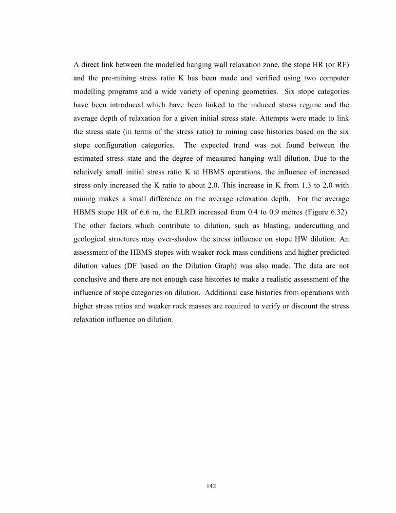
142
A direct link between the modelled hanging wall relaxation zone, the stope HR (or RF)
and the pre-mining stress ratio K has been made and verified using two computer
modelling programs and a wide variety of opening geometries. Six stope categories
have been introduced which have been linked to the induced stress regime and the
average depth of relaxation for a given initial stress state. Attempts were made to link
the stress state (in terms of the stress ratio) to mining case histories based on the six
stope configuration categories. The expected trend was not found between the
estimated stress state and the degree of measured hanging wall dilution. Due to the
relatively small initial stress ratio K at HBMS operations, the influence of increased
stress only increased the K ratio to about 2.0. This increase in K from 1.3 to 2.0 with
mining makes a small difference on the average relaxation depth. For the average
HBMS stope HR of 6.6 m, the ELRD increased from 0.4 to 0.9 metres (Figure 6.32).
The other factors which contribute to dilution, such as blasting, undercutting and
geological structures may over-shadow the stress influence on stope HW dilution. An
assessment of the HBMS stopes with weaker rock mass conditions and higher predicted
dilution values (DF based on the Dilution Graph) was also made. The data are not
conclusive and there are not enough case histories to make a realistic assessment of the
influence of stope categories on dilution. Additional case histories from operations with
higher stress ratios and weaker rock masses are required to verify or discount the stress
relaxation influence on dilution.

143
CHAPTER 7
INFLUENCE OF UNDERCUTTING ON STOPE STABILITY AND DILUTION
7.1 Introduction
Undercutting the stope hanging wall (HW) on both the overcut and undercut
development drifts are well recognized factors which contribute to hanging wall
instability and dilution (Wang et al., 2002; Yao et al., 1999; Suorineni et al., 1999;
Suorineni, 1998). Undercutting occurs when the drifts that are driven for stope
development extend past the desired mining limit. Development drifts are commonly
located at stope sub-levels or on the overcut and undercut levels of a stope. The HBMS
database does not include stopes developed with sub-levels so only undercutting of the
hanging wall on the overcut and undercut drifts are considered. Undercutting may or
may not occur along the total stope strike length. Where it does occur, the degree of
undercutting may vary.
Observations and case history studies show that undercutting on both overcut and
undercut drifts has a similar influence on overall dilution. Yao et al. (1999) state
“Cutting into the hanging wall with production development can be a major cause of
instability. Undercutting can occur during development of the overcuts/undercuts
and/or by upward caving of previously mined stopes that have had hanging wall
slough.”
Many factors can cause an open stope hanging wall to be undercut. These factors
include: drift location design errors caused by incorrect geological ore definition,
changes in ore contact orientation or ore width, drift development errors, drill equipment

144
space requirements, and undercutting by underlying stope caving. The HBMS database
shows that approximately 74% of stopes (111 cases out of 150) have a degree of
undercutting. Of these cases, approximately half of them have an average undercutting
depth of 1 to 2 metres. Figure 7.1 shows undercutting information for the HBMS
database. Undercutting depth is defined by the distance the drifts cut into the stope
hanging wall past the ore contact, as shown in Figure 7.2. The database shows that
undercutting of the stope hanging wall is a very common problem for open stope
mining.
Figure 7.1. Percentage of undercutting (UC) and the undercutting depth from theHBMS database
No UC 26%
UC Cases74%
39 Cases
111 Cases
UC 0.5~1.0m
26%UC 1.0~2.0m
43%
UC >2.0m5% UC < 0.5m
26%
29 Cases
47 Cases
29 Cases
6 C
ases
UC74%
No UC26%

145
Undercut Drift
Overcut Drift
StopeFootwall
Hanging Wall
Unstable Zone
.Undercutting depth in undercut drift
Undercutting depth in overcut drift.
Figure 7.2. Schematic illustration of instability caused by undercutting
Undercutting the stope hanging wall has the following effect on a hanging wall rock
mass:
• An additional free face is developed with the creation of the undercut
• Confinement of the immediate hanging wall is reduced which allows a jointed
rock mass to “loosen up”
• The beam created by the immediate hanging wall is broken
• There is an increased zone of relaxation associated with hanging wall
undercutting
These factors can be summarized into two main categories.

146
1. Reduction of immediate hanging wall confinement and support due to removal of
the hanging wall abutment and
2. Increasing the zone of stress relaxation in the hanging wall by changing the stope
geometry.
In many mines, the major discontinuities in the HW rock mass consist of foliation or
bedding planes orientated parallel to the HW contact. This is true for the HBMS
database. Undercutting the hanging wall breaks the integrity of the “beam” that may
form along continuous foliation or bedding planes parallel to the stope HW contact.
This reduces the stope HW stability. Undercutting the stope HW removes the support
and “hangs” the jointed rock mass for the portion of HW being undercut. The dead
weight of wedges and blocks formed by joints and foliation may fall due to gravity in
the undercut area (Figure 7.2). Undercutting also influences the zone of relaxation in
the HW and this is discussed in Section 7.3.
7.2 Quantifying Hanging Wall Undercutting
In order to try and account for the undercutting influence on stope HW stability and
dilution, an undercutting influence factor (UF) has been developed as part of this
research. The first step is to quantify the contributing geometry factors.
Undercutting of the hanging wall can occur on both the overcut and undercut drifts and
has a similar influence on the overall dilution. Undercutting may not occur along the
total stope strike length and where it does occur, the degree of undercutting may vary.
As the total stope up dip height (H) increases, the overall influence of undercutting in
the drifts decreases. An equation has been proposed to account for the influence of
these contributing geometry factors. The term quantifying the degree of undercutting is
called the undercut factor (UF). It is proposed that an undercutting factor should be
dependent on the following terms
1. The average depth of undercutting

147
2)dd( uo +
(7.1)
where, do = Average depth of undercutting along the overcut drift length lo (m)
du = Average depth of undercutting along the undercut drift length lu (m)
2. The fraction of the stope strike length where undercutting occurs and the distance
between the undercut and overcut drifts. This can be expressed as the length
where undercutting occurs divided by the stope perimeter or total abutment
length.
)HL(ll uo
++
2(7.2)
where, lo = Drift length where undercutting occurs on the overcut drift (m)
lu = Drift length where undercutting occurs on the undercut drift (m)
L = Stope strike length (m)
H = Stope height (up dip height, this reflects the true stope dimension) (m)
These factors which contribute to the influence of hanging wall undercutting are shown
in Figure 7.3. The UF is expressed as:
2)(
)(2uouo dd
HLll
UF+
×
++
= (7.3)
where, UF = Undercutting Factor (m), note: 2(L+H) = Stope perimeter
Figure 7.3 shows the geometric parameters that contribute to the undercutting factor.
This simplification was used for ease of application. It assesses a similar length of
undercutting on both the overcut and undercut drifts. If a significant difference exist, the
overcut and undercut should be assessed independently.

148
H
StopeHanging wall
Footwall
Stope
Ore
Ore
Overcut Drift
Undercut Drift
L (lu)
du
do
lo
Figure 7.3. Stope isometric showing the undercutting parameters
Figure 7.4 shows the distribution of the calculated UF values for the HBMS database.
The majority of the stopes are in the range of UF values between 0 and 0.4.
7.3 Interaction of Undercutting and Stress
Chapter 6 discussed the influence of stress on the volume of stope HW rock in
relaxation. The relaxation zone is dependent on the stress state prior to mining as well
as the shape of the stope. Undercutting a stope HW will also increase the volume of the
tensile or relaxation zone (Diederichs and Kaiser, 1999).
When drifts cut into a HW, the stope HW abutment location will be pushed back into
the HW. The total HW zone of relaxation, which is a zone of decreased stability, may
contribute to increased dilution (Figure 7.5).

149
39
67
27
12
40 1 0
0
10
20
30
40
50
60
70
80
0 0.2 0.4 0.6 0.8 1 1.2 More
UF
# of
Cas
es
0 0 0.2 0.4 0.6 0.8 1.0 1.2 More
Figure 7.4. Distribution of the calculated UF values for the HBMS database (150 cases)
Relaxation Zone without undercutting
Relaxation Zone with undercutting
Undercut Drift
Overcut Drift
FootwallHanging Wall
Stope
Figure 7.5. Schematic showing influence of undercutting on stope relaxation

150
Numerical modelling, using Examine 2D (Curran and Corkum, 1994) on a 40 metre
exposure height with a width of 5 metres, shows the difference between the case without
undercutting (Figure 7.6) and the case with 5 metres of undercutting on both of the stope
top and bottom (Figure 7.7). Comparison of the stress distributions in the two figures
shows an increase in the relaxation zone with undercutting (Figure 7.7), resulting in a
larger zone of potential instability or dilution.
3D numerical modelling was conducted to quantify the effect of undercutting on the
extent of the stope HW relaxation zone. The modelling was conducted on a 40 x 30 x
5m vertical stope as shown in Figure 7.8. The 3D boundary element program, Examine
3D, was used (Curran and Corkum, 1993).
Figure 7.6. Stress relaxation zone (shaded) around a stope with no undercutting

151
Figure 7.7. Stress relaxation zone (shaded) around a stope with 5 metres of undercutting
40 m
30 m
5 m (Stope width)
K =
1 m
1 m2m3m
2m
3m
Sto
pe h
eigh
t
Strike length
σ3
σ2σ1
σ1
σ3
Figure 7.8. Effect of undercutting on stress relaxation modelling model

152
The undercutting geometry factor, UF, was calculated by substituting the stope HW and
undercutting geometries, lo = lu = L = 30 m, H = 40m, and 2
)( uo dd + = 1, 1.5, 2, 3 m
respectively, into equation 7.3. The calculated UF values are shown in Table 7.1.
Table 7.1. Calculated UF for test case Examine 3D model stope
do (m) du (m) (do+du)/2 UF
1.0 1.0 1.0 0.4
1.0 2.0 1.5 0.6
2.0 2.0 2.0 0.9
3.0 3.0 3.0 1.3
Computer models were run showing combinations of 0, 1, 2 and 3 metres of
undercutting on both the overcut and undercut drifts (Figure 7.8). The undercutting into
the hanging wall was set at a constant depth for the total stope strike length. However,
the degree of undercutting was varied between the undercut and overcut drifts. The
zone of relaxation was quantified as the zone of rock with a modelled confining stress,
σ3, of zero or less. The relaxation zone was expressed as a depth of relaxation averaged
over the hanging wall surface or ELRD (Equivalent Linear Relaxation Depth). Three
initial or original stress regimes were modelled: K=1.5, 2.0 and 2.5. The maximum
stress direction was set perpendicular to the stope HW. The ELRDs due to undercutting
(ELRDuc) were calculated by subtracting the ELRD with undercutting from the ELRD
without undercutting for each case modelled.
Figures 7.9, 7.10 and 7.11 show the modelled σ3 stress distribution plots for a stress
ratio of K = 2. Figure 7.9 shows the model without undercutting. The average depth of
stress relaxation (ELRD) in the stope HW is approximately 1.8 m. Figure 7.10 shows
the σ3 stress distribution for 1m and 2m of undercutting in the overcut and undercut
drifts, respectively (with an average undercutting depth of 1.5m). For this geometry, the
ELRD is approximately 2.5m. There is about a 0.7m ELRD increase due to undercutting

153
Figu
re 7
.9.
Exam
ine
3D σ
3 plo
t for
the
stop
e ge
omet
ry w
ithou
t und
ercu
tting
with
K =
2
HW
FW
153

154
Figu
re 7
.10.
Exa
min
e 3D
σ3 p
lot f
or th
e st
ope
geom
etry
with
1.5
m a
vera
ge u
nder
cutti
ng w
ith K
= 2
HW
FW
154

155
Figu
re 7
.11.
Exa
min
e 3D
σ3 p
lot f
or th
e st
ope
geom
etry
with
3m
ave
rage
und
ercu
tting
with
K =
2
HW
FW
155

156
of the stope HW. Figure 7.11 shows the model with a depth of 3m of undercutting in
both overcut and undercut drifts. This geometry shows 2.9m of ELRD, which presents a
1.1m of ELRD increase compared to the case with no undercutting.
Table 7.2 summarizes the results of this modelling. Figure 7.12 shows the ELRD for
undercutting factors (UF) from 0.0 to 1.3 metres, for various stress ratios. Figure 7.13
shows the component of relaxation due to the undercutting (ELRDUC) for the same
geometries and stress conditions.
The modelling results showed that the ELRD due to undercutting the stope HW
(ELRDuc) has a linear relationship with the average depth of undercutting in the overcut
and undercut drifts for a constant stope height. With an increase in the average depth of
undercutting, the ELRDuc increases. The stress state (in terms of the stress ratio) has a
significant influence on this linear relationship. A higher stress ratio results in a higher
ELRDuc for a given average depth of undercutting.
This modelling test case shows the importance of undercutting on the hanging wall zone
of relaxation. As well as increasing the hanging wall zone of relaxation, undercutting the
hanging wall removes the abutment support and increased the probability of failure due
to gravity loading. The next section discusses these combined undercutting influences
on hanging wall dilution.
Table 7.2. ELRDuc results for test case Examine 3D model stope
ELRD
K=1.5 K=2.0 K=2.5u/c*depthin oc*drift(m)
u/c*depthin uc*drift(m)
Avg.
depth of
u/c* (m)TotalELRD
(m)
ELRDuc (m)
TotalELRD
(m)
ELRDuc(m)
TotalELRD
(m)
ELRDuc(m)
0.0 0.0 0.0 0.8 0.0 1.8 0.0 3.2 0.01.0 1.0 1.0 0.9 0.1 2.3 0.5 4.0 0.81.0 2.0 1.5 1.0 0.2 2.5 0.7 4.3 1.12.0 2.0 2.0 1.1 0.3 2.7 0.9 4.8 1.63.0 3.0 3.0 1.2 0.4 2.9 1.1 5.2 2.0
* oc =overcut, uc = undercut, u/c =undercutting

157
Figure 7.12. Example plots of ELRD versus average depth of undercutting (for a40x30x5 m stope)
Figure 7.13. Example plots of additional ELRD due to undercudepth of undercutting (for a 40x30x5m stope)
0
0.8
1.1
1.6
2
0
0.50.7
0.91.1
0 0.1 0.2 0.3 0.4
0.0
0.5
1.0
1.5
2.0
2.5
0.0 0.5 1.0 1.5 2.0 2.5 3.0 3.5 Avg. undercutting depth (m)
ELR
Duc
(m)
K=2.5
K=2.0
K=1.5
UF ( geometry only) 0.0 0.4 0.6 0.9 1.3 ( )
)
m,m
t
(m
ting versus average

158
7.4 General Interaction of Undercutting on Stability and Dilution
Undercutting the hanging wall decreases stability by increasing the zone of relaxation as
well as by reducing abutment support. The loss of abutment support will not extend past
the depth of undercutting, as shown in Figure 7.14. The additional relaxation due to
undercutting may extend well past the area of lost abutment support for high K ratios.
For low values of the K stress ratio, the additional zone of relaxation caused by the
undercut may be entirely within the zone of lost abutment support (Figure 7.14). For this
reason, the influence of undercutting will be considered as two factors with the ELRDUC
representing the influence of the increased zone of relaxation. The UF term, which is
based on the average depth of undercutting and the total distance along which
undercutting occurs, should be related to the increased dilution due to the loss of
abutment support.
Relaxation Zone without undercutting
Relaxation Zone with undercutting
Undercut Drift
Overcut Drift
Footwall
Hanging Wall
Stope
Additional Relaxation Zone due to undercutting
Possible unstable zone due to undercutting geometry
Figure 7.14. Schematic cross section showing the zones of undercutting influence

159
The overall competence of the HW rock mass also plays an important role on the
influence of undercutting on stope HW stability. With increasing rock mass quality, the
influence of undercutting on the stope HW stability decreases. The stability of a stope
HW is closely related to the HW rock mass strength, joint frequency and joint condition
as well as the dip of the stope HW. The modified stability number N’ accounts for both
rock mass quality and stope HW dip. Therefore N’ should be included in the influence
of the undercutting factor.
7.5 Case History Assessment
It is not easy to accurately determine the influence of undercutting on hanging wall
stability and a purely empirical approach is taken. The database for Trout Lake and
Callinan Mines has been analyzed and the dilution factor has been determined for each
stope. The equation developed (Eq. 7.3) was used to calculate the undercutting factor
UF for these two mines’ case histories. The two components of undercutting, relaxation
and abutment loss, are assessed separately.
7.5.1 Stress Influence
Figure 7.13 shows the additional ELRD that can be expected due to undercutting for a
typical HBMS stope geometry with a HR about 8.6 m. Figure 7.15 shows the additional
ELRD due to undercutting that can be expected for the 6 stope stress categories. The
fact that UF values less than 0.4 metres (Figure 7.4) were calculated for the majority of
stopes for the HBMS database indicates that the majority of ELRDuc values will be well
under 0.5 metres (Figure 7.15). An estimate can be made for the total average depth of
relaxation by adding the ELRDuc from Figure 7.15 and the ELRD from Figure 6.32. The
ELRDuc is only an estimate based on a typical HBMS stope geometry. However, since
75% of the HBMS case histories have HR values between 6.0 to 9.0 metres, the ELRDuc
correction should be reasonable. Figure 7.16 shows a graph of the combined ELRDtotal
versus the actual dilution minus the dilution factor. There is no apparent trend relating
the total depth of relaxation to additional dilution (prediction error). This is perhaps due

160
Figure 7.15. Additional ELRD due to undercutting that can be expected for the 6 stopestress categories (for a typical HBMS stope geometry with a HR of 8.6m)
Figure 7.16. ELRDtotal versus the actual dilution minus the dilution factor case historyplots (88 cases)
0.0 0.5 1.0 1.5 2.0 2.5 3.0 3.5
0.0 0.4 0.6 0.9 1.3
0.0
0.5
1.0
1.5
UF (m)
Avg. undercuttingdepth (m)
K=1.3 (category 1)K=1.4 (category 2)K=1.5 (category 3)K=1.6 (category 4)K=1.7 (category 5)
K=2.0 (category 6)E
LRD
uc (m
)
-2
-1
0
1
2
3
4
0 0.2 0.4 0.6 0.8 1 1.2 1.4
ELRD_total (m)
ELO
S_a
ct. -
DF
(m)

161
to the low initial stress state and relatively competent nature of the hanging wall rocks.
Figure 7.17 shows the same data for the case histories where N’ is less than 10 (29
cases). No significant trend was found. Other contributing factors may overshadow the
stress influence.
7.5.2 Abutment Loss Influence
The actual recorded stope dilution (ELOSact.) minus the dilution factor (DF) has been
plotted versus the calculated undercutting factor (UF) and is shown in Figure 7.18.
There is a wide variation in the individual stope cases. However, Figure 7.18 does show
a general trend of increasing average unpredicted dilution with an increasing
undercutting factor. As discussed in Section 7.4, the influence of undercutting increases
as rock mass quality decrease and the UF/N’ can be used to quantify this combined
R2 = 0.1189
-2
-1
0
1
2
3
4
0 0.2 0.4 0.6 0.8 1 1.2
ELRD_total (m)
ELO
S_a
ct. -
DF
(m)
Figure 7.17. ELRDtotal versus the actual dilution minus the dilution factor case historyplots for the cases with N’ < 10 (29 cases)

162
Figure 7.18. Comparison between UF and dilution in excess of predicted values
Figure 7.19. UF versus average dilution in excess of predicted values
y = 1.2779x + 0.2282R2 = 0.0714
-2.0
-1.0
0.0
1.0
2.0
3.0
4.0
5.0
6.0
0.0 0.2 0.4 0.6 0.8 1.0 1.2
Undercutting Factor, UF
ELO
S_ac
t. - D
F (m
)
0.0
0.2
0.4
0.6
0.8
1.0
1.2
1.4
>0-0.1 0.1-0.2 0.2-0.4 >0.4
Undercutting Factor (UF)
ELO
S_a
ct.-p
red.
(m
)
45 Cases
28 cases
37 Cases
10 Cases
ELR
D_a
ct. -
DF
(m)
ELO
S

163
influence. The UF/N’ versus ELOS prediction error plot (Figure 7.20) also shows a
similar weak trend. The absence of trends suggests that other factors may overshadow
much of the influence of undercutting on dilution.
7.5.3 Case History Example
The 900 M3-3 stope of Trout Lake Mine case history gives some evidence of the effect
of undercutting on stope HW slough. The 900 M3-3 stope is located in the Middle Zone
orebody of Trout Lake Mine. The stope has a strike length of 23m, exposed height of
34m, and ore width of 5.2m. The stope HW contact dips at 67o. Both overcut and
undercut drifts partially undercut the HW. Figure 7.21 is the plan view of the stope drift
layouts. The shaded areas are the undercut areas outside the ore contact. The blastholes
within the orebody were drilled from the overcut drift down to the undercut drift.
Figure 7.20. UF/N’ versus ELOS prediction e
y = 11.533x + 0.3373R2 = 0.0248
-2.0
-1.0
0.0
1.0
2.0
3.0
4.0
5.0
6.0
0 0.01 0.02 0.03 0.04 0.05 0.06 0.07 0.08
'
ELO
S_a
ct. -
DF
(m)
’
UIF/NUF/Nrror case history plot

164
Figure 7.21. Plan view of stope drift layout and undercutting (shaded areas)
The plan view shows a gradual increase in undercut depth, on the undercut drift, from
line 6 to line 14. Figure 7.22 shows the cross sections of drill lines 7, 8 and 9. These
three typical sections show that the stope HW overbreak tends to extend to the outer
limits of the undercut drifts, to form an arched failure showing the importance of the
HW abutment support in the undercutting area.
Undercut Drift
Overcut drift

165
Figu
re 7
.22.
Dril
ling
cros
s sec
tion
show
ing
CM
S su
rvey
ed o
verb
reak
pro
files
and
und
ercu
tting
a). D
rill l
ine
7 cr
oss
sect
ion
b). D
rill l
ine
8 cr
oss
sect
ion
c). D
rill l
ine
9 cr
oss
sect
ion
Muc
k st
illin
sto p
eM
uck
still
in st
ope
165

166
7.6 Summary
The influence of undercutting on the stope HW stability and dilution was quantified by
analytical and numerical methods. Instability caused by undercutting on the stope HW
consists of two parts in general:
a). Jointed rock mass rock failure caused by removal of support due to
undercutting (abutment loss);
b). Increased zone of destressed or relaxed rock failure due to undercutting.
An equation has been developed to account for the undercutting geometry influence on
the stope HW stability and dilution (called undercutting factor, UF). The UF is
proportional to the portion of stope HW being undercut and the average depth of
undercutting. Attempts have been made to account for the rock mass condition and
stress on the undercutting influence. The UF term has an influence on the zone of
relaxation. Increased HW ELRD due to undercutting occurs for highly deviatoric stress
conditions with σ1 perpendicular to the HW. The influence of undercutting on stope
HW ELOS ELRDUC can be added to the ELRD estimated based on the overall hanging
wall geometry (HR or RF) and stress state (Figure 7.5 and 7.14)
The proposed relationships were examined with the existing database and comparisons
were conducted with the prediction error (ELOSAct. – DF). No obvious trend of
increasing unpredicted dilution (average) with an increasing undercutting factor or with
UF/N’ can be discovered. The influence of the ELRD & ELRDuc was not apparent
with the HBMS database, perhaps due to the low initial K ratio.

167
CHAPTER 8
INFLUENCE OF BLASTING ON STOPE HANGING WALL STABILITY AND
DILUTION
8.1 Introduction
The drilling, blasting and mucking cycle is the most commonly used method for
obtaining ore in open stope mining. Blasting of the ore is conducted to sufficiently
destroy the structural integrity of the rock mass to allow mechanical mucking and
transport. A good blast design results in the ore breaking into easily handled fragments
with a uniform block size distribution. Unbroken ore left in the stope results in lost
revenue and the creation of large blocks create handling problems which may require
secondary blasting and create costly delays. These goals for a good blast lead the blast
engineer to design a blast which can sufficiently fragment the ore within the design line,
but minimises the blast damage to adjacent waste rock to reduce ore dilution. These
conflicting general goals for good blasting create much of the driving force for blasting
research.
An ideal blast creates easily handled fragments of ore, leaves no unbroken ore behind in
the stope and does no damage to the waste rock past the ore contact. All these goals
cannot be met and some degree of hanging wall damage results after a blast. Hanging
wall blast damage acts to loosen the rock mass and induce new fractures. Blast damage
can degrade the rock mass quality and this can result in hanging wall instability in the
form of increased hanging wall slough and dilution.

168
This chapter reviews some blasting theory, describes the parameters which have been
collected in the data base and looks at their theoretical and actual influence on hanging
wall dilution.
8.2 Blasting Background
The technique of rock breakage using explosives involves drilling blastholes, loading
the blastholes with explosive and then sequentially detonating the explosive in each
hole. Before discussing the influence of blasting damage on the stope HW, it is
necessary to have a general understanding of the mechanism of rock blasting.
In a rock blast, there are at least eight rock breakage mechanisms that have been
identified (Hagan, 1967 & 1973; Mercer, 1980; Carlos et al., 1995). They are:
• Crushing of rock
• Relative radial motion
• Release of load
• Reflection breakage or spalling
• Gas extension of strain wave-generated and /or natural cracks
• Flexural rupture
• Shear fracturing along natural and strain wave generated cracks
• In-flight collisions.
The following descriptions of rock blast mechanisms are based on Mercer (1980). When
an explosive detonates, the ingredients of the explosive are rapidly converted into
gaseous products at very high temperatures and pressures. The gases, usually exceeding
about 18,000 atmospheres, impact the blast hole wall and transmit a shock wave or
shock strain, which travels at a speed of 2000 - 6000 metres per second, into the
surrounding rock as shown in Figure 8.1 (Hagan, 1967). Crushing occurs around a
blasthole wall when the pressure of the detonation front exceeds the dynamic
compressive strength of the rock (Hagan, 1967; Bauer, 1978). The out-going strain
wave (strain pulse) generated by the high-pressure detonation front disperses and loses

169
First Radical Cracks
Shattered Rock
Strain Wave Positions With Time
Free
Fac
e
4
12 3
5
Figure 8.1. First stage of explosive /rock interaction (after Mercer, 1980)
energy rapidly. Crushing ceases when the strain level in the pulse drops below the
elastic limit of the rock. The rock directly outside the crushing zone is subject to very
sudden compression due to the dispersing strain pulse. This radial compression results
in tangential tensile stresses, which can cause cracks to develop radically from the
blasthole. Fractures occur immediately after the strain or compression pulse passes due
to the release of compressive loading.
During and after the stress wave propagation, high-pressure explosion gases penetrate
the available fractures, which include natural fractures and the fractures developed by
shock waves, and wedge them open as shown in Figure 8.2 (Mercer, 1980). This leads
to an increase in the volume and permeability of the rock mass and a subsequent
reduction in the pressure of the explosion gases. The opening of fractures and the
creation of new fractures effectively reduce the rock mass strength.

170
When the stress/strain waves reach a free face, an imbalance of forces occurs. This will
cause the burden rock to move. Burden rock is defined as the rock between the blast
hole and the open excavation, or free face, as shown in Figure 8.1.
Eventually the gases dissipate through the fracture network or are released to the
atmosphere. The confining pressure then rapidly drops and rock movement reduces
until the driving force is consumed.
Stope blast layout and design is generally conducted by mine engineers and technicians
and is strongly based on past experience. Blast design can vary significantly between
mines based on the individual experience and preferences of the operators. Many
factors influence the performance of a blast and the degree of blast damage that can
result. Not all of these factors are measured at mines. These contributing factors
include rock mass quality, blast design, blasthole diameter and length, drillhole layout,
Detached, broken mass moves forwardUnloading, the rock breaks under tension
Expanded Borehole
Original Borehole
Free
Fa c
e
Figure 8.2. Later stages of explosive/rock interaction (after Mercer, 1980)

171
drilling accuracy, explosive distribution, initiation sequence and wall control technique
etc.. The next section discusses methods of assessing blast damage, which is difficult to
both quantify and determine a cause for.
8.3 Methods of Assessing Blast Damage
There are no consistent methods to measure and quantify blast induced damage (Yang
et al., 1993). Joint mapping before and after blasting can sometimes highlight damage
to the rock mass induced by blasting. This approach is highly subjective and cannot be
used in this study because of the lack of access after blasting. The measurement of peak
particle velocity (PPV) induced by blasting has been used as a measurement of blast
damage. This approach is discussed in this chapter. It cannot be used in this study
because these measurements have not been consistently recorded at the mine. The Hoek
and Brown failure criterion, discussed in Section 2.2.1, has been used to assess the
failure criteria for undisturbed and disturbed rock masses. The disturbed and
undisturbed description can be applied to blast damaged and undamaged rock masses.
This approach does not give an indication of the degree of blast damage, but does give a
suggested limit to the influence of blast damage. After the blast, an indication of the
degree of blast damage can be obtained from CMS surveys or visual inspection of the
walls of the excavation created. Instability may be an indication of blast damage. The
problem is determining if the failure is caused by blasting or other factors such as a
weak rock mass.
8.3.1 Peak Particle Velocity Method
Peak particle velocity has been used for the measurement of blast damage to structures
and to rock masses. The fragmentation of rock by detonation of an explosive charge
depends on the effects of both strain induced in the rock and upon the gas pressure
generation of the explosive. The particle velocity is a measure of the velocity during the
passage of the vibration wave, not the velocity of the wave itself. Many empirical
relationships between blast geometries and vibration velocities have been developed.

172
Most of them relate the PPV to the explosive charge and the distance from the charge.
Holmberg and Persson (1980) suggested the following empirical equation for estimation
of PPV:
β
α
RwkPPV = (8.1)
where PPV is the Peak Particle Velocity in mm/sec.,
w is the charge weight per single blast in kg.,
R is the radial distance from the point of detonation in metres,
k, α and β are constants which depend upon the structure and elastic properties
of the rock mass, which vary from site to site.
The constants k, α and β are site specific. The constants k, α and β must be determined
for each site in order to apply equation 8.1 to estimate the PPV. This can be done by
carrying out a series of trial blasts and monitoring the induced particle velocities at
different distances from these blasts. Once the PPV has been estimated, the blast
damage thresholds of PPV can be applied to estimate the blast damage. Hagan (1996)
reported a list of Peak Particle Velocity threshold damage levels as shown in Table 8.1.
Table 8.1. Peak Particle Velocity threshold damage levels (from Hagan, 1996)
PPV (mm/sec.) Damage Level
50 Limit below which risk of damage to structure is very slight
230 Cracks in concrete blocks
300 Rock falls in unlined tunnel
635 Onset of cracking in rock
2500 Breakage of rock
Two problems exist for trying to use this approach. The site specific constants k, α and
β are not available for the HBMS rock mass. Also, there is no way to link the damage
level shown in Table 8.1 with the expected hanging wall damage or an increase in

173
dilution. This may be a valid approach for trying to link blast damage and hanging wall
dilution. An extensive test program would be required which is beyond the scope of this
study.
8.3.2 Blast Damage Consideration in the Hoek and Brown Failure Criterion
Hoek and Brown (1980) developed a rock mass failure criterion to assess the stability of
a rock mass, as discussed in Section 2.2.1. The Hoek and Brown failure criterion is
expressed as:
2331 cc sm σσσσσ ++= (8.2)
where σ1 is the major principal stress at failure,
σ3 is the minor applied principal stress,
σc is the uniaxial compressive strength of the intact rock,
m and s are constants which depend upon the properties of the rock
The constants m and s have been linked to the rock type and the rock mass classification
values. Two sets of values for m and s were introduced to account for blast damage and
the two sets of values refer to an undisturbed rock mass and a disturbed rock mass
(Hoek and Brown, 1988) as shown in Table 8.2. The drop in the m and s value for a
given rock mass condition can be equated to a drop in the rock classification value
caused by blasting as shown in the following equation (Milne et al., 1998).
)RMR.(RMRRMR DisturbedDisturbeddUndisturbe 5050 −+= (8.3)
The equation can be solved for RMRDisturbed with RMRUndisturbed as the initial rock mass
classification assessment. An approximated correlation between RMR and Q is
(Bieniawski, 1979 and 1993):

174
RMR = 9lnQ + 44 (8.4)
For the average rock classification values for Trout Lake Mine of Q’ = 6 (disturbed), the
undisturbed Q’ of 55 before blast damage can be calculated by using equations 8.3 and
8.4. This indicates a Q’ reduction of 49 can be caused by blast damage. This reduction
in Q’ would correspond to an increase in the average dilution prediction (based on the
dilution graph, Figure 2.16) from about 0.1 metres to 1 metre for the HBMS mines’
average stope HW dip and HR values. This is an interesting approach for looking at the
effect of blasting on dilution. The approach is not substantiated by empirical data and
cannot consider the degree of blast damage or the effect of changing blasting practice
and only gives an indication of a possible role of blast damage on increasing hanging
wall dilution.
8.3.3 Visual Inspection and CMS Survey Methods
Visual inspections or CMS survey data can provide useful information on the blast
damage on opening walls by observing or measuring the wall profile. Slough or failure
off the stope walls is readily measured with a CMS and the degree of slough may be an
indication of blast damage. The problem with this approach is the difficulty in
distinguishing between stress or structurally controlled instability and the instability
caused by blast damage. This research attempts to estimate blast induced damage to the
hanging wall by assessing the large number of case histories in the HBMS database.
8.4 Factors Influencing HW Blast Damage and Dilution
The previous section discussed possible methods of measuring blast damage after it has
occurred. From an operational point of view, a method of predicting blast damage
based on the method of blasting and current ground conditions is needed. There are
many blasting procedures that the operator can vary. Their influence on blast damage is
hard to quantify. Some of the main factors include:

175
Table 8.2. Hoek and Brown failure criterion m and s constants values (Hoek & Brown,1988)
Approximate relationship between rock mass quality and material constants
Disturbed rock mass m & s values Undisturbed rock mass m & s values
Empirical Failure Criterion
2331 cc sm σσσσσ ++=
σ1 = major principal stressσ3 = minor principal stressσc = uniaxial compressive strength of intactrock, andm & s are empirical constants
Car
bona
te R
ocks
With
Wel
l Dev
elop
edC
ryst
al C
leav
age
dol
omite
, lim
esto
nean
d m
arbl
e
Lith
ifiel
s Arg
illac
eous
Roc
ksm
udsto
ne, s
iltst
one,
shal
e an
d sla
te(n
orm
al to
cle
avag
e)
Are
nace
ous R
ocks
With
Str
ong
Cry
stal
s and
Poo
rly
Dev
elop
ed C
ryst
alcl
eava
geSa
ndsto
ne a
nd q
uartz
ite
Fine
Gra
ined
Pol
ymin
eral
lic Ig
neou
sC
ysta
lline
Roc
ksA
ndes
ite, d
oler
ite a
nd rh
ylite
Coa
rse
Gra
ined
Plly
min
eral
lic Ig
neou
san
d M
etam
orph
ic C
ryst
allin
e R
ocks
Am
phib
olite
, gab
bro,
gne
iss,
gran
ite,
norit
e an
d qu
artz
-dio
rite
Intact Rock SamplesLab .size specimens free from discontinuitiesCSIR rating: RMR = 100NGI rating = 500
msms
7.001.007.001.00
10.001.0010.001.00
15.001.0015.001.00
17.001.0017.001.00
25.001.0025.001.00
Very Good Quality Rock MassTightly interlocking undisturbed rock with unweatheredjoints at 1 to 3 mCSIR rating : RMR = 85NGI rating = 100
msms
2.40.0824.10.189
3.430.0835.850.189
5.140.0828.780.189
5.820.0829.950.189
8.560.08214.630.189
Good Quality Rock MassFresh to slightly weathered rock. Slightly disturbedwith joints at 1 to 3 mCSIR rating: RMR = 65NGI rating = 10
msms
0.5750.002932.0060.0205
0.8210.002932.8650.0205
1.2310.002934.2980.0205
1.3950.002934.8710.0205
2.0520.002937.1630.0205
Fair Quality Rock MassSeveral sets of moderately weathered joints spaced at 0.3 to 1 mCISR rating: RMR = 44NGI rating = 1
msms
0.1280.000090.9470.00198
0.1830.000091.3530.00198
0.2750.00092.030.00198
0.3110.000092.3010.00198
0.4580.000093.3830.00198
Poor Quality Rock MassNumerous weathered joints at 30 -500mm, some gouge;clean compacted waste rockCSIR rating: RMR = 23NGI rating = 0.1
msms
0.0290.0000030.4470.00019
0.0410.0000030.6390.00019
0.0610.0000030.9590.00019
0.0690.0000031.0870.00019
0.1020.0000031.5980.00019
Very Poor Quality Rock MassNumerous heavily weathered joints spaced <50mmwith gouge. Waste rock with finesCSIR rating: RMR = 3NGI rating = 0.01
msms
0.0070.00000010.2190.00002
0.010.00000010.3130.00002
0.0150.00000010.4690.00002
0.0170.00000010.5320.00002
0.0250.00000010.7820.00002

176
• Rock mass properties
• Drillhole design (drillhole size, length, spacing, burden, and orientation)
• Drillhole accuracy (drillhole deviation)
• Explosive type
• Wall control methods
• Explosive distribution
• Explosive per delay
• Initiation sequence
• Availability of a free face
The influence of these factors is briefly discussed in the following sections.
8.4.1 Rock Mass Properties
The rock mass properties are of fundamental importance to the design of blasts. Rock
mass properties in a stope hanging wall will influence the effect of blasting practice on
dilution. A poorly designed blast may result in significant dilution and hanging wall
damage in a poor quality rock mass (low N or Q’ values). The same blasting practice
may not show up as dilution or instability in a good quality hanging wall. This
influence of rock mass condition is shown in equation 8.3, where the reduction in the
rock mass classification value due to blasting is less for good quality rock (high RMR
values). Initial rock mass properties need to be considered to assess the influence of
blasting practices on hanging wall dilution. The dynamic strength of the rock and the
rock joint characteristics are two important rock mass properties for blasting. The
strength of rocks is normally quite well correlated with their density (Carlos et al.,
1995). In general, low-density rocks are deformed and broken quite easily, requiring
relatively low energy factors, whereas dense rocks need a higher energy to achieve a
satisfactory fragmentation. Rocks generally have discontinuities (such as bedding
planes, planes of lamination or foliation, fractures and joints), which influence the
physical and mechanical properties of the rocks and, consequently, the blasting results.
Neglecting the rock mass properties when blasting will lead to either over blasting in

177
some areas or under blasting in other areas. Over blasting can cause damage to the
adjacent rock mass (e.g., stope walls in open stope mining), and under blasting can
result in the loss of economic ore. The expense of these deviations from expected
performance can be costly. In open stope mining, overbreak-caused wall damage is a
significant problem. Blast damage cannot only increase dilution, but also can cause
mine opening instability problems. Blasting performance is determined by the
interaction of the detonation of an explosive and the surrounding confining rock mass.
Rock mass properties strongly influence this process.
8.4.2 Drillhole Design
Drillhole design is also a major factor in blast design. The drillhole design governs the
distribution of explosive in the rock mass. In general, blast performance improves with
better explosive distribution. In theory, smaller more frequent holes improve the
explosive distribution. However, drilling more holes increases expense and the smaller
holes will increase the chance of drillhole deviation.
Drillhole design is related to the drill machine’s capabilities and the desired explosive
distribution. Drillhole design includes drillhole length, hole diameter, drillhole spacing
and burden. Drillhole length and diameter are closely related since long holes need to
be drilled with a larger diameter hole size to reduce hole wander or deviation. Spacing
is the distance between drillholes in the direction parallel to the available free surface,
and burden is the distance between drillholes in the direction perpendicular to the
available free surface (Figure 8.3). These parameters depend upon the drillhole
diameter, the properties of the rock and the explosives used, as well as the desired
degree of fragmentation. A larger hole diameter results in more explosive being loaded
per hole. To maintain a certain explosive consumption per tonne of rock being blasted,
larger hole diameters will require a larger spacing and burden. Too large a burden or
too large a hole spacing will cause underbreak of the ore leading to handling and
mucking problems. On the other hand, too small a burden will create fly rock and waste
explosive energy. Figure 8.3 illustrates the effect of burden change on the blast

178
Figu
re 8
.3. S
chem
atic
illu
stra
tion
of th
e ef
fect
of b
urde
n on
exp
losi
ves f
ired
in ro
ck (f
rom
Atla
s Pow
der C
ompa
ny, 1
987)
178

179
behaviour. The drillhole diameter, length, spacing and burden reflect the explosive
distribution. For the same hole length, a smaller drillhole size has a better explosive
distribution and less explosive concentration than larger drillholes. Smaller diameter
drillholes usually have more hole deviation compared to larger diameter drillholes. The
drillhole deviation will be discussed in detail in section 8.4.7.
8.4.3 Explosive Type
The type of explosive used forms an important part of blast design. The selection of
explosive type is usually based on the analysis of factors that include rock mass
characteristics, volume of rock to be blasted, presence of water, safety conditions,
supply problems as well as the cost of rock breakage. For underground open stope
mining, including HBMS mines, the most commonly used explosive is ANFO
(Ammonium Nitrate and Fuel Oil) due to its low cost and safety. ANFO has some
shortcomings which include poor water resistance and low density. Other explosives
also are used for special purposes, such as Dyno Split and low ANFO for wall control
and emulsion for wet conditions. Explosive type also effects HW stability and dilution.
High energy explosives (e.g., emulsion, Dyno Split) produce good fragmentation but
may cause damage to the stope HW. Low energy explosives (e.g., low ANFO) cause
less damage to the HW but more drilling metres are required to get satisfactory
fragmentation.
8.4.4 Wall Control Methods
Many wall control methods exist to avoid damage to the stope HW. A reasonable wall
control technique can create better blasting results and protect the adjacent structure
from damage. This is especially important for weak, heavily jointed or foliated stope
walls. The methods for wall control blasting can vary depending on the rock mass
condition and the operation’s preference. The general approach for wall control
blasting is to reduce the detonated explosive energy in the areas close to structures
which need to be protected from damage. There are many ways to reduce the

180
detonating explosive energy to the hanging wall. Using low energy explosives (e.g.,
low ANFO), traced small diameter explosive cartridges (e.g., Dyno split cartridge or
cartridged ANFO) or drilling smaller diameter drillholes with a closer spacing along the
HW contact are some of the options. Optimizing initiation sequence and reducing the
explosive per delay are other alternatives for reducing blast damage.
The cartridge or traced small diameter explosive cartridge (e.g., Dyno cartridge or Dyno
split traced cartridge) was the most frequently used methods for wall control blasting in
HBMS open stopes.
8.4.5 Explosive Distribution
The distribution of explosives within a blast influences both the rock fragmentation and
the degree of damage to the adjacent rock mass. The explosive distribution is controlled
by several drilling and blasting parameters. These parameters include drillhole size,
drillhole spacing and burden, charging geometry (e.g., charge length and location in a
drillhole and stemming parameters), and the drillhole accuracy (drillhole deviation).
Stemming is the portion of a blasthole which has been packed with inert material
(usually drill cuttings), above the explosive charge. Stemming is used to confine and
retain the gases produced by the explosion. A good explosive distribution tends to
create better ore fragmentation and often results in less hanging wall damage. A high
concentration of explosive energy can result in increased blast damage. Usually when
designing a blast, the drillhole burden and drillhole spacing are determined based on the
drillhole size. A larger hole size will result in a larger burden and spacing. As
described in section 8.4.2, for the same hole length, a smaller drillhole size has better
explosive distribution and less explosive concentration than larger drillholes. The
overall explosive distribution for a blast is usually expressed in terms of powder factor.
The powder factor (PF) is the average weight of explosive (in kilograms or pounds)
used to break each cubic metre of solid rock. The powder factor is not necessarily
related to overbreak or blast damage, it only indicates an average consumption of
explosive used to break a cubic metre of ore. The explosive contribution is controlled

181
by the drillhole size, drillhole spacing and burden as well as the explosive charging
geometry in holes. Drillhole deviation also can affect the explosive distribution.
Evenly distributing the available explosive within the whole planned stope is expected.
However, hole deviation can significantly alter the expected explosive distribution.
8.4.6 Initiation Sequence, Explosive Per Delay and Availability of Free Surface
Initiation sequence, explosive per delay and available free surface are other important
blasting aspects, which can significantly affect blasting results. The outcome of a multi-
hole production blast is very dependent on interactions between blastholes (Hagan,
1996). The sequence in which blastholes are initiated and the time interval between
successive detonations has a major influence on overall blast performance. The
performance of a production blast can only be optimised when charges detonate in a
controlled sequence at suitable discrete but closely spaced time intervals. The initiation
sequence should make use of the available free surface to maximize the use of explosive
energy and minimize the damage to stope walls. Explosive per delay shows the weight
of explosive being initiated at the same time. The explosive per delay is the single most
important factor which indicates the shock and heave energy from a single delay blast.
The bigger the explosive per delay the greater the damage. An optimized initiation
sequence can fully use the available free surface and detonating explosive energy to
create desired fragmentation with minimal surrounding damage.
8.4.7 Drillhole Deviation
Drillhole deviation is normally defined as the distance between the actual and planned
toe location of blast holes, divided by the hole length:
100holeplannedtheoflengthTrue
toehole planned and actualthebetweenDistance(%)deviation Hole ×= (8.5)

182
Drillhole deviation can be a result of many factors. These include the inaccurate
placement of drill reference marks, incorrect drill set-up (collaring and alignment errors,
which can be due to human error or equipment limitations), inconsistent drill operation,
and geological structure. Both the trend and plunge of boreholes can deviate. There are
two ways the drillholes can deviate along stope height (dip). The drillholes can deviate
toward the stope HW or away from the stope HW (Figure 8.4). Drillhole deviation can
also cause the loading of explosives away from designed locations (Figure 8.5) causing
undesired explosive concentrations in some areas and a lack of explosive in other areas.
An explosive concentration will cause excessive energy in some areas which can result
in damage to adjacent structures, and lack of explosive in other area will cause larger
fragmentation or underbreak. In general, drillhole deviation often results in poor blasts
and can result in blast damage and increased dilution. When explosives are loaded into
holes which deviate into the stope hanging walls, significant damage is done to the
hanging walls (Figure 8.4).
Figure 8.4. Cross section showing the drillhole deviation orientations
Hanging wall
Footwall
O/C drift
U/C drift
Stope
HW overbreak dueto drillholedeviation

183
Figure 8.5. Plan view showing surveyed drillhole deviation along strike (Trout LakeMine, HBMS, 2000)
Magnetometer drillhole deviation survey data shows that hole deviation at HBMS mines
is an average of 7% of the drillhole length at the toe of surveyed holes, giving an
average toe deviation of 2.1metres (30m stope average height). A study from the
Noranda Technology Centre also shows that most of their surveyed holes have a
deviation range from 0% to an occasional 20% of the hole length at the toe (Piché et al.,
2000). Borehole deviation has not been measured frequently at HBMS operations and
cannot be used in the database as a direct measure of possible causes of dilution.
8.5 Database Assessment of Blasting Parameters and Dilution
The HBMS database includes several parameters important to blast performance which
were introduced in Section 4.2.5. These parameters include drillhole size, drillhole

184
pattern and powder factor. The drillhole size and powder factor were found to show no
correlation with observed dilution or with the predicted minus observed dilution
(Figures 8.6 to 8.9).
8.5.1 Drillhole Pattern versus Stope HW Dilution
Different drillhole patterns are used at HBMS operations. The drillhole patterns in this
study are defined as:
a). Parallel drillhole pattern - hole patterns where the holes close to the stope
HW on cross section, are parallel or near parallel to the HW;
b). Fanned drillhole patterns – hole patterns where the holes close to the stope
HW on cross section are angled toward the HW contact.
Figure 8.6. Drillhole size versus actual ELOS case history plots
0
0.5
1
1.5
2
2.5
3
3.5
4
4.5
1 1.5 2 2.5 3 3.5 4 4.5 5
Drillhole size (inch)
ELO
S_a
ct.
(m)

185
Figure 8.7. Drillhole size versus actual ELOS minus DF case history plots
Figure 8.8. Powder factor versus actual ELOS case history plots
-2
-1
0
1
2
3
4
1 1.5 2 2.5 3 3.5 4 4.5 5
Drillhole size (inch)
ELO
S_a
ct. -
DF
(m)
0
0.5
1
1.5
2
2.5
3
3.5
4
4.5
0 0.5 1 1.5 2 2.5 3
Powder Factor, PF (lb/t)
ELO
S_ac
t. (m
)

186
Figure 8.9. Powder factor versus actual ELOS minus DF case history plots
Figure 8.10 (a and b) illustrates parallel drillhole patterns. Figure 8.10 (b) is an example
where most of the holes (other than the holes close to stope HW) are fanned out from
the overcut drift. The drillhole pattern is classified as a parallel drillhole pattern in this
study, because the holes closest to the hanging wall are parallel or nearly parallel to the
stope HW. Figure 8.11 shows a fanned drillhole pattern. The influence of parallel
drilled versus fan drilled blast patterns was compared in this study.
From a rock mechanics perspective, blast damage can be reduced by drilling holes
parallel to the planned opening wall. Parallel drilling gives a better explosive
distribution and allows for the application of wall control blasting techniques. Fan
drilling results in blast holes butting into the stope hanging wall and this can locally
concentrate the blast energy and cut into the hanging wall. From a mining perspective,
however, stope hanging wall stability is very sensitive to drillhole deviation for the blast
holes drilled parallel to the hanging wall. A 30 metre hole that deviates 5 degrees from
the planned orientation towards the hanging wall can result in a blast hole toe located
-1.5
-1
-0.5
0
0.5
1
1.5
2
2.5
3
3.5
4
0 0.5 1 1.5 2 2.5 3
Powder Factor (lb/t)
ELO
S_ac
t. - D
F (m
)

187
Figure 8.10. Definition of parallel drillhole pattern
Figure 8.11. Definition of fanned drillhole pattern
(a).
(b)..
(b) (a)
188
over 2.5 metres into the hanging wall (Figure 8.12). This can result in significant overall
stope hanging wall slough. For fan drilled holes, the steeper the angle between the
drillhole and the contact, the less influence drillhole deviation will have on the toe
location of the hole relative to the hanging wall.
Drillhole deviation is a well recognized factor contributing to stope dilution at HBMS
operations (Yao et al., 2002). A case history study was conducted on the established
database of 131 cases with drilling information. Figure 8.13 looks at stopes with blast
holes drilled parallel to the hanging wall contact and those that had fanned drill patterns.
The two types of stopes are compared to the average metres of slough from the hanging
wall (Figure 8.13). On average there is about 40% (0.4m) more slough for parallel
drilled stopes versus fan drilled stopes. When the average actual slough minus
predicted metres of slough is compared for the two drill patterns, the difference is much
more striking. The discrepancy between the actual and predicted average metres of
5°
30m
~2.5m
Designed hole location
Deviated hole location
Stope HW
Stope FW
Figure 8.12. Schematic Illustration of drillhole deviation

189
Figure 8.13. Histograms showing the influence of parallel and fanned drillhole patternon stope dilution (Wang et al., 2002)
0
1
2
3
4
5
Drillhole Pattern
ELO
S_a
ct. (
m)
-2
-1
0
1
2
3
4
Drilling Pattern
ELO
S a
ct. -
pred
. (m
)
Parallel Fanned
Parallel
Fanned
Figure 8.14. Individual cases showing the influence of parapatterns on stope dilution. (Wang et al., 2002)
)
1.17
0.80
0
0.2
0.4
0.6
0.8
1
1.2
Parallel (62 cases) Fanned (69 cases)
Drillhole Pattern
Aver
age
(ELO
S_ac
t.) (
m)
0.674
0.19
0
0.2
0.4
0.6
0.8
1
1.2
Parallel (62 cases) Fanned (69 cases)
Drillhole Pattern
Ave
rage
(ELO
S_a
ct.-p
red.
) (m
)
Max. =4mMin. = 0m
Max. = 3.3mMin. = 0.2m Max. =3.3m
Min. =-0.70m
Max. =2.5mMin. = 0m
S.D. =0.92S.D. =0.66
S.D. =0.86
S.D. =0.68
(a) (b)
=-1.5m
(b)
(allel and fanned drillhole

190
slough is 3.5 times as much for parallel drilled stopes for an additional half metre of
slough, compared to fanned drillhole pattern. The plot of actual minus predicted
dilution accounts for factors ignored by the dilution graph method. The 0.5 metre
difference between the fanned and parallel drilled stopes can be related to increased
slough associated with the influence of drillhole deviation on parallel drilled stopes.
Only the average values of slough were plotted in Figure 8.13. There is a wide range in
the actual metres of slough measured (Figure 8.14) (Wang et al., 2002).
To verify the observed relationship for individual mines, similar studies were carried
out on Callinan and Trout Lake mines, respectively. The analyses showed an identical
pattern: parallel drillhole patterns have more average dilution than fanned drillhole
patterns. Figure 8.15 and Figure 8.16 show the comparison between two drillhole
patterns on HW dilution for Callinan Mine and Trout Lake Mine, respectively. The
influence of the drillhole pattern in the HBMS database was examined in more detail
and the drillhole pattern was compared to undercutting. The database showed that
stopes drilled with a parallel drillhole pattern had, on average, more undercutting than
fanned holes (Figure 8.17). Based on conversations with mine engineers, it was
suggested that the occurrence of more undercutting with a parallel drillhole pattern was
purely a coincidence. No undercutting was made to provide space for a parallel
drillhole pattern. The drillhole design is decided based on the actual surveyed drift
locations and geological ore definition. The drillhole pattern was mainly decided by the
stope orebody shape, the developed overcut drift location and width relative to the ore
width. Parallel drillhole patterns were generally used when the overcut drift wall on the
stope hanging wall side was aligned or undercut into stope hanging wall, so there was
enough space to enable drilling equipment to drill holes close to and parallel to the stope
HW. On the other hand, stopes with the drill drift located on the footwall side of the
orebody were more likely designed with a fanned drillhole pattern to get a maximum
ore recovery.

191
Figure 8.15. Comparison between two drillhole patterns on HW dilution at CallinanMine
1.31
0.97
0.00
0.20
0.40
0.60
0.80
1.00
1.20
1.40
P F
Drillhole Pattern
ELO
S(a
ct.)
(m)
0.68
0.22
0.00
0.10
0.20
0.30
0.40
0.50
0.60
0.70
0.80
P F
Drillhole Pattern
ELO
S(a
ct.-p
red.
) (m
)
Figure 8.16. Comparison between two drillhole patterns on HW dilution at TroutLake Mine
0.86
0.55
0.000.100.200.300.400.50
0.600.700.800.901.00
P F
Drillhole Pattern
ELO
S(a
ct.)
(m
)
0.58
0.25
0.00
0.10
0.20
0.30
0.40
0.50
0.60
0.70
P F
Drillhole Pattern
ELO
S(a
ct.-
pre
d.)
(m
)
Avg
.
Avg
.A
vg.Avg
.

192
Figure 8.17. Drillhole pattern versus undercutting factor
The average undercutting influence on the drillhole pattern on the dilution was
compared between the two drillhole patterns. The average UF value difference between
parallel and fanned patterns is about 0.1 m on average (Figure 8.17). The average
ELOS prediction error between the parallel and fanned drilled stopes differed by
approximately 0.48 m (Figure 8.13). This indicates that the drillhole pattern and not the
associated difference in undercutting is influencing the recorded ELOS.
8.6 Summary
Numerous factors can cause blasting damage to a stope hanging wall. Based on current
blasting design techniques and operational practice, it was found that drillhole deviation
is a factor that significantly influences blast damage to stope hanging walls. Analysis of
the HBMS database showed that parallel drillholes cause more damage to hanging walls
than fanned drillholes due to a combination of drillhole deviation and undercutting. The
overall HW average metres of overbreak difference between parallel drillhole and
0.00
0.20
0.40
0.60
0.80
1.00
1.20
1 2 3 4
Drillhole Pattern (P = parallel, F = Fanned)
Und
ercu
tting
Fac
tor,
UF
(m)
P F

193
fanned drillhole is about 0.37m (Figure 8.13(a)). If considering a HBMS average stope
HW size of 30x30m, then the 0.37m of additional overbreak will present about 900 t of
dilution. Using a direct cost of $20 per tonne, (Yao et al., 1999), this gives an additional
cost to the mine of over $18,000 per stope, ignoring any milling and processing costs.
At a yearly production of 1 million tonnes, the additional overbreak represents a
significant cost.

194
CHAPTER 9
INFLUENCE OF STOPE EXPOSURE TIME ON HANGING WALL
STABILITY AND DILUTION
9.1 Introduction
The open time or the length of time a surface is left exposed is a contributing factor
influencing the stability of underground openings. Lauffer (1958) and Bieniawski
(1976) noticed time-dependent instability in tunnel excavations. They introduced the
term “stand-up time” for an unsupported tunnel. The stand-up time was defined as “the
length of time which an underground opening will stand unsupported after excavation”
(Hoek and Brown, 1980). Better ground conditions were found to have longer stand-up
times for a given span. After the stand-up time was exceeded, instability was likely to
occur. With increasing time, the stability of an opening decreases.
Time is an important factor influencing mine opening stability as well as tunnel
stability. Ran (2002) presented a case history from Ruttan Mine showing the influence
of time on stope stability. Three subsequent CMS surveys were conducted over a
period of one year as shown in Figure 9.1. The CMS profiles show the progressive
sloughing of the stope, highlighting the importance of exposure time on stability.
Both the Q and RMR classification systems can be used for estimating tunnel stability
and in both systems there is an approach that can be used to incorporate the influence of
time (Barton et al., 1974; Bieniawski, 1989). With the RMR system, a graph has been
developed to relate tunnel span, RMR and unsupported stand-up time (Figure 9.2).

195
Figure 9.1. CMS surveyed progressive caving with time (from Ran, 2002)
Figure 9.2. Stand-up time guidelines (from Hutchinson and Diederichs, 1996)

196
With the Q system, the Excavation Support Ratio (ESR) is used with a graphical design
technique for estimating support requirements. The ESR value is used to reduce the
effective drift span for tunnels that require shorter stand-up times. The Q classification
approach with the ESR term infers rather than quantifies the influence of time on
stability. The HBMS database has been assessed to determine the influence of exposure
time on the magnitude of slough. Additional case histories have been assessed from
Geco Mine in northern Ontario. These different methods of assessing the influence of
time on stability have been compared with trends obtained from the HBMS database.
9.2 Mechanism of the Influence of Time on Stability and Dilution
The time influence on stope stability and dilution is related to the redistribution of stress
caused by the creation of nearby openings, as well as a time dependent
crushing/buckling mechanism along existing structures. This general crushing/buckling
mechanism is illustrated in Photo 9.1. The hanging wall and footwall surfaces of a large
stope are de-stressed (relaxed) and more prone to the effects of gravity loading. Stress
redistribution around a stope may also have a time dependent component. In the highly
stressed stope abutments, the rock may fail under compression. This leads to an
increased zone of stress shedding around the stope hanging wall which in turn increases
the stress levels in the abutment, as well as increasing the zone of relaxation. Figure 9.3
is a schematic illustration of this time influence mechanism on stope stability and
dilution. The figure shows that before the creation of an excavation, the virgin stress is
in a state of equilibrium (Figure 9.3.a). When an excavation is made in a pre-stressed
rock, the stress field is disturbed. The magnitude and orientation of stresses in the
vicinity of the excavation will be changed to form a new state of equilibrium.
Following the creation of the excavation, the stresses previously existing in the hanging
wall and footwall cannot go through the void created and will be transferred to the
abutments. At the hanging wall and footwall abutments, high stress concentrations are
created. The surfaces of the hanging wall and footwall will be de-stressed (Figure
9.3.b). At the highly stressed hanging wall and footwall abutments the rock mass may

197
undergo deformation and shed the induced stresses. This will cause the stress
concentration to occur farther away from the opening (Figure 9.3.c). This process in
turn will increase the hanging wall and footwall zone of relaxation. This stress shedding
and redistribution can be time dependent.
Excavationabutment
StressRelaxationZone
Crush andshearing zone
Excavation
Photo 9.1. Illustration of instability caused by stress redistribution process (Mount Isa,lead mine)

198
Figu
re 9
.3.
Sche
mat
ic il
lust
ratio
n of
tim
e de
pend
ent s
tress
redi
strib
utio
n
a). B
efor
e ex
cava
tion
b). I
mm
edia
tely
afte
r exc
avat
ion
c). T
ime
depe
nden
t stre
ss re
dist
ribut
ion
Exc
avat
ion
to b
e m
ade
Stre
ss c
once
ntra
tion
at th
e st
ope
imm
edia
te a
butm
ents
Cru
shin
g an
d bu
cklin
g at
the
stop
e ab
utm
ents
, th
e st
ress
con
cent
ratio
n zo
ne m
oves
aw
ay fr
omth
e st
ope
abut
men
ts
Stre
ss re
laxa
tion
in th
e st
ope
FW a
nd H
WIn
crea
sed
stre
ss re
laxa
tion
zone
s in
the
stop
e FW
and
HW
Sto
pe E
xten
d
Effe
ctiv
e st
ope
exte
nd
198

199
9.3 Influence of Exposure Time on the HBMS Database
As shown in Figure 9.1, exposure time can have a significant influence on the measured
open stope dilution. An open stope is usually blasted in stages so the initial time when
the stope is open is not a definite date. The creation of an open stope hanging wall
starts with a slot which is a small void created with closely spaced blast holes or with a
boring machine. Little ground is opened with a slot, which is typically approximately 2
metres by 2 metres (by blasting) or 1.2 metres in diameter (by boring machine), open
for the height of the stope. The slot creates the necessary free surfaces for the rest of the
stope blasting. After the slot is created, the rest of the stope is typically blasted in a
series of rings or rows of blast holes, over a period of several days to several months. In
this study, the opening exposure time is measured as the time between the first blast
after the creation of the slot and the time of the CMS survey. The CMS survey is
usually conducted near the end of the stope mucking.
For most of stopes included in the database from HBMS, the stope exposure time ranges
from 4 days to 300 days. Eighty four percent (84%) of case histories have stope
exposure time less than 60 days. Figure 9.4 shows a stope exposure time pie chart.
Figure 9.5 shows the CMS surveyed actual ELOS versus stope exposure time. It shows
a general trend of increasing ELOS with increased exposure time. Although there is no
statistically significant relationship, the general trend indicates that ELOS increases at a
rate of 0.008 m/day or 0.24 metres per month. The large amount of scatter shown in
Figure 9.5 is due to the many factors which influence open stope dilution. Some, but
not all the factors influencing dilution have been examined in this study. As discussed
in Chapter 1, factors such as discrete geological structure (e.g., shears and faults) as well
as data on blasthole deviation, have not been well-recorded at the mine site and are
therefore not included in this study.
A further analysis was conducted trying to minimise the scatter due to other factors
influencing dilution. Figure 9.2 suggests that the influence of time on the rock mass

200
rating or classification is more significant for weaker rock masses. The influence of
rock mass quality (in terms of modified stability number N’) and the stope hanging wall
geometry (in terms of HR) were corrected from the measured ELOS. The dilution
factor (DF) (dilution graph prediction) is used to represent the combined influence of N’
and HR. The N’ value represents the overall rock mass strength. Figure 9.6 shows the
average actual measured ELOS minus the dilution factor (DF) against grouped time
plotted as a histogram. It shows a trend of increasing dilution with time. Figure 9.7
shows the individual case histories actual ELOS minus dilution factor plotted against
stope exposure time. Subtracting the dilution factor from actual ELOS will eliminate the
influence of rock mass condition and the stope surface geometry factors on dilution. No
trend of increasing dilution with time can be discovered.
Figure 9.4. Stope exposure time case histories
91-120d(2 cases)
1%
>120d (5 cases)
3%
61-90d(18 cases)
12%
4-30d (86 cases)
59%31-60d
(37 cases)25%

201
Figure 9.5. CMS measured ELOS versus exposure time case history plots
Figure 9.6. Histogram plot of average ELOS prediction error versus stope exposure time(Wang, et al., 2003)
ELOS = 0.008T + 0.7373
0.0
1.0
2.0
3.0
4.0
5.0
6.0
0 20 40 60 80 100 120 140
Stope exposed time (d)
ELO
S (m
)

202
Figure 9.7. Stope exposure time versus ELOS prediction error case history plots
It is also noticed that the exposure time is related to the stope size. A longer exposure
time is usually corresponds to a larger stope size, since a bigger stope takes more time
to muck out.
Figure 9.2 suggests that the influence of time on an excavation stability is more
significant for weaker rock masses. To account for this, an additional analysis was
considered where actual ELOS – DF was plotted against exposure time in days divided
by the N’ value for each case history (Figure 9.8). The N’ value represents the overall
rock mass strength. However, the analysis did not show a trend.
ELOS_act.-DF = 0.0065T + 0.1878
-2
-1
0
1
2
3
4
5
6
-10 10 30 50 70 90 110 130 150
Stope Exposure Time (d)
ELO
S_ac
t. - D
F (m
)

203
Figure 9.8. Stope exposure time divided by N’ versus ELOS prediction error casehistory plots
9.4 Complementary Data on the Influence of Exposure Time
9.4.1 Stand-up Time Graph Analysis
Lauffer (1958) and Bieniawski (1976) both noticed the influence of time on drift
stability. Figure 9.2 shows the RMR Stand-up time graph as presented by Hutchinson
and Diederichs (1996). Figure 9.2 shows that the influence of time on the stability of a
rock mass is much more pronounced for a weaker rock mass (lower RMR value).
The stand-up time graph (Figure 9.2) predicts immediate collapse for a 10 metre tunnel
span with an RMR of 44. An RMR of 50 will remain stable for about 3 days and an
RMR of 65 will have a stand-up time of approximately 150 days. The stand-up time
relationship can also be expressed as a reduction in RMR. An RMR of 50 will have the
stability of an RMR of 44 after 3 days of exposure while an RMR of 65 will take 150
days to have stability of an RMR of 44. This can be expressed as a reduction of RMR
y = 0.0147x + 0.3863R2 = 0.0032
-2.0
-1.0
0.0
1.0
2.0
3.0
4.0
5.0
6.0
-1.0 1.0 3.0 5.0 7.0 9.0 11.0 13.0 15.0
Exposure time(d) / N'
ELO
S_ac
t. - D
F (m
)

204
with time. The reduction in RMR with time can also be expressed as a reduction in Q
with time based on an empirical equation relating RMR and Q (equation 8.4).
Table 9.1 shows the influence of exposure time on stability and classification values as
indicated by the stand-up time graph (Figure 9.2). Table 9.1 also shows the influence of
the initial rock mass condition on the sensitivity of the rock mass behaviour on exposure
or stand-up time. The reduction in RMR or Q with time can be equated to an increase
in dilution. For this comparison, a rock mass condition similar to that found in the
HBMS database is used. The Q’ values for the HBMS database averaged about 6.3 for
Trout Lake Mine and 18.8 for Callinan Mine for an average value of approximately 13.
For a 10 metre span, a Q of 13 would have a stand-up time of approximately 180 days.
Since immediate collapse on the stand-up time graph corresponds to a Q of 1.0 for a 10
metre span, the reduction in Q with exposure time can be expressed as a rate of Q
reduction of approximately 0.067 per day.
On the Dilution Graph, the HBMS case histories plot (Figure 9.9) showed a cluster of
data corresponding to a Modified Stability Number (N’) of 11 and a hydraulic radius of
7.0. In this region of the graph, an increase in dilution from 0.5 metres ELOS to 1.0
metres ELOS can be obtained from a decrease in the Q’ classification value built into
the N’ term. In the HBMS database, the average Q’ value of 13 corresponds to an N’
value of 11. A decrease in Q’ from 13 to 5.9 reduces the N’ value from 11 to 7,
increasing the estimated ELOS from 0.5 metres to 1.0 metres. Based on average
conditions in the HBMS database, a 0.5 metre increase in ELOS would correspond to an
exposure time of 106 days, based on Q’ being reduced at a rate of 0.067 per day.
Considered over a 30-day period, this can be expressed as an ELOS rate of 0.14 metres
of slough per month of exposure.

205
Table 9.1. Influence of stand-up time on stability and effective classification values(10m span) based on the RMR Stand-up Time Graph (Wang et al., 2003)
Initial RMR Initial Q
Time to ImmediateCollapse(days)
Reduction inEffective RMR
Reduction inEffective Q
44 1.0 0 0 0
50 2.0 3 6 1.0
55 3.4 8 11 2.4
60 5.9 45 16 4.9
65 10.3 150 21 9.3
70 18 300 26 17
75 31.5 730 31 30
Figure 9.9. Manipulating the N’ change for the ELOS increase on Clark’s (1998)dilution graph (HBMS Database)
N’≅ 11
N’≅ 7
1
10
100
2 4 6 8 10 12
HR (m)
Mod
ified
Sta
bilit
y N
umbe
r N'
.
ELOS |act-pred|<0.5
ELOS 0.5<|act-pred|<1.0
ELOS 1.0<|act-pred|<2.0
ELOS |act-pred|>2.0
ELOS |act.-pred.| <0.5m 70 cases
ELOS |act.-pred.|>0.5m72 cases
0.5 m
1.0 m
2.0 m
N’≅11
N’≅7
ELOS

206
9.4.2 Geco Mine Case History Study
A brief dilution study was conducted at Noranda’s Geco Mine in 1986 (Milne, 1996;
Wang et al., 2003). Hanging wall conditions at Geco mine were worse than average
conditions found at the HBMS mines. The average Q’ value for the Geco hanging wall
was 4. This study looked at dilution from 8 open stopes where dilution values were
estimated from records of tonnes mucked from the stopes. A very tentative relationship
was proposed which suggested dilution was dependent on the hydraulic radius of the
stope hanging wall and the exposure time expressed in months. The case histories of 8
stopes had exposure time between 8 to 65 months and had hydraulic radius values that
ranged between 15.3 metres to 30.5 metres. The recorded dilution ranged between
approximately 1.7 metres to 4.6 metres ELOS. A relationship between exposure time
and dilution was estimated at approximately 0.16 metres of slough per month. This is
comparable to the 0.14m/month from the RMR stand-up time graph.
9.5 Summary
This study revealed that stope exposure time is an important factor that can significantly
influence open stope stability and dilution. Although the HBMS database did not show
any clear trend, work conducted by Bieniawski (1989) suggests that the influence of
exposure time on rock mass behaviour increases as the rock quality decreases. For a
rock mass similar to conditions encountered at HBMS, the Stand-up time graph (Figure
9.2) would indicate approximately 0.14 metres of ELOS per month of exposure. A
database of 8 stopes from Geco Mines reported a similar influence of exposure time on
ELOS with a rate of 0.16 metres additional ELOS per month. Data from these analyses
suggest that hanging wall slough increases between 0.14 to 0.16 metres per month for a
rock mass Q’ value between 4 to 31 (N’ between 3 to 60). This slough rate can produce
a significant amount of dilution from an open stope hanging wall with a long exposure
time.

207
Minimizing stope exposure time by promptly mucking after blasting and minimizing the
mucking time has been recognized as an effective way of significantly reducing stope
dilution.

208
CHAPTER 10
STATISTICAL ANALYSIS OF EMPIRICAL DATA
10.1 Introduction
The database described in Chapter 4 and the analyses conducted in Chapters 6 through
9 showed that there are many variables that contribute to open stope hanging wall
dilution. A statistical analysis was conducted to evaluate the approaches in previous
chapters, to further investigate the relationship between these variables and to verify
their influence on dilution or ELOS. There were two objectives for this analysis. The
first objective involved using multiple parameter regression analysis to build a
probabilistic model that related the dependent variable, ELOS, to the available hanging
wall dilution contribution factors (parameters). The significance of the contributing
factors was also determined. The second objective was to establish a simplified stope
hanging wall ELOS model using the most significant contributing factors. The SPSS
(Statistics Package for Social Sciences) for Windows (SPSS Inc., 1989-1999) software
package was used for the statistics analysis. The statistical analysis results were
compared to results drawn from the previous studies.
10.2 Parameters in the Statistical Analysis
The parameters involved in the analysis included stope geometry parameters, rock mass
stability number N’, undercutting parameters, drilling and blasting parameters, stope
exposed time and CMS surveyed ELOS in the established HBMS database, which was
presented in Chapter 4. Table 10.1 lists the parameters included in the statistical
analysis. Although there are 150 cases in the database, some of the cases have missing

209
parameters and cannot be used in the statistical analysis. Only 115 cases, without
missing data, were included in the statistical analysis.
Table 10.1. Parameters included in the analysis and descriptive statistics
Parameter Max.Value
Min.Value
Mean Std.Deviation
Number ofCase
ELOS (m) 4.00 0 0.97 0.81 115Hydraulic Radius, HR (m) 9.50 3.0 6.58 1.24 115
Ore Width, OW (m) 52.00 1.9 7.02 5.31 115Modified Stability Number, N’ 60.00 2.9 14.40 10.80 115
Hole Size, HS (m) 0.14 0.05 0.08 0.02 115Drill Pattern, DP* 2 1 1.43 0.49 115
Powder Factor, PF (lb./ton) 2.70 0.30 1.10 0.42 115Stope Exposed Time, T (day) 137 4 32.44 24.24 115Undercutting Factor, UF* (m) 0.7 0 0.15 0.18 115
* The drillhole pattern is defined as the drillhole pattern in stope cross section. Twopatterns were defined: fanned and parallel patterns. For fanned patterns, DP = 1and for parallel pattern, DP = 2. More details on drillhole pattern definition weregiven in Chapter 9.
** The undercutting factor UF is derived from quantifying the influence ofundercutting parameters on hanging wall overbreak. UF is defined as:
)dd()HL(
llUF uo
uo +×++
=4
The terms are described in detail in Chapter 7.
10.3 Multiple Parameter Statistical Analysis
Multiple parameter regression analysis was conducted on the parameters listed in Table
10.1. The stress factor was not included in the statistical analysis as there was not
sufficient quantitative information available. The analysis starts with the assumption
that the parameters (except ELOS) listed in Table 10.1 are the contributing factor to
ELOS. The ELOS is defined as a “dependent” variable and the remaining parameters
are referred to as “independent” variables in the study.

210
In a multiple parameter regression, the objective is to build a statistical model that
relates a dependent variable to multiple “independent” variables (Devore, 1995). In this
analysis, the objective is to build a statistical model that relates the dependent variable
ELOS, to the multiple independent variables (listed in Table 10.1) which contribute to
ELOS.
The general additive multiple parameter regression model takes the form of (Devore,
1995):
Y=β0 + β1x1 + β2x2 + …βιxi …+ βkxk + ∈ (10.1)
where,
Y is the dependent variable
βι are coefficients
k represent the number of independent variables
xi denotes the independent variables
∈ is a random variable and usually is referred to as the random deviation or
random error term. When ∈ is normally distributed, the ∈ term vanishes.
By Replacing the dependent variable Y in equation 10.1 by ELOS and the independent
variables xi by HR, OW, N’, HS, DP, PF, T and UF, (defined in Table 10.1), we have
the multiple parameter regression model given as equation 10.2:
ELOS = β0 + β1*HR +β2*OW + β3*N’ + β4*HS + β5*DP + β6*PF
+ β7*T + β8*UF + ∈ (10.2)
The objective of the multiple parameter regression is to obtain the quantitative
coefficients β0 to β8 and the random deviation ∈.
The case history data were imported into the statistical analysis package SPSS and a
multiple parameter regression was conducted. The correlations between parameters and

211
the multiple parameter regression quantitative coefficients were obtained. Table 10.2
presents the correlation matrix for the parameters involved in the analysis. Table 10.3
shows the calculated coefficients.
The correlations shown in Table 10.2 display Pearson correlation coefficients and
significance values for the cases with non-missing values. Pearson correlation
coefficients assume the data are normally distributed. The Pearson correlation
coefficient is a measure of linear association between two normally distributed
variables.
The values of the correlation coefficients in the Table 10.2 can range from -1 to 1. The
sign of the correlation coefficient indicates the direction of the relationship (positive or
negative). The absolute value of the correlation coefficient indicates the strength, with
larger absolute values indicating stronger relationships. The correlation coefficients on
the main diagonal are always 1.0, because each variable has a perfect positive linear
relationship with itself. Correlations above the main diagonal are a mirror image of
those below. Table 10.2 shows that the exposure time T has the strongest correlation
with ELOS (with a correlation coefficient of 0.233) and the powder factor has the
weakest correlation with ELOS (with a correlation coefficient of 0.01) among the
independent variables. Table 10.2 also shows that stronger correlations exist between
some of the independent variables, such as blasting hole size with modified stability
number N’, blasting hole size with HW hydraulic radius HR, and undercutting factor
with drillhole pattern.
The significance of each correlation coefficient is also displayed in the correlation table
(Table 10.2). The significance level is the probability (likelihood) that a particular
correlation could occur by chance. The significance (or p value) represents the degree
of rarity of a certain result. A significance less than 0.05 (p<0.05) means that there is
less than a 5% chance that this relationship occurred by chance. If the significance level
is very small (less than 0.05) then the correlation is significant and the two variables are

212
Tabl
e 10
.2. C
orre
latio
ns b
etw
een
para
met
ers
ELO
SH
RO
WN
HS
DP
PFTI
ME
UF
ELO
S1.
000
.215
.087
-.197
.085
.012
.010
.233
.160
HR
.215
1.00
0-.0
51.0
28.2
92-.0
73-.0
84.1
04-.0
20O
W.0
87-.0
511.
000
.000
-.055
-.140
-.234
.145
-.081
N’
-.197
.028
.000
1.00
0-.3
31.0
59.1
41-.0
13-.0
52H
S.0
85.2
92-.0
55-.3
311.
000
.024
-.008
-.068
.042
DP
.012
-.073
-.140
.059
.024
1.00
0.2
42-.2
49.2
46PF
.010
-.084
-.234
.141
-.008
.242
1.00
0-.1
46-.1
00T
.233
.104
.145
-.013
-.068
-.249
-.146
1.00
0-.0
18
Pear
son
Cor
rela
tion
UF
.160
-.020
-.081
-.052
.042
.246
-.100
-.018
1.00
0EL
OS
..0
11.1
78.0
18.1
84.4
51.4
56.0
06.0
44H
R.0
11.
.294
.384
.001
.218
.187
.134
.414
OW
.178
.294
..4
99.2
79.0
68.0
06.0
61.1
94N
’.0
18.3
84.4
99.
.000
.264
.067
.444
.292
HS
.184
.001
.279
.000
..4
01.4
67.2
34.3
27D
P.4
51.2
18.0
68.2
64.4
01.
.005
.004
.004
PF.4
56.1
87.0
06.0
67.4
67.0
05.
.060
.145
T.0
06.1
34.0
61.4
44.2
34.0
04.0
60.
.424
Sign
ifica
nce
(p v
alue
)
UF
.044
.414
.194
.292
.327
.004
.145
.424
.
212

213
linearly related. If the significance level is relatively large (for example, 0.50) then the
correlation is not significant and the two variables are not linearly related.
The strength of the correlations for the analyzed “independent” variables (parameters)
to the dependent variable (ELOS) are sequenced from strongest to the weakest as: T →
HR → N’ → UF → OW → HS → DP → PF.
The Unstandardized Coefficients in Table 10.3 are the coefficients βi for equation 10.2.
The “independent” variables in Table 10.3 are often measured in different units. It is
difficult to compare the Unstandardized Coefficients (B’s) to each other. The
standardized coefficients or betas are an attempt to make the regression coefficients
more comparable. The t-statistic helps determine the relative importance of each
variable in the model. The bigger the values, the more important the parameters in the
model. The t-statistics in Table 10.3 show that stope HW shape factor HR, modified
stability number N’ and stope exposure time T are the most important influence factors
for ELOS, compared to the other contributing factors. The drillhole pattern DP has the
smallest t value compared to the other factors listed. This means that the drillhole
pattern is the least important influence factor among the independent variables. The t-
statistic and its significance value are used to test the null hypothesis that the regression
coefficient is zero (or that there is no linear relationship between the dependent and
independent variables). If the significance value is small (less than 0.05) then the
coefficient is considered significant. The significance values in Table 10.3 indicate that
the coefficients for HR, N’ and T have values smaller than 0.05 and these coefficients
can be considered significant. This agrees with the t-statistic indications.
From the multiple parameter regression results, the relationship between “independent”
variables and the dependent variable ELOS can be established as:
ELOS = -0.477 + 0.125*HR + 1.746E-02*OW – 1.705E-02*N’
- 4.761E-02*HS + 6.645E-02*DP + 0.25*PF + 7.299E-03*T
+ 0.79*UF + ∈ (10.3)

214
Table 10.3. Multiple parameter regression coefficients
UnstandardizedCoefficients
StandardizedCoefficientsModel
VariablesB Std. Error Beta
t Sig.
(Constant) -.4770 .586 .000 -.814 .418
HR .1520 .062 .234 2.476 .015
OW .0175 .014 .114 1.240 .218
N’ -.0171 .007 -.227 -2.371 .020
HS -.0476 .106 -.045 -.449 .654
DP .0665 .159 .041 .419 .676
PF .2500 .188 .127 1.328 .187
T .0073 .003 .218 2.351 .021
UF .7900 .430 .170 1.840 .069
As defined in equation 10.1, ∈ is a random variable and usually is referred to as the
random deviation or random error term. When ∈ is normally distributed, the ∈ term
vanishes. This can be tested by plotting a histogram of the data with a normal curve
superimposed to see if the data appear to be normally distributed. Figure 10.1 shows
the histogram of regression standardized residual. It shows a reasonable fit to a normal
distribution, so equation 10.3 becomes:
ELOS = -0.477 + 0.125*HR + 1.746E-02*OW – 1.705E-02*N’
- 4.761E-02*HS + 6.645E-02*DP + 0.25*PF + 7.299E-03*T
+ 0.79*UF (10.4)
Figure 10.2 shows the comparison between CMS measured ELOS and the multiple
parameter regression model calculated ELOS on case histories. The average error
between CMS measured ELOS and the multiple parameter regression derived model
calculated ELOS is about 0.1 m.

215
Figure 10.1. Histogram of regression standardized residual
It was noticed that some of the parameters have low input values and very small
coefficients, which tends to result in negligible influence on ELOS. In the next section,
another method of statistical analysis was used to eliminate some of the least influential
parameters and to simplify the model.
10.4 Stepwise Multiple Parameter Regression Analysis
To simplify the model and to verify the major factors influencing ELOS, a further
analysis was carried out by using a stepwise multiple parameter regression method.
The stepwise multiple parameter regression procedure first analyses all the parameters
entered, and then removes variables one at a time based on a preset significance value
(probability of value) for removal. The default value from the program is p ≥ 0.05.
Regression Standardized Residual
3.002.75
2.502.25
2.001.75
1.501.25
1.00.75.50.250.00
-.25-.50
-.75-1.00
-1.25-1.50
-1.75
Histogram
Dependent Variable: ELOS
Freq
uenc
y
16
14
12
10
8
6
4
2
0
Std. Dev = .96 Mean = 0.00N = 115.00

216
Figure 10.2. Comparison between CMS measured ELOS and multiple parameterregression model calculated ELOS
However, due to the high variability of the input factors, a p ≥ 0.075 was chosen as the
cut-off. This means that the parameters with a probability of obtaining a result by
chance larger than 7.5% will be removed. It initially removes the least significant
variable from the variables entered. The remaining variables are reanalyzed and the
excluding criterion is applied again to eliminate the second least significant variable.
This is continued in a step by step procedure to eliminate the least significant variable
one at a time, until none of the variables meet the requirement for removal.
Initially, all the parameters listed in Table 10.1 were entered. Table 10.4 is a list of the
parameters removed at each step. The least significant parameters that were removed at
each step were: drillhole pattern (DP) → drillhole size (HS) → ore width (OW) →
powder factor (PF).
There is no further progress at step four for the applied removal criteria. The
parameters having significant influence on ELOS were determined to be hydraulic
radius (HR), modified stability number (N’), undercutting factor (UF) and stope
R2 = 0.1356
0.0
0.5
1.0
1.5
2.0
2.5
3.0
0.0 0.5 1.0 1.5 2.0 2.5 3.0
CMS Measured ELOS (m)
Mul
tiple
Reg
ress
ion
Calc
ulat
ed E
LOS
(m)

217
exposure time (T) as shown in Table 10.5. The terms used in Table 10.5 are the same as
the ones used in Table 10.3 and were described in Section 10.3. The t-test and
significance values in Table 10.5 indicate the four parameters that have significant
influence on ELOS from strongest to weakest are: T → HR → N’ → UF. The modified
stability number and hydraulic radius are well recognized parameters influencing stope
hanging wall stability. This study indicates that, for a certain range of rock mass
conditions, the stope exposure time and undercutting of the stope hanging wall have a
significant influence on stope hanging wall stability and dilution based on the database
compiled from HBMS Mines.
Table 10.4. Variables Entered/Removed
Model(step) Variables Entered Variables
Removed Removal Criteria
1 UF, T, N’, HR, OW, PF, DP, HS . All Entered
2 UF, T, N’, HR, OW, PF, HS. DP Significance value toremove p>=0.075).
3 UF, T, N’, HR, OW, PF HS Significance value toremove p>= 0.075).
4 . UF, T, N’, HR, PF OW Significance value toremove p>= 0.075).
5 . UF, T, N’, HR PF Significance value toremove p>= 0.075).
* Dependent Variable: ELOS
Figure 10.3 shows the histogram of regression standardized residual. It shows a normal
distribution and the random variable ∈ therefore vanishes.
The simplified model for the parameters that have significant influence on ELOS can be
written as follows, based on the stepwise analysis calculated coefficients (Bs) in Table
10.5:
ELOS = -0.0213 + 0.131*HR – 0.0144*N’ + 0.0071*T +0.731*UF (10.5)

218
Table 10.5. Stepwise multiple parameter regression coefficients
Unstandardized Coefficients StandardizedCoefficients
ModelB Std. Error Beta
t Sig.
(Constant) -.4770 .586 .000 -.814 .418HR .1520 .062 .234 2.476 .015OW .0175 .014 .114 1.240 .218N’ -.0171 .007 -.227 -2.371 .020HS -.0476 .106 -.045 -.449 .654DP .0665 .159 .041 .419 .676PF .2500 .188 .127 1.328 .187T .0073 .003 .218 2.351 .021
1
UF .7900 .430 .170 1.840 .069(Constant) -.3960 .552 .000 -.719 .474
HR .1510 .061 .232 2.471 .015OW .0172 .014 .113 1.229 .222N’ -.0169 .007 -.225 -2.362 .020HS -.0465 .106 -.044 -.440 .661PF .2670 .182 .136 1.464 .146T .0070 .003 .209 2.324 .022
2
UF .8400 .411 .181 2.041 .044(Constant) -.5040 .492 .000 -1.025 .308
HR .1420 .058 .219 2.474 .015OW .0173 .014 .113 1.238 .218N’ -.0158 .007 -.209 -2.371 .020PF .2620 .181 .134 1.446 .151T .0072 .003 .214 2.392 .018
3
UF .8330 .410 .180 2.033 .044(Constant) -.2930 .463 .000 -.634 .527
HR .1360 .057 .209 2.367 .020N’ -.0155 .007 -.206 -2.326 .022PF .2090 .177 .107 1.185 .239T .0076 .003 .227 2.554 .012
4
UF .7790 .408 .168 1.908 .059(Constant) -.0213 .402 .000 -.053 .958
HR .1310 .057 .201 2.279 .025N’ -.0144 .007 -.191 -2.179 .031T .0071 .003 .212 2.408 .018
5
UF .7310 .407 .158 1.796 .075• Dependent Variable: ELOS

219
Figure 10.3. Histogram of standardized residual for stepwise analysis
Figure 10.4 shows the comparison between actual CMS surveyed ELOS and the most
influential parameter regression model (Equation 10.5) calculated ELOS from case
histories. It shows a reasonable fit. Figure 10.5 shows the comparison between Figure
10.2 and Figure 10.4. Though the model expressed in equation 10.5 has four
parameters, compared to eight parameters in equation 10.4, it gives a correlation similar
to the multiple parameter regression model (Equation 10.3), and is much easier to use.
Regression Standardized Residual
3.252.75
2.251.75
1.25.75.25-.25
-.75-1.25
-1.75
Dependent Variable: ELOS
Freq
uenc
y
20
10
0
Std. Dev = .96 Mean = -.00
N = 139.00

220
R2 = 0.0953
0.0
0.5
1.0
1.5
2.0
2.5
3.0
0.0 0.5 1.0 1.5 2.0 2.5 3.0CMS Measured ELOS (m)
The
Mos
t Inf
luen
ce P
aram
eter
Reg
ress
ion
calc
ulat
ed E
LOS
(m)
Figure 10.4. Comparison between CMS measured ELOS and the most influenceparameter regression model calculated ELOS
Figure 10.5. Comparison between the models shown in Figure 10.2 and Figure 10.4
R2 = 0.8352
0.0
0.5
1.0
1.5
2.0
2.5
3.0
0.0 0.5 1.0 1.5 2.0 2.5 3.0
Multiple Parameter Regression Calculated ELOS (m)
The
Mos
t Inf
luen
ce P
aram
eter
Reg
ress
ion
calc
ulat
ed E
LOS
(m)

221
10.5 Graphical Presentation of the Statistical Analysis Results
The model derived from the stepwise multiple regression analysis (Equation 10.4)
showed that the stope hanging wall geometry, modified stability number N’, exposure
time and undercutting factor (HR, N’, T and UF, respectively) are the most important
parameters for assessing ELOS. The model showed that the stope hanging wall ELOS
is directly proportional to stope hanging wall HR, degree of undercutting in terms of UF
and exposure time T, and inversely proportional to the hanging wall modified stability
number N’. This means that with the increase of stope hanging wall size, extent of
undercutting and exposure time, the stope hanging wall ELOS increases, and with the
increase of modified stability number N’, the ELOS decreases.
Figure 10.6 shows the ELOS model lines for the ELOS of 0.5 m, 1.0 m and 2.0 m
respectively based on N’ and HR, with case histories superimposed. The plots are
based on setting UF and T to the average values from the HMBS database. The
average values of UF and T are 0.15 m and 33 days respectively. The case histories
poorly fit the model design lines. This is because the stope exposure time and
undercutting values have a significant influence on stope hanging wall ELOS and the
average values of T and UF do not account for this. To use the design lines in Figure
10.6, the additional influence from T and UF should be considered by using Equation
10.4 to add or subtract the additional contributions of T and UF from the average
values used for the design lines.
To illustrate the influence of T on ELOS, the variable UF was fixed and set to zero.
The ELOS was calculated by changing the T value for different HR and N’
combinations. Figure 10.7 illustrates the influence of T on stope hanging wall ELOS.
The example ELOS design lines for 1 metre of ELOS were plotted on the N’ versus
HR graph for 30, 60 and 90 days. Figure 10.7 shows that with an increase in stope
exposure time, the stope HW ELOS increases. For example, for an N’ of 10, HW
dilution of 1 metre would be expected for an HR of 4.0 metres, if the stope remained
open for 90 days. With more rapid mining the same amount of dilution would be

222
Figure 10.6. The model design lines for the average T and UF values with case historiesplots
expected if the stope HW was opened to a HR of 7.0 metre, if the stope was only open
30 days. This shows that rapid mining makes a significant difference on HW dilution
and will help mine operators put a dilution cost to mining delays. A similar procedure
was used to demonstrate the influence of UF by fixing the T to 30 days and changing
the UF value. Figure 10.8 illustrates the influence of UF on hanging wall ELOS for
the UF values of 0, 0.5 and 1.0m for the ELOS =1.0 m design lines. The UF value can
also have a significant effect on dilution. For example, for an N’ of 10, an HR of only
about 1.0 metre could be opened to give 1.0 metres of dilution for a UF of 1.0 metres,
whereas, the same dilution would be expected for an HR of 7.0 metres if there was no
undercutting. Both Figures 10.7 and 10.8 showed that T and UF have a significant
influence on ELOS with increasing stope exposure time T and/or undercutting.
0.01
0.1
1
10
100
1000
0 5 10 15 20 25
HR (m)
Mod
ified
Sta
bilit
y N
umbe
r N'
ELOS<=0.5m0.5m<ELOS<=1.0m
1.0m<ELOS<=2.0mELOS>2.0m
ELOS=0.5 m
ELOS=1.0 m
ELOS=2.0 m

0.1
1
10
100
1000
0 5 10 15 20 25
HR (m)
Mod
ified
Sta
bilit
y N
umbe
r N'
Figure 10.7. Illustration of the influence of stope exposed time (T) on hanging wallELOS (ELOS = 1.0 m)
1000
'
Figu
T = 90 days
T = 60 days
T = 30 days
UF = 1.0 m′
Longer Exposure Time
Less Exposure Time
Larger UF
223
0.1
1
10
100
0 5 10 15 20 25
HR (m)
Mod
ified
Sta
bilit
y N
umbe
r N
re 10.8. Illustration of the influence of undercutting factor (UF) on stope hangingwall ELOS (ELOS = 1.0 m)
UF = 0 m
UF = 0.5 m
Smaller UF

224
10.6 Comparison of the Empirical and Statistical Analysis of the HBMS
Database
Chapters 6 to 9 assessed the individual parameters of stress, undercutting, drillhole
pattern and exposure time, to determine influence factors for the measured ELOS.
The approach in these chapters was a simplified analysis that did not look at the
possible interaction between variables. In this initial analysis the influence of HR and
N’ was accounted for with the Dilution Graph (Clark, 1998). The statistical analysis
discussed in this chapter has looked at all these variables, as well as additional
variables, to determine their combined influence on ELOS. These two approaches are
compared in this section.
In the empirical assessment the HR and N’ terms were assessed with the Dilution
Graph. Figure 10.9 shows the Dilution Graph with the HBMS data plotted. The HR
and N’ values do not vary linearly with ELOS on the Dilution Graph. However, in the
area where the HBMS data is concentrated, a rough estimate of a linear relationship
can be made on this semi-log plot.
Figure 10.9 shows that if the N’ increases from 4 to 8 for an HR of 5 m, the predicted
ELOS decreases from 1.0 m to 0.5 m or with an increase of HR from 5 m to about 8 m
for a N’ of 8, the predicted ELOS increases from 0.5 to about 1.0 m. Also, if N’
increases from 4 to 18 for an HR of 8, ELOS decreases from 2.0 m to 0.5 m. In this
design region, the Dilution Graph shows that the correlations between ELOS and N’
and between ELOS and HR are:
ELOS = - 0.11 to -0.13 N’, and (10.6)
ELOS = 0.17 HR (10.7)

225
Figure 10.9. Example interpretation of dilution graph (dilution graph with the HBMSdata plotted)(after Clark, 1998)
Table 10.6 shows the comparison between empirically analysed results and
statistically analysed results for the HBMS database. Overall, the statistically
analysed results generally agreed well with the empirically analysed results, except for
the N’ value and the drill pattern factors, which shows a significant difference. The
difference between the empirically and statistically assessed influence of N’ on ELOS
is because the empirical approach, with the Dilution Graph, has assumed a logarithmic
relationship between ELOS and N’, whereas the statistical approach assumes a linear
relationship. Figure 10.10 shows the empirically and statistically derived approaches
for assessing N’ and the HR value plotted on the Dilution Graph.
0.1
1
10
100
0 5 10 15 20 25
HR (m)
Mod
ified
Sta
bilit
y N
umbe
r N'
ELOS<=0.5m0.5m<ELOS<=1.0m1.0m<ELOS<=2.0mELOS>2.0m
ELOS=0.5 m
ELOS=1.0 m
ELOS=2.0 m
8
4
8
18

226
Table 10.6. Comparison between empirical and statistical analyses (stepwise results)
Rate of contribution to ELOSFactor Empirically
analysed resultsStatistical
analysed results
Comparison
ModifiedStability Number,
N’ (-0.11 to -0.13)N’-0.0144 N’ Poor fit
Hydraulic RadiusHR (m)
0.17 HR 0.13 HR Good fit
Exposure Time, T(days)
0.0065 T 0.0071 T Good fit
UndercuttingFactor (UF) (m)
(1.278 UF) 0.731 UF Reasonable fit
Drill Hole Pattern 0.19m for Fanned
0.67m for ParallelNo relationship Poor fit
The drill pattern factor appears to have a significant influence on dilution when it is
empirically assessed on its own. The statistical assessment did not indicate any
significant relationship between the drill pattern and ELOS, possibly because the
undercutting factor tends to account for the cases with parallel drilling (Section 8.5.1).
(Case histories with parallel drilled blast holes tend to have a significant amount of
undercutting.)
10.7 Summary
The statistical approach is a valuable tool for the empirical database analysis. Based on
available data, a relationship between ELOS and contributing factors was derived from
the statistical analysis. The statistical analysis results showed that each parameter
included in the analysis has a contribution to ELOS. Two models were obtained from
the analysis. One is the multiple parameter regression derived model. The other is the
stepwise multiple parameter regression model, which applied certain criteria to
eliminate the least important ELOS contribution parameters, and considers the
parameters that have significant influence on ELOS.

227
Figure 10.10. The model design lines for the average T and UF values with casehistory data and Clark’s dilution design lines
The multiple parameter regression derived model (Equation 10.3), which included all
the available parameters, showed a reasonable fit with the case history data (Figure
10.2) but would benefit from simplification. The stepwise multiple regression derived
model (Equation 10.4) only included the four most significant parameters which
contribute to ELOS. It showed a reasonable fit to case histories (Figure 10.4) and is
easier to apply.
The statistical analysis results indicated that the parameters which have significant
influence on stope hanging wall ELOS from strongest to weakest are: stope hanging
wall exposure time T, hanging wall shape factor HR, modified stability number N’, and
stope HW undercutting factor UF.
0.1
1
10
100
1000
0 5 10 15 20 25
HR (m)
Mod
ified
Sta
bilit
y N
umbe
r N
ELOS<=0.5m0.5m<ELOS<=1.0m
1.0m<ELOS<=2.0mELOS>2.0m
ELOS=0.5 m
ELOS=1.0 m
ELOS=2.0 mELOS=0.5 m
ELOS=1.0 m
ELOS=2.0 m
Clark’s dilution design lines

228
The statistical analysis further confirmed the trends relating ELOS to the contributing
factors of undercutting (UF), exposure time (T), rock mass condition (N’) and stope
geometry (HR). The statistical analysis did not confirm the initially assessed
importance of the drill hole pattern, possibly due to the fact that the undercutting factor
and drill pattern do not appear to be independent factors or normally distributed.

229
CHAPTER 11
CONCLUSIONS AND RECOMMENDATIONS
Unplanned open stope dilution is a major cost factor for many mining operations. The
objective of this thesis was to quantify the influence of the factors of stress,
undercutting, blasting and stope exposure time, on dilution (ELOS). These factors were
poorly accounted for or ignored by existing open stope stability and dilution design
methods. These four factors were evaluated and quantified based on the established
empirical database as well as 2D and 3D computer numerical modelling. The major
achievements for this research include the following:
• Established a comprehensive geomechanics database
• Developed a simple approach to relate mining geometry to an induced stress state
for assessing stress relaxation related dilution.
• Evaluated the undercutting influence on open stope HW stability and dilution
• Analysed the influence of blasting on open stope stability and dilution
• Quantified the influence of exposure time on open stope stability and dilution
• Statistically evaluated the factors influencing open stope stability and dilution
11.1 Establishment of a Comprehensive Database
Two full summers of field work were conducted to collect data for this research at the
mines of Hudson Bay Mining and Smelting Co. Ltd.. Site geomechanics rock mass
mapping and classification were conducted and case histories were collected from
Cavity Monitoring System (CMS) surveyed stopes. Based on stope mining information,
rock mass mapping and classification, as well as CMS survey data, a comprehensive

230
empirical database was established for the study. The database includes most of the
CMS surveyed stopes from Callinan Mine, Ruttan Mine and Trout Lake Mine
consisting of 150 case histories. The following information was included in the
database:
• General stope information
• Stope geometry
• Rock mass properties and classification
• Undercutting information
• Adjacent mining information
• Drilling parameters
• Blasting information
• Time between blasting and CMS survey, and
• CMS survey data and calculations.
The database is an importance resource for the dilution study. The comprehensive
database is presented in the Appendix II.
11.2 Quantifying Stress Relaxation as a Factor Influencing HW Dilution
Open stope hanging walls are usually in a state of low confining stress or relaxation.
Numerical stress modelling of open stopes will often result in zones of tensile stress
being predicted in the stope hanging wall with the tensile stresses oriented parallel to the
hanging wall. Instability in the HW of an underground excavation has been closely
related to the zone of relaxation (Potvin, 1988; Clark and Pakalnis, 1997; Kaiser et al.,
1997; Diederichs and Kaiser, 1999; Martin et al., 2000). Much of the dilution or slough
adjacent to open stopes occurs in the HW zone of relaxation where there is a lack of
confining stresses locking the jointed rock mass together.
The extent of the zone of relaxation in the stope HW increases with the HW extent,
expressed as the HW hydraulic radius, and is also related to the stress ratio (K) existing
prior to mining the stope. Initial work by Clark (1998) showed a preliminary

231
relationship between hanging wall extent and the stress state. In this study, extensive
2D and 3D numerical modelling was conducted and it was found that the zone of
hanging wall relaxation was much larger than initially predicted by Clark (1998).
A new term, the equivalent linear relaxation depth (ELRD), was introduced in this
study. It is the average depth of relaxation on the excavation surface, and is expressed
as:
AreaSurfaceStopeSurfaceStopeaonlaxationReofVolumeELRD = (11.1)
A relationship between the size of the relaxation zone, the pre-mining stress state and
the size and shape of the opening surface has been established. The size of the
relaxation zone is directly related to the pre-mining stress ratio K (K=σ1/σ3). Various
excavation geometries were modelled to determine if either the hydraulic radius or
radius factor terms have a consistent effect on the relaxation zone adjacent to an
underground opening. Models were run on rectangular, disc shaped and tunnel
geometries. In all cases the opening surface was quantified using both the HR and RF
terms. Three stress regimes, K=1.5, 2.0 and 2.5, were assessed for each opening
geometry. The average depth of the relaxation zone, ELRD, was determined by
calculating the volume of the relaxation zone and dividing by the area of the surface.
The relaxation zone was bounded by the zero stress iso-surface and the surface
investigated.
The stope location relative to adjacent mined stopes will affect the stress condition, and
the shape factor (Radius factor (RF) or hydraulic radius (HR)) of the stope hanging wall
has been found to correlate linearly with the size of the relaxation zone. Two design
graphs have been developed to relate stope geometry, pre-mining stress state and the
zone of hanging wall relaxation in terms of the depth of the relaxation at the centre of a
stope HW (Figure 6.25 and Figure 6.26) and the ELRD on stope HW surface (Figure
6.27 and Figure 6.28) respectively. Both the depth of relaxation at the centre of a stope

232
HW and the average relaxation depth (ELRD) vary linearly with radius factor for all
modelled geometries. The slope of the ELRD versus RF and HR lines was controlled
by the stress ratio K.
The stope hanging wall geometry is easily determined. However, estimating the stress
state for a stope prior to mining can involve time consuming numerical modelling work
that is difficult for a mine to do on a production schedule. A series of 6 stope categories
were introduced as part of this research. The approximate stress ratio K has been
estimated for each stope category, based on 3 dimensional boundary element modelling.
This relationship is only valid for the HBMS database, since it is dependent on the
initial mine stress state prior to all mining activity.
A relationship between the stress condition, hanging wall geometry (HR or RF) and
zone of relaxation (ELRD) has been coupled with a simple approach for estimating the
stress state for open stope hanging walls based on adjacent stope mining activity. The
HBMS dilution database was analysed to determine if increased dilution was observed
in stopes mined in a higher stress ratio. No trend was found, possibly due to the
influence of other dilution contributing factors. Other factors such as the rock mass
condition, blasting, undercutting, geological structures may over-shadow the stress
influence on stope HW dilution. It is also believed that the relatively low stress ratio,
even for category 6 situation at the HBMS operations (K=2.0), may be the reason for a
lack of correlation between the observed dilution and the stoping categories.
11.3 Influence of Undercutting, Blasting and Exposure Time on Open Stope HW
Dilution
The three factors of hanging wall undercutting, blasting and exposure time influence
hanging wall dilution. These factors are currently ignored with the established methods
of estimating dilution. In the case of undercutting, a factor has been introduced to
quantify the degree of hanging wall undercutting. The influence of these factors on
dilution has been assessed with the HBMS database. To assess these factors, an

233
estimate of expected dilution was made for each case history in the database, based on
the dilution graph (Clark, 1998). The difference between the measured and predicted
dilution was then compared to the three factors.
11.3.1 Influence of Undercutting on Open Stope HW Dilution
The influence of undercutting on stope HW dilution was quantified by analytical and
numerical methods. The mechanism of the undercutting effect and the influence on
case histories were investigated. Instability and dilution caused by undercutting on the
stope HW has two main causes:
a). Jointed rock mass rock failure caused by removal of the HW abutment
support due to undercutting;
b). Increased zone of destressed or relaxed rock failure due to undercutting.
An equation has been developed to quantify the undercutting geometry with a new term
called the undercutting factor, UF. The UF is proportional to the portion of stope HW
being undercut, and the average depth of undercutting. The UF is expressed as:
22)dd(
)HL(ll
UF uouo +×
++
= (11.2)
where, UF = Undercutting Factor (m)
lo = Drift length where undercutting occurs on the overcut drift (m)
lu = Drift length where undercutting occurs on the undercut drift (m)
L = Stope strike length (m)
H = Stope height (up dip) (m)
do = Average depth of undercutting along the overcut drift length lo (m)
du = Average depth of undercutting along the undercut drift length lu (m)
Note: 2(L+H) = Stope perimeter

234
The parameters contributing to the UF are shown in Figure 7.3. This equation can be
applied when undercutting is similar on both the overcut and undercut drifts.
The influence of the undercut factor (UF) on the zone or relaxation was quantified and
compared to the HBMS database. No trends were observed. The UF term was then
directly compared to the actual dilution minus predicted with the dilution graph design
method (ELOS_act-ELOS_pred.). It shows a weak general trend of increasing
unpredicted dilution with an increasing undercutting factor UF, with a wide variation in
the individual stope cases.
11.3.2 Influence of Blasting on Open Stope HW Stability and Dilution
The influence of blasting on open stope stability and dilution is a complex factor to
assess. Numerous factors can cause blasting damage to a stope hanging wall, some of
which are listed below:
• Rock mass properties
• Drillhole design (drillhole size, length, spacing, burden, and orientation)
• Drillhole accuracy (drillhole deviation)
• Explosive type
• Wall control methods
• Explosive distribution
• Explosive per delay
• Initiation sequence
• Availability of free face (e.g. slot)
Wherever possible, these factors were assessed with the HBMS database to determine if
they influenced the dilution obtained for the open stope hanging walls. In some cases,
factors such as drillhole deviation, could not be measured directly. Blast hole or
drillhole deviation is occasionally measured at the mine and it is recognized as a
problem. Unfortunately, it is not recorded for most stopes. An indirect measure of

235
drillhole deviation was assessed based on the drilling pattern used closest to the hanging
wall.
At the HBMS mines the blast engineer endeavours to drill blast holes parallel to the
hanging wall surface. This provides a better explosive distribution to reduce hanging
wall blast damage. In some cases the mining geometry requires that the blast holes are
fanned into the hanging wall resulting in blast holes butting into the stope hanging wall.
This can locally concentrate the blast energy and cut into the hanging wall resulting in
more blast damage. The two sets of case histories with parallel and fanned drilling on
the hanging wall contact were analysed with the HBMS database. It was found that
parallel drilled hanging wall holes had more hanging wall dilution. This was not the
expected result. However, parallel drilled holes are more sensitive to the HW stability
due to borehole deviation and this was felt to be the cause of the increased dilution.
The overall HW average meters of overbreak difference between parallel drillhole and
fanned drillhole is about 0.37m. For an HBMS average stope HW size of 30x30m, this
0.37m of additional overbreak will represent about 900t of dilution. This significantly
increases the mining costs. It was also found that stopes with parallel drilling on the
hanging wall also had more hanging wall undercut on the drill drifts. This increased
undercutting may have a greater influence on hanging wall dilution than the probable
increase in drillhole deviation associated with parallel drilling.
11.3.3 Influence of Stope Exposure Time on Open Stope HW Stability and
Dilution
Stope exposure time is a recognized factor contributing to stope dilution. Little work
has been done to try and quantify the influence of exposure time on hanging wall
dilution for open stope mining. This study quantifies the influence of exposure time
on the HBMS database and compares the result to an assessment of the stand-up time
graph (Bieniawski, 1989) and a complementary case history database from Geco Mine
in Northern Ontario. Work conducted by Bieniawski (1989) suggests that the influence

236
of exposure time on rock mass behaviour increases as the rock quality decreases. For a
rock mass similar to conditions encountered at HBMS, the Stand-up time graph (Figure
9.2) would indicate approximately 0.14 metres of ELOS per month of exposure. A
database of 8 stopes from Geco Mines indicated a similar influence of exposure time on
ELOS with a rate of 0.16 metres additional ELOS per month. The analyses of the
Stand-up time graph and the Geco Mines data suggest that hanging wall slough
increases between 0.14 to 0.16 meters per month for a rock mass Q’ value between 4 to
31 (N’ between 3 to 60). The HBMS database was also assessed to see if the hanging
wall was more sensitive to exposure time for weaker rock masses. No apparent trends
were observed on HBMS database.
Minimizing stope exposure time by promptly mucking after blasting and minimizing the
mucking time has been recognized as an effective way of significantly reducing stope
dilution.
11.4 Statistical Evaluation of the Factors Influencing Open Stope Stability and
Dilution
A statistical analysis was conducted to assess the relationships obtained from the
empirical and numerical analyses of the HBMS database. Based on available data, a
relationship between ELOS and contributing factors was derived from the statistical
analysis. The statistical analysis results showed that each parameter included in the
analysis had a certain contribution to ELOS. Two models were obtained from the
analysis. One is a multiple parameter regression derived model, and the other one is a
stepwise multiple parameter regression model which determined the 4 parameters with
the most significant influence on hanging wall dilution.
The multiple parameter regression derived model (Equation 10.4), which included the
available parameters, showed a reasonable fit with case history data (Figure 10.2) but is
too complicated for application. The stepwise multiple regression derived model

237
(Equation 10.5) only included the four most significant parameters which contribute to
ELOS. It showed a reasonable fit to case histories (Figure 10.4) and is easy to apply.
The statistical analysis results indicated that the parameters which have significant
influence on stope hanging wall ELOS from strongest to weakest are: stope hanging
wall exposure time T, hanging wall shape factor HR, modified stability number N’, and
stope HW undercutting factor UF. Due to the limited available data on stress, stress
was not included in the statistical analysis.
The statistical analysis, and the individual assessment of factors in the HBMS database
coupled with the Dilution Graph analysis, showed the same factors strongly influence
dilution, except for the drill pattern factor. The statistical analysis indicated that parallel
or fanned drilling had no significant influence on hanging wall dilution, whereas,
assessed individually, the drilling pattern appeared significant. The database shows that
parallel drilling was conducted more frequently when hanging wall undercutting was
present. The hanging wall undercutting made the stope geometry more conducive to
parallel drilling and it is likely that the undercutting was the larger contributing factor to
dilution, highlighting the value of the statistical analysis. More work is needed to
determine if fanned or parallel drilling does significantly influence hanging wall
dilution.
The influence of the hanging wall hydraulic radius (HR), the undercutting factor (UF)
and exposure time are generally similar for the empirically analysed approach with the
Dilution Graph and for the statistically analysed approach (Table 10.6). The two
approaches, however, give a significantly different assessment of the influence of the
stability number N’. This is because the dilution graph is based on a log N’ relationship
with dilution whereas the statistical analysis has been done based on a linear
relationship.

238
11.5 Summary and Assessment of Findings
Factors influencing hanging wall dilution have been assessed in this research. The
approach taken for assessing the stope stress state based on the mining configuration is a
quick, simple approach that can be used in the mine planning process. This mine
configuration, based on adjacent mining coupled with the initial stress state, can be
combined with the stope geometry to estimate the zone of hanging wall relaxation
(ELRD). This zone of ELRD may be related to the zone of stope dilution (ELOS). The
HBMS database did not show a relationship, possibly due to the low initial stress ratio
K at the HBMS mines.
The Dilution Graph assessment of hanging wall dilution accounts for the factors of rock
mass strength (Q’), joint orientation and surface geometry (hanging wall dip and
hydraulic radius (HR)). The simplified statistical analysis looks at all these factors as
well as undercutting and exposure time, with the following result:
ELOS = -0.0213 + 0.131HR – 0.0144N’ + 0.0071T + 0.731UF (10.5)
Figure 10.9 shows a comparison of the actual measured ELOS versus the ELOS
predicted from the Dilution Graph. Only 115 cases (with no missing data) statistically
analysed are shown. Figure 10.10 shows the actual measured ELOS versus the ELOS
predicted from the statistical analysis shown by Equation 10.5. The statistical analysis
shows a slight improvement in dilution prediction. With the Dilution Graph analysis 12
of the case histories had a discrepancy of more than 1.5 metres between the actual and
predicted dilution. With the statistical assessment only 6 of the case histories differed
by more than 1.5 metres between the actual and predicted dilution.
The improvement in dilution prediction is not overly significant. Of more importance is
the assessment of the influence of exposure time and undercutting. The relationship

239
between exposure time and undercutting, shown in equation 10.5, allows the mining
engineer to assign a probable magnitude of dilution due to hanging wall undercutting
and mining delays. This enables a cost to be associated with these activities and will
greatly assist in mine planning decisions.
11.6 Recommendations for Future Research
This study has investigated and quantified a stress factor, undercutting factor, blasting
factor and a time factor for assessing open stope stability and dilution. Further work
should be conducted in the following areas:
• Additional studies are needed to try and link the size of the hanging wall relaxation
zone with stope HW dilution
• Additional data need to be collected to study the influence of the blasting drill
pattern (parallel versus fanned patterns). It is unclear whether parallel drilling does
influence dilution, or if it only appears to be a factor because parallel drilling tends
to be used in areas where the hanging wall has been undercut.
• Case histories with more diverse ground conditions need to be analysed to determine
if the factors influencing dilution, such as exposure time and undercutting, are
influenced by ground conditions. Studies at other mine sites are required to do this.

240
REFERENCES
Ame, D.A. and Taylor, C., 1996. Geology of the West Anomaly orebody, Ruttanvolcanic-hosted massive suphide deposit, Proterozoic Rusty Lake Belt. GeologicalSurvey of Canada, Bulletin 426.
Anderson, B and Grebence, B., 1995. Controlling dilution at the Golden Giant Mine,1995 CIM Operators Conference.
Andrieux, P., 2003. Personal communication.
Anon, 1990. The geology of Callinan Mine. Internal Report, HBMS.
Arjang, B., 1991. Pre-mining stresses at some hard rock mines in the Canadian Shield,CIM Bulletin, January 1991.
Atlas Powder Company, 1987.
Autodesk Inc. AutoCAD – Automatic Computer Aid Design program, 1982-1997.
Barton, N., Grimstad, E., Aas, G., Opsahl, O.A., Bakken, A., Pedersen, L., andJohanson, E.D., 1992. Norwegian method of tunnelling. World Tunnelling andSubsurface Excavation, August, pp.324-331.
Barton, N., Lien, R. and Lunde, J., 1974. Engineering classification of rock masses forthe design of tunnel support. Rock Mech. Vol. 6, pp. 189-236.
Bauer, A., 1978. Trends in drilling and blasting, CIM Bulletin, September.
Beer, G. and Meek, J.L., 1982. Design curves for roofs and hangingwalls in beddedrock based on voussoir beam and plate solutions. Trans. Instn. Min. Metall. Vol.91, pp. A18-22.
Bieniawski, Z.T., 1974. Estimating the strength of rock materials. J.S. Afr. Inst. Min.Metall., 74, pp. 312-320.
Bienawski, Z.T., 1976. Rock mass classification in rock engineering, ProceedingsSymposium on Exploration for Rock Engineering, Johannesburg, Volume 1, pp.97-106.
Bienawski, Z.T., 1979. The geomechanics classification in rock engineeringclassifications. Proc. 4th Int. Congress on Rock Mechanics, ISRM, Montreux,Rotterdam: A.A. Balkema, 2,41 –48.

241
Bienawski, Z.T., 1989. Engineering rock mass classifications. New York: Wiley.
Bienawski, Z.T., 1993. Classification of rock masses for engineering: The RMR systemand future trends. Comprehensive Rock Engineering, (ed. Hudson), Oxford:Pergamon, 3, 553-573.
Brady, B,H.G., and Brown, E.T., 1993. Rock mechanics for underground mining, 2nd
edition. Chapman & Hall.
Brady, B.H.G., and Brown, E.T., 1985. Rock mechanics for underground mining.London: Allen and Unwin.
Brady, B.H.G., and Brown, E.T., 1993. Rock mechanics for underground mining. 2nd
edition, Chapman & Hall. ISBN 041247550 2.
Carlos, L.J., Emilio, L.J., Carcedo, A., Javier. F., 1995. Drilling and blasting of rocks.Rotterdam, Netherlands, Brookfield, VT : A.A. Balkema.
Carvalho, J.L., Hoek, E., Li, B., 1992-95. Unwedge program. Department of CivilEngineering, University of Toronto.
Carvalho, J.L., Hoek, E. and Corkum, B.T., 1991. Phases program, Department of CivilEngineering, University of Toronto.
Clark, L. and Pakalnis, R., 1997. An empirical design approach for estimatingunplanned dilution from open stope hangingwalls and footwalls. CIM AGM,Vancouver.
Clark, L., 1998. Minimizing dilution in open stope mining with a focus on stope designand narrow vein longhole blasting, Msc. Thesis, University of British Columbia,Canada, 316p.
Coulomb, C.A., 1776. Essai sur une application des règles de maximis et minimis àquelque problèmes de statique, relatifs à I’architecture. Mémoires deMathematique et de Physique, L’Académie Royale des Scences, 7, pp. 343-82.
Crouch, S.L. and Starfield, A.M., 1983. Boundary element methods in solid mechanics.George Allen & Unwin Ltd. London. ISBN 0-04-620010-X.
Curran, J.H.& Corkum, B.T., 1994. Examine 2D boundary element method code User’sManual. Version 5.11.
Curran, J.H.& Corkum, B.T., 1993. Examine 3D Code, three-dimensional excavationanalysis for mines. User’s Manual, Version 3.0.

242
Devore, J. L., 1995. Probability and statistics for engineering and the sciences. 4th
edition. Duxburry Press.
Diederichs, M.S., and Kaiser, P.K., 1999. Tensile strength and abutment relaxation asfailure control mechanisms in underground excavations. Int. Journal of RockMech. And Mining Sci. 36(1999) pp. 69-96.
Dunne, K., Pakalnis, R., Vongpaisal, S., 1996. Design analysis of an open stope at theDetour Lake Mine, 98th CIM AGM, Edmonton, Alberta.
Evans, W.H., 1941. The strength of underground strata. Trans. Instn. Min. Metall., 50,pp. 475-532.
Gipson, G.S., 1987. Boundary element fundamental-basic concepts and recentdevelopments in the Poisson Equation. Topics in Engineering, Vol. 2.Computational Mechanics Publication. 110p.
Goodman, R. E., 1989. Introduction to rock mechanics. 2nd edition, John Wiley & Sons.pp.257-280.
Graaf, De, P.J.H., Hyett, A.J. and Bawden, W.F., 1998. Optimisation of cable boltreinforcement for underground mining – geology and rock mass characterisationat Callinan Mine, Flin Flon, Manitoba. Report to HBMS, 81p.
Griffith, A.A., 1921. The phenomena of rupture and flow in solids. Phil. Trans Roy.Soc., A221, pp. 163-97.
Griffith, A.A., 1924. Theory of rupture, in Proc. 1st Congr. Appl. Mech., Delft, pp.55-63.
Hagan, T.N., 1967. Performance characteristics of ammonium nitrate/fuel explosives,Ph.D. Thesis, University of Queensland.
Hagan, T.N., 1973. Rock breakage by explosives, National Symp. On RockFragmentation, Australian Geomechanics Society.
Hagan, T., 1996. Safe and cost effective blasting for surface mines and quarries, shortcourses by Golder Associates Ltd. and ICI Australia Operations Pty. Ltd.
Hendricks, C., Scoble, M. and Boudreault, F., 1994. A study of blasthole drillingaccuracy: monitoring instrumentation and practice. CIM Bulletin Vol. 87. No.977, February.
Hoek, E., & Brown, E.T., 1980. Underground excavation in rock. The Institution ofMining and Metallurgy.

243
Hoek, E., & Brown, E.T., 1988. The Hoek-Brown failure criterion – a 1988 update.Rock Engineering for Underground Excavations, Pro. 15th Canadian Rock Mech.Symp., (ed. J.C. Curran), 31-38. Toronto: Dept. of Civil Engineering, Universityof Toronto.
Holmberg, R. and Persson, P.A., 1980. Design of tunnel perimeter blasthole patterns toprevent rock damage. Trans. Inst. Min. Metall., London, Vil. 89, pp. A37-40.
Hudson Bay Mining and Smelting Co. Ltd., 1996. Flin Flon area stress. Internal report.
Hudson Bay Mining and Smelting Co. Ltd., 2000. Drillhole deviation survey map.
Hudson Bay Mining and Smelting Co. Ltd., 2001a. Map - Longitudinal view of theCallinan Mine orebody.
Hudson Bay Mining and Smelting Co. Ltd., 2001b. Map - Longitudinal view of theTrout Lake Mine orebody.
Hudson Bay Mining and Smelting Co. Ltd., 2001c. Map - Longitudinal view of theRuttan Mine orebody.
Hudson, J.A., & Harrison J.P., 1997. Engineering rock Mechanics – An introduction tothe principles, Pergamon.
Hutchinson, D.J. and Diederichs, M.S., 1996. Cablebolting in underground mines.BiTech Publishers Ltd. pp. 265-273.
Kaiser, P.K., Falmagne, V., Suorineni, F.T., Diederichs, M., Tannant, D.D., 1997.Incorporation of rockmass relaxation and degration into empirical stope design.CIM AGM 1997, Vancouver.
Kirsch, G., 1898. Die Theorie der elastizitat und die bedürfnisse der festigkeitslehre,Veit. Ver. Deut. Ing., 42, pp. 797-802.
Ko, C., 1986. Geology of the Trout Lake copper-zinc sulphide deposit, Hudson BayMine and Smelting Co. Ltd.. Unpubl. Co. Report.
Laubscher, D.H., 1977. Geomechanics classification of jointed rock mass – miningapplications. Trans. Inst. Min. Metall., 86, A1 – A8.
Lauffer, H., 1958. Gebirgsklassifizierung fur den stollenbau. geologie und bauwesen,Volume 24, Number 1, pp. 46-51.
Liu, Q., 1998. Methods and tools for dilution control. Ground Control Bulletin, IssueNo. 3, Winter ‘98-’99.

244
HBMS, 2001. Longitudinal View of Callinan Mine Orebody. AutoCAD drawing,Department of engineering, Callinan Mine.
HBMS, 2001. Longitudinal view of Trout Lake Mine orebody. AutoCAD drawing,Department of Engineering, Trout Lake Mine.
Mah, S., Pakalnis, R., Poulin, R., Clark, L., 1996. Obtaining quality cavity monitoringsurvey data, CIM AGM.
Martin, C.D., Yazici, S., Espley, S., and Tan, G., 2000. Using numerical models toquantify stope dilution. CIM AGM, Toronto, Ontario.
Mathews, K.E., Hoek, E., Wyllie, D., and Stewart, S.B., 1981. Prediction of stableexcavation spans for mining below 1000 metres in hard rock, Canada: CANMET,Dept. of Energy, Mines and Resources, DSS Serial No. OSQ80-00081, DSS FileNo. 17SQ.23440-0-9020.
Mercer, J.K., 1980. Some aspect of blasting physics, Quarry Mine & Pit, Vol. 19, No.2.
Merrill R. H., 1954. Design of underground mine opening, oil shale mine, Rifle,Colorado. Rep. Invest. U.S. Bur. Mines 5089, 56p.
Miller, F, Potvin, Y. Jacob, D., 1992a. Cavity Monitoring System update andapplications, 94th CIM AGM, Montreal, paper #106.
Miller, F., Potvin, Y., Jacob, D., 1992b. Laser measurement of open stope dilution, CIMBull., Vol. 85, Jul. – Aug.
Milne, D., 1997. Underground design and deformation based on surface geometry, Ph.DThesis, University of British Columbia, Vancouver, Canada.
Milne, D., Hadjigeoriou, J., and Pakalnis, R., 1998. Rock mass characterization forunderground hard rock mines.” Tunnelling and Underground Space Technology,Oct. 1998, vol. 13, no 4, pp 383-391.
Milne, D., Pakalnis, R. and Lunder, P., 1996a. Approach to the quantification ofhanging-wall behaviour, Trans. Inst. Min. Metal., Vol.105, pp. A69-A74.
Milne, D., Pakalnis, R., and Felderer, M., 1996b. Surface geometry assessment for openstope design, North American Rock Mechanics Symposium, Montreal.
Mines location map, 2001. Central Mine Engineering, Hudson Bay Mine and SmeltingCo. Ltd.
Morrison , R.G.K., 1970. A philosophy of ground control. Ontario Department ofMines. Toronto, pp. 40-59.

245
New report shows offending drillers how to go straight – the hole truth and nothing but…, Mining Construction, 1-97.
Nickson, S.D., 1992. Cable support guidelines for underground hard rock mineoperations. M.Sc. Thesis, University of British Columbia.
NTC & Optech Inc., 1997. Cavity Monitory System (CMS) User Manual. NorandaTechnology Centre and Optech Systems Inc..
Obert, L., Duval, W., 1967. Rock mechanics and the design of structure in rock. JohnWiley & Sons, Inc.
Pakalnis, R., 1986. Empirical stope design at the Ruttan Mine, Sherritt Gordon MinesLtd.. Ph.D. Thesis, University of British Columbia.
Pakalnis, R., Poulin, R., Hadjigeorgiou, J., 1995a. Quantifying the cost of dilution inunderground mines, SME Annual Meeting, Denver, CO.
Pakalnis, R., Poulin, R., and Vongpaisal, S., 1995b. Quantifying dilution forunderground mine operations, CIM AGM, Halifax, N.S.
Palmström A., 1985. Application of the volumetric joint count as a measure of rockmass jointing. Int. symp. on Fundamentals of Rock Joints, Björkliden, Sweden.
Palmström, A., 1995. RMi – a rock mass characterization system for rock engineeringpurposes. PhD thesis, University of Oslo, Department of Geology.
Pande, G.N., Beer, G., & Williams, J.R., 1990. Numerical methods in rock mechanics,John Wiley & Sons Ltd.
Peterson, J. and Tannant, D.D., 2001. Wall control blasting practices at the Ekatidiamond mine. CIM Bulletin, Vol. 94, No 1050, May.
Piché, A., Liu, Q., Tran, H., and Van Hijfte, L., 2000. Drilling and blasting research atthe Noranda Technology Centre. CIM Bulletin, Vol. 93, No. 1039, April.
Potvin, Y, Hudyma, M.R. and Miller, H.D.S., 1988. The stability graph method foropen stope design. Presented at the 90th CIM AGM, Edmonton, Alberta, May 6th
to May 12th.
Potvin, Y. and Milne, D., 1992. Empirical cable bolt support design, proceedings RockSupport in Mining and Underground Construction. Pp. 269-275, Rotterdam:Balkema.

246
Potvin, Y., 1988. Empirical open stope design in Canada. PhD. Thesis, University ofBritish Columbia.
Potvin, Y., Hudyma, M.R. and Miller, H.D.S., 1988. Stope design. NSERC Project#CRD-8612, Integrated Mine Design Project.
Potvin, Y., Hudyma, M.R., and Miller, H.D.S., 1989. Design guidelines for open stopesupport. CIM Bulletin, 82, (926), pp. 53-62.
Ran, J., 2002. Hanging wall sloughing mechanism in open stope mining, CIM Bulletin,Vol. 95, No. 1064, pp. 74-77.
Page, C.H., Robert, S. and Kirsten, 1987. Controlled blasting for underground mining.Proceedings of the 13th Conference on Explosives and Blasting Technique,Society of Explosives Engineers. Miami, USA.
Saada, A.S., 1974. Elasticity theory and applications. Pergamon Press Inc. ISBN 0-08-017972-X.
Scoble, M.J., Moss, A., 1994. Dilution in underground bulk mining: Implications forproduction management, mineral resource evaluation II, methods and casehistories, Geological Society Publication No. 79, pp. 95-108.
Sepehr, K. and Stimpson, B., 1988. Roof deflections and sag in jointed, horizontallybedded strata – a numerical study. Rock Mech. And Rock Eng.. 21: 207-218.
Speakman, D., Chornoby, P., Holmes, G. and Haystead, B. 1976. Geology of the Ruttandeposit. Internal Reports – Sherritt Gordon Mines.
SPSS for windows software. 1989-1999. SPSS Inc.
Stauffer, M.R., 1990. The Missi Formation: An Aphebian Molasse deposit in theReindeer Lake zone of the trans-Hudson orogen. Canada. Geol. Assoc. Canada,Special Paper.
Stimpson, B., 1989. Ultimate collapse of cross-jointed, thinly bedded horizontal roofstrata. International Journal of Min. and Geol. Eng.. 7: 147-162.
Suorineni, F.T., 1998. Effects of faults and stress on open stope design. PhD. Thesis,University of Waterloo.
Suorineni, F.T., Tannant D.D. and Kaiser P.K., 1999. Fault factor for the stability graphmethod of open-stope. Trans. Instn Min. Metall. (Sect. A: Min. industry), 108,May-August.
Syme, E.C., Bailes, A.H., 1993. Stratigraphic and tectonic settings of early proterozoic

247
volcanogenic massive sulphide deposits, Flin Flon, Manitoba. Economic Geology,Vol. 88.
Wang, J., Milne, D., Yao, M. and Allen, G., 2002a. Factors influencing stope dilution atHudson Bay Mining and Smelting, NARMS-TAC 2002, Hammah et al. (eds)University of Toronto, pp. 195-202.
Wang, J., Milne, D., Yao, M. and Allen, G., 2002b. Quantifying the effect of hangingwall undercutting on stope dilution, CIM AGM, Vancouver, British Columbia.
Wang, J., Milne, D., Yao, M., Allen, G. and Capes, G., 2003. Open stope exposure timeand stope dilution, CIM –AGM 2003, Montreal
Wiles, T., 1995. Map3D version 35 user’s manual, Mine Modelling Limited, CopperCliff, Ont.
Willet, M., 2002. Dilution control practice at Trout Lake Mine. PowerPointpresentation. Trout Lake Mine, Flin Flon, Manitoba.
Yang, R.L., Rocque, P., Katsabanis P. and Bawden, W.F., 1993. Blast damage study bymeasurement of blast vibration and damage in the area adjacent to blast hole,Rock Fragmentation by Blasting, Rossmanith (ed.), Balkema, Rotterdam.
Yao, M., 2002 and 2003. Personal communications.
Yao, X., Gary, A., and Willett, M., 1999. Dilution evaluation using Cavity MonitoringSystem at HBMS – Trout Lake Mine. CIM AGM, Calgary, Alberta.

248
APPENDIX I
BRIEF DESCRIPTION OF INDIRECT BOUNDARY ELEMENT METHOD
(BEM) – FICTITIOUS STRESS METHOD
1. Introduction
Boundary Element Methods (BEM) are useful tools for stress analysis in rock
engineering. There are two general types of BEM - direct boundary element method
and indirect boundary element method. The direct boundary element method uses the
weighted residual approach to obtain the governing equations to formulate boundary
elements (Gipson, 1987). The indirect boundary element method uses fictitious stresses
on the boundary to formulate boundary elements (Crouch & Starfield, 1983). This
appendix is a brief review of fictitious stress method for two dimensional (2D)
modelling.
2. Assumptions for the Application of the Method
The assumptions for using the indirect boundary element method – fictitious stress
method (2D) are as follows (Hoek and Brown, 1980):
a. the modelling material is homogeneous, isotropic and linear elastic;
b. plane strain conditions;
c. the medium is infinite, or closed by a finite external boundary of arbitrary shape;
d. the medium may contain a number of holes of arbitrary shape;

249
e. the loading may consist of any combination of uniform field stresses or
uniformly distributed loads on the boundaries. Gravitational load is simulated by
increasing the field stresses with depth.
These conditions cannot be met in the field. Rock does not exist in a perfectly
homogeneous, isotropic or purely elastic state. For modelling purposes, a very large
volume of rock is considered. It is assumed that the fractures and joints present in the
rock mass break the rock into blocks, which can be treated like soil grains if a
sufficiently large volume of material is considered. Figure I-1 from Hoek and Brown
(1980) demonstrates this approach. This is an idealized approach required to
sufficiently simplify rock mass properties for modelling purposes.
Figure I-1. Idealized diagram showing the transition from intact rock to a heavily
jointed rock mass with increasing sample size (from Hoek and Brown, 1980)
Hoek and Brown (F63) Scan

250
3. The Principal of Indirect BEM
An example problem to be solved is as shown in Figure I-2, assuming we know the field
stress pv and ph. The gravitational stress field can also be considered by giving the pv
(vertical stress) and horizontal stress to vertical stress ratio, K. Much of the following
paragraph is taken from Hoek and Brown (1980).
Before an excavation is made, the stresses are evenly distributed in the rock medium
(under the homogeneous, isotropic assumptions). The rock that is to be removed
provides support for the surrounding rock. This support may be presented in terms of
normal and tangential tractions (σ, τ) on the potential boundary of the excavation
(Figure I-3). The magnitude of these tractions is the addition of the transformation of
field stresses Pv and Ph in the normal and tangential directions to the potential boundary.
The magnitude of these tractions will vary from point to point, depending on the
orientation of the various parts of the potential boundary. When an excavation (hole)
has been made, these tractions are reduced to zero (zero boundary stresses). These can
be simulated as being equivalent to applying a system of negative tractions to the
boundary of the excavation (Figure I-4). The resultant state of stress can then be
considered as the superposition of two stress systems (Figure I-5):
a. The original uniform stress state due to far field stress Pv and Ph;
b. The stresses induced by negative excavation boundary surface tractions (-σ, -τ).
The problem now becomes to first determine the distribution of induced stresses
corresponding to the negative boundary surface tractions.
To solve the problem, first assume that we have another infinite plate, which has a
curved section as show in Figure I-6. The curve is divided into a series of elements and
the elements are numbered consecutively, 1, 2, 3 … N. The curve has the same shape
as the curve in Figure I-4 which defines a excavation; however, it does not represent a
boundary; it only marks the locations of the line segments in an infinite plate that are

251
Figure I-2. The problem to be solved (after Hoek and Brown, 1980)
Figure I-3. Tractions on potential boundary before excavation (after Hoek and
Brown, 1980)
phph = Kpv
pv
pv
ph
pv
Ph
Pv
Ph στ σ
τ
ττ
τ
τσσ
σσ

252
Figure I-4. Negative tractions representing effects of excavation (after Hoek and Brown,
1980)
The Problem to be solvedTranctions induced by far field stresses on potential boundary before excavation
Stresses induced by negative surface tractions
Figure I-5. The approach of solving of the problem - superposition
-σ
-τ
-σ-τ
-τ
-τ
-τ
-τ
-σ
-σ
-σ
-σ
pv
Ph Ph
pv
pv
Ph Ph
pv
τ τ
τ
τττ
σσ
σσσσ -σ
-σ-σ -σ
-σ-σ
-τ-τ -τ
-τ-τ
-τ
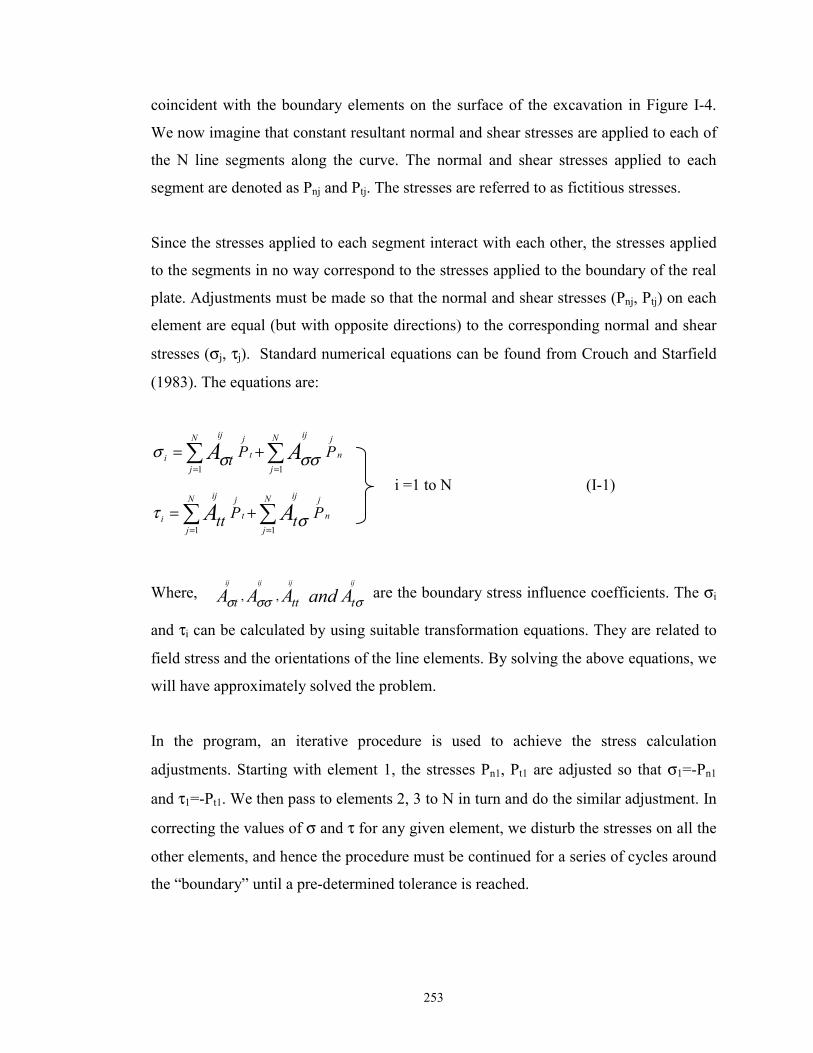
253
coincident with the boundary elements on the surface of the excavation in Figure I-4.
We now imagine that constant resultant normal and shear stresses are applied to each of
the N line segments along the curve. The normal and shear stresses applied to each
segment are denoted as Pnj and Ptj. The stresses are referred to as fictitious stresses.
Since the stresses applied to each segment interact with each other, the stresses applied
to the segments in no way correspond to the stresses applied to the boundary of the real
plate. Adjustments must be made so that the normal and shear stresses (Pnj, Ptj) on each
element are equal (but with opposite directions) to the corresponding normal and shear
stresses (σj, τj). Standard numerical equations can be found from Crouch and Starfield
(1983). The equations are:
n
jN
j
ij
t
jN
j
ij
i PPt AA ∑∑==
+=11
σσσσ
n
jN
j
ij
t
jN
j
ij
i PtPtt AA ∑∑==
+=11
στ
Where, σσσσ tttt AandAAAijijijij
,, are the boundary stress influence coefficients. The σi
and τi can be calculated by using suitable transformation equations. They are related to
field stress and the orientations of the line elements. By solving the above equations, we
will have approximately solved the problem.
In the program, an iterative procedure is used to achieve the stress calculation
adjustments. Starting with element 1, the stresses Pn1, Pt1 are adjusted so that σ1=-Pn1
and τ1=-Pt1. We then pass to elements 2, 3 to N in turn and do the similar adjustment. In
correcting the values of σ and τ for any given element, we disturb the stresses on all the
other elements, and hence the procedure must be continued for a series of cycles around
the “boundary” until a pre-determined tolerance is reached.
i =1 to N (I-1)

254
Figure I-6. Illustration of numerical model
Once this process is complete, the distribution of stresses σi and τi are identical to that
of the stresses Pni and Pti. To compute the stresses at any point in the imaginary plate, all
that has to be done is to sum the contributions of the various fictitious stresses Pni and Pti
(i =1 to N).
Once the stresses due to the negative surface tractions have been determined, they may
be added to those of the original stress field (Figure I-5) to give the required stresses
following excavation.
σ1
σ3
Pn1
τ1
τ3
Pt1
Pt3
Pn3
BoundaryElement

APPENDIX II - DATABASE
H/L ratio
1 Callinan Mine 545-#1 20 26 1.3 5.7 37 3.5 14.22 Callinan Mine 580-2 20.3 23.4 1.2 5.4 44 7.3 16.4
3 Callinan Mine 580-3 20 15 0.8 4.3 49 9.9 184 Callinan Mine 605-3 32.8 14.2 0.4 5 37 3.6 14.25 Callinan Mine 630-6 11 40 3.6 4.3 37 3.6 14.26 Callinan Mine 630-7 11 40 3.6 4.3 37 3.6 14.27 Callinan Mine 865-5-1 57 26 0.5 8.9 41 5.9 32.38 Callinan Mine 865-1-2 22 24 1.1 5.7 56 5.8 39.49 Callinan Mine 885-1-1 26.5 33 1.2 7.3 57 3.3 40.210 Callinan Mine 885-1-2 25.5 26.4 1.0 6.5 60 5.3 42.511 Callinan Mine 885-1-3 33.4 33 1.0 8.3 50 6.7 35.212 Callinan Mine 910-1-2 26.8 31 1.2 7.2 75 9.6 54.713 Callinan Mine 910-1-3 26.8 32 1.2 7.3 71 11.8 51.314 Callinan Mine 910-7-1 13.9 22.2 1.6 4.3 47 2.4 16.615 Callinan Mine 920-7-1B 28.5 19.9 0.7 5.9 50 2.3 17.716 Callinan Mine 920-7-3 36 20 0.6 6.4 50 3.8 17.717 Callinan Mine 935-1-1 31 24 0.8 6.8 68 3.1 48.818 Callinan Mine 935-1-2 21 19.5 0.9 5.1 43 5.8 33.619 Callinan Mine 935-5-1 20.2 30 1.5 6 43 5.8 33.620 Callinan Mine 935-7-2 25 19 0.8 5.4 40 2.2 14.521 Callinan Mine 935-7-3 23 22 1.0 5.6 48 6.7 1722 Callinan Mine 935-7-4 17 20 1.2 4.6 65 8 23.323 Callinan Mine 935-7-5 17 19 1.1 4.5 85 5 31.924 Callinan Mine 950-7-2 25 22 0.9 5.9 69 8.6 24.925 Callinan Mine 950-7-3 23 23 1.0 5.8 65 2.9 23.326 Callinan Mine 1075-2 29.5 30 1.0 7.4 45 20.4 20.127 Callinan Mine 1075-4 29.5 25.9 0.9 6.9 51 16.8 22.628 Callinan Mine 1075-5 16.5 28.4 1.7 5.2 48 8.9 21.329 Callinan Mine 1095-2 35.6 32 0.9 8.4 50 16.2 22.130 Callinan Mine 1095-6 29.2 26.8 0.9 7 42 4.3 18.9
31 Callinan Mine 1120-1 33 26.2 0.8 7.3 56 9.7 24.832 Callinan Mine 1100-2-4 15 10 0.7 3 39 9.3 3.833 Callinan Mine 1100-2-5 16.5 13 0.8 3.6 40 9.8 3.934 Callinan Mine 545-2 24 24 1.0 6 25 3.5 11.435 Callinan Mine 545-3 28 28 1.0 7 28 5.4 1236 Callinan Mine 650-4 25 35 1.4 7.3 40 3.1 15.137 Callinan Mine 845-7-2 55 22 0.4 7.9 75 11.8 6038 Callinan Mine 865-1-1 33 15 0.5 5.2 60 2.6 46.539 Callinan Mine 865-7-3 42 21 0.5 7 55 16.8 38.740 Callinan Mine 885-7-4 26 32 1.2 7.2 40 4.7 28.941 Callinan Mine 910-7-3 21 22 1.0 5.4 45 3.7 1642 Callinan Mine 910-7-4 22 28 1.3 6.2 46 5 16.343 Callinan Mine 920-7-4 31 24 0.8 6.8 60 3.8 14.244 Callinan Mine 777-1100-2-12 18 23 1.3 5 24 11.2 2.945 Callinan Mine 865-1-1 33 15 0.5 5.2 60 2.6 35.446 Ruttan Mine 630-4B2 33.5 75 2.2 11.6 67 4.9 20.047 Ruttan Mine 540-12.5B 20 56 2.8 7.4 85 35 20.048 Ruttan Mine 440-0B2 28.6 44 1.5 8.7 75 13 20.149 Ruttan Mine 1050-29J6 23.5 67 2.9 8.7 70 24 15.050 Ruttan Mine 550-28JS 36 85 2.4 12.6 70 9.5 12.951 Ruttan Mine 440-5B2 19 47 2.5 6.8 65 13 14.652 Ruttan Mine 440-1B2 23 35 1.5 6.9 50 7 5.053 Ruttan Mine 590-14B 25 50 2.0 8.3 89 12 36.254 Trout Lake Mine 840-N9-4 21 40.2 1.9 6.9 66 3.4 10.555 Trout Lake Mine 950-W1-2 12.8 36.6 2.9 4.7 65 6 1256 Trout Lake Mine 1070-W2-7 19 45 2.4 6.7 48 2.2 8.757 Trout Lake Mine 950-N12-1 22.2 38 1.7 7 60 4.2 8.158 Trout Lake Mine 810-N10-5 18.4 45.2 2.5 6.5 51 8.2 9.359 Trout Lake Mine 1040-H1-4 18.4 45.2 2.5 6.5 51 8.2 9.360 Trout Lake Mine 950-W1-4 24.4 37.6 1.5 7.4 60 4.7 1161 Trout Lake Mine 950-N12-3 26.4 44.4 1.7 8.3 51 3.4 6.862 Trout Lake Mine 980-N11-1 20.3 34 1.7 6.4 56 3.9 7.1
No. Stope #Strike
Length, L (m)
Exposed Height, H
(m)
General Info (HW)
HR (m)
Dip (degree)
Ore Width (m)
N'Mine Name
255

APPENDIX II DATABASE
H/L ratio
63 Trout Lake Mine 980-N12-2 30.9 40.6 1.3 8.8 52 1.9 764 Trout Lake Mine 950-W1-3 24 36.8 1.5 7.3 60 5.1 1165 Trout Lake Mine 840-M3-2 21.6 38.6 1.8 6.9 60 6 9.566 Trout Lake Mine 1010-N9-1 31.6 45.2 1.4 9.3 58 3.2 7.167 Trout Lake Mine 980-N11-3 24 32 1.3 6.9 68 5.1 8.868 Trout Lake Mine 810-N10-4 24 39.2 1.6 7.4 61 4.4 11.169 Trout Lake Mine 870-N11-1 15.7 46.2 2.9 5.9 55 5.6 770 Trout Lake Mine 950-N12-2 24 41 1.7 7.6 58 5 7.871 Trout Lake Mine 980W1-6 39.7 36.8 0.9 9.5 71 2.5 13.272 Trout Lake Mine 900 M3 3 23.4 34 1.5 6.9 67 52 10.773 Trout Lake Mine 980 W1 2 22 36 1.6 6.8 59 5.6 10.874 Trout Lake Mine 1010N11 6 20.8 37.8 1.8 6.7 68 4.9 8.875 Trout Lake Mine 1010N9 2 17.4 42.8 2.5 6.2 65 4.8 876 Trout Lake Mine 980N11 2 23.7 31.2 1.3 6.7 67 5.3 8.777 Trout Lake Mine 980N12 3 23.8 40.6 1.7 7.5 51 5 6.878 Trout Lake Mine 865M3 3 18.4 44 2.4 6.5 47 4.8 7.479 Trout Lake Mine 1010N11 5 27 44 1.6 8.4 64 3.6 8.280 Trout Lake Mine 840M1 3 24 35.4 1.5 7.2 69 6 9.581 Trout Lake Mine 840N9-2 20.8 37.8 1.8 6.7 55 14.4 6.782 Trout Lake Mine 980N12 4 24.7 38.2 1.5 7.5 56 4.4 7.583 Trout Lake Mine 980W1 5 20.4 39.6 1.9 6.7 50 9.2 9.184 Trout Lake Mine 810N5 1 12.4 38.8 3.1 4.7 54 7.6 8.585 Trout Lake Mine 1070W2 6 22 41 1.9 7.2 51 3.4 7.386 Trout Lake Mine 10193 16.8 40 2.4 5.9 66 4.9 8.287 Trout Lake Mine 101114 20.6 46.2 2.2 7.1 53 6.5 6.788 Trout Lake Mine 10186 23.4 33.6 1.4 6.9 68 3.3 12.689 Trout Lake Mine 10181 24.8 38.4 1.5 7.5 62 7.6 11.490 Trout Lake Mine 8491 20.8 40.6 2.0 6.9 63 6 7.891 Trout Lake Mine 9883 14.2 34.6 2.4 5 59 6.3 10.892 Trout Lake Mine 8152 23.4 37.2 1.6 7.2 51 5.9 893 Trout Lake Mine 8454 19.8 37.4 1.9 6.5 77 8.5 12.694 Trout Lake Mine 81103 21.4 34.5 1.6 6.6 66 4.3 12.295 Trout Lake Mine 9884 24.2 40 1.7 7.5 50 6.6 9.196 Trout Lake Mine 8433 17.5 37 2.1 5.9 62 9.7 9.897 Trout Lake Mine 101113 19.3 42.6 2.2 6.6 62 9.9 7.998 Trout Lake Mine 98125 31.3 34.4 1.1 8.2 63 3.8 8.599 Trout Lake Mine 10182 20.8 37.5 1.8 6.7 62 8.9 11.4
100 Trout Lake Mine 8412 15.5 38 2.5 5.5 75 7.6 12.2101 Trout Lake Mine 101122 25.8 33.4 1.3 7.3 50 3.5 6.7102 Trout Lake Mine 8411 18.8 37 2.0 6.2 74 4.4 12103 Trout Lake Mine 87112 30.5 44.6 1.5 9.1 75 4.6 9.9104 Trout Lake Mine 81102 16.6 30.8 1.9 5.4 75 7.4 14.1105 Trout Lake Mine 101112 19.6 42.7 2.2 6.7 64 5.4 8.2106 Trout Lake Mine 10488 22.3 32.6 1.5 6.6 73 4.7 13.7107 Trout Lake Mine 101123 27.4 37 1.4 7.9 55 3.4 7108 Trout Lake Mine 10183 13.2 40.4 3.1 5 57 11.1 10.4109 Trout Lake Mine 8792 17.2 39.1 2.3 6 73 10.7 9.2110 Trout Lake Mine 8452 20 41.8 2.1 6.8 65 6.9 10.3111 Trout Lake Mine 10184 27.8 42 1.5 8.4 54 5.2 9.8112 Trout Lake Mine 7031 36.7 20.7 0.6 6.6 75 10 12.2113 Trout Lake Mine 8753 15.4 39 2.5 5.5 70 10.5 11.2114 Trout Lake Mine 1018\5 16 37 2.3 5.6 72 8.9 13.5115 Trout Lake Mine 8793 19.8 36 1.8 6.4 66 9.4 8.2116 Trout Lake Mine 8451\1 15 34 2.3 5.2 69 6.2 11.1117 Trout Lake Mine 1048\2 13.8 37.4 2.7 5 61 6.5 11.1118 Trout Lake Mine 8410\2 24.2 37.8 1.6 7.4 61 9.1 11.1119 Trout Lake Mine 1048\1 26 34.4 1.3 7.4 62 7.2 11.4120 Trout Lake Mine 7311 35.3 35 1.0 8.8 60 4.6 9.5121 Trout Lake Mine 8791\4 27.4 39.4 1.4 8.1 58 6.7 7.1122 Trout Lake Mine 8791\3 27.4 39.4 1.4 8.1 58 6.7 7.1123 Trout Lake Mine 1048\5 14 34 2.4 5 64 8.2 11.8124 Trout Lake Mine 8754 17.7 42 2.4 6.2 69 6.3 11.1125 Trout Lake Mine 1078\1 20.5 34.9 1.7 6.5 63 8.4 11.6126 Trout Lake Mine 8791\E 25.4 43 1.7 8 52 8.4 6.3127 Trout Lake Mine 1048\3 21.5 40 1.9 7 54 12.7 9.8
Strike Length, L
(m)
Exposed Height, H
(m)
HR (m)
Dip (degree)
Ore Width (m)
N'No. Stope #
General Info (HW)
Mine Name
256

APPENDIX II DATABASE
H/L ratio
128 Trout Lake Mine 84105 37.6 33.4 0.9 8.8 66 10.8 12.2129 Trout Lake Mine 8410\3 22 30 1.4 6.3 65 5.2 12130 Trout Lake Mine 1078\2 20 30 1.5 6 58 10 10.6131 Trout Lake Mine 87102 25 44 1.8 8 62 10 11.4132 Trout Lake Mine 10486 23 35 1.5 6.9 72 4.3 13.5133 Trout Lake Mine 10783 25 37 1.5 7.5 54 10.4 9.8134 Trout Lake Mine 84104 20 30 1.5 6 60 5 11135 Trout Lake Mine 10484 22 36 1.6 6.8 67 22.4 12.4136 Trout Lake Mine 9051#1 30 35 1.2 8.1 64 7 10.1137 Trout Lake Mine 6451b 28 32 1.1 7.5 63 8 10138 Trout Lake Mine 6451 30 21 0.7 6.2 60 5.5 9.5139 Trout Lake Mine 1010H1-4 24.7 25.5 1.0 6.3 65 6.9 10.3140 Trout Lake Mine 875C2F-8 24 24.3 1.0 6 62 8.4 8.2141 Trout Lake Mine 950N5-1 25 26 1.0 6.4 72 8.6 11.6142 Trout Lake Mine 765C2-1 20 25.2 1.3 5.6 58 8 7.7143 Trout Lake Mine 765C2-5 21 24.5 1.2 5.7 62 13 8.2144 Trout Lake Mine 980N9-2 20.2 26.2 1.3 5.7 70 7.7 9.1145 Trout Lake Mine 1040H1-6/7 45 27.1 0.6 8.5 55 5.2 8.2146 Trout Lake Mine 810N10-7 24.8 31.4 1.3 6.9 57 9.6 10.4147 Trout Lake Mine 950N9-2 20 26.9 1.3 5.7 80 6.5 10.6148 Trout Lake Mine 950W1-6 23.5 28.5 1.2 6.4 60 6.8 9.5149 Trout Lake Mine 980N11-6 17.4 27.4 1.6 5.3 78 5.4 12.8150 Trout Lake Mine 920N12-3 22.5 23.3 1.0 5.7 58 5 9.9
No. Stope #
General Info (HW)
Mine NameStrike
Length, L (m)
Exposed Height, H
(m)
HR (m)
Dip (degree)
Ore Width (m)
N'
257

APPENDIX II DATABASE
Undercutting
% of u/c along strike
Max. depth (m)
Avg. depth
_strike (m)
u/c length along
strike (m)
Avg.depth _u/c
portion (m)
% of u/c along strike
Max. depth (m)
1 Callinan Mine 545-#1 0% 0 0.0 0.0 0.0 0.7 3.42 Callinan Mine 580-2 0% 0 0.0 0.0 0.0 0.8 2.3
3 Callinan Mine 580-3 10% 1.7 0.1 2.0 1.0 100% 1.54 Callinan Mine 605-3 80% 1.8 0.7 26.2 0.9 100% 1.85 Callinan Mine 630-6 50% 1 0.5 5.5 1.0 0% 06 Callinan Mine 630-7 0% 0 0.0 0.0 0.0 100% 0.77 Callinan Mine 865-5-1 100% 1.5 0.2 57.0 0.2 50% 18 Callinan Mine 865-1-2 30% 1 1.0 6.6 3.3 0% 09 Callinan Mine 885-1-1 100% 2 0.7 26.5 0.7 0% 010 Callinan Mine 885-1-2 0% 0 0.0 0.0 0.0 0% 011 Callinan Mine 885-1-3 10% 0.6 0.6 3.3 6.0 0% 012 Callinan Mine 910-1-2 0% 0 0.0 0.0 0.0 0% 013 Callinan Mine 910-1-3 0% 0 0.0 0.0 0.0 0% 014 Callinan Mine 910-7-1 100% 1.2 1.0 13.9 1.0 0% 015 Callinan Mine 920-7-1B 0% 0 0.0 0.0 0.0 100% 0.916 Callinan Mine 920-7-3 100% 2.5 1.1 36.0 1.1 60% 217 Callinan Mine 935-1-1 0% 0 0.0 0.0 0.0 0% 018 Callinan Mine 935-1-2 100% 1.3 1.0 21.0 1.0 100% 119 Callinan Mine 935-5-1 100% 4.2 2.1 20.2 2.1 0% 020 Callinan Mine 935-7-2 100% 1.6 0.9 25.0 0.9 0% 021 Callinan Mine 935-7-3 100% 3 1.4 23.0 1.4 100% 2.822 Callinan Mine 935-7-4 30% 3 0.2 5.1 0.7 0% 023 Callinan Mine 935-7-5 100% 4 3.5 17.0 3.5 100% 124 Callinan Mine 950-7-2 0% 0 0.0 0.0 0.0 0% 025 Callinan Mine 950-7-3 0% 0 0.0 0.0 0.0 0% 026 Callinan Mine 1075-2 80% 1.5 0.8 23.6 1.0 70% 1.527 Callinan Mine 1075-4 0% 0 0.0 0.0 0.0 0% 028 Callinan Mine 1075-5 60% 1 0.4 9.9 0.7 0% 029 Callinan Mine 1095-2 95% 1.6 1.0 33.8 1.1 0% 030 Callinan Mine 1095-6 0% 0 0.0 0.0 0.0 0% 0
31 Callinan Mine 1120-1 0% 0 0.0 0.0 0.0 0% 032 Callinan Mine 1100-2-4 0% 0 0.0 0.0 0.0 0% 033 Callinan Mine 1100-2-5 0% 0 0.0 0.0 0.0 100% 1.534 Callinan Mine 545-2 90% 7 2.0 21.6 2.2 0% 035 Callinan Mine 545-3 0% 0 0.0 0.0 0.0 0% 036 Callinan Mine 650-4 30% 5 1.2 7.5 4.0 60% 2.537 Callinan Mine 845-7-2 50% 2.5 1.1 27.5 2.2 0% 038 Callinan Mine 865-1-1 0% 0 0.0 0.0 0.0 0% 039 Callinan Mine 865-7-3 20% 2 0.2 8.4 1.0 0% 040 Callinan Mine 885-7-4 0% 0 0.0 0.0 0.0 0% 041 Callinan Mine 910-7-3 0% 0 0.0 0.0 0.0 0% 042 Callinan Mine 910-7-4 100% 1 0.5 22.0 0.5 0% 043 Callinan Mine 920-7-4 50% 3 1.5 15.5 3.0 0% 044 Callinan Mine 777-1100-2-12 0% 0 0.0 0.0 0.0 0% 045 Callinan Mine 865-1-1 0% 0 0.0 0.0 0.0 0% 046 Ruttan Mine 630-4B2 100% 4 1.3 33.5 1.3 100% 147 Ruttan Mine 540-12.5B 0% 0 0 0.0 0.0 0% 048 Ruttan Mine 440-0B2 0% 0 0 0.0 0.0 0% 049 Ruttan Mine 1050-29J6 0% 0 0 0.0 0.0 0% 050 Ruttan Mine 550-28JS 0% 0 0 0.0 0.0 100% 451 Ruttan Mine 440-5B2 0% 0 0 0.0 0.0 0% 052 Ruttan Mine 440-1B2 0% 0 0 0.0 0.0 0% 053 Ruttan Mine 590-14B 0% 0 0 0.0 0.0 0% 054 Trout Lake Mine 840-N9-4 20% 0.4 0.1 4.2 0.5 20% 255 Trout Lake Mine 950-W1-2 57% 2.2 0.6 7.3 1.1 100% 156 Trout Lake Mine 1070-W2-7 20% 1.8 0.3 3.8 1.5 0% 057 Trout Lake Mine 950-N12-1 13% 1.2 0.1 2.9 0.8 80% 2.358 Trout Lake Mine 810-N10-5 63% 3.8 1.1 11.6 1.7 0% 059 Trout Lake Mine 1040-H1-4 0% 0 0.0 0.0 0.0 0% 060 Trout Lake Mine 950-W1-4 64% 3.8 1.2 15.6 1.9 60% 1.361 Trout Lake Mine 950-N12-3 37% 1.4 0.2 9.8 0.5 0% 062 Trout Lake Mine 980-N11-1 0% 0 0.0 0.0 0.0 0% 0
No. Stope #
O/C Drift
Mine Name
U/C Drift
258

APPENDIX II DATABASE
Undercutting
% of u/c along strike
Max. depth (m)
Avg. depth
_strike (m)
u/c length along
strike (m)
Avg.depth _u/c
portion (m)
% of u/c along strike
Max. depth (m)
63 Trout Lake Mine 980-N12-2 0% 0 0.0 0.0 0.0 0% 064 Trout Lake Mine 950-W1-3 70% 1.5 0.8 16.8 1.1 75% 265 Trout Lake Mine 840-M3-2 50% 6 1.5 10.8 3.0 0% 066 Trout Lake Mine 1010-N9-1 90% 0.7 0.4 28.4 0.4 100% 1.567 Trout Lake Mine 980-N11-3 62% 2.8 0.8 14.9 1.3 30% 2.568 Trout Lake Mine 810-N10-4 85% 2 0.8 20.4 0.9 0% 069 Trout Lake Mine 870-N11-1 65% 5.5 1.4 10.2 2.2 0% 070 Trout Lake Mine 950-N12-2 50% 1.4 0.6 12.0 1.2 0% 071 Trout Lake Mine 980W1-6 85% 10.2 2.2 33.7 2.6 20% 1.272 Trout Lake Mine 900 M3 3 15% 2.9 0.4 3.5 2.7 20% 1.273 Trout Lake Mine 980 W1 2 0% 0 0.0 0.0 0.0 0% 074 Trout Lake Mine 1010N11 6 0% 0 0.0 0.0 0.0 0% 075 Trout Lake Mine 1010N9 2 100% 1.5 0.6 17.4 0.6 25% 1.376 Trout Lake Mine 980N11 2 0% 0 0.0 0.0 0.0 0% 077 Trout Lake Mine 980N12 3 0% 0 0.0 0.0 0.0 15% 1.578 Trout Lake Mine 865M3 3 20% 2 0.4 3.7 2.0 25% 679 Trout Lake Mine 1010N11 5 0% 5.5 0.0 0.0 0.0 0% 080 Trout Lake Mine 840M1 3 0% 0 0.0 0.0 0.0 0% 081 Trout Lake Mine 840N9-2 15% 4.4 0.5 3.1 3.3 0% 082 Trout Lake Mine 980N12 4 90% 2.4 1.2 22.2 1.3 0% 083 Trout Lake Mine 980W1 5 0% 0 0.0 0.0 0.0 0% 084 Trout Lake Mine 810N5 1 60% 4 1.8 7.4 3.0 100% 185 Trout Lake Mine 1070W2 6 95% 2 0.7 20.9 0.7 90% 386 Trout Lake Mine 10193 50% 0.6 0.2 8.4 0.4 0% 087 Trout Lake Mine 101114 40% 0.6 0.1 8.2 0.3 0% 088 Trout Lake Mine 10186 25% 2.6 0.3 5.9 1.2 0% 089 Trout Lake Mine 10181 75% 4.2 1.0 18.6 1.3 50% 290 Trout Lake Mine 8491 50% 2.8 0.6 10.4 1.2 30% 3.591 Trout Lake Mine 9883 90% 0.5 0.2 12.8 0.2 60% 292 Trout Lake Mine 8152 50% 1.6 0.6 11.7 1.2 100% 1.593 Trout Lake Mine 8454 30% 2.4 0.6 5.9 2.0 0% 094 Trout Lake Mine 81103 100% 1.8 1.0 21.4 1.0 60% 1.295 Trout Lake Mine 9884 60% 1.8 0.4 14.5 0.7 0% 096 Trout Lake Mine 8433 10% 4 0.3 1.8 3.0 0% 097 Trout Lake Mine 101113 50% 3.6 0.9 9.7 1.8 0% 098 Trout Lake Mine 98125 0% 0 0.0 0.0 0.0 50% 399 Trout Lake Mine 10182 50% 1.2 0.5 10.4 1.0 0% 0
100 Trout Lake Mine 8412 0% 0 0.0 0.0 0.0 100% 3.5101 Trout Lake Mine 101122 0% 0 0.0 0.0 0.0 0% 0102 Trout Lake Mine 8411 0% 0 0.0 0.0 0.0 0% 0103 Trout Lake Mine 87112 25% 1.4 0.2 7.6 0.8 0% 0104 Trout Lake Mine 81102 55% 1.8 0.6 9.1 1.1 0% 0105 Trout Lake Mine 101112 60% 1.3 0.6 11.8 1.0 10% 3106 Trout Lake Mine 10488 0% 0 0.0 0.0 0.0 0% 0107 Trout Lake Mine 101123 0% 0 0.0 0.0 0.0 0% 0108 Trout Lake Mine 10183 0% 0 0.0 0.0 0.0 0% 0109 Trout Lake Mine 8792 45% 8 1.1 7.7 2.4 0% 0110 Trout Lake Mine 8452 50% 4 1.5 10.0 3.0 20% 2111 Trout Lake Mine 10184 100% 2.7 1.8 27.8 1.8 0% 0112 Trout Lake Mine 7031 100% 1.9 1.4 36.7 1.4 0% 0113 Trout Lake Mine 8753 100% 1.8 1.2 15.4 1.2 70% 3114 Trout Lake Mine 1018\5 20% 2 0.1 3.2 0.5 0% 0115 Trout Lake Mine 8793 100% 1.8 0.6 19.8 0.6 30% 3116 Trout Lake Mine 8451\1 100% 8 4.9 15.0 4.9 15% 4117 Trout Lake Mine 1048\2 50% 1.6 0.5 6.9 1.0 60% 3118 Trout Lake Mine 8410\2 100% 2.4 1.3 24.2 1.3 30% 1119 Trout Lake Mine 1048\1 0% 0 0.0 0.0 0.0 100% 1.1120 Trout Lake Mine 7311 0% 0 0.0 0.0 0.0 100% 3121 Trout Lake Mine 8791\4 45% 1.8 1.0 12.3 2.2 0% 0122 Trout Lake Mine 8791\3 45% 1.8 1.0 12.3 2.2 0% 0123 Trout Lake Mine 1048\5 50% 3 0.8 7.0 1.6 0% 0124 Trout Lake Mine 8754 100% 5.8 2.4 17.7 2.4 0% 0125 Trout Lake Mine 1078\1 30% 2.2 0.5 6.2 1.7 100% 2126 Trout Lake Mine 8791\E 0% 0 0.0 0.0 0.0 80% 5127 Trout Lake Mine 1048\3 90% 10.1 2.7 19.4 3.0 100% 3.2
U/C Drift O/C Drift
No. Mine Name Stope #
259

APPENDIX II DATABASE
Undercutting
% of u/c along strike
Max. depth (m)
Avg. depth
_strike (m)
u/c length along
strike (m)
Avg.depth _u/c
portion (m)
% of u/c along strike
Max. depth (m)
128 Trout Lake Mine 84105 50% 1.6 0.6 18.8 1.2 0% 0129 Trout Lake Mine 8410\3 60% 2.5 0.8 13.2 1.3 100% 3130 Trout Lake Mine 1078\2 15% 1.5 0.1 3.0 0.7 0% 0131 Trout Lake Mine 87102 70% 1.5 0.6 17.5 0.9 100% 2.5132 Trout Lake Mine 10486 70% 3.5 1.5 16.1 2.1 80% 1133 Trout Lake Mine 10783 100% 3 1.0 25.0 1.0 0% 0134 Trout Lake Mine 84104 30% 3.5 0.6 6.0 2.0 0% 0135 Trout Lake Mine 10484 0% 0 0.0 0.0 0.0 0% 0136 Trout Lake Mine 9051#1 80% 3 1.2 24.0 1.5 40% 1.2137 Trout Lake Mine 6451b 70% 3.5 2.0 19.6 2.9 0% 0138 Trout Lake Mine 6451 20% 2 0.2 6.0 1.0 100% 3.5139 Trout Lake Mine 1010H1-4 0% 0 0.0 0.0 0.0 50% 2.5140 Trout Lake Mine 875C2F-8 20% 3 0.2 4.8 1.0 0% 0141 Trout Lake Mine 950N5-1 30% 3 0.7 7.5 2.3 0% 0142 Trout Lake Mine 765C2-1 50% 1.6 0.8 10.0 1.6 100% 0.7143 Trout Lake Mine 765C2-5 0% 0 0.0 0.0 0.0 0% 0144 Trout Lake Mine 980N9-2 55% 5 1.5 11.1 2.7 45% 2145 Trout Lake Mine 1040H1-6/7 20% 2.2 0.3 9.0 1.5 0% 0146 Trout Lake Mine 810N10-7 0% 0 0.0 0.0 0.0 0% 0147 Trout Lake Mine 950N9-2 25% 2.5 0.3 5.0 1.2 0% 0148 Trout Lake Mine 950W1-6 35% 2 0.6 8.2 1.7 0% 0149 Trout Lake Mine 980N11-6 100% 2 1.6 17.4 1.6 30% 1150 Trout Lake Mine 920N12-3 100% 3.5 2.0 22.5 2.0 35% 1
No.
U/C Drift O/C Drift
Mine Name Stope #
260

APPENDIX II DATABASE
Undercutting (cont.d)
Avg.depth _strike (m)
u/c length along
strike (m)
Avg. depth _u/c
portion (m)
Portion of u/c along perimeter
Avg. depth in u/c
portion (m)
Overall avg. depth
u/c_strike (m)
1 Callinan Mine 545-#1 3 14.0 4.29 0.15 2.14 1.52 Callinan Mine 580-2 1.5 16.2 1.88 0.19 0.94 0.75
3 Callinan Mine 580-3 1.3 20.0 1.30 0.31 1.15 0.74 Callinan Mine 605-3 1.2 32.8 1.20 0.63 1.04 0.955 Callinan Mine 630-6 0 0.0 0.00 0.05 0.50 0.256 Callinan Mine 630-7 0.6 11.0 0.60 0.11 0.30 0.37 Callinan Mine 865-5-1 0.2 28.5 0.40 0.52 0.30 0.28 Callinan Mine 865-1-2 0 0.0 0.00 0.07 1.67 0.59 Callinan Mine 885-1-1 0 0.0 0.00 0.22 0.35 0.3510 Callinan Mine 885-1-2 0 0.0 0.00 0.00 0.00 011 Callinan Mine 885-1-3 0 0.0 0.00 0.03 3.00 0.312 Callinan Mine 910-1-2 0 0.0 0.00 0.00 0.00 013 Callinan Mine 910-1-3 0 0.0 0.00 0.00 0.00 014 Callinan Mine 910-7-1 0 0.0 0.00 0.19 0.50 0.515 Callinan Mine 920-7-1B 0.6 28.5 0.60 0.29 0.30 0.316 Callinan Mine 920-7-3 0.8 21.6 1.33 0.51 1.22 0.9517 Callinan Mine 935-1-1 0 0.0 0.00 0.00 0.00 018 Callinan Mine 935-1-2 0.5 21.0 0.50 0.52 0.75 0.7519 Callinan Mine 935-5-1 0 0.0 0.00 0.20 1.05 1.0520 Callinan Mine 935-7-2 0 0.0 0.00 0.28 0.45 0.4521 Callinan Mine 935-7-3 1.2 23.0 1.20 0.51 1.30 1.322 Callinan Mine 935-7-4 0 0.0 0.00 0.07 0.33 0.123 Callinan Mine 935-7-5 0.8 17.0 0.80 0.47 2.15 2.1524 Callinan Mine 950-7-2 0 0.0 0.00 0.00 0.00 025 Callinan Mine 950-7-3 0 0.0 0.00 0.00 0.00 026 Callinan Mine 1075-2 0.6 20.7 0.86 0.37 0.93 0.727 Callinan Mine 1075-4 0 0.0 0.00 0.00 0.00 028 Callinan Mine 1075-5 0 0.0 0.00 0.11 0.33 0.229 Callinan Mine 1095-2 0 0.0 0.00 0.25 0.53 0.530 Callinan Mine 1095-6 0 0.0 0.00 0.00 0.00 0
31 Callinan Mine 1120-1 0 0.0 0.00 0.00 0.00 032 Callinan Mine 1100-2-4 0 0.0 0.00 0.00 0.00 033 Callinan Mine 1100-2-5 0.8 16.5 0.80 0.28 0.40 0.434 Callinan Mine 545-2 0 0.0 0.00 0.23 1.11 135 Callinan Mine 545-3 0 0.0 0.00 0.00 0.00 036 Callinan Mine 650-4 0.7 15.0 1.17 0.19 2.58 0.9537 Callinan Mine 845-7-2 0 0.0 0.00 0.18 1.10 0.5538 Callinan Mine 865-1-1 0 0.0 0.00 0.00 0.00 039 Callinan Mine 865-7-3 0 0.0 0.00 0.07 0.50 0.140 Callinan Mine 885-7-4 0 0.0 0.00 0.00 0.00 041 Callinan Mine 910-7-3 0 0.0 0.00 0.00 0.00 042 Callinan Mine 910-7-4 0 0.0 0.00 0.22 0.25 0.2543 Callinan Mine 920-7-4 0 0.0 0.00 0.14 1.50 0.7544 Callinan Mine 777-1100-2-12 0 0.0 0.00 0.00 0.00 045 Callinan Mine 865-1-1 0 0.0 0.00 0.00 0.00 046 Ruttan Mine 630-4B2 0.5 33.5 0.50 0.31 0.90 0.947 Ruttan Mine 540-12.5B 0 0.0 0.00 0.00 0.00 048 Ruttan Mine 440-0B2 0 0.0 0.00 0.00 0.00 049 Ruttan Mine 1050-29J6 0 0.0 0.00 0.00 0.00 050 Ruttan Mine 550-28JS 3 36.0 3.00 0.15 1.50 1.551 Ruttan Mine 440-5B2 0 0.0 0.00 0.00 0.00 052 Ruttan Mine 440-1B2 0 0.0 0.00 0.00 0.00 053 Ruttan Mine 590-14B 0 0.0 0.00 0.00 0.00 054 Trout Lake Mine 840-N9-4 0.1 4.2 0.50 0.07 0.50 0.155 Trout Lake Mine 950-W1-2 0.8 12.8 0.80 0.20 0.93 0.756 Trout Lake Mine 1070-W2-7 0 0.0 0.00 0.03 0.75 0.1557 Trout Lake Mine 950-N12-1 0.5 17.8 0.63 0.17 0.70 0.358 Trout Lake Mine 810-N10-5 0 0.0 0.00 0.09 0.87 0.5559 Trout Lake Mine 1040-H1-4 0 0.0 0.00 0.00 0.00 060 Trout Lake Mine 950-W1-4 0.9 14.6 1.50 0.24 1.69 1.0561 Trout Lake Mine 950-N12-3 0 0.0 0.00 0.07 0.27 0.162 Trout Lake Mine 980-N11-1 0 0.0 0.00 0.00 0.00 0
OverallO/C Drift (cont'd)
No. Stope #Mine Name
261

APPENDIX II DATABASE
Undercutting (cont.d)
Avg.depth _strike (m)
u/c length along
strike (m)
Avg. depth _u/c
portion (m)
Portion of u/c along perimeter
Avg. depth in u/c
portion (m)
Overall avg. depth
u/c_strike (m)
63 Trout Lake Mine 980-N12-2 0 0.0 0.00 0.00 0.00 064 Trout Lake Mine 950-W1-3 1.6 18.0 2.13 0.29 1.64 1.265 Trout Lake Mine 840-M3-2 0 0.0 0.00 0.09 1.50 0.7566 Trout Lake Mine 1010-N9-1 1.2 31.6 1.20 0.39 0.82 0.867 Trout Lake Mine 980-N11-3 0.7 7.2 2.33 0.20 1.81 0.7568 Trout Lake Mine 810-N10-4 0 0.0 0.00 0.16 0.47 0.469 Trout Lake Mine 870-N11-1 0 0.0 0.00 0.08 1.08 0.770 Trout Lake Mine 950-N12-2 0 0.0 0.00 0.09 0.60 0.371 Trout Lake Mine 980W1-6 0.1 7.9 0.50 0.27 1.54 1.1572 Trout Lake Mine 900 M3 3 0.1 4.7 0.50 0.07 1.58 0.2573 Trout Lake Mine 980 W1 2 0 0.0 0.00 0.00 0.00 074 Trout Lake Mine 1010N11 6 0 0.0 0.00 0.00 0.00 075 Trout Lake Mine 1010N9 2 0.1 4.4 0.40 0.18 0.50 0.3576 Trout Lake Mine 980N11 2 0 0.0 0.00 0.00 0.00 077 Trout Lake Mine 980N12 3 0.1 3.6 0.67 0.03 0.33 0.0578 Trout Lake Mine 865M3 3 0.8 4.6 3.20 0.07 2.60 0.679 Trout Lake Mine 1010N11 5 0 0.0 0.00 0.00 0.00 080 Trout Lake Mine 840M1 3 0 0.0 0.00 0.00 0.00 081 Trout Lake Mine 840N9-2 0 0.0 0.00 0.03 1.67 0.2582 Trout Lake Mine 980N12 4 0 0.0 0.00 0.18 0.67 0.683 Trout Lake Mine 980W1 5 0 0.0 0.00 0.00 0.00 084 Trout Lake Mine 810N5 1 0.5 12.4 0.50 0.19 1.75 1.1585 Trout Lake Mine 1070W2 6 1.7 19.8 1.89 0.32 1.31 1.286 Trout Lake Mine 10193 0 0.0 0.00 0.07 0.20 0.187 Trout Lake Mine 101114 0 0.0 0.00 0.06 0.13 0.0588 Trout Lake Mine 10186 0 0.0 0.00 0.05 0.60 0.1589 Trout Lake Mine 10181 0.7 12.4 1.40 0.25 1.37 0.8590 Trout Lake Mine 8491 0.7 6.2 2.33 0.14 1.77 0.6591 Trout Lake Mine 9883 0.8 8.5 1.33 0.22 0.78 0.592 Trout Lake Mine 8152 1 23.4 1.00 0.29 1.10 0.893 Trout Lake Mine 8454 0 0.0 0.00 0.05 1.00 0.394 Trout Lake Mine 81103 0.6 12.8 1.00 0.31 1.00 0.895 Trout Lake Mine 9884 0 0.0 0.00 0.11 0.33 0.296 Trout Lake Mine 8433 0 0.0 0.00 0.02 1.50 0.1597 Trout Lake Mine 101113 0 0.0 0.00 0.08 0.90 0.4598 Trout Lake Mine 98125 1.5 15.7 3.00 0.12 1.50 0.7599 Trout Lake Mine 10182 0 0.0 0.00 0.09 0.50 0.25
100 Trout Lake Mine 8412 2 15.5 2.00 0.14 1.00 1101 Trout Lake Mine 101122 0 0.0 0.00 0.00 0.00 0102 Trout Lake Mine 8411 0 0.0 0.00 0.00 0.00 0103 Trout Lake Mine 87112 0 0.0 0.00 0.05 0.40 0.1104 Trout Lake Mine 81102 0 0.0 0.00 0.10 0.55 0.3105 Trout Lake Mine 101112 0 2.0 0.00 0.11 0.50 0.3106 Trout Lake Mine 10488 0 0.0 0.00 0.00 0.00 0107 Trout Lake Mine 101123 0 0.0 0.00 0.00 0.00 0108 Trout Lake Mine 10183 0 0.0 0.00 0.00 0.00 0109 Trout Lake Mine 8792 0 0.0 0.00 0.07 1.22 0.55110 Trout Lake Mine 8452 0.1 4.0 0.50 0.11 1.75 0.8111 Trout Lake Mine 10184 0 0.0 0.00 0.20 0.90 0.9112 Trout Lake Mine 7031 0 0.0 0.00 0.32 0.70 0.7113 Trout Lake Mine 8753 1.5 10.8 2.14 0.24 1.67 1.35114 Trout Lake Mine 1018\5 0 0.0 0.00 0.03 0.25 0.05115 Trout Lake Mine 8793 0.5 5.9 1.67 0.23 1.13 0.55116 Trout Lake Mine 8451\1 0.2 2.3 1.33 0.18 3.12 2.55117 Trout Lake Mine 1048\2 1.4 8.3 2.33 0.15 1.67 0.95118 Trout Lake Mine 8410\2 0.5 7.3 1.67 0.25 1.48 0.9119 Trout Lake Mine 1048\1 1 26.0 1.00 0.22 0.50 0.5120 Trout Lake Mine 7311 1 35.3 1.00 0.25 0.50 0.5121 Trout Lake Mine 8791\4 0 0.0 0.00 0.09 1.11 0.5122 Trout Lake Mine 8791\3 0 0.0 0.00 0.09 1.11 0.5123 Trout Lake Mine 1048\5 0 0.0 0.00 0.07 0.80 0.4124 Trout Lake Mine 8754 0 0.0 0.00 0.15 1.20 1.2125 Trout Lake Mine 1078\1 1.4 20.5 1.40 0.24 1.53 0.95126 Trout Lake Mine 8791\E 3 20.3 3.75 0.15 1.88 1.5127 Trout Lake Mine 1048\3 1.1 21.5 1.10 0.33 2.05 1.9
Stope #
O/C Drift (cont'd) Overall
Mine NameNo.
262

APPENDIX II DATABASE
Undercutting (cont.d)
Avg.depth _strike (m)
u/c length along
strike (m)
Avg. depth _u/c
portion (m)
Portion of u/c along perimeter
Avg. depth in u/c
portion (m)
Overall avg. depth
u/c_strike (m)
128 Trout Lake Mine 84105 0 0.0 0.00 0.13 0.60 0.3129 Trout Lake Mine 8410\3 1.7 22.0 1.70 0.34 1.52 1.25130 Trout Lake Mine 1078\2 0 0.0 0.00 0.03 0.33 0.05131 Trout Lake Mine 87102 1.7 25.0 1.70 0.31 1.28 1.15132 Trout Lake Mine 10486 0.7 18.4 0.88 0.30 1.51 1.1133 Trout Lake Mine 10783 0 0.0 0.00 0.20 0.50 0.5134 Trout Lake Mine 84104 0 0.0 0.00 0.06 1.00 0.3135 Trout Lake Mine 10484 0 0.0 0.00 0.00 0.00 0136 Trout Lake Mine 9051#1 0.4 12.0 1.00 0.28 1.25 0.8137 Trout Lake Mine 6451b 0 0.0 0.00 0.16 1.43 1138 Trout Lake Mine 6451 2 30.0 2.00 0.35 1.50 1.1139 Trout Lake Mine 1010H1-4 1 12.4 2.00 0.12 1.00 0.5140 Trout Lake Mine 875C2F-8 0 0.0 0.00 0.05 0.50 0.1141 Trout Lake Mine 950N5-1 0 0.0 0.00 0.07 1.17 0.35142 Trout Lake Mine 765C2-1 0.5 20.0 0.50 0.33 1.05 0.65143 Trout Lake Mine 765C2-5 0 0.0 0.00 0.00 0.00 0144 Trout Lake Mine 980N9-2 0.6 9.1 1.33 0.22 2.03 1.05145 Trout Lake Mine 1040H1-6/7 0 0.0 0.00 0.06 0.75 0.15146 Trout Lake Mine 810N10-7 0 0.0 0.00 0.00 0.00 0147 Trout Lake Mine 950N9-2 0 0.0 0.00 0.05 0.60 0.15148 Trout Lake Mine 950W1-6 0 0.0 0.00 0.08 0.86 0.3149 Trout Lake Mine 980N11-6 0.3 5.2 1.00 0.25 1.30 0.95150 Trout Lake Mine 920N12-3 0.2 7.9 0.57 0.33 1.29 1.1
Stope #
O/C Drift (cont'd) Overall
Mine NameNo.
263

APPENDIX II DATABASE
1 Callinan Mine 545-#1 2.5" f n/a y 0 12 Callinan Mine 580-2 2.5" f 1.5/0/.7 y 1//3 1.2
3 Callinan Mine 580-3 3" f 1/0/.3 y 1//5 0.94 Callinan Mine 605-3 2" p 0.5/0/.3 y 1.15 Callinan Mine 630-6 2.5" 0 y 1.16 Callinan Mine 630-7 2.5" f n/a y 1.17 Callinan Mine 865-5-1 2.5" f n/a y 1.48 Callinan Mine 865-1-2 3" f n/a y 1.49 Callinan Mine 885-1-1 2.5 p 1/0/0.5 y 1.310 Callinan Mine 885-1-2 3" f n/a y 1.311 Callinan Mine 885-1-3 2.5" p 1/0/0.3 y 0.912 Callinan Mine 910-1-2 3" p 1.5/0/0.5 y 1.213 Callinan Mine 910-1-3 3" f n/a y 1.414 Callinan Mine 910-7-1 2.5" p 1/-1/0.5 n 2.715 Callinan Mine 920-7-1B 2.5 p 1/0/0.5 y 2.516 Callinan Mine 920-7-3 2.5" p 1.6/0/1 y 0 1.717 Callinan Mine 935-1-1 2.5" p 1.2/0/0.5 y /2 1.418 Callinan Mine 935-1-2 2.5" f n/a y 1//3 0.919 Callinan Mine 935-5-1 2.5" f n/a y 1.420 Callinan Mine 935-7-2 2.5" p 1.8/0/0.6 n 1.921 Callinan Mine 935-7-3 2.5" p 2/0/0.8 n 1.322 Callinan Mine 935-7-4 2.5" p 1.5/0/0.6 n 1.123 Callinan Mine 935-7-5 2.5" p 1.5/0/0.6 n 24 Callinan Mine 950-7-2 3" f n/a n 1.325 Callinan Mine 950-7-3 2.5" f n/a n 26 Callinan Mine 1075-2 2.5" p 1/0/0.5 y 3 27 Callinan Mine 1075-4 2.5" f n/a y 5 1.228 Callinan Mine 1075-5 3" f n/a y 1 29 Callinan Mine 1095-2 f n/a y 30 Callinan Mine 1095-6 2.5" f n/a y 1//6
31 Callinan Mine 1120-1 2.5" f n/a n 8 0.732 Callinan Mine 1100-2-4 3.0" f n/a n 4 1.833 Callinan Mine 1100-2-5 3.0" f n/a y 3 1.434 Callinan Mine 545-2 2.5" p 2/-2/.5 y /5 1.235 Callinan Mine 545-3 2.5" f n/a y 5 1.136 Callinan Mine 650-4 2.5" f n/a y 4 0.937 Callinan Mine 845-7-2 3" p 1/0/0.5 y 8 138 Callinan Mine 865-1-1 2.5" f n/a y 39 Callinan Mine 865-7-3 3" f n/a y 40 Callinan Mine 885-7-4 2.5" f n/a y 6 1.141 Callinan Mine 910-7-3 2.5" p 2/-1/.5 y 5 242 Callinan Mine 910-7-4 2.5" p 1.4/0/0.7 y 7 1.243 Callinan Mine 920-7-4 3" p 1/0/0.5 y 5 1.244 Callinan Mine 777-1100-2-12 2.5" f n/a y 5 1.245 Callinan Mine 865-1-1 2.5" f n/a y 5 1.346 Ruttan Mine 630-4B2 3" f n/a y 647 Ruttan Mine 540-12.5B 3" f n/a y 648 Ruttan Mine 440-0B2 3.6" f n/a y 649 Ruttan Mine 1050-29J6 3" f n/a y 1050 Ruttan Mine 550-28JS 3" p y 751 Ruttan Mine 440-5B2 3" f n/a y 552 Ruttan Mine 440-1B2 3.6" f n/a y 453 Ruttan Mine 590-14B 4.5" f n/a y 654 Trout Lake Mine 840-N9-4 4 1/2" p 1.5/0/0.7 y 0//2 1.755 Trout Lake Mine 950-W1-2 5 1/2" p 2/0.1/0.5 y 0//1 1.6356 Trout Lake Mine 1070-W2-7 0 f n/a y 0//2 1.1557 Trout Lake Mine 950-N12-1 0 p 1/0/0.5 y //1 1.2358 Trout Lake Mine 810-N10-5 0 f n/a y 2//2 1.359 Trout Lake Mine 1040-H1-4 3" f n/a y 4//2 1.3160 Trout Lake Mine 950-W1-4 4 1/2" L p 1.2/0/0.6 y //2 0.961 Trout Lake Mine 950-N12-3 4 1/2" L f n/a y 2//2 0.762 Trout Lake Mine 980-N11-1 3" f n/a y 2//2 0.9
Blasting
Drill hole size
Dillhole offset from HW
(Max/Min/Avg) (m)
Wall Control
# of blasts Slot//main
Powder Factor (lb/ton)
Orientation (f-fanned p-parallel)
No. Stope #Mine Name
264

APPENDIX II DATABASE
63 Trout Lake Mine 980-N12-2 4 1/2" L p 0.2/0.2/0.2 y 2//2 1.464 Trout Lake Mine 950-W1-3 0 f 0.5/0/0.25 y 2//1 165 Trout Lake Mine 840-M3-2 3" f n/a y 3//2 0.866 Trout Lake Mine 1010-N9-1 4 1/2" p 1.7/0/1 y 2//2 2.167 Trout Lake Mine 980-N11-3 4 1/2" L p 2/0/0.6 y 2//2 1.368 Trout Lake Mine 810-N10-4 4 1/2" L f n/a y 2//1 0.769 Trout Lake Mine 870-N11-1 3" & 4 1/2" f n/a y 1//2 170 Trout Lake Mine 950-N12-2 4 1/2" p 1.5/0/0.7 y 1//1 0.971 Trout Lake Mine 980W1-6 4 1/2" L f n/a y 1//2 172 Trout Lake Mine 900 M3 3 3" f n/a y 2//3 1.0473 Trout Lake Mine 980 W1 2 4 1/2" L f n/a y 2//1 1.0574 Trout Lake Mine 1010N11 6 4 1/2" L p 0 y 2//1 1.975 Trout Lake Mine 1010N9 2 4 1/2" L f n/a y 2//1 1.576 Trout Lake Mine 980N11 2 3" f n/a y 2//2 0.977 Trout Lake Mine 980N12 3 4 1/2" L f n/a y 2//2 178 Trout Lake Mine 865M3 3 3" f n/a y 2//2 0.7279 Trout Lake Mine 1010N11 5 3", 4 1/2" f n/a y 2//2 180 Trout Lake Mine 840M1 3 3" f n/a y 1//2 0.881 Trout Lake Mine 840N9-2 3" F n/a y 2//3 0.6382 Trout Lake Mine 980N12 4 3" f n/a y 2//1 0.983 Trout Lake Mine 980W1 5 3" & 4 1/2" f n/a y 2//2 1.384 Trout Lake Mine 810N5 1 4 1/2 L f n/a y 1//1 1.0385 Trout Lake Mine 1070W2 6 3" p 1.5/0/0.3 y 2//2 0.886 Trout Lake Mine 10193 3" f n/a y 3//1 0.887 Trout Lake Mine 101114 4 1/2" f n/a y 3//1 1.388 Trout Lake Mine 10186 0 f n/a y 0//3 0.789 Trout Lake Mine 10181 3" f n/a y 2//2 0.6590 Trout Lake Mine 8491 3" p 2/0/.7 y 2//2 191 Trout Lake Mine 9883 3" p 1.5/0/0.7 y 2//1 0.992 Trout Lake Mine 8152 4 1/2" 0 y 1//1 0.8893 Trout Lake Mine 8454 4 1/2" f n/a y 1//1 0.394 Trout Lake Mine 81103 3" p 2/0/0.8 y 2//1 0.8895 Trout Lake Mine 9884 3" f n/a y 3//3 0.796 Trout Lake Mine 8433 3" f n/a y 0 0.597 Trout Lake Mine 101113 4 1/2" f n/a y 3//2 1.298 Trout Lake Mine 98125 3" f n/a y 2//3 0.9399 Trout Lake Mine 10182 4 1/2" 0 y 1//2 0.9
100 Trout Lake Mine 8412 0 f n/a y 1.03101 Trout Lake Mine 101122 3" 0 y 2//2 1.3102 Trout Lake Mine 8411 3" 0 y 2//2 1.33103 Trout Lake Mine 87112 4 1/2" 0 y 2//4 1.94104 Trout Lake Mine 81102 3" p 1.6/0/0.8 y 2//1 0.82105 Trout Lake Mine 101112 3" f n/a y 1//1 1.4106 Trout Lake Mine 10488 3" f n/a y 1//1 1.14107 Trout Lake Mine 101123 3" f n/a y 2//2 1.2108 Trout Lake Mine 10183 3" f n/a y 2//2 0.45109 Trout Lake Mine 8792 3" p 2/-2/0.6 y 2//1 1110 Trout Lake Mine 8452 4 1/2" L f n/a y 2//1 1.2111 Trout Lake Mine 10184 3" f n/a y 2//2 0.7112 Trout Lake Mine 7031 3" 0 y 1//2 0.95113 Trout Lake Mine 8753 3" 0 y Raise borehole//6 1.3114 Trout Lake Mine 1018\5 3" f n/a y 2//1 0.73115 Trout Lake Mine 8793 3" f n/a y 2//1 0.83116 Trout Lake Mine 8451\1 4 1/2" p 1.5/0/0.5 y 2//1 1.14117 Trout Lake Mine 1048\2 3" f n/a y 3//1 0.6118 Trout Lake Mine 8410\2 4 1/2" L f n/a y 2//1 1.04119 Trout Lake Mine 1048\1 4 1/2", 2 1/2" f n/a y 2//2 1.15120 Trout Lake Mine 7311 3" f n/a n 0.95121 Trout Lake Mine 8791\4 3" 0 y 3//1 0.77122 Trout Lake Mine 8791\3 3" f n/a y 2//1 0.89123 Trout Lake Mine 1048\5 3" f n/a y 2//3 0.73124 Trout Lake Mine 8754 4 1/2" L 0 y 2//2 0.88125 Trout Lake Mine 1078\1 3" p 0.8/0/0.5 y 2//1 1.1126 Trout Lake Mine 8791\E 3" 0 y 3//3 0.9127 Trout Lake Mine 1048\3 3" p 1.2 0.7 2//2 0.61
Mine Name Stope #
Blasting
Drill hole size
Orientation (f-fanned p-parallel)
Dillhole offset from HW
(Max/Min/Avg) (m)
Wall Control
# of blasts Slot//main
Powder Factor (lb/ton)
No.
265

APPENDIX II DATABASE
128 Trout Lake Mine 84105 4 1/2" L f n/a y 0//3 0.65129 Trout Lake Mine 8410\3 4 1/2" p 0.8/0/0.4 y 1//1 0.7130 Trout Lake Mine 1078\2 3" f n/a y 2//2 0.77131 Trout Lake Mine 87102 3" f n/a y 1//2 0.78132 Trout Lake Mine 10486 3" p 1.5/-2.5/0.4 y 2//2 1.2133 Trout Lake Mine 10783 3" p 1/0/0.5 y 2//2 0.7134 Trout Lake Mine 84104 3", 3 8/5" p 1/0/0.4 y 0//2 1.47135 Trout Lake Mine 10484 3", 3 8/5" f n/a y 2//6 0.67136 Trout Lake Mine 9051#1 4 1/2" p 2/0/0.9 y 1//2 1.12137 Trout Lake Mine 6451b 3" f n/a y 0//4 0.43138 Trout Lake Mine 6451 3" p 1.6/0/0.8 y 0//4 1.03139 Trout Lake Mine 1010H1-4 3" p 1.3/0/0.7 y 1//1140 Trout Lake Mine 875C2F-8 3 5/8" p 2.5/0/0.9 y 0//2 0.65141 Trout Lake Mine 950N5-1 3" f n/a y 0//3 0.86142 Trout Lake Mine 765C2-1 3 5/8" p 1.5/0.2/0.9 y 0//2 1.03143 Trout Lake Mine 765C2-5 3 5/8" p 2/0.5/0.9 y 0//4 0.8144 Trout Lake Mine 980N9-2 4 1/2" p 1/0/.3 y 0//1 0.69145 Trout Lake Mine 1040H1-6/7 3 5/8" f n/a y 0//2 2.3146 Trout Lake Mine 810N10-7 3" p 1.3/.1/.6 y 2 1.26147 Trout Lake Mine 950N9-2 3 5/8" p 2.5/-1/.7 y 0//2 0.73148 Trout Lake Mine 950W1-6 3" f n/a y 0//2 149 Trout Lake Mine 980N11-6 4 1/2" p 1/0/0.5 y 0//2 150 Trout Lake Mine 920N12-3 3" p 1.5/0/.5 y 0//3
Stope #
Blasting
Drill hole size
Orientation (f-fanned p-parallel)
Dillhole offset from HW
(Max/Min/Avg) (m)
Wall Control
# of blasts Slot//main
Powder Factor (lb/ton)
No. Mine Name
266

APPENDIX II DATABASE
1 Callinan Mine 545-#1 1 s f 37 1352 2.62 Callinan Mine 580-2 2 s o o 80 902.5 1.9
3 Callinan Mine 580-3 2 s o o 83 570 1.94 Callinan Mine 605-3 2 s o o 55 1350.7 2.95 Callinan Mine 630-6 5 s b/o b/o 38 176 0.46 Callinan Mine 630-7 2 s o o 38 176 0.47 Callinan Mine 865-5-1 5 s b/o b/o 52 1185.6 0.88 Callinan Mine 865-1-2 5 s b/o b/o 21 211.2 0.49 Callinan Mine 885-1-1 5 s b/o b/o 36 524.7 0.610 Callinan Mine 885-1-2 5 s b/o b/o 25 740.5 1.111 Callinan Mine 885-1-3 5 s b/o b/o 14 881.8 0.812 Callinan Mine 910-1-2 5 s b/o b/o 20 913.9 1.113 Callinan Mine 910-1-3 5 s b/o b/o 20 0 014 Callinan Mine 910-7-1 3 s b b 13 370.3 1.215 Callinan Mine 920-7-1B 3 s b b 12 1134.3 216 Callinan Mine 920-7-3 5 s b/o b/o 31 432 0.617 Callinan Mine 935-1-1 3 s b b 14 148.8 0.218 Callinan Mine 935-1-2 5 s b/o b/o 28 163.8 0.419 Callinan Mine 935-5-1 1 m f 30 606.3 120 Callinan Mine 935-7-2 5 s b/o b/o 7 25 0.121 Callinan Mine 935-7-3 5 b/o b/o 24 0 022 Callinan Mine 935-7-4 5 s b/o b/o 32 0 023 Callinan Mine 935-7-5 5 s b/o b/o 16 289 124 Callinan Mine 950-7-2 2 s o o 21 110 0.225 Callinan Mine 950-7-3 2 s o o 14 158.7 0.326 Callinan Mine 1075-2 2 s o o 95 2035.5 2.327 Callinan Mine 1075-4 2 s o o 60 916.9 1.228 Callinan Mine 1075-5 2 s o o 56 281.2 0.629 Callinan Mine 1095-2 2 s o o 68 529.7 0.630 Callinan Mine 1095-6 2 s o o 62 234.8 0.3
31 Callinan Mine 1120-1 3 s b b 55 1815.7 2.132 Callinan Mine 1100-2-4 5 s b/o b/o 12 15 0.133 Callinan Mine 1100-2-5 2 s o o 18 150.2 0.734 Callinan Mine 545-2 5 s b/o b/o 64 0 035 Callinan Mine 545-3 5 s b/o b/o 15 78.4 0.136 Callinan Mine 650-4 5 s b/o b/o 36 1575 1.837 Callinan Mine 845-7-2 5 s b/o b/o 75 121 0.138 Callinan Mine 865-1-1 3 m b b 21 148.5 0.339 Callinan Mine 865-7-3 5 s b/o b/o 30 176.4 0.240 Callinan Mine 885-7-4 5 s b/o b/o 22 0 041 Callinan Mine 910-7-3 2 s o o 31 277.2 0.642 Callinan Mine 910-7-4 5 s b/o b/o 17 369.6 0.643 Callinan Mine 920-7-4 2 s o o 16 297.6 0.444 Callinan Mine 777-1100-2-12 2 s o o 86 331.2 0.845 Callinan Mine 865-1-1 3 s b b 21 848.3 0.746 Ruttan Mine 630-4B2 2 s o o 0.647 Ruttan Mine 540-12.5B 2 m o o 0.248 Ruttan Mine 440-0B2 2 s o o 249 Ruttan Mine 1050-29J6 1 s f 2.150 Ruttan Mine 550-28JS 2 s o o 3.451 Ruttan Mine 440-5B2 2 s o o 1052 Ruttan Mine 440-1B2 2 s o o 053 Ruttan Mine 590-14B 5 s b/o b/o 054 Trout Lake Mine 840-N9-4 3 m b/o b/o 18 475 0.655 Trout Lake Mine 950-W1-2 2 m o o 15 75.9 0.256 Trout Lake Mine 1070-W2-7 5 s b/o b/o 22 41.8 0.157 Trout Lake Mine 950-N12-1 2 s o o 29 685.1 0.858 Trout Lake Mine 810-N10-5 6 s a/b/o a/b/o 54 1027.4 1.259 Trout Lake Mine 1040-H1-4 7 s a/o a/o 40 782.2 0.960 Trout Lake Mine 950-W1-4 5 m b/o b/o 18 1166.3 1.361 Trout Lake Mine 950-N12-3 5 s b/o b/o 27 3059.1 2.662 Trout Lake Mine 980-N11-1 5 m b/o b/o 40 731.6 1.1
Time Opened
(day)
HW Dilution
O/B Volume
(m3)
ELOS Actual (m)
Stope situation
No. Stope #Mine NameLens
Adjacent mined
Adjacent filled
Stope config.
Category
267

APPENDIX II DATABASE
63 Trout Lake Mine 980-N12-2 2 m os os 57 2850.1 2.364 Trout Lake Mine 950-W1-3 6 m a/b/o a/b/o 32 1813.5 2.165 Trout Lake Mine 840-M3-2 1 m f 12 112.8 0.166 Trout Lake Mine 1010-N9-1 2 s o o 13 1884.1 1.367 Trout Lake Mine 980-N11-3 5 m b/o b/o 15 97 0.168 Trout Lake Mine 810-N10-4 5 s b/o b/o 79 0 069 Trout Lake Mine 870-N11-1 5 m b/o b/o 65 273.6 0.470 Trout Lake Mine 950-N12-2 2 s o o 18 1031.9 1.171 Trout Lake Mine 980W1-6 5 m b/o b/o 65 273.6 0.472 Trout Lake Mine 900 M3 3 7 s a a 62 1461.8 1.873 Trout Lake Mine 980 W1 2 5 m b/o b/o 55 1164.7 1.574 Trout Lake Mine 1010N11 6 2 m o o 20 1646.8 2.175 Trout Lake Mine 1010N9 2 2 m o o 15 275.1 0.476 Trout Lake Mine 980N11 2 3 m b b 13 401.3 0.577 Trout Lake Mine 980N12 3 2 s o o 25 1288 1.378 Trout Lake Mine 865M3 3 3 s b b 30 307.1 0.479 Trout Lake Mine 1010N11 5 2 m o o 30 2505.6 2.180 Trout Lake Mine 840M1 3 2 s o o 32 749.9 0.981 Trout Lake Mine 840N9-2 5 m b/o b/o 32 98.8 0.182 Trout Lake Mine 980N12 4 5 s b/o b/o 41 1005.8 1.183 Trout Lake Mine 980W1 5 5 m b/o b/o 43 957.6 1.284 Trout Lake Mine 810N5 1 5 m b/o b/o 15 569.6 1.285 Trout Lake Mine 1070W2 6 3 s b b 90 544.9 0.686 Trout Lake Mine 10193 1 m f f 28 912.3 1.487 Trout Lake Mine 101114 2 m o o 16 1063.1 1.188 Trout Lake Mine 10186 2 s o o 8 622 0.889 Trout Lake Mine 10181 5 m b/o b/o 13 1100.4 1.290 Trout Lake Mine 8491 2 m o o 19 1598 1.991 Trout Lake Mine 9883 5 m b/o b/o 11 282.5 0.692 Trout Lake Mine 8152 5 m b/o b/o 26 1022.3 1.293 Trout Lake Mine 8454 5 s b/o b/o 41 276.9 0.494 Trout Lake Mine 81103 5 s b/o b/o 8 0 095 Trout Lake Mine 9884 3 m b b 88 3215.5 3.396 Trout Lake Mine 8433 2 s o o 26 335.4 0.597 Trout Lake Mine 101113 5 m b/o b/o 22 211.5 0.398 Trout Lake Mine 98125 2 s o o 9 781.4 0.799 Trout Lake Mine 10182 5 m b/o b/o 16 397.4 0.5
100 Trout Lake Mine 8412 2 m o os 258.8 0.4101 Trout Lake Mine 101122 2 s o o 55 968.8 1.1102 Trout Lake Mine 8411 5 m b/o b/o 10 1219.9 1.8103 Trout Lake Mine 87112 5 m b/o b/o 22 1928 1.4104 Trout Lake Mine 81102 5 s b/o b/o 15 92.2 0.2105 Trout Lake Mine 101112 2 m o o 28 782.8 0.9106 Trout Lake Mine 10488 2 s o o 31 51.6 0.1107 Trout Lake Mine 101123 1 s f 16 638.4 0.6108 Trout Lake Mine 10183 5 m b/o b/o 37 507.8 1109 Trout Lake Mine 8792 5 m b/o b/o 15 179.1 0.3110 Trout Lake Mine 8452 7 s a/b a/b 29 1516.8 1.8111 Trout Lake Mine 10184 5 s b/o b/o 21 2074.8 1.8112 Trout Lake Mine 7031 2 s o o 73 197.5 0.3113 Trout Lake Mine 8753 5 s b/o b/o 26 171.6 0.3114 Trout Lake Mine 1018\5 5 m b/o b/o 65 526.2 0.9115 Trout Lake Mine 8793 5 m b/o b/o 28 1473.1 2.1116 Trout Lake Mine 8451\1 3 m b b 23 216.8 0.4117 Trout Lake Mine 1048\2 4 s b/bs b/bs 9 252.9 0.5118 Trout Lake Mine 8410\2 5 s b/o b/o 8 1896 2.1119 Trout Lake Mine 1048\1 1 s f 125 825.6 0.9120 Trout Lake Mine 7311 3 s b b 21 591.3 0.5121 Trout Lake Mine 8791\4 1 m f 26 628.1 0.6122 Trout Lake Mine 8791\3 5 m b/o b/o 29 628.1 0.6123 Trout Lake Mine 1048\5 5 m b/o b/o 27 47.6 0.1124 Trout Lake Mine 8754 3 s b b 6 1614.2 2.2125 Trout Lake Mine 1078\1 2 s o o 8 407.8 0.6126 Trout Lake Mine 8791\E 3 m b b 50 6098.1 5.6127 Trout Lake Mine 1048\3 5 s b/o b/o 39 3440 4
Stope situation
Time Opened
(day)
HW Dilution
Stope config.
CategoryLens
Adjacent mined
Adjacent filled
O/B Volume
(m3)
ELOS Actual (m)
No. Stope #Mine Name
268

APPENDIX II DATABASE
128 Trout Lake Mine 84105 5 s b/o b/o 10 0 0129 Trout Lake Mine 8410\3 5 s b/o b/o 22 462 0.7130 Trout Lake Mine 1078\2 2 s o o 29 86 0.1131 Trout Lake Mine 87102 5 s b/o b/o 12 1053 1132 Trout Lake Mine 10486 3 m b b 7 644 0.8133 Trout Lake Mine 10783 1 s f 16 1387.5 1.5134 Trout Lake Mine 84104 3 s b b 4 662 1.1135 Trout Lake Mine 10484 1 s f 31 538 0.7136 Trout Lake Mine 9051#1 1 m f n/a 26 3041 2.9137 Trout Lake Mine 6451b 2 s o o 137 1164 1.3138 Trout Lake Mine 6451 1 s f 1613 2.6139 Trout Lake Mine 1010H1-4 1 s f 21 723 1.2140 Trout Lake Mine 875C2F-8 2 s o o 31 287 1.1141 Trout Lake Mine 950N5-1 1 m f 20 287 0.4142 Trout Lake Mine 765C2-1 3 s b b 23 743 1.5143 Trout Lake Mine 765C2-5 5 s b/o b/o 30 1222 2.4144 Trout Lake Mine 980N9-2 5 m b/o b/o 23 404 0.8145 Trout Lake Mine 1040H1-6/7 2 s o o 86 2763 2.3146 Trout Lake Mine 810N10-7 2 s o o 36 5857 2.3147 Trout Lake Mine 950N9-2 5 m b/o b/o 12 74 0.1148 Trout Lake Mine 950W1-6 5 m b/o b/o 33 742 1.1149 Trout Lake Mine 980N11-6 5 m b/o b/o 49 1021 2.1150 Trout Lake Mine 920N12-3 5 s b/o b/o 36 391 0.8
Stope #
HW Dilution
Adjacent filled
O/B Volume
(m3)
ELOS Actual (m)
Mine NameStope config.
CategoryLens
Adjacent mined
No.
Stope situation
Time Opened
(day)
269

APPENDIX II DATABASE
1 Callinan Mine 545-#1 See CMS section.
2 Callinan Mine 580-2 Small HR and L/H ratio.
3 Callinan Mine 580-3diminished ore at upper part of stope. Stope was not blasted through to overcut drift. HR should be smaller than calculated (about 2/3 of the calculated HR, e.g. HR=~5).
4 Callinan Mine 605-3 Small HR and L/H ratio. Possible stress and u/c problems.
5 Callinan Mine 630-6 Possibly u/c and stress effects
6 Callinan Mine 630-7 HW u/b. Favorable HW shape (HW curve out).
7 Callinan Mine 865-5-18 Callinan Mine 865-1-29 Callinan Mine 885-1-110 Callinan Mine 885-1-2 Possibly stress problem
11 Callinan Mine 885-1-312 Callinan Mine 910-1-213 Callinan Mine 910-1-314 Callinan Mine 910-7-1 stope lies in stress path. Maybe stress problem.
15 Callinan Mine 920-7-1B16 Callinan Mine 920-7-317 Callinan Mine 935-1-1 Most likely ELOS due to U/C and O/C. Some blast damage in fan drilling area.
18 Callinan Mine 935-1-2 Possibly blast damage / higher stress
19 Callinan Mine 935-5-120 Callinan Mine 935-7-221 Callinan Mine 935-7-3 Very short strike length. Stress shadow.
22 Callinan Mine 935-7-4 Maybe High stress
23 Callinan Mine 935-7-5 o/b due to u/c (all o/b happened around u/c)
24 Callinan Mine 950-7-2 Small HR and L/H ratio.
25 Callinan Mine 950-7-3 Small HR and L/H ratio.
26 Callinan Mine 1075-227 Callinan Mine 1075-428 Callinan Mine 1075-529 Callinan Mine 1095-230 Callinan Mine 1095-6 Blast Damaged HW. See blast info sheet p10.
31 Callinan Mine 1120-1No Blast Damage, No U/C. No stress Problem. Possible stress shadow (Middle zone #1 all stopes mined to date).
32 Callinan Mine 1100-2-4 stress problem (drillhole squeezed before blast loading)
33 Callinan Mine 1100-2-5 Small HR and L/H ratio.
34 Callinan Mine 545-235 Callinan Mine 545-3 Stress problem (Squeezed drillholes)
36 Callinan Mine 650-4 Possibly stress problems
37 Callinan Mine 845-7-2 good blast, no stress problem, less u/c effect.
38 Callinan Mine 865-1-1 Possibly blast damage / higher stress
39 Callinan Mine 865-7-3 Water problem, possible stress problem.
40 Callinan Mine 885-7-441 Callinan Mine 910-7-3 Small HR and L/H ratio.
42 Callinan Mine 910-7-4 Blast against fill stope 10185. No pillar between.
43 Callinan Mine 920-7-4 Poor blasting? Larger HR -bigger stress relaxation.
44 Callinan Mine 777-1100-2-12curved (unfavorable) stope geometry. Stressed location?
45 Callinan Mine 865-1-1 Special case. This stope blast through to #2. #2 have very little ELOS. See paper file.
46 Ruttan Mine 630-4B247 Ruttan Mine 540-12.5B Maybe High stress
48 Ruttan Mine 440-0B249 Ruttan Mine 1050-29J6 Good Blasts (blast records), stress shadow.
50 Ruttan Mine 550-28JS Overblasting and poor HW shape (from blast log). Drillholes fanned into HW. (JW)
51 Ruttan Mine 440-5B2 May has stress problem due to mining sequence and stope location.
52 Ruttan Mine 440-1B253 Ruttan Mine 590-14B54 Trout Lake Mine 840-N9-4 HW has little underbreak.
55 Trout Lake Mine 950-W1-256 Trout Lake Mine 1070-W2-757 Trout Lake Mine 950-N12-158 Trout Lake Mine 810-N10-559 Trout Lake Mine 1040-H1-4 Narrow ore body,
60 Trout Lake Mine 950-W1-461 Trout Lake Mine 950-N12-3 lots of u/b.
62 Trout Lake Mine 980-N11-1
NotesMine NameNo. Stope #
270

APPENDIX II DATABASE
63 Trout Lake Mine 980-N12-2 stress problem (drillholes were squeezed before blast loading). Narrow orebody.
64 Trout Lake Mine 950-W1-3 Good example for overcut drift undercutting effects.
65 Trout Lake Mine 840-M3-2 Very good stope profile.
66 Trout Lake Mine 1010-N9-167 Trout Lake Mine 980-N11-368 Trout Lake Mine 810-N10-4 HW u/b and FW o/b.
69 Trout Lake Mine 870-N11-170 Trout Lake Mine 950-N12-2 Squeezing ground, HW failing during mucking (From Blast log).
71 Trout Lake Mine 980W1-672 Trout Lake Mine 900 M3 373 Trout Lake Mine 980 W1 2 FW O/B ELOS=1.4m. HW has a little underbreak.
74 Trout Lake Mine 1010N11 6 FW O/B ELOS=1.8m
75 Trout Lake Mine 1010N9 2 vanished orebody. Almost half of the stope didn't break through to undercutting drift.
76 Trout Lake Mine 980N11 2 Not be considered to be a regular stope!
77 Trout Lake Mine 980N12 3 Large ore width.
78 Trout Lake Mine 865M3 3 stope may lay in stress shadow.
79 Trout Lake Mine 1010N11 5 Diminished orebody.
80 Trout Lake Mine 840M1 3 Cubex drill accuracy test stope. Controlled blast-buffer (2.5" stick, presplit 1.5")
81 Trout Lake Mine 840N9-2 A lots of dilution from back rather than from HW.
82 Trout Lake Mine 980N12 4 Possibly poor blast.
83 Trout Lake Mine 980W1 5 Maybe High stress
84 Trout Lake Mine 810N5 185 Trout Lake Mine 1070W2 6 HW underbreak.
86 Trout Lake Mine 1019387 Trout Lake Mine 10111488 Trout Lake Mine 10186 funnel shaped stope.
89 Trout Lake Mine 1018190 Trout Lake Mine 849191 Trout Lake Mine 9883 special case. Only upper half of the stope was mined.
92 Trout Lake Mine 815293 Trout Lake Mine 8454 HW o/b & u/b exist at the same time
94 Trout Lake Mine 8110395 Trout Lake Mine 988496 Trout Lake Mine 843397 Trout Lake Mine 10111398 Trout Lake Mine 98125 No U/C, may has stress problem due to mining sequence location.
99 Trout Lake Mine 10182 FW O/B ELOS=1.4m. Sub-level between upper and lower drifts. Special case.
100 Trout Lake Mine 8412 Blasting problems-powder concerntrated close to HW-hole faaned into HW
101 Trout Lake Mine 101122102 Trout Lake Mine 8411103 Trout Lake Mine 87112 only lower half of the stope was blasted.
104 Trout Lake Mine 81102105 Trout Lake Mine 101112106 Trout Lake Mine 10488 Possibly stress shadow.
107 Trout Lake Mine 101123 Stress, U/C effect possibly.
108 Trout Lake Mine 10183 Maybe stress problem
109 Trout Lake Mine 8792 little underbreak on both FW & HW.
110 Trout Lake Mine 8452111 Trout Lake Mine 10184112 Trout Lake Mine 7031113 Trout Lake Mine 8753114 Trout Lake Mine 1018\5115 Trout Lake Mine 8793 Maybe High stress
116 Trout Lake Mine 8451\1117 Trout Lake Mine 1048\2 Excellent HW
118 Trout Lake Mine 8410\2 blast damage?
119 Trout Lake Mine 1048\1 U/C effect mostly plus some degree of stress effect.
120 Trout Lake Mine 7311 Very short strike length. Stress shadow.
121 Trout Lake Mine 8791\4122 Trout Lake Mine 8791\3123 Trout Lake Mine 1048\5 Possibly stress problem
124 Trout Lake Mine 8754125 Trout Lake Mine 1078\1126 Trout Lake Mine 8791\E127 Trout Lake Mine 1048\3
Stope # NotesNo. Mine Name
271

APPENDIX II DATABASE
128 Trout Lake Mine 84105 stress problem or poor blasting.
129 Trout Lake Mine 8410\3 Large N', Smaller HR and L/H ratio.
130 Trout Lake Mine 1078\2 stope may laid in stress shadow area.
131 Trout Lake Mine 87102132 Trout Lake Mine 10486133 Trout Lake Mine 10783134 Trout Lake Mine 84104135 Trout Lake Mine 10484 Hockey stick Stope, no U/C in u/c drift, Drillhole at lower half too close to HW (0m)
136 Trout Lake Mine 9051#1137 Trout Lake Mine 6451b long strike length.
138 Trout Lake Mine 6451 Small HR and L/H ratio.
139 Trout Lake Mine 1010H1-4 Small HR and L/H ratio.
140 Trout Lake Mine 875C2F-8 the stope laid in stress path. Stress problem.
141 Trout Lake Mine 950N5-1142 Trout Lake Mine 765C2-1 Maybe stress problem
143 Trout Lake Mine 765C2-5144 Trout Lake Mine 980N9-2145 Trout Lake Mine 1040H1-6/7 maybe stress shadow (lower stress).
146 Trout Lake Mine 810N10-7147 Trout Lake Mine 950N9-2148 Trout Lake Mine 950W1-6149 Trout Lake Mine 980N11-6 Stress problem (Squeezed drillholes) 150 Trout Lake Mine 920N12-3 Small slot blasted for destress.
Stope # NotesMine NameNo.
272
J w

273
APPENDIX III
VARIATION OF THE DEPTH OF THE RELAXATION ZONE WITH
LOCATION ON THE SURFACE EXPRESSED AS THE EFFECTIVE RADIUS
FACTOR
The simulations conducted in Chapter 6 showed that the relaxation depth will change
from location to location on a stope HW surface and that the stress ratio will change
the relaxation depth significantly.
To better describe the relaxation depth change along stope HW surface, a term called
the effective radius factor ERF (Milne et al., 1996a; Milne et al., 1996b) is introduce
as follows:
ERF is a surface geometry parameter that equals half of the harmonic average radius
(Rh) of a surface, measured from any point on the surface (Milne et al., 1996a; Milne
et al., 1996b). Harmonic average radius is defined as the average distance from a
location to the abutments and McGaughey suggested (Milne, 1997) that “this
approximation of the average distance to the abutments could be better quantified by
taking distance measurements to abutments at small angular increments (Milne,
1996)”. It is expressed as:
∑ =
=n
h
rn
R
1
111
θθ
(III-1)
where

274
Rh-Harmonic average radius,
rθ--distance from any point within a surface to the abutments at angle θ, and
n- number of rays measured to the surface edge.
ERF has a maximum value at the center of a surface that is defined as the Radius
Factor (RF) and the ERF value drops to zero at the abutments. ERF and RF are
expressed as:
∑ =
==n
h
rn
RERF
1
115.0
21
θθ
(III-2)
==∑ =
nh
rn
MaxRMaxRF
1
115.0.)
21.(
θθ
(III-3)
Figure III-1 illustrates the ERF and RF calculation.
Figure III-1. An irregular stope back showing the calculated ERF value and RFvalue (from Milne et al., 1996)

275
In general, for a given location on a stope HW, an increase in the stress ratio, increases
the depth of relaxation. For a lower stress ratio (e.g. K≤1.5) the depth of relaxation
increases with the location moving from abutments to the centre of the surface and the
centre of the surface has the maximum depth of relaxation. For a higher stress ratio
(e.g. K>=2.0), the maximum depth of relaxation location will not be the centre of the
surface but will occur between the abutments and the surface centre.
The following two example modelled results show the ERF change with the changing
of location on the surface and the corresponding depth of relaxation for different stress
ratios.
Figure III-2 shows how the effective radius factor value changes along the surface
centre lines (A-A and B-B) for a 40m x 40m square shaped surface, measured at 2
metre interval. Figure III-3 shows the ERF value plotted against the distance from the
centre of the surface. Figure III-3 shows that the maximum ERF is at the centre of the
surface and the minimum ERF values are found at the boundary (abutments) of the
surface.
Figure III-4 shows the ERF versus depth of relaxation on two mutual perpendicular
axes for three stress regimes (K=1.5, K=2.0 and K=2.5) plots for the 40m x 40m
square shaped surface.
For a rectangular shape, the ERF values along two perpendicular axes are different as
shown in Figure III-5. Figure III-6 shows the ERF values plotted as a distance from
the centre, measure along the two axes. The shapes of relaxation zone along the two
perpendicular axes also have different shapes. Figure III-7 shows the depth of
relaxation along the long axis of the 40 x 100m2 rectangular shaped surface,
corresponding to distance and ERF. Figure III-8 shows the depth of relaxation along
short axes of the 40x100m2 rectangular shaped surface corresponding to distance and
ERF.

276
Figure III-2. Effective Radius Factor (ERF) values along centre lines of a 40m x 40msurface
Figure III-3. Effective radius factor changes with the distance change along axes for a40m x 40m rectangular surface
B
A
B
A
40m
2.0m 19x2.0m
Center of the surface
0
2.8
5
6.8 8.
1 9.1 9.
9 10.5
10.8
11 11.1
11 10.8
10.5
9.9
9.1
8.1
6.8
5
2.8
0
02468
1012
-20 -18 -16 -14 -12 -10 -8 -6 -4 -2 0 2 4 6 8 10 12 14 16 18 20
Distance from center (m)
ERF
(m)

277
Figure III-4. Depth of relaxation along axes of a 40m x 40m square shaped surfacecorresponding to distance (from centre of the surface) and ERF
Figure III-5. ERF values along two mutual perpendicular axes, measured at 5 metersintervals, for a 40m x 100m rectangular surface
01234567
-20 -18 -16 -14 -12 -10 -8 -6 -4 -2 0 2 4 6 8 10 12 14 16 18 20 Distance (m)
Dep
th o
f re
laxa
tio
n (
K=1.5
K=2.0
K=2.5
0 2.8 5.0 6.8 8.1 9.1 9.8 10.5 10.8 11.0 11 11.0 10.8 10.5 9.8 9.1 8.1 6.8 5.0 2.8 0 ERF (m)
0
6.7
11.2
13.7
12.80 9.66.1 11.7 14.313.6 14.0 14.614.5 14.6
13.7
11.2
6.7
0
14.014.514.6 14.3 13.6 12.8 11.7 6.19.6 0
19x5.0m5.0m
5 m
7x5.
0 m
Center of the surface
40 m
100 m

278
Figure III-6. ERF changes with the distance from the surface center along two axes fora 40m x 100 m rectangular surface
Figure III-7. Depth of relaxation along the long axis of a 40 x100m2 rectangularshaped surface corresponding to distance from the centre or ERF
Figure III-8. Depth of relaxation along the short axis of a 40x100m2 rectangularshaped surface corresponding to distance from the centre or ERF
0
6.1
9.6 11
.7 12.8
13.6
14 14.3
14.5
14.6
14.6
14.6
14.5
14.3
14 13.6
12.8
11.7
9.6
6.1
0
0
6.7
11.213.7 14.6 13.7
11.2
6.7
00
5
10
15
20
-50 -45 -40 -35 -30 -25 -20 -15 -10 -5 0 5 10 15 20 25 30 35 40 45 50
Dictance from center (m)
ERF
(m)
Long Axis Short Axis
Long Axis
0
2
4
6
8
-50 -45 -40 -35 -30 -25 -20 -15 -10 -5 0 5 10 15 20 25 30 35 40 45 50 Distance (m)De
pth
of r
elax
atio
n (m
K=1.5
K=2.0
K=2.5
0 6.1 9.6 11.7 12.8 13.6 14.0 14.3 14.5 14.6 14.6 14.6 14.5 14.3 14.0 13.6 12.8 11.7 9.6 6.1 0 ERF (m)
Short Axis
0123456789
-20 -15 -10 -5 0 5 10 15 20 Distance (m)
Dept
h of
rela
xatio
n (m
) K=1.5
K=2.0
K=2.5
0 6.7 11.2 13.7 14.6 13.7 11.2 6.7 0 ERF (m)

279
Two factors could affect the variation of relaxation depth on a surface. One is the
location on the surface which can be represented by Effective Radius Factor (ERF)
and another is the stress factor as expressed as stress ratio K. The depth of relaxation
at or near abutments is zero followed by a sudden increase away from abutments. For
all types of surface shapes examined, the surface centre has the maximum relaxation
depth for stress ratios equal to and less than 1.5. For stress ratio larger than 1.5 for
circular shaped, square shaped surface as well as the rectangular shaped surface along
short axis, the maximum depth of relaxation is not at the centre of the surface. The
maximum depth of relaxation is between abutments and the centre of the surface.