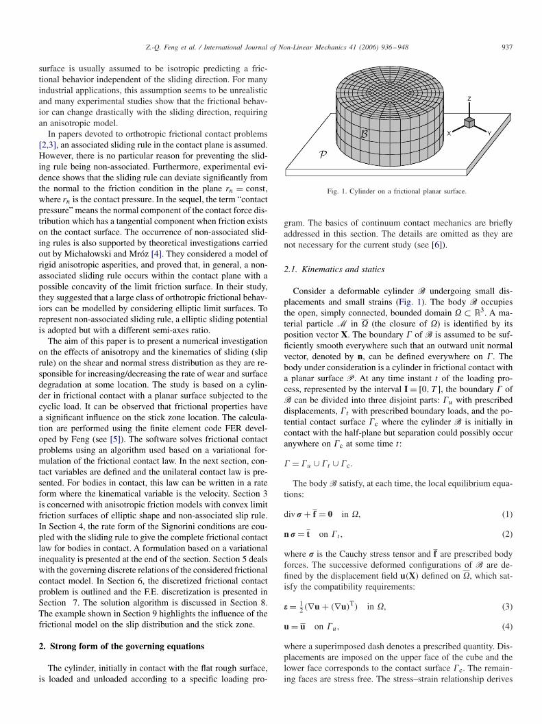
International Journal of Non-Linear Mechanics 41 (2006) 936–948www.elsevier.com/locate/nlm

Influence of frictional anisotropy on contacting surfaces duringloading/unloading cycles

Z.-Q. Fenga, M. Hjiajb,∗, G. de Saxcéc, Z. Mrózd

aLaboratoire de Mécanique d’Evry, Université d’Evry-Val d’Essonne, 40 rue du Pelvoux, 91020 Evry Cedex, FrancebLGCGM-INSA de Rennes, 20, avenue des Buttes de Coësmes, 35043 Rennes Cedex, France

cLaboratoire de Mécanique de Lille CNRS/UMR 8107, Boulevard Paul Langevin, F-59655 Villeneuve d’Ascq Cedex, FrancedInstitute of Fundamental Technological Research, Polish Academy of Sciences, Swietokrzyska 21, 00-049 Warsaw, Poland

Received 2 October 2004; received in revised form 24 May 2005; accepted 27 July 2006

Abstract

This paper presents numerical investigations on the loading and unloading of a three-dimensional body in frictional contact with a rigidfoundation. The evolution of the sliding process during loading/unloading cycles is analyzed. The important case of anisotropy is examinedalong with the effect of the sliding rule. The solution algorithm is based on a variational inequality which combine the contact problem andthe frictional problem. The numerical results of the punch problem show the hysteretic and irreversible behavior occurring when friction isanisotropic.� 2006 Elsevier Ltd. All rights reserved.

Keywords: Elliptic friction criterion; Non-associated slip rule; Variational formulation; Uzawa algorithm; Cyclic loading

1. Introduction

In many tribological applications contacting surfaces areloaded not just once but for several thousands of cycles. There-fore, understanding the behavior of a contacting surface thatundergoes a large number of load cycles is essential in orderto get a better insight into the wearing process. Because en-gineering surfaces are rough, friction will take place. Furtherfriction is known to be very sensitive to surface roughness pat-tern which can change from point to point. The roughness of anengineering surface is caused by the presence of protuberancescalled asperities and hollows.

Often friction is assumed to be constant and modelled us-ing the isotropic Coulomb model where the friction propertiesare independent of the sliding direction. However, the size andthe distribution of the asperities and hollows are not in prac-tice identical everywhere through the surface. The anisotropic

∗ Corresponding author. Tel.: +33 2 23 23 87 11; fax: +33 2 23 23 84 48.E-mail address: mohammed.hijaj@insa-rennes.fr (M. Hjiaj).

0020-7462/$ - see front matter � 2006 Elsevier Ltd. All rights reserved.doi:10.1016/j.ijnonlinmec.2006.08.002

friction is one whose properties varies with direction of sliding.From a physical point of view, anisotropy of friction and wearresults from the roughness anisotropy of contacting surfaces andfrom anisotropy and heterogeneity present in many materialsdue to their particular structure. An anisotropic surface rough-ness is then a surface in which highs and hollows in the surfaceare clearly oriented. The source of the roughness anisotropy istechnological; the industrial process used to fabricate the bod-ies can create striations along preferential directions. In fact,most machining, finishing and superfinishing operations are di-rectional, and machined surfaces have particular striation pat-terns unique to type of machining. Also specific techniques ofmanufacture produce a surface with anisotropic frictional prop-erties. For a large number of machining processes, the striationdirections are mutually orthogonal. For such surfaces, an or-thotropic friction condition will provide a better description ofthe frictional behavior.

A friction model is completely defined by the friction con-dition which specify a set of admissible contact forces andthe sliding rule which stipulates what directions of sliding areallowed. More sophisticate models which take into account thesliding path have been developed by Zmitrowicz [1]. The limit

Z.-Q. Feng et al. / International Journal of Non-Linear Mechanics 41 (2006) 936–948 937

surface is usually assumed to be isotropic predicting a fric-tional behavior independent of the sliding direction. For manyindustrial applications, this assumption seems to be unrealisticand many experimental studies show that the frictional behav-ior can change drastically with the sliding direction, requiringan anisotropic model.

In papers devoted to orthotropic frictional contact problems[2,3], an associated sliding rule in the contact plane is assumed.However, there is no particular reason for preventing the slid-ing rule being non-associated. Furthermore, experimental evi-dence shows that the sliding rule can deviate significantly fromthe normal to the friction condition in the plane rn = const,where rn is the contact pressure. In the sequel, the term “contactpressure” means the normal component of the contact force dis-tribution which has a tangential component when friction existson the contact surface. The occurrence of non-associated slid-ing rules is also supported by theoretical investigations carriedout by Michałowski and Mróz [4]. They considered a model ofrigid anisotropic asperities, and proved that, in general, a non-associated sliding rule occurs within the contact plane with apossible concavity of the limit friction surface. In their study,they suggested that a large class of orthotropic frictional behav-iors can be modelled by considering elliptic limit surfaces. Torepresent non-associated sliding rule, a elliptic sliding potentialis adopted but with a different semi-axes ratio.

The aim of this paper is to present a numerical investigationon the effects of anisotropy and the kinematics of sliding (sliprule) on the shear and normal stress distribution as they are re-sponsible for increasing/decreasing the rate of wear and surfacedegradation at some location. The study is based on a cylin-der in frictional contact with a planar surface subjected to thecyclic load. It can be observed that frictional properties havea significant influence on the stick zone location. The calcula-tion are performed using the finite element code FER devel-oped by Feng (see [5]). The software solves frictional contactproblems using an algorithm used based on a variational for-mulation of the frictional contact law. In the next section, con-tact variables are defined and the unilateral contact law is pre-sented. For bodies in contact, this law can be written in a rateform where the kinematical variable is the velocity. Section 3is concerned with anisotropic friction models with convex limitfriction surfaces of elliptic shape and non-associated slip rule.In Section 4, the rate form of the Signorini conditions are cou-pled with the sliding rule to give the complete frictional contactlaw for bodies in contact. A formulation based on a variationalinequality is presented at the end of the section. Section 5 dealswith the governing discrete relations of the considered frictionalcontact model. In Section 6, the discretized frictional contactproblem is outlined and the F.E. discretization is presented inSection 7. The solution algorithm is discussed in Section 8.The example shown in Section 9 highlights the influence of thefrictional model on the slip distribution and the stick zone.

2. Strong form of the governing equations

The cylinder, initially in contact with the flat rough surface,is loaded and unloaded according to a specific loading pro-

Fig. 1. Cylinder on a frictional planar surface.

gram. The basics of continuum contact mechanics are brieflyaddressed in this section. The details are omitted as they arenot necessary for the current study (see [6]).

2.1. Kinematics and statics

Consider a deformable cylinder B undergoing small dis-placements and small strains (Fig. 1). The body B occupiesthe open, simply connected, bounded domain � ⊂ R3. A ma-terial particle M in � (the closure of �) is identified by itsposition vector X. The boundary � of B is assumed to be suf-ficiently smooth everywhere such that an outward unit normalvector, denoted by n, can be defined everywhere on �. Thebody under consideration is a cylinder in frictional contact witha planar surface P. At any time instant t of the loading pro-cess, represented by the interval I = [0, T ], the boundary � ofB can be divided into three disjoint parts: �u with prescribeddisplacements, �t with prescribed boundary loads, and the po-tential contact surface �c where the cylinder B is initially incontact with the half-plane but separation could possibly occuranywhere on �c at some time t :

� = �u ∪ �t ∪ �c.

The body B satisfy, at each time, the local equilibrium equa-tions:

div � + f = 0 in �, (1)

n � = t on �t , (2)

where � is the Cauchy stress tensor and f are prescribed bodyforces. The successive deformed configurations of B are de-fined by the displacement field u(X) defined on �, which sat-isfy the compatibility requirements:

� = 12 (∇u + (∇u)T) in �, (3)

u = u on �u, (4)

where a superimposed dash denotes a prescribed quantity. Dis-placements are imposed on the upper face of the cube and thelower face corresponds to the contact surface �c. The remain-ing faces are stress free. The stress–strain relationship derives

938 Z.-Q. Feng et al. / International Journal of Non-Linear Mechanics 41 (2006) 936–948

Fig. 2. Kinematics of contact.

from a convex quadratic elastic energy potential V (�)

� = �V (�)

��. (5)

The potential V (�) and its complementary W(�) satisfy thefollowing inequality:

V (�) + W(�)�� · � (6)

which becomes a strict equality for pairs (�, �) related by theconstitutive law.

2.2. Contact mechanics

Prior to loading, the lower face of the cylinder is in full con-tact with the rigid plane P. The loading starts with a uniformvertical motion of the upper face which will maintain the cylin-der in contact with the planar surface during the subsequentloading cycles. At each time instant, contact conditions must befulfilled and material points in contact with P must not crossthe half-plane. On the surface P, an orthogonal vector n di-rected towards B is defined (see Fig. 2). The unit normal ncoincide here with the unit vector associated with the z-axis ofthe coordinate system. Within the half-plane P two unit vectorstx and ty are defined such that with n, they form an orthogo-nal local basis. Several options are possible for setting up thebase vectors, depending on a particular choice of the unit tan-gent vectors. A natural choice for the unit tangent vectors is theprincipal orthotropy directions. The relative slip velocity cor-responds to the cylinder velocity u since the planar surface ismotionless. As a result of the external loading a contact forcedistribution equilibrating the loads is developed. The surfacetraction vector r∗ at a material point M ∈ �c is given by

r∗ = �n. (7)

The contact force distribution r∗ acts on the half-plane P. Ac-cording to the principle of action and reaction, the cylinder Bis subjected to

r = −�n. (8)

In the local coordinate system defined by the plane P and thenormal n, any variable u or r may be uniquely decomposed

into normal and tangential components according to

u = ut + unn, ut ∈ P, un ∈ R, (9)

r = rt + rnn, rt ∈ P, rn ∈ R. (10)

The frictional force rt is dissipative and always opposes sliding(see Fig. 2). To emphasis that the dissipation is positive, thevelocity u will be preceded by a “minus” sign (–u). The unilat-eral contact condition requires that material points X ∈ �c areeither in contact or not in contact with the plane P. Therefore,the body B is allowed to separate but not to cross the planeP. This condition constraints the displacement of the body Bby requiring that the normal component of the displacement ofmaterial points located at the boundary �c is non-negative. Inthe problem under consideration, the lower face of the cube re-main in contact with the planar surface during the whole load-ing process. Using the above decomposition and taken into ac-count that the initial gap (distance between the cylinder andthe planar surface projected on the normal) is null, the non-penetration condition can be expressed by

−un �0. (11)

A dual relation involves the contact pressure rn acting on theblock which must be positive (rn �0), where there is contactand zero where there is no contact. This condition is oftenreferred to the non-adhesion condition. This set of relationsmay be summarized by the so-called Signorini conditions:

−un �0, rn �0, unrn = 0 (12)

which has to be satisfied at each time instant t ∈ I. In themore general case of two bodies that may come into contact,the previous relations must take into account an initial normalgap existing between contacting bodies. This normal gap isdetermined by calculating the proximal points (nearest point).In the case of persistent contact (un = 0), the unilateral contactlaw can be formulated in a rate form:

−un �0, rn �0, unrn = 0 on �c. (13)

The relation (13a) imposes that bodies in contact must eitherremain in contact (un = 0) or must separate (un > 0). The rateformulation of the Signorini conditions (13) can be combinedwith the sliding rule to derive the full frictional contact law ap-plicable to material points of �c already in contact. This com-plete law specifies allowable velocities of these points such thatimpenetrability, non-adhesion and the sliding rule are satisfied.In a more general situation, a positive gap may appear (un > 0).In that case, the normal relative velocity is arbitrary (un ∈ R)

and the normal reaction force is equal to zero (rn = 0). Theequations developed above need to be completed by a set ofrelations specifying the friction model and the slip rule.

3. Elliptical friction models

A rate-independent friction model with a linear dependenceof the limit tangential force on the normal force is considered.A theoretical investigation on friction surfaces and sliding rules

Z.-Q. Feng et al. / International Journal of Non-Linear Mechanics 41 (2006) 936–948 939

has been carried out by Michałowski and Mróz [4] (see also[7]). Their study, based on a model of rigid anisotropic asperi-ties to model surface roughness, shows that level curves of thesliding potential could be slightly non-convex but can be ap-proximated accurately by ellipses. Further the friction criterioncan have an arbitrary shape, possibly non-convex too. Accord-ingly the sliding velocity is no longer normal to the frictioncone in the contact plane (rn = const), as it is often assumed.This means that the frictional contact relation becomes non-associated with respect to both components, the normal and thetangential one. This feature will make the frictional contact re-lations (already highly non-linear) more complicate and resultsin extra numerical difficulties.

A family of anisotropic friction models, described by a fric-tion criterion and a sliding potential of elliptic shape (in theplane rn = const) but with different semi-axes ratio are con-sidered. The principal axes of both ellipses coincide with theorthotropy axes x and y. A non-associated sliding rule is thenobtained by simply choosing different semi-axes ratio for thefriction criterion and the sliding potential. Therefore, the slidingrule is no longer associated with the limit friction condition inthe plane rn = const as it occurs when the sliding potential co-incides (up to an arbitrary constant) with the friction conditionfor a known contact pressure. Such models, although simple,provide a valuable insight into the character of limit frictionand sliding rules.

3.1. Friction criterion

The asperity model used by Michałowski and Mróz ([4]) tostudy anisotropic frictional contact phenomenon generates limitfriction curves that can be accurately approximated by ellipses.The generic form of such convex friction criterion is given by

f (rtx , rty , rn) = ‖rt‖� − rn = 0, (14)

where ‖ • ‖� denotes the elliptic norm

‖rt‖� =√√√√( rtx

�x

)2

+(

rty

�y

)2

. (15)

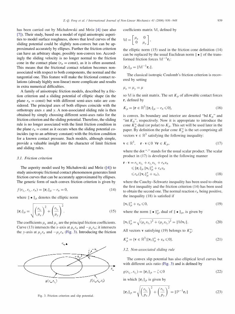
The coefficients �x and �y are the principal friction coefficients.Curve (13) intersects the x-axis at �xrn and −�xrn; it intersectsthe y-axis at �yrn and −�yrn (Fig. 3). Introducing the friction

Fig. 3. Friction criterion and slip potential.

coefficients matrix M, defined by

M =[�x 00 �y

],

the elliptic norm (15) used in the friction cone definition (14)can be replaced by the usual Euclidean norm ‖ • ‖ of the trans-formed friction forces M−1rt :

‖rt‖� = ‖M−1rt‖.

The classical isotropic Coulomb’s friction criterion is recov-ered by setting

�x = �y = �

so M is the unit matrix. The set K� of allowable contact forcesr, defined by

K� = {r ∈ R3|‖rt‖� − rn �0}, (16)

is convex. Its boundary and interior are denoted “bd K�” and“int K�”, respectively. Now it is appropriate to introduce thecone K∗

� dual (or polar) to K�. This set will be used later in thepaper. By definition the polar cone K∗

� is the set comprising all

vectors v ∈ R3 satisfying the following inequality:

v ∈ R3, r · v�0 ∀r ∈ K�, (17)

where the dot “·” stands for the usual scalar product. The scalarproduct in (17) is developed in the following manner

r · v = rtx vtx + rty vty + rnvn

�‖rt‖� ‖vt‖∗� + rnvn

�rn(‖vt‖∗� + vn), (18)

where the Cauchy–Schwartz inequality has been used to obtainthe first inequality and the friction criterion (14) has been usedto obtain the second one. The normal reaction rn being positive,the inequality (18) is satisfied if

‖vt‖∗� + vn �0, (19)

where the norm ‖ • ‖∗�, dual of ‖ • ‖�, is given by

‖vt‖∗� =

√(�xvtx )

2 + (�yvty )2 = ‖Mvt‖. (20)

All vectors v satisfying (19) belongs to K∗� :

K∗� = {v ∈ R3|‖vt‖∗

� + vn �0}. (21)

3.2. Non-associated sliding rule

The convex slip potential has also elliptical level curves butwith different axis ratio (Fig. 3) and is defined by

g(rtx , rty ) = ‖rt‖p − ��0 (22)

in which ‖rt‖p is given by

‖rt‖p =√(

rtx

px

)2

+(

rty

py

)2

= ‖P−1rt‖ (23)

940 Z.-Q. Feng et al. / International Journal of Non-Linear Mechanics 41 (2006) 936–948

with

P =[px 00 py

](24)

and � is a constant whose magnitude is irrelevant. The semi-axes ratio of the slip potential is related to that of the frictioncondition by the following relation

py

px

=(

�y

�x

)k

. (25)

In the general case, we have k = 1, which leads to a non-associated sliding rule

−un = 0, (26)

−utx = ��g

�rtx= �

rtx

p2x ‖rt‖p

, (27)

−uty = ��g

�rty= �

rty

p2y ‖rt‖p

, (28)

where the multiplier � is equal to

� =√

p2xu

2tx

+ p2yu

2ty

= ‖ut‖∗p. (29)

Equivalently, the sliding rule can be written as

−utx = �′ rtx

p2x‖rt‖�

, −uty = �′ rty

p2y ‖rt‖�

. (30)

In this case, the multiplier �′

is equal to

�′ = ‖Q(ut )‖∗

p, (31)

where

Q = PM−1 = M−1P =⎡⎢⎣

px

�x

0

0py

�y

⎤⎥⎦ (32)

is called the sliding non-associativity matrix.

4. Frictional contact law

The frictional contact law aims at describing contact in-teractions. To derive this relationship, we add the geometricconstraints (impenetrability condition) to the friction law. Thesliding rule is then combined with the rate form of the uni-lateral contact conditions so we obtain the frictional contactlaw.

4.1. Analytical formulation

The complete form of the frictional contact law deals with thethree possible physical situations, which are separation, contactwith sticking, and contact with sliding. Mechanical dissipationoccurs only for the last case. This law is applicable only tomaterial points in contact. Two overlapped “if . . . then . . . else”

statements can be used to write it analytically (Box 1):

Box 1

if rn = 0 then! separation−un �0

elseif r ∈ int K� then! stickingun = 0 and ut = 0

else (r ∈ bd K� and rn > 0)! sliding

un = 0 and −ut• = �

p2•rt•

‖rt‖p

, � > 0

endif

In the first and the second part of the statement, the multi-valued character of the frictional contact constitutive model isrevealed. If rn is null then the velocity u is arbitrary but itsnormal component un should be positive. In other words, aninfinite number of velocity vectors u ∈ R3 are related to thesingle contact force r = 0. Further, if −u is null then the re-action r should be in K� but its direction or magnitude arenot specified. They are arbitrary. Again, one element of R3

( −u = 0) can be related to an infinite number of r ∈ R3. Theinverse constitutive frictional contact law, i.e. the relationshipr(−u) can be written as (Box 2):

Box 2

if un > 0 then! separationrn = 0

elseif u = 0 then! stickingr ∈ K�

else (u ∈ T − {0})! sliding

rn > 0 and rt• = −rnp2• ut•

‖Q(−ut )‖∗p

endif

Similar considerations regarding the multi-valued characterof the relationship can be drawn for the inverse law.

4.2. Inequality-based formulation

The previous forms of the frictional contact law, given inBoxes 1 and 2, could be very well used in numerical imple-mentations where the contact problem is dissociated from thefriction problem. This class of algorithm has been very muchdeveloped. However ones can expect that a coupled algorithmwhere both problems are solved in a single step could improvethe computational performances and robustness. With this aimin mind, the frictional contact law need to be reformulated.The main idea behind this reformulation is to provide a natural

Z.-Q. Feng et al. / International Journal of Non-Linear Mechanics 41 (2006) 936–948 941

basis for the application of the Uzawa algorithm where a singleprojection will be performed.

The slip rule, as written in relations (26)–(28), exhibits astructure similar to the non-associated flow rule in plasticityeven if the slip rule is associated. Indeed, during sliding, contactis maintained. Therefore the normal velocity, which is equal tozero (un = 0), is not related to the normal component of thereaction rn through normality. In fact, if we regard the contactforce r and the velocity −u as conjugate quantities of eachother and consider an associate slip rule, the normality willnot occur since it would require that the velocity would have anormal separating component.

During sliding, the components of the velocity vector aregiven by

−un = 0, −Q2(ut ) = �′ �f (r)

�rt

(33)

but can be rewritten in the following obvious way:

−(un + �′) = �

′ �f

�rn, −Q2(ut ) = �

′ rt

‖rt‖�, (34)

where � is obtained after eliminating the tangential reactioncomponents from the slip rule:

�′ = ‖Q2(ut )‖∗

�. (35)

Indeed the first relation of (34) yields back −un = 0, that isduring sliding contact must hold. An obvious vector additiongives:

−(Q2(ut ) + (un + �′)n) = �

′grad f . (36)

The gradient vector is unique everywhere except at the apex(r = 0) where the friction criterion is not differentiable. Thenon-differentiability issue is addressed simply by replacing thegradient operator by the subgradient one (see [8]):

−(Q2(ut ) + (un + ‖Q2(ut )‖∗�)n) ∈ �f (r). (37)

The above relationship, called differential inclusion, is a con-densed formulation of the frictional contact relationship whichis appropriate everywhere on the friction cone, including theapex. Whenever the f (r) is differentiable, the subdifferentialoperator will coincide with the gradient operator. Let us intro-duce now the following vector:

v = vt + vnn (38)

with

vt = −Q2(ut ), vn = −(un + ‖Q2(ut )‖∗�) (39)

and rewrite (39) as

v ∈ �f (r). (40)

The differential inclusion (40), is equivalent to the follow-ing inequality, known as the convexity inequality for non-differentiable function (see [8]):

f (r′)�f (r) + (r′ − r) · v ∀r′ ∈ R3. (41)

Taking into account that

f (r′)�f (r) (42)

inequality (41) reduces to

r ∈ K� : (r − r′) · v�0 ∀r′ ∈ K�. (43)

In particular, at the apex (r = 0) we have

r′ · v�0 ∀r′ ∈ K�. (44)

Accordingly at the apex, any vector v belonging the cone K∗� is

an admissible velocity, i.e. it is related to r=0 through the fric-tional contact law. Indeed, it can be easily checked by combin-ing the definition of v (38)–(39) and K∗

� (21) that such vectordoes not violate the non-penetration condition. The inequalityformulation of the frictional contact law (43) provides the basisto derive projection-type algorithms.

5. Discrete frictional contact law

The inequality developed in the previous section is now dis-cretized so it can be used during the local stage where the reac-tion are computed. The time interval [ 0, T ] is partitioned intoN sub-intervals of size �t , not necessarily equal, according to

0 = t0 < t1 < · · · < tn−1 < tn < · · · < tN = T .

We set �n=�(tn) and ��=�n−�n−1, where � represents anyvariable. Between two time instants, the velocity is assumedto be constant. In order to ensure convergence and stabilityrequirements, the implicit scheme is considered. As a resultof a backward-Euler-type approximation of (43), the frictionalcontact law is satisfied at the end of each time step:{

rn+1 ∈ K� such that�v · (r′ − rn+1)�0 ∀ r′

t ∈ K�,(45)

where the components of the vector �v are given by

�vt = −Q2�ut , �vn = −(�un + ‖Q2�ut‖∗�).

The previous inequality can be transformed into a projectioninequality{

Find rn+1 ∈ K� such that(rn+1 − �) · (r′ − rn+1)�0 ∀ r′ ∈ K�,

(46)

where the vector � is given by

� ={

�t

�n

}(47)

with

�t = rn+1t − Q2�ut (48)

and

�n = rn+1n − (�un + ‖Q2�ut‖∗

�). (49)

942 Z.-Q. Feng et al. / International Journal of Non-Linear Mechanics 41 (2006) 936–948

The last inequality (46) means that the reaction at the end ofthe time step is the projection of the augmented surface traction� onto the convex Coulomb’s cone K�:

rn+1 = proj(�, K�). (50)

Three different situations emerge according to the position ofthe prediction in the forces space. The first case correspondsto a prediction located in the cone K�. Its projection is theprediction itself, i.e. rn+1 = �. The second one relates to aprediction situated in the cone K∗

� , where its projection turns

out to be the origin of the forces space, i.e. rn+1 =0. In the lastcase, the prediction is neither in K� nor in K∗

� and the correctorstep requires computing the projection of the prediction. Theprojection of a point onto a convex set is equivalent to theminimization of the distance between this point and the convexset. In the present situation (orhtotropic friction condition), itleads to a quartic equation that has one positive root. The detailsof the derivation can be found in [9].

6. Finite-step boundary value problem and variationalformulation

The solution of the elastic frictional-contact initial boundaryvalue problem, under a given history of external actions, re-quires following the evolution of the body response since thefrictional contact law is intrinsically path-dependent. A numer-ical technique, which combines a space and time discretization,is used to solve this problem. The time discretization is basedon a subdivision of the external actions history into a sequenceof loading conditions at selected time instants. The solutionis then achieved by solving a sequence of problems in whichthe load increments are applied and the variables at the end ofeach increment are updated. We suppose that the solution of

the problem is known at time tn. Given the body force fn+1

,the surface traction tn+1

and the imposed displacement un+1,it is required to solve the governing equations listed below:

• in �:

div �n+1 + fn+1 = 0, (51)

�n+1 = 12 (∇un+1 + (∇un+1)T), (52)

�n+1 = �W(�)

��

∣∣∣∣n+1

, (53)

• on �t :

�n+1n = tn+1, (54)

• on �u:

u = un+1, (55)

• on �c:

rn+1 = proj(�(�u), K�). (56)

The standard approach to derive the principle of virtual workover an increment consists in taking the inner product of the

local equilibrium equation (51) with a test function u satis-fying u = 0 on �u and un �0 on �c (virtual displacementincrement):∫�

div �n+1 · u d� +∫�

fn+1 · u d� = 0. (57)

Integrating by parts the first term and taking into account theboundary conditions leads to the following variational equation:∫

��n+1 · � d� −

∫�

fn+1 · u d�

−∫�t

tn+1 · u d� −∫�c

rn+1 · u d� = 0. (58)

Taking into account that the stress filed is in equilibrium at tn,the weak form can be written in terms of finite increments asfollows:

{∫�

�W(��) d� −∫�

�f · �u d�

−∫�t

�t · �u d� −∫�c

�r · �u d�

}= 0. (59)

If the behavior on contact surface is frictionless, the functional(59) becomes with the classical energy functional:

{∫�

�W(��) d� −∫�

�f · �u d�

−∫�t

�t · �u d�

}= 0. (60)

7. Finite element discretization

The displacement increment field and the transformation gra-dient are approximated according to

�u = N(X)�U, (61)

where �U is the unknown nodal displacement increment vector,N(X) is the matrix of polynomial shape functions and the matrixB(X) is given by

B(X) = �N(X)

�X.

The compatibility conditions (55) on �u are enforced by sub-stituting nodal unknowns by their corresponding values. Takinginto account (61), the fully discrete form of the functional isgiven by∫�

�W(��(Un, �U)) d� − �Fext · �U − �R · �U, (62)

where �Fext corresponds to the generalized nodal force incre-ment vector

�Fext =∫�

NT�f d� +∫�t

NT�t d� (63)

and �R is the equivalent contact reaction increment vector atnodes. The equilibrium equations over a time step are given by∫�

��W(��(Un, �U))

��Ud� − �Fext − �R = 0. (64)

Z.-Q. Feng et al. / International Journal of Non-Linear Mechanics 41 (2006) 936–948 943

Combining the structural equilibrium equations (64) with theincremental frictional contact constitutive relation (56), the so-lution of the boundary value problem over a time step is ob-tained by solving the following system of equations:

Find �U and �R satisfying:

K�U − �Fext − �R = 0, (65)

Rn+1 = proj(�(�U), K�) on �c, (66)

�U = �U on �u. (67)

8. Solution algorithm

The system of equations (65)–(67) has to be solved itera-tively since the displacement increment vector, the contact sur-face and the reactions �R are unknown. The solution algo-rithm (see Box 3) tackle separately the equilibrium equationsand the contact non-linearities. At the beginning of each loadstep, �R is set equal to zero and �U is computed accordingto (66). Having an estimate of the displacement increment, thereactions have to be computed and the penetration that has oc-curred by assuming �R=0 must be corrected. This is achievedby applying the Uzawa iterative scheme as shown in Box 3.This procedure involves only variables associated with contactnodes. In contrast with classical methods (penalty, Lagrangemultiplier, see [10,11]), the present algorithm does not requirean update of the global stiffness matrix during the contact it-erations. Furthermore the total number of degree of freedomremain unchanged.

Box 3

• Read the problem data• Assemble the stiffness matrix K• Modify K for essential boundary conditions

For Each Load Step:• Initialisation: �U0 = 0 and �R0 = 0• Compute the external load vector: �Fext

• Detect contact node using a gap function• Solve: �U = K−1(�Fext + �R0)

On �c

• Initialisation: �R0 = 0• Contact Loop k : 0 → m

�Uk+1 = W�Rk

�Rk+1 = proj(�k+1(�Uk+1), K�) − Rn

Convergence?: k = k + 1• Solve: �U = K−1(�Fext + �R)

• Update: U = U + �U, R = R + �R

The displacement increments on the contact surface are com-puted using the flexibility matrix W, defined in the local coor-dinate system by

W =[

wnn wntx wnty

wntx wtxx wntx

wnty wtxy wtyy

].

Next, the prediction � is computed and projected on the coneK� to give the reaction (see Box 3). The Uzawa algorithm isknown for being convergent but requiring quite a few iterations.The convergence rate strongly depends on the regularizationfactor . A good choice is crucial to ensure that the algorithmwill convergence within a few iterations. Our experience hasshown that a different factor for each contact node gives abetter convergence. In our calculations, the factor is calculatedusing the diagonal terms of the flexibility matrix:

= 1

min(wnn, wtxx , wtyy ).

This choice has proven to be satisfactory for most of the cases.

9. Numerical application

The numerical strategy detailed in the previous sections hasbeen applied successfully to a wide range of problems involv-ing an isotropic friction condition with associated sliding rule(see Refs. [12–14]). The examples treated have shown that thealgorithm is very competitive as the augmentation phase in-volves only one prediction-correction step. The present appli-cation is a further test of the algorithm robustness when thefriction criterion is anisotropic, the slip rule is non-associatedand unloading occurs. The results show the strong influenceof the frictional properties on the stick zone and therefore thecontact (normal and tangential) stress distribution.

The problem under consideration is a deformable elasticcylinder in contact with a rigid surface (Fig. 1). The radius andthe height of the cylinder are both equal to 10 mm. The Youngmodulus E of the cylinder is taken equal to 210 000 MPa andthe Poisson ratio is 0.3. On the surface contact, the friction con-dition is assumed to be anisotropic. The cylinder is subdividedinto 1280 eight-node brick-like elements as shown in Fig. 1.Each element has 27 integration points. The base of the cylin-der is in contact with the rigid plate whose normal vector is

Table 1Frictional properties and number of load cycles

Case �x �y px py Load cycle

A 0.20 0.20 0.20 0.20 1B 0.30 0.25 0.30 0.15 3C 0.30 0.15 0.05 0.20 1

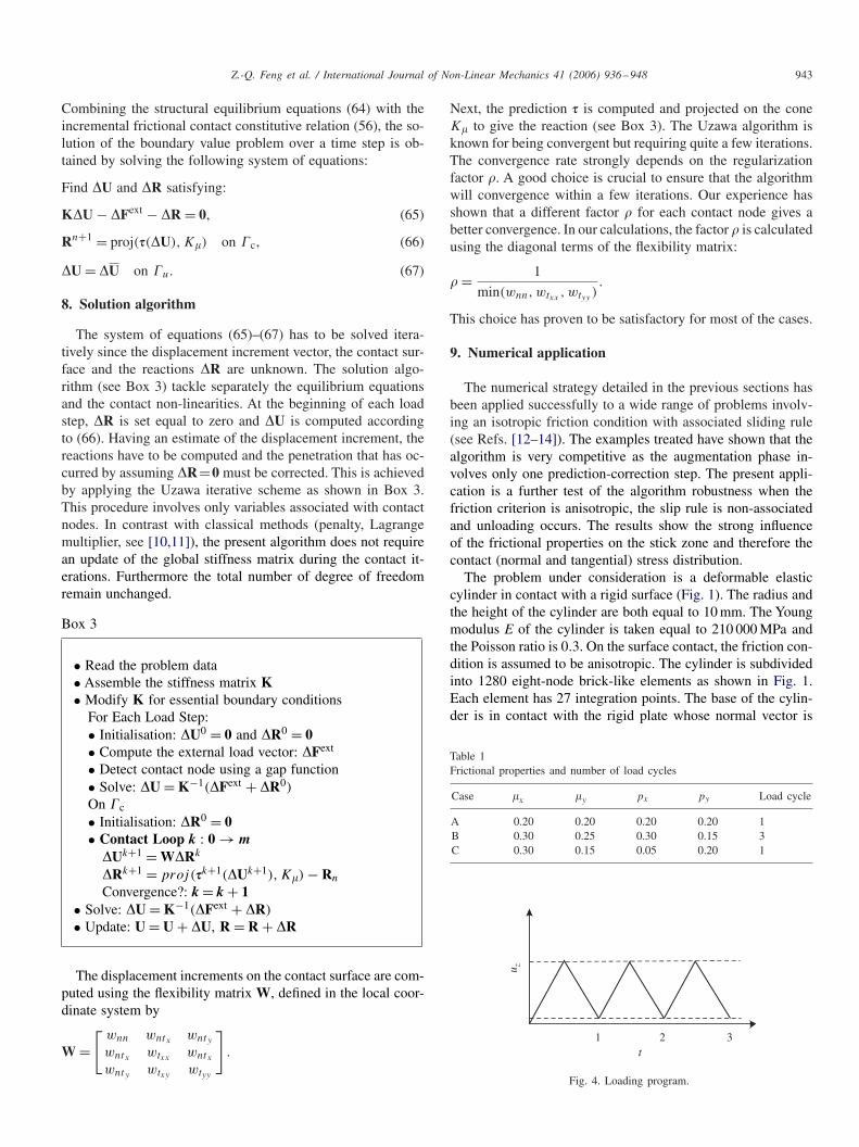
u z

t1 2 3

Fig. 4. Loading program.

944 Z.-Q. Feng et al. / International Journal of Non-Linear Mechanics 41 (2006) 936–948

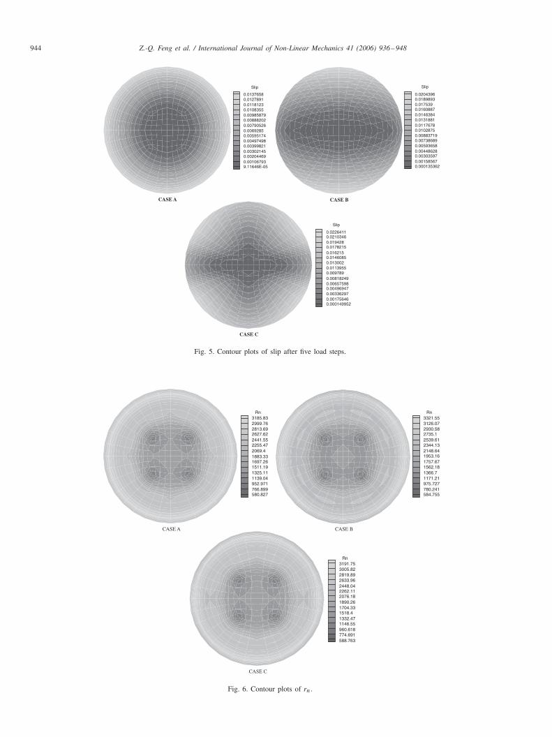
0.01376580.01278910.01181230.01083550.009858790.008882020.007905260.00692850.005951740.004974980.003998210.003021450.002044690.001067939.11646E-05

Slip Slip

0.02043960.01898930.0175390.01608870.01463840.01318810.01176780.01028750.008837190.007386890.005936580.004486280.003035970.001585670.000135362

Slip

0.02264110.02103460.0194280.01782150.0162150.01460850.0130020.01139550.0097890.008182490.006575980.004969470.003362970.001756460.000149952

CASE A CASE B

CASE C

Fig. 5. Contour plots of slip after five load steps.

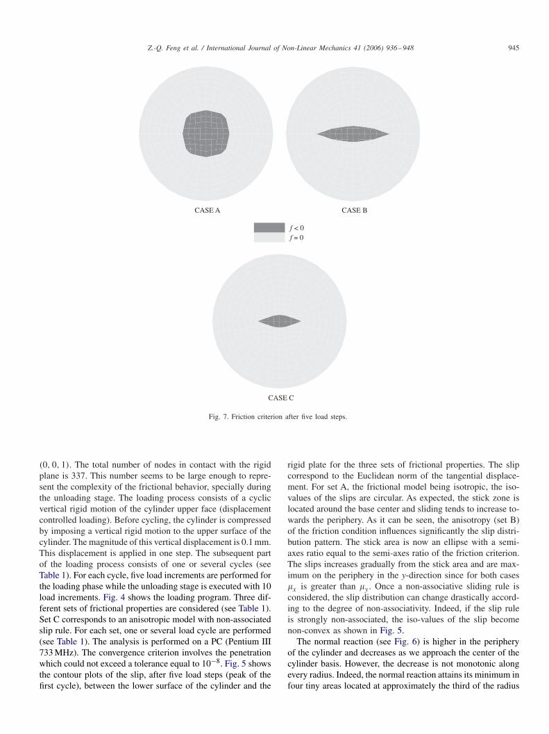
Rn3185.832999.762813.692627.622441.552255.472069.41883.331697.261511.191325.111139.04952.971766.899580.827

Rn3321.553126.072930.582735.12539.612344.132148.641953.161757.671562.181366.71171.21975.727780.241584.755

Rn3191.753005.822819.892633.962448.042262.112076.181890.261704.331518.41332.471146.55960.618774.691588.763

CASE A CASE B

CASE C

Fig. 6. Contour plots of rn.

Z.-Q. Feng et al. / International Journal of Non-Linear Mechanics 41 (2006) 936–948 945

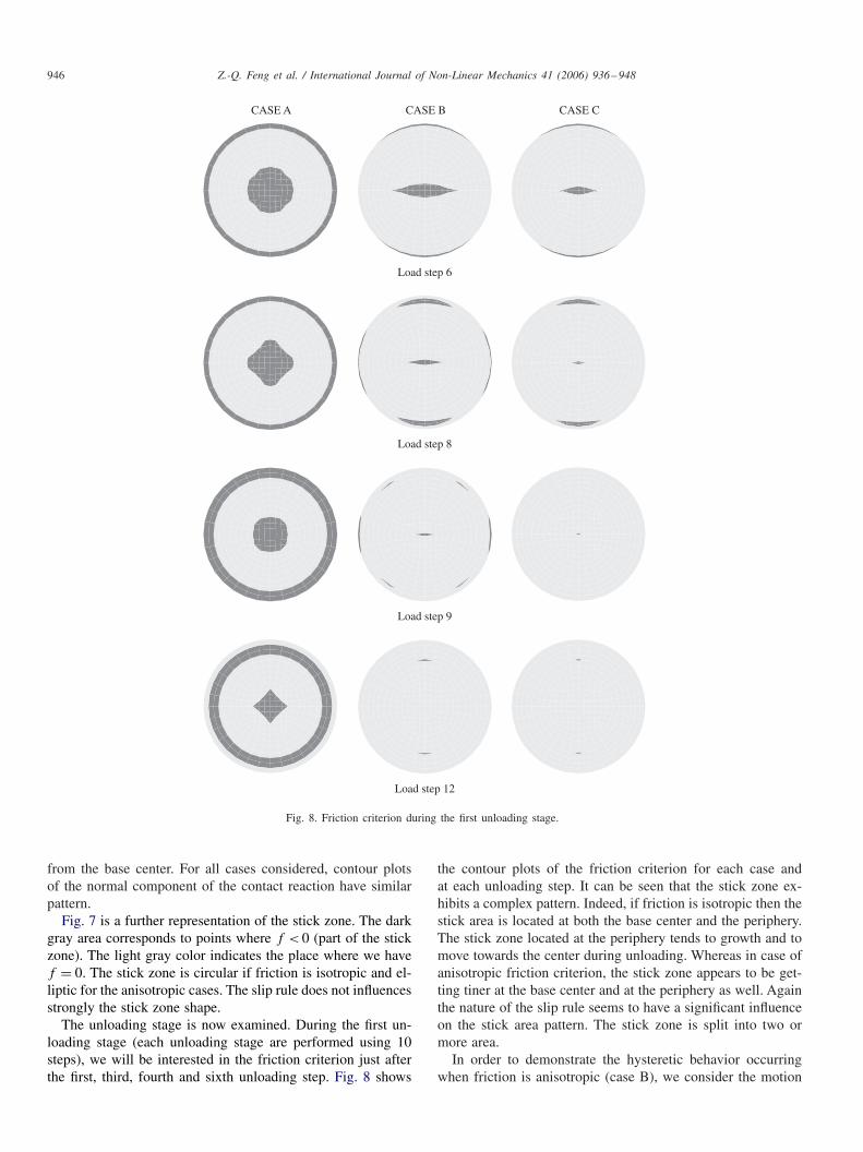
f < 0f = 0

CASE A CASE B

CASE C

Fig. 7. Friction criterion after five load steps.

(0, 0, 1). The total number of nodes in contact with the rigidplane is 337. This number seems to be large enough to repre-sent the complexity of the frictional behavior, specially duringthe unloading stage. The loading process consists of a cyclicvertical rigid motion of the cylinder upper face (displacementcontrolled loading). Before cycling, the cylinder is compressedby imposing a vertical rigid motion to the upper surface of thecylinder. The magnitude of this vertical displacement is 0.1 mm.This displacement is applied in one step. The subsequent partof the loading process consists of one or several cycles (seeTable 1). For each cycle, five load increments are performed forthe loading phase while the unloading stage is executed with 10load increments. Fig. 4 shows the loading program. Three dif-ferent sets of frictional properties are considered (see Table 1).Set C corresponds to an anisotropic model with non-associatedslip rule. For each set, one or several load cycle are performed(see Table 1). The analysis is performed on a PC (Pentium III733 MHz). The convergence criterion involves the penetrationwhich could not exceed a tolerance equal to 10−8. Fig. 5 showsthe contour plots of the slip, after five load steps (peak of thefirst cycle), between the lower surface of the cylinder and the

rigid plate for the three sets of frictional properties. The slipcorrespond to the Euclidean norm of the tangential displace-ment. For set A, the frictional model being isotropic, the iso-values of the slips are circular. As expected, the stick zone islocated around the base center and sliding tends to increase to-wards the periphery. As it can be seen, the anisotropy (set B)of the friction condition influences significantly the slip distri-bution pattern. The stick area is now an ellipse with a semi-axes ratio equal to the semi-axes ratio of the friction criterion.The slips increases gradually from the stick area and are max-imum on the periphery in the y-direction since for both cases�x is greater than �y . Once a non-associative sliding rule isconsidered, the slip distribution can change drastically accord-ing to the degree of non-associativity. Indeed, if the slip ruleis strongly non-associated, the iso-values of the slip becomenon-convex as shown in Fig. 5.

The normal reaction (see Fig. 6) is higher in the peripheryof the cylinder and decreases as we approach the center of thecylinder basis. However, the decrease is not monotonic alongevery radius. Indeed, the normal reaction attains its minimum infour tiny areas located at approximately the third of the radius

946 Z.-Q. Feng et al. / International Journal of Non-Linear Mechanics 41 (2006) 936–948

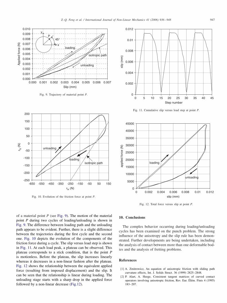
Load step 6

Load step 8

Load step 9

Load step 12

CASE A CASE B CASE C

Fig. 8. Friction criterion during the first unloading stage.

from the base center. For all cases considered, contour plotsof the normal component of the contact reaction have similarpattern.

Fig. 7 is a further representation of the stick zone. The darkgray area corresponds to points where f < 0 (part of the stickzone). The light gray color indicates the place where we havef = 0. The stick zone is circular if friction is isotropic and el-liptic for the anisotropic cases. The slip rule does not influencesstrongly the stick zone shape.

The unloading stage is now examined. During the first un-loading stage (each unloading stage are performed using 10steps), we will be interested in the friction criterion just afterthe first, third, fourth and sixth unloading step. Fig. 8 shows

the contour plots of the friction criterion for each case andat each unloading step. It can be seen that the stick zone ex-hibits a complex pattern. Indeed, if friction is isotropic then thestick area is located at both the base center and the periphery.The stick zone located at the periphery tends to growth and tomove towards the center during unloading. Whereas in case ofanisotropic friction criterion, the stick zone appears to be get-ting tiner at the base center and at the periphery as well. Againthe nature of the slip rule seems to have a significant influenceon the stick area pattern. The stick zone is split into two ormore area.

In order to demonstrate the hysteretic behavior occurringwhen friction is anisotropic (case B), we consider the motion

Z.-Q. Feng et al. / International Journal of Non-Linear Mechanics 41 (2006) 936–948 947

0.010

0.009

0.008

0.007

0.006

0.005

0.004

0.003

0.002

0.001

0.0000.000 0.001 0.002 0.003 0.004 0.005 0.006 0.007

App

lied

forc

e (N

)

Slip (mm)

loading

unloading

isotropic path

x

45°P

y

Fig. 9. Trajectory of material point P.

200

-200

-250-650 -550 -450 -350 -250 -150 -50 50 150

150

-150

100

-100

50

-50

0

r ty (

N)

rtx (N)

unloading

loadingisotropic path

Fig. 10. Evolution of the friction force at point P.

of a material point P (see Fig. 9). The motion of the materialpoint P during two cycles of loading/unloading is shown inFig. 9. The difference between loading path and the unloadingpath appears to be evident. Further, there is a slight differencebetween the trajectories during the first cycle and the secondone. Fig. 10 depicts the evolution of the components of thefriction force during a cycle. The slip versus load step is shownin Fig. 11. At each load peak, a plateau can be observed. Thisplateau corresponds to a stick condition, that is the point Pis motionless. Before the plateau, the slip increases linearlywhereas it decreases in a non-linear fashion after the plateau.Fig. 12 shows the relationship between the equivalent appliedforce (resulting from imposed displacement) and the slip. Itcan be seen that the relationship is linear during loading. Theunloading stage starts with a sharp drop in the applied forcefollowed by a non-linear decrease (Fig.12).

0.012

0.01

0.006

0.004

0.002

00 5 10 15 20 25 30 35 40 45

0.008

Step number

slip

(m

m)

Fig. 11. Cumulative slip versus load step at point P.

45000

40000

35000

30000

25000

20000

15000

10000

5000

0

appl

ied

forc

e (N

)

loading

unloading

0 0.002 0.004 0.006 0.008 0.01 0.012

slip (mm)

Fig. 12. Total force versus slip at point P.

10. Conclusions

The complex behavior occurring during loading/unloadingcycles has been examined on the punch problem. The stronginfluence of the anisotropy and the slip rule has been demon-strated. Further developments are being undertaken, includingthe analysis of contact between more than one deformable bod-ies and the analysis of fretting problems.

References

[1] A. Zmitrowicz, An equation of anisotropic friction with sliding pathcurvature effects, Int. J. Solids Struct. 36 (1999) 2825–2848.

[2] P. Alart, A. Heege, Consistent tangent matrices of curved contactoperators involving anisotropic friction, Rev. Eur. Élém. Finis 4 (1995)183–207.

948 Z.-Q. Feng et al. / International Journal of Non-Linear Mechanics 41 (2006) 936–948

[3] Q.-C. He, A. Curnier, Anisotropic dry friction between two orthotropicsurfaces undergoing large displacements, Eur. J. Mech. A/Solids 12(1993) 631–666.

[4] R. Michałowski, Z. Mróz, Associated and non-associated sliding rulesin contact friction problems, Arch. Mech. 30 (1978) 259–276.

[5] Z.-Q. Feng, P. Joli, N. Seguy, FER/Mecha software with interactivegraphics for dynamic analysis of multibody system, Adv. Eng. Software35 (2006) 1–8.

[6] P. Wriggers, Computational Contact Mechanics, Wiley, New York, 2002.[7] Z. Mróz, S. Stupkiewicz, An anisotropic friction and wear model, Int.

J. Solids Struct. 31 (1994) 1113–1131.[8] R.-T. Rockafellar, J-B. Wets, Variational Analysis, Springer, Berlin, 1998.[9] M. Hjiaj, Z.Q. Feng, G. de Saxcé, Z. Mróz, Three-dimensional finite

element computations for frictional contact problems with non-associatedsliding rule, Int. J. Numer. Methods Eng. 60 (2004) 2045–2076.

[10] P.W. Christensen, A. Klarbring, J.S. Pang, N. Strömberg, Formulationand comparison of algorithms for frictional contact problems, Int. J.Numer. Methods Eng. 42 (1998) 145–173.

[11] P. Alart, A. Curnier, A mixed formulation for frictional contact problemsprone to Newton-like solution methods, Comput. Methods Appl. Mech.Eng. 92 (1991) 353–375.

[12] G. de Saxcé, Z.-Q. Feng, New inequality and functional for contactfriction: the implicit standard material approach, Mech. Struct. Mach.19 (1991) 301–325.

[13] G. de Saxcé, Z-Q. Feng, The bi-potential method: a constructive approachto design the complete contact law with friction and improved numericalalgorithms, Math. Comput. Modelling 28 (1998) 225–245.

[14] Z.-Q. Feng, Some test examples of 2D and 3D contact problems involvingcoulomb friction and large slip, Math. Comput. Modelling 28 (1998)469–477.