An improved discrete element method basedon a variational formulation of the

frictional contact law

J. Fortina, M. Hjiajb,*,1, G. de Saxceb

aLaboratoire de Mecanique et CAO, IUT de Saint-Quentin, 48, rue d’Ostende, 02100 Saint-Quentin, FrancebLaboratoire de Mecanique de Lille, URA CNRS 1441, Boulevard Paul Langevin, Bat. M6, Cite scientifique,

59655 Villeneuve d’Ascq cedex, France

Received 8 June 2000; received in revised form 15 April 2002; accepted 2 May 2002

Abstract

An improved algorithm based on the contact dynamics approach is proposed. Like pre-vious developed algorithms it involves two stages. In the first one (local stage) for each parti-cle, forces are computed from the relative displacement using an interaction law, which

models frictional contact and shock. In the second stage (global stage) Newton’s second law isused to determine, for each particle, the resulting acceleration which is then time-integrated tofind the new particle positions. This process is repeated for each time step until convergence is

achieved. The two distinguishing features of the present algorithm are the local integration ofthe frictional contact law and the convergence criterion. By adopting a variational statementof the frictional contact law based on the bi-potential concept, the integration procedure is

reduced to a single predictor-corrector step and a new convergence criterion is introduced.Both aspects significantly reduce the computing time and enhance the convergence. Numericalapplications show the robustness of the algorithm. # 2002 Elsevier Science Ltd. All rightsreserved.

Keywords: Granular media; Contact dynamics; Discrete element method; Coulomb’s dry friction; Varia-

tional inequality

Computers and Geotechnics 29 (2002) 609–640

www.elsevier.com/locate/compgeo

0266-352X/02/$ - see front matter # 2002 Elsevier Science Ltd. All rights reserved.

PI I : S0266-352X(02 )00016 -2

* Corresponding author at present address. Tel.: +61-2-4921-5582; fax: +61-2-4921-6991.

E-mail address: mohammed.hjiaj@newcastle.edu.au (M. Hjiaj).1 Currently ARC Research Fellow at Civil Engineering, Faculty of Engineering and Built Environ-

ment, The University of Newcastle, University Drive, Callaghan, NSW 2308, Australia.

1. Introduction

Due to their particulate nature and random structure, granular materials areunique in their behavior in the sense that they can respond to external loads like aliquid, a solid or a gas. For example, a granular material flows under gravity like aliquid when it is poured from one container to another. However, unlike mostliquids, a granular material can sustain a shear stress whenever the confining stress isgreater than zero, as it is for a solid. The gas-like behavior of a granular assembly isdisplayed whenever a periodic force vibrates the granules.The behavior of granular assemblies is of central importance for a large number of

engineering disciplines, finding applications in soil mechanics, material handling andpowder technology, to name a few. For example, the stability of slopes underweight, the analysis of the settlement response of a soil under service loads and itsflow behavior under ultimate loads are central problems in soil mechanics. Granularflows, such as the movement during discharge of material from a hopper are ofspecial interest in material handling. Also, the pressure exerted by the material onthe container is of first importance in design of containers in material storage.It is the complex range of behavior that makes granular material difficult to

understand and explain why modeling such material is still a challenge. So far, mostmodels of granular materials are developed within the phenomenological frameworkthat considers the media as a continuum. Several constitutive models have beendeveloped, most of them for geotechnical applications. The implementation of suchconstitutive models in finite element codes allows predicting the soil behavior understructures subjected to loads. Although results of such analysis depend highly on themodel chosen, they can give pertinent information at the global level [4]. However,granular materials are difficult to class among the usual states of matter, namelysolids, liquids or gas. Consequently, the continuous model cannot capture the realbehavior of a granular media where the effects of micro-structure (distribution ofparticle size, friction coefficient,. .) on the overall response of granular media have astrong influence. A better understanding of the behavior of granular materials canbe achieved through a micro-mechanical approach that means a detailed analysis ofthe mechanical interactions between particles. There are naturally a large number ofmicroscopic parameters likely to influence the mechanical behavior of granularmaterials such as granularity, shape and arrangement, to name a few. Consequently,it is necessary to reduce their number in order to keep the problem more tractable.In the most current models, the beads have a circular or spheric shape [23]. A

micro-mechanical study of granular materials can be performed in several ways,which are numerical simulation, analytical computation and experimentation onanalogical materials. In analytical approaches, assemblies of spheres such as cubicarrays are considered. The spheres are often assumed to be of uniform size. A non-linear stress–strain relation can be predicted and the ultimate failure is also accom-modated in the formulation. However, this approach is restricted to spheres that areuniform in size and to simple loading conditions. The experimental studies make useof the Schneebeli model with complex equipment that allows a relatively precisemeasure of kinematical quantities [1,8]. It was successfully used to validate some

610 J. Fortin et al. / Computers and Geotechnics 29 (2002) 609–640

macroscopic models of granular flows. Unfortunately, statical quantities such ascontact forces remain generally inaccessible and the model seems to be practicallylimited to simple geometries of the boundaries. This drawback can be removed forquasi-static problems by using optically sensitive materials for disks. Although thisapproach is quite accurate, the analysis is time-consuming.A very useful alternative to experiments is numerical simulations that take into

account the discrete character of granular materials. The discrete element method(DEM), pioneered by Cundall and Strack [3], is the first approach proposed in theliterature. The name DEM refers to the fact that the method considers the granularmaterial as a system of individual particles and not as a continuum [7]. The advan-tage of such a micromechanical simulation is that for all grains and at every timeinstant, the displacements, rotations and acting contact forces are known. Thennumerical simulations can be used as an experimental-numerical tool for funda-mental research since pertinent information that can be used, for example, in con-stitutive modeling, are accessible. The algorithm involves two stages. In the first one,forces are computed from the relative displacement using an interaction law thatallows particles to interpenetrate each other. There is a range of possible interactionlaws available in the literature. The most popular is the spring–dashpot model,which consists of spring to provide the repulsive force and a dashpot to dissipate aportion of the relative kinetic energy. In the second stage, Newton’s second law isused to determine, for each particle, the resulting acceleration, which is then time-integrated to find the new particle positions. This process is repeated until thesimulation is achieved. In the same way, the molecular dynamics method (MDM)use regularizing approximations of the governing equations. The results obtainedare less accurate but the approximating equations are smoother resulting in a betterconvergence [24]. Granular materials are more realistically modeled by a system ofrigid bodies that do not interpenetrate and are subjected to friction and shocks.Numerical methods based on a exact formulation of the problem are the event-

driven method (EDM) and more recently the contact dynamics method (CDM),developed by Moreau [22] and Jean [15]. In the latter approach, unilateral condi-tions, friction and shocks between particles are taken into account within a rigorousmathematical framework developed by Moreau [21]. This method is described asnon-smooth in both space (frictional contact law) and time (shocks). The non-smoothness of the equations is the source of numerical difficulties. Furthermore,computing time increases rapidly with respect to the number of contacts and thetraditional convergence criterion based on the contact forces [15] can appear notstrong enough in some situations or unnecessarily severe in complicated examples.These technical difficulties make hard the simulation of systems with a large numberof grains and explain why the DEM is not widely used for engineering applications.In this study, a robust numerical tool for the simulation of granular materials

subjected to various mechanical loadings is proposed. The granular material is sup-posed to be composed of rigid discrete circular particles, which are subjected togravity, contact forces, imposed loads and kinematical constraints imposed byboundary objects (rigid walls). During loading, grains interact at contacts throughforces that depend upon the frictional properties of their surfaces and equilibrium

J. Fortin et al. / Computers and Geotechnics 29 (2002) 609–640 611

configurations. The grains slip and roll, contacts are made and broken and contactforces adjust to support the imposed load. The arrangement of the grains in a sam-ple, the disposition of their points of contact, and the directions and magnitudes ofthe contact forces are extremely sensitive to the initial state of the sample and thedetails of the subsequent loading. Since the interactions between particulates arefrictional in nature, the computing time needed to perform an analysis is prohibitivemainly due to the local stage where the contact law with friction has to be inte-grated. Also, classical convergence criterion based on contact forces can be toostrong in some situations. Improvements of both the local stage and the convergencecriterion are addressed in this paper. The developed code has been proven to be anefficient tool for understanding the behavior of a great number of rigid bodies frommicro-mechanical informations such as kinematics and contact forces.The proposed algorithm is based on the assumptions and the equations developed

by Moreau for rigid body dynamics. The main difference is the formulation of theCoulomb’s frictional contact law resulting in a more efficient treatment of the dis-crete governing equations [10,11]. More precisely, by adopting a variationalinequality-based formulation of the frictional contact law, firstly proposed by deSaxce and Feng [6], its time-integration, corresponding to the local stage in thealgorithm, is reduced to a single predictor-corrector step. This contrast with theclassical method where contact and friction are treated separately leading to a timestepping algorithm that involves two predictor-corrector steps, one for the contactproblem and another for the friction problem [2]. The contact problem is solved firstsince the solution of the friction problem requires the normal contact force obtainedin the first step. A scalar-valued function, called bi-potential, is associated with thevariational formulation. A remarkable property of this function, generalizing thepseudo-potential (non-differentiable potential), proposed by Moreau [19,20], to non-associated behavior, is that it satisfies an inequality, the equality being reached forpairs of forces and velocities related by the frictional contact law. Accordingly, apositive residual can be associated with pairs that are not related by the interface lawproviding a convergence criterion that appears to improve the convergence rate.Let � be a material system described by a space V of generalized velocities v,

carrying a structure of vector space over the field of real numbers and a dual vectorspace F of forces f. Concerning the notations, both vectors and matrix are bold. Thesuperimposed dot denotes a time-derivative, T in the exponent stands for the usualtransposition and the inner product is represented by a ‘‘�’’. Generally speaking, aconstitutive law defines a mapping R between some velocities v 2 V and some forcesf 2 F. This law describes a dissipative behavior if the power of the forces f associatedto the corresponding velocity v is non-negative (resistance-type law):

v R f ) v � f5 0:

The frictional law is dissipative but dissipation may occur only if bodies are incontact. For contacting bodies, Signorini’s conditions can be stated in term of velo-city and combined with the sliding rule to give the frictional contact law, referred toas interface law herein. This law defines a multivalued mapping and involves three

612 J. Fortin et al. / Computers and Geotechnics 29 (2002) 609–640

statuses, which are separating, contact with sticking, and contact with sliding. Torecover a ‘‘potential’’ form for some set-valued law like perfect plasticity, Moreauused and developed tools of convex analysis and introduced the pseudo-potentialconcept. More precisely, Moreau has shown that for an associated multi-valued law,there exists a real valued, convex and lower semi-continuous function ’, defined onV, such that the constitutive law v(f) takes the form of a differential inclusion:

v R f ) f 2 @’ vð Þ

where the function ’ is the so-called pseudo-potential of dissipation and ‘‘@’’ is thesubgradient operator coinciding with the gradient one when apply to a differentiablefunction (see Appendix). Applying the Legendre–Fenchel transform

’� fð Þ ¼ supv

v�f ’ vð Þ½ �

the inversion of the law is achieved

v 2 @’� fð Þ ð1Þ

where ’� is the dual pseudo-potential. The two convex pseudo-potentials are relatedby the Fenchel inequality

’ v0ð Þþ’� f0ð Þ5 v0 �f 0 ; 8 v 0; f 0ð Þ 2 V� F: ð2Þ

The equality is reached for a pair satisfying the constitutive law

’ vð Þ þ ’� fð Þ ¼ v�f: ð3Þ

Applied first to the frictionless contact problem and the associated perfect plasti-city model, it was extended later to more complex plastic behavior by Halphen andNguyen Quoc Son [12]. They defined the generalized standard materials (GSM) classas the subset of constitutive models that admit a (non)-differentiable potential.However, the Coulomb’s frictional contact law is non-associated and the concept ofpseudo-potential cannot be used. The senior author [5] has proposed to generalizethe normal dissipation rule (1) by constructing a unique function of both dual vari-ables v and f. Let b:V� F ! 1;þ1½ � be a lower semi-continuous function,which is bi-convex, i.e. convex with respect to v when f is fixed and convex withrespect to f when v is fixed. This function is called a bi-potential if the followinginequality is satisfied:

8 v0; f 0ð Þ 2 V� F; b v0; f 0ð Þ5 v0 �f0 ð4Þ

The previous inequality generalizes the Fenchel inequality (2) to non-associatedbehaviors. Moreover, the pairs (v, f) satisfying the constitutive law are extremal in

J. Fortin et al. / Computers and Geotechnics 29 (2002) 609–640 613

the sense that the equality is reached in (4) for these pairs. Accordingly, the con-stitutive relation takes the form of an implicit differential inclusion (Section 3). Anew class of material, called implicit standard materials (ISM), is defined. This classincludes all material models that admit a bi-potential. It is relevant to quote thefundamental difference between the GSM class and the ISM class. A GS Material isdescribed by two dual pseudo-potentials while an IS Material is described by aunique function, the bi-potential. With regards to boundary value problems, theapplication of the bi-potential concept to the law of unilateral contact with Cou-lomb’s friction leads naturally to define a bi-convex functional which depends onboth stresses and velocities. As a result of the convexity property, coupled extremumprinciples can be derived.A brief outline of the paper follows. Section 2, presents primitive variables used to

describe the configuration of the system composed of rigid bodies. The governingequations as well as the dual variables intervening in the interface law are presented.In Section 3, the Coulomb’s frictional contact law is discussed in details. By writingthe Signorini’s conditions in terms of velocities, the complete frictional contact law,valid for contacting bodies, is obtained. It is shown that the interface law derivesfrom a bi-potential. The time-integration of the interface law is outlined in Section 4.The variational form of the frictional contact law is exploited to derive a time-inte-gration algorithm that involves only one predictor-corrector step. Section 5 dealswith the global algorithm and numerical examples of validation while simulations ofquasi-static and compacted granular media problems are presented in Section 6.Finally, in Section 7, an estimator of relative error in constitutive law is proposed toimprove the convergence of the algorithm.

2. Configuration of the system

Rigid bodies do not change their shape; at most they can be subject to rigidtransformations: translations and rotations. Unlike elastic bodies, the state of a rigidbody (relative to its initial or reference state) can be defined by a finite number of co-ordinates. For two dimensions there are two translation co-ordinates and one rota-tional co-ordinate (the angle of a reference line relative to the horizontal). Usinggeneralized co-ordinates gives considerable freedom to represent the state of a rigidbody, although some systems are more convenient than others. We consider amechanical system composed of p rigid bodies that evolve in a subset of R2, definedfor instance, by rigid barriers. The bodies interact between themselves and with thebarriers according to unilateral constraints specified by the Signorini conditions andthe Coulomb frictional law is also taken into account. If we denote by c the numberof contacts between rigid bodies themselves and rigid bodies and barriers, the totalnumber of unknowns in two dimensions is 3p þ 2c corresponding to 2c normal andtangential forces and 3p accelerations (2 translational accelerations and a rotationalacceleration for each body). In the next subsection, we present a description of thestate of the mechanical system using generalized co-ordinates and recall the equa-tions of motion using the Lagrangian formulation.

614 J. Fortin et al. / Computers and Geotechnics 29 (2002) 609–640

2.1. Primitive variables

Let � be a collection of p rigid bodies �i (Fig. 1). The coordinate system, X~ i, isassociated to an inertial Cartesian coordinate system (O; E1, E2, E3) while thecoordinate system xi is associated to the moving Cartesian coordinate system (o0; t1,t2, t3) attached to any rigid body �i.The position and velocity of any point M of a body � are respectively written as:

X~ tð Þ ¼ X tð Þ þ R tð Þ x 0ð Þ ; X~:tð Þ ¼ X

:tð Þ þ j w tð Þð Þ X~ tð Þ X tð Þ

� �ð5Þ

where X(t) is the position vector of the mass center of �, t the current time, x(0) theinitial position vector of M, R(t) the rotation matrix defines by ti(t)=R(t)Ei. Thismatrix satisfies the orthonormal property: RRT ¼ I and j w tð Þð Þ is defined by

j w tð Þð Þ ¼ R:RT

where j(x) is the linear mapping ‘‘cross product by x’’ operator such that

j xð Þy � x� y 8y:

To study a mechanical system composed of rigid bodies with a finite number ofdegrees of freedom, it is necessary to be able to characterize their positions in areference coordinate system. Moreover, bodies cannot move freely since they cannotpenetrate each other (unilateral constraints) and their positions are restricted byboundary conditions provided, for instance, by barriers. Classically, the generalized

Fig. 1. Configuration of the system.

J. Fortin et al. / Computers and Geotechnics 29 (2002) 609–640 615

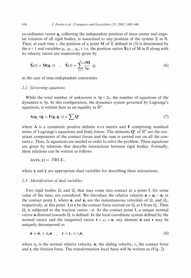
co-ordinates vector q, collecting the independent position of mass center and angu-lar rotation of all rigid bodies, is associated to any position of the system � in R.Then, at each time t, the position of a point M of � defined in (5) is determined bythe n+1 real variables q1; q2::; qn; t, i.e. the position vector X~ tð Þ of M in R along withits velocity vector are respectively given by

X~ tð Þ ¼ M q; tð Þ ; X~:tð Þ ¼

Xni¼1

@M

@qiq:i ð6Þ

in the case of time-independent constraints.

2.2. Governing equations

While the total number of unknowns is 3p+2c, the number of equations of thedynamics is 3p. In this configuration, the dynamics system governed by Lagrange’sequations, is written here as an equality in Rn:

A q; tð Þq€ ¼ F q; q:; tð Þ þ

XQc ð7Þ

where A is a symmetric positive definite n�n matrix and F comprising standardterms of Lagrange’s equations and body forces. The elements Qc of Rn are the cov-ariant components of the contact forces and the sum is carried out on all the con-tacts c. Thus, 2c equations are needed in order to solve the problem. These equationsare given by relations that describe interactions between rigid bodies. Formally,these relations can be written as follows

law x; yð Þ ¼ :TRUE:;

where x and y are appropriate dual variables for describing these interactions.

2.3. Identification of dual variables.

Two rigid bodies �i and �j that may come into contact at a point I, for somevalue of the time, are considered. We introduce the relative velocity u

:¼ u:i u

:j at

the contact point I, where u:i and u

:j are the instantaneous velocities of �i and �j,

respectively, at this point. Let r be the contact force exerted on �i at I from �j. Then�j is subjected to the traction vector r. At the contact point I, a unique normalvector n directed towards �i is defined. In the local coordinate system defined by thenormal vector and the tangential vector t ¼ e3 � n, any element u

:and r may be

uniquely decomposed as

u:¼ u:t þ u

:nn ; r ¼ rt þ rnn; ð8Þ

where u:n is the normal relative velocity, u

:t the sliding velocity, rn the contact force

and rt the friction force. The transformation local basis will be written as (Fig. 2)

616 J. Fortin et al. / Computers and Geotechnics 29 (2002) 609–640

T ¼�n ..

.t�:

Classically for scleronomic systems, there exits an affine relation between thevelocity u

:in the local coordinate system and q

:. The duality between dynamic and

kinematic quantities gives an expression of the components of the contact reaction Rin the reference coordinate system with respect to the components specified in thelocal coordinate system

u:¼ PT qð Þq

:; Qc ¼ P qð Þr ð9Þ

where PT(q) is obtained through the matrix representing the coordinate systemchange, i.e.

PT qð Þ ¼ TT I ain~ I ajn~� �

:

3. Coulomb’s frictional contact lawAs mentioned before, the circular bodies are assumed to be rigid and cannot

overlap as in Cundall’s approach. Further, it is assumed that contacting bodiesinteract according to Coulomb’s frictional contact law. However, since inelasticcollisions occur during the evolution of the system, the relative velocity of animpacting particle is discontinuous and contact forces are replaced by impulses. Thisimportant aspect of the problem will be discussed in Section 5.1. In this section, theemphasis is put on a variational formulation of the frictional contact law. The firststep consists in rewriting the Signorini conditions in terms of the normal relative

Fig. 2. Local coordinate system.

J. Fortin et al. / Computers and Geotechnics 29 (2002) 609–640 617

velocity gap. Next, this condition is combined with the sliding rule to give the fric-tional contact law for contacting bodies, which can be written as a ‘‘if . . . then . . .else’’ statement. Then, it is shown that the interface law along with its inverse canderived from a unique scalar-valued function, called bi-potential, and has an implicitform.

3.1. Signorni’s conditions

In the case of unilateral contact, Signorini’s conditions, i.e. impenetrability, non-adhesion and state of contact or no contact are classically written as

un 5 0 ; rn 5 0 ; un rn ¼ 0; ð10Þ

where the gap is identified with un which represents the interstice or the relative dis-placement between the rigid bodies projected on the local coordinate system,

un ¼ Xi Xj

�� �� ai þ aj� �

; ð11Þ

where ai and aj are radii of bodies �i and �j. Here, Signorini’s conditions areexpressed in terms of velocities. This formulation allows us to write the completefrictional contact law for contacting bodies and to include a shock law, which takescare of the dissipative phenomenon occurring when bodies came into contact. It is,however, necessary to distinguish a persisting contact and an open contact. A per-sistent contact is a contact where the interstice and the relative normal velocity arenull. On the other hand, for an opened contact, the interstice is always equal to zerobut the normal relative velocity is positive. For contacting bodies, Signorini’s con-ditions can be expressed equivalently in terms of velocities:

u:n 5 0 rn 5 0 u

:n rn ¼ 0; ð12Þ

allowing to write the complete frictional contact law. These relations are valid forun ¼ 0, i.e. the bodies are in contact. In other words, the previous relations areconstraint on the relative normal velocity and the reaction when bodies are in con-tact. When un is greater than zero, the reaction is equal to zero and the normalvelocity is unconstrained. So, relations (12) has to be understood with relations (10)which shall not be written down. The unilateral contact law in term of velocities isrepresented graphically in Fig. 3.We observe (Fig. 3) that the unilateral contact law is not the graph of a mapping

in the sense that neither u:n is a function of rn is a function of u

:n. This is a monotone

multi-valued law. At the point u:n=0 the ‘‘function’’ representing the law of uni-

lateral contact is not differentiable. There is infinity of hyper-planes in contact withthe graph of the function at u

:n=0 with positive or null slope. For a proper treat-

ment of such law, it is necessary to invoke the subdifferentials calculus (see Appendixand [13]). Using convex analysis tools, Moreau [19] introduces the concept ofpseudo-potential as an elegant extension of the potential one to multi-valued law. A

618 J. Fortin et al. / Computers and Geotechnics 29 (2002) 609–640

key concept is the indicatory function of a convex set, which is equal to zero for allelement belonging to the convex set and equal to +1 for elements that does notbelong to the convex set. In the present situation, the pseudo-potential ’n u

:nð Þ is

simply the indicatory function of R ¼ ½1; 0�, denoted by �Ru:nð Þ, which is

equal to zero when u:n 2 R and to +1 otherwise.

Definition 1. The inverse interface law rn u:nð Þ can be derived from the pseudo-

potential ’n u:nð Þ, in the form of a differential inclusion,

rn 2 @’n u:nð Þ: ð13Þ

The interface law being also a monotone multi-valued function, it derives from apseudo-potential, denoted by �n rnð Þ, which is the indicatory function ofRþ ¼ ½0;þ1�, denoted by �Rþ

rnð Þ. This function is equal to zero if rn 2 Rþ and to+1 otherwise.

Definition 2. The interface law that relates the normal velocity to the contact forcetakes the following form:

u:n 2 @�n rnð Þ: ð14Þ

The previous relation can also be recovered by means the Legendre–Fenchel trans-form. The two pseudo-potentials are related by the Legendre–Fenchel inequality

’n u: 0n

� �þ �n r0n

� �5 u

: 0n r

0n 8 u

: 0n; r

0n

� �:

The equality is reached for a pair u:n; rnð Þ satisfying the contact law (Signorini’s

conditions)

’n u:nð Þ þ �n rnð Þ ¼ u

:n rn:

Fig. 3. The unilateral contact law.

J. Fortin et al. / Computers and Geotechnics 29 (2002) 609–640 619

3.2. Coulomb’s law of friction

The Coulomb’s law is quite different when compared to the contact law. Its basicfeatures are as follows:

� The friction force rt acting on sliding bodies has magnitude proportional tothe normal force. The constant of proportionality � is called the coefficient offriction.

� If there is sliding, the friction force rt exerted by �j on �i has the samedirection as the sliding velocity u

:t : rt � u

:t ¼ 0, but with opposite sense to the

sliding velocity u:t : u:t �rt < 0. The magnitude of the friction forces is propor-

tional to the normal reaction rtk kmax¼ � rn.� If the bodies are not sliding, the friction forces may have any value provided

that its magnitude did not exceed � times the normal contact force:rtk k < � rn.

Geometrically, the contact reaction r is located inside a circular cone. This cone hasas axis the normal to the tangent plan at the point I and as generatrix the straightline inclined with respect to the vertical by an angle � ¼ arctan � (Fig. 5). This coneis called the friction cone. The inverse friction law (2D) is graphically represented inthe (Fig. 4)From energetical consideration, Moreau [20] has specified that the value of the

pseudo-potential of dissipation function for a resistance-type law is equal to the rateof dissipation. If we consider that rn is given (from equilibrium conditions, forexample), the sliding rule can be determined by applying the normality rule. Inothers word, the sliding rule can be derived from the following quasi-pseudo-poten-tial of dissipation ’rn u

:tð Þ ¼ � rn u

:t

�� ��. We use the term ‘‘quasi’’ to stress thedependence of the convex set on the contact pressure.

Definition 3. The inverse law of friction relating the friction force and the slidingvelocity takes the form of the following differential inclusion

Fig. 4. The inverse friction law (2D).

620 J. Fortin et al. / Computers and Geotechnics 29 (2002) 609–640

rt 2 @’rn u:tð Þ: ð15Þ

In the same way, the sliding rule can be written as a differential inclusion. Forthat, the interval Irn ¼ 0; � rn½ � and the following quasi-pseudo-potential �rn rtð Þ ¼

�Irn rtð Þ are introduced where �Irn rtð Þ is an indicatory function equal to zero if rt 2 Irnand to +1 otherwise. The following result holds.

Definition 4. The frictional law that relates the sliding velocity and the tangentialreaction can be written in the form of a differential inclusion:

u:t 2 @�K rnð Þ rtð Þ ð16Þ

Defining, as in plasticity, a yield function frn rtð Þ ¼ rtk k � rn Coulomb’s criterioncan be expressed as frn rtð Þ4 0. The set of the admissible friction forces is K rnð Þ ¼

rt j frn rtð Þ4 0

and sliding occur for rt situated on the boundary of K(rn). For thisevent, the sliding velocity is normal to the iso-curve of the Coulomb’s cone for anassumed value of rn. The sliding law can be then deduced by a normality rule: u

:t ¼

l:@ f@ rt

¼ l:

rtrtk k

where the multiplier is such that l:5 0.

3.3. Frictional contact law based on a bi-potential

However, if we regard force and velocity as conjugate quantities of each other, thenormality will not occur since it would require that the velocity would have a normalseparating component. Using Signorini’s conditions in terms of velocity in conjunc-tion with the sliding rule, all possible evolutions of contacting bodies can be speci-fied. The complete form of the frictional contact law is a complex non-smoothdissipative law including three states, which are separating, contact with sticking andcontact with sliding. The separating state has to be understood in the sense of loss ofcontact un ¼ 0 ; u

:n > 0 ) rn ¼ 0ð Þ. Here again, conditions related to positive gap

are not written down. Evolutions for bodies that are not in contact are arbitraryuntil contact is made. This choice is motivated by the fact that the emphasis is puton the definition of admissible evolutions for contacting bodies. Another advantageof this setting is a more easy incorporation of the shock law in the formulation. Thecomplete frictional contact law can be stated as:

if rn ¼ 0 thenu:n 5 0; !separating;

else if rn > 0 and rtk k < � rn thenu:n ¼ 0 and u

:t ¼ 0; !sticking

else rn > 0 and rtk k ¼ � rn

u:n ¼ 0 and 9l

:such that u

:t ¼ l

: rt

rtk k

� �!sliding:

endif

ð17Þ

Let K� be the isotropic Coulomb’s cone, which defines the set of admissible forcessatisfying f rn; rtð Þ ¼ rtk k � rn 4 0. The inverse law may be written as follows:

J. Fortin et al. / Computers and Geotechnics 29 (2002) 609–640 621

if u:n > 0 then

rn ¼ 0; !separating;else if u

:¼ 0 then

r 2 K�; !sticking;else u

:2 T 0f gð Þ then

rn > 0 and rt ¼ � rnu:t

u:t

�� ��( )

!sliding:

endif

ð18Þ

It is clear from geometrical consideration that the relative velocity u:is not normal

to Coulomb’s cone, because the normal relative velocity u:n is equal to zero (Fig. 5).

In addition, at the vertex of Coulomb’s cone, all vectors u:such that u

:n 4 0 are

admissible.These previous observations clearly indicate that the normality does not apply.

Therefore, the frictional contact law cannot be written under the form of the differ-ential inclusion of the type u

:2 @ K� rð Þ. de Saxce and Feng [6] have shown that

this complete contact law can be written in the form of the following differentialinclusion

u:t þ u

:n þ � u

:t

�� ��� �n

� �2 @�K� rð Þ ð19Þ

The behavior of materials admitting this kind of constitutive law is qualified asnon-standard or non-associated. By developing the previous relation, de Saxce has

Fig. 5. The frictional contact law.

622 J. Fortin et al. / Computers and Geotechnics 29 (2002) 609–640

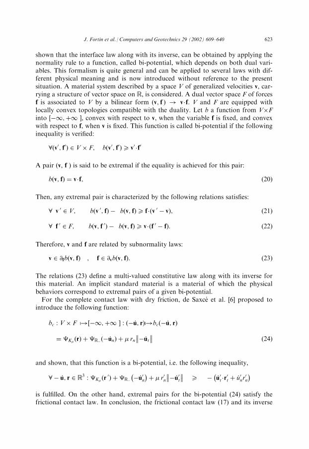
shown that the interface law along with its inverse, can be obtained by applying thenormality rule to a function, called bi-potential, which depends on both dual vari-ables. This formalism is quite general and can be applied to several laws with dif-ferent physical meaning and is now introduced without reference to the presentsituation. A material system described by a space V of generalized velocities v, car-rying a structure of vector space on R, is considered. A dual vector space F of forcesf is associated to V by a bilinear form v; fð Þ ! v�f. V and F are equipped withlocally convex topologies compatible with the duality. Let b a function from V�Finto 1;þ1½ �, convex with respect to v, when the variable f is fixed, and convexwith respect to f, when v is fixed. This function is called bi-potential if the followinginequality is verified:

8 v0; f0ð Þ 2 V� F; b v0; f0ð Þ5 v0 �f0

A pair (v, f ) is said to be extremal if the equality is achieved for this pair:

b v; fð Þ ¼ v�f; ð20Þ

Then, any extremal pair is characterized by the following relations satisfies:

8 v 0 2 V; b v 0; fð Þ b v; fð Þ5 f� v 0 vð Þ; ð21Þ

8 f 0 2 F; b v; f 0ð Þ b v; fð Þ5 v� f 0 fð Þ: ð22Þ

Therefore, v and f are related by subnormality laws:

v 2 @fb v; fð Þ ; f 2 @vb v; fð Þ: ð23Þ

The relations (23) define a multi-valued constitutive law along with its inverse forthis material. An implicit standard material is a material of which the physicalbehaviors correspond to extremal pairs of a given bi-potential.For the complete contact law with dry friction, de Saxce et al. [6] proposed to

introduce the following function:

bc : V� F 7! 1;þ1½ � : u:; rð Þ7!bc u

:; rð Þ

¼ �K� rð Þ þ �Ru:nð Þ þ � rn u

:t

�� �� ð24Þ

and shown, that this function is a bi-potential, i.e. the following inequality,

8 u:; r 2 R3 : �K� r

0ð Þ þ �Ru: 0n

� �þ � r0n u

: 0t

�� �� 5 u: 0t �r

0t þ u

: 0nr

0n

� �is fulfilled. On the other hand, extremal pairs for the bi-potential (24) satisfy thefrictional contact law. In conclusion, the frictional contact law (17) and its inverse

J. Fortin et al. / Computers and Geotechnics 29 (2002) 609–640 623

(18) can be written respectively, in the following compact form of implicit sub-normality rules:

u:2 @rbc u

:; rð Þ ; r 2 @u:bc u

:; rð Þ:

4. Local stage of projection equation onto Coulomb’s cone

The classical formulation of the unilateral contact problem with friction is basedon two variational inequalities. The first inequality express the unilateral contactcondition and the last the friction one. Based on this formulation, efficient predictor-corrector algorithms have been proposed in the literature. Basically such algorithmssolve alternatively the contact and the friction problems until convergence. As aconsequence, two predictor-corrector steps are needed. By adopting the variationalformulation presented in the previous section, a faster and more robust time step-ping algorithm with only on predictor-corrector step can be devised. This formula-tion is quite general and well suited for non-standard behaviors admitting a bi-potential.By applying (22) to the bi-potential (24), we obtain

r 2 K�bc u

:; r0ð Þ bc u

:; rð Þ5 u

:� r0 rð Þ; 8 r0 2 K� :

ð25Þ

During the local stage, the relative velocity u:is given for each contact. Our aim

now is to find the correspondent contact reaction r, solution of the previousinequality. Then, let � be a number chosen in a suitable range to ensure numericalconvergence. Inequality (25) can be easily rewritten as:

r 2 K��bc u

:; r0ð Þ �bc u

:; rð Þ þ r r þ � u

:ð Þð Þ½ �� r0 rð Þ5 0 ; 8 r0 2 K�:

ð26Þ

This new inequality means that r is the proximal point [18] of the augmented forcer ¼ r �u

:, with respect to the function r ! � bc u

:; rð Þ:

r ¼ prox r �u:; � bc u

:; rð Þð Þ: ð27Þ

Next, for the contact bi-potential bc, given by (24), one has, provided that u:n 5 0

and r 2 K�,

8 r0 2 K� ; �� r0n rn� �

u:t

�� ��þ r r þ � u:

ð Þð Þ½ �� r0 rð Þ5 0: ð28Þ

which can be also written:

8 r0 2 K� ; r �ð Þ� r0 rð Þ5 0: ð29Þ

624 J. Fortin et al. / Computers and Geotechnics 29 (2002) 609–640

where � is the modified augmented surface traction defined by

� ¼ r � u:t þ u

:n þ � u

:t

�� ��� �n

� �: ð30Þ

The last inequality (29) means that r is the projection of � onto the closed convexCoulomb’s cone:

r ¼ proj �;K�� �

: ð31Þ

The primary attribute of the method is that the projection can be analytically cal-culated with respect to the three possible statuses:

� separating if � 2 K��, where K�

� ¼ u:t; u:nð Þ��� u

:t

�� ��þ u:n 4 0

is the dual cone

of K�,� contact with sticking if � 2 K�,� contact with sliding if � 2 R3

K� [ K��

� �.

Finally, at the (i+1)th iteration of the main algorithm, the local stage involves onepredictor-corrector step:

Predictor : �iþ1 ¼ ri � u: it þ u

: in þ � u

: it

�� ��� �n

� �;

Corrector : riþ1 ¼ proj �iþ1;K�� �

:ð32Þ

The corrector step requires computing the projection of the prediction and can bereformulated as solution the following convex non-linear programming problemwith constraints

riþ1 ¼ infriþ12K�

1

2riþ1 �iþ1�� ��2 ð33Þ

Next, (33) is transformed into an unconstrained minimization problem by means ofLagrange multipliers technique [9,16],

r ¼ supl5 0

infriþ1t ;riþ1

n

L riþ1t ; riþ1

n ; l� �

with

L riþ1t ; riþ1

n ; l� �

¼1

2riþ1t �iþ1

t

�� ��2þ 1

2riþ1n �iþ1

n

� �2þl riþ1

t

�� ���riþ1

n

� �� �:

Expressing the Kuhn–Tucker optimality conditions for an extremal pointriþ1t ; riþ1

n ; l� �

, the solution of the problem is

J. Fortin et al. / Computers and Geotechnics 29 (2002) 609–640 625

if � �iþ1t

�� �� < �iþ1n then

riþ1 ¼ 0 ! separating

else if �iþ1t

�� ��4��iþ1n then

riþ1 ¼ �iþ1 ! contact with sticking

else

riþ1 ¼ �iþ1 �iþ1�� �� � �iþ1

n

� �1þ �2ð Þ

�iþ1

�iþ1�� �� � n

!! contact with sliding

endif

ð34Þ

5. Global stage

At the local stage, the contact reactions are computed from the values of therelative velocities, which have been calculated during the global stage. During thisstage, Newton’s second law is used to determine for each particle the resultingacceleration and velocity, which are then integrated in time to find the new particlestates. Since collisions occur during the evolution of the system, the relative velocityof an impacting particle is discontinuous and energy is dissipated. Furthermore,contact forces have to be replaced by impulsive forces to allow an instantaneouslychange of the velocity. Consequently, the classical Lagrange’s equations (section 2)have to be set in a more adequate mathematical framework and the frictional con-tact law should be conveniently modified to take into account the dissipationoccurring during collisions.

5.1. Non-smooth formulation

As the bodies are regarded as perfectly rigid and no flexibility is taken intoaccount for the interparticle contact, possible collisions then appear as instanta-neous processes. In this case, the velocity function q

:that associated for each t 2

0;T½ � an element of Rn is discontinuous, as there are velocity jump. Consider, forexample, a rigid ball that falls onto a rigid table. Before impact there is no contactforce, and the ball accelerates downward. But at the moment of contact, the down-ward velocity of the ball must be changed instantaneously. This requires impulsiveforce at the moment of contact. The present of these discontinuities requires using themeasure differential equation, invented by Moreau, to formulate rigorously this non-smooth problem. Then, the dynamics equation (34) is considered in its measure form:

A q:þ q

:� �¼ F q; q

:; tð Þdtþ

XPTs ð35Þ

where q:þ and q

: represent, respectively, the right-limit (after impact) and the left-limit (before impact) of q

:. The term s in Eq. (35) constitutes the contact impulsion

measure and ‘‘dt’’ has to be understood in the Lesbegue measure’s sense. This fric-tional contact law is adapted to take into account of the collision by introducing thelocal average velocity u

:~ in Moreau’s sense [22]:

626 J. Fortin et al. / Computers and Geotechnics 29 (2002) 609–640

u:~t ¼

u:þt þ et u

:t

1þ et; u

:~n ¼

u:þn þ en u

:n

1þ en: ð36Þ

where u: ¼ PTq

:, u:þ ¼ PTq

:þ (see Eq. (9)) and where en and et represent the normaland tangential restitution coefficients respectively. Finally, relations (32) forimpacting bodies are:

Predictor : �iþ1 ¼ si � u:~ it þ u

:~ in þ � u

:~ it

��� ���� �n

h i;

Corrector : siþ1 ¼ proj �iþ1;K�� �

:ð37Þ

5.2. Time integration algorithm

The three key parts of a DEM algorithm are:

� A search algorithm used to construct a particle near-neighbor interaction list.� A local stage where collisional forces for each collision are estimated using

the discrete interface law (37).� A global stage where all collisional and other forces acting on the particles

are summed and the resulting equation of motion (35) is integrated.

The time interval, during which the evolution of the system is sought, is partitionedinto N sub-interval of size h, not necessarily equal, according to

0 ¼ t0 < t1 < :: < tn1 < tn < :: < tN ¼ T:

We set ! tnð Þ ¼ !n and

.! ¼ !n !n1;

where ! represents any variable. The solution of the problem within the interval[0,T] is the obtained by solving N successive finite-step problems. For each iteration,two stages are performed.A global stage: starting with given values qn and q

:n at the beginning tn of the step,

the time integration is performed by use a global predictor-corrector scheme. Forthis, we introduce a middle time tm and a prediction of the generalized coordinatesqm:

tm ¼ tn þ1

2h; qm ¼ qn þ

1

2h q:n: ð38Þ

In order to reduce the size of the non-smooth problem, only established or potentialcontacts are considered. To select the candidates to contact, we introduce a routinebased on the relation (11) rewritten in the form

J. Fortin et al. / Computers and Geotechnics 29 (2002) 609–640 627

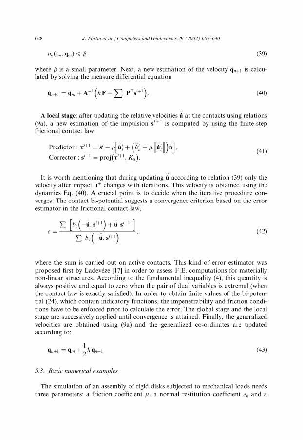
un tm; qmð Þ4� ð39Þ

where � is a small parameter. Next, a new estimation of the velocity q:nþ1 is calcu-

lated by solving the measure differential equation

q:nþ1 ¼ q

:m þ A1 hF þ

XPTsiþ1

� �: ð40Þ

A local stage: after updating the relative velocities u:~ at the contacts using relations

(9a), a new estimation of the impulsion si+1 is computed by using the finite-stepfrictional contact law:

Predictor : �iþ1 ¼ si � u:~ it þ u

:~ in þ � u

:~ it

��� ���� �n

h i;

Corrector : siþ1 ¼ proj �iþ1;K�� �

:ð41Þ

It is worth mentioning that during updating u:~ according to relation (39) only the

velocity after impact u:þ changes with iterations. This velocity is obtained using the

dynamics Eq. (40). A crucial point is to decide when the iterative procedure con-verges. The contact bi-potential suggests a convergence criterion based on the errorestimator in the frictional contact law,

" ¼

Pbc u

:~; siþ1� �

þ u:~ �siþ1

h iP

bc u:~; siþ1

� � ; ð42Þ

where the sum is carried out on active contacts. This kind of error estimator wasproposed first by Ladeveze [17] in order to assess F.E. computations for materiallynon-linear structures. According to the fundamental inequality (4), this quantity isalways positive and equal to zero when the pair of dual variables is extremal (whenthe contact law is exactly satisfied). In order to obtain finite values of the bi-poten-tial (24), which contain indicatory functions, the impenetrability and friction condi-tions have to be enforced prior to calculate the error. The global stage and the localstage are successively applied until convergence is attained. Finally, the generalizedvelocities are obtained using (9a) and the generalized co-ordinates are updatedaccording to:

qnþ1 ¼ qm þ1

2h q:nþ1 ð43Þ

5.3. Basic numerical examples

The simulation of an assembly of rigid disks subjected to mechanical loads needsthree parameters: a friction coefficient �, a normal restitution coefficient en and a

628 J. Fortin et al. / Computers and Geotechnics 29 (2002) 609–640

tangential restitution coefficient et. Here, two examples are presented in order tovalidate the algorithm and to show the influence of these parameters.The first example deals with a rigid ball that falls onto a rigid table (Fig. 6). The

initial position of the ball is 10 cm above the table (h0 ¼ 10 cm) and its initial velo-city is assumed to be equal to zero. The ball accelerates downward and touches, atan instant t0, the table with a velocity v0. Next, the ball bounces with a velocity justafter impact equal to v1. Generally, the impact of the particle on the table is accom-panied with dissipation of a part of the kinetic energy. For this example, the time stepis taken equal to 104 s. For each impact, the convergence was obtained after 2iterations. Fig. 7 shows for two different normal restitution coefficients en, (0.9;1) thesuccessive maximal heights hp of the particle in function of the time impact tp.

Fig. 6. Rigid ball falling on a rigid table.

Fig. 7. Influence of the normal restitution coefficient en.

J. Fortin et al. / Computers and Geotechnics 29 (2002) 609–640 629

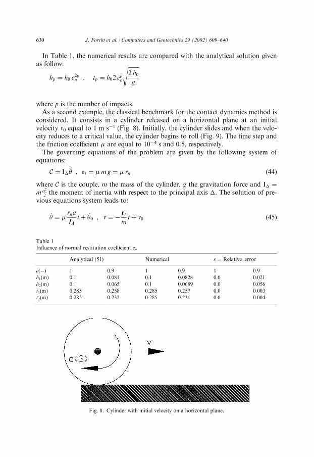
In Table 1, the numerical results are compared with the analytical solution givenas follow:

hp ¼ h0 e2pn ; tp ¼ h02 e

pn

ffiffiffiffiffiffiffiffi2 h0g

s

where p is the number of impacts.As a second example, the classical benchmark for the contact dynamics method is

considered. It consists in a cylinder released on a horizontal plane at an initialvelocity v0 equal to 1 m s1 (Fig. 8). Initially, the cylinder slides and when the velo-city reduces to a critical value, the cylinder begins to roll (Fig. 9). The time step andthe friction coefficient � are equal to 104 s and 0.5, respectively.The governing equations of the problem are given by the following system of

equations:

C ¼ I.�€ ; rt ¼ �mg ¼ � rn ð44Þ

where C is the couple, m the mass of the cylinder, g the gravitation force and I. ¼

m a2

2 the moment of inertia with respect to the principal axis .. The solution of pre-vious equations system leads to:

�:¼ �

rna

IDtþ �

:0 ; v ¼

rt

mtþ v0 ð45Þ

Table 1

Influence of normal restitution coefficient en

Analytical (51) Numerical " ¼ Relative error

e() 1 0.9 1 0.9 1 0.9

h1(m) 0.1 0.081 0.1 0.0828 0.0 0.021

h2(m) 0.1 0.065 0.1 0.0689 0.0 0.056

t1(m) 0.285 0.258 0.285 0.257 0.0 0.003

t2(m) 0.285 0.232 0.285 0.231 0.0 0.004

Fig. 8. Cylinder with initial velocity on a horizontal plane.

630 J. Fortin et al. / Computers and Geotechnics 29 (2002) 609–640

The cylinder starts to roll when the velocity is equal to

v1 ¼ a �:1 and t ¼ t1; ð46Þ

where a is the radius of the cylinder and �:1 its rotational velocity. Combining Eq.

(45) gives:

t1 ¼v0

3� g; v1 ¼

2

3v0: ð47Þ

By comparison, the elementary analytical solution (47) gives the same numericalvalues, see Table 2.

Fig. 9. Cylinder velocity versus time.

Table 2

Influence of friction coefficient �

Analytical (53) Numerical

v1 ms1� �

0.666 0.666

t1(s) 0.0679 0.0679

J. Fortin et al. / Computers and Geotechnics 29 (2002) 609–640 631

6. Numerical applications

6.1. Quasi-static problems

Quasi-static examples, presented in Fig. 10, are considered. A regular array ofequal-size disks confined in a box is considered. The box is composed of two verticaland two horizontal flat walls. The particles as well as the walls are assumed to beperfectly rigid. Each particle is subjected to the gravitation force g and to contactforce resulting from neighborhood particles and walls. For three different geome-tries, the normal contact forces for each particle are computed. The assumptionsand results are displayed in (Fig. 10). The widths of inter-center segments are pro-portional to the corresponding normal contact force intensity. For the rectangulararrangement, according to obvious physical reasons, the normal force increaseswhen the height of disk center with respect to base of the box decreases. For the

Fig. 10. The normal contact forces for three different arrangements. The widths of inter-center segments

are proportional to the corresponding contact forces.

632 J. Fortin et al. / Computers and Geotechnics 29 (2002) 609–640

triangular arrangement, we observe that contacts between the particles and the ver-tical wall exist. This situation is typical regarding the complex behavior of granularmaterials. By comparison with the analytical computation [14], we obtain the samevalues concerning the normal contact forces. For the cannon-ball arrangement, thefriction, which is not displayed here, is essential to the stability of the system.

6.2. Numerical examples of compacted granular media

Results related to two kind of compaction are presented. Fig. 11 shows a com-paction obtained by gravity. In the cell, we introduce 342 particles subjected to thegravitation force g. The sample in Fig. 9 contains 25% of particles of radius 0.65mm, 50% of particles of radius 0.75 mm and 25% of particles of radius 0.9 mm. Theparticle to particle and particle to wall coefficients of friction are both equal to 0.1. Itcan be observed that the friction produces rotational motion of beads. The tangen-tial and normal restitution coefficients are equal to 1.0 and 0.1, respectively. Unlikethe experimental evidence concerning granular media, no conical heap appears atthe top. This can be explained by the fact that the beads are cylindrical and the baseis rigorously plane. As a result, the system is not rough and imperfect enough toinitiate and conserve the conical heap. Concerning the normal contact forces, onecan observe both large contact-to-contact fluctuations and a sub-network of ‘‘forcechains’’ (according to similar observations by other authors).Fig. 12 presents a compaction under isotropic compression. A two-dimensional

system with 2470 circular particles contained in a box of four rigid walls is con-sidered. The sample is composed of 25% of particles of radius 0.8 mm, 50% ofparticles of radius 0.9 mm and 25% of particles of radius 1.0 mm. The granulometryis compact. The particle to particle and particle to wall coefficients of friction areequal to 0.1 and 0.1, respectively. The tangential and normal coefficients of restitu-tion are respectively equal to 1.0 and 0.0. Each wall is subjected to a force of 5000 N.We observe after 300 time step of 7�105 s, that the distribution of normal contactforces is concentrated on the right hand side of the sample even though it is quasihomogeneous in the horizontal direction. This paradoxical situation disappearswhen considering the average over a larger time interval. In fact, the change in theforce configurations is so fast that such inhomogeneous chain of forces disappearsinstantaneously.

Remark. Generally, for simulation, we take the value of � equal to

� ’ Oreaction

velocity

� �’

1þ enð Þmi mj

h mi þmj

� �where mi and mj are mass of bodies �i and �j. The choice of the value of the factor �is delicate and we found that the previous expression of � give good results regard-less of the nature of the problem. For a particular problem, probably a better valuecould be found but it will not be optimal for another problem. That explains ourchoice to keep a general expression of � for all problems.

J. Fortin et al. / Computers and Geotechnics 29 (2002) 609–640 633

Fig. 11. Compaction by gravity.

634 J. Fortin et al. / Computers and Geotechnics 29 (2002) 609–640

Fig. 12. Isotropic compaction.

J. Fortin et al. / Computers and Geotechnics 29 (2002) 609–640 635

7. The error in constitutive law

Generally, DE methods make use of a convergence criterion based on Euclideannorm of the difference between contact forces at consecutive iterations. One of the ori-ginal features of the present algorithm is the ability to control the convergence by meansof the error in constitutive law estimator, which involves the contact bi-potential:

" ¼

Pbc u

:~; siþ1� �

þ u:~ �siþ1

h iP

bc u:~; siþ1

� �Generally speaking, the convergence rate of the error in the constitutive law

depends strongly on the nature of the considered problem. The convergence ofquasi-static problems seems to be more delicate than the one of the dynamical pro-blems. For instance, concerning the simulation presented in Section 6.1 (rectangulararrangement), the sensitivity of the error with respect to the iteration number ispresented in a log–log plot in the Fig. 13. During a transient phase of about twentyiterations, the computation is unstable. This can be explained by the fact that thecomputation of contact forces is implicit (37) with null initial values of the contactforces at the beginning of the step when no relevant information is available. Inorder to reduce this instability it would be necessary to give better initial values tothe contact forces left as a topic for future research. After reaching a critical

Fig. 13. Convergence criterion versus number of particles for a rectangular arrangement of particles of

equal size.

636 J. Fortin et al. / Computers and Geotechnics 29 (2002) 609–640

threshold of 20 iterations, the convergence rate quickly accelerates. Besides, it isrelevant to quote that Usawa-like algorithms, such as the one used here and basedon (31) are very stable and give after a few iterations good approximations of thesolution while more accurate values require many more additional iterations.Finally, for an example of rectangular arrangement of homogeneous particles with

the assumptions given in Subsection 6.1, Fig. 14 exhibits in a log–log plot the sen-sitivity of the number of iterations required. Except for small samples, the depen-dency is quasi linear. This shows that the computation time depends on the problemsize following a power law of which the exponent is given by the slope of the straightline in Fig. 14, and found to be approximatively equal to 1.042. The previousobservation is quite heartening because this sensitivity study, although peculiar,seems to indicate that the computation time for larger scale problems does notincrease in an exponential way, as it may have been expected.

8. Conclusion and forthcoming

The D.E. method provides an effective means to get greater insight into thebehavior of granular materials. A precise modeling of granular materials shouldassume that particles are rigid and take into account unilateral constraints alongwith shocks that occur during the evolution of the system. The framework ofmeasure differential equation, constructed by Moreau, allows a rigorous setting of

Fig. 14. Number of iterations versus number of particles for a rectangular arrangement of particles of

equal size.

J. Fortin et al. / Computers and Geotechnics 29 (2002) 609–640 637

the governing equations of rigid body dynamics. In this paper, this framework hasbeen adopted and improvements have been made, by using a variational formula-tion of the frictional contact law based on the bi-potential concept. By doing so, thelocal stage involves only a single predictor-corrector step reducing significantly thecomputing time for this stage and a new convergence criterion can be derived. Thiscriterion appears to be more appropriate for this kind of problem than the classicalcriterion based on Euclidean norm of the contact forces, which seems to be lessstringent in some situations and too strong in others. Accordingly, the convergencerate of the global algorithm is enhanced. Both applications, in quasi-static anddynamics show the convergence and the robustness of the algorithm even in pre-sence of numerous contacts. In future, we hope to extend the algorithm to threedimensional situations and to implement subroutines that compute a consistentmean stress tensor in the granular system.

Appendix. Duality, convexity and subdifferentiality

Let A and B be two vector spaces associated through the duality pairing definedby a bilinear form:

a; b ! a�b

A� B ! R

Let f(a) be a real function taking its values in [1, +1]. The effective domain off(a), denoted dom f, is defined by

dom f ¼ a 2 A : f að Þ <1

:

We recall that f(a) is convex if

f l a1 þ 1 lð Þa2ð Þ 4 l f a1ð Þ þ 1 lð Þf a2ð Þ 8l 2 0; 1½ �;

8 a1; a2 2 AðA1Þ

and strictly convex if the above inequality is satisfied in a strict sense,8 a1; a2 2 A; a1 6¼ a2. If the function f(a) is differentiable, the convexity condition(30) can be equivalently expressed as

f a2ð Þ f a1ð Þ 5@f að Þ

@a

����a1

a2 a1ð Þ 8 a1; a2 2 A: ðA2Þ

The generalization of (31) to a non-differentiable function at a1 is

f a2ð Þ f a1ð Þ 5 b� a2 a1ð Þ 8 a2 2 A: ðA3Þ

638 J. Fortin et al. / Computers and Geotechnics 29 (2002) 609–640

Any solution b of the above inequality is a subgradient, collected in a set @af a1ð Þ,called subdifferential of f(a) at a1. The variational inequality (32) is equivalent to thefollowing differential inclusion

b 2 @af a1ð Þ: ðA4Þ

By definition, the Legendre-Fenchel transform of f(a), denoted f*(b), is:

f � bð Þ ¼ supa2A

a�b f að Þ½ �: ðA5Þ

As a consequence of (34), we have

f a0ð Þ þ f � b0ð Þ 5 a0 �b0 8 a0; b0ð Þ 2 A� B; ðA6Þ

called Legendre–Fenchel inequality. The equality is reached in (35) for a pair (a, b)satisfying

b 2 @af að Þ ; a 2 @bf bð Þ: ðA7Þ

Finally, the function f(a) is positively homogenous of degree one if

f � að Þ ¼ � f að Þ 8 a 2 A ; 8� > 0:

References

[1] Abriak N-E. Ecoulement d’un materiau granulaire a travers un orifice, effet de paroi. PhD thesis,

University of Lille, France; 1999.

[2] Alart P, Curnier A. A mixed formulation for frictional contact problems prone to Newton like

solution methods. Computer Methods in Applied Mechanics and Engineering 1991;92:353–75.

[3] Cundall PA, Strack ODL. A discrete numerical model for granular assemblies. Geotechnique 1979;

29:47–65.

[4] Darves F, Laouafa F. Plane strain instabilities in soil: application to slopes stability. To appear in

Proceeding of Int. Symp. on Numerical Models in Geomechanics, 1–3 September, Graz, Austria;

1999.

[5] de Saxce G. Une generalisation de l’inegalite de Fenchel et ses applications aux lois constitutives.

Comptes Rendus de l’Academie des Sciences de Paris 1992; t. 314, Serie II: 125–9.

[6] de Saxce G, Feng ZQ. The bi-potential method: a constructive approach to design the complete

contact law with friction and improved numerical algorithms. Mathematical and Computer Model-

ling 1998;28(4–8):225–45.

[7] Duran J. Introduction a la physique des milieux granulaires. Paris: Eyrolles Sciences; 1997.

[8] Evesque P, Meftha W, Biarez J. Mise en evidence de variations brutales et d’evolutions quasi dis-

continues dans les courbes contrainte-deformation d’un milieu granulaire bi-dimensionnel de rou-

leaux. Comptes Rendus de l’Academie des Sciences de Paris 1993; t. 316, Serie IIb: 321–7.

[9] Fortin M, Glowinski R. Methodes de Lagrangien augmente. Dunod; 1982.

[10] Fortin J, de Saxce G. Modelisation des milieux granulaires par l’approche du bipotentiel. Comptes

Rendus de l’Academie des Sciences de Paris 1999; t. 327, Serie II b: 721–4.

J. Fortin et al. / Computers and Geotechnics 29 (2002) 609–640 639

[11] Fortin J, de Saxce G. Dynamique des milieux granulaires par l’approche du bipotentiel. In: 4eme

Colloque National en Calcul des Structures 1999: 141–6, Giens, France.

[12] Halphen B, Nguyen Quoc Son. Sur les materiaux standards generalises. Journal de Mecanique 1975;

14 (1): 39–63.

[13] Hiriart-Urruty J-B. Optimisation et analyse convexe. Presses Universitaires de France 1998.

[14] Hong DC. Stress distribution of a hexagonally packed granular pile. Physical Review E 199 1999;

47(1):760–2.

[15] Jean M. Frictional contact in collections of rigid or deformable bodies: numerical simulation of

geomaterial motions. In: Selvadurai APS, Boulon MJ, editors. Mechanics of geomaterial interfaces,

1995, p. 463–6. Elsevier Sciences Publishers, Oxford.

[16] Klarbring A. Mathematical programming and augmented Lagrangian methods for frictional contact

problems. In: Curnier A, editor. Proceedings of the Contact Mechanics International Symposium.

PPUR; 1992. p. 409–22.

[17] Ladeveze P. Mecanique nonlineaire des structures: nouvelle approche et methodes de calcul non

incrementales. Paris: Hermes; 1996.

[18] Moreau J-J. Fonctions convexes duales et points proximaux dans un espace hilbertien. Comptes

Rendus de l’Academie des Sciences de Paris 1962, seance du 26 novembre.

[19] Moreau J-J. Sur les lois de frottement, de plasticite et de viscosite. Comptes Rendus de l’Academie

des Sciences de Paris 1970;t. 271:608–11.

[20] Moreau J-J. Fonctions de resistance et fonctions de dissipation. Seminaire d’analyse convexe 1971,

Expose No. 6, Montpellier.

[21] Moreau J-J, Panagiotopoulos PD. Nonsmooth mechanics and applications. Wien, New York:

CISM courses and lectures No. 302. Springer-Verlag; 1988.

[22] Moreau J-J. Some numerical methods in multibody dynamics: application to granular materials.

European Journal of Mechanics A/Solids 1994;13(4):93–114.

[23] Schneebeli G. Une analogie mecanique pour les terres sans cohesion. Comptes Rendus de l’Academie

des Sciences de Paris; 1956. seance du 9 Juillet. p. 125–126.

[24] Walton OR. Application of molecular dynamics to macroscopic particles. International of Engi-

neering Sciences 1984;22:1097–107.

640 J. Fortin et al. / Computers and Geotechnics 29 (2002) 609–640