ORIGINAL PAPER

Z. -Q. Feng Æ M. Hjiaj Æ G. de. Saxce Æ Z. Mroz

Effect of frictional anisotropy on the quasistatic motion of a deformablesolid sliding on a planar surface

Received: 18 September 2004 / Accepted: 2 February 2005 / Published online: 15 September 2005� Springer-Verlag 2005

Abstract In this paper, the motion of a deformable bodysliding on a half-plane is considered. The solid under-goes large displacements but small strains. An ortho-tropic friction model described by an elliptic cone isconsidered. This model allows to describe the sliding-direction dependence of the frictional behavior observedin experience. The algorithm used to solve the problem isbased on a weak variational statement of the frictionalcontact law. The Uzawa algorithm is used to solve thediscrete problem. The corresponding algorithm is robustand can deal with large sliding increments. The studyshows that frictional properties can influence signifi-cantly the trajectory of a deformable body sliding on africtional surface.

Keywords Elliptic friction criterion Æ Largesliding Æ Variational formulation Æ Uzawa algorithm

1 Introduction

Planning the motion of a body in contact with a planarsurface is an usual task for a robotic system. The goal ofplanning is to determine force commands which, ifexecuted, would achieve a pre-specified motion of thebody. If the task is to be done as quickly as possible,dynamic effects must be included. Otherwise, a quasi-static model, one which ignores inertial forces, mayprove a good alternative. Models used in roboticsassume that the pushed body is rigid so the motioncannot always be uniquely predicted. However, if thebody is assumed deformable, the static indeterminacy isremoved which makes the solution of the problem easy.An accurate description of the body motion cannot beachieved unless an adequate friction model is used.Though, usually assumed to be constant, the frictioncoefficient often varies with the sliding direction. So theusual isotropic Coulomb’s model is a gross approxima-tion and more complex models have to be introduced. Inwhat follows, the effect of the friction model on themotion of an object being pushed over a floor is inves-tigated.

A friction model is defined by the friction conditionwhich specifies a convex set of admissible contact forcesand the sliding rule which stipulates what directions ofsliding are allowed. The shape of the friction surface andthe nature of slip rule have a fairly strong influence onthe motion of sliding objects. In most studies, the limitsurface is used under its isotropic form. As a result, thefrictional behavior is independent of the sliding direc-tion. However this assumption seems to be unrealistic.Indeed many experimental studies show that the fric-tional behavior can change drastically with the slidingdirection, requiring an anisotropic model. This anisot-ropy can be attributed to two main sources. The first oneis the anisotropy of the material constituting the solidand the planar surface that manifest themselves on thecontact surface as well. The second one is technological.The industrial process used to fabricate the bodies can

Comput Mech (2006) 37: 349–361DOI 10.1007/s00466-005-0674-5

Supported by the Australian Research Council

Z. -Q. FengLaboratoire de Mecanique d’Evry,Universite d’Evry-Val d’Essonne, 40 rue du Pelvoux,91020 Evry Cedex, France

M. Hjiaj (&)Department of Civil Engineering, The University of Newcastle,Callaghan, NSW, 2308, AustraliaE-mail: mohammed.hjiaj@insa-rennes.frTel.: +33-2-23238711Fax: +33-2-23238448

Present address: M. HjiajINSA de Rennes, 20 avenue des Buttes de Coesmes,35043 Rennes cedex, France

G. de. SaxceLaboratoire de Mecanique de Lille CNRS/UMR 8107,Boulevard Paul Langevin, F-59655 Villeneuve d’Ascq Cedex,France

Z. MrozPolish Academy of Sciences,Institute of Fundamental Technological Research,Swietokrzyska 21, 00-049 Warsaw, Poland

create striations along preferential directions. In fact,most machining, finishing and superfinishing operationsare directional, and machined surfaces have particularstriation patterns unique to type of machining. Alsospecific techniques of manufacture produce a surfacewith anisotropic frictional properties. For a large num-ber of machining processes, the striation directions aremutually orthogonal. For such surfaces, an orthotropicfrictional model will provide a better description of thefrictional behavior.

A common way to model frictional anisotropy is toadopt an elliptic friction condition in the planern ¼ const, where rn is the contact pressure. In thesequel, the term ‘‘contact pressure’’ means the normalcomponent of the contact stress vector which has atangential component when friction exists on the contactsurface. Two friction coefficients, one in the x-directionand another in the y-direction (orthogonal to thex-direction), have to be determined. These coefficientscorrespond to the ellipse semi-axes for rn ¼ 1. It will beshown that frictional anisotropy has a significant impactfor problems such as motion of sliding objects. For aspecified pushing force the trajectory of an objectdepends on the frictional properties of the planar sur-face.

In this paper, the motion of a pushed deformableblock sliding on a frictional planar surface is studied.The block is assumed to be elastic. Large displacementsare allowed but the block is assumed to undergo smallstrain. The supporting surface has anisotropic frictionalproperties. The problem is solved in a quasi-staticfashion using the finite element method and the totallagrangian technique. The algorithm used to solve theproblem is based on a variational formulation of thefrictional contact law. In the next section, contact vari-ables are defined and the unilateral contact law is pre-sented. For bodies in contact, this law can be written in arate form where the kinematical variable is the velocity.Section 3 is concerned with anisotropic friction modelswith convex limit friction surfaces of elliptic shape. InSect. 4, the rate form of the Signorini conditions arecoupled with the sliding rule to give the complete fric-tional contact law for bodies in contact. A formulationbased on a variational inequality is presented at the endof the section. Section 5 deals with the governing discreterelations of the considered frictional contact model. In

Sect. 6, the discretized frictional contact problem isoutlined and the F.E. algorithm is presented in Sect. 8.The example shown in Sect. 9 highlights the influence ofthe frictional model on the motion of sliding objects.

2 Deformable block sliding on a planarsurface – Governing equations

The pushed block undergoes large displacements whichrequire an appropriate setting of the problem. The basicsof continuum contact mechanics in the large displace-ment setting are briefly addressed in this section. Thedetails are omitted as they are not necessary for thecurrent study (see, [4]).

2.1 Kinematics and statics

Consider a deformable block B undergoing large dis-placements and small strains (Fig. 1). The body Boccupies in a referential configuration the open, simplyconnected, bounded domain X � R3 . The closure X ofX represents the reference configuration of B whichcorresponds to the initial one in the total Lagrangianformulation, adopted here. A material particle M in X isidentified by its reference position vector X. The suc-cessive deformed configurations Bt, t 2 ½0; T �, aredefined by a differentiable and invertible mapping u :

uðX; tÞ : X� ½0; T � ! R3;

where I ¼: ½0; T � is the time domain of interest, corre-sponding to the loading process. The time t 2 I charac-terizing the reference configuration is t0 ¼ 0. Theposition of a particle of the body in the current config-uration Bt is defined using the current coordinate vectorx ¼ uðX; tÞ. The displacement of a material point fromthe initial configuration is the difference between itscurrent and its initial position

u ¼ uðX; tÞ � X

The velocity of a material point in the reference con-figuration is given by

_uðX; tÞ ¼ @u@tðX; tÞ

Fig. 1 Block sliding on africtional surface

350

The boundary CðtÞ of Bt is assumed to be sufficientlysmooth everywhere such that an outward unit normalvector, denoted by n, can be defined everywhere on CðtÞ.To fix the ideas, the body under consideration is a cubein frictional contact with a planar surface, denoted S.We assume that the boundary CðtÞ of Bt can be dividedinto three disjoint parts: CuðtÞ with prescribed displace-ments, CtðtÞ with prescribed boundary loads, and thepotential contact surface CcðtÞ where Bt may possiblycome into contact with the half-plane at some time t:

CðtÞ ¼ CuðtÞ [ CtðtÞ [ CcðtÞDisplacements are imposed on the upper face of the cubeand the lower face corresponds to the contact surface Cc.The remaining faces are stress free. The transformationgradient F relates the current configuration to the ref-erence configuration by

FðX; tÞ ¼ @xðX; tÞ@X

¼ Iþ @uðX; tÞ@X

; det F > 0 ð1Þ

The space Uad defined by

Uad ¼nu2U jdetðIþruÞ> 08X2X and u¼ u 8X2Cu

o

contains all admissible displacement fields that satisfykinematic relations. The strain measure adopted here isthe Green-Lagrange strain tensor E which refers to theinitial configuration B0

E ¼ 1

2ðC� IÞ ¼ 1

2ðruþ ðruÞT þ ðruÞTruÞ ð2Þ

where C ¼ FTF is the right Cauchy-Green tensor.The strong form of the equilibrium equations in the

reference configuration is given by

Div Pþ f0 ¼ 0 in Xð0Þ ð3Þ

Pn0 ¼ t0 on Ctð0Þ ð4Þwhere P denotes the first Piola-Kirchhoff stress tensor,f0 ¼ J f the body forces per unit undeformed volume, n0the normal to Ctð0Þ and t the imposed surface tractions.The body B is modelled using the linear St Venantconstitutive relation where the Green-Lagrange strainsare related to the second Piola-Kirchhoff stresses by

S ¼ F�1P ¼ @W ðEÞ@E

ð5Þ

with W ðEÞ being the energy density function (quadratic).

2.2 Contact mechanics

In the initial configuration B0, the lower face of theblock is in full contact with the half-plane. The externalloading starts with with a uniform vertical motion of theupper face which compress the block so it remains incontact with the planar surface during sliding. Thesliding motion is obtained by imposing a uniform hori-zontal displacement to the upper surface. During the

motion of the block, contact conditions must be fulfilledat each time-instant and material points in contact withS in the initial configuration B0 must not cross the half-plane. Accordingly, contact conditions must be formu-lated in the current configuration Bt. On the surface S,an orthogonal vector n directed towards B is defined(Fig. 2). The unit normal n coincide here with the unitvector associated with the z-axis of the coordinate sys-tem. Within the half-plane S two unit vectors tx and tyare defined such that with n, they form an orthogonallocal basis. Several options are possible for setting up thebase vectors, depending on a particular choice of theunit tangent vectors. A natural choice for the unit tan-gent vectors is the principal orthotropy directions. Therelative slip velocity corresponds to the block velocity _usince the planar surface is motionless. As a result of theexternal loading a contact force distribution equilibrat-ing the loads is developed. The surface traction vector r�

at a material point M 2 Cc is given by

r� ¼ P n0 ð6ÞThe contact force distribution r� acts on the half-planeS. According to the principle of action and reaction, theblock S is subjected to

r ¼ �P n0 ð7ÞIn the local coordinate system defined by the plane Sand the normal n, any variable _u or r may be uniquelydecomposed into normal and tangential componentsaccording to

_u ¼ _ut þ _unn _ut 2S; _un 2 R ð8Þ

r ¼ rt þ rnn rt 2S; rn 2 R ð9ÞThe frictional force rt are dissipative and always opposessliding (see Fig. 2). To ensure that the dissipation ispositive the velocity _u will be preceded by a sign ‘‘minus’’(� _u). The unilateral contact condition requires thatmaterial points X 2 Cc are either in contact or not incontact with the plane S. Therefore, the body B isallowed to separate but not to cross the plane S. Thiscondition constraints the placement of the body B. Inthe problem under consideration, the lower face of thecube remain in contact with the planar surface duringthe whole loading process. Using the above decompo-sition and taken into account that the initial gap (dis-tance between the block and the planar surface projected

Fig. 2 Kinematics of contact

351

on the normal) is null, the non-penetration conditioncan be expressed by

�un � 0 ð10ÞA dual relation involves the contact pressure rn acting onthe block which must be positive ðrn � 0Þ where there iscontact and zero where there is no contact. This condi-tion is often referred to the non-adhesion condition. Thisset of relations may be summarized by the so-calledSignorini conditions:

�un � 0 rn � 0 unrn ¼ 0 ð11Þwhich has to be satisfied at each time-instant t 2 I. In thecase of persistent contact ðun ¼ 0Þ, the unilateral contactlaw can be formulated in a rate form:

� _un � 0 rn � 0 _unrn ¼ 0 on Cc ð12ÞThe relation (12.a) imposes that contacting bodies musteither remain in contact ð _un ¼ 0Þ or must separateð _un > 0Þ (only a loss of contact is allowed). The rateformulation of the Signorini conditions (12) can becombined with the sliding rule to derive the full fric-tional contact law applicable to material points of Ccalready in contact. This complete law specifies allowablevelocities of these points such that impenetrability,non-adhesion and the sliding rule are satisfied. In a moregeneral situation, a positive gap may appear ðun > 0Þ. Inthat case, the normal relative velocity is arbitraryð _un 2 RÞ and the normal reaction force is equal to zeroðrn ¼ 0Þ. The equations developed above need to becompleted by a set of relations specifying the frictionmodel and the slip rule.

3 Orthotropic friction model

A rate-independent friction model is considered where alinear dependence of the limit tangential force on thenormal force holds. A theoretical investigation on fric-tion surfaces and sliding rules has been carried out byMichałowski and Mroz [2]. Their study, based on a

model of rigid anisotropic asperities, shows that crosssections of the friction cone could be slightly non-con-vex. However they can be approximated accurately byellipses. A family of anisotropic friction models,described by a friction condition of elliptic shape (in theplane rn ¼ const) is considered. The principal axes of theellipse coincide with the orthotropy axes x and y.

3.1 Friction criterion

The asperity model used by Michałowski and Mroz ([2])to study anisotropic frictional contact phenomenongenerates limit friction curves that can be accuratelyapproximated by ellipses. The generic form of suchconvex friction criterion is given by

f ðrtx ; rty ; rnÞ ¼ krtkl � rn ¼ 0 ð13Þ

where k � kl denotes the elliptic norm

krtkl ¼

ffiffiffiffiffiffiffiffiffiffiffiffiffiffiffiffiffiffiffiffiffiffiffiffiffiffiffiffiffiffiffirtx

lx

� �2

þrty

ly

!2vuut ð14Þ

The coefficients lx and ly are the principal frictioncoefficients. The curve (13) intersects the x-axis at lxrnand �lxrn; it intersects the y-axis at lyrn and �lyrn (Fig.3). Introducing the friction coefficients matrix M,defined by

M ¼ lx 00 ly

� �;

the elliptic norm (14) used in the friction criterion defi-nition (13) can be replaced by the usual Euclidean norm�k k:krtkl ¼ M�1rt

�� ��The classical isotropic Coulomb’s friction criterion isrecovered by setting

lx ¼ ly ¼ l

so M is the unit matrix. The set Kl of allowable contactforces r, defined by

Fig. 3 Elliptic frictioncondition

352

Kl ¼ r 2 R3 j krtkl � rn � 0n o

; ð15Þ

is convex. Its boundary and interior are denoted ‘‘bdKl’’ and ‘‘int Kl’’, respectively. Now it is appropriate tointroduce the cone K�l dual (or polar) to Kl. This set willbe used later in the paper. By definition the polar coneK�l is the set comprising all vectors v 2 R3 satisfying thefollowing inequality

v 2 R3; r v � 0; 8r 2 Kl ð16Þwhere the dot ‘‘’’ stands for the usual scalar product.The scalar product in (16) is developed in the followingmanner

r v ¼ rtx vtx þ rty vty þ rnvn ð17Þ� krtklkvtk�l þ rnvn ð18Þ

� rn kvtk�l þ vn

� �ð19Þ

where the Cauchy-Schwartz inequality has been used toobtain the first inequality and the friction criterion (15)has been used to obtain the second one. The normalreaction rn being positive, the inequality (19) is satisfied if

kvtk�l þ vn � 0 ð20Þ

where the norm k � k�l ,dual of k � kl, is given by

kvtk�l ¼ffiffiffiffiffiffiffiffiffiffiffiffiffiffiffiffiffiffiffiffiffiffiffiffiffiffiffiffiffiffiffiffiffiffilxvtxð Þ2þ lyvty

2q¼ Mvtk k ð21Þ

All vectors v satisfying (20) belongs to K�l :

K�l ¼ v 2 R3 j kvtk�l þ vn � 0n o

ð22Þ

3.2 Slip rule

An associated sliding rule (in the plane rn ¼ cte) isadopted where the direction of sliding (up to the sign ) isgiven by the gradient to the friction cone and its mag-nitude by the multiplier _k:

� _un ¼ 0 ð23Þ

� _utx ¼ _k@f@rtx¼

_kl2

x

rtx

krtklð24Þ

� _uty ¼ _k@f@rty¼

_kl2

y

rty

krtklð25Þ

The multiplier _k is required to satisfy the complemen-tarity relations

f ðrt; rnÞ � 0; _k � 0; _kf ðrt; rnÞ ¼ 0 ð26ÞThe components of the tangential reaction can beeliminated from the slip rule (24–25) so the expression of_k as function of � _ut is obtained

_k ¼ k � _utk�l ð27Þ

The inverse of the relationships (23–25) is

rn > 0 ð28Þ

rtx ¼ rnl2

xð� _utxÞk � _utk�l

ð29Þ

rty ¼ rnl2

yð� _uty Þk � _utk�l

ð30Þ

4 The frictional contact law

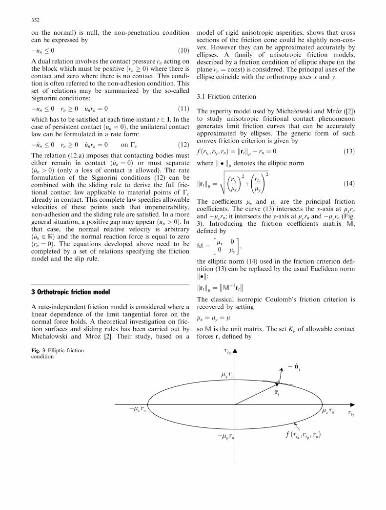
The frictional contact law aims to describe contactinteractions. We consider now the previous friction lawembedding the impenetrability condition for complete-ness. The sliding rule is combined with the rate form ofthe unilateral contact conditions to obtain the frictionalcontact law. The multivalued nature of this strongly non-linear law makes problems involving frictional contactamong the most difficult ones in solid mechanics.

4.1 Analytical formulation

The complete form of the frictional contact law dealswith the three possible physical situations, which areseparation, contact with sticking, and contact withsliding. Dissipation occurs only for the last case. Thislaw is applicable only to material points in contact. Twooverlapped ‘‘if . . . then . . . else’’ statements can be usedto write it analytically (Box 1):

In the first and the second part of the statement, themultivalued character of the frictional contact constit-utive model is revealed. If rn is null then the velocity _u isarbitrary but its normal component _un should be posi-tive. In others words, an infinite number of velocityvectors _u 2 R3 can be related to one element of r 2 R3.On the other hand, if � _u is null then the reaction r

should be in Kl but its direction or magnitude are notspecified. They are arbitrary. Again, one element of R3

353

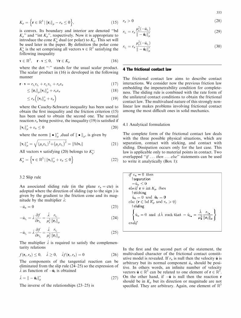
(� _u ¼ 0) can be related to an infinite number of r 2 R3.The inverse constitutive frictional contact law, i.e. therelationship rð� _uÞ can be written as (Box 2):

Similar considerations regarding the multi-valued char-acter of the relatioship can be drawn for the inverse law.

4.2 Variational inequality-based formulation

The previous forms of the frictional contact law, given inBox 1 and Box 2, are well suited for classical numericalimplementations where the contact problem is dissoci-ated from the friction problem. However on the contactsurface, contact cannot be separated from friction.Therefore a coupled algorithm that solved both prob-lems in one step could improve the computational per-formances and robustness. With this aim in mind, thefrictional contact law need to be reformulated. The mainidea behind this reformulation is to provide a naturalbasis for the application of the Uzawa algorithm.

The slip rule, as written in relations (23–25), exhibitsa structure similar to the non-associated flow rule inplasticity. Indeed, during sliding, contact is maintained.Therefore the normal velocity is equal to zero ( _un ¼ 0)and not related to the normal component of the reactionrn through normality. In fact, if we regard the contactforce r and the velocity � _u as conjugate quantities ofeach other, the normality will not occur since it wouldrequire that the velocity would have a normal separatingcomponent.

To avoid complex notations due to elliptic norms, thevariational-inequality based formulation is derived forthe isotropic model lx ¼ ly . The sliding rule is given by

� _un ¼ 0; � _ut ¼ _k@f ðrÞ@rt

ð31Þ

but can be rewritten in the following obvious way:

�ð _un þ l _kÞ ¼ _k@f@rn

; � _ut ¼ _krt

krtkð32Þ

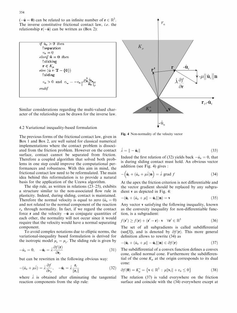
where _k is obtained after eliminating the tangentialreaction components from the slip rule:

_k ¼ k � _utk ð33ÞIndeed the first relation of (32) yields back � _un ¼ 0, thatis during sliding contact must hold. An obvious vectoraddition (see Fig. 4) gives :

� _ut þ ð _un þ l _kÞn� �

¼ _k grad f ð34Þ

At the apex the friction criterion is not differentiable andthe vector gradient should be replaced by any subgra-dient v as depicted in Fig. 4:

� _ut þ _un þ lk � _utkð Þnð Þ ¼ v ð35ÞAny vector v satisfying the following inequality, knownas the convexity inequality for non-differentiable func-tion, is a subgradient:

f ðr0Þ � f ðrÞ þ ðr0 � rÞ v 8r0 2 R3 ð36ÞThe set of all subgradients is called subdifferential(see[3]), and is denoted by @f ðrÞ. This more generaldefinition allows to rewrite (34) as

�ð _ut þ ð _un þ lk � _utkÞnÞ 2 @f ðrÞ ð37ÞThe subdifferential of a convex function defines a convexcone, called normal cone. Furthermore the subdifferen-tial of the cone Kl at the origin corresponds to its dualcone:

@f ð0Þ ¼ K�l ¼ v 2 R3 : lkvtk þ vn � 0� �

ð38Þ

The relation (37) is valid everywhere on the frictionsurface and coincide with the (34) everywhere except at

Fig. 4 Non-normality of the velocity vector

354

the origin (r ¼ 0). Therefore this relation corresponds tothe frictional contact law. As it is well known fromConvex Analysis, the normality rule (37) is equivalent tothe following variational inequality:

r 2 Kl : ðr� r0Þ v � 0; 8r0 2 Kl ð39Þwhere the components of the vector v are

vt ¼ � _ut; vn ¼ � _un þ lk � _utknð Þ ð40ÞAgain the vector v satisfying the inequality (39) is uniqueexcept at the apex (r ¼ 0) where this inequality becomes

K�l ¼ v 2 R3 : r0 v � 0; 8r0 2 Kl� �

ð41Þ

Combining the definition of the dual cone (22) and thedefinition of the vector v (40), we can see that at theorigin (r ¼ 0), the non-penetration condition for con-tacting bodies is recovered. The slip rule in the form (37)is obtained for an anisotropic model by simply replacing‘‘lk � ð _utÞk’’ with ‘‘k � ð _utÞk�l’’.

5 Discrete frictional contact law

The inequality developed in the previous section is nowdiscretized so it can be used in the local stage where thereaction are computed. The time interval ½0; T � is parti-tioned into N sub-intervals of size 4t, not necessarilyequal, according to

0 ¼ t0 < t1 < < tn�1 < tn < < tN ¼ T

We set xðtnÞ and 4x ¼ xn � xn�1, where x representsany variable. Between two time instants, the velocity isassumed to be constant. In order to ensure convergenceand stability requirements, the implicit scheme is con-sidered. As a result of a backward-Euler type approxi-mation of (39), the frictional contact law is satisfied atthe end of each time step:

rnþ1 2 Kl such thatDv ðr0 � rnþ1Þ � 0; 8r0 2 Kl

ð42Þ

where the components of the vector Dv are given by

Dvt ¼ �Dut and Dvn ¼ � Dun þ k � Dutk�l� �

The previous inequality can be transformed into a pro-jection inequality

Find rnþ1 2 Kl such thatðrnþ1 � sÞ ðr0 � rnþ1Þ � 0; 8r0 2 Kl

ð43Þ

where the vector s is given by

s ¼ st

sn

�¼

rnþ1t � qDut

rnþ1n � q Dun þ ð�DutÞk k�l

� �( )

ð44Þ

The last inequality means that the reaction at the end ofthe time step is the projection of the augmented surfacetraction s onto the convex Coulomb’s cone Kl:

rnþ1 ¼ proj s;Kl

ð45Þ

Three different situations emerge according to the posi-tion of the prediction in the forces space. The first casecorresponds to a prediction located in the cone Kl. Itsprojection is the prediction itself, i.e. rnþ1 ¼ s. The secondone relates to a prediction situated in the cone K�l , whereits projection turns out to be the origin of the forces space,i.e. rnþ1 ¼ 0. In the last case, the prediction is neither inKl

nor in K�l and the corrector step requires computing theprojection of the prediction. The projection of a pointonto a convex set is equivalent to the minimization of thedistance between this point and the convex set. In thepresent situation (orhtotropic friction condition), it leadsto a quartic equation that has one positive root. Thedetails of the derivation can be found in [1].

6 Finite-step boundary value problem and variationalformulation

The solution of the elastic frictional-contact initialboundary value problem, under a given history ofexternal actions, requires following the evolution of thebody response since the frictional contact law is intrin-sically path-dependant. A numerical technique, whichcombines a space and time discretization, is used to solvethis problem. The time discretization is based on asubdivision of the external actions history into a se-quence of loading conditions at selected time instants.The solution is then achieved by solving a sequence ofproblems in which the load increments are applied andthe variables at the end of each increment are updated.We suppose that the solution of the problem is known attime tn. Given the body force f

nþ1, the surface traction

tnþ1

and the imposed displacement u nþ1, it is required tosolve the governing equations listed below:

� in Xð0Þ :

Div Pnþ1 þ fnþ10 ¼ 0 ð46Þ

Enþ1 ¼ 1

2Fnþ1 þ ðFnþ1ÞT þ ðFnþ1ÞTFnþ1� �

ð47Þ

Fnþ1 ¼ runþ1

Snþ1 ¼ @W ðEÞ@E

����nþ1

; Pnþ1 ¼ Fnþ1Snþ1 ð48Þ� on Ctð0Þ :

Pnþ1n0 ¼ tnþ10 ð49Þ

� on Cuð0Þ :

u ¼ unþ1 ð50Þ� on Ccð0Þ :

rnþ1 ¼ proj ðsðDuÞ;KlÞ ð51Þ

355

The standard approach to derive the principle of virtualwork over an increment consists in taking the innerproduct of the local equilibrium equation (46) with a testfunction du satisfying du ¼ 0 on Cu and dun � 0 on Cc(virtual displacement increment):Z

Xð0Þ

Div P nþ1 du dXþZ

Xð0Þ

fnþ10 du dX ¼ 0 ð52Þ

Integrating by parts the first term and taking intoaccount the boundary conditions leads to the followingvariational equation:Z

Xð0Þ

Snþ1 dE dX�Z

Xð0Þ

fnþ10 du dX

�Z

Ctð0Þ

tnþ10 du dC�

Z

Ccð0Þ

r nþ1 du dC ¼ 0 ð53Þ

where the first Piola-Kirchhoff stress tensor P nþ1 hasbeen exchanged with the second Piola-Kirchhoff tensorSnþ1. Taking into account that the stress filed is inequilibrium at tn, the weak form can be written in termsof finite increments as follows:

d

Z

Xð0Þ

DW ðDEÞ dX�Z

Xð0Þ

Df0 Du dX

�Z

Ctð0Þ

Dt0 Du dC�Z

Ccð0Þ

Dr Du dC

�¼ 0 ð54Þ

where DW ðDEÞ is given by

DW ðDEÞ ¼ 1

2ðDEÞTDðDEÞ ð55Þ

and DE by

DEðun;DuÞ ¼ Eðun þ DuÞ � EðunÞ ð56ÞIf the behavior on contact surface is frictionless, thefunctional (52) becomes the classical energy functional:

d

Z

Xð0Þ

DW ðDEÞ d X�Z

Xð0Þ

Df Du dX

�Z

Ctð0Þ

Dt0 Du dC

�¼ 0 ð57Þ

Then, the problem in not path-dependant anymore andthe total variables are used instead of their increments.

7 Finite element discretization

The displacement increment field and the transforma-tion gradient are approximated according to:

Du ¼ NðXÞDU; DF ¼ BðXÞDU ð58Þ

where DU is the unknown nodal displacement incrementvector, NðXÞ is the matrix of polynomial shape functionsand the matrix BðXÞ is given by

BðXÞ ¼ @NðXÞ@X

The strain increment can be decomposed as

DE ¼ BLðUnÞ þ BNLðDUÞð ÞDU ð59Þ

The operator BL relates the linear part of the straintensor to the nodal displacement vector and BNL relatesthe nonlinear part of the strain tensor to the nodal dis-placement vector. The compatibility conditions (50) onCu are enforced by substituting nodal unknowns by theircorresponding values. Taking into account (58) and (59),the fully discrete form of the functional is given byZ

Xð0Þ

DW ðDEðUn;DUÞÞ dX� DFext DU� DR DU

ð60Þwhere DFext corresponds to the generalized nodal forceincrement vector

DFext ¼Z

Xð0Þ

NTDf0 dXþZ

Ctð0Þ

NTDt0 dC ð61Þ

and DR is the equivalent contact reaction incrementvector at nodes. The equilibrium equations over a timestep are given byZ

Xð0Þ

@DW ðDEðUn;DUÞÞ@DU

dX� DFext � DR ¼ 0 ð62Þ

where

@DW ðDEðUn;DUÞÞ@DU

¼ KT

Combining the structural equilibrium equations (62)with the incremental frictional contact constitutiverelation (51), the solution of the boundary value prob-lem over a time step is obtained by solving the followingsystem of equations:

KTDU� DFext � DR ¼ 0 ð63Þ

Rnþ1 ¼ projðsðDUÞ;KlÞ on Cc ð64Þ

DU ¼ DU on Cu ð65Þ

8 Solution algorithm

The system of equations (63–65) has to be solved itera-tively since the displacement increment vector, the con-tact surface and the reactions DR are unknown. Thesolution algorithm (see Box 3) tackle separately thegeometric and the contact nonlinearities. At the begin-

356

ning of each load step, DR is set equal to zero and DU iscomputed according to (63). Since the problem is geo-metrically nonlinear, the process is iterative. Now thereactions have to be computed and the penetration thathas occurred by assuming DR ¼ 0 must be corrected.This is achieved by applying the Uzawa iterative schemeas shown in Box 4. This procedure involves only vari-ables associated with contact nodes. In contrast withclassical methods (penalty, Lagrange multiplier), thepresent algorithm does not require an update of theglobal stiffness matrix during the contact iterations.Furthermore the total number of degree of freedomremain unchanged.

The displacement increments on the contact surfaceare computed using the flexibility matrix W, defined inthe local coordinate system:

W ¼wnn wntx wntywntx wtxx wntxy

wnty wtxy wtyy

24

35

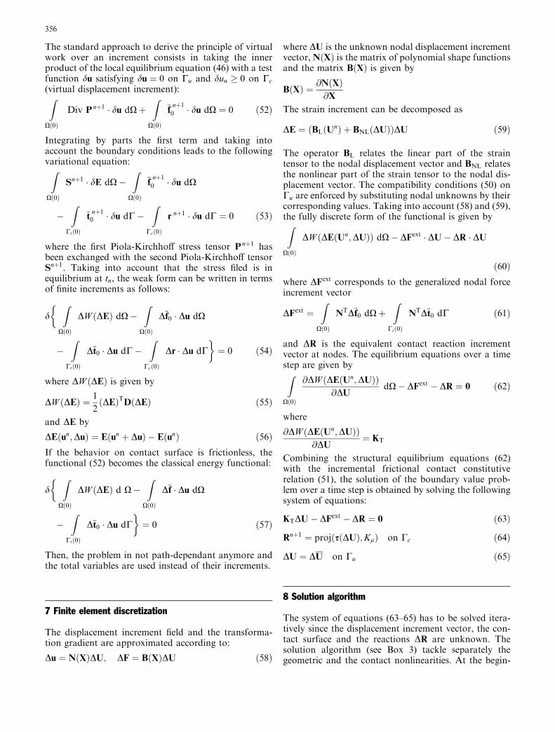
Fig. 5 Block mesh

(a) (b)

(c)

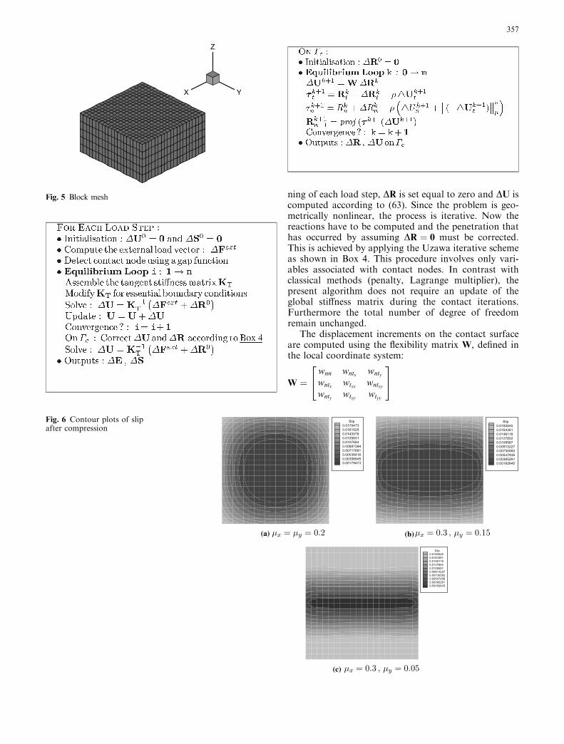
Fig. 6 Contour plots of slipafter compression

357

Next, the prediction s is computed and projected on thecone Kl to give the reaction (see Box 4). The Uzawaalgorithm is known for being convergent but requiring

quite a few iterations. The convergence rate stronglydepends on the regularization factor q. A good choice iscrucial to ensure that the algorithm will convergencewithin a few iterations. Our experience has shown that adifferent factor q for each contact node gives a betterconvergence. In our calculations, the factor q is calcu-lated using the diagonal terms of the flexibility matrix:

q ¼ 1

minðwnn;wtxx ;wtyy ÞThis choice has proven to be satisfactory for most cases.

9 Numerical application

The numerical algorithm developed above is used tostudy the motion of a block pushed on a frictional pla-nar surface. The block is a rectangular prism with thefollowing dimensions: base = 20 mm� 20 mm andheight = 10 mm. The block is subdivided into 2000eight-node brick-like elements as shown in Fig. 5. Eachelement has 27 integration points. The lower surface ofthe cube is in contact with a planar surface whose nor-mal vector is (0, 0, 1). The loading process involves 5steps and is displacement-controlled. During the firststep, the block is compressed by applying a uniformvertical displacement on the upper surface. The magni-tude of the vertical displacement is 0.1 mm. Next, theblock is pushed horizontally by applying, in 4 steps, auniform horizontal displacement on the upper surface.The direction of the horizontal motion is inclined at 45

with respect to the x-axis. The magnitude of each hori-zontal displacement increment is 0.32 mm. The block isassumed to be elastic with the following material prop-erties:

– Young’s modulus: E = 210000 N/mm2,– Poisson’s ratio: = 0.3

The effect of frictional anisotropy is examined by con-sidering three different sets of frictional coefficients lxand ly :

– Case 1 : lx ¼ ly ¼ 0:2, (isotropic)– Case 2 : lx ¼ 0:3 and ly ¼ 0:15,– Case 3 : lx ¼ 0:3 and ly ¼ 0:05

The first case corresponds to the classical isotropicfrictional model where the frictional behavior is iden-tical for all sliding directions. A mild anisotropy isconsidered in the second case where the friction coef-ficient in the x-direction is twice the friction coefficientin the y-direction. In Case 3, the anisotropy is evenstronger with a ratio lx=ly equal to 6.

9.1 Compression of the block

The frictional properties of the planar surface have asignificant influence on the slip distribution. Figure 6shows the contour plots of the slip for the three cases.The slip corresponds to the Euclidean norm of the

(a)

(b)

(c)

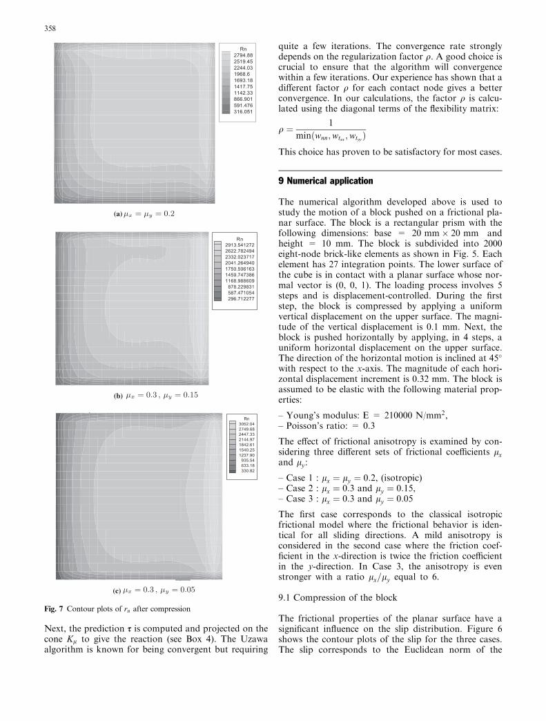
Fig. 7 Contour plots of rn after compression

358

tangential displacement of contact nodes. As expected,the stick zone is located around the base center andsliding increases monotonically as we get closer to the

periphery. The shapes of the slip iso-values are similar tothe friction criterion. The iso-values are circular forthe isotropic case and elliptic for the anisotropic cases.The tangential displacement is obviously larger in they-direction if the friction coefficient is smaller in thisdirection. The slip iso-values are flat ellipses for thestrongly anisotropic model, exactly like the friction cri-terion. Contour plots of the normal reaction rn areshown in Fig. 7. The largest value of rn occurs aroundthe base center but does not change notably with thefrictional properties of the planar surface. The minimumof the normal reaction occurs at the periphery.

9.2. Sliding motion of the block

Figure 8 shows contour plots of the total slip at the endof the loading process. The maximum value of thesliding occurs at the front corner (with respect tomotion). There is no significant difference between thevalue of the maximum slip for the isotropic modeland the mildly anisotropic one. A larger displacement inthe y-direction is observed for the strongly anisotropicmodel as a result of a low friction coefficient in thisdirection. The contour plots of the normal reaction atthe end of the loading are shown in Fig. 9. Again, themaximum and the minimum of rn are very close for allmodels. The maximum occurs in the ‘‘front’’ area whilethe minimum occurs in the ‘‘back’’ area. The deformedmeshes for the three models are shown in Fig. 10. Themotion of the upper face is imposed but the motion ofthe lower face depends strongly on the frictional prop-erties of the planar surface. If the frictional behavior isindependent of the sliding direction (isotropic model),the lower and the upper faces of the block move in thesame direction. Therefore no twist (distortion due todifferent motion directions for the lower and upper fa-ces) of the cube occurs. However, deformation due tothe relative displacement between the upper and thelower faces takes place. The amplitude of this defor-mation depends on the elastic properties of the cube. Onthe other hand if an anisotropic frictional model isconsidered then the motion direction of the lower facedoes not coincide with the motion direction of the upperface and the block is twisted. The magnitude of thisdistortion depends on the friction coefficients and theelastic properties. The distortion is stronger for thestrongly anisotropic model.

10 Conclusion

In this paper, the motion of a deformable body slidingon a half-plane has been investigated. Large displace-ments but small strains have been considered. The fric-tional behavior has been modelled by an elliptic cone.The algorithm used to solve the problem is based on aweak variational statement of the frictional contact law.An uncoupled strategy was used to solve the discreteequations. The study shows that frictional properties

(a)

(b)

(c)

Fig. 8 Contour plots of slip after sliding. a lx ¼ ly ¼ 0:2 blx ¼ 0:3;ly ¼ 0:15 c lx ¼ 0:3; ly ¼ 0:05

359

(a) (b)

(c)

Fig. 9 Contour plots of rnafter sliding

(a) (b)

(c)

Fig. 10 3D deformed meshafter sliding

360

have a strong influence on the trajectory of a deformablebody sliding on a frictional surface.

References

1. Hjiaj M, Feng ZQ, de Saxce G, Mroz Z. (2004) Three-dimen-sional finite element computations for frictional contact prob-

lems with non-associated sliding rule. Int. J. Numer. Meth. Eng.60: 2045–2076

2. Michałowski R, Mroz Z. (1978) Associated and non-associatedsliding rules in contact friction problems. Arch. Mech. 30: 259–276

3. Rockafellar RT, Wets J-B. (1998) Variational analysis.Springer, Berlin, Heidelberg New York

4. Wriggers P. (2002) Computational contact mechanics. Wiley,New York

361