Inflation Inertia and Inliers: The Case of Brazil*

Ana Katarina Campelo**

Francisco Cribari-Neto***

Summary: 1. The issue; 2. The data; 3. Unit root tests; 4. Mea-suring inflation inertia; 5. Some simulation results; 6. Concludingremarks and discussion.

Keywords: inflation inertia; inliers; persistence; unit roots.

JEL codes: C22; C12; C15.

This paper addresses the issue of measuring the degree of inertiain inflation in the presence of potential ‘inliers’. It shows that byusing robust unit root tests one reaches the same inference on theorder of integration of the series as what is revealed by the modifiedprocedure proposed by Cati et al. (1999). The results also suggestthat, contrary to previous findings, the degree of inertia in inflationis rather small. Finally, the paper presents simulation results onthe finite–sample behavior of unit root tests and of a persistencemeasure when the data contain inliers.

Este artigo analisa a mensuracao do grau de inercia na inflacao napresenca de potenciais inliers. O artigo mostra que testes robustosde raızes unitarias conduzem a mesma inferencia sobre a ordem deintegracao da serie do que o procedimento modificado proposto porCati et al. (1999). Os resultados sugerem que o grau de inercia nainflacao brasileira e pequeno. Por fim, o artigo apresenta resultadosde simulacao de Monte Carlo sobre o desempenho em amostrasfinitas de testes de raızes unitarias e de uma medida de persistenciaquando os dados contem inliers.

*Paper received in Aug. 2001 and approved in Sep. 2002. We gratefully acknowledge finan-cial support from CAPES and CNPq. We thank Roger Koenker, and seminar participants atthe XVII Latin American Meeting of the Econometric Society (Cancun), 1998 Illinois EconomicAssociation Meeting (Chicago), Getulio Vargas Foundation, University of Brasilia, Federal Uni-versity of Minas Gerais, Federal University of Pernambuco, Federal University of Rio de Janeiro,and Brazilian Meeting on Probability and Statistics for comments and suggestions. We also thanktwo anonymous referees.

**Department of Economics, Federal University of Pernambuco. E-mail: campelo@ufpe.br.***Department of Statistics, Federal University of Pernambuco. E-mail: cribari@ufpe.br.

RBE Rio de Janeiro 57(4):713-739 OUT/DEZ 2003

714 Ana Katarina Campelo, Francisco Cribari-Neto

1. The Issue

It has been argued that some inflationary processes contain an ‘inertial com-ponent’ thus implying that, in the absence of economic shocks, inflation displays atendency to reproduce itself from one period to the next.1 The fully inertial casecorresponds to a random walk in inflation, that is, yt = yt−1 +ut, where yt denotesthe inflation rate at time t and ut is a white noise disturbance with mean 0 andvariance σ2. A 1% shock to inflation then becomes fully persistent in the sensethat it changes one’s long-run forecast of the inflation rate by exactly 1%. Thiscan be easily seen when the process is rewritten, under the assumption that theprocess starts at zero (i.e., y0 = 0), as yt =

∑tj=1 uj . That is, the inflation rate

at time t is nothing more than the accumulation of past innovations. When ut isnot a white noise disturbance but has some stationary and invertible ARMA(p, q)representation, the degree of long–run persistence is not necessarily equal to 1,and can take any value in the interval (0,∞). Here, inflation displays some inertiawhich can be quite small (say, close to zero) or large (say, greater than 1). Whenyt is integrated of order zero instead, shocks to inflation have no long-run effectsand there is no inertia in inflation.

Brazil has often been cited as the prime example of a country with a largeinertial component in inflation. Simonsen (1988:260), for instance, analyzingthe Brazilian experience writes that “anti–inflationary policies in the 1980s werepainful enough to suggest that inflation rates might be held back by a force ignoredin rational expectations models, namely, inertia caused by strategic interdepen-dence among private economic agents”. “The inertia was considered so large thatnegative shocks to inflation, such as the oil–price hikes in the 1970s, were believedto shift inflation to a new level, where it would stay until a new shock occurred.Empirical studies of the Phillips curve and the finding of a random–walk compo-nent in the inflation rate supported the hypothesis of inertial inflation” (Durevall,1998:424).

Novaes (1993) measured the degree of inertia in the Brazilian inflation usingcumulative impulse response functions from fitted ARIMA models, and foundit to be roughly 1/3, thus implying that one third of the inflationary dynamicsis due to inertia. Durevall (1998), using an error correction formulation, foundthe level of inflation inertia in Brazil to be 0.41. Cati et al. (1999) have arguedthat nearly all of the so-called shock plans which were designed to curb inflationand were implemented in Brazil since the mid-1980s brought inflation down for

1See, for instance, Simonsen (1988), Novaes (1993) and Durevall (1998, 1999) concerning theBrazilian experience.

RBE Rio de Janeiro 57(4):713-739 OUT/DEZ 2003

Inflation Inertia and Inliers: The Case of Brazil 715

a few months and then failed.The observations corresponding to these monthswhen inflation was artificially low have been termed ‘inliers’, and the authors haveclaimed that they tend to bias traditional unit root tests. This motivated them todesign corrected tests by adding dummy variables to the usual augmented Dickey-Fuller (ADF) test. The initial puzzle they addressed was the following: the ADFtest rejected the unit root null (thus suggesting no inertia), and yet an estimateof the degree of long-run persistence (i.e., inertia) indicated that such persistencewas 0.97, i.e., nearly what is expected for a pure random walk process (i.e., fullinertia). The modified tests they proposed, unlike the ADF test, did not rejectthe unit root null at the usual significance levels, thus being consistent with thehigh inertia levels they found. The main idea behind their approach was to movethe shock plans from the noise to the trend function, thus isolating their effects.Overall, they identify five shock plans that took place between 1986 and 1991 andcovered a total of 22 months. Durevall (1999) finds that inflation inertia is low inBrazil. However, the data he used does not include the most recent period of theBrazilian economic history, and hence he does not have to deal with the issue ofhandling potential inliers.

In this paper we show that robust unit root tests achieve the same conclusionas ADF-type tests that have been properly modified to account for inliers andshock plans through the specification and placement of dummy variables. Therobust tests require no such variables. The tests suggest that there is some inertiain the Brazilian inflationary dynamics. We then measure how much inertia hasbeen driving Brazilian inflation, and find that inflation inertia is, conversely towhat has been previously found, small and of second order. In effect, we find thatprior to 1986 the Brazilian inflationary dynamics displayed no inflation inertia. Asa consequence, the series of shock plans put into effect after February 1986 mayhave been based on an incorrect diagnosis of the inflationary driving forces.

2. The Data

We use two different monthly time series for the Brazilian inflation. The firstone is the series used by Cati et al. (1999), which ranges from January 1974 toJune 1993 (234 observations). It consists of the so-called ‘official inflation index’and is a splice of several indices that were used by the Brazilian governmentas the official index to all mandatory indexation schemes. The series has beenmodified by the authors, who have replaced each observation by the geometricmean of every two consecutive observations. The second series used in this paperis considerably longer. It ranges from February 1944 through February 2000 (673

RBE Rio de Janeiro 57(4):713-739 OUT/DEZ 2003

716 Ana Katarina Campelo, Francisco Cribari-Neto

observations) and consists of the IGP-DI (ındice geral de precos-disponibilidadeinterna) computed by the Getulio Vargas Foundation. The series is presented infigure 1. The source of the data are several issues of Conjuntura Economica andInstituto Brasileiro de Geografia e Estatıstica (1990).

Figure 1Monthly inflation rate (IGP-DI)

Time

1950 1960 1990 20001970 1980

020

40

60

80

Figure 1Monthly inflation rate (IGP-DI)

3. Unit Root Tests

Although augmented Dickey-Fuller tests are useful for testing the null hypoth-esis of nonstationarity, they may not be robust when the data generating processfollows a fat-tailed distribution. In such cases, the ADF test may suffer from lowpower. An alternative test based on regression rank scores was recently proposedby Hasan and Koenker (1997). Their test is based on the following model:

yt = ρyt−1 + ut,

ut = α1ut−1 + · · · + αput−p + εt

where the εt’s are a sequence of i.i.d. variates with mean zero and constant varianceσ2, and the roots of 1−α1z−· · ·−αpz

p = 0 lie outside the unit circle. The modelcan be written using an ADF–like specification as

RBE Rio de Janeiro 57(4):713-739 OUT/DEZ 2003

Inflation Inertia and Inliers: The Case of Brazil 717

∆yt = δ0 + γyt−1 +p∑

j=1

δj∆yt−j + εt

or, more concisely, as

∆yt = Xtγ + Z ′tδ + εt

with Xt = yt−1, Zt = 1, ∆yt−1, . . . ,∆yt−p. The null hypothesis of a unit au-toregressive root is H0 : γ = 0, which is equivalent to ρ = 1 in the originalformulation. In order to perform the test, we estimate the restricted model (i.e.,omitting the yt−1 term), obtain the regression rank score process aT (t) and theassociated ‘ranks’

bT =(−

∫ 1

0ψ(τ)dai(τ)

)T

t=1

where ψ(·) is the score function, and then compute the statistic

ST =∑

(yt−1 − yt−1)bt√∑(yt−1 − yt−1)2

,

where yt−1 denotes the projection of yt−1 on the matrix Zt = 1, ∆yt−1, . . . ,∆yt−p.When the model includes a time trend, we use Zt = 1, t, ∆yt−1, . . . ,∆yt−p. Thestatistic above has a complicated non-normal asymptotic null distribution, but itcan be shown that a modified version of it has a limiting standard normal nulldistribution. Hence, critical values for the test can be easily obtained from anormal table. The modified ‘statistic’ can be written as

ST =σ

∆1/2ST − Σ12σyt−1

∆1/2σ

(T γ − σ2 − σ2

u

2σ2yt−1

)with

σ2 = Σ11 = limT→∞

T−1E(∑

ut

)2, σ2

u = limT→∞

T−1∑

E(u2t )

σ2yt−1

= T−2∑

(yt−1 − yt−1)2, ∆ = |Σ|,where

RBE Rio de Janeiro 57(4):713-739 OUT/DEZ 2003

718 Ana Katarina Campelo, Francisco Cribari-Neto

Σ = limT→∞

var[T−1/2

∑(ut, vt)′

]with (ut, vt) being a bivariate process where vt = ψ(F (εt)).

The modified test statistic is then defined by replacing the unknown parametersby consistent estimators. The resulting statistic has a limiting standard normaldistribution. Such a modified test statistic requires one to select a value for an-other lag truncation parameter, .This parameter is needed for the estimation of Σ,which is performed using a Newey-West type covariance matrix estimator (Neweyand West, 1987).2 Thompson (2001) argues that this modification seriously af-fects the power of the test, especially when the innovation distribution is similarto the normal distribution, e.g., a t distribution with a large number of degrees offreedom. The simulation results in this paper are in agreement with Thompson’sclaim. This led us to also consider unmodified versions of robust M-tests (type eand type t tests) proposed by Thompson (2001). Thompson’s type t test is analo-gous to the test suggested by Gutenbrunner et al. (1993). Indeed, the unmodifiedtype t test has proven to work quite well in the presence of inliers in the simula-tions in this paper, while the Hasan and Koenker (1997) test, a modified versionof the t test, does not work well in this case. The test statistics (two versions, ane and a t test) suggested by Thompson (2001) are given by

ts = σ−1ψ ST and es = σε[ϕ−1(1)](T−2X ′MX)−1/2ST

with

σ2ε = T−1

∑(εt − ε)2 and ϕ(1) = 1 − δR,3 − . . . − δR,p+2

where the εt = ∆yt −Z ′tδR are the residuals from estimating the model under the

null, ε is their average, δR,i is the ith element of δR, and M = I − (Z ′Z)−1Z ′ isthe projection matrix.3 Here we consider the model which includes a time trend.Thompson (2001) approximates the critical values of the test using a Cornish-Fisher expansion. The approximations to the 5% quantiles of the asymptotic null

2See Hasan (1993), Hasan and Koenker (1997), and Koenker (1997) for further details.3Denote the cumulative distribution function of the errors εt by F (·). For the rank test

based on Wilcoxon scores, ψ(x) behaves asymptotically as F (x)− 0.5. For normal scores, ψ(x) isasymptotically Φ−1(F (x)), where Φ(·) is the standard normal cumulative distribution function.For sign scores, ψ(x) behaves asymptotically as 0.5 × sign(F (x) − 0.5). The σ2

ψ parameter doesnot depend on the error density. For tests based on normal, Wilcoxon and sign ranks, it can beshown to be equal to 1, 1/12 and 1/4, respectively.

RBE Rio de Janeiro 57(4):713-739 OUT/DEZ 2003

Inflation Inertia and Inliers: The Case of Brazil 719

distributions are given by expansions in the correlation parameter (�),4

ke(�) ≈ −22.128 + 16.104(1 − �) − 1.066(1 − �)2 − 0.040(1 − �)3

kt(�) ≈ −3.445 + 1.404(1 − �) + 0.370(1 − �)2 + 0.011(1 − �)3

One can estimate � as

� = T−1∑

εtψ(εt)/(σεσψ)

The main motivation for working with robust unit root tests is that they enjoyrobustness properties that the traditional least squares-based tests do not enjoy.In particular, their performance is not as sensitive to extreme observations as thatof the ADF test.5

At the outset, we have run the ADF test for the two series, i.e., the CGPand the IGP-DI series. The former is the series used by Cati et al. (1999) andthe latter is the longer series that ranges from February 1944 through February2000. Since the presence of inliers in the data can potentially bias the inference,we have also used truncated versions of these two datasets. Their truncated ver-sions (CGP(T) and IGP-DI(T)) stop in December 1985. Since the first shock planwas introduced in early 1986, these two truncated series are known to not containinliers. Finally, the truncation lag parameter in the ADF especification (p) waschosen using four different approaches, namely: minimization of the Bayesian in-formation criterion (BIC); minimization of the Akaike information criterion (AIC);general-to-specific sequential testing at the 10% level (SQ10); general-to-specificsequential testing at the 5% level (SQ5). In all cases the ADF regression wasrun using p = 20, 19, . . . , 1, 0, where p denotes the lag truncation parameter. Theresults are summarized in table 1.

4Thompson (2001) computed � by numerical integration for the three score functions(Wilcoxon, normal and sign-median) and several densities including normal, Student t3 anddouble exponential.

5One could argue that any identified outliers (or inliers) should be removed from the seriesprior to unit root testing. However, this approach can have an adverse effect on the power of thetest since extreme observations usually convey important information as to whether or not thereis mean reversion. Removing observations one believes to be outliers thus has important powerimplications. This point is made by Maddala and Kim (1998:449), who also discuss the HK test.

RBE Rio de Janeiro 57(4):713-739 OUT/DEZ 2003

720 Ana Katarina Campelo, Francisco Cribari-Neto

Table 1ADF test results

Series Lag truncation p selected ADF statistic ConclusionCGP BIC 1 −6.60 Rejects unit root at 1%CGP AIC 1 −6.60 Rejects unit root at 1%CGP SQ10 19 −3.12 Does not reject unit root at 10%CGP SQ5 13 −3.54 Rejects unit root at 5%CGP(T) BIC 2 −3.65 Rejects unit root at 5%CGP(T) AIC 8 −2.68 Does not reject unit root at 10%CGP(T) SQ10 8 −2.68 Does not reject unit root at 10%CGP(T) SQ5 8 −2.68 Does not reject unit root at 10%IGP-DI BIC 0 −5.91 Rejects unit root at 1%IGP-DI AIC 3 −5.10 Rejects unit root at 1%IGP-DI SQ10 18 −2.85 Does not reject unit root at 10%IGP-DI SQ5 14 −3.40 Rejects unit root at 10%IGP-DI(T) BIC 2 −4.17 Rejects unit root at 1%IGP-DI(T) AIC 13 −0.49 Does not reject unit root at 10%IGP-DI(T) SQ10 15 −0.92 Does not reject unit root at 10%IGP-DI(T) SQ5 11 −0.81 Does not reject unit root at 10%Note: The 0.10, 0.05 and 0.01 (asymptotic) critical values are −3.13, −3.41 and −3.96, respectively.

Table 1 reveals that inference based on the ADF test regarding a unit rootin the inflationary dynamics is dependent on the approach used for selecting thelength of the autoregressive augmentation in the unit root test. Consider forinstance the IGP–DI series. The four approaches for lag truncation selection leadto different inferences: the use of the BIC and AIC yields a strong rejection ofthe unit root null (at the 1% significance level), sequential testing at 5% rendersrejection of the unit root null at the 10% significance level, and finally sequentialtesting at 10% leads one to not reject the null hypothesis that there is a unit rootin the data generating process. It is noteworthy that the use of the BIC leads tosmall values of autoregressive orders and to strong rejections of the unit root nullin all but one case (where rejection occurs at the 5% significance level), regardlessof whether there are inliers in the data. The use of the BIC in conjunction withthe ADF test is not recommended by some simulation studies. For example,Agiakloglou and Newbold (1996) found the AIC and sequential testing at the 5%level to be far superior to the BIC for selecting the lag truncation parameter ofADF unit root tests. They find that the use of the BIC in this context leadsto severe size distortions due to its tendency to select very low values for thetruncation parameter, and they conclude that “the performance of the BIC in thisregard is unacceptable for practical use” (p. 232).

Next, we apply the Hasan and Koenker’s and Thompson’s rank tests to the twoinflation time series (CGP and IGP-DI). These will be denoted as HK test and STtests throughout the paper, respectively. We report results for the lag truncation

RBE Rio de Janeiro 57(4):713-739 OUT/DEZ 2003

Inflation Inertia and Inliers: The Case of Brazil 721

parameter of the ADF specification (p) ranging from 1 to 20 and for three differentscore functions (Wilcoxon, sign-median, and normal). For the HK test, the valuesof the lag truncation parameter of the Newey-West covariance matrix estimatorwere = 2, 4, 6, 8. The results of the ST type t test (with the respective estimatedcritical values) for the CGP series and the longer IGP-DI series are given in table2.

Table 2ST type t test (5% level)

CGP IGP-DI

p Wilc. c.v. normal c.v. sign c.v. Wilc. c.v. normal c.v. sign c.v.

1 −0.781 −2.764 −1.069 −2.959 −0.322 −2.454 −0.012 −2.780 −0.464 −2.962 0.742 −2.4932 −0.162 −2.767 −0.452 −2.964 0.252 −2.455 0.030 −2.780 −0.567 −2.962 0.907 −2.4943 −0.168 −2.771 −0.434 −2.967 0.276 −2.458 0.414 −2.783 −0.093 −2.965 1.097 −2.4974 −0.016 −2.772 −0.049 −2.969 0.319 −2.458 0.379 −2.783 −0.121 −2.965 1.161 −2.4975 0.182 −2.765 0.013 −2.963 0.529 −2.448 0.448 −2.785 −0.083 −2.966 1.133 −2.4996 0.221 −2.765 0.051 −2.963 0.529 −2.447 0.342 −2.785 −0.170 −2.967 1.151 −2.4997 0.322 −2.766 0.077 −2.965 1.029 −2.446 0.516 −2.785 −0.019 −2.967 1.077 −2.4998 0.389 −2.773 0.109 −2.972 1.039 −2.450 0.495 −2.786 −0.085 −2.968 1.027 −2.4999 0.455 −2.777 0.168 −2.977 1.104 −2.453 0.578 −2.787 0.013 −2.968 1.160 −2.50010 0.405 −2.778 0.126 −2.977 0.977 −2.454 0.604 −2.786 0.101 −2.968 1.167 −2.50011 0.254 −2.757 −0.005 −2.960 0.741 −2.437 0.797 −2.791 0.319 −2.974 1.458 −2.50212 0.345 −2.756 0.194 −2.959 0.921 −2.436 0.768 −2.788 0.255 −2.971 1.399 −2.50013 −0.121 −2.753 −0.347 −2.957 0.108 −2.431 0.612 −2.786 0.148 −2.970 1.220 −2.49814 −0.079 −2.752 −0.319 −2.955 0.209 −2.431 0.777 −2.785 0.267 −2.968 1.372 −2.49815 0.175 −2.756 0.032 −2.959 0.307 −2.433 0.775 −2.785 0.249 −2.968 1.611 −2.49616 −0.064 −2.763 −0.232 −2.965 0.022 −2.438 0.833 −2.785 0.301 −2.968 1.410 −2.49717 −0.091 −2.764 −0.264 −2.967 0.067 −2.440 0.811 −2.787 0.266 −2.971 1.504 −2.49818 0.250 −2.752 0.139 −2.957 0.137 −2.429 0.962 −2.788 0.483 −2.971 1.448 −2.49819 0.099 −2.757 0.042 −2.962 −0.264 −2.433 0.845 −2.785 0.339 −2.969 1.475 −2.49520 −0.024 −2.750 −0.051 −2.956 −0.242 −2.428 0.772 −2.784 0.263 −2.967 1.424 −2.494

The results in table 2 show that the ST type t test does not reject the unit rootnull against a stationary alternative for both series in any of the cases consideredat the 5% significance level. The same conclusion holds for the ST type e testand the HK test.6 That is, for both series, the HK and ST tests lead one to notreject a unit root in the Brazilian inflationary dynamics regardless of the scorefunction used and regardless of the values of the truncation parameters. Giventhe good power properties of the ST t test under a wide range of distributionalforms for the error term, even when the data contain atypical observations (seethe simulation results in section 5), we view such strong acceptance of the unitroot null as evidence of some inflation inertia.

6The tables are available from the authors upon request.

RBE Rio de Janeiro 57(4):713-739 OUT/DEZ 2003

722 Ana Katarina Campelo, Francisco Cribari-Neto

It is noteworthy that Cati et al. (1999) developed modified ADF tests thatuse dummy variables to account for the shock plans. Their modified tests didnot reject the unit root null when applied to the Brazilian inflation. In order toconstruct the dummies used in the test, one needs to know the starting and endingdates of all ‘shock plans’, and yet it is not easy to determine when a plan was nolonger in effect.7

Table 3HK tests, truncated CGP and IGP-DI series.

CGP(T) series IGP-DI(T) seriesp � = 2 � = 4 � = 6 � = 8 � = 2 � = 4 � = 6 � = 81 −2.579 −4.545 −5.049 −5.111 −14.071 −18.188 −20.839 −22.7072 −1.987 −3.341 −3.989 −4.197 −10.229 −14.107 −17.203 −18.9373 −2.107 −4.243 −5.335 −5.694 −9.599 −13.788 −17.230 −19.0604 −2.569 −4.257 −4.657 −4.640 −9.426 −13.352 −16.869 −18.6745 −1.991 −4.086 −4.811 −4.982 −9.596 −12.519 −16.047 −17.7156 −1.981 −4.360 −5.443 −5.774 −9.684 −12.629 −16.325 −18.2397 −1.631 −3.709 −4.735 −5.135 −9.724 −12.238 −15.445 −17.6378 −2.362 −4.262 −5.144 −5.265 −9.551 −11.440 −13.876 −15.5829 −2.234 −3.838 −4.472 −4.464 −10.090 −12.276 −14.915 −16.42410 −2.757 −4.657 −5.431 −5.313 −10.017 −12.380 −15.090 −16.54411 −2.582 −3.966 −4.371 −4.241 −10.036 −11.974 −13.950 −14.82512 −2.457 −3.538 −3.719 −3.582 −9.860 −11.739 −13.785 −14.69113 −1.887 −3.112 −3.323 −3.177 −9.252 −10.730 −12.338 −13.24814 −1.773 −3.180 −3.431 −3.220 −8.941 −10.555 −12.285 −13.26315 −1.583 −3.011 −3.265 −3.077 −9.236 −11.181 −13.157 −14.35316 −1.572 −3.032 −3.350 −3.225 −9.400 −11.171 −12.948 −13.68517 −1.590 −3.069 −3.469 −3.325 −9.737 −12.001 −14.450 −15.19618 −1.889 −3.386 −3.798 −3.699 −9.860 −11.880 −14.224 −14.99619 −1.825 −3.413 −3.840 −3.693 −9.880 −11.990 −14.442 −15.35220 −1.501 −3.120 −3.654 −3.566 −9.986 −12.084 −14.490 −15.312

The HK, ST, and modified ADF tests therefore do not reject the unit rootnull for the full sample, as one would expect. The two complete samples includeperiods of uncontrolled growth in inflation, some failed attempts at stabilizing itslevel and even brief periods of hyperinflation, thus yielding evidence that the serieshas a stochastic trend (i.e., a unit root). All tests appear to deliver the correctinference, but the HK and ST tests do so without requiring the specification andplacement of dummy variables.

We also applied the HK and ST tests to the two truncated series, i.e., theCGP(T) and IGP-DI(T) series. For brevity, we concentrate on the results based

7The authors recognize the difficulty involved in choosing the ending dates of the severalstabilization plans, and opt for choosing such dates in a way that minimizes the number of possibleoutliers in the residuals from an error correction model that includes inflation and nominal interestrates.

RBE Rio de Janeiro 57(4):713-739 OUT/DEZ 2003

Inflation Inertia and Inliers: The Case of Brazil 723

on the Wilcoxon score function, which is the most commonly used score function.8

The results are given in tables 3 and 4, respectively.

Table 4ST tests, truncated CGP and IGP-DI series (5% level)

CGP(T) series IGP-DI(T) seriests es ts es

p Wilc. c.v. Wilc. c.v. Wilc. c.v. Wilc. c.v.1 −4.251 −3.381 −41.596 −21.406 −5.962 −3.354 −78.254 −21.1042 −3.306 −3.334 −22.368 −20.883 −4.444 −3.342 −40.641 −20.9703 −3.337 −3.328 −25.786 −20.821 −4.019 −3.339 −33.702 −20.9414 −2.724 −3.333 −19.633 −20.877 −3.714 −3.340 −29.036 −20.9485 −2.514 −3.326 −17.783 −20.802 −3.160 −3.340 −22.380 −20.9546 −2.298 −3.319 −16.851 −20.722 −3.034 −3.341 −21.182 −20.9597 −2.451 −3.321 −16.561 −20.744 −3.052 −3.340 −19.833 −20.9508 −2.433 −3.324 −12.661 −20.773 −3.157 −3.332 −17.897 −20.8639 −2.304 −3.331 −10.227 −20.854 −2.990 −3.339 −15.993 −20.94610 −2.493 −3.341 −12.459 −20.965 −2.874 −3.339 −14.918 −20.94711 −2.321 −3.331 −9.126 −20.855 −2.573 −3.347 −11.152 −21.02612 −2.350 −3.319 −8.631 −20.726 −2.381 −3.346 −9.966 −21.02013 −1.872 -3.315 −6.443 −20.679 −1.969 −3.343 −7.579 −20.98114 −1.610 −3.331 −5.368 −20.855 −2.145 −3.343 −8.710 −20.98115 −1.497 −3.329 −5.176 −20.837 −2.458 −3.345 −11.246 −21.00616 −1.540 −3.325 −5.392 −20.790 −2.453 −3.343 −9.966 −20.98717 −1.688 −3.330 −6.026 −20.844 −2.403 −3.340 −10.081 −20.94718 −2.088 −3.330 −7.711 −20.840 −2.450 −3.342 −10.409 −20.97119 −2.103 −3.326 −7.954 −20.797 −2.400 −3.341 −10.371 −20.96620 −1.792 −3.310 −6.797 −20.631 −2.348 −3.341 −10.231 −20.959

We conclude from table 3 that the HK test yields rejection of the unit root nullhypothesis at the 5% level in all but one case (CGP(T) series, p = 7, = 2). Innearly all cases we reject the unit root null at the 1% siginificance level. Indeed,rejection of the null occurs at very low significance levels for the longer IGP-DI(T)series. Moving to table 4, rejection of the unit root null by the ST tests occursfor low values of the lag truncation parameter p. That is, the figures in table 4and, particularly, in table 3, indicate that the Brazilian inflation rate followed astationary inflationary dynamics up until the introduction of the first shock plan inearly 1986. Such dynamics had no inertial component. This is in agreement withthe persistence values (close to zero) for these truncated series given in section 4.Therefore, the first shock plan (the so-called Cruzado Plan) may have been basedon a mistaken diagnosis of the Brazilian inflation.

8The Wilcoxon score function enjoys the property that its asymptotic relative efficiency isbounded below by 0.86 for all symmetric distributions. Overall, the simulation results in Hasan(1993) favor this score function; see the discussion on pages 86–87.

RBE Rio de Janeiro 57(4):713-739 OUT/DEZ 2003

724 Ana Katarina Campelo, Francisco Cribari-Neto

4. Measuring Inflation Inertia

A unit root in inflation indicates the existence of some inertia, that is, somelong–run persistence. It remains to be determined how much inertia there is in theinflationary process. In this section, we use a nonparametric measure of long-runpersistence known as the ‘variance ratio’ (Cochrane, 1988) to measure the degreeof inertia in the Brazilian inflationary process. The persistence measure can bewritten either as a ratio of variances or as a function of autocorrelations:

Vk ≡ 1k + 1

var(yt+k+1 − yt)var(yt+1 − yt)

≡ 1 + 2k∑

j=1

(1 − j

k + 1

)ρj

where ρj is the jth autocorrelation of ∆yt. One can estimate the persistencemeasure Vk by replacing the population autocorrelations with the sample auto-correlations.9 If yt follows a random walk, the above ratio equals 1. On the otherhand, if the series is stationary, the ratio approaches zero as k increases. Finally, itis noteworthy that an asymptotic standard error for the estimated variance ratiocan be obtained using Bartlett’s formula: s.e.(Vk) = Vk/

√(3T/4(k + 1)). We have

computed the variance ratios up to k = 84, but, for brevity, we only report resultsfor some selected values of the parameter k in table 5.

Table 5Variance ratio estimates

Vk

k 10 20 30 40 50 60 70 80CGP 0.49 0.31 0.22 0.19 0.14 0.12 0.12 0.12

(0.12) (0.11) (0.09) (0.09) (0.07) (0.07) (0.07) (0.08)IGP-DI 0.51 0.33 0.25 0.21 0.15 0.17 0.17 0.16

(0.08) (0.07) (0.06) (0.06) (0.05) (0.06) (0.06) (0.07)Note: Standard errors in parentheses.

The results in table 5 suggest that the degree of inertia in the Brazilian infla-tionary dynamics is rather small, ranging from 0.12 (CGP series) to 0.16 (IGP-DIseries). It is noteworthy that these numbers are smaller than the degree of inertiafound by Novaes (1993) who used a parametric measure from fitted ARIMA mod-els and a shorter series. As a check of the results presented above, we considerthe yearly inflation rate from 1862 through 1999 (138 observations), this serieshaving been constructed using estimates from Contador and Haddad (1975) and

9It is customary to multiply the estimated variance ratio by T/(T − k) to correct for adownward finite-sample bias.

RBE Rio de Janeiro 57(4):713-739 OUT/DEZ 2003

Inflation Inertia and Inliers: The Case of Brazil 725

data on the yearly IGP-DI obtained from Conjuntura Economica. It is noteworthythat the effects of possible outliers/inliers are downplayed when we work with alonger yearly series since the impact of a couple of atypical monthly observationson the yearly inflation figure is partially offset by the remaining monthly inflationrates and, as a consequence, the yearly figure does not end up being as atypical.We have computed the variance ratio for this series up to k = 30 and found thatV30 = 0.11, which is in agreement with the previous results.

One could argue that when using the variance ratio as a measure of long-run persistence, the choice of k is arbitrary and that the variance ratio is biasedtowards zero when k is large. The key is to note that k must be large so thatthe variance ratio is able to capture the long-run dynamics of the series, and yetk must not be large in relation to the sample size, in which case bias towardszero would occur. The conclusion drawn from table 5 is based on k = 84 (i.e., 84months or seven years after the initial shock) and 672 observations (IGP-DI series,after differencing), thus yielding k/T = 0.125 (less than 13%).

A different persistence measure oftentimes used is based on an autoregressivespectral estimation:

A(1) =h∆y(0)var(∆y)

where

h∆y(0) =s2ep

(1 − d(1))2

with

s2ep = T−1

T∑t=1

e2tp

and d(1) =∑p

j=1 dj . Here, T is the number of observations, and dj and etp areobtained from a pth order autoregression (Perron and Ng, 1998):

∆yt = c +p∑

j=1

dj∆yt−j + etp

The truncation parameter p must be large enough to filter any serial correlationso that etp is white noise. Cati et al. (1999) used this measure. They selected the

RBE Rio de Janeiro 57(4):713-739 OUT/DEZ 2003

726 Ana Katarina Campelo, Francisco Cribari-Neto

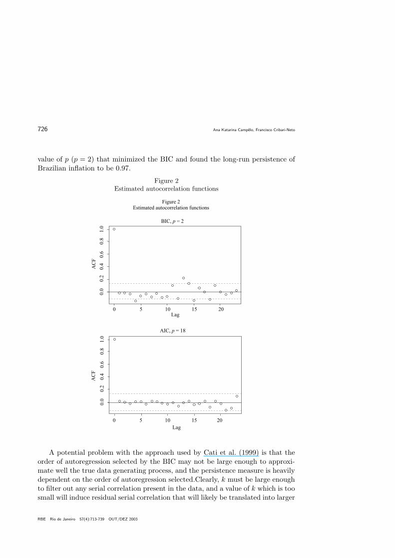
value of p (p = 2) that minimized the BIC and found the long-run persistence ofBrazilian inflation to be 0.97.

Figure 2Estimated autocorrelation functions

AC

F

0 5 10 15 20

0.0

0.2

0.4

0.6

0.8

1.0

AIC, = 18p

Lag

AC

F

Figure 2Estimated autocorrelation functions

0 5 10 15 20

0.0

0.2

0.4

0.6

0.8

1.0

BIC, = 2p

Lag

A potential problem with the approach used by Cati et al. (1999) is that theorder of autoregression selected by the BIC may not be large enough to approxi-mate well the true data generating process, and the persistence measure is heavilydependent on the order of autoregression selected.Clearly, k must be large enoughto filter out any serial correlation present in the data, and a value of k which is toosmall will induce residual serial correlation that will likely be translated into larger

RBE Rio de Janeiro 57(4):713-739 OUT/DEZ 2003

Inflation Inertia and Inliers: The Case of Brazil 727

persistence levels. In order to investigate that, we have computed the persistencemeasure above for both series and for p = 0, ..., 25. We have also computed theAIC for each of the estimated models. Unlike the AIC, the BIC is consistent underquite general conditions. However, for autoregressive models the AIC is, unlikethe BIC, asymptotically efficient (Brockwell and Davis, 1991). The AIC has atendency to overparameterize the selected model. If we think of p as a parameterto be estimated, then it is well known that the BIC yields a consistent estimateof p. However, if we do not think of the autoregressive specification as the correctone, but as an approximation to an unknown data generating mechanism, then itmay be sensible to use the AIC and choose a more elaborate model in the hopethat this may provide a better approximation (Newbold and Bos, 1994:263).

The estimated persistence levels for the CGP and IGP-DI series correspondingto the values of p which minimize the AIC (18 both series) are 0.10 and 0.17,respectively. For the CGP series, p = 15 and p = 19 also deliver small AIC values,and their respective persistence levels are 0.13 and 0.12. These numbers are inagreement with the results obtained using the nonparametric variance ratio intable 5, and are considerably smaller than Cati et al.’s (1999) persistence estimate(which corresponds to p = 2). The estimated persistence levels are quite sensitiveto the order of autoregression selected, and the high persistence level obtained bythese authors is due to the small value of p they have used. Figure 2 shows theestimated autocorrelation functions of the two residual series (p = 2 and p = 18,CGP series). Some of the residual autocorrelations for the residual series obtainedusing p = 2 (i.e., lag truncation selection based on the BIC) lie outside the 95%confidence bands, thus suggesting that the autoregression was not long enough tofilter out all serial correlation. The same does not happen for the residuals obtainedusing p = 18 (i.e., lag truncation selection using the AIC). Cati et al. (1999) showthat, when the data contain inliers, the autoregressive spectral persistence measureis biased towards 1 when p is less than the duration of the plans (n). When p ischosen at least as large as n, the result depends on the specific values of p and n.When int(n/p) = 1, the persistence measure converges in probability to 1/3. Theycorrect the persistence measure in much the same way they correct the ADF test,and find the corrected persistence figure to be even higher, namely 1.67. Again,p = 2 was selected using the BIC. It is noteworthy that using the AIC to selectp for the corrected persistence meausure delivers substantially smaller persistencevalues. We computed Cati et al. (1999) corrected persistence measure for p rangingfrom 1 to 25, and the estimated persistence levels for the CGP and IGP-DI seriescorresponding to the values of p which minimize the AIC are 0.01 (p = 22) and0.15 (p = 15), respectively.

RBE Rio de Janeiro 57(4):713-739 OUT/DEZ 2003

728 Ana Katarina Campelo, Francisco Cribari-Neto

In order to investigate whether the low persistence estimates we obtain are dueto inliers-induced biases, we have computed the variance ratio for up to k = 84 forthe IGP-DI(T) series. That is, we restrict the data to the period from February1944 through December 1985. This subperiod does not include any so-called shockplans, and hence has no potential inliers. Figure 3 displays the variance ratios(solid lines) for both the entire period and the subsample of interest. The dottedlines represent the variance ratio estimates plus and minus their correspondingstandard errors. The ‘inner’ solid line displays the variance ratio for the no-inlierssubsample and the ‘outer’ solid line plots the variance ratio for the entire sample.Figure 3 shows that inflation long-run persistence is even lower when there are noinliers in the sample. Indeed, the variance ratio estimate for the chosen subsamplecorresponding to k = 84 is 0.08, i.e., half of that found for the entire sample (seetable 5). The autoregressive spectral persistence estimate (with p selected by theAIC: p = 16) for the IGP-DI(T) series equals 0.04. Accordingly, this figure is evensmaller than the one obtained for the entire sample (0.17). For the persistencemeasures to be inliers-biased, one would expect the estimated persistences for thetruncated sample periods (which do not contain inliers) to be larger than theones for the complete sample periods (which may include inliers). This does nothappen. Indeed, the opposite happens. This therefore suggests that the low degreeof inflation inertia obtained is not inliers-based biased.

Figure 3Estimated variance ratios for the IGP-DI series based on the entire sample and on a

no-inliers subsample

Figure 3Estimated variance ratios for the IGP-DI series

based on the entire sample and on a no-inliers subsample

Lag

0 20 8040 60

0.2

0.4

0.6

0.8

1.0

Full sample

Var

iance

rati

o

Subsample

RBE Rio de Janeiro 57(4):713-739 OUT/DEZ 2003

Inflation Inertia and Inliers: The Case of Brazil 729

We also note that the measured degree of inflation inertia in the truncatedIGP-DI series is nearly zero regardless of the measure used, which is in agreementwith the inference (rejection of the unit root null) based on the HK test (table 3).The HK test rejected the unit root null for this series, thus indicating no inflationinertia prior to 1986. Since the truncated series has no inliers, one cannot claimthat the results of the HK test and the persistence estimates are biased towardsmean reversion due to inliers.

5. Some Simulation Results

In this section we report the results of Monte Carlo experiments designed toevaluate the finite sample performance of the ADF and rank tests (HK and STtests) in the presence of inliers. For means of comparison we also present simulationresults for the case where the data generating process (DGP) is inliers-free.10 Weconsider the first order autoregressive model

yt = y0 + µt + ut, ∆ut = γut−1 + vt, vt = 0.5vt−1 + ξt, t = 1, . . . , T

ξt being a white noise disturbance. When the data contain shock plans, the aboveDGP is interrupted by occasional ‘inliers’,

yt = a for t ∈ ti,j(j = 1, . . . m; i = 1, . . . , nj)

Here, ti,j refers to the time index of the ith observation of plan j. Thereare m shock plans and each contains nj observations. We consider two errordistributions: standard normal and Student t3. We used the following specificvalues for the parameters. First, a = 4, which can be viewed as an initial level of4% for the inflation rate. There are m = 3 plans irrespective of the sample sizeand each plan contains nj = 6 (j = 1, 2, 3) observations corresponding to plansthat last six months. To complete the specifications, the initial condition is y0 = aand µ = 0.1. We consider three different sample sizes: T = 250, 500, 750; thefirst and the latter are roughly the sample sizes of the CGP and IGP-DI series,respectively. The starting dates of the inliers are T = 50, 100, 150. All resultsare based on 1,000 replications. The critical value for the ADF test is taken fromFuller (1976) (−3.41, 5% level), the critical values for the HK tests are taken from

10We used the same starting seed for each entry to enable one to compare the simulationresults across tables.

RBE Rio de Janeiro 57(4):713-739 OUT/DEZ 2003

730 Ana Katarina Campelo, Francisco Cribari-Neto

a normal table, and the critical values for the ST tests are based on the Cornish-Fisher approximations given in section 3 with the values of � taken from table 1of Thompson (2001).

Starting with the ADF simulation results, the figures in table 6 show that theADF test is severely oversized in the presence of inliers. Next, the figures in table7 reveal that the HK test is undersized under normal errors. This problem is moresevere in the presence of inliers under both the normal and Student t3 densities(tables 7 and 8), regardless of the score function used. The figures in tables 7and 8 show that Thompson’s type e test is also biased in the presence of inliers,with the bias occuring in the same direction as that of the ADF test. The biasis of minor significance only for the sign score, particularly under normal errors.The results in tables 7 and 8 also suggest that the size of the type t version ofThompson’s test is close to the nominal 5% level in the presence of inliers, forboth the normal and Student t3 densities, except for the sign score under normalerrors.

Moving to the power results, the figures in table 9 reveal that the power ofthe HK rank tests for the inliers-free DGP is significantly lower than the powerof the ADF and of Thompson’s tests under normal errors. For this specification,Thompson’s tests (both versions e and t) have power similar to that of the ADFtest under the normal distribution (particularly for Wilcoxon and normal scores)and have power at least as good as the ADF test for T = 500, 750 and higherpower for T = 250 under the Student t3 distribution. The results in table 9also reveal that Thompson’s tests still have good power in the presence of inliersunder the normal distribution, the best performance being the rank test based onnormal scores, as expected, followed by the Wilcoxon scores. The tests based onthe sign score are the least powerful. The power performance of the ST tests inthe presence of inliers is even better under the Student t3 density (see table 10),being close to 1 for the rank tests based on the scores Wilcoxon and normal for allsample sizes considered and (1 + γ) = 0.9.11 Again, the sign scores have the leastaccurate performance. We, therefore, conclude that the ST t test based on normaland Wilcoxon scores (which also have size close to the nominal level) seems tohave an adequate performance in the presence of inliers.

11The sample kurtosis of the first differences of CGP and IGP-DI series are much greater thanthe kurtosis of a normal variate (39.9 and 161.5, respectively; the kurtosis of a normal randomvariable is 3). The sample kurtosis of ∆yt for the (complete) IGP-DI series is therefore over 50times greater than that of the first difference of a Gaussian random walk. This can be viewed asan indication of fat tails or generation of atypical observations by the data generating process.

RBE Rio de Janeiro 57(4):713-739 OUT/DEZ 2003

Inflation Inertia and Inliers: The Case of Brazil 731

Table 6ADF test simulation results

normal Student−t31 + γ Inliers T = 250 T = 500 T = 750 T = 250 T = 500 T = 750

1.0 No 0.042 0.046 0.040 0.055 0.040 0.0510.9 No 0.699 0.999 1.000 0.716 0.999 1.000

(0.728) (0.999) (1.000) (0.705) (0.999) (1.000)0.8 No 0.995 1.000 1.000 0.989 1.000 1.000

(0.997) (1.000) (1.000) (0.987) (1.000) (1.000)

1.0 Yes 0.457 0.347 0.251 0.402 0.252 0.198

Note: Size corrected power in parentheses.

Table 7Size of rank tests under normal errors (5% level)

Normal errors, α = 5% T = 250 T = 500 T = 750Inliers Test Wilc. Normal Sign Wilc. Normal Sign Wilc. Normal Sign

No STt 0.037 0.031 0.044 0.033 0.034 0.037 0.041 0.036 0.045No STe 0.041 0.039 0.039 0.040 0.039 0.039 0.040 0.039 0.039No HK 0.035 0.032 0.035 0.018 0.012 0.034 0.017 0.008 0.042Yes STt 0.048 0.077 0.019 0.053 0.084 0.019 0.052 0.078 0.025Yes STe 0.135 0.224 0.044 0.216 0.293 0.062 0.242 0.290 0.102Yes HK 0.004 0.008 0.005 0.002 0.001 0.006 0.002 0.000 0.007

Table 8Size of rank tests under Student-t errors with 3 degrees of freedom (5% level)

Student−t3 errors, α = 5% T = 250 T = 500 T = 750Inliers Test Wilc. Normal Sign Wilc. Normal Sign Wilc. Normal Sign

No STt 0.050 0.045 0.046 0.038 0.039 0.056 0.047 0.049 0.053No STe 0.051 0.048 0.053 0.040 0.043 0.042 0.044 0.043 0.050No HK 0.045 0.035 0.046 0.041 0.030 0.053 0.035 0.028 0.050Yes STt 0.055 0.085 0.048 0.066 0.099 0.033 0.081 0.104 0.053Yes STe 0.193 0.251 0.111 0.277 0.332 0.133 0.267 0.306 0.160Yes HK 0.009 0.010 0.012 0.008 0.006 0.014 0.014 0.012 0.020

As suggested by a referee, we have also carried out simulations with smallersample sizes. For instance, consider the situation where T = 150 and there aretwo shock plans of six months each; the first shock plan starts at observation 50and the second at observation 100, as before. Here, we only report results forThompson’s t test (STt) with Wilcoxon scores, since this test outperformed theother ones in the previous simulations. The error distribution was Student-t withthree degrees of freedom, and the remaining simulation settings are as before. Thenull rejection rate of the test at the 5% significance level was 5.6%. As for thepower of the test, the estimated powers for 1+γ = 0.8, 0.9 were 86.6% and 54.8%,respectively. The results for normal scores were similar; the use of sign scoresresulted in a test with poorer performance, as in the previous simulations.

RBE Rio de Janeiro 57(4):713-739 OUT/DEZ 2003

732 Ana Katarina Campelo, Francisco Cribari-Neto

Table 9Power of rank tests under normal errors (5% level)

Normal errors, α = 5% T = 250 T = 500 T = 750

1 + γ Inliers Test Wilc. Normal Sign Wilc. Normal Sign Wilc. Normal Sign

0.9 No STt 0.597 0.618 0.371 0.993 0.998 0.874 1.000 1.000 0.990

(0.686) (0.706) (0.402) (0.996) (0.999) (0.901) (1.000) (1.000) (0.991)

0.9 No STe 0.719 0.717 0.637 0.999 1.000 0.987 1.000 1.000 1.000

(0.784) (0.791) (0.689) (1.000) (1.000) (0.992) (1.000) (1.000) (1.000)

0.9 No HK 0.136 0.165 0.094 0.151 0.191 0.079 0.176 0.201 0.087

(0.178) (0.201) (0.106) (0.241) (0.304) (0.095) (0.292) (0.392) (0.095)

0.8 No STt 0.967 0.987 0.768 1.000 1.000 0.997 1.000 1.000 1.000

(0.986) (0.993) (0.796) (1.000) (1.000) (0.998) (1.000) (1.000) (1.000)

0.8 No STe 0.995 0.996 0.954 1.000 1.000 1.000 1.000 1.000 1.000

(0.996) (1.000) (0.967) (1.000) (1.000) (1.000) (1.000) (1.000) (1.000)

0.8 No HK 0.492 0.557 0.227 0.659 0.766 0.281 0.751 0.848 0.327

(0.535) (0.600) (0.257) (0.748) (0.838) (0.333) (0.828) (0.907) (0.357)

t 0.9 Yes STt 0.266 0.524 0.060 0.984 0.998 0.300 1.000 1.000 0.778

(0.281) (0.379) (0.121) (0.983) (0.988) (0.565) (1.000) (1.000) (0.887)

0.9 Yes STe 0.757 0.861 0.204 1.000 1.000 0.923 1.000 1.000 1.000

(0.522) (0.525) (0.230) (0.985) (0.980) (0.889) (1.000) (1.000) (0.999)

0.9 Yes HK 0.013 0.023 0.009 0.018 0.059 0.011 0.039 0.119 0.016

(0.079) (0.110) (0.045) (0.214) (0.358) (0.053) (0.270) (0.454) (0.053)

0.8 Yes STt 0.576 0.892 0.071 1.000 1.000 0.457 1.000 1.000 0.975

(0.598) (0.802) (0.123) (1.000) (1.000) (0.737) (1.000) (1.000) (0.990)

0.8 Yes STe 0.978 0.995 0.246 1.000 1.000 0.995 1.000 1.000 1.000

(0.892) (0.909) (0.270) (1.000) (1.000) (0.991) (1.000) (1.000) (1.000)

0.8 Yes HK 0.050 0.103 0.011 0.217 0.426 0.018 0.442 0.674 0.038

(0.240) (0.291) (0.055) (0.648) (0.761) (0.085) (0.795) (0.910) (0.102)

Note: Size corrected power in parentheses.

Table 10Power of rank tests under Student-t errors with 3 degrees of freedom (5% level)

Student−t3 errors, α = 5% T = 250 T = 500 T = 750

1 + γ Inliers Test Wilc. Normal Sign Wilc. Normal Sign Wilc. Normal Sign

0.9 No STt 0.971 0.929 0.899 1.000 1.000 0.999 1.000 1.000 1.000

(0.972) (0.934) (0.907) (1.000) (1.000) (0.999) (1.000) (1.000) (1.000)

0.9 No STe 0.968 0.934 0.959 1.000 1.000 1.000 1.000 1.000 1.000

(0.968) (0.936) (0.957) (1.000) (1.000) (1.000) (1.000) (1.000) (1.000)

0.9 No HK 0.670 0.528 0.573 0.922 0.821 0.842 0.986 0.938 0.952

(0.685) (0.581) (0.580) (0.944) (0.878) (0.830) (0.987) (0.958) (0.952)

0.8 No STt 1.000 0.999 0.994 1.000 1.000 1.000 1.000 1.000 1.000

(1.000) (0.999) (0.996) (1.000) (1.000) (1.000) (1.000) (1.000) (1.000)

0.8 No STe 1.000 0.999 1.000 1.000 1.000 1.000 1.000 1.000 1.000

(1.000) (0.999) (1.000) (1.000) (1.000) (1.000) (1.000) (1.000) (1.000)

0.8 No HK 0.923 0.861 0.826 0.998 0.982 0.976 0.999 0.998 0.997

(0.929) (0.878) (0.830) (0.998) (0.990) (0.975) (1.000) (0.998) (0.997)

0.9 Yes STt 0.895 0.906 0.547 1.000 1.000 0.976 1.000 1.000 1.000

(0.878) (0.821) (0.571) (1.000) (1.000) (0.989) (1.000) (1.000) (1.000)

0.9 Yes STe 0.978 0.972 0.846 1.000 1.000 0.999 1.000 1.000 1.000

(0.857) (0.775) (0.693) (1.000) (0.996) (0.998) (1.000) (1.000) (1.000)

0.9 Yes HK 0.340 0.371 0.192 0.778 0.752 0.507 0.959 0.928 0.775

(0.604) (0.582) (0.416) (0.927) (0.895) (0.729) (0.990) (0.968) (0.879)

0.8 Yes STt 0.997 0.996 0.653 1.000 1.000 1.000 1.000 1.000 1.000

(0.997) (0.993) (0.674) (1.000) (1.000) (1.000) (1.000) (1.000) (1.000)

0.8 Yes STe 1.000 1.000 0.940 1.000 1.000 1.000 1.000 1.000 1.000

(0.996) (0.987) (0.864) (1.000) (1.000) (1.000) (1.000) (1.000) (1.000)

0.8 Yes HK 0.640 0.669 0.245 0.975 0.966 0.654 0.999 0.998 0.922

(0.841) (0.819) (0.463) (0.997) (0.987) (0.839) (1.000) (0.999) (0.961)

Note: Size corrected power in parentheses.

RBE Rio de Janeiro 57(4):713-739 OUT/DEZ 2003

Inflation Inertia and Inliers: The Case of Brazil 733

Next, we address the following question: Does the same hold for measures oflong-run shock persistence? Here we shall focus on the variance ratio, since it isnonparametric and does not require model selection or the choice of truncationparameters. We note that second moments are assumed finite for the variance ratioto be defined, which rules out infinite variance processes, although many otherforms of leptokurtosis, such as ARCH, are allowed (Cambpell, Lo and MacKinlay,1997:54). We again consider DGPs with and without inliers.

Our Monte Carlo simulation is based on a random walk process (yt = yt−1+ut),for which the variance ratio is expected to equal 1 for all lags, where the errorterm (ut) is generated from the following distributions: normal; t5; t3. Note, inparticular, that the third case allows for very fat tails. The sample size consists of101 observations (so that ∆yt has 100 observations), and all results are based on10,000 Monte Carlo replications. The mean variance ratios for k = 1, 2, . . . , 25 aregiven in table 11. Note that the sample size is considerably smaller than either ofthe series we use in section 4.

Table 11Variance ratio simulation results (no inliers)

Mean variance ratios (Vk) for different distributionsk normal (t∞) t5 t30 1.00 1.00 1.001 1.00 1.00 1.002 1.00 1.00 1.003 1.00 1.00 1.004 1.00 1.00 1.005 1.00 1.00 1.006 1.00 1.00 1.007 1.00 1.00 1.008 1.00 1.00 1.009 1.00 1.00 1.00

10 1.00 1.00 1.0011 1.00 1.00 1.0012 1.00 1.01 1.0113 1.00 1.01 1.0114 1.01 1.01 1.0115 1.01 1.01 1.0116 1.01 1.01 1.0117 1.01 1.01 1.0118 1.01 1.01 1.0119 1.01 1.02 1.0220 1.01 1.02 1.0221 1.02 1.02 1.0222 1.02 1.02 1.0223 1.02 1.02 1.0224 1.02 1.03 1.0325 1.02 1.03 1.03

RBE Rio de Janeiro 57(4):713-739 OUT/DEZ 2003

734 Ana Katarina Campelo, Francisco Cribari-Neto

The figures in table 11 show that the variance ratios are all close to 1 (theirtrue value), regardless the lag (k) considered or the underlying distribution of theprocess, even when obtained from a sample considerably smaller than the ones usedin this paper. That is, the variance ratio appears to be robust against fat-tailedprocesses. Therefore, the low measures of inflation inertia obtained in this studyare not likely to be biased as a result of a long-tailed data generating process.12

Table 12Variance ratio simulation in the presence of inliers

(normal errors, T = 250)

Variance ratios mean and s.e.

k (Vk) k (Vk) k (Vk)0 1.00 (0.00) 29 0.51 (0.22) 58 0.44 (0.25)1 1.00 (0.04) 30 0.50 (0.22) 59 0.44 (0.25)2 0.99 (0.06) 31 0.50 (0.22) 60 0.44 (0.25)3 0.99 (0.08) 32 0.50 (0.22) 61 0.44 (0.25)4 0.99 (0.09) 33 0.49 (0.23) 62 0.44 (0.26)5 0.99 (0.11) 34 0.49 (0.23) 63 0.43 (0.26)6 0.90 (0.12) 35 0.48 (0.23) 64 0.43 (0.26)7 0.84 (0.13) 36 0.48 (0.23) 65 0.43 (0.26)8 0.79 (0.14) 37 0.48 (0.23) 66 0.43 (0.26)9 0.75 (0.15) 38 0.48 (0.23) 67 0.43 (0.26)

10 0.72 (0.16) 39 0.47 (0.23) 68 0.43 (0.26)11 0.70 (0.17) 40 0.47 (0.23) 69 0.43 (0.26)12 0.67 (0.17) 41 0.47 (0.23) 70 0.43 (0.26)13 0.65 (0.18) 42 0.46 (0.23) 71 0.43 (0.27)14 0.64 (0.19) 43 0.46 (0.23) 72 0.43 (0.27)15 0.62 (0.19) 44 0.45 (0.24) 73 0.43 (0.27)16 0.61 (0.19) 45 0.44 (0.24) 74 0.43 (0.27)17 0.60 (0.20) 46 0.44 (0.25) 75 0.43 (0.27)18 0.58 (0.20) 47 0.43 (0.25) 76 0.43 (0.27)19 0.58 (0.20) 48 0.42 (0.25) 77 0.43 (0.27)20 0.57 (0.21) 49 0.41 (0.26) 78 0.43 (0.27)21 0.56 (0.21) 50 0.42 (0.26) 79 0.43 (0.28)22 0.55 (0.21) 51 0.42 (0.25) 80 0.43 (0.28)23 0.54 (0.21) 52 0.43 (0.25) 81 0.43 (0.28)24 0.54 (0.22) 53 0.43 (0.25) 82 0.43 (0.28)25 0.53 (0.22) 54 0.44 (0.25) 83 0.43 (0.28)26 0.52 (0.22) 55 0.44 (0.25) 84 0.43 (0.28)27 0.52 (0.22) 56 0.44 (0.25)28 0.51 (0.22) 57 0.44 (0.25)Note: Standard errors in parenthesis.

12We have also performed Monte Carlo simulations as described above, but using a stationarydata generating process. In all three cases, the variance ratio approaches zero, as expected.

RBE Rio de Janeiro 57(4):713-739 OUT/DEZ 2003

Inflation Inertia and Inliers: The Case of Brazil 735

Table 13Variance ratio simulation in the presence of inliers

(normal error, T = 750)

Variance ratios mean and s.e.

k (Vk) k (Vk) k (Vk)0 1.00 (0.00) 29 0.62 (0.22) 58 0.57 (0.26)1 1.00 (0.03) 30 0.62 (0.22) 59 0.57 (0.26)2 0.99 (0.05) 31 0.62 (0.23) 60 0.57 (0.26)3 0.99 (0.06) 32 0.61 (0.23) 61 0.57 (0.27)4 0.99 (0.07) 33 0.61 (0.23) 62 0.57 (0.27)5 0.99 (0.08) 34 0.61 (0.23) 63 0.57 (0.27)6 0.92 (0.09) 35 0.61 (0.23) 64 0.57 (0.27)7 0.88 (0.11) 36 0.60 (0.23) 65 0.56 (0.27)8 0.84 (0.12) 37 0.60 (0.23) 66 0.56 (0.27)9 0.81 (0.13) 38 0.60 (0.24) 67 0.56 (0.27)

10 0.79 (0.15) 39 0.60 (0.24) 68 0.56 (0.27)11 0.77 (0.15) 40 0.59 (0.24) 69 0.56 (0.28)12 0.75 (0.16) 41 0.59 (0.24) 70 0.56 (0.28)13 0.73 (0.17) 42 0.59 (0.24) 71 0.56 (0.28)14 0.72 (0.18) 43 0.59 (0.24) 72 0.56 (0.28)15 0.71 (0.18) 44 0.58 (0.25) 73 0.56 (0.28)16 0.70 (0.19) 45 0.58 (0.25) 74 0.56 (0.28)17 0.69 (0.19) 46 0.57 (0.25) 75 0.56 (0.28)18 0.68 (0.19) 47 0.56 (0.26) 76 0.56 (0.28)19 0.67 (0.20) 48 0.56 (0.26) 77 0.56 (0.28)20 0.67 (0.20) 49 0.55 (0.27) 78 0.56 (0.29)21 0.66 (0.20) 50 0.56 (0.26) 79 0.56 (0.29)22 0.66 (0.21) 51 0.56 (0.26) 80 0.56 (0.29)23 0.65 (0.21) 52 0.56 (0.26) 81 0.55 (0.29)24 0.65 (0.21) 53 0.57 (0.26) 82 0.55 (0.29)25 0.64 (0.21) 54 0.57 (0.26) 83 0.55 (0.29)26 0.64 (0.22) 55 0.57 (0.26) 84 0.55 (0.29)27 0.63 (0.22) 56 0.57 (0.26)28 0.63 (0.22) 57 0.57 (0.26)Note: Standard errors in parenthesis.

Tables 12, 13 and 14 report simulation results for the variance ratio inthe presence of inliers under normally distributed errors and sample sizesT = {250, 750, 5000}. The DGP is the same as that which generated the results intable 11 but is now interrupted by inliers or shock plans.13 The figures in tables12, 13 and 14 show that the variance ratio is biased in the presence of inliers.However, its bias tends to vanish as the sample size increases. For samples sizesof T = 250, 750 the bias is roughly half the true value and for T = 5000 the biasis of second order.

13Here we also set y0 = a so that the shock plans bring inflation to its initial level.

RBE Rio de Janeiro 57(4):713-739 OUT/DEZ 2003

736 Ana Katarina Campelo, Francisco Cribari-Neto

Table 14Variance ratio simulation in the presence of inliers

(normal errors, T = 5000)

Variance ratios mean and s.e.

k (Vk) k (Vk) k (Vk)0 1.00 (0.00) 29 0.97 (0.06) 58 0.96 (0.08)1 1.00 (0.01) 30 0.97 (0.06) 59 0.96 (0.08)2 1.00 (0.01) 31 0.97 (0.06) 60 0.96 (0.08)3 1.00 (0.02) 32 0.97 (0.06) 61 0.96 (0.08)4 1.00 (0.02) 33 0.97 (0.06) 62 0.96 (0.08)5 1.00 (0.02) 34 0.97 (0.06) 63 0.96 (0.08)6 0.99 (0.02) 35 0.97 (0.06) 64 0.96 (0.08)7 0.99 (0.03) 36 0.97 (0.06) 65 0.96 (0.08)8 0.99 (0.03) 37 0.97 (0.06) 66 0.96 (0.08)9 0.98 (0.03) 38 0.97 (0.06) 67 0.96 (0.08)

10 0.98 (0.03) 39 0.97 (0.07) 68 0.96 (0.08)11 0.98 (0.04) 40 0.97 (0.07) 69 0.96 (0.08)12 0.98 (0.04) 41 0.97 (0.07) 70 0.96 (0.08)13 0.98 (0.04) 42 0.97 (0.07) 71 0.96 (0.08)14 0.98 (0.04) 43 0.97 (0.07) 72 0.96 (0.08)15 0.98 (0.04) 44 0.97 (0.07) 73 0.96 (0.09)16 0.97 (0.04) 45 0.96 (0.07) 74 0.96 (0.09)17 0.97 (0.05) 46 0.96 (0.07) 75 0.96 (0.09)18 0.97 (0.05) 47 0.96 (0.07) 76 0.96 (0.09)19 0.97 (0.05) 48 0.96 (0.07) 77 0.96 (0.09)20 0.97 (0.05) 49 0.96 (0.07) 78 0.96 (0.09)21 0.97 (0.05) 50 0.96 (0.07) 79 0.96 (0.09)22 0.97 (0.05) 51 0.96 (0.07) 80 0.96 (0.09)23 0.97 (0.05) 52 0.96 (0.07) 81 0.96 (0.09)24 0.97 (0.05) 53 0.96 (0.08) 82 0.96 (0.09)25 0.97 (0.05) 54 0.96 (0.08) 83 0.96 (0.09)26 0.97 (0.06) 55 0.96 (0.08) 84 0.96 (0.09)27 0.97 (0.06) 56 0.96 (0.08)28 0.97 (0.06) 57 0.96 (0.08)Note: Standard errors in parenthesis.

6. Concluding Remarks and Discussion

Many time series contain groups of observations which are not typical butdue to abrupt governmental interventions. One example is the time series on theBrazilian inflation rate, which contain several groups of observations that wereartificially lowered below their ‘natural level’ by soon-to-fail stabilization plans.Such observations have been termed ‘inliers’ and can potentially bias traditionalunit root tests. Cati et al. (1999) have focused on this time series and proposedmodified Dickey-Fuller tests that are not size-distorted in the presence of such

RBE Rio de Janeiro 57(4):713-739 OUT/DEZ 2003

Inflation Inertia and Inliers: The Case of Brazil 737

inliers. They show that the ADF test rejects the unit root null in favor of astationary alternative and that their modified test does not reject the unit rootnull. We show that the same conclusion can be reached when one uses robust rankregression-based unit root tests whose size and power robustness properties alsohold against fat-tailed innovational processes. The simulation results in this studyalso suggest that Thompson’s (2001) t test performs well in the presence of inliersin terms of both size and power when the rank tests are based on the Wilcoxonand normal scores. In addition, the results of the rank tests together with apersistence measure value close to zero for the two truncated series (CGP(T) andIGP-DI(T)) suggest that the Brazilian inflation may have followed a stationarydynamics (with no inflation inertia) up until the introduction of the first shockplan by the Brazilian government in early 1986.

Our second main result relates to the degree of inertia in the Brazilian infla-tionary process. Cati et al. (1999) obtained an estimate for such an inertial levelclose to what is expected for a random walk process, which would correspond to afully inertial inflationary dynamics. At the closing of their paper, they write: “Themacroeconomic interpretation of our results is a support of the inflation inertiahypothesis which essentially states that shocks to inflation are highly persistent”.Our results, however, reveal a different picture, that is, a low degree of inflationinertia regardless of the persistence measure or the dataset used. In particular, ourresults suggest that the size of the inertial component in the Brazilian inflation-ary dynamics is somewhere between 0.1 and 0.2, thus implying that it is a minorcomponent relative to other inflationary forces. Durevall (1998:430) found thatthe degree of inflation inertia in Brazil is 0.41, and noted that “this is much lessthan obtained from other studies and much less than what is assumed by manytheoretical models”. Our results point to inflation inertia levels even lower. Thatis, we find that inflation inertia is a minor driving force in the inflationary dynam-ics in Brazil, and that its importance has been overstated since the mid 1980s. Aclear example of that was the sudden and large devaluation of the Brazilian cur-rency in early 1999. The inflation rate suddenly rose from 1.2% in January 1999to 4.4% in the following month. By April 1999 the inflation rate was nearly zero.Such dynamics is consistent with our results. Although the estimated persistencevalues for the complete series may be biased downward due to the presence ofgovernmental interventions, it is also low for the corrected persistence measure(using the AIC to select the lag truncation parameter), which takes into accountthe shock plans, and for the truncated series, which do not contain inliers. Thus,our results suggest that the inertial component is of second order in the Brazilianinflationary dynamics.

RBE Rio de Janeiro 57(4):713-739 OUT/DEZ 2003

738 Ana Katarina Campelo, Francisco Cribari-Neto

References

Agiakloglou, C. & Newbold, P. (1996). The balance between size and power indickey-fuller tests with data-dependent rules for the choice of the truncation lag.Economics Letters, 52:229–234.

Brockwell, P. J. & Davis, R. A. (1991). Time Series: Theory and Methods.Springer-Verlag, New York, 2nd edition.

Campbell, J. Y., Lo, A. W., & MacKinlay, A. C. (1997). The Econometrics ofFinancial Markets. Princeton University Press, Princeton.

Cati, R. C., Garcia, M. G. P., & Perron, P. (1999). Unit roots in the presenceof abrupt governmental interventions with an application to Brazilian data.Journal of Applied Econometrics, 14:27–56.

Cochrane, J. (1988). How big is the random walk in GNP? Journal of PoliticalEconomy, 96:893–920.

Contador, C. R. & Haddad, C. L. (1975). Produto real, moeda e precos: Aexperiencia brasileira no perıodo 19861-1970. Revista Brasileira de Estatıstica,36:407–440.

Durevall, D. (1998). The dynamics of chronic inflation in Brazil, 1968-1985. Jour-nal of Business and Economic Statistics, 16:423–432.

Durevall, D. (1999). Inertial inflation, indexation and price stickness: Evidencefrom Brazil. Journal of Development Economics, 60:407–421.

Fuller, W. A. (1976). Introduction to Statistical Time Series. Wiley, New York.

Gutenbrunner, C., Jureckova, J., Koenker, R., & Portnoy, S. (1993). Tests oflinear hypotheses based on regression rank scores. Journal of NonparametricStatistics, 2:307–331.

Hasan, M. N. (1993). Robust testing for unit roots based on regression rankscores. Dissertation Ph.D. – Department of Economics, University of Illinois atUrbana–Champaign.

Hasan, M. N. & Koenker, R. W. (1997). Robust rank tests of the unit roothypothesis. Econometrica, 65:133–161.

RBE Rio de Janeiro 57(4):713-739 OUT/DEZ 2003

Inflation Inertia and Inliers: The Case of Brazil 739

Instituto Brasileiro de Geografia e Estatıstica (1990). Estatısticas historicas doBrasil: Series economicas, demograficas e sociais. v. 3, 2 ed. Rio de Janeiro,IBGE.

Koenker, R. (1997). Rank tests for linear models. In Maddala, G.S. & Rao, C. E.,editor, Handbook of Statistics. Elsevier Science, New York.

Maddala, G. S. & Kim, I.-M. (1998). Unit Roots, Cointegration, and StructuralChange. Cambridge University Press, New York.

Newbold, P. & Bos, T. (1990). Introductory Business and Economic Forecasting.South-Western Publishing, Cincinnati, 2nd edition.

Newey, W. K. & West, K. D. (1987). A simple, positive semi-definite, heteroskedas-ticity and autocorrelation consistent covariance matrix. Econometrica, 55:819–847.

Novaes, A. D. (1993). Revisiting the inertial inflation hypothesis for Brazil. Journalof Development Economics, 42:89–110.

Perron, P. & Ng, S. (1998). An autoregressive spectral density estimator at fre-quency zero for nonstationarity tests. Econometric Theory, 14:560–603.

Simonsen, M. H. (1988). Price stabilization and income policies: Theory and theBrazilian case study. In Bruno, M., Di Tella, G., & Dornbusch, R. & Fischer,S. E., editors, Inflation Stabilization: The Experiences of Israel, Argentina,Brazil, Bolivia, and Mexico. MIT Press., Cambridge.

Thompson, S. (2001). Robust unit root testing with correct size and good power.Department of Economics, Harvard University. Working paper.

RBE Rio de Janeiro 57(4):713-739 OUT/DEZ 2003