Available online at www.sciencedirect.com

ScienceDirect

EconomiA 14 (2013) 158–170

New macroeconomic consensus and inflation targeting: MonetaryPolicy Committee directors’ turnover in Brazil

Maria Helena Ambrosio Dias a,b,∗, Anderson Mutter Teixeira c,d,e, Joilson Dias a,f

a State University of Maringá (UEM), Brazilb Graduate Program in Economics, Department of Economics, Fellow Researcher of the Araucária Foundation, Brazil

c Federal University of Goias (FACE/UFG), Brazild Master of Science by the Graduate Program in Economics, State University of Maringá, Brazil

e National University of Brasília (UnB), Brazilf Graduate Program in Economics, Department of Economics, Fellow Researcher of the National Counsel of Research (CNPq), Brazil

Abstract

The main objective of this paper is to estimate a Central Bank reaction function that accounts for the effects of directors’ rotation ofthe Brazilian COPOM (Monetary Policy Committee). The reaction function proposed is assumed to be the mechanism for inflationtargeting policy. It accounts for the COPOM rotation to examine COPOM’s policy credibility. The empirical analysis use monthlydata from 2001 to 2008 to estimate a structural vector auto-regression (SVAR) in order to learn about the long run effects. The SVARresults suggest that the turnover of the COPOM board of directors affects inflation expectation and interest rate of the Brazilianeconomy in the long run. This means that the turnover causes economic agents to increase their expectations about inflation, resultingin increases of the rate of change of the interest rate level. This break in credibility leads to an additional cost to society throughhigher future interest rates to be paid by government bonds.© 2013 National Association of Postgraduate Centers in Economics, ANPEC. Production and hosting by Elsevier B.V. All rightsreserved.

JEL classification: E52; E58

Keywords: Monetary policy; New consensus macroeconomics; Interest rates; Central Bank

Resumo

A política de metas de inflacão tem sido implementada em vários países para atingir estabilidade de precos. No entanto, a literaturaaponta que a rotatividade dos dirigentes do Banco Central interfere nas decisões sobre as metas e seus vieses. Assim, este trabalhoestima o efeito da rotatividade dos diretores do Comitê de Política Monetária (COPOM) sobre a determinacão da taxa de juros,utilizada como instrumento para atingir as metas de inflacão no Brasil, com dados mensais de 2001 a 2008. Então, um modelo

de vetores auto-regressivos estruturais (SVAR) é estimado para a economia brasileira. Além disso, a análise empírica inclui testesexogeneidade em bloco, funcões impulso-resposta e decomposicão da variância. Os resultados indicam significância para a variávelrotatividade dos diretores no longo prazo que leva os agentes a aumentarem suas expectativas de aumento da taxa de inflacão

∗ Corresponding author at: State University of Maringá (UEM), Brazil.E-mail addresses: mhadias@uem.br (M.H.A. Dias), mutterteixeira@yahoo.com.br (A.M. Teixeira), jdias@uem.br (J. Dias).

Peer review under responsibility of National Association of Postgraduate Centers in Economics, ANPEC.

1517-7580 © 2013 National Association of Postgraduate Centers in Economics, ANPEC. Production and hosting by Elsevier B.V. All rights reserved.http://dx.doi.org/10.1016/j.econ.2013.10.002

ddE©r

P

1

ifceoct

pit

(aTmC

3m

2

iMetflBhatrbi

d

M.H.A. Dias et al. / EconomiA 14 (2013) 158–170 159

emandando aumentos maiores da taxa de juros da economia. Esta quebra de credibilidade da politica monetária devida ao aumentoas mudancas na diretoria do COPOM leva a aumentos maiores no longo prazo da taxa de juros a serem pagas nos títulos do tesouro.m resumo, causa um aumento no custo social da economia.

2013 National Association of Postgraduate Centers in Economics, ANPEC. Production and hosting by Elsevier B.V. All rightseserved.

alavras chave: Política Monetária; Novo Consenso Macroeconômico; Taxas de Juros; Banco Central

. Introduction

Since July 1999, Brazil has adopted inflation targeting as its monetary policy regime. This policy uses the nominalnterest rate as a mechanism to affect real and nominal economic variables. The COPOM (Monetary Policy Committee)ocuses on nominal interest rate to control future expectations about inflation and, thus, achieve price stability andontrol inflation. By announcing its inflation target range, they believe that the interest rate policy will not causexpectations to go wild and, thus, lose control of the inflation target. This mechanism of controlling expectations, inur view, depends upon COPOM members’ permanence in their positions in order for the monetary policy to haveredibility. The replacement of COPOM members may lead economic agents to see as a weakening of the inflationarget policy1 and, thus, inflation may not converge to the expected rate proposed by the previous COPOM members.

This paper examines this proposition by verifying the importance of COPOM directors’ turnover for inflation targetolicy. This paper also investigates the role played by variables like output gap, inflation target level, rate of change innflation, and output gap expectations for the inflation target policy in Brazil. The empirical analysis brings as innovationhe use of SVAR-Structural Vector Auto Regression, which is a technique that is able to account for causality.

The COPOM inflation target policy follows a theoretical model known as dynamic stochastic general equilibriumDSGE). This model is based on Gali (2008) and Woodford (2008), as well as the contributions made by Goodfriendnd King (1997), McCallum (1999, 2001, 2005), Clarida et al. (1999), Meyer (2001) and Goodfriend (2004, 2005).he model contains a reaction function that supposedly combines key macroeconomic variables that enables policyakers to set interest rate level. This paper focuses on this reaction function by adapting it to consider the turnover ofOPOM members.

In addition to this introduction, the paper is divided into six sections: Section 2 is the theoretical framework; Section exhibits some empirical evidence on the estimation of the reaction functions; Section 4 presents the empiricalethodology; Section 5 discusses the econometric results; and, finally, Section 6 outlines final considerations.

. Monetary policy rules in the new macroeconomic consensus

The new macroeconomic consensus, which provides tools for many Central Banks worldwide, is formally describedn the pioneering work of Clarida et al. (1999) together with improvements made by McCallum (1999, 2001, 2005),

eyer (2001) and Arestis and Sawyer (2002a,b,c, 2006). This new consensus also includes reasoning from openconomy models and monetary policy rules, as discussed in Arestis (2007) and Angeriz and Arestis (2007). Accordingo Meyer (2001), this new consensus is represented by a dynamic model with three equations. This set of equations isexible enough to accepted new formulations like ours without losing its main characteristics and objective of a Centralank’s reaction function. In this way, equations may differ in the number of variables or the number of lags used,owever the model remains essentiality the same. The three equations of the consensus model are (i) an equation ofggregate demand; (ii) a Phillips curve, and (iii) a Monetary Policy Rule. The first equation follows the structure of theraditional IS curve with the difference that it comes from an intertemporal optimization framework. It relates productesponses to changes in the real interest rate. The second equation is the relative price adjustment, which specifies theehavior of inflation in response to variations in production capacity and expectations; and, finally, the third equation

s a monetary policy rule similar to the one in Meyer (2001).

We start with the model developed by Clarida et al. (1999) because it is the specification that provides the foun-ation for this new monetary arrangement. This model’s main proposition is that monetary policy plays a key role

1 Cukierman (1992).

160 M.H.A. Dias et al. / EconomiA 14 (2013) 158–170

in determining short-term economic activity by advocating the presence of temporary nominal price rigidities as inthe traditional IS-LM model. Therefore, the model is based on a dynamic general equilibrium framework with moneyand temporary nominal rigidities in prices. The final equations to be presented are obtained by solving the process ofoptimizing decisions of firms and consumers.

Formally, defining πt as the inflation rate in period t and it the nominal interest rate, the behavior of the economycan be represented by two equations, one on the demand side, called the IS curve, and the other on the supply side, thePhillips curve.2

xt = −ϕ(it − Etπt+1) + Etxt+1 + gt (1)

πt = λxt + βEtπt+1 + ut (2)

where πt is the inflation rate at period t, defined as the percentage change in the price level between t − 1 and t; xt isthe output gap; Etπt+1 is the expected inflation rate at period t over t + 1 inflation; Etxt+1 is the expected output gap att over period t + 1 output gap; Rt is the short-run nominal interest rate. In Addition, gt and ut are errors terms obeyingthe following structures, respectively:

gt = μgt−1 + gt (3)

ut = ρut−1 + ut (4)

0 ≤ μ, ρ ≤ 1, gt and ut are independent and identically distributed random variables (i.i.d), with mean zero, variancesσ2

s and σ2u, respectively.

The main characteristic of this new IS curve is the dependence of aggregate demand with respect to changes inexpectations about the product and the interest rate. Therefore, an expected increase in the output would raise currentoutput because individuals will prefer to smooth future consumption. However, the negative effect of the increase inthe interest rate would occur from agents’ intertemporal substitution between consumption and savings. That is, a risein the interest rate can raise the level of savings at the expense of present consumption.

The Phillips curve in Eq. (2) is derived from an explicit optimization problem in a context of monopolistic compe-tition, in which each firm sets its price level subject to future adjustments. The main difference of this proposition inrelation to the original Phillips curve is the inclusion of the variable regarding future expected inflation rate, Etπt+1.So, this is a forward looking process instead of the traditional backward looking process, Et−1πt . Also, note that thecoefficient of the output gap is decreasing in the degree of rigidities in prices and ut represents possible supply shocks.

To close the model specification we need a core equation that determines interest rate, which is in our case theCOPOM reaction function. In the model proposed by Clarida et al. (1999) there is an innovation in relation to thetraditional Taylor Rule (1993). More precisely, inflation expectation is explicit and a forward-looking process.

i∗t = α + γπ(Etπt+1 − π) + γxxt. (5)

As highlighted by the authors, this monetary policy rule responds to the expected inflation rather than to pastinflation. The innovation makes it more consistent with the overall model represented by Eqs. (1)–(4). Hence, Eq. (5)is the focus of our next section and of our empirical work.

3. Empirical evidence on reaction functions estimates

A seminal work about monetary policy rules with inflation targeting is Taylor (1993). It highlights the determinationof the interest rate as a monetary instrument to achieve the inflation target. According to the author, policymakers shouldidentify relevant variables for the economy’s price stability. By managing the interest rate in response to changes inthese variables, policymakers would achieve price stability in the economy. The first estimates made by Taylor (1993)

considered a simple linear reaction function that expressed the behavior of interest rates. His estimates for the UnitedStates for the period 1987–1992 had as main characteristic explaining variables like the deviation of inflation from its

2 According to the authors, Eq. (2) comes from the identity Yt = Ct + Gt , where Ct and Gt are household consumption and government expendi-tures, respectively. Then, it can be written as a log-linear Euler equation to consumption: Yt − et = −ϕ(it − Etπt+1) + Et(yt+1 − et+1) such thatet = − log(1 − Gt/Yt) comes exogenously. After that, taking an output gap definition and making gt = (Zt+1 − et+1) result in Eq. (2).

ew

wd(

r2lTd

dbtote

tettoTswad

Pial

wtEwb

a

V

M.H.A. Dias et al. / EconomiA 14 (2013) 158–170 161

quilibrium value (or target), and the deviation from real output relative to its potential level. The proposed functionas:

it = πt + r∗ + 0.5(πt − π∗) + 0 + 0.5(yt), (6)

here it is the Federal Funds interest rate; r* is the equilibrium real interest rate; π is the inflation rate (from GDPeflator); π* is the inflation target; and y is the percentage deviation of real output in relation to the potential outputoutput gap).

The author’s empirical results show that the predicted interest rate was a close approximation to the actual interestate in the U.S. economy for the period 1987–1992. Note that Taylor points to a target or equilibrium inflation rate of%. The U.S. Federal Reserve (Fed) would respond to deviations from the actual inflation rate from the equilibriumevel of 2% and to deviations of output based on a backward-looking process. Despite his notorious contribution, theaylor’s Rule (1993) lacked variables that account for future expectations about inflation and output. To address thiseficiency, several studies have modified slightly the Taylor’s reaction function.

Among the pioneering works, Judd and Rudebush (1998) estimated a reaction function for the Fed during threeifferent institutional presidents.3 The purpose of work was to evaluate the hypothesis that the turnovers of centralank presidents might also influence monetary policy. Their first estimate was of Taylor’s reaction function in ordero use it as baseline. As expected, this function did not adhere well to the overall data sample. It means that each onef the Central Bank administration had its own way of conducting monetary policy. To adjust the reaction functiono capture such change in administration, the authors assumed that the authorities did not react instantaneously toconomic changes. This assumption led the authors to propose the following reaction function specification

Δit = γα − γit−1 + γ(1 + λ1)πt + γλ2yt + λ3yt−1 + ρΔit−1. (7)

Lagged interest rate and its change (it − 1, Δit − 1) and the output gap (yt − 1) were added to the new function in ordero capture past behavior or the autoregressive process of the interest rate. By using OLS – Ordinary Least Squaresstimates the results obtained by the authors showed to be different from the Taylor model. For the period Greenspan,he coefficient of the lagged output gap was not significant. However, as expected the lagged interest rate did showo be significant. The coefficient estimate of 0.42 led to the conclusion that the monetary policy conducted indeedbeyed a more gradual process. Thus, the monetary policy conducted was more smoothing than in previous periods.he results also reinforced that each administration had its own monetary policy conduct. In other words, there is noingle rule for all administrations. Although the changes did not affect the Central Bank credibility since price stabilityas guaranteed; it, however, demanded from agents’ new learning on the execution of the monetary policy for each

dministration. Do the change cause any extra cost to society in terms of high interest rates? Unfortunately, their studyoes not answer this question.

A broader research conducted by Clarida et al. (2000) focuses on evaluating the monetary policy before and afteraul Volker (the breaking period was 1979). They propose a reaction function that considers the deviation from expected

nflation or the interest rate deviation from a target one. Though not formally assumed in their paper, this can be seens a way of comparing the Central Bank’s Credibility in the two periods. The reaction function specification follows ainear relationship:

r∗t = r∗ + β

(E

{πt,k

Ωt

}− π∗

)+ γE

{Xt,q

Ωt

}, (8)

here r∗t is the nominal interest rate of period t; πt,k represents the percentage change of the price level between periods

and t + k; π∗ is the inflation target; Xt,q is a measurement of the proportion of the output gap from period t to t + q; is the expectation operator; Ωt is the information set available to the individuals; and r* is the desired interest ratehen the inflation and output do not deviates from their respective goals. The authors indicated that the interest rate

ehavior is measured by the sign and the size of the coefficients (β) and (γ).

Nevertheless, Clarida et al. (2000, p. 153) point out limitations of such a reaction function. First, the specificationssumes an instantaneous change in the interest rate. Second, it ignores any smoothing changes in the interest rate over

3 The authors subdivided the sample into three periods. The period over which the Fed was conducted by Arthur Burns (1971:Q1–1978:Q1), Paulolcker (1979:Q3–1987:Q2) and Alan Greenspan (1987:Q3–1997:Q1).

162 M.H.A. Dias et al. / EconomiA 14 (2013) 158–170

time. Third, it reflects constant and systematic change in the Fed’s conduct of monetary policy in response to actualeconomic conditions. Fourth, it assumes that the Fed has total control over the interest rate in keeping it around a desiredlevel. To overcome these limitations the authors made additional assumptions by bringing the expected autoregressiveprocess of the interest rate back into the equation. More precisely,

rt = (1 − ρ){r∗ − (β − 1)π∗ + βπt,k + γXt,q} + ρ(L)rt−1 + εt. (9)

They also use the generalized method of moments (GMM) to obtain estimates of the parameters (α, β, γ, ρ). Themethod was applied to data that was divided into two periods. The first considers the years 1960:1 to 1979:2. Thisperiod includes the following Fed’s Chairmans: William M. Martin, Arthur Burns and G. William Miller. The secondperiod represented by the years of 1979:3 through 1996:4 corresponds to the administrations of Paul Volcker and AlanGreenspan.

Their results can be summarized as follows: (i) the inflation and output gap expectation do play a role, especiallywhen considered the forward looking process; (ii) the authors identified significant changes in the conduct of monetarypolicy between the periods of pre and post 1979; (iii) the estimate for the coefficient associated with expected inflationis significant in both periods, but below the unit in the period before Volcker, around 0.83, and greater than unity forthe Volcker–Greenspan period, 2.15; (iv) the coefficient (γ) related to the output gap is significant in both periods,but negligible in the Volcker–Greenspan period; and (v) the coefficient (ρ) that captures the smoothing effect of themonetary policy being conducted showed to be significant; hence it confirms that the Fed did practice smoothingprocedure in setting up the interest rate in both periods.

Again, the results state that changes in Central Bank administration did impose changes in monetary policy, especiallywhen both periods of administration are compared. Precisely, before 1979 the interest rate was not adjusted enoughto meet agents expectation, therefore there was constant rise in inflation expectations. This can be interpreted asthe Central Bank’s lack of credibility before economic agents. However, in the Volcker–Greenspan period, the Fedincreased the interest rate more intensely in response to successive increases in inflation expectations, thus meetingagents’ expectations. Thus, Central Bank’s credibility plays an important role in determining price stability in the U.S.economy.

The results above suggest that sometimes administration changes do improve the Central Bank credibility as in theU.S. case post 1979. However, changes in the Brazilian monetary administration have yet to been fully examined.

Regarding Brazil, there are some studies on Central Bank reaction function. Minella et al. (2002, 2003)’s reactionfunction captured the effect or the lagged effect of the interest rate over aggregate demand. This effect can be seen asa weighted average of the deviations of present and future inflation expectations. The major objective of this reactionfunction was to see how long the effect of actual interest rate policy lasts. The weighted average of the deviation ofexpected inflation from the target for this year may be losing relevance when looking the lagged ones. However, forwardlooking measures of this variable may be gaining importance. This innovative way of viewing inflation expectation isrepresented by the following reaction function

it = (1 − φ)it−1 + β(α0 + γ1Xt−1 + βDj) + Vt, (10)

where Dj is the deviation between the expected inflation from the inflation target, and the nominal interest rate is afunction of the lagged output gap and the lagged interest rate. The reaction function (10) is estimated for the periodJuly 1999 to June 2002. The authors main results are (i) the COPOM adjusts the interest rate gradually, since thesmoothing coefficient is around 0.8; (ii) the coefficient of the output gap is not statistically significant when usinginflation expectations of the market and has an inverted signal when using inflation expectations; (iii) the coefficient ofthe deviations of inflation expectations in relation to the inflation target are far superior to the unit; (iv) when exchangerate was included, its coefficient was not significant. Therefore, the authors point out that during the period analyzed,the BCB – Brazilian Central Bank policy showed a forward-looking attitude, i.e., responding quickly to deviationsof inflation expectations from the target previously established. In sum, the Central Bank credibility was not so highbecause the inflation expectation of the target was superior to the unit. This indicates that agents were expecting inflationto rise in the future.

Using a model close to the ones represented by Eqs. (1)–(4) and with Eq. (5), Freitas and Muinhos (2002) estimatea model based on three equations. An IS curve, a Phillips curve and interest rate rule a la Taylor, which can be dividedinto two, one traditional Taylor rule and a rule called optimal rule. The authors obtained the following results: (i)the lagged interest rate impacts negatively the output gap; (ii) the lagged output gap affects the actual inflation rate

nPrm

tftrt

eoa

igw

Bocr

mue

4

wtcEwCmord

uum

(

M.H.A. Dias et al. / EconomiA 14 (2013) 158–170 163

egatively; (iii) the two lagged period of quantity of money affects inflation positively not the actual one; (iv) thehillips curve has a direct effect on inflation rate, but it is not influenced by the exchange rate policy; and lastly, (v) theeaction function with optimal rule did not do well compared to the traditional basic Taylor rule; the last one presentsore favorable results than those obtained via a optimal rule in explaining interest rate.The optimal rule study did return in the paper written by Almeida et al. (2003). By using dynamic programming

echniques, they derived a rule for optimal monetary policy conduct using an IS curve, a Phillips curve and a reactionunction for a closed economy and an open economy. Estimates for the reaction function suggest that the BCB haso calibrate the rate of interest intensively to contain the rise of inflation compared to developed countries. When theeaction function considers the exchange rate, the authors suggest that the cost to curb inflation rate is lower comparedo a closed economy. Thus, exchange rate is an important mechanism to help price stability in Brazil.

The importance of the exchange rate is also studied by Holland (2005). Empirically the author analyzed whethermerging countries, specifically Brazil, respond to exchange rate shocks via its reaction function. Inspired by the workf Clarida et al. (1998), the author assume that the interest rate is a function of the expected inflation, the output gapnd the exchange rate, as can be seen in the following equation:

ii = φ

[α + βE

[πt+n

Ωt

]+ γE

[Xt

Ωt

]+ ζE

[Zt

Ωt

]]+ (1 − φ)it−1 + Vi. (11)

Using the GMM method, the results obtained indicate that the COPOM had an aggressive monetary policy conductn curbing inflation during the period 1999–2005. First, the coefficient of the output gap was negative. One explanationiven for such result was that the energy crisis was considerable in the period. Second, the exchange rate depreciationas not significant indicating that the monetary policy does not respond to the depreciation in the exchange rate.Such contradictory results motivate Furlani et al. (2008) to estimate a reaction function for the Brazilian Central

ank using the Bayesian method. The question to be answered was very direct. Does the Central Bank alter its conductn monetary policy due to changes in the exchange rate? The reported results by the authors suggest that there is nohange in the conduct of monetary policy due to changes in the exchange rate. Besides this, they confirmed the resultseported in the literature that inflation targeting regime reacts strongly to the output gap variable.

As we may see from the literature review, our proposed study on the effects of COPOM turnover as way of measuringonetary policy credibility do complement the existing ones in the literature. Nonetheless, the literature showed to

s the importance of considering forward looking mechanism for expected inflation and output gap. Moreover, thexchange rate need not be considered based on the two last consistent results.

. Empirical methods: the proposed reaction function

The proposed COPOM’s reaction function for the Brazilian economy is as follow.

it = α + β(LDESVIO) + γ(GAPPIB) + δ(EXPGAP) + ROTADIR + εt (12)

here it is the variation of the monthly Selic rate in log terms (Selic in log difference); LDESVIO is the variablehat represents the deviation of market inflation expectations regarding inflation target for a given period t, which wasomposed monthly in order to compare it to the year inflation rate target; GAPPIB is the output gap in log terms;XPGAP is the expectation of the output gap also in logarithm; and the ROTADIR variable is a dummy variable,hose goal is to capture the effect of turnover of at least one member of the Board of Governors of Monetary Policyommittee (COPOM in Brazil), with voting decision, in the period studied. An alternative approach is also utilized toeasure turnover of COPOM directors. It is represented by ROTAPER, which is the percentage change in the number

f directors from the previous meeting. Another important variable in the model is the log difference of the interestate or its rate of growth change. This is used to make the model consistent with the new macroeconomic consensusescribed by our set of equations.

The empirical analysis is conducted using vector autoregression (VAR). In particular, structural VAR (SVAR) allowss to establish some degree of precedence among the variables based on the theoretical model result. In addition to the

sual tests, we present the impulse-response functions. The format of the system of equations representing the SVARodel follows the one in Dias and Dias (2010).The dataset covers the period between January 2001 and July 2008. We chose this period for two reasons, namely:

i) to dismiss the first two years of the inflation targeting regime, in order to analyze only the interval in which the

164 M.H.A. Dias et al. / EconomiA 14 (2013) 158–170

Table 1Unit root tests.

Variable Integration order

ADF DF-GLS PP KPSS

LSELIC I(1) I(1) I(1) I(0)GAPPIB I(0) – I(0) I(0)EXPGAP I(0) I(0) I(1) I(0)LDESVIO I(0) I(0) I(1) I(0)

ROTAPER I(0) I(0) I(0) I(0)

Source: Research dataset.

regime is already established as an anchor of monetary policy, and (ii) the availability of inflation expectation data;which began to be collected by COPOM in 2001.

Inflation rate (IPCA): Represents the change in the price level (CPI), which is the rate of inflation in 12 months(IBGE source), defined as the COPOM official price index of the inflation targeting regime.

Market inflation expectation (EXPIPCA): The variable inflation expectation is collected monthly by the BrazilianCentral Bank from the main market players and made available through its Focus Report (Relatório Focus) since 2001.

Nominal interest rate (LSELIC): The nominal interest rate is the government bonds interest rate that is set by theCOPOM. It is also known as the Selic rate.

Deviation of the inflation rate expectations (LDESVIO): Calculated as the difference between the inflation expec-tations of the market in relation to the inflation target for a given period t.

Output gap (GAPPIB): The output gap indicates the difference between current real output and potential output.The current and potential outputs are based on the Industrial Production Index – (IPI). The Hodrick–Prescott (HP) isapplied to the current output series to obtain its tendency or trend series. The output gap is then the log of the currentminus potential output.

Output gap expectations (EXPGAP): The expectation of the output gap refers to the expectation of the differencebetween current real output and potential output. The output gap expectation used in our calculation was obtained usingthe GDP expected growth rate predicted monthly by the market players. However, the growth rate of potential GDPis not available in the Brazilian macroeconomic databases. Thus, this variable was calculated based on the geometricinterpolation methodology used by Gordon (2011).

The two variables used to represent COPOM members’ turnover were obtained from the COPOM Report, which ismade available after each meeting.

ROTADIR: Dummy variable whose goal is to capture the effect of turnover (replacement or rotation) of at least onemember of the COPOM – Board of Governors of the Monetary Policy Committee. So it is one (1) if there is changein the members of COPOM otherwise zero (0).

ROTAPER: The percentage change of COPOM members.

5. Econometric results

Table 1 summarizes the unit root tests obtained from the methodology proposed by Dickey–Fuller (ADF), PhillipsPerron (PP), Dickey–Fuller GLS (stochastically detrended variables) and KPSS. The results indicate that the output gap(GAPPIB), the expectation of the gap in GDP (EXPGAP), and the LDESVIO are stationary variables.4 The variableLSELIC (interest rate) is non-stationary in level and stationary in first difference. For the sake of simplicity, we renamedthe first difference of LSELIC to DLSELIC. The variable ROTAPER is stationary in level.

Table 2 presents the lag-order selection criteria. The VAR lag order selection was based on the Likelihood Ratio

(LR), Final Prediction Error (FPE), Akaike (AIC), Schwarz (SC) and Hannan–Quinn (HQ). The selection criteriaindicate that the system of equations of the VAR should contain 1 (one) lag by SC and HQ criteria and 3 (three) lagsby LR, FPE and AIC criteria. Initially, the equation considers the variables lagged DLSELIC, LDESVIO, EXPGAP,

4 The authors subdivided the sample into three periods. The period over which the Fed was conducted by Arthur Burns (1971:Q1–1978:Q1), PaulVolcker (1979:Q3–1987:Q2) and Alan Greenspan (1987:Q3–1997:Q1).

M.H.A. Dias et al. / EconomiA 14 (2013) 158–170 165

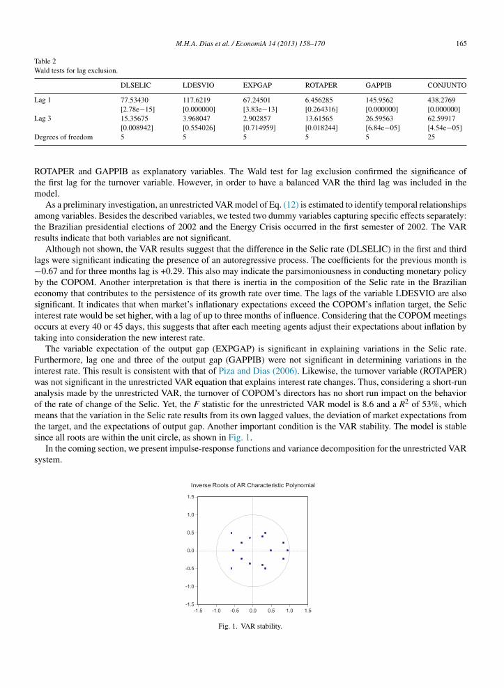
Table 2Wald tests for lag exclusion.

DLSELIC LDESVIO EXPGAP ROTAPER GAPPIB CONJUNTO

Lag 1 77.53430 117.6219 67.24501 6.456285 145.9562 438.2769[2.78e−15] [0.000000] [3.83e−13] [0.264316] [0.000000] [0.000000]

Lag 3 15.35675 3.968047 2.902857 13.61565 26.59563 62.59917[0.008942] [0.554026] [0.714959] [0.018244] [6.84e−05] [4.54e−05]

D

Rtm

atr

l−besiot

Fiwaomts

s

egrees of freedom 5 5 5 5 5 25

OTAPER and GAPPIB as explanatory variables. The Wald test for lag exclusion confirmed the significance ofhe first lag for the turnover variable. However, in order to have a balanced VAR the third lag was included in the

odel.As a preliminary investigation, an unrestricted VAR model of Eq. (12) is estimated to identify temporal relationships

mong variables. Besides the described variables, we tested two dummy variables capturing specific effects separately:he Brazilian presidential elections of 2002 and the Energy Crisis occurred in the first semester of 2002. The VAResults indicate that both variables are not significant.

Although not shown, the VAR results suggest that the difference in the Selic rate (DLSELIC) in the first and thirdags were significant indicating the presence of an autoregressive process. The coefficients for the previous month is

0.67 and for three months lag is +0.29. This also may indicate the parsimoniousness in conducting monetary policyy the COPOM. Another interpretation is that there is inertia in the composition of the Selic rate in the Brazilianconomy that contributes to the persistence of its growth rate over time. The lags of the variable LDESVIO are alsoignificant. It indicates that when market’s inflationary expectations exceed the COPOM’s inflation target, the Selicnterest rate would be set higher, with a lag of up to three months of influence. Considering that the COPOM meetingsccurs at every 40 or 45 days, this suggests that after each meeting agents adjust their expectations about inflation byaking into consideration the new interest rate.

The variable expectation of the output gap (EXPGAP) is significant in explaining variations in the Selic rate.urthermore, lag one and three of the output gap (GAPPIB) were not significant in determining variations in the

nterest rate. This result is consistent with that of Piza and Dias (2006). Likewise, the turnover variable (ROTAPER)as not significant in the unrestricted VAR equation that explains interest rate changes. Thus, considering a short-run

nalysis made by the unrestricted VAR, the turnover of COPOM’s directors has no short run impact on the behaviorf the rate of change of the Selic. Yet, the F statistic for the unrestricted VAR model is 8.6 and a R2 of 53%, whicheans that the variation in the Selic rate results from its own lagged values, the deviation of market expectations from

he target, and the expectations of output gap. Another important condition is the VAR stability. The model is stable

ince all roots are within the unit circle, as shown in Fig. 1.

In the coming section, we present impulse-response functions and variance decomposition for the unrestricted VARystem.

-1.5

-1.0

-0.5

0.0

0.5

1.0

1.5

-1.5 -1.0 -0.5 0.0 0.5 1.0 1.5

Inverse Roots of AR Characteristic Polynomial

Fig. 1. VAR stability.

166 M.H.A. Dias et al. / EconomiA 14 (2013) 158–170

-.08

-.04

.00

.04

.08

.12

1 2 3 4 5 6 7 8 9 10 11 12

Response of DLSELIC to DLSELIC

-.08

-.04

.00

.04

.08

.12

1 2 3 4 5 6 7 8 9 10 11 12

Response of DLSELIC to LDESVIO

-.08

-.04

.00

.04

.08

.12

1 2 3 4 5 6 7 8 9 10 11 12

Response of DLSELIC to ROTAPER

-.08

-.04

.00

.04

.08

.12

1 2 3 4 5 6 7 8 9 10 11 12

Response of DLSELIC to GAPPIB

Response to Cholesky One S.D. Innovations ± 2 S.E.

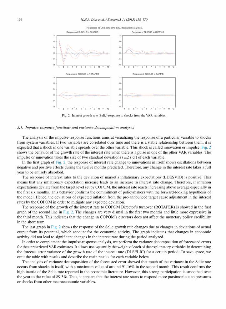
Fig. 2. Interest growth rate (Selic) response to shocks from the VAR variables.

5.1. Impulse-response functions and variance decomposition analyses

The analysis of the impulse-response functions aims at visualizing the response of a particular variable to shocksfrom system variables. If two variables are correlated over time and there is a stable relationship between them, it isexpected that a shock in one variable spreads over the other variable. This shock is called innovation or impulse. Fig. 2shows the behavior of the growth rate of the interest rate when there is a pulse in one of the other VAR variables. Theimpulse or innovation takes the size of two standard deviations (±2 s.d.) of each variable.

In the first graph of Fig. 2, the response of interest rate change to innovations in itself shows oscillations betweennegative and positive effects during the twelve months predicted. Therefore, any change in the interest rate takes a fullyear to be entirely absorbed.

The response of interest rates to the deviation of market’s inflationary expectations (LDESVIO) is positive. Thismeans that any inflationary expectation increase leads to an increase in interest rate change. Therefore, if inflationexpectations deviate from the target level set by COPOM, the interest rate reacts increasing above average especially inthe first six months. This behavior confirms the commitment of policymakers with the forward-looking hypothesis ofthe model. Hence, the deviations of expected inflation from the pre-announced target cause adjustment in the interestrates by the COPOM in order to mitigate any expected deviation.

The response of the growth of the interest rate to COPOM Director’s turnover (ROTAPER) is showed in the firstgraph of the second line in Fig. 2. The changes are very dismal in the first two months and little more expressive inthe third month. This indicates that the change in COPOM’s directors does not affect the monetary policy credibilityin the short term.

The last graph in Fig. 2 shows the response of the Selic growth rate changes due to changes in deviations of actualoutput from its potential, which account for the economic activity. The graph indicates that changes in economicactivity did not lead to significant changes in the interest rate during the period analyzed.

In order to complement the impulse-response analysis, we perform the variance decomposition of forecasted errorsfor the unrestricted VAR estimates. It allows us to quantify the weight of each of the explanatory variables in determiningthe forecast error variance of the growth rate of the interest rate (DLSELIC) for a certain period. To save space, weomit the table with results and describe the main results for each variable below.

The analysis of variance decomposition of the forecasted error showed that much of the variance in the Selic rateoccurs from shocks in itself, with a maximum value of around 91.16% in the second month. This result confirms the

high inertia of the Selic rate reported in the economic literature. However, this strong participation is smoothed overthe year to the value of 89.3%. Thus, it appears that the interest rate starts to respond more parsimonious to pressuresor shocks from other macroeconomic variables.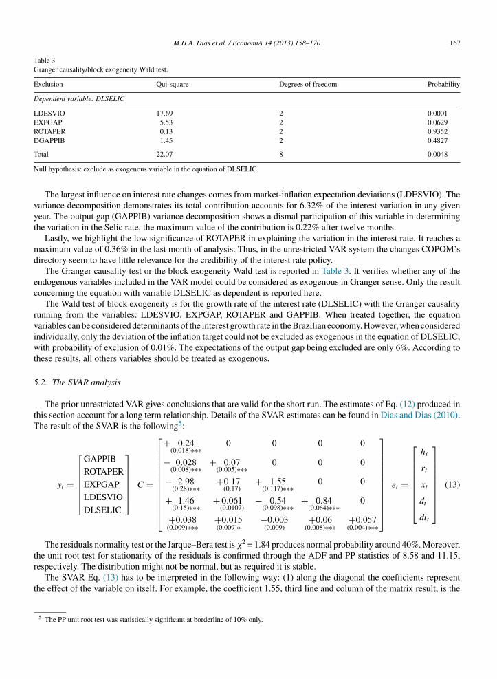

M.H.A. Dias et al. / EconomiA 14 (2013) 158–170 167

Table 3Granger causality/block exogeneity Wald test.

Exclusion Qui-square Degrees of freedom Probability

Dependent variable: DLSELIC

LDESVIO 17.69 2 0.0001EXPGAP 5.53 2 0.0629ROTAPER 0.13 2 0.9352DGAPPIB 1.45 2 0.4827

T

N

vyt

md

ec

rviwt

5

tT

tr

t

otal 22.07 8 0.0048

ull hypothesis: exclude as exogenous variable in the equation of DLSELIC.

The largest influence on interest rate changes comes from market-inflation expectation deviations (LDESVIO). Theariance decomposition demonstrates its total contribution accounts for 6.32% of the interest variation in any givenear. The output gap (GAPPIB) variance decomposition shows a dismal participation of this variable in determininghe variation in the Selic rate, the maximum value of the contribution is 0.22% after twelve months.

Lastly, we highlight the low significance of ROTAPER in explaining the variation in the interest rate. It reaches aaximum value of 0.36% in the last month of analysis. Thus, in the unrestricted VAR system the changes COPOM’s

irectory seem to have little relevance for the credibility of the interest rate policy.The Granger causality test or the block exogeneity Wald test is reported in Table 3. It verifies whether any of the

ndogenous variables included in the VAR model could be considered as exogenous in Granger sense. Only the resultoncerning the equation with variable DLSELIC as dependent is reported here.

The Wald test of block exogeneity is for the growth rate of the interest rate (DLSELIC) with the Granger causalityunning from the variables: LDESVIO, EXPGAP, ROTAPER and GAPPIB. When treated together, the equationariables can be considered determinants of the interest growth rate in the Brazilian economy. However, when consideredndividually, only the deviation of the inflation target could not be excluded as exogenous in the equation of DLSELIC,ith probability of exclusion of 0.01%. The expectations of the output gap being excluded are only 6%. According to

hese results, all others variables should be treated as exogenous.

.2. The SVAR analysis

The prior unrestricted VAR gives conclusions that are valid for the short run. The estimates of Eq. (12) produced inhis section account for a long term relationship. Details of the SVAR estimates can be found in Dias and Dias (2010).he result of the SVAR is the following5:

yt =

⎡⎢⎢⎢⎢⎢⎣

GAPPIB

ROTAPER

EXPGAP

LDESVIO

DLSELIC

⎤⎥⎥⎥⎥⎥⎦

C =

⎡⎢⎢⎢⎢⎢⎢⎢⎢⎢⎢⎢⎣

+ 0.24(0.018)∗∗∗

0 0 0 0

− 0.028(0.008)∗∗∗

+ 0.07(0.005)∗∗∗

0 0 0

− 2.98(0.28)∗∗∗

+0.17(0.17)

+ 1.55(0.117)∗∗∗

0 0

+ 1.46(0.15)∗∗∗

+ 0.061(0.0107)

− 0.54(0.098)∗∗∗

+ 0.84(0.064)∗∗∗

0

+0.038(0.009)∗∗∗

+0.015(0.009)∗

−0.003(0.009)

+0.06(0.008)∗∗∗

+0.057(0.004)∗∗∗

⎤⎥⎥⎥⎥⎥⎥⎥⎥⎥⎥⎥⎦

et =

⎡⎢⎢⎢⎢⎢⎢⎢⎢⎣

ht

rt

xt

dt

dit

⎤⎥⎥⎥⎥⎥⎥⎥⎥⎦

(13)

The residuals normality test or the Jarque–Bera test is χ2 = 1.84 produces normal probability around 40%. Moreover,he unit root test for stationarity of the residuals is confirmed through the ADF and PP statistics of 8.58 and 11.15,

espectively. The distribution might not be normal, but as required it is stable.

The SVAR Eq. (13) has to be interpreted in the following way: (1) along the diagonal the coefficients representhe effect of the variable on itself. For example, the coefficient 1.55, third line and column of the matrix result, is the

5 The PP unit root test was statistically significant at borderline of 10% only.

168 M.H.A. Dias et al. / EconomiA 14 (2013) 158–170

impact of EXPGAP changes on itself; (2) column one represents the impact of GAPPIB on all the variables, being thefirst coefficient the column the impact on itself; (3) column two is the effect of ROTAPER on the remaining variables,again the second line coefficient 0.07 is its own impact; and so on for the remaining columns.

The output gap (GAPPIB) is considered as an exogenous variable that influences all others in the above estimate.This specification follows the reviewed literature findings.6 It is also important to emphasize that this specification andresults are consistent with economic theory.

The results show that the interest rate does stabilize or converge to its long-run value due to any change in thevariables included in the model. An output gap increase or the increase in the output above its potential level leadsto increases in ROTAPER, EXPGAP, LDESVIO and DLSELIC. Therefore, it influences the rate of change of theCOPOM members; it raises the expectation of output gap increase; it causes the market inflation expectation to rise;and it causes the growth rate of change of interest rate to increase.

The COPOM directors’ turnover influences EXPGAP, LDESVIO and DLSELIC. For the purpose of this paper, themost important variables are the following ones. Increases in the number of replacement of COPOM directors leadto an increase in the expected output gap (EXPGAP), coefficient of 0.17, which is significant at 1%. This means thatagents foresee that actual output will surpass its potential level. In addition, agents expect that inflation may surpass itsannounced target level or band. The coefficient 0.061 on LDESVIO is also significant at 1%. Therefore, the influenceon changes on the interest rate will increase DLSELIC, according to the positive coefficient of 0.015 that is significantat 1%.

How do we see the credibility impact on this model? We measure it through the influence of ROTAPER on theLDESVIO variable. The coefficient is positive and significant. This means that the turnover increases expected inflationclose or above to its target level. This is an important result since it says that directors’ turnover contributes to priceinstability over the long run in Brazil. In other words, inflation instability might be an outcome from directors’ turnoverin the long run. How serious is this matter for the conduct of monetary policy through interest rate determination? Itis very serious since it leads to an increase in the rate of change in order to curb inflation expectations.

The EXPGAP increase lowers LDESVIO and it does not impact DLSELIC in the long run. This means that thebusiness cycle does not affect interest rate changes or the monetary policy. Furthermore, the market inflation expectation(LDESVIO) has a positive impact on DLSELIC. It means that inflation is more important for monetary policy thanoutput growth above its trend level.

The last column just states that over the long run the average change in the interest rate is around 0.057 or 0.57%.This is consistent with the changes in the interest rate set by the COPOM meetings. They normally increase or decreasethe level of the interest by 0.25% up 0.50% points; rarely the COPOM takes any decision beyond those values.

To examine if the analysis performed is robust, we use the result from the unrestricted model where the expectedoutput gap variable (EXPGAP) is not significant in affecting the interest rate growth in the long run. This variable isdropped in the new SVAR estimates represented by Eq. (14) below.

yt =

⎡⎢⎢⎢⎣

GAPPIB

ROTAPER

LDESVIO

DLSELIC

⎤⎥⎥⎥⎦ C =

⎡⎢⎢⎢⎢⎢⎢⎢⎣

+ 0.18(0.014)∗∗∗

0 0 0

− 0.018(0.008)∗∗∗

+ 0.072(0.005)∗∗∗

0 0

+ 0.88(0.15)∗∗∗

+ 0.29(0.128)∗∗∗

+ 1.08(0.08)∗∗∗

0

+ 0.032(0.010)∗∗∗

+ 0.023(0.009)∗∗∗

+ 0.067(0.008)∗∗∗

+ 0.060(0.005)∗∗∗

⎤⎥⎥⎥⎥⎥⎥⎥⎦

et =

⎡⎢⎢⎢⎢⎢⎣

ht

rt

dt

dit

⎤⎥⎥⎥⎥⎥⎦

(14)

The COPOM turnover effect is accounted for in column two. The effect on itself is 0.072 meaning that, on average,7.2% of the directors were changed over the span period. The coefficient in LDESVIO is 0.29 and significant at 1%. Itis bigger than the previous one indicating that changes in the COPOM’s Board of Directors cause positive impact oninflation expectations. Moreover, it also leads to positive increase in the rate of change of the interest rate determined

by the Board of Directors. This confirms previous results that the lack of credibility compromises the monetary policyconduct. Therefore, keeping board members seems to be a good policy to follow in order to prevent increases in inflationexpectations, which – according to our results – demands further increases in interest rate level. Tests of normality

6 Asterisks indicate the statistical significance of the coefficients at 10% (*), 5% (**) and 1% (***). For example Holland (2005) and Furlani et al.(2008).

aie

6

mte

eebonts

ctd

R

A

A

A

A

A

AACC

C

CD

F

G

G

G

G

G

M.H.A. Dias et al. / EconomiA 14 (2013) 158–170 169

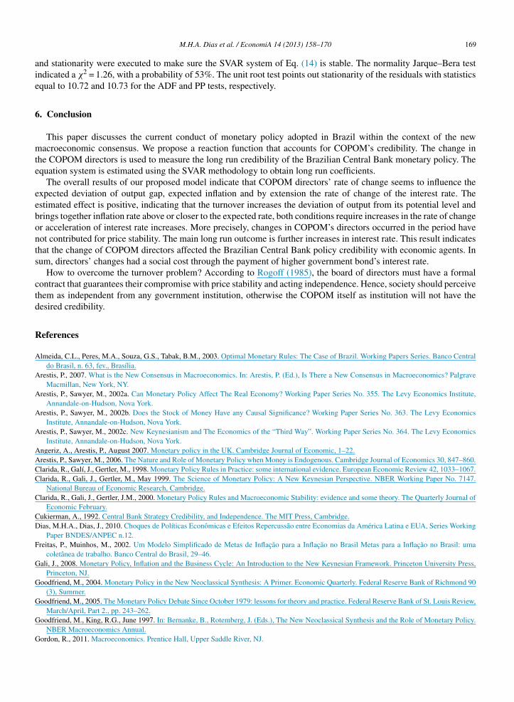
nd stationarity were executed to make sure the SVAR system of Eq. (14) is stable. The normality Jarque–Bera testndicated a χ2 = 1.26, with a probability of 53%. The unit root test points out stationarity of the residuals with statisticsqual to 10.72 and 10.73 for the ADF and PP tests, respectively.

. Conclusion

This paper discusses the current conduct of monetary policy adopted in Brazil within the context of the newacroeconomic consensus. We propose a reaction function that accounts for COPOM’s credibility. The change in

he COPOM directors is used to measure the long run credibility of the Brazilian Central Bank monetary policy. Thequation system is estimated using the SVAR methodology to obtain long run coefficients.

The overall results of our proposed model indicate that COPOM directors’ rate of change seems to influence thexpected deviation of output gap, expected inflation and by extension the rate of change of the interest rate. Thestimated effect is positive, indicating that the turnover increases the deviation of output from its potential level andrings together inflation rate above or closer to the expected rate, both conditions require increases in the rate of changer acceleration of interest rate increases. More precisely, changes in COPOM’s directors occurred in the period haveot contributed for price stability. The main long run outcome is further increases in interest rate. This result indicateshat the change of COPOM directors affected the Brazilian Central Bank policy credibility with economic agents. Inum, directors’ changes had a social cost through the payment of higher government bond’s interest rate.

How to overcome the turnover problem? According to Rogoff (1985), the board of directors must have a formalontract that guarantees their compromise with price stability and acting independence. Hence, society should perceivehem as independent from any government institution, otherwise the COPOM itself as institution will not have theesired credibility.

eferences

lmeida, C.L., Peres, M.A., Souza, G.S., Tabak, B.M., 2003. Optimal Monetary Rules: The Case of Brazil. Working Papers Series. Banco Centraldo Brasil, n. 63, fev., Brasília.

restis, P., 2007. What is the New Consensus in Macroeconomics. In: Arestis, P. (Ed.), Is There a New Consensus in Macroeconomics? PalgraveMacmillan, New York, NY.

restis, P., Sawyer, M., 2002a. Can Monetary Policy Affect The Real Economy? Working Paper Series No. 355. The Levy Economics Institute,Annandale-on-Hudson, Nova York.

restis, P., Sawyer, M., 2002b. Does the Stock of Money Have any Causal Significance? Working Paper Series No. 363. The Levy EconomicsInstitute, Annandale-on-Hudson, Nova York.

restis, P., Sawyer, M., 2002c. New Keynesianism and The Economics of the “Third Way”. Working Paper Series No. 364. The Levy EconomicsInstitute, Annandale-on-Hudson, Nova York.

ngeriz, A., Arestis, P., August 2007. Monetary policy in the UK. Cambridge Journal of Economic, 1–22.restis, P., Sawyer, M., 2006. The Nature and Role of Monetary Policy when Money is Endogenous. Cambridge Journal of Economics 30, 847–860.larida, R., Galí, J., Gertler, M., 1998. Monetary Policy Rules in Practice: some international evidence. European Economic Review 42, 1033–1067.larida, R., Gali, J., Gertler, M., May 1999. The Science of Monetary Policy: A New Keynesian Perspective. NBER Working Paper No. 7147.

National Bureau of Economic Research, Cambridge.larida, R., Gali, J., Gertler, J.M., 2000. Monetary Policy Rules and Macroeconomic Stability: evidence and some theory. The Quarterly Journal of

Economic February.ukierman, A., 1992. Central Bank Strategy Credibility, and Independence. The MIT Press, Cambridge.ias, M.H.A., Dias, J., 2010. Choques de Políticas Econômicas e Efeitos Repercussão entre Economias da América Latina e EUA, Series Working

Paper BNDES/ANPEC n.12.reitas, P., Muinhos, M., 2002. Um Modelo Simplificado de Metas de Inflacão para a Inflacão no Brasil Metas para a Inflacão no Brasil: uma

coletânea de trabalho. Banco Central do Brasil, 29–46.ali, J., 2008. Monetary Policy, Inflation and the Business Cycle: An Introduction to the New Keynesian Framework. Princeton University Press,

Princeton, NJ.oodfriend, M., 2004. Monetary Policy in the New Neoclassical Synthesis: A Primer. Economic Quarterly. Federal Reserve Bank of Richmond 90

(3), Summer.oodfriend, M., 2005. The Monetary Policy Debate Since October 1979: lessons for theory and practice. Federal Reserve Bank of St. Louis Review,

March/April, Part 2., pp. 243–262.oodfriend, M., King, R.G., June 1997. In: Bernanke, B., Rotemberg, J. (Eds.), The New Neoclassical Synthesis and the Role of Monetary Policy.

NBER Macroeconomics Annual.ordon, R., 2011. Macroeconomics. Prentice Hall, Upper Saddle River, NJ.

170 M.H.A. Dias et al. / EconomiA 14 (2013) 158–170

Holland, M, 2005. Monetary Exchange Rate Policy in Brazil After Inflation Targeting. In: Anais do XXXIII Encontro Nacional de Economia -ANPEC, Natal-RN.

Judd, J., Rudebush, G.D., 1998. Taylor’s Rule and the FED: 1970–1997. Federal Reserve Bank of San Francisco. Economic Review 3, 3–16.Furlani, L.G.C., Portugal, M.S., Laurini, M., 2008. Exchange Rate Movements Policy in Brazil: Econometric and Simulation Evidence. Working

Paper Insper. Insper Institute, São Paulo.McCallum, B.T., April 1999. Recent Developments in Monetary Policy Analysis: The Roles of Theory and Evidence. NBER Working Paper No.

7088. National Bureau of Economic Research, Cambridge.McCallum, B.T., 2001. Monetary policy analysis in models without money. Federal Reserve Bank of St. Louis Review, July/August.McCallum, B.T., 2005. What have we learned since October 1979? Federal Reserve Bank of St. Louis Review, March/April, Part 2.Meyer, L.H., 2001. Does Money Matter? The 2001 Hower Jones Memorial Lecture. Washington University, Missouri.Minella, A., Freitas, P., Goldfajn, S., Muinhos, I.M., November 2002. Inflation Targeting in Brazil: Lessons and Challenges. Working Paper. 53.

Banco Central do Brasil, Brasília.Minella, A., Freitas, P.S., Goldfajn, I., Muinhos, M., July 2003. Inflation Targeting in Brazil: Constructing Credibility Under Exchange Rate Volatility.

Working Paper No. 77. Banco Central do Brasil, Brasília.Piza, E.C., Dias, J., December 2006. Novo Consenso Macroeconômico, Risco Moral e Política de Metas no Brasil: uma avaliacão empírica. In:

Anais do XXXIV Encontro Nacional da ANPEC, Salvador (BA).Rogoff, K., 1985. The Optimal Degree of Commitment to an Intermediate Monetary Target. Quarterly Journal of Economic 100, 1169–1190.Taylor, J., 1993. Discretion Versus Policy Rules in Practice. Carnegie-Rochester Conference on Public Policy 39, 195–214.Woodford, M., 2008. Convergence in Macroeconomics: Elements of the New Synthesis. Columbia University Press, New York, NY.