Inflation Illusion and the Taylor Principle: An Experimental

Study

Wolfgang J. Luhan∗ Johann Scharler†

Abstract

We develop a simple experimental setting to evaluate the role of the Taylor principle,which holds that the nominal interest rate has to respond more than one-for-one to fluctu-ations in the inflation rate to exert a stabilizing effect. In our setting, the average inflationrate fluctuates around the inflation target if the computerized central bank obeys the Taylorprinciple. If the Taylor principle is violated, the average inflation rate persistently deviatesfrom the target. These deviations from the target are less pronounced, if inflation ratescannot be as readily observed as nominal interest rates. This result is consistent with theinterpretation that subjects underestimate the influence of inflation on the real return tosavings if the inflation rate is only observed ex post.

Key words: Taylor principle, Interest Rate Rule, Inflation Illusion, Laboratory Experiment

JEL codes: E30, E52, C90

∗Corresponding author: Ruhr-Universitat Bochum, Institute for Macroeconomics & Bochum Lab for Exper-imental Economics (RUBex), Universitaetsstrasse 150, 44801 Bochum, Germany, Phone +49 157 745 035 69,e-mail: wolfgang.luhan@rub.de†University of Innsbruck, Department of Economics, Universitaetsstrasse 15, A-6020 Innsbruck, Austria,

Phone: +43 512 507 7357, e-mail: johann.scharler@uibk.ac.at.

1

1 Introduction

Research on interest rate rules indicates that the strength of the feedback from the inflation

rate to the nominal interest rate plays a crucial role for macroeconomic outcomes. The intuition

is straight-forward: suppose that the inflation rate increases. If the central bank adjusts the

nominal interest rate less than one-for-one, then the real interest rate declines, which stimulates

aggregate demand resulting in even more inflationary pressure. Thus, monetary policy can exert

a stabilizing influence only if it adjusts the nominal interest rate sufficiently to offset the influence

of the inflation rate on the real interest rate. This proposition, which is known as the Taylor

principle, is obtained in many models featuring interest rate rules. In New Keynesian Dynamic

Stochastic General Equilibrium (DSGE) models, for instance, the Taylor principle ensures the

determinacy of the rational expectations equilibrium. If the Taylor principle is violated, the

equilibrium is indeterminate and fluctuations arising from self-fulfilling expectations may occur

in this class of models (see, e.g., Woodford, 2003).

Empirically, the view that the Taylor principle plays a decisive role is supported by evidence

indicating that major central banks have started to follow interest rate rules that satisfy the

Taylor principle in the early 1980s, whereas inflationary pressure was accommodated to a larger

extent prior to the 1980s (see, e.g., Judd and Rudebush, 1998; Clarida et al., 1998, 2000).

Since this regime change in monetary policy roughly coincides with the beginning of the Great

Moderation period in the mid 1980s, which is characterized by stable output growth and steadily

low inflation, it appears that the Taylor Principle is indeed crucial.1

In this paper, we explore the role of the Taylor principle for inflation outcomes in a simple

experimental setting: subjects repeatedly make two-period consumption and savings decisions

and these decisions influence inflation dynamics via a Phillips curve relationship. A computerized

central bank sets the interest rate according to an interest rate rule and aims at implementing

an inflation target. To evaluate the Taylor principle in this setting, we vary the strength of the

feedback from inflation to the interest rate across treatments.

The experimental method offers the advantage that we do not have to impose any behav-

ioral assumptions. In fact, we are able to test whether subjects in the lab act in line with

1However, this view has also been questioned. Orphanides (2004) estimates interest rate rules with real-timedata and finds that the Taylor principle was satisfied before and after 1980. In addition, several studies arguethat low inflation rates and reduced business cycle volatility are not due to better monetary policy but rather theresult of other factors such as structural change (see, e.g., Blanchard and Simon, 2001; Dynan et al., 2006; Davisand Kahn, 2008) or simply a reduction in the size of the shocks hitting the economy (see, e.g., Ahmed et al., 2004;Stock and Watson, 2005).

2

the main behavioral assumption underlying the Taylor principle, namely, that intertemporal

decisions are governed by the real interest rate. While this behavior is implicitly assumed in

standard macroeconomic models, a number of contributions document that decisions are fre-

quently subject to money illusion, which refers to a disposition to think in nominal rather than

in real terms.2 Similarly, with respect to intertemporal decision making, people may be subject

to inflation illusion; that is, they may neglect the effect of inflation on the real return on savings

and perceive the nominal interest rate to be the real return.3 This type of behavior can have

important implications for monetary policy. If, for instance, the nominal interest rate is more

relevant for aggregate demand than the inflation rate, then the Taylor principle ceases to be a

necessary requirement for stability, a point that is also emphasized by Fair (2005).

Another advantage of the experimental setting is that we are able to isolate the impact of

the interest rate by ruling out any other influences. Hence, we can focus on the interest rate

channel of the monetary transmission mechanism, which is strongly emphasized in the standard

New Keynesian model.

We find that the inflation rate fluctuates around the inflation target if the computerized

central bank sets the nominal interest rate in line with the Taylor principle. If, in contrast, the

Taylor principle is violated, the inflation rate deviates persistently from the target rate. Nev-

ertheless, these deviations are substantially smaller than expected in settings in which subjects

can only observe the nominal interest rate and have to infer the inflation rate when making

decisions. Since inflation rates can only be observed ex post in reality, this is the empirically

relevant case.

We show that the reason for this result is that although people understand the influence of

inflation on the real return on savings, the inflation rate is fully taken into account only if it can

be readily observed. If the inflation rate cannot be observed ex ante, people base their decisions

to a larger extent on the nominal interest rate. While the computational and cognitive costs are

still relatively minor in the treatments in which the inflation rate has to be inferred, subjects

over-emphasize the nominal interest rate over the inflation rate.

There are only few studies examining monetary policy issues using lab experiments. Peter-

son (2012) and Peterson and Krystov (2013) study experimental implementations of the New

2See Fisher (1928) for a seminal discussion of money illusion. Experimental studies of money illusion includeTyran (2007), Fehr and Tyran (2001), and Petersen and Winn (2014).

3Modigliani and Cohn (1979) argue that this type of behavior can lead to deviations of asset prices fromfundamentals. See also Campbell and Vuolteenaho (2004), Piazzesi and Schneider (2008), and Brunnermeier andJulliard (2008).

3

Keynesian model, which also motivates our setting, and Orland and Roos (2013) provide an

experimental evaluation of the New Keynesian Phillips curve. Engle-Warnick and Turdaliev

(2010) and Noussair et al. (2011) investigate interest rate setting in an experimental economy.

These last two contributions explore the behavior of human central bankers in a computerized

economy and find that subjects behave largely in line with the Taylor principle. Our focus, in

contrast, lies on the interaction between human subjects with a computerized central bank.4

Pfajar and Zakelj (2011) and Assenza et al. (2011) study how the design of interest rate rules

influences the formation of expectations in an experimental New Keynesian model economy.

They find that inflation expectations are heterogeneous and that the design of the interest rate

rule influences the stability of the inflation rate, since different rules provide different amounts

of feedback for subjects. In constrast to these two papers, we abstract from the formation of

expectations and focus on the consequences of inflation illusion.5

The remainder of the paper is structured as follows: Section 2 discusses the theoretical basis

of our experimental investigation and briefly reviews the related literature. Section 3 presents

the experimental design and procedure and discusses the treatments that we implement. In

Section 4, we present our results, and Section 5 concludes the paper.

2 Illustrating the Taylor Principle

To illustrate the idea that the strength of the feedback from inflation to the nominal interest

rate has a crucial influence on macroeconomic stability, consider a simple model adopted from

Taylor (1999):

Yt = −a(Rt − πt), (1)

πt = πt−1 + bYt−1, (2)

Rt = δπt, (3)

where a > 0, b > 0 and δ > 0. Yt is the output gap, Rt is the nominal interest rate, and πt

denotes the inflation rate. Equation (1) is an IS relationship, equation (2) is a Phillips curve,

and equation (3) is a simple interest rate rule that describes the behavior of the central bank.

For this model, it is easy to see that stability requires the Taylor principle to be satisfied:

δ > 1. Suppose that the inflation rate increases. If δ > 1, then the central bank increases the

4Noussair et al. (2011) also implement treatments in which the interest rate rule is exogenously imposed.However, the interest rate rule always obeys the Taylor principle in these treatments.

5Bao et al. (2013) distinguish between forecasting and optimizing. According to this distinction, we rely on alearning-to-optimize design.

4

nominal interest rate sufficiently to also increase the real interest rate, Rt − πt. The higher real

interest rate lowers aggregate demand according to equation (1), which puts downward pressure

on inflation according to equation (2). By reacting sufficiently strongly to inflationary pressure,

the central bank can offset the initial increase in inflation by contracting demand. If δ < 1

the increase in inflation actually results in a lower real interest rate, which in turn stimulates

aggregate demand and leads to even stronger upward pressure on inflation rendering the system

unstable.

In New Keynesian DSGE models, equation (1) is replaced with a forward-looking IS relation-

ship derived from the solution to the intertemporal optimization problem of the representative

household (see, e.g., Clarida et al., 1999; Woodford, 2003, for detailed discussions):

Yt = −a(Rt − Etπt+1) + EtYt+1, (4)

where Et denotes the expectation conditional on information available at time t. Equation (2)

is replaced with the forward-looking New Keynesian Phillips curve, which is derived from the

price-setting behavior of monopolistically competitive firms:

πt = c Etπt+1 + dYt, (5)

where c > 0 and d > 0. The main difference between equations (1) and (2) and their New

Keynesian counterparts is that the latter contain conditional expectations of future output and

inflation. It is well known that in this class of forward-looking models, the Taylor principle

guarantees the determinacy, that is, local uniqueness and stability, of the rational expectations

equilibrium.6

Note that in the models discussed here, aggregate demand depends either on the real interest

rate, Rt − πt in equation (1), or on the expected real interest rate, Rt − Etπt+1, in equation

(4). Thus, both types of models impose variants of the Fisher equation, which boils down to the

behavioral assumption that agents take the inflation rate appropriately into account when they

calculate the real return on savings. However, agents may, for instance, suffer from inflation

illusion, and neglect the effect of inflation on the real return on savings. In this case, even

a value of δ below unity may be consistent with stability, since it may suffice to stabilize the

nominal interest rate in order to stabilize demand. In contrast, if agents perceive the effect of

6In addition to the implications for equilibrium determinacy, Bullard and Mitra (2002) show that the rationalexpectations equilibrium in the New Keynesian model is learnable in the sense of expectational stability if theTaylor principle holds. While this result puts additional emphasis on the role of the Taylor principle for stability,Duffy and Xiao (2011) find that it does not necessarily apply when capital investment is incorporated. Arifovicet al. (2013) find that the Taylor Principle is not necessary for convergence with evolutionary learning agents.

5

inflation on the real return to be stronger than it actually is, the standard Taylor principle may

be insufficient since a proportional adjustment of the nominal interest rate may not stabilize the

perceived real interest rate. Agents may, for instance, overestimate the undesirable effects of

inflation as the result of the memory of high inflation episodes as it is well known that opinions

about the adverse effects of inflation are influenced by past experience of high inflation episodes

(see, e.g. Shiller, 1997; Ehrmann and Tzamourani, 2012).

Thus, it is not clear whether the Taylor principle remains a sufficient, or even necessary

condition for stability under alternative behavioral assumptions. We summarize our conjectures

as follows:7 The Taylor principle is necessary and sufficient to stabilize inflation around the target

if subjects calculate the real return on savings according to the Fisher equation. If subjects are

prone to inflation illusion, the Taylor principle is still sufficient, but no longer necessary. If, in

contrast, subjects overestimate the influence of inflation on the real return, an interest rate rule

that satisfies the Taylor principle may not be sufficient to stabilize the perceived real interest

rate and lead to instability.8

In the next section, we describe an experimental setup that allows us to explore these issues.

3 Experimental Design and Procedure

In this section we describe our experimental design. Rather than implementing a specific model

in a laboratory environment, we aim at designing a setup which is as simple as possible while

still incorporating those features that are essential for our research question.

Although the Taylor principle is generally discussed in infinite horizon models, we study the

influence of real and nominal factors on consumption and savings decisions, and the resulting

inflation dynamics, in a two-period setting. Since we are not primarily interested in issues

related to intertemporal optimization, we can simplify the subjects’ task by explicitly ruling out

complications arising from, for example, long planning horizons.9

7Appendix A provides a formal discussion of the determinacy properties of a variant of the New Keynesianmodel that incorporates inflation illusion.

8While we focus on inflation illusion, the Taylor principle may generally neither be necessary nor sufficientfor determinacy in more elaborated versions of the model, such models incorporating, for instance, more generalinterest rate rules (see, e.g., Woodford, 2003), rule-of-thumb consumers (Galı et al., 2004), capital investment(Carlstrom and Fuerst, 2005; Sveen and Weinke, 2007), openness (De Fiore and Liu, 2005), or switches in theinterest rate rule (Davig and Leeper, 2007). Depending on the specific formulation of the model, modified versionsof the Taylor principle apply.

9A number of authors experimentally examine intertemporal decision making in more general settings anddocument deviations from theoretical predictions (see, e.g., Hey and Dardanoni, 1988; Noussair and Matheny,2000; Lei and Noussair, 2002; Ballinger et al., 2003; Carbone and Hey, 2004).

6

3.1 Experimental Design

Each treatment of the experiment comprises τ = 1, ..., 20 rounds and each round consists of two

periods t = 1, 2. In each round, each subject i = 1, ..., N has to solve a two-period decision

problem: In the first period of each round, subjects receive a nominal endowment of 100 units

of the experimental currency. This endowment can be exchanged for consumption goods at a

price Pτ,1 in the first period of round τ , or saved and (automatically) exchanged in the second

period of the round at a price of Pτ,2. Everything that is not used to buy consumption goods

in the first period earns a nominal interest rate of Rτ percent between periods 1 and 2 of round

τ . So consumption of subject i in the second period is Ci,τ,2 = (100 − Ci,τ,1)(1 + Rτ )/Pτ,2,

where Ci,τ,1 is the subjects’ consumption in the first period. The subjects’ decision problem is

to choose consumption in the first period of each round to maximize total consumption in each

round: Ci,τ = Ci,τ,1 + Ci,τ,2. Note that the endowment cannot be stored or transferred across

rounds.

With this set-up we are able to study consumption decisions in a rather stationary environ-

ment, since subjects face the same decision problem in each round. While this setting is simple

and easy to explain in the instructions, we are still able to to focus on how subjects respond

to changes in the nominal interest rate and in the inflation rate. In other words, we are able

to isolate a behavioral mechanism underlying the Taylor principle while preserving a simple

structure.

Although consumption decisions are independent across rounds, the inflation rate between

the two periods of round τ , denoted by πτ = Pτ,2/Pτ,1 − 1, depends on average consumption in

the first period of round τ − 1. This assumption allows us to analyze longer-run, inter-round

inflation dynamics, despite the fact that subjects solve intra-round decision problems.

Inflation is determined as

πτ = π + θ

(1

N

N∑i=1

Ci,τ−1,1 − C)

+ ετ , (6)

where 1N

∑Ni=1Ci,τ−1,1 is average consumption in the first period of round τ − 1. π is the rate

of inflation that prevails if 1N

∑Ni=1Ci,τ−1,1 = C. Equation (6) represents a Phillips Curve rela-

tionship and captures, in a simple way, the idea that aggregate consumption demand influences

inflation. The parameter θ determines how strongly inflation responds to the deviation of av-

erage first-period consumption in the previous round from C. We include an exogenous shock

to the inflation rate, ετ , which helps to make the link between aggregate consumption and in-

7

flation less salient in some of our treatments, since inflation illusion, in the sense that subjects

overemphasize the nominal interest rate relative to the inflation rate, may be more prevalent in

such a setting. The shock is uniformly distributed with an expected value of zero.

When setting the interest rate for round τ , the central bank observes consumption in ag-

gregate terms in round τ − 1, but not the realization of the shock for the current period.

Since the shock has an unconditional mean of zero, the computerized central banks expects

πτ = π + θ(

1N

∑Ni=1Ci,τ−1,1 − C

)to be the inflation rate for round τ , given the information

available at the beginning of round τ . Based on πτ , the nominal interest rate is determined by

the computerized central bank according to the interest rate rule

Rτ = R+ δ(πτ − π). (7)

Here, the central bank increases the interest rate above R if the inflation rate is greater than

π and vice versa. So the central bank targets the rate of inflation that prevails if average

consumption is equal to C.

To summarize, in our baseline treatments, the timing of events is as follows: First, the

computerized central bank observes aggregate demand in the previous round, calculates πτ and

sets the nominal interest, Rτ , according to equation (7). Second, subjects are informed about

the nominal interest rate and decide on consumption in the two periods of the current round.

Third, the shock ετ is drawn and the inflation rate πτ for the current round is determined. And

finally, after decisions were made, subjects are informed about the inflation rate, their period

pay-off as well as aggregate consumption in the current round.

The assumption that the inflation rate, in contrast to the nominal interest rate, can only be

observed after the consumption decision was made comes close to the timing of events in reality

as well as in forward-looking models where the inflation rate relevant for savings decisions is

not known with certainty ex ante.10 Although subjects are not informed about the inflation

rate prior to decision making, we informed them about how inflation and interest rates were

determined. Specifically, we included equations (6) and (7) in addition to verbal explanations

in the instructions. Since, the shock, ετ , has only a relatively minor influence on the inflation

rate, subjects were able, in principle, to calculate the relevant inflation rate given the observed

nominal interest rate in conjunction with equation (7).11

10To study the influence of the observability of the inflation rate in detail, we also conduct treatments in whichsubjects can observe the nominal interest rate as well as the inflation rate at the beginning of each round, seeSection 5.

11Note that we are not interested in the formation of expectations, which is a related but distinct issue. The

8

To maximize total consumption in any round τ , the entire endowment has to be consumed

in the first period of the round if the real interest rate, (1 +Rτ )/(1 + πτ )− 1, is negative. If the

real interest rate is positive, it is optimal to fully postpone consumption until the second period.

Thus, optimal first period consumption is

C∗i,τ,1 =

100 if Rτ > πτ

0 if Rτ < πτ(8)

For Rτ = πτ , optimal consumption is indeterminate.

3.2 Calibration

The experimental economy is parameterized as follows: we set R = π = 5 percent, C = 50,

and θ = 0.03. This calibration of θ ensures that the nominal interest rate remains strictly

positive throughout all treatments. The exogenous shock to the inflation rate, ετ , is uniformly

distributed on the interval [−0.0005, 0.0005]. As starting values, we use π1 = 5.05 percent and

R1 = 5 percent in the first round. The price in the first period is set to Pτ,1 = 1 in all rounds.

The parameterization was common knowledge.

3.3 Experimental Predictions

To study the role of the Taylor principle, we vary δ in the interest rate rule (7) as the main treat-

ment variable. Throughout the analysis, we consider two parameterizations of δ: In Treatment

A2, we set δ = 2, which is a value that satisfies the Taylor principle, and in Treatment A05, we

set δ = 0.5, which violates the Taylor principle.12 While we also implement additional treat-

ments, which we describe below, we view Treatments A2 and A05 as our baseline treatments.

Note that in both treatments, we keep the relative distance to δ = 1 constant.

If subjects choose consumption according to (8), the inflation rate will fluctuate around the

inflation target only if the interest rate rule (7) satisfies the Taylor principle. Otherwise, if

the Taylor principle is violated, inflation will persistently deviate from the target. Intuitively,

suppose that average consumption in the first period of round τ is above C. According to

equation (6), the inflation rate will increase in round τ + 1. If δ > 1, then the nominal interest

rate increases more than proportional, and, as a consequence, the real interest rate also increases.

The higher real interest rate, in turn, should induce subjects to reduce consumption in the first

design of interest rate rules in environments in which the formation of expectations is more involved is studied inPfajar and Zakelj (2011) and Assenza et al. (2011).

12Empirical studies of central bank behavior suggest(see e.g. Clarida et al., 1998) suggest that values around 2are plausible since the early 1980s.

9

period of round τ + 1, which leads to lower inflation in τ + 2. Since this mechanism also works

when first-period consumption drops below C, we should observe that inflation fluctuates around

π. For δ < 1, this stabilizing mechanism is absent. In this case, if 1N

∑Ni=1Ci,τ−1,1 > C, then

inflation increases in τ+1 and so does the nominal interest rate but to a lesser extent. Therefore,

the real interest rate decreases, which makes it optimal to maintain a high consumption level in

future rounds. Consequently, the inflation rate remains persistently above π.

Given the parameterization described above, we should observe that the inflation rate in

Treatment A2 fluctuates between 3.5 percent and 6.5 percent and should on average be equal

to the inflation target. In Treatment A05, the parameterization implies that the inflation rate

remains close to 6.5 percent from period 2 onwards, depending on the realizations of the shock

to the inflation rate.

Note that we expect the inflation rate to fluctuate within a range of three 3 percentage

points when δ = 2, while it should remain constant, either below or above the inflation target,

when δ = 0.5. These predictions may seem counterintuitive at first glance as one would ex-

pect the inflation rate not only to remain close to the inflation target, if the interest rate rule

obeys the Taylor principle, but also to be stable in the sense of only small fluctuations.13 These

relatively large fluctuations in the stable case of our setting are a consequence of the fact that

the round consumption Ci,τ depends linearly on Ci,τ,1 and Ci,τ,2. Therefore subjects optimally

choose corner-solutions as they have no incentive to smooth consumption across periods. Con-

sequently, the inflation rate also fluctuates relatively strongly as the computerized central bank

counteracts deviations from the inflation target. We could obtain a less volatile inflation rate

as the theoretical prediction in the stable case by choosing a more complex functional form for

round consumption Ci,τ . This would, however, unnecessarily complicate the set-up and might

be a source of confusion in the instructions. Thus, we will analyze inflation outcomes only in

terms of average deviations from the inflation target and not in terms of the volatility of the

inflation rate, which would be misleading in our set-up.

3.4 Procedure

The experiments were implemented computerized using z-Tree (see Fischbacher, 2007) at the

Ruhr-University Bochum Lab for Experimental Economics (RUBex). Participants were under-

graduate students from various departments of the University of Bochum and participated only

13In fact, welfare analysis conducted using the New Keynesian model shows that inflation volatility has adverseconsequences (see e.g. Galı, 2008).

10

once in the experiment. Upon arrival, participants were randomly assigned to workstations,

which were separated by blinds. Instructions were distributed and read aloud;14 participants

were given a few more minutes to study the instructions and ask questions. We ran five practice

rounds to acquaint the participants with the software and the structure of the experiment. These

practice rounds were not payoff-relevant. The duration of one round was set to two minutes, but

subjects were informed that they could go beyond this time limit if necessary (which virtually

never happened).

Note that while the subjects’ task is to maximize total consumption in each round, decisions

made in earlier rounds may influence the payoff in later rounds to some degree, since inflation

rates are linked across rounds.15 To avoid strategic super-game effects, we designed a payoff-

function that induces subjects to focus on each round in isolation: in each round τ , subjects

earn Pointsτ according to

Pointsτ = 500− 0.05(Cτ,1 − C∗τ,1)2, (9)

where C∗τ,1 is consumption level in the first period that maximizes total consumption in the

round. Since earnings do not depend on total round consumption, supergame-effects are elim-

inated.16 For the total payoff, we summed up the earned points from all 20 rounds. The

conversion rate was 18.9 cents (0.267 $) per 100 points, which was common knowledge.

4 Aggregate Inflation Dynamics

We implemented Treatments A2 and A05 in four sessions with 10 subjects participating in each

session. Each session constituted one experimental economy with N = 10 participants.. A

session lasted on average 75 minutes, and the average pay-off was 19.4 euros (max. 22.9 euros,

min. 10.5 euros) including a show-up-fee of 4 euros.17

Figures 1 and 2 display the time series of the inflation rate for each of the sessions in the

A2 and the A05 treatment. The vertical axis indicates the inflation rate and the horizontal axis

shows the round. The horizontal lines indicate the inflation target.

14The instructions can be found in Appendix B.15Suppose, for example, that the inflation rate equals the nominal interest rate in some round. In this round,

any choice maximizes round consumption. However, if subjects consume everything in the first period of thisround, the nominal interest rate in the next round will the higher than the inflation rate if δ > 1.

16Since C∗τ ∈ {0, 100} and Cτ,1 ∈ [0, 100] it follows that (Cτ,1 − C∗τ )2 ≤ 10000. So if a subject makes the worstdecision in round τ , then Pointsτ = 0. If, in contrast, the subject makes the optimal decision, then Pointsτ = 500.

17Although pay-offs vary strongly across subjects, the average pay-off is relatively close to the maximum pay-off,which is due to the overall good performance of the participants. The payoffs converted into USD for treatmentsA2 and A05 were mean 27.4 USD, max. 32.35 USD, and min. 14.8 USD.

11

(PLEASE INSERT FIGURE 1 ABOUT HERE.)

(PLEASE INSERT FIGURE 2 ABOUT HERE.)

Figure 1 shows that the inflation rates fluctuate around the target rate of 5 percent in all

four sessions of Treatment A2. Recall that optimal behavior together with an interest rate that

satisfies the Taylor principle implies alternating inflation rates of 3.5 and 6.5 percent and an

average inflation rate equal to the inflation target of 5 percent. Although the pattern is not too

clearly visible during early rounds, especially in Session 1, the oscillating pattern is generally

quite pronounced and in line with the theoretical prediction. Turning to the dynamics of the

inflation rate in Treatment A05, it is readily evident from Figure 2 that the inflation rate tends

to persistently exceed the inflation target in each of the sessions, which is also consistent with

the theoretical prediction given that the initial inflation rate is calibrated to be slightly above

the inflation target.

(PLEASE INSERT TABLE 1 ABOUT HERE.)

Table 1 shows the inflation rate averaged over rounds for each session: (∑20τ=2 πτ )/19. We

drop the inflation rate for the first round since it is determined exogenously. According to

the table, inflation deviates on average by 0.051 percentage points from the inflation target in

the four sessions of Treatment A2, and, using a Wilcoxon signed-rank test, we cannot reject

the hypothesis that the inflation rate is, on average, equal to the inflation target at standard

significance levels (p = 0.717). In Treatment A05, the average deviation from the inflation

target is 0.581 percentage points, which is significantly different from zero at the ten percent

significance level (p = 0.068) and substantially larger than in Treatment A2.

The deviations from target appear to be less systematic in Treatment A2. Here, we obtain

average inflation rates above the inflation target in Sessions 1 and 4 and average inflation rates

below the inflation target in Sessions 2 and 3. In Treatment A05, in contrast, the average

inflation rate is above the target in each session.

We summarize these observations as our first result:

12

Result 1: The computerized central bank manages to keep the average inflation rate close to

the target rate if the Taylor principle is satisfied (Treatment A2). When inflationary pressure is

tolerated to a greater extent (Treatment A05), inflation deviates persistently from the target.

Nevertheless, we also see that the inflation rates in Treatment A05 fall substantially short

of the theoretically predicted value of 6.5 percent and we still observe some, albeit only mild,

tendencies to revert back to the target in Sessions 2 and 3. Based on an a Wilcoxon signed-rank

test, we can reject the hypothesis that the average inflation rate is equal to 6.5 percent at the

ten percent level of significance ( p = 0.068). So, although our results match the theoretical

predictions qualitatively, deviations from the inflation target are not as pronounced as expected,

when the Taylor principle is violated. Apparently subjects do not fully take the effect of inflation

on the return on savings into account and base their decisions on the nominal interest rate.

This outcome is consistent with at least two interpretations: First, subjects may simply not

understand the influence of the inflation rate on the return to savings. That is, they may suffer

from inflation illusion in a conventional sense. Alternatively, while they may understand that

inflation influences the return on savings, subjects somewhat neglect its influence since it has to

be inferred prior to making decisions. To see if a lack of understanding or limited information is

the main reason for this behavior, we modify the environment and conduct additional treatments,

which we describe in the next section, to discriminate between these two interpretations.

5 Observability of the Inflation Rate

To shed more light on the role of the inflation rate relative to the nominal interest rate, we

implement four additional treatments, which differ from the baseline treatments discussed above

along two dimensions: first, we exclude aggregation by making the inflation rate relevant for

subject i dependent on only the consumption decisions of subject i. This means we implement

each treatment described in this section with individual observations (N = 1). The Philipps

curve (6) therefore reduces to

πi,τ = π + θ(Ci,τ−1,1 − C) + ετ (10)

for subject i. Recall that although subjects have to infer the inflation rate in the baseline

treatments, the inflation rate, apart from the shock, can in principle be calculated by using the

observed nominal interest rate and the interest rate rule (7) without any additional complications

arising from the aggregation of consumption choices. Nevertheless, subjects may still perceive the

13

inflation rate to be harder to infer simply because inflation depends on aggregate consumption.

Setting N = 1 should eliminate any perceived influence of the other participants.18 And second,

while δ remains the main treatment variable, we now also vary the degree to which the inflation

rate can be observed. Comparing inflation outcomes across these treatments allows us to analyze

in detail how the salience of the inflation rate influences our results.

Treatments with full information: FI2 and FI05 In treatment FI2, we set δ = 2, and in

treatment FI05, δ = 0.5. In these two treatments, we make the inflation rate readily observable

by presenting it on screen in the first period. Thus, if subjects understand the influence of the

inflation rate on the real return, they can determine optimal consumption by comparing the

displayed nominal interest rate with the displayed inflation rate. Put differently, we change the

timing of events in these two treatments in the sense that the shock is drawn and also observed

by the participants prior to decision making. To keep the framework and the instructions as

simple as possible, we do not inform subjects that the rounds are linked through the inflation

rate in these two treatments. Since the planning horizon for optimal decisions is limited to the

two periods of the current round, any additional information about the underlying structure of

the experimental economy is in fact redundant.19

Treatments with limited information: LI2 and LI05 In these two treatments, the in-

flation rate is again less salient since subjects are still informed about the nominal interest rate

when they decide on consumption, but learn about the inflation rate only after the consumption

decision was made as in the A2 and A05 treatments. Thus, in these two treatments, the timing

of events is the same as in the baseline treatments A2 and A05. To evaluate the role of the

Taylor principle, we set δ = 2 in Treatment LI2 and δ = 0.5 in Treatment LI05.

In contrast to the presentation of the results for the baseline treatment, we analyze the

outcomes of the FI and LI treatments in terms of time averages of individual inflation rates.20

For each subject participating in one of the full information or limited information treatments,

we calculate the average inflation rate across rounds as (∑19τ=2 πi,τ )/19, where we again drop

the initial round. If subjects understand the structure of the experimental economy and use the

provided information correctly, then we should observe similar outcomes as in the corresponding

18Reducing N allows us to analyze a larger number of independent inflation outcomes given a certain numberof subjects participating.

19Although the shock εt in the Phillips curve is irrelevant in Treatments FI2 and FI05, we still include it toensure that the structure remains as similar as possible across treatments.

20See Appendix C for time series plots of the inflation rates for these treatments.

14

baseline treatments A2 and A05. In total, 153 subjects participated in these treatments: 40

subjects in Treatment FI2, 34 subjects in Treatment FI05, 39 subjects in Treatment LI2, and 40

subjects in Treatment LI05. Again, sessions lasted on average 75 minutes, and the average pay-

off in the FI and LI treatments was 19.90 euros (max. 22.90 euros, min. 7.70 euros) including

a show-up fee of 4.00 euros.

(PLEASE INSERT FIGURE 3 ABOUT HERE.)

The histograms in Figure 3 summarize the distributions of average inflation rates in the full

information treatments (left Column) and in the limited information treatments (right Column).

We see from the top sub-figure in the first column that the average inflation rate is between 4.5

and 5.5 percent for roughly 90 percent of the subjects who participated in the FI2 Treatment.

Thus, for the vast majority of subjects in this treatment, the computerized central bank manages

to keep average inflation close to the target of 5 percent, as predicted.

Given our calibration, we should observe average inflation rates of around 6.5 percent in

Treatment FI05. The second sub-figure in the first column of Figure 3 shows that the distribution

of average inflation rates in Treatment FI05 is indeed strongly skewed. For slightly more than

50 percent of the subjects, the average inflation rate is between 6 percent and 7 percent.

In this treatment, we also observe relatively low average inflation rates. This is partly due

to the fact that several subjects make mistakes in early rounds and choose low consumption

levels despite a negative real interest rate. Subsequently, low consumption in the first period is

reinforced, since the real interest rate becomes positive as consumption is now below C = 50.

Consequently, the optimal choice for first-period consumption in the remaining rounds becomes

C∗τ,1 = 0. Hence, while our calibration implies that the average inflation rate should be around

6.5 percent in Treatment FI05, early mistakes and optimal behavior afterwards should indeed

lead to an average inflation rate of around 3.5 percent.

In any case, average inflation rates are either above or below the inflation target for the

majority of subjects in Treatment FI05. In fact, the computerized central bank manages to keep

the average inflation rate close to the inflation target of 5 percent for less than 10 percent of the

subjects when δ = 0.5. Hence, when the inflation rate is displayed on screen, obeying the Taylor

principle is not only sufficient for hitting the inflation target on average, but also appears to be

a necessary requirement as expected.

15

Do the results change when the inflation rate is less salient? If it is indeed primarily the

salience of the inflation rate that matters, then the violation of the Taylor principle in Treatment

LI05 should lead to no or only small deviations from the inflation target on average and we should

observe similar inflation outcomes in the LI2 and LI05 treatments.

The second column of Figure 3 shows histograms of the average inflation rates in the LI2

(top) and LI05 (bottom) treatments. For the LI2 treatment, we still observe a qualitatively

similar picture as in the corresponding full information treatment. The distribution is centered

around the inflation target, and for around 80 percent of the subjects, the average inflation

rate is between 4.5 percent and 5.5 percent. Nevertheless, deviations are now somewhat more

pronounced and the range of observed average inflation rates is now a bit wider, which is not

unexpected given the somewhat more involved task in this treatment. The bottom sub-figure

in the second column shows that we obtain average inflation rates between 4.5 percent and

5.5 percent for almost 50 percent of the subjects in Treatment LI05. Thus, the distribution of

average inflation rates in Treatment LI05 is also centered around the inflation target, although

the interest rate rule violates the Taylor principle.

(PLEASE INSERT TABLE 2 ABOUT HERE.)

Table 2 shows the average inflation rates in the full and limited information treatments and

reports the p-values based on the Wilcoxon signed-ranks test for comparisons between observed

inflation rates and the inflation target, and for Mann-Whitney rank sum tests for comparing

inflation outcomes across treatments.21 We summarize the main results as follows:

Result 2: If the interest rate rule satisfies the Taylor principle, then the average inflation rate

is close to the inflation target regardless of information available to subjects.

Support for Result 2: The average inflation rates are 5.127 percent and 5.067 percent in Treat-

ments FI2 and LI2, respectively and we cannot reject the null hypothesis that the observed

inflation rates in the FI2 and LI2 treatments are from populations characterized by the same

distribution (p = 0.556). Although the deviation from the target is insignificant in Treatment

LI2 (p = 0.171), it is significantly different from zero at the one percent level (p = 0.002), albeit

still small in an economic sense, in Treatment FI2.

21Note that we perform the test with inflation rates averaged across rounds since the individual observationsare serially correlated by construction. Consequently, we reduce the sample to one observation per subject, andtherefore, we use non-parametric tests to take the small sample size into account. In addition, we conductedstandard t-tests, which yield qualitatively identical results.

16

Result 3: If the inflation rate can be readily observed, deviations from the inflation target are

on average more pronounced when the interest rate rule violates the Taylor principle.

Support for Result 3: The average inflation rate of 5.583 percent in Treatment FI05, is sub-

stantially higher than in Treatment FI2 (5.127 percent),22 and the hypothesis that the observed

inflation rates in these two treatments are from the same distribution can be rejected at the one

percent level (p = 0.001).23

Result 4: When the inflation rate is less salient, the average inflation rate is close to the

inflation target even when the interest rate rule violates the Taylor principle.

Support for Result 4: The average inflation rate of 4.957 percent in Treatment LI05, is not

significantly different from the inflation target (p = 0.657 ) nor from the average inflation rate

in the corresponding treatment with full information (p = 0.290), which is 5.067 percent.

Overall, these results confirm our previously reported findings suggesting that as long as the

interest rate rule satisfies the Taylor principle, average inflation rates are close to the inflation

target, regardless of the amount of information available to subjects. We also see that as long

as subjects are fully aware of the inflation rate, an interest rate rule that does not satisfy the

Taylor principle leads to systematic deviations from the inflation target, which is in line with

theoretical predictions.

Thus, we conclude that subjects understand how inflation influences the return on savings.

Hence, we find no evidence for inflation illusion in the sense that subjects are either not aware

of the consequences of inflation nor that they simply ignore the inflation rate. Nevertheless, we

also see that a less salient inflation rate leads to rather different outcomes. If the inflation rate

cannot be easily observed, subjects tend to pay less attention and equate the nominal return

with the real return.

6 Additional Analysis

To better understand the subjects’ choices in the experiment, we evaluate answers provided in a

debriefing questionnaire. Since Smith (2003), amongst others, questions the validity of such self-

reported descriptions of behavior, we restrict our analysis to the depicted components and a clear

22Recall that in the treatments with δ = 0.5 we expect that inflation rates exceed the target since we set theinitial inflation rate above the target.

23Note that we can also reject the null hypothesis that π is equal to the predicted value of 6.5 in TreatmentFI05 at the one percent level (p < 0.000).

17

description of the correct behavior. We find that 22 percent of the subjects who participated in

the limited information treatments state that they relied only on the nominal interest rate when

making decisions, while this is true for less than 3 percent in the full information treatments.

Hence, the nominal interest rate indeed plays a more relevant role when the inflation rate is less

salient. Moreover, in the treatments with full information, 52 percent of the subjects describe

their behavior as being based on the real interest rate, and for 35 percent, the description of

their behavior corresponds to the optimal decision rule. In contrast, in the treatments with

limited information, where the inflation rate is less salient, only 16 percent of the subjects state

that they took the real interest rate into account and only 6 percent stated to have used the

correct decision rule.24

In short, the nominal interest rate gains importance and the real interest rate turns out to

be less relevant when the inflation rate becomes less salient. These additional results support

our conclusion that it is mainly the less salient inflation rate that can explain deviations from

the Fisher equation in some of our treatments.

Although we designed the experiment in a way that isolates the effects of the nominal interest

rate and the inflation rate, it still remains conceivable that subjects behave in a different way.

It is well known that repetitive tasks in experimental settings and the associated boredom

may give rise to behavior that is hard to interpret (Smith, 1976; Siegel, 1961). One conceivable

scenario would be random choice behavior due to the humdrum assignment of repeatedly entering

the same value(s). However, this type of behavior seems unlikely in our setting for at least

two reasons. First, boredom-related behavior would emerge or increase over the course of the

experiment, while we observe a rather stable pattern. And second, using a Kolmogorv-Smirnov

test, we are able to reject the null hypothesis that the observed consumption choices are simply

drawn from a random distribution between 0 and 100 at least at the 5 percent level for all

treatments.

Since our setting has the interesting feature that optimal solutions are corner-solutions in the

sense that it is optimal to either consume the entire endowment in the first period or nothing,

we report the frequencies of chosen corner-solutions in Table 3. For each treatment, the table

shows the fractions of subjects who chose the correct corner-solution to obtain the maximum

payoff for the round, and the fractions of subjects who also chose a corner-solutions, but the

incorrect one, leading to payoff of zero in this round. The last column of the table shows the

24In the baseline treatments with aggregation, 28 percent of subjects emphasize the nominal interest rate, 20percent report that they focused on the real interest rate, and 12 percent provide a description of their behaviorthat matches the optimal decision rule.

18

averages across rounds for each treatment.

(PLEASE INSERT TABLE 3 ABOUT HERE.)

The table shows that the fractions of correctly chosen corner-solutions increase over rounds

in all treatments, which indicates that subjects were more willing to choose the corner solu-

tion, as they became more familiar with the environment. The fraction of correctly chosen

corner-solutions is higher in the treatment with full information which is consistent with the

interpretation that the task is less demanding in this treatment.25 While a few subjects chose

the incorrect corner solution, resulting in a payoff of zero, this outcome occurs relatively rarely

even in the limited information treatments.

7 Conclusion

In this paper, we propose an experimental approach to evaluate the stability properties associ-

ated with interest rate rules. In theory, monetary policy can stabilize the economy by responding

to inflationary pressure in accordance with the Taylor principle.

In line with this view, we find in essentially all the treatments we analyze that the average

inflation rate is close to the inflation target when the computerized central bank sets interest

rates in line with the Taylor principle. However, we also find that even if the interest rate

rule violates the Taylor principle, deviations from the target are less pronounced than predicted

by the theory if the inflation rate has to be inferred. These results are consistent with the

interpretation that subjects display some mild inflation illusion and overemphasize the nominal

interest rate relative to the inflation rate if the inflation rate cannot be as readily observed as

the nominal interest rate. While the direct effect of inflation illusion is small, since subjects

understand the influence of inflation and take these properly into account, a less salient inflation

rate strongly amplifies the effect. In this sense, our result shares some similarities with Fehr and

Tyran (2001) who show that money illusion per se has only small implications, while becoming

more relevant when coordination issues are introduced. We show – in a different setting without

coordination issues – that limited information acts in a similar way.

Acknowledgments

T.B.A25We can reject the null hypothesis that the fractions of correctly chosen corner-solutions are equal in the full

information and limited information treatments at the one percent level, for δ = 0.5 (p < 0.000) and for δ = 2(p < 0.000).

19

References

Ahmed, S., Levin, A., Wilson, B. A., 2004. Recent U.S. macroeconomic stability: Good policies,

good practices, or good luck? The Review of Economics and Statistics 86 (3), 824–832.

Arifovic, J., Bullard, J., Kostyshyna, O., 03 2013. Social learning and monetary policy rules.

Economic Journal 123 (567), 38–76.

Assenza, T., Heemeijer, P., Hommes, C., Massaro, D., May 2011. Individual expectations and

aggregate macro behavior. DNB Working Papers 298, Netherlands Central Bank, Research

Department.

Ballinger, T., Palumbo, M., Wilcox, N., 2003. Precautionary saving and social learning across

generations: An experiment. The Economic Journal 113 (490), 920–947.

Bao, T., Duffy, J., Hommes, C., 2013. Learning, forecasting and optimizing: An experimental

study. European Economic Review 61, 186–204.

Blanchard, O., Simon, J., 2001. The long and large decline in U.S. output volatility. Brookings

Papers on Economic Activity 32 (2001-1), 135–174.

Brunnermeier, M. K., Julliard, C., January 2008. Money illusion and housing frenzies. Review

of Financial Studies 21 (1), 135–180.

Bullard, J., Mitra, K., 2002. Learning about monetary policy rules. Journal of Monetary Eco-

nomics 49 (6), 1105–1129.

Campbell, J. Y., Vuolteenaho, T., 2004. Inflation illusion and stock prices. American Economic

Review 94 (2), 19–23.

Carbone, E., Hey, J., 2004. The effect of unemployment on consumption: An experimental

analysis. The Economic Journal 114 (497), 660–683.

Carlstrom, C. T., Fuerst, T. S., 2005. Investment and interest rate policy: a discrete time

analysis. Journal of Economic Theory 123 (1), 4–20.

Clarida, R., Galı, J., Gertler, M., 1999. The science of monetary policy: A New Keynesian

perspective. Journal of Economic Literature 37 (4), 1661–1707.

Clarida, R. H., Galı, J., Gertler, M., 1998. Monetary policy rules in practice: Some international

evidence. European Economic Review 42 (6), 1033–1067.

20

Clarida, R. H., Galı, J., Gertler, M., 2000. Monetary policy rules and macroeconomic stability:

Evidence and some theory. Quarterly Journal of Economics 115 (1), 147–180.

Davig, T., Leeper, E. M., June 2007. Generalizing the taylor principle. American Economic

Review 97 (3), 607–635.

Davis, S. J., Kahn, J. A., 2008. Interpreting the great moderation: Changes in the volatility

of economic activity at the macro and micro levels. NBER Working Papers 14048, National

Bureau of Economic Research, Inc.

De Fiore, F., Liu, Z., 2005. Does trade openness matter for aggregate instability? Journal of

Economic Dynamics and Control 27 (7), 1165–1192.

Duffy, J., Xiao, W., 2011. Investment and monetary policy: Learning and determinacy of equi-

librium. Journal of Money, Credit and Banking 43 (5), 959–992.

Dynan, K. E., Elmendorf, D. W., Sichel, D. E., January 2006. Can financial innovation help to

explain the reduced volatility of economic activity? Journal of Monetary Economics 53 (1),

123–150.

Ehrmann, M., Tzamourani, P., 2012. Memories of high inflation. European Journal of Political

Economy 28, 174–191.

Engle-Warnick, J. E., Turdaliev, N., 2010. An experimental test of Taylor-type rules with inex-

perienced central bankers. Experimental Economics 13 (2), 146–166.

Fair, R. C., 2005. Estimates of the effectiveness of monetary policy. Journal of Money, Credit

and Banking 37 (4), 645–60.

Fehr, E., Tyran, J., 2001. Does money illusion matter? American Economic Review 91 (5),

1239–62.

Fischbacher, U., 2007. z-tree: Zurich toolbox for ready-made economic experiments. Experimen-

tal Economics 10 (2), 171–178.

Fisher, I., 1928. The Money Illusion. Adelphi Company, New York.

Galı, J., 2008. Monetary Policy, Inflation, and the Business Cycle: An Introduction to the New

Keynesian Framework. Princeton University Press, Princeton, New Jersey.

21

Galı, J., Lopez-Salido, D. J., Valles, J., 2004. Rule-of-thumb consumers and the design of interest

rate rules. Journal of Money, Credit and Banking 36 (4), 739–764.

Hey, J., Dardanoni, V., 1988. Optimal consumption under uncertainty: An experimental inves-

tigation. Economic Journal 98 (390), 105–16.

Judd, J. F., Rudebush, G. D., 1998. Taylor’s rules and the Fed. Federal Reserve Bank of San

Francisco Economic Review, 3–16.

Lei, V., Noussair, C., 2002. An experimental test of an optimal growth model. American Eco-

nomic Review 92 (3), 411–433.

Modigliani, F., Cohn, R., 1979. Inflation, rational valuation and the market. Financial Analyst

Journal 37 (3), 24–44.

Noussair, C., Matheny, K., 2000. An experimental study of decisions in dynamic optimization

problems. Economic Theory 15 (2), 389–419.

Noussair, C. N., Pfajar, D., Zsiros, J., August 2011. Frictions, persistence, and central bank

policy in an experimental dynamic stochastic general equilibrium economy, mimeo.

Orland, A., Roos, M. W., 2013. The new keynesian phillips curve with myopic agents. Journal

of Economic Dynamics and Control 37 (11), 2270–2286.

Orphanides, A., 2004. Monetary policy rules, macroeconomic stability and inflation: A view

from the trenches. Journal of Money, Credit, and Banking 36 (2), 151–175.

Petersen, L., Winn, A., 2014. Does money illusion matter?: Comment. The American Economic

Review 104 (3), 1047–1062.

Peterson, L., Krystov, O., 2013. Expectations and monetary policy: Experimental evidence

expectations and monetary policy: Experimental evidence.

Peterson, L. a., 2012. Non-neutrality of money, preferences and expectations in laboratory New

Keynesian economics. Working Paper 8, Sury Initiative for Global Finance and International

Risk Management (SIGFIRM) at the University of California.

Pfajar, D., Zakelj, B., July 2011. Inflation expectations and monetary policy design: Evidence

from the laboratory, mimeo.

22

Piazzesi, M., Schneider, M., 2008. Inflation illusion, credit, and asset prices. In: Asset prices

and monetary policy. University of Chicago Press, pp. 147–189.

Shiller, R. J., 1997. Why do people dislike inflation? In: Romer, C., Romer, D. (Eds.), Reducing

Inflation: Motivation and Strategy. National Bureau of Economic Research, Inc, pp. 13–70.

Siegel, S., 1961. Decision making and learning under varying conditions of reinforcement. Annals

of the New York Academy of Sciences 89 (5), 766–783.

Smith, V., 1976. Experimental economics: Induced value theory. The American Economic Re-

view 66 (2), 274–279.

Smith, V., 2003. Constructivist and ecological rationality in economics. The American Economic

Review 93 (3), 465–508.

Stock, J. H., Watson, M. W., 2005. Understanding changes in international business cycle dy-

namics. Journal of the European Economic Association 3 (5), 968–1006.

Sveen, T., Weinke, L., 2007. Firm-specific capital, nominal rigidities, and the taylor principle.

Journal of Economic Theory 136 (1), 729–737.

Taylor, J. B., 1999. A historical analysis of monetary policy rules. In: Taylor, J. B. (Ed.),

Monetary Policy Rules. University of Chicago Press, Chicago, pp. 1305–1311.

Tyran, J., 2007. Money Illusion and the Market. Science 317 (5841), 1042–1043.

Woodford, M., 2003. Interest and Prices: Foundations of a Theory of Monetary Policy. Princeton

University Press, Princeton, New Jersey.

23

A Inflation Illusion and the Taylor Principle

Consider equations (4) and (5) together with the interest rate rule (3). To see how inflation illu-

sion may influence the determinacy properties of the New Keynesian model we modify equation

(4) in the sense that the expected inflation rate enters with a coefficient γ > 0:

Yt = −a(Rt − γEtπt+1) + EtYt+1. (A.1)

This parameter indexes the strength of inflation illusion: For γ < 1 we obtain inflation illusion

in the sense that expected inflation is not fully taken into account. γ = 1 is the standard case,

and γ > 1 corresponds to an excessive influence of expected inflation.

Using equations equations (3) and (5), the modified Euler equation (A.1) can be written as:

Yt =aγ − aδc1 + adδ

Etπt+1 +1

1 + adδEtYt+1 (A.2)

Let zt = (πt, Yt)′, then the system (5) and (A.1) can be written as

A0Etzt+1 = A1zt (A.3)

where

A0 =

c 0

aγ−aδc1+adδ

11+adδ

, (A.4)

and

A1 =

1 −d

0 1

. (A.5)

Rearranging gives

Etzt+1 = Azt, (A.6)

where

A = A−10 A1 =

1c −d

c

a(δc−γ)c

adγ+cc

. (A.7)

Since yt and πt are both non-predetermined variables, the rational expectations equilibrium of

the model is determinate if and only if the matrix A has both eigenvalues outside the unit circle.

As shown in Woodford (2003),26 this condition is satisfied if

det(A) > 0, (A.8)

1 + det(A) + tr(A) > 0, (A.9)

26See Appendix C.

24

and

1 + det(A)− tr(A) > 0. (A.10)

Since det(A) = (1 + adδ)/c > 0 and tr(A) = (1 + c+ adγ)/c > 0, conditions (A.8) and (A.9) are

satisfied and condition (A.10) can be written as

ad(δ − γ)

c> 0. (A.11)

Hence, the equilibrium is determinate if and only if δ > γ. Note that for the standard model

with γ = 1, this condition is simply the standard Taylor principle. In the case of inflation illusion

(γ < 1), values of δ below unity may be consistent with a determinate equilibrium. And for

γ > 1, the standard Taylor principle is no longer sufficient for determinacy.

25

B Instructions for Treatment A2

Welcome to the experiment. Please do not talk to any other participant from now on. We

kindly ask you to use only those functions of the PC that are necessary for the conduct of the

experiment.

The purpose of the experiment is to study decision behavior. You can earn real money in this

experiment. Your payment will be determined solely by your own decisions according to the rules

on the following pages.

The data from the experiment will be anonymized and cannot be related to the identities of the

participants. Neither the other participants nor the experimenter will find out which choices you

have made and how much you have earned during the experiment.

Groups

At the beginning of the experiment you will be randomly assigned to one of two groups consisting

of 10 persons each. During the experiment, your group, either 1 or 2, will be displayed at the

upper margin of the screen. The group you are assigned to has no impact on the task or the

payoff.

Task

In this experiment you have to make decisions concerning consumption and saving. Your task

is to decide on the allocation of a virtual wealth of 100 Taler between two periods in order

to maximize your aggregate consumption over both periods. Thus, your goal is to choose

consumption in period 1 to maximize consumption in periods 1 AND 2.

Period 1 consumption

In period 1 you are endowed with 100 Taler. You have to decide how many goods to buy in

this period. The price of the good in period 1 is P1. If you want to consume a quantity C1 in

period 1, you will have to spend C1 × P1 Taler. The time limit for your decision is 2 minutes.

The remaining time is displayed (in seconds) at the top part of the screen.

Saving and period 2 consumption

After you have decided on consumption in period 1, the remaining endowment will be saved

automatically yielding a return of i%.

The remaining endowment and the interest income constitute your disposable income in

26

period 2:

Disposable Income in per. 2 = (1 + i%)× remaining endowment

Your entire disposable income will be used to buy goods at the price effective in period 2, P2.

Hence, your consumption in period 2 is:

C2 =remaining endowment× (1 + i%)

P2

Your consumption choice in period 1 will therefore also determine your consumption in

period 2, depending on prices and the interest rate.

Rounds

We refer to two periods involving your consumption decisions as one round. The experiment

consists of 20 rounds. As soon as you have decided on the consumption in period 1 (and hence

also in period 2) the round is over. You will receive information about your consumption in each

period and on your aggregate consumption in this round.

Subsequently the next round will start. You will again be endowed with 100 Taler and have to

decide on the consumption in period 1.

Neither Taler nor goods can be transferred between rounds. Note that prices and the interest

rate may change from period to period.

Display and entries

At the beginning of each round, before you make your decision, the price P1 and the interest

rate i will be displayed. You will not be informed about the price change between the periods

or the price in period 2 (P2) until the end of the round.

In this experiment all numbers have three decimal places. You can enter your consumption

choice up to the third decimal place—but this is not obligatory.

Should you require a calculator, you can either use your own or click on the calculator symbol

at the lower margin of the screen to open the Windows calculator.

Price change within one round

The price in every round’s first period is equal to one: P1 = 1. The price in the second period,

P2, may deviate from one. The price change from the first to the second period of one round

depends on the average consumption of your group in the previous round. More precisely,

27

the price change depends on the average consumption in the first period of the previous round.

The price change is determined as follows:

Price change (in %) = 5% + 0.03× (C1 in the last round− 50) + u,

where C1 is the average consumption of all participants in your group.

On average, the price increases by 5% between period 1 and period 2. If average consumption

in the previous round has exceeded 50 units, the price will increase by more than 5% in the

current round. If the average consumption was less than 50 units the price increase will be

smaller.

The price change does not only depend on the consumption in the previous round but contains

an additional random component. This component is denoted by u in the equation above and

can be any arbitrary number between −0.05% and +0.05%. Each value in this interval has the

same probability.

Interest rate

The interest rate is set by the Experimental Central Bank (ECB) depending on the price change

in the current round. The ECB cannot, however, observe the random component u and will

therefore use the expected price change, that is, the price change that would result if u were

equal to zero, as a basis for interest rate setting:

i = 5% + 2× (expected price change in %− 5%).

If the ECB expects the price change to be above 5% the interest rate will also rise above 5%. If

the expected price change is smaller than 5% the interest rate will fall below 5%.

Note that the change in the interest rate will always exceed the price change.

Example

Assume the interest rate is 5% and the price of the good is 1 Taler in period 1 and 1.1 Taler in

period 2.

If you consume e.g. 83 units in the first period, you automatically spend 17× (1 + 0.05) = 17.85

Taler for goods in period 2. Given the price of 1.1 Taler in period 2 you would consume

17.85/1.1 = 16.23 units of the consumption good in the second period, yielding a total con-

sumption of 83 + 16.23 = 99.23 goods in this round.

28

Payoff

You receive an upfront payment of 4.00 euro for attending this session. Your total payoff in

euros depends on the total amount of goods consumed in both periods of one round. The higher

your total round consumption, the more you earn at the end of the experiment.

Your payoff is calculated as follows: For every round, there is one specific value of consumption

in period 1 that will maximize your total consumption in both periods. This optimal value of

one round depends on the prices and the interest rate in this round.

The closer your chosen consumption comes to the optimal value, the more “points” you earn in

the round. Points are calculated as

Points = 500− 0.05(C1 − C∗1 )2.

where C1 is the consumption you chose in the first period of this round and C∗1 is the optimal

value. You can earn between 0 and 500 points in each round. One point is worth 0.0019 euro

and 100 points are worth 19 cents. 526 points therefore correspond to 1 euro. For the total

payoff, all rounds’ earnings are added and converted into euros.

Trial

Before the experiment starts there will be a trial run consisting of 5 rounds. The results from

the trial do not affect your final payoffs.

End

After completing a short questionnaire you will be paid privately. Please bring the receipt and

the card indicating your workstation number with you.

29

C Inflation Rates in the FI and LI Treatments

(PLEASE INSERT FIGURE C.1 ABOUT HERE.)

(PLEASE INSERT FIGURE C.2 ABOUT HERE.)

(PLEASE INSERT FIGURE C.3 ABOUT HERE.)

(PLEASE INSERT FIGURE C.4 ABOUT HERE.)

30

Table 1: Average Inflation Rates in the Baseline Treatments

TreatmentSession A2 A05

1 5.402 5.7892 4.800 5.4103 4.985 5.4004 5.017 5.726

Average 5.051 5.581

Notes: The table shows average inflation rates in each session of the A2 (δ = 2) and A05(δ = 0.5) Treatments. The averages are taken over rounds, and the first round is dropped sincethe initial inflation rate is determined exogenously. The last line reports the overall averagestaken over time and over the sessions in each treatment.

31

Tab

le2:

Aver

age

Infl

atio

nR

ates

inth

eF

ull

Info

rmat

ion

and

Lim

ited

Info

rmat

ion

Tre

atm

ents

δ=

2p

(H0

:π

=5

per

cent)

δ=

0.5

p(H

0:π

=5

per

cent)

Tre

atm

ent

FI2

Tre

atm

ent

FI0

5p

(H0:

FI2

=F

I05)

Fu

llIn

form

atio

nA

vera

geIn

flat

ion

5.12

70.

002

5.58

30.0

03

0.0

01

Sta

nd

ard

Dev

iati

on0.

258

1.09

3O

bse

rvat

ion

s40

.000

34.0

00T

reat

men

tL

I2T

reatm

ent

LI0

5p

(H0:

LI2

=L

I05)

Lim

ited

Info

rmat

ion

Ave

rage

Infl

atio

n5.

067

0.17

14.

957

0.6

57

0.2

90

Sta

nd

ard

Dev

iati

on0.

377

0.81

1O

bse

rvat

ion

s39

.000

40.0

00

p(H

0:F

I2=

LI2

)p

(H0:F

I05=

LI0

5)

0.55

60.

002

Not

es:

Th

eta

ble

rep

orts

aver

ages

and

stan

dar

dd

evia

tion

sof

the

infl

atio

nra

tes

inth

etr

eatm

ents

wit

hfu

llin

form

ati

on

(FI2

an

dF

I05)

and

lim

ited

info

rmat

ion

(LI2

and

LI0

5).

p(H

0:π

=5

per

cent)

den

otes

the

sign

ifica

nce

leve

las

soci

ated

wit

hth

enu

llhyp

oth

esis

that

the

aver

age

infl

atio

nra

te,

den

oted

byπ

iseq

ual

toth

ein

flat

ion

targ

etof

5p

erce

nt,

bas

edon

the

Wil

coxon

sign

ed-r

an

kte

st.

Th

ep-v

alu

esre

por

ted

inth

ela

stco

lum

nan

din

the

last

lin

ere

fer

toth

etw

o-sa

mp

leW

ilco

xon

ran

k-s

um

(Man

n-W

hit

ney

)te

stan

dare

ass

oci

ate

dfo

rth

enu

llhyp

oth

esis

that

aver

age

infl

atio

nra

tes

are

equ

alb

etw

een

the

two

full

info

rmat

ion

trea

tmen

tsan

dfo

rth

enu

llhyp

oth

esis

that

aver

age

infl

atio

nra

tes

are

equ

alw

ith

inan

dac

ross

full

and

lim

ited

info

rmat

ion

trea

tmen

ts.

32

Tab

le3:

Fre

qu

enci

esof

Ch

osen

Cor

ner

Sol

uti

ons

round

treatm

ent

extreme

12

34

56

78

910

11

12

13

14

15

16

17

18

19

20

Mean

A2

corr

ect

0.20

0.18

0.25

0.23

0.2

80.3

50.3

50.2

80.3

80.3

80.4

80.4

80.5

50.4

30.5

80.5

30.6

50.5

00.5

30.5

80.4

1in

corr

ect

0.05

0.03

0.00

0.00

0.0

00.0

00.0

30.0

30.0

30.0

00.0

30.0

00.0

00.0

00.0

00.0

00.0

00.0

30.0

30.0

00.0

1A

05co

rrec

t0.

250.

200.

250.

250.2

50.3

50.2

80.3

50.4

00.3

00.4

00.3

50.3

50.4

00.3

50.3

50.4

30.3

80.4

80.5

30.3

4in

corr

ect

0.05

0.13

0.15

0.15

0.1

80.1

00.1

80.1

50.1

00.1

00.0

50.0

80.0

50.0

80.0

80.0

50.0

00.0

50.0

00.1

00.0

9F

I2co

rrec

t0.

480.

480.

600.

530.6

30.6

00.6

50.6

50.6

30.6

80.6

80.6

80.6

30.6

80.6

80.6

80.6

30.6

00.7

30.6

80.6

3in

corr

ect

0.00

0.03

0.03

0.03

0.0

30.0

30.0

00.0

00.0

00.0

30.0

00.0

30.0

30.0

00.0

00.0

30.0

00.0

30.0

00.0

00.0

1F

I05

corr

ect

0.49

0.49

0.54

0.63

0.6

00.5

10.5

40.6

30.6

00.6

30.6

30.6

30.6

90.5

70.6

60.6

00.6

30.6

90.6

60.6

90.6

0in

corr

ect

0.03

0.03

0.03

0.03

0.0

00.0

30.0

30.0

00.0

00.0

00.0

00.0

00.0

00.0

30.0

00.0

00.0

00.0

00.0

00.0

00.0

1L

I2co

rrec

t0.

030.

210.

210.

150.1

80.2

10.2

10.2

80.3

10.3

10.3

60.2

80.3

10.3

10.3

30.3

60.3

80.3

60.3

60.4

40.2

8in

corr

ect

0.05

0.00

0.00

0.03

0.0

00.0

00.0

00.0

00.0

30.0

00.0

30.0

00.0

30.0

00.0

30.0

00.0

00.0

00.0

30.0

30.0

1L

I05

corr

ect

0.08

0.13

0.15

0.13

0.1

80.2

00.2

00.1

50.2

00.2

50.3

30.2

80.3

00.3

00.3

00.3

50.3

80.3

30.4

00.3

30.2

5in

corr

ect

0.05

0.08

0.10

0.03

0.0

50.0

30.0

80.0

80.1

00.0

80.0

00.0

50.0

50.0

30.0

30.0

50.0

00.0

50.0

30.0

50.0

5

Not

es:

Th

eta

ble

rep

orts

the

freq

uen

cies

ofth

eco

rner

solu

tion

s,ei

therc i,τ,1

=0

orc i,τ,1

=100

wh

ich

are

eith

er(c

orr

ect)

,in

the

sen

seof

giv

ing

the

max

imu

mp

ayoff

,or

lead

toth

ew

orst

outc

ome

ofa

zero

pay

off

(in

corr

ect)

.T

he

last

colu

mn

conta

ins

the

trea

tmen

t-av

erages

.

33

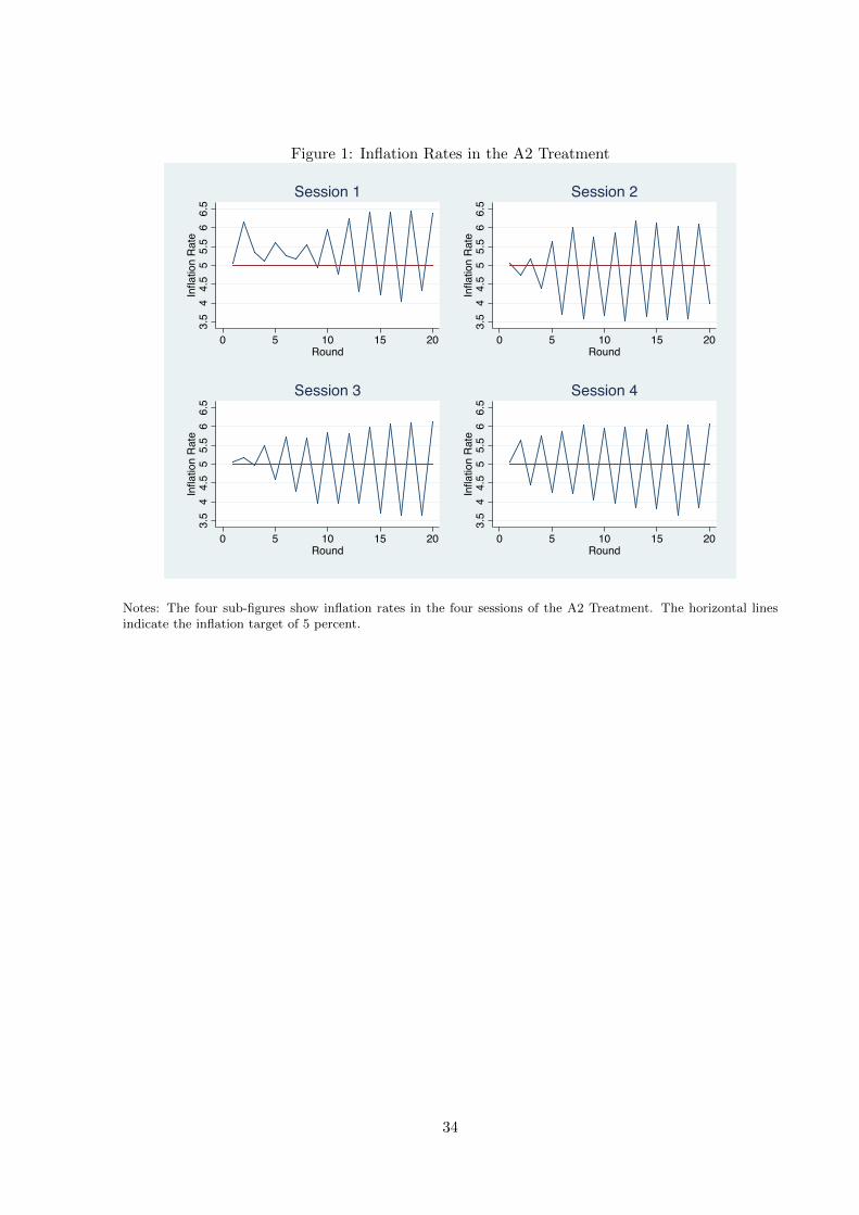
Figure 1: Inflation Rates in the A2 Treatment

3.5

44.

55

5.5

66.

5In

flatio

n R

ate

0 5 10 15 20Round

Session 1

3.5

44.

55

5.5

66.

5In

flatio

n R

ate

0 5 10 15 20Round

Session 23.

54

4.5

55.

56

6.5

Infla

tion

Rat

e

0 5 10 15 20Round

Session 3

3.5

44.

55

5.5

66.

5In

flatio

n R

ate

0 5 10 15 20Round

Session 4

Notes: The four sub-figures show inflation rates in the four sessions of the A2 Treatment. The horizontal linesindicate the inflation target of 5 percent.

34

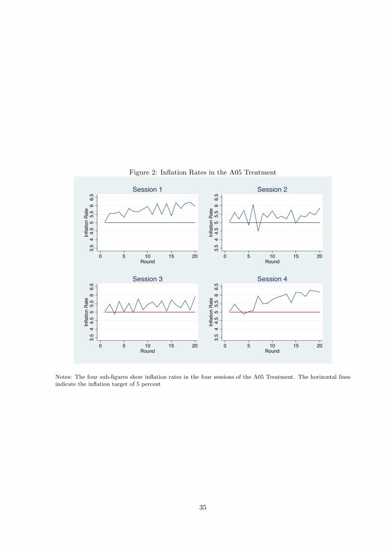
Figure 2: Inflation Rates in the A05 Treatment

3.5

44.

55

5.5

66.

5In

flatio

n R

ate

0 5 10 15 20Round

Session 1

3.5

44.

55

5.5

66.

5In

flatio

n R

ate

0 5 10 15 20Round

Session 2

3.5

44.

55

5.5

66.

5In

flatio

n R

ate

0 5 10 15 20Round

Session 3

3.5

44.

55

5.5

66.

5In

flatio

n R

ate

0 5 10 15 20Round

Session 4

Notes: The four sub-figures show inflation rates in the four sessions of the A05 Treatment. The horizontal linesindicate the inflation target of 5 percent

35

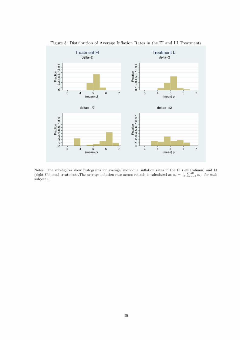
Figure 3: Distribution of Average Inflation Rates in the FI and LI Treatments

0.1.

2.3.

4.5.

6.7.

8.91

Frac

tion

3 4 5 6 7(mean) pi

delta=2Treatment FI

0.1.

2.3.

4.5.

6.7.

8.91

Frac

tion

3 4 5 6 7(mean) pi

delta=2Treatment LI

0.1

.2.3

.4.5

.6.7

.8.9

1Fr

actio

n

3 4 5 6 7(mean) pi

delta= 1/2

0.1

.2.3

.4.5

.6.7

.8.9

1Fr

actio

n

3 4 5 6 7(mean) pi

delta= 1/2

Notes: The sub-figures show histograms for average, individual inflation rates in the FI (left Column) and LI(right Column) treatments.The average inflation rate across rounds is calculated as πi = 1

19

∑20

τ=2πi,τ for each

subject i.

36

Figure C.1: Inflation Rates in Treatment FI2

34

56

73

45

67

34

56

73

45

67

34

56

73

45

67

0 5 10 15 20 0 5 10 15 20

0 5 10 15 20 0 5 10 15 20 0 5 10 15 20 0 5 10 15 20 0 5 10 15 20

1201 1202 1203 1204 1205 1206 1207

1208 1209 1210 1211 1212 1213 1214

1401 1402 1403 1404 1405 1501 1502

1503 1504 1505 1506 1507 1508 1509

1510 1511 1512 1513 1514 1515 1516

1517 1518 1519 1520 1521

Infla

tion

Rat

e

RoundGraphs by participant

37

Figure C.2: Inflation Rates in Treatment FI05

34

56

73

45

67

34

56

73

45

67

34

56

73

45

67

0 5 10 15 20 0 5 10 15 20

0 5 10 15 20 0 5 10 15 20 0 5 10 15 20 0 5 10 15 20

1101 1102 1301 1302 1304 1305

1306 1307 1308 1309 1310 1311

1312 1313 1601 1602 1603 1604

1605 1606 1607 1608 1609 1610

1611 1612 1613 1614 1615 1616

1617 1618 1619 1620

Infla

tion

Rat

e

RoundGraphs by participant

38

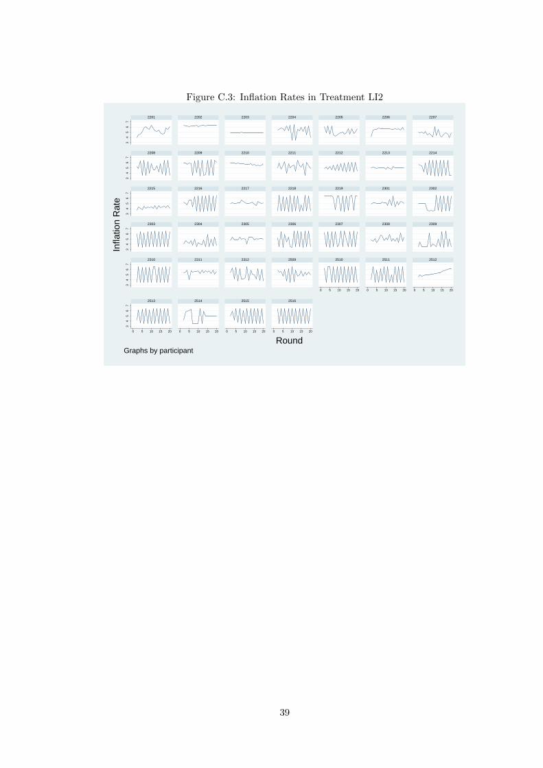
Figure C.3: Inflation Rates in Treatment LI2

34

56

73

45

67

34

56

73

45

67

34

56

73

45

67

0 5 10 15 20 0 5 10 15 20 0 5 10 15 20

0 5 10 15 20 0 5 10 15 20 0 5 10 15 20 0 5 10 15 20

2201 2202 2203 2204 2205 2206 2207

2208 2209 2210 2211 2212 2213 2214

2215 2216 2217 2218 2219 2301 2302

2303 2304 2305 2306 2307 2308 2309

2310 2311 2312 2509 2510 2511 2512

2513 2514 2515 2516

Infla

tion

Rat

e

RoundGraphs by participant

39

Figure C.4: Inflation Rates in Treatment LI05

34

56

73

45

67

34

56

73

45

67

34

56

73

45

67

0 5 10 15 20 0 5 10 15 20

0 5 10 15 20 0 5 10 15 20 0 5 10 15 20 0 5 10 15 20 0 5 10 15 20

2101 2102 2103 2104 2105 2106 2107

2108 2109 2110 2111 2112 2113 2114

2115 2116 2117 2118 2119 2120 2401

2402 2403 2404 2405 2406 2407 2408

2409 2410 2411 2412 2501 2502 2503

2504 2505 2506 2507 2508

Infla

tion

Rat

e

RoundGraphs by participant

40