Indian Journal of Economics and DevelopmentEditorial Board

Chief EditorDr. S.S. Chahal, India

EditorsDr. S.S. Chhina, IndiaDr. P. Kataria, India

MembersDr. Inderpal Singh, AustraliaDr. Timothy Colwill, CanadaDr. I.P. Singh, IndiaDr. J.L. Sharma, IndiaDr. K.K. Datta, IndiaDr. Ravinderpal Singh Gill, CanadaDr. A.K. Vasisht, IndiaDr. Gian Singh, IndiaDr. Y.C. Singh, IndiaDr. Pratibha Goyal, IndiaDr. Seema Bathla, IndiaDr. Shalini Sharma, IndiaDr. Sanjay Kumar, IndiaDr. Rohit Singla, USA

Correspondence AddressDr. Parminder KaurGeneral SecretarySociety of Economics and DevelopmentDepartment of Economics and SociologyPunjab Agricultural UniversityLudhiana-141004

Website: www.soed.inContact:+91-95015-58090Email: editorijed@yahoo.com

Registered Office72-Sector 4, Ranjit AvenueAmritsar-143001

The Journal can also be accessed on www.indianjournals.com

Print ISSN 2277-5412Online ISSN 2322-0430

Indian Journal of Economics and Development 

Society of Economics and Developmentwww.soed.in

Indian Journal of Economics and DevelopmentVolume 11 (2) 2015

©Society of Economics and Development

Printed and Published by Dr. Parminder Kaur on the behalf of the Society ofEconomics and Development

Email: editorijed@yahoo.comWebsite: www.soed.inJournal is available on www.indianjournals.com

Printed at PRINTVIZION1766/1, Street No. 2Maharaj NagarLudhiana-141004Phone: 0161-2442233Email: printvizionprinters@gmail.com

Indian Journal of Economics and Development(Journal of the Society of Economics and Development)

Volume 11 April-June, 2015 No. 2Contents

Research Articles

An application of positive mathematical programming to the Canadian hog sector in the CanadianRegional Agricultural Model

449

Ravinderpal S. Gill, Robert J. MacGregor, Bruce Junkins, Glenn Fox, GeorgeBrinkman and Greg Thomas

Multidimensional poverty in India: Has the growth been pro-poor on multiple dimensions? 457Anupama

Discrimination against migrants in the world of work in Punjab 471P. Kataria and S.S.Chahal

Role of microfinance in generating income and employment for rural households in Punjab-Aneconometric approach

481

Munish Kapila, Anju Singla and M.L.GuptaInflation-unemployment-poverty nexus in Nigeria, 2000-2013: An empirical evidence 489

Obansa Joseph and Ajidani Moses SaboPradhan Mantri Jan Dhan Yojana: A vehicle for financial inclusion 499

Amita Shahid and Taptej SinghStructural shift in the milk composition of cattle with increase in cross-bred species in Punjab -Time torevise milk standards

509

Kushal Bhalla, Varinder Pal Singh, Inderpreet Kaur and Pranav K. SinghPlight of women labourers in rural Punjab 517

Dharam Pal and Gian SinghImplications of privatization of school education in rural areas of Punjab: Some field level observations 533

Sukhdev Singh,Tanu Monga and Gaganpreet KaurProfit efficiency of Egusi melon (Colocynthis citrullus var. lanatus) production in Bida localgovernment area of Niger state, Nigeria

543

Sadiq Mohammed SanusiPoverty, inequality and inclusive growth during post-reform period in India 533

Sunil Kumar Gupta, Pyare Lal, Vinod Negi and Karan Gupta

An economic analysis of direct marketing of potato and onion in Ludhiana city 563Moti Arega and M.S.Toor

Inter-zonal efficiency differences: Study based on farmers of West Bengal 571Chandan Kumar Maity and Atanu Sengupta

Research Notes

Marketing of coriander spice in Rajasthan 583Vinod Kumar Verma and S.S. Jheeba

Performance of wheat crop in Punjab: A case study of Amritsar district 589Narinderpal Singh and Kirandeep Kaur

An analysis of growth of productivity of paddy in post-reform period in Odisha 595 Rabindra Kumar Mishra

Abstracts of Theses 600

Society of Economics and DevelopmentObjectives

1. To promote awareness on the issues relating to economic development.2. To promote better social and ethical values to promote development.3. To promote economic prosperity and serve as a tool to create the consciousness for development.4. To conduct research and publish reports on economic issues.5. To organize seminars, symposia, workshops to discuss the economic problems.6. To offer consultancy, liaison and services as a facilitator.

Office BearersFounder President

Dr. S.S. Chhina

PresidentDr. M.S. Toor

Vice PresidentsDr. D.K. GroverDr. A.K. ChauhanDr. Simran K. SidhuDr. Narinder Pal Singh

General SecretaryDr. Parminder Kaur

Finance SecretaryDr. Mini Goyal

Joint SecretaryMr. Taptej Singh

Executive Committee MembersDr. Gurmail SinghDr. V.K. SinghDr. Sukhdev SinghDr. S.S. BurakDr. Effat Yasmin WaniDr. Ranjit KumarDr. J.M. SinghDr. Raj KumarDr. Arjinder KaurDr. Varinder KumarDr. Jatinder Kumar BhatiaDr. H.S. KingraDr. Deepak ShahDr. A.A. DeviMs. Amritpal Kaur

Subscription ChargesParticular Academics Students Institutional

Annual Life Retired Annual Life AnnualIndian (`) 500.00 3000.00 250.00 250.00 1500.00 1000.00Developed Countries ($) 25.00 250.00 - - - 200.00Developing Countries ($) 10.00 100.00 - - - 100.00Membership should be paid by demand draft drawn in favour of Society of Economics and Development payableat Ludhiana and be sent to the General Secretary, Society of Economics and Dev elopment, Department o fEconomics and Sociology, Punjab Agricultural University, Ludhiana-141004 (Punjab). Alternately, the membershipfee can be deposited in Saving Bank Account No. 29380100009412 (IFSC: BARB0PAULUD), Bank of Baroda,Punjab Agricultural University, Ludhiana.

449

Indian J Econ Dev DOI No. 10.5958/2322-0430.2015.00053.0Volume 11 No. 2 (2015): 449-456 Research Article

AN APPLICATION OF POSITIVE MATHEMATICALPROGRAMMING TO THE CANADIAN HOG SECTOR

IN THE CANADIAN REGIONAL AGRICULTURALMODEL

Ravinderpal S. Gill, Robert J. MacGregor, Bruce Junkins*,Glenn Fox, George Brinkman** and Greg Thomas#

ABSTRACT

This paper describes the Positive Mathematical Programming (PMP), amethod for calibrating models of agricultural livestock production andresource use using a nonlinear marginal cost function and illustrates theapplication of this method in agricultural sectoral models used to studychanges in policy and market signals. The Canadian Regional AgriculturalModel (CRAM) is a regional, multi-sectoral, comparative static, partialequilibrium, mathematical programming model developed and maintainedby Agriculture and Agri-Food Canada. The hog sector is one of thecomponents of the CRAM. In this application, the introduction of non-linear relationships to improve the performance of sectoral models isemphasized for the hog sector. A cubic total cost function was chosen,based on the empirical research for the hog sector in Canada. Empiricalresearch shows that the marginal cost function is convex for the hog sectorin Canada. The calibration constraints are removed and the modelautomatically calibrates at the base year production levels. The resultsindicate that the model is able to predict the impacts of changes in feedprices on the breeding herd size. Similarly, the model can predict changesin the herd size with respect to changes in pork prices.

Keywords: CRAM, feed prices, hog, marginal cost function, PMPJEL Classification: C02, D24, Q11, Q18

*Research Economist, Chief (Retired) and SenoirEconomist (Retired), Strategic Policy Branch,Agriculture and Agri-Food Canada, Ottawa.** Professor and Professor (Retired), Departmentof Food, Agricultural and Resource Economics,University of Guelph, 50 Stone Road East, Guelph,ON N1G 2W1, Canada#Vice President of Pricing Research andAnalytics at Pricing  Solutions Limited,  Toronto,Ontario, Canada, M5E 1E3

INTRODUCTIONThis paper describes the Positive

Mathematical Programming (PMP), developedby Howitt (1995), method for calibrating models

of agricultural livestock production andresource use using a nonlinear marginal costfunction and illustrates the application of thismethod in agricultural sectoralmodels used tostudy changes in policy and market signals.The PMP approach uses more flexiblespecification than traditional linear constraints.Over the past decade the PMP approach hasbeen used on several policy models at thesectoral, regional and farm level. Nationalsectoral models using PMP for the US, Canada,and Turkey include House (1987), Ribaudo etal. (1994), Horner et al. (1992) and Kasnakogluand Bauer (1988). The regional models include

450

Hatchett et al. (1991), Oamek and Johnson(1988) and Quinby and Leuck (1988). Rosenand Sexton (1993) apply PMP to individualfarms. The PMP approach uses the observedlevel of production in the base year to generateself calibrating models of agriculturalproduction and resource use consistent withmicroeconomic theory.

There are several reasons that mathematicalprogramming models are widely used foragricultural economic policy analysis. First,they can be constructed from a minimal dataset. Second, the constrained structure inherentin programming models is well suited tocharacterising resource, environmental orpolicy constraints. The PMP approachemploys both programming constraints andpositive inferences from base year level ofproduction. The PMP approach automaticallycalibrates models using minimal data andwithout flexibility constraints. The resultingmodels are more flexible in their response topolicy changes (Howitt, 1995). In thisapplication, the introduction of non-linearrelationships to improve the performance ofsectoral models is emphasized. A cubic totalcost function was chosen, based on theempirical research for the hog sector in Canada.An empirical research shows that the marginalcost function is convex for the hog sector inCanada. The calibration constraints areremoved and the model automaticallycalibrates at the base year production levels.Background

The CRAM is a regional, multisectoral,comparative static, partial equilibrium,mathematical programming model developedand maintained by Agriculture and Agri-FoodCanada. CRAM provides significant regionaland commodity detail of the Canadianagricultural sector. It has become an importantinstrument for the analysis of the impact ofpolicy changes on the Canadian agriculturalindustry at a disaggregated level. The modelhas been used for both short and medium termanalysis. One of its first applications was tolook at the implications of the introduction of

medium quality wheat on the prairies (Webber,1986). Since then, it has been used to examinethe impact of the 1985 US Food Security Acton the Canadian grain sector (MacGregor andGraham,1988) and the impact of directgovernment assistance programs on the beefand hog sector (Webber et al., 1988). CRAMhas been used to examine the implications ofthe Canada-U.S. Trade Agreement (CUSTA),the Multilateral Trade Negotiations (MTN)(Graham et al., 1990), changing the WesternGrain Transportation Act (WGTA) (Klein etal., 1991), and licencing BST for dairy cows(Stennes et al., 1990). CRAM has also beenused for the environmental assessment of thecrop insurance program (Giraldez et al., 1998)and return on investment (ROI) studies forwheat (Klein and Freeze, 1995) and (Klein etal., 1995), potatoes (Oxley et al., 1996), andmore recently ROI for hogs research (Fox etal., 1998).

The model identifies fifty five cropproducing regions, twenty-two of which arein the praire provinces-seven in Alberta, ninein Saskatchewan, and six in Manitoba. Thereare eight regions in British Columbia, ten inOntario and eleven in Quebec. Each of theAtlantic Provinces are modelled as a cropregion. The livestock production is modelledat the provincial level. The current version ofCRAM specifies crop production, beefproduction and hog production as PositiveMathematical Programming (PMP) activitiesthat allow crop area, beef production and hogproduction to be a function of observed levelof production, the marginal value ofproduction and the marginal cost ofproduction. The crops produced in theseregions are transferred to the provincial levelto meet the demand for livestock feed anddomestic consumption, or transferred to portfor export.

The hog sector is one of the componentsof the CRAM. The hog production is specifiedat the provincial level. The two categories ofhogs modelled on an annual basis are sowsand growers. The opening stock of sows can

451

be set exogenously. The growers are modelledbased on the opening stocks of sows and thenumber of farrowing cycles per year. Sowsgive birth to growers at the start of each cycle.Sows are then either culled or join the openingstock of sows for the next cycle. The growerscan be slaughtered, exported as live animalsor replace culled sows. The ratio of growersto sows, replacement rates, market hogs persow, birth rates and death losses are part ofthe data requirements and these vary for eachprovince.

To complete the representation of the hogproduction activities, the followingcoefficients are attached to each category ofhogs in each province: cash costs, proteincosts, feed requirements (in terms of barleyequivalents) and the yield per animal. The cashcosts (which are not itemized e.g., veterinaryand animal health, insurance, marketing,labour, maintenance and repair, supplies,manure disposal, taxes and utilities) and theyields are recorded at the provincial level. Thetotal cash costs and total amount of porkproduced are related to the number of sowsand growers in a specific province. The barleyrequirements are different for sows andgrowers; however, it is assumed that there isonly one feed mix for sows and growers ineach province. The linkages between crop andanimal production through feed supply anddemand relationships are important feature ofagriculture which, among all the availablemethodologies, can be best modelled with aprogramming approach. The barley required(or its equivalent) is drawn from provincialsupplies, and provides the link to the cropproduction sector. Wheat, corn, oats and feedpotatoes, grown in the crop sector of the modelare converted into barley equivalents througha commodity substitution matrix.The PMP Calibration Approach

The PMP approach, developed by Howitt(1995), can use data needed to construct alinear programming (LP) model in a moreflexible manner than traditional LP models,while generating endogenous calibration

models of agricultural production and resourceuse that are consistent with microeconomictheory, and prior estimates of demand andsupply elasticities PMP allows modellers tointegrate traditional input-output data witheconometric estimates of economicrelationships in a manner that is consistentwith microeconomic theory. The PMPspecification results in a smooth andcontinuous response to parameterization of themodel. While, the production and costspecification implied by the PMP specificationis unconventional, the method works, in thatit automatically calibrates models withoutusing flexibility constraints. The resultingmodels are more flexible than traditional LPmodels in their response to policy changes,and priors on the supply elasticities can bespecified.

Figure I illustrate the use of the PMPmethod using hog production as an example.In the CRAM, the PMP method is applied togrowers. In this example there are three typesof costs associated with growers: variable cashcosts, protein costs and barley costs.Associated costs of sows and replacementsare included for each grower. Given the grossreturns and average costs per grower, the baseyear production level has to be constrainedby calibration constraints to observed outputlevel (X0). Hog production is derived from asow herd that produces market hogs and otherbyproducts (cull animals). The herd consumesgrain and other input cash costs. Theproducer’s problem becomes maximizing netreturns from the production of market hogsand cull animals. The maintained hypothesisin the following model is that producersmaximize producer’s surplus as well asconsumers’ surplus taking into account:1) Given product prices (world price).2) Supply and demand remains in balance.

The stocks are ignored in this model. Theproducers solve the following model:

X)CCBCPC(XPZMax 0X,XX toSubject 0

452

Where,Z = Net returnsP = Revenue per growerX = Number of growers, with X0 the

number of growers in the base periodPC = Protein costs per growerBC = Barley costs per growerCC = Cash costs per grower

A LP model contains most of theinformation required to parameterize themarginal factor cost curves for the hog sectorof CRAM which can then be used for predictivepurposes. The information on the marginalrevenue (MR) and marginal cost (MC) ofgrowers at the observed level of productioncan be determined from the solution to the LPmodel. These represent the elements of thefirst order necessary conditions (FONC) thatsolved the firm’s original problem. Therelationship at an optimum is MR = MC.Stage II. Derivation of the PMP Cost Function

In the LP phase the observed level ofproduction is imposed on the solution as aconstraint in the PMP method. This representsa positive rather than a normative solutionwhich replicates the base period byconstruction. The requirement now is toimpose additional structure on the model thatwill allow it to find the observed behaviour asa normative solution to the firms’ optimizationproblem without use of arbitrary constraints.The PMP approach uses observed averagefactor cost data (fixed input coefficients permarket hog times factor prices), the observedlevel of hog production, and the shadow values(l) generated by the calibration constraints inthe LP model. The marginal values (l) oncalibration constraints represents the implicitmarginal cost over and above the observedaverage factor cost, that producers must havetaken into account when selecting the profitmaximization level of activity (X0). Thisformulation ensures that the marginal valuesof real constraining resources, (l), are the sameat the observed base year level for allproduction activities that use limitingresources.

To link the Positive MathematicalProgramming procedure to the CRAM aquadratic marginal cost function is specifiedfor total variable costs for the grower hogs.The specified marginal cost function consistsof variable costs, feed costs and the observedshadow value (l). The variable costs and feedcosts are assumed to be independent of thelevel of output. The shadow value varies as aquadratic function of output. The marginalcost function is specified as a quadraticfunction where the elasticity of the price ofhogs is assumed to be equal to 2 (h=2). As aresult, the total variable cost function, whichis the integral of the specified marginal costfunction, is a cubic function of output. Thisresults in a cubic optimization problem thatequilibrates marginal cost with marginalrevenue at the base period’s actual outputlevel.

The PMP procedure now incorporates anon-linear supply response into the model.Advantages of the PMP specification are notonly the endogenous calibration feature, butalso its ability to respond smoothly to changesin market conditions and policy measures.Paris (1993) shows that input demandfunctions and output supply functionsobtained by parameterizing a PMP problemsatisfy the Hicksian conditions for thecompetitive firm. In addition, the input demandand supply functions are shown continuousand differentiable with respect to prices, costs,and right-hand side quantities. The PMPformulation has the properties that thenonlinear calibration can take place at any levelof aggregation. That is, one can nest an LPsub component within the quadratic objectivefunction and obtain the optimum solution tothe full problem.

The number of sows at this stage isdetermined by the number of growers. Barleycost is implicit in the objective function in themodel. This is the simplest specification thatcan explain the observed behaviour. Thecalibration constraints are removed and themodel becomes:

453

1

11

XXPXZMax

Subject to1X

1

11

X)(

X is a non-linear cost

function for total variable costs which isderived from the shadow values (l) from thecalibration constraints. The unknownparameters a and b can be calculated from theoptimal solution of the LP problem in Stage I.

n

n

n

X

XMC

MCPP

CCPCBCX

XX

Therefore,

productionoflevelobservedtheat

(MC)costMarginal

11costvariableTotal 1

Using the calibration constraint shadowvalues from Stage I, can be solve for theintercept and slope parameters that result in anon-linear optimization program thatequilibrates at the base period production level.

In Figure 1, the calibration constraint shadowvalue, (l), is equal to the difference betweenMC and a at the optimal level of production.The intercept (a) is equal to the sum of barleycosts, protein costs and cash costs. A non-linear supply response has now beenincorporated into the model.

The structural features of this model willbe discussed below. It should be pointed outthat, depending on the assumptions onewishes to impose, that alternative calibrationprocess can be used that would alter thestructural properties of the model.Conceptually, they are equivalent to the aboveexplanation.Retention Functions

The retention functions are used tocapture the investment/disinvestmentdecisions in the hog sector in the without PMPversion. Only under certain circumstances itis necessary to activate retention functions tomodel the change in herd size Retentionfunction information is specified by animaltype and by province. This includes: openingstock levels, number of arguments in theretention function where each argument is theprice of some good, and for each argument:1) Elasticity of stocks with respect to price

(own price or price of an input);

Marginal cost from PMP solution

Marginal revenue

Shadow value from LP solution

Marginal cost from base year solution

X0 (Number of growers)

Price

Figure I: CRAM Supply Function Derived using PMP

454

2

2

21

X

XX

MFCMFC

X.

2) Current market price of good (as a percentof base price);

3) Current government payment to producerof good (as a percent of base price);

4) Expected market price (as a percent of baseprice);

5) Expected government payment (as apercent of base price).

All prices and payments are expressed asa percentage of current market prices which isset at 100 percent (Government payments areexpressed as dollars per $100 of market receiptsor market cost for an input). The governmentpayment (adjusted for any deviation of marketprice from the index of 100) is added to themarket price to determine the effective price,or unit revenue, to the producer. Thepercentage change in effective producer pricecan then be determined. The range parameteris used to set a limit on the change in stocklevels, and is expressed as proportion ofopening stocks.

The GAMS version calculates openingand closing stocks as an adjusted closingstock coefficient was calculated based onchanges in own price, feed prices andgovernment payments over base level values(the retention function was used and openingstocks were set equal to closing stocks). Thismeans the retention function is always active.Therefore, if a short run analysis is beingundertaken, the data in the hog stock andelasticity table needs to reflect the baseconditions with expected prices set equal tocurrent prices or payments (in percentageterms). It is easy to make policy runs usingspecified opening and closing coefficientssimilar to the original model.RESULTS

In order to compare the PMP and non-PMPversions of the CRAM, the model was run withrespect to changes in key variables that isincrease in protein, barley and cash costs by10 percent, decrease in barley costs by 10percent (by reducing the feed requirements by10 percent), and increase in the export price ofpork by 5 percent, increase in market hogs per

sow by 5 percent and increase in carcassweights by 5 percent to capture movementalong the MFC curve. The supply responseof the model without PMP (Retentionfunctions) was limited to changes in porkprices and barley prices only.

The percentage changes in the breedingherd size with respect to each scenario andinverse elasticity of MFC are reported in Table1. An inverse elasticity of MFC1 can beexpressed as the supply elasticity for thegrowers at the observed level of production(X0).

The supply elasticities ranged from 1.28for Manitoba to 3.72 for Newfoundland. Thesupply elasticities for Ontario and Quebecwere 2.17 and 1.93, respectively. Theseelasticities may be higher than expected. ThePMP procedure can be modified to meet priorestimates of elasticities.

The breeding herd size decreased by 28,23 and 22 percent for Saskatchewan, PrinceEdward Island and Newfoundland,respectively, as protein, barley and cash costswere increased by 10 percent. For the rest ofthe provinces, breeding herd size decreasedfrom 5 to 19 percent. As barley costs weredecreased by 10 percent, breeding herd sizeincreased by about 5 percent for most of theprovinces with the exception ofNewfoundland, Manitoba and Saskatchewanwhere breeding herd size increased by 12, 3and 7 percent, respectively. As market hogsper sow were increased by 5 percent, thebreeding herd size increased by about 4 percentfor all the provinces. As carcass weights areincreased by 5 percent, the increase in herdsize ranged from 6 percent for Manitoba to 17percent for Newfoundland. As pork priceswere increased by 5 percent, the breeding herdsize increased from 6.44 percent for Manitobato 16.51 percent for Newfoundland.

The model was also run with respect tochanges in replacement rates, death rates and

455

the hog index, but the supply response wasless than one percent. The supply responseof the model without PMP was limited tochanges in Pork prices and Barley prices only.As barley prices are decreased by 5 percentthe breeding herd size increases by about 2percent on an average for all provinces. Aspork prices are increased by 5 percent, thebreeding herd size increased by 6 percent forAtlantic Provinces and Quebec. For BritishColombia, Saskatchewan and Alberta, thebreeding herd size expanded by about onepercent. The largest expansion in the breedingherd size is in Manitoba (11.4 percent).

The model is able to predict the impacts ofchanges in feed prices on the breeding herdsize. Similarly, the model can predict changesin the herd size with respect to changes in porkprices. The supply response of the model canbe captured with respect to change in severalother parameters for example market hogs persow, feeding efficiency, replacement rates,mortality rates, yield per animal and marketingperformance measures.SUMMARY AND CONCLUSIONS

The programming models have a strongrole to play in agricultural policy analysis. ThePositive Mathematical Programmingrepresents a method of incorporatinginformation from econometric estimation andinferences from economic theory in a direct

and parsimonious way. The calibration of aPMP model starts with a base year data set.Empirical information, typically in the form ofelasticity estimates, is then added. The ultimatetest of a policy model is its ability to predictbehavioural responses out of the sample baseyear. An empirical tests of the stability of thePMP values are required to evaluate thestability of the calibrated models.

The PMP approach is shown to satisfy themain criteria for calibrating sectoral andregional models in an application to theCanadian hog industry. A quadratic marginalcost function is specified for the total variablecosts. As a result, the total variable costfunction, which is the integral of specifiedmarginal cost function, is a cubic function ofoutput. The cubic form for the total costfunction was chosen based on the empiricalresearch for the hog sector in Canada. Anempirical analysis shows that the marginal costfunction is convex in shape for the hog sectorin Canada. Using PMP, the model calibratesprecisely to the output and input quantities.In addition, the PMP approach can incorporatepriors on supply elasticities.REFERENCESFox, G., George, B., and Greg, T. 1998. The economic

benefits of Canadian swine research. ResearchReport. Agriculture and Agri-Food Canada,Ottawa.

Table 1: Supply response with respect to change in key variablesProvince Sows

(000)With PMP Without PMP

(RetentionFunctions)

Base IncreasePC, BCand CCby 10%

Decreasebarley

requirementsby 10%

Increasemarket

hogs persow by 5%

Increasecarcass

weights by5%

Increaseporkpricesby 5%

Increasepork

prices by5%

Decreasebarley

prices by10%

Inverse

British Colombia 23.20 -9.00 4.63 -4.50 8.77 8.97 1.10 2.20 1.83Alberta 197.01 -18.71 4.92 -4.44 12.69 13.38 1.10 2.20 2.70Saskatchewan 90.00 -27.98 6.67 -4.17 16.58 17.30 0.70 1.40 3.60Manitoba 170.00 -5.19 2.73 -4.62 6.20 6.44 11.40 2.00 1.28Ontario 321.99 -9.79 5.98 -4.22 10.28 10.58 3.95 2.00 2.17Quebec 319.99 -9.21 5.41 -4.32 9.24 9.58 5.95 2.00 1.93New Brunswick 8.50 -16.46 4.21 -4.24 7.36 7.30 5.95 2.00 2.85Prince Edward Island 12.00 -23.15 5.19 -4.05 9.09 9.34 5.95 2.00 3.61Nova Scotia 12.30 -13.42 4.02 -4.34 6.54 6.49 5.95 2.00 2.53Newfoundland 0.60 -22.38 11.71 -3.95 17.15 16.51 5.95 2.00 3.72PC: Protein cost; BC: Barley cost and CC: Cash cost

456

Giraldez, J., MacGregor, R.J., Junkins, B., Gill, R.,Campbell, I., Wall, G., Shelton, I., Padbury, G.,and Stephen, B. 1998. The federal-provincialcrop insurance program: An integratedenvironmental-economic assessment. ResearchReport. Agriculture and Agri-Food Canada,Ottawa.

Graham, J.D., Stennes, B., MacGregor, R.J., Meilke,K., and Moschini, G. 1990. The effects of tradeliberalization on Canadian dairy and poultrysectors. Agriculture Canada Working Paper.Number 3, Ottawa.

Hatchett, S.A., Horner, G.L., and Howitt, R.E.1991. A Regional Mathematical ProgrammingModel to assess drainage control policies. In:Dinar, A. and Zilberman, D. (eds.) TheEconomics and Management of Water andDrainage in Agriculture. Springer US: 465-489.

Horner, G.L., Corman, J., Howitt, R.E., Carter,C.A., and MacGegor, R.J. 1992. The CanadianRegional Agricultural Model: Structure,operation and development. Technical Report1/92. Agriculture Canada, Ottawa.

House, R.M. 1987. USMP Regional AgriculturalModel. National Economics Division ReportERS, US Department of Agriculture, WashingtonDC: 30.

Howitt, R.E. 1995. Positive mathematicalprogramming. American Journal of AgriculturalEconomics. 77 (5): 329-342.

Kasnakoglu, H. and Bauer, S. 1988. Concepts andapplication of an agricultural sector model forpolicy analysis in Turkey. In: Bauer, S. andHenrichsmeyer, W. (eds.) Agricultural SectorModelling. Proceedings of the 16th Symposiumof the EAAE, Wisssenschaftsuerlag Vauk, Kiel.

Klein, K.K., Fox, G., Kerr, W.A., Kulshreshtha,S.N., and Stennes, B. 1991. Regionalimplications of compensatory freight rates forprairie grains and oilseeds. Agriculture CanadaWorking Paper. Number 3, Ottawa.

Klein, K.K. and Freeze, B. 1995. Economics ofloss avoidance research on wheat in Canada.Research Report. Research Branch, Agricultureand Agri-Food Canada, Ottawa.

Klein, K.K., Freeze, B., and Walburger, A.M. 1995.Economic returns to yield increasing researchon wheat in Canada. Research Report. ResearchBranch, Agriculture and Agri-Food Canada,Ottawa.

MacGregor, R.J. and Graham, J.D. 1988. The

impact of lower grains and oilseed prices onCanada’s grain sector: A regional programmingapproach. Canadian Journal of AgriculturalEconomics. 36: 51-67.

Oamek, G. and Johnson, S.R. 1988. Economic andenvironmental impacts of a large scale watertransfer in the Colorado River Basin. Paperpresented at the WAEA annual meeting, HonoluluHI, 10-12.

Oxley, J., Junkins, B., Dauncy, C., and MacGregor,R.J. 1996. The economic benefits of publicpotato research in Canada. Research Report.Research Branch, Agriculture and Agri-FoodCanada, Ottawa.

Paris, Q. 1993. PQP, PMP, parametricprogramming and comparative Statics. In:Chapter 11 in Notes for AE253. Department ofAgricultural Economics, University ofCalifornia, Davis.

Quinby, B. and Leuck, D.J. 1988. Analysis ofselected E.C. agricultural policies and Dutch feedcomposition using Positive MathematicalProgramming. Paper presented at AAEA AnnualMeeting, Knoxville, TN.

Ribaudo, M.O., Osborn, C.T., and Konyar, K.1994. Land retirement as a tool for reducingagricultural non-point source pollution. LandEconomics. 70: 77-87.

Rosen, M.D. and Sexton, R.J. 1993. Irrigationdistricts and water markets: An application ofCooperative Decision-making Theory. LandEconomics. 69: 39-53.

Stennes, B.K., Barichello, R.R., and Graham, J.D.1991. Bovine somatotropin and the Canadiandairy industry: An economic analysis. WorkingPaper-1/91. Agriculture Canada, Ottawa.

Webber, C.A. 1986. Determining the productionand export potential for medium quality wheatusing a sectoral model for Canada. UnpublishedM.Sc. Thesis. Department of AgriculturalEconomics, University of British Columbia,Vancouver, British Columbia

Webber, C.A., Graham, J.D., and MacGregor, R.J.1988. A regional analysis of Direct GovernmentAssistant Programs in Canada and their impactson the beef and hog sectors. Working Paper.Agriculture Canada, Ottawa.

Received: October 16, 2014Accepted: December 31, 2014

457

Indian J Econ Dev DOI No. 10.5958/2322-0430.2015.00054.2Volume 11 No. 2 (2015): 457-470 Research Article

MULTIDIMENSIONAL POVERTY IN INDIA: HAS THEGROWTH BEEN PRO-POOR ON MULTIPLE

DIMENSIONS?Anupama*

ABSTRACT

The present investigation is an attempt to synergize the uni-dimensional aswell as multidimensional approaches to measure poverty as well as pro-poor growth. This analysis is based upon FGT indices for measuring uni-dimensional poverty, the Alkire and Foster (2008) methodology for multi-dimensional poverty and then pro-poor growth rates on non-incomeindicators have been computed by using Klasen (2008) approach which isbased upon Ravillion and Chen (2003) index. It can be stated that both theuni-dimensional and multidimensional poverty in India had declinedbetween 2004-05 and 2009-10. But, it had not been pro-poor across all thedimensions and for all social groups. It has been observed that thedimensions of education, expenditure and regular salary had not been pro-poor in most of the cases. Among the social groups, the SCs and the STs arethe poorest categories and by household types, the labour households arethe poorest one. These households suffer from the deprivations of multipledimensions. It has been observed that the dimension of education andcooking fuel are the biggest contributors to overall poverty rate and thepoorest suffer the most from these deprivations.

Keywords: FGT indices, inequality, pro-poor growth, poverty, social groupsJEL Classification: D63, I32, P24, P36

*Professor of Economics, Department ofEconomics, Punjabi University, Patiala-147002Email: anupamauppal@yahoo.com

INTRODUCTIONThe concepts of multidimensional poverty

and pro-poor growth have recently capturedthe attention of researchers and policy makers.Actually, it is being widely felt that neither thebenefits of growth trickle down automaticallyto the lower rungs of the income ladder northe reduction in income poverty is an indicatorof general rise in standard of living of themasses. It is being felt that the linkagesbetween income and well being as well as the

distribution of income are not straightforward(Sen, 1992, Streeten, 1994 and Berenger andBresson, 2010).

The recent studies on pro-poor growthhave the shortcoming of not including the non-income indicators. The estimates measuringthe pro-poor growth are purely based uponthe income indicators and do not reflect anychange in the non-income indicators of thepro-poor growth. The shortcoming of the one-dimensional focus on income is that a reductionin income poverty does not guarantee areduction in the non-income dimensions ofpoverty, such as education or health (Grosseet al., 2005). This means that finding income

458

pro-poor growth does not automatically meanthat non-income poverty has also beenreduced. The outcome of any growth processis needed to be evaluated regardingachievements on front of many dimensions.

The idea of multidimensional poverty hasactually started with Sen’s CapabilityApproach which gives more emphasis to non-income indicators (Sen, 1988). Thus, if thegrowth is pro-poor, the deprivations onaccount of non-income indicators must havereduced. There are two differentmethodologies-one measuring pro-poorgrowth another measuring themultidimensional poverty.

The multidimensional poverty indicatorsmeasure the headcount ratio, poverty gap andsquared poverty gap (or severity of poverty),while the pro-poor growth indicators showwhether the benefits of growth have beenlarger for the poor or not. Can one have asynergy of two types of indicators? A rangeof methodologies are available to measure theextent, degree and severity of poverty usingthe income indicators (FGT indexes) and theattempts to measure the pro-poorness ofgrowth on multiple dimensions are scanty, herean attempt would be made to compare the pro-poor growth rates on account of incomeindicators with that of the non-incomeindicators. In this perspective, this paperdiscusses the deprivations on account ofmany cardinal and ordinal measures.

This analysis is based upon FGT indicesfor measuring uni-dimensional poverty, theAlkire and Foster (2008) methodology for multi-dimensional poverty and then pro-poor growthrates on non-income indicators have beencalculated by using Klasen (2008) approachwhich is based upon Ravillion and Chen (2003)index. Thus, this paper has been divided intofive sections. Apart from this introductorysection, Section II gives the data andmethodology used in this paper, Section IIIanalyses the extent of uni-dimensional andmultidimensional poverty in India, section IVmeasures the pro-poor growth indicators and

finally Section V concludes the paper and givessome policy suggestions.DATA AND METHODOLOGY

This paper uses NSSO data on consumerexpenditure for measuring income as well asnon-income poverty. The analysis would berestricted to the 61st and 66th Round of NSSO.For measuring multidimensional poverty Alkireand Foster (2008) methodology has been used.This methodology allows measurement ofpoverty on ten different dimensions. Basedupon the availability of data we have tried toidentify the poverty/deprivations on accountof 8 dimensions.

The poverty line of these dimensions hasbeen fixed according to the MDG indicators.An attempt has been made to capture thedeprivations on account of the livingconditions, the nutritional status, ownershipof the assets, and attainment of human capital.These indicators are discussed below alongwith their poverty lines:Expenditure

The expenditure has been taken on monthlyper capita basis and the official poverty lines,given by the Planning Commission have beenused as a cut-off to identify the poor. Theexpenditure in 2009-10 has been deflated andthe poverty line for year 2004-05 has beenused.Cooking Fuel

This dimension has 10 different categories.These are discussed below along with theirranks:1. No cooking arrangements2. Firewood and chips3. Dung cake4. Charcoal5. Coke, coal6. Others7. Kerosene8. Gobar gas9. Electricity10. LPG

We set Z=7 and classify those as non-poorwho use kerosene, gobar gas, electricity andLPG.

459

LightingThere are seven different categories.

1. No lighting arrangements2. Candle3. Kerosene4. Other oils5. Gas6. Others7. Electricity

Here, persons not using electricity forlighting are termed as poor.Dwelling

There are four different categories:1. No dwelling unit2. Others3. Hired4. Owned

The persons without ownership of thedwelling unit and the unspecified categoriesare identified as poor.Regular salary/wage income

If none of the person in the family is havinga regular source of income, then all themembers of the household are identified aspoor.Number of meals per day

The persons having less than two meals aday are termed as poor.Education

The illiterate persons and those havingeducation below primary are termed as poor.Ownership of land

The persons without ownership of land aretermed as poor.

The methodology proposed by Alkire andFoster (2008) can also be broken down in toindividual dimensions to identify whichdeprivations are driving multidimensionalpoverty in different regions or groups. Thischaracteristic makes it a powerful tool forguiding policies to address deprivations indifferent groups effectively. For analysingmultidimensional poverty using thismethodology, it is important to understand afew concepts. As in the Foster GreerThorbecke class of income poverty measures,each value can also be squared, to emphasize

the condition of the poorest of the poor. So,this methodology proposes a class ofmeasures M, comprising three measures:

M0: the measure described below, suitablefor ordinal and binary and qualitative data,which represents the headcount and thebreadth of poverty. This is the adjustedheadcount index (H) which shows theweighted sum of average deprivations (A).This can also be represented as M0 = H×A oraverage deprivations can be calculated bydividing M0 with H or A = M0/H.

M1 : M0 times the average normalized gap(G), this is represented as HAG or M1=M0×Gor G=M1/M0.

M2 : M0 times the average squarednormalized gap (S), represented as HAS. Thus,M2=M0×S or the severity of poverty or S=M2/M0.Measuring Poverty and Pro-Poor Growth

As discussed in the introductory section,for calculation of uni-dimensional poverty, thehead count ratio, poverty gap and the severityof poverty (squared poverty gap) arecalculated using the FGT indices. Although,growth of income generally leads to decline inpoverty rates, yet it may not have benefittedthe poor and rich in a similar way. The growthmay result in to increase in income inequalitieswhich push the marginalized sections of thesociety in to deeper morass of poverty.Therefore, for past many years there is a generalconsensus that growth alone is a ratherinsufficient tool for poverty reduction. Hence,for the past decade, the poverty analyses arelargely dealing with the relationship betweeneconomic growth and rising inequality withreference to the concept of pro-poor growth.

The concept of pro-poor growth has beendefined in a variety of ways: the growth canbe termed as pro-poor when the increase ingross domestic product simply reduces thepoverty (Ravallion, 2004); if the poor benefitproportionately more than the non-poor(Pasha and Palanivel, 2003 and Zepeda, 2004)or if the relative shares of poor in income,population and variance of poor’s share of

460

income have favourably changed (White andAnderson, 2001). Clearly, different definitionsof pro-poor growth lead to differentassessments of growth processes using adifferent measurement tool. Recent studiesemploy different concepts and thus, definevarying tools to quantify the impact of growthon poverty. Among the most widely usedconcepts and hence the indices are those usedby Ravallion and Chen (2003) and Kakwaniand Pernia (2000). Ravallion and Chenmeasures the rate of pro-poor growth (RPPG)which is based upon the concept of growthincidence curve (GIC) and marks the areaunder the GIC up to the headcount ratio. If theRPPG exceeds the mean growth rate, growth isjudged to be pro-poor in its relative meaning.On the other hand Kakwani and Pernia (2000)measure the Poverty Equivalent Growth Rate(PEGR) which captures the change in povertywhen inequality changes without affecting thereal mean income. Thus, the estimated growthrate gives more weight to the incomes of thepoor. Thus, we have two different sets ofmethodologies. One, is used in calculating themultidimensionality of poverty and another,the pro-poorness of growth. However, it isbeing felt that the pro-poor growth may or maynot be multi-dimensional. Similarly, reductionin multidimensional poverty may or may notbe pro-poor. Thus, improving income situationof households need not automatically implyan improving non-income situation (Klasen,2000). Hence, there is a need to have a rationalsynergy between the pro-poor growthindicators and multi-dimensional povertyindicators. Although, Grosse et al. (2005) havesuggested making use of the tools developedfor pro-poor growth on non-income indicatorsas well but there are several limitations of usingthese upon the same.

A useful tool for measuring growth rate isGIC, which can also be applied to non-incomeindicators which helps us in examining whetherthe growth has been pro-poor or not in thecase of multiple dimensions. In the case of non-income indicators, we rank the individuals by

each respective non-income variable andcalculate the population centiles based uponthis ranking which further enables us tocalculate the pro-poor growth index in the caseof each dimension. This type of exercise givesus an indication that how growth has behavedfor each dimension which may further specifiesthe direction of public spending for anypoverty removal strategy. However, there arecertain limitations of using the GIC on non-income indicators.

As we know that the calculation of non-income indicators is mainly based upon theranking of different scales of attainments. Twotypes of problems may arise in this case, first,shifting of one rank in the lower orders maynot mean the same thing as shifting of onerank in higher orders for example, in the caseof education, the shift from below primary toprimary may not improve the living standardof a person as compared to the shift fromgraduation to post-graduation. This problemcan be corrected by assigning higher weightsto the higher order of education. Secondly,some variables of non-income indicators donot vary much, that is, the variables arebounded. These variable show very smallvariations and so for these variables anddummy variables, the use of GIC is barelyfeasible. This problem can be solved by usingconditional GIC in which the population is firstranked by income indicator and then by thenon-income indicator.

Lastly and more importantly, the problemis that of a composite index. Whereas, UNDPhas recently added multidimensional povertyindex (MPI) which looks at overlappingdeprivations in health, education and standardof living, Grosse et al. (2005) have alsoproposed a composite welfare index which isbased upon the same methodology used byUNDP. The question is do we really need acomposite index? This is an important questionparticularly when in order to target the policystance, our aim is to identify (and also toquantify) whether, the growth is pro-poor ornot.

461

Moreover, in the case of developingeconomies, for different dimensions, we haveto depend upon different data sets particularlyin the case of India, though many dimensionsof poverty are met through the National FamilyHealth Survey (NFHS) data set and evenConsumer Expenditure Survey by NSSO(National Sample Survey Organisation) canalso be used with some proxy variables but foremployment related variables we have todepend upon the NSSO surveys onEmployment-Unemployment Situation inIndia. This poses a problem as we would bedealing with different reference units. As wehave seen that multidimensional povertyanalyses are based upon a mix of deprivationsand their sources which vary across groups/regions. Here we take note of two possiblesituations:1. The data regarding income, expenditure

and source of living of the family is givenin consumer expenditure survey, these canalso be found in survey on employment-unemployment situation which givesadditional information on otheremployment characteristics such aswhether the person is employed on full-time basis or part-time basis; has a jobcontract or not; entitled to paid leave ornot; is covered by job security or not, etc.These two data sets do not provide anyinformation on other deprivations suchas sanitation, access to drinking water,nutritional status, etc. Now, the questionis if it would be rational to calculatedifferent deprivations from differentsources? And also would it be rational todrop these sources of deprivations?

2. The growth may not be pro-poor formarginalized social groups (categorizedaccording to gender, caste, ethnicity, etc)on various dimensions and clubbing themtogether would not be a rational option.Moreover, the status of a person being ina particular group cannot be changed; wecan only deal with his/her specificdeprivation targeting that group only.

Deprivations on different dimensionssuch as health, education, employmentcharacteristics, etc. need involvement ofdifferent departments so a compositeindex may only show an overall situationor trends over a period of time but forpoverty removal strategy we need tocalculate the size, degree of poverty andits pro-poorness on different dimensionsseparately. Thus, whereas framing acomposite welfare index can be importantfor analyzing overall changes in pro-poorness of multidimensional poverty, fortargeting policy, the separate calculationsof these indicators across groups andacross dimensions are more important.

Section IIIUni-dimensional and MultidimensionalPoverty in India

By using the FGT indices on eachdimension, we have calculated the headcountratio of the population which is deprived of aparticular dimension which is shown in Table1. The results show that the proportion ofpopulation living below poverty line is thehighest in the case of regular salary income,followed by education, lighting andconsumption expenditure.

As compared to 2004-05, the populationliving below poverty line in all the dimensions(except in the case of regular salary income)has declined and in percentage terms, thisdecline is the highest in the case of educationin rural areas and dwelling unit in urban areas.Now moving to the multidimensional povertyrates, it can be observed that in 2004-05, 98.9per cent of total population in rural areas and89.5 per cent in urban areas was deprived of atleast one dimension (Table 2). This ratiodeclined to 97.9 and 89.3, respectively in theyear 2009-10. The results show that as weincrease the number of dimensions in whichthe people are deprived of, the head count ratiofalls. In 2004-05, 52.4 per cent of population inrural areas and 16.9 per cent in urban areaswere deprived of 4 dimensions and this ratiodeclined to 31.9 and 8.9 per cent respectively

462

by the year 2009-10. Thus, we can say that asthe economy is growing, the share of deprivedpopulation is declining. Using the samemethods, we can also see the changes in uni-dimensional and multidimensional indicatorsof poverty gap (= 1) and severity of poverty(= 2).

The perusal of Table 3 shows that in thecase of uni-dimensional poverty, the povertygap as well as severity of poverty has declinedfor most of the dimensions. But, in the case of

Table 2: Multidimensional poverty rates(% Population)

Dimensions(No.)

2004-05 2009-10Rural Urban Rural Urban

1 98.9 89.5 97.9 82.32 94.8 64.7 89.7 48.43 83.8 37.0 65.5 23.84 52.4 16.9 31.9 8.95 17.1 5.2 8.3 2.36 1.3 0.8 0.6 0.27 0.1 0.2 0.00 0.008 0.00 0.00 0.00 0.00

Table 3: Changes in degree of povertyDimensions Rural Urban

Poverty gap Severity of poverty Poverty gap Severity of poverty2004-05 2009-10 2004-05 2009-10 2004-05 2009-10 2004-05 2009-10

Uni-dimenstionalExpenditure 0.075 0.044 0.030 0.017 0.050 0.032 0.021 0.013Meals per day (No.) 0.019 0.013 0.019 0.013 0.015 0.013 0.015 0.013Education 0.629 0.418 0.524 0.387 0.424 0.244 0.318 0.221Dwelling 0.007 0.007 0.002 0.003 0.014 0.001 0.005 0.001Ownership of land 0.021 0.016 0.010 0.008 0.122 0.114 0.058 0.054Regular salary income 0.419 0.427 0.198 0.202 0.271 0.284 0.128 0.134Cooking fuel 0.609 0.599 0.423 0.420 0.208 0.180 0.143 0.128Lighting 0.228 0.179 0.114 0.090 0.040 0.031 0.020 0.016Multidimenional1 0.576 0.580 0.378 0.387 0.534 0.541 0.328 0.3482 0.575 0.580 0.378 0.389 0.536 0.552 0.338 0.3703 0.576 0.579 0.380 0.394 0.545 0.558 0.347 0.3854 0.568 0.567 0.372 0.386 0.543 0.563 0.348 0.3755 0.550 0.547 0.358 0.358 0.529 0.533 0.353 0.3336 0.600 0.750 0.400 0.500 0.429 0.500 0.286 0.500

Table 1: Uni-dimensional poverty rates (FGT indices)(Percent population)

Dimensions 2004-05 2009-10 Change in poverty rateRural Urban Rural Urban Rural Urban

Expenditure 26.57 16.54 17.32 11.57 -9.25 -4.97(34.81) (30.05)

Number of Meals Per Day 1.88 1.51 1.28 1.32 -0.60 -0.18(31.92) (11.92)

Education 89.11 69.01 56.76 35.68 -32.35 -33.33(36.30) (48.30)

Dwelling 2.04 4.08 1.72 0.20 -0.33 -3.88(16.18) (95.08)

Ownership of Land 4.41 25.81 3.35 24.00 -1.07 -1.81(24.26) (7.01)

Regular Salary Income 88.39 57.11 90.19 59.86 +1.80 +2.74(2.04) (4.80)

Cooking Fuel 90.40 32.24 87.65 27.30 -2.75 -4.93(3.04) (15.29)

Lighting 45.74 7.96 35.68 6.05 -10.06 -1.91(21.99) (23.99)

Figures in parentheses show the percent change in 2009-10 over 2004-05

463

regular salary income, the poverty gap as wellas the severity of poverty has increased. Wecan also see from the Table 3 that in rural areas,the severity of poverty has also increased inthe case of dwelling unit in rural areas.

However, if we observe the poverty gap aswell as the severity of poverty in the case ofmultiple dimensions, it was be observed thatboth have increased over a period of time(Table 3). It was also observed that as thenumber of deprivations increases to 6dimensions, the poverty as well as severity ofpoverty reaches to its highest, particularly inrural areas (note that the head count ratio wasvery low for 6 deprivations as shown in Table2). Thus, over a period of time the degree ofpoverty has increased for the poorest segmentof the population. Thus, one can encountercontrasting results as compared to the uni-dimensional FGT indices of poverty gap aswell as severity of poverty. This poses thequestion. Has the growth been pro-poor onmultiple dimensions?

Section IVPro-Poor Growth and MultidimensionalPoverty

As it have already been discussed in themethodology section that Ravallion and Chenindex measures the area below GIC curve upto head count ratio, therefore, the values ofthese indices are the same for all povertymeasures as the index is not linked to givensocial order. The indices would only bedifferent if there was first order pro-poordominance (Duclos and Widen, 2009), whichis not the case for our distribution. However,for measuring the poverty gap and severity ofpoverty, we have to rely upon the PEGRindices. The perusal Table 4 shows that in ruralareas, the growth has been pro-poor in absolutesense in the case of expenditure, education,ownership of land, cooking fuel and lightingbut in relative sense, it remains pro-poor onlyin the case of ownership of land and lighting.

The indicator of regular salary also joinsthis group even though its mean growth rate

Table 4: The degree of poverty and pro-poor growth indicesDimensions Expenditure Meals per

day (No.)Education Dwelling Ownership

of landRegular salary

incomeCooking

fuelLighting

RuralAverage growth rate (g) 0.217 0.006 1.065 0.001 0.006 -0.016 0.061 0.077Ravallion and Chen Index 0.157 -0.443 0.423 -0.002 0.155 -0.013 0.015 0.148Ravallion and Chen Index-g -0.059 -0.449 -0.642 -0.003 0.15 0.003 -0.046 0.071Poverty gapKakwani and Pernia 0.789 51.54 0.517 17.56 21.095 0.589 0.222 1.518PEGR 0.171 0.325 0.55 0.021 0.115 -0.01 0.014 0.117PEGR-g -0.046 0.319 -0.515 0.02 0.11 0.007 -0.048 0.04Severity of povertyKakwani and Pernia 0.702 26.176 0.328 -18.01 10.61 0.289 0.066 0.802PEGR 0.152 0.165 0.349 -0.021 0.058 -0.005 0.004 0.062PEGR-g -0.065 0.158 -0.716 -0.022 0.052 0.012 -0.057 -0.015UrbanAverage Growth Rate (g) 0.303 0.001 0.793 0.012 0.01 -0.019 0.061 0.01Ravallion and Chen Index 0.147 0.209 0.439 0.358 0.045 -0.031 0.239 0.13Ravallion and Chen Index-g -0.156 0.208 -0.354 0.346 0.035 -0.012 0.179 0.119Poverty gapKakwani and Pernia 0.571 130.04 0.629 26.558 3.23 1.162 1.542 10.281PEGR 0.173 0.118 0.499 0.307 0.034 -0.022 0.094 0.106PEGR-g -0.13 0.117 -0.295 0.296 0.023 -0.003 0.033 0.096Severity of povertyKakwani and Pernia 0.529 64.79 0.402 12.207 1.633 0.569 0.701 4.437PEGR 0.16 0.059 0.319 0.141 0.017 -0.011 0.043 0.046PEGR-g -0.143 0.058 -0.474 0.13 0.007 0.008 -0.018 0.036

464

is negative. Actually, in the case of regularsalary income the average growth rate hasdeclined by a lesser rate for poor as comparedto the total population. This result is againjustified by the fact that the poverty gap aswell as the severity of poverty has also beenfavourable to the poor in the case of thisindicator. In the case of expenditure, educationand cooking fuel, it has been seen earlier thatthe head count ratio, the poverty gap as wellas the severity of poverty has declinedbetween 2004-05 and 2009-10 (Table 1 and 3).However, the perusal of Table 4 shows thatthe growth had not been pro-poor in the caseof these dimensions and the poorest of thepoor are further deprived of the benefits ofgrowth in both of these indicators. In urbanareas, the growth had not been pro-poor inthe case of expenditure, education and regularsalary income and the degree of deprivationincreases for the poorest of the poor in urbanareas.

We can further add new dimensions to ouranalysis by measuring the multidimensionalpoverty and pro-poor growth indicators forvarious dimensions across groups. The perusalof Table 5 shows the profile of multi-dimensional poverty across social groups. Theresults revealed that in the rural areas, therelative contribution of the Scheduled Castes(SCs) and Scheduled Tribes (STs) in adjustedheadcount ratio (M0), poverty gap (M1) andseverity of poverty (M2) is much higher ascompared to their share in total population.Their combined share in 2004-05 in totalpopulation was about 31 per cent while theirshare in above poverty indices was about 39per cent. On the other hand the relativecontribution of ‘others’ in all the povertyindices is much lower as compared to theirshare in total population. The average numberof deprivations (A), the poverty gap (G) andSeverity of Poverty (S) are also very high forSCs and STs. In 2009-10, the situationworsened for the SCs while in the case of STsthe increase in their share in poverty is equallymatched by the increase in their share in

population while for SCs, the increase in theshare in the poverty indicators is higher thanthe increase in population share. Thus, moreof them have joined the category of the poor.In contrast to it, the social group of ‘others’have improved their situation as the decline intheir share in extent and degree of poverty ishigher vis-à-vis the decline in share in totalpopulation.

On the whole, it was observed thatalthough, the average number of deprivationshas declined for all of the social groups, thepoverty gap has increased for SCs and OBCswhile the severity of poverty has increasedfor STs, SCs and OBCs. It is only, the ‘others’category, which has shown improvement onall fronts. It seems that the growth favouringonly one-fourth of total rural population.Looking at the urban figures, we can see thatall the lower social classes have greater sharein poverty vis-à-vis their share in population.Their combined share (combined of STs, SCsand OBCs) in total urban population was about54 per cent while their share in povertyindicators is about 75 per cent. Thus, the uppersocial classes constitute about 46 per cent oftotal urban population and only 25 per cent ofpoor population.

As far as the average number ofdeprivations, the poverty gap and severity ofpoverty was concerned, the results presentedin Table 5 clearly indicate that these were thehighest for the STs, followed by SCs in thecase of average number of deprivations andOBCs in the case of poverty gap and severityof poverty. By the year 2009-10, veryinteresting changes can be observed fromTable 5. For STs, the share in populationincreased but their share in poverty declined;for OBCs both these shares increased but theincrease in share in poverty is smaller than theincrease in their share in total population; forSCs, the share in population declined but theirshare in all poverty indices increased and forothers, the decline in share in adjustedheadcounts (M0) is higher but this decline islower in the case of M1 and M2 vis-à-vis the

465

decline in their share in total urban population.Interestingly, in urban areas, the averagenumber of deprivations have declined for allsocial groups, except the ‘others’ while thepoverty gap as well as the severity of povertyhas increased for all social groups in urbanareas. Thus, in rural as well the urban areas,the condition of the poorest of the poor haveactually worsened even though the averagenumber of deprivations has declined in boththe areas.

Further, the results presented in Table 6show the profile of multidimensional povertyby household type. In rural areas, 35 per centof all households belong to the category oflabour (agricultural as well as in non-agricultural sectors) but their share in povertyindices was close to 42 per cent. On the otherhand, the households in others category have

relatively lower share in poverty than theirshare in total rural population. The labourhouseholds were experiencing highest numberof average deprivations and the poverty gapas well as severity of poverty was also thehighest among them. By the year 2009-10, thesituation of this type of households worsenedas increase in their share in total number ofrural households was accompanied by arelatively higher increase in their share inpoverty indices. The average number ofdeprivations has declined for all types ofhouseholds, yet the poverty gap and severityof poverty has increased for each categoryexcept a marginal decline in poverty gap in thecase of self-employed in agriculture. In urbanareas, the conditions of casual labour seemsto be most pitiable as their share in totalpopulation was about 12 per cent as compared

Table 5: Profile of poverty by social group(k = 4)

Particulars 2004-05 2009-10ST SC OBC Others All ST SC OBC Others All

RuralContribution to population (%) 10.6 20.9 42.8 25.7 100 10.8 22.2 43 24 100H 0.674 0.607 0.518 0.405 0.524 0.408 0.394 0.314 0.22 0.319Relative contribution 13.6 24.2 42.3 19.9 100 13.8 27.4 42.2 16.5 100M0 (HA) 0.374 0.332 0.281 0.218 0.285 0.218 0.212 0.168 0.116 0.171Relative contribution 13.9 24.4 42.1 19.6 100 13.8 27.6 42.3 16.3 100M1 (HAG) 0.217 0.189 0.159 0.12 0.162 0.125 0.121 0.096 0.065 0.097Relative contribution 14.2 24.4 42.2 19.1 100 13.9 27.6 42.4 16 100M2 (HAS) 0.145 0.124 0.104 0.077 0.106 0.085 0.082 0.065 0.043 0.066Relative contribution 14.5 24.6 42.2 18.7 100 14.1 27.7 42.3 15.9 100A 0.555 0.547 0.542 0.538 0.544 0.534 0.538 0.535 0.527 0.536G 0.58 0.569 0.566 0.55 0.568 0.573 0.571 0.571 0.56 0.567S 0.388 0.373 0.37 0.353 0.372 0.39 0.387 0.387 0.371 0.386UrbanContribution to population (%) 2.9 15.6 35.6 45.8 100 3.5 15.1 38.5 43 100H 0.284 0.273 0.209 0.096 0.169 0.123 0.16 0.106 0.046 0.089Relative contribution 4.9 25.3 43.9 25.9 100 4.8 27.1 45.8 22.3 100M0 (HA) 0.159 0.151 0.113 0.051 0.092 0.066 0.086 0.056 0.025 0.048Relative contribution 5 25.6 43.8 25.6 100 4.8 27.3 45.7 22.2 100M1 (HAG) 0.09 0.083 0.063 0.027 0.05 0.038 0.049 0.032 0.014 0.027Relative contribution 5.2 25.6 44.4 24.8 100 4.9 27.3 45.6 22.2 100M2 (HAS) 0.059 0.053 0.041 0.017 0.032 0.026 0.033 0.021 0.009 0.018Relative contribution 5.3 25.6 44.7 24.3 100 5 27.2 45.6 22.2 100A 0.56 0.553 0.541 0.531 0.544 0.537 0.538 0.528 0.543 0.539G 0.566 0.55 0.558 0.529 0.543 0.576 0.57 0.571 0.56 0.563S 0.371 0.351 0.363 0.333 0.348 0.394 0.384 0.375 0.36 0.375

466

Table 6: Profile of poverty by household type(k = 4)

Particulars 2004-05 2009-10SNA AL SA Others SNA AL SA Others

RuralContribution to population (%) 16.5 35.3 39.4 8.7 16.3 39.8 35.3 8.6H 0.493 0.61 0.525 0.229 0.296 0.379 0.306 0.144Relative contribution 15.5 41 39.5 3.8 15.1 47.2 33.8 3.9M0 (HA) 0.268 0.335 0.283 0.125 0.158 0.204 0.163 0.077Relative contribution 15.5 41.4 39.1 3.8 15.1 47.4 33.6 3.9M1 (HAG) 0.15 0.191 0.16 0.069 0.089 0.117 0.092 0.044Relative contribution 15.3 41.7 39.1 3.7 14.9 47.7 33.5 3.9M2 (HAS) 0.097 0.126 0.104 0.045 0.06 0.079 0.062 0.03Relative contribution 15.2 42.1 38.9 3.7 14.8 47.8 33.4 3.9A 0.544 0.549 0.539 0.546 0.534 0.538 0.533 0.535G 0.56 0.57 0.565 0.552 0.563 0.574 0.564 0.571S 0.362 0.376 0.367 0.36 0.38 0.387 0.38 0.39UrbanContribution to population (%) 42.9 39.4 11.7 5.8 42 37.3 14.1 6.6H 0.204 0.041 0.482 0.146 0.104 0.014 0.249 0.075Relative contribution 51.7 9.7 33.3 5 49.1 5.8 39.5 5.6M0 (HA) 0.111 0.022 0.267 0.079 0.056 0.007 0.134 0.039Relative contribution 51.5 9.4 33.9 5 49.2 5.6 39.8 5.4M1 (HAG) 0.06 0.012 0.148 0.043 0.031 0.004 0.077 0.023Relative contribution 51.3 9.2 34.3 4.9 48.2 5.7 40.4 5.7M2 (HAS) 0.039 0.008 0.096 0.026 0.021 0.003 0.052 0.016Relative contribution 51.3 9.2 34.6 4.7 47.6 5.8 40.6 5.9A 0.544 0.537 0.554 0.541 0.538 0.5 0.538 0.52G 0.541 0.545 0.554 0.544 0.554 0.571 0.575 0.59S 0.351 0.364 0.36 0.329 0.375 0.429 0.388 0.41SNA: Self-employed in non-agricultural sectorAL: Agricultural labour and other labourSA: Self-employed in agricultural sector

to 35 per cent share in all poverty indicators.While for regular salary/wage earners theseshares were 40 and 9 per cent, respectively.However, in 2004-05, the average number ofdeprivations and poverty gap was the highestfor casual labour but the severity for povertywas the highest among regular salaried/wageworkers. By the year 2009-10, for the self-employed as well as the regular salaried/wageworkers, the share in poverty declined at agreater rate vis-à-vis the decline in the sharein total population while for casual labour theshare in poverty increased at a greater ratevis-à-vis the increase in their share in totalpopulation. However, the average number ofdeprivations declined the gap and severity ofpoverty for all household types increased in2009-10 as compared to 2004-05. This again

indicates that the growth of income during2004-05 and 2009-10 would not have favouredthe poorest population, particularly in the caseof multidimensional poverty. This gives usinducement to verify if the growth had reallybeen pro-poor on all dimensions? For this anpurpose, the poor population growth rates(PPGR) were calculated using the Ravallion andChen (2003) methodology and then these werecompared with average growth rates (g) to seewhether the growth had been pro-poor or noton each dimension for each social group andhousehold type. The results presented in Table7 and 8 show that the dimension of expenditurehad not been pro-poor for any social groupand household type in both the rural and urbanareas (except for self-employed in non-agriculture in rural areas). Same results were

467

Table7: Pro-poor growth on multiple dimensions across social groupsSocial groups Expenditure Meals per

day (No.)Education Dwelling Ownership

of landRegular salary

incomeCooking

fuelLighting

RuralScheduled tribesAverage growth rate (g) 0.233 0.004 1.324 0.001 0.003 -0.016 0.088 0.145PPGR 0.227 -0.685 0.415 0.083 0.08 -0.012 0.027 0.207PPGR-g -0.007 -0.689 -0.91 0.081 0.077 0.004 -0.061 0.061Scheduled castesAverage growth rate (g) 0.194 0.002 1.133 0.001 0.008 -0.016 0.039 0.093PPGR 0.122 0.035 0.418 -0.049 0.226 -0.013 -0.004 0.144PPGR-g -0.072 0.033 -0.715 -0.05 0.218 0.004 -0.043 0.052Other backward classesAverage growth rate (g) 0.188 0.006 1.095 0.001 0.006 -0.011 0.066 0.073PPGR 0.153 -0.335 0.423 -0.047 0.181 -0.009 0.013 0.143PPGR-g -0.035 -0.34 -0.672 -0.049 0.175 0.002 -0.053 0.07OthersAverage growth rate (g) 0.295 0.011 0.974 0.001 0.003 -0.022 0.082 0.055PPGR 0.17 -0.955 0.433 0.059 0.091 -0.019 0.045 0.143PPGR-g -0.125 -0.966 -0.541 0.058 0.087 0.003 -0.038 0.088UrbanScheduled tribesAverage growth rate (g) 0.746 -0.006 1.088 0.025 0.005 0.03 0.105 0.04PPGR 0.132 0.541 0.441 0.297 0.019 0.051 0.291 0.264PPGR-g -0.614 0.547 -0.647 0.271 0.014 0.021 0.186 0.224Scheduled castesAverage growth rate (g) 0.302 -0.001 1.011 0.013 0.011 -0.024 0.093 0.021PPGR 0.134 -0.305 0.438 0.362 0.045 -0.039 0.139 0.121PPGR-g -0.168 -0.305 -0.573 0.349 0.035 -0.015 0.046 0.1Other backward classesAverage growth rate (g) 0.354 0.001 0.896 0.01 0.006 -0.023 0.097 0.016PPGR 0.172 0.281 0.437 0.394 0.026 -0.033 0.272 0.194PPGR-g -0.182 0.28 -0.459 0.383 0.02 -0.01 0.176 0.177OthersAverage growth rate (g) 0.279 -0.003 0.703 0.011 0.015 -0.014 0.038 0.002PPGR 0.14 0.192 0.442 0.333 0.068 -0.025 0.326 0.018PPGR-g -0.14 0.195 -0.261 0.322 0.052 -0.011 0.287 0.016

observed in the case with education (withoutany exception), even though the average rateof growth of this particular dimension was thehighest among all the dimensions for all socialgroups. As far as, number of meals wasconcerned, the growth had not been pro-poorfor STs in rural areas, OBCs in both rural andurban areas and others in rural areas. Byhousehold type, the poor persons in thecategory of self-employed in non-agricultureand others in rural areas and casual labour inurban areas, have not improved much in thecase of number of meals as compared to themean growth for this dimension in eachcategory. Therefore, the growth had not beenpro-poor in these cases. Considering the typeof dwelling unit, it has been observed, the

growth had favoured the poor in urban areasin all social groups and all household typesbut in urban areas, this had not been pro-poorfor SCs, OBCs and self-employed (both inagriculture and non-agriculture). In most of thecases, the growth of mean value had beenpositive while that of the PPGR been negative.Thus, growth has been pro-poor neither inabsolute nor in the relative sense. Interestingly,pro-poor growth was observed in the case ofownership of land and lighting facilities for allcategories in rural as well as urban areas. Onthe other hand, the dimension of cooking fuelhad shown pro-poor growth for all categoriesin the urban areas while in rural areas; it hadnot been pro-poor for any social group andhousehold type. This was due to the fact that

468

Table 8: Pro-poor growth on multiple dimensions by household typeSocial groups Expenditure Meals per

day (No.)Education Dwelling Ownership

of landRegular salary

incomeCooking

fuelLighting

RuralSelf-employed in non-agricultureAverage growth rate (g) 0.133 0.003 1.065 0.001 0.009 -0.003 0.067 0.05PPGR 0.173 -3.617 0.426 -0.166 0.202 -0.002 0.023 0.11PPGR-g 0.04 -3.62 -0.639 -0.167 0.193 0.001 -0.044 0.06LabourAverage growth rate (g) 0.293 0.006 1.367 0.0003 0.003 0.039 0.176 0.111PPGR 0.176 0.355 0.423 0.125 0.054 0.03 0.058 0.184PPGR-g -0.117 0.349 -0.944 0.125 0.051 -0.01 -0.118 0.073Self-employed in agricultureAverage growth rate (g) 0.2 0.012 1.072 -0.002 0.001 -0.017 0.096 0.085PPGR 0.163 0.227 0.428 -0.279 0.238 -0.012 0.032 0.159PPGR-g -0.037 0.215 -0.644 -0.277 0.236 0.005 -0.064 0.074OthersAverage growth rate (g) 0.402 0.008 0.831 0.006 0.01 -0.027 0.047 0.032PPGR 0.198 -0.931 0.43 -0.02 0.099 -0.074 0.025 0.119PPGR-g -0.205 -0.939 -0.401 -0.026 0.09 -0.047 -0.022 0.087

UrbanSelf-employedAverage growth rate (g) 0.219 -0.008 0.835 0.006 0.012 0.001 0.085 0.009PPGR 0.132 0.298 0.436 0.301 0.075 0.001 0.235 0.126PPGR-g -0.087 0.307 -0.399 0.295 0.063 -0.0002 0.151 0.117Regular salary/wage earningsAverage growth rate (g) 0.277 -0.001 0.765 0.013 0.007 -0.011 0.057 0.008PPGR 0.182 0.12 0.446 0.365 0.022 -0.308 0.455 0.239PPGR-g -0.095 0.122 -0.319 0.352 0.015 -0.297 0.398 0.231Casual labourAverage growth rate (g) 0.181 0.022 1.201 0.022 0.025 -0.019 0.194 0.054PPGR 0.166 -0.429 0.434 0.394 0.096 -0.014 0.143 0.232PPGR-g -0.015 -0.451 -0.767 0.372 0.071 0.005 -0.051 0.178OthersAverage growth rate (g) 0.624 0.01 0.685 0.014 -0.01 0.021 -0.013 -0.012PPGR 0.255 0.506 0.448 0.389 -0.041 0.017 0.672 -0.42PPGR-g -0.369 0.496 -0.236 0.375 -0.031 -0.004 0.685 -0.408

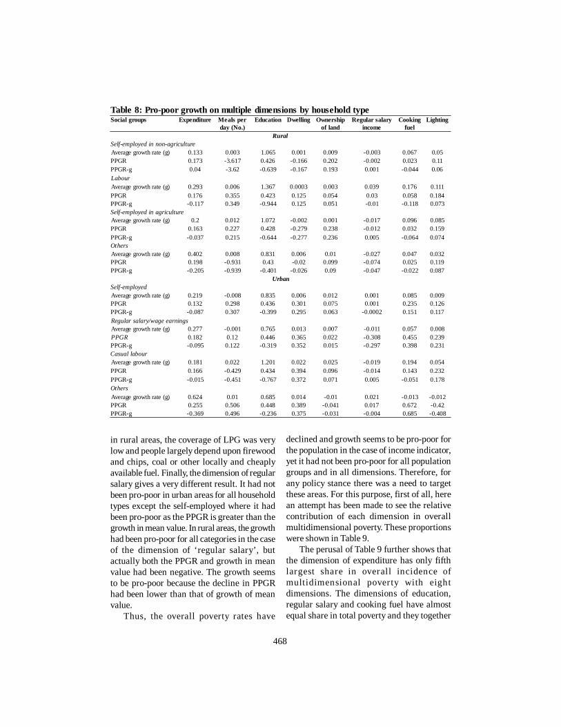
in rural areas, the coverage of LPG was verylow and people largely depend upon firewoodand chips, coal or other locally and cheaplyavailable fuel. Finally, the dimension of regularsalary gives a very different result. It had notbeen pro-poor in urban areas for all householdtypes except the self-employed where it hadbeen pro-poor as the PPGR is greater than thegrowth in mean value. In rural areas, the growthhad been pro-poor for all categories in the caseof the dimension of ‘regular salary’, butactually both the PPGR and growth in meanvalue had been negative. The growth seemsto be pro-poor because the decline in PPGRhad been lower than that of growth of meanvalue.

Thus, the overall poverty rates have

declined and growth seems to be pro-poor forthe population in the case of income indicator,yet it had not been pro-poor for all populationgroups and in all dimensions. Therefore, forany policy stance there was a need to targetthese areas. For this purpose, first of all, herean attempt has been made to see the relativecontribution of each dimension in overallmultidimensional poverty. These proportionswere shown in Table 9.

The perusal of Table 9 further shows thatthe dimension of expenditure has only fifthlargest share in overall incidence ofmultidimensional poverty with eightdimensions. The dimensions of education,regular salary and cooking fuel have almostequal share in total poverty and they together

469

Table 9: Marginal contributions of various dimensions in extent, gap and severity ofpovertyParticulars Expenditure Meals per day

(No.)Education Dwelling Ownership of

landRegular salary

incomeCooking

fuelLighting

Rural2004-05M0 10.61 0.74 22.70 0.81 1.39 22.50 22.87 18.39M1 5.33 1.29 29.83 0.49 1.16 18.82 26.85 16.21M2 3.28 1.97 39.30 0.26 0.84 13.62 28.33 12.402009-10M0 10.27 0.82 21.28 0.94 1.34 23.06 23.23 19.05M1 4.74 1.43 28.44 0.64 1.12 19.21 27.63 16.79M2 2.69 2.11 39.42 0.40 0.79 13.49 28.57 12.54

Urban2004-05M0 12.90 1.00 22.45 3.36 9.06 21.10 21.12 9.01M1 7.59 1.81 29.21 2.07 7.85 18.27 24.96 8.23M2 5.27 2.81 38.23 1.10 5.81 13.52 26.76 6.502009-10M0 13.42 1.43 20.98 0.07 8.04 22.41 22.30 11.36M1 7.37 2.51 28.16 0.08 6.75 18.81 25.97 10.35M2 4.65 3.70 38.91 0.08 4.73 13.18 26.75 8.00

contribute about 67 per cent of overall poverty.However, it was noted that the relativecontribution of regular salary falls while thatof the education and cooking fuel increasesas the degree of poverty increases.

This shows that for poorest persons, thedeprivation of education and cooking fuel werethe largest contributor to their poverty. Thisseems to be equally applicable to both the ruralas well as urban areas. This contributes animportant policy direction.

Finally, here an attempt was made to findthe impact of a constant lump-sum amount onoverall poverty reduction. For this purpose,the data has been taken from the latest roundonly. The results of such targeting scheme

Table 10: Targeting by social group andpovertyParticulars ST SC OBC Others PopnRuralFGT Index 21.8 21.39 17.11 11.83 17.32IG -0.011 -0.005 -0.002 -0.003 -0.001IP -0.0012 -0.001 -0.0008 -0.0006 -0.001UrbanFGT Index 14.69 17.19 13.98 7.19 11.57IG -0.0142 -0.0038 -0.0012 -0.0007 -0.0004IP -0.0005 -0.0006 -0.0004 -0.0003 -0.0004IG: Impact on groupIP: Impact on populationPopn: Population

have been shown in Table 10 and 11. Thetargeting by social groups shows thatexpenditure of one currency unit (` in presentcase) reduces the poverty for all groups andthe impact on the proportion of total populationbelow poverty line was nearly the same in ruralas well as urban areas.

However, in both the rural and urban areas,expenditure of one ` reduces the poverty rateby a greater amount in the case of scheduledtribes as compared to all other social groups.Similarly, by household type, the impact ofspending one rupee upon population was

Table 11: Targeting by household type andpovertyHousehold type FGT Index IG IPRuralSelf-employed in non-agriculture 15.41 -0.0053 -0.0009Agricultural labour 20.29 -0.0039 -0.0009Other labour 17.6 -0.0063 -0.0009Self-employed in agriculture 18.75 -0.0025 -0.0009Others 5.93 -0.0044 -0.0004Population 17.32 -0.001 -0.001UrbanSelf-employed 15.16 -0.0012 -0.0005Regular salary/wage earning 5.25 -0.0006 -0.0002Casual labour 20.64 -0.0046 -0.0006Others 4.98 -0.0021 -0.0001Population 11.57 -0.0004 -0.0004IG: Impact on groupIP: Impact on population

470

same by all social groups but if the impactupon individual groups was observed, then itcan be the largest in the case of other labour inrural areas and casual labour in urban areas. Inurban areas, targeting the casual labour hasthe ability to reduce the poverty of populationby the largest amount.CONCLUSIONS

To sum up, it can be stated that both theuni-dimensional and multidimensional povertyin India had declined between 2004-05 and2009-10. But, it had not been pro-poor acrossall the dimensions and for all social groups. Ithas been observed that the dimensions ofeducation, expenditure and regular salary hadnot been pro-poor in most of the cases. Amongthe social groups, the SCs and the STs are thepoorest categories and by household types,the labour households are the poorest one.These households suffer from thedeprivations of multiple dimensions. It hasbeen observed that the dimension of educationand cooking fuel are the biggest contributorsto overall poverty rate and the poorest sufferthe most from these deprivations. Therefore,it is suggested that the government shouldspend more on education and cooking fuel forwhich appropriate subsidy should be providedand if the subsidy is of lump sum type, theSCs, STs and labour households should betargeted on priority basis. Targeting thesegroups is very necessary as average numberof deprivations as well as poverty gap andseverity of poverty is the highest among thesegroups. Moreover, by targeting these groups,the overall poverty rate of population can bereduced at a greater speed and the time toachieve the MDG target of removal of povertycan be reduced.REFERENCESAlkire, S. and Foster, J. 2008. Counting and

multidimensional poverty measurement. OPHIWorking Paper Series, Working Paper No. 7,Oxford Poverty and Human DevelopmentInitiative, Department of InternationalDevelopment, Oxford.

Berenger, V. and Bresson, F. 2010. On the pro-poorness of growth in a multidimensionalcontext. Paper presented in 31st GeneralConference of The International Association forResearch in Income and Wealth, St. Gallen,Switzerland, August 22-28.

Duclos, J-Y. and Wodon, Q. 2009. What is pro-Poor? Social Choice and Welfare. 32 (1): 37–58.

Grosse, M., Harttgen, K. and Klasen, S. 2005.Measuring pro-poor growth with non-incomeind icators. Department of Economics,University of Göttingten, Göttingten, Germany.

Kakwani, N. and Pernia, E. 2000. What is a pro-poor growth. Asian Development Review. 16 (1):1-22.

Klasen, S. 2000. Measuring poverty and deprivationin South Africa. Reveiw of Income and Wealth.42 (1): 33-58.

Klasen, S. 2008. Economic growth and povertyreduction: Measurement issues using income andnon-income indicators. World Development. 36(3): 420-425.

Pasha, H.A. and Palanivel, T. 2003. Pro-poor growthand policies-The Asian experience. The PakistanDevelopment Review. 42 (4 Part I): 313-348.

Planning Commission 2012. Press note on povertyestimates, 2009-10. Government of India, NewDelhi, March.

Ravallion, M. 2004. Pro-poor growth: A primerpolicy. Research Working Paper No. 3242. TheWorld Bank, Washington D.C.

Ravallion, M and Chen, S. 2003. Measuring pro-poor growth. Economic Letters. 78 (1): 93-99.

Sen, A. 1988. The concept of development. In:Chenery, H. and Srinivasan, T. (eds) Handbookof Development Economics. 1: 9–26. OxfordUniversity Press. Oxford.

Sen, A. 1992. Inequality re-examined, HarvardUniversity Press. Cambridge. Massachusetts.

Streeten, P. 1994. Human development: Means andends. American Economic Review. 84: 232-237.

White, H. and Anderson, E. 2001. Growth versusdistribution: Does the pattern of growth matter?Development Policy Review. 19 (3): 267-289.

Zepeda, E. 2004. Pro-poor growth: What is it?International Poverty Center, Number 1, OnePager, UNDP. Culled from www.undp.org

Received: November 19, 2014Accepted: March 05, 2015

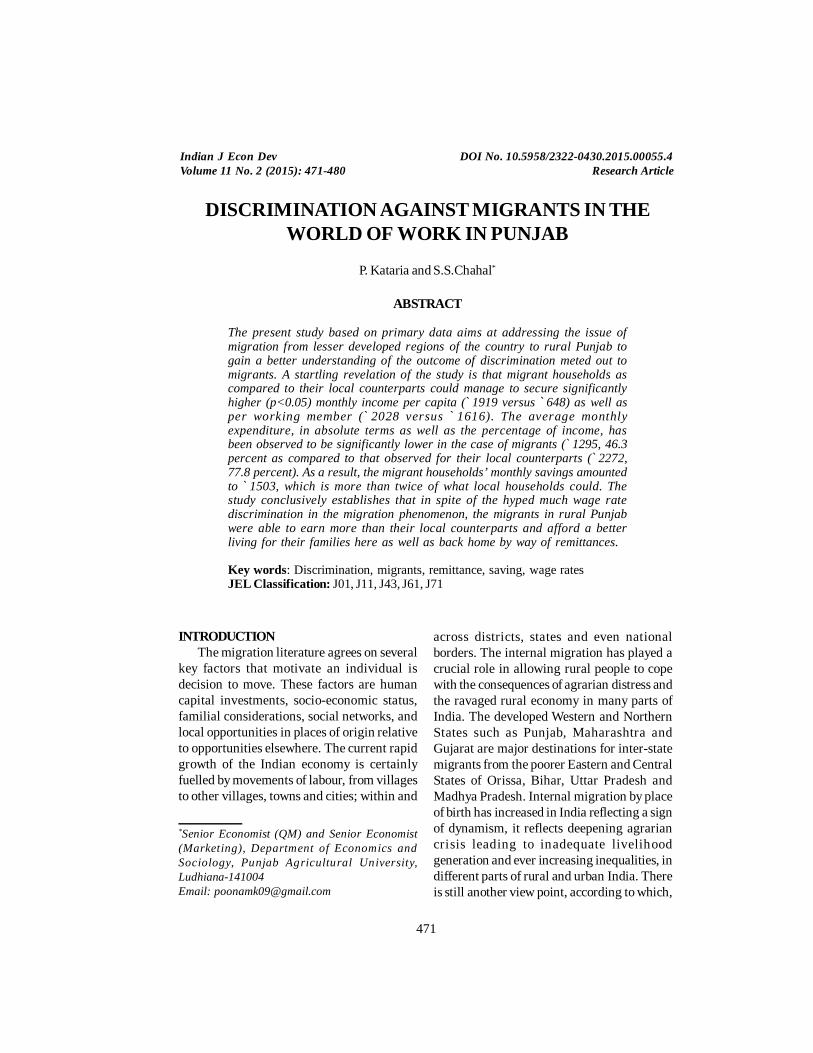
471

Indian J Econ Dev DOI No. 10.5958/2322-0430.2015.00055.4Volume 11 No. 2 (2015): 471-480 Research Article

DISCRIMINATION AGAINST MIGRANTS IN THEWORLD OF WORK IN PUNJAB

P. Kataria and S.S.Chahal*

ABSTRACT

The present study based on primary data aims at addressing the issue ofmigration from lesser developed regions of the country to rural Punjab togain a better understanding of the outcome of discrimination meted out tomigrants. A startling revelation of the study is that migrant households ascompared to their local counterparts could manage to secure significantlyhigher (p<0.05) monthly income per capita (`1919 versus `648) as well asper working member (`2028 versus `1616). The average monthlyexpenditure, in absolute terms as well as the percentage of income, hasbeen observed to be significantly lower in the case of migrants (`1295, 46.3percent as compared to that observed for their local counterparts (`2272,77.8 percent). As a result, the migrant households’ monthly savings amountedto `1503, which is more than twice of what local households could. Thestudy conclusively establishes that in spite of the hyped much wage ratediscrimination in the migration phenomenon, the migrants in rural Punjabwere able to earn more than their local counterparts and afford a betterliving for their families here as well as back home by way of remittances.

Key words: Discrimination, migrants, remittance, saving, wage ratesJEL Classification: J01, J11, J43, J61, J71

*Senior Economist (QM) and Senior Economist(Marketing), Department of Economics andSociology, Punjab Agricultural University,Ludhiana-141004Email: poonamk09@gmail.com

INTRODUCTIONThe migration literature agrees on several

key factors that motivate an individual isdecision to move. These factors are humancapital investments, socio-economic status,familial considerations, social networks, andlocal opportunities in places of origin relativeto opportunities elsewhere. The current rapidgrowth of the Indian economy is certainlyfuelled by movements of labour, from villagesto other villages, towns and cities; within and

across districts, states and even nationalborders. The internal migration has played acrucial role in allowing rural people to copewith the consequences of agrarian distress andthe ravaged rural economy in many parts ofIndia. The developed Western and NorthernStates such as Punjab, Maharashtra andGujarat are major destinations for inter-statemigrants from the poorer Eastern and CentralStates of Orissa, Bihar, Uttar Pradesh andMadhya Pradesh. Internal migration by placeof birth has increased in India reflecting a signof dynamism, it reflects deepening agrariancrisis leading to inadequate livelihoodgeneration and ever increasing inequalities, indifferent parts of rural and urban India. Thereis still another view point, according to which,

472

the relationship between migration andinequality is two-way: inequality may drivemigration and migration, in its own right, hasan effect on inequality both within the sendingarea and between the sending and destinationregions (Mukherji, 2001). The tale of woes doesnot end here, as the destination regionshappen to be the discriminating ground forthe migrants. The literature is replete with theinstances of labour market discrimination,which refers to a situation of unequal treatmentof the workers, possessing same productivity,in hiring or in wage payment due to noneconomic characteristics such as race, genderor caste. Of late, the concerns are being raisedon the discrimination against migrant workersin the labour market. Realising the importanceof moral, social and economic considerationsin combating the problem of discriminationagainst migrants, the present study has beenenvisaged to address the issue of migrationfrom lesser developed regions of the countryto Rural Punjab to gain a better understandingof the outcome of discrimination meted out tomigrants.MATERIALS AND METHODS

The formulations of the present study arebased on primary data collected from ruralPunjab. The multi-stage random samplingtechnique was used for the purpose of sampleselection. Due to the lack of recordedinformation on number of labour in-migrantsin rural Punjab, the selection of first samplingunit, that is, the districts was based on thestudies conducted earlier on this issue (Grewaland Sidhu, 1979; Sidhu and Grewal, 1984 andSidhu et. al., 1997). The present study hasbeen conducted in two districts, namelyLudhiana and Patiala, having comparativelyhigher concentration of in-migrants, relativeto other districts of Punjab. The second stageentailed the random selection of two blockseach from both the selected districts. In orderto reach the ultimate sampling units, a clusterof two to three villages from each block waschosen depending upon the concentration ofin-migrants in each village. At the final stage,

a total of 200 in-migrants and 200 local labourers(synonymously referred to as non-migrantshereafter), equitably distributed over blocksand districts, were selected randomly. Thesample details are given below.

Sample selection detailsDistrict Villages Sampling Units, No.

Migrants Non-migrants OverallLudhianaMulanpur Jangpur 50 50 100block Rudka

MohiPakhowal Jassowal 50 50 100block Mansooran

VeelaPatialaPatiala Hirdapur 50 50 100block Bakshiwala

KharimaniaNabha Rohdikhas 50 50 100block LohandaTotal 200 200 400

In order to ascertain the discriminationbetween the migrant and local labourers, thepertinent variables like duration ofemployment, wage rate, family income,expenditure and saving were subjected tostatistical tools like t-test/ Z-test to assess thesignificance of difference between therespective means.In-migration in Punjab: Reflections from theLiterature

In India, the process of economic and socialdevelopment in general and industrialisationand urbanisation in particular had startedyielding results since 1960, as a consequenceof planned economic development. During thisperiod, the process of socio-economic growthhas fastened in the northwestern regionespecially in the State of Punjab because ofagricultural growth with a remarkable increasein gross cropped area. Consequently, since thebeginning of the green revolution, relativeincrease in daily wages and the demand forlabour under free market conditions had startedattracting migrant labour in the State. Themigration trends have seen myriad changes

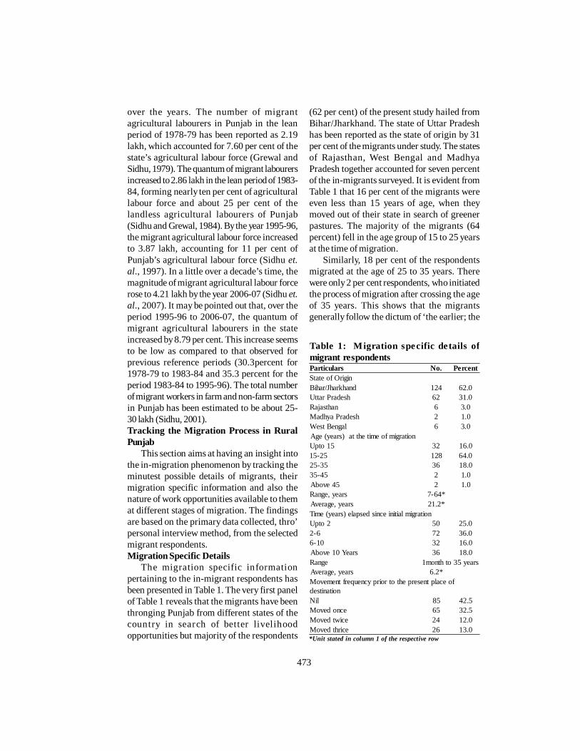
473

over the years. The number of migrantagricultural labourers in Punjab in the leanperiod of 1978-79 has been reported as 2.19lakh, which accounted for 7.60 per cent of thestate’s agricultural labour force (Grewal andSidhu, 1979). The quantum of migrant labourersincreased to 2.86 lakh in the lean period of 1983-84, forming nearly ten per cent of agriculturallabour force and about 25 per cent of thelandless agricultural labourers of Punjab(Sidhu and Grewal, 1984). By the year 1995-96,the migrant agricultural labour force increasedto 3.87 lakh, accounting for 11 per cent ofPunjab’s agricultural labour force (Sidhu et.al., 1997). In a little over a decade’s time, themagnitude of migrant agricultural labour forcerose to 4.21 lakh by the year 2006-07 (Sidhu et.al., 2007). It may be pointed out that, over theperiod 1995-96 to 2006-07, the quantum ofmigrant agricultural labourers in the stateincreased by 8.79 per cent. This increase seemsto be low as compared to that observed forprevious reference periods (30.3percent for1978-79 to 1983-84 and 35.3 percent for theperiod 1983-84 to 1995-96). The total numberof migrant workers in farm and non-farm sectorsin Punjab has been estimated to be about 25-30 lakh (Sidhu, 2001).Tracking the Migration Process in RuralPunjab

This section aims at having an insight intothe in-migration phenomenon by tracking theminutest possible details of migrants, theirmigration specific information and also thenature of work opportunities available to themat different stages of migration. The findingsare based on the primary data collected, thro’personal interview method, from the selectedmigrant respondents.Migration Specific Details

The migration specific informationpertaining to the in-migrant respondents hasbeen presented in Table 1. The very first panelof Table 1 reveals that the migrants have beenthronging Punjab from different states of thecountry in search of better livelihoodopportunities but majority of the respondents

(62 per cent) of the present study hailed fromBihar/Jharkhand. The state of Uttar Pradeshhas been reported as the state of origin by 31per cent of the migrants under study. The statesof Rajasthan, West Bengal and MadhyaPradesh together accounted for seven percentof the in-migrants surveyed. It is evident fromTable 1 that 16 per cent of the migrants wereeven less than 15 years of age, when theymoved out of their state in search of greenerpastures. The majority of the migrants (64percent) fell in the age group of 15 to 25 yearsat the time of migration.

Similarly, 18 per cent of the respondentsmigrated at the age of 25 to 35 years. Therewere only 2 per cent respondents, who initiatedthe process of migration after crossing the ageof 35 years. This shows that the migrantsgenerally follow the dictum of ‘the earlier; the

Table 1: Migration specific details ofmigrant respondentsParticulars No. PercentState of OriginBihar/Jharkhand 124 62.0Uttar Pradesh 62 31.0Rajasthan 6 3.0Madhya Pradesh 2 1.0West Bengal 6 3.0Age (years) at the time of migrationUpto 15 32 16.015-25 128 64.025-35 36 18.035-45 2 1.0Above 45 2 1.0Range, years 7-64*Average, years 21.2*Time (years) elapsed since initial migrationUpto 2 50 25.02-6 72 36.06-10 32 16.0Above 10 Years 36 18.0Range 1month to 35 yearsAverage, years 6.2*Movement frequency prior to the present place ofdestinationNil 85 42.5Moved once 65 32.5Moved twice 24 12.0Moved thrice 26 13.0*Unit stated in column 1 of the respective row

474

better’ as far as the transmigration of labourfrom one place to another is concerned. Theresults presented in the third panel of Table 1elicit information regarding the time elapsedsince their initial migration from their nativeplace. The time elapsed has been recorded aslow as one month to as high as 35 years. It canbe seen that nearly two third of the migrantrespondents studied have migrated to Punjabwithin last six years.

In an effort to track the migration process,the migrants were asked to give overview oftheir movement prior to their present place ofemployment. The information pertaining to themovement frequency prior to taking up theirpresent employment has been presented in thefourth panel of Table 1. The results presentedtherein reveal that for 42.5 per cent of themigrants, their present employment was thefirst one since their migration from their nativeplaces. Nearly one third (32.5percent)respondents had moved once prior to theirpresent place of destination. It was noticedthat 12 per cent of the migrants moved twice,from one place to another for employment,before settling down at their present place. In

the case of 13 per cent of respondents, theirpresent destination happened to be their fourthplace of settlement since their migration. Thisshows that the migrants keep on looking forbetter employment opportunities, even if theyhave to move from place to place.Nature of Work at different Stages ofMigration

In the case of initial movement, a majority(52.2 percent) of migrants work as agriculturallabourers (Table 2). At the initial stages,agriculture acts as an occupation of the firstresort. The brick kilns are the second bestemployers (31.3percent) at the initial movementstage. It is worth mentioning that 0.9 per centof the migrants could not get the job at theinitial stage. At the secondary movement stage,the preference to work as construction workerand brick kiln worker has been found to beincreasing as shown by the higher proportionof workers going in for it. The tertiarymovement has seen decreasing charm foragricultural labour and increasing preferenceto work as brick kiln worker and factory worker.

The perusal of Table 2 revealed that on theday of data collection, 46 per cent of the

Table 2: Nature of work at different stages of migrationParticulars Initial movement Secondary movement Tertiary movement Present destination

(n1=115) (n2=50) (n3=26) (N=200)Agricultural labourers 60 23 9 92

(52.20) (46.00) (34.60) (46.00)Construction work 2 3 2 9

(1.70) (6.00) (7.70) (4.50)Brick kiln 36 17 12 53

(31.3) (34.0) (46.2) (26.5)Trading/business - 1 - -

- (2.0) - -Self employed 1 - - 2

(0.90) - - (1.00)Factory/Rice Sheller/Flour Mill

7 1 2 28

(6.10) (2.00) (7.70) (14.00)Daily wage labour 2 4 1 12

(1.70) (8.00) (3.80) (6.00)Sales person in shops 6 1 - 4

(5.20) (2.00) (2.00)No work 1 - - -

(0.90) - - -Figures in parentheses indicate percentages

475

migrants were employed as agriculturallabourers. The brick kilns providedemployment to 26.5 per cent of the migrantwork force. Working in a factory/ rice sheller/flour mill was the third in preference based onthe proportion of migrant work force absorbedby the factories. The above discussion clearlyshows that the migrants keep switching fromone employment to another, whenever theyget better earning opportunities.Employment Pattern of Migrant and LocalLabourers: Is there any Discrimination?

This section includes a comparative workprofile of migrant and local labourers so as tomake an assessment of the nature of workoffered to migrants and to see if there is anywork related discrimination meted out to them.

The results presented in Table 3 revealedthat 19.5 per cent of the local labour force asagainst 31.5 per cent of the migrant labour has

been engaged in crop production. Thisobservation justifies a general belief thatmigrant labour has replaced the local labourand more so in crop production. Of late, it hasbeen seen that landholders of Punjab hire themigrant labour on monthly basis, who aresupposed to work for both the crop and dairyproduction. As can be seen from Table 3, atotal of 7 per cent of the in-migrants in Punjabhave been working for landholders in theircrop-dairy enterprises. These labourers arehired on monthly basis and payment patternis need based and flexible rather than followinga fixed schedule. Needless to mention, the jobsecurity all through the year is the chiefcharacteristic of this type of work. This typeof work arrangement finds acceptability by themigrants, as low wages (`47 per man day) tosome extent get compensated by the provisionof food and the place to stay by the employer.

Table 3: Comparative work profile of migrant and local labourParticulars Frequency Duration, months/year Wage rate, `day-1

Migrant Local Migrant Local Migrant LocalCrop production 63 39 11.3a 9.2b 59y 71x

(31.50) (19.50)Dairy enterprises 15 2 12.0a 9.5b 52y 80x

(7.50) (1.00)Crop and dairy 14 - 12 - 47 -

(7.00)Brick kiln worker 53 33 6.3a 5.7b 144x 158x

(26.50) (16.50)Poultry - 2.00 - 5.5 - 125

(1.00)Masonry 8 28 8.8a 7.1b 91y 128x

(4.00) (14.00)Black Smithy 1 - 12 - 50 -

(0.50)Carpentry - 3 - 9 - 115

(1.50)Self employed 2 14 9.0b 11.6a 95x 85x

(1.00) (7.00)Other* 44 79 7.5a 6.4b 77y 93x

(22.00) (39.50)Overall 200 200 9.1a 7.3b 86y 104x

* include daily wage labourer, sales person in shops, factory/rice sheller/ flour millFigures in parentheses indicate percentagesab different superscripts in a row indicate significant (p<0.05) discrimination in two groups with respect to duration ofemploymentxy different superscripts in a row indicate significant p<0.05) discrimination in two groups with respect to wage rate

476

The local labourers were conspicuous by theirinsignificant presence in the case of dairy andpoultry enterprises. The percentage of themigrants employed with the brick kilns hasbeen recorded at 26.5 as against 16.5 per centin the case of non-migrant respondents.

It is further revealed that dairying absorbs7.5 per cent, masonry 4 per cent and blacksmithy only 0.5 per cent of the migrant labourforce. It has been noticed that 22 percent ofthe migrant respondents were employed inother diverse occupations such as flour/ricemill worker and other factory workers, etc. Acomparatively higher percentage (7.0 percent)of local respondents was found to be selfemployed, running their own kirana shop orselling on the rehris. It was found that 22 percent of migrant and 39.5 per cent of the non-migrant respondents were working as dailywage earners and sought seasonalemployment in regulated markets as labourerswith the FCI for lifting of food stocks, etc.

As regards the duration of employment, itvaried from 6.3 months a year for brick kilnworkers to 12 months for migrants employedin dairy enterprises. Wide differentials,between migrant and local labour have alsobeen noticed. Quoting the case of cropproduction, the duration of employment formigrants (11.3 months per year) has beensignificantly higher (p<0.05) as compared tothat for local labourers (9.2 months per year).Barring the self employed respondents, theduration of employment in dairy enterprises,brick kilns and other occupations has beensignificantly higher for migrants as comparedto local labour. This is a clear indication ofpreferential treatment given to migrantlabourers. A study conducted by Grewal andSidhu way back in 1985 had cautioned that theincreased influx of migrant labourers mightdepress the employment levels of the locallabour.

There is a general consensus that in India,a large proportion of migrant workers belongto the lower castes and tribes, with a poorerasset base than other social groups. While

some have argued that migration provides anescape from traditional structures of caste-based oppression in villages and gives poorlabourers some bargaining power vis-à-vistheir traditional employers, others maintain thatstructures of oppression are reproducedthrough labour contracting arrangements atthe destination and may even be moreexploitative (Mosse, 2002, Olsen andRamanamurthy, 2000). The results of thepresent study also highlight the discriminationagainst migrant workers. The non migrantrespondents, except for self employed andthose working in brick kilns, could manage tosecure significantly higher (p<0.05) wages ascompared to migrants.

The reasons for this discrimination can bemanifold; the migrant workers’ readinesses towork at lower wages or the consciousness onthe part of local labour about their rights tominimum wages and/or their better bargainingpower. The highest degree of discriminationhas been recorded in terms of 35 per cent lowerwages in dairy enterprises, followed by 29 percent in masonry work and 17 per cent in cropproduction. In spite of low wage rate and thehighest degree of discrimination, the yearround availability of work in dairy enterpriseis what makes this occupation sustainableespecially for new migrants entering the labourmarket.

The migrants working in brick kilns did getlower wages (`144 per man day) as comparedto their local counterparts (`158) but thisdifference cannot be deemed significantstatistically. No significant discrimination canwell be attributed to the fact that theremuneration in brick kilns is performancebased.

As is clear from Table 3 that as high as 58per cent of labour force migrated to ruralPunjab is engaged in crop production and brickkilns, it is deemed imperative to study differentfacets of employment ( like nature of work,duration of employment, wage rate andpayment pattern to name a few) in these twoemployment avenues.

477

Employment pattern discrimination in cropproduction

The results presented in Table 4 exhibit thepattern of labour employment in cropproduction in the study area. The results showthat 90.5 per cent of the migrant respondents,in comparison to 69.2 per cent of local labour,work within the same village, where they stay.Nearly one tenth of migrant labourers at timesneed to go outside the village in connectionwith their work. Since, the migrant labourersare notorious for depressing the wages; acomparatively higher percentage (31 percent)of local respondents crossed the villageboundaries for work in anticipation of higherwages. It has been reported that 55.6 per centof the migrant respondents engaged in cropproduction were hired on annual basis,

providing them with the much needed senseof job security. Another 17.5 per cent of themigrants were hired on daily basis, as and whenthe need arose.

The proportion of local respondentsemployed in crop production on daily basishas been recorded as 38.5 per cent. The higherpercentage of local respondents working asdaily wagers is more by choice than by default,as it gives them an opportunity to switch overto another land holder offering better terms ofwork. As regards the payment, the generalpractice is that of making the payment afterthe completion of work though there are certainexceptional cases wherein the employers payin advance also, keeping in view the urgencyof the requirement of money. The locallabourers are more privileged in this regard as23 percent of them (as against 5 percentmigrants) managed to get the payment inadvance.

The results further revealed that 6.3 percent of the migrant respondents received someamount in advance and the remaining after thecompletion of the work. As regards the durationof employment, as many as 84 per cent ofmigrants employed in crop production enjoyedyear round availability of work. There wereonly one tenth of migrants who got employmentfor nine months or less. The averageavailability of work for migrants in cropproduction has been estimated as 11.3 months.The results testify the fact that migrantlabourers have to some extent displaced thelocal labour force from the crop productionscene.

The result revealed that 84.6 percent of localrespondents in comparison to 69.8 per cent ofmigrant respondents employed in cropproduction received more than `50 per day.The results further revealed that the dailywages ranged from `22 to `83 for migrantsand from `30 to `100 for non-migrants, withan average of 70.56 which is higher than thatreceived by migrant labourers (`58.8). Thisshows that the positive aspect of year roundavailability of labour in crop production is

Table 4: Comparative employment patterno f migra nt a nd loc a l labour in c ropproductionParticulars Migrant

(n1=63)Local (n1=39)

No. Percent No. PercentPlace of workWithin the village 57 90.5 27 69.2Outside the village 0 0 7 17.9Both inside andoutside

6 9.5 5 12.8

Type of contractDaily basis 11 17.5 15 38.5Monthly 17 27 3 7.7For crop season 0 0 3 7.7Annual 35 55.6 18 46.2Payment patternAfter work completion 56 88.9 30 76.9Advance 3 4.8 9 23.1Either of the two 4 6.3  - - Duration of employment, Months/Year)76 3 4.8 15 38.506-09 4 6.3 2 5.1>9 56 88.9 22 56.4All thro’ the year 53 84.1 22 56.4Range, months/year 4-12* 4-12*

Average, months/year 11.3* 9.23*

Wage rate per man day<50 19 30.2 6 15.450-100 44 69.8 33 84.6Range, `man day-1 22-83* 30-100*

Average, `man day-1 58.8* 70.6*

*Unit stated in Column 1 of the respective row

478

negated to some extent by the low wage ratesprevalent in crop sector.Employment Pattern Discrimination in BrickKilns

It has been discussed earlier also that asmany as one fourth of the migrant labourershave been working in brick kilns. Theemployment details of brick kiln workers havebeen furnished in Table 5. The percentage ofthe migrants working in the brick kilns in thesame village, where they stay, has beenrecorded at 70 per cent. The rest 30 per cent gofor work to brick kilns in nearby villages orelse in the brick kilns situated at the outskirtsof the villages. The results show that only 30.3per cent of local brick kiln workers could securethe work within the same village. Nearly onefifth of local brick kiln workers had to gooutside the village for work. The proportion ofnon-migrant workers, who have been eitherworking within the village or had to go to thebrick kilns located outside the village in searchof work, stood at 48.5 per cent.

As a common practice, the brick kilnowners hire the labour on the daily basis. Thepercentage of such workers has been recordedat 58.5 per cent for the migrant and 63.6 percent for local brick kiln workers. The rest ofthe brick kiln workers were hired and paid onmonthly basis, although, the wages areperformance based. A total of three-fourth ofmigrant brick kiln workers got the payment afterthe completion of work. The rest of the migrantrespondents, who had good rapport with thebrick kiln owners and have been working forthem for quite some time, have the privilege oftaking advance as well. It has been noticedthat 97 per cent of the local brick kiln workersreceived their remuneration after thecompletion of the work. There was only onerespondent, who received the payment inadvance which might have been due to somefinancial crunch faced by the labourer.

As regards the duration of the employment,it has been seen that the brick kilns provide 3to 8 months employment in a year, which canbe attributed to closure of brick kilns during

the rainy season. The proportion of brick kilnworkers, who were employed for more than sixmonths, has been recorded at 19 per cent formigrant and 12 per cent for local labour. On anaverage, the migrant brick kiln workers havebeen getting the employment for 6.3 monthsas contrasted to 5.67 months for local workers.The peculiarity of labour in brick kilns is thatthe payment is based on the work done. Theprevalent rate varies from `165 to `193 perthousand bricks made. It has been observedthat 96 per cent of migrant and 85 percent ofnon-migrant brick kiln workers were gettingmore than `100 per day as wages. The wagerate received by the local brick kiln workershas been estimated as 158, which is higher, inabsolute terms, than that received by migrantbrick kiln workers (`144 per man day). It hasbeen seen that smaller duration of employmentis well compensated with higher wages as

Table 5: Comparative employment patternof migrant and local labour in brick kilnsParticulars Migrant

(n1=53)Local

(n2=33)No. Percent No. Percent

Place of workWithin the village 37 69.8 10 30.3Outside the village 16 30.2 7 21.2Both within andoutside

0 0 16 48.5

Type of contractDaily basis 31 58.5 21 63.6Monthly 21 39.6 12 36.4Daily/monthly 1 1.9Payment patternAfter work completion 40 75.5 32 97Advance 0 0 1 3Either of the two 13 24.5 - -Duration of employment, Months/Year6 43 81.1 29 87.96-9 10 18.9 4 12.1All thro’ the year Nil NilRange, months/year 3-8 4-8Average, months/year 6.27 5.67Wage rate per man day (`)50-100 2 3.8 5 15.2100-150 30 56.6 14 42.4>150 21 39.6 14 42.4Range, `man day-1 80-200 70-225Average, `man day-1 144.3 157.97

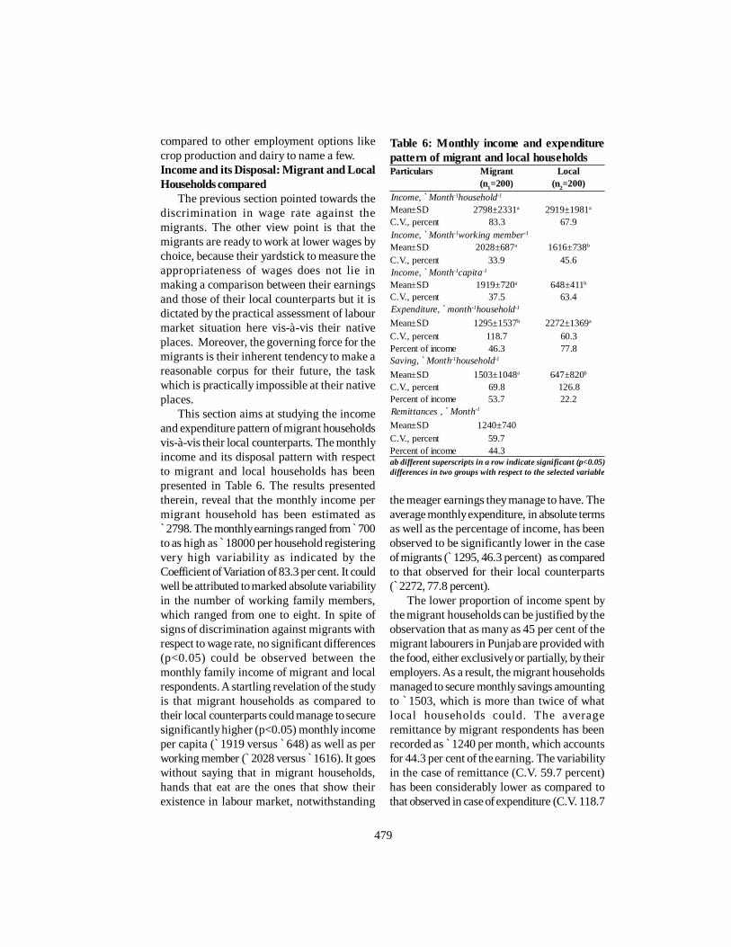
479

compared to other employment options likecrop production and dairy to name a few.Income and its Disposal: Migrant and LocalHouseholds compared

The previous section pointed towards thediscrimination in wage rate against themigrants. The other view point is that themigrants are ready to work at lower wages bychoice, because their yardstick to measure theappropriateness of wages does not lie inmaking a comparison between their earningsand those of their local counterparts but it isdictated by the practical assessment of labourmarket situation here vis-à-vis their nativeplaces. Moreover, the governing force for themigrants is their inherent tendency to make areasonable corpus for their future, the taskwhich is practically impossible at their nativeplaces.

This section aims at studying the incomeand expenditure pattern of migrant householdsvis-à-vis their local counterparts. The monthlyincome and its disposal pattern with respectto migrant and local households has beenpresented in Table 6. The results presentedtherein, reveal that the monthly income permigrant household has been estimated as`2798. The monthly earnings ranged from 700to as high as `18000 per household registeringvery high variability as indicated by theCoefficient of Variation of 83.3 per cent. It couldwell be attributed to marked absolute variabilityin the number of working family members,which ranged from one to eight. In spite ofsigns of discrimination against migrants withrespect to wage rate, no significant differences(p<0.05) could be observed between themonthly family income of migrant and localrespondents. A startling revelation of the studyis that migrant households as compared totheir local counterparts could manage to securesignificantly higher (p<0.05) monthly incomeper capita (`1919 versus `648) as well as perworking member (`2028 versus 1616). It goeswithout saying that in migrant households,hands that eat are the ones that show theirexistence in labour market, notwithstanding

the meager earnings they manage to have. Theaverage monthly expenditure, in absolute termsas well as the percentage of income, has beenobserved to be significantly lower in the caseof migrants (`1295, 46.3 percent) as comparedto that observed for their local counterparts(`2272, 77.8 percent).

The lower proportion of income spent bythe migrant households can be justified by theobservation that as many as 45 per cent of themigrant labourers in Punjab are provided withthe food, either exclusively or partially, by theiremployers. As a result, the migrant householdsmanaged to secure monthly savings amountingto `1503, which is more than twice of whatlocal households could. The averageremittance by migrant respondents has beenrecorded as `1240 per month, which accountsfor 44.3 per cent of the earning. The variabilityin the case of remittance (C.V. 59.7 percent)has been considerably lower as compared tothat observed in case of expenditure (C.V. 118.7

Table 6: Monthly income and expenditurepattern of migrant and local householdsParticulars Migrant Local

(n1=200) (n2=200)Income, `Month-1household-1

Mean±SD 2798±2331a 2919±1981a

C.V., percent 83.3 67.9Income, `Month-1working member-1

Mean±SD 2028±687a 1616±738b

C.V., percent 33.9 45.6Income, `Month-1capita-1

Mean±SD 1919±720a 648±411b

C.V., percent 37.5 63.4Expenditure, `month-1household-1

Mean±SD 1295±1537b 2272±1369a

C.V., percent 118.7 60.3Percent of income 46.3 77.8Saving, `Month-1household-1

Mean±SD 1503±1048a 647±820b

C.V., percent 69.8 126.8Percent of income 53.7 22.2Remittances , `Month-1

Mean±SD 1240±740C.V., percent 59.7Percent of income 44.3ab different superscripts in a row indicate significant (p<0.05)differences in two groups with respect to the selected variable

480

percent).The above discussion conclusivelyestablishes that in spite of the hyped wagerate discrimination in the migrationphenomenon, the migrants are able to earnmore than their local counterparts and afford abetter living for their families here as well asback home by way of remittances.CONCLUSIONS

The study conclusively establishes thatin spite of the much hyped wage ratediscrimination in the migration phenomenon;the migrants are able to earn more than theirlocal counterparts and afford a better livingfor their families here as well as back home byway of remittances. It is time for policymakersand the public in general to become much moresensitive to the manifold implications ofmigration, and to take whatever measures arenecessary to ensure that something driven bydistress does not create further trauma. Thisrequires measures at different levels. Thereshould be active interventions for theprotection of and assistance to migrants atboth source and destination areas. It isimportant to address the central cause ofdistress migration by improving the economicconditions in the lesser developed regions ofthe country, rest everything wouldautomatically start falling into place totransform the Starving India into ShiningIndia.REFERENCESGrewal, S.S. and Sidhu, M.S. 1979. A Study on

migrant agricultural labour in Punjab. ResearchReport. Department of Economics andSociology, PAU, Ludhiana: 1-28

Grewal, S.S. and Sidhu, M.S.1985. Economic profileof migrant farm labour in Punjab. The EconomicTimes, New Delhi, April 4: 5 and 8.

Grewal, S.S. and Sidhu, M.S. 1988. Punjab problem:Economic dimensions. Financial Express, NewDelhi, December 02, 1988: 7.

Mosse, D. 2002. Brokered livelihoods: Debt, labourmigration and development in Tribal WesternIndia. Journal of Development Studies. 38 (5):59–87.

Mukherji, S. 2001. Causal linkages betweenmigration, urbanisation, and regional disparitiesin Ind ia: Required planning strategies.Research Report No 31. International Institutefor Population Sciences, Bombay.

Olsen, W. and Ramanamurthy, R.V. 2000. Contractlabour and bondage in Andhra Pradesh (India).Journal of Social and Political Thought. 1 (2)http://www.yorku.ca/jspot.

Sidhu, M.S. 2001. Youth unemployment problemin Punjab: An appraisal. The Indian Journal ofEconomics. 82 (325):161-176.

Sidhu, M.S. and Grewal, S.S. 1984. A study onmigrant agricultural labour in Punjab. ResearchBulletin. Department of Economics andSociology, PAU, Ludhiana: 1-56.

Sidhu, M.S., Joshi, A.S. and Kaur, I.P. 2007. Astudy on migrant agricultural labour in Punjab.Research Report. Department of Economicsand Sociology, PAU, Ludhiana. : 1-61.

Sidhu, M.S., Rangi, P.S. and Singh, K. 1997. Astudy on migrant agricultural labour in Punjab.Research Bulletin. Department of Economicsand Sociology, PAU, Ludhiana: 1-62.

Received: December 25, 2014Accepted: March 15, 2015

481

Indian J Econ Dev DOI No. 10.5958/2322-0430.2015.00056.6Volume 11 No. 2 (2015): 481-488 Research Article

ROLE OF MICROFINANCE IN GENERATINGINCOME AND EMPLOYMENT FOR RURAL

HOUSEHOLDS IN PUNJAB-AN ECONOMETRICAPPROACH

Munish Kapila, Anju Singla and M.L.Gupta*

ABSTRACT

The present study was carried out to assess the impact of microfinance onthe generation of income and employment of the rural households’ of Punjab.The results revealed that the proportion of rural households earning incomemore than `5000 per month have increased by 69.18 per cent and nearly 52per cent of the rural households gained employment of more than 180 mandays per year with access of microfinance through Self Help Groups (SHGs).The results obtained from Logit model showed that the extent of the ruralhouseholds earning income more than `5000 per month is likely to beincreased by 3 times with credit facility through SHGs. Similarly, the numberof rural households having employment more than 180 days was likely toincrease by 1.28 times with microfinance in the Punjab. Hence, it isconcluded that better access of microfinance through SHGs is helpful togenerate the households’ income and employment on sustainable basis inthe rural area. It is suggested that an adequate amount of microfinancemust be assured to participants by developing links of SHGs with bankinginstitutions and NGOs for efficient functioning of the SHGs in Punjab.

Key words: Employment, income, microfinance, rural household, SHGJEL Classification: A13, A14, E24, H31, I38, P46

*Research Scholar, Assistant Professor andProfessor (Retired), Department of Applied Science,PEC University of Technology, Chandigarh-160012Email: munish_phd@yahoo.com

INTRODUCTIONPoverty alleviation in the developing

countries is the major issue. In India, a majorpart of the below poverty line (BPL) populationhas been living in the rural areas. Accordingto the recent estimates, the percentage ofpersons below the poverty line in 2011-12 hasbeen estimated as 25.7 percent in rural areas,13.7 percent in urban areas and 21.9 percent

for the country as a whole (Anonymous, 2013).Thus, the rural population has high extent ofunemployment and under employment and haslimited option for other employmentopportunities. With all those constraints notmany families can cross the poverty line byaugmenting their income without support fromthe government. It is pertinent to mention here,that while some families will come out ofpoverty through extra income, but there is asimultaneous process of pauperization bywhich a family with reasonable income looselivelihood and become poor or has to spendbeyond their means to cope with problems like

482

ill health or to meet some social obligation(Malshet et al. 2005). Guarding against sucheventualities and reducing vulnerability of thepoor people (through insurance, etc.) fromlanding up in such problems is also animportant step in reducing poverty. However,the most visible anti-poverty programmes arethose related to direct increase of income ofthe poor through wage employment to meetthe short term need and through self-employment for augmenting income on asustainable basis (Roy, 2011).

The self-help group is a method oforganizing the poor people and themarginalized to come together to solve theirindividual problem. The SHG method is usedby the government, NGOs and othersworldwide. The poor collect their savings andsave it in banks. In return they receive easyaccess to loans with a low rate of interest tostart their micro unit enterprise. Thousands ofthe poor and the marginalized population inIndia are building their lives, their families andtheir society through self-help groups. TheNinth Five Year Plan of the Government of Indiahad given due recognition on the importanceand the relevance of the self-help groups toimplement developmental schemes at thegrassroots level (Sundaram, 2012).

Another important feature of self-helpgroups has been the establishment of linksbetween self-help groups and the formalmicrofinance institutions, NGO and commercialbanks. The Firsipur branch of the Bank ofMaharashtra is financing more than 400 self-help groups in the district, lending on averageabout $1,600 per group. The bank has set upits own in-house NGO to support these efforts.Loans are provided only to the groups, notindividuals (although the groups normally on-lend to individual members). The recovery rateson the loans stand at 99 per cent. In additionto lending to self-help group, which isprofitable for the bank, ancillary business hasbeen brought in through self-help groupmembers opening deposit accounts and takingloans as individuals (Anonymous, 2010).

The self-help groups are thus, beingstrengthened by various banking institutionsand NGO’s under different microfinanceprogrammes. The SHGs have further extendedthis micro-credit facility to their members(Puhazhendh and Satyasai, 2000). The presentstudy was designed to evaluate the impact ofsuch microfinance programme on income andemployment of rural households of the Punjab.METHODOLOGYSampling Design

In order to achieve the stipulatedobjectives of the study, the present study wasconducted in the Punjab. A multi-stage randomsampling technique was used to draw arepresentative sample. A district-wise list ofSHGs was obtained from Department ofWomen and Child Development, Governmentof Punjab. This list was then arranged inascending order on the basis of theconcentration of the SHGs. Then, theCumulative Cube Root Frequency Method wasused to divide the whole Punjab into threegroups based on the concentration of SHGsin each districts. The districts having SHGsup to 350 represented Group-I, while thedistricts having SHGs from 350 to 900represented Group-II and the districts havingSHGs more than 900 represented Group-III. Outof these three groups, one district has beenselected at random from each group.

Hence, three districts namely Hoshiarpur,Ludhiana, and Ferozepur have been selectedrepresenting high, medium and lowconcentration of SHGs, respectively. At thesecond stage, three blocks from each selecteddistricts have been chosen at random. Fromeach selected blocks, a cluster of two villageswere selected on the basis of concentration ofthe SHGs. At the next stage, a total sample of106 SHGs (15 percent from each block) havebeen taken with 51 SHGs from Hoshiarpurdistrict, 44 SHGs from Ludhiana district and 11SHGs from Ferozepur district, respectively. Atthe last stage, finally an overall 318 membersrepresenting the whole Punjab state (3members from each SHG) have been selected

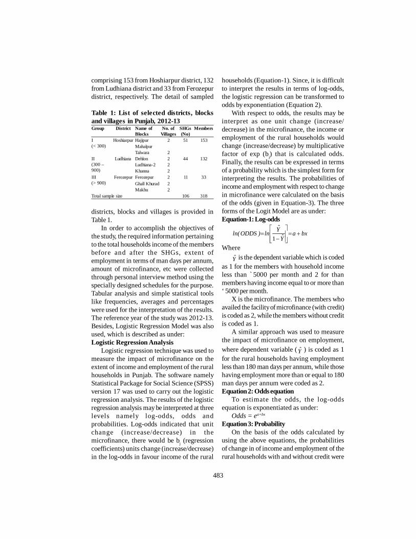
483

comprising 153 from Hoshiarpur district, 132from Ludhiana district and 33 from Ferozepurdistrict, respectively. The detail of sampled

households (Equation-1). Since, it is difficultto interpret the results in terms of log-odds,the logistic regression can be transformed toodds by exponentiation (Equation 2).

With respect to odds, the results may beinterpret as one unit change (increase/decrease) in the microfinance, the income oremployment of the rural households wouldchange (increase/decrease) by multiplicativefactor of exp (bj) that is calculated odds.Finally, the results can be expressed in termsof a probability which is the simplest form forinterpreting the results. The probabilities ofincome and employment with respect to changein microfinance were calculated on the basisof the odds (given in Equation-3). The threeforms of the Logit Model are as under:Equation-1: Log-odds

bxaY

Yln)ODDSln(

1Where

Y is the dependent variable which is codedas 1 for the members with household incomeless than `5000 per month and 2 for thanmembers having income equal to or more than‘ 5000 per month.

X is the microfinance. The members whoavailed the facility of microfinance (with credit)is coded as 2, while the members without creditis coded as 1.

A similar approach was used to measurethe impact of microfinance on employment,where dependent variable ( Y ) is coded as 1for the rural households having employmentless than 180 man days per annum, while thosehaving employment more than or equal to 180man days per annum were coded as 2.Equation 2: Odds equation

To estimate the odds, the log-oddsequation is exponentiated as under:

Odds = ea+bx

Equation 3: ProbabilityOn the basis of the odds calculated by

using the above equations, the probabilitiesof change in of income and employment of therural households with and without credit were

Table 1: List of selected districts, blocksand villages in Punjab, 2012-13Group District Name of

BlocksNo. of

VillagesSHGs(No)

Members

I(< 300)

Hoshiarpur Hajipur 2 51 153MahalpurTalwara 2

II(300 –900)

Ludhiana Dehlon 2 44 132Ludhiana-2 2Khanna 2

III(> 900)

Ferozepur Ferozepur 2 11 33Ghall Khurad 2Makhu 2

Total sample size 106 318

districts, blocks and villages is provided inTable 1.

In order to accomplish the objectives ofthe study, the required information pertainingto the total households income of the membersbefore and after the SHGs, extent ofemployment in terms of man days per annum,amount of microfinance, etc were collectedthrough personal interview method using thespecially designed schedules for the purpose.Tabular analysis and simple statistical toolslike frequencies, averages and percentageswere used for the interpretation of the results.The reference year of the study was 2012-13.Besides, Logistic Regression Model was alsoused, which is described as under:Logistic Regression Analysis

Logistic regression technique was used tomeasure the impact of microfinance on theextent of income and employment of the ruralhouseholds in Punjab. The software namelyStatistical Package for Social Science (SPSS)version 17 was used to carry out the logisticregression analysis. The results of the logisticregression analysis may be interpreted at threelevels namely log-odds, odds andprobabilities. Log-odds indicated that unitchange (increase/decrease) in themicrofinance, there would be bj (regressioncoefficients) units change (increase/decrease)in the log-odds in favour income of the rural

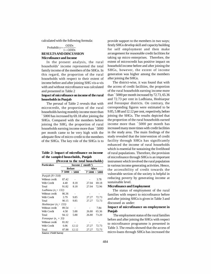
484

calculated with the following formula:

ODDsODDs

1

yProbabilit

RESULTS AND DISCUSSIONMicrofinance and Income

In the present analysis, the ruralhouseholds’ income represented the totalfamily income of the members of the SHGs. Inthis regard, the proportion of the ruralhouseholds with respect to their extent ofincome before and after joining SHG vis-a-viswith and without microfinance was calculatedand presented in Table 2Impact of microfinance on income of the ruralhouseholds in Punjab

The perusal of Table 2 reveals that withmicrocredit, the proportion of the ruralhouseholds having monthly income more than`5000 has increased by 69.18 after joining theSHGs. Compared with the members beforejoining the SHG, the proportion of ruralhouseholds earning income more than `5000per month came to be very high with theadequate flow of micro-credit to the membersof the SHGs. The key role of the SHGs is to

provide support to the members in two ways;firstly SHGs develop skill and capacity buildingfor self employment and then makearrangement for reasonable credit facilities fortaking up micro enterprises. Therefore, theextent of microcredit has positive impact onhousehold income before and after joining theSHGs, however, the extent of incomegeneration was higher among the membersafter joining the SHGs.

The district-wise, it was found that withthe access of credit facilities, the proportionof the rural households earning income morethan 5000 per month increased by 72.73, 65.36and 72.73 per cent in Ludhiana, Hoshiarpurand Ferozepur districts. On contrary, thecorresponding figures were estimated to be9.85, 5.88 and 12.12 per cent, respectively, beforejoining the SHGs. The results depicted thatthe proportion of the rural households earnedincome more than `5000 per month hasincreased many more times with credit facilitiesin the study area. The main findings of thestudy revealed that the intervention of creditfacility through SHGs has significantlyenhanced the income of rural householdswhich is essential for sustaining the livelihoodof rural populations. Therefore, the provisionof microfinance through SHGs is an importantinstrument which involved the rural populationin various income generating activities. Hence,the accessibility of credit towards thevulnerable section of the society is helpful inreducing poverty by generating income atsustainable level.Microfinance and Employment

The status of employment of the ruralfamilies with respect to microfinance beforeand after joining SHGs is given in Table 3 anddiscussed as under:Impact of microfinance on employment inPunjab

The employment status of the rural familiesbefore and after joining the SHGs with respectto microfinance programme is presented inTable 3. The results showed that the access ofmicro-loans through SHGs has increased the

Table 2: Impact of microfinance on incomeof the sampled households, Punjab

(Percent to the total households)Particulars Income (`month-1)

Before After75000 > 5000 75000 > 5000

Punjab (N=318)Without credit 87.42 - - 3.78With Credit 4.40 8.18 27.04 69.18Total 91.82 8.18 27.04 72.96Ludhiana (n1= 132)Without credit 86.36 - - -With Credit 3.79 9.85 27.27 72.73Total 90.15 9.85 27.27 72.73Hoshiarpur (n2= 153)Without credit 89.54 - - 7.84With Credit 4.58 5.88 26.80 65.36Total 94.12 5.88 26.80 73.20Ferozepur (n3 = 33)Without credit 81.82 - - -With Credit 6.06 12.12 27.27 72.73Total 87.88 12.12 27.27 72.73Source: Field Survey

485

proportion of rural households havingemployment more than six months per annumby 52.20 percent. However, with credit facility,nearly eight per cent of the total householdsgot employment for more than 180 man daysin a year before joining SHGs. Before joiningthe SHGs, the proportion of rural familiesemployed less than six months and more thansix months was found to be 47.17 and 40.25without credit facility which is very high ascompared to the members after joining SHGsin the Punjab (Table 3). This was due to thefact that many of the members before joiningthe SHGs were engaged on daily wages basedincome generating activities. And the extentof income generated from such activities wasvery low as compared to the income generatedthrough the employment in terms of selfemployed entrepreneurship after joining theSHGs.

The utilization of credit through SHGs forproductive purpose has positive impact onemployment and provided an employment tothe tune of more than six months annually toabout 55 per cent of the total households. The

microfinance are helpful for the participants tomeet financial requirement such as purchaseof raw materials, inputs, etc. for taking up newmicro-enterprise and to provide support fordeveloping linkages with the market. Therefore,an adequate amount of micro-loans throughSHGs has generated significant employmentfor rural households. Bansal (2010) found thatbefore joining the microfinance programme 49per cent of the total participants wereemployed and 51 per cent were unemployed.But microfinance programme changed thisscenario. The participants started utilizing theloan to adopt economic activities. As a result,80 per cent of the participants are employed inpost-SHG situation. Hence, 31 per cent of theparticipants who were unemployed in pre-SHGsituation gained employment.

The district-wise results indicated that56.82 per cent of the total rural families afterjoining SHGs got employment more than 180man days per annum after receiving the benefitof micro-credit in Ludhiana district. Thecorresponding figures for Hoshiarpur andFerozepur districts came to be 50.98 and 39.39percent, respectively (Table 3). It was foundthat the all the rural households remainedunemployment without the assistance offinance facility after joining the SHGs in thecase of Ludhiana and Ferozepur districts. Onthe whole, it may be concluded that themembers after joining the SHGs has utilizedthe micro loan for productive purposes andthe amount of loan was invested on microenterprises and thus, a reasonable amount ofemployment has been generated in terms ofself-employment.Impact of microfinance on income of the ruralhouseholds-Logistic regression analysis

The results presented in Table 4 showedthat on an overall basis, the odd ratio in favourof household income revealed that the numberof members earning income more than 5000per month was as likely to increase by 3.26times with microfinance in Punjab. It isindicated that with credit the probability ofearning income more than `5000 per month

Table 3 : Impact o f mic ro finance onemployment, Punjab

(Percent to the total households)Particulars Employment (Man days/annum)

Before After7180 >180 7180 >180

Punjab (N = 318)Without credit 47.17 40.25 0.94 2.83With Credit 4.40 8.18 44.03 52.20Total 51.57 48.43 44.97 55.03Ludhiana (n1=132)Without credit 50.00 36.36 - -With Credit 3.79 9.85 43.18 56.82Total 53.79 46.21 43.18 56.82Hoshiarpur (n2=153)Without credit 49.02 40.52 1.96 5.88With Credit 4.58 5.88 41.18 50.98Total 53.59 46.41 43.14 56.86Ferozepur (n3=33)Without credit 27.27 54.55 - -With Credit 6.06 12.12 60.61 39.39Total 33.33 66.67 60.61 39.39Source: Field Survey

486

increased by 0.76 in Punjab.The odd ratio of districts indicated that the

number of households having income morethan `5000 per month was as likely to increaseby 4.77 times in Ludhiana, 2.93 times inHoshiarpur and 1.60 times in Ferozepurdistr icts, respectively. Similarly, theprobabilities of rural households earningincome more than 5000 per month came to be0.82, 0.74 and 0.61 in the case of Ludhiana,Hoshiarpur and Ferozepur distr icts,respectively. The results indicated that thechange in income with respect to microfinancewas highly significant statistically in Punjab.Thus, our model indicated that themicrofinance has significantly raised theincome level of the respondents.Impact of microfinance on employment-Logistic regression analysis

The results depicted in Table 5 indicatedthat the odd ratio in favour of extent ofemployment revealed that the extent ofhouseholds’ members having employmentmore than 180 many days was as likely toincrease by 1.28 times with microfinance in thePunjab state. With microfinance, the

probability of members got employment morethan 180 days per annum turned out to be 0.56while the probability of members havingemployment less than 180 man days wasrelatively low (0.46) in the study area. The oddratio of districts indicated that the number ofhouseholds’ members having employmentmore than 180 man days per annum was aslikely to increase by 1.42 times in Ludhiana,1.31 times in Hoshiarpur and 0.77 times inFerozepur districts, respectively. Similarly, theprobabilities of members got employment morethan 180 man days per annum came to be 0.59,0.57 and 0.44 in the case of Ludhiana,Hoshiarpur and Ferozepur distr icts,respectively. It is evident from the results thatthe change in employment with respect tomicrofinance is highly significant at one percent level of probability in Punjab. Hence, onan overall basis, it is indicated that themicrofinance has significantly generatedemployment among rural households in thestudy area.CONCLUSIONS

The main findings of the study revealedthat the interventions of credit facility through

Table 5: Role of microfinance in generating employment: Result of logistic regressionanalysisDistrict Coefficients Odd ratios

(OR)OR of household income (`month-1) Probability of household income

<180 8180 <180 8180Ludhiana 0.67*** 1.95 0.73 1.42 0.42 0.59Hoshiarpur 0.46** 1.59 0.83 1.31 0.45 0.57Ferozepur -0.95NS 0.39 2.00 0.77 0.67 0.44Punjab 0.41*** 1.50 0.85 1.28 0.46 0.56Source: Field Survey*** and ** significant at one and five percent level, respectivelyOdd ratio and probability is calculated on the basis of equations given in Appendix-II

Table 4: Role of microfinance in generating income-Result of logistic regression analysisDistrict Coefficients Odd

ratioOdd ratio of household income (`month-1) Probability of household income

75000 >5000 75000 >5000Ludhiana 2.08*** 8.00 0.14 4.77 0.12 0.82Hoshiarpur 1.99*** 7.31 0.16 2.93 0.14 0.74Ferozepur 1.22** 3.40 0.28 1.60 0.22 0.61Punjab 1.95*** 7.05 0.16 3.26 0.14 0.76Source: Field Survey*** and ** significant at one and five percent level, respectivelyOdd ratio and probability is calculated on the basis of equations given in Appendix-I

487

SHGs increased the income of rural householdswhich is essential for sustaining the livelihoodof rural populations. The results showed thatthe proportion of rural households earningincome more than `5000 increased by 72.73per cent with access of microfinance afterjoining the SHGs. The Logit Model showedthat the extent of the rural households earningincome more than 5000 per month as likely toincreased by 3 times with credit facility throughSHGs. Similarly, the probability of the ruralhouseholds earning monthly income more than`5000 with credit came to very high (0.76).Nearly 52 per cent of the rural householdsgained employment of more than 180 man daysper year through microfinance programme.The results of Logit Model indicated thatnumber of rural households havingemployment more than 180 days was as likelyto increase by 1.28 times with microfinance inthe Punjab state. Hence, it is concluded thatbetter access of microfinance through SHGsis helpful to generate the households’ incomeand employment on sustainable basis in therural areaREFERENCESAnonymous. 2010. Empowering women through

self-help groups. Retrieved from www.ifad.orgAnonymous. 2013. Poverty estimates for 2011-12.

Government of India, Planning Commission

Retrieved from www.planningcommission.nic.inBansal, D. 2010. Impact of microfinance on poverty,

employment and women empowerment in ruralPunjab. Ph.D. Dissertation, Faculty of SocialSciences of the Punjabi University, Patiala

Malshet, K.K., Manjunath, L., Ashalatha, K.V., andGeeta, S.C. 2005. Income generating activitiesof women self help groups of Dharwad districtof Karnataka: An insight. Retrieved fromwww.scribd.com

Mishra, J.P., Verma, R.R., and Singh, V.K. 2001.Socio-economic analysis of rural self help groupsschemes in block Amaniganj, district Faizabad(Uttar Pradesh). Indian Journal of AgriculturalEconomics. 56 (3): 473-474.

Puhazhendhi V. and Satyasai K.J.S. 2000.Microfinance for rural people: An impactevaluation. Microcredit InnovationsDepartment, National Bank for Agriculture andRural Development, Mumbai.

Roy, M.N. 2011. Alleviation of Rural Poverty andthe Self Help Groups. Retrieved fromwww.atiwb.gov.in

Sundaram, A. 2012. Impact of self-help group insocio-economic development of India. Journalof Humanities and Social Science (JHSS). 5 (1):20-27.

Received: September 29, 2014Accepted: January 25, 2015

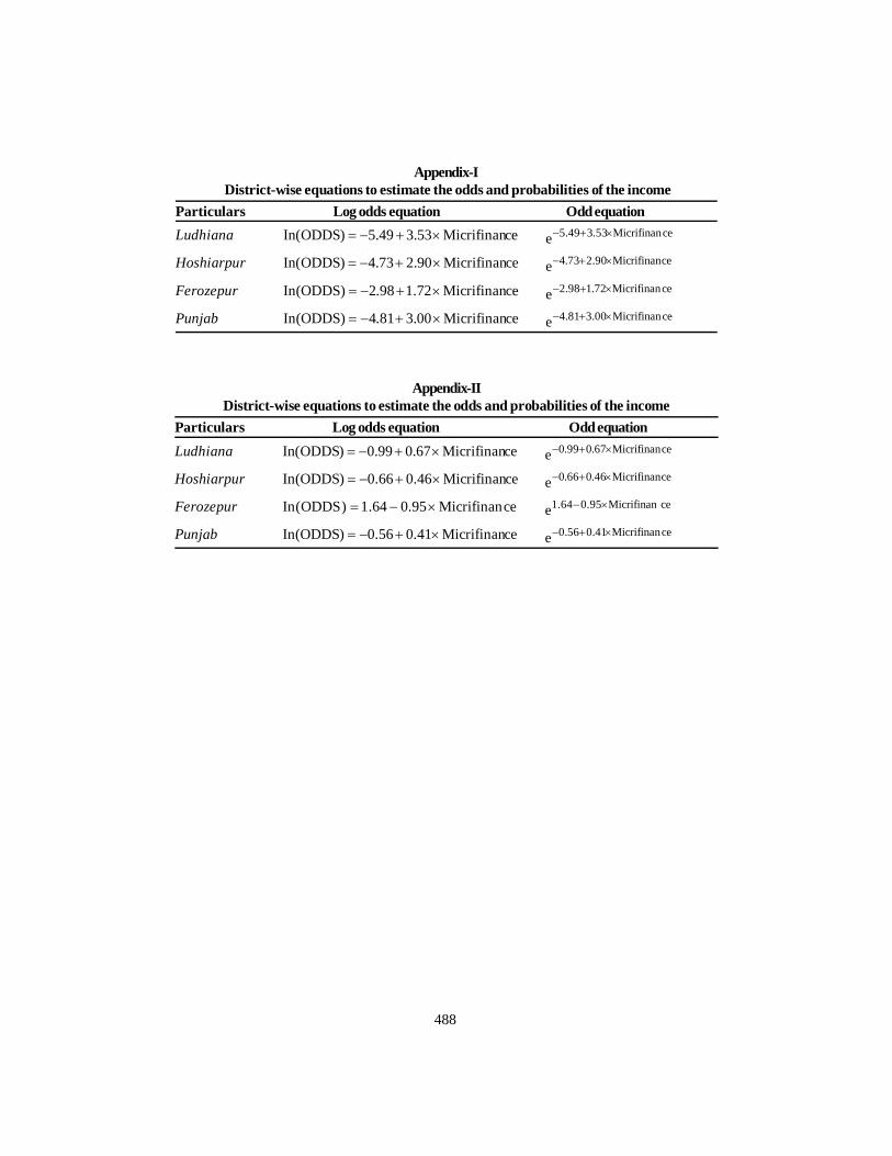
488

Appendix-I District-wise equations to estimate the odds and probabilities of the income

Particulars Log odds equation Odd equationLudhiana ceMicrifinan53.349.5)ODDS(In ceMicrifinan53.349.5e

Hoshiarpur ceMicrifinan90.273.4)ODDS(In ceMicrifinan90.273.4e

Ferozepur ceMicrifinan72.198.2)ODDS(In ceMicrifinan72.198.2e

Punjab ceMicrifinan00.381.4)ODDS(In ceMicrifinan00.381.4e

Appendix-IIDistrict-wise equations to estimate the odds and probabilities of the income

Particulars Log odds equation Odd equationLudhiana ceMicrifinan67.099.0)ODDS(In ceMicrifinan67.099.0e

Hoshiarpur ceMicrifinan46.066.0)ODDS(In ceMicrifinan46.066.0e

Ferozepur ceMicrifinan95.064.1)ODDS(In ceMicrifinan95.064.1e

Punjab ceMicrifinan41.056.0)ODDS(In ceMicrifinan41.056.0e

489

Indian J Econ Dev DOI No. 10.5958/2322-0430.2015.00057.8Volume 11 No. 2 (2015): 489-498 Research Article

INFLATION-UNEMPLOYMENT-POVERTY NEXUS INNIGERIA, 2000-2013: AN EMPIRICAL EVIDENCE

Obansa Joseph* and Ajidani Moses Sabo#

ABSTRACT

The study was conducted to empirically measure the effect of economicconditions-unemployment and inf lation and some demographiccharacteristics on poverty rate in Nigeria during the 2000-2013. Relatedliteratures were reviewed. Two multiple regression models, one relatinginflation and unemployment to head-count poverty, and another relatingadult literacy, real wage and dependency ratio to poorest of the poor, wereformulated, estimated and analyzed. The findings showed that all theexplanatory variables were critical factors which combine in variousdegrees to influence poverty in Nigeria. Thus, it was recommended thatgovernment should urgently implement policies that promote employmentgeneration, reduce public deficits, encourage private investments, reducebirth rate and stabilize foreign exchange rate.

Keywords: Head-count ratio, inflation, poverty, real wage, unemploymentJEL Classification: E24, E31, I32, P24, P44, P46

INTRODUCTIONInflation and employment are the two major

plagues that have persisted in Nigeria, and theyhave combine to cause poverty, crimes andunderdevelopment in the country especiallyin the recent times. An economy is commonlyregarded as suffering from inflation if it isexperiencing a period of general and persistentrise in prices of goods and services resultingin a loss of monetary purchasing powers(Folorunso and Abiola, 2000). The problem ofinflation has been in Nigeria for quitesometimes now.

A general increase in the price level inNigeria was first noticed in the 1970s.

Although, inflation rate has been stochasticover time, it has generally shown upward trend,reaching 73 percent in 1995 compared to 13.8percent in 1970 and 5.5 percent in 1985(Folorunso and Abiola, 2000). Recently,inflation has gathered greater momentumacquiring further inflationary potentialcompounding poverty in Nigeria.Unfortunately, we are now reaching the levelof runaway inflation in which money ceasesto be a store of value which poses a muchgreater threat to the entire economy. Theproducers are confronted with higher costs ofproduction, low capacity utilization andsometimes outright business closure. The highcost of production has reduced output whichaffects per unit price of goods. The consumersbear the burden of higher prices which reducesthe value of their disposable income. Theworkers tend to demand higher wages evenwithout corresponding increase in the marginal

*Department of Economics, Faculty of SocialSciences, University of Abuja, Abuja, Nigeria and#Department of Economics, Faculty of SocialSciences, Nasarawa State University, Keffi, NigeriaEmail: ajidanims@gmail.com

490

production of labour. Economic growth isstagnated as average propensity to save andinvest is continuously on the decline.

Workers are being retrenched to cut cost.The financial sectors continue to contend witha serious liquidity crisis due to deposit runs.In fact, we are neck deep in what is referred toas double digit inflation, which is universallyacknowledged as a hindrance to economicdevelopment (World Bank, 1990). Thedescription above is true about Nigeria inparticular and developing countries in general.

The World Bank Development report(1990) drew attention to the serious problemof poverty in developing countries. It reportsand considers as more shameful a conditionthat relegates more than a billion people indeveloping countries to a life of poverty andmisery. The bank identifies the poor to be thenumber of people struggling to live on lessthan $370 a year.

Poverty takes various forms including: lownutritional status; low level of education;decline in spending on socials services; highinfant mortality rate, and low life expectancyamong others. Although, poverty in Nigeria isa general phenomenon, its depth and severityis felt more among the landless uneducatedrural dwellers, those without regular jobs orother income sources; that always move in andout of the unorganized, casual informal labourmarket (Nyong, 1999).

Ahluwalia et al. (1979) reported that almost40 percent of the population of the developingcountries lives in absolute poverty defined interms of income levels insufficient to provideadequate nutrition. The bulk of the poor are inSouth East Asia, Indonesia and Sub-SaharanAfrica which fall under poorest category ofcountries.

According to Todaro (1989) about three-fourth of the population are poor in sub-Saharan Africa. The World Bank (1996) reportsthat on average 45 to 50 percent of sub-SaharanAfricans live below the poverty line and thatthe depth of poverty that is, how far incomesfall below the poverty line is greatest in the

sub-region than anywhere else in the world.Nigeria is the most populous country in

sub-Saharan Africa. it has experienced boomson four occasions during its fifty-four yearsof nationhood that is agricultural boom of the1960s, oil boom of the 1970s, financial boom ofthe 1980s and oil boom again of the 2000s.None of the booms (including the present oilboom) could transform Nigeria into anindustrial giant, rather inflation, unemploymentand poverty continue to rise.

The explanations above raise a number offundamental questions such as, what are thecauses of and solution of inflation,unemployment and poverty? What is thenature of the relationship between thesevariables, that is, which determine the other(s)?

We recognized the fact that quite a numberof researches have been carried out oninflation. The present study will bridge the gapand update the knowledge in the relationshipsbetween inflation, unemployment and poverty.

Thus, the basic objectives of this paperwere to quantify empirically, the relationshipbetween the macroeconomic conditions andinflation in Nigeria during the 2000-2013. Thisexercise is important because it will assists nmacroeconomic planning.THEORETICAL ISSUES

The inability of developing countries toattain sustainable economic growth anddevelopment has been variously associatedwith several factors, including financialindiscipline inherent in the implementation oftheir monetary and fiscal policies (Folorunsoand Abiola, 2000). This has caused manymacroeconomic problems such as inflations,unemployment and poverty among others.

While there is a modicum of consensus onthe concept of inflation among economiststhere are some variations in its root cause(s).According to monetarists, inflation is a stateof disequilibrium in which an expansion inpurchasing power not accompanied byincrease in productivity tends to cause anincrease in the quantity of money leads to an

491

increase in the general price level and a fall inthe value of money. On the other hand, thefiscalists believed that increased in governmentexpenditure and /or decrease in taxation resultin rising inflation.

On unemployment, the monetaristsgenerally agreed that, it is functionally relatedto fall in quantity of money supply. Theydescribed unemployment as an economiccondition in which many people who werewilling to work and present them to work butare not gainfully engaged. On the other hand,unemployment, according to fiscalists, isusually caused by decrease in governmentexpenditure and/or increase in taxation leadingto fall in purchasing power of people in theeconomy (Eggon et al., 2009). Other causes ofinflation and unemployment include naturalfactors like drought, flood, earthquakes andcontemporary factors such as bottlenecks inthe distr ibution system, bribery andcorruption, mismanagement, etc.

The review above indicates that there aninverse relationship between inflation andunemployment. Conceptually, poverty islooked at differently by different writers.Balogun (1999) defines poverty in its absolutesense, as a situation where a population or asection of the population is able to meet onlyits bare subsistence essentials of food,clothing and shelter in order to maintainminimum standard of living. This definitionrequires that a yardstick be set which can beused to assess living standards so as todetermine who is poor and who is not. Thisled to the emergence of the concept of povertyline based on the level of per capita income orconsumption of individuals or householdswithin a region or country. This is usuallydefined as the cut-off living standard levelbelow which a person is classified as poor.

The World Development Report (1990)used a lower poverty of $370 income (in 1985purchasing power parity dollar) per capita as acut off for absolute poverty. People whoseconsumption levels fall below that level areconsidered poor and those below US $275 as

very poor.Englama and Bamidele (1997) and Balogun

(1999) summarized the definition of poverty inboth absolute and relative terms as a “statewhen an individual is not able to cateradequately for his/her basic needs of food,clothing and shelter, meet social and economicobligations; lack gainful employment, skillsassets and self-esteem; and has limited accessto social and economic infrastructure such aseducation, health, potable water, andsanitation, and as a result has limited chanceof advancing his/her welfare to the limit of his/her capabilities.

Oladunni (1999) defines poverty in term ofinsufficient income for securing the basicnecessities of life such as food, potable water,clothing and shelter. She also says povertymay be viewed in terms of the consequences,such as deficient provision of goods andservices, deprivation and lack of rights suchas it affects the girl-child due to male childpreference, insufficient capability as well associal and economic exclusion mechanisms.

Poverty may be absolute, relative, chronic,transient, mass or localized. Absolute povertyis lack of physical minimum requirements for aperson’s or household’s existence. On theother hand, relative poverty refers to a situationwhere a person or households is/are withprovision of goods and services which is lowerthan that of other person(s) or group.

Consequently, poverty is defined simplyas a condition in which an individual does nothave enough food to eat, poor drinking water,sanitation, nutrition, high infant mortality rate,low life expectancy, energy, low consumption,educational opportunities, and lack ofproductive participation in the decision makingprocess either as it affects the individuals ornational arena be it management or political.

Awoseyila (1999) defines relative povertyas a condition in which households, overtimefall short of the resources to maintain theirstandard of living.

By applying the concept of poverty toNigeria, Awoseyila (1999) states that those

492

classified as poor included households belowthe poverty like those lacking access to basiceconomic and social services, rural dwellerswith lack of essential infrastructure, theunemployed, among others.

Measured in absolute and relative terms,poverty in Nigeria is generally more sever inrural communities and among vulnerablegroups in urban centres. The incidence differswith household size, gender, educational, ageand occupational distribution of households’heads.

Although, the poverty can be linked tounemployment, there are other causes of itwhich are identified in literature.

Given the focus of this study, a theory ofpoverty must identify the factors of productionparticularly as it relates to the structures ofthe interpersonal and intergroup differentialsin wealth and income. Five theories may beidentified in literature which attempt to explainthe causes of income inequality and poverty.These theories are of the theory of personalincome distribution, the necessity theory, theindividual attribute theory, the naturalcircumstantial theory, and the power theory.Of these, the power theory and the theory ofpersonal income distr ibution (Sizeddistribution of income) provide greater insightinto the causes of poverty and hence, arediscussed below.The Power Theory

The power theory which took its root fromMarxian Theory of exploitative property systemstates that the allocation of opportunities,income and wealth is determined by using theapparatus of state power.

According to the theory, poverty is anecessary concomitant of any situation inwhich the few poses much political power toorganize the economy system in their ownselfish interest. It insists that poverty willremain prevalent as long as there is no effectivepressure from the poor to restructure thedistribution of political power in the society infavour of the majority. The concentration ofwealth in the hands of the few while the

majority languishes in poverty is amanifestation of the same historical process(Akeredolu-Ale, 1976). The implication of thetheory for poverty alleviation is that povertywill continue unless there is a revolutionaryconsciousness of the subject class, of theirorganizational capacity to resist exploitationto overthrow the property system and to whathappens over time. The power theory seemsmore relevant to developing countries in viewof the tendency of those without economicpower to seek political power to amass ill-gotten wealth. This is compounded by the lowpolitical consciousness of the generality of thepeople, the high degree of centralization ofnational resources, and the tendency towardsone-partyism and dictatorship. The powertheory explains the paradoxical situation in acountry like Nigeria which is rich, yet thegenerality of the people are poor.The Theory of Personal Income Distribution

The Theory of Personal IncomeDistribution otherwise described as sizedistr ibution of income provide themicroeconomic foundation of incomeinequality and an organizing framework todetermine the channel by whichmacroeconomic variables are transmitted intochanges in poverty rates. It focuses attentionon the labour market and the determinants oflabour incomes based on demand and supplyfactors. According to the marginal productivitytheory of labour, the income received by labouris due to their marginal productivity. Themarginal productivity of an individual dependson educational level (credentialism or skills andattitude), motivation, regional location, and ageamong others. According to this theory,majority of families or households rely onlabour market earning for most of their income.Consequently a rise in unemployment mayresult in income declines particularly amongthose whose income are low, to begin with.Hence, the theory predicts a positive relationthat may be mitigated by government transferpayments which reduce the role of earnedincome.

493

With respect to inflation, another variablereflecting the macroeconomic condition of acountry, the theory is unambiguous. It is wellknown that during periods of inflation, thosedepending on fixed income payments such aspensioners suffer. Thus, we find thathouseholds are driven into poverty wheninflation rises. This phenomenon is consistentwith the positive relationship predictedbetween unemployment and inflation rate. Thetheory suggests that policies to eradicatepoverty should reduce inflation, inequality anddeal with problems of unemployment. Theimportance of these issues in economicdevelopment was empathized in Seers (1969).

The questions to ask about a country’sdevelopment are, therefore:1. What has been happening to poverty?2. What has been happening to

unemployment?3. What has been happening to inequality?

If all these have declined from high levels,then beyond doubt, this has been a period ofdevelopment for the country concerned. If oneor two of these central problem have beengrowing worse, especially if all three have, itwould be strange to call the result developmenteven if per capita income doubled.

This concern reflects the thinking thatbetter employment opportunities were theprincipal avenues by which the poor could earnhigh incomes. Consequently, we maintain thatwhether poverty is measured by consumptionor by income, employment generation stillremains an important factor in eradication ofpoverty. If household is liquidity-constrained,both income and consumption poverty willoccur during spell of employment. Similarly,periods of high unemployment may be periodof heightened uncertainty about the future,leading to reduced consumption and hencehigher incidence of consumption poverty.

For inflation, the channel is more direct.Inflation tends to benefit debtors at theexpense of creditors thereby eroding assetsvalues. Liquidity-constrained household maytherefore be weekly hedged against inflations.

In an environment of rapidly rising prices,households may be slow to adjust theirconsumption patterns to rapidly rising prices.The result is higher rate of consumptionpoverty.Empirical Issues

The consequences of inflation in terms ofits adverse effect on income distribution andhence on poverty has been documented by anumber of authors including Blinder and Esaki(1978) and Powers (1995). According to Powers,In sheer constraint to previous findings thatinflation has very little effect on incomepoverty. I find a robust and relatively largepositive effect relationship between inflationand the consumption poverty rate. Thus, myfindings suggest that inflation may have moreadverse effect on poverty than was previouslythought.

Blank and Blinder (1986), Blank (1993),Cutler and Katz (1991) and Mocan (1995) inthe United States and Yoshino (1993) in Japan,examine the relationship betweenunemployment, inflation and poverty rates forfamilies and persons. Their results indicatesignificant correlation between poverty andinflation, and between poverty rate andunemployment. Blinder and Blank concludethat between unemployment and inflation.Unemployment, not inflation is the cruelesttax factor.

Whereas, Blank (1993) find a significantpositive relationship, Cutler and Katz (1991)and Mocan (1995) reported a negativerelationship between inflation and poverty.However, all these studies indicate strong,robust, and positive relationship betweenpoverty and unemployment.

Whereas, the studies above focused onthe effect of macroeconomic conditions onpoverty, Fields (1999) investigated anotherdimension of the poverty debate in terms ofthe effect of other factors, namely the extentof income inequality. Gary first examinesKuznets’ hypothesis which states that incomeinequality first increases in the early stages ofdevelopment but decreases in later stages,

494

thereby generating an inverted-U curve. Insimple language, this means that things mustfirst worse before they get better.ANALYTICAL METHODOLOGY

The exposition thus, far indicates thatinflation and unemployment have direct effecton poverty in Nigeria. In order to investigateempirically the relationship between inflation,unemployment and poverty in Nigeria, multipleregression analysis was carried out by theauthors in the model, two measures of povertyare used.

The first measure of poverty in this studyis the head-count ratio which according toAhluwalia (1976) is the number of those livingbelow poverty line, (consumption or income-based poverty line) to total population in acountry. It is called the poverty rate (expressedin percentage). Thus, the model is:

Ph = f (N, I) .........1(a)Ph = ao+a1N+a2I+U .........1(b)

WherePh = Poverty rate or head-count ratio (%)N = Unemployment rateI = Inflation rate (consumer price index)

However, poverty also includes lack ofnon-material benefits such as education healthand nutritional status (Morris, 1979, WorldBank, 1993, Kakwani, 1990 and, Ogwumike andEkpeyong, 1995).

Following the writers above, the secondmeasure of poverty used in this study is lifeexpectancy at birth (which is a proxy of thenon material benefits). Thus, the second modelis:

Pc = f (L,W, D) ........2(a)Pc = b0 + b1L+b2W +b3D + U ........2(b)

WherePc = Poverty rate of the core poor (or

poorest of the poor)L = Adult literacy rate (a proxy for

education)W = Real Wage measure by GL 01 which

is the lowest level in wages andsalaries grading system (it rangesbetween 01-16 in the public services).

D = Dependency ratio (or number of

population age 0-15 years as apercentage of total population)

U = Error terma0 and b0 = Intercepts of the regression

models (1) and (2) respectivelya1 and b1 = Slopes of the respective

regression modelsBefore running the regression, all the

variables are first-differenced (D). This is doneto detrending the variables to obtain reliableparameter estimates in time series regression.Our econometric models take the form of twolog equations, the first with head-count ratio(Ph) the second with life expectancy at birth(Pc) as the dependent variables:Log Pn=a0 +a1LogN +a2LogI + U ....1(c)

andLog Pc=b0+b1LogL+b2LogW+b3D+U ....2(c)

All the explanatory variables are expectedto have positive coefficient except in the caseof adult literacy (L) and real wage (W) whichare expected to be negative.

The secondary data used for the studywere collected from various sources, includingCentral Bank of Nigeria economic and financialreview (Various issues), and National Bureauof Statistics (NBS). The models were estimatedusing Ordinary Least Square procedure andthe results are presented and analyzed insection 4. EMPIRICAL RESULTS AND ANALYSIS

The multiple regression models derived insection 3 were estimated using computersoftwares such as SPSS and E-views, and theresults are presented in Table 1.

The effect of unemployment and inflationon poverty was examined. The coefficient ofunemployment is positive, indicating positiverelationship between it and poverty in Nigeriaduring the 2000-2013. Unemployment did notpass the significant test since its t-calculated(1.002) is less than its tabular t-value (2.16) at 5percent level of significance.

Besides, the coefficient of inflation ispositive, meaning there is positive relationshipbetween it and poverty in Nigeria during theperiod under review. However, inflation did not

495

This was in agreement with Blank and Blinders(1986) that while unemployment and inflationworsens, poverty will rise.

Of the three additional variables includedin the poverty equation in Table 2, the resultshowed that dependency ratio was the mostimportant variable affecting the incidence ofpoverty with poverty elasticity at 0.715 for thecore poor. The findings suggest that theincidence of poverty increase more in the corepoverty group with an increase in dependencyratio. This was also consistent withexpectation (Nyong, 1999). The result furthershows that real wage rate has positive effecton poverty rate. This was in line with Morgan’s(1995) findings.CONCLUSIONS

The study finds that unemployment andinflation consistently have positive effect onpoverty rate suggesting that idleness andinflationary pressures are responsible forpushing many households consumptionbelow the poverty level. The perusal of studyshows that no matter which index was beingused, unemployment and inflation, incollaboration with other variables such asdependency ratio, real wage rate and adultliteracy rate were critical factors influencingpoverty in Nigeria. This finding was empiricallyrobust with different specifications of thepoverty rate. Consequently, these variablesmust be included in any realistic andmeaningful attempt at tackling poverty in

Table 1: Regression results for Model-1and related statisticsDependent variable Regression coefficientsConstant 59706**

(4.182)Unemployment rate (N) 0.296NS

(1.002)Inflation rate (I) 0.135 NS

(0.458)R2 0.088DW test 0.250

F value 0.530**Significant at 5 percentNS: Non-significantFigures in parentheses are calculated t values

pass the significant test as its t-calculated(0.458) is less than its tabular t-value (2.16) at 5percent level of significance.

The fit of the model in terms of itsexplanatory power is poor at R2 = 0.088 whichis approximately 8.8 percent. This implies thatthe explanatory variables could account foronly 8.8 percent of the total variation inpoverty.

The small values of DW test = 0.250 and Fvalue = 0.530 showed that there is noautocorrelation in the data used for theestimation.

An examination of Table 2, showed thatthe coefficients of the explanatory variables-adult literacy, real wage and dependency ratiowere positive, indicating that each of them haspositive effect on poverty in Nigeria duringthe 2000-2013. The results also showed thatdependency ratio was significant since its t-calculated (2.547) was greater than its tabulart-value (2.16). However, the joint effect of theindependent variables was fair, at R2 = 0.649,which is 64.9 percent. Besides, the small valueof DW test = 0.744 indicates that thesesecondary data used to estimate the model wasfree of serial correlation.

The perusal of Table 1 showed thateconomic conditions like unemployment andinflation have positive but weak effect onpoverty. This implies that as economicconditions become worse, poverty becamecompounded. This is consistent with theory.

Table 2: R e gre ss ion re sult for M ode 2 andre late d s tatis ticsD e pendent variable R egres sion coe fficientsConstant - 8.865 NS

(-0.104)Adult literacy rate (L) 0.065 N S

(0.215)Real wage (W) 0.084 N S

(0.373)Dependency ratio (D) 0.715 N S

(2.547)R2 0.649DW test 0.744F value 6.156N S: Non-significantFigures in parentheses are calculated t values

496

Nigeria.It is important to observe that the results

from this study were rather disturbing for bothmonetary and fiscal policies. For policy makerswho believe that expansionary measures couldimprove the well-being of the average personby reducing unemployment without theunpleasant side effect of making some peopleworse off through inflation, the positive effectestimated for both inflation and unemploymentshould not be seen as a joy. The policyimplications of our findings is thatexpansionary measures which create more jobsand reducing unemployment thereby, makingthe average person better of will however,eliminates the initial gains of those alreadyworking through the distributional effect ofrising inflation which alternately drives morepeople into poverty.

Overall, the findings of this study showedthat reductions in unemployment and inflationare two important elements in themacroeconomic environment that should betargeted along with other factors to arrive atrealistic poverty alleviation policies andprogrammes in Nigeria .

Therefore, the following recommendationswere made:1. There is urgent need for government to

target policies that promote employmentgeneration. To this end, governmentshould encourage private investment andstabilized the exchange rate.

2. The government should reduce fiscaldeficits through prudent spending andaccountability. The reduced fiscal deficitsshould be financed through foreignborrowing, use of reserves and domesticborrowing instead of resorting to the CBNways and means advance.

3. To address the issue of inflation, increasein productivity should be taken as anurgent national priority. All aspects of ourproduction and services need to raise theirefficiency and output. A substantialincrease in the supply of goods isnecessary to bring down inflation.

4. The households should be encouragedthrough moral suasion to reduce thenumber of children born. This will help tocontrol birth rate and hence reducedependency ratio.

5. The efforts of government should also bechannelled to rural development byproviding more infrastructural facilities inthe area. This will go a long way to createwealth and reduce poverty.

REFERENCESAhluwalia, M.S., Carter, N.G. and Chenery, H.B.

1979. Growth and poverty in developingcountries. Journal of Development Economics6: 299-341.

Akeredole-Ale, D. 1976. Inequality, poverty anddevelopment. Journal of DevelopmentEconomics. 3 (4): 230-251.

Awoseyila, A.P. 1999. The dimensions of povertyin Nigeria spatial, sectoral gender, occupational,etc. Central Bank of Nigeria Bullion. 23 (4): 31-38.

Balogun, E.D. 1999. Analyzing poverty: Conceptsand methods. Central Bank of Nigeria Bullion.23 (4): 11-15.

Blank, R.M. 1993. Why were poverty rates so highin the 1980s? In: Dimitri, B.P. and Edward, N.W.(Eds.) Poverty and prosperity in the USA in thelate twentieth century. New York St. Martin PressIncorporated: 21-55.

Blank, R.M. and Blinder, A.S. 1986.Macroeconomics, income distribution, andpoverty,-Fighting poverty: What works and whatdoes not. In. Danziger, S. (ed .). HarvardUniversity Press, Cambridge, MA 02138, USA.

Blinder, A.S. and Esaki, H.Y. 1978. Macroeconomicactivity and income distribution in post-warUnited States. Review of Economic Statistics. 6(4): 604-609.

Cutler, D. M. and Katz, L. F. 1991. Macroeconomicperformance and the disadvantaged. BrookingPaporson Economic Activity. 2: 1-61.

Eggon, A.H., Ajidani, M.S. and Oseshi, B.I. 2009.Basic Principles and Theories of Economic.Revised Edition: Rossen Production andServices Limited, Keffi, Nasarawa State, Nigeria.

Englama, A. and Bamidele, A. 1997. Measurementissues in poverty. Central Bank of NigeriaEconomic and Financial Review. 35 (3): 315-331.

Fields, G. 1990. Income distribution and economic

497

growth. In: Gustav, R. and Schultz, P. (Eds.)The state of Development Economic: Progressand Perspectives, Chapter-15: 459-481.

Folorunso, B.A. and Abiola, A.G. 2000. The long-man determinants of inflation in Nigeria (1970-1988). The Nigerian Journal of Economic andSocial Studies. 42(1): 37-53.

Kakwani, N. 1990. Poverty and economic growthwith application to Cote D’ivoire. World Bank:Washington, D.C.

Mocan, H.N. 1995. Income inequality, poverty andmacroeconomic conditions. Paper Presented atthe American Economy Association Meetings,Washington, D.C. January 07, 1995.

Morries, M.D. 1979. Measuring the condition ofthe world’s poor: The physical quality of life index.New York: Permagon Press

Nyong, M.O. 1999. Inflation, unemployment andpoverty alleviation in a developing economy:The Nigerian experience. First Bank of NigeriaPlc Bi-Annual Review. 7 (15): 1-24.

Ogwumike, F. and Ekpeyong, D. 1995. Impact ofstructural adjustment policies on poverty andincome distribution in Nigeria. ResearchReport. African Economic Research Consortium(AERC), Kenya.

Oladunni, B.E.I. 1999. The dimensions of povertyin Nigeria spatial, sectoral, gender, etc. Central

Bank of Nigeria Bullion. 23 (4): 17-29.Powers, E. 1995. Inflation, unemployment and

poverty revisited. Economic Review of theFederal Reserve Bank of Cleveland. 31(3): 2-13.

Seers, D. 1969. The meaning of development.International Development Review. 11(4): 3-4.

Todaro, M. 1989. Economic development in the thirdword. 4th Edition, Longman, New York.

World Bank. 1990. World development report:Poverty. Culled from https://openknowledge.worldbank.org/handle/10986/5973.

World Bank.1993. Poverty reduction handbook.Culled from http://documents.worldbank.org/curated/en/1993/04/699047/poverty-reduction-handbook

World Bank.1996. Poverty in Sub-Saharan Africa:Issues and recommendations. EconomicManagement and Social polices.

Yoshino, O. 1993. Size of distribution of workers’household income and macro-economicactivities in Japan: 1963-1988. Review of Incomeand Wealth. 39 (4): 387-402.

Received: September 29, 2014Accepted: March 18, 2015

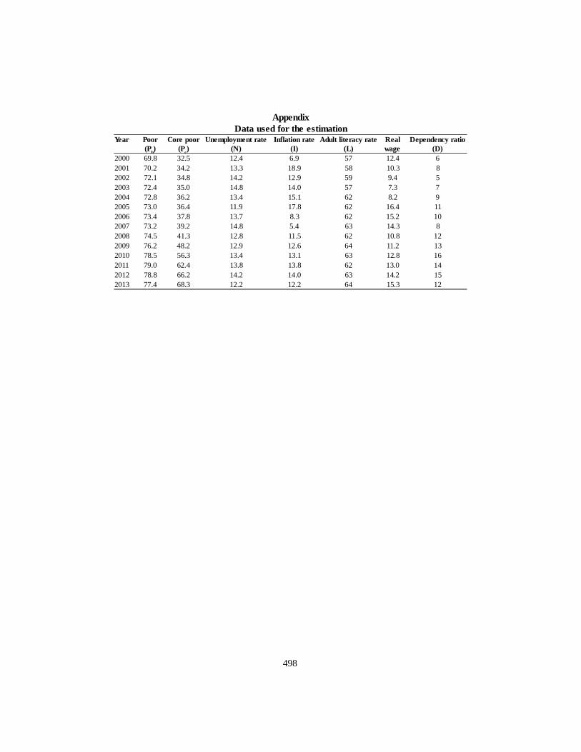
498

AppendixData used for the estimation

Year Poor(Ph)

Core poor(Pc)

Unemployment rate(N)

Inflation rate(I)

Adult literacy rate(L)

Realwage

Dependency ratio(D)

2000 69.8 32.5 12.4 6.9 57 12.4 62001 70.2 34.2 13.3 18.9 58 10.3 82002 72.1 34.8 14.2 12.9 59 9.4 52003 72.4 35.0 14.8 14.0 57 7.3 72004 72.8 36.2 13.4 15.1 62 8.2 92005 73.0 36.4 11.9 17.8 62 16.4 112006 73.4 37.8 13.7 8.3 62 15.2 102007 73.2 39.2 14.8 5.4 63 14.3 82008 74.5 41.3 12.8 11.5 62 10.8 122009 76.2 48.2 12.9 12.6 64 11.2 132010 78.5 56.3 13.4 13.1 63 12.8 162011 79.0 62.4 13.8 13.8 62 13.0 142012 78.8 66.2 14.2 14.0 63 14.2 152013 77.4 68.3 12.2 12.2 64 15.3 12

499

Indian J Econ Dev DOI No. 10.5958/2322-0430.2015.00058.XVolume 11 No. 2 (2015): 499-508 Research Article

PRADHAN MANTRI JAN DHAN YOJANA: A VEHICLEFOR FINANCIAL INCLUSION

Amita Shahid* and Taptej Singh#

ABSTRACT

The present study seeks to investigate the current status of the PMJDY inIndia. The results revealed that the contribution of rural sector in terms ofaccounts opened under PMJDY was relatively higher than the urban sectorin all the banking sectors namely, public sector banks, regional rural banksand private banks. The results further revealed that more than 70 percentof the accounts opened under PMJDY were opened with zero balance(626.34 lakh) depicting the weakness in the implementation strategy ofthe plan regarding easy access to banking system. From the public sectorbanks and RRBs, the State Bank of India plays an important and leadingrole in the opening accounts under PMJDY. The state-wise scenario ofPMJDY shows that the highest number of accounts was opened in UttarPradesh including both rural and urban sectors due to its highest populationrate. Whereas, Punjab has become the third state after Kerala and MadhyaPradesh where all households have at least one bank account.

Keywords: DPTs, financial inclusion, PMJDY, RRBs.JEL Classification: G21, O16, R51

*Assistant Professor, Post Graduate Department ofCommerce, Lyallpur Khalsa College, Jalandhar and#Research Fellow, Technology Marketing and IPRCell, Punjab Agricultural University, Ludhiana-141004Email: sartajchhina1974@gmail.com

INTRODUCTIONFinancial inclusion or inclusive financing

is the delivery of financial services at affordablecosts to sections of disadvantaged and lowincome segments of society, in contrast tofinancial exclusion where those services arenot available or affordable. This malaise hasled to generation of financial instability andpauperism among the income group, who donot have access to financial products andservices. Financial Inclusion is one of the topmost priorities of the present UnionGovernment. Exclusion of a large number of

people from across to financial servicesinhibits the growth of our country. There wasalso evidence that financial inclusion is crucialto poverty reduction. The success of financialinclusion is primarily breaking the link betweenpoor public service, patronage and corruption.The term financial inclusion has gainedimportance since early 2000s, as a result offindings about financial exclusion and its directcorrelation to poverty. In India, the financialinclusion initiatives were under taken since2005-06 (Subbarao, 2009, Divya, 2013, Chowhanand, Pande, 2014, and Rafiq and Premavathy,2014). In the Indian context, financial inclusionhas been described as the provision ofaffordable financial services namely, access topayments and remittance facilities, savings,loans and insurance services by the formalfinancial system to those who are excluded

500

(Anonymous, 2014). The earlier campaign onfinancial inclusion started in 2011 had a limitedobjective. The focus was on the coverage ofvillages with population of 2000 or more withbanking services. The coverage of individualhouseholds with bank accounts was not thefocus. Out of the 5.92 lakh villages in thecountry, only 74000 villages could be covered(Anonymous, 2014a).

Though, our country‘s economy isgrowing at a one digit, still the growth is notinclusive with the economic condition of thepeople in rural areas worsening further. Thereare few people who are enjoying all kinds ofservices from savings to net banking, but stillin our country around 40 percent of peoplelack access to even basic financial serviceslike savings, credit and insurance facilities.Mainly, the rural area suffers from lack of accessto basic financial services. India is the secondlarge only to China in the number of peopleexcluded from financial facilities. Even after 68years of independence, around ten crorehouseholds were not connected with banking(Jayadev et al., 2012 and Khuntia, 2014).According to Rural Finance Access Survey(2003), 70 percent of marginal/landless farmersdo not have a bank account, 87 percent haveno access to credit from a formal sources. As aresult, they were forced to rely on informalfinance who charged exorbitant rates ofinterest (Basu and Srivastva, 2005).

Since independence, the Government ofIndia initiates various policies likeNationalization of Banks in 1969 and 1980,establishment of Lead Bank Scheme (1969),Regional Rural Banks (1975), National Bank ofAgriculture and Rural Development(NABARD) in 1982, and innovations likeMicro-finance, Rural InfrastructureDevelopment Fund, Kisan Credit Card (1998-99), General Credit Card (2005), etc. However,all these policies have almost failed to reachthe unreached people (Das, 2010 and 2014).Consequently, Prime Minister Narandra Modiin his Independence Day speech introduced anew scheme namely Prime Minister Jan Dhan

Yojana (PMJDY) where he mentions thatevery household will have at least a basic bankaccount with a RuPay debit card and an in-built accident insurance cover of `1 lakh aswell as an additional `30,000 life insurancecover for those opening bank account beforeJanuary 26, 2015.Prime Minister Jan Dhan Yojana (PMJDY)

PMJDY scheme has been started with anaim/objective to provide universal access tobanking facilities for all households througha bank branch or fixed point (businesscorrespondent), under the slogan Mera KhataBhagya Vidhaata (My Bank Account-Thecreator of the Good Fortune). The crux of theplan is to link every household with the bank.The Prime Minister through his mails to CEOsof all PSU Banks made clear that a bank accountfor every household was a National Priority.It envisages that anyone who was not havingbank account in any bank may open a bankaccount, just by presenting the identity cardeither by Aadhaar Card, NREGA card or VoterID Card, Ration Card, Driving License, PANCard, Passport that is the officially validdocuments, etc.

The scheme aims at creating (at least one)two bank accounts for every household. TheIndian scenario is that most of the people, mayit be from urban population or rural population,live below the poverty line (Anonymous, 28th

August, 2014 [350 million people in India areunder poverty line]). It has been observed thatin majority of the cases, these poor familiesborrow funds/avail loan below `5000.00 tomeet their petty household needs. Apart frompaying exorbitant rates of interest, they alsobecome victims of exploitation by the moneylenders and shopkeeper of the local area. Thisfacility of overdraft will bring financial relief tosuch poor families and help them towardsleading a better life by saving them fromeconomic crises that they have to face withtheir volatile and meager earning abilities. Thisscheme undoubtedly has proved to be the firststep towards providing financial assistance toone and all, may it be the masses from the

501

urban area or rural areas, and may it be thepeople who are literate or illiterate. This schemewould provide financial help to the needy andthe poor. The only requirement is to generateawareness among the masses, which ispossible through more sustained financialliteracy drive and consumer protectioninitiators.

Under various other schemes, governmentis providing a number of subsidies,scholarships and pensions for fulfilling theminimum basic requirements of the needy. Butnumber of times it had been debated that 40percent of such relief reaches the realbeneficiary. The reports about corruption hadbeen appearing in the papers in different areasof the country. The proposals to deposit theamount of subsidy directly in the account ofthe person was having big obstacle thateveryone was not the account holder in bank.Once every household is connected with bank,there would be no chance of such malpracticeof retaining 60 percent of the sanctioned reliefby the corrupt officials or person occupyingresponsible posts for serving the purpose. Themoney would then reach at the specific pointfor which it was meant. Thus, it would help incontrolling and eroding and eradicatingcorruption to a large extent.

Under the PMJDY plan, the lady of thehousehold has been given priority for openinga bank account. Some people in certain areasof Indian Economy are still using the age oldbarter system, in certain villages they areexchanging goods instead of moneyparticularly in areas of Orissa, MP and Bihar.This financial inclusive scheme would be arevolutionary step in this regard, as the womenget an opportunity to fulfill their needsthrough the micro finances facility offeredunder this scheme. This financial inclusivescheme has been envisioned with genderequality and women empowerment that is thosewho constitute half of the population. Thebank account opening drive has to be followedup with a more sustained financial literacydrive and consumer protection initiatives.

PMJDY would touch the lives of everyone ina positive and constructive way. Financialliteracy enables them to be more informedabout their financial decisions.PMJDY: Some Opinions

This ambitious comprehensive financialinclusion scheme plan launched by PM,Narendra Modi, is likely to have far reachingimpact on the lives of millions of people ofIndia. The Prime Minister said on the occasionof Independence Day, Let us celebrate todayas the day of financial freedom. In order toeradicate poverty we have to get rid offinancial untouchability , adding thatinclusion will also act as an important tool inthe fight against corruption. He also said theprogramme would break the vicious circle ofpoverty and debt and boost the economy,which slowed to decadal low in the past twoyears. He further added that when a personopens a bank account, he or she takes the firststep to get connected with the economicsystem and this gives boost to the economy.

Union Health Minister Harsh Vardhan said,there are several people in India who don’thave even basic facilities. After 67 years, 350million people are under poverty line and 37percent people are illiterate. In this situation,such scheme will be very useful for poorpeople. Lt. Governor Najeeb Jung said, in lastseveral years many schemes were introducedto help poor people, but these schemes couldnot run effectively. It is the responsibility ofbanks which have to effectively participatein Jan Dhan Yojana.

As on 2nd October, 2014, the FinanceMinistry announced that 5.29 crore bankaccounts have been opened under PMJDY; ofwhich 3.12 crore are in rural and 2.17 crore arein urban areas. 1.78 crore Rupay debit cardshave been issued under Jan Dhan Yojana(Anonymous, 2014). The benefits of PMJDYcan also be extended to existing accountholders without opening a new account. It isan innovative and much needed step in theright direction which will address the biggestnational challenge that is, eradication of

502

poverty through financial inclusion, CIIDirector General Chandrajit Banerjee said.

One reason, said VB Bhagavati, GeneralManager for financial inclusion at AndhraBank, is the government’s announcement thatall government benefit will only flow throughbank accounts. Union Minister for Micro Smalland Medium Enterprises Mishra (2014) saidPradhan Mantri Jan Dhan Yojana will notjust strengthen the Indian Economy but is alsoa new beginning of an economic revolutionin the country, at the launch of PMJDY. Hefurther added, this scheme will also help Indiato stand at par with the developed nations.Financial Services Secretary G.S Sandhu said,it has to be beyond just a bank account. Theidea is to convert cash economy into acashless and digital economy.

The benefits under government welfareschemes running into thousands of crores ofrupees can be directly transferred to thebeneficiaries’ accounts. Huge pilferage in themiddle will be eliminated . AssochamSecretary General D.S. Rawat said. He furtheradded that the plan seeks to give India’s pooraccess to affordable financial services likesavings account, easy credit and insurance.Birla added, Linking financial literacy anddirect cash transfer with this programmeensures demand inducement andsustainability of this model.

Bill and Melinda Gates Foundation (BMGF)have offered to help in Monitoring of theprogress made with regard to Pradhan MantriJan Dhan Yojana (PMJDY), the flagshipfinancial inclusion scheme of the government.BMGF can help in mapping the different sitesacross the country and can inform wherevera saturation level with regard to opening ofaccounts has reached or likely to reach sothat focus can be made in other areas,Microsoft founder Bill Gates said during hisinteraction with the Finance Minister ArunJaitely.

Amid this background, the presentinvestigation endeavours with the objectivesto study the current status and recent progress

of Pradhan Mantri Jan Dhan Yojana (PMJDY)in India.METHODOLOGY

As the study is descriptive in nature,secondary data have been employed toaccomplish the objectives of present study.The secondary data have been collected fromwww.pmjdy.gov.in and relevant publicationswere used for analysis. The secondary datapertaining to number of accounts opened bypublic sector banks, RRBs, private banks,amount deposited in the accounts, accountswith zero balance, etc. were collected from theofficial website of PMJDY (www.pmjdy.gov.in).The data were further analyzed using variousdescriptive statistics such as average,percentage, etc.RESULTS AND DISCUSSION

Unlike the previous scheme of the UPAgovernment which focused on villages, thePMJDY focuses on households, therebycovering both urban and rural areas.Moreover, unlike previous efforts, thePMJDY’s design is focused not just on bankaccounts, but also on other products thatprovide incentives to people to open accountssooner rather than later-specifically, the 1 lakhinsurance cover and `5,000 overdraft facility.The scheme also envisages expanding thebanking and ATM number, as well as, theremuneration and coverage of BusinessCorrespondents or Bank Mitra’s (Kapur, 2014).

The information regarding the details ofaccounts opened in Pradhan Mantri Jan-DhanYojana (PMJDY) has been presented in Table1. The results revealed that the contributionof rural sector in terms of accounts openedunder PMJDY was relatively higher than theurban sector in all the banking sectors namely,public sector banks, regional rural banks andprivate banks. In rural sector, the public sectorbanks, regional rural banks and private bankscomprising 73.43, 24.27 and 2.31 percent,respectively of total accounts opened underPMJDY. Whereas, in urban sector, more than90 percent accounts were opened in publicsector banks and other two banking sector

503

were comprising very few proposition ofaccounts opened that is, 6.34 percent byregional rural banks and 3.27 percent by privatebanks.

On the overall level, more than 80 percentof the total accounts were opened in publicsector banks, 17 percent were opened inregional rural banks and only 2.70 percent wereopened in private banks. The results furtherrevealed that more than 70 percent of theaccounts opened under PMJDY were openedwith zero balance (626.34 lakh) depicting theweakness in the implementation strategy ofthe plan regarding easy access to bankingsystem. The rest 30 percent accounts openedin PMJDY mobilize the deposit of `6557.36crores under the Pradhan Mantri Jan DhanYojana (PMJDY) as on December, 2014.

Public Sector BanksThe information pertaining to the

contribution of public sector banks in theopening of account under PMJDY waspresented in Table 2. The results revealed thatState Bank of India plays an important andlead role in PMJDY with the opening of 155.18lakh accounts. The SBI contributed both inrural and urban sector with 63.59 and 91.60lakh accounts, respectively. Though, 143.72lakh accounts were opened with zero balance,the deposits comprises 136.62 crores in StateBank of India as on December, 2014.

The other public sector banks performingwell in the opening of accounts under PMJDYwas Bank of Baroda (45.18 lakh), Canara Bank(44.44 lakh), Punjab National Bank (43.79 lakh),Central Bank of India (38.41 lakh), Bank of India

Table 1: Details of accounts opened in Pradhan Mantri Jan-Dhan Yojana up to December,2014

(Lakhs)Particulars Accounts Balance in accounts

(` crore)Accounts with zero

balanceRural Urban TotalPublic Sector Banks 366.29 307.31 673.6 5232.94 500.83

(73.43) (90.39) (80.30)Regional Rural Banks 121.05 21.57 142.61 942.75 109.6

(24.27) (6.34) (17.00)Private Banks 11.52 11.11 22.63 381.66 15.91

(2.31) (3.27) (2.70)Total 498.86 339.99 838.84 6557.36 626.34

(100.00) (100.00) (100.00)Source: www.pmjdy.gov.in

Table 2: Details of accounts opened in public sector banks under PMJDY scheme(Lakhs)

Name of Bank Accounts Balance in accounts(` crore)

Accounts with zerobalanceRural Urban Total

State Bank of India 63.59 91.60 155.18 136.62 143.72Bank of Baroda 18.62 26.56 45.18 335.16 24.79Canara Bank 29.93 14.50 44.44 730.43 23.64Punjab National Bank 35.03 8.76 43.79 775.69 35.90Central bank of India 29.12 9.29 38.41 117.60 29.76Bank of India 15.59 22.55 38.13 147.94 28.03Union Bank of India 23.88 7.72 31.60 127.16 24.04Syndicate Bank 16.25 8.81 25.06 118.61 19.41UCO Bank 11.33 11.81 23.14 337.12 16.90United Bank of India 12.85 8.98 21.83 390.49 7.70Total 366.29 307.31 673.6 5232.94 500.83Source: www.pmjdy.gov.in

504

(38.13 lakh), Union Bank of India (31.60 lakh),etc. In terms of balance, Punjab National Bankaccounts the highest deposits of 775.69 crorefollowed by Canara Bank, United Bank of India,UCO Bank and Bank of Baroda with thedeposits of `730.43, `390.49, `337.12 and`335.16 crores, respectively under the PMJDYas on December, 2014.Regional Rural Banks

The Regional Rural Banks plays a key roleas an important vehicle of credit delivery inrural areas with the objective of credit dispersalto small, marginal farmers and economicallyweaker section of population for thedevelopment of agriculture, trade and industry.In India, RRBs have a large branch network inthe rural area forming around 43 percent of thetotal rural branches of commercial banks. Therural orientation of RRBs is formidable withrural and semi-urban branches constitutingover 97 percent of their branch network. Thegrowth in the branch network has enabled theRRBs to expand banking activities in theunbanked areas and mobilize rural savings(Mishra, 2006 and Soni and Kapre, 2012).

The performance of regional rural banks inthe opening of account under PMJDY as onDecember, 2014 was presented in Table 3.Similar trend was found in RRBs as the StateBank of India again contributes highest interms of accounts opened under PMJDY withthe opening of 22.37 lakh accounts. The

contribution of rural sector was found to behigher as compared to urban sector impliesthe large branch network of RRBs in the ruralarea. The other major banks in terms ofaccounts opened in PMJDY were United Bankof India, Central Bank of India, Punjab NationalBank and Bank of Baroda with the opening of17.00, 15.31, 14.07 and 12.32 lakh accounts,respectively.

The similar trend was observed in accountsopened with zero balance as RRBs deals withthe economically weaker section ofpopulation. As concerning the weaker sectionof India, the balances in accounts were alsoless in RRBs as compared to public sectorbanks. Among the RRBs, the highest depositswere accounted by Punjab National Bank(`210.04 crores) followed by Central Bank ofIndia (`177.70 crore), State Bank of India(`140.96 crores), United Bank of India (`95.43crore), Syndicate Bank (`76.62 crore), etc. underthe PMJDY as on December, 2014.Private Banks

In 1951, there were 566 private banks inIndia, 474 non-scheduled and 92 scheduled asclassified on the basis of their capital size. Therole of private sector banks started decliningwhen the Government of India entered bankingsector with the establishment of State Bank ofIndia in 1955. Consequently, the existence ofpublic sector banks has increased. At present,there are 32 private banks comprising of 24 old

Table 3: Details of accounts opened in Regional Rural Banks under PMJDY scheme(Lakhs)

Name of Bank Accounts Balance in accounts(` crore)

Accounts with zerobalanceRural Urban Total

State Bank of India 19.17 3.20 22.37 140.96 15.21United Bank of India 16.72 0.28 17.00 95.43 12.69Central Bank of India 12.81 2.50 15.31 177.70 13.33Punjab National Bank 11.66 2.40 14.07 210.04 10.21Bank of Baroda 9.46 2.85 12.32 61.12 10.19Bank of India 9.11 2.20 11.31 11.64 10.60Syndicate Bank 7.28 2.25 9.53 76.62 7.32State Bank of Bikaner and Jaipur 5.29 0.17 5.46 42.23 4.87Allahabad Bank 4.27 0.88 5.16 6.95 3.93Union Bank of India 3.89 1.07 4.96 27.06 4.59Total 121.05 21.57 142.61 942.75 109.6Source: www.pmjdy.gov.in

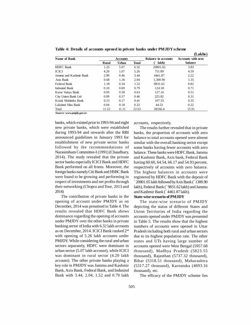
505

banks, which existed prior to 1993-94 and eightnew private banks, which were establishedduring 1993-94 and onwards after the RBIannounced guidelines in January 1993 forestablishment of new private sector banksfollowed by the recommendations ofNarasimham Committee-I (1991) (Chaudhary,2014). The study revealed that the privatesector banks especially ICICI Bank and HDFCBank performed on all fronts. Moreover, theforeign banks namely Citi Bank and HSBC Bankwere found to be growing and performing inrespect of investments and net profits throughtheir networking (Chopra and Toor, 2013 and2014)

The contribution of private banks in theopening of account under PMJDY as onDecember, 2014 was presented in Table 4. Theresults revealed that HDFC Bank showsdominance regarding the opening of accountsunder PMJDY over the other banks in privatebanking sector of India with 6.32 lakh accountsas on December, 2014. ICICI Bank ranked 2nd

with opening of 5.26 lakh accounts underPMJDY. While considering the rural and urbansectors separately, HDFC were dominant inurban sector (5.07 lakh account), while ICICIwas dominant in rural sector (4.20 lakhaccount). The other private banks playing akey role in PMJDY was Jammu and KashmirBank, Axis Bank, Federal Bank, and IndusindBank with 3.44, 2.04, 1.52 and 0.79 lakh

accounts, respectively.The results further revealed that in private

banks, the proportion of accounts with zerobalance to total accounts opened were almostsimilar with the overall banking sector exceptsome banks having fewer accounts with zerobalance. These banks were HDFC Bank, Jammuand Kashmir Bank, Axis bank, Federal Bankhaving 60.60, 64.54, 66.17 and 54.93 percent,respectively of accounts with zero balance.The highest balances in accounts wereregistered by HDFC Bank with the deposit of`20801.65 lakh followed by Axis Bank ( 1300.90lakh), Federal Bank (`9831.62 lakh) and Jammuand Kashmir Bank (`4461.87 lakh).State-wise scenario of PMJDY

The state-wise scenario of PMJDYdepicting the status of different States andUnion Territories of India regarding theaccounts opened under PMJDY was presentedin Table 5. The results show that the highestnumbers of accounts were opened in UttarPradesh including both rural and urban sectorsdue to its highest population rate. The otherstates and UTs having large number ofaccounts opened were West Bengal (5957.68thousand), Madhya Pradesh (5823.55thousand), Rajasthan (5737.32 thousand),Bihar (5318.51 thousand), Maharashtra(5317.27 thousand), Karnataka (4693.16thousand), etc.

The efficacy of the PMJDY scheme lies

Table 4: Details of accounts opened in private banks under PMJDY scheme(Lakhs)

Name of Bank Accounts Balance in accounts(` lakh)

Accounts with zerobalanceRural Urban Total

HDFC Bank 1.25 5.07 6.32 20801.65 3.83ICICI 4.20 1.07 5.26 751.89 4.59Jammu and Kashmir Bank 2.99 0.46 3.44 4461.87 2.22Axis Bank 0.68 1.36 2.04 1,300.90 1.35Federal Bank 1.18 0.34 1.52 9831.62 0.82Indusind Bank 0.10 0.69 0.79 124.58 0.71Karur Vaisya Bank 0.05 0.58 0.63 127.16 0.51City Union Bank Ltd 0.09 0.37 0.46 225.82 0.31Kotak Mahindra Bank 0.23 0.17 0.41 107.55 0.35Lakshmi Vilas Bank 0.04 0.18 0.22 44.53 0.22Total 11.52 11.11 22.63 38166.4 15.91Source: www.pmjdy.gov.in

506

only with the number of accounts opened aslarge number of accounts lies dormant withzero balance. While, the government tries tolink direct benefit transfers (DBTs) to thesebank accounts which is dependent onadequate Aadhaar seeding and resolving otherinfrastructural, targeting and technical glitches(Kapur, 2014).

The results presented in Table 5 revealedthat Telangana was top ranked in terms of

Aadhaar seeded with the accounts (72.08percent). The other states and UTs were Sikkim,Andhra Pradesh, Lakshadweep, HimachalPradesh and Pondicherry with seeding of 70.54,65.86, 60.88, 59.08 and 58.56 percent,respectively.Access to the Banking Facility in Punjab

To check the efficacy of the PMJDYscheme, the Government of India conductsvarious surveys in different states of India.

Table 5: State-wise scenario of PMJDY i n India(Thousand)

State and UT Rural Urban Total Aadhaar seeded (%)Andaman and Nicobar Islands 21.37 7.38 28.75 20.48Andhra Pradesh 2130.01 1670.76 3800.77 65.86Arunachal Pradesh 36.07 8.53 44.60 3.54Assam 1907.64 627.64 2535.29 2.75Bihar 3790.99 1527.53 5318.51 8.05Chandigarh 20.31 124.03 144.34 56.10Chattisgarh 1318.89 832.07 2150.96 10.20Dadra and Nagar Haveli 16.48 5.10 21.58 26.99Daman and Diu 9.78 2.86 12.64 29.37Goa 63.86 21.71 85.57 55.98Gujarat 1731.86 1423.22 3155.08 22.44Haryana 1319.45 1107.12 2426.57 39.42Himachal Pradesh 443.59 58.27 501.86 59.08Jammu and Kashmir 321.41 106.12 427.53 11.63Jharkhand 1124.76 592.01 1716.77 56.75Karnataka 2973.74 1719.42 4693.16 53.39Kerala 709.04 601.69 1310.72 49.72Lakshadweep 3.78 0.15 3.93 60.88Madhya Pradesh 2884.75 2938.80 5823.55 34.31Maharashtra 2562.56 2754.71 5317.27 58.17Manipur 103.45 102.11 205.56 15.62Meghalaya 61.94 32.95 94.89 1.40Mizoram 19.03 34.06 53.08 3.74Nagaland 32.45 28.72 61.17 11.72NCT of Delhi 189.36 1484.27 1673.64 54.78Odisha(Orissa) 1874.08 777.29 2651.37 21.72Pondicherry 38.02 35.66 73.68 58.56Punjab 1807.10 1223.16 3030.25 54.25Rajasthan 3362.39 2374.94 5737.32 38.87Sikkim 37.31 6.33 43.65 70.54Tamil Nadu 2294.90 1697.13 3992.03 21.52Telangana 1735.10 1530.15 3265.24 72.08Tripura 150.77 69.06 219.82 51.84Uttar Pradesh 8242.29 4985.62 13227.91 10.74Uttrakhand 931.02 485.10 1416.12 12.61West Bengal 3997.75 1959.93 5957.68 15.95Total 48267.27 32955.57 81222.84 31.96Source: www.pmjdy.gov.in

507

The information pertaining to the district-wisesurvey on the access to the banking facility inPunjab was presented in Table 6.

banking facilities for all households through abank branch or fixed point (businesscorrespondent), under the slogan MeraKhaata Bhagya Vidhaata (My Bank Account-The creator of the Good Fortune). The crux ofthe plan is to link every household with thebank. The present study seeks to investigatethe current status of the P MJDY in India. Theresults revealed that the contribution of ruralsector in terms of accounts opened underPMJDY was relatively higher than the urbansector in all the banking sectors namely, publicsector banks, regional rural banks and privatebanks. The results further revealed that morethan 70 percent of the accounts opened underPMJDY were opened with zero balance (626.34lakh) depicting the weakness in theimplementation strategy of the plan regardingeasy access to banking system. From the publicsector banks and RRBs, the State Bank of Indiaplays an important and leading role in PMJDYin the opening accounts under PMJDY. Thestate-wise scenario of PMJDY shows that thehighest numbers of accounts were opened inUttar Pradesh including both rural and urbansectors due to its highest population rate.Whereas, Punjab has become the third stateafter Kerala and Madhya Pradesh where allhouseholds have a bank account.REFERENCESAnonymous. 2014. Reserve Bank of India,

Government of India. Retrieved fromwww.rbi.org.in

Anonymous. 2014a. Press Information Bureau.Government of India, New Delhi.

Anonymous. 2014b. The Economic Times. 2nd

October, 14th December, New Delhi.Basu, P. and Srivastava, P. 2005. Scaling-up

microfinance for India’s rural poor. World BankPolicy Research Working Paper No. 3646.Culled from http://web.worldbank.org/archive/website01080/WEB/IMAGES/WPS3646.PDF

Chaudhary, G. 2014. Performance comparison ofprivate sector banks with the public sectorbanks in India. International Journal of EmergingResearch in Management and Technology. 3 (2):5-12.

Chopra, S. and Toor, M.S. 2013. Performance ofprivate sector commercial banks in India after

Table 6: Access to the banking facility inPunjab: The district-wise survey

(Thousand)District Households

surveyedHouseholds

havingA/Cs

District levelcoverage(Percent)

Gurdaspur 234.66 211.86 90.28Kapurthala 57.50 53.37 92.81Jalandhar 429.18 411.61 95.91Hoshiarpur 265.48 141.48 53.29SBS Nagar 112.85 108.76 96.37Fatehgarh Sahib 92.29 88.64 96.04Ludhiana 351.30 307.27 87.46Moga 161.66 144.55 89.42Firozpur 92.91 74.79 80.50Muktsar 154.84 132.42 85.52Faridkot 106.39 95.09 89.38Bathinda 223.58 214.50 95.94Mansa 116.92 112.25 96.01Patiala 301.09 288.58 95.85Amritsar 232.64 181.73 78.12Tarn Taran 146.87 128.22 87.30Rupnagar 246.95 244.69 99.08SAS Nagar 158.91 149.91 94.34Sangrur 284.30 271.16 95.38Barnala 105.09 96.03 91.38Fazilka 123.76 103.37 83.52Pathankot 59.27 54.04 91.18Source: www.pmjdy.gov.in

The results revealed that all the district ofPunjab were having more than 80 percent ofhouseholds having access to banking facilityexcept Amritsar (78.12 percent) and Hoshiarpur(53.29 percent). The highest percentage ofhouseholds having access to banking facilitywas reported in Rupnagar district (99.08percent) followed by SBS Nagar (96.37 percent),Fatehgarh Sahib (96.04 percent), Mansa (96.01percent), and Bathinda (95.94 percent).According to The Economic Times, 14th

December, 2014, Punjab has become the thirdstate after Kerala and Madhya Pradesh whereall households have a bank account(Anonymous, 2014b).CONCLUSIONS

PMJDY scheme has been started with anaim/objective to provide universal access to

508

reforms. Indian Journal of Economics andDevelopment. 9 (1): 50-59.

Chopra, S. and Toor, M.S. 2014. Private sectorcommercial banks in India: Evaluation ofperformance indicators. Indian Journal ofEconomics and Development. 10 (1): 63-70.

Chowhan, S.S. and Pande, J.C. 2014. PradhanMantra Jan Dhan Yojana: A giant leap towardsfinancial inclusion. International Journal ofResearch in Management and Business Studies.1 (4): 19-22.

Das, D. 2010. Informal microfinance in Assam:Empirical evidence from Nalbari and Baksadistricts. Centre for Micro Finance, Institutefor Financial Management and Research,Chennai, Tamil Nadu.

Das, T. 2014. Financial untouchability vis-à-visPrime Minister Jan Dhan Yojana in Assam.Indian Journal of Economics and Development.10 (4): 387-390.

Divya, K.H. 2013. A study on impact of financialinclusion with reference to daily wage earners,India. Journal of Business Management andSocial Sciences Research. 2 (6): 85-92.

Jayadev, M., Moser, R. , Kaul, M., and Tandon, C.2012. Rural retail banking in India: 2020. Culledfrom http://tejas.iimb.ac.in/articles/74.php

Kapur, A. 2014. Let’s not get lost in the numbers:

Highlights of Pradhan Mantri Jan Dhan Yojana(PMJDY). Retrieved fromwww.accounatabilityindia.in.

Khuntia, R. 2014. Pradhan Mantri Jan Dhan Yojana(PMJDY): A new drive towards financialinclusion in India. Zenith International Journalof Business Economics and ManagementResearch. 4 (11): 10-20.

Mishra, B.S. 2006. The performance of regionalrural banks (RRBs) in India: Has past anythingto suggest for future? Reserve Bank of IndiaOccasional Papers. 27 (1-2): 89-118.

Rafiq, N.M. and Premavathy, N. 2014. Financialinclusion: The road ahead. International Journalof Business and Administration Research Review.3 (6): 1-5.

Soni, A.K. and Kapre, A. 2012. Performanceevaluation of regional rural banks in India.Abhinav-National Monthly Refereed Journal ofResearch in Commerce and Management. 1 (11):132-144.

Subbarao. D. 2009. Financial inclusion: Challengesand opportunities. Remarks at the Bankers Club,Kolkata. Retrieved from www.rbi.org.in.

Received: October 07, 2014Accepted: February 16, 2015

509

Indian J Econ Dev DOI No. 10.5958/2322-0430.2015.00059.1Volume 11 No. 2 (2015): 509-515 Research Article

STRUCTURAL SHIFT IN THE MILK COMPOSITIONOF CATTLE WITH INCREASE IN CROSS-BREDSPECIES IN PUNJAB - TIME TO REVISE MILK

STANDARDSKushal Bhalla, Varinder Pal Singh, Inderpreet Kaur and Pranav K. Singh*

ABSTRACT

The present study was conducted to gauge the significant changes thathave come in the composition of milk obtained from cattle species in Punjabover a period of time. Milk standards that have been followed in the state nomore reflect the actual milk quality and composition. Greater prevalence ofexotic strains of cattle have undoubtedly increased the total milk productionin the state but there had been an associated decline in the Fat/SNF (Solidnot fat) levels of milk as compared to the indigenous breeds. Based on afield survey conducted in Bathinda, Gurdaspur and Ludhiana districts ofPunjab state during July 2013 to April 2014, the fat and SNF content ofcommercially predominant Holstein Friesien (H.F) breed of cross bred cattlewere found to be lower than the milk standards which were fixed soon afterindependence when India had only indigenous cattle breed. The emergingdisparity between the milk standards set by the central government and theactual milk composition of cross bred cattle obtained at the farmers’ levelin the state present a strong case for revisiting the existing milk standards.

Keywords: Fat, SNF, indigenous, cross-bred, milk composition, milk standardsJEL Classification: I 18, Q12, Q18

*Research Associate, Assistant Professors(Livestock Economics) and Assistant Professor(Dairy Technology), College of Dairy Science andTechnology, GADVASU, Ludhiana-141004Email: kushal.bhalla@gmail.com

Dairy farming is a complementaryenterprise of agriculture and is the future ofPunjab’s farmers as milch animals provides aregular flow of income whereas cropproduction generates income only after sometime lag. Dairy sector in Punjab has witnessedsome positive structural changes in animalpopulation which has now stabilized. Cattleand buffalo population has declined by 8 and16.4 percent respectively during 1997-2012

(Anonymous, 2012 and 2013). Unproductiveanimals are going out of the production system.That is the reason why milk production isincreasing consistently despite decline inanimal population. But due to fast rising inputcosts as compared to milk procurement prices,the viability of smaller sized dairy farms is atthreat. To make it a viable enterprise, itscommercialization is need of the hour. The sizeof dairy farm should be increased to at least 7-8 milch animals to ensure good returns fromthis profession (Kaur et al. 2012).

Cross bred cows are important animals forcommercial dairy farming. During 2012, therewere 20.65 lakh cross bred cattle in Punjabwhich constitutes about 85 percent of the total

INTRODUCTION

510

cattle population in the state and thisproportion is increasing over time(Anonymous, 2012). Among cross bred cattle,H.F breed is most predominant andcommercially important breed in the statewhich constitutes about 3/4th of Cross bredcattle population in the state (Anonymous,2013a). Most of the large commercial dairyfarms in the state rear H.F. breed because of itshigher productivity. Procurement price of cowmilk is determined based on fat and SNFcontent. It is a fact that H.F. breed milk has lowfat and SNF content due to its higherproductivity. Low fat and SNF content of H.F.breed fetch a lower price as compared to buffalomilk. MILKFED Punjab has fixed 8.2 SNF asstandard value above which premium price of`10 per kg of SNF is paid in cow milk. Up toSNF content of 8.0 no premium price is givenand below 8.0 SNF some deduction is made onprocurement price. Profitability of the dairyfarms depends upon cost of milk production,milk yield and procurement price of milk. Hence,the standards fixed for fat and SNF contentplay an important role in profitability levels ofthese farms. According to prevention of foodadulteration (PFA) Rules, 1954, the fat and SNFcontent for cow milk in the states of Punjab,Haryana and Chandigarh has been fixed at 4.0fat and 8.5 percent SNF (Anonymous, 1954).There are interstate variations in thesestandards too. In other states, these standardsfor fat and SNF are fixed at 3.5 and 8.5 percentrespectively for cow milk.

The milk standards that are prevailing inthe state were set up in the early postindependence era when India was having onlyindigenous cattle and therefore, thesestandards need adequate and quick revisionto take into account the changes that havecome up in the genetic structure of the cattle(Srivastava, 2014). More rigorous checks needto be undertaken to take cognisance of thechanges that have come up in the compositionof milk over a period of time throughintroduction of more exotic strains of cattle.The lower fat levels obtained from the cross

bred cows as a part of their transformed geneticmakeup is wrongly construed as an act of milkadulteration on the part of the farmers. Thisputs the farmer at a position of loss since theproduct is not valued accordingly. Aggravatingthings further, detection of such anadulteration, will be construed as an offencewhich would attract a life term, be cognizable,non-bailable and triable by the sessions court(Sharma, 2014).

Therefore, it becomes imperative tounderstand the changes that have come up inthe dairy sector. This study sheds light on thepattern of growth and resurgence of the crossbred species of cattle in comparison to theindigenous breeds in the Punjab and alsopresents the case for a thorough scrutiny ofthe milk standards as per the prevalent strainsof dairy cattle in the region. With theseconsiderations in mind, we planned andconducted this study to examine the changingtrends in the population of cross bred andindigenous cattle in Punjab vis-à-vis theireffect on milk composition.DATA FOR THE STUDY

For the study, we have available with usboth primary as well as secondary data fromdifferent sources. Data pertaining to milkstandards and milk composition of indigenousand cross bred cattle were reproduced fromthe prevention of food adulteration (PFA)website and from the book Outlines of DairyTechnology by Sukumar De. Further, datarelated to change in cattle population in Indiaover time, state-wise growth and distributionof cattle population in India, breed-wisegrowth of cattle population in Punjab andincrease in milk production and milk yield inPunjab over time were obtained from basicanimal husbandry statistics, livestock census,animal husbandry department of Punjab andother published sources.Study Area

For getting the actual data on fat and SNFcontent of cross bred cattle in the state, asurvey was conducted in three districts viz.Ludhiana and Gurdaspur from Central Zone

511

and Bathinda from South-Western Zone.Year of Study

The survey was conducted for ten monthsduring the period July 2013 to April 2014Sampling Design and Technique

From each selected district, three blockswere selected randomly namely, Pakhowal,Machhiwara and Sidhwan Bet from Ludhiana;Dhariwal, Kahnowal and Fatehgarh Churianfrom Gurdaspur; Moud Mandi, Sangat andPhul from Bathinda districts. Five farmersrearing H.F. cattle were selected from a clusterof 2-4 villages from each selected blockrandomly. Hence 15 farmers were selected fromeach district and total sample constituted of45 farmers from all the three selected districts.One H.F. cow preferably in initial stage oflactation was identified from each of selected45 farmers for recording the fat and SNF dataon monthly basis. The data was recordedpreferably on same dates in each month. Themilk sample of 200 ml was taken early in morningfor each cow between 6.00 am to 7.30 am. Themilk from selected cow was well mixed with aplunger in a separate container before takingthe sample. Then the sample was taken tonearby Verka milk plant or milk co-operativesociety for fat and SNF testing. The animalwhich got dried in later months of study periodwas excluded from the survey and fat and SNFdata of remaining animals were recorded. Thedata are presented in tabular format to drawthe inferences.Analytical Tools

Simple statistical tools like averages andpercentages were used to compare the dataand draw inferences.

Parameters to be estimated:Fat and SNF Content in milk of H.F. cross

bred cowsRESULTS AND DISCUSSIONS

In the following tables we try to understandthe milk composition, pattern of growth anddecay in the population of cross bred andindigenous cattle at the state and national level,prevalence of different breeds of cattle inPunjab, their milk production and milk yield

over time. More specifically, Table 1 presentedbelow provides the chemical composition ofmilk in the indigenous breeds.

Based upon the compositional values, themilk standards were fixed by the Prevention ofFood Adulteration (PFA) Act in 1954(Anonymous, 1954) and subsequentlyadopted as such by FSSA 2006 and FSSR 2011which set the minimum Fat and SNF values forcow milk to be 4 and 8.5 respectively for thestate of Punjab, Chandigarh, and Haryana inIndia (Anonymous, 2011). These standardswere promulgated or derived based upon themilk obtained from indigenous breeds and arestill adhered to. We can see from the Table 1that water constitutes nearly 86 percent of themilk followed by SNF and Fat. The SNF portionof the milk comprises of protein, lactose andash. The Fat content varied from as high as4.90 in Sindhi to as low as 4.55 in the case ofTharparkar and Sahiwal breeds of cow. Sindhiand Sahiwal had the highest SNF of 9.03followed by Tharparkar (8.87) and Gir (8.83).

In case of Punjab, the indigenous breedstoday make up nearly 15 percent of the totalcattle population and cross bred cowsconstitute almost 85 percent. The milkstandards that exist today were set up decadesago considering the milk composition of onlyindigenous breeds which are todaysignificantly replaced by cross bred cows, onaccount of their higher productivity, but adifferent milk composition. Given thistransformation, it stands to reason that theobsolete and outdated milk standards shouldnot be imposed on the milk producers of the

Table 1: Chemical composition of milk forindigenous cattle breedsCompostion(%)

Breed of cowSindhi Gir Tharparkar Sahiwal

Water 86.07 86.44 86.58 86.42Fat 4.9 4.73 4.55 4.55Protein 3.42 3.32 3.36 3.33Lactose 4.91 4.85 4.83 5.04Ash 0.7 0.66 0.68 0.66SNF 9.03 8.83 8.87 9.03Source: De, 2005

512

Punjab state. Even in Haryana, which is aneighboring state of Punjab, there has been apalpable shift in the cattle population fromindigenous to cross bred cows. Since theexisting milk standards do not meet the milk ofcross bred cows, therefore, the dairy farmersoppose these conventional milk standards anddemand lowering the fat and SNF content to3.2 and 8.2 percent respectively (Anonymous,2010). Taking cognizance of the fact that milkfrom cross bred and exotic cattle does notmatch the minimum 4 percent fat requirement(Anonymous, 2013a), a panel of experts alongwith the Haryana Kisan Ayog has suggestedrecommendations, to address this problemfaced by farmers through adoption of revisedand updated milk standards.

Next, if we have a look at the change incattle population in India over time from 1982to 2012, it is evident there is a significantdecline in indigenous cattle head from as highas 95.39 percent in 1982 to as low as 79.19percent in 2012 (Table 2). The decline becamemore apparent since 1992. On the other handthe percent cattle head of cross bred cowsincreased from as low as 4.61 percent in 1982to as high as 20.81 percent in 2012. This clearlyshows the structural change that has occurred

in the cattle population over a period of time.The cross bred cattle population increasedcontinuously whereas the indigenous cattlepopulation noticed a significant decline since1992. The cross bred cows are becoming moreand more popular among the dairy farmers.

The results presented in Table 3 portraythe state wise evolution of the number of crossbred and indigenous cows from 1987 to 2012.There was a noticeable increase in cross bredcattle population in Punjab, with numbersincreasing from 1579 thousand in 1987 to 2065thousand in 2012. At the same time, the numberof indigenous cattle in the state declinedabruptly from 2830 thousand to a mere 363thousand. Such a huge drop in the number ofindigenous cattle breeds in the state of Punjabmake a strong case for revoking the old milkstandards and setting up new standards thatmatch the current reality of the cattle mix.Haryana being a neighboring state of Punjabhas also noticed an increase in the number ofcross bred cows and a significant decline inthe number of indigenous cows. Most otherstates like Andhra Pradesh, Bihar, Gujarat,Karnataka, Rajasthan, Tamil Nadu, UttarPradesh and West Bengal noticed a significantincrease in the number of cross bred cattle from1987 to 2012. Apart from states like Gujarat,Assam, and Rajasthan where the number ofindigenous cattle had increased over a periodof time, almost all the other states have noticeda decline in the number of indigenous cattle.At the national level the cross bred cowsincreased from 11413 thousand in 1987 to 39731thousand in 2012 and the indigenous breedsof cattle decreased from 199695 thousand in1987 to 151172 thousand in 2012.

The paradox at this point of time is the factthat although the proportion of cross bredcattle in Punjab, Haryana and Chandigarhstands huge at 85, 55 and 78 percentrespectively, the current milk standard for Fatthat prevails in these states is still 4 percent ascompared to 3.5 percent in rest of the states.

Breed-wise population of cross bred andindigenous cattle in Punjab during 2007 (18th

Table 2: Cattle population in India overtime

(Thousands)Year Cross bred Indigenous Total cattle1982 8805 182011 190816

(4.61) (95.39) (100.00)1987 11413 188282 199695

(5.72) (94.28) (100.00)1992 15216 189367 204583

(7.44) (92.56) (100.00)1997 20099 178782 198881

(10.11) (89.89) (100.00)2003 24687 160495 185182

(13.33) (86.67) (100.00)2007 33060 166015 199075

(16.61) (83.39) (100.00)2012 39730 151170 190900

(20.81) (79.19) (100.00)Source: Anonymous, 2012 and 2013bFigures in parentheses indicate percentage to total cattlepopulation in respective years

513

Livestock Census) has been presented in Table4. It is revealed that out of 17.61 lakh cattle,cross bred constitutes 12.59 lakh (71.5 per cent)and as per 19th Livestock Census 2012, thisproportion increased to as high as 85 per cent.Among the cross bred cattle, H.F. is the mostimportant breed which constitutes 9.41 lakh(75 per cent). Next important breed is Jerseywhich constitutes 1.64 lakh (13 per cent). Theimportant indigenous cattle breeds areHaryana and Sahiwal. Of the total cattlepopulation, H.F. breed constitutes more than53 per cent.

The perusal of Table 5 casts light on the

Table 3: State-wise dynamics of crossbred cattle(Thousand)

States/UTs Cross Bred Indigenous1987 1992 1997 2003 2007 2012 1987 1992 1997 2003 2007 2012

Andhra Pradesh 390 484 751 1107 1898 2397 12375 10946 9851 8193 9325 7199Arunachal Pradesh 22 19 11 13 29 23 310 324 441 445 474 441Assam 228 325 369 440 410 396 7279 10118 7727 7999 9631 9912Bihar 173 191 232 1274 1976 3475 20839 22154 24366 9455 10583 8757Chhattisgarh - - 105 253 186 178 - - 8680 8629 9305 9637Goa 162 233 7 12 16 18 6240 6804 81 63 55 39Gujarat 5 6 342 639 1142 1927 112 98 6406 6785 6834 8057Haryana 242 417 848 573 566 996 2198 2136 1552 967 986 812Himachal Pradesh 160 281 368 677 793 984 2244 2165 1805 1559 1476 1165Jammu & Kashmir 527 793 1083 1320 1677 1470 2765 3055 2092 1764 1766 1328Jharkhand - - - 145 191 256 - - - 7513 8590 8474Karnataka 719 626 1293 1602 2193 2913 10174 13173 9539 7936 8309 6603Kerala 1701 1759 1957 1735 1621 1252 3408 3524 533 387 119 77Madhya Pradesh 108 208 177 317 475 841 28549 28688 19320 18595 21441 18761Maharashtra - 1773 2457 2776 3122 3651 16979 17446 15615 13527 13061 11833Manipur 65 71 69 69 66 44 770 719 439 349 276 220Meghalaya 19 15 17 23 27 35 587 635 738 744 860 861Mizoram 5 6 8 9 11 11 50 59 26 27 24 24Nagaland 74 131 154 243 254 129 203 332 230 208 216 106Orissa 563 600 912 1063 1703 1306 13636 13841 12898 12840 10607 10315Punjab 1579 1628 1828 1531 1278 2065 2830 2909 810 508 498 363Rajasthan 73 121 211 464 816 1735 10920 11699 11931 10390 11304 11589Sikkim 43 45 52 80 73 127 184 198 91 79 62 13Tamilnadu 1141 1839 3506 5140 7383 6354 9342 9278 5541 4001 3806 2460Tripura 61 108 73 57 79 133 827 949 1155 702 875 816Uttar Pradesh 2586 2498 2105 1634 1945 3579 26320 25635 17911 16917 16938 15978Uttaranchal - - 103 228 339 498 - - 1927 1961 1896 1508West Bengal 712 960 936 1119 2642 2796 20311 17453 16895 17794 16546 13718A& Nicobar 3 1 6 13 14 16 46 50 54 51 36 30Chandigarh 5 5 6 5 5 7 7 5 1 1 1 2Haveli 1 0 1 1 1 1 47 49 59 49 55 41Daman & Diu - - 0.01 0.08 0 0 - 8 6 4 3 2Delhi 4 13 60 58 44 61 53 41 36 34 47 25Lakshadweep - 0 1 2 4 1 1 2 3 2 3 2Pondicherry 42 60 50 63 78 57 89 90 23 16 6 3All India 11413 15216 20099 24686 33060 39731 199695 204583 178783 160495 166015 151172 Source: Anonymous 2013b

Table 4: Breed wise population of cows inPunjab, 2007

(Lakhs)Breed Male Female TotalCross bredExotic 0.02 0.08 0.10Jersey 0.26 1.38 1.64H.F. 1.45 7.96 9.41Others exotic 0.23 1.20 1.44Sub-total 1.96 10.62 12.59Desi cattleSahiwal 0.13 0.36 0.49Haryana 1.23 0.99 2.22Others 0.91 1.41 2.32Sub-total 2.27 2.76 5.03Total cows 4.24 13.37 17.61Source: Anonymous 2007

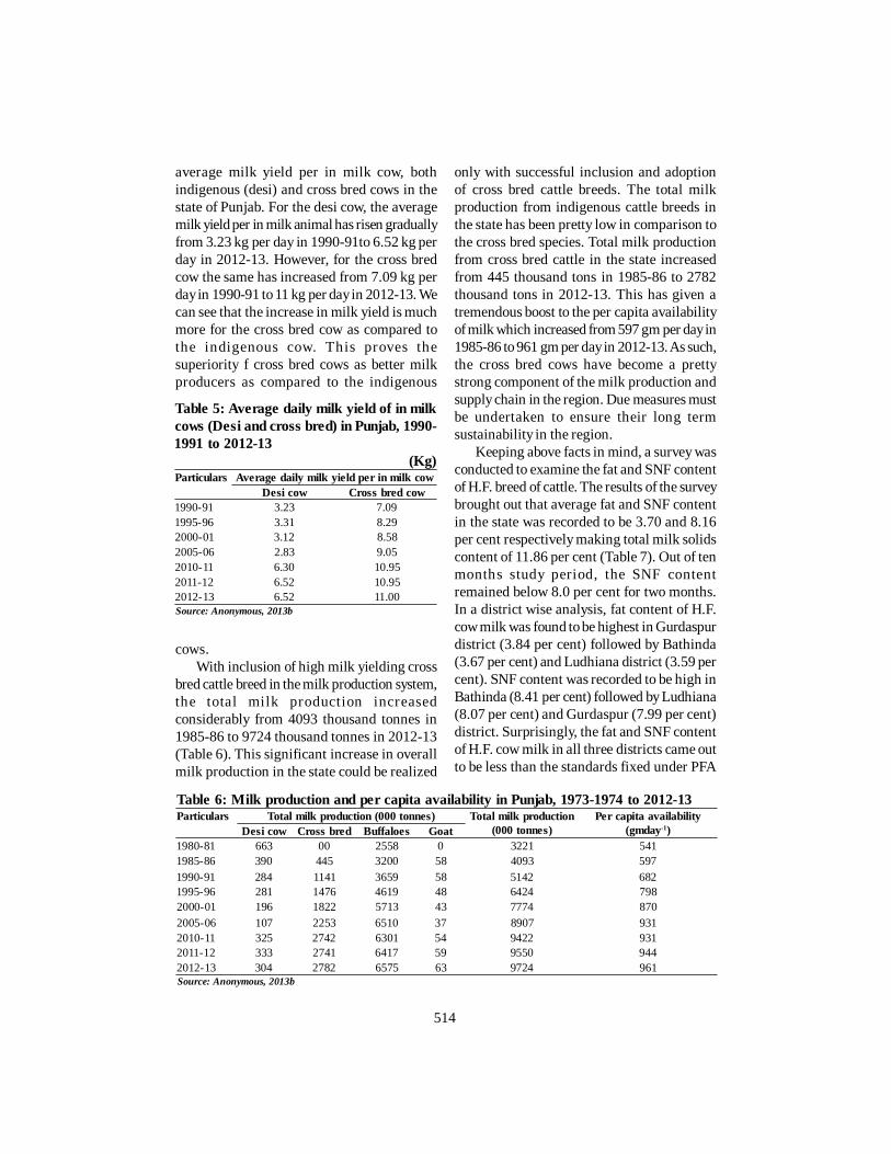
514

average milk yield per in milk cow, bothindigenous (desi) and cross bred cows in thestate of Punjab. For the desi cow, the averagemilk yield per in milk animal has risen graduallyfrom 3.23 kg per day in 1990-91to 6.52 kg perday in 2012-13. However, for the cross bredcow the same has increased from 7.09 kg perday in 1990-91 to 11 kg per day in 2012-13. Wecan see that the increase in milk yield is muchmore for the cross bred cow as compared tothe indigenous cow. This proves thesuperiority f cross bred cows as better milkproducers as compared to the indigenous

only with successful inclusion and adoptionof cross bred cattle breeds. The total milkproduction from indigenous cattle breeds inthe state has been pretty low in comparison tothe cross bred species. Total milk productionfrom cross bred cattle in the state increasedfrom 445 thousand tons in 1985-86 to 2782thousand tons in 2012-13. This has given atremendous boost to the per capita availabilityof milk which increased from 597 gm per day in1985-86 to 961 gm per day in 2012-13. As such,the cross bred cows have become a prettystrong component of the milk production andsupply chain in the region. Due measures mustbe undertaken to ensure their long termsustainability in the region.

Keeping above facts in mind, a survey wasconducted to examine the fat and SNF contentof H.F. breed of cattle. The results of the surveybrought out that average fat and SNF contentin the state was recorded to be 3.70 and 8.16per cent respectively making total milk solidscontent of 11.86 per cent (Table 7). Out of tenmonths study period, the SNF contentremained below 8.0 per cent for two months.In a district wise analysis, fat content of H.F.cow milk was found to be highest in Gurdaspurdistrict (3.84 per cent) followed by Bathinda(3.67 per cent) and Ludhiana district (3.59 percent). SNF content was recorded to be high inBathinda (8.41 per cent) followed by Ludhiana(8.07 per cent) and Gurdaspur (7.99 per cent)district. Surprisingly, the fat and SNF contentof H.F. cow milk in all three districts came outto be less than the standards fixed under PFA

cows.With inclusion of high milk yielding cross

bred cattle breed in the milk production system,the total milk production increasedconsiderably from 4093 thousand tonnes in1985-86 to 9724 thousand tonnes in 2012-13(Table 6). This significant increase in overallmilk production in the state could be realized

Table 5: Average daily milk yield of in milkcows (Desi and cross bred) in Punjab, 1990-1991 to 2012-13

(Kg)Particulars Average daily milk yield per in milk cow

Desi cow Cross bred cow1990-91 3.23 7.091995-96 3.31 8.292000-01 3.12 8.582005-06 2.83 9.052010-11 6.30 10.952011-12 6.52 10.952012-13 6.52 11.00Source: Anonymous, 2013b

Table 6: Milk production and per capita availability in Punjab, 1973-1974 to 2012-13Particulars Total milk production (000 tonnes) Total milk production

(000 tonnes)Per capita availability

(gmday-1)Desi cow Cross bred Buffaloes Goat1980-81 663 00 2558 0 3221 5411985-86 390 445 3200 58 4093 5971990-91 284 1141 3659 58 5142 6821995-96 281 1476 4619 48 6424 7982000-01 196 1822 5713 43 7774 8702005-06 107 2253 6510 37 8907 9312010-11 325 2742 6301 54 9422 9312011-12 333 2741 6417 59 9550 9442012-13 304 2782 6575 63 9724 961Source: Anonymous, 2013b

515

Table 7: Fat and SNF of cow milk from July, 2013 to April, 2014 Months Bathinda Gurdaspur Ludhiana Punjab

Fat SNF TS Fat SNF TS Fat SNF TS Fat SNF TSJuly 3.69 8.17 11.86 3.59 8.15 11.74 3.43 8.37 11.80 3.57 8.23 11.80August 3.47 8.37 11.85 3.61 8.27 11.89 3.38 8.08 11.46 3.49 8.24 11.73September 3.82 8.17 11.99 3.69 8.02 11.71 3.59 8.28 11.87 3.70 8.16 11.86October 3.67 8.35 12.02 3.75 8.16 11.90 3.75 6.98 10.73 3.72 7.83 11.55November 3.75 8.45 12.21 3.75 8.22 11.96 3.78 7.24 11.02 3.76 7.97 11.73December 3.78 8.65 12.43 3.88 8.17 12.05 3.83 8.35 12.18 3.83 8.39 12.22January 3.65 8.53 12.17 3.91 7.96 11.87 3.54 8.31 11.85 3.70 8.26 11.96February 3.57 8.53 12.10 4.03 7.86 11.88 3.67 8.39 12.05 3.75 8.26 12.01March 3.65 8.42 12.07 4.05 7.60 11.65 3.47 8.35 11.82 3.72 8.12 11.85April 3.62 8.45 12.07 4.18 7.47 11.65 3.45 8.37 11.82 3.75 8.10 11.85Overall 3.67 8.41 12.08 3.84 7.99 11.83 3.59 8.07 11.66 3.70 8.16 11.86Source: Field SurveyTS: Total solids

act. SNF content in Ludhiana district turnedout to be less than standard SNF value of 8.2fixed by MILKFED below which no premiumprice is given for cow milk. SNF content inGurdaspur district was even less than 8.0 forfour months where further deduction is madefor procurement price of milk.CONCLUSIONS

From the ongoing discussion, it may beconcluded that the standards of fat and SNFfixed under PFA rules need to be revised sothat the farmers rearing H.F. breed should notbe at disadvantage compared to other cattlebreeds and buffaloes. These standards shouldbe brought down to some reasonable level sothat farmers can get remunerative price for milkand at the same time, they may not becomedefaulters under PFA rules on the ground thatthey have done some adulteration in milk andface some legal action. Therefore, the need isto create more favorable environment for thedomestication and rearing of cross bredspecies through more accurate and revisedmilk standards that justify the milk compositionof the exotic strains of cattle.REFERENCESAnonymous. 1954. Prevention of Food Adulteration

Act and Rules, 1954 (Act 37 of 1954)Anonymous. 2007. 18th Livestock Census-2007

All India Report, Government of India, Ministryof Agriculture, Department of AnimalHusbandry, Dairying and Fisheries, Krishi

Bhawan, New DelhiAnonymous. 2010. Report on policy issues and

options based on interface with farmers,Haryana Kisan Ayog.

Anonymous. 2011. Food Safety Regulation 2011,Ministry of health and family welfare (FoodSafety and Standards Authority of India,Government of India, New Delhi.

Anonymous. 2012. 19th Livestock census -2012All India Report, Government of India, Ministryof Agriculture, Department of AnimalHusbandry, Dairying and Fisheries, KrishiBhawan, New Delhi.

Anonymous. 2013. Haryana Kisan Ayog. AQuarterly Newsletter. 3 (2): 3-4.

Anonymous. 2013a. Basic Animal HusbandryStatistics, Ministry of Agriculture, Departmentof Animal Husbandry, Dairying and Fisheries,Krishi Bhawan, New Delhi

De, S. 2005. Outlines of Dairy Technology, Publishedin India by Oxford University Press, Universityof Delhi.

Kaur, I., Singh, V.P., Kaur, H., and, P, Singh. 2012.Cost-benefit analysis of cow milk productionin Punjab. Journal of Agriculture Developmentand Policy. 22 (1): 67-74.

Sharma. P. 2014. Selling adulterated milk in Punjabmay lead to life in jail. Hindustan Times, May14, 2014

Srivastava A.K. 2014. Need to change old rules ofmilk standards. Hindustan Times, May 14,2014.

Received: January 22, 2015Accepted: April 16, 2015

516

517

Indian J Econ Dev DOI No. 10.5958/2322-0430.2015.00060.8Volume 11 No. 2 (2015): 517-532 Research Article

PLIGHT OF WOMEN LABOURERS IN RURALPUNJAB

Dharam Pal* and Gian Singh#

ABSTRACT

The present study revealed that a large majority of the respondents have toface the problem of irregularity of work. Almost, all the respondents in thesampled districts do not enjoy any facility at their workplace. About one-third of the female respondents were not being paid equal wages for equalwork with men. Majority of the sampled women labourers are not awareabout the standard working hours fixed by the government. The study alsorevealed that a majority of the women labourers were suffering from someserious diseases. In addition to the problems faced at the workplace, thewomen labourers have to face many problems on their domestic front also.After the whole day work, they have the responsibility to look after theirchildren and attend the domestic chores. Even during the period of theirillness, more than one-fourth of the respondents have reported that they donot get the co-operation of their husbands rather they are ill-treated andforced to go for work. Some of the respondents have complained that theyhave been the victims of domestic violence. Apart from this, slightly morethan one-third of the respondents have revealed that they were not involvedin all important family matters. All this makes their situation moremiserable.

Keywords: Domestic violence, wages, women labourer, work placeJEL Classification: C81, E24, J12, J31, J43, J81

*Assistant Professor in Economics, GGDSDCollege Kheri Gurna, Banur, Patiala and #Professor,Department of Economics, Punjabi University,Patiala-147001.Email: dharampaleco@gmail.com

INTRODUCTIONThe situation of women labourers in rural

India is quite deplorable. They are one amongthe worst suffers of socio-cultural, political andeconomic exploitation, injustice, oppressionand violence. Their woes and miseries areboundless. They are mainly employed inunorganized sector of the Indian economy as

daily wagers and marginal workers. The lackof adequate employment opportunities, limitedskills and illiteracy have made their mobilityextremely limited and prevented them fromachieving an independent status. They do notenjoy any social security, maternity benefits,pension schemes or any other kind ofeconomic protection. With the adoption ofpolicies of globalization in India, theiremployment opportunities are likely to befurther reduced as they will have to suffer stiffcompetition from foreign technology andmodern methods of agriculture (Jaiswal, 2009).

In the rural areas, women are more likely to

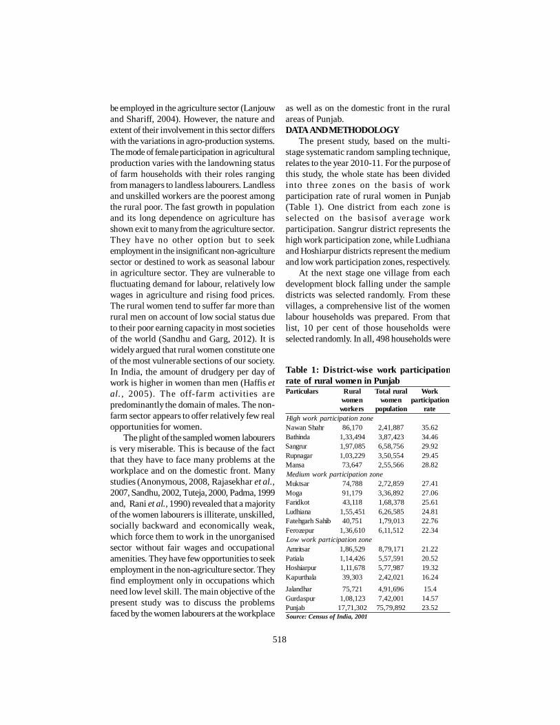
518

be employed in the agriculture sector (Lanjouwand Shariff, 2004). However, the nature andextent of their involvement in this sector differswith the variations in agro-production systems.The mode of female participation in agriculturalproduction varies with the landowning statusof farm households with their roles rangingfrom managers to landless labourers. Landlessand unskilled workers are the poorest amongthe rural poor. The fast growth in populationand its long dependence on agriculture hasshown exit to many from the agriculture sector.They have no other option but to seekemployment in the insignificant non-agriculturesector or destined to work as seasonal labourin agriculture sector. They are vulnerable tofluctuating demand for labour, relatively lowwages in agriculture and rising food prices.The rural women tend to suffer far more thanrural men on account of low social status dueto their poor earning capacity in most societiesof the world (Sandhu and Garg, 2012). It iswidely argued that rural women constitute oneof the most vulnerable sections of our society.In India, the amount of drudgery per day ofwork is higher in women than men (Haffis etal. , 2005). The off-farm activities arepredominantly the domain of males. The non-farm sector appears to offer relatively few realopportunities for women.

The plight of the sampled women labourersis very miserable. This is because of the factthat they have to face many problems at theworkplace and on the domestic front. Manystudies (Anonymous, 2008, Rajasekhar et al.,2007, Sandhu, 2002, Tuteja, 2000, Padma, 1999and, Rani et al., 1990) revealed that a majorityof the women labourers is illiterate, unskilled,socially backward and economically weak,which force them to work in the unorganisedsector without fair wages and occupationalamenities. They have few opportunities to seekemployment in the non-agriculture sector. Theyfind employment only in occupations whichneed low level skill. The main objective of thepresent study was to discuss the problemsfaced by the women labourers at the workplace

as well as on the domestic front in the ruralareas of Punjab.DATA AND METHODOLOGY

The present study, based on the multi-stage systematic random sampling technique,relates to the year 2010-11. For the purpose ofthis study, the whole state has been dividedinto three zones on the basis of workparticipation rate of rural women in Punjab(Table 1). One district from each zone isselected on the basisof average workparticipation. Sangrur district represents thehigh work participation zone, while Ludhianaand Hoshiarpur districts represent the mediumand low work participation zones, respectively.

At the next stage one village from eachdevelopment block falling under the sampledistricts was selected randomly. From thesevillages, a comprehensive list of the womenlabour households was prepared. From thatlist, 10 per cent of those households wereselected randomly. In all, 498 households were

Table 1: District-wise work participationrate of rural women in PunjabParticulars Rural

womenworkers

Total ruralwomen

population

Workparticipation

rateHigh work participation zoneNawan Shahr 86,170 2,41,887 35.62Bathinda 1,33,494 3,87,423 34.46Sangrur 1,97,085 6,58,756 29.92Rupnagar 1,03,229 3,50,554 29.45Mansa 73,647 2,55,566 28.82Medium work participation zoneMuktsar 74,788 2,72,859 27.41Moga 91,179 3,36,892 27.06Faridkot 43,118 1,68,378 25.61Ludhiana 1,55,451 6,26,585 24.81Fatehgarh Sahib 40,751 1,79,013 22.76Ferozepur 1,36,610 6,11,512 22.34Low work participation zoneAmritsar 1,86,529 8,79,171 21.22Patiala 1,14,426 5,57,591 20.52Hoshiarpur 1,11,678 5,77,987 19.32Kapurthala 39,303 2,42,021 16.24Jalandhar 75,721 4,91,696 15.4Gurdaspur 1,08,123 7,42,001 14.57Punjab 17,71,302 75,79,892 23.52Source: Census of India, 2001

519

selected for the survey. These 498 selectedhouseholds were visited personally to collectinformation on the various socio-economicaspects of their families. The information wasrecorded by personal interview methodthrough a pre-tested structured scheduledesigned for the purpose. The results wereanalysed by using the mean values andpercentages.

The whole analysis has been divided intotwo sections. Section-I discusses the problemsfaced by women labourers at their workplacein the rural areas of the sampled districts ofPunjab; and Section-II relates with theirproblems on the domestic front.RESULTS AND DISCUSSION

Section-IProblems Faced by Women Labourers at theirWorkplace

The inter-district analysis of the sectoralemployment of the sampled women labourersindicates that a majority of the respondentswere working both in agriculture and non-agriculture sectors (Table 2). The results showthat the percentage of respondents workingin both agriculture and non-agriculture sectorswas the highest in Ludhiana district (81.64 percent) followed by Sangrur (77.90 per cent) andHoshiarpur (68.32 per cent) districts. The labourabsorption capacity of the agriculture sectorhas reached the plateau and it is not able tokeep the rural workers engaged throughoutthe year. The rural households also seekemployment outside the agriculture sector totide over the inter-year and intra-year variationsin agricultural income (Bhakar et al., 2007).

Further, the percentage of respondentsworking in agriculture sector alone was thehighest (16.84 per cent) in Sangrur district andthe lowest (12.08 per cent) in Ludhiana district.It was 13.86 per cent in Hoshiarpur district.While in the case of respondents working onlyin non-agriculture sector, the highestproportion of the respondents (17.82 per cent)was in Hoshiarpur district, followed by 6.28per cent in Ludhiana district and 5.26 per centin Sangrur district. The proportion of the

respondents working in their native villageswas higher in Hoshiarpur district (82.18 percent) than both Sangrur (72.63 per cent) andLudhiana (64.25 per cent) districts. It alsoimplies that a higher proportion of the

Table 2: Sectoral distribution of sampledwomen labourersParticulars Workplace Sampled

womenlabourers

In nativevillage

Outsidenative village

SangrurAgriculture 29 3 32

(21.02) (5.77) (16.84)[90.62] [9.38] [100.00]

Non-agriculture 3 7 10(2.17) (13.46) (5.26)[30.00] [70.00] [100.00]

Both agricultureand non-agriculture

106 42 148(76.81) (80.77) (77.90)[71.62] [28.38] [100.00]

Total 138 52 190(100.00) (100.00) (100.00)[72.63] [27.37] [100.00]

LudhianaAgriculture 23 2 25

(17.29) (2.70) (12.08)[92.00] [8.00] [100.00]

Non-agriculture 5 8 13(3.76) (10.81) (6.28)[38.46] [61.54] [100.00]

Both agricultureand non-agriculture

105 64 169(78.95) (86.49) (81.64)[62.13] [37.87] [100.00]

Total 133 74 207(100.00) (100.00) (100.00)[64.25] [35.75] [100.00]

HoshiarpurAgriculture 13 1 14

(15.66) (5.56) (13.86)[92.86] [7.14] [100.00]

Non-agriculture 10 8 18(12.05) (44.44) (17.82)[55.56] [44.44] [100.00]

Both agricultureand non-agriculture

60 9 69

(72.29) (50.00) (68.32)[86.96] [13.04] [100.00]

Total 83 18 101(100.00) (100.00) (100.00)[82.18] [17.82] [100.00]

Source: Field Survey, 2010-11Note: The figures given in upper and lower brackets indicatecolumn-wise and row-wise percentages respectively

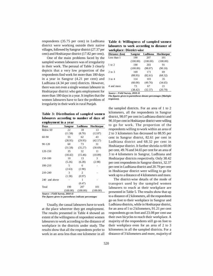
520

respondents (35.75 per cent) in Ludhianadistrict were working outside their nativevillages, followed by Sangrur district (27.37 percent) and Hoshiarpur district (17.82 per cent).

One of the main problems faced by thesampled women labourers was of irregularityin their work. The perusal of Table 3 clearlydepicts that a very low proportion of therespondents find work for more than 180 daysin a year in Sangrur (4.21 per cent) andLudhiana (4.34 per cent) districts. However,there was not even a single woman labourer inHoshiarpur district who gets employment formore than 180 days in a year. It implies that thewomen labourers have to face the problem ofirregularity in their work in rural Punjab.

the sampled districts. For an area of 1 to 2kilometers, all the respondents in Sangrurdistrict, 98.07 per cent in Ludhiana district and90.10 per cent in Hoshiarpur district were willingto go for work. The proportion of therespondents willing to work within an area of2 to 3 kilometers has decreased to 88.95 percent in Sangrur district, 82.61 per cent inLudhiana district and 68.32 per cent inHoshiarpur district. It further shrinks to 60.00per cent, 49.76 and 34.65 per cent for an area of3 to 4 kilometers in Sangrur, Ludhiana andHoshiarpur districts respectively. Only 38.42per cent respondents in Sangrur district, 32.37per cent in Ludhiana district and 20.79 per centin Hoshiarpur district were willing to go forwork up to a distance of 4 kilometers and more.

The district-wise details of the mode oftransport used by the sampled womenlabourers to reach at their workplace arepresented in Table 5. The results show that upto a distance of 2 kilometers, all the respondentsgo on foot to their workplace in Sangrur andLudhiana districts, while in Hoshiarpur district,for an area of 1 to 2 kilometers, 91.21 per centrespondents go on foot and 23.08 per cent usetheir own bicycles to reach their workplace. Amajority of the respondents still go on foot totheir workplace even for an area of 2 to 3kilometers in all the sampled districts. For adistance of 3 kilometers and more, majority of

Table 3: Distribution of sampled womenlabourers according to number of days ofemployment in a yearDays Sangrur Ludhiana HoshiarpurBelow 60 22 18 13

(11.58) (8.70) (12.87)60-90 55 62 43

(28.95) (29.95) (42.57)90-120 60 73 31

(31.58) (35.27) (30.69)120-150 35 32 11

(18.42) (15.46) (10.89)150-180 10 13 3

(5.26) (6.28) (2.98)180-210 5 6 -

(2.63) (2.90)210-240 3 2 -

(1.58) (0.97)240 and above - 1 -

(0.47)Total 190 207 101

(100.00) (100.00) (100.00)Source : Field Survey, 2010-11The figures given in parentheses indicate percentages

Usually, the casual labourers have to workat the place wherever they get employment.The results presented in Table 4 showed anextent of the willingness of respondent womenlabourers to work according to the distance ofworkplace in the districts under study. Theresults show that all the respondents prefer towork in an area less than one kilometer in all

Table 4: Willingness of sampled womenlabourers to work according to distance ofworkplace: District-wiseDistance (km) Sangrur Ludhiana HoshiarpurLess than 1 190 207 101

(100.00) (100.00) (100.00)1 to 2 190 203 91

(100.00) (98.07) (90.10)2 to 3 169 171 69

(88.95) (82.61) (68.32)3 to 4 114 103 35

(60.00) (49.76) (34.65)4 and more 73 67 21

(38.42) (32.37) (20.79)Source : Field Survey, 2010-11The figures given in parentheses denote percentages (Multipleresponses).

521

the respondents reach their workplace usingemployer’s means of transport in all the sampledistricts. The public transport facility is onlyviable for a distance exceeding 3 kilometers inall the sampled districts.

There is no doubt about the fact that basicfacilities such as arrangement of toilet, canteen,creche, etc. made available to the labourers attheir workplace, contribute highly towardstheir involvement in the work. The resultspresented in Table 6 clearly show that basicfacilities were not available to the majority of

the respondents at their workplace in sampledistricts. As high as, 96.04 per cent respondentsin Hoshiarpur district and 95.26 and 93.72 percent of the respondents in Sangrur andLudhiana districts, respectively did not enjoyany facility at their workplace. During the fieldsurvey, it has been observed that theagricultural labourers do not get any facility attheir workplace, while labourers in non-agriculture sector are getting some of thosefacilities.

With regard to the type of facilities, only

Table 5: Mode of transport use to reach at the workplace by women labourersParticulars Distance (km)

Less than 1 1 to 2 2 to 3 3 to 4 4 and moreSangrurOn foot 190 190 136 43 14

(100.00) (100.00) (80.47) (37.72) (19.18)Bicycle - - 25 27 27

(14.79) (23.68) (36.99)Employer transport - - 57 83 65

(33.73) (72.81) (89.04)Public transport - - 18 24

(15.79) (32.88)Total 190 190 169 114 73

(100.00) (100.00) (100.00) (100.00) (100.00)LudhianaOn foot 207 203 132 41 16

(100.00) (100.00) (77.19) (39.81) (23.88)Bicycle - - 30 30 28

(17.54) (29.13) (41.79)Employer transport - - 63 84 61

(36.84) (81.55) (91.04)Public transport - - - 15 18

(14.56) (26.87)Total 207 203 171 103 67

(100.00) (100.00) (100.00) (100.00) (100.00)HoshiarpurOn foot 101 83 45 8 -

(100.00) (91.21) (65.22) (22.86)Bicycle - 21 21 19 17

(23.08) (30.43) (54.29) (80.95)Employer transport - - 44 30 20

(63.77) (85.71) (95.24)Public transport - - - 8 10

(22.86) (47.62)Total 101 91 69 35 21

(100.00) (100.00) (100.00) (100.00) (100.00)Source : Field Survey, 2010-11The figures given in parentheses represent column-wise percentages (multiple responses)

522

4.83 per cent respondents in Ludhiana district,4.21 per cent in Sangrur district and 3.96 percent in Hoshiarpur district have been providedthe toilet facility at their workplace. Thecanteen facility was available to only 4.35, 3.16and 1.98 per cent respondents in Ludhiana,Sangrur and Hoshiarpur districts respectively.A negligible proportion of the respondents(0.99 per cent) in Hoshiarpur district and 0.97per cent in Ludhiana district have the facilityof first aid at their workplace. However, thereis not even a single woman labourer in thesample who has the facility of creche at theirworkplace in all the sampled districts.

In India, despite the existence of EqualRemuneration Act 1976, the wagediscrimination among men and womenlabourers for a similar type of work stillprevails, particularly in the case of labourersworking in the unorganised sector. The perusalof Table 7 revealed that 78.22, 70.53 and 64.73of the respondents in Hoshiarpur, Sangrur andLudhiana districts feel that wages were paidequally to both men and women labourers forthe same type of work. On the other hand, theremaining 21.78 per cent respondents inHoshiarpur district, 29.47 per cent in Sangrurdistrict and 35.27 per cent in Ludhiana district

find discrimination in this regard.Further, 25.60 per cent respondents in

Ludhiana district, 18.95 per cent in Sangrurdistrict and 11.88 per cent in Hoshiarpur districthave revealed that wages were not equal inthe operation of growing vegetables. Another14.74 per cent respondents in Sangrur district,13.04 per cent in Ludhiana district and 7.92 percent in Hoshiarpur district have reported thatwages are not paid equally in constructionwork. As many as 10.14, 9.90 and 6.32 per centrespondents in Ludhiana, Hoshiarpur andSangrur districts respectively have stated thatthey have to face the problem of wage

Table 6: Facilities available to sampledwomen labourers at their workplaceParticulars Sangrur Ludhiana HoshiarpurFacilitiesAvailable 9 13 4

(4.74) (6.28) (3.96)Not available 181 194 97

(95.26) (93.72) (96.04)Total 190 207 101

(100.00) (100.00) (100.00)Type of facilities (multiple responses)Canteen 6 9 2

(3.16) (4.35) (1.98)Toilet 8 10 4

(4.21) (4.83) (3.96)First aid - 2 1

(0.97) (0.99)Source : Field Survey, 2010-11The figures given in parentheses indicate percentages

Table 7: Wage Discrimination among menand women labourersParticulars Sangrur Ludhiana HoshiarpurWage discriminationYes 56 73 22

(29.47) (35.27) (21.78)No 134 134 79

(70.53) (64.73) (78.22)Total 190 207 101

(100.00) (100.00) (100.00)Area of work in which wage discrimination prevails(multiple responses)Growingvegetables

36 53 12(18.95) (25.60) (11.88)

Threshing 6 7 -(3.16) (3.38)

Construction work 28 27 8(14.74) (13.04) (7.92)

White-washing 8 14 6(4.21) (6.76) (5.94)

Local industries 12 21 10(6.32) (10.14) (9.90)

Reasons for wage discrimination (multiple responses)Male able to do allkinds of work

31 45 15(16.32) (21.74) (14.85)

Lack of mobility 13 17 13(6.84) (8.21) (12.87)

Traditional wayfollowed

21 20 6(11.05) (9.67) (5.94)

Less output 25 37 12(13.16) (17.87) (11.88)

Hard labourinvolved in work

28 26 11(14.74) (12.56) (10.89)

No response 15 12 3(7.89) (5.80) (2.97)

Source : Field Survey, 2010-11The figures given in parentheses indicate percentages

523

discrimination in local industry. Another, 6.76per cent respondents in Ludhiana district, 5.94per cent in Hoshiarpur district and 4.21 percent in Sangrur district have revealed that wagedifferentiation exists in the operation of white-washing. Wage discrimination also prevails inthe operation of threshing as expressed by3.38 per cent respondents in Ludhiana districtand 3.16 per cent in Sangrur district.

When the respondents were asked to spellout the reasons for such differences in wages,they came up with the following responses:· Men were able to do all types of work and

hence, they were given higher wages,which was stated by 21.74, 16.32 and 14.85per cent of the respondents in LudhianaSangrur and Hoshiarpur distr icts,respectively;

· Lower output by the women labourers forthe same work as assigned to their mencounterparts was the second reason,

· As many as, 14.74, 12.56 and 10.89 percent of the respondents in Sangrur,Ludhiana and Hoshiarpur districts wereof the opinion that many types of workrequire hard labour and only men canjustify such work. Hence, they were paidmore as compared to women;

· Another 11.05 per cent respondents inSangrur district, 9.67 per cent in Ludhianadistrict and 5.94 per cent in Hoshiarpurdistrict have stated that the system forhigher wage rate for men was beingfollowed traditionally; and

· Lack of mobility among the womenlabourers was another reason which waslisted out by 12.87 per cent respondentsin Hoshiarpur district, 8.21 per cent inLudhiana district and 6.84 per cent inSangrur district; and a small proportionof the respondents did not have anyresponse in this regard.

The perusal of Table 8 exhibited the varioustypes of exploitation faced by the womenlabourers in getting their wages in all thesampled districts. It is evident from the Table 8that 76.24 per cent of the respondents in

Hoshiarpur district, 72.11 per cent in Sangrurdistrict and 65.22 per cent in Ludhiana districtdid not face any problem in getting their wages.It implies that a high percentage of therespondents in Ludhiana district (34.78) haveto face the problems in this regard, followedby Sangrur (27.89) and Hoshiarpur (23.76)districts. Delay in payment of wages was themain problem expressed by the respondentsin all the sample districts. As many as, 27.54per cent respondents in Ludhiana district,22.63 per cent in Sangrur district and 16.83 percent in Hoshiarpur district suffer from thisproblem. The demand for commission by thecontractors/agents was another problem statedby 13.04, 11.05 and 6.93 per cent respondentsin Ludhiana, Sangrur and Hoshiarpur districtsrespectively. Another 9.18 per centrespondents in Ludhiana district, 6.32 per centin Sangrur district and 4.95 per cent inHoshiarpur district complain that they have todo overtime work without any extra wages.

During the field survey, it has beenobserved that there was no direct link betweenthe employers and women labourers. Figure 1reflects the position of women labourers at theworkplace in a hierarchical manner in rural

Table 8: Exploitation faced by sampledwomen labourers in getting their wagesParticulars Sangrur Ludhiana HoshiarpurExploitationYes 53 72 24

(27.89) (34.78) (23.76)No 137 135 77

(72.11) (65.22) (76.24)Total 190 207 101

(100.00) (100.00) (100.00)Type of exploitation (multiple responses)Delay in payment 43 57 17

(22.63) (27.54) (16.83)Overtime workwithout any extrawages

12 19 5

(6.32) (9.18) (4.95)

Commission tocontractors/agents

21 27 7(11.05) (13.04) (6.93)

Source : Field Survey, 2010-11The figures given in parentheses indicate percentages

524

Punjab. The employers usually deal either withthe contractors or the male members. Thewomen labourers fall at the bottom of thehierarchy. On the top are the employers,followed by the contractors, male labourers orhusbands and at the lowest level are thewomen labourers. It was quite rare that womenlabourers have a direct dealing with theemployers and contractors. As a result of this,some of the women labourers have to faceexploitation in getting their wages.

The details of the awareness among thesampled women labourers about standardworking hours are given in Table 9. The resultsclearly indicate that although, a majority of thesample women labourers were not aware aboutthe standard working hours fixed by thegovernment for such labour in all the districtsunder the study, yet awareness about suchhours among the respondents in Hoshiarpurdistrict (22.77 per cent) has been noticedrelatively more than Ludhiana (4.35 per cent)and Sangrur (2.11 per cent) districts.

The results further depict that 84.21 percent respondents in Sangrur district, 83.17 percent in Hoshiarpur district and 82.61 per centin Ludhiana district have to work for 8 to 9hours in a day, if the work was on daily basis.However, where the work is on contract basis;85.99 per cent, 83.68 per cent and 67.33 percent respondents were required to work formore than 10 hours in a day in Ludhiana,

Sangrur and Hoshiarpur districts respectively.Though, no scientific evidence was

available to the effect that the womenlabourers contract occupational diseases, yeta risk to contact any disease always persistsdue to their continuous exposure to dust andheat at the workplace and unhygienic housingconditions. It has been observed that amajority of the women labourers were sufferingfrom some of the serious diseases or generalhealth problems. The perusal of Table 10reveals that 82.63 per cent respondents inSangrur district, 77.78 per cent in Ludhianadistrict and 62.38 per cent in Hoshiarpur districtsuffer from body aches. It may have been dueto the manual work, which they have to performat their workplace. In Ludhiana district, 71.98per cent respondents complain of havingbronchial and respiratory diseases like cough,cold, allergies and tuberculosis. Thecorresponding for Sangrur and Hoshiarpur

Table 9 : Aware ne s s among wome nlabourers about standard working hoursParticulars Sangrur Ludhiana HoshiarpurAwarenessYes 4 9 23

(2.11) (4.35) (22.77)No 186 198 78

(97.89) (95.65) (77.23)Total 190 207 101

(100.00) (100.00) (100.00)Working hours: If work is on daily basisBelow 8 14 12 8

(7.37) (5.80) (7.92)8 to 9 160 171 84

(84.21) (82.61) (83.17)9 to 10 10 19 9

(5.26) (9.18) (7.92)10 and above 6 5 -

(3.16) (2.42)Working hours: If work is on contract basis8 to 9 6 8 14

(3.16) (3.86) (13.86)9 to 10 25 21 19

(13.16) (10.14) (18.81)10 and above 159 178 68

(83.68) (85.99) (67.33)Source : Field Survey, 2010-11The figures given in parentheses indicate percentages

Employers

Contractors

Husbands/Male Labourers

Women Labourers

Rarely Often

Figure I: Position of Women Labourers at Workplace

Note: Based on Field Survey.

525

districts were 70.53 and 51.49 per cent,respectively. It may have been because of theircontinuous exposure to dust. About three-fourth of the respondents suffering from heatexhaustion in Ludhiana and Sangrur districtsrespectively while it was encouraging to notethat this proportion is just 36.63 per cent inHoshiarpur district. The reason for therelatively low proportion of respondentssuffering from heat exhaustion in Hoshiarpurdistrict was its relatively lower temperaturethan the other two sample districts. Anotherreason has been observed during the fieldsurvey was that in most of the cases, therespondents in Hoshiarpur district work eitherin the early morning or the late evening and asa result, they do not have much sun exposure.

The results further revealed that 54.59,41.05, and 27.72 per cent respondents inLudhiana, Sangrur district, and Hoshiarpurdistricts have suffered injuries during theirwork. Also, 29.47 per cent respondents inLudhiana district, 25.79 per cent in Sangrurdistrict and 22.77 per cent in Hoshiarpur districthave been the victims of malaria during thesummer season, because they have to live inunhygienic conditions. It has been observedthat in most of the cases, the respondents andtheir family members have to sleep in the open

at night during the summer season, so theyare more prone to mosquito bites. Other 21.26,18.95 and 17.82 per cent respondents sufferfrom one or the other genealogical problemsin Ludhiana, Sangrur and Hoshiarpur districtsrespectively. An excessive manual work andlittle rest were the reasons given by them forthe problems that occurred during theirpregnancy period. The snake bite has beenreported by 5.79, 3.86 and 2.97 per cent of therespondents in Sangrur, Ludhiana andHoshiarpur districts, respectively. Since, suchlabourers work and sleep in the open, theywere more prone to insect and snake bites.

The district-wise details of the sexualexploitation/harassment faced by the samplewomen labourers at their workplace are givenin Table 11. The information regarding thisaspect is collected in a different way from theirhusbands, employers and the male co-workers,besides the respondent women labourers. Asmall proportion (8.42 per cent) of therespondents in Sangrur district, 6.76 per centin Ludhiana district and 3.96 per cent inHoshiarpur district have revealed that they facesexual exploitation at their workplace. As manyas 28.71 per cent respondents in Hoshiarpurdistrict, 12.56 per cent in Ludhiana district and10.53 per cent in Sangrur district have statedthat they face no harassment at their workplace.However, a majority of the respondents inSangrur district (81.05 per cent) in Ludhianadistrict (80.68 per cent) and 67.33 per cent in

Table 10: Distribution of women labourersaccording to type of diseases: District-wiseParticulars Sangrur Ludhiana HoshiarpurBronchial diseases 134 149 52

(70.53) (71.98) (51.49)Body aches 157 161 63

(82.63) (77.78) (62.38)Heat exhaustion 138 152 37

(72.63) (73.43) (36.63)Injuries 78 113 28

(41.05) (54.59) (27.72)Malaria 49 61 23

(25.79) (29.47) (22.77)Gynaecologicaldiseases

36 44 18(18.95) (21.26) (17.82)

Snake bites 11 8 3(5.79) (3.86) (2.97)

Source : Field Survey, 2010-11The figures given in parentheses indicate percentages

Table 11: Sexual exploitation/harassmentfaced by sample d wome n laboure rs atworkplaceParticulars Sangrur Ludhiana HoshiarpurSexual exploitation/ harassmentYes 16 14 4

(8.42) (6.76) (3.96)No 20 26 29

(10.53) (12.56) (28.71)No response 154 167 68

(81.05) (80.68) (67.33)Total 190 207 101

(100.00) (100.00) (100.00)Source : Field Survey, 2010-11The figures given in parentheses indicate percentages

526

Hoshiarpur district gave no response on thisissue. It is a fact widely acknowledged thatsexual harassment hampers women’sconstitutional rights to equality and dignity. Itsabotages work performance, affects workingenvironment, and diminishes women’sprogress (Kapur, 2013).

Section-IIProblems on Domestic Front

In addition to the problems faced at theworkplace, the women labourers have to facemany problems on their domestic front, whichare discussed as below:

The marital status is an importantdeterminant of women’s employment. In therural areas, women labourers are allowed towork only on the willingness and acceptanceof their husbands. Of the total sample womenlabourers, 92.63, 85.37 and 79.21 per cent inSangrur, Ludhiana and Hoshiarpur district wereliving with their husbands and the remainingwere either unmarried or widowed/divorced.Thus, the response data pertains to 176respondents in Sangrur district, 185 inLudhiana district and 80 in Hoshiarpur districtonly. The perusal of Table 12 reveals whetherthe husbands of the sample women labourersapprove that their wives should hire out theirlabour or not. The reasons for their approvalor disapproval have also been highlighted. In96.59 per cent cases in Sangrur district, 96.22per cent in Ludhiana district and 73.75 per centin Hoshiarpur district, the husbands of samplewomen labourers have no objection if theirwives hire out their labour.

Furthermore, most of the women labourers(54.55 per cent) in Sangrur district and 51.89per cent in Ludhiana district hire out theirlabour to run their families, while in Hoshiarpurdistrict, most of the women labourers (57.50per cent) hire out their labour for the reasonthat employment was available within thevillage. There were only 28.75 per centrespondent women labourers in Hoshiarpurdistrict who hire out their labour to run theirfamilies. The respondents who hire out theirlabour for the reason that employment was

available within the village are 13.64 per centin Sangrur district and 12.97 per cent inLudhiana district. Another 51.25 per centrespondents in Hoshiarpur district, 36.93 percent in Sangrur district and 35.14 per cent inLudhiana district hire out their labour togenerate additional income for their families.As many as 14.77 per cent respondents inSangrur district, 14.05 per cent in Ludhianadistrict and 8.75 per cent in Hoshiarpur districthire out their labour only to pay off their debt.

The main reason of the husbands forobjecting to the working of their wives was noproper care of children as stated by 25.00 percent respondents in Hoshiarpur district, 3.24per cent in Ludhiana district and 2.27 per centin Sangrur district. Another reason includeslonger working hours as reported by 15.00 percent respondents in Hoshiarpur district, 1.62per cent in Ludhiana district and 1.14 per cent

Table 12: Attitude of husbands towardsworking of their wives as labourersParticulars Sangrur Ludhiana HoshiarpurAcceptanceYes 170 178 59

(96.59) (96.22) (73.75)No 6 7 21

(3.41) (3.78) (26.25)Total 176 185 80

(100.00) (100.00) (100.00)Reasons for acceptance (multiple responses)Additional income 65 65 41

(36.93) (35.14) (51.25)To run family 96 96 23

(54.55) (51.89) (28.75)To pay off debt 26 26 7

(14.77) (14.05) (8.75)Employment withinthe village

24 24 46(13.64) (12.97) (57.50)

Reasons for non-acceptance (multiple responses)Longer workinghours

2 3 12(1.14) (1.62) (15.00)

No proper care ofchildren

4 6 20(2.27) (3.24) (25.00)

Very low wages 2 2 4(1.14) (1.08) (5.00)

Source : Field Survey, 2010-11The figures given in parentheses indicate percentages

527

in Sangrur district. As many as 5.00 per centrespondents in Hoshiarpur district, 1.14 percent in Sangrur district and 1.08 per cent inLudhiana district have stated that very lowwage rate is the reason of the husbands forobjecting to the working of their wives .

Generally, men hold most or all of the powerin the rural households, which leads to genderdiscrimination. Ignorance, low social status andilliteracy among the women were the mainreasons that can be attributed to their problem.Males, especially those who were in the lowerstrata, are in the habit of incurring unnecessaryand unwanted expenditure and this aggravatestheir economic problems further (Balakrishnan,2005). Here, an attempt has been made to knowfrom the respondent women labourers whetherthey have any sort of problems against theirhusbands. The perusal of Table 13 revealedthat 82.50 per cent respondents in Hoshiarpurdistrict, 65.91 per cent in Sangrur district and58.92 per cent in Ludhiana district have noproblem to complain against their husbands.It implies that relatively a higher proportion ofthe respondents in Ludhiana district (41.08 percent) have one or the other problem with theirhusbands, followed by those in Sangrur (34.09per cent) and Hoshiarpur (17.50 per cent)districts.

With regard to the nature of problems facedby the sample women labourers, 34.05 per centrespondents in Ludhiana district, 27.84 percent in Sangrur district and 11.25 per cent inHoshiarpur district have related their problemsto the drinking and smoking habit of theirhusbands. As many as 19.46, 18.18 and 3.75per cent respondents in Ludhiana, Sangrur andHoshiarpur districts respectively have reportedthat they have been the victims of domesticviolence. However, another 16.76 per centrespondents in Ludhiana district, 13.07 percent in Sangrur district and 6.25 per cent inHoshiarpur district have related their problemsto the ill treatment made by their husbands.

It is also quite important to understand thebehaviour of the husbands of the samplewomen labourers during the illness of their

wives. It is a moral duty of a husband to takecare of his wife and assist her in domesticchores, whenever she falls ill. The resultspresented in Table 14 exhibited the district-wise details about the type of assistanceprovided to the respondent women labourersby their husbands during the period of theirillness. The results bring out that 86.25 percent respondents in Hoshiarpur district, 74.59per cent in Ludhiana district and 66.48 per centin Sangrur district are getting such assistancefrom their husbands. On the other hand, theremaining respondents (13.75 per cent) inHoshiarpur district, 25.41 per cent in Ludhianadistrict and 33.52 per cent in Sangrur districtdo not get any assistance from their husbandsduring their illness.

Table 13: Problems of sampled womenlabourers with respect to their husbandsParticulars Sangrur Ludhiana HoshiarpurProblems with husbandsYes 60 76 14

(34.09) (41.08) (17.50)No 116 109 66

(65.91) (58.92) (82.50)Total 176 185 80

(100.00) (100.00) (100.00)Nature of problem (multiple responses)Scolding 23 31 5

(13.07) (16.76) (6.25)Drinking andsmoking

49 63 9(27.84) (34.05) (11.25)

Quarrel 32 36 3(18.18) (19.46) (3.75)

Source : Field Survey, 2010-11The figures given in parentheses indicate percentages

As many as, 83.75 per cent respondents inHoshiarpur district, 68.11 per cent in Ludhianadistrict and 59.09 per cent in Sangrur districthave revealed that their husbands take themto a nearby medical practitioner/dispensary/hospital for treatment. However, 81.25 per centrespondents in Hoshiarpur district, 41.62 percent in Ludhiana district and 32.39 per cent inSangrur district have stated that theirhusbands take care of the children at such a

528

Table 15: Behaviour of in-laws towardssampled women labourers for doing work aslabourersParticulars Sangrur Ludhiana HoshiarpurEncouragementYes 49 61 38No (92.45) (91.04) (84.44)

4 6 7(7.55) (8.96) (15.56)

Total 53 67 45(100.00) (100.00) (100.00)

Reasons for encouragement (multiple responses)To share the familyexpenditure

38 27 29(71.70) (40.30) (64.44)

To run the family 45 55 13(84.91) (82.09) (28.89)

To pay off thedebt

24 35 6(45.28) (52.24) (13.33)

For the purpose ofsavings

2 5 20(3.77) (7.46) (44.44)

Supported activities (multiple responses)House maintenance 34 43 26

(64.15) (64.18) (57.78)Child rearing 43 52 33

(81.13) (77.61) (73.33)Kitchen work 24 45 36

(45.28) (67.16) (80.00)Washing 41 35 18

(77.36) (52.24) (40.00)Source : Field Survey, 2010-11The figures given in parentheses indicate percentages

critical time. While in 78.75, 52.43 and 41.48 percent cases in Hoshiarpur, Ludhiana andSangrur districts respectively the requiredmedicine was provided to them by theirhusbands. It has also been found that in only32.50 per cent cases in Hoshiarpur district, 5.11per cent in Sangrur district and 4.32 per cent inLudhiana district the husbands share thedomestic responsibilities at such a difficulttime.

With regard to the behaviour of thehusbands towards their wives during theillness, 23.86 per cent respondents in Sangrurdistrict, 17.84 per cent in Ludhiana district and8.75 per cent in Hoshiarpur district have statedthat their husbands generally neglect them atsuch time. Another 14.77 per cent respondentsin Sangrur district, 9.19 per cent in Ludhianadistrict and 5.00 per cent in Hoshiarpur districthave reported that they are ill-treated by theirhusbands.

The perusal of Table 15 shows thebehaviour of the in-laws towards sampledwomen labourers for doing work as labourersin all the sampled districts. It is pertinent tonote that only 67, 53, and 45 respondents inLudhiana, and Hoshiarpur districts are livingwith their in-laws. The results clearly depictthat a large majority of the respondents (92.45per cent) in Sangrur district, 91.04 per cent inLudhiana and 84.44 per cent in Hoshiarpurdistrict are encouraged by their in-laws to hireout their labour services.

On the other hand, the remainingrespondents (7.55 per cent) in Sangrur district,8.96 per cent in Ludhiana district and 15.56 percent in Hoshiarpur district were discouragedin this regard. The main reason for whichwomen labourers are encouraged to hire outtheir labour by their in-laws in Sangrur (84.91

Table 14: Assistance provided to the womenlaboure rs during their illnes s by theirhusbandsParticulars Sangrur Ludhiana HoshiarpurAssistanceGiven 117.00 138 69

(66.48) (74.59) (86.25)Not given 59 47 11

(33.52) (25.41) (13.75)Total 176 185 80

(100.00) (100.00) (100.00)Nature of help (multiple responses)Take to medicalpractitioner/dispensary/hospital

104 126 67

(59.09) (68.11) (83.75)

Provide medicine 73 97 63(41.48) (52.43) (78.75)

Sharing of familywork

9 8 26(5.11) (4.32) (32.50)

Take care ofchildren

57 77 65(32.39) (41.62) (81.25)

Behaviour of the husband (multiple responses)Neglect 42 33 7

(23.86) (17.84) (8.75)Ill-treatment 26 17 4

(14.77) (9.19) (5.00)Source : Field Survey, 2010-11The figures given in parentheses indicate percentages

529

per cent) and Ludhiana (82.09 per cent)districts was to run their families, while inHoshiarpur district (64.44) the main reason inthis regard was to share the family expenditure.There were only 28.89 per cent respondentwomen labourers in Hoshiarpur district whowere encouraged for hiring out their labour torun their families. The percentages ofrespondents who were encouraged by theirin-laws to hire out their labour for the reasonthat their earnings help to share familyexpenditure were 71.70 per cent in Sangrurdistrict and 40.30 per cent in Ludhiana district.Another, 52.24 per cent respondents inLudhiana district, 45.28 per cent in Sangrurdistrict and 13.33 per cent in Hoshiarpurdistricts are encouraged to work as labourersbecause their employment helps in paying offthe family debt. Another 44.44 per centrespondents in Hoshiarpur district, 7.46 percent in Ludhiana district and 3.77 per cent inSangrur district have stated that they wereencouraged because their earnings help to savesomething for the future.

As far as the supporting activitiesundertaken by their in-laws are concerned, inSangrur district they include, child rearing,washing, house maintenance, and kitchen workwith the percentages of 81.13, 77.36, 64.15 and45.28 respectively. The corresponding figureswere 77.61, 52.24, 64.18 and 67.16 percent inLudhiana district, while in Hoshiarpur district;these were estimated to be 73.33, 40.00, 57.78and 80.00 percent respectively.

The district-wise details of child care ofwomen labourers during their stay at theworkplace are presented in Table 16. It ispertinent to note that only 82, 67, and 27respondents in Ludhiana, Sangrur, andHoshiarpur districts need the help of theirfamily members to look after their children whilethey are on work in agriculture and non-agriculture sectors. The results clearly revealthat 70.37, 62.20, and 56.72 percentrespondents in Hoshiarpur, Ludhiana, andSangrur district have their own son/daughterto take care of the younger children during

Table 16: Child care of women labourersduring their stay at the workplaceParticulars Sangrur Ludhiana HoshiarpurFather-in-law 16 18 7

(23.88) (21.95) (25.93)Mother-in-law 11 21 13

(16.42) (25.61) (48.15)Husband 21 29 8

(31.34) (35.37) (29.63)Sister-in-law 17 17 5

(25.37) (20.73) (18.52)Own son/daughter 38 51 19

(56.72) (62.20) (70.37)Anganwari 15 23 17

(22.39) (28.05) (62.96)Number ofrespondents

67 82 27100.00 (100.00) (100.00)

Source : Field Survey, 2010-11The figures given in parentheses indicate percentages

their stay at work.As many as, 62.96, 28.05, and 22.39 per cent

respondents in Hoshiarpur, Ludhiana, andSangrur districts leave their children in theAnganwari . Another, 35.37 per centrespondents in Ludhiana, 31.34 per cent inSangrur, and 29.63 per cent in Hoshiarpur havestated that their husbands take theresponsibility to look after their children. It hasbeen noticed that in 48.15, 25.61 and 16.42 percent cases in Hoshiarpur, Ludhiana andSangrur districts respectively the childrenbelonging to women labourers were lookedafter by their mother-in-laws. Another 25.93per cent respondents in Hoshiarpur district,23.88 per cent in Sangrur district and 21.95 percent in Ludhiana district have stated that theirfathers-in-laws look after their children duringtheir stay at work. Besides, 25.37 per centrespondents in Sangrur district, 20.73 per centin Ludhiana district and 18.52 per cent inHoshiarpur district have stated that their sister-in-laws take care of their children while theyare on work.

The decision-making role of women in thefamily is as important as that of men. In fact,the degree of involvement in decision-makingprocess related to family matters can serve as

530

a good indicator of the status of women inhouseholds, which, in turn, determines theirstatus in the society (Balakrishnan, 2005). Anexamination of Table 17 depicts the extent ofinvolvement of women labourers in thedecision-making process of their families in thedistricts under study.

The perusal of Table 17 clearly reveals that86.14 per cent respondents in Hoshiarpurdistrict, 63.77 per cent in Ludhiana district and58.95 per cent in Sangrur district were involvedin all important family matters. It implies thatrelatively a higher percentage of respondentsin Sangrur district (41.05) were not involved insuch matters, while the percentages for suchrespondents in Ludhiana and Sangrur districtswere 36.23 and 13.86 per cent respectively. Thefact matches the empirical finding of anotherresearch study (Sethi, 1989) which concludesthat all the major decisions are taken by men inthe rural women households, eitherindividually or sometimes jointly with women.

The results further depicts that the mainreason for non-involvement of the womenlabourers in the family decision-making was acustomary practice as expressed by 30.00 percent respondents in Sangrur district, 22.22 percent in Ludhiana district and 7.92 per cent inHoshiarpur district. Another reason for non-

involvement in family decision-making was justbeing females, stated by 18.42 per centrespondents in Sangrur district, 17.87 per centin Ludhiana district and 4.95 per cent inHoshiarpur district. However, 10.53 per centrespondents in Sangrur district, 6.76 per centin Ludhiana district and 2.97 per cent inHoshiarpur district gave no response in thisregard.CONCLUSIONS

The foregoing analysis clearly revealedthat a big majority of the respondent womenlabourers in sample districts under study donot find work for more than 180 days in a year.This means that they have to face the problemof irregularity of work. Almost, all therespondents do not enjoy any facility at theirworkplace. Further, 35.27, 29.47, and 21.78 percent respondents in Ludhiana, Sangrur, andHoshiarpur districts were not being paid equalwages for equal work with men. Although, amajority of the sample women labourers werenot aware about the standard working hoursfixed by the government for such labour, yetawareness about this among the respondentswas relatively higher in Hoshiarpur district thanin Ludhiana and Sangrur districts. The studyrevealed that relatively a higher proportion ofthe respondents belonging to Sangrur andLudhiana districts were suffering from someserious diseases as compared to those inHoshiarpur district.

In addition to the problems faced at theworkplace, the women labourers have to facemany problems on their domestic front. Afterthe whole day work, the women labourershave the responsibility to look after theirchildren and attend the domestic chores also.Even during the period of their illness, a higherproportion of respondents in Sangrur district(33.52 per cent) have reported that they do notget the co-operation of their husbands ratherthey are ill-treated and forced to go for workas compared to the respondents from Ludhiana(25.41 per cent) and Hoshiarpur (13.75 per cent)districts. Some of the respondents havecomplained that they have been the victims of

Table 17: Involvement of sample womenlabourers in family decision-makingParticulars Sangrur Ludhiana HoshiarpurInvolvement in family decision makingYes 112 132 87

(58.95) (63.77) (86.14)No 78 75 14

(41.05) (36.23) (13.86)Total 190 207 101

(100.00) (100.00) (100.00)Reasons for no involvement (multiple responses)Customarypractice

57 46 8(30.00) (22.22) (7.92)

Being female 35 37 5(18.42) (17.87) (4.95)

No response 20 14 3(10.53) (6.76) (2.97)

Source : Field Survey, 2010-11The figures given in parentheses indicate percentages

531

domestic violence. Apart from this, relativelya higher percentage of respondents in Sangrurdistrict (41.05) were not involved in allimportant family matters, while thepercentages for such respondents in Ludhianaand Sangrur districts are 36.23 and 13.86respectively.POLICY IMPLICATIONS

The results of the study and field surveyhave the following important implications:· The central and state governments must

take strong initiatives for creatingsufficient employment opportunities andshould effectively implement the policiesfor improving the economic condition ofthe women labour households in the ruralareas of Punjab.

· To reduce the seasonal unemployment,the government should effectivelyimplement employment-orientedprogrammes, especially during the off-season.

· The agro-based small-scale industriesshould be established in the rural areason priority basis.

· There is an urgent need to createawareness among the women labourersabout the various employmentprogrammes meant for them.

· Adult education programmes should beeffectively implemented for the labourersto curtail the illiteracy level among them.

· The government should make itmandatory for the employers to provideminimum basic facilities such as day carecentre, first-aid, canteen and toilet to thewomen labourers at their workplace.

· The provisions of the Minimum WagesAct and Equal Remuneration Act whichprotect the rights of women and providethem equality with men in relation to wagesneed to be implemented more stringently.

· The women labourers remain deprived oftheir rights due to non-existence of anyrepresentative bodies. Thus, efforts needto be made in this regard.

· The conditions under which women

labourers work and live expose them tomany kinds of diseases. Thus, thesituation demands improvement in theirworking and living conditions, andmedical facilities as well.

REFERENCESAnonymous. 2008. Socio-economic Conditions of

Women Workers in Selected Food ProcessingIndustries including Sea Food and MarineProducts, Ministry of Labour and EmploymentLabour Bureau, Shimla/Chandigarh.

Balakrishnan, A. 2005. Rural Landless WomenLabourers: Problems and Prospects, KalpazPublications, New Delhi.

Bhakar, R., Banafar, K.N.S., Singh, N.P., andGauraha, A.K. 2007. Income and employmentpattern in rural areas of Chhattisgarh: A macroview. Agricultural Economics Research Review.20 (2): 395-406.

Haffis, S., Reddy, Y.R., and Ramakrishna, Y.S. 2005.Male-female differences in agriculturalproductivity: A decomposition. AgricultureSituation in India. 62 (7): 507-511.

Jaiswal, R.P. 2009. Plight of dalit women in India:A sociological analysis. International Conferenceon Social Science and Humanities, Singapore,9th to 11th October: 366-370.

Kapur, N. 2013. Workplace sexual harassment: Theway things are. Economic and Political Weekly.48 (24): 27-29.

Lanzouw, P. and Shariff, A. 2004. Rural non-farmemployment in India: Access, income andpoverty impact. Economic and Political Weekly.39 (40): 4429-4446.

Padma, K. 1999. Changing cropping pattern andemployment conditions of women workers: Acase study. The Indian Journal of LabourEconomics. 42 (4): 687-698.

Rajasekhar, D. Suchitra, J.Y., and Manjula, R. 2007.Women workers in urban informal employment:The status of agarbathi and garment workers inKarnataka. The Indian Journal of LabourEconomics. 50 (4): 835-846.

Rani, P.S., Raju, V.T., Ram, P.R., and Naidu, G.M.1990. Wage differentials and factors governingemployment of women in agriculture.Agriculture Situation in India. 45 (4): 240-252.

Sandhu, P. 2002. Female labour force in Punjab:Socio-economic profile, participation rate andproblems faced. The Indian Journal of SocialWork. 63 (4): 552-565.

532

Sandhu, A.K. and Garg, B.R. 2012. Non-farm sectorand women in the rural landless households ofPunjab. Indian Journal of Economics andDevelopment. 8 (1): 1-10.

Sethi, R.M. 1989. Status and power of rural women,in R.K. Sapru (ed.), Women and Development,Ashish Publication House, New Delhi: 38-61.

Tuteja, U. 2000. Female employment in agriculture:A district-wise analysis of Haryana. The IndianJournal of Labour Economics. 43 (2): 339-347.

Received: October 01, 2014Accepted: March 08, 2015

533

Indian J Econ Dev DOI No. 10.5958/2322-0430.2015.00061.XVolume 11 No. 2 (2015): 533-541 Research Article

IMPLICATIONS OF PRIVATIZATION OF SCHOOLEDUCATION IN RURAL AREAS OF PUNJAB: SOME

FIELD LEVEL OBSERVATIONSSukhdev Singh, Tanu Monga and Gaganpreet Kaur*

ABSTRACT

The study revealed that private education is turning a profitable venture,as 67 per cent of the schools are owned by businessmen followed bycorporate etc. The proportion of students attending private school 97 percent is quite high as compared to government school 3 percent whichindicated that the population is highly turning towards private educationdue to a variety of factors. Better infrastructural facilities of the privateschools, modern teaching aids, co-curriculum activities and English as amedium of instructions, turned out to be the most attractive factors promotingprivate education. The logistic regression analysis revealed that occupationand income of the respondents were significantly associated to promoteprivate education. The respondents were found inclined to send their wardsin the private schools even sacrificing the mother tongue and other culturalaspects. About one-fourth of the respondents were found spending half oftheir total income on private education, while 37 and 39 percent spent one-third and one-fourth of their income, respectively indicating towards highspending on private education. The respondent families were tended to domore hard work and faced many economic and psychological problems tomeet the exorbitant charges of private education.

Key Words: Factors, impact, implications, private education, rural areaJEL Classification: H52, H75, I21, I24, Z10

*Professor of Sociology and Research Students,Department of Economics and Sociology, PunjabAgricultural University, Ludhiana-141004Email:drsdsingh_pau@yahoo.co.in

INTRODUCTIONDown the ages, education has remained

an important component in the societies acrossthe world. Indian society has also a proudhistory with regard to the education as thereferences are available which indicate that inthe traditional society education used to bean integral part of the social lifenotwithstanding having some religiousorientations and deprivation to some sections

(Dash 2000). It is the firm view of the scholarsthat education plays an important role in thedevelopment of a community and societies(Mathur 2007, and Sharma 2003). Historicalaccounts indicate that the nations which madeappropriate investments in education,particularly at the school level, developed at asignificant higher rate as compared to thosewhich neglected such investments (Altbach2009, and Xavier 2004). In the ancient Indiansociety education used to be provided largelyin religious places and some other specifiedtraining centres (Kaur et al., 1998). The Britishrule in India, particularly after MaCaulayCommission 1835, proved as a big force to start

534

formal education in India. School education atvarious levels was started largely to producesupportive skills for the Britishers. When Indiaattained political independence the overallsituation of the education was not asencouraging as the literacy rate was just about18 per cent.

In order to mitigate this dismal situation,Indian Government initiated a lot of plannedefforts with the view to improve the literacyrate. The spread of school education in freeIndia has been quite impressive. Theeducation system in the country is the secondlargest educational system in the world afterChina. There are 550220 primaries, 210796middle, 39166 high schools and 30565 highersecondary schools in the country up to 2010(Anonymous, 2011). In Punjab, whereas, thetotal numbers of these schools were 3819 in1947-48 further rose to 16580 in 1990-91 andreached to 23399 in 2010-11. The pattern ofeducation system has undergone numerouschanges and expanded rapidly during the lastcouple of decades.

Till 1990, the school education in India usedto be provided largely by the public sector.After this, ingress of the private sector highlycaptured the educations sector mainly due toliberal policy adopted in India as a part of thenew economic policies. Consequently, thereis rapid emergence of private schools in Indiain general and Punjab in particular. The studiesconcerning to private education indicate thatprivate sector education is adversely affectingthe socio-economic aspects of the ruralpeople.

The present study is a modest attempt tohighlight the implications of private educationin the rural areas of Punjab with the followingspecific objectives:i. to assess the status of education among

children of farmers and labourers,ii. to identifying the factors promoting

privatized education in the rural areas, andiii. to examine the socio-economic and

psychological implications of privatizededucation in rural area.

METHODOLOGY AND SAMPLEThe present study was conducted in

Ferozepur district of the Punjab state. Thisdistrict was selected purposively as the ruralliteracy in this district was quite low. Moreover,the upcoming of private schools in this districtis quite impressive. From all the six blocks ofthe district, two blocks namely Ferozepurhaving maximum number of private schoolsand Makhu having lowest number of privateschools were selected for the study. Further,four villages namely Jamalwala, Ilmewala,Mallanwala and Baharwali from each selectedblock were taken randomly for data collection.The respondents of the study were the farmersand labourers families of the various sectionswhose children have been studying in theschools of rural areas. Finally, a representativesample of 200 respondents comprising 100farmer families and 100 labourer families wereselected to carry out the study. Data werecollected with the help of structured and pre-tested schedule by personal interview method.The Logistic regression technique, andKruskal Wallis Test of analysis of variancewere applied to analyse the data so collected.RESULTS AND DISCUSSIONSocio-economic Profile of the Respondents

Regarding the socio-economiccharacteristics of the respondents studyindicated that a large majority of therespondents from farmers and labourersfamilies were upto 40 years of age. Similarly, 90per cent belonged to Sikh religion, while 10per cent belonged to Hindu religion. Theresults showed that about 3/4 th of therespondents in the sample were from GeneralCategory, while 7.50 per cent were fromScheduled Caste and remaining 18.50 per centwere from backward caste category. Most ofthe respondents (60.50 percent) were living innuclear family system, whereas about 39.50 percent were having joint families and averagefamily size turned out to be 5.8 membersindicating towards a smaller family sizeemerging in the rural areas. Forty nine percent of the respondents have been earning

535

more than `1,50,000 per annum, while 40 percent of them were having their gross familyincome between 1,00,000 to 1,50,000 and 10per cent were earning annual income rangedbetween `50,000 to `1,00,000. As regard tothe occupation, agriculture was the mainsource of income among farmer familieswhereas most of the labourers were engagedin non-farm activities like job in factories,drivers, technician, milk men, etc. Most of therespondents were having education up tomatriculation while 19 percent, largely farmers,were having graduate level degrees.School going Children and type of School

Which type of school for childreneducation is being chosen by the parents’respondents these days? To probe this issuean effort was made under the present studyand data is shown in Table 1. It was seen thatthe number of students in the private schoolswere quite high as compared to Governmentschools that is, 96.55 per cent going to privateschool, while others 3.45 percent going to

and bearing capacity of the parents, it wasobserved that the well to do families do notbothered about the mode of fees structure ofthe school and wanted to have better qualityeducation for their ward at any cost. Therewere two type of mode of fees payments in theprivate schools: one was the full payment andother was the incentives in the form ofscholarship for outstanding students in the

Table 1: Types of school for children'seducationSchool Farmers Labourers OverallGovernment 3 10 13

(1.61) (5.24) (3.45)Private 183 181 364

(98.39) (94.76) (96.55)Total 186 191 377

(100) (100) (100)Figures in parentheses are the percentages to the total

government school.Many reasons discussed elsewhere

identified as why the parents preferred to sendtheir children in the private schools such aspoor infrastructure in government schools,absence of the teachers and inefficiency ofworking and not working even when present.During field work it was noted that most of theparents, rich or poor, were giving preferenceto send their wards in private school to whichthey perceived as a better option in the presenttime.Mode of Fees and Willingness of Parents

In an attempt to know the mode of fees

Table 2: Distribution of the respondents onthe basis of the mode of fees of school goingchildrenMode of fees Farmers Labourers OverallFull fee paying 98 96 194

(98.00) (96.00) (97.00)Scholarship 2 4 6

(2.00) (4.00) (3.00)Figures in parentheses are the percentages to the total

study area.It was seen that all the respondents were

paying full fees while a very little (only 3percent) were getting incentives in the form ofscholarships. Further, it was noticed that in 1/4th of the schools full fee was paid in a one gowhile in majority of the schools parents werepaying fee on quarterly basis.Expenditure on Education

How much money did the parents-respondents spend on children’s education?To this question data revealed (Table 3) thatabout 46 per cent of the total respondents spentupto 3,000 per month on child education whilean equal proportion of the respondents whowere spending an amount ranged from 3,000

Table 3: Distribution of the respondentsaccording to expenditure on child education

(`month-1)Expenditure Farmers Labourers OverallUp to 3000 43 48 91

(43.00) (48.00) (45.50)3000 – 6000 47 43 90

(47.00) (43.00) (45.00)Above 6000 10 9 19

(10.00) (9.00) (9.50)Total 100 100 200

(100.00) (100.00) (100.00)Figures in parentheses are the percentages to the total

536

to `6,000 per month.There were about 9.5 per cent of the families

where more than one kid was going to schooland they were even spending more than 6,000per month for their school education of theirchildren. Though category-wise no significantdifference was noted, yet it was felt that peoplein rural areas were willing to bear any cost forthe their children education through privateschools to which they believe of having betterquality of education.Factors Promoting Private Education in theRural Areas

Why the people are preferring privateschools education for their wards? Keepingthis in view, an attempt has been made toidentify various factors that are promotingprivate education in the rural areas (Table 4).On the basis of the favourable responses givenby the sample households, ranking of thevarious factors responsible for promotingprivate education was done by using theKruskal Wallis Test. The school infrastructurelike good class rooms with adequate electricitysupply, installation of electric fans in eachroom, hygienic toilet facility, good qualitydrinking water, etc. were some of the visiblefactors promoting private education. A largeproportion (92.50 per cent) of the totalhouseholds reported that the infrastructure ofthe private schools was excellent. Thisresponse was reported by 97 percent farminghouseholds and 88 per cent in the case oflabour households. Hence, good infrastructureof the school was the most considerable factors

by the rural households while making choiceamong the schools. Therefore, schoolinfrastructure was the most important factorattracting people to send their ward in theprivate schools and rank I was given to thisfactor. Based on the comparison betweengovernment and private schools, variousinfrastructural facilities including theavailability of fans, audio-video aids, variousitems relating to health and hygiene, safetyand comfort are quite better in private schoolsthan its counterpart government schools. Thesecond most important factor came out to bethe teaching aids methods being followed inthe private schools. The third important factorresponsible for promoting private educationturned out to be the co-curriculum activitiesfor kids in private schools as 92 per cent of therespondents held this view. Sarangapani (2009)has also observed that presence of teachersin various co-curriculum activities is the mainindicator of promoting quality education in theprivate schools.

The private schools adopt many suchactivities that motivate the parents to enrolltheir wards in the private schools.Advertisement is one of them and it turnedout to be the 4th important factor responsiblefor promotion of privatized education. As highas, 80 per cent of the respondents felt thatprivatized schools were having well qualifiedand trained staff and hence they preferredthese schools. Further 14 per cent of thefarming and 19 per cent labourer householdssent their ward to the private school due to

Table 4: Distribution on the basis of various factors promoting private education in thestudy areaFactors Farmers

(n1=100)Labourers(n2=100)

Overall(N=200)

Meanrankscore

Rank

Yes No Yes No Yes NoInfrastructure 97 3 88 12 92.5 7.5 886 IModern teaching aids method of education 94 6 90 10 92 8 882.5 IIExtra Curriculum activities 93 7 90 10 91.5 8.5 875.5 IIIAdvertisement 87 13 74 26 80.5 19.5 798.5 IVProfessional staff 80 20 80 20 80 20 798 VDemonstration effect 14 86 19 81 16.5 83.5 350.5 VISocial status 13 87 8 92 10.5 89.5 312 VII

537

the demonstration effect, that is, followingneighboured households. One-tenth of thesampled respondents felt private schooleducation is a good status symbol and hencesend their wards in such educationalinstitutions.Socio-economic Factors Promoting PrivateEducation in the Rural Area-Results ofLogistic Regression Analysis

Many socio-economic factors that wereidentified which were responsible forpromoting private education. The mostimportant factors that determined the privateeducation were economic factors which weredirectly related to the type of occupation(Table 5). The caste of the family, social status,education level of parents, preference ofEnglish as a medium of instructions, adequatefacilities of private schools were some notablesocial factors which promote privateeducation, among rural families in the studyarea. In order to quantify the contribution ofthese factors to promote private education alogistic regression technique was used. Thistechnique was used to predict the probabilitiesof the factors included in the model to promoteprivate education. It was observed that theprobability of sending their ward to the privateschool was 0.97 in the case of respondentsinvolved in farming occupation, while it was0.90 in the case of labour class category. Theodd ratio indicated that the capacity to keeptheir children in the private school was 3.59times higher among farmers class categorythan the labour class. The economic condition

of the family was also an important determinantof access of education. The well to do familiescan send their kids to expensive privateschools, while the poor send them to thegovernment schools. The probabilities withrespect to the decision of the families to keeptheir child in the private school were also seento be higher among the higher income group.

The logistic regression analysis revealedthat the probability of sending their ward inthe private school was found to be higheramong general caste (0.98), following bybackward caste (0.92) and scheduled caste(0.74). This indicates that general castes wereeconomically better-off and bears theexpensive private education than all othercategories (Table 6). The caste disparityparameter has played a significant role topromote private education in the rural society.Statistical model approved the significantassociation among the different caste groupto promote private education. It is also revealedthat the parent education was an importantparameter to determine the private educationin the rural areas. The odds ratio in favour offamilies who preferred private school indicatedthat with one unit increase in advertisementand demonstration, the capacity of parents to

Table 5: Socio-economic factors promotingprivate education in the rural area-resultsof logistic regression analysisFactors Coefficient Odd ratioOccupation 1.279** 3.59Income 2.565** 13.01Caste -1.482** 0.23Social status 0.271 1.31Education of parents 2.367** 10.66Awareness of government school facilities -0.336 0.71Adequate facilities 0.803* 2.23Advertisement and demonstration 1.61** 5.00Preferences for english medium school 2.485** 11.99** and * Significant at one and five percent level of probability

Table 6: Probabilitie s of various sociope rs ona l factors promoting priva tee ducation in the rural are a-re s ults oflogistic regression analysisFactors Probability Odd ratioOccupationFarmer 0.97 32.33Labour 0.9 8.99Income (`annum-1)< 1,00,000 0.8 4.061,00,000-2,00,000 0.98 52.83> 2,00,000 0.99 686.77CasteGeneral caste 0.98 58.03Backward caste 0.92 13.18Scheduled caste 0.74 2.99Education of parentsHigh education level 0.99 87.97Low education level 0.89 8.25Adequate facilities of private school 0.89 7.74Preferences for English medium school 0.97 33.02

538

send their wards in the private schoolsincreased by five units. It was observed thatthe English was a medium of instruction and isconsidered as most important indicatorimparting quality education in the rural society.The rural public greatly influenced by the welldressed, English spoken staff of privateschool than all other factor. The probabilitysuch families to send their ward in the Englishmedium private schools was calculated to be0.97 which was statistically significant.Effect on Socio-economic Status

The probabilities of various socio-personalfactors promoting private education usinglogistic regression analysis was also seen andresults are given in Table 7. It was observedthat the exorbitant high fee structure, hightuition fees and high charges of co-curriculumactivities, etc. of the private schools hasadversely affected the socio-economic statusof rural households in the study areas.

presented in Table 8. It was reflected from theresponses of respondents that they put allefforts to provide quality and good educationto their wards. Many of them do not want toengage their child to the family occupationThus; the rural families do more hard work toearn more income. A proportion of 85.50 percent of the rural households do more hard workto supplement their income to meet the highcost of private education. In many cases, ruralhouseholds took loan to keep their children inthe private schools. All these practices led topsychological impact on the rural householdsand put adverse effect on their physical health.It was further noted that the mental strainshave increased among 57.50 per cent of thetotal respondents. This problem was reportedby 54.00 per cent of the farming families and61.00 per cent of labour class families. Theincreased mental strains had resulted intomany physical diseases like regular depression,high blood pressure, etc. About 12.00 per centfarmers and 8.00 per cent labourers weresuffered from this disease. A little more than1/4th of the respondents reported that theyhave high blood pressure while 1/10th wasfound suffering from depression. Further, thesediseases were considered to be the major causeof negative effects on families like disturbanceof family peace, frequent quarrelling in thefamily, etc.

The burden of indebtedness increasedamong 18.50 per cent of the total families tomeet the financial requirement to provideprivate education. About half of therespondents opined that there was wastageof their time and labour to attend the parentteachers meeting and other functions beingorganized by the private schools from time totime. Some of the families were sending theirwards in private school even by mortgagingor selling their land.Psychological Impact of Privatized Education

The efforts were also made to highlight thepsychological impact of private schooleducation and results in this regards are

Table 8: Distribution of the respondents onthe basis of psychological impact of privateeducation in Punjab

(Number)Particulars Farmers Labourers OverallDo more hard work 79 92 171

(79.00) (92.00) (85.50)Mental strains increased 54 61 115

(54.00) (61.00) (57.50)Depression 12 8 20

(12.00) (8.00) (10.00)High blood pressure 32 23 55

(32.00) (23.00) (27.50)Frequent quarrelling 6 9 15

(6.00) (9.00) (7.50)Figures in parentheses are the percentages to the totalDue to multiple response percent exceed 100.

Table 7: Distribution of the families on thebas is of the effects on socio-economicstatus of the respondents

(Number)Particulars Farmers Labourers OverallIncrease indebtedness 15 22 37

(15.00) (22.00) (18.50)Loss of labour/wastage of time 30 68 98

(30.00) (68.00) (49.00)Land mortgaged/sold out 7 5 12

(7.00) (5.00) (6.00)Figures in parentheses are the percentages to the total

539

Social Impact of Private EducationIt is seen that many social changes are

taking place due to the access of privateeducation in the rural society. Various changessuch as the increasing social distance andincreasing expectations from child to becomea professional are taking place. It was tried tosolicit information on this issue too. More thanhalf (56 per cent) of the parent-respondentsopined that the social distances have beenincreased due to private education as thesedays most parents do not want to send theirwards in old government run schools (Table9). This is one of the major changes takingplace in the countryside.

Also, out of the total families, 91.00 percent were expecting that their child shouldbecome doctor, engineer, or other professionalas these professions govern more money andrespect. The expectation of the farmers wasquite higher (96.00 percent) than the labourclass families (86.00 percent). Apart from this,the private schools develop confidence levelof the children by organizing manycompetitions in the field of education, sports,debates, etc. from time to time. On the overallbasis, 91.00 per cent of the respondentsobserved significant changes in the behavior,attitude and study of their children. It wasvery interesting to note that almost all the farmfamilies did not express positive responsetowards adoption of traditional occupation(agriculture) by their children. The stagnantagricultural production, high cost of inputs andlow prices of crops has been decreasing theincome from agricultural sector in the rural areasmay be attributed to these issues. The income

from other non-farming occupations was alsofound to be stagnant. Therefore, the majorityof the rural families neither want to engagetheir child in farming nor their familyoccupation. They wish to join their children insome white collar jobs. They said in local termsAasin tan aukhoe saukhe jindgi kad laee perchauneh han ke bachian dee joon sudharjave (We have spent our life in hardships butwish that our children should lead a better life).Perception of the Respondent FamiliesRegarding the Private Education

While conducting the study efforts weremade to gather perception of the respondentstowards private education in the rural areaseven if they are sending their children in theseschool and the findings in this regard arepresented in Table 10. As high as, 90.50 percent of the respondents, reported that theprivate school charged exorbitant tuition fees.Many a times, the private schools charged extrafees for imparting cocurriculum course amongthe students. Data indicated that 52.50 per centof the total respondents paid extra money forco-curriculum activities. It was not only thetuition fees but also expenditure on every itemsuch as books, stationary, uniforms, privatecoaching and other expenses all time higher inprivate schools than the government schools.Tilak (2000) has also arrived at some similartypes of conclusions.

Another important issue of the study wasto find out the harmful impact of the privateeducation on cultural aspects of the society.In this regard, 70.00 percent of the respondentswere presumed that access of privateeducation depicts some negative or harmful

Table 9: Distribution of the respondents on the basis of social impact of private educationin the study area

(Percent)Factors Farmers (n1=100) Labourers (n2=100) Overall (N=200)

Yes No Yes No Yes NoSocial distance increasing 54.00 46.00 58.00 42.00 56.00 44.00Expectation from child* 96.00 4.00 86.00 14.00 91.00 9.00Develop changes in child 92.00 8.00 90.00 10.00 91.00 9.00Adopted family occupation 7.00 93.00 3.00 97.00 5.00 95.00* To become engineer/doctor/pilot

540

effect on the cultural aspects of the society.The students seeking education in the privateschools seems to getting far away from ourculture. This effect of the private educationwas reported by 67.00 percent by the farmingfamilies and 73.00 per cent of the labour classfamilies. Further, an equal important issue isundermining the status of mother tongue andthe results showed that 24.00 per cent of therespondents accepted that the private schoolsdiscourage the Punjabi languages (mothertongue) and promoted English languageamong the students. Mother tongue orregional language is the medium of instructionsfor most Indian primary schools, although thestudents from elite families are typically sentto English medium private schools as Englishis considered as a distinction of social class inthe rural areas (Cheney et al., 2005).CONCLUSIONS

The study led to the conclusion thatprivate sector education is spreading in therural areas on a fast pace and its acceptanceamong the ruralities was also noted positiveand most of the parents respondents wantedto send their wards in private schools.Attractive infrastructural facilities, availabilityof modern and progressive teaching aids, co-curriculum activities, advertisement by theprivate schools, and demonstrations effectswere some of the notable factors responsiblefor promoting privatized education in the rural

areas. Other factors such as caste disparitywhich is quite apparent in the rural society,facilities provided by the private schools,preference of English medium schools etc.affected the promotion of private education inthe rural areas. Among these factors, incomeof the family, type of occupation, caste,education level of the parents, preferences forEnglish as a medium of instructions in theschool are significantly correlated to promotionof private education in the rural areas. Theincreased acceptance of the privatizededucation in rural areas is also yielding manyfold socio-economic and psychologicalchanges. Respondents had to do more hardwork for earning and coping up with the risenexpenditure on private education. Theincreased mental strains resulted into manyphysical diseases like regular depression, highblood pressure etc. and led manypsychological effects on families likedisturbance of family peace, frequentquarrelling in the family, etc. On the social frontchanges are taking place due to the access ofprivate education in the rural society as majorityof the respondents were of the opinion thatthe social distances have been increased dueto private education. Interestingly, by andlarge, all the respondents did not want theirchildren to adopt their family occupationlargely due to hardships attached and stagnantagricultural production, high cost of inputs and

Table 10: Perception of the respondents towards private education in the study area(Number)

Particulars Farmers Labourers OverallHigh tuition fee 88 93 181

(88.00) (93.00) (90.50)Money wastage on co curriculum activities 48 57 105

(48.00) (57.00) (52.50)Harmful for cultural aspect of the society 67 73 140

(67.00) (73.00) (70.00)Undermining the status of mother tongue 19 29 48

(19.00) (29.00) (24.00)Better employment 58 86 144

(58.00) (86.00) (72.00)No discrimination among boy or girl for study related decisions 88 95 183

(88.00) (95.00) (91.50)Figures in parentheses are the percentages to the totalDue to multiple responses in some case the percent exceed 100.

541

low output prices. Some of the respondentsalso felt that private education is harmful formother tongue and our culture. Keeping in viewthe emerging scenario there is a need to ponderupon the issue as in the future privateeducation may create divisions in the societywhich may prove a non-conducive model forsynergistic and cohesive social order.Improvement in the old government runschools education by a visionary policy mayyield good result in which everyone can take abenefit of school education at an affordablefees structure.REFERENCESAltbach, P.G. 2009. The giants: higher education

systems in China and India, Economic andPolitical Weekly. 44: 39-51.

Anonymous. 2011. Government of Punjab,Directorate of Punjab Education, Chandigarh,Punjab

Beteille, A. 2008. Access to education, Economicsand Political Weekly. 43: 40-48.

Chandra, S. 2000. Education challenges andprospectus: Man and Development. 22: 30-42

Cheney, G.R., Ruzzi, B.B., and Muralidharan, K.2005. A Profile of Indian Education Systempaper prepared for the new commission on theskills of the American Workforce. NationalCentre on Education and the Economy: 1-28.

Dash, B.N. 2000. Foundations of educationalthoughts and practices. Kalyani Publications,New Delhi.

Goyal, R.P. 1999. Punjab vich sikhia diyanSamasiawan, Smazak Vigiyan Patar. 44-46: 425-432.

Kaur, M., Singh, S., and Gill, S.S. 1998. Facets ofprimary education in rural Punjab: An AppraisalJournal of Indian Education. 22: 110-115.

Kumar, K. 1998. Education and society in postindependent India looking towards the future.Economic and Political Weekly. 33: 1391-1396.

Kuper, W. 1985. Some comments on the furtherdevelopment of the primary school system inBangladesh and necessary changes. Journal ofEducation. 31: 62-66.

Mathur, S.S. 2007. A sociological approach toIndian education. Vinod Pustak Mandir

Rani, G.P. 2008. Economic reforms and privatizationof education in India. Man and Development.30: 67-91.

Reddy, N.A. 2007. Financing of secondary educationin India. Man and Developmt. 29: 39-65.

Sarangapani, P.M. 2009. Quality, feasibility anddesirability of low cost private schoolingEconomic and Political Weekly. 44: 67-69.

Sharma, K.Y. 2003. Sociological Philosophy ofEducation. Kanishka Publishers, New Delhi.

Tilak, J.B.G. 2000. Household expenditure oneducation in India: A preliminary examinationof the 52th Round of National Sample Survey,New Delhi: National Institute of EducationalPlanning and Administration, New Delhi.

Xavier, B. 2004. Is the world bank education policyadequate for fighting poverty? Journal ofEducational Development. 24: 649-666.

Received: November 26, 2014Accepted: March 05, 2015

542

543

Indian J Econ Dev DOI No. 10.5958/2322-0430.2015.00062.1Volume 11 No. 2 (2015): 543-552 Research Article

PROFIT EFFICIENCY OF EGUSI MELON (Colocynthiscitrullus var. lanatus) PRODUCTION IN BIDA LOCALGOVERNMENT AREA OF NIGER STATE, NIGERIA

Sadiq Mohammed Sanusi*

ABSTRACT

The study applied a stochastic frontier profit function to measure profitefficiency of Egusi melon farmers’ in Bida LGA of Niger State, Nigeria,thereby examining the opportunities available to the farmers in the LGA. Amultistage sampling technique was used to select a total of 125 Egusi melonfarmers’ from Bida LGA. The average profit efficiency of 87 percent indicatesthat an estimated 13 percent of the profit was lost owing to a mixture of bothtechnical and allocative inefficiencies in Egusi melon production. In otherwords, profit efficiency among the sample farmers can be increased by 13percent through improved use of existing production resources, given thecurrent state of technology. From the inefficiency model, it was found thateducation, farm experience, access to credit, membership of cooperative,soil management techniques and extension contact were positivelysignificant factors influencing profit efficiency. Consequently, investmentsin farmers’ education through effective extension delivery programmes andprovision of credit will help farmers’ to increase their profit efficiency.

Keywords: Egusi melon, factors, inefficiency, Niger state, profit efficiencyJEL Classification: C40, C50, D22, D24

INTRODUCTION The economic portion of several members

of the Cucurbitaceae, cultivated widely withinthe smallholder traditional food cropproduction systems in Nigeria, is the seed,known as egusi (Olufemi and Ayodeji, 2006),its existence in Nigeria dates back to the 17thcentury (Oloko and Agbetoye, 2006). Egusimelon (Colocynthis citrullus L.) is animportant crop in Nigeria and most other AfricaCountries, an Africa native, which has probablybeen introduced to Asia, Iran and Ukraine

(Schippers, 2000).The commonest species areegusi melon (Cucumeropsis edulis, Hook; C.mannii, Naudin), gourd melons (snake gourdand bottle gourd, Lagenaria siceraria, Molina,Standley) and watermelon (Citrullus lanatus,Thunb., Matsum and Natai) (Gusmini et al.,2004).

Egusi differs from the closely relatedwatermelon (C. lanatus ssp. vulgaris) by thewhite, bitter and inedible pulp and seeds, whichhave soft testa that can be easily removed(Grubben and Denton, 2004). Seed type andcoat colour were used to classify egusi as Bara(large brown seeds with black edges), Serewe(smooth brown seeds without distinctiveedges), N (small seeds uniformly brown) andE (large seeds with white edges) (Adeniran et

*Research Scholar, Department of AgriculturalEconomics and Extension Technology, FederalUniversity of Technology, Minna, NigeraEmail: sadiqsanusi@gmail.com

544

al., 1997); E and N are morphotypes of theBara and Serewe, respectively (Denton andOlufolaji, 2000 and Grubben and Denton, 2004).The Bara has the widest distribution. Thegeographical distribution can be attributed toconsumers’ preference rather thanphysiological adaptation of the crop (Olokoand Agbetoye, 2006).

The cross-ability between egusi melon andwater melon has been explored by NIHORT toproduce new cultivars with edible seeds(NIHORT, 1986). The seed yields are oftenlow (<0.25 metric tonne per hectare) such thatthe estimated 0.347 million MT produced inNigeria in 2002 must have required thecultivation of almost 1.4 million ha in mixtureswith staple food crops such as yam, cassava,maize, sorghum and millet. Cultivation of egusias a sole crop is, however, becomingwidespread, which with the mixed croppingproduction systems would ensure the 4.5percent annual growth in egusi seed output in1990-2005, to satisfy the demands of humandietary consumption and raw materials for theindustrial processing to edible oil and livestockfeedstuff (FMAWRRD, 1990).

In Nigeria, egusi melon is usually grownmixed with other crops like yam, cassava, maize,etc. in the typical mixed cropping systempracticed by farmers in West Africa (NAERLS-PCU, 2005), in such crop combination, theegusi melon is regarded as a minor cropreceiving lesser attention of the farmer(Ogbonna, 2009). In some cases, it serves as acover crop to smoother weeds in the farm(Akobundu, 1987). The role of egusi as live-mulch for weed control and soil moistureconservation has been recognised forpineapple, plantain/banana, citrus, okra, yam,maize and cassava based intercroppingsystems, in which complete soil cover isattained at high populations (Emerole et al.,2001).

According to Fakou et al.(2004), it ispurposely cultivated for the seed which is usedin preparing various dishes (egusi soup is themost popular among these dishes); seeds are

shelled by breaking and removing the softtesta, ground and used as condiment in soup(egusi soup). Egusi melon is important for theirseeds in Sudan and Ethiopia and the Extractedyellow oil in high demand (Schippers, 2000).The seed is an excellent source of dietary oil(53.1 percent), high in protein (33.8 percent),and containing higher levels of most aminoacids than soyabean meal (Nwokolo and Sim,1987). The oil is clear, semi-drying and easilyrefinable, suitable for cooking and use in soapmaking, illuminants and pharmaceuticals; thisform of utilization classifies egusi as an oil seed(Adewusi et al., 2000).

The production of the crop is more popularin the northern parts of Nigeria where there isabundance of cultivable land which has madethe practice of sole and mixed croppingpossible (Yusuf et al., 2008). Despite the socio-economic importance of egusi melon,production output has been on the decline.To achieve economic optimum output and thusprofitability, resources have to be optimallyand efficiently utilized. Sadiq (2012) stated that,the efficiency of input utilization in anyagricultural enterprise enhances theprofitability of such an enterprise. Anefficiency measurement is very importantbecause it is a factor for productivity growth.The low productivity in egusi melonproduction has led to increase in the price ofegusi.

However, it appears that egusi farmers inNigeria are not getting maximum return fromthe resources committed to the enterprise. Theproduction of egusi melon is declining in thestudy area, but the crop plays many vital socio-economic and cultural roles in the well-beingof the farmers and communities. Since therewas no study done to determine the profitefficiency of egusi melon production in thearea, therefore, this study was timely. It istherefore necessary to examine the factors thatreduce profit from egusi melon production.These findings would help in policy advocacythat would enhance sustainability andimprovement in production of the crop.

545

THEORITICAL FRAMEWORKFollowing Farrell’s (1957) work there has

been a proliferation of studies in the field ofmeasuring efficiencies in all fields. But in thefield of agriculture, the modelling andestimation of stochastic function, originallyproposed by Aigner et al. (1977) and Meeusenand Broeck (1977) has proved to be invaluable.A critical narrative of the frontier literaturedealing with farm level efficiency in developingcountries conducted by Battese (1992), Bravo-Ureta and Pinheiro (1993), Coelli (1995) andThiam et al. (2001) indicated that there werewide ranging theoretical issues that had to bedealt with in measuring efficiency in the contextof frontiers and these included selection offunctional forms and relevant approaches(parametric as opposed to non-parametric).

According to Ali et al. (1994) the profitfunction approach combines the concepts oftechnical and allocative efficiency in the profitrelationship and any error in the productiondecision is assumed to be translated into lowerprofits or revenue for the producer. Ali andFlinn (1989) argued that a production functionapproach to measure efficiency may not beappropriate when farmers face different pricesand have different factor endowments Thus,this led to the application of stochastic profitfunction models to estimate farm specificefficiency directly (Rahman, 2003 andOgundari, 2006).

Akinwumi and Djato (1997), stated that, aprofit function is much superior to productionfunction because first it permits straightforward derivation of own-price and cross-price elasticities and output supply and inputdemand functions, second, the indirectelasticity estimates via profit function have adistinct advantage of statistical consistency,third, it avoids problems of simultaneity biasbecause input prices are exogenouslydetermined. Quismbing (1994), confirms thatproblems of endogeneity can be avoided byestimating the profit or cost function insteadof the production function. Nevertheless,profit functions are extensively used in

literature (Akinwumi and Djato, 1997 andAbdulai and Huffman, 2000).

A number of functional forms exist inliterature for estimating the profit functionwhich includes the Cobb-Douglas (C-D) andflexible functional forms, such as normalizedquadratic, normalized translog and generalizedLeontif. The C-D functional form is popularand is frequently used to estimate farmefficiency despite its known weaknesses(Battesse and Safraz, 1998). The translog modelhas its own weaknesses as well but it has alsobeen used widely (Wang et al., 1996). The maindrawbacks of the translog model are itssusceptibility to multicollinearity and potentialproblems of insufficient degrees of freedomdue to the presence of interaction terms. Theinteraction terms of the translog also don’t haveeconomic meaning (Abdulai and Huffman,2000).

Ogunniyi (2011) investigated profitefficiency among maize producers in Oyo State,Nigeria using normalized translog functionalform. The results showed. The results showedthat there existed a high level of inefficiency inmaize farming because gamma was close toone. The average profit efficiency scores were41.4 percent, which implied that 58.6 percentof the profit is lost due to a combination ofboth technical and allocative inefficiencies inmaize production. Ogundari (2006) investigatedfactors that determine the profit efficiencyamong small scale rice farmers in Nigeria. Theresults showed that their profit efficiencywhere positively influence by age, educationallevel, farming experience and household size.

Rahman (2003) estimated a stochasticprofit function for Bangladesh rice farmers. Theresults showed that there existed a high levelof inefficiency in rice farming because gammawas close to one. The average profit efficiencyscores were 60 percent, which implied that thefarmers could improve their profitability by asmuch as 40 percent. The farmers also exhibiteda lot of profit inefficiency. The farm-specificfactors responsible were poor access to inputmarkets, unfavourable tenancy arrangements,

546

and off farm employment.This study therefore, used Battese and

Coelli (1995) model by postulating a profitfunction, which is assumed to behave in amanner consistence with the stochasticfrontier concept. The model was applied toegusi melon producers in Bida LGA of NigerState, Nigeria.

The stochastic frontier profit function isdefined as:

.(1)..........UVXP iii )(exp)(f

where = normalized profit of ith farmer Pi = vector of variable inputs X = vector of fixed inputs = output price

)(exp ii UV = composite error term.The stochastic error term consist of two

independent elements V and U and areassumed to behave in a manner consistent withthe frontier concept (Ali and Flinn, 1989). Theelement V account for random variations inprofit attributed to factors outside the farmer’scontrol. A one sided component U 0 reflectseconomic efficiency relatives to the frontier.Thus, when U = 0, it implies that farm profitlies on the efficiency frontier (100 percenteconomic efficiency) and when U < 0, it impliesthat the farm profit lies below the efficiencyfrontier. Both, V and U are assumed to beindependently and normally distributed withzero means and constant variances. Thus,economic efficiency of an individual farmer isderived in terms of the ratio of the observedprofit to the corresponding frontier profitgiven the price of variable inputs and the levelof fixed factors of production of farmers.

farmer ifor profit farmFrontier farmer ifor profit farm Observed

EE th

th

or (2)..........)(VexpZ);f(q

)U(VexpZ);f(q

ii

iii ..

..(3)..........)Uexp()(Vexp

)U(VexpEE ii

ii

RESEARCH METHODOLOGYStudy Area

The study area is Niger State of Nigeria.The State is located in North-central Nigeriabetween Latitudes 8o20´N and 11o30´N andLongitudes 330´E and 720´E with a total landarea of 76,363 square kilometres and apopulation of 4.08 million (Wikipedia, 2008).Agriculture is the predominant source oflivelihood with small scale traditional farmingsystem predominant in the area. The State iswell suited for production of a wide variety ofcrops such as yam, cassava, maize, millet, rice,cowpea, egusi melon, etc because of thefavourable climatic condition. Annual rainfallis between 1100mm and 1600mm with averagemonthly temperature hovering around 23C to37C (NSADP, 1994). The vegetation consistsmainly of short grasses, shrubs and scatteredtrees. The range of local climatic and soilconditions, resource availability, and marketsallows a wide variety of cereal, pulse and tubercrops to be grown.Sampling Size and Technique

The sampling frame for this studycomprised of all the egusi melon farmers inBida Local Government Area of Niger State.The data used for this study were mainly fromprimary sources collected from farmers whowere selected using multi-stage sampling. BidaLocal Government Area was convenientlytaken as the sampling unit in the first stage. Inthe second stage, five villages were randomlyselected from the Local Government Area. Thelast stage involved random selection of twentyfive (25) egusi melon farmers from each village,thus, a total sample size of 125 respondents.Pre-tested questionnaire was used to collectinput-output data from the farmers. Datacollected were analyzed using stochasticfrontier profit function model.Empirical Model

The explicit Cobb-Douglas functional formof the stochastic frontier profit function inequation (1) for the egusi melon farmers in thestudy area was therefore specified as follows:In i = b0+b1InP1i+b2InP2i+b3InP3i+b4InP4i

547

+b5InP5i+b6InX6i+(Vi+Ui) .......... (4)where,

i = Restricted normalized profit computedfor ith farm defined as gross revenueless variable costs divided by farmspecific egusi melon price (Py);

ln = Natural log;P1 = Cost of labour normalized by price of

egusi melon (Py);P2 = Cost of seed normalized by price of

egusi melon (Py);P3 = Cost of fertilizer normalized by price

of egusi melon (Py);P4 = Imputed cost of other inputs

normalized by the price of egusimelon (Py);

P5 = Rental value of land normalized byprice of egusi melon (Py); and

X6 = Farm size (ha).b0 = Constantb1-n = Coefficients of the parameters to be

estimated.Note: All variables normalized by unit price ofoutput (Py).

The inefficiency model (Ui) is defined asUi = a0+a1Z1i+a2Z2i+a3Z3i+a4Z4i+a5Z5i+

a6Z6i+a7Z7i+a8Z8i+a9Z9i+a10Z10i ..... (5)where,

Z1 = Age (in years);Z2 = Educational level (Formal=1,

Otherwise 0);Z3 = Farming experience (in years);Z4 = Access to credit (Yes =1,

Otherwise = 0);Z5 = Household size (numbers);Z6 = Membership of co-operative (Yes =1,

Otherwise= 0);Z7 = Proximity to market (Yes=1,

Otherwise = 0);Z8 = Non-farm employment (Yes=1,

Otherwise = 0);Z9 = Soil management technique (Yes =1,

Otherwise= 0); andZ10 = Extension contact (Yes =1,

Otherwise= 0).a0 = Constanta1 = Coefficients of the parameters

Profit loss due to inefficiency was thencalculated as maximum profit at farm-specificprices, fixed factors, and soil dummiesmultiplied by farm-specific profit inefficiency.Profit loss is defined as the amount that hasbeen lost due to inefficiency in productiongiven prices and fixed factor endowments andis calculated by multiplying maximum profit by(1-PE). Maximum profit per hectare is computedby dividing the actual profit per hectare ofindividual farms by its efficiency score.

PL = Maximum profit (1-PE)where,PL = Profit lossPE = Profit efficiency

RESULTS AND DISCUSSIONSIn this section, the results of the estimates

of parameters of the stochastic profit function,factors affecting inefficiency and profit lossare presented and discussed.Estimation of Frontier Profit Function

The maximum likelihood estimates of theparameters of the stochastic profit frontiermodel are presented in Table 1. The dependentvariable was restricted profit from an outputof one season. All the estimated coefficientscarry the theoretically expected signs in theMLE model and are statistically significant.This implies that all the variables are influentialvariables in egusi melon production; estimatedfunctions reveals that price of fertilizer, price

Table 1: Maximum likelihood estimates ofthe stochastic profit frontier functionVariables Coefficient t-ratioConstant 8.72 1.8*

Labour -0.12 -3.04**

Seed 0.14 2.4***

Fertilizer 0.09 1.89*

Other inputs -0.03 2.96*

Rental value of land -0.16 0.05*

Farm size 0.04 1.13**

Sum of elasticities 0.16Diagnostic statisticsSigma squared (s2) 0.17 3.24**

Gamma (g) 0.52 2.71***

Log likehood function -8.69LR test 20.17***, **,* significant at 1, 5 and 10 percent, respectively.

548

of seed, wage rate, cost of other inputs; rentalvalue of land and farm size significantlyaffected the farm level profit of egusi melonfarmers in the study area. The coefficients offarm size, seed and fertilizer were positive whilethe cost of labour, cost of other inputs andrental value of land were found to be negative.The coefficient of seed price (0.14) andfertilizer price (0.09) and had positivesignificant relationship with farm profit. Tenpercent or ten naira increase in these factorprices will bring about a marginal increase infarm profit by 1.40 and 0.90 naira respectively;the slope coefficient of farm size (0.04) impliesthat a unit increase in farm size will alsoincrease farm-level profit by N0.40. However,the coefficient of wage rate (-0.12), price ofother inputs (-0.03) and rent on land (-0.16)had negative significant relationship with farmprofit.

Ten percent or ten naira increase in thesefactor prices will bring about a marginaldecrease in farm profit by 1.20, 0.30 and 1.60naira, respectively. The negative cost of labourmay be due to excessive availability of cheaplabour in the area; negative cost of otherinputs may perhaps be due to wrong usage,thereby resulting in extra cost burdensustained by the farmer while the negativesign of rent on land may be due to high coston rental paid on land. The estimated sigmasquared was significant statistically deferentfrom zero indicated a good of fit andcorrectness of the specified distributionassumption of the composite error term for themodel.

This implies that the Cobb-Douglasstochastic profit frontier model is an adequaterepresentation of the date. This agrees with(Orefi and Demenongo, 2011 and Oladeebo andOluwaranti, 2012).The estimated gammaparameter ( γ ) of 0.52 was significant at onepercent level of significance, implying that 48percent of the variation in actual profit frommaximum profit (profit frontier) between farmswas due mainly to differences in farmers’practices rather than random variability.

Factors Explaining Inefficiency The variables included in the model were

in line with theory. These are age, education,farm experience, access to credit, householdsize, membership of co-operative, proximity tomarket, non-farm employment, soilmanagement technique and extension contact.The results (Table 1) showed that the estimatedcoefficient on education is negative andstatistically significant, indicating reduction inprofit inefficiency. This implies that to an extentmore education brings about decreaseinefficiency (increase in efficiency) in egusimelon production. This also indicates thatfarmers with more years of schooling incursignificantly higher profit efficiency thanfarmers with less years of schooling. Theseresults agree with (Ogunniyi, 2011, Orefi andDemenongo, 2011 and Oladeebo andOluwaranti, 2012).

The estimated coefficient associated withfarm experience, carries the expected negativesign and is statistically significant. The resultimplies that those with experience tend tooperate at significantly higher level of profitefficiency than those without. This findingconforms to (Ogundari, 2007, Nwachukwu,2007, Ogunniyi, 2011, Orefi and Demenongo,2011 and Oladeebo and Oluwaranti, 2012). Theestimated coefficient associated with accessto credit, carries the expected negative signand is statistically significant. The resultimplies that those with access to credit tend tooperate at significantly higher level of profitefficiency than those without. This findingconforms to (Orefi and Demenongo, 2011). Theestimated coefficient associated withmembership of association, carries theexpected negative sign and is statisticallysignificant. The result implies that membershipin farmers association affords the farmers theopportunity of sharing information on modernegusi practices by interacting with otherfarmers increasing their profit efficiency thanthose without.

The estimated coefficient on soilmanagement technique is negative and

549

statistically significant, indicating reduction inprofit inefficiency. This implies that to an extentimprovement on soil fertility brings aboutdecrease inefficiency in egusi melonproduction. This finding agrees with(Oladeebo and Oluwaranti, 2012). Theestimated coefficient associated with theextension contact is (negative) significant inthe study area. This result reveals that farmerswho have access to extension contact performsignificantly better in operating at higher levelof efficiency. This result is also consistent withfindings obtained by other researchers(Ogunniyi, 2011 and Orefi and Demenongo,2011). This result, therefore, emphasizes theimportance of extension contact in reducingprofit inefficiency in egusi melon production.The estimated coefficient on age is positiveand statistically significant, indicatingreduction in profit efficiency. This implies thatproductivity of labour decrease as farmer getolder thereby decreasing efficiency in egusimelon production. This finding agrees with(Orefi and Demenongo, 2011).

The coefficient of household size had apositive significant effect on profit efficiency.This implies that increased household sizewould increase the quantity of farm produceconsume by the family in addition to increasefamily consumption expenditure, therebyreducing farmer’s income, farm investment andeventually profit efficiency in farm resourceutilization since a large proportion of revenue

will be lost. This agrees with the findings of(Oladeebo and Oluwaranti, 2012). Theestimated coefficient on proximity to market ispositive and statistically significant, indicatingreduction in profit efficiency. This means thatfarness of farmers from market sourceinvariably implies excess transportation costsincurred thereby decreasing efficiency in egusimelon production. The positive and significantcoefficient of the non-farm employmentvariable indicates that farmers who engagedin non-farm activities operate at significantlylower levels of efficiency. Non-farm activitiesinvariable imply reduction in time devoted tofarm activities. Similar results were reportedby (Rahman, 2003 and Ogunniyi, 2011).Deciles Range of Profit Efficiency ScoreEstimates

The frequency distribution of farm- specificefficiency scores for the egusi farmers is shownin Table 3. The results revealed that profitefficiency score ranged between 0.52 and 0.92with a mean profit efficiency of 0.87. Thisimplies that on an average about 13 percent ofprofit is lost due to both technical andallocative inefficiencies.

It could be seen that despite the variationin efficiency, about 92 percent of egusi melonfarmers seemed to be skewed towardsefficiency level of 71 percent and above, whilethe least of these farmers obtained a profitefficiency score of 0.52. In other words, profitefficiency among the sampled farmers can beincreased by 13 percent through improved useof existing production resources, given thecurrent state of technology. This would allowthe farmers to obtain maximum profit andhence increase their farm incomes, thus

Table 2: Maximum likelihood estimates ofdeterminants of profit efficiencyVariables Coefficient t-ratioConstant 0.32 0.52*

Age 0.12 1.72*

Education -0.26 -2.76**

Farming experience -0.07 -0.45*

Access to credit -0.58 -2.32*

Household size -0.60 -1.79***

Membership of co-operative -0.52 -1.22**

Proximity to market 0.33 1.13**

Non-farm employment 0.24 1.91*

Soil management technique -0.10 -1.01***

Extension contact -0.08 -3.02*

***, **,* significant at 1, 5 and 10 percent, respectively.

Table 3: Deciles frequency distribution ofprofit efficienciesProfit efficiency level Frequency Percent0.51- 0.70 10 8.000.71- 0.90 42 33.6080.91 73 58.40Mean 0.87Minimum 0.52Maximum 0.92

550

reducing poverty. In spite of this, the resultsimplied that a considerable amount of profitcan be obtained by improving technical andallocative efficiency in egusi melon productionin the area. CONCLUSIONS

A stochastic profit frontier function wasused to examine profit efficiency of egusi melonfarmers in Bida LGA of Niger State, Nigeria, inorder to examine the prospects available tofarmers in the LGA. The average profitefficiency was 87 percent suggesting that anestimated 13 percent of the profit was lost dueto a combination of both technical andallocative inefficiency in egusi melonproduction among the sampled farmers. Themean level of efficiency indicates that thereexists room to increase profit by improving thetechnical and allocative efficiency. Amongthose factors that have significant positiveinfluence on profit efficiency are education,farming experience, extension contact, accessto credit, soil management technique andmembership of co-operative. Consequently,provision of credit as well as investments inrural education through effective extensiondelivery programmes will go a long way inhelping farmers to overcome their inefficiencyif all things being equal. Most important arethe extension services and the existingtechnological packages that need to becritically examined. Judging from this result itis evident that considerable opportunitiesabound in egusi melon production, if resourcesare used efficiently. Therefore, engaging inegusi melon production could be one sure waythat would assist resource poor farm householdto increase their income levels thereby reducingpoverty in the state.REFERENCESAbdulai, A. and Huffman, W. 2000. Structural

adjustment and economic efficiency of ricefarmers in Northern Ghana. EconomicDevelopment and Cultural Change. 48 (3): 503-520.

Adeniran, M.O., Babatola, L.A., Oyeleke, O.O.,and Oladosu, I.O. 1997. Performance of 10inbred lines of egusi melon (Citrullus lanatus,

Thunb, Mansf.) in the southern Guinea savannahzone of Nigeria. In: Adejoro, M.A. andAiyelaagbe, I.O.O. (eds.) Proceedings of 15thAnnual Conference of Horticultural Society ofNigeria, National Horticultural ResearchInstitute, Ibadan, October, 1997: 74-77.

Adewusi, H.G., Ladipo, O.O., Sarumi, M.B.,Adebisi, A.A., and Vodouhe, R. 2000. Egusiproduction, utilization and diversity in Nigeria.In: Akoroda, M.O. (ed.) Agronomy in Nigeria.A book in support of Agronomy Re-Union Dayon 4th October, 2000. Department of Agronomy,University of Ibadan, Nigeria: 94-100.

Aigner, D.J., Lovell, C.A.K., and Schmidt, P. 1977.Formulation and estimation of stochasticfrontier production function models. Journal ofEconometrics. 6: 21-37.

Akinwumi, A. and Djato, K.K. 1997. Relativeefficiency of women as farm managers: Profitfunction analysis in Cote d’Ivoire. Journal ofAgricultural Economics. 16: 47-53.

Akobundu, I.O. 1987. Weed science in the tropics:Principles and practices. John Wiley and SonsLimited, New York: 522.

Ali, F., Parikh A., and Shah M.K. 1994.Measurement of profit efficiency usingbehavioural and stochastic frontier approaches.Journal of Applied Economics. 26: 181-188.

Ali, M. and Flinn, J. 1989. Profit efficiency amongbasmati rice producers in Punjab, Pakistan.American Journal of Agricultural Economics.71 (2): 303-310.

Battese, G.E. 1992. Frontier production functionsand technical efficiency: A survey of empiricalapplications in agricultural economics.Agricultural Economics. 7 (3-4): 185-208.

Battese, G.E., and Coelli, T.J. 1995. A model fortechnical inefficiency effects in a stochasticfrontier production function for panel data.Empirical Economics. 20: 325-335.

Battese, G.E. and Safraz, H. 1998. Technicalefficiency of cotton farmers in Vehari District ofPunjab, Pakistan. Working Papers No. 8/98,Centre for Efficiency and Productivity Analysis(CEPA), Department of Econometrics,University of New England, Armidale, Australia.

Bravo-Ureta, B.E. and Pinheiro, A.E. 1993.Efficiency analysis of developing countryagriculture: A review of the frontier functionliterature. Agriculture and Resource EconomicsReview. 22: 88-101.

Coelli, T. J. 1995. Recent development in frontier

551

modelling and efficiency measurement.Australian Journal of Agricultural Economics.39: 219-245.C

Denton, O.A. and Olufolaji, A.O. 2000. Nigeria’smost important vegetable crops. In: Akoroda,M.O. (ed.) Agronomy in Nigeria. A book insupport of Agronomy Re-union Day on 4October, 2004. Department of Agronomy,University of Ibadan, Nigeria: 85-93.

Emerole, C.O., Chinaka, C.C., Ekpe, E.O., andEzeh, C.I. 2001. Cost-effectiveness of weedcontrol alternatives in cassava (TMS30572) intercropped with maize and egusi.Nigeria Agricultural Journal. 32: 212- 219.

Fakou, E., Achu, M.B., and Tchounguep, F.M.2004. Preliminary nutritional evaluation of fivespecies of egusi seeds in Cameroon. AfricanJournal of Food, Agriculture and Development.4 (1): 1-3

FMAWRRD. 1990. The Perspective Plan forAgricultural Development in Nigeria, FederalMinistry of Agriculture, Water Resources andRural Development, Lagos.

Grubben, G.J.H. and Denton, O.A. 2004. PlantResources of Tropical Africa. 2: Vegetables.PROTA Foundation, Wageningen, TheNetherlands, Backkuys Publications, Leiden.

Gusmini, G., Wehner, T.C., and Jerret R.L. 2004.Inheritance of egusi seed types in watermelon.Journal of Heredity 95 (3): 268-270.

Meeusen, W. and Broeck, J.V.D. 1977. Efficiencyestimation from Cobb-Douglas ProductionFunctions with composed Error. InternationalEconomic Review. 18 (2): 435-444.

NAERLS. 2005. Field Situation Assessment of 2005Wet Season Agricultural Production in Nigeria.National Agricultural Extension Research andLiaison Services (NAERLS) and ProjectCoordinating Unit, Ahmadu Bello University,Zaria and Federal Ministry of Agriculture andRural Development, Abuja: 12.

NIHORT. 1986. Advances in Fruits and VegetableResearch (1976–1986). National HorticulturalResearch Institute, Ibadan: 20-27.

NSADP. 1994. Impact study final report. ResearchReport. Niger State Agricultural DevelopmentProgramme: 24

Nwachukwu, T.N. and Onyenweaku, C. 2007.Economic of fadama telfairia production in ImoState, Nigeria: A translog profit functionapproach, Munich personal RePEc Archive(MPRA). Paper No. 123469.

Nwokolo, E. and Sim, J.S. 1987. Nutritionalassessment of defatted pumpkin (Telferiaoccidentalis Hook) by chick assay. Journal ofthe Science of Food and Agriculture. 38 (3): 237-246.

Ogundari, K. 2006. Determinants of profitefficiency among small scale rice farmers inNigeria: A profit function approach. ResearchJournal of Applied Sciences. 1 (1-4): 116-122.

Ogunniyi, L.T. 2011. Profit efficiency among maizeproducers in Oyo State, Nigeria. ARPN Journalof Agricultural and Biological Science. 6 (11):11-17.

Oladeebo, J.O and Oluwaranti, A.S. 2012. Profitefficiency among cassava producers: Empiricalevidence from South western Nigeria. Journalof Agricultural Economics and Development. 1(2): 46-52.

Oloko, S. and Agbetoye, L 2006. Development andperformance evaluation of a melon depoddingmachine. Agricultural Engineering International:The CIGR Ejournal. Manuscript PM 06 018. 8.

Olufemi, J. A. and Ayodeji, E.S 2006. Physiologicalresponse of two variants of egusi melon(Citrullus lanatus) to plant population densityin a humid environment. Journal of Food,Agriculture and Environment. 4 (3-4): 110-113.

Orefi, A. and Demenongo, J.A. 2011. Opportunitiesof smallholder spinach farmers in Nigeria: A profitefficiency analysis. Journal of Economics. 2 (2):75-79.

Quismbing, A.R. 1994. Gender differences inagricultural productivity: A survey of empiricalevidence. Paper Series No. 36. Education andSocial Policy Department, The World Bank,Washington D.C.

Rahman, S. 2003. Profit efficiency amongBangladeshi rice farmers. Food Policy. 28 : 483-503.

Schippers, R.R. 2000. African IndigenousVegetables: An Overview of Cultivated Species.Natural Resources Institute, University ofGreenwich: 24-27.

Thiam A., Boris, B.U.E. and Teodoro E.R. 2001.Technical efficiency in developing countryagriculture: A meta-analysis. AgriculturalEconomics. 25: 235-243.

Wang J., Cramer G.L and Wailes E.J. 1996.Production efficiency of Chinese agriculture:Evidence from rural household survey data.Agricultural Economics. 15: 17-28.

Wikipedia, 2008. Encyclopaedia. Retrieved from

552

www.wikipedia.org.Yusuf, O.S., Sanni, A, Ojuekaiye, E.O., and Ugbabe,

O.O. 2008. Profitability of Egusi melon(Citrullus Lanatus Thunb. Mansf) productionunder sole and mixed cropping systems in Kogi

State, Nigeria. ARPN Journal of Agricultural andBiological Science. 3 (2): 14-18.

Received: August 26, 2014Accepted: December 25, 2014

553

Indian J Econ Dev DOI No. 10.5958/2322-0430.2015.00063.3Volume 11 No. 2 (2015): 553-562 Research Article

POVERTY, INEQUALITY AND INCLUSIVE GROWTHDURING POST-REFORM PERIOD IN INDIA

Sunil Kumar Gupta*, Pyare Lal#, Vinod Negi** and Karan Gupta**

ABSTRACT

It is widely accepted fact that since inception of New Economic Policy in1991, the Indian economy is growing on remarkably higher economicgrowth trajectory. However impact of this reform led growth on poverty,inequality and inclusive growth is a matter of debate. The economic growthwithout inclusive growth cannot help an economy in reducing poverty,inequality and other associated disparities. In present paper the performanceof various inclusive growth parameters during the post reform periods arelooked upon. The study concludes that whereas impact of reforms led growthon proportion of population living below national poverty line is positive;its impact on the inclusive growth parameters such as inequality and incomeshare held by lowest quintile is negative. The causal relationship betweenpoverty headcount below the $2 Line taken as proxy to represent InclusiveGrowth and per capita income and Gini coefficient shows the existence ofnegative and significant relationship between inclusive growth and growthof per capital income.

Keywords: Inclusive growth, inequality, poverty.JEL Classification: D63, I32, O47, P23, P24

INTRODUCTIONIt is unarguably accepted fact that since

the adoption of economic reforms major globaleconomies have experienced a push in theirgrowth path and the economies have grownrelatively faster than during pre-reform era(Bhattacharya and Sakthivel, 2004 and Hu andKhan, 1997). However, on the impact of thisreform led economic growth on poverty andinequality of the country is much of a debate.Ravallion (2004) found that an one per cent

increase in per capita incomes may reduceincome poverty by as much as four per cent orby less than one per cent, depending on thecountry and time period.

Major early policy measures during postreform periods were aimed at achieving thehigher economic growth rate. They were ofthe belief that the higher economic growthbenefits through trickledown effect willautomatically result into fall in the majoreconomic problems such as poverty andinequality. However, the Millennium Summitof United Nations held in 2000 put povertyremoval at the centre of the policy making. TheSummit acknowledged that the during the1990s decade whereas the reform initiativesacross the globe has resulted in increase inincome, fall in the number of population livingin extreme poverty; however, the progress has

*Professor, Department of Commerce, HimachalPradesh University, Shimla-171005, #AssistantProfessor (Economics), Government CollegeKarsog, District Mandi-175011 and **AssistantProfessors, School of Management, BahraUniversity, Waknaghat Solan-173234 (HimachalPradesh)Email: gupta7907@gmail.com

554

been far from uniform across the world.Disparities both across and within countriesand amongst the rural-urban areas are stillexistent. These outcomes led to theintensification of debate on the impact ofreform led economic growth on poverty andinequality. The World Development Report2000-01 entitled Attacking Poverty placed thepoverty and inequality back to the limelightand led to the transformation of policy makersfocus upon Pro-Poor Growth and then morerecently on Inclusive Growth.Pro-Poor versus Inclusive Growth

The terms pro-poor and inclusive growthare often used interchangeably. However thereare some fundamental differences in thegrowth strategies under the two. Conceptuallyany growth is considered to be pro-poor if theincomes of the poor people grow faster thanthose of population as a whole. The AsianDevelopment Bank (1999) defined pro-poorgrowth as growth is pro-poor when it is laborabsorbing and accompanied by policies andprograms that mitigate inequalities andfacilitate income and employment generationfor the poor, particularly women and othertraditionally excluded groups. As per thisdefinition pro-poor growth benefits the poorand provides them with opportunities toimprove their economic situations (UN, 2000and OECD, 2001). Therefore the concept ofpro-poor growth is aimed at addressing theissue of absolute and relative poverty directlythan the earlier indirect trickledown effect. Itfurther stressed on depending more oncountries abundant factor of production forgrowth than scarce factor (Pernia, 2003). Butthe pro-poor growth strategy didn’t lasted forlong due to the policies required for pro-poorgrowth didn’t take into consideration thepolicies required to maintain the higher rate ofeconomic growth. Failure of pro-poor growthstrategy resulted in evolution of new growthstrategy namely inclusive growth.

Conceptually, the concept of inclusivegrowth is also meant to reduce inequality andpoverty. World Bank defined inclusive growth

as the growth is said to be inclusive when thegrowth to be sustained in long run and itshould be broad based across the sector andinclusive of large part of countries labourforce. Inclusive growth in a way meansequality of opportunity in terms of access tomarket, resources and unbiased regulatoryenvironment for business and individual.

Under pro-poor growth reducing inequalityby way of reducing absolute and relativepoverty was the main concern of growthprocess. According to absolute definition ofpro-poor growth as long as poor obtain moreincome, it is pro-poor growth regardless ofwhether the growth rate is high or not(Ravallion and Chen, 2003). Whereas accordingto relative definition, only when poor benefitmore from economic growth it is pro-poorgrowth. It can be achieved by way of theredistribution of income. There has not beenmuch consideration for increasing the rate ofgrowth of GDP. On the other hand inclusivegrowth is concerned with the attainment ofquality and justice in the growth process.Therefore proponents of inclusive growthfocused on accelerating economic growth,expanding the scale of economies, providinga fair, competitive environment and increasingproductive employment opportunities. Theiremphasis is on equal opportunities to allirrespective of social and economicbackground. In short growth is pro-poorsimply if it reduce poverty and growth isinclusive if it is not associated with an increasein inequality (Ravallion and Chen, 2003,Rauniyar and Kanbur, 2010 and, Balakrishananet al., 2013). Therefore, reducing inequality andpoverty remains the core of inclusive growthstrategy.Economic Growth, Poverty and Inequality: AReview

The relationship between growth andinequality has been debated extensively. Thefirst major work on establishing the possibleimpact of economic development on povertyand inequality was done by Simon Kuznet in1955 and Solow in 1956. Kuznet with the help

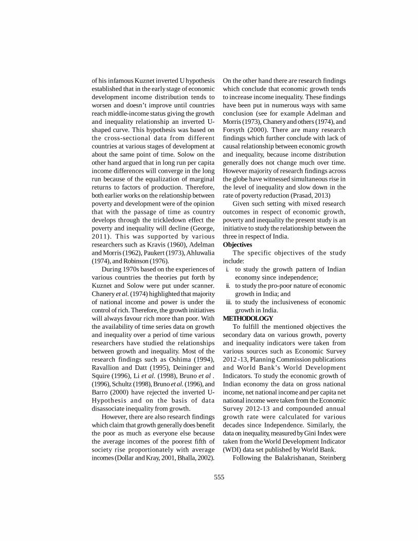
555

of his infamous Kuznet inverted U hypothesisestablished that in the early stage of economicdevelopment income distribution tends toworsen and doesn’t improve until countriesreach middle-income status giving the growthand inequality relationship an inverted U-shaped curve. This hypothesis was based onthe cross-sectional data from differentcountries at various stages of development atabout the same point of time. Solow on theother hand argued that in long run per capitaincome differences will converge in the longrun because of the equalization of marginalreturns to factors of production. Therefore,both earlier works on the relationship betweenpoverty and development were of the opinionthat with the passage of time as countrydevelops through the trickledown effect thepoverty and inequality will decline (George,2011). This was supported by variousresearchers such as Kravis (1960), Adelmanand Morris (1962), Paukert (1973), Ahluwalia(1974), and Robinson (1976).

During 1970s based on the experiences ofvarious countries the theories put forth byKuznet and Solow were put under scanner.Chanery et al. (1974) highlighted that majorityof national income and power is under thecontrol of rich. Therefore, the growth initiativeswill always favour rich more than poor. Withthe availability of time series data on growthand inequality over a period of time variousresearchers have studied the relationshipsbetween growth and inequality. Most of theresearch findings such as Oshima (1994),Ravallion and Datt (1995), Deininger andSquire (1996), Li et al. (1998), Bruno et al .(1996), Schultz (1998), Bruno et al. (1996), andBarro (2000) have rejected the inverted U-Hypothesis and on the basis of datadisassociate inequality from growth.

However, there are also research findingswhich claim that growth generally does benefitthe poor as much as everyone else becausethe average incomes of the poorest fifth ofsociety rise proportionately with averageincomes (Dollar and Kray, 2001, Bhalla, 2002).

On the other hand there are research findingswhich conclude that economic growth tendsto increase income inequality. These findingshave been put in numerous ways with sameconclusion (see for example Adelman andMorris (1973), Chanery and others (1974), andForsyth (2000). There are many researchfindings which further conclude with lack ofcausal relationship between economic growthand inequality, because income distributiongenerally does not change much over time.However majority of research findings acrossthe globe have witnessed simultaneous rise inthe level of inequality and slow down in therate of poverty reduction (Prasad, 2013)

Given such setting with mixed researchoutcomes in respect of economic growth,poverty and inequality the present study is aninitiative to study the relationship between thethree in respect of India.Objectives

The specific objectives of the studyinclude:i. to study the growth pattern of Indian

economy since independence;ii. to study the pro-poor nature of economic

growth in India; andiii. to study the inclusiveness of economic

growth in India.METHODOLOGY

To fulfill the mentioned objectives thesecondary data on various growth, povertyand inequality indicators were taken fromvarious sources such as Economic Survey2012 -13, Planning Commission publicationsand World Bank’s World DevelopmentIndicators. To study the economic growth ofIndian economy the data on gross nationalincome, net national income and per capita netnational income were taken from the EconomicSurvey 2012-13 and compounded annualgrowth rate were calculated for variousdecades since Independence. Similarly, thedata on inequality, measured by Gini Index weretaken from the World Development Indicator(WDI) data set published by World Bank.

Following the Balakrishanan, Steinberg

556

and Syed (2013) methodology followingregression equation is used to study therelationship between economic growth andpoverty reduction:

ln Pt = bi ln Yt + d ln GINIt + rd + etIn the regression model poverty reduction

represented by poverty headcount below $2line at time t (Pt) depends upon per capitaincome (Yt) and Gini Coefficient (GINIt).

Similarly, the degree of inclusiveness ofeconomic growth has been studied with thehelp of following regression equation:

ln Qi, t = (li -1) ln Yt + ei, twhere

Qi,t = Income share of ith quintile at time t.Yt = The GDP per capita at time t.

Growth Story of Indian EconomyAfter independence with the aim to achieve

the socialist pattern of society Indiangovernments adopted the developmentplanning strategy of the former Soviet Russianin a mixed economic framework. Three decadesof planning, state interventionist and importsubstitution strategy adopted by the IndianGovernment resulted in many flaws in Indianeconomy lead by an average growth rate ofreal GDP of 3.75 per cent per year during 1950-1980. During this era Indian economy continueto plague by low rate of economic developmentcoupled with over dependence upon thedeveloped economies for its basic needs. Forits food needs Indian economy was dependent

upon the concessional food imports fromUnited States under Public Law 480 (PL 480).From the Table 1 it is observed that since 1951-52 to 1980-81 Indian economy has witnessednearly stagnant growth rate. During this periodwith government control being the centre ofall plans Indian planners has experimented alot with economy.

Growth of various sectors of Indianeconomy shown in the Table 2 further revealsthat during the 1950-1980 the sectoraldifferences in growth rates. Whereas,agriculture continues to grow at a rate of nearly2.5 per cent per annum the manufacturingsector growth rate also witnessed a downwardtrend since 1950s decade till 1970s decade.Since 1981-82, the sector grew with increasingrate experienced in each decade. Mohan (2008)pointed out two notable features of our growthhistory: first agriculture has been subject tolarge variation over the decades and secondlyservice sector over the decades hascontributed in overall GDP growth rate by wayof a consistent and ever acceleration growthrate.

Under the influence of World Bank andInternational Monetary Fund (IMF,) fewattempts to reform Indian economy were madeduring late 1960s but were reversed amidstpressure from within (Srinivasan, 2006). Thisera of planning was replaced in 1980s by thedebt-led growth of 1980-90 decade resulting

Table 1: Compound annual growth rate of GNI, NNI and per capita NNI(Percent)

Period Gross national income atfactor cost

Net national income atfactor cost

Per capita net nationalincome

At currentprices

At 2004-05prices

At currentprices

At 2004-05prices

At currentprices

At 2004-05prices

1951-52 to 1960-61 5.74 3.85 5.81 4.10 3.79 2.111961-62 to 1970-71 11.11 3.51 10.98 3.30 8.57 1.061971-72 to 1980-81 11.95 3.74 11.68 3.61 9.19 1.301981-82 to 1990-91 13.88 5.24 13.66 5.13 11.26 2.911991-92 to 2000-01 14.59 6.42 14.65 6.40 12.44 4.342001-02 to 2010-11 14.67 8.26 14.66 8.10 12.99 6.531951-52 to 1970-71 8.57 3.69 8.54 3.68 6.30 1.541971-72 to 1990-91 13.19 4.36 12.94 4.25 10.50 1.991991-92 to 2010-11 13.07 6.86 13.04 6.77 11.10 4.94Source: Economic Survey 2012-13

557

in unsustainable but high growth rate of Indianeconomy. During this decade Indian economygrew by an average growth rate of 5.5 per centper annum. But too much debt coupled withother global and national factors led to theinfamous Balance of Payment crisis of 1991.To come out of this crisis Indian governmentstarted to reform the economy from its earlierapproach towards more reformist and moreopen economy. The results of the reformistmeasures were evident in the growth rate ofIndian economy.

Since, 1991 Indian economy continues togrow at a very high growth rate. Since, 1991-92 to 2010-11 Indian economy grew by 6.86per cent per annum as compared to 4.36 during1971-72 to 1990-91. During the twenty years ofreforms the real per capita income also grew atan annual rate of 4.94 per cent in comparisonto less than 2 per cent per annum in previousperiods. Agriculture continues to grow atdismal rate of less than 3.5 per cent per annumwhereas other sectors such as manufacturingand services sector grew at very fast rate andsignificantly contributing to India’s growthrate. This continuous and sustainable high

growth rate led development whereas is goodfor the economy, it further raises the questionsabout the possible impact of this reformistmeasures and reform led higher economicgrowth on the common man of the country.Whereas with the continuously increasingGDP and fall in population growth rate the percapita income is bound to rise, the possibleimpact of economic growth on poverty andinequality is a matter of debate. In the followingsection the nature and extent of poverty andinequality is discussed.Poverty and Inequality in India

Various agencies, researchers andgovernment organizations have made estimateof poverty and inequality in India. Whereasthe official poverty line estimatedapproximately 22 per cent of India’s populationliving below poverty line, Suresh TendulkarCommittee estimate it at 37 per cent, NC SaxenaCommittee put it at 50 per cent and in 2007 theArjun Sengupta Commission identified 77 percent Indians as poor and vulnerable. TheWorld Bank’s estimate put 40 per centpopulation living below poverty line in 2005while Asian Development Bank and UNDPs

Table 3: Poverty estimates in post reform period using mixed reference period (MRP)Year Poverty ratio (%) Number of poor (million)

Rural Urban Total Rural Urban Total1993-94 50.1 31.8 45.3 328.6 74.5 403.72004-05 41.8 25.7 37.2 326.3 80.8 407.12011-12* 25.7 13.7 21.9 216.5 52.8 269.3Annual average decline (percentage points per annum)1993-94 to 2004-05 0.75 0.55 0.74 - - -2004-05 to 2011-12 2.32 1.69 2.18 - - -Sources: Planning Commission, (2013), Press Note on Poverty Estimates, 2011-12, Government of India.Based on the new methodology recommended by the Tendulkar Committee.

Table 2: Growth rate of various sectors of Indian economy since 1950(Percent)

Particulars 1951-52 to

1960-61

1961-62 to

1970-71

1971-72 to

1980-81

1981-82 to

1990-91

1991-92 to

2000-01

2001-02 to

2010-11Agriculture, forestry and fishing, mining and quarrying 2.85 2.41 2.26 3.48 3.44 3.39Manufacturing, construcion, electricity, gas and water supply 6.61 5.29 4.56 5.83 6.73 9.4Trade, hotels, transport and communications 5.69 4.5 5.49 5.97 8.89 10.5Finanacing, insurance, real estate and business services 3.05 3.18 4.38 9.28 7.76 10.77Community social and personal services 3.76 5.11 3.89 6.45 7.32 6.73Source: Economic Survey 2012-13

558

Multidimensional Poverty Index estimate thisto be approximately 50 and 55 per centrespectively (Ghosh, 2011). However thesepoverty estimates are challenged by variousresearchers.

The official poverty line estimates in Indiaare prepared by the Planning Commission.Planning commission with the help of LargeSample Survey on Household ConsumptionExpenditure conducted by National SampleSurvey Office (NSSO) of the Ministry ofStatistics and Programme Implementationprepares the poverty line and poverty ratiosfor each of the survey years. The poverty ratioand number of poor in India in three referenceperiods is shown in the Table 3.

From the Table 3, the percentage of personsliving below the Poverty Line in 2011-12 hasbeen estimated as 25.7 per cent in rural areas,13.7 per cent in urban areas and 21.9 per centfor the country as a whole. This has been lowerthan respective figures of 41.8 per cent, 25.7per cent and 37.2 per cent in 2004-05. As perthis estimate there are approximately 270 millionpersons below Poverty Line. From thestatistics on the average decline in povertyratio it has been observed that the rate ofdecline in the poverty ratio during the 2004-05to 2011-12 periods was about three times fasterthan the same during the period of 1993-94 to2004-05. Therefore the study concludes asignificant reduction in the percentage ifpopulation living below poverty line in India.Planning Commission attributed thisremarkable decline in poverty to increase inreal per capita consumption. According toPlanning Commission this increase wasequitably distributed across all deciles ofpopulation and the distribution wasparticularly equitable in rural areas (PlanningCommission, 2014).

The extent of inequality in any economy isbeing estimated by using the Gini Index. TheGini Index values for Indian economy areshown in the Table 4. The results show nosignificant change in Gini Index. Rising valueof Gini Index during the post reform period

reflects the increase in inequality. The incomedistribution among highest and lowestquintiles also reveals nothing much haschanged for the poor during the post reform.In the year 2010, lowest quintile constitutes toshare a dismal 8.54 per cent income sharewhereas the highest quintile accounted forroughly 42.81 per cent of income sharerevealing existence of income inequality inIndia.

Therefore whereas the poverty ratesduring the post reform period have showndownwards trends, on inequality the picturehas not changed much since 1980s. Given suchcontrasting the present paper is an attempt tostudy the impact of relatively higher economicgrowth achieved in the post reform period onthe poverty and inequality of India.Growth-Poverty Relationship

As proposed by Balakrishanan, Steinbergand Syed (2013) the impact of economicgrowth represented by per capita income (Yt)on poverty measured by poverty headcountbelow $2 line at time t (Pt) was calculated withthe help of regression. The study made use ofthe following regression equation to study therelationship between economic growth andpoverty reduction:

ln Pt = bi ln Yt + d ln GINIt + rd + et ......(1)In the regression model poverty reduction

represented by poverty headcount below $2line at time t (Pt) depends upon per capitaincome (Y t) and Gini coefficient(GINIt).Outcomes of the regression analysisfor India using the World Development

Table 4: Gini index and income share heldby different income quintiles in IndiaYear GINI

indexLowest

20%Second

20%Third20%

Fourth20%

Highest20%

1980 33.44 8.41 12.26 15.94 21.07 42.261985 31.42 8.75 12.69 16.49 21.56 40.511990 31.52 8.92 12.65 16.32 21.34 40.761995 31.04 9.05 12.75 16.39 21.46 40.342000 32.19 8.84 12.48 16.10 21.21 41.332005 33.38 8.64 12.22 15.81 20.97 42.362010 33.90 8.54 12.14 15.69 20.82 42.81Source: Author's Compilation from the World DevelopmentIndicators for India.

559

Indicator data on the variables under studyare shown in the Table 5.

The regression outcomes reveals that therelationship between economic growthrepresented by growth of GDP per capita(constant 2004 US$) and poverty representedby poverty headcount at $2 a day issignificantly negative across all time periods.During the 1980s, 1990s and 2000s decades 1per cent increase in per capital GDP leads to0.104, 0.129, 0.345 per cent decline in povertyheadcount respectively. Therefore studyconcludes that economic growth hassignificantly resulted in the fall in poverty levelof the country. This fall in poverty level wasmore rapid during the 2000s as compared tothe previous decades.

However impact of Gini coefficient onpoverty headcount suggests that in postreform period, rise in Gini coefficient (increasein inequality) results in fall in povertyheadcount. Over the period of time, thisnegative casual relationship between thepoverty and inequality gets significantlystrengthened shown by the regressioncoefficients. During 1980s decade 1 per centrise in inequality shown by Gini index resultsin 0.285 per cent rise in poverty headcountratio at $2 a day. Whereas during 1990s oneper cent rise in Gini index leads to 0.184 percent fall in poverty headcount and during 2000ssimilar change in Gini index leads to 1.633 percent fall in poverty headcount. Therefore risein inequality during post reform period is

associated with fall in poverty headcount.Inclusiveness of Economic Growth

To study the inclusiveness of theeconomic growth the change in per capitaincome was regressed with the change in theincome share of bottom and highest quintileincome group. The economic growth will beinclusive if the changes in income of all thequintiles are changes proportionately and inthe same direction. In the study the degree ofinclusiveness of economic growth has beenanalyzed with the help of following regressionequation:

ln Qi, t = (li -1) ln Yt + ei, tWhere Qi, t is income share of ith quintile at

time t. Yt is the GDP per capita at time t.The regression outcomes from Table 6

reveals that with per capita increase in incomeof the economy the income share of the bottomquintile population have fallen whereas theincome of the highest quintile population haveincreased. This relationship was uniformacross post reform decades for both the bottomand highest quintile income groups.

From the regression coefficient it can beseen that during 1980s an increase of one percent in per capita GDP results in significant0.143 per cent increase in the income share ofbottom quintile of the population whereasduring the same decade one per cent increasein per capita income results in 0.004 per centincrease in the income of the highest quintilepopulation. This means that the economicgrowth achieved by the Indian economy

Table 5: Pro-poor growth regression outcomeParameters 1981-82 to 1990-91 1991-92 to 2000-01 2001-02 to 2010-11 Overall (1981-82 to 2010-11)Constant 4.062*** 5.821*** 0.875NS 6.067***

(0.20) (0.17) (1.76) (0.31)Log of GDP per capita(constant US$2005) (Yt)

-0.104*** -0.129*** -0.345*** -0.154***

(0.01) (0.01) (0.05) (0.01)Log of Gini index (GINIt) 0.285*** -0.184** -1.633** -0.212**

(0.06) (0.06) (0.59) (0.10)N 10 10 10 30Adjusted R2 0.968 0.995 0.976 0.977Source: Author's Calculation based on WDI dataset.Note: Dependent variable is the Poverty headcount ratio at $2 a day (PPP) (% of population).Values in parentheses are standard errors.*** and ** significant at 1 and 5 percent level, respectively.NS: Non-significant

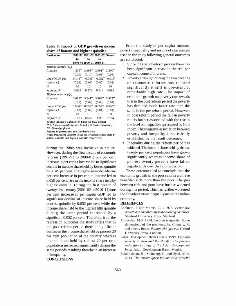
560

during the 1980s was inclusive in nature.However, during the first decade of economicreforms (1991-92 to 2000-01) one per centincrease in per capita income led to significantdecline in income share held by lowest quintileby 0.049 per cent. During the same decade oneper cent increase in per capita income led to0.059 per cent rise in the income share held byhighest quintile. During the first decade oftwenty first century (2001-02 to 2010-11) oneper cent increase in per capita GDP led tosignificant decline of income share held bypoorest quintile by 0.052 per cent while theincome share held by the highest fifth quintileduring the same period increased by asignificant 0.052 per cent. Therefore, from theregression outcomes the study infers that inthe post reform period there is significantdecline in the income share held by poorest 20per cent population of the country whereasincome share held by richest 20 per centpopulation increased significantly during thesame periods resulting thereby in an increasein inequality.CONCLUSIONS

From the study of per capita income,poverty, inequality and results of regressionsused in the study following general outcomesare concluded:1. Since the start of reform process there has

been significant increase in the real percapita income of Indians.

2. Poverty although during the two decadesof economic reforms has reducedsignificantly it still is prevalent atremarkably high rate. The impact ofeconomic growth on poverty rate revealsthat in the post reform period the povertyhas declined much faster rate than thesame in the pre reform period. However,in post reform period the fall in povertyrate is further associated with the rise inthe level of inequality represented by Giniindex. This negative association betweenpoverty and inequality is statisticallyestablished by the result outcomes.

3. Inequality during the reform period haswidened. The income share held by richesttwenty per cent population have grownsignificantly whereas income share ofpoorest twenty percent have fallensignificantly over the reform period.

These outcomes led to conclude that theeconomic growth in the post reform era havebenefited rich more than the poor. The gapbetween rich and poor have further widenedduring this period. This has further worsenedthe already existent inequality inside the Indianeconomy.REFERENCESAdelman, I. and Morris, C.T. 1973. Economic

growth and social equity in developing countries.Stanford University Press, Stanford.

Ahluwalia, M.S. 1974. Income inequality: Somedimensions of the problems. In: Chenery, H.and others, Redistribution with growth. OxfordUniversity Press, London.

Asian Development Bank (ADB). 1999. Fightingpoverty in Asia and the Pacific: The povertyreduction strategy of the Asian developmentbank. Asian Development Bank. Manila.

Balakrishnan, R., Steinberg, C. and Syed, M.H.2013. The elusive quest for inclusive growth:

Table 6: Impact of GDP growth on incomeshare of bottom and highest quintilesParticulars 1981-82

to 1990-91

1991-92to

2000-01

2001-02to

2010-11

Overall

Bottom quintile (Q1)Constant 1.335** 2.498** 2.501** 2.290**

(0.10) (0.10) (0.03) (0.06)Log of GDP percapita (Yt)

0.143** -0.049* - 0.052** -0.019*

(0.02) (0.02) (0.00) (0.01)N 10 10 10 30Adjusted R2 0.884 0.473 0.948 0.093Highest quintile (Q5)Constant 3.682** 3.341** 3.402** 3.422**

(0.20) (0.09) (0.03) (0.04)Log of GDP percapita (Yt)

0.004NS 0.059** 0.052** 0.048**

(0.03) (0.02) (0.01) (0.01)N 10 10 10 30Adjusted R2 -0.123 0.606 0.93 0.704Source: Author's Calculation based on WDI dataset** & * shows significant at 1% and 5 % level, respectivelyNS: Non-significantFigures in parentheses are standard errorsNote: Dependent variable is the log of income share held bybottom quintile and highest quintile respectively

561

Growth, poverty and inequality in Asia. IMFWorking Paper No. 13/152.

Barro, R.J. 2000. Inequality and growth in a panelof countries. Journal of Economic Growth. 5(1): 5-32.

Bhalla, S.S. 2002. Imagine there’s no country:Poverty, inequality and growth in the era ofglobalization. The Institute for InternationalEconomics, Washington DC.

Bhattacharya, B.B. and Sakthivel, S. 2004. Regionalgrowth and disparity in India: Comparison ofpre- and post-reform decades. Economic andPolitical Weekly. 39 (10): 1071-1077.

Bruno, M., Ravallion, M. and Squire, L. 1996. Equityand growth in developing countries: Old andnew perspectives on the policy issues. PolicyResearch Working Paper Series 1563. TheWorld Bank. Washington, DC.

Bruno, M., Ravallion, M. and Squire, L. 1998.Equity and growth in developing countries: Oldand new perspectives on the policy issues. In:Tani, V. and Chu, K.Y. (ed.) Income distributionand high growth. MIT Press. Cambridge.

Chenery, H., Ahluwalia, M., Bell, C.L.G., Duloy, J.and Jolly, R. 1974. Redistribution with growth.Oxford University Press. New York.

Deininger, K. and Squire, L. 1996. A new data setmeasuring income inequality. World BankEconomic Review. 10 (3): 565-591.

Dollar, D. and Kray, A. 2001. Growth is good forthe poor. World Bank Policy ResearchWorking Paper #2587. World Bank.Washington, DC.

Forsyth, J. 2000. Letter to the editor. The Economist.20 (2000): 6.

Gelaw, F. 2009. The relationship between poverty,inequality and growth in the rural Ethiopia: Microevidence. Contributed paper prepared forpresentation at the International Association ofAgricultural Economists Conference. Beijing,Chinal, August 16-22.

George, J. 2011. Growth and development...inclusive growth: What went wrong withdevelopment? Munich Personal RePEc Archive(MPRA) Paper No. 33182. Munich.

Ghosh, J. 2011. India’s official poverty line doesn’tmeasure up. The Guardian. 4 October 2011.

Hongyi, L., Squire, L. and Zou, H.F. 1998.Explaining international and intertemporalvariations in income inequality. EconomicJournal, Royal Economic Society. 108 (446): 26-43.

Hu, Z. and Khan. M.S. 1997. Why is china growingso fast? International Monetary Fund .Washington, D.C.

Kravis, I.B. 1960. International differences in thedistribution of income. Review of Economics andStatistics. 42: 408-416.

Kuznets, S. 1955. Economic growth and incomeinequality. American Economic Review. 45 (1):1-28.

Mohan, R. 2008. The growth record of the Indianeconomy, 1950-2008: A story of sustainedsavings and investment. Keynote Address at theConference Growth and Macroeconomic Issuesand Challenges in India organised by theInstitute of Economic Growth, New Delhi onFebruary 14, 2008.

OECD. 2001. Rising to the global challenge:Partnership for reducing world poverty.Statement by the DAC High Level Meeting.April 25-26, Paris.

Oshima, H.T. 1994. The impact of technologicaltransformation on historical trends in incomedistribution of Asia and the West. DevelopingEconomies. 32 (3): 237-55.

Paukert, F. 1973. Income distribution at differentlevels of development: A survey of evidence.International Labour Review. 108 (2-3): 97-125.

Pernia, E.M. 2003. Pro-poor growth: What is itand how is it important? ERD Policy Brief No.17. Asian Development Bank, Manila.

Prasad, S. 2013. Polarization, inequality andinclusive growth: Kerala’s experience in thereform period. Journal of South Asian Studies. 1(2): 91-103.

Rauniyar, G. and Kanbur, R. 2010. Inclusivedevelopment: Two papers on conceptualization,application and the ADB perspective. AsianDevelopment Bank. Manila.

Ravallion, M. 2004. Pro-poor growth: A primer.World Bank Policy Research Working Paper3242. Washington, DC.

Ravallion, M. and Che, S. 2003. Measuring pro-poor growth. Economics Letters. 78: 93-99.

Ravallion, M. and Datt, G. 1995. Growth andpoverty in rural India. Policy ResearchWorking Paper Series-1405. The World Bank.

Robinson, S. 1976. A note on the U-hypothesisrelating income inequality and economicdevelopment. The American Economic Review.66: 437-440.

Schultz, T.P. 1998. Inequality in the distribution ofpersonal income in the world: How is it changing

562

and why? Journal of Population Economics. 11(3): 307-344.

Srinivasan, T.N. 2006. India’s economic growth andglobal integration: Experiences since reforms andfuture challenges. Paper presented at The NewEconomic Geography: Effects and PolicyImplications A Symposium Sponsored by TheFederal Reserve Bank of Kansas City. August24-26, Jackson Hole, Wyoming.

UN. 2000. A better world for all. Research Report.IMF, OECD, United Nations and WBG. NewYork, United Nations.

World Bank. 2000. World development report 2000/2001: Attacking poverty. The World Bank.Washington DC.

Received: September 25, 2014Accepted: March 18, 2015

563

Indian J Econ Dev DOI No. 10.5958/2322-0430.2015.00064.5Volume 11 No. 2 (2015): 563-569 Research Article

AN ECONOMIC ANALYSIS OF DIRECT MARKETINGOF POTATO AND ONION IN LUDHIANA CITY

Moti Arega and M.S.Toor*

ABSTRACTThe study was undertaken in Ludhiana city of Punjab state to examinemarketing cost, price spreads, marketing problems, and to suggest suitableremedial measures to improve the marketing of fruits and vegetables inApni Mandi. Primary data were collected from 60 farmers, 40 consumersand 20 retailers based on simple random sample without replacement andSecondary data were collected from the office of Market Committee,Ludhiana. Index of Arrivals was calculated and Price spreads were workedout using mode method. Index of arrivals of Ludhiana Apni Mandi washighest in the month of March and lowest in the month of September.Moreover, the study showed that index of income of Market Committee washighest in the month of January and lowest in the month of July. The resultsshowed that the producer’s share in consumer’s rupee was highest in ApniMandi for potato (90.00 percent) and onion (94.20 per cent), respectivelywhile it was lowest in the wholesale vegetable market. The study calls foradequate infrastructural facilities to be provided by government for theproper and efficient operation of Apni Mandi. In order to add value for thefarmers produce, there should be provision of grading/standardization,branding, labeling, and packing facilities by the concerned body.

Keywords: Apni Mandi, market arrivals, price spreadsJEL Classification: Q13, Q18, C43

*Research Scholar and Professor of Economics,Department of Economics and Sociology, PunjabAgricultural University, Ludhiana-141 004Email: drmstoor@yahoo.com

INTRODUCTIONThe most important factor determining the

pattern of diversification is the market. Theprice response, however, is one aspect of theimpact of market on the cropping pattern.Equally important is the marketing efficiency.The profitability of the crop/enterprise is theguiding force for resource allocation decisionsof the farmers, which apart from the productionefficiency, depends upon the prices receivedby the producers in terms of consumer’s rupee.

Empirical studies have shown that a largenumber of intermediaries are involved in themovement of horticultural produce fromproducer to consumer, who appropriate a largeproportion of the consumer price and the shareof producer becomes very low. In the case ofperishables, the storage of which is verydifficult, the share of the producer is in therange of 30 to 60 percent and the marketefficiency is low (Anonymous, 2001, Anantia,2008, and Dastagiri et al., 2009).

Traditional marketing system of fruits andvegetables is unfavorable for farmers as thetrader’s pocketed major share of consumer’srupee. The farmers used to get low price fortheir produce, whereas, the consumer had to

564

pay higher price for poor quality productsavailable in the market. An efficient system ofmarketing is a key for the prosperity of farmersas it can ensure a fair price for the marketablesurplus, which in itself is an incentive to thefarmers to grow more, and thus may help inraising the production. Marketing is as criticalto better performance in agriculture as farmingitself. Therefore, market reform and marketingsystem improvement ought to be integral partof policy and strategy for agriculturaldevelopment. Agricultural marketing includesall the functions like assembling, storing,financing, risk bearing, sale, purchase,transportation, etc. (Rangi and Sidhu, 2005).

It was envisaged that Apni Mandi (DirectMarket) will give boost to the employment andincome of small farmers around cities so as toprovide direct access to the consumers byeliminating the middlemen, which thus mutuallyadvantageous to both farmers and consumers.Initially Apni Mandi was introduced inFebruary 1987 at SAS Nagar Mohali (Punjab)and then in the same year in Ludhiana.Ludhiana is the largest city in the state ofPunjab with an estimated population of 1613878as per Census 2011.The study was undertakento work out the price spread in Apni Mandivis-à-vis traditional vegetable marketing alongwith socio-economic indicators of theparticipating farmers.MATERIALS AND METHODS

This paper is based on both primary andsecondary data sources. Primary data werecollected from 60 farmers, 40 consumers and20 retailers, randomly selected from eachselected Apni Mandis and traditionalvegetable market. Secondary data werecollected from the office of Market Committee,Ludhiana.

The price spread was worked out by usingthe Mode Method. Price spreads were studiedat a point of time in the selected markets. Thechannels studied for this purpose were:1. Apni Mandi

Producer DConsumer2. Wholesale Vegetable Market

Producer DWholesaler-cum-commissionagent DRetailer DConsumer

The index of market arrivals of vegetablesovertime were worked out as follows:

Index of arrivals for ith month = 100YYi

where,i = 1, 2………..12Yi = Average arrivals for ith monthY = Overall average arrivals

Producer’s share in Consumer’s RupeeThe producer’s share in consumer’s rupee

was worked out by the following method(Acharya and Agrawal, 2004):

100PPP

r

Fs

where,Ps = producer’s share in consumer’s rupee

(`kg-1)PF = Producer’s price (`kg-1)Pr = Price paid by consumer’s (`kg-1)

RESULTS AND DISCUSSIONSSocio-economic Indicators of Farmers

The information regarding the compositionof the sample farmers and their socio-economiccharacteristics are given in this section. Theirperception towards various operationsundertaken by them as well as their viewstowards facilities provided by the marketcommittee/Mandi Board and benefits accruedare also discussed in this section. The resultsare discussed under various sub-heads asunder:Socio-economic Characters

The information relating to family size,education level and size of operationalholdings of farmers participating in LudhianaApni Mandi is shown in Table 1. The resultsindicated that, 33.33 per cent of farmers had 9to 10 family members. Further, 28.33 and 25.00per cent of farmers had 7 to 8 and 5 to 6members, respectively. In the category of morethan 10 family members, 8.34 per cent farmerswere reported. The results further revealed that5 per cent of the farmers in study area hadfamily members up to 4. The study concluded

565

that in the sample market, the maximumpercentage of farmers had large family size.

The information about literacy levelrevealed that the educational level of 45 percent of farmers was up to primary. Further, thestudy shows that, 25 per cent of farmers havestudied up to middle class. Moreover, 15 and6.67 per cent of farmers had education up tohigh school and higher secondary,respectively. Lastly, from the sample farmers,8.33 per cent are illiterate. As per theinformation given above, it can be concludedthat the majority of farmers in the study areahad education up to primary school. Thosefarmers having education and able to read arebeneficiary in keeping their farm records,getting information about marketing andhaving more bargain power to sale theirproduce and buy inputs needed for theirfarming.

The information regarding operational sizeof holdings of farmers revealed that 35 per centof the sample farmers had operational holdingof up to 3 acres of land. Further, the percentage

of farmers who had operational holding up to3-6, 6-9, 9-12, 12-15 and 18-21 acres was foundto be 30, 8.34, 21.66, 3.34 and 1.66, respectively.This result shows that a vast majority of farmersholding small area of land are participating invegetable production because of their largefamily size.Composition of Farmers and Commodities

The information given in Table 2 indicatedthat migrant sellers were found to bedominating in vegetable markets of Punjab.The results show that 50.36 and 28.93 per centof sellers belong to Bihar and Punjab,respectively. It was noticed that, 19.64 and 1.07per cent of the sellers in Ludhiana are comingfrom Uttar Pradesh and Orissa, respectively.The share of Bihar state was highest inLudhiana markets, this may be due to thereason that migrants who are not able to getthe job in the industrial units take up the job ofvegetables and fruits selling.

The results showed the overallcomposition of sellers of Ludhiana Apni Mandion monthly basis. The study revealed that 50per cent of sellers were engaged in selling bothvegetables and fruits. Further, it was indicatedthat 25 per cent sellers of Ludhiana Apni Mandiwere selling vegetables. The study shows that15 per cent of sellers were engaged in sellingfruits alone. Further, it was found that 10 per

Table 1: Socio-e conomic indicators offarmers participating in Ludhiana ApniMandi, 2013Particulars Farmers (No.) Percent to totalFamily size (members)0-4 3 5.005-6 15 25.007-8 17 28.339-10 20 33.33More than 10 5 8.34Education levelIlliterate 5 8.33Primary 27 45.00Middle 15 25.00High School 9 15.00Higher Secondary 4 6.67Size of holdings (in acres)Up to 3 21 35.003-6 18 30.006-9 5 8.349-12 13 21.6612-15 2 3.3415-18 - -18-21 1 1.66

Table 2: Compos ition of farme rs andcommodities in Ludhiana Apni Mandi, 2013Particulars Farmers (No.) Percent to totalStatePunjab 81 28.93Bihar 141 50.36Uttar Pradesh (U.P) 55 19.64Orissa 3 1.07CommodityVegetables 70 25.00Fruits 42 15.00Vegetables and fruits 140 50.00Any other* 28 10.00Duration (in years)Up to 15 29 48.3416-20 27 45.0021-26 4 6.66*Selling plastic goods, fast food, tea stall, coconut sellers etc.

566

cent sellers were selling other commodities likeplastic goods, fast food, etc. (Table 2).

The information regarding the time-periodsince farmers of Ludhiana started participatingin Apni Mandi indicated that 48.34 per cent offarmers started participation for the last 15years. The results further revealed that 45 percent of the farmers had been participating since16-20 years in the study area. Lastly, 6.66 percent farmers have been participating in thismarket since 21-26 years. The abovediscussion shows that most of the farmersselling in Apni Mandi have startedparticipating in this market recently, may bedue to advantage of this market discussedearlier.Frequency of Visit and Mode of Transportation

The perusal of the Table 3 indicated that50 per cent farmers of Ludhiana visit ApniMandi five times a week. It was found that26.66 and 15.00 per cent of farmers visit ApniMandi six and four times a week, respectively.Further, the result revealed that 8.34 per centof farmers visit Apni Mandi thrice a week.

The information regarding mode oftransportation used by farmers of the samplemarket shown that mode of transportation of75 per cent of farmers of Ludhiana was tractors-trolley. The result further shows that 25 per

cent farmers of Ludhiana use other mode oftransportation such as bicycles, mopeds, carts,etc. It may be concluded that quantity ofproduce to be brought in the market determinesthe mode of transportation to be used.

It was further indicated by the investigationthat 55 per cent farmers of Ludhiana sold theirproduce in Apni Mandi because of higher andquick returns. Further, 25 per cent farmers soldtheir produce in Apni Mandi because of quickreturns. Moreover, 20 per cent of farmers soldtheir produce in Apni Mandi because of higherreturns. It was concluded that majority of thefarmers sold their produce in Apni Mandibecause of higher and quick returns. Theseresults are inconsonance with the findingsreported by Kaur (2014).Composition and Pattern of Arrivals in ApniMandi

The information regarding number offarmers’ participated, total sales and seasonalindices relating to market arrivals in ApniMandis of Ludhiana from the period of 2011-13 are presented in Table 4. The figuresrevealed that in the year 2011, highest numberof farmers participated was 1992 with highestarrivals of 2480 quintals and total sales werehighest at `25.15 lacks in the month of March.During the year 2012, highest number offarmers participated was 2000 in the month ofJanuary, highest arrivals and maximum totalsales were 2310 quintals and `25.35 lakhs,respectively in the month of July. In the year2013, the highest number of farmersparticipated was 1710, highest arrivals andmaximum total sales were 2150 quintals and`24.25 lakhs, respectively in the month of April.The result showed that average highest arrivalswere 2166.67 quintals in the month of Marchwhile average lowest arrivals were 1483.33quintals in the month of September. Furtherthe study indicated that index of arrivals washighest in the month of March (116.42) andlowest (79.70) in the month of September. Thisfluctuation in arr ivals appears due toseasonality in the production of agriculturalproduce. Therefore, from the above results,

Table 3: Mode of transportation used byfarmers in Ludhiana Apni Mandi, 2013Particulars Farmers

(No.)Percent to total

Visiting days per weekThrice 5 8.34Four times 9 15.00Five times 30 50.00Six times 16 26.66Total 60 100.00SourcesTractor-trolley 45 75.00Any others* 15 25.00Total 60 100.00ReasonsHigher returns 12 20.00Quick returns 15 25.00Higher and quick returns 33 55.00Total 60 100.00*Bicycles, Mopeds, Carts etc.

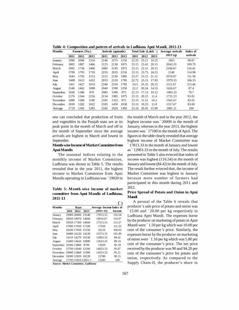
567

one can concluded that production of fruitsand vegetables in the Punjab state are at itspeak point in the month of March and off inthe month of September since the averagearrivals are highest in March and lowest inSeptember.Month-wise Income of Market Committee fromApni Mandis

The seasonal indices relating to themonthly income of Market Committee,Ludhiana was shown in Table 5. The resultsrevealed that in the year 2011, the highestincome to Market Committee from ApniMandis operating in Ludhiana was 19920 in

the month of March and in the year 2012, thehighest income was `20000 in the month ofJanuary, whereas in the year 2013, the highestincome was `17100 in the month of April. Thefigures in the table clearly revealed that averagehighest income of Market Committee was`17813.33 in the month of January and lowestas `12903.33 in the month of July. The resultspresented in Table 5 also evinced that index ofincome was highest (116.54) in the month ofJanuary and lowest (84.42) in the month of July.The result further evinced that, the income ofMarket Committee was highest in Januarybecause more number of farmers hadparticipated in this month during 2011 and2012.Price Spread of Potato and Onion in ApniMandi

A perusal of the Table 6 reveals thatproducer’s sale price of potato and onion was`15.00 and `20.00 per kg respectively inLudhiana Apni Mandi. The expenses borneby the producer on marketing of potato in ApniMandi were `1.50 per kg which was 10.00 percent of the consumer’s price. Similarly, theexpenses borne by the producer on marketingof onion were 1.16 per kg which was 5.80 percent of the consumer’s price. The net pricereceived by the producer was 90 and 94.20 percent of the consumer’s price for potato andonion, respectively. As compared to theSupply Chain-II, the producer’s share in

Table 4: Composition and pattern of arrivals in Ludhiana Apni Mandi, 2011-13Months Farmers (No.) Arrivals (quiantls) Total Sale (Lakh `) Average arrivals

2013 (q)Index ofarrivals2011 2012 2013 2011 2012 2013 2011 2012 2013

January 1990 2000 1354 2140 2275 1150 22.25 25.21 10.25 1855 99.67February 1802 1807 1466 2125 2130 1875 23.15 23.43 20.15 2043.33 109.79March 1992 1736 1466 2480 2145 1875 25.15 22.15 20.15 2166.67 116.42April 1700 1705 1710 2235 2035 2150 23.15 23.75 24.25 2140 114.98May 1643 1705 1515 2115 2130 1985 23.27 23.15 21.12 2076.67 111.58June 1608 1612 1452 2033 2120 1785 22.72 23.15 17.85 1979.33 106.35July 1411 1427 1033 2240 2310 1785 24.5 25.35 20.15 2111.67 113.46August 1540 1462 1088 2040 1590 1250 22.2 20.24 14.55 1626.67 87.4September 1650 1386 870 2085 1390 975 22.15 17.13 10.12 1483.33 79.7October 1576 1564 1256 2134 1985 1075 23.15 20.15 11.4 1731.33 93.02November 1890 1286 1190 2185 1525 975 23.15 11.51 10.2 1561.67 83.91December 1830 1282 1022 2185 1450 1038 23.15 10.25 11.8 1557.67 83.69Average 1719 1581 1285 2166 1924 1493 23.16 20.45 15.99 1861.11 100

Table 5: Month wise income of marketcommittee from Apni Mandis of Ludhiana,2011-13

(`)Months Years Average Income

(2011-13)Index ofIncome2011 2012 2013

January 19900 20000 13540 17813.33 116.54February 18020 18070 14660 16916.67 110.67March 19920 17360 14660 17313.33 113.27April 17000 17050 17100 17050 111.55May 16430 17050 15150 16210 106.05June 16080 16120 14520 15573.33 101.89July 14110 14270 10330 12903.33 84.42August 15400 14620 10880 13633.33 89.19September 16500 13860 8700 13020 85.18October 15760 15640 12560 14653.33 95.87November 18900 12860 11900 14553.33 95.21December 18300 12820 10220 13780 90.15Average 17193 15810 12851.7 15285 100Source: Market Committee, Ludhiana

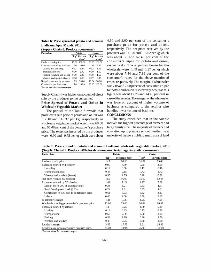
568

Supply Chain-I was higher on account of directsale by the producer to the consumer.Price Spread of Potato and Onion inWholesale Vegetable Market

The perusal of the Table 7 reveals thatproducer’s sale price of potato and onion was`12.10 and `16.37 per kg, respectively inwholesale vegetable market which was 60.50and 65.48 per cent of the consumer’s purchaseprice. The expenses incurred by the producerwere `0.90 and 0.75 per kg which were about

4.50 and 3.00 per cent of the consumer’spurchase price for potato and onion,respectively. The net price received by theproducer was `11.20 and `15.62 per kg whichwas about 56 and 62.48 per cent of theconsumer ’s rupee for potato and onion,respectively. The expenses borne by thewholesaler were `1.49 and 1.97 per kg whichwere about 7.44 and 7.89 per cent of theconsumer’s rupee for the above mentionedcrops, respectively. The margin of wholesalerwas 7.05 and 7.00 per cent of consumer’s rupeefor potato and onion respectively, whereas thisfigure was about 17.75 and 14.43 per cent incase of the retailer. The margin of the wholesalerwas lowe on account of higher volume ofbusiness as compared to the retailer whohandles lower volume of business.CONCLUSIONS

The study concluded that in the samplemarket, the highest percentage of farmers hadlarge family size. The majority of farmers hadeducation up to primary school. Further, vastmajority of farmers holding small area of land

Table 6: Price spread of potato and onion inLudhiana Apni Mandi, 2013(Supply Chain-I: Producer-consumer)Particulars Potato Onion

`kg-1 Percentshare*

`kg-1 Percentshare*

Producer’s sale price 15.00 100.00 20.00 100.00Expenses incurred by producer 1.50 10.00 1.16 5.80 Loading and unloading 0.52 3.47 0.52 1.95 Transportation cost 0.30 2.00 0.30 1.50 Packing, weighing and sewing 0.30 2.00 0.30 1.50 Wastage and spoilage (losses) 0.38 2.53 0.17 0.85Net price received by producer 13.5 90.00 18.84 94.20Consumer’s purchase price 15.0 100.0 20.00 100.00*Percent share in consumers rupee

Table 7: Price spread of potato and onion in Ludhiana wholesale vegetable market, 2013(Supply Chain-II: Producer-Wholesaler-cum-commission agent-retailer-consumer)Particulars Potato Onion

`kg-1 Percent share* `kg-1 Percent share*

Producer’s sale price 12.1 60.50 16.37 65.48Expenses incurred by producer 0.90 4.50 0.75 3.00 Unloading 0.12 0.60 0.12 0.48 Transportation cost 0.43 2.15 0.43 1.72 Wastage and spoilage (losses) 0.35 1.75 0.20 0.80Net price received by producer 11.2 56.00 15.62 62.48Expenses incurred by Wholesaler: 1.49 7.45 1.97 7.89 Market fee @ 2% of purchase price 0.24 1.21 0.33 1.31 Rural Development fund @ 2% 0.24 1.21 0.33 1.31 Commission @ 5% paid to commission agent 0.61 3.03 0.82 3.27 Labour 0.40 2.00 0.50 2.00Wholesaler’s margin 1.41 7.06 1.75 7.00Wholesaler’s selling price/retailer’s purchase price 15.00 75.00 20.09 80.37Expenses incurred by retailer: 1.45 7.25 1.30 5.20 Loading 0.13 0.63 0.13 0.50 Transportation 0.50 2.50 0.50 2.00 Packing 0.38 1.88 0.38 1.50 Wastage and spoilage 0.45 2.25 0.30 1.20Retailer’s margin 3.55 17.75 3.61 14.43Retailer’s sale price/consumer’s purchase price. 20.00 100.00 25.00 100.00*Percent share in consumers rupee

569

are participating in vegetable productionbecause of their large family size. The share ofBihar state was highest in Ludhiana markets;this may be due to the reason that migrantswho are not able to get the job in the industrialunits take up the job of vegetables and fruitsselling. It was also noticed that most of thefarmers disposing of their produce in ApniMandi have started participating recently, maybe due to higher and quick returns

It was observed that if producer’s share inconsumer’s rupee is considered as a soleindicator to judge the efficiency of the system,then the direct marketing system of agriculturalproduce, as transacted in Apni Mandi isconsidered as an efficient one as it provides afair deal to the farmers. The system alsobenefits the consumers purchasing fromfarmers directly as they pay lower pricecompared to the other systems. The study callsfor adequate infrastructural facilities to beprovided by government for the proper andefficient operation of Apni Mandi (directmarket). Also, in order to add value for thefarmers produce, to secure more money for thesame amount of produce, there should be

provision of grading/standardization,branding, labeling and packing facilities by theconcerned body.REFERENCEAcharya, S.S. and Agrawal, N.L. 2004. Agricultural

marketing in India. Oxford and IBH PublishingCooperation Private Limited, New Delhi.

Anantia. 2008. What is India’s share in globalvegetable and fruit market? Retrieved fromwww.managementparadise.com

Anonymous. 2001. Report of the Working Groupon Horticulture Development for 10th Five YearPlan (main report) Planning Commission,Government of India, New Delhi.

Dastagiri, M.B., Kumar, B.G., and Diana, S. 2009.Innovative models in horticulture marketing inIndia. Indian Journal of Agricultural Marketing.23 (3): 83-94.

Kaur, G. 2014. An economics analysis of Apni Mandiin District Patiala. Indian Journal of Economicsand Development. 10 (1a): 65-68.

Rangi, P.S. and Sidhu, M.S. 2005. Role ofcommission agents in agricultural marketing inPunjab. Indian Journal of AgriculturalMarketing. 19 (1): 38-52.

Received: August 27, 2014Accepted: March 15, 2015

570

571

Indian J Econ Dev DOI No. 10.5958/2322-0430.2015.00065.7Volume 11 No. 2 (2015): 571-582 Research Article

INTER-ZONAL EFFICIENCY DIFFERENCES: STUDYBASED ON FARMERS OF WEST BENGAL

Chandan Kumar Maity* and Atanu Sengupta**

ABSTRACT

The present study uses Data Envelopment Analysis to study inter-zonalvariation in farm productivity in West Bengal. Malmquist ProductivityIndices was used to delineate the performance of different farmers acrossvarious agro climatic regions of West Bengal. The results indicate thatfarmers from some of the advance zone in terms of agro-climatic featuresare failed to optimize their inputs in order to obtain a targeted level ofoutput. While some of the backward zone perform better. We have takenenvelop of frontier of all zones as reference for comparisons betweenproductivity performances of different zones. The productivity indices arecomparable with the zonal efficiencies except in few cases.

Keywords: Agricultural growth, efficiency, economy, productivity indicesJEL Classification: O13, Q12, Q16, Q19

* Research Scholar, Burdwan University, WestBengal, India and ** Associate Professor, BurdwanUniversity, West Bengal IndiaEmail: cmaity_28@yahoo.co.in

INTRODUCTIONOne of the main assumptions for measuring

farm efficiency using frontier and non frontierapproach is that there exists perfectcompetition in both the product and factormarket1. In this context, one may raise doubtsabout the plausibility of making thisassumption, particularly in an under developedcountry like ours. It is well known that, forvarious reasons (such as dominance ofinformal credit in the rural sector, unequalrelationship between employer and labour/tenant, price discrimination due to theexistence of various marketing channels foragricultural products, etc.), the product and

factor markets do not behave in a competitivemanner. In that case, it will not be proper toascertain the exact nature of the productionfunction to be applicable in the agriculturalsector. To overcome this problem, analternative to the above approach known asData Envelopment Analysis (DEA), whichdoes not make any prior assumption about theproduction function, is used to measure theefficiency of a production unit. The presentstudy uses DEA methodologies to study inter-zonal variation in farm efficiency in westBengal.

The basic argument is the ability of smallfarmers in reaping the benefit of newtechnology (Sharma and Sharma, 2000). In thetraditional logic, new technology is heavilybiased towards rich farmers because of thelarge setup cost involved in adopting suchtechnologies (Dyer, 1998). However, recentlyseveral authors feel that there are certainaspects of new technology (such as efficientuse of water resources, proper selection of

1In fact, this assumption is implicit in the analysis ofallocative efficiency which infers that the productiveunits are price takers.

572

crop mix, etc.) that might benefit even the smallfarmers particularly in a situation when thegovernment assistance favored the poor(Chattopadhyay and Sengupta, 1997 and 1999).The large farmers tend to diversify in order toalleviate risks involved in agrarian production.Small farmers with their limited resource abilityconcentrate only on a few crops. As suchcomparison between these types of farmersshould involve inter-crop variation2. As arguedby Lee and Somwaru (1993), land productivityand input intensity are valid measures ofrelative efficiency only under very restrictiveassumptions such as Constant Returns toScale. They suggest the use of efficiency asan ideal parameter in this regard. The simpleproductivity analysis using yield per hectareand farm size might not be sufficient tounderstand the pattern of farm efficiency. Thisis because efficiency depends on a number offactors that could not be captured by yield perhectare alone (productivity of other inputsbesides land, level of technology used, etc.,may be incorporated in the analysis3).DATA DESCRIPTION

The farmers in underdeveloped areasexhibit wide differences in their resource usepattern. It thus, seems interesting to studyefficiency differentials among farmers ofdifferent categories. West Bengal is one of thestates in India where large-scale land reforms

have resulted in breaking up of vested interestsin land holding pattern to a certain extent(Dyer, 1998). Several authors have argued thatsuch measures have contributed to significantefficiency gain (Banarjee et al., 2002). It thusremains imperative to examine the extent towhich these gains have been translated inproduction economies. However, since this isa micro level analysis, it is difficult to includepolicy variables directly. Their effects can onlybe gauged indirectly. In the region under studypaddy is the main crop. The crop is generallycultivated more than once in a year (normallyreferred to as aman, boro, and aus) aman is thetraditional variety while boro is the modernvariety with high return, huge investment andlarge risk involved.

The data used in this exercise werecollected by the Ministry of Agriculture,Government of West Bengal through the Costof Cultivation Scheme. The data were collectedfor every district of this province each year. Amultistage random sampling design wasadapted from blocks to mouza and then frommouza to households. The landless labourerswere excluded from the set of households. Thisdata set supplies information on various inputslike human labour, bullock labour, fertilizer,manure, machine and output of all the cropscultivated both in value and quantitative terms.For our efficiency estimates we have takenonly three inputs namely human labour hour,bullock hour and fertilizer that presumablyexplain production of most of the crops verywell. All these variables are measured in perunit area. The data were collected every yearbeginning 1971 from various part of WestBengal. In this study we have used farm leveldisaggregated data pertaining to the year 2009-10 for West Bengal.

For the purpose of collecting CSSCC datain West Bengal, the entire state was dividedinto six agro climatic zones on cultivationpractices, type of soil, irrigation facilities andrainfall, namely : (1) Hilly Zone; (II) Terai Zone(III) Old Alluvial Zone: (IV) New Alluvial Zone:(V) Coastal Saline Zone and (VI) Red Laterite

2Two issues are important here. Firstly large farmerstake their decision on the perspective of cultivatinga whole gamut of crops while the small farmersconcentrate on the cultivation of a single or a fewcrops. In a multi-crop setup, input used andefficiency achieved for a particular crop has its spill-over effect over input decisions of other crops (Paland Sengupta, 1999). Hence it would be wrong totreat them identically as is usually done. Secondly,large farmers generally prefer highly remunerativecrops that may require substantial cost and use ofmodern inputs. Small farmers are more cautious.They normally prefer traditional crops with low riskthat are essential for their survival.3 It is difficult to accept yields as a comprehensivemeasure of efficiency.

573

Zone. A single zone may contain blocksbelonging to different districts. There existwide differences in cultivation practices,topographic features and climatic conditionsacross these zones. METHODOLOGY

The DEA Methodology has been used tostudy inter-Zonal productivity differences.DEA is a linear-programming methodology,which uses data on the input and outputquantities of farmers to construct a piece-wiselinear surface over the data points. The frontiersurface is constructed by the solution of asequence of linear programming problems-onefor each farmer in a sample. This methodologyprovides an analysis of relative efficiency offarmers for a particular time point or over timepoints. The methodological approach of DEAmakes no room for noise and so does not nearlyenvelop a data set as the way most econometricmodels do. It is now possible to define Farrell’s(1957) input saving efficiency measure basedon frontier technology as4

0,α,F:αminE iiiαi i

xy ..........(1)

The linear programming approach tomeasure efficiency from the envelop is to

iE Emaxiλ

..........(2)Subject to

Yλyi

ii xEXλ

0λ Where X is a n l input matrix with columns

ix , Y is a m l output matrix with columnsiy , λ is a l 1 intensity vector and I is thenumber of firms in a particular set ofobservations. Problem (4) has been solved forI time to get each producer’s efficiency scorewhich is being evaluated under different setsof observations as envelope5.

The above measure of efficiency isrestricted to a single set of observations. For across country or region-wise comparison,efficiency measure of a production unit incountry j should be based on frontiertechnology of country i (which is called thereference technology). Then the efficiency ofa unit in jth country/ region given the referencetechnology of ith country may be written as

0x,α,yF:αminE jijjiijαi ij ......(3)

Now to obtain the efficiency scores a LinearProgramming Problem has to be solved foreach production unit with respect to thereference set. The performances of differentproductive units across different regions (ortime periods) are usually measured byproductivity indices. The standard practice inthe literature has been to use the Malmquistproductivity index which measures the relativechanges in efficiency between two time periodsor two regions with an exogenously giventechnology as a reference point; that is, thetechnological efficiency of these processes arecompared through their shortfall from theefficiency of the reference technology. It hasbeen argued that such indices satisfy certainwell defined properties that one may imposeon an arbitrary productivity index.

We may now turn to the concept ofMalmquist productivity index using the DEAapproach6. Productivity index between twounits observed in the input-output set 1 andinput output set 2 with frontier technologyfrom a reference frontier i is defined as:

0.F:amin

0.F:aminEE(1,2)M

i1

i2

i1

i2i

....(4)

4Similarly one can define output-saving measure(see Färe, Lovel and Grasskopf,1994)

5Following this analysis, we get efficiency score foreach of the individual firms. For example, sincethere are about 59 farms belonging to zone-I, wewill have about 59 different efficiency scores. Wehave taken the mean of these scores to be the averageefficiency scores or the efficiency score of the averagefarm belonging to this zone.

574

It is easily established by noting that Ei1and Ei2 are inverses of the relevant DebreuFarrell distance functions (Chakravarty, 1995).Moreover, the Malmquist Index (4) is in theratio form. It may also be treated as a form ofgeneralized productivity index.

Now productivity indices may change dueto two main reasons (Kalirajan and Shand,1994). Productivity indices may change if thereis a change in relative efficiencies of firmsbelonging to two different sets ofobservations. Farms belonging to differentobservation sets might improve theirperformances by moving from an interior pointto a point on the frontier. As a result, theirefficiency parameters are altered which causea change in the Malmquist Productivity indexMi. This is the catching up effect. Productivityalso changes if the frontier functionsthemselves shift without any change in therelative efficiencies. This is the puretechnology shift. The Malmquist Index can bedecomposed into two parts showing thecatching up effect MC (1,2) and the puretechnology shift MFi (1,2) :

11

i1

22

i2

11

22

i1

i2i

EEEE

EE

EE(1,2)M

= ),,(MF),MC( i 2121 i=reference technologyHence, M i (1,2) is the net effect of

differences in relative efficiency MC(1,2) orthe catching up component and thedifferences in frontier production MFi (1,2)function which captures the shift intechnology with reference to the technologyi.

But this measure has the deficiency ofbeing dependent on an arbitrary reference i.Since, we are concerned with inter-zonal

efficiency differences; we always choose thereference frontier to be the envelope of thezonal frontiers. Thus, index (4) is no longerdependent on any arbitrary choice of i. In fact,it captures efficiency differentials across zoneswith respect to the envelope. We provide someempirical findings using the index (4) in thefollowing section.RESULTS AND DISCUSSION

In order to address the methodologicalissues raised above, we have constructedproduction frontiers and Malmquist indices forsix agro climatic zones of the state of WestBengal. Estimation of Malmquist productivityindices essentially involves three steps. First,we have to estimate zone-wise efficiency offarms. Next, we calculate the inter-zonalefficiency scores whereby productiveperformances of farms belonging to differentzones are adjudged with reference to theenvelope. Hence, for any farm belonging to aspecified zone, we have two efficiency scores-one that is calculated with reference to the zoneto which the farm belongs (Zone-wiseefficiency scores), and the second is calculatedwith reference to the envelope (inter-Zonalefficiency scores). These two efficiency scoresare finally used to calculate Malmquist input-based productivity index.

In our analysis we have used both theConstant Return to Scale (CRS) and VariableReturn to Scale (VRS) assumptions. Followingthe discussions in the previous section, weselect envelope of the zonal frontiers to be thereference of inter-zonal comparisons. Theempirical results can thus be divided undertwo headings: (a) Zone-wise efficiency of farmsand (b) inter-zonal comparison of efficiency.Zone-wise Efficiency of Farms

We have calculated the efficiency score ofeach farm both for constant returns to scale(CRS) and variable returns to scale (VRS)technology. The perusal of Table 1 shows theaverage efficiency scores of each zone andvariance of the efficiency scores. It is observedfrom the Table 1 that efficiency scores withVRS are generally higher than those of CRS

6Actually there are different types of Malmquist index,here we use input based index. An input based indexutilizes the concept of input saving efficiency. In asimilar fashion, one can use output based index.

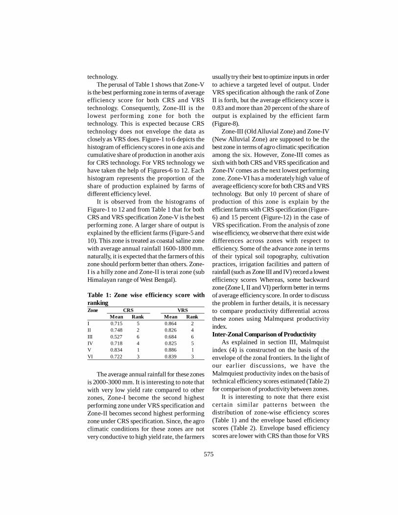
575

technology.The perusal of Table 1 shows that Zone-V

is the best performing zone in terms of averageefficiency score for both CRS and VRStechnology. Consequently, Zone-III is thelowest performing zone for both thetechnology. This is expected because CRStechnology does not envelope the data asclosely as VRS does. Figure-1 to 6 depicts thehistogram of efficiency scores in one axis andcumulative share of production in another axisfor CRS technology. For VRS technology wehave taken the help of Figures-6 to 12. Eachhistogram represents the proportion of theshare of production explained by farms ofdifferent efficiency level.

It is observed from the histograms ofFigure-1 to 12 and from Table 1 that for bothCRS and VRS specification Zone-V is the bestperforming zone. A larger share of output isexplained by the efficient farms (Figure-5 and10). This zone is treated as coastal saline zonewith average annual rainfall 1600-1800 mm.naturally, it is expected that the farmers of thiszone should perform better than others. Zone-I is a hilly zone and Zone-II is terai zone (subHimalayan range of West Bengal).

usually try their best to optimize inputs in orderto achieve a targeted level of output. UnderVRS specification although the rank of ZoneII is forth, but the average efficiency score is0.83 and more than 20 percent of the share ofoutput is explained by the efficient farm(Figure-8).

Zone-III (Old Alluvial Zone) and Zone-IV(New Alluvial Zone) are supposed to be thebest zone in terms of agro climatic specificationamong the six. However, Zone-III comes assixth with both CRS and VRS specification andZone-IV comes as the next lowest performingzone. Zone-VI has a moderately high value ofaverage efficiency score for both CRS and VRStechnology. But only 10 percent of share ofproduction of this zone is explain by theefficient farms with CRS specification (Figure-6) and 15 percent (Figure-12) in the case ofVRS specification. From the analysis of zonewise efficiency, we observe that there exist widedifferences across zones with respect toefficiency. Some of the advance zone in termsof their typical soil topography, cultivationpractices, irrigation facilities and pattern ofrainfall (such as Zone III and IV) record a lowestefficiency scores Whereas, some backwardzone (Zone I, II and VI) perform better in termsof average efficiency score. In order to discussthe problem in further details, it is necessaryto compare productivity differential acrossthese zones using Malmquest productivityindex.Inter-Zonal Comparison of Productivity

As explained in section III, Malmquistindex (4) is constructed on the basis of theenvelope of the zonal frontiers. In the light ofour earlier discussions, we have theMalmquiest productivity index on the basis oftechnical efficiency scores estimated (Table 2)for comparison of productivity between zones.

It is interesting to note that there existcertain similar patterns between thedistribution of zone-wise efficiency scores(Table 1) and the envelope based efficiencyscores (Table 2). Envelope based efficiencyscores are lower with CRS than those for VRS

Table 1: Zone wise efficiency score withrankingZone CRS VRS

Mean Rank Mean RankI 0.715 5 0.864 2II 0.748 2 0.826 4III 0.527 6 0.684 6IV 0.718 4 0.825 5V 0.834 1 0.886 1VI 0.722 3 0.839 3

The average annual rainfall for these zonesis 2000-3000 mm. It is interesting to note thatwith very low yield rate compared to otherzones, Zone-I become the second highestperforming zone under VRS specification andZone-II becomes second highest performingzone under CRS specification. Since, the agroclimatic conditions for these zones are notvery conductive to high yield rate, the farmers

576

0 .0 00 .1 00 .2 00 .3 00 .4 00 .5 00 .6 00 .7 00 .8 00 .9 01 .0 0

0.0 0.1 0.2 0 .4 0 .6 0 .8

E fficiency lev el

Cum u lative s hare o f o utput

Figure 1: Farm Eff iciency for CRS technolo gy for Zo ne I

0 .0 00 .1 00 .2 00 .3 00 .4 00 .5 00 .6 00 .7 00 .8 00 .9 01 .0 0

0 .0 0 .1 0.3 0.4 0 .5 0 .7 0.9

E fficiency L ev el

Cu m u lative s hare o f o utput

Figure 2: Farm ef ficiency fo r CRS techno lo gy for Zone-II

0.00

0.10

0.20

0.30

0.40

0.50

0.60

0.70

0.80

0.90

1.00

0.0 0.1 0.3 0.4 0.5 0.7 0.8

Efficiency level

Cumulative share of output

Figure 3: Farm efficiency for CRS technology for Zone-III

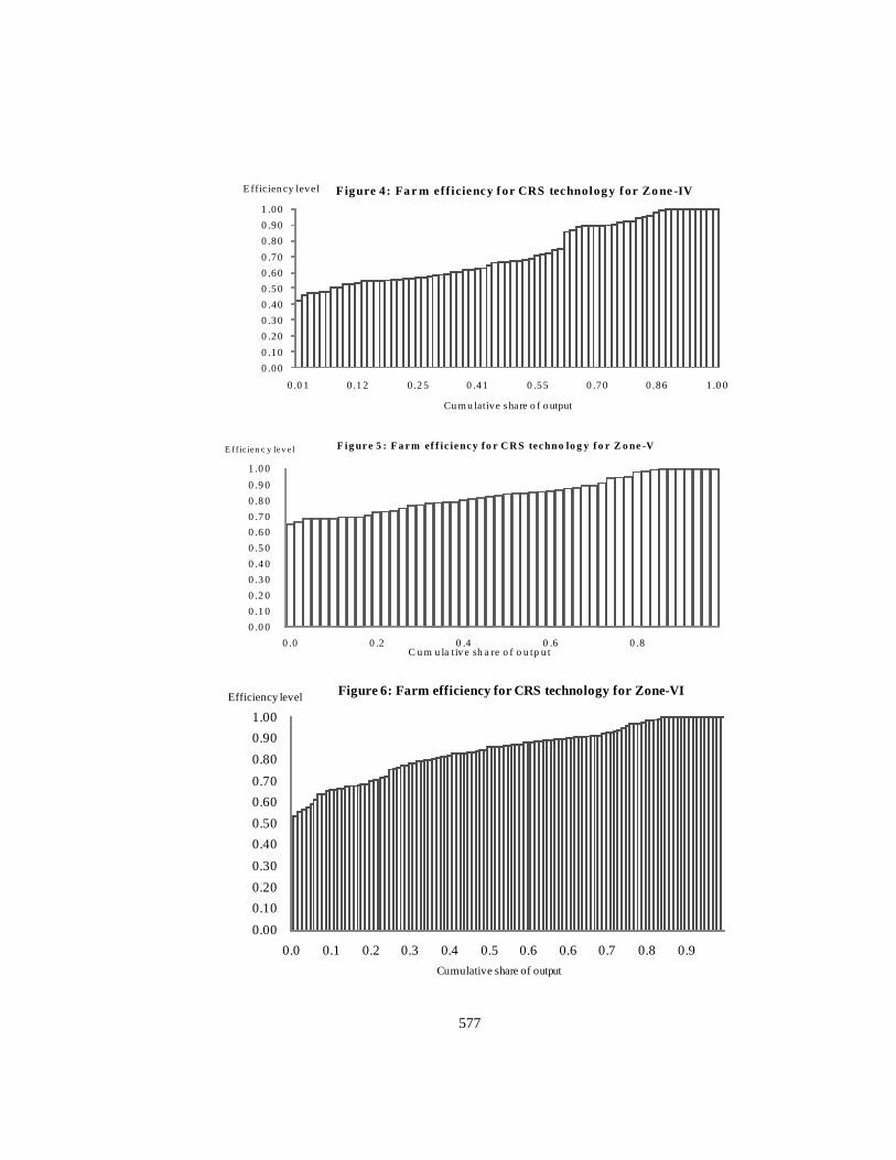
577

0 .000 .100 .200 .300 .400 .500 .600 .700 .800 .901 .00

0 .0 1 0 .1 2 0 .2 5 0 .41 0 .55 0 .70 0 .86 1 .0 0

E ffic ien cy level

Cu m u lative share o f o utput

Figure 4: Fa r m eff iciency f or CRS technolog y f or Zo ne -IV

0 .0 0 0 .1 0 0 .2 0 0 .3 0 0 .4 0 0 .5 0 0 .6 0 0 .7 0 0 .8 0 0 .9 0 1 .0 0

0 .0 0 .2 0 .4 0 .6 0 .8

E ff ic ien c y lev e l

C u m u la t iv e sh a re o f o u tp u t

F i g ur e 5 : F a r m ef f ic ie nc y fo r C R S tec hn o lo g y f o r Z o ne -V

0.0 0.1 0.2 0.3 0.4 0.5 0.6 0.6 0.7 0.8 0.90.000.100.200.300.400.500.600.700.800.901.00

Cumulative share of output

Efficiency level Figure 6: Farm efficiency for CRS technology for Zone-VI

578

0 .0 0

0 .1 0

0 .2 0

0 .3 0

0 .4 0

0 .5 0

0 .6 0

0 .7 0

0 .8 0

0 .9 0

1 .0 0

0 .0 0 .2 0 .3 0 .5 0 .7 0 .8

E fficien cy lev el

Cu m u lativ e s hare o f o utput

Fig ure 7 : Fa rm e f f iciency f o r VRS techno lo g y f o r Z o ne -I

0.00

0 .10

0 .20

0 .30

0 .40

0 .50

0 .60

0 .70

0 .80

0 .90

1 .00

0 .0 0 .1 0 .3 0.4 0 .6 0 .7 0 .9

E ff ic ien cy lev e l

Cu m u lativ e s hare o f o utput

F ig ure 8 : F a rm e f f ic iency fo r VRS techno lo g y f o r Z o ne -II

0.000.10

0.20

0.300.40

0.50

0.60

0.700.80

0.90

1.00

0.0 0.1 0.3 0.4 0.5 0.7 0.8

Efficiency Level

Cumulative share of output

Figure 9: Farm efficiency for VRS technology for Zone-III

579

0.000.10

0.20

0.30

0.400.50

0.60

0.700.800.901.00

0.02 0.17 0.29 0.43 0.54 0.70 0.86 1.00

Efficiency level

Cumulative share of output

Figure 10: Farm efficiency for VRS technology for Zone-IV

0 .0 0

0 .1 00 .2 00 .3 00 .4 00 .5 0

0 .6 00 .7 00 .8 00 .9 01 .0 0

0 .0 0 .2 0 .4 0 .6 0 .8

E ff icien cy lev e l

Cu m u la tiv e s ha re o f o utput

F ig ur e 1 1 : F a rm e f f i c ie nc y f o r V R S te ch no l o g y f o r Z o ne -V

0 .0 0

0 .1 0

0 .2 0

0 .3 0

0 .4 0

0 .5 0

0 .6 0

0 .7 0

0 .8 0

0 .9 0

1 .0 0

0.0 0.1 0.2 0.3 0.4 0.5 0.6 0.6 0.7 0.8 0.9

Eff ic ien cy lev el

C u m u la tive sh a re o f o u tp u t

F ig ure 1 2 : F a rm ef f ic iency f o r VRS techno lo g y f or Z o ne -VI

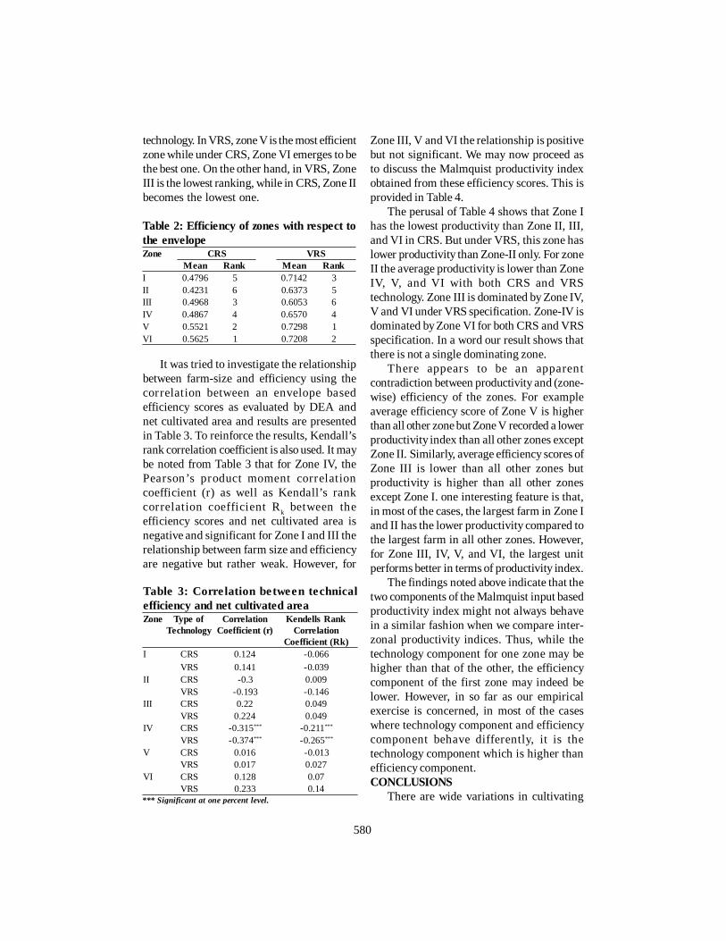
580

technology. In VRS, zone V is the most efficientzone while under CRS, Zone VI emerges to bethe best one. On the other hand, in VRS, ZoneIII is the lowest ranking, while in CRS, Zone IIbecomes the lowest one.

Zone III, V and VI the relationship is positivebut not significant. We may now proceed asto discuss the Malmquist productivity indexobtained from these efficiency scores. This isprovided in Table 4.

The perusal of Table 4 shows that Zone Ihas the lowest productivity than Zone II, III,and VI in CRS. But under VRS, this zone haslower productivity than Zone-II only. For zoneII the average productivity is lower than ZoneIV, V, and VI with both CRS and VRStechnology. Zone III is dominated by Zone IV,V and VI under VRS specification. Zone-IV isdominated by Zone VI for both CRS and VRSspecification. In a word our result shows thatthere is not a single dominating zone.

There appears to be an apparentcontradiction between productivity and (zone-wise) efficiency of the zones. For exampleaverage efficiency score of Zone V is higherthan all other zone but Zone V recorded a lowerproductivity index than all other zones exceptZone II. Similarly, average efficiency scores ofZone III is lower than all other zones butproductivity is higher than all other zonesexcept Zone I. one interesting feature is that,in most of the cases, the largest farm in Zone Iand II has the lower productivity compared tothe largest farm in all other zones. However,for Zone III, IV, V, and VI, the largest unitperforms better in terms of productivity index.

The findings noted above indicate that thetwo components of the Malmquist input basedproductivity index might not always behavein a similar fashion when we compare inter-zonal productivity indices. Thus, while thetechnology component for one zone may behigher than that of the other, the efficiencycomponent of the first zone may indeed belower. However, in so far as our empiricalexercise is concerned, in most of the caseswhere technology component and efficiencycomponent behave differently, it is thetechnology component which is higher thanefficiency component.CONCLUSIONS

There are wide variations in cultivating

Table 2: Efficiency of zones with respect tothe envelopeZone CRS VRS

Mean Rank Mean RankI 0.4796 5 0.7142 3II 0.4231 6 0.6373 5III 0.4968 3 0.6053 6IV 0.4867 4 0.6570 4V 0.5521 2 0.7298 1VI 0.5625 1 0.7208 2

Table 3: Correlation between technicalefficiency and net cultivated areaZone Type of

TechnologyCorrelation

Coefficient (r)Kendells Rank

CorrelationCoefficient (Rk)

I CRS 0.124 -0.066VRS 0.141 -0.039

II CRS -0.3 0.009VRS -0.193 -0.146

III CRS 0.22 0.049VRS 0.224 0.049

IV CRS -0.315*** -0.211***

VRS -0.374*** -0.265***

V CRS 0.016 -0.013VRS 0.017 0.027

VI CRS 0.128 0.07VRS 0.233 0.14

*** Significant at one percent level.

It was tried to investigate the relationshipbetween farm-size and efficiency using thecorrelation between an envelope basedefficiency scores as evaluated by DEA andnet cultivated area and results are presentedin Table 3. To reinforce the results, Kendall’srank correlation coefficient is also used. It maybe noted from Table 3 that for Zone IV, thePearson’s product moment correlationcoefficient (r) as well as Kendall’s rankcorrelation coefficient Rk between theefficiency scores and net cultivated area isnegative and significant for Zone I and III therelationship between farm size and efficiencyare negative but rather weak. However, for

581

Table 4: Inter-zonal productivity comparisons for average unitZone (Envelope=i First=1 Second= 2

Malmquist Productivity Index Efficiency Component Technology ComponentMi (1, 2) MC (1, 2) MF (1, 2)

CRS VRS CRS VRS CRS VRSI-IIAverage Unit 1.1803 1.0399 0.8334 0.8403 1.163 1.2375Largest Unit 1.159 1.3013 0.8583 0.9147 1.6729 1.4227I-IIIAverage Unit 1.0192 0.8357 0.8209 0.8516 1.2416 0.9813

Largest Unit 2.1 1.6583 1.7684 1.6026 1.1878 1.0347I-IVAverage Unit 0.9792 0.9172 1.1984 1.075 0.8171 0.8532Largest Unit 1.3309 1.137 1.7125 1.4858 0.7771 0.7652I-VAverage Unit 0.9552 0.9125 1.2176 1.1028 0.7845 0.8275Largest Unit 1.1775 1.007 1.7026 1.449 0.6916 0.695I-VIAverage Unit 1.0157 0.9717 1.1026 1.0537 0.9211 0.9221Largest Unit 1.1391 1.1851 1.3453 1.2821 0.8467 0.9241II-IIIAverage Unit 1.223 0.9945 0.6955 0.8189 1.7585 1.2144Largest Unit 2.1576 1.7388 1.1447 1.2213 1.8849 1.4236II-IVAverage Unit 1.7505 1.0914 1.0153 1.0337 1.1573 1.0559Largest Unit 1.367 1.1922 1.1085 1.1323 1.2332 1.0529II –VAverage Unit 1.1462 1.0859 1.0316 1.0604 1.111 1.0241Largest Unit 1.2091 1.0559 1.1021 1.1043 1.0974 0.9562II-VIAverage Unit 1.2187 1.1563 0.9342 1.0132 1.3046 1.1412Largest Unit 1.1699 1.2425 0.8708 0.9771 1.3435 1.2717III-IVAverage Unit 0.9608 1.0975 1.4598 1.2623 0.6581 0.8694Largest Unit 0.6336 0.6856 0.9684 0.9271 0.6542 0.7395III-VAverage Unit 0.9372 1.0919 1.4833 1.2949 0.6318 0.8432Largest Unit 0.5605 0.6073 0.9628 0.9042 0.5822 0.6717III-VIAverage Unit 0.9965 1.1627 1.3432 1.2373 0.7419 0.9339Largest Unit 0.5422 0.7146 0.7607 0.8 0.7128 0.8932IV-VAverage Unit 0.9754 0.9949 1.0161 1.0259 0.96 0.9699Largest Unit 0.8847 0.8858 0.9942 0.9753 0.8899 0.9082IV-VIAverage Unit 1.0371 1.0594 0.92 0.9802 1.1272 1.0808Largest Unit 0.8558 1.0423 0.7855 0.8629 1.0895 1.2078V-VIAverage Unit 1.0633 1.0648 0.9055 0.9555 1.1742 1.1144Largest Unit 0.9674 1.1767 0.7902 0.8848 1.2243 1.3299

practice and in the yield rate of production ofthese zones. The results suggest that with boththe CRS and VRS specification, Zone-V

(Coastal Saline) of West Bengal is the mostefficient zone compared to the others and ZoneIII (Old Alluvial) is the lowest ranking zones in

582

terms of Structural efficiency. Our resultsindicate that the farmers from agriculturallyadvance zone in terms of their typical soiltopography, cultivation practices, irrigationfacilities, pattern of rainfall (Zone III which iscalled old Alluvial Zone) are failed to optimizeinputs to obtain a targeted level of output.However, Zone I, II and VI, which are so calledagriculturally backward zone, perform betterin terms of average Efficiency score. We havetaken the envelope of frontiers of all zones asthe reference for comparisons betweenproductivity performances of different zones.We find that the productivity indices arecomparable with the corresponding zonalefficiencies except in few cases. The efficiencycomponent and the technology component ofthe Malmquist Productivity Index do notalways go in the same direction. Although, insome cases the technology componentbecomes the main factor in determiningMalmquist productivity indices, empiricalevidences also show that the efficiencycomponent becomes the main factor indetermining the index for some other zones.REFERENCESBanerjee, A.V. Gertler, P.J. and Ghatak, M. 2002.

Empowerment and efficiency: Tenancy reformin West Bengal. Journal of Political Economy.110 (2): 239-280.

Chakravarty, S.R. 1995. Issues in industrialeconomies. Avebury, Brookfield. England.

Chattopadhyay, M. and Sengupta A. 1997. Farm

size and productivity: A new look at the olddebate. Economic and Political Weekly. 32 (52):A172-176

Chattopadhyay, M. and Sengupta A. 1999. Farmsize and productivity. Economic and PoliticalWeekly. 34 (19): 1147-1148.

Dyer, G. 1998. Farm size and productivity: A newat the old debate revisited. Economic and PoliticalWeekly. 33 (26): A113-A116.

Färe, R. Grosskopf, A. and Lovell, C.A.K. 1994.Production frontiers. Cambridge UniversityPress, Cambridge.

Farrell, M.J. 1957. The measurement of productiveefficiency. Journal of the Royal Statistical Society.Series A, 120 (3): 253-281.

Kalirajan, K. and Shand, R.T. 1994. Economics indisequilibrium: An approach from the frontier,Macmillan India Limited, New Delhi

Lee, H. and Somwaru, A. 1993: Share tenancy andefficiency in U.S. agriculture. In: Fried, H.O.,Lovell, C.A.K. and Schmidt, S.S. (eds.) Themeasurement of productive efficiency. OxfordUniversity Press, New York: 288-299.

Pal, M and Sengupta, A. 1999. A model of FPFwith correlated error components: Anapplication to Indian agriculture. Sankhya B. 61(2): 337-350

Sharma, H.R. and Sharma, R.K. 2000. Farm size-productivity relationship: Empirical evidencefrom an agriculturally developed region ofHimachal Pradesh. Indian Journal of AgriculturalEconomics. 55 (4): 605-615.

Received: May 19, 2014Accepted: January 08, 2015

583

Indian J Econ Dev DOI No. 10.5958/2322-0430.2015.00066.9Volume 11 No. 2 (2015): 583-588 Research Note

MARKETING OF CORIANDER SPICE IN RAJASTHANVinod Kumar Verma and S.S. Jheeba*

ABSTRACT

This study is based on the data collected from 50 coriander-producers inRajasthan in 2012-13. The coriander producers were using two marketingchannels for the disposal of coriander. Channel-I comprised of farmer, villagetrader, wholesaler-cum-commission agent and retailer while Channel-IIwas having farmer, wholesaler-cum-commission agent (Mandi) and retailer.The total marketing cost in Channel-I and II was estimated to be `1466.46and `1359.45 per quintal, respectively. The marketing cost has been foundto be higher in Channel-I due to involvement of more number of middlemenas compared to Channel-II. The producer’s share in the consumer’s pricewas estimated to be 66.32 and 70.27 per cent in Channel-I and II,respectively. It has been suggested to take measures to increase access offarmers to market information and they should be motivated to market theproduce collectively to reduce the cost on transportation.

Key words: Coriander, marketing channel, price spread, RajasthanJEL Classification: C81, M31, Q13

INTRODUCTIONIndia is the foremost country in the

production, consumption and export of spices,and popularly known as Spice Basket or Landof Spices. About 59.51 metric tonnes of spiceswere produced from 32.12 lakh ha land in Indiaduring 2011-12 (Anonymous, 2012). The seedspices are mainly cultivated in Rajasthan andGujarat. These states are called as Seed SpiceBowl of India accounting for 80 percent of thetotal seed spice production. One of the mostimportant spice crops in the world is coriander(Coriandrum sativam). India produces about80 percent of world coriander production. InIndia, the coriander was grown over an area of5.57 lakh hectares land with a production 5.33lakh metric tonnes in 2011-12. The major

coriander growing states in the country areRajasthan (62 percent), Madhya Pradesh (17percent) remaining 21 percent is produced bystates like Andhra Pradesh, Assam, TamilNadu, Odisha and Gujarat. Rajasthan ranksfirst in area as well as production among thecoriander growing states in the country. Thearea under coriander in the state was 2.68 lakhha with a production of 3.29 lakh metric tonnesin 2011-12. The main coriander growingdistricts of Rajasthan are Jhalawar, Baran,Kota, Bundi and Chittorgar (Anonymous,2012).

An efficient marketing channels ensuringremunerative prices to the producers for theirproducts and to deliver maximum satisfactionto the end consumers for the price they pay.This motivates the producers to increase theproduction and productivity on the one handand can generate additional income andemployment to their farm family on anotherhand. An efficient marketing system is animportant means for raising the income level

*Research Scholar and Associate Professor,Department of Agricultural Economics S.K.N.College of Agriculture, Jobner-Jaipur (Rajasthan)303329Email: dr.vinod4u@rediffmail.com

584

of the farmers. The good marketing facilities,efficient marketing channels and marketingmachinery ensure remunerative prices for theproduce in the market (Agarwal and Meena,1995). There is a need to carry out micro levelstudies on these aspects in differentgeographical areas under the varyingmarketing environments. As such, there isneed to evaluate the marketing system andestimate costs, margins and price spread inmarketing of coriander. The involvement oflarge number of marketing intermediariesincrease the marketing cost and producers getlower shares in consumer’s rupee (Agrawal,1998). In the back drop this, the present studywas carried out to examine producers share inconsumer’s rupee, marketing cost and margins,marketing channels involved in marketing ofcoriander. In this view, an analytical study ofmarketing channels of coriander, to know theproblems associated with marketing ofcoriander and preferences of producerstowards different marketing channels.METHODOLOGY

The study was based on primary datacollected from farmers, village trader,wholesaler-cum-commission agent andretailers. In order to achieve the stipulatedobjectives of the present study Jhalawardistrict purposively as it has highest areaunder coriander among all the districts inRajasthan. Similarly, at the next stage Khanpurtehsil was selected having highest area undercoriander crop. In order to reach out theultimate sampling units namely corianderproducers, three villages were selectedrandomly. A complete remuneration of thecoriander produces was done in order draw arepresentative sample. The coriander growerswere categorized into five standard categoriesnamely, marginal (<1ha), small (1-2 ha), semi-medium (2-4 ha), medium (4-10 ha) and large(>10 ha) based on the area under coriander. Arandom sample of 50 farmers was taken fromsample villages. To make the sampling designself weighing, the number of farmers selectedfrom each category was in proportion to their

number in that category. The category-wisenumber of marginal, small, semi-medium andmedium farmers was 8, 18, 14 and 10 fromsample villages. For the estimation of pricesspreads and marketing efficiency Bhawanimandi local market was falling in the corianderproducing area.

The data were collected with the help ofpre-tested interview schedules for theagricultural year 2012-13. The primary dataregarding various aspect of marketing such asmarketing channels, marketing costs, andmargins in marketing of coriander werecollected through personal interview methodwith farmers, village traders, wholesaler-cum-commission agent and retailers by actual spotobservations. Simple tabular analysis was donefor analysis of data so collected to draw theinference in accordance with the objectives.The brief account which given as under:Total Cost of Marketing

The total cost incurred on marketing ofparticular crop by the farmers and theintermediaries involved in the process ofmarketing was calculated as:

C = CF + Cm1 + Cm2 + Cm3 …….. + Cmnwhere

C = Total cost of marketingCF = Cost borne by the producer-farmer in

marketing of particular crop; andCmi = Cost incurred by the ith middlemen in

the process of marketingAbsolute Margin (AM)

The absolute and percentage margins ofmiddlemen involved in the process ofmarketing were calculated as:

AM of ith middlemen = PRi - (Ppi + Cmi)

Margin of ith middlemen (%) = 100P

)C(PP

Ri

mipiRi

where,PRi = Sale price of the ith middlemenPPi = Purchase price of the ith middlemen;

andCmi = Marketing cost incurred by i th

middlemenPrice Spread

The price spread refers to the difference

585

between the price paid by the ultimateconsumer and the price received by theproducer that is, seller, it includes cost ofperforming various marketing functions andmargins of different agencies involved inmarketing.Producer’s Share

It represents the percentage share ofproducer in the price paid by the consumer.

100PPP

c

fs

where,Ps = Producer’s share in consumer’s rupeePf = Price of the produce received by the

farmer; andPc = Price of the produce paid by the

ultimate consumerRESULTS AND DISCUSSIONMarketing Channels

Two marketing channels were identified incoriander marketing in the study area.Channel-I: ProducerVillage trader

Wholesaler-cum-commissionagentRetailerConsumer.

Channel-II: ProducerWholesaler-cum-commission agent RetailerConsumer.

The results presented in Table 1 show that78 and 22 percent of coriander was transactedthrough Channel-II and I, respectively. Thesefindings are inconsonance with Singh andSingh (1999). The further split of data revealedthat 37.50 and 62.50 per cent of the marginalfarmers disposed of their produce in Channel-I and II, respectively. The correspondingfigures for small, semi-medium and mediumwere estimated to be 22.22 and 77.78, 21.43 and

78.57 and 9.00 and 90.00 percent in above saidchannels, respectively. This indicated that asthe farm size increases the farmers prefer todispose of their produce in regulated marketrather than to the village traders as they getcompetitive prices in the regulated market asthe produce is sold through open auction.Marketing cost, Margins and Price Spread

It was found that farmers adopted followingtwo channels in marketing of coriander. Themarketing costs in both the channels wereworked out and are presented below:Costs of coriander marketing in incurred inChannel-I

The perusal of Table 2 that shows that thetotal marketing costs were estimated to be`1466.46 per quintal in Channel-I. Out of this`49.47 (3.37 per cent), 137.55 (9.38 per cent),`687.81 (46.90 per cent) and 591.63 (40.34 percent) were incurred by the producer farmers,village traders, wholesalers and retailer,respectively. It was noticed that thewholesalers had borne highest amount due tothe payment of the value added tax (`232.46),commission charges (`116.23) and mandi fee(`92.99). These findings are inconsonance withVerma et al. (2013).Channel-II (Producer D Wholesaler-cum-Commission agent D Retailer)

The producer farmers took the produce tothe Krishi Upaj Mandi and sold it to thewholesalers through commission agents in thelocal regulated market. The marketing costincurred in movement of the produce throughthis channel is presented in Table 2. On averagemarketing costs were turned out to be 1359.45per quintal in Channel-II. The results revealedthat 80.01, 687.81 and 591.63 were incurredby the producer-farmer and the wholesaler-cum-commission agent, respectively whichaccounted for 5.89, 50.59 and 43.52 percent ofthe total costs of marketing. The processing(`500.00), transportation charges (`90.09),value added tax (`232.46), Commission charges(`116.23), mandi fee (`92.99), value of quantitylost (`96.20), cost of gunny bag (`80.00) andmiscellaneous charges (`81.23) were the main

Table 1: Distribution of farmers adoptingdifferent marketing channels

(Percent)Size groups Channel-I Channel-II OverallMarginal (n1=8) 37.5 62.5 100Small (n2=18) 22.22 77.78 100Semi medium (n3=14) 21.43 78.57 100Medium (n4=10) 9.00 90.00 100Total (N=50) 22 78 100

586

items of cost for marketing of coriander which,together accounted for 94.83 per cent of thetotal costs of marketing. These cost itemsindividually accounted for 36.78, 6.63, 17.10,8.55, 6.84, 7.08, 5.98 and 5.88 percent,respectively. These findings are inconsonancewith Kumar and Bururk (2011)Price spread

Price spread in coriander in both themarketing channels is discussed below:Channel-I: ProducerVillage TraderWholesaler-cum-Commission agentRetailer

The price spread in marketing of corianderby the producer farmer at village level to the

village trader and then to the wholesaler-cum-commission agent and retailer are presentedin Table 3. The producer’s net share inconsumers rupee in the sale of corianderthrough the Channel-I was 66.32 percent. Inthis channel the village traders purchasedcoriander from the producer-farmers at theirown shop on an average price of 5458.80 perquintal. The village traders took it to the KrishiUpaj Mandi and sold to the wholesaler throughthe commission agents at on average price of`5811.58 per quintal. In this channel of salethe producer farmers and the village tradersincurred on an average 49.47 and 137.55 perquintal towards marketing costs, respectively.

Table 2: Marketing cost of coriander in Channel-I and II in Rajasthan, 2012-13(`q-1)

Particulars Charges paid by Total marketingcostProducer Village trader Wholesaler-cum-CA Retailer

C-I C-II C-I C-I C-II C-I C-II C-I C-IITransportation 6.82 30.63 65.50 33.18 33.18 26.28 26.28 131.78 90.09

(13.79) (38.28) (47.62) (4.82) (4.82) (4.44) (4.44) (8.99) (6.63)VAT - - - 232.46 232.46 - - 232.46 232.46

(33.80) (33.80) (15.85) (17.10)Commission charges - - - 116.23 116.23 - 116.23 116.23

(16.90) (16.90) (7.93) (8.55)Mandi Fee - - - 92.99 92.99 - 92.99 92.99

(13.52) (13.52) (6.34) (6.84)Loading charges 6.50 5.50 5.50 5.50 5.50 5.50 5.50 23.00 16.50

(13.14) (6.87) (4.00) (0.80) (0.80) (0.93) (0.93) (1.57) (1.21)Unloading charges 3.75 3.75 3.75 3.75 3.75 3.75 3.75 15.00 11.25

(7.58) (4.69) (2.73) (0.55) (0.55) (0.63) (0.63) (1.02) (0.83)Weighing charges 3.50 2.50 2.50 2.50 2.50 2.50 2.50 11.00 7.50

(7.07) (3.12) (1.82) (0.36) (0.36) (0.42) (0.42) (0.75) (0.55)Grading - - - 30.00 30.00 - 30.00 30.00

(4.36) (4.36) (2.05) (2.21)Cost of gunny bags* 15.00 20.00 5.00 60.00 60.00 - 80.00 80.00

(30.32) (25.00) (3.64) (8.72) (8.72) (5.46) (5.88)Value of quantity losses 8.60 8.60 30.00 63.00 63.00 25.00 25.00 126.60 96.20

(17.38) (10.25) (21.81) (9.16) (9.16) (4.23) (4.23) (8.63) (7.08)Cleaning - - - 5.00 5.00 - 5.00 5.00

(0.73) (0.73) (0.34) (0.37)Processing - - - - - 500.00 500.00 500.00 500.00

(84.51) (84.51) (34.10) (36.78)Miscellaneous charges** 5.30 9.43 25.30 43.20 43.20 28.60 28.60 102.40 81.23

(10.71) (11.79) (18.39) (6.28) (6.28) (4.83) (4.83) (6.98) (5.98)Total Cost 49.47 80.01 137.55 687.81 687.81 591.63 591.63 1466.46 1359.45

(100.00) (100.00) (100.00) (100.00) (100.00) (100.00) (100.00) (100.00) (100.00)Figures in parentheses are the percentages of total* Farmers purchased gunny bags @ `80/bag and sold it to the village trader @ ` 65/bag, village trader sold toWholesaler-cum-commission agent @ ` 60/bag (cost of gunny bag borne by the farmer was ` 15/bag)** Miscellaneous charges include cost of sutli, food, tea and mobile charges.CA: Commission agentC-I: Channel-IC-II: Channel-II

587

The village traders got a net margin of 215.23per quintal. This accounted for 2.64 percent ofthe consumer ’s price. The wholesalerspurchased coriander at an average price of`5811.58 per quintal and sold it to the retailerat `6934.65 per quintals. The margin ofwholesaler retained was 435.26 per quintal ofcoriander. The retailer purchased coriander atan average price of `6934.65 per quintal andsold it to the consumer at 8156.53 per quintals.The margin of retailer in this process was`630.25 per quintal of coriander. Among thethree market functionaries involved inChannel-I retailer received the highest margindue to sale of coriander at high prices to theconsumers in small quantity. Similar resultshave been reported by Verma et al. (2013). Thetotal marketing costs incurred by variousintermediaries constituted 17.98 percent of theconsumer’s price. The price spread in thischannel was 2747.20 (33.61 percent). The smallproducer farmers preferred to sell coriander invillage to the village traders because of theirpoor economic condition as well as smallquantity of produce available with them.Channel-II: ProducerWholesaler-cum-Commission agentRetailer

The price spread in the marketing ofcoriander in Channel-II is presented in Table3. In this channel, producer-farmers directly

sold the produce in the mandis to thewholesalers through commission agents. Theproducer’s net share in consumer‘s price onthe sale of coriander through the Channel-IIwas `5731.57 (70.27 per cent). The producer-farmer has incurred on an average 80.01 perquintal of coriander before selling it to thewholesaler at an average price of 5811.58 perquintal. In this channel, the producer-farmerand the wholesaler-cum-commission agent hasincurred on an average 80.01 and 687.81 perquintal, respectively in the disposal ofcoriander. The wholesaler-cum-commissionagent received a net margin of `435.26 perquintal. This accounted for 5.34 percent of theconsumer’s price. The retailer purchasedcoriander at an average price of 6934.65 perquintal and sold it to the consumers at`8156.53 per quintals. The margin of retailer inthis process was estimated to be `630.25 perquintal of coriander. These findings were inline with Verma et al. (2013). Among the twomarket functionaries involved in Channel-IIretailers retained the highest margin due to saleof coriander to the consumers in smallquantities. The total marketing costs incurredby various intermediaries constituted 16.67percent of the consumer’s price. The pricespread in absolute terms in Channel-II wasestimated to be 2424.96 (29.73 percent).

Table 3: Price spread in marketing of coriander in Channel-I and II in Rajasthan, 2012-13Particulars `q-1 Share in consumer's rupee (Percent)

Channel-I Channel-II Channel-I Channel-IIProducer’s net share 5409.33 5731.57 66.32 70.27Costs incurred byProducer 49.47 80.01 0.61 0.98Village trader 137.55 1.69Wholesaler-cum-commission agent 687.81 687.81 8.43 8.43Retailer 591.63 591.63 7.25 7.25Total costs 1466.46 1359.45 17.98 16.67Margins earned byVillage trader 215.23 2.64Wholesaler-cum-commission agent 435.26 435.26 5.34 5.34Retailer 630.25 630.25 7.73 7.73Total margins 1280.74 1065.51 15.70 13.06Consumers price 8156.53 8156.53 100.00 100.00Price spread 2747.20 2424.96 33.61 29.73

588

CONCLUSIONSThe price spread of coriander with respect

to various marketing channels has indicatedthat the producers’ share in consumer rupeehas an inverse relationship with the number ofintermediaries. The net price received by theproducers was relatively higher in the channelsin which the produce is directly sold to theregulated markets as they receive competitiveprice therein. The producer used differentchannels for the disposal of coriander keepingin mind price elasticity of demand by doing sothey were acting as rational economic agents.RECOMMENDATION

The farmer’s should be educated todispose of their produce in the regulatedmarkets which fetch higher returns ascompared to village level marketing.REFERENCESAgarwal, N.L. 1998. Costs margin and price spread

in marketing of spices crops in Rajasthan.Niyamit Mandi. 8 (2): 13-16.

Agarwal, N.L. and Meena, B.L. 1995. Agriculturalmarketing in India: Performance of cuminmarketing in Rajasthan. The Bihar Journal ofAgricultural Marketing. 5 (3): 319-328.

Agarwal, N.L. and Vijay, R. 1993. Marketing ofcoriander in Rajasthan. Niyamit Mandi. 4 (3-4):13-15.

Anonymous. 2012. Spices Board of India.Retrieved from www.indianspices.com

Anonymous. 2012a. Commissionerate ofAgriculture, Rajasthan. Retrieved fromwww.krishi.rajasthan.gov.in.

Dodke, L.B., Kalamkar, S.S., Shende, N.V., andDeoghare, B.L. 2002. Economics of productionand marketing of turmeric in Maharastra state.Indian Journal of Agricultural Marketing. 16(2): 69-72.

Kumar, K. and Burark, S.S. 2011. Marketing ofcoriander in Jhalawar district of Rajasthan.Indian Journal of Agricultural Marketing. 25(2): 37- 49.

Singh,G. and Chahal, S.S. 2008. An economicanalysis of green chilli marketing in Punjab.Indian Journal of Agricultural Marketing. 22(3): 1-10.

Tripathi, A.K., Mandal, S., Datta, K.K., and Verma,M.R. 2006. A study on marketing of ginger inRi-Bhoi district of Meghalaya. Indian Journalof Marketing. 20 (2): 106-115.

Verma,V.K., Meena,V., Kumar, P., and Kumawat,R.C. 2013. Production and marketing of cuminin Jodhpur district of Rajasthan: An economicanalysis. Agricultural Economic ResearchReview. 26 (2): 287-292.

Received: October 20, 2014Accepted: January 15, 2015

589

Indian J Econ Dev DOI No. 10.5958/2322-0430.2015.00067.0Volume 11 No. 2 (2015): 589-594 Research Note

PERFORMANCE OF WHEAT CROP IN PUNJAB: ACASE STUDY OF AMRITSAR DISTRICT

Narinderpal Singh* and Kirandeep Kaur**

ABSTRACT

Inspite of diversification efforts made in Punjab as well as in the districtAmritsar, trend in cropped area shows continue dominance of paddy wheatrotation. The study revealed that 87 per cent of the net cropped area wasunder wheat crop in district Amritsar. The average yield of different varietiesduring the study period observed from 34.1 to 52.3 q per ha. The recordaverage wheat yield 49.5 q per ha was achieved in the district during2011-12. PBW 343 (77.68 percent area and 44.2 q per ha yield in 2007-08)and HD 2967 (65.85 percent area and 50.3 q per ha yield in 2013-14) werepredominantly adopted varieties in Amritsar district. At present there isincreasing trend of adoption under HD 2967 which indicating that areaunder it may further increase in future. Therefore, PBW 621 for timely sownand PBW 590 for late sown conditions can be promoted to maintain asignificant area under other recommended varieties. Some nonrecommended varieties grown in the district may have possibility of theirsusceptibility for insect pest and diseases therefore they can deterioratethe recommended varieties through prolong exposures. The average perhectare gross return and returns over variable cost for the wheat crop indistrict Amritsar on sample farms during 2007-08 were `47990 and `29934,respectively which increased to `80520 and `51055, respectively in 2013-14.

Keywords: Adoption, economics, HD 2967, wheat, PBW 343JEL Classification: O31, O33, Q16, Q18

*District Extension specialist (Farm Management),FASS, Amritsar.-143001 and **District ExtensionSpecialist (Agronomy), FASS, Tarn Taran-143401Email: nindi@pau.edu

INTRODUCTIONWheat is the world’s most widely

cultivated cereal crop. In developing countriesit is second after rice as a source of calories inthe diets of consumers and is first as a sourceof protein (Braun et al., 2010). Wheat is a staplefood of about 2.5 billion poor in the world wholive on less than $US 2 per day (FAOSTAT,2010). The major Wheat producing countriesin the world are China, India, and USA. The

food security issues are on high agenda ofpolicy planners in the world. The cerealsproduction in world is projected to grow at 0.9per cent per year from 2005 to 2050, down fromthe 1.9 per cent per year from 1961 to 2007(Alexandratos and Bruinsma, 2012). It indicatesconcern to feed the large number of poorpopulation in the world especially indeveloping countries like India.

India contributed about 13 per cent in theworld wheat production during 2012-13 with aproduction of 95 MT. The population of Indiawill be 1.4 billion by 2020 and to fulfill its needapproximately 109 MT of wheat is required.Any unforeseen food shortages may push the

590

price of wheat beyond the purchasing powerof the 270 million poor people which are belowthe poverty line in India (Anonymous, 2013).The growth in wheat production in the countrymainly depends upon its productivity andprofitability. In Punjab no uniform trend in termsof profitability of wheat was observed and costof cultivation has generally increased atrelatively faster rate during 1990s(Narayanamoorthy, 2013). The growth of wheatproductivity is attributed to various biologicaland socio-economic factors. The variety is oneof the most important factor among them whichcan influence the overall production of wheat.Therefore, the present study was carried outto examine the performance and adoption ofdifferent wheat varieties in Amritsar district ofPunjab.METHODOLOGY

To achieve the stipulated objectives of thepresent study both secondary as well as theprimary data were collected. The crop cuttingexperiments time series data were collectedfrom Chief Agriculture Officer, Amritsar. Thesystematic random sampling technique wasused and the sample size was 100 farmers forcollection of primary data.The primary datapertaining to the area under wheat, sowing,varietal change, etc. were collected every yearby the District Extension Specialist (FarmManagement) from 2007-08 to 2013-14. Thedata were collected by personal interviewmethod with the help of specially designedschedule. The statistical tools such asaverage, percentage, etc. were used for theanalysis of the data. The tabular presentationwas undertaken to bring forth the fruitfulconclusions and suggestions.RESULTS AND DISCUSSIONShare of Wheat Crop in the Cropping Pattern

The trends of the area under rice and wheatcrops in Punjab are shown in Table 1. Theresults show that the over the years croppingpattern in Punjab was shifted towards anddominated by rice and wheat crops with theirrespective share of 69 and 85 per cent of thenet sown area during 2012-13.

The share of wheat and rice crop in thegross cropped area of the district Amritsar wasincreased from 31 and 9 per cent to 44 and 43per cent, respectively from 1960-61 to 2011-12(Table 2). As compared to the wheat and rice,the area under maize crop in the district was 33thousand hectares during 1960-61 whichincreased to 45 thousand hectares during 1970-71 and afterwards the area under maize cropwas decreased over time and it was only onethousand hectares during 2011-12. Similar trendwas observed in the case of other crops like

Table 1: Trend of area under rice and wheatin Punjab

Rice WheatYear 000'ha % to NSA 000'ha % to NSA1960-61 227 6 1400 371970-71 390 10 2299 611980-81 1183 28 2812 671990-91 2015 48 3237 772001-02 2611 61 3408 802005-06 2647 63 3469 832006-07 2621 63 3467 832007-08 2609 62 3488 832008-09 2734 66 3526 852009-10 2802 67 3522 842010-11 2831 68 3510 842011-12 2818 68 3528 852012-13 2845 69 3522 85Source: Compiled from Statistical Abstract of Punjab (various issues)NSA: Net sown area

Table 2: Year wise distribution of areaunder main crops in district Amritsar

(000' ha)Year Rice Wheat Sugarcane Maize Oilseed#

1960-61 41 138 13 33 121970-71 89 242 11 45 321980-81 196 298 6 19 241990-91 277 355 5 11 112001-02 319 363 11 5 32004-05* 334 372 7 4 22007-08 179 184 6 2 22008-09 183 187 4 1 22009-10 185 185 3 1 12010-11 186 189 3 1 12011-12 184 190 3 1 1Source: Statistical Abstract of Punjab (various issues)*Up to 2004-05the data was of united Amritsar district(including Tarn Taran district)# Rapeseed and Mustard

591

sugarcane, rapeseed and mustard. The areaunder paddy and wheat was increased overthe years with some fluctuations and itincreased up to 184 and 190 thousand hectare,respectively during the year 2011-12. Due tothe bifurcation of the district into Amritsar andTarn Taran the area of the district was dividedafter the year 2004-05. Therefore, it is clear fromthe Table 2 that still the district is movingtowards mono culture of paddy-wheat rotationProductivity and Varietal Performance

The introduction of high yielding varietiesof wheat developed by the Punjab AgriculturalUniversity, Ludhiana resulted in a big jump ofthe productivity of wheat crop in Punjab aswell as in district Amritsar (Table 3). Theproductivity of wheat in district Amritsar aswell as in Punjab was significantly higher (morethan 35 per cent) as compared to India duringall the years. The average productivity of thewheat crop in Amritsar district was comparablewith the state average with little fluctuations.The average yield of wheat in district Amritsarwas only 11.5 quintal per ha during 1960-61which increased to 46.7 q per ha during 2012-13. The record highest wheat productivity of49.5 q per ha was observed in district Amritsarduring 2011-12 due to new high yielding anddisease resistant varieties as well as favorableweather conditions. The fall in the level ofproductivity of wheat was observed from 2001-02 onwards decade with little variations in

district Amritsar. The biggest fall (-8.0 percent)in wheat productivity over previous year wasobserved in 2008-09 in district Amritsar ascompared to India and Punjab during 2009-10.The negative productivity over the last yearat national level was observed in 2009-10.

The crop cutting experiments conductedby Chief Agricultural Officer, Amritsar in allthe blocks shows that the average productivityof different varieties of wheat crop ranged from34.1 to 52.3 q per ha for the study period of2007-08 to 2013-14 in district Amritsar (Table4). The data reveals that the top high yieldingvarieties in the study period were DBW 17 andHD 2967 with an average yield of 52.3 and 51.9q per ha, respectively during the year 2011-12.But after the year 2011-12, HD 2967 emergedas top most yielding variety in district Amritsarfollowed by PBW 621. The results shows thatHD 2967, PBW 621 and PBW 550 were emergedas the top three varieties with average yield of50.3, 47.9 and 45.2 q per ha respectively indistrict Amritsar during the year 2012-13. It wasalso observed that during the year 2008-09,and 2010-11, the average yield of non-recommended varieties were on the higher sideas compared to the recommended varieties ofPunjab Agricultural University, Ludhiana.Varietal Adoption of Wheat Crop in Amritsar

The per cent area under different wheatvarieties based on sample survey for theselected years is being depicted in the Table 5.

Table 3: Wheat crop productivity over the years in district Amritsar, Punjab and IndiaYear Amritsar Punjab India

Yield(qha-1)

Per cent change overprevious year

Yield(qha-1)

Per cent change overprevious year

Yield(qha-1)

Per cent change overprevious year

1960-61 11.5 - 12.4 - 8.5 -1970-71 23.3 102.60 22.4 80.60 13.1 53.601980-81 27.1 16.30 27.3 21.90 16.3 24.701990-91 37.1 36.90 37.2 36.30 22.8 39.902000-01 46.8 26.10 45.6 22.60 27.1 18.802007-08 44.0 6.00 45.1 -1.1 28.0 3.402008-09 40.5 8.00 44.6 -1.1 29.1 3.902009-10 40.7 0.50 43.6 -2.2 28.4 -2.42010-11 42.8 5.20 46.9 7.60 29.9 5.302011-12 49.5 15.70 50.9 8.50 31.8 6.40Source: Statistical Abstracts of Punjab and India (Various issues)

592

It was observed that more than 15 wheatvarieties were being cultivated in the studyarea from 2007-08 to 2013-14. The share of avariety towards total wheat area is alsoimportant. The highest area (77.68 percent) wasobserved under PBW 343 variety for the year2007-08. The area under PBW 343 was

decreased over time due to its susceptibilitydeveloped towards the yellow rust. PBW 550was adopted in the 47.67 per cent area during2009-10. The fall in area under PBW 550 wasobserved after the year 2011-12 due to theintroduction of new high yielding varieties HD2967 and PBW 621. It was observed that 65.8

Table 5: Year wise distribution of area under different varieties of wheat crop on samplefarms in district Amritsar

(Percent)Variety 2007-08 2008-09 2009-10 2010-11 2011-12 2012-13 2013-14Recommended varietiesPBW 343 77.68 74.62 11.28 16.23 2.02 1.11 -PBW 502 15 17.88 10.12 1.88 - 0.44 -PBW 509 2.18 0.96 - - - - -PBW 373 1.33 0.19 7.26 3.15 - - -PDW 314 - - - 0.73 - -PBW 550 0.28 3.17 47.67 45.12 46.19 27.01 12.05DBW 17 0.38 0.87 18.94 21.8 13.23 1.33 2.23HD 2967 - - - - 7.46 37.8 65.85PBW 621 - - - - 5.61 16.27 12.95PBW 590 - - - - - - 0.67Sub total 96.85 97.69 95.27 88.91 74.51 83.96 93.75Non recommended varietiesHD 2687 1.04 0.67 - - - - -HD 2733 0.95 - - - - - -HD2851 1.16 1.64 1.56 - - - -WH 711 - - - 1.45 - - -HD 2932 - - 1.87 6.25 15.85 13.05 1.45Others - - 1.3 3.39 9.64 2.99 4.8Sub total 3.15 2.31 4.73 11.09 25.49 16.04 6.25Total 100 100 100 100 100 100 100Source: Survey Method

Table 4: Year wise crop cutting yield data for wheat varieties in district Amritsar(ha-1)

Variety 2007-08 2008-09 2009-10 2010-11 2011-12 2012-13 2013-14Recommended varietiesPBW 343 44.2 40.4 41.4 40.5 47.2 34.3 -PBW 502 46.7 37.3 40.6 44.9 39.7 -PBW 373 - - 34.1 42.5 - - 40.5PBW 550 - - 42.17 43.5 41.9 44.1 45.2DBW 17 - - 42.47 42.6 52.3 45.7 -HD 2967 - - - - 51.9 48.9 50.3PBW 621 - - - - - 46.3 47.9Average yield 44.4 40.3 41.4 42.0 49.6 46.0 50.0Non recommended varietiesHD 2851 50.4 44.1 36.3 - - - 41.3HD 2932 - - 42.4 45.7 49.5 45.2 -Others 46.1 - - 51.6 42.1 - 44.3Average yield 43.4 44.1 40.2 49.5 49.53 45.2 41.4Source: Chief Agriculture Officer, Amritsar

593

per cent of the wheat area was covered by HD2967 during the year 2013-14. The good returnsfrom HD 2967 under various agro-situationsmay result into further increase in the share ofwheat area in the district. The lion’s share ofcontribution of HD 2967 was observedtowards the area under recommended varietiesof Punjab Agricultural University, Ludhiana.The area under recommended varieties ofwheat crop was 93.75 per cent during the year2013-14.Economics of Wheat Cultivation

The gross returns, variable costs andreturns over variable costs of wheat crop indistrict Amritsar for the years 2007-08 to 2012-13 are given in Table 6.

pattern in Punjab as well as in district Amritsarwas dominated by wheat and paddy crops. Assuch, 87 per cent of the net cropped area wasunder wheat crop in district Amritsar duringthe year 2012-13. In spite of the best effortsmade by the Government to diversifyagriculture in the district, the overall area underwheat crop is still on higher side. The increasewas obviously due to the fact that wheat is amore remunerative crop, having least marketrisk, efficient infrastructure and availabletechnology.

At present most of the wheat area in districtAmritsar was under recommended varieties byPunjab Agricultural University, Ludhiana(93.75 per cent during 2013-14) and HD 2967was emerged as most preferred variety indistrict Amritsar with 65.85 per cent coverageof the wheat area and with 50.3 q per ha averageproductivity. HD 2967 was able to performbetter under wider situations on the samplefarms. Due to uniform market price of wheatcrop, profitability of wheat crop mainlydepends upon the wheat yield; therefore mostof the farmer prefers top yielding variety andignore other factors like higher risk of insectand diseases attack on a single variety, time ofsowing, varietal response to various moistureand stress conditions etc. Hence, there is aneed to promote other varieties like PBW 621for timely sowing, PBW 550 for mid period andPBW 590 for late sowing conditions. PBW590 can be promoted in the district becausethere are sufficient late sown wheat area in thedistrict due to the significant acreage undervegetables and Basmati crops. An economicanalysis shows that average per hectare grossreturn and returns over variable cost for thewheat crop in district Amritsar during 2007-08were `47990 and `29934, respectively whichincreased to `80520 and `51055, respectivelyin 2013-14.SUGGESTIONS Due to uniform market prices of wheat,

farmers’ response was quick and massivetowards distinct high yielding variety.Therefore, there is a need to develop a

Table 6: Economics of wheat cultivation onsample farms in district Amritsar

(`ha-1)Year Main product

valueBy-product

valueGrossreturns

TVC ROVC

2007-08 44306 3684 47990 18053 299342008-09 43740 3034 46777 19034 277402009-10 44968 6395 51363 20433 309272010-11 50038 6743 56782 24387 323932011-12 57985 7260 65245 25531 397122012-13 61114 10035 71148 25573 45573Source: Survey Method

The results reveal that per hectare grossreturn and returns over variable cost during2007-08 were `47990 and `29934, respectivelywhich increased to `71148 and `45573,respectively in 2012-13. Therefore, an increaseof 52.2 per cent of the returns over variablecosts was observed from 2007-08 to 2012-13as compared to 41.65 per cent increase in thetotal variable costs for the same period. Therewere continuous increase in the total variablecosts over the years but only a fall of returnsover variable costs over the previous year wasobserved in 2008-09 due to the fall in the wheatproductivity in the distr ict. However,continuation of the monoculture in croppingpattern over the last four decades has putsevere pressure on the water resources of thestate (Kaur and Kaur, 2012).CONCLUSIONS

It can be concluded that the cropping

594

potential competitor of HD 2967 with agood response to heat and moisture stressfor wider agro-situations.

PBW 621, PBW 550 and PBW 590 varietiesare next best available alternatives whichcan be promoted according to the time ofsowing through subsidized seed insufficient quantity for the next year tomaintain the varietal diversity and higherwheat productivity in district Amritsar.

Non-recommended wheat varieties shouldbe discouraged to check the possiblespread of insect pest and diseasesthrough intense extension efforts.

REFRENCESAlexandratos, N. and Bruinsma, J. 2012. World

agriculture towards 2030/2050: The 2012revision. ESA Working paper No. 12-03. Rome,FAO.

Anonymous. 2013. NSSO poverty estimates.Planning Commission of India. Goverment ofIndia, New Delhi.

Braun, H.J., Atlin, G., and Payne, T. 2010. Multi-location testing as a tool to identify plant responseto global climate change. In: Reynolds CRP(Ed.). Climate change and crop production,

CABI, London, UK.FAOSTAT. 2010. Food and Agricultural

commodities production, 2007. Rome, Italy.Available online at www.aostat.fao.org

Kaur, A. and Kaur, P. 2012. Shift in croppingpattern vis-a-vis stress on water resources inPunjab. Indian Journal of Economics andDevelopment. 8 (3): 91-98

Narayanamoorthy A. 2013. Profitability in cropscultivation in India: some evidence from cost ofcultivation data. Indian Journal of AgriculturalEconomics. 68 (1):104-121

Rosegrant, M.W., Sombilla, M.A., Gerpacio, R.V.,and Ringler, C. 1997. Global food markets andUS exports in the twenty-first century. Paperprepared for the Illinois World Food andSustainable Agriculture Program Conference‘Meeting the Demand for Food in the 21 s t

Century: Challenges  and Op-portunities  forIllinois Agriculture, May 27, 1997.

Statistical Abstract of Punjab.1962-2014. Ministryof Consumer Affairs. Government of Punjab,Chandigarh

Received: July 08, 2014Accepted: December 08, 2014

595

Indian J Econ Dev DOI No. 10.5958/2322-0430.2015.00068.2Volume 11 No. 2 (2015): 595-599 Research Note

AN ANALYSIS OF GROWTH OF PRODUCTIVITY OFPADDY IN POST-REFORM PERIOD IN ODISHA

Rabindra Kumar Mishra*

ABSTRACT

In post-reform period, in paddy producing areas, farmers are more accessibleto new ideas and interested to take risks by using high yielding seeds,machine labour, hired labour and applying high dose of fertilizer, pesticides,insecticides, etc. As a result of which, the production of paddy is growingand accomplishing self reliance, household food security as well as servingas a means to tone down the age old problem relating to hunger and povertyin under developed Asian countries including India.

Keywords: Agricultural production, growth, pre-reform, post-reform, paddyJEL Classification: B41, C81, D24, Q16, Q18

INTRODUCTIONThe biggest challenges faced by the

planners earlier relating to the mitigation offood crisis, hunger and poverty in India havebeen surmounted to some extent by the growthof production of paddy caused by the moreuse of purchased inputs like high yieldingvariety seeds, fertilizer, pesticides, insecticides,machine labour, hired labour, etc., andimplementation of up to date agriculturalpractices. After receiving new inspirations fromdifferent institutions established and agenciesdeveloped by the government, Indian farmershave left the traditional approach in theespousal of the modern agricultural practices.So, agricultural sector exemplifies perceptiveway out to the problem of food crisis in Indiaby enhancing production of paddy in post-reform period. Prior to 1990, the total food grainproduction in India was 170 million tonnes(Anonymous, 2010). Out of this, the

production of paddy was 75 million tonnes.However, food grain production has increasedin 20012-13 to 257.13 million tonnes, out of this,the production of paddy is 105.24 milliontonnes (Anonymous, 2014). But, it is a matterof regret that though the production of paddyhas increased after 1991-92 (Post-reformperiod), still the yield per hectare of paddy isless than that in neighboring countriesBangladesh and Myanmar and only a third ofthat in Egypt (Tripathy, 2011). The averagepaddy yield of China is more than double ofIndia (Mahanty, 2010).Thus, in order toaugment the production and productivity offood grain in general and paddy in particularin post-reform period, there is an imperativeneed to support the farmers technologicallyas well as financially.

Farmers are more acquiescent to new ideasand interested to take risks in post-reformperiod. Institutions have been established andagencies have been developed for ensuringservices required for the adoption of modernagricultural practices. In connection to theadoption of modern agricultural practices,

*Lecturer in Economics, Sohela Degree College,At/PO-Sohela, Disrict Bargarh-768033 (Odisha)Email: mishra.rabindrakumar@gmail.com

596

intensity and degree of adoption, theproportion of households adopting the modernvarieties increases with an increase in the sizeof holding. But, the adoption of moderntechnology depends upon the available creditand farm size (Sarap and Vasisth, 1993). Incountries like Maxico and Japan, agriculturehas more contented several times than that ofIndia. It is not because that they have relativelysuperior quality of land but due to theimproved technology, skill, better qualityseeds, better financial facilities, etc. (Desai,2001). Accordingly, agricultural productionand efficiency that is productivity largelydepend upon the inputs applied and themethods adopted. Various moderntechnologies developed and adopted by thefarmers over the period have continued tomake a considerable impact on paddyproductivity growth (Mamoria and Tripathy,2003). In fact, the major challenge which liesahead is to achieve the future augmentation inproduction, essentially through increase inproductivity. Since, the area under agricultureis likely to reduce with increasing urbanization.It puts a question on food security as foodsecurity remains a global challenge today andfamine still threatens several parts of the globeand that is why development and adoption ofmodern agricultural practices and technologiesare necessary to increase yields and eliminatecrop failures and famines (Mohanty,2010).Moreover, rapid growth of agriculture isessential not only to achieve self reliance atnational level but also for household foodsecurity and bring down about equity indistribution of income and wealth resulting inrapid reduction in poverty level (Mahato,2014).

Most of the studies show the importanceof the use of modern technology in agriculturalfield and financial support for the growth ofagricultural production. But, distinctively thestudy of the growth of the production of paddyin post-reform over pre-reform period is foundto be lacking. So, in this paper an effort hasbeen made to examine the growth of production

of paddy in post-reform over pre-reform period.More specifically, the objective of the studywas to examine the percentage growth ofproduction of paddy in post-reform over pre-reform period across the villages and farm sizes.METHODOLOGY

The present study was confined to Bargarhdistrict of Orissa (India). The study district isbasically composed of two distinct agro-climatic zones. Zone one is canal irrigation andanother zone rain fed farms. The district understudy is agriculturally rich being majorbeneficiaries of the canal irrigation system ofHirakud (Dam) command area. The entiredistrict experiences extreme type of climate withhot and dry summer followed by humidmonsoon and severe cold. The temperaturevaries from 100 to 460 C. The undulating alluvialplain is also suitable to grow good quality ofpaddy and accordingly agriculture continuesto be the foundation of the district’s economywith its major contribution. Taking into accountthe high role by this agricultural sector, largepercentage of the people are reliant on thissector.

This study is based on the primary sourceof data collected through a pre-designedschedule as well as secondary source of datacollected from the published/unpublishedrecords of the government and other sources.The secondary data have been taken to crosscheck the primary data for the year under study2012-13.The sample villages were selected bystratified random sampling method as such onevillage is chosen from irrigated (double croparea) pocket, the other one from semi-irrigated(where irrigation for one crop is assured) andthe other from rain fed (non-irrigated) pocket.The selection of the sample farmers of thesample villages is made on the basis of censusmethod. 227 numbers of samples respondentsselected at random have been considered forthe present study. The farmers werecategorized into three strata such as Small (75ha), Medium (85.01-710 ha) and Large (>10ha) based on the operational holdings. Theinformation from all the farms of different size

597

groups in each of the village under study wascollected. The year 1989-90 was selected asthe pre-reform period. During this period andprior to that the percentage of farmers notinterested to take r isks by using newtechnology and adopting modern agriculturalpractices was more. The analysis of variance(ANOVA) was applied to test the differencebetween villages (Irrigated, semi-irrigated, andnon-irrigated) and farm size categories (Small,medium and large).RESULTS AND DISCUSSION

In pre-reform period, most of the farmersof the study villages were not interested totake risks by using new technology andadopting modern agricultural practices for theproduction of paddy. It was due to lack ofawareness and conservative attitude inacceptance of the modern agricultural practices.On the other hand, some of the farmers of theirrigated and large farmers of semi- irrigatedvillages were aware and interested to adoptmodern agricultural practices. But, due to thedearth of short term credit (Crop loan) as wellas less access of these farmers in to formalsector for financial support, they were unableto use the purchased inputs and hence, it wasan impediment in the growth of production ofpaddy in pre-reform period.

However, in comparison to pre-reformperiod, in post-reform period there is anoutstanding alterations in production of paddyin the study villages owing to the use ofpurchased inputs like high yielding varietyseeds, fertilizer, pesticides, insecticides,machine labour, hired labour, etc. andimplementation of the latest agriculturalpractices. It was possible due to the extensionof short term credit by the financial institutions,acceptance of new inspirations from differentorganizations established and agenciesdeveloped by the government. Consequently,farmers of these villages have left the long-established approach in the support of themodern agricultural practices. So, productionof paddy has grown in the study villages inpost-reform period over pre-reform period. The

number of farms surveyed for the study andthe production of paddy (quintals) both in pre-reform and post-reform period are representedin Table 1. It is observed from the Table 1 thatin irrigated village (V1) the production of paddyin pre-reform period is found highest in thecase of medium farm followed by small andlarge farms respectively.

Like the irrigated village (V1), in semiirrigated village (V2) also, the production ofpaddy in pre-reform period is found highest incase of medium farm followed by small andlarge farms respectively. However, in nonirrigated village (V3), unlike the irrigated village,in pre-reform period the production of paddyis found highest in the case of large farm. Butit is followed by medium and small farmsrespectively. In all villages (all the V) theproduction of paddy is found highest in thecase of medium farms followed by small andlarge farms, respectively.

Similarly, in post-reform period, the samescenario of production of paddy is observedas pre-reform period. In irrigated (V1), semi

Table 1: Production of paddyFarm size No. of

farmsProduction period

Pre-reform Post-reformIrrigated village (V1)Small 46 3114.0 3973.5Medium 27 3943.5 5362.0Large 4 962.5 1299.5Total 77 8020.0 10635Semi-irrigated village (V2)Small 41 2013 3144Medium 24 2085 3785Large 10 1600 2751Total 75 5698 9681Non-irrigated village (V3)Small 30 580 866Medium 20 1425 2302Large 25 2250 3452Total 75 4255 6620All villages(All V)Small 117 5707.0 7983.5Medium 76 7453.5 11450.0Large 24 4812.5 7502.5Total 227 17973.0 26936Source: Field Survey (2012-13)V= Villages

598

Table 3: Percentage of growth of productionof paddy across villages and farm sizesFirm sizes Irrigated Semi-irrigated Non-irrigatedSmall 27.60 55.41 49.31Medium 35.97 81.53 61.54Large 35.01 71.93 53.42V.R or F-ratio for Column (across thevillages)

45.043***

V.R or F-ratio for Row (across the farmsizes)

7.891**

*** and ** Significant at 1 and 5 percent levels

irrigated (V2) and all villages (all V) theproduction of paddy is found highest in caseof medium farms followed by small and largefarms respectively. But the scenario ofproduction of paddy is different in non irrigatedvillage (V3) that is the production of paddy inpost-reform period is found highest in case oflarge farms followed by medium and small farmsrespectively. However, the growth ofproduction of paddy in term of percentage isdifferent. From the Table 2, it is observed thatin irrigated village (V1) the percentage ofgrowth of production of paddy in post-reformperiod over pre-reform period is found highestin the case of medium farm followed by largeand small farms respectively. In semi irrigatedvillage (V2), like the irrigated village it is foundhighest in the case of medium farm andfollowed by large and small farms. Like theirrigated and semi irrigated villages, in nonirrigated village (V3), the same scenario isobserved that is production of paddy in post-reform period over pre-reform period is found

highest in case of medium farm which isfollowed by large and small farms respectively.

However, in all villages (all V) thepercentage of growth of production of paddyin post-reform period over pre-reform periodis found highest in the case of large farmfollowed by medium and small farmsrespectively.

The hypotheses taken for the study weretested on the basis of the result of ‘F’ Testshown in the Table 3. The ‘F’ Statistics showsthat the difference in the percentage of growthin production of paddy in post-reform overthe pre-reform period across the villages isfound statistically significant.

From the above study it was found thatthe production of paddy has grown in post-reform over pre-reform period irrespective ofvillages and farm size categories. This spellsout the outcome of using the purchasedinputs by the farmers such as high yieldingseeds, application of high quantity of fertilizer,pesticides, insecticides, machine labour, hiredlabour, etc. which comes about due to the croploan provided by different banks in studyvillages. In addition, it substantiates that inpost-reform period the farmers have receivednew ideas and financial support from differentformal and institutional sources and for thatreason, left the customary attitude to augmentproduction of paddy in response of the modernagricultural practices.CONCLUSIONS

It is concluded that the production ofpaddy in the sample villages has grownsignificantly in the post-reform period. This

Table 2: Percentage of growth of productionof paddy in post-reform period over pre-reform periodFarm Size Growth of production of

paddy*

Irrigated village (V1)Small 27.60Medium 35.97Large 35.01Total 32.60Semi-irrigated village (V2)Small 55.41Medium 81.53Large 71.93Total 69.90Non-irrigated village (V3)Small 49.31Medium 61.54Large 53.42Total 55.58All villages (All V)Small 39.88Medium 53.61Large 55.89Total 49.86*Percentage of growth of production of paddy in post-reformperiod over pre-reform period

599

implies the result of the user-friendliness tonew thoughts and interest of the farmers totake risks by using high yielding seeds,machine labour, hired labour and applying rightdose of fertilizer, pesticides, insecticides, etc.Moreover, it is correct that the production ofpaddy has grown in post-reform over pre-reform period, but whether it is profitable forthe farmers or not, it is really a matter of greatconcern. For that it is extremely indispensableto compare the cost of production and theagricultural earning to ascertain the truegrowth and achievement of the use of modernagricultural practices in post-reform over pre-reform period. So, it is the high time for theresearchers to study in this line and policymakers to take in need of attention andnecessary measures to improve more of theproduction of paddy in post-reform period bysupporting the farmers technologically as wellas financially.

REFERENCESAnonymous. 2014. Editorial. Economic and

Political Weekly. March 08, 2014.Desai, R.G. 2001. Agricultural Economics. Himalaya

Publishing House, Bangalore: 19-21.Mahato, L.K. 2014. Agricultural development-

Policy dimension. Kurukshetra. 62 (8). June.11-15.

Mamoria, C.B. and Tripathy B.B. 2003.Agricultural problem of India. Kitab Mahal,New Delhi: 35-46.

Mohanty, B.K. 2010. Agriculture-It is the time forgene revolution. Kurukshetra. 58 (9): 5-6.

Sarap, K. and Vashist, D.C. 1993. Adoption ofmodern varieties paddy in Orissa: A farm levelanalysis. Indian Journal of AgriculturalEconomics. 49 (1): 86-93.

Tripathy, K.K. 2011. India’s agricultural growthand stagnation: A Review. Kurukshetra. 60 (2):3-10.

Received: July 22, 2014Accepted: November 22, 2014

600

ABSTRACTS(M.Sc. Theses)

Nirbhai Singh. 2015. An Economic Evaluationof Enterprises Adopted by Self Help Group MemberHouseholds in Punjab. Department of Economicsand Sociology, Punjab Agricultural University,Ludhiana-141004. 1-64.

Subject: Agricultural EconomicsMajor Advisor: Dr. Sanjay KumarJEL: Classification: Y40

The present study examined the economics ofenterprises adopted and to assess the impact ofSelf Help Groups (SHGs) on various socio-economic parameters of the member households inPunjab. Amongst the activities, the sample SHGmembers were found to adopt pickle and murabba,bee-keeping, papad/baddi and candle makingenterprise, which were finally selected for thedetailed analysis. The reference year of the studywas 2014. The results of the study showed thatthe net returns per annum were the highest frombee-keeping with absolute value of `263806followed by pickle and murabba (`39870), papad/baddi (`9623), and candle making (`1714). So,bee-keeping enterprise was economically the mostsuccessful/viable enterprise for the memberhouseholds followed by pickle and murabba,papad/baddi, and the candle making enterprise.SHGs had the impact on saving, income, assetsformation, employment and other social aspectsof the members. All members had started saving inthe post SHG situation. After joining the SHGs,the average income of the member householdsincreased to 199650 from 130117, average valueof assets became `170345 from `118731 andaverage borrowing increased to 73625 from 53129in the pre SHG situation. Almost, all the membershad started the economic activities after joiningthe group. Majority of the member householdsrevealed that their influence on economic resources,decision making ability and the status of theirfamily in the society had increased after joiningthe groups. The problems faced by SHG memberhouseholds were found to be the opening of bankaccount, low credit delivery, high rate of intereston credit amount, lack of training, marketingproblems and competition from MNCs. The studysuggested that the socio-economic impact of the

SHG led to increase in income and employment.But it requires a lot more efforts on part of thegovernment as well as the banking sector topromote SHGs in the state. There is need to focuson awareness programmes for adopted economicactivities, training facilities and providing creditdelivery.

Amandeep Chhabra. 2015. Impact of DairyCooperatives on Income, Employment and InputUse in Sri Mukatsar Sahib District of Punjab.Department of Economics and Sociology, PunjabAgricultural University, Ludhiana-141004. 1-46.

Subject: Agricultural EconomicsMajor Advisor: Dr. V.K.SharmaJEL: Classification: Y40

The present study was conducted with a view toanalyze the impact of milk cooperatives on economicconditions of milk producers in Sri Mukatsar Sahibdistrict of Punjab. The results of the study showedthat the overall total input use per milch animal bymember group was `81402 and by non-membergroup was `82501. The overall expenditure on totalenergy use by member group was 730 and by non-member group was `761. The overall total fixedcosts per milch animal were `15867 in membergroup and `17193 in non-member group. The totalvariable costs of maintaining a milch animal werehigher in non-member group (`83876) as comparedto member group (`82759). The overall net incomeper milch animal was `27446 in member group butin non-member group was `20355. The overalllabour utilization per milch animal was higher (101man days) in the member group than the non-member group (92 man days). The overall per litreincome was `7.61 in member group and `6.90 innon-member group. The results of Logit analysisrevealed that education, herd size and land holdingsize were the variables that positively influencedthe inclusion of members in cooperative societies.Age and access to information were the variablesresponsible for exclusion of non-members incooperative societies. It was evident from resultsof the study that dairy farmers in member groupwere better as compared to non-member group.Thus, the study suggested that steps should betaken to bring greater number of milk producers inthe cooperatives network by making them awareabout the benefits of the dairy cooperativesprogrammes for their economic development.