Incorporation of Residual Stresses in the Fatigue Performance Design of Ti6Al4V

Proceedings International Conference on Fatigue Damage of Structural Materials V

Hyannis, MA, Sept. 19-24, 2004 (LT Paper 253)

Incorporation of Residual Stresses in the Fatigue Performance Design of Ti-6Al-4V

P.S. Prevéy and N. Jayaraman

Lambda Research, 5521 Fair Lane, Cincinnati, OH 45227, USA

R. Ravindranath U.S. Navy, NAVAIR, Bldg. 2272, Patuxent River, MD 20670, USA

ABSTRACT The high cycle fatigue (HCF) performance of turbine engine components has long been improved by the introduction of a surface layer of compressive residual stress, usually by shot peening. However, credit has not been taken for the improved fatigue performance in component design; rather shot peening is used primarily as an additional safe guard against fatigue failure. Recently, laser shock processing (LSP) and low plasticity burnishing (LPB) have been shown to provide spectacular fatigue and damage tolerance improvement by introducing deep or through-thickness compression in fatigue critical areas. These new processes have been introduced primarily to improve an existing inadequate design, and credit for the fatigue benefits is not taken in the initial design. This paper describes a design methodology and testing protocol to take credit for beneficial residual stresses in component design to achieve a required or optimal fatigue performance. A protocol has been developed for designing a residual stress distribution using surface treatments to achieve a targeted HCF performance. The protocol is applied to a 1st stage Ti-6Al-4V compressor blade to provide the optimal leading edge damage tolerance. The use of finite element modeling (FEM), linear elastic fracture mechanics, and x-ray diffraction (XRD) mapping of the residual stress field to develop an LPB generated residual stress distribution is described. A novel adaptation of the traditional Haigh diagram to estimate the compressive residual stress magnitude for optimal fatigue performance is introduced. Fatigue results on both blade-edge feature samples and fretting damaged samples with various kf are compared with analytical predictions provided by the design methodology.

Keywords: design credit, fatigue, low plasticity burnishing (LPB), residual stress, Haigh diagram, fatigue, high cycle fatigue (HCF) INTRODUCTION Residual compressive stresses in metallic components have long been recognized [1-4] to enhance fatigue strength. Engineering components have been shot-peened or cold worked to create a surface layer of residual compressive stress with fatigue strength enhancement as the primary objective, or as a by-product of a surface hardening treatment like carburizing, nitriding, induction hardening, etc. Over the last decade, additional surface enhancement methods including LPB,[5] LSP,[6] and ultrasonic peening have emerged. These surface treatment methods have been shown to improve the fatigue performance of engineering components to different degrees. LPB has been demonstrated to provide a deep (~1mm), thermally and mechanically stable, surface layer of high magnitude compression in aluminum, titanium, and nickel based alloys, and steels. Thermal and mechanical stability are obtained when compression is introduced with minimal cold working of the surface. A deep stable compressive residual stress state on the surface of these materials has been shown to be effective in mitigating fatigue damage due to foreign object damage (FOD),[7-8] fretting,[9] corrosion fatigue[10], and corrosion pitting.[11] Because the shallow layer of compression produced by shot peening is easily damaged and may not be retained in service, designers have used shot peening primarily for added safety, and have not taken credit for the fatigue benefits in component design. In contrast, LPB and LSP produce thermally and mechanically stable compression over 1 mm deep, providing reliable

Incorporation of Residual Stresses in the Fatigue Performance Design of Ti-6Al-4V (LT paper 253) Page -2-

mitigation of the fatigue debit of FOD, fretting, and corrosion pits. In high strength alloys, the original fatigue performance of the virgin material is achieved even in the presence of typical service generated damage. In the absence of compressive residual stresses, the allowable damage is generally limited to a fatigue notch sensitivity factor, kf , on the order of 3. This design constraint leads to reduced allowable design stresses and heavier sections to achieve the required damage tolerance. Although surface treatments have been demonstrated to improve damage tolerance, a comprehensive approach to designing structures by taking specific design credit for surface compressive residual stresses has not been developed. Additional design factors including the compensatory tension necessary for equilibrium and distortion due to the introduction of residual compression into the structure must also be taken into account in this design process. This paper proposes a design approach suitable for structural alloys in HCF, and describes applications to Ti-6Al-4V for improved damage tolerance in a simulated vane edge and fretting fatigue in a dovetail contact surface. STRESS-LIFE ANALYSIS The Haigh diagram[12], or constant fatigue life diagram, widely used to illustrate the effects of mean stresses on fatigue life, is shown in Figure 1 as a map of the allowable stresses for a constant cyclic life in high cycle fatigue plotted as solid lines for a given alloy. It is customary to plot the allowable alternating stress as the ordinate for a given mean stress on the abscissa, with the stress ratios R = σmin/σmax shown as radial lines. The stress axes may be normalized with respect to the tensile strength of the material. The Haigh diagram is usually prepared from empirical fatigue data. Effects of the notch fatigue sensitivity factor (kf = unnotched σe / notched σe), where σe is the endurance limit or fatigue strength for a given life at R=-1, are also plotted as dotted lines in Figure 1, again based upon experimental results. Although Haigh’s fatigue tests included compressive mean stresses, the Haigh diagrams shown subsequently in the fatigue literature usually show only the tensile mean stress range. Fatigue life predictive models, including the Goodman, Gerber and Soderberg constant life curves, can be plotted on the Haigh diagram as functions of alternating stress amplitude as

functions of mean stress, as shown schematically in Figure 2. Correspondingly,

Soderberg: σα = σε {1 − σµ/ σΨΣ} [1] Goodman: σα = σε {1 − σµ/ σΥΤΣ} [2] Gerber: σα = σε {1�−(σµ/ σΥΤΣ)2} [3]

FIG. 1. Haigh diagram for establishing influence of mean stress in fatigue for AISI 4340 steel for fatigue lives from 104 to 107 cycles, kf = 1 and kf=3.3. (from MIL-HBDK-5, US Dept. of Defense, Dieter (1986), Mechanical Metallurgy, McGraw-Hill, Third Edition pg. 386, FIG. 12-9.)

FIG. 2. Constant life curves for fatigue loading with nonzero mean stress. (Suresh (1998), Fatigue of Materials, Cambridge University Press, Second Edition, pg. 226, FIG. 7.4 (b)) where σa is the allowable alternating stress, σe is the fatigue strength at R = -1, and σm is the mean stress at which the allowable alternating stress is to be determined. Thus, these predictive models give the allowable alternating stress for a predetermined cyclic life knowing only the fatigue strength in fully reversed cyclic loading, the mean stress, and the yield or tensile strength of the material.


Early HCF experimental work attempted in the 1950s and 1960s with compressive mean stresses at R < -1 met with limited success primarily due to difficulties with specimen alignment when testing in compression.[13-16]

Although test methods have improved, the literature contains little HCF data for high negative R suitable to extend the Haigh diagram into the compressive mean stress region, perhaps due to the primary interest in tensile mean stresses in design. O’Connor and Morrison[13] constructed a Haigh diagram for an alloy steel, shown in Figure 3, with a triangular bounding region to indicate the limits of applied alternating stress, summed with both tensile and compressive mean stress, up to the yield strength stress limits.

FIG. 3. Haigh diagram for alloy steel showing yield strength limits in both tension and compression. (H.C. O’Connor, J.L.M. Morrison, (1956), “The Effect of Mean Stress on the Push-Pull Fatigue Properties of an Alloy Steel,” Intn’l Conf. on Fatigue, Inst. of Mechanical Engineers, pg. 108, FIG. 2.26.) Because of the limited availability of data for R < -1, Haigh diagrams are seldom used to predict the fatigue performance under a compressive mean stress. Other than for academic curiosity, there has not been a serious need for fatigue predictions under compressive applied mean loads. The lack of reliable fatigue life prediction methods has further limited the ability to take credit for compressive residual stresses in design. With the recognition of the fatigue improvement achievable with modern surface enhancement treatments, there is a need for predicting fatigue behavior with residual compressive mean stresses. In the following section, the application of a simple stress-strain function to unify available

HCF data for different R-ratios and kf values is developed. The resulting fatigue design diagram is a modified Haigh diagram extended to include compressive mean stresses. The proposed fatigue design diagram enables: (a) prediction of fatigue behavior in the presence of damage, (b) prediction of fatigue behavior in the presence of both damage and residual stresses, and more importantly, (c) provides a design guideline to determine the compressive residual stress magnitude needed to achieve a target damage tolerance. The fatigue design diagram provides a design tool to allow credit to be taken for residual compressive stress distributions in the design of fatigue critical components. Model Development: Smith, Watson and Topper[17] (SWT) suggested a single stress-strain function, �(σmaxεaltE) = constant [4] to combine the effects of mean stress and alternating stress. They demonstrated that this function, when plotted against log(Nf), effectively unified the fatigue results for tensile and compressive mean stresses in SAE1015 steel, 2024-T4 Al alloy, SAE4340 steel and 24S-T3 Al alloy. Assuming that elasticity conditions dominate HCF (and therefore, εaltE=σalt,) Fuchs and Stephens[18] considered application of the stress function, �(σmaxσalt) = constant [5] in place of the stress-strain function in HCF. Additionally, the effect of notches can be included by considering the Neuber’s rule expressed in terms of kf ≤ kt, σε = kf

2Se [6] where σ and ε represent the local notch root stress and strain, S and e represent the global nominal stress and strain, and kf is the tensile notch sensitivity factor. The combination of the stress function, �(σmaxσalt) and Neuber’s rule in the essentially elastic HCF stress range leads to a new stress function kf�(SmaxSalt) = constant [7] Since Smax = Smean+Salt, the unifying stress function including the notch effects can be written as kf

2(Smean+Salt)Salt = constant [8]


In the limiting case of kf = 1 and Smean = 0, the stress function is simply Se

2, where Se is the nominal fatigue strength under fully-reversed cyclic loading (R = -1) conditions. Therefore, kf

2(Smean+Salt)Salt = Se2 [9]

Based on the above analysis, it is possible to theoretically construct a series of Haigh diagrams for various kf values, simply based upon a single fatigue strength value, Se, for the material. Further, the series of lines when plotted within the bounds of the yield strength triangle provides the engineering design limits. Fuchs and Stephens, when plotting this triangle, chose to use the cyclic yield stress for the maximum allowable alternating stress at the apex of the triangle. Because the allowable stress limits are much less than either yield strength in HCF limited designs, for the purposes of the present discussion, the difference between the yield limits is not significant, and the exact location of the yield boundaries are of interest only at extreme design limits. Clearly, similar constant fatigue life functions can be derived beginning with the Walker equation,[19] introducing an additional material constant as the power term, or the Jasper equation as suggested by Nicholas and Maxwell.[19] Combining any such function with the Neuber relation to introduce the effect of damage with kf will generate a similar set of curves relating the allowed mean and alternating stress for different combinations kf and life. The SWT approach is presented here for its simplicity in requiring only knowledge of σe at R=-1, the material dependent fatigue property most common available, and because it is demonstrated here to be sufficiently accurate in predicting the damage tolerance of Ti-6Al-4V. The fatigue design diagram for Ti-6Al-4V is presented in Figure 4 as a plot of Salt vs Smean, with the yield strength triangle indicating the elastic limits. Fatigue strength data from Aerospace Structural Metals Handbook[20] for kt

(≈ kf) values of 1 and 2.82 are plotted for R of –1, 0 and 0.5 in Figure 5. The results from 4-point bending fatigue tests conducted at Lambda Research are also plotted. For the sake of reference, constant R lines for R=0.1, R=-1 and R=-2 are shown.

-200 -100 0 100 2000

5 0

100

150

200

250

SW

T, k

f = 2

SAFE

Smith linesArrow indicates increasing k

f

Goodman linesArrow indicates increasing k

f

SWT, k

f = 1

Goodman, kf = 1

R = -1

Data from literatureAerospace Structural Metals Handbook

kt = 1

kt = 2.82

Lambda Research (to be published) Smooth bar 30 mil notch

R = -INFk

f = INF

Fatigue Design Diagram for Ti-6Al-4V Alloy

Sy = YS

Se = Fatigue Strength at R=-1S

UTS = Ultimate Tensile Strength

Sy

-SyS

UTSSy

R = 0.1

Se

Sal

t, k

si

Smean

, ksi

-1500 -1000 -500 0 500 1000 1500

0

250

500

750

1000

1250

1500

Smean, MPa

Sal

t, M

Pa

FIG. 4. Fatigue design diagram for Ti-6Al-4V showing allowed alternating and mean stresses for 107 cycle life for different R-ratios and fatigue notch sensitivity factors kf. Goodman lines for kf=1 and kf=3 were constructed using the endurance limit at R=-1 and the true fracture strength value from the Aerospace Structural Metals Handbook.[20] Similarly, the modified SWT lines are plotted using equation 9 and the single fatigue strength value, Se at R = –1 for the smooth bar. The modified SWT line for kf=2 shows a substantial debit in fatigue performance. The lines for kf=3 and beyond practically converge in both the compressive and tensile mean stress regimes. For kf�5, and for the limiting notch condition (kf approaching �), the modified SWT line coincides with R=-� in the compressive mean stress region, and shows practically no allowable alternating stress in the tensile mean stress regime. In the region to the left of the R=-� line, the material is entirely in compression throughout the loading cycle. If the assumption that fatigue damage and failure by crack propagation (mode I crack propagation) is not possible in the absence of a cyclic tensile stress component, then there exists a safe triangular region, marked “SAFE” in the fatigue design diagram, where no fatigue failure is possible. For the sake of completeness, additional data from ML and ASE[19] taken from the HCF annual Report Section 2.2 are shown in Figure 5. As seen in this figure, there is general agreement between different sources of fatigue data in the mean stress regime corresponding to R≥ 0, while in the mean stress regime with R<0, there is some significant scatter in the data, particularly around R=-1. The modified SWT line is conservative, in that it under-predicts the fatigue strength.


-200 -100 0 100 2000

5 0

100

150

200

250

SAFE

R = -0.5R = -2

R = -1

Data from literature

Data from Nicholas2 0

ASE data2 0

R = -INFk

f = INF


Sy = YS

Se = Fatigue strength at R=-1

SUTS

= Ultimate Tensile Strength

Sy

-SySUTSSy

R = 0.1

Se

Sal

t, ks

i

Smean

, ksi

-1500 -1000 -500 0 500 1000 1500

0

250

500

750

1000

1250

1500

Smean, MPa

Sal

t, M

Pa

FIG. 5. Same as FIG. 4, with the inclusion of additional experimental data (smooth bar results) from reference 20, showing reasonable agreement for R<-2 and R> -0.5 Prediction Method: In using this fatigue design diagram to estimate the allowable mean and alternating stresses, the stresses in the region where fatigue damage initiates are of interest. For example, if fatigue damage initiates at a corrosion pit, FOD, or other surface damage, the local stresses in the affected region are of interest, including the immediate sub-surface region through which the crack would necessarily grow during the initiation and small crack growth stages. The knowledge of the applied stresses, R, and the depth of damage to be tolerated (and resulting kf) are needed to determine the appropriate surface residual stress magnitude for a successful design. In the absence of a specified target depth of damage tolerance, the maximum possible damage tolerance may be assumed. In this section, a hypothetical case is discussed with the help of a magnified section of the fatigue design diagram from Figure 6a. Let us assume that the part is subjected to fatigue loading at R=0.1. The modified SWT line for kf=1 (no surface defects) predicts a nominal mean stress of 300 MPa (44 ksi) and a nominal alternating stress of 250 MPa (36 ksi) plotted as point A in Figure 6a. In the presence of defects such that kf=3, the allowed stresses drop to nominally 106 and 87 MPa (15.4 and 12.6 ksi), respectively moving the allowed operating point to point B along the R=0.1 line. In order to achieve full mitigation of the damage and restore the fatigue strength in the presence of the kf=3 damage, the surface mean stress (residual plus applied) must be moved into higher compression along the kf=3 modified SWT line up to the point C. The difference in the mean

stress of point C with respect to point B (i.e., the distance BD in Figure 6a) represents the amount of compressive residual stress required to fully mitigate the surface damage. This compressive residual stress magnitude is needed at the point of fatigue crack initiation at the bottom edge of the damage in the material through which the crack must grow.

-80 -60 -40 -20 0 20 40 60 800

20

40

60

80

Goodman, kf = 3

SW

T, kf = 10

SW

T, kf = 3

SWT, k

f = 2

D

C

B

A

SAFE

SWT, k

f = 1

Goodman, kf = 1

R = -1

R = 0.1

Sal

t, ks

iS

mean, ksi

-400 -200 0 200 400

0

100

200

300

400

500(a)

Smean

, MPa

Sal

t, M

Pa

(a)

-80 -60 -40 -20 0 20 40 60 800

20

40

60

80

Goodman, kf = 3

SW

T, kf = 10

SW

T, kf = 3

SWT, k

f = 2

D

C

B

A

SAFE

SWT, k

f = 1

Goodman, kf = 1

R = -1

R = 0.1

Sal

t, ks

i

Smean

, ksi

-400 -200 0 200 400

0

100

200

300

400

500(b)

Smean, MPa

Sal

t, M

Pa

(b)

FIG. 6. Magnified sections of the fatigue design diagram illustrating the fatigue design process with residual stresses in the presence of defects (FOD, pits or cracks). (a) Illustrates the effect of compressive stress (BD) to mitigate kf = 3 for a fatigue condition of R=0.1 and in (b) the effect of compressive stress (BD) to mitigate a kf= � is shown. In a second example, consider fully reversed loading at R=-1. Under this condition, (Point A in Figure 6b) the modified SWT line for kf=1 (smooth surface) predicts a Salt of 370 MPa (54 ksi) with zero mean stress. For the limiting FOD condition as kf approaches infinity, corresponding to even a modest size crack or sharp notch, the fatigue


strength becomes negligible (Point B in Figure 6b). In order to fully mitigate even this extreme condition, residual compression can be introduced into the surface at the depth of the FOD or crack tip sufficient to move along the kf=� modified SWT line to point C. The difference in the mean stress of Point C with respect to Point B (i.e., the distance BD in Figure 6b) is the amount of surface compressive residual stress, nominally –400 MPa (-58 ksi), needed to fully restore the fatigue strength with the damage present. Again, this compressive residual stress must exist in the region covering the tip of the defect or crack from which fatigue cracks will originate. Case Study of Mitigating FOD in blade-edge simulation feature specimens: The following examples are taken from a study involving HCF of blade-edge feature specimens designed to simulate the fatigue conditions experienced by the edge of a compressor vane in a turbine engine. Figures 7(a) and (b) show two specimen designs for HCF testing at R=0.1 and –1, respectively, chosen to investigate the effect of stress ratio on HCF behavior. All HCF tests were run at room temperature in 4-point bending on a Sonntag SF-1U fatigue machine at 30 Hz with the specimens loaded in the hard-bending mode (edges, not sides, under maximum stress). FOD was simulated with electrical discharge machining (EDM) notches ranging from 0.25 to 2.5 mm (0.010 to 0.100 in.) deep cut into the edges of the specimens as shown in figures 7 (a) and (b).

(a)

(b) FIG. 7. (a) Single Edge Blade (SEB) and (b) Double Edge Blade (DEB) feature specimens used for simulation of HCF damage in the trailing edge at R=0.1 and –1, respectively. The specimen edges were LPB treated to impart through-thickness compressive residual stresses. Residual stresses were measured by x-ray diffraction methods, and the residual stress

distributions are plotted in Figure 8, showing the full residual stress map as a function of distance (chord-wise) from the edge of the specimen at the various depths indicated. Subsurface measurements were obtained by electrochemical polishing to remove layers up to the mid-thickness of the specimen before x-ray measurements, and the results were corrected for stress relaxation. The minimum compression occurs at mid-thickness, and fatigue failure initiated from this region. The residual stress results are shown in Figure 8 spanning the LPB treated region and into the region of compensatory tension developed behind the LPB processed edge. The maximum compensatory tension of 220 MPa (~ 32 ksi) occurs in the mid plane of the specimen just behind the LPB processed region. Compensatory tensile stresses near the surface are lower. A discussion of the incorporation of the compensatory tension into design is presented later in this paper.

0.0 0.1 0.2 0.3 0.4 0.5 0.6 0.7 0.8-125

-100

-75

-50

-25

0

25

50

Surface 0.005 in. 0.015 in. Mid-Thickness

Residual Stress (ksi)

Distance From T.E. (in.)

0 2 4 6 8 10 12 14 16 18 20

-750

-500

-250

0

250LPBZone

Residual Stress (MPa)

Distance From T.E. (mm)

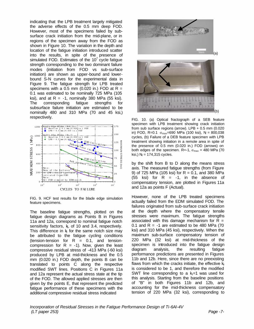
FIG. 8. Residual stress map of the LPB processed vane obtained by x-ray diffraction measurements of the spanwise residual stress at various distances from the trailing edge and at several depths from the surface. The HCF test results are shown in Figure 9 as S-N plots for both single-edge samples tested at R=0.1 and double-edge samples tested at R=-1. Although HCF tests were performed for a variety of FOD depths, for the sake of brevity and clarity, only the results from FOD of 0.5 mm (0.020 in.) depth are presented. In the presence of 0.5 mm deep FOD, the baseline (untreated) fatigue strengths at R = 0.1 and –1 are nominally 70 and 105 MPa (10 and 15 ksi), respectively. As indicated in Figure 9, none of the LPB treated specimens with 0.5 mm FOD tested at either stress ratio failed from the FOD. The fatigue performance of the LPB treated specimens was substantially better than the baseline specimens for either stress ratio and sample design,


indicating that the LPB treatment largely mitigated the adverse effects of the 0.5 mm deep FOD. However, most of the specimens failed by sub-surface crack initiation from the mid-plane, or in regions of the specimen away from the FOD as shown in Figure 10. The variation in the depth and location of the fatigue initiation introduced scatter into the results, in spite of the presence of simulated FOD. Estimates of the 107 cycle fatigue strength corresponding to the two dominant failure modes (initiation from FOD vs sub-surface initiation) are shown as upper-bound and lower-bound S-N curves for the experimental data in Figure 9. The fatigue strength for LPB treated specimens with a 0.5 mm (0.020 in.) FOD at R = 0.1 was estimated to be nominally 725 MPa (105 ksi), and at R = -1, nominally 380 MPa (55 ksi). The corresponding fatigue strengths for subsurface failure initiation are estimated to be nominally 480 and 310 MPa (70 and 45 ksi,) respectively.

1 03

1 04

1 05

1 06

1 07

0

2 0 0

4 0 0

6 0 0

8 0 0

1000

1200

Note: All FOD simuled by EDM notch

Sub surface initiation

FOD Initiation

Sub surface initiation

FOD Initiation

Note: None of the failures in LPB treated specimens initiated from FOD

Single Edge Blades (R=0.1) Baseline + 0.5 mm (0.020 in.) FOD LPB + 0.5 mm (0.020 in.) FOD

Double Edge Blades (R=-1) Baseline + 0.5 mm (0.020 in.) FOD LPB + 0.5 mm (0.020 in.) FOD

CYCLES TO FAILURE

MAXIMUM STRESS (MPa)

0

2 5

5 0

7 5

1 0 0

1 2 5

1 5 0

1 7 5

MA

XIM

UM

ST

RE

SS

(ks

i)

FIG. 9. HCF test results for the blade edge simulation feature specimens. The baseline fatigue strengths, plotted on the fatigue design diagrams as Points B in Figures 11a and 12a, correspond to nominal fatigue notch sensitivity factors, kf, of 10 and 3.4, respectively. This difference in kf for the same notch size may be attributed to the fatigue cycling conditions (tension-tension for R = 0.1, and tension-compression for R = -1). Now, given the least compressive residual stress of -413 MPa (-60 ksi) produced by LPB at mid-thickness and the 0.5 mm (0.020 in.) FOD depth, the points B can be translated to points C along the respective modified SWT lines. Positions C in Figures 11a and 12a represent the actual stress state at the tip of the FOD. The allowed applied stresses are then given by the points E, that represent the predicted fatigue performance of these specimens with the additional compressive residual stress indicated

(a)

(b) FIG. 10. (a) Optical fractograph of a SEB feature specimen with LPB treatment showing crack initiation from sub surface regions (arrow). LPB + 0.5 mm (0.020 in) FOD, R=0.1 σmax=690 MPa (100 ksi), Nf = 800,038 cycles, (b) Failure of a DEB feature specimen with LPB treatment showing initiation in a remote area in spite of the presence of 0.5 mm (0.020 in.) FOD (arrows) on both edges of the specimen. R=-1, σmax = 480 MPa (70 ksi,) Nf = 174,315 cycles. by the shift from B to D along the means stress axis. The measured fatigue strengths (from Figure 9) of 725 MPa (105 ksi) for R = 0.1, and 380 MPa (55 ksi) for R = -1, in the absence of compensatory tension, are plotted in Figures 11a and 12a as points F (Actual). However, none of the LPB treated specimens actually failed from the EDM simulated FOD. The failures originated from sub-surface crack initiation at the depth where the compensatory tensile stresses were maximum. The fatigue strengths associated with this damage mechanism for R = 0.1 and R = -1 are estimated to be 480 MPa (70 ksi) and 310 MPa (45 ksi), respectively. When the maximum sub-surface compensatory tension of 220 MPa (32 ksi) at mid-thickness of the specimen is introduced into the fatigue design diagram analysis, the resulting fatigue performance predictions are presented in Figures 11b and 12b. Here, since there are no preexisting flaws from which the cracks initiate, the effective kf is considered to be 1, and therefore the modified SWT line corresponding to a kf=1 was used for this analysis. Starting from the baseline positions of “B” in both Figures 11b and 12b, and accounting for the mid-thickness compensatory tension of 220 MPa (32 ksi), corresponding to


distance BD in Figures 11b and 12b, the stress state is translated to positions C. Since the entire specimen is subjected to fatigue cycling at R of 0.1 and –1, the predicted fatigue strengths with the subsurface compensatory tension are marked by points E in Figures 11b and 12b. Again, in both Figures 11b and 12b, the corresponding measured fatigue strengths of 480 MPa (70 ksi) and 310 MPa (45 ksi) are also indicated by points F (Actual). It is evident from these figures that the predicted fatigue strengths are lower than the predictions from 11a and 12a. Therefore, the preferred failure mechanism is sub-surface crack initiation, as observed in testing. It is also evident that in the absence of the compressive residual stresses, the fatigue strengths would have been 10 ksi and 15 ksi, respectively, plotted as points X in Figures 11b and 12b. Even with sub-surface crack initiation from the region of maximum compensatory tension, the fatigue strengths of the specimens with LPB treatments were increased by a factor of 3 and 5 times for R = -1 and R = 0.1, respectively. The differences between predictions and actual fatigue results are on the order of the accuracy of the underlying residual stress and fatigue data, and may be attributed to cumulative error in both the residual stress measurements and fatigue test data. Additional analyses of Ti-6Al-4V and other alloy systems are currently under way to further validate this predictive design procedure. Case Study of mitigating fretting damage in Ti-6Al-4V specimens: Application of the design method to fretting damage in HCF of Ti-6Al-4Vwas investigated using thick section specimens tested at room temperature in 4-point bending, 30 Hz, and R = 0.1. Contact fretting was induced using an instrumented bridge-type fretting device similar to the apparatus described by Frost, Marsh and Pook [1] that pressed two Ti-6Al-4V cylindrical pins against the sample surface with a normal force of 150 lb. The 0.25 in. diameter cylindrical pins were spaced 0.5 in. apart, and were renewed for each test. The assembled fretting fatigue fixture is shown in Figure 13. The residual stress distributions produced by LPB in the surface of the fretting fatigue samples are shown in Figure 14, before and after thermal exposure to 375°C for 10 hours to simulate engine service. The thermal stability of the LPB induced compression is attributed to the low cold work associated with the LPB process.

-80-80 -60-60 -40-40 -20-20 00 2020 4040 6060 808000

2020

4040

6060

8080R - r a t i o = 0 . 1F O D = 0 . 0 2 0 i n .

F

A c t u a l

Pred ic t ion

D

C

B

E

SAFE

SWT, k

f = 1

Goodman, kf = 1

R = - 1

R = -INFk

f = INF

Sal

t, k

si

Smean

, k s i

-400-400 -200-200 00 200200 400400

00

100100

200200

300300

400400

500500

S mean, M P a

Sal

t, M

Pa

(a)

-80-80 -60-60 -40-40 -20-20 00 2020 4040 6060 808000

2020

4040

6060

8080

X

R - r a t i o = 0 . 1

S u b - s u r f a c e f a i l u r e

f r o m c o m p e n s a t o r y

t e n s i l e s t r e s s e s

F

A c t u a l

Pred ic t ion

D

C

B

E

SAFE

SWT, k

f = 1

Goodman, kf = 1

R = - 1

R = -INFk

f = INF

Sal

t, k

si

Smean

, k s i

-400-400 -200-200 00 200200 400400

00

100100

200200

300300

400400

500500

S mean, M P a

Sal

t, M

Pa

(b)

FIG. 11. Validation of the design methodology for LPB treated specimens fatigue tested at an R-ratio of 0.1. The design analysis is performed (a) using in FOD initiated failure process, and in (b) using subsurface failure initiation process. The fatigue test results shown in Figure 15(a) for the untreated baseline condition show a fatigue strength of 480 MPa (70 ksi) at 107 cycles. Fretting damage reduced the fatigue strength to nominally 185 MPa (27 ksi), an effective fatigue notch severity factor (kf) of 2.8. The effect of LPB treating the surface of the fatigue specimens is shown in Figure 15(b) with fatigue performance to the baseline results both with and without fretting. Surface initiated cracking was seen in LPB treated specimens tested at high stress levels, and subsurface crack initiation was observed at lower stress levels. Correspondingly, two sets of fatigue strength values can be extracted from Figure 15(b), one for surface and one for subsurface initiation. Fretting scars produced during testing


on the baseline and LPB treated specimens are shown in Figures 16(a) and (b), respectively. Even though the fretting scars are larger for the LPB treated specimens due to higher alternating applied stresses, the fatigue performance was superior, and the fret scar often was not the site of crack initiation in the LPB samples. Figures 17(a) and (b) show typical optical fractographs of surface initiation in the baseline, and subsurface crack initiation in the LPB samples, respectively.

-80 -60 -40 -20 0 20 40 60 800

20

40

60

80R-ratio = -1FOD = 0.020 in.

FActual

Prediction

D

C

B

E

SAFE

SWT, k

f = 1

Goodman, kf = 1

R = -1R = -INFK = INF

Sal

t, ks

i

Smean

, ksi

-400 -200 0 200 400

0

100

200

300

400

500

Smean

, MPa

Sal

t, M

Pa

(a)

-80-80 -60-60 -40-40 -20-20 00 2020 4040 6060 808000

2020

4040

6060

8080

X

R - r a t i o = 0 . 1

Sub-sur face fa i lu re

f r o m c o m p e n s a t o r y

tens i le s t resses

F

A c t u a l

Pred ic t ion

D

C

B

E

SAFE

SWT, k

f = 1

Goodman, kf = 1

R = - 1R = -INFK = INF

Sal

t, k

si

Smean

, ksi

-400-400 -200-200 00 200200 400400

00

100100

200200

300300

400400

500500

S mean, M P a

Sal

t, M

Pa

(b) FIG. 12. Validation of the design methodology for LPB treated specimens fatigue tested at an R-ratio for –1. The design analysis is performed (a) using in FOD initiated failure process, and in (b) using subsurface failure initiation process.

FIG. 13. Fretting fixture with instrumented loading ring and bridge device to hold two fretting cylindrical pins clamped on to the fatigue specimen surface under a controlled normal force.

0 5 10 15 20 25 30 35 40 45 50 55 60-120

-100

-80

-60

-40

-20

0

20

40

No Thermal Exp. 375C/10 Hrs.

AXIAL RESIDUAL STRESS DISTRIBUTION

Residual Stress (ksi)

Depth (x 10-3 in.)

0 200 400 600 800 1000 1200 1400

-800

-700

-600

-500

-400

-300

-200

-100

0

100

200

Residual Stress (MPa)

Depth (x 10-3 mm)

FIG. 14 – Residual stress distributions for LPB, showing a depth of compression over 0.04 in. and not significantly altered by thermal exposure to 375C for 10 hr.

104

105

106

107

0

200

400

600

800

Baseline + Fretting

Baseline

Lambda Research674-10201

CYCLES TO FAILURE

MA

XIM

UM

ST

RE

SS

(M

Pa)

HIGH CYCLE FATIGUE DATA Ti-6Al-4V Thick Section Specimens, 4-point Bending, R=0.1, 30 Hz, RT

0

25

50

75

100

125

MA

XIM

UM

ST

RE

SS

(ksi)

FIG. 15a - HCF tests in the form of S-N curves baseline test on untreated Ti-6Al-4V.


1 04

1 05

1 06

1 07

0

200

400

600

800

Lambda Research674-10201

CYCLES TO FAILURE

MA

XIM

UM

ST

RE

SS

(M

Pa

)

HIGH CYCLE FATIGUE DATA Ti-6Al-4V Thick Section Specimens, 4-point Bending, R=0.1, 30 Hz, RT

0

2 5

5 0

7 5

100

125

LPB FrettingSub-surface Crack Initiation

LPB BaselineSub-surface Crack Initiation

LPB FrettingSurface Crack Initiation

LPB BaselineSurface Crack Initiation

MA

XIM

UM

ST

RE

SS

(ks

i)

FIG. 15(b). Ti-6Al-4V fretting fatigue HCF test results.

FIG. 16(a). Typical fretting scar on Baseline specimen surface (Smax=35 ksi and Nf=427,787)

FIG. 16(b). Typical fretting scar on LPB surface. (Smax=78 ksi and Nf=1,550,922) The application of the fretting fatigue strength data to the fatigue design diagram is shown in Figures

18(a) and (b). The baseline fatigue strength is shown as point A on the R = 0.1 line. Fretting damage reduces the fatigue to point B, with kf = 2.8. The high LPB compression of –700 MPa (-100 ksi) would move the fretting damaged surface operating point along the SWT line to a point well above the fatigue elastic limit line. This would imply that the local compression at the crack tip is limited to the elastic limit line at point C, and the corresponding predicted global fatigue performance is at point E. The actual performance corresponding to surface initiated cracks is shown by point F. The fatigue performance for subsurface initiation in the compensatory tension at depths beyond 1mm (0.040 in.), is shown by point G, well above the performance of the untreated baseline specimens with fretting damage.

Multiple Initiations Along Fretting Zone

FIG. 17(a) Optical fractograph showing typical crack initiation sites from fretting damage.

Subsurface Initiation

FIG. 17(b). Optical fractograph showing typical subsurface crack initiation in LPB treated specimens tested with and without fretting at lower stresses.


-200 -100 0 100 2000

5 0

100

150

200

250

F

EC

B

A

Tensile Yield Strength

LPB + FrettingLPB

Subsurface Initiation

LPB or LPB + Fretting

Baseline - FrettingBaseline

Fatigue Elastic Limit

RSSAFE

R = -∞kf = ∞

Fatigue Design Diagram for Ti-6Al-4V

Sy

-Sy

Sy

R = 0.1

Se

Sal

t, ks

i

Smean

, ksi

-1500 -1000 -500 0 500 1000 1500

0

250

500

750

1000

1250

1500

Smean, MPa

Sal

t, M

Pa

FIG. 18(a). Application of fatigue strength data from FIG.s 14(a) and (b) to Fatigue Design Diagram

- 1 0 0 - 5 0 0 5 0 1 0 00

2 5

5 0

7 5

1 0 0

F

EC

B

A

LPB Pred ic t ion

LPB + Fre t t ing

L P B

Subsur face In i t ia t ionLPB or LPB + Fre t t ing

Basel ine + Fret t ing

Base l ine

Fat igue Elast ic L imi t

R S

SAFE

R = - ∞k f = ∞

Fatigue Design Diagram for Ti-6Al-4V

R = 0.1

Se

Sa

lt,

ks

i

Smean

, ksi

-500 0 500

0

250

500

G

S mean, MPa

Sal

t, M

Pa

FIG. 18(b). A magnified version of FIG. 17(a). WEIGHT SAVINGS AND OTHER DESIGN ISSUES

The fatigue design diagram analysis is presented here mainly as a means of introducing compressive residual stress into the component design for the purpose of mitigating damage that may occur in service. However, this design method has the potential to provide significant material weight and cost savings, if used in the early stages of the design. As a simple example, consider a plate containing a central hole loaded in tension with some superimposed vibratory stresses, at R = 0.7. The allowable stress is the net section stress adjusted for the tensile notch severity factor, kt = 3,assumed equal to the fatigue notch severity factor, kf, for the purpose of this example. For Ti -6Al-4V, the upper limit of the yield strength is nominally 172 ksi (1186 MPa), so a kt of 3 reduces the maximum applied stress to 57 ksi (393 MPa).

The fatigue strength in the absence of the hole is represented by Smax = 143 ksi (985 MPa), and in the presence of a hole (kf = 3) is reduced to, Smax = 47 ksi (324 MPa). Correspondingly, the plate thickness would have to be tripled to meet design requirements. However, the introduction of a compressive residual stress of –50 ksi (-345 MPa) around the hole will restore the full fatigue strength. This is illustrated using the fatigue design diagram in Figure 19. Points A, B, and C, represent the original fatigue strength, the loss of fatigue strength due to introducing a hole, and the increase in the allowed alternating stress due to introducing the –50 ksi compressive residual stress to restore the original fatigue strength, respectively. Clearly, additional properties, such as section stiffness, must be considered along with fatigue strength that will limit the benefits achievable, but taking credit for the residual stress introduced in design could offer substantial material weight and cost savings in component design.

0 100 2000

20

40

60

C

B

A

R = 0.7


σσfS

y

Se

Sal

t, ks

i

Smean

, ksi

-1500 -1000 -500 0 500 1000 1500

0

250

500

750

1000

1250

1500

Smith, kf = 3

Smith, k

f = 1

Goodman, kt = 3

Goodman, kt = 1

Smean, MPa

Sal

t, M

Pa

FIG 19. Section of the Fatigue Design Diagram illustrating the required magnitude of compression to fully mitigate the effect of FOD of kf of 3. SUMMARY AND CONCLUSIONS A fatigue design method based upon a modified SWT model for unifying fatigue data under various conditions of stress ratio, R, and fatigue notch sensitivity factor, kf , has been developed.[21] A Fatigue Design Diagram (modified Haigh Diagram) has been developed defining the allowed alternating stress for given applied and residual mean stresses in both the net tensile and compressive mean stress regions. A series of modified SWT lines for various notch sensitivities, kf, allows the prediction of safe zones. The fatigue design methodology allows the determination of


the amount of residual compression that must be introduced into the surface at the depth of fatigue crack initiation to achieve optimum fatigue strength for a given damage state specified by the notch sensitivity, kf. The method further allows the prediction of surface or subsurface fatigue initiation based upon the measured residual stress field. The proposed fatigue design methodology provides a means to incorporate surface compressive residual stresses imparted through various surface treatments like LSP, LPB, etc., into component design for maximum fatigue benefit. The model has been validated through experimental results for damage tolerance of Ti-6Al-4V for R=-1 and 0.1 and for fretting. ACKNOWLEDGEMENT The authors wish to gratefully acknowledge constructive discussions and review provided by Dr. Gary Halford of NASA, Glenn Research Center, and Dr. Theodore Nicholas of the Air Force Institute of Technology which have contributed to the development of this paper. REFERENCE 1. N.E. Frost, K.J. Marsh, L.P. Pook, 1974, Metal

Fatigue, Oxford University Press 2. H.O. Fuchs, R.I. Stephens, 1980, Metal Fatigue In

Engineering, John Wiley & Sons. 3. H. Berns, L. Weber, 1984, "Influence of Residual

Stresses on Crack Growth," Impact Surface Treatment, edited by S.A. Meguid, Elsevier, 33-44.

4. J.A.M. Ferreira, L.F.P. Boorrego, J.D.M. Costa, 1996, "Effects of Surface Treatments on the Fatigue of Notched Bend Specimens," Fatigue, Fract. Engng. Mater., Struct., Vol. 19 No.1, pp 111-117.

5. P.S. Prevéy, J. Telesman, T. Gabb, and P. Kantzos, March 2000, “FOD Resistance and Fatigue Crack Arrest in Low Plasticity Burnished IN718,” Proceedings of the 5th National High Cycle Fatigue Conference, Chandler, AZ.

6. A.H. Clauer, 1996, "Laser Shock Peening for Fatigue Resistance," Surface Performance of Titanium, J.K. Gregory, et al, Editors, TMS Warrendale, PA, pp 217-230.

7. P.S. Prevéy, N. Jayaraman, R. Ravindranath, April 2003, “Effect of Surface Treatments on HCF Performance and FOD Tolerance of a Ti-6Al-4V Vane,” Proceedings 8th National Turbine Engine HCF Conference, Monterey, CA.

8. P.S. Prevéy, et. al., March 2001, “The Effect of Low Plasticity Burnishing (LPB) on the HCF Performance and FOD Resistance of Ti-6Al-4V,” Proceedings: 6th National Turbine Engine High Cycle Fatigue (HCF) Conference, Jacksonville, FL.

9. M. Shepard, P. Prevéy, N. Jayaraman, “Effect of Surface Treatments on Fretting Fatigue Performance of Ti-6Al-4V,” submitted to International Journal of Fatigue

10. N. Jayaraman, P.S. Prevéy, M. Mahoney, March 2003, “Fatigue Life Improvement of an Aluminum Alloy FSW with Low Plasticity Burnishing,” Proceedings 132nd TMS Annual Meeting, San Diego, CA.

11. P.S. Prevéy, J.T. Cammett, 2004, “The Influence of Surface Enhancement by Low Plasticity Burnishing on the Corrosion Fatigue Performance of AA7075-T6,” International Journal of Fatigue, Vol. 26, pg. 975-982

12. S. Suresh, 2001, Fatigue of Materials, Cambridge University Press, p. 226-227

13. H.C. O’Connor, J.L.M. Morrison, 1956, International Conference on Fatigue, Institution of Mechanical Engineers, pp 102-109.

14. A.R. Woodward, K.W. Gunn, G. Forrest, 1956, “The Effect of Mean Stress on the Fatigue of Aluminum Alloys,” International Conference on Fatigue, Institution of Mechanical Engineers, pp 158-170.

15. W.N. Findley, 1954, “Experiments in Fatigue Under Ranges of Stress in Torsion and Axial Load from Tension to Extreme Compression,” ASTM, vol. 54, pp 836-846.

16. F.M. Howell, J.L. Miller, 1955, “Axial-Stress Fatigue Strengths of Several Structural Aluminum Alloys,” ASEM, vol. 55, pp 955-968.

17. K.N. Smith, P. Watson, T.H. Topper, Dec. 1970, “A Stress-Strain function for the Fatigue of Metals,” Journal of Materials, Vol. 5, No. 4, pp 767-778.

18. H.O. Fuchs, R.L. Stephens, 1980, “Metal Fatigue,” John Wiley & Sons, New York, p.153.

19. T. Nicholas, D.C. Maxwell, 2002, “Mean Stress Effects on the High Cycle Fatigue Limit Stress in Ti-6Al-4V,” Fatigue and Fracture Mechanics: 33rd Vol., ASTM STP 1417, W.G. Reuter and R.S. Piascik, Eds., American Society for Testing and Materials, West Conshohocken, PA

20. Aerospace Structural Metals Handbook, 3704 21. Patent pending.

Incorporation of Residual Stresses in the Fatigue Performance Design of Ti6Al4V

Documents

Transcript of Incorporation of Residual Stresses in the Fatigue Performance Design of Ti6Al4V