Incorporation of Operational Variables in Stochastic ...
231
DEPARTAMENTO DE INGENIERÍA CIVIL HIDRÁULICA, ENERGÍA Y MEDIO AMBIENTE E.T.S.I. CAMINOS, CANALES Y PUERTOS Incorporation of Operational Variables in Stochastic Hydrological Dam Safety Analysis Iván Gabriel Martín Máster Ingeniero de Caminos, Canales y Puertos Directores: Luis Garrote de Marcos Dr. Ingeniero de Caminos, Canales y Puertos Álvaro Sordo Ward Dr. Ingeniero de Caminos, Canales y Puertos 2020
-
Upload
khangminh22 -
Category
Documents
-
view
0 -
download
0
Transcript of Incorporation of Operational Variables in Stochastic ...

DEPARTAMENTO DE INGENIERÍA CIVIL
HIDRÁULICA, ENERGÍA Y MEDIO
AMBIENTE
E.T.S.I. CAMINOS, CANALES Y PUERTOS
Incorporation of Operational Variables
in Stochastic Hydrological Dam Safety
Analysis
Iván Gabriel Martín
Máster Ingeniero de Caminos, Canales y Puertos
Directores: Luis Garrote de Marcos
Dr. Ingeniero de Caminos, Canales y Puertos
Álvaro Sordo Ward Dr. Ingeniero de Caminos, Canales y Puertos
2020

ii

Tribunal nombrado por el Mgfco. Y Excmo. Sr. Rector de la Universidad Politécnica de
Madrid, el día …… de ………………………….. de 2020.
Presidente D. ……………………………………………………………………
Vocal D. ………………………………………………………………………...
Vocal D. ………………………………………………………………………...
Vocal D. ………………………………………………………………………...
Secretario D. ……………………………………………………………………
Realizando el acto de defensa y lectura de la Tesis el día ……….de …………………. de
2020, en ………………………………..
Calificación: …………………………………


A mis abuelos y a mis padres,
por enseñarme la importancia del esfuerzo y la perseverancia.
A Irene,
por complementarme y llenarme de ilusión.


" Lo peor no es cometer un error, sino tratar de justificarlo, en
vez de aprovecharlo como aviso providencial de nuestra ligereza o
ignorancia."
Santiago Ramón y Cajal

ii

vi
Agradecimientos
Llegado este apartado, no sé cómo empezar, pues son muchos los momentos
vividos y el apoyo recibido que han derivado en la elaboración de esta tesis.
En primer lugar, agradecer el apoyo a mis Directores. A Álvaro Sordo, por despertar
en mí la pasión por la hidrología. Podría escribir páginas y páginas, y nunca serian
suficientes para expresar mi agradecimiento. Desde que nos conocimos en la clase de
grado, despertaste mi interés por esta ciencia. Sin ti, no hubiera sido posible nada de esto,
desde el principio hasta el final. Recuerdo los descansos entre clases, hablando con los
compañeros sobre el trabajo de la asignatura y comentando entre risas mi obsesión por
las “cuencas” y Témez. Y no sólo has sido partícipe en motivarme a realizar esta tesis,
sino en despertar otra motivación en mí: la programación. Siempre he tenido la espinita
clavada de no haber estudiado informática y, gracias a tu apoyo y confianza en mí, he
podido iniciar mi andadura en este mundo a lo largo del desarrollo de esta tesis. Por
supuesto, no tengo más que palabras de agradecimiento para Loles y Dieguito, que habéis
compartido gran parte de vuestro tiempo juntos conmigo, incluyendo fines de semana y
vacaciones. Desde aquí, agradeceros vuestra compresión. Álvaro, me alegro que hayamos
podido compartir tantos momentos juntos y, desde aquí, te deseo lo mejor y espero que
sigamos viviendo muchos más. Para mí, no sólo has sido y eres un estupendo profesor,
tutor y persona; sino un gran amigo.
Agradecer a Luis Garrote, por confiar en mí y apoyarme en todo momento. Sin ti,
nada de esto hubiera sido posible. Muchas gracias por todo, sin duda eres un gran profesor
y tutor. Gracias a tus comentarios a lo largo de la tesis, has hecho que cosas que parecían
montañas inalcanzables se conviertan en propósitos abarcables y sencillos.
Gracias a los dos por adentrarme en el mundo de la ciencia y darme esta
oportunidad. Gracias a vosotros he podido conocer a investigadores de todo el mundo,
participar en eventos que jamás hubiera imaginado y conocer mundo. Extender este
agradecimiento a todos los compañeros de Departamento.
Esta investigación tampoco hubiera sido posible sin apoyo económico. Quiero
expresar mi agradecimiento a la Fundación José Entrecanales Ibarra, que me ayudó en los
inicios de esta tesis. Asimismo, agradecer al Programa Propio de UPM, por haberme dado
la oportunidad de seguir realizando esta investigación, así como al Centro de

vii
Supercomputación y Visualización de Madrid; por haberme facilitado acceso a su
supercomputador. También me gustaría agradecer al Consejo Social por otorgarme una
ayuda para haber realizado una estancia doctoral en Arizona State University, sin su
ayuda no hubiera sido posible.
La estancia tampoco hubiera sido posible sin Enrique Vivoni y Giuseppe Mascaro
a los que quiero extender mis agradecimientos. Me habéis dado luz en el uso del modelo
tRIBS, y me habéis brindado la oportunidad de conocer cómo se desarrolla el mundo de
la ciencia en Estados Unidos. Además, quiero agradecer el apoyo de Ara Ko, Adil Mounir
y el resto de compañeros del grupo, que me hicieron sentirme parte del mismo durante mi
estancia en Tempe. Asimismo, agradecer a Riccardo Nalesso su apoyo durante su estancia
en Madrid.
Agradecer a la Escuela de Caminos, que tan buenos (y tan malos) momentos me ha
hecho pasar. Agradecer a todos los profesores, que me han enseñado a que el esfuerzo es
la clave para conseguir nuestros objetivos. De esta escuela me llevo desazones, pero sobre
todo risas, alegrías y grandes amigos; a los que quiero hacer partícipes: a Ibagaza por
haber estado a mi lado a lo largo de todos estos años; a Ángel, Castillo, Javi, Laura y Sara,
que hicisteis que el sufrimiento de primero fuera más ameno; a Rodrigo, Castillo e
Ingelmo, compañeros durante muchos años de tardes de estudio en Leganés y Alcorcón;
a Andrés y a sus apuntes de colores, que nos dieron la oportunidad de iniciar una bonita
amistad; a Cristian, Jacobo y Kike, que hicisteis que el segundo año resultara hasta
divertido; a Laura, Andrea y toda la clase de cuarto de grado, a los que la pasión por las
aguas (y las centrales) nos unieron como uña y carne; al equipo de nuestras visitas técnicas
a Benidorm, Calpe, Lisboa… y a todos los que quedáis en el tintero. Habéis formado parte
de este largo camino de diez años en la escuela, os quiero mucho camineros.
Tampoco quiero olvidarme de todas las personas que han sido partícipes sin los que
nunca habría conseguido llegar hasta aquí, empezando por el colegio Vicente Aleixandre.
En particular tengo mucho que agradecer a Doña Margarita, Doña Sonsoles y en especial
a Don José Luis. Es muy probable qué, sin tu apoyo, no hubiera llegado hasta aquí. Te
estaré eternamente agradecido. A pesar de qué no estés ya entre nosotros, te tenemos muy
presente y te seguimos haciendo partícipe de cada logro y alegría de esta vida. Si decidí
estudiar Ingeniería de Caminos, es por haber seguido uno de tus sabios consejos.
Agradecer también a todos los profesores del Colegio CEU de Montepríncipe, por
haber sido un pilar clave en mi educación, tanto académica cómo personal; así como a

viii
todos mis compañeros y entrenadores del mundo del water polo, que me han acompañado
en mi infancia y adolescencia.
También agradecer a Assist haberme brindado la oportunidad de vivir la
experiencia de estudiar en un colegio americano. Sobre todo, especialmente, haber podido
conocer a Susan y a Nick. Susan, Nick, gracias por haberme cuidado y haberme incluido
en vuestra familia, siempre os estaré agradecido. Como ya sabéis, para mí sois mi madre
y hermano americanos, y seguiremos siempre estando juntos para lo bueno y lo malo.
Parte de esta tesis es gracias a vosotros.
No puedo terminar mi agradecimiento sin mencionar a la familia que se elige. A
mis amigos, que me habéis apoyado siempre: Carlos, Samu, Alfredo, Óscar, Adri, Pérez,
Alberto, Alex … a todos. Y en especial a ti, Morata, que sé que desde allí arriba nos
seguirás acompañando con tu saxo en todos los momentos que nos quedan por vivir.
Nunca te olvidaremos, hermanito, te queremos.
Por último, mi familia. A vosotros, primos y tíos, por enseñarme lo importante que
es ser una piña en todo momento. A vosotros, abuelos, a los que no estáis y me cuidáis
desde arriba; y a ti, abuelo Mario. Estar a tu lado y al lado de la abuela desde pequeñito
me ha enseñado a afrontar el día a día con una sonrisa. Te quiero mucho abuelo.
Agradecerte a ti, Irene, tu apoyo y que formes parte de mi vida estos últimos años de tesis.
Me devolviste la alegría, y espero que este sea el comienzo de toda una vida juntos. Te
quiero mucho. Papá, Mamá, no tengo palabras ni las tendré nunca para agradeceros todo
lo que hacéis por mí en esta vida. Sois mis ejemplos a seguir. Recuerdo que, desde que
tengo uso de razón, os habéis desvivido por mí y me habéis apoyado en todo momento.
Habéis trabajado lo qué no está escrito por ayudarme a tener un futuro mejor. Esta tesis
es resultado de vuestro esfuerzo, sacrificio, de haberme ayudado siempre y, en definitiva,
de enseñarme que, lo más importante en esta vida, es ser buena persona. Os quiero.
Siempre os voy a estar agradecido.

ix

x
Resumen
A lo largo de la historia, se han dado situaciones en las que, presas diseñadas y
construidas acordes a la buena práctica ingenieril han sufrido accidentes con
consecuencias catastróficas. En consecuencia, las nuevas regulaciones y normativas
tienden a aumentar las exigencias de seguridad hidrológica de las Grandes Presas,
influyendo tanto en el diseño como en la adaptación de las presas existentes a los nuevos
criterios exigidos. Es necesario por tanto definir metodologías de evaluación que puedan
aplicarse al conjunto de presas existentes con la finalidad de identificar aquéllas que
tengan un margen de seguridad menos holgado y requieran actuación. En España, se
adopta el criterio de establecer la seguridad hidrológica en función de un periodo de
retorno asociado a las Avenidas de Proyecto. Sin embargo, no existe un criterio riguroso
en la definición de este periodo de retorno, dado que la misma avenida puede ser
caracterizada a través de su caudal punta, volumen o duración; o por una combinación de
estos factores. En la definición de la Avenida de Proyecto, a excepción de la obtención
de la Tormenta de Proyecto, la mayoría de variables involucradas se toman como
determinísticas, cuando en realidad tienen un carácter estocástico. Variables como el
reparto temporal de la lluvia o las condiciones de humedad antecedentes a la avenida son,
entre otras, fijadas de manera determinista por el proyectista a pesar del grado de
incertidumbre existente sobre la determinación de éstas. Gracias a los avances en
informática, la modelación distribuida presenta una alternativa para abordar estas
cuestiones. Modelos distribuidos físicamente basados acoplados con generadores
estocásticos de clima permiten simular los procesos hidrológicos de manera detallada;
tanto temporalmente, como espacialmente.
Además de las variables expuestas, existen otros factores extrínsecos no
contemplados en la definición del periodo de retorno de las avenidas asociados a la
seguridad hidrológica de la presa, como son el nivel inicial en el embalse, o la operación
y disponibilidad de los distintos órganos de desagüe de la presa. Por ello, se considera
que las leyes de frecuencia de niveles máximos en el embalse y de caudales máximos
desaguados son las variables más representativas de la seguridad hidrológica; tanto de la
presa como aguas abajo de ésta. Avenidas de caudales de elevados periodos de retorno
pueden resultar menos comprometedoras que otras de menor periodo de retorno si los
órganos de desagüe no pueden ser operados correctamente. Por lo que se refiere al nivel

xi
inicial en el embalse, no sólo afecta desde el punto de vista del diseño frente a
solicitaciones extremales, sino que mantiene una relación directa con la capacidad de
regulación del embalse. En muchos de los embalses existentes se adoptan resguardos para
paliar las consecuencias de las avenidas extremas, que conllevan una reducción de los
recursos disponibles para el suministro de las demandas y, por consiguiente, pérdidas
económicas derivadas. Sin embargo, en la literatura y en la práctica profesional, ambos
aspectos son generalmente estudiados de forma independiente.
La temática expuesta es de importancia en la actualidad, dado el gran número de
presas existentes que han de ser evaluadas para garantizar la seguridad de la población,
así como el suministro de recursos hídricos. La presente tesis doctoral busca proporcionar
una metodología que, dentro de un entorno de modelación estocástica, mejore: a) la
generación estocástica de avenidas, b) la operación de los órganos de desagüe en situación
de avenida, c) el análisis de la influencia de variables operacionales (nivel inicial en el
embalse y probabilidad de fallo de los órganos de desagüe) y d) la definición de
resguardos estacionales en presas teniendo en cuenta la operación ordinaria de la mismas.

xii
Abstract
Throughout history, there have been situations in which dams designed and built in
accordance with good engineering practice have suffered accidents with catastrophic
consequences. Consequently, new regulations and standards tend to increase the
hydrological safety requirements of Large Dams, influencing both the design and the
adaptation of existing dams to the new criteria required. It is, therefore, necessary to
define assessment methodologies that can be applied to all the existing dams in order to
identify those that have a smaller safety margin and require action. In Spain, the criterion
for hydrological safety is adopted according to a return period associated with the Design
Flood. However, there is no rigorous criterion in the definition of this return period, given
that the same flood can be characterized by its peak flow, volume or duration; or by a
combination of these factors. In the definition of the Design Flood, with the exception of
the Design Storm, most of the variables involved are taken as deterministic, when in fact
they have a stochastic nature. Variables such as the temporal distribution of rainfall or the
humidity conditions in the basin prior to the flood are, among others, determined in a
deterministic manner by the designer despite the degree of uncertainty that exists
regarding their calculation. Thanks to the advances in computer science, distributed
modeling presents an alternative for addressing these issues. Distributed physically-based
models coupled with stochastic climate generators provide a framework to simulate
hydrological processes in a detailed manner; both temporally and spatially.
In addition to the aforementioned variables, there are other extrinsic factors not
contemplated in the definition of the return period of the floods associated with the
hydrological safety of the dam, such as the initial reservoir level, or the operation and
availability of the different spillway outlets of the dam. For this reason, the frequency
curves of maximum reservoir levels and of maximum released outflows are considered
to be the most representative variables of the hydrological safety; both of the dam and the
downstream riverbed. Floods with high return periods may be less compromising than
others with a smaller return period if the spillways cannot be properly operated. With
regard to the initial level in the reservoir, not only does it affect the design regarding dam
safety, but it also maintains a direct relationship with the reservoir's regulation capacity.
In many of the existing reservoirs, the flood control volume is increased to alleviate the
consequences of extreme floods, which lead to a reduction in the water resources

xiii
available for the supply of the demands and, consequently, derive in economic losses.
However, in the literature and in professional practice, both aspects are generally studied
independently.
The subject matter presented is of current importance, given the large number of
existing dams that must be evaluated to guarantee the safety of the population, as well as
the supply of water resources. This doctoral thesis seeks to provide a methodology which,
within a stochastic modeling environment, will improve: a) the stochastic generation of
floods, b) the operation of the spillway and dam outlets in a flood situation, c) the analysis
of the influence of operational variables (initial level in the reservoir and probability of
failure of the spillway outlets) and d) the definition of seasonal conservation levels in
dams taking into account the regular operation in the reservoir.

xiv
List of acronyms
A Area of the watershed.
a, b Dimensionless parameters of Equation (3.4).
selected from the CEDEX (MARM, 2011;
Jimenez-Alvarez et al., 2012) national study.
AL Activation level.
ARMA Autoregressive moving average model.
AWE-GEN Advanced weather generator.
CDF Cumulative distribution functions.
CEDEX The Public Works Studies and Experimentation
Centre of Spain, Ministry of Development.
Cg1-g2% Scenarios represented by the independent rate of
failure of each gate (g1 and g2).
CN Curve number.
COD Crest of dam (m.a.s.l.).
Costbreak Damage cost if the dam fails.
D Damage function.
DEvent Duration of a storm event.
DFL Design flood level.
dj Duration of the maximum annual observed flood
events (days).
DMO Damage function associated with Maximum
Outflows.
DMWRL Damage function associated with Maximum Water
Reservoir Levels.
DO Function of damage costs associated with the
maximum outflows.
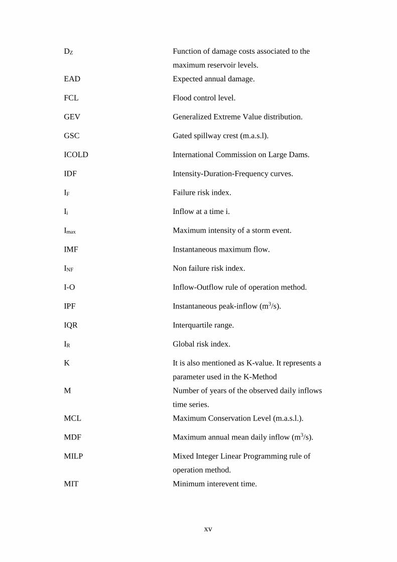
xv
DZ Function of damage costs associated to the
maximum reservoir levels.
EAD Expected annual damage.
FCL Flood control level.
GEV Generalized Extreme Value distribution.
GSC Gated spillway crest (m.a.s.l).
ICOLD International Commission on Large Dams.
IDF Intensity-Duration-Frequency curves.
IF Failure risk index.
Ii Inflow at a time i.
Imax Maximum intensity of a storm event.
IMF Instantaneous maximum flow.
INF Non failure risk index.
I-O Inflow-Outflow rule of operation method.
IPF Instantaneous peak-inflow (m3/s).
IQR Interquartile range.
IR Global risk index.
K It is also mentioned as K-value. It represents a
parameter used in the K-Method
M Number of years of the observed daily inflows
time series.
MCL Maximum Conservation Level (m.a.s.l.).
MDF Maximum annual mean daily inflow (m3/s).
MILP Mixed Integer Linear Programming rule of
operation method.
MIT Minimum interevent time.

xvi
MNL Maximum Normal Level (maximum reservoir
level to which water might rise under normal
operation (ICOLD,1994)) (m.a.s.l).
MO Maximum outflow (m3/s).
MOTR=500y Maximum outflow that corresponds to a return
period of 500 years.
MSM10 Mean soil moisture in the top 10 cm of the soil
layer of the basin.
MSM10Event MSM10 associated to the beginning of a storm
event.
MWL; MWRL Maximum Water Level (maximum reservoir level
which the dam has been designed to stand
(ICOLD,1994)) (m.a.s.l).
MWRLTR=1000y Maximum Water Reservoir Level that corresponds
to a return period of 1,000 years.
N Number of events considered.
n Number of time intervals until the reservoir runs
out of flood control capacity.
NSE Nash Sutcliffe Efficiency Coefficient (Nash and
Sutcliffe, 1970).
OALT Alert outflow.
OEMER Emergency outflow.
Oi Outflow at a time i.
OMAX Maximum released outflows.
Omax.disch.(Si) Maximum outflow that can be discharged at the
current reservoir level.
Omax.Gr Maximum gate opening/closing gradient.
OWARN Warning outflow.
P Objective penalty function applied in MILP.
p Probability of exceedance.

xvii
p(break|MWRLi) Probability of overtopping failure conditioned to
reaching a certain level in the reservoir.
p(MWRLMAX≥COD| MWRLi) Probability of reaching the reservoir level at crest
of dam once a certain reservoir level has been
reached during a flood event.
PC Peacheater creek.
PF Maximum annual hydrograph peak-flow.
PFFC Peak flow frequency curve.
Po Penalty function of released outflows.
Ps Penalty function of storage volume.
Pt Total maximum rainfall depth (mm).
Q1 First quartile (25 % percentile).
Q2 Median.
Q3 Third quartile (75 % percentile).
QI, QII, QIII, QIV Quadrants of the comparative scheme: first,
second, third and fourth respectively.
QMAX. Maximum mean daily peak-inflows (m3/s).
Qmin. Minimum inflow between the two flood peaks
compared (m3/s).
Qo Start of the receding limb (m3/s).
Qp Outflow proposed by VEM.
Qt Recession flow at any time (t) after the beginning
of the receding limb (m3/s).
R Reference model.
R2 Coefficient of determination.
RE Relative error.
RIBS Real-time integrated basin simulator.

xviii
RMSE Root mean square error.
SAL Volume at the activation level.
Sc.1 Scenario in which initial reservoir level was set
equal to Maximum Normal Level.
Sc.2 Scenario in which initial reservoir level was set
equal to Flood Control Level.
Sc.3 Scenario in which initial reservoir level was
considered variable.
SCS Soil Conservation Service.
SFCL Volume at the flood control level.
Si Reservoir storage at a time i.
Si-1 Reservoir storage at time i−1.
SiF Available flood control capacity at a time i.
SPANCOLD Spanish National Committee on Large Dams.
STCP Volume at the top of conservation pool.
T Tested model.
TCP Top of control pool.
TIN Triangulated irregular networks.
TK Kendall’s return period.
Tr Return period (years).
tRIBS TIN-based real-time integrated basin simulator.
TrMNL. Return period of maximum water reservoir levels
or maximum outflows obtained assuming constant
initial reservoir level equal to MNL (years).
TrVAR. Return period of maximum water reservoir levels
or maximum outflows obtained assuming variable
initial reservoir level (years).
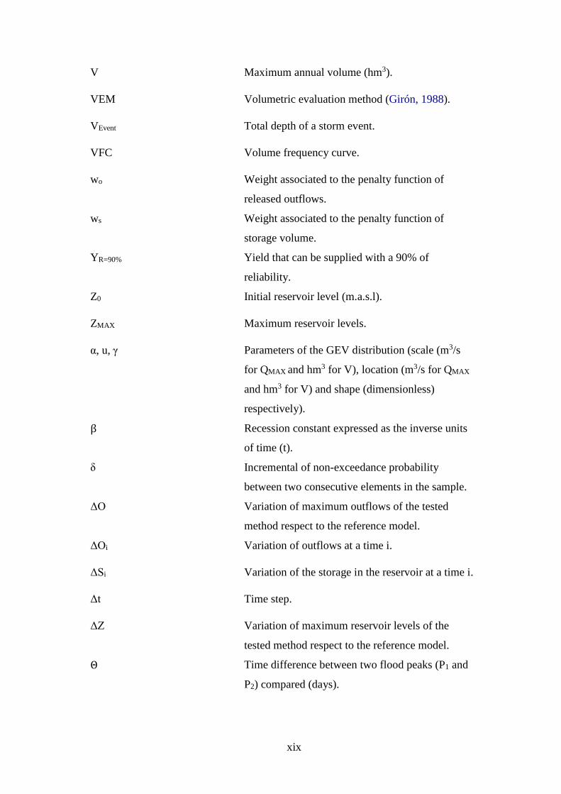
xix
V Maximum annual volume (hm3).
VEM Volumetric evaluation method (Girón, 1988).
VEvent Total depth of a storm event.
VFC Volume frequency curve.
wo Weight associated to the penalty function of
released outflows.
ws Weight associated to the penalty function of
storage volume.
YR=90% Yield that can be supplied with a 90% of
reliability.
Z0 Initial reservoir level (m.a.s.l).
ZMAX Maximum reservoir levels.
α, u, γ Parameters of the GEV distribution (scale (m3/s
for QMAX and hm3 for V), location (m3/s for QMAX
and hm3 for V) and shape (dimensionless)
respectively).
β Recession constant expressed as the inverse units
of time (t).
δ Incremental of non-exceedance probability
between two consecutive elements in the sample.
ΔO Variation of maximum outflows of the tested
method respect to the reference model.
ΔOi Variation of outflows at a time i.
ΔSi Variation of the storage in the reservoir at a time i.
Δt Time step.
ΔZ Variation of maximum reservoir levels of the
tested method respect to the reference model.
Θ Time difference between two flood peaks (P1 and
P2) compared (days).

xx
r̅ The variability of the date of occurrence about the
mean date (θ�).
θ� Mean date of occurrence of the annual maximum
peak-flow/volume.

xxi

Index
xxii
Index
Agradecimientos .............................................................................................................. vi
Resumen ...................................................................................................................... x
Abstract ................................................................................................................... xii
List of acronyms ............................................................................................................ xiv
Index ................................................................................................................. xxii
1. Introduction .............................................................................................................. 1
Research motivation and aims ................................................................................ 1
1.1.1. What is hydrological dam safety? ...................................................................... 1
1.1.2. Why is important to analyse the hydrological safety of dams in Spain? ........... 2
1.1.3. How we analyse hydrological dam safety? Objectives of this thesis. ............... 4
Thesis structure ....................................................................................................... 6
Summary of research outcomes of this thesis ......................................................... 7
2. Literature review ...................................................................................................... 8
Hydrological dam and downstream safety .............................................................. 9
Hydrological forcing ............................................................................................. 10
Spillway operation ................................................................................................ 13
Initial reservoir level ............................................................................................. 15
Spillway reliability ................................................................................................ 17
Definition of Maximum Conservation Levels ...................................................... 19

Index
xxiii
3. Methodology .......................................................................................................... 22
Hydrological forcing ............................................................................................. 23
3.1.1. A Hybrid stochastic event-based continuous distributed approach ................. 24
3.1.2. A stochastic data-based hydrological forcing generator .................................. 32
3.1.3. A stochastic event-based hydrological forcing generator ................................ 36
Spillway operation ................................................................................................ 37
3.2.1. Volumetric Evaluation Method (VEM) ........................................................... 37
3.2.2. The proposed K-Method .................................................................................. 39
3.2.3. I-O and MILP ................................................................................................... 43
Initial reservoir level analysis ............................................................................... 43
3.3.1. Use of historic reservoir levels ........................................................................ 44
3.3.2. Simulation of reservoir levels .......................................................................... 45
Spillway reliability ................................................................................................ 46
Hydrological dam and downstream Safety ........................................................... 47
Economic risk analysis .......................................................................................... 48
Stochastic procedure for the definition of Maximum Conservation Levels ......... 50
3.7.1. Study set of seasonal Maximum Conservation Levels .................................... 51
3.7.2. Reservoir operation simulations ...................................................................... 51
3.7.3. Results analysis and solutions proposal ........................................................... 53
Introduction to the case studies and software used ............................................... 54
4. Hydrological forcing: The Hybrid method ............................................................ 62
Application to Peacheater Creek basin ................................................................. 62
4.1.1. Study basin ....................................................................................................... 62

Index
xxiv
4.1.2. Setup of modelling experiments ...................................................................... 63
4.1.3. Limitations of the experiment .......................................................................... 64
4.1.4. Validation of the method. Hybrid method Vs. Continuous simulation ........... 64
Obtained results ..................................................................................................... 68
4.2.1. Stochastic weather generation. Rainfall extremes validation. ......................... 68
4.2.2. Rainfall versus flood comparison .................................................................... 70
4.2.1. Initial soil moisture: simulation and probability distributions ......................... 82
4.2.2. Hybrid method performance ............................................................................ 83
The Hybrid method: Summary and conclusions ................................................... 87
4.3.1. Criterion for storm selection for the Hybrid method. ...................................... 87
4.3.2. Initial soil moisture conditions and performance of the Hybrid Method ........ 89
5. Spillway operation: The K-Method ....................................................................... 92
Application to the Dam in the Segura river basin ................................................. 92
Performance assessment of the K-Method ............................................................ 94
The K-Method: Summary and conclusions ......................................................... 102
6. Operational variables I: The Influence of the initial reservoir level. ................... 104
Application to the Dam in the Tagus river basin ................................................ 104
6.1.1. Generation of synthetic reservoir inflow hydrographs .................................. 106
6.1.2. Initial reservoir level. Scenarios and uncertainty analysis ............................. 107
6.1.3. Reservoir-Dam flood operation ..................................................................... 111
6.1.4. Risk Index analysis ........................................................................................ 114
Influence of initial reservoir level: partial conclusions ....................................... 116

Index
xxv
7. Operational variables II: The influence of gate failure combined with initial
reservoir level variability ............................................................................................... 118
Application to the Dam in the Douro river basin ................................................ 118
7.1.1. Generation of series of stochastic initial reservoir levels .............................. 120
7.1.2. Generation of synthetic reservoir inflow hydrographs .................................. 123
7.1.3. Reservoir-Dam system routing ...................................................................... 125
7.1.4. Results analysis .............................................................................................. 132
The influence of gate failure combined with initial reservoir level variability: Partial
conclusions. .................................................................................................................. 137
8. On the definition of Maximum Conservation Levels .......................................... 138
Application to the Dam in the Douro river basin ................................................ 138
8.1.1. Definion of the study set of Maximum Conservation Levels and proposed
solutions ...................................................................................................................... 139
8.1.2. Seasonal hydrographs .................................................................................... 139
8.1.3. Simulation of the dam operation rules ........................................................... 141
8.1.4. Solutions proposal .......................................................................................... 143
8.1.5. Comparison between the proposed configurations in the two scenarios ....... 144
On the definition of Maximum Conservation Levels: Partial conclusions ......... 145
9. Conclusions .......................................................................................................... 148
Main conclusions ................................................................................................ 148
9.1.1. Hydrological forcing: The Hybrid method .................................................... 148
9.1.2. Spillway operation: The proposed K-Method ............................................... 150
9.1.3. Operational variables I: Influence of initial reservoir level ........................... 151
9.1.4. Operational variables II: Influence of gate failure ......................................... 153
9.1.5. Definition of seasonal conservation levels .................................................... 153

Index
xxvi
Original contributions ......................................................................................... 154
Further research ................................................................................................... 156
References .................................................................................................................. 160
Figures List .................................................................................................................. 178
Tables List .................................................................................................................. 188
APPENDIX: Front and last page of JCR published papers ........................................... 1
1.1. Influence of initial reservoir level and gate failure in dam safety analysis. Stochastic
approach.......................................................................................................................... A1
1.2. Dependence Between Extreme Rainfall Events and the Seasonality and Bivariate
Properties of Floods. A Continuous Distributed Physically-Based Approach. .............. A3
1.3. Hydrological Risk Analysis of Dams: The Influence of Initial Reservoir Level
Conditions. ...................................................................................................................... A5
1.4. A Parametric Flood Control Method for Dams with Gate-Controlled Spillways. A7
1.5. Flood Control Versus Water Conservation in Reservoirs: A New Policy to Allocate
Available Storage. .......................................................................................................... A9

1. Introduction
1
1. Introduction
This introduction shows a general overview of the relevant aspects of prior
knowledge that lead to the contributions of this thesis. The key motivation of this thesis
is to provide new methods and tools for improving the analysis of hydrological dam
safety:
• First, in Section 1.1, the motivation and objectives of the research are described,
focusing on answering the triplet: what is hydrological dam safety, why its important
and how this thesis proposes a new framework for its analysis.
• In Section 1.2, the structure of this doctoral thesis is presented.
• In Section 1.3, the publications associated to this research are listed.
Research motivation and aims
1.1.1. What is hydrological dam safety?
Historically, the concept of dam safety has been characterized by a unique
relationship with absolute safety. Generally, society assumes that dams are absolutely
safe, and its exigencies are not related to the execution of the dam as civil works but to
the correct response to the uses for which they were designed (Aranda Domingo, 2014).
However, the concept of absolute safety is not possible from a practical point of view.
From the point of view of the safety of the dam, the citizen demands no risk, regardless
of whether or not the different regulations are enforced. Throughout history, there have
been situations in which dams designed and built in accordance with good engineering
practice have suffered accidents with catastrophic consequences. Today's society needs
the following message to be conveyed: "dams are safe", but, as field practitioners, this
assertion cannot be made without some nuances. However, in view of the current
situation, what is indispensable is the precision and transmission to society of the concept,
as well as the quantification of the level of safety of the dams. All dams must be
"sufficiently" safe and conceived as such by the citizen. Therefore, a specific evaluation
of each of the existing dams will be needed, but the basic problem is the establishment of
this criterion of sufficiency (De Andrés Rodríguez-Trelles and Mazaira, 2003).
However, this evolution in the thinking of society has not been reflected in the
methods for analysing hydrological safety of dams, which have changed relatively little

1. Introduction
2
in recent decades (Sordo-Ward et al., 2012; 2013). Hydrology and dams are two fields of
study with a close relationship. However, even though both fields are related, hydrology
is studied independently of the type of dam and its characteristics in most of the studies
(ICOLD, 2018). Worldwide, the greatest cause of dam failure is overtopping, with an
estimated 36% of the total registered dam breaks (ICOLD, 1995). These overtopping
failures, in many cases, were not exclusively caused by extreme flood events but also by
other causes such as gate operational failures (Hartford et al, 2016).
Furthermore, dams can also cause catastrophic consequences without breaking.
Under flood control operation conditions, the spilled outflows may cause floods in the
downstream riverbed when the capacity of the river channel is overpassed (Bianucci et
al., 2013).
Therefore, hydrological dam safety can be understood as the analysis of how likely:
a) a dam can be overtopped and b) the capacity of the downstream river can be
overpassed.
1.1.2. Why is important to analyse the hydrological safety of dams in
Spain?
Dams in Spain play an important role due to geographical, climatic and
socioeconomic characteristics of the country. Spain is a Mediterranean country which
presents a great irregularity both spatially and temporally regarding to water runoff
resources. Due to these characteristics, the proportion of the net amount of water from
natural resources that can be used does not reach 10% (Berga, 2006).
In order to increase water availability, it has been necessary to retain water in the
territory through the construction of hydraulic infrastructures such as dams and reservoirs.
Currently, the number of catalogued dams in Spain is 1,583 dams (MAPA, 2019). Around
60% percent of the dams in Spain have been constructed between 1950 and 2000, being
therefore a key factor in Spain’s economic development since mid of the last century.
Dams have played a key role in Spain, protecting from floods, producing hydroelectric
energy, and serving as operation points of the water resources management. Under the
International Commission On Large Dams (ICOLD) guidelines, Spain accounts for a total

1. Introduction
3
of 1,082 Large Dams1. This figure situates Spain as the ninth country in terms of number
of Large Dams around the globe (ICOLD, 2019).
Due to the number of Large Dams in Spain and their importance, there is a variety
of different dam owners in Spain, both public and private holders. Around one third of
the total Spanish Large dams are owned and operated by Spanish Ministry for the
Ecological Transition through the River Basin Authorities which, in addition, hold the
authority to enforce and develop integrated water resources planning and management,
flood control and environmental protection, among other activities. In accordance with
the Water Framework Directive, 18 River Basin Districts have been defined in Spain.
River Basin Authorities are public entities with autonomy of action and their own legal
personality. Two types of them can be distinguished: inter-regional basins (e.g. Jucar
River Basin) and intra-regional basins (e.g. Catalonia Intra-Regional Basins) (Castillo-
Rodriguez et al., 2015).
With more than 1,400 dams (including also small dams and ponds), functions and
responsibilities of dam owners regarding dam safety management have evolved as a result
of a changing dam safety regulation framework. The evolution of the regulations of Dams
in Spain is closely related to the catastrophes that have occurred throughout history. After
the breakage of the Ribadelago Dam, which occurred in 1959, the Spanish Large Dams
Standards Commission was created, which in 1962 proposed “Instrucción para el
Proyecto, Construcción y Explotación de Grandes Presas” (Instruction for the Design,
Construction and Exploitation of Large Dams), which was finally approved by Order of
the Ministry of Public Works on March 31, 1967. This law is partially in force today
(MAPA, 2018), being complemented with and partially abolished by “Reglamento
Técnico sobre Seguridad de Presas y Embalses” (Technical Code of Dams and Reservoirs
Safety), approved on March 12, 1996.
Due to the ageing of dams in Spain, new regulations and standards tend to increase
the hydrological safety requirements of dams, influencing both the design and adaptation
of existing dams to the new criteria required. It is therefore necessary to define assessment
methodologies that can be applied to all existing dams in order to identify those that are
less safe and require action plans. This need has been reflected in the National Law
Project of the Technical Safety Standards for Dams and Reservoirs (MAPA, 2018),
1 ICOLD criteria: A Large Dam is a dam with a height of 15 metres or greater from lowest foundation
to crest or a dam between 5 metres and 15 metres with a storage of more than 3 million cubic metres.

1. Introduction
4
presently pending approval, which will abolish the previous legislation associated to Dam
Safety, providing a new legal framework.
Therefore, as exposed, there is a need on assessing the current state of dams in
Spain, in which hydrological dam safety plays a key role.
1.1.3. How we analyse hydrological dam safety? Objectives of this thesis.
The hydrological methods for analysing dam safety have evolved little in recent
decades. Specifically, in Spain a methodology based on the characterization of a "Design
Storm" is still being applied, which by means of hydrometeorological models turns into
the "Design Flood", with which the spillways are designed or checked.
This methodology is mainly deterministic, introducing a single probabilistic
component in the determination of the accumulated precipitation in 24 h associated with
a specific return period that varies between 100 and 10,000 years. The rest of the variables
are defined according to the designer's criteria and intervene in the calculation in a
deterministic manner, despite the fact that there is a high degree of uncertainty about
them. Among them, we can differentiate:
1. Parameters that characterize the generation of runoff in the basin and its
transportation: the duration of the storm, the spatio-temporal simultaneity of storms,
the initial state of the basin at the beginning of the storm event, among others.
2. Parameters associated to the dam-reservoir system: the manoeuvring of the different
spillways and outlets, the initial reservoir level at the beginning of the flood event, or
the probability of blockage or malfunctioning of discharge outlets and spillways.
When accounting for this variables probabilistically, the uncertainties of them can
be assessed, and stochastic procedures can be performed to obtain results that resemble
more to the reality of nature and the reality of dam-reservoir systems.
Moreover, in many cases, the probability of flood events tells little about the
probability of dam overtopping, as the maximum reservoir levels and outflows can be
reached due to other circumstances, such as low reservoir storage or various operational
faults. Thus, it is essential to change the focus of hydrological dam and downstream safety
from floods to an overall overview of the dam-reservoir system.
Therefore, within this thesis, not only the probability of overtopping due to extreme
flooding is analysed but also the influence of operational variables such as the initial

1. Introduction
5
reservoir level, the probability of failure of spillways or the flood control operational
methods. As a consequence, the main objective of the thesis is the analysis of the
influence of the variables of the operation of the dam on its hydrological safety through
the development of a complete stochastic methodology for its analysis (Figure 1.1).
Figure 1.1: General scheme of the stochastic methodological approach proposed in this thesis.
To fulfil these purposes, the following specific objectives are defined:
O.1. Development of a stochastic methodology based on hydrological modelling that
allows to generate a representative set of hydrographs at the entrance to the dam
for the evaluation of its hydrological safety.
O.2. Analysis of the operation of spillways and discharge outlets under flood
operation scenarios and improvement of their management strategies. To fulfil
this objective, by analysing the traditional methodology used in Spanish dams, a
new flood operation method has been developed that can be easily applied by the
dam operators, reducing the associated risks in terms of hydrological safety, both
in the operation of ordinary and extreme floods.
O.3. Development of a stochastic methodology for the study of different operating
variables related to hydrological dam safety, such as the level of the reservoir
previous to a flood event. By the use of probabilistic approaches, an assessment
of the influence of initial reservoir level is carried out for different case studies.
O.4. In relation to objective O.3, this thesis develops a framework to asses the
influence of the probability of malfunctioning or failure of gated-spillways. Thus,

1. Introduction
6
the objective is to analyse the influence of this operational variable within
hydrological dam and downstream safety.
O.5. Joint analysis of the operation of the reservoir, both in regular and flood
situations. Development of a methodology that takes into account both factors in
the definition of seasonal conservation levels in dams.
Within the framework of the thesis, different case studies have been selected to
analyse the performance of the methods proposed in different basins and dam
configurations.
Thesis structure
The results of the research are shown in this doctoral thesis, which is organized
according to ten chapters. The motivation, aims and organization of the thesis have
already been introduced in the present Chapter 1. A review of the studies performed over
the literature leading to the present research is displayed in Chapter 2. The general
methodology followed to accomplish the research, including the description and
connection among the specific methodologies proposed for each part into which the
research is divided, as well as a summary of the considered case studies are shown in
Chapter 3. The next chapters are focused on the results of this research, according to the
objectives shown in the previous section:
• Chapter 4: An analysis of the number of rainfall events to be considered for a proper
hybrid event-based modelling is performed, being this the first part of the proposed
hydrological modelling framework. Afterwards, the proposed hydrological Hybrid
model is applied, showing its performance in one of the case studies of the thesis.
• Chapter 5: Within this chapter, a new method for the operation of flood discharge
structures is presented.
• Chapter 6: In this chapter, an economic analysis through risk indexes is carried out,
assessing the impact of accounting for the influence of initial reservoir level and the
uncertainty associated to this variable.
• Chapter 7: Within this chapter, the influence of initial reservoir level and gate failure
in hydrological dam safety is analysed.
• Chapter 8: A stochastic procedure for defining seasonal conservation levels is
proposed.

1. Introduction
7
Finally, conclusions and further research approaches are presented in Chapter 9.
Summary of research outcomes of this thesis
The research outcomes of this thesis have been published in several journal articles
and conferences. A summary of the main publications is shown:
• Papers published in peer-reviewed journals indexed in the Journal Citation Reports
(first and last page of each manuscript shown in the Appendix):
1. Gabriel-Martin, I.; Sordo-Ward, A.; Garrote, L.; Castillo, L.G..; 2017. Influence of initial reservoir level and gate failure in dam safety analysis. Stochastic approach. Journal of Hydrology, 550, 669-684. doi:10.3390/w11030461 JCR: Q1 SJR: Q1
2. Gabriel-Martin, I.; Sordo-Ward, A.; Garrote, L.; T. García, J. Dependence Between Extreme Rainfall Events and the Seasonality and Bivariate Properties of Floods. A Continuous Distributed Physically-Based Approach. Water 2019, 11, 1896. doi:10.3390/ w11091896 JCR: Q2 SJR: Q1
3. Gabriel-Martin, I.; Sordo-Ward, A.; Garrote, L.; Granados, I.; 2019. Hydrological Risk Analysis of Dams: The Influence of Initial Reservoir Level Conditions. Water, 11 (3), 461. doi:10.3390/w11030461. JCR: Q2 SJR: Q1
4. Sordo-Ward, A.; Gabriel-Martin, I.; Bianucci, P.; Garrote, L.; 2017. A Parametric Flood Control Method for Dams with Gate-Controlled Spillways. Water, 9(4), 237. doi: 10.3390/w9040237. JCR: Q2 SJR: Q1
5. Gabriel-Martin, I.; Sordo-Ward, A.; Santillán, D; Garrote, L.; 2020. Flood Control Versus Water Conservation in Reservoirs: A New Policy to Allocate Available Storage. Water, 12(4), 994. doi: 10.3390/w12040994. JCR: Q2 SJR: Q1
• Paper published in peer-reviewed journals indexed in the Emerging Sources Citation
Index:
6. Gabriel-Martin, I.; Sordo-Ward, A.; Garrote, L.; 2018. Influencia del nivel inicial en la definición de resguardos estacionales en presas. Ingeniería del agua, 22 (4), 225-238. doi: 10.4995/ia.2018.9526. (In Spanish) JCR: - SJR: -.
Furthermore, alongside the research outcomes previously exposed, research in
fields related to this thesis has been performed during the PhD studies:
• Paper published in peer-reviewed journal indexed in the Journal Citation Reports:
7. Bejarano M.; Sordo-Ward, A.; Gabriel-Martin I.; Garrote, L.; 2019. Tradeoff between economic and ecological effects of hydropower production under different environmental flows scenarios. Journal of Hydrology, 572, 790-804,. doi:10.1016/j.jhydrol.2019.03.048. JCR: Q1 SJR: Q1
• Paper published in peer-reviewed journal indexed in the Scopus Database:
8. Sordo-Ward, A.; Gabriel-Martin, I.; Perales-Momparler, S.; Garrote, L.; 2019. Influencia de la precipitación en el diseño de SUDS. Revista de Obras Públicas, 166(3607), 28-31. ISSN: 00348619 JCR: - SJR:Q4

2. Literature review
8
2. Literature review
An analysis of the developments in hydrological safety in both scientific and
professional fields is carried out within this chapter, focusing on the aspects exposed in
Chapter 1. This chapter is divided into the following subsections (Figure 2.1):
• Section 2.1: An introduction to this chapter is presented, comparing the proposed
stochastic framework of this thesis with the current traditional approach. The
relationship of hydrological dam and downstream safety with the maximum reservoir
level and maximum outflow frequency curve is analysed.
• Section 2.2: An analysis of the literature regarding to the determination of
hydrological forcing in hydrological dam safety is carried out.
• Section 2.3: An analysis of the different operative schemes for the management of
controlled spillways under flood conditions is carried out.
• Section 2.4: The influence of accounting for the variability of initial reservoir level is
reviewed, analysing how different authors have accounted for this variable.
• Section 2.5: A review of the different ways of accounting for spillway reliability is
performed.
• Section 2.6: Finally, a review of the literature regarding to the definition of seasonal
maximum conservation levels is performed.
Figure 2.1: Sections of the Literature review associated to the hydrological dam safety stochastic approach proposed.

2. Literature review
9
Hydrological dam and downstream safety
Failure of Large Dams is a concern in many countries due to the high economic and
social consequences associated to it. When designing a dam, engineers usually apply
techniques to assure that the risk associated to dam failure is low, being the standards
applied differently depending on the country in which the dam is located (Rettemeier and
Köngeter, 1998; Ren et al, 2017). Even though the risk assumed is low, the associated
risk should be recalculated, as the legal regulations, climate conditions, basin and dam
characteristics may vary along time (Fluixá-Sanmartín et al, 2018).
In the standard engineering approach, hydrological assessment of dam and
downstream safety for a given return period is analysed with deterministic methods. A
design flood hydrograph is obtained and routed through the reservoir-dam system
assuming constant reservoir level prior to the arrival of the flood and equal to the
maximum normal operating level. The Design Flood, characterized by its peak flow, is
used for the design of the dam outlets without considering any safety coefficient as is
usual in other types of structures. The Design Flood in Spain is associated with the return
period of total accumulated precipitation in 24 hours, thus characterizing the risk
associated with it and therefore the safety of the dam (Sordo-Ward et al., 2012).
The wide use of this methodology has been due to its easy application and few
information requirements. However, scientific advances in the field of hydrology
combined with an increase in computational capacity, the development of geographic
information systems and spatial modelling processes have made it possible to propose
stochastic models for the extreme characterization of the hydrological behaviour of
basins.
Many of the involved variables in hydrology have a stochastic nature (Carvajal et
al., 2009; Sordo-Ward et al., 2013). In recent decades, many authors proposed
probabilistic approaches accounting for the randomness associated with different
variables (e.g.: Eagleson, 1972; Arnaud and Lavabre, 2002; De Michele et al., 2002,
2005; Carvajal et al., 2009; Sordo-Ward et al., 2012; 2013; Paquet et al., 2013; Bianucci
et al., 2013, 2015; Brigode et al., 2014; Flores-Montoya et al., 2015, 2016). Several
authors had been able to obtain accurate maximum peak-inflow frequency curves within
a Monte Carlo Framework (Loukas, 2002; Rahman et al., 2002; Arnaud and Lavabre,
2002; Aronica and Candela, 2007). However, it is a matter of importance to characterize

2. Literature review
10
not only the extremal incoming reservoir floods but the hydraulic behaviour and response
of dams, as their failure could have catastrophic socio-economic consequences (Serrano-
Lombillo et al., 2010; 2016).
Flood control has two fundamental objectives, which are to guarantee the safety of
the dam, by preventing the maximum level of the reservoir from being exceeded as well
as to avoid overflows to minimize the damage caused by flooding downstream of the
dam. Several authors (Mediero et al., 2010; Bianucci et al., 2013; Serrano-Lombillo et
al., 2012a; Aranda Domingo, 2014; Micovic et al., 2016; Michailidi and Bacchi,2017)
pointed out that hydrological dam safety and downstream safety should be assessed by
analysing the return periods of the maximum reservoir water levels and maximum
outflows respectively. This way, the hydrological dam safety analysis does not only
depend on the hydrological forcing, but also on the dam and reservoir characteristics and
operation rules.
Hydrological forcing
Firstly, a distinction should be made between the basic evaluation criteria for the
selection of floods and the calculation methods for developing these criteria. The former
is generally defined by the risk that a given community is willing to accept in the face of
possible failure or collapse of the dam and depends not only on technical and economic
considerations but also on social, political, cultural and environmental ones.
As far as flood estimation methods are concerned, there are numerous classification
criteria based on: the origin of the information to be considered (based on rainfall or flow
data), calculation methodology (deterministic or probabilistic), expected results (peak
flows or hydrographs), temporal scope (continuous or event-based methods), among
others.
In Spain, the Technical Guidelines for Dam Safety (SPANCOLD, 1997) define two
large groups, the deterministic type and the probabilistic type. In these groups, the
deterministic method is understood to be that which unequivocally calculates the
maximum flood flow from meteorological and hydrological data. In this group, the
"Probable Maximum Flood (PMF)" method is highlighted (USACE, 1991). Probabilistic
methods are considered to be those that carry out a study based on available data (rainfall

2. Literature review
11
and/or flow) and determine peak flows and flood hydrographs for different return periods.
The latter is the one currently applied in Spain.
This methodology makes it possible to characterize hydrological risk as a function
of peak flow, but there are other factors that influence the response of the dam and
reservoir to floods. In fact, the entire hydrograph is of interest for the design and risk
assessment of dams. The hydrograph must be abated by the reservoir through the dam to
know how it transforms into a series of outflows and different level variations in the
reservoir. For this reason, the univariate analysis of peak flows should be extended to a
multivariate analysis that takes into account other variables such as volume and duration
that allow the construction of complete hydrographs.
The national regulations of different countries establish a return period for the
design of dams (in Spain from 500 to 10,000 years) (Rettemeier and Köngeter, 1998; Ren
et al, 2017). However, they do not specify whether the return period is associated with
the peak flow, the volume of the hydrograph or the entire hydrograph. Design return
periods are commonly associated to the return period of the design flood hydrograph,
considering that rainfall events generate hydrographs with peak-inflows with the same
return period. Many authors questioned this hypothesis (e.g.: Adams and Howard, 1986;
Alfieri et al., 2008; Viglione and Blösch, 2009; Sordo-Ward et al., 2014). It is also well-
known that return periods associated to peak-inflows are not the same as those associated
to hydrograph volume, existing a trend to analyse this issue by using copulas for
multivariate flood frequency analysis (e.g.: De Michele et al., 2002; Shiau et al. 2006;
Salvadori et al., 2011; Requena et al., 2013; 2016; Aranda Domingo, 2014). This question
can be extended to the return period associated to the hydrological safety of dams. In
addition, the risk associated with an event may be undervalued (or overvalued) if only the
return period associated with one of the variables that characterize the hydrograph is
analysed (De Michele et al., 2002; Salvadori et al., 2011). In fact, as exposed in Section
2.1, the return period should be defined in terms of the risk associated with overtopping
the crest of the dam or with the downstream damage, rather than in terms of the
probability of occurrence of natural events, to take into account the characteristics of the
reservoir, the dam and its spillway (Mediero et al., 2010; Bianucci et al., 2013; Serrano-
Lombillo et al., 2012a; Aranda Domingo, 2014; Micovic et al., 2016; Michailidi and
Bacchi,2017).

2. Literature review
12
To characterize the hydrological forcing, several methods can be applied and are
mainly classified according to two main groups:
• Statistical flood frequency analysis: statistical methods are generally based on
processing existing local and regional flow through statistical procedures such as
distribution fitting (USWRC, 1976; USGS, 1982), making appropriate use of
historical references where available.
• Derived flood frequency simulation methods: by the use of a hydrological model, a
set of hydrographs is obtained from which a flood frequency distribution can be
derived.
Statistical methods need large flow records (hardly available (Zhang and Shing,
2017; Klein et al., 2010)), have the drawback of the uncertainty associated to the
distribution fitting for large return periods (Katz et al., 2002), and provide a value of peak-
flow, volume, or duration but not the hydrograph shape. Furthermore, when they are
applied in ungauged basins, the physical processes that occur in the watershed are not
usually considered and the uncertainty on the flood quantiles estimation increases
(Salinas et al., 2013).
Due to these reasons, derived flood frequency methods are generally preferred over
statistical ones (Li et al., 2014a). Derived flood frequency methods can be divided into
two approaches: continuous simulation and stochastic event-based methods (Li et al.,
2014a).
Using a continuous distributed hydrological model provides the user the possibility
of deriving flood frequency distributions from the continuous hourly streamflow obtained
at any desired point in the drainage network of the basin by forcing the distributed
hydrological model with an hourly stochastic weather generator. This approach has the
advantage of estimating the variables for the entire period of simulation. However,
continuous models tend to be more complex than event-based models, with computational
efforts that could be very intensive, even when using high performance computing and
parallelization processes.
On the other hand, event-based simulations require much shorter simulation times.
However, these methods are based on the assumption that the flood hydrograph has the
same return period as the storm event, which is (as previously exposed) not realistic
(Adams and Howard, 1986; Alfieri et al., 2008; Viglione and Blösch, 2009). Furthermore,

2. Literature review
13
different properties of storm events could affect the derivation of flood frequency curves:
rainfall temporal distribution, event duration, maximum intensity, and total storm depth,
among others.
Examples of both derived flood frequency approaches can be found in the existing
literature. In the case of event-based approaches, some studies have combined non-
complex stochastic storm generators (i.e., Sordo-Ward et al., 2012; 2013) or complex
rainfall generators (i.e., Foufoula-Georgiou, 1989); with semidistributed (i.e., Franchini
et al., 1996) or distributed models (i.e., Flores-Montoya et al., 2016). In the case of
continuous simulations, in order to reduce the computational cost, most authors have
worked with lumped or semidistributed models (i.e., Haberlandt et al., 2008; Brocca et
al., 2013), and some of them have worked with distributed models by using high
performance computers (Blazkova and Beven, 2004; Vivoni et al., 2011).
To overcome the limitations in the two approaches, several authors have proposed
combining event-based models with continuous models. Paquet et al. (2013) proposed
the SCHADEX model, which consists on replacing stochastic rainfall events within a
short continuous simulation with observed data and a Monte Carlo framework. Li et al.
(2014a) developed the hybrid-CE approach, which consists of combining continuous
long-term simulations of rainfall and short continuous hydrological simulations to
probabilistically characterize the rainfall and initial soil moisture (respectively) to force
an event-based model. Both approaches used lumped models.
Spillway operation
Flood management aims to guarantee dam safety, minimize downstream floods,
and maintain the full operational capacity of reservoirs once a flood is over (Wurbs, 2005;
Wang et al., 2010; Hossain and El-Shafie, 2013; Feng and Liu, 2014; Pan et al., 2015).
Dams with gated spillways represent around 30% of large dams around the world
(ICOLD, 2003), and provide more possibilities for water conservation and flood
abatement than those with fixed‐crested spillways (Sordo-Ward et al., 2013). Gate
management during a flood event represents a challenge for the dam operator, who makes
decisions under pressure and during uncertain conditions. In addition, the time frame for
decision making is usually extremely short, the information available is generally sparse,
and the predictability of the meteorological situation is limited (Afshar and Salehi, 2011;
Molina et al., 2005). Real-time flood control operations at dams have been historically

2. Literature review
14
approached via predefined rules obtained by simulation techniques (Li et al., 2014b), or
by using simulation methods such as the Volumetric Evaluation Method (VEM) (Girón,
1988), commonly used in Spain. Flood control policies generally establish the discharge
at each time step by considering the available information at a previous time, e.g., inflow,
reservoir stage, stored volume, and outflow discharge downstream, among others (Loucks
and Sigvaldason, 1982). Dam Master Plans include this information, which helps
operators to be efficient (Wurbs, 2005). These operation rules are represented and
assessed by simulation models, which are usually more flexible and easier to interpret for
the dam operators than other schemes, such as optimization (Needham et al., 2000;
Rahman and Chandramouli, 1996; Chang, 2008; Le Ngo et al., 2007; Oliveira and
Loucks, 1997; Bianucci et al., 2013) or data-based learning models (Chang and Chang,
2006; Chang et al., 2010; Ishak et al., 2011; Khalil et al., 2005; Mediero et al., 2007;
Cuevas Velasquez, 2015).
Several simulation frameworks have been developed to tackle this issue. The
software HEC-ResSim (Klipsch and Hurst, 2007) permits one to obtain the discharged
outflow for each time step, accounting for the operation rules and simulating the
behaviour of the reservoir. Flood Control-Reservoir Operator’s System software
(Karbowski, 1991) supports decision making by providing important data and possible
operation alternatives (as a result of the control algorithms implemented in the program).
Other models integrate real-time reservoir operation with flood forecasting. They account
for the uncertainty associated with the hydrologic loads, by analysing different
forecasting techniques for reservoir inflows and by including deterministic and
probabilistic approaches (Zhao et al., 2011). A further example is the integrated
management system for flood control at reservoirs developed by Cheng and Chau (2001),
which gathers real-time information. This is processed in a central database management
system in order to evaluate the alternatives of flood operation.
The improvements in the field of optimization and data-based learning allow an
approach to the problem which accounts for the uncertainty of the hydrologic loads in
real-time forecasting (Liu et al., 2015a) and permits the development of operation policies
incorporating different objectives (Choong and El-Shafie, 2015; El-Shafie et al., 2014;
Hosseini-Moghari et al., 2015; Ahmadi et al., 2014). Most of the optimization methods
are based on an objective function, which minimizes the outflows and the maximum
reached reservoir levels (Bianucci et al., 2013). A wide variety of optimization models

2. Literature review
15
have been applied to flood reservoir operations: linear programming, non-linear
programming, successive linear programming, stochastic dynamic programming, genetic
algorithm, genetic programming, particle swarm optimization, Honey-Bee mating,
Artificial Bee Colony, and a combination of the aforementioned (Choong and El-Shafie,
2015). However, there is still a gap between the theoretical development and practical
implementation of these models (Hossain and El-Shafie, 2013; Ahmed and Mays, 2013).
Optimization models are usually limited as they depend on specific parameters (penalty
functions and coefficients of the objective function, among others) which need the
operator’s expertise on mathematical programming (Bianucci et al., 2013). In addition,
due to the uncertainty associated with hydrologic loads and the limitations of the flood
forecasting, dam managers usually prefer simulation methods (Jood et al., 2012).
Therefore, the operation of the flood discharge structures defines how the dam–
reservoir system should respond when forced by a flood event (Fluixá-Sanmartín et al.,
2018). The correct operation of the dam outlets and spillways permits to maintain the
safety levels, downstream and within the dam.
Initial reservoir level
The field of dam risk assessment has evolved worldwide, with the appearance of
different guides and procedures in several countries (ANCOLD, 2003; USACE 2011;
SPANCOLD, 2012) to support dam stake-holders in the decision-making process related
to dam safety. It is also well-known that, due to the high variability of the natural
processes, the assessment of dam safety introduces uncertainties that should be assessed
as part of the process. However, analysing this uncertainty is a complex task (Bianucci et
al., 2015; Sordo-Ward et al., 2014).
Moreover, human actions also provide additional sources of uncertainty to the
analysis. One of those variables related to human actions is the variability of initial
reservoir level, due to its connection to the operation of the reservoir. As reservoir levels
fluctuate (when a flood arrives the reservoir may be partially full) the assumption of
considering the reservoir full prior to a flood event could be conservative in hydrological
safety analysis (Carvajal et al., 2009). However, this assumption is a practice commonly
implemented among dam designers and national technical guidelines (Bianucci et al.,
2013).

2. Literature review
16
Thus, many authors considered initial reservoir level as constant (e.g.: Hsu et al.,
2011; Serrano-Lombillo et al., 2012b; Sordo-Ward et al., 2012; 2013; Bianucci et al.,
2013), but some considered its variability:
• In 2005, a study was carried out using a probabilistic methodology on the Ceppo
Morrelli dam, a vaulted dam with a fixed-crest spillway located in Italy (De Michele
et al., 2005). Within the framework of their work, they used a previous level in the
reservoir obtained randomly by means of an empirical distribution function of the
historical level in the reservoir.
• Kwon and Moon (2006) analysed overtopping probability in Soyang Dam (South
Korea). They assessed initial reservoir level by accounting for the reservoir levels
probability distribution of the rainy season in the dam, concluding that initial reservoir
level was the most sensitive variable for the estimation of dam overtopping
probability.
• In 2009, a team of engineers (Carvajal et al., 2009) analysed, among other factors, the
influence of the variability of the initial level in the reservoir at the time of flooding.
They analysed three dams of different characteristics. They concluded, in general, that
the inclusion of the variability of the initial level in the reservoir is appreciable in the
case of reservoirs in which there are considerable seasonal fluctuations in the level,
being of less interest in the case of dams with constant levels throughout the year.
• Peyras et al. (2012) studied the operation of a roller-compacted gravity dam by
modelling the initial situation of the reservoir based on an empirical distribution of
monitored levels in the reservoir following the methodology of Carvajal et al. (2009).
• In a thesis presented in the Technical University of Valencia, Aranda Domingo (2014)
analysed the influence of this factor on a dam with a fixed-crest spillway, specifically
in the Cueva Foradada reservoir. He concluded that the influence of this factor is
significant, being closer to the current reality of the dam-reservoir system.
• Micovic et al. (2016) analysed three dams in cascade in Canada. In their modelling
framework, the stochastic simulation of floods on the system of three dams shows
progression from exceedance probabilities of reservoir inflow to exceedance
probabilities of overtopping depending on the initial reservoir level, storage
availability, reservoir operating rules and availability of discharge facilities on
demand. They concluded that overtopping is more likely to be caused by a

2. Literature review
17
combination of a small flood event and an operational component failure than by an
extreme flood event on its own.
It is therefore important to take this factor into account for the realistic treatment of
the hydrological safety of dams. All previously mentioned studies concluded that
accounting for reservoir levels fluctuations in hydrological dam safety is desirable,
moreover when the dam is operated in seasonal basis as is the case of reservoirs which
main purpose is irrigation, regardless of the spillway and dam typology.
Spillway reliability
As aforementioned, dams are built with different purposes, such as power
production, water supply, flood mitigation and other things. A dam system, comprises the
body of the dam along with all the facilities to trespass the water from the reservoir, such
as outlets, conduits, channels or spillways. Nowadays, dam safety assessment is currently
based on analysing if the dam is able to withstand extreme loads, such as the Design Flood
or its ability to withstand the design earthquake. Even though the importance of extreme
loads is unquestionable, experiences have shown that many dam failures have been
caused due to operational events rather than geophysical extreme events (Hartford et al,
2016). One of the dam facilities that are more relevant to hydrological dam safety are
spillways. Specifically, those spillways that are composed by gates. In this type of dams,
the manoeuvring of spillways is fundamental. As previously exposed, gated-spillway
dams represent about 30% of the large dams around the world (ICOLD, 2003). The
malfunction of gates has caused important dam failures along history in different parts of
the world. Among them, some dam failures can be highlighted in which spillway
malfunctioning was one of the causes of failure:
• Elko Dam in Canada in June of 2013.
• Folson Dam in The United States of America, in July of 1995.
• Noppikoski Dam in Sweden, on September 7, 1985.
• Tous Dam in Spain, on October 20, 1982.
• Canyon Lake Dam in The United States of America, on June 9, 1972.
Therefore, accounting for gate functionality may be of importance as gate blockage
may result in an increase of the risk of dam failure (Lewin et al., 2003; Patev and Putcha,

2. Literature review
18
2005; Escuder-Bueno et al., 2012; SPANCOLD, 2012; Micovic et al., 2016). Gates may
not open when needed because of human, mechanical, electrical failures, lack of access
to the manoeuvring chamber, blockage of spillway outlets, or failure of gate or valve
control software (Lewin et al., 2003; Patev and Putcha, 2005; SPANCOLD, 2012; Fluixá-
Sanmartín et al., 2018).
Observed data regarding gate functionality is sparse. Some studies in literature have
analysed the unavailability of gates:
• In the case of the Directorate-General for Public Works and Water Management of
the Netherlands, they conducted a reliability analysis of gates in a Storm Surge
Barrier, estimating an unavailability of 0.1% on demand (van Iperean, 1984)
• Lagerholm (1996) performed a survey on major dam stakeholders in Sweden,
obtaining a statistic of annual failure of gates of the order of 0.1 in common gate types
such as radial or vertical roller gates.
• Lewin et al. (2003) estimated that the value of failure on demand associated to a single
gate was 10%, while the multiple failure rate of gates due to common causes was
assumed as 1% per demand.
• In other study about the Thames River defences (UKAEA, 1987) an unavailability
per gate demand of 0.0155 % was estimated.
• Micovic et al. (2016) assumed a probability of 1% for single gate failure on demand,
but pointed that this assumption could not be safe.
Therefore, gate malfunctioning is a field in which stats samples are scarce. One of
the important issues about gate malfunctioning is its maintenance. Deterioration could
derive in a useless spillway. In dam risk analysis qualitative description could be an
alternative to analyse the probability of failure within the context of hydrological dam
and downstream safety. To do so, the quantitative individual reliability of a gate can be
associated with the description of the condition of the gates (Fluixá-Sanmartín et al.,
2018). Thus, Escuder-Bueno et al. (2012) proposed the following relationship between
the condition of gates and its probability of failure (Table 2.1)

2. Literature review
19
Table 2.1: Reliability estimation of gates with respect to their maintenance condition.
Gate Condition Reliability (%) Brand-New / Non-gated 100 Very well maintained 95 Some minor problems 85
Some problems 75 Non-Reliable 50
Unreliable at all 0
This individual gate-failure rates can be complemented with more complex analysis
such as the use of fault trees, indicating different manners in which the gate can fail and
disaggregating the probabilities of failure (Lewin et al., 2003).
Definition of Maximum Conservation Levels
Up to this section, the focus was on hydrological dam safety. As exposed, owing to
the increasingly risk-averse societies, stronger hydrological safety requirements are being
imposed on dams in order to fulfil new regulations and prevent dam failures (Bocchiola
and Rosso, 2014). This problem can be approached with two different kinds of technical
solutions: hard solutions, which could be the refurbishment of dam spillways or elevation
of dam crest; and soft solutions as the allocation of additional flood control volumes. Hard
solutions increase the flood control capacity while maintaining reservoir storage available
for water supply. However, their main drawback is the need to allocate resources for
infrastructure works. On the other hand, the implementation of soft solutions is easier and
quicker, but can reduce the reliability of the system regarding to water supply.
Allocation of flood control volume is addressed by defining a Maximum
Conservation Level, also known as Flood-Limited Water Level (Li et al., 2010) or Flood
Control Level. The Maximum Conservation Level is the maximum operating level that
the reservoir is allowed to reach under regular operation conditions. This reservoir level
is below the Maximum Normal operating Level, and can vary along the seasons of the
year.
When increasing flood control volumes by soft solutions, there is a trade-off
between flood control and water supply demands supplied in which the most significant
parameter is the Maximum Conservation Level (Xie et al., 2018).
Traditionally, practitioners only focused on hydrological dam and downstream
safety when defining Maximum Conservation Levels, not accounting for other purposes

2. Literature review
20
of the reservoir, such as water supply. This may imply economic consequences related to
water demand reliability (Solera-Solera et al., 2012).
Some authors have focused on accounting simultaneously for both, regular
(associated to water supply purposes of the reservoir) and flood control dam operation
when defining Maximum Conservation Levels. Liu et al. (2015b) proposed a
methodology to define seasonal Maximum Conservation Levels accounting for both flood
control and water supply and Chang et al. (2017) defined variable sub-seasonal Maximum
Conservation Levels to increment hydropower benefits by using fuzzy logic techniques.
Other authors have studied seasonal Maximum Conservation Levels within deterministic
approaches (Chen et al., 2013; Zhou and Guo, 2014; Fu et al., 2014; Ouyang et al., 2015;
Moridi and Yazdi, 2017; Xie et al., 2018).
Other relevant factor is that practitioners usually define Maximum Conservation
Levels assuming that the reservoir is at the maximum level under normal operating
conditions prior to flood arrival (USACE, 1972; Sordo-Ward et al., 2013). While this
hypothesis, as previously mentioned, results into conservative hydrological safety
assessments, it can reduce the reliability of the water supply system as it has an effect on
the definition of Maximum Conservation Levels.
As exposed, accounting for all the operational variables (i.e.: reservoir level
variability) in hydrological dam and downstream safety leads to more realistic results,
which consequently can lead to a better definition of Maximum Conservation Levels.

2. Literature review
21

3. Methodology
22
3. Methodology
The general methodology proposed to carry out the present research is described in
this chapter. Summarized explanations regarding the specific methodologies performed
for each part forming the research, as well as the links among them, are also shown.
Further explanations are developed within the following chapters, in the context of the
different research studies. Besides, a summary of the case studies considered for the
application of such methodologies, and an outline of the software used are included.
As exposed in Section 1.1.3, the objective of this thesis is to develop a stochastic
methodology to assess hydrological dam and downstream safety while accounting for
operational variables such as the initial reservoir level, the availability of spill outlets or
the influence of the flood operational methods.
Even though the methodology must be understood as a whole unit, the following
chapters develop specifics parts of it that can be combined into the following scheme
(Figure 3.1).
Figure 3.1: Stochastic proposed framework of hydrological dam and downstream safety assessment.

3. Methodology
23
Thus, following the objectives shown in Section 1.1.3, the methodology framework
is introduced in the following subsections:
• Section 3.1: Hydrological forcing.
• Section 3.2: Spillway operation.
• Section 3.3: Initial reservoir level.
• Section 3.4: Spillway reliability.
• Section 3.5: Hydrological dam and downstream safety.
• Section 3.6: Economic risk analysis.
• Section 3.7: Maximum Conservation Levels.
Finally, a brief introduction to the case studies and software used in the thesis is
shown in Section 3.8.
Hydrological forcing
Three methods have been used in this thesis to generate a representative ensemble
of inflow hydrographs. Two of them are fully developed within the framework of this
thesis and described in this section. The third one is an application of the method
developed by Sordo-Ward et al. (2012, 2013) and is also introduced. The main
characteristics of the methods are:
• A Hybrid stochastic event-based continuous distributed approach (herein Hybrid
method). It consists on the use of a distributed physically based model, coupled to a
stochastic climate generator. The recent advances in parallel computing are accounted
by using a High Performance Computing system. This method can be applied to any
case study, but it requires high-detailed spatio-temporal weather and flow data.
• A stochastic data-based hydrological forcing generator. It consists on a simpler
approach of multivariate flood modelling using a lumped stochastic event-based
model that allows the generation of hydrographs from historical floods observed at
the dam entrance. This method can be applied to any dam with daily inflow data.
• A stochastic event-based hydrological forcing generator. This method, previously
developed by Sordo-Ward et al. (2012, 2013), consists on a stochastic semi-

3. Methodology
24
distributed event-based hydrometeorological model. This method has been
successfully applied in a consistent set of dams within Spain.
It is important to point out that, for obtaining results representative up to 10,000
years of return period, the ensemble size should be at least ten times the maximum return
period analysed (Loukas et al., 1996; Loukas, 2002; Blazkova and Beven, 2004; Sordo-
Ward et al., 2012). The ensembles generated within this thesis have a simple size of
100,000 hydrographs, with the exception of those related to the development of the
Hybrid method, due to computational and timing issues (a continuous simulation of
100,000 years would take years of simulation). In order to validate the methodology
proposed, a continuous simulation of 5,000 years was performed. Thus, the method
shown was validated only up to return periods of 500 years. However, as the Hybrid-
event based method reduces the computational times from months to hours, ensembles of
100,000 years could be generated.
3.1.1. A Hybrid stochastic event-based continuous distributed approach
In this thesis, a Hybrid method to derive the flood frequency curve is presented,
combining the advantages of both continuous and event-based hydrological models
within a distributed physically-based approach.
Distributed physically-based hydrological models appeared in the 1960s and have
been the object of critics due to their complexity and difficulty of use (Fatichi et al., 2016).
Nowadays, the availability of higher resolution spatio-temporal datasets, the appearance
of high performance computers, and the development of parallel computing (Blazkova
and Beven, 2004; Cui et al., 2005; Kollet et al., 2010; Vivoni et al., 2011) have opened
the possibility of using these models for large size basins and long-term hydrological
continuous simulations. Thus, challenges such as the influence of land-use changes
(Pumo et al., 2017; Arnone et al., 2018) or the impact of climate change (Liuzzo et al.,
2010; Piras et al., 2014) on the involved hydrological processes can be analysed with
these models.
Another use of distributed hydrological models is the estimation of extreme floods
for the design of civil infrastructures, such as bridges, levees, or dams. For these
structures, it is necessary to estimate hydrographs of low probability of occurrence, that
is, with return periods that go from hundreds to thousands of years in the case of dams
(Rettemeier and Köngeter, 1998; Ren et al., 2017). As indicated, one of the main

3. Methodology
25
disadvantages of physically distributed hydrological models is the computation time.
When these models simulate flood events, the computational cost is lower. However, the
main disadvantage of event-based models is the uncertainty in the estimation of the
humidity in the basin prior to the storm event to be simulated, which is crucial in deriving
the corresponding hydrograph. Likewise, the spatio-temporal distribution of storms
implicates that the rain with the greatest total depth or intensity of the year does not have
to be directly associated with the hydrograph of maximum peak flow or volume of the
same year.
These sources of uncertainty can be minimized by continuously simulating the
response variables of the basin. However, the possibility of obtaining flows with a high
temporal resolution at any point of the drainage network entails a high computational
cost. This reason makes it difficult to use it for the derivation of frequency curves of peak
flows and volumes for extreme return periods where continuous simulations of thousands
of years would be necessary.
This thesis proposes a methodology that combines the advantages of distributed
event-based and continuous models, for the derivation of frequency curves of maximum
flow and maximum annual flood volume, by combining a stochastic continuous climate
generator with a physically-based distributed hydrological model based on both event and
continuous simulations.
For the definition of the proposed Hybrid method, the focus was on two critical
aspects of event-based simulations:
• Relationship between storm events and floods.
• Initial moisture conditions in the basin prior to storm events.
3.1.1.1. Criterion for storm selection for the Hybrid method.
The focus of this first part of the Hybrid method is, by using a fully physically-
based distributed hydrological model coupled with a stochastic weather generator in a
continuous simulation, to provide a guideline to select the minimum necessary storm
events that should be simulated in event-based approaches to obtain similar results to
those obtained by continuous simulations in the derivation of flood frequency curves.
Sordo-Ward et al. (2016) carried out a similar analysis in some watersheds in mainland
Spain, by using a semi-distributed event-based model coupled with a continuous

3. Methodology
26
stochastic rainfall generator. They separated all the events within the generated series and
analysed the relationship between the storms and the maximum annual peak-flow in the
Manzanares river basin (Spain) and two of its sub-basins. Flores-Montoya et al. (2016)
also carried a similar analysis using a distributed event-based model in two basins in
France. However, in both studies, the lack of a continuous simulation required the
estimation of the initial soil moisture (same curve number value in Sordo-Ward et al.
(2016) and probabilistically in Flores-Montoya et al. (2016)).
Within this thesis, the continuous simulation with a fully physically-based
distributed hydrological model enables to account for the variations of the initial soil
moisture. Thus, not only can the magnitude and recurrence of events be analysed, but also
the relation between storms and the seasonality of the flood hydrographs. Furthermore,
within this thesis, the relationship within storms and flood hydrographs is analysed, not
only in a univariate way, but with a bivariate approach through the use of copulas for a
better assessment between the relation of storms and the dependence of the maximum
annual peak-flow and volume.
Therefore, the first objective of the methodology is to propose a criterion for the
selection of the minimum number of storm events per year to guarantee a correct
derivation of the bivariate flood frequency curve. Figure 3.2 presents a general scheme of
the modelling framework and methodology proposed:
Figure 3.2: Criterion for storm selection for the Hybrid method.
• Stochastic weather generation. It consists on the generation of 5,000 years of hourly
weather series using the Advanced WEather GENerator (herein AWE-GEN)
developed by (Fatichi et al., 2011). In the present study, this model is used to simulate
hourly point series of climate from the statistical properties of the observed series in

3. Methodology
27
the case study. AWE-GEN (Fatichi et al., 2011) is a generator capable of reproducing
low and high-frequency characteristics of hydro-climatic variables and essential
statistical properties of these variables.
The weather generator employs both the physically-based and stochastic approaches
and is a substantial evolution of the model presented by Ivanov et al. (2007). AWE-
GEN is a statistical hourly stationary model capable of reproducing statistical
properties of several weather variables including precipitation, cloud cover,
shortwave incoming radiation, air temperature, vapour pressure, wind speed, and
atmospheric pressure over a range of time scales. Since rainfall is the main weather
variable involved in the framework of this work, a brief introduction of the
precipitation model is reported.
The AWE-GEN uses the point Neyman–Scott rectangular pulse approach to generate
the internal structure of the precipitation process, based on Cowpertwait (2004)
studies. Such models are able to capture the main observed rainfall time-series
statistic characteristics; for the case of the AWE-GEN model: (1) mean waiting time
between adjacent storm origins (h); (2) mean waiting time for rain cell origins after
the storm origin (h); (3) mean duration of the rain cell (h); (4) mean number of cells
per storm (-); (5) shape parameter (-) and (6) scale parameter (mm/h) of the Gamma
distribution of rainfall intensity. These six parameters are fitted minimizing an
imposed objective function using the simplex method (Nelder et al., 1965) on a
monthly basis, i.e., the six parameters are inferred for each month in order to account
for seasonality. As exposed by Fatichi et al. (2011), to validate the generated series it
is recommendable to analyse statistics different from those used in the calibration.
Within this thesis, as the focus is on rainfall events and floods, an analysis on how the
stochastic generated series were able to reproduce the observed rainfall extreme
properties is performed. The reader is referred to Fatichi et al. (2011) and Ivanov et
al. (2007) for further details on AWE-GEN.
• Distributed physically-based hydrological modelling. The basin response is modelled
by using the TIN-based real-time integrated basin simulator (herein tRIBS (Ivanov et
al., 2004a; Vivoni et al., 2007)). tRIBS (Ivanov et al., 2004a; Vivoni et al., 2007) is a
physically based, distributed continuous hydrologic model. Its predecessor, the real-
time integrated basin simulator (RIBS) of Garrote and Bras (1995) implemented an
event-based model for rainfall–runoff analysis. tRIBS has inherited the functionality

3. Methodology
28
of RIBS while adding the hydrology necessary for continuous operation. tRIBS uses
an adaptive multiple resolution approach, described by Vivoni et al. (2004), based on
triangulated irregular networks (TIN) to represent the terrain topography. tRIBS
considers the spatial variability in precipitation fields, land-surface descriptors, and is
able to solve the basin hydrologic response at an hourly temporal resolution and a
very fine spatial (10–100 m) scale. tRIBS includes parameterizations of rainfall
interception, evapotranspiration, infiltration with continuous soil moisture
accounting, lateral moisture transfers in the unsaturated and saturated zones, and
kinematic-wave runoff routing. The model computational basis, structure, and
description of process parameterizations are given in full detail in (Ivanov et al.,
2004a; Vivoni et al., 2007). This model has been implemented in watersheds of
various sizes (up to 21,000 km2 (Ko et al., 2019)) and in different locations
characterized by different climates.
The results of the simulation are 5,000 years of continuous flow at the basin outlet,
with a warming period of ten years to reduce the influence of initial conditions in the
results obtained.
• Separation of storm events. Analysing the rainfall series within the stochastic weather
series generated, the independent storm events are separated. There are different
methodologies (Restrepo-Posada and Eagleson, 1982; Sifalda, 1963; Yen and Chow,
1980; Bonta and Rao, 1988) to identify independent rainfall events.
Rain events are usually identified by fixing the duration of the minimum inter-event
time (MIT) that follows, or precedes, a rainfall event. Two rainfall events are
independent if there is no rainfall (considering a minimum rainfall threshold of 0.25
mm/h) between them in a period equal or superior to the MIT (Figure 3.3). Within
this study, the exponential method (Restrepo-Posada and Eagleson, 1982) is selected
to determine the value of the MIT. This method assumes that the storm arrival time
and the time between two storms follows an exponential distribution. Consequently,
the duration of dry periods can be approximated by an exponential distribution with
a mean that is equal to the standard deviation, and therefore the coefficient of variation
(CV) is equal to one. To obtain the value of the MIT, the CV for different dry-period
durations is obtained applying Equation (3.1):

3. Methodology
29
CVk=std(dpk)/dp����k, (3.1)
where k is the dry-period duration (1 h, 2 h, …), dp����k is the average of dry-period
durations greater than the duration of k, and std(dpk) its standard deviation. The value
of the MIT is determined as the value of k in which CVk approximates to one.
Once the MIT is obtained, all the storm events within the rainfall time-series are
obtained. The separation is performed to the observed and generated series for: (a)
The validation of AWE-GEN simulations, and (b) for the comparison of rainfall
versus floods.
Figure 3.3: Example of two independent rainfall events (black and grey for events one and two,
respectively). The total depth of the event (VEvent) is represented by the shaded area, the maximum intensity (Imax) is represented by the dots, and the duration (DEvent) by the lower line. Two dry periods are represented in the figure. The first one, has a shorter duration than the minimum inter-event time (MIT)
and therefore, the two wet periods belong to the same event. In the second dry period, the duration is longer than the MIT and it represents the separation between the two events.
Ranking of storm events. Afterwards, each storm is ranked within its year of
occurrence following three main criteria: total depth (VEvent), maximum intensity
(Imax), and duration (DEvent) (Figure 3.3). The events in the 5,000 years are ranked
within the same year from the highest to the lowest according to the three criteria.
Therefore, for each criterion, the biggest rainfall event of each year is identified as
rank one, the second one as rank two, etc.
Finally, for each criterion, the rank of the storm event (maximum intensity, total
depth, and total duration) that generate the maximum peak-flow and maximum flood
volume of each year within the 5,000-year time-series is identified.

3. Methodology
30
• Rainfall versus flood comparison. The flood hydrograph related to each storm event
is obtained. Afterwards, an analysis of the relationship between the storm rank and
(a) the maximum annual peak-flow and maximum annual volume, (b) the seasonality
of flood hydrographs, (c) the dependence between the peak-flow and volume, and (d)
the bivariate frequency of floods through a copula-based analysis is carried out.
Thus, a minimum number of events per year to be simulated can be proposed for
event-based modelling purposes and, therefore, for the application to the Hybrid
method.
3.1.1.2. Initial soil moisture conditions in the basin: simulation and probability
distributions
Another critical aspect for the development of the Hybrid method is the initial
moisture conditions in the basin prior to storm events. It is important to point out that the
Hybrid method developed is based on the hypothesis of independence between rainfall
events and prior hydrological soil moisture conditions. The validity of this hypothesis,
previously assumed by other authors with similar purposes (Paquet et al., 2013), will be
studied in Chapter 4.
1. First, a continuous simulation of 50 years is carried out forcing tRIBS with 50 years
of weather forcing of the 5,000-year weather series for the study of the criterion for
storm selection. From the simulation, the mean soil moisture in the top 10 cm
(MSM10) of the soil layer of the basin at an hourly time step is extracted.
2. Afterwards, from the times series of hourly MSM10, the values associated to all the
storm events within the 50 years of hourly weather series are extracted. Therefore,
each storm event has an initial soil moisture value associated (MSM10Event).
3. Finally, the probability distribution of MSM10Event for each month of the year is
obtained.
By the assumption of the hypothesis of independence between rainfall events and
prior hydrological soil moisture conditions, not only MSM10Event values associated to the
larger events are accounted, but all MSM10Event values within the series. Therefore, a
larger set of initial soil moisture conditions can be obtained with shorter continuous
simulations, thus reducing computational costs.

3. Methodology
31
3.1.1.3.The Hybrid method application
Finally, the proposed Hybrid method is presented, based on the results obtained
from the study of the criterion of storm selection and the initial soil moisture conditions.
Figure 3.4 presents a general scheme of the modelling framework and methodology
of the Hybrid model:
Figure 3.4: General scheme of the Hybrid method.
• First, a continuous set of 5,000 years’ hourly weather forcing series is generated using
a stochastic weather generator. The chosen stochastic weather generator is AWE-
GEN (Advanced Weather Generator (Fatichi et al., 2011)). The time-series used are
the same as those generated for analysing the criterion for storm selection.
• Continuous simulation of 50 years of the climate series generated with tRIBS (Ivanov
et al., 2004a).
• Simultaneously, the separation of storm events is performed by applying the
exponential method (Restrepo-Posada and Eagleson, 1982) to the 5,000 years climate
series. As the weather time series are the same as those generated for analysing the
criterion for storm selection, so are the storm events.
• According to the criterion developed in Chapter 4, the five major events of each of
the 5,000 years in terms of total depth are simulated in an event-based framework in
tRIBS, assigning an initial moisture state value for the basin using a Monte Carlo
framework. This initial soil moisture value is obtained from the probability

3. Methodology
32
distribution of initial soil moisture values of all events within that month in the
continuous simulation of 50 years.
• Finally, the maximum annual hydrographs are obtained in terms of maximum peak
flow and volume, and the associated frequency curves are derived.
To validate the method, the results obtained by the Hybrid method are compared to
those obtained by deriving the flood frequency curves from the continuous simulation of
5,000 years, analysing (a) the maximum annual peak-flow and maximum annual volume,
(b) the seasonality of flood hydrographs, (c) the dependence between the peak-flow and
volume, and (d) the bivariate frequency of floods through a copula-based analysis.
3.1.2. A stochastic data-based hydrological forcing generator
This methodology permits to obtain stochastic inflow hydrographs representative
of the observed daily annual floods. As previously exposed, to assure that the results
obtained are representative, a set of 100,000 hydrographs is generated.
This method allows, by applying a simple Monte Carlo approach, to generate
ensembles of 100,000 maximum annual floods within any location with available daily
flow data, accounting for three observed variables: volume, duration and daily peak-
inflow. The methodology is as follows (Figure 3.5):
1. Generation of 100,000 hydrograph durations. First step consisted on separating
maximum annual flood events from the continuous observed time series (daily time
step) by applying the methodology described in Bulletin 17B (USGS,1982). The start
of the flood hydrograph is identified as an abrupt rise of the inflows by more than
20%. The end is considered as the point in which the receding limb follows the
expression (Equation (3.2)):
Qt=Qo·e-βt, (3.2)
where Qt is the recession flow in m3/s at any time t after the beginning of the receding
limb, Qo represents the start of the receding limb, and β is a recession constant
expressed as the inverse units of time (t). When Equation (3.2) is represented in
logarithm scale, the flows that follow the equation represent a straight line, useful for
identifying the end of the hydrograph (and applied in this study). Furthermore, the
dependence between two consecutive peaks is identified by applying the

3. Methodology
33
independence criteria of daily peak-flows proposed on the Bulletin 17B
(USGS,1982). The second peak is not part of the hydrograph if any of the following
conditions is not fulfilled (Equation (3.3)):
θ<5+ log(A) or Qmin>0.75·min(P1,P2) , (3.3)
where θ (days) is the time difference between two peaks, A (mi2) is the area of the
basin, Qmin (m3/s) is the minimum flow between the two peaks and P1 (m3/s) and P2
(m3/s) are the two peaks compared. Applying this technique, the maximum annual
flood (associated to the maximum daily peak-inflow of the year) duration is obtained.
Afterwards, the observed probability distribution of flood durations is calculated, and
a random sample of 100,000 durations (daily time step) is generated.
2. Generation of 100,000 hydrograph volumes. For the range of the durations identified
above, for each duration and observed year, the maximum annual volume is
calculated. It is assumed that the maximum annual daily peak-inflow and the
maximum annual volume for the different durations are generated by the same flood
event (hypothesis previously done by other authors, e.g.: De Michele et al. (2005),
Sordo-Ward et al. (2016)). Then, a statistic distribution is fitted to the maximum
annual volume for each hydrograph duration considered. Several distributions are
considered (LP-III, Gumbel, GEV) being their parameters estimated using L-
Moments technique (Hosking, 1990). The distribution chosen is the one that passed
Kolmogorov-Smirnov test with the highest P-Value. For each duration of the 100,000
generated durations, a random value of volume is generated following the statistic
distribution of the associated duration.
3. Obtainment of 100,000 maximum annual rainfall depth values. Each flood volume
value (set of 100,000) is divided by the basin area in order to obtain the cumulated
runoff. Then, each cumulated rainfall depth is determined applying a runoff-rainfall
transformation based on Curve Number Method (USDA, 1972). The Curve Number,
can be obtained from a national study performed by CEDEX (MARM, 2011;
Jimenez-Alvarez et al., 2012) that provided Curve Numbers in a 500 by 500 meters
grid based on different parameters (soil characteristics, land uses, infiltration data…)
within Spain. For basins in other country, the Curve Number can be obtained through
traditional procedures (USDA, 1972).

3. Methodology
34
4. Temporal distribution of the 100,000 cumulated rainfall depth values associated to
the sample of 100,000 durations. A hydrological event-based model based on Sordo-
Ward et al. (2012) is applied. Each cumulated rainfall depth value had a duration
associated. The cumulated rainfall depth values are distributed along the duration
associated in an hourly time step. This is done by applying an autoregressive moving
average (ARMA) (2,2) model (Sordo-Ward et al., 2012) with an hourly time step.
Therefore, 100,000 hourly hyetographs are obtained.
5. Generation of 100,000 reservoir hourly inflow hydrographs. The Curve Number
method (USDA, 1972) is applied to each of the 100,000 hyetographs in order to
estimate the corresponding net hyetographs (using the same Curve Number as step 3
to preserve the volume). Finally, the sample of 100,000 hourly hydrographs is
obtained applying the Soil Conservation Service dimensionless unit hydrograph
procedure (USDA, 1972) to the set of net hyetographs. The sample of 100,000 hourly
hydrographs has volume and duration values that follow the observed probability
distributions of both variables. In order to calibrate the model, a local factor of
intermittency (torrentiality, Ft) can be applied to the ARMA (2,2) model previously
calibrated by Sordo-Ward et al. (2012) by the consideration of hourly rain-gauges
close to the basin. The factor of intermittency marks the minimum percentage of event
time in which rainfall occurred, discarding unitary hyetographs that do not fulfil this
condition. Finally, the model validity is checked by comparing the simulated and
observed peak flow frequency curves. In order to compare the peak flow frequency
curves, instantaneous peak-inflows based on observed mean daily peak-inflows can
be obtained. To do so, Fuller’s formula (Equation (3.4)) proposed by CEDEX from a
study performed for the entire continental Spain (MARM, 2011; Jimenez-Alvarez et
al., 2012) is applied. They fitted the formula for different homogeneous regions based
on measured data:
IPF=MDF·�1+a·Ab�, (3.4)
where IPF is the instantaneous peak-inflow (m3/s), MDF is the maximum annual
mean daily inflow (m3/s) and A is the area of the basin in km2. The parameters a and
b are selected from the mentioned study (MARM, 2011; Jimenez-Alvarez et al.,
2012).

3. Methodology
35
Figure 3.5: Generation of synthetic reservoir inflow hydrographs
3.1.2.1. Seasonal characterization of inflow hydrographs
For the analysis of Maximum Conservation Levels, a seasonal characterization of
the hydrological forcing needs to be performed. It should be noticed that this procedure
is only applicable in locations with magnitude of floods homogeneous along the year.
Each of the seasons is determined by applying a graphical test to the observed daily
inflows proposed by Ouarda (1993) and Ouarda et al. (2006). This test is based on a peak
over threshold (POT) analysis. In order to identify the seasons, Ouarda et al. (2006) test
different thresholds values while assuring independence between the selected POT. To
define the range of thresholds values to be considered, the criteria recommended by Lang
et al. (1999) is applied. Furthermore, the criteria proposed by the Water Resources

3. Methodology
36
Council (USWRC, 1976) to assure the independence between two consecutive floods is
also applied.
Afterwards, the cumulative empirical probability of POT during the year is plotted
against the time of the year, for each tested threshold value. The slope changes within the
plot indicate the significant seasons. Then, the probability of occurrence of floods within
each season is calculated and, following a Monte Carlo framework, each hydrograph is
associated to one of the seasons. Figure 3.6 shows a general scheme of the seasonal
characterization of the stochastic floods.
Figure 3.6: Seasonality characterization of hydrological forcings.
3.1.3. A stochastic event-based hydrological forcing generator
A semi-distributed event-based hydrometeorological model was applied to generate
the ensemble of flood hydrographs for the study of the Dam in the Segura River Basin,
based on the Monte Carlo simulation framework proposed by Sordo-Ward et al. (2012).
The model stochastically generates a set of probability of exceedance values and
their corresponding return periods. By applying an extremal distribution SQRT-Et max
(Etoh et al., 1986; Ministerio de Fomento, 1999) function, intensity-duration-frequency
curves (IDF) (Ministerio de Fomento, 2016), and a stochastic rainfall temporal
distribution (Sordo-Ward et al., 2012), a set of hyetographs is generated. Afterwards, the
set of storm events are transformed into hydrographs by applying the Curve Number
method (USDA, 1972), the Soil Conservation Service dimensionless unit hydrograph
procedure (USDA, 1972), and the Muskingum method (McCarthy,1939).
The reader may refer to Sordo-Ward et al. (2012) for a more detailed description of
the processes involved.

3. Methodology
37
Spillway operation
The lamination and spillway operation main objective is to know the response of
the dam-reservoir system to hydrological stresses by calculating the flow regime
discharged by the dam downstream as a function of time, as well as the levels reached in
the reservoir. This provides the necessary data for calculating the consequences
downstream of the dam, and for knowing the probabilities of reaching certain loads
(maximum level in the reservoir, possible overtopping, duration of the overtopping
situation...), which will serve to quantify the probabilities of failure of the dam.
Two gated real time operational methods are presented. First, the current
operational method used by most of Spanish dam practitioners is presented. Secondly, a
proposed method based on the improvement of the first one is developed. These two
methods are compared to an optimization method (MILP) proposed by Bianucci et al.
(2013) and the Inflow-Outflow (I-O) method, which exchanges inflows to the reservoir
by discharges.
3.2.1. Volumetric Evaluation Method (VEM)
VEM is a method proposed by Girón (1988) that calculates, in real-time, the
outflow during a flood event in reservoirs with gated spillways. Figure 3.7 shows the
general scheme of the method implementation.
Figure 3.7: General scheme of the Volumetric Evaluation Method based on Girón (1988).

3. Methodology
38
VEM is based on four principles:
1. Outflows are lower than or equal to the maximum antecedent inflows.
2. Outflows increase when inflows increase.
3. The higher the reservoir level, the higher the percentage of outflow increase.
4. If the reservoir is at maximum capacity, outflows are equal to inflows while gates
are partially opened.
The VEM progressively manages the available SiF, increasing the outflows as the
SiF decreases. Given the reservoir inflow at time i (Ii), and by assuming a constant inflow
in the future, the number of intervals left (n) until the reservoir runs out of SiF are given
by Equation (3.5):
n = SiF
(Ii−Oi−1)·∆t, (3.5)
where Oi−1 is the outflow at time i − 1 and Δt represents the operation time step. In this
study, a time step of one hour is adopted. Considering that outflows must be equal to
inflows when SiF = 0 and that outflows increase linearly until equaling the inflows at time
∆t · n, and by assuming a constant inflow in the future, the increment of outflows
(∆Oi = Oi − Oi−1) at each time step is (Ii−Oi−1)n
, and can be expressed by Equation (3.6)
(replacing n by Equation (3.5)):
∆Oi = (Ii−Oi−1)n
= (Ii−Oi−1)2·∆tSiF = ∆Si
2
SiF·∆t
, (3.6)
Equation (3.6) is valid when the time intervals (n) until the reservoir runs out of
flood control capacity are higher than one (SiF > ∆Si). When n ≤ 1, the method aims to
balance the outflows and the inflows. When SiF = 0, the gates are in operation, maintaining
the reservoir level at FCL until they are fully open. Although both antecedent assumptions
are not real, by selecting a short time operation step and by recalculating the decision
process at each time step, possible deviations are minimized. ∆Oi can be expressed as:
∆Oi = Ii − Oi−1. (3.7)

3. Methodology
39
The proposed outflow (Qp) is determined, taking into account Si and whether the
reservoir volume is increasing (ΔSi = Si − Si−1 ≥ 0) or decreasing (ΔSi < 0) (Figure 3.7).
The different outflows are proposed as follows:
1. If Si ≤ STCP, the method aims to increase the reservoir level to reach the maximum
normal operative level (TCP):
Qp = 0. (3.8)
2. When Si > STCP, the outflow proposed depends on ΔSi:
If ΔSi ≥ 0, the method releases outflows according to the ΔO previously defined by
VEM, as follows:
• If SiF ≤ ∆Si, the time intervals (n) until the reservoir runs out of flood control capacity
are equal to or lower than one, and the method aims to balance the outflows and
inflows:
Qp = Oi−1 + ∆Si∆t
. (3.9)
• On the other hand, if SiF > ∆Si, the VEM progressively manages the available SiF,
increasing the outflows as the SiF decreases:
Qp = Oi−1 + ∆Si2
SiF·∆t
. (3.10)
If ΔSi < 0 (and Si > STCP), the VEM aims to continue decreasing the reservoir level
until reaching the TCP:
Qp = Oi−1 + 0.5 · (Ii − Ii−1). (3.11)
Once Qp is obtained, it is compared to the maximum discharge capacity at the
current reservoir level (Omax.disch.(Si)) and the maximum of the antecedent inflows (I1, I2,
…, Ii), and the minimum of the three values is the flow selected to be released through
the gates (Oi).
3.2.2. The proposed K-Method
As previously exposed in Section 3.2.1., the main advantage of the VEM is its
simplicity. However, it is a fixed method, in the sense that it cannot be adapted to the
specific conditions of the basin, the reservoir, or the spillway, other than the flood control

3. Methodology
40
volume. The K-Method, based on the VEM (Girón, 1988), proposes the application of a
corrective parameter K to the expressions that govern the dam operation rules while the
reservoir level is rising. By varying parameter K, the proportion in which the outflows
are increased is changed, until the FCL is reached. In addition, several improvements to
the VEM are included, considering: (1) more reservoir zones to avoid abrupt changes of
outflows; (2) an alert outflow (OALT) as the maximum admissible flow for avoiding
downstream damage; and (3) a maximum gate opening/closing gradient (Omax.Gr). Figure
3.8 shows the general scheme of the K-Method implementation.
Figure 3.8: General scheme of the K-Method.
The method defines three characteristic levels and reservoir volumes, the
aforementioned TCP and FCL, and incorporates the activation level into the scheme (AL,
the corresponding volume is SAL). The activation level is the reservoir level in which the
rules of operation change, increasing the outflows. The aforementioned characteristic
levels determine four zones: 1, 2, 3, and 4 (Figure 3.8). The proposed outflow (Qp) is
determined as a function of Si, the corresponding zone (1, 2, 3, or 4), and whether the
reservoir storage is increasing (ΔSi = Si − Si−1 ≥ 0) or decreasing (ΔSi < 0).

3. Methodology
41
3.2.2.1.Proposed outflow in zone 1
If the reservoir level is within Zone 1, the method aims to increase the reservoir
level to reach the maximum normal operative level (TCP):
Qp = 0. (3.12)
3.2.2.2.Proposed outflow in zone 2
If the reservoir level reaches Zone 2 and it is rising (ΔSi ≥ 0), the method gradually
starts to release flow, avoiding abrupt changes of outflows that could be dangerous
downstream the dam. The proposed outflow is as follows:
1. If SiF > ∆Si, releases increase linearly from 0 m3/s (when the reservoir level is equal
to TCP) to the proposed outflow in Zone 3 at AL:
Qp = �Oi−1 + K · ∆Si2
SiF·∆t
� · Si−STCPSAL−STCP
. (3.13)
2. If SiF ≤ ∆Si, the method aims to balance the outflows and inflows:
Qp = Oi−1 + ∆Si∆t
. (3.14)
If the reservoir level is within Zone 2 and falling (ΔSi < 0), the method aims to
continue gradually decreasing the reservoir level, avoiding abrupt changes of outflows
and minimizing downstream floods:
3. If Ii < OALT, the method releases the maximum precedent outflow limited by the alert
outflow:
Qp = min (OALT , max(O1, O2, … , Oi−1)) (3.15)
4. Otherwise, the method maintains the reservoir level, avoiding an increment of
downstream floods:
Qp = Ii. (3.16)
3.2.2.3. Proposed outflow in zone 3
If the reservoir level is within Zone 3 and rising (ΔSi ≥ 0):

3. Methodology
42
1. If SiF > ∆Si, the method progressively manages the available SiF, increasing the
outflows as the SiF decreases:
Qp = Oi−1 + K · ∆Si2
SiF·∆t
. (3.17)
2. Otherwise, if SiF ≤ ∆Si, the method aims to balance the outflows and inflows:
Qp = Oi−1 + ∆Si∆t
. (3.18)
If the reservoir level is within Zone 3 and falling (ΔSi < 0), the K-Method decreases
the reservoir level at a linear rate, from the maximum antecedent outflow to the outflow
proposed at AL (limit of Zones 2 and 3):
3. If Ii < OALT, the method releases more than the maximum precedent outflow limited
by the alert outflow:
Qp = QEq.(3.15) + �max (O1, O2, … , Oi−1) − QEq.(3.15)� · (Si−SAL)(max (S1,S2,…,Si−1))−SAL)
, (3.19)
QEq.(3.15) is the proposed outflow in Equation (3.15).
4. Otherwise, the method decreases the reservoir level, minimizing downstream floods:
Qp = Ii + (max (O1, O2, … , Oi−1) − Ii) · (Si−SAL)(max (S1,S2,…,Si−1))−SAL)
. (3.20)
3.2.2.4.Proposed outflow in zone 4
If the reservoir level is within Zone 4 and rising (ΔSi ≥ 0), the gates are operated,
maintaining the reservoir level at FCL until they are fully open:
Qp = Oi−1 + ∆Si∆t
, (3.21)
Conversely, if the reservoir level is within Zone 4 and falling (ΔSi < 0), the K-
Method aims to decrease the reservoir level as soon as possible. The proposed outflow is
the one defined during the last interval:
Qp = Oi−1. (3.22)

3. Methodology
43
3.2.2.5.Determination of the released outflow at each time step
Once Qp is obtained, it is compared to the maximum discharge capacity at the
current reservoir level (Omax.disch.(Si)), the maximum of the previous inflows (I1, I2, …, Ii),
and the maximum gate opening/closing gradient (Omax.Gr.(Si)), and the minimum of the
four values is selected as the flow to be released through the gates (Oi).
3.2.3. I-O and MILP
Finally, the I-O and MILP methods are presented as extreme performance cases.
The I-O exchanges inflows to the reservoir by discharges, so no attenuation effect of the
reservoir is considered while the gates are partially opened. I-O corresponds to the
extreme case of VEM, where no control flood volume is considered (TCP = AL = FCL).
In this case, only Zones 1 and 4 are operative.
The MILP is applied to obtain optimal operation rules in terms of the maximum
outflow and maximum level reached in the reservoir for each flood event. MILP was
proposed by Bianucci et al. (2013), based on the mixed integer linear programming
theory, minimizing an objective cost (penalty) function considering the hydraulic and
operational restrictions. This objective function (P) is based on the weighted sum of two
penalty functions, the Ps associated with the reservoir volumes (and affecting the dam
safety) and the Po associated with the outflows (and affecting the downstream safety), as
shown in Equation (3.23):
P = wo · Po + ws · Ps, (3.23)
where wo and ws represent the weight associated with Po and Ps respectively. The
reader may refer to Bianucci et al. (2013) for a detailed description of the MILP model.
It should be stressed that, unlike the three other methods, the MILP method requires
knowledge in advance of the entire inflow hydrographs, and therefore, it corresponds to
an unrealistic situation.
Initial reservoir level analysis
The distribution of the water storage in the reservoir, and thus of the initial reservoir
level, depends basically on the inflows, the demands, the reservoir management rules,
and the water losses (evaporation, infiltration, etc.). Within this section, two approaches
for assessing initial reservoir level are presented. One is based on the use of the historical

3. Methodology
44
reservoir volumes registered in the reservoir, whereas the second one is based on the
simulation of the regular operation of the reservoir.
Either by using the register of historic reservoir levels in the dam-reservoir system
or by simulating the operation of the reservoir, the initial reservoir level can be analysed
obtaining the distribution of empirical levels. This distribution is then used within the
Monte Carlo framework of the stochastic methodology proposed, associating an initial
reservoir level to each inflow hydrograph.
In Chapter 6, the impact of initial reservoir level and its uncertainty is assessed
through the use of historical reservoir levels data. Within Chapter 7 and Chapter 8, the
assessment of initial reservoir level is performed by simulating the regular operation of
the reservoir.
3.3.1. Use of historic reservoir levels
To obtain a relationship between probability and levels in the reservoir, the
historical levels in the reservoir can be used. To do this, it is necessary to have a
sufficiently long record that is representative of the current operating situation.
The data must satisfy certain conditions in order to be valid for the hydrological
dam safety assessment.
Firstly, the data must be consistent and reliable, so the series must be filtered to
eliminate erroneous data. To be able to use these data, it is necessary that the data correctly
represent the distribution of levels in the reservoir. To this end, the length of the series of
data must be sufficient to correctly represent the variability of the levels. The literature
states that a length of 25 years is sufficient (SPANCOLD, 2012). In any case, it is
important to study the influence of the length of the data series on the shape of the
probability curve obtained and to ensure that the length taken is sufficient, since the length
of the data period may influence the results (SPANCOLD, 2012).
In addition, to avoid introducing into the probability curve data which are not
representative of the normal situation of the reservoir, data corresponding to exceptional
situations such as the process of filling the reservoir, emptying the reservoir for repair
works or other situations which are not usual in the normal operation of the reservoir.
In order to obtain a correct characterization of the current situation of the levels in
the reservoir, it is also important to eliminate the data prior to the occurrence of any event

3. Methodology
45
that considerably modifies the variation in levels, such as the construction of a dam
upstream or a re-growth of the dam. Furthermore, it is necessary to eliminate flood
situations in the record, since the level rise caused by floods is introduced independently
through the flood operation simulation of the ensemble of hydrographs.
However, the data corresponding to other unusual situations in the reservoir, such
as periods of drought, should be included in the analysis of the historical level records as
floods can occur on these situations.
If the level records in the reservoir do not meet the aforementioned conditions or if
a possible future situation (such as the definition of different maximum conservation
levels, as in Chapter 8), it is necessary to perform simulations to obtain the necessary
initial reservoir level data.
3.3.2. Simulation of reservoir levels
An alternative to the use of historical records to obtain the probability distribution
of initial reservoir levels is to carry out a simulation of the water resources dam-reservoir
system. The aim of a simulation model is to obtain the distribution functions of a variable
by analysing its behaviour. In this case, the simulation reproduces the operation of the
reservoir according to the current or proposed management rules of the system.
In general, the simulation of the operation of the reservoir is carried out within a
more complex simulation of the planning of the complete water resource system, which
may include several reservoirs. These models consist of a sequential calculation of the
location and use of the water resources. For this purpose, the mass balance equation is
used, taking into account the physical restrictions of the water and the rules of
management of the infrastructures.
There are several programs developed for basin planning such as AQUATOOL-
DMA (Andreu et al., 1996) or HEC-ResSim (Klipsch and Hurst, 2007) that can facilitate
this type of calculation. To perform these simulations is necessary to have a set of
observed reservoir inflows time series, monthly demands, reservoir management policies
and evaporation rates and ecological flows.
Event though the amount of information and work required result into a more
laborious task than using historical reservoir levels, the simulation framework presents
several advantages such as:

3. Methodology
46
• It allows to have a wide register of reservoir levels. This advantage is used in Chapter
7, as the historical data set is increased by the simulation of reservoir levels.
• The levels are representative of the operation of the reservoir. For the optimization of
Maximum Conservation Levels, as performed in Chapter 8, the only way of
accounting for the multiple scenarios is through simulation of the regular operation
of the reservoir.
• It allows alternatives to be considered in the safety of the dam and in the planning or
management of the water resources system.
Spillway reliability
The reliability of spillways is of great importance to the safety of dams, and has
been a key part of many catastrophic failures as exposed in the literature review. Despite
its obvious importance, traditionally the reliability of the spillway outlets has been an
aspect that has been difficult to integrate into the overall safety of a dam and has been
taken into account in isolation. Through the methodology proposed in this section,
spillway reliability can be integrated into the hydrological dam safety analysis, being its
impact on safety quantifiable as will be shown in Chapter 7.
The effect on the safety of the dam of the reliability of the spillways is indirect: low
reliability results into a greater probability of reaching high (or even overtopping)
reservoir levels during a flood, which increases the probability of dam failure.
Therefore, the information that must be included is the probability that each outlet
can be used for this purpose, i.e. that at the time of a flood each dam outlet may or may
not be used. It is usual and usually sufficient to make the assumption that each dam outlet
(each span of a spillway, each pipe of an outlet) may be fully functional or not functional
at all. A study could also be carried out to contemplate intermediate scenarios of partial
operation, although it would be necessary to assess whether the improvements in terms
of the precision of the results would be relevant.
The reliability of the dam outlets should not be confused with the possibility of their
sudden collapse or opening causing an artificial flood downstream. This aspect should
also be analysed, but not as a component of the system loads but as a potential failure
mode (out of the scope of this thesis). In summary, this section does not address the

3. Methodology
47
possibility of floodgates opening when they are not wanted, but rather the possibility that
they will not open when they are.
Figure 3.9: Scheme of the fault tree proposed.
To consider the possibility of gate failure, in this thesis a combination of fault trees
with gate functionality is proposed. The fault tree is designed combining different rates
of gate failure based on expert judgment (Figure 3.9).
Two different failure types are considered: independent cause failure affecting a
single gate and common cause failure affecting a group of gates. Each node of the fault
tree represented an event that could happen or not, that is, a binary event (Kuo et al, 2008).
Once the fault-tree is designed, the process consists on generating as many gate
functionality cases as hydrographs are routed within the Monte Carlo framework.
Hydrological dam and downstream Safety
Once the ensemble of flood hydrographs (100,000 hydrographs within this thesis)
is routed through the reservoir-dam system, an ensemble of time series of reservoir levels
and outflows is obtained (Figure 3.10). From each time series of the ensemble, the
maximum outflows and maximum reservoir levels are extracted, obtaining a set of
100,000 values each.
These series allow the calculation of the non-parametric frequency distribution of
the annual maximums of the different variables considered (maximum outflow and
maximum reservoir level) by applying the plotting position formula of Gringorten (1963)

3. Methodology
48
and the relationship between the exceedance probability and the return period (Equation
(3.24)):
1𝑇𝑇𝑟𝑟𝑟𝑟
= 𝑝𝑝𝑖𝑖 = 𝑖𝑖−0.44𝑛𝑛+0.12
, (3.24)
where n is the number of data, i is the position that the data occupies when the data
is ranked from lowest to highest, pi is the estimate of the cumulative frequency and Tri is
the return period of the data found in position i of the sorted data list.
Figure 3.10: Analysis of hydrological dam and downstream safety through maximum outflows and reservoir levels frequency curves
The frequency distribution of maximum reservoir levels permits to analyse the
hydrological dam safety, analysing the probability of reaching certain reservoir levels
under flood operation conditions. In the case of the frequency distribution of maximum
outflows, the probability of reaching certain downstream flow that could overpassed the
riverbed can be analysed, focusing on the downstream river safety.
Economic risk analysis
In order to transfer the concepts of hydrological dam and downstream safety into a
risk analysis context, the global risk indexed proposed by Bianucci et al. (2013) is used
in this thesis.
This method accounts for a single indicator of the global risk associated for the
maximum reservoir levels and maximum outflows. To do so, it relies on the concept of
expected annual damage (EAD) (Arnell, 1989). EAD is frequently used for quantifying
the damage associated to floods (Bianucci et al., 2013). It represents the area under the
damage-probability curve, which is calculated as follows (Equation (3.25)):
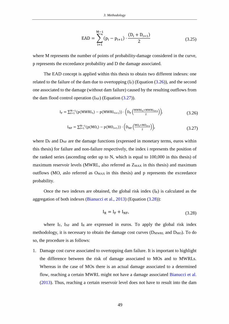
3. Methodology
49
EAD = �(pi − pi+1) ·(Di + Di+1)
2
M−1
i=1
(3.25)
where M represents the number of points of probability-damage considered in the curve,
p represents the exceedance probability and D the damage associated.
The EAD concept is applied within this thesis to obtain two different indexes: one
related to the failure of the dam due to overtopping (IF) (Equation (3.26)), and the second
one associated to the damage (without dam failure) caused by the resulting outflows from
the dam flood control operation (INF) (Equation (3.27)).
IF = ∑ (p(MWRLi) − p(MWRLi+1)) · �DF �MWRLi+MWRLi+1
2��N−1
i=1 , (3.26)
INF = ∑ (p(MOi) − p(MOi+1)) · �DNF �MOi+MOi+1
2��N−1
i=1 , (3.27)
where DF and DNF are the damage functions (expressed in monetary terms, euros within
this thesis) for failure and non-failure respectively, the index i represents the position of
the ranked series (ascending order up to N, which is equal to 100,000 in this thesis) of
maximum reservoir levels (MWRL, also referred as ZMAX in this thesis) and maximum
outflows (MO, aslo referred as OMAX in this thesis) and p represents the exceedance
probability.
Once the two indexes are obtained, the global risk index (IR) is calculated as the
aggregation of both indexes (Bianucci et al., 2013) (Equation (3.28)):
IR = IF + INF, (3.28)
where IF, INF and IR are expressed in euros. To apply the global risk index
methodology, it is necessary to obtain the damage cost curves (DMWRL and DMO). To do
so, the procedure is as follows:
1. Damage cost curve associated to overtopping dam failure. It is important to highlight
the difference between the risk of damage associated to MOs and to MWRLs.
Whereas in the case of MOs there is an actual damage associated to a determined
flow, reaching a certain MWRL might not have a damage associated Bianucci et al.
(2013). Thus, reaching a certain reservoir level does not have to result into the dam

3. Methodology
50
failing, but a risk of failing. Therefore, following the approach proposed by Bianucci
et al. Bianucci et al. (2013), the damage cost curve is calculated as (Equation (3.29)):
DMWRL(MWRLi)=p(break|MWRLi)·Costbreak , (3.29)
where Costbreak represents the damage cost if the dam fails (expressed in euros),
whereas p(break|MWRLi) is the probability of overtopping failure conditioned to
reaching a certain level in the reservoir (MWRLi). Costbreak is estimated as the cost of
reconstruction of the dam aggregated to the estimated downstream damage when
overtopping failure occurs. In this thesis, Costbreak is considered as a constant value,
as there was only data of the estimated downstream damage associated to the flood
wave caused by the overtopping failure mode accounted in the Dam Master Plans
(failure when reservoir level is at dam crest level (COD)). Regarding to
p(break|MWRLi), according to Bianucci et al. (2013) can be represented as the
probability of reaching the reservoir level at COD once MWRLi has been reached
during a flood event (Equation (3.30)):
p(break|MWRLi) = p(MWRLMAX ≥ COD|MWRLi) = nº events MWRL MAX ≥CODnºevents MWRL MAX ≥MWRL i
, (3.30)
This expression is estimated by routing 100,000 synthetic floods with a moderate to
extreme return period of peak-flow (10 to 200,000 years). By assuming that
overtopping leads to dam failure, p(break|MWRLi) is calculated as the number of
events in which MWRLMAX≥COD over the number of events in which MWRLMAX≥
MWRLi.
2. Damage cost curves associated to non-failure. Regarding to DMO, it is estimated by
analysing the possible damages downstream. As the dams studied within this thesis
are in Spain, the damage cost curve associated to non-failure was estimated based on
the information included in the Spanish National GIS viewer about flood risk
assessments through flood plain analysis (MAPA, 2019).
Stochastic procedure for the definition of Maximum
Conservation Levels
Maximum Conservation Levels (MCLs) represent the linking variable between
flood control operation and water conservation operation of the reservoir (Figure 3.11).

3. Methodology
51
To obtain the optimal set of seasonal MCLs accounting for both hydrological safety (dam
and downstream) and water supply with a specific reliability, a stochastic methodology
is proposed, graphically summarized in Figure 3.11.
Figure 3.11: General Scheme of the methodology proposed.
3.7.1. Study set of seasonal Maximum Conservation Levels
The number of possible configurations of MCLs vary according to the number of
seasons (n) defined and the possible Maximum Conservation Levels selected for a proper
discretization to analyse all the outcomes accounting for computation time (k). As the
position of the MCLs matters (it is not the same to have the same MCL in one season or
another), the number of configurations were given by a variation with repetition (𝑉𝑉𝑉𝑉𝑘𝑘𝑛𝑛 =
𝑘𝑘 𝑛𝑛). To define the seasons, the procedure exposed in Section 3.1.2.1 is used in this thesis.
3.7.2. Reservoir operation simulations
For each configuration of seasonal MCLs of the study set, two different reservoir
operation simulations were carried out: simulation of flood control operation and simulation
of water conservation (regular) operation.
3.7.2.1. Simulation of flood control operation
For each configuration of MCLs, the maximum water level in the reservoir
corresponding to a return period of 1,000 years (MWRLTR=1000y) and the maximum
outflow corresponding to a return period of 500 years (MOTR=500y) were obtained,
corresponding to the set of 100,000 seasonal maximum annual inflow hydrographs
generated following the procedure of Section 3.1.2, and routed by applying the VEM
(Section 3.2.1). The analysis was carried out in two different scenarios of the initial
reservoir level prior the flood event (Zo) (Figure 3.11).

3. Methodology
52
• Scenario 1 (Sc.1): Zo is constant and corresponds to the seasonal MCL. The
reservoir is assumed to be at its maximum operating level when the reservoir gets
the maximum annual flood.
• Scenario (Sc.2): Zo is variable, and the reservoir can be at any level when the
maximum annual flood occurs. Zo is obtained (within a Monte Carlo framework)
from the cumulative probability distribution of Zo associated to the season of
occurrence of the maximum annual flood event. This distribution is obtained from
the simulation of the water conservation operation of the reservoir (Section 3.3.2).
3.7.2.2. Simulation of water conservation operation
The yield reliability (YR) was considered as the ratio of total volume supplied and
the total volume demanded (Chavez-Jimenez et al., 2013; Sordo-Ward et al., 2019a, b)
during the period analysed. For each configuration of MCLs (k), the reservoir yield with
reliability of 90% (YR=90%) and the cumulative probability distribution of Zo are obtained,
by developing a monthly water balance model. The model manages the dam as an isolated
element. The water balance considers time series of monthly inflows, environmental flow
restrictions, evaporation rates, monthly demand distribution, storage-area-height
reservoir curves and dead storage volume (data extracted from “Duero National Water
Master Plan” (CHD, 2015). The main purpose of the reservoir is irrigation and therefore
a required yield reliability of 90 % (YR=90%) was adopted, adequate for irrigation demands
in the region (Garrote et al., 2015).
To identify the maximum amount of water that can be supplied to satisfy a regular
demand with a specified reliability, a bipartition method was applied: excessive values of
demands were set (for example, similar to mean monthly runoff) and the simulation was
carried out. The deficits were obtained, and specified yield reliability requirements were
checked. If the specified reliability requirements were not fulfilled, the demand was
reduced by half and simulated again. If the specified reliability requirements were
satisfied, half of the difference was added and simulated again, and so on until the deficit
(or gain) was smaller than a pre-set tolerance (e.g., 0.1 hm3/year). In addition, the
operation of the reservoir was simulated with the associated mean annual current demand.
The procedure was repeated for both Sc.1 and Sc.2 scenarios.

3. Methodology
53
3.7.3. Results analysis and solutions proposal
In order to propose the optimal configurations of MCLs within the case study, as
exposed, the main decision variables selected were MWRLTR=1000y, MOTR=500y and
YR=90%. It was assumed that the MCLs configuration would not fulfil the standards if
MWRLTR=1000y was above the DFL and/or MOTR=500y was greater than the emergency
flow (OEMER.). MWRLTR=1000y, MOTR=500y and YR=90% were compared, for all the
configurations in the study set of MCLs (Figure 3.11), by identifying configurations that
are non-inferior solutions (Pareto framework) in terms of maximum volume of water
supplied (with a specific yield reliability of 90%) and hydrological safety.
3.7.3.1.Determination of possible MCLs by applying a Pareto analysis
The selected variables for conducting the Pareto analysis were MOTR=500y and
YR=90% (Figure 2). In this thesis, it was assumed that higher levels in the reservoir (and
above MNL) imply greater outflows. This assumption is always fulfilled either for dams
with fixed crest spillways or if the Volumetric Evaluation Method is applied in gated
spillways (as in this study). It should be noted that this assumption may not hold for all
possible specific characteristics of dams, all rules of operation adopted, and all specific
values adopted for the hydrological dam and downstream safety. Moreover, in this study,
the outflow corresponding to the DFL condition is higher than that corresponding to
OEMER, that is, the MOTR=500y is the most restrictive variable. Therefore, for each scenario
(Sc.1 or Sc.2), there was a set of kn MCLs configurations with kn pairs of values
MOTR=500y and YR=90%. The purpose was to obtain the configurations of MCLs that
minimize the value of MOTR=500y while maximizing YR=90%, which implies a two-
objective minimization problem (Equation (3.31)):
Min{f1(xi), f2(xi)} (3.31)
in which xi = [MCLS1, MCLS2, …, MCLSn], f1(xi)= [MOTR=500yi] and f2(xi) = [- YR=90%i];
being i=1,2…, kn. Once the non-dominated solutions were identified, for Sc.1 and Sc.2,
the non-dominated solutions from both scenarios those that did not fulfil the hydrological
safety regulation standards (both for MWRLTR=1000y and/or MOTR=500y) and those
providing a YR=90% lower than the annual demand that is currently satisfied were
eliminated. Afterwards, a comparison of the proposed solutions was carried out,
providing dam stakeholders with a set of possible configurations depending on their main

3. Methodology
54
objectives: increasing hydrological dam and downstream river safety or increasing the
water supply with a specific reliability within the system.
Figure 3.12: Scheme of the procedure for solutions proposal.
Introduction to the case studies and software used
The methodology proposed for each part of the present research is applied different
case studies (Figure 3.13). A total of four case studies are considered: three of them are
based in reservoir-dam configurations in Spain, whereas the other one is a watershed in
the United States. The watershed case study is analysed to develop the Hybrid method
explained in Section 3.1.1. The different reservoir-dam configurations are selected to
show the applicability of the proposed stochastic methodology regardless the dam
characteristics (volume of the reservoir, purpose, etc.) or its location (climate, size of the
reservoir basin, etc.). Each case study is briefly summarized below. The data used and the
specific details of each case study are developed in its corresponding chapters:

3. Methodology
55
(a)
(b)
Figure 3.13: Location of the case studies of the research (figure generated with Google Earth).(a) Dam case studies (b) Peacheater Creek.

3. Methodology
56
• Dam in Tagus River Basin: based on a gated-spillway gravity dam located in the
Tagus river basin. The dam is located in the west of Spain (province of Caceres). The
dam watershed has an extension of 1,850 km2. The climate within the area of study is
Continental with mean annual precipitation of 1,000 mm. The main purpose of the
reservoir is irrigation.
The volume of the reservoir at its maximum normal level is 911 hm3. The dam height
is 73 meters.
(a)
(b)
(c)
Figure 3.14: Plans and picture of the dam-reservoir system of the Tagus river basin. a) section, b) plant c) view. Source: MAPA, 2019

3. Methodology
57
• Dam in Segura River Basin: This case study is based on a gated-spillway dam located
in the province of Albacete, in the southeast of Spain, which belongs to the Mundo
river basin. The basin has an area of 766.5 km2. The climate of the region is
Mediterranean (mean annual precipitation of 557 mm). The main purposes of the
reservoir are flood regulation, hydropower generation, and water supply for the
Region of Murcia.
The volume of the reservoir at its maximum normal level is 35 hm3. The dam height
is 46 meters.
(a)
(b)
(c)
Figure 3.15: Plans and picture of the dam-reservoir system of the Segura river basin. a) section, b) plant c) view. Source: MAPA, 2019

3. Methodology
58
• Dam in Douro River Basin. This case study is based on a gated-spillway dam located
in the headquarters of Esla river, a tributary of the river Douro. The dam is located in
the northwest of Spain (province of Leon). The dam river basin has an extension of
582 km2. The area has a continental climate characterized by flood events of several
days of continuous rainfall of medium intensity (mainly generated by frontal
systems). The mean annual precipitation within the basin is 1,650 mm. The main
purpose of the reservoir is irrigation and hydropower generation.
The volume of the reservoir at its maximum normal level is 651 hm3. The dam height
is 100 meters.
(a)
(b)
(c)
Figure 3.16: Plans and picture of the dam-reservoir system of the Douro river basin. a) section, b) plant c) view. Source: MAPA, 2019

3. Methodology
59
• Peacheater Creek: This case study is a basin, located in the Oklahoma State, in the
United States. This watershed is a subbasin of the Baron Fork basin. The Peacheater
Creek basin has a drainage area of 64 km2. It was selected since it was originally used
to test, calibrate, and validate the tRIBS model (Ivanov et al., 2004a), model selected
and explained in Section 3.1.1. Further details on the basin and the model
implementation are given in Chapter 4.
All the experiments were developed under the environment of the Matlab
programming platform. Its matrix calculation concept allows handling large volumes of
data (both in its generation and subsequent process and analysis) with reasonable
calculation time costs. It also adapts well to the execution of systematic and intensive
calculation processes, and it has a powerful graphic interface that facilitates the analysis
and post-processing of results (The MathWorks, 2018).
Another important aspect to take into account in this type of studies where the
volumes of data generated are important, is the design of a database associated with the
calculation processes, which should be simple, robust and allow the traceability of each
of the cases analysed. In this sense, Matlab environment is flexible and allows for
automation and correct interface between the calculation processes and the databases
(both with the model input data, the data generated and the post-process data).
Furthermore, in some parts of this research, intensive repetitive calculations where
necessary under the Monte-Carlo framework performed. To perform intensive tasks, such
as those shown in Chapter 4, Chapter 6 and Chapter 8, the use of a High Performance
Computer reduced the computational times.
The cluster used was Magerit, a High Performance Computer (HPC) owned by
Universidad Politécnica de Madrid. The experiments were carried out using the Intel
family processors architecture, which consists of 41 nodes with two intel processors Intel
XEON E5-2670 of eight cores each, and 64 GB RAM/Core. Thus, multiple independent
simulations are carried out at the same time by using multiple processors in Chapter 6 and
Chapter 8.
Regarding to the distributed hydrological model (tRIBS) used in Chapter 4, the code
of the model is programmed in C++ (Ivanov et al., 2004a). Matlab within this case is used
as a pre-processing and post processing tool, whereas Magerit capabilities are used to

3. Methodology
60
perform simulations accounting for parallel computation techniques as will be detailed in
Chapter 4.
The following table shows the relation of the chapters with the methodology (Table
3.1).
Table 3.1: Relationship between chapters, methodological key aspects, case studies, software used and role of the High Performance Computer (HPC).
Chapter Key aspects Case study Software used Role of HPC
4 Hybrid method Peacheater Creek
Matlab
tRIBS
AWE-GEN
Parallel Computing
Intensive experiment repetition
5 K-Method Global risk index
Segura River Dam Matlab Not used
6 Uncertainty associated to initial reservoir level
Global risk index
Tagus River Dam Matlab Intensive experiment repetition
7 Initial reservoir level Spillway reliability
Douro River Dam
Matlab Not used
8 Maximum Conservation Levels Matlab Intensive experiment repetition

3. Methodology
61

4. Hydrological forcing: The Hybrid method
62
4. Hydrological forcing: The Hybrid method
This first part of this chapter focuses on proposing the minimum number of storms
necessary to derive the extreme flood hydrographs accurately through event-based
modelling, by using a distributed physically-based model. To do so, the methodology
exposed in Section 3.1.1.1. is applied. Afterwards, initial soil moisture conditions are
analysed in order to the develop the Hybrid method (Section 3.1.1.2), which combines
the advantages of continuous and event-based hydrological models. Finally, the Hybrid
method is applied, analysing its performance (Section 3.1.1.3).
Application to Peacheater Creek basin
4.1.1. Study basin
The Hybrid method was applied to Peacheater Creek (herein, PC), using the hourly
climate data of Westville, a weather station located within the basin (Figure 4.1a).
(a) (b) (c)
Figure 4.1: Case study and model setup. (a) Basin location, elevation, and drainage network. (b) Discretization of the basin into Voronoi polygons for triangulated irregular network real-time integrated
basin simulator (tRIBS). (c) Partitioning of the basin for parallel computation using eight processors.
This sub-basin is located in Baron Fork at Eldon river basin (Oklahoma, USA) and
it was selected since it was originally used to test, calibrate, and validate the tRIBS model
(Ivanov et al., 2004a; 2004b). The Peacheater Creek basin has a drainage area of 64 km2,
with elevations ranging between 248 and 432 m.a.s.l. The sub-basin is characterized by
gentle (slopes between 2% and 5%) to steep (slopes between 15% and 40%) hillslopes.
The vegetation is a mixture of oak-hickory-pine forest grasslands (mainly located in the
southern part of the basin) and cropland-urban areas (mainly in the northern region). The

4. Hydrological forcing: The Hybrid method
63
impervious fraction of the sub-basin is estimated to be about 1.56%. The predominant
soil consists of gravelly silt loams (Ivanov et al., 2004a ; 2004b).
Additional details on the climate, hydrology, and basin characteristics have been
presented in (Ivanov et al., 2004a ; 2004b; Vivoni et al., 2007).
4.1.2. Setup of modelling experiments
Two different modelling experiments were carried out:
1. Stochastic weather generation: 5,000 years of punctual hourly weather were generated
with AWE-GEN (Fatichi et al., 2011); calibrated with the climate data recorded from
1997 to 2016 (both years included) at the Westville weather station: Rainfall,
temperature, wind speed, radiation, cloudiness, relative humidity, and atmospheric
pressure. Raw data had a resolution of 5 min. The data was processed into hourly
values, in order to force AWE-GEN and perform the stochastic weather generation.
2. Hydrological simulations: Numerical simulations in PC were carried out using the
tRIBS model with a TIN of 6,680 nodes (Figure 4.1b) derived from a US Geological
Survey (USGS) 30-m DEM using the procedure described in Vivoni et al. (2004).
The simulations were based on a model calibration conducted by Ivanov et al. (2004a
; 2004b) as part of the distributed model intercomparison project. Ivanov et al. (2004a
; 2004b) obtained a correlation coefficient of 0.763 and a Nash-Sutcliffe coefficient
of 0.565 (which can be considered as satisfactory following the guidelines exposed in
Sirisena et al. (2018)) for the hourly simulated streamflow at the outlet of Baron Fork
basin (in which PC is located), compared to the hourly observed streamflow from
April of 1994 to July of 2000. To make the experiment approachable, the
computational load was balanced by using parallel computing techniques. The basin
was partitioned into eight different parts using a surface-flow partitioning script
(Vivoni et al., 2011) with the graph-partitioning software METIS (Karypis and
Kumar, 1999), which balances the number of TIN nodes across processors
minimizing the dissections that occur in the channel network. Each processor
calculates tRIBS variables within each part of the basin and, every time step each
processor sends messages to the others to sum up all the calculations done within the
basin. Thus, the computational load is balanced between the different processors
(Figure 4.1c) and the experiment is approachable.

4. Hydrological forcing: The Hybrid method
64
The experiment was carried out by using Magerit, a high performance computer
owned by the Technical University of Madrid. The Intel family processors architecture,
which consists of 41 nodes with two intel processors Intel XEON E5-2670 of eight cores
each, and 64 GB RAM/Core was used. The time spent in the continuous hydrological
simulations was two and a half months, whilst the weather simulations were carried out
within one day of computation. Regarding to the Hybrid method simulations, they were
performed within fourteen hours (due to the continuous simulation of 50 years, whilst the
event-based simulations took one hour).
4.1.3. Limitations of the experiment
The applied methodology has some limitations that should be noted:
1. Rainfall was considered uniform within the whole basin, as a result of using a punctual
stochastic weather generator. As pointed out by Liuzzo et al. (2010), due to the small
size of PC, there is not a big difference between considering the spatial and punctual
rainfall. However, within the same study, accounting or not for the rainfall spatially
had an appreciable difference for a basin with a bigger drainage area (Baron Fork,
808 km2).
2. The study is focused on return periods up to 500 years. For higher return periods, the
length of the generated weather forcing series should be analysed to ensure that it is
representative enough of the return period studied.
3. The procedure did not account for climate-change effects or land-use changes, but
considered stationary climate conditions. However, interannual variations of the mean
annual rainfall were accounted for due to the nature of AWE-GEN.
4. The methodology is applied to one basin, which limits the extrapolation of the results
obtained.
4.1.4. Validation of the method. Hybrid method Vs. Continuous simulation
In several sections within this chapter, in order to compare the values obtained at
the different storm ranks and the results of the Hybrid method to the reference value (the
one obtained from the continuous simulation), the relative error (RE) was obtained as
follows (Equation (4.1)):

4. Hydrological forcing: The Hybrid method
65
RE (%) = �1 − Compared valueReference value
� · 100, (4.1)
4.1.4.1. Magnitude and recurrence. Univariate frequency analysis
An analysis of how the storm events were related to the maximum annual peak-
flow and volume was carried out, focusing on the:
1. Probability that a storm with a determined rank generates the maximum annual value
of the (a) peak-flow and (b) volume.
2. Relation between the storm rank and the return period associated to the (a) maximum
annual peak-flow and (b) maximum annual volume.
3. Maximum storm rank required to obtain 95% and 99% probability of achieving the
(a) maximum peak-flow and (b) maximum volume for a specific year and for different
ranges of the return period.
The return periods associated to the maximum annual peak-flows and to the
maximum annual volumes were obtained independently, by using the Gringorten plotting
position formula (Gringorten, 1963).
4.1.4.2. Seasonality
A seasonality analysis was carried out based on circular statistics (Berens, 2009).
As exposed by (Parajka et al., 2010), circular statistics are an effective method to define
the basis of the timing of hydrological extreme events within a year. The date of
occurrence of an event in year i can be graphed on a unitary circle to give the angle (θi)
in polar coordinates (Equation (4.2)):
θi = D · 2π/L, (4.2)
where D stands for the day of the year (one for 1 January, two for 2 January, etc.) and L
the number of days within the year (365, or 366 if it is a leap year). Then, the mean
seasonality can be defined as the average vector from the origin which represents the
mean date of occurrence (θ�) of all the maximum annual floods (peak-flow or volume)
within the case study basin. The x� and y� coordinates of the average vector are obtained
from the sample of 5,000 extreme events by (Equations (4.3) and (4.4)):

4. Hydrological forcing: The Hybrid method
66
x� = ∑ cos (θi)5,000i=15,000
, (4.3)
y� = ∑ sin (θi)5,000i=15,000 , (4.4)
therefore (Equation (4.5)):
θ� = tan−1 y�x� , (4.5)
whereas the variability of the date of occurrence about the mean date is characterized by
the length parameter r̅ (Equation (4.6)):
r̅ = �x�2 + y�2, (4.6)
which ranges from zero (uniform distribution around the year) to one (all extreme events
occur on the same date of the year).
The values of θ� and r̅ obtained from the continuous simulation to those obtained
from the different storm ranks and from the Hybrid method.
4.1.4.3. Dependence
An analysis on how the different storm ranks and the Hybrid method affected the
dependence between the peak-flow and volume was performed. To do so, (1) graphical
techniques and (2) numerical measures were used.
1. The Chi-Plot, which is a technique that displays a measure of location of an
observation regarding the whole of the observations (λi) against a measure of the Chi-
square test statistic for independence (Χi) was used. Therefore, the bigger the distance
between the points and the horizontal axis is, the larger the dependence is. The
dependence is positive if the points are above the upper control limit, and negative if
they are located below the lower control limit (Fisher and Switzer, 1985; 2001), which
was established with a probability of 90% as shown in Genest et al. (2007).
2. Spearman’s rho and Kendall’s tau. Moreover, dependence measures are needed to
procure a quantitative value of the dependence relation between variables. For this
purpose, the Spearman’s rho and Kendall’s tau were adopted as rank-based non-
parametric measures of dependence.

4. Hydrological forcing: The Hybrid method
67
4.1.4.4. Magnitude and recurrence. Copula-based frequency analysis.
Finally, an analysis on how the rank of storms and the Hybrid method affected the
bivariate properties of the pairs of peak-flow and volume by carrying out a copula-based
analysis. To do so, the MATLAB toolbox MhAST Toolbox (Sadegh et al., 2018) was
used. Within that toolbox, a total of 26 parametric models of copula families can be fitted
to bivariate data. Within this study, for the sake of simplicity, the focus was established
on three well-known Archimedean one-parameter copula families for their uses in
hydrological sciences: Clayton, Gumbel and Frank. The procedure was as follows:
First, the three studied copulas were fitted to the pairs peak-flow and volume values
obtained from the continuous simulation using MhAST. For these three copulas, MhAST
uses the MATLAB built-in function, which estimates the parameter (θc) of each copula
using the method of maximum likelihood. The selection of the copula that provided the
best fit was based on the root mean square error (RMSE) (Equation (4.7)) and the Nash–
Sutcliffe efficiency (NSE) (Equation (4.8)) coefficient, which measures how different the
empirical observed bivariate probabilities (Y�) and their modelled bivariate counterpart
(Y) are:
RMSE = �∑ [y�i−yi(θc)]2ni=1
n, (4.7)
NSE = 1 −∑ [y�i − yi(θc)]2ni=1
∑ [y�i − y�ı�]2ni=1
, (4.8)
RMSE values are within the range [0, ∞) with zero being a perfect fit, whereas NSE
ranges in the interval (-∞,1], with one being the perfect fit. The best fit is the one that had
a lower value of RMSE and a higher value of NSE.
Once the copula family was chosen, that copula was fitted to the different pairs of
peak-flow and volume obtained considering different storm ranks, according to the
rainfall criteria separation studied. The RE of the estimated copula parameter with respect
to the copula parameter of the continuous simulation was obtained.
Finally, an graphical analysis was performed to analyse the differences between the
Kendall’s return period (TK) (Salvadori and De Michele, 2011) calculated by both,
continuous simulation and a) different storm ranks according to the VEvent and Imax criteria
b) the Hybrid method. Kendall’s return period represents the mean inter-arrival time of

4. Hydrological forcing: The Hybrid method
68
critical events lying on the probability level t, and can be obtained as follows (Equation
(4.9)):
TK = μ1−KC(t)
= 11−KC(t)
, (4.9)
where μ is the average interarrival time of events (i.e., μ = 1 in this Chapter, as
annual maxima are being analysed) and KC(t) is the Kendall’s distribution function, where
t represents the probability level. For the sake of brevity, the reader is referred to
(Salvadori and De Michele, 2011; Brunner et al., 2016) for further details. Finally, the
isolines of TK of 10, 50, and 100 years were obtained using the MhAST toolbox, estimated
through continuous simulation and a) through different storm ranks for the studied criteria
separation b) through the Hybrid method.
Obtained results
4.2.1. Stochastic weather generation. Rainfall extremes validation.
The ability of the weather generator (AWE-GEN) to reproduce rainfall extremes
was analysed by comparing the stochastic rainfall frequency curves with those observed
at different aggregation periods (Figure 4.2a–d, 1 h, 6 h, 12 h, 24 h, respectively). As
shown, the behaviour of the observed rainfall frequency curves was mostly within the
range of the simulated ones.
Furthermore, it was analysed how the seasonality of the storm events was retained
by AWE-GEN. To carry out the analysis, it was necessary to separate the storm events.
By applying the exponential method (exposed in Section 3.1.1.1) a MIT of 15 h was
determined from the observed hourly rainfall time-series of Westville Station. Applying
the methods shown in Section 4.1.4.2, the seasonality of two main characteristics of storm
events (Figure 3.3) was compared: The maximum annual Imax (Figure 4.2e) and the
maximum annual VEvent (Figure 4.2f).

4. Hydrological forcing: The Hybrid method
69
(a)
(b)
(c)
(d)
(e)
(f)
Figure 4.2: Validation of the generated rainfall series. (a–d) Comparison between the observed rainfall frequency curve (blue dots) (obtained by applying the Gringorten plotting position formula (Gringorten,
1963) and synthetic rainfall frequency curves obtained by bootstrapping 1,000 series of 40 years of hourly rainfall obtained from the 5,000 years of synthetic weather series generated: (a) Maximum annual
cumulated rainfall (P) in: (a) 1 h, (b) 6 h, (c) 12 h, and (d) 24 h. (e) Comparison between the seasonality of the observed maximum annual intensity (blue circles), with the predominant direction (blue line)
compared to the predominant direction of the seasonality of 1,000 series of 20 years of maximum annual depth obtained by bootstrapping from the 5,000 years of synthetic weather generated (in grey lines), with the mean predominant direction represented in black. (f) The same as e, but for total depth, with observed
values represented in red circles.
The seasonality is well-reproduced by AWE-GEN for the maximum annual Imax
(Figure 4.2e). The mean occurrence (θ�) (represented by the direction of the vectors) is
late June (observed, in blue) and early July (simulated, in black), with a similar variability
of seasonality (r̅) (represented by the length of the vectors (Figure 4.2e)), with an

4. Hydrological forcing: The Hybrid method
70
observed and simulated value of 0.61 and 0.56, respectively). However, in the case of
VMax (Figure 4.2f), the observed seasonality is slightly more disperse than the generated
(the length of the observed vector is 0.16, whereas the simulated is 0.29) and θ� is delayed
by one month. Overall, the generated synthetic series are able to reproduce extreme
rainfall properties.
4.2.2. Rainfall versus flood comparison
Once the weather series had been generated, they were used as weather forcing for
the hydrological model tRIBS performing the simulations. Afterwards, the relationship
between the storm ranks and the flood hydrographs generated at the basin outlet was
obtained.
4.2.2.1. Magnitude and Recurrence. Univariate Frequency Analysis
Table 4.1 shows the probability that a storm of a specific rank generates the (a)
maximum annual peak-flow and (b) the maximum annual volume. The three ranking
criteria are shown: VEvent, Imax, and DEvent. It can be seen that the VEvent criteria was the
most relevant; that is, a lower storm rank is required for obtaining both the maximum
annual peak-flow and volume.
According to the different storm rank criteria:
1. VEvent. Considering the biggest storm (rank one) results in a probability of generating
the maximum annual peak-flow (Table 4.1) of more than 53%, whereas considering
the storms of rank one and two this probability increases to more than 75%. If the
storms considered are up to rank 3, this probability exceeds 86%. When analyzing the
maximum annual volume (Table 4.1), the same probabilities are greater than 68%,
86%, and 93%, respectively.
2. Imax. The probability of generating the maximum annual peak-flow (Table 4.1) is more
than 45%, 63%, and 75% for a storm rank up to one, two, and three, respectively. In
the case of maximum annual volume (Table 4.1), the same Figures are 35%, 52%,
and 64%.
3. DEvent. The probability of achieving the maximum annual peak-flow and volume with
these criteria is the lowest. Considering storms up to rank ten, the probability of
achieving the maximum peak-flow is less than 40% (Table 4.1), and less than a 60%
(Table 4.1) probability of resulting in the maximum annual volume.

4. Hydrological forcing: The Hybrid method
71
Table 4.1: Relative and cumulated frequency that a storm of a specific rank generates the maximum annual peak-flow and the maximum annual volume.
Storm Rank
Relative/Cumulated Frequency of Coincidence with Maximum Annual Peak-
Flow (%)
Relative/Cumulated Frequency of Coincidence with Maximum Annual
Volume (%)
Total Depth
Maximum Intensity
Total Duration
Total Depth
Maximum Intensity
Total Duration
1 53.5/53.5 45.2/45.2 9/9 68.8/68.8 35.6/35.6 17.2/17.2
2 21.7/75.2 18.6/63.8 5.8/14.8 17.9/86.7 17.3/52.9 8.6/25.9
3 11.4/86.6 11.5/75.3 4.8/19.6 6.9/93.6 11.3/64.2 7/32.9
4 5.3/91.9 6.9/82.2 3.3/22.9 2.7/96.3 8/72.2 4.7/37.5
5 3.4/95.3 4.2/86.4 3.6/26.5 1.8/98.1 5.5/77.7 4.5/42
6 1.7/97 3.1/89.4 2.9/29.5 0.7/98.8 4.2/81.9 3.4/45.4
7 1.3/98.2 2.2/91.7 2.9/32.3 0.5/99.3 3.1/85 3/48.4
8 0.8/99 2.1/93.7 2.5/34.8 0.3/99.6 2.8/87.9 3/51.4
9 0.3/99.3 1.5/95.2 2.3/37.1 0.1/99.7 2.5/90.4 2.4/53.8
≥10 0.7/100 4.8/100 62.9/100 0.3/100 9.6/100 46.2/100
Therefore, for PC, the best criterion of the storm rank is VEvent, followed up by Imax
when analyzing the correspondence between the storms and maximum annual peak-flow
and volume. For the sake of simplicity, the following results only focused on these two
criteria, excluding DEvent.
Afterwards, the focus was on the magnitude of peak-flows and volumes. The
different storm ranks (Figure 4.3, total depth criteria (red) maximum intensity criteria
(blue)) were related to the associated return period (Tr) of peak-flows (Figure 4.3a) and
volumes (Figure 4.3b) obtained from the analysis of the 5,000 years flow simulated at the
basin outlet. According to the two criteria selected, it can be seen that:
1. VEvent. The higher the Tr of the peak-flow (Figure 4.3a) and volume (Figure 4.3b) are,
the lower the storm rank needed. Therefore, there is a strong correlation between the
Tr and the storm rank. For the Tr of the peak-flow over 10 years, all the storm events
have a rank lower than or equal to four, whereas for the Tr over 100 years all the
storms are of rank one or two. For the Tr of volume over 10 years, all the storm events
have a rank lower than or equal to three, whereas for the return periods over 100 years
all the storms are also of rank one or two.

4. Hydrological forcing: The Hybrid method
72
2. Imax. There is more dispersion than in the VEvent criteria. For the Tr of the peak-flow
over 10 years, storms have a rank of ten or lower, whereas for the Tr over 100 years
all the storms up to rank three should be considered. In the case of volume, the Tr
higher than 10 years corresponds to storms with ranks up to 23 (not shown in Figure
4.3), whereas for the Tr over 100 years, storms up to rank ten can generate the
maximum annual volume.
(a)
(b)
Figure 4.3: Storm order that corresponds to every return period (Tr) of maximum annual peak-flow (a) and maximum annual volume (b) represented as red dots for the total depth criteria and as blue dots for the maximum intensity rank criteria. The numbers on the right represent the probability that a storm of a
specific rank generates the maximum peak-flow (a) or volume (b) of given a year.
Finally, regarding the analysis of magnitude and recurrence, the maximum storm
rank required to obtain 95% and 99% probability of achieving the maximum annual peak-
flow and the maximum annual volume for a specific year and for different ranges of Tr
for the VEvent and IMax criteria was calculated (Table 4.2). Considering storms up to rank
six according to the VEvent criteria, there is a 95% probability of achieving the maximum
annual peak-flow and volume for all ranges of the Tr, which increases to 99% if all storm
1 2 5 10 20 50 100 200 500
1
2
3
4
5
6
7
8
9
10
Stor
m ra
nk
53 %
22 %
11 %
5 %
3 %
2 %
1 %
<1 %
1 2 5 10 20 50 100 200 500
Tr Peak-flow (years)
1
2
3
4
5
6
7
8
9
10
45 %
19 %
12 %
7 %
4 %
3 %
2 %
2 %
2 %
5 %
1 2 5 10 20 50 100 200 500
1
2
3
4
5
6
7
8
9
10
Stor
m ra
nk
69 %
18 %
7 %
3 %
2 %
<1 %
1 2 5 10 20 50 100 200 500
Tr Volume (years)
1
2
3
4
5
6
7
8
9
10
36 %
17 %
11 %
8 %
6 %
4 %
3 %
3 %
3 %
10 %

4. Hydrological forcing: The Hybrid method
73
events up to rank nine are considered. For IMax, the ranks are 13 and 22 for the same
probability values. As also shown in Figure 4.3, the storm rank required is less as the Tr
increases in the two ranking criteria. It is remarkable that, in the case of VEvent, for return
periods higher than 50 there is a probability of achieving the maximum annual peak-flow
and the maximum annual volume of 99% if the three highest events are considered.
Table 4.2: Maximum storm rank required to obtain 95% and 99% probability of achieving the maximum peak-flow or volume for a specific year, depending on the ranking criteria used and
the range of return periods studied.
Probability (%) Tr (Years)
Maximum Storm Rank to be Considered Peak-Flow
Maximum Storm Rank to be Considered
Volume Total Depth Maximum Intensity Total Depth Maximum Intensity
95/99 All range 5/8 9/16 4/7 13/22 95/99 1 ≤ Tr < 10 6/9 10/16 4/7 13/22 95/99 10 ≤ Tr < 50 3/3 4/7 1/2 8/14 95/99 50 ≤ Tr < 100 2/3 2/3 1/2 6/10 95/99 Tr ≥ 100 2/2 2/3 1/2 6/6
4.2.2.2.Seasonality
The preservation of seasonality by the storms depending on the rank considered
was analysed. Figure 4.4 shows the seasonal behaviour of storms regarding the maximum
peak-flow (Figure 4.4a–d and Figure 4.4i–l) and maximum volume (Figure 4.4e–f and
Figure 4.4m–p). Comparisons were carried out with the seasonality of the continuous
simulation (red in Figure 4.4a–f and blue in Figure 4.4i–p) and the consideration of storms
up to rank one, three, five and ten for the VEvent (Figure 4.4a–f) and IMax (Figure 4.4i–p)
criteria.
According to the two rainfall criteria selected:
1. VEvent. The seasonality is preserved almost equally if storms are at least considered up
to rank three for both the maximum peak-flow and maximum volume.
2. IMax. Within this case, to preserve the seasonality obtained from the continuous
simulation, storms up to rank ten should be considered in both cases, the maximum
peak-flow and maximum volume.

4. Hydrological forcing: The Hybrid method
74
(a)
(b)
(c) (d)
(e)
(f)
(g)
(h)
(i)
(j)
(k)
(l)
(m)
(n)
(o)
(p)
Figure 4.4: Comparison between the seasonality of the maximum annual peak-flow (red lines in (a–d); and blue lines in (i–l) and maximum annual volume (red lines e–h; and blue lines (m–p) of the continuous
simulation with respect to that obtained by applying different criteria (total depth (a–h) and maximum intensity (i–p)) and accounting for different rank orders (up to one, three, five and ten), in which the
predominant direction of the seasonality is represented by a circle with a black line.
To quantify the impact of the rank of storms in seasonality, the values of θ� and r̅
were obtained from the continuous simulation and compared to the ones obtained from
the different storm ranks, obtaining the RE (Equation (4.1)).
Jan
Feb
MarAprMay
Jun
Jul
Aug
SepOct
Nov
Dec
Rank 1
0.20
0.4
Jan
Feb
MarAprMay
Jun
Jul
Aug
SepOct
Nov
Dec
Rank 3
0.20
0.4
Jan
Feb
MarAprMay
Jun
Jul
Aug
SepOct
Nov
Dec
Rank 5
0.20
0.4
Jan
Feb
MarAprMay
Jun
Jul
Aug
SepOct
Nov
Dec
Rank 10
0.20
0.4
Jan
Feb
MarAprMay
Jun
Jul
Aug
SepOct
Nov
Dec
Rank 1
0.20
0.4
Jan
Feb
MarAprMay
Jun
Jul
Aug
SepOct
Nov
Dec
Rank 3
0.20
0.4
Jan
Feb
MarAprMay
Jun
Jul
Aug
SepOct
Nov
Dec
Rank 5
0.20
0.4
Jan
Feb
MarAprMay
Jun
Jul
Aug
SepOct
Nov
Dec
Rank 10
00.2
0.4
Jan
Feb
MarAprMay
June
July
Aug
SepOct
Nov
Dec
Rank 1
0
0.4
0.8
Jan
Feb
MarAprMay
June
July
Aug
SepOct
Nov
Dec
Rank 3
0.4
0
0.8
Jan
Feb
MarAprMay
June
July
Aug
SepOct
Nov
Dec
Rank 5
0.4
0
0.8
Jan
Feb
MarAprMay
June
July
Aug
SepOct
Nov
Dec
Rank 10
0.4
0
0.8
Jan
Feb
MarAprMay
June
July
Aug
SepOct
Nov
Dec
Rank 1
0.4
0
0.8
Jan
Feb
MarAprMay
June
July
Aug
SepOct
Nov
Dec
Rank 3
0.4
0
0.8
Jan
Feb
MarAprMay
June
July
Aug
SepOct
Nov
Dec
Rank 5
0.4
0
0.8
Jan
Feb
MarAprMay
June
July
Aug
SepOct
Nov
Dec
Rank 10
0.4
0
0.8

4. Hydrological forcing: The Hybrid method
75
Table 4.3 and Table 4.4 show the different values of θ� and r̅ depending on the
criteria and the RE, for the maximum peak-flow (Table 4.3) and for maximum volume
(Table 4.4). According to the two rank criteria:
1. VEvent. With storms up to rank five, there is less than 1% absolute RE in the estimation
of the mean direction of seasonality for both the peak-flow (Table 4.3) and volume
(Table 4.4). Regarding the radius, which measures the dispersion of the seasonality,
considering storms up to rank five have an absolute RE lower than 4%.
2. IMax. With this criterion, the smaller absolute values of RE are in the estimation of the
mean direction of the maximum peak-flow seasonality (2% if storms up to rank five
are considered). When analysing the mean direction of volume seasonality, RE is over
6% for storms up to rank ten. When it comes to the radio, all RE values are over 10%.
Therefore, the VEvent sorting criterion is the best for preserving the seasonality of
floods in this case study.
Table 4.3: Seasonality of the maximum annual peak-flow represented by the angle of its mean direction (θ�) and its radio (r̅), for different storm ranks and for the two different criteria
studied. The relative error (RE) is also shown.
Maximum Storm Rank Considered
Total Depth Maximum Intensity Total Depth Maximum Intensity 𝛉𝛉� �̅�𝐫 𝛉𝛉� �̅�𝐫 𝐑𝐑𝐑𝐑𝛉𝛉� 𝐑𝐑𝐑𝐑�̅�𝐫 𝐑𝐑𝐑𝐑𝛉𝛉� 𝐑𝐑𝐑𝐑�̅�𝐫
Continuous Simulation 169.7 0.29 169.7 0.29 − − − − Rank 1 146.7 0.20 187.2 0.59 13.5 29.8 −10.3 −101 Rank 3 168.1 0.26 176.5 0.47 0.9 10.1 −4.0 −61.5 Rank 5 169.7 0.28 173.0 0.41 0.0 3.8 −2.0 −40.4
Rank 10 169.9 0.29 170.9 0.33 −0.1 0.0 −0.7 413.1
Table 4.4: Seasonality of the maximum annual volume represented by the angle of its mean direction (θ�) and its radio (r̅), for different storm ranks and for the two different criteria
studied. The relative error (RE) is also shown.
Maximum Storm Rank Considered
Total Depth Maximum Intensity Total Depth Maximum Intensity 𝛉𝛉� �̅�𝐫 𝛉𝛉� �̅�𝐫 𝐑𝐑𝐑𝐑𝛉𝛉� 𝐑𝐑𝐑𝐑�̅�𝐫 𝐑𝐑𝐑𝐑𝛉𝛉� 𝐑𝐑𝐑𝐑�̅�𝐫
Continuous Simulation 142.9 0.25 142.9 0.25 − − − − Rank 1 146.7 0.20 187.2 0.59 −2.7 18.9 −31.0 −133 Rank 3 145.4 0.25 172.7 0.44 −1.7 −0.3 −20.8 −76.1 Rank 5 143.7 0.25 162.7 0.38 −0.6 −0.6 −13.8 −51.6
Rank 10 143.2 0.25 151.8 0.30 −0.2 −0.6 −6.2 −20.0
4.2.2.3.Dependence
The preservation of the dependence between the peak-flow and volume of the
continuous simulation by the storm ranks was analysed. To do so, as exposed in the
methodology, the chi-plots comparing the peak-flow volume dependence from the
continuous simulation (red (Figure 4.5a–d) and blue (Figure 4.5e–h) dots) to the different

4. Hydrological forcing: The Hybrid method
76
storm ranks according to the VEvent and IMax criteria (grey dots in Figure 4.5) were
graphed.
(a)
(b)
(c)
(d)
(e)
(f)
(g)
(h)
Figure 4.5: Chi-plots of the maximum annual peak-flow and volume. Grey dots represent the values obtained considering specific storm orders up to different ranks (a,e) rank one (b,f) rank three, (c,g) rank five, (d,h) rank ten). Color dots represent the values obtained from the continuous simulation (red in (a–
d), blue (e–h)). Storm rank criteria are total depth in (a–d) and maximum intensity in (e–h).
For all cases (Figure 4.5), there is a positive dependence between the peak-flow and
volume. Furthermore, when focusing on the upper tail dependence (first quadrant within
all the plots in Figure 4.5), the points are located far from the zero value of the y axis,
which is the independence hypothesis. Depending on the criteria:
1. VEvent. The dependence is well preserved, and both scatterplots are visually almost
identical when the storm ranks up to three or more are considered. If the biggest storm
of the year is considered, the dispersion is bigger.
2. Imax. Dependence is also preserved for this criterion, but a higher dispersion is shown
in rank periods up to one and three. In the case of considering only the biggest storm
(rank one), a big dispersion is found in the upper tail.
To numerically compare the degree of dependence of the peak-flow and volume of
the continuous simulation with respect to different storm ranks, values of Spearman’s rho
and Kendall’s tau were computed (Table 4.5), and their RE (Equation (4.1)). In the case
of the VEvent criterion, all the absolute values of RE obtained from the different ranks are
-1 -0.5 0 0.5 1
i
-1
-0.5
0
0.5
1
i
Rank 1
-1 -0.5 0 0.5 1
i
-1
-0.5
0
0.5
1
i
Rank 3
-1 -0.5 0 0.5 1
i
-1
-0.5
0
0.5
1
i
Rank 5
-1 -0.5 0 0.5 1
i
-1
-0.5
0
0.5
1
i
Rank 1
-1 -0.5 0 0.5 1
i
-1
-0.5
0
0.5
1
i
Rank 3
-1 -0.5 0 0.5 1
i
-1
-0.5
0
0.5
1
i
Rank 5
-1 -0.5 0 0.5 1
i
-1
-0.5
0
0.5
1
i
Rank 10
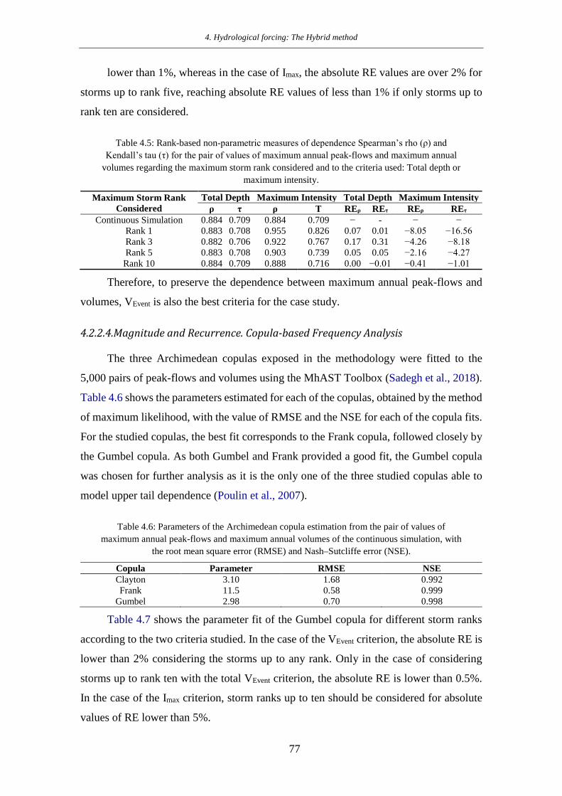
4. Hydrological forcing: The Hybrid method
77
lower than 1%, whereas in the case of Imax, the absolute RE values are over 2% for
storms up to rank five, reaching absolute RE values of less than 1% if only storms up to
rank ten are considered.
Table 4.5: Rank-based non-parametric measures of dependence Spearman’s rho (ρ) and Kendall’s tau (τ) for the pair of values of maximum annual peak-flows and maximum annual
volumes regarding the maximum storm rank considered and to the criteria used: Total depth or maximum intensity.
Maximum Storm Rank Considered
Total Depth Maximum Intensity Total Depth Maximum Intensity ρ τ ρ Τ REρ REτ REρ REτ
Continuous Simulation 0.884 0.709 0.884 0.709 − - − − Rank 1 0.883 0.708 0.955 0.826 0.07 0.01 −8.05 −16.56 Rank 3 0.882 0.706 0.922 0.767 0.17 0.31 −4.26 −8.18 Rank 5 0.883 0.708 0.903 0.739 0.05 0.05 −2.16 −4.27
Rank 10 0.884 0.709 0.888 0.716 0.00 −0.01 −0.41 −1.01
Therefore, to preserve the dependence between maximum annual peak-flows and
volumes, VEvent is also the best criteria for the case study.
4.2.2.4.Magnitude and Recurrence. Copula-based Frequency Analysis
The three Archimedean copulas exposed in the methodology were fitted to the
5,000 pairs of peak-flows and volumes using the MhAST Toolbox (Sadegh et al., 2018).
Table 4.6 shows the parameters estimated for each of the copulas, obtained by the method
of maximum likelihood, with the value of RMSE and the NSE for each of the copula fits.
For the studied copulas, the best fit corresponds to the Frank copula, followed closely by
the Gumbel copula. As both Gumbel and Frank provided a good fit, the Gumbel copula
was chosen for further analysis as it is the only one of the three studied copulas able to
model upper tail dependence (Poulin et al., 2007).
Table 4.6: Parameters of the Archimedean copula estimation from the pair of values of maximum annual peak-flows and maximum annual volumes of the continuous simulation, with
the root mean square error (RMSE) and Nash–Sutcliffe error (NSE).
Copula Parameter RMSE NSE Clayton 3.10 1.68 0.992 Frank 11.5 0.58 0.999
Gumbel 2.98 0.70 0.998
Table 4.7 shows the parameter fit of the Gumbel copula for different storm ranks
according to the two criteria studied. In the case of the VEvent criterion, the absolute RE is
lower than 2% considering the storms up to any rank. Only in the case of considering
storms up to rank ten with the total VEvent criterion, the absolute RE is lower than 0.5%.
In the case of the Imax criterion, storm ranks up to ten should be considered for absolute
values of RE lower than 5%.

4. Hydrological forcing: The Hybrid method
78
Table 4.7: Parameters of the Gumbel copula estimation from the pair of values of maximum annual peak-flows and maximum annual volumes regarding the maximum storm rank
considered and the criteria used: Total depth or maximum intensity, and relative error (RE) respect to the continuous simulation.
Maximum Storm Rank Considered Total Depth Maximum Intensity Gumbel Parameter RE Gumbel Parameter RE
Continuous Simulation 2.98 − 2.98 − Rank 1 2.94 1.37 4.84 −62.34 Rank 3 3.00 −0.79 3.82 −28.32 Rank 5 3.02 −1.18 3.40 −13.91
Rank 10 2.99 −0.25 3.08 −3.26
The results of Table 4.7 have a reflection when TK are estimated. Figure 4.6 shows
the TK of 10 (dashed), 50 (dashed-dotted) and 100 (continuous) years of the continuous
simulation (red (Figure 4.6a–d) and blue (Figure 4.6e–h) lines) compared to the different
storm ranks according to VEvent and Imax criteria (grey lines in Figure 4.6).
(a)
(b)
(c)
(d)
(e)
(f)
(g)
(h)
Figure 4.6: Kendall return periods of 10 (dashed), 50 (dashed-dotted) and 100 (continuous) years. Grey dots represent the values obtained considering specific storm orders up to different ranks (a,e) rank one
(b,f) rank three, (c,g) rank five, (d,h) rank ten). Color dots represent the values obtained from the continuous simulation (red in (a–d), blue (e–h)). Storm rank criteria is total depth in (a–d) and maximum
intensity in (e–h).
According to each ranking criterion:
1. VEvent. Visually, there is a good agreement between the TK estimated with the VEvent
criterion and the continuous simulation (Figure 4.6a–d). Worse agreement is shown
for high return periods (100 years). In the case of considering storms with ranks up to
ten (Figure 4.6d), the TK are almost coincident.
0 100 200 300 400 500
Peak-flow (m 3 /s)
0
5
10
15
Volu
me
(hm
3)
Rank 1
0 100 200 300 400 500
Peak-flow (m 3 /s)
0
5
10
15
Volu
me
(hm
3)
Rank 3
0 100 200 300 400 500
Peak-flow (m 3 /s)
0
5
10
15
Volu
me
(hm
3)
Rank 5
0 100 200 300 400 500
Peak-flow (m 3 /s)
0
5
10
15
Volu
me
(hm
3)
Rank 10
0 100 200 300 400 500
Peak-flow (m 3 /s)
0
5
10
15
Volu
me
(hm
3)
Rank 1
0 100 200 300 400 500
Peak-flow (m 3 /s)
0
5
10
15
Volu
me
(hm
3)
Rank 3
0 100 200 300 400 500
Peak-flow (m 3 /s)
0
5
10
15
Volu
me
(hm
3)
Rank 5
0 100 200 300 400 500
Peak-flow (m 3 /s)
0
5
10
15
Volu
me
(hm
3)
Rank 10

4. Hydrological forcing: The Hybrid method
79
2. Imax. There is not a good agreement between the TK estimated with this criterion
compared to the continuous simulation for ranks up to three. If the biggest storm is
considered, the TKs are underestimated. In the case of considering storm ranks up to
three, the return periods of 50 and 100 years are highly overestimated. TKs are closer
with storms up to rank five (still overestimated for 50 and 100 years TKs), and almost
a perfect agreement is achieved if rank periods up to 10 are considered.
4.2.2.5.Analysis of previous works
As exposed, some studies in the literature have previously analysed the influence
of storms on the derivation of the flood frequency curve through event-based approaches.
Table 4.8 shows the main characteristics of the research on this topic. Flores-Montoya et
al. (2016) (extended analysis in Flores-Montoya (2018)) carried out a similar experiment
in two French basins. They extracted the storms from the synthetic time series of spatial-
punctual rainfall generated with the Rainsim V3 (Burton et al., 2008), and forced the
event-based distributed model RIBS (Garrote and Bras, 1995) (predecessor of tRIBS)
with them. As they accounted for spatial variability, they separated the storms based on
the mean area rainfall, and ranked them by total depth, mean intensity (instead of
maximum intensity), and total duration. They carried out the analysis only for the five
highest storms of each year, and performed the experiment simultaneously for Générarges
and Corbès. Sordo-Ward et al. (2015; 2016) performed a similar analysis in four Spanish
basins, by also coupling the RainSim V3 with a simpler semi distributed model (Sordo-
Ward et al. 2012; 2013). Thus, they were able to analyse all the events each year as the
experiment resulted less computationally expensive.
When comparing to the present study, Sordo-Ward et al. (2015; 2016) and Flores-
Montoya et al. (2016) both used event-based approaches instead of a continuous
approach. As a consequence, they needed to characterize the soil-moisture in the basin
prior to the storm events. In the case of Sordo-Ward et al. (2015; 2016), they considered
a constant value of the curve number in each of the sub-basins for all the storms.
Regarding Flores-Montoya et al. (2016), they determined the initial soil moisture in a
probabilistic way. Within this study, as the simulations were performed with tRIBS, all
the conditions prior to the storm events were given by the continuous simulation.

4. Hydrological forcing: The Hybrid method
80
Table 4.8: Comparison between similar case studies and the methodology used in each of them. For comparison purposes, the basin area, weather/rainfall generator, hydrological model and
the way of accounting soil moisture are shown.
Case Study Area (km2)
Weather/Rainfall Generator
Spatial Resolution
Hydrological Model Type Initial Soil
Moisture
Peacheater Creek 64 AWE-GEN5 Punctual TRIBS7
Fully distributed-Continuous
Continuous assessment
Générargues1,2 245 RainSim V36 Spatial-Punctual RIBS8
Fully distributed-Event based
Probabilistic
Corbès1,2 262.3 RainSim V36 Spatial-Punctual RIBS8 Semidistributed-
Event based Probabilistic
Navacerrada3 20 RainSim V36 Spatial-Punctual
Stochastic HEC-HMS9
Semidistributed-Event based Deterministic
Santillana4 211 RainSim V36 Spatial-Punctual
Stochastic HEC-HMS10
Semidistributed-Event based Deterministic
El Pardo4 495 RainSim V36 Spatial-Punctual
Stochastic HEC-HMS11
Semidistributed-Event based Deterministic
Manzanares 4 1294 RainSim V36 Spatial-Punctual
Stochastic HEC-HMS12
Semidistributed-Event based Deterministic
1Flores-Montoya et al. (2016) 2 Flores-Montoya (2018) 3 Sordo-Ward et al. (2015) 4 Sordo-Ward et al. (2016) 5Fatichi et al.
(2011) 6 Burton et al. (2008) 7 Ivanov et al. (2004a;b) 8 Garrote and Bras. (1995) 9 Sordo-Ward et al. (2012; 2013)
Table 4.9 shows a summary of the results obtained within this Chapter and the
comparison of the results obtained in other studies (some aspects have not been studied
by the other compared studies and are therefore not shown). Several aspects can be
remarked when analyzing Table 4.9:
Table 4.9: Results obtained for the different case studies considered in Table 4.8. PF represents the maximum annual peak-flow, V represents the maximum annual volume, and RE represents
the relative error.
Case Study Best Criteria
1st Rank PF Coincidence
(%)
1st rank V Coincidence
(%)
Rank 95% PF
Rank 95%
V
Rank Seasonality PF and V (<5% RE)
Rank Copula
Parameter (<5% RE)
Peacheater Creek
Total depth 53 69 5 4 3 1
Générargues1,2 Total depth 70 88 4 2 − −
Corbès1,2 Total depth 70 88 4 2 − −
Santillana4 Total depth 66 − 4 − − −
El Pardo4 Total depth 67 − 4 − − −
Manzanares 4 Total depth 55 − 6 − − −
Navacerrada3 Total depth 63 − 6 − − −
1Flores-Montoya et al. (2016) 2 Flores-Montoya (2018) 3 Sordo-Ward et al. (2015) 4 Sordo-Ward et al. (2016)

4. Hydrological forcing: The Hybrid method
81
1. In all the case studies, among the three criteria of storm event ranking, the best was
total depth. This suggests that the choice between one criterion or another has a low
dependence on the hydrological model used or how the initial moisture is accounted.
Accounting or not for the spatial variability of rainfall does not seem to influence
either, but this might be due to the small size of Peacheater Creek.
2. Regarding the probability of achieving the maximum annual peak-flow, the lowest
values (55% and 53%) correspond to the Manzanares and Peacheater Creek,
respectively. The first is the biggest basin (1294 km2), and the reduction of probability
can be due to the importance of propagation processes and the temporal patterns of
the storm events. However, Peacheater Creek is the second smallest basin in Table
4.9. The reduction of the coincidence with the maximum annual peak-flow might be
due to how antecedent basin conditions prior to the storm event are considered. As
the model is continuous, some lower rank events may concur with wetness states of
the basin, incurring higher peak-flows. This phenomenon cannot occur in the Sordo-
Ward et al. (2015; 2016) study basins, as the initial soil moisture was considered
constant and equal for all the storm events.
3. When the coincidence of the first rank total depth storm with the maximum annual
volume is analysed (Peacheater Creek and Flores-Montoya et al. (2016)), it can be
seen that there is a higher probability of coincidence than that of the peak-flow. This
suggests that total depth has a better correlation with the maximum annual volume
than with the maximum annual peak-flow. This can also be seen when the minimum
rank of storm required is analysed. Smaller ranks are required to achieve a 95%
probability of obtaining the maximum annual volume than for obtaining the
maximum annual peak-flow with the same probability.
4. In all the case studies shown, the maximum peak-flow can be obtained with a 95%
probability considering all the storms up to rank four, five or six. In the case of total
volume, the maximum rank required is reduced to two or four.
5. Within this section, it has been shown that seasonality and bivariate properties of
extreme floods can be well-preserved if storms up to rank three and one are
considered, respectively.
Therefore, to sum up, as a general recommendation, considering the five biggest
storms per year classified by their total depth can result in an accurate derivation of the

4. Hydrological forcing: The Hybrid method
82
flood frequency curve when using event-based models, close to that obtained from
continuous simulations. Based on the results obtained, the five major events of each year
in terms of total depth were selected from all the storm events within the 5,000 years to
perform the Hybrid method simulations.
4.2.1. Initial soil moisture: simulation and probability distributions
A continuous simulation of 50 years was performed, forcing tRIBS with 50 years
of continuous hourly weather. As previously mentioned, to develop the Hybrid method it
was assumed that there is independence between rainfall events and prior hydrological
soil moisture conditions.
The relationship between MSM10Event and VEvent for all the storm events in the 50
years of simulation was analysed (Figure 4.7). If all the storm events (3,797 events in the
50 years) are considered, the value of Kendall’s tau for the pair of values MSM10Event -
VEvent is 0.034, whereas if considering only the five largest values (2500 events) the value
is 0.063. Thus, the storm events can be considered as independent (Kendall’s tau values
tend to zero) of the prior initial soil moisture conditions of the basin, as previously stated
by Paquet et al. (2013).
It should be pointed out that this hypothesis, in the case of modelling frameworks
that couple hydrological with atmospheric models (i.e.: WRF-Hydro (Gochis et al.,
2015)), might not be valid due to the relationship between terrestrial hydrology and
weather.
Figure 4.7: Comparison of the initial soil moisture value associated to each storm event (MSM10Event) and
the total depth associated to the storm event (VEvent) in the 50 years of continuous simulation for: all the storm events (blue dots) and for the 5 largest total depth events per year (red dots).
Afterwards, the cumulated frequency distributions of MSM10Event values of the 50
years’ continuous simulation for each month of the year were obtained (Figure 4.8).

4. Hydrological forcing: The Hybrid method
83
Figure 4.8: Cumulated Frequency distributions of MSM10Event values within the 50 years of simulation
for each month of the year.
These frequency distributions are used as input for the Hybrid method. Each storm
event is associated with the frequency distribution corresponding to the month of
occurrence of the storm.
Afterwards, within a Monte Carlo framework, a value of MSM10Event is associated
to each storm event. Once MSM10Event is obtained, a synthetic spatio-temporal basin state
is generated, with a MSM10 value in the basin equal to the MSM10Event. Figure 4.9 shows
as an example three synthetic initial basin states for different MSM10Event values.
(a) (b)
(c)
Figure 4.9: Examples of synthetic initial basin states with a MSM10 value of (a) 0.5 (b) 0.6 and (c) 0.7. Colorbar represents the values of soil moisture in the different voronoi polygons.
4.2.2. Hybrid method performance
Once the initial basin states were obtained, they were coupled to each of the 25,000
storm events (5 x 5,000 years), serving both as forcing for the hydrological model tRIBS

4. Hydrological forcing: The Hybrid method
84
simulations. Thus, 5 flood hydrographs per year were obtained, amounting 25,000 flood
hydrographs which were compared to those obtained from the 5,000 years of continuous
simulation.
4.2.2.1. Seasonality
Figure 4.10 shows the seasonal behaviour of the Hybrid method regarding the
maximum peak-flow (Figure 4.10a) and maximum volume (Figure 4.10b). Comparisons
were carried out with the seasonality of the continuous simulation (red lines). It can be
seen the mean of the date of occurrence is well preserved for both maximum annual peak-
flows and maximum annual volumes, whereas the variability of the date of occurrence
about the mean date is lower in the Hybrid method in both cases.
(a)
(b)
Figure 4.10: Comparison between the seasonality of the continuous (red) maximum annual peak-flow (a); and and maximum annual volume (b) with respect to that obtained by applying the Hybrid method (black), in which the predominant direction of the seasonality is represented by a circle with a line.
To quantify the seasonal performance of the Hybrid method, the values of θ� and r̅
were obtained from the continuous simulation and compared to the ones obtained from
the Hybrid method, obtaining the RE (Equation (4.1)).
Table 4.10 shows the different values of θ� and r̅ depending on the criteria and the
RE, for the maximum peak-flow and for maximum volume (Table 4.10)::
3. Maximum peak-flow. There is less than 8% absolute RE in the estimation of the mean
direction of seasonality. Regarding the radius, which measures the dispersion of the
seasonality, the Hybrid method has an absolute RE of almost 52 %.
4. Maximum volume. In this case, the Hybrid method is more accurate than in the
maximum annual peak-flow. The mean direction of seasonality is estimated with an

4. Hydrological forcing: The Hybrid method
85
absolute value of RE lower than 6 %, whereas the dispersion of the seasonality is
estimated with an RE of 32 %.
Table 4.10: Seasonality of the maximum annual peak-flow represented by the angle of its mean direction (θ�) and its radio (r̅), for different storm ranks and for the two different criteria
studied. The relative error (RE) is also shown.
Method Maximum Peak Flow Maximum Volume Maximum Peak Flow Maximum Volume 𝛉𝛉� �̅�𝐫 𝛉𝛉� �̅�𝐫 𝐑𝐑𝐑𝐑𝛉𝛉� 𝐑𝐑𝐑𝐑�̅�𝐫 𝐑𝐑𝐑𝐑𝛉𝛉� 𝐑𝐑𝐑𝐑�̅�𝐫
Continuous Simulation 169.7 0.29 142.9 0.25 − − − −
Hybrid 157.7 0.14 151.0 0.17 7.1 51.7 −5.7 32.0
4.2.2.2. Dependence
An analysis of how the Hybrid method is able to preserve the dependence between
the peak-flow and volume of the continuous simulation is performed. To do so, the chi-
plot was graphed comparing the peak-flow volume dependence from the continuous
simulation (red dots in Figure 4.11) to the Hybrid event-based model (black dots in Figure
4.11).
There is a positive dependence between the peak-flow and volume. Furthermore,
when focusing on the upper tail dependence (first quadrant in Figure 4.11), the points are
located far from the zero value of the y axis, which is the independence hypothesis.
Figure 4.11: Chi-plot of the maximum annual peak-flow and volume. Red dots represent the values the values obtained from the continuous simulation, whereas black dots represent the values obtained from
the Hybrid-based method.
To numerically compare the degree of dependence of the peak-flow and volume of
the continuous simulation with respect to Hybrid event-based model, values of
Spearman’s rho and Kendall’s tau were computed (Table 4.11), and their RE (Equation
(4.1)). Spearman’s rho is obtained with a RE lower than 7 %, whereas Kendall’s tau
differs around 13 % in terms of RE values among the continuous simulation and the
Hybrid model.
-1 -0.8 -0.6 -0.4 -0.2 0 0.2 0.4 0.6 0.8 1
i
-1
-0.5
0
0.5
1
i

4. Hydrological forcing: The Hybrid method
86
Table 4.11: Rank-based non-parametric measures of dependence Spearman’s rho (ρ) and Kendall’s tau (τ) for the pair of values of maximum annual peak-flows and maximum annual
volumes of the continuous and Hybrid-based simulation.
Maximum Storm Rank Considered Total Depth Total Depth ρ τ REρ REτ
Continuous Simulation 0.884 0.709 − - Event Based Simulation 0.941 0.803 -6.44 -13.3
4.2.2.3. Magnitude and recurrence. Copula-based frequency Analysis
The Archimedean Gumbel copula was fitted, as it is the only one of the three studied
copulas able to model upper tail dependence (Poulin et al., 2007) to both the 5,000 pairs
of peak-flows and volumes of the continuous and Hybrid-based model respectively using
the MhAST Toolbox (Sadegh et al., 2018). Table 4.12 shows the parameters estimated
for each of the copulas, obtained by the method of maximum likelihood for each of the
copula fits. The absolute RE is lower than 13%.
Table 4.12: Parameters of the Archimedean Gumbel copula estimation from the pair of values of maximum annual peak-flows and maximum annual volumes of the continuous simulation
and Hybrid simulation, and relative error (RE) respect to the continuous simulation.
Copula Parameter Continuous Parameter Hybrid RE Gumbel 2.98 3.36 -12.75
Furthermore, a comparison of the Kendall’s return performed. Figure 4.12 shows
the TK of 10 (dashed), 50 (dashed-dotted) and 100 (continuous) years of the continuous
simulation (red lines) and the Hybrid-based method (grey lines).
Figure 4.12: Kendall return periods of 10 (dashed), 50 (dashed-dotted) and 100 (continuous) years. Grey dots represent the values obtained from the Hybrid-based method, whereas red dots represent the values
obtained from the continuous simulation.
0 50 100 150 200 250 300 350 400 450 500
Peak-flow (m 3 /s)
0
5
10
15
Volu
me
(hm
3)

4. Hydrological forcing: The Hybrid method
87
Visually, there is a good agreement between the TK estimated with for TK of 10
years (Figure 4.12). However, for TK of 50 and 100 years, the Hybrid method
overestimates TK in terms of volume, having a good agreement with peak-flows.
This can be explained by the analysis of the univariate distributions of maximum
annual peak-flows (Figure 4.13a) and volumes (Figure 4.13b).
(a)
(b)
Figure 4.13: Univariate flood frequency distributions of maximum annual peak-flows (a) and volumes (b). Black dots represent the results obtained by the Hybrid-based method, whereas red dots represent the
values obtained from the continuous simulation.
It can be seen that, in the case of peak-flows, there is an almost perfect agreement
between the frequency curves of both the continuous and the Hybrid-based method
(Figure 4.13a). When analysing the maximum annual volume frequency curve, it can be
seen how the Hybrid-method underestimates the maximum annual volumes for return
periods over 100 years (Figure 4.13b). In the case of the peak flow frequency curve, the
Nash-Sutcliffe coefficient (Nash and Sutcliffe, 1970) has a value of 0.98, comparing the
Hybrid-based values to those obtained by the continuous peak-flow; while in the case of
the maximum annual volume frequency curve, the Nash-Sutcliffe coefficient is 0.97.
The Hybrid method: Summary and conclusions
4.3.1. Criterion for storm selection for the Hybrid method.
This Chapter approaches a focus on providing guidance on selecting the minimum
number of storm events for deriving the flood frequency curve through event-based
approaches. To do so, the methodology applied compares the resulting flow of coupling
10 0 10 1 10 2
Return Period (years)
0
200
400
600
Peak
flow
(m3
/s) Hybrid
Continuous
10 0 10 1 10 2
Return Period (years)
0
5
10
15
Volu
me
(hm
3)
Hybrid
Continuous

4. Hydrological forcing: The Hybrid method
88
a stochastic weather generator with a fully distributed physically-based model with the
flow resulting from selecting only a limited number of storms per year. The methodology
has only been applied to one basin, and therefore the results and conclusions are restricted
to this watershed. Despite this, the study shows how the number of storms selected has
an influence on the derivation of extreme floods, and its characteristics: Univariate
magnitude and recurrence of maximum annual peak-flows and volumes, their seasonality,
their dependence, and their statistic bivariate properties. Specifically, for Peacheater
Creek:
1. When analysing the correspondence between storms and maximum annual peak-flow
and volume, the best ranking criterion is total depth, followed by maximum intensity.
Considering storms up to rank five sorted by the total depth criterion, resulted in a
probability of generating the maximum annual peak-flow of 94% and the maximum
annual volume of 99%.
2. In the case of the total depth criterion, the higher the return period of peak-flow or
volume is, the lower the storm rank needed. For return periods of peak-flow or volume
over ten years, all the storms have a rank equal or lower than four. For return periods
higher than 50 years, there is a probability of achieving the maximum annual peak-
flow and the maximum annual volume of 99% if the three highest events are
considered.
3. For preserving the seasonality of maximum annual peak-flows and volumes, total
depth was also the best criterion. With storms up to rank five, there is less than 1%
absolute relative error in the estimation of the mean direction of seasonality for both
the peak-flow and volume. Regarding the dispersion of the seasonality, considering
storms up to rank five resulted in an absolute relative value lower than 4%.
4. Total depth was also the best criterion for preserving the dependence and bivariate
properties of the floods derived from the continuous simulation. Even by considering
only the biggest storm of each year, the absolute relative errors when estimating
Spearman’s rho and Kendall’s tau are less than 1%. When estimating the parameter
of the copula family selected (Gumbel), the relative error was less than 2% if storms
up to rank five were considered, and was less than 0.5% if storms up to rank ten were
considered. Regarding Kendall’s return period, considering the same number of
storms produces Kendall’s return periods of 10 and 50 years very similar to those
obtained by continuous simulation, and the 100 years return period is slightly

4. Hydrological forcing: The Hybrid method
89
underestimated. If the ten biggest storms are considered, all the studied Kendall’s
return periods are almost equal.
Therefore, to sum up, as a general recommendation, considering the five biggest
storms per year classified by their total depth can result in an accurate derivation of the
flood frequency curve when using event-based models, close to that obtained from
continuous simulations. Based on the results obtained, the five major events of each year
in terms of total depth were selected from all the storm events within the 5,000 years to
perform the Hybrid method simulations.
4.3.2. Initial soil moisture conditions and performance of the Hybrid
Method
A Hybrid methodology has been presented. Through the use of an hourly climate
stochastic generator and a physically based distributed hydrological model, the Hybrid
method represents the frequency curves of peak flows and maximum annual volumes and
its characteristics: Univariate magnitude and recurrence of maximum annual peak-flows
and volumes, their seasonality, their dependence, and their statistic bivariate properties.
The model represents these results in a precise way, reducing the computation times on
the order from months to hours. This methodology has been applied to the Peacheater
Creek case study, concluding that:
1. Independence between rainfall events and prior hydrological soil moisture conditions
has been proved within the framework of the Hybrid method developed.
2. The Hybrid method preserves the seasonality of maximum annual peak-flows and
volumes. The method provides less than 8% absolute relative error in the estimation
of the mean direction of seasonality of both maximum annual peak-flows and volumes
compared to the continuous modelling results. However, regarding the dispersion of
seasonality, the Hybrid method provides less dispersion around the mean direction of
seasonality, providing a relative error up to 52 % and 32 % in maximum annual peak-
flows and volumes respectively.
3. The Hybrid method is able to preserve the dependence and bivariate properties of the
floods derived from the continuous simulation. The correlation between maximum
annual peak-flows and volumes is preserved by the Hybrid-based method similarly to
the continuous modelling approach. Spearman’s rho is obtained with a relative error
lower than 7 %, whereas Kendall’s tau differs around 13 % respect to the values
4. Hydrological forcing: The Hybrid method
90
obtained through continuous modelling. When estimating the parameter of the
Gumbel copula family selected, the relative error was less than 13%. Regarding
Kendall’s return period, Kendall’s return period of 10 is very similar to those obtained
by continuous simulation. However, for Kendall’s return period of 50 and 100 years,
the Hybrid method overestimates volume values, having a good agreement with peak-
flows.
4. The proposed Hybrid method is capable of reproducing the univariate flood frequency
curves with a good agreement to those obtained by the continuous simulation. The
maximum annual peak-flow frequency curve is obtained with a Nash-Sutcliffe
coefficient of 0.98, whereas the maximum annual volume frequency curve is obtained
with a Nash-Sutcliffe value of 0.97.
5. The proposed Hybrid method reduces the time computation of continuous simulations
from two and half months to fourteen hours of computation for Peacheater Creek
basin (due to the continuous simulation of 50 years). Regarding to the event-based
simulations, they were performed within one hour of computation.

4. Hydrological forcing: The Hybrid method
91

5. Spillway operation: The K-Method
92
5. Spillway operation: The K-Method
This Chapter presents a method which can be used to define real-time operation
rules for gated spillways (named the K-Method). The K-Method is defined to improve
the performance of the Volumetric Evaluation Method (VEM), by adapting it to the
particular conditions of the basin, the reservoir, or the spillway. The VEM was proposed
by the Spanish engineer Fernando Girón in 1988 (Girón, 1988) and is largely used for the
specification of dam management rules during floods in Spain. This method states that
outflows are lower than or equal to antecedent inflows, outflows increase when inflows
increase, and the higher the reservoir level, the higher the percentage of outflow increase.
The K-Method was developed by modifying the VEM and by including a K parameter
which affects the released flows. A Monte Carlo environment was developed to evaluate
the method under a wide range of inflow conditions (100,000 hydrographs) and with
return periods up to 10,000 years.
Application to the Dam in the Segura river basin
The proposed methodology was applied to a dam located in the Segura river basin,
the Talave reservoir. This dam is located in the province of Albacete, in the southeast of
Spain, and belongs to the Mundo river basin. The Talave basin has an area of 766.5 km2.
The climate of the region is Mediterranean (mean annual precipitation of 557 mm). The
main purposes of the reservoir are flood regulation, hydropower generation, and water
supply for the Region of Murcia.
The characteristics of the basin and dam-reservoir system configuration are shown
in Table 5.1 and Figure 5.1.
Table 5.1: Characteristic reservoir levels and outflows of the dam configuration.
Reservoir Levels (m.a.s.l)
Maximum Outflow Capacity at Design Flood Level (DFL)
(m3/s)
Characteristic Outflows (m3/s)
Top of control pool (TCP) 508.9 Gated-spillway 2 × 142.5 Alert outflow (OALT) 100
Activation level (AL) 509.3 Flood control level (FCL) 509.9 Bottom outlet 1 × 99.5 Warning outflow (OWARN) 150 Design flood level (DFL) 511.3 Dam body
water intakes 2 × 9.0 Emergency outflow (OEMER) 300 Crest of dam (COD) 512.4

5. Spillway operation: The K-Method
93
Two vertical wagon gates, each one being six meters wide by four meters high,
compose the main spillway. The other operative discharge structures are one bottom
outlet and two water intakes in the dam body.
(a)
(b)
Figure 5.1: Case study scheme. (a) Location of the Talave dam. (b) Scheme of the discharge structures and the elevation of their axis (left). Details of gated spillways (right). Abbreviations are defined in
Table 5.1.
Figure 5.2 shows a general scheme of the probabilistic approach.
Figure 5.2: Scheme of the proposed probabilistic approach.
A probabilistic approach was implemented, combining a Monte Carlo framework
and deterministic flood control operation rules for dams with gated spillways. The main
components of the process are:
• Rainfall generation and a hydrometeorological model. A Monte Carlo environment
was produced to generate a set of storms and its corresponding hydrographs were used

5. Spillway operation: The K-Method
94
as the input to the reservoir. An ensemble of 100,000 inflow hydrographs was
generated by applying the methodology developed by Sordo-Ward et al. (2012)
(Section 3.1.3)
• Flood routing in the reservoir and dam operation by applying VEM, the K-Method, I-
O, and MILP. The proposed K-method was compared with VEM, in order to assess
the performance improvement. As exposed in Section 3.2, two other methods were
used for references as extreme cases: the Inflow-Outflow Method (I-O) and the Mixed
Integer Linear Programming method (MILP) proposed by Bianucci et al. (2013). The
I-O is a very simple scheme that tries to maintain the reservoir level by equating
reservoir releases to reservoir inflows while the gates are partially opened, so no flood
attenuation effect is achieved during the controlled phase of dam operation. On the
other end, the MILP method is a full optimization method that achieves the best
possible management of an inflow hydrograph, according to a given objective
function. It represents perfect management under the unrealistic assumption of full
knowledge of the inflow hydrograph, and thus, is taken as the reference for maximum
improvement.
Performance assessment of the K-Method
Once the different gate controlled operation rules were applied, the maximum level
reached in the reservoir (ZMAX) and the maximum outflow downstream (OMAX) were
selected as representative variables for a comparison of the methods’ performance.
A comparative analysis by means of two different approaches was implemented.
On the one hand, a comparative scheme organized in quadrants was applied, which
showed the increasing (or decreasing) of the maximum reservoir level and maximum
outflow compared to the VEM. The points located in the upper right quadrant (QI)
represent events where the maximum level reached in the reservoir and the maximum
outflow were higher than by applying the VEM. The points located in the upper left
quadrant (QII) show an intermediate situation, with lower maximum levels but higher
outflows. The lower left quadrant (QIII) represents cases for which both the maximum
level and maximum outflow were lower than by applying the VEM (i.e., the best
situation). The lower right quadrant (QIV) represents intermediate situations with higher
maximum levels and lower maximum outflows. On the other hand, the global risk-index
presented in Section 3.6 was used as a comparative assessment tool.

5. Spillway operation: The K-Method
95
Results comparing a representative range of K-values, I-O, and MILP with the
VEM, are reported in Figure 5.3, Figure 5.4 and Figure 5.5. For K-values lower than one,
no improvement with respect to the VEM was achieved for the Talave dam. The K-
Method is equal to the VEM when the K-value is equal to one. For K-values higher than
one, all analysed cases were located in QII and QIII. Following this, the analysis of the K-
Method focused on K-values higher or equal to one. When analysing the variations of the
maximum reservoir level compared to VEM (ΔZ), a higher K-value resulted in a lower
ZMAX, regardless of the range of inflow Trs studied, reaching up to −0.15 m for K = 2 and
−0.64 m for K = 50 (Figure 5.3). However, when analysing the variations of the maximum
outflows compared to VEM (ΔO), different behaviours were found, depending on the Trs
analysed. Figure 5.3 shows, for different ranges of Trs, the percentage of cases located in
QIII (the best situation), Figure 5.5 (a1–a6) shows the median and quartiles associated
with the maximum reservoir levels (ZMAX), and Figure 5.5 (b1–b6) shows the variations
of the median and quartiles associated with the maximum outflows (OMAX).
Figure 5.3: Comparison of the K-Method (for different K-values), I-O and MILP with respect to the
VEM. The horizontal axis shows the increments of the maximum reservoir level in m (ΔZ). The vertical axis shows the increments of the maximum outflow in m3/s (ΔO). The red points correspond to events with Tr ranging from one to 10 years, blue points ranging from 10 to 25, green points from 25 to 50,
black points from 50 to 100, cyan points from 100 to 500, and magenta points from 500 to 10,000 years.
For Tr values lower than 25 years, all events were located in QII, regardless of the
analysed K-value (Figure 5.4 (a1,a2)), decreasing the maximum levels but increasing the
maximum outflows when compared with VEM (Figure 5.3 and Figure 5.5 (a1,a2,b1,b2).
Even though the maximum outflows increased, the OMAX values did not jeopardize the

5. Spillway operation: The K-Method
96
downstream safety for K-values lower than ten, because OALT was not exceeded (OMAX =
97.2 m3/s for K = 10).
Figure 5.4: Percentage of cases in QIII from K = 1.25 to K = 50, for different ranges of Tr of the inflow
hydrographs. The red colour corresponds to events with Tr ranging from one to 10 years (a1), blue from 10 to 25 (a2), green from 25 to 50 (a3), black from 50 to 100 (a4), cyan from 100 to 500 (a5), and
magenta from 500 to 10,000 years (a6).
For Tr values ranging from 25 to 50 years, lower K-values included more cases in
QIII, decreasing from 73% for K = 1.25, to 4% for K = 10. For K-values higher than 20,
all events were located in QII (Figure 5.4 (a3). Higher K-values achieved lower ZMAX
values, but the opposite occurred for OMAX. For example, the ZMAX median decreased
from 509.8 to 509.5 m and the OMAX median increased from 111 to 118 m3/s for K = 1
(VEM) and K = 10, respectively (Figure 5.5 (a3–b3)). For K-values higher than ten, the
median of ZMAX decreased to 509.3 m for K = 50, while the OMAX median increased to
124 m3/s for K = 50.
For Tr values ranging from 50 to 100 years, more than 99% of the analysed cases
were included in QIII for K-values from 1.25 to 6.5, more than 92% for K-values lower
than ten, and this decreased down to 17% for K = 50 (Figure 5.4 (a4)). The median of
ZMAX decreased from 509.9 m for K = 1 (VEM), to 509.5 m for K = 10 and 509.3 m for
K = 50. (Figure 5.5 (a4)). The median of OMAX decreased from 177 m3/s to 170 m3/s with
K ranging from one (VEM) to three, but increased for K-values higher than three, up to
180 m3/s for K = 50 (Figure 5.5 (b4)).
For Tr values within the range of 100 to 500 years, all events were located in QIII
for K-values ranging from one to ten (Figure 5.3 and Figure 5.4 (a5)) and more than 93%
for K-values higher than ten (Figure 5.4 (a5) and Figure 5.5 (a5,b5)). The ZMAX and OMAX
median values decreased from 510.0 m and 270 m3/s for K = 1 (VEM), to 509.6 m and
252 m3/s for K = 10, respectively. For K-values higher than ten, the ZMAX and OMAX
median values remained almost constant.

5. Spillway operation: The K-Method
97
For Tr values higher than 500 years, regardless of the K-value (except for those
lower than one), all events were located in QIII (Figure 5.3 and Figure 5.4 (a6)). The ZMAX
and OMAX median values ranged from 511.0 m and 375 m3/s for K = 1 (VEM), to 510.8
m and 360 m3/s for K = 10, respectively (Figure 5.5 (a6,b6)). For K-values higher than
ten, the ZMAX and OMAX median values remained almost constant. I-O and MILP were
also compared with VEM. As expected, the I-O behaviour was similar to the K-Method
for higher K-values (Figure 5.3). By comparing MILP and VEM, the results showed that
all events with a Tr higher than 25 years were located in QIII, and those with a Tr lower
than 25 years located in QII presented outflows that did not jeopardize the downstream
safety (Figure 5.3).
Figure 5.5:Comparison of the K-Method (for different K-values) with respect to the VEM (K = 1). The
continuous line shows the median and the shaded areas show the range between the 25th and 75th percentile of the maximum reservoir levels (ZMAX) (a) and the maximum outflows (OMAX) (b), from K = 1
(VEM) to K = 50. The horizontal axis shows the different values of K. The red colour corresponds to events with Tr ranging from one to 10 years (a1,b1), blue from 10 to 25 (a2,b2), green from 25 to 50 (a3,b3), black from 50 to 100 (a4,b4), cyan from 100 to 500 (a5,b5), and magenta from 500 to 10,000 years (a6,b6). For specific K-values (K = 1, 2, 4, 6, 8, 10, 20, 50), box plots are presented with their
corresponding outliers (when existing) represented by red dots.
An analysis of the frequency curves of ZMAX and OMAX for the different methods
(Figure 5.6) was also carried out. For the K-values analysed (and for K-values greater
than one), they showed an intermediate behaviour between VEM and I-O. For the ZMAX
frequency curves, the higher the K-value, the lower ZMAX obtained for the same return
period (Figure 5.6a). However, when analysing the OMAX frequency curves, they

5. Spillway operation: The K-Method
98
intersected the VEM maximum outflow frequency curve (Figure 5.6b). For Tr values
higher than one, and until the intersection of the OMAX frequency curves, the greater the
K-value, the greater the OMAX was for the same Tr. Moreover, the intersection with VEM
occurred at higher Trs, corresponding to a Tr of 31, 50, 86, and 102 years for K = 2, 10,
50, and I-O, respectively. Once the OMAX frequency curves intersected, the behaviour was
the opposite.
Therefore, the choice of the best operation rule was not univocal for the entire range
of analysed Tr and depended on the priorities selected by the dam damager (MILP was
not accounted for as it needs to know the whole inflow hydrograph in advance). If an
ordinary reservoir operation and the management of floods with a Tr between one and 25
years were prioritized, the best rule operation was the K-Method for the highest K-value
that minimized ZMAX and avoided damages associated with the released outflows. As
mentioned, for this case study, it was K = 10.
Figure 5.6: Frequency curves. (a) Maximum reservoir level frequency curves for VEM (blue continuous line), different values of K (black lines of different types, see legend), I-O (dashed-dotted blue line), and
MILP (dashed red line). (b) Maximum outflows frequency curves for VEM (blue continuous line), different values of K (black lines of different types, see legend), I-O (dashed-dotted blue line), and MILP
(dashed red line).
If the management of floods with a Tr ranging from 25 to 500 years was prioritized,
the best operation rule depended on whether the number of events included in QIII or the
entity of the decrease of ZMAX and OMAX was prioritized. In the case study, K = 1.25
maximized the number of events improved for 25 < Tr < 50 years and K = 10 for 50 < Tr
< 500 years. The reservoir levels reached Zones 3 (in all events with Tr values higher
than 50 years) and 4. The influence of the K-value on Equation (3.13) implied an increase
of the released outflows at the beginning of the operation (Zone 2), increasing the
available flood control capacity with respect to VEM for the next time steps. Therefore,
Zones 3 and 4 were reached later, for which the OMAX was reduced (Figure 3.8).

5. Spillway operation: The K-Method
99
If the dam safety and management of extreme floods (Tr > 500 years) were
prioritized, I-O simultaneously minimized the maximum levels and maximum outflows.
However, as the Tr of the inflows increased, ΔO and ΔZ tended to be zero. In these cases,
Qp was higher than the maximum discharge capacity when the gates were fully opened
and the outflow responded to an un-controlled fixed-crested spillway (Figure 3.8). This
explains why ZMAX and OMAX tended to be constant when analysing K-values higher than
ten for Tr values higher than 500 years (Figure 5.5 (b6) and Figure 5.6b). This also
explains the shape of the half loop of the comparative scheme between the K-Method and
VEM (Figure 5.3).
In a practical case, even if the skill required to forecast the inflow hydrograph is
limited, there may be ways to identify the entity of the flood that is being managed in the
reservoir. According to the general meteorological situation, the dam manager may be
able to estimate the return period of the event that is occurring, and therefore, the
conclusions of the above discussion could be applied to decide on the best K-value to
adopt.
Finally, Figure 5.6b shows changes in the slope for both the ZMAX and OMAX
frequency curves, and regardless of the analysed operation rule. For small and medium
floods, the outflows are governed by the operation of the partially opened gates. Once the
FCL is exceeded and gates become fully open, the spillways work as un-controlled fixed-
crested spillways, justifying the behavior of the frequency curves.
Figure 5.7 shows the evolution of the ratio between the maximum outflow and the
maximum inflow as a function of the return period of each event for different dam
operation methods. Although MILP showed the most peak attenuation, as previously
stated, it represents perfect management under the unrealistic assumption of full
knowledge of the inflow hydrograph; thus, it was taken only as the reference for
maximum improvement. Regarding the behaviors of the real-time methods, three main
phases were distinguished. For a lower Tr, when all methods were active (gates partially
opened), the VEM was the real-time method which showed the highest peak attenuation,
because the other real-time methods specify greater outflows than those of VEM. In
addition, the other methods reached the fully opened gate situation earlier than VEM,
because they released greater outflows and the spillways started to work earlier as un-
controlled fixed-crested spillways. For medium and high Tr values, the mentioned change
in the release mechanism justifies an increase of peak attenuation and the differences

5. Spillway operation: The K-Method
100
among the methods decrease. Finally, for the biggest floods where the crest of the dam is
overtopped and the entire length of the dam works as an un-controlled fixed-crested
spillway, peak attenuation decreased, regardless of the method.
Figure 5.7: Peak flow attenuation for different return periods and methods of operation of dams. Y axes represent the ratio between the maximum outflow and the maximum inflow for each event with their
corresponding Tr (X axes). Blue dots represent the events routed by the dam by applying the VEM, dark grey dots by applying the K-Method with a K-value = 2, grey dots with a K-value = 10, light grey dots
with a K-value = 50, cyan dots by applying the I-O method, and red dots by applying the MILP.
Figure 5.8 shows two examples of application of the different proposed dam
operation methods. Although MILP showed the most attenuation of peak flows for both
cases and good behaviour regarding the maximum reservoir level, it represents perfect
management under the unrealistic assumption of full knowledge of the inflow
hydrograph. Therefore, it was only taken as the reference for maximum improvement.
For a moderate flood, Figure 11a shows considerable differences of maximum peak flows
and maximum reservoir levels, and the VEM was the real-time method which presented
the highest peak attenuation, but the highest maximum reservoir level. In the analysis of
a large flood (Tr = 1,000 years, Figure 5.8b), it can be seen that the gates became fully
open (around 20 h) for all methods. From this time on, the spillways start to work as un-
controlled fixed-crested spillways. The peak attenuation effect is mainly due to the un-
controlled fixed-crested spillway mechanism and the differences among the methods
decrease.

5. Spillway operation: The K-Method
101
Figure 5.8: Comparison of outflow hydrographs (top) and reservoir levels (bottom) resulting from the aplication of different dam operation methods. (a) Hydrograph corresponding to Tr = 20 years and (b)
corresponding to Tr = 1,000 years. Colored lines represent the application of the different methods: VEM (blue continuous line), different values of K (red lines of different types, see legend), I-O (dashed-dotted
blue line), and MILP (magenta continuous line). Coloured shading (bottom) represents the different Zones of application of the K-Method (Zone 1 in green, Zone 2 in yellow, Zone 3 in orange, and Zone 4
in red).
In order to better quantify the influence of the K-value, the global risk index was
applied. Using the damage curves (Figure 5.9a,b), the failure risk index (IF), the non-
failure risk index (INF), and the global risk index (IR) for the Talave dam were obtained
(Figure 5.9c).
Figure 5.9 shows that K-values larger than one reduce the IR value for the Talave
dam with respect to the VEM. There is also a range of K-values for which the IR is even
lower than for the I-O, which is a very conservative flood management strategy. This
global reduction is due to the effect of management strategies on the INF. If INF is analysed,
I-O is found to be the worst strategy, since it implies no peak attenuation during the
controlled phase of the flood. The K-Method outperforms the VEM for K-values smaller
than 20. For the case of the IF, the minimum values are obtained for the I-O strategy,
which emphasizes controlling the reservoir level. This strategy is even better than MILP
optimization. In the case of the K-Method, it always outperforms VEM, and IF tends to
be the value obtained for I-O for large values of K. MILP represented the minimum
expected value for IR.
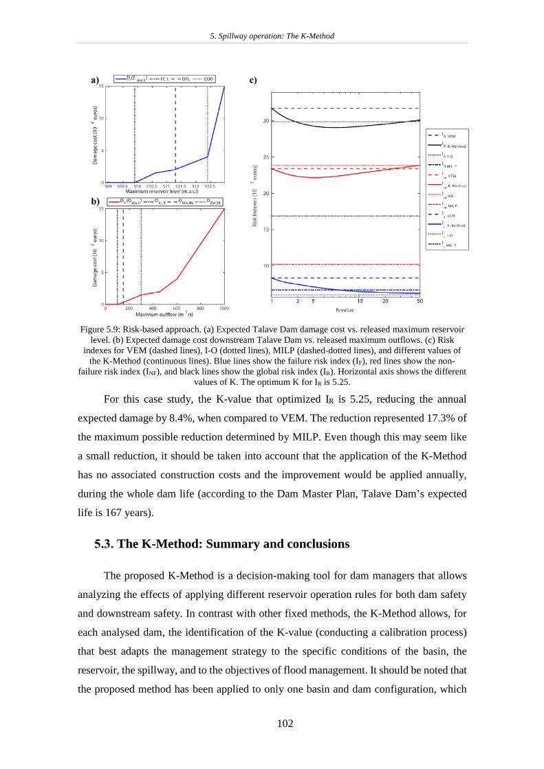
5. Spillway operation: The K-Method
102
Figure 5.9: Risk-based approach. (a) Expected Talave Dam damage cost vs. released maximum reservoir
level. (b) Expected damage cost downstream Talave Dam vs. released maximum outflows. (c) Risk indexes for VEM (dashed lines), I-O (dotted lines), MILP (dashed-dotted lines), and different values of
the K-Method (continuous lines). Blue lines show the failure risk index (IF), red lines show the non-failure risk index (INF), and black lines show the global risk index (IR). Horizontal axis shows the different
values of K. The optimum K for IR is 5.25.
For this case study, the K-value that optimized IR is 5.25, reducing the annual
expected damage by 8.4%, when compared to VEM. The reduction represented 17.3% of
the maximum possible reduction determined by MILP. Even though this may seem like
a small reduction, it should be taken into account that the application of the K-Method
has no associated construction costs and the improvement would be applied annually,
during the whole dam life (according to the Dam Master Plan, Talave Dam’s expected
life is 167 years).
The K-Method: Summary and conclusions
The proposed K-Method is a decision-making tool for dam managers that allows
analyzing the effects of applying different reservoir operation rules for both dam safety
and downstream safety. In contrast with other fixed methods, the K-Method allows, for
each analysed dam, the identification of the K-value (conducting a calibration process)
that best adapts the management strategy to the specific conditions of the basin, the
reservoir, the spillway, and to the objectives of flood management. It should be noted that
the proposed method has been applied to only one basin and dam configuration, which

5. Spillway operation: The K-Method
103
limits the generalization of the results and conclusions obtained. Although the results are
promising, further research should be developed to ensure that the K-method improves
the operation of flood control rules through a wide range of gated-spillway dams.
For the case study under analysis, the K-Method improved the results obtained with
VEM, by reducing the maximum reservoir levels reached in the dam (the higher the K-
value. the lower the maximum reservoir level), while the corresponding increase of
outflows did not endanger downstream safety. In addition, by carrying out a dam risk
analysis, a K-value of 5.25 lowered the global risk index, IR, by 8.4% compared to VEM,
and represented 17.3% of the maximum possible reduction determined by MILP.
Different behaviors were identified, depending on the Trs analysed. For events with
a Tr ranging from one to 25 years, K-value = 10 resulted in an important decrease in the
maximum reservoir levels, while the corresponding increase of outflows did not endanger
downstream safety.
For events with a Tr ranging from 25 to 100 years, higher K-values reduced the
number of events that simultaneously achieved lower maximum levels and outflows. For
events with a Tr higher than 500 years, I-O simultaneously achieved the lowest maximum
levels and outflows. In a practical case, even if the skill required to forecast the inflow
hydrograph is limited, according to the general meteorological situation, the dam manager
may be able to estimate the return period of the event that is occurring and therefore the
conclusions obtained could be applied to decide on the best K-value to adopt.

6. Operational variables I: The Influence of the initial reservoir level.
104
6. Operational variables I: The Influence of the initial
reservoir level.
This Chapter presents a method to assess the influence of the initial reservoir level
in hydrological dam safety and risk analysis. Traditionally, in professional practice, the
procedures applied are basically deterministic. Several physical processes are defined
deterministically according to the criteria of the designer (usually in the conservative
side), although there is a high degree of uncertainty regarding to these processes. A
relevant variable is the reservoir level considered at the beginning of flood events.
Hydrological dam safety assessment methods traditionally assume that the reservoir is
initially full when it receives the design flood, thus staying in the conservative side when
designing a new dam. However, the distribution of reservoir levels at the beginning of
flood episodes takes more importance for evaluating the real risk associated to dams in
operation.
In this chapter, an analysis of three different scenarios is carried out: initial reservoir
level equal to maximum normal level, equal to a maximum conservation level and
following the probability distribution from the historical records. To do so, a methodology
is proposed to analyse economically the affection of initial reservoir level in hydrological
dam and downstream safety by the application of the global risk index (Bianucci et al.,
2013). Furthermore, the uncertainty associated to initial variable level is studied in a novel
approach for the case study.
Application to the Dam in the Tagus river basin
A probabilistic approach was implemented (Figure 6.1), based on a Monte Carlo
approach (dotted points in Figure 6.1) to analyse a Dam in the Tagus river basin. The
process was as follows:
1. Generation of synthetic inflow hydrographs. An ensemble of 100,000 synthetic inflow
hydrographs representative of the observed historical annual maximum floods was
generated, applying the methodology exposed in Section 3.1.2.
2. Stochastic initial reservoir level assignation. Depending on the scenario studied (a
total of three, as will be explained in Section 6.1.1), an initial reservoir level was

6. Operational variables I: The Influence of the initial reservoir level.
105
assigned to each inflow hydrograph. Furthermore, an uncertainty analysis of the
variable initial reservoir level (Scenario 3) was carried out.
3. Reservoir-Dam flood operation. For each analysed scenario (total of three), the
ensemble of hydrographs was routed through the reservoir, obtaining a set of
maximum reservoir levels and maximum outflows. The methodology applied was the
VEM (Section 3.2.1).
4. Risk-Index analysis. By using the global risk index analysis (Bianucci et al., 2013)
explained in Section 3.6 , all the scenarios studied were compared.
Figure 6.1: General scheme of the methodological approach. Sc.1, Sc.2 and Sc.3 stand for the three
different scenarios of initial reservoir level (Zo) studied.
The proposed methodology was applied in a case study based on a gated-spillway
gravity dam located in the Tagus river basin. The dam is located in the west of Spain
(province of Caceres). The dam watershed has an extension of 1,850 km2. The climate
within the area of study is Continental with mean annual precipitation of 1,000 mm and
a mean annual runoff value of 1,020 hm3. The main purpose of the reservoir is irrigation.
Table 6.1 shows the main characteristics of the dam and its reservoir. The dam main
spillway consists of five Tainter gates, which are ten meters wide by 5.75 meters high
each. The other operative discharge structure considered is a bottom outlet in the dam
body.
To carry out the study, a gauge station located at the dam location with available
data of daily inflows and reservoir volumes from 1958/59 to 2012/13 (hydrological years,
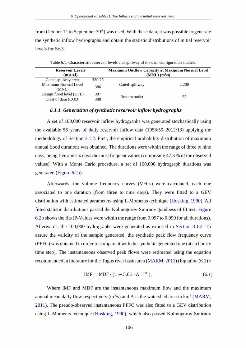
6. Operational variables I: The Influence of the initial reservoir level.
106
from October 1st to September 30th) was used. With these data, it was possible to generate
the synthetic inflow hydrographs and obtain the statistic distributions of initial reservoir
levels for Sc.3.
Table 6.1: Characteristic reservoir levels and spillway of the dam configuration studied.
Reservoir Levels (m.a.s.l)
Maximum Outflow Capacity at Maximum Normal Level (MNL) (m3/s)
Gated spillway crest 380.25 Gated-spillway 2,200 Maximum Normal Level
(MNL) 386
Design flood level (DFL) 387 Bottom outlet 57 Crest of dam (COD) 388
6.1.1. Generation of synthetic reservoir inflow hydrographs
A set of 100,000 reservoir inflow hydrographs was generated stochastically using
the available 55 years of daily reservoir inflow data (1958/59–2012/13) applying the
methodology of Section 3.1.2. First, the empirical probability distribution of maximum
annual flood durations was obtained. The durations were within the range of three to nine
days, being five and six days the most frequent values (comprising 47.3 % of the observed
values). With a Monte Carlo procedure, a set of 100,000 hydrograph durations was
generated (Figure 6.2a).
Afterwards, the volume frequency curves (VFCs) were calculated, each one
associated to one duration (from three to nine days). They were fitted to a GEV
distribution with estimated parameters using L-Moments technique (Hosking, 1990). All
fitted statistic distributions passed the Kolmogorov-Smirnov goodness of fit test. Figure
6.2b shows the fits (P-Values were within the range from 0.997 to 0.999 for all durations).
Afterwards, the 100,000 hydrographs were generated as exposed in Section 3.1.2. To
assure the validity of the sample generated, the synthetic peak flow frequency curve
(PFFC) was obtained in order to compare it with the synthetic generated one (at an hourly
time step). The instantaneous observed peak flows were estimated using the equation
recommended in literature for the Tagus river basin area (MARM, 2011) (Equation (6.1)):
IMF = MDF · (1 + 5.01 · A−0.38), (6.1)
Where IMF and MDF are the instantaneous maximum flow and the maximum
annual mean daily flow respectively (m3/s) and A is the watershed area in km2 (MARM,
2011). The pseudo-observed instantaneous PFFC was also fitted to a GEV distribution
using L-Moments technique (Hosking, 1990), which also passed Kolmogorov-Smirnov

6. Operational variables I: The Influence of the initial reservoir level.
107
goodness of fit test with a P-Value of 0.997. Afterwards, by using Gringorten plotting
position formula (Gringorten, 1963), the 100,000 peak flows (synthetic PFFC) of the
sample generated were compared with the pseudo-observed PFFC (Figure 6.2c). Finally,
Figure 6.2d shows the peak flow volume relationship between the observed and generated
sample, showing how the synthetic events properly represent the main hydrograph
characteristics.
(a) (b)
(c) (d)
Figure 6.2: Synthetic inflow hydrograph generation. (a) Frequency distribution of observed (blue) and simulated (red) reservoir inflow hydrograph duration (b) GEV fits using L-Moments (L-MOM) technique
of maximum annual hydrograph volume for the different observed durations (blue lines) and simulated volumes (red dots). (c) GEV fits using L-Moments (L-MOM) technique of the maximum annual
instantaneous peak flows. Blue circles represent the maximum annual instantaneous peak flow with return periods obtained by applying Gringorten plotting position formula, blue continuous line represents GEV L-MOM fit, blue dashed lines represent the 99 % confidence bounds whereas the red dots represent the maximum peak flows generated with a return period obtained by applying Gringorten plotting position
formula. (d) Sample of 100,000 simulated floods (red dots) plotted with the observed floods (blue-edged circles).
6.1.2. Initial reservoir level. Scenarios and uncertainty analysis
In order to assess initial reservoir level, a previous analysis of the observed data
was carried out:

6. Operational variables I: The Influence of the initial reservoir level.
108
1. First, the months in which annual maximum mean daily flow occurred (from the
hydrological year of 1958/59 to 2012/13) were identified. Once they were identified,
the probability distribution of occurrence of monthly annual floods was obtained
(Figure 6.3a).
2. Afterwards, an analysis of the daily reservoir volumes was performed to obtain the
initial reservoir volume frequency distributions. Reservoir data from 1958/59 to
1965/1966 was discarded, as those years the reservoir was filling-up and did not
represent normal operation years. It was also checked that no significant changes in
the reservoir operation strategy happened during the analysed period (1966/67 to
2012/13). To do so, the cumulative monthly supply, cumulative monthly storage and
cumulative monthly ratio of supply over storage were calculated (Figure 6.3b, from
left to right). It is shown that the relations are almost linear, being the small variations
due to the natural variability of inflows.
3. Finally, the cumulative frequency distribution of exceedance of the monthly daily
reservoir levels using the reservoir level time series from 1966/67 to 2012/13 was
obtained (Figure 6.3c).
Afterwards, three different scenarios were studied:
• Scenario 1 (Sc.1): For all the 100,000 hydrographs, initial reservoir level was set equal
to Maximum Normal Level (MNL). MNL is a constant level, and refers to the
maximum acceptable level in the reservoir under ordinary operation. This reservoir
level is set in the design phase of the dam. For all the 100,000 hydrographs, initial
reservoir level was set at MNL (386 m.a.s.l.) and corresponds to a volume in the
reservoir of 924 hm3 (vertical black continuous line, in Figure 6.3c).
• Scenario 2 (Sc.2): For all the 100,000 hydrographs, initial reservoir level was set equal
to the Flood Control Level (FCL). FCL is the level which cannot be overpassed under
ordinary operation of the reservoir (prior to a flood event), assuring that the design
flood does not compromise the hydrological dam safety. This level is defined in this
thesis as the initial reservoir level that, after routing the set of 100,000 synthetic flood
events through the reservoir, results into a maximum water reservoir level of return
period 1,000 years (MWRLTR=1000y) which is equal to the Design Flood Level (DFL),
fulfilling the regulation standards. FCL is always lower or equal to the MNL, as it is
usually defined to fulfil with regulation standards that are set in the years after the
construction of the dam. For all the 100,000 hydrographs, initial reservoir level was

6. Operational variables I: The Influence of the initial reservoir level.
109
set at FCL (384 m.a.s.l.) and corresponds to a volume in the reservoir of 841.9 hm3
(black vertical dashed line in Figure 6.3c).
• Scenario 3 (Sc.3): First, each one of the 100,000 hydrographs was associated to a
month of occurrence using the empirical distribution of months of occurrence of
historical annual maximum floods. Afterwards, for each one of the 100,000
hydrographs, a variable initial reservoir level was assigned. To do so, fist an analysis
of daily reservoir levels measurements in the reservoir was carried out. Afterwards,
the period of filling-up of the reservoir was removed as it does not represent the
normal operation of the reservoir (SPANCOLD, 2012). Afterwards, the empirical
monthly distribution of historical reservoir levels was obtained. Using this
distribution, a set of 100,000 initial reservoir levels was generated, each one
associated to each month in the aforementioned series of 100,000 months, and,
consequently, to each one of the 100,000 inflow hydrographs. For each one of the
100,000 hydrographs, a variable initial reservoir level was assigned within a Monte
Carlo framework and a set of 100,000 initial reservoir levels were generated.
Finally, in order to assess the uncertainty associated to initial reservoir level, a set
of 1,000 simulations of Sc. 3 was carried out within a Monte Carlo framework (Figure
6.1), obtaining 1,000 frequency distributions of monthly initial reservoir volumes (in red
in Figure 6.3c). This way, it is evaluated how the variability of this variable affects
hydrological dam and downstream safety.
When analysing Figure 6.3c it can be seen how the annual fluctuation of the
reservoir reflects in the cumulative probability frequency curves. The reservoir presents
the lowest levels in October (discarding from June to September, months in which no
floods were registered), due to the end of irrigation season. This operation policy might
be of importance when analysing the influence of initial reservoir level, as pointed in by
(Carvajal et al., 2009).

6. Operational variables I: The Influence of the initial reservoir level.
110
(a)
(b)
(c)
Figure 6.3: Initial reservoir level assessment. (a) Occurrence probability of monthly maximum annual flood. (b) Cumulative monthly supply, storage and supply over storage values. The whole period is
represented in grey (1958/59 to 2012/13), whereas the selected period is represented in red (1966/67 to 2012/13) (c) Empirical monthly reservoir level distributions associated to each month in (a). Different
color lines (red, green, blue and cyan) represented the observed (Obs.) reservoir level distribution. Grey lines represent the 1,000 simulations of monthly initial reservoir levels distributions for Scenario 3.
Scenario 1 is represented in a black continuous line, whereas Scenario 2 is represented in a dashed black line.

6. Operational variables I: The Influence of the initial reservoir level.
111
6.1.3. Reservoir-Dam flood operation
For each generated hydrograph (100,000 incoming floods) and scenario, the
operation of the dam gates applying the Volumetric Evaluation Method (VEM, Section
3.2.1) was simulated. The initial reservoir level depended on the scenario studied. After
applying the VEM to all scenarios, the following results were obtained:
1. Scenario 1 and Scenario 2: For each scenario a set of 100,000 reservoir level and
100,000 outflow flood control time series is obtained, from which derivation of the
Maximum Water Reservoir Levels (MWRL) and Maximum Outflows (MO)
frequency curves can be performed.
2. Scenario 3: In this scenario, due to the uncertainty assessment, a set of 1,000 MWRL
and MO frequency curves is obtained, derived from 1,000 sets of 100,000 reservoir
level and outflow time series.
Therefore, 100,000 MWRLs and 100,000 MOs are obtained for Sc.1 (red in Figure
6.4) and Sc. 2 (green lines in Figure 6.4), whereas 1,000 sets (to analyse uncertainty
related to initial variable reservoir level) of 100,000 MWRLs and 100,000 MOs are
obtained for Sc. 3 (each one of the 1,000 sets represented in grey within Figure 6.4,
whereas the mean of the 100,000 simulations is represented in a blue continuous line and
the 2.5 % and 97.5 % percentiles are represented in blue dashed lines).
(a)
(b)
Figure 6.4: Maximum water reservoir level (MWRL) and maximum outflow (MO) frequency curves. (a) Red line represents the MWRL frequency curve assuming initial level equal to MNL (Scenario 1). Green
line represents the MWRL frequency curve assuming initial reservoir level equal to FCL (Scenario 2). Grey lines represent the 1,000 MWRL frequency curves assuming variable initial level (Scenario 3),
being the median of these simulations represented by a blue continuous line and the 2.5 % and 97.5 % percentiles with blue dashed-lines. Dotted grey line represents MNL, dashed grey line represents the DFL, continuous grey line represents COD. (b) Same as figure (a) but applied to Maximum Outflow.
The most adverse situation regarding to hydrological dam and downstream safety
is Sc.1 (Figure 6.4). DFL is reached at a return period of 751 years, with an initial

6. Operational variables I: The Influence of the initial reservoir level.
112
reservoir level of 386 m.a.s.l.. Setting FCL at 384 m.a.s.l. (Sc. 2), the DFL is reached at
a return period of 1,000 years. Regarding to Sc. 3, the DFL is reached by the median
MWRL frequency curve at 5,647 years, whereas the 1,000 frequency curves reach DFL
between 3,710 and 9,470 years. Overtopping occurs at 4,427 and 5,840 years in Scenario
1 and 2 respectively, whereas no overtopping occurs up to 10,000 years of return period
in Scenario 3.
When analysing MO frequency curves, the maximum capacity at MNL (2,428 m3/s)
is reached at a return period of 87 years in Sc.1, 111 years in Sc.2 and 831 years for the
median of the 1,000 frequency curves. The 1,000 frequency curves reach 2,428 m3/s
between 709 and 1,092 years.
In order to evaluate how the initial reservoir level affects to hydrological dam and
downstream safety in terms of return period, an indicator is proposed to analyse how
initial variable level affects to hydrological dam and downstream safety. This indicator
represents the return period which corresponds to the same MWRL or MO that has a
return period of 1,000 years if MNL is assumed as initial reservoir level (Sc. 1),
represented as TrVAR. In the case study, for the median MWRL frequency curve TrVAR.
was equal to 7,063 years whereas for the MO frequency curve TrVAR. was equal to 7,064
years. This behaviour is similar to the one obtained in the Dam of the Douro river basin
of Chapter 7 and to the ones obtained in previous works (Carvajal et al., 2009; Aranda
Domingo, 2014), in which this indicator went from 3,200 to 9,000 years for reservoirs
which main purpose is irrigation.
It should be highlighted that, if uncertainty due to initial reservoir level is evaluated,
it can be seen how this indicator varies. TrVAR. ranges from a minimum of 4,902 years to
a maximum of 12,320 years, being the same minimum and maximum value in the case
study in both MWRLs and MOs. This procedure is helpful to have an order of magnitude
of how initial reservoir level can influence on hydrological dam and downstream safety,
but uncertainty should be accounted for more detailed results. The value of this indicator
compared to other studies in literature will be discussed in the following chapter, coupled
with the results obtained in the analysis of initial reservoir level in the Dam of the Douro
river basin.
To analyse the uncertainty associated to initial reservoir level an analysis similar
the one proposed by Flores-Montoya et al. (2016) was carried out. The different values
associated with a given return period of MWRL were analysed (Table 6.2 represented as

6. Operational variables I: The Influence of the initial reservoir level.
113
the height water above the Flood Control Level (m) for the sake of clarity) and MO (Table
6.3) obtaining the 25 % percentile (Q1), the 50 % percentile (Q2 or median) and the 75
% percentile (Q3) quartiles. Moreover, in order to quantify the uncertainty of the
estimations, the interquartile range (IQR) is calculated. The IQR is the difference between
the upper and lower quartiles and permits to measure statistical dispersion.
Table 6.2: Values of the first (Q1), second (Q2), third (Q3) quartiles, the interquartile range IQR, and the relative value of the IQR against Q2 for different return periods (Tr) of maximum
water reservoir levels. Values are represented as the water height above the Flood Control Level.
Tr (years) Q1 (m)
Q2 (m)
Q3 (m)
IQR (m)
IQR/Q2 (%)
100 1.748 1.753 1.757 0.009 0.5 1,000 2.050 2.075 2.093 0.043 2.1 5,000 2.865 2.925 2.989 0.123 4.2 10,000 3.222 3.340 3.424 0.202 6.0
Table 6.3: Values of the first (Q1), second (Q2), third (Q3) quartiles, the interquartile range IQR, and the relative value of the IQR against Q2 for different return periods (Tr) of maximum
outflows.
Tr (years) Q1
(m3/s) Q2
(m3/s) Q3
(m3/s) IQR
(m3/s) IQR/Q2
(%) 100 1,200.3 1,212.8 1,222.8 22.5 1.9
1,000 2,455.8 2,472.5 2,483.3 27.5 1.1 5,000 2,949.5 2,986.4 3,025.4 76.0 2.5 10,000 3,174.6 3,250.1 3,303.6 129 4.0
It can be seen how the uncertainty increases considerably after the return period of
1,000 years(Figure 6.4, Table 6.2 and Table 6.3). This behaviour can be related to the
configuration of spillway studied. Gated-spillway dams are designed with a maximum
outflow capacity. When the outflow capacity corresponding to MNL is reached, VEM is
not able to maintain the target reservoir level by operating the gates, gates open and floods
cannot be controlled, which results into more variability. Furthermore, this variability is
possibly related to the size of the sample of synthetic inflow hydrographs used (100,000),
as shown by other authors when studying stochastic approaches for deriving flood
frequency curves (Loukas et al., 1996; Loukas, 2002; Blazkova and Beven, 2004). The
affection of initial reservoir level for MWRLs and MOs frequency curves have a small
uncertainty (IQR/Q2 < 2.1 %) for return periods below 1,000 years, by using 100,000
inflow hydrographs and 100,000 initial reservoir levels.

6. Operational variables I: The Influence of the initial reservoir level.
114
6.1.4. Risk Index analysis
Finally, the influence of initial reservoir variability in dam and downstream safety
was quantified by applying the global risk index procedure (Bianucci et al. (2013)). To
do so, the damage cost curves DMWRL (Figure 6.5a) and DMO (Figure 6.5b) were obtained.
By applying the procedure explained Section 3.6, the IF, INF and IR values for the different
scenarios were calculated. Figure 6.5c presents the values IF, INF and IR associated to Sc.1
and Sc.2, and the median values of the 1,000 simulations of Sc.3. Regarding to the
different risk index values obtained:
• Failure risk index (IF): In the case of Sc.1, IF had a value of 526.4x10³ euros, whereas
in Sc.2 IF reduced to 242.6x10³ euros. Regarding to Sc. 3, the median value of IF in
the 1,000 simulations was 85.2x10³ euros, with values ranging from 77.6x10³ euros
to 99.0x10³ euros (minimum and maximum value respectively). Therefore, IF reduces
its value up to 83.8% from Sc. 1 to Sc. 3, and 64.8 % from Sc.2 to Sc.1.
• Non failure risk index (INF): In the case of Sc.1, INF had a value of 1,442.6x103 euros,
whereas in Sc.2 INF reduced to 978.1x10³ euros. Regarding to Sc. 3, the median value
of INF in the 1,000 simulations was 89.8x10³ euros, with values ranging from 83.6
x103 euros to 94.0 x 10³ euros (minimum and maximum value respectively).
Therefore, INF reduces its value up to 94 % from Sc. 1 to Sc. 3, and 91 % from Sc.2
to Sc.1.
• Global risk index (IR): In the case of Sc.1 IR had a value of 1,968.9x103 euros, whereas
in Sc.2 IR reduced to 1,220.7x103 euros. Regarding to Sc. 3, the median value of IR in
the 1,000 simulations was 175.1 x10³ euros, with values ranging from 163.7x10³
euros to 191.6x10³ euros (minimum and maximum value respectively). Therefore, IR
reduces its value up to 91 % from Sc. 1 to Sc. 3, and 86 % from Sc.2 to Sc.1.
The uncertainty related to IF, INF and IR was calculated with a similar procedure as
the one exposed in Section 6.1.3, shown in Table 6.4. There is an uncertainty of 6.6 %,
3.2 % and 4.2 % associated to IF, INF and IR respectively, regarding to initial reservoir
level. The value of uncertainty of IF is higher than the uncertainty associated to INF. When
evaluating IF, the MWRLs values that have more importance for the risk index are those
related to extreme return periods (as can be seen in Figure 6.5a, there is no risk of damage
below MNL). Therefore, the part of the MWRL frequency curve (Figure 6.4a) which is
affecting the index in Sc.3 is the one related to return periods over 1,000 years, in which

6. Operational variables I: The Influence of the initial reservoir level.
115
uncertainty increases (Table 6.2). However, when evaluating INF, it can be seen that
damage (Figure 6.4b) starts for values which correspond to medium return periods in Sc.3
(from 40 years of return period (Figure 6.4b)). As these values have less uncertainty
(Table 6.3) and a higher value of exceedance probability (Figure 6.4b) than those
affecting to IF (Figure 6.4a and Table 6.2), uncertainty results higher in IF than INF, being
the uncertainty of IR between both values (consequence of being the result of summing
both IF and INF).
(a)
(b)
(c)
Figure 6.5: Damage cost curves. (a) Damage cost curves associated with maximum water reservoir levels. (b) Damage cost curves associated with maximum outflows. (c) Values of dam failure (IF, red bars), non-failure (INF, blue bars) and global (IR, black bars) risk index for each of the three scenarios. Colored lines
are added for a better comparison between scenarios and risk indexes.

6. Operational variables I: The Influence of the initial reservoir level.
116
Table 6.4: Values of the minimum, maximum, first (Q1), second (Q2), third (Q3) quartiles, the interquartile range IQR, and the relative value of the IQR against Q2 for the dam failure (IF),
non-failure (INF)and global (IR) risk index.
Risk Index
Minimum (103 €)
Maximum (103 €)
Q1 (103 €)
Q2 (103 €)
Q3 (103 €)
IQR (103 €)
IQR/Q2 (%)
IF 77.6 99.0 82.5 85.2 88.2 5.6 6.6 INF 83.6 94.0 88.3 89.8 91.1 2.8 3.2 IR 163.7 191.6 171.2 175.1 178.6 7.4 4.2
It is important to point out that other aspects that may have impact in the risk index
analysis were not considered, such as the probability of failure due to blockage or
malfunction of gates. This would have resulted in higher values of MWRLs for lower
return periods, thus resulting into higher values of INF for all the scenarios. Furthermore,
this analysis could be complemented with studies of human loss life with societal risk
indexes (Fluixá-Sanmartín et al (2018), SPANCOLD (2012)) for a full comprehensive
risk analysis.
Influence of initial reservoir level: partial conclusions
The proposed methodology permits to assess through a stochastic procedure the
influence of initial reservoir level, the uncertainty related to this variable and its influence
in economic risk indexes. The results obtained showed:
1. For the case study, considering the fluctuation of initial reservoir level provided a
more realistic assessment of hydrological dam and downstream safety. When a
conventional approach was used (initial reservoir level equal to Maximum Normal
Level), the Design Flood Level was reached at a return period of 751 years, which
does not fulfil therefore with the regulation standards (1,000 years). However, when
initial reservoir level was accounted, the results showed that the Design Flood Level
was not reached in any of the set of 100,000 simulations carried out. When analysing
a portfolio of different reservoirs, a dam that may seem safer than other at first, may
not be if this variable is included in the analysis (for example, in an extreme case,
comparing a hydroelectric dam, which is usually full, with a flood control reservoir,
which is usually empty). Thus, this methodology can help stakeholders when carrying
out decisions about prioritizing their investments.
2. The influence of initial variable reservoir level in maximum reservoir water level and
maximum outflows frequency curves in the case study was within the range of other
case studies like in Chapter 7 and in previous research works (Carvajal et al., 2009;

6. Operational variables I: The Influence of the initial reservoir level.
117
Aranda Domingo, 2014). Within the case study, the return period considering variable
initial reservoir for the value corresponding to 1,000 years assuming initial reservoir
level equal to MNL was 7,063 and 7,064 years for the maximum reservoir water level
and maximum outflow frequency curve respectively.
3. For the case study, the affection of initial reservoir level for the maximum reservoir
water level and maximum outflow frequency curve has a small uncertainty (less than
2.1 %) for return periods below 1,000 years, by using 100,000 inflow hydrographs
and 100,000 initial reservoir levels.
4. Within the case study, the global risk index reduced its value up to 91 % if variable
initial reservoir level is accounted, from 1,968.9x103 (initial reservoir level equal to
maximum normal level) to a median value of 175.1x10³ euros (variable initial
reservoir level).
5. The uncertainty associated to initial reservoir level fluctuation when calculating the
global risk index was 4.2 % (values ranging from 163.7 to 191.6 thousands of euros).
The proposed methodology was applied to one case study and dam configuration.
Thus, extrapolation of results requires further work and applications to different case
studies.

7. Operational variables II: The influence of gate failure combined with initial reservoir level variability
118
7. Operational variables II: The influence of gate failure
combined with initial reservoir level variability
This chapter focuses on proposing a stochastic methodology to assess the influence
of considering variable reservoir levels prior to the arrival of floods in hydrological dam
safety; introducing probability associated to gate failure scenarios.
Four scenarios with different gate failure rates are studied. Futhermore, a
comparison is carried out regarding assuming initial reservoir level equal to the maximum
level allowed in the reservoir under normal operation conditions with those considering
variable initial reservoir levels.
Application to the Dam in the Douro river basin
A stochastic methodology within a Monte Carlo framework is proposed and applied
to the Dam in the Douro river basin. The process is as follows (Figure 7.1):
Figure 7.1: General scheme of the stochastic methodology
• Stochastic initial reservoir level series generation. The probability of the levels
reached in the reservoir for the maximum annual flood event is obtained.
• Synthetic reservoir inflow hydrographs generation. An ensemble of hydrologic loads
according to available data, considering the following observed hydrograph
characteristics: duration, volume and daily peak-inflow is generated, applying the
methodology exposed in Section 3.1.2.

7. Operational variables II: The influence of gate failure combined with initial reservoir level variability
119
• Dam operation. The dam operation is simulated applying the Volumetric Evaluation
Method (VEM) (Section 3.2.1). Furthermore, gate reliability was considered based on
a fault tree analysis (Lewin et al., 2003; Escuder-Bueno et al., 2012; Serrano-
Lombillo, 2011; SPANCOLD, 2012), applying the concepts exposed in Section 3.4.
The methodology was applied to Riaño arch dam; a reservoir which main purpose
is irrigation. It is located on the headwaters of Esla River, a tributary of the Duero River.
Riaño region has a continental climate characterized by flood events of several days of
continuous rainfall of medium intensity (mainly generated by frontal systems). The dam
has two bottom and two intermediate outlets, which were considered closed during the
flood. Two Tainter gates and a complementary fixed-crest spillway compose the spillway.
The width of each gate is eight meters, while its height is seven meters. Main
characteristics of Riaño Dam and its basin are summarized in Figure 7.2 and Table 7.1.
Figure 7.2: Location of Riaño basin and schemes of Riaño Dam spillways. COD: Crest of Dam. MWL: Maximum Water Level. MNL: Maximum Normal Level. GSC: Gated Spillway Crest.
A gauge station located at the reservoir location with data of daily flows from 1954
to 1984 was used. Also, a set of monthly reservoir inflows from 1940 to 2013 was
considered. In order to identify the month when the maximum annual flood occurred, the
daily flows data set was used. The maximum annual floods were also identified using the
daily data and obtaining the necessary information about the hydrograph variables
(volume, duration and daily peak-inflow) to generate the set of 100,000 inflow reservoir
hydrographs. In order to estimate reservoir levels capturing the inter-decade climate
variability of the region, the observed monthly reservoir inflow time series from 1940 to

7. Operational variables II: The influence of gate failure combined with initial reservoir level variability
120
2013 were used. Based on the available observed monthly reservoir storage series (1988
to 2013), the water balance model was calibrated (from 1988 to 2004) and validated (from
2005 to 2013). Afterwards, the whole set of monthly inflow time series (1940-2013) was
used to estimate the distribution of reservoir levels.
Table 7.1: Main characteristics of Riaño basin and dam. MNL: Maximum Normal Level.
(maximum reservoir level to which water might rise under normal operation (ICOLD,1994)). MWL:
Maximum Water Level (maximum reservoir level which the dam has been designed to stand
(ICOLD,1994))
Characteristic Value Area (km2) 582
Concentration time (h) 11 Mean annual runoff (mm) 1167
Mean annual precipitation (mm) 1650 10-year maximum daily precipitation (mm) 95
Reservoir volume (hm3) 651 (MNL) Capacity Gate 1 (m3/s) 310.5 (MNL) Capacity Gate 2 (m3/s) 310.5 (MNL)
Capacity Fixed-Crest spillway (m3/s) 98.7 (MWL)
7.1.1. Generation of series of stochastic initial reservoir levels
Randomness of natural events and dam operation cause variability in reservoir
levels (Carvajal et al., 2009). These two aspects were considered simultaneously for the
generation of a stochastic set of variable initial reservoir levels, as follows (Figure 7.3):
Figure 7.3: Generation of series of stochastic initial reservoir levels

7. Operational variables II: The influence of gate failure combined with initial reservoir level variability
121
1. Generation of a sample of 100,000 months in which maximum annual flood event
occurred. First, for each year of the available reservoir inflow time series the month
when the maximum annual flood occurred was identified. The maximum annual flood
corresponds to maximum annual reservoir daily peak-inflow. Second, the empirical
cumulative frequency distribution of occurrence of each month was calculated.
Finally, a random sample of 100,000 months following the mentioned distribution
was generated.
2. Generation of a sample of 100,000 variable initial reservoir levels. In order to estimate
the evolution of the reservoir levels a monthly water balance model of reservoir
operation was developed. The observed monthly reservoir inflows time series,
monthly demands, reservoir management policies and monthly evaporation rates were
used for this purpose. The aim of simulating long reservoir level time-series was to
capture the current operation practice of the dam while accounting for the inter-decade
climate cycles variability. The current monthly demands were used during the whole
simulation period. By analysing the simulated and observed reservoir storage, the
rules of operation were defined in order to represent the dam historic water supplied
to demands. Once the water balance model was calibrated and validated, the monthly
reservoir level series for the observed monthly inflows period was determined. For
each month of the year the cumulative frequency distribution of monthly reservoir
levels was calculated. A random initial reservoir level was obtained sampling from
the probability distribution associated to each month in the aforementioned series of
100,000 months. Therefore, a set of 100,000 initial reservoir levels associated to
100,000 maximum-flood months was generated.
Applying the aforementioned procedure to Riaño, the cumulative frequency
distribution of the months in which the maximum annual observed floods occurred (from
1954 to 1984) was obtained. 100,000 months of occurrence of maximum annual flood
following the observed distribution were generated within a Monte Carlo framework.
Figure 5.3a shows the probability of occurrence of the different observed months in which
the maximum annual flood occurred and the corresponding probabilities for the
stochastically generated series (100,000 months). As expected both distributions were
similar.

7. Operational variables II: The influence of gate failure combined with initial reservoir level variability
122
Figure 7.4: Results from the simulation of initial reservoir levels. a) Probability associated to the months in which the maximum annual flood occurred. Grey blocks: observed data; black blocks: sample of
100,000 months generated. b) Calibration (left) and validation (right) of Riaño water balance model. Grey circles show the observed reservoir monthly storage (Obs.) compared to the simulated series (Sim.) from
1988 to 2004 for the calibration process and from 2005 to 2013 for the validation process; grey line represents the linear regression and dotted lines the confidence bounds of 95 % (Conf.). c) Empirical
reservoir level distributions associated to each month of the year obtained from the simulation of 73 years (1940 to 2013)
Afterwards, in order to estimate the historic behaviour of the reservoir levels a
monthly water balance model of the reservoir was developed. The model was calibrated
from 1988 to 2004 and validated from 2005 to 2013 (Figure 5.3b), defining the rules of
operation as exposed in the methodology. Comparing the observed and simulated
monthly series, a coefficient of determination (R2) of 0.822 and a Nash Sutcliffe
Efficiency (NSE) coefficient (Nash and Sutcliffe, 1970) of 0.802 was obtained. For
validation R2 was 0.905 and NSE 0.901. Once calibrated and validated, the cumulative
frequency distribution of exceedance of the monthly reservoir level using the inflow
series from 1940 to 2013 was obtained(Figure 5.3c). Finally, the set of 100,000 initial
reservoir levels following the stated methodology was generated.

7. Operational variables II: The influence of gate failure combined with initial reservoir level variability
123
7.1.2. Generation of synthetic reservoir inflow hydrographs
A stochastic sample of 100,000 reservoir inflow hydrographs using the 30 year-
long series of daily inflow data (1954-1984) was generated applying the methodology of
Section 3.1.2.
First, the probability distribution of observed maximum annual flood duration was
obtained. The durations ranged from four to nine days being five days the most common
value (30.0%). A set of 100,000 hydrograph durations through a Monte Carlo procedure
(Figure 7.5a) was generated. The Volume Frequency Curves (VFCs) associated to the
range of observed durations from four to nine days were obtained, fitting them to different
statistical distributions (Gumbel, GEV and LP-III with parameters estimated using L-
Moments technique (Hosking,1990)). All fits passed the Kolmogorov-Smirnov goodness
of fit test, finally choosing GEV as it was the one with the highest P-Value in all cases.
Results of the estimation of parameters are shown in Table 7.2, while the fits are shown
in Figure 7.5b (P-Values were within the range from 0.936 to 0.998 for all durations).
Through the hydrological event-based model (calibrated with the parameters shown in
Table 7.2), 100,000 hydrographs were generated.
To check the validity of the procedure, the synthetic peak-inflow frequency curve
(PFFC) was obtained to compare it with the simulated hourly PFFC. Instantaneous
observed peak-inflows were estimated with Equation (3.4) using a=1.78 and b=-0.29,
parameters previously obtained for the Case Study region by CEDEX (MARM, 2011;
Jimenez-Alvarez et al., 2012). The observed instantaneous PFFC was fitted to the same
statistic distributions aforementioned, being their parameters estimated using L-Moments
technique. All fits passed the Kolmogorov-Smirnov goodness of fit test, being GEV
chosen because it was the fit with the highest P-Value (P-Value equalled to 0.999).
Estimated parameters are shown in Table 7.2.

7. Operational variables II: The influence of gate failure combined with initial reservoir level variability
124
Figure 7.5: Generation of synthetic reservoir inflow hydrographs. a) Cumulative frequency distribution of observed and simulated reservoir inflow hydrograph durations. b) Fits of reservoir inflow hydrograph
volume for the different durations and simulated volumes c) Sample of 100,000 simulated floods (asterisks) and its comparison to the observed floods (circles). Horizontal axis shows values of peak-
inflows while vertical axis shows flood volumes.
Table 7.2: Estimated values of GEV parameters using L-Moments technique and hydrological event-based model parameters. V stands for the maximum mean daily observed volumes of the year of different durations (defined by its subscript), QMAX stands for the maximum mean daily peak-inflows, M represents the length of observed data, α is the scale parameter (m3/s for QMAX
and hm3 for V), u is the location parameter (m3/s for QMAX and hm3 for V) and γ is the shape parameter (dimensionless). AR(1), AR(2), MA(1) and MA(2) are the parameters of the
ARMA(2,2) model used, Ft stands for the factor of intermittency used as calibration and CN is the curve number used
Parameters of the GEV distributions fitted to the observed data Parameters QMAX V4days V5days V6days V7days V8days V9days
M 30 30 30 30 30 30 30 α 148.6 21.6 24.2 25.6 26.3 26.4 26.1 u 301.1 54.4 62.6 69.9 75.9 81.5 87.3 γ 0.002 0.110 0.125 0.113 0.068 0.041 0.014
Hydrological event-based model parameters
ARMA model Parameters (Sordo-Ward et al., 2012) Calibration
SCS Parameters (MARM, 2011;
Jimenez-Alvarez et al., 2012) AR(1) AR(2) MA(1) MA(2) Ft (%) CN
0.9 0.1 0.2 -0.1 81 66
To compare the 100,000 peak-inflows (synthetic PFFC) of the sample generated
with the observed PFFC, Gringorten plotting position formula (Gringorten, 1963) was
used. NSE value of the observed and synthetic PFFCs was 0.767. Table 7.3 shows the

7. Operational variables II: The influence of gate failure combined with initial reservoir level variability
125
values associated to different return periods and their relative error. Finally, the sample
of 100,000 hydrographs generated with the observed values was compared. As can be
seen in Figure 7.5c, synthetic events provided a correct reproduction of the main
hydrograph variables.
Table 7.3: Comparison between quantiles of PFFCs of simulated and observed IPF (estimated) for
different Tr
Tr (years) Observed (m3/s) Simulated (m3/s) Relative Error (%) 50 879 954 8
100 982 1,047 7 500 1,219 1,248 2
1,000 1,321 1,318 0 10,000 1,651 1,587 4
7.1.3. Reservoir-Dam system routing
The set of 100,000 hourly hydrographs was routed through the reservoir accounting
the set of 100,000 initial reservoir levels. In addition, the possibility of gate failure was
considered applying the methodology shown in Section 3.4. This way, 100,000 maximum
outflows and 100,000 maximum reservoir water levels were obtained, as follows (Figure
7.6):
Figure 7.6: Scheme for Reservoir-Dam system routing
1. Fault tree with assigned gate failure rates. A fault tree combining different rates of
gate failure was designed based on expert judgment (Lewin et al., 2003; Patev and
Putcha, 2005; Escuder-Bueno et al., 2012; SPANCOLD, 2012; Serrano-Lombillo,
2011; Figure 3.9). Two failure types were differentiated: independent cause failure
affecting a single gate and common cause failure affecting a group of gates. Each

7. Operational variables II: The influence of gate failure combined with initial reservoir level variability
126
node of the fault tree represented an event that could happen or not, that is, a binary
event (Kuo et al, 2008; SPANCOLD, 2012). It is should be pointed out that rates of
failure were estimated through expert judgment because the historic sample was not
big enough. However, the situation when designers and operators do not have enough
data about gate functionality is common (SPANCOLD, 2012). It was also considered
that gate failure was independent of the season, intensity or dynamics of the flood
event. In order to analyse different situations of flood management, the four scenarios
shown in Table 7.4 were studied.
Table 7.4: Failure scenarios of gates functionality. Independent gate failure of 5% and 15 % per
demand was considered for the assumption of a well-maintained gate and gates with minor operation
issues, respectively (Escuder-Bueno et al., 2012). Failure of both gates due to common causes was
considered as 1% per demand (Lewin et al., 2003). Fixed-crest spillway was fully working for all
scenarios
Scenario Failure on demand (%)
Common cause failure
Independent failure of gate one
Independent failure of gate two
C0-0% 0 0 0 C5-5% 1 5 5 C5-15% 1 5 15 C15-15% 1 15 15
2. Generation of 100,000 cases of gate functionality. The cumulative relative frequency
distribution associated to the functionality of the different gates of the spillway was
obtained. Afterwards, a sample of 100,000 cases that followed the aforementioned
gate functionality distribution was generated.
3. The set of 100,000 hydrographs accounting the set of 100,000 initial reservoir levels
was routed through the reservoir. To do so, the volumetric evaluation method (VEM)
was applied obtaining a set of 100,000 outflow hydrographs. A detailed description
of the method can be found in Girón (1988) and in Section 3.2.1. Following this
procedure, the maximum reservoir water level and the maximum outflow frequency
curves are obtained.
Therefore, for the case study, two sets of 100,000 MWRLs and 100,000 MOs
resulted in each one of the four scenarios. In the first set, Z0 was considered constant and
equal to MNL while in the second one the sample of 100,000 stochastic initial levels was
used. The MWRL frequency curves for the four scenarios and the two sets of MWRLs
(Figure 7.7) were calculated.

7. Operational variables II: The influence of gate failure combined with initial reservoir level variability
127
Figure 7.7: Maximum water reservoir level frequency curves. Black markers represent MWRL frequency curves assuming initial level equal to MNL (ZMNL.). Grey markers represent MWRL frequency curves
assuming variable initial level (ZVAR.). Tr stands for return period, while m.a.s.l stands for meters above sea level. MNL refers to Maximum Normal Level. MWL refers to Maximum Water Level while COD
stands for Crest Of Dam. Scenarios (C0-0% (top-left), C5-5% (top-right), C5-15% (bottom-left), C15-15% (bottom-right)) are represented by the independent rate of failure of each gate
Assuming constant Z0, for the maximum water level (MWL), the return period
reduced as gate failure probability increased, ranging from 504 years in C0-0% to 19 years
in C15-15%. While in C0-0% there was not overtopping in the range of 10,000 years, the
return period for overtopping was 468 years in C15-15%. Therefore, when variable Z0 was
assumed, the probability of overtopping decreased (Table 7.5).
Table 7.5: Different return periods obtained for MWL (Maximum Water Level) and COD (Crest Of Dam) levels for return periods ranging from one to 10,000 years
Reservoir Level
(m.a.s.l.)
Tr (years) C0-0%
Tr (years) C5-5%
Tr (years) C5-15%
Tr (years) C15-15%
ZMNL. ZVAR. ZMNL. ZVAR. ZMNL. ZVAR. ZMNL. ZVAR. MWL 504 1681 45 138 29 88 19 56 COD - - 1273 4864 858 2735 468 1708
Table 7.6 shows in its first row, for each maximum level reached in the reservoir
(total of 100,000), the ratio of the corresponding return period assuming variable Z0
(TrVAR.) and constant Z0 (TrMNL.) for each of the scenarios studied (C0-0%, C5-5%, C5-15%,
C15-15%). The ratios ranged from 2.0 to 4.1.

7. Operational variables II: The influence of gate failure combined with initial reservoir level variability
128
Table 7.6: For each Maximum Reservoir Water Level (MWRL) and Maximum Outflow (MO),
range of variations of the ratio between the return period obtained assuming variable initial reservoir level
(TrVAR.) and assuming MNL (TrMNL.) for the different scenarios. Scenarios (C0-0%, C5-5%, C5-15%, C15-15%)
are represented by the independent rate of failure of each gate, being each subscript associated to one of
the two gates.
Variable analysed TrVAR. / TrMNL. C0-0%
TrVAR. / TrMNL. C5-5%
TrVAR. / TrMNL. C5-15%
TrVAR. / TrMNL. C15-15%
MWRL (2.1-4.1) (2.1-4.0) (2.1-3.9) (2.0-3.9)
MO (2.5-6.0) (2.6-6.1) (2.5-6.1) (2.5-6.1)
On the other hand, the maximum outflow frequency curves obtained considering Z0
equal to MNL and considering Z0 as variable were analysed. Figure 7.8 shows that
variable Z0 provided higher return periods for the same MO. For example, in C0-0%, a
value of 870 m3/s of MO had a return period of 500 years if Z0 was assumed as constant
and 1669 years if variable Z0 was considered. Regarding to gate failure, MO frequency
curves calculated for both constant and variable Z0 showed that for the same MO value
the return period obtained was higher when gate failure rate increased; however,
differences were not as remarkable as in MWRL frequency curves. For example, for the
return period of 500 years, MOs ranged from 870 to 856 m3/s with Z0 equal to MNL and
from 800 m3/s to 785 m3/s assuming variable Z0.
Figure 7.8: Maximum outflow frequency curves. Black markers represent MO frequency curves assuming initial level equal to MNL (ZMNL.). Grey markers represent MWRL frequency curves assuming variable
initial level (ZVAR.). Tr stands for return period. Scenarios (C0-0% (top-left), C5-5% (top-right), C5-15%
(bottom-left), C15-15% (bottom-right)) are represented by the independent rate of failure of each gate

7. Operational variables II: The influence of gate failure combined with initial reservoir level variability
129
Table 7.6 shows in its second row, for each MO reached, the comparison between
the return period of the maximum outflow obtained assuming Z0 as MNL (TrMNL.) and the
return period obtained assuming variable Z0 (TrVAR.). TrVAR. ranged from 2.5 to 6.1 times
TrMNL..
The results obtained were also compared among the different gate failure scenarios.
For the same MWRL, the return period of C0-0% (no gate failure was assumed) was
compared to the other three scenarios in which failure was considered (C5-5%, C5-15%, C15-
15%). Considering Z0 equal to MNL, the ratio of the return periods obtained in the scenario
C0-0% and the scenarios considering failure of gates ranged from one to 240, 160 and 93
in C15-15%, C5-15% and C5-5% respectively. This ratio was reduced to a range from one to
110, 80 and 41 in C15-15%, C5-15% and C5-5% respectively when Z0 was considered as
variable (Figure 7.9).
Figure 7.9:Comparison between return periods obtained assuming failure of gates (C5-5%, C5-15%, C15-15%)
and those obtained with no failure associated (C0-0%.) for the same MRWL. Results are shown for MNL
(left) and variable initial reservoir level (right). Scenarios are represented by the independent rate of
failure of gate one (g1) and gate two (g2)
It is remarkable that the higher the return period was, the higher was the difference
between accounting or not for failure of gates (C5-5%, C5-15%, C15-15%). The same analysis
was performed considering maximum outflows reached (not shown). Considering initial
level equal to MNL, for each maximum outflow the ratio of the return period obtained in
the scenarios with failure of gates (C5-5%, C5-15%, C15-15%) and C0-0% ranged from 0.8 to

7. Operational variables II: The influence of gate failure combined with initial reservoir level variability
130
1.0. When variable Z0 was assumed, the ratio ranged from 0.7 to 1.1. Both ratios remained
similar for return periods ranging from one to 10,000 years.
In order to explain the different behaviors of the ratio between the Tr of the non-
gate failure scenario and the Tr corresponding to the gate failure scenario, an analysis of
how MWRLs and MOs were affected by gate failure events and their implications on
their associated frequency curves was performed. Figure 7.10 shows this analysis for C0-
0% and C15-15% with Zo equal to MNL. Events with low MWRL in C0-0% corresponded to
higher MWRL in C15-15% (Figure 7.10a). This was reflected in the decomposition of the
MWRL frequency curve of C15-15% (Figure 7.10b), in which events associated to gate
failure (middle and lower plots in Figure 7.10b) were related to high Trs of the MWRL
frequency curve, while the non-failure events (upper plot in Figure 7.10b) represented the
lower Trs of the curve. When comparing both frequency curves (Figure 7.10c), MWRLs
which corresponded to Trs up to 10,000 years in C0-0% corresponded to less than 100 years
Trs in C15-15%, being the rest of curve represented by events affected by gate-failure, and
therefore increasing the difference between C0-0% and C15-15% as the Tr increased. When
analyzing MOs, gate failure implied a reduction of MO respect to C0-0% (Figure 7.10d).
As the events associated to gate failure represented lower MOs, they corresponded to low
return periods of the MO frequency curve, being the events in which no gate failure
occurred representative of the whole range of Trs analysed (Figure 7.10e). This resulted
into small differences between C0-0% and C15-15% MO frequency curves (Figure 7.10f),
being the differences located in return periods lower than ten. The results were similar
with variable initial Zo, adding a mitigation of the effect of gate failure for both MO and
MWRL.
Finally, the relationship among inflow hydrograph volume, peak-inflow
hydrograph and maximum reservoir water level was analysed. Figure 7.11 shows the
results for the scenario C0-0%. When Z0 was considered as a constant, there were two
different relationships between peak-inflow and MWRL (Figure 7.11a). The first was a
linear relation with values of maximum levels similar to MNL (84.2 % of the 100,000
events); the second was a more scattered relation (15.8 % of the 100,000 events). There
were also two trends when hydrograph volume was compared to MWRL (Figure 7.11b).
When Z0 was assumed as variable, more than half of the 100,000 MWRLs (58.5 %) were
below MNL, and the aforementioned relations between the variables scattered (Figure
7.11c, d).

7. Operational variables II: The influence of gate failure combined with initial reservoir level variability
131
Figure 7.10: Analysis of gate failure affection to maximum water reservoir levels (a, b, c) and maximum outflows (d, e, f) for C15-15% (failure scenario). Comparison between maximum reservoir levels (a) and maximum outflows (d) for C15-15% and C0-0% (non-failure scenario). Decomposition of Maximum water
reservoir levels (b) and maximum outflows (e) frequency curves according to events in which no failure occurred (upper), events in which one gate fails (intermediate) and events in which both gate fail (lower).
Comparison between C15-15% and C0-0% maximum reservoir water levels (c) and maximum outflows (f) frequency curves. Dashed dotted lines represents C0-0% frequency curves, different grey color dots
represented C15-15% values (See legends).
Figure 7.11: Comparison of peak-inflow, volume hydrograph and maximum reservoir level reached for the 100,000 hydrographs generated and for C0-0% scenario. Black dots consider initial level equal to MNL.
Grey dots consider variable initial level. Right Y-Axis shows the percentage of the sample in each interval of reservoir levels.
For gate failure scenarios C5-5%, C5-15% and C15-15%, Table 7.7 shows the percentage
of the sample of 100,000 MWRL that belongs to each interval of reservoir levels defined.

7. Operational variables II: The influence of gate failure combined with initial reservoir level variability
132
Overtopping occurred in the gate failure scenarios in 96% to 98% of the cases for return
periods of inflow hydrographs lower than 1,000 years for both MNL and variable Z0.
Table 7.7: Percentage of the sample of 100,000 MWRL that belongs to each interval of reservoir
levels defined considering the different gate failure scenarios (C0-0%, C5-5%, C5-15% and C15-15%) and initial
reservoir level conditions (constant and variable)
MRWL range (m.a.sl.)
C0-0% % of Sample
C5-5% % of Sample
C5-15% % of Sample
C15-15% % of Sample
ZMNL. ZVAR. ZMNL. ZVAR. ZMNL. ZVAR. ZMNL. ZVAR.
MRWL<MNL 0.0 58.5 0.0 58.5 0.0 58.5 0.0 58.5
MNL<MRWL<MWL 99.8 41.4 97.8 40.8 96.7 40.4 94.8 39.7 MWL<MRWL<COD 0.2 0.1 2.1 0.7 3.2 1.1 5.0 1.7
MRWL>COD 0.0 0.0 0.1 0.0 0.1 0.0 0.2 0.1
7.1.4. Results analysis
Using a stochastic approach, assement of the effect of initial level and gate failure
in hydrological safety of the dam associated to the case study has been performed. First,
MWRL frequency curves and MO frequency curves were analysed. For the MWRL
frequency curve (Figure 7.7), there was a displacement of the curve to the right when
accounting for variable Z0 in all the scenarios (C0-0%, C5-5%, C5-15% and C15-15%). The
reason is the increase of flood storage capacity in the reservoir for considering a variable
Z0. For the case of MO, variable Z0 also caused a displacement of the frequency curve
(Figure 7.8). For all scenarios, 58.5 % of the 100,000 events did not generate outflows,
being the whole incoming floods stored in the reservoir (Table 7.7). Therefore, accounting
for variable Z0 implied a more realistic way of hydrological safety assessment, leading to
a higher level of estimated dam and downstream river safety, because of the reduction of
maximum reservoir levels (Figure 7.7 and Table 7.5) and outflows (Figure 7.8). In
contrast, when comparing all the scenarios for the constant initial reservoir level
hypothesis, the increase of gate failure implied less conservative results (only C0-0%
satisfied the Spanish National Safety Regulations in force when the dam was built (MOP,
1967) regarding overtopping (Figure 7.7). The reason is the decrease of the discharge
capacity of the dam. Even though the analysed dam had a complementary fixed-crest
spillway, its discharge capacity (98,7 m3/s) was very low compared to the discharge
associated to the gated spillway (2 gates of 310.5 m3/s each); not being able to counteract
the effect of gate failure. When it comes to MO frequency curves (Figure 7.8), variable
Z0 provided lower outflows than accounting for Z0 as MNL. However, the MOs were

7. Operational variables II: The influence of gate failure combined with initial reservoir level variability
133
similar for all the considered scenarios (C0-0%, C5-5%, C5-15% and C15-15%). An increase in
gate failure rate was associated to an increase in overtopping cases, but the maximum
outflows kept similar (Figure 7.8, Figure 7.10f). When overtopping occurred, maximum
outflows increased neutralizing the decrease of discharge capacity associated to gate
failure.
The analysis done in the preceding paragraph was extended in Table 7.6 and Figure
7.9. In Table 7.6, for the same maximum reservoir water level, the return period TrMNL.
(return period obtained assuming Z0 as MNL) was compared to TrVAR. (return period
obtained assuming Z0 as variable) in each of the scenarios (C0-0%, C5-5%, C5-15% and C15-
15%). TrVAR. ranged from 2.0 to 4.1 times TrMNL. for all the scenarios. This result
highlighted the influence of variable Z0 with respect to the assumption of MNL as Z0,
pointing that the variability of the initial level accounted in the reservoir provided higher
flood storage volume. However, the range between TrVAR. and TrMNL. for each one of the
scenarios was similar. Therefore, variations in discharge capacity did not necessary imply
variations in the influence of variable Z0. In the case of MO (Table 7.6), the same
behaviour was identified according to variable Z0 and gate failure, being the ratio
TrVAR./TrMNL ranged from 2.5 to 6.1 times. Therefore, variable Z0 increased both
hydrological safety of the dam (MWRLs) and downstream safety for all gate failure
scenarios. However, it seemed that gate failure did not make a difference on the influence
of variable Z0, as the ratios for both MWRLs and MOs remained similar for all the
scenarios.
In Figure 7.9, the difference between the return periods obtained was shown for the
same MWRLs in C5-5%, C5-15% and C15-15% compared to C0-0% for both assumptions of Z0
(MNL and variable). As stated, the increase of failure rate implied a decrease of the
hydrological safety of the dam (MWRLs) for both assumptions of Z0. The larger the return
period was in C0-0%, the larger was the affection of gate failure. Comparing the two
assumptions of Z0 (Figure 7.9: left for MNL and right for variable initial reservoir level),
it can be seen that the affection of gate failure was reduced by a half when variable Z0
was accounted (from 240, 160 and 93 to 110, 80 and 41 for C15-15%, C5-15% and C5-5%
respectively). The influence in MOs of gate failure was also studied. When analyzing
MOs for all the scenarios, TrC5-5%, TrC5-15% and TrC15-15% ranged 0.8 to 1.0 times TrC0-0%
when MNL assumed, while the range changed to 0.7 to 1.1 when variable Z0 accounted.

7. Operational variables II: The influence of gate failure combined with initial reservoir level variability
134
Gate failure had little influence regarding to MOs for both either constant or variable Z0
(as stated, overtopping neutralized the decrease of discharge capacity).
The results obtained had some similitudes and differences with those presented by
other authors. Carvajal et al. (2009) and Aranda Domingo (2014) obtained MWRL
frequency curves and compared the results between accounting or not variable Z0. Aranda
Domingo (2014) also compared initial reservoir level assumptions for the MO frequency
curve. Furthermore, in Chapter 6, the influence of initial reservoir level in MWRL and
MO frequency curves was studied for a Dam in the Tagus river basin. Two of the dams
studied had a gated spillway, and the other three a fixed-crest spillway. In the gated dam
studied by Carvajal et al. (2009), variable Z0 had no influence to the MWRL frequency
curve (Case 3-Carvajal et al. (2009) Table 7.8). However, in the case of Riaño and the
studied Dam of Chapter 6, the influence was apparent (Table 7.8). From the different
characteristics associated to the dams, it seemed that fluctuation of reservoir levels (Table
7.8) is the determinant that affected the most the results obtained. The variability in
reservoir levels is associated to the operation of the dam, which depends on the main
purpose of the dam. Irrigation dams might be the ones where accounting for variable Z0
is more important (Table 7.8). It seems that the typology of spillway did not affect the
results, however it is noticeable to point that no gate failure was assumed in any of the
study cases shown in Table 7.8 (Riaño case shown is C0-0%).
Regarding the analysis of the effect of gate failure, it has been shown in the case of
study the importance of accounting for gate functionality in order to analyse hydrological
safety (MWRLs). Other authors also accounted for failure scenarios (eg: Lewin et al.,
2003; Micovic et al., 2016). Lewin et al. (2003) estimated qualitatively that considering
gate reliability produced an increase of overtopping probability by a ratio that varies
between two and 250 for individual dams. The ratios for Riaño for all gate failure
scenarios (240 to 93 depending on the gate failure rate assigned, obtained dividing by the
Tr in the gate failure scenario for the same MWRL in which TrC0-0% equals to 10,000
years), were within the qualitative range stated by Lewin et al. (2003). In the study of
Micovic et al. (2016), the same ratios for the dams affected by gate failure were also
within the range exposed for a return period of 10,000 years. Furthermore, for higher
return periods than 10,000 years these ratios increased proportionally, which matches
what happenend in the Riaño case (Figure 7.9: The higher the return period was in C0-0%,
the higher was the affection of gate failure). The width in the range proposed by Lewin
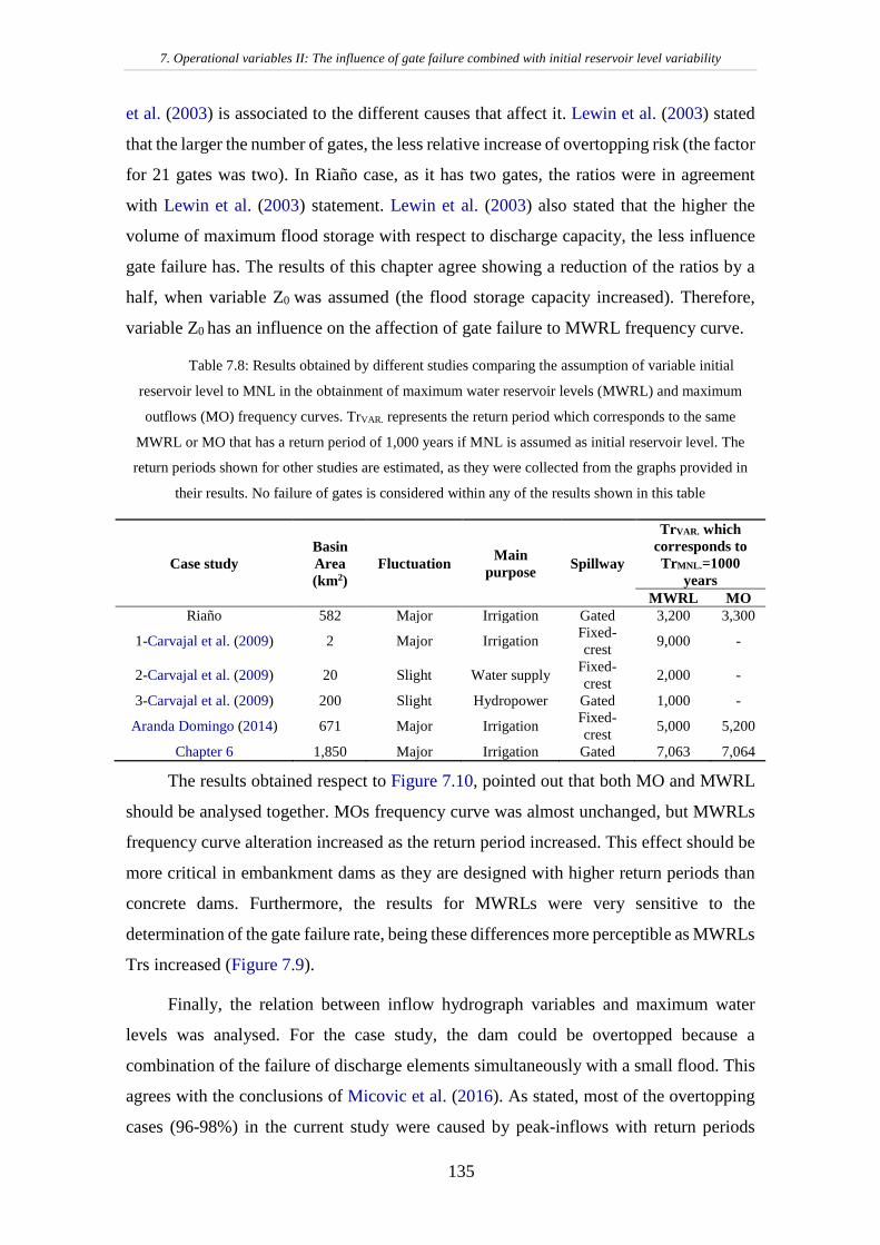
7. Operational variables II: The influence of gate failure combined with initial reservoir level variability
135
et al. (2003) is associated to the different causes that affect it. Lewin et al. (2003) stated
that the larger the number of gates, the less relative increase of overtopping risk (the factor
for 21 gates was two). In Riaño case, as it has two gates, the ratios were in agreement
with Lewin et al. (2003) statement. Lewin et al. (2003) also stated that the higher the
volume of maximum flood storage with respect to discharge capacity, the less influence
gate failure has. The results of this chapter agree showing a reduction of the ratios by a
half, when variable Z0 was assumed (the flood storage capacity increased). Therefore,
variable Z0 has an influence on the affection of gate failure to MWRL frequency curve.
Table 7.8: Results obtained by different studies comparing the assumption of variable initial
reservoir level to MNL in the obtainment of maximum water reservoir levels (MWRL) and maximum
outflows (MO) frequency curves. TrVAR. represents the return period which corresponds to the same
MWRL or MO that has a return period of 1,000 years if MNL is assumed as initial reservoir level. The
return periods shown for other studies are estimated, as they were collected from the graphs provided in
their results. No failure of gates is considered within any of the results shown in this table
Case study Basin Area (km2)
Fluctuation Main purpose Spillway
TrVAR. which corresponds to TrMNL.=1000
years MWRL MO
Riaño 582 Major Irrigation Gated 3,200 3,300
1-Carvajal et al. (2009) 2 Major Irrigation Fixed-crest 9,000 -
2-Carvajal et al. (2009) 20 Slight Water supply Fixed-crest 2,000 -
3-Carvajal et al. (2009) 200 Slight Hydropower Gated 1,000 -
Aranda Domingo (2014) 671 Major Irrigation Fixed-crest 5,000 5,200
Chapter 6 1,850 Major Irrigation Gated 7,063 7,064
The results obtained respect to Figure 7.10, pointed out that both MO and MWRL
should be analysed together. MOs frequency curve was almost unchanged, but MWRLs
frequency curve alteration increased as the return period increased. This effect should be
more critical in embankment dams as they are designed with higher return periods than
concrete dams. Furthermore, the results for MWRLs were very sensitive to the
determination of the gate failure rate, being these differences more perceptible as MWRLs
Trs increased (Figure 7.9).
Finally, the relation between inflow hydrograph variables and maximum water
levels was analysed. For the case study, the dam could be overtopped because a
combination of the failure of discharge elements simultaneously with a small flood. This
agrees with the conclusions of Micovic et al. (2016). As stated, most of the overtopping
cases (96-98%) in the current study were caused by peak-inflows with return periods

7. Operational variables II: The influence of gate failure combined with initial reservoir level variability
136
lower than 1000 years for the entire gate failure scenarios. As failure of gates decreases
the discharge capacity, smaller floods can increase the maximum reservoir water levels
reached in the reservoir. As shown in Table 7.7 and Figure 7.11, variable Z0 also affected
as 58.5 % of the cases in all the scenarios studied (C0-0%, C5-5%, C5-15%and C15-15%) were
below MNL when taking this assumption. The percentage therefore for MWRLs above
MNL decreased. Flood storage volume, incoming hydrographs, gate failure and initial
reservoir level, among others; affect the maximum reservoir water level reached in the
reservoir. Small return periods of the inflow hydrograph relied to overtopping (and
therefore high return periods of the maximum reservoir water level). High return periods
of the inflow hydrograph resulted into maximum reservoir water levels below MNL (and
therefore a low return period of the maximum reservoir water level). This opens a
discussion about how hydrological dam safety is determined and which variable best
characterizes the hydrological safety of a dam. Design return periods are commonly
associated to the return period of the design flood hydrograph, considering that rainfall
events generate hydrographs with peak-inflows with the same return period. Many
authors questioned this hypothesis (e.g: Adams and Howard, 1986; Alfieri et al., 2008;
Viglione and Blösch, 2009; Sordo-Ward et al., 2014). It is also well-known that return
periods associated to peak-inflows are not the same as those associated to hydrograph
volume, existing a trend to analyse this by using copulas for multivariate flood frequency
analysis (e.g.: De Michele et al., 2005; Shiau et al. 2006; Salvadori et al., 2011; Requena
et al., 2013, 2016; Aranda Domingo, 2014; Volpi and Fiori, 2014). This question can be
extended to the return period associated to the hydrological safety of dams. Therefore, it
should be noted the existence of
uncertainty associated to the concept of return period, considering that the variable
that best represents the hydrological safety and the corresponding return period is the
maximum level reached on the reservoir, being downwards river safety represented by
the maximum outflows. The methodology proposed can be used to provide a
homogeneous tool to obtain the hydrological loads input to a complete risk analysis of a
system of dams, important in countries like Spain where many dam spillways will require
an upgrade due to new safety regulations (San Mauro, 2016).

7. Operational variables II: The influence of gate failure combined with initial reservoir level variability
137
The influence of gate failure combined with initial reservoir level
variability: Partial conclusions.
The main conclusions extracted from this research are as follow:
• To account for variable initial reservoir level is important when assessing
hydrological safety, especially in dams which main purpose is irrigation. (TrVAR./
TrMNL. ranged from 2.0 to 4.1 regardless of gate malfunction).
• To account for variable initial reservoir level implied that many of the incoming
floods produced no outflow, increasing the estimated downstream river safety in
comparison with common design practice. (TrVAR./ TrMNL. ranged from 2.5 to 6.1
regardless of gate malfunction).
• Gate failure decreased the return period of maximum water reservoir levels obtained
in the common design practice situation (constant initial reservoir level) up to 240,
160 and 93 (depending on the gate failure scenario considered). This affection was
reduced by a half when variable initial reservoir level was considered.
• The higher the return period of maximum water reservoir levels, the higher the
affection of gate failure and the differences by assessing different values to the gate
failure rate.
• When overtopping occurred, maximum outflows increased and neutralized the
decrease of discharge capacity associated to gate failure scenarios. Maximum
outflows return periods assuming gate failure were almost the same as return periods
of the non-failure scenario, regardless considering constant or variable initial
reservoir level.
• The variables that best characterize the hydrological dam safety are the return period
of the maximum reservoir water level and maximum outflow frequency curves.
It should be noted that the methodology and analysis is based on a case study and
needs to be extended to other systems in order to validate the conclusions presented.

8. On the definition of Maximum Conservation Levels
138
8. On the definition of Maximum Conservation Levels
The aim of this Chapter is to solve the conflicts that arise in the operation of
multipurpose reservoirs when determining Maximum Conservation Levels, as they may
imply a reduction in the reliability of the water supply system.
The presented procedure consists on the joint optimization of water supply
reliability as well as dam and downstream river safety optimizing water demand supply
reliability as well as dam and downstream river safety. Two different scenarios were
analysed: accounting and not accounting for the variability of initial reservoir level prior
to extreme flood events. In order to achieve the global optimum configuration of
Maximum Conservation Levels for each season, the optimization of three variables was
proposed: maximum reservoir level (return period of 1,000 years), maximum released
outflow (return period of 500 years) and maximum reservoir yield with 90 % reliability.
To do so, a stochastic methodology is proposed to determine the seasonal Maximum
Conservation Levels which combines three main innovative aspects:
• Stochastic assessment of hydrological dam and downstream river safety through
return periods related to maximum reservoir levels and maximum outflows.
• Determination of MCLs that increase/maintain the water yield for a specific reliability
while maintaining/improving the hydrologic dam safety.
• Determination of MCLs accounting for the variability of initial reservoir level prior
to flood events.
The methodology is applied to a gated-spillway dam located in Spain, but can be
applied to any reservoir regardless its location or spillway typology.
Application to the Dam in the Douro river basin
To obtain the optimal set of seasonal Maximum Conservation Levels (MCLs)
accounting for both hydrological safety (dam and downstream) and water supply, the
methodology explained in Section 3.7 has been applied to Riaño Dam, which main
characteristics have been defined in Chapter 7 (Section 7.1). Flood damage analyses
summarized in the Dam Master Plan concluded that discharges above 700 m3/s create a

8. On the definition of Maximum Conservation Levels
139
flood emergency condition in the downstream reach. This value (OEMER) was adopted to
identify catastrophic flood damages. The following data were used to perform the study:
• Simulation of flood control operation. Besides the flood control structures and dam
configuration shown, a gauge located right downstream Riaño reservoir with 30 years
of daily flows was used, as in Chapter 7. With this time series, the 100,000 seasonal
synthetic flood hydrographs were generated.
• Simulation of regular operation. A monthly time series of inflows from 1940 to 2013,
environmental flow restrictions, evaporation rates, monthly demand distribution,
Storage-Area-Height Reservoir Curves and Dead Storage Volume (all data obtained
from Duero River Basin Management Plan (CHD, 2015)) and the reservoir
characteristics previously stated were used. An mean annual demand of 545 hm3 was
accounted.
8.1.1. Definion of the study set of Maximum Conservation Levels and
proposed solutions
A set of MCLs that comprised from 651 hm3 (volume at MNL) to 400 hm3 was
studied. For the sake of simplicity, the flood hydrograph volume of Tr=5,000 years (247
hm3) was estimated, and a maximum flood control volume of 251 hm3 was defined. The
ranges of the difference between the volume in the reservoir at MNL and the different
MCLs were discretized in intervals of 5 hm3. Thus, a set of k=51 possible MCLs per
season was defined (associated to a volume in the reservoir of 651, 645, 640, …, 405, 400
hm3).
According to Section 8.1.2, three main seasons regarding to maximum annual
floods exist within Riaño: season 1 from the beginning of November to the end of
January, season 2 from the beginning February to the end of April, and season 3 from the
beginning of May to the end of October.
Therefore, as n=3 seasons, a set of 513=132,651 configurations of MCLs per
scenario was analysed.
8.1.2. Seasonal hydrographs
A set of 100,000 annual synthetic flood hydrographs representative of the 30 years
of observed events (1954–1984) as illustrated in Figure 8.1a, previously generated in

8. On the definition of Maximum Conservation Levels
140
Chapter 7 (Section 7.1.2) was used. The marginal distributions of the synthetic peak-
flows and hydrograph volumes (100,000 each) were analysed by using Gringorten
plotting position formula (Gringorten, 1963).
(a) (b)
(c)
(d)
Figure 8.1: a) Sample of the 100000 simulated inflow hydrographs associated to different seasons (color
dots: blue, season 1; magenta, season 2 and green, season 3) and its comparison to the observed floods
(black dots). b) Determination of the range of thresholds analysing the mean of the exceedances above the
threshold (XS-S) (right axis) and the mean annual exceedance (λ) above threshold test (left axis). c)
Validation of the threshold range using the Dispersion Index (DI) Test. The blue line represents the
different values of DI for the different thresholds. The blue shaded area represents the values of DI within
the confidence intervals determined with a level of significance of 0.05. d) Delimitation of the seasons in
Riaño Basin applying the seasonality test based on Ouarda et al. (1993). Grey plots represent the test for
different values of the S thresholds. Straight dashed-lines represent the different seasons.
To define the seasons, the POT analysis (Section 3.1.2.1) was performed. The range
of thresholds by accounting for independence of POTs was defined. Figure 8.1b shows
the mean of the number of annual POTs (λ) on the right y-axis and the mean of the

8. On the definition of Maximum Conservation Levels
141
exceedances above the threshold (XS-S) plotted against the threshold (S). XS-S was a
linear function of S values from 100 m3/s to 190 m3/s. Figure 8.1c shows the Dispersion
Index (DI) test, with confidence intervals associated to a level of significance of 0.05. It
can be seen that the range of values previously defined were within the confidence
intervals, being the DI values stabilized between 0.805 and 1.207 for values of S from
120.5 m3/s to 162.5 m3/s. This range of S values, that corresponded to values of λ from 3
(S=120.5 m3/s) to 2 (S=162.5 m3/s) (lambda values recommended by Lang et al. (1999))
events per year respectively (Figure 8.1b), was the one chosen to define the seasons.
Figure 8.1d shows the graphical test based on Ouarda (1993) and Ouarda et al. (1993,
2006). Three different seasons were identified, associating each hydrograph to a season
of occurrence within a Monte Carlo Framework.
The seasons defined were: season 1 from the beginning of November to end
January, being the probability of occurrence of floods within this season 41.4 %; season
2 from the beginning February to end April, being the probability of occurrence 45.3 %;
and season 3 from the beginning of May to end October; being the probability of
occurrence 13.3 %.
8.1.3. Simulation of the dam operation rules
Once the configurations of MCLs were defined, for each configuration the values
of MWRLTR=1000y, MOTR=500y were obtained by simulating the flood operation of the
reservoir for Sc.1 and Sc.2. By simulating the regular operation of the reservoir, YR=90%
was obtained.
Figure 8.2 shows the values of MWRLTR=1000y, MOTR=500y and YR=90% with respect
to the MCLs of each season corresponding to each of the 132,651 configurations. Figure
8.2a shows that variation of MCLs in S1 did not affect YR=90%. The reasons are: the water
demands associated to the reservoir in S1 were less than 1 % of the annual demand (Da),
and, as the irrigation season in the Riaño system extends from May to September (98 %
of Da), the reservoir was able to recover the reduced volume in S1 within the months
previous to irrigation (February, March and April). Figure 8.2b and Figure 8.2d shows
that, for the case of Sc.1, the effects of MCLs were similar in the three seasons in terms
of hydrological dam safety (Figure 8.2b) and downstream river safety (Figure 8.2d).
However, in Sc. 2 (Figure 8.2c and Figure 8.2e), as regular operation was linked to the
flood control operation by the initial reservoir level, MCLs in S1 and S3 did not affect

8. On the definition of Maximum Conservation Levels
142
neither the hydrological dam safety nor downstream river safety. Variations of MCLS2
are the main affection to values MWRLTR=1000y and MOTR=500y in Figure 8.2c and Figure
8.2e respectively.
Figure 8.2: Representations of the 132,651 values of MWRLTR=1000y, MOTR=500y and YR=90% obtained
respect to the MCLs for each of the seasons studied. MCLS1, MCLS2 and MCLS3 represent the Maximum
Conservation Levels in season 1, season 2 and season 3 respectively. (a) Representation of the values
YR=90%, with a colorbar, which are the same in Scenario 1 (initial reservoir level equal to MCL) and
Scenario 2 (variable initial reservoir level). (b, c) Representation of the values MOTR=500y with a colorbar
in Scenario 1 (b) and Scenario 2 (c). (d, e) Representation of the values MWRLTR=1000y with a colorbar in
Scenario 1 (d) and Scenario 2 (e).

8. On the definition of Maximum Conservation Levels
143
8.1.4. Solutions proposal
First, the configurations which did not fulfil hydrological dam safety
(MWRLTR=1000y>DFL) and/or downstream safety (MOTR=500y>OEMER.) were identified in
both scenarios. A total of 826 configurations (0.6 % of 132,651 configurations) had a
value of MWRLTR=1000y higher than DFL in Sc.1. (red dots in Figure 8.3a), while none of
the configurations had MWRLTR=1000y values higher than the DFL in Sc.2 (Figure 8.3c).
It should be noted that, in Sc.1 the 826 configurations that did not fulfil hydrological dam
safety, they also did not fulfil the downstream safety condition. On the other hand, 59,013
configurations (44.5 % of the total number of configurations) had a value of MOTR=500y
higher than OEMER. in Sc.1, whereas 4,944 (3.7 %) in Sc.2. Figure 8.3a and Figure 8.3c
show the pair of values YR=90% and MOTR=500y (grey points) for each analysed
configuration in Sc.1 and Sc.2 respectively.
In Sc.1, the pareto-solutions consisted of 277 (Figure 8.3a, magenta points)
configurations, being 98 configurations those that satisfy: YR=90% ≥ Da, MOTR=500y ≤
OEMER. and MWRLTR=1000y≤DFL (proposed solutions, cyan in Figure 8.3a). In Sc.2, for
the same analysis, 247 configurations (magenta points in Figure 8.3c) and 135 (cyan
points in Figure 8.3c) were obtained respectively. For both scenarios, the extreme
proposed solutions were identified. On the one hand, in the case of
MOTR=500y=OEMER=700 m3/s (Figure 8.3a and Figure 8.3c, black point), YR=90% =587 hm3
(for Sc.1) and 600 hm3 (for Sc.2) it represents an improvement (compared to Da) of 7.7
% and 10.1 % respectively. On the other hand, in the case of YR=90% = Da = 545 hm3
(Figure 8.3a and Figure 8.3c, dark blue point), MOTR=500y= 452 m3/s (for Sc.1) and 366
m3/s (for Sc.2) representing a 64.2 % and 52.3 % of OEMER, respectively. It is important
to point out that, in the case of using a deterministic procedure focused in hydrological
dam and downstream safety (conventional procedure), any studied configuration of
MCLs could be a potential solution (grey dots within Figure 8.3a and Figure 8.3c). Thus,
if MOTR=500y = OEMER, the proposed stochastic procedure presented improvements up to
146 hm3 (26.8 % of Da) compared to the worst regular operation configuration
(YR=90%=454 hm3 in Sc.1; (Figure 8.3a)). The corresponding configurations of MCLs for
the extreme proposed solutions are represented in Figure 8.3b (Sc.1) and Figure 8.3d
(Sc.2) with the same colour scheme as in Figure 8.3a and Figure 8.3c respectively. In both
scenarios, the highest MCLs were associated to S3, while the lowest to S1.

8. On the definition of Maximum Conservation Levels
144
Figure 8.3: (a, c) Representation in grey of the pair of values YR=90% and MOTR=500y for Scenario 1 and
Scenario 2 respectively. Red points represent the pair of values which do not fulfil overtopping
requirements (MWRLTR=1000y >DFL). The pareto front is represented with magenta dots, while the
proposed solutions are represented in cyan. The black dot represents the solution that maximizes the
demand fulfilling the Maximum Outflow released requirement (MOTR=500y=OEMER). The blue dot
represents the solution in which YR=90% equals the current annual demand, minimizing the Maximum
Outflow released. (b, d) MCLs for each month/season that correspond to the proposed solutions
previously selected (blue and black dots), for S1 and S2 respectively. The red dashed line represents the
Maximum Normal Level (MNL), the red dashed-dotted line represents the Design Flood Level (DFL),
and the red continuous line represents the Crest of Dam (COD).
8.1.5. Comparison between the proposed configurations in the two
scenarios
Finally, the limit proposed solutions in both scenarios, Sc.1 and Sc.2, were
compared (Figure 8.4). In the case of MOTR = 500y = OEMER = 700 m3/s, MWRLTR = 1000y
was 1100.6 m.a.s.l. The hydrological dam and downstream river safety were invariant for
Sc.1 and Sc.2. However, higher MCLs were obtained for Sc.2, which increased the YR =
90% of the system. In the case of YR = 90% = Da = 545 hm3, the differences between Sc.2
and Sc.1 for MWRLTR = 1000y and MOTR = 500y were 0.2 m.a.s.l and 86 m3/s, respectively.
Moreover, the MCL of season two were lower when the variable initial reservoir level
was considered. This is because of the increase of MCLs in the other seasons. Despite

8. On the definition of Maximum Conservation Levels
145
this, the demand supplied with a reliability of 90% was the same, accounting for lower
values of MWRLTR=1000y and MOTR = 500y if variable initial level was considered.
Figure 8.4: Spider plot comparing the value of the maximum conservation levels for different seasons
(MCLsx), MWRLTR = 1000y, MOTR = 500y, and YR = 90%. In black, solutions that maximize the volume
supplied with MOTR = 500y = OEMER. In blue, the solutions that supply the current annual demand minimize
the maximum outflow released. The continuous line corresponds to Sc.1 and the dashed line to Sc.2.
Within the framework of the present study, accounting for the variability of initial
reservoir level implied a reduction of flood control volumes (increase of MCLs)
maintaining the risk of overtopping and downstream river safety. Consequently, the
volume for satisfying the demands increased, providing a more reliable system in terms
of regular operation.
On the definition of Maximum Conservation Levels: Partial
conclusions
The main conclusions extracted from this study are as follow:

8. On the definition of Maximum Conservation Levels
146
• The use of a stochastic methodology allowed to assess hydrological dam safety and
downstream safety by obtaining the frequency curves of Outflow and Maximum
Reservoir Water Levels, while accounting for the variability in hydrological loads
with respect to deterministic procedures. As a drawback, it implied a more complex
procedure and computational effort.
• Considering the initial reservoir level equal to the Maximum Conservation Level for
each season, a set of 98 non-inferior solutions is proposed, and 135 possible
configurations by considering variable initial reservoir level. From the proposed
configurations, dam stakeholders are able to decide which configuration to use
depending on their preferences: increasing dam and downstream hydrological safety
or increasing water supply (with a specific reliability) in the water resources system.
In Riaño case study, the presented procedure showed improvements in the regular
operation that can satisfy an increase up to 10.1% of the current annual demand of
545 hm3 (with a reliability of 90%) while maintaining the same hydrological dam
safety.
• Accounting for initial reservoir variability resulted in the possibility to supply an extra
demand of 13 hm3 (2.4% of the current annual demand) compared to the optimal
solution without accounting for initial reservoir level variability.
• The proposed stochastic procedure can improve the results obtained by deterministic
procedures, increasing supply up to 26.8 % the current annual demand, from the worst
regular operation configuration (not accounting for initial reservoir level variability)
to the optimal configuration (accounting for initial reservoir level variability) of
Maximum Conservation Levels.

8. On the definition of Maximum Conservation Levels
147

9. Conclusions
148
9. Conclusions
The conclusions that have been reached as a result of the present research, the
original contributions to hydrological dam and downstream safety assessment, as well
as possible further research are presented in this final chapter.
Main conclusions
The present research provides methodologies for guiding practitioners to perform
hydrological dam and downstream safety assessments through stochastic approaches
while accounting for operational variables such as the initial reservoir level, the
availability of spillways or operational flood management procedures among others.
In this regard, the present research has focused in analysing and improving key
aspects in hydrological dam and downstream safety assessment.
9.1.1. Hydrological forcing: The Hybrid method
The proposed procedure has been divided into two main focuses: a) providing
guidance on selecting the minimum number of storm events for deriving the flood
frequency curve through event-based approaches and b) proposing a methodology that
combines the advantages of distributed event-based and continuous models, for the
derivation of frequency curves of maximum flow and maximum annual flood volume, by
combining a stochastic continuous climate generator with a physically-based distributed
hydrological model based on both event and continuous simulations.
To do so, the methodology applied compares the resulting flow of coupling a
stochastic weather generator with a fully distributed physically-based model with the
flow: a) resulting from selecting only a limited number of storms per year b) resulting
from the application of the proposed Hybrid method.
For the Case Study of Peacheater Creek, regarding to the number and criterion for
selecting the storms to be simulated in an event or hybrid based modelling approach:
• When analysing the correspondence between storms and maximum annual peak-flow
and volume, the best ranking storm criterion is total depth, followed up by maximum
intensity. Considering storms up to rank five sorted by the total depth criterion,

9. Conclusions
149
resulted in a probability of generating the maximum annual peak-flow of 94% and the
maximum annual volume of 99%.
• In the case of the total depth criterion, the higher the return period of peak-flow or
volume is, the lower the storm rank needed.
• For preserving the seasonality of maximum annual peak-flows and volumes, total
depth was also the best criterion.
• When estimating the parameter of the copula family selected (Gumbel), the relative
error was less than 2% if storms up to rank five were considered, and was less than
0.5% if storms up to rank ten were considered. Regarding Kendall’s return period,
considering the same number of storms produces Kendall’s return periods of 10 and
50 years very similar to those obtained by continuous simulation, and the 100 years
return period is slightly underestimated.
Regarding to the application of the Hybrid method in Peacheater Creek Case Study,
by applying the criterion of selecting the five highest storms per year in terms of total
depth:
• Independence between rainfall events and prior hydrological soil moisture conditions
has been proved within the framework of the Hybrid method developed.
• The Hybrid method preserves the seasonality of maximum annual peak-flows and
volumes. The method provides less than 8% absolute relative error in the estimation
of the mean direction of seasonality of both maximum annual peak-flows and volumes
compared to the continuous modelling results. However, regarding the dispersion of
seasonality, the Hybrid method provides less dispersion around the mean direction of
seasonality, providing a relative error up to 52 % and 32 % in maximum annual peak-
flows and volumes respectively.
• The Hybrid method is able to preserve the dependence and bivariate properties of the
floods derived from the continuous simulation. The correlation between maximum
annual peak-flows and volumes is preserved by the Hybrid-based method similarly to
the continuous modelling approach.
• When estimating the parameter of the Gumbel copula family selected, the relative
error was less than 13%. Regarding Kendall’s return period, Kendall’s return period
of 10 is very similar to those obtained by continuous simulation. However, for

9. Conclusions
150
Kendall’s return period of 50 and 100 years, the Hybrid method overestimates volume
values, having a good agreement with peak-flows.
• The proposed Hybrid method is capable of reproducing the univariate flood frequency
curves with a good agreement to those obtained by the continuous simulation. The
maximum annual peak-flow frequency curve is obtained with a Nash-Sutcliffe
coefficient of 0.98, whereas the maximum annual volume frequency curve is obtained
with a Nash-Sutcliffe value of 0.97.
The proposed Hybrid method permits to generate hydrological forcings by using a
fully distributed physically based model reducing the computation times on the order
from months to hours.
9.1.2. Spillway operation: The proposed K-Method
The proposed K-Method is a decision-making tool for dam managers that allows
analysing the effects of applying different reservoir operation rules for both dam safety
and downstream safety. In contrast with other fixed methods, the K-Method allows, for
each analysed dam, the identification of the K-value (conducting a calibration process)
that best adapts the management strategy to the specific conditions of the basin, the
reservoir, the spillway, and to the objectives of flood management.
The method was applied to a dam in the Segura river basin:
• For the case study under analysis, the K-Method improved the results obtained with
the Volumetric Evaluation Method, by reducing the maximum reservoir levels
reached in the dam (the higher the K-value. the lower the maximum reservoir level),
while the corresponding increase of outflows did not endanger downstream safety.
• In addition, by carrying out a dam risk analysis, a K-value of 5.25 lowered the global
risk index by 8.4% compared to Volumetric Evaluation Method, and represented
17.3% of the maximum possible reduction determined by the Mixed Integer Linear
Programming rule of operation method.
• Different behaviours of the method were identified depending on the return periods
analysed. For events with a return period ranging from one to 25 years, K-value = 10
resulted in an important decrease in the maximum reservoir levels, while the
corresponding increase of outflows did not endanger downstream safety. For events
with a Tr ranging from 25 to 100 years, higher K-values reduced the number of events

9. Conclusions
151
that simultaneously achieved lower maximum levels and outflows. For events with a
Tr higher than 500 years, the Inflow-Outflow rule of operation method simultaneously
achieved the lowest maximum levels and outflows. In a practical case, even if the skill
required to forecast the inflow hydrograph is limited, according to the general
meteorological situation, the dam manager may be able to estimate the return period
of the event that is occurring and therefore the conclusions obtained could be applied
to decide on the best K-value to adopt.
9.1.3. Operational variables I: Influence of initial reservoir level
The influence of initial reservoir level has been assessed in two Case Studies: two
gated-spillway dams, one in the Tagus River system and the other one in the Douro River
system. In the case of the Tagus River system, a set of 100,000 simulations of initial
reservoir level was carried out, in order to asses the uncertainty associated to this variable.
The main conclusions associated to the influence of initial reservoir level are:
• To account for variable initial reservoir level is important when assessing
hydrological safety, specially in dams which main purpose is irrigation. When
analysing a portfolio of different reservoirs, a dam that may seem safer than other at
first, may not be if this variable is included in the analysis (for example, in an extreme
case, comparing a hydroelectric dam, which is usually full, with a flood control
reservoir, which is usually empty). Thus, this methodology can help stakeholders
when carrying out decisions about prioritizing their investments.
• The use of a stochastic methodology allowed to assess hydrological dam safety and
downstream safety by obtaining the frequency curves of Outflow and Maximum
Reservoir Water Levels, while accounting for the variability in hydrological loads
with respect to deterministic procedures. As a drawback, it implied a more complex
procedure and computational effort.
Regarding to the Dam in the Tagus River Basin, results obtained showed:
• For the case study, considering the fluctuation of initial reservoir level provided a
more realistic assessment of hydrological dam and downstream safety. When a
conventional approach was used, the Design Flood Level was reached at a return
period of 751 years, which does not fulfil therefore with the regulation standards
(1,000 years). However, when initial reservoir level was accounted, the results

9. Conclusions
152
showed that the Design Flood Level was not reached in any of the set of 100,000
simulations carried out.
• Within the case study, the return period considering variable initial reservoir for the
value corresponding to 1,000 years assuming initial reservoir level equal to Maximum
Normal Level was 7,063 and 7,064 years for the maximum reservoir water level and
maximum outflow frequency curve respectively.
• For the case study, it has been found out that the affection of initial reservoir level for
the maximum reservoir water level and maximum outflow frequency curve has a
small uncertainty (less than 2.1 %) for return periods below 1,000 years, by using
100,000 inflow hydrographs and 100,000 initial reservoir levels.
• Within the case study, the global risk index reduced its value up to 91 % if variable
initial reservoir level is accounted, from 1,968.9x103 (initial reservoir level equal to
maximum normal level) to a median value of 175.1x10³ euros (variable initial
reservoir level).
• The uncertainty associated to initial reservoir level fluctuation when calculating the
global risk index was 4.2 % (values ranging from 163.7 to 191.6 thousands of euros).
Regarding to the Douro River Dam and the impact of initial reservoir level in
hydrological dam safety, it has been found out that:
• The return period of maximum reservoir levels reached in the reservoir, increases
when considering variable initial reservoir for the same reservoir level. This return
period ranged from 2.0 to 4.1 times the one by considering the reservoir at its
maximum operative level when the flood arrives, depending on the return period
studied.
• To account for variable initial reservoir level implied that many of the incoming
floods produced no outflow, increasing the estimated downstream river safety in
comparison with common design practice. In this case, return periods for the same
maximum outflow ranged from 2.5 to 6.1 times the ones obtained by applying
common design procedures (initial reservoir level equal to Maximum Normal Level)).

9. Conclusions
153
9.1.4. Operational variables II: Influence of gate failure
Regarding the analysis of the effect of gate failure, it has been shown the importance
of accounting for gate functionality in order to analyse hydrological safety in the dam
located in the Douro River basin:
• Gate failure decreased the return period of maximum water reservoir levels obtained
in the common design practice situation (constant initial reservoir level) up to 240,
160 and 93 (depending on the gate failure scenario considered). This affection was
reduced by a half when variable initial reservoir level was considered.
• The higher the return period of maximum water reservoir levels, the higher the
affection of gate failure and the differences by assessing different values to the gate
failure rate.
• When overtopping occurred, maximum outflows increased and neutralized the
decrease of discharge capacity associated to gate failure scenarios. Maximum
outflows return periods assuming gate failure were almost the same as return periods
of the non-failure scenario, regardless considering constant or variable initial
reservoir level.
9.1.5. Definition of seasonal conservation levels
When it came to the definition of Maximum Conservation Levels accounting for
both regular and flood operation, in the Douro River Dam, it has been found out that:
• Considering the initial reservoir level equal to the Maximum Conservation Level for
each season, the procedure presented within this thesis showed improvements in the
regular operation that can increase up to 10.1% of the current annual demand of 545
hm3 for the same hydrological dam safety.
• Accounting for initial reservoir variability resulted in an increase of the maximum
demand supplied of 13 hm3 (2.4% of the current annual demand) compared to the
optimal solution without accounting for initial reservoir level variability.
• The proposed stochastic procedure can improve the results obtained by deterministic
procedures up to 26.8 % the current annual demand, from the worst regular operation
configuration (not accounting for initial reservoir level variability) to the optimal

9. Conclusions
154
configuration (accounting for initial reservoir level variability) of Maximum
Conservation Levels.
Original contributions
As previously exposed, the objective of this thesis was to develop a stochastic
methodology to assess hydrological dam and downstream safety while accounting for
operational variables such as the initial reservoir level, the availability of spillways or the
influence of the flood operational methods.
In this regard, the main contribution of this the thesis is the development of a
stochastic framework for the analysis of dam and downstream safety basement for
hydrological dam safety assessment (Figure 9.1), which includes:
Figure 9.1: Stochastic proposed framework of hydrological dam and downstream safety assessment.
• Development of a simulation chain that covers all the process of hydrological
dam and downstream safety assessment within a Monte Carlo simulation
framework. This simulation chain includes the processes involved in hydrological
forcings, follow up by ways of assessing the impacts of operational variables such as
initial reservoir level or the unavailability of spillways. Afterwards, the floods are
managed through reservoir operational rules. This procedure provides a set of
maximum reservoir level reached in the reservoir and maximum outflows derived
through the spillways, which permits to assess hydrological dam and downstream
safety and serve as an input for hydrological dam risk analysis.
• Proposals for stochastic generation of hydrological forcings. The first link in the
simulation chain is the generation of synthetic hydrographs. Two approaches have
been developed within this thesis.

9. Conclusions
155
The first one, consists on the use of a physically based model, distributed, coupled to
a climate generator. This method can be applied to case studies in which high
resolution spatio-temporal data is available. It provides a high-detailed modelling
framework in which hydrological processes can be accounted in all the units in which
the basin has been discretized.
In cases in which high-detailed analysis is not necessary or possible, the stochastic
data-based hydrological forcing generator proposed can be applied. This generator
provides a simpler approach of multivariate flood modelling using a lumped
stochastic event-based model that allows the generation of hydrographs from
historical floods observed at the dam entrance.
• Development of a simple flood management procedure improving the current
procedure implemented in most of the dams in Spain. This thesis develops the K-
Method, a simple method which can be used to define real-time operation rules for
gated spillways. The K-Method is defined to improve the performance of the
Volumetric Evaluation Method largely used for the specification of dam management
rules during floods in Spain.
• Assessment of the impact of initial reservoir levels in hydrological dam and
downstream safety. Hydrological dam safety assessment methods traditionally
assume that the reservoir is initially full when it receives the design flood, thus staying
in the conservative side when designing a new dam. However, the distribution of
reservoir levels at the beginning of flood episodes takes more importance for
evaluating the real risk associated to dams in operation. This thesis has shown the
importance of accounting for this variable. Furthermore, a procedure to quantify the
uncertainty associated to the affection of initial reservoir level to hydrological dam
safety has been proposed.
• Impact of the availability of the spillways of a certain dam in its hydrological
safety. This thesis has highlighted the importance of considering gate failure
scenarios in hydrological dam and downstream safety, providing guidelines for its
incorporation within a stochastic framework.
• Hydrological dam and downstream safety as frequency curves of maximum
reservoir levels reached in the reservoir and maximum downstream outflows. In
the standard engineering approach, hydrological assessment of dam and downstream

9. Conclusions
156
safety is associated to the Design flood for a given return period. Throughout this
thesis it has been shown that the return periods of maximum levels reached in the
reservoir and maximum outflows are the variables that best represent dam and
downstream hydrological safety. This thesis has shown that these return periods do
not have to correspond to those associated to the Design Flood, moreover if
operational variables are accounted.
• Maximum reservoir levels reached in the reservoir and maximum downstream
outflows as inputs for hydrological risk analysis. Within the framework of this
thesis, it has been shown how the frequency curves of maximum reservoir levels and
outflows can serve as inputs for complete hydrological risk analysis. An economic
index has been proposed which combines the hydrological risk for the dam, linked to
the maximum water level reached in the reservoir during the flood routing, and the
flood risk in the downstream river reach, linked to the discharge releases from the
dam.
• A proposal for the allocation of flood available storage accounting for initial
reservoir levels. A conflict arises in the operation of multipurpose reservoirs when
determining Maximum Conservation Levels, as they may imply a reduction in the
reliability of the water supply system. This thesis presents a new procedure that
consists on the joint optimization of water supply reliability as well as dam and
downstream river safety. This procedure provides dam stakeholders a set of pareto-
optimal configurations depending on their main focus: hydrological safety or water
supply reliability.
Further research
Future research studies to continue the present line of research could be related to:
• Combination of all the proposals of this thesis. Throughout the thesis, different
parts of the proposed methodology have been developed and improved. However, the
methodology must be understood as a whole unit. For instance, the influence of initial
reservoir level and gate-failure can be assessed accounting for the use of the proposed
flood operational procedure (K-Method), including the definition of Maximum
Conservation Levels accounting for all this factors.

9. Conclusions
157
• Analysis of reservoir systems. The proposed hybrid hydrological model can be
applied to case studies with one or more dams. The use of a distributed hydrological
model provides a framework for accounting for the operational variables of all the
dams located within the modelled basin.
Furthermore, when applying water resource management models within this thesis,
only the operation of one reservoir has been accounted. However, for assessing the
impact of initial reservoir level, it would be interesting to account for the variations
of all the water supply infrastructures managed under the same water resources
system.
Thus, the affection of upstream dams into the downstream reservoirs can be
accounted, providing a more realistic assessment of the hydrological downstream
safety assessment.
The simulation of a reservoir system is very important since poor flood management
in headwater reservoirs can have catastrophic consequences downstream, but
introduces a large number of variables which increase its complexity.
• Improvement of the assessment of potential spillway failures. Other further
research objective could be finding a more robust technique combining historic data
and experts’ judgement to obtain the gate failure rate. This research pointed out the
importance between choosing one gate failure or another. Furthermore, the
dependence of failure respect to intensity, magnitude and season of floods could be
better analysed.
• Application of the proposed K-Method to other case studies. Although the results
are promising, further research should be developed to ensure that the K-method
improves the operation of flood control rules through a wide range of gated-spillway
dams.
• Impact of Climate and Land Use changes in hydrological dam and downstream
safety. Within the hydrological hybrid modelling framework proposed, climate
change impacts on risk analysis can be assessed. For instance, stochastic weather
generators can be perturbed in order to assess the impact of climate change in flood
events. Also, future modifications in land use can be considered in distributed
modelling frameworks which, combined with population growth and changes in
reservoir operation policies, can affect the complete cycle of dam risk assessment.

9. Conclusions
158
• Assessment of the uncertainties associated to the different variables involved in
the stochastic methodology. Within this the thesis, the impact of the uncertainty
associated to initial reservoir levels has been analysed. However, other aspects such
as the uncertainty in the hydrological forcings, affection of gate failure rates or the
uncertainty in the flood management strategies could be assessed in future works.
• Proposal of simple risk key performance indicators. Through the application of
the proposed methodology to a representative set of dams, it would be possible to
propose simple indicators to assess, for instance, the influence of variable initial
reservoir levels and gate failure, which can be used by practitioners within the dam
risk assessment context or by the development of national dam safety plans.

9. Conclusions
159

References
160
References
Adams, B.J., Howard, C.D., 1986. Design storm pathology. Can. Water Resour. J., 11(3):
49-55.
Afshar, A., Salehi, A., 2011. Gated spillways operation rules considering water surface
elevation and flood peak: Application to Karkheh Dam. In Proceedings of the
World Environmental and Water Resources Congress 2011: Bearing Knowledge
for Sustainability, Palm Springs, CA, USA, 22–26 May 2011, Beighley, R.E.,
Killgore, R.W., Eds., American Society of Civil Engineers: Reston, VA, USA, pp.
3007–3015.
Ahmadi, M., Bozorg-Haddad, O., Marino, M.A., 2014. Extraction of flexible multi-
objective real-time reservoir operation rules. Water Resour. Manag., 28, 131–147.
Ahmed, E.M.S., Mays, L.W., 2013. Model for determining real-time optimal dam
releases during flooding conditions. Nat. Hazards, 65, 1849–1861.
Alfieri, L., Laio, F., Claps, P., 2008. A simulation experiment for optimal design
hyetograph selection. Hydrol. Process., 22(6): 813-820. doi:10.1002/hyp.6646
Andreu, J., Capilla, J., Sanchís, E., 1996. AQUATOOL, a generalized decision-support
system for water-resources planning and operational management. Journal of
Hydrology 177(3-4), 269-291, doi: 10.1016/0022-1694(95)02963-X.
Aranda Domingo, J.A., 2014. Estimación de la probabilidad de sobrevertido y caudales
máximos aguas abajo de presas de embalse. Efecto del grado de llenado inicial.
Dissertation, Technical University of Valencia. doi:10.4995/thesis/10251/36537
Arnaud, P., Lavabre, J., 2002. Coupled rainfall model and discharge model for flood
frequency estimation. Water Resour. Res., 38(6). doi:10.1029/2001wr000474
Arnell, N.W., 1989. Expected annual damages and uncertainties in flood frequency
estimation. J. Water Resour. Plan. Manag., 115, 94–107.
Arnone, E., Pumo, D., Francipane, A., La Loggia, G., Noto, L.V., 2018. The role of urban
growth, climate change, and their interplay in altering runoff extremes. Hydrol.
Process., 32, 1755–1770.

References
161
Aronica, G., Candela, A., 2007. Derivation of flood frequency curves in poorly gauged
Mediterranean catchments using a simple stochastic hydrological rainfall-runoff
model. J. Hydrol., 347, 132-142.
Australian National Committee on Large Dams (ANCOLD), 2003. Guidelines on Risk
Assessment, Tech. rep., Australian National Committee on Large Dams.
Berens, P., 2009. CircStat: A MATLAB Toolbox for Circular Statistics. J. Stat. Softw.,
31, 1–21.
Berga, L., 2006. Dams in Spain, Spanish Professional Assoc. of Civ. Eng., ISBN-84-380-
0318-4.
Bianucci, P., Sordo-Ward, A., Moralo, J., Garrote, L. Probabilistic-Multiobjective
Comparison of User-Defined Operating Rules. Case Study: Hydropower Dam in
Spain. Water 2015, 7, 956-974. https://doi.org/10.3390/w7030956
Bianucci, P., Sordo-Ward, A., Perez, J.I., Garcia-Palacios, J., Mediero, L., Garrote, L.,
2013. Risk-based methodology for parameter calibration of a reservoir flood control
model. Nat. Hazards Earth Syst. Sci., 13(4): 965-981. doi:10.5194/nhess-13-965-
2013
Blazkova, S., Beven, K., 2004. Flood frequency estimation by continuous simulation of
subcatchment rainfalls and discharges with the aim of improving dam safety
assessment in a large basin in the Czech Republic. J. Hydrol., 292, 153–172.
Bocchiola, D., Rosso, R., 2014. Safety of Italian dams in the face of flood hazard. Adv.
Water Resour. 71: 23–31. doi: 10.1016/j.advwatres.2014.05.006
Bonta, J.V., Rao, A.R., 1988. Factors affecting the identification of independent storm
events. J. Hydrol., 98, 275–293.
Brigode, P., Bernardara, P., Paquet, E., Gailhard, J., Garavaglia, F., Merz, R., Micovic,
Z., Lawrence, D., Ribstein, P., 2014. Sensitivity analysis of SCHADEX extreme
flood estimations to observed hydrometeorological variability. Water Resour. Res.,
50(1): 353-370.
Brocca, L., Liersch, S., Melone, F., Moramarco, T., Volk, M., 2013. Application of a
model-based rainfall-runoff database as efficient tool for flood risk management.
Hydrol. Earth Syst. Sci., 17, 3159–3169.

References
162
Brunner, M.I., Seibert, J., Favre, A.C., 2016. Bivariate return periods and their importance
for flood peak and volume estimation. Wiley Interdiscip. Rev. Water, 3, 819–833.
Burton, A., Kilsby, C.G., Fowler, H.J., Cowpertwait, P.S.P., O’Connell, P.E., 2008.
RainSim: A spatial–temporal stochastic rainfall modelling system. Environ. Model.
Softw., 23, 1356–1369.
Carvajal, C., Peyras, L., Arnaud, P., Boissier, D., Royet, P., 2009. Probabilistic Modeling
of Floodwater Level for Dam Reservoirs. J. Hydrol. Eng., 14(3): 223-232.
doi:10.1061/(asce)1084-0699(2009)14:3(223)
Castillo-Rodriguez, J. T., Morales-Torres, A., Escuder-Bueno, I., 2015. A risk-informed
journey towards improved dam safety governance in Spain. Second International
Dam World Conference, Lisbon. De Andrés Rodríguez-Trelles, M., Mazaira, J. P.
2013. Presas. Seguridad y percepción del riesgo, Ingeniería y territorio, 62, 22-27.
Chang, F.-J., Chang, Y.-T., 2006. Adaptive neuro-fuzzy inference system for prediction
of water level in reservoir. Adv. Water Res., 29, 1–10.
Chang, J., Guo, A., Du, H., Wang, Y., 2017. Floodwater utilization for cascade reservoirs
based on dynamic control of seasonal flood control limit levels. Environ. Earth. Sci.
76(6): 260. doi:10.1007/s12665-017-6522-z
Chang, L.C., 2008. Guiding rational reservoir flood operation using penalty-type genetic
algorithm. J. Hydrol., 354, 65–74.
Chang, L.C., Chang, F.J., Hsu, H.C., 2010. Real-time reservoir operation for flood control
using artificial intelligent techniques. Int. J. Nonlinear Sci. Numer. Simul., 11, 887–
902.
Chavez-Jimenez, A., Lama, B., Garrote, L., Martin-Carrasco, F., Sordo-Ward, A.,
Mediero, L., 2013. Characterisation of the sensitivity of water resources systems to
climate change. Water Resources Management 27, 4237–4258.
doi:10.1007/s11269-013-0404-2
Chen, J., Guo, S., Li, Y., Liu, P., Zhou, Y., 2013. Joint operation and dynamic control of
flood limiting water levels for cascade reservoirs. Water Resour. Manag.
27(3):749–763. doi: 10.1007/s11269-014-0700-5

References
163
Cheng, C.T., Chau, K.W., 2001. Fuzzy iteration methodology for reservoir flood control
operation. J. Am. Water Resour. Assoc., 37, 1381–1388.
Choong, S.M., El-Shafie, A., 2015. State-of-the-art for modelling reservoir inflows and
management optimization. Water Resour. Manag., 29, 1267–1282.
Chow, V.T., Maidment, D., Mays, L., 1988. Applied Hydrology, Mc Graw Hill, New
York, 572 pp.
Confederación Hidrográfica del Duero (CHD), 2015. Plan hidrológico de la parte
española de la D.H.Duero (2015–2021) (Duero National Water Master Plan).
Official Report of the Ministry of Agriculture, Food and Environment of Spain,
Valladolid, Spain.
Cowpertwait, P.S.P., 2004. Mixed rectangular pulses models of rainfall. Hydrol. Earth
Syst. Sci., 8, 993–1000.
Cuevas Velasquez, V., 2015. Modelo de Gestión de un Embalse en Tiempo Real Durante
Avenidas Basado en Redes Bayesianas Entrenadas con el Método de Optimización
PLEM. Ph.D. Thesis, Technical University of Madrid, Madrid, Spain. (In Spanish)
Cui, Z., Vieux, B.E., Neeman, H., Moreda, F, 2005.Parallelisation of a distributed
hydrologic model. Int. J. Comput. Appl. Technol. ,22, 42–52.
De Andrés Rodríguez-Trelles, M., Mazaira, J. P., 2013. Presas. Seguridad y percepción
del riesgo, Ingeniería y territorio, 62, 22-27.
De Michele, C., Salvadori, G., 2002. On the derived flood frequency distribution:
analytical formulation and the influence of antecedent soil moisture condition. J.
Hydrol. 262, 245-258.
De Michele, C., Salvadori, G., Canossi, M., Petaccia, A., Rosso, R., 2005. Bivariate
statistical approach to check adequacy of dam spillway. J. Hydrol. Eng., 10(1): 50-
57. doi:10.1061/(asce)1084-0699(2005)10:1(50)
Eagleson, P.S., 1972. Dynamics of flood frequency. Water Resour. Res., 8(4): 878-&.
doi:10.1029/WR008i004p00878
El-Shafie, A., El-Shafie, A.H., Mukhlisin, M., 2014. New approach: Integrated risk-
stochastic dynamic model for dam and reservoir optimization. Water Resour.
Manag. 2014, 28, 2093–2107.

References
164
Escuder-Bueno, I., Serrano-Lombillo, A., Fluixa-Sanmartin, J., Morales-Torres, A.,
2012. Evaluation of the hidrological safety of dams through simplifyed risk models,
in: Escuder-Bueno et al. (Eds.), Risk Analysis, Dam Safety, Dam Security and
Critical Infrastructure Management. Taylor and Francis Group, London, pp. 335-
342.
Escuder-Bueno, I., González-Pérez, J., 2014. Metodología para la evaluación del riesgo
hidrológico de presas y priorización de medidas correctoras, Colegio de Ingeniero
de Caminos, Canales y Puertos, Madrid, Spain
Etoh, T., Murota, A., Nakanishi, M., 1987. SQRT-Exponential Type Distribution of
Maximum. In Proceedings of the International Symposium on Flood Frequency and
Risk Analyses, Louisiana State University, Baton Rouge, LA, USA, 14–17 May
1986; Shing, V.P., Ed.; Reidel Publishing Company: Boston, MA, USA; pp. 253–
264.
Fatichi, S., Ivanov, V.Y., Caporali, E., 2011. Simulation of future climate scenarios with
a weather generator. Adv. Water Resour. 34 (4), 448–467
Fatichi, S., Vivoni, E.R., Ogden, F.L., Ivanov, V.Y., Mirus, B., Gochis, D., Downer,
C.W., Camporese, M., Davison, J.H., Ebel, B., et al., 2016. An overview of current
applications, challenges, and future trends in distributed process-based models in
hydrology. J. Hydrol., 537, 45–60.
Feng, M., Liu, P., 2014. Spillways scheduling for flood control of Three Gorges Reservoir
using mixed integer linear programming model. Math. Probl. Eng., 2014, 1–9.
Fisher, N.I., Switzer, P., 1985. Chi-Plots for Assessing Dependence. Biometrika, 72, 253–
265.
Fisher, N.I., Switzer, P., 2001. Graphical assessment of dependence: Is a picture worth
100 tests? Am. Stat., 55, 233–239.
Flores-Montoya, I., 2018. Generación de Hidrogramas de Crecida Mediante Simulación
Estocástica Multivariada de Lluvia y Modelación Hidrológica Distribuida:
Aplicación a Seguridad de Presas. Ph.D. Thesis, Technical University of Madrid,
Madrid, Spain, doi:10.20868/UPM.thesis.52508. (In Spanish)
Flores-Montoya, I., Sordo-Ward, A., Garrote L., 2015. Probabilistic methods for
hydrologic dam safety analysis, in: Toledo, M.A., Moran, R., Oñate, E., (Eds.) Dam

References
165
Protections against Overtopping and Accidental Leakage. Taylor and Francis
Group, London, pp. 261-273
Flores-Montoya, I., Sordo-Ward, A., Mediero, L., Garrote, L., 2016. Fully Stochastic
Distributed Methodology for Multivariate Flood Frequency Analysis. Water, 8(6).
doi:10.3390/w8060225
Fluixá-Sanmartín, J., Altarejos-García, L., Morales-Torres, A., and Escuder-Bueno, I.,
2018.Review article: Climate change impacts on dam safety. Nat. Hazards Earth
Syst. Sci. 2018, 18, 2471-2488, https://doi.org/10.5194/nhess-18-2471-2018
Foufoula-Georgiou, E., 1989. A probabilistic storm transposition approach for estimating
exceedance probabilities of extreme precipitation depths. Water Resour. Res., 25,
799–815.
Franchini, M., Helmlinger, K.R., Foufoula-Georgiou, E., Todini, E., 1996. Stochastic
storm transposition coupled with rainfall-runoff modeling for estimation of
exceedance probabilities of design floods. J. Hydrol., 175, 511–532.
Fu, X., Li, A., Wang, H., 2014. Allocation of flood control capacity for a multireservoir
system located at the Yangtze River Basin. Water Resour. Manag. 28(13):4823–
4834. doi: 10.1007/s11269-014-0778-9
Garrote, L., Brass, R.L., 1995. An integrated software environment for real-time use of a
distributed hydrologic model. J. Hydrol., 167, 307–326
Garrote, L., Iglesias, A., Granados, A., Mediero, L., Martin-Carrasco, F., 2015.
Quantitative assessment of climate change vulnerability of irrigation demands in
Mediterranean Europe. Water Resources Management 29, 325–338. doi:
10.1007/s11269-014-0736-6.
Genest, C., Favre, A.C., 2007. Everything you always wanted to know about copula
modeling but were afraid to ask. J. Hydrol. Eng., 12, 347–368.
Girón, F., 1988. The evacuation of floods during the operation of reservoirs. In
Transactions Sixteenth International Congress on Large Dams, Report 75, ICOLD:
San Francisco, CA, USA, Volume 4, pp. 1261–1283.

References
166
Gochis, D.J., W. Yu, D.N. Yates., 2015. The WRF-Hydro model technical description
and user's guide, version 3.0. NCAR Technical Document. Pp 1-120. 2016.
Retrieved from: https://www.ral.ucar.edu/projects/wrf_hydro
Gringorten, II, 1963. A plotting rule for extreme probability paper. J. Geophys. Res.,
68(3): 813-&. doi:10.1029/JZ068i003p00813
Haberlandt, U., Ebner von Eschenbach, A.D., Buchwald, I., 2008. A space-time hybrid
hourly rainfall model for derived flood frequency analysis. Hydrol. Earth Syst. Sci.,
12, 1353–1367.
Hartford, D. N., Baecher, G.B., Zielinski, P.A., Patev, R.C., Romanas, A., Rytters, K.,
2016. Operational Safety of Dams and Reservoirs-Understanding the reliability of
flow-control systems. ICE Publishing, One Great George street, Westminster,
London SW1P 3AA.
Hosking, J.R.M., 1990. L-moments: analysis and estimation of distributions using linear
combinations of order statistics. J. R. Stat. Soc., 52, 105–124.
http://dx.doi.org/10.2307/2345653.
Hossain, M.S., El-Shafie, A., 2013. Intelligent systems in optimizing reservoir operation
policy: A review. Water Resour. Manag., 27, 3387–3407.
Hosseini-Moghari, S.M., Morovati, R., Moghadas, M., Araghinejad, S. 2015. Optimum
operation of reservoir using two evolutionary algorithms: Imperialist competitive
algorithm (ICA) and cuckoo optimization algorithm (COA). Water Resour. Manag.,
29, 3749–3769.
Hsu, Y.C., Tung, Y.K., Kuo, J.T., 2011. Evaluation of dam overtopping probability
induced by flood and wind. Stoch. Environ. Res. Risk Assess., 25(1): 35-49.
doi:10.1007/s00477-010-0435-7
International Commission on Large Dams (ICOLD), 1994. Technical Dictionary on
Dams: A Glossary of Words and Phrases Related to Dams. ICOLD, Paris, France.
International Commission on Large Dams (ICOLD), 1995. Dam failures: statistical
analysis. Bulletin 99. ICOLD, Paris, 73 pp.
International Commission on Large Dams (ICOLD), 2003. World Register of Dams.
ICOLD, Paris, 224 pp.

References
167
International Commission on Large Dams (ICOLD), 2018. Flood Evaluation and Dma
Safety. CRC Press, London, 306 pp. ISBN: 9781351031103
International Commission on Large Dams (ICOLD), 2019. World register of dams.
Retrieved from: https://www.icold-
cigb.org/article/GB/world_register/general_synthesis/number-of-dams-by-
country-members
Ishak, W.W., Ku-Mahamud, K.-R., Norwawi, N.M., 2011. Mining temporal reservoir
data using sliding window technique. CiiT Int. J. Data Min. Knowl. Eng., 3, 473–
478.
Ivanov, V.Y., Vivoni, E.R., Bras, R.L., Entekhabi, D., 2004a. Catchment hydrologic
response with a fully distributed triangulated irregular network model. Water
Resour. Res., 40, W11102
Ivanov, V.Y., Vivoni, E.R., Bras, R.L., Entekhabi, D., 2004b.Preserving high-resolution
surface and rainfall data in operational-scale basin hydrology: A fully-distributed
physically-based approach. J. Hydrol., 298, 80–111.
Ivanov, V.Y.; Bras, R.L.; Curtis, D.C., 2007. A weather generator for hydrological,
ecological, and agricultural applications. Water Resour. Res., 43, 40.
Jimenez-Alvarez, A., Garcia-Montañes, C., Mediero, L., Inicio, L., Garrote, J., 2012. Map
of maximum flows of intercommunity basins in Spain. Revista De Obras Públicas,
(3533), 7-32.
Jood, M.S., Dashti, M., Abrishamchi, A., 2012. A system dynamics model for improving
flood control operation policies. In Proceedings of the World Environmental and
Water Resources Congress, Albuquerque, NM, USA, 20–24 May 2012, Loucks,
D., Ed., American Society of Civil Engineers: Reston, VA, USA, pp. 962–972.
Karbowski, A., 1991. FC-ROS—Decision Support System for reservoir operators during
flood. Environ. Model. Softw., 6, 11–15.
Karypis, G., Kumar, V., 1999. A fast and high quality multilevel scheme for partitioning
irregular graphs. SIAM J. Sci. Comput., 20, 359–392.
Katz, R.W., Parlange, M.B., Naveau, P., 2002. Statistics of extremes in hydrology. Adv.
Water Resour., 25, 1287–1304, doi:10.1016/S0309-1708(02)00056-8.

References
168
Khalil, A., McKee, M., Kemblowski, M., Asefa, T., 2005. Sparse bayesian learning
machine for real-time management of reservoir releases. Water Resour. Res. 2005,
41, doi:10.1029/2004WR003891.
Klein, B., Pahlow, M., Hundecha, Y., Schumann, A., 2010. Probability analysis of
hydrological loads for the design of flood control systems using copulas. J. Hydrol.
Eng., 15, 360–369.
Klipsch, J., Hurst, M., 2007. HEC-ResSim Reservoir System Simulation User's Manual
Version 3.0, USACE: Davis, CA, USA, 512.
Ko, A, Mascaro, G., Vivoni, E.R., 2019. Strategies to improve and evaluate physics-based
hyperresolution hydrologic simulations at regional basin scales. Water Resources
Research 55 (2) 1129-1152
Kollet, S.J., Maxwell, R.M., Woodward, C.S., Smith, S., Vanderborght, J., Vereecken,
H., Simmer, C., 2010. Proof of concept of regional scale hydrologic simulations at
hydrologic resolutions utilizing massively parallel computing resources. Water
Resour. Res., 46, W0421. doi:10.1029/2009WR008730.
Kuo, J.T., Hsu, Y.C., Tung, Y.K., Yeh, K.C., Wu, J.D., 2008. Dam overtopping risk
assessment considering inspection program. Stoch. Environ. Res. Risk Assess.,
22(3): 303-313.
Kwon, H.H., Moon, Y.I., 2006. Improvement of overtopping risk evaluations using
probabilistic concepts for existing dams. Stoch. Environ. Res. Risk Assess., 20(4):
223-237. doi:10.1007/s00477-005-0017-2
Lagerholm, S., 1996. Safety and reliability of spillway gates. Repair and Upgrading of
Dams, Stockholm, Sweden ICOLD Proceedings supplement. ICOLD, Paris,
France.
Lang, M., Ouarda, T.B.M.J., Bobee, B., 1999. Towards operational guidelines for over-
threshold modeling. J. Hydrol. 225:103–117. doi:10.1016/S0022-1694(99)00167-5
Le Ngo, L., Madsen, H., Rosbjerg, D., 2007. Simulation and optimisation modelling
approach for operation of the Hoa Binh reservoir, Vietnam. J. Hydrol., 336, 269–
281.

References
169
Lewin, J., Ballard, G., Bowles, D.S., 2003. Spillway gate reliability in the context of
overall dam failure risk, in: Proceedings of the 23rd annual United States Society
on Dams conference, Charleston.
Li, J., Thyer, M., Lambert, M., Kuczera, G., Metcalfe, A., 2014a. An efficient causative
event-based approach for deriving the annual flood frequency distribution. J.
Hydrol., 510, 412–423, doi:10.1016/j.jhydrol.2013.12.035.
Li, X., Guo, S.L., Liu, P., Chen, G.Y., 2010. Dynamic control of flood limited water level
for reservoir operation by considering inflow uncertainty. J. Hydrol. 391(1–2):124–
132. doi:10.1016/j.jhydrol.2010.07.011
Li, Y., Guo, S., Quo, J., Wang, Y., Li, T., Chen, J. 2014b. Deriving the optimal refill rule
for multi-purpose reservoir considering flood control risk. J. Hydro-Environ. Res. ,
8, 248–259.
Liu, P., Li, L., Guo, S., Xiong, L., Zhang, W., Zhang, J., Xu, C-Y. , 2015b. Optimal design
of seasonal flood limited water levels and its application for the three gorges
reservoir. J. Hydrol. 527:1045–1053. doi: 10.1016/j.jhydrol.2015.05.055
Liu, P., Lin, K.R., Wei, X.J., 2015a. A two-stage method of quantitative flood risk
analysis for reservoir real-time operation using ensemble-based hydrologic
forecasts. Stoch. Environ. Res. Risk Assess., 29, 803–813.
Liuzzo, L., Noto, L.V., Vivoni, E.R., La Loggia, G., 2010. Basin-scale water resources
assessment in Oklahoma under synthetic climate change scenarios using a fully
distributed hydrological model. J. Hydrol. Eng., 15, 107–122,
doi:10.1061/(ASCE)HE.1943-5584.0000166.
Loucks, D., Sigvaldason, O., 1982. Multiple-reservoir operation in North America. In
The Operation of Multiple Reservoir System, Kaczmarek, Z., Kindler, J., Eds.,
International Institute for Applied System Analysis: Laxenburg, Austria.
Loukas, A., 2002. Flood frequency estimation by a derived distribution procedure. J.
Hydrol., 255(1-4): 69-89. doi:10.1016/s0022-1694(01)00505-4
Loukas, A., Quick, M.C., Russell, S.O., 1996. A physically based stochastic-deterministic
procedure for the estimation of flood frequency. Water Resour. Manag., 10, 415–
437.

References
170
McCarthy, 1939. The Unit Hydrograph and Flood Routing. In Proceedings of the
Conference of the North Atlantic Division USACE, New London, CT, USA, 24
June 1938; North Atlantic Division—USACE: New London, CT, USA
Mediero, L., Garrote, L., Martin-Carrasco, F., 2007.A probabilistic model to support
reservoir operation decisions during flash floods. Hydrol. Sci. J., 52, 523–537.
Mediero, L., Jiménez-Álvarez, A. and Garrote, L., 2010. Design flood hydrographs from
the relationship between flood peak and volume, Hydrology and Earth System
Sciences, 14, 2495-2505.
Michailidi, E. M., Bacchi, B., 2017. Dealing with uncertainty in the probability of
overtopping of a flood mitigation dam. Hydrology and Earth System Sciences
21(5), 2497, doi: 10.5194/hess-21-2497-2017.
Micovic, Z., Hartford, D.N.D., Schaefer, M.G., Barker, B.L., 2016. A non-traditional
approach to the analysis of flood hazard for dams. Stochastic Environmental
Research Risk Assessment 30 (2), 559–581, doi: 10.1007/s00477-015-1052-2
Ministerio de Agricultura, Pesca y Alimentación (MAPA), 2018. R.D. XX/ 2018 por el
que se aprueban las Normas Técnicas de Seguridad para las Grandes Presas y sus
Embalse. Ministerio de Medio Ambiente, Pesca y Agricultura, Spain. Retrieved
from: https://www.miteco.gob.es/es/agua/participacion-publica/PP-Proyecto-RD-
Normas-Tecnicas-Seguridad-Grandes-Presas.aspx
Ministerio de Agricultura, Pesca y Alimentación (MAPA), 2019. SCNZI-Inventario de
Presas y Embalses. Retrieved from:https://sig.mapama.gob.es/snczi/
Ministerio de Fomento, 1999. Máximas Lluvias Diarias en la España Peninsular;
Dirección General de Carreteras; Ministerio de Fomento: Madrid, Spain, 1999. (In
Spanish)
Ministerio de Fomento, 2016. Instrucción de Carreteras 5.2-IC Drenaje Superficial;
Dirección General de Carreteras; Ministerio de Fomento: Madrid, Spain, 2016. (In
Spanish)
Ministerio de Medio Ambiente y Medio Rural y Marino (MARM), 2011. Guía
metodológica para el desarrollo del Sistema Nacional de Cartografía de Zonas
Inundables, Secretaría General Técnica del Ministerio de Medio Ambiente y Medio
Rural y Marino, Madrid, Spain. (In Spanish)

References
171
Ministerio de Obras Públicas (MOP), 1967. Instrucción para proyecto, construcción y
explotación de grandes presas. BOE 257, 27/10/1967, pp. 14716-14738.
Molina, M., Fuentetaja, R., Garrote, L., 2005. Hydrologic models for emergency decision
support using bayesian networks. In Symbolic and Quantitative Approaches to
Reasoning with Uncertainty, Proceedings of the 8th European Conference,
ECSQARU 2005, Barcelona, Spain, 6–8 July 2005, Godo, L., Ed., Springer:
Berlin/Heidelberg, Germany, pp. 88–99.
Moridi, A., Yazdi, J., 2017. Optimal Allocation of Flood Control Capacity for Multi-
Reservoir Systems Using Multi-Objective Optimization Approach. Water Resour.
Manag. 31(14): 4521-4538. doi: 10.1007/s11269-017-1763-x
Nash, J. E. and Sutcliffe, J. V., 1970. River flow forecasting through conceptual models
part I, A discussion of principles. J. Hydrol., 10 (3) 282-290. doi:10.1016/0022-
1694(70)90255-6
Needham, J.T., Watkins, D.W., Lund, J.R., Nanda, S.K., 2000. Linear programming for
flood control in the Iowa and Des Moines rivers. J. Water Resour. Plan. Manag.,
126, 118–127.
Nelder, J., Mead, R., 1965. A simplex method for function minimization. Comput. J., 7,
308–313.
Oliveira, R., Loucks, D., 1997. Operating rules for multireservoir systems. Water Resour.
Res., 33, 839–852.
Ouarda, T.B.M.J., Ashkar, F., Ejabi, N., 1993. Peaks over threshold model for seasonal
flood variations. In: Kuo, C.Y. (Ed.). Engineering hydrology (Proc. of the
Symposium of San Francisco, California, 25-30 July). ASCE Publication, pp. 341–
346.
Ouarda, T.B.M.J., Cunderlik, J.M., St-Hilaire, A., Barbet, M., Brunear, P., Bobée, B.,
2006. Data-based comparison of seasonality-based regional flood frequency
methods. J. Hydrol. 330 (1–2):329–339. doi: 10.1016/j.jhydrol.2006.03.023
Ouyang, S., Zhou, J., Li, C., Liao, X., Wang, H., 2015. Optimal design for flood limit
water level of cascade reservoirs. Water Resour. Manag. 29(2):445–457. doi:
10.1007/s11269-014-0879-5

References
172
Pan, L., Housh, M., Liu, P., Cai, X., Chen, X., 2015. Robust stochastic optimization for
reservoir operation. Water Resour. Res., 51, 409–429.
Paquet, E., Garavaglia, F., Garcon, R., Gailhard, J., 2013. The SCHADEX method: A
semi-continuous rainfall-runoff simulation for extreme flood estimation. J. Hydrol.,
495: 23-37. doi:10.1016/j.jhydrol.2013.04.045
Parajka, J., Kohnová, S., Bálint, G., Barbuc, M., Borga, M., Claps, P., Cheval, S.,
Dumitrescu, A., Gaume, E., Hlavcová, K., et al., 2010. Seasonal characteristics of
flood regimes across the Alpine–Carpathian range. J. Hydrol., 394, 78–89.
Patev, R. C., and Putcha, C. S., 2005. Development of fault trees for risk assessment of
dam gates and associated operating equipment. Int. J. Model. Simul., 25.3: 190-201
Peyras, L., Carvajal, C., Felix, H., Bacconnet, C., Royet, P., Becue, J. P., Boissier, D.,
2012. Probability-based assessment of dam safety using combined risk analysis and
reliability methods–application to hazards studies, European Journal of
Environmental and Civil Engineering, 16(7), 795-817.
Piras, M., Mascaro, G., Deidda, R., Vivoni, E.R., 2014. Quantification of hydrologic
impacts of climate change in a Mediterranean basin in Sardinia, Italy, through
highresolution simulations. Hydrol. Earth Syst. Sci., 18, 5201–5217,
doi:10.5194/hess-18-5201-2014.
Ponce, V., 1989. Engineering Hydrology. Principles and Practices. Prentice Hall, New
Jersey, USA.
Poulin, A., Huard, D., Favre, A.C., Pugin, S., 2007. Importance of Tail Dependence in
Bivariate Frequency Analisys. J. Hydrol. Eng., 12, 394–403.
Pumo, D., Arnone, E., Francipane, A., Caracciolo, D., Noto, L.V., 2017. Potential
implications of climate change and urbanization on watershed hydrology. J.
Hydrol., 554, 80–99, doi:10.1016/j.jhydrol.2017.09.002.
Rahman A., Weinmann P.E., Hoang T.M.T., Laurenson E.M., 2002. Monte Carlo
simulation of flood frequency curves from rainfall. J. Hydrol. 256, 196-210.
Raman, H., Chandramouli, V. Deriving a general operating policy for reservoirs using
neural network, 1996. J. Water Resour. Plan. Manag., 122, 342–347.

References
173
Ren, M., He, X., Kan, G., Wang, F., Zhang, H., Li, H., Cao, D., Wang, H., Sun, D., Jiang,
X., Wang, G., Zhang, Z., 2017. A Comparison of Flood Control Standards for
Reservoir Engineering for Different Countries. Water, 9, 152.
https://doi.org/10.3390/w9030152
Requena, A.I., Flores, I., Mediero, L., Garrote, L., 2016. Extension of observed flood
series by combining a distributed hydro-meteorological model and a copula-based
model. Stoch. Environ. Res. Risk Assess., 30(5): 1363-1378. doi:10.1007/s00477-
015-1138-x
Requena, A.I., Mediero, L., Garrote, L., 2013. A bivariate return period based on copulas
for hydrologic dam design: accounting for reservoir routing in risk estimation.
Hydrol. Earth. Syst. Sci., 17(8): 3023-3038. doi:10.5194/hess-17-3023-2013
Restrepo-Posada, P.J., Eagleson, P.S., 1982. Identification of independent rainstorms. J.
Hydrol. 55, 303–319
Rettemeier, K., Köngeter, J., 1998. Dam safety management: overview of the state of the
art in Germany compared to other European countries, in: Proceedings of the
International symposium on new trends and guidelines on dam safety, Barcelona,
pp. 55–62
Sadegh, M., Moftakhari, H.M., Gupta, H.V., Ragno, E., Mazdiyasni, O., Sanders, B.F.,
Matthew, R.A., AghaKouchak, A., 2018. Multi-Hazard Scenarios for Analysis of
Compound Extreme Events. Geophys. Res. Lett., 45, 5470–5480.
Salinas, J.L., Laaha, G., Rogger, M., Parajka, J., Viglione, A., Sivapalan, M., Blöschl, G.,
2013. Comparative assessment of predictions in ungauged basins – Part 2: Flood
and low flow studies. Hydrol. Earth Syst. Sci., 17, 2637–2652, doi:10.5194/hess-
17-2637-2013.
Salvadori, G., De Michele, C., 2010. Multivariate multiparameter extreme value models
and return periods: A copula approach. Water Resour. Res., 46, W10501,
doi:10.1029/2009WR009040.
Salvadori, G., De Michele, C., Durante, F., 2011. On the return period and design in a
multivariate framework. Hydrol. Earth. Syst. Sci., 15(11): 3293-3305.
doi:10.5194/hess-15-3293-2011

References
174
San Mauro, J., Salazar, F., Toledo, M., Caballero, F., Ponce-Farfán, C., Ramos, T. 2016.
Modelación física y numérica de aliviaderos en laberinto con fondo poliédrico.
Ingeniería del agua, 20(3), 127-138, doi:10.4995/ia.2016.4614
Serrano-Lombillo, A., Escuder-Bueno, I., Membrillera-Ortuño, M.G., Altarejos-García,
L., 2010. Methodology for the Calculation of Annualized Incremental Risks in
Systems of Dams. Risk Anal. doi: 10.1111/j.1539-6924.2010.01547.x
Serrano-Lombillo, A., 2011. Desarrollo de una herramienta completa de análisis y
evaluación de riesgos en seguridad de presas. Dissertation, Technical University of
Valencia. doi:10.4995/thesis/10251/11400
Serrano-Lombillo, A., Fluixa-Sanmartin, J., Espert-Canet, V.J., 2012a. Flood routing
studies in risk analysis, in: Escuder-Bueno et al. (Eds.), Risk Analysis, Dam Safety,
Dam Security and Critical Infrastructure Management. Taylor and Francis Group,
London, pp. 99-105.
Serrano-Lombillo, A., Morales-Torres, A., Escuder-Bueno, I., Altarejos-García, L., 2016.
A new risk reduction indicator for dam safety management combining efficiency
and equity principles. Struct. Infrastruct. Eng.: 1-10.
doi:10.1080/15732479.2016.1245762
Serrano-Lombillo, A., Sordo, A., Bianucci, P., Garrote, L., Escuder-Bueno, I., 2012b.
Inclusion in models of risks of dams of an estimated hydrologic methodology based
on Monte Carlo techniques, in: Escuder-Bueno et al. (Eds.), Risk Analysis, Dam
Safety, Dam Security and Critical Infrastructure Management. Taylor and Francis
Group, London, pp. 191-198.
Shiau, J.T., Wang, H.Y., Tsai, C.T., 2006. Bivariate frequency analysis of floods using
copulas. J. Am. Water Resour. Assoc., 42(6): 1549-1564. doi:10.1111/j.1752-
1688.2006.tb06020.x
Sifalda, V., 1963. Entwicklung eines Berechnungsregens für die Bemessung von
Kanalnetzen. Wasser Abwasser, 114, 435–440.
Sirisena, T.A.J.G., Maskey, S., Ranasinghe, R., Babel, M.S., 2018. Effects of different
precipitation inputs on streamflow simulation inthe Irrawaddy River Basin,
Myanmar. J. Hydrol. Reg. Stud., 19, 265–278.

References
175
Solera-Solera, A., Morales-Torres, A., Serrano-Lombillo, A., 2011. Cost estimation of
freeboard requirements in water resources management. In: Risk Analysis, Dam
Safety, Dam Security and Critical Infrastructure Management. CRC Press, pp. 9–
14. doi:10.1201/b11588-4
Sordo-Ward, A., Bianucci, P., Garrote, L., 2015. Influencia del número de tormentas
consideradas por año para la generación de la ley de frecuencia de caudales. In
Proceedings of the 4th Jornadas de Ingeniería del Agua: La Precipitación y Los
Procesos Erosivos, Cordoba, Spain, 21–22 October 2015. (In Spanish)
Sordo-Ward, A., Bianucci, P., Garrote, L., Granados, A., 2014. How Safe is Hydrologic
Infrastructure Design? Analysis of Factors Affecting Extreme Flood Estimation. J.
Hydrol. Eng., 19(12). doi:10.1061/(asce)he.1943-5584.0000981
Sordo-Ward, A., Bianucci, P., Garrote, L., Granados, A., 2016. The Influence of the
Annual Number of Storms on the Derivation of the Flood Frequency Curve through
Event-Based Simulation. Water, 8, 335.
Sordo-Ward, A., Garrote, L., Bejarano, M.D., Castillo, L.G., 2013. Extreme flood
abatement in large dams with gate-controlled spillways. J. Hydrol., 498: 113-123.
doi:10.1016/j.jhydrol.2013.06.010
Sordo-Ward, A., Garrote, L., Martin-Carrasco, F., Bejarano, M.D., 2012. Extreme flood
abatement in large dams with fixed-crest spillways. J. Hydrol., 466: 60-72.
doi:10.1016/j.jhydrol.2012.08.009
Sordo-Ward, A., Granados, A., Iglesias, A., Garrote, L., Bejarano, M.D., 2019a.
Adaptation Effort and Performance of Water Management Strategies to Face
Climate Change Impacts in Six Representative Basins of Southern Europe. Water
11, 1078. doi: 10.3390/w11051078
Sordo-Ward, A., Granados, I., Iglesias, A., Garrote, L., 2019b. Blue Water in Europe:
Estimates of Current and Future Availability and Analysis of Uncertainty. Water
11, 420. doi: 10.3390/w11030420
Spanish National Committe on Large Dams (SPANCOLD), 2012. Risk Analysis as
Applied to Dam Safety, Technical Guide on Operation of Dams and Reservoirs,
Professional Association of Civil Engineers, Madrid, available online:
http://www.spancold.es/Archivos/Monograph_Risk_Analysis.pdf.

References
176
Spanish National Committee on Large Dams (SPANCOLD), 1997. Avenida de proyecto.
Technical Guides on Dam safety vol. 4. Madrid, 139 pp.
The MathWorks, 2018. Matlab 2018a. The MathWorks, Inc., Natick, Massachussets, The
United States.
United Kingdom Atomic Energy Authority (UKAEA), 1987. A reliability asssessment of
the Thames tidal defences. Safety and reliability directorate SRS/ASG/31447.
United States Army Corps of Engineers (USACE), 1976. Flood Control by Reservoirs.
International Hydrological Decade. Volume 7.
United States Army Corps of Engineers (USACE), 1991. Inflow design floods for Dams
and Reservoirs. USACE (U.S. Army Corps of Engineers). USA. ER 1110-8-2(FR).
United States Army Corps of Engineers (USACE), 2011. Safety of dams – Policy and
procedures, Tech. Rep. ER 1110-2- 1156, Washington, DC.
United States Department of Agriculture (USDA) Soil Conservation Service. National
Engineering Handbook, Section 4: Hydrology, USDA: Washington, DC, USA,
1972.
United States Geological Survey (USGS), 1982. Guidelines for determining Flood Flow
Frequency, Bulletin Nº17B of the Hydrology Subcommittee. USGS, USA.
United States Water Resources Council (USWRC), 1976. Guidelines for determining
flood flow frequency., Bulletin 17, of the Hydrology Subcommittee. Washington
D.C., USA.
van Iperean, A., 1984. Design of the new waterway storm surge barrier in the Netherlands.
Hydropower and Dams. May, 66-72.
Viglione, A., Bloschl, G., 2009. On the role of storm duration in the mapping of rainfall
to flood return periods. Hydrol. Earth. Syst. Sci., 13(2): 205-216.
Vivoni, E.R., Entekhabi, D., Bras, R.L., Ivanov, V.Y., 2007. Controls on runoff
generation and scale-dependence in a distributed hydrologic model. Hydrol. Earth
Syst. Sci., 11, 1683–1701.
Vivoni, E.R., Ivanov, V.Y., Bras, R.L., Entekhabi, D., 2004. Generation of triangulated
irregular networks based on hydrologic similarity. J. Hydrol. Eng., 9, 288–302.

References
177
Vivoni, E.R., Mascaro, G., Mniszewski, S., Fasel, P., Springer, E.P., Ivanov, V.Y., Bras,
R.L., 2011. Real-world hydrologic assessment of a fully-distributed hydrological
model in a parallel computing environment. J. Hydrol., 409, 483–496,
doi:10.1016/j.jhydrol.2011.08.053.
Volpi, E., Fiori, A., 2014. Hydraulic structures subject to bivariate hydrological loads:
return period, design and risk assessment. Water Resour. Res. 50, 885–897.
Wang, L., Nyunt, C.T., Koike, T., Saavedra, O., Nguyen, L.C., Van Sapt, T., 2010.
Development of an integrated modelling system for improved multi-objective
reservoir operation. Front. Archit. Civ. Eng. China, 4, 47–55.
Wurbs, R., 2005. Comparative Evaluation of Generalized River/Reservoir System
Models, Texas Water Resources Institute: College Station, TX, USA.
Xie, A., Liu, P., Guo, S., Zhang, X., Jiang, H., Yang, G., 2018. Optimal Design of
Seasonal Flood Limited Water Levels by Jointing Operation of the Reservoir and
Floodplains. Water Resour. Manag. 32(1): 179-193. doi: 10.1007/s11269-017-
1802-7
Yen, B.C., Chow, V.T., 1980. Design hyetographs for small drainage structures. J.
Hydraul. Div., 106, 1055–1076.
Zhang, L., Singh, V.P., 2017. Trivariate flood frequency analysis using the Gumbel–
Hougaard copula. J. Hydrol. Eng., 12, 431–439.
Zhao, T.T.G., Cai, X.M., Yang, D.W., 2011. Effect of streamflow forecast uncertainty on
real-time reservoir operation. Adv. Water Res., 34, 495–504.
Zhou, Y., Guo, S., 2014. Risk analysis for flood control operation of seasonal flood-
limited water level incorporating inflow forecasting error. Hydrol. Sci. J.
59(5):1006–1019. doi: 10.1007/s11269-017-1802-7

Figure List
178
Figures List
Figure 1.1: General scheme of the stochastic methodological approach proposed in this
thesis. ....................................................................................................................... 5
Figure 2.1: Sections of the Literature review associated to the hydrological dam safety
stochastic approach proposed. ................................................................................. 8
Figure 3.1: Stochastic proposed framework of hydrological dam and downstream safety
assessment. ............................................................................................................ 22
Figure 3.2: Criterion for storm selection for the Hybrid method. .................................. 26
Figure 3.3: Example of two independent rainfall events (black and grey for events one
and two, respectively). The total depth of the event (VEvent) is represented by the
shaded area, the maximum intensity (Imax) is represented by the dots, and the
duration (DEvent) by the lower line. Two dry periods are represented in the figure.
The first one, has a shorter duration than the minimum inter-event time (MIT) and
therefore, the two wet periods belong to the same event. In the second dry period,
the duration is longer than the MIT and it represents the separation between the two
events..................................................................................................................... 29
Figure 3.4: General scheme of the Hybrid method. ....................................................... 31
Figure 3.5: Generation of synthetic reservoir inflow hydrographs ................................ 35
Figure 3.6: Seasonality characterization of hydrological forcings. ................................ 36
Figure 3.7: General scheme of the Volumetric Evaluation Method based on Girón (1988).
............................................................................................................................... 37
Figure 3.8: General scheme of the K-Method. ............................................................... 40
Figure 3.9: Scheme of the fault tree proposed. ............................................................... 47
Figure 3.10: Analysis of hydrological dam and downstream safety through maximum
outflows and reservoir levels frequency curves .................................................... 48
Figure 3.11: General Scheme of the methodology proposed. ........................................ 51
Figure 3.12: Scheme of the procedure for solutions proposal. ....................................... 54

Figure List
179
Figure 3.13: Location of the case studies of the research (figure generated with Google
Earth).(a) Dam case studies (b) Peacheater Creek. ............................................... 55
Figure 3.14: Plans and picture of the dam-reservoir system of the Tagus river basin. a)
section, b) plant c) view. Source: MAPA, 2019 ................................................... 56
Figure 3.15: Plans and picture of the dam-reservoir system of the Segura river basin. a)
section, b) plant c) view. Source: MAPA, 2019 ................................................... 57
Figure 3.16: Plans and picture of the dam-reservoir system of the Douro river basin. a)
section, b) plant c) view. Source: MAPA, 2019 ................................................... 58
Figure 4.1: Case study and model setup. (a) Basin location, elevation, and drainage
network. (b) Discretization of the basin into Voronoi polygons for triangulated
irregular network real-time integrated basin simulator (tRIBS). (c) Partitioning of
the basin for parallel computation using eight processors. ................................... 62
Figure 4.2: Validation of the generated rainfall series. (a–d) Comparison between the
observed rainfall frequency curve (blue dots) (obtained by applying the Gringorten
plotting position formula (Gringorten, 1963) and synthetic rainfall frequency curves
obtained by bootstrapping 1,000 series of 40 years of hourly rainfall obtained from
the 5,000 years of synthetic weather series generated: (a) Maximum annual
cumulated rainfall (P) in: (a) 1 h, (b) 6 h, (c) 12 h, and (d) 24 h. (e) Comparison
between the seasonality of the observed maximum annual intensity (blue circles),
with the predominant direction (blue line) compared to the predominant direction
of the seasonality of 1,000 series of 20 years of maximum annual depth obtained
by bootstrapping from the 5,000 years of synthetic weather generated (in grey
lines), with the mean predominant direction represented in black. (f) The same as
e, but for total depth, with observed values represented in red circles. ................ 69
Figure 4.3: Storm order that corresponds to every return period (Tr) of maximum annual
peak-flow (a) and maximum annual volume (b) represented as red dots for the total
depth criteria and as blue dots for the maximum intensity rank criteria. The numbers
on the right represent the probability that a storm of a specific rank generates the
maximum peak-flow (a) or volume (b) of given a year. ....................................... 72
Figure 4.4: Comparison between the seasonality of the maximum annual peak-flow (red
lines in (a–d); and blue lines in (i–l) and maximum annual volume (red lines e–h;
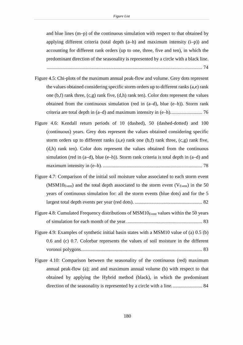
Figure List
180
and blue lines (m–p) of the continuous simulation with respect to that obtained by
applying different criteria (total depth (a–h) and maximum intensity (i–p)) and
accounting for different rank orders (up to one, three, five and ten), in which the
predominant direction of the seasonality is represented by a circle with a black line.
............................................................................................................................... 74
Figure 4.5: Chi-plots of the maximum annual peak-flow and volume. Grey dots represent
the values obtained considering specific storm orders up to different ranks (a,e) rank
one (b,f) rank three, (c,g) rank five, (d,h) rank ten). Color dots represent the values
obtained from the continuous simulation (red in (a–d), blue (e–h)). Storm rank
criteria are total depth in (a–d) and maximum intensity in (e–h). ......................... 76
Figure 4.6: Kendall return periods of 10 (dashed), 50 (dashed-dotted) and 100
(continuous) years. Grey dots represent the values obtained considering specific
storm orders up to different ranks (a,e) rank one (b,f) rank three, (c,g) rank five,
(d,h) rank ten). Color dots represent the values obtained from the continuous
simulation (red in (a–d), blue (e–h)). Storm rank criteria is total depth in (a–d) and
maximum intensity in (e–h). ................................................................................. 78
Figure 4.7: Comparison of the initial soil moisture value associated to each storm event
(MSM10Event) and the total depth associated to the storm event (VEvent) in the 50
years of continuous simulation for: all the storm events (blue dots) and for the 5
largest total depth events per year (red dots). ....................................................... 82
Figure 4.8: Cumulated Frequency distributions of MSM10Event values within the 50 years
of simulation for each month of the year. ............................................................. 83
Figure 4.9: Examples of synthetic initial basin states with a MSM10 value of (a) 0.5 (b)
0.6 and (c) 0.7. Colorbar represents the values of soil moisture in the different
voronoi polygons. .................................................................................................. 83
Figure 4.10: Comparison between the seasonality of the continuous (red) maximum
annual peak-flow (a); and and maximum annual volume (b) with respect to that
obtained by applying the Hybrid method (black), in which the predominant
direction of the seasonality is represented by a circle with a line. ........................ 84

Figure List
181
Figure 4.11: Chi-plot of the maximum annual peak-flow and volume. Red dots represent
the values the values obtained from the continuous simulation, whereas black dots
represent the values obtained from the Hybrid-based method. ............................. 85
Figure 4.12: Kendall return periods of 10 (dashed), 50 (dashed-dotted) and 100
(continuous) years. Grey dots represent the values obtained from the Hybrid-based
method, whereas red dots represent the values obtained from the continuous
simulation. ............................................................................................................. 86
Figure 4.13: Univariate flood frequency distributions of maximum annual peak-flows (a)
and volumes (b). Black dots represent the results obtained by the Hybrid-based
method, whereas red dots represent the values obtained from the continuous
simulation. ............................................................................................................. 87
Figure 5.1: Case study scheme. (a) Location of the Talave dam. (b) Scheme of the
discharge structures and the elevation of their axis (left). Details of gated spillways
(right). Abbreviations are defined in Table 5.1. ................................................... 93
Figure 5.2: Scheme of the proposed probabilistic approach. ......................................... 93
Figure 5.3: Comparison of the K-Method (for different K-values), I-O and MILP with
respect to the VEM. The horizontal axis shows the increments of the maximum
reservoir level in m (ΔZ). The vertical axis shows the increments of the maximum
outflow in m3/s (ΔO). The red points correspond to events with Tr ranging from
one to 10 years, blue points ranging from 10 to 25, green points from 25 to 50, black
points from 50 to 100, cyan points from 100 to 500, and magenta points from 500
to 10,000 years. ..................................................................................................... 95
Figure 5.4: Percentage of cases in QIII from K = 1.25 to K = 50, for different ranges of Tr
of the inflow hydrographs. The red colour corresponds to events with Tr ranging
from one to 10 years (a1), blue from 10 to 25 (a2), green from 25 to 50 (a3), black
from 50 to 100 (a4), cyan from 100 to 500 (a5), and magenta from 500 to 10,000
years (a6). .............................................................................................................. 96
Figure 5.5:Comparison of the K-Method (for different K-values) with respect to the VEM
(K = 1). The continuous line shows the median and the shaded areas show the range
between the 25th and 75th percentile of the maximum reservoir levels (ZMAX) (a)
and the maximum outflows (OMAX) (b), from K = 1 (VEM) to K = 50. The

Figure List
182
horizontal axis shows the different values of K. The red colour corresponds to
events with Tr ranging from one to 10 years (a1,b1), blue from 10 to 25 (a2,b2),
green from 25 to 50 (a3,b3), black from 50 to 100 (a4,b4), cyan from 100 to 500
(a5,b5), and magenta from 500 to 10,000 years (a6,b6). For specific K-values (K =
1, 2, 4, 6, 8, 10, 20, 50), box plots are presented with their corresponding outliers
(when existing) represented by red dots................................................................ 97
Figure 5.6: Frequency curves. (a) Maximum reservoir level frequency curves for VEM
(blue continuous line), different values of K (black lines of different types, see
legend), I-O (dashed-dotted blue line), and MILP (dashed red line). (b) Maximum
outflows frequency curves for VEM (blue continuous line), different values of K
(black lines of different types, see legend), I-O (dashed-dotted blue line), and MILP
(dashed red line). ................................................................................................... 98
Figure 5.7: Peak flow attenuation for different return periods and methods of operation
of dams. Y axes represent the ratio between the maximum outflow and the
maximum inflow for each event with their corresponding Tr (X axes). Blue dots
represent the events routed by the dam by applying the VEM, dark grey dots by
applying the K-Method with a K-value = 2, grey dots with a K-value = 10, light
grey dots with a K-value = 50, cyan dots by applying the I-O method, and red dots
by applying the MILP. ........................................................................................ 100
Figure 5.8: Comparison of outflow hydrographs (top) and reservoir levels (bottom)
resulting from the aplication of different dam operation methods. (a) Hydrograph
corresponding to Tr = 20 years and (b) corresponding to Tr = 1,000 years. Colored
lines represent the application of the different methods: VEM (blue continuous
line), different values of K (red lines of different types, see legend), I-O (dashed-
dotted blue line), and MILP (magenta continuous line). Coloured shading (bottom)
represents the different Zones of application of the K-Method (Zone 1 in green,
Zone 2 in yellow, Zone 3 in orange, and Zone 4 in red). .................................... 101
Figure 5.9: Risk-based approach. (a) Expected Talave Dam damage cost vs. released
maximum reservoir level. (b) Expected damage cost downstream Talave Dam vs.
released maximum outflows. (c) Risk indexes for VEM (dashed lines), I-O (dotted
lines), MILP (dashed-dotted lines), and different values of the K-Method
(continuous lines). Blue lines show the failure risk index (IF), red lines show the
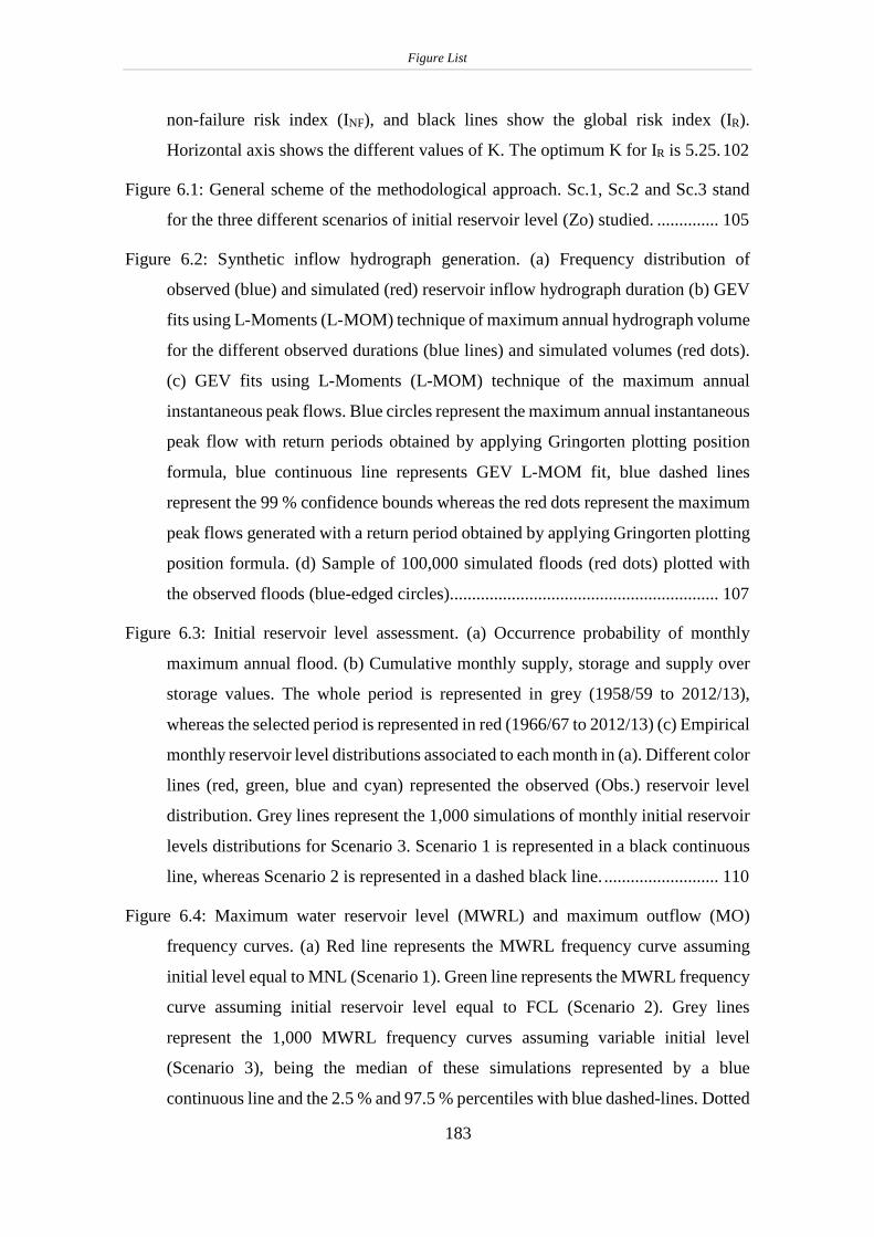
Figure List
183
non-failure risk index (INF), and black lines show the global risk index (IR).
Horizontal axis shows the different values of K. The optimum K for IR is 5.25. 102
Figure 6.1: General scheme of the methodological approach. Sc.1, Sc.2 and Sc.3 stand
for the three different scenarios of initial reservoir level (Zo) studied. .............. 105
Figure 6.2: Synthetic inflow hydrograph generation. (a) Frequency distribution of
observed (blue) and simulated (red) reservoir inflow hydrograph duration (b) GEV
fits using L-Moments (L-MOM) technique of maximum annual hydrograph volume
for the different observed durations (blue lines) and simulated volumes (red dots).
(c) GEV fits using L-Moments (L-MOM) technique of the maximum annual
instantaneous peak flows. Blue circles represent the maximum annual instantaneous
peak flow with return periods obtained by applying Gringorten plotting position
formula, blue continuous line represents GEV L-MOM fit, blue dashed lines
represent the 99 % confidence bounds whereas the red dots represent the maximum
peak flows generated with a return period obtained by applying Gringorten plotting
position formula. (d) Sample of 100,000 simulated floods (red dots) plotted with
the observed floods (blue-edged circles)............................................................. 107
Figure 6.3: Initial reservoir level assessment. (a) Occurrence probability of monthly
maximum annual flood. (b) Cumulative monthly supply, storage and supply over
storage values. The whole period is represented in grey (1958/59 to 2012/13),
whereas the selected period is represented in red (1966/67 to 2012/13) (c) Empirical
monthly reservoir level distributions associated to each month in (a). Different color
lines (red, green, blue and cyan) represented the observed (Obs.) reservoir level
distribution. Grey lines represent the 1,000 simulations of monthly initial reservoir
levels distributions for Scenario 3. Scenario 1 is represented in a black continuous
line, whereas Scenario 2 is represented in a dashed black line. .......................... 110
Figure 6.4: Maximum water reservoir level (MWRL) and maximum outflow (MO)
frequency curves. (a) Red line represents the MWRL frequency curve assuming
initial level equal to MNL (Scenario 1). Green line represents the MWRL frequency
curve assuming initial reservoir level equal to FCL (Scenario 2). Grey lines
represent the 1,000 MWRL frequency curves assuming variable initial level
(Scenario 3), being the median of these simulations represented by a blue
continuous line and the 2.5 % and 97.5 % percentiles with blue dashed-lines. Dotted

Figure List
184
grey line represents MNL, dashed grey line represents the DFL, continuous grey
line represents COD. (b) Same as figure (a) but applied to Maximum Outflow. 111
Figure 6.5: Damage cost curves. (a) Damage cost curves associated with maximum water
reservoir levels. (b) Damage cost curves associated with maximum outflows. (c)
Values of dam failure (IF, red bars), non-failure (INF, blue bars) and global (IR, black
bars) risk index for each of the three scenarios. Colored lines are added for a better
comparison between scenarios and risk indexes. ................................................ 115
Figure 7.1: General scheme of the stochastic methodology ......................................... 118
Figure 7.2: Location of Riaño basin and schemes of Riaño Dam spillways. COD: Crest
of Dam. MWL: Maximum Water Level. MNL: Maximum Normal Level. GSC:
Gated Spillway Crest........................................................................................... 119
Figure 7.3: Generation of series of stochastic initial reservoir levels .......................... 120
Figure 7.4: Results from the simulation of initial reservoir levels. a) Probability associated
to the months in which the maximum annual flood occurred. Grey blocks: observed
data; black blocks: sample of 100,000 months generated. b) Calibration (left) and
validation (right) of Riaño water balance model. Grey circles show the observed
reservoir monthly storage (Obs.) compared to the simulated series (Sim.) from 1988
to 2004 for the calibration process and from 2005 to 2013 for the validation process;
grey line represents the linear regression and dotted lines the confidence bounds of
95 % (Conf.). c) Empirical reservoir level distributions associated to each month of
the year obtained from the simulation of 73 years (1940 to 2013) ..................... 122
Figure 7.5: Generation of synthetic reservoir inflow hydrographs. a) Cumulative
frequency distribution of observed and simulated reservoir inflow hydrograph
durations. b) Fits of reservoir inflow hydrograph volume for the different durations
and simulated volumes c) Sample of 100,000 simulated floods (asterisks) and its
comparison to the observed floods (circles). Horizontal axis shows values of peak-
inflows while vertical axis shows flood volumes. .............................................. 124
Figure 7.6: Scheme for Reservoir-Dam system routing ............................................... 125
Figure 7.7: Maximum water reservoir level frequency curves. Black markers represent
MWRL frequency curves assuming initial level equal to MNL (ZMNL.). Grey
markers represent MWRL frequency curves assuming variable initial level (ZVAR.).

Figure List
185
Tr stands for return period, while m.a.s.l stands for meters above sea level. MNL
refers to Maximum Normal Level. MWL refers to Maximum Water Level while
COD stands for Crest Of Dam. Scenarios (C0-0% (top-left), C5-5% (top-right), C5-15%
(bottom-left), C15-15% (bottom-right)) are represented by the independent rate of
failure of each gate .............................................................................................. 127
Figure 7.8: Maximum outflow frequency curves. Black markers represent MO frequency
curves assuming initial level equal to MNL (ZMNL.). Grey markers represent MWRL
frequency curves assuming variable initial level (ZVAR.). Tr stands for return period.
Scenarios (C0-0% (top-left), C5-5% (top-right), C5-15% (bottom-left), C15-15% (bottom-
right)) are represented by the independent rate of failure of each gate ............... 128
Figure 7.9:Comparison between return periods obtained assuming failure of gates (C5-5%,
C5-15%, C15-15%) and those obtained with no failure associated (C0-0%.) for the same
MRWL. Results are shown for MNL (left) and variable initial reservoir level
(right). Scenarios are represented by the independent rate of failure of gate one (g1)
and gate two (g2) ................................................................................................. 129
Figure 7.10: Analysis of gate failure affection to maximum water reservoir levels (a, b,
c) and maximum outflows (d, e, f) for C15-15% (failure scenario). Comparison
between maximum reservoir levels (a) and maximum outflows (d) for C15-15% and
C0-0% (non-failure scenario). Decomposition of Maximum water reservoir levels (b)
and maximum outflows (e) frequency curves according to events in which no
failure occurred (upper), events in which one gate fails (intermediate) and events in
which both gate fail (lower). Comparison between C15-15% and C0-0% maximum
reservoir water levels (c) and maximum outflows (f) frequency curves. Dashed
dotted lines represents C0-0% frequency curves, different grey color dots represented
C15-15% values (See legends). ............................................................................... 131
Figure 7.11: Comparison of peak-inflow, volume hydrograph and maximum reservoir
level reached for the 100,000 hydrographs generated and for C0-0% scenario. Black
dots consider initial level equal to MNL. Grey dots consider variable initial level.
Right Y-Axis shows the percentage of the sample in each interval of reservoir
levels. .................................................................................................................. 131
Figure 8.1: a) Sample of the 100000 simulated inflow hydrographs associated to different
seasons (color dots: blue, season 1; magenta, season 2 and green, season 3) and its

Figure List
186
comparison to the observed floods (black dots). b) Determination of the range of
thresholds analysing the mean of the exceedances above the threshold (XS-S) (right
axis) and the mean annual exceedance (λ) above threshold test (left axis). c)
Validation of the threshold range using the Dispersion Index (DI) Test. The blue
line represents the different values of DI for the different thresholds. The blue
shaded area represents the values of DI within the confidence intervals determined
with a level of significance of 0.05. d) Delimitation of the seasons in Riaño Basin
applying the seasonality test based on Ouarda et al. (1993). Grey plots represent the
test for different values of the S thresholds. Straight dashed-lines represent the
different seasons. ................................................................................................. 140
Figure 8.2: Representations of the 132,651 values of MWRLTR=1000y, MOTR=500y and
YR=90% obtained respect to the MCLs for each of the seasons studied. MCLS1,
MCLS2 and MCLS3 represent the Maximum Conservation Levels in season 1,
season 2 and season 3 respectively. (a) Representation of the values YR=90%, with a
colorbar, which are the same in Scenario 1 (initial reservoir level equal to MCL)
and Scenario 2 (variable initial reservoir level). (b, c) Representation of the values
MOTR=500y with a colorbar in Scenario 1 (b) and Scenario 2 (c). (d, e) Representation
of the values MWRLTR=1000y with a colorbar in Scenario 1 (d) and Scenario 2 (e).
............................................................................................................................. 142
Figure 8.3: (a, c) Representation in grey of the pair of values YR=90% and MOTR=500y for
Scenario 1 and Scenario 2 respectively. Red points represent the pair of values
which do not fulfil overtopping requirements (MWRLTR=1000y >DFL). The pareto
front is represented with magenta dots, while the proposed solutions are represented
in cyan. The black dot represents the solution that maximizes the demand fulfilling
the Maximum Outflow released requirement (MOTR=500y=OEMER). The blue dot
represents the solution in which YR=90% equals the current annual demand,
minimizing the Maximum Outflow released. (b, d) MCLs for each month/season
that correspond to the proposed solutions previously selected (blue and black dots),
for S1 and S2 respectively. The red dashed line represents the Maximum Normal
Level (MNL), the red dashed-dotted line represents the Design Flood Level (DFL),
and the red continuous line represents the Crest of Dam (COD). ....................... 144

Figure List
187
Figure 8.4: Spider plot comparing the value of the maximum conservation levels for
different seasons (MCLsx), MWRLTR = 1000y, MOTR = 500y, and YR = 90%. In black,
solutions that maximize the volume supplied with MOTR = 500y = OEMER. In blue, the
solutions that supply the current annual demand minimize the maximum outflow
released. The continuous line corresponds to Sc.1 and the dashed line to Sc.2.. 145
Figure 9.1: Stochastic proposed framework of hydrological dam and downstream safety
assessment. .......................................................................................................... 154

Table List
188
Tables List
Table 2.1: Reliability estimation of gates with respect to their maintenance condition. 19
Table 3.1: Relationship between chapters, methodological key aspects, case studies,
software used and role of the High Performance Computer (HPC)...................... 60
Table 4.1: Relative and cumulated frequency that a storm of a specific rank generates the
maximum annual peak-flow and the maximum annual volume. .......................... 71
Table 4.2: Maximum storm rank required to obtain 95% and 99% probability of achieving
the maximum peak-flow or volume for a specific year, depending on the ranking
criteria used and the range of return periods studied. ........................................... 73
Table 4.3: Seasonality of the maximum annual peak-flow represented by the angle of its
mean direction (θ) and its radio (r), for different storm ranks and for the two
different criteria studied. The relative error (RE) is also shown. .......................... 75
Table 4.4: Seasonality of the maximum annual volume represented by the angle of its
mean direction (θ) and its radio (r), for different storm ranks and for the two
different criteria studied. The relative error (RE) is also shown. .......................... 75
Table 4.5: Rank-based non-parametric measures of dependence Spearman’s rho (ρ) and
Kendall’s tau (τ) for the pair of values of maximum annual peak-flows and
maximum annual volumes regarding the maximum storm rank considered and to
the criteria used: Total depth or maximum intensity. ........................................... 77
Table 4.6: Parameters of the Archimedean copula estimation from the pair of values of
maximum annual peak-flows and maximum annual volumes of the continuous
simulation, with the root mean square error (RMSE) and Nash–Sutcliffe error
(NSE). ................................................................................................................... 77
Table 4.7: Parameters of the Gumbel copula estimation from the pair of values of
maximum annual peak-flows and maximum annual volumes regarding the
maximum storm rank considered and the criteria used: Total depth or maximum
intensity, and relative error (RE) respect to the continuous simulation. ............... 78

Table List
189
Table 4.8: Comparison between similar case studies and the methodology used in each of
them. For comparison purposes, the basin area, weather/rainfall generator,
hydrological model and the way of accounting soil moisture are shown. ............ 80
Table 4.9: Results obtained for the different case studies considered in Table 4.8. PF
represents the maximum annual peak-flow, V represents the maximum annual
volume, and RE represents the relative error. ....................................................... 80
Table 4.10: Seasonality of the maximum annual peak-flow represented by the angle of its
mean direction (θ) and its radio (r), for different storm ranks and for the two
different criteria studied. The relative error (RE) is also shown. .......................... 85
Table 4.11: Rank-based non-parametric measures of dependence Spearman’s rho (ρ) and
Kendall’s tau (τ) for the pair of values of maximum annual peak-flows and
maximum annual volumes of the continuous and Hybrid-based simulation. ....... 86
Table 4.12: Parameters of the Archimedean Gumbel copula estimation from the pair of
values of maximum annual peak-flows and maximum annual volumes of the
continuous simulation and Hybrid simulation, and relative error (RE) respect to the
continuous simulation. .......................................................................................... 86
Table 5.1: Characteristic reservoir levels and outflows of the dam configuration. ........ 92
Table 6.1: Characteristic reservoir levels and spillway of the dam configuration studied.
............................................................................................................................. 106
Table 6.2: Values of the first (Q1), second (Q2), third (Q3) quartiles, the interquartile
range IQR, and the relative value of the IQR against Q2 for different return periods
(Tr) of maximum water reservoir levels. Values are represented as the water height
above the Flood Control Level. ........................................................................... 113
Table 6.3: Values of the first (Q1), second (Q2), third (Q3) quartiles, the interquartile
range IQR, and the relative value of the IQR against Q2 for different return periods
(Tr) of maximum outflows. ................................................................................. 113
Table 6.4: Values of the minimum, maximum, first (Q1), second (Q2), third (Q3)
quartiles, the interquartile range IQR, and the relative value of the IQR against Q2
for the dam failure (IF), non-failure (INF)and global (IR) risk index. ................... 116

Table List
190
Table 7.1: Main characteristics of Riaño basin and dam. MNL: Maximum Normal Level.
(maximum reservoir level to which water might rise under normal operation
(ICOLD,1994)). MWL: Maximum Water Level (maximum reservoir level which
the dam has been designed to stand (ICOLD,1994)) .......................................... 120
Table 7.2: Estimated values of GEV parameters using L-Moments technique and
hydrological event-based model parameters. V stands for the maximum mean daily
observed volumes of the year of different durations (defined by its subscript), QMAX
stands for the maximum mean daily peak-inflows, M represents the length of
observed data, α is the scale parameter (m3/s for QMAX and hm3 for V), u is the
location parameter (m3/s for QMAX and hm3 for V) and γ is the shape parameter
(dimensionless). AR(1), AR(2), MA(1) and MA(2) are the parameters of the
ARMA(2,2) model used, Ft stands for the factor of intermittency used as calibration
and CN is the curve number used ....................................................................... 124
Table 7.3: Comparison between quantiles of PFFCs of simulated and observed IPF
(estimated) for different Tr.................................................................................. 125
Table 7.4: Failure scenarios of gates functionality. Independent gate failure of 5% and
15 % per demand was considered for the assumption of a well-maintained gate and
gates with minor operation issues, respectively (Escuder-Bueno et al., 2012).
Failure of both gates due to common causes was considered as 1% per demand
(Lewin et al., 2003). Fixed-crest spillway was fully working for all scenarios .. 126
Table 7.5: Different return periods obtained for MWL (Maximum Water Level) and COD
(Crest Of Dam) levels for return periods ranging from one to 10,000 years ...... 127
Table 7.6: For each Maximum Reservoir Water Level (MWRL) and Maximum Outflow
(MO), range of variations of the ratio between the return period obtained assuming
variable initial reservoir level (TrVAR.) and assuming MNL (TrMNL.) for the different
scenarios. Scenarios (C0-0%, C5-5%, C5-15%, C15-15%) are represented by the
independent rate of failure of each gate, being each subscript associated to one of
the two gates. ....................................................................................................... 128
Table 7.7: Percentage of the sample of 100,000 MWRL that belongs to each interval of
reservoir levels defined considering the different gate failure scenarios (C0-0%, C5-

Table List
191
5%, C5-15% and C15-15%) and initial reservoir level conditions (constant and variable)
............................................................................................................................. 132
Table 7.8: Results obtained by different studies comparing the assumption of variable
initial reservoir level to MNL in the obtainment of maximum water reservoir levels
(MWRL) and maximum outflows (MO) frequency curves. TrVAR. represents the
return period which corresponds to the same MWRL or MO that has a return period
of 1,000 years if MNL is assumed as initial reservoir level. The return periods
shown for other studies are estimated, as they were collected from the graphs
provided in their results. No failure of gates is considered within any of the results
shown in this table ............................................................................................... 135

Appendix. Front page and last page of published papers
A1
APPENDIX: Front and last page of JCR published papers
1.1. Influence of initial reservoir level and gate failure in dam safety analysis.
Stochastic approach.

Appendix. Front page and last page of published papers
A2

Appendix. Front page and last page of published papers
A3
1.2. Dependence Between Extreme Rainfall Events and the Seasonality and Bivariate
Properties of Floods. A Continuous Distributed Physically-Based Approach.

Appendix. Front page and last page of published papers
A4

Appendix. Front page and last page of published papers
A5
1.3. Hydrological Risk Analysis of Dams: The Influence of Initial Reservoir Level
Conditions.

Appendix. Front page and last page of published papers
A6

Appendix. Front page and last page of published papers
A7
1.4. A Parametric Flood Control Method for Dams with Gate-Controlled Spillways.

Appendix. Front page and last page of published papers
A8

Appendix. Front page and last page of published papers
A9
1.5. Flood Control Versus Water Conservation in Reservoirs: A New Policy to
Allocate Available Storage.

Appendix. Front page and last page of published papers
A10