Michigan Technological University Michigan Technological University

Digital Commons @ Michigan Tech Digital Commons @ Michigan Tech

College of Business Publications College of Business

Summer 2008

Improving capital budgeting decisions with real options Improving capital budgeting decisions with real options

David E. Stout Youngstown State University

Yan Alice Xie University of Michigan - Dearborn

Howard Qi Michigan Technological University, howardqi@mtu.edu

Follow this and additional works at: https://digitalcommons.mtu.edu/business-fp

Part of the Business Commons

Recommended Citation Recommended Citation Stout, D. E., Xie, Y. A., & Qi, H. (2008). Improving capital budgeting decisions with real options. Management accounting quarterly, 9(4), 1-10. Retrieved from: https://digitalcommons.mtu.edu/business-fp/17

Follow this and additional works at: https://digitalcommons.mtu.edu/business-fp

Part of the Business Commons

brought to you by COREView metadata, citation and similar papers at core.ac.uk

provided by Michigan Technological University

1M A N A G E M E N T A C C O U N T I N G Q U A R T E R L Y S U M M E R 2 0 0 8 , V O L . 9 , N O . 4

The process of evaluating the desirability of

long-term investment proposals is referred

to as “capital budgeting.” Making opti-

mum capital budgeting decisions (e.g.,

whether to accept or reject a proposed

project), often requires recognizing and correctly

accounting for flexibilities associated with the project.

Such flexibilities are more formally termed real

options.1 From a valuation standpoint, these options

are valuable because they allow decision makers to

react to favorable or unfavorable new situations by

dynamically adjusting the capital budgeting decision

process. Unfortunately, the value of real options is not

explicitly considered in conventional procedures

(such as discounted cash flow (DCF) models) used to

evaluate long-term investment proposals. In some

sense, therefore, real options can be viewed as an

extension of DCF that incorporates a simple model of

strategic learning.2

In this article we present a short tutorial regarding

real options—what they are and how they can be for-

mally incorporated into the capital budgeting process.

We also illustrate how to price a capital investment

project containing real options. To explain these con-

cepts to a wide audience in accounting, we take more

of an intuitive approach and therefore abstract from

more technical treatments of the topic, such as those

explicitly linked to the Black-Scholes pricing model

for financial options.3 To illustrate basic concepts

regarding real options, we use a straightforward exam-

ple that relates to a rental car company that is consid-

ering whether to purchase a conventional gasoline-

powered car or a hybrid car as an addition to its rental

fleet, a decision complicated by uncertainties regard-

Improving CapitalBudgeting DecisionsWith Real Options

B Y D A V I D E . S T O U T , P H . D . ; Y A N A L I C E X I E , P H . D . ; A N D

H O W A R D Q I , P H . D .

EXECUTIVE SUMMARY In this article we provide accounting practitioners with a primer on how to supplement tradi-

tional discounted cash flow (DCF) analysis with real options. We use an example of a rental car company that is con-

sidering the purchase of a new car for its rental fleet. Management is trying to decide whether to buy a conventional

gasoline-engine automobile or a hybrid vehicle. Within this decision context we illustrate the embedded options the

company should consider given uncertainty of a new energy bill offering income-tax credits for the purchase of com-

mercially operated hybrid vehicles. Our step-by-step approach shows how to incorporate these real options formally

into the capital budgeting process.

2M A N A G E M E N T A C C O U N T I N G Q U A R T E R L Y S U M M E R 2 0 0 8 , V O L . 9 , N O . 4

ing tax incentives for commercial purchases of hybrid

vehicles.

INCOME-TAX INCENTIVES REGARDING THE

PURCHASE OF HYBRID VEHICLES

In 2002, Congress instituted a $2,000 income-tax

credit for the purchase of a new hybrid vehicle, but,

according to the proposal by Congress in late 2003,

that tax incentive was to have been phased out

entirely by 2007. Specifically, the $2,000 tax credit

would be cut by 25% in 2004, 50% in 2005, and 75%

in 2006. In late 2004, however, Congress reenacted

the $2,000 tax credit for hybrid cars purchased in

2004 and 2005. In 2006, Congress passed a new bill

that allowed a maximum tax credit of more than

$3,000 for hybrid car purchases, but the determina-

tion of which hybrid vehicles qualified for the credit

and the amount of credit to be taken was based on a

complicated set of rules.

We use the preceding historical review to illustrate

one type of cash-flow uncertainty associated with long-

term investments in depreciable assets: income-tax

consequences. As illustrated, tax effects on such

investments are subject to the whim of Congress.

Suppose that, at the present (say the beginning of

2008), Congress is debating a bill that would give

commercial owners a tax break for purchasing (and

using) hybrid vehicles. Assume, however, that passage

of the bill is uncertain and that our rental car company

is currently considering whether to add a hybrid vehi-

cle or a gas-powered vehicle to its rental fleet. Uncer-

tainties regarding income-tax provisions in the new

energy bill complicate the analysis of this capital bud-

geting decision. One of the advantages of real options

is the ability to deal explicitly with these and other

uncertainties.

For simplicity, we make a few additional assump-

tions regarding this investment decision. First, we

assume that the company plans to keep either car for

four years, after which time the car will be sold for an

estimated salvage value. Second, if the new energy

bill is passed, we assume that the income-tax credit

for operating commercial hybrid vehicles will start one

year hence, that is, in January 2009. Management

believes there is a 40% chance that the bill will be

passed and that the final fate of the bill will be known

by January 2009. Third, if the bill is passed, the annu-

al after-tax cash flow from operating the hybrid car is

estimated to be $10,000; assume, too, a net-of-tax sal-

vage value of $5,000 for the hybrid car at the end of

year four. If the bill is not passed, the annual after-tax

cash flow for the hybrid car drops to $4,000, and its

net-of-tax salvage value at the end of year four would

be $3,000.

For the gas-powered vehicle, assume that the annual

after-tax cash flow is $6,000, regardless of whether the

new bill passes; further, assume that the net salvage

value for this asset would be $3,000 with and $4,000

without the bill. This difference reflects the fact that

the passage of the energy bill would make gas-powered

cars less attractive than hybrids.

Finally, assume that the (annual) risk-free rate of

interest (estimated, for example, by the current yield

on Treasury Bonds) is 6% and that for the business

under consideration the appropriate risk-adjusted,

after-tax discount rate (i.e., weighted-average cost of

capital) is 10%.4

CONVENTIONAL ANALYSIS: HYBRID OR

GAS-POWERED VEHICLE?

First, note that the decision alternatives in this exam-

ple (whether to purchase a hybrid or a gas-powered

car) are mutually exclusive. According to a conven-

tional DCF analysis, we would calculate the expected

net present value (NPV) for each decision alternative

and then choose the one with the higher (and posi-

tive) NPV. In our example, as shown in the top por-

tion of Figure 1, the expected NPV for buying the

hybrid car is negative, as follows:

NPVHybrid = PV (after-tax cash flows) – PV (investment)

(1)

The negative expected NPV suggests that we should

not buy the hybrid car now, i.e., at T = 0.

( ) ( )

( ) ( ) ( ) ( )4 4

4 41 1

-

10,000 $5,000 $4,000 $3,0000.4 0.6 $25,0001 0.1 1 0.1 1 0.1 1 0.1

$2,117

Gas

i ii i

NPV PV after tax cash flows PV investment

= =

= −

= + × + + × − + + + +

=

∑ ∑ $

3M A N A G E M E N T A C C O U N T I N G Q U A R T E R L Y S U M M E R 2 0 0 8 , V O L . 9 , N O . 4

The company buys new cars and keeps them in business for four years. At the end of year four,

the car is sold for the indicated salvage value. Suppose the company has to make the investment

decision now (i.e., January 2008, or T = 0) regarding the purchase of a gas-powered or a hybrid

car. The new energy bill, currently under debate in Congress, offers a hefty income-tax credit on

the purchase of commercially operated hybrid cars. The proposed tax credit can alter the annual

after-tax cash flows and salvage values of both types of cars. With the tax credit, the hybrid car

offers both higher annual after-tax cash flows ($10,000) and a higher salvage value ($5,000) for

hybrid cars, while the salvage value for gas-powered cars drops from $4,000 to $3,000. These

potential cash-flow changes are strictly contingent on whether the new energy bill is passed in

January 2009. At time T = 0, management estimates a 40% chance that the new energy bill will be

passed. Figure 1 shows that the optimal choice is to choose the gas-powered car since this alter-

native has an NPV of $1,478, while the NPV of the hybrid car is –$2,117. The shaded bottom por-

tion of the figure indicates the optimal decision: Invest in a gas-powered car now.

Figure 1: Investment Assumptions

Gas-poweredInv = $20,000

HybridInv = $25,000

Gas-powered or

Hybrid?

Year 1-4 after-tax cash flows = $10,000Year 4 salvage value = $5,000

Year 1-4 after-tax cash flows = $4,000Year 4 salvage value = $3,000

Year 1-4 after-tax cash flows = $6,000Year 4 salvage value = $3,000

Year 1-4 after-tax cash flows = $6,000Year 4 salvage value = $4,000

Tax credit forHybrid?

Yes: P = 0.4

Estimated at T = 0,Expected NPV = –$2,117

No: P = 0.6

Tax credit forHybrid?

No: P = 0.6

CF0 (INV) CF1

T = 1

CF2

T = 2

CF3

T = 3

CF4+Salvage Value

T = 4T = 0

Yes: P = 0.4

Estimated at T = 0,Expected NPV = $1,478

4M A N A G E M E N T A C C O U N T I N G Q U A R T E R L Y S U M M E R 2 0 0 8 , V O L . 9 , N O . 4

As shown in the bottom portion of Figure 1, the expect-

ed NPV for the gas-powered car is positive, as follows:

NPVGas = PV (after-tax cash flows) – PV (investment)

(2)

Because the NPVGas alternative is positive and greater

than NPVHybrid, a conventional DCF analysis indicates

that the company should invest in the gas-powered car.

The corresponding cash flows associated with Figure 1

are presented in Table 1.

THE POTENTIAL VALUE OF REAL OPTIONS

To this point, we have presented the decision as a capi-

tal budgeting problem analyzed using a conventional

DCF analysis. Yet in this decision problem we have

already seen, but not dealt with, an embedded real

option: the flexibility of our choice between the two

types of cars—what we might call an “asset flexibility”

option. While seemingly of little importance, this exam-

ple of a real option carries an important message that is

true for all forms of real options:

NPV (w/options) > NPV (w/o options). (3)

As such, real options will be exercised if and only if

they increase the value of a capital investment project.

Consider, for example, each investment choice in a

“go” vs. “no-go” decision (i.e., accept or reject). This

would be the situation if we did not have the

flexibility to choose between the two types of

cars. When the gas-powered car is the only can-

didate, the expected NPV would be $1,478, and

the project would be accepted; if the hybrid car were

the only option being considered, we would reject this

investment because its NPV is negative. (Equivalently,

failure to invest results in an NPV of $0.) As stated by

statement (3), when we introduce asset choice (i.e.,

when we embed asset flexibility into the decision), the

expected NPV is the higher of the two—in this case,

$1,478. For this situation, we would not exercise the option of

asset flexibility—it adds no expected value to the investment

decision.

AN INVESTMENT-TIMING OPTION:

BUY NOW OR BUY LATER?

The next question management might ask is: “Should

we purchase a car now, or should we delay the invest-

ment for one year—until January 2009?” The flexibility

offered in the timing of the capital budgeting decision

is called an investment-timing option. Figure 2 expands

the original decision problem (Figure 1) to address the

A: Purchase a Hybrid CarYear 0 (now) 1 2 3 4New energy bill is passed -$25,000 $10,000 $10,000 $10,000 $10,000(40% probability) + $5,000 salvage valueNew energy bill is NOT -$25,000 $4,000 $4,000 $4,000 $4,000passed (60% probability) + $3,000 salvage value

B: Purchase a Gas-Powered CarYear 0 (now) 1 2 3 4New energy bill is passed -$20,000 $6,000 $6,000 $6,000 $6,000(40% probability) + $3,000 salvage valueNew energy bill is NOT -$20,000 $6,000 $6,000 $6,000 $6,000passed (60% probability) + $4,000 salvage value

Table 1: Comparative After-Tax Cash Flow Data—Two DecisionAlternatives, Purchase Made at T = 0 (i.e., Today)

( ) ( ) ( ) ( )4 4

4 41 1

$6,000 $3,000 $6,000 $4,0000.4 0.6 $20,0001 0.1 1 0.1 1 0.1 1 0.1

$1,478

i ii i= =

= + × + + × − + + + +

=

∑ ∑

5M A N A G E M E N T A C C O U N T I N G Q U A R T E R L Y S U M M E R 2 0 0 8 , V O L . 9 , N O . 4

investment-timing question: invest now (T = 0) or delay

the investment one year (i.e., invest at T = 1)?

The benefit of delaying the investment decision is

that we will have more accurate (or complete) informa-

tion in January 2009 when the fate of the new energy

bill will be known. This new information may lead to a

decision that differs from the one made based on the

more limited information set available today. Intuitively

speaking, if we can “wait and see” for one year, we will

not get stuck for four years with a car that, based on

updated information, turns out to be a suboptimal

choice. The benefit of the “wait and see” option, how-

ever, comes at a cost: the after-tax cash flows that the

business forgoes during the coming year. Because mon-

ey has a time value, delaying the investment reduces

the expected NPV of the project. If this “hidden cost”

outweighs the benefit, then the embedded investment-

timing option does not add value, and the investment

should be made now. Thus, the optimal decision

depends on the trade-off between these two

considerations.

Now suppose we do defer the investment decision to

January 2009. If the new energy bill is passed, the

expected NPV for the hybrid alternative is

NPVHybrid = PV (after-tax cash flows) – PV (investment)

(4)

Note that in this case all cash flows are pushed for-

ward by one year compared to the situation depicted in

Figure 1. Also, the investment outlay of $25,000 to be

made one year from now is discounted by the risk-free

interest rate (6%) because we assume that this amount

is known with certainty.

We now find that the expected NPV for the gas-

powered alternative is $285,5 which is much less than

$8,337. Therefore, after incorporating the potential val-

ue of the “wait and see” option, we find that purchas-

ing the hybrid car is the optimal choice (based on

maximizing expected NPV). This is shown in the shad-

ed upper area of Figure 3. The corresponding after-tax

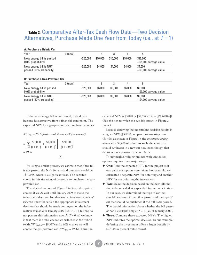
cash flows are presented in Table 2.

An “investment-timing option,” one form of

real option, is created if the rental car compa-

ny has the flexibility to invest today (T = 0) or

to defer the investment for at least one year

(T =1). At T = 0, management estimates that

the new energy bill has a 40% chance of being

passed. At T =1, it will be known for certainty

whether the new bill has passed. The benefit

of deferring the investment decision for one

year is that the company can avoid the less

profitable (or money-losing) choice. The draw-

back of the delay decision is that the expected

future after-tax cash flows are deferred. The

trade-off of these two effects tells us whether

the company should defer the investment to

January 2009 (i.e., make the decision at T = 1).

Figure 2: Investment-TimingOption

Invest now:40% chance of tax credit for hybrid cars starting next year

Invest now or wait one

year?

Wait one year:tax credit will

be known for sure.

( ) ( ) ( )5

5 12

$10,000 $5,000 $25,0001 0.1 1 0.1 1 0.06

$8,337

ii=

= + −

+ + + =

∑

6M A N A G E M E N T A C C O U N T I N G Q U A R T E R L Y S U M M E R 2 0 0 8 , V O L . 9 , N O . 4

If the company has the flexibility to wait a year to make the investment, an investment-timing

option exists. Whether the company should invest now (i.e., go back to the situation depicted in

Figure 1) or wait (in a sense, exercise the option to wait) depends on the expected NPV of the

delayed investment. It makes sense to defer the investment only when two conditions are satis-

fied: (1) the expected NPV of the delayed investment is positive, and (2) this NPV is higher than

the expected NPV without deferral. In our case, the shaded bottom portion in Figure 1 indicates

the optimal path for the company. By waiting one year, the company can take full advantage of

the knowledge that becomes available at T = 1 but that is unavailable at T = 0. Estimated at T = 0,

and as shown in Figure 3 above, the overall expected NPV under the delay option is $3,878, which

exceeds the $1,478 optimal result when the decision is made now (see Figure 1).

Figure 3: Incorporating an Investment-Timing Option

Year 2–5 after-tax cash flows = $6,000Year 5 salvage value = $4,000

CF0 = 0 CF1 (INV)

T = 1

CF2

T = 2

CF3

T = 3

CF5+Salvage Value

T = 5T = 0

CF4

T = 4

Estimated at T = 0, with 1-yeardeferral, the overall expected NPV =($8,337 x 0.4) + ($906 x 0.6) = $3,878

Situation inFigure 1 Year 2–5 after-tax cash flows = $10,000

Year 5 salvage value = $5,000

Wait one year:tax credit will

be known for sure.

Invest now Probability estimatedat T = 0, P = 0.4

Estimated at T = 0, Expected NPV= $8,337, conditional on “Yes.”

Estimated at T = 0, Expected NPV= $906, conditional on “No.”

Probability estimatedat T = 0, P = 0.6

Tax credit forHybrid?

No

Yes

Invest now or wait one

year?

HybridInv = $25,000

Gas-poweredInv = $20,000

➔

➔

7M A N A G E M E N T A C C O U N T I N G Q U A R T E R L Y S U M M E R 2 0 0 8 , V O L . 9 , N O . 4

If the new energy bill is not passed, hybrid cars

become less attractive from a financial standpoint. The

expected NPV for a gas-powered car purchase becomes

NPVGas = PV (after-tax cash flows) – PV (investment)

(5)

By using a similar process, we estimate that if the bill

is not passed, the NPV for a hybrid purchase would be

–$10,195, which is a significant loss. The sensible

choice in this situation, of course, is to purchase the gas-

powered car.

The shaded portions of Figure 3 indicate the optimal

choices if we do wait until January 2009 to make the

investment decision. In other words, from today’s point of

view we know for certain the appropriate investment

decision that should be made contingent on the infor-

mation available in January 2009 (i.e., T = 1), but we do

not possess this information now. At T = 0, all we know

is that there is a 40% chance we will choose the hybrid

(with NPVHybrid = $8,337) and a 60% chance we will

choose the gas-powered car (NPVGas = $906). Thus, the

expected NPV is $3,878 (= [$8,337×0.4] + [$906×0.6]).

(See the box to which the two big arrows in Figure 3

point.)

Because deferring the investment decision results in

a higher NPV ($3,878) compared to investing now

($1,478, as shown in Figure 1), the investment-timing

option adds $2,400 of value. As such, the company

should not invest in a new car now, even though that

decision has a positive expected NPV.

To summarize, valuing projects with embedded

options requires three major steps:

◆ One: Find the expected NPV for the project as if

one particular option were taken. For example, we

calculated a separate NPV for deferring and another

NPV for not deferring the investment.

◆ Two: Make the decision based on the new informa-

tion to be revealed at a specified future point in time.

In our case, we determined the type of car that

should be chosen if the bill is passed and the type of

car that should be purchased if the bill is not passed.

The crucial information about whether the bill passes

or not is available only at T = 1 (i.e., at January 2009).

◆ Three: Compare these expected NPVs. The higher

NPV indicates the optimal decision. In our example,

deferring the investment offers a larger benefit by

$2,400 (in present-value terms).

A: Purchase a Hybrid CarYear 0 (now) 1 2 3 4 5New energy bill is passed -$25,000 $10,000 $10,000 $10,000 $10,000(40% probability) + $5,000 salvage valueNew energy bill is NOT -$25,000 $4,000 $4,000 $4,000 $4,000passed (60% probability) + $3,000 salvage value

B: Purchase a Gas-Powered CarYear 0 (now) 1 2 3 4 5New energy bill is passed -$20,000 $6,000 $6,000 $6,000 $6,000(40% probability) + $3,000 salvage valueNew energy bill is NOT -$20,000 $6,000 $6,000 $6,000 $6,000passed (60% probability) + $4,000 salvage value

Table 2: Comparative After-Tax Cash Flow Data—Two DecisionAlternatives, Purchase Made One Year from Today (i.e., at T = 1)

( ) ( ) ( )5

5 12

$6,000 $4,000 $20,0001 0.1 1 0.1 1 0.06

$906

ii=

= + − + + +

=

∑

8M A N A G E M E N T A C C O U N T I N G Q U A R T E R L Y S U M M E R 2 0 0 8 , V O L . 9 , N O . 4

OTHER TYPES OF REAL OPTIONS

Thus far, we have looked at two specific types of real

options: asset options and investment-timing options. The

concepts and valuation techniques we have discussed to

this point also can be extended to other types of real

options. Here we briefly explain a few additional types

of real options. All of these examples fall under the

umbrella of providing decision makers with increased

investment flexibility.

Growth options typically refer to the flexibility to

increase the scale of an investment. Companies tend to

build facilities with a certain amount of slack (or “cush-

ion”) because the slack provides a valuable growth

option. For example, a computer with a few more emp-

ty slots costs more than a comparable machine without

such slots. Michigan Tech University offers its under-

graduate engineering students the option to earn a

“shortcut MBA” as an add-on to their undergraduate

program by having them take required business courses

and allowing these students to apply credits earned in

their engineering program (such as engineering man-

agement, statistics, etc.) toward the MBA degree. So we

can say that Michigan Tech has an embedded (academ-

ic) growth option for which it may charge a higher

tuition to its undergraduate engineering students.

How do we value growth options? We can slightly

modify the framework presented in the earlier example

to deal with this question. For instance, we can ask

whether operating a gas-powered rental car without the

possibility to grow is more valuable than operating a

hybrid car with the flexibility to grow in the future, say

at point T = 1. In this case, we would compare the NPV

for a gas-powered car (viz., $1,478) with that for a

hybrid. Given our assumed data, the expected NPV for

the “hybrid-car-with-growth option” is

(6)

where $0×0.6 means that the growth option to buy a

hybrid car at T = 1 is given up (hence the cash flows are

zero) if the new energy bill is not passed. This situation

has a 60% probability of occurrence. The example indi-

cates that operating hybrid cars with the flexibility to

grow is still less attractive than operating gas-powered

cars without the possibility to grow because the expect-

ed NPV of the former is $260 less than that of the latter.

Expansion options are similar to growth options. For

example, a traditional phone company may choose to

expand into the wireless communications business. A

company may subsidize an existing product line (e.g.,

traditional phone) because it allows the company to

quickly expand in another line (e.g., wireless) when the

opportunity is deemed favorable. Ford has not aban-

doned its pickup truck production even though profits

on pickup sales have been negative for a couple of

years. A rental car company more likely may hire tech-

nicians (at the same salary level) with expertise on both

gas-powered and hybrid cars, even if it is currently

operating gas-powered cars only, because the flexibility

in its labor force increases the value of the option to

expand into operating hybrid cars at some point in the

future. All these behaviors would be hard to justify without

recognizing the embedded expansion options. Valuing long-

term investments that offer the flexibility to expand

would essentially follow the three-step procedure

described above for growth options.

Abandonment options represent yet another type of

real option. A product is more salable if the buyer is giv-

en an option to return it for, say, 70% of the original

price if the buyer is not satisfied. A house can sell at a

higher price if it has a higher resale value. Perhaps a

company prefers to outsource its research and develop-

ment (R&D) function to an external party rather than

keep its own in-house scientists. Abandonment options

allow the company to avoid getting stuck with a money-

losing business when things are not going right. A high-

er abandonment (or salvage) value increases the

attractiveness of the product (or project). In fact, we

have actually addressed abandonment options in our

rental-car example when we assumed different sal-

vage values depending on the outcome of the new

energy bill and the type of car purchased.

To value a project with an embedded abandonment

option, we focus on the salvage values. The three steps

and the techniques explained above are once again

applicable. To illustrate, suppose there exists an option

to sell (i.e., abandon) the gas-powered car in one year

( ) [ ]Hybrid-Growth 1

$2,117 $8,337 0.4 $0 0.6

$1, 218

Operating hybrid now Option to buy hybrid at TNPV NPV NPV == +

= − + × + × =

9M A N A G E M E N T A C C O U N T I N G Q U A R T E R L Y S U M M E R 2 0 0 8 , V O L . 9 , N O . 4

for $18,000 (salvage or abandonment value). Now we

can ask whether operating a gas-powered car with such

an abandonment option would be more valuable than

operating a gas-powered car without this option. Intu-

itively, this option to abandon is valuable because it

allows the company to react dynamically to the uncer-

tain result of the new energy bill debate. If the bill is

passed in one year, the company can sell the gas-

powered car and switch to the more profitable hybrid.

The question is how much value this abandonment

option would add to operating the gas-powered car.

Equation (7) shows how this estimation is done.

NPVGas = PV (after-tax cash flows) – PV (investment)

(7)

The $18,000 abandonment value appears in year one

with an associated probability of 40%. Now we see that

this abandonment option makes the gas-powered car

more attractive by $300; i.e., it increases the expected

NPV for a gas-powered car from $1,478 (without aban-

donment option, see Figure 1) to $1,778 (with abandon-

ment option).

BENEFITS AND COSTS OF CONSIDERING

REAL OPTIONS

The biggest benefit of considering real options in the

capital budgeting process is that they help decision

makers reach optimal investment decisions. In this

regard, real options complement or extend, not replace,

traditional DCF decision models. As shown in our

example, some embedded real options may lead to

completely different investment decisions compared to

those based solely on a traditional DCF analysis. Put

another way, a less attractive investment proposal may

be worth significantly more once we recognize its hid-

den treasures—investment flexibility based on the exis-

tence of real options.

In principle, because they can help optimize the cap-

ital budgeting process, real options should always be

considered when making long-term investment deci-

sions. Once managers grasp the concepts and are famil-

iar with the basic framework for valuing projects

embedded with real options, we would expect practice

to change to the point where such options are routinely

considered in the analysis of capital budgeting projects.

Not long ago, DCF models were new to many man-

agers who typically relied more on simple decision

models, such as payback or accounting rate of return

(ARR), for making capital budgeting decisions. Today,

NPV has become a common financial management tool.

Because of their role as management advisors, manage-

ment accountants now need to become knowledgeable

about what real options are and how they can extend

DCF models in a meaningful way.

Real options have a flipside, too. The major

cost of incorporating real options is that the deci-

sion process can quickly become quite complex.

In our previous example, we assumed that the

only factor that affected the choice of vehicles was the

passage of a new energy bill within one year. Other

4

1 41

$6,000 $18,000 $6,000 $4,000 0.4 0.6 $20,000(1 0.1) (1 0.1) (1 0.1)

$1,778

ii=

+= × + + × − + + + =

∑

Further Reading

For those who would like to know more about real

options analysis, here are some additional sources.

The following book provides comprehensive cover-

age of the topic: Lenos Trigeorgis, Real Options:

Managerial Flexibility and Strategy in Resource Allo-

cation, MIT Press, Cambridge, Mass., 1996.

For practitioners, we recommend: Tom Copeland and

Vladimir Antikarov, Real Options: A Practitioner’s

Guide, Texere LLC, New York, N.Y., 2003, or Prasad

Kodukula and Chandra Papudesu, Project Valuation

Using Real Options: A Practitioner’s Guide, J. Ross

Publishing, Inc., Fort Lauderdale, Fla., 2006.

For advanced readers, i.e., those who are familiar

with stochastic processes, we suggest: Avinash K.

Dixit and Robert S. Pindyck, Investment Under

Uncertainty, Princeton University Press., Princeton,

N.J., 1994.

10M A N A G E M E N T A C C O U N T I N G Q U A R T E R L Y S U M M E R 2 0 0 8 , V O L . 9 , N O . 4

sources of risk can be associated with this investment

decision. For instance, we might consider possible fluc-

tuations in the price of gas or innovations in the auto-

mobile industry. The more factors we consider, the

more complex the analysis becomes. When we attempt

to incorporate more factors into the capital budgeting

valuation framework, the more “noise” we introduce,

making the results of our analysis potentially less

accurate.

Second, incorporating real options into the analysis

typically requires an array of probability estimates, one

for each possible event, outcome, or scenario. For

example, we assumed a 40% probability that the pro-

posed energy bill would pass. In practical terms, this

assessment may turn out to be the largest source of

uncertainty.

Third, a typical capital investment project may have

many embedded real options simultaneously, and it

may be impractical to consider all of them. Neverthe-

less, real-life decisions are inherently complex; these

complexities do not go away simply because we choose

to ignore them in the decision models we use. Put

another way, complexity of the situation only makes

real options analysis a bit less reliable.

Now that we have presented an analysis of costs and

benefits, we predict that real options analysis will

become one of the common tools managers and

accounting professionals use to evaluate long-term

investment projects. Thus, management accountants

need to learn as much as they can about real options so

they can use them in their decision making. ■

David E. Stout, Ph.D., is a professor and the holder of the

Andrews Chair in Accounting at the Williamson College of

Business Administration, Youngstown State University,

Youngstown, Ohio. You can contact him at (330) 941-3509

or destout@ysu.edu.

Yan (Alice) Xie, Ph.D., is an assistant professor of finance

in the School of Management at the University of Michi-

gan—Dearborn. You can contact her at (313) 593-4686 or

yanxie@umd.umich.edu.

Howard Qi, Ph.D., is an assistant professor of finance,

School of Business and Economics, Michigan Technological

University in Houghton, Mich. You can reach him at (906)

487-3114 or howardqi@mtu.edu.

ENDNOTES

1 Richard A. Brealey, Stewart C. Meyers, and Alan J. Marcus,Fundamentals of Corporate Finance, McGraw-Hill, New York,N.Y., 2007, p. 637.

2 Raul Guerrero, “The Case for Real Options Made Simple,”Journal of Applied Corporate Finance, Spring 2007, pp. 39-49.

3 For example, Richard Shockley relies heavily on the Black-Scholes option-pricing formula as a way of discussing realoptions vis-à-vis financial options. (See Richard Shockley, “AReal Option in a Jet Engine Maintenance Contract,” Journal ofApplied Corporate Finance, Spring 2007, pp. 88-94.) In a similarvein, Scott Mathews, Blake Johnson, and Vinay Datar rely on avariation of the Black-Scholes framework, which they call the“DM method,” to explain the theory and use of real options.(See Scott Mathews, Blake Johnson, and Vinay Datar, “A Practi-cal Method for Valuing Real Options: the Boeing Approach,”Journal of Applied Corporate Finance, Spring 2007, pp. 95-104.)

4 For an exposition of how to estimate the weighted-average costof capital (WACC), see Michael S. Pagano and David E. Stout,“Calculating a Firm’s Cost of Capital,” Management AccountingQuarterly, Spring 2004, pp. 13-20.

5 We leave out the calculation procedure because it is similar toEquation (4).

Reproduced with permission of the copyright owner. Further reproduction prohibited without permission.