Anticipating ECB monetary policy

decisions through the RND

extrapolation from Liffe 3M

EURIBOR options.

PierPaolo Cassese∗

Assicurazioni Generali

Finance Department†

November 17, 2013

∗The article is based upon a research conducted for a personal purpose: By analyzingthe options markets is it possible to comprehend the monetary policy decisions before-hand?. I would apologize with the reader as far as all errors and omissions are minealone†Group Strategic Asset allocation and ALM

1

Abstract

The price of derivative contracts has always played a strategic role

in extracting valid information to be employed in one′s own investment

strategies. Shimko (1993) was a pioneer in this arena.

Taking up where Shimko left off, this paper will demonstrate how to

extract Risk neutral density function using two different techniques

from derivative contracts.

Shimko proposed a technique to build up the risk neutral density func-

tion starting by employing the implied volatility smile of 3M Liffe EU-

RIBOR derivative contracts.

The procedures adopted here in are based on the implementation of

an interpolation model, a polynomial splines, applied to the implied

volatility smile of future Liffe EURIBOR 3 M from which RNDs will

be created. The flexibility of the model, as will be explained, is en-

tirely attributed to the differentiability of the call and put prices found

in the Black-Scholes model, as well as the log-normality on which the

Black-Scholes model rests.

Finally, the paper will include the impact the Lehman Brothers col-

lapse had on the Future EURIBOR 3 M.

Key words: implied volatility smile, risk neutral density function,

second partial derivative call/put vs. strike price, ECB monetary pol-

icy expectations.

2

Contents

1 Introduction 4

2 RNDs methodologies 7

2.1 The non-parametric method. . . . . . . . . . . . . . . . . . . 9

2.2 RNDs estimated with the lognormal distribution function. . . 13

3 Fitting the implied Black-Scholes volatility smile using the

spline. 15

4 Case study. 19

4.1 Lehman Brothers market reaction . . . . . . . . . . . . . . . . 20

5 Concluding remarks. 24

6 Figures and summary statistics 27

7 Table 33

3

1 Introduction

In this paper two different approaches to extrapolate the risk neutral den-

sity function (hereafter referred to as RND) from 3M Liffe EURIBOR option

prices traded on the future prices of EURIBOR 3M will be presented.

Financial operators are continuously in search of vital information from fi-

nancial instruments. Excluding insiders, who would be able to unethically

benefit from their privileged positions, many financial operators look to

derivative markets to gather useful information for their analyses. A valid

example is the forward interest rate market that represents the market con-

sensus with respect to the likely interest rate levels expected in the future.

Investors follow derivative markets where they look at the implied volatility

smile (hereafter referred to as IVS) to quantify the sense of future risk per-

ception.

By applying RND extrapolation techniques from interest rate derivative op-

tions prices, it will be possible to estimate a probability function that should

demonstrate how unforeseen events could affect the contingency interest rate

level.

The pioneer of the RND abstracting technique from derivative contracts was

first and foremost, Shimko (1993), whereas later RND research was done by

Breeden, Litzenberger and other researchers; Shimko attempted to interpo-

late Black-Scholes IVS using a quadratic methodology.

The cornerstone of his work consists in fitting a curve that should grip all

points of IVS using a two degree polynomial function .1 Interpolation of

IV is calculated using a different space than the surface used in the Black-

Scholes2. Although it is widely common to consider the IV in canonical

space (such as IV versus strike prices) Shimko preferred to switch the strike

prices with the delta of the options3.

As debated above, IV is a proxy taken into account from policy makers in

order to evaluate market sentiment, analyzing the future price of interest

1In Shimko, the polynomial degree chosen to fit the implied volatility is equal to two.This means that Shimko′s interpolation technique is a quadratic function.

2The Black-Scholes model is used to show volatility smile in an implied volatility-strikeprices plan. This convention is useful when either investors or analysts are going to pricethe option, while for RND extrapolation, the same surface seems to be better for impliedvolatility delta space. The main reason for this is to recognize that the range that deltacovers, is shorter than the broad range that could be covered by strike prices.

3Delta is indeed known as the first partial derivative of call/put price with respect tostrike price. For the interest rate derivatives, the strike price is future price.

4

rate contracts. This would mean that futures are a very good predictor for

policy decision makers seeing as how when a future contract rebounds, it

may predict a potential cut in the key interest rate on the refinancing op-

eration4. Otherwise, in the case that future prices should drop, they might

transmit a message about a possible increase in key interest rates, because

the market operators have already discounted this unpredictable event in

future prices. Monetary authorities may decide to apply changes to the in-

terest rate in accordance with the market by analyzing risk factors.

One method of doing so may be to use the changes in RND main statistics5.

Two RND estimation techniques will be introduced in more detail further

on.

Firstly, an explanation on how to extract RNDs from second partial deriva-

tives of call/put prices against their strike price. This methodology referred

to as the non-parametric technique6, will allow us to abstract the collected

information on how interest rates are going to evolve, with a probability

derived by option prices.

The second methodology consists of using the lognormal density function

from which the RND can be extrapolated using four key measures: IV, fu-

ture prices (converted to the interest rate simply by subtracting the price of

the future from one hundred), The maturity of the options and, finally, the

mean and standard deviation of lognormal density function. In conclusion,

both methodologies mentioned above will provide the user with two RNDs

that will then be compared to the RND estimated from the market.

The paper is organized as follows. Section 2 describes the general methodol-

ogy behind the RND, including a detailed description of the two techniques

adopted in this dissertation. Then, Section 3 will focus on the interpolation

exploit to fit the IVS with the polynomial splines. Section 4 will be dedicated

to the description of the results found after both the two RND methodolo-

gies are considered with respect to real market events. The case study used

in this paper will be that of the market crash caused by Lehman Brothers,

4Here it is advisable to consider the key interest rate as the ECB interest rate fixed bythe Governing Council.

5A valid example could be the RND main statistics evolution on a time window thatanticipates the meeting of the ECB Governing Council. For instance RND that shows ahigher daily skewness than previous week could represent a situation where market feelingis uncertain and volatile.

6To distinguish the second technique from the first, here it is simply cited as theparametric method

5

which will be shown with constant horizon RNDs in order to prove how

these unforgettable circumstances affected monetary policy decision-making

around the world.

6

2 RNDs methodologies

Many researchers studying the behaviour of financial assets have intensified

their interest in RND extrapolation techniques.

As modern finance theory dictates, the prices of financial instruments follow

stochastic paths. Researchers are therefore obligated to consider whether a

scenario of price could be realized. This should be thought of as a combina-

tion of probability functions that return an expected result not completely

in line with reality.

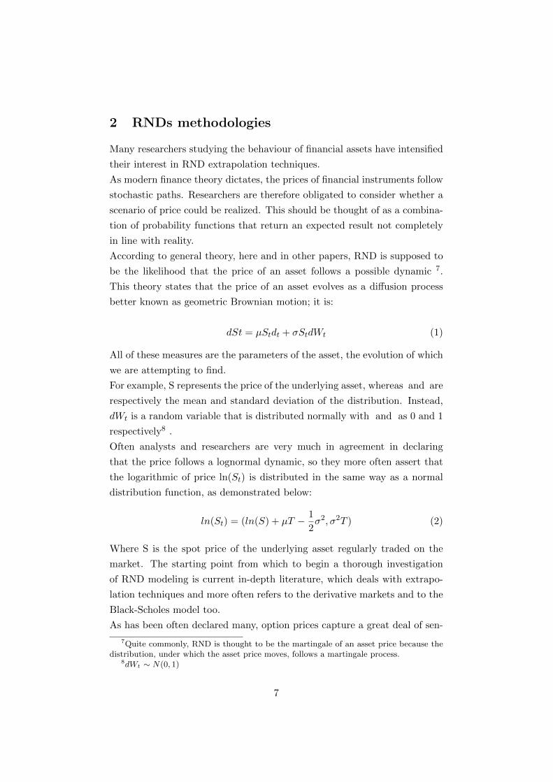
According to general theory, here and in other papers, RND is supposed to

be the likelihood that the price of an asset follows a possible dynamic 7.

This theory states that the price of an asset evolves as a diffusion process

better known as geometric Brownian motion; it is:

dSt = µStdt + σStdWt (1)

All of these measures are the parameters of the asset, the evolution of which

we are attempting to find.

For example, S represents the price of the underlying asset, whereas and are

respectively the mean and standard deviation of the distribution. Instead,

dWt is a random variable that is distributed normally with and as 0 and 1

respectively8 .

Often analysts and researchers are very much in agreement in declaring

that the price follows a lognormal dynamic, so they more often assert that

the logarithmic of price ln(St) is distributed in the same way as a normal

distribution function, as demonstrated below:

ln(St) = (ln(S) + µT − 1

2σ2, σ2T ) (2)

Where S is the spot price of the underlying asset regularly traded on the

market. The starting point from which to begin a thorough investigation

of RND modeling is current in-depth literature, which deals with extrapo-

lation techniques and more often refers to the derivative markets and to the

Black-Scholes model too.

As has been often declared many, option prices capture a great deal of sen-

7Quite commonly, RND is thought to be the martingale of an asset price because thedistribution, under which the asset price moves, follows a martingale process.

8dWt ∼ N(0, 1)

7

sitive information that could drive the gambler to make rational investment

strategies.

Looking toward the Black-Scholes formula, it is possible to infer that the

probability of the price of a call or put option might breach a particular

level on the next future.

Take into consideration, for instance, the price of a European call option

where no dividend is paid out and the interest rate is the risk free interest

rate with the duration perfectly equal to the call maturity.

If written as a formula, it would look as follows:

c = exp(−rT )E[max(St −X; 0)] = e(−rT )∫ ∞

0max(St −X; 0)f(St)dSt (3)

Where c is the discounted price of the European call option, St is the price of

the underlying asset at T (time), as long as T corresponds to the expiry date,

or the time to maturity. X is the strike price, r is the risk-free interest rate

and,E[max(St-X;0)] is the expected value of the risk neutral density of the

value of the future asset price f(St). Converting the call price in the integral

instead of the discrete function will result in the call price returning to the

area under which the call option will assume a particular value conditioned

from its probability density function f(St).

Although risk neutral density function should be computed using a closed

formula, its real value is never known as it might assume all possible values

in the strike price domain.

The main goal of this paper is to provide two techniques that help the user

of these models to calculate a plausible measure of RND for the possible

pricing of its options or other types of financial assets.

8

2.1 The non-parametric method.

The first methodology mentioned in this paper to create RND is the non-

parametric technique.

This topic has been dealt with in many publications, more specifically, how

to extract RND from the second derivative of the call or put pricing function

with respect to the exercise price.

All the current literature revolves around the paper written by Breeden and

Litzenberger (1976) entitled ”Prices of state contingent claims implicit in

option prices”.

In this work, the authors accurately introduced the elementary formula to

derive the RND from a combination of option strategies.

The framework is based on the general option theory that introduces the

claims on the option as a right to buy or sell on a specific maturity a number

of claims in the case that a hypothetical scenario will be realized. Predating

Breeden and Litzenbergers work by several years, Debrau (1959) and Arrow

(1964) developed the concept of contingency claims.

Their theory was based upon the fact that the willingness of the investor to

allocate e1 on an underlying asset is driven by the expectation of earning a

positive future payoff.

Of course, no one is able to foresee the feasibility of this strategy since the

dynamic of the underlying asset on which the claim has been paid is un-

known.

Moreover, the investor is at risk to make no money at all when the contract

expires. In the case that the desired scenario will not be realized their initial

investment will be lost. Breeden and Litzenberger managed to demonstrate

the thoroughness of this model by replicating the pay-off of a butterfly op-

tion strategy in order to reconcile with Arrow and Debraus basic premise.

To further their assumption, they first attributed one feature to the option

markets as well as making the assumption that the capital markets were

going to be perfect9.

In order to prove their theory, the two authors simulated buying a miscel-

laneous of complex option contracts (also referred to as a butterfly spread)

in order to enhance their goal of extracting RND from option prices.

9”Perfect capital markets” means that all participants in the negotiations may have attheir disposal the same information which is spread broadly over the market.

9

The option spread strategy is managed in the following way10 :

• Buy put option out of the money with strike price X

• Sell put option at the money with strike price Y

• Buy call option out of the money with strike price J

• Sell call option at the money with strike price Y

This is shown in Figure 1.

Breeden and Litzenberger argued that the price strategy could be compared

to a variation of the strike price at T, which can be expressed as:

1

∆X∗ [C(X −∆X)− C(X)]− [C(X)− C(X + ∆X)] (4)

Considering that the investment will be delivered taking into consideration

the risk neutral world, the strategy acts in respect to the concept of the

Martingala11. Hence, in order to abide by the previous rule, we should

compute the price of an elementary claim as:

px

∆X=

1

∆X2∗ [C(X −∆X)− C(X)]− [C(X)− C(X + ∆X)] (5)

Calculating the limit that tends to zero, both Breeden and Litzernberger

showed that the result of this equation becomes:

lim∆X→0

px

∆X=∂2C(X)

∂X2(6)

The above formula represents the second partial derivative of the call price

with respect to its strike price.

In comparing the last formula calculated with the (5), we should be able to

elaborate the risk neutral density function through an extension of the fun-

damental rule of the theory of asset pricing, working under the assumption

that the asset pricing is resting on a risk neutral environment. In conse-

quence of thinking in the risk neutral world, the fundamental theorem of

10Morten Bergendahl Nitteberg. ”Implied Risk-Neutral Densities: An application tothe WTI Crude Oil market” November 2011. Pg.11

11A martingale is a zero drift stochastic process. A variable f follows a martingale if itsprocess has the form: df=s dWt. Where dWt is a Wiener process. The variable s mayitself be stochastic. It can depend on f and other stochastic variables. A martingale hasthe convenient property that its expected value at any time is equal to its value today.This means that E(fT )=f0

10

asset pricing evaluates the price of the call or put option as the expected

payoff under a specific probability level, the risk neutral probability, dis-

counted at the risk free interest rate Rf.

c = exp(−RfT )E[max(St−X; 0)] = exp(−RfT )∫ ∞

0max(St −X; 0)f(St)dSt

(7)

As Breeden and Litzernberger attempted to demonstrate, the second deriva-

tive of the call price with respect to the exercise price is equal to the dis-

counted risk neutral density function (RND).

∂2C(X)

∂X2= exp(−RfT )fQ(St) (8)

fQ(St) = exp(RfT )∂2C(X)

∂X2(9)

As long as the second partial derivative works correctly, it is necessary for the

Black-Scholes call option pricing function to be twice as differentiable as the

strike price. Checking this assumption on various cases, it has been possible

to find that the Black-Scholes pricing formula allows for the recognition of

the second partial derivative such as a function of RND discounted for the

risk free interest rate. Moreover, to confirm the robustness of the idea of

extracting RND from the Black-Scholes option pricing, the calculation of

the second partial derivative in a discrete world will be demonstrated.

In order to find the calculation, we need to consider the second derivative

as a composition of some of the Black-Sholes measures.

Firstly, we have to compute the d2 of the call option price.

The d2 should be thought of as the key function in order to assess the

robustness of all procedures.

In this paper, d2 is calculated for the future contract of Liffe 3 M EURIBOR,

and therefore d2 is12 :

d2 =ln( F

X )− (12σ

2)T

σ√T

(10)

Then, d2 requires the estimation of both the IV and the strike prices. Hence,

IV will be interpolated from a series of volatilities and then rescaled to the

square root of time (T).

The last step is finding the value of the Normal distribution function for d2

12Bhupinder Bahra. ”Implied risk-neutral probability density function from optionprices: theory and application”. Bank of England Working paper. 1997.

11

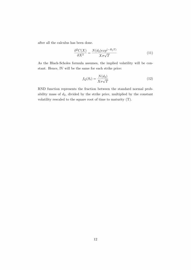
after all the calculus has been done.

∂2C(X)

∂X2=N(d2)exp(−RfT )

Xσ√T

(11)

As the Black-Scholes formula assumes, the implied volatility will be con-

stant. Hence, IV will be the same for each strike price:

fQ(St) =N(d2)

Xσ√T

(12)

RND function represents the fraction between the standard normal prob-

ability mass of d2, divided by the strike price, multiplied by the constant

volatility rescaled to the square root of time to maturity (T).

12

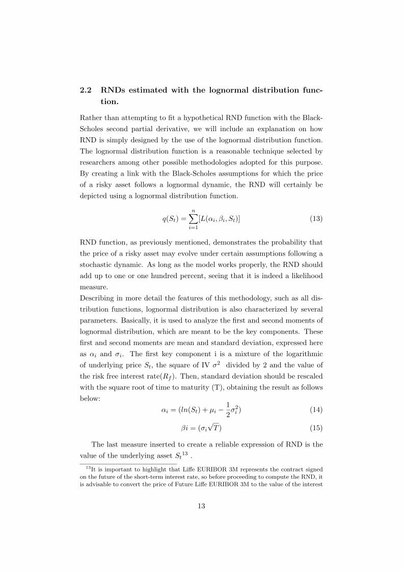
2.2 RNDs estimated with the lognormal distribution func-

tion.

Rather than attempting to fit a hypothetical RND function with the Black-

Scholes second partial derivative, we will include an explanation on how

RND is simply designed by the use of the lognormal distribution function.

The lognormal distribution function is a reasonable technique selected by

researchers among other possible methodologies adopted for this purpose.

By creating a link with the Black-Scholes assumptions for which the price

of a risky asset follows a lognormal dynamic, the RND will certainly be

depicted using a lognormal distribution function.

q(St) =n∑

i=1

[L(αi, βi, St)] (13)

RND function, as previously mentioned, demonstrates the probability that

the price of a risky asset may evolve under certain assumptions following a

stochastic dynamic. As long as the model works properly, the RND should

add up to one or one hundred percent, seeing that it is indeed a likelihood

measure.

Describing in more detail the features of this methodology, such as all dis-

tribution functions, lognormal distribution is also characterized by several

parameters. Basically, it is used to analyze the first and second moments of

lognormal distribution, which are meant to be the key components. These

first and second moments are mean and standard deviation, expressed here

as αi and σi. The first key component i is a mixture of the logarithmic

of underlying price St, the square of IV σ2 divided by 2 and the value of

the risk free interest rate(Rf ). Then, standard deviation should be rescaled

with the square root of time to maturity (T), obtaining the result as follows

below:

αi = (ln(St) + µi −1

2σ2i ) (14)

βi = (σi√T ) (15)

The last measure inserted to create a reliable expression of RND is the

value of the underlying asset St13 .

13It is important to highlight that Liffe EURIBOR 3M represents the contract signedon the future of the short-term interest rate, so before proceeding to compute the RND, itis advisable to convert the price of Future Liffe EURIBOR 3M to the value of the interest

13

Once all of the features of the parameters have been presented, it will be

possible to compute the RND function from short-term interest rate op-

tion prices. Although the literature on RND suggests adopting two or more

lognormal distributions through an optimization procedure such as the one

used by Melick and Thomas (1994), the RND here will be estimated us-

ing only one lognormal distribution. The decision to use only one lognormal

distribution is justified in order to avoid the optimization procedure to elim-

inate some errors. These errors could occur when the key parameters of the

distribution are optimized to search for the best parameters ensured to fit

the RND.

Below is a summary regarding the method of implementation of this numer-

ical tractability:

• Compute mean and standard deviation of the lognormal distribution

function for the pre-selected underlying asset.

• Since RND is extracted from a constant horizon time period, it is

necessary to fix the next expiry date both for the call or put option

contract before carrying out the calculus of the RND. Indeed, the

shape of the RND will be modified by this parameter depending on

the mean and standard deviation.

• Converting the price of the future on Liffe EURIBOR 3 M into the

level of interest rate. To respect the guidelines suggested by the model,

it is recommended that:

rt = (100− FuturePrice) (16)

After following the above procedure step by step, the next stage consists

of interpolating the right implied volatility smile in order to compose a

thorough RND function.

rate.

14

3 Fitting the implied Black-Scholes volatility smile

using the spline.

14

The Black-Scholes model, as previously mentioned, is primarily concerned

with the concept of implied volatility. This measure is intended as the un-

known variable with which the entire model is calibrated. The Black-Scholes

model allows the analyst or investor to fairly evaluate the price of call or

put option. Implied volatility (IV) is only that value for which the above

stochastic differential equation is solved; the result of the equation will give

one the fair option price after the system of equations have found the appro-

priated implied option volatility. Despite the fact that market participants

are able to easily find σMkt, the IV is not a quantifiable measure with a

closed formula or with an explicit format. The only way to proceed is by

solving an equation 15 that will numerically return the IV value seeing that

all Black- Scholes parameters are known at the beginning of computation.

Why the volatility covers an important role in the option context is well

understood by the forecast capability that it owns. In fact, looking at the

implied volatility surface that is structured on a three dimensional plane,

(IV put on vertical axis, strike price occupies the horizontal axis and the

time to maturity on the third axis respectively) it should be possible to fig-

ure out the evolution of the volatility against the time.

The higher the IV for the next expiry date, the more volatile the expected

fluctuation of dicey asset returns will be.

One could have a negative perception of the market if IV was lower than

the historical volatility (HV) calculated up to date.

Mentioning this difference between HV and IV, a careful operator could

predict the stability around the dynamic of asset returns by deciding, for

example, to invest if IV was lower than HV, otherwise they should divest or

reduce their stake in case they are risk adverse, when IV is higher than HV.

No numerical example of this will be given here, as this goes beyond the

14Allan Bodskov Andersen and Tom Wagener. ”Extracting risk neutral probability den-sities by fitting implied volatility smiles: some methodological points and an applicationto the 3M EURIBOR futures option prices” European Central Bank Working paper n198. December 2002.

15Looking at put call parity formula, Ct-Pt=St-K∗exp(−rT ), the implied volatility isthat value which the equation shows before equal to zero. Hull ”Option futures and otherderivatives”. Chapter 13rd VII Edition

15

scope of our interest.16 .

The purpose of this chapter is analyzing the technique used to fit a reason-

able implied volatility against the implied volatility surface estimated by the

market.

Shimko (1993) formulated a new type of implied volatility to use for ex-

trapolating RND function. Rather than making an interpolation with the

pair IV vs. strike price, Shimko changed this last measure with the delta

of call/put option. This is due to the fact that strike prices could change

more frequently than the delta, whereas the delta is strictly embedded in

the domain zero-one17 . In fact, the region on that IV may be relied on

against the strike price, and this is generally not fixed a priori. The avail-

able observations may vary much more than the delta option observations,

in the case that only the surface is built upon.

The ability to restrict the domain strangely allows for the second technique

( Shimko′s approach) both the implied fitted volatility smile and the RND

to be more flexible and smooth.

Research in this context has provided many results used to make laudable

progress in improving the fitting of the implied volatility smile.

Unfortunately, Shimko′s methodology was basically limited by the use of

a parabolic function that fit the IV smile. If the next step consisted of ex-

tracting RND from the second partial derivative, Shimko′smethodology lost

credibility and flexibility. Of course while making a careful examination of

Shimko′s RND, one will note the lack of a part of the RND, specifically the

tails18 . In order to improve the overall fit and flexibility of the fitted smile,

Clews, Panigirtzoglou and Proudman (2000) proposed the use of a natural

smoothing cubic spline, a bit different than the standard technique19 . In

cubic spline formulations, the IV surface is fitted with a polynomial function

knotted in more inflection points by differentiable functions.

The goal of the cubic spline, is however, to create a series of points that

16Noteworthy: to find out more about implied volatility with numerical examples, pleaseconsult Hull Option futures and other derivatives. Chapter 16th VII Edition.

17As introduced in Chapter 2, the delta of option could be stretched between zero toone only. The space that IV could occupy is limited on this domain.

18Noteworthy: the shape of the RND was incomplete using Shimko′s technique.19This methodology is clearly described in Campa, Chang and Reider (1997).”Implied

exchange rate distributions: Evidence from OTC option markets”. NBER Working Paperno.6179. and in Clews, Panigirtzouglou and Proudman.(2000), Recent developments in ex-tracting information from option markets. Bank of England Quarterly Bulletin. February,pp 50-60.

16

replicate the implied volatility smile well. As in Clews, Panigirtzoglou and

Proudman, by augmenting the degree of a polynomial function, one could

tend to the implied volatility smile estimated by the market with a variant:

improving fit means raising the value of the IV with some effects on the

smoothness of the RND function.

Consequently, in this paper a polynomial function with fourth order de-

grees20 has been adopted in order to achieve the best compromise between

the smoothness of the polynomial function to replicate the knots and the

value of the IV. If the starting point is the fourth order polynomial function,

improving the accuracy of the interpolation solution in this paper can opti-

mize the distance to the IV estimated from the market using the MATLAB

fitting toolbox.

In the following rows, how to valorize the implementation of the spline will

be shown:

σ(δ; θ) = α0 + α1δ + α2δ2 + α3δ

3 + α4δ4 +

n∑i=1

α4+i|δ − ki|4 (17)

Where σ(δ, θ) is the IV yields with the spline polynomial technique.

αi, where i is the degrees and parameters of spline, and, finally δ is the

value of delta option. The value of n is the number of knot points selected

in implementing the spline. Because n will have just one knot point, n is

equal to 1. For a model that contemplates one knot point, its value is 0.5.

If volatility is estimated using interpolation technique, each single outcome

does not perfectly match with the delta computed with the Black-Scholes

model.

Thereafter the delta option should also correspond to the relative implied

volatility. By assigning the true to the IV, it will finally be possible to build

the fair (σ, δ) surface. Notewothy: while we interpolate across delta space

we can keep the smoothing parameter constant daily.

When RND is estimated, it should eventually change on a daily basis in

terms of shape. At this point it is possible to understand that the reason for

the change in RND is due to the variation in the underlying value, or the

20Four degrees is a rather parsimonious level for the replication of the route of IV.Here despite using a simple polynomial function, it is preferred to rely on the MatlabPolynomial Fitting toolbox to reduce the calculus efforts.

17

Future price, rather than in the estimation technique21. Once the observed

IV is fitted against the market IV, to reduce the potential gap it is suggested

to minimize the distance across the values of collected observed and market

values.

The minimization procedure is established by starting from the parameter

vector (α0, .....,α5) and then minimizing the square of the difference between

IVMkt and IVObs. The optimized function is expressed as follows:

(α0, ...α5) = minn∑

i=1

[σi − σ(δ; θ)]2 (18)

For all values that minimize the problem above, a new volatility value is

found for the corresponding δ.

No assumption is made with respect to the penalty on the curvature of the

fitted smile as is usually found in the current literature22 .

21All parameters remained constant. Constant horizon means that volatility for i daywill be the same. The volatility will vary day by day but not the estimation technique.Clews, Panigirtzouglou and Proudman.(2000), ”Recent developments in extracting infor-mation from option markets”. Bank of England Quarterly Bulletin. February, pp 50-60.

22For an exhaustive example please look at the paper written by Allan Bodskov Ander-sen and Tom Wagener. ”Extracting risk neutral probability densities by fitting impliedvolatility smiles: some methodological points and an application to the 3M EURIBORfutures option prices” European Central Bank Working paper n 198. December 2002

18

4 Case study.

Up to now mainly the methodologies adopted to extrapolate RND with the

assistance of two different techniques have been discussed.

In the last section the results that the two methods were able to produce

during a significant period in the global banking system will be examined.

Following the chronological events, the next section will present the analysis

conducted on the Lehman Brothers failure of 15th September 2008, which

dramatically substituted risk perception across the markets.

The case has been managed with the support of the Bloomberg platform.

To put together all the data, we have decided to refer to Bloomberg for

information regarding the IV surface. As previously mentioned, the main

step is to find an accurate implied volatility smile in order to correctly price

options or futures.

To carefully perform the analysis, the accuracy of the data is the begin-

ning point without which the research could not be continued. Hence all

data are collected with great care, excluding those days when negotiations

were banned or temporarily suspended23. Further, Datastream Thompson

Reuters was used for gathering the time series of EURIBOR 3M, the key

ECB interest rate and the prices of at the money options traded on the

EURIBOR 3M.

The spot prices of Future 3M EURIBOR were compared to the interest rate

forward contract with constant horizon. The daily corresponding implied

volatility was also downloaded from Datastream but only with the strike

prices listed as at the money.

Certainly, the focus of this paper is to provide a forecasting tool to antici-

pate ECB monetary policy decisions.

We assert that the pertinent timeframe to study is that corresponding to the

fifteen days prior to the event in question, in this case, the Lehman failure,

as well as the following two weeks.

We have chosen this approach because ECB decisions were taken and made

known to the market two weeks after the Lehman Brothers failure.

23Notable are the days when the Authorities who supervise financial markets, such asthe SEC in the USA, CONSOB for the Italian market or the FSA for the British marketdid not allow short the stocks to be quoted on the markets.

19

4.1 Lehman Brothers market reaction

In hindsight, it is obvious that the events of 15th September were completely

unexpected. This is reflected in the market volatility revealed by the implied

Liffe 3M EURIBOR volatility smile.

Unless we blame the rating agencies for the setback regarding the last rating

valuation released on Lehman Brothers debt issuances, no one could have

predicted the market storm.

The historical series of implied EURIBOR 3M volatility options for the first

two weeks of September remained constant or mostly unchanged in value.

The financial tsunami of 15th September24 came as the Lehman Brothers

board went to court to file for bankruptcy25.

The implied volatility for Liffe EURIBOR 3M quickly soured for the next

three weeks, until monetary authorities and policy makers decided to coop-

erate to placate a jumpy market. Figure 6b represents the evolution of IV

through September until the first half of October 2008.

If the variation in futures was revealed from the raising of IV, the corre-

sponding means of RND shape moves further and further to the left in the

plan IV-interest rate strike price.

As each step is depicted in Figure 3, one can clearly discern not only the

changes in risk expectation, but the somewhat predictive feature assigned

to this measure in advance of the successive moves of the ECB. In fact an-

alyzing the main statistics, (see Table 1) one can see how the probability

masses become fatter with each passing day.

The skewness and kurtosis leave their peaks making the distributions mesokur-

totic26 ; whereas the means reduce, standard deviation of distributions vary

more rapidly than the reduction in other measures.

This is probably due to the uncertainty about what would have happened

for the other pool of American banks involved in the subprime tsunami.

24See Figure 6 for clarification.25Chapter 11 is a chapter belonging to the Title 11 of the United States Bankruptcy

Code, which permits reorganization under the bankruptcy laws of the United States.Chapter 11 Bankruptcy is available to every business, whether organized as a corpora-tion or sole proprietorship, and to individuals, although it is most prominently used bycorporate entities.

26If a return distribution has no excess kurtosis or little excess kurtosis, meaning it hasthe same kurtosis as the normal distribution, it is said to be mesokurtotic, or normal tailedand to exhibit mesokurtosis. Mark J.P Anson ”CAIA LEVEL1 An introduction to CoreTopics in Alternative Investments”. SECOND EDITION 2013

20

In order to understand how the market anticipated the potential cut in the

ECB main interest rate after 15th September, one must make a brief intro-

duction to Liffe EURIBOR 3M contract.

Liffe EURIBOR 3M options are very liquid products because they are fre-

quently traded.

Beyond their liquidity, this contract has a constant expiry date that rolls

each three months, expiring on the third Friday of March, June, September

and December respectively.

When each contract is over, the next one is ready to be traded27 .

This characteristic graphically demonstrates that when the price of future

Liffe EURIBOR 3M converges to the natural expiry date, the relative value

of its interest rate tends to be narrower seeing that market operators are

more likely to exercise their forward rate contract at the spot price.

Consequently, in case the RND shape is changed during a short period, the

explanation should be attributed to the new market information.

Next, we will give an in depth analysis on how it possible is to extract RND

from option prices with the two methods previously described in detail. Only

the option prices that are slightly in the money and far out of the money

were chosen because their liquidity is much wider than the at the money

option.

The monotonicity of both call and put prices are warranted, hence it is

easier to differentiate their prices against the strike price to get the RND.

Once all range of put and call prices are selected, the next step is to project

the implied volatility smile referring to the RND shape on the day in ques-

tion. The IV for each day is chosen as the at the money IV that Thompson

Reuters directly provides for the contract. This does not mean that the pro-

cedure has been changed in order to elaborate the RND, but only to make

the description more agile.

However Figure 2 shows how the market IV is fitted using the polynomial

spline methodology. Although the observed IV extrapolated to the surface

T-IV-δ is yielded, to assure the smoothness in RND shape, remember to

transform IV-δ back to IV vs. K space corresponding to the true IV found.

The next formula will complete the central phase of the second order deriva-

tives methodology by inverting the first partial derivative of call price against

27As is commonly said, the contract is continuously rolled on each expiry.

21

the strike price, which corresponds to the option:

δ =∂C(X)

∂X= exp(−rT )φ(

ln(FtX ) + (1

2σ2)T

σ√T

) (19)

Then:

K = Ft ∗ exp(σ2T

2− σ

√(T )φ−1(exprtδ)) (20)

Once the previous formula is respected, the last step is to compute RND

for a vector of hypothetical values that interest rates could assume.

If the first technique is related to the extrapolation from the second partial

derivatives, the next one is easier to implement in terms of calculus as it

is directly dependent on the lognormal distribution function. The unique

measures that one must consider are the following:

• Future prices downloaded by DataStream. The value of Future should

be expressed in terms of interest rate, so to express the interest rate

in basis points one needs to replicate formula (16)

• After converting the future price into the interest rate, one must calcu-

late mean and standard deviation of the lognormal distribution. (See

14,15).

• After completing the above steps, one will have abstracted the RND

from the future of EURIBOR 3M seeing that RND is the lognormal

distribution function of EURIBOR 3M future contract. 28.

Referring to the appendix, the shapes of RND obtained with the support

of first methodology, second partial derivative, and the previously described

technique is visible. Some differences will be evident in their shapes.

The RND on the right demonstrates less smoothness than the lognormal

RND. Despite the lognormal RND being more homogenously distributed

across the strike prices with no lack of tails, the RND extrapolated with

second partial derivative is less smooth.

Missing values at the tails of distribution are one of the issues that Shimko

and other researchers have mentioned in their papers.

28Rupert de Vincent-Humphreys and Joseph Noss. ”Estimating probability distribu-tions of future asset prices: empirical transformations from option-implied risk-neutral toreal-world density functions”. Working Paper No. 455 June 2012.

22

To close the gap, the literature proposes the use of extreme value theory in

order to limit the problem that affects Shimko′s scheme.

23

5 Concluding remarks.

In this paper we used an extension of Shimko′s (1993) model to extract

RNDs. The article employed a double and straightforward methodology

beginning from an alternative interpolation technique to find the true value

from options volatility surface.

Even if these two methods give the same results, a comparison of the shapes

of RNDs reveals that the lognormal function is smoother than the RND

extracted using the second partial derivative. A careful examination of the

RND found using the second partial derivative, reveals an easily visible peak

at its top.

The vertex is due to the perfect match with the RND that belongs to call

prices with the second half of the RND that is linked to the put prices.

The lack of the curvature at the top of the RND depends on the choice made

at the beginning. To prepare the fair RND, options that are far out of the

money and nearly in the money are selected for this purpose.

The most important element in looking for the RND in order to forecast the

evolution of interest rates etc., is to not merely rely on the outcome, but

to take into consideration both the consistency of the data quality and the

market consensus.

24

References

[1] Mark J.P Anson, ”CAIA LEVEL1 An introduction to Core Topics in

Alternative Investments.” SECOND EDITION 2013.

[2] Bhupinder Bahra.,”Implied risk-neutral probability density function

from option prices:theory and application” Bank of England Working

paper.1997.

[3] Morten,Bergendahl,Nitteberg. ”Implied Risk-Neutral Densities:An ap-

plication to the WTI Crude Oil market”Pg.11, November 2011.

[4] Allan Bodskov, Andersen and Tom Wagener., ”Extracting risk neutral

probability densities by fitting implied volatility smiles: some method-

ological points and an application to the 3M EURIBOR futures option

prices” European Central Bank Working paper n 198. December 2002.

[5] Campa, Chang and Reider ,”Implied exchange rate distribu-

tions:Evidence from OTC option markets”NBER Working Paper

no.6179.

[6] Clews, Panigirtzouglou and Proudman. ,”Recent developments in ex-

tracting information from option markets” pp 50-60.Bank of England

Quarterly Bulletin. February 2000.

[7] John Hull”Option futures and other derivatives.” Chapter 13rd VII

Edition.

[8] John Hull”Option futures and other derivatives.” Chapter 16th VII

Edition.

[9] ”Matlab Polynomial Fitting toolbox.”

[10] Rupert de Vincent-Humphreys and Joseph Noss. ”Estimating prob-

ability distributions of future asset prices: empirical transforma-

tions from option-implied risk-neutral to real-world density func-

tions”.Working Paper No. 455 June 2012.

Bloomberg

Thompson Reuters Datastream

European Central Bank Data Warehouse

25

List of Figures

1 Example of Butterfly Spread . . . . . . . . . . . . . . . . . . 27

2 A comparison across IV interpolation techniques . . . . . . . 28

3 RND extrapolated from second partial derivative from option

prices.’Lehman Brothers case study’ . . . . . . . . . . . . . . 29

4 Implied RNDs constant horizon.”Lehman Brothers case study’ 30

5 LIFFE EURIBOR 3M vs. Forward rate . . . . . . . . . . . . 31

6 A summary of main statistics collected from RNDs 9-12-2008

to 10-17-2008 . . . . . . . . . . . . . . . . . . . . . . . . . . . 32

26

6 Figures and summary statistics

Butterfly spread

Figure 1: Example of Butterfly Spread

27

Estimated smiles with two techniques

Figure 2: A comparison across IV interpolationtechniques

Source:Bloomberg

28

RNDs Liffe EURIBOR 3M

Figure 3: RND extrapolated from second par-tial derivative from option prices.’Lehman Broth-

ers case study’

Source:Thompson Reuters

29

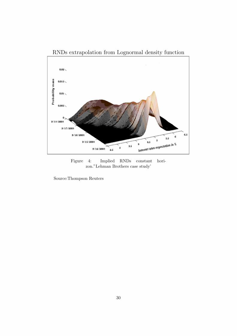
RNDs extrapolation from Lognormal density function

Figure 4: Implied RNDs constant hori-zon.”Lehman Brothers case study’

Source:Thompson Reuters

30

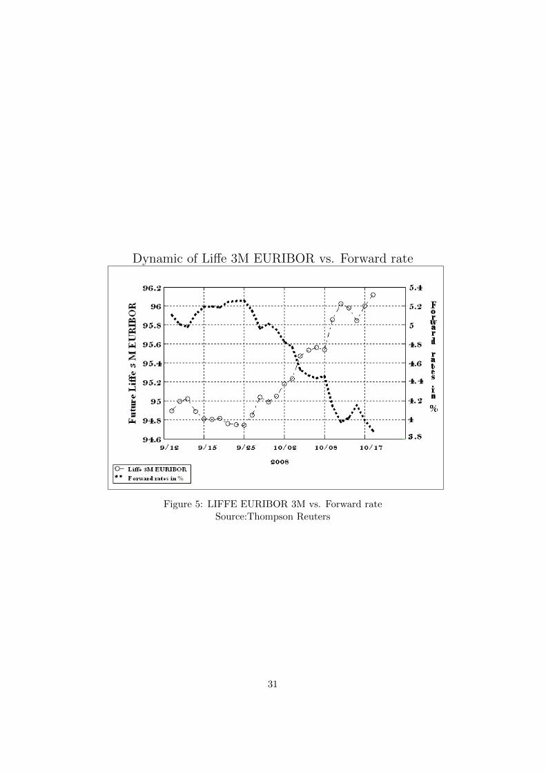
Dynamic of Liffe 3M EURIBOR vs. Forward rate

Figure 5: LIFFE EURIBOR 3M vs. Forward rateSource:Thompson Reuters

31

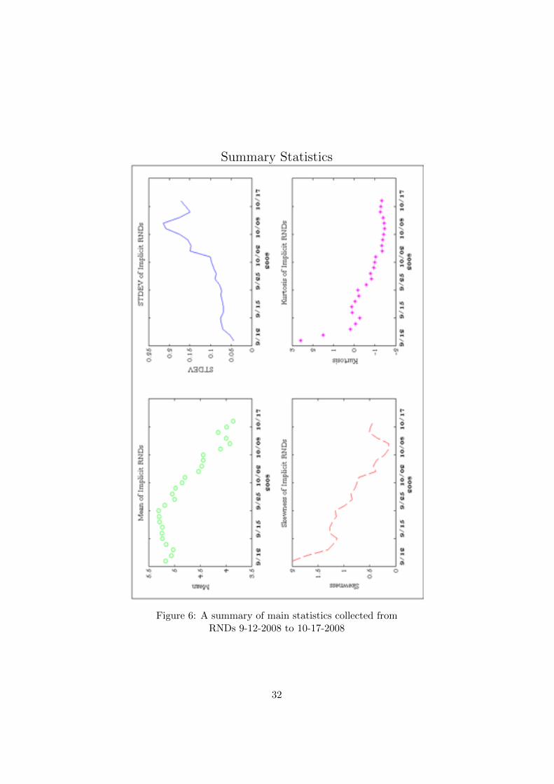
Summary Statistics

Figure 6: A summary of main statistics collected fromRNDs 9-12-2008 to 10-17-2008

32

7 Table

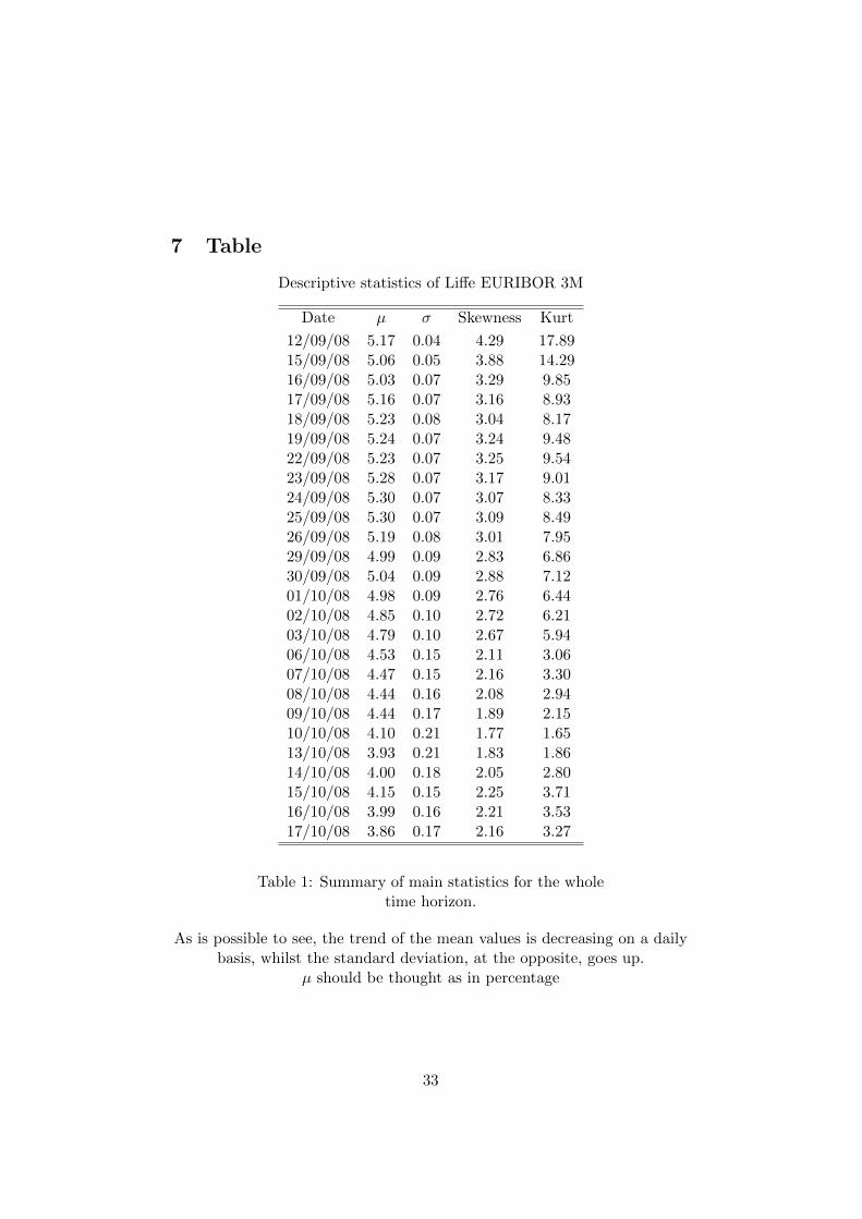
Descriptive statistics of Liffe EURIBOR 3M

Date µ σ Skewness Kurt

12/09/08 5.17 0.04 4.29 17.8915/09/08 5.06 0.05 3.88 14.2916/09/08 5.03 0.07 3.29 9.8517/09/08 5.16 0.07 3.16 8.9318/09/08 5.23 0.08 3.04 8.1719/09/08 5.24 0.07 3.24 9.4822/09/08 5.23 0.07 3.25 9.5423/09/08 5.28 0.07 3.17 9.0124/09/08 5.30 0.07 3.07 8.3325/09/08 5.30 0.07 3.09 8.4926/09/08 5.19 0.08 3.01 7.9529/09/08 4.99 0.09 2.83 6.8630/09/08 5.04 0.09 2.88 7.1201/10/08 4.98 0.09 2.76 6.4402/10/08 4.85 0.10 2.72 6.2103/10/08 4.79 0.10 2.67 5.9406/10/08 4.53 0.15 2.11 3.0607/10/08 4.47 0.15 2.16 3.3008/10/08 4.44 0.16 2.08 2.9409/10/08 4.44 0.17 1.89 2.1510/10/08 4.10 0.21 1.77 1.6513/10/08 3.93 0.21 1.83 1.8614/10/08 4.00 0.18 2.05 2.8015/10/08 4.15 0.15 2.25 3.7116/10/08 3.99 0.16 2.21 3.5317/10/08 3.86 0.17 2.16 3.27

Table 1: Summary of main statistics for the wholetime horizon.

As is possible to see, the trend of the mean values is decreasing on a dailybasis, whilst the standard deviation, at the opposite, goes up.

µ should be thought as in percentage

33