Impact of spatial filters during sensor selection in avisual P300 Brain-Computer Interface

B. Rivet 1, H. Cecotti 1, E. Maby 2, J. Mattout 2

1 GIPSA-lab CNRS UMR 5216Grenoble Universities

F-38402 Saint Martin d’Heres, France2 INSERM, U821, Lyon, F-69500, France

Institut Federatif des Neurosciences, Lyon, F-69000, FranceUniversite Lyon 1, Lyon, F-69000, France

Abstract. A challenge in designing a Brain-Computer Interface (BCI) is the choiceof the channels, e.g. the most relevant sensors. Although a setup with many sensorscan be more efficient for the detection of Event-Related Potential (ERP) like theP300, it is relevant to consider only a low number of sensors for a commercial orclinical BCI application. Indeed, a reduced number of sensors can naturally increasethe user comfort by reducing the time required for the installation of the EEG(electroencephalogram) cap and can decrease the price of the device. In this study, theinfluence of spatial filtering during the process of sensor selection is addressed. Threesensor selection approaches based on a recursive backward elimination are compared.Two of them maximize the Signal to Signal-plus-Noise Ratio (SSNR) for the differentsensor subsets while the third one maximizes the differences between the averagedP300 waveform and the non P300 waveform. We show that the locations of the mostrelevant sensors subsets for the detection of the P300 are highly dependent on the useof spatial filtering. Applied on data from 20 healthy subjects, this study proves thatsubsets obtained where sensors are suppressed in relation to their individual SSNR areless efficient than when sensors are suppressed in relation to their contribution oncethe different selected sensors are combined for enhancing the signal. In other words,it highlights the difference between estimating the P300 projection on the scalp andevaluating the more efficient sensor subsets for a P300-BCI. Finally, this study exploresthe issue of channel commonality across subjects. The results support the conclusionthat spatial filters during sensor selection procedure allow selecting better sensors fora visual P300 Brain-Computer Interface.

Keywords: Brain-Computer Interface, P300, EEG, BLDA, Sensor selection

hal-0

0660

288,

ver

sion

1 -

16 J

an 2

012

Author manuscript, published in "Brain Topography 25, 1 (2012) 55-63" DOI : 10.1007/s10548-011-0193-y

Impact of spatial filters during sensor selection in a visual P300 Brain-Computer Interface2

1. Introduction

A Brain-computer interface (BCI) enables a user to communicate through the direct

and real-time measurements of brain activity [1]. For patients suffering from severe

motor disabilities, e.g. locked-in patients, a BCI may often represent the only mean

of communication between the patients and their family. BCIs may actually provide

the only communication pathway for patients who are unable to communicate via

conventional means [2]. Although a remaining challenge is to get an efficient working

BCI, other challenges aim at reducing the cost of a BCI and to bring BCI technology to

mass market, to healthy persons for new BCI applications [3, 4]. This necessary step can

require the reduction of the number of electrodes and the adaptation of their locations

for each user [5]. Indeed, reducing the number of sensors yields more comfort for the

user, decreases installation time duration and may substantially reduce the financial

cost of the BCI setup since the cost of an EEG cap and an amplifier vary in relation

to the number of channels. Besides, the reduction of the number of sensors can also

reduce the power consumption for wireless EEG caps [6]. This point is relevant for BCI

applications like video games or for other applications where the number of sensors is

limited. Finally sensor selection may facilitate the classifier work by selecting a reduced

and more relevant set of input features.

Several strategies are possible for selecting a subset of sensors. For instance, one

can select sensors based on prior knowledge from neuroscience studies that can provide

the source of the potentials. In such a case, the subset is fixed and may jeopardize the

performance in some subjects as the optimal sensor subset is subject-dependent [7].

To obtain optimal performance, it is mandatory to clearly identify subject-specific

optimal sensor subsets. For a given set of N sensors, there are 2N − 1 different possible

subsets, without the empty subset. To find the optimal subset, three main searching

hal-0

0660

288,

ver

sion

1 -

16 J

an 2

012

Impact of spatial filters during sensor selection in a visual P300 Brain-Computer Interface3

approaches can be considered: exhaustive, random or sequential search. The exhaustive

search is usually not possible: the search space is often exponentially prohibitive. The

sequential and random search does not guarantee optimality as it gives up completeness.

However, it is easily implementable and can provide suboptimal solutions given some

evaluation criterion. Several variations are described in the literature like the greedy hill-

climbing approach, forward selection, backward elimination or bi-directional selection.

For instance, recursive feature elimination was used for sensor selection in BCI based

on motor imagery [8, 9]. In this paper, we consider a recursive backward elimination

strategy to determine which sensor should be removed in the widely used P300 speller

paradigm [10]. The impact of spatial filtering during the selection of the more relevant

sensor subsets is then evaluated with the P300 speller accuracy. Moreover an analysis

of commonality of selected channels across subjects is studied. The remainder of the

paper is organized as follows: the sensor selection strategy and the different methods

are described in the second section; the materials and the experimental protocol are

presented in the third section; and finally, results are compared and discussed in the

last section.

2. Methods

2.1. Data modeling: xDAWN framework

The proposed method to select adaptively a relevant subset of sensors is intimately

related to the special structure shared by the data due to the oddball paradigm used

in a visual P300 BCI. Indeed, the xDAWN framework [11] provides an algebraic model

of the recorded signals X ∈ RNt×Ns (where Nt is the number of time samples in the

recorded EEG signal and Ns the number of sensors) by considering that X is composed

of three additive terms: (i) the P300 responses A1 related to target stimuli, (ii) responses

hal-0

0660

288,

ver

sion

1 -

16 J

an 2

012

Impact of spatial filters during sensor selection in a visual P300 Brain-Computer Interface4

A2 common to every stimuli, and (iii) the residual noise H. As a consequence, one can

write X as

X = D1A1 +D2A2 +H, (1)

where A1 ∈ RN1×Ns and A2 ∈ RN2×Ns are the patterns representing one target evoked

potential (i.e. the P300 response) whose length is N1 samples and one common evoked

potential whose length is N2 samples, respectively. D1 ∈ RNt×N1 (resp. D2 ∈ RNt×N2)

is a Toeplitz matrix whose first column entries are set to zero except for those that

correspond to a target (resp. every) onset which are equal to one. D1A1 and D2A2 thus

represent the superposition of all targets and common responses, respectively. This

parametrization takes into account the possible overlapping between target potentials

and/or between common potentials and it allows to estimate these responses in the least

mean square sense by A1

A2

= ([D1;D2]T [D1;D2])−1[D1;D2]TX (2)

where [D1;D2] is a matrix of size Nt × (N1 +N2) obtained by concatenation of D1 and

D2. xDAWN model (1) and estimation (2) are useful to define the Signal to Signal plus

Noise Ratio (SSNR) of the i-th sensor by

ρ(ei, X) = eTi A

T1D

T1 D1A1ei

eTi X

TXei

, (3)

where ei ∈ RNs is a zero vector but the i-th element equal to 1. Y ei is thus the i-th

column of a matrix Y .

The purpose of applying spatial filter u ∈ RNs is to create a virtual sensor so

that the resulting signal Xu provides a larger SSNR ρ(u, X) than SSNR achieved by

actual sensors maxi ρ(ei, X). xDAWN framework [11] also provides a way to estimate

Nf spatial filters ui, i ∈ {1, · · · , Nf}, that maximize the SSNR (3).

hal-0

0660

288,

ver

sion

1 -

16 J

an 2

012

Impact of spatial filters during sensor selection in a visual P300 Brain-Computer Interface5

2.2. Sensor selection

The chosen method for adaptively selecting a relevant subset of sensors is based on a

recursive backward elimination. Starting with all sensors, it consists in alternatively

testing each sensor for its significance and in removing the least relevant one at each

iteration step. An irrelevant sensor is a sensor whose removal barely impairs the

performance or selection criterion. In this work, we eliminate two sensors at a time,

leaving us with the most significant remaining subset. Elimination goes on until every

sensor has been eliminated. At the end of the selection process, sensors can be ranked

according to their revealed significance. A relevant sensor will be eliminated at the

end of the iterative process while a useless one will be eliminated along the very first

iterations.

The cost function that determines the relevance of a sensor subset is based on the

evaluation of the SSNR. The cost function of the sensor subset I can be estimated as a

function of the individual SSNR ρ(ei, X) of each actual sensor

sa(I) =∑i∈I

ρ(ei, X). (4)

This solution is denoted AS as actual sensor. Moreover, the SSNR can also be estimated

after some spatial filtering. In this case, the score function is estimated globally as a

function of the grouped SSNR from the virtual sensors

sv(I) =Nf∑k=1

ρ(uk, XEI), (5)

where EI is the matrix whose columns are the concatenation of vectors ei with i ∈ I.

This technique is referred as V S as virtual sensor.

As a reference, the score function based on the largest difference between the

averaged P300 trials waveform and the averaged non P300 trials waveform is finally

considered and this method is denoted (Ref). In this case the score function of the

hal-0

0660

288,

ver

sion

1 -

16 J

an 2

012

Impact of spatial filters during sensor selection in a visual P300 Brain-Computer Interface6

AS: SSNRV S: Spatial Filters (SF) + SSNRRef: Largest difference between P300 and Non P300 trials

Table 1. The three criteria for backward selecting the most relevant sensors.

sensor subset I is estimated as

sr(I) =∑i∈I

(xP 300i − xNP 300

i )T (xP 300i − xNP 300

i ), (6)

where xP 300i (resp. xNP 300

i ) is the vector of the averaged P300 (resp. non P300) trials

waveform at channel i.

Finally, the backward elimination procedure is summarized in Algorithm 1 where

the considered score functions are presented in Table 1.

Algorithm 1 Backward elimination to sensor selection.Initialize I = {1, · · · , Ns}for i = 1 to Ns do

for all j ∈ I doCompute score function s.(I \ j) of I \ j = {i ∈ I|i 6= j}

end forEstimate less relevant sensor j = arg maxj s.(I \ j)Remove less relevant sensor: I ← I \ j

end for

The objectives of the experiments are to evaluate and to compare the impact of

the spatial filters during the selection process, i.e. the difference between method AS

which eliminates the individual less relevant sensors in relation to their individual SSNR

ρ(ei, X), and method V S that selects the most relevant sensors in relation to their

grouped SSNR ρ(u, XEI).

3. Materials

The EEG signal was recorded on 20 healthy subjects (mean age= 26, sd= 5.7; 7 females)

with the OpenViBE framework [12]. Each subject filled a consent form prior to the

hal-0

0660

288,

ver

sion

1 -

16 J

an 2

012

Impact of spatial filters during sensor selection in a visual P300 Brain-Computer Interface7

experiment. Subjects were wearing a standard EEG cap with 32 electrodes subsampled

from the 10-10 system [13]. The EEG activity was recorded continuously from 32 active

electrodes (actiCap, Brain Products GmbH, Munich). The electrodes for the ground

and the reference were placed on the forehead and the nose, respectively.

For the evaluation of the spatial filters impact during sensor selection, two sessions

were considered. The P300 speller was presented to the subjects as described in [14],

with a square matrix of 36 symbols, where one symbol is a letter or a digit. The first

session was dedicated to the estimation of different subsets of sensors and for training

the classifier. The second session was for testing the P300 speller. In both sessions, the

number of repetitions was fixed to 10, i.e. each symbol is spelt 10 consecutive times.

The first and second sessions contained 50 and 60 symbols, respectively. The Interval

Stimulus Interval (ISI) was 170ms for the training session. For the test session, four

groups of 15 characters had an ISI of 110, 150, 190 and 230ms, respectively‡. The

average ISI in the test session was like the training session, i.e. 170ms.

The EEG signal was sampled at 100Hz and was bandpass filtered between 1Hz and

12.5Hz with a Butterworth filter (order=4). Finally the features vector is obtained by a

downsampling to 25Hz for speeding up the computation time and reducing the number

of features. Such decimation parameter has been successfully applied in other studies

about the P300 speller [15, 16]. For each sensor and for each trial, the signals were

normalized so that they had a zero mean and a standard deviation equal to one. A

Bayesian linear discriminant analysis (BLDA) classifier is considered for the detection

of the P300 [7, 17].

‡ Note that in this study, the different ISI are not exploited as a parameter.

hal-0

0660

288,

ver

sion

1 -

16 J

an 2

012

Impact of spatial filters during sensor selection in a visual P300 Brain-Computer Interface8

1 2 3 4 5 6 7 8 9 10 11 12 13 14 15 16 17 18 19 20 Mean0

20

40

60

80

100

Subject number

Cla

ssifi

catio

nac

cura

cy [%

]

RefASVSAll

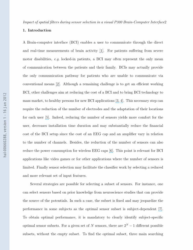
Figure 1. Impact of the sensor subsets on the recognition rate of the P300 speller.

4. Results

The P300 speller was evaluated with different sensor subsets as defined in the previous

section. For each selected sensor subset, the signal was first enhanced by using spatial

filters before the classification stage performed by a BLDA for the detection of the P300.

For the classification, a sequence of 0.6s from a visual stimulus has been considered for

each trial. Therefore, the P300 response is expected to be centered on the chosen time

sequence. For each subject, the number of P300 trials and non P300 trials are 1200 and

6000, respectively, for the test session. Based on a previous study [18], we only consider

a subset of four selected sensors by the different methods (AS, V S and Ref) since it

has been shown that four sensors is a good tradeoff between the number of sensors and

the classification accuracy. The impact of spatial filters during the selection process

is firstly assessed (Section 4.1). The commonality of channels across subjects is then

studied (Section 4.2).

4.1. Impact of spatial filters during sensor selection

Figure 1 presents the recognition rate of the P300 speller, with 10 repetitions, for the

subsets of four sensors obtained with the three methods (AS, V S, Ref), and for the

whole set of 32 sensors (All). The average recognition rate is 80.4%, 76.4%, 90.3% and

95.8% for the subsets obtained with Ref , AS, V S and the whole set (All), respectively.

hal-0

0660

288,

ver

sion

1 -

16 J

an 2

012

Impact of spatial filters during sensor selection in a visual P300 Brain-Computer Interface9

The performance of the P300 speller is always better (excepted for subject 2) with the

four sensors selected with method V S (i.e. with spatial filters) compared to AS or to

Ref . Two-tailed t-tests (5% significance level) indicate that the method V S provides

better sensors than AS (t(19) = 4.42, sd = 8.4, p < 5e−4) and than Ref (t(19) = 4.10,

sd = 6.49, p < 1e−3). A pairwise two-tailed t-test has also been used to compare the

speller accuracy with sensors obtained with V S and the whole set. As expected, the

result of the t-test indicates a rejection of the null hypothesis at the 5% significance

level. It shows that the whole set of 32 sensors (All) provides a better performance than

the 4 sensors obtained with V S (t(19) = 2.62, sd = 5.36, p < 2e−2).

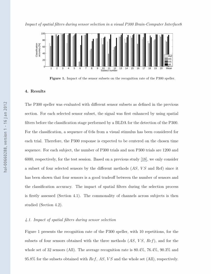
The position of the best sensors selected with the methods AS and V S is depicted

for every subject in Figure 2. The grey color represents the sensor relevance, i.e. a

dark grey means the location is relevant. For both methods, the sensor subsets are

not homogeneously located across subjects, highlighting the variability across subjects.

In a general way, V S provides sparser sensors than AS. Nevertheless, as depicted in

Figure 3, the grand average of the evoked response obtained after the spatial filtering

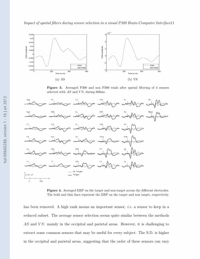
step of the four sensors selected by AS and V S show that the V S method provides a

better defined evoked response, i.e. a less large P300 wave, than the AS method. Note

that the N200 component is also visible before the P300 peak for both AS and V S.

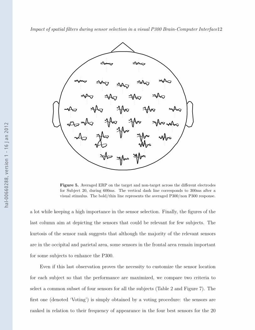
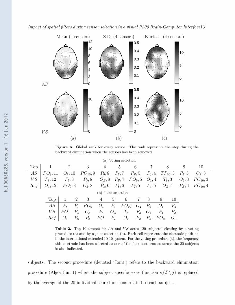
Figure 4 (resp. Figure 5) depicts the averaged P300 and non P300 waves across all

subjects (resp. for Subject 20) and all sessions. This latter subject is a good example

to provide evidence that electrodes with a relative low amplitude can be relevant in a

sensor selection procedure. Indeed, one may directly point out the projection of the

P300 over PZ as the amplitude of the P300 is higher than with other sensors. However,

this electrode was not selected in the best sensor subsets as presented in Figure 1, (S20

(AS) and S20 (VS)). Instead, electrodes closer to the bilateral occipito-temporal parts

hal-0

0660

288,

ver

sion

1 -

16 J

an 2

012

Impact of spatial filters during sensor selection in a visual P300 Brain-Computer Interface10

S1 (AS) S1 (V S) S2 (AS) S2 (V S) S3 (AS) S3 (V S) S4 (AS) S4 (V S)

S5 (AS) S5 (V S) S6 (AS) S6 (V S) S7 (AS) S7 (V S) S8 (AS) S8 (V S)

S9 (AS) S9 (V S) S10 (AS) S10 (V S) S11 (AS) S11 (V S) S12 (AS) S12 (V S)

S13 (AS) S13 (V S) S14 (AS) S14 (V S) S15 (AS) S15 (V S) S16 (AS) S16 (V S)

S17 (AS) S17 (V S) S18 (AS) S18 (V S) S19 (AS) S19 (V S) S20 (AS) S20 (V S)

Figure 2. Position of the 4 best sensors for the criteria AS and VS. A dark/light greyrepresents a relevant/non relevant sensor location.

were selected.

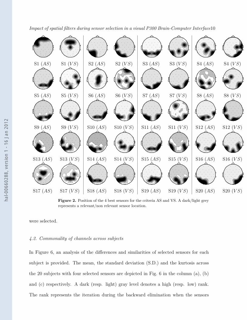
4.2. Commonality of channels across subjects

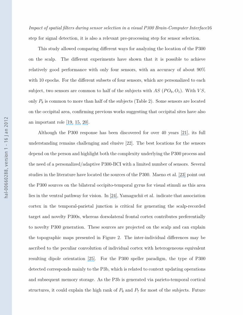
In Figure 6, an analysis of the differences and similarities of selected sensors for each

subject is provided. The mean, the standard deviation (S.D.) and the kurtosis across

the 20 subjects with four selected sensors are depicted in Fig. 6 in the column (a), (b)

and (c) respectively. A dark (resp. light) gray level denotes a high (resp. low) rank.

The rank represents the iteration during the backward elimination when the sensors

hal-0

0660

288,

ver

sion

1 -

16 J

an 2

012

Impact of spatial filters during sensor selection in a visual P300 Brain-Computer Interface11

0 200 400 600−0.02

−0.015

−0.01

−0.005

0

0.005

0.01

0.015

0.02

0.025

Time (in ms)

P30

0 A

mpl

itude

P300Non P300

(a) AS

0 200 400 600−4

−2

0

2

4

6x 10

−3

Time (in ms)

P30

0 A

mpl

itude

P300Non P300

(b) VS

Figure 3. Averaged P300 and non P300 trials after spatial filtering of 4 sensorsselected with AS and V S, during 600ms.

Figure 4. Averaged ERP on the target and non-target across the different electrodes.The bold and thin lines represent the ERP on the target and non target, respectively.

has been removed. A high rank means an important sensor, i.e. a sensor to keep in a

reduced subset. The average sensor selection seems quite similar between the methods

AS and V S: mainly in the occipital and parietal areas. However, it is challenging to

extract some common sensors that may be useful for every subject. The S.D. is higher

in the occipital and parietal areas, suggesting that the order of these sensors can vary

hal-0

0660

288,

ver

sion

1 -

16 J

an 2

012

Impact of spatial filters during sensor selection in a visual P300 Brain-Computer Interface12

Figure 5. Averaged ERP on the target and non-target across the different electrodesfor Subject 20, during 600ms. The vertical dash line corresponds to 300ms after avisual stimulus. The bold/thin line represents the averaged P300/non P300 response.

a lot while keeping a high importance in the sensor selection. Finally, the figures of the

last column aim at depicting the sensors that could be relevant for few subjects. The

kurtosis of the sensor rank suggests that although the majority of the relevant sensors

are in the occipital and parietal area, some sensors in the frontal area remain important

for some subjects to enhance the P300.

Even if this last observation proves the necessity to customize the sensor location

for each subject so that the performance are maximized, we compare two criteria to

select a common subset of four sensors for all the subjects (Table 2 and Figure 7). The

first one (denoted ‘Voting’) is simply obtained by a voting procedure: the sensors are

ranked in relation to their frequency of appearance in the four best sensors for the 20

hal-0

0660

288,

ver

sion

1 -

16 J

an 2

012

Impact of spatial filters during sensor selection in a visual P300 Brain-Computer Interface13

Mean (4 sensors) S.D. (4 sensors) Kurtosis (4 sensors)

AS

0

2

4

6

8

10

12

0.1

0.2

0.3

0.4

0.5

0

5

10

V S

0

5

10

0

0.1

0.2

0.3

0.4

0.5

0

5

10

(a) (b) (c)

Figure 6. Global rank for every sensor. The rank represents the step during thebackward elimination when the sensors has been removed.

(a) Voting selection

Top 1 2 3 4 5 6 7 8 9 10AS PO9; 11 O1; 10 PO10; 9 P8; 8 P7; 7 PZ ; 5 P3; 4 TP10; 3 P4; 3 O2; 3V S P8; 12 P7; 8 P3; 8 OZ ; 8 PZ ; 7 PO9; 5 O1; 4 T8; 3 O2; 3 PO10; 3Ref O1; 12 PO9; 8 O2; 8 P3; 6 P8; 6 P7; 5 P4; 5 OZ ; 4 PZ ; 4 PO10; 4

(b) Joint selection

Top 1 2 3 4 5 6 7 8 9 10AS P8 P7 PO9 O1 P3 PO10 O2 P4 Oz Pz

V S PO9 P3 CZ P8 OZ T8 F3 O1 P4 PZ

Ref O1 P8 P3 PO9 P7 O2 PZ P4 PO10 OZ

Table 2. Top 10 sensors for AS and V S across 20 subjects selecting by a votingprocedure (a) and by a joint selection (b). Each cell represents the electrode positionin the international extended 10-10 system. For the voting procedure (a), the frequencythis electrode has been selected as one of the four best sensors across the 20 subjectsis also indicated.

subjects. The second procedure (denoted ‘Joint’) refers to the backward elimination

procedure (Algorithm 1) where the subject specific score function s.(I \ j) is replaced

by the average of the 20 individual score functions related to each subject.

hal-0

0660

288,

ver

sion

1 -

16 J

an 2

012

Impact of spatial filters during sensor selection in a visual P300 Brain-Computer Interface14

Ind. Ref Ind. AS Ind. VS Joint Ref Joint AS Joint VS Vot. Ref Vot. AS Vot. VS All0

20

40

60

80

100

Cla

ssifi

catio

nac

cura

cy [%

]

Figure 7. Comparison of classification accuracy achieved for all the 20 subjectsby several sensor selection procedures (Ref , AS and V S). ‘Ind.’, ‘Joint’ and ‘Vot.’refer to a subject specific selection, to the joint selection and to the voting selection,respectively. All refers to the classification accuracy achieved with all the 32 sensors.On each box, the central mark is the median, the edges of the box are the 25th and75th percentiles, the whiskers extend to the most extreme data points not consideredoutliers, and outliers are plotted individually.

As already mentioned, there is a large diversity across subjects about the location

of the most relevant sensors. Indeed, the largest value of the frequency of appearance

among the four most relevant sensors is only 11 or 12 depending of the selection criterion:

this means that this sensor is only common to about half of the subjects. It is also worth

noting that the voting and joint selection procedures provide quite different selected

sensors. Actually, for the V S method, if P8 and P3 are among the four selected sensors

for both voting and joint selection methods, PO9 is only ranked as the sixth most

relevant method by the voting selection whereas it is the most relevant sensor for the

joint selection. Even more surprising, CZ (resp. P7) is in the four most relevant sensor

for the joint (resp. voting) method while it is not among the 10 most relevant sensors

for the voting (resp. joint) selection. Furthermore, as shown by Figure 7, among the

joint and voting selection, the joint and voting selections with virtual sensor (Joint V S

and V ot. V S) provide the best classification accuracy. Indeed, with these four sensors

common to all the 20 subjects selected by Joint V S (resp. V ot. V S), the classification

accuracy is larger than 60% for 17 (resp. 16) of them and 16 (resp. 14) subjects achieved

even more than 75% of classification accuracy. Moreover eleven subjects achieved an

hal-0

0660

288,

ver

sion

1 -

16 J

an 2

012

Impact of spatial filters during sensor selection in a visual P300 Brain-Computer Interface15

impressive classification accuracy larger than 90% with only four sensors selected by

V ot. V S. Finally, this latter result highlights one more time the fact that using spatial

filters during the sensor selection is essential to provide accurate subsets of channels

since classification accuracy for both Joint V S and V ot. V S is larger than with AS or

Ref methods.

5. Conclusion and discussion

Three ways for the analysis of the best sensor location for P300 detection have been

proposed. In every solution, the method is based on a recursive backward elimination.

In the first case, sensors are suppressed in relation to their individual SSNR. In the

second case, sensors are suppressed in relation to their contribution once the different

selected sensors are combined for enhancing the signal. In the third solution, sensors

are suppressed in relation to the largest differences between P300 and Non P300 trials

waveforms. The results indicate that the sensors, which are contained in the best sensor

subset are different than the sensors that provide individually the best SSNR. In other

words, it proves that given a low number of sensors, the sensors contained in the best

subset are not individually the best sensors. This observation shows that the sensor

subset should be consider directly as a whole and not as the aggregation of individual

sensors in spite of the backward elimination procedure. Sensors should complement each

other in the subset to enhance the P300 detection. This highlights the difference between

two problems: evaluating the best sensor subsets for a P300-BCI, and estimating the

best P300 projection on the scalp.

Finally, the sensor selection method is not based on the detection of the P300

but only on the estimation of the SSNR, thus avoiding different stages like classifiers

training and cross validation. Spatial filtering is not only a necessary pre-processing

hal-0

0660

288,

ver

sion

1 -

16 J

an 2

012

Impact of spatial filters during sensor selection in a visual P300 Brain-Computer Interface16

step for signal detection, it is also a relevant pre-processing step for sensor selection.

This study allowed comparing different ways for analyzing the location of the P300

on the scalp. The different experiments have shown that it is possible to achieve

relatively good performance with only four sensors, with an accuracy of about 90%

with 10 epochs. For the different subsets of four sensors, which are personalized to each

subject, two sensors are common to half of the subjects with AS (PO9, O1). With V S,

only P8 is common to more than half of the subjects (Table 2). Some sensors are located

on the occipital area, confirming previous works suggesting that occipital sites have also

an important role [19, 15, 20].

Although the P300 response has been discovered for over 40 years [21], its full

understanding remains challenging and elusive [22]. The best locations for the sensors

depend on the person and highlight both the complexity underlying the P300 process and

the need of a personalized/adaptive P300-BCI with a limited number of sensors. Several

studies in the literature have located the sources of the P300. Maeno et al. [23] point out

the P300 sources on the bilateral occipito-temporal gyrus for visual stimuli as this area

lies in the ventral pathway for vision. In [24], Yamaguchii et al. indicate that association

cortex in the temporal-parietal junction is critical for generating the scalp-recorded

target and novelty P300s, whereas dorsolateral frontal cortex contributes preferentially

to novelty P300 generation. These sources are projected on the scalp and can explain

the topographic maps presented in Figure 2. The inter-individual differences may be

ascribed to the peculiar convolution of individual cortex with heterogeneous equivalent

resulting dipole orientation [25]. For the P300 speller paradigm, the type of P300

detected corresponds mainly to the P3b, which is related to context updating operations

and subsequent memory storage. As the P3b is generated via parieto-temporal cortical

structures, it could explain the high rank of P8 and P7 for most of the subjects. Future

hal-0

0660

288,

ver

sion

1 -

16 J

an 2

012

Impact of spatial filters during sensor selection in a visual P300 Brain-Computer Interface17

works will deal with the sensor selection in relation

hal-0

0660

288,

ver

sion

1 -

16 J

an 2

012

Impact of spatial filters during sensor selection in a visual P300 Brain-Computer Interface18

Acknowledgment

The authors thank the anonymous reviewers for their pertinent comments which allow

to drastically improve the quality of this paper.

This work has been supported by French National Research Agency (ANR) through

TecSan program (project RoBIK ANR-09-TECS-013) and through DEFIS program

(project Co-Adapt ANR-09-EMER-002).

References

[1] B. Z. Allison, E. W. Wolpaw, and J. R. Wolpaw. Brain-computer interface systems: progress and

prospects. Expert Review of Medical Devices, 4(4):463–474, 2007.

[2] N. Birbaumer and L. G. Cohen. Brain-computer interfaces: communication and restoration of

movement in paralysis. Journal of Physiology-London, 579(3):621–636, 2007.

[3] C. Guger, G. Edlinger, W. Harkam, I. Niedermayer, and G. Pfurtscheller. How many people

are able to operate an EEG-based brain-computer interface (BCI)? IEEE Trans. Neural Syst

Rehabil Eng., 11(2):145–147, 2003.

[4] C. Guger, S. Daban, E. Sellers, C. Holznera, G. Krausza, R. Carabalonac, F. Gramaticac, and

G. Edlinger. How many people are able to control a P300-based brain.computer interface (BCI)?

Neuroscience Letters, 462:94–98, 2009.

[5] C. Sannelli, T. Dickhaus, S. Halder, E.-M. Hammer, K.-R. Muller, and B. Blankertz. On optimal

channel configurations for SMR-based brain-computer interfaces. Brain Topogr, 23(2):186–193,

2010.

[6] E. I. Shih, A. H. Shoeb, and J. V. Guttag. Sensor selection for energy-efficient ambulatory medical

monitoring. In Proc. of the 7th International Conference on Mobile Systems, Applications and

Services, pages 347–358, 2009.

[7] U. Hoffmann, J. M. Vesin, K. Diserens, and T. Ebrahimi. An efficient P300-based brain-computer

interface for disabled subjects. Journal of Neuroscience Methods, 167(1):115–125, 2008.

[8] T. N. Lal, M. Schroder, T. Hinterberger, J. Weston, M. Bogdan, N. Birbaumer, and B. Scholkopf.

Support vector channel selection in BCI. IEEE Trans. Biomed. Engineering, 51(6):1003–1010,

2004.

hal-0

0660

288,

ver

sion

1 -

16 J

an 2

012

Impact of spatial filters during sensor selection in a visual P300 Brain-Computer Interface19

[9] M. Schroder, T. N. Lal, T. Hinterberger, M. Bogdan, J. N. N. Jeremy Hill, N. Birbaumer,

W. Rosenstiel, and B. Scholkopf. Robust EEG channel selection across subjects for brain-

computer interfaces. EURASIP Journal on Applied Signal Processing, 19:3103–3112, 2005.

[10] E. Donchin, K. M. Spencer, and R. Wijesinghe. Assessing the speed of a P300-based brain-

computer interface. IEEE Trans. Neural Sys. Rehab. Eng., 8(2):174–179, 2000.

[11] B. Rivet, A. Souloumiac, V. Attina, and G. Gibert. xDAWN algorithm to enhance evoked

potentials: application to brain-computer interface. IEEE Trans Biomed Eng., 56(8):2035–43,

2009.

[12] E. Maby, G. Gibert, P.-E. Aguera, M. Perrin, O. Bertrand, and J. Mattout. The OpenViBE

P300-Speller scenario: a thorough online evaluation. In Human Brain Mapping Conference,

2010.

[13] F. Sharbrough, G. Chatrian, and R. P. et al. Lesser. Guidelines for standard electrode position

nomenclature. Bloomfield, IL: American EEG Society, 1990.

[14] L. Farwell and E. Donchin. Talking off the top of your head: toward a mental prosthesis utilizing

event-related brain potentials. Electroencephalogr. Clin. Neurophysiol., 70:510–523, 1988.

[15] H. Cecotti and A. Graser. Convolutional neural networks for P300 detection with application to

brain-computer interfaces. IEEE Trans. Pattern Analysis and Machine Intelligence, 2010.

[16] A. Rakotomamonjy and V. Guigue. BCI competition iii : Dataset ii - ensemble of SVMs for BCI

P300 speller. IEEE Trans. Biomedical Engineering, 55(3):1147–1154, 2008.

[17] D. J. C. MacKay. Bayesian interpolation. Neural Comput., 4(3):415–447, 1992.

[18] B. Rivet, A. Souloumiac, G. Gibert, V. Attina, and O. Bertrand. Sensor selection for P300 speller

brain computer interface. In Proc. European Symposium on Artificial Neural Networks, pages

431–438, Bruges, Belgiunm, 2009.

[19] L. Bianchi, S. Sami, A. Hillebrand, I. P. Fawcett, L. R. Quitadamo, and S. Seri. Which

physiological components are more suitable for visual ERP based brain-computer interface?

a preliminary MEG/EEG study. Brain Topogr, 23(2):180–185, 2010.

[20] D. J. Krusienski, E. W. Sellers, D.J. McFarland, T. M. Vaughan, and J. R. Wolpaw. Toward

enhanced P300 speller performance. Journal of Neuroscience Methods, 167:15–21, 2008.

[21] S. Sutton, M. Braren, J. Zubin, and E. R. John. Evoked potential correlates of stimulus

uncertainty. Science, 150:1187–1188, 1965.

[22] J. Polich. Updating P300: An integrative theory of P3a and P3b. Clinical Neurophysiology,

hal-0

0660

288,

ver

sion

1 -

16 J

an 2

012

Impact of spatial filters during sensor selection in a visual P300 Brain-Computer Interface20

118:2128–2148, 2007.

[23] T. Maeno, A. Kaneko, K. Iramina, F. Eto, and S. Ueno. Source modeling of the P300 event-

related response using magnetoencephalography and electroencephalography measurements.

IEEE Trans on Magnetics, 39(5):3396–3398, 2003.

[24] S. Yamaguchii and R. T. Knight. Anterior and posterior association cortex contributions to the

somatosensory P300. Journal of Neuroscience, 11(7):2039–2054, 1991.

[25] I. M. Tarkka and D. S. Stokic. Source localization of P300 from oddball, single stimulus, and

omitted-stimulus paradigms. Brain Topography, 1(2):141–151, 1998.

hal-0

0660

288,

ver

sion

1 -

16 J

an 2

012