ICSEA 2018 Proceedings - ThinkMind

ICSEA 2018

The Thirteenth International Conference on Software Engineering Advances

ISBN: 978-1-61208-668-2

October 14 - 18, 2018

Nice, France

ICSEA 2018 Editors

Luigi Lavazza, Università dell'Insubria - Varese, Italy

Roy Oberhauser, Aalen University, Germany

Radek Koci, Brno University of Technology, Czech Republic

1 / 160

ICSEA 2018

Forward

The Thirteenth International Conference on Software Engineering Advances (ICSEA 2018), heldon October 14 - 18, 2018- Nice, France, continued a series of events covering a broad spectrum ofsoftware-related topics.

The conference covered fundamentals on designing, implementing, testing, validating andmaintaining various kinds of software. The tracks treated the topics from theory to practice, in terms ofmethodologies, design, implementation, testing, use cases, tools, and lessons learnt. The conferencetopics covered classical and advanced methodologies, open source, agile software, as well as softwaredeployment and software economics and education.

The conference had the following tracks:

Advances in fundamentals for software development

Advanced mechanisms for software development

Advanced design tools for developing software

Software engineering for service computing (SOA and Cloud)

Advanced facilities for accessing software

Software performance

Software security, privacy, safeness

Advances in software testing

Specialized software advanced applications

Web Accessibility

Open source software

Agile and Lean approaches in software engineering

Software deployment and maintenance

Software engineering techniques, metrics, and formalisms

Software economics, adoption, and education

Business technology

Improving productivity in research on software engineering

Trends and achievements

Similar to the previous edition, this event continued to be very competitive in its selection processand very well perceived by the international software engineering community. As such, it is attractingexcellent contributions and active participation from all over the world. We were very pleased to receivea large amount of top quality contributions.

We take here the opportunity to warmly thank all the members of the ICSEA 2018 technical programcommittee as well as the numerous reviewers. The creation of such a broad and high quality conferenceprogram would not have been possible without their involvement. We also kindly thank all the authorsthat dedicated much of their time and efforts to contribute to the ICSEA 2018. We truly believe thatthanks to all these efforts, the final conference program consists of top quality contributions.

2 / 160

This event could also not have been a reality without the support of many individuals, organizationsand sponsors. We also gratefully thank the members of the ICSEA 2018 organizing committee for theirhelp in handling the logistics and for their work that is making this professional meeting a success.

We hope the ICSEA 2018 was a successful international forum for the exchange of ideas and resultsbetween academia and industry and to promote further progress in software engineering research. Wealso hope Nice provided a pleasant environment during the conference and everyone saved some timefor exploring this beautiful city.

ICSEA 2018 Steering Committee

Herwig Mannaert, University of Antwerp, BelgiumMira Kajko-Mattsson, Royal Institute of Technology, SwedenLuigi Lavazza, Università dell'Insubria - Varese, ItalyRoy Oberhauser, Aalen University, GermanyElena Troubitsyna, Abo Akademi University, FinlandRadek Koci, Brno University of Technology, Czech RepublicStephen W. Clyde, Utah State University, USASébastien Salva, University Clermont Auvergne (UCA), Limos, FranceChristian Kop, Universitaet Klagenfurt, AustriaLuis Fernandez-Sanz, Universidad de Alcala, SpainBidyut Gupta, Southern Illinois University, USA

ICSEA 2018 Industry/Research Advisory Committee

Teemu Kanstrén, VTT Technical Research Centre of Finland - Oulu, FinlandJ. Paul Gibson, Telecom Sud Paris, FranceAdriana Martin, National University of Austral Patagonia (UNPA), ArgentinaMuthu Ramachandran, Leeds Beckett University, UKMichael Gebhart, iteratec GmbH, Germany

3 / 160

ICSEA 2018

Committee

ICSEA Steering CommitteeHerwig Mannaert, University of Antwerp, BelgiumMira Kajko-Mattsson, Royal Institute of Technology, SwedenLuigi Lavazza, Università dell'Insubria - Varese, ItalyRoy Oberhauser, Aalen University, GermanyElena Troubitsyna, Abo Akademi University, FinlandRadek Koci, Brno University of Technology, Czech RepublicStephen W. Clyde, Utah State University, USASébastien Salva, University Clermont Auvergne (UCA), Limos, FranceChristian Kop, Universitaet Klagenfurt, AustriaLuis Fernandez-Sanz, Universidad de Alcala, SpainBidyut Gupta, Southern Illinois University, USA

ICSEA Industry/Research Advisory CommitteeTeemu Kanstrén, VTT Technical Research Centre of Finland - Oulu, FinlandJ. Paul Gibson, Telecom Sud Paris, FranceAdriana Martin, National University of Austral Patagonia (UNPA), ArgentinaMuthu Ramachandran, Leeds Beckett University, UKMichael Gebhart, iteratec GmbH, Germany

ICSEA 2018 Technical Program Committee

Shahliza Abd Halim, Universiti of Technologi Malaysia (UTM), MalaysiaErika Abraham, RWTH Aachen University, GermanyMuhammad Ovais Ahmad, University of Oulu, FinlandJacky Akoka, CNAM & IMT, FranceSaadia Binte Alam, Advanced Medical Engineering Center (AMEC) | University of Hyogo, JapanMohammad Alshayeb, King Fahd University of Petroleum and Minerals, Saudi ArabiaZakarya Alzamil, King Saud University, Saudi ArabiaDaniel Andresen, Kansas State University, USAGilbert Babin, HEC Montréal, CanadaDoo-Hwan Bae, School of Computing - KAIST, KoreaAleksander Bai, Norsk Regnesentral, NorwayJorge Barreiros, ISEC (Instituto Superior de Engenharia de Coimbra) / NOVA-LINCS, PortugalBernhard Bauer, University of Augsburg, GermanyAteet Bhalla, Independent Consultant, IndiaKenneth Boness, University of Reading, UKMina Boström Nakicenovic, NetEnt, Stockholm, SwedenNadia Bouassida, Higher Institute of Multimedia and Informatics, Sfax, TunisiaHongyu Pei Breivold, ABB Corporate Research, SwedenFernando Brito e Abreu, Instituto Universitário de Lisboa (ISCTE-IUL), Portugal

4 / 160

Georg Buchgeher, Software Competence Center Hagenberg GmbH, AustriaLuigi Buglione, Engineering Ingegneria Informatica SpA, ItalyCarlos Henrique Cabral Duarte, Brazilian Development Bank (BNDES), BrazilHaipeng Cai, Washington State University, Pullman, USAGabriel Campeanu, Mälardalen University, SwedenRicardo Campos, Polytechnic Institute of Tomar | LIAAD / INESC TEC - INESC Technology and Science,Porto, PortugalJosé Carlos Metrolho, Polytechnic Institute of Castelo Branco, PortugalEverton Cavalcante, Federal University of Rio Grande do Norte, BrazilAntonin Chazalet, Orange, FranceFuxiang Chen, Hong Kong University of Science and Technology, Hong KongFederico Ciccozzi, Mälardalen University, SwedenMarta Cimitile, University Unitelma Sapienza of Rome, ItalySiobhán Clarke, Trinity College Dublin | University of Dublin, IrelandStephen W. Clyde, Utah State University, USAMethanias Colaço Júnior, Federal University of Sergipe, BrazilRebeca Cortazar, University of Deusto, SpainMonica Costa, Politechnic Institute of Castelo Branco, PortugalBeata Czarnacka-Chrobot, Warsaw School of Economics, PolandDarren Dalcher, Hertfordshire Business School, UKYuetang Deng, Tencent, ChinaVincenzo Deufemia, University of Salerno, ItalyThemistoklis Diamantopoulos, Aristotle University of Thessaloniki, GreeceIvan do Carmo Machado, Federal University of Bahia (UFBA), BrazilTadashi Dohi, Hiroshima University, JapanLydie du Bousquet, Université Grenoble-Alpes (UGA), FranceJorge Edison Lascano, Universidad de las Fuerzas Armadas - ESPE, EcuadorHolger Eichelberger, University of Hildesheim, Software Systems Engineering, GermanyYounes El Amrani, University Mohammed-V Rabat, MoroccoGledson Elias, Federal University of Paraíba (UFPB), BrazilRomina Eramo, University of L'Aquila, ItalyFarima FarimahiniFarahani, University of California - Irvine, USAKleinner Farias, University of Vale do Rio dos Sinos, BrazilAdel Ferdjoukh, University of Nantes, FranceLuis Fernandez-Sanz, Universidad de Alcala, SpainM. Firdaus Harun, RWTH Aachen University, GermanyMohammed Foughali, INSA Toulouse, FranceJicheng Fu, University of Central Oklahoma, USAFelipe Furtado, CESAR - Recife Center for Advanced Studies an Systems, BrazilLuiz Eduardo Galvão Martins, Federal University of São Paulo, BrazilJose Garcia-Alonso, University of Extremadura, SpainMichael Gebhart, iteratec GmbH, GermanyWided Ghardallou, Faculty of Sciences of Tunis, TunisiaJ. Paul Gibson, Telecom Sud Paris, FrancePascal Giessler, Karlsruhe Institute of Technology, GermanyGregor Grambow, AristaFlow GmbH, GermanyJiaping Gui, University of Southern California, USAJoe Zhensheng Guo, Siemens AG - Muenchen, Germany

5 / 160

Bidyut Gupta, Southern Illinois University, USAKonstantin Gusarov, Riga Technical University, LatviaNahla Haddar Ouali, Higher Institute of Business Administration of Gafsa, TunisiaRachel Harrison, Oxford Brookes University, UKShinpei Hayashi, Tokyo Institute of Technology, JapanQiang He, Swinburne University of Technology, AustraliaPhilipp Helle, Airbus, GermanyJosé R. Hilera, University of Alcalá, SpainSiv Hilde Houmb, Secure-NOK AS, NorwayHelena Holmström Olsson, Malmö University, SwedenLiGuo Huang, Southern Methodist University, USAJun Iio, Chuo University, JapanGustavo Illescas, Universidad Nacional del Centro-Tandil-Bs.As., ArgentinaEmilio Insfran, Universitat Politecnica de Valencia, SpainShareeful Islam, University of East London, UKJudit Jász, University of Szeged, HungaryKashif Javed, Åbo Akademi University, FinlandMira Kajko-Mattsson, Royal Institute of Technology, SwedenHerwig Mannaert, University of Antwerp, BelgiumAdriana Martin, National University of Austral Patagonia (UNPA), ArgentinaAhmed Kamel, Offutt School of Business | Concordia College, USATeemu Kanstrén, VTT Technical Research Centre of Finland - Oulu, FinlandChia Hung Kao, National Taitung University, TaiwanCarlos Kavka, ESTECO SpA, ItalySiffat Ullah Khan, University of Malakand, PakistanReinhard Klemm, Avaya, USAMourad Kmimech, ISIMM | University of Monastir, TunisiaTakashi Kobayashi, Tokyo Institute of Technology, JapanRadek Koci, Brno University of Technology, Czech RepublicMieczyslaw Kokar, Northeastern University, Boston, USAChristian Kop, Universitaet Klagenfurt, AustriaGeorges Edouard Kouamou, National Advanced School of Engineering - Yaoundé, CameroonEmil Krsak, University of Žilina, Slovak RepublicRob Kusters, Eindhoven University of Technology & Open University, The NetherlandsAlla Lake, LInfo Systems, LLC - Greenbelt, USADieter Landes, University of Applied Sciences Coburg, GermanyJannik Laval, University of Lyon, FranceLuigi Lavazza, Università dell'Insubria - Varese, ItalyValentina Lenarduzzi, Tampere University of Technology, FinlandMaurizio Leotta, University of Genova, ItalyPanos Linos, Butler University, USAPeizun Liu, Northeastern University, USAAndré Magno Costa de Araújo, Federal University of Pernambuco, BrazilSajjad Mahmood, King Fahd University of Petroleum and Minerals, Saudi ArabiaNicos Malevris, Athens University of Economics and Business, GreeceNeel Mani, ADAPT Center for Digital Content Technology | Dublin City University, IrelandAlexandre Marcos Lins de Vasconcelos, Federal University of Pernambuco, BrazilAlessandro Margara, Politecnico di Milano, Italy

6 / 160

Daniela Marghitu, Auburn University, USABeatriz Marín, Universidad Diego Portales, ChileCélia Martinie, IRIT, University Toulouse 3 Paul Sabatier, FranceVanessa Matias Leite, Universidade Estadual de Londrina, BrazilFuensanta Medina-Dominguez, Carlos III University of Madrid, SpainMariem Mefteh, University of Sfax, TunisiaJose Merseguer, Universidad de Zaragoza, SpainVojtech Merunka, Czech University of Life Sciences in Prague / Czech Technical University in Prague,Czech RepublicSanjay Misra, Covenant University, NigeriaMd Rakib Hossain Misu, University of Dhaka, BangladeshÓscar Mortágua Pereira, Telecommunications Institute | University of Aveiro, PortugalMohammad Reza Nami, TUDelft University of Technology, The NetherlandsMarcellin Nkenlifack, University of Dschang, CameroonMarc Novakouski, Software Engineering Institute, USARoy Oberhauser, Aalen University, GermanyPablo Oliveira Antonino, Fraunhofer IESE, GermanyFlavio Oquendo, IRISA (UMR CNRS) - University of South Brittany, FranceMuhammed Maruf Öztürk, Suleyman Demirel University, TurkeyMarcos Palacios, University of Oviedo, SpainFabio Palomba, TU Delft, The NetherlandsMike Papadakis, University of Luxembourg, LuxembourgBeatriz Pérez Valle, University of La Rioja, SpainPasqualina Potena, RISE SICS Västerås, SwedenRafael Queiroz Gonçalves, Federal University of Santa Catarina, BrazilAbdallah Qusef, Princess Sumaya University for Technology, JordanClaudia Raibulet, Universita' degli Studi di Milano-Bicocca, ItalyMuthu Ramachandran, Leeds Beckett University, UKRaman Ramsin, Sharif University of Technology, IranGianna Reggio, DIBRIS - Università di Genova, ItalyFernando Reinaldo Ribeiro, Polytechnic Institute of Castelo Branco, PortugalMichele Risi, University of Salerno, ItalyGabriela Robiolo, Universidad Austral, ArgentinaRodrigo G. C. Rocha, Federal Rural University of Pernambuco - UFRPE, BrazilDaniel Rodriguez, University of Alcalá, SpainColette Rolland, University of Paris 1 Pantheon-Sorbonne, FranceSandro Ronaldo Bezerra Oliveira, UFPA - Federal University of Pará, BrazilÁlvaro Rubio-Largo, Universidade NOVA de Lisboa, PortugalMehrdad Saadatmand, RISE SICS Västerås, SwedenGunter Saake, Otto-von-Guericke-Universitaet, Magdeburg, GermanyFrancesca Saglietti, University of Erlangen-Nuremberg, GermanyDjamel Eddine Saidouni, University Constantine 2 - Abdelhamid Mehri, AlgeriaSébastien Salva, University Clermont Auvergne (UCA), Limos, FranceMaría-Isabel Sanchez-Segura, Carlos III University of Madrid, SpainHiroyuki Sato, University of Tokyo, JapanSagar Sen, Simula Research Laboratory, NorwayVesna Sesum-Cavic, Vienna University of Technology, AustriaIstvan Siket, University of Szeged, Hungary

7 / 160

Felipe Silva Ferraz, CESAR School, BrazilMaria Spichkova, RMIT University, AustraliaFausto Spoto, University of Verona / JuliaSoft Srl, ItalySidra Sultana, National University of Sciences and Technology, PakistanMahbubur Rahman Syed, Minnesota State University, Mankato, USASahar Tahvili, RISE SICS Västerås AB, SwedenShigeaki Tanimoto, Chiba Institute of Technology, JapanSobhan Yassipour Tehrani, King's College London & Jaguar Land Rover, UKDhafer Thabet, University of Mannouba, TunisiaPierre F. Tiako, Tiako University, USAElena Troubitsyna, Abo Akademi University, FinlandMariusz Trzaska, Polish-Japanese Academy of Information Technology, PolandMasateru Tsunoda, Kindai University, JapanSylvain Vauttier, LGI2P - Ecole des Mines d'Alès, FranceColin Venters, University of Huddersfield, UKLaszlo Vidacs, Hungarian Academy of Sciences / University of Szeged, HungaryVinay Vkulkarni, Tata Consultancy Services, IndiaStefan Voget, Continental Automotive GmbH, GermanySong Wang, University of Waterloo, CanadaHironori Washizaki, Waseda University / National Institute of Informatics / SYSTEM INFORMATION,JapanBingyang Wei, Texas Christian University, USAXusheng Xiao, Case Western Reserve University, USARihito Yaegashi, Kagawa University, JapanRohith Yanambaka Venkata, University of North Texas, USAGuowei Yang, Texas State University, USAStoyan Yordanov Garbatov, OutSystems, PortugalHaibo Yu, Shanghai Jiao Tong University, ChinaSaad Zafar, Riphah International University, Islamabad, PakistanMichal Žemlička, AŽD Praha / Charles University, Czech RepublicQiang Zhu, The University of Michigan, Dearborn, USAMartin Zinner, Technische Universität Dresden, Germany

8 / 160

Copyright Information

For your reference, this is the text governing the copyright release for material published by IARIA.

The copyright release is a transfer of publication rights, which allows IARIA and its partners to drive the

dissemination of the published material. This allows IARIA to give articles increased visibility via

distribution, inclusion in libraries, and arrangements for submission to indexes.

I, the undersigned, declare that the article is original, and that I represent the authors of this article in

the copyright release matters. If this work has been done as work-for-hire, I have obtained all necessary

clearances to execute a copyright release. I hereby irrevocably transfer exclusive copyright for this

material to IARIA. I give IARIA permission or reproduce the work in any media format such as, but not

limited to, print, digital, or electronic. I give IARIA permission to distribute the materials without

restriction to any institutions or individuals. I give IARIA permission to submit the work for inclusion in

article repositories as IARIA sees fit.

I, the undersigned, declare that to the best of my knowledge, the article is does not contain libelous or

otherwise unlawful contents or invading the right of privacy or infringing on a proprietary right.

Following the copyright release, any circulated version of the article must bear the copyright notice and

any header and footer information that IARIA applies to the published article.

IARIA grants royalty-free permission to the authors to disseminate the work, under the above

provisions, for any academic, commercial, or industrial use. IARIA grants royalty-free permission to any

individuals or institutions to make the article available electronically, online, or in print.

IARIA acknowledges that rights to any algorithm, process, procedure, apparatus, or articles of

manufacture remain with the authors and their employers.

I, the undersigned, understand that IARIA will not be liable, in contract, tort (including, without

limitation, negligence), pre-contract or other representations (other than fraudulent

misrepresentations) or otherwise in connection with the publication of my work.

Exception to the above is made for work-for-hire performed while employed by the government. In that

case, copyright to the material remains with the said government. The rightful owners (authors and

government entity) grant unlimited and unrestricted permission to IARIA, IARIA's contractors, and

IARIA's partners to further distribute the work.

9 / 160

Table of Contents

LSTM Recurrent Neural Networks for Cybersecurity Named Entity RecognitionHoussem Gasmi, Jannik Laval, and Abdelaziz Bouras

1

A Practical Way of Testing Security PatternsLoukmen Regainia and Sebastien Salva

7

An Ontology-Driven Framework for Security and Resiliency in Cyber Physical SystemsRohith Yanambaka Venkata, Patrick Kamongi, and Krishna Kavi

13

An Experimental Evaluation of ITL, TDD and BDDLuis A. Cisneros, Marisa Maximiano, Catarina I. Reis, and Jose A. Quina

20

Reinforcement Learning for Reliability OptimisationPrasuna Saka and Ansuman Banerjee

25

Concurrency Analysis of Build SystemsVasil Tenev, Bo Zhang, and Martin Becker

33

Measuring Success in Agile Software Development Projects: a GQM ApproachAbdullah Aldahmash and Andy Gravell

38

A Method to Optimize Technical Debt Management in Timed-boxed ProcessesLuigi Lavazza, Sandro Morasca, and Davide Tosi

45

Continuous Improvement and Validation with Customer Touchpoint Model in Software DevelopmentTanja Sauvola, Markus Kelanti, Jarkko Hyysalo, Pasi Kuvaja, and Kari Liukkunen

52

Measuring and Improving the Quality of Services Provided by Data Centers: a Case StudyMartin Zinner, Kim Feldhoff, Michael Kluge, Matthias Jurenz, Ulf Markwardt, Daniel Sprenger, Holger Mickler,Rui Song, Andreas Tschipang, Bjorn Gehlsen, and Wolfgang E. Nagel

61

The Various Challenges Faced by the Software Startup Industry in Saudi ArabiaAbdullah Alqahtani

72

Software Engineering Education: Sharing an Approach, Experiences, Survey and Lessons LearnedJose Carlos Metrolho and Fernando Reinaldo Ribeiro

79

Multi-Clustering in Fast Collaborative Filtering Recommender SystemsUrszula Kuzelewska

85

1 / 2 10 / 160

So You Want to Build a Farm: An Approach to Resource and Time Consuming Testing of Mobile ApplicationsEvgeny Pyshkin and Maxim Mozgovoy

91

Considerations for Adapting Real-World Open Source Software Projects Within the ClassroomHyunju Kim

95

Sentiment-aware Analysis of Mobile Apps User Reviews Regarding Particular UpdatesXiaozhou Li, Zheying Zhang, and Kostas Stefanidis

99

Database Model Visualization in Virtual Reality: A WebVR and Benediktine Space ApproachRoy Oberhauser

108

Redefining KPIs with Information Flow Visualisation – Practitioners’ ViewJarkko Hyysalo, Markus Kelanti, and Jouni Markkula

114

Tracing and Reversing the Run of Software Systems Implemented by Petri NetsRadek Koci and Vladimir Janousek

122

ADA Language for Software EngineeringDiana ElRabih

128

Supercomputer Calculation of Gas Flow in Metal Microchannel Using Multiscale QGD-MD ApproachViktoriia Podryga and Sergey Polyakov

132

An Enumerative Variability Modelling Tool for Constructing Whole Software Product FamiliesChen Qian and Kung-Kiu Lau

138

Feature-Oriented Component-Based Development of Software Product Families: A Case StudyChen Qian and Kung-Kiu Lau

144

Powered by TCPDF (www.tcpdf.org)

2 / 2 11 / 160

LSTM Recurrent Neural Networks

for Cybersecurity Named Entity Recognition

Houssem Gasmi1,2, Abdelaziz Bouras1

1Computer Science Department, College of Engineering, Qatar University

Doha, Qatar 2Université Lumière Lyon 2, Lyon, France

email:[email protected] email:[email protected]

Jannik Laval DISP Laboratory

Université Lumière Lyon 2 Lyon, France

email:[email protected]

Abstract— The automated and timely conversion of cybersecurity information from unstructured online sources, such as blogs and articles to more formal representations has become a necessity for many applications in the domain nowadays. Named Entity Recognition (NER) is one of the early phases towards this goal. It involves the detection of the relevant domain entities, such as product, version, attack name, etc. in technical documents. Although generally considered a simple task in the information extraction field, it is quite challenging in some domains like cybersecurity because of the complex structure of its entities. The state of the art methods require time-consuming and labor intensive feature engineering that describes the properties of the entities, their context, domain knowledge, and linguistic characteristics. The model demonstrated in this paper is domain independent and does not rely on any features specific to the entities in the cybersecurity domain, hence does not require expert knowledge to perform feature engineering. The method used relies on a type of recurrent neural networks called Long Short-Term Memory (LSTM) and the Conditional Random Fields (CRFs) method. The results we obtained showed that this method outperforms the state of the art methods given an annotated corpus of a decent size.

Keywords- Information Extraction; Named Entity Recognition; Cybersecurity; LSTM; CRF.

I. INTRODUCTION

Timely extraction of cybersecurity information from diverse online web sources, such as news, vendor bulletins, blogs, forums, and online databases is vital for many types of applications. One important application is the conversion of unstructured cybersecurity information to a more structured form like ontologies. Knowledge modeling of cyber-attacks for instance simplifies the work of auditors and analysts [1]. At the heart of the information extraction tasks is the recognition of named entities of the domain, such as vendors, products, versions, or programming languages. The current NER tools that give the best performance in the field are based on feature engineering. These tools rely on the specific characterizing features of the entities in the field, for example, a decimal number that follows a product is very likely to be the version of that product and not quantities of

it. A sequence of words starting with capital letters is likely to be a product name rather than a company name and so on.

Feature engineering has many issues and limitations. Firstly, it relies heavily on the experience of the person and the lengthy trial and error process that accompanies that. Secondly, feature engineering relies on look-ups or dictionaries to identify known entities [2]. These dictionaries are hard to build and harder to maintain especially with highly dynamic fields, such as cybersecurity. These activities constitute the majority of the time needed to construct these NER tools. The results could be satisfactory despite requiring considerable maintenance efforts to keep them up to date as more products are released and written about online. However, these tools are domain specific and do not achieve good accuracy when applied to other domains. For instance, a tool that is designed to recognize entities in the biochemistry field will perform very poorly in the domain of cybersecurity [3].

CRFs emerged in recent years as the most successful and de facto standard method for entity extraction. In this paper, we show that a domain agnostic method that is based on the recent advances in the deep learning field and word embeddings outperforms traditional methods, such as the CRFs. The first advancement, which is the word2vec word embedding method was introduced by Mikolov et al. [4] . It represents each word in the corpora by a low dimensional vector. Besides the gain in space, one of the main advantages of this representation compared to the traditional one-hot vectors [5] is the ability of these vectors to reflect the semantic relationship between the words. For instance, the difference between the vectors representing the words ‘king’ and ‘queen’ is similar to the difference between the vectors representing the words ‘man’ and ‘woman’. These relationships result in the clustering of semantically similar words in the vector space. For instance, the words ‘IBM’ and ‘Microsoft’ will be in the same cluster, while words of products like ‘Ubuntu’ and ‘Web Sphere Server’ appear together in a different cluster. The second advancement is the recent breakthroughs in the deep learning field. It became feasible and practical because of the increase in the hardware processing power

1Copyright (c) IARIA, 2018. ISBN: 978-1-61208-668-2

ICSEA 2018 : The Thirteenth International Conference on Software Engineering Advances

12 / 160

especially GPUs and the surge in the data available for training. Deep neural networks can automatically learn non-linear combinations of features with enough training data. Hence, they alleviate the user from the time-consuming feature engineering [6]. Besides requiring feature engineering, traditional methods such as CRFs can only learn linear combinations of the defined features. The specific deep learning method we used is LSTM, which is a type of Recurrent Neural Networks (RNNs) that are particularly suitable for processing sequences of data, such as time series and natural language text [7].

We applied the LSTM-CRF architecture suggested by Lampal et al. [8] to the domain of cybersecurity NER. This architecture combines LSTM, word2vec models, and CRFs. The main characteristic of this method is that it is domain and entity type agnostic and can be applied to any domain. All it needs as input is an annotated corpus in the same format as the CoNLL-2000 dataset [9]. We compared the performance of LSTM-CRF with one of the fastest and most accurate CRF implementations, which is CRFSuite [10]. Unlike domains such as the biomedical domain, annotated corpora in the field of cybersecurity are not widely available. The corpora used to train the model were generated as part of the work of Bridges et al [1]. LSTM-CRF achieved 2% better overall item accuracy than the CRF tool.

The paper is organized as follows: Section II reviews the related work in the field. Section III provides an overview of the LSTM-CRF model. The next Section describes our evaluation method and the data pre-processing steps. Section V outlines and discusses the results. Finally, Section VI concludes the paper.

II. RELATED WORK

Approaches to NER are mainly either rule-based or machine learning/statistical-based [11], although quite often the two techniques are mixed [12]. Rule-based methods typically are a combination of Gazette-based lookups and pattern matching rules that are hand-coded by a domain expert. These rules use the contextual information of the entity to determine whether candidate entities from the Gazette are valid or not. Statistical based NER approaches use a variety of models, such as Maximum Entropy Models [13], Hidden Markov Models (HMMs) [14],Support Vector Machines (SVMs) [15], Perceptrons [16], Conditional Random Fields (CRFs) [17], or neural networks [18]. The most successful NER approaches include those based on CRFs. CRFs address the NER problem using a sequence-labeling model. In this model, the label of an entity is modeled as dependent on the labels of the preceding and following entities in a specified window. Examples of frameworks that are available for CRF-based NER are Stanford NER and CRFSuite.

More recently, deep neural networks have been considered as a potential alternative to the traditional statistical methods as they address many of their shortcomings [19]. One of the main obstacles that prevent the adoption of the methods

mentioned above is feature engineering. Neural networks essentially allow the features to be learned automatically. In practice, this can significantly decrease the amount of human effort required in various applications. More importantly, empirical results across a broad set of domains have shown that the learned features in neural networks can give very significant improvements in accuracy over hand-engineered features. RNNs, a class of neural networks have been studied and proved that they can process input with variable lengths as they have a long time memory. This property resulted in notable successes with several NLP tasks like speech recognition and machine translation [20]. LSTM further improved the performance of RNNs and allowed the learning between arbitrary long-distance dependencies [21].

Various methods have been applied to extract entities and their relations in the cybersecurity domain. Jones et al. [22] implemented a bootstrapping algorithm that requires little input data to extract security entities and the relationship between them from the text. An SVM classifier has been used by Mulwad et al. [23] to separate cybersecurity vulnerability descriptions from non-relevant ones. The classifier uses Wikitology and a computer security taxonomy to identify and classify domain entities. The two previously mentioned works relied on standard NER tools to recognize the domain concepts. While these NER tools obtained satisfactory results in general texts, such as news, they performed poorly when applied to more technical domains, such as cybersecurity because these tools are not trained on domain-specific concept identification. For instance, the Stanford NER tool is trained using a training corpus consisting mainly of news documents that are largely annotated with general entity types, such as names of people, locations, organizations, etc.

To overcome the limitations of NER tools in technical domains and identify mentions of domain-specific entities, Goldberg [5] adopted an approach that trains the CRF classifier of the Stanford NER framework on a hand-labeled training data. He achieved acceptable results that are much better than the two previous efforts. Although they produced good results, the effort involved in painstakingly annotating even a small corpus prohibits the practical implementation of this approach. To address this problem, Joshi et al. [3] developed a method to automate the labeling of training data when there is no domain-specific training data available. The labeling process leverages several data sources by combining several related domain-specific structured data to infer entities in the text. Next, a Maximum Entropy Markov Model has been trained on a corpus of nearly 750,000 words and achieved precisions above 90%. This type of training relies on external sources for corpus annotation. These resources need to be regularly maintained and updated to maintain the quality and precision of the text labeling.

Given the benefits of neural networks, this paper aims to apply the LSTM method on the problem of NER in the cybersecurity domain using the corpora made available by



13 / 160

Joshi et al. [3]. We analyzed the results achieved and compared them with the CRF method.

III. LSTM-CRF MODEL

In this Section, we will provide an overview of the LSTM-CRF architecture as presented by Lample et al. [8].

A. LSTM-CRF Model

RNNs are neural networks that have the capability to detect and learn patterns in data sequences. These sequences could be natural language text, spoken words, genomes, stock market time series, etc. Recurrent networks combine the current input (e.g., current word) with the previous perceived input (earlier words in the text). However, RNNs are not good at handling long-term dependencies. When the previous input becomes large, RNNs suffer from the vanishing or exploding gradient problems. They can also be challenging to training and very unlikely to converge when the number of parameters becomes large. LSTMs were first introduced by Hochreiter et al. [7] They are an improvement on RNNs and can learn arbitrary long-term dependencies, hence can be used for a variety of applications such as natural language processing and stock market analysis. LSTMs have a similar chain structure as RNNs, but the structure of the repeating nodes is different. LSTMs have multiple layers that communicate with each other in a particular way. A typical LSTM consists of an input gate, an output gate, a memory cell, and a forget gate. Briefly, these gates control which input to pass to the memory cell to remember it in the future and which earlier state to forget. The implementation used is as follows [8]:

The sigma sign σ is the elementwise sigmoid function and

⊙ is the elementwise product. Assuming we have a sequence of n words X = (x1, x2,…, xn) and each word is represented by a vector of dimension d. LSTM computes the left context lht which represents all the words that precede the word t. A right context rht is also computed using another LSTM that reads the same text sequence in reverse order by starting from the end and go backward. This technique proved very useful and the resulting architecture, which consists of a forward LSTM and a backward LSTM, is called a Bidirectional LSTM. The resulting representation of a word is obtained by concatenating the left and right contexts to get the

representation ht = [lht;rht]. This representation is useful for various tagging applications, such as the NER problem at hand in this paper. Figure 1 shows the architecture of the Bidirectional LSTM-CRF model. It consists of three layers.

Figure 1. Bidirectional LSTM Architecture

From the bottom, the first layer is the embedding layer.

This layer takes as input the sequence S of words w1, w2, …, wt.

and emits a dense vector representation (embedding) xt for each of the words in the sequence. The sequence of embeddings x1, x2,… , xt is then passed to the bi-directional LSTM layer which refines the input and feeds it to the final CRF layer. In the last layer, the Viterbi algorithm is applied to generate the output of the neural network, which represents the most probable tag for the word.

IV. EVALUATION

In this section, we will introduce the benchmark tool, the preprocessing performed on the gold standard corpora, and the metrics we used for evaluation.

A. Competitor System

We compare the performance of the LSTM-CRF architecture against a CRF tool that uses a generic feature set for NER with word embeddings. These features were designed for domain-independent NER and defined by the tool writer. Using word embeddings in both systems will help us compare only the CRF method with the suggested LSTM-CRF architecture and negate the effect of word embeddings. We used the CRFSuite to train a CRF model using the default settings of the tool.

B. Gold standard corpora

We performed our evaluation on around 40 entity types defined in three corpora and also analyzed the performance of the model on a subset of the seven most significant entities of the domain. Each word in these corpora is auto-annotated with an entity type. The corpus is an auto-labeled cyber security domain text that was generated for use in the Stucco project. It includes all descriptions from CVE/NVD entries starting in 2010, in addition to entries from MS Bulletins and Metasploit. As stated in [1]: “While labelling these descriptions may be useful in itself, the intended purpose of this corpus is to serve as training data for a supervised learning algorithm that accurately labels other text



14 / 160

documents in this domain, such as blogs, news articles, and tweets.”.

C. Text Preprocessing

In its original form as provided by Bridges et al [1], all the corpora were stored in a single JSON file with each corpus represented by a high-level JSON element. To facilitate further processing, we converted the file to the CoNLL2000 format as the input for the LSTM-CRF model. In the newly single annotated corpus, we removed the separation between each of the three corpora and annotated every word in a separate line. Each line contains the word mentioned in the text and its entity type as show in the following example: … Apple B-vendor QuickTime B-application before B-version 7.7 I-version allows B-relevant_term remote B-relevant_term attackers I-relevant_term to O … As for the CRF model, the CRFSuite requires the training data to be in the CoNLL2003 format that includes the Part of Speech (POS) and chunking information with the NER tag appearing first as shown below: … B-vendor Apple NNP O B-application QuickTime NNP O B-version before IN O I-version 7.7 CD O B-relevant_term allows NNS O B-relevant_term remote VBP O I-relevant_term attackers NNS O O to TO O … As the original corpus did not contain the POS and chunking information, the training corpus had to be reprocessed. We started by converting it to its original form (i.e., a set of paragraphs). Then, we used the python NLTK library to extract the necessary information for each word in the corpus. Finally, we converted the text back to the expected format shown above.

D. Evaluation Metrics

We divided the annotated corpus into 3 disjoint subsets. 70% was allocated for the training of the model, 10% for the holdout cross-validation set (or development), and 20% for the evaluation of the model. We compared the two models (LSTM-CRF and CRF) in terms of accuracy, precision, recall, and F1-score for the full set of tags and for a subset of the most relevant tags of the domain. In our experiments, the hyperparameters of the LSTM-CRF model were set to the default values used by Lample et al. [8].

V. RESULTS AND DISCUSSION

We evaluated the performance of the NER method that is based on the LSTM-CRF architecture against a traditional state of the art CRF tool that uses standard NER features. The evaluation was performed on three different sets covering over 40 entity types from the cybersecurity domain. For evaluation purposes, we will analyze the average performance of models across all the entity types, then we will consider the most popular entities that appear frequently in the cybersecurity vulnerability descriptions and evaluate the performance on these entities only. The entities considered are vendor, application, version, file, operating system (os), hardware, and edition. The reason for this is that we are usually not interested in extracting all entity types but only a subset of them that are most relevant to the application at hand.

A. Performance of LSTM-CRF and CRF

Starting with the global item accuracy of both models, Figure 2 shows the accuracy values measured on the test set at each iteration of the training stage for 100 iterations. LSTM-CRF achieved an accuracy of 95.8% after the first iteration and increased gradually to reach values between 98.2% and 98.3% starting from iteration 23 until the end of the training. On the other hand, the CRF method started slowly at accuracies of 65% and increased rapidly to reach accuracies of 96% where it leveled off to reach eventually 96.35% at the end of the training.

Figure 2. Item Accuracy for LSTM-CRF and CFR

The average performance of the two models across all the entity types in the training set is shown in the table below:

TABLE I. AVERAGE PERFORMANCE METRICS FOR ALL ENTITY TYPES

Precision (%) Recall (%) F1-score (%)

LSTM-CRF 85.16 80.70 83.37 CRF 80.26 73.55 75.97

As we can see, the performance metrics in terms of precision, recall, and F1-score show that the results for LSTM-CRF are better that their CRF counterparts.



15 / 160

We then compared the performance of LSTM-CRF and CRF on the most popular seven entity types in the domain. The results for each method for the different entities in terms of F1-score, precision, and recall are shown in Tables II, III, and IV. LSTM-CRF achieved the best performance for all the entities types with the exception of the hardware, and edition tags, which affected the average considerably. On average (macro average), F1-scores are 82.8% for the generic LSTM-CRF method and 84.4% for the generic CRF method. In terms of precision, the results are close at 87.2% and 89% respectively. As for the recall, it is 80.1% and 81.8% respectively.

TABLE II. F1-SCORES OF CRF AND LSTM-CRF

FOR SEVEN ENTITY TAGS

Entity type LSTM-CRF (%) CRF (%) Development Test

Vendor 94 93 92 Application 90 89 87

Version 98 98 95 Edition 80 60 80

OS 95 95 93 Hardware 60 46 63

File 99 99 84 Average 88 82.8 84.4

TABLE III. PRECISION OF CRF AND LSTM-CRF

FOR SEVEN ENTITY TAGS.

Entity type LSTM-CRF (%) CRF (%) Development Test



OS 98 97 95 Hardware 69 57 79

File 99 1 85 Average 89.8 87.2 89

TABLE IV. RECALL OF CRF AND LSTM-CRF FOR SEVEN ENTITY TAGS

Entity type LSTM-CRF (%) CRF (%)

Development Test



OS 95 93 91 Hardware 54 39 52

File 100 99 84 Average 86.8 80.1 81.8

We can see that the overall item accuracy of the resulting LSTM-CRF model is higher by 2% than the CRF model. Likewise, the average precision, recall, and F1-score across all entity types are better by an average of 6.5%. As for the performance metrics per entity type, the LSTM-CRF model performed better on five entity types and poorly on the hardware and edition tags. The reason for this poor performance is related to the size of the training data. Deep learning algorithms such as LSTM, needs lots of data for

better predictions. The more data we have, the better the prediction model can get. Upon analyzing the data set, it turned out that very few entities are tagged with these two tags compared to the other entities. There are 549 entities tagged as hardware and 565 tagged as edition. These numbers are relatively low compared to other tags, such as application (19093 tags) and vendor (10518 tags). Therefore, the first five tags overwhelmed the other poorly performing two tags. Increasing the size of the training data that contains more examples of these tags will improve the prediction of the model.

VI. CONCLUSION AND FUTURE WORK

As this paper showed, the results demonstrate that LSTM-CRF improved the accuracy of NER extraction over the state-of-art traditional pure statistical CRF method. What is impressive about the LSTM-CRF method is that it does not require any feature engineering and is entirely entity type agnostic. Even the format of the training corpus is much simpler, thus requiring less text pre-processing. This alleviates the need to develop domain-specific tools and dictionaries for NER. In the future, our research will concentrate on applying the LSTM-CRF method on entity Relations Extraction (RE). RE is concerned with attempting to find occurrences of relations among domain entities in text. This would provide a better understanding of product vulnerability descriptions. For example, RE could extract information from a vulnerability description that would help us distinguish between the product or tool that is the mean of an attack and the product being attacked. With information extraction becoming more accurate, more automated, and easier to achieve using recent neural networks advancements, there is a pressing need to turn this advancement into applications in the domain of cybersecurity. One such application is the conversion of the textual descriptions of cybersecurity vulnerabilities that are available in the web into a more formal representation like ontologies. This gives cybersecurity professionals the necessary tools that grant them rapid access to the information needed for decision-making.

ACKNOWLEDGEMENTS

This publication was made possible by NPRP grant # NPRP 7-1883-5-289 from the Qatar National Research Fund (a member of Qatar Foundation). The statements made herein are solely the responsibility of the authors.

REFERENCES

[1] R. A. Bridges, C. L. Jones, M. D. Iannacone, K. M. Testa, and J. R. Goodall, "Automatic labeling for entity extraction in cyber security," arXiv preprint arXiv:1308.4941, 2013.

[2] T. H. Nguyen and R. Grishman, "Event detection and domain adaptation with convolutional neural networks," in Proceedings of the 53rd Annual Meeting of the Association for Computational Linguistics and the 7th International Joint



16 / 160

Conference on Natural Language Processing (Volume 2: Short Papers), pp. 365–371, 2015.

[3] A. Joshi, R. Lal, T. Finin, and A. Joshi, "Extracting cybersecurity related linked data from text," in Semantic Computing (ICSC), 2013 IEEE Seventh International Conference on, pp. 252-259, 2013.

[4] T. Mikolov, I. Sutskever, K. Chen, G. S. Corrado, and J. Dean, "Distributed representations of words and phrases and their compositionality," in Advances in neural information processing systems, pp. 3111-3119, 2013.

[5] Y. Goldberg, "A primer on neural network models for natural language processing," Journal of Artificial Intelligence Research, vol. 57, pp. 345-420, 2016.

[6] J. Schmidhuber, "Deep learning in neural networks: An overview," Neural networks, vol. 61, pp. 85-117, 2015.

[7] S. Hochreiter and J. Schmidhuber, "Long short-term memory," Neural computation, vol. 9, pp. 1735-1780, 1997.

[8] G. Lample, M. Ballesteros, S. Subramanian, K. Kawakami, and C. Dyer, "Neural architectures for named entity recognition," arXiv preprint arXiv:1603.01360, 2016.

[9] E. F. Tjong Kim Sang and S. Buchholz, "Introduction to the CoNLL-2000 shared task: Chunking," in Proceedings of the 2nd workshop on Learning language in logic and the 4th conference on Computational natural language learning-Volume 7, pp. 127-132, 2000.

[10] N. Okazaki, CRFsuite: a fast implementation of Conditional Random Fields (CRFs), 2007.

[11] P. Cimiano, S. Handschuh, and S. Staab, "Towards the self-annotating web," in Proceedings of the 13th international conference on World Wide Web, pp. 462-471, 2004.

[12] P. Pantel and M. Pennacchiotti, "Automatically Harvesting and Ontologizing Semantic Relations," in Proceedings of the 2008 Conference on Ontology Learning and Population: Bridging the Gap Between Text and Knowledge, Amsterdam, The Netherlands, The Netherlands, pp. 171-195, 2008.

[13] H. L. Chieu and H. T. Ng, "Named entity recognition: a maximum entropy approach using global information," in Proceedings of the 19th international conference on Computational linguistics-Volume 1, pp. 190-196, 2002.

[14] A. McCallum, D. Freitag, and F. C. N. Pereira, "Maximum Entropy Markov Models for Information Extraction and Segmentation.," in Icml, pp. 591-598, 2000.

[15] H. Isozaki and H. Kazawa, "Efficient support vector classifiers for named entity recognition," in Proceedings of the 19th international conference on Computational linguistics-Volume 1, pp. 1-7, 2002.

[16] X. Carreras, L. Màrquez, and L. Padró, "Learning a perceptron-based named entity chunker via online recognition feedback" in Proceedings of the seventh conference on Natural language learning at HLT-NAACL 2003-Volume 4, pp. 156-159, 2003.

[17] A. McCallum and W. Li, "Early results for named entity recognition with conditional random fields, feature induction and web-enhanced lexicons," in Proceedings of the seventh conference on Natural language learning at HLT-NAACL 2003-Volume 4, pp. 188-191, 2003.

[18] R. Collobert, J. Weston, L. Bottou, M. Karlen, K. Kavukcuoglu, and P. Kuksa, "Natural language processing (almost) from scratch," Journal of Machine Learning Research, vol. 12, pp. 2493-2537, 2011.

[19] Y. Goldberg, "A Primer on Neural Network Models for Natural Language Processing.," J. Artif. Intell. Res.(JAIR), vol. 57, pp. 345-420, 2016.

[20] A. Graves, A. Mohamed, and G. Hinton, "Speech recognition with deep recurrent neural networks," in Acoustics, speech and signal processing (icassp), ieee international conference on, pp. 6645-6649, 2013.

[21] F. A. Gers, J. A. Schmidhuber and F. A. Cummins, "Learning to Forget: Continual Prediction with LSTM,", Neural Compution, vol. 12, pp. 2451-2471, 10 2000.

[22] L. Jones, R. A. Bridges, K. M. T. Huffer and J. R. Goodall, “Towards a relation extraction framework for cyber-security concepts,” in Proceedings of the 10th Annual Cyber and Information Security Research Conference, pp. 11, 2015

[23] V. Mulwad, W. Li, A. Joshi, T. Finin and K. Viswanathan, “Extracting information about security vulnerabilities from web text,” in Web Intelligence and Intelligent Agent Technology (WI-IAT), 2011 IEEE/WIC/ACM International Conference on, 2011.



17 / 160

A Practical Way of Testing Security Patterns

Loukmen Regainia and Sebastien SalvaLIMOS - UMR CNRS 6158

University Clermont Auvergne, Franceemail: [email protected], [email protected]

Abstract—We propose an approach for helping developersdevise more secure applications from the threat modelling stageup to the testing one. This approach relies on a Knowledgebase integrating varied security data to perform these tasks. Itfirstly assists developers in the design of Attack Defence Trees(ADTrees) expressing the attacker possibilities to compromisean application and the defences that may be implemented.These defences are expressed by means of security patterns,which are generic and re-usable solutions to design secureapplications. ADTrees are then used to guide developers inthe generation of test cases and Linear Temporal Logic (LTL)specifications. The latter encoding properties about securitypattern behaviours. Test verdicts show whether an applicationis vulnerable to the attack scenarios and if the security patternproperties hold in the application traces.

Keywords-Security pattern ; Security Testing ; Attack DefenceTree ; Test Case Generation.

I. INTRODUCTION

Preventing attackers from exploiting software defects,in order to compromise the security of applications or todisclose and delete user data, may be considered as themain motivations for software security. It is well admittedthat the choice of security solutions and the audit of thesesolutions are two tasks of the software life cycle requiringtime, expertise and experience. Unfortunately, developerslack resources and guidance on how to design or implementsecure applications and test them. Furthermore, differentkinds of expertise are required, e.g., to represent threats, tochoose the most appropriate security solutions w.r.t. an ap-plication context, or to ensure that the latter are implementedas expected.

Several digitalised security bases, documents and papershave been proposed to guide developers in these activi-ties. For instance, the Common Attack Pattern Enumerationand Classification (CAPEC) base makes publicly avail-able around 1000 attack descriptions, including their goals,steps, techniques, the targeted vulnerabilities, etc. In anothercontext, security pattern catalogues, e.g., [1], list 176 re-usable solutions for helping developers design more secureapplications. The security pattern, which is a topic of thispaper, intuitively relates countermeasures to threats andattacks in a given context [2]. This profusion of documentsmakes developers drown in a sea of recommendations takingsecurity with different viewpoints (attackers, defenders, etc.),abstraction levels (security principles, attack steps, exploits,

etc.) or contexts (system, network, etc.). In this paper,we focus on this issue and propose an approach to assistdevelopers devise more secure applications from the threatmodelling stage up to the testing one. The originality of thisapproach resides in the facts that it relies on a Knowledgebase to automate some steps and it does not require thatdevelopers have skills in (formal) modelling.

Brief review of related work, and contributions: Nu-merous papers proposed methods for generating test casesfrom models to check the security of systems, protocolsor applications. Among them, several papers, e.g., [3],[4], focused on models not to describe the implementationbehaviour but rather to express attacker goals or vulnerabilitycauses of a system. These works take Threat models asinputs, which are manually written. If these lack of details(parameters, attack steps, etc.), the final test cases will betoo abstract as well. Furthermore, these methods do not giveany recommendation on how to write tests and on how tostructure them. Hence, developers lack guidance to writetests and to reuse them.

We proposed in [5] a preliminary approach for helpingdevelopers devise more secure applications with a guidedtest case generation approach. It is based on a first Knowl-edge base integrating security data. The approach firstlyqueries the Knowledge base to help developers write anAttack Defense Tree (ADTree) encoding the attack scenariosthat may be performed by an adversary and the defences,materialised with security patterns, which have to be inte-grated and implemented into the application. Thereafter, theapproach helps generate security test cases to check whetherthe application is vulnerable to these attacks. However, itdoes not assist developers to ensure that security patternshave been correctly implemented in the application. Thiswork supplements our early study by covering this part.

Few works dealt with the testing of security patterns,which is the main topic of this paper. Yoshizawa et al.introduced a method for testing whether behavioural andstructural properties of patterns may be observed in applica-tion traces [6]. Given a security pattern, two test templates(Object Constrant Languauge (OCL) expressions) are manu-ally written, one to specify the pattern structure and anotherto encode its behaviour. Then, developers have to maketemplates concrete by manually writing tests for experiment-ing the application. The latter returns traces on which the



18 / 160

OCL expressions are verified. Our approach requires neithercomplete models nor formal properties. It generates ADtreesto help developers choose security patterns. Furthermore,with our approach, developers do not need to have a goodknowledge and skills on the writing of formal properties.Instead, we propose a practical way to generate them.Intuitively, after the choice of security patterns, our approachprovides UML sequence diagrams, which can be modifiedby the developer. From these diagrams, we generate LTLproperties, which capture the cause-effects relations amongpairs of method calls. After the test case execution, we checkif these properties hold in application traces. The developeris hence not aware of the LTL formula processing.

Paper Organisation: Section II introduces the Knowledgebase used by our approach. Section III gives the first threesteps of the approach, which aim at generating threat models,proposing security patterns and providing UML sequencediagrams. Section IV addresses the generation of test casesand LTL properties, which are used to return test verdicts.We finally conclude in Section V.

II. KNOWLEDGE BASE OVERVIEW

Figure 1. Knowledge Base meta-model part 1

Figure 2. Knowledge Base meta-model part 2

Our approach relies on a Knowledge base to automatesome of its steps. Its meta-model is depicted in Figures1 and 2. We summarise its architecture in the followingbut we refer to [5] for a complete description and forthe data integration. The meta-model associates attacks,techniques, security principles, security patterns, test casesand UML sequence diagrams. To increase the precision

of the relations, we chose to decompose attacks into sub-attacks, and into attack steps. These steps are associatedto countermeasures, allowing to prevent attack steps. Wealso decompose security patterns into strong points, whichare sub-properties expressing pattern key design features.Relying on a hierarchical organisation of security principles,the method maps countermeasure clusters to principles andstrong points to principles. As countermeasures usually aredetailed properties, we gather them into clusters (groups)to reach about the same abstraction levels as those of thesecurity principles.

In Figure 2, an attack step is also associated to oneApplication context and one Test architecture. The contextrefers to an application family, e.g., Web sites. The Testarchitecture entity refers to textual paragraphs explaining thepoints of observation and control, testers or tools requiredto execute the attack step on an application, which belongsto an Application context. Next, we map attack steps ontoGiven When Then (GWT) test case sections. For readabilityand re-usability purposes, we chose to consider the “GivenWhen Then” pattern to break up test cases into several parts:• the Given section aims at putting an application under

test in a known state;• the When section triggers some actions;• the Then section is used to check whether the condi-

tions of success of the test case are met (assertions).We suppose that a Then section returns the message“Passst” if an attack step st has been successfullyexecuted, “Inconclusivest” if some test case proce-dures have not been executed due to various problems(e.g., incomplete test architecture, network issues, etc.)or “Failst” otherwise.

A test case section is linked to one procedure stored inthe Procedure table, which implements the section. Theseprocedures may be completed with comments or with blocksof code to ease the test case development. But, they mustremain generic, i.e., re-usable with any application in aprecise context.

For this paper, we have updated the Knowledge base insuch a way that a security pattern is also associated toUML sequence diagrams, themselves adapted to applicationcontexts. Indeed, security pattern catalogues often provideUML sequence diagrams expressing the security pattern be-haviours. These diagrams show how to implement a securitypattern with regard to an Application context.

As a proof of concept, we generated a Knowledge basespecialised to Web applications (The paper [5] details somedata acquisition and integration steps). It includes informa-tion about 215 attacks (209 attack steps, 448 techniques),26 security patterns, 66 security principles. We also gener-ated 627 GWT test case sections (Given, When and Thensections) and 209 procedures. The latter are composedof comments explaining: which techniques can be usedto execute an attack step and which observations reveal



19 / 160

that the application is vulnerable. We manually completed32 procedures, which cover 43 attack steps. We used thetesting framework Selenium and the penetration testing toolZAProxy [7], which covers varied Web vulnerabilities. ThisKnowledge base is available here [8].

III. SECURITY AND SECURITY PATTERN TESTING

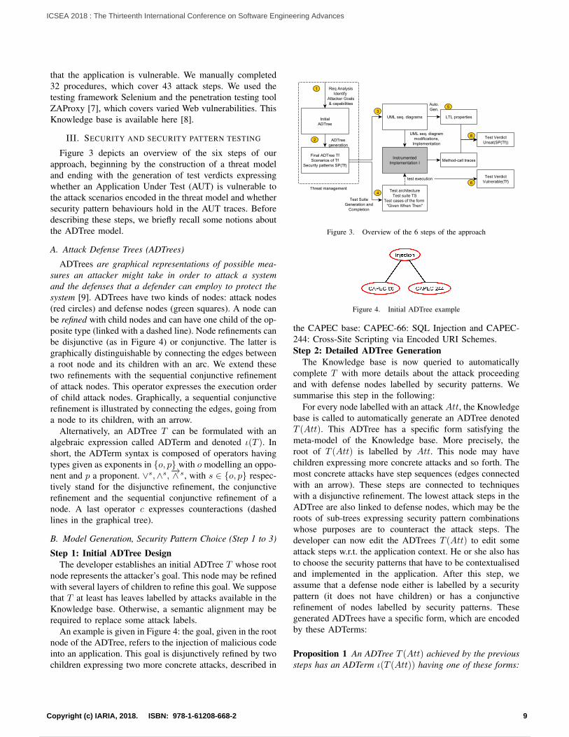
Figure 3 depicts an overview of the six steps of ourapproach, beginning by the construction of a threat modeland ending with the generation of test verdicts expressingwhether an Application Under Test (AUT) is vulnerable tothe attack scenarios encoded in the threat model and whethersecurity pattern behaviours hold in the AUT traces. Beforedescribing these steps, we briefly recall some notions aboutthe ADTree model.

A. Attack Defense Trees (ADTrees)

ADTrees are graphical representations of possible mea-sures an attacker might take in order to attack a systemand the defenses that a defender can employ to protect thesystem [9]. ADTrees have two kinds of nodes: attack nodes(red circles) and defense nodes (green squares). A node canbe refined with child nodes and can have one child of the op-posite type (linked with a dashed line). Node refinements canbe disjunctive (as in Figure 4) or conjunctive. The latter isgraphically distinguishable by connecting the edges betweena root node and its children with an arc. We extend thesetwo refinements with the sequential conjunctive refinementof attack nodes. This operator expresses the execution orderof child attack nodes. Graphically, a sequential conjunctiverefinement is illustrated by connecting the edges, going froma node to its children, with an arrow.

Alternatively, an ADTree T can be formulated with analgebraic expression called ADTerm and denoted ι(T ). Inshort, the ADTerm syntax is composed of operators havingtypes given as exponents in {o, p} with o modelling an oppo-nent and p a proponent. ∨s,∧s,−→∧ s, with s ∈ {o, p} respec-tively stand for the disjunctive refinement, the conjunctiverefinement and the sequential conjunctive refinement of anode. A last operator c expresses counteractions (dashedlines in the graphical tree).

B. Model Generation, Security Pattern Choice (Step 1 to 3)

Step 1: Initial ADTree DesignThe developer establishes an initial ADTree T whose root

node represents the attacker’s goal. This node may be refinedwith several layers of children to refine this goal. We supposethat T at least has leaves labelled by attacks available in theKnowledge base. Otherwise, a semantic alignment may berequired to replace some attack labels.

An example is given in Figure 4: the goal, given in the rootnode of the ADTree, refers to the injection of malicious codeinto an application. This goal is disjunctively refined by twochildren expressing two more concrete attacks, described in

Figure 3. Overview of the 6 steps of the approach

Figure 4. Initial ADTree example

the CAPEC base: CAPEC-66: SQL Injection and CAPEC-244: Cross-Site Scripting via Encoded URI Schemes.Step 2: Detailed ADTree Generation

The Knowledge base is now queried to automaticallycomplete T with more details about the attack proceedingand with defense nodes labelled by security patterns. Wesummarise this step in the following:

For every node labelled with an attack Att, the Knowledgebase is called to automatically generate an ADTree denotedT (Att). This ADTree has a specific form satisfying themeta-model of the Knowledge base. More precisely, theroot of T (Att) is labelled by Att. This node may havechildren expressing more concrete attacks and so forth. Themost concrete attacks have step sequences (edges connectedwith an arrow). These steps are connected to techniqueswith a disjunctive refinement. The lowest attack steps in theADTree are also linked to defense nodes, which may be theroots of sub-trees expressing security pattern combinationswhose purposes are to counteract the attack steps. Thedeveloper can now edit the ADTrees T (Att) to edit someattack steps w.r.t. the application context. He or she also hasto choose the security patterns that have to be contextualisedand implemented in the application. After this step, weassume that a defense node either is labelled by a securitypattern (it does not have children) or has a conjunctiverefinement of nodes labelled by security patterns. Thesegenerated ADTrees have a specific form, which are encodedby these ADTerms:

Proposition 1 An ADTree T (Att) achieved by the previoussteps has an ADTerm ι(T (Att)) having one of these forms:



20 / 160

1) ∨p(t1, . . . , tn) with ti(1 ≤ i ≤ n) an ADTerm alsohaving one of these forms:

2) −→∧ p(t1, . . . , tn) with ti(1 ≤ i ≤ n) an ADTerm havingthe form given in 2) or 3);

3) cp(st, sp), with st an ADTerm expressing an attackstep and sp an ADTerm modelling a security patterncombination.

The first ADTerm expresses children nodes labelled by moreconcrete attacks. The second one represents sequences ofattack steps. The last ADTerm is composed of an attack stepst refined with techniques, which can be counteracted by asecurity pattern combination sp = ∧o(sp1, . . . , spm). Wecall this ADTerm a Basic Attack Defence Step cp(st, sp),shortened BADStep. BADStep(Tf ) denotes the set ofBADSteps of Tf (final ADTree).

Figure 5 depicts a part of the ADTree of the attackCAPEC-66. Each lowest attack step has a defense nodeexpressing pattern combinations. Step 2.1, which identifiesthe possibilities to inject malicious code through the appli-cation inputs, requires more patterns than the other stepsto filter these inputs. Some of them have relations: forinstance the pattern “Application Firewall” can be replacedby “Intercepting Validator” or “Output Guard”.

Figure 5. Part of the ADTree of the Attack CAPEC-66

In the initial ADTree T , each attack node labelled by Attis now automatically replaced with the ADTree T (Att). Thiscan be done by substituting every term Att in the ADTermι(T ) by ι(T (Att)). We denote Tf the resulting ADTree, andSP (Tf ) the security pattern set found in ι(Tf ).

In this step, we finally extract from the Knowledge base adescription of the test architecture required to run the attackson the application under test and to observe its reactions.

Step 3: UML Sequence Diagram ExtractionFor every security pattern found in Tf , we extract a

list of UML sequence diagrams from the Knowledge base,each being related to the application context. These showthe behavioural activities of the patterns. We now supposethat the developer implements every security pattern inthe application. At the same time, he/she can choose tomodify the generic class and method names labelled inthe UML sequence diagrams. In this case, we assume thatthe sequence diagrams are annotated to point out thesemodifications.

As example, Figure 6 illustrates the UML sequence dia-gram of the security pattern “Intercepting Validator”, whosepurpose is to control the compliance of user requests withregard to a specification. The validation must be performedin the server side. For instance, while the pattern imple-mentation, if the name of the method “process” has to bemodified by “send”, the new label must be of the form“process/send” to express the substitution.

Figure 6. Intercepting Validator sequence diagram

IV. ATTACK AND SECURITY PATTERN TESTING

At this stage, an ADTree encodes the notion of attackscenarios over BADSteps, a scenario being is a minimalcombination of events leading to the root attack.

Definition 2 (Attack scenarios) Let Tf be an ADTree andι(Tf ) be its ADTerm. The set of Attack scenarios of Tf ,denoted SC(Tf ) is the set of clauses of the disjunctivenormal form of ι(Tf ) over BADStep(Tf ).

An attack scenario s is still an ADTerm over BADSteps.BADStep(s) denotes the set of BADSteps of s.Step 4: Test suite generation

Let us consider a security scenario s ∈ SC(Tf ). Given aBADStep b = cp(st, sp) ∈ BADStep(s), we generate theGWT test case TC(b), which aims at checking whether theapplication under test AUT is vulnerable to the attack stepst. TC(b) is constructed by extracting from the Knowledgebase, for the attack step st, one Given section, one Whensection and one Then section, each related to one procedure.The Then section aims to assert whether the application is



21 / 160

vulnerable to the attack step st; these sections are assembledto make up the GWT test case stub TC(b).

After having iteratively applied this test case constructionon the scenarios of SC(Tf ), we obtain the test suite TS withTS = {TC(b) | b = cp(st, sp) ∈ BADStep(s) and s ∈SC(Tf )}.Step 5: Security Pattern LTL Property Generation

Our approach aims at checking whether security patternbehavioural properties hold in the AUT. Instead of asking thedeveloper to write these properties, we automatically gener-ate them from UML sequence diagrams. This step analysessequence diagrams, recognises behavioural characteristicsand translates them into LTL properties.

Given a security pattern sp and its UML sequence dia-gram, the latter is firstly transformed into a UML activitydiagram. We propose 5 transformation rules whose three aredepicted in Table I. Intuitively, these rules transform eachmethod call in the sequence diagram by an action state in theactivity diagram. We took inspiration from the transforma-tions of UML sequence diagrams to state machines proposedin [10]. This transformation allows us to use the mappingof UML activity diagrams to LTL properties proposed byMuram et al. [11]. The transformation rules are based uponthe Response Property Pattern [12], which describes thecause-effect relations among method calls. Three examplesof transformations are given in Table I. At the end of thistransformation sequence, we have a set of LTL propertiesP (sp) for every security pattern sp ∈ SP (Tf ). Althoughthe LTL properties of P (sp) do not necessarily cover allthe possible behavioural properties of a security pattern sp,this process offers the advantages to not require genericLTL properties modelling pattern behaviours, and to notask developers to instantiate these generic LTL propertiesto match the application model or code.

TABLE ITRANSFORMATION RULES

Sequence Activity LTL properties

�(B.1 −→♦C.2)

�(B.1 −→(♦B.2)xor(♦C.3))

�(B.1 −→(♦B.2)and(♦C.3))

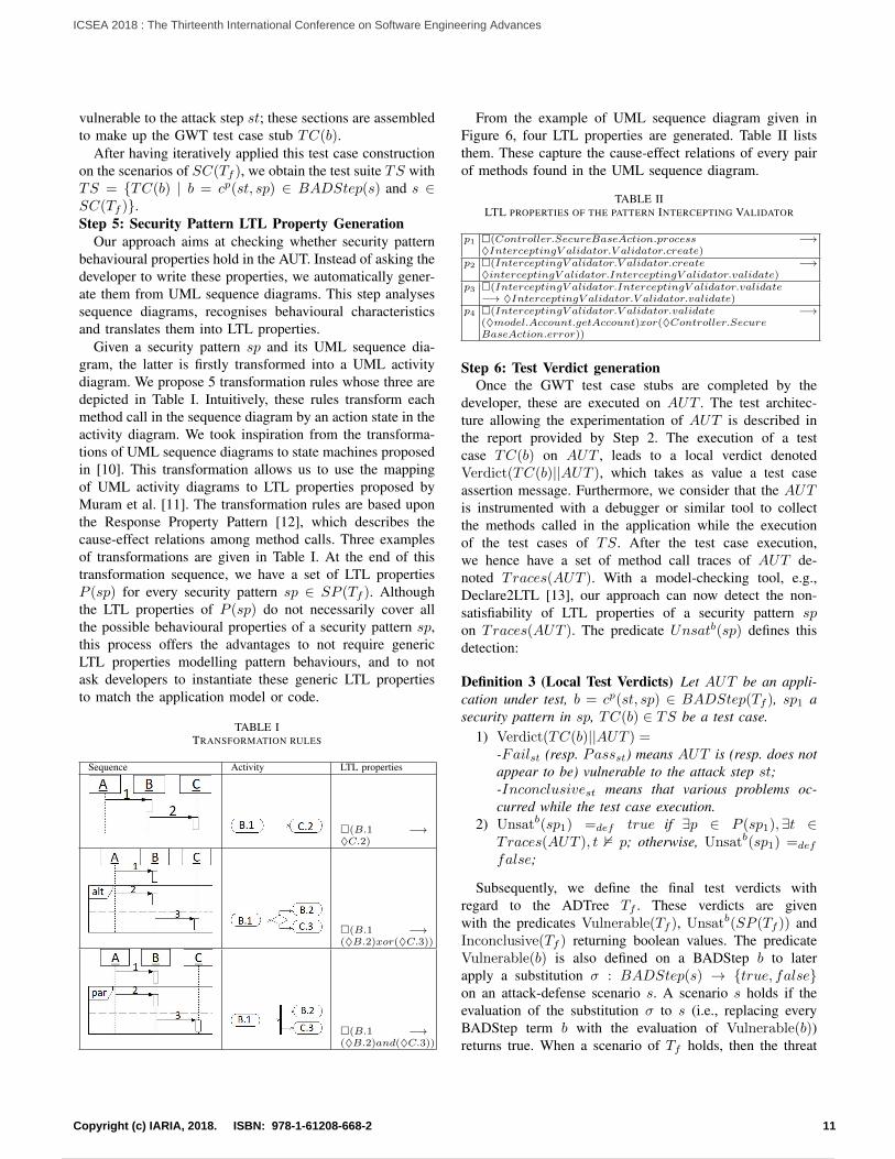
From the example of UML sequence diagram given inFigure 6, four LTL properties are generated. Table II liststhem. These capture the cause-effect relations of every pairof methods found in the UML sequence diagram.

TABLE IILTL PROPERTIES OF THE PATTERN INTERCEPTING VALIDATOR

p1 �(Controller.SecureBaseAction.process −→♦InterceptingV alidator.V alidator.create)

p2 �(InterceptingV alidator.V alidator.create −→♦interceptingV alidator.InterceptingV alidator.validate)

p3 �(InterceptingV alidator.InterceptingV alidator.validate−→ ♦InterceptingV alidator.V alidator.validate)

p4 �(InterceptingV alidator.V alidator.validate −→(♦model.Account.getAccount)xor(♦Controller.SecureBaseAction.error))

Step 6: Test Verdict generationOnce the GWT test case stubs are completed by the

developer, these are executed on AUT . The test architec-ture allowing the experimentation of AUT is described inthe report provided by Step 2. The execution of a testcase TC(b) on AUT , leads to a local verdict denotedVerdict(TC(b)||AUT ), which takes as value a test caseassertion message. Furthermore, we consider that the AUTis instrumented with a debugger or similar tool to collectthe methods called in the application while the executionof the test cases of TS. After the test case execution,we hence have a set of method call traces of AUT de-noted Traces(AUT ). With a model-checking tool, e.g.,Declare2LTL [13], our approach can now detect the non-satisfiability of LTL properties of a security pattern spon Traces(AUT ). The predicate Unsatb(sp) defines thisdetection:

Definition 3 (Local Test Verdicts) Let AUT be an appli-cation under test, b = cp(st, sp) ∈ BADStep(Tf ), sp1 asecurity pattern in sp, TC(b) ∈ TS be a test case.

1) Verdict(TC(b)||AUT ) =-Failst (resp. Passst) means AUT is (resp. does notappear to be) vulnerable to the attack step st;-Inconclusivest means that various problems oc-curred while the test case execution.

2) Unsatb(sp1) =def true if ∃p ∈ P (sp1),∃t ∈Traces(AUT ), t 2 p; otherwise, Unsatb(sp1) =def

false;

Subsequently, we define the final test verdicts withregard to the ADTree Tf . These verdicts are givenwith the predicates Vulnerable(Tf ), Unsatb(SP (Tf )) andInconclusive(Tf ) returning boolean values. The predicateVulnerable(b) is also defined on a BADStep b to laterapply a substitution σ : BADStep(s) → {true, false}on an attack-defense scenario s. A scenario s holds if theevaluation of the substitution σ to s (i.e., replacing everyBADStep term b with the evaluation of Vulnerable(b))returns true. When a scenario of Tf holds, then the threat



22 / 160

TABLE IIITEST VERDICT SUMMARY AND SOLUTIONS

Vulnera-ble(Tf )

Unsatb(SP (Tf ))

Incon(Tf )

Corrective actions

False False False No issue detectedTrue False False At least one scenario is successfully applied on AUT.

Fix the pattern implementation. Or the chosen patternsare inconvenient.

False True False Some pattern behavioural properties do not hold. Checkthe pattern implementations with the UML seq. diag. Oranother pattern conceals the behaviour of the former.

True True False The chosen security patterns are useless or incorrectlyimplemented. Review the ADTree, fix AUT.

T/F T/F True The test case execution crashed or returned unexpectedexceptions. Check the Test architecture and the test casecodes.

modelled by Tf can be achieved on AUT . This is definedwith the predicate Vulnerable(Tf ). Unsatb(SP (Tf )) is trueas soon as a security pattern property does not hold onTraces(AUT ). Table III informally summarises the mean-ing of some test verdicts and some corrections that may befollowed in case of failure.

Definition 4 (Final Test Verdicts) Let AUT be an appli-cation under test, Tf be an ADTree, s ∈ SC(Tf ) andb = cp(st, sp) ∈ BADStep(Tf ).

1) Vulnerable(b) =def true if Verdict(TC(b)||AUT ) =Failst; otherwise, Vulnerable(b) =def false;

2) σ : BADStep(s) → {true, false} is a substitution{b1 → Vulnerable(b1), . . . , bn → Vulnerable(bn)};

3) Vulnerable(Tf ) =def true if ∃s ∈ SC(Tf ) :eval(sσ) returns true; otherwise, Vulnerable(Tf ) =def false;

4) Inconclusive(Tf ) =def true if ∃s ∈ SC(Tf ),∃b ∈ BADStep(s): Verdict(TC(b)|| AUT ) =Inconclusivest; otherwise, Inconclusive(Tf ) =def

false.5) Unsatb(SP (Tf )) =def true if ∃sp ∈

SP (Tf ),Unsatb(sp) = true; otherwise, Unsatc(

SP (Tf )) =def false;

V. CONCLUSION

This paper proposes an approach taking advantage of aKnowledge base to assist developers in the implementationof secure applications through six steps covering threat mod-elling, the choice of security patterns, security testing andthe verification of security pattern behavioural properties.It guides developers in the generation of ADTrees and testcases. In addition, it automatically generates LTL properties,encoding security pattern behaviours. As a consequence,the approach does not require developers to have skills in(formal) modelling or in formal methods. We have imple-mented this approach in a tool prototype [8]. We brieflysummarise its features in this paper: it generates ADTreesstored into XML files, which can be edited with ADTool[9]. Our tool also builds GWT test case compatible with theCucumber framework [14], which supports a large number

of languages. These test cases can be imported with the IDEEclipse. The verification of LTL properties is performed withthe Declare2LTL model checker. We started to perform someexperiments on Web applications to assess the user benefits.An evaluation will be presented in a future work.

REFERENCES

[1] R. Slavin and J. Niu. (retrieved: 07, 2018) Securitypatterns repository. [Online]. Available: http://sefm.cs.utsa.edu/repository/

[2] M. Schumacher, Security Engineering with Patterns: Origins,Theoretical Models, and New Applications. Secaucus, NJ,USA: Springer-Verlag New York, Inc., 2003.

[3] A. Morais, E. Martins, A. Cavalli, and W. Jimenez, “Se-curity protocol testing using attack trees,” in 2009 Interna-tional Conference on Computational Science and Engineer-ing, vol. 2, Aug 2009, pp. 690–697.

[4] N. Shahmehri et al., “An advanced approach for modelingand detecting software vulnerabilities,” Inf. Softw. Technol.,vol. 54, no. 9, pp. 997–1013, Sep. 2012.

[5] S. Salva and L. Regainia, “Using data integration for securitytesting,” in Proceedings 29th International Conference, ICTSS2017, 10 2017, pp. 178–194.

[6] Y. Masatoshi et al., “Verifying implementation of securitydesign patterns using a test template,” in 2014 Ninth Inter-national Conference on Availability, Reliability and Security,Sept 2014, pp. 178–183.

[7] OWASP. (retrieved: 07, 2018) Zap proxy project. [Online].Available: https://www.owasp.org/index.php/OWASP ZedAttack Proxy Project

[8] R. Loukmen and S. Sbastien. (retrieved: 07, 2018) Zap proxyproject. [Online]. Available: http://regainia.com/research/companion.html

[9] B. Kordy, S. Mauw, S. Radomirovic, and P. Schweitzer,“Attack–defense trees,” Journal of Logic and Computation,p. exs029, 2012.

[10] R. Grønmo and B. Møller-Pedersen, “From sequence dia-grams to state machines by graph transformation,” in The-ory and Practice of Model Transformations, L. Tratt andM. Gogolla, Eds. Berlin, Heidelberg: Springer BerlinHeidelberg, 2010, pp. 93–107.

[11] F. U. Muram, H. Tran, and U. Zdun, “Automated mappingof UML activity diagrams to formal specifications for sup-porting containment checking,” in Proceedings FESCA 2014,Grenoble, France, 12th April 2014., 2014, pp. 93–107.

[12] L. Patterns. (retrieved: 07, 2018) response ltl pattern. [Online].Available: http://patterns.projects.cs.ksu.edu/documentation/patterns/response.shtml

[13] M. M. Fabrizio et al. (retrieved: 07, 2018) Declare toolkit.[Online]. Available: http://www.win.tue.nl/declare/

[14] Cucumber. (retrieved: 07, 2018) Cucumber website. [Online].Available: https://cucumber.io/



23 / 160

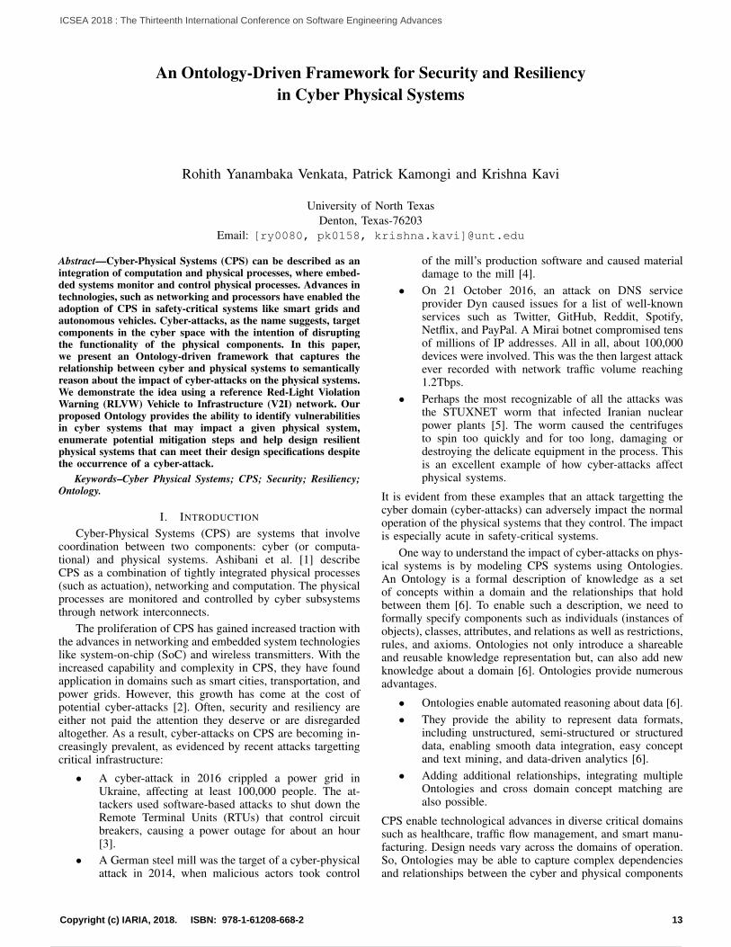
An Ontology-Driven Framework for Security and Resiliencyin Cyber Physical Systems

Rohith Yanambaka Venkata, Patrick Kamongi and Krishna Kavi

University of North TexasDenton, Texas-76203

Email: [ry0080, pk0158, krishna.kavi]@unt.edu

Abstract—Cyber-Physical Systems (CPS) can be described as anintegration of computation and physical processes, where embed-ded systems monitor and control physical processes. Advances intechnologies, such as networking and processors have enabled theadoption of CPS in safety-critical systems like smart grids andautonomous vehicles. Cyber-attacks, as the name suggests, targetcomponents in the cyber space with the intention of disruptingthe functionality of the physical components. In this paper,we present an Ontology-driven framework that captures therelationship between cyber and physical systems to semanticallyreason about the impact of cyber-attacks on the physical systems.We demonstrate the idea using a reference Red-Light ViolationWarning (RLVW) Vehicle to Infrastructure (V2I) network. Ourproposed Ontology provides the ability to identify vulnerabilitiesin cyber systems that may impact a given physical system,enumerate potential mitigation steps and help design resilientphysical systems that can meet their design specifications despitethe occurrence of a cyber-attack.

Keywords–Cyber Physical Systems; CPS; Security; Resiliency;Ontology.

I. INTRODUCTION

Cyber-Physical Systems (CPS) are systems that involvecoordination between two components: cyber (or computa-tional) and physical systems. Ashibani et al. [1] describeCPS as a combination of tightly integrated physical processes(such as actuation), networking and computation. The physicalprocesses are monitored and controlled by cyber subsystemsthrough network interconnects.

The proliferation of CPS has gained increased traction withthe advances in networking and embedded system technologieslike system-on-chip (SoC) and wireless transmitters. With theincreased capability and complexity in CPS, they have foundapplication in domains such as smart cities, transportation, andpower grids. However, this growth has come at the cost ofpotential cyber-attacks [2]. Often, security and resiliency areeither not paid the attention they deserve or are disregardedaltogether. As a result, cyber-attacks on CPS are becoming in-creasingly prevalent, as evidenced by recent attacks targettingcritical infrastructure:

• A cyber-attack in 2016 crippled a power grid inUkraine, affecting at least 100,000 people. The at-tackers used software-based attacks to shut down theRemote Terminal Units (RTUs) that control circuitbreakers, causing a power outage for about an hour[3].

• A German steel mill was the target of a cyber-physicalattack in 2014, when malicious actors took control

of the mill’s production software and caused materialdamage to the mill [4].

• On 21 October 2016, an attack on DNS serviceprovider Dyn caused issues for a list of well-knownservices such as Twitter, GitHub, Reddit, Spotify,Netflix, and PayPal. A Mirai botnet compromised tensof millions of IP addresses. All in all, about 100,000devices were involved. This was the then largest attackever recorded with network traffic volume reaching1.2Tbps.

• Perhaps the most recognizable of all the attacks wasthe STUXNET worm that infected Iranian nuclearpower plants [5]. The worm caused the centrifugesto spin too quickly and for too long, damaging ordestroying the delicate equipment in the process. Thisis an excellent example of how cyber-attacks affectphysical systems.

It is evident from these examples that an attack targetting thecyber domain (cyber-attacks) can adversely impact the normaloperation of the physical systems that they control. The impactis especially acute in safety-critical systems.

One way to understand the impact of cyber-attacks on phys-ical systems is by modeling CPS systems using Ontologies.An Ontology is a formal description of knowledge as a setof concepts within a domain and the relationships that holdbetween them [6]. To enable such a description, we need toformally specify components such as individuals (instances ofobjects), classes, attributes, and relations as well as restrictions,rules, and axioms. Ontologies not only introduce a shareableand reusable knowledge representation but, can also add newknowledge about a domain [6]. Ontologies provide numerousadvantages.

• Ontologies enable automated reasoning about data [6].• They provide the ability to represent data formats,

including unstructured, semi-structured or structureddata, enabling smooth data integration, easy conceptand text mining, and data-driven analytics [6].

• Adding additional relationships, integrating multipleOntologies and cross domain concept matching arealso possible.

CPS enable technological advances in diverse critical domainssuch as healthcare, traffic flow management, and smart manu-facturing. Design needs vary across the domains of operation.So, Ontologies may be able to capture complex dependenciesand relationships between the cyber and physical components



24 / 160

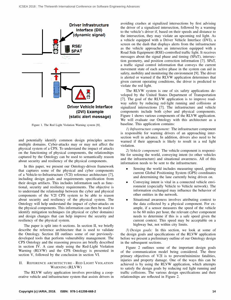
Figure 1. The Red Light Violation Warning system [8].

and potentially identify common design principles acrossmultiple domains. Cyber-attacks may or may not affect thephysical system of a CPS. To understand the impact of attackson the functioning of physical components, the relationshipscaptured by the Ontology can be used to semantically reasonabout security and resiliency of the physical components.

In this paper, we present our Ontology-driven frameworkthat captures some of the physical and cyber componentsof a Vehicle-to-Infrastructure (V2I) reference architecture [7],including design goals and requirements specification fromtheir design artifacts. This includes information such as func-tional, security and resiliency requirements. The objective isto understand the relationship between the cyber and physicalcomponents of the V2I CPS system to be able to reasonabout security and resiliency of the physical system. TheOntology will help understand the impact of cyber-attacks onthe physical components. This information can then be used toidentify mitigation techniques (in physical or cyber domains)and design changes that can help improve the security andresiliency of the physical system.

The paper is split into 6 sections. In section II, we brieflydescribe the reference architecture that is used to validatethe Ontology. Section III outlines some of our previously-developed tools that perform vulnerability management. TheCPS Ontology and the reasoning process are briefly describedin section IV. A case study using the Red-Light ViolationWarning (RLVW) and the CPS Ontology is presented insection V, followed by the conclusion in section VI.

II. REFERENCE ARCHITECTURE - RED LIGHT VIOLATIONWARNING (RLVW)

The RLVW safety application involves providing a coop-erative vehicle and infrastructure system that assists drivers in

avoiding crashes at signalized intersections by first advisingthe driver of a signalized intersection, followed by a warningto the vehicle’s driver if, based on their speeds and distance tothe intersection, they may violate an upcoming red light. Asa vehicle equipped with a Driver Vehicle Interface (DVI), ascreen on the dash that displays alerts from the infrastructureas the vehicle approaches an intersection equipped with aRoad Side Equipment (RSE)-controlled traffic light. It receivesmessages about the signal phase and timing (SPaT), intersec-tion geometry, and position correction information [7]. SPaT,a traffic signal control information that conveys the currentmovement state of each active phase in the system can aid insafety, mobility and monitoring the environment [9]. The driveris alerted or warned if the RLVW application determines thatgiven current operating conditions, the driver is predicted toviolate the red light.

The RLVW system is one of six safety applications de-veloped by the United States Department of Transportation[7]. The goal of the RLVW application is to improve road-way safety by reducing red-light running and collisions atsignalized intersections [7]. The infrastructure and vehiclecomponents include both cyber and physical components.Figure 1 shows various components of the RLVW application.We will evaluate our Ontology with this architecture as abaseline. This application contains:

1) Infrastructure component: The infrastructure componentis responsible for warning drivers of an approaching inter-section well in advance. In addition, drivers also need to bewarned if their approach is likely to result in a red lightviolation.

2) Vehicle component: The vehicle component is responsi-ble for sensing the world, conveying intent (to other vehiclesand the infrastructure) and situational awareness. All of thisinformation needs to be sent to the infrastructure.

• Sensing the world includes measuring speed, gettingcurrent Global Positioning System (GPS) coordinatesand determining the lane currently being driven on.

• Conveying intent is vital in a connected vehicle envi-ronment (especially Vehicle to Vehicle network). Theinformation exchanged may influence the behavior ofother entities in the network.

• Situational awareness involves attributing context tothe data collected by a physical component. For ex-ample, if a sensor measures the speed of the vehicleto be 60 miles per hour, the relevant cyber componentneeds to determine if this is a safe speed given thecurrent context. This speed may be acceptable on ahighway but, not within city limits.

3) Design goals: In this section, we look at some ofthe design goals and specifications of the RLVW applicationbefore we present a preliminary outline of our Ontology designin the subsequent sections.

Figure 2 outlines some of the important design goalsof the communication model being considered. The threeprimary objectives of V2I is to prevent/minimize fatalities,injuries and property damage. One of the ways this can beachieved is by using the RLVW application, which attemptsto satisfy the design goals by reducing red light running andtraffic collisions. The various design specifications and theirrelationships are reflected in Figure 2.



25 / 160

Figure 2. Design goals for RLVW.

The National Institute of Standards and Technology (NIST)has published a framework that provides guidance in design-ing, building, verifying, and analyzing complex CPS systems[10]. The CPS Framework captures the generic functionalitiesthat CPS provide, and the activities and artifacts needed tosupport conceptualization, realization, and assurance of CPS[10]. The framework describes the following series of stepswithin a reference architecture.

• The domain of the CPS needs to be identified.• Facets or views on CPS encompassing identified re-

sponsibilities in the system engineering process [10]need to be identified. These include conceptualization,realization, and assurance. They contain well-definedactivities and artifacts (outputs) for addressing designgoals (or concerns) [10].

• Aspects need to be consolidated. Aspects are high-level groupings of cross-cutting concerns. Concernsare interests in a system relevant to one or morestakeholders. These may include Functional, Business,Timing, Data, Trustworthiness, etc [10].

Our objective is to reason about security and resiliencyso, we focus only on the trustworthy concerns. Trustworthi-ness is the demonstrable likelihood that the system performsaccording to designed behavior under any set of conditionsas evidenced by characteristics including, but not limited to,safety, security, privacy, reliability and resilience [10]. In thenext section, we briefly describe vulnerability assessment forcyber systems using some of our previous work.

III. VULNERABILITY-BASED THREATS ASSESSMENT

Given a deployed Cyber-Physical System that leveragesone or more IT (or cyber) components for normal operations,security evaluation of the IT system is a priority.

In our previous work, we have designed solutions (VUL-CAN [11], and NEMESIS [12]) to automate essential security

management tasks to assist in identifying, assessing and mit-igating the threats that may affect any given IT system (thisapply to the Cyber components that power a Cyber-PhysicalSystem).

Let us consider an example of an IT component (that ispart of a Cyber-Physical System) such as the “Qualcomm SD820 Firmware”. Our VULCAN Framework [11], enable us tomodel and represent such an IT component using a CommonPlatform Enumeration (CPE) standard [13].

An Ontology Knowledge Base (OKB), which is a pop-ulated Ontology, plays a central role within the VULCANframework by capturing various critical public data feeds of ITproducts (e.g., Application/Software, Operating System, andHardware) vulnerability, attack, and mitigation informationusing an evolving and semantically rich Ontology model.

The vulnerability index generated by VULCAN capturesinformation about publicly known vulnerabilities (includingtheir insightful information) that affect our assessed IT com-ponent. Figure 3 shows a simplified view of the generatedvulnerability index to highlight a few vulnerabilities (includingtheir vulnerability description, severity score and CommonWeakness Enumeration (CWE) [14] identifier) that affects ourassessed IT product (viz., Qualcomm SD 820 Firmware). ThisSystem-on-Chip (SoC) is commonly used in level 3 and level4 autonomous vehicles.

With the amount of semantically rich information capturedwithin the generated vulnerability index of the assessed ITcomponent, we can reason and infer various insights in regardsto the current vulnerability status of the ”Qualcomm SD820 Firmware” and how many of its vulnerabilities have adamaging impact (if exploited by a malicious actor) to thecore of the Cyber-Physical System in operation.

Using this vulnerability index, our NEMESIS architecturecan assist in performing various threat modeling, and riskassessment tasks of the for the IT product. This information



26 / 160

may be useful towards designing and CPS that are inherentlyresilient to the modeled threats.

Table I illustrates a sample view of how NEMESIS clas-sifies vulnerabilities (that affect the assessed IT component“Qualcomm SD 820 Firmware”) into possible threat types(using STRIDE threat model [15]) that could arise from theirexploitation. For instance, “CVE-2018-3594” [16] vulnerabil-ity was identified by VULCAN that it affects our assessed ITcomponent, then NEMESIS determines that this vulnerabilitycould lead to “Tampering, Information Disclosure, Repudi-ation, and Elevation of Privilege” STRIDE threat types (asshown in Table I).

TABLE I. QUALCOMM SD 820 FIRMWARE: THREATCLASSIFICATION SAMPLE

Vulnerability S T R I D ECVE-2018-3594 0 1 1 1 0 1

CVE-2017-18140 0 0 1 0 0 0CVE-2016-10414 0 1 0 0 0 0CVE-2016-10446 0 1 0 1 0 1CVE-2016-10434 1 1 1 0 1 1

In Table II we illustrate how NEMESIS ranks all theclassified threat types by the average severity of all the foundvulnerabilities that can lead to each of the STRIDE threattypes. For instance, “Information Disclosure” threat type is themost severe threat that the assessed IT component “QualcommSD 820 Firmware” is exposed to.

TABLE II. QUALCOMM SD 820 FIRMWARE: THREAT TYPESRANKING

Threat Type Severity [0-10]Tampering 8.19

Denial of Service 5.0Spoofing 7.5

Information Disclosure 9.0Repudiation 8.57

Elevation of Privilege 8.78

Security practitioners can use the information for assessingIT products (or cyber component of CPS) to strategize cybermitigations and resiliency measures to counter any of theperceived threat types that could impact the critical missionsof the operational Cyber-Physical System.

Figure 3. Qualcomm SD 820 Firmware – Vulnerability Index Sample

IV. CPS ONTOLOGY DESIGN AND REASONING PROCESS

Cyber systems usually include processors, memory mod-ules, network interfaces and software products. We brieflydiscussed vulnerability assessment and management for cybersystems by introducing some of our previous work in SectionIII. We also previously demonstrated the ability to enforcedifferentiated levels of security for Internet of Things (IoT)devices in [17]. Now, our goal is to understand how thesecyber (or IT) vulnerabilities affect physical systems. Thechallenge is to capture the relationship between cyber andphysical components to semantically reason about security andresiliency. The Ontology will be able to provide an insight intopotential mitigation techniques, which may involve changes inthe design or patching and updating software packages in thecyber domain. The various stages in the reasoning process arelisted below.

• Design goals and components of a CPS domain needto be identified in consultation with domain experts.

• The relationships between various components in thedomain need to be identified within the context of thedesign goals identified in the previous step.

• Given all components and their relationships, threatmodeling needs to be performed so that only threatsrelevant to the given CPS are considered.

• The CPS needs to be redesigned if required.• The redesigned system needs to be validated to ensure

it still complies with the design specifications.

We have constructed an Ontology for the trustworthinessconcern based on NIST’s CPS framework. Figure 4 depictsa preliminary design for the CPS Ontology that is capable ofreasoning against a limited set of vulnerabilities that we willdiscuss in Section V. The Ontology was implemented usingOWL web semantic language [18] on Protege Ontology editor[19].

The Ontology identifies components and subcomponents ofRLVW system under consideration at conceptual level, assignroles and responsibilities to them and capture dependenciesamong the components (following NIST CPS Framework[10]). In the realization phase, our framework relates how theconceptual level components will be implemented using cybersystems (processors, memory, network). Since each of thesecomponents will be identified using a unique CPE (CommonPlatform Enumeration), VULCAN system can capture securityinformation about the components from NVD repositories.This information, including vulnerabilities, severity scores,attack vectors, patches are indexed and analyzed, generatingcomprehensive reports about individual components as well asfor the entire cyber system.

NEMESIS [12] uses the VULCAN [11] to collect informa-tion in providing a risk score for the cyber components. It usesa Bayesian model that combines vulnerabilities, dependenciesamong components, severity scores, and threat types exposedby vulnerabilities to compute risks scores and prioritize threattypes faced by the system.

The design specifications from Figure 2 were translatedinto an Ontology. The RLVW concept contains five differentknowledge points: physical components and cyber componentswhich are self-explanatory, Abstract, Vehicle and Infrastruc-ture. The infrastructure and vehicle components are mapped



27 / 160

Figure 4. An example of the CPS ontology.

to the cyber and physical concepts. A knowledge point calledAbstract captures all the design goals of a CPS domain(The RLVW safety application in this scenario). The twocomponents of interest in this Ontology are the traffic lightand RSE. The traffic light interacts with the RSE to displaytraffic lights and transition between them.

Design goals may be security requirements (from SecurityService Level Agreements or SSLAs), Resiliency goals andFunctional requirements. Lee et al., [20] describe an Ontologyto capture SSLAs, which can be used to understand securityagreements of a service provider or to audit compliance todesign specifications [20].

V. CASE STUDY

Let us evaluate this Ontology using a few simple examples.We use the STRIDE threat modeling discussed in Section IIIand the design specifications from Section 2. The configurationof system components is as follows:

• Qualcomm 820a SoC powers a vehicle.• The DVI is controlled by Android Auto operating

system [21].• RSE is a facility server running Ubuntu 16.04 LTS.• No identification scheme exists to authenticate entities

in the network.• The data exchanged is not validated (neither by RSE

nor the vehicle).• The traffic light is not designed with any fail-safe

modes.• No personally-identifiable information is

collected/stored.

A. An attack on the RSELet us consider the RLVW application discussed before.

We were able to determine using the CPE identifier forSnapdragon 820a that five significant vulnerabilities couldaffect the SoC as discussed in section III. One of the mostimportant steps in threat modelling for CPS is to assign acontext to a threat/vulnerability i.e, try to understand how avulnerability affects a physical system. In the first example, letus consider a scenario where an adversary attacks the RSE (asdepicted in Figure 5). RSE is no longer trustworthy. Potentialattacks are:

• Spoofing : The adversary may masquerade as theRSE, sending false data to vehicles or the traffic light.The lights may flash randomly or be turned off. Thevehicle may not receive a warning from the RSEeven if a potential red light violation is detected. Forexample, CVE-2018-1111 [22] may be used to createmalicious DHCP packets to compromise the server.

• Tampering : Data is maliciously modified beforebeing sent to vehicles or the traffic light. The potentialimpact is similar to that of the Spoofing attack. Forexample, an adversary may use CVE-2017-1000366[23] to create a specially crafted environment variableto perform a buffer overflow attack.

• Repudiation : Non-repudiation is a state of affairswhere a source of specific information denies evercreating/issuing it. In this case, the RSE can deny everhaving issued an alert to a vehicle or the traffic light.In this case, the Ontology will help us understand thatthis attack is not relevant to us because it is easy to



28 / 160

Figure 5. An attack on the RSE.

validate the RSE by using data from the vehicle. Thismay not be as critical as spoofing or tampering in oursystem.

• Information Disclosure : Since no personally iden-tifiable information is collected, this attack does notsubstantially impact the physical system. However, ifthe RSE captures images of the vehicle that violatedthe red-light, information disclosure may violate pri-vacy goals. If information about the cyber domain isleaked, VULCAN can help mitigate it.

• Denial of Service : The adversary may use any ofthe CVEs previously discussed to render the RSEunresponsive. This means that the vehicles may notreceive alerts and the traffic lights are not controlled.The impact may be similar to that of the Spoofingattack.

• Elevation of Prvilege : Elevation of privilege orprivilege escalation attacks involve gaining escalatedaccess to a resource that is normally protected from auser. This is a cyber-attack so, VULCAN or NEMESISmay be able to suggest mitigation techniques.

B. Mitigation techniquesThe Ontology will be able to reason about potential mitiga-

tion techniques for a given cyber-vulnerability logically. Thisalso includes changes to the design specification. Let us lookat some of them:

• For most of the cyber-attacks like elevation of priv-ilege, updating software packages, applying patchesshould suffice.

• Cyber system can be designed to protect against spoof-ing attacks by authenticating network entities using adigital certificate-based identification scheme.

• Physical systems can be designed to protect againstspoofing attacks by using a physical unclonable func-tion (PUF) based identification scheme.

• The traffic light can be built to flash yellow lights if noresponse is received from the RSE for a preset amountof time.

• SPaT data can be transmitted by the RSE so that thevehicles can validate the alerts that were sent.

• Similarly, speed and location information can be sentby the vehicles approaching the intersection. The RSEcan validate the data collected by the sensors on thevehicle with the data collected by the RSE. Cross-validation may prove to be a useful design feature.

The Ontology can suggest mitigation techniques. Cost VsRisk estimates may be used to pick the appropriate mitigationscheme. The insight provided by the Ontology can be used todesign resilient physical systems.

C. An attack on the cyber component of a vehicleWe briefly discussed how specific threats that target the

cyber component of the RSE might impact the CPS. Similarly,the cyber component of a vehicle (such as the Qualcomm 820aSoC) may be targetted by spoofing, tampering, repudiation,information disclosure, denial of service and elevation ofprivilege attacks, which may violate the trustworthy concernof the V2I system. However, due to the limitation in space,we are unable to elaborate on this further.

VI. CONCLUSION

In this paper, we have presented an argument for modelingCPS using Ontologies. As systems grow more complex, under-standing the relationship between various components becomesharder but, more critical.

We have introduced an Ontology-driven framework thatis capable of capturing the relationship between cyber andphysical domains. We use the example of a V2I communi-cation model to demonstrate the capability of the Ontology.This Ontology, designed in consultation with domain expertshelps identify potential vulnerabilities in the cyber domain thatmay impact a physical system. Also, it helps in identifyingpossible mitigation steps (in the cyber or physical domain)that can be used to protect against the threats modeled andalso help design resilient physical systems that may providereduced functionality to meet design specifications (resilient)despite the occurrence of a cyber-attack.

In the future, we intend to develop a more detailed Ontol-ogy framework that captures complex relationships betweenvarious components. This will also include tools that will beable to translate design specifications from the NIST frame-work into our Ontology to reason about the trustworthiness ofa CPS design.

REFERENCES

[1] Y. Ashibani and Q. H. Mahmoud, “Cyber physical systemssecurity: Analysis, challenges and solutions,” Computers andSecurity, vol. 68, 2017, pp. 81 – 97. [Online]. Available:http://www.sciencedirect.com/science/article/pii/S0167404817300809

[2] Z. DeSmit, A. E. Elhabashy, L. J. Wells, and J. A. Camelio,“An approach to cyber-physical vulnerability assessment forintelligent manufacturing systems,” Journal of Manufacturing Systems,vol. 43, 2017, pp. 339 – 351, high Performance Computingand Data Analytics for Cyber Manufacturing. [Online]. Available:http://www.sciencedirect.com/science/article/pii/S027861251730033X



29 / 160

[3] “Why the Ukraine power grid attacks should raise alarm,” Mar.2017, URL:https://www.csoonline.com/article/3177209/security/why-the-ukraine-power-grid-attacks-should-raise-alarm.html/ [accessed:2018-06-16].

[4] K. Zetter, “A cyber-attack has caused confirmed physical damage for thesecond time ever,” URL:https://www.wired.com/2015/01/german-steel-mill-hack-destruction/ [accessed: 2018-06-13].

[5] K. Zetter, “An unprecedented look at STUXNET, the world’s first digi-tal weapon,” URL:https://www.wired.com/2014/11/countdown-to-zero-day-stuxnet/ [accessed: 2018-06-16].

[6] “What are Ontologies?” URL:https://ontotext.com/knowledgehub/fundamentals/what-are-ontologies/ [accessed: 2018-06-13].

[7] B. Christie, “Vehicle-to-infrastructure (V2I) safety applications per-formance requirements, vol. 3, red light violation warning (RLVW),”United States. Dept. of Transportation. ITS Joint Program Office; UnitedStates. Federal Highway Administration, techreport, 2015.

[8] B. Christie, “Vehicle-to-Infrastructure (V2I) Safety Applications: Per-formance Requirements, Vol. 1, Introduction and Common Require-ments,” United States. Dept. of Transportation. ITS Joint ProgramOffice; United States. Federal Highway Administration, Tech. Rep.,2015.

[9] United States Dept. of Transportation,URL:https://www.its.dot.gov/presentations/pdf/SPaT.pdf [accessed:2018-06-10].

[10] Cyber-Physical Systems Public Working Group, “Framework for Cyber-Physical SystemsRelease 1.0,” National Institute of Standards andTechnology, Tech. Rep., 2016.

[11] P. Kamongi, S. Kotikela, K. Kavi, M. Gomathisankaran, and A. Singhal,“Vulcan: Vulnerability assessment framework for cloud computing,”in Proceedings of The Seventh International Conference on SoftwareSecurity and Reliability. SERE (SSIRI) 2013. IEEE, June 2013, pp.218–226.

[12] P. Kamongi, M. Gomathisankaran, and K. Kavi, “Nemesis: Automatedarchitecture for threat modeling and risk assessment for cloud comput-ing,” in The Sixth ASE International Conference on Privacy, Security,Risk and Trust (PASSAT). ASE, December 2014.

[13] National Institute of Standards and Technology, “Common platformenumeration (cpe),” https://nvd.nist.gov/cpe.cfm, June 2018.

[14] MITRE, “Common weakness enumeration (cwe),” http://cwe.mitre.org,June 2018.

[15] “The STRIDE Threat Model,” http://msdn.microsoft.com/en-US/library/ee823878(v=cs.20).aspx, June 2018.

[16] National Institute of Standards and Technology,https://nvd.nist.gov/vuln/detail/CVE-2018-3594, June 2018.

[17] R. Y. Venkata and K. Kavi, “CLIPS: Customized Levels of IoT Privacyand Security,” in Proceedings of the 12th The Twelfth InternationalConference on Software Engineering Advances Oct 12–14, 2017,Athens, Greece, pp. 41–47.

[18] “OWL web semantic language,” URL:https://www.w3.org/OWL/ [ac-cessed: 2018-06-10].

[19] M. A. Musen and the Protege team, “The protege project:A look back and a look forward,” AI Matters, vol. 1,no. 4, Jun 2015, pp. 4–12, 27239556[pmid]. [Online]. Available:http://www.ncbi.nlm.nih.gov/pmc/articles/PMC4883684/

[20] C.-Y. Lee, K. Kavi, R. Paul, and M. Gomathisankaran, “Ontologyof secure service level agreement,” 2015 IEEE 16th InternationalSymposium on High Assurance Systems Engineering, 2015, pp. 166–172.

[21] Google, “The Android Auto Operating System,”URL:https://www.android.com/auto/ [accessed: 2018-06-08].

[22] National Institute of Standards and Technology, “CVE-2018-1111,”URL:https://nvd.nist.gov/vuln/detail/CVE-2018-1111 [accessed: 2018-05-18].

[23] National Institute of Standards and Technology, “CVE-2017-1000366,”URL:https://nvd.nist.gov/vuln/detail/CVE-2017-1000366 [accessed:2018-05-18].



30 / 160

An Experimental Evaluation of ITL, TDD and BDD

Luis A. Cisneros, Marisa Maximiano, Catarina I. Reis Computer Science and Communication Research Centre

Polytechnic of Leiria Leiria, Portugal

email: [email protected], {marisa.maximiano, catarina.reis}@ipleiria.pt

José Antonio Quiña MeraCarrera de Ingeniería de Sistemas Computacionales

Universidad Técnica del Norte Ibarra, Ecuador

email: [email protected]

Abstract— Agile development embodies a distancing from traditional approaches, allowing an iterative development that easily adapts and proposes solutions to changing requirements of the clients. For this reason, the industry has recently adopted the use of its practices and techniques, e.g., Test-Driven Development (TDD), Behavior-Driven Development (BDD), amongst others. These techniques promise to improve the software quality and the productivity of the programmers; therefore, several experiments, especially regarding TDD, have been carried out within academia and in industry. These show variant results (some of them with positive effects and others not so much). The main goal of this work is to verify the impact made by the TDD and BDD techniques in software development by analyzing their main promises regarding quality and productivity. We aim to conduct the experience in academia, with a group of students from the Systems Engineering Degree of the Universidad Técnica del Norte, Ecuador. The students will receive training and appropriate education to improve knowledge about it, and we aspire to achieve interesting results concerning both quality and productivity. The challenge that it is also desirable, is to reproduce the experiment in industry or other adequate contexts.

Keywords—Empirical research; ITL; TDD; BDD; Software Engineering; productivity; code quality; Incremental Test-Last; Test-Driven Development; Behavior-Driven Development.

I. INTRODUCTION

In software development, quality is probably the most important aspect [1]. The industry in this area is well aware of this because users prefer products that provide a satisfying and productive experience. However, these kind of products are difficult to build. To do this, teams make use of software development methodologies such as: traditional or agile that allow planning and controlling the process of creating a software [2]. Agile methods have been very popular in industry in contrast to traditional methods [1]. They use an iterative approach that responds quickly to the changing needs of the client [2][3]. They improve the quality and also increase the productivity of programmers [4]. A question arises: Do agile practices such as Test-Driven Development (TDD) or Behavior-Driven Development (BDD) help increase product quality and developer productivity? In this context, we intend to run a workshop and a controlled experiment that will answer that question.

The document is structured as follows: Section II introduces software testing and the techniques used in the experiment, Section III provides a summary of the related work, Section IV defines the goals, Section V contains the design of the study. Finally, the expected results and the

conclusion and future work are presented in Section VI and VII, respectively.

II. BACKGROUND

Testing is one of the cornerstones of software development because it ensures the quality of the product [3]. In the traditional software development approach, Test-Last Development (TLD) is usually used. Tests are written at the final phase of the development cycle [4]. This means that the quality of the products is only determined in the final phase and, at that moment, making any change can present severe difficulties. On the contrary, in an agile approach that promotes the early development of tests; changes are welcomed and advancing with functional components and correcting defects is made earlier in the process [5].

A. Incremental Test-Last

Incremental software development is modeled around a gradual increase of feature additions to a system. This allows the programmer to take advantage of what was being learned during the development of the earlier ones and provide more user-visible functionality with each addition [6][7].

Incremental Test-Last (ITL) is a natural evolution of the TLD approach and became available upon the introduction of the Revised Waterfall model that enabled the Royce's iterative feedback [8]. Thus, it consists of the development of small portions of the production code, followed immediately by the performance tests of the corresponding unit [9]. The ITL flow is present in Figure 1.

Figure 1. Incremental Test-Last flow.

B. Test-Driven Development

TDD, created by Kent Beck (inventor of Extreme Programming [10] and JUnit [11]) refers to a style of programming where three activities are closely intertwined: Coding, Testing (in the form of unit tests) and Design (in the form of refactoring) [12]. Its main idea is to



31 / 160

perform initial unit tests for the code that must be implemented [13], and then implement the actual feature.

The TDD process [4][5] is presented in Figure 2, and consists of the following steps: (1) select a user story, (2) write a test that fulfills a small task of the user story and that produces a failed test, (3) write the production code necessary to implement the feature, (4) execute the pre-existing tests again. Where if any test fails, the code is corrected and the test set is re-executed and finally (5) the production code and the tests are re-factored. This method produces some benefits that focus on the promise of increasing the quality of the software product and the productivity of programmers [13][14].

Figure 2. Test-Driven Development flow (based on [4]).

Figure 3. Behavior-Driven Development flow.

C. Behavior-Driven Development

BDD, initially proposed by Dan North [15], is a synthesis and refinement of software engineering practices that help teams generate and deliver higher quality software quickly [16][17]. It has core values that are guided by some agile practices and techniques, including, in particular: Test-Driven Development (TDD) and Domain Driven Design (DDD). Most importantly, BDD provides a common language based on simple structured sentences expressed in something extremely similar to spoken English (Gherkin) [18]. This aspect facilitates

communication between project team members and business stakeholders [16]. Gherkin is used to write the acceptance tests as examples and descriptions of scenarios that anyone on the team can read [18].

The BDD process is similar to TDD (see Figure 3) and follows these steps: (1) write a scenario, (2) run the scenario that fails, (3) write the test that corresponds to the specifications of the scenario, (4) write the simplest code to pass the test and the scenario, and lastly, (5) refactor to eliminate duplication.

III. RELATED WORK

Test-Driven Development has been exposed to several scientific experiments developed by researchers in order to validate the advantages offered by its use in software development. O. Dieste et al. [4] studied the produced effect by the technique on the developer's experience through analysis of external quality and productivity. By imparting theoretical and practical knowledge of ITL and TDD to a group of master's students and evaluating the application of techniques in the execution of programming exercises, the study showed that the effectiveness of TDD is lower than ITL. Although the differences are not significant, both productivity and quality improved in half of the cases. They deduced that the technique does not produce immediate benefits and that an intensive training for the subjects is of the utmost importance.

The research directed by Munir et al. [1] was developed in the industry with professional Java developers with previous knowledge of software testing. It aimed to visualize the impact produced by TDD on the quality of internal code, the quality of external code, and productivity, when compared to TLD (Test-Last Development). For this purpose, a programming exercise consisting of 7 user stories was executed. This allowed the participants to put into practice the aforementioned techniques. The results of the analysis by the number of approved test cases: McCabe's Cyclomatic complexity, branch coverage, the number of lines of code per person per hour, and the number of user stories implemented per person per hour. The tests showed slightly significant improvements in favor of TDD, especially in reducing the number of defects. In terms of productivity, the tests suggest that subjects who used TDD achieved an average productivity slightly lower than TLD. This indicates that the adoption of TDD requires compliance with the guidelines of all aspects of software development and adequate training to improve the skill set of the tests.

There is also a recent study designed by Fucci et al. [19], where TDD was compared to ITL through a controlled experiment with professionals within software companies (two in Europe and one in Asia). To achieve a more exact qualification of the effect produced by the techniques within quality and productivity four characteristics were formulated: sequencing, granularity, uniformity, and refactoring effort. The resolution of programming exercises of different levels of difficulty revealed that the improvements found in TDD were associated with granularity and uniformity. The remaining characteristics did not have a relevant influence on the experiment. Thus, the benefits of TDD are due to encouraging stable and precise steps that improve the



32 / 160

focus and flow of software development which in turn promise to improve quality and productivity.

Regarding Behavior-Driven Development (BDD), no experiments have been found that evaluate the benefits proposed by the technique, but being based on a set of practices including Test-Driven Development, we hope that it improves or, at least, maintains benefits granted by TDD. In addition, some investigations were found [20][21][22] in which BDD is put into practice in the development of computer solutions while obtaining good results.

IV. STUDY DESIGN

The goal of this empirical experiment is to analyze the impact on software quality and developer productivity produced by applying test-based techniques in software development. The project goal will be achieved through four related steps:

Step 1: Teach a group of computer systems engineering students about Software Testing, JUnit, Incremental Test-Last, Test-Driven Development, and Behavior-Driven Development.

Step 2: Provide a workshop about software development and testing techniques with the execution of code katas (programming exercise).

Step 3: Provide a challenge to the students so that they can apply the techniques in an autonomous way.

Step 4: Analyze and evaluate the results obtained by the challenge in order to show the incidence in the quality of the developed software and the productivity with the mentioned techniques.

A. Research questions

The experiment is focused on the following research questions with regard to three outcomes: external software quality (fulfillment of stakeholder requirements), internal software quality (the way that the system has been constructed) and developer productivity. External quality is based on functional correctness, and specifically, average percentage correctness [4][19]. Internal code quality deals with the code quality in-terms of code complexity, branch coverage, coupling and cohesion between objects [1]. Developer productivity is based on speed of production, or amount of functionality delivered per effort unit [4][19].

RQ1: Does TDD and BDD improve external code quality compared to ITL?

RQ2: Does TDD and BDD improve internal code quality compared to ITL?

RQ3: Does TDD and BDD improve productivity compared to ITL?

RQ4: Does BDD improve external code quality compared to TDD?

RQ5: Does BDD improve internal code quality compared to TDD?

RQ6: Does BDD improve productivity compared to TDD?

B. Experimental description

The experiment will be done with students (approximately 20) from the Systems Engineering Degree

of the Universidad Técnica del Norte (Ibarra - Ecuador). It will have an approximate duration of 30 hours and will consist of three phases: knowledge, training, and experimentation.

In the initial phase (knowledge phase), information will be given such as: Introduction to agile development, Testing, JUnit, Incremental Test-Last, Test-Driven Development, Behavior-Driven Development, and Cucumber [18]. In addition, at the end of the explanation of each of the techniques, a simple calculator will be created that allows the calculations of adding and dividing. The application will not have graphical interface so that the students can focus on the understanding of the execution of the technique.

In the training phase, jointly done with the students, two code katas will be developed: Rock Paper Scissors (RPS) and Roman Numerals (RM). They will be developed using the techniques chosen for the experiment. RPS is a traditional game involving two players making pre-defined hand gestures while playing against each other, with the winner being decided based on the rules [23]. RM is about the conversion of Arabic numbers into their Roman numeral equivalents, and vice versa [24].

In the third phase (experimental phase), students will develop two code katas through the techniques learned: FizzBuzz variant (FB) and String Calculator (SC). FB is a counting and number replacement game, where: any number that is divisible by 3 is replaced with the word 'fizz', any number divisible by 5 is replaced with the word 'buzz', any prime number is replaced with the word 'whiz', any number simultaneously divisible by 3 and 5 is replaced with 'fizz buzz', any prime number divisible by 3 is replaced with 'fizz whiz', and any prime number divisible by 5 is replaced with 'buzz whiz' [21]. SC is about building a string calculator with a simple add method [26]. It receives a string with some numbers separated by one or multiple delimiters and returns the sum of all the numbers. An estimation of four hours duration was made to ensure the total resolution of each exercise.

It is important to emphasize that each code kata was evaluated with the function point metric that provides a measure to the difficulty of the exercise. The purpose is to solve exercises of similar difficulty both in the training phase as well as in the practice phase. This metric allows the evaluation of the functionality of a software at any stage of its life cycle [27][28].

C. Design and threats

The order of the interventions used in an experiment can affect the behavior of the subjects or elicit a false response due to fatigue, carry-over, resolution order, or outside factors [4][29]. To counteract this, a counterbalanced design could be applied (see Figure 4), which reduces the impact of the order of interventions or other factors adversely influencing the results [29][30]. This process is called “Latin Square”.

Our experiment will have three interventions (ITL - A, TDD - B and BDD – C). We will divide the subjects into 6 groups and choose the interventions’ order according to the following: ABC, ACB, BAC, BCA, CAB and CBA.



33 / 160

Figure 4. Counterbalanced design for three conditions.

The experimental sessions will be applied contiguously in time, so the main obstacle is fatigue. To counteract this threat, we will provide an adequate time period for the execution of each exercise and grant breaks within the resolution of each technique.

D. Factors and metrics

The experiment will be based upon two factors. The development approach level [4]: ITL, TDD, or BDD, will be used as the main factor. The tasks [4] corresponding to the development of code katas (FB and SC) will be used as the secondary factor. The effectiveness of the development approach will be studied under the perspective of the experiments [1][4][19].

The external quality metric (QLTY) represents the degree of agreement of the system with the functional requirements [4][19]. The formula for calculating QLTY is defined as:

�� = ∑ ��

#��

#�� 100 (1)

where QLTYi is the quality of the user history ith implemented by the subject. QLTYi is defined as:

�� = #��(��)

#��(��)(2)

In turn, the number of user stories addressed (#TUS) is defined, such as:

#�� = ∑ �10

��

#��(��) > 0��ℎ��

(3)

where n is the number of user stories that make up the task. In both cases, it represents the number of passing JUnit assert statements in the set of tests associated with the ith user history. Consequently, a user history is considered addressed if it passes at least one of its JUnit assert statements. For example, supposing that a person assesses two user stories (#TUS = 2), this means that there are two user stories for which at least one assert statement passes in the test suite. Let us assume that the acceptance tests of the first analyzed user story contains twelve assertions, out of which six are passing. The acceptance tests of the second user story contain nine assertions, of which three are passing. The quality value of the first assessed user story (QLTY1) is 0.50, while the second user story has a quality value of 0.33 (QLTY2). Therefore, the QLTY measure for the subject is 41.5 percent, i.e., (QLTY = (0.50 + 0.33) / 2 * 100).

The productivity metric (PROD) represents the work done by the subjects with the required quality and within the specified time [19]. Its formula is defined as:

�� = ��

��(4)

OUTPUT symbolizes the percentage of passing JUnit assert statements found in the set of tests for a task.

�� = #��(��)

#��(��) � 100 (5)

TIME (minutes) is an estimate of the amount of work used in the resolution of a task and is based on the time records (milliseconds) collected by the IDE.

�� = ��

��(6)

For example, a person implements a task with a total of 50 assert statements in a test suite. After running the acceptance test suite against the person’s solution, 40 assert statements are passing. Then OUTPUT = (40 / 50) x 100 = 80%. Suppose that the solution was delivered in one and a half hours (i.e., TIME = 90 minutes). The person’s PROD is therefore 0.89 (80/90), denoting an assertion passing rate of 0.89 percent per minute.

Regarding the internal quality analysis, the metric used in the experiment by Munir et al. [1], McCabe's cyclomatic complexity metric, provides a quantitative measurement of the logical complexity of a software; that is, it indicates how a program can be difficult to test and maintain [1][31]. Furthermore, the Source Code Analyzer PMD will be applied to find common programming flaws like: unused variables, empty catch blocks, unnecessary object creation, and so forth [32].

E. Development Environment Operationalization

The development environment that the participants will use includes: Java 8 using the IDE: IntelliJ IDEA with the 4 additional plugins of Cucumber, Activity Tracker, Metrics Reloaded, and QAPlug. The Cucumber plugin will allow the implementation of the BDD technique in the resolution of the exercises. The Activity Tracker plugin is intended to track and record the activity of the IDE user, such as the time spent on tasks. McCabe's cyclomatic complexity metric will be applied with the use of Metrics Reloaded plugin. In addition, QAPlug plugin implements PMD module to manage code quality.

V. EXPECTED RESULTS

We expect that the descriptive statistics analysis of the information compiled from the code katas implementation by ITL, TDD and BDD responds positively to questions RQ1, RQ2, RQ4 and RQ5. Meaning that the exercises developed through TDD and BDD should present improvement of internal and external quality. A slight decrease of the productivity is expected due to the fact that both TDD and BDD present more steps in its process (RQ3 and RQ6).

VI. CONCLUSION

The experiments that analyze TDD against other techniques mention that the benefits are not very evident and emphasize training as one of the relevant facts for obtaining such results. Therefore, this work focuses on increasing training and performing exercises at the same level of difficulty with the intention of maximizing understanding of the implementation of the techniques used and obtaining better results. This work is now complete after the initial application of the study, held between May and June 2018. We are currently gathering all the information and conducting the statistical analysis



34 / 160

that will be of great benefit if the research applied in other environments such as in industry and other countries.

ACKNOWLEDGMENTS

This work is financed by national funds through the FCT - Foundation for Science and Technology, I.P., under project UID / CEC / 04524/2016.

REFERENCES

[1] H. Munir, K. Wnuk, K. Petersen, and M. Moayyed, “An experimental evaluation of test driven development vs. test-last development with industry professionals,” Proc. 18th Int. Conf. Eval. Assess. Softw. Eng. - EASE ’14, pp. 1–10, 2014.

[2] J. Shore and S. Warden, The Art of Agile Development. O’Reilly Media, Inc, 2008.

[3] T. D. Hellmann, A. Sharma, J. Ferreira, and F. Maurer, “Agile testing: Past, present, and future - Charting a systematic map of testing in agile software development,” Proc. - 2012 Agil. Conf. Agil. 2012, pp. 55–63, 2012.

[4] O. Dieste, E. R. Fonseca, G. Raura, and P. Rodríguez, “Efectividad del Test-Driven Development: Un Experimento Replicado,” Rev. Latinoam. Ing. Softw., vol. 3, no. 3, p. 141, 2015.

[5] D. Janzen and H. Saiedian, “Test-driven development: Concepts, taxonomy, and future direction,” Computer (Long. Beach. Calif)., vol. 38, no. 9, pp. 43–50, 2005.

[6] C. Larman and V. R. Basili, “Iterative and incremental developments. a brief history,” Computer (Long. Beach. Calif)., vol. 36, no. 6, pp. 47–56, 2003.

[7] I. Sommerville, Software Engineering. Pearson, 2016. [8] R. Martin, “Iterative and incremental development (iid),”

C++ Rep., vol. 11, no. 2, pp. 26–29, 1999. [9] D. S. Janzen, “On the Influence of Test-Driven Development

on Software Design,” pp. 0–7, 2006. [10] K. Beck and M. Fowler, Planning Extreme Programming.

Addison-Wesley, 2000. [11] K. Beck, JUnit pocket guide. O’Reilly Media, 2004. [12] Agile Alliance, “What is Test Driven Development (TDD)?”

[Online]. Available: https://www.agilealliance.org/glossary/tdd/. [Accessed: 11-Nov-2017].

[13] R. Martinez, “TDD, una metodología para gobernarlos a todos,” 2017. [Online]. Available: https://www.paradigmadigital.com/techbiz/tdd-una-metodologia-gobernarlos-todos/. [Accessed: 11-Nov-2017].

[14] K. Beck, Test-driven development: by example. Addison-Wesley, 2003.

[15] D. North, “Introducing BDD | Dan North & Associates,” 2006. [Online]. Available: https://dannorth.net/introducing-bdd/. [Accessed: 07-Dec-2017].

[16] J. F. Smart, BDD In Action: Behavior Driven Development for the Whole Software Lifecycle. Manning, 2014.

[17] Agile Alliance, “BDD: Learn about Behavior Driven Development.” [Online]. Available: https://www.agilealliance.org/glossary/bdd/. [Accessed: 16-Nov-2017].

[18] M. Wynne and A. Hellesoy, The Cucumber Book: Behaviour-Driven Development for Testers and Developers, Pragmatic. 2012.

[19] D. Fucci, H. Erdogmus, B. Turhan, M. Oivo, and N. Juristo, “A Dissection of the Test-Driven Development Process: Does It Really Matter to Test-First or to Test-Last?,” IEEE Trans. Softw. Eng., vol. 43, no. 7, pp. 597–614, 2017.

[20] M. Rahman and J. Gao, “A reusable automated acceptance testing architecture for microservices in behavior-driven development,” Proc. - 9th IEEE Int. Symp. Serv. Syst. Eng. IEEE SOSE 2015, vol. 30, pp. 321–325, 2015.

[21] R. A. De Carvalho, F. Luiz, D. Carvalho, R. S. Manhães, and G. L. De Oliveira, “Implementing Behavior Driven Development in an Open Source ERP,” pp. 242–249, 2013.

[22] P. L. De Souza, A. F. Do Prado, W. L. De Souza, S. M. Dos Santos Forghieri Pereira, and L. F. Pires, “Combining behaviour-driven development with scrum for software development in the education domain,” ICEIS 2017 - Proc. 19th Int. Conf. Enterp. Inf. Syst., vol. 2, no. Iceis, pp. 449–458, 2017.

[23] Agile Katas, “Rock Paper Scissors Kata.” [Online]. Available: http://agilekatas.co.uk/katas/RockPaperScissors-Kata. [Accessed: 16-Feb-2018].

[24] Agile Katas, “Roman Numerals Kata.” [Online]. Available: http://agilekatas.co.uk/katas/RomanNumerals-Kata. [Accessed: 16-Feb-2018].

[25] M. Whelan, “FizzBuzzWhiz Kata.” [Online]. Available: https://github.com/mwhelan/Katas/tree/master/Katas.FizzBuzzWhiz. [Accessed: 16-Feb-2018].

[26] R. Osherove, “TDD Kata 1 - String Calculator.” [Online]. Available: http://osherove.com/tdd-kata-1/. [Accessed: 16-Feb-2018].

[27] Ifpug, “Function Point Counting Practices Manual,” Group, vol. on06/23/. 2010.

[28] F. Sánchez, “Medida del tamaño funcional de aplicaciones software,” Univ. Castilla-La Mancha, 1999.

[29] N. J. Salkind, Encyclopedia of Research Design. SAGE Publications, 2010.

[30] D. J. Saville and G. R. Wood, Statistical Methods: The Geometric Approach. Springer New York, 1991.

[31] T. J. McCabe, “A Complexity Measure,” IEEE Trans. Softw. Eng., vol. SE-2, no. 4, pp. 308–320, 1976.

[32] PMD Open Source Project, “PMD Source Code Analyzer.” [Online]. Available: https://pmd.github.io/. [Accessed: 19-Feb-2018].



35 / 160

Reinforcement Learning for Reliability Optimisation

Prasuna Saka

Advanced Systems LaboratoryDRDO, India

Email: [email protected]

Ansuman Banerjee

Indian Statistical InsituteKolkata, India


Abstract—Software Reliability Optimization problem is aimed atbridging the reliability gap in an optimal way. In an industrialsetting, focussed testing at the component level is the most favoredsolution exercised to fill the reliability gap. However, with theincreased complexity in the software systems coupled with limitedtesting timing constraints finding an optimal set of test suiteto bridge the reliability gap has become an area of intenseresearch. Furthermore, the stochastic nature of the reliabilityimprovement estimates associated with each test suite manifoldsthe complexity. Here, we propose Reinforcement Learning (RL),as a mechanism to find an optimal solution. We have shown howan interactive learning is used to estimate the true outcome ofthe selection and the action selection policy so as to maximise thelong term reward. The estimation methodology and the selectionpolicy is inspired by Multi-armed bandit solution strategies.Firstly, we employ a sample average estimation technique forderiving the true outcomes. Secondly, a variant of simple greedyalgorithm coined as epsilon-greedy algorithm is considered foraction selection policy. These two steps are iteratively exerciseduntil the selection criteria converges. The efficacy of the proposedapproach is illustrated on a real time case study.

Keywords–Reliability Optimisation; Reinforcement Learning;Multi-armed bandit.

I. INTRODUCTIONTo beat the modern systems software complexity, softwaredesigns are built hierarchically - from the conceptual ar-chitectural model gradually progressing towards leaf-nodecomponents/blocks. In parallel, architectural based softwarereliability analysis [1][2] has gained prominence in recentyears to asses the reliability of the overall system. Intuitively, inan hierarchical system, overall reliability of a system improvesby improving the reliability of the underlying components.Often it is found that the existing reliability of the system isless than the intended reliability - we call this difference as thereliability gap. Ensuring that the reliability gap is closed is ofa major concern for mission critical software and thereforehas been the forefront of active research over decades. Ingeneral, the reliability of the components can be improved inthe following ways:

• By using more focussed test suites so that more testingwill increase its functional reliability.

• By introducing redundancy for weak functional parts.

We may select any (or a combination) of the above men-tioned approach. However, improving reliability by focussedtesting is the preferred option over providing software redun-dancy for two notable reasons i) Redundant software addsmore to the existing complexity ii) Increased foot print size by

incorporating software redundancy leads to undesirable loadson the memory needs of the system.

Focussed testing looks for testing a sub-set of the softwarecomponents so that the reliability is enhanced to the intendedlevel. As each component testing has different contribution tothe reliability improvement figure, their exists multiple non-dominating solutions to raise the reliability of the overallsoftware to the desired level. Each of these solutions acts as arepresentative to the problem. Now, the reliability optimizationproblem tries to minimize the efforts of testing so that the op-timized solution maps to any of the non-dominating solutions.

The remainder of the paper is organised as follows. Section2 emphasises the problem area using a motivating example.Section 3 presents a brief description of the methodologyadopted in seeking the solution. Section 4 describes a real casestudy, and formulates the numericals of the problem. Section5 presents experimental results considering several indicativescenarios. Section 6 discusses the related work and Section 7offers concluding remarks.

II. MOTIVATING EXAMPLE AND PROBLEMFORMULATION

We introduce a small instructive example to disclose theintricacies involved with the problem. For illustration purpose,let us consider a software having 6 basic components swc1,swc2,.... swc6 and each component is provided with a test suitetc1, tc2,.... tc6. As each component has its own contribution tothe overall software reliability, reliability improvement figuresRii’s which can be obtained by testing the component with itsassociated test suite would be different. Column 2 of TableI represents Rii’s, and column 3 corresponds to test suiteexecution times. Assume the current reliability Rcurr as 0.6and target reliability Rd be 0.95. Now, our objective is to findan optimal set of test suites such that the reliability gap of0.35 is closed. In general, one can figure out the solution setsinformally by treating it as a combinatorial problem and makedifferent combinations of test suites until the reliability gap isfilled or one can attempt on a formal note using heuristic searchbased algorithms. For this simple case, one can informallyderive the solution sets using pen and paper. Multiple solutionforms to fill the reliability gap are presented in Table II.Among the various solutions sets, the set represented by S2 isthe optimal. Note that these solution sets are not complete andhence there is a possibility of having a better selection set thanS2. It is worthy to note that, both pen and paper and heuristicsearch based methods become intractable with the increase inthe test suite collection.



36 / 160

TABLE I. AN EXAMPLE SHOWING THE RELIABILITYIMPROVEMENT FIGURES Rii’s and EXECUTION TIMES OF

EACH TEST SUITE.

Test suite Rii ti(man hours)tc1 0.05 7tc2 0.1 5tc3 0.15 5.5tc4 0.125 6tc5 0.195 9tc6 0.23 8

TABLE II. SOLUTION SETS.

Id Solution set ti(man hours)S1 {tc6 , tc5} 17S2 {tc2 , tc3 , tc4} 16.5S3 {tc6 , tc2 , tc3} 18.5S4 {tc1 , tc2 , tc3 , tc4} 23.5

Now, we introduce another element which manifolds theproblem scenario - the scenario when the Rii’s representedare just estimates not actual values. In this consequence, itis a natural choice to associate a confidence figure for eachestimate. These figures represent the certainty (indirectly, theuncertainty factor) element involved with the estimates made.It is to note that, the estimates made would be certain ifand only if the testing data is adequate enough to constructa Software Reliability Growth Model (SRGM). However, incase, where test history is not available or limited, estimates aremade using subjective guess method. For these estimates to bemore effective, one can associate a confidence/certainty factorwith each estimate. Now, we try to look for an optimal solutionfor the same problem illustrated in the previous paragraph withthe certainty factors in picture. Table III represents this case,here the numbers in column 3 (Pi) denotes the confidencevalues. Though, tc6 has the highest improvement value, asthe probability figure associated with it is comparatively muchlesser than the confidence figure of tc5 and also its reliabilityfigure is not much lesser than tc6 we should favour tc5 overtc6. Evidently, with the increase in the number of components,neither pen and paper methods nor heuristics based methodscan address this scenario. Also, to the best of our knowledgenone of the existing works are fit to handle the software relia-bility optimisation problem with uncertainty elements in play.The literature review presented in the Section VI strengthensour statement. Now, we proceed ahead with a formal definitionof the problem and the solution methodology adopted.

TABLE III. AN EXAMPLE WITH CONFIDENCE VALUES.

Test suite Rii Pi titc1 0.05 0.7 7tc2 0.1 0.63 5tc3 0.15 0.5 5.5tc4 0.125 0.95 6tc5 0.195 0.9 8tc6 0.23 0.75 8

• Problem FormulationGiven:◦ A set of software components, swc1, swc2 ......

swcn.

◦ A set of test suites, one test suite for eachcomponent, tc1, tc2,.... tcn along with theirexecution times t1, t2,.... tn.

◦ Reliability improvement estimates for each testsuite, Ri1, Ri2,.... Rin.

◦ Probability/Confidence figure for each esti-mate, P1, P2, ..... Pn.

◦ The desired reliability of the system as Rd, andcurrent reliability as Rcurr.

Assumptions:◦ Test suite is either tested fully or not executed

at all (0-1).◦ Time tn indicates the total time taken to sim-

ulate/execute the test suite tcn and◦ Testing will improve the reliability of compo-

nents.Output:Selection of a optimal set of test suites such thatthe reliability of the system meets the target/desiredreliability Rd, having a minimum test execution time.

III. METHODOLOGY OVERVIEWThis section talks in detail about the solution methodologyproposed to find an optimal set of test components to betargeted in attaining the desired reliability.

The problem ahead of us can be treated as a class ofoptimal testing-resource allocation problem concerned withallocating resources among several alternative (competing)options. The options are to be favored keeping the objectivefunction in mind. Here, the objective function involves the costfactor together with reliability, which means that we have mul-tiple objectives in terms of both maximizing system reliabilityand minimizing testing cost. If there is no uncertainty elementinvolved in the problem domain, we can consider this problemas a multi-objective optimization problem whose solution istrivial: we would always select the test-suites having themaximum outcome, i.e., more reliability improvement in lesstime. The important point to note here is that, the environmentbefore us now is not a deterministsic environment rather itis a probabilistic environment. It is a well known fact fromthe history of statistics that, the probabilistic environments areefficiently handled by learning and exploration is a necessaryprerequisite of probability learning. The uncertainty aboutparameters drives learning and it is by exploration and byinteractive interaction one can learn the behaviour of thesystem. Here, we summarise that some learning mechanismis indeed required to address the scenario.

Looking forward for the kind of learning theories thatcan be considered for, we see that learning under uncertaintycan be well handled by Reinforcement Learning [3]. RL isa goal directed learning which gathers knowledge about theenvironment through interaction. Every interaction produces awealth of information about the consequences of actions, andabout what to do in order to achieve goals. The informationgain over a number of interactions thus can be used to weedout the uncertainty element involved in and one can come upwith a definite average consequence of chosing a particularoption.

This is to say until we explore the selections a numberof times, it is not trivial to know the true outcomes of each



37 / 160

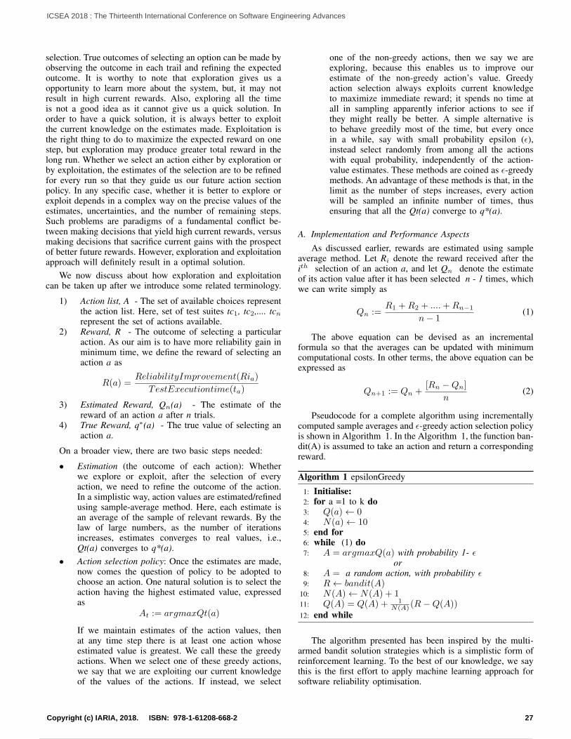
selection. True outcomes of selecting an option can be made byobserving the outcome in each trail and refining the expectedoutcome. It is worthy to note that exploration gives us aopportunity to learn more about the system, but, it may notresult in high current rewards. Also, exploring all the timeis not a good idea as it cannot give us a quick solution. Inorder to have a quick solution, it is always better to exploitthe current knowledge on the estimates made. Exploitation isthe right thing to do to maximize the expected reward on onestep, but exploration may produce greater total reward in thelong run. Whether we select an action either by exploration orby exploitation, the estimates of the selection are to be refinedfor every run so that they guide us our future action sectionpolicy. In any specific case, whether it is better to explore orexploit depends in a complex way on the precise values of theestimates, uncertainties, and the number of remaining steps.Such problems are paradigms of a fundamental conflict be-tween making decisions that yield high current rewards, versusmaking decisions that sacrifice current gains with the prospectof better future rewards. However, exploration and exploitationapproach will definitely result in a optimal solution.

We now discuss about how exploration and exploitationcan be taken up after we introduce some related terminology.

1) Action list, A - The set of available choices representthe action list. Here, set of test suites tc1, tc2,.... tcnrepresent the set of actions available.

2) Reward, R - The outcome of selecting a particularaction. As our aim is to have more reliability gain inminimum time, we define the reward of selecting anaction a as

R(a) =ReliabilityImprovement(Ria)

TestExecutiontime(ta)

3) Estimated Reward, Qn(a) - The estimate of thereward of an action a after n trials.

4) True Reward, q∗(a) - The true value of selecting anaction a.

On a broader view, there are two basic steps needed:

• Estimation (the outcome of each action): Whetherwe explore or exploit, after the selection of everyaction, we need to refine the outcome of the action.In a simplistic way, action values are estimated/refinedusing sample-average method. Here, each estimate isan average of the sample of relevant rewards. By thelaw of large numbers, as the number of iterationsincreases, estimates converges to real values, i.e.,Qt(a) converges to q*(a).

• Action selection policy: Once the estimates are made,now comes the question of policy to be adopted tochoose an action. One natural solution is to select theaction having the highest estimated value, expressedas

At := argmaxQt(a)

If we maintain estimates of the action values, thenat any time step there is at least one action whoseestimated value is greatest. We call these the greedyactions. When we select one of these greedy actions,we say that we are exploiting our current knowledgeof the values of the actions. If instead, we select

one of the non-greedy actions, then we say we areexploring, because this enables us to improve ourestimate of the non-greedy action’s value. Greedyaction selection always exploits current knowledgeto maximize immediate reward; it spends no time atall in sampling apparently inferior actions to see ifthey might really be better. A simple alternative isto behave greedily most of the time, but every oncein a while, say with small probability epsilon (ε),instead select randomly from among all the actionswith equal probability, independently of the action-value estimates. These methods are coined as ε-greedymethods. An advantage of these methods is that, in thelimit as the number of steps increases, every actionwill be sampled an infinite number of times, thusensuring that all the Qt(a) converge to q*(a).

A. Implementation and Performance Aspects

As discussed earlier, rewards are estimated using sampleaverage method. Let Ri denote the reward received after theith selection of an action a, and let Qn denote the estimateof its action value after it has been selected n - 1 times, whichwe can write simply as

Qn :=R1 +R2 + ....+Rn−1

n− 1(1)

The above equation can be devised as an incrementalformula so that the averages can be updated with minimumcomputational costs. In other terms, the above equation can beexpressed as

Qn+1 := Qn +[Rn −Qn]

n(2)

Pseudocode for a complete algorithm using incrementallycomputed sample averages and ε-greedy action selection policyis shown in Algorithm 1. In the Algorithm 1, the function ban-dit(A) is assumed to take an action and return a correspondingreward.

Algorithm 1 epsilonGreedy

1: Initialise:2: for a =1 to k do3: Q(a)← 04: N(a)← 105: end for6: while (1) do7: A = argmaxQ(a) with probability 1- ε

or8: A = a random action, with probability ε9: R← bandit(A)

10: N(A)← N(A) + 111: Q(A) = Q(A) + 1

N(A) (R−Q(A))12: end while

The algorithm presented has been inspired by the multi-armed bandit solution strategies which is a simplistic form ofreinforcement learning. To the best of our knowledge, we saythis is the first effort to apply machine learning approach forsoftware reliability optimisation.



38 / 160

IV. DEMONSTRATION USING REAL CASE STUDY

In this section, we present a real case scenario which formsthe basis for our motivation to pursue this investigation. As anillustrative example, a relatively simple redundant system isconsidered, the configuration of which is depicted in Figure1. The system is a heterogeneous dual redundant systemcomprising of a main system and a standby system. Eachsystem houses two packages and each package in turn holds3 sensors. Both Main and Standby systems acquires realtime data from these sensors. The dynamics of main systemand standby system are heterogeneous in nature. The mainsystem is highly accurate, with less acceptable operationaltime, whereas the standby system is less accurate with longeroperational time.

For the missions, whose working duration is of the orderof the performance of main system, it is naturally good toconsider the data of the main system so long it is healthy.As the data provided by this system is crucial from missionperspective, the redundancy management is employed at thecomponent (sensor) level. If multiple component failure occursthen system level reconfiguration is considered. Componentlevel redundancy management adds more to the complexityof the software logics coded. Thus, the functional correctnessof redundancy management software logics play a significantrole in determining the overall reliability of the system. Thesoftware architecture of such logics should be failure resilentand robust enough. From the verification perspective, it is ofparamount interest to ensure the reliability of these logics. Thesection below details the software architecture considered forrealising the component level redundancy.

Ms1

Ms4

Ms5

Ms6

Ss1

Ms2

Ms3

Ss2

Ss3

Ss4

Ss5

Ss6

Main Standby

Figure 1. System Configuration.

A. Software Architecture

Redundancy management software core has 3 basic mod-ules viz., i) Fault detection module ii) Fault Diagnosis moduleiii) Reconfiguration module. Fault detection logic recognizesthat something unexpected has occurred in the system. Todo so, it monitors the behavioral parameters of a compo-nent/system to asses the health of it. Once a fault is detected,the next step is to identify the faulty component (failurelocation), and also the nature of the fault (whether the faultis transient nature or permanent). Finally, a remedial actionto be performed based on the decision logics of the system.This phase leads to reconfiguration of the system either at thecomponent level or system level. Successful reconfigurationrequires robust and flexible software architecture and theassociated reconfiguration schemes.

Software realization for the system is depicted in Figure 2.In total, there are 12 modules labelled as swci. Each moduleis associated with a test suite (tci) and its execution time (ti).

Figure 2. Software Architecture.

As stated earlier, each software component has its owncontribution to the overall software reliability. The reliabilityimprovement figure Ri upon testing different components isdifferent. For the illustrated system, the Ri for each compo-nent is assigned based on the complexity and the functionalcriticality of the logic associated with it. In the Table IV,the 2nd row shows the Ri that can be obtained by testing asoftware component swci with its test suite tci. We see there isa variation in the Ri’s. For example, software logics identifiedby swc2 corresponds to package validity checks of the secondpackage. For the system which is described above, the designelements for package2 are more in number when compared topackage1, hence the logics are complex, as a result, the Ri ismore for swc2 when compared to swc1. Similarly, swc10 dealswith identifying permanent faults. As permanent faults leadto reconfiguration of the system, the decisions are made afterobservation of the fault for a persistent amount of time. Hence,this logic is obviously the most complex of all the components,hence the Ri awarded to it is the highest. 3rd row of the tablerefers the test suite execution times ti. As our aim is to find anoptimal test suite with minimum execution time, the reward Rfor each test component is

Rn =Rintn

which are placed in 4th row. 5th row corresponds to the uncer-tainties associated with this reward estimates. The uncertaintiesare assigned using subjective guess method. When there aremore elements of uncertainty in the logics, the probabilities areassigned less. For example, the software logics for packagevalidity checks, which are meant to asses the health of thesensor, depend on operational environmental conditions. Thephysical quantities like temperature of the chamber, numberof operational hours, misalignment factors, calibration stateof the package play a role in the sensor behaviour. As perthe system design, package2 is highly sensitive and moredependent on the external factors. Hence, it is very difficult toascertain Ri with great confidence, so the probability associatedto it is on the lower side. On the other hand, there is no



39 / 160

TABLE IV. SOFTWARE COMPONENT NUMERICALS.

Parameter tc1 tc2 tc3 tc4 tc5 tc6 tc7 tc8 tc9 tc10 tc11 tc12Reliability Improvement (Rii ) 9 11.5 6 6 6 8 8 8 7.5 13 10 7

Execution Time (ti) 7 8 5 5 5 5 5 5 6 10 9 7Reward (R) 1.285 1.4375 1.2 1.2 1.2 1.6 1.6 1.6 1.25 1.3 1.11 1.0

Probability (Pi) 0.75 0.65 0.65 0.65 0.6 0.6 0.6 0.6 0.9 0.85 0.9 0.9

involvement of external factors on the reconfiguration logicsof the system. Only the design criteria as per system needs areto be coded, hence, the uncertainty factor associated to it isless. All components are assigned values following the sameanalogy.

V. EXPERIMENTAL RESULTSThis section demonstrates the evaluation results of the pro-posed algorithm to the case study illustrated in the previoussection. In essence, two aspects are considered during eval-uation. Firstly, the applicability of the bandit algorithm inarriving at an optimal solution is studied. To demonstrate this,4 case studies each depicting an indicative practical scenario istaken up. Secondly, the aspect of exploration and exploitationtradeoff for the given task at hand is studied. Here, variousexploration fractions are considered to arrive at a suitableexploration probability for the illustrated example. Also, onan explorative note, a simple variant of ε greedy algorithmtermed as ε decaying strategy is applied. Here, rather thanusing a fixed value for ε, it is started with a high value initially,and decreased gradually over time. This way, we can favorexploration initially, and then favor exploitation later on. Thefollowing subsections elucidates the experimental results on adetailed note.

A. Application of Bandit AlgorithmTo illustrate the application of bandit algorithm for finding

an optimal test suite, four different scenarios/cases consideringthe different possibilities of having rewards and probabilitystructures are taken. Each scenario results are illustrated usingtwo graphs. The first graph depicts the preferred action choicesand the second graph elucidates the reward history. The detailsof which are stated below:

• Case1: This case corresponds to the state where therewards and probability figures of the case study arekept unchanged. The rewards and confidence figuresdepicted in Table IV are considered as it is. Byintuition we can make some guess on the optimal testsuite selection, but it may not be the possible bestsolution. By running the algorithm designed, we seethe order of preference of test suite is as tc9, tc10,tc11, tc1, tc6, tc12, tc7, tc2, tc8, tc3/tc4/tc5. The Ri’s oftc6, tc7, tc8 are the highest(1.6), but the probabilitiesassociated with them are less. Though the Ri of tc9is lesser than tc6, since the associated probability of itis much more than tc6, tc9 is given preference. Also,we see the reward of tc10 is higher than the rewardof tc9 , but in long run tc9 is given preference as thecertainity factor of it is higher than tc10. Similarly, allother test suites are preferred. The results shown inFigure 3 after running the epsilon greedy algorithmdepict the optimal test suite selection for this case.

• Case2: This considers the scenario where the esti-mates made are certain, means there is no elementof uncertainty. Thus, all the estimates are assigned aprobability of 1 (equal probability distribution). In thiscase, the test suite having the highest initial estimateshould be given preference. For our case, tc6, tc7, tc8are to be favored first. The graphs illustrated in Figure4 confirm the expected notion.

• Case3: Here, we consider the case where the rewardsobtained by selecting each action is equal, but eachreward is having its own uncertainty factor. Naturally,the one having the highest probability of occurenceshould be given preference over the other. For illus-tration purpose, the initial rewards of all the test suitesis set to a value of 1. Here, the test suites tc9, tc11,tc12 with the highest probability are to be favored. Thegraphs depicted in Figure 5 stand to this opinion.

• Case4: This case pertains to the scenario where thereis no uncertainty in the estimates made and all com-ponents have equal reward. Ideally, in this case allactions are to be chosen with equal importance. Thegraphs presented in Figure 6 confirm the analogy.

Figure 3. Case 1 Results.


The true reward of selecting a particular test suite besidesthe uncertainty factor in place can be concluded by consideringthe long term rewards. Table V summarizes the long termrewards Rl of every test suite obtained after running theproposed algorithm for the 4 different scenarios explained inthe previous paragraph. For every case, row 1 corresponds toconfidence figures, row 2 represents initial reward estimatesand row 3 represents the true rewards of each test suite. We



40 / 160



see the long term rewards Rl’s for each test suite entirelydepends on the initial estimates on the probability of occurenceof that estimate. The results depicted in Table V are found to beintuitive. Once the true rewards are known for each test suite,choosing an optimal set of test suites to fill the reliability gapis trivial.

B. Exploration-Exploitation TradeoffNow we look into the aspect of Exploration and Exploita-

tion trade off by running the algoritm over various exploitationfactors. Figure 7 compares a greedy method with three ε-greedy methods (ε = 0.01, ε = 0.1, ε = 0.5). All the methodsformed their action-value estimates using the sample averagetechnique. The greedy method improved slightly faster thanthe other methods at the very beginning, but then leveledof at a lower level. It achieved a reward-per-step of onlyabout 1.21, compared with the best possible of about 1.26 onthis testbed. The greedy method performed significantly worsein the long run because it often got stuck performing sub-optimal actions.The ε-greedy methods eventually performedbetter because they continued to explore and to improve theirchances of recognizing the optimal action. The ε = 0.1 methodexplored more, and usually found the optimal action earlier,but it never selected that action more than 91% of the time.The ε = 0.01 method improved more slowly, but eventuallywould perform better than the ε = 0.1 method. As seen fromthe figures, exploring more often (ε = 0.5) is also not good.We say that this exploration-exploitation trade-off varies fromproblem to problem. For the given case study exploration rateof 0.01 is relatively effective in long run, but this needs morenumber of iteration to achieve sub-optimal rewards. Hence achoice can be made between exploration rate of 0.1 or 0.01.

One issue with the epsilon-greedy strategy is how to set thevalue of ε, and how we continue exploring suboptimal choicesat that rate even after the algorithm identifies the optimalchoice. Rather than using a fixed value for ε , we can start witha high value that decreases over time. This way, we can favorexploration initially, and then favor exploitation later on. Thisstrategy is known as ε decaying strategy. Figure 8 and Figure

9 illustrates this strategy. The initial ε is set to 0.1. Figure 8illustrates the case where the exploration factor is decreasedto 0.01 after half the trials are over. We see that there is noperformance degradation upon decreasing exploration rate asby half of the trials all the actions rewards might have reachedvery close to their optimal values, hence little exploration isenough. Figure 9 decreases the exploration factor by a largefactor (to 0.001) which is not an advisable scenario for our casestudy. The initial choice of exploration rate and the decayingfactor varies from problem to problem.

ε = 0.1ε = 0.01ε = 1ε = 0.5

Figure 7. Exploration-Exploitation tradeoff.

Non-decaying Decaying

Figure 8. Epsilon Decreasing Strategy-1.

Decaying

Non-decaying

Figure 9. Epsilon Decreasing Strategy-2.

VI. RELATED WORKA lot of work in the past considered the optimal allocation ofthe reliabilities to minimize a cost function, related to the de-sign or the verification phase costs. Much initial research dealtwith hardware systems (e.g., the series-parallel redundancy-allocation problem has been widely studied [4]-[5]); softwaresystems received attention more recently. For a software ap-plication, the objective of the optimization will depend onthe phase of the software life cycle. During the design phase[6], structural optimisation of the software architecture is paidattention with two leading objectives i) reliability constrained



41 / 160

TABLE V. OVERALL RESULTS.

Case No. Parameter tc1 tc2 tc3 tc4 tc5 tc6 tc7 tc8 tc9 tc10 tc11 tc12

1Pi 0.75 0.65 0.65 0.65 0.6 0.6 0.6 0.6 0.9 0.85 0.9 0.9Rii 1.285 1.437 1.2 1.2 1.2 1.6 1.6 1.6 1.25 1.3 1.11 1.0Rli 0.96 0.93 0.78 0.78 0.78 0.95 0.95 0.95 1.11 1.09 0.99 0.90

2Pi 1 1 1 1 1 1 1 1 1 1 1 1Rii 1.285 1.437 1.2 1.2 1.2 1.6 1.6 1.6 1.25 1.3 1.11 1.0Rli 1.28 1.43 1.2 1.2 1.2 1.59 1.59 1.59 1.25 1.3 1.11 1.0

3Pi 0.75 0.65 0.65 0.65 0.6 0.6 0.6 0.6 0.9 0.85 0.9 0.9Rii 1 1 1 1 1 1 1 1 1 1 1 1Rli 0.75 0.65 0.65 0.65 0.65 0.6 0.58 0.58 0.88 0.84 0.88 0.88

4Pi 1 1 1 1 1 1 1 1 1 1 1 1Rii 1 1 1 1 1 1 1 1 1 1 1 1Rli 1.0 1.0 1.0 1.0 1.0 0.99 1 1 1 1 0.99 1

cost minimization ii) cost constrained reliability maximization.During the testing phase, the objective of the optimization isto determine the allocation of testing effort so that the desiredreliability objective is achieved [7][8]. During the operationalphase, optimization is used to explore alternative configura-tions and to determine an optimal allocation of components tovarious nodes in a distributed network to achieve the desiredperformance and reliability.

At the software front, we see much of the research workin the community is biased on design phase optimisation side[9][10]. This work, however, does not consider testing-time ofsoftware components and the growth of their reliability. Notmany papers considered the problem in the software verifica-tion phase, where the issue is either to allocate reliabilities thatcomponents need to achieve during their testing or to determinethe allocation of testing effort so that the desired reliabilityobjective is reached. Looking at the work in this direction,chronologically, the very initial work by Okumoto and Goel[11] investigated the optimal software release problem by usinga software reliability growth model based on NonHomoge-neous Poisson Process (NHPP) by considering the cost andsoftware reliability as two different independent criterion. Thiswork was carry forwarded by Shigeru Yamada et al. [12] whoconsider both cost and reliability criteria.

Also, authors in [7][13] proposed an optimization modelwith the cost function based on well known reliability growthmodels. They also include the use of a coverage factor foreach component, to take into account the possibility that afailure in a component could be tolerated (but fault tolerancemechanisms are not explicitly taken into account, and thecoverage factor is assumed to be known). The authors in [14]also try to allocate optimal testing times to the componentsin a software system (here, the reliability growth model islimited to the Hypergeometric (S-shaped) Model). Some of thecited papers [7][14][15] also consider the solution for multipleapplications, i.e., they aim to satisfy reliability requirements fora set of applications.

In recent times, traditional reliability growth modellingtechniques are replaced by machine learning techniques toimprove the prediction accuracy of the constructed SRGM.A number of machine learning strategies such as artificialneural networks (ANN), support vector machine (SVM) andgenetic programming (GP), are in practice in recent times forreliability modeling. Gene Expression Programming (GEP),a new evolutionary algorithm based on Genetic algorithm(GA) and GP, has been acknowledged as a powerful ML for

reliability modelling[16]. We infer from the literature surveythat the application of AI in software engineering domain [17]is also concentrated on software relaibility modelling.

Though, SRGM is probably one of the most successfultechniques in the literature for software reliability modelling,with more than 100 models existing in one form or another,through hundreds of publications, in practice, however, theyencounter major challenges. First of all, software testers sel-dom follow the operational profile to test the software, sowhat is observed during software testing may not be directlyextensible for operational use. Secondly, when the numberof failures collected in a project is limited, it is hard tomake statistically meaningful reliability predictions. Thirdly,some of the assumptions of SRGM are not realistic, e.g., theassumptions that the faults are independent of each other, thateach fault has the same chance to be detected in one class, andthat correction of a fault never introduces new faults. Theselimitations impediments the use of SRGM based methods. Insuch cases, subjective knowledge of the system can be takenas an aid in making the reliability estimates. Estimates canbe made subject to some criteria like - complexity, functionalcriticality etc. Since these are just estimates, one can assignconfidence factor for the estimates made and can address theoptimal selection issue.To the best of our knowledge, no workaddresses this scenario and hence motivated us to consider alearning strategy and frame a solution methodology.

VII. CONCLUSIONSIn this paper, we have proposed a learning based paradigmfor addressing the software reliability optimisation problem.We have shown how an interactive learning can address theproblem of finding an optimal test suite whose rewards arestochastic in nature. In the proposed solution, every interactionis used to learn about the system and in a way the rewards arerefined. As a result, over a period of time, the stochastic rewardvalues are converted into true rewards. Once the true rewardsare computed, the problem at hand becomes as simple as amulti-objectuive optimisation problem. The learning strategyemployed here is inspired by a well known multi-armed banditsolution strategies. The application of the proposed solutionstrategy to the real case study demonstrates the potential ofReinforcement Learning in addressing the problem stated.

In future, we intend to enhance our existing algorithm byconsidering various practical scenarios. The random actionselection policy considered during exploration phase in ε-greedy solution can be improved using Upper-Confidence-Bound strategy. The ε greedy action selection forces the



42 / 160

non-greedy actions to be tried, but indiscriminately, with nopreference for those that are nearly greedy or particularlyuncertain. It would be better to select among the non-greedyactions according to their potential for actually being optimal,taking into account both how close their estimates are to beingmaximal and the uncertainties in those estimates. We findthere is a proper mathematical basis to work out this idea.Using this refined startegy, we guess that global optimumcan be obtained in a fewer iterations. Furthermore, based onsome numerical preference Gradient Bandit Algorithms can beconsidered to improve further. Furthermore, contextual banditscan be explored for associative search policies. In summary, wesee a good potential in the application of RL for optimisationdomain.

REFERENCES

[1] M. R. Lyu, “Software reliability engineering: A roadmap,” in 2007Future of Software Engineering, ser. FOSE ’07. Washington, DC,USA: IEEE Computer Society, 2007, pp. 153–170. [Online]. Available:http://dx.doi.org/10.1109/FOSE.2007.24

[2] S. S. Gokhale, “Architecture-based software reliability analysis:Overview and limitations,” IEEE Transactions on Dependable andSecure Computing, vol. 4, no. 1, Jan 2007, pp. 32–40.

[3] R. S. Sutton and A. G. Barto, Reinforcement Learning: An Introduction.The MIT Press, 2017.

[4] Y. Nakagawa and S. Miyazaki, “Surrogate constraints algorithm for reli-ability optimization problems with two constraints,” IEEE Transactionson Reliability, vol. R-30, no. 2, June 1981, pp. 175–180.

[5] F. A. Tillman, C. L. Hwang, and W. Kuo, “Determining componentreliability and redundancy for optimum system reliability,” IEEE Trans-actions on Reliability, vol. R-26, no. 3, Aug 1977, pp. 162–165.

[6] M. E. Helander, M. Zhao, and N. Ohlsson, “Planning models for soft-ware reliability and cost,” IEEE Transactions on Software Engineering,vol. 24, no. 6, Jun 1998, pp. 420–434.

[7] M. R. Lyu, S. Member, S. Rangarajan, and A. P. A. V. Moorsel,“Optimal allocation of test resources for software reliability growthmodeling in software development,” IEEE Transactions on Reliability,2001.

[8] J. Rajgopal and M. Mazumdar, “Modular operational test plans forinferences on software reliability based on a markov model,” IEEETransactions on Software Engineering, vol. 28, no. 4, Apr 2002, pp.358–363.

[9] F. Zahedi and N. Ashrafi, “Software reliability allocation basedon structure, utility, price, and cost,” IEEE Trans. Softw. Eng.,vol. 17, no. 4, Apr. 1991, pp. 345–356. [Online]. Available:http://dx.doi.org/10.1109/32.90434

[10] O. Berman and N. Ashrafi, “Optimization models for reliability of mod-ular software systems,” IEEE Transactions on Software Engineering,vol. 19, no. 11, Nov 1993, pp. 1119–1123.

[11] K. Okumoto and A. L. Goel, “Optimum release time for softwaresystems,” in Computer Software and Applications Conference, 1979.Proceedings. COMPSAC 79. The IEEE Computer Society’s ThirdInternational, 1979, pp. 500–503.

[12] S. Yamada and S. Osaki, “Cost-reliability optimal release policies forsoftware systems,” IEEE Transactions on Reliability, vol. R-34, no. 5,Dec 1985, pp. 422–424.

[13] M. R. Lyu, S. Rangarajan, and A. P. A. van Moorsel, “Optimization ofreliability allocation and testing schedule for software systems,” in Pro-ceedings The Eighth International Symposium on Software ReliabilityEngineering, Nov 1997, pp. 336–347.

[14] R.-H. Hou, S.-Y. Kuo, and Y.-P. Chang, “Efficient allocation of testingresources for software module testing based on the hyper-geometricdistribution software reliability growth model,” in Software ReliabilityEngineering, 1996. Proceedings., Seventh International Symposium on,Oct 1996, pp. 289–298.

[15] N. Wattanapongsakorn and S. P. Levitan, “Reliability optimizationmodels for embedded systems with multiple applications,” IEEE Trans-actions on Reliability, vol. 53, no. 3, Sept 2004, pp. 406–416.

[16] B. Kotaiah and R. A. Khan, “A survey on software reliability assessmentby using different machine learning techniques,” 2012.

[17] M. Harman, “The role of artificial intelligence in software engineering,”in 2012 First International Workshop on Realizing AI Synergies inSoftware Engineering (RAISE), June 2012, pp. 1–6.



43 / 160

Concurrency Analysis of Build SystemsVasil Tenev, Bo Zhang, Martin Becker

Fraunhofer Institute for Experimental Software Engineering (IESE)Kaiserslautern, Germany

Email: {vasil.tenev, bo.zhang, martin.becker}@iese.fraunhofer.de

Abstract—In order to derive executable software artefacts, abuild system needs to be maintained properly along with theevolution of source code. However, in large software projectsthe build process often becomes effort-consuming, which is oftencaused by suboptimal concurrency either in the design of thebuild system or in the execution of the build process. To copewith these challenges, we present our concurrency analysis withpractical experiences in this paper. In particular, we proposea new metric called Degree of Freedom for evaluating theconcurrency potential of a build system based on dependenciesamong build jobs and artefacts. In fact, this metric is not limitedto build analysis. It can be used for analyzing the concurrencypotential of any executable process in general.

Index Terms—concurrency, build system, control flow

I. INTRODUCTION

While normal source code (also as known as productionsource code) implement the behavior of a software, its buildsystem (including build tools and build code such as makefiles)derives the executable software from its production sourcecode. In large industrial software systems, the complexity ofthe build system is often high (in terms of build jobs and builddependencies), and the build process is time-consuming (overone hour in large systems) even in a distributed environmentusing high-performance and multi-core computers. This is notacceptable in real continuous integration settings with frequentcode revisions and builds per day.

In order to understand the build process and related issues,in our previous work [18] we have depicted the build processvia the notion of Build Dependency Structure. Theoretically,the build dependency structure contains two dimensions asillustrated in Figure 1 on page 1. On the one hand, the rootbuild command triggers a flow of build actions that can furtherrun atomic build jobs (e. g., compiling and linking). Thesebuild actions and jobs are invoked and executed in a treestructure (vertical in Figure 1 on page 1). On the other hand,the build jobs with different build tools indicate dependenciesbetween input build artefacts and output build artefacts, whichfurther constitute a dependency graph (horizontal in Figure 1on page 1).

In the build dependency structure, some build jobs needto be executed sequentially due to the dependencies amongbuild jobs and artefacts. However, independent build jobscould be executed in parallel, which helps improving the buildefficiency. Therefore, in practice it is important to analyzethe build system and make sure that build jobs are executedwith optimal concurrency. Although there was some endeavorin build dependency extraction and optimization [6], [12] a

Figure 1: Notion of the Build Dependency Structure

comprehensive analysis focusing on build concurrency is stilllacking.

In order to optimize the build concurrency and improvebuild efficiency, we would like to conduct automated anal-yses both on the build execution process and also on thebuild system architecture. At build execution time, we useexisting commercial tools for monitoring the build processand analyzing the execution of build jobs in different threadsand on different machines. This shows whether build jobsare actually executed in parallel. Moreover, we also conductstatic analysis on build dependencies of the build system andmeasure concurrency potential of the build architecture. Thishelps identify root causes of concurrency problems in the buildprocess.

In this paper, we provide the following contributions:

• Practices of dynamic and static concurrency analysis inan industrial study.

• An innovative metric called Degree of Freedom for staticconcurrency analysis.

• Lessons learned during the concurrency analysis andoptimization.

This paper is presented in the following structure. Section IIpresents our practice of dynamic concurrency analysis. Sec-tion III introduces our static concurrency analysis approach.While Section Section IV discusses related work, Section Vpresents conclusions, summarizes lessons learned during ourconcurrency analysis study, and discusses future work at theend.



44 / 160

Figure 2: Dynamic Concurrency Analysis by ElectricInsight

II. DYNAMIC CONCURRENCY ANALYSIS

The dynamic concurrency analysis shows the actual exe-cution of different build jobs in a distributed environment.There exists commercial tools like ElectricInsight [2] for suchpurpose. Typically, these tools monitor the build process byinstrumenting the GNU (GNU is a recursive acronym for"GNU’s Not Unix!") make tool or even replacing it withtheir own make tool. As a result, a build execution graphis generated to visualize concurrent scheduling and executionof build jobs. For instance, in an industrial case study weused ElectricInsight and generated the build execution graphas shown in Figure 2 on page 2. While some build jobsare executed in parallel in different threads (by build agents)and CPU (Central processing unit) cores, other build jobs areexecuted sequentially in the same thread.

Besides monitoring build execution, ElectricInsight alsoclaims to optimize the scheduling of concurrent build execu-tion (to reduce the overall build duration). However, from ourexperience the build concurrency is often not optimal. As seenin Figure 2 on page 2, while a few build threads keep executingbuild jobs sequentially, many other threads finish early andremain idle until the end of the build process. It seems thatsome build jobs have to be executed sequentially due to builddependencies defined in the build system (e. g., makefiles).In order to investigate the root causes of this suboptimalbuild concurrency, it is necessary to further analyze builddependencies and identify the actual concurrency potential.

III. STATIC CONCURRENCY ANALYSIS

While dynamic concurrency analysis shows the actual be-havior of build job execution during the build process, staticconcurrency analysis focuses on the concurrency potential of

(a) Artefact View (b) Process View

(c) Execution View

Figure 3: Different Views of Build Dependencies.

build jobs and artefacts based on their dependencies. In thissection, we assume an arbitrary but fixed environment for theexecution of the build process, i. e., number of CPU cores,parallel threads, RAM (Random-access memory) size, etc.Moreover, we assume that the build process has only oneconnected graph component.

A. Build Dependencies

Various dependencies exist between build jobs and artefacts.We consider three views to analyze the different aspects of thebuild dependencies structure:

The Artefact View contains source code artefacts, interme-diate and final artefacts of a build process. In Figure 3a onpage 2 an artefact “A.o” depends on artefact “A.c”.

On the other hand, the Process View shows build jobs andthe process dependencies in-between, that represent finish-to-finish relationships. For an example of a clean build seeFigure 3b on page 2, where the job “link” can finish, only ifjob “compile” has finished. The job “link” may however startbefore, in parallel, or after the job “compile”. In any case,“link” can’t finish before “compile” is finished.

The Execution View describes three kind of dependencies(see Figure 3c on page 2):

• Execution Dependency: Job “compile_A2” executes job“clean”;

• Input Dependency: Job “compile_A2” depends on inputartefact “A2.c”; and

• Output Dependency: Artefact “A2.o” is result of job“compile_A2”.

These views depict all build dependencies in the vertical andhorizontal dimensions of the Build Dependencies Structurein [18]. Accounting the different views and the number ofpossibilities for scheduling build jobs make the basis of thestatic concurrency analysis.

In any of the views on a well-defined build dependencystructure, we deal with an acyclic directed graph. Such struc-ture is equivalent to a partial order over the set of artefacts andbuild jobs, respectively. This partially ordered set is consideredby a build tool (like GNU Make [3], Ninja [5], etc.) tocompute a schedule over all build jobs and execute them inthe right order. The richer the scheduling possibilities with



45 / 160

Figure 4: Process view of a best-case example for maximalparallelization

respect to the build dependencies structure, the bigger theoptimization space, the greater the degree of freedom forconcurrent execution.

B. Degree of Freedom

Here, we propose a new metric called Degree of Freedomthat quantifies the parallelization property of a build process,i. e.,the degree to which extent a build process can be paral-lelized. This stands intuitively in direct correlation with thenumber of possible scheduling plans.

Examples: (a) Consider a build process where the depen-dency graph in the process view is a chain (e. g., Figure 3b onpage 2). For such a process, there is only one possible planfor scheduling its execution and it is not parallelizable. (b) Incomparison, for a star-shaped build process, like in Figure 4on page 3, there are 8! = 40320 possible scheduling plans toexecute it in one processing thread and 8 of the 9 jobs can beparallelized.

We assume that a build process always has exactly onestarting point (i. e., the main build job) and only one finalresulting artefact (i. e., the product that is build). Thus, thedependency graph always has exactly one root in every viewand therefore a star-shaped build process is the best possiblecase for maximal parallelization. Using this and the correlationfrom above, we define a metric that compares a given buildprocess with a same-size, star-shaped build process by thenumber of possible scheduling plans.

However, the number of scheduling possibilities dependsnot only on the partial order, but also on the environment,i. e., mostly the number of parallel threads available for theexecution. To get an environment independent metric, that is tomultiply out the factor depending on the number of threads forparallel computing, we use the number of possible executionsequences for a single thread computation. Therefore, wedefine the Degree of Freedom by

Freedom (P ) = logS(P∗) S (P )

where S (P ) is the number of possible execution sequencesfor build process P and S (P ∗) is the number of possibleexecution sequences for a star-shaped build process with thesame number of build jobs/artefacts as in P . Thus, S (P ∗)equals(|P | − 1)!. Formally, S (P ) is the number of linearextensions over the partially ordered set (poset) P (see [11]).

Example: Let P be a build process with process view of 9build jobs, such that P is a sequence. Then the correspondingstar-shaped build process P ∗ is equivalent to this on Figure4 on page 3. Therefore Freedom (P ) = logS(P∗) S (P ) =log8! 1 = 0 and Freedom (P ∗) = logS(P∗) S (P ∗) =log8! 8! = 1.

C. Implementation

At its heart, our metric is based on the number of possibleexecution sequences for a build process, which is a partialordered set as discussed in III-A. The number of all sequenceswith respect to a poset is the number of all linear extensions ofthe poset [11]. In general, computing S (P ) is a #P-completeproblem for arbitrary posets [8].

Although there are several algorithms that can find onelinear extension in linear time [10], it is not clear if there existseven a polynomial time algorithm for computing the numberof all linear extensions [16]. However, there are polynomialapproximation schemes [9], which can be used to computethe number of all linear extensions by counting. In contrastto these works, we deal with special case of partial orderedsets. From the fact that they correspond to the dependencygraph of a build process, we can expect that the posets are‘almost’ trees. This means, that they contain a small number ofedges that are in contradiction with the tree properties. Thus,we based our approach on the algorithm for computing thenumber of linear extensions in a tree-shaped poset proposedby Atkinson [7]. He proposes an O

(n2

)algorithm for trees

with n being the number of elements. Since we deal with‘almost’ trees, we develop two algorithms for computing aupper and lower bounds for S (P ).

1) Upper Bound: We apply Atkinson’s algorithm in com-bination with Prim’s minimum spanning tree algorithm [15] toapproximate a minimum tree-shaped poset that is a supersetof P . Firstly, it will take all edges that are conform to theproperties of a tree. All remaining edges are evaluated withrespect to the minimal number of linear extensions resultingfrom taking one edge and recursively applying the sameprocedure until we end up with a tree on which we applyAtkinson’s algorithm. This minimal number defines the edgeweight. Afterwards, a minimal spanning tree is constructed.The number of linear extensions of that tree gives a upperbound for the number of linear extensions of P , since theset of dependencies (edges) of the tree is a subset of thedependencies of P . This algorithm runs in O

(k2n2

), where

k is the number of edges that contradict to the tree propertiesfrom graph theory.

2) Lower Bound: For the approximation of the lowerbound, we use a simple scheduling strategy that is more restric-tive than an optimal strategy for the given poset. We traverse



46 / 160

the poset graph bottom-up starting with leaf nodes — elementswith no outgoing dependencies — and moving towards a rootnode — element without ingoing dependencies. Hereby, wedetect independent sequences of nodes between branchinglocations in the graph. This gives us a sequence of layers inthe graph. Each layer consists of independent subsequences.The scheduling strategy is to run all subsequences in paralleland synchronizing the build process where a branching takesplace. We compute the number of linear extensions lj for layerj using the multinomial coefficient. More precisely, for everylayer j of m independent subsequences, we have

lj =

(k1 + k2 + · · ·+ km

k1, k2, . . . , km

)with ki being the number of nodes in i-th subsequence forall 1 ≤ i ≤ m. In total, we need the product of all lj .Computing the lower bound requires only one traversal of thegraph without repetitions, as described above, which implieslinear time.

Example: In the following, let P be the build dependencygraph from Figure 3c on page 2 to illustrate a computa-tion for both lower and upper bounds. We compute theupper bound, as described earlier, based on Prim’s minimumspanning tree algorithm. In this example, only two edgescontradict to the tree properties from graph theory — these are“clean”←”compile_A1” and “clean”←”compile_A2”. Choos-ing either edge results in equivalent trees with respect to thenumber of linear extensions due to symmetry. By applyingAtkinson’s algorithm we get S (P ) < 70 linear extensionsand we get Freedom (P ) < 0.4, since|P | = 9.

On the other hand, the lower bound is computed very easily.Following the introduced algorithm, we end with three layers(l1, l2, l3). From left to right:

• l1 consists of 3 independent subsequences each of a singlenode. These are “A1.c”, “clean”, and “A2.c” and implyl1 =

(1+1+11,1,1

)= 6.

• l2 consists of 2 independent subsequences each of length2: ”compile_A1”←“A1.o” and ”compile_A2”←”A2.o”.Here we get l2 =

(2+22,2

)= 6.

• Finally, l3 consists of one subsequences of 2 nodes“link_A”←“A”, that means l3 =

(22

)= 1.

Since S(P ) > l1 · l2 · l3 = 36, Freedom (P ) > 0.337 holdsand in total Freedom (P) = 0.3685± 0.0315.

D. Optimization and Visualization

The Degree of Freedom is a metric for the static concur-rency analysis, that measures the parallelization potential of abuild process as a whole. While it is an objective measurement,it does not provide direct recommendations for optimization.However, in cases where the build process can be separated inseveral independent sub-processes (see Figure 5 on page 4), adomain expert would be able to detect high-potential regionsby applying our metric.

Here we recommend our »GAME-changing« method with:• The Goal to increase concurrency• by taking Actions to restructure dependencies.

Figure 5: Visualization of Static Concurrency Analysis

• This is achieved by identifying the high potential usingMeasurements to detect large sub-process size with lowDegree of Freedom and

• Executing the following steps:1) relationship analysis in high potential subgraphs by

domain experts;2) alignment of process and artefact dependency

graphs;3) reconnection of wrongly routed dependencies; and4) removal of unnecessary dependencies.

Additional visualization of the build process can also provideinsights and support for further analysis. In Figure 5 on page 4,we provide an example visualization using Cytoscape [1]. Herewe see the execution view of a (disconnected) build process,where each edge color represents different execution context,i. e., different execution scripts, different execution variableset, etc. Figure 5 on page 4.

IV. RELATED WORK

There have been approaches and tools for both dynamic andstatic build analysis. In our previous work [18], we focusedon the build process of Android and extracted the buildjobs and dependencies by instrumenting the shell of GNUmake. Gligoric et al. [12] intercepted file reads and writesin Windows by instrumenting Win32 functions using Detours[13]. In Linux there is the strace tool [14] for capturingsuch information like file read and write, process invocations,time measurement, etc. Moreover, there are tools for staticmakefile analysis, such as MAKAO [6], SYMake [17], andMakefile::Parser [4]. However, these tools are for general buildextraction and analysis, and they do not support analyzing theconcurrency of build execution.

V. CONCLUSION

This paper presents our approach for concurrency potentialanalysis we developed to support the maintenance of buildsystem for constantly evolving software in big projects wherethe build process consumes an important amount of effort. Weaddress these challenges providing our experience on dynamicand static analysis that we gained in our industry case. Whileconducting the concurrency analysis and optimization in thisstudy, we have the following lessons learned:

1) Conduct dynamic concurrency analysis to monitor theconcurrency performance of the actual build process.

2) Conduct static concurrency analysis to evaluate concur-rency of the designed build process.



47 / 160

3) In order to optimize concurrency, deficits in the buildsystem (e. g., obsolete/redundant build jobs) should befirst fixed.

4) To prioritize concurrency optimization, consider to firstfocus on larger build subprocesses that have lowerDegree of Freedom.

Moreover, we propose a new metric for measuring the con-currency potential of a build process. In fact, this metric isnot limited to build analysis. It can be used for analyzing theconcurrency potential of any executable process in general.Our implementation also provides a polynomial algorithm forcomputing lower and upper bounds for the number of linearexertions of a partial order set.

ACKNOWLEDGMENT

Thanks to our colleges from Fraunhofer IESE: MarkusDamm for pointing to the right terminology by the problemformulation; and Sören Schneickert for many fruitful discus-sions and his constructive criticism.

REFERENCES

[1] Cytoscape. http://www.cytoscape.org, August 2018.[2] ElectricInsight. http://electric-cloud.com/, August 2018.[3] GNU Make. https://www.gnu.org/software/make, August 2018.[4] Makefile::Parser. https://github.com/agentzh/makefile-parser-pm, August

2018.[5] Ninja. https://ninja-build.org, August 2018.

[6] B. Adams, H. Tromp, K. de Schutter, and W. de Meuter. Design recoveryand maintenance of build systems. In Proc. IEEE Int. Conf. SoftwareMaintenance, pages 114–123, October 2007.

[7] M. D. Atkinson. On computing the number of linear extensions of atree. Order, 7(1):23–25, Mar 1990.

[8] Graham Brightwell and Peter Winkler. Counting linear extensions.Order, 8(3):225–242, 1991.

[9] Russ Bubley and Martin Dyer. Faster random generation of linearextensions. Discrete Mathematics, 201(1-3):81–88, apr 1999.

[10] Thomas H. Cormen, Charles E. Leiserson, Ronald L. Rivest, andClifford Stein. Introduction to Algorithms, Second Edition, chapter 22.4Topological sort, pages 549–552. The MIT Press, 2001.

[11] Chaabane Djeraba Dan A. Simovici. Mathematical Tools for DataMining. Springer London, 2008.

[12] Milos Gligoric, Wolfram Schulte, Chandra Prasad, Danny van Velzen,Iman Narasamdya, and Benjamin Livshits. Automated migration of buildscripts using dynamic analysis and search-based refactoring. SIGPLANNot., 49(10):599–616, October 2014.

[13] Galen Hunt and Doug Brubacher. Detours: Binary Interception of Win32Functions. In Proceedings of the 3rd USENIX Windows NT Symposium,pages 135–144, Seattle, Washington, July 1999.

[14] D. V. Levin, R. McGrath, and W. Akkerman. strace. linux syscall tracer.http://sourceforge.net/projects/strace, August 2018.

[15] R. C. Prim. Shortest Connection Networks And Some Generalizations.Bell System Technical Journal, 36(6):1389–1401, nov 1957.

[16] Ivan Rival, editor. Graphs and Order. Springer Netherlands, 1985.[17] A. Tamrawi, H. A. Nguyen, H. V. Nguyen, and T. N. Nguyen. Symake:

a build code analysis and refactoring tool for makefiles. In Proc. 27thIEEE/ACM Int. Conf. Automated Software Engineering 2012, pages 366–369, September 2012.

[18] Bo Zhang, V. Tenev, and M. Becker. Android build dependency analysis.In Proc. IEEE 24th Int. Conf. Program Comprehension (ICPC), pages1–4, May 2016.



48 / 160

Measuring Success in Agile Software Development Projects: a GQM Approach

Abdullah Aldahmash Electronics and Computer Science

University of Southampton Southampton, UK

e-mail: [email protected]

Andy Gravell Electronics and Computer Science

University of Southampton Southampton, UK


Abstract— Agile software development has become one of the most commonly used methodologies for developing software. It promises to deliver many benefits, but nevertheless, the implementation of agile practices and techniques require many changes that might be a challenge for organizations attempting to succeed with agile software development projects. Claiming the success of agile software projects is difficult, and there is a need for more measurements with which agile success could be evaluated. This paper develops an instrument with which the success of an agile software development project could be measured. The criteria of the success are driven from the Critical Success Factors (CSFs) of agile development which have been identified prior developing this instrument. The proposed instrument will evaluate the success of agile software development projects in achieving these identified success factors. The instrument was developed following the Goal Question Metric (GQM) approach. This study conducted semi-structured interviews with 13 experts in the field of agile development. The aim of these interviews was to review and confirm the proposed instrument for measuring the success of agile projects. Following comments from the interviews, the instrument was revised. The developed instrument proposes measuring the agile success using 6 goals, 30 questions, and 7 metrics.

Keywords—Agile; Agile success; GQM; Software metrics; Agile project

I. INTRODUCTION Agile practices and techniques have been adopted by many

organizations. These organizations face many challenges during the agile transformation. These challenges are related to a variety of aspects, such as people, culture, and technology. During a previous study [1] we identified the critical success factors of agile software development. Having identified the success factors of agile software development, now we will focus on studying how the success could be measured; claiming the success of agile software development is problematic. Therefore, there should be more metrics and systematic measurements that could evaluate the success of agile software development projects. There is also a need for more measurements with which the adoption of agile practices and techniques could be assessed.

The nature of agile software development requires new metrics that address the agility. One study [2] concluded that not all the software traditional lifecycle metrics are suitable for agile software development. It was suggested that future work should focus on how the use of the traditional software measurement could be adapted to work with agile development or to develop new metrics for agile development.

Recent research [3] reviewed a total of 22 software metrics and resulted with only 10 metrics that could be used in agile software development. Therefore, there is a need for more software metrics that could be used to measure the status of agile software development.

This study selected the GQM approach to develop an instrument for measuring the success of agile software development. This selection was based on a suggestion from [4] findings, which revealed that the GQM approach is more relevant to the nature of agile software projects with short-cyclic iterations. GQM will provide measurements with clear purposes and goals and will result in saving the time of developing the measurement which is one of the agile development objectives. In this paper, an instrument is developed using the GQM approach. This instrument aimed to measure the success of agile software development projects.

This paper is organized as follows: Section I is an introduction. Following which, Section II is a background where the literature review is discussed. In Section III, the related work is presented. Section IV discusses the research methodology used in this study is presented. Section V is pertaining to the development of the proposed instrument. Following that, Section VI discusses the review of the instrument. Lastly, Section VII concludes the paper and puts forth the future work.

II. BACKGROUND In this section, the relevant literature was reviewed. Section

A reviews the literature of the agile software development. Section B discusses the introduction of the GQM approach and how it could be employed.

A. Agile Software Development In 2001, a group of software engineers established the

agile manifesto [5] during which, they introduced four values and twelve principles of agile software development. Since then, agile practices and techniques have evolved. According to Agile Alliance network, agile software development defined as “an umbrella term for a set of methods and practices based on the values and principles expressed in the Agile Manifesto. Solutions evolve through collaboration between self-organizing, cross-functional teams utilizing the appropriate practices for their context” [6].

The main characteristics that the agile development include: communication and collaboration, support innovation/creativity, embrace changes, and the development should be iterative and indivisible [7]. Agile development advocates frequent delivery of working software. This ensures



49 / 160

that feedback will be received early and so will be the changes in requirements. Agile development also embraces changes and conflicts during the development rather than rejecting them [8].

The latest State of Agile Survey 2018 [9] revealed that the top three reasons which drive the organizations to adopt agile were to accelerate product delivery, to manage changing requirements, and to increase productivity. According to a survey from Microsoft research, the top three paybacks from agile development are: improve the communication, enhance the delivery, and better respond to the changes. Conversely, the three top difficulties with agile development are: large-scale projects, number of required meetings, and rigorous management culture [10].

B. Goal-Question-Metric Approach The instrument will be developed by using the GQM

approach. GQM was proposed by Basili and Weiss [11] with the aim of introducing a systematic way of defining goals that could easily be refined into questions and linked to metrics. The GQM approach has three levels: conceptual level (Goal), operational level (Question), and quantitative level (Metric).

The goals are usually defined for specific purposes from a certain perspective and for a given object. Therefore, the usage of GQM will help in ensuring that the defined measurements will be defined with the aim of achieving specific goals [12]. The questions are used to describe the approach to achieving the goals and how it is going to be achieved. The metrics are set of data linked to each question aiming to answer it and it could be objective or subjective. Defining goals is beneficial to focus on the important aspects. Writing questions will make the goals more specific and will suggest the relevant metrics [13]. An example of the structure of GQM is illustrated in Figure 1.

Figure 1. An Example of GQM Structure.

Using GQM approach to develop software measurements is associated with many benefits. Some of these benefits are improving the software product quality, enhancing software processes, and increasing the team cooperation [14]. The GQM-based measurement approach will help in avoiding

irrelevant measurements through the regular feedback and by involving the project team to define measurements that are linked to the agreed upon goals [15]. GQM is a systematic approach of representing and combining a set of high-level goals into measurements. The result of implementing GQM is the specification of a set of metrics addressing a particular set of goals and rules for interpreting these results [16]. It is hoped that by implementing the GQM approach it will be possible to define a list of metrics which could measure the success of an agile software development project in an organization.

III. RELATED WORK A great deal of studies has investigated the status of

measurements in agile software development. According to Javdani et. al [17], measurements in agile software development are unlike the measurements in traditional software development. It was suggested that there is a need for more agile measurements especially in the following areas: productivity and velocity, and the changing requirements in agile. Furthermore, Ayed et. al [18] introduced a measurement-based framework for measuring the adoption and customization of agile methods. A set of metrics have been introduced and categorised into three categories: organisation level metrics, product level metrics, and process level metrics. However, the introduced metrics were not introduced in a practical way which the organizations are looking for. Agile measurements need to be confirmed and validated through empirical methodologies in order to gain an acceptance from the agile practitioners. This paper is planning to validate the proposed instrument by conducting experts’ interviews. Heidenberg et. al [19] introduced a metrics model following GQM to measure the impact of agile transformation in software development organizations. Their model focused on measuring the business value, lead-time, and efficiency of the agile software development transformation. It was indicated that more measurements are necessary to assess the agile software development status in organizations attempting for agile transformation.

A recent study [20] has also attempted to provide a quantitative measurement of the impact of agile transformation in software development organizations. They proposed a model with quantitative metrics following the GQM approach. The proposed model consists of one goal, four questions, and eight metrics following the structure of the GQM approach. While they introduced quantitative metrics, they indicated that qualitative metrics are needed as well. It was suggested that future work might concentrate on providing qualitative metrics with which the status of agile software development could be evaluated and measured.

Fontana et. al [21] conducted a systematic review on the agile development maturity models and they compared these models aiming to develop a model which could evaluate the adoption of agile practices and techniques in an organisation. They found and reviewed fourteen models which assess the agile maturity, of which six models were introduced in the last four years. Most of these available models are built on a combination between agile principles and Capability Maturity Model Integration (CMMI). Fontana et. al [21] recommended that future works should focus on empirical validation of these

Goal 1

Goal 2

Question Question Question Question

Metric Metric Metric



50 / 160

measurements which this research already achieved. While our instrument focused on measuring the success of implementing each success factor, these models were designed to measure the maturity of each agile practice independently. Both ways could be used to indicate the success in implementing agile software development projects.

Chita [22] suggested that the activity theory, which is usually used in social science, could be used to assess the factors for successful agile software development implementation, since the agile success is built on organisational, cultural, and social factors. They developed a model following the activity theory for successful agile adoption and they indicated that their on-going research will validate this model by conducting a case study.

Laanti [23] introduced a framework which could assess the agile transformation in large software development organisations. The framework classified the status of the organisations into five categories from beginner organisations to world-class organisations. While the framework assesses the agile adoption in the organisations, it lacks details on how organisations could evaluate their own adoption and how they could improve their agile transformation.

The findings obtained as a result of this paper and of the abovementioned emerging related work focused on understanding how the organizations could succeed in implementing agile practices. Furthermore, how the success in implementing agile practices could be measured and assessed. This shows the needs for more research that could work to validate these measurements and to introduce them to be used by agile software development practitioners.

In this paper, the proposed instrument used a mix of qualitative metrics and quantitative metrics to measure the success of agile software development projects. The proposed instrument will be reviewed by agile experts and it will be validated through conducting practical case studies.

IV. RESEARCH METHODOLOGY The proposed instrument was developed using the GQM

approach. This study followed a qualitative method which is semi-structured interviews with agile experts. These interviews were necessary to validate the proposed instrument. An invitation of participation was sent to a total of 28 experts. The criterion of selecting the experts which was used is that the expert should have at least 5 years of experience with agile software development. Out of the 28-reached experts, 13 experts were willing to participate in this research. These participants came from various countries, including the USA, Saudi Arabia, the UK, and France. The industries which the interview participants represent include, but are not limited to: Education sector, Finance and Banking sector, and Information Technology & Software sector. The interviewed experts represent different types of organizations which ranges from small organizations with only 15-30 employees to big multi-nation organizations. The participants were shown the instrument, following which they had the chance to ask for clarifications if needed. Then, they were asked about each item and to propose new items to the instrument. The interviews last, on average, approximately from 35 to 60 minutes.

V. INSTRUMENT DEVELOPMENT As identified in the literature, more measurements are

needed for agile projects. The proposed instrument was developed for the purpose of measuring the success of agile software development projects. The GQM approach was selected to build the instrument considering its effeteness in detecting a systematic way of linking the metrics to the organizational goals and needs.

The first step of following the GQM approach is to identify the goal or the set of goals. The goal of this study was to measure the success of agile projects. Along with 6 sub goals selected as a result of a review of the success factors of agile software development [1], which identified the following factors as critical success factors of agile projects: Communication, Customer Involvement, Team Capability and Training, Top management Support, Organizational Culture, Delivery Strategy, Agile Software Development Practices and Techniques, and Project Management (PM) Process [1].

As suggested by GQM, the eight identified CSFs will be rewritten to be a set of goals. The two success factors of agile practices and techniques, and project management approach merged into one goal. This is because these two factors are about a selection process of available agile techniques and PM approaches; also, this was done to avoid the replication of having two goals about a selection process. Thus, the goal will be to have an appropriate selection of these available agile practices and techniques and PM approaches.

The organization culture is a soft factor which is hard to be measured and it contains many aspects which overlap with other success factors such as communication and top management support factors as per [24]. Thus, in the developed instrument, the organizational culture factor will not be an independent goal. Alternatively, organizational culture success factor will be included in the first, second, third, and fourth goal. The goals of the proposed instrument are listed as follows:

1. Improve the communication throughout the agile project.

2. Increase the customer involvement during the agile project.

3. Improve the training of the agile project team members.

4. Increase the support from top management in the agile project.

5. Enhance the delivery strategy. 6. Appropriate selection of agile techniques,

practices, and PM approach.

A. Experts Interviews Design This research applied semi-structured interviews

encompassing open-ended questions and closed-ended questions to review the proposed instrument. The purposes of these interviews were: firstly, to review and confirm the proposed instrument’s goals, questions, and metrics, and secondly to suggest any other questions and metrics that need to be considered when measuring the success of an agile software development project. The experts’ interview process comprised many steps, which were as follows:



51 / 160

•Emails were sent to experts briefing them on the research and the objectives of the instrument. In the email, the experts were also asked to identify their preferred date and time for the interview. •Depending on where the experts lived, some interviews were conducted online via Skype and Zoom, which are video calling applications. In contrast, other interviews were conducted on a face-to-face basis. •Prior to the start of the interviews, all participants were requested to read the participant information sheet, following which they were asked to sign the consent form and return it by email. •The participants were shown the instrument, and then had the opportunity to ask for further explanation if needed. This lasted approximately 5-10 minutes. •Following this, the experts were asked about each goal in the instrument, starting with the first goal and ending with the last one. The experts were also asked about each item in the instrument and whether they felt that any additional item(s) needed to be added to the instrument. •In the last part of the interview, the participants were asked to answer open-ended questions concerning how the instrument could be improved. This allowed the researcher to ensure that, according to the opinions of the interviewed experts, different aspects of agility were addressed in the proposed instrument. This also made it possible to confirm whether or not, according to the experts’ interviewee responses, additional items were needed. •The interviews were recorded and lasted, on average, approximately 35-60 minutes. •The interviews were voice-recorded and summarised by the researcher using a pen and notebook. However, one participant refused to have his voice recorded, and that interview was hence not recorded.

VI. INSTRUMENT REVIEW This study applied semi-structured interviews

encompassing open-ended questions and closed-ended questions to review the proposed instrument. The aims of these interviews were: firstly, to review and confirm the proposed instrument’s goals, questions, and metrics. Secondly, to suggest any other questions and metrics that need to be considered when measuring the success of an agile software development project. Therefore, interviews were conducted with 13 agile experts where the instrument was shown to them in order to review the proposed instrument.

The experts’ interviews resulted with many modifications to the proposed instrument. Following the received feedback, the instrument was revised accordingly. These modifications ranged from some language and editing notes to additional questions and metrics to be added. There were number of amendments which were applied to the proposed instrument to address the received feedbacks. It is difficult to list all the discussions with the agile experts about the instrument in this paper. Alternatively, the final version of the instrument is provided. The focus will be shifted now on how the proposed instrument could be validated. The researchers intended to use the instrument in three case studies. The evaluation obtained as

a result of these case studies will make it possible to validate the practical usage of the instrument.

The final version of the proposed instrument after the review from the interviewed experts is shown in Tables I, II, and III. The separation of the instrument into three tables is only for presentational purposes.

TABLE I. THE PROPOSED INSTRUMENT (PART 1 OF 3)

Measuring the Success of Agile Software Development Projects

1st Goal: Improve the communication throughout the agile project

Q1. Rate your use of the ready communication platforms across the team (e.g. Slack, etc.) or your own developed platform? Q2. Rate the team practice of daily meetings (physical or virtual) where the team sit together to discuss the project progress? Q3. Rate your use of centralized repositories to enable documents and knowledge sharing throughout the project? Q4. How often the project team is sharing and communicating development’s aspects? Q5. How often the team have access to task boards (or smart boards) to communicate with co-located members and video conferences capabilities to communicate with different-located members? Q6. How often do you communicate informally (face to face communication) during the project when it is possible?

• Very Good • Good

• Acceptable • Poor

• Very Poor

• Always • Often

• Sometimes • Seldom • Never

2nd Goal: Increase the customer involvement during the agile project

Q1. Rate the customers’ participation in planning meetings, demos, retrospectives and how they contribute to the success of these events? Q2. Rate the response time (e.g. how fast they are) from the customers to development queries? Q3. Rate the commitment and the support of the customers in the project toward resolving development issues and difficulties? Q4. How often do the customers attend the meetings (planning meetings, demos, and retrospectives) when they are requested to do so by the project team? Q5. How often do the customers express their needs to the project team, or suggest improvement for enhancing the project to the team?



• Very Poor





52 / 160

TABLE II. THE PROPOSED INSTRUMENT (PART 2 OF 3)


3rd Goal: Improve the training of the agile project team members

Q1. Rate the available training resources in covering all aspects needed by the project team members? Q2. Rate the appropriateness of the contents of the training received by the project team? Q3. Rate the participation (e.g. attending, supporting, and facilitating) of the project team members in the available training programs? Q4. How often did the project team members practice self-training (e.g. watching learning videos, attending webinar, etc.)?



• Very Poor



4th Goal: Increase the support from top management in the agile project

Q1. Rate the role of top management support toward the success of the attended planning meetings, demos, and retrospectives during the project? Q2. Rate the role of top management support in facilitating development issues? Q3. Rate the role of top management support in expediting development issues? Q4. Rate the overall support (budget, time, resources, etc.) from top management in the project? Q5. How often are the top management involved in planning meetings, demos, and retrospectives when they are requested to be there? Q6. How often do the top management initiate or propose events (meetings, emails, requests, etc.) whenever it is necessarily to do so?



• Very Poor



In Tables I, II, and III each question is associated with the corresponding used metric. The developed instrument has been reviewed by 13 agile experts. These experts’ interviews allowed the researcher to refine and improve the instrument. It is intended that the proposed instrument will be validated by conducting case studies to use the instrument. Three organizations agreed to use the instrument to measure the success of their agile software development projects. The instrument will be validated by these case studies and the participants’ evaluations will make it possible for further improvement of the instrument. By conducting case studies, the researcher will be able to validate the proposed instrument. It is hoped that the evaluation from these case studies will

generate further understanding about the concept of success in adopting agile software development practices.

TABLE III. THE PROPOSED INSTRUMENT (PART 3 OF 3)


5th Goal: Enhance the delivery strategy

Q1. How long it takes to deliver a story point? Q2. How much of the sprint’s (or iteration) planned story points actually delivered by the end of the current sprint? Q3. What is the percentage of planned to delivered story points in the current release? Q4. What is your schedule efficiency (how fast you are progressing against the rate of progress planned)?

Story point cycle time

Sprint Burndown

Release Burndown

Schedule Performance Index

(SPI) 6th Goal: Appropriate selection of agile techniques, practices, and

project management PM approach Q1. Do the team use an existing agile method “off the shelf” without adjusting it to suit their needs? Q2. How often are the current knowledge and capabilities of the team are considered when selecting agile techniques, practices and PM approach? Q3. How often are the needs of the customers and top management considered when selecting agile techniques, practices and PM approach? Q4. How often do the team conduct retrospectives (sprint reviews) to discuss the improvement of the selection of agile techniques, practices and PM approach? Q5. How often do these retrospectives (sprint reviews) lead to a change in agile techniques, practices and PM approach?

Yes/No.



The proposed instrument followed a scoring scale with

which the success of agile software development projects could be measurement. The scoring is set to be used as an indication of how the participants of the instrument are doing and how they could achieve the defined goals of the proposed instrument, and ultimately achieve success with agile software development projects. With regard to the scoring of the instrument, the final score will range from 0 to 6, whereby 6 is the highest score. The final score is a result of totalling the scores of the six goals, each goal’s score ranges from 0 to 1, whereby 1 is the highest score for each goal. The score of each goal is a result of summing of the scores for each question (0



53 / 160

to 1) dividing by the number of questions in that specific goal. This means that each question has the same weight when calculating the goal’s score. Eventually, every goal of the six goals has the same weight when calculating the final score of the instrument. The scoring of the instrument will make it easy for the organizations to know their weaknesses and strengths. For instance, if the scoring of the instrument resulted in 0.90 for communication goal and 0.50 for the delivery strategy goal, it will be obvious that the work should be shifted to improve the delivery strategy.

VII. CONCLUSION AND FUTURE WORK In this paper, an instrument to measure the success of agile

software development was proposed. The development of the instrument followed the GQM approach. Semi-structured interviews were conducted with agile software development experts. These experts came from different industries and from different countries. The criterion with which the experts were chosen is that each expert must have at least five years of experience with agile development. The instrument was shown to 13 agile experts. Following this, the instrument was revised and amended based on the feedback received from the experts. The final version of the instrument comprised of 6 goals, 30 questions, and 7 metrics.

With regard to the future work, it is intended that this instrument will be applied in three organizations. These organizations will be used as case studies to apply the instrument. In each case study, the data regarding the agile software development will be gathered and the instrument will be filled. The instrument’s score of the agile success will be provided to the organizations. During the case studies, there will be an evaluation of the use of the instrument and how the instrument could be improved. The three organization have been identified and contacted regarding this manner and they approved to host the case studies. By conducting these case studies, the instrument will be validated and further improvement might be added to the instrument.

ACKNOWLEDGMENT We would like to thank all the 13 experts whom we

interviewed during this study for their participation, experience, feedback, and knowledge without which this work could not be completed.

REFERENCES [1] A. Aldahmash, A. Gravell, and Y. Howard, "A review on the

critical success factors of agile software development," In European Conference on Software Process Improvement EUROSPI2017, pp. 504-512. Springer, Cham, 2017.

[2] M. Kunz, R. Dumke, and N. Zenker. "Software metrics for agile software development," In Software Engineering, 2008. ASWEC 2008. 19th Australian Conference on, pp. 673-678. IEEE, 2008.

[3] K. J. Padmini, H. D. Bandara, and I. Perera, "Use of software metrics in agile software development process," In IEEE Moratuwa Engineering Research Conference (MERCon), pp. 312-317, 2015.

[4] R. Solingen, "Agile GQM: Why Goal/Question/Metric is more Relevant than Ever and Why It Helps Solving the Agility Challenges of Today's Organizations." In Software Measurement and the International Conference on Software Process and Product Measurement (IWSM-MENSURA), 2014 Joint

Conference of the International Workshop on, pp. 271-271. IEEE, 2014.

[5] Beck, Kent, et al. (2001). Manifesto for agile software development.

[6] Agile 101, Agile Alliance, retrieved: August, 2018, https://www.agilealliance.org/agile101/.

[7] T. Dyba, and T. Dingsoyr. "What do we know about agile software development?," IEEE software vol. 26, no. 5, pp. 6-9, 2009.

[8] J. Highsmith and A. Cockburn, "Agile software development: The business of innovation," Computer 34, no. 9, pp. 120-127, 2001.

[9] Agile State Report. (2018). 12th Annual State of Agile Report, State of Agile Report 2018, retrieved: August, 2018, https://explore.versionone.com/state-of-agile/versionone-12th-annual-state-of-agile-report-2.

[10] A. Begel and N. Nagappan, "Usage and perceptions of agile software development in an industrial context: An exploratory study," In Empirical Software Engineering and Measurement ESEM 2007, pp. 255-264, 2007.

[11] V. Basili, and V. Weiss, "A methodology for collecting valid software engineering data," IEEE Transactions on software engineering, vol. 6. pp. 728-738, 1984.

[12] A. Gray, and S. MacDonell, "GQM++ A Full Life Cycle Framework for the Development and Implementation of Software Metric Programs." In Proceedings of ACOSM’97 Fourth Austrailian Conference on Software Metrics, pp. 22-35. 1997.

[13] V. Basili, G. Caldiera, and D. Rombach, "Goal question metric paradigm," Encyclopedia of software engineering vol. 1, pp. 528-532, 1994.

[14] A. Birk, R. Solingen, and J. Jarvinen, "Business impact, benefit, and cost of applying GQM in industry: an in-depth, long-term investigation at Schlumberger RPS," In Software Metrics Symposium 1998, pp. 93-96, IEEE, 1998.

[15] F. Latum, et al., "Adopting GQM based measurement in an industrial environment," IEEE software vol. 15, no. 1, pp. 78-86, 1998.

[16] R. Solingen, and E. Berghout, "Integrating goal-oriented measurement in industrial software engineering: industrial experiences with and additions to the Goal/Question/Metric method (GQM)," In Software Metrics Symposium 2001, pp. 246-258. IEEE, 2001.

[17] T. Javdani, H. Zulzalil, A. AbdGhani, A. Sultan, and R.Parizi, "On the current measurement practices in agile software development," arXiv preprint arXiv, pp. 1301-5964, 2013.

[18] H. Ayed, N. Habra, and B. Vanderose. "Am-quick: a measurement-based framework for agile methods customisation," In Software Measurement and the 2013 Eighth International Conference on Software Process and Product Measurement (IWSM-MENSURA), pp. 71-80, IEEE, 2013.

[19] J. Heidenberg, M. Weijola, K. Mikkonen, and I. Porres. "A metrics model to measure the impact of an agile transformation in large software development organizations," In International Conference on Agile Software Development, pp. 165-179. Springer, 2013.

[20] M. Olszewska, J. Heidenberg, M. Weijola, K. Mikkonen, and I. Porres, "Quantitatively measuring a large-scale agile transformation," Journal of Systems and Software vol. 117, pp. 258-273, 2016.

[21] R.M Fontana, R. Albuquerque, R. Luz, A.C Moises, A. Malucelli, and S. Reinehr, “Maturity Models for Agile Software Development: What Are They?,” In European Conference on Software Process Improvement EUROSPI 2018. Communications in Computer and Information Science, vol. 896. Springer, Cham, pp. 3-14, 2018.

[22] P. Chita, “Agile Software Development – Adoption and Maturity: An Activity Theory Perspective,” In Agile Processes in Software Engineering and Extreme Programming. XP 2018.



54 / 160

Lecture Notes in Business Information Processing, vol. 314. Springer, Cham, pp. 160-176, 2018.

[23] M. Laanti, “Agile transformation model for large software development organizations,” In Proceedings of the XP2017 Scientific Workshops, ACM, pp.19, 2017.

[24] D. Stankovic, V. Nikolic, M. Djordjevic, and D. Cao, "A survey study of critical success factors in agile software projects in former Yugoslavia IT companies," Journal of Systems and Software vol. 86, no.6, pp.1663-1678, 2013.



55 / 160

A Method to Optimize Technical Debt Management in Timed-boxed Processes

Luigi Lavazza, Sandro Morasca and Davide Tosi

Dipartimento di Scienze Teoriche e ApplicateUniversita degli Studi dell’Insubria

21100 Varese, ItalyEmail: [email protected]

[email protected]@uninsubria.it

Abstract—Technical debt is currently receiving great attentionfrom researchers, because it is believed to affect software de-velopment to a great extent. However, it is not yet clear howtechnical debt should be managed. This is specifically truein time-boxed development processes (e.g., in agile processesorganized into development sprints of fixed duration), where itis possible to remove technical debt as soon as it is discovered,or wait until the debt reaches a given threshold, or wait untila whole sprint can be dedicated to technical debt removal, etc.We aim at investigating the consequences of different technicaldebt management options, especially as far as debt removaland program enhancements are concerned. We are interestedin the consequences on both the amount of functionality andthe quality of the delivered software. We propose a SystemDynamics model that supports the simulation of various scenariosin time-boxed software development and maintenance processes.The proposed model is conceived to highlight the consequencesof management decisions. Since this is our focus, our modelabstracts from a few confounding factors that may be presentin software projects, which would basically introduce some noiseand blur the effect we want to study. Nonetheless, the model canbe easily extended and adapted to represent these other factorsadequately. The proposed model shows how productivity andproduct quality depend on the way technical debt is managed.Our model yields quantitative indications that can support theestimation of the economic consequences of different managementstrategies. Our study shows that different strategies for managingtechnical debt in a time-boxed development and maintenanceprocess may yield different results—in terms of both productivityand delivered software quality—depending on a few conditions.Software project managers can use customized System Dynamicsmodels to optimize the development and maintenance processes,by making the proper decisions on when to carry out maintenancededicated to decreasing the technical debt, and how much effortshould be devoted to such activities.

Keywords–Technical debt; System Dynamics; Technical debtmanagement.

I. INTRODUCTION

Both practitioners and researchers are dedicating a growingamount of attention to Technical Debt (TD). In general, TDis connected with a lack of quality in the code. The idea isthat, if maintaining a piece of software of “ideal” quality has agiven cost, maintaining a piece of software of “less than ideal”quality implies an extra cost.

It is also common knowledge that if no action is performedto improve code quality, a sequence of maintenance interven-tions will decrease quality, that is, TD increases and the cost of

maintenance increases as well. Not managing TD at all couldlead to code that is not maintainable.

These considerations pose the problem of managing TD:project managers need to identify the best TD managementstrategies and methods, and evaluate their effectiveness beforeputting them in practice.

For this purpose, we propose a System Dynamics modelthat represents the development of software via a sequenceof time-boxed development phases (e.g., Scrum sprints). Likeany System Dynamics model, the proposed model can be sim-ulated, thus providing quantitative indications concerning theeffectiveness of development in terms of amount and qualityof code delivered. The proposed model is used in this paper toillustrate a few development scenarios and the consequencesof TD and the adopted TD management practices.

The paper is organized as follows. In Section II, weprovide background concerning Technical Debt and SystemDynamics. In Section III, we introduce our model of softwaredevelopment and maintenance, characterized by time-boxedincremental phases. In Section IV, the model is used tosimulate the behavior of the process when different strategiesfor allocating effort to repay the technical debt are used. InSection V, we discuss the outcomes of simulations, especiallyas far as productivity and delivered quality are concerned.Section VI accounts for related work. Finally, in Section VIIwe draw some conclusions and outline future work.

II. BACKGROUND

In the last few years, TD has received great attention fromresearchers. For example, a recent Systematic Mapping Studyon TD and TD management (TDM) covering publicationsfrom 1992 and 2013 detected 94 primary studies to obtaina comprehensive understanding on the TD concepts and anoverview on the current state of research on TDM [1].

An updated Systematic Mapping Study identified elementsthat are considered by researchers to have an impact on TDin the industrial environment [2]. The authors classified thesetwelve elements in three main categories: (1) Basic deci-sion making factors, (2) Cost estimation techniques, and (3)Practices and techniques for decision-making. They mappedthese elements to the stakeholders’ point of view, specifically,for business organizational management, engineering manage-ment, and software engineering areas.

Several authors proposed definitions for TD and its inter-ests. Nugroho et al. [3] define TD as “the cost of repairing



56 / 160

quality issues in software systems to achieve an ideal qualitylevel” and the interests of the debt as “the extra maintenancecost spent for not achieving the ideal quality level.” Otherworks try to empirically correlate TD with software size,software quality, customer satisfaction, and other softwareproperties, in the context of enterprise software systems [4].

In a recent Dagstuhl Seminar [5], the following definitionof TD was proposed: “In software-intensive systems, technicaldebt is a collection of design or implementation constructsthat are expedient in the short term, but set up a technicalcontext that can make future changes more costly or impossi-ble. Technical debt presents an actual or contingent liabilitywhose impact is limited to internal system qualities, primarilymaintainability and evolvability.”

The Software Quality Assessment based on Lifecycle Ex-pectations (SQALE) method [6] addresses a set of externalqualities (like Reliability, Efficiency, Maintainability, etc.).Each of these qualities is associated with a set of requirementsconcerning internal qualities, each provided with a “remedia-tion function,” which represents the cost of changing the codeso that the requirement is satisfied. Based on these functions,the cost of TD is computed for each external quality and forall qualities.

The Object Management Group has published a beta ver-sion of the specification of a measure of TD principal, definedas “The cost of remediating must-fix problems in productioncode” [7]. The measure can be computed automatically as aweighted sum of the “violations of good architectural andcoding practices,” detected according to the occurrence ofspecific code patterns. The weight is computed according to theexpected remediation effort required for each violation type.

System Dynamics was developed by Jay Forrester [8] asa modeling methodology that uses feedback control systemsprinciples to represent the dynamic behavior of systems. Theelements of System Dynamics models are levels, constants,auxiliary variables and rates. The dynamics of systems isdetermined by how levels work: given a level L, its valuein time is always determined by an equation L(t + ∆t) =L(t) + (in(t) − out(t))∆t, where in(t) and out(t) are rates.Levels and rates can concern anything (e.g., people, rabbits,bricks, lines of code, etc.), depending on the application scopeand goal of the model. The value of a rate at time t is definedbased on the values of auxiliary variables, other rates andlevels at time t. Likewise for auxiliary variables, which arenot necessary, but are useful to write readable models.

The elements of a System Dynamics model are intercon-nected just like in the real world, to form a network, wherecauses and effects are properly represented. Models can beexecuted, so that the behavior of the modeled system can besimulated. Via System Dynamics models it is quite easy toperform what-if analyses: you obtain different behaviors bychanging the initial state of the system (given by the values oflevels), how rates and variable are computed, how they dependon each other, etc.

III. THE PROPOSED MODEL

As already mentioned, the proposed model describes in anoperational way the time-boxed development process, espe-cially in terms of maintenance activities concerning the reduc-tion of Technical Debt. The proposed model aims at evaluating

the productivity of development and maintenance activities,and the quality of the released product. Here productivity isdefined as the ratio of the amount of product—measured inFunction Points (FP) [9][10]—developed in a time period tothe amount of effort/resources used.

To focus on the main objectives, we abstract from all thoseaspects of the model that deal with activities and softwareproducts that are not directly connected with TD management.For instance, in a real process, the productivity of individualstends to increase because of learning effects, the number ofdevelopers allocated may change during a project, etc.: weexclude all of these variables because they would introducenoise in our investigation, which focuses on the effects of TDmanagement decisions.

A. AssumptionsThe main reason why practitioners and researchers are

interested in TD is that maintaining code burdened with a bigTD (i.e., low-quality code) costs much more than maintainingcode with little TD (i.e., high-quality code). This is becausemore work is needed to carry out any code-related activitywhen code is of low quality (e.g., difficult to understand, poorlystructured, full of hidden dependencies, etc.).

To account for the relation that links TD to maintenancecost, we need a measure of TD. To this end, we measureTD via a “TD index,” an indicator that takes into account theinternal qualities of code that concur to determine the amountof TD embedded in the code. Here, we are not interested indefining precisely the TD index, based on the measures ofindividual internal qualities, because this is not relevant forour purposes. Clearly, accurately modeling individual internalqualities of code would make the model more apt at reproduc-ing the behavior of real development environments. But thisis not our purpose: we aim at building a model that shows—at a fairly high level—the effects of decisions concerning TDmanagement in a generic realistic development environment.

We assume that the TD index ranges between 0 (highestquality) and 1 (worst quality). The extreme values representlimiting cases, which may not occur in practice. When the TDindex is 1, maintenance is so difficult that one is better off bysimply throwing away the code and building a new versionfrom scratch, and productivity is null, i.e., prod = 0. Whenthe TD index is 0, maintenance activities attain their optimalproductivity prodopt. When 1>TD index>0, prod steadilyincreases from 0 to prodopt when the TD index decreases.

Figure 1. Effect of technical debt on productivity.



57 / 160

The value of productivity for a given value of the TDindex prod(TDindex) can be expressed as prodMult(TDindex)×prodopt. Figure 1 shows a possible behavior of prod-Mult(TDindex). We use the function illustrated in Figure 1 tobuild models to exemplify our proposal. Other monotonicallydecreasing functions that go through points (0, 1) and (1, 0)could be used as well, but that would not change the way webuild models in our proposal.

Here, we assume that development is carried out in atime-boxed way. This is coherent with the organization ofdevelopment in most agile processes. We assume that thedevelopment is composed of a sequence of “sprints,” each ofwhich has a fixed duration and involves a constant numberof developers, hence a sprint “consumes” a fixed number ofPerson Days (PD). For instance, if sprints last 20 work daysand involve 5 developers, then each sprint “costs” 100 PD. Ifat the end of 5 sprints 416 FP are released, we have achieved aproductivity of 416/(5·100)=0.832 FP/PD; if at the end of thesesprints 378 FP are released, we have achieved a productivityof 378/500=0.756 FP/PD. Quite clearly, in the former case themanagement of technical debt was more effective, a higherproductivity was achieved, more functionality was released,and bigger returns can be expected.

A consequence of our assumptions is that the amount ofeffort spent is strictly proportional to development duration,which can be expressed in number of sprints. Given thisproportionality between effort and the number of sprints, wecan express productivity as the amount of code released afterN sprints. Thus, we measure the productivity values above as416/5=83.2 FP/Sprint (instead of 416/500=0.832 FP/PD) and378/5=75.6 FP/Sprint (instead of 378/500=0.756 FP/PD).

During each sprint, the developers can carry out two typesof activities: 1) increase the functionality of the system, byadding new code, and 2) decrease TD, by refactoring codestructure, removing defects and improving the qualities thatmake development and maintenance easier. Since in eachsprint the amount of work is fixed, managers have to decidewhat fraction of work has to be dedicated to new codedevelopment—the remaining fraction being dedicated to TDmanagement. Several different criteria can be used in settingsuch fraction, as illustrated in Section IV.

We assume that during each sprint a constant fraction of thenew code affected by quality problems (hence, increasing thetechnical debt) is released. This fraction depends on severalfactors, like the experience and ability of developers, theavailability of sophisticated tools, problem complexity, etc.We assume that these factors are constant throughout all thesprints: in this way, we do not generate noise and we canhighlight the effects of TDM decisions.

B. The ModelThe proposed System Dynamics model involves two level

variables: CodeSize (measured in FP) and TDIndex.The constants in the model are:

nominal_maintenance_productivity, the productivity inFP/Sprint in ideal conditions, i.e., when the TD index is zero.We assume that the nominal productivity is 80 FP/Sprint, cor-responding to 0.1 FP/PersonHour, a fairly typical value [11].nominal_TDimprovement_productivity, the amount ofcode that can be optimized—i.e., whose TD is completely

repaid—in a sprint, when the effort is completely devoted toTD improvement. We assume that this value is 40 FP/Sprint.In real developments, this amount is not necessarily constant:a sprint could be sufficient to “clean” 40 FP or relatively goodcode, but not to “clean” 40 FP of very bad quality code.bad_fraction_of_new_code, the fraction of the new code(released at the end of each sprint) that contributes to increas-ing TD. We here assume that the value of this constant is 0.2.available_effort: the effort available at each sprint. Asalready mentioned, we assume it to be a constant. The actualvalue is not relevant, however, we can take 100 PD as areference value.

The rate and auxiliary variables of the model are:fraction_of_effort_for_quality_maintenance:the fraction of available_effort dedicated torepaying TD. This variable is computed via functionfracEffortForQuality, which has the TD index as anargument.quality_maintenance_effort: the effort available forimproving the quality of code in a sprint.maintenance_effort: the effort available for developingnew code in a sprint.maintenance_productivity: the productivityof developing new code in a sprint. It dependson the nominal_maintenance_productivity,the maintenance_effort and the decrease ofproductivity due to the TD (computed via functionproductivity_considering_TD).TD_dec_rate: the TD decrease rate.TD_inc_rate: the TD increase rate.

The values of the aforementioned variables are determinedby the following equations:

available_effort=1fraction_of_effort_for_quality_maintenance=fracEffortForQuality(TDindex)

quality_maintenance_effort=available_effort*fraction_of_effort_for_quality_maintenance

maintenance_effort=available_effort-quality_maintenance_effort

maintenance_productivity=nominal_maintenance_productivity*maintenance_productivity_considering_TD(TDindex)

TDimprovement_productivity=nominal_TDimprovement_productivity*quality_maintenance_effort

TD_inc_rate=bad_fraction_of_new_code*maintenance_productivity/CodeSize

TD_dec_rate=TDimprovement_productivity/CodeSize

where the following functions are used:maintenance_productivity_considering_TD(TDindex):the loss of productivity due to TD, as described in Figure 1.fracEffortForQuality(TDindex): this function describesthe strategy used for tackling TD. In Section IV, we use a fewdifferent strategies, hence, a few different function definitions.

The levels are computed as follows (where all auxiliaryand rate variables are computed at time t):CodeSize(t+∆t)=CodeSize(t)+

∆t*maintenance_productivityTDindex(t+∆t)=TDindex(t)+

∆t*(TD_inc_rate-TD_dec_rate))



58 / 160

IV. SIMULATING THE MODEL

We simulate the model with a few different TD man-agement strategies. The considered case is characterized asfollows. Initially, the software system to be maintained hassize 80 FP and its TD index is 0.2 (representing the qualitygap between the “ideal” quality and the actual initial qualityaccepted to speed up development and release the productearly). The nominal productivity (i.e., new code developmentproductivity in ideal conditions, when no extra effort is duebecause of TD) is 80 FP/Sprint. The nominal TD repaymentproductivity (i.e., the amount of functionality for which theTD is completely repaid in a sprint) is 40 FP/Sprint. At theend of every sprint, 20% of the added code is “bad” code.

Our software organization goes through a sequence of 30maintenance sprints. We assume that there are always enoughnew requirements to implement to use up the developmentcapacity of sprints. This is a situation that occurs quite oftenin practice. We also assume that the same amount of effortis allocated to all sprints. In actual developments, this doesnot always happen. Anyway, simulations that do not dependon variations in the available effort provide better indicationsof the effects of TD management strategies, since they do notdepend on accidental phenomena, like the amount of availableworkforce.

A. Constant Effort for TD ManagementIn the first simulation, we assume that the considered

software development organization allocates a constant fractionof the effort available in each sprint, to tackle the technicaldebt. It is reasonable to expect that the achieved results dependon how big the fraction of effort dedicated to TD managementis. Hence, we run the simulation a few times, with differentfractions of the available effort dedicated to TD management,ranging from zero (i.e., nothing is done to decrease the TD)to 40%. The main results of the simulation are given inFigure 2, which shows, from left to right: the functional sizeof the software product version released after each sprint;the functional size increment due to each sprint (i.e., theenhancement productivity of each sprint); the evolution of theTD through sprints (i.e., the quality of the software productversions released after each sprint).

We can examine the achieved results starting with the solidblack lines, which represent the case in which no effort at all isdedicated to repaying the TD. It is easy to see that the resultsobtained by this TD management strategy (a no-managementstrategy, actually) are quite bad. In fact, after 30 sprints we getonly 1248 FP: about 500 FP less than the most efficient TDmanagement strategy. Not only: the final product has TD index= 0.84, that is, a very low quality, probably hardly acceptablein practice. The effects of TD on maintenance productivity areapparent: the continuously growing TD makes maintenanceless efficient over sprints and, at the end, more than 60% ofthe initial productivity is lost, due to TD. So, just ignoringthe TD is not a good practice. Definitely, we have to allocatesome effort to decrease the TD, but how much effort shouldwe dedicate to repaying TD?

By looking at Figure 2, it is easy to see that dedicating 10%of the available effort to repaying TD improves the situationwith respect to not managing the TD at all: the final size (1580FP) is bigger, and the final TD index (0.64) is better, thoughnot really good. When we dedicate 20% of the available effort

to repaying TD the results improve further: the final size (1743FP) is bigger, and the final TD index (0.41) is better, thoughstill not very good.

In summary, by increasing the fraction of effort dedicatedto repaying TD from 0 to 20% we improve both the amount offunctionality that we are able to release, and the quality of thesoftware product. Hence, it would be natural to hypothesizethat, by further increasing the fraction of effort dedicated torepaying TD, we obtain improvements in both the amount andquality of delivered software. Actually, this is not the case:when 30% of the available effort is dedicated to repayingTD, we obtain a fairly good product (the final TD index is0.13, better than it was initially) but the amount of releasedfunctionality is slightly less (1723 FP). When an even biggerfraction (40%) of effort is dedicated to repying TD, we achievepractically ideal quality (the final TD index is 0.007), butsubstantially less functionality (the final size being 1517 FP).

The explanation of these results is that it is clear thatincreasing the fraction of effort dedicated to TD improvementimproves maintenance productivity by decreasing TD, but atthe same time subtracts effort from enhancement maintenanceactivities. Hence, one should look for a trade-off, to achieveboth a reasonably high productivity level and an acceptablequality level (i.e., a sufficiently small TD).

Via a series of simulations, it is possible to find thefraction of effort dedicated to repaying TD that maximizes thereleased functionality, hence maintenance productivity. In theconsidered case, allocating 24% of the available effort to TDimprovement eventually results in yielding 1758 FP. However,the final TD index is 0.31: not a small debt, and a bigger debtthan initially. So, one could easily prefer to go for a bit lessfunctionality but a much better code.

Finally, it should be noticed that in the short term—i.e., inthe first 10 sprints or less—not managing TD does not seemto cause relevant negative consequences. For instance, in theconsidered case, if the goal is to achieve a 500 FP softwareproduct, not managing the TD may be a viable choice: youget the product faster than by managing TD. Of course, oneshould be sure that no further maintenance will be needed,otherwise maintenance cost would be quite high, that is, onehas just postponed paying the debt.

B. Variable Effort for TD ManagementIn the previous section, the fraction of effort dedicated to

quality improvement was fixed, i.e., it was constant over thesprints. This is not a good managerial choice, for at least thefollowing two reasons. First, the initial TD could be greaterthan in the case described in Section IV-A. Hence, it wouldbe a good practice to devote a substantial amount of effortto improve quality at the beginning of development, withthe objective of decreasing the TD, and then proceed witheasier and more productive maintenance. This corresponds torepaying (all or a substantial part of) the TD in the first sprints:the following sprints will have to pay low or null interests.

Second, the effort dedicated to TD management could beexcessive. Consider the evolution of the TD index throughsprints illustrated in Figure 2: when the fraction of effortdedicated to quality improvement is 40%, the TD is practicallynil after 10 sprints. In the following sprints, the fraction ofeffort for TD management is partly used to balance the increase



59 / 160

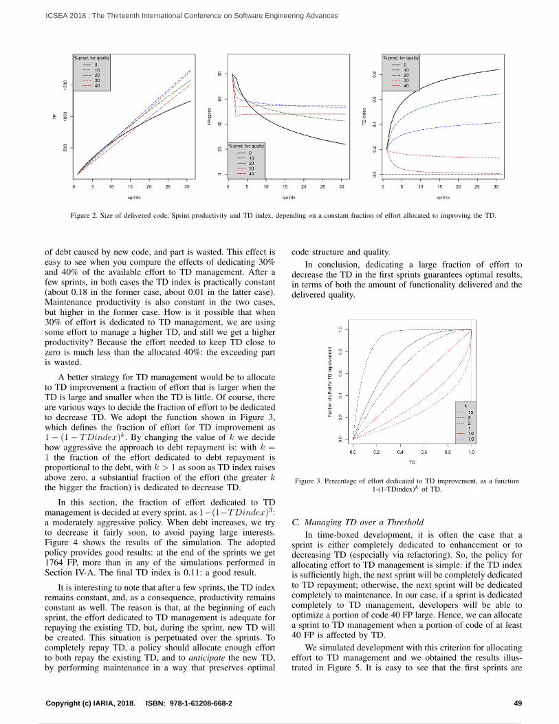
Figure 2. Size of delivered code, Sprint productivity and TD index, depending on a constant fraction of effort allocated to improving the TD.

of debt caused by new code, and part is wasted. This effect iseasy to see when you compare the effects of dedicating 30%and 40% of the available effort to TD management. After afew sprints, in both cases the TD index is practically constant(about 0.18 in the former case, about 0.01 in the latter case).Maintenance productivity is also constant in the two cases,but higher in the former case. How is it possible that when30% of effort is dedicated to TD management, we are usingsome effort to manage a higher TD, and still we get a higherproductivity? Because the effort needed to keep TD close tozero is much less than the allocated 40%: the exceeding partis wasted.

A better strategy for TD management would be to allocateto TD improvement a fraction of effort that is larger when theTD is large and smaller when the TD is little. Of course, thereare various ways to decide the fraction of effort to be dedicatedto decrease TD. We adopt the function shown in Figure 3,which defines the fraction of effort for TD improvement as1 − (1 − TDindex)k. By changing the value of k we decidehow aggressive the approach to debt repayment is: with k =1 the fraction of the effort dedicated to debt repayment isproportional to the debt, with k > 1 as soon as TD index raisesabove zero, a substantial fraction of the effort (the greater kthe bigger the fraction) is dedicated to decrease TD.

In this section, the fraction of effort dedicated to TDmanagement is decided at every sprint, as 1−(1−TDindex)3:a moderately aggressive policy. When debt increases, we tryto decrease it fairly soon, to avoid paying large interests.Figure 4 shows the results of the simulation. The adoptedpolicy provides good results: at the end of the sprints we get1764 FP, more than in any of the simulations performed inSection IV-A. The final TD index is 0.11: a good result.

It is interesting to note that after a few sprints, the TD indexremains constant, and, as a consequence, productivity remainsconstant as well. The reason is that, at the beginning of eachsprint, the effort dedicated to TD management is adequate forrepaying the existing TD, but, during the sprint, new TD willbe created. This situation is perpetuated over the sprints. Tocompletely repay TD, a policy should allocate enough effortto both repay the existing TD, and to anticipate the new TD,by performing maintenance in a way that preserves optimal

code structure and quality.In conclusion, dedicating a large fraction of effort to

decrease the TD in the first sprints guarantees optimal results,in terms of both the amount of functionality delivered and thedelivered quality.

Figure 3. Percentage of effort dedicated to TD improvement, as a function1-(1-TDindex)k of TD.

C. Managing TD over a ThresholdIn time-boxed development, it is often the case that a

sprint is either completely dedicated to enhancement or todecreasing TD (especially via refactoring). So, the policy forallocating effort to TD management is simple: if the TD indexis sufficiently high, the next sprint will be completely dedicatedto TD repayment; otherwise, the next sprint will be dedicatedcompletely to maintenance. In our case, if a sprint is dedicatedcompletely to TD management, developers will be able tooptimize a portion of code 40 FP large. Hence, we can allocatea sprint to TD management when a portion of code of at least40 FP is affected by TD.

We simulated development with this criterion for allocatingeffort to TD management and we obtained the results illus-trated in Figure 5. It is easy to see that the first sprints are



60 / 160

Figure 4. Size of delivered code, Sprint productivity and TD index through sprints, when the fraction of effort for TD improvement is 1-(1-TDindex)3.

Figure 5. Size of delivered code, Sprint productivity and TD index through sprints, when sprints are dedicated to either TD management or maintenance.

dedicated to TD improvement and enhancement maintenancealternatively. Then, when TD has improved enough, we havea TD improvement sprint every two enhancement sprints.TD progressively decreases until it becomes practically nil(oscillating between 0.01 and 0.03). At the end of sprints,1674 FP are released, that is, a bit less than with the policydescribed in Section IV-B. However, the achieved TD index ismuch better, compared to the 0.11 achieved in Section IV-B.

V. DISCUSSION

The results obtained with the different criteria for allocatingeffort to TD improvement are summarized in Table I. Notethat in Table I, we have added the results—not given inSection IV-B—obtained when the fraction of effort dedicatedto TD improvement is 1-(1-TDindex)1/3. In such case, thefraction of effort dedicated to TD improvement decided at thebeginning of each sprint, is based on the current TD index, butthe approach is not aggressive, on the contrary, a substantialfraction of effort is dedicated to TD improvement only whenthe TD index is relatively large.

The results given in Table I, along with the more detailedresults reported in Section IV, suggest a few observations.

TABLE I. RESULTS WITH VARIOUS CRITERIA

Criterion Delivered size Final TD indexConstant (0%) 1248 FP 0.84Constant (10%) 1580 FP 0.64Constant (20%) 1743 FP 0.41Constant (30%) 1723 FP 0.13Constant (40%) 1517 FP 0.0071-(1-TDindex)3 1764 FP 0.111-(1-TDindex)1/3 1601 FP 0.51Threshold 1674 FP 0.01–0.03

First, allocating a constant amount of effort to TD im-provement does not seem a good idea. In fact, if the chosenfraction of effort allocated to TD improvement is too high orloo low, the productivity of enhancement maintenance will belower than possible. Also, the final quality of the product (asindicated by the TD index) could be quite low. In practice,allocating a constant amount of effort to TD improvementworks well only if the right fraction of effort is allocated, butchoosing such fraction may not be easy.

On the contrary, computing the amount of effort for TDimprovement at the beginning of each sprint, based on thecurrent TD index seems very effective, especially as far as



61 / 160

optimizing the productivity of enhancement maintenance isconcerned.

One could observe that in some situations it may be hard toseparate clearly the effort devoted to enhancements from theeffort devoted to TD improvement. This is particularly truewhen developers perform refactoring activities while they areenhancing the existing code. For this reason, an organizationmay want to have sprints entirely dedicated to refactoringand other TD improving activities, and sprints entirely ded-icated to enhancements. In this case, the evaluations givenin Section IV-C show that allocating an entire sprint to TDimprovement whenever there is enough TD to absorb onespring effort provides quite good results, in terms of bothproductivity and quality.

In any case, we have to stress that all the presentedstrategies for TD management are based on the quantitativeevaluation of TD, which results in the TD index. So, devisinga way to measure TD appears fundamental to managing TDeffectively and efficiently.

VI. RELATED WORK

System Dynamics was first applied in Software Engineer-ing by Abdel-Hamid and Madnick [12], who proposed a modelthat accounted for human resource management, softwaredevelopment, and planning and control. System Dynamics wasthen extensively used to model software development and itsmanagement. A survey of System Dynamics applied to projectmanagement was published by Lyneis and Ford [13], whilein [14] De Franca and Travassos propose a set of reportingguidelines for simulation-based studies with dynamic modelsin the context of SE to highlight the information a study ofthis type should report.

Cao et al. [15] proposed a System Dynamics simulationmodel that considers the complex interdependencies among thevariety of practices used in Agile development. The model canbe used to evaluate—among others—the effect of refactoringon the cost of implementing changes.

Glaiel et al. [16] used System Dynamics to build the AgileProject Dynamics model, which captures each of the Agilemain characteristics as a separate component of the modeland allows experimentation with combinations of practices andmanagement policies.

Although less comprehensive than the mentioned models,our proposal allows for better undrstanding the consequencesof technical debt and the effectiveness of its managementstrategies.

VII. CONCLUSIONS

The term “Technical Debt” indicates several concepts andissues related to software development and maintenance. Thelatter are complex and multifaceted activities: accordingly, itis not surprising that managing TD is quite difficult [5].

In this paper, we have provided a formal, executable modelof time-boxed software development, where the effects of TDare explicitly and quantitatively represented and accounted for.The model is usable to show—via simulation—the effects thatTD have on relevant issues such as productivity and quality,depending on how TD is managed, with special reference onhow much effort is dedicated to TD repaiment and when—ina sequence of sprints—such effort is allocated.

The model can be used to prove or disprove conceptsand hypotheses, to perform what-if analyses, etc. However,our model is not intended to be used in practical softwareproject management as-is, becase, the model illustrated aboveis too abstract and contains hypotheses that could not matchthe target development environment. Whoever wants to usethe presented model for practical project management shouldfirst enhance it; examples of models representing all the mainaspects of software development can be found in the papersby Cao et al. [15] and Glaiel et al. [16].

We plan to extend the presented model in several direc-tions: to account for different effects of TD on productivity(i.e., with functions different from the one in Figure 1), toexplicitly model defects, to test different debt managementpolicies, etc.

ACKNOWLEDGMENT

This work was partly supported by the “Fondo di ricercad’Ateneo” funded by the Universita degli Studi dell’Insubria.

REFERENCES[1] Z. Li, P. Avgeriou, and P. Liang, “A systematic mapping study on

technical debt and its management,” Journal of Systems and Software,vol. 101, 2015, pp. 193–220.

[2] C. Fernandez-Sanchez, J. Garbajosa, A. Yague, and J. Perez, “Iden-tification and analysis of the elements required to manage technicaldebt by means of a systematic mapping study,” Journal of Systems andSoftware, vol. 124, 2017, pp. 22 – 38.

[3] A. Nugroho, J. Visser, and T. Kuipers, “An empirical model of technicaldebt and interest,” in Proceedings of the 2nd Workshop on ManagingTechnical Debt. ACM, 2011, pp. 1–8.

[4] N. Ramasubbu and C. F. Kemerer, “Managing technical debt in enter-prise software packages,” IEEE Transactions on Software Engineering,vol. 40, no. 8, Aug. 2014, pp. 758–772.

[5] P. Avgeriou, P. Kruchten, I. Ozkaya, and C. Seaman, “Managingtechnical debt in software engineering (dagstuhl seminar 16162),” inDagstuhl Reports, vol. 6, no. 4. Schloss Dagstuhl-Leibniz-Zentrumfuer Informatik, 2016, pp. 110–138.

[6] J. Letouzey, “The SQALE method for evaluating technical debt,” in Pro-ceedings of the Third International Workshop on Managing TechnicalDebt, MTD 2012, Zurich, June 5, 2012, 2012, pp. 31–36.

[7] “Automated technical debt measure – beta,” Object Management Group,specification ptc/2017-09-08, September 2017.

[8] J. Forrester, Industrial Dynamics. Cambridge: MIT Press, 1961.[9] A. J. Albrecht, “Function points as a measure of productivity,” in Act

as do 53 rd meeting of GUIDE International Corp., Guidance for usersof integrated data processing equipment conference, Dallas, 1981.

[10] IFPUG, “Function point counting practices manual, release 4.2,” IF-PUG, Tech. Rep., 2004.

[11] L. Lavazza, S. Morasca, and D. Tosi, “An empirical study on the factorsaffecting software development productivity,” e-Informatica SoftwareEngineering Journal, vol. 12, no. 1, 2018, pp. 27–49.

[12] T. Abdel-Hamid and S. E. Madnick, Software project dynamics: anintegrated approach. Prentice-Hall, Inc., 1991.

[13] J. M. Lyneis and D. N. Ford, “System dynamics applied to projectmanagement: a survey, assessment, and directions for future research,”System Dynamics Review, vol. 23, no. 2-3, 2007, pp. 157–189.

[14] B. B. Franca and G. H. Travassos, “Experimentation with dynamicsimulation models in software engineering: Planning and reportingguidelines,” Empirical Software Engineering, vol. 21, no. 3, June 2016,pp. 1302–1345.

[15] L. Cao, B. Ramesh, and T. Abdel-Hamid, “Modeling dynamics in agilesoftware development,” ACM Transactions on Management InformationSystems (TMIS), vol. 1, no. 1, 2010, pp. 5:1–5:27.

[16] F. S. Glaiel, A. Moulton, and S. E. Madnick, “Agile project dynamics: Asystem dynamics investigation of agile software development methods,”2014.



62 / 160

Continuous Improvement and Validation

with Customer Touchpoint Model in Software Development

Tanja Sauvola, Markus Kelanti, Jarkko Hyysalo, Pasi Kuvaja and Kari Liukkunen

M3S Research Unit, Faculty of Information Technology and Electrical Engineering,

University of Oulu

PO BOX 4500, FI-90014 University of Oulu, Finland

e-mail: {tanja.sauvola, markus.kelanti, jarkko.hyysalo, pasi.kuvaja, kari.liukkunen}@oulu.fi

Abstract—Experimental-driven software development

approach has gained momentum as a way to incrementally

build and validate customer value. In-depth understanding of

customer needs and reasons behind constantly changing

requirements are essential for building successful software

products. However, identifying, validating and reacting to

these changes is often difficult and requires short iteration

cycles and feedback from customers. This paper reports a 12-

month case study conducted in an agile software team

following a practical customer touchpoint (CTP) model for

continuous improvement and validation. The objective of the

study was to implement CTP into software team practices in

order to determine what kind of effect it has on the

development of a web application. The contribution of this

paper is twofold. First, an in-depth case study is presented that

identifies the practices a CTP model should adopt when

implemented in the software development process. The CTP

model is then extended based on the identified

recommendations. Second, the benefits and challenges of the

extended CTP in software development are presented. The

main benefits relate to learning, decision-making, innovation,

co-creation and communication. The model had a positive

impact on the software development process, but some

challenges, such as stakeholder availability and customer value

measurement, were identified.

Keywords—lean UX; service design; customer involvement;

software development; continuous improvement.

I. INTRODUCTION

Customer value determines the success of a product or a service in the marketplace, and software has become essential to value creation and delivery [1]. Software development teams face high pressure to develop innovative products and services at increasing speeds in a dynamic and continuously changing business environment. To this aim, development teams seek to become more data-driven, which requires using customer feedback and product data to support learning and decision-making during the development process and throughout a product’s lifecycle. This presents the challenge in software development to adopt iterative and agile practices for the continuous deployment of new features and enhancements to provide customers with added value [1]-[3]. Customer value and the ability to

experiment with business ideas have been considered in Agile methods [4] and the Lean Startup [5] philosophy, both very popular in the software industry. Recently, concepts like continuous experimentation—where software development teams constantly experiment with product value—have been introduced in the literature as well [3][6][7]. The continuous experiment approach involves customers and end-users of the service in the decision-making process, providing feedback to developers by interacting with experimental materials like early prototypes of the features under development.

User experience (UX) has also become an increasingly important determinant of the success or failure of software systems. Approaches such as Design Sprint, introduced by Google Ventures [8], and Lean UX [9] using Lean Startup principles, now appear. These experiment-driven approaches interrelate with business strategy decisions and tend to focus on customer centricity. Forward-thinking companies see the benefits and importance of UX design in their product and service development activities. Even with these methodologies, software teams still encounter challenges when involving customers and integrating customer feedback into short development cycles [2][6].

In this paper, the customer touchpoint (CTP) model introduced by Sauvola et al. [2] is examined as a way for software development teams to become more customer centric and data driven. The study focuses on finding answers to the following research questions:

RQ1: What practices should the CTP model adopt when implemented in the software development process?

RQ2: What are the benefits and challenges of CTP in software development?

To address the research questions, a case study in the software development context has been performed. The CTP model is validated and extended by proposing practices for the continuous validation of customer value in short development cycles to increase customer understanding. The benefits and challenges of the extended CTP model are then identified.

The paper is organized as follows. Section 2 studies the related work. Section 3 presents research approach and describes the case project. Section 4 presents the results and



63 / 160

analyses. Section 5 discusses the results. Section 6 concludes the work with a summary and topics for further research.

II. RELATED WORK

A. Value creation through continuous experimentation

In software development, short product development and deployment cycles and shorter feedback loops are enabled by practices such as agile and lean development [4][5], continuous deployment [10] and DevOps [11]. An organisation’s ability to deploy new functional and non-functional features continuously enables faster responses to customer needs [10][12]. However, these practices provide only a little guidance on how to constantly validate product assumptions while experiment-driven approaches focus more on value delivery with validated learning.

The literature presents several methods for establishing continuous experimentation with customers. Bosch et al. [13], for example, suggests exposing products to customers in two- to four-week experimentation iterations to solicit feedback. Studies of software engineering also propose ideas for continuous experimentation. Fagerholm et al. [3] suggest their RIGHT model for continuous experimentation, in which the key element is the start-up company’s ability to release prototypes with suitable instrumentation. In this model, business strategies form the basis of experiments, and results guide future development activities. Holmström Olsson et al. [6] present the concept of an innovation experiment system (IES) in which software development teams constantly develop hypotheses and test them with customers. The IES approach also recommends that software teams continuously deploy individual features rather than plan larger product releases. This enables short feedback loops and facilitates data-driven decisions, reducing the risk of failing to build customer value by continuously identifying, prioritising and validating product assumptions in all software development phases. Holmström Olsson et al. also coined the hypothesis experiment data-driven development (HYPEX) model, which introduces a set of practices to integrate feature experimentation into the software development process by combining feature experiments and customer feedback. The model aims to improve the correlation between customer needs and research and development efforts [14]. More recently, Holmström Olsson et al. also presented a quantitative/qualitative customer-driven development (QCD) model. This model presents available customer feedback techniques and aims to help companies become more data-driven by combining qualitative feedback with quantitative customer data [15]. Such methods are supported by Kohavi et al. [16], who report that companies use experiments to guide product development and accelerate innovation. Companies adapting the experimentation approach are typically developing internet related product and services, such as Amazon, eBay, Facebook, Google, LinkedIn, Microsoft and Netflix [16]. While experimentations are recognized as beneficial approach to software development, barriers to related resources, organisational culture and data knowledge persist [17].

B. Service design in software development

Service design (SD) is a methodological approach that can be utilized during software development to involve customers and collect feedback. It is a holistic, multidisciplinary approach that aids innovation and improves existing products to make them more useful and desirable to customers [18]. SD provides an outside-in-development approach, where products and services are developed holistically from customers’ and end-users’ points of view, and applies design thinking and methodologies in product and service development. Recently, some process models and working practices, such as Lean UX [9] and Design Sprint [8], have been introduced under SD and UX design titles with the aim of synthesising design thinking, agile software development and lean start-up philosophies. Lean principles and Lean Startup apply to Lean UX in three ways: 1) removing waste by only creating the design artifact that enables the software development team to move their learning forward; 2) embracing cross-functional collaboration and bringing all relevant stakeholders into the design process; and 3) adopting the experimentation mindset. Lean UX is the evolution of product design, aiming at breaking down the barriers between software development teams, designers and users [9]. Similarly, Google Ventures introduced Design Sprint to integrate product discovery, product validation and delivery activities in a five-day process [8].

Experiments with customers require the ability to elicit customer feedback. For example, visualisation techniques nurture the co-design process and elicit feedback without relying on existing technical infrastructure or up-front development efforts. Different visualisation techniques are used, e.g., in agile development to design a product or a service, support the development process, enhance communication and track the process [19]. The SD approach emphasises the co-design process, whereby stakeholders are involved in concrete, productive design tasks such as workshop sessions. These sessions typically include collaborative prototyping and other means of expressing the information needed in the design and development process [20].

III. RESEARCH APPROACH

The software development process and related activities are presented in this paper through a case study that follows the guidelines set by Runeson and Höst [21]. A qualitative case study method was chosen to gain a practical view on the topic. In principle, the study is an in-depth, single-case study, where the involved participants represent different public and private organisations with fundamentally different roles, such as user, data provider, company representative and ecosystem leader. According to Yin [22], the single-case design is appropriate for testing a specific theory, which in this case is the CTP model. The study is also confirmatory in nature, as it aims to evaluate the robustness of a theory.



64 / 160

A. Case description

Our case study was conducted in the Fenix project (www.fenix.vip), where the software team develops a cloud-based service for real-time business case management for the Allied ICT Finland (AIF) (www.alliedict.fi) In the AIF program, a need was identified as currently information about companies, research institutes, business opportunities and product offerings are scattered into various databases and services. Thus, there is a need to aggregate this information under one digital service-point. Fenix was therefore designed to provide one place for finding and meeting new business opportunities, solution providers, experts, start-ups, business incubators and research institutes. The aim is that the tool would allow users to browse information about potential business partners and opportunities across multiple third-party systems from a single point. For example, the utilization of Business Finland (www.businessfinland.fi) database to follow cases and offers from municipalities and governments as starting cases.

The specific challenge of the Fenix system was to gain the commitment of user stakeholders, namely companies, universities and other organisations, which AIF and Business Finland aimed to support. The idea was that Fenix would promote Finnish industry by increasing overall trade and exports through the improved exposition of business opportunities, expertise and new company and research ecosystem growth. The challenge was that there were no clear requirements to fulfil due to the changing group of stakeholders and the need to develop an efficient mechanism to expose and promote business cases and ecosystem formation. Further more, development funding depended on the success of committing enough stakeholders to create ecosystems in Fenix.

The development team consisted of nine people: a designer/product owner, seven developers and a scrum master in total. During development, one researcher acted as product owner and UX designer and another adopted the role of software architect. Experience levels ranged from novice to expert with several years of industrial experience. The software team followed scrum methodology with iterative two-week development cycles. Customer collaboration was guided by the CTP approach during the design and implementation of the system (see [2] for details).

B. Data collection and analysis

Empirical data was collected between January and December 2017 from observations and field notes, 13 interview recordings and 20 workshops. Semi-structured interviews with open-ended questions [23] were used to collect data from six customer interviews and seven development team interviews. Customer participants were selected to best represent the companies, research institutions and local public actors.

The interviewed customers represented the AIF, Business Finland, trade associations and local companies. The themes discussed in the interviews were customer collaboration practices, agile ways of working and the benefits and challenges involved in the current way of working. The interviews were conducted face-to-face and lasted

approximately 60 minutes. All interviews were recorded and transcribed for analysis in QSR NVivo tool (www.qsrinternational.com). The obtained material was analysed in continuous collaboration by three researchers, following the recommendations for thematic analysis in software engineering by Cruzes and Dybå [24]. The interview data was first coded based on the interview topics and then analysed and coded according to emerging themes. The themes were first examined independently, then cross-analysed.

The workshops, besides being an integral part of the development cycles, occurred bi-weekly after every sprint. Workshops lasted approximately one hour and included software product demonstrations and collaborative prototyping sessions. Customers and other stakeholders were invited to see the latest version of the prototype software and to try, test and give feedback. Workshop participant groups consisted of the whole development team and between two and 15 customers. Before these workshops, a new version of the software in question was deployed. During the bi-weekly workshops, the product owner presented the changes and new features introduced in that particular software version and collected feedback and new development ideas. New features ideas were experimented with using UI mock-ups and interactive prototypes during the workshop sessions. The developers summarised the key points of each workshop, and the researchers observed and made notes about stakeholder reactions and documented relevant comments. Following the workshops, the development team analysed the feedback, prioritised next tasks and planned the next iteration.

C. Validity and reliability of the study

The design of the present study was carefully planned to consider validity concerns. We discuss four threats to validity: internal and external validity, construct validity, and reliability [22].

Internal validity regarding cause–effect relations was addressed via multiple sources of evidence, and with iterative research gradually building the final outcome. Evaluation of utility, quality and efficacy was done extensively with the help of industrial experts and real users. Immediate feedback was gathered, and the use of prototypes was observed. Based on the rich feedback and analysis, further development and corrective actions were carried out.

External validity concerning the generalisability of results was addressed by involving several industrial experts to provide their views. In addition, the involvement of several organisations of different types and domains increased the external validity and generalisability of the results. However, further study will be needed to generalise the results fully.

Construct validity was mitigated by several activities. First, an interview guide was developed and piloted. A pilot interview was used to refine and clarify the interview questions. Second, interview candidates were vetted for suitability to the study, and interview themes were introduced with background information.

The reliability of the data and derived results was ensured by applying a peer-reviewed research protocol. Threats to



65 / 160

reliability were mitigated, particularly in the analysis phase, by involving all three researchers. The data itself was recorded using Jira (atlassian.com/software/jira) and Confluence tools (atlassian.com/software/confluence), which allowed other researchers and experts to review and correct the data.

Some danger of positive bias exists in the study’s results and activities due the way the case study was implemented. The constant communication among researchers, the development team and customer representatives, as well as the inclusion of researchers on the development team, increased the likelihood of producing only positive results. This danger was mitigated by having one researcher to evaluate the plan, results and actions without participating in the development team activities. Further, clear roles and rigorous research methods helped the researchers to maintain an objective perspective throughout the study.

IV. RESULTS AND ANALYSIS

This section presents the extended CTP model (Figure 1.) with identified practices for continuous improvement and customer validation adapted from SD and Lean UX approaches. The practices are defined based on the empirical findings of the data collection and analysis as well as the authors’ previous experiences when working with software development teams. The benefits and challenges of applying the extended CTP model in agile software development are then discussed.

A. Recommended practices for the CTP model

Continuous improvement of the service unfolds true

qualitative and quantitative data collected from customers

and products in the field. Various experimentation

techniques and combinations can be applied throughout the

development process. The role of the CTP model in the

present study was to guide the development team to

experiment and collaborate with several internal and

external stakeholders during the development process and

collect feedback.

The purpose of extending the CTP model was to allow

the continuous identification, prioritisation and validation of

product assumptions in short development cycles with the

help of customers, using identified practices presented in

touchpoints T1-T4 in the model. These practices should be

applied as continuous activities to improve service and

validate product hypotheses. The findings of this study

indicate that to fully utilise the practices, the development

team must have an agile and lean mindset, be self-

organising and share responsibility. Also, the team must be

cross-functional, with one designer onboard. In-depth

analysis of the quantitative data requires data analytics and

data knowledge expertise, as analysing and utilising data is

much more complicated than collecting it.

Discovery: The first customer touchpoint T1, is used to

discover and compile customer needs and translate them

into product requirements and product hypotheses, which

can be used in experiments. Typically, new ideas and

requirements are collected from various sources, including

market and competitor intelligence, feedback from

customers and product usage data (after the first release of

the product has been made).

Figure 1. Lean UX practices in extended CTP model. R refers to the main

activities: R1 Collection; R2 Prioritization; R3 R&D Verification and R4 Deployment. T indicate where companies and customers exchange

information: T1 Release learnings or new customer requirements, T2 Release trade-offs and cost/benefit analysis, T3 Release features and

delivery commitments and T4 Release configurations and real usage vs.

planned usage of the product/feature. R1–R4 are also sources for requirements for new product ideas, including market and competitor

intelligence, product usage data, customer feedback data collected, etc.

Techniques for collecting qualitative data can vary, from

surveys and interviews to observations. Product

assumptions are then turned into hypotheses for validation.

The practices identified and utilised by the development

team in this study included customer journey and

stakeholder mapping, user analysis and creation of user

stories. Journey mapping [9] provides a structured

visualisation of a specific element, be it a single feature or

an overview of the entire customer experience. Stakeholder

mapping [18] on the other hand governs the overall complex

situation and the expectations from various stakeholder

groups. Benchmarking through online research and market

data collection can also be used as an input to these

practices.

Key learning: Balance discovery activities with

development efforts by testing only high-risk hypotheses

and conducting smaller amounts of research more often.

Journey: The second customer touchpoint T2, is used to

visualise an organisation’s service vision and the customer

journey. Such visualisation, considered as MVPs in this

study, lends insight to improve the understanding of

information. In the early phases of product development,



66 / 160

many uncertainties related to customer expectations arise.

Concept work is required when envisioning the idea for a

service, or even at the feature level when designing

prototypes and mock-ups. Visualisation techniques like

wireframes, UI mock-ups, interactive prototypes and

evolutionary prototypes guide development teams to

prioritise development tasks continuously through

experimentation with product concepts and design artefacts.

In terms of prototyping, interactive prototypes are

simulations that typically illustrate few predefined

scenarios. They look and function like end product but do

not handle real data input, processing or output. This

technique proposes a quick and cost-effective way to

concretise and test new ideas before any development work

is done and help software teams to avoid developing

unnecessary features. Evolutionary prototypes, build based

on lessons learned from the interactive prototypes, however

handle real data and form the basis for the actual software

evolving after every iteration. Results of the present study

indicate that design tasks should be treated as equal to

development tasks and executed in the same or parallel

cycles during software development. Digital product

prototyping tools, such as Invision (invisionapp.com),

UXPin (uxpin.com), and Sketch (sketchapp.com) were

determined to be useful in this phase because they allowed

for more effective collaboration and experimentation with

product assumptions.

Key learning: Visualisation techniques create a common

understanding by which to resolve communication-related

issues. However, adapting these techniques require the role

of UX designer in the development team.

Validation: Most of the validation in touchpoint T3

occurs through testing activities. Testing activities are an

opportunity to validate mismatches between customer needs

and product offerings. As experienced in our previous

research [2], this opportunity is often overlooked. Adopting

the journey validation practice, trough different visualisation

techniques, helps a development team to identify their

needed steps, possible pain points and gaps. Internal

validation then covers practices like daily scrum meetings,

wikis and other communication channels to provide quick

and frequent feedback from executives and team members.

During daily scrum meetings in the present study, it was

observed that the work that had been visualised on Kanban

boards was often the work that got done. This demonstrates

the importance of making product discovery and UX design

tasks visible in a backlog. In this case, the UX tasks were

visualised, executed and tracked in two-week sprint cycles

alongside development tasks. External validation was done

by exposing experiment materials to customers in two-week

cycles to elicit and collect feedback. The experiment

materials included interactive prototypes, mock-ups and

evolutionary prototypes. Feedback was collected from

customer workshops after every cycle, and utilizing

usability testing with direct feedback mechanism in the

working software integrated into the product development

practices. It was concluded that it is important to involve the

entire development team in external validation activities like

workshops, as doing so helps the team avoid

misunderstandings and the incorrect implementation of

features.

Key learning: Customer needs and requirements change

constantly. Backlog prioritisation should be done with high

flexibility in short cycles against validated learnings.

Value: The ability to combine qualitative and

quantitative customer feedback data is important, as often

they complement each other. For example, by monitoring

feature usage, quantitative data can be used to validate

qualitative data. Analytic tools and collected product

operation and performance data allows development teams

to make data-driven decisions to improve the service in

customer touchpoint Value T4 continuously. In the present

case, project log files and product usage data such as clicks,

page views and number of visits were recorded and

analysed. Especially in the field of web development,

collecting and analysing product usage data has been eased

by general tools such as Google Analytics. Target areas for

quantitative data collection can range from system

performance and UX improvements to business-level

decision-making. In the present study, corrective actions

based on quantitative data were done for example by

improving the system level performance as well as

placement and visibility of UI elements and workflows.

Techniques such as A/B testing can also serve as a

potential approach to collect product usage data. In the

present case study, A/B testing was not conducted because

developing different variations of the same feature required

vast resources and a large user base. In addition, a more

detailed analysis of the log data would require specific skills

and resources, such as adding a data scientist to the team.

Key learning: Quantitative data reveals tacit and

complex knowledge of product usage. Detailed analyses of

data and systematic, controlled experiments require the

active presence of a data scientist.

B. Benefits of the extended CTP model in software

development

The use of the extended CTP model with the identified

practices as part of the two-week software development

cycle was determined to be beneficial from the customer

and development team points of view, but some challenges

were identified. The benefits (Table I) and challenges (Table

II) based on the research data are discussed next.

The most significant observed benefit of using the

extended CTP model in software development was that it

assisted both business and technical decision-making by

promoting a better understanding of information (i.e., tacit

knowledge is transformed into tangible knowledge). For the

development team, direct interaction with customers

enabled them to understand the reasons behind customer

requirements and validate which features brought real value.

Shared understanding also facilitated faster decision-



67 / 160

making, which enabled the team to prioritise tasks ‘on the

fly’ and estimate the validity of tasks in the product backlog.

The findings from this case study demonstrate that at

their best, these practices increased customer involvement

and nurtured innovation. Involving users in the early phases

of development made customers more active and

experienced with the product. This increased the motivation

of development team and especially users, as they

experienced the impact of their involvement during the

process.

In terms of decision-making, the present results indicate

that visualisation is one of the most important ways to

concretise and test new ideas, as information is made visible

to both customers and the development team through design

artefacts.

TABLE I. IDENTIFIED BENEFITS

Benefit Description

Learning and

decision-making

Accelerate the decision-making process and

concretise functions before actual development

work. Innovation and

value co-creation

Accelerate co-creation and innovation between

development team and users. Receive the first

user feedback in the product/service idea phase. Motivation Interaction and co-creation between development

team and users motivated both the development

team and the users. Communication

improvement

Visualisation and prototyping methods improved

communication and helped avoid

misunderstandings between different stakeholders (e.g., management, development team, customers

and end-users).

Transparency Increase transparency between customers, users and the development team. Reveals grassroots

knowledge exploitable in development.

Direct feedback Presents an opportunity to receive instant and direct feedback from end-users in short cycles.

Integrated UX

work

Design activities take place in the same cycle

with development activities. Service vision in

communicable

form

Developers have a clear, precise schematic by

which to see the intended service from the

customer perspective and can choose precise specifications.

Prioritisation

Prioritisation ‘on the fly’ allows the development

team to capture changing priorities in short cycles and react flexibly and accurately.

Holistic approach Holistic approach to software development from customers' and end-users' point of view.

The interviews stressed the need to produce proper

visualisations, such as interactive prototypes and UI mock-

ups, to concretise the service vision and improve

communication to avoid misunderstandings. According to

the interviewees, UX work was often perceived as a

separate function, one asynchronous with research and

development activities. It was also stated in the development

team interviews that sometimes UX work was overlooked,

as things like code quality, software scalability and security

issues were deemed more important. “Usability and user

interface design… perhaps we cannot appreciate these or

we consider more important that the software itself works or

the code is good quality, the software is scalable and safe

and so one, which is of course important… but from my

perspective, I see that it is old-fashioned engineering

thinking. …today, in my mind it (usability) is the biggest

competitive advantage of software, (senior software

developer).”

Visualisation techniques used in the workshop sessions

also bridged the communication gap between those with

business mindsets and those more technically oriented. It

was important that the whole development team participated

in the workshop sessions to get direct and instant feedback

from customers. This helped the development team to

understand the reasons behind customer needs, the kind of

behaviours expected from the service and what created

value for customer. During the sessions, the development

team was able to identify design improvement ideas for the

future and problem areas in the existing design. This had a

clear impact on project work such as planning, scheduling

and prioritising tasks, as the team was able to capture and

react to changing priorities in short cycles. The practices

presented in the extended CTP model facilitated better

alignment and transparency of different functions, from UX

design, business development and product management to

short cycles with research and development activities.

By adopting visualisation techniques as suggested in the

extended CTP model, the development team was able to

obtain their first user feedback after very short iterations (a

few days to a few weeks). The model also guided the entire

development team to holistic thinking by following a

customer centric design and development process

throughout the project lifecycle.

C. Challenges of the extended CTP model in software

development

Stakeholder availability and commitment represented

some challenges for example, if few or no visible functions

were delivered in a short iteration cycle, customer and

stakeholder commitment to participate in the workshops

could suffer. In addition, customers may feel disrupted from

their own work by being involved in development activities

too often. The development team reported the two-week

cycle as optimal, but based on the interviews it could be

shortened to one week. For customers, the two-week

development cycle with a workshop at the end of each sprint

was sometimes seen too often.

New requirements appear all the times and they may

disrupt the old ones, often this is related to different user

groups and customer roles with conflicting needs. This may

also add complexity to defining feature maturity and

identifying metrics for measuring customer value.

For a software team to adapt practices presented in the

extended CTP model, certain key roles must be filled, which

may cause some challenges. The current case study required

expertise of back-end and front-end development, database

development, server and tool management, a product owner

to represent the customer and a UX/UI designer to conduct

and facilitate design tasks. While the development team and



68 / 160

effort were kept as minimal as possible, it was evident that

UX design and different visualisation techniques required

significant effort; the person in charge of the design had to

discuss and make decisions on the design with different

stakeholders who often held conflicting demands and

priorities. In order to mitigate this problem, a stakeholder

analysis method [25] was used to gain further insight on the

conflicting issues and resolve them. The UX work alone

was often full-time work for a single person, even in a

lightweight web application project. Furthermore, detailed

analysis of the log data would require specific skills and

resources, such as adding a data scientist to the team and a

large user base. In this study, analytic support was

integrated to working software and some corrective actions

were continuously taken based on quantitative data.

However, small user base and lack of resources hindered

more detailed analyses. It should be noted that in some

industries, laws and regulations or other limitations could

prevent quantitative feedback collection.

TABLE II. IDENTIFIED CHALLENGES

Challenge Description

Stakeholder availability and

commitment

Finding suitable time for all stakeholders to participate workshops. Balancing workshop

frequency and getting customer commitment to

participate and give feedback. Customer role Different user groups might have different needs,

and those can change according to context.

Measurement of customer value

Identify metrics for how to measure customer value is challenging.

Resources Successful implementation required having a

cross-functional team with an active UX/UI designer and data scientist in the team.

Direct

communication

Developers may not always be confident or

comfortable with increased and direct customer interaction.

Visualised

features might be understood as

‘easy to do’

Workload estimation can be challenging from the

customer perspective. E.g., features in an interactive prototype and real effort for actual

implementation might come as a surprise.

Maturity and definition of done

(DOD)

Changing priorities and stakeholders make it hard to analyse the maturity and DOD of features.

Quantitative metrics / analytics

Quantitative metrics and analyses become possible after implementing analytics support,

once the software is in use and there is a

sufficient stakeholder pool using it. Before that, obtaining quantitative data is nearly impossible.

Physical distances Technical issues and lack of tools for sharing

local demonstrations.

Development team interviews of the present study

revealed that some developers were more confident when

allowed to focus simply on building the software, preferring

to keep their interactions with customers at a minimum or

restricted to key individuals.

While a working prototype proved an efficient way to

involve stakeholders in the development process, the

downside was that customer expectations rose when they

saw how ‘easy’ it was to produce something visible that

matched their needs. This led to situations where customers

expected that the feature’s implementation would be easy as

well. The challenge therefore is the increased risk of

customers developing unrealistic expectations related to

work estimations for the complete functional feature.

During the study, this was addressed by maintaining a

careful balance between keeping stakeholders satisfied even

the workload would be bigger and prioritizing these features

over those that are not visible but can be important for

system stability, security and other issues that do not show

in day-to-day work.

Physical distances reduced the development teams

ability to interact with their customers face to face, as well

as posed a challenge during the workshops and meetings

due to technical issues, such as connection quality and

faulty communication equipment. While these technologies

enable participation regardless of physical location,

communication tools do fail at times, or stakeholders are not

used to hold online meetings. Mistakes like using a low

volume of voice, moving away from the microphone or

demonstrating locally something not visible to those

participating remotely can slow down the meeting, make

communication difficult and increase the risk of

misunderstanding.

V. DISCUSSION

Software development is not an easy or straightforward

task. It is even more challenging when requirements are

constantly changing and there are many involved customer

organisations with different demands. Previous research [2]

shows that, delivering value and meeting customer needs in

constantly changing markets are key success factors for any

business. Multitude of existing methods and approaches for

identification, prioritization and validation of customer

needs are presented in literature, with more recent being

continuous experimentation. From a process perspective,

Schermann et al. [26] reports a lack of clear guidelines for

conducting experiments. Our extended CTP model fills the

gap and presents an approach for continuous improvement

and customer validation.

Typically, existing methods and approaches for

continuous experimentation (presented in Section II of the

paper) are influenced by the ‘build-measure-learn’ loop and

include the phases of planning, collecting customer

feedback and analysing of data for learning and decision-

making purposes. While some of the approaches focus on

the technical implementation and instrumentation for

collecting customer feedback data, the extended CTP model

offers a more holistic outside-in approach and integrates UX

work in the same development cycle. The model can be seen

as a framework that guides development team to experiment

and collaborate with internal and external stakeholders

during the development process. Experimentation does not

always require working software as experiments can be

conducted with other kinds of experimental artefacts, such

as visualizations or mock-ups. Multiple variations of the



69 / 160

extended CTP model can be derived based on context and

available resources.

The study found two main contributions from the

extended CTP model. First, the extended CTP model

enhances software development process with practices to

improve feedback elicitation, continuous improvement and

customer validation through its suggested practises in 1)

Discovery, 2) Journey, Validation and 4) Value customer

touchpoints. Second, the extended CTP model integrates

collaborative product discovery with product delivery tasks

in short cycles while recognizing the role and importance of

UX work. Conducting smaller amounts of research but more

often, involving the entire development team and testing the

high-risk hypothesis with visualisation techniques are

encouraged. In this way, the model offers a new holistic

approach to continuous improvement and customer

validation.

The research results highlight that teams adopting

recommended practices need to have a cross-functional

competences, innovative and experimental mindset in which

experimentation is seen as a learning opportunity. This is in

line with previous continuous experimentation research

where organisational culture act as barrier to the

incorporation of the practices [17]. In general, adopting

these practices benefited both the development team and

users and enabled the team to become more customer-driven

while focusing on the tasks most relevant to the users. The

main benefits relate to learning and decision-making,

innovation, value co-creation and communication. We also

identified number of challenges that may hinder customer

involvement and adapting identified practises, such as

stakeholder availability, commitment and measuring

customer value. We acknowledge that adapting visualisation

practices and quick prototyping requires a cross-functional

team with UX design activities and tasks aligned together

with the research and development tasks. In addition,

experimentation with quantitative data requires a data

scientist to be present in the team. Unlike large companies,

such as Microsoft [27], this may not always be feasible due

to limited resources. We also argue that analysis of

quantitative data is not a sole responsibility of a data

scientist, as it requires deep customer insight from

qualitative data. It this sense, data analysis could fall under

product management tasks as the shared responsibility of a

product owner, UX designer and data scientist were also

business aspects are taken into consideration. This

reinforces the fact that there is not one right approach for

software teams to become more customer centric. Rather,

practices should be tailored to meet specific domain and

contexts, distinct business goals and different organisational

cultures.


In this paper, we presented a case study aiming to help

software teams to continuously validate customer value in

short development cycles to increase customer

understanding trough practises presented in the extended

CTP model. The current findings are based on empirical

data gathered from a software development team developing

a modern software-as-a-service platform called Fenix. The

Fenix system was designed to help companies grow their

revenue through digital partnering and ecosystem creation

strategies.

This study shows that several methods and practices can

be utilised during software development to capture and

validate customer needs thus helping development teams to

reduce the gap between user expectations and actual

implementation. The extended CTP model presents the

identified practises through customer touchpoints. By

recognising the synergies between continuous customer

collaboration, integration of design tasks and involving all

the relevant stakeholders, along with the ability to combine

qualitative and quantitative feedback, software teams can

speed up their delivery process and become more data-

driven in their learning and decision-making processes.

Future work on this topic should examine how the

extended CTP model works when the web application in

question is developed further and the user base is substantial

enough to use controlled experiments. This would allow for

interesting evaluations of the different practices used in the

extended CTP model when used to develop already

established software rather than restricting investigations

into new software development.

ACKNOWLEDGMENTS

This work was supported by the Six City Strategy

(6Aika) and the European Regional Development Fund

(ERDF), Business Finland, Allied ICT Finland and its

ecosystems.

REFERENCES

[1] A. Nguyen-Duc, X. Wang, and P. Abrahamsson, “What influences the speed of prototyping? An empirical investigation of twenty software startups”. In: Software Engineering and Extreme Programming, XP 2017. Lecture Notes in Business Information Processing, vol. 283, pp. 20–36. Springer, Cham, 2017.

[2] T. Sauvola et al., ”Towards customer-Centric software development, A multiple-Case study”. In: 41st Euromicro Conference on Software Engineering and Advanced Applications (SEAA), 2015, pp. 9–17. IEEE, Funchal, Portugal, 2015.

[3] F. Fagerholm, A. S Guinea, H. Mäenpää, and J. Münch, “The RIGHT model for continuous experimentation”. J Syst Software vol. 123, pp. 292–305, 2017.

[4] K. Beck, J. Grenning, and R. C. Martin, Agile Manifesto. http://www.agilemanifesto.org/ [retrieved: August, 2018]

[5] E. Ries, The Lean Startup: How Constant Innovation Creates Radically Successful Businesses. Penguin Group, London, 2011.

[6] H. Holmström Olsson, J. Bosch, and H. Alahyari, “Towards R&D as innovation experiment systems: A framework for moving beyond agile software development”. Proceedings of the IASTED, pp. 798–805, 2013.

[7] S. G. Yaman et al., “Transitioning towards continuous experimentation in a large software product and service



70 / 160

development organization: A case study”. In: P. Abrahamsson, A. Jedlitschka, A. Nguyen Duc, M. Felderer, S. Amasaki, and T. Mikkonen (eds). Product-focused Software Process Improvement, PROFES 2016. Lecture Notes in Computer Science, vol. 10027, pp. 344–359. Springer, Cham, 2016.

[8] J. Knapp, J. Zeratsky, and B. Kowitz, Sprint: How to Solve Big Problems and Test New Ideas in Just Five Days. Simon and Schuster, New York, 2016.

[9] J. Gothelf and J. Seiden, Lean UX: Designing Great Products with Agile Teams. O’Reilly Media Inc., Sebastopol, 2016.

[10] J. Bosch, “Building products as innovation experiment systems”. In: M. A. Cusumano, B. Iyer, N. Venkatraman (eds). Software Business, ICSOB 2012. Lecture Notes in Business Information Processing, vol 114, pp. 27–39. Springer, Berlin, Heidelberg, 2012.

[11] F. Elberzhager, T. Arif, M. Naab, I. Süß, and S. Koban, “From agile development to devops: Going towards faster releases at high quality: Experiences from an industrial context”. International Conference on Software Quality, 2017, pp. 33–44. Springer, 2017.

[12] E. Anderson, S. Y. Lim, and N. Joglekar, “Are more frequent releases always better? Dynamics of pivoting, scaling, and the minimum viable product”. Proceedings of the 50th Hawaii International Conference on System Sciences, 2017, pp. 5849–5858, 2017.

[13] J. Bosch, H. Holmström Olsson, J. Björk, and J. Ljungblad, “The early stage software startup development model: A framework for operationalizing lean principles in software startups”. In: B. Fitzgerald, K. Conboy, K. Power, R. Valerdi, L. Morgan, K.-J Stol, (eds). LESS 2013. LNBIP, vol. 167, pp. 1–15, Springer, Heidelberg, 2013.

[14] H. Holmström Olsson and J. Bosch, “The HYPEX model: From opinions to data-driven software development”. In: Bosch J. (ed). Continuous Software Engineering. Springer, Cham, 2014.

[15] H. Holmström Olsson and J. Bosch. “Towards continuous customer validation: A conceptual model for combining qualitative customer feedback with quantitative customer observation”. In: J. Fernandes, R. Machado, K. Wnuk (eds). Software Business, ICSOB 2015. Lecture Notes in Business Information Processing, vol. 210, pp 154-166, Springer, Cham, 2015.

[16] R. Kohavi, A. Deng, and B. Frasca. “Online controlled experiments at a large scale”. Proceedings of the 19th ACM SIGKDD International Conference on Knowledge Discovery and Data Mining, 2013, pp. 1168–1176, 2013.

[17] E. Lindgren and J. Münch, “Raising the odds of success: The current state of experimentation in product development”. Inform Software Tech, vol. 77, pp. 80–91, 2016.

[18] M. Stickdorn and J. Schneider, This is Service Design Thinking (1st ed). 2012.

[19] J. Parades, C. Anslow, and F. Maurer, “Information visualization for agile software development teams”. In: Second IEEE Working Conference on Software Visualization (VISSOFT), 2014, pp. 157–166, 2014.

[20] Y. Lee, “Design participation tactics: The challenges and new roles for designers in the co-design process”. J Co-design, vol. 4(1), pp. 31–50, 2008.

[21] P. Runeson and M. Höst, “Guidelines for conducting and reporting case study research in software engineering”. Empirical Software Engineering, vol. 14(2), pp. 131–164, 2009.

[22] R. K. Yin, Case Study Research: Design and Methods (5th edn). Sage Publications, 2013.

[23] M. D. Myers and M. Newman, “The qualitative interview in IS research: Examining the craft”. Inf Organ, vol. 17(1), pp. 2–26, 2007.

[24] D. S. Cruzes and T. Dyba, “Recommended steps for thematic synthesis in software engineering”. In: International Symposium on Empirical Software Engineering and Measurement (ESEM), 2011, pp. 275–284, 2011.

[25] M. Kelanti, J. Hyysalo, J. Lehto, S. Saukkonen, P. Kuvaja and M. Oivo “Soft Systems Stakeholder Analysis Methodology”. Proceedings of the 10th International Conference on Software Engineering Advances (ICSEA 2015), pp.122–130, Barcelona, Spain, 2015.

[26] G. Schermann, J. Cito, P. Leitner, U.Zdun, and H.C. Gall, “We’re doing it right live: A multi-method empirical study on continuous experimentation”. Information and Software Technology, 99, pp.41-57, 2018

[27] M. Kim, T. Zimmermann, R.DeLine, and A. Begel. “Data Scientists in Software Teams: State of the Art and Challenges. IEEE Transactions on Software Engineering”, 2017, pp. 1–17, http://dx.doi.org/10.1109/TSE.2017.2754374



71 / 160

Measuring and Improving the Quality of ServicesProvided by Data Centers: a Case Study

Martin Zinner∗, Kim Feldhoff∗, Michael Kluge∗, Matthias Jurenz∗, Ulf Markwardt∗, Daniel Sprenger∗,Holger Mickler∗, Rui Song†, Andreas Tschipang∗, Björn Gehlsen∗, Wolfgang E. Nagel∗

∗ Center for Information Services and High Performance Computing (ZIH)Technische Universität Dresden

Dresden, GermanyE-mail: {martin.zinner1, kim.feldhoff, michael.kluge, matthias.jurenz}@tu-dresden.de,{ulf.markwardt, daniel.sprenger, holger.mickler, andreas.tschipang}@tu-dresden.de,

{bjoern.gehlsen, wolfgang.nagel}@tu-dresden.de† Technical Information SystemsTechnische Universität Dresden

Dresden, GermanyE-mail: [email protected]

Abstract—As data centers become increasingly complex anddeliver services of high importance, it is very important thatthe quality of the delivered services can be objectively evaluatedand can fulfill the expectations of the customers. In this paper, wepresent a novel, general, and formal methodology to determineand improve the Quality of Services(QoS) delivered by a datacenter. We use a formal mathematical model and methodology inorder to calculate the overall indicator of the service quality anddiscuss methods of improving the QoS. Since the considerationswere conceived and results have been proved in a formal model,the considerations and results also hold in a more general case.

Keywords–Quality of Services; QoS; Performance data center;Little’s Law; Kingman’s equation; Flow factor; Operating curvemanagement; Customer satisfaction; Key performance indicators.

I. INTRODUCTION

A. Motivation and Short Overview

Nowadays, the services of a data center are indispensablefor the good functioning of a company or a research institute.However, due to the advanced digitalization, data centers arebecoming more and more complex and difficult to manage.According to a survey of Symantec [1], the main reasons are theraise of the Cloud Computing and the Virtualization. Basically,such complex infrastructures are more error-prone and requiremore maintenance efforts than simple ones. Thus, it is ofcrucial importance to measure the Quality of Services (QoS)provided by a data center, in order to detect which components /services are low performers and should be improved. This way,measuring the QoS also avoids service degradations. Serviceswhich underperform can be detected and measures can betaken (like relocation of resources) such that these serviceswill perform better again. An optimized usage of the availableresources does not only improve the QoS and thus, the imageof the service provider, but also helps to save costs.

Furthermore, Butnaru [2] states that “quality has become astrategic element in companies dealing with services becauseit determines competitiveness at its highest level”. Thus, bymeasuring and improving the QoS provided by companies/ research institutes, the service providers can improve theirranking when compared to the competition.

Estimating the QoS of a data center is a complex endeavor.On the one hand, there are objectively measurable indicators likethe duration and number of unplanned down times. On the otherhand, the customer satisfaction has very important subjectivecomponents, which should not be neglected. Thus, if a customerhas full confidence in the technical skills, seriousness, andprofessionalism of the operating staff, then his attitude ispermissive and indulgent regarding possible malfunctions. Forexample, let us consider the scenario that a service has anunplanned downtime. If the operating staff can predict the timewhen the resumption of the service will occur with satisfyingaccuracy, the impression of the customer regarding the serviceprovider will be very good. Otherwise, the customer will assumethat the service provider does not have his processes undercontrol and a failure of the system will sooner or later occur.

In this paper, we will focus on the perspective from thedata center side. We will define and make use of differentmetrics in order to be able to establish objective criteria whichcharacterize the Quality of Services and the performance of adata center.

B. Main Challenges and Objectives

If a customer is asked about the quality of the services ofa data center he or she usually will answer: Yes, quality isgood, but it could be better. This answer only describes thesubjective perception of the customer. Our aim is to go further.Thus, searching for a positive response to the questions “Is theQoS measurable and if this is the case, how?” is one of themain challenges, we had to accept and take up.

Establishing and choosing meaningful performance indica-tors form the basis for improving the QoS.

The challenges described above lead us to the followingmain objectives:

1) Receive responses to the question whether the QoSis quantifiable / metrisable or not, i.e., whether theQoS can be expressed numerically in a reasonable nontrivial way, such that this number is independent of thesubjective perception of humans.



72 / 160

2) Establish a general approach on the modalities toquantify the QoS such that a single indicator (or onlyvery few) expresses the service quality of the serviceprovider.

3) Find possibilities to improve the QoS and implicitlythe performance of the service provider.

C. Outline

The remainder of the paper is structured as follows:Section II gives a short overview of the state of the art and detailsome difference of our approach. Section III introduces theproposed strategy for measuring the QoS, first in an informalway, afterwards formalized by introducing a mathematicalmodel. Different metrics are defined and used in order tobe able to establish objective criteria which characterize thequality of the services and the performance of a data center.Section IV introduces the formal queuing model, makes theconnection to the models used in practice, and discussesmodalities to improve the performance of a data center byusing the operation curve. In order to be able to balancethe performance of the services of different departments ofa data center, a formula to calculate the flow factor of thedata center out of the flow factor of each department, isestablished. Section V gives some details of a use case andfinally, Section VI concludes this paper and sketches the futurework.

II. RELATED WORK

An important part of the existing approaches for qualityimprovement focus merely on the QoS from the user perspective– established through questionnaires (e.g., SERVQUAL and/orSERVPERF [3]) – and on the discrepancies between the userperception and the user expectation of the QoS.

Most approaches concerning the measurement of QoS havetended to avoid the use of pre-defined objective performanceindicators and focus instead on the relationship betweenwhat consumers expect from a particular service and whatthey actually get [4]. The conclusion [3] is that customersatisfaction with services or perception of QoS can be viewedas confirmation or disconfirmation of customer expectationsof a service offer. The role of emotions in customer-perceivedservice quality is analyzed [5] by widening the scope ofservice quality, i.e., by focusing on dimensions beyond cognitiveassessment.

We concentrate our study primarily on the service providerperspective by using metrics to characterize the QoS andsubsequently establish strategies on how those metrics canbe combined together to generate a unique indicator, whichcharacterizes the overall performance of the service provider.

Measuring and ranking service quality has been an issuefor study for decades [4], whereby the difficulties lied in thedevelopment of the most suitable method of measurement.Approaches to the measurement of QoS are based on theanalysis of the relationship between customer expectation ofa service and their perceptions of it’s the quality. Indicesto provide measures of expectation, perceptions, and overallsatisfaction from the customer side are set up and compared [4].

In [6], the authors report the insights obtained in anextensive exploratory investigation of quality in four business

(retail banking, credit card, security brokerage, and productrepair and maintenance) by developing a model of servicequality. The most important insight obtained from analyzing theexecutive responses is the following: “A set of key discrepanciesor gaps exists regarding executive perception of service qualityand the tasks associated with service delivery to consumers.These gaps can be major hurdles in attempting to deliver aservice which consumers would perceive as being of highquality”.

Metrics in order to establish the QoS have been used forexample by the Systemwalker [7], which supports “InformationTechnology Infrastructure Library” (ITIL) based IT servicemanagement. The focus in [7] is on the service delivery area,such as capacity, availability, and service level management. Thecomposition of metrics is outside the scope of the Systemwalker.

In [8], a framework for the evaluation of QoS for WebServices within the OPTIMACS project is presented, such thatService Level Agreements (SLAs) are established in orderto calculate / guarantee the QoS, then the properties arenormalized by using statistical functions. The goal is to obtaina final Quality grade, that allows to rank the services. Finally,aggregation is performed using weighted sum of the differentquality items.

As a final note, the studies regarding the normalization andcomposition of metrics considered for QoS for Web Servicesare straightforward and are based on statistics (min, max, meanvalue, standard deviation, Z-score) [8], the committed SLA timeprovides the QoS level. The metrics used to measure the QoSof a data center are so diverse that a case-by-case approachis necessary to determine the normalization and compositionstrategy. Moreover, statistical values as above are generally nota priori known for unconverted metrics such as “cycle time”,etc.

III. MEASURING THE QOS

We describe the general strategy how to measure the QoS inan informal way in Subsection III-A and formalize this strategyin Subsection III-B.

A. Description of the Strategy

According to ITIL [9] (and similar), the (incomplete) listof processes comprises the following managements:

• “incident management”,

• “problem management”,

• “information security management”,

• “service level management”,

• “change management”,

• “project management”, and

• “release and deployment management”.

A list of metrics is specified for each process according toITIL [9] and / or to the “Key Performance Indicator (KPI)Library"(KPI Library) [10], see [11] regarding developing,implementing and using KPIs. Some of the most important



73 / 160

metrics for the ITIL process “incident management” are givenin the following:

• “Total number of incidents”,

• “Number of repeated incidents, with known resolutionmethods”,

• “Number of incidents escalated which were not resolvedin the intended resolution time”,

• “Average cycle time associated to the subsequent re-sponses”, i.e., including the average cycle time to resolvethe incident,

• “Average waiting time from user side associated to thesubsequent responses”,

• “Average work effort for resolving the incident associ-ated to the subsequent responses”,

• “Average time between the occurrence of an incidentand its resolution”,

• “Total number of incidents resolved within service levelagreement (SLA) time divided by the total number ofincidents”.

In order to establish objective criteria for measuring the QoS, itis not sufficient to consider simply one metric. Indeed, differentmetrics have to be combined. The following example illustratesthis issue.

The metric “Total number of incidents” is a revealing metricregarding the performance of a service provider. Of course, thismetric is important for reporting per se, as a non anticipatedsharply increasing trend can be the cause for major concerns.Another important metric is "the average cycle time to solve anincident". If the metric “Total number of incidents” is increasing,but in the mean time the “Average cycle time to solve anincident” is decreasing, the balance is restored and the serviceprovider will not face a total collapse of the service.

Hence, composition rules for metrics are needed, suchthat indicators that characterize the health of the services,can be established. Since we cannot directly compare thedifferent metrics, we transform / normalize the metrics usingrelative values. By dividing the “Total number of incidents”by an artificially generated “Maximum number of incidentssupported”, we receive a relative value between 0 and 1.Unfortunately, the value 1 is the worst value you can everget. In order to circumvent this impediment, we subtract 1 andchange the sign. Using the same considerations (by definingthe “Minimum average cycle time”) analogue relative valuefor the cycle time can be established. In this case, this newindicator is directed in the sense, that the best cycle time isachieved when this value is equal to 1. This example is just toillustrate the technique. One may argue that an increase of theindicator value “Average waiting time of the incidents duringprocessing” also indicates a congestion.

Thus, in order to combine different metrics, we willnormalize them to the range [0; 1] in such a way that the lowestvalue correspond to the poorest quality, the highest value tothe best quality. Once, all the relevant metrics of a process arenormalized, we can proceed with the composition such that foreach process a single, composed metric is established.

The composed metric should also take values between 0 and1, such that a greater value implies a better QoS. An exampleof a straightforward composing strategy is to establish weightsfor each metric, such that the sum of all weights is equal to 1and important metrics have bigger weights. Hence, the decisivemetrics are much better considered. Of course for practicalpurposes, we can define groups of incidents having the sameimportance and accordingly appropriate distribution functions(linear, exponential, etc.). The calculation of the associatedweights is then immediate.

Normally, explicitly defining importance grouping anddistribution functions is not always necessary. We can set uppriority strategies regarding the QoS. As an example, undersome circumstances, a fast but not necessarily very detailedanswer is more helpful for IT professionals, who can elaboratethe details themselves. In other cases, detailed and very accurateanswers are necessary, especially for customers with little orno experience. Then, customers could return the ticket of theincident (if the answer is not accurate enough, e.g.) and askfor more information and assistance.

Hence, the development of an appropriate strategy for thequality improvement is essential, in some cases this strategycan be even customer dependent. For example, we can improvethe quality:

• by improving only the accuracy of the responses, or

• by reducing only the response times, or

• by minimizing a metric which takes both accuracy andthe response time into account.

In accordance with the improvement strategy, the grouping ofmetrics regarding their performance is more or less straightfor-ward and easy to follow.

In effect, we can establish for each process a unique(abstract) indicator, which characterizes the quality of theprocess such that a greater value means better quality of theprocess according to the improvement strategy as above. Theabsolute value of this indicator has no particular interpretation,only the increment or decrement of this value in time issignificant.

Same considerations using the indicators established for theprocesses lead to a unique indicator of the QoS for the wholeservice provider, i.e., the data center. By evaluating the timebehavior of this indicator and / or the component indicatorswe can have a good overview which process and / or metricsperformed better or worse.

This unique indicator can be deployed for example on dailybases, such that the performance of the service provider canbe easily followed and appropriate measures can be takenif performance degradation occurs. Moreover, even if theoverall unique indicator has improved in value, there canbe some components, whose performance has degraded. Bysetting up appropriate Graphical User Interfaces (GUIs), andappropriate colors (for example red for degradation and greenfor improvement) the deviation with respect to the previousday can be visualized.

The only process through which the customers interactwith the data center as the service provider is through the



74 / 160

“incident management”, the performance of the other processesis practically hidden for the regular customer. In order toimprove the “incident management” we will analyze the impactof some important processes on the “incident management”.

An important direct impact on the “incident management”has the “problem management” in the sense that by a veryefficient “problem management” the number of repetitiveincidents or the time to solve the repetitive incidents canbe dramatically reduced. For this, each incident should becorrectly assigned to the appropriate issue, have a correct andexhaustive root analysis, such that the causes of the incident areunambiguously elucidated. It seems a bit of common sense thatall the detailed information regarding the incident includinggood ways of searching, finding, and retrieving the informationshould be stored in an appropriate knowledge database. Next,the probability of recurring should be estimated and if necessary,appropriate measures should be taken in order to avoid the nextoccurrence of the same incident.

Proactive methods are very efficient to avoid the occurrenceof incidents, e.g., improving “change management”, “releaseand deployment management”, etc. By significantly reducingthe impact of new releases on the services, the peaks on theQoS can be significantly reduced.

B. Formalization of the Strategy

We will formalize the strategy proposed in Subsection III-Aby introducing a mathematical model in order to use theadvantages of the rigor of a formal approach over the inaccuracyand the incompleteness of natural languages.

Let A be an arbitrary set. We notate by 2A the power setof A, i.e., the set of all subsets of A, including the empty setand A itself, and the cardinality of A by card(A).

We use a calligraphic font to denote index sets. We denoteby S := {Si | i ∈ S and Si is a service} the finite setof the services. Analogously, we denote by P := {Pi |i ∈ P and Pi is a process} the finite set of processes and byT := {[t1; t2] | t1 and t2 are points in time, such that t1 ≤t2} time intervals.

A metric M is a measurement that monitors progresstowards achieving the targeted objectives. We denote byM := {Mi | i ∈ M and Mi is a metric} the finite set ofmetrics. Generally speaking, a metric M is defined for anenvironment containing subsets of S and P .

For example, let us define the ratio between the "totalnumber of incidents with known resolution method" andthe "total number of incidents". Depending on the strategicorientation of the company, different goals can be pursued.On the one hand, having for most of the incidents correctivemeasures in place can be a targeted objective, one the otherhand, avoiding repetitive incidents is crucial for the economicsuccess of companies like fabs running 24x7 continuousmanufacturing operations. A mixed strategy (for example 10%known errors) can be also targeted. Hence, the scope of ametric is most of the time business oriented.

In order to be able to compare and compose different metricsin a reasonable way, we introduce the value of a metric suchthat it is greater or equal 0 and lower or equal 1. A greater

value of the metric means a closer value to the targeted businessobjectives. Formally, the range of values of the possible businessvalues, including the targeted ones is 2R. Hence, the progresstowards achieving the targeted Business Objectives (BO) canbe represented as a function.

BO :M×P × S → BusinessObjectives,

(M,P, S) 7→ BO(M,P, S).

Analogously, the value (V ) of a metric is represented as:

V :M×P × S × T → [0; 1],

(M,P, S, [t1; t2]) 7→ V (M,P, S, [t1; t2]).

A greater value for V (M,P, S, [t1; t2]) means a closer value tothe targeted business objectives for (M,P, S). The definitionabove highlights the fact that the same metric can have differentbusiness objectives and definition (values) depending on theenvironment (services and/or processes) it is used.

We illustrate the above considerations based on a simpleexample and consider the "average cycle time" of the incidents.The business demands short cycle times for all departments.In order to be able to compare the cycle times of differentdepartments, we determine the minimal cycle time (i.e., thetheoretical cycle time needed if there are no unplanned downtimes, etc.) and assign the ratio of minimal cycle time to thecycle time as the value of the metric. Hence, the performanceof the different departments regarding the same metric (i.e.,cycle time) can be easily compared, on the assumption that therespective minimal cycle time has been evaluated correctly.

Our aim is to establish a single indicator for the serviceperformance (i.e., the QoS) of the service provider. In order toevaluate the performance of the different metrics of the sameprocess (for example ITIL process), we set up a methodologyto compose the different metrics in a reasonable way, suchthat the new metric (indicator) outlines the performance of theinvestigated process.

In order to simplify the notation, we will notate in thefollowing the value of a metric M by V (M), meaning that themetrics involved are defined on the same environment and thesame time interval.

Definition III.1 (Composition of metrics) LetM := {Mi| i ∈ {i1, i2, . . . , ik} ⊆ M } a subset of M.We define

COMP : 2M →M,

M 7→ COMP(M),

such that there is an aggregation function AGG

AGG : 2M → [0; 1],

V (COMP(M)) 7→ AGG(V (Mi1), V (Mi2), . . . , V (Mik))

and

v1i1 ≤ v2i1 , v

1i1 ≤ v

2i1 , . . . , v

1ik≤ v2ik

⇒ AGG(v1i1 , v1i2 , . . . , v

1ik

) ≤ AGG(v2i1 , v2i2 , . . . , v

2ik

)

Except for the case of trivial aggregations, the compositiongenerates a new metric out of known ones.



75 / 160

In order to keep our notation simple and straightforward,we will not make any distinction in the formal representation ofthe initial metrics and those obtained by consolidation. Hence,M contains the initial metrics as well as the consolidated ones.Therefore, a consolidated metric can be finally set up for theentire service. We note:

Lemma III.2 (Composition properties) Let M := {Mi| i ∈{i1, i2, . . . , ik} ⊆ M } a subset of M arbitrarily chosen. Then,COMP(M) is a metric, i.e., fulfills the following properties:

a) 0 ≤ V (COMP(M)) ≤ 1,

b) A greater value for V (COMP(M)) means a closervalue to the targeted business objectives for this metric.

Hint These properties are a direct consequence of Defini-tion III.1.

Next, we give a small example to illustrate the aggregationstrategies. Let M := {Mi1 ,Mi2 , . . . ,Mik} be a subset of M.We suppose, that the value of the new characteristic COMP(M)is a linear combination of the values of the components, i.e.,

V (COMP(M)) :=

ik∑i=i1

αi · V (Mi)

with weights αi > 0 ∀i ∈ {i1, i2, . . . , ik} and∑ik

i=i1αi = 1. If

the value of αi is high, then the metric Mi within COMP(M)is important. In practice, it suffices to build weight groups{Gi| i ∈ {i1, i2, . . . , il}} out of M such that each M ∈ Mbelongs to a group Gi and all Mj ∈ Gi are equally weighted.Furthermore, a weighting function W can be set up, such thatall αi can be explicitly determined, for example set

ki :=αi

αi+1for all i ∈ {i1, i2, . . . , il−1}.

The values ki can be regarded as the “ratio of relevancy” ofthe corresponding metrics.

IV. IMPROVING THE QOS

In the last section, we proposed a strategy how to measurethe QoS of a data center. In this section, we will establishmetrics controlling the performance of a data center. Thus,we can determine in which cases the service of a data centercollapses or the QoS substantially degrades.

A. Queuing Model and Basic Metrics

We model the processing line of a data center by introducinga queuing model and give some basic definitions related to it.In order to keep the presentation accessible and avoid technicalcomplications, we will maintain our model as simple as possible.It is the task of the practitioners to map the real world ontothis model according to their needs. We will analyze the entireprocessing line as well as subsystems of it.

A queuing system consists of discrete objects, termed unitsor items that arrive at some rate to the system. Within thesystem, the units may form one or more queues and eventuallybe processed. After being processed, the units leave the queue.

The finest granularity in our model is unit, step, time stamp,section and classification. For example, in practice, the unit

can be a ticket, the section can be an employee of the servicecenter, a group of employees having the same profile or aspecific section of the service center, etc. The classificationis the finest attribute which characterizes the unit (like bug,disturbance, project, etc.) and it can be distinguished in theprocessing phase.

In our model the unit enters the system (service center), isprocessed according to the specifications and leaves the system.The step is the finest abstraction level of processing whichis tracked by the reporting system. When the material unitu enters the system, it is assigned to a classification c. Thisassignment remains valid till the unit u leaves the system. Wewill analyze the entire processing line as well as subsystemsof it.

We denote by S the set of all steps of the processing line,by U the set of the units that entered the system, and by T the(ordered and discrete) points in time when events may occur inthe system. Since we are merely interested in daily calculations,we will set D as the set of all points in time belonging to aspecific day D, i.e., D := {t ∈ T | t belongs to day D}.

Let s ∈ S and u ∈ U . We denote by TrInT s(u) the trackin time of u, i.e., the point in time when the processing of unitu is started at step s. Analogously, TrOutT s(u) is the trackout time of u, i.e., the point in time when the processing ofunit u has been finished at the step s.

We assume that for a step s, the function succs(u), whichidentifies the succeeding step of s for the unit u is well defined.Analogously, we assume that the history of the productionprocess is tracked, so the predecessor function preds(u) of eachstep s is well defined. For formal reasons we set succs(u) := sfor the last step on the route and preds(u) := s for the firststep on the route.

By cycle time (CT ), we generally denote the time intervala unit or a group of material units spent in the system /subsystem [12]. We do not make any restrictions on the timeunit we use, but are merely interested on daily calculations.For formal reasons, – in order to be able to calculate averagevalues – we denote by 24h the cardinality of an arbitrary dayD. For t ∈ T we denote by t± 24h the point in time t shiftedforward or backwards by 24 hours.

We assume that events in the system are repeated on a dailybasis, i.e.,

∀u ∈ U and ∀s ∈ S : TrInT s(u) = t

=⇒ ∃v ∈ U : TrInT s(v) = t+ 24h andTrOutT s(v) = TrOutT s(u) + 24h

and

∀u ∈ U and ∀s ∈ S : TrInT s(u) = t

=⇒ ∃w ∈ U : TrInT s(w) = t− 24h andTrOutT s(w) = TrOutT s(u)− 24h.

Under a stable system we mean a system according to theconditions above.

In practice, systems pass through a ramp up phase such thatthe above conditions are eventually reached, i.e., ∃tb ∈ T suchthat the above conditions are satisfied for all t > tb. For our



76 / 160

investigations, it is sufficient that the systems reach the stablestate after some time (eventually stable systems). For reasonsof a simple notation, we will use the term stable system orsystem in a stable state. However, the statements of this workare also valid for eventually stable systems.

The raw process time / service time of unit u ∈ U relatedto step s inS is the minimum processing time to completethe step s without considering waiting times or down times.We denote the raw process time of unit u related to step s byRPT s(u).

Let u ∈ U , let {s1, s2, . . . , sn} ⊂ S be the complete listof steps according to the processing history to process unit u.Let RPT si(u) be the raw process times of unit u related tostep si for all i = 1, 2, . . . , n. Then the raw process time ofunit u can be represented as follows:

RPT (u) =

n∑i=1

RPT si(u).

The work in progress is defined as the inventory at timet ∈ T and will be denoted by WIP(t). If the work in processis used in connection with Little’s Theorem then it denotes theaverage inventory for a given period of time. We use the notationavgWIP instead of WIP to denote the average inventory.

We denote by Th the throughput of the material units by.Usually, we consider the daily throughput and refer to it asThD for a specific day D.

The cycle time of a unit u ∈ U spent at a step s ∈ S inthe system can be represented as:

CT s(u) := TrOutT s(u)− TrOutT preds(u)(u).

Let {u1, u2, . . . , un} be the set of units that were processedat step s on a specific day D ⊂ T i.e., ∀i ∈ {1, 2, . . . , n} ∃ti ∈D such that TrOutT s(ui) = ti. Then, the average cycle timeavgCTD

s the units ui spent in the system at step s on a specificday D can be represented as:

avgCTDs =

1

n·

n∑i=1

CT s(ui).

For t ∈ T , u ∈ U we define the indicator function 1s at aprocess step s ∈ S as follows:

1s : U × T → {0, 1},

(u, t) 7→ 1s(u, t) :=

1 if t ≥ TrOutT pred(s)(u) and

t < TrOutT s(u),

0 otherwise.

Throughout this work we assume that T is discrete, i.e.,units arrive and depart only at specific points in time, sincethe time is usually measured in seconds or milliseconds.

Lemma IV.1 (Representation of average inventory) Theaverage inventory avgWIPD

s for a process step s ∈ S on aspecific day D can be represented as follows:

avgWIPDs =

1

card(D)·∑t∈D

∑u∈U

1s(u, t) (1)

= avgCTDs · Th

Ds . (2)

By interchanging the order of summation, we receive anexpression for WIPD

s , which is much easier to calculate inpractice.

Hint Let Un,D := {u1, u2, . . . , un} be the set of units thatleft the step s on a specific day D ⊂ T , i.e., ∀i ∈{1, 2, . . . , n} ∃ti ∈ D such that TrOutT s(ui) = ti. Then,in stable systems the following relation holds:

avgWIPDs =

1

card(D)·∑t∈D

∑u∈U

1s(u, t)

=1

card(D)·∑t∈T

∑u∈Un,D

1s(u, t).

By interchanging the order of summation and considering thatfor i ∈ {1, 2, . . . , n} the average cycle time (measured in days)of the material unit ui at step s is given by:

avgCT s(ui)

:=1

card(D)·(TrOutT s(ui)− TrOutT pred(s)(ui)

)=

1

card(D)·∑t∈T

1s(ui, t).

Thus, we get:

avgWIPDs = avgCTD

s · ThDs .

Since in stable systems the variables above do not depend onthe day chosen for their calculation, Little’s Theorem follows.The consideration above do not hold in steady state systemsused by Stidham and Sigman (see [13] or [14]). �

Remark IV.3 (Case: Set of points in time is continuous)Actually, in theoretical models it is not necessary to considera discrete set T in order to be able to calculate avgWIPD

s .Let ΣU be the discrete σ-algebra on U (i.e., the powerset 2U of U ). Let µ be the counting measure on ΣU , i.e.,µ(U) := |U| for U ∈ ΣU . Then, (U,ΣU , µ) is a measurespace. For T ⊂ R+ let ΣT be the σ-algebra of all Lebesguemeasurable sets on T and let λ the usual Lebesgue measureon T . Analogously (T,ΣT , λ) is also a measurable space.Since both spaces are σ-finite, the product measure µ ⊗ λis well defined and for U ⊂ U and T ⊂ T the equalityµ ⊗ λ(U × T ) = µ(U) · λ(T ) holds. Since 1s is a simplefunction (i.e., a finite linear combination of indicator functionsof measurable sets) it is ΣU × ΣT measurable. Then, asexpected card(D) =

∫D

dλ(t) = 24h and the theorem of

Fubini-Tonelli gives:

avgWIPDs =

1

card(D)·∫D

∫U

1s(u, t)dµ(u)dλ(t)

=1

card(D)·∫

U×D

1s(u, t)d(µ⊗ λ)(u, t)

=1

card(D)·∫U

∫D

1s(u, t)dλ(t)dµ(u).

The last integral is much easier to evaluate.

In stable systems the value avgWIPDs does not depend on the

specific day D that was considered for the calculation.



77 / 160

B. Expected Inventory

Next, we define one of the relevant metric for bottleneckcontrol and present formulas to calculate them.

WIP24 s,c(t) denotes the inventory which is expected inthe next 24 hours at a specific step s ∈ S, classification c andt ∈ T . Usually, WIP24 s,c(t) at midnight is considered. In thiscase, we will omit the time constraint and use the notationWIP24 s,c.

Let us suppose {s1, s2, . . . , sn} is the planned (ordered) listof steps as provided by the route for the classification c. Thereare of course different strategies to estimate WIP24 sl,c

(t) fora specific l ∈ {1, 2, . . . , n}. One alternative supposes thatthe units moves across the line as planned by the route. LetrefCT si,c be the target cycle time to process the unit at thestep si ∈ S, let WIPsi,c(t) be the inventory at the step sifor the classification c and time t ∈ T . For l determine j :=min(k : k ≤ l) such that

∑k≤i≤l

refCT si,c ≤ 24h. Then the

expected inventory can be written as follows:

WIP24 sl,c(t) =

∑j≤i≤l

WIPsi,c(t).

Most of the time, the unit is not processed according tothe specifications (route), reworks or alternative processingstrategies are necessary. In this case, the formula as above doesnot hold, and other more complex approaches are necessary.

C. Little’s Theorem

In the following, we will introduce Little’s Theorem [15][16]. Little’s Theorem which is mostly called Little’s Law is amathematical theorem giving a rather simple relation betweenthe average cycle time, the throughput, and the average workin process in the system. It will be used later on for calculatingthe flow factor and thus, controlling the performance of thedata center. The relation of Little’s Theorem is valid if someconvergence criteria are fulfilled and if the underlying systemis in steady state and non-preemptive. The latter means thatthe properties of the system are unchanging in time, there areno interrupts and later resumes. In many systems, steady stateis not achieved until some time has elapsed after the system isstarted or initiated. In stochastic systems, the probabilities thatsome events occur in the system are constant. The result isentirely independent of the probability distribution involved andhence it requires no assumption whether the units are processedin the order they arrive or the time distribution they enter orleave the system.

We give now a formal definition for Little’s formula. Ourexplanation is based on [14] slightly modified to use ournotations. We consider the queuing system above where –unlimited but countable – units arrive, spend some time inthe system, and then leave. Material units enter at most oncethe system, i.e., units that left do not enter the system again.Let T := {ti| i ∈ N} be the countable set of points in timewhen those events occur. At any point in time t ∈ T at most afinite number of units enter or leave the system. Let un denotethe unit which enters the system at the time ten. Upon enteringthe system, un spends CTn time units in the system (the cycletime of un) and then leaves the system at time tdn = tn +CTn.The departure times are not necessary ordered in the same

way as the enter times. This means that we do not require thatthe units leave the system in the same order as they arrived.Let 1eui

(t) := 1 if ti ≤ t and 0 else. We denote by Ne(t) thenumber of units which entered the system until time t, i.e.,

Ne(t) =

∞∑i=1

1eui(t).

Analogously, we denote by N l(t) the number of units whichhave left until time t. Let L(t) be the total number of the unitsin the system by time t. A unit un is in the system at time t ifand only if tn ≤ t < tn +CTn. Hence L(t) = Ne(t)−N l(t).Let be (if the limit exists)

Th := limt→∞

Ne(t)

t

the arrival rate into the system,

avgCT := limn→∞

( 1

n·

n∑j=1

CT j

)the average cycle time the unit spends in the system,

avgWIP := limt→∞

(1

t·

t∫0

L(s)ds)

the average number of units in the system.

Theorem IV.4 (Little’s theorem) If both the arrival rate Thand the average cycle time avgCT exist and are finite, then theabove limit in the definition of the average inventory avgWIPexists and it holds:

avgWIP = avgCT · Th. (3)

Corollary IV.5 If both Th and avgCT exist and are finite,then the departure rate exists and equals the arrival rate:

limt→∞

N l(t)

t= Th.

Little used a stochastic framework to define and prove of whatis known as Little’s Law, the approach we are presenting makesno stochastic assumptions, i.e., the quantities and processes aredeterministic. There are other versions of Little’s Theorem thatallow batch arrivals, see section 6.2 of [14].

D. Calculation of the Flow Factor

Next, we establish a formula for the calculation of theflow factor for the processing line. For this, we restrict tothe following queuing model: The adapted queuing model isbased on the one given in Subsection IV-A with the followingmodifications:

• Units can enter and leave the system only through afinite number of gates.

• Each gate on the entering side has its correspondenceon the exit side.

• The entering and the corresponding exit gate areconnected by a lane.

• Once, the person entered the system, he can moveforward only on the lane set up by the entering gate.



78 / 160

He cannot switch the lane or leave the system exceptthe exit gates.

• Each lane contains a number of clerks, not defined indetail, such that before each clerk an internal queue isformed and the clerk does not necessarily process therequests instantly.

• The sum of the time the clerks process the requests ofa person during his voyage through a given lane (i.e.,the raw process time) does not depend on the particularperson involved. Hence, the system has a predefinedraw process time (RPT l) for each lane, i.e., the sumof the time the clerks process the requests of a personduring his voyage through the lane.

Table I illustrates the queuing model.

Table I. ILLUSTRATION OF A QUEUING SYSTEM WITH 5 LANESl1, l2, . . . , l5 AND 8 PROCESSING STEPS.

l1 ⇒ ⇒l2 ⇒ ⇒l3 ⇒ ⇒l4 ⇒ ⇒l5 ⇒ ⇒

We will denote by L the set of the lanes and by Th l thethroughput at lane l ∈ L.

Definition IV.6 (Flow factor) Let {u1, u2, u3, . . .} be the or-dered list of units which enter the system, such that ui entersthe system at time ti and i < j ⇒ ti ≤ tj . The cycle timeCT i a unit ui ∈ U spent in the system can be split into thewaiting time (WT i) and raw process time RPT i such thatCT i = WT i + RPT i. If the limit exists, then the (average)flow factor avgFF is defined as:

avgFF := limn→∞

n∑i=1

CT i

n∑i=1

RPT i

. (4)

Remark IV.7 If CT := limn→∞(1n ·

n∑i=1

CT i

)and RPT :=

limn→∞(1n ·

n∑i=1

RPT i

)exists (and are finite), then the above

limit exists and it holds:

avgFF =CT

RPT.

Corollary IV.8 (Representation of raw process time) LetNe

l (t) be the number of units which entered the lane l ∈ Luntil time t ∈ T . Let n := Ne(tn) :=

∑l∈L

Nel (tn). Then, the

average raw process time RPT of the whole processing linecan be represented as follows:

RPT := limn→∞

( 1

n·

n∑i=1

RPT i

)=∑l∈L

Th l

Th· RPT l. (5)

Hint We obtain:

1

n·

n∑i=1

RPT i =1

n·∑l∈L

n∑il=1

RPT li =

∑l∈L

Nel (tn)

Ne(tn)· RPT l.

Since

limn→∞

Nel (tn)

tn· tnNe(tn)

=Th l

Th∀l ∈ L

it follows that

RPT := limn→∞

( 1

n·

n∑i=1

RPT i

)=∑l∈L

Th l

Th· RPT l.

Corollary IV.10 (Representation of flow factor) Assumedthat the conditions of Little’s Theorem are satisfied. Then, theflow factor can be represented as follows:

1

avgFF=∑l∈L

WIP l

WIP· 1

FF l. (6)

Hint Easy calculations using Little’s Theorem for each lanel ∈ L yields to the relationship between the flow factor for thewhole system and the flow factors of its components / lanes asgiven in (6).

We can calculate the average number of units in the systemfirst by considering the whole system and secondly consideringthe reduced system with one lane. Little’s formula is valid inboth cases. Since units cannot switch to another lane, it followsthat

WIP =∑l∈L

WIP l.

Using Little’s formula and the definition of the average cycletime it follows that:

limn→∞

( 1

n·

n∑i=1

CT i

)= CT =

∑l∈L

Th l

Th· CT l.

Hence, as expected:

avgFF =

∑l∈L

Thl

Th · CTl

∑l∈L

Thl

Th · RPTl

=CT

RPT.

Let us suppose that the service center has different departments,such as for “incidents”, “problems”, “projects”, “releases”, etc.,which operate independently. By abstracting those departmentsas lanes and calculating for each department the flow factor, theflow factor of the service center can be established as in (6).

Moreover, Equation (6) determines the correlation betweenthe flow factors of each department and the flow factor of thedata center. Thus, the flow factor of the data center can beimproved within an existing budget, for example by resourcereallocation, if the flow factor of some departments will beimproved and the flow factor of some other departments willbe degraded, see also the discussion regarding the operatingcurve.

A formula of the type given in (6) was proposed byHilsenbeck in [17, p. 36]:

avgFF =∑l∈L

Th l

Th· FF l. (7)



79 / 160

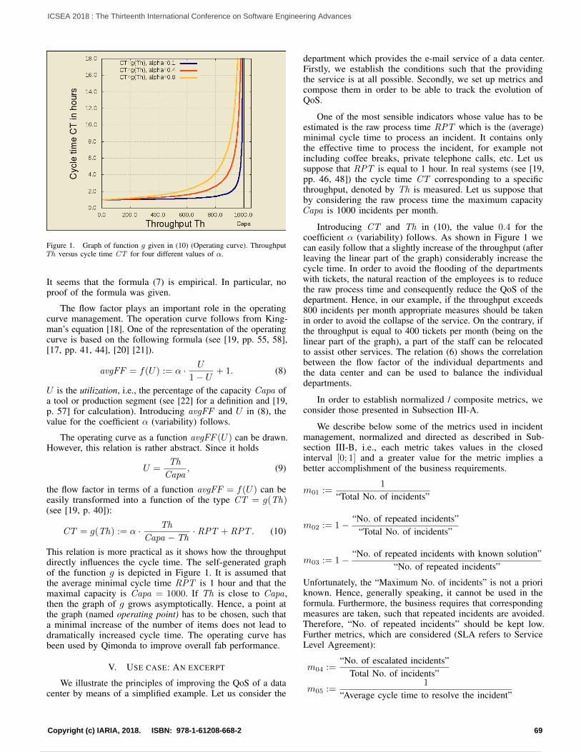
Figure 1. Graph of function g given in (10) (Operating curve). ThroughputTh versus cycle time CT for four different values of α.

It seems that the formula (7) is empirical. In particular, noproof of the formula was given.

The flow factor plays an important role in the operatingcurve management. The operation curve follows from King-man’s equation [18]. One of the representation of the operatingcurve is based on the following formula (see [19, pp. 55, 58],[17, pp. 41, 44], [20] [21]).

avgFF = f(U) := α · U

1− U+ 1. (8)

U is the utilization, i.e., the percentage of the capacity Capa ofa tool or production segment (see [22] for a definition and [19,p. 57] for calculation). Introducing avgFF and U in (8), thevalue for the coefficient α (variability) follows.

The operating curve as a function avgFF (U) can be drawn.However, this relation is rather abstract. Since it holds

U =Th

Capa, (9)

the flow factor in terms of a function avgFF = f(U) can beeasily transformed into a function of the type CT = g(Th)(see [19, p. 40]):

CT = g(Th) := α · Th

Capa − Th· RPT + RPT . (10)

This relation is more practical as it shows how the throughputdirectly influences the cycle time. The self-generated graphof the function g is depicted in Figure 1. It is assumed thatthe average minimal cycle time RPT is 1 hour and that themaximal capacity is Capa = 1000. If Th is close to Capa ,then the graph of g grows asymptotically. Hence, a point atthe graph (named operating point) has to be chosen, such thata minimal increase of the number of items does not lead todramatically increased cycle time. The operating curve hasbeen used by Qimonda to improve overall fab performance.

V. USE CASE: AN EXCERPT

We illustrate the principles of improving the QoS of a datacenter by means of a simplified example. Let us consider the

department which provides the e-mail service of a data center.Firstly, we establish the conditions such that the providingthe service is at all possible. Secondly, we set up metrics andcompose them in order to be able to track the evolution ofQoS.

One of the most sensible indicators whose value has to beestimated is the raw process time RPT which is the (average)minimal cycle time to process an incident. It contains onlythe effective time to process the incident, for example notincluding coffee breaks, private telephone calls, etc. Let ussuppose that RPT is equal to 1 hour. In real systems (see [19,pp. 46, 48]) the cycle time CT corresponding to a specificthroughput, denoted by Th is measured. Let us suppose thatby considering the raw process time the maximum capacityCapa is 1000 incidents per month.

Introducing CT and Th in (10), the value 0.4 for thecoefficient α (variability) follows. As shown in Figure 1 wecan easily follow that a slightly increase of the throughput (afterleaving the linear part of the graph) considerably increase thecycle time. In order to avoid the flooding of the departmentswith tickets, the natural reaction of the employees is to reducethe raw process time and consequently reduce the QoS of thedepartment. Hence, in our example, if the throughput exceeds800 incidents per month appropriate measures should be takenin order to avoid the collapse of the service. On the contrary, ifthe throughput is equal to 400 tickets per month (being on thelinear part of the graph), a part of the staff can be relocatedto assist other services. The relation (6) shows the correlationbetween the flow factor of the individual departments andthe data center and can be used to balance the individualdepartments.

In order to establish normalized / composite metrics, weconsider those presented in Subsection III-A.

We describe below some of the metrics used in incidentmanagement, normalized and directed as described in Sub-section III-B, i.e., each metric takes values in the closedinterval [0; 1] and a greater value for the metric implies abetter accomplishment of the business requirements.

m01 :=1

“Total No. of incidents”

m02 := 1− “No. of repeated incidents”“Total No. of incidents”

m03 := 1− “No. of repeated incidents with known solution”“No. of repeated incidents”

Unfortunately, the “Maximum No. of incidents” is not a prioriknown. Hence, generally speaking, it cannot be used in theformula. Furthermore, the business requires that correspondingmeasures are taken, such that repeated incidents are avoided.Therefore, “No. of repeated incidents” should be kept low.Further metrics, which are considered (SLA refers to ServiceLevel Agreement):

m04 :=“No. of escalated incidents”

Total No. of incidents”

m05 :=1

“Average cycle time to resolve the incident”



80 / 160

m06 :=1

“Average waiting time from user side”

m07 :=1

“Average working time on the incident”

m08 :=“Total No. of incidents resolved within SLA time”

“Total No. of SLA relevant incidents”

m09 :=1

“First reaction time to repair the incident”

m10 :=1

“No. of responses from service center side”Unfortunately, defining metrics fulfilling the conditions asabove, is not always straightforward. Let us consider Incidout

as the total number of incidents closed and Incid in as the totalnumber of incidents opened in the time frame considered. Inorder to avoid the flooding of the data center with incidents themetric k := Incidout/Incid in could be tracked. Unfortunately,this metric does not fulfill our requirements, since it can takevalues outside the interval [0; 1]. In order to avoid this impedi-ment, we define kin := Incid in/“Total No. of incidents” andkout := Incidout/“Total No. of incidents” and set

m11 :=1 + kout − kin

2.

Then, m11 is normalized and satisfies the above conditionsimposed for metrics. Generally speaking, the effective minimaland maximal value of a metric is not known, nor is thedistribution a priori known. Thus, for example, a metric m1

takes values in the interval [0.5; 0.6] and another metric m2 inthe interval [0.2; 0.7] with nearly uniform distribution. Hence,the metric m2 varies more widely than m1 and this should beconsidered – for example using the standard deviation – whensetting up the groupings for the composition of the metrics,such that metrics having a low standard deviation should beassigned to more important groups.

Now, let us consider in our use case five composition groups,G0, G1, . . . , G4, such that G1 is the most relevant group. Letus associate the weight wi to group Gi and let us consider theweighting according to an exponential function, such that k0 :=1 and ki := wi−1/wi for i > 0. This yields to the relation:wi = w0/

∏l=il=0 kl. In our example k1 := e1, k2 := e0.75,

k3 := e0.5, etc. The values for ki are illustrated in Figure 2.Let us assign the above metrics to the composition groups,such that index set of the metrics assigned to the group Gl

is equal to Il and let nl the number of metrics in the group

Gl. Then, according to the composition rules:4∑

i=0

ni · wi = 1.

Hence, the weight values follow. The value of the compositionmetric M is:

V (M) :=

4∑i=0

wi ·∑l∈Ii

V (ml).

Examples of services at the ZIH of the Technische Univer-sität Dresden (TU Dresden) are: “E-Mail Service”, “Backup andArchive Service”, “Data Exchange Service”, “Access to HighPerformance Computing Resources”, etc. [23] We conclude thissection by presenting the assistance system for a data centerin Figure 4 and by summarizing the composition strategy viathe flow diagram given in Figure 3.

Figure 2. Graphical construction of values ki such that metrics are weightedaccording to an exponential function, depicted for f(x) = ex.

Start

Establish all metricsfor each department, for each process, for each service, etc.

Normalize the metrics,such that a greater value fulfills better the business requirements.

Establish grouping of indicators.

Establish the grouping strategyand set up a unique indicator for the data center.

End

Figure 3. Simplified flow diagram regarding the composition strategy.


We set up a formal, mathematical model and analyzed theQoS and the modalities to enhance it within this model. In thatway, the QoS provided by the TU Dresden can be improved,which implicitly leads to a good ranking of the TU Dresdenbetween the universities in Germany and world wide.

The main result of our research is that from a serviceprovider perspective QoS can be characterized in mathematicalterms pretty accurately, such that the improvement / degradationof the overall service or part of it can be tracked in IT systemsand can be visualized through GUIs. According to Definition ofITU-T Rec. E.800 [24]: QoS is the “Collective effect of serviceperformances which determine the degree of satisfaction of auser of a service”. The long term experience of the first author,working in the semiconductor industry is very similar to thedefinition above, such that it does not suffice to consider onlythe service provider perspective, but the user’s perception of theQoS should also be considered. Further research is necessary toestablish the correlation (or lack of it) between the objectively



81 / 160

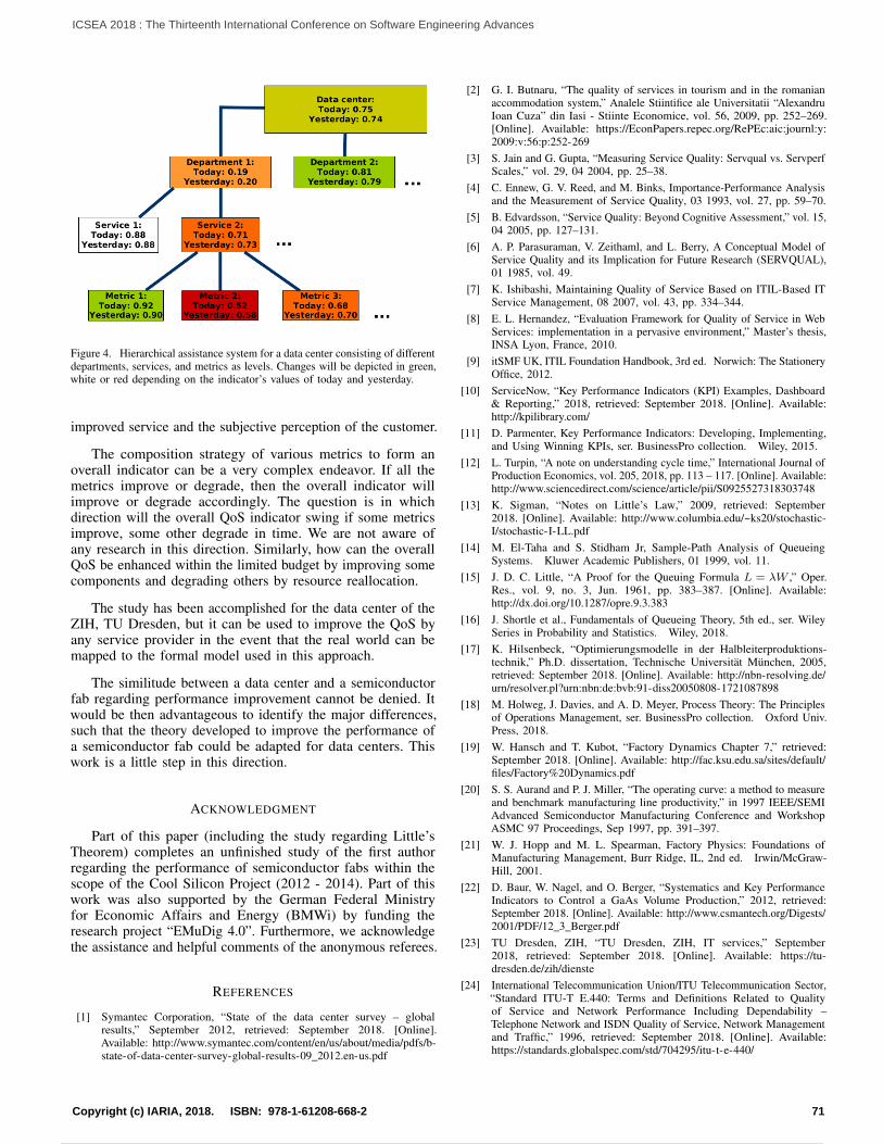
Figure 4. Hierarchical assistance system for a data center consisting of differentdepartments, services, and metrics as levels. Changes will be depicted in green,white or red depending on the indicator’s values of today and yesterday.

improved service and the subjective perception of the customer.

The composition strategy of various metrics to form anoverall indicator can be a very complex endeavor. If all themetrics improve or degrade, then the overall indicator willimprove or degrade accordingly. The question is in whichdirection will the overall QoS indicator swing if some metricsimprove, some other degrade in time. We are not aware ofany research in this direction. Similarly, how can the overallQoS be enhanced within the limited budget by improving somecomponents and degrading others by resource reallocation.

The study has been accomplished for the data center of theZIH, TU Dresden, but it can be used to improve the QoS byany service provider in the event that the real world can bemapped to the formal model used in this approach.

The similitude between a data center and a semiconductorfab regarding performance improvement cannot be denied. Itwould be then advantageous to identify the major differences,such that the theory developed to improve the performance ofa semiconductor fab could be adapted for data centers. Thiswork is a little step in this direction.

ACKNOWLEDGMENT

Part of this paper (including the study regarding Little’sTheorem) completes an unfinished study of the first authorregarding the performance of semiconductor fabs within thescope of the Cool Silicon Project (2012 - 2014). Part of thiswork was also supported by the German Federal Ministryfor Economic Affairs and Energy (BMWi) by funding theresearch project “EMuDig 4.0”. Furthermore, we acknowledgethe assistance and helpful comments of the anonymous referees.

REFERENCES

[1] Symantec Corporation, “State of the data center survey – globalresults,” September 2012, retrieved: September 2018. [Online].Available: http://www.symantec.com/content/en/us/about/media/pdfs/b-state-of-data-center-survey-global-results-09_2012.en-us.pdf

[2] G. I. Butnaru, “The quality of services in tourism and in the romanianaccommodation system,” Analele Stiintifice ale Universitatii “AlexandruIoan Cuza” din Iasi - Stiinte Economice, vol. 56, 2009, pp. 252–269.[Online]. Available: https://EconPapers.repec.org/RePEc:aic:journl:y:2009:v:56:p:252-269

[3] S. Jain and G. Gupta, “Measuring Service Quality: Servqual vs. ServperfScales,” vol. 29, 04 2004, pp. 25–38.

[4] C. Ennew, G. V. Reed, and M. Binks, Importance-Performance Analysisand the Measurement of Service Quality, 03 1993, vol. 27, pp. 59–70.

[5] B. Edvardsson, “Service Quality: Beyond Cognitive Assessment,” vol. 15,04 2005, pp. 127–131.

[6] A. P. Parasuraman, V. Zeithaml, and L. Berry, A Conceptual Model ofService Quality and its Implication for Future Research (SERVQUAL),01 1985, vol. 49.

[7] K. Ishibashi, Maintaining Quality of Service Based on ITIL-Based ITService Management, 08 2007, vol. 43, pp. 334–344.

[8] E. L. Hernandez, “Evaluation Framework for Quality of Service in WebServices: implementation in a pervasive environment,” Master’s thesis,INSA Lyon, France, 2010.

[9] itSMF UK, ITIL Foundation Handbook, 3rd ed. Norwich: The StationeryOffice, 2012.

[10] ServiceNow, “Key Performance Indicators (KPI) Examples, Dashboard& Reporting,” 2018, retrieved: September 2018. [Online]. Available:http://kpilibrary.com/

[11] D. Parmenter, Key Performance Indicators: Developing, Implementing,and Using Winning KPIs, ser. BusinessPro collection. Wiley, 2015.

[12] L. Turpin, “A note on understanding cycle time,” International Journal ofProduction Economics, vol. 205, 2018, pp. 113 – 117. [Online]. Available:http://www.sciencedirect.com/science/article/pii/S0925527318303748

[13] K. Sigman, “Notes on Little’s Law,” 2009, retrieved: September2018. [Online]. Available: http://www.columbia.edu/~ks20/stochastic-I/stochastic-I-LL.pdf

[14] M. El-Taha and S. Stidham Jr, Sample-Path Analysis of QueueingSystems. Kluwer Academic Publishers, 01 1999, vol. 11.

[15] J. D. C. Little, “A Proof for the Queuing Formula L = λW ,” Oper.Res., vol. 9, no. 3, Jun. 1961, pp. 383–387. [Online]. Available:http://dx.doi.org/10.1287/opre.9.3.383

[16] J. Shortle et al., Fundamentals of Queueing Theory, 5th ed., ser. WileySeries in Probability and Statistics. Wiley, 2018.

[17] K. Hilsenbeck, “Optimierungsmodelle in der Halbleiterproduktions-technik,” Ph.D. dissertation, Technische Universität München, 2005,retrieved: September 2018. [Online]. Available: http://nbn-resolving.de/urn/resolver.pl?urn:nbn:de:bvb:91-diss20050808-1721087898

[18] M. Holweg, J. Davies, and A. D. Meyer, Process Theory: The Principlesof Operations Management, ser. BusinessPro collection. Oxford Univ.Press, 2018.

[19] W. Hansch and T. Kubot, “Factory Dynamics Chapter 7,” retrieved:September 2018. [Online]. Available: http://fac.ksu.edu.sa/sites/default/files/Factory%20Dynamics.pdf

[20] S. S. Aurand and P. J. Miller, “The operating curve: a method to measureand benchmark manufacturing line productivity,” in 1997 IEEE/SEMIAdvanced Semiconductor Manufacturing Conference and WorkshopASMC 97 Proceedings, Sep 1997, pp. 391–397.

[21] W. J. Hopp and M. L. Spearman, Factory Physics: Foundations ofManufacturing Management, Burr Ridge, IL, 2nd ed. Irwin/McGraw-Hill, 2001.

[22] D. Baur, W. Nagel, and O. Berger, “Systematics and Key PerformanceIndicators to Control a GaAs Volume Production,” 2012, retrieved:September 2018. [Online]. Available: http://www.csmantech.org/Digests/2001/PDF/12_3_Berger.pdf

[23] TU Dresden, ZIH, “TU Dresden, ZIH, IT services,” September2018, retrieved: September 2018. [Online]. Available: https://tu-dresden.de/zih/dienste

[24] International Telecommunication Union/ITU Telecommunication Sector,“Standard ITU-T E.440: Terms and Definitions Related to Qualityof Service and Network Performance Including Dependability –Telephone Network and ISDN Quality of Service, Network Managementand Traffic,” 1996, retrieved: September 2018. [Online]. Available:https://standards.globalspec.com/std/704295/itu-t-e-440/



82 / 160

The Various Challenges Faced by the Software Startup Industry in Saudi Arabia

Abdullah Saad H., Alqahtani

Imam Abdulrahman Bin Faisal University

Dammam, Saudi Arabia


Abstract—With the increasing use of the Internet, Web and

mobile technologies at present, software startups, which are

newly created software companies with no history, have

become an important phenomenon in the software industry.

They have a wide impact on the technology market and a

significant impact on the global economy. However, even with

the increase in the importance of software startups for the

economy and communities, little research has investigated the

challenges of this phenomenon, especially with new software

markets, such as the Saudi Arabia market. This study aimed to

investigate the challenges faced by the software startup

industry in Saudi Arabia. It presents a mixed-methodology

study based on semi-structured interviews and questionnaires.

The findings of this study revealed a list of challenges that need

to be considered in order to improve the industry for software

startups. The lack of transparency and funding can be

considered the biggest concern for software startups in Saudi

Arabia.

Keywords-Software startups; startup challenges; small

software development; software industry; information startups

I. INTRODUCTION

Software startups are newly created companies with little or no history that aim to grow rapidly in the software industry [16]. Software startups aim at innovation and building software products within a limited time and with few resources [32]. Blank [9] described startups as temporary human organizations with no prior operating history that aim to create new, high-tech products or services. Software startups are considered to be an important phenomenon in the modern economy and society. This phenomenon creates approximately three million new jobs each year in the USA. Information technology companies, such as Facebook, LinkedIn, Instagram and Dropbox, are good examples of how startups can transform into successful businesses, provide tremendous support to their national economies and have a significant impact on the global economy [18]. However, about 60% of startups do not survive the first five years [16]. Early stage software startups face key challenges to success in this industry such as lack of resources and experiences [18]. The competition in the industry drives most of the startups to exit the market within two years form creation [25]. Due to the high failure rates of software startups, communities, organizations and even countries are beginning to investigate this phenomenon. There is a current need for research to support startups with their software engineering practices [25]. This study is aiming to provide deep investigation of the challenges faced

by the software startup industry in Saudi Arabia in order to address the current gap of knowledge.

The remainder of this paper is structured as follows: background and previous studies is reported in Section 2. Section 3 addresses the research methodology. Results are reported in Section 4. Then the discussion is presented within Section 5. Finally, the study concludes in Section 6.

II. STATE OF THE ART

Software startups are considered to face several challenges; they may encounter obstacles when attempting to sell their first products, acquire paying customers and establish entrepreneurial teams [32]. Giardino et al. [18] highlighted several challenges for software startups, including lack of resources, lack of experience, dependence on one product, the uncertainty of their conditions, time pressure and lack of sustainability. The nature of software startups, as newly created organizations working in uncertain markets and using cutting-edge technology, make them challenging endeavors [32]. Klonowski et al. [19] investigated software startups in Central and Eastern Europe and placed the challenges into four categories, namely problems with funding, problems with management, the change in corporate culture and acceptance of the business model and financial underperformance. Giardino et al. [16] also reported that the main challenges for many startups are thriving despite technological uncertainty and finding the first paying customers. Giardino et al. [17] reported similar challenges, as well as others such as obtaining initial funding, creating entrepreneurial teams, providing value to customers, starting to make a profit and configuration management. Little relevant research pertaining to software startups exists; Pateronster studied software startups via a systematic map study and reported a few studies in the area of software startups [25]. Unterkalmsteiner et al. [32] stated that research on software startups has increased over the last year, but there is still a need for more investigation in this area.

Alnafjan [2] investigated the applied software practices in Saudi Arabia and reported clear weaknesses in adopting software engineering practices, particularly for small organizations. Alnuem [3], who also investigated the software industry in Saudi Arabia, reported serious issues in the industry, such as culture, communications and understanding the requirements clearly.

The software industry in Saudi Arabia is considered to be in the early stages. A few companies could survive in this industry. The Saudi government has established a new vision



83 / 160

called “Vision 2030.” One of its goals is to help software startups to develop a successful market in order to support the national economy. The government also aims to support e-government transformation. On the other hand, there is a gap in the current knowledge regarding challenges faced by software startups in Saudi Arabia. There is a lack of empirical updated studies that provide deep investigation of the Saudi software industry. This paper aims to investigate this area in order to provide a better understanding of the challenges software startups face and to help the community to build a better software industry.

III. RESEARCH METHODOLOGY

This paper presents a mixed-methodology study that includes both quantitative and qualitative data. Semi-structured interviews and questionnaires will be used as tools to collect data. The combination of quantitative and qualitative data aims to add more reliability and validity to the study’s results. Bryman [12] referred to mixed-methods research as follows: “This term is widely used nowadays to refer to research that combines methods associated with both quantitative and qualitative research”. Employing the mixed approach matches the study aims and objectives and should allow for a better understanding of the specific challenges of software startups in more detail. The quantitative form will provide the critical numbers and statistics needed to study the challenges, while the qualitative data will be applied as a secondary methodology to provide richer information and an explanation of the study findings. The findings from both approaches will be integrated to form a better understanding of software startup challenges.

A. Research question

This study aims to investigate the software industry in Saudi Arabia in order to provide a better understanding of the current barriers that software startups encounter by addressing the following research question:

RQ: What are the main challenges encountered by software startups in the Kingdom of Saudi Arabia (KSA) from the perspective of software development?

B. Data collection

1) The quantitative data The quantitative data were collected via a self-completed

online survey. About 10 people were invited to pilot the questionnaire, including project managers, software developers and testers, most of whom were experts in software development. The questionnaire was distributed during two main startup events in the KSA (the SAP Startup Focus Forum Saudi Arabia in Riyadh, 2016, and the Small and Medium Enterprise Forum in Jeddah, 2017). It was also distributed online to approximately 120 software companies in the Kingdom. By the end of the data collection phase, 74 completed and eligible responses were received. The questionnaire investigated 19 phrases, which will be treated as possible hypotheses for the challenges faced by software startups in Saudi Arabia.

TABLE I. THE RESEARCH HYPOTHESES: THE EXPECTED OBSTACLES

TO SOFTWARE DEVELOPMENT BASED ON PREVIOUS STUDIES

There is a lack of communication and collaboration during all the development stages. [4][21]

PH1

The development team has estimation difficulties with the development cost, scope, and development schedule. [4] [21]

PH2

There is a lack of communication between the developers and the product owners.[4][21]

PH3

There is lack of team management skills.[16] [19] PH4 During the development, we face issue with sharing knowledge and information. [13] [18]

PH5

There is a security risk during the development.[2] [3] PH6 Some development teams have issues with poor infrastructures.[21][25]

PH7

The visibility level of the development progress is low. [13][18][29]

PH8

Customers sometimes do not have a clear idea for their requirement. [1][3]

PH9

There is lack of talent in the software industry in KSA. [13][17][25]

PH10

Provide high quality software is a challenge regarding the development ream's capabilities.[2][13][16]

PH11

There is lack of providing initial funding.[16] [19] [25][29] PH12 There are barriers to access the market.[16] [17][29] PH13 Some customers like to work with big software companies. [17][21]

PH14

Government regulations could challenge software companies. [1][3]

PH15

Software projects have issues with building a sufficient business model. [19] [25][29]

PH16

Providing products with competitive prices is a challenge. [13][19]

PH17

There is lack of information and transparency about the software market in Saudi Arabia.[13][17]

PH18

Customers are not aware of how software could add value to their business. [13][17][19][29]

PH19

These phrases represent the expected obstacles to

software development based on previous studies. A five-

point Likert scale was used to explore the questionnaire

respondents’ degrees of agreement with these challenges.

Table Ι presents the invested hypotheses and their references

from the previous studies.

2) The qualitative data The qualitative data were collected via structured

interviews. The interviews were face-to-face and were recorded using a voice recorder. In addition, notes of the main ideas and answers were taken during the interviews. The transcribed documents were then compared to the notes from the interviews to ensure the reliability of the data. Following this, a thematic analysis, which is an approach to identify the themes and patterns from the collected qualitative data, was conducted [11][14]. In addition, the data-driven method was selected for the thematic analysis of this study [5]. The interpretation of data has been reviewed by a ccolleague to ensure its accuracy.

IV. RESULTS

This section reports the result of this study. First of all, it

states the results of the descriptive analysis. Then, it will

address the result of reliability test. Finally, the quantitative

results and qualitative results will be reported.



84 / 160

A. Descriptive analysis

This section describes the background information about the study participants, including their experience, team size and the location of their development teams.

1) Development experience Table ΙΙ shows the participants’ number of years of

experience in software development. Most of the participants had from four to seven years of software development experience, while about 35% had from one to four years of experience. This shows that the study’s participants had substantial software development experience.

TABLE II. THE EXPERIENCE OF THE STUDY'S PARTICIPANTS

Answer Count Percent Less

than 1 10 13%

1-4 25 35% 4-7 33 44%

More than 7

6 8%

Total 74 100%

2) Team size Table ΙΙΙ below indicates the size of the team that

developers usually have. Most of the participants (42%) came from teams with five to 15 members; the second highest figure was 15 to 25 team members (37% of the sample), while less than 13% of the sample were from teams that had more than 25 members, and only 8% of the participants came from teams with fewer than five team members. This information is expected due to the nature of startup companies’ sizes.

TABLE III. THE TEAM SIZE

Answer Count Percent Less than 5 7 8%

5- 15 30 42% 15-25 27 37% 25-45 3 3 % 45-60 5 7%

Greater than 60

2 3%

Total 74 100%

3) Outsourced development Table ΙV shows that most of the study’s participants had

outsourced or offshore teams. About 87% of the sample explained that some of their functions were developed outside of the country. Only 10 participants did not have outsourced teams. This result could relate to the difficulty of the software industry in Saudi Arabia, which leads most companies to outsource some of their development.

TABLE IV. OUTSOURCED DEVELOPMENT

Answer Count Percent Yes 64 87% No 10 13%

Total 74 100%

B. Reliability

According to Bryman and Cramer [12], “The reliability of measure refers to its consistency.” Pallant [23] also stated,

“The reliability of a scale indicates how free it is from random error”. With multiple-item scales, such as the Likert scale, variables of internal reliability need to be tested. The aim is to examine whether each scale is measuring a single idea and how each item affects the internal consistency of the scale [12]. Cronbach’s alpha coefficient has been applied to test data reliability. This shows the correlation among all the items in the scale. The ideal Cronbach’s alpha level is above 0.7 [23]. Table V shows the Cronbach’s alpha values for the challenges under investigation. The alpha value was 0.776, which means that the items were internally consistent.

TABLE V. RELIABILITY STATISTICS

Cronbach's Alpha

Cronbach's Alpha Based on

Standardized Items

N of Items

0.776 0.784 19

C. Quantitative results

TABLE VI. TESTS OF NORMALITY

Phrase

Kolmogorov-

Smirnova

Shapiro-Wilk

Statistic df Sig. Statistic df Sig.

PH1 .358 74 .000 .745 74 .000

PH2 .278 74 .000 .856 74 .000

PH3 .249 74 .000 .828 74 .000

PH4 .250 74 .000 .868 74 .000

PH5 .239 74 .000 .865 74 .000

PH6 .240 74 .000 .890 74 .000

PH7 .279 74 .000 .875 74 .000

PH8 .240 74 .000 .866 74 .000

PH9 .269 74 .000 .861 74 .000

PH10 .269 74 .000 .881 74 .000

PH11 .410 74 .000 .681 74 .000

PH12 .427 74 .000 .652 74 .000

PH13 .369 74 .000 .755 74 .000

PH14 .298 74 .000 .848 74 .000

PH15 .250 74 .000 .853 74 .000

PH16 .255 74 .000 .868 74 .000

PH17 .307 74 .000 .821 74 .000

PH18 .292 74 .000 .805 74 .000

PH19 .336 74 .000 .800 74 .000

Table VΙ shows the results of the normality test. The results show that the data were not normally distributed, with a significance of less than 0.05 for both the Shapiro-Wilk and the Kolmogorov-Smirnov tests. This means that the data pertaining to those scales will be treated as nonparametric data [23]. The median and mode should be used to describe nonparametric data [10][12]. Table VII shows the mean, median and mode for each phrase. It also shows the results of testing each phrase. The hypothesis will be accepted if the median is above 2.5 and rejected if it is less than 2.5.



85 / 160

TABLE VII. HYPOTHESES RESULTS

Accepted or

Rejected

Mode Median Mean Phrase

Accepted 4 4.00 3.11 PH1

Rejected 2 2.00 2.35 PH2


















Table VΙΙ shows that five of the hypotheses “phrases” have been rejected (PH2, PH4, PH5, PH6 and PH7). These challenges were not considered significant based on the median value. The other 14 hypotheses were accepted and are summarized as shown in the table below; they will be discussed in the discussion section. The challenges have been ranked based on their importance according to the degree of agreement on the part of the study’s participants and each phrase’s mean value, as show in Table VIII.

TABLE VIII. HYPOTHESES RANK

Hypotheses Phrase

number

Challenge

number

There is lack of information and transparency about the software market in

Saudi Arabia

PH18 CH1

Providing products with competitive prices is a challenge.

PH17 CH2

Provide high quality software is a challenge

regarding the development ream's

capabilities.

PH11 CH3

Government regulations could challenge

software companies

PH15 CH4

Customers are not aware of how software

could add value to their business

PH19 CH5

There is lack of providing initial funding PH12 CH6

There are barriers to access the market PH13 CH7

Some customers like to work with big

software companies.

PH14 CH8

Software projects have issues with building a sufficient business model.

PH16 CH9

There is lack of talent in the software

industry in KSA.

PH10 CH10

Customers sometimes do not have a clear idea for their requirement.

PH9 CH11

There is a lack of communication and

collaboration during all the development stages.

PH1 CH12

The visibility level of the development

progress is low.

PH8 CH13

There is a lack of communication between the developers and the product owners.

PH3 CH14

D. Qualitative results

The results of the thematic analysis indicated eight main challenges, as described below:

1) A1- Lack of funding and financial support: Finding sufficient financial support was considered to be

one of the main issues for software startups in the KSA. Company A stated, “Providing the needed funding was one of our main concerns, you need to make sure you have enough cash flow.” Company B reported that “one of our main challenges was to have enough funds to start our project. We made many meetings with investors and investment companies but, unfortunately, we could not have any financial collaboration with them. In addition, the government’s financial support programmes were not sufficient and not available in many cases.” Companies C and D both agreed that the funding challenge was one of the main challenges for their projects.

2) A2- Difficulty of gaining customers’ trust and access

to the market: Company B, which was an online store, reported that

“gaining customers’ trust was one of the main challenges; first, it is a challenge to have people sell their product using our on-line store and secondly, it is also a challenge to have people buy from our on-line store.” Company C stated, “It is a big challenge to access the market; we had our biggest challenge when we tried to sell our product.” Company D also reported that signing the first contract was the biggest challenge. Company E mentioned that it had experienced tremendous competition with social media stores and that it was difficult to compete with them in terms of cost.

3) A3- Making a product that suited the market: Company A said that one difficulty was creating a

product that did not suit the current market. The company cited the example of having had a product “website” that worked on meta search technologies and failing to sell it to the market because the market was not ready to use this technology to compare hotel prices at the time. Thus, their product was too far ahead of the current market. A few years later, a different company developed and launched an almost identical product and experienced a huge success.

4) A4- Lack of transparency and market information: Company C reported that access to information and data

were also major obstacles, citing difficulty when developing a business model due to the lack of transparency in the software market.

5) A5- Government barriers: Company E reported issues with the government’s

regulations because many steps and complicated processes are required in order to open a software startup.

6) A6- Access to talent: According to Company C, graduates with degrees in

software were not qualified to be professionals in the software market, and there was a lack of Saudi talent in the market. Company D’s CEO, who is also a professor at one of the larger universities in the Kingdom within the software field, reported a need to create partnerships between colleges and software companies to improve the quality of colleges’ graduate student outcomes. Company E reported a lack of



86 / 160

expert graduates in the field of software development management and that no courses covering the concepts of “lean” or “agile” were offered in academic programs.

Company B used outsourced teams due to the lack of software developers in Saudi Arabia, which created other barriers in terms of language and cultural differences.

7) A7- Lack of clear ideas about customer

requirements: According to Company C, people do not have sufficient

understanding regarding what software could do for their businesses. In addition, customers sometimes did not have a clear idea of their requirements. For example, many customers asked the company to compare their competitors’ websites and make better websites for their companies without providing a clear idea of their requirements.

V. DISCUSSION

This section will combine the results of the descriptive analysis (quantitative results) and the results of the thematic analysis (qualitative results). It will provide a general discussion about the challenges in light of previous studies. The challenges will be classified into two main groups. Table IX shows the links between the study’s results. It also organizes the challenges into two main groups. The first group contains challenges related to finance and market access, and the second is for software quality challenges.

TABLE IX. STUDY RESULTS

Group Challenge Related results Funding

and market access

Lack of transparency CH1, A4 lack of funding and financial support

CH6, A1

Government regulations

CH4, A5

Obstacles of market access

CH2, CH 7,CH8, A2, A3

Software quality and awareness

Lack of software quality and talent

CH3, CH9, CH10, A6

Lacking of clear idea about customer

requirement

CH1, CH5, A7

Lack of communication and

visibility

CH12, CH13, CH14

A. Funding and transparency

1) Lack of transparency The quantitative results revealed the lack of information

and transparency in the software market in Saudi Arabia (CH1) as one of the main challenges within the market. Startups need information and transparency in order to build their business models and develop strategies. The qualitative data supported this: (A4) “Lack of transparency and market information.”

2) Lack of funding and financial support The first challenge that software startups face is finding

funding resources. This barrier was revealed to be one of the main issues according to the quantitative results (CH6), and

it was also revealed to be the main concern in the qualitative results. An investigation about the startup industry in Australia reported that around 67% of startups needed financial support to survive until their second year of business, and about 41% of the startups investigated had difficulty with funding [29]. Gilardino et al. [16] reported the challenge of not having initial funding for startups.

3) Government regulations The government’s regulations were reported as a

challenge for software startups (CH4 and A5). When establishing a new company, there are many regulations that make the task difficult for startups. Gilardino et al. [16] reported the same issue and agreed that government regulations need to be addressed during software startups’ development phases.

4) Obstacles of market access Accessing the market is the second phase for startups.

There are barriers to accessing the market (CH7). Startups will experience challenges in gaining customers’ trust (A2). They have no history and not enough experience. Customers usually prefer to work with big software names rather than with small, newly established software companies (CH8). In addition, due to a lack of experience, the software startups could have difficulty providing a product that suits the market (A3). Finally, providing products at competitive prices is a challenge (CH2). Gilardino et al. [16] referred to acquiring the first paying client as one of the main obstacles for software startups. Klonowski et al. [19] mentioned that identifying the available opportunities in the software market was not an easy task due to changes in the clients’ requirements and technological uncertainty. Furthermore, the market should be accessed in a time-efficient way [19].

B. Software quality and awareness

1) Lack of quality software and talent Providing high-quality software was a challenge due to

the development team’s capabilities (CH3). The startups had limited resources, which decreased their development capabilities. They usually had problems with building a sufficient business model (CH9). Furthermore, access to talent was a major challenge due to the lack of talent in the software industry in Saudi Arabia (CH10 and A6). Gilardino et al. [16] identified the general lack of resources as one of the main features of startups. Software startups use external solutions to address the limitations of their resources, such as outsourcing and open-source software [18]. The use of new concepts in software, such as agile methods, is poor, which could reflect on the quality of the software developed [2].

2) Lack of clears idea about customer requirements Software startups are challenged by the lack of software

awareness on the part of their customers (A7). Customers are not aware of how software could add value to their businesses (CH5). They are uncertain about paying for a software service because they are not sure how this service could improve their businesses. Furthermore, customers often lack a clear idea of their requirements.



87 / 160

3) Lack of communication and visibility The results from the quantitative data showed the lack of

communication and collaboration during all stages of development (CH12). The visibility level of the development progress was low (CH13). Moreover, there was a lack of communication between the developers and the product owners (CH14). The quantitative data revealed that about 88% of software projects had outsourced or offshore teams. The distance among teams affects the visibility level of development. The lack of communication could create barriers for customers when attempting to follow the progress of development and could make it difficult for developers to communicate with customers. Therefore, this could decrease the visibility of development [26]. Providing a high-quality communication channel could be expensive and add substantial costs to the project. Sometimes the development teams, particularly those offshore, experienced technical issues such as poor Internet connection or poor infrastructure. As a result, the cost of communication could be increased [35].

VI. CONCLUSION

The software startup industry in Saudi Arabia was investigated in this study. This paper applied a mixed-method approach to collect both quantitative and qualitative data. The lack of transparency and funding can be considered to be the biggest concern. There is a lack of available information about the IT industry, including the size of the market and the existing companies in the market. In addition, the government’s regulations limited the startups and created serious difficulties in terms of their business models and plans. The second major difficulty experienced by software startups was access to the market. For a company with no history, gaining customers’ trust was considered a major challenge. Customers also lack software awareness and are not aware of how the software can help them to grow their businesses. Furthermore, there is a lack of quality software and talent. Accessing talented people in software development in Saudi Arabia is one of the main issues for the startups. This has an impact on the software’s quality and leads many startups to outsource development or to develop software offshore, which is a common practice in software development. However, this could create a lack of communication and decrease the visibility level of development.

In summary, this study reported on the main challenges experienced by software startups in Saudi Arabia, and provided a general investigation into the software industry in order to provide a better understanding of the phenomenon of software startups. This information could be useful for the Saudi government to improve their regulations to support software development industry. The first recommendation of this study is to establish funding channels, either by the government or the private sector. The current regulations need to be updated to attract more investments to the industry. Moreover, it is important to update the current software curricula in universities and computer colleges to provide more qualified developers to the community.

Future work will investigate the relationship between the challenges described and other factors affecting success in the software industry (such as cost, quality and time) in order to identify the factors for success in the Saudi software industry.

REFERENCES

[1] Adebanjo, D., 2010, "Challenges and approaches to customer development in co- located high tech start-ups", Proceedings of the International Conference on Industrial Engineering and Engineering Management (IEEM), pp. 163–167.

[2] Alnafjan, K., 2012, "An empirical investigation into the adoption of Software Engineering Practice in Saudi Arabia", International Journal of Computer Science Issues (IJCSI), vol. 9, no. 3, pp. 328-332.

[3] Alnuem, M. A., Ahmad, A. and Khan, H., 2012, "Requirements Understanding: A Challenge in Global Software Development, Industrial Surveys in Kingdom of Saudi Arabia", IEEE, ,pp. 297-305.

[4] Alqahtani, A.S., Moore, J.D., Harrison, D.K. and Wood, B.M., 2013. The Challenges of Applying Distributed Agile Software Development: A Systematic Review. International Journal of Advances in Engineering & Technology, 5(2), p.23-36.

[5] Asnawi, A., Gravell, A., and Wills, G., 2012, "Emergence of Agile methods: Perceptions from software practitioners in Malaysia" AGILE India, 2012, pp. 30-39.

[6] Bajwa, S. S., Wang, X., Duc, A.N., and Abrahamsson, P., 2017, "Failures to be celebrated: an analysis of major pivots of software startups", Empirical Software Engineering, vol. 22, no. 5, pp. 2373-2408.

[7] Barney, S., Petersen, K., Svahnberg, M., Aurum, A., and Barney, H., 2012, "Software quality trade-offs: a systematic map, Inf. Softw. Technol, pp. 651–662.

[8] Bertram, D., 2007, "Likert scales", Faculty of Mathematics, University of Belgrade.

[9] Blank, S., 2005, "The Four Steps to the Epiphany: Successful Strategies for Startups That Win". Cafepress.com.

[10] Boone, H.N., and Boone, D.A., 2012, "Analyzing Likert Data", Journal of Extension, vol. 50, no. 2, pp. 1-5.

[11] Boyatzis, R., 1998," Transforming qualitative information: Thematic analysis and code development", SAGE publications incorporated.

[12] Bryman, A., and Cramer, D., 2012, "Quantitative data analysis with IBM SPSS 17, 18 and 19: A guide for social scientists", Routledge, Psycholofy Press.

[13] Cbinsight, 2018, The Top 20 Reasons Startups Fail, from:

https://www.cbinsights.com/research/startup-failure-reasons-top/

[14] Dawson, C., 2009, "Introduction to research methods: A practical guide for anyone undertaking a research project", Oxford: How To Books Ltd.

[15] Gerald, H.B., Donch, J.C., Fesnak, R., and Stiles, A.R., 2014, "Intellectual Property in Consumer Electronics", Software and Technology Startups, Springer, New York, NY.

[16] Giardino, C., Bajwa, S.S., Wang, X., and Abrahamsson, P., 2015, "Key challenges in early-stage software startups", in Proceedings 16th International XP Conference (XP). Helsinki, Finland: Springer, pp. 52-63.

[17] Giardino, C., Paternoster, N., Unterkalmsteiner, M., Gorschek, T., and Abrahamsson, P., 2016, "Software Development in Startup Companies: The Greenfield Startup Model", IEEE Transactions on Software Engineering, vol. 42, no. 6, pp. 585-604.



88 / 160

[18] Giardino, C., Unterkalmsteiner, M., Paternoster, N., Gorschek, T., and Abrahamsson, P., 2014, "What Do We Know about Software Development in Startups?", IEEE Software, vol. 31, no. 5, pp. 28-32.

[19] Klonowski, D., and Golebiowska-Tataj, D., 2010, "Challenges and opportunities in developing a high-tech business in Central and Eastern Europe", International Journal of Emerging Markets, vol. 5, no. 2, pp. 138-152.

[20] Lee, S., and Yong, H. S., 2010, "Distributed agile: Project management in a global environment", Empirical software engineering, Vol. 15, no. 2, pp. 204-217.

[21] Martinez, M., S., 2016. Good Practices of the Lean Startup Methodology: Benefits, challenges and recommendations, Aato University.

[22] May, B., 2012, "Applying lean startup: an experience report – lean and lean ux by a ux veteran: Lessons learned in creating and launching a complex consumer app", in: Agile Conference (AGILE), pp. 141–147.

[23] Pallant, J., 2013, "The SPSS survival manual: A step by step guide to data analysis using IBM SPSS", Open University Press McGraw-Hill Education, England.

[24] Paspallis, N., et al, 2008, "A pluggable and reconfigurable architecture for a context-aware enabling middleware system", in: Proceedings of the OTM Confederated International Conferences, pp. 553–570.

[25] Paternoster, N., Giardino, C., Unterkalmsteiner, M., Gorschek, T., and Abrahamsson, P., 2014, "Software development in startup companies: A systematic mapping study", Information and Software Technology, vol. 56, no. 10, pp. 1200-1218.

[26] Phalnikar, R., Deshpande, V., and Joshi, S., 2009, "Applying agile principles for distributed software development", Advanced computer control,. ICACC'09. International conference on IEEE, pp. 535-239.

[27] Salamzadeh, A. and Kawamorita Kesim, H., 2015. Startup companies: life cycle and challenges.

[28] Smutny, P., 2012, "Mobile development tools and cross-platform solutions", in: 13th International Carpathian Control Conference (ICCC), pp. 653–656.

[29] Startup Muster, 2015, The most comprehensive data on the Australian startup ecosystem, from:

https://www.startupmuster.com/reports

[30] Sutton, S. M., 2000, "The role of process in a software startup." IEEE Software 17.4, pp. 33-39.

[31] Terho, H., Suonsyrja, S., Karisalo, A., and Mikkonen, T.O., 2015, "Ways to cross the rubicon: Pivoting in software startups", pp. 555-568.

[32] Unterkalmsteiner, M., et al, 2016, "Software Startups: A Research Agenda," E-Informatica Software Engineering Journal, vol. 10, (1), pp. 89-124.

[33] Unterkalmsteiner, M., et al, 2012, "Evaluation and measurement of software process improvement a systematic literature review", Trans. Softw. Eng. pp. 398–424.

[34] Wulff, M., 2015,"Startup Muster", UTS, pp. 1-18.

[35] Yoo, C., Yang, D., Kim, H., and Heo, E., 2012, "Key value drivers of startup companies in the new media industry – the case of online games in Korea", J. Media Econ. 25, pp. 244–260.



89 / 160

Software Engineering Education: Sharing an Approach, Experiences, Survey and

Lessons Learned

José Carlos Metrôlho R&D Unit in Digital Services, Applications and Content

Polytechnic Institute of Castelo Branco Castelo Branco, Portugal

[email protected]

Fernando Reinaldo Ribeiro R&D Unit in Digital Services, Applications and Content

Polytechnic Institute of Castelo Branco Castelo Branco, Portugal

[email protected]

Abstract—To provide the best training in software engineering, several approaches and strategies are carried out. Some of them are more theoretical, learned through books and manuals, while others have a practical focus and often done in collaboration with companies. In this paper, we share an approach based on a balanced mix to foster the assimilation of knowledge, the approximation with what is done in software companies and student motivation. A survey was also carried out involving students who had successfully completed the subject in past academic years; some had already graduated, and others are still students. We analyse the results of the survey and share some of the experiences and lessons learned.

Keywords- agile methodologies; education; software engineering; teaching; teamwork.

I. INTRODUCTION One of the biggest challenges in teaching software

engineering is empowering students with the knowledge and skills they need to be well prepared to face the labour market. This includes providing students with technical skills but also providing them with the non-technical skills associated to the software engineering process. It is also known that the teaching of software engineering cannot be limited to the presentation of concepts and methodologies as a set of abstract concepts. Wherever possible, it should be adequately complemented with the practice of software engineering projects so that the students can assimilate and understand them successfully [1]–[3] Additionally, it is important to consider the growing importance of human factors in the software development process [4] and consequently the role that some of them play in the software engineering process, namely: communication, coordination, collaboration, trust, expert recommendation, program comprehension, knowledge management and culture.

Several approaches and strategies have been proposed and used to improve the teaching and learning of software engineering. They all hold the importance of giving students hands-on experience. However, the way they propose to do so differs greatly.

This paper describes an experience in teaching Software Engineering, of a Computer Engineering program, using a

project-based approach. This project-based approach is enriched with the collaboration of two software houses giving the students a real-word experience of software engineering projects development. We also try to understand how the main concepts of the course are assimilated by the students and if they are applied in the professional life of our past students. Finally, we present some lessons learned through our experience and challenges faced.

The remainder of this paper will be as follows: Section 2 presents a brief review of related work; Section 3 we present an overview of our project-based approach for software engineering; Section 4 provides a brief description of the survey that was conducted to achieve feedback from former students; In Section 5 we present the survey results and analysis; Section 6 presents some lessons learned and challenges faced and finally, in Section 7, we present some conclusions and we outline some of the future work.

II. RELATED WORK To provide the best training in software engineering,

several approaches and strategies have been proposed. Some of them are more theoretical, more focused on the study of theory through books and manuals, while others have a more practical focus and often done in collaboration with companies. Nowadays, it seems to be a well-accepted fact that the software engineering training should not be strictly focused on the theoretical study of concepts and methodologies. It is important to provide students with hands-on experience in a software engineering project and provide them with the non-technical skills in a software project. It is important to promote hands-on ability training and the rapprochement between teaching and practice. Additionally, the recent diffusion of agile methodologies in software development brings many difficulties and challenges to software engineering teaching. In this context, several authors refer that current approaches to teaching software engineering are outdated and lack authenticity [5], [6]. However, as referred in [5], it is not clear which should be the best approach and there are different perspectives with different proposed approaches. Some authors (e.g., Clear and Damian [5][7]) suggest that the best approach is to emulate the workplace through distributed software development



90 / 160

projects, through cross-university or cross-course courses, others (e.g., [8]–[10] suggest involving students in a project where they have the possibility to experience team working and understanding in the practice of the theoretical concepts dealt with in the course and others (e.g., [11]–[13]) argue for using simulations and games to provide students with a variety of experiences that would not be possible within the constraints of an academic environment. Next, a brief analysis of some works that have been proposed for each one of the perspectives identified before is presented.

The emulation of the workplace through distributed projects or cross-university courses was approached and experienced by some authors. The DOSE [7], a Distributed and Outsourced Software Engineering course, followed an approach to teaching distributed software engineering centred in a distributed software development project. They experienced teaching software engineering using a geographically distributed software project involving various countries with different cultures, native languages and time zones. This approach gives the students the opportunity of facing the challenges of distributed software development and helps them understand typical software engineering issues, such as the importance of software requirements specifications, or the relevance of adequate system design. However, they also identify some time scheduling inconveniences, and difficulties in keeping teams committed to their peers. The Undergraduate Capstone Open Source Projects (UCOSP) program [14] ran for ten terms over six years providing for over 400 Canadian students from more than 30 schools. After this period, the authors identified some lessons they had learned: Students work on real distributed open-source projects as full members of software development teams; They use the same software development processes as regular team members and are provided with explicit mentorship from volunteer mentors from each project; Students integrate and apply the skills they have learned in their courses in a real development setting; Students develop and improve their technical communication skills in a real development setting.

A project-oriented course is followed in several software engineering training programmes. Its purpose is to teach students the theoretical and the practical aspects of developing software systems in a team environment giving students a chance to experience a work scenario that is closer to a real-world experience. A Project-Based learning in software engineering Lab, teaching through an e-Portfolio approach is described in [9]. In this approach, the e-Portfolio allows students to carry out a software project, addressing each phase collaboratively with other students and obtaining appropriate feedback from instructors. The e-Portfolio includes a single problem statement for the development of a complete software project comprising of a set of deliverables. To support the implementation, they chose the Moodle Platform. To assess the students’ e-portfolios, various rubrics were implemented by scoring and weighting the sections and categories for every deliverable to be evaluated. Another project-based learning approach for teaching software engineering concepts is described in [10]. Their goal is to teach software engineering concepts using

the Scrum framework in real life projects. Usually, projects have a capacity of about 1000 person-hours. To make the projects more relevant real customers were incorporated. They bring in requirements from industry and present their topics during a kick-off meeting. During the project, students work together as self- organized teams (5-7 elements). They chose an appropriate project management and team coordination process and they are only asked to use some core tools that are needed to monitor the projects.

A game-based learning methodology of teaching software engineering is presented in [12]. They suggest a methodology of two-fold use of learning games for teaching software engineers. Students, experienced in programming, develop learning games, and then they use the games that are developed for teaching the next generation of students. Students developing games learn the software development life cycle phases including testing, deployment and maintenance, they contact with customers (teachers of corresponding subjects act as customers) and users (students, learning these subjects). In their approach, they find both advantages and disadvantages. As advantages, they identify the increasing students’ motivation and revealing their creativity. The main problems observed include difficulty of organization of team work especially for students of early years and lack of time for coordinating them. Schäfer [13] describes some lessons learned after two teaching periods in using scrum with gamification to learn and train the agile principles. They found that their approach has both advantages and disadvantages. Gamification is motivating and helps to bring participants with different backgrounds together in project teams. The game helps in focusing on the project management part and learning the Scrum methodology. As drawbacks, they refer to the importance of having a real external stakeholder or customer defining a project goal externally in a Scrum learning project.

There are different approaches and strategies that may be followed to provide students with the best training in software engineering. All of them agree that the theoretical study of concepts and methodologies should be complemented with hands-on experiences in a software engineering project. This would allow to provide students with a better understanding of the theoretical concepts and to provide them with the non-technical skills in software projects. However, the way different approaches propose to provide the students with the practical experience is very different. Some of them propose to emulate the workplace through distributed projects, which may involve several entities and thus provide interesting experiences in software engineering. Others suggest a project-oriented course where students can practice requirements analysis, project management, development methodologies and teamwork. Another recommendation is using simulations and games to simulate distinct scenarios in software engineering teaching and training. However, regardless of the approach or strategy, it is necessary to understand whether students have acquired the knowledge and skills they need for the performance of their duties, and whether they apply them in their professional activity in software engineering.



91 / 160

III. OVERVIEW OF OUR PROJECT-BASED APPROACH FOR SOFTWARE ENGINEERING

In this case a project-based approach was adopted for teaching Software Engineering. It is part of a second year of a computer science course (undergraduate course). This is a discipline that has 5 ECTS and whose semester load is 30 hours for theoretical classes and 45 hours for laboratory classes. The focus of the adopted approach was to combine theory and practice. One teacher is responsible for the course management and theoretical lectures. In these classes, the teacher presents the concepts and methodologies and promotes discussion about them. Students are also provided with an introduction to some software development methodologies namely waterfall, Extreme Programming, SCRUM, Spiral, etc. In the assessment, this theoretical part has a weight of 40% for the final grade; the remaining 60% is from the practical component. Another teacher is responsible for the practical classes. In these classes, students acquire some practice of software engineering through the specification, design, implementation and validation of a software application, as a project for teams of 4-6 students. Scrum is the adopted agile software development methodology. The teacher acts as a product owner. Each team member has a specific function (e.g., Scrum Master, Designer, etc.). Each team develops a different project. However, all the projects are focused on the development of a game from a software engineering perspective. This is important to maintain the students motivated and engaged with the project. The first deliverable is revised to accommodate feedback from the product owner. Trello is used for project management and to track progress on tasks.

A. Additional Realism One class of the course has been taught by professionals

from software house companies. In this class, software development processes like Feature Driven Development (FDD) and Behaviour Driven Development (BDD) were approached and some of their practical aspects are discussed.

Another important initiative to enable students to get in touch with practice in software engineering is a one-day visit to the premises of another software house company. This company (Outsystems) is well-known for the software development platform they hold and that is used by many software companies worldwide. Their platform is a low-code platform for rapid application development. It is especially designed for developing applications in the context of agile projects. During this journey, students were able to have closer contact with some Scrum activities (namely Daily Scrum, Sprint, Sprint Execution) and contact with some SCRUM Roles (Scrum Master, Development Team). Professionals explain to the students what they are doing, and which technologies and tools are used to support their activities. Students also had a brief session about software cost estimation.

These events are very important since they provide students with the contact and interaction with real software engineering projects with real stakeholders. They help to improve the understanding and the assimilation of the concepts learned in the course.

B. Student evaluation The student evaluation comprises both theoretical and

practical evaluation. The theoretical evaluation is a written exam over the course material. The exam consists of 10 questions chosen from the list of 30 questions that were made available to the students at the beginning of the course. This is different from the usual practice on other courses. Most questions are reflexive questions about software engineering subjects. With this approach, the intent is to avoid students wanting to memorise the matters learned along the course period (15 weeks). Also, it is desirable that students learn and acquire knowledge for a long-life period, mainly to be used after graduation on their job integration experience. In section V some gathering data that wants to evaluate results about the achievement to this goal of our approach will be presented.

For the practical evaluation, along the semester, during the 15 working weeks, students´ working teams develop the product on 6 sprints (sprints here are defined as having 2 weeks each). The teacher (i.e. product owner) meets with each team at the end of the sprint to evaluate the work in progress, the achievements and the goals for the next sprint. The team works in class (3h/week) and out of class. Half way through the semester, after sprint 4, and at the end of the semester, after sprint 7, each team has an assessment session were both teachers are present to evaluate different parameters. Some of the parameters are: clear goals, state of the art, requirements (functional and non-functional), software development process (roles, artefacts, timings, hits and misses), team member´s description (roles, skills) task scheduling (monitoring using Trello tool), modelling (user stories), implementation (code), budget (estimated based on the lesson learned during the visit to the company referred to on the previous section of this paper), conclusions (pros and cons) and future work, used literature and citation on the final report, and final presentation and discussion.

One of the achievements that sometimes students realize is learning from mistakes. For instance, if they do not communicate within the team the achieved results are poor, when compared with other more cohesive teams. On the other hand, in collaboration with the “Scrum Master” of the team, a deeper evaluation to eventually gave different grades within the members of the team.

IV. KNOWLEDGE ASSIMILATION AND PRACTICE In order to gauge the post-retention cognitive load, a

survey of former students was conducted in order to obtain feedback on the importance of the subject to the current professional activity (of those who finished the course and work in the area), and also to know if the knowledge



92 / 160

transmitted in the theoretical classes remains. For this last component, the survey included questions that had been already used in the theoretical evaluation of the course. The answers were evaluated with the same evaluation criteria, graded in a scale of 0-20. The questions were selected from the same set of 30 questions referred to in Section III-B. Respondents were informed that the results were for one study and would not be disclosed to third parties. They were asked to respond without recourse to extra help, because what was at issue was whether the concepts and knowledge remained present. The survey was also used to gather insights about the usefulness of the course for the practical life of each graduate. Thus, questions about aspects that may be used in the day to day of their professional activities in the companies where they currently work, were included in the survey.

A. Survey Description The survey was designed to be direct to our objectives

and be filled quickly and simply. Some questions were answered in free text (case of questions of theoretical knowledge) and others are multiple choice questions (e.g., used software methodologies). The survey was organized in three parts: Questions about the current professional activity of the respondents; theoretical questions about software engineering; and space for feedback on the importance of topics in their current professional life (for those who had already finished the course).

As examples of questions, we asked if the graduated students are working. If yes, we asked about that actual tasks in their companies (planning, requirements, analysis, design, Code, Quality Control, Tester, Project Management, other), the used methodologies (waterfall, SCRUM, XP, Prototyping, Spiral, FDD, Lean, RUP, other, none). About the theoretical questions we asked about the fundamentals of Software Engineering, Software Quality, Verifications vs Validation, traditional vs Agile, team dimensions and roles, among other questions and feedback.

V. SURVEY RESULTS AND ANALYSIS This section presents the results gathered in the survey

and highlights some of the main findings.

A. Data Collection/Methodology As a universe of respondents, surveys were sent to 97

students. Of these, 56 were undergraduate students (although they had passed in this subject) and 41 graduated.

The survey was done online, using the LimeSurvey webtool.

The response rate was of 24.4% of the graduated students and of 21,4% of the undergraduate students.

It is important to note also that some respondents did not answered to all questions.

B. Results and Analysis Figure 1 shows the activities the respondents are

involved in in their work. 84% of the respondents are

involved in more than one activity. 50% of them are involved in planning, analysis and testing but they are not involved in implementation.

Figure 1. Activities carried out.

Students were also asked to identify the software development methodologies they use in their activities. They were able to identify the methodologies they use considering a list of given methodologies. Results are presented in Figure 2.

Figure 2. Software development methodologies.

More than 70% of the respondents refer that they use the Scrum methodology. This appears to be in line with the results presented in the “12th annual State of Agile report” [15] that refer that 52% of respondents stated that more than half of the teams in their organizations are using agile practices. And it is also in accordance with the results presented in another survey of more than 2,000 active Scrum and Agile practitioners [16]. This study refers that 94% of agile users use the Scrum approach in their agile practice (78% use Scrum with other approaches).

With respect to the importance of the subjects learned in the course, 87.5 percent, of the 8 graduated students that respond to this question, said that the content learned in the course has been considerably useful for their actual professional activity (see Figure 3).

The second part of the survey was related to theoretical questions about software engineering. This part was evaluated in a 0-20 scale and we compare these results with the results achieved by the same individual during the



93 / 160

course. We consider the individual “maintained” if (grade achieved in the course -1.5 £ grade achieved in the survey £ (grade achieved in the course +1.5).

After evaluating the answers to the questions, we conclude that there is a majority (58%) that has maintained or increased the result (41% maintained, 17% increased) (see Figure 4).

Figure 3. Course content vs profissional activity.

Figure 4. Grades evolution (not graduated respondents).

In the case of students already graduated, the results, presented in Figure 5, are better (less cases (37,5%) of lowering grades). Despite the long period of time after they attend the course, this is probably a consequence of the practical experience they get in the field of software development.

Figure 5. Grades evolution (graduated respondents).

VI. LESSONS LEARNED AND CHALLENGES FACED The contributions of this paper are in the form of the

lessons learnt, which may be seen as guidance for others looking to approximate the know-how of students to the methods and techniques used by software companies. In summary, these are:

• Students should learn by doing and, wherever possible, software engineering principles should be assessed in the context of practical work, rather than by regurgitating material taught or extracted from text books.

• Students must have well defined and known goals. The assessment of the theoretical subjects does not need to be a surprise in the exam.

• Opening classes to external stakeholders (by promoting talks or visiting companies) during the last part of the semester helps students to reinforce knowledge (some of which are not in books) and motivate them to the subjects.

• It is very important to get feedback from past students and evaluate if the transmitted concepts and knowledge are still there, and if it was improved by the work experience in the labour market.

• It is important to choose projects that are of interest to the students and that can motivate them and involve them in their development. Projects that are related to games development can be very interesting.

However, during our experience, we faced challenges like:

• Difficulty to maintain all team members equally motivated and engaged in the same way throughout the entire project development period;

• Keeping all students involved in the project. Some students may drop out, leaving the team during the semester, and affecting the workflow and scheduling of the remaining members of the team;

• Allowing students to experience various roles within the team. It is necessary to find a way to rotate the roles of each one within the team, to avoid each student being too focused on just one role. It is important that everyone experiences a diversity, as broad as possible, of different roles;

• Allowing students to experience different methodologies in real environments. More field trips and contact with companies that use different methodologies, must be promoted to foster more diversity of experiences.

VII. CONCLUSIONS AND FUTURE WORK Our survey was the starting point of a reflexion about the

impact of the approach followed in previous years in the course of Software Engineering. Based on the results, we think that allowing students to know the pool of questions in advance, fosters the students on important knowledge in the field and to understand these items, that we want students to maintain over a long period of time.



94 / 160

In future, the pool of questions will be increased to improve the effect of randomisation for the next exams. As for the practical component, based on the results, Scrum is still used as a case study since it is one of the most used processes by companies where our graduated students work. We will work to increase the number of respondents on the survey. Also, in future we will also extend and analyse data from a survey done to the employees of our graduated students and reach more feedback to improve and actualize the contents of this course.

REFERENCES [1] R. Chatley and T. Field, “Lean Learning: Applying Lean

Techniques to Improve Software Engineering Education,” in Proceedings of the 39th International Conference on Software Engineering: Software Engineering and Education Track, 2017, pp. 117–126.

[2] S. D. Zorzo, L. de Ponte, and D. Lucrédio, “Using scrum to teach software engineering: A case study,” in 2013 IEEE Frontiers in Education Conference (FIE), 2013, pp. 455–461.

[3] M. Kuhrmann and J. Münch, “Enhancing Software Engineering Education Through Experimentation: An Experience Report.” 2018.

[4] C. Amrit, M. Daneva, and D. Damian, “Human factors in software development: On its underlying theories and the value of learning from related disciplines; A Guest Editorial Introduction to the Special Issue,” Inf. Softw. Technol., vol. 56, no. 12, pp. 1537–1542, 2014.

[5] S. Beecham, T. Clear, D. Damian, J. Barr, J. Noll, and W. Scacchi, “How Best to Teach Global Software Engineering? Educators Are Divided,” IEEE Softw., vol. 34, no. 1, pp. 16–19, 2017.

[6] F. Matthes, C. Neubert, C. Schulz, C. Lescher, J. Contreras, R. Laurini, B. Rumpler, D. Sol, and K. Warendorf, “Teaching Global Software Engineering and International Project Management - Experiences and Lessons Learned from Four Academic Projects,” 3rd Int. Conf. Comput. Support. Educ. CSEDU 2011, p. 12, 2011.

[7] M. Nordio, C. Ghezzi, B. Meyer, E. Di Nitto, G. Tamburrelli, J. Tschannen, N. Aguirre, and V. Kulkarni,

“Teaching Software Engineering Using Globally Distributed Projects: The DOSE Course,” in Proceedings of the 2011 Community Building Workshop on Collaborative Teaching of Globally Distributed Software Development, 2011, pp. 36–40.

[8] D. Dahiya, “Teaching Software Engineering: A Practical Approach,” SIGSOFT Softw. Eng. Notes, vol. 35, no. 2, pp. 1–5, 2010.

[9] J. A. Macias, “Enhancing Project-Based Learning in Software Engineering Lab Teaching Through an E-Portfolio Approach,” IEEE Trans. Educ., vol. 55, no. 4, pp. 502–507, 2012.

[10] A. Heberle, R. Neumann, I. Stengel, and S. Regier, “Teaching agile principles and software engineering concepts through real-life projects,” in 2018 IEEE Global Engineering Education Conference (EDUCON), 2018, pp. 1723–1728.

[11] M. Yampolsky and W. Scacchi, “Learning Game Design and Software Engineering Through a Game Prototyping Experience: A Case Study,” in Proceedings of the 5th International Workshop on Games and Software Engineering, 2016, pp. 15–21.

[12] O. Shabalina, N. Sadovnikova, and A. Kravets, “Methodology of teaching software engineering: Game-based learning cycle,” Proc. - 2013 IEEE 3rd East. Eur. Reg. Conf. Eng. Comput. Based Syst. ECBS-EERC 2013, pp. 113–119, 2013.

[13] U. Schäfer, “Training scrum with gamification: Lessons learned after two teaching periods,” in 2017 IEEE Global Engineering Education Conference (EDUCON), 2017, pp. 754–761.

[14] R. Holmes, M. Craig, K. Reid, and E. Stroulia, “Lessons Learned Managing Distributed Software Engineering Courses,” in Companion Proceedings of the 36th International Conference on Software Engineering, 2014, pp. 321–324.

[15] VersionOne Inc, “12th annual State of Agile report,” 2018. [16] Scrum Alliance, “STATE OF SCRUM 2017-2018. Scaling

and agile transformation.,” 2017.



95 / 160

Multi-Clustering in Fast Collaborative Filtering Recommender Systems

Urszula Kuzelewska

Bialystok University of Technology,15-351 Bialystok, Wiejska 45a, PolandEmail: [email protected]

Abstract—Searching the huge amount of information availableon the Internet is undoubtedly a challenging task. A lot of newWeb sites are created every day, containing not only text, butother types of resources: e.g., songs, movies or images. As aconsequence, a simple search result list from search enginesbecomes insufficient. Recommender systems are the solutionsupporting users in finding items, which are interesting forthem. These items may be information as well as products, ingeneral. The main distinctive feature of recommender systemsis taking into account the personal needs and tastes of users.Collaborative filtering approach is based on users’ interactionswith the electronic system. Its main challenge is generatingon-line recommendations in reasonable time when coping witha large data size. Appropriate tools to support recommendersystems in increasing time efficiency are clustering algorithms,which find similarities in off-line mode. Commonly, this causesa decrease in prediction accuracy of the final recommendations.This article presents a high time efficiency approach based onmulti-clustered data, which avoids negative consequences. Theinput data is represented by clusters of similar items or users,where one item or user may belong to more than one cluster.When recommendations are generated, the best cluster for theuser or item is selected. The best cluster means that the user oritem is the most similar to the center of the cluster. As a result,the final accuracy is not decreased.

Index Terms—Recommender systems; Multi-clustering; Col-laborative filtering.

I. INTRODUCTION

Recommender Systems (RS) are electronic applicationswith the aim to generate for a user a limited list of itemsfrom a large item set. The list is constructed basing on theactive user’s and other users’ past behaviour. People interactwith recommender systems by visiting web sites, listening tomusic, rating items, doing shopping, reading items’ descrip-tion, selecting links from search results. This behaviour isregistered as access log files from Web servers, or values indatabases: direct ratings for items, the numbers of song plays,content of shopping basket, etc. After each action users can seedifferent, adapted to them, recommendation lists depending ontheir tastes [1].

Recommender systems are used for many purposes invarious areas. They offer great opportunities for business,government, education, e-commerce, leisure activities andother domains, with successful developments in commercialapplications [2]. Recommender systems are often used ine-shops proposing products, which are the most similar to

the content of customers’ shopping baskets. Some examplesinclude: a shopping assistant on website Qwikshop.com [3]and a mobile personalized recommender system to suggestnew products to supermarket shoppers [4]. A practical exampleis also What2Buy [5] which contains results of a recommendersystem deployed in an e-store. Multimedia services, such asNetflix [6] or Spotify [7], are places, where recommendationsare extremely helpful. A music recommender is described in[8] and a method applied in MoveLens system in [9].

Scalability and performance are key metrics for deployinga recommender system in a real environment [10]. Althoughthey are precise, CF techniques are not time effective, be-cause they calculate items for suggestion by searching similarusers or items in the whole archived data. They deal withlarge amount of dynamic data, however the time of resultsgeneration should be reasonable to apply them in real-timeapplications. A user reading news expects to see the next offerfor him/her in seconds, after analysis of millions of archivednews.

Clustering algorithms can be used to increase neighboursearching efficiency and thus to decrease the time of recom-mendations generation. A drawback is that the quality of pre-dictions is usually slightly reduced in comparison to k-NearestNeighbours (kNN ) neighbourhood identification strategy [11][12]. The reason is due to the way clustering algorithms work.The typical approach is based on one partitioning scheme,which is generated once and then not updated significantly.The neighbourhood of data located on borders of clusters isnot modelled precisely (see Figure 1).

To improve the quality of the neighbourhood modellingone can use multiple clustering schemes and select the mostappropriate one to the particular data object. As a result, multi-clustering approach eliminates the inconvenience of decreasedquality of predictions while keeping a high time effectiveness.Figure 2 presents two different clustering results for the samedataset. For a particular data object, one can select the schemewith this object located closer to the cluster center, thus havingmore neighbours around.

This paper contains results of experiments on a collaborativefiltering recommender system, which is based on similaritiesamong items identified a priori as multi-clusters. The aimof the experiments is to improve quality of recommendationsystems (which is typically measured by Root Mean Squared



96 / 160

Fig. 1. Inadequate neighbourhood modelling for data located on clusterborder in case of conventional k-means clustering

Fig. 2. Various neighbourhood modelling for particular data in case ofk-means multi-clustering

Error - RMSE - of estimated vs real ratings) as well as tomaintain a short time for recommendations generation (due toa real application - recommender systems in WWW services).

The set of clustering schemes was generated by k-meansalgorithm with the same values of their input parameters atevery time. While searching the most similar items, everycluster is examined, and the one in which the appropriate itemsare the most similar to the center is selected.

The rest of the paper is organised as follows: Section IIdescribes general aspects in recommendation systems, includ-ing problems in this domain and the role of clustering andmulti-clustering algorithms. This section contains a descriptionof related work, as well. The following section, Section IIIdescribes the proposed approach, whereas Section IV containsthe results of the performed experiments. The last sectionconcludes the paper.

II. DETERMINING NEIGHBOURHOOD IN ACOLLABORATIVE FILTERING DOMAIN - RELATED WORK

Collaborative Filtering (CF) techniques search similaritiesamong users or items based on archives of registered users’behaviour. As an example, similar users have mostly the same

products in their baskets and similar items are bought by thesame customers. Collaborative filtering methods can be clas-sified into model-based and memory-based. The first categorybuilds a model on the ratings, which is then used in the processof generating recommendations. The other category calculatesrecommendations by searching similar users or items in thewhole archived dataset.

Recommender systems face many challenges and problems.The most important one, from the point of view of on-linerecommendations, is scalability. Despite dealing with largeamounts of dynamic data, recommender systems should gener-ate results reasonably fast to be used in real-time applications.Nowadays, internet users are used to immediate displayingof each website. The most effective recommender systemsare hybrid approaches, which combine at least two differentmethods that are complement to one another. Complementaritymeans that if one of the methods has a drawback or weaknessin a certain area, then the other one has the considered featuresstrong [1]. Clustering algorithms are good tools to analyzethe neighborhood before a proper recommendation process,positively influencing its scalability [11].

A. Clustering Methods

Clustering has been and continues to be an importantsubject of research in the area of recommender systems [12].The most often used method in memory-based collaborativefiltering to identify neighbours is the kNN algorithm, whichrequires calculating distances between an active user and allthe registered ones. In contrast, clustering (in model-basedcollaborative filtering) reduces computation time, due to theintroduction of clusters models.

There are two approaches, which apply clustering in therecommender systems domain, namely: Cluster-based andCluster-only [13]. In both, the computation efficiency ofsystems increases as the clustering phase is performed off-line. The first approach is the most common one and focusesonly on time efficiency improvement; this is achieved bythe application of clustering to find the neighbourhood ofactive users. Further generation of a recommendation listfor the particular active user is performed by memory-basedcollaborative filtering methods. The process is executed onpart of input data and identifies the most similar cluster.The final precision of recommendations can be lower incomparison with memory-based collaborative filtering. Thesecond approach uses clustering as a main module of arecommender system. The partitioning applied on input databuilds its model and further calculations are performed onlyon this model. The final precision of recommendations canbe also lower in comparison with memory-based collaborativefiltering methods.

B. Multi-Clustering Model of Data

Multi-clustering or alternative clustering is variously definedin literature. This term is usually used to describe the cluster-ing, which is different than a typical partitioning based only



97 / 160

on a single scheme. It can be a technique which tries to finddifferent partitioning schemes on the same data, as well asa method that combines the results from clustering items’description with clustering users’ demographic data. Bailey[14] provided a thorough survey on alternative clusteringmethods.

An example of multi-clustering algorithm is COALA(Constrained Orthogonal Average Link Algorithm) [15] thatsearches for alternative clusterings of better quality and dissim-ilarity with respect to the given clustering. It starts by treatingeach object as a single cluster and then iteratively merges a pairof the most similar clusters. The idea bases on cannot− linkconstraints that guide the generation of a new, dissimilar clus-tering. Another example is MSC (Multiple Stable Clusterings)[16] that generates stable multiple clusterings. The advantageof this method is that it does not require to specify the numberof clusters and provides users a feature subspace to understandeach clustering solution.

The advantages of multi-clustering methods can be benefi-cial to the recommender systems domain. The better quality ofthe neighbourhood modelling leads to high quality of predic-tions keeping high time effectiveness provided by clusteringmethods. Despite of this, there are few publications describingapplication multi-clustering methods in recommendations.

The method described in [17] combines content-based andcollaborative filtering approaches to recommendations. Thesystem uses multi-clustering, however it is interpreted as asingle scheme clustering on the following input data: items’description, users’ information and item-user ratings matrix.It groups the items and the users based on their content, thenuses the result, which is represented by the fuzzy set, to createan item group-rating matrix and a user group-rating matrix. Asa clustering algorithm, it uses k-means combined with a fuzzyset theory to represent the level of membership (which is anumber from the interval [0,1]) an object has to the cluster.Then, finally, the prediction rating matrix is calculated torepresent the whole dataset. In the last step of this process, k-means is used again on the new rating matrix to find a group ofsimilar users. The groups represent the neighbourhood of usersin order to reduce a search space for collaborative filteringmethod.

Another algorithm is presented in [18]. The authors ob-served that users might have different interests over topics,thus might share similar preferences with different groupsof users over different sets of items. The Co-Clustering ForCollaborative Filtering (CCCF) method first clusters users anditems into several subgroups, where each subgroup includes aset of like-minded users and a set of items in which theseusers share their interests. The groups are analysed by collab-orative filtering methods and the resulting recommendationsare aggregated over all the subgroups.

III. THE ALGORITHM USED IN THE EXPERIMENTS

The recommendation algorithm proposed in this article iscomposed of two steps. The first step (off-line) prepares the

set of neighbourhoods of the most similar users in the formof a set of many clustering schemes. The method k-means isrun several times with the same value of the k parameter. Theresults are stored as an input for the recommendation process.

In the second step, while calculating items for recommenda-tion for a particular user, the most appropriate neighbourhoodis selected for searching for the candidates. The level ofadequacy is calculated as a value of similarity between theparticular user and a cluster centre. As a similarity value(1) it can be used one of several common measures, e.gbased on Euclidean distance, cosine value, Pearson correlation,LogLikehood based, Tanimoto, adopted from mathematicalapplications [19].

µxi =

∑q∈V (xi)

r(xiq)

|V (xi)|(1)

An example similarity formula based on Pearson correlationis as follows (2):

simP (xi, xj) =

∑k∈Vij

rik · rjk√∑k∈Vij

(rik)2 ·√∑

k∈Vij(rjk)2

(2)

where Vij = V (xi) ∩ V (xj) is a set of ratings present inboth user’s vectors: i and j, rik = r(xik) − µxi and rjk =r(xjk)− µxj .

In the recommendation list generation process, a similaritymeasure is estimated in the same way like it was describedabove. Then, the candidate clusters are searched by the col-laborative filtering item-based technique, but only within thecluster.

The recommendation step of the algorithm is described inAlgorithm 1. The input set contains data of n users, who rateda subset of items - A = {a1, . . . , ak}. The set of possibleratings - V - contains values v1, . . . , vc. The input data areclustered ncs times into nc clusters every time giving as aresult a set of clustering schemes CS. The algorithm generatesa list of recommendations Rxa

for the active user.

IV. EXPERIMENTS

This section contains the results of experiments with multi-clustering recommender system with respect to quality ofrecommendations and time effectiveness. Quality of recom-mendations was calculated with the Root Mean Square Error(RMSE) measure in the following way. For every user fromthe input set, their ratings were divided into training (70%) andtesting parts. The values from the testing parts were removedand estimated with the selected recommender system. Thedifference between the original and the estimated number istaken for calculations. The time effectiveness is measured asthe average time of generating recommendations list composedof 5 elements for every of 100 users. The tests were performedon a computer with Windows 7 OS, running on Intel Core i73.40 GHz with 8 GB of RAM.



98 / 160

Algorithm 1: A general algorithm of a recommendersystem based on multi-clustering used in the experi-ments

Data:• U = (X,A, V ) - matrix of clustered data, whereX = {x1, . . . , xn} isa set of users, A = {a1, . . . , ak} is a set of items andV = {v1, . . . , vc}is a set of ratings values,

• δ : v ∈ V - a similarity function,• nc ∈ [2, n] - a number of clusters,• ncs ∈ [2,∞] - a number of clustering schemes,• CS = {CS1, . . . , CSncs} - a set of clustering schemes,• CSi = {C1, . . . , CSnc} - a set of clusters for a

particular clustering scheme,• CSr = {cr,1, . . . , cr,nc·ncs} - the set of cluster centres,

Result:• Rxa - a list of recommended items for an active user xa,

beginδ1..δncs ←−calculateSimilarity(xa, CSr, δ);C ←− findTheBestCluster(δ1..δncs, CS);Rxa←− recommend(xa, C, δ);

The clustering algorithm as well as the recommendationsystem were created using Apache Mahout library [20]. Themethods were tested with various similarity measures imple-mented in Apache Mahout: Euclidean based (Eucl), cosine co-efficient (Cos), Pearson correlation measure (Prs), CityBlock(CBl), Tanimoto (Ta) and loglikehood (LL) similarity.

Recommendations were executed on benchmark LastFMmusic data [21]. The whole set contains over 16 millionratings: 345 652 users who rated 158 697 songs. The datawas split into several smaller sets presented in Table I.

TABLE I. DESCRIPTION OF DATA USED IN THE EXPERIMENTS

Name of Number of Number of Number ofdataset users items ratings100k 2032 22 174 99 998500k 10 236 49 602 499 9921M 20 464 66 798 999 9812M 40 914 86 348 1 999 9603M 61 367 98 924 2 999 945

First, the data was used as input to the traditional collab-orative filtering item-based system. Tables II and III containresults of RMSE values and time (in s) of execution whilegenerating 5 recommendation elements.

The next experiment compared the previous results withthe results of the recommender system with modelling ofneighbourhood by k-means clusters from a single clusteringscheme. Tables IV and V contain results of RMSE values andtime (in s) of execution while generating 5 recommendationelements. It can be noticed that in every case of the secondexperiment RMSE is greater than in the first one, regardless

TABLE II. RMSE OF ITEM BASED COLLABORATIVE FILTERINGRECOMMENDATIONS

Number ofcases Similarity Measurein data LL Cos Prs Eucl CBl Ta100k 0.58 0.58 0.61 0.48 0.58 0.58500k 0.58 0.58 0.57 0.51 0.58 0.581M 0.58 0.58 0.56 0.52 0.58 0.582M 0.58 0.58 0.56 0.52 0.58 0.583M 0.58 0.58 0.56 0.53 0.58 0.58

TABLE III. TIME [S] OF ITEM BASED COLLABORATIVE FILTERINGRECOMMENDATIONS

Number of Similarity Measurein data LL Cos Prs Eucl CBl Ta100k 0.090 0.125 0.127 0.121 0.071 0.077500k 0.71 1.02 1.03 1.03 0.663 0.6771M 1.774 2.718 2.791 2.800 1.761 1.7892M 4.587 10.186 10.250 7.954 5.782 5.7883M 6.516 16.021 16.820 8.020 6.210 6.272

of type of similarity measure. However, the time needed togenerate 5 recommendation elements is a few hundred timeslower than in the first experiment.

TABLE IV. RMSE OF ITEM BASED COLLABORATIVE FILTERINGRECOMMENDATIONS WITH NEIGHBOURHOOD DETERMINED BY K-MEANS

Number of Similarity Measureclusters LL Cos Prs Eucl CBl Ta20 0.65 0.65 0.64 0.64 0.65 0.6650 0.67 0.67 0.67 0.66 0.67 0.68100 0.68 0.67 0.67 0.66 0.68 0.67400 0.65 0.65 0.64 0.63 0.63 0.651000 0.66 0.64 0.65 0.62 0.65 0.66

TABLE V. TIME [S] OF ITEM BASED COLLABORATIVE FILTERINGRECOMMENDATIONS WITH NEIGHBOURHOOD DETERMINED BY K-MEANS

Number of Similarity Measureclusters LL Cos Prs Eucl CBl Ta20 0.017 0.019 0.018 0.019 0.015 0.01650 0.026 0.027 0.027 0.027 0.024 0.024100 0.011 0.012 0.011 0.011 0.010 0.010400 0.036 0.041 0.035 0.040 0.035 0.0351000 0.010 0.02 0.020 0.020 0.010 0.010

The following experiment was based on 3 clusteringschemes generated for 20 and 200 clusters. The dataset usedfor this experiment contained 100 000 ratings (100k). TablesVI and VII contain RMSE and time of recommender systemexecuted separately for every scheme. It is visible that theobtained values differ in all cases of schemes generated for thesame number of clusters. Different values of RMSE indicatethat, by selecting a suitable clustering scheme, particularly foreach active user, it is possible to decrease that value.

The last experiment concerns generating recommendationbased on a set of 3 clustering schemes (multi-clustering)generated for 20 and 200 clusters. The dataset used for thisexperiment is the same - 100k. Tables VIII and IX containRMSE and time of recommender system executed for multi-clustering. The time is slightly greater than in the experimentswhere the neighbourhood was modelled by a single clusteringscheme, however the value of RMSE is tremendously lower.



99 / 160

TABLE VI. RMSE OF ITEM BASED COLLABORATIVE FILTERINGRECOMMENDATIONS WITH NEIGHBOURHOOD DETERMINED BY K-MEANS

PERFORMED FOR SELECTED SCHEMES

Number of Similarity Measureclusters LL Cos Prs Eucl CBl Ta20 (1) 0.637 0,640 - 0.480 0.660 0.66020 (2) 0.644 0.642 3.36 0.486 0.672 0.67220 (3) 0.638 0.637 - 0.483 0.663 0.663200 (1) 0.963 0.954 0.500 0.870 1.004 0.995200 (2) 0.717 0.716 4.876 0.565 0.753 0.754200 (3) 0.682 0.682 - 0.545 0.724 0.727

TABLE VII. TIME [S] OF ITEM BASED COLLABORATIVE FILTERINGRECOMMENDATIONS WITH NEIGHBOURHOOD DETERMINED BY K-MEANS

PERFORMED FOR SELECTED SCHEMES

Number of Similarity Measureclusters LL Cos Prs Eucl CBl Ta20 (1) 0.05 0.051 0.053 0.052 0.050 0.04920 (2) 0.048 0.049 0.052 0.049 0.057 0.04720 (3) 0.047 0.049 0.052 0.050 0.048 0.046200 (1) 0.0002 0.0001 0.0002 0.0002 0.0001 0.0002200 (2) 0.027 0.025 0.026 0.025 0.025 0.024200 (3) 0.024 0.049 0.052 0.050 0.048 0.046

The experiments proved that the application multi-clustering inrecommender systems and dynamic selection the most suitableclusters is very promising and worthy of further research.Figures 3 and 4 depict the summary of values from ourexperiments. The charts compare all of the examined methodsto determine a neighbourhood: k-Nearest Neighbours (IB),k-means single clustering (IBSC), k-means multi-clustering(IBMC). The multi-clustering approach, even though it takesadditional time for dynamic selection of the most suitableclusters, is very valuable due to its extremely low value ofRMSE (green and yellow columns in 3 and 4). In case ofgreater number of clusters (200) the error is bigger, but theprocessing time is lower.

TABLE VIII. RMSE OF ITEM BASED COLLABORATIVE FILTERINGRECOMMENDATIONS WITH NEIGHBOURHOOD DETERMINED BY

MULTI-CLUSTERING K-MEANS

Number of Similarity Measureclusters LL Cos Prs Eucl CBl Ta20 0.15 0.15 - 0.11 0.15 0.15200 0.18 0.18 - 0.16 0.19 0.19

TABLE IX. TIME [S] OF ITEM BASED COLLABORATIVE FILTERINGRECOMMENDATIONS WITH NEIGHBOURHOOD DETERMINED BY

MULTI-CLUSTERING K-MEANS

Number of Similarity Measureclusters LL Cos Prs Eucl CBl Ta20 0.0633 0.0707 0.0673 0.0668 0.0717 0.0693200 0.0316 0.0600 0.0411 0.0323 0.0545 0.0404

V. CONCLUSION

Clustering algorithms support recommender systems in in-creasing time efficiency and scalability. This benefit usuallyinvolves decreased accuracy of prediction while generatingrecommendations. It results from inaccurate modelling ofobject neighbourhood in case of data located on borders of

Fig. 3. RMSE of item based collaborative filtering recommendations basedon different methods to determine neighbourhood

Fig. 4. Time [s] of item based collaborative filtering recommendations basedon different methods to determine neighbourhood

clusters. Multi-clustering approach eliminates the inconve-nience of decreased quality of predictions while maintaininga high time effectiveness.

This article presented an approach based on multi-clustereddata, which prevents the negative consequences, keeping hightime efficiency. The neighbourhood is modelled by multipleclustering schemes and the most appropriate one to the partic-ular data object is selected for recommendations. The resultsconfirmed a significant reduction of RMSE without an increasein time.

Future work will concern deeper examination of the multi-clustering technique, as well as testing it in various types ofrecommender systems and on other benchmark datasets.

ACKNOWLEDGMENT

The present study was supported by a grant S/WI/1/2018from Bialystok University of Technology and founded fromthe resources for research by the Ministry of Science andHigher Education of Poland.

REFERENCES

[1] D. Jannach, Recommender Systems: an Introduction. CambridgeUniversity Press, 2010.

[2] L. Jie, W. Dianshuang, M. Mingsong, W. Wei, and Z. Guangquan,“Recommender system application developments: A survey,” DecisionSupport Systems, vol. 74, pp. 12–32, 2015.

[3] R. Lawrence, G. Almasi, V. Kotlyar, M. Viveros, and S. Duri, “Person-alization of supermarket product recommendations,” Data Mining andKnowledge Discovery, vol. 5, pp. 11–32, 2001.

[4] K. McCarthy, J. Reilly, L. McGinty, and B. Smyth, “Thinking positively-explanatory feedback for conversational recommender systems,” inProceedings of the European Conference on Case-Based Reasoning(ECCBR-04), 2004, pp. 115–124.



100 / 160

[5] U. Kuzelewska, Contextual Modelling Collaborative Recommender Sys-tem—Real Environment Deployment Results. Springer, 2016, pp. 119–126.

[6] “Netflix Website,” URL: (https://www.netflix.com/) [accessed: 2018-10-02].

[7] “Spotify Website,” URL: (https://www.spotify.com/) [accessed: 2018-10-02].

[8] A. Nanopoulos, D. Rafailidis, P. Symeonidis, and Y. Manolopoulos,“Musicbox: personalized music recommendation based on cubic analysisof social tags,” IEEE Transactions on Audio, Speech and LanguageProcessing, vol. 18, pp. 407–412, 2010.

[9] J. Recio-Garcia, G. Jimenez-Diaz, A. Sanchez-Ruiz, and B. Diaz-Agudo,“Personality aware recommendations to groups,” in Proceedings of theThird ACM Conference on Recommender Systems, 2009, pp. 325–328.

[10] J. Bobadilla, F. Ortega, A. Hernando, and A. Gutierrez, “RecommenderSystems Survey,” Knowledge-Based Systems, vol. 46, pp. 109–132,2013.

[11] B. Sarwar, “Recommender Systems for Large-Scale E-Commerce: Scal-able Neighborhood Formation Using Clustering,” in Proceedings of the5th International Conference on Computer and Information Technology,2002.

[12] U. Kuzelewska, “Clustering algorithms in hybrid recommender systemon MovieLens data,” Studies in logic, grammar and rhetoric, vol. 37,pp. 125–139, 2014.

[13] J. Rongfei, “A new clustering method for collaborative filtering,” inProceedings of the International IEEE Conference on Networking andInformation Technology, 2010, pp. 488–492.

[14] J. Bailey, Alternative clustering analysis: a review. Chapman andHall/CRC, 2014, pp. 533–548.

[15] E. Bae and J. Bailey, “COALA: a novel approach for the extractionof an alternate clustering of high quality and high dissimilarity,” inProceedings of the IEEE international conference on data mining, 2006,pp. 53–62.

[16] J. Hu, Q. Qian, J. Pei, R. Jin, and S. Zhu, “Finding multiple stableclusterings,” Knowledge and Information Systems, vol. 51, pp. 991–1021, 2017.

[17] S. Puntheeranurak and H. Tsuji, “A Multi-clustering Hybrid Recom-mender System,” in Proceedings of the 7th IEEE International Confer-ence on Computer and Information Technology, 2007, pp. 223–238.

[18] Y. Wu, X. Liu, M. Xie, M. Ester, and Q. Yang, “Cccf: Improving col-laborative filtering via scalable user-item co-clustering,” in Proceedingsof the Ninth ACM International Conference on Web Search and DataMining. ACM, 2016, pp. 73–82.

[19] F. Ricci, L. Rokach, and B. Shapira, “Recommender systems: Introduc-tion and challenges,” in Recommender systems handbook. Springer,2015, pp. 1–34.

[20] “Apache Mahout,” URL: (http://mahout.apache.org/) [accessed: 2017-07-14].

[21] “A Million Song Dataset,”URL: https://labrosa.ee.columbia.edu/millionsong/lastfm/ [accessed:2017-11-02].



101 / 160

So You Want to Build a Farm: An Approach to Resource and Time Consuming Testing

of Mobile Applications

Evgeny Pyshkin and Maxim MozgovoyUniversity of Aizu

Tsuruga, Ikki-Machi, Aizu-Wakamatsu, Fukushima, 965-8580, JapanEmail: {pyshe, mozgovoy}@u-aizu.ac.jp

Abstract—The focus of this research is on improving a process ofresource and time-consuming automated software testing. Parti-cularly, we address the problem of testing mobile applicationswith rich non-native or hand-drawn graphical user interface,as well as resource-consuming dynamic applications, such asmobile games. We introduce an approach to creating a mobiletesting farm, which is relatively easy to build with inexpensivecomponents and open source software. This approach can beuseful for supporting a product development cycle for a companyon lean budget. It is suitable for a wide range of mobileapplications with a high variety of human-computer interactionmechanisms.

Keywords–Non-native GUI; mobile applications; testing frame-work; human factors.

I. INTRODUCTION

Though there are many existing frameworks supportingsoftware development and testing automation, creating opentesting platforms and sharable pragmatic solutions remains oneof strategic parts of software quality assurance [1]. For thespecific case of mobile testing (including mobile user interface(UI) testing automation), there is a gap between rapid evolutionof mobile software and availability of comprehensive auto-mated solutions focusing peculiarities of mobile applicationsdevelopment and testing [2]. One of such particular aspects ofmobile software testing is the problem of creating flexible toolsthat would facilitate running automated tests of large-scale andresource-intensive on mobile applications [3].

One of obvious requirements for automated UI tests isthat they should be able to access applications similarly asusers do. Particularly, testing graphical UI (GUI) provides anontrivial case of testing automation for both traditional andmobile applications [4][5]. Existing tools for testing automa-tion (such as Jemmy library [6], Microsoft UI Automation [7],or Android UI Automator [8]) provide features for testingGUI applications in regular cases. They allow accessing pro-grammatically many GUI elements and performing differentoperations such as pushing a button, scrolling a window,hovering an area, and so on. However, there are specificcases when testing process is time- and resource-consuming.Unlike to traditional applications rewritten to be runnable onmobile devices, applications developed primarily for mobiledevices have significant particularities such as connectivity de-pendency, limitations in available computing resources, batterydischarging, specufic GUI based touch screen gestures, rapidevolution and diversity of devices, as well as rapidly evolvingnew operating systems [9]. Many of these factors are connected

and mutually dependent. For example, in mobile games, wemight have to run the relatively long-lasting process and collectmany screenshots necessary for reproducing the test cases andfor making further fine-grain analysis of possible applicationfailures. For arranging such time- and effort-consuming tests,device emulators (being a widely used solution allowing todecrease the testing costs) are often not enough. There are thefollowing reasons:

1) We have to be sure that a program works properlyon real devices (it is mentioned above that a widediversity of mobile devices is one of the significantpeculiarities of mobile applications).

2) An emulator could not help in testing applicationswith intensive CPU and GPU load required for re-vealing battery drain problems.

3) Test failures might be device-sensitive: a test mightsuccessfully pass on one device, while (often unex-pectedly) crashing on the another one.

4) Testing on emulators makes difficult to reveal lowperformance problems.

5) It is hard to model connectivity-sensitive test cases.

In order to decrease testing complexity and save testingtime, the developers often use the restricted test suites knownas smoke tests, which are useful for some sanity checks: theyare aimed at checking whether the whole application works,provides its basic functionality, and operates with user controlsproperly. Smoke testing is an important element of softwaredeployment process, particularly in case of severe time andcost pressure [10][11].

Simple test scripts can check whether a program works ingeneral, but also they can reveal many potential problems likelack of interaction with a server backend, incorrect processingof user requests, failures in user interactions with UI (probablycontaining non-standard hand-drawn elements), etc.

In the domain of mobile development including (withrespect to the scope of our particular interests) virtualized en-vironments, mobile games, learning environments, etc., arrang-ing smoke tests is far from being a trivial problem. Complextesting scenarios might require the use of specialized smoketesting frameworks. As it has been mentioned above, mobileapplications often do not have a platform-native GUI, but aset of hand-drawn elements built without using standard GUIlibraries. One relevant project is the recently launched Unity-based mobile game “World of Tennis: Roaring ’20s” [12],which is a good example illustrating the complexity of testinggaming applications running primarily on mobile devices [13].



102 / 160

Apart from mobile games, there are more application types thatmay be built with non-native UI components. For example,map-based travel applications often use GUI elements, whichare not ordinary user controls supported by standard testingframeworks, but specially designed components integratedwith an electronic map [14]. Hand-drawn GUI is also widelyused in educational mobile applications, for example, in lan-guage learning applications with non-standard UI elements forrepresenting language grammar structures [15].

The remaining paper is organized as follows. In Section IIwe describe the application context for our approach andbriefly examine recent works in the domain of mobile softwaretesting automation. In Section III we introduce our approachand discuss its current implementation, as well as the lessonslearned from using this approach in a mobile developmentproject. In Conclusion we summarize our current contributionand briefly describe the planned future steps.

II. RELATED WORK

The standard approach to mobile application testing is toconnect mobile devices to a “test server” running some specialsoftware, in order to execute test scripts on a remote machine(as shown in Figure 1).

Figure 1. Client-server interaction in a mobile testing environment.

For the server-side software, one can rely on existingsolutions, such as Appium [16] and Calabash [17]: a test scriptis usually a set of instructions containing such activities aswaiting, tapping screen location, asserting that an expected UIelements appears on the screen, pressing the button, tapping acertain GUI element within some screen area, etc.

In such test scripts for native GUI applications, usercontrols can be accessed programmatically: normally, thiscapability is supported by an operating system. However, ina case of applications that do not rely on the natively renderedGUI components of an underlying operating system and do notuse standardized GUI libraries, this approach does not work.Various sources [18][19], including our own works [5][20],suggest to use pattern recognition methods to identify GUIelements on the screen. In a sense, human intelligence (e. g.,constructing smoke test scripts) meets the algorithms of ma-chine intelligence (e. g., using image recognition to find GUIelements on the screen).

This technique requires experimenting with the settings ofpattern matching and image transformation algorithms (pro-vided, e. g., by OpenCV library), and in general, slows downthe testing process. It might be difficult to estimate “typical”duration of a test, since simple smoke tests can reveal theabsence of crashes within seconds, while stress tests, designedto check the stability of an application in a prolonged timeinterval, can take hours. Furthermore, ideally every new buildshould be tested on a variety of mobile devices.

A common way to run automated tests on a selection ofreal mobile devices is to use cloud mobile farm providers (suchas Amazon Web Services, or Bitbar). Such cloud farms havemany advantages: they support many different mobile devices;they can be easily set up; they do not require specific clientside equipment. However, there are significant drawbacks aswell: most providers still do not support an adequate varietyof devices or a selection of devices that can be particularlyinteresting for the mobile software developers. The testing costcan be quite high for a small team, freelance developer orstartup company.

III. OUR APPROACH AND CURRENT IMPLEMENTATION

A possible alternative to cloud mobile farms (which areeasy to deploy, but expensive and often insufficient) is tobuild own farms that can be configured to fit exact developers’requirements and specific purposes of the testing process.The expected functionality of such farms includes supportfor the follwing processes: 1) getting builds from a buildmachine (such as TeamCity [21]); 2) running all tests on allconnected devices; 3) generating HTML reports containing theapplication action logs and screenshots; 4) sending the reportsand related data to the subscribed users.

A. Prototype mobile farm

Figure 2 shows the organization of the current prototypewe use.

Figure 2. Mobile farm organization: major components.

In our implementation, Client testing server is a Windows-based mini-PC, used to run Appium test scripts. There aretwo servers supporting tests on connected devices: Server 1 isa Windows-based mini-PC, running Appium server softwarefor Android devices mostly (but Windows devices can also beconnected to this server); Server 2 is a Mac mini computer,running Appium server software for iOS devices mostly. Thesecond server is required, since it is not possible to run iOStests on the devices connected to non-macOS machines.

Testing devices (where the mobile software under testing isrunning) are connected with the computers via Plugable USBhubs that support simultaneous data transfer and charging withcharging rate up to 1.4A depending on the device. Figure 3demonstrates a working mobile farm prototype with threeservers, a RAID array based storage and a variety of connectedmobile devices under tests.

Though the current implementation is a relatively simplecompact solution, it helped us to analyze many difficulties



103 / 160

Figure 3. A prototype mobile farm.

that a quality assurance engineer might face while building areliable and convenient infrastructure for automated testing ofmobile applications on real devices, including (but not limitedto) the following problems:

• How to support a representative variety of deviceswith regards to their operating and eco-systems (e. g.,solutions which are perfectly deployed for Androiddevices might not be working for iOS-based devices).

• How to find appropriate hardware for connecting areasonable number of devices (with respect to batterydraining, difference in charging/connection interfaces,charging rate and time, capabilities to charge andtransfer data at the same time, etc.).

B. Case Study: Using Appium and Image Recognition forTesting Non-Native GUI of Mobile Applications

Appium is a test automation framework designed to as-sist functional testing of compiled native (iOS, Android orWindows) and hybrid applications [22]. By accessing anapplication from Appium scripts, we can simulate differentuser interactions. Appium is responsible for the following ac-tivities: 1) receiving connections from a client; 2) listening forcommands; 3) passing received commands to the applicationunder testing (the application is run on the same machine asAppium or on a USB-connected mobile device); 4) sendingresponses from the application back to the client.

Thus, Appium just provides a client-server layer that hastesting script on the client side and application on the serverside. All the work of test scheduling, interaction with Team-City, storing and retrieving test logs and other things has to bedone in our own code, so there is much work for test engineers.

According to the above described process, remote clientsconnect to Appium servers and run test scripts that sendcommands for execution. Native application GUI elementscan be accessed using a specialized API. However, in orderto access non-native or hand-drawn GUI elements, one needsto recognize them on the screen first. From one’s first look,identifying objects of interest on the screen (such as non-native GUI controls or game characters) can be reduced to thetask of perfect matching of a requested bitmap image inside ascreenshot. However, there is a reasonable number of factorsmaking such a naıve approach insufficient for reliable GUIelement recognition and thus requiring approximate matching:

• Onscreen objects may be rendered differently (becauseof GPUs or rendering quality settings.

• Screens vary in dimensions, thus, game scenes mighthave to be rescaled before rendering. Such a transfor-mation might cause significant distortions.

• Game designers might slightly change the UI elements(fonts, colors, background, etc.).

• Onscreen objects might interfere with complex back-ground or with other objects.

• Many interactions are performed with non-GUI on-screen game objects (such as game characters).

The idea of using OpenCV-supported approximate imagematching in Appium is discussed in several tutorials [23][24].We rely on OpenCV function matchTemplate() called with theparameter TM CCOEFF NORMED. This parameter definesthe pattern matching algorithm used by matchTemplate(). Thepattern matching function allows us to get image similarity co-efficients and analyze testing results from the viewpoint of UIelements recognition quality. Unfortunately, matchTemplate()function is unable to match scaled patterns. Since a mobileapplication may run on devices with different screen sizes, wehave to scale the screenshots to match the dimensions of theoriginal screen used to record graphical patterns.

Image processing functions (including operations with alarge number of screenshots) slows down the testing pro-cedures significantly and makes the whole testing processresource- and time-consuming.

C. Assessment and Lessons Learned

Our current experience to use the suggested approach isbased on two prototype farm implementations for testing thelarge scale software project, which is the above mentionedUnity-based mobile game “World of Tennis: Roaring ’20s”.Our experiments taught us a number of interesting facts aboutmobile farms.

Due to very intensive application usage in test runs, mobiledevices quickly discharge while testing. Unfortunately, it is notenough to plug a device into a computer or a USB hub to keepthe level of battery at an acceptable level: typical USB chargingrates are inadequate. Our experiments demonstrated that evenpowered USB hubs can be insufficient, hence, one might need ahub supporting simultaneous charge and intensive data transfer.However, we realized that even if one uses special poweredhubs, there are devices charging very slowly or refusing tocharge in such conditions.

Though Appium is a mature project with a significant userbase, there are still some unresolved issues that can lead tounreliable test execution. However, we have to admit that thereis a visible progress in this project, since many problems (thatwe faced in the past) have been already fixed.

A device may have its own oddities. While testing, unex-pected behavior may be conditioned by a particular version ofthe operating system or firmware, or even default onscreen key-board. For example, we tested one device that was randomlycrashing until we installed CyanogenMod. Another devicereported the lack of available memory space after several



104 / 160

dozens of installation-uninstallation cycles of the applicationunder testing. The problem was resolved by installing analternative Android version.

IV. CONCLUSION

In this contribution, we demonstrated that building a mobiletesting farm is not a trivial task. We introduced an approach,which includes a process, a working system, and a set ofsample applications using this testing infrastructure. Someprimary evaluation results of testing professional softwareproducts proves the applicability of the suggested method tothe practical cases of mobile software testing.

Particularly, our contribution include a mobile testing in-frastructure; a working prototype supporting testing of Win-dows, Android, and iOS devices; Appium extensions (forhandling application distribution across a number of connecteddevices, load balancing and supporting additional types of UIinteraction, which were not included to the Appium imple-mentation we used; and pattern matching-based technique forrecognition of non-native GUI elements in test scripts. Allabove mentioned elements of our solution can be consideredas parts of continuous integration process.

We do not argue that creating a farm is always better thanrenting through the alternatives. However, it is important tonote that our approach is not only about implementing smoketests for a particular case: it should be considered as a stageof a continuous integration pipeline, similar to automated unittesting and automated builds.

We believe that the proposed approach provides a prac-tical solution for real world problems of software analysisand verification automation. Our primary experiments showfeasibility of the suggested process for testing automation withthe combined use of several technologies including traditionalautomated unit tests, functional testing frameworks, and imagerecognition algorithms.

As a future work, we expect to create an open sourceframework for small-scale mobile farms that would allow usersto use facilities of users’ own computers and connected devicesas a part of the whole testing framework. We expect thatsuch an approach will make smoke testing easier to set up,encourage mobile software developers to extend their testingautomation practices, and, therefore, improve mobile softwarequality. As a result of our efforts, paraphrasing on the thefamous Glenn Gould’s conceptual composition “So you wantto write a fugue” [25], we believe to be able to say: “So youwant to build a farm – so go ahead and build a farm”.

REFERENCES

[1] D. Amalfitano, A. R. Fasolino, P. Tramontana, and B. Robbins, “Testingandroid mobile applications: Challenges, strategies, and approaches,” inAdvances in Computers. Elsevier, 2013, vol. 89, pp. 1–52.

[2] M. Linares-Vasquez, K. Moran, and D. Poshyvanyk, “Continuous,evolutionary and large-scale: A new perspective for automated mobileapp testing,” in Software Maintenance and Evolution (ICSME), 2017IEEE International Conference on. IEEE, 2017, pp. 399–410.

[3] T. Ki, A. Simeonov, C. M. Park, K. Dantu, S. Y. Ko, and L. Ziarek,“Fully automated ui testing system for large-scale android apps usingmultiple devices,” in Proceedings of the 15th Annual InternationalConference on Mobile Systems, Applications, and Services, 2017, p.185.

[4] K. Moran, M. L. Vsquez, and D. Poshyvanyk, “Automated gui testingof android apps: From research to practice,” in 2017 IEEE/ACM 39thInternational Conference on Software Engineering Companion (ICSE-C), May 2017, pp. 505–506.

[5] M. Mozgovoy and E. Pyshkin, “Unity application testing automationwith appium and image recognition,” in Tools and Methods of ProgramAnalysis, V. Itsykson, A. Scedrov, and V. Zakharov, Eds. Cham:Springer International Publishing, 2018, pp. 139–150.

[6] “Jemmy library,” retrieved: Aug 1, 2018. [Online]. Available:https://jemmy.java.net/

[7] “Ui automation,” retrieved: Aug 1, 2018. [Online].Available: https://docs.microsoft.com/en-us/windows/desktop/WinAuto/entry-uiauto-win32

[8] “Automate user interface tests,” retrieved: Aug 1, 2018.[Online]. Available: https://developer.android.com/training/testing/ui-testing/index.html

[9] H. Muccini, A. Di Francesco, and P. Esposito, “Software testingof mobile applications: Challenges and future research directions,”in Proceedings of the 7th International Workshop on Automation ofSoftware Test. IEEE Press, 2012, pp. 29–35.

[10] J. Humble and D. Farley, Continuous Delivery: Reliable SoftwareReleases through Build, Test, and Deployment Automation (AdobeReader). Pearson Education, 2010.

[11] G. Mustafa, A. A. Shah, K. H. Asif, and A. Ali, “A strategy for testingof web based software,” Information Technology Journal, vol. 6, no. 1,2007, pp. 74–81.

[12] “World of tennis: Roaring 20’s,” retrieved: Aug 1, 2018. [Online].Available: http://worldoftennis.com/

[13] K. Haller, “Mobile testing,” ACM SIGSOFT Software EngineeringNotes, vol. 38, no. 6, 2013, pp. 1–8.

[14] E. Pyshkin and M. Pyshkin, “Towards better requirement definition formultimedia travel guiding applications,” in Computational Intelligence(SSCI), 2016 IEEE Symposium Series on. IEEE, 2016, pp. 1–7.

[15] M. Purgina, M. Mozgovoy, and V. Klyuev, “Developing a mo-bile system for natural language grammar acquisition,” in Depend-able, Autonomic and Secure Computing, 14th Intl Conf on Per-vasive Intelligence and Computing, 2nd Intl Conf on Big DataIntelligence and Computing and Cyber Science and TechnologyCongress (DASC/PiCom/DataCom/CyberSciTech), 2016 IEEE 14th IntlC. IEEE, 2016, pp. 322–325.

[16] “Appium: Automation for apps,” retrieved: Aug 1, 2018. [Online].Available: http://appium.io

[17] “Calabash: Automated acceptance testing for mobile apps,” retrieved:Aug 1, 2018. [Online]. Available: http://calaba.sh

[18] T. Yeh, T.-H. Chang, and R. C. Miller, “Sikuli: Using gui screenshotsfor search and automation,” in Proceedings of the 22nd Annual ACMSymposium on User Interface Software and Technology, ser. UIST ’09.New York, NY, USA: ACM, 2009, pp. 183–192.

[19] T.-H. Chang, T. Yeh, and R. C. Miller, “Gui testing using computervision,” in Proceedings of the SIGCHI Conference on Human Factorsin Computing Systems, ser. CHI ’10. New York, NY, USA: ACM,2010, pp. 1535–1544.

[20] M. Mozgovoy and E. Pyshkin, “Using image recognition for testinghand-drawn graphic user interfaces,” in 11th International Conferenceon Mobile Ubiquitous Computing, Systems, Services and Technologies(UBICOMM 2017), IARIA. IARIA, Nov 2017, pp. 25–28.

[21] M. Mahalingam, Learning Continuous Integration with TeamCity.Packt Publishing Ltd, 2014.

[22] M. Hans, Appium Essentials. PACKT, 2015, retrieved:Aug 1, 2018. [Online]. Available: https://www.packtpub.com/application-development/appium-essentials/

[23] S. Kazmierczak, “Appium with image recog-nition,” February 2016, retrieved: Aug 1,2018. [Online]. Available: https://medium.com/@SimonKaz/appium-with-image-recognition-17a92abaa23d\#.oez2f6hnh

[24] V.-V. Helppi, “Using opencv and akaze for mobile app and game test-ing,” January 2016, retrieved: Aug 1, 2018. [Online]. Available: http://bitbar.com/using-opencv-and-akaze-for-mobile-app-and-game-testing

[25] G. Gould, So you want to write a fugue? G. Schirmer, 1964.



105 / 160

Considerations for Adapting Real-World Open Source Software Projects within the

Classroom

Hyunju Kim

Department of Mathematics and Computer Science

Wheaton College

Wheaton, IL, USA


Abstract—As Open Source Software (OSS) has become one of

the main approaches for developing new software products,

efforts to incorporate real-world OSS projects into the

computer science classroom have increased. This paper

reviews such efforts and discusses the benefits and challenges

of adapting OSS projects in software development or

engineering courses. It also presents considerations for

selecting and using OSS projects for in-classroom software

development.

Keywords-open source software; OSS; software engineering

education.

I. INTRODUCTION

Open Source Software (OSS) has been widely used in many areas and has become one of the main approaches for developing new software products. As a result, efforts to adapt OSS and its community structures in computer science education have also increased. Findings from such efforts show that using OSS to teach various aspects of software engineering benefits students by providing opportunities for real-world software development, software reengineering, and team activities, such as project management and group communications. These opportunities are rarely available within the traditional classroom environment; thus, adapting OSS in software engineering education can be an effective supplemental teaching approach to prepare students for their future careers.

Section II of this paper will review previous efforts to use OSS projects in the computer science classroom, along with benefits of using OSS components in software engineering education. Section III will present two different approaches to utilizing real-world OSS projects for software development education, and the corresponding challenges and considerations based on our classroom experience. Section IV concludes our experience and discusses future work that will be necessary for better utilizing real-world OSS projects in the classroom setting.

II. PREVIOUS STUDIES

Several studies have already adapted real-world OSS projects to the computer science classroom environment. A study by Hislop et al. [3] identified the effects of adapting Humanitarian Free and OSS projects in undergraduate software engineering or OSS development courses at diverse educational institutions. Findings from the study indicate that

students were motivated by participating in such OSS projects and learned various aspects of collaborative software development. Similarly, a study by Stroulia et al. [8] reported on the Undergraduate Capstone Open-Source Project, which offered a distributed software engineering course to students from multiple universities. The course asked students to work on existing, active OSS projects so that they could learn and participate in real-world team activities for developing software. This distributed environment was helpful for students in learning communication skills, as well as in learning from others and through examples. Another study by Krogstie [4] reported the roles and benefits of a broker between a student development team and an OSS community in a senior project course. While working as the gatekeeper, the broker strengthened the programmer’s authority within the team and increased the communication credibility of both parties. As a result, the broker’s role became significant for the student team in acquiring the necessary development knowledge from the OSS community.

While most of the previous efforts have introduced OSS projects to the senior level of computer science studies, a couple of them have incorporated OSS projects into second or third year studies [5][6]. Students were asked to contribute to active OSS projects, so they might learn software evolution processes, such as reverse engineering and software maintenance. Students’ feedback from those courses was positive and reflected their having learned values of documentation, software development tools, and communication with real-world developers.

It seems obvious that incorporating real-world OSS projects into the classroom provides valuable opportunities for students to learn technical and social aspects of software development, such as:

Communication skills

Project management activities

Distributed software development tools

Problem analysis and solution development according to given constraints

Learning from others and by example However, despite these benefits, one of the challenges is

to identify OSS projects that are appropriate for student development. A study by Smith et al. [7] initially considered programming language, code size, team development, and buildability as the criteria when choosing appropriate OSS



106 / 160

projects to teach software engineering. Later, the study also considered additional criteria, such as the project’s application domain, modular design, recent activity, and documentation quality. Results from this study showed that it was not easy to find appropriate projects of proper size. In addition, buildability problems existed among small, single developer projects; levels of documentation varied; and a project’s code organization could mislead its code modularity.

This paper reports findings from adapting two different types of OSS projects into software development courses. We will also discuss the pros and cons of the two adaptation forms so that they can serve as criteria for selecting future OSS student development projects.

III. UTILIZING OSS PROJECTS WITHIN THE CLASSROOM

According to Black Duck’s 2015 Future of Open Source Survey [1], over 65% of the companies surveyed took an OSS-first approach in developing or using software for daily business. The 2016 survey revealed that about 65% of the companies contributed to OSS projects to influence OSS markets, and 59% of respondents participated in OSS projects to gain competency [2]. Computer Science education must not only respond to these trends and needs, but also integrate learning opportunities that will prepare students for the contemporary corporate environment. OSS projects provide such opportunities in the following areas:

Community activities: OSS projects require participants to take on diverse roles, such as end-users, project managers, programmers, and testers. Thus, all levels of computer science students can participate in the community activities, which provide a learning area for students according to their interests and knowledge levels. As members of the community, they can learn from others, including real-world professionals. Students will also learn how to effectively work and communicate with others and how to follow community rules and standards.

Project management: OSS projects are continuously evolving. Thus, students can witness and participate in ongoing activities for forking and merging projects, release planning, code repository management, risk management, and quality management.

Software reengineering or reverse engineering: Traditional software engineering courses usually focus more on forward engineering. On the other hand, OSS projects require students to understand existing code, including algorithms, software architectures, data structures, and documentation. The code may include good and bad coding practices, and thus students can learn through examples. This will also be a practical teaching resource for software reengineering.

Communication and development tools: Although traditional computer science labs provide hands-on exercises with tools, they are usually limited in terms

of type and scope. Real-world OSS projects can expose students to diverse and cutting-edge documentation, builds, version controls, and testing tools.

A. Adapting Two Types of OSS Projects

Wheaton College is a liberal arts college, and its undergraduate enrollment is about 2,400. In 2017, the computer science program at Wheaton offered a software development course to sophomores and juniors and an OSS development course to juniors and seniors. Both courses were offered to computer science majors and minors. The software development course was required for computer science majors, and the OSS development course was offered as an elective, project course. The sizes of the classes were twelve and three respectively.

Students in each course worked on OSS projects of their choice. Those in the software development course worked on projects that were forked from an existing OSS project, and each of the three students in the OSS development course participated in a different, active OSS project. This paper presents preliminary findings based on the student course evaluations and the instructor’s observations. The course evaluations included survey questions about their experiences on OSS projects. Because of the small class sizes, the instructor was also able to closely observe students’ project activities and their interactions with the existing projects.

As mentioned, there were two different types of student OSS projects. Students either joined active OSS projects or initiated their own OSS projects by forking existing ones. The former type provides the various learning opportunities outlined above, while benefits of the latter type were identified as follows:

Students have full control over the projects. They can execute the projects according to their own pace and set their own rules and standards for project activities.

Students can become involved in various management activities. First-time OSS participants, especially student participants, can hardly contribute to management tasks in a large, active OSS project due to their lack of reputation, knowledge, and experience. However, this type of OSS project allows students to practice the full set of management tasks.

Students can better exercise reengineering activities. This type of OSS project is relatively small, and thus students can understand the existing code better and more quickly. Consequently, the quality of the outputs from refactoring and documenting the code can be improved.

Despite these benefits, initiating a new OSS project may

not provide the full benefits of joining preexisting OSS projects because, in a new project, students’ interactions are limited to themselves. Thus, it is necessary to consider the pros and cons of both project adaptation types according to students’ needs and constraints.



107 / 160

B. Considerations for Using OSS Projects

As previously discussed, one of the challenges in utilizing OSS projects is identifying appropriate OSS projects for students. Feedback from our two courses shows that the following criteria should be considered when selecting OSS projects:

Personal interest: Students indicated that a significant factor motivating them the most was their personal interest. Students were interested in particular applications, technologies, systems, subjects, or programming languages. They preferred choosing OSS projects freely rather than choosing ones from a list of pre-selected OSS projects. Maintaining their interest while working on the projects was considered one of the keys to having successful projects.

Community-related aspects: Project popularity and status (i.e., active or inactive) should be considered. These aspects can be measured by considering the number of developers, weekly downloads, and the organization of project websites.

Software product-related aspects: Depending on course requirements and students’ interests, programming language, lines of code, platform or system, development tools, code modularity, and documentation can be used to screen projects for students.

We found that prompt and helpful responses from the

OSS project’s existing developers highly encouraged students to become deeply involved in the project’s activities. Those students in the OSS development course started to collaborate with the real-world developers, and their contributions to the projects were reviewed by the developers and adapted by the projects. Such collaborative activities encouraged the students to keep working on the projects even after the semester ended. Thus, the criteria to measure community activities should be thoroughly considered. Among the product-related aspects, code modularity and documentation are essential factors for estimating software quality. Yet, it is difficult to automatically measure modularity and documentation levels. Students should be guided to carefully examine these two aspects while investigating potential OSS projects.

Another challenge is the steep learning curve during the early phase of an OSS project. Students need to handle development and/or build tools and set up the specific environment that the development requires. Those tools may be completely new to students, and the project may not provide full instructions for building and configuring the system. Software tools that are frequently involved in the early phase include IDE, version control systems, build tools, automatic testing tools, and bug/issue trackers.

For instructors, assessing students’ contributions to the OSS project is a challenging task as well. When real-world projects are brought to the classroom, the traditional methods for evaluating student performance may not work properly. Instructors then need to utilize information and data from the

project’s version control system and communication tools to evaluate the students’ performances. At the same time, the types, scopes, and difficulties of tasks should be considered. Therefore, developing and presenting a rubric for code commits, documentation, and communication activities will be helpful in establishing course expectations.

IV. CONCLUSION

This paper presents the considerations, benefits, and challenges of adapting real-world OSS projects to software development courses. The use of OSS projects within the classroom can be a good supplement to traditional approaches for teaching software development. Despite the aforementioned challenges, OSS projects provide various opportunities for computer science students to explore and learn new technologies according to their own interests. OSS projects also allow students to take their knowledge from the classroom and apply it to real-world experiences.

Student feedback from our courses shows that participants gained a significant amount of knowledge from different projects and people. Working on an OSS project helped them build a comprehensive understanding of software development, and contributing to real-world projects was highly rewarding for them.

However, to better utilize real-world OSS projects in the classroom, the following future work should be done:

Criteria must be carefully considered to select appropriate OSS projects according to course requirements and student interests.

Instructors should formulate guidelines to help students cope with technical difficulties involved in real-world development activities.

Student performance evaluation criteria and procedures must be specifically developed for non-traditional, real-world, interactive activities.

We will keep utilizing OSS projects as supplementary

teaching tools for the software development course as well as other related courses. Student feedback and data form the courses will be used for the future work.

As another approach to better exploit OSS projects within computer science courses, OSS components can be introduced during the early stages of computer science studies. This will encourage students to continuously work on OSS projects according to their interests and knowledge levels, and contributions to the projects will become a great portfolio of their software development activities.

REFERENCES

[1] Black Duck, 2015 Future of Open Source Survey Results [Online]. Availave from https://info.blackducksoftware.com/web-future-of-open-source-LP.html, 2018.08.07

[2] Black Duck, Future of Open Source Survey 2016 Results [Online]. Available from https://www.brighttalk.com/webcast/13983/199027, 2018.08.07

[3] G. Hislop, et al., “A Multi-institutional Study of Learning via Student Involvement in Humanitarian Free and Open Source Software Projects”, Proc. ICER 2015, 2015, pp. 199-206.



108 / 160

[4] B. R. Krogstie, “Power through Brokering: Open Source Community Participation in Software Engineering Student Projects”, Proc. ICSE 2008, 2008, pp. 791-800.

[5] R. Marmorstein, “Open Source Contribution as an Effective Software Engineering Class Project”, Proc. ITICSE 2011, 2011, pp. 268-272.

[6] R. McCartney, S. Gokhale, and T. Smith, “Evaluating an Early Software Engineering Course with Projects and Tools

from Open Source Software”, Proc. ICER 2012, 2012, pp. 5-10.

[7] T. Smith, R. McCartney, S. Gokhale, and L. Kaczmarczyk, “Selecting Open Source Software Projects to Teach Software Engineering”, Proc. SIGCSE 2014, 2014, pp. 397-402.

[8] E. Stroulia, K. Bauer, M. Craig, K. Reid, and G. Wilson, “Teaching Distributed Software Engineering with UCOSP: The Undergraduate Capstone Open-Source Project”, Proc. CTGDSD 2011, 2011, pp. 20-25.



109 / 160

Sentiment-aware Analysis of Mobile Apps User Reviews Regarding Particular Updates

Xiaozhou Li, Zheying Zhang, Kostas Stefanidis

Faculty of Natural Sciences, University of TampereTampere, Finland

Email: [email protected], [email protected], [email protected]

Abstract—The contemporary online mobile application (app)market enables users to review the apps they use. These reviewsare important assets reflecting the users needs and complaintsregarding the particular apps, covering multiple aspects of themobile apps quality. By investigating the content of such reviews,the app developers can acquire useful information guiding thefuture maintenance and evolution work. Furthermore, togetherwith the updates of an app, the users reviews deliver particularcomplaints and praises regarding the particular updates. Despitethat previous studies on opinion mining in mobile app reviewshave provided various approaches in eliciting such critical in-formation, limited studies focus on eliciting the user opinionsregarding a particular mobile app update, or the impact theupdate imposes. Hence, this study proposes a systematic analysismethod to elicit user opinions regarding a particular mobile appupdate by detecting the similar topics before and after this update,and validates this method via an experiment on an existing mobileapp.

Keywords–Mobile app; review; sentiment analysis; topic model-ing; topic similarity

I. INTRODUCTION

The increasing number of smart phone users has led toa continuous increase in the number of mobile apps andtheir overall usage. Users browse and download apps viadifferent digital distribution platforms (e.g., Apple app store,and Google Play). These platforms also provide an importantchannel enabling the users to provide feedback to the app. Theratings and comments given by the users at a particular timereflect their opinions regarding the overall app and the specificversion of that app. While the app developers, continuouslyor sporadically, update their apps, the retrieved user reviewsreflect not only their overall opinion changes throughout theevolution time but also their specific complaints and praises re-garding the specific app version [1]. Such specific complaints,regarding various aspects [2], shall enable the developers to beaware of the issues and tackle them accordingly.

Existing studies have proposed different approaches toidentifying change requests from user reviews for mobile appmaintenance. With various opinion mining techniques, suchas Natural Language Processing (NLP), Sentiment Analysis(SA) and supervised learning, many studies have been con-ducted regarding the classification of reviews towards differentissue perspectives [3] [4]. Other perspectives, such as userpreferences, app evaluation, user satisfaction, relation betweendownload and rating, feature extraction, review prioritizationand so on, have also been widely studied [5]–[9]. However,limited studies focus on the use of such methods in opinionmining on particular updates of a mobile app and the impacton the app’s updates in the following releases, despite the

importance of such information. It is unclear how users’attitude towards a particular issue changes when new updatesare released and how the reviews have impacts on app’smaintenance and evolution.

In this paper, we investigate the correlation between users’positive and negative reviews before and after an app’s release.We consider two dimensions: time and sentiment. Specifically,we divide user reviews based on major updates, and distinguishthem between those precede and follow the particular updates.Each group of reviews are further divided into positive andnegative ones using sentiment analysis. We devise an approachto measuring the similarity of each group of reviews. Themeasurement reveals the similarity and changes between dif-ferent groups of reviews and helps to gain insight into howto detect users’ opinion changes regarding a particular update.Furthermore, detecting the users’ update-specific opinions shallalso help the developers be aware of the users opinion on aparticular release and guides them proactively to address themost important issues early.

The remainder of this paper is organized as follows. SectionII introduces the method with details. Section III presents acase study using this method. Section IV introduces the relatedworks when Section V concludes the paper.

II. METHOD DESCRIPTION

In this section, we introduce our method with the main goalto detect the correlation between the content of app reviewsbefore and after the app updates done by the app companythrough the app maintenance lifecycle. Such correlation shallshow the degree in which the users comments are reflectedin the sequence of updates and such updates are acceptedby the users. The factors that influence and reflect suchcorrelation include the main topics of the reviews between eachtwo updates, the sentiment of those reviews, and the topicssimilarities before and after each update. Next, we illustratehow to detect the correlation via investigating these factors.Accordingly, Subsection A introduces the overall procedureof the method and brings forth the hypotheses it aims toverify. Subsection B and C introduce respectively how toanalyze the sentiment and topics of user reviews. Subsection Dintroduces how to calculate the similarity between topics, whenSubsection E presents how to identify the matching similartopics between review sets.

A. PreliminariesLet R be a collection of user reviews for a particular mobile

app A, covering a particular time period. Therein, each reviewri ∈ R is associated with a particular time point, at which



110 / 160

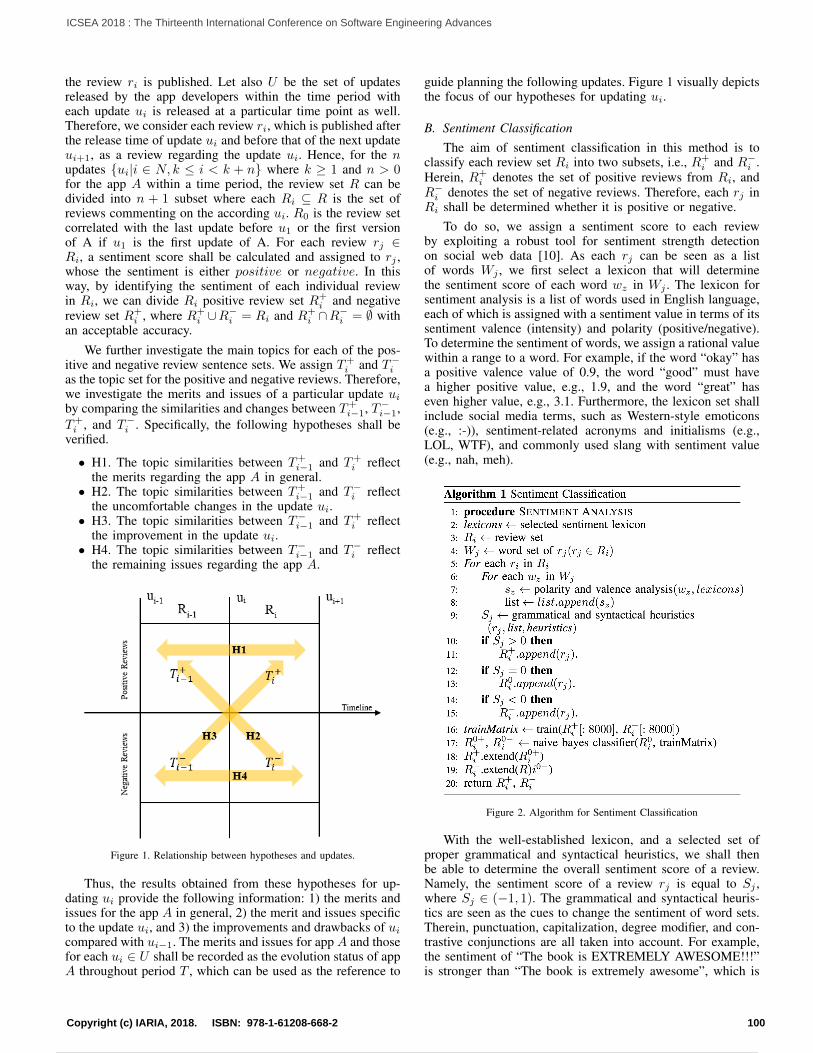
the review ri is published. Let also U be the set of updatesreleased by the app developers within the time period witheach update ui is released at a particular time point as well.Therefore, we consider each review ri, which is published afterthe release time of update ui and before that of the next updateui+1, as a review regarding the update ui. Hence, for the nupdates {ui|i ∈ N, k ≤ i < k + n} where k ≥ 1 and n > 0for the app A within a time period, the review set R can bedivided into n + 1 subset where each Ri ⊆ R is the set ofreviews commenting on the according ui. R0 is the review setcorrelated with the last update before u1 or the first versionof A if u1 is the first update of A. For each review rj ∈Ri, a sentiment score shall be calculated and assigned to rj ,whose the sentiment is either positive or negative. In thisway, by identifying the sentiment of each individual reviewin Ri, we can divide Ri positive review set R+

i and negativereview set R+

i , where R+i ∪R

−i = Ri and R+

i ∩R−i = ∅ with

an acceptable accuracy.We further investigate the main topics for each of the pos-

itive and negative review sentence sets. We assign T+i and T−i

as the topic set for the positive and negative reviews. Therefore,we investigate the merits and issues of a particular update ui

by comparing the similarities and changes between T+i−1, T−i−1,

T+i , and T−i . Specifically, the following hypotheses shall be

verified.

• H1. The topic similarities between T+i−1 and T+

i reflectthe merits regarding the app A in general.• H2. The topic similarities between T+

i−1 and T−i reflectthe uncomfortable changes in the update ui.• H3. The topic similarities between T−i−1 and T+

i reflectthe improvement in the update ui.• H4. The topic similarities between T−i−1 and T−i reflect

the remaining issues regarding the app A.

Figure 1. Relationship between hypotheses and updates.

Thus, the results obtained from these hypotheses for up-dating ui provide the following information: 1) the merits andissues for the app A in general, 2) the merit and issues specificto the update ui, and 3) the improvements and drawbacks of ui

compared with ui−1. The merits and issues for app A and thosefor each ui ∈ U shall be recorded as the evolution status of appA throughout period T , which can be used as the reference to

guide planning the following updates. Figure 1 visually depictsthe focus of our hypotheses for updating ui.

B. Sentiment ClassificationThe aim of sentiment classification in this method is to

classify each review set Ri into two subsets, i.e., R+i and R−i .

Herein, R+i denotes the set of positive reviews from Ri, and

R−i denotes the set of negative reviews. Therefore, each rj inRi shall be determined whether it is positive or negative.

To do so, we assign a sentiment score to each reviewby exploiting a robust tool for sentiment strength detectionon social web data [10]. As each rj can be seen as a listof words Wj , we first select a lexicon that will determinethe sentiment score of each word wz in Wj . The lexicon forsentiment analysis is a list of words used in English language,each of which is assigned with a sentiment value in terms of itssentiment valence (intensity) and polarity (positive/negative).To determine the sentiment of words, we assign a rational valuewithin a range to a word. For example, if the word “okay” hasa positive valence value of 0.9, the word “good” must havea higher positive value, e.g., 1.9, and the word “great” haseven higher value, e.g., 3.1. Furthermore, the lexicon set shallinclude social media terms, such as Western-style emoticons(e.g., :-)), sentiment-related acronyms and initialisms (e.g.,LOL, WTF), and commonly used slang with sentiment value(e.g., nah, meh).

Figure 2. Algorithm for Sentiment Classification

With the well-established lexicon, and a selected set ofproper grammatical and syntactical heuristics, we shall thenbe able to determine the overall sentiment score of a review.Namely, the sentiment score of a review rj is equal to Sj ,where Sj ∈ (−1, 1). The grammatical and syntactical heuris-tics are seen as the cues to change the sentiment of word sets.Therein, punctuation, capitalization, degree modifier, and con-trastive conjunctions are all taken into account. For example,the sentiment of “The book is EXTREMELY AWESOME!!!”is stronger than “The book is extremely awesome”, which is



111 / 160

stronger than “The book is very good.”. With both the lexiconvalue for each word of the review, and the calculation based onthe grammatical and syntactical heuristics, we can then assignunique sentiment values to each review. That is, each reviewrj is classified into positive, neutral or negative, as following:

rj is

{ positive, if 0 < Sj < 1,neutral, if Sj = 0,negative, if − 1 < Sj < 0.

Overall, each review set Ri is divided into R+i , R0

i , andR−i , denoting the positive, neutral and negative review sets. Tofurther investigate the information in R0

i , after experimentallyobserving that typically includes a big number of reviews,we classify it into positive and negative using the NaiveBayes Classifier with the training data from R+

i and R−i . Thisway, R0

i is classified into R0+i and R0−

i , which in turn, areadded to R+

i and R−i , respectively. The reason to performsupervised classification after sentiment analysis instead ofdirectly applying classification is twofold. Firstly, manuallycreating training data is time-consuming and less accurate thanusing existing sentiment analysis methods. Secondly, trainingthe sentiment classified reviews will provide domain specificand reliable results. The process is described in Figure 2.

C. Topic Analysis

After dividing the review sets Ri and Ri−1, i.e., the reviewsets related to update ui, into R+

i , R−i , R+i−1 and R−i−1 based

on the sentiment classification method, we elicit the maintopics from each of the classified review sets by exploitingthe Latent Dirichlet Allocation (LDA) method [11]. First, weconsider each review sentence rj in a particular set of reviewsas a list of words Wj , where the sequence of the words isnot recorded. The number of topics in this review set is setas t. Presumably, there is a distribution for the probability ofa particular word appears in a particular topic, when there isalso one for that of a particular review in a topic. We buildthe set of Review − Topic, where each word of each reviewis assigned with a topic out of the t topics. As preparation, wedefine Review−topic−numbers, Topic−words−numbers,and Topic− numbers denoting the number of occurrence ofeach topic in each review, the number of occurrence of eachword in each topic, and the number of words in each topic,respectively. For example, Review− topic− numbers(rj , k)denotes the number of occurrences of topic k in review rj .Then, we randomly assign each word wz of each review rjwith a topic tk. Accordingly, the Review− topic−numbers,Topic − words − numbers, and Topic − numbers willbe updated as the referencing weight of the distribution thewords for each topic. Then iteratively, for each word, weassign a new topic based on such weight of distributionand adjust the weight with the Review − topic − numbers,Topic − words − numbers, and Topic − numbers for thenext iteration. After a given number of iteration, t topics willbe determined by the Topic − words − numbers, which isthe number of occurrences of the words in each topic. Eachtk is then denoted by the most common keywords used in thistopic. Then, the set of topics T are returned as result. For thereview sets R+

i , R−i , R+i−1 and R−i−1, we will have the topics

sets T+i , T−i , T+

i−1 and T−i−1 accordingly.

D. Calculating Topics SimilaritiesBased on the topic sets T+

i , T−i , T+i−1 and T−i−1 elicited

from the review sets R+i , R−i , R+

i−1 and R−i−1, we furtheranalyze the similarities between the individual topics betweeneach pair of the topic sets. As the result from the previoustopic analysis, each topic set T encompasses k topics, each ofwhich is represented by the list of the most possible appearingkeywords. Thus, each topic set T with k topics each of whichis represented by w keywords, can be denoted as:

T =

[kw1,1 kw1,2 ... kw1,w

... ... ... ...kwk,1 kwk,2 ... kwk,w

]with each ti ∈ T can be denoted as [kwi,1, kwi,2, ...kwi,k]. Tocompare the similarity between two topic sets, each consistingof t topics, we compare all pairs of topics. Due to the fact thateach topic is represented as a set of keywords, the similarityof two topics shall be denoted by the common keywords ofthese topics. Hence, an easy way for calculating the similaritybetween any two topics ti and tj is by using the Jaccardsimilarity. This similarity function reflects the percentage ofthe common keywords of the two sets in the whole keywordsset of the two: J(ti, tj) =

|ti∩tj ||ti∪tj | .

However, by using the Jaccard Similarity, we consider twogiven topics are similar only when they contain a particularnumber of common keywords, regardless of the probabilityof them. The meaning of each topic ti ∈ T , denoted as[kwi,1, kwi,2, ...kwi,k], shall be more likely reflected by thehigh-probability keywords of ti. Furthermore, the subset ofonly low-probability keywords may reflect different meanings.For example, a topic is denoted as {’update’: 0.143, ’problem’:0.096, ’fix’: 0.064, ’install’: 0.03, ’uninstall’: 0.029, ’open’:0.027, ’stop’: 0.025, ’plea’: 0.025, ’get’: 0.022, ’reinstall’:0.019, ’bug’: 0.019, ’start’: 0.019, ’need’: 0.014, ’applica-tion’: 0.014, ’issue’: 0.011, ’battery’: 0.011, ’help’: 0.01,’face’: 0.009, ’frustrate’: 0.009, ’day’: 0.008}. From the high-probability keywords of this topic, we can summarize that thetopic is regarding the problems of updating, which requiresbeing fixed. However, the low-probability keywords hardlyreflect the topic, e.g., a keyword subset, {’reinstall’, ’bug’,’start’, ’need’, ’application’, ’issue’, ’battery’}, reflects a verydifferent issue regarding bugs and batteries.

Hence, when comparing the similarity of two given top-ics, the probability of the common keywords shall be takeninto account. Considering that Jaccard coefficient is the nor-malized inner product [12], we herein adopt the similaritymeasure method incorporating also the inner product, theKumar-Hassebrook (KH) similarity [13]. Provided betweentopic ti and tj , the c common keywords are denoted as[kwij,1, kwij,2, ...kwij,c], with the according probability listin ti and tj is [pi,1, pi,2, ...pi,c] and [pj,1, pj,2, ...pj,c]. Thesimilarity of the two given topics are calculated as follows.

KH(ti, tj) =

∑cx=1 pi,x · pj,x∑k

x=1 p2i,x +

∑kx=1 p

2j,x −

∑cx=1 pi,x · pj,x

The probability for each keyword of any topic belongsto (0,1). Hence, for this formula, when ti and tj containmore common keywords, the numerator increases monotoni-cally, and the denominator decreases monotonically. Therefore,KH(ti, tj) increases when ti and tj have more keywords in



112 / 160

common. In addition, when the probability of the commonkeywords increases,

∑cx=1 pi,x · pj,x increases. Because the

denominator is greater than the numerator, and both are greaterthan 0, KH(ti, tj) increases when the probabilities of thecommon keywords of ti and tj increase.

In this way, for two given topics ti and tj , when eachkeyword of these two topics is assigned the average value ofthe probability value set, then KH(ti, tj) = J(ti, tj). Consid-ering the monotonical increasing of the KH Similarity formula,it means that for ti and tj , when KH(ti, tj) <J(ti, tj),the common keywords of these two topics hardly reflect themeaning of them. For example, two topics, denoted as thefollowing set of keywords with the according probability ofeach keywords, are listed in Table I.

TABLE I. EXAMPLE TOPICS WITH KEYWORDS AND PROBABILITY

Topic 1 {’problem’: 0.145, ’fix’: 0.081, ’download’: 0.051, ’please’:0.032, ’use’: 0.025, ’reason’: 0.021, ’service’: 0.02, ’user’:0.015, ’issue’: 0.015, ’data’: 0.014}

Topic 2 {’version’: 0.197, ’please’: 0.121, ’go’: 0.069, ’use’: 0.043,’option’: 0.036, ’one’: 0.028, ’lot’: 0.027, ’revert’: 0.021,’way’: 0.018, ’download’: 0.018}

The Jaccard Similarity of these two topic is 0.176 whenthe KH Similarity is 0.064. We can observe that the commonkeywords, {’download’, ’please’, ’use’}, are of low probabilityin Topic 1 and keywords {’please’, ’use’} in Topic 2, whileneither topic is reflected by the common keywords. Topic 1can be seen regarding the requests of fixing problems/bugswhen Topic 2 is more related to keyword ’version’ instead of’download’. Thus, these two given topics cannot be consideredas similar despite the high Jaccard Similarity.

E. Identifying Matching Topics

After computing similarities between pairs of review topicswith KH similarity, we shall identify which are the matchingtopics when cross-comparing the topics of the topics sets T+

i ,T−i , T+

i−1 and T−i−1. Hence, to identify the matching topicsbetween two review topic sets Ta and Tb, the aim is to identifyall the topic pairs (tai, tbj), tai ∈ Ta and tbj ∈ Tb, that havethe high similarity. Starting from the pair of topics with highestsimilarity values,

We firstly use the Jaccard Similarity value of two particulartopics as the threshold for their KH similarity. According to theformula of KH similarity given previous, we set the probabilityof each keyword in each topic equal to the average. Then

KH(tai, tbj) =

∑cx=1 p

2∑kx=1 p

2 +∑k

x=1 p2 −

∑cx=1 p

2

=c

k + k − c= J(tai, tbj)

Therefore, we select the topic pairs, whose KH similarityvalue greater than their Jaccard similarity value, as similartopics. Furthermore, from the topic pairs with the highestKH similarity value, we select the top n pairs of topicsto investigate the changes and similarities of users opinionregarding the app.

Figure 3. Algorithm for Matching Topic Identification

The aim of the algorithm (shown in Figure 3) is to selectthe similar topic pairs with the highest similarity value. Whena particular topic pair is selected, the other pairs, which eitherof these two selected topics is also pairing with and have alsohigh similarity, will be considered as references to interpretthe users opinions. Each particular topic generated by the LDAmodel contains a number of perspectives that can be interpretedby the keywords. Thus, it is possible that one particular topichave the similar similarity value to multiple topics, when theyare similar regarding different perspectives which representedby their different common keywords.

TABLE II. EXAMPLE TOPICS WITH KEYWORDS AND PROBABILITY

Topic 1 {’time’: 0.12, ’friend’: 0.091, ’talk’: 0.081, ’way’: 0.069,’see’: 0.048, ’people’: 0.045, ’communication’: 0.038,’want’: 0.03, ’face’: 0.023, ’world’: 0.02 }

Topic 2 {’friend’: 0.111, ’bring’: 0.07, ’connect’: 0.068, ’talk’: 0.06,’keep’: 0.059, ’family’: 0.054, ’application’: 0.037, ’way’:0.021, ’touch’: 0.017, ’contact’: 0.016 }

Topic 3 {’see’: 0.077, ’use’: 0.056, ’people’: 0.046, ’want’: 0.044,’contact’: 0.034, ’thing’: 0.031, ’year’: 0.027, ’find’: 0.023,’know’: 0.023, ’number’: 0.019 }

For example, in Table II Topic 1 has the same Jaccard sim-ilarity value to both Topic 2 and 3. The two pairs of commonkeywords are {’friend’, ’talk’, ’way’} and {’people’, ’see’,’want’}. Their KH similarity values are different but both high(0.276 and 0.137). From Topic 1, we could summarize that itis regarding using the app enabling people to communicatewith friends any time they want and can see their faces aswell. Despite it is considered similar to both Topic 2 and 3,Topic 2 focuses on the perspective of enabling communicationbetween families and friends, when Topic 3 focus more onthe perspective of contacting people with phone numbers andseeing them. Thus, by identifying both similar topic pairs, weshall have more thorough understanding of the users’ opinionsregarding the app.

III. CASE STUDY

A. PreprocessingBefore starting the experiment with the proposed method,

preprocessing on the raw review data is required. The whole



113 / 160

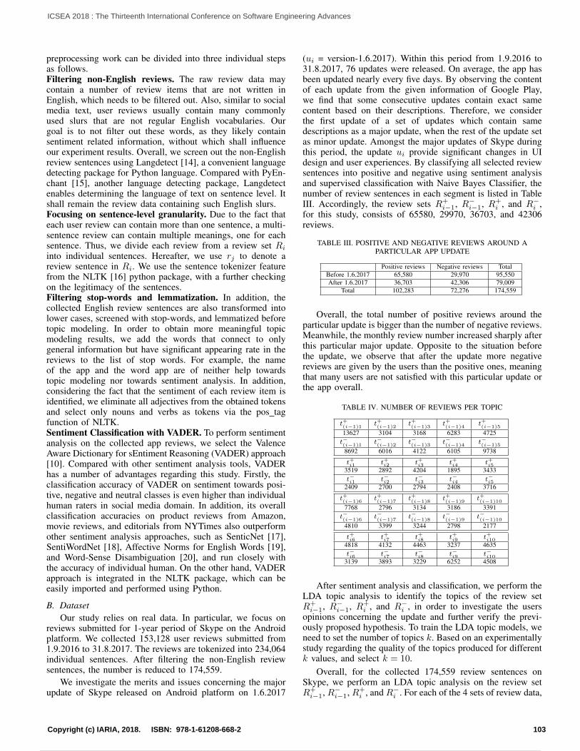
preprocessing work can be divided into three individual stepsas follows.Filtering non-English reviews. The raw review data maycontain a number of review items that are not written inEnglish, which needs to be filtered out. Also, similar to socialmedia text, user reviews usually contain many commonlyused slurs that are not regular English vocabularies. Ourgoal is to not filter out these words, as they likely containsentiment related information, without which shall influenceour experiment results. Overall, we screen out the non-Englishreview sentences using Langdetect [14], a convenient languagedetecting package for Python language. Compared with PyEn-chant [15], another language detecting package, Langdetectenables determining the language of text on sentence level. Itshall remain the review data containing such English slurs.Focusing on sentence-level granularity. Due to the fact thateach user review can contain more than one sentence, a multi-sentence review can contain multiple meanings, one for eachsentence. Thus, we divide each review from a review set Ri

into individual sentences. Hereafter, we use rj to denote areview sentence in Ri. We use the sentence tokenizer featurefrom the NLTK [16] python package, with a further checkingon the legitimacy of the sentences.Filtering stop-words and lemmatization. In addition, thecollected English review sentences are also transformed intolower cases, screened with stop-words, and lemmatized beforetopic modeling. In order to obtain more meaningful topicmodeling results, we add the words that connect to onlygeneral information but have significant appearing rate in thereviews to the list of stop words. For example, the nameof the app and the word app are of neither help towardstopic modeling nor towards sentiment analysis. In addition,considering the fact that the sentiment of each review item isidentified, we eliminate all adjectives from the obtained tokensand select only nouns and verbs as tokens via the pos tagfunction of NLTK.Sentiment Classification with VADER. To perform sentimentanalysis on the collected app reviews, we select the ValenceAware Dictionary for sEntiment Reasoning (VADER) approach[10]. Compared with other sentiment analysis tools, VADERhas a number of advantages regarding this study. Firstly, theclassification accuracy of VADER on sentiment towards posi-tive, negative and neutral classes is even higher than individualhuman raters in social media domain. In addition, its overallclassification accuracies on product reviews from Amazon,movie reviews, and editorials from NYTimes also outperformother sentiment analysis approaches, such as SenticNet [17],SentiWordNet [18], Affective Norms for English Words [19],and Word-Sense Disambiguation [20], and run closely withthe accuracy of individual human. On the other hand, VADERapproach is integrated in the NLTK package, which can beeasily imported and performed using Python.

B. DatasetOur study relies on real data. In particular, we focus on

reviews submitted for 1-year period of Skype on the Androidplatform. We collected 153,128 user reviews submitted from1.9.2016 to 31.8.2017. The reviews are tokenized into 234,064individual sentences. After filtering the non-English reviewsentences, the number is reduced to 174,559.

We investigate the merits and issues concerning the majorupdate of Skype released on Android platform on 1.6.2017

(ui = version-1.6.2017). Within this period from 1.9.2016 to31.8.2017, 76 updates were released. On average, the app hasbeen updated nearly every five days. By observing the contentof each update from the given information of Google Play,we find that some consecutive updates contain exact samecontent based on their descriptions. Therefore, we considerthe first update of a set of updates which contain samedescriptions as a major update, when the rest of the update setas minor update. Amongst the major updates of Skype duringthis period, the update ui provide significant changes in UIdesign and user experiences. By classifying all selected reviewsentences into positive and negative using sentiment analysisand supervised classification with Naive Bayes Classifier, thenumber of review sentences in each segment is listed in TableIII. Accordingly, the review sets R+

i−1, R−i−1, R+i , and R−i ,

for this study, consists of 65580, 29970, 36703, and 42306reviews.

TABLE III. POSITIVE AND NEGATIVE REVIEWS AROUND APARTICULAR APP UPDATE

Positive reviews Negative reviews TotalBefore 1.6.2017 65,580 29,970 95,550After 1.6.2017 36,703 42,306 79,009

Total 102,283 72,276 174,559

Overall, the total number of positive reviews around theparticular update is bigger than the number of negative reviews.Meanwhile, the monthly review number increased sharply afterthis particular major update. Opposite to the situation beforethe update, we observe that after the update more negativereviews are given by the users than the positive ones, meaningthat many users are not satisfied with this particular update orthe app overall.

TABLE IV. NUMBER OF REVIEWS PER TOPIC

t+(i−1)1

t+(i−1)2

t+(i−1)3

t+(i−1)4

t+(i−1)5

13627 3104 3168 6283 4725t−(i−1)1

t−(i−1)2

t−(i−1)3

t−(i−1)4

t−(i−1)5

8692 6016 4122 6105 9738

t+i1 t+i2 t+i3 t+i4 t+i53519 2892 4204 1895 3433t−i1 t−i2 t−i3 t−i4 t−i5

2409 2700 2794 2408 3716

t+(i−1)6

t+(i−1)7

t+(i−1)8

t+(i−1)9

t+(i−1)10

7768 2796 3134 3186 3391t−(i−1)6

t−(i−1)7

t−(i−1)8

t−(i−1)9

t−(i−1)10

4810 3399 3244 2798 2177

t+i6 t+i7 t+i8 t+i9 t+i104818 4132 4463 3237 4635t−i6 t−i7 t−i8 t−i9 t−i10

3139 3893 3229 6252 4508

After sentiment analysis and classification, we perform theLDA topic analysis to identify the topics of the review setR+

i−1, R−i−1, R+i , and R−i , in order to investigate the users

opinions concerning the update and further verify the previ-ously proposed hypothesis. To train the LDA topic models, weneed to set the number of topics k. Based on an experimentallystudy regarding the quality of the topics produced for differentk values, and select k = 10.

Overall, for the collected 174,559 review sentences onSkype, we perform an LDA topic analysis on the review setR+

i−1, R−i−1, R+i , and R−i . For each of the 4 sets of review data,



114 / 160

we use the Gensim topic modeling toolbox to train the 10-topicLDA models. For the 4 LDA models, each individual topicis represented by 20 keywords. Then, we assign each reviewsentence in the LDA models to the topic to which it has thehighest probability to belong. The numbers of reviews for eachtopic of the 4 data sets appear in Table IV (t+in represents thenth topic of R+

i ). In general, reviews are divided into topicssmoothly and, in most cases, each topic consists of around4000 review sentences.

C. Topics Similarity AnalysisWith the 40 identified topics, each of which is represented

by 20 keywords, we compare the similarity between each topicfrom the 20 topics before the update and each one from the20 topics after the update, which provides 400 topics pairs.The Jaccard similarity values for those 400 pairs range from 0to 0.429 (i.e., 0 - 12 common keywords between two topics).Meanwhile, the KH similarity values range from 0 to 0.676.Therein, we identify the potential similar topics from the high-est KH similarity value and eliminate the results where the KHsimilarity value is lower than the according Jaccard similarityvalue. In this way, we guarantee the common keywords ofeach identified topic pairs contain the overall probability valuegreater than average. We select the seven topic pairs with thehighest KH similarity values for each comparison set. Foreach topic pair, we analyze the similarity of the two topicsby observing their common keywords. Furthermore, from theunique keywords of each topic from one particular topic pair,we could also see the topic changes. The seven topic pairswith the highest KH similarity value are depicted in Table V.

TABLE V. PAIRS OF SIMILAR TOPICS

T+i−1 - T+

i (t+(i−1)8

, t+i5) (t+(i−1)6

, t+i6) (t+(i−1)7

, t+i9) (t+(i−1)6

, t+i1)(t+

(i−1)6, t+i5) (t+

(i−1)1, t+i7) (t+

(i−1)8, t+i3)

T+i−1 - T−

i (t+(i−1)6

, t−i10) (t+(i−1)6

, t−i5) (t+(i−1)8

, t−i7) (t+(i−1)5

,t−i6) (t+

(i−1)7, t−i8) (t+

(i−1)8, t+i10) (t+

(i−1)2, t+i3)

T−i−1 - T+

i (t−(i−1)3

, t+i6) (t−(i−1)7

, t+i3) (t−(i−1)5

, t+i1) (t−(i−1)3

, t+i5)(t−

(i−1)10, t+i8) (t+

(i−1)1, t+i4) (t+

(i−1)6, t+i9)

T−i−1 - T−

i (t−(i−1)3

, t−i10) (t−(i−1)10

, t−i3) (t−(i−1)6

, t−i8) (t−(i−1)7

,t−i9) (t+

(i−1)7, t+i6) (t+

(i−1)8, t+i6) (t−

(i−1)8, t−i9)

By further analyzing the common keywords in the obtainedsimilar topic pairs, we verify the hypothesis H1 - H4 asfollows.H1. The topic similarities between T+

i−1 and T+i reflect

the merits regarding the app A in general. The commonkeywords of the seven topics pairs with the highest KHsimilarity value appear in Table VI. For example, the commonkeywords of topics (t+(i−1)8, t+i5) reflects the acknowledgementfrom the users before and after the update. Because, thecommon keywords ’work’ and ’call’ indicate that the corefunction of the app works properly. The common keywordsof topics (t+(i−1)6, t+i6) reflect the users acknowledge also thebenefits brought by the app, e.g., enabling people to chatin groups, with video or by calling, so that people can seeand hear from their friends. On the other hand, topic pair(t+(i−1)7, t+i9) contains the common keywords that reflect theusers needs in adding features and fixing bugs. Consideringthe overall positive sentiment of the review sets, it is alsopossible the users reflect their satisfaction towards the workdone by the developers regarding such matters. Topic pair

(t+(i−1)6, t+i5) reflects the users satisfied with the video andaudio quality of the app. As topic t+i5 is also similar to t+(i−1)8,both topic pairs reflect similar information. Topic pair (t+(i−1)1,t+i7) reflects the contribution of the app to the society in a biggerpicture, regarding the communication between friends andfamily and helping people keep in touch. Topic pair (t+(i−1)6,t+i1) contain few common keywords; however, as t+(i−1)6 is alsosimilar to topic t+i6 and t+i5, all these topic pairs reflect similarinformation.

TABLE VI. COMMON KEYOWRDS IN POSITIVE-POSITIVE REVIEWS

Topic Pairs Common Keywords(t+

(i−1)8, t+i5) [’call’, ’phone’, ’sound’, ’work’]

(t+(i−1)6

, t+i6) [’call’, ’chat’, ’friend’, ’group’, ’hear’, ’make’, ’people’,’person’, ’phone’, ’see’, ’video’]

(t+(i−1)7

, t+i9) [’add’, ’bug’, ’everything’, ’fix’, ’hope’, ’issue’, ’make’,’need’, ’please’]

(t+(i−1)6

, t+i1) [’people’, ’use’, ’year’]

(t+(i−1)6

, t+i5) [’call’, ’make’, ’phone’, ’quality’, ’video’, ’voice’]

(t+(i−1)1

, t+i7) [’application’, ’communicate’, ’connect’, ’family’, ’friend’,’get’, ’help’, ’touch’, ’way’]

(t+(i−1)8

, t+i3) [’connection’, ’internet’, ’keep’, ’nothing’, ’work’]

H2. The topic similarities between T+i−1 and T−i reflect

the uncomfortable changes in the update ui. The commonkeywords of the selected similar topic pairs are shown in TableVII. The common keywords of topics (t+(i−1)6, t−i10) reflectsnegative user reviews regarding the apps core feature exist,despite the positive feedback before this update. According tot−i10, the aspects which users complain about include callingin general, the user interface, video and sound quality, andconnections. Meanwhile, t−i10 is also considered similar tot+(i−1)8. Topic t+(i−1)8 indicates that before the update manyusers like the internet connection of this app with wifi oncomputer and tablet. Topic pair (t+(i−1)5, t−i6) reflects that issuesconcerning the user accounts, including logging in, signing up,passwords emerge after the update, where the users complainquite often. Furthermore, the topic pair (t+(i−1)7, t−i8) indicatesthat many users complain about the developers fixing problemsnegatively, despite many others reflect the issue with positivesentiment (see topic pair (t+(i−1)7, t+i9)).

TABLE VII. COMMON KEYOWRDS IN POSITIVE-NEGATIVEREVIEWS

Topic Pairs Common Keywords(t+

(i−1)6, t−i10) [’call’, ’connect’, ’hear’, ’make’, ’person’, ’phone’, ’qual-

ity’, ’video’, ’voice’](t+

(i−1)6, t−i5) [’make’, ’use’, ’year’]

(t+(i−1)8

, t−i7) [’need’, ’work’]

(t+(i−1)5

, t−i6) [’account’, ’go’, ’keep’, ’let’, ’log’, ’password’, ’sign’, ’try’,’win’]

(t+(i−1)7

, t−i8) [’fix’, ’please’, ’problem’, ’thing’]

(t+(i−1)8

, t−i10) [’call’, ’connection’, ’drop’, ’phone’, ’sound’, ’work’]

(t+(i−1)2

, t−i3) [’conversation’, ’get’, ’take’, ’time’, ’type’]

H3. The topic similarities between T−i−1 and T+i reflect the

improvement in the update ui. The common keywords ofthe selected similar topic pairs are shown in Table VIII. Thecommon keywords of topics (t−(i−1)3, t+i6) reflect that before theupdate, many users have complaint regarding using the app forphone calls in general. After the update, a number of positive



115 / 160

reviews towards this matter appear. Considering the topic pair(t−(i−1)3, t+i5), users also switch the attitude regarding the videoand sound quality to positive after the update. Topic pair(t−(i−1)7, t+i3) reflects the general positive acknowledgement ofthe update. Topic pair (t−(i−1)10, t+i8) reflects the users attitudetowards the message notification feature has changed intopositive. (t−(i−1)1, t+i4) reflects the general positive feedbackregarding the new version while (t−(i−1)6, t+i9) reflects thepositive feedback on having some bugs fixed in this version.

TABLE VIII. COMMON KEYOWRDS IN NEGATIVE-POSITIVEREVIEWS

Topic Pairs Common Keywords(t−

(i−1)3, t+i6) [’call’, ’get’, ’hear’, ’make’, ’people’, ’person’, ’phone’,

’see’, ’talk’, ’time’, ’video’](t−

(i−1)7, t+i3) [’get’, ’update’, ’win’, ’work’]

(t−(i−1)5

, t+i1) [’get’, ’try’, ’use’, ’year’]

(t−(i−1)3

, t+i5) [’call’, ’make’, ’phone’, ’quality’, ’sound’, ’time’, ’video’,’voice’]

(t−(i−1)10

, t+i8) [’message’, ’notification’, ’open’, ’see’, ’send’, ’show’,’take’]

(t−(i−1)1

, t+i4) [’version’]

(t−(i−1)6

, t+i9) [’bug’, ’fix’, ’get’, ’lot’, ’please’]

H4. The topic similarities between T−i−1 and T−i reflectthe remaining issues regarding the app A. The commonkeywords of the selected similar topic pairs are shown in TableIX. For example, the common keywords of topics (t−(i−1)3,t−i10) reflects the users complaint regarding the general qualityof the app remains after the update, specifically concerningconnections, calling, audio and video quality, etc. On theother hand, topic pair (t−(i−1)10, t−i3) reflects the problem withsending and receiving messages with notifications still exist.Furthermore, crashing is also a persisting issue that many userscomplained about based on topic pair (t−(i−1)6, t−i8). Topicpair (t−(i−1)7, t−i9), despite having only one common keyword,reflects the users general negativity towards the update. Topicpair (t−(i−1)7, t−i6) and (t−(i−1)8, t−i6) reflect the issues regardinglogging in and signing up with Microsoft account. Topic pair(t−(i−1)8, t−i9) reflects the issues regarding user contact list whenspecially t−i9 reflects the users’ complaints regarding contactlist syncing and status.

TABLE IX. COMMON KEYOWRDS IN NEGATIVE-NEGATIVEREVIEWS.

Topic Pairs Common Keywords(t−

(i−1)3, t−i10) [’call’, ’connect’, ’drop’, ’hear’, ’make’, ’person’, ’phone’,

’quality’, ’sound’, ’time’, ’video’, ’voice’](t−

(i−1)10, t−i3) [’get’, ’message’, ’notification’, ’open’, ’see’, ’send’, ’show’,

’take’, ’time’](t−

(i−1)6, t−i8) [’crash’, ’fix’, ’give’, ’keep’, ’please’, ’problem’, ’star’,

’think’, ’time’](t−

(i−1)7, t−i9) [’update’]

(t−(i−1)7

, t−i6) [’let’, ’login’, ’microsoft’, ’time’, ’try’, ’turn’, ’update’,’win’]

(t−(i−1)8

, t−i6) [’account’, ’keep’, ’make’, ’sign’]

(t−(i−1)8

, t−i9) [’add’, ’contact’, ’list’, ’sync’]

Conclusively, we could summarize the users’ opinionbefore and after the particular update (version 1.6.2017) asfollows:

The merits in general:

1) (t+(i−1)8, t+i5): calling feature works.2) (t+(i−1)6, t+i6), (t+(i−1)1, t+i7): people can chat in group with

video and calls, connecting with family and friends.3) (t+(i−1)7, t+i9): added features and bugs fixed.4) (t+(i−1)6, t+i5): the video and sound quality.

The uncomfortable changes:1) (t+(i−1)6, t−i10): user interface, connection, and calling

quality in general.2) (t+(i−1)5, t−i6): the user accounts, including logging in,

signing up, passwords.3) (t+(i−1)7, t−i8): bugs fixes.

The improvement:1) (t−(i−1)7, t+i3): update in general.2) (t−(i−1)10, t+i8): message notification.3) (t−(i−1)3, t+i6), ((t−(i−1)3, t+i5): calling in general, video and

sound quality.

The remaining issues:1) (t−(i−1)3, t−i10): update in general.2) (t−(i−1)10, t−i3): sending and receiving messages with no-

tifications.3) (t−(i−1)6, t−i8): crashing.4) (t−(i−1)7, t−i9): the new version5) (t−(i−1)7, t−i6), (t−(i−1)8, t−i6): login and signup with Mi-

crosoft accounts.6) (t−(i−1)8, t−i9): contact list syncing and status update.

Interestingly, these points are verified by the short notesof Skype developers regarding their updates [21]. Specifically,the above topics can be associated with the following origi-nal developers claims: (a) General performance and reliabil-ity improvements (Version 2017.08.15, Version 2017.08.29:phone calls, video calls and messaging quality), (b) Improvedsign in - sign back into your account more easily (Version2017.08.15: ”log in” features, user account related functions),(c) New controls added to help users manage vibration andLED notification alerts. (Version 2017.07.05: notification), (d)Improvements to PSTN call stability (Version 2017.07.05:connection), (e) Messaging improvements Add content tochats via the + button and enjoy more room for your messages.(Version 2017.08.02: messaging), (f) The ability to add orremove contacts from your profile (Version 2017.08.01), (g)Activity indicators - see who’s currently active in your Chatslist (Version 2017.08.02: contacts and statuses). Hence, dueto the correlation between the previously mentioned issuesdetected using our method and the content of the followingup updates, we can verify the existence of those issues.However, whether the reason of the according update is theuser reviews is unknown. On the other hand, we can alsodetect the disagreement amongst users’ opinions. For example,a number of users think the calling quality deteriorated afterthe update while many others think it was improved ((t+(i−1)6,t−i10) and (t−(i−1)3, t+i6)). A number of users also think theupdate improves the app when other users think it is justas bad as the previous ((t−(i−1)7, t+i3) and (t−(i−1)3, t−i10)). Wecan obtain more details regarding users’ different opinions byfurther investigating the keywords-related review texts.



116 / 160

IV. RELATED WORK

The spontaneous feedback from the users, i.e., the userreviews, helps effectively the evolution of the target system,where a key to enable such feedback is to ease the users effortin composing and uploading it [22]. For the contemporarymobile apps, the app distribution platforms, e.g., Apple App-Store, and Google Play, enable such spontaneous reviews of theusers and facilitate the developers in terms of maintaining andevolving mobile apps [23]. Such feedback and reviews containhelpful information for developers in terms of identifyingmissing features and improving software quality [24]. Fromthose review information, user requirements can be elicitedcontinuously and, in a crowd-based fashion [25] [26].

The reviews of the mobile app users reflect a variety oftopics, which majorly cover the perspectives of bug reports,feature requests, user experiences, solution proposal, informa-tion seeking and giving, and general ratings [2]–[4].

For such purpose, NLP, SA, and supervised learning arethe common techniques used to classify user reviews [3] [4].According to recent studies, the combination of NLP and SAtechniques has high accuracy in detecting useful sentences [4].These techniques are also used in many other studies in termsof review opinion mining [7] [9] [24].

Many studies have contributed to the user opinion miningof mobile apps. Fu et al. [5] proposes WisCom, which candetect why the users like or dislike a particular app basedon the users reviews throughout time and provide insightsregarding the users concerns and preferences in the app market.Similar studies regarding mining information from app storesdata focus on different perspectives of the issues, e.g., thecorrelations between ratings and download rank [6], ratingsand API use [27], review classification and useful sentencesdetection [4]. On the other hand, Chen et al. [7] providesthe AR-miner framework, which facilitates the informativereviews extraction, review grouping based on topics, reviewprioritization and informative reviews presentation with visual-ization. Guzman and Maalej [8] proposes an approach focusingon feature extraction and sentiment analysis, which facilitatesthe evaluation of individual app features. Similarly, Iacob andHarrison [9] focuses also on the feature requests extraction butvia means of linguistic rules and LDA topic modeling. Manystudies also provide methods of using automatic classificationmethod to study mobile app user reviews [28] [29] [30]

Compared to the previous mentioned approaches in userreview opinion mining, our method aims towards the similartopic detection and analysis concerning not only the app ingeneral but also the particular major updates. Furthermore, wefocus on the topic similarity of data segments, classified bysentiment analysis and supervised learning, which is differentfrom the methods mentioned above. It enables the developersto acquire information regarding each individual update andwill provide insights on the future updates.

V. CONCLUSION

In this study, we propose a method for analyzing thecorrelation of mobile apps user reviews before and after aparticular app updates in order to detect how users’ opin-ions change with the update released. After classifying thereviews before and after a particular update by positive andnegative sentiment, we extract the topics of each segment.

By comparing the similarities of these extracted topics, weidentify both the positive and negative issues reflected by thesereviews regarding the particular update and the app in general.Overall, this study is an exploratory investigation on using userreview opinion mining techniques in detecting update-specificissues. The future studies shall extend the use of this method tothe whole maintenance lifecycle of mobile apps to investigatethe broader correlation between users feedback and the apps’update trends. Releasing strategies improvement based on thismethod will also be studied. Other factors, e.g., the differentapp categories, different platforms, and different mining andanalysis techniques will also be taken into account.

REFERENCES

[1] X. Li, Z. Zhang, and J. Nummenmaa, “Models for mobile applica-tion maintenance based on update history,” in Evaluation of NovelApproaches to Software Engineering (ENASE), 2014 InternationalConference on. IEEE, 2014, pp. 1–6.

[2] H. Khalid, E. Shihab, M. Nagappan, and A. E. Hassan, “What do mobileapp users complain about?” IEEE Software, vol. 32, no. 3, 2015, pp.70–77.

[3] W. Maalej and H. Nabil, “Bug report, feature request, or simplypraise? on automatically classifying app reviews,” in 2015 IEEE 23rdinternational requirements engineering conference (RE). IEEE, 2015,pp. 116–125.

[4] S. Panichella, A. Di Sorbo, E. Guzman, C. A. Visaggio, G. Canfora,and H. C. Gall, “How can i improve my app? classifying user reviewsfor software maintenance and evolution,” in Software maintenance andevolution (ICSME), 2015 IEEE international conference on. IEEE,2015, pp. 281–290.

[5] B. Fu, J. Lin, L. Li, C. Faloutsos, J. Hong, and N. Sadeh, “Why peoplehate your app: Making sense of user feedback in a mobile app store,”in Proceedings of the 19th ACM SIGKDD international conference onKnowledge discovery and data mining. ACM, 2013, pp. 1276–1284.

[6] M. Harman, Y. Jia, and Y. Zhang, “App store mining and analysis: Msrfor app stores,” in Proceedings of the 9th IEEE Working Conferenceon Mining Software Repositories. IEEE Press, 2012, pp. 108–111.

[7] N. Chen, J. Lin, S. C. Hoi, X. Xiao, and B. Zhang, “Ar-miner: mininginformative reviews for developers from mobile app marketplace,” inProceedings of the 36th International Conference on Software Engi-neering. ACM, 2014, pp. 767–778.

[8] E. Guzman and W. Maalej, “How do users like this feature? a finegrained sentiment analysis of app reviews,” in Requirements Engineer-ing Conference (RE), 2014 IEEE 22nd International. IEEE, 2014, pp.153–162.

[9] C. Iacob and R. Harrison, “Retrieving and analyzing mobile apps featurerequests from online reviews,” in Proceedings of the 10th WorkingConference on Mining Software Repositories. IEEE Press, 2013, pp.41–44.

[10] C. H. E. Gilbert, “Vader: A parsimonious rule-based model for senti-ment analysis of social media text,” in ICWSM, 2014.

[11] D. M. Blei, A. Y. Ng, and M. I. Jordan, “Latent dirichlet allocation,”Journal of Machine Learning Research, vol. 3, 2003, pp. 993–1022.

[12] T. T. Tanimoto, “Ibm internal report,” Nov, vol. 17, 1957, p. 1957.[13] B. V. Kumar and L. Hassebrook, “Performance measures for correlation

filters,” Applied optics, vol. 29, no. 20, 1990, pp. 2997–3006.[14] Langdetect, https://pypi.python.org/pypi/langdetect, last accessed on

06/20/18.[15] Pyenchant, https://pypi.python.org/pypi/pyenchant, last accessed on

06/20/18.[16] NLTK, http://www.nltk.org, last accessed on 06/20/18.[17] E. Cambria, R. Speer, C. Havasi, and A. Hussain, “Senticnet: A

publicly available semantic resource for opinion mining.” in AAAI fallsymposium: commonsense knowledge, vol. 10, no. 0, 2010.

[18] S. Baccianella, A. Esuli, and F. Sebastiani, “Sentiwordnet 3.0: anenhanced lexical resource for sentiment analysis and opinion mining.”in Lrec, vol. 10, no. 2010, 2010, pp. 2200–2204.



117 / 160

[19] M. M. Bradley and P. J. Lang, “Affective norms for english words(anew): Instruction manual and affective ratings,” Citeseer, Tech. Rep.,1999.

[20] M. Stevenson and Y. Wilks, “Word sense disambiguation,” The OxfordHandbook of Comp. Linguistics, 2003, pp. 249–265.

[21] “Skype on Google Play,” URL: https://play.google.com/store/apps/details?id=com.skype.raider, last accessed on 06/20/18.

[22] K. Schneider, “Focusing spontaneous feedback to support system evo-lution,” in RE, pp. 165–174.

[23] D. Pagano and W. Maalej, “User feedback in the appstore: An empiricalstudy,” in Requirements Engineering Conference (RE), 2013 21st IEEEInternational. IEEE, 2013, pp. 125–134.

[24] L. V. Galvis Carreno and K. Winbladh, “Analysis of user comments:an approach for software requirements evolution,” in Proceedings of the2013 International Conference on Software Engineering. IEEE Press,2013, pp. 582–591.

[25] N. Seyff, F. Graf, and N. Maiden, “Using mobile re tools to give end-users their own voice,” in Requirements Engineering Conference (RE),2010 18th IEEE International. IEEE, 2010, pp. 37–46.

[26] E. C. Groen, J. Doerr, and S. Adam, “Towards crowd-based re-quirements engineering a research preview,” in International WorkingConference on Requirements Engineering: Foundation for SoftwareQuality. Springer, 2015, pp. 247–253.

[27] G. Bavota, M. Linares-Vasquez, C. E. Bernal-Cardenas, M. Di Penta,R. Oliveto, and D. Poshyvanyk, “The impact of api change-and fault-proneness on the user ratings of android apps,” IEEE Trans. on Soft.Engin., vol. 41, no. 4, 2015, pp. 384–407.

[28] S. McIlroy, N. Ali, H. Khalid, and A. E. Hassan, “Analyzing andautomatically labelling the types of user issues that are raised in mobileapp reviews,” Empirical Software Engineering, vol. 21, no. 3, 2016, pp.1067–1106.

[29] W. Maalej, Z. Kurtanovic, H. Nabil, and C. Stanik, “On the automaticclassification of app reviews,” Requirements Engineering, vol. 21, no. 3,2016, pp. 311–331.

[30] Z. Sun, Z. Ji, P. Zhang, C. Chen, X. Qian, X. Du, and Q. Wan,“Automatic labeling of mobile apps by the type of psychological needsthey satisfy,” Telematics and Informatics, vol. 34, no. 5, 2017, pp. 767–778.



118 / 160

Database Model Visualization in Virtual Reality: A WebVR and Benediktine Space Approach

Roy Oberhauser Computer Science Dept.

Aalen University Aalen, Germany


Abstract - As the data era and the Internet of Everything unfolds, databases are becoming ubiquitous and an integral part of software while alternative database types such as NoSQL grow in popularity. Thus, software engineers, not just database specialists, are more likely to encounter and need to deal with these databases. While Virtual Reality (VR) technology has increased in popularity, its integration in software development tooling has been limited. One application area for WebVR technology includes database-model visualization, permitting web-based cross-platform and remote VR access. This paper describes Virtual Reality Immersion in Data Models (VRiDaM), a generic database-model approach for visualizing, navigating, and conveying database-model information interactively in a web browser using WebVR technology utilizing Benediktine space visualization for heterogeneous (relational and NoSQL) database models. A prototype shows its viability and an empirical study looked at usability, effectiveness, and efficiency.

Keywords - virtual reality; database visualization; database tools; visual development environments; database modeling; software engineering; WebVR; Benediktine space.

I. INTRODUCTION

Data has become the most coveted "raw material" of both our time and the foreseeable future, in some respects analogous to a gold rush. Cisco estimates there will be 27bn networked devices by 2021 [1]. The ongoing digitalization involving Industry 4.0 and the Internet of Everything will imply a large increase in databases to be able to store and retrieve this data, in particular embedded databases. IDC estimates the current annual data creation rate at 16.1ZB (Zettabytes), and by 2025 163ZB, with embedded data by then constituting nearly 20% of all data created [2]. As data explodes, software engineers are increasingly faced with the daunting task of structuring and analyzing such databases across various DataBase Management System (DBMS) types, including relational and NoSQL types such as document (semi-structured), key-value, wide column (extensible record), in memory, and graph [3].

Thus, software engineers are increasingly faced with developing and maintaining software that integrates some form of data repository, data store, or database. While the original developers may have a clear (and correct to a certain degree) mental model of their actual data model, the maintenance situation is exacerbated by proliferation of relational (mostly SQL) and NoSQL database types and the relatively high turnover rates common in the software

industry, resulting in developers unfamiliar with the data models attempting to quickly comprehend the database structures involved with these software applications.

Humans tend to be visually-oriented and can detect and remember visual patterns well. Information visualization has the potential to support human understanding and insight while dealing with resource constraints on the human as well as computer side. Common ways for visually conveying database structures include 2D entity-relationship (E-R) modeling and diagrams [4], but these are typically applied to relational databases (RDB) and NoSQL databases may or may not have a tool that includes visual support. As to DBMS tools, often a database product has a preferred product-specific tool offering web-based or standard 2D graphical user interfaces (GUIs), while certain tools support multiple database products of one specific type (e.g., MySQL workbench for SQL databases).

Contemporaneously, VR has made inroads in its accessibility as hardware prices have dropped and capabilities have improved. The VR market is rapidly expanding, with VR revenue reaching $2.7bn in 2016, a 10-fold increase to $25bn by 2021 [5]. However, software engineers mostly do not have access to integrated VR capabilities in their development tools. Broad VR usage is relatively new and this market segment small compared to the general VR market.

This application paper contributes Virtual Reality Immersion in Data Models (VRiDaM, pronounced like freedom), a generalized approach to heterogeneous (relational and non-relational) database-model visualization in VR , using WebVR in a web browser and a Benediktine-space [6]-[9] visualization paradigm. Thus, database models fromdifferent data store types can be visualized and navigated(locally or remotely) in VR via a cross-platform web browserand a VR headset and controller. We describe its principlesand features for visualizing, navigating, and conveyingdatabase information interactively to support exploratory,analytical, and descriptive cognitive processes [10]. Aprototype implementation demonstrates its viability and itsusability is evaluated in an empirical study.

The paper is organized as follows: the following section discusses related work; Section 3 presents our solution approach. In Section 4, our implementation is described. An evaluation is described in Section 5, followed by a conclusion.



119 / 160

II. RELATED WORK We are unaware of directly related work regarding

database visualization using VR. VR Juggler [11] provides VR support for developing VR applications, but not for database modeling and visualization. As to VR approaches for software structure visualization, ExplorViz [12] is a WebVR application that supports VR exploration of 3D software cities using Oculus Rift together with Microsoft Kinect for gesture recognition. As to non-VR visualization, [13] provides an overview and survey of 3D software visualization tools across various software engineering areas. Software Galaxies [14] gives a web-based visualization of dependencies among popular package managers and supports flying, with each star representing a package clustered by dependencies. CodeCity [15] is a 3D software visualization approach based on a city metaphor and implemented in SmallTalk on the Moose reengineering framework. X3D-UML [16] provides 3D support with UML grouping classes in planes. In contrast, VRiDaM focuses on visualizing database structures and leverages WebVR capabilities without requiring gestures.

Database management (DBM) tools are typically DB type-specific and require some installation. Each professional RDB product usually offers its own tool, but since most RDBs support the Structured Query Language (SQL), certain RDB tools can access other RDBs using RDB-specific drivers. For example, MySQL Workbench works across multiple databases and supports reverse-engineering of 2D E-R diagrams. Schemaball [17] provides a 2D circular composite schema diagram for SQL databases. As to 3D RDB tools, DIVA (Database Immersive Visual Analysis) uses stacked rings with rectangular tables attached to them (forming a cylinder), with the tables with the most foreign keys sorted to the top of the stack. Alternatively, stacked square layers of tables can be displayed and 2D E-R diagrams shown. Actual data values are not visualized. For NoSQL databases, each database type differs and the associated DBM tools. One example of a popular wide-column database (WDB) is Apache Cassandra, for which DataStax Studio is a Java-based DBM tool with a web GUI (Graphical User Interface). As to document-oriented databases (DDBs), MongoDB is a popular example and MongoDB Compass, Robomongo, and Studio 3T being example DBM tools. For graph databases (GDB), Neo4j is popular and graph DBM tools include Neo4j admin, Structr, Gephi, Graffeine, etc. In contrast, the VRiDaM approach is more generalized to work across heterogeneous DB types, thus permitting users to only ramp up on one tool, it is cross-platform and provides an immersive web-based VR experience. Furthermore, in contrast to the 3D DIVA or 2D Schemaball, our approach avoids the visual connection 'yarnballs' as the number of connections and tables scale.

Work on big data visualization techniques in conjunction with VR is discussed by Olshannikova et al. in [18]. Herman, Melançon, and Marshall [19] survey work on graph visualization and navigation for information visualization. In contrast, our focus is displaying the database-model structure, not on displaying and analyzing large amounts of data per se, and we apply Benediktine spatial placement in conjunction with a dynamic self-organizing force-directed graph [20].

III. SOLUTION Visualization, especially VR with its wide viewing angles,

can leverage peripheral vision for information, whereby visual data is both consciously and unconsciously seen and processed. If leveraged well, visualization can be cognitively easier in providing insights than an equivalent textual analysis would require. Traditional text-centric tabular formats or boxes in E-R diagrams do not explicitly take advantage of such visual capabilities. Also, if the contents of each database table were visualized as a rectangular 2D object, as it scales both in number of tables and the size of various tables, lucidity issues occur that nullify the advantage of VR visualization.

To provide some background context for our solution, we describe several perspectives that were considered. Information can be grouped and large amounts of information provided in a relatively small amount of graphical space. Yet humans are limited in their sensory perception and focus, and thus visualization considerations include: determining the proper balance for what to place into visual focus in which context, what to place into the periphery, what to hide or show, and to what extent and at what point should what be visualized. To develop actionable insights from visualization, the knowledge crystallization cognitive process involves acquiring information, making sense of it, creating something new, and acting on it [21]. Regarding visual perception, gestalt psychology [22] is based on the four principles of emergence, reification, multistable perception, and invariance. Formulated gestalt grouping laws regarding visual perception include proximity, similarity, closure, symmetry, common fate, continuity, good gestalt, past experience, common region, and element connectedness. For visual representation, we considered Don Norman’s design principles, in particular affordance, consistency, and mapping [23]. Other concepts considered were [9] information space, cognitive space, spatialization, ordination, and pre-attentive processing, which refers to the accumulation of information from the environment subconsciously [24]. Visualization techniques explicitly analyzed with regard to their appropriateness for displaying data models in VR included books, cone trees, fisheye views, information cubes, perspective walls, spheres, surface plots/cityscapes/3D bar graphs, viewpoints, workspace/information space/3D rooms, worlds in worlds, and Benediktine space [19][21].

A. Benediktine Space Benediktine space transforms or maps an information

object’s attributes to extrinsic (e.g., Cartesian coordinates, time) and intrinsic (e.g., size, shape, color) information spatial dimensions. To keep objects from overlapping, mapping principles include exclusion, maximal exclusion, scale, and transit [6][7][8][9].

B. WebVR WebVR is a Mozilla JavaScript API that enables web

browsers to access VR hardware. A-Frame is an open source framework for displaying VR content within HTML. It is based on an entity component system architecture in which each object in a scene is an entity (a container) consisting of components that provide desired functionality or behavior for



120 / 160

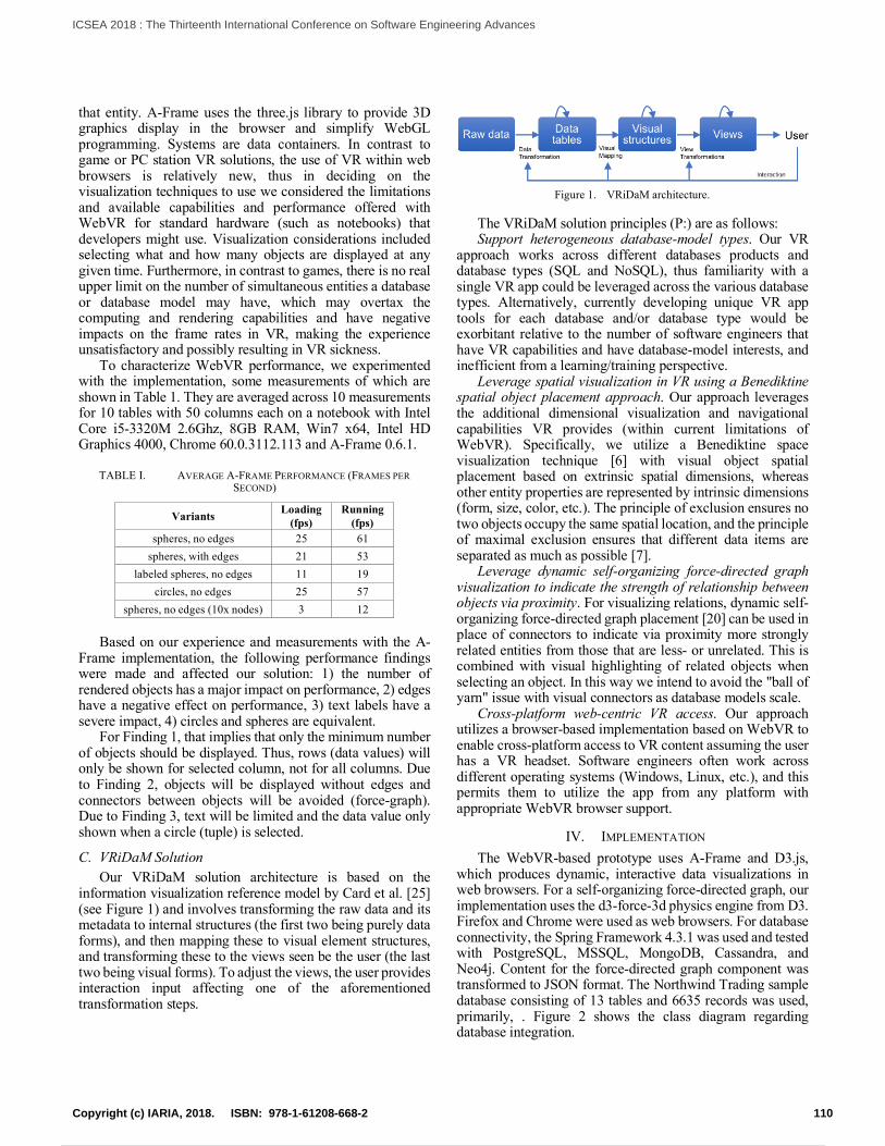
that entity. A-Frame uses the three.js library to provide 3D graphics display in the browser and simplify WebGL programming. Systems are data containers. In contrast to game or PC station VR solutions, the use of VR within web browsers is relatively new, thus in deciding on the visualization techniques to use we considered the limitations and available capabilities and performance offered with WebVR for standard hardware (such as notebooks) that developers might use. Visualization considerations included selecting what and how many objects are displayed at any given time. Furthermore, in contrast to games, there is no real upper limit on the number of simultaneous entities a database or database model may have, which may overtax the computing and rendering capabilities and have negative impacts on the frame rates in VR, making the experience unsatisfactory and possibly resulting in VR sickness.

To characterize WebVR performance, we experimented with the implementation, some measurements of which are shown in Table 1. They are averaged across 10 measurements for 10 tables with 50 columns each on a notebook with Intel Core i5-3320M 2.6Ghz, 8GB RAM, Win7 x64, Intel HD Graphics 4000, Chrome 60.0.3112.113 and A-Frame 0.6.1.

TABLE I. AVERAGE A-FRAME PERFORMANCE (FRAMES PER SECOND)

Variants Loading (fps)

Running (fps)

spheres, no edges 25 61 spheres, with edges 21 53

labeled spheres, no edges 11 19 circles, no edges 25 57

spheres, no edges (10x nodes) 3 12 Based on our experience and measurements with the A-

Frame implementation, the following performance findings were made and affected our solution: 1) the number of rendered objects has a major impact on performance, 2) edges have a negative effect on performance, 3) text labels have a severe impact, 4) circles and spheres are equivalent.

For Finding 1, that implies that only the minimum number of objects should be displayed. Thus, rows (data values) will only be shown for selected column, not for all columns. Due to Finding 2, objects will be displayed without edges and connectors between objects will be avoided (force-graph). Due to Finding 3, text will be limited and the data value only shown when a circle (tuple) is selected.

C. VRiDaM Solution Our VRiDaM solution architecture is based on the

information visualization reference model by Card et al. [25] (see Figure 1) and involves transforming the raw data and its metadata to internal structures (the first two being purely data forms), and then mapping these to visual element structures, and transforming these to the views seen be the user (the last two being visual forms). To adjust the views, the user provides interaction input affecting one of the aforementioned transformation steps.

Figure 1. VRiDaM architecture.

The VRiDaM solution principles (P:) are as follows: Support heterogeneous database-model types. Our VR

approach works across different databases products and database types (SQL and NoSQL), thus familiarity with a single VR app could be leveraged across the various database types. Alternatively, currently developing unique VR app tools for each database and/or database type would be exorbitant relative to the number of software engineers that have VR capabilities and have database-model interests, and inefficient from a learning/training perspective.

Leverage spatial visualization in VR using a Benediktine spatial object placement approach. Our approach leverages the additional dimensional visualization and navigational capabilities VR provides (within current limitations of WebVR). Specifically, we utilize a Benediktine space visualization technique [6] with visual object spatial placement based on extrinsic spatial dimensions, whereas other entity properties are represented by intrinsic dimensions (form, size, color, etc.). The principle of exclusion ensures no two objects occupy the same spatial location, and the principle of maximal exclusion ensures that different data items are separated as much as possible [7].

Leverage dynamic self-organizing force-directed graph visualization to indicate the strength of relationship between objects via proximity. For visualizing relations, dynamic self-organizing force-directed graph placement [20] can be used in place of connectors to indicate via proximity more strongly related entities from those that are less- or unrelated. This is combined with visual highlighting of related objects when selecting an object. In this way we intend to avoid the "ball of yarn" issue with visual connectors as database models scale.

Cross-platform web-centric VR access. Our approach utilizes a browser-based implementation based on WebVR to enable cross-platform access to VR content assuming the user has a VR headset. Software engineers often work across different operating systems (Windows, Linux, etc.), and this permits them to utilize the app from any platform with appropriate WebVR browser support.

IV. IMPLEMENTATION The WebVR-based prototype uses A-Frame and D3.js,

which produces dynamic, interactive data visualizations in web browsers. For a self-organizing force-directed graph, our implementation uses the d3-force-3d physics engine from D3. Firefox and Chrome were used as web browsers. For database connectivity, the Spring Framework 4.3.1 was used and tested with PostgreSQL, MSSQL, MongoDB, Cassandra, and Neo4j. Content for the force-directed graph component was transformed to JSON format. The Northwind Trading sample database consisting of 13 tables and 6635 records was used, primarily, . Figure 2 shows the class diagram regarding database integration.



121 / 160

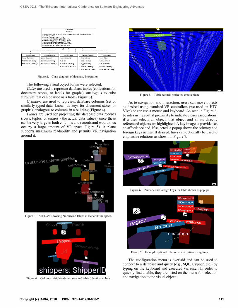
Figure 2. Class diagram of database integration.

The following visual object forms were selected: Cubes are used to represent database tables (collections for

document stores, or labels for graphs), analogous to cube furniture that can be used as a table (Figure 3).

Cylinders are used to represent database columns (set of similarly typed data, known as keys for document stores or graphs), analogous to columns in a building (Figure 4).

Planes are used for projecting the database data records (rows, tuples, or entries - the actual data values) since these can be very large in both columns and records and would thus occupy a large amount of VR space Figure 5). A plane supports maximum readability and permits VR navigation around it.

Figure 3. VRiDaM showing Northwind tables in Benediktine space.

Figure 4. Columns visible orbiting selected table (identical color).

Figure 5. Table records projected onto a plane.

As to navigation and interaction, users can move objects as desired using standard VR controllers (we used an HTC Vive) or can use a mouse and keyboard. As seen in Figure 6, besides using spatial proximity to indicate closer associations, if a user selects an object, that object and all its directly referenced objects are highlighted. A key image is provided as an affordance and, if selected, a popup shows the primary and foreign keys names. If desired, lines can optionally be used to emphasize relations as shown in Figure 7.

Figure 6. Primary and foreign keys for table shown as popups.

Figure 7. Example optional relation visualization using lines.

The configuration menu is overlaid and can be used to connect to a database and query (e.g., SQL, Cypher, etc.) by typing on the keyboard and executed via enter. In order to quickly find a table, they are listed on the menu for selection and navigation to the visual object.



122 / 160

Figure 8. VRiDaM of MongoDB with dbkoda example data [26],

showing spatial orientation and not intended to be readable.

Figure 9. VRiDaM of Neo4j with Northwind example data.

Figure 8 shows the VRiDaM visualization for MongoDB with dbkoda example data [26] (a Northwind port was no longer available), while Figure 9 shows Neo4j with Northwind example data.

V. EVALUATION To evaluate VRiDaM, we compared its usage with a

typical 2D database tool, DbVisualizer 10.0.13 (Free), shown in Figure 10 with the Northwind database loaded to provide an impression of the model’s complexity, not meant to be readable. A convenience sample of eleven computer science students was selected. One experienced VR sickness symptoms and thus only the remaining ten were included in the results. All indicated they had some familiarity with SQL and they lacked NoSQL experience, so we chose to compare VRiDaM with an SQL tool. Three had not experienced VR before. The subjects were randomly selected to start in either VR mode (6) or the common tool (4). PostgreSQL Version 10 with the Northwind sample database (Figure 11Figure 10. ) was used. Java 8 update 151, Apache Tomcat v8.0, AFRAME 0.8.2, Firefox 61, and SteamVR Version 2018-05-24 (1527117754).

Figure 10. Northwind Traders data model in DbVisualizer.

These database tasks were given verbally and equivalent but not the exact same five questions asked in the other mode:

1) Which tables have a relation to table X? 2) To which table(s) does the table X have a relation? 3) What columns does table X have? 4) What are the foreign or primary keys of table X? 5) What are the keys in table X?

TABLE II. VRIDAM VS. DBVISUALIZER TASKS (AVERAGED)

VRiDaM DbVisualizer Task duration (mm:ss) 4:48 1:46

Cumulative answers given (total/incorrect/missing) 130/6/4 140/1/6

Task correctness 92% 95% The tasks results are shown in Table II. VRiDaM task

duration was 2.7 times longer, and this can be expected since VR requires navigation time through space that 2D tools do not incur. The number of correct answers across the five tasks were 13 in VR and 14 in DbVisualizer, with ten subjects resulting in 130 or 140 cumulatively correct answers respectively. These longer VR task durations may be acceptable for certain user scenarios, and gives insight into what liabilities can be expected. A correctness difference of 3% across ten subjects is not necessarily significant and shows that the users were able to immerse themselves within minutes into a Benediktine space paradigm and perform tasks effectively. The task correctness differences could be attributed to personality, human alertness, distraction, or other factors beyond the paradigms or VR influence, as only 4 subjects in VR and only 3 subjects in non-VR were responsible for all errors, the rest had no mistakes.

Subjective impressions are shown in Figure 11 for VRiDaM intuitiveness and suitability of the controller interface and visualization as well as overall enjoyment. We note no significant difference between the interaction and the visualization intuitiveness or suitability. Only one preferred VRiDaM. This may indicate that more training and experience would be needed for them to feel more comfortable with a VR tool than with a 2D tool. Various debriefing comments indicated that the Benediktine spatial arrangement was either liked or not an issue for the subjects. When debriefed about what they liked about VRiDaM, comments included that it was a better database-model visualization, that tables were real objects instead of text boxes, how tables where displayed in space, and the highlighting effect.

Figure 11. Average responses for VRiDaM (scale of 1 to 5 with 5 best).



123 / 160

The evaluation shows some of the challenges in utilizing VR for database-model visualization and interaction. VR object interaction is not standardized nor do users have familiarity and experience with it as they do with 2D mouse-based user interfaces. While VR enables new immersive paradigms and metaphors, these are not necessarily immediately intuitive. VR movement (moving the camera perspective) is more time consuming than scrolling or zooming a 2D perspective. For simpler tasks, VR tends to require more interaction time to accomplish the same task and thus entails efficiency costs. A 3D space permits objects to hide other objects, and for opaque objects requires movement to determine that no other objects are hidden. Given that the subjects were already familiar with E-R diagrams and SQL tools, yet had no prior training with VRiDaM and Benediktine space, we are satisfied with the ratings on suitability and intuitiveness. Based on comments about what subjects liked about VRiDaM we see it as a positive indicator and intend to investigate this approach further.

VI. CONCLUSION This paper contributes VRiDaM, an immersive WebVR

heterogeneous database visualization approach, applying Benediktine space visualization and force-directed graphs to (relational and non-relational) database models. It thus avoids the connection "yarn-balls" other techniques have in visualizing connections by leveraging spatial locality. A prototype was used to verify its viability and an empirical study evaluated its usability.

The empirical evaluation showed VRiDaM to be less efficient for equivalent analysis tasks while correctness was slightly worse. Intuitiveness, suitability, and enjoyment were given a better than neutral rating on average. One case of VR sickness occurred and we hope to address it in future work.

One ongoing challenge for a generic tool approach is the plethora of non-standardized interfaces to NoSQL and other databases. However, by providing driver plugins we believe that the adaptation overhead is small in relation to the advantages of a VR visualization that VRiDaM brings. Future work includes a more comprehensive empirical study and will investigate various optimizations to improve usability, performance, and scalability.

ACKNOWLEDGMENT The author thanks Christoph Bauer and Camil Pogolski for

assistance with the design, implementation, and evaluation.

REFERENCES [1] Cisco. The Zettabyte Era: Trends and Analysis. (Jun 7, 2017).

Whitepaper. Available from https://www.cisco.com/c/en/us/ solutions/collateral/service-provider/visual-networking-index-vni/vni-hyperconnectivity-wp.html 2018.07.24

[2] D. Reinsel, J. Gantz, and J. Rydning, “Data Age 2025: The Evolution of Data to Life-Critical,” IDC Whitepaper (April, 2017).

[3] R. Cattell, “Scalable SQL and NoSQL data stores,” Acm Sigmod Record 39, no. 4, pp. 2-27, 2011.

[4] P. Chen, “Entity-Relationship Modeling: Historical Events, Future Trends, and Lessons Learned,” In Software pioneers. Springer-Verlag, pp. 296-310, 2002.

[5] T. Merel, “The reality of VR/AR growth,” Jan 11, 2017. Available from http://techcrunch.com/2017/01/11/the-reality-of-vrar-growth/ 2018.07.24

[6] M. Benedikt, “Cyberspace: some proposals,” In Cyberspace, Michael Benedikt (Ed.). MIT Press, Cambridge, MA, pp. 119-224, 1991.

[7] P. Young, “Three Dimensional Information Visualisation,” Technical Report, University of Durham, 1991.

[8] U. Fayyad, A. Wierse, and G. Grinstein (Eds.), Information Visualization in Data Mining and Knowledge Discovery. Morgan Kaufmann, 2002. ISBN: 1558606890.

[9] S. Fabrikant and B. Buttenfield, "Formalizing Semantic Spaces for Information Access," Annals of the Association of American Geographers, 91(2), pp. 263-280, 2001.

[10] D. Butler, J. Almond, R. Bergeron, K. Brodlie, and R. Haber, “Visualization reference models,” In Proc. Visualization '93 Conf., IEEE CS Press, pp. 337-342, 1993.

[11] A. Bierbaum et al, “VR Juggler: A virtual platform for virtual reality application development,” In Proc. IEEE Virtual Reality. IEEE, pp. 89-96, 2001.

[12] F. Fittkau, A. Krause, and W. Hasselbring. “Exploring software cities in virtual reality,” In Proc. IEEE 3rd Working Conf. on Software Visualization (VISSOFT). IEEE, pp. 130-134, 2015.

[13] A. Teyseyre and M. Campo, “An overview of 3D software visualization,” In IEEE Trans. on Visualization and Computer Graphics. IEEE, 15(1), pp. 87-105, 2009.

[14] A. Kashcha, “Software Galaxies,” Available from http://github.com/anvaka/pm/ 2018.07.24

[15] J. Rilling and S. Mudur, “On the use of metaballs to visually map source code structures and analysis results onto 3d space,” In Proc. 9th Work. Conf. on Reverse Engineering. IEEE, pp. 299-308, 2002.

[16] P. McIntosh, “X3D-UML: user-centered design, implementation and evaluation of 3D UML using X3D,” Ph.D. dissertation, RMIT University, 2009.

[17] M. Krzywinski, “Schemaball: A New Spin on Database Visualization,” In Dr. Dobb's: The World of Software Development,, 2004.

[18] E. Olshannikova, A. Ometov, Y. Koucheryavy, and T. Olsson, “Visualizing Big Data with augmented and virtual reality: challenges and research agenda,” J. of Big Data, 2(22), 2015.

[19] I. Herman, G. Melancon, and M. Scott Marshall, “Graph visualization and navigation in information visualization: A survey,” In IEEE Transactions on visualization and computer graphics, 6(1), pp. 24-43, 2000.

[20] G. Di Battista, P. Eades, R. Tamassia, and I. Tollis, Graph drawing: algorithms for the visualization of graphs. Prentice Hall PTR, 1998.

[21] S. Card, “Information Visualization,” In: Human Computer Interaction Handbook: Fundamentals, Evolving Technologies, and Emerging Applications (Ed: Jacko, J.), Third Edition. CRC Press, pp. 544-545, 2012.

[22] S. Palmer, Vision Science. MIT Press, Cambridge (USA) 1999, ISBN 978-0262161831.

[23] D. Norman, The Design of Everyday Things: Revised and Expanded Edition. Hachette UK, 2013.

[24] A. Van der Heijden, “Perception for selection, selection for action, and action for perception,” Visual Cognition, 3(4), pp. 357-361, 1996.

[25] S. Card, J. Mackinlay, and B. Schneiderman (editors), Readings in Information Visualization: Using Vision to Think. Morgan Kaufman, 1999.

[26] [Online] Available from https://github.com/ SouthbankSoftware/dbkoda-data 2018.08.12



124 / 160

Redefining KPIs with Information Flow Visualisation – Practitioners’ View

Jarkko Hyysalo, Markus Kelanti and Jouni Markkula M3S Research Unit, Faculty of Information Technology and Electrical Engineering,

University of Oulu Oulu, Finland

e-mail: {jarkko.hyysalo, markus.kelanti, jouni.markkula}@oulu.fi

Abstract—We investigate Key Performance Indicators (KPIs) in a large and multi-national telecommunication company and discover needs and requirements for understanding, analysing and using KPIs from practitioner’s perspective. Utilising an action research approach, we identified the existing challenges with KPIs in a large-scale software-intensive systems development in a global setting. Our study revealed several issues with organisations KPIs, e.g., measuring the wrong things or not basing the measurements on reliable data. Based on the identified issues, a visualisation and modelling approach was introduced to reform the KPI representation and formulation to improve understanding and communicating KPIs, as well as their use in decision-making. We suggest that KPI information flow visualisation with appropriate tool support allows redefining usable, valid and reliable KPIs. The problem is addressed with a simple solution that is easily adopted and taken into use at all levels of an organisation.

Keywords—key performance indicators; KPIs; modelling; visualisation.

I. INTRODUCTION Managing the development of software systems requires

careful attention. Companies operate in turbulent environment with fierce competition and tight time-to-market requirements [1], where knowledge of the performance of the development process, in addition to understanding the system and its development is necessary [2]. Companies use Key Performance Indicators (KPIs) to provide this vital information. KPIs are used to measure, for example, the quality of the product, the features developed, the resources spent in the development and the value delivered to customers. KPIs provide a way to evaluate and improve the product and the process.

There is evident value in defining KPIs for the company. However, it is challenging to formulate KPIs so that they provide useful, valid and reliable information, and many organisations struggle to measure their projects, products and units [3]. Thus, our research question: “How to easily formulate KPIs so that they effectively and reliably measure the product development process performance?”

In this paper, we report an action research study, conducted within a large telecommunications company. The study revealed critical practical challenges in defining and using KPIs in organisation. For solving the challenges, the visualisation of the KPI information flow was found to be essential to provide a better understanding of the process. An approach and supporting tools were developed for the

modelling and visualisation of the KPI information flow. Supporting the developers’ understanding about the KPI formulation process resulted in KPIs that provide more real value for the organisation, and thus improve the KPI process. Visualisation and supporting tools provided means also to understand and communicate KPIs.

The rest of the paper is organised as follows. Section 2 discusses the related works, Section 3 presents the research approach, Section 4 presents the action research intervention and its results, Section 5 discusses the findings of the empirical work, and Section 6 concludes this work.

II. RELATED WORK KPIs provide many kinds of information about the

development, thus, it is important to select KPIs according to organisation’s strategy and objectives [4][5]. Deep understanding of the software development process is needed—providing the understanding of the “why”, “what” and “how”, defining also the motivations and rationales for activities and flows [6]. Different stakeholders have different views of and needs for the process [6]: Process performers often focus on the “hows”, process managers on the “whats”, and process engineers on the “whys”. Thus, different views are necessary, and KPIs address different needs. Our focus is on how KPIs are used and defined, as well as understanding KPIs and recognising stakeholders’ views.

A. Formulating KPIs Production of good KPI values starts from the reliable

source data, but in practice it is hard to collect consistent and comparable data. Further challenge is to decide upon the importance of individual performance measures for decision-makers and prioritisation is a challenge as well. There are approaches that guide KPI work and measure organisational performance; some of them are shortly introduced next.

del-Rey-Chamorro et al. [4] presents a framework for creating KPIs for knowledge management solutions, with eight steps to create KPIs from the strategic level business plan all the way to operational level measurable KPIs utilising templates for KPI formulation and how to bridge the strategic level and operational level. The aim is to evaluate the effectiveness of knowledge management solutions.

Analytical Hierarchy Process (AHP) constructs a pairwise comparison between different KPIs and their hierarchies to evaluate and prioritise them based on SMART (Specific, Measurable, Attainable, Realistic, Time-sensitive) goal setting [5]. The focus is the prioritisation of KPIs to find



125 / 160

the most relevant KPIs for the organisation [5]. However, it does not consider how KPIs should be formulated.

Balanced Scorecard [7] measures the organisational performance and aims at transforming the vision and strategy into concrete objectives, aligning departments and units towards common goals, etc. Yet, the following shortcomings are identified: Inaccurate and subjective measures, communication is not participative (only top-down), and inappropriate benchmarks are used for evaluation [8].

ISO standards provide guidelines as well. ISO 9001:2015 specifies requirements for a quality management system. It does not specifically mention “KPIs” but requires metrics to measure the system to ensure: a) the ability to consistently provide products and services that meet customer and applicable statutory and regulatory requirements, and b) aims to enhance customer satisfaction through the effective application of the system, including processes for improvement of the system and the assurance of conformity to the customer and applicable statutory and regulatory requirements [9]. ISO quality management principles [10][11] aims for customer focus, leadership, the involvement of people, process approach, system approach to management, continual improvement, factual approach to decision making, and mutually beneficial supplier relationship.

However, several challenges are identified in current ways for defining KPIs and ensuring that they are based on valid data [12]-[15]: Selecting and defining KPIs is not easy. KPIs are often defined in siloed terms instead of considering the whole organisation, e.g., they only focus on financial aspects and may lack the other aspects like manufacturing. Accurate calculations are hard to create and they easily measure something else than the intended objective. It is difficult to have metrics reflecting strategic drivers and be in line with the organisation’s visions and goals. KPIs must also be aligned through the whole organisation and every level of work, from visions and goals to actual implementation. Local optimisation should be avoided, and short-term and long-term goals should be balanced. There are nuances and unforeseeable variables that affect the measures. Finally, KPIs must be put in practice in order to see how they impact the performance and behaviour, and they should be adjusted accordingly. Hence, continuous refining is necessary.

To address the identified issues, improvements are necessary. Properly selected and measured KPIs help decision-making, but getting the measures right requires considerable effort [16]-[18]: Even though the measures are classified into different categories, they are often correlated due to the inherent internal relations of different processes in the supply chain. Complex dependencies, changing goals and tight deadlines make organisations prone to making rushed decisions. Thus, it is important to have a simple way to identify and analyse the KPI data flows and relationships in order to avoid flawed decisions. Due to the complicated relationships, dependencies and conflicts, modelling the relationships is proposed and quick feedback loops are suggested. Furthermore, the goals and KPIs should be adjusted when they are no longer realistic.

In a nutshell, KPIs should be based on data that is available and measurable, and KPIs should provide relevant information. Effective performance measurement system “should provide timely, accurate feedback on the efficiency and effectiveness of operations” [19]. Measurements are also necessary for process improvement purposes—if it can’t be measured it can’t be improved [20].

B. KPI Visualisation It is important to understand how to present the

measurements and act accordingly. Visualisation helps ensuring that the actions are taken and transparency is achieved [21]. Benefits of KPI visualisation are many: Visualisation is an important factor in thought and communication [22]; Information visualisation and graphical representation help in complex cognitive tasks [23]; Information visualisation supports comprehension and data analysis [24], especially for non-technical users [12]; Visualisation enables smarter decisions and improved productivity [12]; Groups supported by visualisation achieve better productivity, the better quality of outcome and greater knowledge gains than groups without such support [24].

Often KPIs and different measures are correlated and create a complex network of interdependencies [18], thus, understanding the results and the process of formulating KPIs is challenging. Visualisation enables the analysis of activities, the flows (i.e., inputs and outputs), dependencies, and the contexts [25]. It can also be used to visualise the components where KPIs are built from, decomposing the higher level KPIs into lower-level components in order to trace the sources of problems [26]. Visualising the process can be done in several ways with different levels of formalism and detail (cf. [27][28]). Finding the correct level depends on the purpose.

There are examples to KPI visualisation, like del-Río-Ortega et al. [29], who propose an XML-based way for a graphical or a template-based textual notation for business processes. To help selecting the visualisation approach, Staron et al. [30] provide a model based on seven dimensions: type of reporting, data acquisition method, type of stakeholders, method of delivery, frequency of updates, aim of the information, and length of data processing flow. However, formal visualisation and modelling approaches can be cumbersome and “too heavy”, e.g., for persons who are not familiar with process modelling concepts [25]. Thus, their benefits are lost. Instead, a simpler approach is proposed. Presenting detailed processes as higher-level entities makes the visualisations more comprehensible, and multiple views or representations for managing the complexity is suggested [25]. Rationale and justification for processes and activities must also be presented as those express why the work is needed. Rationale and reason tell what is meant to be accomplished and why [31][32].

III. RESEARCH APPROACH The case company was chosen as it could provide data

related to the research question. The case organisation is one of the largest data networking and telecommunication technology providers in the world in its field. The



126 / 160

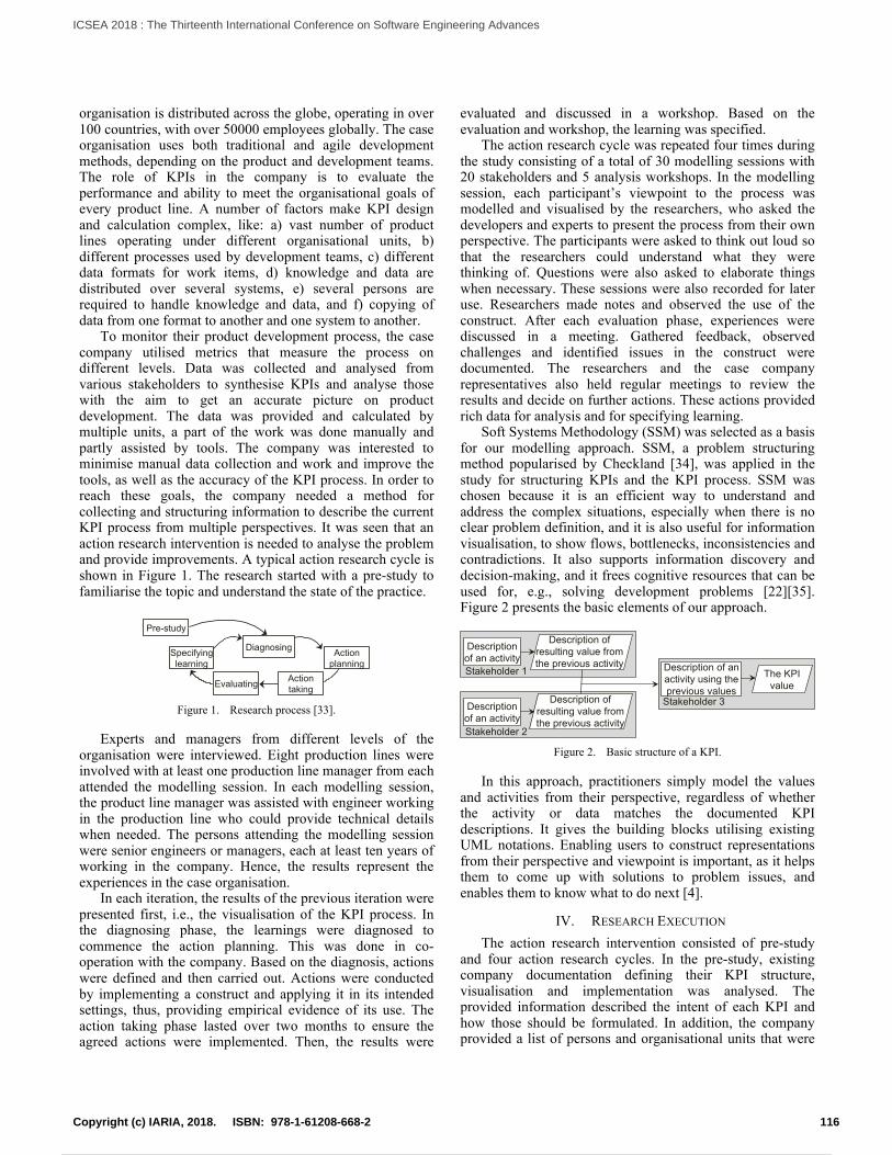
organisation is distributed across the globe, operating in over 100 countries, with over 50000 employees globally. The case organisation uses both traditional and agile development methods, depending on the product and development teams. The role of KPIs in the company is to evaluate the performance and ability to meet the organisational goals of every product line. A number of factors make KPI design and calculation complex, like: a) vast number of product lines operating under different organisational units, b) different processes used by development teams, c) different data formats for work items, d) knowledge and data are distributed over several systems, e) several persons are required to handle knowledge and data, and f) copying of data from one format to another and one system to another.

To monitor their product development process, the case company utilised metrics that measure the process on different levels. Data was collected and analysed from various stakeholders to synthesise KPIs and analyse those with the aim to get an accurate picture on product development. The data was provided and calculated by multiple units, a part of the work was done manually and partly assisted by tools. The company was interested to minimise manual data collection and work and improve the tools, as well as the accuracy of the KPI process. In order to reach these goals, the company needed a method for collecting and structuring information to describe the current KPI process from multiple perspectives. It was seen that an action research intervention is needed to analyse the problem and provide improvements. A typical action research cycle is shown in Figure 1. The research started with a pre-study to familiarise the topic and understand the state of the practice.

Pre-study

Evaluating

Action planning

Specifying learning

Action taking

Diagnosing

Figure 1. Research process [33].

Experts and managers from different levels of the organisation were interviewed. Eight production lines were involved with at least one production line manager from each attended the modelling session. In each modelling session, the product line manager was assisted with engineer working in the production line who could provide technical details when needed. The persons attending the modelling session were senior engineers or managers, each at least ten years of working in the company. Hence, the results represent the experiences in the case organisation.

In each iteration, the results of the previous iteration were presented first, i.e., the visualisation of the KPI process. In the diagnosing phase, the learnings were diagnosed to commence the action planning. This was done in co-operation with the company. Based on the diagnosis, actions were defined and then carried out. Actions were conducted by implementing a construct and applying it in its intended settings, thus, providing empirical evidence of its use. The action taking phase lasted over two months to ensure the agreed actions were implemented. Then, the results were

evaluated and discussed in a workshop. Based on the evaluation and workshop, the learning was specified.

The action research cycle was repeated four times during the study consisting of a total of 30 modelling sessions with 20 stakeholders and 5 analysis workshops. In the modelling session, each participant’s viewpoint to the process was modelled and visualised by the researchers, who asked the developers and experts to present the process from their own perspective. The participants were asked to think out loud so that the researchers could understand what they were thinking of. Questions were also asked to elaborate things when necessary. These sessions were also recorded for later use. Researchers made notes and observed the use of the construct. After each evaluation phase, experiences were discussed in a meeting. Gathered feedback, observed challenges and identified issues in the construct were documented. The researchers and the case company representatives also held regular meetings to review the results and decide on further actions. These actions provided rich data for analysis and for specifying learning.

Soft Systems Methodology (SSM) was selected as a basis for our modelling approach. SSM, a problem structuring method popularised by Checkland [34], was applied in the study for structuring KPIs and the KPI process. SSM was chosen because it is an efficient way to understand and address the complex situations, especially when there is no clear problem definition, and it is also useful for information visualisation, to show flows, bottlenecks, inconsistencies and contradictions. It also supports information discovery and decision-making, and it frees cognitive resources that can be used for, e.g., solving development problems [22][35]. Figure 2 presents the basic elements of our approach.

Stakeholder 2

Stakeholder 1

Description of an activity

Description of an activity

Stakeholder 3

The KPI value

Description of an activity using the previous values

Description of resulting value from the previous activity

Description of resulting value from the previous activity

Figure 2. Basic structure of a KPI.

In this approach, practitioners simply model the values and activities from their perspective, regardless of whether the activity or data matches the documented KPI descriptions. It gives the building blocks utilising existing UML notations. Enabling users to construct representations from their perspective and viewpoint is important, as it helps them to come up with solutions to problem issues, and enables them to know what to do next [4].

IV. RESEARCH EXECUTION The action research intervention consisted of pre-study

and four action research cycles. In the pre-study, existing company documentation defining their KPI structure, visualisation and implementation was analysed. The provided information described the intent of each KPI and how those should be formulated. In addition, the company provided a list of persons and organisational units that were



127 / 160

involved in the KPI process, including also description how they provided or processed KPI information in the process. In addition, related research was also analysed.

A. First Action Research Cycle DIAGNOSING: The pre-study revealed that the system

was more complex than the company documentation indicated. The process included hundreds of stakeholders and multiple variations of the data items. Based on the pre-study, it became necessary to study the overall information flow and stakeholder involvement to determine how the actual system providing the KPIs was structured.

ACTION PLANNING AND TAKING: The plan was to start the KPI system modelling with the pre-study information to formulate a proper soft system model based on SSM. UML flowchart approach and SSM [34] were used to create a KPI soft system model.

EVALUATION AND LEARNING: At the end of the first cycle, the resulting model was evaluated in a workshop with the company representatives. The participants agreed that the model allowed examining KPIs in more detail, which showed that the company documentation did not represent the real KPI behaviour or process. The lack of information about how the data is obtained, undocumented sources, how data is created and how data is used in the decision-making demonstrated that KPIs did not present accurate information or what KPIs were intended to present. Moreover, a simple collapse/expand feature was requested from the tool hiding the complexity or bringing out the details when needed. Participants agreed that this kind of feature would improve visualisation and understanding. Finally, a decision was made to include the stakeholders of KPI modelling in the next research cycle to provide the information missing from the model.

B. Second Action Research Cycle DIAGNOSING: At the previous cycle, the soft system

model of the KPI process showed that there was missing information and dead ends not documented in the official documentation. This indicated that there are information only known by involved stakeholders and they should be contacted to provide the missing information.

ACTION PLANNING AND TAKING: The plan was to involve the stakeholders to add the missing information to the model. The stakeholders who would know how data items were created or what information was used to create them were invited to a modelling session, where the information provided by the stakeholder was added to the soft system model created in the previous research cycle. Each modelling session continued updating the same KPI soft system model created in the first cycle. After the sessions, a workshop was organised to evaluate, correct and analyse the KPI soft system model.

EVALUATION AND LEARNING: The new version of the soft system model was discussed with company representatives in a workshop. Based on the analysis of the soft system model, workshop participants thought that the visualisation was complex. They suggested that using stakeholder viewpoints allowed adjusting abstraction levels

to manage the complexity. With viewpoints, they were able to examine selected parts of the process and keep the visualisation comprehensible. The feedback for the soft system model indicated that it allowed stakeholders to understand how KPIs were constructed and the model offered enough information to interpret KPIs correctly. According to the participants and the analysis in the workshop, both the UML visualisation and SSM principles created a KPI model that was easy to interpret, translated concepts from one domain to another in a meaningful way and allowed the evaluation of KPIs. Finally, the participants considered it necessary to adjust the way the model was created to support simpler notation and logic to allow users with varying experience to contribute. They thought that the current approach was labour intensive and required deep knowledge of modelling and SSM methodology, which was seen as hindrance as it required an expert to help.

C. Third Action Research Cycle DIAGNOSING: The ability to understand how KPIs

actually work was very important for the company personnel as the KPIs did not work as intended and they did not provide the correct information. The modelling of the KPI process needed to continue to provide a better big picture. However, the process needed to be simplified, allowing anyone to understand it and input his or her own viewpoints without the help of the researcher or an expert.

ACTION PLANNING AND TAKING: The existing KPI soft system model was transformed to a digital format utilising Microsoft’s Visio tool, allowing anyone to access the model at any time. In addition, the participating stakeholders, developers and managers were taught the modelling method so that they could add their own viewpoints. Teaching the approach also allowed the researchers to develop it further and make it easier to understand and learn. In addition, modelling sessions were continued with those stakeholders who preferred to work with the researchers instead of doing the modelling alone.

EVALUATION AND LEARNING: At the end of the cycle, a workshop was held to discuss the results with all company stakeholders involved in the cycle. Based on the discussion and analysis of the new version of the KPI soft system model, it was quickly noticed that the selected visualisation approach was approved and the process representation it provided was very informative and usable. The KPI soft system model provided a shared understanding about the process and work activities regardless of the expertise or work position. It was easy to discuss the specifics of the process with the representation as a reference point, where each participant could pinpoint the activity or information flow they were interested in.

Further, the findings from second research cycle were re-examined, as more data was available from different teams and product lines. The model started to show its efficiency, as it confirmed that the data that the organisation bases its KPI measurements is not sufficient and that lead to situation where KPIs were not indicating the measurements that they were intended to do. For example, two different organisational units could get different figures based on their



128 / 160

source information or interpretation during the data handling. Another concrete example was that the calculation of delivered backlog items didn’t take into account the size of the items or items finalised by collaborators, thus, resulting in skewed efficiency measures. Finally, simplifying the modelling process was seen as a way to speed up the modelling process and to help others to understand the modelling process and the modelling language [cf. 36]. This also allowed persons with no prior knowledge on UML to understand process and contribute.

D. Fourth Action Research Cycle DIAGNOSING: Diagnosis of the previous action

research cycle called for an analysis of KPIs and presentation on how they can be re-constructed as meaningful KPIs that accurately reflect the development process. Furthermore, additional focus was needed on KPI visualisation due the growing amount of information in a single model. A proper system visualisation was required from different stakeholder perspectives in order to effectively communicate the KPIs to different levels of management, developers and support staff.

ACTION PLANNING AND ACTION TAKING: Based on the diagnosis, this action research cycle was focused on analysing which KPIs the company would benefit on utilising, and use that information to propose how the previously modified KPIs should be constructed. In order to do so, in addition to the existing model, a new KPI soft system model was created to represent the meaningful and accurate KPIs perceived by company management. In addition, special attention was given to the viewpoints to make the visualisation easier to read. The analysis and modelling were done in separate sessions with management stakeholders, similarly to previous research cycles. After a selection of 8 KPIs was fully remodelled, they were compared to the original KPI soft system model to show the

current implementation and how the KPIs should be changed to match the desired situation.

EVALUATION AND LEARNING: After the action planning and taking, a workshop was held with all participants. Based on the workshop discussions, it was clear that the stakeholders preferred this approach as it provided the following benefits: 1) It allowed stakeholders to see the current situation and what should be made to the existing KPI system to have meaningful KPIs. 2) The model showed the disparities between stakeholder viewpoints that weren’t visible before and the visualisation enabled effective communication on disparities. 3) The resulting model allowed practitioners to re-evaluate their current process and data in order to determine the best course of action. 4) The model was easy to comprehend and it provided reliable results that were accurately reflecting the state of the process.

The fourth action research cycle was the final iteration, as the results were satisfying for both researchers and case organisation. The resulting model worked as the description of KPIs and allowed to construct, analyse and describe KPIs with a single model. The participants also agreed that the measures could now be relied upon, and the KPIs showed effectively what they were supposed to show.

V. DISCUSSION Our action research intervention revealed several issues

with the organisations KPIs and KPI formulation process. The company’s process provided KPIs that did not fulfil their intended purpose. There was a clear need to understand the process better—to know more about the reasons KPIs were used for and from what source data the analyses were done from. This called for modelling the KPI information flows from stakeholders’ perspectives that contribute to or calculate any KPI data. The focus was to provide visualised and accurate KPIs. Table 1 summarises our findings.

TABLE I. SUMMARY OF THE MAIN FINDINGS

Finding Implication Describing KPI as an information flow allowed stakeholders to comprehend the actual meaning of KPI versus what was described in the official documentation.

- Modelling, visualisation and constant analyses are necessary to find out the relevant KPIs and to keep the KPI process up to date. - Modelling and visualisation enables to see where the data originates and how it is manipulated. - Modelling and visualisation enables simplification. - Modelling and visualisation enables the evaluation of the validity of the data and whether KPIs perform as intended.

Visualising the KPI information flow eased communication between stakeholders with different backgrounds.

- Visualising the workflow improves the coordination and understanding of others work. - Modelling and visualisation enables more accurate analyses, reveals bottlenecks and problem areas, and finally makes possible process improvement activities. - Visualisation improves understanding and communication.

Showing different stakeholder viewpoints as a part of the information flow allowed comprehension of KPI, data items and complexity of the implementation in different parts of the organisation.

- Viewpoints can be used to adjust the abstraction levels and to manage the complexity. - Hiding and expanding parts simplifies the presentation. - Viewpoints allows for focusing on the matter at hand. - Modelling tools should provide viewpoints functionality.

Allowing stakeholders to see their viewpoints and modify them motivated stakeholders to participate and extend the model further.

- Understanding the process for KPIs is paramount for motivation. - Modelling KPIs reveals information on how the data is obtained and created, and how it is used in the decision-making. - Showing the viewpoints help understanding and agreeing upon the perspectives (e.g., quality vs. efficiency).

With the proposed approach the KPI information flow model became both the actual description and formulation of a KPI.

- Stakeholders should be involved in the modelling. - Accurate and reliable source data is required for meaningful KPIs. - Measurements and comparisons over the product lines can be achieved.



129 / 160

Utilizing common UML-tools (e.g., Visio) and the modelling method presented in [36] as our tools we could provide the visualisations. With the help of the visualisations, the case organisation personnel understood better KPIs and how they were formulated, and they noticed serious flaws. KPIs were neither reliable nor commensurable between different units or product lines, e.g., there was inconsistency with measurements, as management focused on effectiveness and engineers focused on quality. In sum, visualisation made the organisation rethink their KPIs and how they are formulated.

Visualisation revealed that the source data was different than originally understood by those who formulate KPIs, providing different results than what originally was intended, and hence decisions were made based on flawed KPIs.

Furthermore, KPIs were not immediately available, instead data was gathered once a month and KPIs were then calculated, KPI data was different between product lines/units, and KPI process had unnecessary workload and loops. One of the key findings was that the changes to the existing process did only change the local processes and work; it did not guarantee that KPIs were changed elsewhere. It was realised that in order to properly formulate KPIs, the whole KPI process and its information flows should be analysed, not just the data sources. Based on our study, we propose that KPI visualisation as a flow is necessary for recognising who is contributing and what data is used in that contribution. It also helps to see if KPIs provided by different teams are commensurable.

The study showed that KPIs were found problematic, as they are often taken for granted and the way that KPIs are implemented is not visible for stakeholders. It is seldom considered where KPIs come from and what they are representing. It is necessary to think carefully what calculations are useful and whether those calculations reveal the issues they are meant to.

Figure 3 below presents a KPI example that shows the average development hours of two different products. In this example, two teams work for product A and input their

working hours directly to Jira for each feature. For product B, the product owner estimates the working hours spent on each feature based on team members compiled a list of features. The example presents a visualised KPI that informs what is the source data used to calculate the KPI and how it is formed. With proper tool support, the data and activity elements can be made to represent real data. Essentially, the visualisation allows stakeholders to identify and ask the questions that matter in regards to validity, representation and usage of a KPI. With a systematic analysis, we found the issues with KPIs and KPI formulation process. Modelling and visualisation enabled the stakeholders to understand the KPI process better and it made the stakeholders think about the relevant data and information concerning KPIs.

With our approach, a soft system model could be built systematically. The model showed where the data originated and how it was manipulated throughout the process. Thus, validating the usefulness of our approach to modelling of KPI information flows. We believe that our approach would be fit for other cases also, however that still requires further validation. Due to improved understanding, modelling and visualisation was found useful as a process improvement tool: It allowed the identification of problems in the process, and unnecessary activities could be identified and the process could be streamlined accordingly. Coordination of activities was also improved.

Our modelling and visualisation approach addresses several needs and is generic enough to be used in various situations and purposes. Our approach is suitable for visualising and analysing the activities and information flows, and showing the dependencies. Moreover, it was easily adopted and personnel committed to use it. Presenting the KPI process as a graphical model provided better understanding for developers and experts, and it also improved communication and helped to analyse the work. It motivated the personnel and they came up with new ideas to further improve their work, work practices and processes. Visualisation was also found to be useful in pinpointing the bottlenecks and problem areas.

Product owner adds both averages together and divide them by two and creates a diagram

presentation

Diagram: Overall average hours spent per feature on

product

Jira Database: Feature data

Number: Average hours spent per

feature on product B

Excel sheet: Previous

estimations

Software team B members input feature

data into Jira

Product B’s owner provides average hours

spent per feature

Excel sheet: Average hours spent per

feature on product B

Software team member creates a

completed feature list

Excel sheet: List of completed features

Product B’s owner estimates the average hours spent by his

team per feature based on previous estimations

Number: Average hours spent per

feature on product A

Product A’s owner provides average hours spent per

feature by team A based on software teams’ data in Jira

Software team A leader inputs feature data into Jira

Figure 3. Example KPI formulation for a system.



130 / 160

Being able to construct representations also improve the readability of visualisations [37]. Our approach complements, e.g., the dashboard selection model by Staron et al. [30] and ways to elicit information by Staron et al. [38], which is more based on a set of questions, and it can also be used as a simple visualisation mechanism on top of other established approaches, such as Balanced Scorecards by Kaplan and Norton [7]. The findings are also in line with Staron [3], stressing the importance of completeness, reliability and early warning signs.

A. Validity of the Study The reliability of the data and results was ensured via

rigorous research protocol with peer reviews by researchers and company representatives. The action research cycles were documented throughout the research. The modelling sessions were recorded and transcribed by the researchers.

The way the action research was implemented introduces a danger of positive bias within researchers and company participants—due to the constant communication and interventions; the company participants could be positively biased, producing only positive results. However, having many different viewpoints presented in the workshops and modelling sessions addressed this issue. Also, agreement over clear roles and rigorous research methods helped participants remain neutral observers.

This study was conducted within a large ICT organization that utilizes product line based development, hence limiting the generalizability of the results. In order to make wider conclusions more domains, smaller companies and different production models should be studied.

VI. CONCLUSION AND FUTURE WORK This paper presents an action research study with the aim

to understand organization’s KPI process and to formulate a meaningful set of KPIs. Several issues in the case organisation were identified during the study, with the most significant being that the original KPIs didn’t measure what they were intended to measure. KPIs were not giving the right information; they were not well defined and were not based on complete and reliable information. When the information was not correct, it caused harm as the decision-making was relying on false data.

Modelling and visualisation was used to understand, analyse and to model the KPI process. Using simple visualisation mechanisms to model and represent the KPI process helped in understanding the purposes and needs of measurements, as well as the source data and its handling during the KPI process. Modelling and visualisation also clearly revealed the different stakeholders that participated in the KPI process, and further improved understanding and communication between the stakeholders; especially non-technical persons’ understanding was improved considerably.

The improved KPI process and well-defined KPIs, in turn, lead to more effective decision-making, as the measurements were more accurate, reliable and descriptive. Also, different units and product lines could be compared when the measurements were commensurable.

Study showed that the KPI information flow should be carefully analysed and KPIs should be based on real needs and real measurable values. To address our research question, KPIs should be formulated in a way that provides real results. For this purpose, the proposed modelling and visualisation approach is a very useful tool. It allows for redefining usable, valid and reliable KPIs so that KPIs and the whole KPI process, with all the interdependencies, can be well understood and analysed. It is also important that the whole product development process is analysed, not just the data sources for KPIs. Analysing the process provides an understanding how KPIs are build from the original data, what the measurements really indicate and how they can be used to understand and improve the development process. Constant follow up and process refining is also an integral part of the process, which helps to keep the KPI process always up to date.

Our approach solves many issues related to KPIs and it is useful especially when there are several teams working on their tasks and the overall picture may be hard to see. Our approach concretises abstract work and defines the relationships of activities associated to it. It provides graphical presentations that are accessible and easy to use for understanding, analysing, communicating and improving processes. The resulting model can be used for presenting the actors, activities and information flows, and describing their logical order and dependencies. Graphical models and modelling helps in understanding the complex problems by enabling breaking those down to understandable entities.

This work benefits both research and industry. Research benefits from new knowledge and the experiences from the industry to expand the knowledge base. Industry practitioners can adopt a simple modelling and visualisation approach to improve their KPI process. We propose simple modelling and visualisation as a recommended practice in formulating KPIs, especially in sociotechnical systems, where persons are in interaction with technology. The solution is simple on purpose. The problems are common in industry and, e.g., in the case organisation the heavy weight solutions have not been useful – they have not been well embraced. However, simple and intuitive solutions are more easily taken into use also at the lower levels of an organisation.

Topics for further studies were also identified, including confirming the results in other domains to improve the generalizability. Furthermore, the question about how to help organisations to act upon KPIs and implement the changes still remains.

REFERENCES [1] P. Helo, “Managing Agility and Productivity in the

Electronics Industry,” Industrial Management & Data Systems 104(7), pp. 567–577, 2004.

[2] J. Froehlich and P. Dourish, “Unifying artifacts and activities in a visual tool for distributed software development teams,” Proceedings of the 26th International Conference on Software Engineering, pp. 387–396. IEEE Computer Society Press, Los Alamitos, CA, 2004.

[3] M. Staron, “Critical role of measures in decision processes: Managerial and technical measures in the context of large



131 / 160

software development organizations,” Information and Software Technology, 54(8), pp. 887–899, 2012.

[4] F. M. del-Rey-Chamorro, R. Roy, B. van Wegen, and A. Steele, ”A framework to create key performance indicators for knowledge management solutions,” Journal of Knowledge management 7(2), pp. 46–62, 2003.

[5] A. Shahin and M. A. Mahbod, “Prioritization of key performance indicators: An integration of analytical hierarchy process and goal setting,” International Journal of Productivity and Performance Management 56(3), pp. 226–240, 2007.

[6] E. S. Yu and J. Mylopoulos, “Understanding “why” in software process modelling, analysis, and design,” Proceedings of the 16th International Conference on Software Engineering, pp. 159–168. IEEE Computer Society Press, Los Alamitos, CA, 1994.

[7] R. Kaplan and D. Norton, “The Balanced Scorecard-Measures that Drive Performance,” Harvard Business Review, 70(1), pp. 71–79, 1992.

[8] M. A. Malina and F. H. Selto, “Communicating and controlling strategy: an empirical study of the effectiveness of the balanced scorecard,” Journal of management accounting research 13(1), pp. 47–90, 2001.

[9] ISO 9001:2015 Quality Management Systems–Requirements. Available from: https://www.iso.org/standard/62085.html 2018.08.01

[10] ISO 9000:2015 Quality Management Systems–Fundamentals and Vocabulary. Available from: https://www.iso.org/standard/45481.html 2018.08.01

[11] ISO 9004:2018 Quality management–Quality of an organization–Guidance to achieve sustained success. Available from: https://www.iso.org/standard/70397.html 2018.08.01

[12] D. Stodder, “Data visualization and discovery for better business decisions,” TDWI Best Practices Report. The Data Warehouse Institute, Renton, WA, 2013.

[13] K. Bauer, “KPIs - The metrics that drive performance management,” DM Review 14(9), 63, 2004.

[14] M. Resinas et al., “KPIshare: A Collaborative Space for BPM Practitioners for Full Definitions and Discussions on Process KPIs,” In BPM (Demos), pp. 61–65, 2014.

[15] W. W. Eckerson, “Creating Effective KPIs,” Information Management 16(6), p. 15, 2006.

[16] A. del-Río-Ortega et al., “Enriching decision making with data-based thresholds of process-related KPIs,” International Conference on Advanced Information Systems Engineering, pp. 193–209. Springer, Cham, 2017.

[17] J. Cai, X. Liu, Z. Xiao, and J. Liu, “Improving supply chain performance management: A systematic approach to analyzing iterative KPI accomplishment,” Decision Support Systems 46(2), pp. 512–521, 2009.

[18] E. R. Randall, B. J. Condry, M. Trompet, and S. K. Campus, “International bus system benchmarking: Performance measurement development, challenges, and lessons learned,” 86th Annual Meeting of the Transportation Research Board, Washington, D.C, pp. 1–12, 2007.

[19] R. S. Kaplan, “New systems for measurement and control,” The Engineering Economist 36(3), pp. 201–218, 1991.

[20] H. J. Harrington, “Improving business processes,” The TQM Magazine 3(1), pp. 39–44, 1991.

[21] W. W. Eckerson, “Performance dashboards: measuring, monitoring, and managing your business,” John Wiley & Sons, Hoboken, New Jersey 2010.

[22] J. B. Ellis, S. Wahid, C. Danis, and W. A. Kellogg, “Task and social visualization in software development: evaluation of a

prototype,” Proceedings of the SIGCHI conference on Human Factors in Computing Systems, pp. 577–586. ACM New York, NY, 2007.

[23] S. K. Card, J. D. Mackinlay, and B. Shneiderman, “Readings in information visualization: Using vision to think,” Morgan Kaufman, San Francisco, CA, 1999.

[24] S. Brescianti and M. J. Eppler, “The Benefits of Synchronous Collaborative Information Visualization: Evidence from an Experimental Evaluation,” IEEE Transactions on Visualization and Computer Graphics 15(6), pp. 1073–1080, 2009.

[25] L. Scott, L. Carvalho, R. Jeffery, and J. D’Ambra, “An evaluation of the spearmint approach to software process modelling,” European Workshop on Software Process Technology, pp. 77–89. Springer, Berlin, 2001.

[26] W. W. Eckerson, “Performance management strategies,” Business Intelligence Journal 14(1), pp. 24–27, 2009.

[27] R. S. Aguilar-Saven, “Business process modelling: Review and framework,” International Journal of Production Economics 90(2), pp. 129–149, 2004.

[28] K. Schneider, K. Stapel, and E. Knauss, “Beyond documents: visualizing informal communication,” Proceedings of the third International Workshop on Requirements Engineering Visualization, pp. 31–40. IEEE, 2008.

[29] A. del-Río-Ortega, C. Cabanillas, M. Resinas, and A. Ruiz-Cortés, “PPINOT tool suite: a performance management solution for process-oriented organisations,” International Conference on Service-Oriented Computing, pp. 675–678. Springer, Berlin, Heidelberg, 2013.

[30] M .Staron, K. Niesel, and W. Meding, “Selecting the Right Visualization of Indicators and Measures–Dashboard Selection Model,” International Workshop on Software Measurement, pp. 130–143. Springer International Publishing, Switzerland, 2015.

[31] M. Kelanti, J. Hyysalo, P. Kuvaja, M. Oivo, and A. Välimäki, “A Case Study of Requirements Management: Toward Transparency in Requirements Management Tools,“ Proceedings of the Eighth International Conference on Software Engineering Advances, pp. 597–604. Curran Associates, Inc., Red Hook, NY, 2013.

[32] J. Hyysalo, M. Kelanti, J. Lehto, P Kuvaja, and M. Oivo, “Software development as a decision-oriented process,” Proceedings of the International Conference of Software Business, pp. 132–147. Springer, Cham, 2014.

[33] G. Susman and R. Evered, “An Assessment of the Scientific Merits of Action Research,” Administrative Science Quarterly 23(4), pp. 582–603, 1978.

[34] P. B. Checkland, “Systems Thinking, Systems Practice,” John Wiley & Sons Ltd, Chichester, 1981.

[35] Y. Rogers, H. Brignull, and M. Scaife, “Designing Dynamic Interactive Visualisations to Support Collaboration and Cognition,“ Sixth International Conference on Information Visualisation, pp. 39–48. IEEE, London, 2002.

[36] M. Kelanti et al., “Soft System Stakeholder Analysis Methodology,” Proceedings of the Tenth International Conference on Software Engineering Advances, pp. 122–130. Associates, Inc., Red Hook, NY, 2015.

[37] A. Dix and G. Ellis, “Starting simple - adding value to static visualisation through simple interaction,” Proceedings of the working conference on Advanced visual interfaces, pp. 124–134. ACM New York, NY, 1998.

[38] M. Staron, W. Meding, G. Karlsson, and C. Nilsson, “Developing measurement systems: an industrial case study,” Journal of Software Maintenance and Evolution: Research and Practice, 23(2), pp. 89–107, 2011.



132 / 160

Tracing and Reversing the Run of Software Systems

Implemented by Petri Nets

Radek Kocı and Vladimır Janousek

Brno University of Technology, Faculty of Information Technology,

IT4Innovations Centre of Excellence

Bozetechova 2, 612 66 Brno, Czech Republic

{koci,janousek}@fit.vutbr.cz

Abstract—Application run tracing and application interactive

debugging are integral part of the software systems development

process. In many cases, the possibility to execute reverse steps of

the system run would make debugging easier and quicker due to

examination of the system state before it got into the wrong or

disabled state. Currently, techniques of reversing the system run

are not widespread, but there are experimental implementations.

Nevertheless, these solutions increase overhead of the application

run due to the logging of the information needed to restore

previous states. Moreover, many of them increase overhead in a

significant way. This article focuses on the possibility of reversing

the run of systems whose behavior is described by Petri nets.

The work follows the methodology of designing and validating

system requirements using functional models that combine formal

notation with objects of production environment and can be used

as a full-fledged application. Due to the nature of Petri Nets

formalisms, it is possible to define reverse operations to reduce

the overhead of application run.

Keywords–Object Oriented Petri Nets; debugging; tracing; re-verse debugging; requirements validation.

I. INTRODUCTION

This work builds on the concepts of formal approach todesign and develop system requirements and, consequently,their implementation using Petri Nets [1]. It is part of theSimulation Driven Development (SDD) approach [2] com-bining basic models of the most used modeling languageUnified Modeling Language (UML) [3][4] and the formalismof Object-Oriented Petri Nets (OOPN) [5]. This approach isbased on ideas of model-driven development dealing with gapsbetween different development stages and focuses on the usageof conceptual models during the development process of sim-ulation models—these techniques are called model continuity[6]. Model continuity concept works with simulation modelsduring design stages, while the approach based on Petri Netsfocuses on live models that can be used in the deployed system.

When testing models or implementations, developers oftenuse the interactive debugging technique, which allows to gothrough the system run and investigate its state step by step.The logging technique and subsequent analysis of the runningsystem is less often used. These techniques are linked tothe limits of their use, notably the inability to make reversesteps. In this case, it is difficult to determine the systemstates before stopping (e.g., at breakpoints). However, theintroduction of reverse interactive debugging leads to increasedoverhead especially for running an application where it is

necessary to collect the information needed to reconstruct theprevious states. There are several approaches that differ intheir possibilities and overhead. A very important factor is,in addition to higher demands on the runtime of application,that there is a higher demand for memory that keeps thecollected information. Another issue is the overhead of reversedebugging, which is not as important as the run overhead.

There are three basic approaches to solving this problem.The first one records the system run and then performs all thesteps from the beginning to the desired point (record-replayapproach). The second approach records all the informationneeded to return to the previous step (trace-based approach).The third approach records only selected checkpoints so theyare reliably replicated (reconstruction-based approach). Re-verse debugging is done by reconstructing the appropriatecheckpoint state and then making forward steps. The approachpresented in this paper is based on the trace-based reversedebugging. Due to the nature of used OOPN formalism, whichhas a formal base working with unambiguously defined events,there is no problem to define and perform reverse operationsassociated to each event.

The paper is organized as follows. Section II introducesrelated work. Section III summarizes basic definitions ofOOPN formalism needed to define tracing concepts. SectionIV discuss the possibilities of OOPN models simulation tracingand introduces the simple demonstrating model. Section Vfocuses on recording states and event during the simulationand Section VI describes reverse events and operation whenreverse debugging performed. The summary and future workis described in Section VII.

II. RELATED WORK

The solution based on recording simulation run and re-playing it from the beginning to the breakpoint may be timeconsuming and, for a long run of the application, unsuitabledue to time lags when debugging. As examples we can mentionInstant Replay debugger [7] or Microsoft Visual Studio 2010IntelliTrace [8].

The trace-based solution logs all steps, so it is possible todetermine the current state and the sequence of steps that led tothis state. In many cases, the simulators record everything and,therefore, it is possible to go back to one of the previous steps.The scope of that solution is limited by what and how canbe traced, especially using multi-processors is very difficult to



133 / 160

work. As examples we can mention Green Hills Time Machine[9], Omniscient Debugger [10] fo Java Virtual Machine, or gnureverse debugger gdb 7.0 [11]. The last mentioned, gdb debug-ger, is very slow, but is the only open-source solution. Thereare tools based on Petri nets that allow reverse debugging,e.g., the TIme petri Net Analyzer TINA [12]. Nevertheless,these tools focus on a specific variant of Petri nets that arenot not usable for the application environment. Besides, thereare also tools suitable for these purposes, e.g., Renew [13],that are similar to the SDD approach but do not allow reversedebugging.

Some solutions allow to go back in the operation stack,change the current state and proceed from this step. Anexample may be the Smalltalk language [14]. Even in this case,however, we do not have the state of the system associated withthe appropriate step, but only the current state whose imagewe see in the context of methods that were called.

III. BASIC DEFINITION OF OOPN FORMALISM

In this section we will introduce the basic definition ofObject-oriented Petri Nets (OOPN) formalism necessary forthe presented purpose.

A. System of classes and objects

For the purposes of this work, we define the ObjectOriented Petri Nets (OOPN) as a system of classes and objectsthat consists of the individual elements [15].

Definition 1: System OOPN is Π = (Σ,Γ, c0, o0), whereΣ is a system of classes, Γ is a system of objects, c0 is an initialclass and o0 is an identifier of the initial object instantiatedfrom the class c0.

Definition 2: System of classes Σ consists of setsof elements constituting classes and is defined asΣ = (CΣ,MSG,NO,NM, SP,NP,P,T,CONST,VAR),where CΣ is a set of classes, MSG is a set of messages, NO

is a set of object nets, NM is a set of method nets, SP is aset of synchronous ports, NP is a set of negative predicates,P is a set of places, T is a set of transitions, CONST is a setof constants and VAR is a set of variables. Messages MSGcorrespond to method nets, synchronous ports, and negativepredicates.

Definition 3: System of objects Γ is a structure containingsets of elements constituting the model runs (the model runcorresponds to the simulation, so that we will use the notationof simulation). Γ = (OΓ,NΓ,MN,MT), where OΓ is a setof object identifiers, NΓ is a set of method nets identifiers,MN ⊂ (OΓ ∪ NΓ) × P × UM is place markings and MT ⊂(OΓ ∪NΓ)× T× P(BIND) is transition markings.

Definition 4: The OOPN system universe U is definedU = {(cnst, cls, oid) | cnst ∈ CONST ∧ cls ∈ CΣ ∧ oid ∈OΓ}. The system universe represents a set of all possible valuesthat may be part of markings or variables.

We can use the following notation to simplify writing. Forconstants, we write down their values directly, e.g., 10, ′a′. Forclasses, we write down their names directly without quotes orapostrophes. To identify an object, we will write its identifierwith a @ character.

Definition 5: The set of all variable bindings BIND usedin OOPN is defined BIND = {b | b : VAR −→ U}.

Definition 6: We define operators for instantiating classes∐C and method nets ∐N that create the appropriate instancesand assign them identifiers from sets OΓ, resp. NΓ. Whencreating a new instance of the class c ∈ CΣ, we will write∐C(c) = o or ∐C(c, o), where o ∈ OΓ. Similarly, for themethod net instance m ∈ NM, we will write ∐N(o,m) = nor ∐N(o,m, n), where o ∈ OΓ is an object where the methodnet instance n ∈ NΓ is created.

Individual class elements are identified by their fully qual-ified names consisting of sub-element names separated by adot. The class is identified by its name, e.g., C. The method isidentified by class and method names, e.g., C.M, the methodplace C.M.P, and so on. In the case of object net, the elementswill be written directly without method identification, e.g.,C.P. Similarly, we will introduce the identification of Γ objectsystem elements. Objects and nets instances are uniquelyidentified by their identifiers, net elements (transitions andplaces) by their names. For instance, the transition t ∈ T of themethod net mi ∈ NΓ can be identified by following notations:mi.t or (mi, t). The object net describes the autonomousactivities of the object, its instance is always created with theinstantiation of the class, and is just one. For this reason, thenotation o ∈ OΓ can identify the class instance as well as itsobject net. Method nets describe the object’s response to thesent message. In case the message is received, the instancen ∈ NΓ of the respective net NM is created and its simulationstarts.

B. Place

The place is represented by a named multi-set. The multi-set AM is a generalization of the set A such that it can containmultiple occurrences of elements. Thus, the multi-set can bedefined as a function AM : A → N, which assigns to eachelement a ∈ A the number of occurrences in the multi-set. Thenumber of occurrences will be denoted by the term frequency.We will denote |A| the cardinality of the set A, i.e., the numberof elements in the set A. We will denote |AM| the cardinalityof multi-set AM, i.e., the sum of frequencies of all elementsin the set A. For an individual element x of the place p ∈ P,we will write x ∈ p a for its frequency m‘x.

Definition 7: The place marking corresponds to its contentand is defined as a multi-set MP = {(m, o) | m ∈ N

+ ∧ o ∈U}, where m is frequency of the member o in the multi-set.Members of multi-set will be written in the form m‘o, markingof the place p ∈ P will be written in the form MP(p) ={m1‘o1,m2‘o2, . . . }.

C. Arc Expression

Arc expression matches the usual approach used in Petrinets. Each arc expression has a form of m‘o, where m ∈N

+ ∪ VAR and o ∈ U ∪ VAR. The expression elementm represents the frequency of o in the multi-set and can bedenoted by a numeric value or a variable. If the variable isused at the position m, the frequency of the member o inmulti-set is assigned to that variable. The element o representsthe object stored in multi-set and can be defined by the elementof the universe U or the variable. If a variable is used at



134 / 160

the position o, an object from multi-set, whose frequencycorresponds to specified m, is bound to that variable. If bothparts of an expression are defined by variables, any object andits frequency are bound to these variables. If the content ofmulti-set does not match the given expression, the boundingprocess fails.

D. Set of Classes

The formalism of OOPN works, in addition to the OOPNobjects (OΓ and the corresponding set of classes CΣ), withobjects that are not a direct part of the formalism. Principleof their usage is based on Smalltalk, which is also used as theinscription language of the formalism of OOPN. These objectsare especially basic constant objects (sometimes also calledprimitive objects) such as numbers, symbols, characters, andstrings. The corresponding classes will be denoted Number,Symbol, Character and String and their set, in sum, CC .Objects of these classes are part of the set of constantsCONST. In addition to these basic objects, OOPN formalismcan work with other objects and classes. In particular, it cov-ers collections, graphical user interface objects, user-definedclasses, etc. We will call the set of these classes as domainclasses and denote with the symbol CD, CC ⊂ CD. A set ofobject identifiers created from classes CD is denoted OD.

Definition 8: Let CΠ = CΣ∪CD be a set of all classes thatcan be used by the formalism of OOPN. Let OΠ = OΓ∪OD bea set of all object identifiers that can be instantiated (created)from classes CΠ.

Definition 9: Extended Universe UΠ of OOPN is definedUΠ = {(cnst, cls, oid) | cnst ∈ CONST ∧ cls ∈ CΠ ∧ oid ∈OΠ}.

IV. SIMULATION TRACING

In this section, we briefly outline the sample model anddiscuss the possibilities of tracing the run of software systemdescribed by the formalism of OOPN. We will call that runsimulation.

A. Sample Model

The basic concept will be outlined using a simple example.Figure 1 shows classes of that example. Figure 1a) depicts theinitial class A1 with its object net and Figure 1b) depicts theclass A2 having the only method calc: with one parameter x.

a := x + 10.b := a * 2.

calc: x

return

t2

x

x

b

o := A2 new.r := o calc: x.

p2

t1x

r

p11) 1‘10

a) b)

2) 1‘10, 1‘20

Figure 1. The sample model consisting of two classes A1 and A2; a) classA1 has only object net and b) class A2 has only method net calc:.

At the simulation start, an instance o0 from the initialclass A1 is created, ∐C(A1, o0). The object net o0 creates aninstance of the class A2, ∐C(A2, o1), and calls its method netcalc: from the transition o0.t1, ∐N(o1, calc:, n1). The methodnet n1 executes the transition n1.t2. This example workswith two variants of initial marking of the object net A1; 1)MP(p1) = {1‘10} and 2) MP(p1) = {1‘10, 1‘20}.

B. Tracing Tree

The simulation progress can be recorded as a tree, wherenodes represent the relevant unit of simulation run and edgesrepresent a sequence of units execution including the bindings.The relevant unit is understand as the least set of events thatthe tracer records. Tree root represents the input point of thecalculation. If a parallel calculation occurs during the executionof the relevant unit, this unit has more successors in its treeview. The current state of the calculation is then representedby all tree leaves. In Figure 2, we can see such a tree forthe model from Figure 1 for the variant of initial markingMP(p1) = {1‘10, 1‘20}. In this example, the relevant unitis one executed command. Edges are recorded with a full-line arrow. Nodes capture on which network and transition thecommand has been performed.

o0

t1 {r := o calc: x.}

o0 t1 {o := A2 new.}

o0

t2 {a := x + 10.}o1.m1

t2 {b := a * 2.}o1.m1

t1 {r := o calc: x.}

o0 t1 {o := A2 new.}

o0

t2 {a := x + 10.}o2.m1

t2 {b := a * 2.}o2.m1

(x=10) (x=20)

(x=10,o=@o1) (x=20,o=@o2)

(x=10)

(x=10, a=20)

(x=20)

(x=20, a=30)

Figure 2. Scenario model of one simulation run.

The tree constructed by that way represents threads thatmay appear while running the simulation. It does not, however,capture the succession of steps that are important for makingbackward steps. The sequence of steps can be different anddepends on the specific conditions of the simulation run. Onesuch variant is captured in Figure 2 with the dashed linearrows.

C. Event

The simulation run is driven by events. Each executed(fired) event changes the system state, and, therefore, repre-sents one step of model simulation. The set of states S of thesystem has a character of the net instances marking, whichincludes marking of places and transitions. One step from thestate s ∈ S to the state s′ ∈ S is written in the form s [ev〉 s′,where ev is an executed event .

Definition 10: Event is ev = (e, id, t, b), where e is a typeof event, id ∈ NΓ∪OΓ is the identifier of net instance the event



135 / 160

executes in, t ∈ T is the transition to be executed (fired), andb ∈ P(BIND) is variables binding the event is to be executedfor.

Event types can be as follows: A represents an atomicevent, the entire transition is done in one step; F representssending a message, i.e., creating an instance of a new methodnet and waiting for its completion; J represents completion ofthe method net called at F event.

D. Event flow subgraph

The object net can describe multiple scenarios, eitherinterconnected or totally disjoint. The structure of each netis defined by a graph of the Petri net, so we can define thescenarios as subgraphs of such nets.

Definition 11: Let S(OΓ ∪ NΓ) be a set of all validsubgraphs of object nets OΓ and method nets NΓ. Individualscenarios will be denoted δc(n) = (ev0, ev1, . . . ), wheren ∈ OΓ ∧ c ∈ N.

Now, we return to the step (i.e., event) sequence entryshown in Figure 2 and write the presented scenario in the formof net subgraph, δ = ([A, o0, t1, (x = 10)〉, [F, o0, t1, (x =10, o = @o1)〉, [A, o0, t1, (x = 20)〉, [F, o0, t1, (x = 20, o =@o2)〉, [A, o1.m1, t2, (x = 10)〉, [A, o1.m1, t2, (x = 10, a =20)〉, [A, o2.m1, t2, (x = 20)〉, [A, o2.m1, t2, (x = 20, a =30)〉).

E. Composite Command

If the transition contains a sequence of messages, eitherstep-by-step or composite ones, this transition can be under-stood, from the OOPN theory point of view, as a sequenceof simple transitions, each of which contains just one simplecommand. An example of such equivalence is shown in Figure3.

p1

p2

≈

a)

b := o doit: (n+2).

(@o1, 10), (@o2, 20)

(o, n)

t1

p1

p2

b)

tmp1 := (n+2).b := o doit: tmp1.

(o, n)

t1

bb

p1

t1_tmp1

c)

tmp1 := (n+2).

(o, n)

t1[1]

(o, n, tmp1)

p2

b := o doit: tmp1.

t1[2]

b

(o, n, tmp1)

≈

(@o1, 10), (@o2, 20)

(@o1, 10), (@o2, 20)

Figure 3. Composite command of the transition.

This model has four variants of execution. In the followingexample, only one is listed, the others are a combination ofdifferent interleaving of two concurrently running transitionst1. The notation of a transition using index, e.g., t1[1], refers

to the corresponding command of the composite transition.

δ1(o0) = ([A, o0, t1[1], {o = @o1, n = 10}〉,

[F, o0, t1[2], {o = @o1, n = 10, tmp1 = 12}〉,

[J, o0, t1[2], {(o = @o1, n = 10, tmp1 = 12}〉,

[A, o0, t1[1], {(o = @o2, n = 20}〉,

[F, o0, t1[2], {o = @o2, n = 20, tmp1 = 22}〉,

[J, o0, t1[2], {o = @o2, n = 20, tmp1 = 22}〉)

V. RECORDING THE SIMULATION

This section focuses on recording states during simulation.We will describe each of the monitored events and how thestate changes are recorded. To record the entire state wouldbe very time consuming and memory intensive, and fromthe means offered by OOPN formalism point of view alsounnecessary. For the purpose of stepping, it is sufficient to savepartial state changes. This avoids storing the whole simulationimage after every step.

A. State Changes Processing

A partial state change may involve inserting or selectingan element from a place, assigning the result to a variable,creating or destroying an object, creating or completing amethod net instance (associated with calling and terminatingthis method), and creating or completing a transition instance.

1) Changing Place State: Changing the place state is theeasiest operation corresponding to removing elements whentransition fires, or adding elements when transition is complete.Within one step, more elements can be inserted or removedinto or out of more places. The change will be recorded in thefollowing notation. Operation add(p,m, o) for adding elementto the place and operation del(p,m, o) for removing elementfrom the place, where p ∈ P is the place and m ∈ N

+ is thefrequency of element o ∈ U.

2) Firing and Completing Composite Transition: Althoughthe composite command in the transition is always interpretedby individual commands, it is necessary to maintain a re-lationship to the original entire transition. Additionally, thetransition can be run multiple times for different bindings,so it is necessary to uniquely identify the specific transitioninstance. Therefore, we will introduce a special event typeB, which represents the transition firing for a given binding,and at the same time assigns a unique identifier to the firedtransition. Similarly, we will introduce a special C event typeto completing the fired transition.

Definition 12: For the purpose of writing state changes, wewill extend the definition of the system of objects Γ to the setof transition instance identifiers TΓ, i.e., transitions fired witha specific binding, Γ = (OΓ,NΓ,TΓ,MN,MT).

3) Changing Variable State: Changing the state of thevariable when executing the transition is denoted by operationswap(ti, v, onew, oold), where ti ∈ TΓ is a transition, v ∈ VARis the transition variable, onew ∈ U is a universe objectassigned to the variable v and oold ∈ U is the original objectassigned to the variable v before this event occurs.



136 / 160

4) Creating Object: Creating an object (a class instance)corresponds to the creation of an object net and its initial-ization. In terms of state recording, it is important to keepinformation about identification of newly created object ∐C

and changes of the object net’s places, i.e., adding objects intoplaces during the net initialization process.

5) Creating Method Net Instances: Creating a methodnet instance corresponds to a method invoking by sending amessage. As with the object, it is necessary to keep informationabout identification of newly created instance ∐N and insertingobjects (values) into the net’s parameter places.

6) Completing Method Net Instances: After the method netinstance is completed, two possible options can be applied torecord changes. First, the current state of entire net is recorded,i.e., marking of all places and all fired transitions (instances).Second, no state is recorded. The first option is more demand-ing for time and memory space during simulation, but it is notnecessary to reconstruct the net’s state so that it matches thestate before its completion. The second option is more efficientduring simulation, but it is more demanding to reconstruct thenet’s state during backward stepping. At this point we willfocus on the option without state recording. We will introducea special operation ∆N(mi), which indicates the completionand cancellation of the net instance mi.

B. Example of Tracing Simulation

We demonstrate the concept of simulation tracking on themodel shown in Figure 1 for variant 1, i.e., with the initialmarking MP(p1) = {1‘10}. For the reasons given in SectionV-A2, we will modify the event definition as follows:

Definition 13: Event is ev = (e, id, t, ti, b), where e isa kind of event, id ∈ NΓ ∪ OΓ is the identifier of the netinstance the event executes in, t ∈ T is the transition to beexecuted (fired), and b ∈ P(BIND) is variables binding forwhich this event is executed, and ti ∈ TΓ is the identifier offired transition.

The sequence of fired transitions does not necessarilycorrespond to the tracing tree, which also takes into account thesimulation branching. Sequence of fired transitions captures aspecific sequence of events, which is always unambiguouslygiven. Figure 4 captures the sequence of events (scenario)completed with state change operations. This is about tracinga simulation with storing relevant information for backwardstepping. We can see individual state changes in the Statecolumn. For the purpose of this text, we will simplify writingevents so that we do not specify the binding b.

VI. REVERSE DEBUGGING

In this section, we describe steps that are performed whenstepping backwards.

A. State Changes Reverse Processing

There is a sequence of reverse operations for each statechange that allows to return to the previous step. We explainthe operations associated with each recorded event. Some ofthe operations will be demonstrated on discussed example, firststeps of reverse debugging are shown in Figure 5.

Event State

∐C(A1, o1)

add(o1.p1, 1, (10, ε, ε))

[B, o1, t1, t11〉 del(o1.p1, 1, (10, ε, ε))

swap(t11, x, (10, ε, ε), ε)

[A, o1, t1[1], t11〉 ∐C(A2, o2)

swap(t11, o, (ε, ε, o2), ε)

[F, o1, t1[2], t11〉 ∐N(o2,A2.calc:,m1)

add(o2.m1.x, 1, (10, ε, ε))

[B, o2.m1, t2, t21〉 del(o2.m1.x, 1, (10, ε, ε))

swap(t21, x, (10, ε, ε), ε)

[A, o2.m1, t2[1], t21〉 swap(t21, a, (20, ε, ε), ε)

[A, o2.m1, t2[2], t21〉 swap(t21, b, (40, ε, ε), ε)

[C, o2.m1, t2, t21〉 add(o2.m1.return, 1, (40, ε, ε))

[J, o1, t1[2], t11〉 ∆N(m1)

swap(t11, r, (40, ε, ε), ε)

[C, o1, t11〉 add(o1.p2, 1, (40, ε, ε))

Figure 4. Scenario record.

1) C-Event Type: The event C represents completing thetransition instance ti. In a step back, our goal is to reconstructthis instance. It is necessary perform the reverse operations thatare associated with this event. Since these operations refer tothe insertion of elements into the output places, the reverseoperations are therefore the removal of these elements. Thenext step is to reconstruct the state of transition instance ti.We find the first entry regarding the instance ti, i.e., [B, t, ti〉,create this instance and perform all the swap operations. Inour example, this would be a sequence of events [B, t1, t11〉,[A, t1[1], t11〉, [F, t1[2], t11〉 and [J, t1[2], t11〉. Event B en-sures creation of the appropriate instance with the t11 iden-tifier. The associated sequence of swap operators is as fol-lows: swap(t11, x, (10, ε, ε), ε), swap(t11, o, (ε, ε, o2), ε) andswap(t11, r, (40, ε, ε), ε). This way we filled all the variableswith appropriate values, and we are in a state where thetransition instance t11 was completed. If the object, resp. itsidentifier, that has been destroyed (e.g., because it was removedby a garbage collector) is assigned to the variable, it is notessential at this point. The object will be reconstructed at thefirst access to it (state handling, work with method net, etc.).

2) J-Event Type: The event J represents completing thecall of method. The reverse swap operation is executed, i.e., thevalue is removed from the variable and replaced with the origi-nal (previous) value. The next step is to perform a reverse oper-ation ∆N(mi) to destroying the method net ∆N(mi), i.e., creat-ing net instance mi and reconstructing its last state. Using oper-ation ∆N(mi), we get a sequence of operations over the net mi

starting with ∐N(oi, class.method name,mi) operation. Fromthis sequence, we will perform add and del operations on thenet instance mi. In our example, it would be a sequence of op-erations add(o2.m1.x, 1, (10, ε, ε)), del(o2.m1.x, 1, (10, ε, ε))and add(o2.m1, return, 1, (40, ε, ε)). As a result, we mademethod net in the state, where the place return contains theobject representing number 40.



137 / 160

Step State

[C, o1, t11〉 del(o1.p2, 1, (40, ε, ε))

[J, o1, t1[2], t11〉 swap(t11, r, ε, (40, ε, ε))

∆N(m1) ⇒

∐N(o2,A2.calc:,m1)

add(o2.m1.x, 1, (10, ε, ε))

del(o2.m1.x, 1, (10, ε, ε))

add(o2.m1.return, 1, (40, ε, ε))

[C, o2.m1, t2, t21〉 del(o2.m1.return, 1, (40, ε, ε))

swap(t21, x, (10, ε, ε), ε)

swap(t21, a, (20, ε, ε), ε)

swap(t21, b, (40, ε, ε), ε)

[A, o2.m1, t2[2], t21〉 swap(t21, b, ε, (40, ε, ε))

Figure 5. Reverse scenario.

It may happen that there are still instances of transitionsthat are not terminated at the method net completion. Theseinstances must also be reconstructed. From the sequence ofoperations ∆N(mi), we find such sequences that correspond tounfinished transitions starting with [B, t, ti〉 event, but havingno event [C, ti〉. For each such sequence we perform actionssimilarly to the backward step of [C, ti〉 event.

3) F-Event Type: The event F represents the method invok-ing on the object. In the reverse step, the appropriate instanceof method net specified in ∐N operator is destroyed.

4) A-Event Type: The event A represents the atomic execu-tion of the operation. The reverse swap operation is executed,i.e., the value is removed from the variable and replaced withthe original (previous) value. If the atomic operation is acreation of a class instance ∐C, this instance is destroyed.

5) B-Event Type: The event B represents the start oftransition execution (creation of a transition instance). In thereverse step, the transition instance ti is destroyed and theadd reverse operation is performed. There is no need to swapvariables, as the entire fired transition is canceled.

B. Object Reconstruction

At the time of access to the object, e.g., due to thereconstruction of the method net, it may happen that the objectno longer exists. The reason may be the loss of all referencesto this object and its removal by the garbage collector. Atthis point, it is necessary to create the object and reconstructits last state. Because the object was destroyed, it meansthat there were no existing method nets. It is necessary toreconstruct the state of the object net, which is done in thesame way as the method net reconstruction. The sequence ofcorresponding operations on the object net oi is obtained byusing ∆O(oi) operation, which is similar to ∆N(oi) operation,but the obtained sequence starts with ∐C(class, oi) operationand the class instance is created instead of method net instance.

VII. CONCLUSION

The paper dealt with the concept of tracing and reversingrun of software system modeled by Petri Nets, especially the

formalism of Object Oriented Petri nets. Presented concept isfully functional, but has not yet taken into account all the pos-sibilities of use. We were only concerned with pure Petri Netsobjects and passed the domain objects, e.g., collections, objectsof user classes etc. We have also abstracted the possibility ofhaving objects that have running method nets, even though theywere collected by garbage collector. The reason is an existenceod cyclic dependencies but unavailable from the initial object.The last constraint is to omit the method from the external(domain) object. At present, we have an experimental partialimplementation of the tool supporting reverse debugging. Wewill complete the implementation in the future and focus onthe above-mentioned limitations.

ACKNOWLEDGMENT

This work has been supported by the internal BUT projectFIT-S-17-4014 and The Ministry of Education, Youth andSports of the Czech Republic from the National Programmeof Sustainability (NPU II); project IT4Innovations excellencein science - LQ1602.

REFERENCES

[1] R. Kocı and V. Janousek, “Specification of Requirements Using UnifiedModeling Language and Petri Nets,” International Journal on Advancesin Software, vol. 10, no. 12, 2017, pp. 121–131.

[2] R. Kocı and V. Janousek, “Modeling and Simulation-Based DesignUsing Object-Oriented Petri Nets: A Case Study,” in Proceeding of theInternational Workshop on Petri Nets and Software Engineering 2012,vol. 851. CEUR, 2012, pp. 253–266.

[3] J. Rumbaugh, I. Jacobson, and G. Booch, The Unified ModelingLanguage Reference Manual. Addison-Wesley, 1999.

[4] C. Raistrick, P. Francis, J. Wright, C. Carter, and I. Wilkie, ModelDriven Architecture with Executable UML. Cambridge UniversityPress, 2004.

[5] M. Ceska, V. Janousek, and T. Vojnar, “Modelling, Prototyping, and Ver-ifying Concurrent and Distributed Applications Using Object-OrientedPetri Nets,” Kybernetes: The International Journal of Systems andCybernetics, vol. 2002, no. 9, 2002.

[6] D. Cetinkaya, A. V. Dai, and M. D. Seck, “Model continuity indiscrete event simulation: A framework for model-driven developmentof simulation models,” ACM Transactions on Modeling and ComputerSimulation, vol. 25, no. 3, 2015.

[7] T. LeBlanc and J. Mellor-Crummey, “Debugging Parallel Programs withInstant Replay,” IEEE Transactions on Computers, vol. 36, no. 4, 1987,pp. 471–482.

[8] I. Huff, “IntelliTrace in Visual Studion 2010 Ultimate,” MSDNBlogs, http://blogs.msdn.com/b/ianhu/archive/2009/05/13/historical-debugging-in-visual-studio-team-system-2010.aspx, 2009.

[9] M. Lindahl, “The Device Software Engineers Best Friend,” in IEEEComputer, 2006.

[10] B. Lewis and M. Ducasse, “Using Events to Debug Java ProgramsBackwards in Time,” in Proc. of the ACM SIGPLAN 2003 Conferenceon Object-oriented programming, systems, languages, and applications(OOPSLA), 2003, pp. 96–97.

[11] The GNU Project Debugger, “GDB and Reverse Debugging,” GNUpages, https://www.gnu.org/software/gdb/news/reversible.html, 2009.

[12] F. V. B. Berthomieu, F. Peres, “Model-checking Bounded PrioriterizedTime Petri Nets,” in Proceedings of ATVA, 2007.

[13] O. Kummer, F. Wienberg, and et al., “Renew User Guide,”http://www.informatik.uni-hamburg.de/TGI/renew/renew.pdf, January2016.

[14] A. GoldBerk and D. Robson, Smalltalk 80: The Language. Addison-Wesley, 1989.

[15] R. Kocı and V. Janousek, “The Object Oriented Petri Net ComponentModel,” in The Tenth International Conference on Software EngineeringAdvances. Xpert Publishing Services, 2015, pp. 309–315.



138 / 160

ADA Language for Software Engineering

Diana ElRabih Research & Development Department

Monty Holding Company Beirut, Lebanon

E-mail: [email protected]

Abstract— Software engineering is significantly more complex than just programming and as a result, then different tools are needed since software reliability cannot be compromised. ADA was designed as a coherent programming language for complex software systems, unlike other languages which grew by gradual addition of features. ADA is a modern programming language designed for large, long-lived applications and embedded systems in particular where reliability and efficiency are essential. Also ADA can be used as a communication language for some aspects of the needs and for some aspects of the design. In this paper, we present the concepts of ADA, as well as the strengths of ADA for software engineering.

Keywords-ADA, software engineering, embedded systems, real time systems

I. INTRODUCTION Software engineering is significantly more complex

than just programming, and it should not be surprising that different tools are needed. The structure of the software market for personal computers has caused reliability to be consciously neglected. Software packages are compared by lists of features as performance (46 seconds is better than 47 seconds), and occasionally price. Vendors feel pressured to bring new versions to market, regardless of the reliability of the product. They can always promise to fix the bug in the next version. But word-processors, presentation graphics and interactive games are not the only type of software being developed. Computers are now controlling the most complex systems in the world: airplanes, spacecraft, communications networks, international banks, stock markets, military systems and medical equipment. The social and economic environment in which these systems are developed is totally different from that of packaged software. Each project pushes back the limits of engineering experience, so delays and cost overruns are usually inevitable. A company’s reputation for engineering expertise and sound management is more important in winning a contract than a list of features. Consistent, up-to- date, technical competence is expected, not the one-time genius of a startup. Above all, system reliability cannot be compromised. The result of a bug is not just a demoted reporter or the loss of a sales commission. A bug in a medical system can mean loss of life. The crash of a communications system can disrupt an entire economy. The failure of a spacecraft can cost hundreds of millions of dollars. In fact, all these have occurred because of software faults. Software engineering is the term used to denote the set of techniques for developing large software projects. It includes for example, managerial techniques, such as cost estimation,

documentation standards, configuration management and quality assurance procedures. It also includes notations and methodologies for analysis, design and testing of the software itself. There are many of us who believe that programming languages play an essential role in software engineering. In the end, a software system is successful if the ‘code’ of the program executes reliably and performs according to the system requirements.

The best managed project with a superb design is a failure if the delivered ‘code’ is no good. Thus, managerial techniques and design methodologies must be supplemented by the use of a programming language that supports reliable programming. The alternative to language support for reliability is ‘bureaucracy’. The project manager must write conventions for interfaces and specifications of data representations, and each convention must be manually checked in code inspections. The result is that all the misunderstandings, to say nothing of cases where conventions were ignored by clever programmers, are discovered at best when the software components are integrated, and at worst after the software is delivered. Why cannot these conventions be formalized in the programming language and checked by the compiler? It is strange that software engineers, who make their living from automating systems in other disciplines, are often resistant to formalizing and automating the programming process itself.

ADA is a modern programming language designed for large, long-lived applications and embedded systems in particular where reliability and efficiency are essential. In fact, ADA is a design language as much as a programming language. It is designed to be read by ADA programmers and programmers not knowing ADA. Then from the point of view of the software engineers, in addition to being a programming language, ADA can be used as a communication language for some aspects of the needs and for some aspects of the design with its embodiment of modern software engineering principles. In this paper, we present the concepts of ADA, as well as the strengths of ADA for software engineering. ADA has rigid requirements for making entities such as subprograms and variables visible globally. This leads to a separation of ADA code into specifications or "specs" and bodies.

In section 2 we describe what ADA is, section 3 presents how ADA can be used for software engineering. In section 4 we talk about the development of ADA, while in section 5 we show the concepts of ADA. In section 6 we present the strengths of ADA. Section 7 concludes the paper.



139 / 160

II. WHAT IS ADA The ADA language was designed to present a general

language, unifying, standardized and supporting the precepts of software engineering. ADA is beginning to prove itself of reliability, robustness but has youthful defects. From 1990 to 1995 the revision of the standard leads to ADA95 , which corrects small defects, fills a big lack by making the language completely object (ADA is the first object language normalized). ADA95 adds its lot of novelties still unpublished 10 years later. Today ADA does not seem to have the place he deserves especially in first learnings of computer science where we must mix the programming itself with the good practice of programming. Since a long time ADA can largely replace Pascal the excellent teaching language. Paradoxically, ADA is more readily taught in high-level training because, again, it makes it possible to teach clearly, this time qualified and more arduous concepts. ADA is well used (even unavoidable) in avionics and embedded computing (rocket Ariane for example), as well as for traffic control (air, rail) where reliability is crucial. It is also appreciated when the code to develop is consequent (so very difficult to maintain). But the fact remains that currently few small or medium-sized companies admit to using ADA. Modest, productivity gains with ADA are proven and very significant.

Computer teachers eager to develop a quality code will be able to use ADA which is the culmination of procedural languages. A free, open and portable compiler (GNAT) allows (especially for academics) to run it and to adopt the language for a formation (or a culture) of computing.

Advantages of ADA by comparing to others: ADA appears more cost-effective compared to other similar languages [5]. ADA, unlike other languages which grew by gradual addition of features, was designed as a coherent programming language for complex software systems. In many instances in other similar languages to ADA such as C language, rules require a non-trivial amount of code development and verification, while the ADA solution is trivial [5]. For instance, achieving object initialization in similar languages requires the use of carefully implemented constructors, while specifying default initialization for ADA records is relatively trivial [5]. Another example is multi-threading with several rules for the use of locks, and condition variables. For ADA, the built-in facilities for direct task communication with protected objects for communication through shared buffers, includes implicit control of locks, and condition variables [5].

III. ADA FOR SOFTWARE ENGINEERING The ADA language is complex because it is intended for developing complex systems, and its advantages are only apparent if engineers are designing and developing such a system. Then, and only then, they will have to face numerous dilemmas, and they will be grateful for the ADA constructs that help them resolve them. Next, we ask questions on ADA

and we respond on these questions: How can I decompose the system? I can decompose the system into packages that can be flexibly structured using containment, hierarchical or client-server architectures. How can I specify interfaces? I can specify interfaces in a package specification that is separate from its implementation. How can I describe data? I can describe data with ADA’s rich type system. How can I ensure independence of components of my system? I can ensure independence of components of my system by using private types to define abstract data types. How can data types relate to one another? Data types can relate to one another either by composition in records or by inheritance through type extension. How can I reuse software components from other projects? I can reuse software components by instantiating generic packages. How can I synchronize dozens of concurrent processes? I can synchronize dozens of concurrent processes synchronously or asynchronously. How can I get at the raw machine when I need to? I can get at the raw machine by using representation specifications. How can I make the most efficient use of my expensive testing facility? I can make the most efficient use of my experience testing facility by testing as much of the software as possible on a host machine using a validated compiler that accepts exactly the same standard language as the target machine.

Programming in ADA is not, of course, a substitute for the classical elements of software engineering. ADA is simply a better tool. The software engineers design their software by drawing diagrams of the package structure, and then each package becomes a unit of work. The effects caused by incompetent engineers, or by personnel turnover, can be localized. Many, if not most, careless mistakes are caught by type checking during compilation, not after the system is delivered. Code inspections can focus on the logical structure of the program, because the consistency of the conventions and interfaces is automatically checked by the compiler. Software integration is effortless, leaving them more time to concentrate on system integration. Though ADA was originally intended for critical military systems, it is now the language of choice for any critical system.

IV. DEVELOPMENT OF ADA The ADA language was developed at the request of the US

Department of Defense which was concerned by the proliferation of programming languages for mission-critical systems. Military systems were programmed in languages not commonly used in science, business and education, and dialects of these languages proliferated. Each project had to acquire and maintain a development environment and to train software engineers to support these systems through decades of deployment. Choosing a standard language would significantly simplify and reduce the cost of these logistical tasks. A survey of existing languages showed that none would be suitable, so it was decided to develop a new language based on an existing language, such as Pascal. There were several unique aspects of the development of ADA: The ADA language was developed to satisfy a formal set of requirements. This ensured that from the very beginning the



140 / 160

ADA language included the necessary features for its intended applications. The language proposal was published for scientific review before it was fully implemented and used in applications. Many mistakes in the design were corrected before they became entrenched by widespread use. The standard was finalized early in the history of the language, and facilities were established to validate compilers against the standard. Adherence to the standard is especially important for training, software reuse and host/target development and testing.

V. CONCEPTS OF ADA This part is a quick overview of some of the strong points

of the ADA language that allow engineers to discipline the development process and thus satisfy the precepts of software engineering.

A. Typing ADA proposes few predefined types (so-called standard

or primitive). Types: character, string, Boolean, integer numeric and actual numeric (comma floating). Their implementation is not specified by the standard and therefore it is recommended to define one's own, even the most basic, types in particular the numerals (integers, real floating and even real fixed) pledge of a safer programming (especially portability). ADA offers unparalleled power for the declaration of new types (and not necessarily numerical). This declaration inserts into the code a knowledge of the domain that usually stays in the comments, or in documents, or ... nowhere. This statement is portable and, in addition, the overflows are checked in the code generated. ADA is strongly typed which implicitly forbids mixtures.

B. Encapsulation

This property remains relevant with classes and objects. It is a question of rendering specific statement, closely intertwined the data of a software component and associated operations. Today, we are talking about member data and methods. In ADA, this software envelope is realized with the packages (package). But unlike Java (which takes this concept 20 years later). It is, in ADA, of a very concrete entity since declared in a clean file. This property is the pledge of a great federation of concepts where nothing is scattered. The package remained with ADA95 the basic structure of the language as it is a Robust and elegant code factorization technique.

C. Specifications and realization

The ADA package (ideal structure of a software component) houses these two entities well distinct (usually in two files). Package declarations on the one hand and package body on the other hand are the labels of these two entities (respectively spec and production). The spec part (not quite specifications but more surely a contract) only presents the declarations (data and sub-programs). The body of the package will realize, meanwhile, the contract proposed by the spec. Brand new entity (subroutine or package) relying on an

already specified package announce this addiction with. The compiler then only refers to the part spec to control the syntax of the new entity. The coding of the realization can be deferred. This separation encourages prototyping without thinking about implementation and this development technique is very important. In the teaching of computing this process helps to force students to think before coding and it's the language (and the compiler) that gives teachers valuable help for this educational challenge. ADA provides novices with solid foundations that these will be able to transgress or use in other languages but with knowledge of be deferred. This separation encourages prototyping without thinking about implementation and this development technique is very important. In the teaching of computing this process helps to force students to think before coding and it's the language (and the compiler) that gives teachers valuable help for this educational challenge. ADA provides novices with solid foundations that these will be able to transgress or use in other languages but with knowledge of cause (and not out of ignorance). For example in the definition of subroutines the scope and direction of information exchanged is very clear. The passage of arguments for the procedures is specified in the prototyping. (Mentions In, Out, or In Out). Note that an ADA function remains a function (it accepts parameters in input and provides a single output result), for a novice, these basic notions appear very clearly. The impacts on the modification of the parameters during the use of an external procedure or function are equally clear.

D. Genericity

In ADA, these parameters (called of genericity) are as complex as desired. The parameters range from very traditional (constant or variable) through the types, subroutines and up to packages themselves generic! This profound degree of abstraction is absolutely remarkable. In ADA, the implementation of the genericity (declaration, instantiation and use) is very simple and elegant (so easy to teach). Packages generic ADA are compiled with authority without waiting for them to be instantiated which is not the case of C++ templates. This authoritative compilation validates the generic contract and to ensure that any instance respecting the contract will compile and will work as expected. Genericity allows and facilitates reuse and is even the safest technique to reuse reliably.

E. Exceptions

The exceptions are present in the language from ADA83. This concept is obviously essential in programming and allows to take into account the "anomalies" during the course of an application. ADA implementation of exceptions (declaration, initiation and treatment) seem to us of great ease and therefore very nice to teach. ADA95 has significantly improved this baggage and allows deeper treatments (a little less simple however to apply). In the same way, we point out a didactic property of importance namely the possibility of put in place, in the code, assertions.



141 / 160

F. Modular approach This concept belongs to Object Oriented Design (OOD)

techniques well illustrated with ADA83. A priori, when we stay at this stage of conception (and it is very often enough in many developments) it is not necessary to the "true" object. That is, it is often unnecessary to provide structures that to be extended by derivation (thus to make the design by analogy). However, if this is the case, ADA95 has an answer to make classes and objects.

G. Classes and objects

To make classes and therefore objects just take the concept of encapsulation, seen with the packages, and declare the first data structure (root) with the name tagged. Clearly any type 'tagged (or rather labeled) "is likely to be derived by extension and this inheritance characterizes the class structure. We can intelligently mix this design technique with the use of the hierarchies of packages seen above allowing, thus, even more flexibility and elegance in developments. Note, however, that the legacy multiple is not expected, indeed the designers of the language did not find useful to add a specific construct for multiple inheritance because too complex for a reduced use. On the other hand, conjunction "derivation and genericity" makes it possible to solve the cases of "mixing inheritance 'much less rare.

VI. STRENGHTS OF ADA We are already talking about the software crisis and

today, the problem is recurrent and even more worrying: development cost exceeded or difficult to predict, deadlines not respected, delivery not according to specifications, programs too greedy, unreliable, often impossible changes, etc. Let us review, briefly, some criteria or properties that must satisfy a consistent application and quality. We present in what follows the strengths of ADA language meeting the stated objectives.

a) Reusability: it is the ability of a software to be taken over, partly or even entirely, to develop new applications. We then talk about components software like the components that are reused in electronics.

b) Extensibility: it is the ease of adaptation of a software to the changes of specifications. Evolution of the data structure or adding features are desirable. This involves quick and reliable changes allowing a safe adaptive maintenance.

c) Portability: it is the possibility for a software product not to depend on a hardware environment, neither a system nor a particular compiler is particularly important for digital applications. Portability makes easier transfer of a hardware configuration and / or software system to another.

d) Testability: it is the implementation of aggressive processes whose purpose is to find errors in software. This phase of software development is important but often neglected or sloppy. This step is prepared before the implementation because we build test plans before coding (during the design stages).

e) Maintainability: it is the ability of a software to be modified elegantly, quickly, without fundamentally questioning the structure already specified or the existing applications.

f) Readability: it is the property of a code accessibility and understanding by more developers. The verbosity of a language sometimes decried can become a quality. As anecdote we could show the traditional "Hello World" to non-specialists, in different languages, The ADA version is the most readable (even compared to Pascal).

g) The ease of certification and validation: it is the ability of software to be able to be associated with properties proving that it meets its specifications, that it ends correctly or that it does not lock up in situations of load saturation or lack of resources. The existence of standardized language and verification possibilities helps to meet this goal.

VII. CONCLUSION ADA is a design language as much as a programming

language. ADA is designed to be read by ADA programmers and programmers not knowing ADA. From the point of view of the software engineers, in addition to being a programming language, ADA can be used as a communication language for some aspects of the needs and for some aspects of the design. With its embodiment of modern software engineering principles ADA is an excellent teaching language for both introductory and advanced computer science courses, and it has been the subject of significant university research especially in the area of real-time technologies. In our future work, we will plan to consider a case study in ADA showing an empirical study about advantages of ADA for software engineering.

REFERENCES [1] M. Ben-Ari, ADA for Software Engineers, Weizmann Institute of

Science, 2005. [2] G. Booch and D. Bryan, Software Engineering with ADA, 3rd Edition,

Addison-Wesley Professional, 1993. [3] A. Wearing, Software Engineering, ADA and metrics, LNCS volume

603, 2005. [4] D. Feneuille , “Teaching ADA-Choose a language: between the

tendant and the reasonable”, Version 3,2, 2005. [5] S. F. Zeigler , “Comapring Development Costs of C and ADA”,

Rational Software Corporation, 1995.



142 / 160

Supercomputer Calculation of Gas Flow in Metal Microchannel Using Multiscale QGD-MD Approach

Viktoriia Podryga1,2 and Sergey Polyakov1,3 1 Keldysh Institute of Applied Mathematics RAS, Moscow, Russia

2 Moscow Automobile and Road Construction State Technical University, Moscow, Russia 3 National Research Nuclear University MEPhI, Moscow, Russia

e-mail: [email protected], [email protected]

Abstract–An important factor in modern development are

promising nanotechnologies. One of the most popular areas of research in this field is modeling the nonlinear gas-dynamic processes in micro- and nanochannels. This problem is relevant for many applications on introducing and using the nanotechnology in various industries. A feature of mathematical problems in this area is the simultaneous study of processes at many scales, including micro- and nanoscales. In this paper, technology of the supercomputer realization of multiscale two-level approach to modeling the gas flow in microchannel is presented. The approach is based on combining the models of continuum mechanics and the Newton's dynamics for single particles. Two scale levels are considered: macroscopic and microscopic. The quasigasdynamic equations system is used as a mathematical model at the macrolevel. The molecular dynamics method is used as a mathematical model at microlevel. Numerical implementation of approach is based on the method of splitting into physical processes. The quasigasdynamic equations are solved by finite volume method on grids of different types. The Newton's equations of motion are solved by Verlet integration in each cell of grid independently or in groups of connected cells. Within the framework of common methodology, the four classes of algorithms and methods of their parallelization are offered. Parallelization technology is based on the principles of geometric parallelism and efficient partitioning the computational domain. Special dynamic algorithm is used for load balancing the computational units. The approach testing was made by the example of the nitrogen flow in the nickel microchannel. Obtained results confirmed the high efficiency of the developed methodology.

Keywords-multiscale mathematical models; parallel algorithms; multiscale computing; gas dynamics

I. INTRODUCTION

Modern computer technology allows modeling very large technical systems and complex physical processes at the level of detailing that was previously not available. In computer models of past years, the lack of detail was often compensated by introducing the correction coefficients in the model that reflected the data obtained experimentally. This approach is still being applied, but with the development of massively parallel computing systems, it becomes possible to get rid of many limitations inherent in simplified models and perform direct predictive modeling of a large set of interacting nonlinear and multiscale processes. The foregoing is relevant to the study of complex gas-dynamic

processes in technical micro- and nanosystems, developed with the aim of introducing the nanotechnology in industry. A feature of mathematical problems in this area is the simultaneous study of processes on many scales, including micro- and nanoscale. One of the modern and actively developing approaches to solving such problems is a multiscale approach that combines the methods of continuum mechanics and particle methods. This combination allows you to replace an expensive and difficult realized physical experiment with computer calculations.

In the paper, the problem of gas flow through a microchannel is considered as an example. A multiscale approach [1][2] is used for modeling the process, which has two levels of detail related to the dimensions of the specific geometry of the problem (tens of mean free paths of gas molecules and more) and the distance between interacting particles (on the order of 1 nm). The implementation of the approach is based on splitting by physical processes. At the macrolevel of detail, a description of the flow of gas media occurs. At the microlevel, the interactions are calculated for: 1) gas molecules among themselves (forming the equation of state, determining transport coefficients); 2) gas molecules and atoms of solid surfaces (describing phenomena in boundary layers). The system of QuasiGasDynamic (QGD) [3] equations is used as the macrolevel model, the Molecular Dynamics (MD) [4] method is used as the microlevel model.

Modeling of tasks with many scales should occur according to certain rules. In the approach used, these rules also apply. The MD calculations can be carried out in a direct way, combining QGD and MD in one implementation, and indirectly, by accumulating a corresponding database, calculated in advance. It is also possible to use partially the MD database and partial direct MD modeling in conjunction with the QGD calculations. As a result, computational technology contains four main classes of algorithms.

The main goal of the work is to describe the details of algorithms in which the QGD and MD models are used directly, alternating at each step, and the results of calculations for these algorithms and analysis of the calculated data obtained will also be presented.

This paper is organized as follows. Section II describes the state of the art. Section III states the problem and the mathematical model. Section IV describes what methods and computing algorithms are used in the research. Section V presents the results of the current research.



143 / 160

II. STATE OF ART

The computing complexity of modeling the gas flows in microchannels is associated with the violation of continuity hypothesis in some parts of the computational domain. The physics for functioning of the similar systems is usually described by whole hierarchy of mathematical models up to the atomic level. The difference in the scales of the computational domain and near-surface interaction of the gas with the metal lead to the necessity to take into account the relief and the properties of the microchannel at the molecular level. As a result, the mathematical model of the research flow can not be fully formulated within the framework of the macroscopic approach.

The way to overcome the problem of boundary processes is molecular modeling of flow-wall interactions [5][6]. In the proposed approach, a joint solution of the gas-metal problem taking into account the wall structure is carried out within the framework of direct MD simulation. Previously, the structure of the walls was not taken into account due to the complexity of the calculations and the lack of computing power.

The way to overcome the problem of discontinuity is using a multiscale approach [7]-[12]. Multiscale approaches have become popular, but existing combinations have many limitations on the type of problems, the size of systems, on taking into account the real boundary conditions, and so on. Most often within the framework of the multiscale approach, the Navier-Stokes equations with a continuous model of the boundary layer are used without taking into account the real structure of the walls. In the proposed approach, there is a combination of two models (QGD, MD) and various methods of this combination (4 classes of algorithms) are presented, and a database calculated by the first class of algorithms is also created. Such an integrated approach did not exist before.

Why and when it is necessary to choose the proposed approach: when precision calculation is needed; when the simulated process is not represented enough and a detailed picture of what is happening is necessary; there is computing power to apply the approach.

Advantages of the developed approach are the possibility of calculations from the first principles; the ability to vary the different parameters of the technique in order to obtain acceptable accuracy results within a reasonable time.

The motivation for a particular study of this work is to show that in reality a continuous boundary layer model can not give an accurate picture of the flow, since all important factors are not known, especially in the case of microflows. In this situation, algorithms of class 4 or direct MD modeling can give an adequate result to reality.

III. STATEMENT OF THE PROBLEM

The mathematical model includes two components corresponding to the scale levels.

At the macroscopic level, the QGD equations are used. In the case of a pure gas of one kind, the system of QGD equations in the three-dimensional case in a form invariant with respect to the coordinate system in dimensional variables, together with the equations of state is written as:

div 0, div 0,

div 0, , , ,k

E

uk

E

t tu

k x y zt

W W

W

21, , .

2 VE с T p Z T u

Here mn is the mass density ( m is the mass of

molecule of gas, n is the concentration), T is the temperature and u is the macroscopic velocity. Other parameters: p is the partial pressure of gas; E and are the total energy density and internal energy. Variables

,Z Z T , V Vс с T and /Bk m are the

compressibility coefficient, specific heat capacity and individual gas constant ( Bk is the Boltzmann constant);

vectors W , kuW , EW coincide, up to sign, with the fluxes of mass density, momentum density of the corresponding components, and energy density.

The system of equations (1)-(2) is closed by the corresponding initial and boundary conditions. The initial conditions are taken in accordance with the equilibrium state of the gas medium in the absence of interaction with external factors. The boundary conditions for the QGD equations on the microchannel walls can be specified by determining the fluxes of mass density, momentum density and energy density across the boundary using Newton's conditions, or by the normal components of them near the walls by the MD method. On the free surfaces of the computational domain, the so-called "soft" boundary conditions [3] are given.

Near the walls, the particles (atoms or molecules) that make up the material of the walls and are potentially capable of detaching from the microchannel surface should be added to the consideration. The evolution of the investigated system of particles is described by Newton's equations [4]. The equations system describing the motion of particles of l kind (gas or metal) has the following form:

, ,, ,, , 1,..., , , ,l i l i

l l i l i l

d dm i N l a b

dt dt

v rF v

where i is the particle number, l is the particle type ( a – molecules of gas, b – atoms of metal in the microchannel),

lN is the total number of particles of type l , lm is the mass

of particle, , , , , , , ,, ,l i x l i y l i z l ir r rr and , , , , , , ,, ,l i x l i y l i z l iv v vv

are the position vector and the velocity vector of the i -th

particle of type l , , , , , , , ,, ,l i x l i y l i z l iF F FF is the resultant

force acting on this particle. The forces include the component of i -th particle

interaction with the surrounding particles and the component responsible for external action:

, ,, , 1,..., , , .

l i l i

extl i lU i N l a b rF F



144 / 160

Here, ,extl iF is the force of interaction with the environment,

U is the total potential energy and it depends on choosing the interaction potential of molecules. The potential energy of the system is represented as a function that depends on the coordinates of considered particles and describes the interaction between the particles of the system.

The initial conditions at the microlevel are determined by the equilibrium or quasiequilibrium thermodynamic state of the particle system at a given temperature, pressure, and average momentum. The boundary conditions at the molecular level depend on the simulated situation.

In the presented technique, there is a choice between the accuracy of the result and arithmetic complexity in combination with a large amount of computation. The compromise is to get the solution with the required accuracy in the minimum time. What parameters can we control: the size of the grid cells at the macrolevel. If the size is large, then QGD is considered fast, the MD is considered very slow; if the size is small, then a statistics for MD calculations is not very representative. In addition, there is a technique for allocating a virtual volume within a cell (see [2]). Also, the database, accumulated from the first principles, makes it possible to reduce the amount of computation in those flow zones where there are no strongly nonequilibrium processes. In particular, most of the metal can be frozen.

A set of benchmarking tests was carried out. For example, the calculations of kinetic coefficients were carried out according to the algorithms of class 1 [13], calculations of gas flows by algorithms 2-4 were carried out in [14][15].

IV. COMPUTING ALGORITHMS

The calculation of the macroparameters according to the QGD equations (1) is carried out using an explicit on time grid numerical algorithm, which is based on the finite volume method on grids of arbitrary type [16][17]. For the convenience of solving the problem in areas of complex geometry, the hybrid block meshes consisting of cells of various shapes and sizes can be used.

In the presented variant of computational technology, a hybrid spatial grid is introduced in the computational domain at the macrolevel. All parameters of gas components (density, pressure, temperature, velocity vector components, etc.) refer to the mass centers of the cells. Flux variables refer to the faces centers of the cells. Spatial approximations of the basic terms of the QGD equations are performed by standard methods (see, for example, [18][19]). The computing scheme on time is chosen explicit and two-stage (predictor-corrector) and is integrated with the variable step.

The system of MD equations (3), (4) is used in additional calculations independently, or as a subgrid algorithm applied within each control volume. To integrate the equations of motion (3), (4), the Verlet integration [20] is used.

To carry out a correct calculation of the QGD, the model is supplemented by real gas equations of state, transport coefficients and other accompanying parameters (enthalpies, average mean free paths, etc.), as well as real boundary conditions. Calculation of these dependencies, coefficients, and conditions is made using MD methods.

Modeling of problems on the basis of the multiscale approach under consideration with two levels of detail is carried out with the help of special algorithms that in general, depending on the degree of microlevel use, are divided into four classes [15].

Algorithms of class 1 suggest the study of the properties of gas medium and the properties of solid surfaces with which the gas medium contacts in technical applications. As a numerical implementation of the approach in this case, the Velocity Verlet scheme acts. With the help of 1 class algorithms, a DataBase of Molecular dynamic Calculations (DBMC) is accumulated for the properties of gases and solid materials, which can be used in the framework of other algorithms.

Algorithms of class 2 assume the solution of problems only at macrolevel based on QGD system of equations. In this case, the properties of the gas (the equations of state by pressure and energy, the kinetic coefficients such as viscosity and thermal conductivity, the parameters of the boundary conditions) are determined from the above-mentioned DBMC accumulated in advance for the desired temperature and pressure range.

Algorithms of class 3 imply the simultaneous use of QGD equations in the calculations and equations of Newtonian mechanics for molecules of a gaseous medium. Algorithms of class 3 are realized within the framework of the method of splitting into physical processes. It is assumed here that in the gaseous medium and on its boundaries it is possible to confine ourselves to a local consideration of the processes of the gases and gases with a solid wall.

Algorithms of class 4 also imply the simultaneous use in the calculation of QGD equations and equations of Newtonian mechanics for molecules of the gaseous medium and atoms of the surface layer of the wall. The difference of this case from the previous one is that in some areas of the medium (usually at the boundary and in the zones of a strong drop of the gas parameters), molecular dynamics calculations are carried out continuously without going to the macrolevel. In the same areas, the principle of locality of molecular interactions is not used, that is, in the general case, the algorithms of class 4 are nonlocal at the molecular level.

Direct MD calculation in the framework of algorithms of 3 and 4 classes seems to be the most justified, since it allows to coordinate the interaction processes at micro- and macrolevels. Also, a direct MD calculation can be performed for a specific set of physical conditions that are not present in the DBMC and appear in it as a result of this calculation.

In this work, the algorithms of class 4 are used for calculation the gas flow in microchannel. The resulting grid equations in the framework of the algorithms of class 4 at the predictor stage are solved not on the whole grid, but on its subset.

In algorithms of class 4, some of the cells are permanently assigned to molecular computations (produced in parallel with the QGD computations at each time step using (1)) and are not considered at the macroscopic level. As a rule, these are grid boundary cells. In some cases, internal cells are added to them, where highly nonequilibrium processes occur, characterized by large



145 / 160

gradients of gas-dynamic parameters. Denote the set of all such cells as B (QGD equations in these cells are not used). The remaining cells of the grid will be denoted by

V (in these cells, both QGD and MD calculations are realized). As a result, the grid is represented as a union of two disjoint sets: V B U . The transition to the MD

calculations in the cells of the set B is carried out once at the beginning of the general calculation. In cells from the set

V the transition to MD calculations is performed at each step in time.

The corrector stage includes the use of MD calculations and is associated with obtaining corrective values of the main gas-dynamic parameters. In algorithms of class 4, this correction is used only in cells of the set V .

Before the calculation begins, a grid is constructed that is split into sets of cells V and B . Then in the cells of the

set V , the equilibrium state of the macrosystem is set; in

the cells of the set B , the equilibrium state of the microsystem, corresponding to the equilibrium state of the macrosystem, is given.

Then, at each step in time, a two-stage procedure is carried out. A two-level calculation is carried out in the cells of the set V , presupposing first the solution of the QGD equations, and then the correction of the obtained gas dynamic characteristics by means of MD calculations. In the cells of the set B , a one-level two-stage calculation is performed on the basis of the equations of molecular dynamics.

At the first stage, gas-dynamic variables are calculated in the cells of the set V according to the QGD equations. Variables are transferred to the MD unit to recalculate the parameters of the conditions at the boundaries of the sets

V and B . In the cells of the set B , the evolution of the boundary microsystems is calculated, the data of which will then form the parameters of the conditions on the boundaries of the sets B and V .

At the second stage, in cell sets V and B the direct calculations are made, which allow obtaining all gas-dynamic variables at the macrolevel taking into account all physical processes.

The calculation step is completed by testing the breakdown criterion, which consists in determining the relative time derivatives of the mass density and the energy density of the gas.

Parallel implementation of algorithms of classes 1-4 is considered in detail in [15] and earlier works. Here, however, it should be noted that the parallel decomposition at the macrolevel is based on the method of static decomposition of the calculated grid into microdomains. Such a partitioning, even with large configurations of computers, is deliberately redundant. It allows to equalize the load of processors and/or special calculators at various stages of calculations by "transferring" a part of microdomains from one calculator to

another. In the implementation of MD calculations, in addition to geometric decomposition, the particle partitioning and dynamic load balancing are used.

The developed approach can be generalized and applied to different types of flows, but additional calibration calculations and the addition of a database for specific gases and metals are needed. The algorithm itself will not change.

V. RESULTS AND DISSCUSSION

In this section, we will briefly present the results of testing the developed modeling technology. For this, we have chosen the problem of the nitrogen flow in a thin microchannel with a nickel coating of the inner walls. The scheme of the computational experiment consisted in calculating, on the basis of the algorithm of class 4, the interaction of a gas with a real crystal lattice of nickel. For simplicity, we chose a channel of rectangular shape, in the middle section of which the gas moves with supersonic speed (Mach is 14), and on the periphery the gas is strongly retarded by the wall. In this case, we took into account the effect of nitrogen adsorption on the nickel surface and heat exchange of the gas with the wall. The calculated region in one of the transverse directions (y) was considered extended and periodic boundary conditions were used along it. This approximation made it possible to reduce the amount of computation and take the following dimensions of the computational domain: 3051xL nm , 101.7yL nm ,

636zL nm (See Figure 1). Within this region, two boundary layers were identified, in which the interaction of the metal atoms of the walls and gas molecules was calculated by the MD method. The magnitude of these layers along the z coordinate was 1 86zL nm . In the remaining

middle layer with thickness of 2 12z z zL L L the gas flow was calculated on the basis of the QGD model. As a result, in the boundary layers, the total number of metal and gas atoms was approximately 488 million particles. In the middle part, a Cartesian mesh measuring 305x10x46 was used. With this size of the QGD grid, the computation takes up no more than 3% of the total computation. Therefore, the general time characteristics of the developed algorithm were analyzed below.

Figure 1. Computational domain. Section 0y .



146 / 160

Test calculations of the flow in the microchannel of the indicated geometry were carried out on two computer systems with central and vector processors (see Table 1). The results of the acceleration and efficiency testing are presented in Figures 2 and 3.

TABLE 1. PARAMETERS OF USED COMPUTER SYSTEMS

Name Node num-ber

Inter-connect

type

Proc. type

Peak perfor-mance, TFlops

Proc. per

node

Cores /Threads per proc.

Memo-ry per node, Gb

K60 78 Infini Band FDR

Intel Xeon E5-

2690 v4

74,2 2 14/2 256

K48 16 Omni Path

Intel Xeon Phi

7250

48,7 1 68/4 96

Figure 2. Speed up for the K60 and K48 systems.

Figure 3. Efficiency of parallelization for the K60 and K48 systems.

Let us briefly discuss the results obtained. On the whole,

it follows from the calculations carried out that the

developed numerical approach and its parallel implementation make it possible to solve the chosen class of problems. A large amount of calculations in the MD block allows us to use rather large configurations of computer systems. However, the effective use of these systems lies in the ways of optimizing both the source algorithm and the developed code. In the case of using the CPU, the concurrency resource is not exhausted and the efficiency of the generated code is quite high. When using VPU of the specified type, there are 2 problems: 1) the cores of these processors are 10-15 times weaker than the CPU cores; 2) the fast VPU memory has a relatively small amount. As a result, in order to get the maximum effect from the VPU, you need to take order of magnitude larger configurations (in this example, containing about 160 nodes or more).

We also give some data on the simulated process. In accordance with the boundary value problem, the evolution of the jet is associated with the dissipative processes of the channel walls. They cause the jet to broaden with time, the flow rate decreases, the energy of the stream is transferred to the walls. This is illustrated by the distribution of the Mach number (Figure 4).

Figure 4: Initial (top) and steady state (bottom) distributions of Mach number averaged on y-coordinate.



147 / 160

VI. CONCLUSION AND FURTHER WORK

The presented approach, computational algorithms and their program implementations work and allow specifying the flow parameters in the required place with the required accuracy.

The results are presented; they show the difference in performance between different computing systems when calculating the same problem. It should be noted that it is not possible to perform the calculation of one problem on one fixed computer system by other methods with the same or higher accuracy. Knowing the results of calculations for this approach, it is possible to form a QGD model or a Navier-Stokes model with a boundary layer and obtain the same result with the same accuracy in less time. However, "blindly" this can not be done.

The prospects of this work lie in further optimizing the code and adapting it to new generations of CPU, VPU and GPU and carrying out of detailed numerical experiments.

Future work involves expanding the database and analyzing the flows of various gases and liquids, as well as multiphase flows.

ACKNOWLEDGMENT

This work was supported by the Program of the Presidium of the Russian Academy of Sciences No. 26.

REFERENCES [1] V. O. Podryga, “Multiscale approach to computation of three-

dimensional gas mixture flows in engineering microchannels,” Doklady Mathematics, vol. 94, no. 1, 2016, pp. 458-460.

[2] V. O. Podryga and S. V. Polyakov, “Parallel realization of multiscale approach for gas microflows calculating,” Numerical Methods and Programming, vol. 17, no. 2, 2016, pp. 147-165 [in Russian].

[3] T. G. Elizarova, Quasi-Gas Dynamic Equations. Berlin, Heidelberg: Springer, 2009.

[4] J. M. Haile, Molecular Dynamics Simulations. Elementary Methods. New York: John Wiley & Sons, Inc., 1992.

[5] V. Ya. Rudyak, A. A. Belkin, V. V. Egorov, and D. A. Ivanov, “Modeling of flows in nanocannels by the molecular dynamics method,” Nanosystems: Physics, Chemistry, Mathematics, vol. 2, no. 4, 2011, pp. 100-112 [in Russian].

[6] V. L. Kovalev and A. N. Yakunchikov, “Accommodation coefficients for molecular hydrogen on a graphite surface,” Fluid Dynamics, vol. 45, no. 6, 2010, pp. 975-981.

[7] V. A. Titarev, “Numerical method for computing two-dimensional unsteady rarefied gas flows in arbitrarily shaped domains,” Comput. Math. Math. Phys., vol. 49, no. 7, 2009, pp. 1197-1211.

[8] M. K. Borg, D. A. Lockerby, and J. M. Reese, “A hybrid molecular–continuum method for unsteady compressible multiscale flows,” J. Fluid Mech., vol. 768, 2015, pp. 388-414.

[9] K. Morinishi, “Numerical simulation for gas microflows using Boltzmann equation,” Computers and Fluids, vol. 35, is. 8-9, 2006, pp. 978-985.

[10] A. Patronis and D. A. Lockerby, “Multiscale simulation of non–isothermal microchannel gas flows,” J. Comput. Phys., vol. 270, 2014, pp. 532-543.

[11] S. Y. Docherty, M. K. Borg, D. A. Lockerby, and J. M. Reese, “Multiscale simulation of heat transfer in a rarefied gas,” Int. J. Heat and Fluid Flow, vol. 50, 2014, pp. 114-125.

[12] A. Alexiadis, D. A. Lockerby, M. K. Borg, and J. M. Reese, “A Laplacian-based algorithm for non-isothermal atomistic-continuum hybrid simulation of micro and nano-flows,” Comput. Methods Appl. Mech. Eng., vol. 264, 2013, pp. 81-94.

[13] V. O. Podryga, “Calculation of kinetic coefficients for real gases on example of nitrogen,” Lecture Notes in Computer Science, vol. 10187, 2017, pp. 542-549.

[14] V. O. Podryga, Yu. N. Karamzin, T. A. Kudryashova, and S. V. Polyakov, “Multiscale simulation of three–dimensional unsteady gas flows in microchannels of technical systems,” Proc. of the VII European Congress on Computational Methods in Applied Sciences and Engineering (ECCOMAS Congress 2016), Crete Island, Greece, 5–10 June 2016, vol. 2, pp. 2331-2345.

[15] V. O. Podryga and S. V. Polyakov, Multiscale Modeling of Gas Jet Outflow to Vacuum. Preprint No. 81. Moscow: Publishing of Keldysh Institute of Applied Mathematics, 2016 [In Russian].

[16] R. Eymard, T. R. Gallouet, and R. Herbin, “The finite volume method,” in Handbook of Numerical Analysis, vol. 7, P. G. Ciarlet and J. L. Lions, Eds. Amsterdam: North Holland Publishing Company, 2000, pp. 713-1020.

[17] R. Li, Zh. Chen, and W. Wu, Generalized Difference Methods for Differential Equations. Numerical analysis of finite volume methods. New York: Marcel Dekker Inc., 2000.

[18] I. V. Popov and I. V. Friazinov, Method of Adaptive Artificial Viscosity of the Numerical Solution of the Gas Dynamics Equations. Moscow: KRASAND, 2015 [In Russian].

[19] W. Gautschi, Numerical Analysis, 2nd ed. New York: Springer / Birkhäuser, 2012.

[20] L. Verlet, “Computer «experiments» on classical fluids. I. Thermodynamical properties of Lennard-Jones molecules,” Phys. Rev., vol. 159, 1967, pp. 98-103.



148 / 160

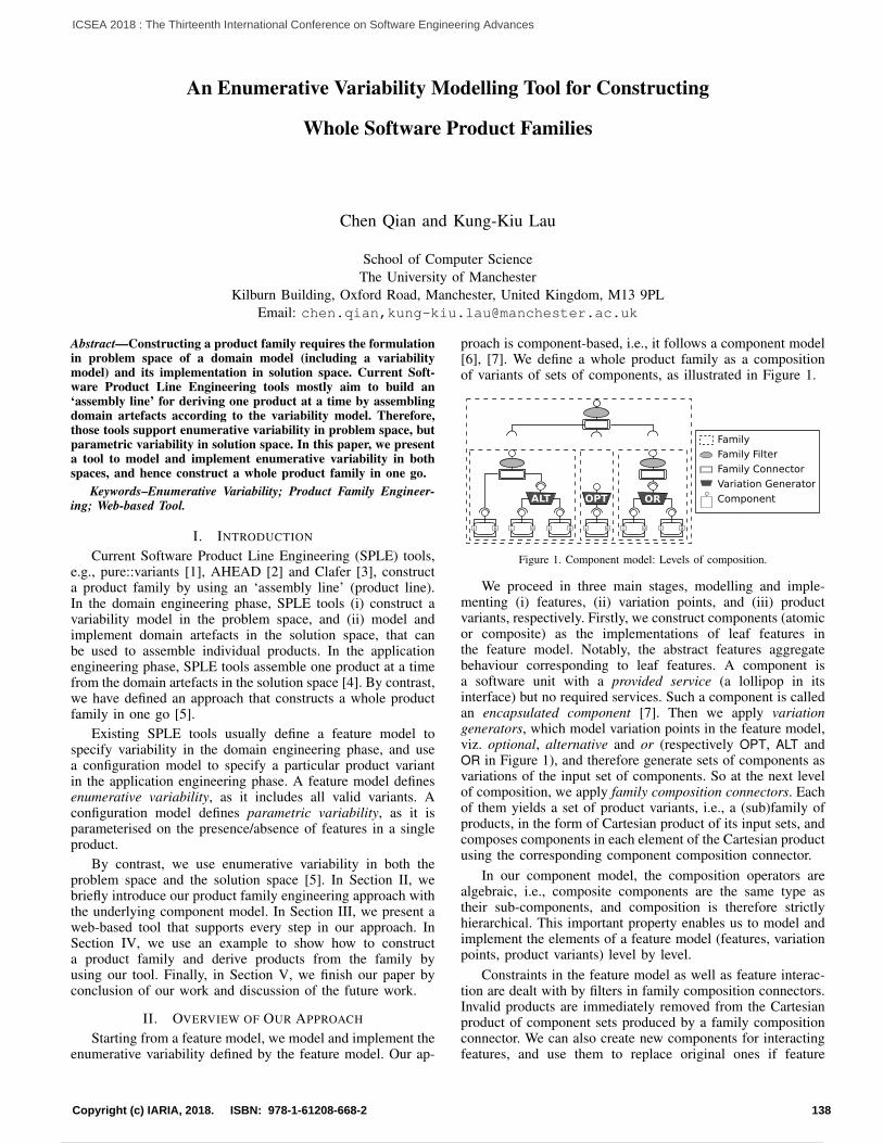
An Enumerative Variability Modelling Tool for Constructing

Whole Software Product Families

Chen Qian and Kung-Kiu Lau

School of Computer ScienceThe University of Manchester

Kilburn Building, Oxford Road, Manchester, United Kingdom, M13 9PLEmail: chen.qian,[email protected]

Abstract—Constructing a product family requires the formulationin problem space of a domain model (including a variabilitymodel) and its implementation in solution space. Current Soft-ware Product Line Engineering tools mostly aim to build an‘assembly line’ for deriving one product at a time by assemblingdomain artefacts according to the variability model. Therefore,those tools support enumerative variability in problem space, butparametric variability in solution space. In this paper, we presenta tool to model and implement enumerative variability in bothspaces, and hence construct a whole product family in one go.

Keywords–Enumerative Variability; Product Family Engineer-ing; Web-based Tool.

I. INTRODUCTION

Current Software Product Line Engineering (SPLE) tools,e.g., pure::variants [1], AHEAD [2] and Clafer [3], constructa product family by using an ‘assembly line’ (product line).In the domain engineering phase, SPLE tools (i) construct avariability model in the problem space, and (ii) model andimplement domain artefacts in the solution space, that canbe used to assemble individual products. In the applicationengineering phase, SPLE tools assemble one product at a timefrom the domain artefacts in the solution space [4]. By contrast,we have defined an approach that constructs a whole productfamily in one go [5].

Existing SPLE tools usually define a feature model tospecify variability in the domain engineering phase, and usea configuration model to specify a particular product variantin the application engineering phase. A feature model definesenumerative variability, as it includes all valid variants. Aconfiguration model defines parametric variability, as it isparameterised on the presence/absence of features in a singleproduct.

By contrast, we use enumerative variability in both theproblem space and the solution space [5]. In Section II, webriefly introduce our product family engineering approach withthe underlying component model. In Section III, we present aweb-based tool that supports every step in our approach. InSection IV, we use an example to show how to constructa product family and derive products from the family byusing our tool. Finally, in Section V, we finish our paper byconclusion of our work and discussion of the future work.

II. OVERVIEW OF OUR APPROACH

Starting from a feature model, we model and implement theenumerative variability defined by the feature model. Our ap-

proach is component-based, i.e., it follows a component model[6], [7]. We define a whole product family as a compositionof variants of sets of components, as illustrated in Figure 1.

Family Filter

Family Connector

Variation Generator

Component

Family

OPT

oi

ALT

oi oi oi

OR

oioi

Figure 1. Component model: Levels of composition.

We proceed in three main stages, modelling and imple-menting (i) features, (ii) variation points, and (iii) productvariants, respectively. Firstly, we construct components (atomicor composite) as the implementations of leaf features inthe feature model. Notably, the abstract features aggregatebehaviour corresponding to leaf features. A component isa software unit with a provided service (a lollipop in itsinterface) but no required services. Such a component is calledan encapsulated component [7]. Then we apply variationgenerators, which model variation points in the feature model,viz. optional, alternative and or (respectively OPT, ALT andOR in Figure 1), and therefore generate sets of components asvariations of the input set of components. So at the next levelof composition, we apply family composition connectors. Eachof them yields a set of product variants, i.e., a (sub)family ofproducts, in the form of Cartesian product of its input sets, andcomposes components in each element of the Cartesian productusing the corresponding component composition connector.

In our component model, the composition operators arealgebraic, i.e., composite components are the same type astheir sub-components, and composition is therefore strictlyhierarchical. This important property enables us to model andimplement the elements of a feature model (features, variationpoints, product variants) level by level.

Constraints in the feature model as well as feature interac-tion are dealt with by filters in family composition connectors.Invalid products are immediately removed from the Cartesianproduct of component sets produced by a family compositionconnector. We can also create new components for interactingfeatures, and use them to replace original ones if feature



149 / 160

Cardinality

Variation Points

(a) Feature model.

(b) All 576 valid variants.

Figure 2. Canvas for constructing feature model.

interactions occur in a product. The interaction rules are setup in the family filters, which are bound with every familycomposition connector, as shown in Figure 1.

III. THE TOOL

Our tool is a web-based graphical tool that implements ourcomponent model [8]. The GUI is realised using HTML5[9]and CSS3 [10], whereas the functionality is implemented usingJavaScript [11]. In particular, we adopt the latest edition ofECMAScript as JavaScript specification since its significantnew syntax, including classes and modules, supports complexapplications. Additionally, we import jQuery [12], the mostwidely deployed JavaScript library, to improve code quality

and enhance system extensibility. Our tool also offers a client-side repository called IndexedDB [13], which is a NoSQLdatabase for massive amounts of structured data, as shown onthe right side of Figure 3 (and Figure 4). For the purpose ofuser-friendliness, all building blocks, including constraints andinteraction, can be easily added through buttons and dialogueboxes, as seen in Figures. 2-5.

The tool provides a workbench with functionalities thatsupport the stages of our approach. Here, we describe thesefunctionalities and illustrate them with the construction of awhole product family with 576 valid variants. The exampleis a family of External Car Lights (ECL) systems, which isadapted from an industrial example provided by pure-systems



150 / 160

Atomic Component

Computation Unit

Unit Test

Execution Result

(a) Atomic component.

Composite Component

Instantiation

Retrieve

Input

Output

Data Channel

Composite Connector

Adapter

(b) Composite component.

Figure 3. Canvases for constructing components for leaf features.

GmbH. The requirement of ECL family is demonstrated inSection IV. Figure 2(a) shows the feature model that containsall 576 valid product variants enumerated in Figure 2(b).

A. Component Construction

Figure 3 shows the canvases provided by our tool forconstructing components for leaf features. After a componentis created, it should be deposited in a repository, and thereforecan be retrieved for further construction.

Figure 3(a) depicts the construction and deposition, of anatomic component, FogLight, which is the implementation

of leaf feature FOG LIGHT. By simply clicking the ‘NewComponent’ button, we can define the component name,service name, input data and output data in a dialogue box,which automatically generates an implementation template forthe computation unit. Additionally, we can immediately testthe component as soon as the computation unit has beenimplemented, and examine the result through browser console.

Figure 3(b) illustrates the construction of a compositecomponent, StaticCornerFogLight. According to re-quirements, it implements the feature interaction caused bySTATIC CORNERING LIGHT and FOG LIGHT. A composite com-



151 / 160

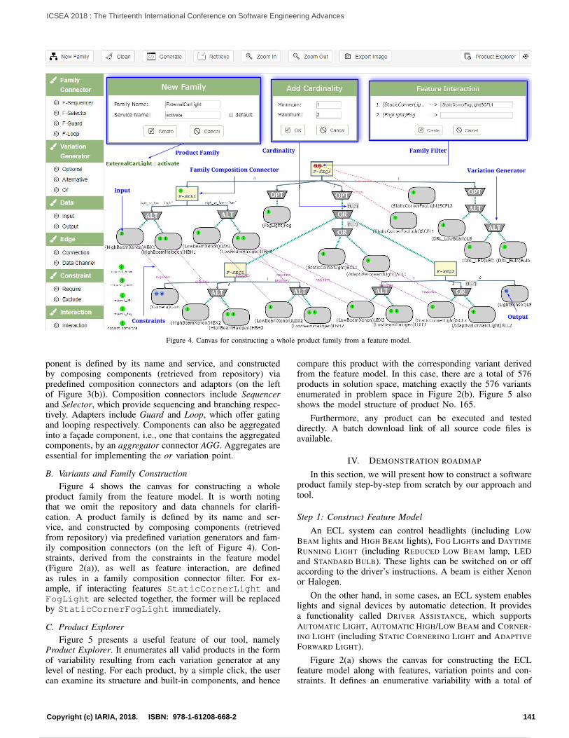
Product Family Family Filter

Input

Cardinality

Variation Generator

OutputConstraints

Family Composition Connector

Figure 4. Canvas for constructing a whole product family from a feature model.

ponent is defined by its name and service, and constructedby composing components (retrieved from repository) viapredefined composition connectors and adaptors (on the leftof Figure 3(b)). Composition connectors include Sequencerand Selector, which provide sequencing and branching respec-tively. Adapters include Guard and Loop, which offer gatingand looping respectively. Components can also be aggregatedinto a façade component, i.e., one that contains the aggregatedcomponents, by an aggregator connector AGG. Aggregates areessential for implementing the or variation point.

B. Variants and Family ConstructionFigure 4 shows the canvas for constructing a whole

product family from the feature model. It is worth notingthat we omit the repository and data channels for clarifi-cation. A product family is defined by its name and ser-vice, and constructed by composing components (retrievedfrom repository) via predefined variation generators and fam-ily composition connectors (on the left of Figure 4). Con-straints, derived from the constraints in the feature model(Figure 2(a)), as well as feature interaction, are definedas rules in a family composition connector filter. For ex-ample, if interacting features StaticCornerLight andFogLight are selected together, the former will be replacedby StaticCornerFogLight immediately.

C. Product ExplorerFigure 5 presents a useful feature of our tool, namely

Product Explorer. It enumerates all valid products in the formof variability resulting from each variation generator at anylevel of nesting. For each product, by a simple click, the usercan examine its structure and built-in components, and hence

compare this product with the corresponding variant derivedfrom the feature model. In this case, there are a total of 576products in solution space, matching exactly the 576 variantsenumerated in problem space in Figure 2(b). Figure 5 alsoshows the model structure of product No. 165.

Furthermore, any product can be executed and testeddirectly. A batch download link of all source code files isavailable.

IV. DEMONSTRATION ROADMAP

In this section, we will present how to construct a softwareproduct family step-by-step from scratch by our approach andtool.

Step 1: Construct Feature ModelAn ECL system can control headlights (including LOW

BEAM lights and HIGH BEAM lights), FOG LIGHTs and DAYTIME

RUNNING LIGHT (including REDUCED LOW BEAM lamp, LEDand STANDARD BULB). These lights can be switched on or offaccording to the driver’s instructions. A beam is either Xenonor Halogen.

On the other hand, in some cases, an ECL system enableslights and signal devices by automatic detection. It providesa functionality called DRIVER ASSISTANCE, which supportsAUTOMATIC LIGHT, AUTOMATIC HIGH/LOW BEAM and CORNER-ING LIGHT (including STATIC CORNERING LIGHT and ADAPTIVE

FORWARD LIGHT).Figure 2(a) shows the canvas for constructing the ECL

feature model along with features, variation points and con-straints. It defines an enumerative variability with a total of



152 / 160

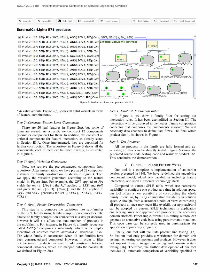
Figure 5. Product explorer and product No.165.

576 valid variants. Figure 2(b) shows all valid variants in termsof feature combinations.

Step 2: Construct Bottom Level ComponentsThere are 20 leaf features in Figure 2(a), but some of

them are reused. As a result, we construct 12 components(atomic or component) for them. In addition, we construct anoptional component for feature interaction, as already statedin Section III-A. Once implemented, they are deposited forfurther construction. The repository in Figure 3 shows all thecomponents, each of them can be tested directly, as illustratedin Figure 6.

Step 3: Apply Variation GeneratorsNow, we retrieve the pre-constructed components from

repository. After instantiation, we have prepared 22 componentinstances for family construction, as shown in Figure 4. Thenwe apply the variation generators according to the featuremodel in Figure 2(a). For example, the OPT applied to Fogyields the set {∅, {Fog}}; the ALT applied to LED and Bulband gives the set {{LED}, {Bulb}}; and the OR applied toAFL1 and SCL1 generates the set {{AFL1}, {SCL1}, {AFL1,SCL1}}.

Step 4: Apply Family Composition ConnectorsThis step is to compose the variations into sub-families

of the ECL family using family composition connectors. Thechoice of family composition connectors is a design decision,however it will not affect the total number of products inthe (sub)family. For instance, in Figure 4, a family sequencercalled F-SEQ1 composes a sub-family, which is the imple-mentation of abstract feature AUTOMATIC HIGH/LOW BEAM.The whole family is constructed when all sub-families havebeen constructed and composed. However, in order to filterout the invalid products, we need to add constraints betweencomponent instances, which are mapped onto the constraintswe defined in Figure 2(a).

Step 4: Establish Interaction RulesIn Figure 4, we show a family filter for setting out

interaction rules. It has been exemplified in Section III. Theinteraction will be displayed in the nearest family compositionconnector that composes the components involved. We addnecessary data channels to define data flows. The final wholeproduct family is shown in Figure 4.

Step 5: Test ProductsAll the products in the family are fully formed and ex-

ecutable, so they can be directly tested. Figure 6 shows thegenerated source code, testing code and result of product 165.This concludes the demonstration.

V. CONCLUSION AND FUTURE WORK

Our tool is a complete re-implementation of an earlierversion presented in [14]. We have re-defined the underlyingcomponent model, added new capabilities including featureinteraction, and used a different technology stack.

Compared to current SPLE tools, which use parametricvariability to configure one product at a time in solution space,our tool offers a new possibility of constructing the wholefamily in one go, by using enumerative variability in solutionspace. Although, from a customer’s point of view, constructingall products at once may seem like overkill, our approach/toolcan be adopted by current SPLE techniques in applicationengineering, since our approach can provide all the necessarydomain artefacts. For example, for the ECL family, our tool cangenerate an annotative code base using pure::variants notations.This code base can be correctly used in pure::variants forapplication engineering (Figure 7).

Finally, our tool will facilitate product line testing [15].So far, our tool only provides a workbench for domain unittesting, i.e., testing components and products. However, it doesnot support domain integration testing and domain systemtesting [16]. Therefore, the further development of our toolincludes (1) automatic comparison of variability specified in



153 / 160

Source Code Testing Code

Execution Result

Figure 6. Product/Component testing.

Figure 7. Generating annotative code base for pure::variants.

the problem space (Figure 2(b)) and implemented in thesolution space (Figure 5), (2) the validity of every data channel,(3) generation of featured statecharts to examine behaviour atfamily level [17], [18].

REFERENCES

[1] D. Beuche, “Modeling and building software product lines withpure::variants,” in Proceedings of the 16th International Software Prod-uct Line Conference-Volume 2. ACM, 2012, pp. 255–255.

[2] D. Batory, “A tutorial on feature oriented programming and the aheadtool suite,” Generative and Transformational Techniques in SoftwareEngineering, 2006, pp. 3–35.

[3] M. Antkiewicz, K. Bak, A. Murashkin, R. Olaechea, J. H. J. Liang,and K. Czarnecki, “Clafer tools for product line engineering,” inProceedings of the 17th International Software Product Line Conferenceco-located workshops. ACM, 2013, pp. 130–135.

[4] K. Berg, J. Bishop, and D. Muthig, “Tracing software product linevariability: From problem to solution space,” 2005, pp. 182–191.

[5] C. Qian and K.-K. Lau, “Enumerative variability in software productfamilies,” in Computational Science and Computational Intelligence(CSCI), 2017 International Conference on. IEEE, 2017, pp. 957–962.

[6] K.-K. Lau and Z. Wang, “Software component models,” IEEE Trans-actions on Software Engineering, vol. 33, no. 10, October 2007, pp.709–724.

[7] K.-K. Lau and S. di Cola, An Introduction to Component-basedSoftware Development. World Scientific, 2017.

[8] C. Qian, “Enumerative Variability Modelling Tool,” http://www.cs.man.ac.uk/~qianc?EVMT, 2018, [Online; accessed 1-July-2018].

[9] G. Anthes, “HTML5 leads a web revolution,” Communications of theACM, vol. 55, no. 7, 2012, pp. 16–17.

[10] T. Celik and F. Rivoal, “CSS basic user interface module level 3 (CSS3UI),” 2012.

[11] D. Flanagan, JavaScript: the definitive guide. O’Reilly Media, Inc.,2006.

[12] D. S. McFarland, JavaScript & jQuery: the missing manual. O’ReillyMedia, Inc., 2011.

[13] S. Kimak and J. Ellman, “The role of html5 indexeddb, the past, presentand future,” in Internet Technology and Secured Transactions (ICITST),2015 10th International Conference for. IEEE, 2015, pp. 379–383.

[14] S. di Cola, K.-K. Lau, C. Tran, and C. Qian, “An MDE tool for definingsoftware product families with explicit variation points,” in Proceedingsof the 19th International Conference on Software Product Line. ACM,2015, pp. 355–360.

[15] T. Thüm, S. Apel, C. Kästner, I. Schaefer, and G. Saake, “Analysisstrategies for software product lines: A classification and survey,”Software Engineering and Management, 2015.

[16] L. Jin-Hua, L. Qiong, and L. Jing, “The w-model for testing softwareproduct lines,” in Computer Science and Computational Technology,2008. ISCSCT’08. International Symposium on, vol. 1. IEEE, 2008,pp. 690–693.

[17] V. H. Fragal, A. Simao, and M. R. Mousavi, “Validated test models forsoftware product lines: Featured finite state machines,” in InternationalWorkshop on Formal Aspects of Component Software. Springer, 2016,pp. 210–227.

[18] A. Classen, P. Heymans, P.-Y. Schobbens, A. Legay, and J.-F. Raskin,“Model checking lots of systems: efficient verification of temporalproperties in software product lines,” in Proceedings of the 32ndACM/IEEE International Conference on Software Engineering-Volume1. ACM, 2010, pp. 335–344.



154 / 160

Feature-Oriented Component-Based Development of Software

Product Families: A Case Study

Chen Qian and Kung-Kiu Lau

School of Computer ScienceThe University of Manchester

Kilburn Building, Oxford Road, Manchester, United Kingdom, M13 9PLEmail: chen.qian,[email protected]

Abstract—Feature-Oriented Software Development (FOSD) iswidely used in Software Product Line Engineering (SPLE). FOSDconstructs product families by incremental feature implementa-tions. In this paper, we introduce a feature-oriented component-based approach, which implements features as an encapsulatedcomponents for further family modelling. A case study of elevatorsystems is also presented to describe the use of our approach.

Keywords–SPLE; FOSD; CBD; Enumerative variability.

I. INTRODUCTION

Software Product Line Engineering (SPLE) traditionallyproceeds in two phases: domain engineering and (ii) applica-tion engineering [1]. In the domain engineering phase, existingSPLE approaches (i) usually use a feature model to specifyvariability, and (ii) from these, identifies and implementsdomain artefacts, e.g., a code base [2]. In the applicationengineering phase, SPLE (i) creates product configurations,and (ii) assembles one product at a time from the domainartefacts based on its configuration [3].

The key abstraction of Feature-Oriented Software Devel-opment (FOSD) is a feature, which represents a logical unitof behaviour specified by a set of functional requirements[4]. FOSD aims at constructing software product families byincremental feature implementations [5]. Thus, variability canbe traced from features directly to the domain artefacts, whichpromises the manageability and maintainability of productfamilies.

In this paper, we present a feature-oriented approach toconstruct product families in a component-based manner, i.e.,following a component model [6]. In [7], we elaboratedthe principles of our component model and discussed thefeasibility of using it in SPLE. Hence, this paper discussesthe concrete details. In Section II, we show the essentialbackground knowledge and related work. In Section III, wepresent a case study to exemplify how to construct a softwareproduct family step-by-step from scratch by our approach andtool. Finally, in Section IV, we finish the paper by conclusionof our work and discussion of the future work.

II. BACKGROUND AND RELATED WORK

The essence of FOSD is to model and implement variabledomain artefacts, and each of them must be mapped onto anon-mandatory feature. In general, three main categories ofvariability mechanisms are adopted in FOSD approaches and

tools [8]: (i) annotative, e.g., CIDE [2], FORM’s macro lan-guage [9] (ii) compositional, e.g., AHEAD [10], FeatureC++[11] and (iii) transformational, e.g., ∆-MontiArc [12], Delta-Oriented Programming (DOP) [13].

Annotative approaches usually build a single, superimposedmodel, namely 150% model, to represent all product variants.The variable features are implemented as code fragments withannotations, i.e., boolean feature expressions. Subsequently,in order to generate a product, code fragments correspond-ing to unselected features have to be removed according tothe product configuration. By comparison, compositional andtransformational approaches develop code fragments isolatedfrom the base programs. Compositional approaches add thefragments correlating with the selected features to the baseprogram for product generation. In regard to transformationalapproaches, fragments are not only added to the base model,but also modified the existing code under some circumstances.

There are two kinds of variability in current FOSD ap-proaches, as known as negative and positive variability [14].The former is adopted by annotative approaches, whereasthe latter is used by compositional approaches. But both ofthem are used in transformational approaches. However, nomatter negative or positive, we consider such a variability asa parametric variability, due to it is parameterised on thepresence or absence of features in a single product. Thus, SPLEapproaches using parametric variability can only generate oneproduct at a time. On contrary, enumerative variability includesall valid variants directly [7]. For example, in the problemspace, feature model defines enumerative variability, whilea configuration model defines parametric variability. In thispaper, our approach construct enumerative variability in thesolution space, which results in a whole product family andtherefore all products can be generated in one go.

Another area where our approach could bring advantagesis feature mapping. The early work on SPLE, such as FODA[15], did not represent features explicitly, instead build n-to-mmappings between features and domain artefacts, which causessevere tangling and scattering in the code base eventually.Hence, the construction of product families are infeasible.FOSD have made a great progress by bringing a distinguishingproperty that aims at 1-to-n feature mappings. However, itbecomes obvious that the ideal mapping is 1-to-1 [16], butit is difficult to be achieved in current FOSD approaches,mostly because of the cross-cutting concern of features. Ourapproach is capable to build 1-to-1 mappings between features



155 / 160

and components. In this paper, we show how to deal with thecross-cutting problem in the case study.

Regarding to the outstanding maintainability and reusabil-ity, component-based development (CBD) is another paradigmthat seems suitable for SPLE. But earlier researches certifiedthat constructing product families only using CBD is barelyfeasible, due to features often do not align well with thedecomposition imposed by component models [5]. Some re-searches [17], [18] try to integrate CBD and FOSD in orderto obtain both their advantages in SPLE, but problems stilloccurs. In this paper, our approach adopts a state-of-the-artcomponent model that partners FOSD very well.

III. A CASE STUDY

We have developed a web-based graphical tool that imple-ments our component model and constructs product families[19]. The graphical user interface (GUI) is realised usingHTML5 and CSS3, whereas the functionality is implementedusing JavaScript. In particular, we adopt the latest edition ofECMAScript as JavaScript specification since its significantnew syntax, including classes and modules, supports com-plex applications. Additionally, we import jQuery, the mostwidely deployed JavaScript library, to improve code qualityand enhance system extensibility. For the purpose of user-friendliness, all building blocks, including constraints andinteraction, can be easily added through buttons and dialogueboxes.

In this section, we use an example of the elevator productfamily, which originates from [20], developed by Feature-Oriented Programming (FOP) in FeatureIDE [21]. The elevatorcontains a control logic mode that can be either Sabbath orFIFO, and an optional feature called Service. In Sabbathmode, the elevator reaches all levels periodically without userinput, whereas in FIFO mode, the elevator moves to specificfloors in turns according to the requests. The Service isspecial, it allows authorised persons to send the elevator to thelowest floor. Notably, Service is a cross-cutting feature, asits implementation scatters across other features’ (Sabbathand FIFO) implementations. Consequently, the behaviour ofService can be triggered at any time, and on any mode,during elevator running period.

We will implement the elevator family in our tool, byextending it with the 3 features one at a time. Notably, forthe clarification, we omit data channels in the figures in thispaper. The design and implementation process is identical tothe original example. Therefore, we can evaluate our approachbased on the scientific control.

A. Adding Feature “Sabbath” to the Elevator Product LineWe add Sabbath as an optional child feature of the root,

as shown in Figure 1. Then we need to implement a componentfor it. It is worth noting the underlying component model isalready described in [6] and [7].

According to the requirement analysis of Sabbath, wecan identify 3 behaviours behind it. Figure 2 shows thecomposite component composed by several atomic componentsand composition connectors. For example, MovingUp controlsthe elevator to move one floor up and returns the next direction,while MovingDown makes the opposite move. Contrariwise,Flooring leaves the elevator in the current floor. The selector

Figure 1. Adding Sabbath to the feature model.

SELs define branching depending on selection conditions,whereas the sequencer SEQ defines sequencing sequentially.As a result, the elevator changes direction when it reachesbottom floor and top floor.

Figure 2. Component Sabbath.

After all, the elevator moves one floor up or down foreach execution of Sabbath. In order to keep the elevatorrunning, we only need to apply an adaptor, called loop, torepeat the control to this component (not discussed in detailhere). Figure 3 shows the transition systems of the Sabbathcomponent within the elevator product, which gives us a clearvision of the behaviour. So far no cross-cutting occurs, due toonly one product exists.

1

2

3

4

5

up_direction

top_floor/MovingDown

down_direction

!top_floor/MovingUp

bottom_floor/MovingUp

!bottom_floor/MovingDown

Flooring

1Sabbath

2

Figure 3. Transition systems of Elevator and Sabbath.

B. Adding Feature “Service” to the Elevator Product LineNow, we add Service feature to the elevator product

family. As this feature has no functional dependencies withSabbath, we put it under the root. In addition, Servicefeature is not always required by every product, thus we set itoptional. Figure 4 shows the change of the feature model.

We can reuse two components implemented before: Mov-ingDown and Flooring. But in order to construct Servicecomponent, we need to implement another, namely StopSer-vice, which allows the authorised persons to deactivate the



156 / 160

Figure 4. Adding Service to the feature model.

Service functionality after the elevator reaches the bottomfloor. Figure 5 shows the construction of Service component.

Figure 5. Component Service.

Next, we need to apply variation generators to the compo-nents, which are mapped onto the variation points specified inthe feature model (Figure 4). A variation generator generatesmultiple variants: it takes (a set of) sets of components asinput and produces (a set of) permuted sets of components,i.e., variants. We have implemented variation generators forthe full range of standard variation points, viz. optional,alternative and or (respectively OPT, ALT and OR. Notably, thecomponents are algebraic and hierarchical at this level, whichmeans the variation generator can be nested.

Figure 6. Elevator product family with Service.

At the next level of composition in our component model,family composition takes place, by means of family compo-sition operators, also defined as connectors. A family compo-sition operator is applied to multiple input component sets toyield a set of product variants, i.e., a (sub)family of products.These operators are defined in terms of the component com-position operators: a family composition connector forms theCartesian product of its input sets, and composes componentsin each element of the Cartesian product using the corre-sponding component composition connector. For example, inFigure 6, the family composition connector F-SEL appliesthe corresponding component composition connector SEL tocomponents in each element of the Cartesian product, as well

as the F-LOP indicates LOP (loop). The result of a familycomposition is thus also a family, so this level of compositionis also algebraic.

The choice of family composition connectors is a designdecision that only depends on the functional requirements,however it will not affect the total number of products in the(sub)families. Figure 6 shows the elevator family with twooptional features. Derived from the family model in Figure 6,Figure 7 shows a featured transition system (FTS) [22] of thefamily, which depicts the cross-cutting feature Service takespart in family behaviour, e.g., 1-2-3-1 workflow.

4

StopServicebottom_floor/Flooring

12 3

!bottom_floor/MovingDown

1 2 3Sabbath Service

Service

Figure 7. FTS of Elevator and Service.

At present, the elevator family generates 3 products, asshown in the product explorer in Figure 8. The productexplorer enumerates all valid products in the form of variabilityresulting from each variation generator at any level of nesting.For each product, the user can examine its structure andbuilt-in components, and hence compare this product with thecorresponding variant derived from the feature model.

Figure 8. Product explorer (3 products).

C. Adding Feature “FIFO” to the Elevator Product LineFIFO (first in, first out) is another control logic of the

elevator. As the name suggests, if more than one floor requestsexist, the oldest request is handled first, i.e., the elevatordirectly move to the required floor. By contrast with the featureService, FIFO is an alternative to the already existingSabbath mode. Therefore, we reform the feature model byadding features and modifying variation points, as Figure 9shows.

Figure 9. Adding FIFO to the feature model.

Likewise, we implement a component FIFO for featureFIFO. Figure 10 shows the architecture of the component,



157 / 160

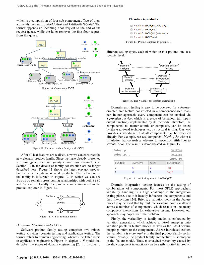
which is a composition of four sub-components. Two of themare newly prepared: FloorQueue and RemoveRequest. Theformer appends an incoming floor request to the end of therequest queue, while the latter removes the first floor requestfrom the queue.

Figure 10. Component FIFO.

Figure 11. Elevator product family with FIFO.

After all leaf features are realised, now we can construct thenew elevator product family. Since we have already presentedvariation generators and family composition connectors inSection III-B, the details of family construction are no longerdescribed here. Figure 11 shows the latest elevator productfamily, which contains 4 valid products. The behaviour ofthe family is illustrated in Figure 12, in which we can seeService remains cross-cutting relationships with both FIFOand Sabbath. Finally, the products are enumerated in theproduct explorer in Figure 13.

1

2

3

4

ServiceFIFO

Sabbath Service

Service

Figure 12. FTS of Elevator family.

D. Testing Elevator Product LineSoftware product family testing comprises two related

testing activities: domain testing and application testing. Theformer refers to domain engineering, whereas the latter refersto application engineering. Figure 14 depicts a V-model thatdescribes the stages of domain engineering [23]. It involves 3

Figure 13. Product explorer (4 products).

different testing types, each of which tests a product line at aspecific level.

DomainAnalysis

DomainDesign

DomainImplementation

Domain UnitTesting

DomainIntegration

Testing

Domain SystemTesting

Figure 14. The V-Model for domain engineering.

Domain unit testing is easy to be operated for a feature-oriented architecture constructed in a component-based man-ner. In our approach, every component can be invoked viaa provided service, which is a piece of behaviour (an input-output function) implemented by its methods. Therefore, thecomponents, no matter atomic or composite, can be testedby the traditional techniques, e.g., structural testing. Our toolprovides a workbench that all components can be executeddirectly. For example, we test component MovingUp within asimulation that controls an elevator to move from fifth floor toseventh floor. The result is demonstrated in Figure 15.

Figure 15. Unit testing result of MovingUp.

Domain integration testing focuses on the testing ofcombinations of components. For most SPLE approaches,variability handling is a huge challenge in the integrationtesting phase, due to it heavily influences the components andtheir interactions [24]. Briefly, a variation point in the featuremodel may be modelled by multiple variation points scatteredacross a number of components, which results in too manycomponent interactions for exhaustive testing. However, ourapproach may copes with the problem.

Firstly, the variability in family model is embodied byvariation generators, which achieve a 1-to-1 mapping ontovariation points in feature model, as well as the 1-to-1 featuremappings refers to the components. As we introduced earlier,the variability is enumerative in the final product family archi-tecture. Notably, the product family architecture is isomorphicto the feature model. Thus, mismatched variability caused byinvalid component interactions can be easily spotted in product



158 / 160

explorer. For example, in Figure 11, if we misplace an ORvariation generator on the top of FIFO and Sabbath insteadof ALT variation generator, then we can observe 5 productsin the product explorer. That is obviously incorrect due to thefeature model only gives 4 product variants in total.

Secondly, the component model adopted in our approachexposes a provided service, but no required service. Suchcomponents are known as encapsulated components [6]. Thereare no coupling between encapsulated components, i.e., theydo not call others. Instead, they are invoked by compositionconnectors. Thereby, we do not need to worry about the faultycomponent compounds, i.e., the incorrect bound interfaces.Moreover, as we mentioned earlier, the level of family com-position is algebraic, as it generates a set of encapsulatedcomponents, which can be tested directly.

In conclusion, the distinguished property of our com-ponent model makes domain integration testing convenientand crystal, especially for the software product families ofnon-trivial size. All we have to do is examining the 1-to-1 mappings between (i) (leaf) features and components, (ii)variation points and variation generators. The correctness ofbehaviours between components will be tested at the next level.

Domain system testing evaluate all products’ compliancewith their requirements. It becomes obvious that verifying thebehaviour of each product individually is difficult due to anexponential number of combinations of assets is unmanageable[25]. Since by our approach, the control flows are clearlycoordinated by exogenous connectors and the componentsare directly mapped onto features, every family model canderive a family-based functional model that describes thecombined behaviour of an entire family, such as FTS [22] orFeatured Finite State Machine (FFSM) [26]. In this section, wehave generated FTS diagrams for different elevator familiesin Figure 7 and Figure 12. The FTS describes the overallbehaviour of family, and hence the behaviours of every productwithin the family. For example, if we misplace a F-SEQ(family sequencer) instead of F-SEL (family selector) in thefamily model in Figure 11, then the derived FTS would notshow the 1-4 workflow as in Figure 12. Therefore, we candetect the problems in family composition, due to the FTSdoes not describe the required behaviour.

Family-based functional model can help us to verify the be-haviour of component interactions, but it is not straightforwardto validate the execution results. However, we cannot order testexecutions for every single product. Thus, we should executea test case in the whole product family, i.e., all configurationsof the family, without actually generating a concrete product.In that case, a product line testing method, called Variability-Aware Testing [27], is perfect for our family model. The keystep of variability-aware testing is to extract an abstract syntaxtree (AST) with explicit variability. In our approach, the finalfamily model has a tree structure with enumerative variability,so it provides a seamless migration to the testing model.The testing model of the elevator example is demonstrated inFigure 16 (not discussed in detail here because of the limitedspace).

E. Product GenerationIn Section II, we have presented that our approach construct

enumerative variability in the solution space. In other words,all valid products are defined during composition. Unlike

FIFO Sabbath

Service

maxFloor=5

currentFloor=2

minFloor=1

direction=up

queue_in=[3,4]

nextFloor=3

queue_out=[4] nextDirection=up

minFloor=1

Figure 16. Variability-aware testing of Elevator.

conventional FOSD approaches, we can ‘pick up’ any numberof products from the product explorer in one go, instead ofone product at a time via configuration.

Here, to exemplify, we choose product No.3 from theproduct explorer in Figure 13. Figure 17(a) shows the productarchitecture, which is executable, and Figure 17(b) expressespartial execution result.

(a) (b)

Figure 17. Product 3.

IV. CONCLUSION AND FUTURE WORK

By comparison with the original elevator family imple-mentation in [20], our implementation has many merits. Forexample, the original example is realised by FOP, in whichevery feature is mapped onto multiple code fragments scat-tering cross three classes. Each feature cannot be tested inisolation. Simply put, our approach provides better maintain-ability, manageability and testability because of the explicit1-to-1 feature mappings. However, our family model onlyrealises behaviour in the family. Contrariwise, in [20], FOPcan define user interface for simulation, because as a low-levelprogramming language, FOP can overwrite any code directly.

To provide step-by-step instructions of how to use ourapproach for family construction, we choose a small examplefor the simplicity. But our approach can be used for productfamilies of non-trivial size. Besides the functions shown in



159 / 160

Section III, our tool can deal with cross-tree constraints (e.g.,‘require’, ‘exclude’) among features, and among components.Our tool can also set cardinalities to narrow down massivefamilies. Moreover, our tool can handle feature interactionproblem, which becomes the most significant challenge inSPLE [28], by importing extra off-the-shelf components duringcomposition. As a matter of fact, we have successfully con-structed product families for industrial cases, i.e., consistingof dozens of features and hundreds of products. In future, weplan to present these results of our research.

According to [29], in the real world, many organisationsadopt product families using three techniques: proactive, re-active and extractive. A proactive approach implies that aproduct family is modelled from scratch. In contrast, a reactiveapproach begins with a small, easy to handle product family,which can be incrementally extended with new features andartefacts. An extractive approach starts with a portfolio ofexisting products and gradually refactors them to constructa product family. At present, it is apparent that our workis proactive. However, recent researches [30], [31] in reverseengineering suggest that our work also has potential to supportreactive and extractive techniques.

REFERENCES

[1] K. Pohl, G. Bockle, and F. J. van Der Linden, Software Product LineEngineering: Foundations, Principles and Techniques. Springer Science& Business Media, 2005.

[2] C. Kastner, S. Trujillo, and S. Apel, “Visualizing software product linevariabilities in source code.” in SPLC (2), 2008, pp. 303–312.

[3] K. Berg, J. Bishop, and D. Muthig, “Tracing software product linevariability: From problem to solution space,” 2005, pp. 182–191.

[4] J. Bosch, Design and use of software architectures: adopting andevolving a product-line approach. Pearson Education, 2000.

[5] S. Apel and C. Kastner, “An overview of feature-oriented softwaredevelopment.” Journal of Object Technology, vol. 8, no. 5, 2009, pp.49–84.

[6] K.-K. Lau and S. di Cola, An Introduction to Component-basedSoftware Development. World Scientific, 2017.

[7] C. Qian and K.-K. Lau, “Enumerative variability in software productfamilies,” in Computational Science and Computational Intelligence(CSCI), 2017 International Conference on. IEEE, 2017, pp. 957–962.

[8] A.-L. Lamprecht, S. Naujokat, and I. Schaefer, “Variability managementbeyond feature models,” Computer, vol. 46, no. 11, 2013, pp. 48–54.

[9] K. C. Kang, J. Lee, and P. Donohoe, “Feature-Oriented Product LineEngineering,” IEEE software, vol. 19, no. 4, 2002, pp. 58–65.

[10] D. Batory, J. Sarvela, and A. Rauschmayer, “Scaling step-wise refine-ment,” IEEE Trans. Software Eng., vol. 30, no. 6, 2004, pp. 355–371.

[11] S. Apel, T. Leich, M. Rosenmuller, and G. Saake, “FeatureC++: onthe symbiosis of feature-oriented and aspect-oriented programming,” inGenerative Programming and Component Engineering. Springer, 2005,pp. 125–140.

[12] A. Haber, T. Kutz, H. Rendel, B. Rumpe, and I. Schaefer, “Delta-oriented architectural variability using MontiCore,” in Proceedings ofthe 5th European Conference on Software Architecture: CompanionVolume. ACM, 2011, p. 6.

[13] I. Schaefer, L. Bettini, V. Bono, F. Damiani, and N. Tanzarella, “Delta-oriented programming of software product lines,” in Software ProductLines: Going Beyond. Springer, 2010, pp. 77–91.

[14] I. Schaefer, “Variability modelling for model-driven development ofsoftware product lines.” VaMoS, vol. 10, 2010, pp. 85–92.

[15] K. Kang, S. Cohen, J. Hess, W. Novak, and A. Peterson, “Feature-oriented domain analysis (FODA) feasibility study,” Software Engineer-ing Institute, Carnegie-Mellon University, Tech. Rep. CMU/SEI-90-TR-021, 1990.

[16] C. Kastner and S. Apel, “Feature-oriented software development,” inGenerative and Transformational Techniques in Software EngineeringIV. Springer, 2013, pp. 346–382.

[17] W. Zhang, H. Mei, H. Zhao, and J. Yang, “Transformation from CIM toPIM: A feature-oriented component-based approach,” in InternationalConference on Model Driven Engineering Languages and Systems.Springer, 2005, pp. 248–263.

[18] P. Trinidad, A. R. Cortes, J. Pena, and D. Benavides, “Mapping featuremodels onto component models to build dynamic software productlines.” in SPLC (2), 2007, pp. 51–56.

[19] C. Qian, “Enumerative Variability Modelling Tool,” http://www.cs.man.ac.uk/∼qianc?EVMT, 2018, [Online; accessed 1-July-2018].

[20] J. Meinicke et al., “Developing an elevator with feature-orientedprogramming,” in Mastering Software Variability with FeatureIDE.Springer, 2017, pp. 155–171.

[21] C. Kastner, T. Thum, G. Saake, J. Feigenspan, T. Leich, F. Wielgorz, andS. Apel, “FeatureIDE: A tool framework for feature-oriented softwaredevelopment,” in Proceedings of 31st ICSE. IEEE, 2009, pp. 611–614.

[22] A. Classen, P. Heymans, P.-Y. Schobbens, A. Legay, and J.-F. Raskin,“Model checking lots of systems: efficient verification of temporalproperties in software product lines,” in Proceedings of the 32ndACM/IEEE International Conference on Software Engineering-Volume1. ACM, 2010, pp. 335–344.

[23] J. Lee, S. Kang, and D. Lee, “A survey on software product linetesting,” in Proceedings of the 16th International Software Product LineConference-Volume 1. ACM, 2012, pp. 31–40.

[24] L. Jin-Hua, L. Qiong, and L. Jing, “The w-model for testing softwareproduct lines,” in Computer Science and Computational Technology,2008. ISCSCT’08. International Symposium on, vol. 1. IEEE, 2008,pp. 690–693.

[25] T. Thum, S. Apel, C. Kastner, I. Schaefer, and G. Saake, “Analysisstrategies for software product lines: A classification and survey,” Soft-ware Engineering and Management 2015. Gesellschaft fr Informatike.V., 2015, pp. 57–58.

[26] V. H. Fragal, A. Simao, and M. R. Mousavi, “Validated test models forsoftware product lines: Featured finite state machines,” in InternationalWorkshop on Formal Aspects of Component Software. Springer, 2016,pp. 210–227.

[27] C. Kastner et al., “Toward variability-aware testing,” in Proceedings ofthe 4th International Workshop on Feature-Oriented Software Develop-ment. ACM, 2012, pp. 1–8.

[28] M. Calder, M. Kolberg, E. H. Magill, and S. Reiff-Marganiec, “Fea-ture interaction: a critical review and considered forecast,” ComputerNetworks, vol. 41, no. 1, 2003, pp. 115–141.

[29] C. Krueger, “Easing the transition to software mass customization,” inSoftware Product-Family Engineering. Springer, 2002, pp. 282–293.

[30] R. Arshad and K.-K. Lau, “Extracting executable architecture fromlegacy code using static reverse engineering,” in Proceedings of 12thInternational Conference on Software Engineering Advances. IARIA,2017, pp. 55–59.

[31] R. Arshad and K.-K. Lau, “Reverse engineering encapsulated com-ponents from object-oriented legacy code,” in Proceedings of The30th International Conference on Software Engineering and KnowledgeEngineering. KSI Research Inc., July 2018, pp. 572–577.



Powered by TCPDF (www.tcpdf.org)

160 / 160

http://www.tcpdf.org

ICSEA 2018 Proceedings - ThinkMind

Documents

Transcript of ICSEA 2018 Proceedings - ThinkMind