IBM SPSS Modeler 17 Source, Process, and Output Nodes

IBM SPSS Modeler 17 Source, Process,and Output Nodes

��

NoteBefore using this information and the product it supports, read the information in “Notices” on page 357.

Product Information

This edition applies to version 17, release 0, modification 0 of IBM(r) SPSS(r) Modeler and to all subsequent releasesand modifications until otherwise indicated in new editions.

Contents

Preface . . . . . . . . . . . . . . vii

Chapter 1. About IBM SPSS Modeler . . 1IBM SPSS Modeler Products . . . . . . . . . 1

IBM SPSS Modeler . . . . . . . . . . . 1IBM SPSS Modeler Server . . . . . . . . . 1IBM SPSS Modeler Administration Console . . . 2IBM SPSS Modeler Batch . . . . . . . . . 2IBM SPSS Modeler Solution Publisher . . . . . 2IBM SPSS Modeler Server Adapters for IBM SPSSCollaboration and Deployment Services . . . . 2

IBM SPSS Modeler Editions . . . . . . . . . 2IBM SPSS Modeler Documentation . . . . . . . 3

SPSS Modeler Professional Documentation . . . 3SPSS Modeler Premium Documentation . . . . 4

Application Examples . . . . . . . . . . . 4Demos Folder . . . . . . . . . . . . . . 4

Chapter 2. Source Nodes . . . . . . . 5Overview . . . . . . . . . . . . . . . 5Setting Field Storage and Formatting . . . . . . 6

List storage and associated measurement levels . . 9Unsupported control characters. . . . . . . . 10Analytic Server Source Node . . . . . . . . 10

Selecting a data source . . . . . . . . . 10Amending credentials . . . . . . . . . . 11Supported nodes . . . . . . . . . . . 11

Database Source Node. . . . . . . . . . . 14Setting Database Node Options. . . . . . . 15Adding a database connection . . . . . . . 16Specifying preset values for a databaseconnection. . . . . . . . . . . . . . 17Selecting a Database Table . . . . . . . . 20Querying the Database . . . . . . . . . 21

Variable File Node . . . . . . . . . . . . 22Setting options for the Variable File Node . . . 23Importing geospatial data into the Variable FileNode . . . . . . . . . . . . . . . 25

Fixed File Node . . . . . . . . . . . . . 26Setting Options for the Fixed File Node . . . . 26

Data Collection Node . . . . . . . . . . . 27Data Collection Import File Options . . . . . 28IBM SPSS Data Collection Import MetadataProperties . . . . . . . . . . . . . . 30Database Connection String . . . . . . . . 31Advanced Properties . . . . . . . . . . 31Importing Multiple Response Sets . . . . . . 31IBM SPSS Data Collection Column Import Notes 31

IBM Cognos BI Source Node . . . . . . . . 32Cognos object icons. . . . . . . . . . . 32Importing Cognos data . . . . . . . . . 33Importing Cognos reports . . . . . . . . 34Cognos connections . . . . . . . . . . 34Cognos location selection . . . . . . . . . 35Specifying parameters for data or reports . . . 35

IBM Cognos TM1 Source Node . . . . . . . . 35Importing IBM Cognos TM1 data . . . . . . 36

SAS Source Node . . . . . . . . . . . . 36Setting Options for the SAS Source Node . . . 37

Excel Source Node . . . . . . . . . . . . 37XML Source Node . . . . . . . . . . . . 38

Selecting from Multiple Root Elements . . . . 39Removing Unwanted Spaces from XML SourceData . . . . . . . . . . . . . . . . 39

User Input Node . . . . . . . . . . . . 40Setting Options for the User Input Node . . . 40

Simulation Generate Node . . . . . . . . . 44Setting Options for the Simulation GenerateNode . . . . . . . . . . . . . . . 45Clone Field . . . . . . . . . . . . . 50Fit Details . . . . . . . . . . . . . . 50Specify Parameters . . . . . . . . . . . 51Distributions . . . . . . . . . . . . . 53

Data View node . . . . . . . . . . . . . 56Setting Options for the Data View Node. . . . 56

Geospatial Source Node . . . . . . . . . . 57Setting Options for the Geospatial Source Node 57

Enterprise View Node . . . . . . . . . . . 58Setting Options for the Enterprise View Node . . 59Enterprise View Connections . . . . . . . 59Choosing the DPD . . . . . . . . . . . 60Choosing the Table . . . . . . . . . . . 60

Common Source Node Tabs . . . . . . . . . 60Setting Measurement Levels in the Source Node 61Filtering Fields from the Source Node . . . . 61

Chapter 3. Record Operations Nodes 63Overview of Record Operations . . . . . . . 63Select Node . . . . . . . . . . . . . . 64Sample Node . . . . . . . . . . . . . . 65

Sample Node Options . . . . . . . . . . 65Cluster and Stratify Settings . . . . . . . . 67Sample Sizes for Strata . . . . . . . . . 68

Balance Node. . . . . . . . . . . . . . 69Setting Options for the Balance Node. . . . . 69

Aggregate Node . . . . . . . . . . . . . 70Setting Options for the Aggregate Node . . . . 70Aggregate optimization settings . . . . . . 72

RFM Aggregate Node . . . . . . . . . . . 73Setting Options for the RFM Aggregate Node . . 73

Sort Node . . . . . . . . . . . . . . . 74Sort Optimization Settings . . . . . . . . 74

Merge Node . . . . . . . . . . . . . . 75Types of Joins . . . . . . . . . . . . 75Specifying a Merge Method and Keys . . . . 77Selecting Data for Partial Joins . . . . . . . 78Specifying Conditions for a Merge. . . . . . 78Specifying Ranked Conditions for a Merge . . . 78Filtering Fields from the Merge Node. . . . . 80Setting Input Order and Tagging . . . . . . 81

iii

Merge Optimization Settings . . . . . . . 81Append Node . . . . . . . . . . . . . 82

Setting Append Options . . . . . . . . . 82Distinct node . . . . . . . . . . . . . . 83

Distinct Optimization Settings . . . . . . . 85Distinct Composite Settings . . . . . . . . 85

Streaming TS Node . . . . . . . . . . . . 87Streaming TS Field Options . . . . . . . . 88Streaming TS Model Options . . . . . . . 88Time Series Expert Modeler Criteria . . . . . 89Time Series Exponential Smoothing Criteria . . 90Time Series ARIMA Criteria . . . . . . . . 91Transfer Functions . . . . . . . . . . . 92Handling Outliers . . . . . . . . . . . 93Streaming TS Deployment Options . . . . . 93

Streaming TCM Node . . . . . . . . . . . 94Streaming TCM Node - Time Series options . . 94Streaming TCM Node - Observations options . . 95Streaming TCM Node - Time Interval options . . 96Streaming TCM Node - Aggregation andDistribution options . . . . . . . . . . 96Streaming TCM Node - Missing Value options. . 97Streaming TCM Node - General Data options . . 97Streaming TCM Node - General Build options . . 97Streaming TCM Node - Estimation Periodoptions . . . . . . . . . . . . . . . 98Streaming TCM Node - Model options . . . . 98

Space-Time-Boxes Node . . . . . . . . . . 99Defining Space-Time-Box density . . . . . . 101

Chapter 4. Field Operations Nodes 103Field Operations Overview . . . . . . . . . 103Automated Data Preparation . . . . . . . . 105

Fields Tab . . . . . . . . . . . . . 106Settings Tab . . . . . . . . . . . . . 107Analysis Tab. . . . . . . . . . . . . 111Generating a Derive Node . . . . . . . . 117

Type Node . . . . . . . . . . . . . . 118Measurement Levels . . . . . . . . . . 119Converting Continuous Data . . . . . . . 122What Is Instantiation? . . . . . . . . . 123Data Values . . . . . . . . . . . . . 123Defining Missing Values. . . . . . . . . 127Checking Type Values . . . . . . . . . 127Setting the Field Role. . . . . . . . . . 128Copying Type Attributes . . . . . . . . 129Field Format Settings Tab . . . . . . . . 129

Filtering or Renaming Fields . . . . . . . . 131Setting Filtering Options. . . . . . . . . 131

Derive Node . . . . . . . . . . . . . 133Setting Basic Options for the Derive Node. . . 134Deriving Multiple Fields. . . . . . . . . 135Setting Derive Formula Options . . . . . . 136Setting Derive Flag Options . . . . . . . 137Setting Derive Nominal Options . . . . . . 138Setting Derive State Options . . . . . . . 138Setting Derive Count Options . . . . . . . 139Setting Derive Conditional Options . . . . . 139Recoding Values with the Derive Node. . . . 139

Filler Node . . . . . . . . . . . . . . 139Storage Conversion Using the Filler Node . . . 140

Reclassify Node . . . . . . . . . . . . 141Setting Options for the Reclassify Node . . . 141Reclassifying Multiple Fields . . . . . . . 142Storage and Measurement Level for ReclassifiedFields . . . . . . . . . . . . . . . 142

Anonymize Node . . . . . . . . . . . . 143Setting Options for the Anonymize Node . . . 143Anonymizing Field Values . . . . . . . . 144

Binning Node . . . . . . . . . . . . . 145Setting Options for the Binning Node . . . . 145Fixed-Width Bins . . . . . . . . . . . 146Tiles (Equal Count or Sum). . . . . . . . 146Rank Cases . . . . . . . . . . . . . 148Mean/Standard Deviation . . . . . . . . 148Optimal Binning . . . . . . . . . . . 149Previewing the Generated Bins . . . . . . 150

RFM Analysis Node . . . . . . . . . . . 150RFM Analysis Node Settings . . . . . . . 151RFM Analysis Node Binning . . . . . . . 152

Ensemble Node . . . . . . . . . . . . 152Ensemble Node Settings . . . . . . . . . 153

Partition Node . . . . . . . . . . . . . 154Partition Node Options . . . . . . . . . 154

Set to Flag Node . . . . . . . . . . . . 155Setting Options for the Set to Flag Node . . . 155

Restructure Node . . . . . . . . . . . . 156Setting Options for the Restructure Node . . . 157

Transpose Node . . . . . . . . . . . . 158Setting Options for the Transpose Node . . . 158

Time Intervals Node . . . . . . . . . . . 159Specifying Time Intervals . . . . . . . . 160Time Interval Build Options . . . . . . . 160Estimation Period . . . . . . . . . . . 161Forecasts . . . . . . . . . . . . . . 162Supported Intervals . . . . . . . . . . 163

History Node . . . . . . . . . . . . . 169Setting Options for the History Node . . . . 170

Field Reorder Node . . . . . . . . . . . 170Setting Field Reorder Options . . . . . . . 170

AS Time Intervals Node . . . . . . . . . . 172AS Time Interval - field options . . . . . . 172AS Time Interval - build options . . . . . . 172

Reprojection Node. . . . . . . . . . . . 173Setting options for the Reproject node . . . . 173

Chapter 5. Graph Nodes. . . . . . . 175Common Graph Nodes Features . . . . . . . 175

Aesthetics, Overlays, Panels, and Animation . . 176Using the Output Tab . . . . . . . . . 177Using the Annotations Tab . . . . . . . . 1783-D Graphs . . . . . . . . . . . . . 178

Graphboard Node . . . . . . . . . . . . 179Graphboard Basic Tab . . . . . . . . . 179Graphboard Detailed Tab . . . . . . . . 183Available Built-in Graphboard VisualizationTypes . . . . . . . . . . . . . . . 184Creating Map Visualizations . . . . . . . 191Graphboard Examples . . . . . . . . . 192Graphboard Appearance Tab . . . . . . . 202Setting the Location of Templates, Stylesheets,and Maps . . . . . . . . . . . . . 203

iv IBM SPSS Modeler 17 Source, Process, and Output Nodes

Managing Templates, Stylesheets, and Map Files 204Converting and Distributing Map Shapefiles . . . 205

Key Concepts for Maps . . . . . . . . . 206Using the Map Conversion Utility . . . . . 206Distributing map files . . . . . . . . . 211

Plot Node . . . . . . . . . . . . . . 212Plot Node Tab . . . . . . . . . . . . 214Plot Options Tab . . . . . . . . . . . 215Plot Appearance Tab . . . . . . . . . . 216Using a Plot Graph . . . . . . . . . . 217

Multiplot Node. . . . . . . . . . . . . 217Multiplot Plot Tab . . . . . . . . . . . 218Multiplot Appearance Tab . . . . . . . . 219Using a Multiplot Graph . . . . . . . . 219

Time Plot Node . . . . . . . . . . . . 220Time Plot Tab . . . . . . . . . . . . 221Time Plot Appearance Tab . . . . . . . . 222Using a Time Plot Graph . . . . . . . . 222

Distribution Node . . . . . . . . . . . . 223Distribution Plot Tab . . . . . . . . . . 223Distribution Appearance Tab . . . . . . . 223Using a Distribution Node . . . . . . . . 224

Histogram Node . . . . . . . . . . . . 226Histogram Plot Tab . . . . . . . . . . 226Histogram Options Tab . . . . . . . . . 226Histogram Appearance Tab. . . . . . . . 226Using Histograms . . . . . . . . . . . 227

Collection Node . . . . . . . . . . . . 228Collection Plot Tab . . . . . . . . . . 228Collection Options Tab . . . . . . . . . 229Collection Appearance Tab . . . . . . . . 229Using a Collection Graph . . . . . . . . 230

Web Node . . . . . . . . . . . . . . 231Web Plot Tab . . . . . . . . . . . . 232Web Options Tab . . . . . . . . . . . 233Web Appearance Tab . . . . . . . . . . 234Using a Web Graph . . . . . . . . . . 235

Evaluation Node . . . . . . . . . . . . 239Evaluation Plot Tab . . . . . . . . . . 243Evaluation Options Tab . . . . . . . . . 244Evaluation Appearance Tab. . . . . . . . 245Reading the Results of a Model Evaluation . . 246Using an Evaluation Chart . . . . . . . . 247

Map Visualization Node. . . . . . . . . . 247Map Visualization Plot Tab . . . . . . . . 248Map Visualization Appearance Tab . . . . . 251

Exploring Graphs . . . . . . . . . . . . 251Using Bands. . . . . . . . . . . . . 252Using Regions . . . . . . . . . . . . 255Using Marked Elements . . . . . . . . . 257Generating Nodes from Graphs . . . . . . 258

Editing Visualizations . . . . . . . . . . 261General Rules for Editing Visualizations . . . 261Editing and Formatting Text . . . . . . . 262Changing Colors, Patterns, Dashings, andTransparency . . . . . . . . . . . . 263Rotating and Changing the Shape and AspectRatio of Point Elements . . . . . . . . . 264Changing the Size of Graphic Elements. . . . 264Specifying Margins and Padding . . . . . . 264Formatting Numbers . . . . . . . . . . 265

Changing the Axis and Scale Settings . . . . 265Editing Categories . . . . . . . . . . . 267Changing the Orientation Panels . . . . . . 268Transforming the Coordinate System . . . . 268Changing Statistics and Graphic Elements . . . 269Changing the Position of the Legend . . . . 270Copying a Visualization and Visualization Data 270Keyboard Shortcuts . . . . . . . . . . 271Adding Titles and Footnotes . . . . . . . 271Using Graph Stylesheets. . . . . . . . . 271Printing, Saving, Copying, and ExportingGraphs . . . . . . . . . . . . . . 272

Chapter 6. Output Nodes . . . . . . 275Overview of Output Nodes. . . . . . . . . 275Managing Output . . . . . . . . . . . . 276Viewing Output . . . . . . . . . . . . 276

Publish to Web . . . . . . . . . . . . 277Viewing Output in an HTML Browser . . . . 278Exporting Output . . . . . . . . . . . 278Selecting Cells and Columns . . . . . . . 279

Table Node . . . . . . . . . . . . . . 279Table Node Settings Tab . . . . . . . . . 279Table Node Format Tab . . . . . . . . . 279Output Node Output Tab . . . . . . . . 279Table Browser . . . . . . . . . . . . 281

Matrix Node . . . . . . . . . . . . . 281Matrix Node Settings Tab . . . . . . . . 281Matrix Node Appearance Tab . . . . . . . 282Matrix Node Output Browser . . . . . . . 283

Analysis Node . . . . . . . . . . . . . 284Analysis Node Analysis Tab . . . . . . . 284Analysis Output Browser . . . . . . . . 285

Data Audit Node . . . . . . . . . . . . 287Data Audit Node Settings Tab . . . . . . . 287Data Audit Quality Tab . . . . . . . . . 288Data Audit Output Browser . . . . . . . 288

Transform Node . . . . . . . . . . . . 293Transform Node Options Tab . . . . . . . 294Transform Node Output Tab . . . . . . . 294Transform Node Output Viewer . . . . . . 294

Statistics Node . . . . . . . . . . . . . 296Statistics Node Settings Tab . . . . . . . 296Statistics Output Browser . . . . . . . . 297

Means Node. . . . . . . . . . . . . . 298Comparing Means for Independent Groups . . 298Comparing Means Between Paired Fields . . . 298Means Node Options . . . . . . . . . . 299Means Node Output Browser . . . . . . . 299

Report Node . . . . . . . . . . . . . 300Report Node Template Tab . . . . . . . . 301Report Node Output Browser . . . . . . . 302

Set Globals Node . . . . . . . . . . . . 302Set Globals Node Settings Tab . . . . . . . 302

Simulation Fitting Node . . . . . . . . . . 303Distribution Fitting . . . . . . . . . . 303Simulation Fitting Node Settings Tab . . . . 305

Simulation Evaluation Node . . . . . . . . 305Simulation Evaluation Node Settings Tab . . . 306Simulation Evaluation Node Output. . . . . 308

IBM SPSS Statistics Helper Applications . . . . 312

Contents v

Chapter 7. Export Nodes . . . . . . 315Overview of Export Nodes . . . . . . . . . 315Database Export Node . . . . . . . . . . 316

Database Node Export Tab . . . . . . . . 316Database Export Merge Options . . . . . . 317Database Export Schema Options. . . . . . 318Database Export Index Options . . . . . . 320Database Export Advanced Options . . . . . 322Bulk Loader Programming . . . . . . . . 323

Flat File Export Node. . . . . . . . . . . 329Flat File Export Tab . . . . . . . . . . 329

IBM SPSS Data Collection Export Node . . . . 330Analytic Server Export Node . . . . . . . . 331IBM Cognos BI Export Node . . . . . . . . 331

Cognos connection . . . . . . . . . . 331ODBC connection . . . . . . . . . . . 332

IBM Cognos TM1 Export Node . . . . . . . 333Connecting to an IBM Cognos TM1 cube toexport data . . . . . . . . . . . . . 334Mapping IBM Cognos TM1 data for export . . 334

SAS Export Node . . . . . . . . . . . . 335SAS Export Node Export Tab . . . . . . . 335

Excel Export Node . . . . . . . . . . . 336Excel Node Export Tab . . . . . . . . . 336

XML Export Node. . . . . . . . . . . . 336Writing XML Data. . . . . . . . . . . 337XML Mapping Records Options . . . . . . 337XML Mapping Fields Options . . . . . . . 337XML Mapping Preview . . . . . . . . . 338

Chapter 8. IBM SPSS Statistics Nodes 339IBM SPSS Statistics Nodes - Overview . . . . . 339Statistics File Node . . . . . . . . . . . 340Statistics Transform Node . . . . . . . . . 341

Statistics Transform Node - Syntax Tab . . . . 341Allowable Syntax . . . . . . . . . . . 341

Statistics Model Node . . . . . . . . . . 343Statistics Model Node - Model Tab . . . . . 344Statistics Model Node - Model NuggetSummary. . . . . . . . . . . . . . 344

Statistics Output Node . . . . . . . . . . 344Statistics Output Node - Syntax Tab . . . . . 344Statistics Output Node - Output Tab. . . . . 346

Statistics Export Node . . . . . . . . . . 346Statistics Export Node - Export Tab . . . . . 347Renaming or Filtering Fields for IBM SPSSStatistics . . . . . . . . . . . . . . 347

Chapter 9. SuperNodes . . . . . . . 349Overview of SuperNodes . . . . . . . . . 349Types of SuperNodes . . . . . . . . . . . 349

Source SuperNodes . . . . . . . . . . 349Process SuperNodes . . . . . . . . . . 349Terminal SuperNodes . . . . . . . . . 350

Creating SuperNodes. . . . . . . . . . . 350Nesting SuperNodes . . . . . . . . . . 351

Locking SuperNodes . . . . . . . . . . . 351Locking and Unlocking a SuperNode . . . . 351Editing a Locked SuperNode . . . . . . . 351

Editing SuperNodes . . . . . . . . . . . 352Modifying SuperNode Types . . . . . . . 352Annotating and Renaming SuperNodes . . . 352SuperNode Parameters . . . . . . . . . 353SuperNodes and Caching . . . . . . . . 355SuperNodes and Scripting . . . . . . . . 355

Saving and Loading SuperNodes . . . . . . . 355

Notices . . . . . . . . . . . . . . 357Trademarks . . . . . . . . . . . . . . 358

Index . . . . . . . . . . . . . . . 363

vi IBM SPSS Modeler 17 Source, Process, and Output Nodes

Preface

IBM® SPSS® Modeler is the IBM Corp. enterprise-strength data mining workbench. SPSS Modeler helpsorganizations to improve customer and citizen relationships through an in-depth understanding of data.Organizations use the insight gained from SPSS Modeler to retain profitable customers, identifycross-selling opportunities, attract new customers, detect fraud, reduce risk, and improve governmentservice delivery.

SPSS Modeler's visual interface invites users to apply their specific business expertise, which leads tomore powerful predictive models and shortens time-to-solution. SPSS Modeler offers many modelingtechniques, such as prediction, classification, segmentation, and association detection algorithms. Oncemodels are created, IBM SPSS Modeler Solution Publisher enables their delivery enterprise-wide todecision makers or to a database.

About IBM Business Analytics

IBM Business Analytics software delivers complete, consistent and accurate information thatdecision-makers trust to improve business performance. A comprehensive portfolio of businessintelligence, predictive analytics, financial performance and strategy management, and analyticapplications provides clear, immediate and actionable insights into current performance and the ability topredict future outcomes. Combined with rich industry solutions, proven practices and professionalservices, organizations of every size can drive the highest productivity, confidently automate decisionsand deliver better results.

As part of this portfolio, IBM SPSS Predictive Analytics software helps organizations predict future eventsand proactively act upon that insight to drive better business outcomes. Commercial, government andacademic customers worldwide rely on IBM SPSS technology as a competitive advantage in attracting,retaining and growing customers, while reducing fraud and mitigating risk. By incorporationg IBM SPSSsoftware into their daily operations, organizations become predictive enterprises - able to direct andautomate decisions to meet business goals and achieve measurable competitive advantage. For furtherinformation or to reach a representative visit http://www.ibm.com/spss.

Technical support

Technical support is available to maintenance customers. Customers may contact Technical Support forassistance in using IBM Corp. products or for installation help for one of the supported hardwareenvironments. To reach Technical Support, see the IBM Corp. website at http://www.ibm.com/support.Be prepared to identify yourself, your organization, and your support agreement when requestingassistance.

vii

http://www-142.ibm.com/software/products/us/en/category/SWQ20


http://www-01.ibm.com/software/analytics/spss/




http://www.ibm.com/spss

http://www.ibm.com/support

viii IBM SPSS Modeler 17 Source, Process, and Output Nodes

Chapter 1. About IBM SPSS Modeler

IBM SPSS Modeler is a set of data mining tools that enable you to quickly develop predictive modelsusing business expertise and deploy them into business operations to improve decision making. Designedaround the industry-standard CRISP-DM model, IBM SPSS Modeler supports the entire data miningprocess, from data to better business results.

IBM SPSS Modeler offers a variety of modeling methods taken from machine learning, artificialintelligence, and statistics. The methods available on the Modeling palette allow you to derive newinformation from your data and to develop predictive models. Each method has certain strengths and isbest suited for particular types of problems.

SPSS Modeler can be purchased as a standalone product, or used as a client in combination with SPSSModeler Server. A number of additional options are also available, as summarized in the followingsections. For more information, see http://www.ibm.com/software/analytics/spss/products/modeler/.

IBM SPSS Modeler ProductsThe IBM SPSS Modeler family of products and associated software comprises the following.v IBM SPSS Modelerv IBM SPSS Modeler Serverv IBM SPSS Modeler Administration Consolev IBM SPSS Modeler Batchv IBM SPSS Modeler Solution Publisherv IBM SPSS Modeler Server adapters for IBM SPSS Collaboration and Deployment Services

IBM SPSS ModelerSPSS Modeler is a functionally complete version of the product that you install and run on your personalcomputer. You can run SPSS Modeler in local mode as a standalone product, or use it in distributedmode along with IBM SPSS Modeler Server for improved performance on large data sets.

With SPSS Modeler, you can build accurate predictive models quickly and intuitively, withoutprogramming. Using the unique visual interface, you can easily visualize the data mining process. Withthe support of the advanced analytics embedded in the product, you can discover previously hiddenpatterns and trends in your data. You can model outcomes and understand the factors that influencethem, enabling you to take advantage of business opportunities and mitigate risks.

SPSS Modeler is available in two editions: SPSS Modeler Professional and SPSS Modeler Premium. Seethe topic “IBM SPSS Modeler Editions” on page 2 for more information.

IBM SPSS Modeler ServerSPSS Modeler uses a client/server architecture to distribute requests for resource-intensive operations topowerful server software, resulting in faster performance on larger data sets.

SPSS Modeler Server is a separately-licensed product that runs continually in distributed analysis modeon a server host in conjunction with one or more IBM SPSS Modeler installations. In this way, SPSSModeler Server provides superior performance on large data sets because memory-intensive operationscan be done on the server without downloading data to the client computer. IBM SPSS Modeler Serveralso provides support for SQL optimization and in-database modeling capabilities, delivering furtherbenefits in performance and automation.

© Copyright IBM Corporation 1994, 2015 1

http://www.ibm.com/software/analytics/spss/products/modeler/

IBM SPSS Modeler Administration ConsoleThe Modeler Administration Console is a graphical application for managing many of the SPSS ModelerServer configuration options, which are also configurable by means of an options file. The applicationprovides a console user interface to monitor and configure your SPSS Modeler Server installations, and isavailable free-of-charge to current SPSS Modeler Server customers. The application can be installed onlyon Windows computers; however, it can administer a server installed on any supported platform.

IBM SPSS Modeler BatchWhile data mining is usually an interactive process, it is also possible to run SPSS Modeler from acommand line, without the need for the graphical user interface. For example, you might havelong-running or repetitive tasks that you want to perform with no user intervention. SPSS Modeler Batchis a special version of the product that provides support for the complete analytical capabilities of SPSSModeler without access to the regular user interface. SPSS Modeler Server is required to use SPSSModeler Batch.

IBM SPSS Modeler Solution PublisherSPSS Modeler Solution Publisher is a tool that enables you to create a packaged version of an SPSSModeler stream that can be run by an external runtime engine or embedded in an external application. Inthis way, you can publish and deploy complete SPSS Modeler streams for use in environments that donot have SPSS Modeler installed. SPSS Modeler Solution Publisher is distributed as part of the IBM SPSSCollaboration and Deployment Services - Scoring service, for which a separate license is required. Withthis license, you receive SPSS Modeler Solution Publisher Runtime, which enables you to execute thepublished streams.

For more information about SPSS Modeler Solution Publisher, see the IBM SPSS Collaboration andDeployment Services documentation. The IBM SPSS Collaboration and Deployment Services KnowledgeCenter contains sections called "IBM SPSS Modeler Solution Publisher" and "IBM SPSS Analytics Toolkit."

IBM SPSS Modeler Server Adapters for IBM SPSS Collaboration andDeployment ServicesA number of adapters for IBM SPSS Collaboration and Deployment Services are available that enableSPSS Modeler and SPSS Modeler Server to interact with an IBM SPSS Collaboration and DeploymentServices repository. In this way, an SPSS Modeler stream deployed to the repository can be shared bymultiple users, or accessed from the thin-client application IBM SPSS Modeler Advantage. You install theadapter on the system that hosts the repository.

IBM SPSS Modeler EditionsSPSS Modeler is available in the following editions.

SPSS Modeler Professional

SPSS Modeler Professional provides all the tools you need to work with most types of structured data,such as behaviors and interactions tracked in CRM systems, demographics, purchasing behavior andsales data.

SPSS Modeler Premium

SPSS Modeler Premium is a separately-licensed product that extends SPSS Modeler Professional to workwith specialized data such as that used for entity analytics or social networking, and with unstructuredtext data. SPSS Modeler Premium comprises the following components.

IBM SPSS Modeler Entity Analytics adds an extra dimension to IBM SPSS Modeler predictive analytics.Whereas predictive analytics attempts to predict future behavior from past data, entity analytics focuses

2 IBM SPSS Modeler 17 Source, Process, and Output Nodes

on improving the coherence and consistency of current data by resolving identity conflicts within therecords themselves. An identity can be that of an individual, an organization, an object, or any otherentity for which ambiguity might exist. Identity resolution can be vital in a number of fields, includingcustomer relationship management, fraud detection, anti-money laundering, and national andinternational security.

IBM SPSS Modeler Social Network Analysis transforms information about relationships into fields thatcharacterize the social behavior of individuals and groups. Using data describing the relationshipsunderlying social networks, IBM SPSS Modeler Social Network Analysis identifies social leaders whoinfluence the behavior of others in the network. In addition, you can determine which people are mostaffected by other network participants. By combining these results with other measures, you can createcomprehensive profiles of individuals on which to base your predictive models. Models that include thissocial information will perform better than models that do not.

IBM SPSS Modeler Text Analytics uses advanced linguistic technologies and Natural LanguageProcessing (NLP) to rapidly process a large variety of unstructured text data, extract and organize the keyconcepts, and group these concepts into categories. Extracted concepts and categories can be combinedwith existing structured data, such as demographics, and applied to modeling using the full suite of IBMSPSS Modeler data mining tools to yield better and more focused decisions.

IBM SPSS Modeler DocumentationDocumentation in online help format is available from the Help menu of SPSS Modeler. This includesdocumentation for SPSS Modeler, SPSS Modeler Server, as well as the Applications Guide (also referredto as the Tutorial), and other supporting materials.

Complete documentation for each product (including installation instructions) is available in PDF formatunder the \Documentation folder on each product DVD. Installation documents can also be downloadedfrom the web at http://www.ibm.com/support/docview.wss?uid=swg27043831.

Documentation in both formats is also available from the SPSS Modeler Knowledge Center athttp://www-01.ibm.com/support/knowledgecenter/SS3RA7_17.0.0.0.

SPSS Modeler Professional DocumentationThe SPSS Modeler Professional documentation suite (excluding installation instructions) is as follows.v IBM SPSS Modeler User's Guide. General introduction to using SPSS Modeler, including how to

build data streams, handle missing values, build CLEM expressions, work with projects and reports,and package streams for deployment to IBM SPSS Collaboration and Deployment Services, PredictiveApplications, or IBM SPSS Modeler Advantage.

v IBM SPSS Modeler Source, Process, and Output Nodes. Descriptions of all the nodes used to read,process, and output data in different formats. Effectively this means all nodes other than modelingnodes.

v IBM SPSS Modeler Modeling Nodes. Descriptions of all the nodes used to create data miningmodels. IBM SPSS Modeler offers a variety of modeling methods taken from machine learning,artificial intelligence, and statistics.

v IBM SPSS Modeler Algorithms Guide. Descriptions of the mathematical foundations of the modelingmethods used in IBM SPSS Modeler. This guide is available in PDF format only.

v IBM SPSS Modeler Applications Guide. The examples in this guide provide brief, targetedintroductions to specific modeling methods and techniques. An online version of this guide is alsoavailable from the Help menu. See the topic “Application Examples” on page 4 for more information.

v IBM SPSS Modeler Python Scripting and Automation. Information on automating the systemthrough Python scripting, including the properties that can be used to manipulate nodes and streams.

Chapter 1. About IBM SPSS Modeler 3

http://www.ibm.com/support/docview.wss?uid=swg27043831

http://www-01.ibm.com/support/knowledgecenter/SS3RA7_17.0.0.0

v IBM SPSS Modeler Deployment Guide. Information on running IBM SPSS Modeler streams andscenarios as steps in processing jobs under IBM SPSS Collaboration and Deployment ServicesDeployment Manager.

v IBM SPSS Modeler CLEF Developer's Guide. CLEF provides the ability to integrate third-partyprograms such as data processing routines or modeling algorithms as nodes in IBM SPSS Modeler.

v IBM SPSS Modeler In-Database Mining Guide. Information on how to use the power of yourdatabase to improve performance and extend the range of analytical capabilities through third-partyalgorithms.

v IBM SPSS Modeler Server Administration and Performance Guide. Information on how to configureand administer IBM SPSS Modeler Server.

v IBM SPSS Modeler Administration Console User Guide. Information on installing and using theconsole user interface for monitoring and configuring IBM SPSS Modeler Server. The console isimplemented as a plug-in to the Deployment Manager application.

v IBM SPSS Modeler CRISP-DM Guide. Step-by-step guide to using the CRISP-DM methodology fordata mining with SPSS Modeler.

v IBM SPSS Modeler Batch User's Guide. Complete guide to using IBM SPSS Modeler in batch mode,including details of batch mode execution and command-line arguments. This guide is available inPDF format only.

SPSS Modeler Premium DocumentationThe SPSS Modeler Premium documentation suite (excluding installation instructions) is as follows.v IBM SPSS Modeler Entity Analytics User Guide. Information on using entity analytics with SPSS

Modeler, covering repository installation and configuration, entity analytics nodes, and administrativetasks.

v IBM SPSS Modeler Social Network Analysis User Guide. A guide to performing social networkanalysis with SPSS Modeler, including group analysis and diffusion analysis.

v SPSS Modeler Text Analytics User's Guide. Information on using text analytics with SPSS Modeler,covering the text mining nodes, interactive workbench, templates, and other resources.

Application ExamplesWhile the data mining tools in SPSS Modeler can help solve a wide variety of business andorganizational problems, the application examples provide brief, targeted introductions to specificmodeling methods and techniques. The data sets used here are much smaller than the enormous datastores managed by some data miners, but the concepts and methods involved should be scalable toreal-world applications.

You can access the examples by clicking Application Examples on the Help menu in SPSS Modeler. Thedata files and sample streams are installed in the Demos folder under the product installation directory.See the topic “Demos Folder” for more information.

Database modeling examples. See the examples in the IBM SPSS Modeler In-Database Mining Guide.

Scripting examples. See the examples in the IBM SPSS Modeler Scripting and Automation Guide.

Demos FolderThe data files and sample streams used with the application examples are installed in the Demos folderunder the product installation directory. This folder can also be accessed from the IBM SPSSModeler program group on the Windows Start menu, or by clicking Demos on the list of recentdirectories in the File Open dialog box.


Chapter 2. Source Nodes

OverviewSource nodes enable you to import data stored in a number of formats, including flat files, IBM SPSSStatistics (.sav), SAS, Microsoft Excel, and ODBC-compliant relational databases. You can also generatesynthetic data using the User Input node.

The Sources palette contains the following nodes:

The Analytic Server source enables you to run a stream on Hadoop Distributed File System(HDFS). The information in an Analytic Server data source can come from a variety of places,such as text files and databases. See the topic “Analytic Server Source Node” on page 10 formore information.

The Database node can be used to import data from a variety of other packages using ODBC(Open Database Connectivity), including Microsoft SQL Server, DB2, Oracle, and others. Seethe topic “Database Source Node” on page 14 for more information.

The Variable File node reads data from free-field text files—that is, files whose records containa constant number of fields but a varied number of characters. This node is also useful forfiles with fixed-length header text and certain types of annotations. See the topic “VariableFile Node” on page 22 for more information.

The Fixed File node imports data from fixed-field text files—that is, files whose fields are notdelimited but start at the same position and are of a fixed length. Machine-generated orlegacy data are frequently stored in fixed-field format. See the topic “Fixed File Node” onpage 26 for more information.

The Statistics File node reads data from the .sav or .zsav file format used by IBM SPSSStatistics, as well as cache files saved in IBM SPSS Modeler, which also use the same format.

The IBM SPSS Data Collection node imports survey data from various formats used bymarket research software conforming to the IBM SPSS Data Collection Data Model. The IBMSPSS Data Collection Developer Library must be installed to use this node. See the topic“Data Collection Node” on page 27 for more information.

The IBM Cognos BI source node imports data from Cognos BI databases.

The IBM Cognos TM1 source node imports data from Cognos TM1 databases.


The SAS File node imports SAS data into IBM SPSS Modeler. See the topic “SAS SourceNode” on page 36 for more information.

The Excel node imports data from Microsoft Excel in the .xlsx file format. An ODBC datasource is not required. See the topic “Excel Source Node” on page 37 for more information.

The XML source node imports data in XML format into the stream. You can import a singlefile, or all files in a directory. You can optionally specify a schema file from which to read theXML structure.

The User Input node provides an easy way to create synthetic data—either from scratch or byaltering existing data. This is useful, for example, when you want to create a test dataset formodeling. See the topic “User Input Node” on page 40 for more information.

The Simulation Generate node provides an easy way to generate simulated data—either fromscratch using user specified statistical distributions or automatically using the distributionsobtained from running a Simulation Fitting node on existing historical data. This is usefulwhen you want to evaluate the outcome of a predictive model in the presence of uncertaintyin the model inputs.

The Data View node can be used to access data sources defined in IBM SPSS Collaborationand Deployment Services analytic data views. An analytic data view defines a standardinterface for accessing data and associates multiple physical data sources with that interface.See the topic “Data View node” on page 56 for more information.

Use the Geospatial source node to bring map or spatial data into your data mining session.See the topic “Geospatial Source Node” on page 57 for more information.

Note: The Enterprise View node was replaced in IBM SPSS Modeler 16.0 by the Data Viewnode. For streams saved in previous releases, the Enterprise View node is still supported.However when updating or creating new streams we recommend that you use the Data Viewnode. The Enterprise View node creates a connection to an IBM SPSS Collaboration andDeployment Services Repository, enabling you to read Enterprise View data into a stream andto package a model in a scenario that can be accessed from the repository by other users. Seethe topic “Enterprise View Node” on page 58 for more information.

To begin a stream, add a source node to the stream canvas. Next, double-click the node to open its dialogbox. The various tabs in the dialog box allow you to read in data; view the fields and values; and set avariety of options, including filters, data types, field role, and missing-value checking.

Setting Field Storage and FormattingOptions on the Data tab for Fixed File, Variable File, XML Source and User Input nodes allow you tospecify the storage type for fields as they are imported or created in IBM SPSS Modeler. For Fixed File,Variable File and User Input nodes you can also specify the field formatting, and other metadata.


For data read from other sources, storage is determined automatically but can be changed using aconversion function, such as to_integer, in a Filler node or Derive node.

Field Use the Field column to view and select fields in the current dataset.

Override Select the check box in the Override column to activate options in the Storage and InputFormat columns.

Data Storage

Storage describes the way data are stored in a field. For example, a field with values of 1 and 0 storesinteger data. This is distinct from the measurement level, which describes the usage of the data, and doesnot affect storage. For example, you may want to set the measurement level for an integer field withvalues of 1 and 0 to Flag. This usually indicates that 1 = True and 0 = False. While storage must bedetermined at the source, measurement level can be changed using a Type node at any point in thestream. See the topic “Measurement Levels” on page 119 for more information.

Available storage types are:v String Used for fields that contain non-numeric data, also called alphanumeric data. A string can

include any sequence of characters, such as fred, Class 2, or 1234. Note that numbers in strings cannotbe used in calculations.

v Integer A field whose values are integers.v Real Values are numbers that may include decimals (not limited to integers). The display format is

specified in the Stream Properties dialog box and can be overridden for individual fields in a Typenode (Format tab).

v Date Date values specified in a standard format such as year, month, and day (for example,2007-09-26). The specific format is specified in the Stream Properties dialog box.

v Time Time measured as a duration. For example, a service call lasting 1 hour, 26 minutes, and 38seconds might be represented as 01:26:38, depending on the current time format as specified in theStream Properties dialog box.

v Timestamp Values that include both a date and time component, for example 2007–09–26 09:04:00,again depending on the current date and time formats in the Stream Properties dialog box. Note thattimestamp values may need to be wrapped in double-quotes to ensure they are interpreted as a singlevalue rather than separate date and time values. (This applies for example when entering values in aUser Input node.)

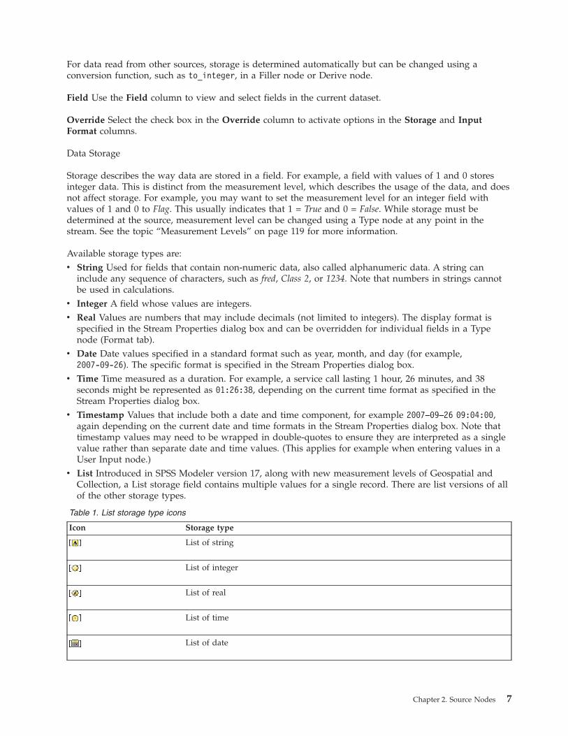
v List Introduced in SPSS Modeler version 17, along with new measurement levels of Geospatial andCollection, a List storage field contains multiple values for a single record. There are list versions of allof the other storage types.

Table 1. List storage type icons

Icon Storage type

List of string

List of integer

List of real

List of time

List of date

Chapter 2. Source Nodes 7

Table 1. List storage type icons (continued)

Icon Storage type

List of timestamp

List with a depth greater than zero

In addition, for use with the Collection measurement level, there are list versions of the followingmeasurement levels.

Table 2. List measurement level icons

Icon Measurement level

List of continuous

List of categorical

List of flags

List of nominal

List of ordinal

Lists can be imported into SPSS Modeler in one of three source nodes (Analytic Server, Geospatial, orVariable File), or created within your streams through use of the Derive or Filler field operation nodes.For more information on Lists and their interaction with the Collection and Geospatial measurementlevels, see “List storage and associated measurement levels” on page 9

Storage conversions. You can convert storage for a field using a variety of conversion functions, such asto_string and to_integer, in a Filler node. See the topic “Storage Conversion Using the Filler Node” onpage 140 for more information. Note that conversion functions (and any other functions that require aspecific type of input such as a date or time value) depend on the current formats specified in the StreamProperties dialog box. For example, if you want to convert a string field with values Jan 2003, Feb 2003,(and so forth) to date storage, select MON YYYY as the default date format for the stream. Conversionfunctions are also available from the Derive node, for temporary conversion during a derive calculation.You can also use the Derive node to perform other manipulations, such as recoding string fields withcategorical values. See the topic “Recoding Values with the Derive Node” on page 139 for moreinformation.

Reading in mixed data. Note that when reading in fields with numeric storage (either integer, real, time,timestamp, or date), any non-numeric values are set to null or system missing. This is because unlikesome applications, IBM SPSS Modeler does not allow mixed storage types within a field. To avoid this,any fields with mixed data should be read in as strings, either by changing the storage type in the sourcenode or in the external application as necessary.

Field Input Format (Fixed File, Variable File and User Input nodes only)

For all storage types except String and Integer, you can specify formatting options for the selected fieldusing the drop-down list. For example, when merging data from various locales, you may need to specifya period (.) as the decimal separator for one field, while another will require a comma separator.

Input options specified in the source node override the formatting options specified in the streamproperties dialog box; however, they do not persist later in the stream. They are intended to parse input


correctly based on your knowledge of the data. The specified formats are used as a guide for parsing thedata as they are read into IBM SPSS Modeler, not to determine how they should be formatted after beingread into IBM SPSS Modeler. To specify formatting on a per-field basis elsewhere in the stream, use theFormat tab of a Type node. See the topic “Field Format Settings Tab” on page 129 for more information.

Options vary depending on the storage type. For example, for the Real storage type, you can selectPeriod (.) or Comma (,) as the decimal separator. For timestamp fields, a separate dialog box opens whenyou select Specify from the drop-down list. See the topic “Setting Field Format Options” on page 130 formore information.

For all storage types, you can also select Stream default to use the stream default settings for import.Stream settings are specified in the stream properties dialog box.

Additional Options

Several other options can be specified using the Data tab:v To view storage settings for data that are no longer connected through the current node (train data, for

example), select View unused field settings. You can clear the legacy fields by clicking Clear.v At any point while working in this dialog box, click Refresh to reload fields from the data source. This

is useful when you are altering data connections to the source node or when you are working betweentabs on the dialog box.

List storage and associated measurement levelsIntroduced in SPSS Modeler version 17, to work with the new measurement levels of Geospatial andCollection, a List storage field contains multiple values for a single record. Lists are enclosed in squarebrackets ([]). Examples of lists are: [1,2,4,16] and ["abc", "def"].

Lists can be imported into SPSS Modeler in one of three source nodes (Analytic Server, Geospatial, orVariable File), created within your streams through use of the Derive or Filler field operation nodes, orgenerated by the Merge node when using the Ranked Condition merge method.

Lists are considered to have a depth; for example, a simple list with items that are contained withinsingle square brackets, in the format [1,3], is recorded in IBM SPSS Modeler with a depth of zero. Inaddition to simple lists that have a depth of zero, you can use nested lists, where each value within a listis a list itself.

The depth of a nested list depends on the associated measurement level. For Typeless there is no setdepth limit, for Collection the depth is zero, and for Geospatial, the depth must be between zero and twoinclusive depending on the number of nested items.

For zero depth lists you can set the measurement level as either Geospatial or Collection. Both of theselevels are parent measurement levels and you set the measurement sublevel information in the Valuesdialog box. The measurement sublevel of a Collection determines the measurement level of the elementswithin that list. All measurement levels (except typeless and geospatial) are available as sublevels forCollections. The Geospatial measurement level has six sublevels of Point, LineString, Polygon, MultiPoint,MultiLineString, and MultiPolygon; for more information, see “Geospatial measurement sublevels” onpage 121.

Note: The Collection measurement level can only be used with lists of depth 0, the Geospatialmeasurement level can only be used with lists of a maximum depth of 2, and the Typeless measurementlevel can be used with any list depth.

The following example shows the difference between a zero depth list and a nested list by using thestructure of the Geospatial measurement sublevels Point and LineString:v The Geospatial measurement sublevel of Point has a field depth of zero:


[1,3] two coordinates[1,3,-1] three coordinates

v The Geospatial measurement sublevel of LineString has a field depth of one:[ [1,3], [5,0] ] two coordinates[ [1,3,-1], [5,0,8] ] three coordinates

The Point field (with a depth of zero) is a normal list where each value is made up of two or threecoordinates. The LineString field (with a depth of one) is a list of points, where each point is made up ofa further series of list values.

For more information about list creation, see “Deriving a list or geospatial field” on page 137.

Unsupported control charactersSome of the processes in SPSS Modeler cannot handle data that includes various control characters. Ifyour data uses these characters you may see an error message such as the following example:Unsupported control characters found in values of field {0}

The unsupported characters are: from 0x0 to 0x3F inclusive, and 0x7F; however, the tab (0x9(\t)), newline (0xA(\n)), and carriage return (0xD(\r)) characters do not cause a problem.

If you see an error message that relates to unsupported characters, in your stream, after your Sourcenode, use a Filler node and the CLEM expression stripctrlchars to replace the characters.

Analytic Server Source NodeThe Analytic Server source enables you to run a stream on Hadoop Distributed File System (HDFS). Theinformation in an Analytic Server data source can come from a variety of places, including:v Text files on HDFSv Databasesv HCatalog

Typically, a stream with an Analytic Server Source will be executed on HDFS; however, if a streamcontains a node that is not supported for execution on HDFS, then as much of the stream as possible willbe "pushed back" to Analytic Server, and then SPSS Modeler Server will attempt to process the remainderof the stream. You will need to subsample very large datasets; for example, by placing a Sample nodewithin the stream.

Data source. Assuming your SPSS Modeler Server administrator has established a connection, you selecta data source containing the data you wish to use. A data source contains the files and metadataassociated with that source. Click Select to display a list of available data sources. See the topic “Selectinga data source” for more information.

If you need to create a new data source or edit an existing one, click Launch Data Source Editor....

Selecting a data sourceThe Data Sources table displays a list of the available data sources. Select the source you want to use andclick OK.

Click Show Owner to display the data source owner.


Filter by enables you to filter the data source listing on Keyword, which checks the filter criteria againstthe data source name and data source description, or Owner. You can enter a combination of string,numeric, or wild card characters described below as filter criteria. The search string is case sensitive.Click Refresh to update the Data Sources table.

_ An underscore can be used to represent any single character in the search string.

% A percent sign can be used to represent any sequence of zero or more characters in the searchstring.

Amending credentialsIf your credentials for accessing Analytic Server are different from the credentials for accessing SPSSModeler Server, you will need to enter the enter the Analytic Server credentials when running a streamon Analytic Server. If you do not know your credentials, contact your server administrator.

Supported nodesMany SPSS Modeler nodes are supported for execution on HDFS, but there may be some differences inthe execution of certain nodes, and some are not currently supported. This topic details the current levelof support.

General

v Some characters that are normally acceptable within a quoted Modeler field name will not beaccepted by Analytic Server.

v For a Modeler stream to be run in Analytic Server, it must begin with one or more AnalyticServer Source nodes and end in a single modeling node or Analytic Server Export node.

v It is recommended that you set the storage of continuous targets as real rather than integer.Scoring models always write real values to the output data files for continuous targets, whilethe output data model for the scores follows the storage of the target. Thus, if a continuoustarget has integer storage, there will be a mismatch in the written values and the data modelfor the scores, and this mismatch will cause errors when you attempt to read the scored data.

Source

v A stream that begins with anything other than an Analytic Server source node will be runlocally.

Record operationsAll Record operations are supported, with the exception of the Streaming TS andSpace-Time-Boxes nodes. Further notes on supported node functionality follow.

Select

v Supports the same set of functions supported by the Derive node.

Sample

v Block-level sampling is not supported.v Complex Sampling methods are not supported.

Aggregate

v Contiguous keys are not supported. If you are reusing an existing stream that is set upto sort the data and then use this setting in the Aggregate node, change the stream toremove the Sort node.

v Order statistics (Median, 1st Quartile, 3rd Quartile) are computed approximately, andsupported through the Optimization tab.

Sort

v The Optimization tab is not supported.


In a distributed environment, there are a limited number of operations that preserve therecord order established by the Sort node.v A Sort followed by an Export node produces a sorted data source.v A Sort followed by a Sample node with First record sampling returns the first N

records.

In general, you should place a Sort node as close as possible to the operations that needthe sorted records.

Merge

v Merge by Order is not supported.v The Optimization tab is not supported.v Analytic Server does not join on empty string keys; that is, if one of the keys you are

merging by contains empty strings, then any records that contain the empty string willbe dropped from the merged output.

v Merge operations are relatively slow. If you have available space in HDFS, it can bemuch faster to merge your data sources once and use the merged source in followingstreams than to merge the data sources in each stream.

R TransformThe R syntax in the node should consist of record-at-a-time operations.

Field operationsAll Field operations are supported, with the exception of the Transpose, Time Intervals, andHistory nodes. Further notes on supported node functionality follow.

Auto Data Prep

v Training the node is not supported. Applying the transformations in a trained AutoData Prep node to new data is supported.

Type

v The Check column is not supported.v The Format tab is not supported.

Derive

v All Derive functions are supported, with the exception of sequence functions.v Split fields cannot be derived in the same stream that uses them as splits; you will

need to create two streams; one that derives the split field and one that uses the fieldas splits.

v A flag field cannot be used by itself in a comparison; that is, if (flagField) then ... endifwill cause an error; the workaround is to use if (flagField=trueValue) then ... endif

v It is recommended when using the ** operator to specify the exponent as a realnumber, such as x**2.0, instead of x**2, in order to match results in Modeler

Filler

v Supports the same set of functions supported by the Derive node.

BinningThe following functionality is not supported.v Optimal binningv Ranksv Tiles -> Tiling: Sum of valuesv Tiles -> Ties: Keep in current and Assign randomlyv Tiles ->Custom N: Values over 100, and any N value where 100 % N is not equal to

zero.


RFM Analysis

v The Keep in current option for handling ties is not supported. RFM recency, frequency,and monetary scores will not always match those computed by Modeler from the samedata. The score ranges will be the same but score assignments (bin numbers) maydiffer by one.

GraphsAll Graph nodes are supported.

ModelingThe following Modeling nodes are supported: Linear, Neural Net, C&RT, Chaid, Quest, TCM,TwoStep-AS, STP, and Association Rules. Further notes on those nodes' functionality follow.

Linear When building models on big data, you will typically want to change the objective toVery large datasets, or specify splits.v Continued training of existing PSM models is not supported.v The Standard model building objective is only recommended if split fields are defined

so that the number of records in each split is not too large, where the definition of "toolarge" is dependent upon the power of individual nodes in your Hadoop cluster. Bycontrast, you also need to be careful to ensure that splits are not defined so finely thatthere are too few records to build a model.

v The Boosting objective is not supported.v The Bagging objective is not supported.v The Very large datasets objective is not recommended when there are few records; it

will often either not build a model or will build a degraded model.v Automatic Data Preparation is not supported. This can cause problems when trying to

build a model on data with many missing values; normally these would be imputed aspart of automatic data preparation. A workaround would be to use a tree model or aneural network with the Advanced setting to impute missing values selected.

v The accuracy statistic is not computed for split models.

Neural NetWhen building models on big data, you will typically want to change the objective toVery large datasets, or specify splits.v Continued training of existing standard or PSM models is not supported.v The Standard model building objective is only recommended if split fields are defined

so that the number of records in each split is not too large, where the definition of "toolarge" is dependent upon the power of individual nodes in your Hadoop cluster. Bycontrast, you also need to be careful to ensure that splits are not defined so finely thatthere are too few records to build a model.


will often either not build a model or will build a degraded model.v When there are many missing values in the data, use the Advanced setting to impute

missing values.v The accuracy statistic is not computed for split models.

C&R Tree, CHAID, and QuestWhen building models on big data, you will typically want to change the objective toVery large datasets, or specify splits.v Continued training of existing PSM models is not supported.v The Standard model building objective is only recommended if split fields are defined

so that the number of records in each split is not too large, where the definition of "too


large" is dependent upon the power of individual nodes in your Hadoop cluster. Bycontrast, you also need to be careful to ensure that splits are not defined so finely thatthere are too few records to build a model.


will often either not build a model or will build a degraded model.v Interactive sessions is not supported.v The accuracy statistic is not computed for split models.

Model scoringAll models supported for modeling are also supported for scoring. In addition, locally-builtmodel nuggets for the following nodes are supported for scoring: C&RT, Quest, CHAID, Linear,and Neural Net (regardless of whether the model is standard, boosted bagged, or for very largedatasets), Regression, C5.0, Logistic, Genlin, GLMM, Cox, SVM, Bayes Net, TwoStep, KNN,Decision List, Discriminant, Self Learning, Anomaly Detection, Apriori, Carma, K-Means,Kohonen, R, and Text Mining.v No raw or adjusted propensities will be scored. As a workaround you can get the same effect

by manually computing the raw propensity using a Derive node with the following expression:if 'predicted-value' == 'value-of-interest' then 'prob-of-that-value' else 1-'prob-of-that-value'endif

v When scoring a model, Analytic Server does not check to see if all fields used in the model arepresent in the dataset, so be sure that's true before running in Analytic Server

R The R syntax in the nugget should consist of record-at-a-time operations.

OutputThe Matrix, Analysis, Data Audit, Transform, Statistics, and Means nodes are supported.

The Table node is supported by writing a temporary Analytic Server data source containing theresults of upstream operations. The Table node then pages through the contents of that datasource.

Export A stream can begin with an Analytic Server source node and end with an export node other thanthe Analytic Server export node, but data will move from HDFS to SPSS Modeler Server, andfinally to the export location.

Database Source NodeThe Database source node can be used to import data from a variety of other packages using ODBC(Open Database Connectivity), including Microsoft SQL Server, DB2, Oracle, and others.

To read or write to a database, you must have an ODBC data source installed and configured for therelevant database, with read or write permissions as needed. The IBM SPSS Data Access Pack includes aset of ODBC drivers that can be used for this purpose, and these drivers are available on the IBM SPSSData Access Pack DVD or from the download site. If you have questions about creating or settingpermissions for ODBC data sources, contact your database administrator.

Supported ODBC Drivers

For the latest information on which databases and ODBC drivers are supported and tested for use withIBM SPSS Modeler 17, see the product compatibility matrices on the corporate Support site(http://www.ibm.com/support).

Where to Install Drivers

Note: ODBC drivers must be installed and configured on each computer where processing may occur.



v If you are running IBM SPSS Modeler in local (standalone) mode, the drivers must be installed on thelocal computer.

v If you are running IBM SPSS Modeler in distributed mode against a remote IBM SPSS Modeler Server,the ODBC drivers need to be installed on the computer where IBM SPSS Modeler Server is installed.For IBM SPSS Modeler Server on UNIX systems, see also "Configuring ODBC drivers on UNIXsystems" later in this section.

v If you need to access the same data sources from both IBM SPSS Modeler and IBM SPSS ModelerServer, the ODBC drivers must be installed on both computers.

v If you are running IBM SPSS Modeler over Terminal Services, the ODBC drivers need to be installedon the Terminal Services server on which you have IBM SPSS Modeler installed.

Access data from a database

To access data from a database, complete the following steps.v Install an ODBC driver and configure a data source to the database you want to use.v In the Database node dialog box, connect to a database using Table mode or SQL Query mode.v Select a table from the database.v Using the tabs in the Database node dialog box, you can alter usage types and filter data fields.

More details on the preceding steps are given in the related documentation topics.

Note: If you call database Stored Procedures (SPs) from SPSS Modeler you might see a single outputfield returned named RowsAffected rather than the expected output of the SP. This occurs when ODBCdoes not return sufficient information to be able to determine the output datamodel of the SP. SPSSModeler has only limited support for SPs that return output and it is suggested that instead of using SPsyou should extract the SELECT from the SP and use either of the following actions.v Create a view based on the SELECT and choose the view in the Database source nodev Use the SELECT directly in the Database source node.

Setting Database Node OptionsYou can use the options on the Data tab of the Database source node dialog box to gain access to adatabase and read data from the selected table.

Mode. Select Table to connect to a table using the dialog box controls.

Select SQL Query to query the database selected below using SQL. See the topic “Querying theDatabase” on page 21 for more information.

Data source. For both Table and SQL Query modes, you can enter a name in the Data Source field orselect Add new database connection from the drop-down list.

The following options are used to connect to a database and select a table using the dialog box:

Table name. If you know the name of the table you would like to access, enter it in the Table Name field.Otherwise, click the Select button to open a dialog box listing the available tables.

Quote table and column names. Specify whether you want table and column names to be enclosed inquotation marks when queries are sent to the database (if, for example, they contain spaces orpunctuation).v The As needed option will quote table and field names only if they include nonstandard characters.

Nonstandard characters include non-ASCII characters, space characters, and any non-alphanumericcharacter other than a full stop (.).

v Select Always if you want all table and field names quoted.


v Select Never if you never want table and field names quoted.

Strip lead and trail spaces. Select options for discarding leading and trailing spaces in strings.

Note. Comparisons between strings that do and do not use SQL pushback may generate different resultswhere trailing spaces exist.

Reading empty strings from Oracle. When reading from or writing to an Oracle database, be aware that,unlike IBM SPSS Modeler and unlike most other databases, Oracle treats and stores empty string valuesas equivalent to null values. This means that the same data extracted from an Oracle database maybehave differently than when extracted from a file or another database, and the data may return differentresults.

Adding a database connectionTo open a database, first select the data source to which you want to connect. On the Data tab, select Addnew database connection from the Data Source drop-down list.

This opens the Database Connections dialog box.

Note: For an alternative way to open this dialog, from the main menu, choose: Tools > Databases...

Data sources Lists the available data sources. Scroll down if you do not see the desired database. Onceyou have selected a data source and entered any passwords, click Connect. Click Refresh to update thelist.

User name and password If the data source is password protected, enter your user name and theassociated password.

Credential If a credential has been configured in IBM SPSS Collaboration and Deployment Services, youcan select this option to browse for it in the repository. The credential's user name and password mustmatch the user name and password required to access the database.

Connections Shows currently connected databases.v Default You can optionally choose one connection as the default. Doing so causes Database source or

export nodes to have this connection predefined as their data source, though this can be edited ifdesired.

v Save Optionally select one or more connections that you want to redisplay in subsequent sessions.v Data source The connection strings for the currently connected databases.v Preset Indicates (with a * character) whether preset values have been specified for the database

connection. To specify preset values, click this column in the row corresponding to the databaseconnection, and choose Specify from the list. See the topic “Specifying preset values for a databaseconnection” on page 17 for more information.

To remove connections, select one from the list and click Remove.

Once you have completed your selections, click OK.

To read or write to a database, you must have an ODBC data source installed and configured for therelevant database, with read or write permissions as needed. The IBM SPSS Data Access Pack includes aset of ODBC drivers that can be used for this purpose, and these drivers are available on the IBM SPSSData Access Pack DVD or from the download site. If you have questions about creating or settingpermissions for ODBC data sources, contact your database administrator.


Supported ODBC Drivers

For the latest information on which databases and ODBC drivers are supported and tested for use withIBM SPSS Modeler 17, see the product compatibility matrices on the corporate Support site(http://www.ibm.com/support).

Where to Install Drivers

Note: ODBC drivers must be installed and configured on each computer where processing may occur.v If you are running IBM SPSS Modeler in local (standalone) mode, the drivers must be installed on the

local computer.v If you are running IBM SPSS Modeler in distributed mode against a remote IBM SPSS Modeler Server,

the ODBC drivers need to be installed on the computer where IBM SPSS Modeler Server is installed.For IBM SPSS Modeler Server on UNIX systems, see also "Configuring ODBC drivers on UNIXsystems" later in this section.

v If you need to access the same data sources from both IBM SPSS Modeler and IBM SPSS ModelerServer, the ODBC drivers must be installed on both computers.

v If you are running IBM SPSS Modeler over Terminal Services, the ODBC drivers need to be installedon the Terminal Services server on which you have IBM SPSS Modeler installed.

Configuring ODBC drivers on UNIX systems

By default, the DataDirect Driver Manager is not configured for IBM SPSS Modeler Server on UNIXsystems. To configure UNIX to load the DataDirect Driver Manager, enter the following commands:cd <modeler_server_install_directory>/binrm -f libspssodbc.soln -s libspssodbc_datadirect.so libspssodbc.so

Doing so removes the default link and creates a link to the DataDirect Driver Manager.

Note: The UTF16 driver wrapper is required to use SAP HANA or IBM DBZ CLI drivers for somedatabases. To create a link for the UTF16 driver wrapper, enter the following commands instead:rm -f libspssodbc.soln -s libspssodbc_datadirect_utf16.so libspssodbc.so

To configure SPSS Modeler Server:1. Configure the SPSS Modeler Server start up script modelersrv.sh to source the IBM SPSS Data Access

Pack odbc.sh environment file by adding the following line to modelersrv.sh:. /<pathtoSDAPinstall>/odbc.sh

Where <pathtoSDAPinstall> is the full path to your IBM SPSS Data Access Pack installation.2. Restart SPSS Modeler Server.

In addition, for SAP HANA and IBM DB2 only, add the following parameter definition to the DSN inyour odbc.ini file to avoid buffer overflows during connection:DriverUnicodeType=1

Note: The libspssodbc_datadirect_utf16.so wrapper is also compatible with the other SPSS ModelerServer supported ODBC drivers.

Specifying preset values for a database connectionFor some databases, you can specify a number of default settings for the database connection. Thesettings all apply to database export.



The database types that support this feature are as follows.v IBM InfoSphere Warehouse. See the topic “Settings for IBM DB2 InfoSphere Warehouse” for more

information.v SQL Server Enterprise and Developer editions. See the topic “Settings for SQL Server” for more

information.v Oracle Enterprise or Personal editions. See the topic “Settings for Oracle” for more information.v IBM Netezza, IBM DB2 for z/OS, and Teradata all connect to a database or schema in a similar way.

See the topic “Settings for IBM Netezza, IBM DB2 for z/OS, IBM DB2 LUW, and Teradata” on page 19for more information.

If you are connected to a database or schema that does not support this feature, you see the message Nopresets can be configured for this database connection.

Settings for IBM DB2 InfoSphere WarehouseThese settings are displayed for IBM InfoSphere Warehouse.

Table space The tablespace to be used for export. Database administrators can create or configuretablespaces as partitioned. We recommend selecting one of these tablespaces (rather than the default one)to use for database export.

Use compression. If selected, creates tables for export with compression (for example, the equivalent ofCREATE TABLE MYTABLE(...) COMPRESS YES; in SQL).

Do not log updates If selected, avoids logging when creating tables and inserting data (the equivalent ofCREATE TABLE MYTABLE(...) NOT LOGGED INITIALLY; in SQL).

Settings for SQL ServerThese settings are displayed for SQL Server Enterprise and Developer editions.

Use compression. If selected, creates tables for export with compression.

Compression for. Choose the level of compression.v Row. Enables row-level compression (for example, the equivalent of CREATE TABLE MYTABLE(...) WITH

(DATA_COMPRESSION = ROW); in SQL).v Page. Enables page-level compression (for example, CREATE TABLE MYTABLE(...) WITH

(DATA_COMPRESSION = PAGE); in SQL).

Settings for OracleOracle settings - Basic option

These settings are displayed for Oracle Enterprise or Personal editions using the Basic option.


Compression for. Choose the level of compression.v Default. Enables default compression (for example, CREATE TABLE MYTABLE(...) COMPRESS; in SQL). In

this case, it has the same effect as the Basic option.v Basic. Enables basic compression (for example, CREATE TABLE MYTABLE(...) COMPRESS BASIC; in SQL).

Oracle settings - Advanced option

These settings are displayed for Oracle Enterprise or Personal editions using the Advanced option.




this case, it has the same effect as the Basic option.v Basic. Enables basic compression (for example, CREATE TABLE MYTABLE(...) COMPRESS BASIC; in SQL).v OLTP. Enables OLTP compression (for example, CREATE TABLE MYTABLE(...)COMPRESS FOR OLTP; in

SQL).v Query Low/High. (Exadata servers only) Enables hybrid columnar compression for query (for

example, CREATE TABLE MYTABLE(...)COMPRESS FOR QUERY LOW; or CREATE TABLE MYTABLE(...)COMPRESSFOR QUERY HIGH; in SQL). Compression for query is useful in data warehousing environments; HIGHprovides a higher compression ratio than LOW.

v Archive Low/High. (Exadata servers only) Enables hybrid columnar compression for archive (forexample, CREATE TABLE MYTABLE(...)COMPRESS FOR ARCHIVE LOW; or CREATE TABLEMYTABLE(...)COMPRESS FOR ARCHIVE HIGH; in SQL). Compression for archive is useful for compressingdata that will be stored for long periods of time; HIGH provides a higher compression ratio than LOW.

Settings for IBM Netezza, IBM DB2 for z/OS, IBM DB2 LUW, and TeradataWhen you specify presets for IBM Netezza, IBM DB2 for z/OS, IBM DB2 LUW, or Teradata you areprompted to select the following items:

Use server scoring adapter database or Use server scoring adapter shema. If selected, enables the Serverscoring adapter database or Server scoring adapter schema option.

Server scoring adapter database or Server scoring adapter schema From the drop-down list, select theconnection you require.

In addition, for Teradata, you can also set query banding details to provide additional metadata to assistwith items such as workload management; collating, identifying, and resolving queries; and trackingdatabase usage.

Spelling query banding. Choose if the query banding will be set once for the entire time you areworking with a Teradata database connection (For Session), or if it will be set every time you run astream (For Transaction).

Note: If you set query banding on a stream, the banding is lost if you copy that stream to anothermachine. To prevent this, you can use scripting to run your stream and use the key word querybanding inthe script to apply the settings you require.

Required database permissions

For SPSS Modeler database capabilities to function correctly, grant access to the following items to anyuser IDs used:

DB2 LUWSYSIBM.SYSDUMMY1

SYSIBM.SYSFOREIGNKEYS

SYSIBM.SYSINDEXES

SYSIBM.SYSKEYCOLUSE

SYSIBM.SYSKEYS

SYSIBM.SYSPARMS

SYSIBM.SYSRELS

SYSIBM.SYSROUTINES


SYSIBM.SYSROUTINES_SRC

SYSIBM.SYSSYNONYMS

SYSIBM.SYSTABCONST

SYSIBM.SYSTABCONSTPKC

SYSIBM.SYSTABLES

SYSIBM.SYSTRIGGERS

SYSIBM.SYSVIEWDEP

SYSIBM.SYSVIEWS

SYSCAT.TABLESPACES

SYSCAT.SCHEMATA

DB2/z SYSIBM.SYSDUMMY1

SYSIBM.SYSFOREIGNKEYS

SYSIBM.SYSINDEXES

SYSIBM.SYSKEYCOLUSE

SYSIBM.SYSKEYS

SYSIBM.SYSPARMS

SYSIBM.SYSRELS

SYSIBM.SYSROUTINES

SYSIBM.SYSROUTINES_SRC

SYSIBM.SYSSYNONYMS

SYSIBM.SYSTABCONST

SYSIBM.SYSTABCONSTPKC

SYSIBM.SYSTABLES

SYSIBM.SYSTRIGGERS

SYSIBM.SYSVIEWDEP

SYSIBM.SYSVIEWS

SYSIBM.SYSDUMMYU

SYSIBM.SYSPACKSTMT

Netezza_V_FUNCTION

_V_DATABASE

TeradataDBC.Functions

DBC.USERS

Selecting a Database TableAfter you have connected to a data source, you can choose to import fields from a specific table or view.From the Data tab of the Database dialog box, you can either enter the name of a table in the Table Namefield or click Select to open the Select Table/View dialog box which lists the available tables and views.


Show table owner. Select if a data source requires that the owner of a table must be specified before youcan access the table. Deselect this option for data sources that do not have this requirement.

Note: SAS and Oracle databases usually require you to show the table owner.

Tables/Views. Select the table or view to import.

Show. Lists the columns in the data source to which you are currently connected. Click one of thefollowing options to customize your view of the available tables:v Click User Tables to view ordinary database tables created by database users.v Click System Tables to view database tables owned by the system (for example, tables that provide

information about the database, such as details of indexes). This option can be used to view the tabsused in Excel databases. (Note that a separate Excel source node is also available. See the topic “ExcelSource Node” on page 37 for more information. )

v Click Views to view virtual tables based on a query involving one or more ordinary tables.v Click Synonyms to view synonyms created in the database for any existing tables.

Name/Owner filters. These fields allow you to filter the list of displayed tables by name or owner. Forexample, type SYS to list only tables with that owner. For wildcard searches, an underscore (_) can beused to represent any single character and a percent sign (%) can represent any sequence of zero or morecharacters.

Set As Default. Saves the current settings as the default for the current user. These settings will berestored in the future when a user opens a new table selector dialog box for the same data source name anduser login only.

Querying the DatabaseOnce you have connected to a data source, you can choose to import fields using SQL queries. From themain dialog box, select SQL Query as the connection mode. This adds a query editor window in thedialog box. Using the query editor, you can create or load one or more SQL queries whose result set willbe read into the data stream.

If you specify multiple SQL queries, separate them with semicolons (;) and ensure that there is nomultiple SELECT statement.

To cancel and close the query editor window, select Table as the connection mode.

You can include SPSS Modeler stream parameters (a type of user-defined variable) in the SQL query. Seethe topic “Using Stream Parameters in an SQL Query” on page 22 for more information.

Load Query. Click to open the file browser, which you can use to load a previously saved query.

Save Query. Click to open the Save Query dialog box, which you can use to save the current query.

Import Default. Click to import an example SQL SELECT statement constructed automatically using thetable and columns selected in the dialog box.

Clear. Clear the contents of the work area. Use this option when you want to start over.

Split text. The default option Never means that the query will be sent to the database as a whole.Alternatively, you can choose As needed which means that SPSS Modeler attempts to parse the queryand identify if there are SQL statements that should be send to the database one after another.


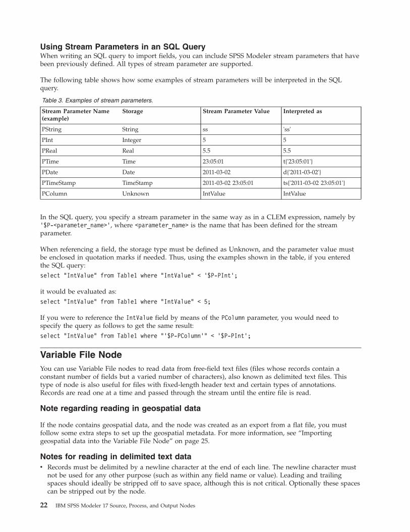
Using Stream Parameters in an SQL QueryWhen writing an SQL query to import fields, you can include SPSS Modeler stream parameters that havebeen previously defined. All types of stream parameter are supported.

The following table shows how some examples of stream parameters will be interpreted in the SQLquery.

Table 3. Examples of stream parameters.

Stream Parameter Name(example)

Storage Stream Parameter Value Interpreted as

PString String ss 'ss'

PInt Integer 5 5

PReal Real 5.5 5.5

PTime Time 23:05:01 t{'23:05:01'}

PDate Date 2011-03-02 d{'2011-03-02'}

PTimeStamp TimeStamp 2011-03-02 23:05:01 ts{'2011-03-02 23:05:01'}

PColumn Unknown IntValue IntValue

In the SQL query, you specify a stream parameter in the same way as in a CLEM expression, namely by’$P-<parameter_name>’, where <parameter_name> is the name that has been defined for the streamparameter.

When referencing a field, the storage type must be defined as Unknown, and the parameter value mustbe enclosed in quotation marks if needed. Thus, using the examples shown in the table, if you enteredthe SQL query:select "IntValue" from Table1 where "IntValue" < ’$P-PInt’;

it would be evaluated as:select "IntValue" from Table1 where "IntValue" < 5;

If you were to reference the IntValue field by means of the PColumn parameter, you would need tospecify the query as follows to get the same result:select "IntValue" from Table1 where "’$P-PColumn’" < ’$P-PInt’;

Variable File NodeYou can use Variable File nodes to read data from free-field text files (files whose records contain aconstant number of fields but a varied number of characters), also known as delimited text files. Thistype of node is also useful for files with fixed-length header text and certain types of annotations.Records are read one at a time and passed through the stream until the entire file is read.

Note regarding reading in geospatial data

If the node contains geospatial data, and the node was created as an export from a flat file, you mustfollow some extra steps to set up the geospatial metadata. For more information, see “Importinggeospatial data into the Variable File Node” on page 25.

Notes for reading in delimited text datav Records must be delimited by a newline character at the end of each line. The newline character must

not be used for any other purpose (such as within any field name or value). Leading and trailingspaces should ideally be stripped off to save space, although this is not critical. Optionally these spacescan be stripped out by the node.


v Fields must be delimited by a comma or other character that ideally is used only as a delimiter,meaning it does not appear within field names or values. If this is not possible, then all text fields canbe wrapped in double quotation marks, if none of the field names or text values contains a doublequotation mark. If field names or values do contain double quotation marks, then text fields can bewrapped in single quotation marks as an alternative, again if single quotation marks are not usedelsewhere within values. If neither single or double quotation marks can be used, then text values needto be amended to remove or replace either the delimiter character, or single or double quotation marks.

v Each row, including the header row, should contain the same number of fields.v The first line should contain the field names. If not, clear Read field names from file to give each field

a generic name such as Field1, Field2, and so on.v The second line must contain the first record of data. There must no blank lines or comments.v Numeric values must not include the thousands separator or grouping symbol—without the comma in

3,000.00, for example. The decimal indicator (period or full-stop in the US or the UK) must be usedonly where appropriate.

v Date and time values should be in one of the formats that are recognized in the Stream Options dialogbox, such as DD/MM/YYYY or HH:MM:SS. All dates and time fields in the file should ideally follow thesame format, and any field that contains a date must use the same format for all values within thatfield.

Setting options for the Variable File NodeYou set the options on the File tab of the Variable File node dialog box.

File Specify the name of the file. You can enter a filename or click the ellipsis button (...) to select a file.The file path is shown once you select a file, and its contents are displayed with delimiters in the panelbelow it.

The sample text that is displayed from your data source can be copied and pasted into the followingcontrols: EOL comment characters and user-specified delimiters. Use Ctrl-C and Ctrl-V to copy and paste.

Read field names from file Selected by default, this option treats the first row in the data file as labelsfor the column. If your first row is not a header, deselect to automatically give each field a generic name,such as Field1, Field2, for the number of fields in the dataset.

Specify number of fields. Specify the number of fields in each record. The number of fields can bedetected automatically as long as the records are new-line terminated. You can also set a numbermanually.

Skip header characters. Specify how many characters you want to ignore at the beginning of the firstrecord.

EOL comment characters. Specify characters, such as # or !, to indicate annotations in the data. Whereverone of these characters appears in the data file, everything up to but not including the next new-linecharacter will be ignored.

Strip lead and trail spaces. Select options for discarding leading and trailing spaces in strings on import.


Invalid characters. Select Discard to remove invalid characters from the data source. Select Replace withto replace invalid characters with the specified symbol (one character only). Invalid characters are nullcharacters or any character that does not exist in the encoding method specified.


Encoding. Specifies the text-encoding method used. You can choose between the system default, streamdefault, or UTF-8.v The system default is specified in the Windows Control Panel or, if running in distributed mode, on

the server computer.v The stream default is specified in the Stream Properties dialog box.

Decimal symbol Select the type of decimal separator that is used in your data source. The Streamdefault is the character that is selected from the Options tab of the stream properties dialog box.Otherwise, select either Period (.) or Comma (,) to read all data in this dialog box using the chosencharacter as the decimal separator.

Line delimiter is newline character To use the newline character as the line delimiter, instead of a fielddelimiter, select this option. For example, this may be useful if there is an odd number of delimiters in arow that cause the line to wrap. Note that selecting this option means you cannot select Newline in theDelimiters list.

Note: If you select this option, any blank values at the end of data rows will be stripped out.

Delimiters. Using the check boxes listed for this control, you can specify which characters, such as thecomma (,), define field boundaries in the file. You can also specify more than one delimiter, such as ", |"for records that use multiple delimiters. The default delimiter is the comma.

Note: If the comma is also defined as the decimal separator, the default settings here will not work. Incases where the comma is both the field delimiter and the decimal separator, select Other in theDelimiters list. Then manually specify a comma in the entry field.

Select Allow multiple blank delimiters to treat multiple adjacent blank delimiter characters as a singledelimiter. For example, if one data value is followed by four spaces and then another data value, thisgroup would be treated as two fields rather than five.

Lines to scan for column and type Specify how many lines and columns to scan for specified data types.

Automatically recognize dates and times To enable IBM SPSS Modeler to automatically attempt torecognize data entries as dates or times, select this check box. For example, this means that an entry suchas 07-11-1965 will be identified as a date and 02:35:58 will be identified as a time; however, ambiguousentries such as 07111965 or 023558 will show up as integers since there are no delimiters between thenumbers.

Note: To avoid potential data problems when you use data files from previous versions of IBM SPSSModeler, this box is turned off by default for information that is saved in versions prior to 13.

Treat square brackets as lists If you select this check box, the data included between opening and closingsquare brackets is treated as a single value, even if the content includes delimiter characters such ascommas and double quotes. For example, this might include two or three dimensional geospatial data,where the coordinates contained within square brackets are processed as a single list item. For moreinformation, see “Importing geospatial data into the Variable File Node” on page 25

Quotes. Using the drop-down lists, you can specify how single and double quotation marks are treatedon import. You can choose to Discard all quotation marks, Include as text by including them in the fieldvalue, or Pair and discard to match pairs of quotation marks and remove them. If a quotation mark isunmatched, you will receive an error message. Both Discard and Pair and discard store the field value(without quotation marks) as a string.


Note: When using Pair and discard, spaces are kept. When using Discard, trailing spaces inside andoutside quotes are removed (for example, ’ " ab c" , "d ef " , " gh i " ’ will result in ’ab c, d ef,gh i’). When using Include as text, quotes are treated as normal characters, so leading and trailingspaces will be stripped naturally.

At any point while you are working in this dialog box, click Refresh to reload fields from the datasource. This is useful when you are altering data connections to the source node or when you areworking between tabs in the dialog box.

Importing geospatial data into the Variable File NodeIf the node contains geospatial data, was created as an export from a flat file, and is used in the samestream in which it was created, the node retains the geospatial metadata and no further configurationsteps are needed.

However, if the node is exported and used in a different stream, the geospatial list data is automaticallyconverted to a string format; you must follow some extra steps to restore the list storage type and theassociated geospatial metadata.

For more information about lists, see “List storage and associated measurement levels” on page 9.

For more information about the details you can set as geospatial metadata, see “Geospatial measurementsublevels” on page 121.

To set up the geospatial metadata, use the following steps.1. On the File tab of the Variable File node, select the Treat square brackets as lists check box. Selecting

this check box means that the data included between opening and closing square brackets is treatedas a single value, even if the content includes delimiter characters such as commas and doublequotation marks. Failure to select this check box means that your data is read as a string storage type,any commas in the field are processed as delimiters, and your data structure is interpreted incorrectly.

2. If your data includes single or double quotation marks, select the Pair and discard option in theSingle quotes and Double quotes fields, as appropriate.

3. On the Data tab of the Variable File node, for the geospatial data fields, select the Override check box,and change the Storage type from a string to a list.

4. By default, the list Storage type is set as a List of real and the underlying value storage type of the listfield is set to Real. To change the underlying value storage type or the depth, click Specify... todisplay the Storage subdialog box.

5. In the Storage subdialog box you can modify the following settings:v Storage Specify the overall storage type of the data field. By default the storage type is set to List;

however, the drop-down list contains all other storage types (String, Integer, Real, Date, Time, andTimestamp). If you select any storage type other than List, Value storage and Depth options areunavailable.

v Value storage Specify the storage types of the elements in the list, as opposed to the field as awhole. When you import geospatial fields, the only relevant storage types are Real and Integer; thedefault setting is Real.

v Depth Specify the depth of the list field. The required depth depends on the type of geospatial fieldand follows these criteria:– Point – 0– LineString – 1– Polygon – 1– MultiPoint – 1– MultiLineString – 2– MultiPolygon – 2


Note: You must know the type of geospatial field you are converting back into a list and therequired depth for that kind of field. If this information is set incorrectly, it is not possible to usethe field.

6. On the Types tab of the Variable File node, for the geospatial data field, ensure the Measurement cellcontains the correct measurement level. To change the measurement level, in the Measurement cell,click Specify... to display the Values dialog box.

7. In the Values dialog box, the Measurement, Storage, and Depth for the list are displayed. Select theSpecify values and labels option and, from the Type drop-down list, select the correct type for theMeasurement. Depending on the Type, you might be prompted for more details such as if the datarepresents 2 or 3 dimensions and which coordinate system is used.

Fixed File NodeYou can use Fixed File nodes to import data from fixed-field text files (files whose fields are not delimitedbut start at the same position and are of a fixed length). Machine-generated or legacy data are frequentlystored in fixed-field format. Using the File tab of the Fixed File node, you can easily specify the positionand length of columns in your data.

Setting Options for the Fixed File NodeThe File tab of the Fixed File node enables you to bring data into IBM SPSS Modeler and to specify theposition of columns and length of records. Using the data preview pane in the center of the dialog box,you can click to add arrows specifying the break points between fields.

File. Specify the name of the file. You can enter a filename or click the ellipsis button (...) to select a file.Once you have selected a file, the file path is shown and its contents are displayed with delimiters in thepanel below.

The data preview pane can be used to specify column position and length. The ruler at the top of thepreview window helps to measure the length of variables and to specify the break point between them.You can specify break point lines by clicking in the ruler area above the fields. Break points can bemoved by dragging and can be discarded by dragging them outside of the data preview region.v Each break-point line automatically adds a new field to the fields table below.v Start positions indicated by the arrows are automatically added to the Start column in the table below.

Line oriented. Select if you want to skip the new-line character at the end of each record.

Skip header lines. Specify how many lines you want to ignore at the beginning of the first record. This isuseful for ignoring column headers.

Record length. Specify the number of characters in each record.

Field. All fields that you have defined for this data file are listed here. There are two ways to definefields:v Specify fields interactively using the data preview pane above.v Specify fields manually by adding empty field rows to the table below. Click the button to the right of

the fields pane to add new fields. Then, in the empty field, enter a field name, a start position, and alength. These options will automatically add arrows to the data preview pane, which can be easilyadjusted.

To remove a previously defined field, select the field in the list and click the red delete button.

Start. Specify the position of the first character in the field. For example, if the second field of a recordbegins on the sixteenth character, you would enter 16 as the starting point.


Length. Specify how many characters are in the longest value for each field. This determines the cutoffpoint for the next field.

Strip lead and trail spaces. Select to discard leading and trailing spaces in strings on import.


Invalid characters. Select Discard to remove invalid characters from the data input. Select Replace withto replace invalid characters with the specified symbol (one character only). Invalid characters are null (0)characters or any character that does not exist in the current encoding.



Decimal symbol. Select the type of decimal separator used in your data source. Stream default is thecharacter selected from the Options tab of the stream properties dialog box. Otherwise, select eitherPeriod (.) or Comma (,) to read all data in this dialog box using the chosen character as the decimalseparator.

Automatically recognize dates and times. To enable IBM SPSS Modeler to automatically attempt torecognize data entries as dates or times, select this check box. For example, this means that an entry suchas 07-11-1965 will be identified as a date and 02:35:58 will be identified as a time; however, ambiguousentries such as 07111965 or 023558 will show up as integers since there are no delimiters between thenumbers.

Note: To avoid potential data problems when using data files from previous versions of IBM SPSSModeler, this box is turned off by default for information saved in versions prior to 13.

Lines to scan for type. Specify how many lines to scan for specified data types.

At any point while working in this dialog box, click Refresh to reload fields from the data source. This isuseful when altering data connections to the source node or when working between tabs on the dialogbox.

Data Collection NodeData Collection source nodes import survey data based on the IBM SPSS Data Collection Survey ReporterDeveloper Kit used by market research software from IBM Corp. This format distinguishes case data—theactual responses to questions gathered during a survey—from the metadata that describes how the casedata is collected and organized. Metadata consists of information such as question texts, variable namesand descriptions, multiple response variable definitions, translations of the text strings, and the definitionof the structure of the case data.

Note: This node requires IBM SPSS Data Collection Survey Reporter Developer Kit, which is distributedalong with IBM SPSS Data Collection software products from IBM Corp. For more information, see theIBM SPSS Data Collection Web page at . Aside from installing the Developer Kit, no additionalconfiguration is required.

Commentsv Survey data is read from the flat, tabular VDATA format, or from sources in the hierarchical HDATA

format if they include a metadata source (requires IBM SPSS Data Collection 4.5 or higher).


v Types are instantiated automatically by using information from the metadata.v When survey data is imported into IBM SPSS Modeler, questions are rendered as fields, with a record

for each respondent.

Data Collection Import File OptionsThe File tab in the Data Collection node enables you to specify options for the metadata and case datayou want to import.

Metadata Settings

Note: To see the full list of available provider file types, you need to install the IBM SPSS Data CollectionSurvey Reporter Developer Kit, available with the IBM SPSS Data Collection software. For moreinformation, see the IBM SPSS Data Collection Web page at http://www.ibm.com/software/analytics/spss/products/data-collection/survey-reporter-dev-kit/

Metadata Provider. Survey data can be imported from a number of formats as supported by IBM SPSSData Collection Survey Reporter Developer Kit software. Available provider types include the following:v DataCollectionMDD. Reads metadata from a questionnaire definition file (.mdd). This is the standard

IBM SPSS Data Collection Data Model format.v ADO Database. Reads case data and metadata from ADO files. Specify the name and location of the

.adoinfo file that contains the metadata. The internal name of this DSC is mrADODsc.v In2data Database. Reads In2data case data and metadata. The internal name of this DSC is mrI2dDsc.v Data Collection Log File. Reads metadata from a standard IBM SPSS Data Collection log file.

Typically, log files have a .tmp filename extension. However, some log files may have another filenameextension. If necessary, you can rename the file so that it has a .tmp filename extension. The internalname of this DSC is mrLogDsc.

v Quancept Definitions File. Converts metadata to Quancept script. Specify the name of the Quancept.qdi file. The internal name of this DSC is mrQdiDrsDsc.

v Quanvert Database. Reads Quanvert case data and metadata. Specify the name and location of the.qvinfo or .pkd file. The internal name of this DSC is mrQvDsc.

v Data Collection Participation Database. Reads a project's Sample and History Table tables and createsderived categorical variables corresponding to the columns in those tables. The internal name of thisDSC is mrSampleReportingMDSC.

v Statistics File. Reads case data and metadata from an IBM SPSS Statistics .sav file. Writes case data toan IBM SPSS Statistics .sav file for analysis in IBM SPSS Statistics. Writes metadata from an IBM SPSSStatistics .sav file to an .mdd file. The internal name of this DSC is mrSavDsc.

v Surveycraft File. Reads SurveyCraft case data and metadata. Specify the name of the SurveyCraft .vqfile. The internal name of this DSC is mrSCDsc.

v Data Collection Scripting File. Reads from metadata in an mrScriptMetadata file. Typically, these fileshave an .mdd or .dms filename extension. The internal name of this DSC is mrScriptMDSC.

v Triple-S XML File. Reads metadata from a Triple-S file in XML format. The internal name of this DSCis mrTripleSDsc.

Metadata properties. Optionally, select Properties to specify the survey version to import as well as thelanguage, context, and label type to use. See the topic “IBM SPSS Data Collection Import MetadataProperties” on page 30 for more information.

Case Data Settings

Note: To see the full list of available provider file types, you need to install the IBM SPSS Data CollectionSurvey Reporter Developer Kit, available with the IBM SPSS Data Collection software. For more


http://www.ibm.com/software/analytics/spss/products/data-collection/survey-reporter-dev-kit/


information, see the IBM SPSS Data Collection Web page at http://www.ibm.com/software/analytics/spss/products/data-collection/survey-reporter-dev-kit/

Get Case Data Settings. When reading metadata from .mdd files only, click Get Case Data Settings todetermine what case data sources are associated with the selected metadata, along with the specificsettings needed to access a given source. This option is available only for .mdd files.

Case Data Provider. The following provider types are supported:v ADO Database. Reads case data using the Microsoft ADO interface. Select OLE-DB UDL for the case

data type, and specify a connection string in the Case Data UDL field. See the topic “DatabaseConnection String” on page 31 for more information. The internal name of this component ismrADODsc.

v Delimited Text File (Excel). Reads case data from a comma-delimited (.CSV) file, such as can beoutput by Excel. The internal name is mrCsvDsc.

v Data Collection Data File. Reads case data from a native IBM SPSS Data Collection Data Format file(IBM SPSS Data Collection 4.5 onwards). The internal name is mrDataFileDsc.

v In2data Database. Reads case data and metadata from an In2data database (.i2d) file. The internalname is mrI2dDsc.

v Data Collection Log File. Reads case data from a standard IBM SPSS Data Collection log file.Typically, log files have a .tmp filename extension. However, some log files may have another filenameextension. If necessary, you can rename the file so that it has a .tmp filename extension. The internalname is mrLogDsc.

v Quantum Data File. Reads case data from any Quantum-format ASCII file (.dat). The internal name ismrPunchDsc.

v Quancept Data File. Reads case data from a Quancept .drs, .drz, or .dru file. The internal name ismrQdiDrsDsc.

v Quanvert Database. Reads case data from a Quanvert qvinfo or .pkd file. The internal name ismrQvDsc.

v Data Collection Database (MS SQL Server). Reads case data to a relational Microsoft SQL Serverdatabase. See the topic “Database Connection String” on page 31 for more information. The internalname is mrRdbDsc2.

v Statistics File. Reads case data from an IBM SPSS Statistics .sav file. The internal name is mrSavDsc.v Surveycraft File. Reads case data from a SurveyCraft .qdt file. Both the .vq and .qdt files must be in the

same directory, with read and write access for both files. This is not how they are created by defaultwhen using SurveyCraft, so one of the files needs to be moved to import SurveyCraft data. Theinternal name is mrScDsc.

v Triple-S Data File. Reads case data from a Triple-S data file, in either fixed-length or comma-delimitedformat. The internal name is mr TripleDsc.

v Data Collection XML. Reads case data from a IBM SPSS Data Collection XML data file. Typically, thisformat may be used to transfer case data from one location to another. The internal name is mrXmlDsc.

Case Data Type. Specifies whether case data is read from a file, folder, OLE-DB UDL, or ODBC DSN, andupdates the dialog box options accordingly. Valid options depend on the type of provider. For databaseproviders, you can specify options for the OLE-DB or ODBC connection. See the topic “DatabaseConnection String” on page 31 for more information.

Case Data Project. When reading case data from an IBM SPSS Data Collection database, you can enterthe name of the project. For all other case data types, this setting should be left blank.

Variable Import




Import System Variables. Specifies whether system variables are imported, including variables thatindicate interview status (in progress, completed, finish date, and so on). You can choose None, All, orCommon.

Import "Codes" Variables. Controls import of variables that represent codes used for open-ended "Other"responses for categorical variables.

Import "SourceFile" Variables. Controls import of variables that contain filenames of images of scannedresponses.

Import multi-response variables as. Multiple response variables can be imported as multiple flag fields(a multiple dichotomy set), which is the default method for new streams. Streams created in releases ofIBM SPSS Modeler prior to 12.0 imported multiple responses into a single field, with values separate bycommas. The older method is still supported to allow existing streams to run as they did previously, butupdating older streams to use the new method is recommended. See the topic “Importing MultipleResponse Sets” on page 31 for more information.

IBM SPSS Data Collection Import Metadata PropertiesWhen importing IBM SPSS Data Collection survey data, in the Metadata Properties dialog box, you canspecify the survey version to import as well as the language, context, and label type to use. Note thatonly one language, context, and label type can be imported at a time.

Version. Each survey version can be regarded as a snapshot of the metadata used to collect a particularset of case data. As a questionnaire undergoes changes, multiple versions may be created. You can importthe latest version, all versions, or a specific version.v All versions. Select this option if you want to use a combination (superset) of all of the available

versions. (This is sometimes called a superversion). When there is a conflict between the versions, themost recent versions generally take precedence over the older versions. For example, if a category labeldiffers in any of the versions, the text in the latest version will be used.

v Latest version. Select this option if you want to use the most recent version.v Specify version. Select this option if you want to use a particular survey version.

Choosing all versions is useful when, for example, you want to export case data for more than oneversion and there have been changes to the variable and category definitions that mean that case datacollected with one version is not valid in another version. Selecting all of the versions for which youwant to export the case data means that generally you can export the case data collected with thedifferent versions at the same time without encountering validity errors due to the differences betweenthe versions. However, depending on the version changes, some validity errors may still be encountered.

Language. Questions and associated text can be stored in multiple languages in the metadata. You canuse the default language for the survey or specify a particular language. If an item is unavailable in thespecified language, the default is used.

Context. Select the user context you want to use. The user context controls which texts are displayed. Forexample, select Question to display question texts or Analysis to display shorter texts suitable fordisplaying when analyzing the data.

Label type. Lists the types of labels that have been defined. The default is label, which is used forquestion texts in the Question user context and variable descriptions in the Analysis user context. Otherlabel types can be defined for instructions, descriptions, and so forth.


Database Connection StringWhen using the IBM SPSS Data Collection node to import case data from a database via an OLE-DB orODBC, select Edit from the File tab to access the Connection String dialog box, which enables you tocustomize the connection string passed to the provider in order to fine-tune the connection.

Advanced PropertiesWhen using the IBM SPSS Data Collection node to import case data from a database that requires anexplicit login, select Advanced to provide a user ID and password to access the data source.

Importing Multiple Response SetsMultiple response variables can be imported from IBM SPSS Data Collection as multiple dichotomy sets,with a separate flag field for each possible value of the variable. For example, if respondents are asked toselect which museums they have visited from a list, the set would include a separate flag field for eachmuseum listed.

After importing the data, you can add or edit multiple response sets from any node that includes a Filtertab. See the topic “Editing Multiple Response Sets” on page 132 for more information.

Importing Multiple Responses into a Single Field (for Streams Created in Previous Releases)

In older releases of IBM SPSS Modeler, rather than import multiple responses as described above, theywere imported into a single field, with values separate by commas. This method is still supported inorder to support for existing streams, but it is recommended that any such streams be updated to use thenew method.

IBM SPSS Data Collection Column Import NotesColumns from the IBM SPSS Data Collection data are read into IBM SPSS Modeler as summarized in thefollowing table.

Table 4. IBM SPSS Data Collection column import summary

IBM SPSS Data Collection ColumnType

IBM SPSS Modeler Storage Measurement Level

Boolean flag (yes/no) String Flag (values 0 and 1)

Categorical String Nominal

Date or time stamp Timestamp Continuous

Double (floating point value within aspecified range)

Real Continuous

Long (integer value within aspecified range)

Integer Continuous

Text (free text description) String Typeless

Level (indicates grids or loops withina question)

Doesn't occur in VDATA and is notimported into IBM SPSS Modeler

Object (binary data such as afacsimile showing scribbled text or avoice recording)

Not imported into IBM SPSS Modeler

None (unknown type) Not imported into IBM SPSS Modeler

Respondent.Serial column (associatesa unique ID with each respondent)

Integer Typeless


To avoid possible inconsistencies between value labels read from metadata and actual values, allmetadata values are converted to lower case. For example, the value label E1720_years would beconverted to e1720_years.

IBM Cognos BI Source NodeThe IBM Cognos BI source node enables you to bring Cognos BI database data or single list reports intoyour data mining session. In this way, you can combine the business intelligence features of Cognos withthe predictive analytics capabilities of IBM SPSS Modeler. You can import relational, dimensionally-modeled relational (DMR) and OLAP data.

From a Cognos server connection, you first select a location from which to import the data or reports. Alocation contains a Cognos model and all of the folders, queries, reports, views, shortcuts, URLs, and jobdefinitions associated with that model. A Cognos model defines business rules, data descriptions, datarelationships, business dimensions and hierarchies, and other administrative tasks.

If you are importing data, you then select the objects that you want to import from the selected package.Objects that you can import include query subjects (which represent database tables) or individual queryitems (which represent table columns). See the topic “Cognos object icons” for more information.

If the package has filters defined, you can import one or more of these. If a filter that you import isassociated with imported data, that filter is applied before the data is imported. Note: The data to beimported must be in UTF-8 format.

If you are importing a report, you select a package, or a folder within a package, containing one or morereports. You then select the individual report you want to import. Note: Only single list reports can beimported; multiple lists are not supported.

If parameters have been defined, either for a data object or a report, you can specify values for theseparameters before importing the object or report.

Cognos object iconsThe various types of objects you can import from a Cognos BI database are represented by differenticons, as the following table illustrates.

Table 5. Cognos object icons.

Icon Object

Package

Namespace

Query subject

Query item

Measure dimension

Measure

Dimension

Level hierarchy


Table 5. Cognos object icons (continued).

Icon Object

Level

Filter

Report

Standalone calculation

Importing Cognos dataTo import data from an IBM Cognos BI database, on the Data tab of the IBM Cognos BI dialog boxensure that Mode is set to Data.

Connection. Click the Edit button to display a dialog box where you can define the details of a newCognos connection from which to import data or reports. If you are already logged in to a Cognos serverthrough IBM SPSS Modeler, you can also edit the details of the current connection. See the topic “Cognosconnections” on page 34 for more information.

Location. When you have established the Cognos server connection, click the Edit button next to thisfield to display a list of available packages from which to import content. See the topic “Cognos locationselection” on page 35 for more information.

Content. Displays the name of the selected package, together with the namespaces associated with thepackage. Double-click a namespace to display the objects that you can import. The various object typesare denoted by different icons. See the topic “Cognos object icons” on page 32 for more information.

To choose an object to import, select the object and click the upper of the two right arrows to move theobject into the Fields to import pane. Selecting a query subject imports all of its query items.Double-clicking a query subject expands it so that you can choose one or more of its individual queryitems. You can perform multiple selections with Ctrl-click (select individual items), Shift-click (select ablock of items) and Ctrl-A (select all items).

To choose a filter to apply (if the package has filters defined), navigate to the filter in the Content pane,select the filter and click the lower of the two right arrows to move the filter into the Filters to applypane. You can perform multiple selections with Ctrl-click (select individual filters) and Shift-click (select ablock of filters).

Fields to import. Lists the database objects that you have chosen to import into IBM SPSS Modeler forprocessing. If you no longer require a particular object, select it and click the left arrow to return it to theContent pane. You can perform multiple selections in the same way as for Content.

Filters to apply. Lists the filters that you have chosen to apply to the data before it is imported. If you nolonger require a particular filter, select it and click the left arrow to return it to the Content pane. You canperform multiple selections in the same way as for Content.

Parameters. If this button is enabled, the selected object has parameters defined. You can use parametersto make adjustments (for example, perform a parameterized calculation) before importing the data. Ifparameters are defined but no default is provided, the button displays a warning triangle. Click thebutton to display the parameters and optionally edit them. If the button is disabled, the report has noparameters defined.


Aggregate data before importing. Check this box if you want to import aggregated data rather than rawdata.

Importing Cognos reportsTo import a predefined report from an IBM Cognos BI database, on the Data tab of the IBM Cognos BIdialog box ensure that Mode is set to Report. Note: Only single list reports can be imported; multiple listsare not supported.

Connection. Click the Edit button to display a dialog box where you can define the details of a newCognos connection from which to import data or reports. If you are already logged in to a Cognos serverthrough IBM SPSS Modeler, you can also edit the details of the current connection. See the topic “Cognosconnections” for more information.

Location. When you have established the Cognos server connection, click the Edit button next to thisfield to display a list of available packages from which to import content. See the topic “Cognos locationselection” on page 35 for more information.

Content. Displays the name of the selected package or folder that contains reports. Navigate to a specificreport, select it, and click the right arrow to bring the report into the Report to import field.

Report to import. Indicates the report that you have chosen to import into IBM SPSS Modeler. If you nolonger require the report, select it and click the left arrow to return it to the Content pane, or bring adifferent report into this field.

Parameters. If this button is enabled, the selected report has parameters defined. You can use parametersto make adjustments before importing the report (for example, specifying a start and end date for reportdata). If parameters are defined but no default is provided, the button displays a warning triangle. Clickthe button to display the parameters and optionally edit them. If the button is disabled, the report has noparameters defined.

Cognos connectionsThe Cognos Connections dialog box enables you to select the Cognos BI server from which to import orexport database objects.

Cognos server URL. Type the URL of the Cognos BI server from which to import or export. This is thevalue of "External dispatcher URI" environment property of IBM Cognos Configuration on the Cognos BIserver. Contact your Cognos system administrator if you are not sure which URL to use.

Mode. Select Set Credentials if you want to log in with a specific Cognos namespace, username andpassword (for example, as an administrator). Select Use Anonymous connection to log in with no usercredentials, in which case you do not fill in the other fields.

Namespace ID. Specify the Cognos security authentication provider used to log on to the server. Theauthentication provider is used to define and maintain users, groups, and roles, and to control theauthentication process. Note this is the Namespace ID, not the Namespace Name (the ID is not alwaysthe same as the Name).

User name. Enter the Cognos user name with which to log on to the server.

Password. Enter the password associated with the specified user name.

Save as Default. Click this button to store these settings as your default, to avoid having to re-enter themevery time you open the node.


Cognos location selectionThe Specify Location dialog box enables you to select a Cognos package from which to import data, or apackage or folder from which to import reports.

Public Folders. If you are importing data, this lists the packages and folders available from the chosenserver. Select the package you want to use and click OK. You can select only one package per Cognos BIsource node.

If you are importing reports, this lists the folders and packages containing reports that are available fromthe chosen server. Select a package or report folder and click OK. You can select only one package orreport folder per Cognos BI source node, though report folders can contain other report folders as well asindividual reports.

Specifying parameters for data or reportsIf parameters have been defined in Cognos BI, either for a data object or a report, you can specify valuesfor these parameters before importing the object or report. An example of parameters for a report wouldbe start and end dates for the report contents.

Name. The parameter name as it is specified in the Cognos BI database.

Type. A description of the parameter.

Value. The value to assign to the parameter. To enter or edit a value, double-click its cell in the table.Values are not validated here, so any invalid values are detected at run time.

Automatically remove invalid parameters from table. This option is selected by default and will removeany invalid parameters found within the data object or report.

IBM Cognos TM1 Source NodeThe IBM Cognos TM1 source node enables you to bring Cognos TM1 data into your data mining session.In this way, you can combine the enterprise planning features of Cognos with the predictive analyticscapabilities of IBM SPSS Modeler. You can import a flattened version of the multidimensional OLAP cubedata.

Note: The TM1 user needs the following permissions: Write privilege of cubes, Read privilege of SPSSprocesses, Read privilege of dimensions, Write privilege of dimension elements, and Write privilege of.blb files.

You need to modify the data in TM1 before the data is imported.

Note: The data to be imported must be in UTF-8 format.

From an IBM Cognos Performance Management connection, you first select a TM1 server from which toimport the data; a server contains one or more TM1 cubes. You then select the required cube and withinthe cube you select the columns and rows you want to import.

Note: Before you can use the TM1 Source or Export nodes in SPSS Modeler, you must copy the followingthree processes from IBM SPSS Modeler to the TM1 server: exporttospss.pro, importfromspss.pro, andspsscreatenewmeasures.pro. To add these processes to the TM1 server you must copy them to the datadirectory of the TM1 server and restart the TM1 server. These files are available from within thefollowing directory: <Modeler install directory>/ext/bin/pasw.tm1/scripts.


Importing IBM Cognos TM1 dataTo import data from an IBM Cognos TM1 database, on the Data tab of the IBM Cognos TM1 dialog boxselect the relevant TM1 Performance Management system and associated server, cube, and data details.

Note: Before importing data you must carry out some preprocessing within TM1 to ensure the data arein a format that is recognizable to IBM SPSS Modeler. This involves filtering your data using the SubsetEditor to get the view into the correct size and shape for import.

Note that zero (0) values imported from TM1 will be treated as "null" values (TM1 does not distinguishbetween blank and zero values). Also, note that non-numeric data (or metadata) from regular dimensionscan be imported into IBM SPSS Modeler. But importing non-numeric measures is not currently supported.

PM System Type the URL of the Performance Management system where the TM1 server you want toconnect to is installed. The Performance Management system is defined as a single URL for all TM1servers. From this URL, all IBM Cognos TM1 servers installed and running on your environment can bediscovered and accessed.

TM1 Server When you have established the connection to the Performance Management system, selectthe server that contains the data you want to import and click Login. If you have not previouslyconnected to this server you are prompted to enter your User name and Password; alternatively, you canselect another server.

Select a TM1 cube view to import Displays the name of the cubes within the TM1 server from whichyou can import data. Double-click a cube to display the view data you can import.

Note: Only cubes with a dimension can be imported into IBM SPSS Modeler.

To choose data to import, select the view and click the right arrow to move it into the View to importpane. If the view you require isn't visible, double-click a cube to expand its list of views.

Column dimension Lists the name of the column dimension in the data that you have chosen to import.Scroll through the list of levels and select the one you require.

Row dimension(s). Lists the name of the row dimension in the data that you have chosen to import.Scroll through the list of levels and select the one you require.

Context dimension(s) Display only. Shows the context dimensions that relate to the selected columns androws.

SAS Source NodeNote: This feature is available in SPSS Modeler Professional and SPSS Modeler Premium.

The SAS source node enables you to bring SAS data into your data mining session. You can import fourtypes of files:v SAS for Windows/OS2 (.sd2)v SAS for UNIX (.ssd)v SAS Transport File (.tpt)v SAS version 7/8/9 (.sas7bdat)

When the data is imported, all variables are kept and no variable types are changed. All cases areselected.


Setting Options for the SAS Source NodeImport. Select which type of SAS file to transport. You can choose SAS for Windows/OS2 (.sd2), SAS forUNIX (.SSD), SAS Transport File (.tpt), or SAS Version 7/8/9 (.sas7bdat).

Import file. Specify the name of the file. You can enter a filename or click the ellipsis button (...) tobrowse to the file's location.

Member. Select a member to import from the SAS transport file selected above. You can enter a membername or click Select to browse through all members in the file.

Read user formats from a SAS data file. Select to read user formats. SAS files store data and dataformats (such as variable labels) in different files. Most often, you will want to import the formats aswell. If you have a large dataset, however, you may want to deselect this option to save memory.

Format file. If a format file is required, this text box is activated. You can enter a filename or click theellipsis button (...) to browse to the file's location.

Variable names. Select a method of handling variable names and labels upon import from a SAS file.Metadata that you choose to include here persists throughout your work in IBM SPSS Modeler and maybe exported again for use in SAS.v Read names and labels. Select to read both variable names and labels into IBM SPSS Modeler. By

default, this option is selected and variable names are displayed in the Type node. Labels may bedisplayed in the Expression Builder, charts, model browsers, and other types of output, depending onthe options specified in the stream properties dialog box.

v Read labels as names. Select to read the descriptive variable labels from the SAS file rather than theshort field names and use these labels as variable names in IBM SPSS Modeler.

Excel Source NodeThe Excel source node enables you to import data from Microsoft Excel in the .xlsx file format.

File type. Select the Excel file type that you are importing.

Import file. Specifies the name and location of the spreadsheet file to import.

Use Named Range. Enables you to specify a named range of cells as defined in the Excel worksheet.Click the ellipses button (...) to choose from the list of available ranges. If a named range is used, otherworksheet and data range settings are no longer applicable and are disabled as a result.

Choose worksheet. Specifies the worksheet to import, either by index or by name.v By index. Specify the index value for the worksheet you want to import, beginning with 0 for the first

worksheet, 1 for the second worksheet, and so on.v By name. Specify the name of the worksheet you want to import. Click the ellipses button (...) to

choose from the list of available worksheets.

Range on worksheet. You can import data beginning with the first non-blank row or with an explicitrange of cells.v Range starts on first non-blank row. Locates the first non-blank cell and uses this as the upper left

corner of the data range.v Explicit range of cells. Enables you to specify an explicit range by row and column. For example, to

specify the Excel range A1:D5, you can enter A1 in the first field and D5 in the second (or alternatively,R1C1 and R5C4). All rows in the specified range are returned, including blank rows.


On blank rows. If more than one blank row is encountered, you can choose whether to Stop reading, orchoose Return blank rows to continue reading all data to the end of the worksheet, including blankrows.

First row has column names. Indicates that the first row in the specified range should be used as field(column) names. If not selected, field names are generated automatically.

Field Storage and Measurement Level

When reading values from Excel, fields with numeric storage are read in with a measurement level ofContinuous by default, and string fields are read in as Nominal. You can manually change themeasurement level (continuous versus nominal) on the Type tab, but the storage is determinedautomatically (although it can be changed using a conversion function, such as to_integer, in a Fillernode or Derive node if necessary). See the topic “Setting Field Storage and Formatting” on page 6 formore information.

By default, fields with a mix of numeric and string values read in as numbers, which means that anystring values will be set to null (system missing) values in IBM SPSS Modeler. This happens because,unlike Excel, IBM SPSS Modeler does not allow mixed storage types within a field. To avoid this, you canmanually set the cell format to Text in the Excel spreadsheet, which causes all values (includingnumbers) to read in as strings.

XML Source NodeNote: This feature is available in SPSS Modeler Professional and SPSS Modeler Premium.

The XML source node enables you to import data from a file in XML format into an IBM SPSS Modelerstream. XML is a standard language for data exchange, and for many organizations it is the format ofchoice for this purpose. For example, a government tax agency might want to analyze data from taxreturns that have been submitted online and which have their data in XML format (seehttp://www.w3.org/standards/xml/).

Importing XML data into an IBM SPSS Modeler stream enables you to perform a wide range ofpredictive analytics functions on the source. The XML data is parsed into a tabular format in which thecolumns correspond to the different levels of nesting of the XML elements and attributes. The XML itemsare displayed in XPath format (see http://www.w3.org/TR/xpath20/).

Read a single file. By default, IBM SPSS Modeler reads a single file, which you specify in the XML datasource field.

Read all XML files in a directory. Choose this option if you want to read all the XML files in a particulardirectory. Specify the location in the Directory field that appears. Select the Include subdirectories checkbox to additionally read XML files from all the subdirectories of the specified directory.

XML data source. Type the full path and file name of the XML source file you want to import, or use theBrowse button to find the file.

XML schema. (Optional) Specify the full path and file name of an XSD or DTD file from which to readthe XML structure, or use the Browse button to find this file. If you leave this field blank, the structure isread from the XML source file. An XSD or DTD file can have more than one root element. In this case,when you change the focus to a different field, a dialog is displayed where you choose the root elementyou want to use. See the topic “Selecting from Multiple Root Elements” on page 39 for more information.

XML structure. A hierarchical tree showing the structure of the XML source file (or the schema, if youspecified one in the XML schema field). To define a record boundary, select an element and click theright-arrow button to copy the item to the Records field.


http://www.w3.org/standards/xml/

http://www.w3.org/TR/xpath20/

Display attributes. Displays or hides the attributes of the XML elements in the XML structure field.

Records (XPath expression). Shows the XPath syntax for an element copied from the XML structure field.This element is then highlighted in the XML structure, and defines the record boundary. Each time thiselement is encountered in the source file, a new record is created. If this field is empty, the first childelement under the root is used as the record boundary.

Read all data. By default, all data in the source file is read into the stream.

Specify data to read. Choose this option if you want to import individual elements, attributes or both.Choosing this option enables the Fields table where you can specify the data you want to import.

Fields. This table lists the elements and attributes selected for import, if you have selected the Specifydata to read option. You can either type the XPath syntax of an element or attribute directly into theXPath column, or select an element or attribute in the XML structure and click the right-arrow button tocopy the item into the table. To copy all the child elements and attributes of an element, select theelement in the XML structure and click the double-arrow button.v XPath. The XPath syntax of the items to be imported.v Location. The location in the XML structure of the items to be imported. Fixed path shows the path of

the item relative to the element highlighted in the XML structure (or the first child element under theroot, if no element is highlighted). Any location denotes an item of the given name at any location inthe XML structure. Custom is displayed if you type a location directly into the XPath column.

Selecting from Multiple Root ElementsWhile a properly formed XML file can only have a single root element, an XSD or DTD file can containmultiple roots. If one of the roots matches that in the XML source file, that root element is used,otherwise you need to select one to use.

Choose the root to display. Select the root element you want to use. The default is the first root elementin the XSD or DTD structure.

Removing Unwanted Spaces from XML Source DataLine breaks in the XML source data may be implemented by a [CR][LF] character combination. In somecases these line breaks can occur in the middle of a text string, for example:<description>An in-depth look at creating applications[CR][LF]with XML.</description>

These line breaks may not be visible when the file is opened in some applications, for example a Webbrowser. However, when the data are read into the stream through the XML source node, the line breaksare converted to a series of space characters.

You can correct this by using a Filler node to remove these unwanted spaces:

Here is an example of how you can achieve this:1. Attach a Filler node to the XML source node.2. Open the Filler node and use the field chooser to select the field with the unwanted spaces.3. Set Replace to Based on condition and set Condition to true.4. In the Replace with field, enter replace(" ","",@FIELD) and click OK.5. Attach a Table node to the Filler node and run the stream.

In the Table node output, the text now appears without the additional spaces.


User Input NodeThe User Input node provides an easy way for you to create synthetic data--either from scratch or byaltering existing data. This is useful, for example, when you want to create a test dataset for modeling.

Creating Data from Scratch

The User Input node is available from the Sources palette and can be added directly to the stream canvas.1. Click the Sources tab of the nodes palette.2. Drag and drop or double-click to add the User Input node to the stream canvas.3. Double-click to open its dialog box and specify fields and values.

Note: User Input nodes that are selected from the Sources palette will be completely blank, with no fieldsand no data information. This enables you to create synthetic data entirely from scratch.

Generating Data from an Existing Data Source

You can also generate a User Input node from any nonterminal node in the stream:1. Decide at which point in the stream you want to replace a node.2. Right-click on the node that will feed its data into the User Input node and choose Generate User

Input Node from the menu.3. The User Input node appears with all downstream processes attached to it, replacing the existing

node at that point in your data stream. When generated, the node inherits all of the data structureand field type information (if available) from the metadata.

Note: If data have not been run through all nodes in the stream, then the nodes are not fully instantiated,meaning that storage and data values may not be available when replacing with a User Input node.

Setting Options for the User Input NodeThe dialog box for a User Input node contains several tools you can use to enter values and define thedata structure for synthetic data. For a generated node, the table on the Data tab contains field namesfrom the original data source. For a node added from the Sources palette, the table is blank. Using thetable options, you can perform the following tasks:v Add new fields using the Add a New Field button at the right in the table.v Rename existing fields.v Specify data storage for each field.v Specify values.v Change the order of fields on the display.

Entering Data

For each field, you can specify values or insert values from the original dataset using the value pickerbutton to the right of the table. See the rules described below for more information on specifying values.You can also choose to leave the field blank—fields left blank are filled with the system null ($null$).

To specify string values, simply type them in the Values column, separated by spaces:Fred Ethel Martin

Strings that include spaces can be wrapped in double-quotes:"Bill Smith" "Fred Martin" "Jack Jones"

For numeric fields, you can either enter multiple values in the same manner (listed with spaces between):


10 12 14 16 18 20

Or you can specify the same series of numbers by setting its limits (10, 20) and the steps in between (2).Using this method, you would type:10,20,2

These two methods can be combined by embedding one within the other, such as:1 5 7 10,20,2 21 23

This entry will produce the following values:1 5 7 10 12 14 16 18 20 21 23

Date and time values can be entered using the current default format selected in the Stream Propertiesdialog box, for example:11:04:00 11:05:00 11:06:00

2007-03-14 2007-03-15 2007-03-16

For timestamp values, which have both a date and time component, double-quotes must be used:"2007-03-14 11:04:00" "2007-03-14 11:05:00" "2007-03-14 11:06:00"

For additional details see comments on data storage below.

Generate data. Enables you to specify how the records are generated when you run the stream.v All combinations. Generates records containing every possible combination of the field values, so

each field value will appear in several records. This can sometimes generate more data than is wanted,so often you might follow this node with a sample node.

v In order. Generates records in the order in which the data field values are specified. Each field valueonly appears in one record. The total number of records is equal to the largest number of values for asingle field. Where fields have fewer than the largest number, undefined ($null$) values are inserted.

Show example

For example, the following entries will generate the records listed in the two following table examples.v Age. 30,60,10

v BP. LOW

v Cholesterol. NORMAL HIGH

v Drug. (left blank)

Table 6. Generate data field set to All combinations.

Age BP Cholesterol Drug

30 LOW NORMAL $null$

30 LOW HIGH $null$


40 LOW HIGH $null$


50 LOW HIGH $null$


60 LOW HIGH $null$


Table 7. Generate data field set to In order.

Age BP Cholesterol Drug


40 $null$ HIGH $null$

50 $null$ $null$ $null$

60 $null$ $null$ $null$

Data Storage

Storage describes the way data are stored in a field. For example, a field with values of 1 and 0 storesinteger data. This is distinct from the measurement level, which describes the usage of the data, and doesnot affect storage. For example, you may want to set the measurement level for an integer field withvalues of 1 and 0 to Flag. This usually indicates that 1 = True and 0 = False. While storage must bedetermined at the source, measurement level can be changed using a Type node at any point in thestream. See the topic “Measurement Levels” on page 119 for more information.

Available storage types are:v String Used for fields that contain non-numeric data, also called alphanumeric data. A string can

include any sequence of characters, such as fred, Class 2, or 1234. Note that numbers in strings cannotbe used in calculations.

v Integer A field whose values are integers.v Real Values are numbers that may include decimals (not limited to integers). The display format is

specified in the Stream Properties dialog box and can be overridden for individual fields in a Typenode (Format tab).

v Date Date values specified in a standard format such as year, month, and day (for example,2007-09-26). The specific format is specified in the Stream Properties dialog box.

v Time Time measured as a duration. For example, a service call lasting 1 hour, 26 minutes, and 38seconds might be represented as 01:26:38, depending on the current time format as specified in theStream Properties dialog box.

v Timestamp Values that include both a date and time component, for example 2007–09–26 09:04:00,again depending on the current date and time formats in the Stream Properties dialog box. Note thattimestamp values may need to be wrapped in double-quotes to ensure they are interpreted as a singlevalue rather than separate date and time values. (This applies for example when entering values in aUser Input node.)

v List Introduced in SPSS Modeler version 17, along with new measurement levels of Geospatial andCollection, a List storage field contains multiple values for a single record. There are list versions of allof the other storage types.

Table 8. List storage type icons

Icon Storage type

List of string

List of integer

List of real

List of time

List of date


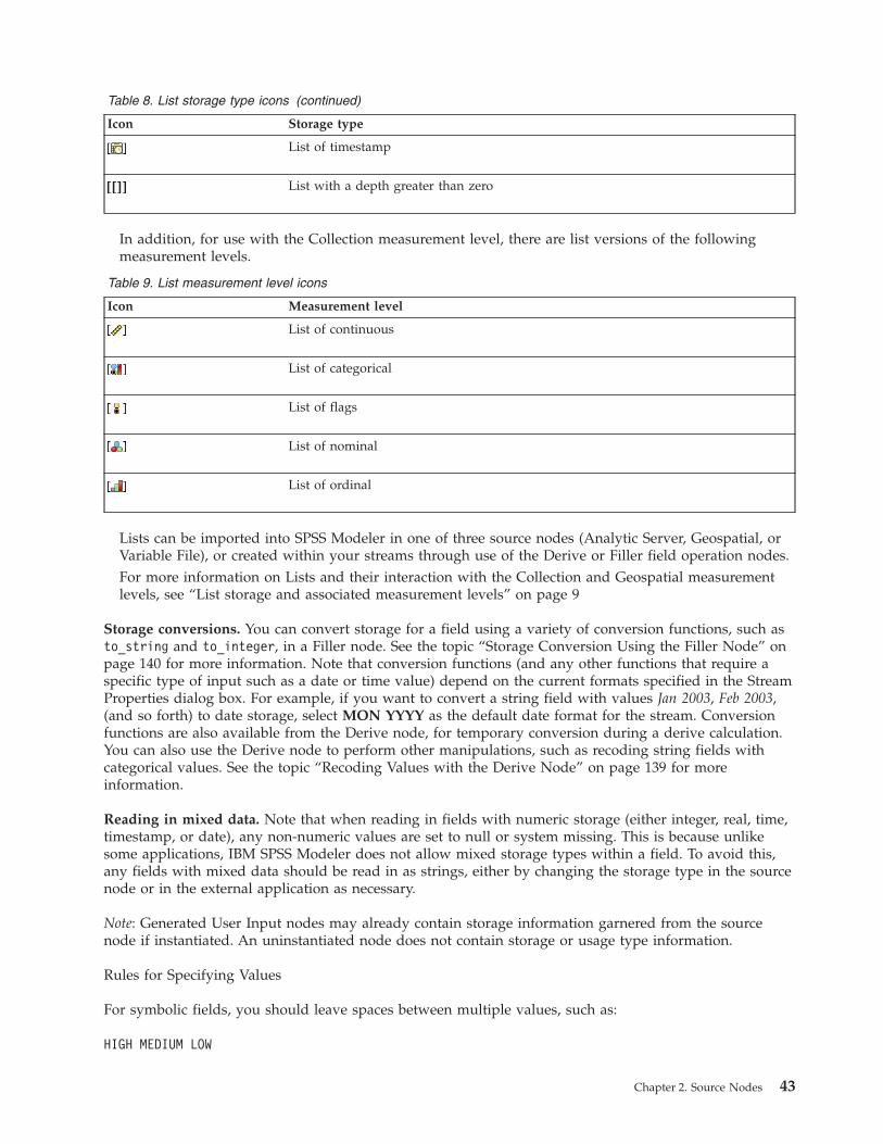
Table 8. List storage type icons (continued)

Icon Storage type

List of timestamp

List with a depth greater than zero

In addition, for use with the Collection measurement level, there are list versions of the followingmeasurement levels.

Table 9. List measurement level icons


List of continuous

List of categorical

List of flags

List of nominal

List of ordinal

Lists can be imported into SPSS Modeler in one of three source nodes (Analytic Server, Geospatial, orVariable File), or created within your streams through use of the Derive or Filler field operation nodes.For more information on Lists and their interaction with the Collection and Geospatial measurementlevels, see “List storage and associated measurement levels” on page 9

Storage conversions. You can convert storage for a field using a variety of conversion functions, such asto_string and to_integer, in a Filler node. See the topic “Storage Conversion Using the Filler Node” onpage 140 for more information. Note that conversion functions (and any other functions that require aspecific type of input such as a date or time value) depend on the current formats specified in the StreamProperties dialog box. For example, if you want to convert a string field with values Jan 2003, Feb 2003,(and so forth) to date storage, select MON YYYY as the default date format for the stream. Conversionfunctions are also available from the Derive node, for temporary conversion during a derive calculation.You can also use the Derive node to perform other manipulations, such as recoding string fields withcategorical values. See the topic “Recoding Values with the Derive Node” on page 139 for moreinformation.

Reading in mixed data. Note that when reading in fields with numeric storage (either integer, real, time,timestamp, or date), any non-numeric values are set to null or system missing. This is because unlikesome applications, IBM SPSS Modeler does not allow mixed storage types within a field. To avoid this,any fields with mixed data should be read in as strings, either by changing the storage type in the sourcenode or in the external application as necessary.

Note: Generated User Input nodes may already contain storage information garnered from the sourcenode if instantiated. An uninstantiated node does not contain storage or usage type information.

Rules for Specifying Values

For symbolic fields, you should leave spaces between multiple values, such as:

HIGH MEDIUM LOW


For numeric fields, you can either enter multiple values in the same manner (listed with spaces between):

10 12 14 16 18 20

Or you can specify the same series of numbers by setting its limits (10, 20) and the steps in between (2).Using this method, you would type:

10,20,2

These two methods can be combined by embedding one within the other, such as:

1 5 7 10,20,2 21 23

This entry will produce the following values:

1 5 7 10 12 14 16 18 20 21 23

Simulation Generate NodeThe Simulation Generate node provides an easy way to generate simulated data, either without historicaldata using user specified statistical distributions, or automatically using the distributions obtained fromrunning a Simulation Fitting node on existing historical data. Generating simulated data is useful whenyou want to evaluate the outcome of a predictive model in the presence of uncertainty in the modelinputs.

Creating data without historical data

The Simulation Generate node is available from the Sources palette and can be added directly to thestream canvas.1. Click the Sources tab of the nodes palette.2. Drag and drop or double-click to add the Simulation Generate node to the stream canvas.3. Double-click to open its dialog box and specify fields, storage types, statistical distributions and

distribution parameters.

Note: Simulation Generate nodes that are selected from the Sources palette will be completely blank, withno fields and no distribution information. This enables you to entirely create simulated data withouthistorical data.

Generating simulated data using existing historical data

A Simulation Generate node can also be created by executing a Simulation Fitting terminal node:1. Right-click on the Simulation Fitting node and choose Run from the menu.2. The Simulation Generate node appears on the stream canvas with an update link to the Simulation

Fitting node.3. When generated, the Simulation Generate node inherits all of the fields, storage types, and statistical

distribution information from the Simulation Fitting node.

Defining an update link to a simulation fitting node

You can create a link between a Simulation Generate node and a Simulation Fitting node. This is useful ifyou want to update one or more fields with the information of the best fitting distribution, determinedby fitting to historical data.1. Right click on the Simulation Generate node.2. From the menu, select Define Update Link. The cursor changes to the Link cursor.


3. Click on another node. If this node is a Simulation Fitting node, a link is made. If this node is not aSimulation Fitting node, no link is made, and the cursor changes back to a normal cursor.

If the fields in the Simulation Fitting node are different to those in the Simulation Generate node, amessage is displayed informing you that there is a difference.

When the Simulation Fitting node is used to update the linked Simulation Generate node, the resultdepends on whether the same fields are present in both nodes, and if the fields are unlocked in theSimulation Generate node. The results of updating a Simulation Fitting node are shown in the followingtable.

Table 10. Results of updating a Simulation Fitting node

Field in Simulation Fitting node

Field in Simulation Generate node Present Missing

Present and unlocked. Field is overwritten. Field is deleted.

Missing. Field is added. No change.

Present and locked. The distribution of the field is notoverwritten. The information in theFit Details dialog box and thecorrelations are updated.

The field is not overwritten. Thecorrelations are set to zero.

Do not clear Min/Max whenrefitting check box is selected.

The field is overwritten, apart from the values in the Min, Max column.

Do not recalculate correlations whenrefitting check box is selected.

If the field is unlocked, it isoverwritten.

The correlations are not overwritten.

Removing an update link to a simulation fitting node

You can remove a link between a Simulation Generate node and a Simulation Fitting node by taking thefollowing steps:1. Right click on the Simulation Generate node.2. From the menu, select Remove Update Link. The link is removed.

Setting Options for the Simulation Generate NodeYou can use the options on the Data tab of the Simulation Generate node dialog box to do the following:v View, specify, and edit the statistical distribution information for the fields.v View, specify, and edit the correlations between the fields.v Specify the number of iterations and cases to simulate.

Select an item. Enables you to switch between the three views of the Simulation Generate node:Simulated Fields, Correlations, and Advanced Options.

Simulated Fields view

If the Simulation Generate node has been generated or updated from a Simulation Fitting node usinghistorical data, in the Simulated Fields view you can view and edit the statistical distribution informationfor each field. The following information about each field is copied to the Types tab of the SimulationGenerate node from the Simulation Fitting node:v Measurement levelv Valuesv Missingv Check


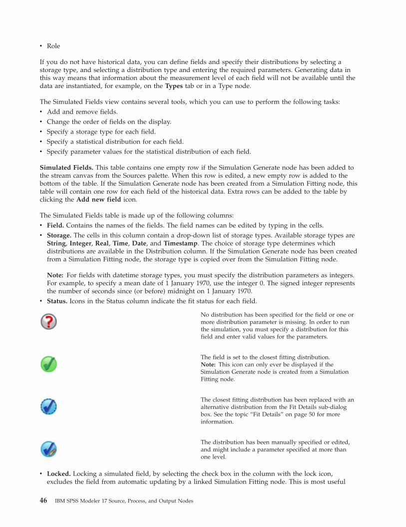
v Role

If you do not have historical data, you can define fields and specify their distributions by selecting astorage type, and selecting a distribution type and entering the required parameters. Generating data inthis way means that information about the measurement level of each field will not be available until thedata are instantiated, for example, on the Types tab or in a Type node.

The Simulated Fields view contains several tools, which you can use to perform the following tasks:v Add and remove fields.v Change the order of fields on the display.v Specify a storage type for each field.v Specify a statistical distribution for each field.v Specify parameter values for the statistical distribution of each field.

Simulated Fields. This table contains one empty row if the Simulation Generate node has been added tothe stream canvas from the Sources palette. When this row is edited, a new empty row is added to thebottom of the table. If the Simulation Generate node has been created from a Simulation Fitting node, thistable will contain one row for each field of the historical data. Extra rows can be added to the table byclicking the Add new field icon.

The Simulated Fields table is made up of the following columns:v Field. Contains the names of the fields. The field names can be edited by typing in the cells.v Storage. The cells in this column contain a drop-down list of storage types. Available storage types are

String, Integer, Real, Time, Date, and Timestamp. The choice of storage type determines whichdistributions are available in the Distribution column. If the Simulation Generate node has been createdfrom a Simulation Fitting node, the storage type is copied over from the Simulation Fitting node.

Note: For fields with datetime storage types, you must specify the distribution parameters as integers.For example, to specify a mean date of 1 January 1970, use the integer 0. The signed integer representsthe number of seconds since (or before) midnight on 1 January 1970.

v Status. Icons in the Status column indicate the fit status for each field.

No distribution has been specified for the field or one ormore distribution parameter is missing. In order to runthe simulation, you must specify a distribution for thisfield and enter valid values for the parameters.

The field is set to the closest fitting distribution.Note: This icon can only ever be displayed if theSimulation Generate node is created from a SimulationFitting node.

The closest fitting distribution has been replaced with analternative distribution from the Fit Details sub-dialogbox. See the topic “Fit Details” on page 50 for moreinformation.

The distribution has been manually specified or edited,and might include a parameter specified at more thanone level.

v Locked. Locking a simulated field, by selecting the check box in the column with the lock icon,excludes the field from automatic updating by a linked Simulation Fitting node. This is most useful


when you manually specify a distribution and want to ensure that it will not be affected by automaticdistribution fitting when a linked Simulation Fitting node is executed.

v Distribution. The cells in this column contain a drop-down list of statistical distributions. The choice ofstorage type determines which distributions are available in this column for a given field. See the topic“Distributions” on page 53 for more information.

Note: You cannot specify the Fixed distribution for every field. If you want every field in yourgenerated data to be fixed, you can use a User Input node followed by a Balance node.

v Parameters. The distribution parameters associated with each fitted distribution are displayed in thiscolumn. Multiple values of a parameter are comma separated. Specifying multiple values for aparameter generates multiple iterations for the simulation. See the topic “Iterations” on page 53 formore information. If parameters are missing, this is reflected in the icon displayed in the Statuscolumn. To specify values for the parameters, click this column in the row corresponding to the field ofinterest and choose Specify from the list. This opens the Specify Parameters sub-dialog box. See thetopic “Specify Parameters” on page 51 for more information. This column is disabled if Empirical ischosen in the Distribution column.

v Min, Max. In this column, for some distributions, you can specify a minimum value, a maximumvalue, or both for the simulated data. Simulated data that are smaller than the minimum value andlarger than the maximum value will be rejected, even though they would be valid for the specifieddistribution. To specify minimum and maximum values, click this column in the row corresponding tothe field of interest and choose Specify from the list. This opens the Specify Parameters sub-dialog box.See the topic “Specify Parameters” on page 51 for more information. This column is disabled ifEmpirical is chosen in the Distribution column.

Use Closest Fit. Only enabled if the Simulation Generate node has been created automatically from aSimulation Fitting node using historical data, and a single row in the Simulated Fields table is selected.Replaces the information for the field in the selected row with the information of the best fittingdistribution for the field. If the information in the selected row has been edited, pressing this button willreset the information back to the best fitting distribution determined from the Simulation Fitting node.

Fit Details. Only enabled if the Simulation Generate node has been created automatically from aSimulation Fitting node. Opens the Fit Details sub-dialog box. See the topic “Fit Details” on page 50 formore information.

Several useful tasks can be carried out using the icons on the right of the Simulated Fields view. Theseicons are described in the following table.

Table 11. Icons on the Simulated Fields view.

Icon Tooltip Description

Edit distribution parameters Only enabled when a single row inthe Simulated Fields table is selected.Opens the Specify Parameterssub-dialog box for the selected row.See the topic “Specify Parameters” onpage 51 for more information.

Add new field Only enabled when a single row inthe Simulated Fields table is selected.Adds a new empty row to thebottom of the Simulated Fields table.

Create multiple copies Only enabled when a single row inthe Simulated Fields table is selected.Opens the Clone Field sub-dialogbox. See the topic “Clone Field” onpage 50 for more information.


Table 11. Icons on the Simulated Fields view (continued).

Icon Tooltip Description

Delete selected field Deletes the selected row from theSimulated Fields table.

Move to top Only enabled if the selected row isnot already the top row of theSimulated Fields table. Moves theselected row to the top of theSimulated Fields table. This actionaffects the order of the fields in thesimulated data.

Move up Only enabled if the selected row isnot the top row of the SimulatedFields table. Moves the selected rowup one position in the SimulatedFields table. This action affects theorder of the fields in the simulateddata.

Move down Only enabled if the selected row isnot the bottom row of the SimulatedFields table. Moves the selected rowdown one position in the SimulatedFields table. This action affects theorder of the fields in the simulateddata.

Move to bottom Only enabled if the selected row isnot already the bottom row of theSimulated Fields table. Moves theselected row to the bottom of theSimulated Fields table. This actionaffects the order of the fields in thesimulated data.

Do not clear Min and Max when refitting. When selected, the minimum and maximum values are notoverwritten when the distributions are updated by executing a connected Simulation Fitting node.

Correlations view

Input fields to predictive models are often known to be correlated--for example, height and weight.Correlations between fields that will be simulated must be accounted for in order to ensure that thesimulated values preserve those correlations.

If the Simulation Generate node has been generated or updated from a Simulation Fitting node usinghistorical data, in the Correlations view you can view and edit the calculated correlations between pairsof fields. If you do not have historical data, you can specify the correlations manually based on yourknowledge of how the fields are correlated.

Note: Before any data are generated, the correlation matrix is automatically checked to see if it is positivesemi-definite, and can therefore be inverted. A matrix can be inverted if its columns are linearlyindependent. If the correlation matrix cannot be inverted, it will be automatically adjusted to make itinvertible.

You can choose to display the correlations in a matrix or list format.


Correlations matrix. Displays the correlations between pairs of fields in a matrix. The field names arelisted, in alphabetical order, down the left and along the top of the matrix. Only the cells below thediagonal can be edited; a value between -1.000 and 1.000, inclusive, must be entered. The cell above thediagonal is updated when focus is changed away from its mirrored cell below the diagonal; both cellsthen display the same value. The diagonal cells are always disabled and always have a correlation of1.000. The default value for all other cells is 0.000. A value of 0.000 specifies that there is no correlationbetween the associated pair of fields. Only continuous and ordinal fields are included in the matrix.Nominal, categorical and flag fields, and fields that are assigned the Fixed distribution are not shown inthe table.

Correlations list. Displays the correlations between pairs of fields in a table. Each row of the table showsthe correlation between a pair of fields. Rows cannot be added or deleted. The columns with theheadings Field 1 and Field 2 contain the field names, which cannot be edited. The Correlation columncontains the correlations, which can be edited; a value between -1.000 and 1.000, inclusive, must beentered. The default value for all cells is 0.000. Only continuous and ordinal fields are included in the list.Nominal, categorical and flag fields, and fields that are assigned the Fixed distribution are not shown inthe list.

Reset correlations. Opens the Reset Correlations dialog box. If historical data is available, you can chooseone of three options:v Fitted. Replaces the current correlations with those calculated using the historical data.v Zeroes. Replaces the current correlations with zeroes.v Cancel. Closes the dialog box. The correlations are unchanged.

If historical data is not available, but you have made changes to the correlations, you can choose toreplace the current correlations with zeroes, or cancel.

Show As. Select Table to display the correlations as a matrix. Select List to display the correlations as alist.

Do not recalculate correlations when refitting. Select this option if you want to manually specifycorrelations and prevent them from being overwritten when automatically fitting distributions using aSimulation Fitting node and historical data.

Use fitted multiway contingency table for inputs with a categorical distribution. By default, all fieldswith a categorical distribution are included in a contingency table (or multiway contingency table,depending on the number of fields with a categorical distribution). The contingency table is constructed,like the correlations, when a Simulation Fitting node is executed. The contingency table cannot beviewed. When this option is selected, fields with a categorical distribution are simulated using the actualpercentages from the contingency table. That is, any associations between nominal fields are recreated inthe new, simulated data. When this option is cleared, fields with categorical distributions are simulatedusing the expected percentages from the contingency table. If you modify a field, the field is removedfrom the contingency table.

Advanced Options view

Number of cases to simulate. Displays the options for specifying the number of cases to be simulated,and how any iterations will be named.v Maximum number of cases. This specifies the maximum number of cases of simulated data, and

associated target values, to generate. The default value is 100,00, minimum value is 1000, andmaximum value is 2,147,483,647.

v Iterations. This number is calculated automatically and cannot be edited. An iteration is createdautomatically each time a distribution parameter has multiple values specified.

v Total rows. Only enabled when the number of iterations is greater than 1. The number is calculatedautomatically, using the equation shown, and cannot be edited.


v Create iteration field. Only enabled when the number of iterations is greater than 1. When selected,the Name field is enabled. See the topic “Iterations” on page 53 for more information.

v Name. Only enabled when the Create iteration field check box is selected, and the number ofiterations is greater than 1. Edit the name of the iteration field by typing in this text field. See the topic“Iterations” on page 53 for more information.

Random seed. Setting a random seed allows you to replicate your simulation.v Replicate results. When selected, the Generate button and Random seed field are enabled.v Random seed. Only enabled when the Replicate results check box is selected. In this field you can

specify an integer to be used as the random seed. The default value is 629111597.v Generate. Only enabled when the Replicate results check box is selected. Creates a pseudo-random

integer between 1 and 999999999, inclusive, in the Random seed field.

Clone FieldIn the Clone Field dialog box you can specify how many copies of the selected field to create, and howeach copy is named. It is useful to have multiple copies of fields when investigating compounded effects,for example interest or growth rates over a number of successive time periods.

The title bar of the dialog box contains the name of the selected field.

Number of copies to make. Contains the number of copies of the field to create. Click the arrows toselect the number of copies to create. The minimum number of copies is 1 and the maximum is 512. Thenumber of copies is initially set to 10.

Copy suffix character(s). Contains the characters that are added to the end of the field name for eachcopy. These characters separate the field name from the copy number. The suffix characters can be editedby typing in this field. This field can be left empty; in this case there will be no characters between thefield name and copy number. The default character is an underscore.

Initial copy number. Contains the suffix number for the first copy. Click the arrows to select the initialcopy number. The minimum initial copy number is 1 and the maximum is 1000. The default initial copynumber is 1.

Copy number step. Contains the increment for the suffix numbers. Click the arrows to select theincrement. The minimum increment is 1 and the maximum is 255. The increment is initially set to 1.

Fields. Contains a preview of the field names for the copies, which is updated if any of the fields of theClone Field dialog box are edited. This text is generated automatically and cannot be edited.

OK. Generates all the copies as specified in the dialog box. The copies are added to the Simulated Fieldstable in the Simulation Generate node dialog box, directly below the row that contains the field that wascopied.

Cancel. Closes the dialog box. Any changes that have been made are discarded.

Fit DetailsThe Fit Details dialog box is only available if the Simulation Generate node was created or updated byexecuting a Simulation Fitting node. It displays the results of automatic distribution fitting for theselected field. Distributions are ordered by goodness of fit, with the closest fitting distribution listed first.In this dialog box you can perform the following tasks:v Examine the distributions fitted to the historical data.v Select one of the fitted distributions.


Field. Contains the name of the selected field. This text cannot be edited.

Treat as (Measure). Displays the measurement type of the selected field. This is taken from the SimulatedFields table in the Simulation Generate node dialog box. The measurement type can be changed byclicking the arrow and selecting a measurement type from the drop-down list. There are three options:Continuous, Nominal, and Ordinal.

Distributions. The Distributions table shows all the distributions that are appropriate for themeasurement type. The distributions that have been fitted to the historical data are ordered by goodnessof fit, from best fitting to worst fitting. Goodness of fit is determined by the fit statistic chosen in theSimulation Fitting node. The distributions that were not fitted to the historical data are listed in the tablein alphabetical order below the distributions that were fitted.

The Distribution table contains the following columns:v Use. The selected radio button indicates which distribution is currently chosen for the field. You can

override the closest fitting distribution by selecting the radio button for the desired distribution in theUse column. Selecting a radio button in the Use column also displays a plot of the distributionsuperimposed on a histogram (or bar chart) of the historical data for the selected field. Only onedistribution can be selected at a time.

v Distribution. Contains the name of the distribution. This column cannot be edited.v Fit Statistics. Contains the calculated fit statistics for the distribution. This column cannot be edited.

The contents of the cell depends on the measurement type of the field:– Continuous. Contains the results of the Anderson-Darling and Kolmogorov-Smirnoff tests. The

p-values associated with the tests are also shown. The fit statistic chosen as the Goodness of fitcriteria in the Simulation Fitting node is shown first and is used to order the distributions. TheAnderson-Darling statistics are displayed as A=aval P=pval. The Kolmogorov-Smirnoff statistics aredisplayed as K=kval P=pval. If a statistic cannot be calculated, a dot is displayed instead of anumber.

– Nominal and Ordinal. Contains the results of the chi-squared test. The p-value associated with thetest is also shown. The statistics are displayed as Chi-Sq=val P=pval. If the distribution was notfitted, Not fitted is displayed. If the distribution cannot be mathematically fit, Cannot be fit isdisplayed.

Note: The cell is always empty for the Empirical distribution.v Parameters. Contains the distribution parameters associated with each fitted distribution. The

parameters are displayed as parameter_name = parameter_value, with the parameters separated by asingle space. For the categorical distribution, the parameter names are the categories and the parametervalues are the associated probabilities. If the distribution was not fitted to the historical data, the cell isempty. This column cannot be edited.

Histogram thumbnail. Shows a plot of the selected distribution superimposed on a histogram of thehistorical data of the selected field.

Distribution thumbnail. Shows an explanation and illustration of the selected distribution.

OK. Closes the dialog box and updates the values of the Measurement, Distribution, Parameters and Min,Max columns of the Simulated Fields table for the selected field with the information from the selecteddistribution. The icon in the Status column is also updated to reflect whether the selected distribution isthe distribution with the closest fit to the data.


Specify ParametersIn the Specify Parameters dialog box you can manually specify the parameter values for the distributionof the selected field. You can also choose a different distribution for the selected field.


The Specify Parameters dialog box can be opened in three ways:v Double click on a field name in the Simulated Fields table in the Simulation Generate node dialog box.v Click the Parameters or Min, Max column of the Simulated Fields table, and choose Specify from the

list.v In the Simulated Fields table, select a row, and then click the Edit distribution parameters icon.

Field. Contains the name of the selected field. This text cannot be edited.

Distribution. Contains the distribution of the selected field. This is taken from the Simulated Fields table.The distribution can be changed by clicking the arrow and selecting a distribution from the drop-downlist. The available distributions depend on the storage type of the selected field.

Sides. This option is only available for the when the dice distribution is selected in the Distribution field.Click the arrows to select the number of sides, or categories, to split the field in to. The minimumnumber of sides is two, and the maximum is 20. The number of sides is initially set to 6.

Distribution parameters. The Distribution parameters table contains one row for each parameter of thechosen distribution.

Note: Distribution uses a rate parameter, with a shape parameter α = k and an inverse scale parameter β= 1/θ.The table contains two columns:v Parameter. Contains the names of the parameters. This column cannot be edited.v Value(s). Contains the values of the parameters. If the Simulation Generate node has been created or

updated from a Simulation Fitting node, the cells in this column contain the parameter values thathave been determined by fitting the distribution to the historical data. If the Simulation Generate nodehas been added to the stream canvas from the Source nodes palette, the cells in this column are empty.The values can be edited by typing in the cells. See the topic “Distributions” on page 53 for moreinformation about the parameters needed by each distribution, and acceptable parameter values.Multiple values for a parameter must be separated by commas. Specifying multiple values for aparameter will define multiple iterations of the simulation. You can only specify multiple values forone parameter.

Note: For fields with datetime storage types, you must specify the distribution parameters as integers.For example, to specify a mean date of 1 January 1970, use the integer 0.

Note: When the dice distribution is selected, the Distribution parameters table is slightly different. Thetable contains one row for each side (or category). The table contains a Value column and a Probabilitycolumn. The Value column contains a label for each category. The default values for the labels are theintegers 1-N, where N is the number of sides. The labels can be edited by typing in the cells. Any valuecan be entered into the cells. If you want to use a value that is not a number, the storage type of the datafield must be changed to string if the storage type is not already set to string. The Probability columncontains the probability of each category. The probabilities cannot be edited, and are calculated as 1/N.

Preview. Shows a sample plot of the distribution, based on the specified parameters. If two or morevalues have been specified for one parameter, sample plots for each value of the parameter are shown. Ifhistorical data is available for the selected field, the plot of the distribution is superimposed on ahistogram of the historical data.

Optional Settings. Use these options to specify a minimum value, a maximum value, or both for thesimulated data. Simulated data that are smaller than the minimum value and larger than the maximumvalue will be rejected, even though they would be valid for the specified distribution.v Specify minimum. Select to enable the Reject values below field. The check box is disabled if the

Empirical distribution is selected.


v Reject values below. Only enabled if Specify minimum is selected. Enter a minimum value for thesimulated data. Any simulated values smaller than this value will be rejected.

v Specify maximum. Select to enable the Reject values above field. The check box is disabled if theEmpirical distribution is selected.

v Reject values above. Only enabled if Specify maximum is selected. Enter a maximum value for thesimulated data. Any simulated values larger than this value will be rejected.

OK. Closes the dialog box and updates the values of the Distribution, Parameters and Min, Max columnsof the Simulated Fields table for the selected field. The icon in the Status column is also updated toreflect the selected distribution.


IterationsIf you have specified more than one value for a fixed field or a distribution parameter, an independentset of simulated cases - effectively, a separate simulation - is generated for each specified value. Thisallows you to investigate the effect of varying the field or parameter. Each set of simulated cases isreferred to as an iteration. In the simulated data, the iterations are stacked up.

If the Create iteration field check box on the Advanced Options view of the Simulation Generate nodedialog is selected, an iteration field is added to the simulated data as a nominal field with numericstorage. The name of this field can be edited by typing in the Name field on the Advanced Options view.This field contains a label which indicates to which iteration each simulated case belongs. The form of thelabels depends on the type of iteration:v Iterating a fixed field. The label is the name of the field, followed by an equals sign, followed by the

value of the field for that iteration, that isfield_name = field_value

v Iterating a distribution parameter. The label is the name of the field, followed by a colon, followed bythe name of the iterated parameter, followed by an equals sign, followed by the value of the parameterfor that iteration, that isfield_name:parameter_name = parameter_value

v Iterating a distribution parameter for a categorical or range distribution. The label is the name of thefield, followed by a colon, followed by "Iteration", followed by the iteration number, that isfield_name: Iteration iteration_number

DistributionsYou can manually specify the probability distribution for any field by opening the Specify Parametersdialog box for that field, selecting the desired distribution from the Distribution list, and entering thedistribution parameters in the Distribution parameters table. Following are some notes on particulardistributions:v Categorical. The categorical distribution describes an input field that has a fixed number of numeric

values, referred to as categories. Each category has an associated probability such that the sum of theprobabilities over all categories equals one.

Note: If you specify probabilities for the categories that do not sum to 1, you will receive a warning.v Negative Binomial - Failures. Describes the distribution of the number of failures in a sequence of

trials before a specified number of successes are observed. The parameter Threshold is the specifiednumber of successes and the parameter Probability is the probability of success in any given trial.

v Negative Binomial - Trials. Describes the distribution of the number of trials that are required before aspecified number of successes are observed. The parameter Threshold is the specified number ofsuccesses and the parameter Probability is the probability of success in any given trial.

v Range. This distribution consists of a set of intervals with a probability assigned to each interval suchthat the sum of the probabilities over all intervals equals 1. Values within a given interval are drawn


from a uniform distribution defined on that interval. Intervals are specified by entering a minimumvalue, a maximum value and an associated probability.For example, you believe that the cost of a raw material has a 40% chance of falling in the range of $10- $15 per unit, and a 60% chance of falling in the range of $15 - $20 per unit. You would model the costwith a Range distribution consisting of the two intervals [10 - 15] and [15 - 20], setting the probabilityassociated with the first interval to 0.4 and the probability associated with the second interval to 0.6.The intervals do not have to be contiguous and they can even be overlapping. For example, you mighthave specified the intervals $10 - $15 and $20 - $25 or $10 - $15 and $13 - $16.

v Weibull. The parameter Location is an optional location parameter, which specifies where the origin ofthe distribution is located.

The following table shows the distributions that are available for custom distribution fitting, and theacceptable values for the parameters. Some of these distributions are available for custom fitting toparticular storage types, even though they are not fitted automatically to these storage types by theSimulation Fitting node.

Table 12. Distributions available for custom fitting

Distribution

Storage typesupported for customfitting Parameters Parameter limits Notes

Bernoulli Integer, real, datetime Probability 0 ≤ Probability ≤ 1

Beta Integer, real, datetime Shape 1Shape 2MinimumMaximum

≥ 0≥ 0< Maximum> Minimum

Minimum andmaximum areoptional.

Binomial Integer, real, datetime Number of trials (n)ProbabilityMinimumMaximum

> 0, integer0 ≤ Probability ≤ 1< Maximum> Minimum

Number of trialsmust be an integer.Minimum andmaximum areoptional.

Categorical Integer, real,datetime, string

Category name (orlabel)

0 ≤ Value ≤ 1 Value is theprobability of thecategory. The valuesmust sum to 1,otherwise a warningis generated.

Dice Integer, string Sides 2 ≤ Sides ≤ 20 The probability ofeach category (side) iscalculated as 1/N,where N is thenumber of sides. Theprobabilities cannotbe edited.

Empirical Integer, real, datetime You cannot edit theempirical distribution,or select it as a type.

The Empiricaldistribution is onlyavailable when thereis historical data.

Exponential Integer, real, datetime ScaleMinimumMaximum

> 0< Maximum> Minimum



Table 12. Distributions available for custom fitting (continued)

Distribution

Storage typesupported for customfitting Parameters Parameter limits Notes

Fixed Integer, real,datetime, string

Value You cannot specifythe Fixed distributionfor every field. If youwant every field inyour generated datato be fixed, you canuse a User Inputnode followed by aBalance node.

Gamma Integer, real, datetime ShapeScaleMinimumMaximum



Distribution uses arate parameter, with ashape parameter α =k and an inverse scaleparameter β = 1/θ.

Lognormal Integer, real, datetime Shape 1Shape 2MinimumMaximum



Negative Binomial -Failures

Integer, real, datetime ThresholdProbabilityMinimumMaximum

≥ 00 ≤ Probability ≤ 1< Maximum> Minimum


Negative Binomial -Trials

Integer, real, datetime ThresholdProbabilityMinimumMaximum

≥ 00 ≤ Probability ≤ 1< Maximum> Minimum


Normal Integer, real, datetime MeanStandard deviationMinimumMaximum

≥ 0> 0< Maximum> Minimum


Poisson Integer, real, datetime MeanMinimumMaximum

≥ 0< Maximum> Minimum


Range Integer, real, datetime Begin(X)End(X)Probability(X)

0 ≤ Value ≤ 1 X is the index of eachbin. The probabilityvalues must sum to 1.

Triangular Integer, real, datetime Mode

MinimumMaximum

Minimum ≤ Value ≤Maximum< Maximum> Minimum

Uniform Integer, real, datetime MinimumMaximum

< Maximum> Minimum

Weibull Integer, real, datetime RateScaleLocationMinimumMaximum

> 0> 0≥ 0< Maximum> Minimum

Location, maximumand minimum areoptional.


Data View nodeUse the Data View node to include data defined in an IBM SPSS Collaboration and Deployment Servicesanalytic data view in your stream. An analytic data view defines a structure for accessing data thatdescribes the entities used in predictive models and business rules. The view associates the data structurewith physical data sources for the analysis.

Predictive analytics requires data organized in tables with each row corresponding to an entity for whichpredictions are made. Each column in a table represents a measurable attribute of the entity. Someattributes may be derived by aggregating over the values for another attribute. For example, the rows ofa table could represent customers with columns corresponding to the customer name, gender, zip code,and the number of times the customer had a purchase over $500 in the past year. The last column isderived from the customer order history, which is typically stored in one or more related tables.

The predictive analytic process involves using different sets of data throughout the lifecycle of a model.During initial development of a predictive model, you use historic data that often has known outcomesfor the event being predicted. To evaluate the model effectiveness and accuracy, you validate a candidatemodel against different data. After validating the model, you deploy it into production use to generatescores for multiple entities in a batch process or for single entities in a real-time process. If you combinethe model with business rules in a decision management process, you use simulated data to validate theresults of the combination. However, although the data that is used differs across the model developmentprocess stages, each data set must provide the same set of attributes for the model. The attribute setremains constant; the data records being analyzed change.

An analytic data view consists of the following components that address the specialized needs ofpredictive analytics:v A data view schema, or data model, that defines a logical interface for accessing data as a set of

attributes organized into related tables. Attributes in the model can be derived from other attributes.v One or more data access plans that provide the data model attributes with physical values. You control

the data available to the data model by specifying which data access plan is active for a particularapplication.

Important: To use the Data View node, an IBM SPSS Collaboration and Deployment Services Repositorymust first be installed and configured at your site. The analytic data view referenced by the node istypically created and stored in the repository by using IBM SPSS Collaboration and Deployment ServicesDeployment Manager.

Setting Options for the Data View NodeUse the options on the Data tab of the Data View node dialog box to specify the data settings for ananalytic data view selected from the IBM SPSS Collaboration and Deployment Services Repository.

Analytic data view. Click the ellipsis button (...) to select an analytic data view. If you are not currentlyconnected to a repository server, specify the URL for the server in the Repository: Server dialog box, clickOK, and specify your connection credentials in the Repository: Credentials dialog box. For moreinformation on logging in to the repository and retrieving objects, see the IBM SPSS Modeler User'sGuide.

Table name. Select a table from the data model in the analytic data view. Each table in the data modelrepresents a concept or entity involved in the predictive analytic process. Fields for the tables correspondto attributes of the entities represented by the tables. For example, if you are analyzing customer orders,your data model could include a table for customers and a table for orders. The customers table mighthave attributes for customer identifier, age, gender, marital status, and country of residence. The orderstable might have attributes for the order identifier, number of items in the order, total cost, and theidentifier for the customer who placed the order. The customer identifier attribute could be used toassociate the customers in the customers table with their orders in the orders table.


Data access plan. Select a data access plan from the analytic data view. A data access plan associates thedata model tables in an analytic data view with physical data sources. An analytic data view typicallycontains multiple data access plans. When you change the data access plan in use, you change the dataused by your stream. For example, if the analytic data view contains a data access plan for training amodel and a data access plan for testing a model, you can switch from training data to testing data bychanging the data access plan in use.

Optional Attributes. If a particular attribute is not required by the application using the analytic dataview, you can mark the attribute as optional. Unlike required attributes, optional attributes can includenull values. You may need to adjust your application to include null value handling for optionalattributes. For example, when invoking a business rule created in IBM Operational Decision Manager,IBM Analytical Decision Management queries the rules service to determine which inputs are required. Ifthe record to be scored contains a null value for any of the rule service's required fields, the rule is notinvoked and the output fields of the rule are populated with default values. If an optional field contains anull value, the rule is invoked. The rule can check for null values to control processing.

To specify attributes as optional, click Optional Attributes and select the attributes that are optional.

Include XML data in field. Select this option to create a field containing the executable object modelXML data for each row of data. This information is required if the data will be used with IBMOperational Decision Manager. Specify the name for this new field.

Geospatial Source NodeYou use the Geospatial source node to bring map or spatial data into your data mining session. You canimport data in one of two ways:v In a shape file (.shp)v By connecting to an ESRI server that contains a hierarchical file system which includes map files.

Note: You can only connect to public map services.

Spatio-Temporal Prediction (STP) models can include map or spatial elements in their predictions. Formore information on these models, see the topic titled "Spatio-Temporal Prediction modeling node" in theTime Series Models section of the Modeler Modeling Nodes guide (ModelerModelingNodes.pdf).

Setting Options for the Geospatial Source NodeDatasource type You can import data from either a Shape file (.shp), or connect to a Map service.

If you are using a Shape file, either enter the file name and the filepath to it, or browse to select the file.

Note: Shape data requires both a .shp and a .dbf file. The two files must have the same name and be inthe same folder. The .dbf file is automatically imported when you select the .shp file. In addition, theremight be a .prj file that specifies the coordinate system for the shape data.

If you are using a Map service, enter the URL to the service and click Connect. After you connect to theservice, the layers within that service are displayed in the bottom of the dialog box in a tree structure inthe Available maps pane; expand the tree and select the layer that you require.

Note: You can only connect to public map services.

Automatic definition of geospatial data

By default, SPSS Modeler automatically defines, when possible, any geospatial data fields in the sourcenode with the correct metadata. Metadata might include the measurement level of the geospatial field(such as Point or Polygon) and the coordinate system that is used by the fields, including details such as


the origin point (for example, latitude 0, longitude 0) and the units of measure. For more informationabout measurement levels, see “Geospatial measurement sublevels” on page 121.

The .shp and .dbf files that make up the shape file contain a common identifier field that is used as akey. For example, the .shp file might contain countries, with the country name field used as an identifier,and the .dbf file might contain information about those countries with the name of the country that isalso used as the identifier.

Note: If the coordinate system is not the same as the default SPSS Modeler coordinate system you mayhave to reproject the data to use the required coordinate system. For more information, see “ReprojectionNode” on page 173.

Enterprise View Node

Note: The Enterprise View node was replaced in IBM SPSS Modeler 16.0 by the Data View node. Forstreams saved in previous releases, the Enterprise View node is still supported. However when updatingor creating new streams we recommend that you use the Data View node.

The Enterprise View node enables you to create and maintain a connection between an IBM SPSSModeler session and an Enterprise View in a shared IBM SPSS Collaboration and Deployment ServicesRepository. Doing so enables you to read data from an Enterprise View into an IBM SPSS Modeler streamand to package an IBM SPSS Modeler model in a scenario that can be accessed by other users of theshared repository.

A scenario is a file containing an IBM SPSS Modeler stream with specific nodes, models, and additionalproperties that enable it to be deployed to an IBM SPSS Collaboration and Deployment ServicesRepository for the purposes of scoring or automatic model refresh. The use of Enterprise View nodeswith scenarios ensures that, in a multi-user situation, all users are working from the same data. Aconnection is a link from an IBM SPSS Modeler session to an Enterprise View in the IBM SPSSCollaboration and Deployment Services Repository.

The Enterprise View is the complete set of the data belonging to an organization, irrespective of wherethe data is physically located. Each connection consists of a specific selection of a single ApplicationView (subset of the Enterprise View tailored for a particular application), a Data Provider Definition(DPD--links the logical Application View tables and columns to a physical data source), and anenvironment (identifies which particular columns should be associated with defined business segments).The Enterprise View, Application Views, and DPD definitions are stored and versioned in the repository,although the actual data resides in one or more databases or other external sources.

Once a connection has been established, you specify an Application View table to work with in IBM SPSSModeler. In an Application View, a table is a logical view consisting of some or all columns from one ormore physical tables in one or more physical databases. Thus the Enterprise View node enables recordsfrom multiple database tables to be seen as a single table in IBM SPSS Modeler.

Requirementsv To use the Enterprise View node, an IBM SPSS Collaboration and Deployment Services Repository

must first be installed and configured at your site, with an Enterprise View, Application Views, andDPDs already defined.

v In addition, the IBM SPSS Collaboration and Deployment Services Enterprise View Driver must beinstalled on each computer used to modify or run the stream. For Windows, simply install the driveron the computer where IBM SPSS Modeler or IBM SPSS Modeler Server is installed, and no furtherconfiguration of the driver is needed. On UNIX, a reference to the pev.sh script must be added to thestartup script. Contact your local administrator for details on installing the IBM SPSS Collaborationand Deployment Services Enterprise View Driver.


v A DPD is defined against a particular ODBC datasource. To use a DPD from IBM SPSS Modeler, youmust have an ODBC datasource defined on the IBM SPSS Modeler server host which has the samename, and which connects to the same data store, as the one referenced in the DPD.

Setting Options for the Enterprise View NodeYou can use the options on the Data tab of the Enterprise View dialog box to:v Select an existing repository connectionv Edit an existing repository connectionv Create a new repository connectionv Select an Application View table

Refer to the IBM SPSS Collaboration and Deployment Services Administrator's Guide for details on workingwith repositories.

Connection. The drop-down list provides options for selecting an existing repository connection, editingan existing connection, or adding a connection. If you are already logged in to a repository through IBMSPSS Modeler, choosing the Add/Edit a connection option displays the Enterprise View Connectionsdialog box, from where you can define or edit the required details for the current connection. If you arenot logged in, this option displays the repository Login dialog box.

For information on logging in to the repository, see the IBM SPSS Modeler User's Guide.

Once a connection to a repository has been established, that connection remains in place until you exitfrom IBM SPSS Modeler. A connection can be shared by other nodes within the same stream, but youmust create a new connection for each new stream.

A successful login displays the Enterprise View Connections dialog box.

Table name. This field is initially empty and cannot be populated until you create a connection. If youknow the name of the Application View table you would like to access, enter it in the Table Name field.Otherwise, click the Select button to open a dialog box listing the available Application View tables.

Enterprise View ConnectionsThis dialog box enables you to define or edit the required details for the repository connection. You canspecify the:v Application View and versionv Environmentv Data Provider Definition (DPD)v Connection description

Connections. Lists existing repository connections.v Add a new connection. Displays the Retrieve Object dialog box, from where you can search for and

select an Application View from the repository.v Copy the selected connection. Makes a copy of a selected connection, saving you from having to

browse again for the same Application View.v Delete the selected connection. Deletes the selected connection from the list.

Connection Details. For the connection currently selected in the Connections pane, displays theApplication View, version label, environment, DPD, and descriptive text.v Application view. The drop-down list displays the selected application view, if any. If connections have

been made to other Application Views in the current session, these also appear on the drop-down list.Click the adjacent Browse button to search for other Application Views in the repository.


v Version label. The drop-down field lists all defined version labels for the specified Application View.Version labels help identify specific repository object versions. For example, there may be two versionsfor a particular Application View. By using labels, you could specify the label TEST for the versionused in the development environment and the label PRODUCTION for the version used in theproduction environment. Select an appropriate label.

Note: Labels should not include bracket characters "(" or ")", square bracket characters ("[" or "]", ordouble-bracket characters (Japanese double-byte), otherwise the table name will not be displayed onthe Data tab of the Enterprise View dialog box.

v Environment. The drop-down field lists all valid environments. The environment setting determineswhich DPDs are available, thus specifying which particular columns should be associated with definedbusiness segments. For example, when Analytic is selected, only those Application View columnsdefined as Analytic are returned. The default environment is Analytic; you can also chooseOperational.

v Data provider. The drop-down list displays the names of up to ten Data Provider Definitions for theselected Application View. Only DPDs that reference the selected Application View are shown. Clickthe adjacent Browse button to view the name and path of all DPDs related to the current ApplicationView.

v Description. Descriptive text about the repository connection. This text will be used for the connectionname--clicking OK causes the text to appear on the Connection drop-down list and title bar of theEnterprise View dialog box, and as the label of the Enterprise View node on the canvas.

Choosing the DPDThe Select Data Provider dialog box shows the name and path of all the DPDs that reference the currentApplication View.

Application Views can have multiple DPDs in order to support the different stages of a project. Forexample, the historic data used to build a model may come from one database, while operational datacomes from another.

A DPD is defined against a particular ODBC datasource. To use a DPD from IBM SPSS Modeler, youmust have an ODBC datasource defined on the IBM SPSS Modeler server host which has the same name,and which connects to the same data store, as the one referenced in the DPD.

To choose a DPD to work with, select its name on the list and click OK.

Choosing the TableThe Select Table dialog box lists all the tables that are referenced in the current Application View. Thedialog box is empty if no connection has been made to an IBM SPSS Collaboration and DeploymentServices Repository.

To choose a table to work with, select its name on the list and click OK.

Common Source Node TabsThe following options can be specified for all source nodes by clicking the corresponding tab:v Data tab. Used to change the default storage type.v Filter tab. Used to eliminate or rename data fields. This tab offers the same functionality as the Filter

node. See the topic “Setting Filtering Options” on page 131 for more information.v Types tab. Used to set measurement levels. This tab offers the same functionality as the Type node.v Annotations tab. Used for all nodes, this tab offers options to rename nodes, supply a custom ToolTip,

and store a lengthy annotation.


Setting Measurement Levels in the Source NodeField properties can be specified in a source node or in a separate Type node. The functionality is similarin both nodes. The following properties are available:v Field Double-click any field name to specify value and field labels for data in IBM SPSS Modeler. For

example, field metadata imported from IBM SPSS Statistics can be viewed or modified here. Similarly,you can create new labels for fields and their values. The labels that you specify here are displayedthroughout IBM SPSS Modeler depending on the selections you make in the stream properties dialogbox.

v Measurement This is the measurement level, used to describe characteristics of the data in a givenfield. If all of the details of a field are known, it is called fully instantiated. For more information, see“Measurement Levels” on page 119.

Note: The measurement level of a field is different from its storage type, which indicates whether thedata are stored as strings, integers, real numbers, dates, times, timestamps, or lists.

v Values This column enables you to specify options for reading data values from the data set, or use theSpecify option to specify measurement levels and values in a separate dialog box. You can also chooseto pass fields without reading their values. For more information, see “Data Values” on page 123.

Note: You cannot amend the cell in this column if the corresponding Field entry contains a list.v Missing Used to specify how missing values for the field will be handled. For more information, see

“Defining Missing Values” on page 127.

Note: You cannot amend the cell in this column if the corresponding Field entry contains a list.v Check In this column, you can set options to ensure that field values conform to the specified values

or ranges. For more information, see “Checking Type Values” on page 127.

Note: You cannot amend the cell in this column if the corresponding Field entry contains a list.v Role Used to tell modeling nodes whether fields will be Input (predictor fields) or Target (predicted

fields) for a machine-learning process. Both and None are also available roles, along with Partition,which indicates a field used to partition records into separate samples for training, testing, andvalidation. The value Split specifies that separate models will be built for each possible value of thefield. For more information, see “Setting the Field Role” on page 128.

See the topic “Type Node” on page 118 for more information.

When to Instantiate at the Source NodeThere are two ways you can learn about the data storage and values of your fields. This instantiation canoccur at either the source node, when you first bring data into IBM SPSS Modeler, or by inserting a Typenode into the data stream.

Instantiating at the source node is useful when:v The dataset is small.v You plan to derive new fields using the Expression Builder (instantiating makes field values available

from the Expression Builder).

Generally, if your dataset is not very large and you do not plan to add fields later in the stream,instantiating at the source node is the most convenient method.

Filtering Fields from the Source NodeThe Filter tab on a source node dialog box enables you to exclude fields from downstream operationsbased on your initial examination of the data. This is useful, for example, if there are duplicate fields inthe data or if you are already familiar enough with the data to exclude irrelevant fields. Alternatively,


you can add a separate Filter node later in the stream. The functionality is similar in both cases. See thetopic “Setting Filtering Options” on page 131 for more information.


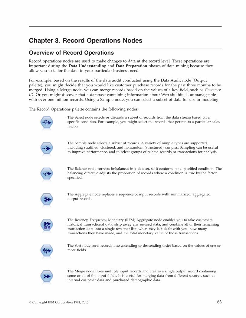
Chapter 3. Record Operations Nodes

Overview of Record OperationsRecord operations nodes are used to make changes to data at the record level. These operations areimportant during the Data Understanding and Data Preparation phases of data mining because theyallow you to tailor the data to your particular business need.

For example, based on the results of the data audit conducted using the Data Audit node (Outputpalette), you might decide that you would like customer purchase records for the past three months to bemerged. Using a Merge node, you can merge records based on the values of a key field, such as CustomerID. Or you might discover that a database containing information about Web site hits is unmanageablewith over one million records. Using a Sample node, you can select a subset of data for use in modeling.

The Record Operations palette contains the following nodes:

The Select node selects or discards a subset of records from the data stream based on aspecific condition. For example, you might select the records that pertain to a particular salesregion.

The Sample node selects a subset of records. A variety of sample types are supported,including stratified, clustered, and nonrandom (structured) samples. Sampling can be usefulto improve performance, and to select groups of related records or transactions for analysis.

The Balance node corrects imbalances in a dataset, so it conforms to a specified condition. Thebalancing directive adjusts the proportion of records where a condition is true by the factorspecified.

The Aggregate node replaces a sequence of input records with summarized, aggregatedoutput records.

The Recency, Frequency, Monetary (RFM) Aggregate node enables you to take customers'historical transactional data, strip away any unused data, and combine all of their remainingtransaction data into a single row that lists when they last dealt with you, how manytransactions they have made, and the total monetary value of those transactions.

The Sort node sorts records into ascending or descending order based on the values of one ormore fields.

The Merge node takes multiple input records and creates a single output record containingsome or all of the input fields. It is useful for merging data from different sources, such asinternal customer data and purchased demographic data.


The Append node concatenates sets of records. It is useful for combining datasets with similarstructures but different data.

The Distinct node removes duplicate records, either by passing the first distinct record to thedata stream or by discarding the first record and passing any duplicates to the data streaminstead.

The Streaming TS node builds and scores time series models in one step, without the need fora Time Intervals node.

Many of the nodes in the Record Operations palette require you to use a CLEM expression. If you arefamiliar with CLEM, you can type an expression in the field. However, all expression fields provide abutton that opens the CLEM Expression Builder, which helps you create such expressions automatically.

Select NodeYou can use Select nodes to select or discard a subset of records from the data stream based on a specificcondition, such as BP (blood pressure) = "HIGH".

Mode. Specifies whether records that meet the condition will be included or excluded from the datastream.v Include. Select to include records that meet the selection condition.v Discard. Select to exclude records that meet the selection condition.

Condition. Displays the selection condition that will be used to test each record, which you specify usinga CLEM expression. Either enter an expression in the window or use the Expression Builder by clickingthe calculator (Expression Builder) button to the right of the window.

If you choose to discard records based on a condition, such as the following:(var1=’value1’ and var2=’value2’)

the Select node by default also discards records having null values for all selection fields. To avoid this,append the following condition to the original one:and not(@NULL(var1) and @NULL(var2))

Select nodes are also used to choose a proportion of records. Typically, you would use a different node,the Sample node, for this operation. However, if the condition you want to specify is more complex thanthe parameters provided, you can create your own condition using the Select node. For example, you cancreate a condition such as:

BP = "HIGH" and random(10) <= 4

This will select approximately 40% of the records showing high blood pressure and pass those recordsdownstream for further analysis.

Figure 1. Expression Builder button


Sample NodeYou can use Sample nodes to select a subset of records for analysis, or to specify a proportion of recordsto discard. A variety of sample types are supported, including stratified, clustered, and nonrandom(structured) samples. Sampling can be used for several reasons:v To improve performance by estimating models on a subset of the data. Models estimated from a

sample are often as accurate as those derived from the full dataset, and may be more so if theimproved performance allows you to experiment with different methods you might not otherwise haveattempted.

v To select groups of related records or transactions for analysis, such as selecting all the items in anonline shopping cart (or market basket), or all the properties in a specific neighborhood.

v To identify units or cases for random inspection in the interest of quality assurance, fraud prevention,or security.

Note: If you simply want to partition your data into training and test samples for purposes of validation,a Partition node can be used instead. See the topic “Partition Node” on page 154 for more information.

Types of Samples

Clustered samples. Sample groups or clusters rather than individual units. For example, suppose youhave a data file with one record per student. If you cluster by school and the sample size is 50%, then50% of schools will be chosen and all students from each selected school will be picked. Students inunselected schools will be rejected. On average, you would expect about 50% of students to be picked,but because schools vary in size, the percentage may not be exact. Similarly, you could cluster shoppingcart items by transaction ID to make sure that all items from selected transactions are maintained. For anexample that clusters properties by town, see the complexsample_property.str sample stream.

Stratified samples. Select samples independently within non-overlapping subgroups of the population, orstrata. For example, you can ensure that men and women are sampled in equal proportions, or that everyregion or socioeconomic group within an urban population is represented. You can also specify adifferent sample size for each stratum (for example, if you think that one group has beenunder-represented in the original data). For an example that stratifies properties by county, see thecomplexsample_property.str sample stream.

Systematic or 1-in-n sampling. When selection at random is difficult to obtain, units can be sampledsystematically (at a fixed interval) or sequentially.

Sampling weights. Sampling weights are automatically computed while drawing a complex sample androughly correspond to the "frequency" that each sampled unit represents in the original data. Therefore,the sum of the weights over the sample should estimate the size of the original data.

Sampling Frame

A sampling frame defines the potential source of cases to be included in a sample or study. In somecases, it may be feasible to identify every single member of a population and include any one of them ina sample--for example, when sampling items that come off a production line. More often, you will not beable to access every possible case. For example, you cannot be sure who will vote in an election untilafter the election has happened. In this case, you might use the electoral register as your sampling frame,even though some registered people won’t vote, and some people may vote despite not having beenlisted at the time you checked the register. Anybody not in the sampling frame has no prospect of beingsampled. Whether your sampling frame is close enough in nature to the population you are trying toevaluate is a question that must be addressed for each real-life case.

Sample Node OptionsYou can choose the Simple or Complex method as appropriate for your requirements.

Chapter 3. Record Operations Nodes 65

Simple Sampling Options

The Simple method allows you to select a random percentage of records, select contiguous records, orselect every nth record.

Mode. Select whether to pass (include) or discard (exclude) records for the following modes:v Include sample. Includes selected records in the data stream and discards all others. For example, if

you set the mode to Include sample and set the 1-in-n option to 5, then every fifth record will beincluded, yielding a dataset that is roughly one-fifth the original size. This is the default mode whensampling data, and the only mode when using the complex method.

v Discard sample. Excludes selected records and includes all others. For example, if you set the mode toDiscard sample and set the 1-in-n option to 5, then every fifth record will be discarded. This mode isonly available with the simple method.

Sample. Select the method of sampling from the following options:v First. Select to use contiguous data sampling. For example, if the maximum sample size is set to 10000,

then the first 10,000 records will be selected.v 1-in-n. Select to sample data by passing or discarding every nth record. For example, if n is set to 5,

then every fifth record will be selected.v Random %. Select to sample a random percentage of the data. For example, if you set the percentage

to 20, then 20% of the data will either be passed to the data stream or discarded, depending on themode selected. Use the field to specify a sampling percentage. You can also specify a seed value usingthe Set random seed control.Use block level sampling (in-database only). This option is enabled only if you choose randompercentage sampling when performing in-database mining on an Oracle or IBM DB2 database. In thesecircumstances, block-level sampling can be more efficient.

Note: You do not get an exact number of rows returned each time you run the same random samplesettings. This is because each input record has a probability of N/100 of being included in the sample(where N is the Random % you specify in the node) and the probabilities are independent; thereforethe results are not exactly N%.

Maximum sample size. Specifies the maximum number of records to include in the sample. This optionis redundant and therefore disabled when First and Include are selected. Also note that when used incombination with the Random % option, this setting may prevent certain records from being selected. Forexample, if you have 10 million records in your dataset, and you select 50% of records with a maximumsample size of three million records, then 50% of the first six million records will be selected, and theremaining four million records have no chance of being selected. To avoid this limitation, select theComplex sampling method, and request a random sample of three million records without specifying acluster or stratify variable.

Complex Sampling Options

Complex sample options allow for finer control of the sample, including clustered, stratified, andweighted samples along with other options.

Cluster and stratify. Allows you to specify cluster, stratify, and input weight fields if needed. See thetopic “Cluster and Stratify Settings” on page 67 for more information.

Sample type.

v Random. Selects clusters or records randomly within each strata.v Systematic. Selects records at a fixed interval. This option works like the 1 in n method, except the

position of the first record changes depending on a random seed. The value of n is determinedautomatically based on the sample size or proportion.


Sample units. You can select proportions or counts as the basic sample units.

Sample size. You can specify the sample size in several ways:v Fixed. Allows you to specify the overall size of the sample as a count or proportion.v Custom. Allows you to specify the sample size for each subgroup or strata. This option is only

available if a stratification field has been specified in the Cluster and Stratify sub dialog box.v Variable. Allows the user to pick a field that defines the sample size for each subgroup or strata. This

field should have the same value for each record within a particular stratum; for example, if thesample is stratified by county, then all records with county = Surrey must have the same value. Thefield must be numeric and its values must match the selected sample units. For proportions, valuesshould be greater than 0 and less than 1; for counts, the minimum value is 1.

Minimum sample per stratum. Specifies a minimum number of records (or minimum number of clustersif a cluster field is specified).

Maximum sample per stratum. Specifies a maximum number of records or clusters. If you select thisoption without specifying a cluster or stratify field, a random or systematic sample of the specified sizewill be selected.

Set random seed. When sampling or partitioning records based on a random percentage, this optionallows you to duplicate the same results in another session. By specifying the starting value used by therandom number generator, you can ensure the same records are assigned each time the node is executed.Enter the desired seed value, or click the Generate button to automatically generate a random value. Ifthis option is not selected, a different sample will be generated each time the node is executed.

Note: When using the Set random seed option with records read from a database, a Sort node may berequired prior to sampling in order to ensure the same result each time the node is executed. This isbecause the random seed depends on the order of records, which is not guaranteed to stay the same in arelational database. See the topic “Sort Node” on page 74 for more information.

Cluster and Stratify SettingsThe Cluster and Stratify dialog box enables you to select cluster, stratification, and weight fields whendrawing a complex sample.

Clusters. Specifies a categorical field used to cluster records. Records are sampled based on clustermembership, with some clusters included and others not. But if any record from a given cluster isincluded, all are included. For example, when analyzing product associations in shopping carts, youcould cluster items by transaction ID to make sure that all items from selected transactions aremaintained. Instead of sampling records—which would destroy information about what items are soldtogether—you can sample transactions to make sure that all records for selected transactions arepreserved.

Stratify by. Specifies a categorical field used to stratify records so that samples are selected independentlywithin non-overlapping subgroups of the population, or strata. If you select a 50% sample stratified bygender, for example, then two 50% samples will be taken, one for the men and one for the women. Forexample, strata may be socioeconomic groups, job categories, age groups, or ethnic groups, allowing youto ensure adequate sample sizes for subgroups of interest. If there are three times more women than menin the original dataset, this ratio will be preserved by sampling separately from each group. Multiplestratification fields can also be specified (for example, sampling product lines within regions orvice-versa).

Note: If you stratify by a field that has missing values (null or system missing values, empty strings,white space, and blank or user-defined missing values), then you cannot specify custom sample sizes forstrata. If you want to use custom sample sizes when stratifying by a field with missing or blank values,then you need to fill them upstream.


Use input weight. Specifies a field used to weight records prior to sampling. For example, if the weightfield has values ranging from 1 to 5, records weighted 5 are five times as likely to be selected. The valuesof this field will be overwritten by the final output weights generated by the node (see followingparagraph).

New output weight. Specifies the name of the field where final weights are written if no input weightfield is specified. (If an input weight field is specified, its values are replaced by the final weights asnoted above, and no separate output weight field is created.) The output weight values indicate thenumber of records represented by each sampled record in the original data. The sum of the weight valuesgives an estimate of the sample size. For example, if a random 10% sample is taken, the output weightwill be 10 for all records, indicating that each sampled record represents roughly ten records in theoriginal data. In a stratified or weighted sample, the output weight values may vary based on the sampleproportion for each stratum.

Commentsv Clustered sampling is useful if you cannot get a complete list of the population you want to sample,

but can get complete lists for certain groups or clusters. It is also used when a random sample wouldproduce a list of test subjects that it would be impractical to contact. For example, it would be easier tovisit all farmers in one county than a selection of farmers scattered across every county in the nation.

v You can specify both cluster and stratify fields in order to sample clusters independently within eachstrata. For example, you could sample property values stratified by county, and cluster by town withineach county. This will ensure that an independent sample of towns is drawn from within each county.Some towns will be included and others will not, but for each town that is included, all propertieswithin the town are included.

v To select a random sample of units from within each cluster, you can string two Sample nodestogether. For example, you could first sample townships stratified by county as described above. Thenattach a second Sample node and select town as a stratify field, allowing you to sample a proportion ofrecords from within each township.

v In cases where a combination of fields is required to uniquely identify clusters, a new field can begenerated using a Derive node. For example, if multiple shops use the same numbering system fortransactions, you could derive a new field that concatenates the shop and transaction IDs.

Sample Sizes for StrataWhen drawing a stratified sample, the default option is to sample the same proportion of records orclusters from each stratum. If one group outnumbers another by a factor of 3, for example, you typicallywant to preserve the same ratio in the sample. If this is not the case, however, you can specify the samplesize separately for each stratum.

The Sample Sizes for Strata dialog box lists each value of the stratification field, allowing you to overridethe default for that stratum. If multiple stratification fields are selected, every possible combination ofvalues is listed, allowing you to specify the size for each ethnic group within each city, for example, oreach town within each county. Sizes are specified as proportions or counts, as determined by the currentsetting in the Sample node.

To Specify Sample Sizes for Strata1. In the Sample node, select Complex, and select one or more stratification fields. See the topic “Cluster

and Stratify Settings” on page 67 for more information.2. Select Custom, and select Specify Sizes.3. In the Sample Sizes for Strata dialog box, click the Read Values button at lower left to populate the

display. If necessary, you may need to instantiate values in an upstream source or Type node. See thetopic “What Is Instantiation?” on page 123 for more information.

4. Click in any row to override the default size for that stratum.


Notes on Sample Size

Custom sample sizes may be useful if different strata have different variances, for example, in order tomake sample sizes proportional to the standard deviation. (If the cases within the stratum are morevaried, you need to sample more of them to get a representative sample.) Or if a stratum is small, youmay wish to use a higher sample proportion to ensure that a minimum number of observations isincluded.

Note: If you stratify by a field that has missing values (null or system missing values, empty strings,white space, and blank or user-defined missing values), then you cannot specify custom sample sizes forstrata. If you want to use custom sample sizes when stratifying by a field with missing or blank values,then you need to fill them upstream.

Balance NodeYou can use Balance nodes to correct imbalances in datasets so they conform to specified test criteria. Forexample, suppose that a dataset has only two values--low or high--and that 90% of the cases are low whileonly 10% of the cases are high. Many modeling techniques have trouble with such biased data becausethey will tend to learn only the low outcome and ignore the high one, since it is more rare. If the data arewell balanced with approximately equal numbers of low and high outcomes, models will have a betterchance of finding patterns that distinguish the two groups. In this case, a Balance node is useful forcreating a balancing directive that reduces cases with a low outcome.

Balancing is carried out by duplicating and then discarding records based on the conditions you specify.Records for which no condition holds are always passed through. Because this process works byduplicating and/or discarding records, the original sequence of your data is lost in downstreamoperations. Be sure to derive any sequence-related values before adding a Balance node to the datastream.

Note: Balance nodes can be generated automatically from distribution charts and histograms. For example,you can balance your data to show equal proportions across all categories of a categorical field, as shownin a distribution plot.

Example. When building an RFM stream to identify recent customers who have positively responded toprevious marketing campaigns, the marketing department of a sales company uses a Balance node tobalance the differences between true and false responses in the data.

Setting Options for the Balance NodeRecord balancing directives. Lists the current balancing directives. Each directive includes both a factorand a condition that tells the software to "increase the proportion of records by a factor specified wherethe condition is true." A factor lower than 1.0 means that the proportion of indicated records will bedecreased. For example, if you want to decrease the number of records where drug Y is the treatmentdrug, you might create a balancing directive with a factor of 0.7 and a condition Drug = "drugY". Thisdirective means that the number of records where drug Y is the treatment drug will be reduced to 70%for all downstream operations.

Note: Balance factors for reduction may be specified to four decimal places. Factors set below 0.0001 willresult in an error, since the results do not compute correctly.v Create conditions by clicking the button to the right of the text field. This inserts an empty row for

entering new conditions. To create a CLEM expression for the condition, click the Expression Builderbutton.

v Delete directives using the red delete button.v Sort directives using the up and down arrow buttons.


Only balance training data. If a partition field is present in the stream, this option balances data in thetraining partition only. In particular, this may be useful if generating adjusted propensity scores, whichrequire an unbalanced testing or validation partition. If no partition field is present in the stream (or ifmultiple partition fields are specified), then this option is ignored and all data are balanced.

Aggregate NodeAggregation is a data preparation task frequently used to reduce the size of a dataset. Before proceedingwith aggregation, you should take time to clean the data, concentrating especially on missing values.Once you have aggregated, potentially useful information regarding missing values may be lost.

You can use an Aggregate node to replace a sequence of input records with summary, aggregated outputrecords. For example, you might have a set of input sales records such as those shown in the followingtable.

Table 13. Sales record input example

Age Sex Region Branch Sales

23 M S 8 4

45 M S 16 4

37 M S 8 5

30 M S 5 7

44 M N 4 9

25 M N 2 11

29 F S 16 6

41 F N 4 8

23 F N 6 2

45 F N 4 5

33 F N 6 10

You can aggregate these records with Sex and Region as key fields. Then choose to aggregate Age with themode Mean and Sales with the mode Sum. Select Include record count in field in the Aggregate nodedialog box and your aggregated output would be as shown in the following table.

Table 14. Aggregated record example

Age (mean) Sex Region Sales (sum) Record Count

35.5 F N 25 4

29 F S 6 1

34.5 M N 20 2

33.75 M S 20 4

From this you learn, for example, that the average age of the four female sales staff in the North region is35.5, and the sum total of their sales was 25 units.

Note: Fields such as Branch are automatically discarded when no aggregate mode is specified.

Setting Options for the Aggregate NodeOn the Aggregate node you specify the following.v One or more key fields to use as categories for the aggregation


v One or more aggregate fields for which to calculate the aggregate valuesv One or more aggregation modes (types of aggregation) to output for each aggregate field

You can also specify the default aggregation modes to use for newly added fields, and use expressions(similar to formulae) to categorize aggregation.

Note that for added performance, aggregations operations may benefit from enabling parallel processing.

Key fields. Lists fields that can be used as categories for aggregation. Both continuous (numeric) andcategorical fields can be used as keys. If you choose more than one key field, the values will be combinedto produce a key value for aggregating records. One aggregated record will be generated for each uniquekey field. For example, if Sex and Region are your key fields, each unique combination of M and F withregions N and S (four unique combinations) will have an aggregated record. To add a key field, use theField Chooser button to the right of the window.

The rest of the dialog box is split into two main areas - Basic Aggregates and Aggregate Expressions.

Basic Aggregates

Aggregate fields. Lists the fields for which values will be aggregated as well as the selected modes ofaggregation. To add fields to this list, use the Field Chooser button on the right. The followingaggregation modes are available.

Note: Some modes are not applicable to non-numeric fields (for example, Sum for a date/time field).Modes that cannot be used with a selected aggregate field are disabled.v Sum. Select to return summed values for each key field combination. The sum is the total of the

values, across all cases with nonmissing values.v Mean. Select to return the mean values for each key field combination. The mean is a measure of

central tendency, and is the arithmetic average (the sum divided by the number of cases).v Min. Select to return minimum values for each key field combination.v Max. Select to return maximum values for each key field combination.v SDev. Select to return the standard deviation for each key field combination. The standard deviation is

a measure of dispersion around the mean, and is equal to the square root of the variance measurement.v Median. Select to return the median values for each key field combination. The median is a measure

of central tendency that is not sensitive to outlying values (unlike the mean, which can be affected by afew extremely high or low values). Also known as the 50th percentile or 2nd quartile.

v Count. Select to return the count of non-null values for each key field combination.v Variance. Select to return the variance values for each key field combination. The variance is a

measure of dispersion around the mean, equal to the sum of squared deviations from the meandivided by one less than the number of cases.

v 1st Quartile. Select to return the 1st quartile (25th percentile) values for each key field combination.v 3rd Quartile. Select to return the 3rd quartile (75th percentile) values for each key field combination.

Note: When running a stream containing an Aggregate node, the values returned for 1st and 3rdQuartiles when pushing back SQL to an Oracle database may differ from those returned in native mode.

Default mode. Specify the default aggregation mode to be used for newly added fields. If you frequentlyuse the same aggregation, select one or more modes here and use the Apply to All button on the right toapply the selected modes to all fields listed above.

New field name extension. Select to add a suffix or prefix, such as "1" or "new," to duplicate aggregatedfields. For example, the result of a minimum values aggregation on the field Age will produce a fieldname called Age_Min_1 if you have selected the suffix option and specified "1" as the extension. Note:


Aggregation extensions such as _Min or Max_ are automatically added to the new field, indicating thetype of aggregation performed. Select Suffix or Prefix to indicate your preferred extension style.

Include record count in field. Select to include an extra field in each output record called Record_Count,by default. This field indicates how many input records were aggregated to form each aggregate record.Create a custom name for this field by typing in the edit field.

Note: System null values are excluded when aggregates are computed, but they are included in therecord count. Blank values, on the other hand, are included in both aggregation and record count. Toexclude blank values, you can use a Filler node to replace blanks with null values. You can also removeblanks using a Select node.

Aggregate Expressions

Expressions are similar to formulas that are created from values, field names, operators, and functions.Unlike functions that work on a single record at a time, aggregate expressions operate on a group, set, orcollection of records.

Note: You can only create aggregate expressions if the stream includes a database connection (by meansof a Database source node).

New expressions are created as derived fields; to create an expression you use the Database Aggregatesfunctions which are available from the Expression Builder.

For more information about the Expression Builder, see the IBM SPSS Modeler User's Guide(ModelerUsersGuide.pdf).

Note that there is a connection between the Key Fields and any aggregate expressions you create becausethe aggregate expressions are grouped by the key field.

Valid aggregate expressions are ones that evaluate to aggregate outcomes; a couple of examples of validaggregate expressions, and the rules that govern them, are as follows:v You can use scalar functions to combine multiple aggregation functions together to produce a single

aggregation result. For example:max(C01) - min(C01)

v An aggregation function can operate on the result of multiple scalar functions. For example:sum (C01*C01)

Aggregate optimization settingsOn the Optimization tab you specify the following.

Keys are contiguous. Select this option if you know that all records with the same key values aregrouped together in the input (for example, if the input is sorted on the key fields). Doing so canimprove performance.

Allow approximation for Median and Quartiles. The Order statistics (Median, 1st Quartile, and 3rdQuartile) are currently not supported when processing data in Analytic Server. If you are using AnalyticServer you can select this check box to use an approximated value for these statistics instead which iscalculated by binning the data and then computing an estimate for the statistic based on the distributionacross the bins. By default, this option is unchecked.

Number of bins. Only available if you select the Allow approximation for Median and Quartiles checkbox. Select the number of bins to be used when estimating the statistic; the number of bins affects theMaximum error %. By default, the number of bins is 1000, which corresponds to a maximum error of 0.1percent of the range.


RFM Aggregate NodeThe Recency, Frequency, Monetary (RFM) Aggregate node enables you to take customers' historicaltransactional data, strip away any unused data, and combine all of their remaining transaction data into asingle row, using their unique customer ID as a key, that lists when they last dealt with you (recency),how many transactions they have made (frequency), and the total value of those transactions (monetary).

Before proceeding with any aggregation, you should take time to clean the data, concentrating especiallyon any missing values.

Once you have identified and transformed the data using the RFM Aggregate node, you may use anRFM Analysis node to carry out further analysis. See the topic “RFM Analysis Node” on page 150 formore information.

Note that once the data file has been run through the RFM Aggregate node, it will not have any targetvalues; therefore, before being able to use it as inputs for further predictive analysis with any modelingnodes such as C5.0 or CHAID, you will need to merge it with other customer data (for example, bymatching the customer IDs). See the topic “Merge Node” on page 75 for more information.

The RFM Aggregate and RFM Analysis nodes in IBM SPSS Modeler are set up to use independentbinning; that is, they rank and bin data on each measure of recency, frequency, and monetary value,without regard to their values or the other two measures.

Setting Options for the RFM Aggregate NodeThe Settings tab of the RFM Aggregate node contains the following fields.

Calculate recency relative to. Specify the date from which the recency of transactions will be calculated.This may be either a Fixed date that you enter, or Today's date, as set by your system. Today's date isentered by default and is automatically updated when the node is executed.

IDs are contiguous. If your data are presorted so that all records with the same ID appear together in thedata stream, select this option to speed up processing. If your data are not presorted (or you are notsure), leave this option unselected, and the node will sort the data automatically.

ID. Select the field to be used to identify the customer and their transactions. To display the fields fromwhich you can select, use the Field Chooser button on the right.

Date. Select the date field to be used to calculate recency against. To display the fields from which youcan select, use the Field Chooser button on the right.

Note that this requires a field with a storage of date, or timestamp, in the appropriate format to use asinput. For example, if you have a string field with values like Jan 2007, Feb 2007, and so on, you canconvert this to a date field using a Filler node and the to_date() function. See the topic “StorageConversion Using the Filler Node” on page 140 for more information.

Value. Select the field to be used to calculate the total monetary value of the customer's transactions. Todisplay the fields from which you can select, use the Field Chooser button on the right. Note: This mustbe a numeric value.

New field name extension. Select to append either a suffix or prefix, such as "12_month", to the newlygenerated recency, frequency, and monetary fields. Select Suffix or Prefix to indicate your preferredextension style. For example, this may be useful when examining several time periods.


Discard records with value below. If required, you can specify a minimum value below which anytransaction details are not used when calculating the RFM totals. The units of value relate to the Valuefield selected.

Include only recent transactions. If you are analyzing a large database, you can specify that only thelatest records are used. You can chose to use the data recorded either after a certain date or within arecent period:v Transaction date after. Specify the transaction date after which records will be included in your

analysis.v Transaction within the last. Specify the number and type of periods (days, weeks, months, or years)

back from the Calculate recency relative to date after which records will be included in your analysis.

Save date of second most recent transaction. If you want to know the date of the second most recenttransaction for each customer, select this box. In addition, you can then select the Save date of third mostrecent transaction box as well. For example, this can help you identify customers who may have carriedout many transactions some considerable time ago, but only one recent transaction.

Sort NodeYou can use Sort nodes to sort records into ascending or descending order based on the values of one ormore fields. For example, Sort nodes are frequently used to view and select records with the mostcommon data values. Typically, you would first aggregate the data using the Aggregate node and thenuse the Sort node to sort the aggregated data into descending order of record counts. Displaying theseresults in a table will allow you to explore the data and to make decisions, such as selecting the recordsof the top 10 best customers.

The Settings tab of the Sort node contains the following fields.

Sort by. All fields selected to use as sort keys are displayed in a table. A key field works best for sortingwhen it is numeric.v Add fields to this list using the Field Chooser button on the right.v Select an order by clicking the Ascending or Descending arrow in the table's Order column.v Delete fields using the red delete button.v Sort directives using the up and down arrow buttons.

Default sort order. Select either Ascending or Descending to use as the default sort order when newfields are added above.

Note: The Sort node is not applied if there is a Distinct node down the model stream. For informationabout the Distinct node, see “Distinct node” on page 83.

Sort Optimization SettingsIf you are working with data you know are already sorted by some key fields, you can specify whichfields are already sorted, allowing the system to sort the rest of the data more efficiently. For example,you want to sort by Age (descending) and Drug (ascending) but know your data are already sorted byAge (descending).

Data is presorted. Specifies whether the data are already sorted by one or more fields.

Specify existing sort order. Specify the fields that are already sorted. Using the Select Fields dialog box,add fields to the list. In the Order column, specify whether each field is sorted in ascending or descendingorder. If you are specifying multiple fields, make sure that you list them in the correct sorting order. Usethe arrows to the right of the list to arrange the fields in the correct order. If you make a mistake in


specifying the correct existing sort order, an error will appear when you run the stream, displaying therecord number where the sorting is inconsistent with what you specified.

Note: Sorting speed may benefit from enabling parallel processing.

Merge NodeThe function of a Merge node is to take multiple input records and create a single output recordcontaining all or some of the input fields. This is a useful operation when you want to merge data fromdifferent sources, such as internal customer data and purchased demographic data. You can merge data inthe following ways.v Merge by Order concatenates corresponding records from all sources in the order of input until the

smallest data source is exhausted. It is important if using this option that you have sorted your datausing a Sort node.

v Merge using a Key field, such as Customer ID, to specify how to match records from one data sourcewith records from the other(s). Several types of joins are possible, including inner join, full outer join,partial outer join, and anti-join. See the topic “Types of Joins” for more information.

v Merge by Condition means that you can specify a condition to be satisfied for the merge to take place.You can specify the condition directly in the node, or build the condition using the Expression Builder.

v Merge by Ranked Condition is a left sided outer join in which you specify a condition to be satisfiedfor the merge to take place and a ranking expression which sorts into order from low to high. Mostoften used to merge geospatial data, you can specify the condition directly in the node, or build thecondition using the Expression Builder.

Types of JoinsWhen using a key field for data merging, it is useful to spend some time thinking about which recordswill be excluded and which will be included. There are a variety of joins, which are discussed in detailbelow.

The two basic types of joins are referred to as inner and outer joins. These methods are frequently used tomerge tables from related datasets based on common values of a key field, such as Customer ID. Innerjoins allow for clean merging and an output dataset that includes only complete records. Outer joins alsoinclude complete records from the merged data, but they also allow you to include unique data from oneor more input tables.

The types of joins allowed are described in greater detail below.

An inner join includes only records in which a value for the key field iscommon to all input tables. That is, unmatched records will not beincluded in the output dataset.

A full outer join includes all records, both matching and nonmatching,from the input tables. Left and right outer joins are referred to as partialouter joins and are described below.


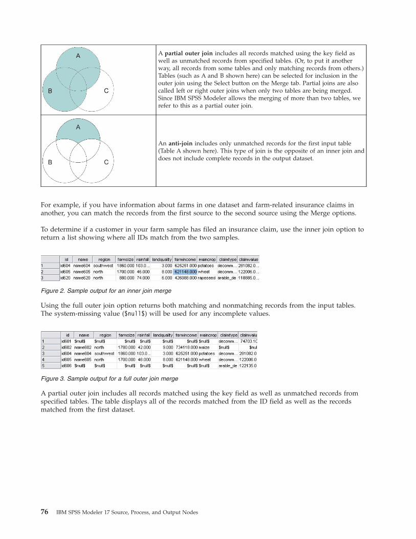
A partial outer join includes all records matched using the key field aswell as unmatched records from specified tables. (Or, to put it anotherway, all records from some tables and only matching records from others.)Tables (such as A and B shown here) can be selected for inclusion in theouter join using the Select button on the Merge tab. Partial joins are alsocalled left or right outer joins when only two tables are being merged.Since IBM SPSS Modeler allows the merging of more than two tables, werefer to this as a partial outer join.

An anti-join includes only unmatched records for the first input table(Table A shown here). This type of join is the opposite of an inner join anddoes not include complete records in the output dataset.

For example, if you have information about farms in one dataset and farm-related insurance claims inanother, you can match the records from the first source to the second source using the Merge options.

To determine if a customer in your farm sample has filed an insurance claim, use the inner join option toreturn a list showing where all IDs match from the two samples.

Using the full outer join option returns both matching and nonmatching records from the input tables.The system-missing value ($null$) will be used for any incomplete values.

A partial outer join includes all records matched using the key field as well as unmatched records fromspecified tables. The table displays all of the records matched from the ID field as well as the recordsmatched from the first dataset.

Figure 2. Sample output for an inner join merge

Figure 3. Sample output for a full outer join merge


If you are using the anti-join option, the table returns only unmatched records for the first input table.

Specifying a Merge Method and KeysThe Merge tab of the Merge node contains the following fields.

Merge Method Select the method to be used for merging records. Selecting either Keys or Conditionactivates the bottom half of the dialog box.v Order Merges records by order such that the nth record from each input is merged to produce the nth

output record. When any record runs out of a matching input record, no more output records areproduced. This means that the number of records that are created is the number of records in thesmallest dataset.

v Keys Uses a key field, such as Transaction ID, to merge records with the same value in the key field.This is equivalent to a database "equi-join." If a key value occurs more than once, all possiblecombinations are returned. For example, if records with the same key field value A contain differingvalues B, C, and D in other fields, the merged fields produce a separate record for each combination ofA with value B, A with value C, and A with value D.Note: Null values are not considered identical in the merge-by-key method and will not join.

v Condition Use this option to specify a condition for the merge. For more information, see “SpecifyingConditions for a Merge” on page 78.

v Ranked condition Use this option to specify whether each row pairing in the primary and allsecondary data sets are to be merged; use the ranking expression to sort any multiple matches intoorder from low to high. For more information, see “Specifying Ranked Conditions for a Merge” onpage 78.

Possible keys Lists only those fields with exactly matching field names in all input data sources. Select afield from this list and use the arrow button to add it as a key field used for merging records. More thanone key field can be used. You can rename non-matching input fields by using a Filter node, or the Filtertab of a source node.

Keys for merge Lists all fields that are used to merge records from all input data sources based on valuesof the key fields. To remove a key from the list, select one and use the arrow button to return it to thePossible Keys list. When more than one key field is selected, the option below is enabled.

Combine duplicate key fields When more than one key field is selected above, this option ensures thatthere is only one output field of that name. This option is enabled by default except in the case when

Figure 4. Sample output for a partial outer join merge

Figure 5. Sample output for an anti-join merge


streams have been imported from earlier versions of IBM SPSS Modeler. When this option is disabled,duplicate key fields must be renamed or excluded by using the Filter tab in the Merge node dialog box.

Include only matching records (inner join) Select to merge only complete records.

Include matching and non-matching records (full outer join) Select to perform a "full outer join." Thismeans that if values for the key field are not present in all input tables, the incomplete records are stillretained. The undefined value ($null$) is added to the key field and included in the output record.

Include matching and selected non-matching records (partial outer join) Select to perform a "partialouter join" of the tables you select in a subdialog box. Click Select to specify tables for which incompleterecords will be retained in the merge.

Include records in the first dataset not matching any others (anti-join) Select to perform a type of"anti-join," where only nonmatching records from the first dataset are passed downstream. You canspecify the order of input datasets using arrows on the Inputs tab. This type of join does not includecomplete records in the output dataset. For more information, see “Types of Joins” on page 75.

Selecting Data for Partial JoinsFor a partial outer join, you must select the table(s) for which incomplete records will be retained. Forexample, you may want to retain all records from a Customer table while retaining only matched recordsfrom the Mortgage Loan table.

Outer Join column. In the Outer Join column, select datasets to include in their entirety. For a partial join,overlapping records will be retained as well as incomplete records for datasets selected here. See the topic“Types of Joins” on page 75 for more information.

Specifying Conditions for a MergeBy setting the merge method to Condition, you can specify one or more conditions to be satisfied for themerge to take place.

You can either enter the conditions directly into the Condition field, or build them with the aid of theExpression Builder by clicking the calculator symbol to the right of the field.

Add tags to duplicate field names to avoid merge conflicts If two or more of the datasets to be mergedcontain the same field names, select this check box to add a different prefix tag to the start of the fieldcolumn headers. For example, if there are two fields called Name the result of the merge would contain1_Name and 2_Name. If the tag has been renamed in the data source, the new name is used instead of thenumbered prefix tag. If you do not select this check box, and there are duplicate names in the data, awarning is displayed to the right of the check box.

Specifying Ranked Conditions for a MergeA Ranked Condition merge can be considered as a left sided outer join merge by condition; the left sideof the merge is the primary data set where each record is an event. For example, in a model that is usedto find patterns in crime data, each record in the primary data set would be a crime and its associatedinformation (location, type, and so on). In this example, the right side might contain the relevantgeospatial data sets.

The merge uses both a merge condition and a ranking expression. The merge condition can use ageospatial function such as within or close_to. During the merge, all of the fields in the right side data setsare added to the left side data set but multiple matches result in a list field. For example:v Left side: Crime datav Right side: Counties data set and roads data set


v Merge conditions: Crime data within counties and close_to roads, along with a definition of what countsas close_to.

In this example, if a crime occurred within the required close_to distance of three roads (and the numberof matches to be returned is set to at least three), then all three roads are returned as a list item.

By setting the merge method to Ranked condition, you can specify one or more conditions to be satisfiedfor the merge to take place.

Primary dataset Select the primary data set for the merge; the fields from all other data sets are added tothe data set you select. This can be considered as the left side of an outer join merge.

When you select a primary data set, all the other input data sets that are connected to the Merge nodeare automatically listed in the Merges table.

Add tags to duplicate field names to avoid merge conflicts If two or more of the data sets to be mergedcontain the same field names, select this check box to add a different prefix tag to the start of the fieldcolumn headers. For example, if there are two fields that are called Name the result of the merge wouldcontain 1_Name and 2_Name. If the tag is renamed in the data source, the new name is used instead ofthe numbered prefix tag. If you do not select this check box, and there are duplicate names in the data, awarning is displayed to the right of the check box.

Merges

DatasetShows the name of the secondary data sets that are connected as inputs to the Merge node. Bydefault, where there is more than one secondary data set, they are listed in the order in whichthey were connected to the Merge node.

Merge Condition

Enter the unique conditions for merging each of the data sets in the table with the primary dataset. You can either type the conditions directly into the cell, or build them with the aid of theExpression Builder by clicking the calculator symbol to the right of the cell. For example, youmight use geospatial predicates to create a merge condition that places crime data from one dataset within the county data of another data set. The default merge condition depends on thegeospatial measurement level, as shown in the list below.v Point, LineString, MultiPoint, MultiLineString - default condition of close_to.v Polygon, MultiPolygon - default condition of within.

For more information about these levels, see “Geospatial measurement sublevels” on page 121.

If a data set contains multiple geospatial fields of different types, the default condition that isused depends on the first measurement level that is found in the data, in the followingdescending order.v Pointv LineStringv Polygon

Note: Defaults are only available when there is a geospatial data field in the secondary database.

Ranking Expression

Specify an expression to rank the merging of the data sets; this expression is used to sort multiplematches into an order that is based on the ranking criteria. You can either type the conditionsdirectly into the cell, or build them with the aid of the Expression Builder by clicking thecalculator symbol to the right of the cell.


Default ranking expressions of distance and area are provided in the Expression Builder and bothrank low to high, meaning that, for example, the top match for distance is the smallest value. Anexample of ranking by distance is when the primary data set contains crimes and their associatedlocation and each other data set contains objects with locations; in this case the distance betweenthe crimes and the objects can be used as a ranking criteria. The default ranking expressiondepends on the geospatial measurement level, as shown in the list below.v Point, LineString, MultiPoint, MultiLineString - the default expression is distance.v Polygon, MultiPolygon - the default expression is area.

Note: Defaults are only available when there is a geospatial data field in the secondary database.

Number of MatchesSpecify the number of matches that are returned, based on the condition and ranking expressions.The default number of matches depend on the geospatial measurement level in the secondarydata set, as shown in the list below; however, you can double-click in the cell to enter your ownvalue, up to a maximum of 100.v Point, LineString, MultiPoint, MultiLineString - default value of 3.v Polygon, MultiPolygon - default value of 1.v Data set that contains no geospatial fields - default value of 1.

As an example, if you set up a merge that is based on a Merge Condition of close_to and aRanking Expression of distance, the top three (closest) matches from the secondary data sets toeach record in the primary data set are returned as the values in the resultant list field.

Filtering Fields from the Merge NodeMerge nodes include a convenient way of filtering or renaming duplicate fields as a result of mergingmultiple data sources. Click the Filter tab in the dialog box to select filtering options.

The options presented here are nearly identical to those for the Filter node. There are, however, additionaloptions not discussed here that are available on the Filter menu. See the topic “Filtering or RenamingFields” on page 131 for more information.

Field. Displays the input fields from currently connected data sources.

Tag. Lists the tag name (or number) associated with the data source link. Click the Inputs tab to alteractive links to this Merge node.

Source node. Displays the source node whose data is being merged.

Connected node. Displays the node name for the node that is connected to the Merge node. Frequently,complex data mining requires several merge or append operations that may include the same sourcenode. The connected node name provides a way of differentiating these.

Filter. Displays the current connections between input and output field. Active connections show anunbroken arrow. Connections with a red X indicate filtered fields.

Field. Lists the output fields after merging or appending. Duplicate fields are displayed in red. Click inthe Filter field above to disable duplicate fields.

View current fields. Select to view information on fields selected to be used as key fields.

View unused field settings. Select to view information on fields that are not currently in use.


Setting Input Order and TaggingUsing the Inputs tab in the Merge and Append node dialog boxes, you can specify the order of inputdata sources and make any changes to the tag name for each source.

Tags and order of input datasets. Select to merge or append only complete records.v Tag. Lists current tag names for each input data source. Tag names, or tags, are a way of uniquely

identifying the data links for the merge or append operation. For example, imagine water from variouspipes that is combined at one point and flows through a single pipe. Data in IBM SPSS Modeler flowssimilarly, and the merging point is often a complex interaction between the various data sources. Tagsprovide a way of managing the inputs ("pipes") to a Merge or Append node so that if the node issaved or disconnected, the links remain and are easily identifiable.

When you connect additional data sources to a Merge or Append node, default tags are automaticallycreated using numbers to represent the order in which you connected the nodes. This order is unrelatedto the order of fields in the input or output datasets. You can change the default tag by entering a newname in the Tag column.v Source Node. Displays the source node whose data is being combined.v Connected Node. Displays the node name for the node that is connected to the Merge or Append

node. Frequently, complex data mining requires several merge operations that may include the samesource node. The connected node name provides a way of differentiating these.

v Fields. Lists the number of fields in each data source.

View current tags. Select to view tags that are actively being used by the Merge or Append node. Inother words, current tags identify links to the node that have data flowing through. Using the pipemetaphor, current tags are analogous to pipes with existing water flow.

View unused tag settings. Select to view tags, or links, that were previously used to connect to theMerge or Append node but are not currently connected with a data source. This is analogous to emptypipes still intact within a plumbing system. You can choose to connect these "pipes" to a new source orremove them. To remove unused tags from the node, click Clear. This clears all unused tags at once.

Merge Optimization SettingsThe system provides two options that can help you merge data more efficiently in certain situations.These options allow you to optimize merging when one input dataset is significantly larger than theother datasets or when your data are already sorted by all or some of the key fields that you are usingfor the merge.

Note: Optimizations from this tab only apply to IBM SPSS Modeler native node execution only; that is,when the Merge node does not pushback to SQL. Optimization settings have no effect on SQLgeneration.

One input dataset is relatively large. Select to indicate that one of the input datasets is much larger thanthe others. The system will cache the smaller datasets in memory and then perform the merge byprocessing the large dataset without caching or sorting it. You will commonly use this type of join withdata designed using a star-schema or similar design, where there is a large central table of shared data(for example, in transactional data). If you select this option, click Select to specify the large dataset. Notethat you can select only one large dataset. The following table summarizes which joins can be optimizedusing this method.

Table 15. Summary of join optimizations.

Type of Join Can be optimized for a large input dataset?

Inner Yes

Partial Yes, if there are no incomplete records in the large dataset.


Table 15. Summary of join optimizations (continued).

Type of Join Can be optimized for a large input dataset?

Full No

Anti-join Yes, if the large dataset is the first input.

All inputs are already sorted by key field(s). Select to indicate that the input data are already sorted byone or more of the key fields that you are using for the merge. Make sure all your input datasets aresorted.

Specify existing sort order. Specify the fields that are already sorted. Using the Select Fields dialog box,add fields to the list. You can select from only the key fields that are being used for the merge (specifiedin the Merge tab). In the Order column, specify whether each field is sorted in ascending or descendingorder. If you are specifying multiple fields, make sure that you list them in the correct sorting order. Usethe arrows to the right of the list to arrange the fields in the correct order. If you make a mistake inspecifying the correct existing sort order, an error will appear when you run the stream, displaying therecord number where the sorting is inconsistent with what you specified.

Depending on the case sensitivity of the collation method used by the database, optimization may notfunction correctly where one or more inputs are sorted by the database. For example, if you have twoinputs where one is case sensitive and the other is case insensitive, the results of sorting could bedifferent. Merge optimization causes records to be processed using their sorted order. As a result, ifinputs are sorted using different collation methods, the Merge node reports an error and displays therecord number where sorting is inconsistent. When all inputs are from one source, or are sorted usingmutually inclusive collations, records can be merged successfully.

Note: Merging speed may benefit from enabling parallel processing.

Append NodeYou can use Append nodes to concatenate sets of records. Unlike Merge nodes, which join records fromdifferent sources together, Append nodes read and pass downstream all of the records from one sourceuntil there are no more. Then the records from the next source are read using the same data structure(number of records, number of fields, and so on) as the first, or primary, input. When the primary sourcehas more fields than another input source, the system null string ($null$) will be used for any incompletevalues.

Append nodes are useful for combining datasets with similar structures but different data. For example,you might have transaction data stored in different files for different time periods, such as a sales datafile for March and a separate one for April. Assuming that they have the same structure (the same fieldsin the same order), the Append node will join them together into one large file, which you can thenanalyze.

Note: In order to append files, the field measurement levels must be similar. For example, a Nominal fieldcannot be appended with a field whose measurement level is Continuous.

Setting Append OptionsMatch fields by. Select a method to use when matching fields to append.v Position. Select to append datasets based on the position of fields in the main data source. When

using this method, your data should be sorted to ensure proper appending.v Name. Select to append datasets based on the name of fields in the input datasets. Also select Match

case to enable case sensitivity when matching field names.


Output Field. Lists the source nodes that are connected to the Append node. The first node on the list isthe primary input source. You can sort the fields in the display by clicking on the column heading. Thissorting does not actually reorder the fields in the dataset.

Include fields from. Select Main dataset only to produce output fields based on the fields in the maindataset. The main dataset is the first input, specified on the Inputs tab. Select All datasets to produceoutput fields for all fields in all datasets regardless of whether there is a matching field across all inputdatasets.

Tag records by including source dataset in field. Select to add an additional field to the output filewhose values indicate the source dataset for each record. Specify a name in the text field. The defaultfield name is Input.

Distinct nodeDuplicate records in a data set must be removed before data mining can begin. For example, in amarketing database, individuals may appear multiple times with different address or companyinformation. You can use the Distinct node to find or remove duplicate records in your data, or to createa single, composite record from a group of duplicate records.

To use the Distinct node, you must first define a set of key fields that determine when two records areconsidered to be duplicates.

If you do not pick all your fields as key fields, then two "duplicate" records may not be truly identicalbecause they can still differ in the values of the remaining fields. In this case, you can also define a sortorder that is applied within each group of duplicate records. This sort order gives you fine control overwhich record is treated as the first within a group. Otherwise, all duplicates are considered to beinterchangeable and any record might be selected. The incoming order of the records is not taken intoaccount, so it does not help to use an upstream Sort node (see "Sorting records within the distinct node"below).

Mode. Specify whether to create a composite record, or to either include or exclude (discard) the firstrecord.v Create a composite record for each group. Provides a way for you to aggregate non-numeric fields.

Selecting this option makes the Composite tab available where you specify how to create the compositerecords. See “Distinct Composite Settings” on page 85 for more information.

v Include only the first record in each group. Selects the first record from each group of duplicaterecords and discards the rest. The first record is determined by the sort order defined below, and notby the incoming order of the records.

v Discard only the first record in each group. Discards the first record from each group of duplicaterecords and selects the remainder instead. The first record is determined by the sort order definedbelow, and not by the incoming order of the records. This option is useful for finding duplicates in yourdata so that you can examine them later in the stream.

Key fields for grouping. Lists the field or fields used to determine whether records are identical. Youcan:v Add fields to this list using the field picker button on the right.v Delete fields from the list by using the red X (remove) button.

Within groups, sort records by. Lists the fields used to determine how records are sorted within eachgroup of duplicates, and whether they are sorted in ascending or descending order. You can:v Add fields to this list using the field picker button on the right.v Delete fields from the list by using the red X (remove) button.v Move fields using the up or down buttons, if you are sorting by more than one field.


You must specify a sort order if you have chosen to include or exclude the first record in each group, andit matters to you which record is treated as the first.

You may also want to specify a sort order if you have chosen to create a composite record, for certainoptions on the Composite tab. See “Distinct Composite Settings” on page 85 for more information.

Default sort order. Specify whether, by default, records are sorted in Ascending or Descending order ofthe sort key values.

Sorting records within the Distinct node

If the order of records within a group of duplicates is important to you, then you must specify the orderusing the Within groups, sort records by option in the Distinct node. Do not rely on an upstream Sortnode. Remember that the incoming order of the records is not taken into account -- only the orderspecified within the node.

If you do not specify any sort fields (or you specify insufficient sort fields), then the records within eachgroup of duplicates will be unordered (or incompletely ordered) and the results may be unpredictable.

For example, assume we have a very large set of log records pertaining to a number of machines. The logcontains data such as the following:

Table 16. Machine log data

Timestamp Machine Temperature

17:00:22 Machine A 31

13:11:30 Machine B 26

16:49:59 Machine A 30

18:06:30 Machine X 32

16:17:33 Machine A 29

19:59:04 Machine C 35

19:20:55 Machine Y 34

15:36:14 Machine X 28

12:30:41 Machine Y 25

14:45:49 Machine C 27

19:42:00 Machine B 34

20:51:09 Machine Y 36

19:07:23 Machine X 33

To reduce the number of records down to the latest record for each machine, use Machine as the key fieldand use Timestamp as the sort field (in descending order). The input order does not affect the resultbecause the sort selection specifies which of the many rows for a given Machine is to be returned, andthe final data output would be as follows.

Table 17. Sorted machine log data


17:00:22 Machine A 31

19:42:00 Machine B 34

19:59:04 Machine C 35

19:07:23 Machine X 33


Table 17. Sorted machine log data (continued)


20:51:09 Machine Y 36

Distinct Optimization SettingsIf the data on which you are working has only a small number of records, or has already been sorted,you can optimize the way in which it is handled to enable IBM SPSS Modeler to process the data moreefficiently.

Note: If you either select Input dataset has a low number of distinct keys, or use SQL generation for thenode, any row within the distinct key value can be returned; to control which row is returned within adistinct key you need to specify the sort order by using the Within groups, sort records by fields on theSettings tab. The optimization options do not affect the results output by the Distinct node as long as youhave specified a sort order on the Settings tab.

Input dataset has a low number of distinct keys. Select this option if you have a small number ofrecords, or a small number of unique values of the key field(s), or both. Doing so can improveperformance.

Input dataset is already ordered by grouping fields and sorting fields on the Settings tab. Only selectthis option if your data is already sorted by all of the fields listed under Within groups, sort records byon the Settings tab, and if the ascending or descending sort order of the data is the same. Doing so canimprove performance.

Disable SQL generation. Select this option to disable SQL generation for the node.

Distinct Composite SettingsIf the data on which you are working has multiple records, for example for the same person, you canoptimize the way in which the data is handled by creating a single composite, or aggregate, record toprocess. If you have IBM SPSS Modeler Entity Analytics installed you can also use this to combine, orflatten, duplicate records that are output from SPSS Entity Analytics.

Note: This tab is only available when you select Create a composite record for each group on theSettings tab.

As an example, suppose SPSS Entity Analytics marks three records up as being the same entity, as shownin the following table.

Table 18. Example of multiple records for the same entity.

$EA-ID Name Age Bank HighestEducation

Total Debt

0003 Bob Jones 27 K School 27000

0003 Robert Jones 35 N Degree 42000

0003 Robbie Jones 27 D PhD 7000

What we want is to aggregate these three into a single record which we then use downstream. We coulduse the Aggregate node to add up the total debt and compute an average age; however, we cannotaverage out details such as names, banks, and so on. If we specify which details to use to create acomposite record we can derive a single record.

From our table we could create a composite record by choosing the following details.


v For Name use the First recordv For Age take the Highestv For Bank Concatenate all values with no delimiterv For Highest Education take the First found in list (PhD Degree School)v For Debt take the Total

By combining (or aggregating) these details we end up with a single composite record that contains thefollowing details.v Name: Bob Jonesv Age: 35v Bank: KNDv Highest Education: PhDv Debt: 76000

This gives us our best picture of Bob Jones, a PhD educated person who is at least 35 years old, with atleast three known bank accounts, and large total debt.

Setting options for the Composite tab

Field. This column shows all fields, except key fields in the data model, in their natural sort order; if thenode is not connected no fields are shown. To sort the rows alphabetically by field name, click on thecolumn header. You can select more than one row using either Shift-click or Ctrl-click. In addition, if youright-click on a field; a menu is displayed from which you can choose to select all rows, sort the rows byascending or descending field name or value, select fields by either measure or storage type, or select avalue to automatically add the same Fill with values based on entry to every selected row.

Fill with values based on. Select the value type to be used for the composite record for the Field. Theavailable options depend on the field type.v For numeric range fields you can choose from:

– First record in group– Last record in group– Total– Mean– Minimum– Maximum– Custom

v For time or date fields you can choose from:– First record in group– Last record in group– Earliest– Most Recent– Custom

v For string or typeless fields you can choose from:– First record in group– Last record in group– First alphanumeric– Last alphanumeric– Custom


In each case you can use the Custom option to exercise more control over which value is used to fill thecomposite record. See “Distinct Composite - Custom Tab” for more information.

Include record count in field. Select this option to include an extra field in each output record, calledRecord_Count by default. This field indicates how many input records were aggregated to form eachaggregate record. To create a custom name for this field type your entry in the edit field.

Distinct Composite - Custom TabThe Custom Fill dialog box gives you more control over which value is used to complete the newcomposite record. Note that must instantiate your data first before using this option if only customizing asingle Field row on the Composite tab.

Note: This dialog box is only available when you select the Custom value in the Fill with values basedon column on the Composite tab.

Depending on the field type, you can choose from one of the following options.v Select by frequency. Choose a value based on the frequency with which it occurs in the data record.

Note: Not available for Fields with a with a type of Continuous, Typeless, or Date/Time.– Use. Select from either Most or Least Frequent.– Ties. If there are two or more records with the same frequency of occurrence, specify how to select

the required record. You can choose from one of four options: Use First, Use Last, Use Lowest, orUse Highest.

v Includes value (T/F). Select this to convert a field to a flag which identifies if any of the records in agroup has a specified value. You can then select the Value from the list of those for the selected field.

Note: Not available if you select more than one Field row on the Composite tabv First match in list. Select this to prioritize which value to give to the composite record. You can then

select one of the Items from the list of those for the selected field.

Note: Not available if you select more than one Field row on the Composite tabv Concatenate values. Select this to retain all the values in a group by concatenating them into a string.

You must specify a delimiter to be used between each value.

Note: This is the only option available if you select one or more Field rows with a type of Continuous,Typeless, or Date/Time.

v Use delimiter. You can choose to use a Space or Comma as a delimiter value in the concatenatedstring. Alternatively, in the Other field, you can enter your own delimiter value character.

Note: Only available if you select the Concatenate values option.

Streaming TS NodeThe Streaming Time Series (TS) node can be used to build and score time series models in one step, andcan be used with or without an upstream Time Intervals node. A separate time series model is built foreach target field, however model nuggets are not added to the generated models palette and the modelinformation cannot be browsed.

It is not always necessary to use a Time Intervals node with the Streaming TS node, providing thefollowing points are satisfied:v The data are evenly spaced.v The data have time series labels.v No additional records need to be added.


v The data have a standard periodicity, for example five days per week or eight hours per day.

Methods for modeling time series data require a uniform interval between each measurement, with anymissing values indicated by empty rows. If your data do not already meet this requirement, an upstreamTime Intervals node can transform values as needed. See the topic “Time Intervals Node” on page 159 formore information.

Other points to note in connection with Time Series nodes are:v Fields must be numeric.v Date fields cannot be used as inputs.v Partitions are ignored.

The Streaming TS node estimates exponential smoothing, univariate Autoregressive Integrated MovingAverage (ARIMA), and multivariate ARIMA (or transfer function) models for time series and producesforecasts based on the time series data. Also available is an Expert Modeler, which attempts toautomatically identify and estimate the best-fitting ARIMA or exponential smoothing model for one ormore target fields. For more information about time series models in general, see the topic Time SeriesModels in the document IBM SPSS Modeler 17 Modeling Nodes.

The Streaming TS node is supported for use in a streaming deployment environment, through IBM SPSSModeler Solution Publisher, using the IBM SPSS Collaboration and Deployment Services Scoring Serviceor IBM InfoSphere Warehouse.

Streaming TS Field OptionsThe Fields tab is where you specify the fields to be used in building the model. Before you can build amodel, you need to specify which fields you want to use as targets and as inputs. Typically the StreamingTS node uses field information from an upstream Type node. If you are using a Type node to select inputand target fields, you don't need to change anything on this tab.

Use type node settings. This option tells the node to use field information from an upstream Type node.This is the default.

Use custom settings. This option tells the node to use field information specified here instead of thatgiven in any upstream Type node(s). After selecting this option, specify the fields below. Note that fieldsstored as dates are not accepted as either target or input fields.v Targets. Select one or more target fields. This is similar to setting a field role to Target in a Type node.

Target fields for a time series model must have a measurement level of Continuous. A separate model iscreated for each target field. A target field considers all specified Input fields except itself as possibleinputs. Thus, the same field can be included in both lists; such a field will be used as a possible inputto all models except the one where it is a target.

v Inputs. Select the input field(s). This is similar to setting a field role to Input in a Type node. Inputfields for a time series model must be numeric.

Streaming TS Model OptionsMethod. You can choose Expert Modeler, Exponential Smoothing, or ARIMA. Select Criteria to specifyoptions for the selected method.v Expert Modeler. Choose this option to use the Expert Modeler, which automatically finds the

best-fitting model for each series.v Exponential Smoothing. Use this option to specify a custom exponential smoothing model.v ARIMA. Use this option to specify a custom ARIMA model.


Derive fields for upper and lower confidence limits. Select this option to generate fields for confidenceintervals for the model predictions and residual autocorrelations. When selected, the Confidence limitwidth (%) control is enabled.

Confidence limit width (%). Specify the confidence intervals that are computed. You can specify anypositive value less than 100. By default, a 95% confidence interval is used.

Time Intervals Options

In this section of the dialog box, you can choose either to use specifications for estimates and forecastsfrom an upstream Time Intervals node, or specify these settings on the Streaming TS node.

Use settings from Time Intervals node. Select this option to use information about specifications forestimates and forecasts that are made on an upstream Time Intervals node.

The first line of the information indicates whether any records are excluded from the model or used asholdouts.

The second line provides information about any forecast periods specified on the Time Intervals node.

If the first line reads No time interval defined, this indicates that no Time Intervals node is connected.This situation will cause an error on attempting to run the stream. If you select Use settings from TimeIntervals node you must include a Time Intervals node upstream from the Streaming TS node.

Specify settings. Select this option to specify the settings for estimates and forecasts if there is no TimeIntervals node upstream from the Streaming TS node.

Estimate up to. Select Last valid observation to estimate the model using all records up to the last validobservation. The records that are used for forecasting start from the first observation that is not valid.Valid observations are those where all the target fields have values that are not null. Select Count backfrom last record to reserve a number of the most recent records for forecasting. The most recent recordsmight have values for the target fields, although this is not necessary. If Count back from last record isselected, the Offset control is enabled where you can specify the number of records to use only forforecasting. The default number of records is four, and the maximum is 99.

Note: The records that are to be used for forecasting must have values for all of the input fields.

Time interval. Specify the time interval used for estimation and forecasting. The following options areavailable: Years, Quarters, Months, Weeks, Days, Hours, Minutes, and Seconds.

Time Series Expert Modeler CriteriaModel Type. The following options are available:v All models. The Expert Modeler considers both ARIMA and exponential smoothing models.v Exponential smoothing models only. The Expert Modeler only considers exponential smoothing

models.v ARIMA models only. The Expert Modeler only considers ARIMA models.

Expert Modeler considers seasonal models. This option is only enabled if a periodicity has been definedfor the active dataset. When this option is selected, the Expert Modeler considers both seasonal andnonseasonal models. If this option is not selected, the Expert Modeler only considers nonseasonal models.

Events and Interventions. Enables you to designate certain input fields as event or intervention fields.Doing so identifies a field as containing time series data affected by events (predictable recurring


situations, for example, sales promotions) or interventions (one-time incidents, for example, power outageor employee strike). The Expert Modeler does not consider arbitrary transfer functions for inputsidentified as event or intervention fields.

Input fields must have a measurement level of Flag, Nominal, or Ordinal and must be numeric (forexample, 1/0, not True/False, for a flag field), before they will be included in this list.

Outliers

Detect outliers automatically. By default, automatic detection of outliers is not performed. Select thisoption to perform automatic detection of outliers, then select the desired outlier types. See the topic“Handling Outliers” on page 93 for more information.

Time Series Exponential Smoothing CriteriaModel Type. Exponential smoothing models are classified as either seasonal or nonseasonal 1. Seasonalmodels are only available if the periodicity is seasonal. The seasonal periodicities are: cyclic periods,years, quarters, months, days per week, hours per day, minutes per day, and seconds per day.v Simple. This model is appropriate for a series in which there is no trend or seasonality. Its only

relevant smoothing parameter is level. Simple exponential smoothing is most similar to an ARIMAwith zero orders of autoregression, one order of differencing, one order of moving average, and noconstant.

v Holt's linear trend. This model is appropriate for a series in which there is a linear trend and noseasonality. Its relevant smoothing parameters are level and trend, and, in this model, they are notconstrained by each other's values. Holt's model is more general than Brown's model but may takelonger to compute estimates for large series. Holt's exponential smoothing is most similar to an ARIMAwith zero orders of autoregression, two orders of differencing, and two orders of moving average.

v Brown's linear trend. This model is appropriate for a series in which there is a linear trend and noseasonality. Its relevant smoothing parameters are level and trend, but, in this model, they are assumedto be equal. Brown's model is therefore a special case of Holt's model. Brown's exponential smoothingis most similar to an ARIMA with zero orders of autoregression, two orders of differencing, and twoorders of moving average, with the coefficient for the second order of moving average equal to onehalf of the coefficient for the first order squared.

v Damped trend. This model is appropriate for a series in which there is a linear trend that is dying outand no seasonality. Its relevant smoothing parameters are level, trend, and damping trend. Dampedexponential smoothing is most similar to an ARIMA with one order of autoregression, one order ofdifferencing, and two orders of moving average.

v Simple seasonal. This model is appropriate for a series in which there is no trend and a seasonaleffect that is constant over time. Its relevant smoothing parameters are level and season. Seasonalexponential smoothing is most similar to an ARIMA with zero orders of autoregression; one order ofdifferencing; one order of seasonal differencing; and orders 1, p, and p+1 of moving average, where p isthe number of periods in a seasonal interval. For monthly data, p = 12.

v Winters' additive. This model is appropriate for a series in which there is a linear trend and aseasonal effect that is constant over time. Its relevant smoothing parameters are level, trend, andseason. Winters' additive exponential smoothing is most similar to an ARIMA with zero orders ofautoregression; one order of differencing; one order of seasonal differencing; and p+1 orders of movingaverage, where p is the number of periods in a seasonal interval. For monthly data, p=12.

v Winters' multiplicative. This model is appropriate for a series in which there is a linear trend and aseasonal effect that changes with the magnitude of the series. Its relevant smoothing parameters arelevel, trend, and season. Winters' multiplicative exponential smoothing is not similar to any ARIMAmodel.

1. Gardner, E. S. 1985. Exponential smoothing: The state of the art. Journal of Forecasting, 4, 1-28.


Target Transformation. You can specify a transformation to be performed on each dependent variablebefore it is modeled. See the topic Series Transformations in the document IBM SPSS Modeler 17 ModelingNodes for more information.v None. No transformation is performed.v Square root. Square root transformation is performed.v Natural log. Natural log transformation is performed.

Time Series ARIMA CriteriaThe Time Series node allows you to build custom nonseasonal or seasonal ARIMA models--also known asBox-Jenkins models--with or without a fixed set of input (predictor) variables 2. You can define transferfunctions for any or all of the input variables and specify automatic detection of outliers or an explicit setof outliers.

All input variables specified are explicitly included in the model. This is in contrast to using the ExpertModeler, where input variables are included only if they have a statistically significant relationship withthe target variable.

Model

The Model tab allows you to specify the structure of a custom ARIMA model.

ARIMA Orders. Enter values for the various ARIMA components of your model into the correspondingcells of the Structure grid. All values must be non-negative integers. For autoregressive and movingaverage components, the value represents the maximum order. All positive lower orders will be includedin the model. For example, if you specify 2, the model includes orders 2 and 1. Cells in the Seasonalcolumn are only enabled if a periodicity has been defined for the active dataset.v Autoregressive (p). The number of autoregressive orders in the model. Autoregressive orders specify

which previous values from the series are used to predict current values. For example, anautoregressive order of 2 specifies that the value of the series two time periods in the past be used topredict the current value.

v Difference (d). Specifies the order of differencing applied to the series before estimating models.Differencing is necessary when trends are present (series with trends are typically nonstationary andARIMA modeling assumes stationarity) and is used to remove their effect. The order of differencingcorresponds to the degree of series trend--first-order differencing accounts for linear trends,second-order differencing accounts for quadratic trends, and so on.

v Moving Average (q). The number of moving average orders in the model. Moving average ordersspecify how deviations from the series mean for previous values are used to predict current values. Forexample, moving-average orders of 1 and 2 specify that deviations from the mean value of the seriesfrom each of the last two time periods be considered when predicting current values of the series.

Seasonal Orders. Seasonal autoregressive, moving average, and differencing components play the sameroles as their nonseasonal counterparts. For seasonal orders, however, current series values are affected byprevious series values separated by one or more seasonal periods. For example, for monthly data(seasonal period of 12), a seasonal order of 1 means that the current series value is affected by the seriesvalue 12 periods prior to the current one. A seasonal order of 1, for monthly data, is then the same asspecifying a nonseasonal order of 12.

Target Transformation. You can specify a transformation to be performed on each target variable before itis modeled. See the topic Series Transformation in the document IBM SPSS Modeler 17 Modeling Nodes formore information.

2. Box, G. E. P., G. M. Jenkins, and G. C. Reinsel. 1994. Time series analysis: Forecasting and control, 3rd ed. Englewood Cliffs, N.J.:Prentice Hall.


v None. No transformation is performed.v Square root. Square root transformation is performed.v Natural log. Natural log transformation is performed.

Include constant in model. Inclusion of a constant is standard unless you are sure that the overall meanseries value is 0. Excluding the constant is recommended when differencing is applied.

Transfer FunctionsThe Transfer Functions tab allows you to define transfer functions for any or all of the input fields.Transfer functions allow you to specify the manner in which past values of these fields are used toforecast future values of the target series.

The tab is displayed only if input fields (with the role set to Input) are specified, either on the Type nodeor on the Fields tab of the Streaming TS node (select Use custom settings—Inputs).

The top list shows all input fields. The remaining information in this dialog box is specific to the selectedinput field in the list.

Transfer Function Orders. Enter values for the various components of the transfer function into thecorresponding cells of the Structure grid. All values must be non-negative integers. For numerator anddenominator components, the value represents the maximum order. All positive lower orders will beincluded in the model. In addition, order 0 is always included for numerator components. For example, ifyou specify 2 for numerator, the model includes orders 2, 1, and 0. If you specify 3 for denominator, themodel includes orders 3, 2, and 1. Cells in the Seasonal column are only enabled if a periodicity has beendefined for the active dataset.

Numerator. The numerator order of the transfer function specifies which previous values from theselected independent (predictor) series are used to predict current values of the dependent series. Forexample, a numerator order of 1 specifies that the value of an independent series one time period in thepast--as well as the current value of the independent series--is used to predict the current value of eachdependent series.

Denominator. The denominator order of the transfer function specifies how deviations from the seriesmean, for previous values of the selected independent (predictor) series, are used to predict currentvalues of the dependent series. For example, a denominator order of 1 specifies that deviations from themean value of an independent series one time period in the past be considered when predicting thecurrent value of each dependent series.

Difference. Specifies the order of differencing applied to the selected independent (predictor) seriesbefore estimating models. Differencing is necessary when trends are present and is used to remove theireffect.

Seasonal Orders. Seasonal numerator, denominator, and differencing components play the same roles astheir nonseasonal counterparts. For seasonal orders, however, current series values are affected byprevious series values separated by one or more seasonal periods. For example, for monthly data(seasonal period of 12), a seasonal order of 1 means that the current series value is affected by the seriesvalue 12 periods prior to the current one. A seasonal order of 1, for monthly data, is then the same asspecifying a nonseasonal order of 12.

Delay. Setting a delay causes the input field's influence to be delayed by the number of intervalsspecified. For example, if the delay is set to 5, the value of the input field at time t doesn't affect forecastsuntil five periods have elapsed (t + 5).

Transformation. Specification of a transfer function for a set of independent variables also includes anoptional transformation to be performed on those variables.


v None. No transformation is performed.v Square root. Square root transformation is performed.v Natural log. Natural log transformation is performed.

Handling OutliersThe Outliers tab provides a number of choices for the handling of outliers in the data 3.

Do not detect outliers or model them. By default, outliers are neither detected nor modeled. Select thisoption to disable any detection or modeling of outliers.

Detect outliers automatically. Select this option to perform automatic detection of outliers, and select oneor more of the outlier types shown.

Type of Outliers to Detect. Select the outlier type(s) you want to detect. The supported types are:v Additive (default)v Level shift (default)v Innovationalv Transientv Seasonal additivev Local trendv Additive patch

See the topic Outliers in the document IBM SPSS Modeler 17 Modeling Nodes for more information.

Streaming TS Deployment OptionsIf you are using the Streaming TS node in a streaming deployment environment, through IBM SPSSModeler Solution Publisher, by default every time a time series model is used to score records, the modelis rebuilt and new forecasts are made. You can change this default behavior using the options on theDeployment tab to specify when the time series models are rebuilt.

Note: The settings on the Deployment tab are ignored for normal use of the Streaming TS node in IBMSPSS Modeler.

Force complete rebuild when needed (may change model type). Select this option if you want the timeseries models to be rebuilt only if there are a specified number of new records. Rebuilding the model forevery third or fourth new record rather than for every new record can improve performance. Selectingthis option enables the Minimum number of new records for rebuild to be needed controls.

Minimum number of new records for rebuild to be needed. You can choose when the time seriesmodels are rebuilt based on the number of new records. Select one of the following options:v If Use percentage of records (%) is selected, the time series models are rebuilt when a specified

percentage of the total number of records are new records. The default percentage is 10%.v If Use absolute number of records is selected, the time series model is rebuilt when a specified

number of records are new records. The minimum number of new records that can be specified for themodel to be rebuilt is one, and the maximum is 100. The default number of records is four.

Field to identify new records. Select the field that is observed to detect when there are new records. Thefield that is chosen must be the one that orders the records in the time series. Only continuous fields canbe chosen.

3. Pena, D., G. C. Tiao, and R. S. Tsay, eds. 2001. A course in time series analysis. New York: John Wiley and Sons.


Streaming TCM NodeThe Streaming TCM node can be used to build and score temporal causal models in one step.

For more information about temporal causal modeling, see the Temporal Causal Models topic in the TimeSeries Models section of the SPSS Modeler Modeling Nodes guide.

Streaming TCM Node - Time Series optionsOn the Fields tab, use the Time Series settings to specify the series to include in the model system.

Select the option for the data structure that applies to your data. For multidimensional data, click SelectDimensions to specify the dimension fields. The specified order of the dimension fields defines the orderin which they appear in all subsequent dialogs and output. Use the up and down arrow buttons on theSelect Dimensions subdialog to reorder the dimension fields.

For column-based data, the term series has the same meaning as the term field. For multidimensional data,fields that contain time series are referred to as metric fields. A time series, for multidimensional data, isdefined by a metric field and a value for each of the dimension fields. The following considerations applyto both column-based and multidimensional data.v Series that are specified as candidate inputs or as both target and input are considered for inclusion in

the model for each target. The model for each target always includes lagged values of the target itself.v Series that are specified as forced inputs are always included in the model for each target.v At least one series must be specified as either a target or as both target and input.v When Use predefined roles is selected, fields that have a role of Input are set as candidate inputs. No

predefined role maps to a forced input.

Multidimensional data

For multidimensional data, you specify metric fields and associated roles in a grid, where each row in thegrid specifies a single metric and role. By default, the model system includes series for all combinationsof the dimension fields for each row in the grid. For example, if there are dimensions for region and brandthen, by default, specifying the metric sales as a target means that there is a separate sales target series foreach combination of region and brand.

For each row in the grid, you can customize the set of values for any of the dimension fields by clickingthe ellipsis button for a dimension. This action opens the Select Dimension Values subdialog. You canalso add, delete, or copy grid rows.

The Series Count column displays the number of sets of dimension values that are currently specified forthe associated metric. The displayed value can be larger than the actual number of series (one series perset). This condition occurs when some of the specified combinations of dimension values do notcorrespond to series contained by the associated metric.

Streaming TCM Node - Select Dimension ValuesFor multidimensional data, you can customize the analysis by specifying which dimension values applyto a particular metric field with a particular role. For example, if sales is a metric field and channel is adimension with values 'retail' and 'web', you can specify that 'web' sales is an input and 'retail' sales is atarget.

All valuesSpecifies that all values of the current dimension field are included. This option is the default.

Select values to include or excludeUse this option to specify the set of values for the current dimension field. When Include is


selected for the Mode, only values that are specified in the Selected values list are included.When Exclude is selected for the Mode, all values other than the values that are specified in theSelected values list are included.

You can filter the set of values from which to choose. Values that meet the filter condition appearin the Matched tab and values that do not meet the filter condition appear in the Unmatched tabof the Unselected values list. The All tab lists all unselected values, regardless of any filtercondition.v You can use asterisks (*) to indicate wildcard characters when you specify a filter.v To clear the current filter, specify an empty value for the search term on the Filter Displayed

Values dialog.

Streaming TCM Node - Observations optionsOn the Fields tab, use the Observations settings to specify the fields that define the observations.

Observations that are defined by date/times

You can specify that the observations are defined by a date, time, or timestamp field. In additionto the field that defines the observations, select the appropriate time interval that describes theobservations. Depending on the specified time interval, you can also specify other settings, suchas the interval between observations (increment) or the number of days per week. The followingconsiderations apply to the time interval:v Use the value Irregular when the observations are irregularly spaced in time, such as the time

at which a sales order is processed. When Irregular is selected, you must specify the timeinterval that is used for the analysis, from the Time Interval settings on the Data Specificationstab.

v When the observations represent a date and time and the time interval is hours, minutes, orseconds, then use Hours per day, Minutes per day, or Seconds per day. When theobservations represent a time (duration) without reference to a date and the time interval ishours, minutes, or seconds, then use Hours (non-periodic), Minutes (non-periodic), orSeconds (non-periodic).

v Based on the selected time interval, the procedure can detect missing observations. Detectingmissing observations is necessary since the procedure assumes that all observations are equallyspaced in time and that there are no missing observations. For example, if the time interval isDays and the date 2014-10-27 is followed by 2014-10-29, then there is a missing observation for2014-10-28. Values are imputed for any missing observations. Settings for handling missingvalues can be specified from the Data Specifications tab.

v The specified time interval allows the procedure to detect multiple observations in the sametime interval that need to be aggregated together and to align observations on an intervalboundary, such as the first of the month, to ensure that the observations are equally spaced.For example, if the time interval is Months, then multiple dates in the same month areaggregated together. This type of aggregation is referred to as grouping. By default,observations are summed when grouped. You can specify a different method for grouping,such as the mean of the observations, from the Aggregation and Distribution settings on theData Specifications tab.

v For some time intervals, the additional settings can define breaks in the normal equally spacedintervals. For example, if the time interval is Days, but only weekdays are valid, you canspecify that there are five days in a week, and the week begins on Monday.

Observations that are defined by periods or cyclic periods

Observations can be defined by one or more integer fields that represent periods or repeatingcycles of periods, up to an arbitrary number of cycle levels. With this structure, you can describeseries of observations that don't fit one of the standard time intervals. For example, a fiscal yearwith only 10 months can be described with a cycle field that represents years and a period fieldthat represents months, where the length of one cycle is 10.


Fields that specify cyclic periods define a hierarchy of periodic levels, where the lowest level isdefined by the Period field. The next highest level is specified by a cycle field whose level is 1,followed by a cycle field whose level is 2, and so on. Field values for each level, except thehighest, must be periodic with respect to the next highest level. Values for the highest levelcannot be periodic. For example, in the case of the 10-month fiscal year, months are periodicwithin years and years are not periodic.v The length of a cycle at a particular level is the periodicity of the next lowest level. For the

fiscal year example, there is only one cycle level and the cycle length is 10 since the next lowestlevel represents months and there are 10 months in the specified fiscal year.

v Specify the starting value for any periodic field that does not start from 1. This setting isnecessary for detecting missing values. For example, if a periodic field starts from 2 but thestarting value is specified as 1, then the procedure assumes that there is a missing value for thefirst period in each cycle of that field.

Streaming TCM Node - Time Interval optionsThe time interval that is used for the analysis can differ from the time interval of the observations. Forexample, if the time interval of the observations is Days, you might choose Months for the time intervalfor analysis. The data are then aggregated from daily to monthly data before the model is built. You canalso choose to distribute the data from a longer to a shorter time interval. For example, if theobservations are quarterly then you can distribute the data from quarterly to monthly data.

The available choices for the time interval at which the analysis is done depend on how the observationsare defined and the time interval of those observations. In particular, when the observations are definedby cyclic periods, then only aggregation is supported. In that case, the time interval of the analysis mustbe greater than or equal to the time interval of the observations.

The time interval for the analysis is specified from the Time Interval settings on the Data Specificationstab. The method by which the data are aggregated or distributed is specified from the Aggregation andDistribution settings on the Data Specifications tab.

Streaming TCM Node - Aggregation and Distribution optionsAggregation functions

When the time interval that is used for the analysis is longer than the time interval of theobservations, the input data are aggregated. For example, aggregation is done when the timeinterval of the observations is Days and the time interval for analysis is Months. The followingaggregation functions are available: mean, sum, mode, min, or max.

Distribution functionsWhen the time interval that is used for the analysis is shorter than the time interval of theobservations, the input data are distributed. For example, distribution is done when the timeinterval of the observations is Quarters and the time interval for analysis is Months. Thefollowing distribution functions are available: mean or sum.

Grouping functionsGrouping is applied when observations are defined by date/times and multiple observationsoccur in the same time interval. For example, if the time interval of the observations is Months,then multiple dates in the same month are grouped and associated with the month in which theyoccur. The following grouping functions are available: mean, sum, mode, min, or max. Groupingis always done when the observations are defined by date/times and the time interval of theobservations is specified as Irregular.

Note: Although grouping is a form of aggregation, it is done before any handling of missingvalues whereas formal aggregation is done after any missing values are handled. When the timeinterval of the observations is specified as Irregular, aggregation is done only with the groupingfunction.


Aggregate cross-day observations to previous daySpecifies whether observations with times that cross a day boundary are aggregated to the valuesfor the previous day. For example, for hourly observations with an eight-hour day that starts at20:00, this setting specifies whether observations between 00:00 and 04:00 are included in theaggregated results for the previous day. This setting applies only if the time interval of theobservations is Hours per day, Minutes per day or Seconds per day and the time interval foranalysis is Days.

Custom settings for specified fieldsYou can specify aggregation, distribution, and grouping functions on a field by field basis. Thesesettings override the default settings for the aggregation, distribution, and grouping functions.

Streaming TCM Node - Missing Value optionsMissing values in the input data are replaced with an imputed value. The following replacement methodsare available:

Linear interpolationReplaces missing values by using a linear interpolation. The last valid value before the missingvalue and the first valid value after the missing value are used for the interpolation. If the first orlast observation in the series has a missing value, then the two nearest non-missing values at thebeginning or end of the series are used.

Series meanReplaces missing values with the mean for the entire series.

Mean of nearby pointsReplaces missing values with the mean of valid surrounding values. The span of nearby points isthe number of valid values before and after the missing value that are used to compute the mean.

Median of nearby pointsReplaces missing values with the median of valid surrounding values. The span of nearby pointsis the number of valid values before and after the missing value that are used to compute themedian.

Linear trendThis option uses all non-missing observations in the series to fit a simple linear regression model,which is then used to impute the missing values.

Other settings:

Maximum percentage of missing values (%)Specifies the maximum percentage of missing values that are allowed for any series. Series withmore missing values than the specified maximum are excluded from the analysis.

Streaming TCM Node - General Data optionsMaximum number of distinct values per dimension field

This setting applies to multidimensional data and specifies the maximum number of distinctvalues that are allowed for any one dimension field. By default, this limit is set to 10000 but itcan be increased to an arbitrarily large number.

Streaming TCM Node - General Build optionsConfidence interval width (%)

This setting controls the confidence intervals for both forecasts and model parameters. You canspecify any positive value less than 100. By default, a 95% confidence interval is used.

Maximum number of inputs for each targetThis setting specifies the maximum number of inputs that are allowed in the model for each


target. You can specify an integer in the range 1 - 20. The model for each target always includeslagged values of itself, so setting this value to 1 specifies that the only input is the target itself.

Model toleranceThis setting controls the iterative process that is used for determining the best set of inputs foreach target. You can specify any value that is greater than zero. The default is 0.001.

Outlier threshold (%)An observation is flagged as an outlier if the probability, as calculated from the model, that it isan outlier exceeds this threshold. You can specify a value in the range 50 - 100.

Number of Lags for Each InputThis setting specifies the number of lag terms for each input in the model for each target. Bydefault, the number of lag terms is automatically determined from the time interval that is usedfor the analysis. For example, if the time interval is months (with an increment of one month)then the number of lags is 12. Optionally, you can explicitly specify the number of lags. Thespecified value must be an integer in the range 1 - 20.

Continue estimation using existing modelsIf you already generated a temporal causal model, select this option to reuse the criteria settingsthat are specified for that model, rather than building a new model. In this way, you can savetime by reestimating and producing a new forecast that is based on the same model settings asbefore but using more recent data.

Streaming TCM Node - Estimation Period optionsBy default, the estimation period starts at the time of the earliest observation and ends at the time of thelatest observation across all series.

By start and end timesYou can specify both the start and end of the estimation period or you can specify just the startor just the end. If you omit the start or the end of the estimation period, the default value isused.v If the observations are defined by a date/time field, then enter values for start and end in the

same format that is used for the date/time field.v For observations that are defined by cyclic periods, specify a value for each of the cyclic

periods fields. Each field is displayed in a separate column.

By latest or earliest time intervals

Defines the estimation period as a specified number of time intervals that start at the earliest timeinterval or end at the latest time interval in the data, with an optional offset. In this context, thetime interval refers to the time interval of the analysis. For example, assume that the observationsare monthly but the time interval of the analysis is quarters. Specifying Latest and a value of 24for the Number of time intervals means the latest 24 quarters.

Optionally, you can exclude a specified number of time intervals. For example, specifying thelatest 24 time intervals and 1 for the number to exclude means that the estimation period consistsof the 24 intervals that precede the last one.

Streaming TCM Node - Model optionsModel Name

You can specify a custom name for the model or accept the automatically generated name, whichis TCM.

ForecastThe option to Extend records into the future sets the number of time intervals to forecast beyondthe end of the estimation period. The time interval in this case is the time interval of the analysis,which is specified on the Data Specifications tab. When forecasts are requested, autoregressive


models are automatically built for any input series that are not also targets. These models arethen used to generate values for those input series in the forecast period. There is no maximumlimit for this setting.

Space-Time-Boxes NodeSpace-Time-Boxes (STB) are an extension of Geohashed spatial locations. More specifically, an STB is analphanumeric string that represents a regularly shaped region of space and time.

For example, the STB dr5ru7|2013-01-01 00:00:00|2013-01-01 00:15:00 is made up of the following threeparts:v The geohash dr5ru7

v The start timestamp 2013-01-01 00:00:00

v The end timestamp 2013-01-01 00:15:00

As an example, you could use space and time information to improve confidence that two entities are thesame because they are virtually in the same place at the same time. Alternatively, you could improve theaccuracy of relationship identification by showing that two entities are related due to their proximity inspace and time.

You can choose the Individual Records or Hangouts mode as appropriate for your requirements. Bothmodes require the same basic details, as follows:

Latitude field. Select the field that identifies the latitude (in WGS84 coordinate system).

Longitude field. Select the field that identifies the longitude (in WGS84 coordinate system).

Timestamp field. Select the field that identifies the time or date.

Individual Record Options

Use this mode to add an additional field to a record to identify its location at a given time.

Derive. Select one or more densities of space and time from which to derive the new field. See “DefiningSpace-Time-Box density” on page 101 for more information.

Field name extension. Type the extension that you would like added to the new field name(s). You canchoose to add this extension as either a Suffix or Prefix.

Hangout Options

A hangout can be thought of as a location and/or time in which an entity is continually or repeatedlyfound. For example, this could be used to identify a vehicle that makes regular transportation runs andidentify any deviations from the norm.

The hangout detector monitors the movement of entities and flags conditions where an entity is observedto be "hanging out" in the area. The hangout detector automatically assigns each flagged hangout to oneor more STBs, and uses in-memory entity and event tracking to detect hangouts with optimum efficiency.

STB Density. Select the density of space and time from which to derive the new field. For example, avalue of STB_GH4_10MINS would correspond to a four-character geohash box of size approximately 20km by 20 km and a 10-minute time window. See “Defining Space-Time-Box density” on page 101 formore information.

Entity ID field. Select the entity to be used as the hangout identifier. This ID field identifies the event.


Minimum number of events. An event is a row in the data. Select the minimum number of occurrencesof an event for the entity to be considered to be hanging out. A hangout must also qualify based on thefollowing Dwell time is at least field.

Dwell time is at least. Specify the minimum duration over which the entity must dwell in the samelocation. This can help exclude, for example, a car waiting at a traffic light from being considered ashanging out. A hangout must also qualify based on the previous Minimum number of events field.

Following is more detail about what qualifies as a hangout:

Let e1, ..., en denote all time ordered events that are received from a given entity ID during a timeduration (t1, tn). These events qualify as a hangout if:v n >= minimum number of events

v tn - t1 >= minimum dwell time

v All events e1, ..., en occur in the same STB

Allow hangouts to span STB boundaries. If this option is selected the definition of a hangout is lessstrict and could include, for example, an entity that hangs out in more than one Space-Time-Box. Forexample, if your STBs are defined as whole hours, selecting this option would recognize an entity thathangs out for an hour as valid, even if the hour consisted of the 30 minutes before midnight and the 30minutes after midnight. If this option is not selected, 100% of hangout time must be within a singleSpace-Time-Box.

Min proportion of events in qualifying timebox (%). Only available if Allow hangouts to span STBboundaries is selected. Use this to control the degree to which a hangout reported in one STB might infact overlap another. Select the minimum proportion of events that must occur within a single STB toidentify a hangout. If set to 25%, and the proportion of events is 26%, this qualifies as being a hangout.

For example, suppose you configure the hangout detector to require at least two events (minimumnumber of events = 2) and a contiguous hover time of at least 2 minutes in a 4-byte-geohash space boxand a 10-minute time box (STB_NAME = STB_GH4_10MINS). When a hangout is detected, say the entityhovers in the same 4-byte-geohash space box while the three qualifying events occur within a 10-minutetime span between 4:57pm and 5:07pm at 4:58pm, 5:01pm, and 5:03pm. The qualifying timebox percentvalue specifies the STBs that be credit for the hangout, as follows:v 100%. Hangout is reported in the 5:00 - 5:10pm time-box and not in the 4:50 - 5:00pm time-box (events

5:01pm and 5:03pm meet all conditions that are required for a qualifying hangout and 100% of theseevents occurred in the 5:00 - 5:10 time box).

v 50%. Hangouts in both the time-boxes are reported (events 5:01pm and 5:03pm meet all conditions thatare required for a qualifying hangout and at least 50% of these events occurred in the 4:50 - 5:00 timebox and at least 50% of these events occurred in the 5:00 - 5:10 time box).

v 0%. Hangouts in both the time-boxes are reported.

When 0% is specified, hangout reports include the STBs representing every time box that is touched bythe qualifying duration. The qualifying duration needs to be less than or equal to the correspondingduration of the time box in the STB. In other words, there should never be a configuration where a10-minute STB is configured in tandem with a 20-minute qualifying duration.

A hangout is reported as soon as the qualifying conditions are met, and is not reported more than onceper STB. Suppose that three events qualify for a hangout, and 10 total events occur within a qualifyingduration all within the same STB. In that case, the hangout is reported when the third qualifying eventoccurs. None of the additional seven events trigger a hangout report.

Note:


v The hangout detector's in-memory event data is not shared across processes. Therefore, a particularentity has affinity with a particular hangout detector node. That is, incoming motion data for an entitymust always be consistently passed to the hangout detector node tracking that entity, which isordinarily the same node throughout the run.

v The hangout detector's in-memory event data is volatile. Whenever the hangout detector is exited andrestarted, any work-in-progress hangouts are lost. This means stopping and restarting the processmight cause the system to miss reporting real hangouts. A potential remedy involves replaying some ofthe historical motion data (for example, going back 48 hours and replaying the motion records that areapplicable to any node that was restarted).

v The hangout detector must be fed data in time-sequential order.

Defining Space-Time-Box densityChoose the size (density) of your Space-Time-Boxes (STB) by specifying the physical area and elapsedtime to be included in each.

Geo density. Select the size of the area to be included in each STB.

Time interval. Select the number of hours to be included in each STB.

Field name. Prefixed with STB, this is automatically completed based on your selections in the precedingtwo fields.


Chapter 4. Field Operations Nodes

Field Operations OverviewAfter an initial data exploration, you will probably have to select, clean, or construct data in preparationfor analysis. The Field Operations palette contains many nodes useful for this transformation andpreparation.

For example, using a Derive node, you might create an attribute that is not currently represented in thedata. Or you might use a Binning node to recode field values automatically for targeted analysis. You willprobably find yourself using a Type node frequently—it allows you to assign a measurement level,values, and a modeling role for each field in the dataset. Its operations are useful for handling missingvalues and downstream modeling.

The Field Operations palette contains the following nodes:

The Automated Data Preparation (ADP) node can analyze your data and identify fixes, screenout fields that are problematic or not likely to be useful, derive new attributes whenappropriate, and improve performance through intelligent screening and sampling techniques.You can use the node in fully automated fashion, allowing the node to choose and applyfixes, or you can preview the changes before they are made and accept, reject, or amend themas desired.

The Type node specifies field metadata and properties. For example, you can specify ameasurement level (continuous, nominal, ordinal, or flag) for each field, set options forhandling missing values and system nulls, set the role of a field for modeling purposes,specify field and value labels, and specify values for a field.

The Filter node filters (discards) fields, renames fields, and maps fields from one source nodeto another.

The Derive node modifies data values or creates new fields from one or more existing fields.It creates fields of type formula, flag, nominal, state, count, and conditional.

The Ensemble node combines two or more model nuggets to obtain more accurate predictionsthan can be gained from any one model.

The Filler node replaces field values and changes storage. You can choose to replace valuesbased on a CLEM condition, such as @BLANK(@FIELD). Alternatively, you can choose to replaceall blanks or null values with a specific value. A Filler node is often used together with aType node to replace missing values.


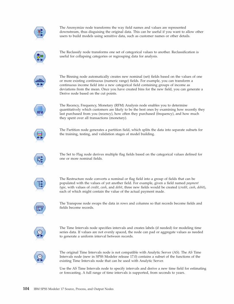
The Anonymize node transforms the way field names and values are representeddownstream, thus disguising the original data. This can be useful if you want to allow otherusers to build models using sensitive data, such as customer names or other details.

The Reclassify node transforms one set of categorical values to another. Reclassification isuseful for collapsing categories or regrouping data for analysis.

The Binning node automatically creates new nominal (set) fields based on the values of oneor more existing continuous (numeric range) fields. For example, you can transform acontinuous income field into a new categorical field containing groups of income asdeviations from the mean. Once you have created bins for the new field, you can generate aDerive node based on the cut points.

The Recency, Frequency, Monetary (RFM) Analysis node enables you to determinequantitatively which customers are likely to be the best ones by examining how recently theylast purchased from you (recency), how often they purchased (frequency), and how muchthey spent over all transactions (monetary).

The Partition node generates a partition field, which splits the data into separate subsets forthe training, testing, and validation stages of model building.

The Set to Flag node derives multiple flag fields based on the categorical values defined forone or more nominal fields.

The Restructure node converts a nominal or flag field into a group of fields that can bepopulated with the values of yet another field. For example, given a field named paymenttype, with values of credit, cash, and debit, three new fields would be created (credit, cash, debit),each of which might contain the value of the actual payment made.

The Transpose node swaps the data in rows and columns so that records become fields andfields become records.

The Time Intervals node specifies intervals and creates labels (if needed) for modeling timeseries data. If values are not evenly spaced, the node can pad or aggregate values as neededto generate a uniform interval between records.

The original Time Intervals node is not compatible with Analytic Server (AS). The AS TimeIntervals node (new in SPSS Modeler release 17.0) contains a subset of the functions of theexisting Time Intervals node that can be used with Analytic Server.

Use the AS Time Intervals node to specify intervals and derive a new time field for estimatingor forecasting. A full range of time intervals is supported, from seconds to years.


The History node creates new fields containing data from fields in previous records. Historynodes are most often used for sequential data, such as time series data. Before using a Historynode, you may want to sort the data using a Sort node.

The Field Reorder node defines the natural order used to display fields downstream. Thisorder affects the display of fields in a variety of places, such as tables, lists, and the FieldChooser. This operation is useful when working with wide datasets to make fields of interestmore visible.

Within SPSS Modeler, items such as the Expression Builder spatial functions, theSpatio-Temporal Prediction (STP) Node, and the Map Visualization Node use the projectedcoordinate system. Use the Reproject node to change the coordinate system of any data thatyou import that uses a geographic coordinate system.

Several of these nodes can be generated directly from the audit report created by a Data Audit node. Seethe topic “Generating Other Nodes for Data Preparation” on page 293 for more information.

Automated Data Preparation

Preparing data for analysis is one of the most important steps in any project—and traditionally, one ofthe most time consuming. Automated Data Preparation (ADP) handles the task for you, analyzing yourdata and identifying fixes, screening out fields that are problematic or not likely to be useful, derivingnew attributes when appropriate, and improving performance through intelligent screening techniques.You can use the algorithm in fully automatic fashion, allowing it to choose and apply fixes, or you canuse it in interactive fashion, previewing the changes before they are made and accept or reject them asyou want.

Using ADP enables you to make your data ready for model building quickly and easily, without needingprior knowledge of the statistical concepts involved. Models will tend to build and score more quickly; inaddition, using ADP improves the robustness of automated modeling processes, such as model refreshand champion / challenger.

Note: when ADP prepares a field for analysis, it creates a new field containing the adjustments ortransformations, rather than replacing the existing values and properties of the old field. The old field isnot used in further analysis; its role is set to None.

Example. An insurance company with limited resources to investigate homeowner's insurance claimswants to build a model for flagging suspicious, potentially fraudulent claims. Before building the model,they will ready the data for modeling using automated data preparation. Since they want to be able toreview the proposed transformations before the transformations are applied, they will use automateddata preparation in interactive mode.

An automotive industry group keeps track of the sales for a variety of personal motor vehicles. In aneffort to be able to identify over- and underperforming models, they want to establish a relationshipbetween vehicle sales and vehicle characteristics. They will use automated data preparation to prepare thedata for analysis, and build models using the data "before" and "after" preparation to see how the resultsdiffer.

What is your objective? Automated data preparation recommends data preparation steps that will affectthe speed with which other algorithms can build models and improve the predictive power of thosemodels. This can include transforming, constructing and selecting features. The target can also betransformed. You can specify the model-building priorities that the data preparation process shouldconcentrate on.

Chapter 4. Field Operations Nodes 105

v Balance speed and accuracy. This option prepares the data to give equal priority to both the speedwith which data are processed by model-building algorithms and the accuracy of the predictions.

v Optimize for speed. This option prepares the data to give priority to the speed with which data areprocessed by model-building algorithms. When you are working with very large datasets, or arelooking for a quick answer, select this option.

v Optimize for accuracy. This option prepares the data to give priority to the accuracy of predictionsproduced by model-building algorithms.

v Custom analysis. When you want to manually change the algorithm on the Settings tab, select thisoption. Note that this setting is automatically selected if you subsequently make changes to options onthe Settings tab that are incompatible with one of the other objectives.

Training The Node

The ADP node is implemented as a process node and works in a similar way to the Type node; trainingthe ADP node corresponds to instantiating the Type node. Once analysis has been performed, thespecified transformations are applied to the data without further analysis as long as the upstream datamodel does not change. Like the Type and Filter nodes, if the ADP node is disconnected it remembers thedata model and transformations so that if it is reconnected it does not need to be retrained; this enablesyou to train it on a subset of typical data and then copy or deploy it for use it on live data as often asrequired.

Using the Toolbar

The toolbar enables you to run and update the display of the data analysis, and generate nodes that youcan use in conjunction with the original data.v Generate From this menu you can generate either a Filter or Derive node. Note that this menu is only

available when there is an analysis shown on the Analysis tab.The Filter node removes transformed input fields. If you configure the ADP node to leave the originalinput fields in the dataset, this will restore the original set of inputs allowing you to interpret the scorefield in terms of the inputs. For example, this may be useful if you want to produce a graph of thescore field against various inputs.The Derive node can restore the original dataset and target units. You can only generate a Derive nodewhen the ADP node contains an analysis which rescales a range target (that is, Box-Cox rescaling isselected on the Prepare Inputs & Target panel). You cannot generate a Derive node if the target is not arange, or if the Box-Cox rescaling is not selected. See the topic “Generating a Derive Node” on page117 for more information.

v View Contains options that control what is shown on the Analysis tab. This includes the graph editingcontrols and the display selections for both the main panel and linked views.

v Preview Displays a sample of the transformations that will be applied to the input data.v Analyze Data Initiates an analysis using the current settings and displays the results on the Analysis

tab.v Clear Analysis Deletes the existing analysis (only available when a current analysis exists).

Node Status

The status of the ADP node on the IBM SPSS Modeler canvas is indicated by either an arrow or tick onthe icon that shows whether or not analysis has taken place.

Fields Tab

Before you can build a model, you need to specify which fields you want to use as targets and as inputs.With a few exceptions, all modeling nodes will use field information from an upstream Type node. If youare using a Type node to select input and target fields, you don't need to change anything on this tab.


Use type node settings. This option tells the node to use field information from an upstream Type node.This is the default.

Use custom settings. This option tells the node to use field information specified here instead of thatgiven in any upstream Type node(s). After selecting this option, specify the fields below as required.

Target. For models that require one or more target fields, select the target field or fields. This is similar tosetting the field role to Target in a Type node.

Inputs. Select the input field or fields. This is similar to setting the field role to Input in a Type node.

Settings Tab

The Settings tab comprises several different groups of settings that you can modify to fine-tune how thealgorithm processes your data. If you make any changes to the default settings that are incompatible withthe other objectives, the Objective tab is automatically updated to select the Customize analysis option.

Field SettingsUse frequency field. This option enables you to select a field as a frequency weight. Use this if therecords in your training data represent more than one unit each; for example, if you are using aggregateddata. The field values should be the number of units represented by each record.

Use weight field. This option enables you to select a field as a case weight. Case weights are used toaccount for differences in variance across levels of the output field.

How to handle fields that are excluded from modeling. Specify what happens to excluded fields; youcan choose either to filter them out of the data or simply set their Role to None.

Note: This action will also be applied to the target if it is transformed. For example, if the new derivedversion of the target is used as the Target field, the original target is either filtered or set to None.

If the incoming fields do not match the existing analysis. Specify what happens if one or more requiredinput fields are missing from the incoming dataset when you execute a trained ADP node.v Stop execution and keep the existing analysis. This stops the execution process, preserves the current

analysis information, and displays an error.v Clear the existing analysis and analyze the new data. This clears the existing analysis, analyzes the

incoming data, and applies the recommended transformations to that data.

Prepare Dates & Times

Many modeling algorithms are unable to directly handle date and time details; these settings enable youto derive new duration data that can be used as model inputs from dates and times in your existing data.The fields containing dates and times must be predefined with date or time storage types. The originaldate and time fields will not be recommended as model inputs following automated data preparation.

Prepare dates and times for modeling. Deselecting this option disables all other Prepare Dates & Timescontrols while maintaining the selections.

Compute elapsed time until reference date. This produces the number of years/months/days since areference date for each variable containing dates.v Reference Date. Specify the date from which the duration will be calculated with regard to the date

information in the input data. Selecting Today’s date means that the current system date is alwaysused when ADP is executed. To use a specific date, select Fixed date and enter the required date. Thecurrent date is automatically entered in the Fixed date field when the node is first created.


v Units for Date Duration. Specify whether ADP should automatically decide on the date duration unit,or select from Fixed units of Years, Months, or Days.

Compute elapsed time until reference time. This produces the number of hours/minutes/seconds sincea reference time for each variable containing times.v Reference Time. Specify the time from which the duration will be calculated with regard to the time

information in the input data. Selecting Current time means that the current system time is alwaysused when ADP is executed. To use a specific time, select Fixed time and enter the required details.The current time is automatically entered in the Fixed time field when the node is first created.

v Units for Time Duration. Specify whether ADP should automatically decide on the time durationunit, or select from Fixed units of Hours, Minutes, or Seconds.

Extract Cyclical Time Elements. Use these settings to split a single date or time field into one or morefields. For example if you select all three date checkboxes, the input date field "1954-05-23" is split intothree fields: 1954, 5, and 23, each using the suffix defined on the Field Names panel, and the originaldate field is ignored.v Extract from dates. For any date inputs, specify if you want to extract years, months, days, or any

combination.v Extract from times. For any time inputs, specify if you want to extract hours, minutes, seconds, or any

combination.

Exclude Fields

Poor quality data can affect the accuracy of your predictions; therefore, you can specify the acceptablequality level for input features. All fields that are constant or have 100% missing values are automaticallyexcluded.

Exclude low quality input fields. Deselecting this option disables all other Exclude Fields controls whilemaintaining the selections.

Exclude fields with too many missing values. Fields with more than the specified percentage of missingvalues are removed from further analysis. Specify a value greater than or equal to 0, which is equivalentto deselecting this option, and less than or equal to 100, though fields with all missing values areautomatically excluded. The default is 50.

Exclude nominal fields with too many unique categories. Nominal fields with more than the specifiednumber of categories are removed from further analysis. Specify a positive integer. The default is 100.This is useful for automatically removing fields containing record-unique information from modeling, likeID, address, or name.

Exclude categorical fields with too many values in a single category. Ordinal and nominal fields with acategory that contains more than the specified percentage of the records are removed from furtheranalysis. Specify a value greater than or equal to 0, equivalent to deselecting this option, and less than orequal to 100, though constant fields are automatically excluded. The default is 95.

Preparing Inputs and TargetsBecause no data is ever in a perfect state for processing, you may want to adjust some of the settingsbefore running an analysis. For example, this might include the removal of outliers, specifying how tohandle missing values, or adjusting the type.

Note: If you change the values on this panel, the Objectives tab is automatically updated to select theCustom analysis option.

Prepare the input and target fields for modeling. Toggles all fields on the panel either on or off.


Adjust Type and Improve Data Quality. For inputs and the target you can specify several datatransformations separately; this is because you may not want to change the values of the target. Forexample, a prediction of income in dollars is more meaningful than a prediction measured in log(dollars).In addition, if the target has missing values there is no predictive gain to filling missing values, whereasfilling missing values in inputs may enable some algorithms to process information that would otherwisebe lost.

Additional settings for these transformations, such as the outlier cutoff value, are common to both thetarget and inputs.

You can select the following settings for either, or both, inputs and target:v Adjust the type of numeric fields. Select this to determine if numeric fields with a measurement level

of Ordinal can be converted to Continuous, or vice versa. You can specify the minimum and maximumthreshold values to control the conversion.

v Reorder nominal fields. Select this to sort nominal (set) fields into order, from smallest to largestcategory.

v Replace outlier values in continuous fields. Specify whether to replace outliers; use this in conjunctionwith the Method for replacing outliers options below.

v Continuous fields: replace missing values with mean. Select this to replace missing values ofcontinuous (range) features.

v Nominal fields: replace missing values with mode. Select this to replace missing values of nominal(set) features.

v Ordinal fields: replace missing values with median. Select this to replace missing values of ordinal(ordered set) features.

Maximum number of values for ordinal fields. Specify the threshold for redefining ordinal (ordered set)fields as continuous (range). The default is 10; therefore, if an ordinal field has more than 10 categories itis redefined as continuous (range).

Minimum number of values for continuous fields. Specify the threshold for redefining scale orcontinuous (range) fields as ordinal (ordered set). The default is 5; therefore, if a continuous field hasfewer than 5 values it is redefined as ordinal (ordered set).

Outlier cutoff value. Specify the outlier cutoff criterion, measured in standard deviations; the default is 3.

Method for replacing outliers. Select whether outliers are to be replaced by either trimming (coerce) withthe cutoff value, or to delete them and set them as missing values. Any outliers set to missing valuesfollow the missing value handling settings selected above.

Put all continuous input fields on a common scale. To normalize continuous input fields, select thischeck box and choose the normalization method. The default is z-score transformation, where you canspecify the Final mean, which has a default of 0, and the Final standard deviation, which has a defaultof 1. Alternatively, you can choose to use Min/max transformation and specify the minimum andmaximum values, which have default values of 0 and 100 respectively.

This field is especially useful when you select Perform feature construction on the Construct & SelectFeatures panel.

Rescale a continuous target with a Box-Cox transformation. To normalize a continuous (scale or range)target field, select this check box. The Box-Cox transformation has default values of 0 for the Final meanand 1 for the Final standard deviation.


Note: If you choose to normalize the target, the dimension of the target will be transformed. In this caseyou may need to generate a Derive node to apply an inverse transformation in order to turn thetransformed units back into a recognizable format for further processing. See the topic “Generating aDerive Node” on page 117 for more information.

Construction and Feature SelectionTo improve the predictive power of your data, you can transform the input fields, or construct new onesbased on the existing fields.

Note: If you change the values on this panel, the Objectives tab is automatically updated to select theCustom analysis option.

Transform, construct and select input fields to improve predictive power. Toggles all fields on the paneleither on or off.

Merge sparse categories to maximize association with target. Select this to make a more parsimoniousmodel by reducing the number of variables to be processed in association with the target. If required,change the probability value from the default of 0.05.

Note that if all categories are merged into one, the original and derived versions of the field are excludedbecause they have no value as a predictor.

When there is no target, merge sparse categories based on counts. If you are dealing with data that hasno target, you can choose to merge sparse categories of either, or both, ordinal (ordered set) and nominal(set) features. Specify the minimum percentage of cases, or records, in the data that identifies thecategories to be merged; the default is 10.

Categories are merged using the following rules:v Merging is not performed on binary fields.v If there are only two categories during merging, merging stops.v If there is no original category, nor any category created during merging, with fewer than the specified

minimum percent of cases, merging stops.

Bin continuous fields while preserving predictive power. Where you have data that includes acategorical target, you can bin continuous inputs with strong associations to improve processingperformance. If required, change the probability value for the homogenous subsets from the default of0.05.

If the binning operation results in a single bin for a particular field, the original and binned versions ofthe field are excluded because they have no value as a predictor.

Note: Binning in ADP differs from optimal binning used in other parts of IBM SPSS Modeler. Optimalbinning uses entropy information to convert a continuous variable to a categorical variable; this needs tosort data and store it all in memory. ADP uses homogenous subsets to bin a continuous variable, thismeans that ADP binning does not need to sort data and does not store all data in memory. The use of thehomogenous subset method to bin a continuous variable means that the number of categories afterbinning is always less than or equal to the number of categories of target.

Perform feature selection. Select this option to remove features with a low correlation coefficient. Ifrequired, change the probability value from the default of 0.05.

This option only applies to continuous input features where the target is continuous, and to categoricalinput features.


Perform feature construction. Select this option to derive new features from a combination of severalexisting features (which are then discarded from modeling).

This option only applies to continuous input features where the target is continuous, or where there is notarget.

Field NamesTo easily identify new and transformed features, ADP creates and applies basic new names, prefixes, orsuffixes. You can amend these names to be more relevant to your own needs and data. If you want tospecify other labels, you will need to do this in a downstream Type node.

Transformed and Constructed Fields. Specify the name extensions to be applied to transformed targetand input fields.

Note that in the ADP node, setting string fields to contain nothing may cause an error depending on howyou chose to handle unused fields. If How to handle fields that are excluded from modeling is set toFilter out unused fields on the Field Settings panel of the Settings tab, the name extensions for inputsand the target can be set to nothing. The original fields are filtered out and the transformed fields savedover them; in this case the new transformed fields will have the same name as your original.

However if you chose Set the direction of unused fields to ‘None’, then empty, or null, name extensionsfor the target and inputs will cause an error because you will be trying to create duplicate field names.

In addition, specify the prefix name to be applied to any features that are constructed via the Select andConstruct settings. The new name is created by attaching a numeric suffix to this prefix root name. Theformat of the number depends on how many new features are derived, for example:v 1-9 constructed features will be named: feature1 to feature9.v 10-99 constructed features will be named: feature01 to feature99.v 100-999 constructed features will be named: feature001 to feature999, and so on.

This ensures that the constructed features will sort in a sensible order no matter how many there are.

Durations Computed from Dates and Times. Specify the name extensions to be applied to durationscomputed from both dates and times.

Cyclical Elements Extracted from Dates and Times. Specify the name extensions to be applied to cyclicalelements extracted from both dates and times.

Analysis Tab1. When you are satisfied with the ADP settings, including any changes made on the Objective, Fields,

and Settings tabs, click Analyze Data; the algorithm applies the settings to the data inputs anddisplays the results on the Analysis tab.

The Analysis tab contains both tabular and graphical output that summarizes the processing of your dataand displays recommendations as to how the data may be modified or improved for scoring. You canthen review and either accept or reject those recommendations.

The Analysis tab is made up of two panels, the main view on the left and the linked, or auxiliary, viewon the right. There are three main views:v Field Processing Summary (the default). See the topic “Field Processing Summary” on page 112 for

more information.v Fields. See the topic “Fields” on page 112 for more information.v Action Summary. See the topic “Action Summary” on page 113 for more information.


There are four linked/auxiliary views:v Predictive Power (the default). See the topic “Predictive Power” on page 114 for more information.v Fields Table. See the topic “Fields Table” on page 114 for more information.v Field Details. See the topic “Field Details” on page 114 for more information.v Action Details. See the topic “Action Details” on page 115 for more information.

Links between views

Within the main view, underlined text in the tables controls the display in the linked view. Clicking onthe text allows you to get details on a particular field, set of fields, or processing step. The link that youlast selected is shown in a darker color; this helps you identify the connection between the contents of thetwo view panels.

Resetting the views

To redisplay the original Analysis recommendations and abandon any changes you have made to theAnalysis views, click Reset at the bottom of the main view panel.

Field Processing SummaryThe Field Processing Summary table gives a snapshot of the projected overall impact of processing,including changes to the state of the features and the number of features constructed.

Note that no model is actually built, so there isn't a measure or graph of the change in overall predictivepower before and after data preparation; instead, you can display graphs of the predictive power ofindividual recommended predictors.

The table displays the following information:v The number of target fields.v The number of original (input) predictors.v The predictors recommended for use in analysis and modeling. This includes the total number of fields

recommended; the number of original, untransformed, fields recommended; the number oftransformed fields recommended (excluding intermediate versions of any field, fields derived fromdate/time predictors, and constructed predictors); the number of fields recommended that are derivedfrom date/time fields; and the number of constructed predictors recommended.

v The number of input predictors not recommended for use in any form, whether in their original form,as a derived field, or as input to a constructed predictor.

Where any of the Fields information is underlined, click to display more details in a linked view. Detailsof the Target, Input features, and Input features not used are shown in the Fields Table linked view. Seethe topic “Fields Table” on page 114 for more information. Features recommended for use in analysis aredisplayed in the Predictive Power linked view. See the topic “Predictive Power” on page 114 for moreinformation.

FieldsThe Fields main view displays the processed fields and whether ADP recommends using them indownstream models. You can override the recommendation for any field; for example, to excludeconstructed features or include features that ADP recommends excluding. If a field has been transformed,you can decide whether to accept the suggested transformation or use the original version.

The Fields view consists of two tables, one for the target and one for predictors that were eitherprocessed or created.

Target table


The Target table is only shown if a target is defined in the data.

The table contains two columns:v Name. This is the name or label of the target field; the original name is always used, even if the field

has been transformed.v Measurement Level. This displays the icon representing the measurement level; hover the mouse over

the icon to display a label (continuous, ordinal, nominal, and so on) that describes the data.If the target has been transformed the Measurement Level column reflects the final transformedversion. Note: you cannot turn off transformations for the target.

Predictors table

The Predictors table is always shown. Each row of the table represents a field. By default the rows aresorted in descending order of predictive power.

For ordinary features, the original name is always used as the row name. Both original and derivedversions of date/time fields appear in the table (in separate rows); the table also includes constructedpredictors.

Note that transformed versions of fields shown in the table always represent the final versions.

By default only recommended fields are shown in the Predictors table. To display the remaining fields,select the Include nonrecommended fields in table box above the table; these fields are then displayedat the bottom of the table.

The table contains the following columns:v Version to Use. This displays a drop-down list that controls whether a field will be used downstream

and whether to use the suggested transformations. By default, the drop-down list reflects therecommendations.For ordinary predictors that have been transformed the drop-down list has three choices: Transformed,Original, and Do not use.For untransformed ordinary predictors the choices are: Original and Do not use.For derived date/time fields and constructed predictors the choices are: Transformed and Do not use.For original date fields the drop-down list is disabled and set to Do not use.Note: For predictors with both original and transformed versions, changing between Original andTransformed versions automatically updates the Measurement Level and Predictive Power settings forthose features.

v Name. Each field's name is a link. Click a name to display more information about the field in thelinked view. See the topic “Field Details” on page 114 for more information.

v Measurement Level. This displays the icon representing the data type; hover the mouse over the iconto display a label (continuous, ordinal, nominal, and so on) that describes the data.

v Predictive Power. Predictive power is displayed only for fields that ADP recommends. This column isnot displayed if there is no target defined. Predictive power ranges from 0 to 1, with larger valuesindicating "better" predictors. In general, predictive power is useful for comparing predictors within anADP analysis, but predictive power values should not be compared across analyses.

Action SummaryFor each action taken by automated data preparation, input predictors are transformed and/or filteredout; fields that survive one action are used in the next. The fields that survive through to the last step arethen recommended for use in modeling, whilst inputs to transformed and constructed predictors arefiltered out.


The Action Summary is a simple table that lists the processing actions taken by ADP. Where any Actionis underlined, click to display more details in a linked view about the actions taken. See the topic “ActionDetails” on page 115 for more information.

Note: Only the original and final transformed versions of each field are shown, not any intermediateversions that were used during analysis.

Predictive PowerDisplayed by default when the analysis is first run, or when you select Predictors recommended for usein analysis in the Field Processing Summary main view, the chart displays the predictive power ofrecommended predictors. Fields are sorted by predictive power, with the field with the highest valueappearing at the top.

For transformed versions of ordinary predictors, the field name reflects your choice of suffix in the FieldNames panel of the Settings tab; for example: _transformed.

Measurement level icons are displayed after the individual field names.

The predictive power of each recommended predictor is computed from either a linear regression ornaïve Bayes model, depending upon whether the target is continuous or categorical.

Fields TableDisplayed when you click Target, Predictors, or Predictors not used in the Field Processing Summarymain view, the Fields Table view displays a simple table listing the relevant features.

The table contains two columns:v Name. The predictor name.

For targets, the original name or label of the field is used, even if the target has been transformed.For transformed versions of ordinary predictors, the name reflects your choice of suffix in the FieldNames panel of the Settings tab; for example: _transformed.For fields derived from dates and times, the name of the final transformed version is used; forexample: bdate_years.For constructed predictors, the name of the constructed predictor is used; for example: Predictor1.

v Measurement Level. This displays the icon representing the data type.For the Target, the Measurement Level always reflects the transformed version (if the target has beentransformed); for example, changed from ordinal (ordered set) to continuous (range, scale), or viceversa.

Field DetailsDisplayed when you click any Name in the Fields main view, the Field Details view contains distribution,missing values, and predictive power charts (if applicable) for the selected field. In addition, theprocessing history for the field and the name of the transformed field are also shown (if applicable).

For each chart set, two versions are shown side by side to compare the field with and withouttransformations applied; if a transformed version of the field does not exist, a chart is shown for theoriginal version only. For derived date or time fields and constructed predictors, the charts are onlyshown for the new predictor.

Note: If a field is excluded due to having too many categories only the processing history is shown.

Distribution Chart

Continuous field distribution is shown as a histogram, with a normal curve overlaid, and a verticalreference line for the mean value; categorical fields are displayed as a bar chart.


Histograms are labeled to show standard deviation and skewness; however, skewness is not displayed ifthe number of values is 2 or fewer or the variance of the original field is less than 10-20.

Hover the mouse over the chart to display either the mean for histograms, or the count and percentage ofthe total number of records for categories in bar charts.

Missing Value Chart

Pie charts compare the percentage of missing values with and without transformations applied; the chartlabels show the percentage.

If ADP carried out missing value handling, the post-transformation pie chart also includes thereplacement value as a label -- that is, the value used in place of missing values.

Hover the mouse over the chart to display the missing value count and percentage of the total number ofrecords.

Predictive Power Chart

For recommended fields, bar charts display the predictive power before and after transformation. If thetarget has been transformed, the calculated predictive power is in respect to the transformed target.

Note: Predictive power charts are not shown if no target is defined, or if the target is clicked in the mainview panel.

Hover the mouse over the chart to display the predictive power value.

Processing History Table

The table shows how the transformed version of a field was derived. Actions taken by ADP are listed inthe order in which they were carried out; however, for certain steps multiple actions may have beencarried out for a particular field.

Note: This table is not shown for fields that have not been transformed.

The information in the table is broken down into two or three columns:v Action. The name of the action. For example, Continuous Predictors. See the topic “Action Details” for

more information.v Details. The list of processing carried out. For example, Transform to standard units.v Function. Only shown for constructed predictors, this displays the linear combination of input fields,

for example, .06*age + 1.21*height.

Action DetailsDisplayed when you select any underlined Action in the Action Summary main view, the Action Detailslinked view displays both action-specific and common information for each processing step that wascarried out; the action-specific details are displayed first.

For each action, the description is used as the title at the top of the linked view. The action-specificdetails are displayed below the title, and may include details of the number of derived predictors, fieldsrecast, target transformations, categories merged or reordered, and predictors constructed or excluded.

As each action is processed, the number of predictors used in the processing may change, for example aspredictors are excluded or merged.


Note: If an action was turned off, or no target was specified, an error message is displayed in place of theaction details when the action is clicked in the Action Summary main view.

There are nine possible actions; however, not all are necessarily active for every analysis.

Text Fields Table

The table displays the number of:v Trailing blank values trimmed.v Predictors excluded from analysis.

Date and Time Predictors Table

The table displays the number of:v Durations derived from date and time predictors.v Date and time elements.v Derived date and time predictors, in total.

The reference date or time is displayed as a footnote if any date durations were calculated.

Predictor Screening Table

The table displays the number of the following predictors excluded from processing:v Constants.v Predictors with too many missing values.v Predictors with too many cases in a single category.v Nominal fields (sets) with too many categories.v Predictors screened out, in total.

Check Measurement Level Table

The table displays the numbers of fields recast, broken down into the following:v Ordinal fields (ordered sets) recast as continuous fields.v Continuous fields recast as ordinal fields.v Total number recast.

If no input fields (target or predictors) were continuous or ordinal, this is shown as a footnote.

Outliers Table

The table displays counts of how any outliers were handled.v Either the number of continuous fields for which outliers were found and trimmed, or the number of

continuous fields for which outliers were found and set to missing, depending on your settings in thePrepare Inputs & Target panel on the Settings tab.

v The number of continuous fields excluded because they were constant, after outlier handling.

One footnote shows the outlier cutoff value; while another footnote is shown if no input fields (target orpredictors) were continuous.

Missing Values Table

The table displays the numbers of fields that had missing values replaced, broken down into:


v Target. This row is not shown if no target is specified.v Predictors. This is further broken down into the number of nominal (set), ordinal (ordered set), and

continuous.v The total number of missing values replaced.

Target Table

The table displays whether the target was transformed, shown as:v Box-Cox transformation to normality. This is further broken down into columns that show the specified

criteria (mean and standard deviation) and Lambda.v Target categories reordered to improve stability.

Categorical Predictors Table

The table displays the number of categorical predictors:v Whose categories were reordered from lowest to highest to improve stability.v Whose categories were merged to maximize association with the target.v Whose categories were merged to handle sparse categories.v Excluded due to low association with the target.v Excluded because they were constant after merging.

A footnote is shown if there were no categorical predictors.

Continuous Predictors Table

There are two tables. The first displays one of the following number of transformations:v Predictor values transformed to standard units. In addition, this shows the number of predictors

transformed, the specified mean, and the standard deviation.v Predictor values mapped to a common range. In addition, this shows the number of predictors

transformed using a min-max transformation, as well as the specified minimum and maximum values.v Predictor values binned and the number of predictors binned.

The second table displays the predictor space construction details, shown as the number of predictors:v Constructed.v Excluded due to a low association with the target.v Excluded because they were constant after binning.v Excluded because they were constant after construction.

A footnote is shown if no continuous predictors were input.

Generating a Derive NodeWhen you generate a Derive node, it applies the inverse target transformation to the score field. Bydefault the node enters the name of the score field that would be produced by an automodeler (such asAuto Classifier or Auto Numeric) or the Ensemble node. If a scale (range) target has been transformedthe score field is shown in transformed units; for example, log($) instead of $. In order to interpret anduse the results, you must convert the predicted value back to the original scale.

Note: You can only generate a Derive node when the ADP node contains an analysis which rescales arange target (that is, Box-Cox rescaling is selected on the Prepare Inputs & Target panel). You cannotgenerate a Derive node if the target is not a range, or if the Box-Cox rescaling is not selected.


The Derive node is created in Multiple mode and uses @FIELD in the expression so you can add thetransformed target if required. For example using the following details:v Target field name: responsev Transformed target field name: response_transformedv Score field name: $XR-response_transformed

The Derive node would create a new field: $XR-response_transformed_inverse.

Note: If you are not using an automodeler or Ensemble node, you will need to edit the Derive node totransform the correct score field for your model.

Normalized continuous targets

By default, if you select the Rescale a continuous target with a Box-Cox transformation check box on thePrepare Inputs & Target panel this transforms the target and you create a new field that will be the targetfor your model building. For example if your original target was response, the new target will beresponse_transformed; models downstream of the ADP node will pick this new target up automatically.

However, this may cause issues, depending on the original target. For example, if the target was Age, thevalues of the new target will not be Years, but a transformed version of Years. This means you cannot lookat the scores and interpret them since they aren’t in recognizable units. In this case you can apply aninverse transformation that will turn your transformed units back into whatever they were meant to be.To do this:1. After clicking Analyze Data to run the ADP analysis, select Derive Node from the Generate menu.2. Place the Derive node after your nugget on the model canvas.

The Derive node will restore the score field to the original dimensions so that the prediction will be inthe original Years values.

By default the Derive node transforms the score field generated by an auto-modeler or an ensembledmodel. If you are building an individual model, you need to edit the Derive node to derive from youractual score field. If you want to evaluate your model, you should add the transformed target to theDerive From field in the Derive node. This applies the same inverse transformation to the target and anydownstream Evaluation or Analysis node will use the transformed data correctly as long as you switchthose nodes to use field names instead of metadata.

If you also want to restore the original name, you can use a Filter node to remove the original target fieldif it’s still there, and rename the target and score fields.

Type NodeField properties can be specified in a source node or in a separate Type node. The functionality is similarin both nodes. The following properties are available:v Field Double-click any field name to specify value and field labels for data in IBM SPSS Modeler. For

example, field metadata imported from IBM SPSS Statistics can be viewed or modified here. Similarly,you can create new labels for fields and their values. The labels that you specify here are displayedthroughout IBM SPSS Modeler depending on the selections you make in the stream properties dialogbox.

v Measurement This is the measurement level, used to describe characteristics of the data in a givenfield. If all of the details of a field are known, it is called fully instantiated. For more information, see“Measurement Levels” on page 119.

Note: The measurement level of a field is different from its storage type, which indicates whether thedata are stored as strings, integers, real numbers, dates, times, timestamps, or lists.


v Values This column enables you to specify options for reading data values from the data set, or use theSpecify option to specify measurement levels and values in a separate dialog box. You can also chooseto pass fields without reading their values. For more information, see “Data Values” on page 123.

Note: You cannot amend the cell in this column if the corresponding Field entry contains a list.v Missing Used to specify how missing values for the field will be handled. For more information, see

“Defining Missing Values” on page 127.

Note: You cannot amend the cell in this column if the corresponding Field entry contains a list.v Check In this column, you can set options to ensure that field values conform to the specified values

or ranges. For more information, see “Checking Type Values” on page 127.

Note: You cannot amend the cell in this column if the corresponding Field entry contains a list.v Role Used to tell modeling nodes whether fields will be Input (predictor fields) or Target (predicted

fields) for a machine-learning process. Both and None are also available roles, along with Partition,which indicates a field used to partition records into separate samples for training, testing, andvalidation. The value Split specifies that separate models will be built for each possible value of thefield. For more information, see “Setting the Field Role” on page 128.

Several other options can be specified using the Type node window:v Using the tools menu button, you can choose to Ignore Unique Fields once a Type node has been

instantiated (either through your specifications, reading values, or running the stream). Ignoringunique fields will automatically ignore fields with only one value.

v Using the tools menu button, you can choose to Ignore Large Sets once a Type node has beeninstantiated. Ignoring large sets will automatically ignore sets with a large number of members.

v Using the tools menu button, you can choose to Convert Continuous Integers To Ordinal once a Typenode has been instantiated. See the topic “Converting Continuous Data” on page 122 for moreinformation.

v Using the tools menu button, you can generate a Filter node to discard selected fields.v Using the sunglasses toggle buttons, you can set the default for all fields to Read or Pass. The Types

tab in the source node passes fields by default, while the Type node itself reads values by default.v Using the Clear Values button, you can clear changes to field values made in this node (non-inherited

values) and reread values from upstream operations. This option is useful for resetting changes thatyou may have made for specific fields upstream.

v Using the Clear All Values button, you can reset values for all fields read into the node. This optioneffectively sets the Values column to Read for all fields. This option is useful to reset values for allfields and reread values and types from upstream operations.

v Using the context menu, you can choose to Copy attributes from one field to another. See the topic“Copying Type Attributes” on page 129 for more information.

v Using the View unused field settings option, you can view type settings for fields that are no longerpresent in the data or were once connected to this Type node. This is useful when reusing a Type nodefor datasets that have changed.

Measurement LevelsMeasurement level (formerly known as "data type" or "usage type") describes the usage of the data fieldsin IBM SPSS Modeler. The measurement level can be specified on the Types tab of a source or Type node.For example, you may want to set the measurement level for an integer field with values of 1 and 0 toFlag. This usually indicates that 1 = True and 0 = False.

Storage versus measurement. Note that the measurement level of a field is different from its storagetype, which indicates whether data are stored as a string, integer, real number, date, time, or timestamp.While data types can be modified at any point in a stream using a Type node, storage must be


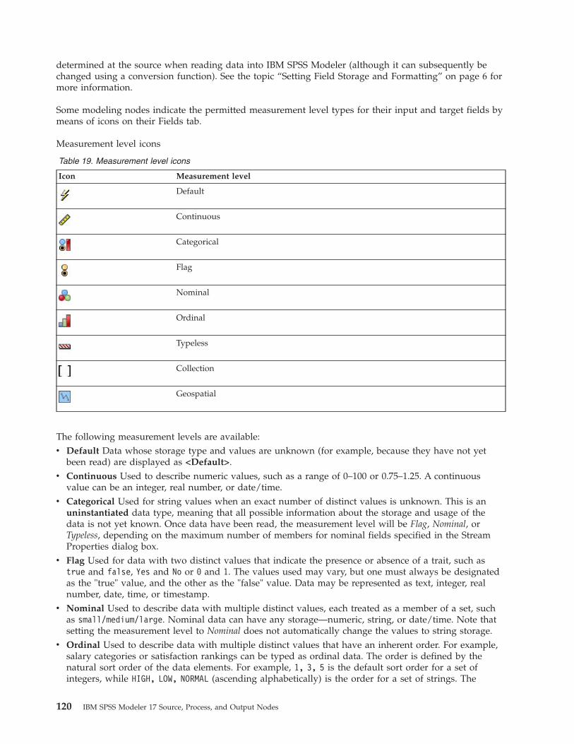
determined at the source when reading data into IBM SPSS Modeler (although it can subsequently bechanged using a conversion function). See the topic “Setting Field Storage and Formatting” on page 6 formore information.

Some modeling nodes indicate the permitted measurement level types for their input and target fields bymeans of icons on their Fields tab.

Measurement level icons

Table 19. Measurement level icons


Default

Continuous

Categorical

Flag

Nominal

Ordinal

Typeless

Collection

Geospatial

The following measurement levels are available:v Default Data whose storage type and values are unknown (for example, because they have not yet

been read) are displayed as <Default>.v Continuous Used to describe numeric values, such as a range of 0–100 or 0.75–1.25. A continuous

value can be an integer, real number, or date/time.v Categorical Used for string values when an exact number of distinct values is unknown. This is an

uninstantiated data type, meaning that all possible information about the storage and usage of thedata is not yet known. Once data have been read, the measurement level will be Flag, Nominal, orTypeless, depending on the maximum number of members for nominal fields specified in the StreamProperties dialog box.

v Flag Used for data with two distinct values that indicate the presence or absence of a trait, such astrue and false, Yes and No or 0 and 1. The values used may vary, but one must always be designatedas the "true" value, and the other as the "false" value. Data may be represented as text, integer, realnumber, date, time, or timestamp.

v Nominal Used to describe data with multiple distinct values, each treated as a member of a set, suchas small/medium/large. Nominal data can have any storage—numeric, string, or date/time. Note thatsetting the measurement level to Nominal does not automatically change the values to string storage.

v Ordinal Used to describe data with multiple distinct values that have an inherent order. For example,salary categories or satisfaction rankings can be typed as ordinal data. The order is defined by thenatural sort order of the data elements. For example, 1, 3, 5 is the default sort order for a set ofintegers, while HIGH, LOW, NORMAL (ascending alphabetically) is the order for a set of strings. The


ordinal measurement level enables you to define a set of categorical data as ordinal data for thepurposes of visualization, model building, and export to other applications (such as IBM SPSSStatistics) that recognize ordinal data as a distinct type. You can use an ordinal field anywhere that anominal field can be used. Additionally, fields of any storage type (real, integer, string, date, time, andso on) can be defined as ordinal.

v Typeless Used for data that does not conform to any of the above types, for fields with a single value,or for nominal data where the set has more members than the defined maximum. It is also useful forcases in which the measurement level would otherwise be a set with many members (such as anaccount number). When you select Typeless for a field, the role is automatically set to None, withRecord ID as the only alternative. The default maximum size for sets is 250 unique values. Thisnumber can be adjusted or disabled on the Options tab of the Stream Properties dialog box, which canbe accessed from the Tools menu.

v Collection Used to identify non-geospatial data that is recorded in a list. A collection is effectively a listfield of zero depth, where the elements in that list have one of the other measurement levels.For more information about lists, see the List Storage and Associated Measurement Levels topic in theSource Nodes section of the SPSS Modeler Source, Process, and Output Nodes Guide.

v Geospatial Used with the List storage type to identify geospatial data. Lists can be either List ofInteger or List of Real fields with a list depth that is between zero and two, inclusive.For more information, see the Geospatial Measurement Sublevels topic in the Type Node section of theSPSS Modeler Source, Process, and Output Nodes Guide.

You can manually specify measurement levels, or you can allow the software to read the data anddetermine the measurement level based on the values that it reads.

Alternatively, where you have several continuous data fields that should be treated as categorical data,you can choose an option to convert them. See the topic “Converting Continuous Data” on page 122 formore information.

To Use Auto-Typing1. In either a Type node or the Types tab of a source node, set the Values column to <Read> for the

desired fields. This will make metadata available to all nodes downstream. You can quickly set allfields to <Read> or <Pass> using the sunglasses buttons on the dialog box.

2. Click Read Values to read values from the data source immediately.

To Manually Set the Measurement Level for a Field1. Select a field in the table.2. From the drop-down list in the Measurement column, select a measurement level for the field.3. Alternatively, you can use Ctrl-A or Ctrl-click to select multiple fields before using the drop-down list

to select a measurement level.

Geospatial measurement sublevelsThe Geospatial measurement level, which is used with the List storage type, has six sublevels that areused to identify different types of geospatial data.v Point - Identifies a specific location; for example, the center of a city.v Polygon - A series of points that identifies the single boundary of a region and its location; for

example, a county.v LineString - Also referred to as a Polyline or just a Line, a LineString is a series of points that identifies

the route of a line. For example, a LineString might be a fixed item, such as road, river, or railway; orthe track of something that moves, such as an aircraft's flight path or a ship's voyage.

v MultiPoint - Used when each row in your data contains multiple points per region. For example, ifeach row represents a city street, the multiple points for each street can be used to identify every streetlamp.


v MultiPolygon - Used when each row in your data contains several polygons. For example, if each rowrepresents the outline of a country, the US can be recorded as several polygons to identify the differentareas such as the mainland, Alaska, and Hawaii.

v MultiLineString - Used when each row in your data contains several lines. Because lines cannotbranch you can use a MultiLineString to identify a group of lines. For example, data such as thenavigable waterways or the railway network in each country.

These measurement sublevels are used with the List storage type. For more information, see “List storageand associated measurement levels” on page 9.

Restrictions

You must be aware of some restrictions when you use geospatial data.v The coordinate system can affect the format of the data. For example, a Projected coordinate system

uses the coordinate values x, y, and (when required) z, whereas a Geographic coordinate system usesthe coordinate values longitude, latitude, and (when required) a value for either altitude or depth.For more information about coordinate systems, see the Setting Geospatial Options for Streams topic inthe Working with Streams section of the SPSS Modeler User's Guide.

v A LineString cannot cross over itself.v A Polygon is not self-closing; for each Polygon you must ensure that the first and last points are

defined as the same.v The direction of the data in a MultiPolygon is important; clockwise indicates a solid form and

clounterclockwise indicates a hole. For example, if you record an area of a country that contains lakes;the main land area border can be recorded in a clockwise direction and the shape of each lake in aclounterclockwise direction.

v A Polygon cannot intersect with itself. An example of this intersection would be if you tried to plot theboundary of the polygon as a continuous line in the form of the figure 8.

v MultiPolygons cannot overlap each other.

Geospatial measurement sublevel icons

Table 20. Geospatial measurement sublevel icons


Point

Polygon

LineString

MultiPoint

MultiPolygon

MultiLineString

Converting Continuous DataTreating categorical data as continuous can have a serious effect on the quality of a model, especially ifit’s the target field; for example, producing a regression model rather than a binary model. To preventthis you can convert integer ranges to categorical types such as Ordinal or Flag.


1. From the Operations and Generate menu button (with the tool symbol), select Convert ContinuousIntegers To Ordinal. The conversion values dialog is displayed.

2. Specify the size of range that will be automatically converted; this applies to any range up to andincluding the size you enter.

3. Click OK. The affected ranges are converted to either Flag or Ordinal and displayed on the Types tabof the Type node.

Results of the Conversionv Where a Continuous field with integer storage is changed to Ordinal, the lower and upper values are

expanded to include all of the integer values from the lower value to the upper value. For example, ifthe range is 1, 5, the set of values is 1, 2, 3, 4, 5.

v If the Continuous field changes to Flag, the lower and upper values become the false and true values ofthe flag field.

What Is Instantiation?Instantiation is the process of reading or specifying information, such as storage type and values for adata field. In order to optimize system resources, instantiating is a user-directed process—you tell thesoftware to read values by specifying options on the Types tab in a source node or by running datathrough a Type node.v Data with unknown types are also referred to as uninstantiated. Data whose storage type and values

are unknown are displayed in the Measurement column of the Types tab as <Default>.v When you have some information about a field's storage, such as string or numeric, the data are called

partially instantiated. Categorical or Continuous are partially instantiated measurement levels. Forexample, Categorical specifies that the field is symbolic, but you don't know whether it is nominal,ordinal, or flag.

v When all of the details about a type are known, including the values, a fully instantiated measurementlevel—nominal, ordinal, flag, or continuous—is displayed in this column. Note: The continuous type isused for both partially instantiated and fully instantiated data fields. Continuous data can be eitherintegers or real numbers.

During the execution of a data stream with a Type node, uninstantiated types immediately becomepartially instantiated, based on the initial data values. Once all of the data have passed through the node,all data become fully instantiated unless values were set to <Pass>. If execution is interrupted, the datawill remain partially instantiated. Once the Types tab has been instantiated, the values of a field are staticat that point in the stream. This means that any upstream changes will not affect the values of aparticular field, even if you rerun the stream. To change or update the values based on new data oradded manipulations, you need to edit them in the Types tab itself or set the value for a field to <Read>or <Read +>.

When to Instantiate

Generally, if your dataset is not very large and you do not plan to add fields later in the stream,instantiating at the source node is the most convenient method. However, instantiating in a separate Typenode is useful when:v The dataset is large, and the stream filters a subset prior to the Type node.v Data have been filtered in the stream.v Data have been merged or appended in the stream.v New data fields are derived during processing.

Data ValuesUsing the Values column of the Types tab, you can read values automatically from the data, or you canspecify measurement levels and values in a separate dialog box.


The options available from the Values drop-down list provide instructions for auto-typing, as shown inthe following table.

Table 21. Instructions for auto-typing

Option Function

<Read> Data will be read when the node is executed.

<Read+> Data will be read and appended to the current data (if any exist).

<Pass> No data are read.

<Current> Keep current data values.

Specify... A separate dialog box is launched for you to specify values and measurement level options.

Executing a Type node or clicking Read Values will auto-type and read values from your data sourcebased on your selection. These values can also be specified manually using the Specify option or bydouble-clicking a cell in the Field column.

Once you have made changes for fields in the Type node, you can reset value information using thefollowing buttons on the dialog box toolbar:v Using the Clear Values button, you can clear changes to field values made in this node (non-inherited

values) and reread values from upstream operations. This option is useful for resetting changes thatyou may have made for specific fields upstream.

v Using the Clear All Values button, you can reset values for all fields read into the node. This optioneffectively sets the Values column to Read for all fields. This option is useful to reset values for allfields and reread values and measurement levels from upstream operations.

Using the Values Dialog BoxClicking the Values or Missing column of the Types tab displays a drop-down list of predefined values.Choosing the Specify... option on this list opens a separate dialog box where you can set options forreading, specifying, labeling, and handling values for the selected field.

Many of the controls are common to all types of data. These common controls are discussed here.

Measurement Displays the currently selected measurement level. You can change the setting to reflect theway that you intend to use data. For instance, if a field called day_of_week contains numbers thatrepresent individual days, you might want to change this to nominal data in order to create a distributionnode that examines each category individually.

Storage Displays the storage type if known. Storage types are unaffected by the measurement level thatyou choose. To alter the storage type, you can use the Data tab in Fixed File and Variable File sourcenodes, or a conversion function in a Filler node.

Model Field For fields generated as a result of scoring a model nugget, model field details can also beviewed. These include the name of the target field as well as the role of the field in modeling (whether apredicted value, probability, propensity, and so on).

Values Select a method to determine values for the selected field. Selections that you make here overrideany selections that you made earlier from the Values column of the Type node dialog box. Choices forreading values include the following:v Read from data Select to read values when the node is executed. This option is the same as <Read>.v Pass Select not to read data for the current field. This option is the same as <Pass>.


v Specify values and labels Options here are used to specify values and labels for the selected field.Used with value checking, use this option to specify values that are based on your knowledge of thecurrent field. This option activates unique controls for each type of field. Options for values and labelsare covered individually in subsequent topics.

Note: You cannot specify values or labels for a field whose measurement level is Typeless or<Default>.

v Extend values from data Select to append the current data with the values that you enter here. Forexample, if field_1 has a range from (0,10), and you enter a range of values from (8,16), the range isextended by adding the 16, without removing the original minimum. The new range would be (0,16).Choosing this option automatically sets the auto-typing option to <Read+>.

Max list length Only available for data with a measurement level of either Geospatial or Collection. Setthe maximum length of the list by specifying the number of elements the list can contain.

Check values Select a method of coercing values to conform to the specified continuous, flag, or nominalvalues. This option corresponds to the Check column in the Type node dialog box, and settings madehere override those in the dialog box. Used with the Specify values and labels option, value checkingallows you to conform values in the data with expected values. For example, if you specify values as 1, 0and then use the Discard option, you can discard all records with values other than 1 or 0.

Define blanks Select to activate the following controls that you use to declare missing values or blanks inyour data.v Missing values Use this table to define specific values (such as 99 or 0) as blanks. The value should be

appropriate for the storage type of the field.v Range Used to specify a range of missing values, for example, ages 1–17 or greater than 65. If a bound

value is left blank, then the range is unbounded; for example, if a lower bound of 100 is specified withno upper bound, then all values greater than or equal to 100 is defined as missing. The bound valuesare inclusive; for example, a range with a lower bound of 5 and an upper bound of 10 includes 5 and10 in the range definition. A missing value range can be defined for any storage type, includingdate/time and string (in which case the alphabetic sort order is used to determine whether a value iswithin the range).

v Null/White space You can also specify system nulls (displayed in the data as $null$) and white space(string values with no visible characters) as blanks.

Note: The Type node also treats empty strings as white space for purposes of analysis, although theyare stored differently internally and may be handled differently in certain cases.

Note: To code blanks as undefined or $null$, use the Filler node.

Description Use this text box to specify a field label. These labels appear in various locations, such as ingraphs, tables, output, and model browsers, depending on selections you make in the Stream Propertiesdialog box.

Specifying Values and Labels for Continuous DataThe Continuous measurement level is used for numeric fields. There are three storage types for continuousdata:v Realv Integerv Date/Time

The same dialog box is used to edit all continuous fields; the storage type is displayed for reference only.

Specifying Values


The following controls are unique to continuous fields and are used to specify a range of values:

Lower. Specify a lower limit for the value range.

Upper. Specify an upper limit for the value range.

Specifying Labels

You can specify labels for any value of a range field. Click the Labels button to open a separate dialogbox for specifying value labels.

Values and Labels Subdialog Box: Clicking Labels in the Values dialog box for a range field opens anew dialog box in which you can specify labels for any value in the range.

You can use the Values and Labels columns in this table to define value and label pairs. Currently definedpairs are shown here. You can add new label pairs by clicking in an empty cell and entering a value andits corresponding label. Note: Adding value/value-label pairs to this table will not cause any new valuesto be added to the field. Instead, it simply creates metadata for the field value.

The labels that you specify in the Type node are displayed in many places (as ToolTips, output labels,and so on), depending on selections that you make in the stream properties dialog box.

Specifying Values and Labels for Nominal and Ordinal DataNominal (set) and ordinal (ordered set) measurement levels indicate that the data values are useddiscretely as a member of the set. The storage types for a set can be string, integer, real number, ordate/time.

The following controls are unique to nominal and ordinal fields and are used to specify values and labels:

Values. The Values column in the table allows you to specify values based on your knowledge of thecurrent field. Using this table, you can enter expected values for the field and check the dataset'sconformity to these values using the Check Values drop-down list. Using the arrow and delete buttons,you can modify existing values as well as reorder or delete values.

Labels. The Labels column enables you to specify labels for each value in the set. These labels appear in avariety of locations, such as graphs, tables, output, and model browsers, depending on selections that youmake in the stream properties dialog box.

Specifying Values for a FlagFlag fields are used to display data that have two distinct values. The storage types for flags can bestring, integer, real number, or date/time.

True. Specify a flag value for the field when the condition is met.

False. Specify a flag value for the field when the condition is not met.

Labels. Specify labels for each value in the flag field. These labels appear in a variety of locations, such asgraphs, tables, output, and model browsers, depending on selections that you make in the streamproperties dialog box.

Specifying Values for Collection DataCollection fields are used to display non-geospatial data that is in a list.

The only item that you can set for the Collection Measurement level is the List measure. By default thismeasure is set to Typeless but you can select another value from to set the measurement level of theelements within the list. You can choose one of the following options:


v Typelessv Continuousv Nominalv Ordinalv Flag

Specifying Values for Geospatial DataGeospatial fields are used to display geospatial data that is in a list.

For the Geospatial Measurement level, you can set the following options to set the measurement level ofthe elements within the list:

Type Select the measurement sublevel of the geospatial field. The available sublevels are determined bythe depth of the list field; the defaults are: Point (zero depth), LineString (depth of one), and Polygon(depth of one).

For more information about sublevels, see “Geospatial measurement sublevels” on page 121.

For more information about list depths, see “List storage and associated measurement levels” on page 9.

Coordinate system This option is only available if you changed the measurement level to geospatial froma non-geospatial level. To apply a coordinate system to your geospatial data, select this check box. Bydefault, the coordinate system set in the Tools > Stream Properties > Options > Geospatial pane isshown. To use a different coordinate system, click the Change button to display the Select CoordinateSystem dialog box and choose the system that you require.

For more information about coordinate systems, see the Setting Geospatial Options for Streams topic inthe Working with Streams section of the SPSS Modeler User's Guide.

Defining Missing ValuesThe Missing column of the Types tab indicates whether missing value handling has been defined for afield. The possible settings are:

On (*). Indicates that missing values handling is defined for this field. This could be done by means of adownstream Filler node, or through an explicit specification using the Specify option (see below).

Off. The field has no missing value handling defined.

Specify. Choose this option to display a dialog where you can declare explicit values to be considered asmissing values for this field.

Checking Type ValuesTurning on the Check option for each field examines all values in that field to determine whether theycomply with the current type settings or the values that you have specified in the Specify Values dialogbox. This is useful for cleaning up datasets and reducing the size of a dataset within a single operation.

The setting of the Check column in the Type node dialog box determines what happens when a valueoutside of the type limits is discovered. To change the Check settings for a field, use the drop-down listfor that field in the Check column. To set the Check settings for all fields, click in the Field column andpress Ctrl-A. Then use the drop-down list for any field in the Check column.

The following Check settings are available:

None. Values will be passed through without checking. This is the default setting.


Nullify. Change values outside of the limits to the system null ($null$).

Coerce. Fields whose measurement levels are fully instantiated will be checked for values that fall outsidethe specified ranges. Unspecified values will be converted to a legal value for that measurement levelusing the following rules:v For flags, any value other than the true and false value is converted to the false value.v For sets (nominal or ordinal), any unknown value is converted to the first member of the set's values.v Numbers greater than the upper limit of a range are replaced by the upper limit.v Numbers less than the lower limit of a range are replaced by the lower limit.v Null values in a range are given the midpoint value for that range.

Discard. When illegal values are found, the entire record is discarded.

Warn. The number of illegal items is counted and reported in the stream properties dialog box when allof the data have been read.

Abort. The first illegal value encountered terminates the running of the stream. The error is reported inthe stream properties dialog box.

Setting the Field RoleThe role of a field specifies how it is used in model building—for example, whether a field is an input ortarget (the thing being predicted).

Note: The Partition, Frequency and Record ID roles can each be applied to a single field only.

The following roles are available:

Input. The field will be used as an input to machine learning (a predictor field).

Target. The field will be used as an output or target for machine learning (one of the fields that themodel will try to predict).

Both. The field will be used as both an input and an output by the Apriori node. All other modelingnodes will ignore the field.

None. The field will be ignored by machine learning. Fields whose measurement level has been set toTypeless are automatically set to None in the Role column.

Partition. Indicates a field used to partition the data into separate samples for training, testing, and(optional) validation purposes. The field must be an instantiated set type with two or three possiblevalues (as defined in the Field Values dialog box). The first value represents the training sample, thesecond represents the testing sample, and the third (if present) represents the validation sample. Anyadditional values are ignored, and flag fields cannot be used. Note that to use the partition in an analysis,partitioning must be enabled on the Model Options tab in the appropriate model-building or analysisnode. Records with null values for the partition field are excluded from the analysis when partitioning isenabled. If multiple partition fields have been defined in the stream, a single partition field must bespecified on the Fields tab in each applicable modeling node. If a suitable field doesn't already exist inyour data, you can create one using a Partition node or Derive node. See the topic “Partition Node” onpage 154 for more information.

Split. (Nominal, ordinal and flag fields only) Specifies that a model is to be built for each possible valueof the field.


Frequency. (Numeric fields only) Setting this role enables the field value to be used as a frequencyweighting factor for the record. This feature is supported by C&R Tree, CHAID, QUEST and Linearmodels only; all other nodes ignore this role. Frequency weighting is enabled by means of the Usefrequency weight option on the Fields tab of those modeling nodes that support the feature.

Record ID. The field will be used as the unique record identifier. This feature is ignored by most nodes;however it is supported by Linear models, and is required for the IBM Netezza in-database miningnodes.

Copying Type AttributesYou can easily copy the attributes of a type, such as values, checking options, and missing values fromone field to another:1. Right-click on the field whose attributes you want to copy.2. From the context menu, choose Copy.3. Right-click on the field(s) whose attributes you want to change.4. From the context menu, choose Paste Special. Note: You can select multiple fields using the Ctrl-click

method or by using the Select Fields option from the context menu.

A new dialog box opens, from which you can select the specific attributes that you want to paste. If youare pasting into multiple fields, the options that you select here will apply to all target fields.

Paste the following attributes. Select from the list below to paste attributes from one field to another.v Type. Select to paste the measurement level.v Values. Select to paste the field values.v Missing. Select to paste missing value settings.v Check. Select to paste value checking options.v Role. Select to paste the role of a field.

Field Format Settings TabThe Format tab on the Table and Type nodes shows a list of current or unused fields and formattingoptions for each field. Following is a description of each column in the field formatting table:

Field. This shows the name of the selected field.

Format. By double-clicking a cell in this column, you can specify formatting for fields on an individualbasis using the dialog box that opens. See the topic “Setting Field Format Options” on page 130 for moreinformation. Formatting specified here overrides formatting specified in the overall stream properties.

Note: The Statistics Export and Statistics Output nodes export .sav files that include per-field formattingin their metadata. If a per-field format is specified that is not supported by the IBM SPSS Statistics .savfile format, then the node will use the IBM SPSS Statistics default format.

Justify. Use this column to specify how the values should be justified within the table column. Thedefault setting is Auto, which left-justifies symbolic values and right-justifies numeric values. You canoverride the default by selecting Left, Right, or Center.

Column Width. By default, column widths are automatically calculated based on the values of the field.To override the automatic width calculation, click a table cell and use the drop-down list to select a newwidth. To enter a custom width not listed here, open the Field Formats subdialog box by double-clickinga table cell in the Field or Format column. Alternatively, you can right-click on a cell and choose SetFormat.


View Current Fields. By default, the dialog box shows the list of currently active fields. To view the listof unused fields, select View unused fields settings.

Context Menu. The context menu for this tab provides various selection and setting update options.Right-click in a column to display this menu.v Select All. Selects all fields.v Select None. Clears the selection.v Select Fields. Selects fields based on type or storage characteristics. Options are Select Categorical,

Select Continuous (numeric), Select Typeless, Select Strings, Select Numbers, or Select Date/Time.See the topic “Measurement Levels” on page 119 for more information.

v Set Format. Opens a subdialog box for specifying date, time, and decimal options on a per-field basis.v Set Justify. Sets the justification for the selected field(s). Options are Auto, Center, Left, or Right.v Set Column Width. Sets the field width for selected fields. Specify Auto to read width from the data.

Or you can set field width to 5, 10, 20, 30, 50, 100, or 200.

Setting Field Format OptionsField formatting is specified on a subdialog box available from the Format tab on the Type and Tablenodes. If you have selected more than one field before opening this dialog box, then settings from thefirst field in the selection are used for all. Clicking OK after making specifications here will apply thesesettings to all fields selected on the Format tab.

The following options are available on a per-field basis. Many of these settings can also be specified inthe stream properties dialog box. Any settings made at the field level override the default specified forthe stream.

Date format. Select a date format to be used for date storage fields or when strings are interpreted asdates by CLEM date functions.

Time format. Select a time format to be used for time storage fields or when strings are interpreted astimes by CLEM time functions.

Number display format. You can choose from standard (####.###), scientific (#.###E+##), or currencydisplay formats ($###.##).

Decimal symbol. Select either a comma (,) or period (.) as a decimal separator.

Grouping symbol. For number display formats, select the symbol used to group values (For example, thecomma in 3,000.00). Options include none, period, comma, space, and locale-defined (in which case thedefault for the current locale is used).

Decimal places (standard, scientific, currency, export). For number display formats, specifies the numberof decimal places to be used when displaying real numbers. This option is specified separately for eachdisplay format.

Justify. Specifies how the values should be justified within the column. The default setting is Auto, whichleft-justifies symbolic values and right-justifies numeric values. You can override the default by selectingleft, right, or center.

Column width. By default, column widths are automatically calculated based on the values of the field.You can specify a custom width in intervals of five using the arrows to the right of the list box.


Filtering or Renaming Fields

You can rename or exclude fields at any point in a stream. For example, as a medical researcher, you maynot be concerned about the potassium level (field-level data) of patients (record-level data); therefore, youcan filter out the K (potassium) field. This can be done using a separate Filter node or using the Filter tabon a source or output node. The functionality is the same regardless of which node it is accessed from.v From source nodes, such as Variable File, Fixed File, Statistics File and XML, you can rename or filter

fields as the data are read into IBM SPSS Modeler.v Using a Filter node, you can rename or filter fields at any point in the stream.v From Statistics Export, Statistics Transform, Statistics Model, and Statistics Output nodes, you can filter

or rename fields to conform to IBM SPSS Statistics naming standards. See the topic “Renaming orFiltering Fields for IBM SPSS Statistics” on page 347 for more information.

v You can use the Filter tab in any of the above nodes to define or edit multiple response sets. See thetopic “Editing Multiple Response Sets” on page 132 for more information.

v Finally, you can use a Filter node to map fields from one source node to another.

Setting Filtering OptionsThe table used on the Filter tab shows the name of each field as it comes into the node as well as thename of each field as it leaves. You can use the options in this table to rename or filter out fields that areduplicates or are unnecessary for downstream operations.v Field. Displays the input fields from currently connected data sources.v Filter. Displays the filter status of all input fields. Filtered fields include a red X in this column,

indicating that this field will not be passed downstream. Click in the Filter column for a selected fieldto turn filtering on and off. You can also select options for multiple fields simultaneously using theShift-click method of selection.

v Field. Displays the fields as they leave the Filter node. Duplicate names are displayed in red. You canedit field names by clicking in this column and entering a new name. Or, remove fields by clicking inthe Filter column to disable duplicate fields.

All columns in the table can be sorted by clicking on the column header.

View current fields. Select to view fields for datasets actively connected to the Filter node. This option isselected by default and is the most common method of using Filter nodes.

View unused field settings. Select to view fields for datasets that were once but are no longer connectedto the Filter node. This option is useful when copying Filter nodes from one stream to another or whensaving and reloading Filter nodes.

Filter Button Menu

Click the Filter button in the upper left corner of the dialog box to access a menu that provides a numberof shortcuts and other options.

You can choose to:v Remove all fields.v Include all fields.v Toggle all fields.v Remove duplicates. Note: Selecting this option removes all occurrences of the duplicate name, including

the first one.v Rename fields and multiple response sets to conform with other applications. See the topic “Renaming

or Filtering Fields for IBM SPSS Statistics” on page 347 for more information.


v Truncate field names.v Anonymize field and multiple response set names.v Use input field names.v Edit Multiple Response Sets. See the topic “Editing Multiple Response Sets” for more information.v Set the default filter state.

You can also use the arrow toggle buttons at the top of the dialog box to specify whether you want toinclude or discard fields by default. This is useful for large datasets where only a few fields are to beincluded downstream. For example, you can select only the fields you want to keep and specify that allothers should be discarded (rather than individually selecting all of the fields to discard).

Truncating Field NamesFrom the Filter button menu (upper left corner of the Filter tab), you can choose to truncate field names.

Maximum length. Specify a number of characters to limit the length of field names.

Number of digits. If field names, when truncated, are no longer unique, they will be further truncatedand differentiated by adding digits to the name. You can specify the number of digits used. Use thearrow buttons to adjust the number.

For example, the following table illustrates how field names in a medical dataset are truncated using thedefault settings (maximum length=8 and number of digits=2).

Table 22. Field name truncation

Field Names Truncated Field Names

Patient Input 1 Patien01

Patient Input 2 Patien02

Heart Rate HeartRat

BP BP

Anonymizing Field NamesYou can anonymize field names from any node that includes a Filter tab by clicking the Filter buttonmenu in the upper left corner and choosing Anonymize Field Names. Anonymized field names consistof a string prefix plus a unique numeric-based value.

Anonymize names of. Choose Selected fields only to anonymize only the names of fields alreadyselected on the Filter tab. The default is All fields, which anonymizes all field names.

Field names prefix. The default prefix for anonymized field names is anon_; choose Custom and typeyour own prefix if you want a different one.

Anonymize multiple response sets. Anonymizes the names of multiple response sets in the samemanner as fields. See the topic “Editing Multiple Response Sets” for more information.

To restore the original field names, choose Use Input Field Names from the filter button menu.

Editing Multiple Response SetsYou can add or edit multiple response sets from any node that includes a Filter tab by clicking the Filterbutton menu in the upper left corner and choosing Edit Multiple Response Sets.

Multiple response sets are used to record data that can have more than one value for each case—forexample, when asking survey respondents which museums they have visited or which magazines they


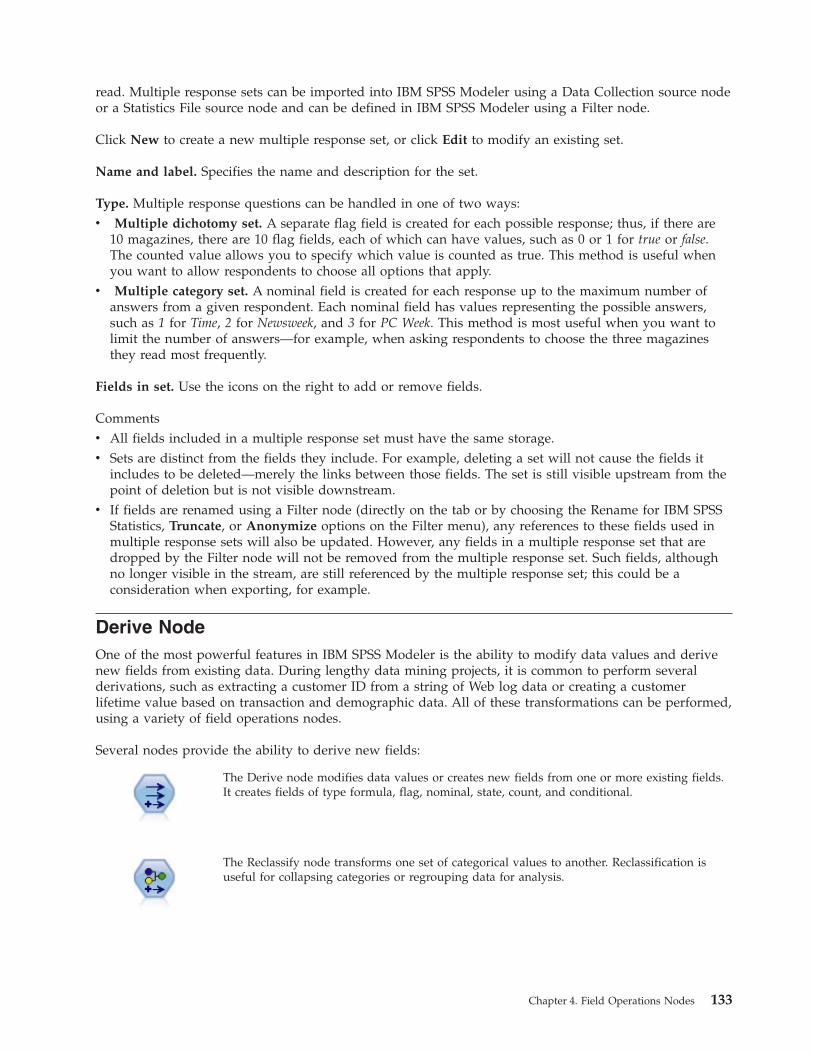
read. Multiple response sets can be imported into IBM SPSS Modeler using a Data Collection source nodeor a Statistics File source node and can be defined in IBM SPSS Modeler using a Filter node.

Click New to create a new multiple response set, or click Edit to modify an existing set.

Name and label. Specifies the name and description for the set.

Type. Multiple response questions can be handled in one of two ways:v Multiple dichotomy set. A separate flag field is created for each possible response; thus, if there are

10 magazines, there are 10 flag fields, each of which can have values, such as 0 or 1 for true or false.The counted value allows you to specify which value is counted as true. This method is useful whenyou want to allow respondents to choose all options that apply.

v Multiple category set. A nominal field is created for each response up to the maximum number ofanswers from a given respondent. Each nominal field has values representing the possible answers,such as 1 for Time, 2 for Newsweek, and 3 for PC Week. This method is most useful when you want tolimit the number of answers—for example, when asking respondents to choose the three magazinesthey read most frequently.

Fields in set. Use the icons on the right to add or remove fields.

Commentsv All fields included in a multiple response set must have the same storage.v Sets are distinct from the fields they include. For example, deleting a set will not cause the fields it

includes to be deleted—merely the links between those fields. The set is still visible upstream from thepoint of deletion but is not visible downstream.

v If fields are renamed using a Filter node (directly on the tab or by choosing the Rename for IBM SPSSStatistics, Truncate, or Anonymize options on the Filter menu), any references to these fields used inmultiple response sets will also be updated. However, any fields in a multiple response set that aredropped by the Filter node will not be removed from the multiple response set. Such fields, althoughno longer visible in the stream, are still referenced by the multiple response set; this could be aconsideration when exporting, for example.

Derive NodeOne of the most powerful features in IBM SPSS Modeler is the ability to modify data values and derivenew fields from existing data. During lengthy data mining projects, it is common to perform severalderivations, such as extracting a customer ID from a string of Web log data or creating a customerlifetime value based on transaction and demographic data. All of these transformations can be performed,using a variety of field operations nodes.

Several nodes provide the ability to derive new fields:

The Derive node modifies data values or creates new fields from one or more existing fields.It creates fields of type formula, flag, nominal, state, count, and conditional.

The Reclassify node transforms one set of categorical values to another. Reclassification isuseful for collapsing categories or regrouping data for analysis.


The Binning node automatically creates new nominal (set) fields based on the values of oneor more existing continuous (numeric range) fields. For example, you can transform acontinuous income field into a new categorical field containing groups of income asdeviations from the mean. Once you have created bins for the new field, you can generate aDerive node based on the cut points.

The Set to Flag node derives multiple flag fields based on the categorical values defined forone or more nominal fields.

The Restructure node converts a nominal or flag field into a group of fields that can bepopulated with the values of yet another field. For example, given a field named paymenttype, with values of credit, cash, and debit, three new fields would be created (credit, cash, debit),each of which might contain the value of the actual payment made.

The History node creates new fields containing data from fields in previous records. Historynodes are most often used for sequential data, such as time series data. Before using a Historynode, you may want to sort the data using a Sort node.

Using the Derive Node

Using the Derive node, you can create six types of new fields from one or more existing fields:v Formula. The new field is the result of an arbitrary CLEM expression.v Flag. The new field is a flag, representing a specified condition.v Nominal. The new field is nominal, meaning that its members are a group of specified values.v State. The new field is one of two states. Switching between these states is triggered by a specified

condition.v Count. The new field is based on the number of times that a condition has been true.v Conditional. The new field is the value of one of two expressions, depending on the value of a

condition.

Each of these nodes contains a set of special options in the Derive node dialog box. These options arediscussed in subsequent topics.

Setting Basic Options for the Derive NodeAt the top of the dialog box for Derive nodes are a number of options for selecting the type of Derivenode that you need.

Mode. Select Single or Multiple, depending on whether you want to derive multiple fields. WhenMultiple is selected, the dialog box changes to include options for multiple Derive fields.

Derive field. For simple Derive nodes, specify the name of the field that you want to derive and add toeach record. The default name is DeriveN, where N is the number of Derive nodes that you have createdthus far during the current session.

Derive as. Select a type of Derive node, such as Formula or Nominal, from the drop-down list. For eachtype, a new field is created based on the conditions that you specify in the type-specific dialog box.

Selecting an option from the drop-down list will add a new set of controls to the main dialog boxaccording to the properties of each Derive node type.


Field type. Select a measurement level, such as continuous, categorical, or flag, for the newly derivednode. This option is common to all forms of Derive nodes.

Note: Deriving new fields often requires the use of special functions or mathematical expressions. To helpyou create these expressions, an Expression Builder is available from the dialog box for all types ofDerive nodes and provides rule checking as well as a complete list of CLEM expressions.

Deriving Multiple FieldsSetting the mode to Multiple within a Derive node gives you the capability to derive multiple fieldsbased on the same condition within the same node. This feature saves time when you want to makeidentical transformations on several fields in your dataset. For example, if you want to build a regressionmodel predicting current salary based on beginning salary and previous experience, it might be beneficialto apply a log transformation to all three skewed variables. Rather than add a new Derive node for eachtransformation, you can apply the same function to all fields at once. Simply select all fields from whichto derive a new field and then type the derive expression using the @FIELD function within the fieldparentheses.

Note: The @FIELD function is an important tool for deriving multiple fields at the same time. It allows youto refer to the contents of the current field or fields without specifying the exact field name. For instance,a CLEM expression used to apply a log transformation to multiple fields is log(@FIELD).

The following options are added to the dialog box when you select Multiple mode:

Derive from. Use the Field Chooser to select fields from which to derive new fields. One output field willbe generated for each selected field. Note: Selected fields do not need to be the same storage type;however, the Derive operation will fail if the condition is not valid for all fields.

Field name extension. Type the extension that you would like added to the new field name(s). Forexample, for a new field containing the log of Current Salary, you could add the extension log_ to the fieldname, producing log_Current Salary. Use the radio buttons to choose whether to add the extension as aprefix (at the beginning) or as a suffix (at the end) of the field name. The default name is DeriveN, whereN is the number of Derive nodes that you have created thus far during the current session.

As in the single-mode Derive node, you now need to create an expression to use for deriving a new field.Depending on the type of Derive operation selected, there are a number of options to create a condition.These options are discussed in subsequent topics. To create an expression, you can simply type in theformula field(s) or use the Expression Builder by clicking the calculator button. Remember to use the@FIELD function when referring to manipulations on multiple fields.

Selecting Multiple FieldsFor all nodes that perform operations on multiple input fields, such as Derive (multiple mode),Aggregate, Sort, Multiplot, and Time Plot, you can easily select multiple fields using the Select Fieldsdialog box.

Sort by. You can sort available fields for viewing by selecting one of the following options:v Natural. View the order of fields as they have been passed down the data stream into the current

node.v Name. Use alphabetical order to sort fields for viewing.v Type. View fields sorted by their measurement level. This option is useful when selecting fields with a

particular measurement level.

Select fields from the list one at a time or use the Shift-click and Ctrl-click methods to select multiplefields. You can also use the buttons below the list to select groups of fields based on their measurementlevel, or to select or deselect all fields in the table.


Setting Derive Formula OptionsDerive Formula nodes create a new field for each record in a data set based on the results of a CLEMexpression. This expression cannot be conditional. To derive values that are based on a conditionalexpression, use the flag or conditional type of Derive node.

Formula Specify a formula by using the CLEM language to derive a value for the new field.

Note: Because SPSS Modeler cannot know what submeasurement level is to be used for a derived listfield, for the Collection and Geospatial measurement levels, you can click Specify... to open the Valuesdialog box and set the required submeasurement level. For more information, see “Setting derived listvalues.”

Setting derived list valuesThe Values dialog box is displayed when you select Specify... from the Derive node Formula Field typedrop-down list. In this dialog box, you set the submeasurement level values to be used for the FormulaField type measurement levels of either Collection or Geospatial.

Measurement Select either Collection or Geospatial. If you select any other measurement level, thedialog box displays a message that there are no editable values.

Collection

The only item that you can set for the Collection Measurement level is the List measure. By default thismeasure is set to Typeless but you can select another value to set the measurement level of the elementswithin the list. You can choose one of the following options:v Typelessv Categoricalv Continuousv Nominalv Ordinalv Flag

Geospatial

For the Geospatial Measurement level, you can select the following options to set the measurement levelof the elements within the list:

Type Select the measurement sublevel of the geospatial field. The available sublevels are determined bythe depth of the list field; the defaults are as follows:v Point (zero depth)v LineString (depth of one)v Polygon (depth of one)v MultiPoint (depth of one)v MultiLineString (depth of two)v MultiPolygon (depth of two)

For more information about sublevels, see the Geospatial Measurement Sublevels topic in the Type Nodesection of the SPSS Modeler Source, Process, and Output Nodes Guide.

For more information about list depths, see the List Storage and Associated Measurement Levels topic inthe Source Node section of the SPSS Modeler Source, Process, and Output Nodes Guide.


Coordinate system This option is only available if you changed the measurement level to geospatial froma non-geospatial level. To apply a coordinate system to your geospatial data, select this check box. Bydefault, the coordinate system set in the Tools > Stream Properties > Options > Geospatial pane isshown. To use a different coordinate system, click the Change button to display the Select CoordinateSystem dialog box and choose the system that matches your data.


Deriving a list or geospatial fieldThere are occasions when data that should be recorded as a list item is imported into SPSS Modeler withthe wrong attributes. For example, as separate geospatial fields, such as an x coordinate and a ycoordinate, or a longitude and latitude, as individual rows in a .csv file. In this situation, you mustcombine the individual fields into a single list field; one way to do this is by using the Derive node.

Note: You must know which is the x (or longitude) field and which is the y (or latitude field) field whenyou combine geospatial data. You must combine your data so that the resulting list field has the order ofelements: [x, y] or [Longitude, Latitude], which are the standard formats for geospatial coordinates.

The following steps show a simple example of deriving a list field.1. In your stream, attach a Derive node to your Source node.2. On the Settings tab of the Derive node, select Formula from the Derive as list.3. In Field Type select either Collection for a non-geospatial list, or Geospatial. By default, SPSS

Modeler uses a "best guess" approach to set the correct list detail; you can select Specify... to open theValues dialog box. In this dialog box, you can enter further information about the data in your list; forexample, for a geospatial list you can change the measurement level.

4. In the Formula pane, enter the formula to combine your data into the correct list format.Alternatively, click the calculator button to open the Expression Builder.A simple example of a formula to derive a list is [x, y], where x and y are separate fields in the datasource. The new derived field that is created is a list where the value for each record is theconcatenated x and y values for that record.

Note: Fields that are combined into a list in this way must have the same storage type.

For more information about lists, and depths of lists, see “List storage and associated measurementlevels” on page 9.

Setting Derive Flag OptionsDerive Flag nodes are used to indicate a specific condition, such as high blood pressure or customeraccount inactivity. A flag field is created for each record, and when the true condition is met, the flagvalue for true is added in the field.

True value. Specify a value to include in the flag field for records that match the condition specifiedbelow. The default is T.

False value. Specify a value to include in the flag field for records that do not match the conditionspecified below. The default is F.

True when. Specify a CLEM condition to evaluate certain values of each record and give the record a truevalue or a false value (defined above). Note that the true value will be given to records in the case ofnon-false numeric values.


Note: To return an empty string, you should type opening and closing quotes with nothing between them,such as "". Empty strings are often used, for example, as the false value in order to enable true values tostand out more clearly in a table. Similarly, quotes should be used if you want a string value that wouldotherwise be treated as a number

Example

In releases of IBM SPSS Modeler prior to 12.0, multiple responses were imported into a single field, withvalues separated by commas. For example:museum_of_design,institute_of_textiles_and_fashionmuseum_of_designarcheological_museum$null$national_art_gallery,national_museum_of_science,other

To prepare this data for analysis, you could use the hassubstring function to generate a separate flagfield for each response with an expression such as:hassubstring(museums,"museum_of_design")

Setting Derive Nominal OptionsDerive Nominal nodes are used to execute a set of CLEM conditions in order to determine whichcondition each record satisfies. As a condition is met for each record, a value (indicating which set ofconditions was met) will be added to the new, derived field.

Default value. Specify a value to be used in the new field if none of the conditions are met.

Set field to. Specify a value to enter in the new field when a particular condition is met. Each value inthe list has an associated condition that you specify in the adjacent column.

If this condition is true. Specify a condition for each member in the set field to list. Use the ExpressionBuilder to select from available functions and fields. You can use the arrow and delete buttons to reorderor remove conditions.

A condition works by testing the values of a particular field in the dataset. As each condition is tested,the values specified above will be assigned to the new field to indicate which, if any, condition was met.If none of the conditions are met, the default value is used.

Setting Derive State OptionsDerive State nodes are somewhat similar to Derive Flag nodes. A Flag node sets values depending on thefulfillment of a single condition for the current record, but a Derive State node can change the values of afield depending on how it fulfills two independent conditions. This means that the value will change (turnon or off) as each condition is met.

Initial state. Select whether to give each record of the new field the On or Off value initially. Note thatthis value can change as each condition is met.

"On" value. Specify the value for the new field when the On condition is met.

Switch "On" when. Specify a CLEM condition that will change the state to On when the condition istrue. Click the calculator button to open the Expression Builder.

"Off" value. Specify the value for the new field when the Off condition is met.

Switch "Off" when. Specify a CLEM condition that will change the state to Off when the condition isfalse. Click the calculator button to open the Expression Builder.


Note: To specify an empty string, you should type opening and closing quotes with nothing betweenthem, such as "". Similarly, quotes should be used if you want a string value that would otherwise betreated as a number.

Setting Derive Count OptionsA Derive Count node is used to apply a series of conditions to the values of a numeric field in thedataset. As each condition is met, the value of the derived count field is increased by a set increment.This type of Derive node is useful for time series data.

Initial value. Sets a value used on execution for the new field. The initial value must be a numericconstant. Use the arrow buttons to increase or decrease the value.

Increment when. Specify the CLEM condition that, when met, will change the derived value based onthe number specified in Increment by. Click the calculator button to open the Expression Builder.

Increment by. Set the value used to increment the count. You can use either a numeric constant or theresult of a CLEM expression.

Reset when. Specify a condition that, when met, will reset the derived value to the initial value. Click thecalculator button to open the Expression Builder.

Setting Derive Conditional OptionsDerive Conditional nodes use a series of If-Then-Else statements to derive the value of the new field.

If. Specify a CLEM condition that will be evaluated for each record upon execution. If the condition istrue (or non-false, in the case of numbers), the new field is given the value specified below by the Thenexpression. Click the calculator button to open the Expression Builder.

Then. Specify a value or CLEM expression for the new field when the If statement above is true (ornon-false). Click the calculator button to open the Expression Builder.

Else. Specify a value or CLEM expression for the new field when the If statement above is false. Click thecalculator button to open the Expression Builder.

Recoding Values with the Derive NodeDerive nodes can also be used to recode values, for example by converting a string field with categoricalvalues to a numeric nominal (set) field.1. For Derive As, select the type of field (Nominal, Flag, etc.) as appropriate.2. Specify the conditions for recoding values. For example, you could set the value to 1 if Drug=’drugA’,

2 if Drug=’drugB’, and so on.

Filler NodeFiller nodes are used to replace field values and change storage. You can choose to replace values basedon a specified CLEM condition, such as @BLANK(FIELD). Alternatively, you can choose to replace all blanksor null values with a specific value. Filler nodes are often used in conjunction with the Type node toreplace missing values. For example, you can fill blanks with the mean value of a field by specifying anexpression such as @GLOBAL_MEAN. This expression will fill all blanks with the mean value as calculated bya Set Globals node.

Fill in fields. Using the Field Chooser (button to the right of the text field), select fields from the datasetwhose values will be examined and replaced. The default behavior is to replace values depending on theCondition and Replace with expressions specified below. You can also select an alternative method ofreplacement using the Replace options below.


Note: When selecting multiple fields to replace with a user-defined value, it is important that the fieldtypes are similar (all numeric or all symbolic).

Replace. Select to replace the values of the selected field(s) using one of the following methods:v Based on condition. This option activates the Condition field and Expression Builder for you to create

an expression used as a condition for replacement with the value specified.v Always. Replaces all values of the selected field. For example, you could use this option to convert the

storage of income to a string using the following CLEM expression: (to_string(income)).v Blank values. Replaces all user-specified blank values in the selected field. The standard condition

@BLANK(@FIELD) is used to select blanks. Note: You can define blanks using the Types tab of the sourcenode or with a Type node.

v Null values. Replaces all system null values in the selected field. The standard condition@NULL(@FIELD) is used to select nulls.

v Blank and null values. Replaces both blank values and system nulls in the selected field. This optionis useful when you are unsure whether or not nulls have been defined as missing values.

Condition. This option is available when you have selected the Based on condition option. Use this textbox to specify a CLEM expression for evaluating the selected fields. Click the calculator button to openthe Expression Builder.

Replace with. Specify a CLEM expression to give a new value to the selected fields. You can also replacethe value with a null value by typing undef in the text box. Click the calculator button to open theExpression Builder.

Note: When the field(s) selected are string, you should replace them with a string value. Using the default0 or another numeric value as the replacement value for string fields will result in an error.

Storage Conversion Using the Filler NodeUsing the Replace condition of a Filler node, you can easily convert the field storage for single ormultiple fields. For example, using the conversion function to_integer, you could convert income from astring to an integer using the following CLEM expression: to_integer(income).

You can view available conversion functions and automatically create a CLEM expression using theExpression Builder. From the Functions drop-down list, select Conversion to view a list of storageconversion functions. The following conversion functions are available:v to_integer(ITEM)

v to_real(ITEM)

v to_number(ITEM)

v to_string(ITEM)

v to_time(ITEM)

v to_timestamp(ITEM)

v to_date(ITEM)

v to_datetime(ITEM)

Converting date and time values. Note that conversion functions (and any other functions that require aspecific type of input such as a date or time value) depend on the current formats specified in the streamoptions dialog box. For example if you want to convert a string field with values Jan 2003, Feb 2003, etc.to date storage, select MON YYYY as the default date format for the stream.


Conversion functions are also available from the Derive node, for temporary conversion during a derivecalculation. You can also use the Derive node to perform other manipulations such as recoding stringfields with categorical values. See the topic “Recoding Values with the Derive Node” on page 139 formore information.

Reclassify NodeThe Reclassify node enables the transformation from one set of categorical values to another.Reclassification is useful for collapsing categories or regrouping data for analysis. For example, you couldreclassify the values for Product into three groups, such as Kitchenware, Bath and Linens, and Appliances.Often, this operation is performed directly from a Distribution node by grouping values and generating aReclassify node. See the topic “Using a Distribution Node” on page 224 for more information.

Reclassification can be performed for one or more symbolic fields. You can also choose to substitute thenew values for the existing field or generate a new field.

When to use a Reclassify node

Before using a Reclassify node, consider whether another Field Operations node is more appropriate forthe task at hand:v To transform numeric ranges into sets using an automatic method, such as ranks or percentiles, you

should use a Binning node. See the topic “Binning Node” on page 145 for more information.v To classify numeric ranges into sets manually, you should use a Derive node. For example, if you want

to collapse salary values into specific salary range categories, you should use a Derive node to defineeach category manually.

v To create one or more flag fields based on the values of a categorical field, such as Mortgage_type, youshould use a Set to Flag node.

v To convert a categorical field to numeric storage, you can use a Derive node. For example, you couldconvert No and Yes values to 0 and 1, respectively. See the topic “Recoding Values with the DeriveNode” on page 139 for more information.

Setting Options for the Reclassify NodeThere are three steps to using the Reclassify node:1. First, select whether you want to reclassify multiple fields or a single field.2. Next, choose whether to recode into the existing field or create a new field.3. Then, use the dynamic options in the Reclassify node dialog box to map sets as desired.

Mode. Select Single to reclassify the categories for one field. Select Multiple to activate optionsenabling the transformation of more than one field at a time.Reclassify into. Select New field to keep the original nominal field and derive an additional fieldcontaining the reclassified values. Select Existing field to overwrite the values in the original fieldwith the new classifications. This is essentially a "fill" operation.Once you have specified mode and replacement options, you must select the transformation field andspecify the new classification values using the dynamic options on the bottom half of the dialog box.These options vary depending on the mode you have selected above.Reclassify field(s). Use the Field Chooser button on the right to select one (Single mode) or more(Multiple mode) categorical fields.New field name. Specify a name for the new nominal field containing recoded values. This option isavailable only in Single mode when New field is selected above. When Existing field is selected, theoriginal field name is retained. When working in Multiple mode, this option is replaced with controlsfor specifying an extension added to each new field. See the topic “Reclassifying Multiple Fields” onpage 142 for more information.Reclassify values. This table enables a clear mapping from old set values to those you specify here.


v Original value. This column lists existing values for the select field(s).v New value. Use this column to type new category values or select one from the drop-down list.

When you automatically generate a Reclassify node using values from a Distribution chart, thesevalues are included in the drop-down list. This allows you to quickly map existing values to aknown set of values. For example, healthcare organizations sometimes group diagnoses differentlybased upon network or locale. After a merger or acquisition, all parties will be required to reclassifynew or even existing data in a consistent fashion. Rather than manually typing each target valuefrom a lengthy list, you can read the master list of values in to IBM SPSS Modeler, run aDistribution chart for the Diagnosis field, and generate a Reclassify (values) node for this fielddirectly from the chart. This process will make all of the target Diagnosis values available from theNew Values drop-down list.

4. Click Get to read original values for one or more fields selected above.5. Click Copy to paste original values over to the New value column for fields that have not been

mapped yet. The unmapped original values are added to the drop-down list.6. Click Clear new to erase all specifications in the New value column. Note: This option does not erase

the values from the drop-down list.7. Click Auto to automatically generate consecutive integers for each of the original values. Only integer

values (no real values, such as 1.5, 2.5, and so on) can be generated.

For example, you can automatically generate consecutive product ID numbers for product names orcourse numbers for university class offerings. This functionality corresponds to the Automatic Recodetransformation for sets in IBM SPSS Statistics.

For unspecified values use. This option is used for filling unspecified values in the new field. You caneither choose to keep the original value by selecting Original value or specify a default value.

Reclassifying Multiple FieldsTo map category values for more than one field at a time, set the mode to Multiple. This enables newsettings in the Reclassify dialog box, which are described below.

Reclassify fields. Use the Field Chooser button on the right to select the fields that you want totransform. Using the Field Chooser, you can select all fields at once or fields of a similar type, such asnominal or flag.

Field name extension. When recoding multiple fields simultaneously, it is more efficient to specify acommon extension added to all new fields rather than individual field names. Specify an extension suchas _recode and select whether to append or prepend this extension to the original field names.

Storage and Measurement Level for Reclassified FieldsThe Reclassify node always creates a nominal field from the recode operation. In some cases, this maychange the measurement level of the field when using the Existing field reclassification mode.

The new field's storage (how data are stored rather than how they are used) is calculated based on thefollowing Settings tab options:v If unspecified values are set to use a default value, the storage type is determined by examining both

the new values as well as the default value and determining the appropriate storage. For example, ifall values can be parsed as integers, the field will have the integer storage type.

v If unspecified values are set to use the original values, the storage type is based on the storage of theoriginal field. If all of the values can be parsed as the storage of the original field, then that storage ispreserved; otherwise, the storage is determined by finding the most appropriate storage typeencompassing both old and new values. For example, reclassifying an integer set { 1, 2, 3, 4, 5 } withthe reclassification 4 => 0, 5 => 0 generates a new integer set { 1, 2, 3, 0 }, whereas with thereclassification 4 => “Over 3”, 5 => “Over 3” will generate the string set { “1”, “2”, “3”, “Over 3” }.


Note: If the original type was uninstantiated, the new type will be also be uninstantiated.

Anonymize NodeThe Anonymize node enables you to disguise field names, field values, or both when working with datathat are to be included in a model downstream of the node. In this way, the generated model can befreely distributed (for example, to Technical Support) with no danger that unauthorized users will be ableto view confidential data, such as employee records or patients' medical records.

Depending on where you place the Anonymize node in the stream, you may need to make changes toother nodes. For example, if you insert an Anonymize node upstream from a Select node, the selectioncriteria in the Select node will need to be changed if they are acting on values that have now becomeanonymized.

The method to be used for anonymizing depends on various factors. For field names and all field valuesexcept Continuous measurement levels, the data are replaced by a string of the form:prefix_Sn

where prefix_ is either a user-specified string or the default string anon_, and n is an integer value thatstarts at 0 and is incremented for each unique value (for example, anon_S0, anon_S1, etc.).

Field values of type Continuous must be transformed because numeric ranges deal with integer or realvalues rather than strings. As such, they can be anonymized only by transforming the range into adifferent range, thus disguising the original data. Transformation of a value x in the range is performedin the following way:A*(x + B)

where:

A is a scale factor, which must be greater than 0.

B is a translation offset to be added to the values.

Example

In the case of a field AGE where the scale factor A is set to 7 and the translation offset B is set to 3, thevalues for AGE are transformed into:7*(AGE + 3)

Setting Options for the Anonymize NodeHere you can choose which fields are to have their values disguised further downstream.

Note that the data fields must be instantiated upstream from the Anonymize node before anonymizeoperations can be performed. You can instantiate the data by clicking the Read Values button on a Typenode or on the Types tab of a source node.

Field. Lists the fields in the current dataset. If any field names have already been anonymized, theanonymized names are shown here.

Measurement. The measurement level of the field.

Anonymize Values. Select one or more fields, click this column, and choose Yes to anonymize the fieldvalue using the default prefix anon_; choose Specify to display a dialog box in which you can eitherenter your own prefix or, in the case of field values of type Continuous, specify whether the


transformation of field values is to use random or user-specified values. Note that Continuous andnon-Continuous field types cannot be specified in the same operation; you must do this separately foreach type of field.

View current fields. Select to view fields for datasets actively connected to the Anonymize node. Thisoption is selected by default.

View unused field settings. Select to view fields for datasets that were once but are no longer connectedto the node. This option is useful when copying nodes from one stream to another or when saving andreloading nodes.

Specifying How Field Values Will Be AnonymizedThe Replace Values dialog box lets you choose whether to use the default prefix for anonymized fieldvalues or to use a custom prefix. Clicking OK in this dialog box changes the setting of Anonymize Valueson the Settings tab to Yes for the selected field or fields.

Field values prefix. The default prefix for anonymized field values is anon_; choose Custom and enteryour own prefix if you want a different one.

The Transform Values dialog box is displayed only for fields of type Continuous and allows you tospecify whether the transformation of field values is to use random or user-specified values.

Random. Choose this option to use random values for the transformation. Set random seed is selected bydefault; specify a value in the Seed field, or use the default value.

Fixed. Choose this option to specify your own values for the transformation.v Scale by. The number by which field values will be multiplied in the transformation. Minimum value

is 1; maximum is normally 10, but this may be lowered to avoid overflow.v Translate by. The number that will be added to field values in the transformation. Minimum value is 0;

maximum is normally 1000, but this may be lowered to avoid overflow.

Anonymizing Field ValuesFields that have been selected for anonymization on the Settings tab have their values anonymized:v When you run the stream containing the Anonymize nodev When you preview the values

To preview the values, click the Anonymize Values button on the Anonymized Values tab. Next, select afield name from the drop-down list.

If the measurement level is Continuous, the display shows the:v Minimum and maximum values of the original rangev Equation used to transform the values

If the measurement level is anything other than Continuous, the screen displays the original andanonymized values for that field.

If the display appears with a yellow background, this indicates that either the setting for the selectedfield has changed since the last time the values were anonymized or that changes have been made to thedata upstream of the Anonymize node such that the anonymized values may no longer be correct. Thecurrent set of values is displayed; click the Anonymize Values button again to generate a new set ofvalues according to the current setting.


Anonymize Values. Creates anonymized values for the selected field and displays them in the table. Ifyou are using random seeding for a field of type Continuous, clicking this button repeatedly creates adifferent set of values each time.

Clear Values. Clears the original and anonymized values from the table.

Binning NodeThe Binning node enables you to automatically create new nominal fields based on the values of one ormore existing continuous (numeric range) fields. For example, you can transform a continuous incomefield into a new categorical field containing income groups of equal width, or as deviations from themean. Alternatively, you can select a categorical "supervisor" field in order to preserve the strength of theoriginal association between the two fields.

Binning can be useful for a number of reasons, including:v Algorithm requirements. Certain algorithms, such as Naive Bayes, Logistic Regression, require

categorical inputs.v Performance. Algorithms such as multinomial logistic may perform better if the number of distinct

values of input fields is reduced. For example, use the median or mean value for each bin rather thanusing the original values.

v Data Privacy. Sensitive personal information, such as salaries, may be reported in ranges rather thanactual salary figures in order to protect privacy.

A number of binning methods are available. Once you have created bins for the new field, you cangenerate a Derive node based on the cut points.

When to use a Binning node

Before using a Binning node, consider whether another technique is more appropriate for the task athand:v To manually specify cut points for categories, such as specific predefined salary ranges, use a Derive

node. See the topic “Derive Node” on page 133 for more information.v To create new categories for existing sets, use a Reclassify node. See the topic “Reclassify Node” on

page 141 for more information.

Missing Value Handling

The Binning node handles missing values in the following ways:v User-specified blanks. Missing values specified as blanks are included during the transformation. For

example, if you designated –99 to indicate a blank value using the Type node, this value will beincluded in the binning process. To ignore blanks during binning, you should use a Filler node toreplace the blank values with the system null value.

v System-missing values ($null$). Null values are ignored during the binning transformation andremain nulls after the transformation.

The Settings tab provides options for available techniques. The View tab displays cut points establishedfor data previously run through the node.

Setting Options for the Binning NodeUsing the Binning node, you can automatically generate bins (categories) using the following techniques:v Fixed-width binningv Tiles (equal count or sum)v Mean and standard deviation


v Ranksv Optimized relative to a categorical "supervisor" field

The lower part of the dialog box changes dynamically depending on the binning method you select.

Bin fields. Continuous (numeric range) fields pending transformation are displayed here. The Binningnode enables you to bin multiple fields simultaneously. Add or remove fields using the buttons on theright.

Binning method. Select the method used to determine cut points for new field bins (categories).Subsequent topics describe the options available in each case.

Bin thresholds. Specify how the bin thresholds are computed.v Always recompute. Cut points and bin allocations are always recomputed when the node is run.v Read from Bin Values tab if available. Cut points and bin allocations are computed only as necessary

(for example, when new data has been added).

The following topics discuss options for the available methods of binning.

Fixed-Width BinsWhen you choose Fixed-width as the binning method, a new set of options is displayed in the dialogbox.

Name extension. Specify an extension to use for the generated field(s). _BIN is the default extension. Youmay also specify whether the extension is added to the start (Prefix) or end (Suffix) of the field name.For example, you could generate a new field called income_BIN.

Bin width. Specify a value (integer or real) used to calculate the “width” of the bin. For example, you canuse the default value, 10, to bin the field Age. Since Age has a range from 18–65, the generated binswould be as shown in the following table.

Table 23. Bins for Age with range 18–65

Bin 1 Bin 2 Bin 3 Bin 4 Bin 5 Bin 6

>=13 to <23 >=23 to <33 >=33 to <43 >=43 to <53 >=53 to <63 >=63 to <73

The start of bin intervals is calculated using the lowest scanned value minus half of the bin width (asspecified). For example, in the bins shown above, 13 is used to start the intervals according to thefollowing calculation: 18 [lowest data value] – 5 [0.5 × (Bin width of 10)] = 13.

No. of bins. Use this option to specify an integer used to determine the number of fixed-width bins(categories) for the new field(s).

Once you have executed the Binning node in a stream, you can view the bin thresholds generated byclicking the Preview tab in the Binning node dialog box. See the topic “Previewing the Generated Bins”on page 150 for more information.

Tiles (Equal Count or Sum)The tile binning method creates nominal fields that can be used to split scanned records into percentilegroups (or quartiles, deciles, and so on) so that each group contains the same number of records, or thesum of the values in each group is equal. Records are ranked in ascending order based on the value ofthe specified bin field, so that records with the lowest values for the selected bin variable are assigned arank of 1, the next set of records are ranked 2, and so on. The threshold values for each bin are generatedautomatically based on the data and tiling method used.


Tile name extension. Specify an extension used for field(s) generated using standard p-tiles. The defaultextension is _TILE plus N, where N is the tile number. You may also specify whether the extension isadded to the start (Prefix) or end (Suffix) of the field name. For example, you could generate a new fieldcalled income_BIN4.

Custom tile extension. Specify an extension used for a custom tile range. The default is _TILEN. Notethat N in this case will not be replaced by the custom number.

Available p-tiles are:v Quartile. Generate 4 bins, each containing 25% of the cases.v Quintile. Generate 5 bins, each containing 20% of the cases.v Decile. Generate 10 bins, each containing 10% of the cases.v Vingtile. Generate 20 bins, each containing 5% of the cases.v Percentile. Generate 100 bins, each containing 1% of the cases.v Custom N. Select to specify the number of bins. For example, a value of 3 would produce 3 banded

categories (2 cut points), each containing 33.3% of the cases.

Note that if there are fewer discrete values in the data than the number of tiles specified, all tiles will notbe used. In such cases, the new distribution is likely to reflect the original distribution of your data.

Tiling method. Specifies the method used to assign records to bins.v Record count. Seeks to assign an equal number of records to each bin.v Sum of values. Seeks to assign records to bins such that the sum of the values in each bin is equal.

When targeting sales efforts, for example, this method can be used to assign prospects to decile groupsbased on value per record, with the highest value prospects in the top bin. For example, apharmaceutical company might rank physicians into decile groups based on the number ofprescriptions they write. While each decile would contain approximately the same number of scripts,the number of individuals contributing those scripts would not be the same, with the individuals whowrite the most scripts concentrated in decile 10. Note that this approach assumes that all values aregreater than zero, and may yield unexpected results if this is not the case.

Ties. A tie condition results when values on either side of a cut point are identical. For example, if youare assigning deciles and more than 10% of records have the same value for the bin field, then all of themcannot fit into the same bin without forcing the threshold one way or another. Ties can be moved up tothe next bin or kept in the current one but must be resolved so that all records with identical values fallinto the same bin, even if this causes some bins to have more records than expected. The thresholds ofsubsequent bins may also be adjusted as a result, causing values to be assigned differently for the sameset of numbers based on the method used to resolve ties.v Add to next. Select to move the tie values up to the next bin.v Keep in current. Keeps tie values in the current (lower) bin. This method may result in fewer total

bins being created.v Assign randomly. Select to allocate the tie values randomly to a bin. This attempts to keep the

number of records in each bin at an equal amount.

Example: Tiling by Record Count

The following table illustrates how simplified field values are ranked as quartiles when tiling by recordcount. Note the results vary depending on the selected ties option.

Table 24. Tiling by record count example.

Values Add to Next Keep in Current

10 1 1


Table 24. Tiling by record count example (continued).

Values Add to Next Keep in Current

13 2 1

15 3 2

15 3 2

20 4 3

The number of items per bin is calculated as:total number of value / number of tiles

In the simplified example above, the desired number of items per bin is 1.25 (5 values / 4 quartiles). Thevalue 13 (being value number 2) straddles the 1.25 desired count threshold and is therefore treateddifferently depending on the selected ties option. In Add to Next mode, it is added into bin 2. In Keep inCurrent mode, it is left in bin 1, pushing the range of values for bin 4 outside that of existing datavalues. As a result, only three bins are created, and the thresholds for each bin are adjusted accordingly,as shown in the following table.

Table 25. Binning example result.

Bin Lower Upper

1 >=10 <15

2 >=15 <20

3 >=20 <=20

Note: The speed of binning by tiles may benefit from enabling parallel processing.

Rank CasesWhen you choose Ranks as the binning method, a new set of options is displayed in the dialog box.

Ranking creates new fields containing ranks, fractional ranks, and percentile values for numeric fieldsdepending on the options specified below.

Rank order. Select Ascending (lowest value is marked 1) or Descending (highest value is marked 1).

Rank. Select to rank cases in ascending or descending order as specified above. The range of values inthe new field will be 1–N, where N is the number of discrete values in the original field. Tied values aregiven the average of their rank.

Fractional rank. Select to rank cases where the value of the new field equals rank divided by the sum ofthe weights of the nonmissing cases. Fractional ranks fall in the range of 0–1.

Percentage fractional rank. Each rank is divided by the number of records with valid values andmultiplied by 100. Percentage fractional ranks fall in the range of 1–100.

Extension. For all rank options, you can create custom extensions and specify whether the extension isadded to the start (Prefix) or end (Suffix) of the field name. For example, you could generate a new fieldcalled income_P_RANK.

Mean/Standard DeviationWhen you choose Mean/standard deviation as the binning method, a new set of options is displayed inthe dialog box.


This method generates one or more new fields with banded categories based on the values of the meanand standard deviation of the distribution of the specified field(s). Select the number of deviations to usebelow.

Name extension. Specify an extension to use for the generated field(s). _SDBIN is the default extension.You may also specify whether the extension is added to the start (Prefix) or end (Suffix) of the fieldname. For example, you could generate a new field called income_SDBIN.v +/– 1 standard deviation. Select to generate three bins.v +/– 2 standard deviations. Select to generate five bins.v +/– 3 standard deviations. Select to generate seven bins.

For example, selecting +/–1 standard deviation results in the three bins as calculated and shown in thefollowing table.

Table 26. Standard deviation bin example.

Bin 1 Bin 2 Bin 3

x < (Mean – Std. Dev) (Mean – Std. Dev) <= x <= (Mean + Std.Dev)

x > (Mean + Std. Dev)

In a normal distribution, 68% of the cases fall within one standard deviation of the mean, 95% within twostandard deviations, and 99% within three standard deviations. Note, however, that creating bandedcategories based on standard deviations may result in some bins being defined outside the actual datarange and even outside the range of possible data values (for example, a negative salary range).

Optimal BinningIf the field you want to bin is strongly associated with another categorical field, you can select thecategorical field as a "supervisor" field in order to create the bins in such a way as to preserve thestrength of the original association between the two fields.

For example, suppose you have used cluster analysis to group states based on delinquency rates forhome loans, with the highest rates in the first cluster. In this case, you might choose Percent past due andPercent of foreclosures as the Bin fields and the cluster membership field generated by the model as thesupervisor field.

Name extension Specify an extension to use for the generated field(s) and whether to add it at the start(Prefix) or end (Suffix) of the field name. For example, you could generate a new field calledpastdue_OPTIMAL and another called inforeclosure_OPTIMAL.

Supervisor field A categorical field used to construct the bins.

Pre-bin fields to improve performance with large datasets Indicates if preprocessing should be used tostreamline optimal binning. This groups scale values into a large number of bins using a simpleunsupervised binning method, represents values within each bin by the mean, and adjusts the caseweight accordingly before proceeding with supervised binning. In practical terms, this method trades adegree of precision for speed and is recommended for large datasets. You can also specify the maximumnumber of bins that any variable should end up in after preprocessing when this option is used.

Merge bins that have relatively small case counts with a larger neighbor. If enabled, indicates that a binis merged if the ratio of its size (number of cases) to that of a neighboring bin is smaller than thespecified threshold; note that larger thresholds may result in more merging.

Cut Point SettingsThe Cut Point Settings dialog box enables you to specify advanced options for the optimal binningalgorithm. These options tell the algorithm how to calculate the bins using the target field.


Bin end points. You can specify whether the lower or upper end points should be inclusive (lower <= x)or exclusive (lower < x).

First and last bins. For both the first and last bin, you can specify whether the bins should beunbounded (extending toward positive or negative infinity) or bounded by the lowest or highest datapoints.

Previewing the Generated BinsThe Bin Values tab in the Binning node allows you to view the thresholds for generated bins. Using theGenerate menu, you can also generate a Derive node that can be used to apply these thresholds from onedataset to another.

Binned field. Use the drop-down list to select a field for viewing. Field names shown use the originalfield name for clarity.

Tile. Use the drop-down list to select a tile, such as 10 or 100, for viewing. This option is available onlywhen bins have been generated using the tile method (equal count or sum).

Bin thresholds. Threshold values are shown here for each generated bin, along with the number ofrecords that fall into each bin. For the optimal binning method only, the number of records in each bin isshown as a percentage of the whole. Note that thresholds are not applicable when the rank binningmethod is used.

Read Values. Reads binned values from the dataset. Note that thresholds will also be overwritten whennew data are run through the stream.

Generating a Derive Node

You can use the Generate menu to create a Derive node based on the current thresholds. This is usefulfor applying established bin thresholds from one set of data to another. Furthermore, once these splitpoints are known, a Derive operation is more efficient (meaning faster) than a Binning operation whenworking with large datasets.

RFM Analysis NodeThe Recency, Frequency, Monetary (RFM) Analysis node enables you to determine quantitatively whichcustomers are likely to be the best ones by examining how recently they last purchased from you(recency), how often they purchased (frequency), and how much they spent over all transactions(monetary).

The reasoning behind RFM analysis is that customers who purchase a product or service once are morelikely to purchase again. The categorized customer data is separated into a number of bins, with thebinning criteria adjusted as you require. In each of the bins, customers are assigned a score; these scoresare then combined to provide an overall RFM score. This score is a representation of the customer'smembership in the bins created for each of the RFM parameters. This binned data may be sufficient foryour needs, for example, by identifying the most frequent, high-value customers; alternatively, it can bepassed on in a stream for further modeling and analysis.

Note, however, that although the ability to analyze and rank RFM scores is a useful tool, you must beaware of certain factors when using it. There may be a temptation to target customers with the highestrankings; however, over-solicitation of these customers could lead to resentment and an actual fall inrepeat business. It is also worth remembering that customers with low scores should not be neglected butinstead may be cultivated to become better customers. Conversely, high scores alone do not necessarilyreflect a good sales prospect, depending on the market. For example, a customer in bin 5 for recency,


meaning that they have purchased very recently, may not actually be the best target customer forsomeone selling expensive, longer-life products such as cars or televisions.

Note: Depending on how your data are stored, you may need to precede the RFM Analysis node with anRFM Aggregate node to transform the data into a usable format. For example, input data must be incustomer format, with one row per customer; if the customers' data are in transactional form, use an RFMAggregate node upstream to derive the recency, frequency, and monetary fields. See the topic “RFMAggregate Node” on page 73 for more information.

The RFM Aggregate and RFM Analysis nodes in IBM SPSS Modeler are set up to use independentbinning; that is, they rank and bin data on each measure of recency, frequency, and monetary value,without regard to their values or the other two measures.

RFM Analysis Node SettingsRecency. Using the Field Chooser (button to the right of the text box), select the recency field. This maybe a date, timestamp, or simple number. Note that when a date or timestamp represents the date of themost recent transaction, the highest value is considered the most recent; where a number is specified, itrepresents the time elapsed since the most recent transaction and the lowest value is considered as themost recent.

Note: If the RFM Analysis node is preceded in the stream by an RFM Aggregate node, the Recency,Frequency, and Monetary fields generated by the RFM Aggregate node should be selected as inputs inthe RFM Analysis node.

Frequency. Using the Field Chooser, select the frequency field to be used.

Monetary. Using the Field Chooser, select the monetary field to be used.

Number of bins. For each of the three output types, select the number of bins to be created. The defaultis 5.

Note: The minimum number of bins is 2, and the maximum is 9.

Weight. By default, the highest importance when calculating scores is given to the recency data, followedby frequency, and then monetary. If required, you can amend the weighting affecting one or several ofthese to change which is given the highest importance.

The RFM score is calculated as follows: (Recency score x Recency weight) + (Frequency score x Frequencyweight) + (Monetary score x Monetary weight).

Ties. Specify how identical (tied) scores are to be binned. The options are:v Add to next. Select to move the tie values up to the next bin.v Keep in current. Keeps tie values in the current (lower) bin. This method may result in fewer total bins

being created. (This is the default value.)

Bin thresholds. Specify whether the RFM scores and bin allocations are always recomputed when thenode is executed or that they are computed only as necessary (for example, when new data has beenadded). If you select Read from Bin Values tab if available you can edit the upper and lower cut pointsfor the different bins on the Bin Values tab.

When executed, the RFM Analysis node bins the raw recency, frequency, and monetary fields and addsthe following new fields to the dataset:v Recency score. A rank (bin value) for Recencyv Frequency score. A rank (bin value) for Frequency


v Monetary score. A rank (bin value) for Monetaryv RFM score. The weighted sum of the recency, frequency, and monetary scores.

Add outliers to end bins. If you select this check box, records that lie below the lower bin are added tothe lower bin, and records above the highest bin are added to the highest bin—otherwise, they are givena null value. This box is available only if you select Read from Bin Values tab if available.

RFM Analysis Node BinningThe Bin Values tab allows you to view, and in certain cases amend, the thresholds for generated bins.

Note: You can only amend values on this tab if you select Read from Bin Values tab if available on theSettings tab.

Binned field. Use the drop-down list to select a field for dividing into bins. The available values arethose selected on the Settings tab.

Bin values table. Threshold values are shown here for each generated bin. If you select Read from BinValues tab if available on the Settings tab, you can amend the upper and lower cut points for each binby double-clicking on the relevant cell.

Read Values. Reads binned values from the dataset and populates the bin values table. Note that if youselect Always recompute on the Settings tab, the bin thresholds will be overwritten when new data arerun through the stream.

Ensemble NodeThe Ensemble node combines two or more model nuggets to obtain more accurate predictions than canbe gained from any of the individual models. By combining predictions from multiple models, limitationsin individual models may be avoided, resulting in a higher overall accuracy. Models combined in thismanner typically perform at least as well as the best of the individual models and often better.

This combining of nodes happens automatically in the Auto Classifier, Auto Numeric and Auto Clusterautomated modeling nodes.

After using an Ensemble node, you can use an Analysis node or Evaluation node to compare theaccuracy of the combined results with each of the input models. To do this, make sure the Filter outfields generated by ensembled models option is not selected on the Settings tab in the Ensemble node.

Output Fields

Each Ensemble node generates a field containing the combined scores. The name is based on the specifiedtarget field and prefixed with $XF_, $XS_, or $XR_, depending on the field measurement level--flag,nominal (set), or continuous (range), respectively. For example, if the target is a flag field named response,the output field would be $XF_response.

Confidence or propensity fields. For flag and nominal fields, additional confidence or propensity fieldsare created based on the ensemble method, as detailed in the following table.

Table 27. Ensemble method field creation.

Ensemble method Field name

VotingConfidence-weighted votingRaw-propensity-weighted votingAdjusted-propensity-weighted votingHighest confidence wins

$XFC_<field>


Table 27. Ensemble method field creation (continued).

Ensemble method Field name

Average raw propensity $XFRP_<field>

Average adjusted raw propensity $XFAP_<field>

Ensemble Node SettingsTarget field for ensemble. Select a single field that is used as the target by two or more upstreammodels. The upstream models can use flag, nominal, or continuous targets, but at least two of the modelsmust share the same target in order to combine scores.

Filter out fields generated by ensembled models. Removes from the output all of the additional fieldsgenerated by the individual models that feed into the Ensemble node. Select this check box if you areinterested only in the combined score from all of the input models. Ensure that this option is deselectedif, for example, you want to use an Analysis node or Evaluation node to compare the accuracy of thecombined score with that of each of the individual input models.

Available settings depend on the measurement level of the field selected as the target.

Continuous Targets

For a continuous target, scores will be averaged. This is the only available method for combining scores.

When averaging scores or estimates, the Ensemble node uses a standard error calculation to work out thedifference between the measured or estimated values and the true values, and to show how close thoseestimates matched. Standard error calculations are generated by default for new models; however, youcan deselect the check box for existing models, for example, if they are to be regenerated.

Categorical Targets

For categorical targets, a number of methods are supported, including voting, which works by tallyingthe number of times each possible predicted value is chosen and selecting the value with the highesttotal. For example, if three out of five models predict yes and the other two predict no, then yes wins by avote of 3 to 2. Alternatively, votes can be weighted based on the confidence or propensity value for eachprediction. The weights are then summed, and the value with the highest total is again selected. Theconfidence for the final prediction is the sum of the weights for the winning value divided by thenumber of models included in the ensemble.

All categorical fields. For both flag and nominal fields, the following methods are supported:v Votingv Confidence-weighted votingv Highest confidence wins

Flag fields only. For flag fields only, a number of methods based on propensity are also available:v Raw propensity-weighted votingv Adjusted propensity-weighted votingv Average raw propensityv Average adjusted propensity

Voting ties. For voting methods, you can specify how ties are resolved.v Random selection. One of the tied values is chosen at random.


v Highest confidence. The tied value that was predicted with the highest confidence wins. Note thatthis is not necessarily the same as the highest confidence of all predicted values.

v Raw or adjusted propensity (flag fields only). The tied value that was predicted with the largestabsolute propensity, where the absolute propensity is calculated as:

abs(0.5 - propensity) *2

Or, in the case of adjusted propensity:abs(0.5 - adjusted propensity) * 2

Partition NodePartition nodes are used to generate a partition field that splits the data into separate subsets or samplesfor the training, testing, and validation stages of model building. By using one sample to generate themodel and a separate sample to test it, you can get a good indication of how well the model willgeneralize to larger datasets that are similar to the current data.

The Partition node generates a nominal field with the role set to Partition. Alternatively, if an appropriatefield already exists in your data, it can be designated as a partition using a Type node. In this case, noseparate Partition node is required. Any instantiated nominal field with two or three values can be usedas a partition, but flag fields cannot be used. See the topic “Setting the Field Role” on page 128 for moreinformation.

Multiple partition fields can be defined in a stream, but if so, a single partition field must be selected onthe Fields tab in each modeling node that uses partitioning. (If only one partition is present, it isautomatically used whenever partitioning is enabled.)

Enabling partitioning. To use the partition in an analysis, partitioning must be enabled on the ModelOptions tab in the appropriate model-building or analysis node. Deselecting this option makes it possibleto disable partitioning without removing the field.

To create a partition field based on some other criterion such as a date range or location, you can also usea Derive node. See the topic “Derive Node” on page 133 for more information.

Example. When building an RFM stream to identify recent customers who have positively responded toprevious marketing campaigns, the marketing department of a sales company uses a Partition node tosplit the data into training and test partitions.

Partition Node OptionsPartition field. Specifies the name of the field created by the node.

Partitions. You can partition the data into two samples (train and test) or three (train, test, andvalidation).v Train and test. Partitions the data into two samples, allowing you to train the model with one sample

and test with another.v Train, test, and validation. Partitions the data into three samples, allowing you to train the model with

one sample, test and refine the model using a second sample, and validate your results with a third.This reduces the size of each partition accordingly, however, and may be most suitable when workingwith a very large dataset.

Partition size. Specifies the relative size of each partition. If the sum of the partition sizes is less than100%, then the records not included in a partition will be discarded. For example, if a user has 10 million


records and has specified partition sizes of 5% training and 10% testing, after running the node, thereshould be roughly 500,000 training and one million testing records, with the remainder having beendiscarded.

Values. Specifies the values used to represent each partition sample in the data.v Use system-defined values ("1," "2," and "3"). Uses an integer to represent each partition; for example,

all records that fall into the training sample have a value of 1 for the partition field. This ensures thedata will be portable between locales and that if the partition field is reinstantiated elsewhere (forexample, reading the data back from a database), the sort order is preserved (so that 1 will stillrepresent the training partition). However, the values do require some interpretation.

v Append labels to system-defined values. Combines the integer with a label; for example, trainingpartition records have a value of 1_Training. This makes it possible for someone looking at the data toidentify which value is which, and it preserves sort order. However, values are specific to a givenlocale.

v Use labels as values. Uses the label with no integer; for example, Training. This allows you to specifythe values by editing the labels. However, it makes the data locale-specific, and reinstantiation of apartition column will put the values in their natural sort order, which may not correspond to their"semantic" order.

Seed. Only available when Repeatable partition assignment is selected. When sampling or partitioningrecords based on a random percentage, this option allows you to duplicate the same results in anothersession. By specifying the starting value used by the random number generator, you can ensure the samerecords are assigned each time the node is executed. Enter the desired seed value, or click the Generatebutton to automatically generate a random value. If this option is not selected, a different sample will begenerated each time the node is executed.

Note: When using the Seed option with records read from a database, a Sort node may be required priorto sampling in order to ensure the same result each time the node is executed. This is because therandom seed depends on the order of records, which is not guaranteed to stay the same in a relationaldatabase. See the topic “Sort Node” on page 74 for more information.

Use unique field to assign partitions. Only available when Repeatable partition assignment is selected.(For Tier 1 databases only) Check this box to use SQL pushback to assign records to partitions. From thedrop-down list, choose a field with unique values (such as an ID field) to ensure that records areassigned in a random but repeatable way.

Database tiers are explained in the description of the Database source node. See the topic “DatabaseSource Node” on page 14 for more information.

Generating select nodes

Using the Generate menu in the Partition node, you can automatically generate a Select node for eachpartition. For example, you could select all records in the training partition to obtain further evaluation oranalyses using only this partition.

Set to Flag NodeThe Set to Flag node is used to derive flag fields based on the categorical values defined for one or morenominal fields. For example, your dataset might contain a nominal field, BP (blood pressure), with thevalues High, Normal, and Low. For easier data manipulation, you might create a flag field for high bloodpressure, which indicates whether or not the patient has high blood pressure.

Setting Options for the Set to Flag NodeSet fields. Lists all data fields with a measurement level of Nominal (set). Select one from the list todisplay the values in the set. You can choose from these values to create a flag field. Note that data must


be fully instantiated using an upstream source or Type node before you can see the available nominalfields (and their values). See the topic “Type Node” on page 118 for more information.

Field name extension. Select to enable controls for specifying an extension that will be added as a suffixor prefix to the new flag field. By default, new field names are automatically created by combining theoriginal field name with the field value into a label, such as Fieldname_fieldvalue.

Available set values. Values in the set selected above are displayed here. Select one or more values forwhich you want to generate flags. For example, if the values in a field called blood_pressure are High,Medium, and Low, you can select High and add it to the list on the right. This will create a field with aflag for records with a value indicating high blood pressure.

Create flag fields. The newly created flag fields are listed here. You can specify options for naming thenew field using the field name extension controls.

True value. Specify the true value used by the node when setting a flag. By default, this value is T.

False value. Specify the false value used by the node when setting a flag. By default, this value is F.

Aggregate keys. Select to group records together based on key fields specified below. When Aggregatekeys is selected, all flag fields in a group will be "turned on" if any record was set to true. Use the FieldChooser to specify which key fields will be used to aggregate records.

Restructure NodeThe Restructure node can be used to generate multiple fields based on the values of a nominal or flagfield. The newly generated fields can contain values from another field or numeric flags (0 and 1). Thefunctionality of this node is similar to that of the Set to Flag node. However, it offers more flexibility. Itallows you to create fields of any type (including numeric flags), using the values from another field. Youcan then perform aggregation or other manipulations with other nodes downstream. (The Set to Flagnode lets you aggregate fields in one step, which may be convenient if you are creating flag fields.)

For example, the following dataset contains a nominal field, Account, with the values Savings and Draft.The opening balance and current balance are recorded for each account, and some customers havemultiple accounts of each type. Let's say you want to know whether each customer has a particularaccount type, and if so, how much money is in each account type. You use the Restructure node togenerate a field for each of the Account values, and you select Current_Balance as the value. Each newfield is populated with the current balance for the given record.

Table 28. Sample data before restructuring.

CustID Account Open_Bal Current_Bal

12701 Draft 1000 1005.32

12702 Savings 100 144.51

12703 Savings 300 321.20

12703 Savings 150 204.51

12703 Draft 1200 586.32

Table 29. Sample data after restructuring.

CustID Account Open_Bal Current_Bal Account_Draft_Current_Bal

Account_Savings_Current_Bal

12701 Draft 1000 1005.32 1005.32 $null$

12702 Savings 100 144.51 $null$ 144.51


Table 29. Sample data after restructuring (continued).

CustID Account Open_Bal Current_Bal Account_Draft_Current_Bal

Account_Savings_Current_Bal

12703 Savings 300 321.20 $null$ 321.20

12703 Savings 150 204.51 $null$ 204.51

12703 Draft 1200 586.32 586.32 $null$

Using the Restructure Node with the Aggregate Node

In many cases, you may want to pair the Restructure node with an Aggregate node. In the previousexample, one customer (with the ID 12703) has three accounts. You can use an Aggregate node tocalculate the total balance for each account type. The key field is CustID, and the aggregate fields are thenew restructured fields, Account_Draft_Current_Bal and Account_Savings_Current_Bal. The following tableshows the results.

Table 30. Sample data after restructuring and aggregation.

CustID Record_Count Account_Draft_Current_Bal_Sum

Account_Savings_Current_Bal_Sum

12701 1 1005.32 $null$

12702 1 $null$ 144.51

12703 3 586.32 525.71

Setting Options for the Restructure NodeAvailable fields. Lists all data fields with a measurement level of Nominal (set) or Flag. Select one fromthe list to display the values in the set or flag, then choose from these values to create the restructuredfields. Note that data must be fully instantiated using an upstream source or Type node before you cansee the available fields (and their values). See the topic “Type Node” on page 118 for more information.

Available values. Values in the set selected above are displayed here. Select one or more values for whichyou want to generate restructured fields. For example, if the values in a field called Blood Pressure areHigh, Medium, and Low, you can select High and add it to the list on the right. This will create a fieldwith a specified value (see below) for records with a value of High.

Create restructured fields. The newly created restructured fields are listed here. By default, new fieldnames are automatically created by combining the original field name with the field value into a label,such as Fieldname_fieldvalue.

Include field name. Deselect to remove the original field name as a prefix from the new field names.

Use values from other fields. Specify one or more fields whose values will be used to populate therestructured fields. Use the Field Chooser to select one or more fields. For each field chosen, one newfield is created. The value field name is appended to the restructured field name—for example,BP_High_Age or BP_Low_Age. Each new field inherits the type of the original value field.

Create numeric value flags. Select to populate the new fields with numeric value flags (0 for false and 1for true), rather than using a value from another field.


Transpose NodeBy default, columns are fields and rows are records or observations. If necessary, you can use a Transposenode to swap the data in rows and columns so that fields become records and records become fields. Forexample, if you have time series data where each series is a row rather than a column, you can transposethe data prior to analysis.

Setting Options for the Transpose NodeNew Field Names

New field names can be generated automatically based on a specified prefix or read from an existingfield in the data.

Use prefix. This option generates new field names automatically based on the specified prefix (Field1,Field2, and so on). You can customize the prefix as needed. With this option, you must specify thenumber of fields to be created, regardless of the number of rows in the original data. For example, ifNumber of new fields is set to 100, all data beyond the first 100 rows will be discarded. If there arefewer than 100 rows in the original data, some fields will be null. (You can increase the number of fieldsas needed, but the purpose of this setting is to avoid transposing a million records into a million fields,which would produce an unmanageable result.)

For example, suppose you have data with series in rows and a separate field (column) for each month.You can transpose this so that each series is in a separate field, with a row for each month.

Read from field. Reads field names from an existing field. With this option, the number of new fields isdetermined by the data, up to the specified maximum. Each value of the selected field becomes a newfield in the output data. The selected field can have any storage type (integer, string, date, and so on), butin order to avoid duplicate field names, each value of the selected field must be unique (in other words,the number of values should match the number of rows). If duplicate field names are encountered, awarning is displayed.v Read Values. If the selected field has not been instantiated, select this option to populate the list of

new field names. If the field has already been instantiated, then this step is not necessary.v Maximum number of values to read. When reading fields names from the data, an upper limit is

specified in order to avoid creating an inordinately large number of fields. (As noted above,transposing one million records into one million fields would produce an unmanageable result.)

For example, if the first column in your data specifies the name for each series, you can use these valuesas fields names in the transposed data.

Transpose. By default, only continuous (numeric range) fields are transposed (either integer or realstorage). Optionally, you can choose a subset of numeric fields or transpose string fields instead.However, all transposed fields must be of the same storage type—either numeric or string but notboth—since mixing the input fields would generate mixed values within each output column, whichviolates the rule that all values of a field must have the same storage. Other storage types (date, time,timestamp) cannot be transposed.v All numeric. Transposes all numeric fields (integer or real storage). The number of rows in the output

matches the number of numeric fields in the original data.v All string. Transposes all string fields.v Custom. Allows you to select a subset of numeric fields. The number of rows in the output matches

the number of fields selected. Note: This option is available only for numeric fields.

Row ID name. Specifies the name of the row ID field created by the node. The values of this field aredetermined by the names of the fields in the original data.


Tip: When transposing time series data from rows to columns, if your original data includes a row, suchas date, month, or year, that labels the period for each measurement, be sure to read these labels into IBMSPSS Modeler as field names (as demonstrated in the above examples, which show the month or date asfield names in the original data, respectively) rather than including the label in the first row of data. Thiswill avoid mixing labels and values in each column (which would force numbers to be read as strings,since storage types cannot be mixed within a column).

Time Intervals NodeThe Time Intervals node allows you to specify intervals and generate labels for time series data to beused in a Time Series modeling node, a Streaming TS node, or a Time Plot node for estimating orforecasting. A full range of time intervals is supported, from seconds to years. For example, if you have aseries with daily measurements beginning January 3, 2005, you can label records starting on that date,with the second row being January 4, and so on. You can also specify the periodicity—for example, fivedays per week or eight hours per day.

In addition, you can specify the range of records to be used for estimating. You can choose whether toexclude the earliest records in the series and whether to specify holdouts. Doing so enables you to testthe model by holding out the most recent records in the time series data in order to compare their knownvalues with the estimated values for those periods.

You can also specify how many time periods into the future you want to forecast, and you can specifyfuture values for use in forecasting by downstream Time Series modeling nodes or Streaming TS nodes.

The Time Intervals node generates a TimeLabel field in a format appropriate to the specified interval andperiod along with a TimeIndex field that assigns a unique integer to each record. A number of additionalfields may also be generated, depending on the selected interval or period (such as the minute or secondwithin which a measurement falls).

You can pad or aggregate values as needed to ensure that measurements are equally spaced. Methods formodeling time series data require a uniform interval between each measurement, with any missingvalues indicated by empty rows. If your data do not already meet this requirement, the node cantransform them to do so.

Commentsv Periodic intervals may not match real time. For example, a series based on a standard five-day work

week would treat the gap between Friday and Monday as a single day.v The Time Intervals node assumes that each series is in a field or column, with a row for each

measurement. If necessary you can transpose your data to meet this requirement. See the topic“Transpose Node” on page 158 for more information.

v For series that are not equally spaced, you can specify a field that identifies the date or time for eachmeasurement. Note that this requires a date, time, or timestamp field in the appropriate format to useas input. If necessary, you can convert an existing field (such as a string label field) to this format usinga Filler node. See the topic “Storage Conversion Using the Filler Node” on page 140 for moreinformation.

v When viewing details for the generated label and index fields, turning on the display of value labels isoften helpful. For example, when viewing a table with values generated for monthly data, you canclick the value labels icon on the toolbar to see January, February, March, and so on, rather than 1, 2, 3,and so on.


Specifying Time IntervalsThe Intervals tab allows you to specify the interval and periodicity for building or labeling the series. Thespecific settings depend on the selected interval. For example, if you choose Hours per day, you canspecify the number of days per week, the day each week begins, the number of hours in each day, andthe hour each day begins. See the topic “Supported Intervals” on page 163 for more information.

Labeling or Building the Series

You can label records consecutively or build the series based on a specified date, timestamp, or time field.v Start labeling from the first record. Specify the starting date and/or time to label consecutive records.

If labeling hours per day, for example, you would specify the date and hour when the series begins,with a single record for each hour thereafter. Aside from adding labels, this method does not changethe original data. Instead, it assumes that records are already equally spaced, with a uniform intervalbetween each measurement. Any missing measurements must be indicated by empty rows in the data.

v Build from data. For series that are not equally spaced, you can specify a field that identifies the dateor time for each measurement. Note that this requires a date, time, or timestamp field in theappropriate format to use as input. For example if you have a string field with values like Jan 2000, Feb2000, etc., you can convert this to a date field using a Filler node. See the topic “Storage ConversionUsing the Filler Node” on page 140 for more information. The Build from data option also transformsthe data to match the specified interval by padding or aggregating records as needed, for example, by"rolling up" weeks into months, or by replacing missing records with blanks or extrapolated values.You can specify the functions used to pad or aggregate records on the Build tab. See the topic “TimeInterval Build Options” for more information.

New field name extension. Allows you to specify a prefix or suffix that is applied to all fields generatedby the node. For example, using the default $TI_ prefix, the fields created by the node would be named$TI_TimeIndex, $TI_TimeLabel, and so on.

Date format. Specifies the format for the TimeLabel field created by the node, as applicable to the currentinterval. Availability of this option depends on the current selection.

Time format. Specifies the format for the TimeLabel field created by the node, as applicable to the currentinterval. Availability of this option depends on the current selection.

Time Interval Build OptionsThe Build tab in the Time Intervals node allows you to specify options for aggregating or padding fieldsto match the specified interval. These settings apply only when the Build from data option is selected onthe Intervals tab. For example, if you have a mix of weekly and monthly data, you could aggregate or"roll up" the weekly values to achieve a uniform monthly interval. Alternatively, you could set theinterval to weekly and pad the series by inserting blank values for any weeks that are missing, or byextrapolating missing values using a specified padding function.

When you pad or aggregate data, any existing date or timestamp fields are effectively superseded by thegenerated TimeLabel and TimeIndex fields and are dropped from the output. Typeless fields are alsodropped. Fields that measure time as a duration are preserved—such as a field that measures the lengthof a service call rather than the time the call started—as long as they are stored internally as time fieldsrather than timestamp. See the topic “Setting Field Storage and Formatting” on page 6 for moreinformation. Other fields are aggregated based on the options specified in the Build tab.

Figure 6. Value labels icon


v Use default fields and functions. Specifies that all fields should be aggregated or padded as needed,with the exception of date, timestamp, and typeless fields as noted above. The default function isapplied based on the measurement level—for example, continuous fields are aggregated using themean, while nominal fields use the mode. You can change the default for one or more measurementlevels in the lower part of the dialog box.

v Specify fields and functions. Allows you to specify the fields to pad or aggregate, and the functionused for each. Any fields not selected are dropped from the output. Use the icons on the right side toadd or remove fields from the table, or click the cell in the appropriate column to change theaggregation or padding function used for that field to override the default. Typeless fields are excludedfrom the list and cannot be added to the table.

Defaults. Specifies the aggregation and padding functions used by default for different types of fields.These defaults are applied when Use defaults is selected and are also applied as the initial default forany new fields added to the table. (Changing the defaults does not change any of the existing settings inthe table but does apply to any fields added subsequently.)

Aggregation function. The following aggregation functions are available:v Continuous. Available functions for continuous fields include Mean, Sum, Mode, Min, and Max.v Nominal. Options include Mode, First, and Last. First means the first non-null value (sorted by date)

in the aggregation group; last means the last non-null value in the group.v Flag. Options include True if any true, Mode, First, and Last.

Padding function. The following padding functions are available:v Continuous. Options include Blank and Mean of most recent points, which means the mean of the

three most recent non-null values prior to the time period that will be created. If there are not threevalues, the new value is blank. Recent values only include actual values; a previously created paddedvalue is not considered in the search for a non-null value.

v Nominal. Blank and Most recent value. Most recent refers to the most recent non-null value prior tothe time period that will be created. Again, only actual values are considered in the search for a recentvalue.

v Flag. Options include Blank, True, and False.

Maximum number of records in resulting dataset. Specifies an upper limit to the number of recordscreated, which can otherwise become quite large, particularly when the time interval is set to seconds(whether deliberately or otherwise). For example, a series with only two values (Jan. 1, 2000 and Jan. 1,2001) would generate 31,536,000 records if padded out to seconds (60 seconds x 60 minutes x 24 hours x365 days). The system will stop processing and display a warning if the specified maximum is exceeded.

Count Field

When aggregating or padding values, a new Count field is created that indicates the number of recordsinvolved in determining the new record. If four weekly values were aggregated into a single month, forexample, the count would be 4. For a padded record, the count is 0. The name of the field is Count, plusthe prefix or suffix specified on the Interval tab.

Estimation PeriodThe Estimation tab of the Time Intervals node allows you to specify the range of records used in modelestimation, as well as any holdouts. These settings may be overridden in downstream modeling nodes asneeded, but specifying them here may be more convenient than specifying them for each nodeindividually.

Begin Estimation. You can begin the estimation period at the beginning of the data or exclude oldervalues that may be of limited use in forecasting. Depending on the data, you may find that shortening


the estimation period can speed up performance (and reduce the amount of time spent on datapreparation) with no significant loss in forecasting accuracy.

End Estimation. You can estimate the model using all records up to the end of the data, or "hold out" themost recent records in order to evaluate the model. In the latter case, you are effectively "forecasting"values that are already known, allowing you to compare observed and predictive values to gauge themodel's effectiveness.

ForecastsThe Forecast tab of the Time Intervals node allows you to specify the number of records you want toforecast and to specify future values for use in forecasting by downstream Time Series modeling nodes orStreaming TS nodes. These settings may be overridden in downstream nodes as needed, but specifyingthem here may be more convenient than specifying them for each node individually.

Extend records into the future. Specifies the number of records to forecast beyond the estimation period.Note that these records may or may not be "forecasts" depending on the number of holdouts that arespecified on the Estimation tab.

Future indicator field. Label of the generated field that indicates whether a record contains forecast data.Default value for the label is $TI_Future.

Future Values to Use in Forecasting. For each record that you want to forecast (excluding holdouts), ifyou are using predictor fields (with the role set to Input), you must specify estimated values for theforecast period for each predictor. You can either specify values manually, or choose from a list.v Field. Click the field selector button and choose any fields that may be used as predictors. Note that

fields selected here may or may not be used in modeling; to actually use a field as a predictor, it mustbe selected in a downstream modeling node. This dialog box simply gives you a convenient place tospecify future values so they can be shared by multiple downstream modeling nodes withoutspecifying them separately in each node. Also note that the list of available fields may be constrainedby selections on the Build tab. For example, if Specify fields and functions is selected on the Buildtab, any fields not aggregated or padded are dropped from the stream and cannot be used inmodeling.Note: If future values are specified for a field that is no longer available in the stream (because it hasbeen dropped or because of updated selections made on the Build tab), the field is shown in red on theForecast tab.

v Values. For each field, you can choose from a list of functions, or click Specify to either enter valuesmanually or choose from a list of predefined values. If the predictor fields relate to items that areunder your control, or which are otherwise knowable in advance, you should enter values manually.For example, if you are forecasting next month's revenues for a hotel based on the number of roomreservations, you could specify the number of reservations you actually have for that period.Conversely, if a predictor field relates to something outside your control, such as a stock price, youcould use a function such as the most recent value or the mean of recent points.The available functions depend on the measurement level of the field.

Table 31. Functions available for measurement levels.

Measurement level Functions

Continuous or Nominal field BlankMean of recent pointsMost recent valueSpecify


Table 31. Functions available for measurement levels (continued).

Measurement level Functions

Flag field BlankMost recent valueTrueFalseSpecify

Mean of recent points—Calculates the future value from the mean of the last three data points.Most recent value—Sets the future value to that of the most recent data point.True/False—Sets the future value of a flag field to True or False as specified.Specify—Opens a dialog box for specifying future values manually, or choosing them from apredefined list.

Future ValuesHere you can specify future values for use in forecasting by downstream Time Series modeling nodes orStreaming TS nodes. These settings may be overridden in the downstream nodes as needed, butspecifying them here may be more convenient than specifying them for each node individually.

You can enter values manually, or click the selector button on the right side of the dialog box to choosefrom a list of values defined for the current field.

The number of future values that you can specify corresponds to the number of records by which you areextending the time series into the future.

Supported IntervalsThe Time Intervals node supports a full range of intervals from seconds to years, as well as cyclic (forexample, seasonal) and non-cyclic periods. You specify the interval in the Time Interval field on theIntervals tab.

PeriodsSelect Periods to label an existing, non-cyclic series that doesn't match any of the other specifiedintervals. The series must already be in the correct order, with a uniform interval between eachmeasurement. The Build from data option is not available when this interval is selected.

Sample Output

Records are labeled incrementally based on the specified starting value (Period 1, Period 2, and so on).New fields are created as shown in the following table.

Table 32. New field creation examples

$TI_TimeIndex (Integer) $TI_TimeLabel (String) $TI_Period (Integer)

1 Period 1 1

2 Period 2 2

3 Period 3 3

4 Period 4 4

5 Period 5 5

Cyclic PeriodsSelect Cyclic Periods to label an existing series with a repeating cycle that doesn't fit one of the standardintervals. For example, you could use this option if you have only 10 months in your fiscal year. The


series must already be in the correct order, with a uniform interval between each measurement. (TheBuild from data option is not available when this interval is selected.)

Sample Output

Records are labeled incrementally based on the specified starting cycle and period (Cycle 1, Period 1, Cycle1, Period 2, and so on). For example, with the number of periods per cycle set to 3, new fields are createdas shown in the following table.

Table 33. New field creation examples.

$TI_TimeIndex (Integer) $TI_TimeLabel (String) $TI_Cycle (Integer) $TI_Period (Integer)

1 Cycle 1, Period 1 1 1





YearsFor years, you can specify the starting year to label consecutive records or select Build from data tospecify a timestamp or date field that identifies the year for each record.

Sample Output

New fields are created as shown in the following table.


$TI-TimeIndex (Integer) $TI-TimeLabel (String) $TI-Year (Integer)

1 2000 2000

2 2001 2001

3 2002 2002

4 2003 2003

5 2004 2004

QuartersFor a quarterly series, you can specify the month when the fiscal year begins. You can also specify thestarting quarter and year (for example, Q1 2000) to label consecutive records or select Build from data tochoose a timestamp or date field that identifies the quarter and year for each record.

Sample Output

For a fiscal year starting in January, new fields would be created and populated as shown in thefollowing table.


$TI-TimeIndex (Integer) $TI-TimeLabel (String) $TI-Year (Integer) $TI-Quarter (Integer withlabels)

1 Q1 2000 2000 1 (Q1)

2 Q2 2000 2000 2 (Q2)

3 Q3 2000 2000 3 (Q3)

4 Q4 2000 2000 4 (Q4)


Table 35. New field creation examples (continued)


5 Q1 2001 2001 1 (Q1)

If the year starts in a month other than January, new fields are as shown in the following table (assuminga fiscal year starting in July). To view the labels that identify the months for each quarter, turn on thedisplay of value labels by clicking the toolbar icon.



1 Q1 2000/2001 1 1 (Q1 Jul-Sep)

2 Q2 2000/2001 1 2 (Q2 Oct-Dec)

3 Q3 2000/2001 1 3 (Q3 Jan-Mar)

4 Q4 2000/2001 1 4 (Q4 Apr-Jun)

5 Q1 2001/2002 2 1 (Q1 Jul-Sep)

MonthsYou can select the starting year and month to label consecutive records or select Build from data tochoose a timestamp or date field that indicates the month for each record.

Sample Output



$TI-TimeIndex (Integer) $TI-TimeLabel (Date) $TI-Year (Integer) $TI-Months (Integer withlabels)

1 Jan 2000 2000 1 (January)

2 Feb 2000 2000 2 (February)

3 Mar 2000 2000 3 (March)

4 Apr 2000 2000 4 (April)

5 May 2000 2000 5 (May)

Weeks (Non-Periodic)For a weekly series, you can select the day of the week on which the cycle begins.

Note that weeks can be only non-periodic because different months, quarters, and even years do notnecessarily have the same number of weeks. However, time-stamped data can be easily aggregated orpadded to a weekly level for non-periodic models.

Sample Output

Figure 7. Value labels icon




$TI-TimeIndex (Integer) $TI-TimeLabel (Date) $TI-Week (Integer)

1 1999-12-27 1

2 2000-01-03 2

3 2000-01-10 3

4 2000-01-17 4

5 2000-01-24 5

The $TI-TimeLabel field for a week shows the first day of that week. In the preceding table, the user startslabeling from January 1, 2000. However, the week starts on Monday, and January 1, 2000, is a Saturday.Thus, the week that includes January 1 starts on December 27, 1999, and is the label of the first point.

The Date format determines the strings produced for the $TI-TimeLabel field.

Days per WeekFor daily measurements that fall into a weekly cycle, you can specify the number of days per week andthe day each week begins. You can specify a starting date to label consecutive records or select Buildfrom data to choose a timestamp or date field that indicates the date for each record.

Sample Output



$TI-TimeIndex (Integer) $TI-TimeLabel (Date) $TI-Week (Integer) $TI-Day (Integer withlabels)

1 Jan 5 2005 1 3 (Wednesday)

2 Jan 6 2005 1 4 (Thursday)

3 Jan 7 2005 1 5 (Friday)

4 Jan 10 2005 2 1 (Monday)

5 Jan 11 2005 2 2 (Tuesday)

Note: The week always starts at 1 for the first time period and does not cycle based on the calendar. Thus,week 52 is followed by week 53, 54, and so on. The week does not reflect the week of the year, just thenumber of weekly increments in the series.

Days (Non-Periodic)Choose non-periodic days if you have daily measurements that do not fit into a regular weekly cycle. Youcan specify a starting date to label consecutive records or select Build from data to choose a timestampor date field that indicates the date for each record.

Sample Output



$TI-TimeIndex (Integer) $TI-TimeLabel (Date)

1 Jan 5 2005


Table 40. New field creation examples (continued)

$TI-TimeIndex (Integer) $TI-TimeLabel (Date)

2 Jan 6 2005

3 Jan 7 2005

4 Jan 8 2005

5 Jan 9 2005

Hours per DayFor hourly measurements that fit into a daily cycle, you can specify the number of days per week, thenumber of hours in the day (such as an eight-hour workday), the day when the week begins, and thehour when each day begins. Hours can be specified down to the minute based on a 24-hour clock (forexample, 14:05 = 2:05 p.m.)

You can specify the starting date and time to label consecutive records or select Build from data tochoose a timestamp field that identifies the date and time for each record.

Sample Output



$TI-TimeIndex (Integer) $TI-TimeLabel(Timestamp)

$TI-Day (Integer withlabels)

$TI-Hour (Integer withlabels)

1 Jan 5 2005 8:00 3 (Wednesday) 8 (8:00)

2 Jan 5 2005 9:00 3 (Wednesday) 9 (9:00)

3 Jan 5 2005 10:00 3 (Wednesday) 10 (10:00)

4 Jan 5 2005 11:00 3 (Wednesday) 11 (11:00)

5 Jan 5 2005 12:00 3 (Wednesday) 12 (12:00)

Hours (Non-Periodic)Choose this option if you have hourly measurements that do not fit into a regular daily cycle. You canspecify the starting time to label consecutive records or select Build from data to choose a timestamp ortime field that indicates the time for each record.

Hours are based on a 24-hour clock (13:00 = 1:00 p.m.), and do not wrap (hour 25 follows hour 24).

Sample Output



$TI-TimeIndex (Integer) $TI-TimeLabel (String) $TI-Hour (Integer with labels)

1 8:00 8 (8:00)

2 9:00 9 (9:00)

3 10:00 10 (10:00)

4 11:00 11 (11:00)

5 12:00 12 (12:00)


Minutes per DayFor measurements by the minute that fall into a daily cycle, you can specify the number of days perweek, the day the week begins, the number of hours in the day, and the time the day begins. Hours arespecified based on a 24-hour clock and can be specified down to the minute and second using colons (forexample, 2:05:17 p.m. = 14:05:17). You can also specify the number of minutes to increment (every minute,every two minutes, and so on, where the increment must be a value that divides evenly into 60).

You can specify the starting date and time to label consecutive records or select Build from data tochoose a timestamp field that identifies the date and time for each record.

Sample Output



$TI-TimeIndex (Integer) $TI-TimeLabel (Timestamp) $TI-Minute

1 2005-01-05 08:00:00 0

2 2005-01-05 08:01:00 1

3 2005-01-05 08:02:00 2

4 2005-01-05 08:03:00 3

5 2005-01-05 08:04:00 4

Minutes (Non-Periodic)Choose this option if you have measurements by the minute that do not fit into a regular daily cycle. Youcan specify the number of minutes to increment (every minute, every two minutes, and so on, where thespecified value must be a number that divides evenly into 60).

You can specify the starting time to label consecutive records or select Build from data to choose atimestamp or time field that identifies the time for each record.

Sample Output



$TI-TimeIndex (Integer) $TI-TimeLabel (String) $TI-Minute

1 8:00 0

2 8:01 1

3 8:02 2

4 8:03 3

5 8:04 4

v The TimeLabel string is created by using a colon between the hour and minute. The hour does notwrap—hour 25 follows hour 24.

v Minutes increment by the value specified in the dialog box. For example, if the increment is 2, theTimeLabel will be 8:00, 8:02, and so on, and the minutes will be 0, 2, and so on.

Seconds per DayFor second intervals that fall into a daily cycle, you can specify the number of days per week, the day theweek begins, the number of hours in the day, and the time the day begins. Hours are specified based ona 24-hour clock and can be specified down to the minute and second using colons (For example, 2:05:17


p.m. = 14:05:17). You can also specify the number of seconds to increment (every second, every twoseconds, and so on, where the specified value must be a number that divides evenly into 60).

You can specify the date and time to start labeling consecutive records or select Build from data tochoose a timestamp field that specifies the date and time for each record.

Sample Output



$TI-TimeIndex (Integer) $TI-TimeLabel (Timestamp) $TI-Minute $TI-Second

1 2005-01-05 08:00:00 0 0

2 2005-01-05 08:00:01 0 1

3 2005-01-05 08:00:02 0 2

4 2005-01-05 08:00:03 0 3

5 2005-01-05 08:00:04 0 4

Seconds (Non-Periodic)Choose this option if you have measurements taken by the second that do not fit into a regular dailycycle. You can specify the number of seconds to increment (every second, every two seconds, and so on,where the specified value must be a number that divides evenly into 60).

Specify the time to start labeling consecutive records or select Build from data to choose a timestamp ortime field the identifies the time for each record.

Sample Output



$TI-TimeIndex (Integer) $TI-TimeLabel (String) $TI-Minute $TI-Second

1 8:00:00 0 0

2 8:00:01 0 1

3 8:00:02 0 2

4 8:00:03 0 3

5 8:00:04 0 4

v The TimeLabel string is created by using a colon between the hour and minute and between minute andsecond. The hour does not wrap—after hour 24 will be hour 25.

v Seconds increment by whatever number is specified as the increment. If the increment is 2, theTimeLabel will be 8:00:00, 8:00:02, and so on, and the seconds will be 0, 2, and so on.

History NodeHistory nodes are most often used for sequential data, such as time series data. They are used to createnew fields containing data from fields in previous records. When using a History node, you may want tohave data that is presorted by a particular field. You can use a Sort node to do this.


Setting Options for the History NodeSelected fields. Using the Field Chooser (button to the right of the text box), select the fields for whichyou want a history. Each selected field is used to create new fields for all records in the dataset.

Offset. Specify the latest record prior to the current record from which you want to extract historical fieldvalues. For example, if Offset is set to 3, as each record passes through this node, the field values for thethird record previous will be included in the current record. Use the Span settings to specify how farback records will be extracted from. Use the arrows to adjust the offset value.

Span. Specify how many prior records from which you want to extract values. For example, if Offset isset to 3 and Span is set to 5, each record that passes through the node will have five fields added to it foreach field specified in the Selected Fields list. This means that when the node is processing record 10,fields will be added from record 7 through record 3. Use the arrows to adjust the span value.

Where history is unavailable. Select one of the following options for handling records that have nohistory values. This usually refers to the first several records at the top of the dataset, for which there areno previous records to use as a history.v Discard records. Select to discard records where no history value is available for the field selected.v Leave history undefined. Select to keep records where no history value is available. The history field

will be filled with an undefined value, displayed as $null$.v Fill values with. Specify a value or string to be used for records where no history value is available.

The default replacement value is undef, the system null. Null values are displayed using the string$null$.

When selecting a replacement value, keep in mind the following rules in order for proper execution tooccur:v Selected fields should be of the same storage type.v If all of the selected fields have numeric storage, the replacement value must be parsed as an integer.v If all of the selected fields have real storage, the replacement value must be parsed as a real.v If all of the selected fields have symbolic storage, the replacement value must be parsed as a string.v If all of the selected fields have date/time storage, the replacement value must be parsed as a

date/time field.

If any of the above conditions are not met, you will receive an error when executing the History node.

Field Reorder NodeThe Field Reorder node enables you to define the natural order used to display fields downstream. Thisorder affects the display of fields in a variety of places, such as tables, lists, and the Field Chooser. Thisoperation is useful, for example, when working with wide datasets to make fields of interest more visible.

Setting Field Reorder OptionsThere are two ways to reorder fields: custom ordering and automatic sorting.

Custom Ordering

Select Custom Order to enable a table of field names and types where you can view all fields and usearrow buttons to create a custom order.

To reorder fields:1. Select a field in the table. Use the Ctrl-click method to select multiple fields.2. Use the simple arrow buttons to move the field(s) up or down one row.


3. Use the line-arrow buttons to move the field(s) to the bottom or top of the list.4. Specify the order of fields not included here by moving up or down the divider row, indicated as

[other fields].

More information on [other fields]

Other fields. The purpose of the [other fields] divider row is to break the table into two halves.v Fields appearing above the divider row will be ordered (as they appear in the table) at the top of all

natural orders used to display the fields downstream of this node.v Fields appearing below the divider row will be ordered (as they appear in the table) at the bottom of

all natural orders used to display the fields downstream of this node.

v All other fields not appearing in the field reorder table will appear between these “top” and “bottom”fields as indicated by the placement of the divider row.

Additional custom sorting options include:v Sort fields in ascending or descending order by clicking on the arrows above each column header

(Type, Name, and Storage). When sorting by column, fields not specified here (indicated by the [otherfields] row) are sorted last in their natural order.

v Click Clear Unused to delete all unused fields from the Field Reorder node. Unused fields aredisplayed in the table with a red font. This indicates that the field has been deleted in upstreamoperations.

v Specify ordering for any new fields (displayed with a lightning icon to indicate a new or unspecifiedfield). When you click OK or Apply, the icon disappears.

Note: If fields are added upstream after a custom order has been applied, the new fields will be appendedat the bottom of the custom list.

Automatic Sorting

Select Automatic Sort to specify a parameter for sorting. The dialog box options dynamically change toprovide options for automatic sorting.

Sort By. Select one of three ways to sort fields read into the Reorder node. The arrow buttons indicatewhether the order will be ascending or descending. Select one to make a change.v Namev Typev Storage

Fields added upstream of the Field Reorder node after auto-sort has been applied will automatically beplaced in their proper position based on the sort type selected.

Figure 8. Diagram illustrating how “other fields” are incorporated into the new field order


AS Time Intervals NodeThe original Time Intervals node in SPSS Modeler is not compatible with Analytic Server (AS). The ASTime Intervals node (new in SPSS Modeler release 17.0) contains a subset of the functions of the existingTime Intervals node that can be used with Analytic Server.

You use the AS Time Intervals node to specify intervals and derive a new time field for estimating orforecasting. A full range of time intervals is supported, from seconds to years.

Use the node to derive a new time field; the new field has the same storage type as the input time fieldyou chose. The node generates the following items:v The field specified on the Fields tab as the Time Field, along with the chosen prefix/suffix. By default

the prefix is $TI_.v The fields specified on the Fields tab as the Dimension fields.v The fields specified on the Fields tab as the Fields to aggregate.

A number of extra fields can also be generated, depending on the selected interval or period (such as theminute or second within which a measurement falls).

AS Time Interval - field optionsUse the Fields tab in the AS Time Intervals node to select the data from which the new time interval isderived.

Fields Displays all of the input fields to the node with their measurement type icons. All time fields havethe ‘continuous’ measurement type. Select the field to be used as the input.

Time Field Shows the input field from which the new time interval is derived; only a single continuousfield is allowed. The field is used by the Time Intervals node as the aggregation key for converting theinterval. The new field has the same storage type as the input time field chosen. If you select an integerfield, it is considered to be a time index.

Dimensions fields Optionally, you can add fields here to create individual time series that is based onthe field values. As an example, with geospatial data, you can use a point field as a dimension. In thisexample, the data output from the AS Time Intervals node is sorted into time series for each point valuein the point field.

Fields to aggregate Select the fields to be aggregated as part of changing the period of the time field.Only the fields that you select here are available on the Build tab for the Custom settings for specifiedfields table. Any fields not included are filtered out of the data that leaves the node. This means that anyfields remaining in the Fields list are filtered out of the data.

AS Time Interval - build optionsUse the Build tab to specify options for changing the time interval and how fields in the data areaggregated, based on their measurement type.

When you aggregate data, any existing date, time, or timestamp fields are superseded by the generatedfields and are dropped from the output. Other fields are aggregated based on the options you specify inthis tab.

Time Interval Select the interval and periodicity for building the series. For more information, see“Supported Intervals” on page 163.


Default settings Select the default aggregation to be applied to data of different types. The default isapplied based on the measurement level; for example, continuous fields are aggregated by the sum, whilenominal fields use the mode. You can set the default for 3 different measurement levels:v Continuous Available functions for continuous fields include Sum, Mean, Min, Max, Median, 1st

Quartile, and 3rd Quartile.v Nominal Options include Mode, Min, and Max.v Flag Options are either True if any true or False if any false.

Custom settings for specified fields You can specify exceptions to the default aggregation settings forindividual fields. Use the icons on the right to add or remove fields from the table, or click the cell in theappropriate column to change the aggregation function for that field. Typeless fields are excluded fromthe list and cannot be added to the table.

New field name extension Specify the Prefix or Suffix applied to all fields generated by the node.

Reprojection NodeWith geospatial or map data, two of the most common ways that are used to identify coordinates areprojected coordinate and geographic coordinate systems. Within IBM SPSS Modeler, items such as theExpression Builder spatial functions, the Spatio-Temporal Prediction (STP) Node, and the MapVisualization Node use the projected coordinate system and therefore any data that you import that isrecorded with a geographic coordinate system must be reprojected. Where possible, geospatial fields (anyfields with a geospatial measurement level) are automatically reprojected when used (not when they areimported). Where any fields cannot be reprojected automatically you use the Reproject node to changetheir coordinate system. Reprojecting in this way means that you can correct situations where an erroroccurs due to use of an incorrect coordinate system.

Example situations where you might have to reproject to change the coordinate system are shown in thefollowing list:v Append If you try to append two data sets with different coordinate systems for a geospatial field SPSS

Modeler displays the following error message:Coordinate systems of <Field1> and <Field2> are notcompatible. Reproject one or both fields to the same coordinate system.

<Field1> and <Field2> are the names of the geospatial fields that caused the error.v If/else expression If you use an expression that contains an if/else statement with geospatial fields or

return types in both parts of the expression, but with different coordinate systems, SPSS Modelerdisplays the following error message: The conditional expression contains incompatible coordinatesystems: <arg1> and <arg2>.

<arg1> and <arg2> are the then or else arguments that return a geospatial type with differentcoordinate systems.

v Constructing a list of geospatial fields To create a list field that consists of numerous geospatial fields, allgeospatial field arguments that are supplied to the list expression must be in the same coordinatesystem. If they are not, then the following error message is displayed: Coordinate systems of <Field1>and <Field2> are not compatible. Reproject one or both fields to the same coordinate system.


Setting options for the Reproject nodeFields

Geo fieldsBy default this list is empty. You can move geospatial fields into this list from the Fields to bereprojected list to ensure that those fields are not reprojected.


Fields to be reprojectedBy default this list contains all geospatial fields that are input to this node. All fields in this listare reprojected to the coordinate system that you set in the Coordinate System area.

Coordinate System

Stream defaultSelect this option to use the default coordinate system.

SpecifyIf you select this option you can use the Change button to display the Select Coordinate Systemdialog box and choose the coordinate system to be used for reprojection.

For more information about coordinate systems, see the Setting Geospatial Options for Streamstopic in the Working with Streams section of the SPSS Modeler User's Guide.


Chapter 5. Graph Nodes

Common Graph Nodes FeaturesSeveral phases of the data mining process use graphs and charts to explore data brought into IBM SPSSModeler. For example, you can connect a Plot or Distribution node to a data source to gain insight intodata types and distributions. You can then perform record and field manipulations to prepare the data fordownstream modeling operations. Another common use of graphs is to check the distribution andrelationships between newly derived fields.

The Graphs palette contains the following nodes:

The Graphboard node offers many different types of graphs in one single node. Using thisnode, you can choose the data fields you want to explore and then select a graph from thoseavailable for the selected data. The node automatically filters out any graph types that wouldnot work with the field choices.

The Plot node shows the relationship between numeric fields. You can create a plot by usingpoints (a scatterplot) or lines.

The Distribution node shows the occurrence of symbolic (categorical) values, such asmortgage type or gender. Typically, you might use the Distribution node to show imbalancesin the data, which you could then rectify using a Balance node before creating a model.

The Histogram node shows the occurrence of values for numeric fields. It is often used toexplore the data before manipulations and model building. Similar to the Distribution node,the Histogram node frequently reveals imbalances in the data.

The Collection node shows the distribution of values for one numeric field relative to thevalues of another. (It creates graphs that are similar to histograms.) It is useful for illustratinga variable or field whose values change over time. Using 3-D graphing, you can also includea symbolic axis displaying distributions by category.

The Multiplot node creates a plot that displays multiple Y fields over a single X field. The Yfields are plotted as colored lines; each is equivalent to a Plot node with Style set to Line andX Mode set to Sort. Multiplots are useful when you want to explore the fluctuation of severalvariables over time.

The Web node illustrates the strength of the relationship between values of two or moresymbolic (categorical) fields. The graph uses lines of various widths to indicate connectionstrength. You might use a Web node, for example, to explore the relationship between thepurchase of a set of items at an e-commerce site.

The Time Plot node displays one or more sets of time series data. Typically, you would firstuse a Time Intervals node to create a TimeLabel field, which would be used to label the x axis.

175

The Evaluation node helps to evaluate and compare predictive models. The evaluation chartshows how well models predict particular outcomes. It sorts records based on the predictedvalue and confidence of the prediction. It splits the records into groups of equal size(quantiles) and then plots the value of the business criterion for each quantile from highest tolowest. Multiple models are shown as separate lines in the plot.

The Map Visualization node can accept multiple input connections and display geospatialdata on a map as a series of layers. Each layer is a single geospatial field; for example, thebase layer might be a map of a country, then above that you might have one layer for roads,one layer for rivers, and one layer for towns.

When you have added a graph node to a stream, you can double-click the node to open a dialog box forspecifying options. Most graphs contain a number of unique options presented on one or more tabs.There are also several tab options common to all graphs. The following sections contain more informationabout these common options.

When you have configured the options for a graph node, you can run it from within the dialog box or aspart of a stream. In the generated graph window, you can generate Derive (Set and Flag) and Selectnodes based on a selection or region of data, effectively "subsetting" the data. For example, you might usethis powerful feature to identify and exclude outliers.

Aesthetics, Overlays, Panels, and AnimationOverlays and Aesthetics

Aesthetics (and overlays) add dimensionality to a visualization. The effect of an aesthetic (grouping,clustering, or stacking) depends on the visualization type, the type of field (variable), and the graphicelement type and statistic. For example, a categorical field for color may be used to group points in ascatterplot or to create the stacks in a stacked bar chart. A continuous numeric range for color may alsobe used to indicate the range's values for each point in a scatterplot.

You should experiment with the aesthetics and overlays to find one that fulfills your needs. Thefollowing descriptions may help you pick the right one.

Note: Not all aesthetics or overlays are available for all visualization types.v Color. When color is defined by a categorical field, it splits the visualization based on the individual

categories, one color for each category. When color is a continuous numeric range, it varies the colorbased on the value of the range field. If the graphic element (for example, a bar or box) representsmore than one record/case and a range field is used for color, the color varies based on the mean of therange field.

v Shape. Shape is defined by a categorical field that splits the visualization into elements of differentshapes, one for each category.

v Transparency. When transparency is defined by a categorical field, it splits the visualization based onthe individual categories, one transparency level for each category. When transparency is a continuousnumeric range, it varies the transparency based on the value of the range field. If the graphic element(for example, a bar or box) represents more than one record/case and a range field is used fortransparency, the color varies based on the mean of the range field. At the largest value, the graphicelements are fully transparent. At the smallest value, they are fully opaque.

v Data Label. Data labels are defined by any type of field whose values are used to create labels that areattached to the graphic elements.

v Size. When size is defined by a categorical field, it splits the visualization based on the individualcategories, one size for each category. When size is a continuous numeric range, it varies the size based


on the value of the range field. If the graphic element (for example, a bar or box) represents more thanone record/case and a range field is used for size, the size varies based on the mean of the range field.

Paneling and Animation

Paneling. Paneling, also known as faceting, creates a table of graphs. One graph is generated for eachcategory in the paneling fields, but all panels appear simultaneously. Paneling is useful for checkingwhether the visualization is subject to the conditions of the paneling fields. For example, you may panela histogram by gender to determine whether the frequency distributions are equal across males andfemales. That is, you can check whether salary is subject to gender differences. Select a categorical fieldfor paneling.

Animation. Animation resembles paneling in that multiple graphs are created from the values of theanimation field, but these graphs are not shown together. Rather, you use the controls in Explore mode toanimate the output and flip through a sequence of individual graphs. Furthermore, unlike paneling,animation does not require a categorical field. You can specify a continuous field whose values are splitup into ranges automatically. You can vary the size of the range with the animation controls in exploremode. Not all visualizations offer animation.

Using the Output TabFor all graph types, you can specify the following options for the filename and display of generatedgraphs.

Note: Distribution node graphs have additional settings.

Output name. Specifies the name of the graph produced when the node is run. Auto chooses a namebased on the node that generates the output. Optionally, you can select Custom to specify a differentname.

Output to screen. Select to generate and display the graph in a new window.

Output to file. Select to save the output as a file.v Output Graph. Select to produce output in a graph format. Available only in Distribution nodes.v Output Table. Select to produce output in a table format. Available only in Distribution nodes.v Filename. Specify a filename used for the generated graph or table. Use the ellipsis button (...) to

specify a specific file and location.v File type. Specify the file type in the drop-down list. For all graph nodes, except the Distribution node

with an Output Table option, the available graph file types are as follows.- Bitmap (.bmp)- PNG (.png)- Output object (.cou)- JPEG (.jpg)- HTML (.html)- ViZml document (.xml) for use in other IBM SPSS Statistics applications.For the Output Table option in the Distribution node, the available file types are as follows.- Tab delimited data (.tab)- Comma delimited data (.csv)- HTML (.html)- Output object (.cou)

Paginate output. When saving output as HTML, this option is enabled to enable you to control the sizeof each HTML page. (Applies only to the Distribution node.)

Chapter 5. Graph Nodes 177

Lines per page. When Paginate output is selected, this option is enabled to enable you to determine thelength of each HTML page. The default setting is 400 rows. (Applies only to the Distribution node.)

Using the Annotations TabUsed for all nodes, this tab offers options to rename nodes, supply a custom ToolTip, and store a lengthyannotation.

3-D GraphsPlots and collection graphs in IBM SPSS Modeler have the ability to display information on a third axis.This provides you with additional flexibility in visualizing your data to select subsets or deriving newfields for modeling.

Once you have created a 3-D graph, you can click on it and drag your mouse to rotate it and view itfrom any angle.

There are two ways of creating 3-D graphs in IBM SPSS Modeler: plotting information on a third axis(true 3-D graphs) and displaying graphs with 3-D effects. Both methods are available for plots andcollections.

To Plot Information on a Third Axis

Figure 9. Collection graph with x, y, and z axes


1. In the graph node dialog box, click the Plot tab.2. Click the 3-D button to enable options for the z axis.3. Use the Field Chooser button to select a field for the z axis. In some cases, only symbolic fields are

allowed here. The Field Chooser will display the appropriate fields.

To Add 3-D Effects to a Graph1. Once you have created a graph, click the Graph tab in the output window.2. Click the 3-D button to switch the view to a three-dimensional graph.

Graphboard NodeThe Graphboard node enables you to choose from many different graphs outputs (bar charts, pie charts,histograms, scatterplots, heatmaps, etc.) in one single node. You begin, in the first tab, by choosing thedata fields you want to explore, and then the node presents you with a choice of graph types that workfor your data. The node automatically filters out any graph types that would not work with the fieldchoices. You can define detailed, or more advanced graph options in the Detailed tab.

Note: You must connect the Graphboard node to a stream with data in order to edit the node or selectgraph types.

There are two buttons that enable you to control which visualization templates (and stylesheets, andmaps) are available:

Manage. Manage visualization templates, stylesheets, and maps on your computer. You can import,export, rename, and delete visualization templates, stylesheets, and maps on your local machine. See thetopic “Managing Templates, Stylesheets, and Map Files” on page 204 for more information.

Location. Change the location in which visualization templates, stylesheets, and maps are stored. Thecurrent location is listed to the right of the button. See the topic “Setting the Location of Templates,Stylesheets, and Maps” on page 203 for more information.

Graphboard Basic TabIf you aren't sure which visualization type would best represent your data, use the Basic tab. When youselect your data, you are then presented with a subset of visualization types that are appropriate for thedata. For examples, see “Graphboard Examples” on page 192.1. Select one or more fields (variables) from the list. Use Ctrl+Click to select multiple fields.

Note that the measurement level of the field determines the type of visualizations that are available.You can change the measurement level by right-clicking the field in the list and choosing an option.For more information about the available measurement level types, see “Field (Variable) Types” onpage 181.

2. Select a visualization type. For descriptions of the available types, see “Available Built-in GraphboardVisualization Types” on page 184.

3. For certain visualizations, you can choose a summary statistic. Different subsets of statistics areavailable depending on whether the statistic is count-based or calculated from a continuous field. Theavailable statistics also depend on the template itself. A full list of statistics that may be availablefollows the next step.

4. If you want to define more options, such as optional aesthetics and panel fields, click Detailed. Seethe topic “Graphboard Detailed Tab” on page 183 for more information.

Summary Statistics Calculated from a Continuous Fieldv Mean. A measure of central tendency. The arithmetic average, the sum divided by the number of cases.v Median. The value above and below which half of the cases fall, the 50th percentile. If there is an even

number of cases, the median is the average of the two middle cases when they are sorted in ascending


or descending order. The median is a measure of central tendency not sensitive to outlying values(unlike the mean, which can be affected by a few extremely high or low values).

v Mode. The most frequently occurring value. If several values share the greatest frequency of occurrence,each of them is a mode.

v Minimum. The smallest value of a numeric variable.v Maximum. The largest value of a numeric variable.v Range. The difference between the minimum and maximum values.v Mid Range. The middle of the range, that is, the value whose difference from the minimum is equal to

its difference from the maximum.v Sum. The sum or total of the values, across all cases with nonmissing values.v Cumulative Sum. The cumulative sum of the values. Each graphic element shows the sum for one

subgroup plus the total sum of all previous groups.v Percent Sum. The percentage within each subgroup based on a summed field compared to the sum

across all groups.v Cumulative Percent Sum. The cumulative percentage within each subgroup based on a summed field

compared to the sum across all groups. Each graphic element shows the percentage for one subgroupplus the total percentage of all previous groups.

v Variance. A measure of dispersion around the mean, equal to the sum of squared deviations from themean divided by one less than the number of cases. The variance is measured in units that are thesquare of those of the variable itself.

v Standard Deviation. A measure of dispersion around the mean. In a normal distribution, 68% of casesfall within one standard deviation of the mean and 95% of cases fall within two standard deviations.For example, if the mean age is 45, with a standard deviation of 10, 95% of the cases would be between25 and 65 in a normal distribution.

v Standard Error. A measure of how much the value of a test statistic varies from sample to sample. It isthe standard deviation of the sampling distribution for a statistic. For example, the standard error ofthe mean is the standard deviation of the sample means.

v Kurtosis. A measure of the extent to which observations cluster around a central point. For a normaldistribution, the value of the kurtosis statistic is zero. Positive kurtosis indicates that, relative to anormal distribution, the observations are more clustered about the center of the distribution and havethinner tails until the extreme values of the distribution, at which point the tails of the leptokurticdistribution are thicker relative to a normal distribution. Negative kurtosis indicates that, relative to anormal distribution, the observations cluster less and have thicker tails until the extreme values of thedistribution, at which point the tails of the platykurtic distribution are thinner relative to a normaldistribution.

v Skewness. A measure of the asymmetry of a distribution. The normal distribution is symmetric and hasa skewness value of 0. A distribution with a significant positive skewness has a long right tail. Adistribution with a significant negative skewness has a long left tail. As a guideline, a skewness valuemore than twice its standard error is taken to indicate a departure from symmetry.

The following region statistics may result in more than one graphic element per subgroup. When usingthe interval, area, or edge graphic elements, a region statistic results in one graphic element showing therange. All other graphic elements result in two separate elements, one showing the start of the range andone showing the end of the range.v Region: Range. The range of values between the minimum and maximum values.v Region: 95% Confidence Interval of Mean. A range of values that has a 95% chance of including the

population mean.v Region: 95% Confidence Interval of Individual. A range of values that has a 95% chance of including

the predicted value given the individual case.v Region: 1 Standard Deviation above/below Mean. A range of values between 1 standard deviation

above and below the mean.


v Region: 1 Standard Error above/below Mean. A range of values between 1 standard error above andbelow the mean.

Count-Based Summary Statisticsv Count. The number of rows/cases.v Cumulative Count. The cumulative number of rows/cases. Each graphic element shows the count for

one subgroup plus the total count of all previous groups.v Percent of Count. The percentage of rows/cases in each subgroup compared to the total number of

rows/cases.v Cumulative Percent of Count. The cumulative percentage of rows/cases in each subgroup compared

to the total number of rows/cases. Each graphic element shows the percentage for one subgroup plusthe total percentage of all previous groups.

Field (Variable) TypesIcons appear next to fields in field lists to indicate the field type and data type. Icons also identifymultiple response sets.

Table 47. Measurement level icons.

Measurement Level Numeric String Date Time

Continuous n/a

Ordered Set

Set

Table 48. Multiple response set icons.

Multiple response set type Icon

Multiple response set, multiple categories

Multiple response set, multiple dichotomies

Measurement Level

A field's measurement level is important when you create a visualization. Following is a description ofthe measurement levels. You can temporarily change the measurement level by right-clicking a field in afield list and choosing an option. In most cases, you need to consider only the two broadest classificationsof fields, categorical and continuous:

Categorical. Data with a limited number of distinct values or categories (for example, gender or religion).Categorical fields can be string (alphanumeric) or numeric fields that use numeric codes to representcategories (for example, 0 = male and 1 = female). Also referred to as qualitative data. Sets, ordered sets,and flags are all categorical fields.v Set. A field/variable whose values represent categories with no intrinsic ranking (for example, the

department of the company in which an employee works). Examples of nominal variables includeregion, zip code, and religious affiliation. Also known as a nominal variable.


v Ordered Set. A field/variable whose values represent categories with some intrinsic ranking (forexample, levels of service satisfaction from highly dissatisfied to highly satisfied). Examples of orderedsets include attitude scores representing degree of satisfaction or confidence and preference ratingscores. Also known as an ordinal variable.

v Flag. A field/variable with two distinct values, such as Yes and No or 1 and 2. Also known as adichotomous or binary variable.

Continuous. Data measured on an interval or ratio scale, where the data values indicate both the order ofvalues and the distance between values. For example, a salary of $72,195 is higher than a salary of$52,398, and the distance between the two values is $19,797. Also referred to as quantitative, scale, ornumeric range data.

Categorical fields define categories in the visualization, typically to draw separate graphic elements or togroup graphic elements. Continuous fields are often summarized within categories of categorical fields.For example, a default visualization of income for gender categories would display the mean income formales and the mean income for females. The raw values for continuous fields can also be plotted, as in ascatterplot. For example, a scatterplot may show the current salary and beginning salary for each case. Acategorical field could be used to group the cases by gender.

Data Types

Measurement level isn't the only property of a field that determines its type. A field is also stored as aspecific data type. Possible data types are strings (non-numeric data such as letters), numeric values (realnumbers), and dates. Unlike the measurement level, a field's data type cannot be changed temporarily.You must change the way the data are stored in the original data set.

Multiple Response Sets

Some data files support a special kind of "field" called a multiple response set. Multiple response setsaren't really "fields" in the normal sense. Multiple response sets use multiple fields to record responses toquestions where the respondent can give more than one answer. Multiple response sets are treated likecategorical fields, and most of the things you can do with categorical fields, you can also do withmultiple response sets.

Multiple response sets can be multiple dichotomy sets or multiple category sets.

Multiple dichotomy sets. A multiple dichotomy set typically consists of multiple dichotomous fields:fields with only two possible values of a yes/no, present/absent, checked/not checked nature. Althoughthe fields may not be strictly dichotomous, all of the fields in the set are coded the same way.

For example, a survey provides five possible responses to the question, "Which of the following sourcesdo you rely on for news?" The respondent can indicate multiple choices by checking a box next to eachchoice. The five responses become five fields in the data file, coded 0 for No (not checked) and 1 for Yes(checked).

Multiple category sets. A multiple category set consists of multiple fields, all coded the same way, oftenwith many possible response categories. For example, a survey item states, "Name up to threenationalities that best describe your ethnic heritage." There may be hundreds of possible responses, butfor coding purposes the list is limited to the 40 most common nationalities, with everything else relegatedto an "other" category. In the data file, the three choices become three fields, each with 41 categories (40coded nationalities and one "other" category).


Graphboard Detailed TabUse the Detailed tab when you know what type of visualization you want to create or when you want toadd optional aesthetics, panels, and/or animation to a visualization. For examples, see “GraphboardExamples” on page 192.1. If you selected a visualization type on the Basic tab, it will be displayed. Otherwise, choose one from

the drop-down list. For information about the visualization types, see “Available Built-in GraphboardVisualization Types” on page 184.

2. To the immediate right of the visualization's thumbnail image are controls for specifying the fields(variables) required for the visualization type. You must specify all of these fields.

3. For certain visualizations, you can select a summary statistic. In some cases (such as with bar charts),you can use one of these summary options for the transparency aesthetic. For descriptions of thesummary statistics, see “Graphboard Basic Tab” on page 179.

4. You can select one or more of the optional aesthetics. These can add dimensionality by allowing youto include other fields in the visualization. For example, you may use a field to vary the size of pointsin a scatterplot. For more information about optional aesthetics, see “Aesthetics, Overlays, Panels, andAnimation” on page 176. Please note that the transparency aesthetic is not supported throughscripting.

5. If you are creating a map visualization, the Map Files group shows the map file or files that will beused. If there is a default map file, this file is displayed. To change the map file, click Select a MapFile to display the Select Maps dialog box. You can also specify the default map file in this dialogbox. See the topic “Selecting Map Files for Map Visualizations” for more information.

6. You can select one or more of the paneling or animation options. For more information aboutpaneling and animation options, see “Aesthetics, Overlays, Panels, and Animation” on page 176.

Selecting Map Files for Map VisualizationsIf you select a map visualization template, you need a map file that defines the geographic informationfor drawing the map. If there is a default map file, this will be used for the map visualization. To choosea different map file, click Select a Map File on the Detailed tab to display the Select Maps dialog box.

The Select Maps dialog box allows you to choose a primary map file and a reference map file. The mapfiles define the geographic information for drawing the map. Your application is installed with a set ofstandard map files. If you have other ESRI shapefiles that you want to use, you first need to convert theshapefiles to SMZ files. See the topic “Converting and Distributing Map Shapefiles” on page 205 for moreinformation. After converting the map, click Manage... on the Template Chooser dialog box to import themap into the Manage system so that it is available in the Select Maps dialog box.

Following are some points to consider when specifying map files:v All map templates require at least one map file.v The map file typically links a map key attribute to the data key.v If the template does not require a map key that links to a data key, it requires a reference map file and

fields that specify coordinates (such as longitude and latitude) for drawing elements on the referencemap.

v Overlay map templates require two maps: a primary map file and a reference map file. The referencemap is drawn first so that it is behind the primary map file.

For information about map terminology such as attributes and features, see “Key Concepts for Maps” onpage 206.

Map File. You can select any map file that is in the Manage system. These include pre-installed map filesand map files that you imported. For more information about managing map files, see “ManagingTemplates, Stylesheets, and Map Files” on page 204.

Map Key. Specify the attribute that you want to use as the key that links the map file to the data key.


Save this map file and settings as the default. Select this checkbox if you want to use the selected mapfile as the default. If you have specified a default map file, you don't need to specify a map file everytime you create a map visualization.

Data Key. This control lists the same value as appears on the Template Chooser Detailed tab. It isprovided here for convenience if you need to change the key because of the specific map file that youchoose.

Display all map features in the visualization. When this option is checked, all features in the map arerendered in the visualization, even if there is no matching data key value. If you want to see only thefeatures for which you have data, clear this option. Features identified by the map keys shown in theUnmatched Map Keys list will not be rendered in the visualization.

Compare Map and Data Values. The map key and data key link to each other to create the mapvisualization. The map key and the data key should draw from the same domain (for example, countriesand regions). Click Compare to test whether the data key and map key values match. The displayed iconinforms you of the state of the comparison. These icons are described below. If a comparison has beenperformed and there are data key values with no matching map key values, the data key values appearin the Unmatched Data Keys list. In the Unmatched Map Keys list, you can also see which map keyvalues have no matching data key values. If Display all map features in the visualization is notchecked, features identified by these map key values will not be rendered.

Table 49. Comparison icons.

Icon Description

No comparison has been performed. This is the defaultstate before you click Compare. You should proceed withcaution because you don't know if the data key and mapkey values match.

A comparison has been performed, and the data key andmap key values match completely. For every value of thedata key, there is a matching feature identified by themap key.

A comparison has been performed, and some data keyand map key values do not match. For some data keyvalues, there is no matching feature identified by themap key. You should proceed with caution. If youproceed, the map visualization will not include all datavalues.

A comparison has been performed, and no data key andmap key values match. You should choose a differentdata key or map key because no map will be rendered ifyou proceed.

Available Built-in Graphboard Visualization TypesYou can create several different visualization types. All of the following built-in types are available onboth the Basic and Detailed tabs. Some of the descriptions for the templates (especially the maptemplates) identify the fields (variables) specified on the Detailed tab using special text.


Table 50. Available graph types.

Chart icon Description Chart icon Description

Bar

Calculates a summary statisticfor a continuous numeric fieldand displays the results for eachcategory of a categorical field asbars.

Requires: A categorical field and acontinuous field.

Bar of Counts

Displays the proportion ofrows/cases in each category of acategorical field as bars. You canalso use the Distribution graphnode to produce this graph. Thatnode offers some additionaloptions. See the topic“Distribution Node” on page 223for more information.

Requires: A single categorical field.

Pie

Calculates the sum of acontinuous numeric field anddisplays the proportion of thatsum distributed in each categoryof a categorical field as slices of apie.


Pie of Counts

Displays the proportion ofrows/cases in each category of acategorical field as slices of a pie.

Requires: A single categorical field.

3-D Bar

Calculates a summary statisticfor a continuous numeric fieldand displays the results for thecrossing of categories betweentwo categorical fields.

Requires: A pair of categoricalfields and a continuous field.

3-D Pie

This is the same as Pie exceptwith an additional 3-D effect.


Line

Calculates a summary statisticfor a field for each value ofanother field and draws a lineconnecting the values. You canalso use the Plot graph node toproduce a line plot graph. Thatnode offers some additionaloptions. See the topic “PlotNode” on page 212 for moreinformation.

Requires: A pair of fields of anytype.

Area

Calculates a summary statistic fora field for each value of anotherfield and draws an areaconnecting the values. Thedifference between a line and areais minimal in that an arearesembles a line with the spacecolored below it. However, if youuse a color aesthetic, this resultsin a simple split of the line and astacking of the area.



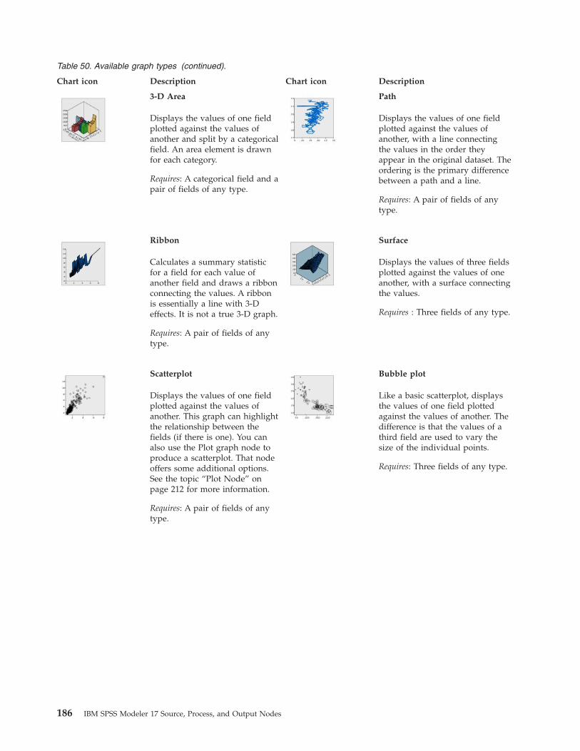
Table 50. Available graph types (continued).


3-D Area

Displays the values of one fieldplotted against the values ofanother and split by a categoricalfield. An area element is drawnfor each category.

Requires: A categorical field and apair of fields of any type.

Path

Displays the values of one fieldplotted against the values ofanother, with a line connectingthe values in the order theyappear in the original dataset. Theordering is the primary differencebetween a path and a line.


Ribbon

Calculates a summary statisticfor a field for each value ofanother field and draws a ribbonconnecting the values. A ribbonis essentially a line with 3-Deffects. It is not a true 3-D graph.


Surface

Displays the values of three fieldsplotted against the values of oneanother, with a surface connectingthe values.

Requires : Three fields of any type.

Scatterplot

Displays the values of one fieldplotted against the values ofanother. This graph can highlightthe relationship between thefields (if there is one). You canalso use the Plot graph node toproduce a scatterplot. That nodeoffers some additional options.See the topic “Plot Node” onpage 212 for more information.


Bubble plot

Like a basic scatterplot, displaysthe values of one field plottedagainst the values of another. Thedifference is that the values of athird field are used to vary thesize of the individual points.

Requires: Three fields of any type.




Binned Scatterplot

Like a basic scatterplot, displaysthe values of one field plottedagainst the values of another. Thedifference is that similar valuesare binned into groups and thatthe color or size aesthetic is usedto indicate the number of casesin each bin.

Requires : A pair of continuousfields.

Hex Binned Scatterplot

See the description of BinnedScatterplot. The difference is theshape of the underlying bins,which are shaped like hexagonsrather than circles. The resultinghex binned scatterplot lookssimilar to the binned scatterplot.However, the number of values ineach bin will differ between thegraphs because of the shape ofthe underlying bins.

Requires: A pair of continuousfields.

3-D Scatterplot

Displays the values of threefields plotted against each other.This graph can highlight therelationship between the fields (ifthere is one). You can also usethe Plot graph node to produce a3-D scatterplot. That node offerssome additional options. See thetopic “Plot Node” on page 212for more information.

Requires: Three fields of any type.

Scatterplot Matrix (SPLOM)

Displays the values of one fieldplotted against the values ofanother for every field. A SPLOMis like a table of scatterplots. TheSPLOM also includes a histogramof each field.

Requires: Two or more continuousfields.

Histogram

Displays the frequencydistribution of a field. Ahistogram can help youdetermine the distribution typeand see whether the distributionis skewed. You can also use theHistogram graph node toproduce this graph. That nodeoffers some additional options.See the topic “Histogram PlotTab” on page 226 for moreinformation.

Requires: A single field of anytype.

Histogram with NormalDistribution

Displays the frequencydistribution of a continuous fieldwith a superimposed curve of thenormal distribution.

Requires: A single continuousfield.




3-D Histogram

Displays the frequencydistribution of a pair ofcontinuous fields.

Requires : A pair of continuousfields.

3-D Density

Displays the frequencydistribution of a pair ofcontinuous fields. This is similarto a 3-D histogram, with the onlydifference being that a surface isused instead of bars to show thedistribution.

Requires: A pair of continuousfields.

Dot plot

Displays the individualcases/rows and stacks them atthe distinct data points on the xaxis. This graph is similar to ahistogram in that it shows thedistribution of the data, but itdisplays each case/row ratherthan an aggregated count for aspecific bin (range of values).

Requires : A single field of anytype.

2-D Dot Plot

Displays the individualcases/rows and stacks them atthe distinct data points on the yaxis for each category of acategorical field.


Boxplot

Calculates the five statistics(minimum, first quartile, median,third quartile, and maximum) fora continuous field for eachcategory of a categorical field.The results are displayed asboxplot/schema elements. Theboxplots can help you see howthe distribution of continuousdata varies among the categories.


Heat map

Calculates the mean for acontinuous field for the crossingof categories between twocategorical fields.

Requires : A pair of categoricalfields and a continuous field.




Parallel

Creates parallel axes for eachfield and draws a line throughthe field value for everyrow/case in the data.

Requires: Two or more continuousfields.

Choropleth of Counts

Calculates the count for eachcategory of a categorical field (Data Key) and draws a map thatuses color saturation to representthe counts in the map featuresthat correspond to the categories.

Requires : A categorical field. Amap file whose key matches theData Key categories.

Choropleth ofMeans/Medians/Sums

Calculates the mean, median, orsum of a continuous field (Color) for each category of acategorical field (Data Key) anddraws a map that uses colorsaturation to represent thecalculated statistics in the mapfeatures that correspond to thecategories.

Requires: A categorical field and acontinuous field. A map filewhose key matches the Data Keycategories.

Choropleth of Values

Draws a map that uses color torepresent values of a categoricalfield (Color) for the map featuresthat correspond to values definedby another categorical field ( DataKey). If there are multiplecategorical values of the Colorfield for each feature, the modalvalue is used.

Requires: A pair of categoricalfields. A map file whose keymatches the Data Key categories.

Coordinates on a Choropleth ofCounts

This is similar to Choropleth ofCounts except that there are twoadditional continuous fields(Longitude and Latitude) thatidentify coordinates for drawingpoints on the choropleth map.

Requires: A categorical field and apair of continuous fields. A mapfile whose key matches the DataKey categories.

Coordinates on a Choropleth ofMeans/Medians/Sums

This is similar to Choropleth ofMeans/Medians/Sums exceptthat there are two additionalcontinuous fields ( Longitude andLatitude ) that identifycoordinates for drawing points onthe choropleth map.

Requires : A categorical field andthree continuous fields. A mapfile whose key matches the DataKey categories.




Coordinates on a Choropleth ofValues

This is similar to Choropleth ofValues except that there are twoadditional continuous fields(Longitude and Latitude) thatidentify coordinates for drawingpoints on the choropleth map.

Requires: A pair of categoricalfields and a pair of continuousfields. A map file whose keymatches the Data Key categories.

Bars of Counts on a Map

Calculates the proportion ofrows/cases in each category of acategorical field (Categories) foreach map feature (Data Key) anddraws a map and the bar chartsat the center of each map feature.


Bars on a Map

Calculates a summary statisticfor a continuous field ( Values)and displays the results for eachcategory of a categorical field(Categories ) for each mapfeature (Data Key ) as bar chartspositioned in the center of eachmap feature.

Requires: A pair of categoricalfields and a continuous field. Amap file whose key matches theData Key categories.

Pie of Counts of a Map

Displays the proportion ofrows/cases in each category of acategorical field ( Categories) foreach map feature ( Data Key) anddraws a map and the proportionsas slices of a pie chart at thecenter of each map feature.


Pie on a Map

Calculates the sum of acontinuous field (Values ) in eachcategory of a categorical field (Categories) for each map feature( Data Key) and draws a mapand the sums as slices of a piechart at the center of each mapfeature.

Requires: A pair of categoricalfields and a continuous field. Amap file whose key matches theData Key categories.

Line Chart on a Map

Calculates a summary statistic fora continuous field (Y) for eachvalue of another field (X) for eachmap feature (Data Key) anddraws a map and line chartsconnecting the values at thecenter of each map feature.

Requires: A categorical field and apair of fields of any type. A mapfile whose key matches the DataKey categories.




Coordinates on a Reference Map

Draws a map and points usingcontinuous fields (Longitude andLatitude) that identifycoordinates for the points.

Requires: A pair of range fields. Amap file.

Arrows on a Reference Map

Draws a map and arrows usingcontinuous fields that identify thestart points (Start Long and StartLat) and end points (End Longand End Lat) for each arrow. Eachrecord/case in the data results inan arrow in the map.

Requires : Four continuous fields.A map file.

Point Overlay Map

Draws a reference map andsuperimposes another point mapover it with point featurescolored by a categorical field(Color).

Requires: A pair of categoricalfields. A point map file whosekey matches the Data Keycategories. A reference map file.

Polygon Overlay Map

Draws a reference map andsuperimposes another polygonmap over it with polygon featurescolored by a categorical field(Color).

Requires: A pair of categoricalfields. A polygon map file whosekey matches the Data Keycategories. A reference map file.

Line Overlay Map

Draws a reference map andsuperimposes another line mapover it with line features coloredby a categorical field (Color).

Requires: A pair of categoricalfields. A line map file whose keymatches the Data Key categories.A reference map file.

Creating Map VisualizationsFor many visualizations, you have to make only two choices: fields (variables) of interest and a templateto visualize those fields. No additional choices or actions are required. Map visualizations require at leastone additional step: select a map file that defines the geographic information for the map visualization.

The basic steps for creating a simple map are the following:1. Select the fields of interest on the Basic tab. For information about the type and number of fields

required for different map visualizations, see “Available Built-in Graphboard Visualization Types” onpage 184.

2. Select a map template.3. Click the Detailed tab.4. Check that the Data Key and other required dropdown lists are set to the correct fields.5. In the Map Files group, click Select a Map File.


6. Use the Select Maps dialog box to choose the map file and map key. The map key's values mustmatch the values for of the field specified by Data Key. You can use the Compare button to comparethese values. If you select an overlay map template, you will also need to choose a reference map. Thereference map is not keyed to the data. It is used as the background for the main map. For moreinformation about the Select Maps dialog box, see “Selecting Map Files for Map Visualizations” onpage 183.

7. Click OK to close the Select Maps dialog box.8. In the Graphboard Template Chooser, click Run to create the map visualization.

Graphboard ExamplesThis section includes several different examples to demonstrate the available options. The examples alsoprovide information for interpreting the resulting visualizations.

These examples use the stream named graphboard.str, which references the data files namedemployee_data.sav, customer_subset.sav, and worldsales.sav. These files are available from the Demos folder ofany IBM SPSS Modeler Client installation. This can be accessed from the IBM SPSS Modeler programgroup on the Windows Start menu. The graphboard.str file is in the streams folder.

It is recommended that you read the examples in the order presented. Subsequent examples build onprevious ones.

Example: Bar Chart with a Summary StatisticWe will create a bar chart that summarizes a continuous numeric field/variable for each category of aset/categorical variable. Specifically, we will create a bar chart that shows the mean salary for men andwomen.

This and several of the following examples use Employee data, which is a hypothetical dataset containinginformation about a company's employees.1. Add a Statistics File source node that points to employee_data.sav.2. Add a Graphboard node and open it for editing.3. On the Basic tab, select Gender and Current Salary . (Use Ctrl+Click to select multiple fields/variables.)4. Select Bar.5. From the Summary drop-down list, select Mean.6. Click Run.7. On the resulting display, click the "Display field and value labels" toolbar button (the second of the

group of two in the center of the toolbar).


We can observe the following:v Based on the height of the bars, it is clear that the mean salary for males is greater than the mean

salary for females.

Example: Stacked Bar Chart with a Summary StatisticWe will now create a stacked bar chart to see whether the difference in mean salary between males andfemales is subject to job type. Perhaps females, on average, make more than males for certain job types.

Note: This example uses Employee data.1. Add a Graphboard node and open it for editing.2. On the Basic tab, select Employment Category and Current Salary . (Use Ctrl+Click to select multiple

fields/variables.)3. Select Bar.4. From the Summary list, select Mean.5. Click the Detailed tab. Note that your selections from the previous tab are reflected here.6. In the Optional Aesthetics group, choose gender from the Color drop-down list.7. Click Run.

Figure 10. Bar chart with a summary statistic


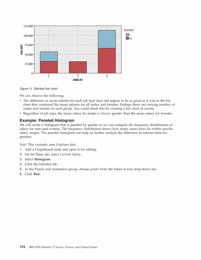
We can observe the following:v The difference in mean salaries for each job type does not appear to be as great as it was in the bar

chart that compared the mean salaries for all males and females. Perhaps there are varying number ofmales and females in each group. You could check this by creating a bar chart of counts.

v Regardless of job type, the mean salary for males is always greater than the mean salary for females.

Example: Paneled HistogramWe will create a histogram that is paneled by gender so we can compare the frequency distributions ofsalary for men and women. The frequency distribution shows how many cases/rows lie within specificsalary ranges. The paneled histogram can help us further analyze the difference in salaries betweengenders.

Note: This example uses Employee data.1. Add a Graphboard node and open it for editing.2. On the Basic tab, select Current Salary .3. Select Histogram.4. Click the Detailed tab.5. In the Panels and Animation group, choose gender from the Panel Across drop-down list.6. Click Run.

Figure 11. Stacked bar chart


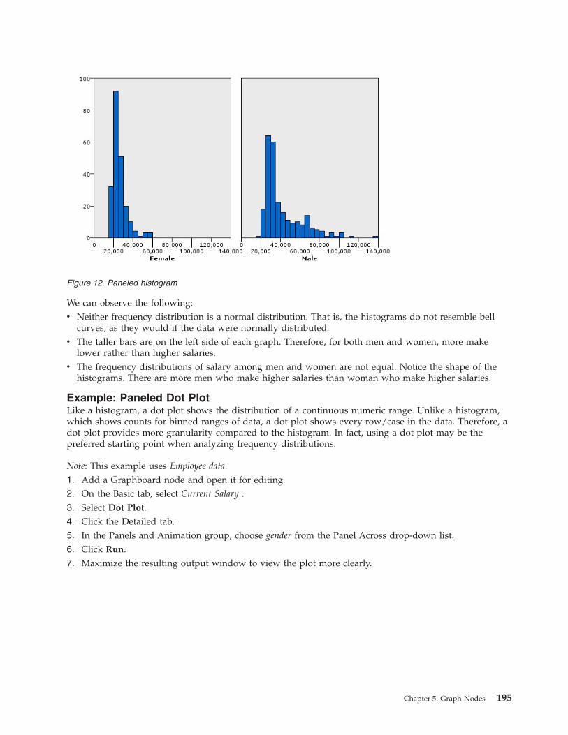
We can observe the following:v Neither frequency distribution is a normal distribution. That is, the histograms do not resemble bell

curves, as they would if the data were normally distributed.v The taller bars are on the left side of each graph. Therefore, for both men and women, more make

lower rather than higher salaries.v The frequency distributions of salary among men and women are not equal. Notice the shape of the

histograms. There are more men who make higher salaries than woman who make higher salaries.

Example: Paneled Dot PlotLike a histogram, a dot plot shows the distribution of a continuous numeric range. Unlike a histogram,which shows counts for binned ranges of data, a dot plot shows every row/case in the data. Therefore, adot plot provides more granularity compared to the histogram. In fact, using a dot plot may be thepreferred starting point when analyzing frequency distributions.

Note: This example uses Employee data.1. Add a Graphboard node and open it for editing.2. On the Basic tab, select Current Salary .3. Select Dot Plot.4. Click the Detailed tab.5. In the Panels and Animation group, choose gender from the Panel Across drop-down list.6. Click Run.7. Maximize the resulting output window to view the plot more clearly.

Figure 12. Paneled histogram


Compared to the histogram (see “Example: Paneled Histogram” on page 194 ), we can observe thefollowing:v The peak at 20,000 that appeared in the histogram for females is less dramatic in the dot plot. There

are many cases/rows concentrated around that value, but most of those values are closer to 25,000.This level of granularity is not apparent in the histogram.

v Although the histogram for males suggests that the mean salary for males gradually declines after40,000, the dot plot shows that the distribution is fairly uniform after that value, to 80,000. At any onesalary value in that range, there are three or more males who earn that particular salary.

Example: BoxplotA boxplot is another useful visualization for viewing how the data are distributed. A boxplot containsseveral statistical measures that we will explore after creating the visualization.

Note: This example uses Employee data.1. Add a Graphboard node and open it for editing.2. On the Basic tab, select Gender and Current Salary . (Use Ctrl+Click to select multiple fields/variables.)3. Select Boxplot.4. Click Run.

Figure 13. Paneled dot plot


Let's explore the different parts of the boxplot:v The dark line in the middle of the boxes is the median of salary. Half of the cases/rows have a value

greater than the median, and half have a value lower. Like the mean, the median is a measure ofcentral tendency. Unlike the mean, it is less influenced by cases/rows with extreme values. In thisexample, the median is lower than the mean (compare to “Example: Bar Chart with a SummaryStatistic” on page 192 ). The difference between the mean and median indicates that there are a fewcases/rows with extreme values that are elevating the mean. That is, there are a few employees whoearn large salaries.

v The bottom of the box indicates the 25th percentile. Twenty-five percent of cases/rows have valuesbelow the 25th percentile. The top of the box represents the 75th percentile. Twenty-five percent ofcases/rows have values above the 75th percentile. This means that 50% of the case/rows lie within thebox. The box is much shorter for females than for males. This is one clue that salary varies less forfemales than for males. The top and bottom of the box are often called hinges.

v The T-bars that extend from the boxes are called inner fences or whiskers. These extend to 1.5 timesthe height of the box or, if no case/row has a value in that range, to the minimum or maximum values.If the data are distributed normally, approximately 95% or the data are expected to lie between theinner fences. In this example, the inner fences extend less for females compared to males, anotherindication that salary varies less for females than for males.

v The points are outliers. These are defined as values that do not fall in the inner fences. Outliers areextreme values. The asterisks or stars are extreme outliers. These represent cases/rows that havevalues more than three times the height of the boxes. There are several outliers for both females andmales. Remember that the mean is greater than the median. The greater mean is caused by theseoutliers.

Example: Pie ChartWe will now use a different dataset to explore some other visualization types. The dataset iscustomer_subset, which is a hypothetical data file that contains information about customers.

We will first create a pie chart to check the proportion of customers in different geographic regions.1. Add a Statistics File source node that points to customer_subset.sav.2. Add a Graphboard node and open it for editing.3. On the Basic tab, select Geographic indicator .4. Select Pie of Counts.

Figure 14. Boxplot


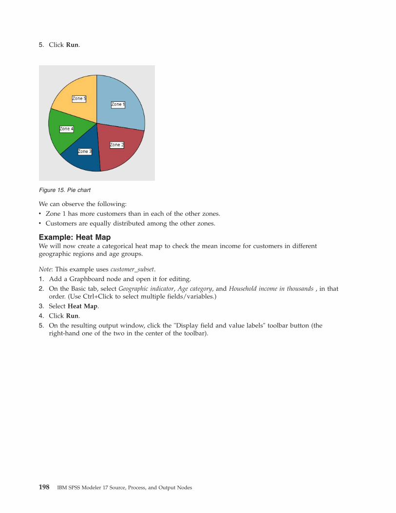
5. Click Run.

We can observe the following:v Zone 1 has more customers than in each of the other zones.v Customers are equally distributed among the other zones.

Example: Heat MapWe will now create a categorical heat map to check the mean income for customers in differentgeographic regions and age groups.

Note: This example uses customer_subset.1. Add a Graphboard node and open it for editing.2. On the Basic tab, select Geographic indicator, Age category, and Household income in thousands , in that

order. (Use Ctrl+Click to select multiple fields/variables.)3. Select Heat Map.4. Click Run.5. On the resulting output window, click the "Display field and value labels" toolbar button (the

right-hand one of the two in the center of the toolbar).

Figure 15. Pie chart


We can observe the following:v A heat map is like a table that uses colors instead of numbers to represent the values for the cells.

Bright, deep red indicates the highest value, while gray indicates a low value. The value of each cell isthe mean of the continuous field/variable for each pair of categories.

v Except in Zone 2 and Zone 5, the group of customers whose age is between 50 and 64 have a greatermean household income than those in other groups.

v There are no customers between the ages of 25 and 34 in Zone 4.

Example: Scatterplot Matrix (SPLOM)We will create a scatterplot matrix of several different variables so that we can determine whether thereare any relationships among the variables in the dataset.

Note: This example uses customer_subset.1. Add a Graphboard node and open it for editing.2. On the Basic tab, select Age in years, Household income in thousands, and Credit card debt in thousands .

(Use Ctrl+Click to select multiple fields/variables.)3. Select SPLOM.4. Click Run.5. Maximize the output window to view the matrix more clearly.

Figure 16. Categorical heat map


We can observe the following:v The histograms displayed on the diagonal show the distribution of each variable in the SPLOM. The

histogram for age appears in the upper left cell, that for income in the center cell, and that for creddebt inthe lower right cell. None of the variables appears normally distributed. That is, none of thehistograms resembles a bell curve. Also, note that the histograms for income and creddebt are positivelyskewed.

v There does not seem to be any relationship between age and the other variables.v There is a linear relationship between income and creddebt. That is, creddebt increases as income increases.

You may want to create individual scatterplots of the these variables and the other related variables toexplore the relationships further.

Example: Choropleth (Color Map) of SumsWe will now create a map visualization. Then, in the subsequent example, we will create a variation ofthis visualization. The dataset is worldsales, which is a hypothetical data file that contains sales revenue bycontinent and product.1. Add a Graphboard node and open it for editing.2. On the Basic tab, select Continent and Revenue. (Use Ctrl+Click to select multiple fields/variables.)3. Select Choropleth of Sums.4. Click the Detailed tab.5. In the Optional Aesthetics group, choose Continent from the Data Label drop-down list.6. In the Map Files group, click Select a Map File.7. In the Select Maps dialog box, check that Map is set to Continents and Map Key is set to

CONTINENT.8. In the Compare Map and Data Values groups, click Compare to ensure the map keys match the data

keys. In this example, all of data key values have matching map keys and features. We can also seethat there is no data for Oceania.

9. In the Select Maps dialog box, click OK.

Figure 17. Scatterplot matrix (SPLOM)


10. Click Run.

From that map visualization, we can easily see that revenue is highest in North America and lowest inSouth America and Africa. Each continent is labeled because we used Continent for the data labelaesthetic.

Example: Bar Charts on a MapThis example shows how revenue breaks down by product in each continent.

Note: This example uses worldsales.1. Add a Graphboard node and open it for editing.2. On the Basic tab, select Continent, Product, and Revenue. (Use Ctrl+Click to select multiple

fields/variables.)3. Select Bars on a Map.4. Click the Detailed tab.

When using more than one field of a specific type, it is important to check that each field is assignedto the correct slot.

5. From the Categories drop-down list, choose Product.6. From the Values drop-down list, choose Revenue.7. From the Data Key drop-down list, choose Continent.8. From the Summary drop-down list, choose Sum.9. In the Map Files group, click Select a Map File.

10. In the Select Maps dialog box, check that Map is set to Continents and Map Key is set toCONTINENT.

Figure 18. Choropleth of Sums


11. In the Compare Map and Data Values groups, click Compare to ensure the map keys match the datakeys. In this example, all of data key values have matching map keys and features. We can also seethat there is no data for Oceania.

12. On the Select Maps dialog box, click OK.13. Click Run.14. Maximize the resulting output window to see the display more clearly.

We can observe the following:v The distribution of total revenue across products is very similar in South America and Africa.v Product C generates the least revenue everywhere except in Asia.v There is no or minimal revenue from Product A in Asia.

Graphboard Appearance TabYou can specify appearance options before graph creation.

General Appearance Options

Title. Enter the text to be used for the graph’s title.

Subtitle. Enter the text to be used for the graph’s subtitle.

Caption. Enter the text to be used for the graph’s caption.

Figure 19. Bar Charts on a Map


Sampling. Specify a method for larger datasets. You can specify a maximum dataset size or use thedefault number of records. Performance is enhanced for large datasets when you select the Sampleoption. Alternatively, you can choose to plot all data points by selecting Use all data, but you shouldnote that this may dramatically decrease the performance of the software.

Stylesheet Appearance Options

There are two buttons that enable you to control which visualization templates (and stylesheets, andmaps) are available:


Location. Change the location in which visualization templates, stylesheets, and maps are stored. Thecurrent location is listed to the right of the button. See the topic “Setting the Location of Templates,Stylesheets, and Maps” for more information.

The following example shows where appearance options are placed on a graph. (Note: Not all graphs useall these options.)

Setting the Location of Templates, Stylesheets, and MapsVisualization templates, visualization stylesheets, and map files are stored in a specific local folder or inthe IBM SPSS Collaboration and Deployment Services Repository. When selecting templates, stylesheets,and maps, only the built-in ones in this location are displayed. By keeping all templates, stylesheets, andmap files in one place, IBM SPSS applications can easily access them. For information about addingadditional templates, stylesheets, and map files to this location, see “Managing Templates, Stylesheets,and Map Files” on page 204.

How to Set the Location of Templates, Stylesheets, and Map Files

Figure 20. Position of various graph appearance options


1. In a template or stylesheet dialog box, click Location... to display the Templates, Stylesheets, andMaps dialog box.

2. Select an option for the default location for templates, stylesheets, and map files:Local Machine. Templates, stylesheets, and map files are located in a specific folder on your localcomputer. On Windows XP, this folder is C:\Documents and Settings\<user>\ApplicationData\SPSSInc\Graphboard. The folder cannot be changed.IBM SPSS Collaboration and Deployment Services Repository. Templates, stylesheets, and map filesare located in a user-specified folder in the IBM SPSS Collaboration and Deployment ServicesRepository. To identify the specific folder, click Folder. For more information, see “Using the IBMSPSS Collaboration and Deployment Services Repository as the Template, Stylesheet, and Map FileLocation”.

3. Click OK.

Using the IBM SPSS Collaboration and Deployment Services Repository as theTemplate, Stylesheet, and Map File LocationVisualization templates and stylesheets can be stored in the IBM SPSS Collaboration and DeploymentServices Repository. This location is a specific folder in the IBM SPSS Collaboration and DeploymentServices Repository. If this is set as the default location, any templates, stylesheets, and map files in thislocation are available for selection.

How to Set a Folder in IBM SPSS Collaboration and Deployment Services Repository as the Location forTemplates, Stylesheets, and Map Files1. In a dialog box with a Location button, click Location....2. Select IBM SPSS Collaboration and Deployment Services Repository.3. Click Folder.

Note: If you are not already connected to the IBM SPSS Collaboration and Deployment ServicesRepository, you will be prompted for connection information.

4. In the Select Folder dialog box, select the folder in which templates, stylesheets, and map files arestored.

5. Optionally, you can select a label from Retrieve Label. Only templates, stylesheets, and map files withthat label will be displayed.

6. If you are looking for a folder that contains a particular template or stylesheet, you may want tosearch for the template, stylesheet, or map file on the Search tab. The Select Folder dialog boxautomatically selects the folder in which the found template, stylesheet, or map file is located.

7. Click Select Folder.

Managing Templates, Stylesheets, and Map FilesYou can manage the templates, stylesheets, and map files in the local location on your computer by usingthe Manage Templates, Stylesheets, and Maps dialog box. This dialog box allows you to import, export,rename, and delete visualization templates, stylesheets, and map files in the local location on yourcomputer.

Click Manage... in one of the dialog boxes where you select templates, stylesheets, or maps.

Manage Templates, Stylesheets, and Maps Dialog Box

The Template tab lists all the local templates. The Stylesheet tab lists all the local stylesheets, as well asdisplaying example visualizations with sample data. You can select one of the stylesheets to apply itsstyles to the example visualizations. See the topic “Applying Stylesheets” on page 272 for moreinformation. The Map tab lists all the local map files. This tab also displays the map keys includingsample values, a comment if one was provided when creating the map, and a preview of the map.

The following buttons operate on whichever tab is currently activated.


Import. Import a visualization template, stylesheet, or map file from the file system. Importing atemplate, stylesheet, or map file makes it available to the IBM SPSS application. If another user sent youa template, stylesheet, or map file, you import the file before using it in your application.

Export. Export a visualization template, stylesheet, or map file to the file system. Export a template,stylesheet, or map file when you want to send it to another user.

Rename. Rename the selected visualization template, stylesheet, or map file. You cannot change a nameto one that's already used.

Export Map Key. Export the map keys as a comma-separated values (CSV) file. This button is enabledonly on the Map tab.

Delete. Delete the selected visualization template(s), stylesheet(s), or map file(s). You can select multipletemplates, stylesheets, or map files with Ctrl-click. There is no undo action for deleting so proceed withcaution.

Converting and Distributing Map ShapefilesThe Graphboard Template Chooser allows you to create map visualizations from the combination of avisualization template and an SMZ file. SMZ files are similar to ESRI shapefiles (SHP file format) in thatthey contain the geographic information for drawing a map (for example, country borders), but they areoptimized for map visualizations. The Graphboard Template Chooser is pre-installed with a selectnumber of SMZ files. If you have an existing ESRI shapefile that you want to use for map visualizations,you first need to convert the shapefile to an SMZ file using the Map Conversion Utility. The MapConversion Utility supports point, polyline, or polygon (shape types 1, 3, and 5) ESRI shapefilescontaining a single layer.

In addition to converting ESRI shapefiles, the Map Conversion Utility allows you to modify the map'slevel of detail, change feature labels, merge features, and move features, among many other optionalchanges. You can also use the Map Conversion Utility to modify an existing SMZ file (including thepre-installed ones).

Editing pre-installed SMZ files1. Export the SMZ file from the Manage system. See the topic “Managing Templates, Stylesheets, and

Map Files” on page 204 for more information.2. Use the Map Conversion Utility to open and edit the exported SMZ file. It is recommended that you

save the file with a different name. See the topic “Using the Map Conversion Utility” on page 206 formore information.

3. Import the modified SMZ file into the Manage system. See the topic “Managing Templates,Stylesheets, and Map Files” on page 204 for more information.

Additional Resources for Map Files

Geospatial data in the SHP file format, which could be used to support your mapping needs, is availablefrom many private and public sources. Check with local government web sites if you seek free data.Many of the templates in this product are based on publicly available data obtained from GeoCommons () and the U.S. Census Bureau (http://www.census.gov).

IMPORTANT NOTICE: Information concerning non-IBM products was obtained from the suppliers ofthose products, their published announcements or other publicly available sources. IBM has not testedthose products and cannot confirm the accuracy of performance, compatibility or any other claims relatedto non-IBM products. Questions on the capabilities of non-IBM products should be addressed to thesuppliers of those products. Any references in this information to non-IBM Web sites are provided forconvenience only and do not in any manner serve as an endorsement of those Web sites. The materials at


http://www.census.gov

those Web sites are not part of the materials for this IBM program, unless indicated in a Notices fileaccompanying this IBM program, and use of the materials sites is at your own risk.

Key Concepts for MapsUnderstanding some key concepts related to shapefiles will help you use the Map Conversion Utilityeffectively.

A shapefile provides the geographic information for drawing a map. There are three types of shapefilesthat the Map Conversion Utility supports:v Point. The shapefile identifies the locations of points, such as cities.v Polyline. The shapefile identifies paths and their locations, such as rivers.v Polygon. The shapefile identifies bounded regions and their locations, such as countries.

Most commonly, you will use a polygon shapefile. Choropleth maps are created from polygon shapefiles.Choropleth maps use color to represent a value within individual polygons (regions). Point and polylineshapefiles are typically overlaid on a polygon shapefile. An example is a point shapefile of U.S. citiesoverlaid on a polygon shapefile of U.S. states.

A shapefile is comprised of features. Features are the individual geographical entities. For example,features may be countries, states, cities, and so on. The shapefile also contains data about the features.These data are stored in attributes. Attributes are similar to fields or variables in a data file. There is atleast one attribute that is the map key for the feature. The map key may be a label, such as country orstate name. The map key is what you will link to a variable/field in a data file to create a mapvisualization.

Note that you will be able to retain only the key attribute or attributes in the SMZ file. The MapConversion Utility does not support saving additional attributes. This means that you will need to createmultiple SMZ files if you want to aggregate at different levels. For example, if you want to aggregate U.S.states and regions, you will need separate SMZ files: one that has a key identifying states and one thathas a key identifying regions.

Using the Map Conversion UtilityHow to start the Map Conversion Utility

From the menus choose:

Tools > Map Conversion Utility

There are four major screens (steps) in the Map Conversion Utility. One of the steps also involvessub-steps for more detailed control over editing the map file.

Step 1 - Choose Destination and Source FilesYou first have to select a source map file and a destination for the converted map file. You will need boththe .shp and .dbf files for the shapefile.

Select a .shp (ESRI) or .smz file for conversion. Browse to an existing map file on your computer. This isthe file that you will convert to and save as an SMZ file. The .dbf file for the shapefile must be stored inthe same location with a base file name that matches the .shp file. The .dbf file is required because itcontains the attribute information for the .shp file.

Set a destination and file name for the converted map file. Enter a path and file name for the SMZ filethat will be created from the original map source.v Import to the Template Chooser. In addition to saving a file on the file system, you can optionally add

the map to the Manage list of the Template Chooser. If you choose this option, the map will


automatically be available in the Template Chooser for IBM SPSS products installed on your computer.If you don't import to the Template Chooser now, you will need to import it manually at a later time.For more information about importing maps into the Template Chooser Manage system, see“Managing Templates, Stylesheets, and Map Files” on page 204.

Step 2 - Choose Map Key

Now you will choose which map keys to include in the SMZ file. You can then change some options thatwill affect rendering of the map. The subsequent steps in the Map Conversion Utility include a previewof the map. The rendering options that you choose will be used to generate the map preview.

Choose primary map key. Select the attribute that is the primary key for identifying and labeling featuresin the map. For example, a world map's primary key may be the attribute identifying country names. Theprimary key will also link your data to the map features, so be sure that the values (labels) of theattribute you choose will match the values in your data. Example labels are displayed when you choosean attribute. If you need to change these labels, you will be able to do so in a later step.

Choose additional keys to include. In addition to the primary map key, check any other key attributesthat you want to include in the generated SMZ file. For example, some attributes may contain translatedlabels. If you expect data coded in other languages, you may want to preserve these attributes. Note thatyou can choose only those additional keys that represent the same features as the primary key. Forexample if the primary key were the full names of U.S. states, you can select only those alternate keysthat represent U.S. States, such as state abbreviations.

Automatically smooth the map. Shapefiles with polygons typically contain too many data points and toomuch detail for statistical map visualizations. The excess details can be distracting and negatively impactperformance. You can reduce the level of detail and generalize the map with smoothing. The map willlook crisper and render more quickly as a result. When the map is automatically smoothed, themaximum angle is 15 degrees and the percentage to keep is 99. For information about these settings, see“Smooth the map” on page 208. Note that you have the opportunity to apply additional smoothing laterin another step.

Remove boundaries between touching polygons in the same feature. Some features may includesub-features that have boundaries internal to the main features of interest. For example, a world map ofcontinents may contain internal boundaries for the countries contained within each continent. If youchoose this option, the internal boundaries will not appear in the map. In the world map of continentsexample, choosing this option would remove the country borders, while retaining the continent borders.

Step 3 - Edit the MapNow that you have specified basic options for the map, you can edit more specific ones. Thesemodifications are optional. This step of the Map Conversion Utility guides you through the associatedtasks and displays a preview of the map so you can verify your changes. Some tasks may not beavailable depending on shapefile type (point, polyline, or polygon) and coordinate system.

Every task has the following common controls on the left side of the Map Conversion Utility.

Show the labels on the map. By default, feature labels are not shown in the preview. You can choose todisplay the labels. Although the labels can help identify features, they may interfere with direct selectionon the preview map. Turn on this option when you need it, for example when you are editing the featurelabels.

Color the map preview. By default, the preview map displays areas with a solid color. All features arethe same color. You can choose to have an assortment of colors assigned to the individual map features.This option may help distinguish different features in the map. It will be especially helpful when youmerge features and want to see how the new features are represented in the preview.


Every task also has the following common control on the right side of the Map Conversion Utility.

Undo. Click Undo to revert to the last state. You can undo a maximum of 100 changes.

Smooth the map: Shapefiles with polygons typically contain too many data points and too much detailfor statistical map visualizations. The excess details can be distracting and negatively impactperformance. You can reduce the level of detail and generalize the map with smoothing. The map willlook crisper and render more quickly as a result. This option is not available for point and polyline maps.

Max. angle. The maximum angle, which must be a value between 1 and 20, specifies the tolerance forsmoothing sets of points that are almost linear. A larger value allows more tolerance for the linearsmoothing and will subsequently drop more points, resulting in a more generalized map. To apply linearsmoothing, the Map Conversion Utility checks the inner angle formed by every set of three points in themap. If 180 minus the angle is less than the specified value, the Map Conversion Utility will drop themiddle point. In other words, the Map Conversion Utility is checking whether the line formed by thethree points is almost straight. If it is, the Map Conversion Utility treats the line as a straight line betweenthe endpoints and drops the middle point.

Percent to keep. The percentage to keep, which must be a value between 90 and 100, determines theamount of land area to keep when the map is smoothed. This option affects only those features that havemultiple polygons, as would be the case if a feature included islands. If the total area of a feature minusa polygon is greater than the specified percentage of the original area, the Map Conversion Utility willdrop the polygon from the map. The Map Conversion Utility will never remove all polygons for thefeature. That is, there will always be at least one polygon for the feature, regardless of the amount ofsmoothing applied.

After you choose a maximum angle and percentage to keep, click Apply. The preview will update withthe smoothing changes. If you need to smooth the map again, repeat until you obtain the level ofsmoothness you want. Note that there is a limit to the smoothing. If you repeatedly smooth, you willreach a point when no additional smoothing can be applied to the map.

Edit the feature labels: You can edit the feature labels as needed (perhaps to match your expected data)and also re-position the labels in the map. Even if you don't think you need to change the labels, youshould review them before creating visualizations from the map. Because labels are not shown by defaultin the preview, you may also want to select Show the labels on the map to display them.

Keys. Select the key containing the feature labels that you want to review and/or edit.

Features. This list displays the feature labels contained in the selected key. To edit the label, double-clickit in the list. If labels are shown on the map, you can also double-click the feature labels directly in themap preview. If you want to compare the labels to an actual data file, click Compare.

X/Y. These text boxes list the current center point of the selected feature's label on the map. The units aredisplayed in the map's coordinates. These may be local, Cartesian coordinates (for example, the StatePlane Coordinate System) or geographic coordinates (where X is longitude and Y is latitude). Entercoordinates for the new position of the label. If labels are shown, you can also click and drag a label onthe map to move it. The text boxes will update with the new position.

Compare. If you have a data file that contains data values that are intended to match the features labelsfor a particular key, click Compare to display the Compare to an External Data Source dialog box. In thisdialog box you will be able to open the data file and compare its values directly with those in the mapkey's feature labels.

Compare to an External Data Source dialog box: The Compare to an External Data Source dialog box allowsyou to open a tab-separated values file (with a .txt extension), a comma-separated values file (with a .csv


extension), or a data file formatted for IBM SPSS Statistics (with a .sav extension). When the file is open,you can select a field in the data file to compare to the feature labels in a specific map key. You can thencorrect any discrepancies in the map file.

Fields in the data file. Choose the field whose values you want to compare to the feature labels. If thefirst row in the .txt or .csv file contains descriptive labels for each field, check Use first row as columnlabels. Otherwise, each field will be identified by its position in the data file (for example, "Column 1","Column 2", and so on).

Key to compare. Choose the map key whose feature labels you want to compare to the data file fieldvalues.

Compare. Click when you are ready to compare the values.

Comparison Results. By default, the Comparison Results table lists only the unmatched field values inthe data file. The application tries to find a related feature label, usually by checking for inserted ormissing spaces. Click the dropdown list in the Map Label column to match the feature label in the mapfile to the displayed field value. If there is no corresponding feature label in your map file, choose LeaveUnmatched. If you want to see all field values, even those that already match a feature label, clear Displayonly unmatched cases. You may do this if you want to override one or more matches.

You can use each feature only once to match it to a field value. If you want to match multiple features toa single field value, you can merge the features and then match the new, merged feature to the fieldvalue. For more information about merging features, see “Merge features”.

Merge features: Merging features is useful for creating larger regions in a map. For example, if youwere converting a map of states, you could merge the states (the features in this example) into largerNorth, South, East, and West regions.

Keys. Select the map key containing the feature labels that will help you identify the features you wantto merge.

Features. Click the first feature that you want to merge. Ctrl-click the other features that you want tomerge. Note that the features will also be selected in the map preview. You can click and Ctrl-click thefeatures directly in the map preview in addition to selecting them from the list.

After selecting the features that you want to merge, click Merge to display the Name the Merged Featuredialog box, where you will be able to apply a label to the new feature. You may want to check Color themap preview after merging features to ensure that the results are what you expect.

After merging features, you may also want to move the label for the new feature. You can do that in theEdit the feature labels task. See the topic “Edit the feature labels” on page 208 for more information.

Name the Merged Feature dialog box: The Name the Merged Feature dialog box allows you to assign labelsto the new merged feature.

The Labels table displays information for each key in the map file and allows you to assign a label foreach key.

New Label. Enter a new label for the merged feature to assign to the specific map key.

Key. The map key to which you are assigning the new label.

Old Labels. The labels for the features that will be merged into the new feature.


Remove boundaries between touching polygons. Check this option to remove the boundaries from thefeatures that were merged together. For example, if you merged states into geographic regions, thisoption would remove the boundaries around the individual states.

Move features: You can move features in the map. This can be useful when you want to put featurestogether, like a mainland and outlying islands.

Keys. Select the map key containing the feature labels that will help you identify the features you wantto move.

Features. Click the feature that you want to move. Note that the feature will be selected in the mappreview. You can also click the feature directly in the map preview.

X/Y. These text boxes list the current center point of the feature on the map. The units are displayed inthe map's coordinates. These may be local, Cartesian coordinates (for example, the State Plane CoordinateSystem) or geographic coordinates (where X is longitude and Y is latitude). Enter coordinates for the newposition of the feature. You can also click and drag a feature on the map to move it. The text boxes willupdate with the new position.

Delete features: You can delete unwanted features from the map. This can be useful when you want toremove some clutter by deleting features that won't be of interest in the map visualization.

Keys. Select the map key containing the feature labels that will help you identify the features you wantto delete.

Features. Click the feature that you want to delete. If you want to delete multiple featuressimultaneously, Ctrl-click the additional features. Note that the features will also be selected in the mappreview. You can click and Ctrl-click the features directly in the map preview in addition to selectingthem from the list.

Delete individual elements: In addition to deleting whole features, you can delete some of theindividual elements that compose the features, such as lakes and small islands. This option is notavailable for point maps.

Elements. Click the elements that you want to delete. If you want to delete multiple elementssimultaneously, Ctrl-click the additional elements. Note that the elements will also be selected in the mappreview. You can click and Ctrl-click the elements directly in the map preview in addition to selectingthem from the list. Because the list of element names is not descriptive (each element is assigned anumber within the feature), you should check the selection in the map preview to ensure you haveselected the elements you want.

Set the projection:

The map projection specifies the way in which the three-dimensional Earth is represented in twodimensions. All projections cause distortions. However, some projections are more suitable depending onwhether you are viewing a global map or a more local one. Also some projections preserve the shape ofthe original features. Projections that preserve shape are conformal projections. This option is availableonly for maps with geographic coordinates (longitude and latitude).

Unlike other options in the Map Conversion Utility, the projection can be changed after a mapvisualization is created.

Projection. Select a map projection. If you are creating a global or hemispherical map, use the Local,Mercator, or Winkel Tripel projections. For smaller areas, use the Local, Lambert Conformal Conic, orTransverse Mercator projections. All projections use the WGS83 ellipsoid for the datum.


v The Local projection is always used when the map was created with a local coordinate system, such asthe State Plane Coordinate System. These coordinate systems are defined by Cartesian coordinatesrather than geographic coordinates (longitude and latitude). In the Local projection, horizontal andvertical lines are equally spaced in a Cartesian coordinate system. The Local projection is notconformal.

v The Mercator projection is a conformal projection for global maps. Horizontal and vertical lines arestraight and always perpendicular to each other. Note that the Mercator projection extends to infinityas it approaches the North and South Poles, so it cannot be used if your map includes the North orSouth Pole. Distortion is greatest when the map approaches these limits.

v The Winkel Tripel projection is a non-conformal projection for global maps. Although it is notconformal, it provides a good balance between shape and size. Except for the Equator and PrimeMeridian, all lines are curved. If your global map includes the North or South Pole, this is a goodprojection choice.

v As its name suggests, the Lambert Conformal Conic projection is a conformal projection and is usedfor maps of continental or smaller land masses that are longer East and West compared to North andSouth.

v The Transverse Mercator is another conformal projection for maps of continental or smaller landmasses. Use this projection for land masses that are longer North and South compared to East andWest.

Step 4 - FinishAt this point you can add a comment to describe the map file and also create a sample data file from themap keys.

Map keys. If there are multiple keys in the map file, select a map key whose feature labels you want todisplay in the preview. If you create a data file from the map, these labels will be used for the datavalues.

Comment. Enter a comment that describes the map or provides additional information that may berelevant to your users, such as the sources for the original shapefiles. The comment will appear in theGraphboard Template Chooser's Manage system.

Create a data set from the feature labels. Check this option if you want to create a data file from thedisplayed feature labels. When you click Browse..., you will be able to specify a location and file name. Ifyou add a .txt extension, the file will be saved as a tab-separate values file. If you add a .csv extension,the file will be saved as a comma-separated values file. If you add a .sav extension, the file will be savedin IBM SPSS Statistics format. SAV is the default when no extension is specified.

Distributing map filesIn the first step of the Map Conversion Utility, you chose a location where to save the converted SMZfile. You may have also chosen to add the map to the Manage system for the Graphboard TemplateChooser. If you chose to save to the Manage system, the map will be available to you in any IBM SPSSproduct that you run on the same computer.

To distribute the map to other users, you will need to send the SMZ to them. Those users can then usethe Manage system to import the map. You can simply send the file whose location you specified in step1. If you want to send a file that's in the Manage system, you first need to export it:1. In the Template Chooser, click Manage...

2. Click the Map tab.3. Select the map you want to distribute.4. Click Export... and choose a location where you want to save the file.

Now you can send the physical map file to other users. Users will need to reverse this process andimport the map into the Manage system.


Plot NodePlot nodes show the relationship between numeric fields. You can create a plot using points (also knownas a scatterplot), or you can use lines. You can create three types of line plots by specifying an X Mode inthe dialog box.

X Mode = Sort

Setting X Mode to Sort causes data to be sorted by values for the field plotted on the x axis. Thisproduces a single line running from left to right on the graph. Using a nominal field as an overlayproduces multiple lines of different hues running from left to right on the graph.

X Mode = Overlay

Setting X Mode to Overlay creates multiple line plots on the same graph. Data are not sorted for anoverlay plot; as long as the values on the x axis increase, data will be plotted on a single line. If thevalues decrease, a new line begins. For example, as x moves from 0 to 100, the y values will be plotted ona single line. When x falls below 100, a new line will be plotted in addition to the first one. The finishedplot might have numerous plots useful for comparing several series of y values. This type of plot isuseful for data with a periodic time component, such as electricity demand over successive 24-hourperiods.

Figure 21. Line plot with X Mode set to Sort


X Mode = As Read

Setting X Mode to As Read plots x and y values as they are read from the data source. This option isuseful for data with a time series component where you are interested in trends or patterns that dependon the order of the data. You may need to sort the data before creating this type of plot. It may also beuseful to compare two similar plots with X Mode set to Sort and As Read in order to determine howmuch of a pattern depends on the sorting.

Figure 22. Line plot with X Mode set to Overlay


You can also use the Graphboard node to produce scatterplots and line plots. However, you have moreoptions to choose from in this node. See the topic “Available Built-in Graphboard Visualization Types” onpage 184 for more information.

Plot Node TabPlots show values of a Y field against values of an X field. Often, these fields correspond to a dependentvariable and an independent variable, respectively.

X field. From the list, select the field to display on the horizontal x axis.

Y field. From the list, select the field to display on the vertical y axis.

Z field. When you click the 3-D chart button, you can then choose a field from the list to display on the zaxis.

Overlay. There are several ways to illustrate categories for data values. For example, you can usemaincrop as a color overlay to indicate the estincome and claimvalue values for the main crop grown byclaim applicants. See the topic “Aesthetics, Overlays, Panels, and Animation” on page 176 for moreinformation.

Overlay type. Specifies whether an overlay function or smoother is displayed. The smoother and overlayfunctions are always calculated as a function of y.

Figure 23. Line plot shown earlier as Sort, executed again with X Mode set to As Read


v None. No overlay is displayed.v Smoother. Displays a smoothed fit line computed using locally weighted iterative robust least squares

regression (LOESS). This method effectively computes a series of regressions, each focused on a smallarea within the plot. This produces a series of "local" regression lines that are then joined to create asmooth curve.

v Function. Select to specify a known function to compare to actual values. For example, to compareactual versus predicted values, you can plot the function y = x as an overlay. Specify a function for y =in the text box. The default function is y = x, but you can specify any sort of function, such as aquadratic function or an arbitrary expression, in terms of x.Note: Overlay functions are not available for a panel or animation graph.

Once you have set options for a plot, you can run the plot directly from the dialog box by clicking Run.You may, however, want to use the Options tab for additional specifications, such as binning, X Mode,and style.

Plot Options TabStyle. Select either Point or Line for the plot style. Selecting Line activates the X Mode control. SelectingPoint will use a plus symbol (+) as the default point shape. Once the graph is created, you can changethe point shape and alter its size.

X Mode. For line plots, you must choose an X Mode to define the style of the line plot. Select Sort,Overlay, or As Read. For Overlay or As Read, you should specify a maximum dataset size used tosample the first n records. Otherwise, the default 2,000 records will be used.

Figure 24. Plot with a LOESS smoother overlay


Automatic X range. Select to use the entire range of values in the data along this axis. Deselect to use anexplicit subset of values based on your specified Min and Max values. Either enter values or use thearrows. Automatic ranges are selected by default to enable rapid graph building.

Automatic Y range. Select to use the entire range of values in the data along this axis. Deselect to use anexplicit subset of values based on your specified Min and Max values. Either enter values or use thearrows. Automatic ranges are selected by default to enable rapid graph building.

Automatic Z range. Only when a 3-D graph is specified on the Plot tab. Select to use the entire range ofvalues in the data along this axis. Deselect to use an explicit subset of values based on your specifiedMin and Max values. Either enter values or use the arrows. Automatic ranges are selected by default toenable rapid graph building.

Jitter. Also known as agitation, jitter is useful for point plots of a dataset in which many values arerepeated. In order to see a clearer distribution of values, you can use jitter to distribute the pointsrandomly around the actual value.

Note to users of earlier versions of IBM SPSS Modeler: The jitter value used in a plot uses a different metricin this release of IBM SPSS Modeler. In earlier versions, the value was an actual number, but it is now aproportion of the frame size. This means that agitation values in old streams are likely to be too large.For this release, any nonzero agitation values will be converted to the value 0.2.

Maximum number of records to plot. Specify a method for plotting large datasets. You can specify amaximum dataset size or use the default 2,000 records. Performance is enhanced for large datasets whenyou select the Bin or Sample options. Alternatively, you can choose to plot all data points by selectingUse all data, but you should note that this may dramatically decrease the performance of the software.

Note: When X Mode is set to Overlay or As Read, these options are disabled and only the first n recordsare used.v Bin. Select to enable binning when the dataset contains more than the specified number of records.

Binning divides the graph into fine grids before actually plotting and counts the number of points thatwould appear in each of the grid cells. In the final graph, one point is plotted per cell at the bincentroid (average of all point locations in the bin). The size of the plotted symbols indicates thenumber of points in that region (unless you have used size as an overlay). Using the centroid and sizeto represent the number of points makes the binned plot a superior way to represent large datasets,because it prevents overplotting in dense regions (undifferentiated masses of color) and reduces symbolartifacts (artificial patterns of density). Symbol artifacts occur when certain symbols (particularly theplus symbol [+]) collide in a way that produces dense areas not present in the raw data.

v Sample. Select to randomly sample the data to the number of records entered in the text field. Thedefault is 2,000.

Plot Appearance TabYou can specify appearance options before graph creation.




X label. Either accept the automatically generated x-axis (horizontal) label or select Custom to specify alabel.

Y label. Either accept the automatically generated y-axis (vertical) label or select Custom to specify alabel.


Z label. Available only for 3-D graphs, either accept the automatically generated z-axis label or selectCustom to specify a custom label.

Display gridline. Selected by default, this option displays a gridline behind the plot or graph thatenables you to more easily determine region and band cutoff points. Gridlines are always displayed inwhite unless the graph background is white; in this case, they are displayed in gray.

Using a Plot GraphPlots and multiplots are essentially plots of X against Y. For example, if you are exploring potential fraudin agricultural grant applications, you might want to plot the income claimed on the application versusthe income estimated by a neural net. Using an overlay, such as crop type, will illustrate whether there isa relationship between claims (value or number) and type of crop.

Since plots, multiplots, and evaluation charts are two-dimensional displays of Y against X, it is easy tointeract with them by defining regions, marking elements, or even drawing bands. You can also generatenodes for the data represented by those regions, bands, or elements. See the topic “Exploring Graphs” onpage 251 for more information.

Multiplot NodeA multiplot is a special type of plot that displays multiple Y fields over a single X field. The Y fields areplotted as colored lines and each is equivalent to a Plot node with Style set to Line and X Mode set toSort. Multiplots are useful when you have time sequence data and want to explore the fluctuation ofseveral variables over time.

Figure 25. Plot of the relationship between estimated income and claim value with main crop type as an overlay


Multiplot Plot TabX field. From the list, select the field to display on the horizontal x axis.

Y fields. Select one or more fields from the list to display over the range of X field values. Use the FieldChooser button to select multiple fields. Click the delete button to remove fields from the list.

Overlay. There are several ways to illustrate categories for data values. For example, you might use ananimation overlay to display multiple plots for each value in the data. This is useful for sets containingupwards of 10 categories. When used for sets with more than 15 categories, you may notice a decrease inperformance. See the topic “Aesthetics, Overlays, Panels, and Animation” on page 176 for moreinformation.

Normalize. Select to scale all Y values to the range 0–1 for display on the graph. Normalizing helps youexplore the relationship between lines that might otherwise be obscured due to differences in the range ofvalues for each series and is recommended when plotting multiple lines on the same graph, or whencomparing plots in side-by-side panels. (Normalizing is not necessary when all data values fall within asimilar range.)

Figure 26. Standard multiplot showing power-plant fluctuation over time (note that without normalizing, the plot forPressure is impossible to see)

Figure 27. Normalized multiplot showing a plot for Pressure


Overlay function. Select to specify a known function to compare to actual values. For example, tocompare actual versus predicted values, you can plot the function y = x as an overlay. Specify a functionfor y = in the text box. The default function is y = x, but you can specify any sort of function, such as aquadratic function or an arbitrary expression, in terms of x.

Note: Overlay functions are not available for a panel or animation graph.

When number of records greater than. Specify a method for plotting large datasets. You can specify amaximum dataset size or use the default 2,000 points. Performance is enhanced for large datasets whenyou select the Bin or Sample options. Alternatively, you can choose to plot all data points by selectingUse all data, but you should note that this may dramatically decrease the performance of the software.

Note: When X Mode is set to Overlay or As Read, these options are disabled and only the first n recordsare used.v Bin. Select to enable binning when the dataset contains more than the specified number of records.

Binning divides the graph into fine grids before actually plotting and counts the number of connectionsthat would appear in each of the grid cells. In the final graph, one connection is used per cell at thebin centroid (average of all connection points in the bin).

v Sample. Select to randomly sample the data to the specified number of records.

Multiplot Appearance TabYou can specify appearance options before graph creation.







Using a Multiplot GraphPlots and multiplots are essentially plots of X against Y. For example, if you are exploring potential fraudin agricultural grant applications, you might want to plot the income claimed on the application versusthe income estimated by a neural net. Using an overlay, such as crop type, will illustrate whether there isa relationship between claims (value or number) and type of crop.


Since plots, multiplots, and evaluation charts are two-dimensional displays of Y against X, it is easy tointeract with them by defining regions, marking elements, or even drawing bands. You can also generatenodes for the data represented by those regions, bands, or elements. See the topic “Exploring Graphs” onpage 251 for more information.

Time Plot NodeTime Plot nodes enable you to view one or more time series plotted over time. The series you plot mustcontain numeric values and are assumed to occur over a range of time in which the periods are uniform.You usually use a Time Intervals node before a Time Plot node to create a TimeLabel field, which is usedby default to label the x axis in the graphs. See the topic “Time Intervals Node” on page 159 for moreinformation.

Figure 28. Plot of the relationship between estimated income and claim value with main crop type as an overlay


Creating Interventions and Events

You can create Event and Intervention fields from the time plot by generating a derive (flag or nominal)node from the context menus. For example, you could create an event field in the case of a rail strike,where the drive state is True if the event happened and False otherwise. For an Intervention field, for aprice rise for example, you could use a derive count to identify the date of the rise, with 0 for the oldprice and 1 for the new price. See the topic “Derive Node” on page 133 for more information.

Time Plot TabPlot. Provides a choice of how to plot time series data.v Selected series. Plots values for selected time series. If you select this option when plotting confidence

intervals, deselect the Normalize check box.v Selected Time Series models. Used in conjunction with a Time Series model, this option plots all the

related fields (actual and predicted values, as well as confidence intervals) for one or more selectedtime series. This option disables some other options in the dialog box. This is the preferred option ifplotting confidence intervals.

Series. Select one or more fields with time series data you want to plot. The data must be numeric.

X axis label. Choose either the default label or a single field to use as the label for the x axis in plots. Ifyou choose Default, the system uses the TimeLabel field created from a Time Intervals node upstream orsequential integers if there is no Time Intervals node. See the topic “Time Intervals Node” on page 159for more information.

Display series in separate panels. Specifies whether each series is displayed in a separate panel.Alternatively, if you do not choose to panel, all time series are plotted on the same graph, and smootherswill not be available. When plotting all time series on the same graph, each series will be represented bya different color.

Normalize. Select to scale all Y values to the range 0–1 for display on the graph. Normalizing helps youexplore the relationship between lines that might otherwise be obscured due to differences in the range ofvalues for each series and is recommended when plotting multiple lines on the same graph, or whencomparing plots in side-by-side panels. (Normalizing is not necessary when all data values fall within asimilar range.)

Display. Select one or more elements to display in your plot. You can choose from lines, points, and(LOESS) smoothers. Smoothers are available only if you display the series in separate panels. By default,

Figure 29. Plotting sales of men's and women's clothing and jewelry over time


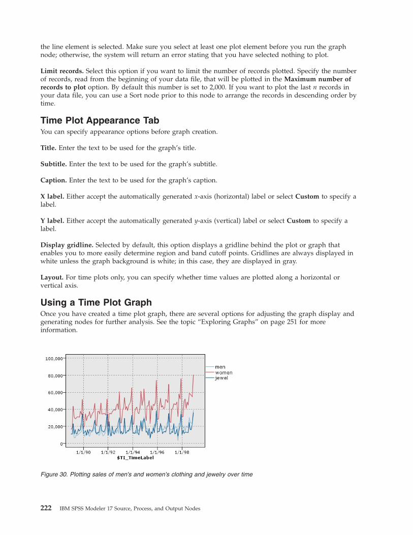
the line element is selected. Make sure you select at least one plot element before you run the graphnode; otherwise, the system will return an error stating that you have selected nothing to plot.

Limit records. Select this option if you want to limit the number of records plotted. Specify the numberof records, read from the beginning of your data file, that will be plotted in the Maximum number ofrecords to plot option. By default this number is set to 2,000. If you want to plot the last n records inyour data file, you can use a Sort node prior to this node to arrange the records in descending order bytime.

Time Plot Appearance TabYou can specify appearance options before graph creation.







Layout. For time plots only, you can specify whether time values are plotted along a horizontal orvertical axis.

Using a Time Plot GraphOnce you have created a time plot graph, there are several options for adjusting the graph display andgenerating nodes for further analysis. See the topic “Exploring Graphs” on page 251 for moreinformation.

Figure 30. Plotting sales of men's and women's clothing and jewelry over time


Once you have created a time plot, defined bands, and examined the results, you can use options on theGenerate menu and the context menu to create Select or Derive nodes. See the topic “Generating Nodesfrom Graphs” on page 258 for more information.

Distribution NodeA distribution graph or table shows the occurrence of symbolic (non-numeric) values, such as mortgagetype or gender, in a dataset. A typical use of the Distribution node is to show imbalances in the data thatcan be rectified by using a Balance node before creating a model. You can automatically generate aBalance node using the Generate menu in the distribution graph or table window.

You can also use the Graphboard node to produce bar of counts graphs. However, you have moreoptions to choose from in this node. See the topic “Available Built-in Graphboard Visualization Types” onpage 184 for more information.

Note: To show the occurrence of numeric values, you should use a Histogram node.

Distribution Plot TabPlot. Select the type of distribution. Select Selected fields to show the distribution of the selected field.Select All flags (true values) to show the distribution of true values for flag fields in the dataset.

Field. Select a nominal or flag field for which to show the distribution of values. Only fields that havenot been explicitly set as numeric appear on the list.

Overlay. Select a nominal or flag field to use as a color overlay, illustrating the distribution of its valueswithin each value of the specified field. For example, you can use marketing campaign response (pep) asan overlay for number of children (children) to illustrate responsiveness by family size. See the topic“Aesthetics, Overlays, Panels, and Animation” on page 176 for more information.

Normalize by color. Select to scale bars so that all bars take up the full width of the graph. The overlayvalues equal a proportion of each bar, making comparisons across categories easier.

Sort. Select the method used to display values in the distribution graph. Select Alphabetic to usealphabetical order or By count to list values in decreasing order of occurrence.

Proportional scale. Select to scale the distribution of values so that the value with the largest count fillsthe full width of the plot. All other bars are scaled against this value. Deselecting this option scales barsaccording to the total counts of each value.

Distribution Appearance TabYou can specify appearance options before graph creation.








Using a Distribution NodeDistribution nodes are used to show the distribution of symbolic values in a dataset. They are frequentlyused before manipulation nodes to explore the data and correct any imbalances. For example, if instancesof respondents without children occur much more frequently than other types of respondents, you mightwant to reduce these instances so that a more useful rule can be generated in later data miningoperations. A Distribution node will help you to examine and make decisions about such imbalances.

The Distribution node is unusual in that it produces both a graph and a table to analyze your data.

Figure 31. Distribution graph showing the number of people with or without children who responded to a marketingcampaign


Once you have created a distribution table and graph and examined the results, you can use options fromthe menus to group values, copy values, and generate a number of nodes for data preparation. Inaddition, you can copy or export the graph and table information for use in other applications, such asMS Word or MS PowerPoint. See the topic “Printing, Saving, Copying, and Exporting Graphs” on page272 for more information.

To Select and Copy Values from a Distribution Table1. Click and hold the mouse button while dragging it over the rows to select a set of values. You can

also use the Edit menu to Select All values.2. From the Edit menu, choose Copy Table or Copy Table (inc. field names).3. Paste to the clipboard or into the desired application.

Note: The bars do not get copied directly. Instead, the table values are copied. This means thatoverlaid values will not be displayed in the copied table.

To Group Values from a Distribution Table1. Select values for grouping using the Ctrl+click method.2. From the Edit menu, choose Group.

Note: When you group and ungroup values, the graph on the Graph tab is automatically redrawn toshow the changes.

You can also:v Ungroup values by selecting the group name in the distribution list and choosing Ungroup from the

Edit menu.v Edit groups by selecting the group name in the distribution list and choosing Edit group from the Edit

menu. This opens a dialog box where values can be shifted to and from the group.

Generate Menu Options

Figure 32. Distribution table showing the proportion of people with or without children who responded to a marketingcampaign


You can use options on the Generate menu to select a subset of data, derive a flag field, regroup values,reclassify values, or balance the data from either a graph or table. These operations generate a datapreparation node and place it on the stream canvas. To use the generated node, connect it to an existingstream. See the topic “Generating Nodes from Graphs” on page 258 for more information.

Histogram NodeHistogram nodes show the occurrence of values for numeric fields. They are often used to explore thedata before manipulations and model building. Similar to the Distribution node, Histogram nodes arefrequently used to reveal imbalances in the data. While you can also use the Graphboard node toproduce a histogram, you have more options to choose from in this node. See the topic “AvailableBuilt-in Graphboard Visualization Types” on page 184 for more information.

Note: To show the occurrence of values for symbolic fields, you should use a Distribution node.

Histogram Plot TabField. Select a numeric field for which to show the distribution of values. Only fields that have not beenexplicitly defined as symbolic (categorical) will be listed.

Overlay. Select a symbolic field to show categories of values for the specified field. Selecting an overlayfield converts the histogram to a stacked chart with colors used to represent different categories of theoverlay field. Using the Histogram node, there are three types of overlays: color, panel, and animation.See the topic “Aesthetics, Overlays, Panels, and Animation” on page 176 for more information.

Histogram Options TabAutomatic X range. Select to use the entire range of values in the data along this axis. Deselect to use anexplicit subset of values based on your specified Min and Max values. Either enter values or use thearrows. Automatic ranges are selected by default to enable rapid graph building.

Bins. Select either By number or By width.v Select By number to display a fixed number of bars whose width depends on the range and the

number of bins specified. Indicate the number of bins to be used in the graph in the No. of binsoption. Use the arrows to adjust the number.

v Select By width to create a graph with bars of a fixed width. The number of bins depends on thespecified width and the range of values. Indicate the width of the bars in the Bin width option.

Normalize by color. Select to adjust all bars to the same height, displaying overlaid values as apercentage of the total cases in each bar.

Show normal curve. Select to add a normal curve to the graph showing the mean and variance of thedata.

Separate bands for each color. Select to display each overlaid value as a separate band on the graph.

Histogram Appearance TabYou can specify appearance options before graph creation.








Using HistogramsHistograms show the distribution of values in a numeric field whose values range along the x axis.Histograms operate similarly to collections graphs. Collections show the distribution of values for onenumeric field relative to the values of another, rather than the occurrence of values for a single field.

Once you have created a graph, you can examine the results and define bands to split values along the xaxis or define regions. You can also mark elements within the graph. See the topic “Exploring Graphs” onpage 251 for more information.

You can use options on the Generate menu to create Balance, Select, or Derive nodes using the data in thegraph or more specifically within bands, regions, or marked elements. This type of graph is frequentlyused before manipulation nodes to explore the data and correct any imbalances by generating a Balancenode from the graph to use in the stream. You can also generate a Derive Flag node to add a fieldshowing which band each record falls into or a Select node to select all records within a particular set orrange of values. Such operations help you to focus on a particular subset of data for further exploration.See the topic “Generating Nodes from Graphs” on page 258 for more information.


Collection NodeCollections are similar to histograms except that collections show the distribution of values for onenumeric field relative to the values of another, rather than the occurrence of values for a single field. Acollection is useful for illustrating a variable or field whose values change over time. Using 3-D graphing,you can also include a symbolic axis displaying distributions by category. Two dimensional Collectionsare shown as stacked bar charts, with overlays where used. See the topic “Aesthetics, Overlays, Panels,and Animation” on page 176 for more information.

Collection Plot TabCollect. Select a field whose values will be collected and displayed over the range of values for the fieldspecified in Over. Only fields that have not been defined as symbolic are listed.

Over. Select a field whose values will be used to display the field specified in Collect.

By. Enabled when creating a 3-D graph, this option enables you to select a nominal or flag field used todisplay the collection field by categories.

Operation. Select what each bar in the collection graph represents. Options include Sum, Mean, Max,Min, and Standard Deviation.

Figure 33. Histogram showing the distribution of increased purchases by category due to promotion


Overlay. Select a symbolic field to show categories of values for the selected field. Selecting an overlayfield converts the collection and creates multiple bars of varying colors for each category. This node hasthree types of overlays: color, panel, and animation. See the topic “Aesthetics, Overlays, Panels, andAnimation” on page 176 for more information.

Collection Options TabAutomatic X range. Select to use the entire range of values in the data along this axis. Deselect to use anexplicit subset of values based on your specified Min and Max values. Either enter values or use thearrows. Automatic ranges are selected by default to enable rapid graph building.

Bins. Select either By number or By width.v Select By number to display a fixed number of bars whose width depends on the range and the

number of bins specified. Indicate the number of bins to be used in the graph in the No. of binsoption. Use the arrows to adjust the number.

v Select By width to create a graph with bars of a fixed width. The number of bins depends on thespecified width and the range of values. Indicate the width of the bars in the Bin width option.

Collection Appearance TabYou can specify appearance options before graph creation.




Over label. Either accept the automatically generated label, or select Custom to specify a label.

Collect label. Either accept the automatically generated label, or select Custom to specify a label.

By label. Either accept the automatically generated label, or select Custom to specify a label.


The following example shows where the appearance options are placed on a 3-D version of the graph.


Using a Collection GraphCollections show the distribution of values for one numeric field relative to the values of another, ratherthan the occurrence of values for a single field. Histograms operate similarly to collections graphs.Histograms show the distribution of values in a numeric field whose values range along the x axis.

Once you have created a graph, you can examine the results and define bands to split values along the xaxis or define regions. You can also mark elements within the graph. See the topic “Exploring Graphs” onpage 251 for more information.

You can use options on the Generate menu to create Balance, Select, or Derive nodes using the data in thegraph or more specifically within bands, regions, or marked elements. This type of graph is frequentlyused before manipulation nodes to explore the data and correct any imbalances by generating a Balancenode from the graph to use in the stream. You can also generate a Derive Flag node to add a fieldshowing which band each record falls into or a Select node to select all records within a particular set orrange of values. Such operations help you to focus on a particular subset of data for further exploration.See the topic “Generating Nodes from Graphs” on page 258 for more information.

Figure 34. Position of graph appearance options on 3-D Collection graph


Web NodeWeb nodes show the strength of relationships between values of two or more symbolic fields. The graphdisplays connections using varying types of lines to indicate connection strength. You can use a Webnode, for example, to explore the relationship between the purchase of various items at an e-commercesite or a traditional retail outlet.

Figure 35. 3-D collection graph showing sum of Na_to_K over Age for both high and normal cholesterol levels

Figure 36. Collection graph without z axis displayed but with Cholesterol as color overlay


Directed Webs

Directed Web nodes are similar to Web nodes in that they show the strength of relationships betweensymbolic fields. However, directed web graphs show connections only from one or more From fields to asingle To field. The connections are unidirectional in the sense that they are one-way connections.

Like Web nodes, the graph displays connections using varying types of lines to indicate connectionstrength. You can use a Directed Web node, for example, to explore the relationship between gender anda proclivity for certain purchase items.

Web Plot TabWeb. Select to create a web graph illustrating the strength of relationships between all specified fields.

Directed web. Select to create a directional web graph illustrating the strength of relationships betweenmultiple fields and the values of one field, such as gender or religion. When this option is selected, a ToField is activated and the Fields control below is renamed From Fields for additional clarity.

Figure 37. Web graph showing relationships between the purchase of grocery items

Figure 38. Directed web graph showing the relationship between the purchase of grocery items and gender


To Field (directed web only). Select a flag or nominal field used for a directed web. Only fields that havenot been explicitly set as numeric are listed.

Fields/From Fields. Select fields to create a web graph. Only fields that have not been explicitly set asnumeric are listed. Use the Field Chooser button to select multiple fields or select fields by type.

Note: For a directed web, this control is used to select From fields.

Show true flags only. Select to display only true flags for a flag field. This option simplifies the webdisplay and is often used for data where the occurrence of positive values is of special importance.

Line values are. Select a threshold type from the drop-down list.v Absolute sets thresholds based on the number of records having each pair of values.v Overall percentages shows the absolute number of cases represented by the link as a proportion of all

of the occurrences of each pair of values represented in the web graph.v Percentages of smaller field/value and Percentages of larger field/value indicate which field/value to

use for evaluating percentages. For example, suppose 100 records have the value drugY for the fieldDrug and only 10 have the value LOW for the field BP. If seven records have both values drugY andLOW, this percentage is either 70% or 7%, depending on which field you are referencing, smaller (BP)or larger (Drug).

Note: For directed web graphs, the third and fourth options above are not available. Instead, you canselect Percentage of "To" field/value and Percentage of "From" field/value.

Strong links are heavier. Selected by default, this is the standard way of viewing links between fields.

Weak links are heavier. Select to reverse the meaning of links displayed in bold lines. This option isfrequently used for fraud detection or examination of outliers.

Web Options TabThe Options tab for Web nodes contains a number of additional options to customize the output graph.

Number of Links. The following options are used to control the number of links displayed in the outputgraph. Some of these options, such as Weak links above and Strong links above, are also available inthe output graph window. You can also use a slider control in the final graph to adjust the number oflinks displayed.v Maximum number of links to display. Specify a number indicating the maximum number of links to

show on the output graph. Use the arrows to adjust the value.v Show only links above. Specify a number indicating the minimum value for which to show a

connection in the web. Use the arrows to adjust the value.v Show all links. Specify to display all links regardless of minimum or maximum values. Selecting this

option may increase processing time if there are a large number of fields.

Discard if very few records. Select to ignore connections that are supported by too few records. Set thethreshold for this option by entering a number in Min. records/line.

Discard if very many records. Select to ignore strongly supported connections. Enter a number in Max.records/line.

Weak links below. Specify a number indicating the threshold for weak connections (dotted lines) andregular connections (normal lines). All connections below this value are considered weak.

Strong links above. Specify a threshold for strong connections (heavy lines) and regular connections(normal lines). All connections above this value are considered strong.


Link Size. Specify options for controlling the size of links:v Link size varies continuously. Select to display a range of link sizes reflecting the variation in

connection strengths based on actual data values.v Link size shows strong/normal/weak categories. Select to display three strengths of

connections--strong, normal, and weak. The cutoff points for these categories can be specified above aswell as in the final graph.

Web Display. Select a type of web display:v Circle layout. Select to use the standard web display.v Network layout. Select to use an algorithm to group together the strongest links. This is intended to

highlight strong links using spatial differentiation as well as weighted lines.v Directed Layout. Select to create a directed web display that uses the To Field selection from the Plot

tab as the focus for the direction.v Grid Layout. Select to create a web display that is laid out in a regularly spaced grid pattern.

Web Appearance TabYou can specify appearance options before graph creation.




Show legend. You can specify whether the legend is displayed. For plots with a large number of fields,hiding the legend may improve the appearance of the plot.

Use labels as nodes. You can include the label text within each node rather than displaying adjacentlabels. For plots with a small number of fields, this may result in a more readable chart.

Figure 39. Web graph showing strong connections from frozenmeal and cannedveg to other grocery items


Using a Web GraphWeb nodes are used to show the strength of relationships between values of two or more symbolic fields.Connections are displayed in a graph with varying types of lines to indicate connections of increasingstrength. You can use a Web node, for example, to explore the relationship between cholesterol levels,blood pressure, and the drug that was effective in treating the patient's illness.v Strong connections are shown with a heavy line. This indicates that the two values are strongly related

and should be further explored.v Medium connections are shown with a line of normal weight.v Weak connections are shown with a dotted line.v If no line is shown between two values, this means either that the two values never occur in the same

record or that this combination occurs in a number of records below the threshold specified in the Webnode dialog box.

Once you have created a Web node, there are several options for adjusting the graph display andgenerating nodes for further analysis.

Figure 40. Web graph showing labels as nodes


For both Web nodes and Directed Web nodes, you can:v Change the layout of the web display.v Hide points to simplify the display.v Change the thresholds controlling line styles.v Highlight lines between values to indicate a "selected" relationship.v Generate a Select node for one or more "selected" records or a Derive Flag node associated with one or

more relationships in the web.

To Adjust Pointsv Move points by clicking the mouse on a point and dragging it to the new location. The web will be

redrawn to reflect the new location.v Hide points by right-clicking on a point in the web and choosing Hide or Hide and Replan from the

context menu. Hide simply hides the selected point and any lines associated with it. Hide and Replanredraws the web, adjusting for any changes you have made. Any manual moves are undone.

v Show all hidden points by choosing Reveal All or Reveal All and Replan from the Web menu in thegraph window. Selecting Reveal All and Replan redraws the web, adjusting to include all previouslyhidden points and their connections.

To Select, or "Highlight," Lines

Selected lines are highlighted in red.1. To select a single line, left-click the line.2. To select multiple lines, do one of the following:v Using the cursor, draw a circle around the points whose lines you want to select.v Hold down the Ctrl key and left-click the individual lines you want to select.

Figure 41. Web graph indicating a number of strong relationships, such as normal blood pressure with DrugX and highcholesterol with DrugY


You can deselect all selected lines by clicking the graph background, or by choosing Clear Selection fromthe Web menu in the graph window.

To View the Web Using a Different Layout

From the Web menu, choose Circle Layout, Network Layout, Directed Layout, or Grid Layout to changethe layout of the graph.

To Turn the Links Slider on or off

From the View menu, choose Links Slider.

To Select or Flag Records for a Single Relationship1. Right-click on the line representing the relationship of interest.2. From the context menu, choose Generate Select Node For Link or Generate Derive Node For Link.

A Select node or Derive node is automatically added to the stream canvas with the appropriate optionsand conditions specified:v The Select node selects all records in the given relationship.v The Derive node generates a flag indicating whether the selected relationship holds true for records in

the entire dataset. The flag field is named by joining the two values in the relationship with anunderscore, such as LOW_drugC or drugC_LOW.

To Select or Flag Records for a Group of Relationships1. Select the line(s) in the web display representing relationships of interest.2. From the Generate menu in the graph window, choose Select Node ("And"), Select Node ("Or"),

Derive Node ("And"), or Derive Node ("Or").v The "Or" nodes give the disjunction of conditions. This means that the node will apply to records for

which any of the selected relationships hold.v The "And" nodes give the conjunction of conditions. This means that the node will apply only to

records for which all selected relationships hold. An error occurs if any of the selected relationships aremutually exclusive.

After you have completed your selection, a Select node or Derive node is automatically added to thestream canvas with the appropriate options and conditions specified.

Adjusting Web ThresholdsAfter you have created a web graph, you can adjust the thresholds controlling line styles using thetoolbar slider to change the minimum visible line. You can also view additional threshold options byclicking the yellow double-arrow button on the toolbar to expand the web graph window. Then click theControls tab to view additional options.


Threshold values are. Shows the type of threshold selected during creation in the Web node dialog box.

Strong links are heavier. Selected by default, this is the standard way of viewing links between fields.

Weak links are heavier. Select to reverse the meaning of links displayed in bold lines. This option isfrequently used for fraud detection or examination of outliers.

Web Display. Specify options for controlling the size of links in the output graph:v Size varies continuously. Select to display a range of link sizes reflecting the variation in connection

strengths based on actual data values.v Size shows strong/normal/weak. Select to display three strengths of connections--strong, normal, and

weak. The cutoff points for these categories can be specified above as well as in the final graph.

Strong links above. Specify a threshold for strong connections (heavy lines) and regular connections(normal lines). All connections above this value are considered strong. Use the slider to adjust the valueor enter a number in the field.

Weak links below. Specify a number indicating the threshold for weak connections (dotted lines) andregular connections (normal lines). All connections below this value are considered weak. Use the sliderto adjust the value or enter a number in the field.

After you have adjusted the thresholds for a web, you can replan, or redraw, the web display with thenew threshold values through the web menu located on the web graph toolbar. Once you have foundsettings that reveal the most meaningful patterns, you can update the original settings in the Web node(also called the Parent Web node) by choosing Update Parent Node from the Web menu in the graphwindow.

Figure 42. Expanded window featuring display and threshold options


Creating a Web SummaryYou can create a web summary document that lists strong, medium, and weak links by clicking theyellow double-arrow button on the toolbar to expand the web graph window. Then click the Summarytab to view tables for each type of link. Tables can be expanded and collapsed using the toggle buttonsfor each.

To print the summary, choose the following from the menu in the web graph window:

File > Print Summary

Evaluation NodeThe Evaluation node offers an easy way to evaluate and compare predictive models to choose the bestmodel for your application. Evaluation charts show how models perform in predicting particularoutcomes. They work by sorting records based on the predicted value and confidence of the prediction,splitting the records into groups of equal size (quantiles), and then plotting the value of the businesscriterion for each quantile, from highest to lowest. Multiple models are shown as separate lines in theplot.

Outcomes are handled by defining a specific value or range of values as a hit. Hits usually indicatesuccess of some sort (such as a sale to a customer) or an event of interest (such as a specific medicaldiagnosis). You can define hit criteria on the Options tab of the dialog box, or you can use the default hitcriteria as follows:v Flag output fields are straightforward; hits correspond to true values.v For Nominal output fields, the first value in the set defines a hit.v For Continuous output fields, hits equal values greater than the midpoint of the field's range.

There are six types of evaluation charts, each of which emphasizes a different evaluation criterion.

Gains Charts

Gains are defined as the proportion of total hits that occurs in each quantile. Gains are computed as(number of hits in quantile / total number of hits) × 100%.


Lift Charts

Lift compares the percentage of records in each quantile that are hits with the overall percentage of hitsin the training data. It is computed as (hits in quantile / records in quantile) / (total hits / total records).

Response Charts

Figure 43. Gains chart (cumulative) with baseline, best line, and business rule displayed

Figure 44. Lift chart (cumulative) using points and best line


Response is simply the percentage of records in the quantile that are hits. Response is computed as (hitsin quantile / records in quantile) × 100%.

Profit Charts

Profit equals the revenue for each record minus the cost for the record. Profits for a quantile are simplythe sum of profits for all records in the quantile. Revenues are assumed to apply only to hits, but costsapply to all records. Profits and costs can be fixed or can be defined by fields in the data. Profits arecomputed as (sum of revenue for records in quantile − sum of costs for records in quantile).

Figure 45. Response chart (cumulative) with best line


ROI Charts

ROI (return on investment) is similar to profit in that it involves defining revenues and costs. ROIcompares profits to costs for the quantile. ROI is computed as (profits for quantile / costs for quantile) ×100%.

ROC Charts

Figure 46. Profit chart (cumulative) with best line

Figure 47. ROI chart (cumulative) with best line


ROC (receiver operator characteristic) can only be used with binary classifiers. ROC can be used tovisualize, organize and select classifiers based on their performance. A ROC chart plots the true positiverate (or sensitivity) against the false positive rate of the classifier. A ROC chart depicts the relativetrade-offs between benefits (true positives) and costs (false positives). A true positive is an instance that isa hit and is classified as a hit. Therefore the true positive rate is calculated as the number of truepositives / number of instances that are actually hits. A false positive is an instance that is a miss and isclassified as a hit. Therefore the false positive rate is calculated as the number of false positives / numberof instances that are actually misses.

Evaluation charts can also be cumulative, so that each point equals the value for the correspondingquantile plus all higher quantiles. Cumulative charts usually convey the overall performance of modelsbetter, whereas noncumulative charts often excel at indicating particular problem areas for models.

Evaluation Plot TabChart type. Select one of the following types: Gains, Response, Lift, Profit, ROI (return on investment),or ROC (receiver operator characteristic).

Cumulative plot. Select to create a cumulative chart. Values in cumulative charts are plotted for eachquantile plus all higher quantiles. (Cumulative plot is not available for ROC charts.)

Include baseline. Select to include a baseline in the plot, indicating a perfectly random distribution ofhits where confidence becomes irrelevant. (Include baseline is not available for Profit and ROI charts.)

Include best line. Select to include a best line in the plot, indicating perfect confidence (where hits =100% of cases). (Include best line) is not available for ROC charts.)

Use profit criteria for all chart types. Select to use the profit criteria (cost, revenue, and weight) whencalculating the evaluation measures, instead of the normal count of hits. For models with certain numeric

Figure 48. ROC chart with best line


targets, such as a model that predicts the revenue obtained from a customer in response to an offer, thevalue of the target field gives a better measure of the performance of the model than the count of hits.Selecting this option enables the Costs, Revenue, and Weight fields for Gains, Response, and Lift charts.To use the profit criteria for these three chart types, it is recommended that you set Revenue to be thetarget field, Cost to be 0.0 so that profit is equal to revenue, and that you specify a user defined hitcondition of "true" so that all records are counted as hits. (Use profit criteria for all chart types is notavailable for ROC charts.)

Find predicted/predictor fields using. Select either Model output field metadata to search for thepredicted fields in the graph using their metadata, or select Field name format to search for them byname.

Plot score fields. Select this check box to enable the score fields chooser. Then select one or more range,or continuous, score fields; that is, fields which are not strictly predictive models but which might beuseful to rank records in terms of propensity to be a hit. The Evaluation node can compare anycombination of one or more score fields with one or more predictive models. A typical example might beto compare several RFM fields with your best predictive model.

Target. Select the target field using the field chooser. Choose any instantiated flag or nominal field withtwo or more values.

Note: This target field is only applicable to score fields (predictive models define their own targets), and isignored if a custom hit criterion is set on the Options tab.

Split by partition. If a partition field is used to split records into training, test, and validation samples,select this option to display a separate evaluation chart for each partition. See the topic “Partition Node”on page 154 for more information.

Note: When splitting by partition, records with null values in the partition field are excluded from theevaluation. This will never be an issue if a Partition node is used, since Partition nodes do not generatenull values.

Plot. Select the size of quantiles to plot in the chart from the drop-down list. Options include Quartiles,Quintiles, Deciles, Vingtiles, Percentiles, and 1000-tiles. (Plot is not available for ROC charts.)

Style. Select Line or Point.

For all chart types except ROC charts, additional controls enable you to specify costs, revenue, andweights.v Costs. Specify the cost associated with each record. You can select Fixed or Variable costs. For fixed

costs, specify the cost value. For variable costs, click the Field Chooser button to select a field as thecost field. (Costs is not available for ROC charts.)

v Revenue. Specify the revenue associated with each record that represents a hit. You can select Fixed orVariable costs. For fixed revenue, specify the revenue value. For variable revenue, click the FieldChooser button to select a field as the revenue field. (Revenue is not available for ROC charts.)

v Weight. If the records in your data represent more than one unit, you can use frequency weights toadjust the results. Specify the weight associated with each record, using Fixed or Variable weights. Forfixed weights, specify the weight value (the number of units per record). For variable weights, click theField Chooser button to select a field as the weight field. (Weight is not available for ROC charts.)

Evaluation Options TabThe Options tab for evaluation charts provides flexibility in defining hits, scoring criteria, and businessrules displayed in the chart. You can also set options for exporting the results of the model evaluation.


User defined hit. Select to specify a custom condition used to indicate a hit. This option is useful fordefining the outcome of interest rather than deducing it from the type of target field and the order ofvalues.v Condition. When User defined hit is selected above, you must specify a CLEM expression for a hit

condition. For example, @TARGET = "YES" is a valid condition indicating that a value of Yes for thetarget field will be counted as a hit in the evaluation. The specified condition will be used for all targetfields. To create a condition, type in the field or use the Expression Builder to generate a conditionexpression. If the data are instantiated, you can insert values directly from the Expression Builder.

User defined score. Select to specify a condition used for scoring cases before assigning them toquantiles. The default score is calculated from the predicted value and the confidence. Use the Expressionfield to create a custom scoring expression.v Expression. Specify a CLEM expression used for scoring. For example, if a numeric output in the

range 0–1 is ordered so that lower values are better than higher, you might define a hit as @TARGET <0.5 and the associated score as 1 − @PREDICTED. The score expression must result in a numeric value.To create a condition, type in the field or use the Expression Builder to generate a condition expression.

Include business rule. Select to specify a rule condition reflecting criteria of interest. For example, youmay want to display a rule for all cases where mortgage = "Y" and income >= 33000. Business rules aredrawn on the chart and labeled in the key as Rule. (Include business rule is not supported for ROCcharts.)v Condition. Specify a CLEM expression used to define a business rule in the output chart. Simply type

in the field or use the Expression Builder to generate a condition expression. If the data areinstantiated, you can insert values directly from the Expression Builder.

Export results to file. Select to export the results of the model evaluation to a delimited text file. You canread this file to perform specialized analyses on the calculated values. Set the following options forexport:v Filename. Enter the filename for the output file. Use the ellipsis button (...) to browse to the desired

folder.v Delimiter. Enter a character, such as a comma or space, to use as the field delimiter.

Include field names. Select this option to include field names as the first line of the output file.

New line after each record. Select this option to begin each record on a new line.

Evaluation Appearance TabYou can specify appearance options before graph creation.



Text. Either accept the automatically generated text label, or select Custom to specify a label.





Reading the Results of a Model EvaluationThe interpretation of an evaluation chart depends to a certain extent on the type of chart, but there aresome characteristics common to all evaluation charts. For cumulative charts, higher lines indicate bettermodels, especially on the left side of the chart. In many cases, when comparing multiple models the lineswill cross, so that one model will be higher in one part of the chart and another will be higher in adifferent part of the chart. In this case, you need to consider what portion of the sample you want (whichdefines a point on the x axis) when deciding which model to choose.

Most of the noncumulative charts will be very similar. For good models, noncumulative charts should behigh toward the left side of the chart and low toward the right side of the chart. (If a noncumulativechart shows a sawtooth pattern, you can smooth it out by reducing the number of quantiles to plot andre-executing the graph.) Dips on the left side of the chart or spikes on the right side can indicate areaswhere the model is predicting poorly. A flat line across the whole graph indicates a model that essentiallyprovides no information.

Gains charts. Cumulative gains charts always start at 0% and end at 100% as you go from left to right.For a good model, the gains chart will rise steeply toward 100% and then level off. A model that providesno information will follow the diagonal from lower left to upper right (shown in the chart if Includebaseline is selected).

Lift charts. Cumulative lift charts tend to start above 1.0 and gradually descend until they reach 1.0 asyou go from left to right. The right edge of the chart represents the entire dataset, so the ratio of hits incumulative quantiles to hits in data is 1.0. For a good model, lift should start well above 1.0 on the left,remain on a high plateau as you move to the right, and then trail off sharply toward 1.0 on the right sideof the chart. For a model that provides no information, the line will hover around 1.0 for the entiregraph. (If Include baseline is selected, a horizontal line at 1.0 is shown in the chart for reference.)

Response charts. Cumulative response charts tend to be very similar to lift charts except for the scaling.Response charts usually start near 100% and gradually descend until they reach the overall response rate(total hits / total records) on the right edge of the chart. For a good model, the line will start near or at100% on the left, remain on a high plateau as you move to the right, and then trail off sharply toward theoverall response rate on the right side of the chart. For a model that provides no information, the linewill hover around the overall response rate for the entire graph. (If Include baseline is selected, ahorizontal line at the overall response rate is shown in the chart for reference.)

Profit charts. Cumulative profit charts show the sum of profits as you increase the size of the selectedsample, moving from left to right. Profit charts usually start near 0, increase steadily as you move to theright until they reach a peak or plateau in the middle, and then decrease toward the right edge of thechart. For a good model, profits will show a well-defined peak somewhere in the middle of the chart. Fora model that provides no information, the line will be relatively straight and may be increasing,decreasing, or level depending on the cost/revenue structure that applies.

ROI charts. Cumulative ROI (return on investment) charts tend to be similar to response charts and liftcharts except for the scaling. ROI charts usually start above 0% and gradually descend until they reachthe overall ROI for the entire dataset (which can be negative). For a good model, the line should startwell above 0%, remain on a high plateau as you move to the right, and then trail off rather sharplytoward the overall ROI on the right side of the chart. For a model that provides no information, the lineshould hover around the overall ROI value.

ROC charts. ROC curves generally have the shape of a cumulative gains chart. The curve starts at the(0,0) coordinate and ends at the (1,1) coordinate as you go from left to right. A chart that rises steeplytoward the (0,1) coordinate then levels off indicates a good classifier. A model that classifies instances atrandom as hits or misses will follow the diagonal from lower left to upper right (shown in the chart ifInclude baseline is selected). If no confidence field is provided for a model, the model is plotted as asingle point. The classifier with the optimum threshold of classification is located closest to the (0,1)


coordinate, or upper left corner, of the chart. This location represents a high number of instances that arecorrectly classified as hits, and a low number of instances that are incorrectly classified as hits. Pointsabove the diagonal line represent good classification results. Points below the diagonal line representpoor classification results that are worse than if the instances were classified at random.

Using an Evaluation Chart

Using the mouse to explore an evaluation chart is similar to using a histogram or collection graph. The xaxis represents model scores across the specified quantiles, such as vingtiles or deciles.

You can partition the x axis into bands just as you would for a histogram by using the splitter icon todisplay options for automatically splitting the axis into equal bands. See the topic “Exploring Graphs” onpage 251 for more information. You can manually edit the boundaries of bands by selecting Graph Bandsfrom the Edit menu.

Once you have created an evaluation chart, defined bands, and examined the results, you can use optionson the Generate menu and the context menu to automatically create nodes based upon selections in thegraph. See the topic “Generating Nodes from Graphs” on page 258 for more information.

When generating nodes from an evaluation chart, you will be prompted to select a single model from allavailable models in the chart.

Select a model and click OK to generate the new node onto the stream canvas.

Map Visualization NodeThe Map Visualization node can accept multiple input connections and display geospatial data on a mapas a series of layers. Each layer is a single geospatial field; for example, the base layer might be a map ofa country, then above that you might have one layer for roads, one layer for rivers, and one layer fortowns.

Although most geospatial datasets ordinarily contain a single geospatial field, when there are multiplegeospatial fields in a single input you can choose which fields to display. Two fields from the same inputconnection cannot be displayed at the same time; however, you can copy and paste the incomingconnection and display a different field from each.

Figure 49. Working with an evaluation chart


Map Visualization Plot TabLayers

This table displays information about the inputs to the map node. The order of the layers dictates theorder in which the layers are displayed in both the map preview and the visual output when the node isexecuted. The top row in the table is the ‘top’ layer and the bottom row is the ‘base’ layer; in otherwords, each layer is shown on the map in front of the layer directly below it in the table.

Note: Where a layer in the table contains a three-dimensional geospatial field only the x and y axes areplotted. The z axis is ignored.

Name Names are automatically created for each layer and are made up using the following format:tag[source node:connected node]. By default, the tag is shown as a number, with 1 representingthe first input that is connected, 2 for the second input, and so on. If required, press the EditLayer button to change the tag in the Change Map Layer Options dialog box. For example, youmight change the tag to be "roads" or "cities" to reflect the data input.

Type Shows the measurement type icon of the geospatial field that is selected as the layer. If the inputdata contains multiple fields with a geospatial measurement type the default selection uses thefollowing sort order:1. Point2. Linestring3. Polygon4. MultiPoint5. MultiLinestring6. MultiPolygon

Note: If there are two fields with the same measurement type, the first field (alphabetically byname) is selected by default.

Symbol

Note: This column is only completed for Point and MultiPoint fields.Shows the symbol that is used for Point or MultiPoint fields. If required, press the Edit Layerbutton to change the symbol in the Change Map Layer Options dialog box.

Color Shows the color that is selected to represent layer on the map. If required, press the Edit Layerbutton to change the color in the Change Map Layer Options dialog box. The color is applied todifferent items depending on the measurement type.v For Points or MultiPoints, the color is applied to the symbol for the layer.v For Linestrings and Polygons, the color is applied to the entire shape. Polygons always have a

black outline; the color that is shown in the column is the color that is used to fill the shape.

Preview

This pane shows a preview of the current selection of inputs in the Layers table. The preview takes intoaccount the order of layers, symbol, color, and any other display settings that are associated with thelayers and, when possible, updates the display whenever the settings change. If you change detailselsewhere in your stream, such as the geospatial fields to use as layers, or if you amend details such asassociated aggregation functions, you might need to click the Refresh Data button to update the preview.

Use the Preview to set your display settings before you run your stream. To protect against time delaysthat could be caused by using a large dataset, the preview samples each layer and creates a display fromthe first 100 records.


Change map layersYou can use the Change Map Layer Options dialog box to amend various details of any layer that isshown on the Plot tab of the Map Visualization node.

Input details

Tag By default, the tag is a number; you can replace this number with a more meaningful tag to helpidentify the layer on the map. For example, the tag might be the name of the data input, such as"Cities".

Layer field

If you have more than one geospatial field in your input data, use this option to select the fieldthat you want to display as a layer on the map.

By default, the layers you can choose from are in the following sort order.v Pointv Linestringv Polygonv MultiPointv MultiLinestringv MultiPolygon

Display settings

Use hex binning

Note: This option affects only point and multipoint fields.

Hex (hexagonal) binning combines proximate points (based on their x and y coordinates) into asingle point to display on the map. The single point is shown as a hexagon, but is effectivelyrendered as a polygon.

Because the hexagon is rendered as a polygon, any point fields with hex binning turned on aretraeted as polygons. This means that if you choose to Order by type on the map node dialog box,any point layers that have hex binning applied are rendered above polygon layers but belowlinestring and point layers.

If you use hex binning for a multipoint field, the field is first converted into a point field bybinning the multipoint values to calculate the central point. Central points are used to calculatethe hex bins.

Aggregation

Note: This column is only available when you select the Use hex binning check box and alsoselect an Overlay.

If you select an Overlay field for a points layer that uses hex binning, all of the values in thatfield must be aggregated for all points within the hexagon. Specify an aggregation function forany overlay fields you want to apply to the map. The available aggregation functions depend onthe measurement type.v Aggregation functions for a Continuous measurement type, with Real or Integer storage:

– Sum– Mean– Min– Max– Median– First Quartile


– Third Quartilev Aggregation functions for a Continuous measurement type, with Time, Date, or Timestamp

storage:– Mean– Min– Max

v Aggregation functions for Nominal or Categorical measurement types:– Mode– Min– Max

v Aggregation functions for a Flag measurement type:– True, if any are true– False, if any are false

Color

Use this option to choose either a standard color to apply to all features of the geospatial field, oran overlay field, which colors the features based on the values from another field in the data.

If you select Standard, you can choose a color from the palette of colors that are shown in theChart Category Color Order pane in the Display tab of the User Options dialog box.

If you select Overlay, you can choose any field from the data source that contains the geospatialfield that was selected as the Layer field.v For nominal or categorical overlay fields, the color palette that you can choose from is the

same as that shown for the Standard color options.v For continuous and ordinal overlay fields a second drop-down list is displayed, from which

you select a color. When you select a color, the overlay is applied by varying the saturation ofthat color according to the values in the continuous or ordinal field. The highest value uses thecolor chosen from the drop-down list and lower values are shown by correspondingly lowersaturations.

Symbol

Note: Only enabled for point and multipoint measurement types.

Use this option to choose whether to have a Standard symbol, which is applied to all records ofyour geospatial field, or an Overlay symbol, which changes the symbol icon for the points basedon the values of another field in your data.

If you select Standard, you can choose one of the default symbols from a drop-down list torepresent the point data on the map.

If you select Overlay, you can choose any nominal, ordinal, or categorical field from the datasource that contains the geospatial field that was selected as the Layer field. For each value in theoverlay field, a different symbol is displayed on the map.

For example, your data might contain a point field that represents the locations of shops and theoverlay might be a shop type field. In this example, all food shops might be identified on themap by a cross symbol and all electronics shops by a square symbol.

Size

Note: Only enabled for point, multipoint, linestring and multilinestring measurement types.

Use this option to choose whether to have a Standard size, which is applied to all records of yourgeospatial field, or an Overlay size, which changes the size of the symbol icon or line thicknessbased on the values of another field in your data.


If you select Standard, you can choose a pixel width value. Options available are 1, 2, 3, 4, 5, 10,20, or 30.

If you select Overlay, you can choose any field from the data source that contains the geospatialfield that was selected as the Layer field. The thickness of the line or point varies depending onthe value of the chosen field.

Transparency

Use this option to choose whether to have a Standard transparency, which is applied to allrecords of your geospatial field, or an Overlay transparency, which changes the transparency ofthe symbol, line, or polygon based on the values of another field in your data.

If you select Standard, you can choose from a selection of transparency levels that start from 0%(opaque) and increase in 10% increments to 100% (transparent).

If you select Overlay, you can choose any field from the data source that contains the geospatialfield that was selected as the Layer field. A different level of transparency is displayed on themap for each value in the overlay field. The transparency is applied to the color chosen from thecolor drop-down list for the point, line, or polygon.

Data Label

Note: This option is not available if you select the Use hex binning check box.

Use this option to select a field to use as data labels on the map. For example, if applied to apolygon layer, the data label might be the name field, containing the name of each polygon. Ifyou select the name field, those names are displayed on the map.

Map Visualization Appearance TabYou can specify appearance options before graph creation.




Exploring GraphsWhile Edit mode allows you to edit the graph's layout and look, Explore mode allows you to analyticallyexplore the data and values represented by the graph. The main goal of exploration is to analyze the dataand then identify values using bands, regions, and marking to generate Select, Derive, or Balance nodes.To select this mode, choose View > Explore Mode from the menus (or click the toolbar icon).

While some graphs can use all of the exploration tools, others accept only one. Explore mode includes:v Defining and editing bands, which are used to split the values along a scale x axis. See the topic

“Using Bands” on page 252 for more information.v Defining and editing regions, which are used to identify a group of values within the rectangular area.

See the topic “Using Regions” on page 255 for more information.v Marking and unmarking elements to hand select the values that could be used to generate a Select or

Derive node. See the topic “Using Marked Elements” on page 257 for more information.v Generating nodes using the values identified by bands, regions, marked elements, and web links to use

in your stream. See the topic “Generating Nodes from Graphs” on page 258 for more information.


Using BandsIn any graph with a scale field on the x axis, you can draw vertical band lines to split the range of valueson the x axis. If a graph has multiple panels, a band line drawn in one panel is also represented in theother panels as well.

Not all graphs accept bands. Some of those graphs which can have bands include: histograms, bar chartsand distributions, plots (line, scatter, time, etc.), collections, and evaluation charts. In graphs withpaneling, bands appears in all panels. And in some cases in a SPLOM, you will see a horizontal band linesince the axis on which the field/variable band was drawn has been flipped.

Figure 50. Graph with the generate menu showing


Defining Bands

In a graph without bands, adding a band line splits the graph into two bands. The band line valuerepresents the starting point, also referred to as the lower bound, of the second band when reading the

Figure 51. Graph with three bands

Figure 52. SPLOM with bands


graph from left to right. Likewise, in a graph with two bands, adding a band line splits one of thosebands into two, which results in three bands. By default, bands are named bandN, where N equals thenumber of bands from left to right on the x axis.

Once you have a defined a band, you can drag-and-drop the band to reposition it on the x axis. You cansee more shortcuts by right-clicking within a band for tasks such as renaming, deleting, or generatingnodes for that specific band.

To define bands:

1. Verify that you are in Explore mode. From the menus, choose View > Explore Mode.2. In the Explore mode toolbar, click the Draw Band button.

3. In a graph that accepts bands, click the x-axis value point at which you want to define a band line.

Note: Alternatively, click the Split Graph into Bands toolbar icon and enter the number of equal bandsyou want and click Split.

Editing, Renaming, and Deleting Bands

Figure 53. Draw Bands toolbar button

Figure 54. Splitter icon used to expand the toolbar with options for splitting into bands

Figure 55. Creating equal bands toolbar with bands enabled


You can edit the properties of existing bands in the Edit Graph Bands dialog box or through contextmenus in the graph itself.

To edit bands:

1. Verify that you are in Explore mode. From the menus, choose View > Explore Mode.2. In the Explore mode toolbar, click the Draw Band button.3. From the menus, choose Edit > Graph Bands. The Edit Graph Bands dialog box opens.4. If you have multiple fields in your graph (such as with SPLOM graphs), you can select the field you

want in the drop-down list.5. Add a new band by typing a name and lower bound. Press the Enter key to begin a new row.6. Edit a band's boundary by adjusting the Lower Bound value.7. Rename a band by entering a new band name.8. Delete a band by selecting the line in the table and clicking the delete button.9. Click OK to apply your changes and close the dialog box.

Note: Alternatively, you can delete and rename bands directly in the graph by right-clicking the band'sline and choosing the option you want from the context menus.

Using RegionsIn any graph with two scale (or range) axes, you can draw regions to group values within a rectangulararea you draw, called a region. A region is an area of the graph described by its minimum and maximumX and Y values. If a graph has multiple panels, a region drawn in one panel is also represented in theother panels as well.

Not all graphs accept regions. Some of those graphs that accept regions include: plots (line, scatter,bubble, time, etc.), SPLOM, and collections. These regions are drawn in X,Y space and cannot, therefore,be defined in 1-D, 3-D, or animated plots. In graphs with paneling, regions appear in all panels. With ascatterplot matrix (SPLOM), a corresponding region will appear in the corresponding upper plots but noton the diagonal plots since they show only one scale field.

Figure 56. Edit Graph Bands dialog box


Defining Regions

Wherever you define a region, you are creating a grouping of values. By default, each new region iscalled Region<N>, where N corresponds to the number of regions already created.

Once you have a defined a region, you can right-click the region line to get some basic shortcuts.However, you can see many other shortcuts by right-clicking inside the region (not on the line) for taskssuch as renaming, deleting, or generating Select and Derive nodes for that specific region.

You can select subsets of records on the basis of their inclusion in a particular region or in one of severalregions. You can also incorporate region information for a record by producing a Derive node to flagrecords based on their inclusion in a region. See the topic “Generating Nodes from Graphs” on page 258for more information.

To define regions:

1. Verify that you are in Explore mode. From the menus, choose View > Explore Mode.2. In the Explore mode toolbar, click the Draw Region button.

Figure 57. Defining a region of high claim values

Figure 58. Exploring the region of high claim values

Figure 59. Draw Region toolbar button


3. In a graph that accepts regions, click and drag your mouse to draw the rectangular region.

Editing, Renaming and Deleting Regions

You can edit the properties of existing regions in the Edit Graph Regions dialog box or through contextmenus in the graph itself.

To edit regions:

1. Verify that you are in Explore mode. From the menus, choose View > Explore Mode.2. In the Explore mode toolbar, click the Draw Region button.3. From the menus, choose Edit > Graph Regions. The Edit Graph Regions dialog box opens.4. If you have multiple fields in your graph (for example, SPLOM graphs), you must define the field for

the region in the Field A and Field B columns.5. Add a new region on a new line by typing a name, selecting field names (if applicable) and defining

the maximum and minimum boundaries for each field. Press the Enter key to begin a new row.6. Edit existing region boundaries by adjusting the Min and Max values for A and B.7. Rename a region by changing the region's name in the table.8. Delete a region by selecting the line in the table and clicking the delete button.9. Click OK to apply your changes and close the dialog box.

Note: Alternatively, you can delete and rename regions directly in the graph by right-clicking the region'sline and choosing the option you want from the context menus.

Using Marked ElementsYou can mark elements, such as bars, slices, and points, in any graph. Lines, areas, and surfaces cannotbe marked in graphs other than time plot, multiplot, and evaluation graphs since lines refers to fields inthose cases. Whenever you mark an element, you are essentially highlighting all of the data representedby that element. In any graph where the same case is represented in more than one place (such asSPLOM), marking is synonymous with brushing. You can mark elements in graphs and even withinbands and regions. Whenever you mark an element and then go back into Edit mode, the marking stillremains visible.

Figure 60. Specifying properties for the defined regions


You can mark and unmark elements by clicking on elements in the graph. When you first click anelement to mark it, the element appears with a thick border color to indicate that it has been marked. Ifyou click the element again, the border disappears and the element is no longer marked. To markmultiple elements, you can either hold down the Ctrl key while clicking elements, or you can drag themouse around each of the elements you want marked using the "magic wand". Remember that if youclick another area or element without holding down the Ctrl key, all previously marked elements arecleared.

You can generate Select and Derive nodes from the marked elements in your graph. See the topic“Generating Nodes from Graphs” for more information.

To mark elements:

1. Verify that you are in Explore mode. From the menus, choose View > Explore Mode.2. In the Explore mode toolbar, click the Mark Elements button.3. Either click on the element you require, or click and drag your mouse to draw a line around the

region containing multiple elements.

Generating Nodes from GraphsOne of the most powerful features offered by IBM SPSS Modeler graphs is the ability to generate nodesfrom a graph or a selection within the graph. For example, from a time plot graph, you can generateDerive and Select nodes based on a selection or region of data, effectively "subsetting" the data. Forexample, you might use this powerful feature to identify and exclude outliers.

Whenever you can draw a band, you can also generate a Derive node. In graphs with two scale axes, youcan generate Derive or Select nodes from the regions drawn in your graph. In graphs with markedelements, you can generate Derive nodes, Select nodes, and in some cases Filter nodes from theseelements. Balance node generation is enabled for any graph showing a distribution of counts.

Figure 61. Marking elements in a SPLOM


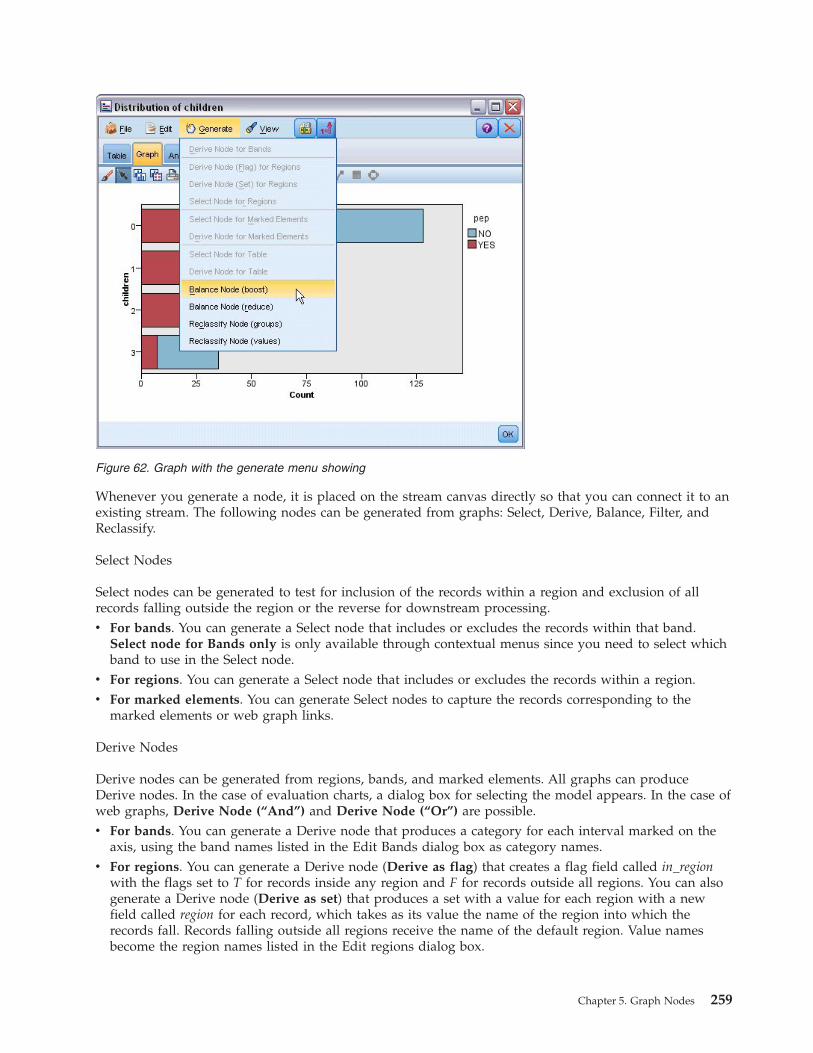
Whenever you generate a node, it is placed on the stream canvas directly so that you can connect it to anexisting stream. The following nodes can be generated from graphs: Select, Derive, Balance, Filter, andReclassify.

Select Nodes

Select nodes can be generated to test for inclusion of the records within a region and exclusion of allrecords falling outside the region or the reverse for downstream processing.v For bands. You can generate a Select node that includes or excludes the records within that band.

Select node for Bands only is only available through contextual menus since you need to select whichband to use in the Select node.

v For regions. You can generate a Select node that includes or excludes the records within a region.v For marked elements. You can generate Select nodes to capture the records corresponding to the

marked elements or web graph links.

Derive Nodes

Derive nodes can be generated from regions, bands, and marked elements. All graphs can produceDerive nodes. In the case of evaluation charts, a dialog box for selecting the model appears. In the case ofweb graphs, Derive Node (“And”) and Derive Node (“Or”) are possible.v For bands. You can generate a Derive node that produces a category for each interval marked on the

axis, using the band names listed in the Edit Bands dialog box as category names.v For regions. You can generate a Derive node (Derive as flag) that creates a flag field called in_region

with the flags set to T for records inside any region and F for records outside all regions. You can alsogenerate a Derive node (Derive as set) that produces a set with a value for each region with a newfield called region for each record, which takes as its value the name of the region into which therecords fall. Records falling outside all regions receive the name of the default region. Value namesbecome the region names listed in the Edit regions dialog box.

Figure 62. Graph with the generate menu showing


v For marked elements. You can generate a Derive node that calculates a flag that is True for all markedelements and False for all other records.

Balance Nodes

Balance nodes can be generated to correct imbalances in the data, such as reducing the frequency ofcommon values (use Balance Node (reduce) menu option) or boosting the occurrence of infrequentvalues (use Balance Node (boost) menu option). Balance node generation is enabled for any graphshowing a distribution of counts, such as Histogram, Dot, Collection, Bar of Counts, Pie of Counts, andMultiplot.

Filter Nodes

Filter nodes can be generated to rename or filter fields based on the lines or nodes marked in the graph.In the case of evaluation charts, the best fit line does not generate a filter node.

Reclassify Nodes

Reclassify nodes can be generated to recode values. This option is used for distribution graphs. You cangenerate a Reclassify node for groups to recode specific values of a displayed field depending upon theirinclusion in a group (select groups using Ctrl+click on the Tables tab). You can also generate a reclassifynode for values to recode data into an existing set of numerous values, such as reclassifying data into astandard set of values in order to merge financial data from various companies for analysis.

Note: If the values are predefined, you can read them into IBM SPSS Modeler as a flat file and use adistribution to display all values. Then generate a Reclassify (values) node for this field directly from thechart. Doing so will put all the target values in the Reclassify node's New values column (drop-down list).

When setting options for the Reclassify node, the table enables a clear mapping from old set values tonew values you specify:v Original value. This column lists existing values for the select field(s).v New value. Use this column to type new category values or select one from the drop-down list. When

you automatically generate a Reclassify node using values from a Distribution chart, these values areincluded in the drop-down list. This allows you to quickly map existing values to a known set ofvalues. For example, healthcare organizations sometimes group diagnoses differently based uponnetwork or locale. After a merger or acquisition, all parties will be required to reclassify new or evenexisting data in a consistent fashion. Rather than manually typing each target value from a lengthy list,you can read the master list of values in to IBM SPSS Modeler, run a Distribution chart for theDiagnosis field, and generate a Reclassify (values) node for this field directly from the chart. Thisprocess will make all of the target Diagnosis values available from the New Values drop-down list.

For more information about the Reclassify Node, see “Setting Options for the Reclassify Node” on page141.

Generating Nodes from Graphs

You can use the Generate menu in the graph output window to generate nodes. The generated node willbe placed on the stream canvas. To use the node, connect it to an existing stream.

To generate a node from a graph:

1. Verify that you are in Explore mode. From the menus, choose View > Explore Mode.2. In the Explore mode toolbar, click the Region button.3. Define bands, regions, or any marked elements needed to generate your node.


4. From the Generate menu, choose the kind of node you want to produce. Only those which arepossible are enabled.

Note: Alternatively, you can also generate nodes directly from the graph by right-clicking and choosingthe generate option you want from the context menus.

Editing VisualizationsWhile Explore mode allows you to analytically explore the data and values represented by thevisualization, Edit mode allows you to change the visualization's layout and look. For example, you canchange the fonts and colors to match your organization's style guide. To select this mode, choose View >Edit Mode from the menus (or click the toolbar icon).

In Edit mode, there are several toolbars that affect different aspects of the visualization's layout. If youfind that there are any you don't use, you can hide them to increase the amount of space in the dialogbox in which the graph is displayed. To select or deselect toolbars, click the relevant toolbar name on theView menu.

Note: To add further detail to your visualizations, you can apply title, footnote, and axis labels. See thetopic “Adding Titles and Footnotes” on page 271 for more information.

You have several options for editing a visualization in Edit mode. You can:v Edit text and format it.v Change the fill color, transparency, and pattern of frames and graphic elements.v Change the color and dashing of borders and lines.v Rotate and change the shape and aspect ratio of point elements.v Change the size of graphic elements (such as bars and points).v Adjust the space around items by using margins and padding.v Specify formatting for numbers.v Change the axis and scale settings.v Sort, exclude, and collapse categories on a categorical axis.v Set the orientation of panels.v Apply transformations to a coordinate system.v Change statistics, graphic element types, and collision modifiers.v Change the position of the legend.v Apply visualization stylesheets.

The following topics describe how to perform these various tasks. It is also recommended that you readthe general rules for editing graphs.

How to Switch to Edit Mode

From the menus choose:

View > Edit Mode

General Rules for Editing VisualizationsEdit Mode

All edits are done in Edit mode. To enable Edit mode, from the menus choose:

View > Edit Mode


Selection

The options available for editing depend on selection. Different toolbar and properties palette options areenabled depending on what is selected. Only the enabled items apply to the current selection. Forexample, if an axis is selected, the Scale, Major Ticks, and Minor Ticks tabs are available in the propertiespalette.

Here are some tips for selecting items in the visualization:v Click an item to select it.v Select a graphic element (such as points in a scatterplot or bars in a bar chart) with a single click. After

initial selection, click again to narrow the selection to groups of graphic elements or a single graphicelement.

v Press Esc to deselect everything.

Palettes

When an item is selected in the visualization, the various palettes are updated to reflect the selection. Thepalettes contain controls for making edits to the selection. Palettes may be toolbars or a panel withmultiple controls and tabs. Palettes can be hidden, so ensure the necessary palette is displayed formaking edits. Check the View menu for palettes that are currently displayed.

You can reposition the palettes by clicking and dragging the empty space in a toolbar palette or the leftside of other palettes. Visual feedback lets you know where you can dock the palette. For non-toolbarpalettes, you can also click the close button to hide the palette and the undock button to display thepalette in a separate window. Click the help button to display help for the specific palette.

Automatic Settings

Some settings provide an -auto- option. This indicates that automatic values are applied. Whichautomatic settings are used depends on the specific visualization and data values. You can enter a valueto override the automatic setting. If you want to restore the automatic setting, delete the current valueand press Enter. The setting will display -auto- again.

Removing/Hiding Items

You can remove/hide various items in the visualization. For example, you can hide the legend or axislabel. To delete an item, select it and press Delete. If the item does not allow deletion, nothing willhappen. If you accidentally delete an item, press Ctrl+Z to undo the deletion.

State

Some toolbars reflect the state of the current selection, others don't. The properties palette always reflectsstate. If a toolbar does not reflect state, this is mentioned in the topic that describes the toolbar.

Editing and Formatting TextYou can edit text in place and change the formatting of an entire text block. Note that you can't edit textthat is linked directly to data values. For example, you can't edit a tick label because the content of thelabel is derived from the underlying data. However, you can format any text in the visualization.

How to Edit Text in Place1. Double-click the text block. This action selects all the text. All toolbars are disabled at this time,

because you cannot change any other part of the visualization while editing text.2. Type to replace the existing text. You can also click the text again to display a cursor. Position the

cursor where you want and enter the additional text.


How to Format Text1. Select the frame containing the text. Do not double-click the text.2. Format text using the font toolbar. If the toolbar is not enabled, make sure only the frame containing

the text is selected. If the text itself is selected, the toolbar will be disabled.

You can change the font:v Colorv Family (for example, Arial or Verdana)v Size (the unit is pt unless you indicate a different unit, such as pc)v Weightv Alignment relative to the text frame

Formatting applies to all the text in a frame. You can't change the formatting of individual letters orwords in any particular block of text.

Changing Colors, Patterns, Dashings, and TransparencyMany different items in a visualization have a fill and border. The most obvious example is a bar in a barchart. The color of the bars is the fill color. They may also have a solid, black border around them.

There are other less obvious items in the visualization that have fill colors. If the fill color is transparent,you may not know there is a fill. For example, consider the text in an axis label. It appears as if this textis "floating" text, but it actually appears in a frame that has a transparent fill color. You can see the frameby selecting the axis label.

Any frame in the visualization can have a fill and border style, including the frame around the wholevisualization. Also, any fill has an associated opacity/transparency level that can be adjusted.

How to Change the Colors, Patterns, Dashing, and Transparency1. Select the item you want to format. For example, select the bars in a bar chart or a frame containing

text. If the visualization is split by a categorical variable or field, you can also select the group thatcorresponds to an individual category. This allows you to change the default aesthetic assigned to thatgroup. For example, you can change the color of one of the stacking groups in a stacked bar chart.

2. To change the fill color, the border color, or the fill pattern, use the color toolbar.Note: This toolbar does not reflect the state of the current selection.To change a color or fill, you can click the button to select the displayed option or click thedrop-down arrow to choose another option. For colors, notice there is one color that looks like whitewith a red, diagonal line through it. This is the transparent color. You could use this, for example, tohide the borders on bars in a histogram.v The first button controls the fill color. If the color is associated with a continuous or ordinal field,

this button changes the fill color for the color associated with the highest value in the data. You canuse the Color tab on the properties palette to change the color associated with the lowest value andmissing data. The color of the elements will change incrementally from the Low color to the Highcolor as the values of the underlying data increase.

v The second button controls the border color.v The third button controls the fill pattern. The fill pattern uses the border color. Therefore, the fill

pattern is visible only if there is a visible border color.v The fourth control is a slider and text box that control the opacity of the fill color and pattern. A

lower percentage means less opacity and more transparency. 100% is fully opaque (notransparency).

3. To change the dashing of a border or line, use the line toolbar.Note: This toolbar does not reflect the state of the current selection.


As with the other toolbar, you can click the button to select the displayed option or click thedrop-down arrow to choose another option.

Rotating and Changing the Shape and Aspect Ratio of Point ElementsYou can rotate point elements, assign a different predefined shape, or change the aspect ratio (the ratio ofwidth to height).

How to Modify Point Elements1. Select the point elements. You cannot rotate or change the shape and aspect ratio of individual point

elements.2. Use the symbol toolbar to modify the points.

v The first button allows you to change the shape of the points. Click the drop-down arrow andselect a predefined shape.

v The second button allows you to rotate the points to a specific compass position. Click thedrop-down arrow and then drag the needle to the position you want.

v The third button allows you to change the aspect ratio. Click the drop-down arrow and then clickand drag the rectangle that appears. The shape of the rectangle represents the aspect ratio.

Changing the Size of Graphic ElementsYou can change the size of the graphic elements in the visualization. These include bars, lines, and pointsamong others. If the graphic element is sized by a variable or field, the specified size is the minimum size.

How to Change the Size of the Graphic Elements1. Select the graphic elements you want to resize.2. Use the slider or enter a specific size for the option available on the symbol toolbar. The unit is pixels

unless you indicate a different unit (see below for a full list of unit abbreviations). You can alsospecify a percentage (such as 30%), which means that a graphic element uses the specified percentageof the available space. The available space depends on the graphic element type and the specificvisualization.

Table 51. Valid unit abbreviations

Abbreviation Unit

cm centimeter

in inch

mm millimeter

pc pica

pt point

px pixel

Specifying Margins and PaddingIf there is too much or too little spacing around or inside a frame in the visualization, you can change itsmargin and padding settings. The margin is the amount of space between the frame and other itemsaround it. The padding is the amount of space between the border of the frame and the contents of theframe.

How to Specify Margins and Padding1. Select the frame for which you want to specify margins and padding. This can be a text frame, the

frame around the legend, or even the data frame displaying the graphic elements (such as bars andpoints).


2. Use the Margins tab on the properties palette to specify the settings. All sizes are in pixels unless youindicate a different unit (such as cm or in).

Formatting Numbers

You can specify the format for numbers in tick labels on a continuous axis or data value labels displayinga number. For example, you can specify that numbers displayed in the tick labels are shown inthousands.

How to Specify Number Formats1. Select the continuous axis tick labels or the data value labels if they contain numbers.2. Click the Format tab on the properties palette.3. Select the number formatting options you want:

Prefix. A character to display at the beginning of the number. For example, enter a dollar sign ($) ifthe numbers are salaries in U.S. dollars.Suffix. A character to display at the end of the number. For example, enter a percentage sign (%) ifthe numbers are percentages.Min. Integer Digits. Minimum number of digits to display in the integer part of a decimalrepresentation. If the actual value does not contain the minimum number of digits, the integer part ofthe value will be padded with zeros.Max. Integer Digits. Maximum number of digits to display in the integer part of a decimalrepresentation. If the actual value exceeds the maximum number of digits, the integer part of thevalue will be replaced with asterisks.Min. Decimal Digits. Minimum number of digits to display in the decimal part of a decimal orscientific representation. If the actual value does not contain the minimum number of digits, thedecimal part of the value will be padded with zeros.Max. Decimal Digits. Maximum number of digits to display in the decimal part of a decimal orscientific representation. If the actual value exceeds the maximum number of digits, the decimal isrounded to the appropriate number of digits.Scientific. Whether to display numbers in scientific notation. Scientific notation is useful for verylarge or very small numbers. -auto- lets the application determine when scientific notation isappropriate.Scaling. A scale factor, which is a number by which the original value is divided. Use a scale factorwhen the numbers are large, but you don't want the label to extend too much to accommodate thenumber. If you change the number format of the tick labels, be sure to edit the axis title to indicatehow the number should be interpreted. For example, assume your scale axis displays salaries and thelabels are 30,000, 50,000, and 70,000. You might enter a scale factor of 1000 to display 30, 50, and 70.You should then edit the scale axis title to include the text in thousands.Parentheses for -ve. Whether parentheses should be displayed around negative values.Grouping. Whether to display a character between groups of digits. Your computer's current localedetermines which character is used for digit grouping.

Changing the Axis and Scale SettingsThere are several options for modifying axes and scales.

How to change axis and scale settings1. Select any part of the axis (for example, the axis label or tick labels).2. Use the Scale, Major Ticks, and Minor Ticks tabs on the properties palette to change the axis and scale

settings.

Scale tab


Note: The Scale tab does not appear for graphs where the data is pre-aggregated (for example,histograms).

Type. Specifies whether the scale is linear or transformed. Scale transformations help you understand thedata or make assumptions necessary for statistical inference. On scatterplots, you might use atransformed scale if the relationship between the independent and dependent variables or fields isnonlinear. Scale transformations can also be used to make a skewed histogram more symmetric so that itresembles a normal distribution. Note that you are transforming only the scale on which the data aredisplayed; you are not transforming the actual data.v linear. Specifies a linear, untransformed scale.v log. Specifies a base-10 log transformed scale. To accommodate zero and negative values, this

transformation uses a modified version of the log function. This "safe log" function is defined assign(x) * log(1 + abs(x)). So safeLog(-99) equals:sign(-99) * log(1 + abs(-99)) = -1 * log(1 + 99) = -1 * 2 = -2

v power. Specifies a power transformed scale, using an exponent of 0.5. To accommodate negativevalues, this transformation uses a modified version of the power function. This "safe power" function isdefined as sign(x) * pow(abs(x), 0.5). So safePower(-100) equals:sign(-100) * pow(abs(-100), 0.5) = -1* pow(100, 0.5) = -1 * 10 = -10

Min/Max/Nice Low/Nice High. Specifies the range for the scale. Selecting Nice Low and Nice Highallows the application to select an appropriate scale based on the data. The minimum and maximum are"nice" because they are typically whole values greater or less than the maximum and minimum datavalues. For example, if the data range from 4 to 92, a nice low and high for scale may be 0 and 100 ratherthan the actual data minimum and maximum. Be careful that you don't set a range that is too small andhides important items. Also note that you cannot set an explicit minimum and maximum if the Includezero option is selected.

Low Margin/High Margin. Create margins at the low and/or high end of the axis. The margin appearsperpendicular to the selected axis. The unit is pixels unless you indicate a different unit (such as cm orin). For example, if you set the High Margin to 5 for the vertical axis, a horizontal margin of 5 px runsalong the top of the data frame.

Reverse. Specifies whether the scale is reversed.

Include zero. Indicates that the scale should include 0. This option is commonly used for bar charts toensure the bars begin at 0, rather than a value near the height of the smallest bar. If this option isselected, Min and Max are disabled because you cannot set a custom minimum and maximum for thescale range.

Major Ticks/Minor Ticks Tabs

Ticks or tick marks are the lines that appear on an axis. These indicate values at specific intervals orcategories. Major ticks are the tick marks with labels. These are also longer than other tick marks. Minorticks are tick marks that appear between the major tick marks. Some options are specific to the tick type,but most options are available for major and minor ticks.

Show ticks. Specifies whether major or minor ticks are displayed on a graph.

Show gridlines. Specifies whether gridlines are displayed at the major or minor ticks. Gridlines are linesthat cross a whole graph from axis to axis.

Position. Specifies the position of the tick marks relative to the axis.

Length. Specifies the length of the tick marks. The unit is pixels unless you indicate a different unit (suchas cm or in).


Base. Applies only to major ticks. Specifies the value at which the first major tick appears.

Delta. Applies only to major ticks. Specifies the difference between major ticks. That is, major ticks willappear at every nth value, where n is the delta value.

Divisions. Applies only to minor ticks. Specifies the number of minor tick divisions between major ticks.The number of minor ticks is one less than the number of divisions. For example, assume that there aremajor ticks at 0 and 100. If you enter 2 as the number of minor tick divisions, there will be one minor tickat 50, dividing the 0–100 range and creating two divisions.

Editing CategoriesYou can edit the categories on a categorical axis in several ways:v Change the sort order for displaying the categories.v Exclude specific categories.v Add a category that does not appear in the data set.v Collapse/combine small categories into one category.

How to Change the Sort Order of Categories1. Select a categorical axis. The Categories palette displays the categories on the axis.

Note: If the palette is not visible, make sure that you have it enabled. From the View menu in IBMSPSS Modeler, choose Categories.

2. In the Categories palette, select a sorting option from the drop-down list:Custom. Sort categories based on the order in which they appear in the palette. Use the arrow buttonsto move categories to the top of the list, up, down, and to the bottom of the list.Data. Sort categories based on the order in which they occur in the dataset.Name. Sort categories alphabetically, using the names as displayed in the palette. This may be eitherthe value or label, depending on whether the toolbar button to display values and labels is selected.Value. Sort categories by the underlying data value, using the values displayed in parentheses in thepalette. Only data sources with metadata (such as IBM SPSS Statistics data files) support this option.Statistic. Sort categories based on the calculated statistic for each category. Examples of statisticsinclude counts, percentages, and means. This option is available only if a statistic is used in the graph.

How to Add a Category

By default, only categories that appear in the data set are available. You can add a category to thevisualization if needed.1. Select a categorical axis. The Categories palette displays the categories on the axis.


2. In the Categories palette, click the add category button:

3. In the Add a new category dialog box, enter a name for the category.4. Click OK.

How to Exclude Specific Categories1. Select a categorical axis. The Categories palette displays the categories on the axis.

Figure 63. Add category button



2. In the Categories palette, select a category name in the Include list, and then click the X button. Tomove the category back, select its name in the Excluded list, and then click the arrow to the right ofthe list.

How to Collapse/Combine Small Categories

You can combine categories that are so small you don't need to display them separately. For example, ifyou have a pie chart with many categories, consider collapsing categories with a percentage less than 10.Collapsing is available only for statistics that are additive. For example, you can't add means togetherbecause means are not additive. Therefore, combining/collapsing categories using a mean is notavailable.1. Select a categorical axis. The Categories palette displays the categories on the axis.


2. In the Categories palette, select Collapse and specify a percentage. Any categories whose percentageof the total is less than the specified number are combined into one category. The percentage is basedon the statistic shown in the chart. Collapsing is available only for count-based and summation (sum)statistics.

Changing the Orientation PanelsIf you are using panels in your visualization, you can change their orientation.

How to Change the Orientation of the Panels1. Select any part of the visualization.2. Click the Panels tab on the properties palette.3. Select an option from Layout:

Table. Lays out panels like a table, in that there is a row or column assigned to every individual value.

Transposed. Lays out panels like a table, but also swaps the original rows and columns. This option isnot the same as transposing the graph itself. Note that the x axis and the y axis are unchanged when youselect this option.

List. Lays out panels like a list, in that each cell represents a combination of values. Columns and rowsare no longer assigned to individual values. This option allows the panels to wrap if needed.

Transforming the Coordinate SystemMany visualizations are displayed in a flat, rectangular coordinate system. You can transform thecoordinate system as needed. For example, you can apply a polar transformation to the coordinatesystem, add oblique drop shadow effects, and transpose the axes. You can also undo any of thesetransformations if they are already applied to the current visualization. For example, a pie chart is drawnin a polar coordinate system. You can undo the polar transformation and display the pie chart as a singlestacked bar in a rectangular coordinate system.

How to Transform the Coordinate System1. Select the coordinate system that you want to transform. You select the coordinate system by selecting

the frame around the individual graph.2. Click the Coordinates tab on the properties palette.3. Select the transformations that you want to apply to the coordinate system. You can also deselect a

transformation to undo it.


Transposed. Changing the orientation of the axes is called transposing. It is similar to swapping thevertical and horizontal axes in a 2-D visualization.Polar. A polar transformation draws the graphic elements at a specific angle and distance from thecenter of the graph. A pie chart is a 1-D visualization with a polar transformation that draws theindividual bars at specific angles. A radar chart is a 2-D visualization with a polar transformation thatdraws graphic elements at specific angles and distances from the center of the graph. A 3-Dvisualization would also include an additional depth dimension.Oblique. An oblique transformation adds a 3-D effect to the graphic elements. This transformationadds depth to the graphic elements, but the depth is purely decorative. It is not influenced byparticular data values.Same Ratio. Applying the same ratio specifies that the same distance on each scale represents thesame difference in data values. For example, 2cm on both scales represent a difference of 1000.Pre-transform inset %. If axes are clipped after the transformation, you may want to add insets to thegraph before applying the transformation. The insets shrink the dimensions by a certain percentagebefore any transformations are applied to the coordinate system. You have control over the lower x,upper x, lower y, and upper y dimensions, in that order.Post-transform inset %. If you want to change the aspect ratio of the graph, you can add insets to thegraph after applying the transformation. The insets shrink the dimensions by a certain percentageafter any transformations are applied to the coordinate system. These insets can also be applied evenif no transformation is applied to the graph. You have control over the lower x, upper x, lower y, andupper y dimensions, in that order.

Changing Statistics and Graphic ElementsYou can convert a graphic element to another type, change the statistic used to draw the graphic element,or specify the collision modifier that determines what happens when graphic elements overlap.

How to Convert a Graphic Element1. Select the graphic element that you want to convert.2. Click the Element tab on the properties palette.3. Select a new graphic element type from the Type list.

Table 52. Graphic element types

Graphic Element Type Description

Point A marker identifying a specific data point. A point element is used inscatterplots and other related visualizations.

Interval A rectangular shape drawn at a specific data value and filling the spacebetween an origin and another data value. An interval element is used inbar charts and histograms.

Line A line that connects data values.

Path A line that connects data values in the order they appear in the dataset.

Area A line that connects data elements with the area between the line and anorigin filled in.

Polygon A multi-sided shape enclosing a data region. A polygon element could beused in a binned scatterplot or a map.

Schema An element consisting of a box with whiskers and markers indicatingoutliers. A schema element is used for boxplots.

How to Change the Statistic1. Select the graphic element whose statistic you want to change.2. Click the Element tab on the properties palette.


How to Specify the Collision Modifier

The collision modifier determines what happens when graphic elements overlap.1. Select the graphic element for which you want to specify the collision modifier.2. Click the Element tab on the properties palette.3. From the Modifier drop-down list, select a collision modifier. -auto- lets the application determine

which collision modifier is appropriate for the graphic element type and statistic.Overlay. Draw graphic elements on top of each other when they have the same value.Stack. Stack graphic elements that would normally be superimposed when they have the same datavalues.Dodge. Move graphic elements next to other graphic elements that appear at the same value, ratherthan superimposing them. The graphic elements are arranged symmetrically. That is, the graphicelements are moved to opposite sides of a central position. Dodging is very similar to clustering.Pile. Move graphic elements next to other graphic elements that appear at the same value, rather thansuperimposing them. The graphic elements are arranged asymmetrically. That is, the graphic elementsare piled on top of one another, with the graphic element on the bottom positioned at a specific valueon the scale.Jitter (normal). Randomly reposition graphic elements at the same data value using a normaldistribution.Jitter (uniform). Randomly reposition graphic elements at the same data value using a uniformdistribution.

Changing the Position of the LegendIf a graph includes a legend, the legend is typically displayed to the right of a graph. You can change thisposition if needed.

How to Change the Legend Position1. Select the legend.2. Click the Legend tab on the properties palette.3. Select a position.

Copying a Visualization and Visualization DataThe General palette includes buttons for copying the visualization and its data.

Copying the visualization. This action copies the visualization to the clipboard as an image. Multipleimage formats are available. When you paste the image into another application, you can choose a "pastespecial" option to select one of the available image formats for pasting.

Figure 64. Copy visualization button

Figure 65. Copy visualization data button


Copying the visualization data. This action copies the underlying data that is used to draw thevisualization. The data is copied to the clipboard as plain text or HTML-formatted text. When you pastethe data into another application, you can choose a "paste special" option to choose one of these formatsfor pasting.

Keyboard ShortcutsTable 53. Keyboard shortcuts

Shortcut Key Function

Ctrl+Space Toggle between Explore and Edit mode

Delete Delete a visualization item

Ctrl+Z Undo

Ctrl+Y Redo

F2 Display outline for selecting items in the graph

Adding Titles and FootnotesFor all graph types you can add unique title, footnote, or axis labels to help identify what is shown in thegraph.

Adding Titles to Graphs1. From the menus, choose Edit > Add Graph Title. A text box containing <TITLE> is displayed above

the graph.2. Verify that you are in Edit mode. From the menus, choose View > Edit Mode.3. Double-click the <TITLE> text.4. Type the required title and press Return.

Adding Footnotes to Graphs1. From the menus, choose Edit > Add Graph Footnote. A text box containing <FOOTNOTE> is

displayed below the graph.2. Verify that you are in Edit mode. From the menus, choose View > Edit Mode.3. Double-click the <FOOTNOTE> text.4. Type the required title and press Return.

Using Graph StylesheetsBasic graph display information, such as colors, fonts, symbols, and line thickness, are controlled by astylesheet. There is a default stylesheet supplied with IBM SPSS Modeler; however, you can makechanges to it if you need. For example, you may have a corporate color scheme for presentations that youwant used in your graphs. See the topic “Editing Visualizations” on page 261 for more information.

In the graph nodes, you can use the Edit mode to make style changes to the look of a graph. You canthen use the Edit > Styles menu to save the changes as a stylesheet to apply to all graphs that yousubsequently generate from the current graph node or as a new default stylesheet for all graphs that youproduce using IBM SPSS Modeler.

There are five stylesheet options available from the Styles option on the Edit menu:v Switch Stylesheet. This displays a list of different, stored, stylesheets that you can select to change the

look of your graphs. See the topic “Applying Stylesheets” on page 272 for more information.v Store Styles in Node. This stores modifications to the selected graph's styles so that they are applied

to any future graphs created from the same graph node in the current stream.


v Store Styles as Default. This stores modifications to the selected graph's styles so that they areapplied to all future graphs created from any graph node in any stream. After selecting this option,you can use Apply Default Styles to change any other existing graphs to use the same styles.

v Apply Default Styles. This changes the selected graph's styles to those that are currently saved as thedefault styles.

v Apply Original Styles. This changes a graph's styles back to the ones supplied as the original default.

Applying StylesheetsYou can apply a visualization stylesheet that specifies stylistic properties of the visualization. Forexample, the stylesheet can define fonts, dashings, and colors, among other options. To a certain extent,stylesheets provide a shortcut for edits that you would have to perform manually. Note, however, that astylesheet is limited to style changes. Other changes such as the position of the legend or the scale rangeare not stored in the stylesheet.

How to Apply a Stylesheet1. From the menus choose:

Edit > Styles > Switch Stylesheet

2. Use the Switch Stylesheet dialog box to select a stylesheet.3. Click Apply to apply the stylesheet to the visualization without closing the dialog. Click OK to apply

the stylesheet and close the dialog box.

Switch/Select Stylesheet Dialog Box

The table at the top of the dialog box lists all of the visualization stylesheets that are currently available.Some stylesheets are pre-installed, while others may have been created in the IBM SPSS VisualizationDesigner (a separate product).

The bottom of the dialog box shows example visualizations with sample data. Select one of thestylesheets to apply its styles to the example visualizations. These examples can help you determine howthe stylesheet will affect your actual visualization.

The dialog box also offers the following options.

Existing styles. By default, a stylesheet can overwrite all the styles in the visualization. You can changethis behavior.v Overwrite all styles. When applying the stylesheet, overwrite all styles in the visualization, including

those styles modified in the visualization during the current editing session.v Preserve modified styles. When applying the stylesheet, overwrite only those styles that were not

modified in the visualization during the current editing session. Styles that were modified during thecurrent editing session are preserved.


Location. Change the location in which visualization templates, stylesheets, and maps are stored. Thecurrent location is listed to the right of the button. See the topic “Setting the Location of Templates,Stylesheets, and Maps” on page 203 for more information.

Printing, Saving, Copying, and Exporting GraphsEach graph has a number of options that enable you to save or print the graph or export it to anotherformat. Most of these options are available from the File menu. In addition, from the Edit menu, you canchoose to copy the graph or the data within it for use in another application.


Printing

To print the graph, use the Print menu item or button. Before you print, you can use Page Setup andPrint Preview to set print options and preview the output.

Saving Graphs

To save the graph to an IBM SPSS Modeler output file (*.cou), choose File > Save or File > Save As fromthe menus.

or

To save the graph in the repository, choose File > Store Output from the menus.

Copying Graphs

To copy the graph for use in another application, such as MS Word or MS PowerPoint, choose Edit >Copy Graph from the menus.

Copying Data

To copy the data for use in another application, such as MS Excel or MS Word, choose Edit > Copy Datafrom the menus. By default, the data will be formatted as HTML. Use Paste Special in the otherapplication to view other formatting options when pasting.

Exporting Graphs

The Export Graph option enables you to export the graph in one of the following formats: Bitmap (.bmp),JPEG (.jpg), PNG (.png), HTML (.html), or ViZml document (.xml) for use in other IBM SPSS Statisticsapplications.

To export graphs, choose File > Export Graph from the menus and then choose the format.

Exporting Tables

The Export Table option enables you to export the table in one of the following formats: tab delimited(.tab), comma delimited (.csv), or HTML (.html).

To export tables, choose File > Export Table from the menus and then choose the format.


Chapter 6. Output Nodes

Overview of Output NodesOutput nodes provide the means to obtain information about your data and models. They also provide amechanism for exporting data in various formats to interface with your other software tools.

The following output nodes are available:

The Table node displays the data in table format, which can also be written to a file. This isuseful anytime that you need to inspect your data values or export them in an easily readableform.

The Matrix node creates a table that shows relationships between fields. It is most commonlyused to show the relationship between two symbolic fields, but it can also show relationshipsbetween flag fields or numeric fields.

The Analysis node evaluates predictive models' ability to generate accurate predictions.Analysis nodes perform various comparisons between predicted values and actual values forone or more model nuggets. They can also compare predictive models to each other.

The Data Audit node provides a comprehensive first look at the data, including summarystatistics, histograms and distribution for each field, as well as information on outliers,missing values, and extremes. Results are displayed in an easy-to-read matrix that can besorted and used to generate full-size graphs and data preparation nodes.

The Transform node allows you to select and visually preview the results of transformationsbefore applying them to selected fields.

The Statistics node provides basic summary information about numeric fields. It calculatessummary statistics for individual fields and correlations between fields.

The Means node compares the means between independent groups or between pairs ofrelated fields to test whether a significant difference exists. For example, you could comparemean revenues before and after running a promotion or compare revenues from customerswho did not receive the promotion with those who did.

The Report node creates formatted reports containing fixed text as well as data and otherexpressions derived from the data. You specify the format of the report using text templatesto define the fixed text and data output constructions. You can provide custom textformatting by using HTML tags in the template and by setting options on the Output tab.You can include data values and other conditional output by using CLEM expressions in thetemplate.


The Set Globals node scans the data and computes summary values that can be used inCLEM expressions. For example, you can use this node to compute statistics for a field calledage and then use the overall mean of age in CLEM expressions by inserting the function@GLOBAL_MEAN(age).

The Simulation Fitting node examines the statistical distribution of the data in each field andgenerates (or updates) a Simulation Generate node, with the best fitting distribution assignedto each field. The Simulation Generate node can then be used to generate simulated data.

The Simulation Evaluation node evaluates a specified predicted target field, and presentsdistribution and correlation information about the target field.

Managing OutputThe Output manager shows the charts, graphs, and tables generated during an IBM SPSS Modelersession. You can always reopen an output by double-clicking it in the manager—you do not have torerun the corresponding stream or node.

To View the Output Manager

Open the View menu and choose Managers. Click the Outputs tab.

From the Output manager, you can:v Display existing output objects, such as histograms, evaluation charts, and tables.v Rename output objects.v Save output objects to disk or to the IBM SPSS Collaboration and Deployment Services Repository (if

available).v Add output files to the current project.v Delete unsaved output objects from the current session.v Open saved output objects or retrieve them from the IBM SPSS Collaboration and Deployment Services

Repository (if available).

To access these options, right-click anywhere on the Outputs tab.

Viewing OutputOn-screen output is displayed in an output browser window. The output browser window has its ownset of menus that allow you to print or save the output, or export it to another format. Note that specificoptions may vary depending on the type of output.

Printing, saving, and exporting data. More information is available as follows:v To print the output, use the Print menu option or button. Before you print, you can use Page Setup

and Print Preview to set print options and preview the output.v To save the output to an IBM SPSS Modeler output file (.cou), choose Save or Save As from the File

menu.v To save the output in another format, such as text or HTML, choose Export from the File menu. See the

topic “Exporting Output” on page 278 for more information.


Note that you can only select these formats if the output contains data that can be sensibly exported inthat way. For example, the contents of a decision tree could be exported as text, but the contents of aK-means model would not make sense as text.

v To save the output in a shared repository so that other users can view it using the IBM SPSSCollaboration and Deployment Services Deployment Portal, choose Publish to Web from the Filemenu. Note that this option requires a separate license for IBM SPSS Collaboration and DeploymentServices.

Selecting cells and columns. The Edit menu contains various options for selecting, deselecting, andcopying cells and columns, as appropriate for the current output type. See the topic “Selecting Cells andColumns” on page 279 for more information.

Generating new nodes. The Generate menu enables you to generate new nodes based on the contents ofthe output browser. The options vary depending on the type of output and the items in the output thatare currently selected. For details about the node-generation options for a particular type of output, seethe documentation for that output.

Publish to WebThe Publish to Web feature enables you to publish certain types of stream output to a central shared IBMSPSS Collaboration and Deployment Services Repository that forms the basis of IBM SPSS Collaborationand Deployment Services. If you use this option, other users who need to view this output can do so byusing Internet access and an IBM SPSS Collaboration and Deployment Services account--they do not needto have IBM SPSS Modeler installed.

The following table lists the IBM SPSS Modeler nodes that support the Publish to Web feature. Outputfrom these nodes is stored in the IBM SPSS Collaboration and Deployment Services Repository in outputobject (.cou) format, and can be viewed directly in the IBM SPSS Collaboration and Deployment ServicesDeployment Portal.

Other types of output can be viewed only if the relevant application (e.g. IBM SPSS Modeler, for streamobjects) is installed on the user's machine.

Table 54. Nodes supporting Publish to Web.

Node Type Node

Graphs all

Output Table

Matrix

Data Audit

Transform

Means

Analysis

Statistics

Report (HTML)

IBM SPSS Statistics Statistics Output

Publishing Output to the WebTo publish output to the Web:1. In an IBM SPSS Modeler stream, execute one of the nodes listed in the table. Doing so creates an

output object (for example, a table, matrix or report object) in a new window.2. From the output object window, choose:

Chapter 6. Output Nodes 277

File > Publish to Web

Note: If you just want to export simple HTML files for use with a standard Web browser, chooseExport from the File menu and select HTML.

3. Connect to the IBM SPSS Collaboration and Deployment Services Repository.When you have connected successfully, the Repository: Store dialog is displayed, offering a number ofstorage options.

4. When you have chosen the storage options you want, click Store.

Viewing Published Output Over the WebYou must have an IBM SPSS Collaboration and Deployment Services account set up in order to use thisfeature. If you have the relevant application installed for the object type you want to view (for example,IBM SPSS Modeler or IBM SPSS Statistics), the output is displayed in the application itself rather than inthe browser.

To view published output over the Web:1. Point your browser to http://<repos_host>:<repos_port>/peb

where repos_host and repos_port are the hostname and port number for the IBM SPSS Collaborationand Deployment Services host.

2. Enter the login details for your IBM SPSS Collaboration and Deployment Services account.3. Click on Content Repository.4. Navigate to, or search for, the object you want to view.5. Click on the object name. For some object types, such as graphs, there may be a delay while the object

is rendered in the browser.

Viewing Output in an HTML BrowserFrom the Advanced tab on the Linear, Logistic, and PCA/Factor model nuggets, you can view thedisplayed information in a separate browser, such as Internet Explorer. The information is output asHTML, enabling you to save it and reuse it elsewhere, such as on a corporate intranet, or Internet site.

To display the information in a browser, click the launch button, situated below the model icon in the topleft of the Advanced tab of the model nugget.

Exporting OutputIn the output browser window, you may choose to export the output to another format, such as text orHTML. The export formats vary depending on the type of output, but in general are similar to the filetype options available if you select Save to file in the node used to generate the output.

Note: You can only select these formats if the output contains data that can be sensibly exported in thatway. For example, the contents of a decision tree could be exported as text, but the contents of a K-meansmodel would not make sense as text.

To Export Output1. In the output browser, open the File menu and choose Export. Then choose the file type that you

want to create:v Tab Delimited (*.tab). This option generates a formatted text file containing the data values. This

style is often useful for generating a plain-text representation of the information that can beimported into other applications. This option is available for the Table, Matrix, and Means nodes.

v Comma Delimited (*.dat). This option generates a comma-delimited text file containing the datavalues. This style is often useful as a quick way to generate a data file that can be imported intospreadsheets or other data analysis applications. This option is available for the Table, Matrix, andMeans nodes.


v Transposed Tab Delimited (*.tab). This option is identical to the Tab Delimited option, but thedata is transposed so that rows represent fields and the columns represent records.

v Transposed Comma Delimited (*.dat). This option is identical to the Comma Delimited option, butthe data is transposed so that rows represent fields and the columns represent records.

v HTML (*.html). This option writes HTML-formatted output to a file or files.

Selecting Cells and ColumnsA number of nodes, including the Table node, Matrix node, and Means node, generate tabular output.These output tables can be viewed and manipulated in similar ways, including selecting cells, copying allor part of the table to the Clipboard, generating new nodes based on the current selection, and savingand printing the table.

Selecting cells. To select a cell, click it. To select a rectangular range of cells, click one corner of thedesired range, drag the mouse to the other corner of the range, and release the mouse button. To selectan entire column, click the column heading. To select multiple columns, use Shift-click or Ctrl-click oncolumn headings.

When you make a new selection, the old selection is cleared. By holding down the Ctrl key whileselecting, you can add the new selection to any existing selection instead of clearing the old selection. Youcan use this method to select multiple, noncontiguous regions of the table. The Edit menu also containsthe Select All and Clear Selection options.

Reordering columns. The Table node and Means node output browsers allow you to move columns inthe table by clicking a column heading and dragging it to the desired location. You can move only onecolumn at a time.

Table NodeThe Table node creates a table that lists the values in your data. All fields and all values in the stream areincluded, making this an easy way to inspect your data values or export them in an easily readable form.Optionally, you can highlight records that meet a certain condition.

Note: Unless you are working with small datasets, it is recommended that you select a subset of the datato pass into the Table node. The Table node cannot display properly when the number of recordssurpasses a size that can be contained in the display structure (for example, 100 million rows).

Table Node Settings TabHighlight records where. You can highlight records in the table by entering a CLEM expression that istrue for the records to be highlighted. This option is enabled only when Output to screen is selected.

Table Node Format TabThe Format tab contains options used to specify formatting on a per-field basis. This tab is shared withthe Type node. See the topic “Field Format Settings Tab” on page 129 for more information.

Output Node Output TabFor nodes that generate table-style output, the Output tab enables you to specify the format and locationof the results.

Output name. Specifies the name of the output produced when the node is executed. Auto chooses aname based on the node that generates the output. Optionally, you can select Custom to specify adifferent name.


Output to screen (the default). Creates an output object to view online. The output object will appear onthe Outputs tab of the manager window when the output node is executed.

Output to file. Saves the output to a file when the node is executed. If you choose this option, enter afilename (or navigate to a directory and specify a filename using the File Chooser button) and select a filetype. Note that some file types may be unavailable for certain types of output.

Data is output in the system default encoding format, which is specified in the Windows Control Panelor, if running in distributed mode, on the server computer.v Data (tab delimited) (*.tab). This option generates a formatted text file containing the data values.

This style is often useful for generating a plain-text representation of the information that can beimported into other applications. This option is available for the Table, Matrix, and Means nodes.

v Data (comma delimited) (*.dat). This option generates a comma-delimited text file containing the datavalues. This style is often useful as a quick way to generate a data file that can be imported intospreadsheets or other data analysis applications. This option is available for the Table, Matrix, andMeans nodes.

v HTML (*.html). This option writes HTML-formatted output to a file or files. For tabular output (fromthe Table, Matrix, or Means nodes), a set of HTML files contains a contents panel listing field namesand the data in an HTML table. The table may be split over multiple HTML files if the number of rowsin the table exceeds the Lines per page specification. In this case, the contents panel contains links toall table pages and provides a means of navigating the table. For non-tabular output, a single HTMLfile is created containing the results of the node.Note: If the HTML output contains only formatting for the first page, select Paginate output and adjustthe Lines per page specification to include all output on a single page. Or if the output template fornodes such as the Report node contains custom HTML tags, be sure you have specified Custom as theformat type.

v Text File (*.txt). This option generates a text file containing the output. This style is often useful forgenerating output that can be imported into other applications, such as word processors orpresentation software. This option is not available for some nodes.

v Output object (*.cou). Output objects saved in this format can be opened and viewed in IBM SPSSModeler, added to projects, and published and tracked using the IBM SPSS Collaboration andDeployment Services Repository.

Output view. For the Means node, you can specify whether simple or advanced output is displayed bydefault. Note you can also toggle between these views when browsing the generated output. See thetopic “Means Node Output Browser” on page 299 for more information.

Format. For the Report node, you can choose whether output is automatically formatted or formattedusing HTML included in the template. Select Custom to allow HTML formatting in the template.

Title. For the Report node, you can specify optional title text that will appear at the top of the reportoutput.

Highlight inserted text. For the Report node, select this option to highlight text generated by CLEMexpressions in the Report template. See the topic “Report Node Template Tab” on page 301 for moreinformation. This option is not recommended when using Custom formatting.

Lines per page. For the Report node, specify a number of lines to include on each page during Autoformatting of the output report.

Transpose data. This option transposes the data before export, so that rows represent fields and thecolumns represent records.


Note: For large tables, the above options can be somewhat inefficient, especially when working with aremote server. In such cases, using a File output node provides much better performance. See the topic“Flat File Export Node” on page 329 for more information.

Table BrowserThe table browser displays tabular data and enables you to perform standard operations includingselecting and copying cells, reordering columns, and saving and printing the table. See the topic“Selecting Cells and Columns” on page 279 for more information. These are the same operations that youcan carry out when previewing the data in a node.

Exporting table data. You can export data from the table browser by choosing:

File > Export

See the topic “Exporting Output” on page 278 for more information.

Data is exported in the system default encoding format, which is specified in the Windows Control Panelor, if running in distributed mode, on the server computer.

Searching the table. The search button (with the binoculars icon) on the main toolbar activates the searchtoolbar, enabling you to search the table for specific values. You can search forward or backward in thetable, you can specify a case-sensitive search (the Aa button), and you can interrupt a search-in-progresswith the interrupt search button.

Generating new nodes. The Generate menu contains node generation operations.v Select Node ("Records"). Generates a Select node that selects the records for which any cell in the

table is selected.v Select ("And"). Generates a Select node that selects records containing all of the values selected in the

table.v Select ("Or"). Generates a Select node that selects records containing any of the values selected in the

table.v Derive ("Records"). Generates a Derive node to create a new flag field. The flag field contains T for

records for which any cell in the table is selected and F for the remaining records.v Derive ("And"). Generates a Derive node to create a new flag field. The flag field contains T for

records containing all of the values selected in the table and F for the remaining records.v Derive ("Or"). Generates a Derive node to create a new flag field. The flag field contains T for records

containing any of the values selected in the table and F for the remaining records.

Matrix NodeThe Matrix node enables you to create a table that shows relationships between fields. It is mostcommonly used to show the relationship between two categorical fields (flag, nominal, or ordinal), but itcan also be used to show relationships between continuous (numeric range) fields.

Matrix Node Settings TabThe Settings tab enables you to specify options for the structure of the matrix.

Fields. Select a field selection type from the following options:v Selected. This option enables you to select a categorical field for the rows and one for the columns of

the matrix. The rows and columns of the matrix are defined by the list of values for the selectedcategorical field. The cells of the matrix contain the summary statistics selected below.

v All flags (true values). This option requests a matrix with one row and one column for each flag fieldin the data. The cells of the matrix contain the counts of double positives for each flag combination. In


other words, for a row corresponding to bought bread and a column corresponding to bought cheese, thecell at the intersection of that row and column contains the number of records for which both boughtbread and bought cheese are true.

v All numerics. This option requests a matrix with one row and one column for each numeric field. Thecells of the matrix represent the sum of the cross-products for the corresponding pair of fields. In otherwords, for each cell in the matrix, the values for the row field and the column field are multiplied foreach record and then summed across records.

Include missing values. Includes user-missing (blank) and system missing ($null$) values in the row andcolumn output. For example, if the value N/A has been defined as user-missing for the selected columnfield, a separate column labeled N/A will be included in the table (assuming this value actually occurs inthe data) just like any other category. If this option is deselected, the N/A column is excluded regardlessof how often it occurs.

Note: The option to include missing values applies only when selected fields are cross-tabulated. Blankvalues are mapped to $null$ and are excluded from aggregation for the function field when the mode isSelected and the content is set to Function and for all numeric fields when the mode is set to AllNumerics.

Cell contents. If you have chosen Selected fields above, you can specify the statistic to be used in thecells of the matrix. Select a count-based statistic, or select an overlay field to summarize values of anumeric field based on the values of the row and column fields.v Cross-tabulations. Cell values are counts and/or percentages of how many records have the

corresponding combination of values. You can specify which cross-tabulation summaries you wantusing the options on the Appearance tab. The global chi-square value is also displayed along with thesignificance. See the topic “Matrix Node Output Browser” on page 283 for more information.

v Function. If you select a summary function, cell values are a function of the selected overlay fieldvalues for cases having the appropriate row and column values. For example, if the row field is Region,the column field is Product, and the overlay field is Revenue, then the cell in the Northeast row and theWidget column will contain the sum (or average, minimum, or maximum) of revenue for widgets soldin the northeast region. The default summary function is Mean. You can select another function forsummarizing the function field. Options include Mean, Sum, SDev (standard deviation), Max(maximum), and Min (minimum).

Matrix Node Appearance TabThe Appearance tab enables you to control sorting and highlighting options for the matrix, as well asstatistics presented for cross-tabulation matrices.

Rows and columns. Controls the sorting of row and column headings in the matrix. The default isUnsorted. Select Ascending or Descending to sort row and column headings in the specified direction.

Overlay. Enables you to highlight extreme values in the matrix. Values are highlighted based on cellcounts (for cross-tabulation matrices) or calculated values (for function matrices).v Highlight top. You can request the highest values in the matrix to be highlighted (in red). Specify the

number of values to highlight.v Highlight bottom. You can also request the lowest values in the matrix to be highlighted (in green).

Specify the number of values to highlight.

Note: For the two highlighting options, ties can cause more values than requested to be highlighted. Forexample, if you have a matrix with six zeros among the cells and you request Highlight bottom 5, all sixzeros will be highlighted.


Cross-tabulation cell contents. For cross-tabulations, you can specify the summary statistics contained inthe matrix for cross-tabulation matrices. These options are not available when either the All Numerics orFunction option is selected on the Settings tab.v Counts. Cells include the number of records with the row value that have the corresponding column

value. This is the only default cell content.v Expected values. The expected value for number of records in the cell, assuming that there is no

relationship between the rows and columns. Expected values are based on the following formula:p(row value) * p(column value) * total number of records

v Residuals. The difference between observed and expected values.v Percentage of row. The percentage of all records with the row value that have the corresponding

column value. Percentages sum to 100 within rows.v Percentage of column. The percentage of all records with the column value that have the

corresponding row value. Percentages sum to 100 within columns.v Percentage of total. The percentage of all records having the combination of column value and row

value. Percentages sum to 100 over the whole matrix.v Include row and column totals. Adds a row and a column to the matrix for column and row totals.v Apply Settings. (Output Browser only) Enables you to make changes to the appearance of the Matrix

node output without having to close and reopen the Output Browser. Make the changes on this tab ofthe Output Browser, click this button and then select the Matrix tab to see the effect of the changes.

Matrix Node Output BrowserThe matrix browser displays cross-tabulated data and enables you to perform operations on the matrix,including selecting cells, copying the matrix to the Clipboard in whole or in part, generating new nodesbased on the matrix selection, and saving and printing the matrix. The matrix browser may also be usedto display output from certain models, such as Naive Bayes models from Oracle.

The File and Edit menus provide the usual options for printing, saving, and exporting output, and forselecting and copying data. See the topic “Viewing Output” on page 276 for more information.

Chi-square. For a cross-tabulation of two categorical fields, the global Pearson chi-square is alsodisplayed below the table. This test indicates the probability that the two fields are unrelated, based onthe difference between observed counts and the counts you would expect if no relationship exists. Forexample, if there were no relationship between customer satisfaction and store location, you would expectsimilar satisfaction rates across all stores. But if customers at certain stores consistently report higher ratesthan others, you might suspect it wasn't a coincidence. The greater the difference, the smaller theprobability that it was the result of chance sampling error alone.v The chi-square test indicates the probability that the two fields are unrelated, in which case any

differences between observed and expected frequencies are the result of chance alone. If this probabilityis very small—typically less than 5%—then the relationship between the two fields is said to besignificant.

v If there is only one column or one row (a one-way chi-square test), the degrees of freedom is thenumber of cells minus one. For a two-way chi-square, the degrees of freedom is the number of rowsminus one times the number of columns minus one.

v Use caution when interpreting the chi-square statistic if any of the expected cell frequencies are lessthan five.

v The chi-square test is available only for a cross-tabulation of two fields. (When All flags or Allnumerics is selected on the Settings tab, this test is not displayed.)

Generate menu. The Generate menu contains node generation operations. These operations are availableonly for cross-tabulated matrices, and you must have at least one cell selected in the matrix.v Select Node. Generates a Select node that selects the records that match any selected cell in the

matrix.


v Derive Node (Flag). Generates a Derive node to create a new flag field. The flag field contains T forrecords that match any selected cell in the matrix and F for the remaining records.

v Derive Node (Set). Generates a Derive node to create a new nominal field. The nominal field containsone category for each contiguous set of selected cells in the matrix.

Analysis NodeThe Analysis node enables you to evaluate the ability of a model to generate accurate predictions.Analysis nodes perform various comparisons between predicted values and actual values (your targetfield) for one or more model nuggets. Analysis nodes can also be used to compare predictive models toother predictive models.

When you execute an Analysis node, a summary of the analysis results is automatically added to theAnalysis section on the Summary tab for each model nugget in the executed stream. The detailed analysisresults appear on the Outputs tab of the manager window or can be written directly to a file.

Note: Because Analysis nodes compare predicted values to actual values, they are only useful withsupervised models (those that require a target field). For unsupervised models such as clusteringalgorithms, there are no actual results available to use as a basis for comparison.

Analysis Node Analysis TabThe Analysis tab enables you to specify the details of the analysis.

Coincidence matrices (for symbolic or categorical targets). Shows the pattern of matches between eachgenerated (predicted) field and its target field for categorical targets (either flag, nominal, or ordinal). Atable is displayed with rows defined by actual values and columns defined by predicted values, with thenumber of records having that pattern in each cell. This is useful for identifying systematic errors inprediction. If there is more than one generated field related to the same output field but produced bydifferent models, the cases where these fields agree and disagree are counted and the totals are displayed.For the cases where they agree, another set of correct/wrong statistics is displayed.

Performance evaluation. Shows performance evaluation statistics for models with categorical outputs.This statistic, reported for each category of the output field(s), is a measure of the average informationcontent (in bits) of the model for predicting records belonging to that category. It takes the difficulty ofthe classification problem into account, so accurate predictions for rare categories will earn a higherperformance evaluation index than accurate predictions for common categories. If the model does nobetter than guessing for a category, the performance evaluation index for that category will be 0.

Evaluation metrics (AUC & Gini, binary classifiers only). For binary classifiers, this options reports theAUC (area under curve) and Gini coefficient evaluation metrics. Both of these evaluation metrics arecalculated together for each binary model. The values of the metrics are reported in a table in the analysisoutput browser.

The AUC evaluation metric is calculated as the area under an ROC (receiver operator characteristic)curve, and is a scalar representation of the expected performance of a classifier. The AUC is alwaysbetween 0 and 1, with a higher number representing a better classifier. A diagonal ROC curve betweenthe coordinates (0,0) and (1,1) represents a random classifier, and has an AUC of 0.5. Therefore, a realisticclassifier will not have and AUC of less than 0.5.

The Gini coefficient evaluation metric is sometimes used as an alternative evaluation metric to the AUC,and the two measures are closely related. The Gini coefficient is calculated as twice the area between theROC curve and the diagonal, or as Gini = 2AUC - 1. The Gini coefficient is always between 0 and 1, witha higher number representing a better classifier. The Gini coefficient is negative in the unlikely event thatthe ROC curve is below the diagonal.


Confidence figures (if available). For models that generate a confidence field, this option reportsstatistics on the confidence values and their relationship to predictions. There are two settings for thisoption:v Threshold for. Reports the confidence level above which the accuracy will be the specified percentage.v Improve accuracy. Reports the confidence level above which the accuracy is improved by the specified

factor. For example, if the overall accuracy is 90% and this option is set to 2.0, the reported value willbe the confidence required for 95% accuracy.

Find predicted/predictor fields using. Determines how predicted fields are matched to the original targetfield.v Model output field metadata. Matches predicted fields to the target based on model field information,

allowing a match even if a predicted field has been renamed. Model field information can also beaccessed for any predicted field from the Values dialog box using a Type node. See the topic “Usingthe Values Dialog Box” on page 124 for more information.

v Field name format. Matches fields based on the naming convention. For example predicted valuesgenerated by a C5.0 model nugget for a target named response must be in a field named $C-response.

Separate by partition. If a partition field is used to split records into training, test, and validationsamples, select this option to display results separately for each partition. See the topic “Partition Node”on page 154 for more information.

Note: When separating by partition, records with null values in the partition field are excluded from theanalysis. This will never be an issue if a Partition node is used, since Partition nodes do not generate nullvalues.

User defined analysis. You can specify your own analysis calculation to be used in evaluating yourmodel(s). Use CLEM expressions to specify what should be computed for each record and how tocombine the record-level scores into an overall score. Use the functions @TARGET and @PREDICTED torefer to the target (actual output) value and the predicted value, respectively.v If. Specify a conditional expression if you need to use different calculations depending on some

condition.v Then. Specify the calculation if the If condition is true.v Else. Specify the calculation if the If condition is false.v Use. Select a statistic to compute an overall score from the individual scores.

Break down analysis by fields. Shows the categorical fields available for breaking down the analysis. Inaddition to the overall analysis, a separate analysis will be reported for each category of each breakdownfield.

Analysis Output BrowserThe analysis output browser displays the results of executing the Analysis node. The usual saving,exporting, and printing options are available from the File menu. See the topic “Viewing Output” onpage 276 for more information.

When you first browse Analysis output, the results are expanded. To hide results after viewing them, usethe expander control to the left of the item to collapse the specific results you want to hide or click theCollapse All button to collapse all results. To see results again after collapsing them, use the expandercontrol to the left of the item to show the results or click the Expand All button to show all results.

Results for output field. The Analysis output contains a section for each output field for which there is acorresponding prediction field created by a generated model.


Comparing. Within the output field section is a subsection for each prediction field associated with thatoutput field. For categorical output fields, the top level of this section contains a table showing thenumber and percentage of correct and incorrect predictions and the total number of records in the stream.For numeric output fields, this section shows the following information:v Minimum Error. Shows the minimum error (difference between observed and predicted values).v Maximum Error. Shows the maximum error.v Mean Error. Shows the average (mean) of errors across all records. This indicates whether there is a

systematic bias (a stronger tendency to overestimate than to underestimate, or vice versa) in the model.v Mean Absolute Error. Shows the average of the absolute values of the errors across all records.

Indicates the average magnitude of error, independent of the direction.v Standard Deviation. Shows the standard deviation of the errors.v Linear Correlation. Shows the linear correlation between the predicted and actual values. This statistic

varies between –1.0 and 1.0. Values close to +1.0 indicate a strong positive association, so that highpredicted values are associated with high actual values and low predicted values are associated withlow actual values. Values close to –1.0 indicate a strong negative association, so that high predictedvalues are associated with low actual values, and vice versa. Values close to 0.0 indicate a weakassociation, so that predicted values are more or less independent of actual values. Note: A blank entryhere indicates that linear correlation cannot be computed in this case, because either the actual orpredicted values are constant.

v Occurrences. Shows the number of records used in the analysis.

Coincidence Matrix. For categorical output fields, if you requested a coincidence matrix in the analysisoptions, a subsection appears here containing the matrix. The rows represent actual observed values, andthe columns represent predicted values. The cell in the table indicates the number of records for eachcombination of predicted and actual values.

Performance Evaluation. For categorical output fields, if you requested performance evaluation statisticsin the analysis options, the performance evaluation results appear here. Each output category is listedwith its performance evaluation statistic.

Confidence Values Report. For categorical output fields, if you requested confidence values in theanalysis options, the values appear here. The following statistics are reported for model confidencevalues:v Range. Shows the range (smallest and largest values) of confidence values for records in the stream

data.v Mean Correct. Shows the average confidence for records that are classified correctly.v Mean Incorrect. Shows the average confidence for records that are classified incorrectly.v Always Correct Above. Shows the confidence threshold above which predictions are always correct

and shows the percentage of cases meeting this criterion.v Always Incorrect Below. Shows the confidence threshold below which predictions are always

incorrect and shows the percentage of cases meeting this criterion.v X% Accuracy Above. Shows the confidence level at which accuracy is X%. X is approximately the

value specified for Threshold for in the Analysis options. For some models and datasets, it is notpossible to choose a confidence value that gives the exact threshold specified in the options (usuallydue to clusters of similar cases with the same confidence value near the threshold). The thresholdreported is the closest value to the specified accuracy criterion that can be obtained with a singleconfidence value threshold.

v X Fold Correct Above. Shows the confidence value at which accuracy is X times better than it is forthe overall dataset. X is the value specified for Improve accuracy in the Analysis options.

Agreement between. If two or more generated models that predict the same output field are included inthe stream, you will also see statistics on the agreement between predictions generated by the models.


This includes the number and percentage of records for which the predictions agree (for categoricaloutput fields) or error summary statistics (for continuous output fields). For categorical fields, it includesan analysis of predictions compared to actual values for the subset of records on which the models agree(generate the same predicted value).

Evaluation Metrics. For binary classifiers, if you requested evaluation metrics in the analysis options, thevalues of the AUC and Gini coefficient evaluation metrics are shown in a table in this section. The tablehas one row for each binary classifier model. The evaluation metrics table is shown for each output field,rather than for each model.

Data Audit NodeThe Data Audit node provides a comprehensive first look at the data you bring into IBM SPSS Modeler,presented in an easy-to-read matrix that can be sorted and used to generate full-size graphs and a varietyof data preparation nodes.v The Audit tab displays a report that provides summary statistics, histograms, and distribution graphs

that may be useful in gaining a preliminary understanding of the data. The report also displays thestorage icon before the field name.

v The Quality tab in the audit report displays information about outliers, extremes, and missing values,and offers tools for handling these values.

Using the Data Audit Node

The Data Audit node can be attached directly to a source node or downstream from an instantiated Typenode. You can also generate a number of data preparation nodes based on the results. For example, youcan generate a Filter node that excludes fields with too many missing values to be useful in modeling,and generate a SuperNode that imputes missing values for any or all of the fields that remain. This iswhere the real power of the audit comes in, enabling you not only to assess the current state of yourdata, but to take action based on the assessment.

Screening or sampling the data. Because an initial audit is particularly effective when dealing with “bigdata,” a Sample node may be used to reduce processing time during the initial exploration by selectingonly a subset of records. The Data Audit node can also be used in combination with nodes such asFeature Selection and Anomaly Detection in the exploratory stages of analysis.

Data Audit Node Settings TabThe Settings tab enables you to specify basic parameters for the audit.

Default. You can simply attach the node to your stream and click Run to generate an audit report for allfields based on default settings, as follows:v If there are no Type node settings, all fields are included in the report.v If there are Type settings (regardless of whether or not they are instantiated), all Input, Target, and Both

fields are included in the display. If there is a single Target field, use it as the Overlay field. If there ismore than one Target field specified, no default overlay is specified.

Use custom fields. Select this option to manually select fields. Use the field chooser button on the rightto select fields individually or by type.

Overlay field. The overlay field is used in drawing the thumbnail graphs shown in the audit report. Inthe case of a continuous (numeric range) field, bivariate statistics (covariance and correlation) are alsocalculated. If a single Target field is present based on Type node settings, it is used as the default overlayfield as described above. Alternatively, you can select Use custom fields in order to specify an overlay.


Display. Enables you to specify whether graphs are available in the output, and to choose the statisticsdisplayed by default.v Graphs. Displays a graph for each selected field; either a distribution (bar) graph, histogram, or

scatterplot as appropriate for the data. Graphs are displayed as thumbnails in the initial report, butfull-sized graphs and graph nodes can also be generated. See the topic “Data Audit Output Browser”for more information.

v Basic/Advanced statistics. Specifies the level of statistics displayed in the output by default. While thissetting determines the initial display, all statistics are available in the output regardless of this setting.See the topic “Display Statistics” on page 289 for more information.

Median and mode. Calculates the median and mode for all fields in the report. Note that with largedatasets, these statistics may increase processing time, since they take longer than others to compute. Inthe case of the median only, the reported value may be based on a sample of 2000 records (rather thanthe full dataset) in some cases. This sampling is done on a per-field basis in cases where memory limitswould otherwise be exceeded. When sampling is in effect, the results will be labeled as such in theoutput (Sample Median rather than just Median). All statistics other than the median are always computedusing the full dataset.

Empty or typeless fields. When used with instantiated data, typeless fields are not included in the auditreport. To include typeless fields (including empty fields), select Clear All Values in any upstream Typenodes. This ensures that data are not instantiated, causing all fields to be included in the report. Forexample, this may be useful if you want to obtain a complete list of all fields or generate a Filter nodethat will exclude those that are empty. See the topic “Filtering Fields with Missing Data” on page 292 formore information.

Data Audit Quality TabThe Quality tab in the Data Audit node provides options for handling missing values, outliers, andextreme values.

Missing Valuesv Count of records with valid values. Select this option to show the number of records with valid values

for each evaluated field. Note that null (undefined) values, blank values, white spaces and emptystrings are always treated as invalid values.

v Breakdown counts of records with invalid values. Select this option to show the number of recordswith each type of invalid value for each field.

Outliers and Extreme Values

Detection method for outliers and extreme values. Two methods are supported:

Standard deviation from the mean. Detects outliers and extremes based on the number of standarddeviations from the mean. For example, if you have a field with a mean of 100 and a standard deviationof 10, you could specify 3.0 to indicate that any value below 70 or above 130 should be treated as anoutlier.

Interquartile range. Detects outliers and extremes based on the interquartile range, which is the rangewithin which the two central quartiles fall (between the 25th and 75th percentiles). For example, based onthe default setting of 1.5, the lower threshold for outliers would be Q1 – 1.5 * IQR and the upperthreshold would be Q3 + 1.5*IQR. Note that using this option may slow performance on large datasets.

Data Audit Output BrowserThe Data Audit browser is a powerful tool for gaining overview of your data. The Audit tab displaysthumbnail graphs, storage icons, and statistics for all fields, while the Quality tab displays informationabout outliers, extremes, and missing values. Based on the initial graphs and summary statistics, you


might decide to recode a numeric field, derive a new field, or reclassify the values of a nominal field. Oryou may want to explore further using more sophisticated visualization. You can do this right from theaudit report browser using the Generate menu to create any number of nodes that can be used totransform or visualize the data.v Sort columns by clicking on the column header, or reorder columns using drag and drop. Most

standard output operations are also supported. See the topic “Viewing Output” on page 276 for moreinformation.

v View values and ranges for fields by double-clicking a field in the Measurement or Unique columns.v Use the toolbar or Edit menu to show or hide value labels, or to choose the statistics you want to

display. See the topic “Display Statistics” for more information.v Verify the storage icons to the left of the field names. Storage describes the way data are stored in a

field. For example, a field with values of 1 and 0 stores integer data. This is distinct from themeasurement level, which describes the usage of the data, and does not affect storage. See the topic“Setting Field Storage and Formatting” on page 6 for more information.

Viewing and Generating GraphsIf no overlay is selected, the Audit tab displays either bar charts (for nominal or flag fields) or histograms(continuous fields).

For a nominal or flag field overlay, the graphs are colored by the values of the overlay.

For a continuous field overlay, two-dimensional scatterplots are generated rather than one-dimensionalbars and histograms. In this case, the x axis maps to the overlay field, enabling you to see the same scaleon all x axes as you read down the table.v For Flag or Nominal fields, hold the mouse cursor over a bar to display the underlying value or label

in a ToolTip.v For Flag or Nominal fields, use the toolbar to toggle the orientation of thumbnail graphs from

horizontal to vertical.v To generate a full-sized graph from any thumbnail, double-click on the thumbnail, or select a

thumbnail and choose Graph Output from the Generate menu. Note: If a thumbnail graph was basedon sampled data, the generated graph will contain all cases if the original data stream is still open.You can only generate a graph if the Data Audit node that created the output is connected to thestream.

v To generate a matching graph node, select one or more fields on the Audit tab and choose GraphNode from the Generate menu. The resulting node is added to the stream canvas and can be used tore-create the graph each time the stream is run.

v If an overlay set has more than 100 values, a warning is raised and the overlay is not included.

Display StatisticsThe Display Statistics dialog box enables you to choose the statistics displayed on the Audit tab. Theinitial settings are specified in the Data Audit node. See the topic “Data Audit Node Settings Tab” onpage 287 for more information.

Minimum. The smallest value of a numeric variable.

Maximum. The largest value of a numeric variable.

Sum. The sum or total of the values, across all cases with nonmissing values.

Range. The difference between the largest and smallest values of a numeric variable, the maximum minusthe minimum.

Mean. A measure of central tendency. The arithmetic average, the sum divided by the number of cases.


Standard Error of Mean. A measure of how much the value of the mean may vary from sample to sampletaken from the same distribution. It can be used to roughly compare the observed mean to ahypothesized value (that is, you can conclude the two values are different if the ratio of the difference tothe standard error is less than -2 or greater than +2).

standard deviation. A measure of dispersion around the mean, equal to the square root of the variance. Thestandard deviation is measured in the same units as the original variable.

Variance. A measure of dispersion around the mean, equal to the sum of squared deviations from themean divided by one less than the number of cases. The variance is measured in units that are the squareof those of the variable itself.

Skewness. A measure of the asymmetry of a distribution. The normal distribution is symmetric and has askewness value of 0. A distribution with a significant positive skewness has a long right tail. Adistribution with a significant negative skewness has a long left tail. As a guideline, a skewness valuemore than twice its standard error is taken to indicate a departure from symmetry.

Standard Error of Skewness. The ratio of skewness to its standard error can be used as a test of normality(that is, you can reject normality if the ratio is less than -2 or greater than +2). A large positive value forskewness indicates a long right tail; an extreme negative value indicates a long left tail.

Kurtosis. A measure of the extent to which observations cluster around a central point. For a normaldistribution, the value of the kurtosis statistic is zero. Positive kurtosis indicates that, relative to a normaldistribution, the observations are more clustered about the center of the distribution and have thinnertails until the extreme values of the distribution, at which point the tails of the leptokurtic distribution arethicker relative to a normal distribution. Negative kurtosis indicates that, relative to a normal distribution,the observations cluster less and have thicker tails until the extreme values of the distribution, at whichpoint the tails of the platykurtic distribution are thinner relative to a normal distribution.

Standard Error of Kurtosis. The ratio of kurtosis to its standard error can be used as a test of normality(that is, you can reject normality if the ratio is less than -2 or greater than +2). A large positive value forkurtosis indicates that the tails of the distribution are longer than those of a normal distribution; anegative value for kurtosis indicates shorter tails (becoming like those of a box-shaped uniformdistribution).

Unique. Evaluates all effects simultaneously, adjusting each effect for all other effects of any type.

Valid. Valid cases having neither the system-missing value, nor a value defined as user-missing. Note thatnull (undefined) values, blank values, white spaces and empty strings are always treated as invalidvalues.

Median. The value above and below which half of the cases fall, the 50th percentile. If there is an evennumber of cases, the median is the average of the two middle cases when they are sorted in ascending ordescending order. The median is a measure of central tendency not sensitive to outlying values (unlikethe mean, which can be affected by a few extremely high or low values).

Mode. The most frequently occurring value. If several values share the greatest frequency of occurrence,each of them is a mode.

Note that median and mode are suppressed by default in order to improve performance but can beselected on the Settings tab in the Data Audit node. See the topic “Data Audit Node Settings Tab” onpage 287 for more information.

Statistics for Overlays

If a continuous (numeric range) overlay field is in use, the following statistics are also available:


Covariance. An unstandardized measure of association between two variables, equal to the cross-productdeviation divided by N-1.

Data Audit Browser Quality TabThe Quality tab in the Data Audit browser displays the results of the data quality analysis and enablesyou to specify treatments for outliers, extremes, and missing values.

Imputing Missing Values: The audit report lists the percentage of complete records for each field, alongwith the number of valid, null, and blank values. You can choose to impute missing values for specificfields as appropriate, and then generate a SuperNode to apply these transformations.1. In the Impute Missing column, specify the type of values you want to impute, if any. You can choose

to impute blanks, nulls, both, or specify a custom condition or expression that selects the values toimpute.There are several types of missing values recognized by IBM SPSS Modeler:v Null or system-missing values. These are nonstring values that have been left blank in the

database or source file and have not been specifically defined as "missing" in a source or Typenode. System-missing values are displayed as $null$. Note that empty strings are not considerednulls in IBM SPSS Modeler, although they may be treated as nulls by certain databases.

v Empty strings and white space. Empty string values and white space (strings with no visiblecharacters) are treated as distinct from null values. Empty strings are treated as equivalent to whitespace for most purposes. For example, if you select the option to treat white space as blanks in asource or Type node, this setting applies to empty strings as well.

v Blank or user-defined missing values. These are values such as unknown, 99, or –1 that areexplicitly defined in a source node or Type node as missing. Optionally, you can also choose to treatnulls and white space as blanks, which allows them to be flagged for special treatment and to beexcluded from most calculations. For example, you can use the @BLANK function to treat thesevalues, along with other types of missing values, as blanks.

2. In the Method column, specify the method you want to use.The following methods are available for imputing missing values:Fixed. Substitutes a fixed value (either the field mean, midpoint of the range, or a constant that youspecify).Random. Substitutes a random value based on a normal or uniform distribution.Expression. Allows you to specify a custom expression. For example, you could replace values with aglobal variable created by the Set Globals node.Algorithm. Substitutes a value predicted by a model based on the C&RT algorithm. For each fieldimputed using this method, there will be a separate C&RT model, along with a Filler node thatreplaces blanks and nulls with the value predicted by the model. A Filter node is then used to removethe prediction fields generated by the model.

3. To generate a Missing Values SuperNode, from the menus choose:Generate > Missing Values SuperNode

The Missing Values SuperNode dialog box is displayed.4. Select All fields or Selected fields only, and specify a sample size if desired. (The specified sample is

a percentage; by default, 10% of all records are sampled.)5. Click OK to add the generated SuperNode to the stream canvas.6. Attach the SuperNode to the stream to apply the transformations.

Within the SuperNode, a combination of model nugget, Filler, and Filter nodes is used as appropriate. Tounderstand how it works, you can edit the SuperNode and click Zoom In, and you can add, edit, orremove specific nodes within the SuperNode to fine-tune the behavior.

Handling Outliers and Extreme Values: The audit report lists number of outliers and extremes is listedfor each field based on the detection options specified in the Data Audit node. See the topic “Data Audit


Quality Tab” on page 288 for more information. You can choose to coerce, discard, or nullify these valuesfor specific fields as appropriate, and then generate a SuperNode to apply the transformations.1. In the Action column, specify handling for outliers and extremes for specific fields as desired.

The following actions are available for handling outliers and extremes:v Coerce. Replaces outliers and extreme values with the nearest value that would not be considered

extreme. For example if an outlier is defined to be anything above or below three standarddeviations, then all outliers would be replaced with the highest or lowest value within this range.

v Discard. Discards records with outlying or extreme values for the specified field.v Nullify. Replaces outliers and extremes with the null or system-missing value.v Coerce outliers / discard extremes. Discards extreme values only.v Coerce outliers / nullify extremes. Nullifies extreme values only.

2. To generate the SuperNode, from the menus choose:Generate > Outlier & Extreme SuperNode

The Outlier SuperNode dialog box is displayed.3. Select All fields or Selected fields only, and then click OK to add the generated SuperNode to the

stream canvas.4. Attach the SuperNode to the stream to apply the transformations.

Optionally, you can edit the SuperNode and zoom in to browse or make changes. Within the SuperNode,values are discarded, coerced, or nullified using a series of Select and/or Filler nodes as appropriate.

Filtering Fields with Missing Data: From the Data Audit browser, you can create a new Filter nodebased on the results of the Quality analysis by using the Generate Filter from Quality dialog box.

Mode. Select the desired operation for specified fields, either Include or Exclude.v Selected fields. The Filter node will include/exclude the fields selected on the Quality tab. For

example you could sort the table on the % Complete column, use Shift-click to select the leastcomplete fields, and then generate a Filter node that excludes these fields.

v Fields with quality percentage higher than. The Filter node will include/exclude fields where thepercentage of complete records is greater than the specified threshold. The default threshold is 50%.

Filtering Empty or Typeless Fields

Note that after data values have been instantiated, typeless or empty fields are excluded from the auditresults and from most other output in IBM SPSS Modeler. These fields are ignored for purposes ofmodeling, but may bloat or clutter the data. If so, you can use the Data Audit browser to generate a Filternode from that removes these fields from the stream.1. To make sure that all fields are included in the audit, including empty or typeless fields, click Clear

All Values in the upstream source or Type node, or set Values to <Pass> for all fields.2. In the Data Audit browser, sort on the % Complete column, select the fields that have zero valid

values (or some other threshold) and use the Generate menu to produce a Filter node which can beadded to the stream.

Selecting Records with Missing Data: From the Data Audit browser, you can create a new Select nodebased on the results of the quality analysis.1. In the Data Audit browser, choose the Quality tab.2. From the menu, choose:

Generate > Missing Values Select Node

The Generate Select Node dialog box is displayed.

Select when record is. Specify whether records should be kept when they are Valid or Invalid.


Look for invalid values in. Specify where to check for invalid values.v All fields. The Select node will check all fields for invalid values.v Fields selected in table. The Select node will check only the fields currently selected in the Quality

output table.v Fields with quality percentage higher than. The Select node will check fields where the percentage of

complete records is greater than the specified threshold. The default threshold is 50%.

Consider a record invalid if an invalid value is found in. Specify the condition for identifying a recordas invalid.v Any of the above fields. The Select node will consider a record invalid if any of the fields specified

above contains an invalid value for that record.v All of the above fields. The Select node will consider a record invalid only if all of the fields specified

above contain invalid values for that record.

Generating Other Nodes for Data PreparationA variety of nodes used in data preparation can be generated directly from the Data Audit browser,including Reclassify, Binning, and Derive nodes. For example:v You can derive a new field based on the values of claimvalue and farmincome by selecting both in the

audit report and choosing Derive from the Generate menu. The new node is added to the streamcanvas.

v Similarly, you may determine, based on audit results, that recoding farmincome into percentile-basedbins provides a more focused analysis. To generate a Binning node, select the field row in the displayand choose Binning from the Generate menu.

Once a node is generated and added to the stream canvas, you must attach it to the stream and open thenode to specify options for the selected field(s).

Transform NodeNormalizing input fields is an important step before using traditional scoring techniques, such asregression, logistic regression, and discriminant analysis. These techniques carry assumptions aboutnormal distributions of data that may not be true for many raw data files. One approach to dealing withreal-world data is to apply transformations that move a raw data element toward a more normaldistribution. In addition, normalized fields can easily be compared with each other—for example, incomeand age are on totally different scales in a raw data file but when normalized, the relative impact of eachcan be easily interpreted.

The Transform Node provides an output viewer that enables you to perform a rapid visual assessment ofthe best transformation to use. You can see at a glance whether variables are normally distributed and, ifnecessary, choose the transformation you want and apply it. You can pick multiple fields and performone transformation per field.

After selecting the preferred transformations for the fields, you can generate Derive or Filler nodes thatperform the transformations and attach these nodes to the stream. The Derive node creates new fields,while the Filler node transforms the existing ones. See the topic “Generating Graphs” on page 295 formore information.

Transform Node Fields Tab

On the Fields tab, you can specify which fields of the data you want to use for viewing possibletransformations and applying them. Only numeric fields can be transformed. Click the field selectorbutton and select one or more numeric fields from the list displayed.


Transform Node Options TabThe Options tab enables you to specify the type of transformations you want to include. You can chooseto include all available transformations or select transformations individually.

In the latter case, you can also enter a number to offset the data for the inverse and log transformations.Doing so is useful in situations where a large proportion of zeros in the data would bias the mean andstandard deviation results.

For example, assume that you have a field named BALANCE that has some zero values in it, and youwant to use the inverse transformation on it. To avoid undesired bias, you would select Inverse (1/x) andenter 1 in the Use a data offset field. (Note that this offset is not related to that performed by the @OFFSETsequence function in IBM SPSS Modeler.)

All formulas. Indicates that all available transformations should be calculated and shown in the output.

Select formulas. Enables you to select the different transformations to be calculated and shown in theoutput.v Inverse (1/x). Indicates that the inverse transformation should be displayed in the output.v Log (log n). Indicates that the logn transformation should be displayed in the output.v Log (log 10). Indicates that the log10 transformation should be displayed in the output.v Exponential. Indicates that the exponential transformation (ex) should be displayed in the output.v Square Root. Indicates that the square root transformation should be displayed in the output.

Transform Node Output TabThe Output tab lets you specify the format and location of the output. You can choose to display theresults on the screen, or send them to one of the standard file types. See the topic “Output Node OutputTab” on page 279 for more information.

Transform Node Output ViewerThe output viewer enables you to see the results of executing the Transform Node. The viewer is apowerful tool that displays multiple transformations per field in thumbnail views of the transformation,enabling you to compare fields quickly. You can use options on its File menu to save, export, or print theoutput. See the topic “Viewing Output” on page 276 for more information.

For each transformation (other than Selected Transform), a legend is displayed underneath in the format:

Mean (Standard deviation)

Generating Nodes for the TransformationsThe output viewer provides a useful starting point for your data preparation. For example, you mightwant to normalize the field AGE so that you can use a scoring technique (such as logistic regression ordiscriminant analysis) that assumes a normal distribution. Based upon the initial graphs and summarystatistics, you might decide to transform the AGE field according to a particular distribution (for example,log). After selecting the preferred distribution, you can then generate a derive node with a standardizedtransformation to use for scoring.

You can generate the following field operations nodes from the output viewer:v Derivev Filler

A Derive node creates new fields with the desired transformations, while the Filler node transformsexisting fields. The nodes are placed on the canvas in the form of a SuperNode.


If you select the same transformation for different fields, a Derive or Filler node contains the formulas forthat transformation type for all the fields to which that transformation applies. For example, assume thatyou have selected the fields and transformations, shown in the following table, to generate a Derivenode.

Table 55. Example of Derive node generation.

Field Transformation

AGE Current Distribution

INCOME Log

OPEN_BAL Inverse

BALANCE Inverse

The following nodes are contained in the SuperNode:

In this example, the Derive_Log node has the log formula for the INCOME field, and the Derive_Inversenode has the inverse formulas for the OPEN_BAL and BALANCE fields.

To Generate a Node1. For each field in the output viewer, select the desired transformation.2. From the Generate menu, choose Derive Node or Filler Node as desired.

Doing so displays the Generate Derive Node or Generate Filler Node dialog box, as appropriate.Choose Non-standardized transformation or Standardized transformation (z-score) as desired. Thesecond option applies a z score to the transformation; z scores represent values as a function ofdistance from the mean of the variable in standard deviations. For example, if you apply the logtransformation to the AGE field and choose a standardized transformation, the final equation for thegenerated node will be:(log(AGE)-Mean)/SD

Once a node is generated and appears on the stream canvas:1. Attach it to the stream.2. For a SuperNode, optionally double-click the node to view its contents.3. Optionally double-click a Derive or Filler node to modify options for the selected field(s).

Generating Graphs: You can generate full-size histogram output from a thumbnail histogram in theoutput viewer.

To Generate a Graph1. Double-click a thumbnail graph in the output viewer.

or

Select a thumbnail graph in the output viewer.2. From the Generate menu, choose Graph output.

Figure 66. SuperNode on canvas


Doing so displays the histogram with a normal distribution curve overlaid. This enables you to comparehow closely each available transformation matches a normal distribution.

Note: You can only generate a graph if the Transform node that created the output is connected to thestream.

Other Operations: From the output viewer, you can also:v Sort the output grid by the Field column.v Export the output to an HTML file. See the topic “Exporting Output” on page 278 for more

information.

Statistics NodeThe Statistics node gives you basic summary information about numeric fields. You can get summarystatistics for individual fields and correlations between fields.

Statistics Node Settings TabExamine. Select the field or fields for which you want individual summary statistics. You can selectmultiple fields.

Statistics. Select the statistics to report. Available options include Count, Mean, Sum, Min, Max, Range,Variance, Std Dev, Std Error of Mean, Median, and Mode.

Correlate. Select the field or fields that you want to correlate. You can select multiple fields. Whencorrelation fields are selected, the correlation between each Examine field and the correlation field(s) willbe listed in the output.

Correlation Settings. You can specify options for displaying the strength of correlations in the output.

Correlation SettingsIBM SPSS Modeler can characterize correlations with descriptive labels to help highlight importantrelationships. The correlation measures the strength of relationship between two continuous (numericrange) fields. It takes values between –1.0 and 1.0. Values close to +1.0 indicate a strong positiveassociation so that high values on one field are associated with high values on the other and low valuesare associated with low values. Values close to –1.0 indicate a strong negative association so that highvalues for one field are associated with low values for the other, and vice versa. Values close to 0.0indicate a weak association, so that values for the two fields are more or less independent.

Using the Correlation Settings dialog box you can control display of correlation labels, change thethresholds that define the categories, and change the labels used for each range. Because the way youcharacterize correlation values depends greatly on the problem domain, you may want to customize theranges and labels to fit your specific situation.

Show correlation strength labels in output. This option is selected by default. Deselect this option toomit the descriptive labels from the output.

Correlation Strength. There are two options for defining and labeling the strength of correlations:v Define correlation strength by importance (1-p). Labels correlations based on importance, defined as 1

minus the significance, or 1 minus the probability that the difference in means could be explained bychance alone. The closer this value comes to 1, the greater the chance that the two fields are notindependent—in other words, that some relationship exists between them. Labeling correlations basedon importance is generally recommended over absolute value because it accounts for variability in thedata—for example, a coefficient of 0.6 may be highly significant in one dataset and not significant at allin another. By default, importance values between 0.0 and 0.9 are labeled as Weak, those between 0.9and 0.95 are labeled as Medium, and those between 0.95 and 1.0 are labeled as Strong.


v Define correlation strength by absolute value. Labels correlations based on the absolute value of thePearson's correlation coefficient, which ranges between –1 and 1, as described above. The closer theabsolute value of this measure comes to 1, the stronger the correlation. By default, correlations between0.0 and 0.3333 (in absolute value) are labeled as Weak, those between 0.3333 and 0.6666 are labeled asMedium, and those between 0.6666 and 1.0 are labeled as Strong. Note, however, that the significance ofany given value is difficult to generalize from one dataset to another; for this reason, definingcorrelations based on probability rather than absolute value is recommended in most cases.

Statistics Output BrowserThe Statistics node output browser displays the results of the statistical analysis and enables you toperform operations, including selecting fields, generating new nodes based on the selection, and savingand printing the results. The usual saving, exporting, and printing options are available from the Filemenu, and the usual editing options are available from the Edit menu. See the topic “Viewing Output”on page 276 for more information.

When you first browse Statistics output, the results are expanded. To hide results after viewing them, usethe expander control to the left of the item to collapse the specific results you want to hide or click theCollapse All button to collapse all results. To see results again after collapsing them, use the expandercontrol to the left of the item to show the results or click the Expand All button to show all results.

The output contains a section for each Examine field, containing a table of the requested statistics.v Count. The number of records with valid values for the field.v Mean. The average (mean) value for the field across all records.v Sum. The sum of values for the field across all records.v Min. The minimum value for the field.v Max. The maximum value for the field.v Range. The difference between the minimum and maximum values.v Variance. A measure of the variability in the values of a field. It is calculated by taking the difference

between each value and the overall mean, squaring it, summing across all of the values, and dividingby the number of records.

v Standard Deviation. Another measure of variability in the values of a field, calculated as the squareroot of the variance.

v Standard Error of Mean. A measure of the uncertainty in the estimate of the field's mean if the meanis assumed to apply to new data.

v Median. The "middle" value for the field; that is, the value that divides the upper half of the datafrom the lower half of the data (based on values of the field).

v Mode. The most common single value in the data.

Correlations. If you specified correlate fields, the output also contains a section listing the Pearsoncorrelation between the Examine field and each correlate field, and optional descriptive labels for thecorrelation values. See the topic “Correlation Settings” on page 296 for more information.

Generate menu. The Generate menu contains node generation operations.v Filter. Generates a Filter node to filter out fields that are uncorrelated or weakly correlated with other

fields.

Generating a Filter Node from StatisticsThe Filter node generated from a Statistics output browser will filter fields based on their correlationswith other fields. It works by sorting the correlations in order of absolute value, taking the largestcorrelations (according to the criterion set in the Generate Filter from Statistics dialog box), and creating afilter that passes all fields that appear in any of those large correlations.


Mode. Decide how to select correlations. Include causes fields appearing in the specified correlations tobe retained. Exclude causes the fields to be filtered.

Include/Exclude fields appearing in. Define the criterion for selecting correlations.v Top number of correlations. Selects the specified number of correlations and includes/excludes fields

that appear in any of those correlations.v Top percentage of correlations (%). Selects the specified percentage (n%) of correlations and

includes/excludes fields that appear in any of those correlations.v Correlations greater than. Selects correlations greater in absolute value than the specified threshold.

Means NodeThe Means node compares the means between independent groups or between pairs of related fields totest whether a significant difference exists. For example, you can compare mean revenues before and afterrunning a promotion or compare revenues from customers who didn't receive the promotion with thosewho did.

You can compare means in two different ways, depending on your data:v Between groups within a field. To compare independent groups, select a test field and a grouping

field. For example, you could exclude a sample of "holdout" customers when sending a promotion andcompare mean revenues for the holdout group with all of the others. In this case, you would specify asingle test field that indicates the revenue for each customer, with a flag or nominal field that indicateswhether they received the offer. The samples are independent in the sense that each record is assignedto one group or another, and there is no way to link a specific member of one group to a specificmember of another. You can also specify a nominal field with more than two values to compare themeans for multiple groups. When executed, the node calculates a one-way ANOVA test on the selectedfields. In cases where there are only two field groups, the one-way ANOVA results are essentially thesame as an independent-samples t test. See the topic “Comparing Means for Independent Groups” formore information.

v Between pairs of fields. When comparing means for two related fields, the groups must be paired insome way for the results to be meaningful. For example, you could compare the mean revenues fromthe same group of customers before and after running a promotion or compare usage rates for aservice between husband-wife pairs to see if they are different. Each record contains two separate butrelated measures that can be compared meaningfully. When executed, the node calculates apaired-samples t test on each field pair selected. See the topic “Comparing Means Between PairedFields” for more information.

Comparing Means for Independent GroupsSelect Between groups within a field in the Means node to compare the mean for two or moreindependent groups.

Grouping field. Select a numeric flag or nominal field with two or more distinct values that dividesrecords into the groups you want to compare, such as those who received an offer versus those who didnot. Regardless of the number of test fields, only one grouping field can be selected.

Test fields. Select one or more numeric fields that contain the measures you want to test. A separate testwill be conducted for each field you select. For example, you could test the impact of a given promotionon usage, revenue, and churn.

Comparing Means Between Paired FieldsSelect Between pairs of fields in the Means node to compare means between separate fields. The fieldsmust be related in some way for the results to be meaningful, such as revenues before and after apromotion. Multiple field pairs can also be selected.


Field one. Select a numeric field that contains the first of the measures you want to compare. In abefore-and-after study, this would be the "before" field.

Field two. Select the second field you want to compare.

Add. Adds the selected pair to the Test field pair(s) list.

Repeat field selections as needed to add multiple pairs to the list.

Correlation settings. Enables you to specify options for labeling the strength of correlations. See the topic“Correlation Settings” on page 296 for more information.

Means Node OptionsThe Options tab enables you to set the threshold p values used to label results as important, marginal, orunimportant. You can also edit the label for each ranking. Importance is measured on a percentage scaleand can be broadly defined as 1 minus the probability of obtaining a result (such as the difference inmeans between two fields) as extreme as or more extreme than the observed result by chance alone. Forexample, a p value greater than 0.95 indicates less than a 5% chance that the result could be explained bychance alone.

Importance labels. You can edit the labels used to label each field pair or group in the output. Thedefault labels are important, marginal, and unimportant.

Cutoff values. Specifies the threshold for each rank. Typically p values greater than 0.95 would rank asimportant, while those lower than 0.9 would be unimportant, but these thresholds can be adjusted asneeded.

Note: Importance measures are available in a number of nodes. The specific computations depend on thenode and on the type of target and input fields used, but the values can still be compared, since all aremeasured on a percentage scale.

Means Node Output BrowserThe Means output browser displays cross-tabulated data and enables you to perform standard operationsincluding selecting and copying the table one row at a time, sorting by any column, and saving andprinting the table. See the topic “Viewing Output” on page 276 for more information.

The specific information in the table depends on the type of comparison (groups within a field orseparate fields).

Sort by. Enables you to sort the output by a specific column. Click the up or down arrow to change thedirection of the sort. Alternatively, you can click on any column heading to sort by that column. (Tochange the direction of the sort within the column, click again.)

View. You can choose Simple or Advanced to control the level of detail in the display. The advancedview includes all of the information from the simple view but with additional details provided.

Means Output Comparing Groups within a FieldWhen comparing groups within a field, the name of the grouping field is displayed above the outputtable, and means and related statistics are reported separately for each group. The table includes aseparate row for each test field.

The following columns are displayed:v Field. Lists the names of the selected test fields.


v Means by group. Displays the mean for each category of the grouping field. For example, you mightcompare those who received a special offer (New Promotion) with those who didn't (Standard). In theadvanced view, the standard deviation, standard error, and count are also displayed.

v Importance. Displays the importance value and label. See the topic “Means Node Options” on page299 for more information.

Advanced Output

In the advanced view, the following additional columns are displayed.v F-Test. This test is based on the ratio of the variance between the groups and the variance within each

group. If the means are the same for all groups, you would expect the F ratio to be close to 1 sinceboth are estimates of the same population variance. The larger this ratio, the greater the variationbetween groups and the greater than chance that a significant difference exists.

v df. Displays the degrees of freedom.

Means Output Comparing Pairs of FieldsWhen comparing separate fields, the output table includes a row for each selected field pair.v Field One/Two. Displays the name of the first and second field in each pair. In the advanced view, the

standard deviation, standard error, and count are also displayed.v Mean One/Two. Displays the mean for each field, respectively.v Correlation. Measures the strength of relationship between two continuous (numeric range) fields.

Values close to +1.0 indicate a strong positive association, and values close to –1.0 indicate a strongnegative association. See the topic “Correlation Settings” on page 296 for more information.

v Mean Difference. Displays the difference between the two field means.v Importance. Displays the importance value and label. See the topic “Means Node Options” on page

299 for more information.

Advanced Output

Advanced output adds the following columns:

95% Confidence Interval. Lower and upper boundaries of the range within which the true mean is likelyto fall in 95% of all possible samples of this size from this population.

T-Test. The t statistic is obtained by dividing the mean difference by its standard error. The greater theabsolute value of this statistic, the greater the probability that the means are not the same.

df. Displays the degrees of freedom for the statistic.

Report NodeThe Report node enables you to create formatted reports containing fixed text, as well as data and otherexpressions derived from the data. You specify the format of the report by using text templates to definethe fixed text and the data output constructions. You can provide custom text formatting using HTMLtags in the template and by setting options on the Output tab. Data values and other conditional outputare included in the report using CLEM expressions in the template.

Alternatives to the Report Node

The Report node is most typically used to list records or cases output from a stream, such as all recordsmeeting a certain condition. In this regard, it can be thought of as a less-structured alternative to theTable node.


v If you want a report that lists field information or anything else that is defined in the stream ratherthan the data itself (such as field definitions specified in a Type node), then a script can be usedinstead.

v To generate a report that includes multiple output objects (such as a collection of models, tables, andgraphs generated by one or more streams) and that can be output in multiple formats (including text,HTML, and Microsoft Word/Office), an IBM SPSS Modeler project can be used.

v To produce a list of field names without using scripting, you can use a Table node preceded by aSample node that discards all records. This produces a table with no rows, which can be transposed onexport to produce a list of field names in a single column. (Select Transpose data on the Output tab inthe Table node to do this.)

Report Node Template TabCreating a template. To define the contents of the report, you create a template on the Report nodeTemplate tab. The template consists of lines of text, each of which specifies something about the contentsof the report, and some special tag lines used to indicate the scope of the content lines. Within eachcontent line, CLEM expressions enclosed in square brackets ([]) are evaluated before the line is sent to thereport. There are three possible scopes for a line in the template:

Fixed. Lines that are not marked otherwise are considered fixed. Fixed lines are copied into the reportonly once, after any expressions that they contain are evaluated. For example, the lineThis is my report, printed on [@TODAY]

would copy a single line to the report, containing the text and the current date.

Global (iterate ALL). Lines contained between the special tags #ALL and # are copied to the report oncefor each record of input data. CLEM expressions (enclosed in brackets) are evaluated based on the currentrecord for each output line. For example, the lines#ALLFor record [@INDEX], the value of AGE is [AGE]#

would include one line for each record indicating the record number and age.

To generate a list of all records:#ALL[Age] [Sex] [Cholesterol] [BP]#

Conditional (iterate WHERE). Lines contained between the special tags #WHERE <condition> and # arecopied to the report once for each record where the specified condition is true. The condition is a CLEMexpression. (In the WHERE condition, the brackets are optional.) For example, the lines#WHERE [SEX = ’M’]Male at record no. [@INDEX] has age [AGE].#

will write one line to the file for each record with a value of M for sex. The complete report will containthe fixed, global, and conditional lines defined by applying the template to the input data.

You can specify options for displaying or saving results using the Output tab, common to various typesof output nodes. See the topic “Output Node Output Tab” on page 279 for more information.

Outputting Data in HTML or XML Format


You can include HTML or XML tags directly in the template in order to write reports in either of theseformats. For example, the following template produces an HTML table.This report is written in HTML.Only records where Age is above 60 are included.

<HTML><TABLE border="2"><TR><TD>Age</TD><TD>BP</TD><TD>Cholesterol</TD><TD>Drug</TD>

</TR>

#WHERE Age > 60<TR>

<TD>[Age]</TD><TD>[BP]</TD><TD>[Cholesterol]</TD><TD>[Drug]</TD>

</TR>#</TABLE>

</HTML>

Report Node Output BrowserThe report browser shows you the contents of the generated report. The usual saving, exporting, andprinting options are available from the File menu, and the usual editing options are available from theEdit menu. See the topic “Viewing Output” on page 276 for more information.

Set Globals NodeThe Set Globals node scans the data and computes summary values that can be used in CLEMexpressions. For example, you can use a Set Globals node to compute statistics for a field called age andthen use the overall mean of age in CLEM expressions by inserting the function @GLOBAL_MEAN(age).

Set Globals Node Settings TabGlobals to be created. Select the field or fields for which you want globals to be available. You can selectmultiple fields. For each field, specify the statistics to compute by making sure that the statistics youwant are selected in the columns next to the field name.v MEAN. The average (mean) value for the field across all records.v SUM. The sum of values for the field across all records.v MIN. The minimum value for the field.v MAX. The maximum value for the field.v SDEV. The standard deviation, which is a measure of variability in the values of a field and is

calculated as the square root of the variance.

Default operation(s). The options selected here will be used when new fields are added to the Globalslist above. To change the default set of statistics, select or deselect statistics as appropriate. You can alsouse the Apply button to apply the default operations to all fields in the list.

Note: Some operations are not applicable to non-numeric fields (for example, Sum for a date/time field).Operations that cannot be used with a selected field are disabled


Clear all globals before executing. Select this option to remove all global values before calculating newvalues. If this option is not selected, newly calculated values replace older values, but globals that are notrecalculated remain available, as well.

Display preview of globals created after execution. If you select this option, the Globals tab of thestream properties dialog box will appear after execution to display the calculated global values.

Simulation Fitting NodeThe Simulation Fitting node fits a set of candidate statistical distributions to each field in the data. The fitof each distribution to a field is assessed using a goodness of fit criterion. When a Simulation Fittingnode is executed, a Simulation Generate node is built (or an existing node is updated). Each field isassigned its best fitting distribution. The Simulation Generate node can then be used to generatesimulated data for each field.

Although the Simulation Fitting node is a terminal node, it does not add a model to the generatedmodels palette, add an output or chart to the outputs tab, or export data.

Note: If the historical data is sparse (that is, there are lots of missing values), it may difficult for thefitting component to find enough valid values to fit distributions to the data. In cases where the data issparse, before fitting you should either remove the sparse fields if they are not required, or impute themissing values. Using the options on the Quality tab of the Data Audit node you can view the number ofcomplete records, identify which fields are sparse, and select an imputation method. If there are aninsufficient number of records for distribution fitting, you can use a Balance node to increase the numberof records.

Using a Simulation Fitting node to automatically create a Simulation Generate node

The first time the Simulation Fitting node is executed, a Simulation Generate node is created with anupdate link to the Simulation Fitting node. If the Simulation Fitting node is executed again, a newSimulation Generate node will be created only if the update link has been removed. A Simulation Fittingnode can also be used to update a connected Simulation Generate node. The result depends on whetherthe same fields are present in both nodes, and if the fields are unlocked in the Simulation Generate node.See the topic “Simulation Generate Node” on page 44 for more information.

A Simulation Fitting node can only have an update link to a Simulation Generate node. To define anupdate link to a Simulation Generate node, follow these steps:1. Right-click the Simulation Fitting node.2. From the menu, select Define Update Link.3. Click the Simulation Generate node to which you want to define an update link.

To remove an update link between a Simulation Fitting node and a Simulation Generate node, right-clickon the update link, and select Remove Link.

Distribution FittingA statistical distribution is the theoretical frequency of the occurrence of values that a variable can take.In the Simulation Fitting node, a set of theoretical statistical distributions is compared to each field ofdata. The distributions that are available for fitting are described in the topic “Distributions” on page 53.The parameters of the theoretical distribution are adjusted to give the best fit to the data according to ameasurement of the goodness of fit; either the Anderson-Darling criterion or the Kolmogorov-Smirnovcriterion. The results of the distribution fitting by the Simulation Fitting node show which distributionswere fitted, the best estimates of the parameters for each distribution, and how well each distribution fitsthe data. During distribution fitting, correlations between fields with numeric storage types, andcontingencies between fields with a categorical distribution, are also calculated. The results of thedistribution fitting are used to create a Simulation Generate node.


Before any distributions are fitted to your data, the first 1000 records are examined for missing values. Ifthere are too many missing values, distribution fitting is not possible. If so, you must decide whethereither of the following options are appropriate:v Use an upstream node to remove records with missing values.v Use an upstream node to impute values for missing values.

Distribution fitting does not exclude user-missing values. If your data have user-missing values and youwant those values to be excluded from distribution fitting then you should set those values to systemmissing.

The role of a field is not taken into account when the distributions are fitted. For example, fields with therole Target are treated the same as fields with roles of Input, None, Both, Partition, Split, Frequency,and ID.

Fields are treated differently during distribution fitting according to their storage type and measurementlevel. The treatment of fields during distribution fitting is described in the following table.

Table 56. Distribution fitting according to storage type and measurement level of fields

Storage typeMeasurement

Level

Continuous Categorical Flag Nominal Ordinal Typeless

String Impossible Categorical,dice and fixeddistributionsare fitted

Integer

Real

TimeAlldistributionsare fitted.Correlationsandcontingenciesare calculated.

The categoricaldistribution is

fitted.Correlations

are notcalculated.

Binomial,negativebinomial andPoissondistributionsare fitted, andcorrelations arecalculated.

Field isignored andnot passed tothe SimulationGenerate node.

Date

Timestamp

Unknown Appropriatestorage type is

determinedfrom the data.

Fields with the measurement level ordinal are treated like continuous fields and are included in thecorrelations table in the Simulation Generate node. If you want a distribution other than binomial,negative binomial or Poisson to be fitted to an ordinal field, you must change the measurement level ofthe field to continuous. If you have previously defined a label for each value of an ordinal field, and thenchange the measurement level to continuous, the labels will be lost.

Fields that have single values are not treated differently during distribution fitting to fields with multiplevalues. Fields with the storage type time, date, or timestamp are treated as numeric.

Fitting Distributions to Split Fields


If your data contains a split field, and you want distribution fitting to be carried out separately for eachsplit, you must transform the data by using an upstream Restructure node. Using the Restructure node,generate a new field for each value of the split field. This restructured data can then be used fordistribution fitting in the Simulation Fitting node.

Simulation Fitting Node Settings TabSource node name. You can generate the name of the generated (or updated) Simulation Generate nodeautomatically by selecting Auto. The automatically generated name is the name specified in theSimulation Fitting node if a custom name has been specified (or Sim Gen if no custom name has beenspecified in the Simulation Fitting node). Select Custom to specify a custom name in the adjoining textfield. Unless the text field is edited, the default custom name is Sim Gen.

Fitting Options With these options you can specify how the distributions are fitted to the fields and howthe fit of the distributions is assessed.v Number of cases to sample. This specifies the number of cases to use when fitting distributions to the

fields in the data set. Select All cases to fit distributions to all of the records in the data. If your dataset is very large, you might want to consider limiting the number of cases that are used for distributionfitting. Select Limit to first N cases to use only the first N cases. Click the arrows to specify thenumber of cases to use. Alternatively, you can use an upstream node to take a random sample ofrecords for distribution fitting.

v Goodness of fit criteria (continuous fields only). For continuous fields, select either theAnderson-Darling test or the Kolmogorov-Smirnoff test of goodness of fit to rank distributions whenfitting distributions to the fields. The Anderson-Darling test is selected by default and is especiallyrecommended when you want to ensure the best possible fit in the tail regions. Both statistics arecalculated for every candidate distribution, but only the selected statistic is used to order thedistributions and determine the best fitting distribution.

v Bins (empirical distribution only). For continuous fields, the Empirical distribution is the cumulativedistribution function of the historical data. It is the probability of each value, or range of values, and isderived directly from the data. You can specify the number of bins that are used for calculating theEmpirical distribution for continuous fields by clicking the arrows. The default is 100 and themaximum is 1000.

v Weight field (optional). If your data set contains a weight field, click the field picker icon and selectthe weight field from the list. The weight field is then excluded from the distribution fitting process.The list shows all fields in the data set that have the measurement level continuous. You can selectonly one weight field.

Simulation Evaluation NodeThe Simulation Evaluation node is a terminal node that evaluates a specified field, provides a distributionof the field, and produces charts of distributions and correlations. This node is primarily used to evaluatecontinuous fields. It therefore compliments the evaluation chart, which is generated by an Evaluationnode and is useful for evaluating discrete fields. Another difference is that the Simulation Evaluationnode evaluates a single prediction across several iterations, whereas the Evaluation node evaluatesmultiple predictions each with a single iteration. Iterations are generated when more than one value isspecified for a distribution parameter in the Simulation Generate node. See the topic “Iterations” on page53 for more information.

The Simulation Evaluation node is designed to be used with data that was obtained from the SimulationFitting and Simulation Generate nodes. The node can, however, be used with any other node. Anynumber of processing steps can be placed between the Simulation Generate node and the SimulationEvaluation node.

Important: The Simulation Evaluation node requires a minimum of 1000 records with valid values forthe target field.


Simulation Evaluation Node Settings TabOn the Settings tab of the Simulation Evaluation node, you can specify the role of each field in your dataset, and customize the output that is generated by the simulation.

Select an item. Enables you to switch between the three views of the Simulation Evaluation node: Fields,Density Functions, and Outputs.

Fields view

Target field. This is a required field. Click the arrow to select the target field of your data set from thedrop-down list. The selected field can have either continuous, ordinal or nominal measurement level, butcannot have date or an unspecified measurement level.

Iteration field (optional). If your data has an iteration field that indicates to which iteration each recordin your data belongs, you must select it here. This means that each iteration will be evaluated separately.Only fields with continuous, ordinal or nominal measurement levels can be selected.

Input data is already sorted by iteration. Only enabled if an iteration field is specified in the Iterationfield (optional) field. Only select this option if you are sure that your input data is already sorted by theiteration field specified in Iteration field (optional).

Maximum number of iterations to plot. Only enabled if an iteration field is specified in the Iterationfield (optional) field. Click the arrows to specify the number of iterations to plot. Specifying this numberavoids trying to plot too many iterations on a single chart, which would make the plot difficult tointerpret. The lowest level that the maximum number of iterations can be set to is 2; the highest level is50. The maximum number of iterations to plot is initially set to 10.

Input fields for correlation tornado. The correlation tornado chart is a bar chart that displays thecorrelation coefficients between the specified target and each of the specified inputs. Click the field pickericon to select the input fields to be included in the tornado chart, from a list of available simulatedinputs. Only input fields with continuous and ordinal measurement levels can be selected. Nominal,typeless, and date input fields are not available in the list and cannot be selected.

Density Functions view

With the options in this view, you can customize the output for probability density functions andcumulative distribution functions for continuous targets, as well as bar charts of predicted values forcategorical targets.

Density functions. Density functions are the primary means of probing the set of outcomes from yoursimulation.v Probability density function (PDF). Select this option to produce a probability density function for the

target field. The probability density function displays the distribution of the target values. You can usethe probability density function to determine the probability that the target is within a particularregion. For categorical targets (targets with a measurement level of nominal or ordinal) a bar chart isgenerated that displays the percentage of cases that fall in each category of the target.

v Cumulative distribution function (CDF). Select this option to produce a cumulative distributionfunction for the target field. The cumulative distribution function displays the probability that thevalue of the target is less than or equal to a specified value. It is only available for continuous targets.

Reference lines (continuous). These options are enabled if Probability density function (PDF),Cumulative distribution function (CDF), or both, are selected. With these options, you can add variousfixed vertical reference lines to probability density functions and cumulative distribution functions.v Mean. Select this option to add a reference line at the mean value of the target field.


v Median. Select this option to add a reference line at the median value of the target field.v Standard Deviations. Select this option to add reference lines at plus and minus a specified number of

standard deviations from the mean of the target field. Selecting this option enables the adjoiningNumber field. Click the arrows to specify the number of standard deviations. The minimum number ofstandard deviations is 1 and the maximum is 10. The number of standard deviations is initially set to3.

v Percentiles. Select this option to add reference lines at two percentile values of the distribution of thetarget field. Selecting this option enables the adjoining Bottom and Top text fields. For example,entering a value of 90 in the Top text field would add a reference line at the 90th percentile of thetarget, which is the value below which 90% of the observations fall. Likewise, a value of 10 in theBottom text field represents the tenth percentile of the target, which is the value below which 10% ofthe observations fall.

v Custom reference lines. Select this option to add reference lines at specified values along thehorizontal axis. Selecting this option enables the adjoining Values table. Every time that you enter avalid number into the Values table, a new empty row is appended to the bottom of the table. A validnumber is a number within the range of values of the target field

Note: When multiple density functions or distribution functions (from multiple iterations) are displayedon a single chart, reference lines (other than custom lines) are separately applied to each function.

Categorical target (PDF only). These options are only enabled if Probability density function (PDF) isselected.v Category values to report. For models with categorical target fields, the result of the model is a set of

predicted probabilities, one for each category, that the target value falls in each category. The categorywith the highest probability is taken to be the predicted category and used in generating the bar chartfor the probability density function. Select Predicted category to generate the bar chart. SelectPredicted probabilities to generate histograms of the distribution of predicted probabilities for each ofthe categories of the target field. You can also select Both to generate both types of chart.

v Grouping for sensitivity analysis. Simulations that include sensitivity analysis iterations generate anindependent target field (or predicted target field from a model) for each iteration that is defined bythe analysis. There is one iteration for each value of the distribution parameter that is being varied.When iterations are present, the bar chart of the predicted category for a categorical target field isdisplayed as a clustered bar chart that includes the results for all iterations. Select either Groupcategories together or Group iterations together.

Outputs view

Percentile values of target distributions. With these options, you can choose to create a table ofpercentile values of the target distributions, and specify the percentiles to display.

Create a table of percentile values. For continuous target fields, select this option to obtain a table ofspecified percentiles of the target distributions. Choose one of the following options to specify thepercentiles:v Quartiles. Quartiles are the 25th, 50th, and 75th percentiles of the target field distribution. The

observations are divided into four groups of equal size.v Intervals. If you want an equal number of groups other than four, select Intervals. Selecting this option

enables the adjoining Number field. Click the arrows to specify the number of intervals. The minimumnumber of intervals is 2 and the maximum is 100. The number of intervals is initially set to 10.

v Custom percentiles. Select Custom percentiles to specify individual percentiles, for example, the 99thpercentile. Selecting this option enables the adjoining Values table. Every time that you enter a validnumber, between 1 and 100, into the Values table, a new empty row is appended to the bottom of thetable.


Simulation Evaluation Node OutputWhen the Simulation Evaluation node is executed, the output is added to the Output manager. TheSimulation Evaluation output browser displays the results of executing the Simulation Evaluation node.The usual saving, exporting, and printing options are available from the File menu, and the usual editingoptions are available from the Edit menu. See the topic “Viewing Output” on page 276 for moreinformation. The View menu is only enabled if one of the charts is selected. It is not enabled for thedistribution table or information outputs. From the View menu you can select Edit Mode to change thelayout and look of the chart, or Explore Mode to explore the data and values represented by the chart.The Static mode fixes the chart reference lines (and sliders) in their current positions so they cannot bemoved. The Static mode is the only mode where you can copy, export, or print the chart with itsreference lines. To select this mode, click Static Mode on the View menu.

The Simulation Evaluation output browser window consists of two panels. On the left of the window,there is a navigation panel that displays thumbnail representations of the charts that were generatedwhen the Simulation Evaluation node was executed. When a thumbnail is selected, the chart output isdisplayed on the panel on the right of the window.

Navigation PanelThe navigation panel of the output browser contains thumbnails of the charts that are generated from asimulation. The thumbnails that are shown on the navigation panel depend on the measurement level ofthe target field, and on the options that are selected in the Simulation Evaluation node dialog box.Descriptions of the thumbnails are given in the following table.

Table 57. Navigation panel thumbnails

Thumbnail Description Comments

Probability density function This thumbnail is shown only if themeasurement level of the target fieldis continuous, and ProbabilityDensity Function (PDF) is selectedon the Density Functions view of theSimulation Evaluation node dialogbox.

If the measurement level of the targetfield is categorical, this thumbnail isnot shown.

Cumulative distribution function This thumbnail is shown only if themeasurement level of the target fieldis continuous, and CumulativeDistribution Function (CDF) isselected on the Density Functionsview of the Simulation Evaluationnode dialog box.



Table 57. Navigation panel thumbnails (continued)

Thumbnail Description Comments

Predicted category values This thumbnail is shown only if themeasurement level of the target fieldis categorical, Probability DensityFunction (PDF) is selected on theDensity Functions view of theSimulation Evaluation node dialogbox, and either Predicted category orBoth is selected in the Categoryvalues to report area.

If the measurement level of the targetfield is continuous, this thumbnail isnot shown.

Predicted category probabilities This thumbnail is shown only if themeasurement level of the target fieldis categorical, Probability DensityFunction (PDF) is selected on theDensity Functions view of theSimulation Evaluation node dialogbox, and either Predictedprobabilities or Both is selected inthe Category values to report area.

If the measurement level of the targetfield is continuous, this thumbnail isnot shown.

Tornado charts This thumbnail is shown only if oneor more input fields are selected inthe Input fields for correlationtornado field on the Fields view ofthe Simulation Evaluation nodedialog box.

Distribution table This thumbnail is shown only if themeasurement level of the target fieldis continuous, and Create a table ofpercentile values is selected on theOutputs view of the SimulationEvaluation node dialog box. TheView menu is disabled for this chart.


Information This thumbnail is always shown. TheView menu is disabled for thisoutput.


Chart OutputThe types of output charts that are available depend on the measurement level of the target field,whether an iteration field is used, and the options that are selected in the Simulation Evaluation nodedialog box. A number of the charts that are generated from a simulation have interactive features thatyou can use to customize the display. Interactive features are available by clicking Chart Options. Allsimulation charts are graphboard visualizations.

Probability density function charts for continuous targets. This chart shows both probability andfrequency, with the probability scale on the left vertical axis and the frequency scale on the right verticalaxis. The chart has two sliding vertical reference lines that divide the chart into separate regions. Thetable below the chart displays the percent of the distribution that is in each of the regions. If multipledensity functions are displayed on the same chart (because of iterations), the table has a separate row forthe probabilities that are associated with each density function, and an extra column that contains theiteration name and a color that is associated with each density function. The iterations are listed in thetable in alphabetical order, according to the iteration label. If no iteration label is available, the iterationvalue is used instead. The table cannot be edited.

Each of the reference lines has a slider (inverted triangle) that you can use to easily move the line. Eachslider has a label that indicates its current position. By default, the sliders are positioned at the 5th and95th percentiles of the distribution. If there are multiple iterations, the sliders are positioned at the 5thand 95th percentiles of the first iteration that is listed in the table. You cannot move the lines to crossthrough each other.

A number of additional features are available by clicking Chart Options. In particular, you can explicitlyset the positions of the sliders, add fixed reference lines, and change the chart view from a continuouscurve to a histogram. See the topic “Chart Options” on page 311 for more information. Right-click thechart to copy or export the chart.

Cumulative distribution function charts for continuous targets. This chart has the same two movablevertical reference lines and associated table that are described for the probability density function chart.The slider controls and table behave the same as the probability density function when there are multipleiterations. The same colors that are used to identify which density function belongs to each iteration areused for the distribution functions.

This chart also provides access to the Chart Options dialog box, which enables you to explicitly set thepositions of the sliders, add fixed reference lines, and specify whether the cumulative distributionfunction is displayed as an increasing function (the default) or a decreasing function. See the topic “ChartOptions” on page 311 for more information. Right-click the chart to copy, export, or edit the chart.Selecting Edit opens the chart in a floating graphboard editor window.

Predicted category values chart for categorical targets. For categorical target fields, a bar chart displaysthe predicted values. The predicted values are displayed as the percent of the target field that is predictedto fall in each category. For categorical target fields with sensitivity analysis iterations, results for thepredicted target category are displayed as a clustered bar chart that includes the results for all iterations.The chart is clustered by category or by iteration, depending on which option was selected in theGrouping for sensitivity analysis area in the Density Functions view of the Simulation Evaluation nodedialog box. Right-click the chart to copy, export, or edit the chart. Selecting Edit opens the chart in afloating graphboard editor window.

Predicted category probabilities chart for categorical targets. For categorical target fields, a histogramdisplays the distribution of predicted probabilities for each of the categories of the target. For categoricaltarget fields with sensitivity analysis iterations, the histograms are displayed by category or by iteration,depending on which option was selected in the Grouping for sensitivity analysis area in the DensityFunctions view of the Simulation Evaluation node dialog box. If the histograms are grouped by category,a drop-down list containing the iteration labels enables you to choose which iteration to display. You canalso select the iteration to display by right-clicking the chart and selecting the iteration from the Iteration


submenu. If the histograms are grouped by iteration, a drop-down list containing the category namesenables you to choose which category to display. You can also select which category to display byright-clicking the chart and selecting the category from the Category submenu.

This chart is only available for a subset of models, and on the model nugget the option to generate allgroup probabilities must be selected. For example, on the Logistic model nugget, you must selectAppend all probabilities. The following model nuggets support this option:v Logistic, SVM, Bayes, Neural Net and KNNv DB2/ISW in-database mining models for logistic regression, decision trees and naïve Bayes

By default, the option to generate all group probabilities is not selected on these model nuggets.

Tornado charts. The tornado chart is a bar chart that shows the sensitivity of the target field to each ofthe specified inputs. The sensitivity is measured by the correlation of the target with each input. The titleof the chart contains the name of the target field. Each bar on the chart represents the correlation betweenthe target field and an input field. The simulated inputs that are included on the chart are the inputs thatare selected in the Input fields for correlation tornado field on the Fields view of the SimulationEvaluation node dialog box. Each bar is labeled with the correlation value. Bars are ordered by theabsolute value of the correlations, from largest value to smallest. If there are iterations, a separate chart isgenerated for each iteration. Each chart has a subtitle, which contains the name of the iteration.

Distribution table. This table contains the value of the target field, below which the specified percent ofthe observations fall. The table contains a row for each percentile value that is specified on the Outputsview of the Simulation Evaluation node dialog box. The percentile values can be quartiles, a differentnumber of equally spaced percentiles, or individually specified percentiles. The distribution table containsa column for each iteration.

Information. This section gives an overall summary of the fields and records that are used in theevaluation. It also shows the input fields and record counts, which are broken down for each iteration.

Chart OptionsIn the Chart Options dialog box you can customize the display of activated charts of probability densityfunctions and cumulative distribution functions that are generated from a simulation.

View. The View drop-down list only applies to the probability density function chart. You can use it totoggle the chart view from a continuous curve to a histogram. This feature is disabled when multipledensity functions (from multiple iterations) are displayed on the same chart. When there are multipledensity functions, the density functions can only be viewed as continuous curves.

Order. The Order drop-down list only applies to the cumulative distribution function chart. It specifieswhether the cumulative distribution function is displayed as an ascending function (the default) or adescending function. When displayed as a descending function, the value of the function at a given pointon the horizontal axis is the probability that the target field lies to the right of that point.

Slider positions. The Upper text field contains the current position of the right sliding reference line. TheLower text field contains the current position of the left sliding reference line. You can explicitly set thepositions of the sliders by entering values in the Upper and Lower text fields. The value in the Lowertext field must be strictly less than the value in the Upper text field. You can remove the left referenceline by selecting -Infinity, effectively setting the position to negative infinity. This action disables theLower text field. You can remove the right reference line by selecting Infinity, effectively setting itsposition to infinity. This action disables the Upper text field. You cannot remove both reference lines;selecting -Infinity disables the Infinity check box, and vice versa.

Reference lines. You can add various fixed vertical reference lines to probability density functions andcumulative distribution functions.v Mean. You can add a reference line at the mean of the target field.


v Median. You can add a reference line at the median of the target field.v Standard Deviations. You can add reference lines at plus and minus a specified number of standard

deviations from the mean of the target field. You can enter the number of standard deviations to beused in the adjoining text field. The minimum number of standard deviations is 1, and the maximumis 10. The number of standard deviations is initially set to 3.

v Percentiles. You can add reference lines at one or two percentile values of the distribution for thetarget field by entering values into the Bottom and Top text fields. For example, a value of 95 in theTop text field represents the 95th percentile, which is the value below which 95% of the observationsfall. Likewise, a value of 5 in the Bottom text field represents the fifth percentile, which is the valuebelow which 5% of the observations fall. For the Bottom text field, the minimum percentile value is 0,and the maximum is 49. For the Top text field, the minimum percentile value is 50, and the maximumis 100.

v Custom positions. You can add reference lines at specified values along the horizontal axis. You canremove custom reference lines by deleting the entry from the grid.

When you click OK, the sliders, labels above the sliders, reference lines, and the table below the chart areupdated to reflect the options that are selected in the Chart Options dialog box. Click Cancel to close thedialog box without making any changes. Reference lines can be removed by deselecting the associatedchoice in the Chart Options dialog and clicking OK.

Note: When multiple density functions or distribution functions are displayed on a single chart (becauseof results from sensitivity analysis iterations), reference lines (other than custom lines) are separatelyapplied to each function. Only the reference lines for the first iteration are shown. The reference linelabels include the iteration label. The iteration label is derived from upstream, typically from a SimulationGenerate node. If no iteration label is available, the iteration value is used instead. The Mean, Median,Standard Deviations, and Percentiles options are disabled for cumulative distribution functions withmultiple iterations.

IBM SPSS Statistics Helper ApplicationsIf a compatible version of IBM SPSS Statistics is installed and licensed on your computer, you canconfigure IBM SPSS Modeler to process data with IBM SPSS Statistics functionality using the StatisticsTransform, Statistics Model, Statistics Output, or Statistics Export nodes.

For information on product compatibility with the current version of IBM SPSS Modeler, see thecorporate Support site at http://www.ibm.com/support.

To configure IBM SPSS Modeler to work with IBM SPSS Statistics and other applications, choose:

Tools > Options > Helper Applications

IBM SPSS Statistics Interactive. Enter the full path and name of the command (for example, C:\ProgramFiles\IBM\SPSS\Statistics\<nn>\stats.exe) to be used when launching IBM SPSS Statistics directly on adata file produced by the Statistics Export node. See the topic “Statistics Export Node” on page 346 formore information.

Connection. If IBM SPSS Statistics Server is located on the same host as IBM SPSS Modeler Server, youcan enable a connection between the two applications, which increases efficiency by leaving data on theserver during analysis. Select Server to enable the Port option below. The default setting is Local.

Port. Specify the server port for IBM SPSS Statistics Server.

IBM SPSS Statistics Location Utility. To enable IBM SPSS Modeler to use the Statistics Transform,Statistics Model, and Statistics Output nodes, you must have a copy of IBM SPSS Statistics installed andlicensed on the computer where the stream is run.


v If running IBM SPSS Modeler in local (stand-alone) mode, the licensed copy of IBM SPSS Statisticsmust be on the local computer. Click this button to specify the location of the local IBM SPSS Statisticsinstallation you want to use for the licensing.

v In addition, if running in distributed mode against a remote IBM SPSS Modeler Server, you also needto run a utility at the IBM SPSS Modeler Server host to create the statistics.ini file, which indicates toIBM SPSS Statistics the installation path for IBM SPSS Modeler Server. To do this, from the commandprompt, change to the IBM SPSS Modeler Server bin directory and, for Windows, run:statisticsutility -location=<IBM SPSS Statistics_installation_path>/

Alternatively, for UNIX, run:./statisticsutility -location=<IBM SPSS Statistics_installation_path>/bin

If you do not have a licensed copy of IBM SPSS Statistics on your local machine, you can still run theStatistics File node against a IBM SPSS Statistics server, but attempts to run other IBM SPSS Statisticsnodes will display an error message.

Comments

If you have trouble running the IBM SPSS Statistics procedure nodes, consider the following tips:v If field names used in IBM SPSS Modeler are longer than eight characters (for versions prior to IBM

SPSS Statistics 12.0), longer than 64 characters (for IBM SPSS Statistics 12.0 and subsequent versions),or contain invalid characters, it is necessary to rename or truncate them before reading them into IBMSPSS Statistics. See the topic “Renaming or Filtering Fields for IBM SPSS Statistics” on page 347 formore information.

v If IBM SPSS Statistics was installed after IBM SPSS Modeler, you may need to specify the IBM SPSSStatistics location, as explained above.


Chapter 7. Export Nodes

Overview of Export NodesExport nodes provide a mechanism for exporting data in various formats to interface with your othersoftware tools.

The following export nodes are available:

The Database export node writes data to an ODBC-compliant relational data source. In orderto write to an ODBC data source, the data source must exist and you must have writepermission for it.

The Flat File export node outputs data to a delimited text file. It is useful for exporting datathat can be read by other analysis or spreadsheet software.

The Statistics Export node outputs data in IBM SPSS Statistics .sav or .zsav format. The .sav or.zsav files can be read by IBM SPSS Statistics Base and other products. This is also the formatused for cache files in IBM SPSS Modeler.

The IBM SPSS Data Collection export node outputs data in the format used by IBM SPSSData Collection market research software. The IBM SPSS Data Collection Data Library mustbe installed to use this node.

The IBM Cognos BI Export node exports data in a format that can be read by Cognos BIdatabases.

The IBM Cognos TM1 Export node exports data in a format that can be read by Cognos TM1databases.

The SAS export node outputs data in SAS format, to be read into SAS or a SAS-compatiblesoftware package. Three SAS file formats are available: SAS for Windows/OS2, SAS forUNIX, or SAS Version 7/8.

The Excel export node outputs data in the Microsoft Excel .xlsx file format. Optionally, youcan choose to launch Excel automatically and open the exported file when the node isexecuted.

315

The XML export node outputs data to a file in XML format. You can optionally create anXML source node to read the exported data back into the stream.

Database Export NodeYou can use Database nodes to write data to ODBC-compliant relational data sources, which areexplained in the description of the Database source node. See the topic “Database Source Node” on page14 for more information.

Use the following general steps to write data to a database:1. Install an ODBC driver and configure a data source to the database you want to use.2. On the Database node Export tab, specify the data source and table you want to write to. You can

create a new table or insert data into an existing one.3. Specify additional options as needed.

These steps are described in more detail in the next several topics.

Database Node Export Tab

Note: Some of the databases to which you can export might not support column names in tables that aremore than 30 characters long. If an error message is displayed that mentions that your table has anincorrect column name, reduce the size of the name to fewer than 30 characters.

Data source. Shows the selected data source. Enter the name or select it from the drop-down list. If youdon't see the desired database in the list, select Add new database connection and locate your databasefrom the Database Connections dialog box. See the topic “Adding a database connection” on page 16 formore information.

Table name. Enter the name of the table to which you want to send the data. If you select the Insert intotable option, you can select an existing table in the database by clicking the Select button.

Create table. Select this option to create a new database table or to overwrite an existing database table.

Insert into table. Select this option to insert the data as new rows in an existing database table.

Merge table. (Where available) Select this option to update selected database columns with values fromcorresponding source data fields. Selecting this option enables the Merge button, which displays a dialogfrom where you can map source data fields to database columns.

Drop existing table. Select this option to delete any existing table with the same name when creating anew table.

Delete existing rows. Select this option to delete existing rows from the table before exporting, wheninserting into a table.

Note: If either of the two options above are selected, you will receive an Overwrite warning messagewhen you execute the node. To suppress the warnings, deselect Warn when a node overwrites adatabase table on the Notifications tab of the User Options dialog box.

Default string size. Fields you have marked as typeless in an upstream Type node are written to thedatabase as string fields. Specify the size of strings to be used for typeless fields.


Click Schema to open a dialog box where you can set various export options (for databases that supportthis feature), set SQL data types for your fields, and specify the primary key for purposes of databaseindexing. See the topic “Database Export Schema Options” on page 318 for more information.

Click Indexes to specify options for indexing the exported table in order to improve databaseperformance. See the topic “Database Export Index Options” on page 320 for more information.

Click Advanced to specify bulk loading and database commit options. See the topic “Database ExportAdvanced Options” on page 322 for more information.

Quote table and column names. Select options used when sending a CREATE TABLE statement to thedatabase. Tables or columns with spaces or nonstandard characters must be quoted.v As needed. Select to allow IBM SPSS Modeler to automatically determine when quoting is needed on

an individual basis.v Always. Select to always enclose table and column names in quotes.v Never. Select to disable the use of quotes.

Generate an import node for this data. Select to generate a Database source node for the data asexported to the specified data source and table. Upon execution, this node is added to the stream canvas.

Database Export Merge OptionsThis dialog enables you to map fields from the source data onto columns in the target database table.Where a source data field is mapped to a database column, the column value is replaced with the sourcedata value when the stream is run. Unmapped source fields are left unchanged in the database.

Map Fields. This is where you specify the mapping between source data fields and database columns.Source data fields with the same name as columns in the database are mapped automatically.v Map. Maps a source data field selected in the field list on the left of the button to a database column

selected in the list on the right. You can map more than one field at a time, but the number of entriesselected in both lists must be the same.

v Unmap. Removes the mapping for one or more selected database columns. This button is activatedwhen you select a field or database column in the table on the right of the dialog.

v Add. Adds one or more source data fields selected in the field list on the left of the button to the liston the right ready for mapping. This button is activated when you select a field in the list on the leftand no field with that name exists in the list on the right. Clicking this button maps the selected fieldto a new database column with the same name. The word <NEW> is displayed after the databasecolumn name to indicate that this is a new field.

Merge Rows. You use a key field, such as Transaction ID, to merge records with the same value in the keyfield. This is equivalent to a database "equi-join." Key values must be those of primary keys; that is, theymust be unique, and cannot contain null values.v Possible keys. Lists all fields found in all input data sources. Select one or more fields from this list

and use the arrow button to add them as key fields for merging records. Any map field with acorresponding mapped database column is available as a key, except that fields added as new databasecolumns (shown with <NEW> after the name) are not available.

v Keys for merge. Lists all fields used to merge records from all input data sources based on values ofthe key fields. To remove a key from the list, select one and use the arrow button to return it to thePossible Keys list. When more than one key field is selected, the option below is enabled.

v Only include records which exist in database. Performs a partial join; if the record is in the databaseand the stream, the mapped fields will be updated.

v Add records to database. Performs an outer join; all records in the stream will be merged (if the samerecord exists in the database) or added (if the record does not yet exist in the database).

Chapter 7. Export Nodes 317

To map a source data field to a new database column1. Click the source field name in the list on the left, under Map Fields.2. Click the Add button to complete the mapping.

To map a source data field to an existing database column1. Click the source field name in the list on the left, under Map Fields.2. Click the column name under Database Column on the right.3. Click the Map button to complete the mapping.

To remove a mapping1. In the list on the right, under Field, click the name of the field for which you want to remove the

mapping.2. Click the Unmap button.

To deselect a field in any of the lists

Hold down the CTRL key and click the field name.

Database Export Schema OptionsOn the database export Schema dialog box, you can set options for database export (for databases thatsupport these options), set SQL data types for your fields, specify which fields are primary keys, andcustomize the CREATE TABLE statement generated upon export.

The dialog box has several parts:v The section at the top (if displayed) contains options for export to a database that supports these

options. This section is not displayed if you are not connected to such a database.v The text field in the center displays the template used to generate the CREATE TABLE command, which

by default follows the format:CREATE TABLE <table-name> <(table columns)>

v The table in the lower portion enables you to specify the SQL data type for each field and to indicatewhich fields are primary keys as discussed below. The dialog box automatically generates the values ofthe <table-name> and <(table columns)> parameters based on the specifications in the table.

Setting database export options

If this section is displayed, you can specify a number of settings for export to the database. The databasetypes that support this feature are as follows.v IBM InfoSphere Warehouse. See the topic “Options for IBM DB2 InfoSphere Warehouse” on page 319

for more information.v SQL Server Enterprise and Developer editions. See the topic “Options for SQL Server” on page 319 for

more information.v Oracle Enterprise or Personal editions. See the topic “Options for Oracle” on page 320 for more

information.

Customizing CREATE TABLE statements

Using the text field portion of this dialog box, you can add extra database-specific options to the CREATETABLE statement.1. Select the Customize CREATE TABLE command check box to activate the text window.


2. Add any database-specific options to the statement. Be sure to retain the text <table-name> and(<table-columns>) parameters because these are substituted for the real table name and columndefinitions by IBM SPSS Modeler.

Setting SQL data types

By default, IBM SPSS Modeler enables the database server to assign SQL data types automatically. Tooverride the automatic type for a field, find the row corresponding to the field and select the desired typefrom the drop-down list in the Type column of the schema table. You can use Shift-click to select morethan one row.

For types that take a length, precision, or scale argument (BINARY, VARBINARY, CHAR, VARCHAR, NUMERIC, andNUMBER), you should specify a length rather than allow the database server to assign an automatic length.For example, specifying a sensible value, such as VARCHAR(25), for length ensures that the storage type inIBM SPSS Modeler will be overwritten if that is your intention. To override the automatic assignment,select Specify from the Type drop-down list and replace the type definition with the desired SQL typedefinition statement.

The easiest way to do this is to first select the type that is closest to the desired type definition and thenselect Specify to edit that definition. For example, to set the SQL data type to VARCHAR(25), first set thetype to VARCHAR(length) from the Type drop-down list, and then select Specify and replace the textlength with the value 25.

Primary keys

If one or more columns in the exported table must have a unique value or combination of values forevery row, you can indicate this by selecting the Primary Key check box for each field that applies. Mostdatabases will not allow the table to be modified in a manner that invalidates a primary key constraintand will automatically create an index over the primary key to help enforce this restriction. (Optionally,you can create indexes for other fields in the Indexes dialog box. See the topic “Database Export IndexOptions” on page 320 for more information. )

Options for IBM DB2 InfoSphere WarehouseTable space. The tablespace to be used for export. Database administrators can create or configuretablespaces as partitioned. We recommend selecting one of these tablespaces (rather than the default one)to use for database export.

Partition the data by field. Specifies the input field to be used for partitioning.

Use compression. If selected, creates tables for export with compression (for example, the equivalent ofCREATE TABLE MYTABLE(...) COMPRESS YES; in SQL).

Options for SQL ServerUse compression. If selected, creates tables for export with compression.

Compression for. Choose the level of compression.v Row. Enables row-level compression (for example, the equivalent of CREATE TABLE MYTABLE(...) WITH

(DATA_COMPRESSION = ROW); in SQL).v Page. Enables page-level compression (for example, CREATE TABLE MYTABLE(...) WITH

(DATA_COMPRESSION = PAGE); in SQL).


Options for OracleOracle settings - Basic option



this case, it has the same effect as the Basic option.v Basic. Enables basic compression (for example, CREATE TABLE MYTABLE(...) COMPRESS BASIC; in SQL).

Oracle settings - Advanced option



this case, it has the same effect as the Basic option.v Basic. Enables basic compression (for example, CREATE TABLE MYTABLE(...) COMPRESS BASIC; in SQL).v OLTP. Enables OLTP compression (for example, CREATE TABLE MYTABLE(...)COMPRESS FOR OLTP; in

SQL).v Query Low/High. (Exadata servers only) Enables hybrid columnar compression for query (for

example, CREATE TABLE MYTABLE(...)COMPRESS FOR QUERY LOW; or CREATE TABLE MYTABLE(...)COMPRESSFOR QUERY HIGH; in SQL). Compression for query is useful in data warehousing environments; HIGHprovides a higher compression ratio than LOW.

v Archive Low/High. (Exadata servers only) Enables hybrid columnar compression for archive (forexample, CREATE TABLE MYTABLE(...)COMPRESS FOR ARCHIVE LOW; or CREATE TABLEMYTABLE(...)COMPRESS FOR ARCHIVE HIGH; in SQL). Compression for archive is useful for compressingdata that will be stored for long periods of time; HIGH provides a higher compression ratio than LOW.

Database Export Index OptionsThe Indexes dialog box enables you to create indexes on database tables exported from IBM SPSSModeler. You can specify the field sets you want to include and customize the CREATE INDEX command, asneeded.

The dialog box has two parts:v The text field at the top displays a template that can be used to generate one or more CREATE INDEX

commands, which by default follows the format:CREATE INDEX <index-name> ON <table-name>

v The table in the lower portion of the dialog box enables you to add specifications for each index youwant to create. For each index, specify the index name and the fields or columns to include. The dialogbox automatically generates the values of the <index-name> and <table-name> parameters accordingly.For example, the generated SQL for a single index on the fields empid and deptid might look like this:CREATE INDEX MYTABLE_IDX1 ON MYTABLE(EMPID,DEPTID)

You can add multiple rows to create multiple indexes. A separate CREATE INDEX command is generatedfor each row.

Customizing the CREATE INDEX Command

Optionally, you can customize the CREATE INDEX command for all indexes or for a specific index only.This gives you the flexibility to accommodate specific database requirements or options and to applycustomizations to all indexes or only specific ones, as needed.


v Select Customize CREATE INDEX command at the top of the dialog box to modify the template usedfor all indexes added subsequently. Note that changes will not automatically apply to indexes thathave already been added to the table.

v Select one or more rows in the table and then click Update selected indexes at the top of the dialogbox to apply the current customizations to all selected rows.

v Select the Customize check box in each row to modify the command template for that index only.

Note that the values of the <index-name> and <table-name> parameters are generated automatically bythe dialog box based on the table specifications and cannot be edited directly.

BITMAP KEYWORD. If you are using an Oracle database, you can customize the template to create abitmap index rather than a standard index, as follows:

CREATE BITMAP INDEX <index-name> ON <table-name>

Bitmap indexes may be useful for indexing columns with a small number of distinct values. The resultingSQL might look this:

CREATE BITMAP INDEX MYTABLE_IDX1 ON MYTABLE(COLOR)

UNIQUE keyword. Most databases support the UNIQUE keyword in the CREATE INDEX command. Thisenforces a uniqueness constraint similar to a primary key constraint on the underlying table.

CREATE UNIQUE INDEX <index-name> ON <table-name>

Note that for fields actually designated as primary keys, this specification is not necessary. Mostdatabases will automatically create an index for any fields specified as primary key fields within theCREATE TABLE command, so explicitly creating indexes on these fields is not necessary. See the topic“Database Export Schema Options” on page 318 for more information.

FILLFACTOR keyword. Some physical parameters for the index can be fine-tuned. For example, SQLServer enables the user to trade off the index size (after initial creation) against the costs of maintenanceas future changes are made to the table.

CREATE INDEX MYTABLE_IDX1 ON MYTABLE(EMPID,DEPTID) WITH FILLFACTOR=20

Other Commentsv If an index already exists with the specified name, index creation will fail. Any failures will initially be

treated as warnings, allowing subsequent indexes to be created and then re-reported as an error in themessage log after all indexes have been attempted.

v For best performance, indexes should be created after data has been loaded into the table. Indexesmust contain at least one column.

v Before executing the node, you can preview the generated SQL in the message log.v For temporary tables written to the database (that is, when node caching is enabled) the options to

specify primary keys and indexes are not available. However the system may create indexes on thetemporary table as appropriate, depending on how the data is used in downstream nodes. Forexample, if cached data is subsequently joined by a DEPT column, it would make sense to index thecached tabled on this column.

Indexes and Query Optimization

In some database management systems, once a database table has been created, loaded, and indexed, afurther step is required before the optimizer is able to utilize the indexes to speed up query execution onthe new table. For example, in Oracle, the cost-based query optimizer requires that a table be analyzed


before its indexes can be used in query optimization. The internal ODBC properties file for Oracle (notuser-visible) contains an option to make this happen, as follows:# Defines SQL to be executed after a table and any associated indexes# have been created and populatedtable_analysis_sql, ’ANALYZE TABLE <table-name> COMPUTE STATISTICS’

This step is executed whenever a table is created in Oracle (regardless of whether primary keys orindexes are defined). If necessary, the ODBC properties file for additional databases can be customized ina similar way - contact Support for assistance.

Database Export Advanced OptionsWhen you click the Advanced button from the Database export node dialog box, a new dialog box isdisplayed in which you can specify technical details for exporting results to a database.

Use batch commit. Select to turn off row-by-row commits to the database.

Batch size. Specifies the number of records to send to the database before committing to memory.Lowering this number provides greater data integrity at the cost of slower transfer speeds. You may wantto fine-tune this number for optimal performance with your database.

InfoSphere Warehouse options. Displayed only if you are connected to an InfoSphere Warehousedatabase (IBM DB2 9.7 or later). Do not log updates enables you to avoid logging events when creatingtables and inserting data.

Use bulk loading. Specifies a method for bulk loading data to the database directly from IBM SPSSModeler. Some experimentation may be required to select which bulk load options are appropriate for aparticular scenario.v Via ODBC. Select to use the ODBC API to execute multiple-row inserts with greater efficiency than

normal export to the database. Choose from row-wise or column-wise binding in the options below.v Via external loader. Select to use a custom bulk loader program specific to your database. Selecting

this option activates a variety of options below.

Advanced ODBC Options. These options are available only when Via ODBC is selected. Note that thisfunctionality may not be supported by all ODBC drivers.v Row-wise. Select row-wise binding to use the SQLBulkOperations call for loading data into the

database. Row-wise binding typically improves speed compared to the use of parameterized insertsthat insert data on a record-by-record basis.

v Column-wise. Select to use column-wise binding for loading data into the database. Column-wisebinding improves performance by binding each database column (in a parameterized INSERT statement)to an array of N values. Executing the INSERT statement once causes N rows to be inserted into thedatabase. This method can dramatically increase performance.

External Loader Options. When Via external loader is specified, a variety of options are displayed forexporting the dataset to a file and specifying and executing a custom loader program to load the datafrom that file into the database. IBM SPSS Modeler can interface with external loaders for many populardatabase systems. Several scripts have been included with the software and are available along withtechnical documentation under the scripts subdirectory. Note that in order to use this functionality, Python2.7 must be installed on the same machine as IBM SPSS Modeler or IBM SPSS Modeler Server, and thepython_exe_path parameter must be set in the options.cfg file. See the topic “Bulk Loader Programming”on page 323 for more information.v Use delimiter. Specifies which delimiter character should be used in the exported file. Select Tab to

delimit with tab and Space to delimit with spaces. Select Other to specify another character, such as acomma (,).


v Specify data file. Select to enter the path to use for the data file written during bulk loading. Bydefault, a temporary file is created in the temp directory on the server.

v Specify loader program. Select to specify a bulk loading program. By default, the software searches thescripts subdirectory of the IBM SPSS Modeler installation for a Python script to execute for a givendatabase. Several scripts have been included with the software and are available along with technicaldocumentation under the scripts subdirectory.

v Generate log. Select to generate a log file to the specified directory. The log file contains errorinformation and is useful if the bulk load operation fails.

v Check table size. Select to perform table checking that ensures that the increase in table sizecorresponds to the number of rows exported from IBM SPSS Modeler.

v Extra loader options. Specifies additional arguments to the loader program. Use double quotes forarguments containing spaces.

Double quotes are included in optional arguments by escaping with a backslash. For example, the optionspecified as -comment “This is a \”comment\"" includes both the -comment flag and the comment itselfrendered as This is a “comment”.

A single backslash can be included by escaping with another backslash. For example, the option specifiedas -specialdir “C:\\Test Scripts\\” includes the flag -specialdir and the directory rendered asC:\Test Scripts\.

Bulk Loader ProgrammingThe Database export node includes options for bulk loading on the Advanced Options dialog box. Bulkloader programs can be used to load data from a text file into a database.

The option Use bulk loading - via external loader configures IBM SPSS Modeler to do three things:v Create any required database tables.v Export the data to a text file.v Invoke a bulk loader program to load the data from this file into the database table.

Typically the bulk loader program is not the database load utility itself (for example, Oracle's sqlldrutility) but a small script or program which forms the correct arguments, creates any database-specificauxiliary files (such as a control file) and then invokes the database load utility. The information in thefollowing sections will help you edit an existing bulk loader.

Alternatively you can write your own program for bulk loading. See the topic “Developing bulk loaderprograms” on page 327 for more information. Note that this is not covered under a standard TechnicalSupport agreement, and you should contact an IBM Services representative for assistance.

Scripts for bulk loading

IBM SPSS Modeler ships with a number of bulk loader programs for different databases that areimplemented using Python scripts. When you run a stream containing a Database export node with theVia external loader option selected, IBM SPSS Modeler creates the database table (if required) via ODBC,exports the data to a temporary file on the host running IBM SPSS Modeler Server, then invokes the bulkload script. This script in turn executes utilities provided by the DBMS vendor to upload data from thetemporary files to the database.

Note: The IBM SPSS Modeler installation does not include a Python runtime interpreter, so a separateinstallation of Python is required. See the topic “Database Export Advanced Options” on page 322 formore information.

Scripts are provided (in the \scripts folder of the IBM SPSS Modeler installation directory) for thedatabases listed in the following table.


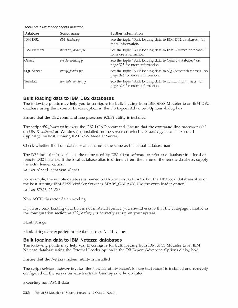
Table 58. Bulk loader scripts provided.

Database Script name Further information

IBM DB2 db2_loader.py See the topic “Bulk loading data to IBM DB2 databases” formore information.

IBM Netezza netezza_loader.py See the topic “Bulk loading data to IBM Netezza databases”for more information.

Oracle oracle_loader.py See the topic “Bulk loading data to Oracle databases” onpage 325 for more information.

SQL Server mssql_loader.py See the topic “Bulk loading data to SQL Server databases” onpage 326 for more information.

Teradata teradata_loader.py See the topic “Bulk loading data to Teradata databases” onpage 326 for more information.

Bulk loading data to IBM DB2 databasesThe following points may help you to configure for bulk loading from IBM SPSS Modeler to an IBM DB2database using the External Loader option in the DB Export Advanced Options dialog box.

Ensure that the DB2 command line processor (CLP) utility is installed

The script db2_loader.py invokes the DB2 LOAD command. Ensure that the command line processor (db2on UNIX, db2cmd on Windows) is installed on the server on which db2_loader.py is to be executed(typically, the host running IBM SPSS Modeler Server).

Check whether the local database alias name is the same as the actual database name

The DB2 local database alias is the name used by DB2 client software to refer to a database in a local orremote DB2 instance. If the local database alias is different from the name of the remote database, supplythe extra loader option:-alias <local_database_alias>

For example, the remote database is named STARS on host GALAXY but the DB2 local database alias onthe host running IBM SPSS Modeler Server is STARS_GALAXY. Use the extra loader option-alias STARS_GALAXY

Non-ASCII character data encoding

If you are bulk loading data that is not in ASCII format, you should ensure that the codepage variable inthe configuration section of db2_loader.py is correctly set up on your system.

Blank strings

Blank strings are exported to the database as NULL values.

Bulk loading data to IBM Netezza databasesThe following points may help you to configure for bulk loading from IBM SPSS Modeler to an IBMNetezza database using the External Loader option in the DB Export Advanced Options dialog box.

Ensure that the Netezza nzload utility is installed

The script netezza_loader.py invokes the Netezza utility nzload. Ensure that nzload is installed and correctlyconfigured on the server on which netezza_loader.py is to be executed.

Exporting non-ASCII data


If your export contains data that is not in ASCII format, you may need to add -encoding UTF8 to theExtra loader options field in the DB Export Advanced Options dialog box. This should ensure thatnon-ASCII data is correctly uploaded.

Date, Time and Timestamp format data

In the stream properties, set the date format to DD-MM-YYYY and the time format to HH:MM:SS.

Blank strings


Different order of columns in stream and target table when inserting data into an existing table

If the order of columns in the stream is different from that in the target table, data values will be insertedinto the wrong columns. Use a Field Reorder node to ensure that the order of columns in the streammatches the order in the target table. See the topic “Field Reorder Node” on page 170 for moreinformation.

Tracking nzload progress

When running IBM SPSS Modeler in local mode, add -sts to the Extra loader options field in the DBExport Advanced Options dialog box to see status messages every 10000 rows in the command windowopened by the nzload utility.

Bulk loading data to Oracle databasesThe following points may help you to configure for bulk loading from IBM SPSS Modeler to an Oracledatabase using the External Loader option in the DB Export Advanced Options dialog box.

Ensure that the Oracle sqlldr utility is installed

The script oracle_loader.py invokes the Oracle utility sqlldr. Note that sqlldr is not automatically included inOracle Client. Ensure that sqlldr is installed on the server on which oracle_loader.py is to be executed.

Specify the database SID or service name

If you are exporting data to a non-local Oracle server or your local Oracle server has multiple databases,you will need to specify the following in the Extra loader options field in the DB Export AdvancedOptions dialog box to pass in the SID or service name:-database <SID>

Editing the configuration section in oracle_loader.py

On UNIX (and optionally, on Windows) systems, edit the configuration section at the start of theoracle_loader.py script. Here, values for ORACLE_SID, NLS_LANG, TNS_ADMIN and ORACLE_HOMEenvironment variables can be specified if appropriate, as well as the full path of the sqlldr utility.


In the stream properties, you should normally set the date format to YYYY-MM-DD and the time formatto HH:MM:SS.

If you need to use different date and time formats from the above, consult your Oracle documentationand edit the oracle_loader.py script file.

Non-ASCII character data encoding


If you are bulk loading data that is not in ASCII format, you should ensure that the environment variableNLS_LANG is correctly set up on your system. This is read by the Oracle loader utility sqlldr. Forexample, the correct value for NLS_LANG for Shift-JIS on Windows is Japanese_Japan.JA16SJIS. For moredetails on NLS_LANG, check your Oracle documentation.

Blank strings


Bulk loading data to SQL Server databasesThe following points may help you to configure for bulk loading from IBM SPSS Modeler to a SQLServer database using the External Loader option in the DB Export Advanced Options dialog box.

Ensure that the SQL Server bcp.exe utility is installedThe script mssql_loader.py invokes the SQL Server utility bcp.exe. Ensure that bcp.exe is installed onthe server where mssql_loader.py is to be executed.

Using spaces as delimiter does not workAvoid choosing space as the delimiter in the DB Export Advanced Options dialog box.

Check table size option recommendedWe recommend that you enable the Check table size option in the DB Export Advanced Optionsdialog box. Failures in the bulk load process are not always detected, and enabling this optionperforms an extra check that the correct number of rows has been loaded.

Blank stringsBlank strings are exported to the database as NULL values.

Specify the fully qualified SQL server named instanceThere may be occasions when SPSS Modeler cannot access SQL Server due to an unqualifiedhostname and displays the following error:Error encountered while executing external bulk loader. The log file may provide more details.

To correct this error, add the following string, including the double-quotes, to the Extra loaderoptions field:"-S mhreboot.spss.com\SQLEXPRESS"

Bulk loading data to Teradata databasesThe following points may help you to configure for bulk loading from IBM SPSS Modeler to a Teradatadatabase using the External Loader option in the DB Export Advanced Options dialog box.

Ensure that the Teradata fastload utility is installed

The script teradata_loader.py invokes the Teradata utility fastload. Ensure that fastload is installed andcorrectly configured on the server on which teradata_loader.py is to be run.

Data can be bulk loaded only to empty tables

You can only use empty tables as targets for a bulk load. If a target table contains any data prior to thebulk load, the operation will fail.


In the stream properties, set the date format to YYYY-MM-DD and the time format to HH:MM:SS.

Blank strings



Teradata process ID (tdpid)

By default, fastload exports data to the Teradata system with tdpid=dbc. Usually, there will be an entry inthe HOSTS file which associates dbccop1 with the IP address of the Teradata server. To use a differentserver, specify the following in the Extra loader options field in the DB Export Advanced Options dialogbox to pass the tdpid of this server:-tdpid <id>

Spaces in table and column names

If table or column names contain spaces, bulk load operation will fail. If possible, rename the table orcolumn names to remove spaces.

Developing bulk loader programsThis topic explains how to develop a bulk loader program that can be run from IBM SPSS Modeler toload data from a text file into a database. Note that this is not covered under a standard TechnicalSupport agreement, and you should contact an IBM Services representative for assistance.

Using Python to build bulk loader programs

By default, IBM SPSS Modeler searches for a default bulk loader program based on the database type.See Table 58 on page 324.

You can use the script test_loader.py to assist in developing batch loader programs. See the topic “Testingbulk loader programs” on page 329 for more information.

Objects passed to the bulk loader program

IBM SPSS Modeler writes two files that are passed to the bulk loader program.v Data file. This contains the data to be loaded, in text format.v Schema file. This is an XML file that describes the names and types of the columns, and provides

information on how the data file is formatted (for example, what character is used as the delimiterbetween fields).

In addition, IBM SPSS Modeler passes other information such as table name, user name and password asarguments when invoking the bulk load program.

Note: To signal successful completion to IBM SPSS Modeler, the bulk loader program should delete theschema file.

Arguments passed to the bulk loader program

The arguments passed to the program are listed in the following table.

Table 59. Arguments passed to bulk loader.

Argument Description

schemafile Path of the schema file.

data file Path of the data file.

servername Name of the DBMS server; may be blank.

databasename Name of the database within the DBMS server; may be blank.

username User name to log into database.

password Password to log into database.

tablename Name of the table to load.


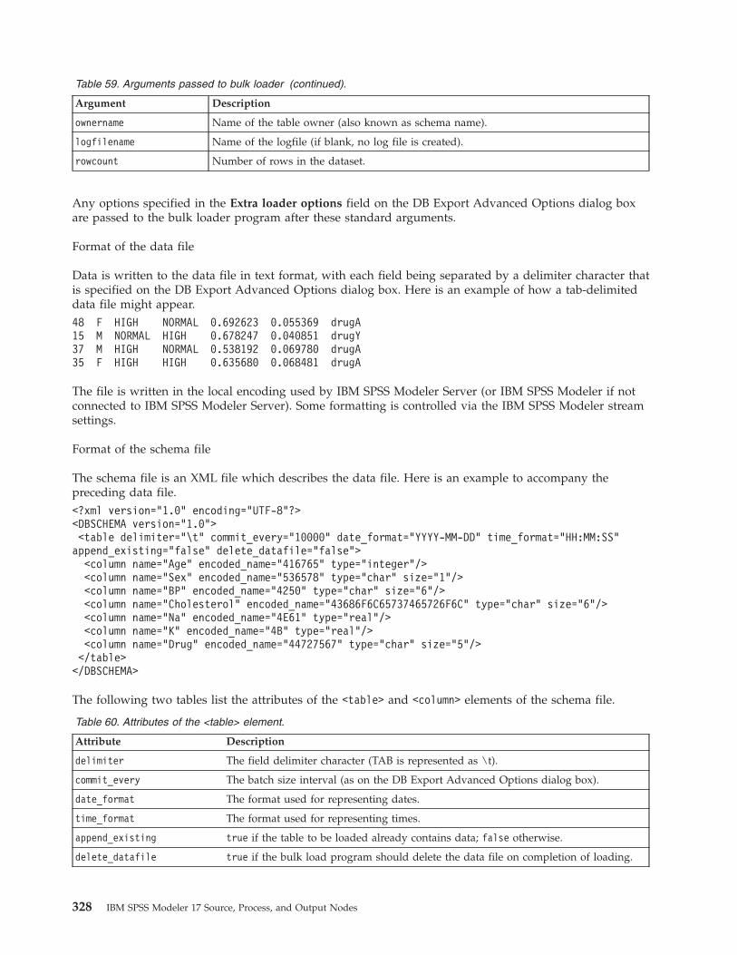
Table 59. Arguments passed to bulk loader (continued).

Argument Description

ownername Name of the table owner (also known as schema name).

logfilename Name of the logfile (if blank, no log file is created).

rowcount Number of rows in the dataset.

Any options specified in the Extra loader options field on the DB Export Advanced Options dialog boxare passed to the bulk loader program after these standard arguments.

Format of the data file

Data is written to the data file in text format, with each field being separated by a delimiter character thatis specified on the DB Export Advanced Options dialog box. Here is an example of how a tab-delimiteddata file might appear.48 F HIGH NORMAL 0.692623 0.055369 drugA15 M NORMAL HIGH 0.678247 0.040851 drugY37 M HIGH NORMAL 0.538192 0.069780 drugA35 F HIGH HIGH 0.635680 0.068481 drugA

The file is written in the local encoding used by IBM SPSS Modeler Server (or IBM SPSS Modeler if notconnected to IBM SPSS Modeler Server). Some formatting is controlled via the IBM SPSS Modeler streamsettings.

Format of the schema file

The schema file is an XML file which describes the data file. Here is an example to accompany thepreceding data file.<?xml version="1.0" encoding="UTF-8"?><DBSCHEMA version="1.0"><table delimiter="\t" commit_every="10000" date_format="YYYY-MM-DD" time_format="HH:MM:SS"append_existing="false" delete_datafile="false"><column name="Age" encoded_name="416765" type="integer"/><column name="Sex" encoded_name="536578" type="char" size="1"/><column name="BP" encoded_name="4250" type="char" size="6"/><column name="Cholesterol" encoded_name="43686F6C65737465726F6C" type="char" size="6"/><column name="Na" encoded_name="4E61" type="real"/><column name="K" encoded_name="4B" type="real"/><column name="Drug" encoded_name="44727567" type="char" size="5"/></table></DBSCHEMA>

The following two tables list the attributes of the <table> and <column> elements of the schema file.

Table 60. Attributes of the <table> element.

Attribute Description

delimiter The field delimiter character (TAB is represented as \t).

commit_every The batch size interval (as on the DB Export Advanced Options dialog box).

date_format The format used for representing dates.

time_format The format used for representing times.

append_existing true if the table to be loaded already contains data; false otherwise.

delete_datafile true if the bulk load program should delete the data file on completion of loading.


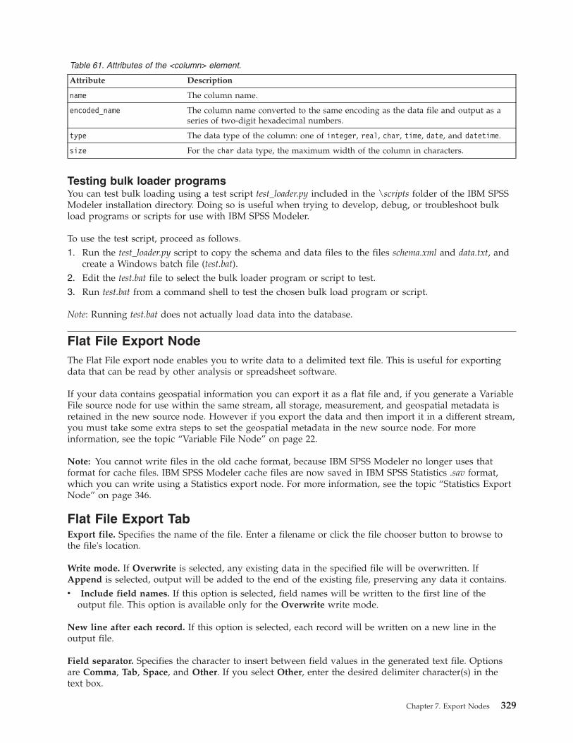
Table 61. Attributes of the <column> element.

Attribute Description

name The column name.

encoded_name The column name converted to the same encoding as the data file and output as aseries of two-digit hexadecimal numbers.

type The data type of the column: one of integer, real, char, time, date, and datetime.

size For the char data type, the maximum width of the column in characters.

Testing bulk loader programsYou can test bulk loading using a test script test_loader.py included in the \scripts folder of the IBM SPSSModeler installation directory. Doing so is useful when trying to develop, debug, or troubleshoot bulkload programs or scripts for use with IBM SPSS Modeler.

To use the test script, proceed as follows.1. Run the test_loader.py script to copy the schema and data files to the files schema.xml and data.txt, and

create a Windows batch file (test.bat).2. Edit the test.bat file to select the bulk loader program or script to test.3. Run test.bat from a command shell to test the chosen bulk load program or script.

Note: Running test.bat does not actually load data into the database.

Flat File Export NodeThe Flat File export node enables you to write data to a delimited text file. This is useful for exportingdata that can be read by other analysis or spreadsheet software.

If your data contains geospatial information you can export it as a flat file and, if you generate a VariableFile source node for use within the same stream, all storage, measurement, and geospatial metadata isretained in the new source node. However if you export the data and then import it in a different stream,you must take some extra steps to set the geospatial metadata in the new source node. For moreinformation, see the topic “Variable File Node” on page 22.

Note: You cannot write files in the old cache format, because IBM SPSS Modeler no longer uses thatformat for cache files. IBM SPSS Modeler cache files are now saved in IBM SPSS Statistics .sav format,which you can write using a Statistics export node. For more information, see the topic “Statistics ExportNode” on page 346.

Flat File Export TabExport file. Specifies the name of the file. Enter a filename or click the file chooser button to browse tothe file's location.

Write mode. If Overwrite is selected, any existing data in the specified file will be overwritten. IfAppend is selected, output will be added to the end of the existing file, preserving any data it contains.v Include field names. If this option is selected, field names will be written to the first line of the

output file. This option is available only for the Overwrite write mode.

New line after each record. If this option is selected, each record will be written on a new line in theoutput file.

Field separator. Specifies the character to insert between field values in the generated text file. Optionsare Comma, Tab, Space, and Other. If you select Other, enter the desired delimiter character(s) in thetext box.


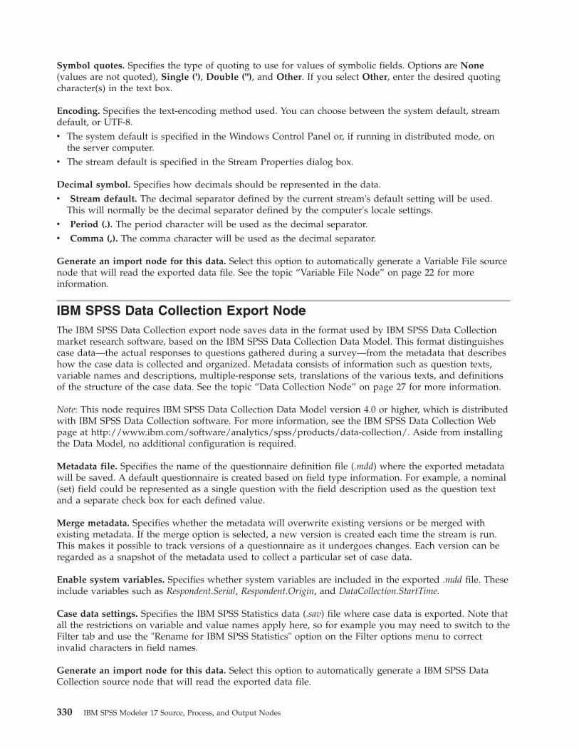
Symbol quotes. Specifies the type of quoting to use for values of symbolic fields. Options are None(values are not quoted), Single ('), Double ("), and Other. If you select Other, enter the desired quotingcharacter(s) in the text box.



Decimal symbol. Specifies how decimals should be represented in the data.v Stream default. The decimal separator defined by the current stream's default setting will be used.

This will normally be the decimal separator defined by the computer's locale settings.v Period (.). The period character will be used as the decimal separator.v Comma (,). The comma character will be used as the decimal separator.

Generate an import node for this data. Select this option to automatically generate a Variable File sourcenode that will read the exported data file. See the topic “Variable File Node” on page 22 for moreinformation.

IBM SPSS Data Collection Export NodeThe IBM SPSS Data Collection export node saves data in the format used by IBM SPSS Data Collectionmarket research software, based on the IBM SPSS Data Collection Data Model. This format distinguishescase data—the actual responses to questions gathered during a survey—from the metadata that describeshow the case data is collected and organized. Metadata consists of information such as question texts,variable names and descriptions, multiple-response sets, translations of the various texts, and definitionsof the structure of the case data. See the topic “Data Collection Node” on page 27 for more information.

Note: This node requires IBM SPSS Data Collection Data Model version 4.0 or higher, which is distributedwith IBM SPSS Data Collection software. For more information, see the IBM SPSS Data Collection Webpage at http://www.ibm.com/software/analytics/spss/products/data-collection/. Aside from installingthe Data Model, no additional configuration is required.

Metadata file. Specifies the name of the questionnaire definition file (.mdd) where the exported metadatawill be saved. A default questionnaire is created based on field type information. For example, a nominal(set) field could be represented as a single question with the field description used as the question textand a separate check box for each defined value.

Merge metadata. Specifies whether the metadata will overwrite existing versions or be merged withexisting metadata. If the merge option is selected, a new version is created each time the stream is run.This makes it possible to track versions of a questionnaire as it undergoes changes. Each version can beregarded as a snapshot of the metadata used to collect a particular set of case data.

Enable system variables. Specifies whether system variables are included in the exported .mdd file. Theseinclude variables such as Respondent.Serial, Respondent.Origin, and DataCollection.StartTime.

Case data settings. Specifies the IBM SPSS Statistics data (.sav) file where case data is exported. Note thatall the restrictions on variable and value names apply here, so for example you may need to switch to theFilter tab and use the "Rename for IBM SPSS Statistics" option on the Filter options menu to correctinvalid characters in field names.

Generate an import node for this data. Select this option to automatically generate a IBM SPSS DataCollection source node that will read the exported data file.


http://www.ibm.com/software/analytics/spss/products/data-collection/

Multiple response sets. Any multiple response sets defined in the stream will automatically be preservedwhen the file is exported. You can view and edit multiple response sets from any node with a Filter tab.See the topic “Editing Multiple Response Sets” on page 132 for more information.

Analytic Server Export NodeThe Analytic Server Export node enables you to write data from your analysis to an existing AnalyticServer data source. This can, for example, be text files on Hadoop Distributed File System (HDFS) or adatabase.

Typically, a stream with an Analytic Server Export node also begins with Analytic Server Source nodes,and is submitted to the Analytic Server and executed on HDFS. Alternatively, a stream with "local" datasources can end with an Analytic Server Export node in order to upload relatively small datasets (nomore than 100,000 records) for use with Analytic Server.

Data source. Select a data source containing the data you wish to use. A data source contains the filesand metadata associated with that source. Click Select to display a list of available data sources. See thetopic “Selecting a data source” on page 10 for more information.

If you need to create a new data source or edit an existing one, click Launch Data Source Editor....

Mode. Select Append to add to the existing data source, or Overwrite to replace the contents of the datasource.

Generate an Import node for this data. Select to generate a source node for the data as exported to thespecified data source. This node is added to the stream canvas.

IBM Cognos BI Export NodeThe IBM Cognos BI Export node enables you to export data from an IBM SPSS Modeler stream toCognos BI, in UTF-8 format. In this way, Cognos BI can make use of transformed or scored data fromIBM SPSS Modeler. For example, you could use Cognos BI Report Studio to create a report based on theexported data, including the predictions and confidence values. The report could then be saved on theCognos BI server and distributed to Cognos BI users.

Note: You can export only relational data, not OLAP data.

To export data to Cognos BI, you need to specify the following:v Cognos connection - the connection to the Cognos BI serverv ODBC connection - the connection to the Cognos data server that the Cognos BI server uses

Within the Cognos connection you specify a Cognos data source to use. This data source must use thesame login as the ODBC data source.

You export the actual stream data to the data server, and the package metadata to the Cognos BI server.

As with any other export node, you can also use the Publish tab of the node dialog box to publish thestream for deployment using IBM SPSS Modeler Solution Publisher.

Cognos connectionThis is where you specify the connection to the Cognos BI server that you want to use for the export. Theprocedure involves exporting the metadata to a new package on the Cognos BI server, while the streamdata is exported to the Cognos data server.


Connection. Click the Edit button to display a dialog box where you can define the URL and otherdetails of the Cognos BI server to which you want to export the data. If you are already logged in to aCognos BI server through IBM SPSS Modeler, you can also edit the details of the current connection. Seethe topic “Cognos connections” on page 34 for more information.

Data source. The name of the Cognos data source (typically a database) to which you are exporting thedata. The drop-down list shows all the Cognos data sources that you can access from the currentconnection. Click the Refresh button to update the list.

Folder. The path and name of the folder on the Cognos BI server where the export package is to becreated.

Package name. The name of the package in the specified folder that is to contain the exported metadata.This must be a new package with a single query subject; you cannot export to an existing package.

Mode. Specifies how you want to perform the export:v Publish package now. (default) Performs the export operation as soon as you click Run.v Export action script. Creates an XML script that you can run later (for example, using Framework

Manager) to perform the export. Type the path and file name for the script in the File field, or use theEdit button to specify the name and location of the script file.

Generate an import node for this data. Select to generate a source node for the data as exported to thespecified data source and table. When you click Run, this node is added to the stream canvas.

ODBC connectionHere you specify the connection to the Cognos data server (that is, the database) to which the streamdata is to be exported.

Note: You must ensure that the data source you specify here points to the same one specified on theCognos connections panel. You must also ensure that the Cognos connection data source uses the samelogin as the ODBC data source.

Data source. Shows the selected data source. Enter the name or select it from the drop-down list. If youdon't see the desired database in the list, select Add new database connection and locate your databasefrom the Database Connections dialog box. See the topic “Adding a database connection” on page 16 formore information.

Table name. Enter the name of the table to which you want to send the data. If you select the Insert intotable option, you can select an existing table in the database by clicking the Select button.

Create table. Select this option to create a new database table or to overwrite an existing database table.

Insert into table. Select this option to insert the data as new rows in an existing database table.

Merge table. (Where available) Select this option to update selected database columns with values fromcorresponding source data fields. Selecting this option enables the Merge button, which displays a dialogfrom where you can map source data fields to database columns.

Drop existing table. Select this option to delete any existing table with the same name when creating anew table.

Delete existing rows. Select this option to delete existing rows from the table before exporting, wheninserting into a table.


Note: If either of the two options above are selected, you will receive an Overwrite warning messagewhen you execute the node. To suppress the warnings, deselect Warn when a node overwrites adatabase table on the Notifications tab of the User Options dialog box.

Default string size. Fields you have marked as typeless in an upstream Type node are written to thedatabase as string fields. Specify the size of strings to be used for typeless fields.

Click Schema to open a dialog box where you can set various export options (for databases that supportthis feature), set SQL data types for your fields, and specify the primary key for purposes of databaseindexing. See the topic “Database Export Schema Options” on page 318 for more information.

Click Indexes to specify options for indexing the exported table in order to improve databaseperformance. See the topic “Database Export Index Options” on page 320 for more information.

Click Advanced to specify bulk loading and database commit options. See the topic “Database ExportAdvanced Options” on page 322 for more information.

Quote table and column names. Select options used when sending a CREATE TABLE statement to thedatabase. Tables or columns with spaces or nonstandard characters must be quoted.v As needed. Select to allow IBM SPSS Modeler to automatically determine when quoting is needed on

an individual basis.v Always. Select to always enclose table and column names in quotes.v Never. Select to disable the use of quotes.

Generate an import node for this data. Select to generate a source node for the data as exported to thespecified data source and table. When you click Run, this node is added to the stream canvas.

IBM Cognos TM1 Export NodeThe IBM Cognos BI Export node enables you to export data from an IBM SPSS Modeler stream toCognos TM1. In this way, Cognos BI can make use of transformed or scored data from IBM SPSSModeler.

Note: You can export only measures not context dimension data; alternatively, you can add new elementsto the cube.

To export data to Cognos BI, you need to specify the following:v The connection to the Cognos TM1 server.v The Cube into which the data will be exported.v The mapping from the SPSS data names to the equivalent TM1 dimensions and measures.

Note: The TM1 user needs the following permissions: Write privilege of cubes, Read privilege of SPSSprocesses, Read privilege of dimensions, Write privilege of dimension elements, and Write privilege of.blb files.

As with any other export node, you can also use the Publish tab of the node dialog box to publish thestream for deployment using IBM SPSS Modeler Solution Publisher.

Note: Before you can use the TM1 Source or Export nodes in SPSS Modeler, you must copy the followingthree processes from Modeler to the TM1 server: exporttospss.pro, importfromspss.pro, andspsscreatenewmeasures.pro. To add these processes to the TM1 server you must copy them to the datadirectory of the TM1 server and restart the TM1 server. These files are available from within thefollowing directory: <Modeler install directory>/ext/bin/pasw.tm1/scripts.


Connecting to an IBM Cognos TM1 cube to export dataThe first step in exporting data to an IBM Cognos TM1 database is to select the relevant TM1Performance Management system, and associated server and cube, on the Connection tab of the IBMCognos TM1 dialog box.

Note: Only actual "null" values will be discarded when exporting data to TM1. Zero (0) values will beexported as a valid value. Also note that only fields with a storage type of string can be mapped todimensions on the Mapping tab. Before exporting to TM1, you must use IBM SPSS Modeler client toconvert non-string data types to string.

PM System Type the URL of the Performance Management system where the TM1 server you want toconnect to is installed. The Performance Management system is defined as a single URL for all TM1servers. From this URL, all IBM Cognos TM1 servers installed and running on your environment can bediscovered and accessed.

TM1 Server When you have established the connection to the Performance Management system, selectthe server that contains the data you want to import and click Login. If you have not previouslyconnected to this server you are prompted to enter your User name and Password; alternatively, you canselect another server.

Select a TM1 cube to export Displays the name of the cubes within the TM1 server into which you canexport data.

To choose the data to export, select the cube and click the right arrow to move the cube into the Exportto cube field. When you have selected the cube, use the Mapping tab to map the TM1 dimensions andmeasures to the relevant SPSS fields or to a fixed value (Slice on operation).

Mapping IBM Cognos TM1 data for exportAfter you select the IBM Cognos TM1 Performance Management system and associated TM1 server andcube, use the Mapping tab of the IBM Cognos TM1 Export dialog box to map TM1 dimensions andmeasures to SPSS fields or slice TM1 dimensions to a fixed value.

Note: Only fields with a storage type of string can be mapped to dimensions. Before exporting to TM1,you must use IBM SPSS Modeler client to convert non-string data types to string.

Fields. Lists the data field names from the SPSS data file that are available for export.

TM1 Dimensions. Shows the TM1 cube selected on the Connection tab, along with its regular andmeasure dimensions. Select the name of the TM1 dimension to either map to the SPSS data field or toslice it to a fixed value. For cubes with many items, it may be helpful to use the buttons at the bottom ofthe list to filter the dimensions shown. For example, you can show all dimensions, just regulardimensions, or just measure dimensions.

The following options are available on the Mapping tab.

Slice on. Fields that have been sliced are labeled with an S. Slice on is a term used by IBM Cognos TM1to fix a dimension to a specific element. See the following example of data imported from TM1. Noticethe first three columns have repeating values for every row (for example, region has a fixed value of worldfor every row). Instead of exporting this data back to TM1 for every row of data, you can use the Sliceon feature to fix the value of the dimension (region in this example) to the element called world.


Table 62. Slice on example

region actvsbud model month units gross margin salesvariablecosts

world variance A January 72 -117.66 -157.11 -39.45

world variance A February 4 -72.09 360.29 432.38

world variance A March -4 -539.21 45.52 584.73

When you select a dimension and click Slice on, a dialog will be displayed that shows the leaf membersof the selected dimension. You can only slice on leaf members.

Map. Maps the selected SPSS data field to the selected TM1 dimension or measure (a regular dimensionor a specific measure from the measure dimension). Mapped fields are labeled with an M.

Unmap. Unmaps the selected SPSS data field from the selected TM1 dimension or measure. Note thatyou can only unmap a single mapping at a time. The unmapped SPSS data field will be moved back tothe left column.

Create New. Creates a new measure in the TM1 measure dimension. A dialog will be displayed allowingyou to enter a name for the new TM1 measure. This option is only available for measure dimensions, notfor regular dimensions.

For more information about TM1, see the IBM Cognos Insight documentation at http://pic.dhe.ibm.com/infocenter/ctm1/v10r2m0/index.jsp.

SAS Export NodeNote: This feature is available in SPSS Modeler Professional and SPSS Modeler Premium.

The SAS export node enables you to write data in SAS format to be read into SAS or a SAS-compatiblesoftware package. You can export in three SAS file formats: SAS for Windows/OS2, SAS for UNIX, orSAS Version 7/8.

SAS Export Node Export TabExport file. Specify the name of the file. Enter a filename or click the file chooser button to browse to thefile's location.

Export. Specify the export file format. Options are SAS for Windows/OS2, SAS for UNIX, or SASVersion 7/8.

Export field names. Select options for exporting field names and labels from IBM SPSS Modeler for usewith SAS.v Names and variable labels. Select to export both IBM SPSS Modeler field names and field labels.

Names are exported as SAS variable names, while labels are exported as SAS variable labels.v Names as variable labels. Select to use the IBM SPSS Modeler field names as variable labels in SAS.

IBM SPSS Modeler allows characters in field names that are invalid in SAS variable names. To preventpossibly creating invalid SAS names, select Names and variable labels instead.

Generate an import node for this data. Select this option to automatically generate a SAS source nodethat will read the exported data file. See the topic “SAS Source Node” on page 36 for more information.


http://pic.dhe.ibm.com/infocenter/ctm1/v10r2m0/index.jsp

http://pic.dhe.ibm.com/infocenter/ctm1/v10r2m0/index.jsp

Excel Export NodeThe Excel export node outputs data in Microsoft Excel .xlsx format. Optionally, you can choose toautomatically launch Excel and open the exported file when the node is executed.

Excel Node Export TabFile name. Enter a filename or click the file chooser button to browse to the file's location. The defaultfilename is excelexp.xlsx.

File type. The Excel .xlsx file format is supported.

Create new file. Creates a new Excel file.

Insert into existing file. Content is replaced beginning at the cell designated by the Start in cell field.Other cells in the spreadsheet are left with their original content.

Include field names. Specifies whether field names should be included in the first row of the worksheet.

Start in cell. The cell location used for the first export record (or first field name if Include field namesis checked). Data are filled to the right and down from this initial cell.

Choose worksheet. Specifies the worksheet to which you want to export the data. You can identify theworksheet either by index or by name:v By index. If you are creating a new file, specify a number from 0 to 9 to identify the worksheet to

which you want to export, beginning with 0 for the first worksheet, 1 for the second worksheet, and soon. You can use values of 10 or higher only if a worksheet already exists at this position.

v By name. If you are creating a new file, specify the name used for the worksheet. If you are insertinginto an existing file, the data are inserted into this worksheet if it exists, otherwise a new worksheetwith this name is created.

Launch Excel. Specifies whether Excel is automatically launched on the exported file when the node isexecuted. Note that when running in distributed mode against IBM SPSS Modeler Server, the output issaved to the server file system, and Excel is launched on the Client with a copy of the exported file.

Generate an import node for this data. Select this option to automatically generate an Excel source nodethat will read the exported data file. See the topic “Excel Source Node” on page 37 for more information.

XML Export NodeThe XML Export node enables you to output data in XML format, using UTF-8 encoding. You canoptionally create an XML source node to read the exported data back into the stream.

XML export file. The full path and file name of the XML file to which you want to export the data.

Use XML schema. Select this check box if you want to use a schema or DTD to control the structure ofthe exported data. Doing so activates the Map button, described below.

If you do not use a schema or DTD, the following default structure is used for the exported data:<records>

<record><fieldname1>value</fieldname1><fieldname2>value</fieldname2>

:<fieldnameN>value</fieldnameN>

</record>


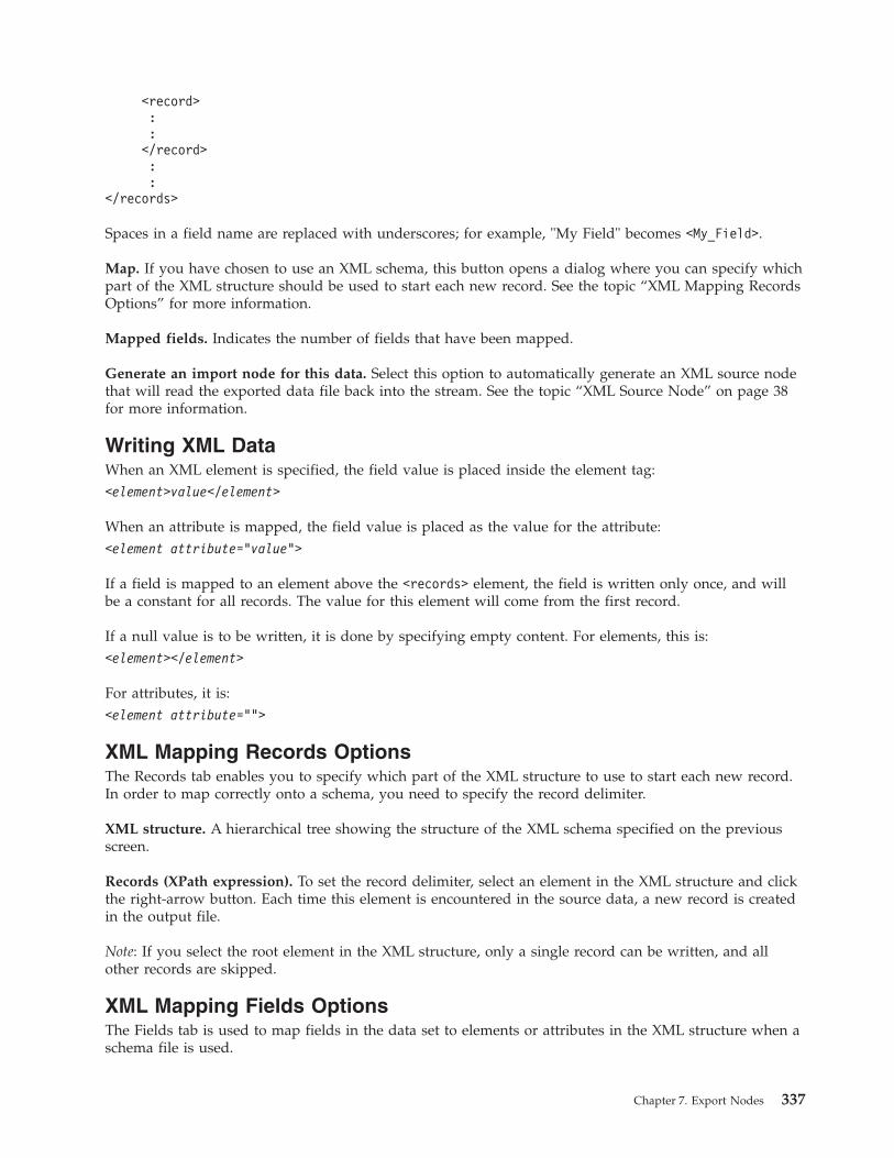
<record>::</record>::

</records>

Spaces in a field name are replaced with underscores; for example, "My Field" becomes <My_Field>.

Map. If you have chosen to use an XML schema, this button opens a dialog where you can specify whichpart of the XML structure should be used to start each new record. See the topic “XML Mapping RecordsOptions” for more information.

Mapped fields. Indicates the number of fields that have been mapped.

Generate an import node for this data. Select this option to automatically generate an XML source nodethat will read the exported data file back into the stream. See the topic “XML Source Node” on page 38for more information.

Writing XML DataWhen an XML element is specified, the field value is placed inside the element tag:<element>value</element>

When an attribute is mapped, the field value is placed as the value for the attribute:<element attribute=”value”>

If a field is mapped to an element above the <records> element, the field is written only once, and willbe a constant for all records. The value for this element will come from the first record.

If a null value is to be written, it is done by specifying empty content. For elements, this is:<element></element>

For attributes, it is:<element attribute=””>

XML Mapping Records OptionsThe Records tab enables you to specify which part of the XML structure to use to start each new record.In order to map correctly onto a schema, you need to specify the record delimiter.

XML structure. A hierarchical tree showing the structure of the XML schema specified on the previousscreen.

Records (XPath expression). To set the record delimiter, select an element in the XML structure and clickthe right-arrow button. Each time this element is encountered in the source data, a new record is createdin the output file.

Note: If you select the root element in the XML structure, only a single record can be written, and allother records are skipped.

XML Mapping Fields OptionsThe Fields tab is used to map fields in the data set to elements or attributes in the XML structure when aschema file is used.


Field names that match an element or attribute name are automatically mapped as long as the element orattribute name is unique. Thus if there is both an element and an attribute with the name field1, there isno automatic mapping. If there is only one item in the structure named field1, a field with that name inthe stream is automatically mapped.

Fields. The list of fields in the model. Select one or more fields as the source part of the mapping. Youcan use the buttons at the bottom of the list to select all fields, or all fields with a particular measurementlevel.

XML structure. Select an element in the XML structure as the map target. To create the mapping, clickMap. The mapping is then displayed. The number of fields that have been mapped in this way isdisplayed below this list.

To remove a mapping, select the item in the XML structure list and click Unmap.

Display attributes. Displays or hides the attributes, if any, of the XML elements in the XML structure.

XML Mapping PreviewOn the Preview tab, click Update to see a preview of the XML that will be written.

If the mapping is incorrect, return to the Records or Fields tab to correct the errors and click Updateagain to see the result.


Chapter 8. IBM SPSS Statistics Nodes

IBM SPSS Statistics Nodes - OverviewTo complement IBM SPSS Modeler and its data mining abilities, IBM SPSS Statistics provides you withthe ability to carry out further statistical analysis and data management.

If you have a compatible, licensed copy of IBM SPSS Statistics installed, you can connect to it from IBMSPSS Modeler and carry out complex, multistep data manipulation and analysis not otherwise supportedby IBM SPSS Modeler. For the advanced user there is also the option to further modify the analyses byusing command syntax. See the Release Notes for information on version compatibility.

If available, the IBM SPSS Statistics nodes are shown on a dedicated part of the nodes palette.

Note: We recommend that you instantiate your data in a Type node before using the IBM SPSS StatisticsTransform, Model, or Output nodes. This is also a requirement when using the AUTORECODE syntaxcommand.

The IBM SPSS Statistics palette contains the following nodes:

The Statistics File node reads data from the .sav or .zsav file format used by IBM SPSSStatistics, as well as cache files saved in IBM SPSS Modeler, which also use the same format.

The Statistics Transform node runs a selection of IBM SPSS Statistics syntax commandsagainst data sources in IBM SPSS Modeler. This node requires a licensed copy of IBM SPSSStatistics.

The Statistics Model node enables you to analyze and work with your data by running IBMSPSS Statistics procedures that produce PMML. This node requires a licensed copy of IBMSPSS Statistics.

The Statistics Output node allows you to call an IBM SPSS Statistics procedure to analyzeyour IBM SPSS Modeler data. A wide variety of IBM SPSS Statistics analytical procedures isavailable. This node requires a licensed copy of IBM SPSS Statistics.

The Statistics Export node outputs data in IBM SPSS Statistics .sav or .zsav format. The .sav or.zsav files can be read by IBM SPSS Statistics Base and other products. This is also the formatused for cache files in IBM SPSS Modeler.

Note: If your copy of SPSS Statistics is licensed for a single user only and you run a stream with two ormore branches, each of which contains an SPSS Statistics node, you may receive a licensing error. This


occurs when the SPSS Statistics session for one branch has not terminated before the session for anotherbranch attempts to start. If possible, redesign the stream so that multiple branches with SPSS Statisticsnodes do not execute in parallel.

Statistics File NodeYou can use the Statistics File node to read data directly from a saved IBM SPSS Statistics file (.sav or.zsav). This format is now used to replace the cache file from earlier versions of IBM SPSS Modeler. If youwould like to import a saved cache file, you should use the IBM SPSS Statistics File node.

Import file. Specify the name of the file. You can enter a filename or click the ellipsis button (...) to selecta file. The file path is shown once you have selected a file.

File is password encrypted. Select this box if you know the file is password protected; you are theprompted to enter the Password. If the file is password protected, and you do not enter the password, awarning message is displayed if you attempt to change to another tab, refresh the data, preview the nodecontents, or try to execute a stream containing the node.

Note: Password protected files can only be opened by IBM SPSS Modeler version 16 or greater.

Variable names. Select a method of handling variable names and labels upon import from an IBM SPSSStatistics .sav or .zsav file. Metadata that you choose to include here persists throughout your work inIBM SPSS Modeler and may be exported again for use in IBM SPSS Statistics.v Read names and labels. Select to read both variable names and labels into IBM SPSS Modeler. By

default, this option is selected and variable names are displayed in the Type node. Labels may bedisplayed in charts, model browsers, and other types of output, depending on the options specified inthe stream properties dialog box. By default, the display of labels in output is disabled.

v Read labels as names. Select to read the descriptive variable labels from the IBM SPSS Statistics .savor .zsav file rather than the short field names, and use these labels as variable names in IBM SPSSModeler.

Values. Select a method of handling values and labels upon import from an IBM SPSS Statistics .sav or.zsav file. Metadata that you choose to include here persists throughout your work in IBM SPSS Modelerand may be exported again for use in IBM SPSS Statistics.v Read data and labels. Select to read both actual values and value labels into IBM SPSS Modeler. By

default, this option is selected and values themselves are displayed in the Type node. Value labels maybe displayed in the Expression Builder, charts, model browsers, and other types of output, dependingon the options specified in the stream properties dialog box.

v Read labels as data. Select if you want to use the value labels from the .sav or .zsav file rather than thenumerical or symbolic codes used to represent the values. For example, selecting this option for datawith a gender field whose values of 1 and 2 actually represent male and female, respectively, willconvert the field to a string and import male and female as the actual values.It is important to consider missing values in your IBM SPSS Statistics data before selecting this option.For example, if a numeric field uses labels only for missing values (0 = No Answer, –99 = Unknown),then selecting the option above will import only the value labels No Answer and Unknown and willconvert the field to a string. In such cases, you should import the values themselves and set missingvalues in a Type node.

Use field format information to determine storage. If this box is cleared, field values that are formattedin the .sav file as integers (i.e., fields specified as Fn.0 in the Variable View in IBM SPSS Statistics) areimported using integer storage. All other field values except strings are imported as real numbers.

If this box is selected (default), all field values except strings are imported as real numbers, whetherformatted in the .sav file as integers or not.


Multiple response sets. Any multiple response sets defined in the IBM SPSS Statistics file willautomatically be preserved when the file is imported. You can view and edit multiple response sets fromany node with a Filter tab. See the topic “Editing Multiple Response Sets” on page 132 for moreinformation.

Statistics Transform NodeThe Statistics Transform node enables you to complete data transformations using IBM SPSS Statisticscommand syntax. This makes it possible to complete a number of transformations not supported by IBMSPSS Modeler and allows automation of complex, multistep transformations, including the creation of anumber of fields from a single node. It resembles the Statistics Output node, except that the data arereturned to IBM SPSS Modeler for further analysis, whereas, in the Output node the data are returned asthe requested output objects, such as graphs or tables.

You must have a compatible version of IBM SPSS Statistics installed and licensed on your computer touse this node. See the topic “IBM SPSS Statistics Helper Applications” on page 312 for more information.See the Release Notes for compatibility information.

If necessary, you can use the Filter tab to filter or rename fields so they conform to IBM SPSS Statisticsnaming standards. See the topic “Renaming or Filtering Fields for IBM SPSS Statistics” on page 347 formore information.

Syntax Reference. For details on specific IBM SPSS Statistics procedures, see the IBM SPSS StatisticsCommand Syntax Reference guide, included with your copy of the IBM SPSS Statistics software. To viewthe guide from the Syntax tab, choose the Syntax editor option and click the Launch IBM SPSS StatisticsSyntax Help button.

Note: Not all IBM SPSS Statistics syntax is supported by this node. See the topic “Allowable Syntax” formore information.

Statistics Transform Node - Syntax TabIBM SPSS Statistics dialog option

If you are unfamiliar with IBM SPSS Statistics syntax for a procedure, the simplest way to create syntaxin IBM SPSS Modeler is to choose the IBM SPSS Statistics dialog option, select the dialog box for theprocedure, complete the dialog box and click OK. Doing so places the syntax onto the Syntax tab of theIBM SPSS Statistics node you are using in IBM SPSS Modeler. You can then run the stream to obtain theoutput from the procedure.

IBM SPSS Statistics Syntax editor option

Check. After you have entered your syntax commands in the upper part of the dialog box, use thisbutton to validate your entries. Any incorrect syntax is identified in the bottom part of the dialog box.

To ensure that the checking process does not take too long, when you validate the syntax, it is checkedagainst a representative sample of your data to ensure that the entries are valid instead of checkingagainst the entire dataset.

Allowable SyntaxIf you have a lot of legacy syntax from IBM SPSS Statistics or are familiar with the data preparationfeatures of IBM SPSS Statistics, you can use the Statistics Transform node to run many of your existingtransformations. As a guideline, the node enables you to transform data in predictable ways--for example,by running looped commands or by changing, adding, sorting, filtering, or selecting data.

Examples of the commands that can be carried out are:

Chapter 8. IBM SPSS Statistics Nodes 341

v Compute random numbers according to a binomial distribution:COMPUTE newvar = RV.BINOM(10000,0.1)

v Recode a variable into a new variable:RECODE Age (Lowest thru 30=1) (30 thru 50=2) (50 thru Highest=3) INTO AgeRecoded

v Replace missing values:RMV Age_1=SMEAN(Age)

The IBM SPSS Statistics syntax that is supported by the Statistics Transform node is listed below.

Command Name

ADD VALUE LABELS

APPLY DICTIONARY

AUTORECODE

BREAK

CD

CLEAR MODEL PROGRAMS

CLEAR TIME PROGRAM

CLEAR TRANSFORMATIONS

COMPUTE

COUNT

CREATE

DATE

DEFINE-!ENDDEFINE

DELETE VARIABLES

DO IF

DO REPEAT

ELSE

ELSE IF

END CASE

END FILE

END IF

END INPUT PROGRAM

END LOOP

END REPEAT

EXECUTE

FILE HANDLE

FILE LABEL

FILE TYPE-END FILE TYPE

FILTER

FORMATS

IF

INCLUDE

INPUT PROGRAM-END INPUT PROGRAM


Command Name

INSERT

LEAVE

LOOP-END LOOP

MATRIX-END MATRIX

MISSING VALUES

N OF CASES

NUMERIC

PERMISSIONS

PRESERVE

RANK

RECODE

RENAME VARIABLES

RESTORE

RMV

SAMPLE

SELECT IF

SET

SORT CASES

STRING

SUBTITLE

TEMPORARY

TITLE

UPDATE

V2C

VALIDATEDATA

VALUE LABELS

VARIABLE ATTRIBUTE

VARSTOCASES

VECTOR

Statistics Model NodeThe Statistics Model node enables you to analyze and work with your data by running IBM SPSSStatistics procedures that produce PMML. The model nuggets you create can then be used in the usualway within IBM SPSS Modeler streams for scoring, and so on.


The IBM SPSS Statistics analytical procedures that are available depend on the type of license you have.


Statistics Model Node - Model TabModel name. You can generate the model name automatically based on the target or ID field (or modeltype in cases where no such field is specified) or specify a custom name.

Select a dialog. Click to display a list of available IBM SPSS Statistics procedures that you can select andrun. The list shows only those procedures that produce PMML and for which you are licensed, and doesnot include user-written procedures.1. Click on the required procedure; the relevant IBM SPSS Statistics dialog is displayed.2. In the IBM SPSS Statistics dialog, enter the details for the procedure.3. Click OK to return to the Statistics Model node; the IBM SPSS Statistics syntax is displayed in the

Model tab.4. To return to the IBM SPSS Statistics dialog at any time, for example to modify your query, click the

IBM SPSS Statistics dialog display button to the right of the procedure selection button.

Statistics Model Node - Model Nugget SummaryWhen you run the Statistics Model node, it executes the associated IBM SPSS Statistics procedure andcreates a model nugget that you can use in IBM SPSS Modeler streams for scoring.

The Summary tab of the model nugget displays information about the fields, build settings, and modelestimation process. Results are presented in a tree view that can be expanded or collapsed by clickingspecific items.

The View Model button displays the results in a modified form of the IBM SPSS Statistics OutputViewer. For more information about this viewer, see the IBM SPSS Statistics documentation.

The usual exporting and printing options are available from the File menu. See the topic “ViewingOutput” on page 276 for more information.

Statistics Output NodeThe Statistics Output node enables you to call an IBM SPSS Statistics procedure to analyze your IBMSPSS Modeler data. You can view the results in a browser window or save results in the IBM SPSSStatistics output file format. A wide variety of IBM SPSS Statistics analytical procedures is accessible fromIBM SPSS Modeler.


If necessary, you can use the Filter tab to filter or rename fields so they conform to IBM SPSS Statisticsnaming standards. See the topic “Renaming or Filtering Fields for IBM SPSS Statistics” on page 347 formore information.

Syntax Reference. For details on specific IBM SPSS Statistics procedures, see the IBM SPSS StatisticsCommand Syntax Reference guide, included with your copy of the IBM SPSS Statistics software. To viewthe guide from the Syntax tab, choose the Syntax editor option and click the Launch IBM SPSS StatisticsSyntax Help button.

Statistics Output Node - Syntax TabUse this tab to create syntax for the IBM SPSS Statistics procedure you want to use to analyze your data.Syntax is composed of two parts: a statement and associated options. The statement specifies the analysisor operation to be performed and the fields to be used. The options specify everything else, includingwhich statistics to display, derived fields to save, and so on.


IBM SPSS Statistics dialog option

If you are unfamiliar with IBM SPSS Statistics syntax for a procedure, the simplest way to create syntaxin IBM SPSS Modeler is to choose the IBM SPSS Statistics dialog option, select the dialog box for theprocedure, complete the dialog box and click OK. Doing so places the syntax onto the Syntax tab of theIBM SPSS Statistics node you are using in IBM SPSS Modeler. You can then run the stream to obtain theoutput from the procedure.

You can optionally generate a Statistics File source node for importing the resulting data. This is useful,for example, if a procedure writes fields such as scores to the active dataset in addition to displayingoutput.

To create the syntax:1. Click the Select a dialog button.2. Choose one of the options:

v Analyze. Lists the contents of the IBM SPSS Statistics Analyze menu; choose the procedure youwant to use.

v Other. If shown, lists dialogs created by the Custom Dialog Builder in IBM SPSS Statistics, as wellas any other IBM SPSS Statistics dialogs that do not appear on the Analyze menu and for whichyou have a licence. If there are no applicable dialogs, this option is not shown.

Note: The Automatic Data Preparation dialogs are not shown.

If you have an IBM SPSS Statistics custom dialog that creates new fields, these fields cannot be used inIBM SPSS Modeler because the Statistics Output node is a terminal node.

Optionally check the Generate an import node for the resulting data box to create a Statistics File sourcenode that can be used to import the resulting data into another stream. The node is placed on the screencanvas, with the data contained in the .sav file specified in the File field (default location is the IBM SPSSModeler installation directory).

Syntax editor option

To save syntax that has been created for a frequently used procedure:1. Click the File Options button (the first one on the toolbar).2. Choose Save or Save As from the menu.3. Save the file as an .sps file.

To use previously created syntax files, replacing the current contents, if any, of the Syntax editor:1. Click the File Options button (the first one on the toolbar).2. Choose Open from the menu.3. Select an .sps file to paste its contents into the Output node Syntax tab.

To insert previously saved syntax without replacing the current contents:1. Click the File Options button (the first one on the toolbar).2. Choose Insert from the menu3. Select an .sps file to paste its contents into the Output node at the point specified by the cursor.

Optionally check the Generate an import node for the resulting data box to create a Statistics File sourcenode that can be used to import the resulting data into another stream. The node is placed on the screencanvas, with the data contained in the .sav file specified in the File field (default location is the IBM SPSSModeler installation directory).


When you click Run, the results are shown in the IBM SPSS Statistics Output Viewer. For moreinformation about the viewer, see the IBM SPSS Statistics documentation.

Statistics Output Node - Output TabThe Output tab lets you specify the format and location of the output. You can choose to display theresults on the screen or send them to one of the available file types.

Output name. Specifies the name of the output produced when the node is executed. Auto chooses aname based on the node that generates the output. Optionally, you can select Custom to specify adifferent name.

Output to screen (the default). Creates an output object to view online. The output object will appear onthe Outputs tab of the manager window when the output node is executed.

Output to file. Saves the output to a file when you run the node. If you choose this option, enter afilename in the Filename field (or navigate to a directory and specify a filename using the File Chooserbutton) and select a file type.

File type. Choose the type of file to which you want to send the output.v HTML document (*.html). Writes the output in HTML format.v IBM SPSS Statistics Viewer File (*.spv). Writes the output in a format that can be read by the IBM

SPSS Statistics Output Viewer.v IBM SPSS Statistics Web Reports File (*.spw). Writes the output in IBM SPSS Statistics Web Reports

format, which can be published to an IBM SPSS Collaboration and Deployment Services repository andsubsequently viewed in a Web browser. See the topic “Publish to Web” on page 277 for moreinformation.

Note: If you select Output to screen the IBM SPSS Statistics OMS directive VIEWER=NO has no effect; also,the scripting APIs (Basic and Python SpssClient module) are not available in IBM SPSS Modeler.

Statistics Export NodeThe Statistics Export node enables you to export data in IBM SPSS Statistics .sav format. IBM SPSSStatistics .sav files can be read by IBM SPSS Statistics Base and other modules. This is also the formatused for IBM SPSS Modeler cache files.

Mapping IBM SPSS Modeler field names to IBM SPSS Statistics variable names can sometimes causeerrors because IBM SPSS Statistics variable names are limited to 64 characters and cannot include certaincharacters, such as spaces, dollar signs ($), and dashes (–). There are two ways to adjust for theserestrictions:v You can rename fields conforming to IBM SPSS Statistics variable name requirements by clicking the

Filter tab. See the topic “Renaming or Filtering Fields for IBM SPSS Statistics” on page 347 for moreinformation.

v Choose to export both field names and labels from IBM SPSS Modeler.

Note: IBM SPSS Modeler writes .sav files in Unicode UTF-8 format. IBM SPSS Statistics only supportsfiles in Unicode UTF-8 format from release 16.0 onwards. To prevent the possibility of data corruption.sav files saved with Unicode encoding should not be used in releases of IBM SPSS Statistics prior to 16.0.For more information, see the IBM SPSS Statistics help.

Multiple response sets. Any multiple response sets defined in the stream will automatically be preservedwhen the file is exported. You can view and edit multiple response sets from any node with a Filter tab.See the topic “Editing Multiple Response Sets” on page 132 for more information.


Statistics Export Node - Export TabExport file. Specifies the name of the file. Enter a filename or click the file chooser button to browse tothe file's location.

File type. Select if the file is to be saved in normal .sav or compressed.zsav format.

Encrypt file with password. To protect the file with a password, select this box; you are the prompted toenter and confirm the Password in a separate dialog box.

Note: Password protected files can only be opened by IBM SPSS Modeler version 16 or greater, or byIBM SPSS Statistics version 21 or greater.

Export field names. Specifies a method of handling variable names and labels upon export from IBMSPSS Modeler to an IBM SPSS Statistics .sav or .zsav file.v Names and variable labels. Select to export both IBM SPSS Modeler field names and field labels.

Names are exported as IBM SPSS Statistics variable names, while labels are exported as IBM SPSSStatistics variable labels.

v Names as variable labels. Select to use the IBM SPSS Modeler field names as variable labels in IBMSPSS Statistics. IBM SPSS Modeler allows characters in field names that are invalid in IBM SPSSStatistics variable names. To prevent possibly creating invalid IBM SPSS Statistics names, select Namesas variable labels instead, or use the Filter tab to adjust field names.

Launch Application. If IBM SPSS Statistics is installed on your computer, you can select this option toinvoke the application directly on the saved data file. Options for launching the application must bespecified in the Helper Applications dialog box. See the topic “IBM SPSS Statistics Helper Applications”on page 312 for more information. To simply create an IBM SPSS Statistics .sav or .zsav file withoutopening an external program, deselect this option.

Generate an import node for this data. Select this option to automatically generate a Statistics File sourcenode that will read the exported data file. See the topic “Statistics File Node” on page 340 for moreinformation.

Renaming or Filtering Fields for IBM SPSS StatisticsBefore exporting or deploying data from IBM SPSS Modeler to external applications such as IBM SPSSStatistics, it may be necessary to rename or adjust field names. The Statistics Transform, Statistics Output,and Statistics Export dialog boxes contain a Filter tab to facilitate this process.

A basic description of Filter tab functionality is discussed elsewhere. See the topic “Setting FilteringOptions” on page 131 for more information. This topic provides tips for reading data into IBM SPSSStatistics.

To adjust field names to conform to IBM SPSS Statistics naming conventions:1. On the Filter tab, click the Filter Options Menu toolbar button (the first one on the toolbar).2. Select Rename For IBM SPSS Statistics.3. On the Rename For IBM SPSS Statistics dialog, you can choose to replace invalid characters in

filenames with either a Hash (#) character or an Underscore (_).

Rename multi response sets. Select this option if you want to adjust the names of multiple response sets,which can be imported into IBM SPSS Modeler using a Statistics File source node. They are used torecord data that can have more than one value for each case, such as in survey responses.


Chapter 9. SuperNodes

Overview of SuperNodesOne of the reasons that the IBM SPSS Modeler visual programming interface is so easy to learn is thateach node has a clearly defined function. However, for complex processing, a long sequence of nodesmay be necessary. Eventually, this may clutter the stream canvas and make it difficult to follow streamdiagrams. There are two ways to avoid the clutter of a long and complex stream:v You can split a processing sequence into several streams that feed one into the other. The first stream,

for example, creates a data file that the second uses as input. The second creates a file that the thirduses as input, and so on. You can manage these multiple streams by saving them in a project. A projectprovides organization for multiple streams and their output. However, a project file contains only areference to the objects it contains, and you will still have multiple stream files to manage.

v You can create a SuperNode as a more streamlined alternative when working with complex streamprocesses.

SuperNodes group multiple nodes into a single node by encapsulating sections of a data stream. Thisprovides numerous benefits to the data miner:v Streams are neater and more manageable.v Nodes can be combined into a business-specific SuperNode.v SuperNodes can be exported to libraries for reuse in multiple data mining projects.

Types of SuperNodesSuperNodes are represented in the data stream by a star icon. The icon is shaded to represent the type ofSuperNode and the direction in which the stream must flow to or from it.

There are three types of SuperNodes:v Source SuperNodesv Process SuperNodesv Terminal SuperNodes

Source SuperNodesSource SuperNodes contain a data source just like a normal source node and can be used anywhere thata normal source node can be used. The left side of a source SuperNode is shaded to indicate that it is"closed" on the left and that data must flow downstream from a SuperNode.

Source SuperNodes have only one connection point on the right, showing that data leaves the SuperNodeand flows to the stream.

Process SuperNodesProcess SuperNodes contain only process nodes and are unshaded to show that data can flow both inand out of this type of SuperNode.

Process SuperNodes have connection points on both the left and right, showing that data enters theSuperNode and leaves to flow back to the stream. Although SuperNodes can contain additional streamfragments and even extra streams, both connection points must flow through a single path connecting theFrom Stream and To Stream points.

Note: Process SuperNodes are also sometimes referred to as Manipulation SuperNodes.


Terminal SuperNodesTerminal SuperNodes contain one or more terminal nodes (plot, table, and so on) and can be used in thesame manner as a terminal node. A terminal SuperNode is shaded on the right side to indicate that it is"closed" on the right and that data can flow only into a terminal SuperNode.

Terminal SuperNodes have only one connection point on the left, showing that data enters theSuperNode from the stream and terminates inside the SuperNode.

Terminal SuperNodes can also contain scripts that are used to specify the order of execution for allterminal nodes inside the SuperNode. See the topic “SuperNodes and Scripting” on page 355 for moreinformation.

Creating SuperNodesCreating a SuperNode "shrinks" the data stream by encapsulating several nodes into one node. Once youhave created or loaded a stream on the canvas, there are several ways to create a SuperNode.

Multiple Selection

The simplest way to create a SuperNode is by selecting all of the nodes that you want to encapsulate:1. Use the mouse to select multiple nodes on the stream canvas. You can also use Shift-click to select a

stream or section of a stream. Note: Nodes that you select must be from a continuous or forkedstream. You cannot select nodes that are not adjacent or connected in some way.

2. Then, using one of the following three methods, encapsulate the selected nodes:v Click the SuperNode icon (shaped like a star) on the toolbar.v Right-click the SuperNode, and from the context menu choose:

Create SuperNode > From Selection

v From the SuperNode menu, choose:Create SuperNode > From Selection

All three of these options encapsulate the nodes into a SuperNode shaded to reflect its type--source,process, or terminal--based on its contents.

Single Selection

You can also create a SuperNode by selecting a single node and using menu options to determine thestart and end of the SuperNode or encapsulating everything downstream of the selected node.1. Click the node that determines the start of encapsulation.2. From the SuperNode menu, choose:

Create SuperNode > From Here

SuperNodes can also be created more interactively by selecting the start and end of the stream section toencapsulate nodes:1. Click on the first or last node that you want to include in the SuperNode.2. From the SuperNode menu, choose:

Create SuperNode > Select...

3. Alternatively, you can use the context menu options by right-clicking the desired node.4. The cursor becomes a SuperNode icon, indicating that you must select another point in the stream.

Move either upstream or downstream to the "other end" of the SuperNode fragment and click on anode. This action will replace all nodes in between with the SuperNode star icon.


Note: Nodes that you select must be from a continuous or forked stream. You cannot select nodes that arenot adjacent or connected in some way.

Nesting SuperNodesSuperNodes can be nested within other SuperNodes. The same rules for each type of SuperNode (source,process, and terminal) apply to nested SuperNodes. For example, a process SuperNode with nesting musthave a continuous data flow through all nested SuperNodes in order for it to remain a processSuperNode. If one of the nested SuperNodes is terminal, then data would no longer flow through thehierarchy.

Terminal and source SuperNodes can contain other types of nested SuperNodes, but the same basic rulesfor creating SuperNodes apply.

Locking SuperNodesOnce you have created a SuperNode, you can lock it with a password to prevent it from being amended.For example, you might do this if you are creating streams, or parts of streams, as fixed-value templatesfor use by others in your organization who have less experience with setting up IBM SPSS Modelerenquiries.

When a SuperNode is locked users can still enter values on the Parameters tab for any parameters thathave been defined, and a locked SuperNode can be executed without entering the password.

Note: Locking and unlocking cannot be performed using scripts.

Locking and Unlocking a SuperNodeWarning: Lost passwords cannot be recovered.

You can lock or unlock a SuperNode from any of the three tabs.1. Click Lock Node.2. Enter and confirm the password.3. Click OK.

A password protected SuperNode is identified on the stream canvas by a small padlock symbol to thetop-left of the SuperNode icon.

Unlock a SuperNode1. To permanently remove the password protection, click Unlock Node; you are prompted for the

password.2. Enter the password and click OK; the SuperNode is no longer password protected and the padlock

symbol no longer shows next to the icon in the stream.

Editing a Locked SuperNodeIf you attempt to either define parameters or zoom in to display a locked SuperNode you are promptedto enter the password.

Enter the password and click OK.

You are now able to edit the parameter definitions and zoom in and out as often as you require until youclose the stream that the SuperNode is in.

Note that this does not remove the password protection, it only allows you access to work with theSuperNode. See the topic “Locking and Unlocking a SuperNode” for more information.

Chapter 9. SuperNodes 351

Editing SuperNodesOnce you have created a SuperNode, you can examine it more closely by zooming in to it; if theSuperNode is locked, you will be prompted to enter the password. See the topic “Editing a LockedSuperNode” on page 351 for more information.

To view the contents of a SuperNode, you can use the zoom-in icon from the IBM SPSS Modeler toolbar,or the following method:1. Right-click a SuperNode.2. From the context menu, choose Zoom In.

The contents of the selected SuperNode will be displayed in a slightly different IBM SPSS Modelerenvironment, with connectors showing the flow of data through the stream or stream fragment. At thislevel on the stream canvas, there are several tasks that you can perform:v Modify the SuperNode type—source, process, or terminal.v Create parameters or edit the values of a parameter. Parameters are used in scripting and CLEM

expressions.v Specify caching options for the SuperNode and its subnodes.v Create or modify a SuperNode script (terminal SuperNodes only).

Modifying SuperNode TypesIn some circumstances, it is useful to alter the type of a SuperNode. This option is available only whenyou are zoomed in to a SuperNode, and it applies only to the SuperNode at that level. The three types ofSuperNodes are explained in the following table.

Table 63. Types of SuperNode.

Type of SuperNode Description

Source SuperNode One connection going out

Process SuperNode Two connections: one coming in and one going out

Terminal SuperNode One connection coming in

To Change the Type of a SuperNode1. Be sure that you are zoomed in to the SuperNode.2. From the SuperNode menu, choose SuperNode Type, and then choose the type.

Annotating and Renaming SuperNodesYou can rename a SuperNode as it appears in the stream as well as write annotations used in a project orreport. To access these properties:v Right-click a SuperNode (zoomed out) and choose Rename and Annotate.v Alternatively, from the SuperNode menu, choose Rename and Annotate. This option is available in

both zoomed-in and zoomed-out modes.

In both cases, a dialog box opens with the Annotations tab selected. Use the options here to customizethe name displayed on the stream canvas and provide documentation regarding SuperNode operations.

Using Comments with SuperNodes

If you create a SuperNode from a commented node or nugget, you must include the comment in theselection to create the SuperNode if you want the comment to appear in the SuperNode. If you omit thecomment from the selection, the comment will remain on the stream when the SuperNode is created.


When you expand a SuperNode that included comments, the comments are reinstated to where theywere before the SuperNode was created.

When you expand a SuperNode that included commented objects, but the comments were not includedin the SuperNode, the objects are reinstated to where they were, but the comments are not reattached.

SuperNode ParametersIn IBM SPSS Modeler, you have the ability to set user-defined variables, such as Minvalue, whose valuescan be specified when used in scripting or CLEM expressions. These variables are called parameters. Youcan set parameters for streams, sessions, and SuperNodes. Any parameters set for a SuperNode areavailable when building CLEM expressions in that SuperNode or any nested nodes. Parameters set fornested SuperNodes are not available to their parent SuperNode.

There are two steps to creating and setting parameters for SuperNodes:1. Define parameters for the SuperNode.2. Then, specify the value for each parameter of the SuperNode.

These parameters can then be used in CLEM expressions for any encapsulated nodes.

Defining SuperNode ParametersParameters for a SuperNode can be defined in both zoomed-out and zoomed-in modes. The parametersdefined apply to all encapsulated nodes. To define the parameters of a SuperNode, you first need toaccess the Parameters tab of the SuperNode dialog box. Use one of the following methods to open thedialog box:v Double-click a SuperNode in the stream.v From the SuperNode menu, choose Set Parameters.v Alternatively, when zoomed in to a SuperNode, choose Set Parameters from the context menu.

Once you have opened the dialog box, the Parameters tab is visible with any previously definedparameters.

To Define a New Parameter

Click the Define Parameters button to open the dialog box.

Name. Parameter names are listed here. You can create a new parameter by entering a name in this field.For example, to create a parameter for the minimum temperature, you could type minvalue. Do notinclude the $P- prefix that denotes a parameter in CLEM expressions. This name is also used for displayin the CLEM Expression Builder.

Long name. Lists the descriptive name for each parameter created.

Storage. Select a storage type from the list. Storage indicates how the data values are stored in theparameter. For example, when working with values containing leading zeros that you want to preserve(such as 008), you should select String as the storage type. Otherwise, the zeros will be stripped from thevalue. Available storage types are string, integer, real, time, date, and timestamp. For date parameters,note that values must be specified using ISO standard notation as shown in the next paragraph.

Value. Lists the current value for each parameter. Adjust the parameter as required. Note that for dateparameters, values must be specified in ISO standard notation (that is, YYYY-MM-DD). Dates specified inother formats are not accepted.


Type (optional). If you plan to deploy the stream to an external application, select a measurement levelfrom the list. Otherwise, it is advisable to leave the Type column as is. If you want to specify valueconstraints for the parameter, such as upper and lower bounds for a numeric range, select Specify fromthe list.

Note that long name, storage, and type options can be set for parameters through the user interface only.These options cannot be set using scripts.

Click the arrows at the right to move the selected parameter further up or down the list of availableparameters. Use the delete button (marked with an X) to remove the selected parameter.

Setting Values for SuperNode ParametersOnce you have defined parameters for a SuperNode, you can specify values using the parameters in aCLEM expression or script.

To Specify the Parameters of a SuperNode1. Double-click the SuperNode icon to open the SuperNode dialog box.2. Alternatively, from the SuperNode menu, choose Set Parameters.3. Click the Parameters tab. Note: The fields in this dialog box are the fields defined by clicking the

Define Parameters button on this tab.4. Enter a value in the text box for each parameter that you have created. For example, you can set the

value minvalue to a particular threshold of interest. This parameter can then be used in numerousoperations, such as selecting records above or below this threshold for further exploration.

Using SuperNode Parameters to Access Node PropertiesSuperNode parameters can also be used to define node properties (also known as slot parameters) forencapsulated nodes. For example, suppose you want to specify that a SuperNode train an encapsulatedNeural Net node for a certain length of time using a random sample of the data available. Usingparameters, you can specify values for the length of time and percentage sample.

Suppose your example SuperNode contains a Sample node called Sample and a Neural Net node calledTrain. You can use the node dialog boxes to specify the Sample node's Sample setting as Random % andthe Neural Net node's Stop on setting to Time. Once these options are specified, you can access the nodeproperties with parameters and specify specific values for the SuperNode. In the SuperNode dialog box,click Define Parameters and create the parameters shown in the following table.

Table 64. Parameters to create

Parameter Value Long name

Train.time 5 Time to train (minutes)

Sample.random 10 Percentage random sample

Note: The parameter names, such as Sample.random, use correct syntax for referring to node properties,where Sample represents the name of the node and random is a node property.

Once you have defined these parameters, you can easily modify values for the two Sample and NeuralNet node properties without reopening each dialog box. Instead, simply select Set Parameters from theSuperNode menu to access the Parameters tab of the SuperNode dialog box, where you can specify newvalues for Random % and Time. This is particularly useful when exploring the data during numerousiterations of model building.


SuperNodes and CachingFrom within a SuperNode, all nodes except terminal nodes can be cached. Caching is controlled byright-clicking a node and choosing one of several options from the Cache context menu. This menuoption is available both from outside a SuperNode and for the nodes encapsulated within a SuperNode.

There are several guidelines for SuperNode caches:v If any of the nodes encapsulated in a SuperNode have caching enabled, the SuperNode will also.v Disabling the cache on a SuperNode disables the cache for all encapsulated nodes.v Enabling caching on a SuperNode actually enables the cache on the last cacheable subnode. In other

words, if the last subnode is a Select node, the cache will be enabled for that Select node. If the lastsubnode is a terminal node (which does not allow caching), the next node upstream that supportscaching will be enabled.

v Once you have set caches for the subnodes of a SuperNode, any activities upstream from the cachednode, such as adding or editing nodes, will flush the caches.

SuperNodes and ScriptingYou can use the IBM SPSS Modeler scripting language to write simple programs that manipulate andexecute the contents of a terminal SuperNode. For instance, you might want to specify the order ofexecution for a complex stream. As an example, if a SuperNode contains a Set Globals node that needs tobe executed before a Plot node, you can create a script that executes the Set Globals node first. Valuescalculated by this node, such as the average or standard deviation, can then be used when the Plot nodeis executed.

The Script tab of the SuperNode dialog box is available only for terminal SuperNodes.

To Open the Scripting Dialog Box for a Terminal SuperNodev Right-click the SuperNode canvas and choose SuperNode Script.v Alternatively, in both zoomed-in and zoomed-out modes, you can choose SuperNode Script from the

SuperNode menu.

Note: SuperNode scripts are executed only with the stream and SuperNode when you have selected Runthis script in the dialog box.

Specific options for scripting and its use within IBM SPSS Modeler are discussed in the Scripting andAutomation Guide, which is available on the IBM SPSS Modeler DVD.

Saving and Loading SuperNodesOne of the advantages of SuperNodes is that they can be saved and reused in other streams. Whensaving and loading SuperNodes, note that they use an .slb extension.

To Save a SuperNode1. Zoom in on the SuperNode.2. From the SuperNode menu, choose Save SuperNode.3. Specify a filename and directory in the dialog box.4. Select whether to add the saved SuperNode to the current project.5. Click Save.

To Load a SuperNode1. From the Insert menu in the IBM SPSS Modeler window, choose SuperNode.2. Select a SuperNode file (.slb) from the current directory or browse to a different one.


3. Click Load.

Note: Imported SuperNodes have the default values for all of their parameters. To change the parameters,double-click on a SuperNode on the stream canvas.


Notices

This information was developed for products and services offered worldwide.

IBM may not offer the products, services, or features discussed in this document in other countries.Consult your local IBM representative for information on the products and services currently available inyour area. Any reference to an IBM product, program, or service is not intended to state or imply thatonly that IBM product, program, or service may be used. Any functionally equivalent product, program,or service that does not infringe any IBM intellectual property right may be used instead. However, it isthe user's responsibility to evaluate and verify the operation of any non-IBM product, program, orservice.

IBM may have patents or pending patent applications covering subject matter described in thisdocument. The furnishing of this document does not grant you any license to these patents. You can sendlicense inquiries, in writing, to:

IBM Director of LicensingIBM CorporationNorth Castle DriveArmonk, NY 10504-1785U.S.A.

For license inquiries regarding double-byte (DBCS) information, contact the IBM Intellectual PropertyDepartment in your country or send inquiries, in writing, to:

Intellectual Property LicensingLegal and Intellectual Property LawIBM Japan Ltd.1623-14, Shimotsuruma, Yamato-shiKanagawa 242-8502 Japan

The following paragraph does not apply to the United Kingdom or any other country where suchprovisions are inconsistent with local law: INTERNATIONAL BUSINESS MACHINES CORPORATIONPROVIDES THIS PUBLICATION "AS IS" WITHOUT WARRANTY OF ANY KIND, EITHER EXPRESS ORIMPLIED, INCLUDING, BUT NOT LIMITED TO, THE IMPLIED WARRANTIES OFNON-INFRINGEMENT, MERCHANTABILITY OR FITNESS FOR A PARTICULAR PURPOSE. Somestates do not allow disclaimer of express or implied warranties in certain transactions, therefore, thisstatement may not apply to you.

This information could include technical inaccuracies or typographical errors. Changes are periodicallymade to the information herein; these changes will be incorporated in new editions of the publication.IBM may make improvements and/or changes in the product(s) and/or the program(s) described in thispublication at any time without notice.

Any references in this information to non-IBM Web sites are provided for convenience only and do not inany manner serve as an endorsement of those Web sites. The materials at those Web sites are not part ofthe materials for this IBM product and use of those Web sites is at your own risk.

IBM may use or distribute any of the information you supply in any way it believes appropriate withoutincurring any obligation to you.

357

Licensees of this program who want to have information about it for the purpose of enabling: (i) theexchange of information between independently created programs and other programs (including thisone) and (ii) the mutual use of the information which has been exchanged, should contact:

IBM Software GroupATTN: Licensing200 W. Madison St.Chicago, IL; 60606U.S.A.

Such information may be available, subject to appropriate terms and conditions, including in some cases,payment of a fee.

The licensed program described in this document and all licensed material available for it are providedby IBM under terms of the IBM Customer Agreement, IBM International Program License Agreement orany equivalent agreement between us.

Any performance data contained herein was determined in a controlled environment. Therefore, theresults obtained in other operating environments may vary significantly. Some measurements may havebeen made on development-level systems and there is no guarantee that these measurements will be thesame on generally available systems. Furthermore, some measurements may have been estimated throughextrapolation. Actual results may vary. Users of this document should verify the applicable data for theirspecific environment.

Information concerning non-IBM products was obtained from the suppliers of those products, theirpublished announcements or other publicly available sources. IBM has not tested those products andcannot confirm the accuracy of performance, compatibility or any other claims related to non-IBMproducts. Questions on the capabilities of non-IBM products should be addressed to the suppliers ofthose products.

All statements regarding IBM's future direction or intent are subject to change or withdrawal withoutnotice, and represent goals and objectives only.

This information contains examples of data and reports used in daily business operations. To illustratethem as completely as possible, the examples include the names of individuals, companies, brands, andproducts. All of these names are fictitious and any similarity to the names and addresses used by anactual business enterprise is entirely coincidental.

If you are viewing this information softcopy, the photographs and color illustrations may not appear.

TrademarksIBM, the IBM logo, and ibm.com are trademarks or registered trademarks of International BusinessMachines Corp., registered in many jurisdictions worldwide. Other product and service names might betrademarks of IBM or other companies. A current list of IBM trademarks is available on the Web at"Copyright and trademark information" at www.ibm.com/legal/copytrade.shtml.

Intel, Intel logo, Intel Inside, Intel Inside logo, Intel Centrino, Intel Centrino logo, Celeron, Intel Xeon,Intel SpeedStep, Itanium, and Pentium are trademarks or registered trademarks of Intel Corporation or itssubsidiaries in the United States and other countries.

Linux is a registered trademark of Linus Torvalds in the United States, other countries, or both.

Microsoft, Windows, Windows NT, and the Windows logo are trademarks of Microsoft Corporation in theUnited States, other countries, or both.


UNIX is a registered trademark of The Open Group in the United States and other countries.

Java and all Java-based trademarks and logos are trademarks or registered trademarks of Oracle and/orits affiliates.

Other product and service names might be trademarks of IBM or other companies.

Notices 359

Glossary

C

Covariance. An unstandardized measure of association between two variables, equal to the cross-product deviationdivided by N-1.

K

Kurtosis. A measure of the extent to which observations cluster around a central point. For a normal distribution, thevalue of the kurtosis statistic is zero. Positive kurtosis indicates that, relative to a normal distribution, theobservations are more clustered about the center of the distribution and have thinner tails until the extreme values ofthe distribution, at which point the tails of the leptokurtic distribution are thicker relative to a normal distribution.Negative kurtosis indicates that, relative to a normal distribution, the observations cluster less and have thicker tailsuntil the extreme values of the distribution, at which point the tails of the platykurtic distribution are thinner relativeto a normal distribution.

M

Maximum. The largest value of a numeric variable.

Mean. A measure of central tendency. The arithmetic average, the sum divided by the number of cases.

Median. The value above and below which half of the cases fall, the 50th percentile. If there is an even number ofcases, the median is the average of the two middle cases when they are sorted in ascending or descending order. Themedian is a measure of central tendency not sensitive to outlying values (unlike the mean, which can be affected by afew extremely high or low values).

Minimum. The smallest value of a numeric variable.

Mode. The most frequently occurring value. If several values share the greatest frequency of occurrence, each ofthem is a mode.

R

Range. The difference between the largest and smallest values of a numeric variable, the maximum minus theminimum.

S

Skewness. A measure of the asymmetry of a distribution. The normal distribution is symmetric and has a skewnessvalue of 0. A distribution with a significant positive skewness has a long right tail. A distribution with a significantnegative skewness has a long left tail. As a guideline, a skewness value more than twice its standard error is taken toindicate a departure from symmetry.

standard deviation. A measure of dispersion around the mean, equal to the square root of the variance. The standarddeviation is measured in the same units as the original variable.

Standard Deviation. A measure of dispersion around the mean. In a normal distribution, 68% of cases fall within onestandard deviation of the mean and 95% of cases fall within two standard deviations. For example, if the mean age is45, with a standard deviation of 10, 95% of the cases would be between 25 and 65 in a normal distribution.

Standard Error. A measure of how much the value of a test statistic varies from sample to sample. It is the standarddeviation of the sampling distribution for a statistic. For example, the standard error of the mean is the standarddeviation of the sample means.

361

Standard Error of Kurtosis. The ratio of kurtosis to its standard error can be used as a test of normality (that is, youcan reject normality if the ratio is less than -2 or greater than +2). A large positive value for kurtosis indicates that thetails of the distribution are longer than those of a normal distribution; a negative value for kurtosis indicates shortertails (becoming like those of a box-shaped uniform distribution).

Standard Error of Mean. A measure of how much the value of the mean may vary from sample to sample taken fromthe same distribution. It can be used to roughly compare the observed mean to a hypothesized value (that is, you canconclude the two values are different if the ratio of the difference to the standard error is less than -2 or greater than+2).

Standard Error of Skewness. The ratio of skewness to its standard error can be used as a test of normality (that is, youcan reject normality if the ratio is less than -2 or greater than +2). A large positive value for skewness indicates a longright tail; an extreme negative value indicates a long left tail.

Sum. The sum or total of the values, across all cases with nonmissing values.

U

Unique. Evaluates all effects simultaneously, adjusting each effect for all other effects of any type.

V

Valid. Valid cases having neither the system-missing value, nor a value defined as user-missing.

Variance. A measure of dispersion around the mean, equal to the sum of squared deviations from the mean dividedby one less than the number of cases. The variance is measured in units that are the square of those of the variableitself.


Index

Special characters-auto- settings 261.dbf files 57.sav files 340.sd2 (SAS) files 36.shp files 57.slb files 355.ssd (SAS) files 36.tpt (SAS) files 36.zsav files 340

Numerics1-in-n sampling 652-D dot plot 1843-D area chart

description 1843-D bar chart 1843-D density 1843-D graphs 1783-D histogram 1843-D pie chart 1843-D scatterplot 184

Aadding

records 70additive outliers

Time Series Modeler 93adjusted propensity scores

balancing data 69ADO databases

importing 28Aggregate node

approximation for median 72approximation for quartile 72optimization settings 72overview 70parallel processing 70performance 70setting options 70

aggregating records 155aggregating time series data 160, 172analysis browser

interpreting 285Analysis node 284

analysis tab 284output tab 279

analytic data views 56Analytic Server export 331Analytic Server source 10Analytic Server Time Intervals node

overview 172animation in graphs 176Anonymize node

creating anonymized values 144overview 143setting options 143

anonymizing field names 132

ANOVAMeans node 298

anti-join 75Append node

field matching 82overview 82setting options 82tagging fields 81

application examples 3area chart 184

3-D 184ARIMA models

autoregressive orders 91constant 91criteria in time series models 91differencing orders 91moving average orders 91outliers 93seasonal orders 91transfer functions 92

AS Time Intervals node 172overview 172

ascending order 74assigning data types 103association plots 231attributes

in maps 206audit

Data Audit node 287initial data audit 287

Auto Data Prep node 105auto-typing 119, 123automated data preparation

action details 115action summary 113derive node generation 117exclude fields 108exclusion of unused fields 107field analysis 112field details 114field processing summary 112field settings 107fields 106fields table 114links between views 111model view 111name fields 111normalize continuous target 117objectives 105predictive power 114prepare dates and times 107reset views 111unused field exclusion 107

automatic data preparationconstruction 110feature selection 110input preparation 108normalize continuous target 108preparing inputs 108preparing targets 108selection of features 110

automatic data preparation (continued)target preparation 108

automatic date recognition 23, 26automatic recode 141autoregression

ARIMA models 91

Bbalance factors 69Balance node

generating from graphs 258overview 69setting options 69

bands in graphs 252bar chart 184

3-D 184example 192, 193of counts 184on a map 184

baselineevaluation chart options 243

best lineevaluation chart options 243

biased data 69binned scatterplot 184

hex bins 184Binning node

equal counts 146equal sums 146fixed-width bins 146mean/standard deviation bins 148optimal 149overview 145previewing bins 150ranks 148setting options 145

BITMAP indexesdatabase tables 320

Blank functionpadding time series 160

blank handling 124Binning node 145filling values 139

blank rowsExcel files 37

blank valuesin Matrix tables 281

blanksin Matrix tables 281

boxplot 184example 196

bubble plot 184bulk loading 322, 323business rule

evaluation chart options 244

363

Ccache

SuperNodes 355cache file node 340case data

IBM SPSS Data Collection sourcenode 27, 28

categorical data 122cell ranges

Excel files 37Chart Options 311chart output 310charts

saving output 279checking types 127chi-square

Matrix node 283choropleth

example 200choropleth map 184clear values 61CLEM expressions 63cluster 261, 269clustered samples 65, 67Codes variables

IBM SPSS Data Collection sourcenode 28

coercing values 127Cognos, see IBM Cognos BI 34coincidence matrix

Analysis node 284collection measurement level 126, 136Collection node 228

appearance tab 229options tab 228, 229using the graph 230

collection type 126collection values for derive formula 136collision modifiers 269color graph overlay 176color map 184

example 200column order

table browser 279, 281column-wise binding 322combining data 82

from multiple files 75comma-delimited files

exporting 278, 336saving 279

comment charactersin variable files 23

commentsusing with SuperNodes 352

commit size 322composite records 85

custom settings 87compute durations

automated data preparation 107concatenating records 82conditions

ranked 78specifying a series 139specifying for a merge 78

confidence intervalsMeans node 299, 300

connectionsto IBM SPSS Collaboration and

Deployment Services Repository 58contiguous data sampling 65contiguous keys 72continuous data 122, 125control characters 10convert measurement levels 122converting sets to flags 155, 156coordinate systems

transforming 268coordinates map 184copying type attributes 129copying visualizations 270correlations 296

absolute value 296descriptive labels 296Means node 300probability 296significance 296statistics output 297

costsevaluation charts 243

Count fieldpadding or aggregating time

series 160Time Intervals node 160

count value for aggregation 70counts

Binning node 146statistics output 297

CREATE INDEX command 320creating

new fields 133, 134CRISP-DM

data understanding 5CRISP-DM process model

data preparation 103cross-tabulation

Matrix node 281, 282CSV data

importing 28currency display format 130cut points

Binning node 145cyclic periods

Time Intervals node 163cyclical time elements

automated data preparation 107

Ddaily measurements

Time Intervals node 166DAT files

exporting 278, 336saving 279

dataaggregating 70anonymizing 143audit 287exploring 287preparation 63storage 139, 140storage type 124understanding 63unsupported control characters 10

data access plans 56data audit browser

Edit menu 288File menu 288generating graphs 293generating nodes 293

Data Audit node 287output tab 279settings tab 287

Data Provider Definition 58data quality

Data Audit browser 291data sources

database connections 16data types 26, 103, 119

instantiation 123Data View node 56

setting options 56database

bulk loading 322, 323database connections

defining 16preset values 17

Database export node 316data source 316export tab 316indexing tables 320mapping source data fields to

database columns 317merge options 317schema 318table name 316

Database source node 14query editor 21, 22selecting tables and views 20SQL queries 15

date recognition 23, 26date/time 119dates

setting formats 130decile bins 146decimal places

display formats 130decimal symbol 23

Flat File export node 329number display formats 130

decreasing data 64, 65degrees of freedom

Matrix node 283Means node 299, 300

deletingmap files 204output objects 276visualization stylesheets 204visualization templates 204

delimited text data 22delimiters 23, 322density

3-D 184density definition in

Space-Time-Boxes 101depth of list 9Derive node

collection values 136conditional 139converting field storage 139count 139


Derive node (continued)deriving a geospatial field 137deriving a list field 137flag 137formula 136formula value 136generating from a Binning node 150generating from automated data

preparation 117generating from bins 145generating from graphs 258generating from Web graph links 235geospatial values 136multiple derive 135nominal 138overview 133recoding values 139setting options 134state 138

descending order 74differencing transformation

ARIMA models 91directed layout for web graphs 233direction of fields 128discarding

fields 131disguising data for use in a model 143display formats

currency 130decimal places 130grouping symbol 130numbers 130scientific 130

Distinct nodecomposite settings 85, 87optimization settings 85overview 83sorting records 83

distribution 226Distribution node 223

appearance tab 223plot tab 223using the graph 224using the table 224

documentation 3dodge 261, 269dot plot 184

2-D 184example 195

DPD 58dummy coding 155duplicate

fields 75, 131records 83

duration computationautomated data preparation 107

Eediting graphs

size of graphic elements 264editing visualizations 261

adding 3-D effects 268automatic settings 261axes 265categories 267collapsing categories 267

editing visualizations (continued)colors and patterns 263combining categories 267dashing 263excluding categories 267legend position 270margins 264number formats 265padding 264panels 268point aspect ratio 264point rotation 264point shape 264rules 261scales 265selection 261sorting categories 267text 262transforming coordinate systems 268transparency 263transpose 268

employee_data.sav data file 341encapsulating nodes 350Ensemble node

combining scores 152output fields 152

Enterprise View node 58EOL characters 23equal counts

Binning node 146ESRI files 205ESRI server 57estimation period 161evaluating models 284Evaluation node 239

appearance tab 245, 251business rule 244hit condition 244options tab 244plot tab 243reading results 246score expression 244using the graph 247

eventscreating 220

examplesApplications Guide 3overview 4

Excellaunching from IBM SPSS

Modeler 336Excel export node 336Excel files

exporting 336Excel Import node

generating from output 336Excel source node 37execution

specifying the order of 355expected values

Matrix node 282expert modeler

criteria in time series models 89exploring data

Data Audit node 287exploring graphs 251

graph bands 252

exploring graphs (continued)magic wand 257marking elements 257regions 255

exponential smoothingcriteria in time series models 90

export decimal places 130export nodes 315

Analytic Server export 331exporting

data from IBM Cognos TM1 334map files 204output 278SuperNodes 355visualization stylesheets 204visualization templates 204

exporting dataDAT files 336flat file format 329geospatial 329IBM Cognos BI Export node 34, 331,

332IBM Cognos TM1 Export node 333SAS format 335text 336to a database 316to Excel 336to IBM SPSS Statistics 346XML format 336

Expression Builder 63extension

derived field 135

FF statistic

Means node 299false values 126features

in maps 206field attributes 129field derivation formula 136field names 132

anonymizing 132data export 316, 329, 335, 347

field operations nodes 103generating from a data audit 293

Field Reorder node 170automatic sorting 170custom ordering 170setting options 170

field storageconverting 139

field typesin visualizations 181

fieldsanonymizing data 143deriving multiple fields 135field and value labels 124reordering 170selecting multiple 135transposing 158

Filler nodeoverview 139

FILLFACTOR keywordindexing database tables 320

Index 365

Filter nodemultiple response sets 132overview 131setting options 131

filtering fields 80, 131for IBM SPSS Statistics 347

First functiontime series aggregation 160

First quartiletime series aggregation 172

fiscal yearTime Intervals node 164

Fixed File nodeautomatic date recognition 26overview 26setting options 26

fixed-field text data 26flag type 119, 126Flat File export node 329

export tab 329flat files 22flow map 184format files 37formats

data 6fractional ranks 148free-field text data 22frequencies

Binning node 146

Ggains charts 239, 246generating flags 155, 157generating nodes from graphs 258

Balance nodes 258Derive nodes 258Filter nodes 258Reclassify nodes 258Select nodes 258

geographic coordinate system 173Geospatial

setting import options 57geospatial data 22

deriving 137exporting 329importing 23in variable files 25lists in variable files 25merging 78ranked condition merge 78restrictions 121

geospatial data in maps 247geospatial data preparation

Reproject node 173geospatial data reprojection 173geospatial measurement level 127, 136geospatial measurement levels 9, 119,

121Geospatial source node

.dbf files 57

.shp files 57Map service 57

geospatial type 127geospatial values for derive formula 136global values 302graph nodes 175

graph nodes (continued)animation 176Collection 228Distribution 223Evaluation 239Graphboard 179Histogram 226map visualization 247Multiplot 217overlays 176panels 176Plot 212Time Plot 220Web 231

graph typesgraphboard 184

graphboardgraph types 184

Graphboard node 179appearance tab 202

graphic elementschanging 269collision modifiers 269converting 269

graphs3-D 178annotations tab 178axis labels 271bands 252collections 228copying 272default color scheme 271deleting regions 255distributions 223evaluation charts 239exploring 251exporting 272footnote 271from Graphboard 179generating from a data audit 293generating nodes 258histograms 226map visualization 247multiplot 217output tabs 177plots 212printing 272regions 255rotating a 3-D image 178saving 272saving edited layouts 271saving layout changes 271saving output 279size of graphic elements 264stylesheet 271time series 220title 271webs 231

grouping symbolnumber display formats 130

grouping values 224

Hhandling missing values 103hassubstring function 137

HDATA formatIBM SPSS Data Collection source

node 27heat map 184

example 198helper applications 312hex binned scatterplot 184hexadecimal control characters 10high-low chart 184high-low-close chart 184histogram 184

3-D 184example 194

Histogram node 226appearance tab 226plot tab 226using the graph 227

History node 170overview 169

hitsevaluation chart options 244

holdoutstime series modeling 161

hourly measurementsTime Intervals node 167

HTMLsaving output 279

HTML outputReport node 301view in browser 278

IIBM Cognos BI Export node 34, 331, 332IBM Cognos BI source node 32, 34, 35

icons 32importing data 33importing reports 34

IBM Cognos TM1 export nodeexporting data 334mapping export data 334

IBM Cognos TM1 Export node 333IBM Cognos TM1 source node 35

importing data 36IBM SPSS Collaboration and Deployment

Services Repositoryconnecting to 58using as location for visualization

templates, stylesheets, andmaps 204

IBM SPSS Data Collection exportnode 330

IBM SPSS Data Collection sourcenode 27, 28, 31

database connection settings 31label types 30language 30log files 28metadata files 28multiple response sets 31

IBM SPSS Data Collection survey dataimporting 27, 28

IBM SPSS Modeler 1documentation 3

IBM SPSS Modeler Server 1


IBM SPSS Statisticslaunching from IBM SPSS

Modeler 312, 344, 347license location 312valid field names 347

IBM SPSS Statistics data filesimporting survey data 28

IBM SPSS Statistics models 343about 343advanced nugget details 344model nugget 344model options 344

IBM SPSS Statistics nodes 339IBM SPSS Statistics Output node

Output tab 346icons, IBM Cognos BI 32if-then-else statements 139imbalanced data 69importance

comparing means 299Means node 299, 300

importingdata from IBM Cognos BI 33data from IBM Cognos TM1 36map files 204reports from IBM Cognos BI 34SuperNodes 355visualization stylesheets 204visualization templates 204

In2data databasesimporting 28

incomplete records 77indexing database tables 320inner join 75innovational outliers

Time Series Modeler 93instantiation 119, 123

source node 61integer ranges 125integration

ARIMA models 91intervals

time series data 159, 172interventions

creating 220

Jjitter 261, 269jittering 215joining datasets 82joins 75, 77

partial outer 78

Kkey fields 70, 155key method 75key value for aggregation 70

Llabel fields

labeling records in output 128

label typesIBM SPSS Data Collection source

node 30labels 126

exporting 335, 347importing 37, 340specifying 124, 125, 126

lagged data 169language


large databases 63performing a data audit 287

Last functiontime series aggregation 160

layer options on maps 249layers in geospatial maps 247legend

position 270level shift outliers

Time Series Modeler 93lift charts 239, 246line chart 184

on a map 184line plots 212, 217LineString 121links

Web node 233list 9, 119

depth 9deriving 137geospatial measurement levels 121maximum length 124

list storage format 9list storage type 25lists

collection data type 126geospatial data type 127

lists in variable files 25local trend outliers

Time Series Modeler 93locally weighted least squares regression

Plot node 214locking SuperNodes 351LOESS smoother

Plot node 214log transformation

Time Series Modeler 92lowess smoother See LOESS smoother

Plot node 214

Mmagic wand in graphs 257main dataset 82managers

outputs tab 276map

color 184overlay 184with arrows 184with bar charts 184with line charts 184with pie charts 184with points 184

Map Conversion Utility 205, 206map data reprojection 173

map filesdeleting 204exporting 204importing 204location 203renaming 204selecting in Graphboard Template

Chooser 183map service

Geospatial source node 57map shapefiles

concepts 206editing pre-installed SMZ maps 205types 206using with Graphboard Template

Chooser 205map visualization

example 200Map visualization node 247

change layer options 249plot tab 248

map visualizationscreating 191

mappingdata for export to IBM Cognos

TM1 334mapping fields 317maps

converting ESRI shapefiles 205deleting features 210deleting individual elements 210distributing 211feature labels 208merging features 209moving features 210projection 210smoothing 207, 208thinning 207, 208

market research dataIBM SPSS Data Collection source

node 27, 31importing 28, 31

marking elements 255, 257matrix browser

Generate menu 283Matrix node 281

appearance tab 282column percentages 282cross-tabulation 282highlighting 282output browser 283output tab 279row percentages 282settings tab 281sorting rows and columns 282

matrix outputsaving as text 279

Max functiontime series aggregation 160, 172

maximumSet Globals node 302statistics output 297

maximum value for aggregation 70MDD documents

importing 28mean

Binning node 148

Index 367

mean (continued)Set Globals node 302statistics output 297

Mean functiontime series aggregation 160, 172

Mean of most recent functionpadding time series 160

mean value for aggregation 70mean value for records 70mean/standard deviation

used to bin fields 148means

comparing 298, 299Means node 298

importance 299independent groups 298output browser 299output tab 279paired fields 298

measurement levelchanging in visualizations 179collection 9, 126, 136defined 119geospatial 9, 121, 127, 136in visualizations 181restrictions in geospatial data 121

medianstatistics output 297

median approximation 72median value for aggregation 70, 72member (SAS import)

setting 37Merge node 75

filtering fields 80optimization settings 81overview 75setting options 77, 78tagging fields 81

merge options, database export 317metadata 124

IBM SPSS Data Collection sourcenode 27, 28

Microsoft Excel source node 37Min function

time series aggregation 160, 172minimum

Set Globals node 302statistics output 297

minimum value for aggregation 70minute increments

Time Intervals node 168missing values 103, 124, 127

in Aggregate nodes 70in Matrix tables 281

modestatistics output 297

Mode functiontime series aggregation 160, 172

model evaluation 239model options

Statistics Model node 344model view

in automated data preparation 111modeling roles

specifying for fields 128models

anonymizing data for 143

models (continued)ARIMA 91

modifying data values 133monthly data

Time Intervals node 165Most recent function

padding time series 160moving average

ARIMA models 91MultiLineString 121multiple category sets 132multiple derive 135multiple dichotomy sets 132multiple fields

selecting 135multiple inputs 75multiple response sets

defining 132deleting 132IBM SPSS Data Collection source

node 27, 28, 31IBM SPSS Statistics source node 340in visualizations 181multiple category sets 132multiple dichotomy sets 132

Multiplot node 217appearance tab 219plot tab 218using the graph 219

MultiPoint 121MultiPolygon 121

Nnatural log transformation

Time Series Modeler 92natural order

altering 170navigation 308network layout for web graphs 233node properties 354nominal data 126nonrandom samples 65normalize continuous target 108, 117normalize values

graph nodes 218, 221null values

in Matrix tables 281nulls 124

in Matrix tables 281number display formats 130

OODBC

bulk loading via 322, 323connection for IBM Cognos BI Export

node 332Database source node 14

ODBC export node. See Database exportnode 316

one-way ANOVAMeans node 298

openingoutput objects 276

optimal binning 149

optionsIBM SPSS Statistics 312

Oracle 14order merging 75order of execution

specifying 355order of input data 81ordering data 74, 170ordinal data 126outer join 75outliers

ARIMA models 93in time series models 93

output 308, 310exporting 278generating new nodes from 276HTML 278printing 276saving 276

output elements 310output files

saving 279output formats 279output manager 276output nodes 275, 279, 281, 284, 287,

296, 300, 302, 303, 305, 306, 308, 310,311, 344

output tab 279publish to web 277

overlap map 184overlays for graphs 176overwriting database tables 316

Pp value

importance 299padding time series data 160palettes

displaying 261hiding 261moving 261

panel graph overlay 176paneling 176parallel coordinates graph 184parallel processing

Aggregate node 70merging 81sorting 74

parametersin IBM Cognos BI 35node properties 354setting for SuperNodes 353SuperNodes 353, 354

partial joins 75, 78partition fields 128, 154Partition node 154partitioning data 154

Analysis node 284evaluation charts 243

path graph 184Pearson chi-square

Matrix node 283Pearson correlations

Means node 300statistics output 297

percentile bins 146


performanceAggregate node 70Binning nodes 150Derive nodes 150merging 81sampling data 65sorting 74

performance evaluation statistic 284periodicity

time series data 159, 172Time Series Modeler 92

periodsTime Intervals node 163

pie chart 1843-D 184example 197on a map 184using counts 184

Plot node 212appearance tab 216options tab 215plot tab 214using the graph 217

plotting associations 231Point 121point plots 212, 217polar coordinates 268Polygon 121preset values, database connection 17primary key fields

Database export node 318printing output 276profit charts 239, 246projected coordinate system 173propensity scores

balancing data 69properties

node 354publish to web 277Python

bulk loading scripts 322, 323

Qquality browser

generating filter nodes 292generating select nodes 292

quality reportData Audit browser 291

Quancept dataimporting 28

Quantum dataimporting 28

Quanvert databasesimporting 28

quarterly dataTime Intervals node 164

quartile approximation 72quartile bins 146quartile value for aggregation 70, 72queries

Database source node 14, 15query banding

Teradata 19query editor

Database source node 21, 22quintile bins 146

quotation marksimporting text files 23

quotesfor database export 316

Rrandom seed value

sampling records 154range

statistics output 297ranges 119

missing values 124rank cases 148ranked conditions

specifying for a merge 78real ranges 125recency

setting relative date 73Reclassify node 141, 142

generating from a distribution 224overview 141, 145

recode 141, 145record

counts 70labels 128length 26

record operations nodes 63AS Time Intervals node 172Time Intervals node 159

recordsmerging 75transposing 158

regions in graphs 255renaming

fields for export 347map files 204visualization stylesheets 204visualization templates 204

renaming output objects 276replacing field values 139report browser 302Report node 300

output tab 279template tab 301

reportssaving output 279

Reproject node 173Reprojection node 173residuals

Matrix node 282response charts 239, 246restrictions in geospatial data 121Restructure node 156, 157

with Aggregate node 156restructuring data 156revenue

evaluation charts 243RFM Aggregate node

overview 73setting options 73

RFM Analysis nodebinning values 152overview 150settings 151

ribbon chart 184

ROIcharts 239, 246

rolesspecifying for fields 128

rolling up time series data 160rotating 3-D graphs 178row-wise binding 322

SSample node

clustered samples 65, 67nonrandom samples 65random samples 65Sample Sizes for Strata 68sampling frame 65stratified samples 65, 67, 68systematic samples 65weighted samples 67

sampling data 68sampling frame 65SAS

setting import options 37SAS export node 335SAS source node

.sd2 (SAS) files 36

.ssd (SAS) files 36

.tpt (SAS) files 36transport files 36

savingoutput 276output objects 276, 279

scale factors 69scatterplot 184

3-D 184binned 184hex binned 184

scatterplot matrixexample 199, 201

scatterplot matrix (SPLOM) 184scatterplots 212, 217scenario 58schema

Database export node 318scientific display format 130scoring

evaluation chart options 244scripting

SuperNodes 355searching

table browser 281seasonal additive outliers

Time Series Modeler 93seasonal differencing transformation

ARIMA models 91seasonal orders

ARIMA models 91second increments

Time Intervals node 168, 169seed value

sampling and records 154Select node

generating from graphs 258generating from Web graph links 235overview 64

selecting rows (cases) 64selecting values 252, 255, 257

Index 369

Set Globals node 302settings tab 302

set random seedsampling records 154

Set to Flag node 155set type 119sets

converting to flags 155, 156transforming 141, 142

shape graph overlay 176shapefiles 205significance

correlation strength 296simulated data

Simulation Generate node 44Simulation evaluation node

settings tab 306Simulation Evaluation node 305, 308,

310, 311output settings 306

Simulation fitting nodedistribution fitting 303settings tab 305

Simulation Fitting node 303distribution fitting 303output settings 305

Simulation generate nodesetting options 45

Simulation Generate nodeoverview 44

size graph overlay 176smoother

Plot node 214SMZ files

creating 205deleting 204editing pre-installed SMZ files 205exporting 204importing 204overview 205pre-installed 205renaming 204

Sort nodeoptimization settings 74overview 74

sortingDistinct node 83fields 170presorted fields 74, 85records 74

source nodesAnalytic Server source 10Database source node 14Enterprise View node 58Excel source node 37Fixed File node 26Geospatial source node 57IBM Cognos BI source node 32, 34,

35IBM Cognos TM1 source node 35instantiating types 61overview 5SAS source node 36Simulation Generate node 44, 45Statistics File node 340User Input node 40Variable File node 22

source nodes (continued)XML source node 38

SourceFile variablesIBM SPSS Data Collection source

node 28Space-Time-Boxes node

defining density 101overview 99

SPLOM 184example 199, 201

SQL queriesDatabase source node 14, 15, 21, 22

square root transformationTime Series Modeler 92

stack 261, 269stacked bar chart

example 193standard deviation

Binning node 148Set Globals node 302statistics output 297

standard deviation for aggregation 70standard error of mean

statistics output 297statistics

Data Audit node 287editing in visualizations 269Matrix node 281

statistics browserGenerate menu 297generating filter nodes 297interpreting 297

Statistics Export node 346Export tab 347

Statistics File node 340Statistics node 296

correlation labels 296correlations 296output tab 279settings tab 296statistics 296

Statistics Output node 344Syntax tab 344

Statistics Transform node 341allowable syntax 341setting options 341Syntax tab 341

storage 124converting 139, 140

storage formats 6storage types

list 25stratified samples 65, 67, 68stream parameters 21, 22streaming TCM node 94, 95, 96, 97, 98Streaming TS node

deployment options 93field options 88model options 88overview 87

stylesheetsdeleting 204exporting 204importing 204renaming 204

sumSet Globals node 302

sum (continued)statistics output 297

Sum functiontime series aggregation 160, 172

summary data 70summary statistics

Data Audit node 287summed values 70SuperNode parameters 353, 354SuperNodes 349

creating 350creating caches for 355editing 352loading 355locking 351nesting 351password protection 351process SuperNodes 349saving 355scripting 355setting parameters 353source SuperNodes 349terminal SuperNodes 350types of 349unlocking 351using comments with 352zooming in 352

supervised binning 149surface graph 184survey data


importing 28, 31Surveycraft data

importing 28syntax tab

Statistics Output node 344synthetic data

User Input node 40system missing values

in Matrix tables 281System variables


systematic samples 65

Tt test

independent samples 298Means node 298, 300paired samples 298

table browserGenerate menu 281reordering columns 279, 281searching 281selecting cells 279, 281

Table node 279output settings 279output tab 279settings tab 279

tablesjoining 75saving as text 279saving output 279

tabular outputreordering columns 279


tabular output (continued)selecting cells 279

tags 75, 81templates

deleting 204exporting 204importing 204renaming 204Report node 301

temporal causal models 97streaming TCM node 94

Teradataquery banding 19

test samplespartitioning data 154

textdata 22, 26delimited 22

text files 22exporting 336

Third quartiletime series aggregation 172

thresholdsviewing bin thresholds 150

tiesBinning node 146

tilesBinning node 146

time formats 130Time Intervals node 160, 161

Analytic Server 172overview 159

Time Plot node 220appearance tab 222plot tab 221using the graph 222

time series 169time series data

aggregating 159, 160, 172building from data 160defining 159, 160, 161estimation period 161holdouts 161intervals 160labeling 159, 160, 161padding 159, 160

time series modelsARIMA criteria 91expert modeler criteria 89exponential smoothing criteria 90outliers 93periodicity 92series transformation 92transfer functions 92

TimeIndex fieldTime Intervals node 160

TimeLabel fieldTime Intervals node 160

timestamp 119training samples

balancing 69partitioning data 154

transfer functions 92delay 92denominator orders 92difference orders 92numerator orders 92

transfer functions (continued)seasonal orders 92

Transform node 293transformations

reclassify 141, 145recode 141, 145

transient outliersTime Series Modeler 93

transparency in graphs 176transport files

SAS source node 36Transpose node 158

field names 158numeric fields 158string fields 158

transposing data 158Triple-S data

importing 28True if any true function

time series aggregation 160, 172true values 126truncating field names 131, 132type 6type attributes 129Type node

blank handling 124clearing values 61collection data type 126continuous data 125copying types 129flag field type 126geospatial data type 127nominal data 126ordinal data 126overview 118setting modeling role 128setting options 119, 121, 122

Uunbiased data 69undefined values 77UNIQUE keyword

indexing database tables 320unique records 83unlocking SuperNodes 351unsupported control characters 10unused field exclusion

automated data preparation 107usage type 6, 119User Input node

overview 40setting options 40

user-missing valuesin Matrix tables 281

Vvalidation samples

partitioning data 154value labels

Statistics File node 340values

field and value labels 124reading 123specifying 124

values for derive formula 136Variable File node 22

automatic date recognition 23geospatial metadata 25importing geospatial data 25setting options 23

variable labelsStatistics Export node 346Statistics File node 340

variable namesdata export 316, 329, 335, 347

variable typesin visualizations 181

variancestatistics output 297

variance value for aggregation 70VDATA format


viewingHTML output in browser 278

vingtile bins 146visualization

graphs and charts 175visualization stylesheets

applying 272deleting 204exporting 204importing 204location 203renaming 204

visualization templatesdeleting 204exporting 204importing 204location 203renaming 204

visualizationsaxes 265categories 267colors and patterns 263copying 270dashings 263edit mode 261editing 261legend position 270margins 264number formats 265padding 264panels 267, 268point aspect ratio 264point rotation 264point shape 264scales 265text 262transforming coordinate systems 268transparency 263transpose 267, 268

WWeb node 231

adjusting points 235adjusting thresholds 237appearance tab 234change layout 235defining links 233

Index 371

Web node (continued)links slider 235options tab 233plot tab 232slider 235using the graph 235web summary 239

weekly dataTime Intervals node 165

weighted samples 67weights

evaluation charts 243worksheets

importing from Excel 37

XXLSX files

exporting 336XML export node 336XML output

Report node 301XML source node 38XPath syntax 38

Yyearly data

Time Intervals node 164

Zzooming 352


��

Printed in USA

IBM SPSS Modeler 17 Source, Process, and Output Nodes

Documents

Transcript of IBM SPSS Modeler 17 Source, Process, and Output Nodes