A Dynamic Behavior Modeler for Future Inclusion into a Multi ...

A Dynamic Behavior Modeler for Future Inclusion into a Multi-Tasking Motion Planning

System for Material Handling in Construction

By

Taylan Dal

Thesis submitted to the Faculty of the

Virginia Polytechnic Institute and State University

in partial fulfillment of the requirements for the degree of

Master of Science

in

Civil Engineering

APPROVED

A 4 Eka Zed Beliveau (Chairman)

Dr. Sankar Jayaram Dr. Thomas Lite

October 199]

Blacksburg, Virginia

A Dynamic Behavior Modeler for Future Inclusion into a Multi-Tasking

Motion Planning System for Material Handling in Construction

By

Taylan Dal

Yvan J. Beliveau, Chairman

The Charles Edward Via, Jr. Department of Civil Engineering

(ABSTRACT)

Construction has multiple material handling equipment that cross each others’ paths. These

equipments have significant dynamic behavior under various load conditions. A system to

model multi-tasking material handling with dynamic behavior capabilities will provide

advances in automation.

Current computer graphics and CAD technology, combined with advanced engineering

concepts provide the capability for a dynamic behavior modeler which is capable of

modeling the dynamics of mechanisms involved in the material handling operations in

construction realistically.

This thesis presents a conceptual dynamic behavior modeler. The conceptual modeler is

envisioned for future inclusion into a multi-tasking motion planning system for material

handling in construction. The conceptual modeler is intended to perform dynamic

simulation of 3-D rigid bodies for computer animation. In addition, the modeler provides a

capability to model and predict real-life behavior of physical objects subject to dynamic

loading.

This thesis also presents a sample animation case involving a mobile crane in a "pick and

place task”. Although traditional animation methods have been employed for the sample

case, the animation provides an insight to the realistic visualization that would be achieved

through dynamic simulation. In order to achieve a real-time animation, no finite element

modeler has been utilized. Also, significant work was done to study approximation

Strategies in the development of the analytical model of the sample case to improve the

efficiency of the animation.

The dynamic behavior modeler presented in this thesis will provide a novel approach to

model the motion planning process. The modeler will ensure realistic visualization of

material handling operations. The modeler will allow engineers to animate the material

handling process based on dynamic simulation. Engineers will be able to realistically

model critical rigging operations. The technology provided by the dynamic behavior

modeler will enable engineers to better plan, model, and control the material handling

process. This will further lead to significant improvements in constructability and overall

performance of construction projects.

ACKNOWLEDGEMENTS

I am very fortunate to have had Dr. Yvan Beliveau as an advisor. His continual guidance,

support and friendship provided an invaluable catalyst during the course of this research

and thesis. He significantly contributed to the quality of this thesis. In fact, his

contributions to my education are not limited with this thesis. The new ideas and

technologies that he introduced to me have reshaped and broadened my view of

construction engineering and management. Dr. Sankar Jayaram’s contributions were of

significant aid throughout this research and thesis. His knowledge of CAD technology and

his superb teaching skills significantly assisted me to understand and work on the technical

aspects of this thesis. Dr. Thomas Murray also contributed to the quality of this thesis with

his constructive comments. I thank my advisory committee for their contributions to my

education and their willingness to review my thesis.

I would like to thank Shrikant Dixit for his assistance in coding the sample animation

program. Without his help, "the funny looking thing" would have never been moving. I

would also like to thank Raul Andruet for his assistance in developing the analytical model

of the sample case.

I would like to find a "word" that can express my gratitude and love for my parents Necati

and Lamia Dal without whom this thesis would have never been written. They have

always been encouraging and supporting throughout my graduate education. Finally, I

would like to dedicate this thesis to my mother, Lamia Dal. I know how deeply she has

suffered from being away from her "biricik" son.

iV

TABLE OF CONTENTS

1. INTRODUCTION

1.1

1.2

1.3

1.4

1.5

1.6

Motivation

Thesis Objectives

Scope & Limitations

Methodology

Technology Review

Presentation of Thesis

2. THE MTMP SYSTEM OVERVIEW

2.1

2.2

2.3

2.4

The Dynamic Motion Planner 2.1.1 Collision-Free Path Modeling 2.1.2 Multi-Tasking Motion Conflict Resolution

Simulation and Control for Automation/Robotics 2.2.1 3-D Computer Modeling of Environment 2.2.2 Automatic Code Generation

Expected Significance of the MTMP System 2.3.1 Technical Significance 2.3.2 Significance in Applications

Summary

3. INTEGRAL PROPERTIES OF SOLIDS ISSUE

3.1 Background and Literature Review

Co CO

ff

13

15

19

22

28

30

34

36

39

43

45

47

3.2

3.3

3.4

3.5

Boundary Representation Scheme

Calculation of Integral Properties

Implementation of the Strategy

Summary

DYNAMIC BEHAVIOR MODELER

4.1

4,2

4.3

Review of Basic Dynamic Behavior Concepts 4.1.1 Basic Concepts of Dynamic Behavior Analysis

Conceptual Dynamic Behavior Modeler 4.2.1 Animation Methodologies 4.2.2 Overview of the Dynamic Behavior Modeler 4.2.3 Links, Joints, and Forces 4.2.4 Dynamic Simulation

4.2.4.1 Execution of Behavior Functions 4.2.4.2 Calculation of Joint Forces 4.2.4.3 Building the Equations of Motion 4.2.4.4 The Equations Solution

4.2.5 Kinematic Constraints and Inverse Dynamics 4.2.5.1 Kinematic Constraints 4.2.5.2 Inverse Dynamics

4.2.6 Summary and Conclusion

Sample Case 4.3.1 Background and Literature Review 4.3.2 Sample Pick and Place Task

4.3.2.1 Description of the Sample Case

DATA MODEL FOR WALKTHRU

5.1

5.2

Data Model 5.1.1 Model Definition

5.1.1.1 Part Assembly 5.1.1.2 Connections 5.1.1.3. Subsystems 5.1.1.4 Information Summary

3.1.2 Dynamic System Modeling Tool

Summary and Conclusion

Vi

52

58

68

70

114

117 117 120 128 136 138 138

141

6. CONCLUSION

6.1 Summary

6.2 | Recommended Uses and Significance

6.3 Future Extensions

6.4 Conclusion

APPENDIX

A. The Triangulation Algorithm

B. The Listing of the Algorithm to Compute Integral Properties

C. Deriving the Equations of Motion

D. Current Version of the "Path-Finder" System

D.1 Problem Environment Representation

D.2 The Objective Function

D.3 —_ The Search Strategy

E. Analytical Model of the Sample Case

F. Source Code of the GL Program

BIBLIOGRAPHY

VITA

Vil

150

150

153

155

157

159

161

167

177

177

179

180

183

196

213

218

LIST OF FIGURES

Figure 1.1:

Figure 2.1:

Figure 2.2:

Figure 3.1:

Figure 3.2:

Figure 3.3:

Figure 4.1:

Figure 4.2:

Figure 4.3:

Figure 4.4:

Figure 4.5:

Figure 4.6:

Figure 4.7:

Figure 4.8:

Figure 5.1:

Figure 5.2:

Figure 5.3:

Figure 5.4:

Figure 5.5:

Thesis Methodology

Data Flow for the MTMP System

Multiple Autonomous Vehicle Control for Masonry Construction

The Boundary Representation of a Solid

Method of Direct Integration

Convex and Concave Polygons

Difference Between Static and Dynamic Loads

Characteristics of Typical Dynamic Loadings

Flow of Control for the Dynamic Behavior Modeler

Joint Types

Joint Limits

Some Sample Behaviors

Diagram of Transportation System

Acceleration Profile

Data Flow in a Simulation Environment

Hierarchical Structure of the Data Model

Components of a Part Assembly

Attributes of a Part Assembly

Attributes of CAD Member Part

Vili

11

21

54

56

61

76

79

86

89

90

92

110

112

118

119

121

122

124

Figure 5.6:

Figure 5.7:

Figure 5.8:

Figure 5.9:

Figure 5.10:

Figure 5.11:

Figure 5.12:

Figure 5.13:

Figure 5.14:

Figure 5.15:

Figure 5.16:

Figure E.1:

Figure E.2:

Figure E.3:

Attributes of Simulation Part Assembly

Attributes of a Reference Frame

Attributes of Visual Parameters of Part Assembly

Attributes of General Connection Reference

Connection Types

Attributes of Rigid Connection

Attributes of a Joint

Options in Force Elements

Contents of Mechanical System Design

Modeling Process

Animation: Link Between Model and Expert

Free Body Diagram of the System

Rotation Parameters

Parameters to Compute Tension in Case of Rotation

125

127

129

130

132

134

135

137

140

145

146

184

188

191

CHAPTER 1

INTRODUCTION

Technological improvements have made new ideas in engineering possible which were not

previously envisioned. As technology reaches new dimensions, the major stages of

engineering (i.e., planning, designing, etc.) are afforded significant benefit.

Parallel to the continuous developments in technology, various engineering disciplines have

been driven to interact with each other more closely. For example, the enhancements in

CAD hardware achieved by computing specialists are utilized by mechanical engineering to

speed up the design process; the automation applications developed by several disciplines

within engineering are utilized by civil engineers to improve the productivity of

construction projects. The close interaction among various engineering disciplines

provides tools, methods, concepts, etc. to reach objectives faster and obtain better results

in terms of quality, functionality, cost and reliability.

Over the recent past, automation of the engineering process has become a major focus.

Increased availability and decreasing costs of CAD/CAE tools have resulted in significant

improvements in automating several distinct stages of the engineering process (Cleveland

1989; Hendrickson and Maher 1989; Baecher et al. 1989).

Construction engineering stands as a field that has significant potential for integration of

various engineering technologies. There is an increasing need to improve

‘constructability’. This need has led the parties involved in the construction industry to

seek remedies in advanced technological concepts and tools. One of the remedies has been

the implementation of automation concepts and tools to construction projects.

Material handling has a critical impact on the successful completion of construction

projects; and material handling is an operation that has potential for automation. Partial and

full automation of mobile construction equipment such as trucks; excavating and grading

equipment such as scrapers, loaders, compactors; material hoisting equipment such as

cranes, forklifts is possible (Paulson 1985).

Efficient transportation of physical objects is an important task in construction and

manufacturing. Efficient transportation has experienced significant advancements for the

manufacturing. Off-line programming systems have been used in manufacturing to

improve transportation efficiency. However, these systems are not capable of handling

large deflections and vibrations of the manipulating equipment and objects found in

construction. Therefore these systems have limited applications for the construction

process.

The capability to predict real-life behavior of physical objects and equipment provides

Significant enhancements for automation of the material handling process. Computer

I. Introduction

animation of such a process based on dynamic simulation provides an excellent tool for

planning material handling operations.

It is believed that the current Computer Graphics and CAD technology, combined with

engineering expertise can provide the technology necessary to achieve a dynamic behavior

modeler capable of realistically modeling the dynamics of mechanisms involved in the

material handling operations.

This thesis presents a dynamic behavior modeler for future inclusion into a Multi-Tasking

Motion Planning (MTMP) system for material handling in construction. The major focus

of this thesis is the research and work done to develop the conceptual aspects of such a

dynamic behavior modeler. The current research does not provide the implementation of

the full MTMP system, since significant effort of many man-years is required for such an

implementation. However, an overview of the MTMP system will be presented.

The dynamic behavior modeler introduced by this thesis is intended to perform dynamic

simulation for computer animation. Modeling and simulating dynamic behavior is an

essential component to achieve a good visualization of real-life performance in the

construction environment.

Future implementation of the dynamic behavior modeler will be performed in

WALKTHRU", which will be the platform for the development of the MTMP system.

WALKTHRU is a 3-D animation software developed by Bechtel Software, Inc. Section

1.5 describes the WALKTHRU system in more detail.

I. Introduction

The development of the dynamic behavior modeler heavily relies on incorporating integral

properties (mass properties) of solids into WALKTHRU. In order to plan or control static

or dynamic behavior of objects in CAD applications, it is necessary to evaluate integral

properties of solids (e.g., volume, center of gravity, mass moments of inertia, etc.). The

incorporation of these properties enables the use of the physical quantities (e.g., inertial

forces, torques, elastic behaviors, etc.) in addition to geometry to better model and control

the environment. The integral properties of solids issue will be discussed later in the

thesis.

Section 1.1 below presents the motivation behind this thesis and research. Following this,

the subsequent sections will provide a look at the thesis objectives, scope and limitations,

methodology of the thesis, and computer technology utilized within the research. Finally,

Section 1.6 will outline the contents of the thesis.

1.1 Motivation

Construction has multiple material handling equipment (cranes, loaders, lifters, etc.) that

cross each others’ paths. These material handling equipment have significant dynamic

behavior under various load conditions. If advances in automation for the construction

industry are to occur, a system to model multi-tasking material handling with dynamic

behavior is required.

I. Introduction

No efficient tool has been developed which can effectively model a multi-tasking system

with more than two material handling components. The construction industry has many

material handling operations all performing concurrently.

The MTMP system for material handling will seek to better plan, model and control multi-

tasking operations, and provide a unique tool for the construction industry. The ability to

better plan multi-tasking material handling lies at the heart of reaching feasible, reliable and

safe working environments. The ability to plan the construction sequence will be of

significance. Given the technology, continuous simulation of the processes will identify

areas of conflict, potential delays, methods to alert for critical safety conditions, and an

overall planning environment currently unavailable (Beliveau et al. 1991).

As mentioned before, the development of a dynamic behavior modeler is an essential

component for the MTMP system. To achieve reliable material handling automation, the

inclusion of such a modeler into the MTMP system is necessary. There are several issues

stated below, which motivated the development of the dynamic modeler.

One of these issues, as revealed by literature review, is that currently there is a significant

need to have a dynamic behavior modeling capability to perform dynamic simulation of

mechanisms such as cranes and robots involved in material handling operations. This

capability is a must to animate the operations with a satisfactory degree of realism, leading

to reliable visualization.

Another issue is the availability of the technology required to develop the capability

mentioned above. It is possible to model construction environments with available CAD

I. Introduction

technology. It is also possible to compute and store mass properties for all objects in these

environments. A provision can be made to describe relationships between objects and the

constraints for manipulating mechanisms. This defines the degrees of freedom for each

object and also the constraints on motion in each degree of freedom. The integral

properties of objects, combined with applied mechanics, enable the prediction of the

physical behavior of these objects. Hence; for a particular object, the effects of inertial

forces can be computed; and deformations due to torques, bending, swaying, etc. can be

obtained. If the external forces are present, the deformations due to these forces can also

be computed. For planning a particular process, deformation of all relevant objects can be

recorded. These deformations can be simulated. Interference detection capabilities built

into the simulation system can predict collision between objects. All of the above is

replayed as a time based animation of the real-life behavior of the given system.

In addition to the realistic visualization provided through a dynamic behavior modeler, a

reliable and simplified modeling technology can be achieved by the incorporation of such a

modeler into a generic data model. A generic data model can serve as a basis for integrating

CAD/CAE and visualization systems. With a dynamic behavior modeling capability, such

a data model can be utilized for dynamic system modeling, dynamic simulation, and

graphical animation.

As a final motivation, the inclusion of the dynamic behavior modeler into the MTMP

system will ensure proper and safe planing of a multi-rigging multi-tasking environment.

The following example is taken from a proposal submitted to the National Science

Foundation by Beliveau et al.:

1. Introduction

"The example is the construction/manufacturing process of installing a

reactor core into a submarine assembly. No method exists where stresses

and strains can be modeled for each component of the material handling

process. The forced rotations, tilts, lift, etc. of this process exert potentially

dangerous loading conditions. Currently, there is no way of modeling how

an object will roll or swing given the inertial forces. There is a need to

simulate a feasible solution while maintaining safe tolerances. The direct

output of control information can serve to provide user augmented control

and with limited real-time sensing a significantly improved multi-rigging

planning process will be provided. The inclusion of a real-time interactive

finite element modeler into the MTMP system should be a future advance to

this system" (Beliveau et al., 1991).

The proposed MTMP system will provide a basis for automation of the construction

industry. The proposed system will improve planning and safety within the construction

industry. It will also provide a novel approach to planning complex robotics systems.

As stated before, the dynamic behavior modeler is an essential component of the MTMP

system. Thus, the modeler will contribute significantly to all the improvements achieved

through MTMP. Major contribution is expected to be the high level of realism which will

be introduced to visualization and simulation of the material handling operations.

Certainly, this will lead to better planning, designing, and control of operations. Hence,

significant improvements in performance (e.g., productivity, safety, quality, timeliness,

etc.), and in constructability (e.g., reduce in rework and accidents, etc.) can be expected

throughout the construction projects involving material handling operations.

Il. Introduction

1.2 Thesis Objectives

The thesis seeks to develop a conceptual model of a dynamic behavior modeler which can

be included at a future date into a multi-tasking motion planning system for material

handling in construction. To accomplish this objective, the research aims to establish the

technology necessary to incorporate the integral properties of solids into WALKTHRU. In

addition to this, the research aims to identify the strategies required to achieve a dynamic

simulation capability for computer animation. Such a capability is essential in order to

generate a data model to integrate WALKTHRU with CAD/CAE systems. The realization

of these goals will extend WALKTHRU from a visualization tool to an enhanced animation

and simulation package with analysis and design capabilities. Hence, these capabilities will

provide a tool which help significantly in modeling and planning material handling

effectively, and in evaluating the design performance of mechanisms .

The thesis will also introduce the Multi-Tasking Motion Planning system. MTMP is a

system envisioned per a proposal to the National Science Foundation. The conceptual and

theoretical aspects of the system are presented. The capabilities of the system are believed

to be able to justify the system's significance for automation of a reliable and efficient

material handling process in construction.

1. Introduction

1.3 Scope & Limitations

This research is partially funded by Bechtel Software, Inc. to provide WALKTHRU with

analysis and design capabilities. In that context, the scope of this thesis is limited to

determine the tasks and procedures to model dynamic behavior. The scope is limited to

identify the strategies to develop a conceptual model of the dynamic behavior modeler.

The implementation of the dynamic behavior modeler into WALKTHRU is not included in

the scope of the thesis due to a significant time period required to modify the restrictions

existing in the current version of WALKTHRU. The implementation of the algorithms

(writing the code), and the modification of data structures of WALKTHRU to store the

required information will be further performed concurrently by other co-researchers.

WALKTHRU with the added capabilities will be more robustly tested by Bechtel Corp.

However, the algorithm required to incorporate integral properties of solids has been coded

and tested as a part of the research. The testing process has yielded good results.

A dynamic model of a load attached to a mobile crane is developed to display the dynamic

behavior of the suspended load and the crane's boom. It has been necessary to introduce

certain limitations to the prediction of the dynamic response in order to have a manageable

problem space and an effective result. Hence, some restrictions are placed on the

complexity of mechanisms. Some approximations are also introduced to the mathematics

involved to compute the dynamic behavior of the objects. Consequently; several

approximations which simplify the problem are used. These approximations are utilized,

provided that a good visualization of real-life performance is achieved. The assumptions

and approximations are further discussed in Chapter 4.

I. Introduction

10

1.4 Methodology

This section describes the research methodology for various tasks involved in the

development of the dynamic behavior modeler.

As stated in section 1.2, the primary objective of this thesis is to identify the theoretical

aspects of a dynamic behavior modeler to perform dynamic simulation for computer

animation; hence to visualize the real-life behavior of objects ina CAD environment. The

attainment of this goal depends on the following tasks which constitute the methodology

for the research. Figure 1.1 illustrates the methodology followed for the research.

1- The study and review of the concepts and technologies (e.g., dynamic

simulation and animation concepts, dynamic behavior analysis, integral

properties of solids, motion planning, etc.) relevant to the tasks involved in

the development .

2- The determination and coding of an algorithm to compute integral properties

of physical objects from their surface models. This is equivalent to

converting hollow 3-D surface models to solid 3-D models.

3- The identification of the strategies to provide WALKTHRU with a modeler

to perform dynamic simulation for animation. The theoretical aspects of

such a modeler serving for the purpose of realistic visualization are

developed.

I. Introduction

11

JUDUIUOITAUA NIQIEA,

SUNLIAA 9POZD

aINjonS Bed

JOF UONCSIFIPOW|

NOILVINAWA IdWI

ABopOpoyyy SISOLL,

TT Nd]

NAHLATVM

JOF poy

BI

B jo

sjoadsy [enjdaou0_D

EE

IJO[Spo|- JOIAvyog

ormeudg

jo sjoodsy

jenjdacu0;

onssl SPOS

jo

sarjiodoig [eisojuy

ee

s}daou0, oy}

Jo Apmsg

ADAING sINjweIIIVT]

punoizyoeg

Se LNdNI

12

The development of an analytical model of a load attached to a mobile crane.

The dynamic behavior of the suspended load is modeled with respect to

different stages involved in a "pick and place task". Based on this analytical

model the displacements along the crane's boom can be determined. Both

the dynamic behavior of the load and the displacements along the boom are

displayed by means of a GL (Graphics Language) program. However, this

GL program does not depend on dynamic simulation for computer

animation. The animator has all the control. The main purpose of this

program is to provide an insight to the visualization that would be achieved

by the dynamic behavior modeler to perform dynamic simulation for

computer animation.

The discussion of an existing generic data model which serves as a basis for

integrating CAD/CAE and visualization systems. An extension to the data

model through the incorporation of the dynamic behavior modeler is

proposed. Such a data model envisioned for WALKTHRU is presented.

As stated earlier, the implementation of the dynamic behavior modeler into WALKTHRU is

not included in the scope of this thesis. However, the tasks involved in such an

implementation process are given briefly below:

1.

Modification of data structures. This task involves creating new data

structures to store physical properties, connectivity relationships between

objects, kinematic constraints, joint definitions, local coordinate frames, etc.

The binary data structure of WALKTHRU has to be modified to attain an

Introduction

13

ability to update and store new coordinates between keyframes during

animation. This is required to achieve dynamic simulation.

b- Writing code. The code writing will be required to implement the behavior

functions (e.g., dynamic response of a load to a sudden acceleration, etc.),

equations of motion as well as inverse/forward dynamics and kinematics.

C- Testing. Due to the fact that dynamic behavior analysis relies on a

considerable degree of approximations, it is required to make experiments to

test the results of analytical models. Therefore, experimental data should be

provided, and compared with the results obtained from the dynamic

behavior modeler.

The above described tasks involved in the implementation process will further be addressed

in the thesis.

1.5 Technology Review

WALKTHRU technology serves as the environment where the implementation of the

dynamic behavior modeler will be performed. Further, the development of the MTMP

system will also take place in the same environment. Therefore, WALKTHRU plays an

important role in this research. This section intends to describe WALKTHRU briefly.

1. Introduction

14

WALKTHRU was developed by Bechtel Software, Inc. The WALKTHRU User's

Manual (WALKTHRU User's Manual, Version 3.0 1988) describes WALKTHRU as

follows:

"WALKTHRU is a real-time, three-dimensional (3-D) simulation system

that allows the user to interact with existing 3-D computer models in a fully

lifelike manner. With WALKTHRU and a color graphics workstation, the

user moves through the 3-D computer model, seeing the physical objects as

they would appear in the real world. WALKTHRU gives the user complete

control of his/her body and head orientation as the user moves through the

model. Real-time animated images, displayed in color with perspective,

provide a lifelike simulation of the user's movements. The user can also

control the motion of individual objects in the model."

Simulation is the process of designing a model (mathematical, logical, or geometric) of a

real system, and experimenting with the model. Visual simulation (animation) is a specific

type of simulation process. Animation is the process of creating the illusion of motion for

the designed model on graphics display (Morad et al. 1991).

Besides the above defined capabilities, WALKTHRU has interfaces with several

CAD/CAM software (such as CADAM, CATIA, AutoCAD). This capability makes

WALKTHRU an excellent tool for modeling the construction environments.

The real-time graphics capability of WALKTHRU provides a lifelike simulation of object

motion. WALKTHRU's "Record" function can record any path of motion, as well as the

motion of the 3-D objects. The "Replay" function can construct this combined viewer and

object motion, resulting in an animated "tour" of the model. The user can replay the motion

I. Introduction

15

of the objects, and review the effects of movement through the 3-D computer model while

the objects are in motion. Another feature of WALKTHRU is the "Interference Detection"

function. While the user moves the objects around, WALKTHRU can check if there are

any interferences with other objects in the environment. Interferences are highlighted on

the screen.

All the capabilities possessed by WALKTHRU are of significance for the development of

the MTMP system. Hence, WALKTHRU provides a good platform to support the

proposed MTMP system.

However, some modifications for WALKTHRU, described briefly in Section 1.5, are

required for the development of a dynamic behavior modeler. These modifications are

believed to extend WALKTHRU from a visualization tool to an enhanced simulation and

animation package with design and analysis capabilities. These modifications are discussed

in more detail in Chapters 3, 4 and 5.

1.6 Presentation of Thesis

This thesis introduces the theoretical aspects involved in the development of a dynamic

behavior modeler to perform dynamic simulation for mechanisms (such as cranes, robots)

involved in material handling operations. Such a modeler is an essential component of a

multi-tasking motion planning system for material handling in construction. The thesis

describes the conceptual model of a dynamic behavior modeler and gives an overview of

the MTMP system. The thesis emphasizes the significance of such a system for better

Zl. Introduction

16

planning and automation of material handling operations. The advances in material

handling operations will enable the construction industry to significantly improve

constructability.

Chapter 2 describes the MTMP system. Two of the three major components of the system;

(1) dynamic motion planner, and (2) control and simulation mechanism for robotics and

automation are discussed in detail. The significance of the system is presented from both

the technical and the application point of view. The emphasis is on the potential

improvements in constructability. Significance in applications is supported by possible

scenarios.

Chapter 3 stresses the significance of the integral properties of solids issue. The

development of a dynamic behavior modeler in a CAD environment heavily relies on the

existence of a capability to evaluate these properties. The algorithm to incorporate these

properties into WALKTHRU is presented.

Chapter 4 focuses on the dynamic behavior modeler, the third major component of the

MTMP system. The literature review and information about current and previous

technologies and some concepts are provided. The theoretical aspects and the strategies

involved in such a modeler are discussed. Chapter 4 also presents a sample case involving

a suspended load transported by a mobile crane. The dynamic behavior of the load and the

response of the crane's boom to dynamic loading are analytically modeled. Such a model

helps to predict the dynamic behavior of the suspended load throughout a material handling

process, and the displacements occurring along the crane's boom. The analytical model is

coded for animation purposes through a GL program written in Virginia Tech. However,

I. Introduction

17

this animation does not depend on the theoretical aspects which will be discussed in

Chapter 4; it is merely for visualization purposes.

Chapter 5 presents a generic data model for rigid body dynamic system modeling, dynamic

simulation, and graphical animation. Such a model can provide a basis for integrating

CAD/CAE systems and WALKTHRU. The dynamic behavior modeler presented in

Chapter 4 is envisioned as a significant component in the data model which is believed to

enhance WALKTHRU with a capability to evaluate the design performance of

mechanisms.

Chapter 6 is the concluding chapter. A summary of the previous chapters is presented.

Recommendations, and future advancements are addressed in this chapter. Also, a

conclusion of the work is presented.

Appendix A describes a triangulation algorithm which was developed in Virginia Tech.

This triangulation algorithm is required to have efficient results from the algorithm which is

to compute integral properties of solids.

Appendix B presents the listing of the algorithm required to incorporate integral properties

into WALKTHRU. The listing has been coded in C programming language.

Appendix C presents a brief derivation of the equations of motion. The equations of

motion are derived from D'Alembert's principle of virtual work.

I. Introduction

18

Appendix D describes the current "pathfinder" algorithm which will be of significance in

the dynamic motion planner component of the MTMP system.

Appendix E presents the derivation of the equations which describe the dynamic behavior

of a load attached to a mobile crane, and the response of the crane's boom to the dynamic

loading for each stage of a sample case.

Appendix F provides the source code of the GL program written to animate the sample

“pick and place" operation. However, this animation is not based on dynamic simulation.

It only provides an insight into the visualization that can be achieved through the dynamic

behavior modeler.

I. Introduction

CHAPTER 2

THE MTMP SYSTEM OVERVIEW

This chapter is an overview of the Multi-Tasking Motion Planning system. The conceptual

and theoretical aspects of the MTMP system were developed by the Construction

Management and Engineering Division of Virginia Polytechnic Institute and State

University, and proposed to National Science Foundation. The proposal is being evaluated

for funding by the National Science Foundation when this thesis was being written.

It is well known that there are multiple material handling equipment (such as cranes,

forklifts) conflicting with each others’ paths in construction. There is a need for a tool

which ensures the productive and safe operation of the material handling equipment. Such

a tool will contribute significantly to the efforts to improve constructability. The need for a

tool to reliably and realistically model the material handling process motivated the

proposition of the MTMP system.

The MTMP system is envisioned as a technology which aims to help better plan, model,

and control material handling equipment found in construction. It is believed that the

19

20

MTMP system will significantly help constructors and designers better plan a multi-task

environment for material handling.

The MTMP system will provide a geometric solution to multi-tasking motion planning for

material handling in construction. The system will provide a method to effectively plan

conflicting multiple material handling operations. MTMP capabilities will play a major role

for automation of the construction process. A new method to plan and model motion of

autonomous vehicles or robots will be provided. MTMP can further provide a mechanism

to directly output code to automate the overall material process. This capability is not

currently available. It is expected that the successful conclusion of the system will bring

about significant development in automation on material handling (Beliveau et al. 1991).

There are three major tasks involved in the development of the MTMP system: (1) the

development of a 3-D dynamic behavior modeler, (2) the development of a dynamic motion

planner, and (3) simulation and control for automation. These areas require differing

technologies and capabilities. The development of the dynamic behavior is the subject of

this research and thesis, and relies on incorporating physical properties into the motion

planning process. The dynamic motion planner provides a geometric solution rather than a

mathematical solution to a multi-tasking motion planning process. The simulation and

control for automation utilizes a simulation system to model the environment and directly

output control code for the multi-tasking automation process (Beliveau et al. 1991).

Figure 2.1 (Beliveau et al. 1991), Data Flow for the MTMP System, taken from the

proposal submitted to the National Science Foundation gives an overview of the system.

The upper left quadrant represents the 3-D dynamic behavior modeler presented by this

2. The MTMP System Overview

(1661 Te

39 neoAljog)

Wayshg GALLIN

94} Joy

MOL, eyed

TZ anstLy

||

Jgjopop, Zuraueyy

uwonopy orumeudg

——

a

sopoqoy pus voREuo my

JO} JaNuOD

3 vOHENANS

f

22

thesis. The right half of the Figure 2.1 depicts the dynamic motion planner. The lower left

quadrant represents the simulation and control for automation.

The theoretical aspects of the dynamic behavior modeler will be discussed in Chapter 4. A

dynamic model of a material handling equipment (mobile crane) which is developed

analytically will also be presented in Chapter 4. The other two major components of the

MTMP system are presented in turn in this chapter. This chapter further looks at the

significance of the MTMP system from both the technical and the application point of view.

2.1 The Dynamic Motion Planner

Creation of autonomous robots is one of the ultimate goals of robotics research. Progress

towards this goal requires advances in many areas, including automatic reasoning,

perception, and real-time control. Motion planning is one of the key topics in reasoning

(Zhu and Latombe 1991).

Motion planning aims to provide objects (such as mechanical manipulators, robots,

autonomous vehicles) with collision-free, cost-effective paths between a start and a goal

position in clustered environments. Motion planning is quite a challenging task due to the

objects’ large number of degree of freedom. Throughout motion planning, another factor

to be considered is the various costs and constraints associated with a path, such as length,

safety, and time of completion. Therefore, management of these costs and constraints is an

important issue for successful motion planning.


23

The "basic problem" - planning a collision-free path for a moving object among fixed

obstacles - has attracted a lot of attention. Several approaches have been proposed, e.g.,

exact cell decomposition (Kedem and Sharir 1986), hierarchical approximate cell

decomposition (Zhu and Latombe 1991), retraction (O'Dunlaing et al. 1983), potential field

(Khatib 1986; Khosla and Volpe 1988). In the case of moving obstacles, Fujimura and

Samet (Fujimura and Samet 1989) defined the extended space by adding time axis to 2-

dimensional work space, and converted the moving obstacles of constant speed as static

ones and then determined a collision-free trajectory in this extended space. Pan and Luo

(Pan and Luo 1990) used the concept of traversability vectors to analyze the spatial

relationship between the object and moving obstacles. In contrast with the collision

avoidance schemes mentioned for a single mobile object, collision-free motion planning

schemes for multiple objects are not many (Lee and Bien 1990; Chang et al. 1990). When

the task needs two objects, collision may occur between the objects if the trajectories are

planned independently, i.e. in the case of multiple robots some robots effectively become

moving obstacles to others. Lee and Bien (Lee and Bien 1990) noted that, when the task

needs more than two robots, the collision-free path of each robot may not be determined

explicitly by the existing methods mentioned above. In particular, the coordination of

designated paths are not easily accomplished. Extension of the existing methods for more

than two robots is either simply impossible or extremely complicated to render any practical

solutions. Heuristic methods such as allowing only one robot to move at one time or

proposing safe robot trajectories to avoid the danger of collision between robots can be

used for the collision avoidance of multiple robots. These schemes can be easily

implemented, but usually do not take advantage of the capabilities of multiple robots

satisfactorily (Chang et al. 1990).


24

It is evident that extensive research has been done in the area of motion planning.

Traditional path planning systems generally have been concerned with single manipulation

mechanisms in static environments. Attempts to extend these methods to environments

containing multiple mobile objects are typically limited to gross movements in sparse

environments or simplified shapes with few degrees of freedom to overcome the additional

complexity. Particularly, the construction environments possess multiple (more than two)

mobile material handling equipments with large degrees of freedom. And most of the time

the material handling equipments are affected by external load conditions. However, the

technologies developed so far do not seem sufficient to serve in a multi-tasking motion

planning for material handling operations in construction. Thus, a motion planning

modeler is needed which determines collision-free paths according to the dynamic

characteristics of the construction environment. The dynamic motion planner proposed by

Beliveau et al. (Beliveau et al. 1991) is envisioned to accomplish the task of motion

planning for material handling equipment in construction.

The dynamic motion planner proposed by Beliveau et al. (Beliveau et al. 1991) aims to

provide "multi-tasking motion planning for the movement of all material handling

equipment within a construction environment during the process of executing different

material handling tasks". To accomplish this goal, the dynamic motion planner will

consider several constraints along with the effects of external load conditions during the

process.

The dynamic behavior of the systems involved (i.e., material handling equipment and its

associated material) will be analyzed during the motion process. This is accomplished by

the dynamic behavior modeler which is presented in this thesis. The outcome of the


25

analysis will have a critical impact on the selected path due to the deflection, swaying, etc.

of the different components of the system. This analysis capability is of significance

towards the goal of simulating a real-life performance. Moreover, the capability obtained

by the integration of the dynamic behavior modeler and the dynamic motion planner is

lacked by the technologies mentioned before in this section.

In the task environment, the material handling equipment motion encounters two types of

constraints: geometry and time constraints (Pan and Luo 1990). Geometry constraints are

imposed by static obstacles, while time constraints are imposed by moving obstacles. To

resolve the geometry constraints, it is desired that the mechanism determines some routes

that bypass static obstacles to reach its destination. When these routes are decided,

occupancy of a path by moving obstacles can then be computed using ‘traversability

vectors’. The results can be registered in a distance-time space chart defined as the

constraint map. Motion planning can be then treated as a 'pathfind' problem on this map.

Another issue to be considered is the constraints on the degrees of freedom of the

manipulation mechanisms which will affect the direction of the selected path. The degrees

of freedom of the manipulation mechanisms will be considered before path finding process.

This will overcome the problem of computing ‘inverse kinematic’ solutions for the

manipulation mechanisms.

In addition, ‘on-line’ interference checking will be considered in the process of finding a

collision-free path. The interference checking will be considered during all stages of the

motion planning process, which is a complex process in a multi-task environment

(Beliveau et al. 1991).


26

Beliveau et al. (Beliveau et al. 1991) indicate that "there are two approaches to plan for a

collision-free path: mathematical and geometric/graphical". The mathematical approach is

usually sophisticated and inefficient, especially in a multi-task construction environment.

The geometric/graphical approach is simpler and efficient in such a environment,

"especially if an on-line interference checking capability is incorporated".

The dynamic motion planner will employ a geometric/graphical approach to plan for the

different paths and trajectories of the material handling equipment. This task will be

accomplished in two stages. First stage is to model a collision-free path for each operation

within the environment. All predefined constraints on the movement of the manipulation

mechanisms will be considered during modeling. Second stage is to provide a conflict

resolution capability between paths of different operations. Beliveau et al. (Beliveau et al.

1991) states that "the conflict resolution will utilize the concepts of process priorities,

queuing parameters, kinematic attributes, etc."

2.1.1 Collision-Free Path Modeling

The dynamic motion planner will utilize in part the pathfinder that has been developed as

part of WALKTHRU by Morad et al. (Morad et al. 1991). The current ‘pathfinder’ aims to

find a feasible path for an object from one position and orientation in a 3-D computer model

to another position and orientation. The path is optimized subject to motion constraints on

mechanisms which manipulate the object and other objects. The pathfinder is based on an

artificial intelligence approach that uses the state-space transformation representation with a

'generate-and-test’ search strategy. The generate-and-test search is developed as a ‘depth-

first’ strategy. The system defines an objective function which improves and expedites the


27

search process by providing a directed-search approach (Beliveau et al. 1991). Appendix

D provides a more detailed description of the current pathfinder strategy.

However, the current pathfinder needs to be modified to incorporate a more suitable search

strategy to optimize the path finding process. This will significantly resolve issues related

to implementing the generated path in a real-life situation by ensuring that the solution is a

path along which the specified object can be moved using available equipment. The

pathfinder will be able to efficiently provide a path solution which can be implemented on

CAD systems. Beliveau et el. (Beliveau et al. 1991) point out the following issues which

will be considered by the new search strategy:

The dynamic behavior of the manipulation mechanisms and the transported

objects. The analysis will be provided by the dynamic behavior modeler

presented in this thesis.

Degrees of freedom of the manipulation mechanisms.

Movement limits of the manipulation mechanisms in the different directions

of the degrees of freedom.

An optimization function to select the most appropriate search fashion to fit

the current situation within the environment (i.e., depth-first, breadth-first,

or both, etc.).

Incorporating a more accurate interference checking mechanism by using

surface description rather than bounding boxes for volumes. This will be

accomplished by incorporating integral properties of solids into

WALKTHRU. This task is a major component for the development of the

dynamic behavior, and discussed in Chapter 3.


28

According to Beliveau et al. (Beliveau et al. 1991), this stage will yield "a list of different

paths that can be assigned to different manipulation mechanisms within the environment."

Each path is generated assuming that there is only one process to be executed at a time.

However, single process execution is not practical, because different operations are

performed at the same time. Therefore, a capability is required to integrate the different

paths in one plan to define a collision-free operation within the multi-task environment.

This capability is the second stage of the dynamic motion planner: multi-tasking motion

conflict resolution.

2.1.2 Multi-Tasking Motion Conflict Resolution

The second stage of the dynamic motion planner aims to evaluate and integrate the different

paths generated by the pathfinder into a set of simultaneous operations such that no conflict

in motion exists. The procedures required to identify the conflict areas will be developed.

In addition, conflicts will be resolved to come up with a feasible solution that is free from

conflicts (Beliveau et al. 1991).

To analyze conflicts and find a solution, the required procedures will utilize a simulation

approach. The simulation is in the form of building mathematical, logical and graphical

models. The following issues are identified by Beliveau et al. (Beliveau et al. 1991) as

critical for conflict resolution.

- Identification of the zones and time periods within the work-space where

multi-tasking motion conflicts exist.


29

Establishment of priorities of different processes within the environment.

Critical operations will be assigned higher priorities than less critical

material handling processes.

Analysis of different types of processes in terms of the continuity or the

splitting of the process. Some processes can not be stopped once they have

Started because of safety, quality, or productivity constraints.

Velocity and acceleration information in addition to position. This will give

a new dimension to the path planning process, and provide the motion

planning process with the ability to resolve a 4-D problem encompassing

position and time. The velocity and acceleration of the manipulation

mechanisms will affect safety and dynamic behavior of manipulation

mechanisms. Limits and controls will be established in these areas.

Development of a queuing model to plan the sequence of the operation to

resolve the conflict between processes executed in the same congested area

at the same time. Queuing parameters will be incorporated along with

priority assignments.

Development of a capability to provide alternative path strategies for certain

sectors of the trajectory of a specific material handling process instead of

queuing the process via stop-and-go alternative.

The multi-tasking motion conflict resolution stage will output a set of paths which are

identified in terms of the trajectory and the location in space within a time domain. This

stage will produce a feasible scenario to perform the various material handling processes in

a congested environment. This scenario will enable the manipulation mechanisms and the


30

materials transported by them to operate without colliding with each other and the

surrounding environment (Beliveau et al. 1991).

When the manipulation mechanisms (such as robots) are required to do some task,

‘control’ is as essential as ‘planning’. In the planning stage, the overall task of each

manipulation mechanism is defined logically and quantitatively, and then the trajectory of

each manipulation mechanism is planned in the work-space. In the control stage each

manipulation mechanism should execute given tasks as planned. To achieve a better

control of the operations, there are some processes, such as simulation and animation

utilized in the control stage. The third major component of the MTMP system, simulation

and control for automation/robotics utilizes a simulation system to model the environment

and directly output control code for the multi-tasking automation process.

2.2 Simulation & Control for Automation /Robotics

As mentioned earlier in this chapter, the MTMP system will be a significant tool to achieve

autonomous material handling operations. Simulation and control for automation/robotics

component of the MTMP system will provide the required platform to automate the material

handling operations in construction.

The development of simulation and control for automation/robotics will involve an 'off-

line’ robot programming facility capable of simulating material handling equipment

behavior. Simulation and control for automation/robotics component will utilize the stored


31

information about the kinematics and the physical properties of the objects within the

environment. Beliveau et al. (Beliveau et al. 1991) state that "this will provide an effective

tool for multi-tasking motion planning."

The material handling equipment and the workspace will be modeled in WALKTHRU,

which was described in Section 1.5. 3-D computer modeling of the environment is an

important issue, because the accuracy of modeling significantly affects the performance of

the simulation and control for automation/robotics. Another important issue is the

automatic code generation for material handling operations which is a significant step

towards the automation of such operations. The following two sections will discuss these

issues.

2.2.1 3-D Computer Modeling of Environment

The MTMP system will be built within WALKTHRU, and will support several commercial

CAD/CAM software, such as CADAM, CATIA, AutoCAD, etc. Models from these

systems can be directly transferred into WALKTHRU, and CAD drawings of objects can

be loaded and manipulated in a single WALKTHRU layout. This makes it easy to model

an environment in WALKTHRU.

The dynamic behavior modeler will provide input to compute the incremental frames at

short time intervals within WALKTHRU. These incremental frames represent the

changing environment. The interference checking will be done for each frame, and motion

conflicts, if any, will be recorded. This will reduce the continuous non-linear time-varying

problem of multiple mobile objects to a finite number of static frames. Each of these


32

frames will be tested for interference. The interference checking will be hierarchical and

will vary from a primitive proximity search using bounding boxes to a more complete

interference detection at the surface level description. Because the tessellation and

interference detection strategy are both variable, accuracy can be controlled interactively

(Beliveau et al. 1991). This strategy has been used in earlier work on an AI based

pathfinder which yielded good results for construction environments (Morad et al. 1991).

The strategy was discussed before in Section 2.1.

The above mentioned facility will enable the user to perform a fast preliminary design, and

efficiently plan material handling operations. This facility will provide the capability to

perform a more accurate analysis as the design is refined. Once the analysis is performed,

the stored frames are used to create a time based animation of activities. This animation can

be seen as 3-D color shaded images showing objects in motion within the environment.

Linear interpolation between these frames will display the animation in real-time.

However, it should be noted that the interpolation performed is only to improve the speed,

and does not affect the accuracy of the actual path. The actual path will be computed before

the animation. Beliveau et al. (Beliveau et al. 1991) clarify that "although the prediction of

the dynamic analysis is not performed in real-time, the animation helps in visualizing

predicted behavior in real-time."

A complete, robust system, with suitable user interfaces will be developed to provide a tool

for interactive multi-tasking motion planning. Libraries for standard material handling

equipment and robots, along with tools such as grippers and hooks, etc. will be provided.

These libraries will be open-ended to allow the user to add more objects. These libraries


33

will enable modeling of material handling operations in a shorter time (Beliveau et al.

1991).

The following items are found to be critical to achieve a successful 3-D computer modeling

of a material handling environment by Beliveau et al. (Beliveau et al. 1991).

- A library to store information on commonly used manipulation mechanisms.

Suitable data structures will be developed to maintain such a library. The

information stored will be the geometric data, ordered lists of links and

joints, the associated physical properties, and the kinematic configuration of

the manipulation mechanisms. The parent-child hierarchy of the links and

the constraints on joint motions will also be stored. A facility will be

provided to add the required objects to the library.

A facility to retrieve any desired manipulation mechanism from the library to

be used in the environment, and to be placed and manipulated as required.

The dynamic behavior modeler to realistically visualize the material handling

environment. The dynamic motion planner to generate collision-free paths

between two positions. The dynamic motion planner will store the

incremental motion along the available degrees of freedom for the

recommended path. This will eliminate the need for computing the inverse

kinematic solution. Hence, the system can have a wide range of

applications for a variety of complex configurations.

- Capability to check interferences between objects within the environment at

each stage, and report when necessary.

A provision to attach other objects such as grippers, hooks, etc. to the

manipulation mechanisms, i.e., robot end-effector.


34

- A provision to allow the user to backup and retrace the performed motion, if

required. The object motion record capabilities of WALKTHRU will be

used to store motion which can be replayed later.

Apart from 3-D computer modeling of material handling environment, automatic code

generation is also a critical issue for simulation and control for automation/robotics. The

following section will provide a look at that issue.

2.2.2 Automatic Code Generation

Automatic code generation is one of the major targets of the MTMP system to achieve

autonomous material handling operations. It is believed that this automation will provide

the capability to significantly improve the operations and safety of material handling

equipment in construction. This section discusses the major issues involved in the

development of automatic code generation for material handling operations.

Beliveau et al. (Beliveau et al. 1991) indicate that "there is no universally accepted neutral

language for robot programming." Robot languages are generally specific to the

manufacturer. Within the MTMP system, two-way interfaces with at least two commonly

used languages will be developed. These interfaces will use the stored object motion file to

generate code to control material handling equipment. The object motion file will be stored

by the dynamic motion planner which was discussed in Section 2.1. The object motion file

will contain the incremental steps along various degrees of freedom for the material

handling equipment. Two-way interfaces will enable simulating objects' motions on the


35

screen and help in automatically generating robot programs off-line from the stored object-

motion file. This will enable to test the code before application (Beliveau et al. 1991).

Another major issue is to achieve reliable off-line programming. A provision will be made

to incorporate workplace sensors, which will help overcome minor inaccuracies arising

because of deflection, backlash, etc. This process is referred to as ‘robot calibration’.

Acceptable generic calibration procedures have not yet been resolved because of complexity

involved in measuring relative positions and orientations. In the absence of calibration

procedures, the system described above may not be able to achieve reliable autonomous

programs for control of robots in a precision manufacturing shop-floor robot work cell.

However, the system will have wide applications in material handling operations in

construction for which available precision will be reliable (Beliveau et al. 1991).

Extensive research needs to be done to successfully complete simulation and control for

automation/robotics component of the MTMP system. However, it should be noted that

such a component undoubtedly is a valuable asset for multi-tasking motion planning in

construction environments.

As stated before, the MTMP system will integrate a dynamic behavior modeler, a dynamic

motion planner, and a simulation and control mechanism for automation/robotics. The aim

of this integration is to better plan, model and control material handling operations. The

dynamic motion planner and simulation and control mechanism for automation/robotics

were discussed in the previous sections. The dynamic behavior modeler on which this

thesis focuses will be discussed in Chapter 4. The following section looks at the

significance of the MTMP system from both the technical and the application view points.


36

2.3 Expected Significance of the MTMP System

Once implemented, it is expected that the MTMP system will add a new dimension to the

planning and execution of the material handling operations in construction. This new

dimension possesses a smart and reliable approach to improve the performance (1.e.,

productivity, quality, timeliness and safety) of such operations. This automatically

introduces significant improvements to constructability of the construction projects.

The MTMP system was proposed as a technically unique system. The elements that create

this uniqueness are brought into the system mainly due to the nature of the construction

environments. This uniqueness does not necessarily mean to invent new technologies, but

instead may mean to modify or combine the existing technologies to achieve the objectives

of the MTMP system.

The significance of the MTMP system can be reviewed from the view point of two areas.

First, the technical significance of the system will be discussed. Then, the potential

significant contributions of MTMP to the construction industry are presented.

2.3.1 Technical Significance

The primary aim of the MTMP system is to better plan, model, and control multi-tasking

material handling operations in construction. To achieve this goal, several technologies, if

necessary with modifications, will be integrated to develop MTMP. Currently, there is no

available system which can accomplish a realistic multi-tasking motion planning for

construction operations. It is expected that MTMP will not only accomplish this, but will


37

generate automatic code to automate material handling operations. Hence, MTMP will be a

technically unique system. The remainder of this section will review the technologies

which are of significance in the development of the MTMP system.

The dynamic behavior component of MTMP will enable to model a realistic construction

environment. So far, there has not been a motion planning system which takes into

consideration the effects of both the external and the internal loads. The motion planning

process of the MTMP system will consider the dynamic behavior of the mechanisms

involved in the operations, equipment constraints on degrees of freedom and overloading,

while checking for collisions. If paths are determined without considering these issues,

they may not be applicable in practice due to the equipment constraints and deflections.

This is particularly true for material handling in construction, since the material handling

equipment manipulating the materials can be very large, and be affected by various loading

conditions.

The MTMP system will provide a geometrically based solution to the motion planning

problem instead of a mathematically based solution. Incremental frames describing the

geometry of the changing environment are computed at short time intervals. Collision

detection is performed for each individual frame to detect collisions. This reduces "the

continuous non-linear time-varying problem of multiple objects in motion to a finite number

of static problems” (Beliveau et al. 1991). Before continuing with the pathfinding strategy,

an important point should be stated. When it is referred as ‘multi-tasking’ or ‘multiple

objects’, it is meant that there may be more than two objects. However, as presented in

Section 2.1.1 of this chapter, almost there has been no realistic motion planning for more

than two objects. On the other hand, MTMP will provide motion planning for more than


38

two objects, and this is a significant contribution to the multi-tasking motion planning

process.

The MTMP system has "a novel approach to the pathfinding problem by eliminating the

necessity to compute the inverse kinematic solution to move the equipment." Basically, the

aim is to manipulate the equipment to move an object from initial position to the final

position without collision and within specified constraints. This differs from the traditional

approach of finding a collision-free path and then computing the inverse kinematic

solutions to determine how the equipment is to be manipulated. In addition to this, the

pathfinding strategy is based on moving the equipment incrementally along available

degrees of freedom. Established parent-child hierarchies result in moving related parts of

the equipment and the material. The path definition is in terms of the movement of the

equipment joints, and hence, the sequence of joint actuation and incremental values of the

joint movement are already known (Beliveau et al. 1991).

Another significant contribution provided by MTMP will be the direct code output to

automate the overall material handling process. This task is performed by simulation and

control component for automation/robotics. This component will enable MTMP to be

interfaced with robot languages. Path information can be translated to automatically

generate programs to control the material handling equipment. Besides, the MTMP system

can be used to check the correctness of previous programs to avoid conflicts when two

formerly distinct processes need to be combined at a later stage. The existing code can be

fed to the MTMP system which performs a simulation and report conflicts, if any (Beliveau

et al. 1991).


39

The implementation of the MTMP system will involve the use of the dynamic motion

planner with interference detection, and conflict resolution capabilities. This is a part of

developing a robust computer system for multi-tasking motion planning, complete with the

dynamic behavior modeler. The final output of MTMP will be system generated code for

manipulating material handling equipment.

This section reviewed the technical significance of the MTMP system. It should be noted

that the technical characteristics of MTMP are heavily based on its application purposes.

The significance of the system in applications is presented in the following section.

2.3.2 Significance in Applications

Construction projects generally involve many material handling operations. Transporting

material with manipulation mechanisms without interferences and collisions is an essential

task. To accomplish this task effectively, the integration of civil engineering knowledge

with motion planning concepts and CAD/CAE tools is considered. This integration leads to

an advanced and reliable tool, MTMP, which will be of significant help in multi-tasking

motion planning for material handling operations in construction. Designers and

constructors will better plan and control the overall material handling operations. The

productivity, safety, quality, and timeliness of such operations will significantly improve.

This further will lead to significant improvements in constructability.

Constructability is defined by The Constructability Task Force of the Construction Industry

Institute (CID as follows:


40

"the optimum use of construction knowledge and experience in planning,

engineering, procurement and field operations to achieve overall objectives"

In order to avoid constructability problems (such as construction rework), it is necessary to

evaluate constructability of each component at the planning stage, within the constraints of

the equipment to be used. This is especially true for material handling operations. The

MTMP system will be of significance in evaluation of the material handling operations at

the planning stage of construction projects. For instance, the evaluations by means of

MTMP will ensure that the scheduling process will generate a feasible sequence for such

operations.

In addition to this, there are many ways that MTMP will help design professionals and

constructors. The MTMP system will let them animate (simulate visually) the material

handling operations during the design phase to avoid future constructability problems.

With MTMP, they can test their initial sequencing of activities for constructability, and

future sequencing due to out of sequence components. MTMP will help them efficiently

organize complex construction operations where many material handling equipments (such

as tower cranes, mobile cranes, forklifts) are involved. Provided with collision-free paths

for these equipments, the designers will achieve significant improvements in the

performance of such operations. Accidents and rework will be reduced, while safety and

productivity will be improved, and timeliness will be ensured throughout the operations

(Beliveau et al. 1991).

MTMP is a multi-path modeler for multi-tasking operations. The system determines the

collision-free routes for the manipulation mechanisms involved in the material handling


41

operations based on position and time. Therefore, if a conflict arises, e.g., two mobile

cranes will interfere with each other, MTMP provides a strategy to avoid the conflict. This

is done by assigning priorities to the equipment which performs the more critical activity.

After the conflict is resolved, the MTMP system continues to determine feasible routes for

the manipulation mechanisms.

The installation of a masonry structure is presented as an example of a construction

application for MTMP. This example is taken from the proposal submitted to the National

Science Foundation by Beliveau et al. (Beliveau et al. 1991). Although there are several

Strategies to build a masonry structure, only one of them is presented. A project consists of

a mortar mixing system, a mortar delivery system, a block feeding system, a block cutting

system, and two automated block laying machines. A starting location for the first block to

be laid is required. All goal states are defined by the final location of each block. Figure

2.2 illustrates the installation of the masonry structure.

The MTMP system would be utilized to locate the components of the operation

interactively. MTMP would provide a strategy to resolve potential conflicts of the overall

process. Locations for each system as well as subsequent relocation during operations will

be analyzed, and a feasible solution would be provided. Then, MTMP would provide

direct control code to each of the systems to meet the goals of building the masonry

Structure. For fine adjustments of positions, and communication between systems sensor

technology would be needed. This would enable the overall installation process to be fully

automated.


42 UOTONIsUOZ)

ATUOSRJAT JO}

JOIJUOD VPIYeA

SnOWOUOINY sIdNIN

:77 BL

gquisnipe st

ulaysAs SuIped,y

Wool”

SOW -£

43

Beliveau et al. (Beliveau et al. 1991) also states that similar examples can be visualized in

the area of multiple tower cranes for concrete placing operations, large steel fabrication

cranes and machining operations, and control of multiple equipments in the hazardous

waste clean-up industry.

Finally, the MTMP system will provide significant advances towards application for multi-

rigging operations. Currently, there is no system which models how an object will roll or

Swing given the inertial forces. There is no system to model strains and stresses for each

component of the material handling process in multi-rigging operations. MTMP will help

in analysis and planning of multi-rigging operations where safety is an important issue.

MTMP will help simulate a feasible solution while maintaining safe tolerances. The direct

output of control information through MTMP will provide user augmented control. And

with limited real-time sensing, planning of multi-rigging process will be significantly

improved (Beliveau et al. 1991).

2.4 Summary

The MTMP system, proposed by Beliveau et al. (Beliveau et al. 1991) involves the

technology required to provide a geometric solution to a multi-tasking motion planning

system for material handling. This will be a reliable solution, and will significantly

improve performance of the overall material handling operations. The improvements in the

performance of such operations will undoubtedly improve the constructability of the

construction projects. MTMP will also lay the basis for future research into multi-rigging

issue with dynamic behavior analysis.


44

The significance of the MTMP system from both the technical and the application

perspectives was discussed in the previous two sections. As mentioned in these sections,

the application purpose of MTMP inspired and shaped the technical uniqueness of the

system.

Multi-tasking motion planning in construction environments requires work in three areas:

(1) modeling dynamic behavior, (2) motion planning, and (3) simulation and control for

automation/robotics. The three components of the MTMP system are based on these areas.

The dynamic motion planner and simulation and control system for automation/robotics

were discussed in Sections 2.1 and 2.2 respectively.

Before looking at the theoretical aspects of the dynamic behavior modeler which is

envisioned to be a major part of the MTMP system, this thesis will discuss the integral

properties of solids issue in the next chapter. This issue is one of the several issues which

are significant requirements for a realistic dynamic behavior modeler within WALKTHRU.

The implementation of these issues will enhance WALKTHRU significantly, and enable

WALKTHRU to be an efficient and effective platform for the MTMP system.


CHAPTER 3

INTEGRAL PROPERTIES OF SOLIDS ISSUE

The primary objective of this thesis has been identified as to provide a tool which helps

visualize real-life performance of material handling operations in construction. This tool is

a dynamic behavior modeler to perform dynamic simulation for computer animation. Such

a tool is believed to model dynamic behavior of material handling equipments (such as

mobile cranes) and potential robots found in construction. The theoretical aspects of the

dynamic behavior modeler are presented further in the thesis.

There are several issues (integral properties of solids, object relationships and constraints,

etc.) involved in the development of such a dynamic behavior modeler in WALKTHRU.

Analysis and resolution of these issues will help in extending WALKTHRU from a

visualization tool to an enhanced 3-D simulation and animation package with design and

analysis capabilities.

One of these issues is the integral properties of solids. A realistic dynamic simulation

within WALKTHRU heavily relies on incorporating integral properties of solids. An

45

46

algorithm introduced by Lien and Kajiya (Lien and Kajiya 1984) is used as the strategy to

incorporate integral properties of solids into WALKTHRU. This algorithm is programmed

in C programming language. The program is tested, and the comparison of the results with

the theoretical ones verifies the validity of the program. Due to its significance, and a

considerable amount of effort put into this issue throughout this research, this issue will be

discussed separately in this chapter.

In order to plan or control the static or dynamic behavior of models in CAD applications, it

is necessary to evaluate integral properties (mass properties) of solid models (i.e. volume,

centroid, moments of inertia, etc.). The evaluation of area, volume, centroid and moments

of inertia of rigid homogeneous solids frequently arises in a large number of engineering

applications, in CAD as well as in robotics.

Incorporating mass properties in a CAD system adds new levels for representing graphics

objects. In addition to geometry -- forces, torques, velocities, accelerations, elastic

behaviors, kinetic and potential energies and other physical properties are used to control

the creation and evolution of solid models.

The integral properties of the solids issue together with the object relationships and

constraints issue is an essential component for the development of the dynamic behavior

modeler. As a consequence, the development of the MTMP system depends heavily on

incorporating integral properties to WALKTHRU.

The first section of this chapter gives background and reviews the work that has been done

in the evaluation of integral properties of solids. The evaluation of such properties depends

3. Integral Properties of Solids Issue

47

on the representation schemes involved in the CAD systems. The boundary representation

scheme which is used in WALKTHRU is discussed in Section 3.2. Following this

section, the strategy employed to convert hollow surface models of WALKTHRU to solid

objects having mass properties is discussed in Section 3.3. The implementation of the

strategy is presented in Section 3.4. Finally, Section 3.5 provides a summary about the

integral properties issue.

3.1 Background and Literature Review

The volume, area, center of mass, moments of inertia, and similar properties of solids are

defined by triple (volumetric) integrals over subsets of three-dimensional Euclidean space.

This section reviews methods for evaluating triple integrals of the form

I -| f{(P)dV = (3-1)

where P = (x,y,z) is a point of Euclidean 3-space (E3), dV is the volume differential, fis a

simple real-valued scalar function, e.g., a polynomial, and S is a solid that may be

geometrically complex, (e.g., a typical mechanical part bounded by many curved faces).

Integrals of this nature arise in many areas of engineering and physics. In CAD, for

example, the mass properties of a homogeneous mechanical part S of density u and mass m

are defined by Equation (3-1) when


48

f(P) =p : =m, or volume when p= 1 (3-2a)

f{(P)=x/m :1=x-coordinate of barycenter (3-2b)

f{(P)=x2+y2 :I=moment of inertia about z (3-2c)

etc.

Quadrature formulas for multiple integration have always been of great interest in computer

applications (Stroud 1967, Krylov 1962). Various attempts have been made in order to get

practical formulas over simplicial complexes. Numerical integration over simplices has

been discussed by Hammer and Stroud (Hammer and Stroud 1956), who obtained exact

formulas for the quadratic and cubic polynomials over n-simplices in the n-space. But the

extension of them for the integration of higher degree polynomials offers, according to the

authors, "significantly greater complexity”.

Several papers on integration relate to solid modeling. As Lee and Requicha (Lee and

Requicha 1982) pointed out most computational studies of multiple integrals deal with

problems in which the domain S (Equation 3-1) is geometrically simple, e.g., a cube or

sphere, but the integrand f is complicated. However, in the calculation of mass properties

the function f is usually simple but the domain S may be very complicated (Braid 1973).

Lee and Requicha (Lee and Requicha 1982) also stated that in evaluating mass property

integrals over complicated solids

1) The particular means used to represent solids dominate the design of

algorithms.


49

2) Errors attributable to approximations in representing solids usually dominate

errors from more traditional and well-studied sources, e.g., round-off,

truncation, numerical cancellation, and approximate integration formulas.

In their paper, Lee and Requicha (Lee and Requicha 1982) have reviewed several

representation-oriented algorithms for evaluating the triple integral described above. The

known methods for representing solids include primitive instancing, disjoint

decomposition, constructive solid geometry, simple sweeping, and boundary

representation. Each of these methods posses particular difficulties in the transfer of theory

into practical application.

Objects described by primitive instancing belong to a finite number of primitive solid

families, each of which is characterized by a finite number of parameters. Algorithms for

computing integral properties of objects represented by primitive instancing are primitive

specific: that is a special formula or method is developed for each primitive. As the number

and complexity of primitives in a representation scheme increases, the programming effort

and the size of the software library also increases.

Decomposition methods suffer from similar drawbacks. Disjoint decomposition partitions

a solid into smaller solids. Three-dimensional triangulation decomposes a solid into a

union of tetrahedra. Octree decompositions (Jackins and Tanimoto 1980) generate displays

of cubical solids whose linear dimensions are power-of-two multiples of some minimal

size. An integral over a solid is then the sum of integrals over each small solid. However,

generating an appropriate decomposition for a solid is usually expensive and requires

considerable human labor and computation time.


50

Likewise, constructive solid geometry (CSG) representation suffers from some relative

inefficiencies. In this scheme, objects are described by the union, intersection, and

difference of primitive solids. A CSG representation is a tree with "branching nodes"

which represent operators and "leaves" which represent primitive solids. Lee and Requicha

(Lee and Requicha 1982) have exploited a divide-and-conquer method for computing the

integral properties of solids represented by CSG. Nevertheless, their method involves

extensive computational time.

Other methods, though theoretically exact, may stretch programming skills to their limit.

Sweeping representations describe a volume by an object moving along a trajectory,

generally with translational and/or rotational motions. The integral properties of solids

represented by translational and rotational sweeping may be computed by exploiting

dimensional separability to convert a triple integral into a double integral. However, Lien

and Kajiya (Lien and Kajiya 1984) have stated that it remains a difficult challenge to devise

a convenient algorithm for this technique.

Finally, some methods trade exactness for efficiency. Integral properties of solids

represented by boundary representation can be evaluated by generating a collection of quasi-

disjoint cells whose union approximates the solid, and computing the integral properties of

the solid by adding the contributions of each individual cell. Wilson and Farrior (Wilson

and Farrior 1976) presented formulas for the computation of main geometrical and inertial

properties of planar polygons and of rotational solids. O'Leary (O'Leary 1982) developed

quadrature formulas based on a quasi-disjoint decomposition of the solid in volume

elements of simple predefined shape. Timmer and Stern (Timmer and Stern 1980)

discussed a theoretical approach to the evaluation of domain integrals over a boundary


51

representation of solids. Cohen and Hickey (Cohen and Hickey 1982) introduced two

algorithms for computing volumes of convex polyhedra. The first algorithm consists of

triangulating a given solid into simplices and adding their individual volumes together.

This algorithm, however, is not applicable to the calculation of arbitrary polynomial

functions. The second algorithm is of the Monte Carlo genre but is specialized to take

advantage of the convexity of polyhedra. However, the result is approximate, and

accuracy can be increased only at the expense of additional computer time. Lien and Kajiya

(Lien and Kajiya 1984) showed a closed formula for volume integration by decomposing

the solid into a set of solid tetrahedra, but they did not handle the problem of surface

integration. Paoluzzi et al. (Paoluzzi et al. 1989) presented a method which might be

considered as a specialization of Timmer and Stern's general method, consisting of the

transformation of a volume integral into a surface integral and then into a parametric line

integral. The authors gave a symbolic solution both to the surface and to the volume

integration of polynomials by triangulation of the volume boundary.

The review and study of the research that has been done in the evaluation of integral

properties of solids has clarified the strategy to incorporate these properties into

WALKTHRU. Due to its simple and systematic characteristic, and easy implementation,

the method introduced by Lien and Kajiya (Lien and Kajiya 1984) was selected as the

Strategy. This method also stands as the most appropriate strategy, considering the

representation of objects in WALKTHRU.

In this research, a significant task has been to incorporate these properties into

WALKTHRU which is the environment for the development of MTMP. The objects in

WALKTHRU are represented by boundary representation scheme. Thus, the strategy to


52

be employed must take the characteristics of boundary representation scheme into account.

Lien and Kajiya's method fulfills this requirement. Before presenting the strategy used to

incorporate integral properties of solids into WALKTHRU, the following section gives

brief information about boundary representation, and discusses the possible methods to

evaluate integral properties in the case of boundary representation.

3.2 Boundary Representation Scheme

As Stated earlier, the algorithm(s) required to incorporate the integral properties of solids

into a CAD system is designed according to the particular means used to represent solids

within the system.

Representation schemes for three-dimensional objects can be classified into two major

categories: volumetric and boundary representations (Requicha 1980). Volumetric

representation techniques describe an object as a combination of primitive volumes. This

class includes all the decomposition techniques related to the underlying space

representation, such as occupancy arrays and octree encoding (Meagher 1982), and object-

based techniques related to predefined primitive volume elements. These techniques are not

directly tied to the coordinate system, such as constructive solid geometry techniques

(Requicha 1980). Boundary (or surface-based) representation (B-Rep) techniques describe

solid volumes in terms of their enclosing surfaces. Such models can be called solid models

when they completely describe the form and the extent of the individual oriented surface of

the objects. They must also contain enough information to determine how the surfaces are

joined together to form completely closed and connected volumes.


53

A boundary representation of an object is a geometric and topological description of its

boundary, which is segmented into a finite number of bounded subsets, called "faces" as

shown in Figure 3.1. Each face is, in turn, represented by its bounding "edges" and

"vertices". Thus, a boundary model is composed of three primitive elements: faces, edges,

and vertices. Faces are contiguous surface areas of the volume enclosed by boundaries.

Edges are the elements that, when joined together, form the closed face boundaries.

Vertices are those points on the surface at which edges intersect. B-Rep scheme maintains

detailed topological data with respect to the face-edge-vertex relation as an internal

description of an object. Thus, the model can adapt itself easily to any stage of design and

manufacturing; also it can treat a three-dimensional object of any shape.

Boundary models are the most widely used representations of solid objects in many

application domains. They have some important properties that make their use within a

geometric model very attractive. Boundary schemes have wide applicability; they are

complete and also unique, provided that a partition of the boundary into maximal faces is

considered (De Floriani and Falcidieno 1988). Furthermore, they are sensitive, in the

sense that they are able to represent finer characteristics of an object.

Apart from geometric consideration, this section further discusses below the methods to

evaluate integral properties of solids represented by boundary representation scheme.

Integral properties of solids represented by their boundaries may be evaluated by surface

integration, using either direct integration or the divergence theorem of vector calculus.

(These two methods are closely related).


54

Zo

Figure 31: The Boundary Representation of a Solid

55

Direct integration is the standard technique discussed in calculus textbooks. For example,

the integral of a function f(x,y,z) over the polyhedral solid depicted in Figure 3.2 may be

evaluated by adding the appropriately signed contributions of the prisms defined by the

faces and their xy projections. The contribution of face F; in Figure 3.2 is the integral

2{X,Y)

- | | oxy | f(x,y,z) dz (3-3) F, 0

where F;’ is the xy projection of face F; and z(x,y) is obtained by solving for z in the

equation of the plane in which F; lies. (Instead of a parallel projection of the object, one

can use a central projection and add the contributions of the pyramids defined by the center

of projection and object's faces (Wesley 1980); choosing a center of projection inside the

object is likely to minimize round-off errors). A similar technique can be used to evaluate

the contribution of each edge of F;' to the integral Equation (3-3).

The method just described is attractive for polyhedral solids, but for curved solids several

difficulties arise:

- Faces may have to be segmented to ensure that z; is a (single-valued)

function of (x,y).

It may be difficult or impossible to solve the surface equations for z and/or

to evaluate (symbolically) the rightmost, one-dimensional integrals in

Equation (3-3).

- The equations of the curves that bound the projected faces F'; may not be

available.


56

Prism associated

with F.

> y

= Figure 3.2: Method of Direct Integration

57

The last difficulty may be resolved by approximating the bounding curves with straight line

segments (Braid 1973), but estimates of the errors that are introduced in integral property

calculations by such approximations are not available (Lee and Requicha 1982).

The divergence theorem provides an alternative method for evaluating the integral

properties of solids represented by their boundaries. For any given continuous function

J(% y,z) it is always possible to find a vector function g(x,y,z) such that div g=f. It

follows from the divergence theorem that

| rev=| ww gav=¥ | g.nj dF, (3-4) S s i F

where F; is a face of the solid S, n; is the unit vector normal to F;, and dF; is the surface

differential, When the faces F, are planar polygons, the integrals on the right side of

Equation (3-4) are not complex to evaluate.

Curved objects can be accommodated by approximating the objects’ faces with triangular

facets (Messner 1970, Messner and Taylor 1980), but the errors introduced by such

approximations have not been analyzed. An alternative procedure is available (Timmer and

Stern 1980) for dealing with objects whose faces are subjects of parametrically defined

patches bounded by parametrically defined edges.

Specifically, the contribution of each face is evaluated by changing variables in the surface

integrals in the right side of Equation (3-4), the results are converted into path integrals via

Green's theorem, and the path integrals are evaluated by approximate integration formulas.


58

In summary, both direct integration and divergence theorem methods are attractive and have

been used for polyhedral objects represented by their boundaries. Curved objects can be

accommodated either through polyhedral approximation or approximate integration over

surface patches; the errors introduced by such techniques do not appear to have been

analyzed.

The strategy employed in this research uses the direct integration technique to evaluate the

integral properties of solids. The direct integration technique reduces the complexity of the

evaluation process. Provided that it is coupled with an appropriate triangulation algorithm,

the strategy involving direct integration technique is certainly efficient to incorporate

integral properties of solids into WALKTHRU, and yields satisfactory results. The

Strategy used to compute integral properties of solids is discussed in the following section.

3.3 Calculation of Integral Properties

This section presents the strategy employed to incorporate integral properties of solids into

WALKTHRU. The strategy depends on the method introduced by Lien and Kajiya (Lien

and Kajiya 1984). This is a simple and systematic method for evaluating the integral of an

arbitrary polynomial function over an arbitrary polyhedron represented by boundary

representation. The implementation of the method is also very simple. Particular

characteristics of the method (such as direct integration technique) has led to the selection

of this method as the strategy. The characteristics of the method, along with its derivation

are presented in this section. Section 3.1.4 will discuss the implementation of the strategy.


59

A general formula for direct evaluation of the integral of a polynomial over a 3-D simplex is

presented first. An integral over a polyhedron can then be easily calculated by using the

central projection method and decomposing a polyhedron systematically into a set of

simplices and accumulating the results from each simplex based on this formula. This

method adopts a systematic and automatic decomposition. It is analytically exact but the

practical accuracy of the result is within the accuracy of floating-point arithmetic.

Furthermore, the time complexity of this method is linearly proportional to the number of

vertices of a polyhedron.

The area of triangle T with vertices (Vo, V1, V2) is equal to the cross product of the vectors

r) = (Vo, V1) and rz = (Vo, V2):

Area (T) = 1/2 (11 Xr2) = 1/2 (yi Z2 - yo Z1, Z1 X2- X1 Z2, X1 Y2-X2yi1) = (3-5)

where rj = (Xj, yi, 21) and r2 = (X2, yo, Z2).

Here the symbol x denotes the cross product of two vectors. The area is defined as a

vector that not only has a quantity but also an associated orientation. The area of an

arbitrary closed planar region R is

Area (R) = 1/2 | rxdl (3-6)

oR


60

where OR is the boundary of the region R and dl is the differential tangent vector of the

boundary. The area of the planar polygon R = (v4, V2, .., Vy) with n vertices {vj = (Xj, Yi,

Zi)}, 18

Area (R) = in| rx dl

oR

n-2

= 1/2 D) (v1, Viet) X (V1, Visa) 3-7) i=1

Using v, as a projection origin, the planar polygon is dissected sequentially into a series of

triangles formed by v, and each directed edge of the polygon in sequence. The area of the

polygon is the vector sum of the areas of all triangles as defined in Equation (3-5). The

dissected triangles are not necessarily mutually disjoint, however, if a polygon is concave.

Equation (3-7) nevertheless holds for either convex or nonconvex polygons.

For example, in Figure 3.3(a), polygon R, is a convex polygon composed of five vertices.

Using v; as a projection origin, R, is dissected sequentially into three triangles {T; = (v1,

Vi+1> Vie2)} fori = 1, 2,3. The area of R, is equal to the sum of the areas of all triangles.

In Figure 3.3(b), polygon Ry is concave and composed of six vertices. Rp can be

dissected into four triangles {Tj = (V1, Vi+1, Vi+2)} fori= 1, ., 4, where the triangles T; =

(V1, V2, V3) and Tz = (v1, V3, V4) are not disjoint. The area of Rp» is equal to the sum of the

appropriately signed areas of all triangles, i.e., Rp = T; - T2 + T3 + T4.


61

Polygon R,

5 V,

(a) a convex polygon composed of five vertices

and dissected into three triangles

Polygon R,

(b) a concave polygon composed of six vertices

and dissected into four triangles Figure 3.3. Convex and Concave Polygons

62

The integral properties of a polyhedron Q can be described by

T= | f(x,y,z) dv (3-8)

Q

where function f is a polynomial. With a linear transformation defined as

X = gy (U, V, W)

y = gy (u, Vv; w)

Z= 2, (u, Vv, W)

Equation (3-8) becomes

[= | | | f(gx,2y.22)|Jidudvdw (3-9)

Q

where the Jacobian J

Og, Og, Ox

ou ov ow

_|78y C8y O8y . y= du ov ow (3-10)

Og, Og, Og,

ou ov ow


63

The integrand f in Equation (3-8) is a polynomial that can be generally represented as

f(x, y,z) = », xDiyn2zns, ny,N2,03

where nj, No, and n3 are integers.

To compute the integral in Equation (3-8), only one typical term is taken:

I= | | | xmytzn3 dxdydz (3-11)

Q

As a simple case, Q can be considered as a 3-D simplex (i.e., a tetrahedron) with four

vertices (Vo, V1, V2, V3), and the vertex vo is located at the origin. The coordinates of the

vertices are

Vo = (0,0,0)

Vi = (X1, Yi, Z1)

V2 = (X2, Y2, Z2)

V3 = (X3, Y3, Z3)

A linear transformation T can be defined as


64

X1 X2 X3

T=|¥1y2y3} (3-12) Zi Z2 23

which relates the old coordinate system (x, y, Z) with the new system (X, Y, Z) by

xX X1 X2X3\/X

5 )-(s Y2Y3 || Y (3-13) Zz Zi Z2 Z3 7,

The original tetrahedron Q is now transformed by T into an orthogonal unit tetrahedron,

W = (Vo, V1, V2, V3) with coordinates

Vo = (0,0,0)

Vi = (X%, Y1, Z1)

V2 = (X2, y2, Z2)

V3 = (X3, Y3, Z3)

Based on the transformation in Equation (3-9), the integral in Equation (3-11) becomes

I=I|T ‘| | | (xy X+x2Y+x3Z) ™ (yyX+yoY+y3Z) 9 (z1X+Z2Y+z3Z) 3 dXdYdZ (3-14)

WwW

where the Jacobian Il T Il is equal to the absolute value of the determinant of the matrix T.


65

Next, a formula for evaluating the integral of a polynomial x2! yn2 z23 over an orthogonal

unit tetrahedron W is presented.

| xDiyhezn3 dv

1 1-z 1-z-y

= | | | xmrymzns dx dydz (3-15)

_ ny! no! n3!

~ (ny+n2+n3+3)!

An arbitrary tetrahedron can always be transformed to an orthogonal unit tetrahedron by

means of a simplex-dependent transformation matrix T as in Equation (3-12). Therefore,

an integral of a polynomial over a tetrahedron can be evaluated by Equations (3-14) and (3-

15).

To calculate the integral in Equation (3-14), first of all the integrand is decomposed to the

following

I=ITID YY cijk) | Xiyizk dV (3-16) i jk W

i! j!k! =ITHD, 2 2, Chi) Giseayt


66

Here the function c(i, j, k) represents the coefficient of a term Xi Yi Zk in the expansion of

the integrand, which can be loosely described by

(X{X+X2Y+X3Z)"'(y X+YoV+y3Z)9(Z1X+Z2V+Z3Z)

= SY clitjrk)xiyizk i+] +k=n1+n2+n3

The volume, center of mass, and moments of inertia of a 3-D simplex can be therefore

evaluated as follows:

The volume of a tetrahedron Q is

vf ovearu{ av=urugh=t7t (3-17) Q Ww

The barycenter (Xoy Yos Zo) Of the tetrahedron Q is

Xo = 1/4 (X1+X2+X3) (3-18)

Yo= 1/4 (yi+y2ty3) (3-19)

Zo = 1/4 (21+2Z2+2Z3) (3-20)

The mass moments of inertia of the tetrahedron Q are


67

y2dv +] z2dv (3-21)

Iyy = _ x2dv + z2dv (3-22)

t= x2dv+ 4 y2dv (3-23)

where

| x2 dv = 10 (X9+X3+X9+X 1 X2+X1X3+X2X3)

Q

| y? dv v= a5 Wit +y3+y3t+yiyotyiy3+y2y3) Q

| z2 dv = 10 (24 +-234+23+2Z127+Z1Z3+Z223)

Q

The product moments of inertia of the tetrahedron Q are

Ix y— | XY dv = Fy 2x11 X2V2+K3Y3)

Q

+ (X1Y2+X2V1+X1Y3+X3V1+X2Y3+X3V2)] (3-24)

I, 2= | xz dv = apt 2(x121+%222+%323)

Q + (X1Z9+X9Z1 +X 1Z3+X3Z1+X2Z3+X3Z2)] (3-25)


68

I, y= | zy dv = apt 2(zayi+22y 242393) Q

+ (Z1¥2+Z2Y1+Z1Y3+Z3Y1+Z2Y3+Z3y2)] (3-26)

3.4 Implementation of the Strategy

The method developed by Lien and Kajiya (Lien and Kajiya 1984) for calculating the

integral of a polynomial function over an arbitrary nonconvex polyhedron is simple and

Systematic. Computation is divided into integrals over a set of cones formed by the faces

of the polyhedron with respect to the origin. An integral over the cone is then divided into

integrals over a set of tetrahedra formed by the triangles dissected from the face with

respect to the origin.

Although Equations (3-14) and (3-15) look complicated, the basic idea is very simple.

Equation (3-15) supplies a direct solution to the evaluation of the integral of a polynomial

function f(x, y, Z) = xn! yn2 zn3 over an orthogonal unit tetrahedron. Equation (3-14) then

shows that an arbitrary tetrahedron can be transformed to an orthogonal unit tetrahedron;

therefore, an integral over the tetrahedron can be computed on the basis of the result from

Equation (3-15).

The implementation of the method is also very simple. The computation involves

sequential scanning over the faces of polyhedron and sequential dissecting of the faces into

triangles. Since a face F, with e; edges is dissected sequentially into (e; - 2) triangles, it


69

requires >(e; - 2) computations. Since an edge is counted twice during the whole scanning

procedure, the following relation is obtained:

Y) (@,- 2) =2E - 2F Fj

where E is the total number of edges and F is the total number of faces of the polyhedron.

According to the Euler equation, in which V - E + F = 2, the total number of computations

is equal to 2(V - 2), Le.,

>) (ei - 2) = CV - 2) Fi

Therefore, the time complexity of the method is linearly proportional to V, the number of

vertices of the polyhedron. Another important aspect about vertices is their order. The

order of vertices in each face should be specified clockwise so that the normal vector

always points away from the tetrahedron. This is necessary, because the current version of

WALKTHRU does not have the capability to determine the direction of the normal vectors,

thus leading to possible miscalculations of integral properties of solids. However, a "ray

tracing" algorithm can be implemented into WALKTHRU to take care of this problem. By

means of such a facility, it is possible to determine the direction of the surface normals.

The algorithm introduced by Lien and Kajiya (Lien and Kajiya 1984) is coded in C

programming language. This C program is presented in Appendix B.


70

Due to the nature of the strategy, there is a need for a triangulation algorithm to dissect the

faces of the polygons into triangles. An algorithm developed at Virginia Tech is utilized for

this purpose. This algorithm has been developed for a project funded by Bechtel, Inc.

Appendix A describes the triangulation algorithm briefly.

As for the final remarks, the numerical accuracy of the method can be improved by shifting

the origin of the coordinate system to the barycenter of the object, especially to prevent the

occurrence of long, thin tetrahedra when an object is far removed from the origin. Also,

the method can be generalized to solids in higher dimensions. Its computation time does

not increase linearly with the number of integral quantities computed, since only one matrix

determinant | T | needs to be computed when several integral quantities are calculated at the

same time.

3.5 Summary

Evaluation of integral properties of solids is required to plan or control the static or dynamic

behavior of models in CAD applications. Such a capability is undoubtedly an essential part

of the dynamic behavior modeler envisioned in the MTMP system.

A method introduced by Lien and Kajiya (Lien and Kajiya 1984) is used as the strategy to

incorporate the integral properties of solids into WALKTHRU, the platform for MTMP.

The algorithm is coded in C programming language, and the program yields satisfactory

results.


71

As mentioned earlier, in addition to integral properties of solids issue, there are several

other issues involved in the development of a dynamic simulation capability to model

dynamic behavior of mechanisms involved in the material handling operations in

WALKTHRU. Theoretical aspects of such a dynamic behavior modeler will be discussed

in the next chapter.


CHAPTER 4

DYNAMIC BEHAVIOR MODELER

As mentioned in the previous chapters, the development of MTMP is envisioned in

WALKTHRU, and a dynamic behavior modeler is a major component of the MTMP

system. It has also been stated that one of the primary objectives of this thesis is to develop

the theoretical aspects of such a dynamic behavior modeler for mechanisms involved in

material handling operations. The scope of this thesis, however, does not encompass the

implementation of the dynamic behavior modeler in WALKTHRU. This is basically due to

a significantly long time period required to modify the binary files of WALKTHRU. But,

such a modification process is unavoidable since it is a must to simulate the motion of

objects by the physical principles of dynamics governing the motion to guarantee a

satisfactory realism in modeling of construction operations involving material handling

equipments (such as mobile cranes) as well as robots which have a significant potential for

application.

Stringent technological problems, increasing demands for more sophisticated equipments,

and increasing need to visualize real-life performance have generated a growing interest in

the development of reliable approaches for the dynamic simulation of systems.

72

73

There has been a steadily-increasing interest in "self-formulating" generalized computer

based programs which can simulate a broad range of mechanical systems such as vehicles,

manipulators, etc. (Richard et al. 1986). The spectrum of desired capabilities in a general-

purpose dynamic design problem is very large -- i.e., large element library, static, free

vibration and transient response analysis, nonlinear analysis, use of composite materials,

design for a variety of objective functions and constraints, and efficient pre- and

postprocessing facilities (Rajan and Bhatti 1986).

The general thrust of the dynamic behavior modeler presented in this thesis is not to

develop a large general-purpose design program with such a wide range of capabilities.

The main thrust has been to develop a conceptual dynamic behavior modeler to perform

dynamic simulation for computer animation. Such a dynamic simulation capability is

essential to accurately model the dynamic response of material handling equipments (such

as mobile cranes, robots, etc.) found in construction. The achievement of this thrust

ensures realistic visualization and simulation required for efficient and effective multi-

tasking motion planning for such equipment.

This chapter provides an insight into the theoretical aspects of a dynamic behavior modeler

based on dynamic simulation for computer animation capable of realistically modeling the

dynamics of rigid bodies. It is believed that realization of the theoretical model of such a

facility will ensure a reliable dynamic simulation and visualization of real-life performance

in WALKTHRU. Also, a basis for successful implementation of the MTMP system will

be laid. Section 4.2 will present the theoretical aspects of the dynamic behavior modeler

envisioned in WALKTHRU. This presentation will encompass the discussion of the

4. Dynamic Behavior Modeler

74

strategies and the issues involved in the development of the dynamic behavior modeler in

WALKTHRU.

As stated before, the main purpose of this thesis is to provide a means to visualize real-life

performance during the motion planning process. This visualization means is the dynamic

behavior modeler for mechanisms involved in the material handling operations. Mobile

cranes are one of these mechanisms that play a major role in such operations. In addition to

the conceptual model of a dynamic simulation capability for computer animation, an

analytical model of the dynamics of a load attached to a mobile crane will be presented.

The dynamic behavior of the suspended load is modeled with respect to different stages

involved in a "pick and place task". Based on this model, the response of the crane's boom

to the dynamic loading can be determined. As a sample case, a GL (Graphics Language)

program has been written at Virginia Tech to animate the dynamic response of the crane's

boom and the dynamic behavior of the load. This program, however, does not perform

dynamic simulation for animation. The intent is just to visualize how the conceptually

developed modeler would perform. Section 4.3 will describe the sample pick and place

task.

First section of this chapter offers a brief insight into basic concepts of dynamics --

dynamic loading, dynamic system and dynamic behavior analysis, before discussing the

dynamic behavior modeler.

4. Dynamic Behavier Medeler

75

4.1 Review of Basic Dynamic Behavior Concepts

This section starts with describing a dynamic load, and differentiating between a dynamic

loading case and a static loading case. Any load where the magnitude, direction or position

varies with time is dynamic. Similarly, the response to a dynamic load, that is the resulting

deflections and stresses, vary with time. These loads and responses can be harmonic (such

as would result from rotating equipment); complex (such as combination of several

harmonic loads); impulsive loads (such as collisions, impacts, or other short-term loads);

or random loads (such as earthquake) (Shapiro 1980).

A dynamic problem differs from its static loading counterpart in two important respects.

The first difference is the time varying nature of the dynamic problem. Since the load and

the response vary with time, it is evident that a dynamic problem does not have a single

solution, as a static problem does. A dynamic problem has a series of solutions

represented by an equation with time as an independent variable or by values at each time of

interest.

However, a more fundamental difference exists between dynamic and static situations.

Under static loading, the external loads on a structure are in equilibrium with the moments

and elastic forces developed within the structure. If a simple beam is subjected to a static

load p, as shown in Figure 4.1(a), its internal moments and shears and deflected shape

depend directly upon the given load, and can be computed from p by established principles

of force equilibrium. On the other hand, if the load p(t) is applied dynamically, as shown

in Figure 4.1(b), the time-varying external loads induce accelerations and displacements in

the structure and the ensuing time-varying inertial forces also enter into equilibrium


76

(a) static loading

inertial forces

(b) dynamic loading Figure 41: Difference Between Static and Dynamic Loads

(Clough and Penzien 1975)

77

equation. Thus, the internal moments and shears must equilibrate not only the externally

applied force but also the inertia forces resulting from the accelerations of the beam.

This section has reviewed the basics of dynamic loading, and now looks at the basics of a

dynamic system and dynamic behavior analysis. A dynamic system can be viewed as a

multi-body system. It is assumed to be composed of mass particles and rigid bodies

interconnected with various common elements such as externally applied forces, torques,

springs and dampers which may be hinged to fixed or moving displacement drivers.

Moreover, the three-dimensional system may also be subjected to a wide variety of

translational or rotational geometric restrictions.

In a dynamic environment, physical objects interact with each other and with the

environment that they inhabit. Hence, in such an environment, not only the motion of an

object but its relationship with the forces that produce motions is studied. The inertial and

physical properties of objects should be defined by a dynamic environment with forces,

constraints, structural elements, controls -- everything needed to define the system. As a

result, an accurate model of the dynamic behavior helps predict the displacements,

velocities, accelerations, and reaction forces due to the inertial and external forces. The

following section offers a brief review of concepts involved in dynamic behavior analysis

of structures or mechanisms.

4.1.1 Basic Concepts of Dynamic Behavior Analysis

Dynamic analysis evaluates forces, moments, time response, and natural frequencies in

systems undergoing time-varying forces. Basically, there are two different approaches for


78

analyzing response to dynamic loads: deterministic and nondeterministic. The choice of

method to be used in any given case depends on how the loading is defined (Clough and

Penzien 1975).

If the time variation of loading is fully known, even though it may be oscillatory or

irregular in character, it is referred as a prescribed dynamic loading; and the analysis of the

response of any system to a prescribed dynamic loading is defined as a deterministic

analysis. On the other hand, if the time variation is not completely known but can be

defined in a Statistical sense, the loading is termed a random dynamic loading; a

nondeterministic analysis is the analysis of response to a random dynamic loading (Clough

and Penzien 1975). In this thesis, the analytical development of the dynamic model of the

mobile crane follows the methods of deterministic dynamic analysis.

In general, the response to any dynamic loading is expressed in terms of the displacements

of the structure. Thus, a deterministic analysis leads to a displacement-time history

corresponding to the prescribed loading history. Other aspects of the deterministic

response, such as stresses, strains, internal forces, etc. are usually obtained as a secondary

phase of the analysis, from the previously established displacement patterns.

From an analytical standpoint, it is convenient to divide prescribed (deterministic) dynamic

loading into two basic categories, periodic and nonperiodic (Clough and Penzien 1975).

Some typical forms of prescribed loadings and examples of situations in which such

loadings might be developed are shown in Figure 4.2.

4. Dynamic Behavior Medeler

79

Periodic

(a) simple harmonic

—| eg, rotating machinery in building

/\/\ L\N (b) complex

—> eg, propeller forces of ship

Nonperiodic

(c) impulsive

—> eg, bomb blast loading on buildin ae

(d) long-duration

—_ eg, earthquake on a structure

Figure 4.2: Characteristics of Typical Dynamic Loadings

(Clough and Penzien 1975)

80

As illustrated in Figures 4.2(a) and (b), periodic loadings are repetitive loads which exhibit

the same time variation successively for a large number cycles. The simplest periodic

loading is the sinusoidal variation shown in Figure 4.2(a), which is termed simple

harmonic.

Nonperiodic loadings may be either short-duration impulsive loadings or long-duration

general forms of loads. A blast or explosion is a typical source of impulsive load, whereas

an earthquake is a typical source of long-duration nonperiodic loading. The nonperiodic

loadings are shown in Figures 4.2(c) and (d).

A brief review of the basic dynamic behavior concepts are of significant help in

understanding the derivation of equations of motion. The equations of motion and their

solution are major elements in analytical development of the mobile crane dynamics

(discussed in Section 4.3) and dynamic simulation for computer animation. The dynamic

simulation issue is discussed in the following section which presents the theoretical aspects

of the dynamic behavior modeler.

4.2 Conceptual Dynamic Behavior Modeler

In this section, theoretical aspects of a dynamic behavior modeler based on dynamic

simulation for computer animation are presented. Provided with a dynamic simulation

capability, it will be possible to implement a dynamic behavior modeler into WALKTHRU

which helps to better plan, model, and control the material handling operations involving


81

cranes and robots. It has been stated before that such a capability is also a requirement for

the development of the MTMP system.

The specification of motion for computer graphic sequences has traditionally been

controlled explicitly by an animator. Also, objects in a scene are looked upon as geometric

shapes devoid of dynamical properties. The result is that the animator is forced to use

his/her intuition about the physical world in planning the motion of objects in the scene

(Hahn 1988). However, motion occurs in the physical world due to forces acting on

objects which have shape and mass. There is a need to think of objects in a scene as real

objects having mass, moment of inertia, elasticity, friction, etc. To achieve a satisfactory

degree of realism, the motion of objects must be simulated by the physical principles of

dynamics governing the motion.

There are good reasons that this is a difficult task. The mathematical principles governing

the motion of objects are both complex and computationally time consuming. Perhaps,

establishing some intuitive link between the parameters of a dynamic simulation and the

resulting motion is even more difficult. For example, it is clear that to pick up an object

one must move his/her hand from its current position to the object. It is much more

difficult to describe the same motion through dynamics, i.e., as a series of forces and

torques on joints of a skeletal structure. However, the simulation must have its roots at this

level.

The term ‘simulation’, rather than ‘animation’ denotes a shift in control from the animator

to the underlying physics of the environment. One would like a system for specifying


82

motion which combines the realism of dynamic simulation without removing control from

the animator.

The dynamic behavior modeler envisioned in this thesis has been conceptualized to perform

dynamic simulation on mechanisms, such as cranes and robots that are or can be involved

in material handling operations in construction. And it is important to note that these

mechanisms, characteristically are composed of links and joints. In addition to performing

dynamic simulation for computer animation, the conceptual modeler contains three means

for achieving control. These means are:

1- The imposition of ‘kinematic constraints’ permits traditional animation systems to

be embedded within a dynamic analysis. Motion of portions of an object can be

explicitly specified while allowing the remaining sections of the body to react to the

dynamic forces created by this motion. Joint limits are also handled in a coherent

means through kinematic constraints.

2- The ability to define ‘behavior functions' allows the object to react to its

surroundings. Behavior functions relate the momentary state of the dynamic

system to desired forces and accelerations within the object.

3- A process of ‘inverse dynamics' provides a means of determining the forces

required to perform a specified motion. Thus, a previously specified action can be

transformed into equivalent forces for development of behavior functions or

evaluation of stresses within linkage.

The above strategies to provide control without disrupting the dynamic integrity of the

resulting motion.


83

The following section will provide a brief background about animation methodologies.

The theoretical aspects of the dynamic behavior modeler will be described further.

4.2.1 Animation Methodologies

Computer animation methodologies can be characterized as belonging to one of three

categories: Keyframe Animation, Procedural Animation, and Dynamic Simulation. These

three are further discussed below.

Keyframe Animation

Keyframe animation is derived directly from traditional animation techniques in which the

animator specifies what is to appear in each frame and thus explicitly specifies the

‘kinematics’ or motion of the system. The computer adds efficiency by interpolating ‘in-

between’ frames from user supplied 'keyframes' (Stern 1983). Although this type of

system gives almost complete control to the animator, it lacks the tools for creating

dynamically correct sequences. The current version of WALKTHRU employs this

methodology as its animation strategy.

Pr ral Animation

Procedural methods rely on the computer's ability to determine the kinematics based on

implicit instructions rather than explicit positions. One class of procedural methods is

‘inverse kinematics’, where the motion of end links in a chain is specified by the animator,

but the motion of interior links is determined algorithmicly (Girard and Maciejewski 1985,


84

Korein and Badler 1982). In Girard and Maciejewski's work some dynamic principles are

invoked to enable the object to interact with the ground in realistic ways. Although

procedural methods have produced good animations, they often lack dynamic integrity.

Dynamic Simulation

General systems for dynamic simulation of linked mechanisms have been described in the

literature relating to robotics and biomechanics as well as computer graphics. Wilhelms

and Barsky (Wilhelms and Barsky 1985) described a system for dynamic simulation

without incorporation of kinematic constraints and the associated control strategies.

Armstrong and Green (Armstrong and Green 1985) also described a system based on an

alternative dynamic formulation. Williams and Seirig (Williams and Seirig 1979)

developed a system for simulating dynamic systems in order to study optimizing strategies

for actuator forces. Development of robot machines through simulation relies heavily on

similar principles. Experiments reported by Raibert (Raibert 1984) of hopping and running

machines reinforce the need for dynamic simulation methods. Witkin et al. (Witkin et al.

1990) aimed to use physical simulation as an interactive medium for building and

manipulating a wide range of models. They presented a mathematical and computational

formulation for constrained dynamics to achieve their goal. Schroder and Zeltzer (Schroder

and Zeltzer 1990) implemented an algorithm for rigid body dynamics which unifies the

advantages of linear recursive algorithms with the advantages of earlier linear algebra based

constraint force approaches.

As the study of the background and the review of literature reveal, a dynamic simulation

capability is essential to visualize the physical environments realistically. There has been a


85

fair amount of research to perform dynamic simulation of 3-D motions of rigid bodies.

Although similar in concept, the major difference between the various methods is basically

the approach as how to formulate and solve the equations of motion. In addition, the

research so far has only dealt with the dynamic motion aspect of the dynamic behavior.

However, the displacements due to dynamic loading should also be considered in computer

animation.

Another outcome of the literature review is that there is a significant need to model dynamic

behavior of mechanisms such as cranes and robots involved in material handling operations

in construction. In this thesis and research, a dynamic behavior modeler is conceptually

developed to be implemented in WALKTHRU. This modeler, based on dynamic

simulation for computer animation is capable of realistically modeling dynamic behavior

(not only the motion but the displacements as well) of such mechanisms. In the future,

when it is embedded in the MTMP system, this facility is believed to contribute

significantly to the realistic visualization, and better planning and modeling of material

handling operations in construction. The following section describes the theoretical aspects

of dynamic behavior modeler based on dynamic simulation.

4.2.2 Overview of the Dynamic Behavior Modeler

As stated earlier, this thesis's major concern is to conceptually model a system to perform

dynamic simulation for computer animation. This section gives an overview of the

dynamic behavior modeler developed theoretically to simulate the dynamics of the

mechanisms involved in the material handling operations. The overview of such a dynamic

behavior modeler is illustrated in Figure 4.3.


86

UPDATE CURRENT STATE

position, velocities, time +

} APPLY BEHAVIOR

state-dependent accelerations [*—

state-dependent forces

SOLVE

accelerations, forces

_

DETERMINE

positions, velocities displacements

new accelerations

new forces

thew? byt tsi

dt = 2 * dt.

Figure 43: Flow of Control for the Dynamic Behavior Modeler

87

The dynamic behavior modeler envisioned by this thesis requires as input the physical and

behavioral characteristics of a linked object placed in an initial state. The physical model

includes descriptions of all links and joints, as well as their connectivity. The initial state of

the system contains the starting position and the velocity of the links and an initial time.

Behavior functions relate the current state of the system to external forces or to specified

motion.

The dynamic simulation is treated as an explicit time series analysis. A simultaneous

solution is performed at each time increment for the accelerations of each degree of freedom

of the dynamic system. These accelerations are integrated with the current state to

determine a new set of positions and velocities. The solution is checked to see if any

constraints have been exceeded and to see if the accuracy is within a tolerable range. If

these tests are passed, the new state becomes the current state and the process is repeated

for the following time increment. Time increment corresponding to frame times are

recorded for display and playback.

The following sections will discuss the issues involved in the modeler in more detail.

These issues mainly are: (1) links, joints and forces, (2) dynamic simulation, (3) kinematic

constraints and inverse dynamics.

4.2.3 Links, Joints and Forces

Each link has size, shape and mass and, thus, a center of gravity and moments of inertia.

(These are computed by the strategy described in Chapter 3). The linkage for each figure

forms a tree structure. Each link possesses one joint at which it is attached to its parent link


88

and may possess one or more joints at which child links are attached. Links move relative

to each other via one to six translational or rotational degrees of freedom, associated with

each joint.

A key to dynamically creating virtual physical objects lies in the proper treatment of joints.

Joints provide the glue that combines simple objects to form complex ones. There are

several types of joint, as shown in Figure 4.4. Each of them has different kinematic

constraints. Each joint may have associated springs and/or dampers which act to exert

internal forces or torques within that joint. Joints may also have associated limits which act

to keep the degrees of freedom from moving beyond some point, e. g., the boom of a crane

can rotate only within a defined arc about the base of the crane. Joint limits for translation

and rotation are illustrated in Figure 4.5.

In addition, the linkage responds to externally applied forces. External forces can be

specified as applied torques, point vector forces, or force fields.

The links, joints, forces, and position and the velocity of the degrees of freedom form a

complete description of the state of the dynamic system at any given time.

The physical model component of the input in Figure 4.3 (p. 86) can be envisioned within

a generic data model for dynamic system modeling, simulation, and graphical animation.

Such a model serves as a basis for integrating CAD/CAE and visualization systems.

Chapter 5 will present the theoretical aspects of such a data model for WALKTHRU in

more detail.


89

Revolute

Universal | Spherical

Cylindrical | Translational

Figure 44: Joint Types

90

a

Translational Limit

Rotational Limit Figure 4.5: Joint Limits

91

The following section will look at the dynamic simulation issue which is essential for

computer animation and central for the dynamic behavior modeler.

4.2.4 Dynamic Simulation

The dynamic simulation within the dynamic behavior modeler can be broken down into

four phases for each time increment. These are: (1) execution of the behaviors, (2)

calculation of joint forces, (3) formation of the equations of the motion, and (4) matrix

solution and evaluation of results.

4.2.4.1 Execution of Behavior Functions

Behavior functions determine, at each moment, forces acting on a linkage and/or specific

motion which is to occur. The forces or specified motion can be determined through any

algorithm of the user's choosing, based on currently available information about the state of

the system (e.g., time, geometry). The user-defined behavior algorithms can be obtained

through analytical modeling of the objects' dynamics. The forces or torques involved in

this model may be various, such as externally and internally applied, centripetal, coriolis,

and coupling. Examples of useful input and associated output for behaviors are shown in

Figure 4.6.

A behavior function's output can specify a single force or a force field such as gravity.

Gravity's simple behavior function always exerts a downward force equal to the mass

times the acceleration of gravity with its point of action at the center of gravity of each link.


SIOIARYOG s[duleg

su0g :op

amM3I7

92

Sse 3nduy

AYOOFSA GUBID “GOTROC] S

BD ‘Spo JAD

nduy

ATABIQ) JOLARYOR

| WK \

5

+

JP =

wouRspOoy nding

Cl Yoear 03 Sig ye sonbsoy, anding

onbuoy Supespoog, Indo

oun pue Weg

yndoy ‘Dav JO somope

puv suormsoy andy Apojaa sengay anduy

qred pourwyAoy JoLARyog

puey surqowsy

OLARyog Suduseq]

O1ALqog

93

Contributions from all external forces are summed for each link into an aggregate force and

torque vector expressed in the global or ‘inertial’ spatial frame.

Motion may also be output from a behavior function using time or other input parameters.

The specified motion can be defined by keyframed paths which depend only on time, or by

procedural means which may depend on other criteria.

The user-designed behavior algorithms can make decisions in virtually any way, ranging

from "begin the keyframed motion of the mechanism when the starting gun sounds" to

"apply torques to all motors that will lift the boom". In addition, these algorithms may be

nested; thus one behavior function may invoke others, allowing for higher level behaviors

such as moving the crane with a pendulating load.

The mixture of specified forces and specified motion expressed through the behavior

functions provides the combination of kinematic control and dynamic integrity.

4.2.4.2 Calculation of Joint Forces

Given the current positions of the degrees of freedom, internal spring and damper forces

are calculated through the equations:

F (spring) =k (spring) * dl (4-1)

F (damper) = k (damper) * v (DOF) (4-2)


94

where k (spring) and k (damper) are the spring and damper constants for that degree of

freedom, dl is the offset from center position, and v (DOF) is the velocity of that degree of

freedom. These equations are used for both translational and rotational degrees of

freedom. The resulting forces are summed into internal force and torque vectors for each

joint.

4.2.4.3 Building the Equations of Motion

At this stage all physical parameters have been determined. Thus, each object may be

regarded as a passive linkage moving in response to applied loads. The links and joints of

an object have a given position and velocity, and they are subjected to internal and external

forces. The primary unknowns are the momentary accelerations of the degrees of freedom

(q”).

A linear equation can be derived for each degree of freedom relating the current state of the

object and the accelerations it undergoes to the forces which are acting on it. (Equations

relating to degrees of freedom with accelerations pre-specified by the behavior functions are

eliminated. This is described in Section 4.2.5). The simplest view of this relationship is

Newton's second law, that force equals mass times acceleration. The series of equations

can be written:

IAI Iq'lI=IBI (4-3)


95

where: | A | is a generalized mass matrix.

| q" lis a vector of the accelerations of each of the degrees of freedom.

|B lis a vector of force terms.

The | A | matrix coefficients are dependent only on the geometry and mass of the system.

This includes the current configuration of all joints and links as well as the mass and

moments of inertia of the links. The | B | vector includes terms for all applied forces as they

relate to each degree of freedom.

Among the numerous texts on dynamics of systems of rigid bodies, Wittenburg

(Wittenburg 1977) has been found to be of the most use in the conceptual development of

the dynamic behavior modeler. A derivation for the equations of motion is presented in

Appendix C.

4.2.4.4 The Equations Solution

There are several approaches as how to solve the equations of motion. Efficient recursive

schemes have been devised to replace the simultaneous equation solution which is the

strategy proposed within the dynamic behavior modeler. The recursive solutions have been

shown efficient for the determination of motion from specified forces (Featherstone 1983)

or for finding actuator forces required to execute specified motion (Schroder and Zeltzer

1990). In addition, an iterative approach to approximately solve the equations of motion

introduced by van Overveld (van Overveld 1991) seems to be a simple and efficient

solution.


96

However, these solutions do not allow the combination of partial force and partial motion

specification within the same link. This combination permits the control that is central to

the dynamic behavior modeler presented in this thesis. This control can be achieved by

forming the set of simultaneous equations and solving it for each time increment. A simple

Gaussian elimination scheme can work well. The remainder of this section describes the

proposed strategy to form and solve the equations of motion.

The solution provides the accelerations of the degrees of freedom for the current time

increment. From these accelerations and the current position and velocity of each degree of

freedom, new positions and velocities are calculated for the following time step. If

constraints are exceeded during the time increment, their constraining accelerations are

determined and explicitly specified, the constrained degrees of freedom are removed from

the system, and the time increment is repeated.

The size of the time increment is crucial to the accuracy and stability of the simulation since

the geometric terms are assumed to remain constant throughout a time increment. If the

geometry is changing rapidly, this assumption can quickly lead to inaccurate solutions. To

overcome this problem without overburdening the machine by enforcing very small time

increments, an adaptive time step sequence is introduced, as shown in Figure 4.3 (p. 86).

A variation on a ‘predictor corrector’ method (Conte and de Boor 1980) allows the time

step to vary based on momentary conditions of the stability of the equations. A starting

sequence is achieved by more expensive ‘Runge-Kutta’ methods for the initial three time

increments to provide a history for following time steps. After the initial time increments,

predictions for the positions and velocities of the degrees of freedom are made for the


97

following time step based on recent past history through a polynomial extrapolation. The

equations of motion are then formed from these "predicted" results and solved to find new

accelerations for the same time step. The new accelerations are interpolated with past

accelerations and integrated to find "corrected" results for the positions and velocities. If

the predicted positions agree sufficiently with the corrected results, then the time step is

held constant. If they do not coincide, then the results are thrown out and the time

increment is halved and repeated. If the agreement is very good, the result is kept and the

increment is doubled for subsequent time steps. In this way the size of the time increment

adapts to changing conditions throughout the simulation. At no time is the time increment

allowed to exceed a frame time, i.e., 1/24th of a second. Results from time increments

representing frames are recorded for later playback.

4.2.5 Kinematic Constraints and Inverse Dynamics

Solving an equation when the forces are given is called Forward Dynamics. On the other

hand, solving for forces when the accelerations are given can be called Inverse Dynamics.

Since it is often difficult to think of motion in terms of the given forces, a system capable of

performing both forward and inverse dynamics is desirable.

Equation 4-3, simply stated, is a relationship between geometry, acceleration, and forces.

If all the values of matrix | A | are known, then there are two ways to view the situation.

The force vector, B, can be specified and solved for the resultant accelerations:

q’=lAl-1 B (4-4: Forward Dynamics)


98

or in the simpler case, the acceleration vector, q", (i.e., kinematic constraints) can be

specified, and the forces which would cause such an acceleration can be determined:

B=IAlq’ (4-5: Inverse Dynamics)

4.2.5.1 Kinematic Constraints

A kinematic constraint consists of an explicit specification for the acceleration of some

degree of freedom during the current time increment, thus removing an unknown degree of

freedom from the system. Kinematic constraints may arise in three ways: (1) they may be

prespecified by the animator as part of a prescribed sequence, (2) they may come into effect

only when some inequality is satisfied, such as when the maximum rotation of a crane

boom joint constraint is exceeded, or (3) they may be invoked by a behavior based on

current criteria in the system, (e.g., the load stays above the ground at a certain height until

lowered).

Within the context of the mathematical formulation, a kinematic constraint consists of

removing a row and a column from the system of equations. As an example, in a system

with three degrees of freedom, if the first and third are prescribed through kinematic

constraints:

Ay Av Aj3 ]} 4! X Ag, A22 Ag3 X |=|Bo (4-6: X's unknown)

A31 A32 A33 " X q3


99

The unknown degree of freedom, q"2 can be solved for using the following general

method:

(a) For each i where q’; is given, move all terms involving q"; to the right side by

subtracting from the force vector the product of q"; and the ith column of the | A |

matrix.

0 Ap 0 7/2] [x An] [An]. 0 Ag 20 X |= |B2]-| Agi | Gi - | Azz | G3 (4-7)

q3

(b) Remove the rows and columns for each equation, i, for which an acceleration, q’j is

prescribed.

[Aza] [X] = [Bz] - [Az1 * qi] - [Avs * qs] = [Bz new] (4-8)

(c) Solve the reduced system for the unknown acceleration, q">.

[q3] = [Asal ! [Bo new] (4-9)

It is important to note that the new acceleration found by this method is in a sense, a

response to the given ones. This is because in step (a), for each degree of freedom with a

prescribed force, a reactant force to the given accelerations is added to the original force.

Hence, the solved motion is reactant to the prescribed motion.


100

The specification of some portion of an object's motion leaves the remaining degrees of

freedom free of respond to the constrained motion under the control of dynamic simulation.

The ability to prespecify some motion within a dynamically based model provides the

animator with the power of dynamic simulation while maintaining the control found in

traditional animation methods. Thus, keyframe techniques can be embedded within a

dynamic simulation system. If all parts of the body are constrained then there are no

unknowns and the system reverts completely to a traditional animation system.

4.2.5.2 Inverse Dynamics

Continuing with the above example, once the unknown degree of freedom acceleration has

been found, the unknown forces can be found from the newly computed accelerations

through inverse dynamics.

(a) Substitute the new-found acceleration (q"2) into the original Equation 4-6.

(b) For each degree of freedom, i, with q"; originally given, multiply row i of | Al by

the acceleration vector to find B; new, the unknown force.

A specific desired motion can thus be converted to the equivalent set of forces. In the

original formulation of Equation 4-3, values are found for B; of all degrees of freedom.

These original B; contain all known internally and externally applied, centripetal, coriolis,

and coupling forces. This knowledge can be used to an advantage, if:


101

B; new - B, =F, (4-10)

for the degrees of freedom with prescribed motion. F, is then the additional force that a

motor would have to exert on that degree of freedom to bring about the prescribed q";. For

example, this permits the determination of robot actuator forces needed to perform a

specified task.

The ability to mix forward and inverse dynamics has two direct implications for animation

purposes. First, a keyframing animation system, such as the one in WALKTHRU can be

embedded within a dynamic system. The key visual elements of a sequence can be

programmed by keyframing them while allowing the other elements to react to them.

Secondly, knowledge of an actuator force can greatly increase the ability to develop

behavior functions.

Sections 4.2.1 through 4.2.5 has presented the theoretical aspects and the strategies

involved in the dynamic behavior modeler. The following section will provide a summary

and conclusion while emphasizing the contributions of such a modeler.

4.2.6 Summary and Conclusion

The theoretical aspects of a system to model dynamic behavior of linked mechanisms (such

as cranes, robots) that can be involved in material handling operations in construction has

been presented. The definition of the mechanisms includes behavioral as well as physical

characteristics. The behaviors cause the mechanisms to react to their momentary state

through the imposition of external and/or internal forces and/or torques or through explicit


102

specification of motion. The formulation of the equations of motion permits the imposition

of kinematic and limiting constraints on the unknown degrees of freedom associated with

each joint. An inverse dynamics procedure evaluates the equivalent force(s) which would

be required to create the same motion as that specified by kinematic constraints. The

dynamic simulation is run as an explicit time series analysis with predictor corrector

methods maintaining accuracy and efficiency in the solution.

The behaviors, kinematic constraints, and inverse dynamics which were introduced in this

chapter provide control mechanisms to achieve a desired motion while maintaining dynamic

integrity throughout the simulation. The dynamic behavior modeler with such control

mechanisms is capable of performing dynamic simulation for computer animation.

The scope of this thesis does not include the implementation of the dynamic behavior

modeler. This is due to a significant time period required to modify particular files and

create new ones within WALKTHRU. However, in Chapter 5 the issues that are involved

in such an implementation are discussed in detail within the context of a data model.

As stated before, the dynamic behavior modeler is envisioned to be a major component of a

multi-tasking motion planning (MTMP, presented in Chapter 2) system for the material

handling operations in construction. The primary aim of MTMP is to better plan, model,

and control such operations.

Within the context of MTMP, the major contribution of the dynamic behavior modeler is its

capability to provide a satisfactory degree of realism in the visualization of the material

handling operations. Such a capability ensures the reliability of the MTMP system. So far,


103

there has not been a system which takes into account the dynamic behavior of mechanisms

during motion planning.

The dynamic behavior modeler will let the engineers animate the material handling

operations during the design and planning phase of the constructions projects. The realistic

and reliable visualization provided through the dynamic behavior modeler will enable

engineers to better plan, model, and control such operations. This will lead to significant

improvements in productivity, safety, quality, and timeliness of these operations. This will

further lead to improvements in constructability by reducing rework and the occurrence of

accidents.

In addition, the dynamic behavior modeler will provide significant advances towards

application of multi-rigging operations. Extended with a capability to analyze stresses and

strains due to dynamic loading, the modeler will ensure proper and safe planning of a multi-

rigging multi-tasking environment.

Finally, the dynamic behavior modeler is of significance for the development of a generic

data model which serves as a basis for integrating CAD/CAE and visualization systems.

The dynamic behavior modeler helps generate the data required for dynamic system

modeling, simulation, and graphical animation. Within such a data model, the dynamic

behavior modeler not only provides a realistic visualization, but ensures a reliable design

evaluation. The data model equipped with the dynamic behavior modeler simplifies the

modeling procedure, hence contributes to the improvements in the engineering design

process. Chapter 5 will present the data model envisioned in WALKTHRU and its

significance for modeling process.


104

The remainder of this chapter will present a possible scenario for computer animation. The

scenario involves the process where a mobile crane picks up a load, transports it, and

finally places it down. The dynamic behavior of the load and the response of the crane's

boom to the dynamic loading are modeled analytically. The analytical model is a basis to

write a GL program to display the dynamic responses of the load and the boom. However,

as stated before, this GL program does not perform dynamic simulation for computer

animation. It is based on key frame animation; however it can provide an insight into the

animation that is supposed to be achieved by the dynamic behavior modeler.

4.3 Sample Case

This section first offers background about the dynamics of cranes. This background

includes a review of the research that has been done in this area. Then, a sample case that

involves a mobile crane carrying a load will be presented.

4.3.1 Background and Literature Review

"A crane that can move freely about the jobsite under its own power without being

restricted to a predetermined travel path requiring extensive preparation" is a mobile crane

(Shapiro 1980). A mobile crane is a self-propelled crane common to many construction

sites. The mobile has found its greatest utility on the construction site because of its ability

to hoist large, heavy loads and to position itself quickly for different tasks (Finn 1982).


105

The mobile cranes are involved in various material handling operations in construction.

Throughout these operations the mobile cranes are subject to external loads as well as

internal loads. Normal operating conditions do not produce dynamic loads which can

affect the cranes stability. However, rapid acceleration or deceleration of the load caused

by an instantaneous release of the load, a sudden application of the brakes during load

lowering, or a collision between the load and a structure within the environment can

produce dynamic forces that will severely affect the crane's response (Finn 1982). As a

result, mobile cranes are subject to dynamic loads during operation, and in some way the

effects of these loads must be accounted for realistic motion planning.

There has been a fair amount of research to study the dynamic behavior of several types of

construction cranes. However, most of this research has been done in Japan, Russia, and

Poland, and unfortunately, a significant portion of the research documentation is in the

researcher's own language. Thus, the literature survey presented in this section is limited

with the documentation published in English.

Johnson (Johnson 1976) and Ward and Johnson (Ward and Johnson 1978) developed

linearized equations of motion for a two-element crane boom using Newton's method. The

boom equations are decoupled using a coordinate transformation, thus neglecting the

inertial coupling terms. Johnson disregarded the nonlinear pendulation of the load, and

elastic backstays, but included nonlinear terms due to large angle rotations.

A rather sophisticated analytical model for a crawler crane has been developed by Patten

(Patten 1980). The development includes an elaborate soil model which allows translation

and rotation of the crane base, pendulation of the load, rotation of the boom, and nonlinear


106

elastic backstays. The crane boom is modeled as a continuum with three bending modes

and rotary inertia. The crane base motion is also modeled to include the effects of tilting.

The nonlinear system equations are numerically integrated using the Hamming-Milne

predictor-corrector technique.

Finn (Finn 1982) studied the same crawler crane which was modeled by Patten. However,

his reduced-order model is simpler than Patten's. Because of its simplicity, Finn's model

provides an opportunity to add auxiliary devices to the crane with comparative ease. Also,

there is a capability to adapt a feedback control system and actuator for the crane to

attenuate the dynamic response induced by adverse loading. This continuous, real-time

controller absorbs energy from the system that might otherwise cause the crane to overturn,

or induce large stresses in the crane components.

Ito et al. (Ito et al. 1985) studied the forward stability of a truck crane. They proposed an

approximate method using a simplified simulation model to analyze the behavior of a truck

crane overturning in the direction of the lifted load by sudden stop during load lowering.

Thus, they were able to determine the minimum acceptable forward stability of a truck

crane. They have also clarified effects of crane specifications and constants on the stability.

Sakawa and Nakazumi (Sakawa and Nakazumi 1985) derived a dynamics model for the

control of a rotary crane, which makes three kinds of motion (rotation, load hoisting, and

boom hoisting) simultaneously. Their objective was to transfer a load to a desired place in

such a way that at the end of the transfer the swing of the load decays as quickly as

possible. They first applied an open-loop control input to the system such that the state of

the system can be transferred to a neighborhood of the equilibrium state. Then they applied


107

a feedback control signal so that the state of the system approaches the equilibrium state as

quickly as possible. The results of the computer simulation showed that the open-loop plus

feedback control scheme work well.

Moustafa and Ebeid (Moustafa and Ebeid 1988) developed a non-linear dynamics model

for an overhead crane. Their model takes into account simultaneous travel and transverse

motions of the crane. Their aim was to transport an object along a specified transport route

in such a way that the swing angles are suppressed as quickly as possible. They also

developed an antiswing control system which adopts a feedback control to specify the crane

speed at every moment. The model and control scheme were simulated on a digital

computer and the results showed that feedback control works well.

Jones and Petterson (Jones and Petterson 1988) presented the mathematics describing

oscillation damped trajectories for simply suspended payloads using controlled

acceleration. They claimed that by properly programming the acceleration of the

transporting device (e.g. crane) an oscillation damped transport and swing free stop is

obtainable. They implemented their theory using a CIMCORP XR6100 robot.

Hara et al. (Hara et al. 1989) studied on the simulation of a jib crane control strategy which

transfers a load under the condition of suppressing the load swing both in the transfer

process and at the objective position, making the transfer time as short as possible. They

derived a non-linear dynamic equation of the load in a jib crane motion. However, they

only worked on the case where the extending or shrinking motion of the boom causes the

load swing. After they linearized the equation of motion, they defined a second-order cost

function, and solved the control problem by the Pontryagin maximum principle.


108

The review of the previous work on analytical modeling of crane dynamics reveals that this

is indeed a significantly complex task. Hence, the researchers have always introduced

approximations and simplifications to the complexity of the mechanisms and mathematics

involved. The following section presents a sample pick and place task involving a

suspended load transported by a mobile crane. The analytical model of the dynamics of the

load and the response of the crane's boom to the dynamic loading for each stage of the

sample scenario will be presented in Appendix E.

4.3.2 Sample Pick and Place Task

A pick and place task, in which an object is grasped, raised, moved to the final position,

and placed down, may be divided into three phases: (1) raising the object, (2) transport of

the object, and (3) placing the object down.

A fundamental requirement of the transport phase is that the object be stationary when the

transport is completed. The object can then be lowered without uncertainty about its

location when placed down. When the object can be grasped so that it is constrained by the

manipulator's end effector (in case of a robot), then the object is certain to be stationary at

the end of transport. However, there are some cases (in case of a crane) where objects can

not be directly grasped. Objects must be picked up by some type of hook. Transport of

the suspended objects will generally result in undesired oscillation, or swinging, of the

object.

The purpose of this section is to describe the sample case which is used to analytically

model the dynamic behavior of a suspended load and to determine the response of the


109

boom of a mobile crane to the dynamic loading. Both the dynamic behavior of the load and

the dynamic response of the boom are discussed for different phases of the pick and place

task. The detailed derivation of equations will be provided in Appendix E.

Given a set of crane configurations and initial conditions, the analytical model has been

used as a basis to write a GL program which is to display the dynamic behavior of the load

and the crane in an animation manner. The source code of the GL program is provided in

Appendix F.

4.3.2.1 Description of the Sample Case

The material handling system under consideration can be simplified as shown in Figure

4.7. The transporting device (mobile crane) moves in a horizontal direction (normal to

gravity) while the suspended load is free to oscillate (pendulate) about the pivot point O. If

the moving pivot point O undergoes a particular acceleration profile, the suspended load

will exhibit an oscillation transport and stop.

For simplicity, the following assumptions are made:

° The effects of wind forces are not considered.

° The boom can be regarded as a rigid body, and the load can be regarded as a point

mass. The dynamics of the crane body and the soil are not considered.

° Elongation of rope due to tensile forces is neglected.

° The boom is considered as a cantilever beam.

° The angle ¢ is so small that cos¢ = 1, and sing = @.


110

> Direction of Motion

Transportation Device

(Mobile Crane)

Figure 4.7: Diagram of Transportation System

111

Figure 4.8 shows an acceleration profile for the moving pivot point O that can result in an

pendulating motion for the load. The following scenario is introduced for a sample pick

and place operation.

1- Stage 1 in Figure 4.8

° Boom lowers by 2 meters

° Load is hooked to the boom

° Boom lifts by 2 meters


° Crane moves forward 100 meters with positive acceleration


° Crane moves forward 100 meters with no acceleration


° Crane moves forward 100 meters with negative acceleration, and stops


° Boom turns left by 45 degrees

° Boom lowers by 2 meters

° Load is unhooked from the boom

° Boom rises by 2 meters

° Boom turns right by 45 degrees

The derivation of equations that describe the dynamic behavior of the suspended load and

the boom's response to this dynamic loading will be discussed in Appendix E. This

discussion will include the presentation of the equations for each stage involved in Figure

4.8.


112

acceleration

A

Figure 4.8: Acceleration Profile

113

The analytical model of the dynamics of the load and the boom has been used to develop a

GL program to display the pick and place scenario. Appendix F will provide the source

code of this GL program.


CHAPTER 5

DATA MODEL FOR WALKTHRU

"Advanced CAD systems provide engineers with geometric modeling, part assembly, and

visualization capabilities” (Wu et al. 1990). Many CAD/CAE systems have been developed

to analyze performance of design from different aspects. Such systems are of significant

help for engineers in evaluating the overall performance of their design. Simulation and

animation packages are undoubtedly among these systems.

There has been some research and development to build an architecture for concurrent

design using loosely coupled integration strategy (West Virginia University 1989). Such

an architecture can be a basis to integrate various kinds of engineering tool systems for

concurrent design to improve engineers’ productivity. Each tool system in the integrated

system represents a local object workspace. Within a local object workspace, a design

model has attributes that are shared with other tool systems. In addition, the design model

also has application specific attributes that are used only in the local object workspace.

Such commonality and difference are caused by data abstraction (Brodie et al.1984).

However, the design models of the same product in local object workspaces are different

and can not be derived from other workspaces easily.

114

115

Wuet al. (Wu et al. 1990) presented a generic mechanical system data model to integrate

CAD/CAE and visualization systems. The contents of the data model are organized in an

object-oriented approach. But, the usage of the data model is not limited to object-oriented

applications. The data model is developed in a generic fashion such that models for

dynamic simulation and animation can be generated. However, the data model was

presented in a conceptual level without considering detail implementation factors. In

addition, the data model presented in their paper focused on describing the model itself.

The attributes for defining the simulation and animation environment are not included in the

data model of a mechanical system.

As revealed by the literature review, the integration of CAD/CAE and visualization systems

is of significant help in the planning and designing phase to improve engineers’

productivity. Such an integration through a data model simplifies the modeling procedure.

In their paper, Wu et al. (Wu et al. 1990) indicated that a dynamic behavior modeler is

central for such a data model, although they did not develop it.

The conceptual dynamic behavior modeler presented in Chapter 4 is of significance not

only in providing a realistic visualization, but also within a data model for design and

analysis purposes.

This chapter presents a data model for rigid body dynamic system modeling, simulation,

and graphical animation. The data model is based on the model introduced by Wu et al.

(Wu et al. 1990). The data model presented in this chapter extends Wu et al.'s model

through the incorporation of the attributes for dynamic simulation for animation. Also, this

model is organized in such a way to consider the characteristics of WALKTHRU as the

5. Data Model for WALKTHRU

116

visualization system. The combination of such a data model with the dynamic behavior

modeler presented in the previous chapter will extend WALKTHRU from a visualization

tool to an enhanced simulation and animation package with design and analysis capabilities.

It is believed that WALKTHRU is an excellent potential platform to be integrated with

CAD/CAE systems. As mentioned in Section 1.5; besides its simulation and animation

characteristics, WALKTHRU is equipped with a capability that enables the transfer of

models from several CAD software such as CADAM, CATIA, AutoCAD, etc. However,

in order to store and retrieve the physical information about the objects within

WALKTHRU, new data structures need to be created. In addition, binary files of

WALKTHRU should be modified so as to enable the animation of the dynamic behavior in

real time. As mentioned earlier, the scope of this thesis does not include the

implementation of this modification and new data structures. The integration of CAD/CAE

systems and WALKTHRU can only be achieved if such modifications are performed along

with the implementation of the dynamic behavior modeler and the data model.

The data model envisioned in this chapter is a structured description about the mechanisms

involved in material handling in construction. Such a model serves as input for modeling,

dynamic simulation, and animation. The data model contains the necessary attributes to

describe: (1) geometry, (2) assembling information, (3) dynamic simulation model, and (4)

visual parameters. The geometry is outlined by polygons. The polygons enclose a region

in 3-D space that is an approximation of the region occupied by an object. Such a data

model provides three different application views. They are CAD view, dynamic simulation

view, and visualization view. Thus, the data model serves as the common basis for

describing the model for these different applications (Wu et al. 1990).


117

The data model serves as a basis for integrating CAD/CAE and WALKTHRU. As shown

in Figure 5.1 (Wu et al. 1990), in an integrated CAD/CAE environment, a CAD system and

a dynamic system modeler first generate the data model of the mechanisms. The data

model is then used to extract the corresponding model for the simulation. Finally,

geometric and assembling information derived from the data model and position and

orientation data obtained from the simulation results are used for animating dynamic

behavior of the mechanisms.

5.1 Data Model

The data model introduced by Wu et al. (Wu et al. 1990) only encompasses the attributes of

assembling information and visual parameters involved in the environment shown in Figure

5.1. Section 5.1.1 will look at these attributes.

The conceptual dynamic behavior modeler presented in Chapter 4 is believed to contain the

required attributes and generate the required simulation data to be considered as a "dynamic

system modeling tool" in the data model. Section 5.1.2 will relate the dynamic behavior

modeler with other components in the environment, and discuss the significance of the

dynamic behavior modeler for the data model.

5.1.1 Model Definition

The hierarchical structure of the data model of rigid body dynamic system for

WALKTHRU is shown in Figure 5.2. The model of such a system is composed of: (1)


118

- CAD System

CAD Part Asem |

iL Dynamic System

Modeling Tool

Lo \ Simulation Part Assemblies

Animation

Part Assemblies Connections & Subsystems

L Simulation Code

iL Position and

Orientation Data

oi ssn

Figure 5.1: Data Flow in a Simulation Environment (Wu et al. 1990)

119 [POY

wIeq OY}

Jo aINJonTIg pBoTyIBIOHY

:7¢ oN3Ly

sua }sASqng suorseuu0,)

(1P0d) Areurains

i | ames

weg

UONeULIO;U]

| sula}sAsqns

>

suOoI}o0uIO7) (Sorpog)

Sol[quiossy je

Ayeurwins

UOMCULIOJU]

120

part assemblies, (2) subsystems, (3) connections, and (4) information summary. The

following sections will describe these four components of the data model.

5.1.1.1 Part Assembly

A part assembly (or an assembly part) is an assembly of several member parts from the

CAD system point of view. However, a part assembly is, in general, a body dynamic

simulation point of view. A body is the smallest entity in the dynamic analysis. A body

has its own kinetic property data and is connected to other bodies through joints. Member

parts are rigidly connected together to form a body.

A part assembly has three application specific representations, as shown in Figure 5.3: (1)

CAD part assembly, (2) simulation part assembly, and (3) animation part assembly. The

attributes of each representation are explained as follows.

CAD Part Assembly

A CAD part assembly is an assembly of several CAD member parts. The CAD part

assembly contains the composite property data and pointers to member parts, as shown in

Figure 5.4, These composite properties can easily be calculated within WALKTHRU once

the algorithm introduced in Chapter 3 is implemented into WALKTHRU.


121

Part Assembly

CAD Part

Assembly

Simulation

Part Assembly

Animation

Part Assembly

Figure 5.3: Components of a Part Assembly

122

CAD Part Assembly

Composite mass

Composite moments of inertia

Composite C. G. location

Pointers to CAD member part

Figure 5.4: Attributes of CAD Part Assembly

123

Each CAD member part consists of the attributes shown in Figure 5.5. Most attributes are

self-explanatory. The attribute "attached part name" is the name of a member part that is

assembled with the current member part. The name of the current member part 1s the

attribute "part name".

An attachment reference frame is triad defined about the local reference frame of the current

member part. The attribute "coordinate transformation" is an operand that can transfer the

coordinates of an attached member part to the local reference frame of the current member

part through an operation. This operation and operand can be a matrix multiplication and

matrix, respectively. The type of connection should be a rigid connection for most CAD

member parts. However, modifying the connection type is allowed when it is needed.

Geometric parameters define the geometry of a part. The form and meaning of these

parameters depend on the geometric modeling system used. Schematic geometry layout is

a rough outline of the geometry of the current member part for reducing graphic displaying

time. Detailed geometry layout can show more detailed geometry. Both types of geometry

layout use polygons to outline geometry of a member part.

Simulation Part Assembly

A CAD part assembly defines how a part assembly is constructed from a geometry point of

view; whereas, a simulation part assembly contains additional information that are needed

for dynamic simulation. The major additional attributes are connection reference frames

and connectivity information. The entities used to define simulation part assembly are

shown in Figure 5.6.


124

CAD Member Part |

Part Connections |

Part name Type

Material type name Attached part name

C. G. location Coordinate transformation

Mass

Moments of inertia

Attachment ref. frame

Pointer to geometric parameters

Pointer to detailed geometry layout

Pointer to schematic geometry layout

Figure 55: Attributes of CAD Member Part

125 Aiquiessy

13eg woHEINUNIg

Jo soInquIY

:9¢ amNdLy

‘DD ousoduics

JO UOTE] BHIOU!

JO =

“WUE PIs

Jo “uMU

[HO], sjusuIOU

SyISsOdW0F «© ‘SJWS

B01} JO

‘UMU [e~O]L

owWIvly ‘Jal

‘DN ‘D

oureu Apog

sseul oy1sodw0;)

syutof jo

“Wind [RIO],

Spelt} ‘Jol

UoLjseNUO;) Ouray

‘Jol poxiy

Apog jopour

ut “pr

Apog

uonewmJoya

Ssourel SoulBl

soniodoid sey

Kroarming : QoUaIIJoy

dorouu07) S0UaIIJOY

DOR suoHeols

usp]

(Apog, woreinutts)

A[quiossy Jeg

uoTje[NUIS

126

The "body name" is a user defined name which does not have to be unique. The attribute

"body id. in the model" is a unique identifier of the body in the model.

The body fixed reference frame and center of gravity reference frame are triads. They have

a composite data type frame. Attributes of a frame are shown in Figure 5.7. The frame

location defines the origin of the reference frame. The frame orientation can be defined by

two non-collinear vectors sharing the same origin that is defined by the attribute "frame

location". The two vectors can be specified by three reference points (Haug 1988). The

attribute "frame id." is the identification of the reference frame. The attribute "frame id. of

rel. frame" is the identification of the reference frame relative to which the current reference

frame is defined.

The connection reference frame, shown in Figure 5.6, is also a triad used to define the

connection between a pair of bodies or part assemblies. The frame type should be of the

three options shown in Fig 5.10 (p. 132), presented later in the thesis.

The composite attribute "mass property" keeps the values of composite mass property data.

The composite mass property data can only be finalized at the model level (i.e., the highest

level of the model). At the model level there is still a chance to attach several part

assemblies to form a body for dynamic analysis.

The summary information contains the derived information, such as total numbers of joint,

force elements, and rigid connections in a body.


127

Frame

Frame location

Frame orientation

Frame id.

Frame id. of the rel. frame

Figure 5.7: Attributes of a Reference Frame

128

Animation Part Assembly

Attributes of an animation part assembly define a general set of visualization parameters, as

shown in Figure 5.8. The body color defines the color and intensity of a body. The

attribute "visibility" defines in what form a body will be displayed on the screen. It can be

wireframe, solid, transparent, etc. The transparency defines the degree of transparency of

bodies, such that designers can see through them.

The body label is a useful aid for review the name of each body, if users forget the name of

a specific body. Some freedom should be provided to manipulate the display of body

labels. With properly selected values for specular and diffuse reflected parameters (Foley

and van Dam 1985), the characteristic of the material surface and shading effects can be

shown in graphical images. The ambient light parameters allow all visible bodies to have

certain color intensity.

5.1.1.2 Connections

A connection is a functional device or relationship that produces kinematic constraints or

forces to a pair of bodies or member parts. Thus, a connection represents a kinematic or

force relationship between bodies and between parts. The connection reference has

connectivity information and a flag, as shown in Figure 5.9.


129

Animation Part ase |

Body Visual Body Label Reflection | Parameters

Body color Label flag Reflection flag

Visibility Label Ambient light

Transparency Label location Specular reflection

Label color Diffuse reflection

Figure 5.8: Attributes of Visual Parameters of Part Assembly

130

Connection Reference

Sibling Frame Connectivity

Necessity of 1 st body id.

sibling frame 1 st connectivity

frame id.

2 nd body id.

2 st connectivity

frame id.

Figure 59: Attributes of General Connection Reference

131

The connectivity information includes body identifications and identifications of

connectionreference frames. It should be noted that sometimes only one reference frame is

needed in defining connections. If the situation that the locations of track supporting rollers

are defined about the reference frame on a sprocket in a track suspension system. Once the

location of the sprocket reference frame is defined about a hull, the locations of the rollers

can be calculated. In this case there is no need to define the second reference frame for the

connection that defines the connection between a hull and roller. The attribute "the

necessity of sibling frame" should be negative for this case.

Three types of connections are considered in the conceptual development of the dynamic

behavior modeler introduced by this thesis. These are: (1) rigid connection, (2) joint, and

(3) force element, as shown in Figure 5.10.

A rigid connection is a device that rigidly fixes parts or subsets of part assemblies together.

There is no relative motion between any pair of parts connected by a rigid connection. In

general, entities connected by a rigid connection are member parts or incompletely defined

part assemblies.

The rigid connection fixes two part assemblies into one composite part. The mass property

data and the location of center of gravity need to be updated after the connection is done.

This updating process will continue until all ngid connections have been considered. The

final values of mass property attributes and the location of center of gravity will be those of

a body in dynamic analysis.


132

Connection

Rigid Joint Force Connection Element

Figure 5.10: Connection Types

133

The attributes of a rigid connection are shown in Figure 5.11. Since the rigid connection is

a special case of general connection (See Figure 5.10), the former will inherit the attributes

of connection reference (See Figure 5.9). The coordinate transformation of the rigid

connection is the same as that of the CAD member part (See Figure 5.5, p. 124). The

attribute "connection id. in catalog” provides a path to get more detailed information, such

as the type of connection (welded, or bolted, etc.).

Joint

A joint represents a kinematic relationship between a pair of bodies. A joint is very similar

to a rigid connection with minor differences, as shown in Figure 5.12.

First, there is at least one relative degree of freedom between bodies connected by a joint.

That means the coordinate transformation will not be constant. There are several types of

joint which were shown in Figure 4.4 (p. 89). Each of them has different kinematic

constraints. It is assumed that the attribute "joint id. in library” of a joint will provide the

type information. Second, a joint can have one or several force elements attaching to it.

Each joint may have associated springs and/or dampers which act to exert internal forces or

torques within that joint.


134

Rigid Connection

ae Relative Identifications Configuration |

Connection id. in model Coordinate Transformation

Connection name

Connection id. in catalog

Figure 5.11 Attributes of Rigid Connection

135

Joint

sficat Attached Relative Identifications Force Element Configuration

Joint id. in model Attached Coordinate Transformation

Joint name force element id.

Joint id. in catalog

Figure 5.12: Attributes of a Joint

136

Force Element

A force element produces forces or torques to bodies or to a joint. When the force or

torque is applied to a joint, the bodies connected by the joint will subject to that force or

torque. This is why a force element is classified the same as a joint. Based on entities on

which forces are applied upon, a force element can be classified as a joint force element,

single body force element, or dual body force element, as shown in Figure 5.13.

A joint force element applies force (or torque) to a joint, such as a motor in a robot system.

A dual body force element applies two forces (or torques) to two bodies. The forces are

the same in magnitude but opposite in direction. For example, a hydraulic actuator between

the dipper and boom of a backhoe system can be modeled as a dual body force element. A

single body force element applies force only on a body. For example, the force applied to a

rocket booster propulsion system can be modeled as a single body force element. Based on

the physical device, force elements can be classified as a spring, damper, or actuator.

5.1.1.3 Subsystems

The subsystem is lists of part assemblies, connections, and subsystems, and summary

information (See Figure 5.2, p. 119). The subsystem is a unit which provides a physical

function for a large system (e.g., suspension system of a vehicle system). Conceptually,

the subsystem is an instance of a model. A subsystem may have its own subsystem.

Ultimately, a subsystem can be a model. With the subsystem structure available in the data

model, recursive model generation is feasible. It also simplifies the modeling procedure

significantly.


137

Joint

Force

Element

Force Element

Device

Spring

Damper

Actuator

Figure 5.13: Options in Force Elements

138

5.1.1.4 Information Summary

As a component of the data model shown in Figure 5.2 (p. 119), a summary of model

information is useful in describing the model, especially for inputting model data to

analysis code. Such a summary may include total numbers of bodies, joints, force

element, degrees of freedom, etc.

Section 5.1.1 has provided a look at the attributes of assembling information and visual

parameters involved in a data model for rigid body dynamic system modeling, simulation,

and graphical animation.

The following section will discuss the dynamic system modeling component of the data

model which is to integrate CAD/CAE systems with WALKTHRU. The dynamic behavior

modeler presented in Chapter 4 contains the required attributes and generates the required

simulation data to be considered as a "dynamic system modeling tool" in the data model.

The following section will look at the position of the dynamic behavior modeler in the data

model and discuss the significance of the dynamic behavior modeler for the data model.

5.1.2 Dynamic System Modeling Tool

As shown in Figure 5.1 (p. 118), dynamic system modeling tool is utilized along with a

CAD system, to generate the data model of a mechanism. Also as mentioned before, the

data model is then used to extract the corresponding model for simulation. Geometric and

assembling information derived from the data model and position and orientation data


139

obtained from simulation results are used for animating the dynamic behavior of the

system.

In presenting their data model, Wu et al. (Wu et al. 1990) lack the development of the

dynamic system modeling tool and the strategies to obtain position and orientation data.

However, the dynamic behavior modeler presented in Chapter 4 is capable of serving as a

dynamic system modeling tool and providing position and orientation data for a generic

data model.

The significance of the dynamic behavior modeler can be seen in Figure 5.14 which

illustrates the contents of mechanical system design. Mechanical system design is a

process to iteratively define, evaluate, and modify the model of a product. In the design

process, a model may be used in several simulations and animations to evaluate the

performance of the design. Hence, it is not enough to have a model generated only with

attributes based on physical and geometrical data (assembling information attributes as

described in Section 5.1.1). It is necessary to generate data based on dynamic simulations

to create a realistic model. The dynamic behavior modeler presented in this thesis is

believed to be capable of serving in a generic data model for dynamic system modeling, and

dynamic simulation for computer animation.

The required input for the dynamic behavior modeler was shown in Figure 4.3 (p. 86).

The "physical model" component of the required input matches with the attributes of part

assemblies (CAD, simulation, and animation) and connections which were discussed in

Section 5.1.1. However, in order to generate simulation data and update the values of the


140

Mechanical System Design |

Model Simulations Animations

Simulation Simulation

Results Plans

Figure 5.14: Contents of Mechanical System Design

141

physical properties under dynamic behavior, there is a need to incorporate the "behavior"

component of the required input into the data model.

There is also a need to perform the "dynamic analysis" module (See Figure 4.3, p. 86) of

the dynamic behavior modeler to determine the orientation and position data. As shown in

Figure 5.1 (p. 118) orientation and position data are essential to achieve a realistic graphical

animation. The dynamic analysis module of the dynamic behavior modeler is capable of

serving this purpose.

The attributes of the components of the dynamic behavior modeler and the strategies

involved in them were discussed in detail in the previous chapter.

5.2 Summary and Conclusion

This chapter has presented a data model for integrating CAD/CAE systems and

WALKTHRU. The data model has been explained in a conceptual level. Such a data

model is envisioned for rigid body dynamic system modeling, simulation, and graphical

animation. The data model is expected to contribute to the productivity improvement in the

design and planning phases of engineering by simplifying the modeling procedure.

WALKTHRU is an appropriate environment to be integrated with CAD/CAE systems.

However, there is a need to create new data structures to define and store the attributes of

the data model. In addition, it is required to modify the binary files of WALKTHRU to

animate the dynamic behavior of the objects realistically.

5. Data Medel for WALKTHRU

142

The data model is based on the conceptual aspects introduced by Wu et al. (Wu et al.

1990). However, a solution for the dynamic system modeling issue which is lacked by

Wuet al. has also been introduced.

This solution is through a dynamic behavior modeler. The main objective of this thesis is

to conceptually develop a dynamic behavior modeler to be included into a multi-tasking

motion planning system for material handling operations in construction. The dynamic

behavior modeler presented in Chapter 4 serves this objective by providing an insight into

real life performance of the mechanisms involved in material handling. Also, the dynamic

behavior component, capable of dynamic simulation for computer animation is believed to

be of significance in a data model which serves as a basis for integrating CAD/CAE

systems and WALKTHRU. Such a data model with the incorporation of the dynamic

behavior modeler will undoubtedly provide WALKTHRU with design and analysis

facilities besides realistic simulation and animation capabilities.

Provided with a technology (a dynamic behavior modeler incorporated in a data model)

which ensures a realistic visualization and a reliable data generation for design evaluation

through dynamic simulation for computer animation, WALKTHRU can significantly

contribute to the modeling process in the following areas:

1- Debugging and verification

2- Validation

3- Analysis

4- Communication and presentation

These four modeling phases will be examined below.


143

D in n rification

From the modeler's perspective, animation is a powerful tool during development of a

model. Since an animation is simply a graphically depicted sequence of events occurring in

the simulation (trace), it provides an informative, user-friendly tool for debugging and

verifying models. Animation provides the capability to follow simultaneously several

objects as they travel through the system. Animation is also useful for understanding

object interaction or events which concurrently occur. Complicated interactions among

many objects in a model are often difficult to grasp when working only with a trace of

model statements.

Initially, WALKTHRU can be used to assist with isolation and removal of errors in the

model. Later, it can be used to examine the underlying control logic of the model. As

Hollocks (Hollocks 1984) states, "Graphics provides a further dimension to the verification

of simulation models." However, the modeler's success in using animation through

WALKTHRU for debugging and verification is at best only a partial verification of the

system. Unless the model is rigorously animated, much of the information which might be

provided by a trace is not displayed. Thus, a correctly functioning animation does not

imply a completely debugged model, much less a verified model. Moreover,

WALKTHRU's animation capability should be viewed as one of many tools in the

verification process. As stated by Smith and Platt (Smith and Platt 1987), "Animation does

not eliminate the need for manual checking of calculations or for statistical verification

methods, but it does serve as an important productivity tool for augmenting these

methods."


144

The link between animation and model validation, while only partial, is still very important.

Model validation is defined as "substantiation that a computerized model within its domain

of applicability possesses a satisfactory range of accuracy consistent with the intended

application of the model" (Schlesinger et al. 1979). Ensuring that a model truly represents

the real system (actual or proposed) is a complex task including validation of model

concept, data and operation. This should not be confused with model verification, which is

the process of ensuring that the computer code is a correct implementation of the conceptual

model, as shown in Figure 5.15.

Since in many cases, the simulation modeler is not the system expert, WALKTHRU's

animation capability can provide a vital link between the modeler and expert, as shown in

Figure 5.16. This contributes to the conceptual model (mathematical/verbal/logical)

validation process.

Such validation is often conducted by the system expert, who inspects and evaluates the

model to determine if it is really reasonable and correct for its intended purpose. In many

cases, the system expert is unfamiliar with the simulation environment, ruling out a direct

inspection of the simulation model (written in computer code). Alternative communication

may take the form of verbal and written descriptions, static graphic representations (L.e.,

flow charts), or relational descriptions (mathematical and logical). WALKTHRU can play

an important role in this process. Since an expert has a thorough understanding of the

system, only a moderate amount of graphical detail is necessary for the expert to fully

recognize the system and understand many of the modeling concept. Such graphic


ss00lg SUTSpOY[

‘STS ans]

uolejueWe[dwy

Joyndutos

THGOW

—

i “THCOW

¢ TVN.LdHONOOD

- CH Z

Taa LNd W

OO

| F

| G > 3 Zz,

uoHeyuoUILIedx7y

WHLSAS

“TVHa

146

Figure 5.16: Animation: Link Between Model and Expert

147

communication is very efficient and provides a basis for constructive criticism and

discussion of the model.

Analysis

AS an analysis tool, animation can be applied in a variety of situations. The ability of the

analyst to observe the interactions of many simultaneous and interrelated events provides

information unavailable in aggregate statistical performance measures. In some cases, the

values of such performance measures indicate problems, but can not identify the source.

For example, WALKTHRU with its enhanced capabilities can be used in the analysis of a

multi-tasking material handling process. The process can be simulated dynamically taking

the effects of external and internal forces on the mechanisms into consideration; and

conflicts, if any, can be detected prior to the actual operations. Through the capabilities of

the dynamic behavior modeler, new constraints and/or new limitations on the motion and

the loads can be determined. Such an analysis capability can be of significant help in

collision avoidance.

mmunication and Presentation

Unquestionably, one of the greatest contributions of animation to the modeling process is

presentation. Through dynamic movement and color, animation portrays the complexity of

system interaction never fully described by static graphics and written communication.

5. Data Medel for WALKTHRU

148

Since the overall objective of any modeling effort is to provide information to the decision

maker, it is critical that the information be credible for it to be considered. While the

decision maker does not validate the model, he/she must decide to accept or reject the

modeler's claims concerning information derived from the model. This acceptance is often

based on the modeler's presentation. Obviously, effective communication is directly linked

to credibility. Animation provides effective communication necessary to sell the proposed

solution.

WALKTHRU already possesses a superb technology for representation purposes in its

current version. However, the current representation information's credibility will certainly

improve due to a more realistic visualization capability provided through the dynamic

behavior modeler.

The dynamic behavior modeler presented in Chapter 4 performs dynamic simulation for

computer animation. One of the major contributions (discussed in Section 4.2.6) of such a

modeler is a realistic visualization capability. The generic data modeler for WALKTHRU

presented in this chapter has the dynamic behavior modeler as its dynamic system modeling

tool. Such a data model will serve a basis for integrating CAD/CAE systems with

WALKTHRU. The data model which helps simplify the modeling process is intended for

dynamic system modeling, dynamic simulation, and graphical animation.

The incorporation of the dynamic behavior modeler and the generic data model will

undoubtedly extend the current capabilities of WALKTHRU. An enhanced WALKTHRU

will be of significant help in the planning, control, modeling and design evaluation phases


149

of engineering projects. Such a tool will contribute to the improvements in productivity of

engineers, and hence to the improvements in the overall performance of the projects.

Next is the concluding chapter. The previous chapters will be briefly reviewed. A

conclusion of the work will be presented. Also, recommendations, and future

advancements will be addressed.


CHAPTER 6

CONCLUSION

This chapter reviews the previous chapters, points out the recommended uses and

significance of the dynamic behavior modeler. Also, the potential future extensions are

stated. The final section of this chapter provides a conclusion.

6.1 Summary

This thesis has presented the theoretical aspects of a dynamic behavior modeler to perform

dynamic simulation for computer animation. In traditional animation, objects in a scene are

looked upon as geometric shapes devoid of dynamical properties. The result is that the

operator is forced to use his/her intuition about the physical world in planning the motion of

objects in the scene. However, such techniques have generally proven unsatisfactory,

since real motions tend to be complex. In order to achieve a satisfactory degree of realism

and a tool for predicting real behavior under dynamic loading, the motion of objects must

be simulated by the physical principles of dynamics governing the motion.

150

151

The dynamic behavior modeler introduced in this thesis has the capability of realistically

modeling the dynamics of 3-D motions of rigid bodies. In addition to performing dynamic

simulation, the system contains three means for achieving control. These three means are:

(1) The imposition of ‘kinematic constraints’ permits traditional animation systems to

be embedded within a dynamic analysis.

(2) The ability to define ‘behavior functions’ allows the objects to react to its

surroundings.

(3) A process of ‘inverse dynamics’ provides a means of determining the forces

required to perform a specified motion.

The above mechanisms provide control without disrupting the dynamic integrity of the

resulting motion. The theoretical aspects of the dynamic behavior modeler were discussed

in detail in Chapter 4.

In addition, Chapter 4 presented a sample case which has been coded in GL programming

language for animation. The sample case involves a mobile crane in a "pick and place"

task. The animation created is not based on dynamic simulation. The traditional animation

methods were employed for the sample case; however, the animation provides an insight to

the realistic visualization that could be achieved through the dynamic behavior modeler

presented in this thesis. Some approximations and assumptions have been made in the

development of the analytical model without disrupting the realism of the dynamics of the

sample case. These approximations and assumptions have been introduced to improve the

efficiency of the animation.

6. Conclusion

152

The major motivation behind the dynamic behavior modeler has been identified as the need

for multi-tasking motion planning for material handling in construction. The modeler is

envisioned as an essential component of a multi-tasking motion planning (MTMP) system.

The MTMP system will provide a geometric solution to multi-tasking motion planning for

material handling in construction. This will lead to an effective plan and control of

conflicting multiple material handling operations. Also, MTMP capabilities will play a

major role for the automation of material handling process in construction. The three major

components of MTMP are: (1) dynamic behavior modeler, (2) dynamic motion planner,

and (3) simulation and control for automation/robotics. The MTMP system was described

in detail in Chapter 2.

The platform to implement the dynamic behavior modeler and the MTMP system is

envisioned to be WALKTHRU, a 3-D simulation and animation software. The

development of the dynamic behavior modeler heavily relies on incorporating integral

properties (mass properties) of solids into WALKTHRU. In order to plan or control static

or dynamic behavior of objects in simulation and animation applications, it is necessary to

evaluate integral properties of solids (e.g., volume, center of gravity, mass moments of

inertia, etc.). The incorporation of these properties enables the use of the physical

quantities (e.g., inertial forces, external forces, torques, etc.) in addition to geometry to

better model and control the environment. The incorporation of the integral properties of

solids into WALKTHRU was discussed in Chapter 3.

Many CAD/CAE systems which provide engineers with geometric modeling, part

assembly, and simulation capabilities have been developed to analyze performance of

design from different aspects. Such systems are of significant help for engineers in

6. Conclusion

153

evaluating the overall performance of their design. Simulation and animation packages are

among these systems. The dynamic behavior modeler introduced in this thesis can be

incorporated into a generic data model which will serve as a basis for integration of

CAD/CAE systems with WALKTHRU. Such a data model can provide the technology for

rigid body dynamic system modeling, simulation, and graphical animation. The attributes

of a data model for WALKTHRU were presented in Chapter 5.

The following section points out the recommended uses and significance of the dynamic

behavior modeler.

6.2 Recommended Uses and Significance

The dynamic behavior modeler presented in this thesis is intended to be used to

dynamically simulate linked 3-D rigid body systems for computer animation. As stated

before, the dynamic behavior modeler is to be included in a multi-tasking motion planning

system for material handling in construction at a future date. Hence, the modeler will

essentially be utilized to model and simulate the material handling operations involving

cranes and robots.

The major contribution of the dynamic behavior modeler will be the capability to ensure a

satisfactory degree of realism in visualization of the material handling operations. This will

be achieved by a realistic prediction of the dynamic behavior of mechanisms involved in

these operations. So far, there has not been a system which considers the dynamic

6. Conclusion

154

behavior of mechanisms during motion planning. The dynamic behavior modeler, once

included into MTMP, will provide a novel approach to realistically model motion planning

process.

Material handling operations in construction is one of the areas which will significantly

benefit from the dynamic behavior modeler. The dynamic behavior modeler will be used

throughout the planning phase of the construction projects by engineers. The modeler will

allow engineers to animate the material handling operations based on dynamic simulation.

The engineers will be able to model critical rigging operations realistically. The realistic

and reliable visualization provided through the modeler will enable engineers to better plan,

model, and control material handling in construction. This will further lead to significant

improvements in constructability and performance of the construction projects. Accidents

and rework will be reduced, while safety and productivity will be improved, and high

quality and timeliness will be ensured throughout the operations.

In addition, the dynamic behavior modeler can be of significance for the development of a

generic data model which serves as a basis for integrating CAD/CAE and visualization

systems. The dynamic behavior modeler can be utilized to generate the data required for

dynamic system modeling, simulation and graphical animation. Once incorporated in such

a data model, the modeler will not only provide a realistic visualization but will also ensure

a reliable design evaluation.

A generic data model with the dynamic behavior modeler will provide the technology

required to extend WALKTHRU from a 3-D simulation and animation package to a system

with design and analysis capabilities. WALKTHRU with such capabilities can be used by

6. Conclusion

155

engineers in modeling process of mechanisms and can contribute in debugging and

verification, validation, analysis, and communication and presentation areas throughout the

modeling process.

The following section will provide a look at the potential future extensions to the dynamic

behavior modeler.

6.3 Future Extensions

Full implementation and testing of the conceptual dynamic behavior modeler presented in

this thesis need to be done in the future. In addition, there are several features which can

be included within the dynamic behavior modeler. However, first a brief look at the work

that should be done to implement the dynamic behavior modeler into WALKTHRU will be

presented.

The dynamic behavior modeler first needs to be coded in C programming language. This

requires that behaviors be compiled and linked with the simulation code. C is a "so-called

higher level language, yet it provides capabilities that enable the user to get in close with the

hardware and deal with the computer on a much lower level" (Kochan 1988). This is

because, while the C language is a general purpose structured programming language, it

was designed with systems programming applications in mind, and as such, provides the

user with an enormous amount of power and flexibility. Hence, a higher level language like

C is a naturel choice for the implementation of the modeler and to enhance the process of

developing behavior functions.

6. Conclusion

156

Also, within WALKTHRU there is a need to create new data structures to store physical

properties, connectivity relationships between objects, kinematic constraints, joint

definitions, local coordinate frames, etc. The binary data structure of WALKTHRU has to

be modified to attain an ability to update and store new coordinates between keyframes

during animation. This will enable the true presentation of deflections and deformations on

the objects within the modeled environment. Ultimately, the extensions and modifications

for WALKTHRU are required for dynamic simulation for computer animation.

Additional desirable features include: the implementation of closed kinematic chains,

behaviors that learn, a flexible user interface for defining linkages and behaviors, and the

ability for objects to interact in parallel through message passing, 1.e., message passed

from behavior to behavior.

Another extension may be a collision analysis capability. Through collision analysis, the

interaction among objects can be simulated realistically in a completely general way. This

includes continuous contact and complex contact geometry, allowing the solution of general

constraint problems including ‘non-holonomic’ constraints. Such a capability has been

introduced by Hahn (Hahn 1990). Hahn states that "collision analysis makes it possible to

solve the constraint problems using only the absolute minimum quantities needed to

describe motion, the first derivatives of position and orientation (velocity and angular

velocity)".

Finally, the dynamic behavior modeler can be extended with a capability to analyze stresses

and strains due to dynamic loading. This can be achieved through incorporation of a finite

element analysis capability. Stresses and strains can be modeled for each component of the

6. Conclusion

157

material handling process. This will ensure proper and safe planning of a multi-rigging

multi-tasking environment. Also, if off-line computation is available in parallel to the

animation, a finite element modeler should be included. However, inclusion of a finite

element modeler hinders the possibility of a real-time animation which has been achieved

for the sample case described in Section 4.3 and Appendices E and F.

This chapter has reviewed the work done throughout this thesis and research, has pointed

out the recommended uses and significance of the dynamic behavior modeler, and has

Stated some potential future extensions to the modeler. The conclusion of the thesis is

found below.

6.4 Conclusion

The increasing availability of high performance computers with fast 3-D graphics has made

it possible to perform non-trivial physical simulations-and see the results-at fully interactive

speeds. The current computer graphics and CAD technology, combined with engineering

principles allows accurate physical modeling of rigid body dynamics.

In computer animation, there is a need to simulate the motions of objects by the physical

principles of dynamics governing the motion in order to achieve a satisfactory degree of

realism. Such a dynamic simulation capability is undoubtedly a requirement for multi-

tasking motion planning for material handling in construction.

6. Conclusion

158

The dynamic behavior modeler presented in this thesis is conceptually modeled to perform

dynamic simulation of 3-D rigid bodies for computer animation. The dynamic behavior

modeler ensures a physically realistic environment. The modeler has the capability to

predict the behavior of objects under dynamic loading within the environment. This

capability provides a tool to analyze the dynamic responses of the objects to each other and

to the environment.

The capabilities provided by the modeler is intended to be utilized within a multi-tasking

motion planning system (MTMP) for material handling in construction. Nevertheless,

there is a significant amount of work to be done to implement the dynamic behavior

modeler and the MTMP system. Also, certain extensions and modifications need to be

performed on WALKTHRU which is the platform for the implementation of the dynamic

behavior modeler and the MTMP system. However, when completed, the dynamic

behavior modeler component of the MTMP system will be of significance use and help for

engineers to model material handling operations in construction. Moreover, the completion

of the system will constitute an important step towards the automation of such operations.

The technology provided through the dynamic behavior modeler will ensure a reliable

motion planning system. This helps engineers better plan, model, and control complex

material handling operations. The engineers will evaluate the performance of these

operations more efficiently. The natural outcome of the benefits of this technology will be

the significant improvements in overall performance and constructability of the construction

projects.

6. Conclusion

Appendix A

The Triangulation Algorithm

As discussed in Chapter 3, the method introduced by Lien and Kajiya (Lien and Kajiya

1984) has been found to be of the most use to incorporate the integral properties (mass

properties) of the solids into WALKTHRU.

Due to the nature of the method, there is a need for a triangulation algorithm to dissect the

faces of the polygons into triangles. The method's efficiency is improved through such

triangulation algorithm. This appendix gives a brief information about the triangulation

algorithm developed at Virginia Tech.

The triangulation algorithm for non-planar polygons was coded in C programming

language. It was developed as a function for easy access from WALKTHRU. The input

parameters to the function are the number of points of the polygon and the array containing

the coordinates of the vertices. The output parameters are the number of triangles, and the

array giving the list of vertices forming the triangles.

The triangulation algorithm was obtained by the following steps:

- Reducing the polygon to a planar polygon using either projection on a plane

perpendicular to the average surface normal or by obtaining an approximate

development of the non-planar polygon.

Planar solution to be reached by using Greedy algorithm for triangulation of non-

planar polygons. Solution consists of the following steps:

159

160

Getting a list of edges which contains all sides of the polygon and all lines

connecting vertices of the polygon which are totally included within the

polygon (This is checked by comparing interior angles with known polygon

boundaries).

Ordering the edge list obtained in an ascending order as per length.

All boundaries of the polygon are edges for triangulation. Edges are picked

from the order list to be edges of triangulation. If an edge intersects any

previously defined edge, it is discarded.

After elimination is complete, the list of triangulation edges is obtained.

Triangulation is computed from edge list by proceeding along the vertex list.

- Extending the planar solution is to the non-planar polygon. The solution is

consistent as the order of the vertices is maintained.

- The obtained triangulation is fast as there are no special considerations specified.

The solution is neither minimum weight nor maximize minimum interior angles.

As mentioned earlier, the algorithm to compute integral properties is a function of the above

described triangulation algorithm. The listing of the algorithm, written in C programming

language will be presented in Appendix B.

Appendix A. The Triangulation Algorithm

Appendix B

The Listing of the Algorithm to Compute Integral Properties

This appendix presents the listing of the algorithm to calculate the integral properties (mass

properties) of the solids.

The algorithm has been coded in C programming language on a Iris workstation. The

algorithm is called within the triangulation algorithm which will be described in Appendix

D. In other words, it is a function (or subroutine) of the triangulation algorithm.

As an input, the integ_prop (name of the algorithm as the function within triangulation

program) receives the number of triangles (nt), the array giving the list of vertices forming

the triangles and the coordinates of the triangles (3 x 3 x n), and the density of the solid.

The algorithm computes the integral properties for each tetrahedron, and sums up these

values for each separate solid. The output are the integral (mass) properties associated with

each solid.

The following pages of this appendix presents the C listing of the algorithm.

161

162

/*

This program, integ_prop.c, computes the integral (mass) properties of solids. The function, integprop, is called within a main program which executes a triangulation algorithm. The following listing is the C code for the algorithm to calculate the integral properties. Explanatory comments are provided along with the code.

*/

/* function to compute integral properties */

integprop (nt, trianglelist, density, totalvolume, totalmass, totalI_xx, totallI_yy, totalI_zz, totalI_xy, totalI_xz, totalI_yz)

/ *

INPUT arguments:

nt: number of triangles, received from the main program

trianglelist: list of triangles, received from the main information=>[x,y,z values] [vertex number] [triangle number]

density: density of the solid, received from the main program, input by the user

OUTPUT arguments:

total volume: summation of the volume of the tetrahedra

totalI_xx, totalI_yy, totalI_zz: summation of the mass moments of inertia

totalI_xy, totalI_xz, totalI_yz: summation of the products of inertia

totalmass: summation of the mass of tetrahedra

The output arguments are sent to the main program. * /

Appendix B. The Listing of Algorithm to Compute Integral Properties

163

/* argument declaration */

float trianglelist[3][3][ ], density; float *totalvolume, *totalI_xx, *totalI_yy, *totalI_zz,

*totalI_xy, *totalI_xz, *totalI_yz,*totalmass;

int nt;

{

/*

volume: volume of each tetrahedron

C_x, C_y, C_z: X,y,zZ coordinates of center of gravity of each tetrahedron

I_xx, I_yy, I_zz: mass moments of inertia for each tetrahedron

I_xy, I_xz, I_yz: products of inertia for each tetrahedron

xX, Y, Z: X, Y, Z coordinates of the vertices of each

tetrahedron received from main program

det: determinant of the transformation matrix

mass: mass of each tetrahedron

*/

/* variable declaration */

float volume[ ], C_x[ ], C_yI ], C_z[ ], I_xx[ ], I_yy[ ], I_zz[ ], I_xy[ ], I_xz[ ], Tyzl ], Xx[3], y[3], z[3], det[ ], mass[ ];

int 1, j, status;

/* error check: if function returns 0 ==> success, if 1 ==>

failure * /

Sstatus=1;

Appendix B. The Listing of Algorithm te Compute Integral Properties

164

/* for loop to get the coordinate values for the vertices of each tetrahedron */

for (1=0;i<nt;i++) /*number of triangles*/

{

for (j=0;5<3;3++) /*vertex number*/

{

x[j]=trianglelist[0][j3] [i];

y[j]=trianglelist[1][(3j] [il]; /*get x,y,z*/

Appendix B.

z[j]=trianglelist[2][j][{il;

}

/*find determinant of the transformation matrix*/

det [i] =(x[0]*(y[1]*z[2]-y[2]*z[1]) -

x[1]*(y[0]*z[2]-y[2]*z[0] ]

+

x[2]*(y[0]*z[1l]-y[1]*z[0 i ) ))

/*£ind volume*/

*totalvolume=0.;

volume[i]=det[i]/6.;

*ctotalvolume += volume[i];

/*find center of mass*/

C_x[i]=(x[0]+x[1]+x[2])/4.;

Cy[il=(y[O]+y[1l]+y[2])/4.;

C z[lil=(z[0]+z[1]+z[2])/4.;

The Listing of Algorithm to Compute Integral Properties

165

/*£ind mass moments of inertia*/

*totalI_xx=0.;

*totalI_yy=0.; *totalI_zz=0.;

I_xx[iJ=(x[0])*x[0O] + x[1]*x[1] + x[2]*x[2]

x[O]*x[1] + x[0]*x[2] + x[1]*x[2]

volume[i] / 10.;

+

) *

Tyyl[il=(y[0]*y[0] + y[1l]*y[1] + yl2]*y[2] + y[O]*y[1] + y[0]*y([2] + y[1l]*y[2]) * volume[i] / 10.;

I_zz[il=(z[0]*z[0O] + z[1]*z[1] + z[2]*z[2] +

z[O]*z[1] + z[{O]*z[2] + z[1]*z[2]) *

volume[i] / 10.;

*totalI_xx += I_yy[i]+I_zz[il; *totalI_yy += I_xx[i]+I_zz[il; *totalI_zz += I_xx[i]+I_yyl[il];

/*find products of inertia*/

*totalI_xy=0.;

*totalI_xz=0.; *totalI_yz=0.;

T_xy[i]=(2*(x[0]*y[0] + x[1l]*y[1] + x[2]*y[2]) + (x[O]*y[1] + x[1]*y[0] + x[0] *y[2]

+

x[2]*y[0] + x[1]*y[2] +x[2]*y[1])) *

volume[i] / 20.;

I_xz[i]J=(2*(x[{0]*z[O] + x[1]*z[1] + x[2]*z[2]) +

(x[O0]*z[1] + x[1]*z[0] + x[0]*z[2] +

x[2]*z[0] + x[1]*z[2]

+x[2]*z[1])) * volume[i] / 20.;


166

T_yz[i]=(2*(y[0]*z[0O] + y[1]*z[1] + y[2]*z[2]) + [O]*z[1] + y[1]*z[0] 2) +

[2] *z[0] + y[l]*z[2] + *z[1])) * [i] / 20.;

*totalI_xy += I_xyl[i]; *totalI_xz += I_xz[il; *totalI_yz += I_yz[il;

/*find mass*/

*totalmass=0.;

mass[i]=volume[i] * density;

*totalmass += mass[i];

}

status=0;

return (status);


Appendix C

Deriving the Equations Of Motion

As mentioned in Chapter 4, Wittenburg (Wittenburg 1977) has been found to be of the

most use in the conceptual development of the dynamic behavior modeler. The equations

of motion are derived from D'Alembert's principle of virtual work (Wittenburg 1977),

which states that if a system is in dynamic equilibrium and the bodies are allowed to move a

small amount (called virtual displacement) then the sum of the work of applied forces, the

work of applied torques, and the work of internal forces will be equal and opposite to the

work of changes in momentum. This is equivalent to saying that all work done in the

system is accounted for. For a system of n links, D'Alembert's equation is:

>) [dry (F - myr;) + dO; (M,-L,) + dwi] = 0 (C-1) 1=0

e dr; (F; - mir) ==> work of applied forces minus work of changes in linear momentum

« d@,(Mj-L,) ==> work of applied torques minus work of changes in angular

momentum

°*dW; ==> work of internal forces

¢( ==> none left over

where:

167

168

dr; = virtual linear displacement of link number i (3-D coordinate)

Fi = total applied force through the center of gravity (COG) of

link i (scalar)

m; = the mass of the link i (scalar)

%, 03,0; = the linear position, velocity, and acceleration of link i (coord)

dg; $= virtual angular displacement of link number i (coord)

M; = total applied torque on link i (coord)

Li = the change in angular momentum of link number i (coord)

where L; =1,. 9) + 6X]. 9;

I; = moment of inertia tensor of link i (3x3 matrix),

$;,03;, 6°; = the angular position, velocity, and acceleration of link 1

(coord)

* this component of the equation is further described in detail.

dW, = virtual work done by internal forces on link i (coord) (i.e., the work done

by springs and dampers in joint i)

D'Alembert's equation is written in terms of variables for position (r) and orientation (@).

If this is treated as a system of n independent linear equations, then each equation will have

six unknowns: the linear acceleration in the x, y, and z directions (r",, r'y, r"z) and the

angular acceleration about the three axes (¢";, 6"y, 6"z). All other variables are calculated

as known quantities from the current state of the system, except for the virtual

displacements, which are later eliminated from the equations. This gives a total of (6 * n)

unknowns.

Appendix C. Deriving the Equations of Motion

169

If, instead, D'Alembert's principle is expressed in terms of the system's degrees of

freedom, the total number of unknowns is reduced to total number of degrees of freedom,

Npor, which is typically much less than (6 * n), because most links have parent joints with

fewer than six degrees of freedom. If the number of unknowns is not reduced in this way,

then (6 - Npof) additional constraint equations would have to be written, one for each

disallowed direction of motion. Thus, by formulating the equations in terms of the degrees

of freedom, the number of unknowns are reduced and the simulation runs more efficiently.

In addition, the resulting motion is expressed in terms of the joint degrees of freedom as

they were constructed.

To express the motion of the system in terms of the degrees of freedom, four generalized

coordinate vectors are used. Each vector has one entry for each degree of freedom:

q a vector of positions (either r or g)

q’ a vector of velocities

q" a vector of accelerations (unknowns)

and dq, a vector of virtual displacements.

Matrix equations describing each of the vector quantities dg, dr, 9", r", and dW in terms of

generalized coordinates and other known quantities are derived:

dg =-TT pT dq (C-2)

dr =[p x T(C+ Z)T- kT]? dq (C-3)


170

gp =-TT (pTq'+f)+6" (C-4)

r=[pxT(C+Z)T-kT]T q’+U (C-5)

dW = -dql (k.X +p. Y) (C-6)

and the following new (known) terms are introduced:

Bo

Appendix C.

= matrix expressing connectivity of the system

= matrix of the unit axes of rotation of all rotational degrees of freedom of

the system (zero for translational degrees of freedom)

= matrix of distances from the joints to the centers of gravity of the links

which they connect

= matrix of current displacement vectors along translational axes of freedom

(zero for rotational degrees of freedom)

= matrix of partial derivatives of relative translational vectors with respect to

each translational degree of freedom

= matrix of values relating angular velocity of one degree of freedom to a

resulting angular acceleration of another degree of freedom

= vector of coordinates each equal to angular acceleration of inertial frame of

reference

= arrays of values, one per link, which relate its linear acceleration to

known quantities in the system

Deriving the Equations of Motion

171

X = vector of internal applied forces (one per degree of freedom)

Y = vector of internal applied torques (one per degree of

freedom)

[details can be found in Wittenburg (Wittenburg 1977), pages 147-163]

All of these new terms above are calculated based on the pre-defined model of the system,

the known values for gq and q’, and the current internally applied forces and torques.

The derivation continues by substituting equations (C-2) through (C-6) into equation (C-1)

to yield:

dq? { [px T(C+Z)T-kT]

.{F-m [px T (C+ Z)T-kT]T q" - mU}

-pT.{M-I.[-Th (pt q’ ++ .]-9 x1. 9}

-k.X-p.Y

}=0 (C-7)

Isolating the terms involving q", the following expression is obtained:

dq? (-A q" +B) =0 (C-8)

where


172

A =[pxT(C+Z)T-kT].m[pxT(C+ZT-kT]t

+(pT).1. (pT)? (C-9)

B= - = [px T(C + Z)T- kT]. (F- mU)

-pT.[M+I.(ITf-9.)-# xI. 9]

-k.X-p.Y (C-10)

Since the motion of all generalized coordinates is independent, the dq term from equation

(C-8) can be removed, yielding the original equation (4-3) (p. 94):

IAI Iq'l=IBI

Although the final form of the equations for A and B appear complicated, it should be

Stressed that all of the quantities are based on a relatively small set of very natural

parameters (mass, size, type of joint, etc.). The only unknowns are q", and the only

required user inputs are F and M, the applied forces and torques.

A note on the coordinate system used: When forming the A matrix and B vector, it does

not matter which coordinate system is used to represent vectors in 3-D space, as long as

they are consistent. The final equation can be calculated in the inertial (world) reference

frame. In many cases, as with axes of a joint and moment of inertia tensors, it is

convenient to store the variables in local coordinates and convert them into inertial

coordinates as they enter the equations.


173

The following sections describe the moment of inertia tensor and rotational dynamics

concepts involved in the D'Alembert's equation.

Moment of Inertia Tensor

In the 3 x 3 matrix form of inertia tensor of an object, the diagonal elements or the moment

of inertia coefficients are given by:

f Ixx= } p (y2 +22) dv

lyy= p (x2 + 22) dv (C-11)

f ee p (x? + y?) dv

and the off-diagonal elements or the product of inertia are given by:

Ixz -| p (x z) dv (C-12)


174

where the subscripts stand for the matrix indices, p is the density of the object, and the

integral is over the volume of the object. The inertia tensor can be transformed to any

coordinate frame. The matrix of the tensor transforms under a 3 x 3 orthogonal matrix D

as a similarity transform:

r=DIDI (C-13)

where the superscript T stands for the matrix transpose. For the purpose of the rotational

transform the matrix D is the direction cosine matrix of the two coordinates. For the

translational transform, by the matrix form of the tensor (C-11) and (C-12):

Vyx = Ix + m (y? + 22)

Dyy = Tyy + m (x2 + 22)

I'yz = Tz + m (x2 + y2) (C-14)

V'yy = Ixy + m (x y)

D'yz = [xz + m (x 2)

Dyz = Tyz + m (y 2)

where x, y, and z gives the translation of the coordinate frame and m is the mass of the

object.

The above described elements of the inertia tensor can be computed by the algorithm

presented in Chapter 3. The C code of the algorithm is provided in Appendix B.


175

Rotational Dynamics

The rotational dynamics is given by:

dL/dt =M (C-15)

L=I1.¢@ (C-16)

where L is the angular momentum of the body, M is the external torque applied to the

body, I is the moment of inertia tensor of the body, and @' is the angular velocity of the

body.

The major obstacle for a simple solution is that the rotational equivalent of mass, the

moment of inertia tensor, is not constant with respect to an inertial reference frame but

changes as the body rotates. This can be avoided by solving the rotational dynamics in a

frame that is fixed in the body. Taking the time derivative of (C-15) with reference to a

coordinate frame fixed in the body:

dL/dt+¢@'xL=M (C-17)

Substituting (C-16) into (C-17)

I.dg/Adt+e@'x(UI.¢')=M (C-18)

If the principal axes are chosen as the fixed axes of the body and (C-18) is transformed to

the body fixed coordinate, a set of simplified differential equations are obtained:


176

I, B's + (I, - Iy) Bz B'y = My,

I, @"y + x - T,) 6x #2 =My (C-19)

I, 6", + (ly - 1x) By 8x = Mz

where the products of inertia do not appear. These are known as the Euler equations

(Goldstein 1950). The x, y, and z are the directions of the principal axes.

This appendix has introduced a brief derivation of the equations of motion based on

D'Alembert's principle of virtual work. Within the dynamic behavior modeler, this

principle is utilized to form the equations of motion.


Appendix D

Current Version of the "Path-Finder" System

This appendix describes the current "Path-Finder" system which was developed by Bechtel

Corporation. The information provided is based on the paper written by Morad et al.

(Morad et al. 1991).

The "Path-Finder" system finds the feasible path of an object from one position and

Orientation in a 3-D computer model to another position and orientation. It optimizes the

path subject to motion constraints on mechanisms which manipulate the object. Also it

ensures that there are no interferences along the path between the moving object and

manipulation mechanisms and other objects in the environment.

The program operates within WALKTHRU. It utilizes AI concepts to find the feasible path

for moving an object from an initial location to a desired location in the 3-D computer

model. The following sections provide a brief description of the problem representation

and the search control strategy used by the system to find a solution for the path problem.

D.1 Problem Environment Representation

The problem environment is formally represented by using the "“State-Space

Representation". The process of developing the state-space representation in "Path-Finder"

is described as follows:

177

178

Definition of the Start State (Start Node):

The attributes of the start state are defined by the initial conditions of the problem. The

initial position and orientation of the object to be moved and its manipulation mechanisms

define the attributes of the start state. The initial position of the object is the position in the

3-D computer model from which the motion process is initiated as defined by the user. The

attributes which define the start state are:

- Position (x, y, Z) of the moving object

- Orientation (G,, fy, Bz) of the moving object

- Position(s) (x, y, z) of the manipulation mechanism(s)

- Orientation(s) (6x, Sy, #2) of the manipulation mechanism(s)

Total cost associated with the start state.

Definition of th ] End N :

The attributes of the goal state are defined by the conditions of the desired solution. The

final position and orientation of the moving object define the attributes of the goal state.

The final position of the object is as defined in the static (original) configuration of the 3-D

computer model. The attributes which define the goal state are:

- Position (x, y, z) of the moving object

- Orientation (9x, Py, Bz) of the moving object at the final position.

Definition of th rators (Action

The operators are the actions which transfer the position and orientation of the moving

object and its manipulation mechanism from one state (parent node) to another state (new

node). Each operator defines a step change in the direction of one degree of freedom

Appendix D. Current Version of the "'Path-Finder" System

179

(transitional or rotational). The step size is variable and it is a function of the relative

distance between the current position of the moving object and the final position.

Accordingly, each state in the state-space represents a discrete position and orientation of

the object in space. Successive states represent the position of the objects after many step

changes in the direction of different degrees of freedom. The degrees of freedom are

defined by the user from the WALKTHRU object motion menus. The user can define a

unit cost for moving along each degree of freedom. The number of degrees of freedom

depend on the configuration of the manipulation mechanisms. Also, the user can define

different penalties (costs) for changing the direction of the degree of freedom between two

successive steps.

D.2 The Objective Function

The objective of the search process is to find the most feasible collision-free path for

moving the object from its initial position to the desired position. The objective function

optimization is minimum total cost. The total cost for a specific state (node) in the search

Space is a function of two cost components: actual cost and estimated cost.

Total Cost = Actual Cost + Estimated Cost

- The actual cost is the accumulated cost due to applying the operators from the start

node.

Actual Cost = & (applied operator cost) + (change in direction cost)

Appendix D. Current Version of the "Path-Finder" System

180

Change in direction cost is added when any two successive operators are not for the

same degree of freedom.

Estimated cost is a function of the distance between the current position of the

Current state and the desired position of the moving object as defined by the goal

State.

D.3 = The Search Strategy

The program uses the Generate-Test approach as the problem solving strategy. The search

process starts from the start state (start node). The generator generates all possible

successor states from the start state using the applicable operators (which represents the

different degrees of freedom allowed by the manipulation mechanisms). The total cost of

each generated node is calculated based on the cost of the applied operators, the direction of

motion, and relative distance to the final position. All generated nodes are posted to a list

called the open-list. For each generated node the following conditions are checked:

- If the node already exists in the open or closed lists

If the position of the manipulation mechanisms are within the allowed motion limits

The next step is to select a node from the open-list which has the minimum total cost. Then

the evaluator will check the following conditions:

- If the goal state is reached (by comparing the new position and orientation with the

final position and orientation). The goal is achieved if the differences are within the

accuracy levels defined by the user.


181

- If there is an interference between the moving object and other objects in the 3-D

computer model as a result of moving the object by the manipulation mechanism to

the position defined by the selected state.

- If there is an interference between the manipulation mechanism of the moving object

and other objects in the 3-D computer model as a result of moving the object to the

position defined by the selected state.

Future extensions of the system will incorporate several constraints which will be imposed

on the search process. These extensions include: equipment integrity (tipping, etc.),

control of object velocity, and safety of the manipulation process.

The search will stop if the final position is reached. If the final position has not been

reached, the current node will be posted to the closed-list and a new set of nodes, which

represent new states, will be generated from the current node. The new set of nodes will

be posted to the open-list. In case of interference, the path will be terminated with no new

nodes to be generated from the current node. The search process will be backtracked one

level. Then, the generator will select a node from the open-list to continue the search

process.

The described search strategy can be classified as a depth-first control search strategy with

a data-driven reasoning direction. However, it is modified to consider the total cost as the

criteria for selecting the next node in the search space from the open-list and not the level at

which the node is created within the nodes hierarchy.


182

The output of the search process is a list of the nodes along the selected path. The position

and orientation of the 3-D computer model objects at each node are saved in a record file.

The record file contains frames of the objects’ position and orientation at each node. This

record file will be executed by the "Play Back" routine of WALKTHRU to visually

simulate the generated path using the 3-D computer model of the facility.


Appendix E

Analytical Model of the Sample Case

This appendix presents the analytical model of the dynamics of a suspended load and the

response of the crane's boom to this dynamic loading for each stage of the sample case

discussed in Section 4.3.2.1. The development of the analytical model has been based on

the assumptions which were listed also in Section 4.3.2.1.

The free body diagram of the dynamic system is shown in Figure E.1.

where:

@= angle between load hoist rope and the vertical (angle of pendulum)

L= _ length of the rope

R= _ length of the boom

W= _ weight of the load

T= _ tensile force of the rope

@r= acceleration of the crane

ag = acceleration of the load in ¢ axis

g= gravity

When the crane moves with an acceleration, the derivation of the general form of the

equation expressing the dynamic behavior of the suspended load is as follows:

ag = L Beg + Agri

Acrd = AcrCOSPEg + AcySinge,

183

184

Figure El: Free Body Diagram of the System

185

Summation of forces in eg axis is zero, hence:

» Feg = 0 ==> -Wsing + mag = 0, where m is the mass of the load

Substitute ag:

-Wsing + (L ¢" + a,,coss) W/g = 0, where g is the gravity

g ==> small, hence:

-§+ ¢@'L/gt+a,/g=0

Multiply every term by g/L:

G@=Gg/L-a,/L

For the differential equation:

A(t) = Dp(t) + H(t)

The particular solution is:

Bp(t) = -ag / L

The homogenous solution is:

On(t) = A cos((g/L)1/2t)

Set 6(0) = 0:

A=ae,/L

Therefore the solution of the g(t) becomes:

A(t) =a / L cos((g/L)/2t) - Ag / L

The tension of the rope can be expressed as follows:

Weos¢ - T =m ae,

Appendix E. Analytical Model of the Sample Case

(E-1)

186

where ae, = a,,Singe, - (9)2/ Le,

Substituting the acceleration:

Weos@¢ - W/g [a,;sing - (9')2/ L] - T=0

Then tension becomes:

T=W[(@)2/L g + cos¢ + agsing / g] (E-2)

When the crane is moving with constant velocity (no acceleration), the dynamic behavior of

the suspended load can be expressed as follows:

-W sing -mL¢g"=0

6+9"L/g=0

g=-¢gg/L

A(t) = Dr(t) + Sp(t)

where ¢,(t) (particular solution) = 0 and

Sp(t) (homogenous solution) = A sin((g/L)1/2t) + B cos((g/L)12t)

Set 6(0) = Be:

B = ¢, (final position of the last stage)

Set (0) = 8c:

A= @, (L/g)!/ (final velocity of the last stage)

Hence the final equation becomes:

Or(t) = Bc (L/g)!? sin((g/L)1t) + B_ cos((g/L)!/2t)


187

The equation expressing the tensile force in the rope is as follows when the crane has no

acceleration:

T=WI[(9)2/Lg + cosg]

In case of rotation of the boom, the load pendulates in an additional plane. Figure E.2

depicts the rotation case where:

8= __ rotation angle

@= angle between the rope and the vertical (angle of pendulum in the rotation plane)

a,;= __ radial acceleration

a= _ tangential acceleration

The equations which express the rotation case are as follows:

a = (a,cos@(t) - a,sinO(t))i + (a,sinO(t) + aycosO(t))j

where:

12 a-=(0) /R

a=R Q

Having the forces in equilibrium:

W acosoL - w sinoL = z L? g

Angle is small and hence:

a- g9=Lo

The equation becomes:

Appendix E. Analytical Medel of the Sample Case

188

Top View

\, Pendulation due to rotation

Figure E.2: Rotation Parameters

189

aug +28 L~* +? The same equations are applicable for the pendulating motion in the rotation plane; hence:

aig'y L ? tr?

Substituting a, and a; in these equations, the following differential equations are obtained:

12 ,

(8) RO gino) =o +2 _ RL cos@(t) L sin@(t) =o + L o (E-3)

12 "

(0) .. RO ~o' +2 . RL sinO(t) + L cosO(t)=@ + L? (E-4)

The solution is in the form of:

) = On + Op for >, and ~ = Op + Op for @

For the homogenous solution:

oy = A sin((g/L)!"t) + B cos((g/L)!t)

where:

Binitiat = 9(0) = initial = => B (last stage's final) and

initial = © (0) = initial ==> A =Oc(L/g)"? (d. is last stage's final) The above expressions are also true for Pn.

For the particular solutions, the equations are expressed through Taylor series (Kreyszig

1979):


190

> cy 2 cost(t) = 2, ( 1) On!

; _ “ hn (t)22+!

sin@(t) = - 5 (-1) (ana)!

n=0

For particular solution, the cosine and sine terms in equations (E-3) and (E-4) can be

expressed respectively as follows:

Sn ORS N

Cc, > ep —= ¥ nai) Age?+2 3d Aye 2n! an? L 0

m 2n+1 N N (t) 2,8 - -|) = - n £ n Ch a (-1) (Ont)! x n(n-1) A, t?°* + L x Ant

where:

m= 2

N= 4n+l

Cy= Apge2(n+2)(n+1) + A, g/L (C, has a value other than zero for even exponents)

angle of rotation, 6 can be represented as kt?/2 (@=kt and @ =k), where k is a constant .

Figure E.3 helps to determine the equation expressing the tension in case of rotation:

a2 + b2 = c2

where:


191

Figure E.3: Parameters to Compute Tension in Case of Rotation

192

a=Rsing and b=R sino

Hence:

c= Va2 + b? ==> R Vsin’@ + sino

To determine angle cosf:

cosB =‘ 1 - sin?B

RV sin*¢ + sin’ —-5 Vsin2o + sin’ sinB = 3 = sin? + sin’

cosB becomes:

cosB = 1- sin@@ - sin2o

The tensile force in case of rotation can be expressed as follows:

12

7-W. WwW @y w g L

-¥ [a-sin®O(t) + « oc6t) +W V1- sin’ - sin? (E-5)

e+e ‘y [a-cos0(t) - a,sin@(t)]

The response of the boom to the dynamic loading can be determined through the equation

given below (Meirovitch 1975).

V(x,t) = D(x) Q-(1)

where:

v(x,t) is the displacement along the beam

©,(x) is the shape function and expresses the natural modes as follows:

Ox) = “ sinta* where r = 1,2,..., m is mass and 1 is length of the beam


193

Q,() is the generalized forces and expressed as follows:

QHD -| f(x,t) Ox) dx, = r= 1,2...

where f(x,t) is the distributed forcing function.

The general response can be obtained by combining these equations:

r

v(x,t) = y 2.0 | Q,(t) sin w,(t-T) dt + Gro COS W,t + te sin w,t r=1 t 0

where:

wy is the natural frequency of the beam and

Gro and Q'ro are the initial conditions and can be expressed as follows:

1

dro -| mv,(x)@,(x) dx, r= 1,2...

0

1

ro -| MVo(x)O,-(x) dx, r=1,2,... 0

The expression v(x,t) is a dynamic response which computes the displacements with

respect to time. However, such a computation requires considerable programming time

and is not within the scope of this thesis. Also, the natural frequencies of the load and the

boom in the sample case are not close enough to demand a computation for the dynamic

response of the boom. The natural frequency (first vibration mode) of a cantilever beam is

expressed as follows (Clough and Penzien 1975):

Wy = (1.875)? 4 {EL mR‘4


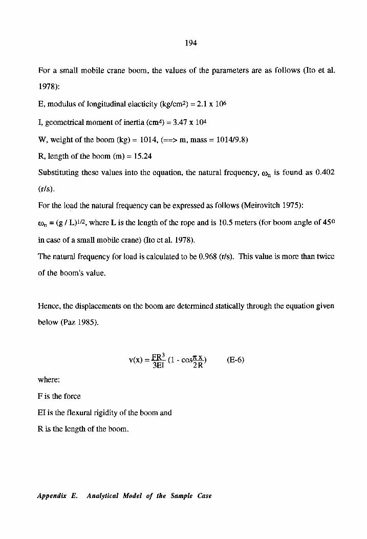
194

For a small mobile crane boom, the values of the parameters are as follows (Ito et al.

1978):

E, modulus of longitudinal elacticity (kg/cm2) = 2.1 x 106

I, geometrical moment of inertia (cm4) = 3.47 x 104

W, weight of the boom (kg) = 1014, (==> m, mass = 1014/9.8)

R, length of the boom (m) = 15.24

Substituting these values into the equation, the natural frequency, q@, is found as 0.402

(r/s).

For the load the natural frequency can be expressed as follows (Meirovitch 1975):

@, = (g/ L)1, where L is the length of the rope and is 10.5 meters (for boom angle of 45°

in case of a small mobile crane) (Ito et al. 1978).

The natural frequency for load is calculated to be 0.968 (t/s). This value is more than twice

of the boom's value.

Hence, the displacements on the boom are determined statically through the equation given

below (Paz 1985).

FR? VO) = SET

- WX - (1 cos) (E-6)

where:

F is the force

EI is the flexural rigidity of the boom and

R is the length of the boom.

Appendix E. Analytical Medel of the Sample Case

195

This appendix provides the discussion of equations for the dynamic behavior of the

suspended load and the response of the crane's boom to this dynamic loading. These

equations have been coded and incorporated in a GL program for each stage of the pick and

place task described in Section 4.3.2.1. The GL program is presented in Appendix F.


Appendix F

Source Code of the GL Program

This appendix presents the source code of the Graphics Language (GL) program written

for the sample case discussed in Section 4.3 and Appendix E. The sample case program

consists of the following functions:

Main program

Compprop, to compute integral properties of solids

Drawmodel, to display the animation

Genframe, to generate the object frames

Showframe, to draw the specified objects

Initgraph, to perform GL drawing

Newint, to compute the new integral properties of solids

Explanatory comments are provided within the code for each function. The functions were

coded in C programming language, and GL functions were used to obtain the required

graphics for the animation. The coding and the animation were performed on a Silicon

Graphics Iris 4D/80GT workstation.

196

197

Sample Case (mtmp c )

/¥* Main program */

7*® Written by Shrikant Dixit */

#include <stdio.h>

extern comp_prop( )3 extern draw_model( )5

7* declare global variables for mass properties (upto 10 objects) */

float obj_voll10],obj_ixx[10],obj_iyy[10],obj_izzl101,o0bj_ixyl101,0b3_ixz[101, obj_ivz[10 1,obj_denf 101,0b3_mass{ 1015

int total_obj; float xshift,yshift,xxshift,zzshift3

/* declare global variables for model geometry */

float obj_points[ 6 J[1500](3),disp_list{6][1500][3]; int obj_polylistl61J[800 11100], total_obj_points[101],total_obj_polyI10]; int points_per_polyl61{800];

maint )

FILE *names int i,j3

xshift = 0.03 yshift = 600.03

7% set mass properties and point and polygon count to zero */

for(i=05i<lOsi++)

obj_volli] = 0.03 obj_ixxfi]} = 0.03 obj_iyyli] = 0.03 obj_izzli] = 0.03 obj}_ixylil] = 0.03 obj_ixzli] = 0.03 obj_iyz[i] = 0.03 obj_den[iJ] = 1.03 obj_mass[i] = 0.03 total_obj_pointsl11] = 0.03 total “obj _poly[i] = 0.03

name = fopen(“truck2.asc","r'')3 comp_prop(name }5

fei write out global properties */ *

for(i=0si<total_objsi++)

printf("\n volume of object 4d is “%f",1i+1,obj_volli]) printf£("\n ix of object “d is 4f",1+1,0b}_ixxli] printf("\n iyy of object 4d is Zf",1+1,0b}]_iyyli] printf("\n izz of object 4d is Zf",i1+1,0b)_izzlil printf£("\n ixy of object 4d is Zf",i+1,0b}_ixyli] printf("\n ixz of object “d is “%f",i+1,ob}_ixzlil prantf€("\n iyz of object 4d is Zf",1+1,0b)_iyzli]

) printf("\n mass of object 74d is Zf",1+1,0b)}_ massli

*/

/*® assign display list */

for(i=05i<6s+4a)

for( 3-05 3<total_obj_pointsfils++3)

disp_listlillj [0] = obj_points[i1[j](1]; disp-listlillJ1l1] = obscpointstiI3It2]5 disp_list£iI[ 312] = obj_pointslilljI0]5

}

Appendix F. Source Code of the GL Program

198

7* go into interactive mode and draw the crane */

(void )draw_model (name ) 5

for(i=0sictotal_objs++i)

for( 3-05 j<total_obj_pointslils++3)

printf ("\n objpointstZditZdItol Z£"51,},0bj_points[i If j 1L31£0))3 printf("\n objpoints[Zd]iZd1[1 74" ,1,4,0b3-pointst i It g1L1)5 printf("N\n objpointsl Zd1[ 4d 112] Z¥",1,3,0b}_points[i1[31121)3

) printf("\n total polygons are 4d",total_obj_polylil);

fort 3-05 }<total_obj_polylils++3) , J printf("\n objpoints( 4d Il 4d Printf("\n objpoints[Zd1{Z% d

) Prantfen objpointsi 4d ll 4d %

} }

Zd", i rj 2»0bj_ polylistl 7d" 51,},0b] polylistl 4d" 51,3,0b)_ polylistl

Ilo] 111] M2)


199

Sample Case (compprop c )

7* This program uses integprop.c to compute mass properties of a RALRTHRU ASC II file */ prop

7*® written by : Shrikant Dixit */

#include <stdio.h> finclude <math.h>

extern int integprop( ); extern int open_polygon( )5 extern int trianguls et )5

extern float obi vol[101,o0b}_ixxl10],o0bj_iyy[10],obj_izz[101,obj_ixyf!101], obj ixzl 10 1,0b)_ iyzl101],0b}_denl10],ob]_massl10]5

extern int to extern float obj poandel 61115001315 extern int 9b). po listl 6 1180011001, total_obj illo],

tota os “pointsl101,points | per _ ~polytel 800];

7*® start of function */

int comp_prop( fname ) FILE frames

{ int obj_nosvol no, oly »numpts »numtri »bnd_ptss int nts Eriangl500its!, ios fat vertex; vone-P int 22232295 rec? P24 opa at gk float points{500][3], resis, trilist[3J[3 11500]; float fl, Fo FS dened ee OL Gne ye eee rs pS eg 5002,

iostat = 03 vol_no = 03

while( ios tat! =EOF)

iostat = fscanf(fname,"\n “4d “4d 4d %d 4d %d 4d Z%d %d_ Z%d Nn"; oo. &numpoly »&numpts »&j1,&452 >& 73 »&34,255,&36,&857,80b}_ no)}s

if(iostat==EOF ) reaks

7* read data */ if (35==5)

numtri = 03 ++vol_no} . for( 1=05icnumpts 5++1)

fscanflfnames"\n ZF ZF Z",&f1,8F2,8F3 )5 points[iJ{0] points[i][1] points[iJ[2] n

aa

“hah

nN =

obj pointsloby no - L]L total_obj_points[obj_no

eerie (obj no - 1]1 total_ob}_pointslobj_no

ob} intslob] tiitzi s as"

3 7* end for over i */

/* update number of points added to model geometry */

total_obj_pointslobj_no - 1] += numpts;

- 11. tetal_obj_pointsl obj_no

/*® get all the faces of the volume, triangulate them and compile ilist and process using integprop */

for(i=05icnumpolysi++)

fscanf( fname,"\n 7d ",&bnd_pts 5

for( 3-05 j<bnd_ptss j++)

fscanf( fname," 4d ",&vertex);


200

for( K=03k<334+k ) bndry_listijI{k] = points[vertex-1I[k];

7® add_the polygon to the global list */ obj_polylistt j_no - 1) total_obj_ polylobj_ no - 1] + 1][31] = total_obj_pointsl[obj_no = 1] - numpts + vertexs

} /* end for over j */

/* record the_points per polygon value */ oo: points_per_polylobj_no -1)]L total_obj_polylebj_no - 1] + ij = [ pts;

get triangles */ nt = U3 for( 3=05 j<bnd_pts-35++])

triangint][0] = 15 triang(ntJ[1]}] = j+23 triang[ntI[2] = 3433 +4nts

}

for( 3-05 j<nts++5)

for(k=0sk<35++k)

for( 1e031<35+41)

trilistl1 Jk ]inumtritj]_= bndry listi(triangl 5]tk)-1)I11)5

} } /7* end for over k */

)} /* end for over j */

numtri += nts 3} /% end for over i */

/® update the object polygon count */ total_obj_polylobj_no - += numpoly;

7* compute mass properties for the triangulated volume */

density = obj_denlobj_no - 1]

(void Jintegprop(numtri,trilist,density,&évolume ,&Ixx,&lyy > &Izz,&Ixy,&Ixz,&alyz,&mass }5

7* put _ mass proper ties in their global slots */ obj_vollobj_no - 1] += volume; obj_ixxlobj"no - 1] += Ixxs obj_iyylob}j"no - 1] += Iyys obj_izzlobj"no - 1) += Izzs obj_ixylobj no - 1] += Ixy3 obj_ixzlobj_no - 1] += Ixzs ob})_iyzlobj"no - 1] 4= Iyzs

_masslobj_no - 1] += mass} . total_obj = obj_nos iy .

7*® printfe"\n ob) no after computing is Zd",total_obj)5 printf("\n_\n obtained vaules for mtmp are:")5

printf("\n volume is Zf",volume)s printft"\Nn Ixx is Z£",Ixx«)3 printf("\n Iyy is Zf",Iyy)s printf("\n Izz is 4f",Izz)5 printf ("\n Ixy is Zf",Ixy)5 printf("\n Ixz is Zf",Ixz)3 printf("\n Iyz is Zf",Iyz)3 rintf("\n mass _is Zf",mass)3 %*/ 7* endif condition over j5 */

} 7* end while condition over EOF */

) return(0)3

7® end of function */


201

Sample Case (drawmodel c )

7% This function initializes graphics, sets up menus and then draws the model. This function also animates the dynamic behavior of the suspended load and the response of the crane's boom to this dynamic oading. *

7* Written by Taylan Dal */

#include <stdio.h> le <gl.h>

#include <device.h> #include <math.h>

tdefine PI 3.141593 9.8

#define E 21000000000 #define I 0.000347 #define W 2300.0 tdefine R 15.24 #define L 5.25 ¥define acc_crane_1 0.08 #define acc_crane_2 -0.08 #define v 0.00136

extern init_graphics( ); extern draw objects( )5 extern truckK_motion( )5 extern boom_rotate( ); extern generate_frame( }3

extern int total_obj; extern float xshift,xxshift,zzshifts

int draw_model( )

float shift,dist, time, baseaxis[3],boomaxis[3],origin[3 15 float gamma, theta,delta,beta,boom_deflect{2J,turn,dips float I_gamma,1_theta,1 delta,1_beta,1] shift,] bd{[2]3 float i_gamma,i_theta,i_delta,i_beta,i_shift,i_bdl2]s float tension,ang_vel,inst_time; , . float s2_fin_delta,s2_fin_ang_vel,s3_fin_delta,s3_fin_ang_vel} float s4¢_fin_delta,s¢ fin_ang_vel,s5I_fin_beta,s5I_fin_ang_vels float s52_fin_beta,s52_fin_ang_vels int i,frames,att_statuss

init_graphics( )3

frontbuf fer ( TRUE )5 clear ( )}3 frontbuf fer ( FALSE )5

7*® draw the initial condition of the model */ shift 5

Huu

° °o

we

3 o=h

-_

a a wo

~ oO

ot

ot 0.03

0.0; generate_frame( shi ft,gamma, theta,delta,beta,boom_deflect,att_status )5

7* execute motion */ dist = 121.84072673 time = 5.03 frames = 53 . for (1=131<(timexframes +1)54++1)

shift = (dist / (time * frames) ds generate_frame( shi ft,gamma, theta ,delta,beta,boom_deflect,att_status }3

} shift = 0.03

7* rotate the boom */ dip = 8,05552673 dip = dip * PI /1603 . for (17131<( time*frames +1)3++1)


202

theta = (dip / (time * frames )); delta = -1.0 * theta; generate_frame(shift,gamma, theta,delta,beta,boom_deflect,att_status J;

} theta = 0.03 delta = 0.03

att_status = 13

7% lift the object */ tension = W / sqrt(2.0)3 boom _deflect[1] = tension * R*¥® R*R / (3. * E * I)5

boom_deflect[0] = tension * R*R*R / (24. * E * I)5 dip = -8.05552673 dap dip * PI /1803 . i_bd[O] = 2.0 * boom_deflect[0] / (time * frames )s i_bd[1] = 2.0 * boom_deflect[1] / (time * frames )s5 for (1=1Lsi<(time*frames +1)3441)

if(i>(timexframes / 2))

i_bd{O] *= -1.03 a_bd[1] *= -1.03

} theta = (dip 7 (time * frames) ); delta = -1.0 * theta; . generate_frame(shift,gamma, theta,delta,beta,i_bd,att_status )3

}

1_bdi0] = boom_deflect[0]; l_bdI1] = boom_deflectI1]}3

theta = 0.0; delta = 0.03

/* The following section of the program is to predict and display the mic behavior of the load and the response of the crane's boom to

this dynamic loading */

dist = 100.03 time = 50.03 frames = 13

1_gamma =0.03 l “theta =0.03

1 -

I~shift =0.05

for (i=13 i<( time*frames +1); ++1)

inst_time = i / (frames);

/* crane moving with acc (+) */

delta = (acc_crane_1 /_L) * cos(sqrtig/L)*inst_time) - acc_crane_1/L3 i_delta = Ita = delta; l“delta = delta;

i_shift = (dist / (time*frames ))5

shift = 0.5 * acc _crane_1 * inst_time * inst_time; i_shift = shift - l_shitts l7shift = shifts

ang_vel = - {ace_crane_I/L) * sqrt(g/L) * sinlsqrt(g/L )*inst_time)s

tension = W * (ang_vel * ang_vel / L / g + cos(delta) + acc_crane_l * sin(delta) / g)3

boom_deflect[1] = tension * R * R * R * (1 - cos(90.*PI/180.0)) 7 (3. * E * I)3

boom_deflect[0] = tension * R * R * R * (1 - cos(90.*PI/360.0)) / (3. * E * 1)3

i_bdl0] = boom_deflect[0] - 1_bdl0]s 1“bdl01 = boom-deflectio];


i_bd[1) 1~bdf 1)

if ( {

203

boom_deflect{1] - l_bd{f1] 5 boom_deflect[1];

i frames )

s2_fin_delta = delta;

)°2-Fin_ang_vel = ang_vel;

generat

}

e_frame(i_shift,gamma, theta,i_delta,beta,i_bd,att_status )3

7*® crane moving with no acc (0) */

dist

I~shift

for (i= {

inst_

delta

i_ delta ldelta i_shift

ang_vel

tension

boom_de

boom_de

i_bdlO] ibd 0] i_bdi 1] l_bdi1]

if { { s3_fin_delta

100.03 25.03 = 13

=0.03 =0.03 =0.03 0.03 =0.03

13 1<(time*frames +1)3 ++i)

time i 7 frames;

(s2_fin_ang_vel * sqrt(L/g) * sin(sqrtl ol eins t_ time) + s2_fin_delta * cos(sqrt(g/L )*inst_time ))5

= delta - 1_delta; = deltas

{dist / (time * frames ));

/L) * cos(saqrt( s2_fin_ang vel * sqrt(L/g) * sqrtt (g/L }*inst_time

git einst_time) - s2_fin_delta * sqrt(g/L) * sin(sqr z

=W/g * (ang_vel * ang_vel / L) + W * cos(delta)s

flect[1] = tension * R * R * R * (1 - cos(90.*PI/180.0)) / (3. * E * I);

flect[0] = tension * R * R * R * (1 - cos(90.*PI/360.0))} 7 (3. * E * I)3

= boom_deflect[0] - 1_bdl0]; = boom deflectI[01]; = boom_deflect{[1] - 1_bd[1]; = boom_deflect{[1]5

i == frames)

= deltas

)52-fin_ang_vel = ang_vels

generat

}

7*® cran

dist time frames

I fhete

l-shift

for (i=

inst_

e_frame(i_shift,gamma, theta,1_delta,beta,i_bd,att_status )3

@ moving with acc (-) */

100.03 50.03

13

=0.03 =0.03 =0.03

0.03 =0.03

1s 1<(time*frames +1)3 ++1)

time 1 / frames;


204

delta = ((s3_fin_delta - acc_crane_2 / L) *® cos(sqrt(g/L)¥inst_time) - acc_crane_2 / T)3

i delta = delta - 1_delta; ldelta = deltas zr shift = (dist / (time*frames })}35

shift = 4.0 * inst_time + 0.5 * acc_crane_2 * inst_time * inst_time; i_shift = shift - I_shifts lshift = shifts

ang_vel = -(s3_fin_delta - acc_crane_2 / L) * sin(sqrt(g/L )*inst_time )* sqrtig/LT);

tension = WH * (ang_vel * ang_vel / (L / g) + cos(delta) + acc_crane_2 * sin(delta) / g)3

boom_deflect{1] = tension * R * R * R * (1 - cos(90.¥PI/180.0)) / (3. * E * TJs

boom_deflect{0] = tension * R * R * R * (1 - cos(90.*PI/360.0)) / (3. * E * I)5

i_bdl0] = boom_deflect[0] - 1_bdl0]; l“bd[0] = boom—deflect(0]; 1_bdi1] = boom—deflect(1] - 1_bdf11]; lbdl11 = boom_deflect[1];5

generate_frame(i_shift,gamma, theta,i_delta,beta,i_bd,att_status )5

}

“/* crane stops, boom rotates (15) with angular acc, v (+) */

shift = 0.03 amma = PI / 12.03 ime = 75.03

frames = 13

1_gamma =0.03 l beta =0.03 ibdl0] =0.05 i7bdI 11 =0:05

for (i=13 1<(time*frames +1)3 ++1)

inst_time = 1 / frames; i_gamma = gamma / (timeframes )}3

zzshift = (600.0 - xshift) * sinli_gamma * i)3

beta = powlinst_time,12) * powlv, 7) / (3840.*R%¥g) -

(11.% powlinst_time, 10)*powlv, 7)*L/(320.*R¥g%g)) +

powlinst time, 8)*powlv, 5)*( g¥*g*(R¥R-8. )4+1188.xvxve L¥L )/T384 . ¥R¥g*Qg%¥qg) +

pow(inst_time, 6)*powlv, 5 3( 7. *g%g*L*(8. —-RER )- 8316. ¥v¥VXLXLEL I/(48.*R¥QKgEgEG) +

powlinst_time, 4)*powlv, 3 )%€( g¥g¥g¥g*( 4. -RR )+ 61580 7%v%VxVEV*LELELEL #35 . evSVEgegeLXL¥( RXR-B. 1/18. XR¥gXgXgXGXG) +

(inst_time*inst_timex*v%vxv )%*(105 “eu evXgeGRLELALA( 8. -RER 43. ¥QxQxXgkeg*L*( R*R-G. J- 124740 . HvHVEVHEVELHLHLELEL )/02.*R*(powlg, 6))) +

VHC «Xv eveong™ QG*L¥EL*( 8. -R¥R 4105, eveVEVEVHQGHGELELHLHL( RER-1E. D+ 2. ¥RERX powlg, 6))+249480.%(powlv, 6) )* (pow(L, 6)))7(2.%R*(powlg, 7))) = +

(s4_fin_ang_yel * sqrt(L/g) * sin(sqrt(g/L)*inst_time) + s4¢_fin_delta * cos(sqrt(g/L )*inst_time))3

ang_vel = powlinst_time, 11)*pow(v, 7)/(320.*R%*g) +

-(11.*powlinst_time, 9)*pow(v, 7)*L/(32.*R¥g*g)) +

powlinst time, 7 }*powlv, 5 )( gg R¥R-8. 141188. evxev% L¥L )/T48 . #R¥EGHGHG) +

powlinst time, 5)*powlv, 5)*(7.*g*g*L*(8.-R*R )- 8316. ¥vxvxLELEL )/( 8. ¥R¥GXG*GXg) +


205

powlinst_time, 3 mPowly » 3 )¥( g¥g¥gXg*(4. -R*R J+ 41580. xveveVeVELELELEL +35 ev eVHEQHGLILR( RXR-B. 1/12. RRRQ*GKHGXGKG) +

(inst Eimesveveey 12 105 -xvxvegegx LELXL#(6 . CRER #3 . KOXGRGEGELE( R*R-G, J- 124740. HvevIeVEVELHLELALEL I/CR¥(powlg, 6))) +

s¢_fin_ang_vel * sqrt(L/g) * sqrt(g/L)} * cos(sqrt(g/L)*inst_time) - s¢_TFin_delta * sqrt(g/L) * sinlsqrt(g/L )*inst_time )5

tension = (W/g) * (ang_velxang_vel/L -_vetimexvxtime/R*(cos(v¥timextime/2) + sin(€vetimextime/2)) + v¥R¥(sin(vetimextime/2)} - cos(vxtimextime)))} + W * sqrt(1.-(sin(beta )*sin( beta) ))5

boom_deflect[1] = tension * R * R * R * (1 - cos(90.*PI/180.)) 7 (3. * E % Ids

boom_deflect[0] = tension * R * R * R * (1 - cos(90.*PI/360.)) 7 (3. * E * I35

if (3 == (time*frames ) )

s51_fin_beta = beta;

)5t_fin_ang_vel = ang_vels

i_beta = beta - 1 beta; lbeta = beta;

generate_frame(0.0,i_gamma,0.0,0.0,1_ beta,i_bd,att_status )5

}

7% boom rotates (15) with no angular acc, v (0) */

shift = 0.03 amma = PI / 12.035 ime = 75.03

frames = 13

1 gamma =0.03 eta =0.03 1

i_bd[0] =0.03 i_bd[1] =0.03

for (i=13} i<(time*frames +1); ++i)

inst_time = i / frames; 1_gamma = gamma 7 [( imex frames );

zzshift = (600.0 - xshift) * sin(PI/12.0 + (i_gamma * 1))3

beta = (s51_fin_ang_vel * sqrt(L/g) * sinl(sqrt(g/L )*inst_time) + s51_fin_beta * cos(sqrt(g/L)*xinst_time})5

ang_vel = s51_fin_ang vel * sqrt(L/g) * sqrt(g/L) * cos{sqrt(g/L )*inst_time) - s51_fin_beta * sqrt(g/L) * sin(sqrt(g/L )*inst_time)s

tension = (W/g) * (ang vel*ang vel/L) + (W ¥* sqrt(1.-(sin( beta )*sin( beta) )))5

boom_deflect[11] tension * R * R * R * (1 - cos(90.*PI/180.)) 7 (3. * E * 13

boom_deflect[0] tension * R * R * R * (1 - cos(90.*¥PI/360.)) 7 (3. * E * I)3

if (i == (timexframes ))

“352_fin_ beta = beta;

)oo2-fin_ang_vel = ang_vels

generate_frame(0.0,i_gamma,0.0,0.0,1_beta,i_bd,att_status )5

}


206

/7*® boom rotates (15) with angular acc, v (-) */

shift = 0.03 gemma = PI / 12.03 ime = 75.03

frames = 135

1_gamma =0.03 I-beta =0.05 i_bd[0] =0.05 i_bd[11 =0.03

for C(i=1s 1<(time*frames +1)5 +41)

inst_time = 1 / frames; i1_gamma = gamma / (time*frames )}

zzshift = (600.0 - xshift) * sin(PI/6.0 + (i_gamma * i1))3

beta = -1.0 * (powlinst_time, 12)*powlv, 7))/(3840.*R¥g) +

(11.% powlinst_time, 10)%* powlv, 7 )*L/(320.*R¥g¥g)) -

(powlinst_time, 8) powlyv, 5 )%( g%g*(R¥R-8. )+1188.%*vxV* L¥L ) )/T384. #REG*gEg) -.

(powlinst_time, 6)*pow(v> BRC 7 xg%gel (8. -R*R I 8316. ¥vev¥L*LEL ) 1/148 . XRegXg*g*g) -

{(powlinst_time, 4)* powly: 3 )( g¥g%g*g*l 4. -R#R )+ 41580 . HveV2eVEVELELRLEL ASS . Rv¥VEGHGEL¥L*(RER-8. 3)I/(18. XR¥QGKGEG*G*G) -

(inst_timexinst_ timexvxv%v )*( 105. xvxv¥g*GHLELHL*( 8. —-RER 43. XQXQHGHGHL*( R¥R-4. )- 124740 . HvHVEVHVELELHLILHL I/(02 HRC powlg, 6))) -

VEC. RVEVXGEGEGRGELELE( B RXR I+105. ev evEVRVEGEGHLELHL¥L¥( R¥R-16. + 2. *R*ER¥Elpowlg, 6}3)4+249480.*(powlyv, 6) )* (pow(L, 633)/012.*#R¥(powlg, 7))) +

(s52_fin_ang vel * sqrt{lég) * sin(sqrt(g/L }*inst_time) + s52_fin_beta * cos(sqrt(g/L }*inst_time)) 5

ang_vel = -1.0 * { powlinst_time, 11)* powlv, 7))/(320.*R¥g) +

(11.% powlinst_time, 9)% powl v»> 7)*L/(32.*R¥g*g)) -

(powl inst_time, 7) powl v, 5)*(g*g*(R¥R-8. )+1188. xv¥v% LL } 7148. ¥REQ*GEG) -

{ powl inst_time, 5)* powlyv, 5)*(7.xg%g*L*(8.-RER )- 8316. XvKVELELEL ) )/18. HREQKGKGHG) -

(pow( inst_time, 3% powl v, 3)*( g*gxgxg*(4.-R*R J+ G1 BBO . VV VRVELALELEAL 435 . RVRVIEQHG¥LELH( RER-B. ))I/(0 2. ¥REQEGEG*gKG) -

Cinst Timexv vey J ( 105 xvevxgeanL¥L¥L¥(B. RAR )43 . Xg¥GXGXG*L*( RER-G. J 124740. xvXeveVEVELHLELELEL I/UTRE( powlg, 6))) +

s52_fin_ang vel * sartiL/a) * sqrt(g/L) * sos(sart( g/L eins t_time) - $52_Tin_beta * sqrt(g/L) * sin(sqrt(g/L )*inst_time)3

tension = (W/g) * Cang_velxang_vel/L-v*inst_timexvxinst_time/R *(cos(-v*inst_timexinst_time/2) + . . . . . sin(-vxinst_time*xinst_time/2 ) )-v*R*(sin(-v*inst_time*inst_time/2 } ~cos(-vinst_timexinst_time))) + W * sqrt(1.-Tsin{ beta )*sin( beta) ))5

tension * R * R * R * (1 - cos(90.*PI/180.)) 7 (3. * E * Ids

tension * R * R *R * (1 - cos(90.*PI/360.))} 7 (3. * E * IDs

boom_deflect[1]

boom_deflectI[0]

generate_frame(0.0,i_gamma,0.0,0.0;i1_beta,i_bd,att_status )s

gexit( );


207

Sample Case (genframe c )

7* This function generates the object frames at the specified transformation values using pseudo-kinematic transformations to achieve desired spatial orientation required */

/* Written by Shrikant Dixit ¥*/

#include <math.h> Finclude <qgl.h> *include <device.h>

extern genrot( ); extern mat4x4( 35 extern initmat( )3 extern show_frame( )5

extern int obj lylistlé 1f800 111001, total_ob) pointsl10]; extern float ob} _points(6 1(1500][31,disp_listlé 1L15001{3]3 extern float xshift,yshift,xxshift,zzshift;

enerate_frame( shi ft, gamma; theta del ta,beta boom _defl,att_status } loat shift,gamma, theta ,delta,beta,boom_defl[2];

int att_statuss

£ float tempx, tempy» tempz; int is} okvobjects; P

color( BLACK )3 clear( }3

xshift += shifts

7* assign display list to normal state fort i=031<6s+42)

for( 3=05 j<total obj_points[115++j)

disp_listLiJ[j1][01] = obj_points{11[31]01]s disp_listliJ][}1(1] = obj_points[i1£j](2]3 disp_listlil[j1[2] = obj_pointsliJ[jIH015

}

7* set objects to be manipulated */

objects = 53 iffatt_status==1)

+tobjectss

/*% deform the boom */

for( 42453585443) isp_listIZ1[j1[1] += boom_defl[0]s

For( 4285 35125444) isp_list[21151[1] += boom_def1[1]};

7* apply boom effect to cable and object */

shift += boom_def1[1]5 or(1=35i<objects 3++i )

for( j=03 j<total eb] ints[i13++j3) disp list ill j1011 += boom dafll11s

7*® move for beta */

for(i=3sicobjectss++i)


tempy = disp_listlil(j]{1]s tempz_= disp_listlill[j[2]s . disp_listlilTjH11 = cos(beta) * (tempy - yshift) .

sin(beta) * (tempz - zzshift) + yshifts disp_listliJ[j1[2] = -1.0 *sin(beta) * (tempy - yshift) |

cos(beta) * (tempz - zzshift) + zzshifts ++!

J }


208

7* wove for delta */

for(i=35i<objects5 ++i)

for( 3=03 j<total_obj_pointsfils++])

tempx = disp_list{i](j1(01; tempy = disp list(11131[11; disp_listlillj]101] = cos(delta) * (tempx - 600.0)

. . a sinidelta) * (tempy - yshift) + 6003 disp_listlil[j]f{1] -1.0 * sinldelta) * (tempx - 600.0)

71+]

}

‘* move for theta */

for(i=2si<objects3++1)

for( j=05 j<total_obj_pointslils++3)

tempx = disp_list[11[j1][0];3 tempy = disp list{iJ[jIf1]5 disp_listliJTjI[0] = cos(theta) * tempx

. sin( theta) * tempys disp_list£i1153111] -1.0 * sin(theta) * tempx

cos( theta) * tempy; +u+ 1

} }

/* move for gamma */

for(i=lsicobjectss +43)


tempx = disp _listlilI1j1[0]5 tempz= disp listlilt3iiz]3 isp_ d ist(iITjI[0] = (cos(gamma) * (tempx - xshift))

- (sin( gamma) * tempz) + xshifts disp_listlil[j][2] = (sin(gamma) * (tempx - xshift))

+ (cos(gamma) * tempz);5 7® xxshift *= sinl( gamma )

) zzshift *= cos( gamma} %

}

7% move for shift */

for(i=0si<objectss++1)

for( ]=03 j<total_ obj intsli]3++j) disp listlill ji] += shifts”

show framel )5 swapbuf fers( )3


cos(delta) * (tempy - yshift) + yshifts

209

Sample Case (showframe c )

7* This functions draws the specified objects */

7* written by shrikant dixit */

#include <stdio.h> include <ql.h> #include <device.h>

extern float disp_listl61L15001[3 1; extern int obj _polylistl 6 1[8001{100], total_obj_polyl101,total_obj_points[10],

points_per_polyI 6 1[800]5

show_frame( )

int i»,jJ»ppbnd,ob_no float parrayl 1000 ILS 15x,y 523

zbuf fer ( TRUE ); zclear( )s

for(ob_ no=1;0b_no<73++ob_no)

makeob j( ob_no)5 color( no J

for(i=05ictotal_ obj, polylob_no - 1]5;i++)

ppbnd = points_per_polylob_no -1][1135

for (3=03 j<ppbnd3;++5)

parray[jI][0] = disp, obs polis 1] . “polviistl ob no -LI[i1£3] - 1] [0]3

parray[j1I[1] = disp ite no - qpoiylistlob_ no -1)[i105] - 1] (113

parray{j1[2] = disp, Te2y ob_no - 1] } Tobj_polylistlob_no -1I[i1[j] - 1] [2]

poly( ppbnd,parray )5

closeobj( ob_no); callobjlob_no);

Need

Ma

at


210

Sample Case (initgraph c )

/*® sample gl drawing */

7* witten by shrikant dixit */

#include <stdio.h> #include <gl.h> #include <device.h>

int init_graphics|( )

static float parray[ 513] oetatate .0,0.0,

int junks

7*® initialize gl */

7® set the text window) */

keepaspect(4,3) /* prefposition( 24, 1000,18,750)3 */ prefsize(1200,900)5 junk = wi ('MTMP™ ) wintitle( "MULTI-TASK MOTION PLANNING" )5 doublebuf fer( )35 gconfig( }5 Gdev ice INPUTCHANGE } 5 qdevice( REDRAW )3 color{ BLACK }3 clear( )3 7*® viewport(100,900, 100; 700)5 ortho(0.0,40.0,0. 0,30. 0,0 0,30. Os *7

7% Viewpor £28 »996 +103, 697)3 ¥/ viewport(0,1200,0,900 )5 perspective( 650, ol. 35555235 00. 12000. 0)3 ookat(1000.0,300.0,1000.0,500.0,300.0,0.0,0)5

7* exit gl */

returns


211

Sample Case (newint c )

7* This program computes the integral properties of solids */

7*® Written by Taylan Dal */

#include <stdio.h> #include <math.h>

7*® function to compute integral properties */

int integprop(nt, trianglelist,density, totalvolume, totalI_xx, totall totall_z2rtotall xy,totall xz,totall yz» totalmass) ° mala

/*® argument decleration */

float trianglelist[3][3][5001],density; float xtotalvolume, *totalI_xx, *totalI_yy, *totalI_zz, *totalI_xy,

*totalI_xz, xtotalI_yz, xtotalmass;

int nts

{

/*® variable decleration */

float volume,C_x,C_y»,C_z,Ix,Iy,Iz»I_xx)I »I_zz> I_xy,I_xzsl_yz»x(3J,y[31,2T31,det,masss

int i,j,statuss

7* error check */

status=1; *totalvolume=0.03

xtoteltn-yo=0, *tota =03 xtotall 2z=03 *totall_xy=03 *totalI_yz=03 *#totalI_xz=03 xtotalmass=0}3

for Cirosicntsate) 7* number of triangles */

for {37053<33 544) 7* vertex number */

7* get x»y»z values */

x{3]=trianglelist{0][j]L1i]s yl} J=trianglelist{1][}J[1i]3 z2[j1=trianglelist£21[ 310113

}

/*® find determinant of the transformation matrix */

det=( x0 Ie(yl 1 dict 2 }oyE2 beat ll )oxCd lat yl0 Ixzt 2 I-yl2 Ixzlol) +x 2 1¢( yl 0 J*201 J-yf1 lezl01))5

7* Find volume */

volume=det/6. 3

*totalvolume += volumes

/* find center of mass */

C_x=(xf0 ]4+xI11+x£21)/4.3

C_y=(ylO]+yl[1l]l+y{21)/4.3

C_z=(zl0J+z[1]+2021)/4.3


212

7* find moments of inertia */

Ix=(x00 Fx 0 4x01 x0 1 14x02 Jx0 2 4x00 x01 14x00 ext 2 4x01 x0 27) xvolume/10. 3

Ty=( yo Jeyl0 J+y01 tyl 1 Jeyl 2 eyl 2 l4+yl0 J*yE 1 l+yl 0 Jeyl 2 Jeyl1 eyl 21) xvolume/10. 3

Iz=( 200 J*z(0 342101 ez0 1 lez 2 bezt 2 J+2z0 0 J*201 )4+200 l¥z0 2 +201 Jx2z02)) xvolume/10. 3

I_xx = Iy + Iz3 I_yy = Ix + Iz3 I_zz = Iy + Ixs

*fotall_xx += Tos *tota yy += 5

xtotalI_zz += rez3

I_xy=( 2x00 Jeyl 0 J4x01 Jeyl1 J4x0 2 }eyl2)) +€x00 Beyl 1 J+x01 beyl0 ]4+x00 Beyl 2 14x02 ]*yl0 14x01 bey 2 )+x02 beyf1])) *xvolume/20. 5

*totall_xy += I_xy3

I_yz=(2%( 210 J*y[0 J+z01 J*yl1 ]+z02 beyl2 1) +(z00 beyC 1 ]4z0 1 eyl0 l+zl0 Keyl 2 lez 2 ley 0 Jez0 1 leyl 2 420 2 Jxyl1])}) xvolume/20. 5

*totalI_yz += I_yz;

I_xz=(2%(x00 Jezl 0 J4x01 J¥z01 14x12 }ez021) +(x[0 J*z0 1 4x01 )*z00]+x£0 Jezf 2 14x02 1*Z00 J4+x0 1 Jezl 2 14x02 Je2f11])) xvolume/20. 5

*totalI_xz += I_xz3

7* find mass */

mass=volumexdensity3

*totalmass += mass}

} status=0}3 return(status )3


BIBLIOGRAPHY

Armstrong, W. W., and Green, M. W., (1985) "The Dynamics of Articulated Rigid Bodies for Purposes of Animation," The Visual Computer, Vol. 1, No. 4, pp. 231-240.

Baecher, G. B., Greenspun, P. G., and Gillet, W. E., (1989) "Integrated Automation for Site Work," Excellence in the Construction Project, Proceedings of Construction Congress I, ASCE, pp. 232-237.

Beliveau, Y. J., Dixit, S., Dal, T., and Morad, A. A., (1991) "Multi-Tasking Motion Planning for Large Scale Material Handling Using Structural Dynamic Behavior and Geometric Modeling," Proposal Submitted to the National Science Foundation, Civil Engineering Department, Virginia Tech.

Braid, I. C., (1973) "Designing with Volumes: Computation of Weight, Center of Gravity, Moments of Inertia, and Principle Axis," CAD Group Document 81, University of Cambridge, U. K.

Brodie, M. L., Mylopoulos, J., and Schmidt, J. W., (1984) On Conceptual Modeling, Springer-Verlag, New York.

Chang, C., Chung, M. J., and Bien, Z., (1990) "Collision-free Motion Planning for Two Articulated Robot Arms Using Minimum Distance Functions," Robotica, Vol. 8, pp. 137- 144.

Cleveland, A. B., Jr., (1989) "Real-time Animation of Construction Activities," Excellence in the Construction Project, Proceedings of Construction Congress I, ASCE, pp. 238-243.

Clough, R. W., and Penzien, J., (1975) Dynamics of Structures, McGraw-Hill, New York.

Cohen, J., and Hickey, T., (1979) "Two Algorithms for Determining Volumes of Convex Polyhedra,”" Journal of the ACM, Vol. 26, No. 3, pp. 401-414.

Conte, S. D., and de Boor, C., (1980) Elementary Numerical Analysis, McGraw-Hill, New York.

Craig, J. J., (1986) Introduction to Robotics, Addison Wesley, Reading, MA.

De Floriani, L., and Falcidieno, B., (1988) "A Hierarchical Boundary Model for Solid Object Representation,” ACM Transactions on Graphics, Vol. 7, No. 1, pp 42-60.

Featherstone, R., (1983) "The Calculation of Robot Dynamics Using Articulated-Body Inertias," The International Journal of Robotics Research, Vol. 2, No. 1, pp. 13-30.

Finn, K. M., (1982) "A Reduced-Order Crawler Crane Model with Active Control to Attenuate the Transient Vibrations," Master's Thesis in Mechanical Engineering, Virginia Tech.

213

214

Foley, J. D., and van Dam, A., (1985) Fundamentals of Interactive Computer Graphics, Addison Wesley, Reading, MA.

Fujimura, K., and Samet, H., (1989) "A Hierarchical Strategy for Path Planning Among Moving Obstacles," IEEE Transactions on Robotics and Automation, RA-5, No. 1, pp. 61- 69,

Functional Specification for the DICE Architecture, (1989) Concurrent Engineering Research Center, West Virginia University, Morgan Town, WV.

Girard, M., and Maciejewski, A. A., (1985) "Computational Modeling for the Computer Animation of Legged Figures," ACM Computer Graphics, (Siggraph Proceedings, July '85), pp. 263-270.

Goldstein, H., (1950) Classical Mechanics, Addison Wesley, Reading, MA.

Hahn, J. K., (1988) "Realistic Animation of Rigid Bodies," Computer Graphics, Vol. 22, No. 4, pp. 299-308.

Hammer, P. C., and Stroud, A. H., (1956) "Numerical Integration over Simplexes," Mathematical Tables Aids Computation, Vol. 10, pp. 137-139.

Hara, K., Yamamoto, T., Kobayashi, A., and Okamoto, M., (1989) "Jib Crane Control to Suppress Load Swing," International Journal of Systems and Sciences, Vol. 20, No. 5, pp. 715-731.

Haug, E. J., (1988) m r Ai Kinemati Dynamics, Allyn and Bacon, Boston.

Hendrickson, C., and Maher, M. L., (1989) "Issues in Computer Based Design / Construction Integration," Excellence in th n ion Project, Proceedings of Construction Congress I, ASCE, pp. 129-136.

Hollocks, B. W., (1984) "Practical Benefits of Animated Graphics in Simulation," Proceedings of 1984 Winter Simulation Conference, San Diego, CA, pp. 323-328.

Ito, H., Hasegawa, M., Tsukasa, I., and Kato, Y., (1985) "Study on Stability of a Truck Crane Carrier," Bulletin of the JSME, Vol. 28, No. 244, pp. 2474-2479.

Jackins, C. L., and Tanimoto, S. L., (1980) "Oct-trees and Their Use in Representing 3-D Objects," Computer Graphics and Image Processing, Vol. 14, No. 3, pp. 249-270.

Johnson, F. R., Jr., (1976) "Dynamic Analysis of the P&H 6250 Truck Crane Employing the 150 Foot Boom Stick Model,” U. S. Naval Civil Engineering Laboratory, T. M. No. M-51-76-16, Port Hueneme, CA.

Jones, J. F., and Petterson, B. J., (1988) "Oscillation Damped Movement of Suspended Objects," Proceedings of the IEEE International Conference on Robotics and Automation, Vol. 2, pp. 956-961.

215

Kedem, K., and Sharir, M., (1986) "An Efficient Motion Planning Algorithm for A Convex Polygonal Object in 2-D Polygonal Space," Courant Institute of Mathematical Science, Technical Report 253, New York University, New York.

Khatib, O., (1986) "Real-time Obstacle Avoidance for Manipulators and Mobile Robots," International Journal of Robotics Research, Vol. 5, No. 1, pp. 90-98.

Khosla, P., and Volpe, R., (1988) “Superquadric Artificial Potentials for Obstacle Avoidance and Approach,” Proceedings of the IEEE International Conference on Robotics and Automation, Vol. 3, pp. 1178-1184.

Kochan, S. G., (1988) Programming in C, Hayden Books.

Korein, J. U., and Badler, N. I., (1982) "Techniques for Generating the Goal-Directed Motion of Articulated Structures," IEEE Computer Graphics Applications, November, pp. 71-81.

Kreyszig, E., (1979) Advanced Engineering Mathematics, John Wiley & Sons.

Krylov, V. I., (1962) Approximate Calculation of Integrals, MacMillan.

Lee, J., and Bien, Z., (1990) "Collision-free Trajectory Control for Multiple Robots Based on Neural Optimization Network," Robotica, Vol. 8, pp. 185-194.

Lee, Y. T., and Requicha, A. A. G., (1982)"Algorithms for Computing the Volume and Other Integral Properties of Solids I: Known Methods and Open Issues," Communications of the ACM, Vol. 25, No. 9, pp. 635-641.

Lien, S., and Kajiya, J. T., (1984) "A Symbolic Method for Calculating the Integral Properties of Arbitrary Nonconvex Polyhedra," IEEE Computer Graphics and Applications, Vol. 4, No. 9, pp. 35-41.

Meagher, D., (1982) "Geometric Modeling Using Octree Encoding," Computer Graphics and Image Processing, Vol. 19, pp. 129-147.

Meirovitch, L., (1975) Elements of Vibration Analysis, McGraw-Hill.

Messner, A. M., (1970) "A Surface Integral Method for Computer Calculation of Mass

Properties," Paper 852, 29th Annual Conference of the Society of Aeronautical Weight Engineers, Washington, D. C.

Messner, A. M., and Taylor, G. Q., (1980) "Algorithm 550: Solid Polyhedron Measures,” ACM Transactions on Mathematical Software, Vol. 6, No. 1, pp. 121-130.

Morad, A. A., Cleveland, A. B., Jr., Beliveau, Y., J., Francisco, V., and Dixit, S., (1991) "Path-Finder, an AI Based System for Constructability Improvement," Paper Accepted by Journal of Construction Engineering and Management, ASCE to be published.

Moustafa, K. A. F., and Ebeid, A. M., (1988) "Nonlinear Modeling and Control of Overhead Crane Load Sway,” Journal of Dynamic Systems, Measurement, and Control, Vol. 110, pp. 266-271.

216

O'Dunlaing, C., Sharir, M., and Yap, C. K., (1983) "Retraction: A New Approach to Motion Planning,” in Proceedings of the 15 FOCS, pp. 207-220.

O'Leary, J. R., (1980) "Evaluation of Mass Properties by Finite Elements," Journal of Guidance and Control, Vol. 3, No. 2, pp. 188-190.

Pan, T.-J., and Luo, R. C., (1990) "Motion Planning for Mobile Robots in a Dynamic Environment with Moving Obstacles," Proceedings of the IEEE International Conference on Robotics and Automation, Vol. 1, pp. 578-583.

Paoluzzi, A., Ramella, M., and Santarelli, A., (1989) "A Boolean Algebra over Linear Polyhedra," Computer-Aided Design, Vol. 21, No. 9, pp. 474-484.

Patten, W. N., (1980) "Transient Response Characteristics of a Construction Crawler Crane," Master's Thesis in Mechanical Engineering, Virginia Tech.

Paulson, B. C., Jr., (1985) "Automation and Robotics for Construction," Journal of Construction Engineering and Management, ASCE, Vol. 111, No. 3, pp. 190-205.

Paz, M., (1985) Structural Dynamics, Van Nostrand Reinhold Company.

Raibert, M. H., (1984) "Experiments in Balance with a 3-D One-Legged Hopping Machine,” The International Journal of Robotics Research, Vol. 3, No. 2, pp. 75-92.

Rajan, S. D., and Bhatti, M. A. (1986) "SADDLE: A Computer-Aided Structural Analysis and Dynamic Design Language -- Part I. Design System," Computers and Structures, Vol. 22, No. 2, pp. 185-204.

Raven, F., (1973) Engineering Mechanics, McGraw-Hill.

Requicha, A. A. V., (1980) "Representations for Rigid Solids: Theory, Methods and Systems," ACM Computing Surveys, Vol. 12, No. 4, pp. 437-464.

Richard, M. J., Anderson, R., and Andrews, G. C. (1986) "Generalized Vector-Network Formulation for the Dynamic Simulation of Multibody Systems," Journal of Dynamic Systems, Measurement, and Control, Vol. 108, pp. 322-329.

Sakawa, Y., and Nakazumi, A., (1985) "Modeling and Control of a Rotary Crane," Journal of Dynamic Systems, Measurement, and Control, Vol. 107, pp. 200-206.

Schlesinger, S., (1979) "Terminology for Model Credibility," Simulation, Vol. 32, No. 3, pp. 103-104.

Schroder, P., and Zeltzer, D., (1990) "The Virtual Erector Set: Dynamic Simulation with Linear Recursive Constraint Propagation,” Computer Graphics, Vol. 24, No. 2, pp. 23- 31.

Shapiro, H. T., (1980) Cranes and Derricks, McGraw-Hill, New York.

Smith, R. L., and Platt, L., (1987) "Benefits of Animation in the Simulation of a

Machining and Assembly Line," Simulation, Vol. 48, No. 1, pp. 28-30.

217

Stern, G., (1983) "Bbop -- A Program for 3-D Animation,” Nicograph '83 Proceedings, December, pp. 403-404.

Stroud, A. H., (1967) "Approximate Multiple Integration," in Ralston, A., and Wilf, H. S. (editors), Mathem atical Methods for Digital Computers, Wiley, pp. 145- 155.

Timmer, H. G., and Stern, J. M., (1980) "Computation of Global Geometric Properties of Solid Objects," Computer-Aided Design, Vol. 12, No. 6, pp. 301-304.

van Overveld, C. W. A. M., (1991) "An Iterative Approach to Dynamic Simulation of 3-D Rigid Body Motions for Real Time Interactive Computer Animation," Visual Computer, Vol. 7, pp. 29-38.

WALKTHRU Bechtel 3-D Simulation System User's Guide, (1988) Version 3.0., Bechtel Corporation, Bechtel Software, Inc.

Ward, C. C., and Johnson, F. R., Jr., (1978) "Dynamic Loads on a Shipboard Crane Boom Due to Ship Motion," U. S. Naval Civil Engineering Laboratory, T. M. No. M-51- 78-12, Port Hueneme, CA.

Wesley, M. A., (1980) "Construction and Use Of Geometric Models," in Encarnacao, J. (editor), Com r Ai ign re N i m r Scien , Springer-Verlag, New York, pp. 79-136.

Wilhelms, J., and Barsky, B., (1985) "Using Dynamic Analysis to Animate Articulated Bodies Such as Humans and Robots," Proceedings of Graphics Interface '85, pp. 97-104.

Williams, R. J., and Seireg, A., (1979) "Interactive Modeling and Analysis of Open or Closed Loop Dynamic Systems with Redundant Actuators," Journal of Mechanical Design, Vol. 101, pp. 407-416.

Wilson, H. B., Jr., and Farrior, D. S., (1976) "Computation of Geometrical and Inertial Properties for General Areas and Volumes of Revolution," Computer-Aided Design, Vol. 8, No. 4, pp. 257-263.

Witkin, A., Gleicher, M., and Welch, W., (1990) "Interactive Dynamics," Computer Graphics, Vol. 24, No. 2, pp. 11-21.

Wittenburg, J., (1977) Dynamics of Systems of Rigid Bodies, B.G. Teubner, Stuttgart, Germany.

Wu, K. J., Kim, S.-S., Kim, S.-S., and Ciarelli, K. J., (1990) "A Generic Mechanical System Data Model for Dynamic Simulation,” Proceedings of 1990 ASME International Computers in Engineering Conference and Exhibition, Boston, MA, pp. 113-119.

Zhu, D., and Latombe, J.-C., (1991) "New Heuristic Algorithms for Efficient Hierarchical Path Planning," IEEE Transactions on Robotics and Automation, Vol.7, No. 1, pp. 9-19.

VITA

Taylan Dal was born on July 16, 1967 in Turkey. He graduated from Istanbul American

Robert College in 1985. He completed his undergraduate degree in Civil Engineering at

Bogazici (Bosphorus) University, Istanbul in July, 1989. In September of the same year,

he entered the graduate program in the Construction Engineering and Management Division

of Civil Engineering at Virginia Polytechnic Institute and State University where he earned

a M.S. Degree in Civil Engineering in October, 1991. The author plans to work towards a

Ph. D following the completion of his M.S. Degree.

The author's work experience includes work as an intern engineer for Mimko Insaat in

Istanbul. In addition, he worked as a manufacturing engineer for the Jonathan Corporation

in Norfolk during the summer of 1990. The author has also worked as a Graduate

Research and Teaching Assistant for the Construction Engineering and Management

Division of Civil Engineering while pursuing his Master's Degree.

Lf DS

218

A Dynamic Behavior Modeler for Future Inclusion into a Multi ...

Documents

Transcript of A Dynamic Behavior Modeler for Future Inclusion into a Multi ...