Hydrography of the Labrador Sea during Active Convection

428 VOLUME 32J O U R N A L O F P H Y S I C A L O C E A N O G R A P H Y

q 2002 American Meteorological Society

Hydrography of the Labrador Sea during Active Convection

ROBERT S. PICKART AND DANIEL J. TORRES

Woods Hole Oceanographic Institution, Woods Hole, Massachusetts

R. ALLYN CLARKE

Bedford Institute of Oceanography, Dartmouth, Nova Scotia, Canada

(Manuscript received 6 June 2000, in final form 25 June 2001)

ABSTRACT

The hydrographic structure of the Labrador Sea during wintertime convection is described. The cruise, partof the Deep Convection Experiment, took place in February–March 1997 amidst an extended period of strongforcing in an otherwise moderate winter. Because the water column was preconditioned by previous strongwinters, the limited forcing was enough to cause convection to approximately 1500 m. The change in heatstorage along a transbasin section, relative to an occupation done the previous October, gives an average heatloss that is consistent with calibrated National Centers for Environmental Prediction surface heat fluxes overthat time period (;200 W m22). Deep overturning was observed both seaward of the western continental slope(which was expected), as well as within the western boundary current itself—something that had not beendirectly observed previously. These two geographical regions, separated by roughly the 3000-m isobath, produceseparate water mass products. The offshore water mass is the familiar cold/fresh/dense classical Labrador SeaWater (LSW). The boundary current water mass is a somewhat warmer, saltier, lighter vintage of classical LSW(though in the far field it would be difficult to distinguish these products). The offshore product was formedwithin the cyclonic recirculating gyre measured by Lavender et al. in a region that is limited to the north, mostlikely by an eddy flux of buoyant water from the eastern boundary current. The velocity measurements takenduring the cruise provide a transport estimate of the boundary current ‘‘throughput’’ and offshore ‘‘recirculation.’’Finally, the overall trends in stratification of the observed mixed layers are described.

1. Introduction

The Labrador Sea has long been known as a site ofintermediate water formation (Nielsen 1928; Smith etal. 1937; Lazier 1973). Cold air blowing off the Ca-nadian landmass during winter chills the surface waters,which destabilizes the water column and causes deepconvection. This overturning—which can extend asdeep as two kilometers—forms a water mass known asLabrador Sea Water (LSW), which then spreads into thegreater North Atlantic Ocean and beyond. LSW con-tributes to the global meridional overturning circulation,both directly and via entrainment into the Nordic over-flows (e.g., McCartney 1992). It impacts as well theoceanic flux of heat (Talley 2000). The strong signatureand convective origin of this water mass helps set thedensity structure of the subpolar and midlatitude NorthAtlantic and provides a climate connection between thehigh-latitude atmosphere and middepth ocean. This con-nection has been shown to be surprisingly fast at times

Corresponding author address: Dr. Robert S. Pickart, Woods HoleOceanographic Institution, Woods Hole, MA 02543.E-mail: [email protected]

(e.g., Sy et al. 1997; Pickart et al. 1997b; Molinari etal. 1998).

Despite its importance to the circulation and venti-lation of the North Atlantic, much is still unknown aboutthe formation of LSW. This is due in a large part to theharsh environment in which it is formed, rendering insitu observing programs challenging and risky. But ourlimited knowledge is also due to the intermittency ofthe convection: in some years LSW is not produced atall (e.g., Lazier 1980). As a result, there have been fewobservations of newly formed LSW, and these have beenlimited to measurements isolated in space and time(Clarke and Gascard 1983; Wallace and Lazier 1988).Consequently, there are fundamental questions that arenot yet answered regarding the formation and spreadingof this important water mass. Among the open questionsare: What is the distribution and extent of overturningin the Labrador Basin? What is the relative role of at-mospheric forcing versus the ambient stratification/cir-culation in dictating the convection? And how quicklyand by what mechanism(s) does LSW restratify andspread?

It was with such questions in mind that the LabradorSea Deep Convection Experiment was undertaken. The

FEBRUARY 2002 429P I C K A R T E T A L .

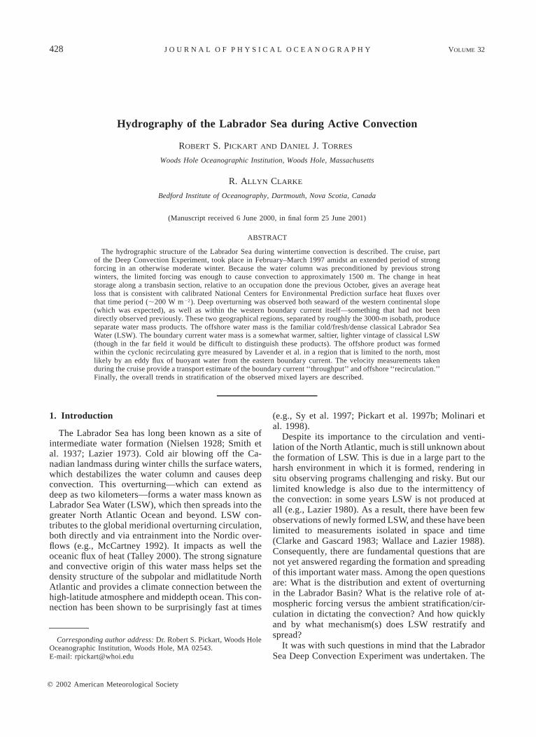
FIG. 1. Boundary currents of the Labrador Sea and the location of the WOCE AR7W hydrographic lineand Bravo mooring. The color represents the standard deviation of the sea surface height anomaly (mm)as measured from satellite altimetry (after Prater 2002). The isobaths shown are 1000, 2000, and 3000 m.

overall goal of the program, principally sponsored bythe U. S. Office of Naval Research (ONR), was to im-prove our understanding of the dynamics of high-lati-tude, open-ocean convection. Details of the Deep Con-vection Experiment and its different efforts are sum-marized by the Lab Sea Group (1998). The field phaseof the experiment was carried out during the winters of1996/97 and 1997/98, and consisted of different com-ponents addressing the hydrography, circulation, air–seafluxes, and meteorology associated with convection inthe Labrador Sea.

The purpose of this paper is to present the first resultsfrom the hydrographic component of the Deep Con-vection Experiment, which consisted of a seven-weekcruise during the winter of 1996/97 (hereafter referredto as the winter of 1997). The cruise covered a largeportion of the Labrador Basin, so these measurementsrepresent the first comprehensive description of the Lab-rador Sea (Fig. 1) during active convection. We presentat least partial answers to some of the questions posedabove, and also show some unexpected features of theoverturning. We begin with a description of the large-scale oceanographic and atmospheric context in whichthe experiment took place, followed by a more detailed

look at the regional hydrographic fields, water massproducts, and circulation. Lastly we present a ‘‘mac-roscopic’’ view of the mixed layer properties, revealingsome surprising and complex structure.

2. Large-scale perspective

A variety of factors conspire to cause deep convectionin the Labrador Sea, including the atmospheric forcing,regional circulation (interior and boundary currents), re-mote input of heat and salt from the Arctic and sub-tropics, and the Labrador Sea’s memory of previousconvective seasons. One of the fascinating and complexaspects of LSW formation is its large interannual anddecadal variability (e.g., Rhines and Lazier 1995), whichlikely occurs because so many factors are at work. Per-haps chief among these, or at least a conspicuous in-dicator of certain key relationships between the differentfactors, is the North Atlantic Oscillation (NAO). TheNAO mode accounts for most of the variance in thelarge-scale atmospheric patterns of the North Atlantic(Rogers 1990; Hurrell and Dickson 2001). The extentto which this mode is present in a given winter is rep-resented by the NAO index, defined as the normalized


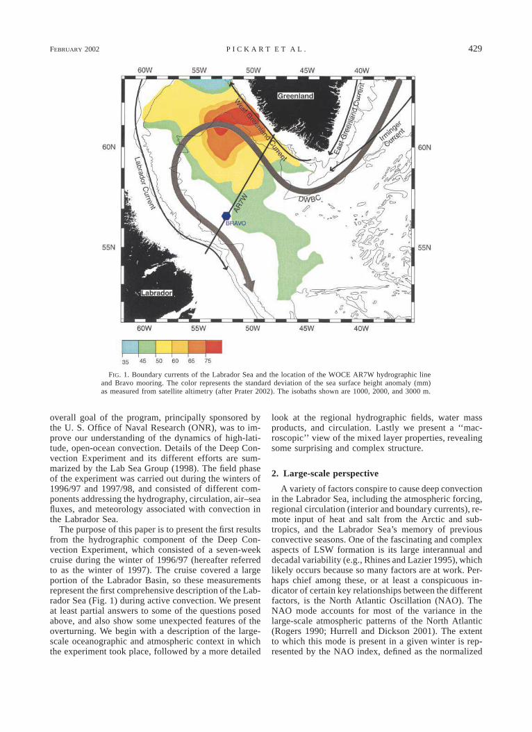
FIG. 2. Averaged calibrated NCEP atmospheric model fields. (left) Average of the three highest NAO winters over the last 20 years (winteris defined as Dec–Mar). (right) Average of the three lowest NAO winters over the last 20 years. The isobaths (gray lines) are 1000, 2000,and 3000 m. The WOCE AR7W hydrographic line is marked.


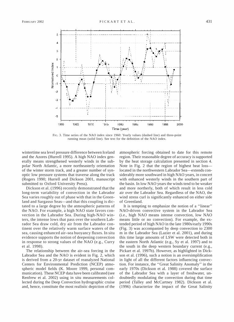
FIG. 3. Time series of the NAO index since 1960: Yearly values (dashed line) and three-pointrunning mean (solid line). See text for the definition of the NAO index.

wintertime sea level pressure difference between Icelandand the Azores (Hurrell 1995). A high NAO index gen-erally means strengthened westerly winds in the sub-polar North Atlantic, a more northeasterly orientationof the winter storm track, and a greater number of syn-optic low pressure systems that traverse along the track(Rogers 1990; Hurrell and Dickson 2001, manuscriptsubmitted to Oxford University Press).

Dickson et al. (1996) recently demonstrated that thelong-term variability of convection in the LabradorSea varies roughly out of phase with that in the Green-land and Sargasso Seas—and that this coupling is dic-tated to a large degree by the atmospheric patterns ofthe NAO. For example, a high NAO state favors con-vection in the Labrador Sea. During high-NAO win-ters, the intense lows that pass over the southern Lab-rador Sea draw cold, dry air from the Labrador con-tinent over the relatively warm surface waters of thesea, causing enhanced air–sea buoyancy fluxes. In situevidence supports the notion of deepening convectionin response to strong values of the NAO (e.g., Curryet al. 1998).

The relationship between the air–sea forcing in theLabrador Sea and the NAO is evident in Fig. 2, whichis derived from a 20-yr dataset of reanalyzed NationalCenters for Environmental Prediction (NCEP) atmo-spheric model fields (K. Moore 1999, personal com-munication). These NCEP data have been calibrated (seeRenfrew et al. 2002) using in situ measurements col-lected during the Deep Convection hydrographic cruiseand, hence, constitute the most realistic depiction of the

atmospheric forcing obtained to date for this remoteregion. Their reasonable degree of accuracy is supportedby the heat storage calculation presented in section 4.Note in Fig. 2 that the region of highest heat loss—located in the northwestern Labrador Sea—extends con-siderably more southward in high NAO years, in concertwith enhanced westerly winds in the southern part ofthe basin. In low NAO years the winds tend to be weakerand more northerly, both of which result in less coldair over the Labrador Sea. Regardless of the NAO, thewind stress curl is significantly enhanced on either sideof Greenland.

It is tempting to emphasize the notion of a ‘‘linear’’NAO-driven convective system in the Labrador Sea(i.e., high NAO means intense convection, low NAOmeans little or no convection). For example, the ex-tended period of high NAO in the late 1980s/early 1990s(Fig. 3) was accompanied by deep convection to 2300m in the Labrador Sea (Lazier et al. 2001), and duringthis time large amounts of LSW were detected both inthe eastern North Atlantic (e.g., Sy et al. 1997) and tothe south in the deep western boundary current (e.g.,Pickart et al. 1997b). However, as highlighted in Dick-son et al. (1996), such a notion is an oversimplificationin light of all the different factors influencing convec-tion. For instance, the ‘‘Great Salinity Anomaly’’ in theearly 1970s (Dickson et al. 1988) covered the surfaceof the Labrador Sea with a layer of freshwater, un-doubtedly modulating the convection during that timeperiod (Talley and McCartney 1982). Dickson et al.(1996) characterize the impact of the Great Salinity


FIG

.4.

Cal

ibra

ted

NC

EP

sea

leve

lpr

essu

rean

omal

y(m

b)re

lati

veto

the

20-y

rm

ean.

Ano

mal

yfo

rth

eco

mpo

site

of(a

)th

eth

ree

high

est

NA

Ow

inte

rs,

(b)

the

thre

elo

wes

tN

AO

win

ters

,(c

)th

ein

divi

dual

win

ter

of19

97.

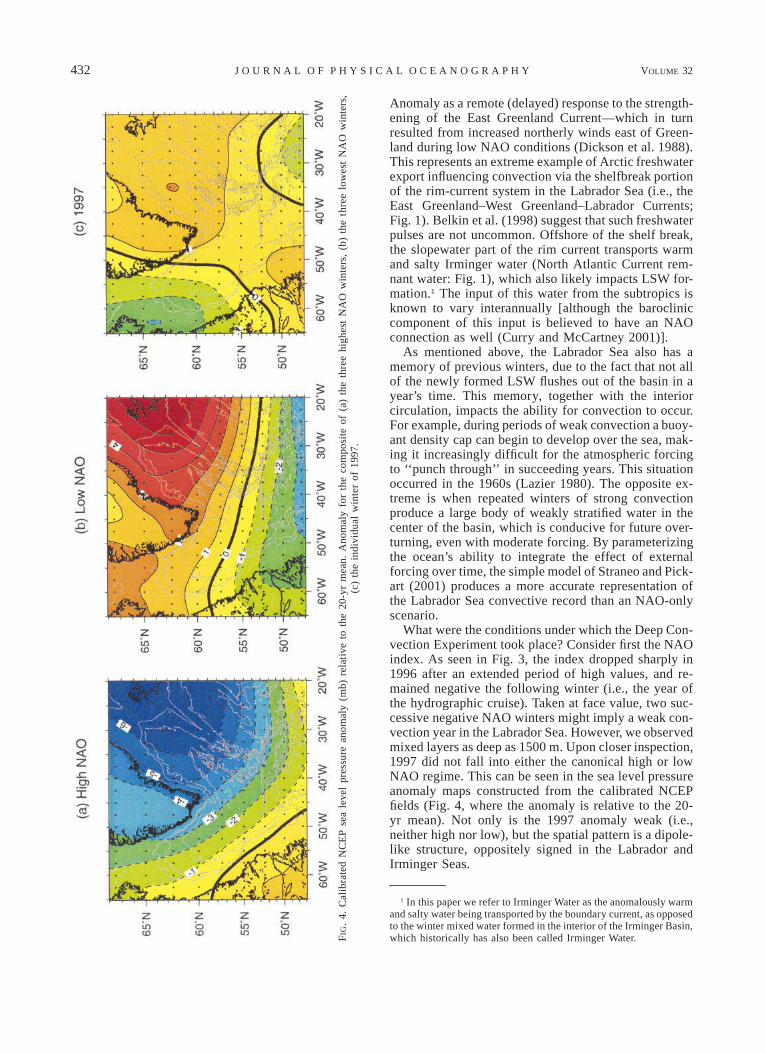
Anomaly as a remote (delayed) response to the strength-ening of the East Greenland Current—which in turnresulted from increased northerly winds east of Green-land during low NAO conditions (Dickson et al. 1988).This represents an extreme example of Arctic freshwaterexport influencing convection via the shelfbreak portionof the rim-current system in the Labrador Sea (i.e., theEast Greenland–West Greenland–Labrador Currents;Fig. 1). Belkin et al. (1998) suggest that such freshwaterpulses are not uncommon. Offshore of the shelf break,the slopewater part of the rim current transports warmand salty Irminger water (North Atlantic Current rem-nant water: Fig. 1), which also likely impacts LSW for-mation.1 The input of this water from the subtropics isknown to vary interannually [although the barocliniccomponent of this input is believed to have an NAOconnection as well (Curry and McCartney 2001)].

As mentioned above, the Labrador Sea also has amemory of previous winters, due to the fact that not allof the newly formed LSW flushes out of the basin in ayear’s time. This memory, together with the interiorcirculation, impacts the ability for convection to occur.For example, during periods of weak convection a buoy-ant density cap can begin to develop over the sea, mak-ing it increasingly difficult for the atmospheric forcingto ‘‘punch through’’ in succeeding years. This situationoccurred in the 1960s (Lazier 1980). The opposite ex-treme is when repeated winters of strong convectionproduce a large body of weakly stratified water in thecenter of the basin, which is conducive for future over-turning, even with moderate forcing. By parameterizingthe ocean’s ability to integrate the effect of externalforcing over time, the simple model of Straneo and Pick-art (2001) produces a more accurate representation ofthe Labrador Sea convective record than an NAO-onlyscenario.

What were the conditions under which the Deep Con-vection Experiment took place? Consider first the NAOindex. As seen in Fig. 3, the index dropped sharply in1996 after an extended period of high values, and re-mained negative the following winter (i.e., the year ofthe hydrographic cruise). Taken at face value, two suc-cessive negative NAO winters might imply a weak con-vection year in the Labrador Sea. However, we observedmixed layers as deep as 1500 m. Upon closer inspection,1997 did not fall into either the canonical high or lowNAO regime. This can be seen in the sea level pressureanomaly maps constructed from the calibrated NCEPfields (Fig. 4, where the anomaly is relative to the 20-yr mean). Not only is the 1997 anomaly weak (i.e.,neither high nor low), but the spatial pattern is a dipole-like structure, oppositely signed in the Labrador andIrminger Seas.

1 In this paper we refer to Irminger Water as the anomalously warmand salty water being transported by the boundary current, as opposedto the winter mixed water formed in the interior of the Irminger Basin,which historically has also been called Irminger Water.


FIG. 5. Anomaly of temperature (left) and salinity (right) at 400 m in the subpolar North Atlantic for three time periods, compared to thelong-term climatological average (after Curry and McCartney 2001). (a) 1965–71 (a low NAO period), (b) 1990–95 (a high NAO period),and (c) the time period of the Deep Convection Experiment.

Regarding the state of the ocean, Curry and Mc-Cartney (2001) recently constructed large-scale maps oftemperature and salinity for the subpolar gyre for dif-ferent time periods. Figure 5 shows that during the timeperiod of the experiment, 1996–98, the subpolar gyredid not fall into either the low- or high-NAO regime aswell. In the low-NAO state (Fig. 5a), the entire upperlayer of the subpolar gyre is warm and salty (comparedto climatology), while in the high-NAO state it is mark-edly colder and fresher (Fig. 5b). Our experiment tookplace during a complex ‘‘transition phase,’’ where en-hanced export of warm and salty subtropical water hadalready flooded the boundary current system of the sub-polar gyre, while the interior portions of the gyre (in-cluding the Labrador Sea) were still colder and fresherthan average.

It is enlightening to diagnose further the particularwinter of 1997 using the NCEP climatology. Figure 6shows the total heat flux averaged over the LabradorBasin, broken down by both winter and month of winter.While the winter-averaged heat loss (solid curve in Fig.6) is significantly correlated at the 99% confidence level

with the yearly NAO index, there is large scatter in themonthly heat loss values (discrete symbols in Fig. 6).Interestingly, the three years during which Decemberexperienced the largest monthly heat flux were lowNAO years, whereas in five out of the seven highest-NAO years January was the month of strongest heatloss. Note the skewness in 1997, showing that February(i.e., during the hydrographic cruise) was anomalouslycold that year. In fact, even though 1997 had the fourthlowest NAO during the 20-yr time period, February1997 had the second largest heat loss of all Februaries.This was largely due to strong winds and, hence, anespecially strong latent heat loss. The two other highskewness years (discounting 1995, which had a verysmall standard deviation) were 1993 and 1982. The for-mer was an extremely strong winter, resulting in thedeepest convection on record (J. Lazier 1999, personalcommunication). The latter was much like 1997, anoverall moderate winter with a particularly strong Feb-ruary. However, four out of the five years preceding1982 were moderate to low-NAO years, whereas fourof the five years prior to 1997 had extremely high NAO


FIG. 6. Calibrated NCEP total heat flux averaged over the Labrador Sea. Winter mean valuesand standard deviations are shown (solid circles and lines), along with the monthly averages fora given winter (open symbols).

values. Hence the system was primed in 1997 so that asingle month of intense forcing was enough to causedeep overturning. Presumably this was not the case in1982, although this cannot be verified because no datawere collected that year.

In summary, 1997 was an overall moderate winter—one that was neither a canonical high- nor low- NAOyear in terms of the atmospheric conditions or state ofthe subpolar gyre. However, the hydrographic cruisetook place during a ‘‘microcosm’’ of classic LabradorSea convective forcing in the harsh month of February1997, when the ocean was well preconditioned fromprevious years.

3. Hydrographic cruise

A hydrographic cruise was carried out on the Re-search Vessel Knorr, which departed Halifax, Nova Sco-tia, on 2 February 1997 and returned to Woods Hole,Massachusetts, on 20 March 1997 (Fig. 7). As indicatedby the NCEP climatology, we experienced conditionsconducive for overturning: frequent storms, cold airtemperatures, and strong winds. The mean air temper-ature was 288C (rising above 08C on only one day).The mean wind speed was 12 m s21 (gusting to morethan 25 m s21), blowing on average out of the west-northwest. Storms arrived, and the sea state built, in asurprisingly short amount of time. It snowed constantly,and white-out conditions frequently reduced visibilityto near-zero. Operationally, one of our biggest chal-lenges was keeping the decks and bulwarks free of ice.The cold air, together with the large amount of sea spray

and wash, caused ice to build up quickly. Consequently,the crew (with occasional help from the science party)would regularly knock ice off the vessel using woodenmallets and snow shovels.

Ice in the water was also a problem during the cruise,since the Knorr is not ice-strengthened. While the centerof the Labrador Sea is free of ice, the boundaries arenot. On the Greenland side the problem was icebergs(advected into the area by the East/West Greenland Cur-rent), in particular the smaller bergs not easily detectedon ship’s radar. During our second visit to the Greenlandcoast numerous icebergs cluttered the working area, in-cluding one that caused us to divert our station track.On the Labrador side the problem was pack ice. Herewe experienced the coldest weather of the cruise(2178C) and were clearly at a disadvantage by not hav-ing an ice-strengthened hull. The reason for samplingnear the western shelf break is that the highest buoyancyfluxes occur just seaward of the ice edge, and we sus-pected that convection might be occurring here as wellas in the central part of the basin.

Figure 7 shows the locations of the hydrographic sta-tions occupied. Each of the conductivity–temperature–depth (CTD) casts extended to the bottom and includedmeasurement of dissolved oxygen, at typically 24 levels.Other tracers were measured at a subset of the stations,including chlorofluorocarbons and tritium–helium (La-mont-Doherty Geological Observatory). A loweredacoustic Doppler current profiler (LADCP) was attachedto the instrument package, providing a vertical profileof absolute horizontal velocity. Three different CTDswere used during the course of the cruise, two EG&G


FIG. 7. Hydrographic stations occupied during Feb–Mar 1997 (section numbers are marked in bold). Aportion of Section 2 was occupied twice (separated by 10 days): stations 57–71 comprise the first occupation(solid circles), and stations 113–121 the second occupation (open triangles, see insert). Stations 7–13 (opencircles, insert) coincided with a small-scale intensive float deployment early in the cruise. The location of thesecond to-yo CTD survey is indicated by the shaded box. The isobaths shown are 1000, 2000, and 3000 m.

Mark-III instruments, and a Falmouth Scientific Instru-ments integrated CTD. Details of instrument perfor-mance and calibration are found in Zimmermann et al.(2000). The temperature accuracy was determined viapre- and postcruise laboratory calibrations, and the sa-linity accuracy calculated by comparison with the insitu bottle data. Salinity is reported using the practical

salinity scale. The overall accuracy of the measurementswas 0.0018C for temperature, and 0.0025 for salinity.An exception to this is the group of stations on theGreenland shelf, which not surprisingly exhibited ahigher salinity standard deviation (0.01) compared tothe bottle data. No shelf data are considered in this paper.It is worth noting that oftentimes the upcast trace of the


FIG

.8.

Com

pari

son

ofth

efa

ll19

96an

dw

inte

r19

97A

R7W

occu

pati

ons:

(a)

pote

ntia

lte

mpe

ratu

re,

(b)

sali

nity

,(c

)po

tent

ial

dens

ity,

(d)

diss

olve

dox

ygen

(win

ter

only

),an

d(e

)pl

anet

ary

pote

ntia

lvo

rtic

ity.


FIG

.8.

(Con

tinu

ed)


FIG. 8. (Continued)

CTD differed significantly from the downcast trace, atestament to the pronounced small-scale variability pre-sent during convection. Such variability has also beenobserved in the convective regions of the MediterraneanSea (Schott et al. 1996) and the Greenland Sea (Schottet al. 1993).

We adopted a multifaceted approach to our surveypattern. We wanted to describe the basinwide state ofthe sea, including the rim current system; at the sametime we sought increased resolution in the western partof the basin where the strongest air–sea forcing occurs(and previous work suggested the deepest mixed layerswould be found). Both the alongbasin line (Section 0)

and the southern cross-basin line (Section 3) were re-peats of the fall 1996 hydrographic cruise done by theBedford Institute of Oceanography as part of the DeepConvection Experiment. The southern line was the firstwintertime occupation of the World Ocean CirculationExperiment (WOCE) AR7W section. Note that the threewestern boundary crossings did not extend onto theshelf: this was due to the proximity of the ice edge.Finally, we wanted to do small-scale mapping of a con-vective feature if the opportunity arose. Toward this endwe conducted two ‘‘to-yo’’ CTD surveys, including a36-h survey at the end of the cruise that sampled thedeepest mixed layers of the experiment (Fig. 7). These


FIG

.9.

Mea

nup

per-

laye

rsa

lini

tyse

ctio

nsfo

rth

epe

riod

1990

–97

(see

P01

a).

(top

)T

helo

cati

ons

ofth

etw

om

ean

sect

ions

.T

heis

obat

hsar

e10

00,

2000

,an

d30

00m

:(b

otto

m)

(a)

Eas

tern

Lab

rado

rS

ea;

(b)

wes

tern

Irm

inge

rS

ea.


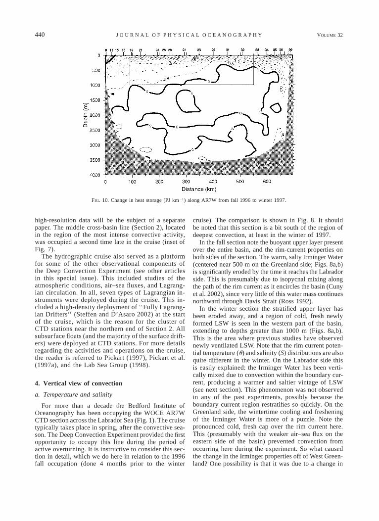
FIG. 10. Change in heat storage (PJ km21) along AR7W from fall 1996 to winter 1997.

high-resolution data will be the subject of a separatepaper. The middle cross-basin line (Section 2), locatedin the region of the most intense convective activity,was occupied a second time late in the cruise (inset ofFig. 7).

The hydrographic cruise also served as a platformfor some of the other observational components ofthe Deep Convection Experiment (see other articlesin this special issue). This included studies of theatmospheric conditions, air–sea fluxes, and Lagrang-ian circulation. In all, seven types of Lagrangian in-struments were deployed during the cruise. This in-cluded a high-density deployment of ‘‘Fully Lagrang-ian Drifters’’ (Steffen and D’Asaro 2002) at the startof the cruise, which is the reason for the cluster ofCTD stations near the northern end of Section 2. Allsubsurface floats (and the majority of the surface drift-ers) were deployed at CTD stations. For more detailsregarding the activities and operations on the cruise,the reader is referred to Pickart (1997), Pickart et al.(1997a), and the Lab Sea Group (1998).

4. Vertical view of convection

a. Temperature and salinity

For more than a decade the Bedford Institute ofOceanography has been occupying the WOCE AR7WCTD section across the Labrador Sea (Fig. 1). The cruisetypically takes place in spring, after the convective sea-son. The Deep Convection Experiment provided the firstopportunity to occupy this line during the period ofactive overturning. It is instructive to consider this sec-tion in detail, which we do here in relation to the 1996fall occupation (done 4 months prior to the winter

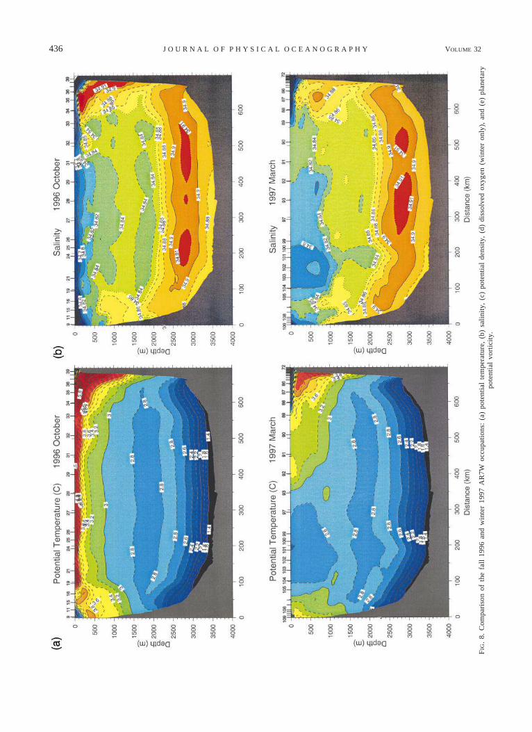
cruise). The comparison is shown in Fig. 8. It shouldbe noted that this section is a bit south of the region ofdeepest convection, at least in the winter of 1997.

In the fall section note the buoyant upper layer presentover the entire basin, and the rim-current properties onboth sides of the section. The warm, salty Irminger Water(centered near 500 m on the Greenland side; Figs. 8a,b)is significantly eroded by the time it reaches the Labradorside. This is presumably due to isopycnal mixing alongthe path of the rim current as it encircles the basin (Cunyet al. 2002), since very little of this water mass continuesnorthward through Davis Strait (Ross 1992).

In the winter section the stratified upper layer hasbeen eroded away, and a region of cold, fresh newlyformed LSW is seen in the western part of the basin,extending to depths greater than 1000 m (Figs. 8a,b).This is the area where previous studies have observednewly ventilated LSW. Note that the rim current poten-tial temperature (u) and salinity (S) distributions are alsoquite different in the winter. On the Labrador side thisis easily explained: the Irminger Water has been verti-cally mixed due to convection within the boundary cur-rent, producing a warmer and saltier vintage of LSW(see next section). This phenomenon was not observedin any of the past experiments, possibly because theboundary current region restratifies so quickly. On theGreenland side, the wintertime cooling and fresheningof the Irminger Water is more of a puzzle. Note thepronounced cold, fresh cap over the rim current here.This (presumably with the weaker air–sea flux on theeastern side of the basin) prevented convection fromoccurring here during the experiment. So what causedthe change in the Irminger properties off of West Green-land? One possibility is that it was due to a change in


FIG. 11. Example of the criterion for determining mixed layer depth (see text for details) using station115 profiles. The linear fit is shown as well.

the subtropical source input, but as noted earlier theoverall rim-current system of the subpolar gyre was be-coming warmer and saltier during this time frame.

Another more plausible explanation is that ventilationoccurred within the boundary current upstream of thislocation, in particular on the eastern side of Greenland.This is consistent with the results of Pickart et al. 2001;manuscript submitted to Deep-Sea Res. (hereafter P01a),who present evidence that deep overturning also occursin the Irminger Basin. Using the mean sections con-structed by P01a (Fig. 9), one sees that the cold, freshArctic waters of the shelfbreak current are more effec-tively trapped to the boundary east of Greenland thanwest of Greenland. This means that a buoyant cap doesnot typically extend over the continental slope in theIrminger Basin, in contrast to the Labrador Basin (asseen in Fig. 9). This, together with the enhanced air–sea forcing east of the Greenland landmass (see P01a)makes it more favorable for convection to occur overthe eastern slope of Greenland than over the westernslope of Greenland. Thus, we pose the following sce-nario [consistent with the view put forth by Smith et al.(1937)]: The Irminger Water in the rim current is par-tially ventilated east of Greenland in the Irminger Basin;it then rounds Cape Farewell and ‘‘subducts’’ under thecold, fresh cap extending off of the West Greenlandboundary. As noted above, a second area where (morerobust) Irminger Water ventilation occurs is next to theLabrador boundary, where the air–sea forcing is partic-ularly strong.

The question now is, why does the buoyant shelfbreakwater extend offshore on the west side of Greenland but

not the east side of Greenland? One reason might bedue to the enhanced eddy activity on the western side,as seen in Fig. 1. There is now strong evidence that therim current system in the eastern Labrador Sea is par-ticularly unstable and, hence, is a source of eddies (Prat-er 2002; Lavender 2001; Lilly et al. 2001a,b, manu-scripts submitted to J. Phys. Oceanogr., hereafter L01aand L01b, respectively; Cuny 2002). The eddy vari-ability is maximum in the region where the continentalslope broadens abruptly near 61.58N (where the 3000-m isobath ‘‘turns the corner;’’ Fig. 1). We conjecturethat the eddy generation in this area results in an en-hanced offshore flux of shelfbreak water, contributingto the freshwater cap in the eastern Labrador Sea (aprocess that is seemingly absent in the Irminger Sea).This view is supported by the results of L01a, who haveobserved surface-intensified ‘‘Irminger rings’’ in thecentral Labrador Sea, which, via their altimetric signal,are believed to emanate from the region of elevated eddyenergy (L01b). Note that the AR7W section is near thesouthern edge of the region of enhanced eddy variability(Fig. 1).

Clearly these ideas require further investigation, but wefeel compelled to present such a scenario as an attempt toexplain the seasonal change in u and S observed in therim current. Other aspects of the winter dataset, presentedbelow, support this eddy flux interpretation as well.

b. Density

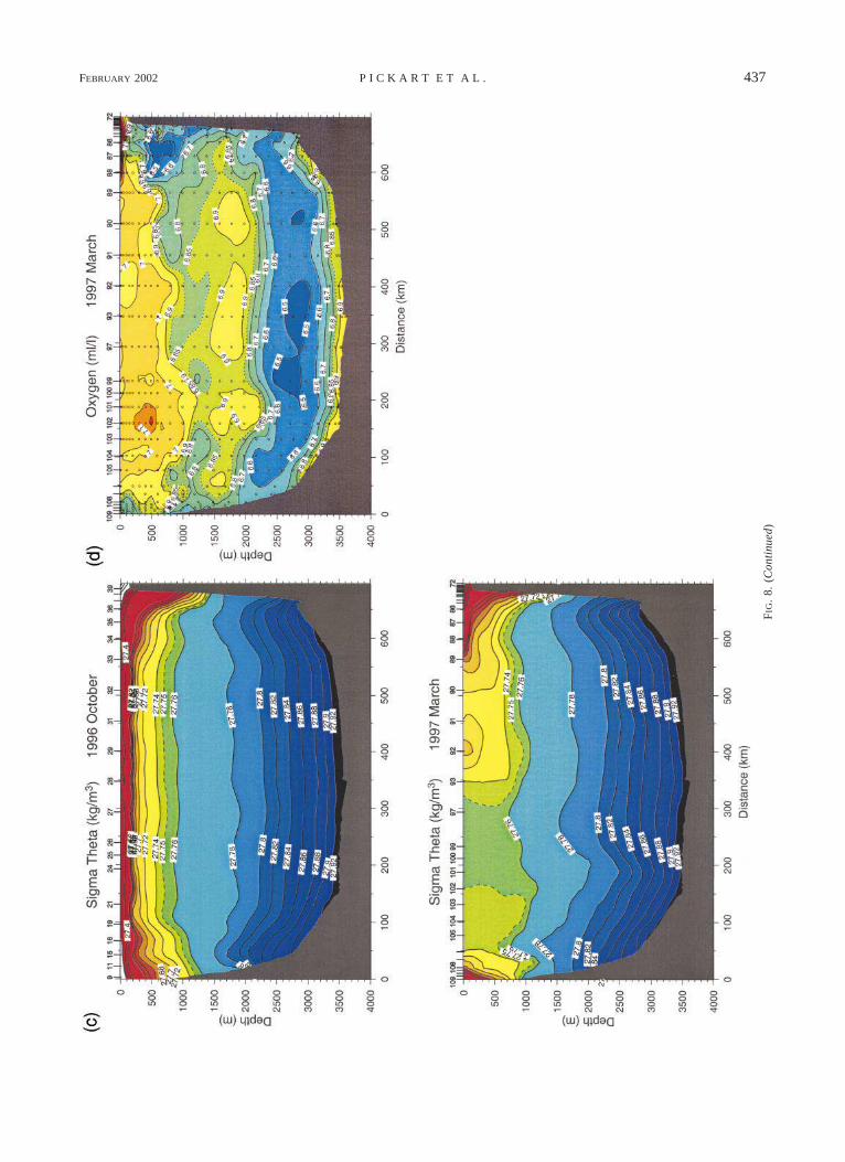
The sections of potential density referenced to the seasurface (su, Fig. 8c) show many of the features de-


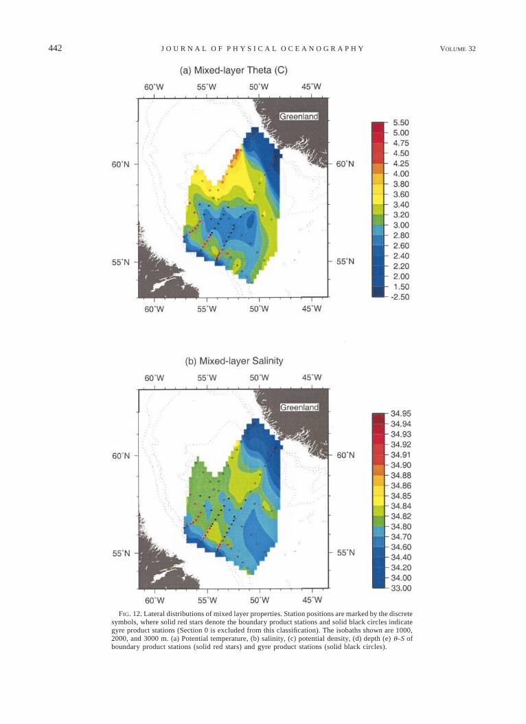
FIG. 12. Lateral distributions of mixed layer properties. Station positions are marked by the discretesymbols, where solid red stars denote the boundary product stations and solid black circles indicategyre product stations (Section 0 is excluded from this classification). The isobaths shown are 1000,2000, and 3000 m. (a) Potential temperature, (b) salinity, (c) potential density, (d) depth (e) u–S ofboundary product stations (solid red stars) and gyre product stations (solid black circles).


FIG. 12. (Continued)


FIG. 12. (Continued)

scribed above. However, one feature that is particularlyevident in the density field is the anomalous nature ofstation 92. This station contained buoyant water in theupper layer, which clearly has its origin in the easternboundary current. A similar feature was also observedin midbasin on the northern hydrographic section of thewinter survey (not shown). It is believed that these arein fact remnants of the eastern boundary current ringsas discussed above (see also the discussion in section5b). Based on the seemingly large population of sucheddies (Prater 2002; L01b) it is not surprising that weencountered some. Unfortunately, we did not take thetime to sample either feature, although some of the RA-FOS floats deployed during the Deep Convection Ex-periment became entrained into eddies in this region,providing some information on their scales (Prater2002).

c. Tracers

Two common tracers used to identify newly ventilatedLSW in the North Atlantic are dissolved oxygen andplanetary potential vorticity [PV ø ( f /r)]r/]z (Talleyand McCartney 1982)]. Our wintertime data allow usto consider the ‘‘boundary conditions’’ for these tracersduring convective formation. The winter vertical sectionof oxygen (Fig. 8d) provides important corroborating

evidence in identifying the newly convected water. Forinstance, the boundary current vintage of LSW does notstay unstratified for long (simply because newly formedconvective lenses are surrounded by buoyant rim currentwater). Hence, elevated values of oxygen provide proofthat the water was formed in 1997. An example of thisis in the Labrador rim current in Fig. 8d: convectionhas occurred shoreward of station 105, which is notespecially obvious in the potential temperature section.This is elaborated on in section 5b.

A striking view of the convective state of the Lab-rador Sea is provided by the potential vorticity (PV)field (Fig. 8e). The new 1997 water extends to roughly1000 m. At the time the section was taken, the depthof penetration had not quite reached the body of weaklystratified water remaining from convection in previousyears. This deeper LSW was at least two years old be-cause 1996 was a very weak convection year. It is pos-sible that later in the season the thin stratified layerseparating the ‘‘old’’ and new water was eroded away(we departed the Labrador Sea on 12 March). One cansee from Fig. 8e that, if this happened, the depth ofconvection could easily have reached 2 km as the weak-ly stratified older water became reventilated. However,evidence of the thin stratified layer, separating the twobodies of water, was present in the spring 1997 occu-pation of the section. This suggests that convection did


FIG. 13. Vertical profiles of (a) potential density and (b) oxygenconcentration from three stations along the central hydrographic line(see Fig. 7). The gyre product (mixed layer depth of 1270 m) ispresent at station 119 (solid line); the boundary product (mixed layerdepth of 825 m) is present at station 62 (dashed line); station 59 wastaken in unventilated nearshore water (dotted line).

not penetrate beyond 1500 m during the remainder ofthe winter. Finally, note the significant presence of thepreviously formed LSW in the eastern rim current (inboth the fall and winter sections); this is another hintof substantial mixing near that boundary.

d. Heat storage

Contrasting the fall and winter potential temperaturesections (Fig. 8a), one can visualize the loss of heat

from the Labrador Sea as a result of convection. Datafrom the Deep Convection Experiment allow us to quan-tify the change in heat storage of the water column andcompare it to the strength of the atmospheric forcing.The heat storage Hs is defined as

H 5 rC uV,s p (1)

where r is the density, Cp is the heat capacity, u is thepotential temperature, and V is the volume of water. Thechange in storage along the AR7W line from Octoberto March is shown in Fig. 10. Note the loss of heatassociated with the erosion of the upper layer in thecenter of the basin; as expected, the depth of heat lossextends roughly to 1000 m on the western side. Notethat the deeper isolines slant downward toward the west,likely because of the stronger air–sea forcing on thatside of the basin.

In the inshore portion of the western rim current thereis heat gain near the surface. This is likely an advectiveeffect. In particular, the time period near October rep-resents a maximum in the strength of the baroclinicbranch of the Labrador Current, which transports fresh-water southward from Baffin and Hudson Bays (Lazierand Wright 1993). The thick cold/fresh layer seen onthe western end of the AR7W section in October (Fig.8b) is likely due to the enhanced presence of this waterin the fall. On the eastern side of the AR7W section theheat loss extends to the depth of the Irminger Waterdespite no local convection there, presumably due tothe upstream boundary ventilation scenario describedabove.

Is the observed heat loss consistent with the forcing?To answer this we limited the area of consideration tothe interior of the basin, where advection is weaker.Integrating the heat loss over the portion of the AR7Wsection delimited in Fig. 10, the net heat loss is 1.04 3103 petajoules/kilometer (PJ km21). To estimate theforcing, we integrated the NCEP heat flux over the timeperiod from October to March along the AR7W line.The amount of heat fluxed through the sea surface, cal-culated as such, was 0.97 3 103 PJ km21. This goodagreement indicates that we can account for the ob-served change in heat storage in the AR7W section interms of the regional atmospheric forcing. Formulatedas fluxes, the above numbers translate to 202 and 188W m22, respectively. This represents the average fromlate October to early March and is reasonable in com-parison to the observed average fluxes at Ocean WeatherStation Bravo (Pickart et al. 1997b).

5. Water mass products

Two different types of Labrador Sea Water have beendescribed in the literature: upper LSW [which has beengiven other names as well (e.g., Rhein et al. 1995)] andclassical LSW. The former is believed to originate inthe vicinity of the Labrador shelf break (Pickart et al.1997b), and is found at relatively shallow depths in the


FIG. 14. Time evolution of mixed layer u–S between the two occupations of Section 2, for thegyre and boundary regions. The final springtime product (see text) is indicated by the large blackcircle.

North Atlantic. We did not investigate its formation be-cause we were unable to collect data far enough onshore(due to the sea ice, as discussed above). Hence upperLSW is not considered in this paper. The second watermass, classical LSW, is significantly denser and foundat greater depths in the North Atlantic (e.g., Talley andMcCartney 1982). Its formation, via deep convection,was the focus of our experiment. A central question forthe hydrographic cruise was, precisely where does thedeep overturning, and hence formation of classical LSW,occur within the Labrador Basin?

The historical notion is that classical LSW is formedseaward of the western continental slope, where the air–sea forcing is strong and the ambient water is mostpreconditioned (Clarke and Gascard 1983). More re-cently, Pickart et al. (1997b) reasoned that, in favorableNAO conditions, overturning probably occurs farthersouth as well, and hence is more readily entrained intothe deep western boundary current (DWBC). This latteridea could not be tested in the present experiment be-cause we focused our activities to the northwest where

the probability of witnessing convection was greatest.However, one of the major findings of this experimentis that deep convection can occur directly into theDWBC on the western side of the Labrador Sea, as wellas in the basin interior. These two geographical regionsproduce distinct vintages of classical LSW (detailed be-low). The ‘‘dividing line’’ is roughly the 3000-m iso-bath. Seaward of this we refer to the water mass productas the ‘‘gyre product.’’ This is the same water mass thatClarke and Gascard (1983) observed being formed in1976. Shoreward of this, in the rim current, we call theresultant water mass the ‘‘boundary product.’’

a. Characterization of mixed layers

In order to quantify the water mass products, as wellas describe the gross characteristics of the observedmixed layers, we systematically identified the depth ofthe mixed layer in each CTD profile. This was done asa two-step process (Fig. 11). Using the profile of po-tential density, the approximate extent of the mixed lay-


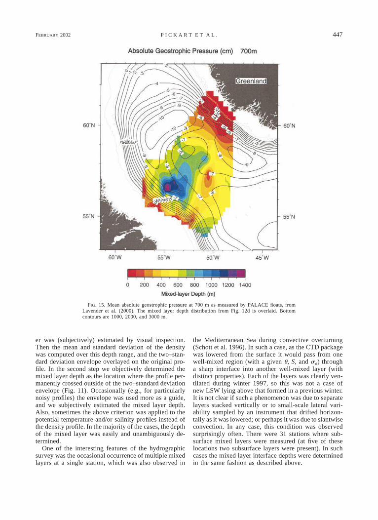
FIG. 15. Mean absolute geostrophic pressure at 700 m as measured by PALACE floats, fromLavender et al. (2000). The mixed layer depth distribution from Fig. 12d is overlaid. Bottomcontours are 1000, 2000, and 3000 m.

er was (subjectively) estimated by visual inspection.Then the mean and standard deviation of the densitywas computed over this depth range, and the two–stan-dard deviation envelope overlayed on the original pro-file. In the second step we objectively determined themixed layer depth as the location where the profile per-manently crossed outside of the two–standard deviationenvelope (Fig. 11). Occasionally (e.g., for particularlynoisy profiles) the envelope was used more as a guide,and we subjectively estimated the mixed layer depth.Also, sometimes the above criterion was applied to thepotential temperature and/or salinity profiles instead ofthe density profile. In the majority of the cases, the depthof the mixed layer was easily and unambiguously de-termined.

One of the interesting features of the hydrographicsurvey was the occasional occurrence of multiple mixedlayers at a single station, which was also observed in

the Mediterranean Sea during convective overturning(Schott et al. 1996). In such a case, as the CTD packagewas lowered from the surface it would pass from onewell-mixed region (with a given u, S, and su) througha sharp interface into another well-mixed layer (withdistinct properties). Each of the layers was clearly ven-tilated during winter 1997, so this was not a case ofnew LSW lying above that formed in a previous winter.It is not clear if such a phenomenon was due to separatelayers stacked vertically or to small-scale lateral vari-ability sampled by an instrument that drifted horizon-tally as it was lowered; or perhaps it was due to slantwiseconvection. In any case, this condition was observedsurprisingly often. There were 31 stations where sub-surface mixed layers were measured (at five of theselocations two subsurface layers were present). In suchcases the mixed layer interface depths were determinedin the same fashion as described above.


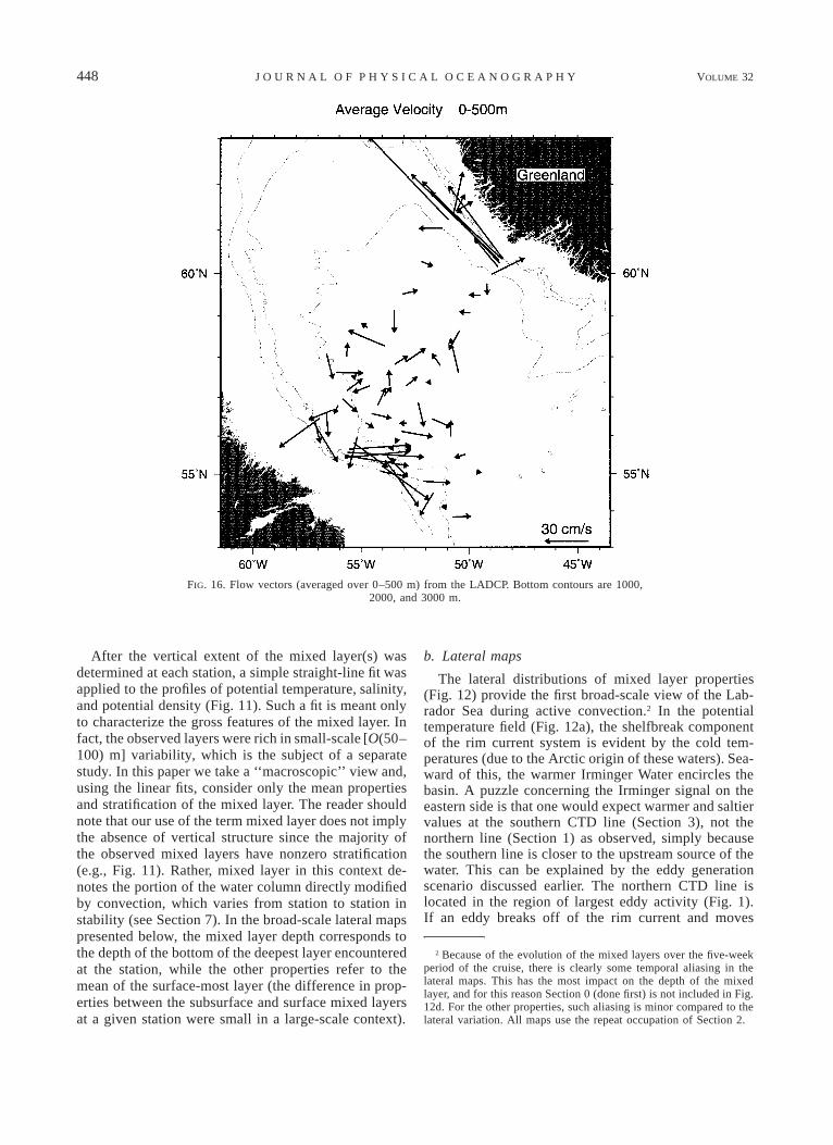
FIG. 16. Flow vectors (averaged over 0–500 m) from the LADCP. Bottom contours are 1000,2000, and 3000 m.

After the vertical extent of the mixed layer(s) wasdetermined at each station, a simple straight-line fit wasapplied to the profiles of potential temperature, salinity,and potential density (Fig. 11). Such a fit is meant onlyto characterize the gross features of the mixed layer. Infact, the observed layers were rich in small-scale [O(50–100) m] variability, which is the subject of a separatestudy. In this paper we take a ‘‘macroscopic’’ view and,using the linear fits, consider only the mean propertiesand stratification of the mixed layer. The reader shouldnote that our use of the term mixed layer does not implythe absence of vertical structure since the majority ofthe observed mixed layers have nonzero stratification(e.g., Fig. 11). Rather, mixed layer in this context de-notes the portion of the water column directly modifiedby convection, which varies from station to station instability (see Section 7). In the broad-scale lateral mapspresented below, the mixed layer depth corresponds tothe depth of the bottom of the deepest layer encounteredat the station, while the other properties refer to themean of the surface-most layer (the difference in prop-erties between the subsurface and surface mixed layersat a given station were small in a large-scale context).

b. Lateral maps

The lateral distributions of mixed layer properties(Fig. 12) provide the first broad-scale view of the Lab-rador Sea during active convection.2 In the potentialtemperature field (Fig. 12a), the shelfbreak componentof the rim current system is evident by the cold tem-peratures (due to the Arctic origin of these waters). Sea-ward of this, the warmer Irminger Water encircles thebasin. A puzzle concerning the Irminger signal on theeastern side is that one would expect warmer and saltiervalues at the southern CTD line (Section 3), not thenorthern line (Section 1) as observed, simply becausethe southern line is closer to the upstream source of thewater. This can be explained by the eddy generationscenario discussed earlier. The northern CTD line islocated in the region of largest eddy activity (Fig. 1).If an eddy breaks off of the rim current and moves

2 Because of the evolution of the mixed layers over the five-weekperiod of the cruise, there is clearly some temporal aliasing in thelateral maps. This has the most impact on the depth of the mixedlayer, and for this reason Section 0 (done first) is not included in Fig.12d. For the other properties, such aliasing is minor compared to thelateral variation. All maps use the repeat occupation of Section 2.


FIG. 17. Vertical sections of alongisobath current (cm s21) from the LADCP (dashed contours are equatorward), for the western end ofthe three hydrographic lines (see Fig. 7). Transport calculations were done over the length of each section. (a) Section 1; (b) Section 2; (c)Section 3; (d) average of the three sections (see text for explanation of averaging); (e) standard error of the average velocity (gray shadingdenotes regions where the average is not significantly different from zero).

toward the center of the basin, it brings with it ‘‘pure’’Irminger properties, with a freshwater cap. As it travelsseaward it will experience an erosion of properties dueto mixing and also be subject to greater air–sea forcing(Fig. 2). Both of these increase the likelihood that con-vection will occur within the feature, resulting in a warmand salty mixed layer compared to the ambient water.Since the eddy population is likely higher at the northernline, this could explain the unexpected trend in the lat-eral distribution.

The pool of cold water seaward of the western con-tinental slope is where the densest/coldest/freshest LSWis being formed, that is, the gyre product. This is mostclearly seen in the density map (Fig. 12c). Interestingly,the location and lateral extent of the dense pool is verysimilar to that observed in February of 1978 by Clarkeand Gascard (1983), even though that winter was weakerand mixed layers were shallower. In strong winters (i.e.,

stronger than 1997) deep convection likely occurs overa greater portion of the Labrador Sea [e.g., to the south-east (Pickart et al. 1997b)]. However, the convection isevidently most predisposed to occur in a limited areaof the sea. This is discussed further in section 6. Aswith density, the lateral distribution of mixed layer depth(Fig. 12d) shows an isolated region of large values.However, there is a subtle but important difference:there are some deep mixed layers present over the Lab-rador continental slope inshore of the densest water. Infact, deep convection also occurred directly within thewestern rim current, hence forming the boundary prod-uct, a lighter/warmer/saltier version of classical LSW.The two products can be seen in vertical plan view inFig. 8 (stations 93–104 are the gyre product; stations105–108 are the boundary product). In the lateral mapsthe two products are denoted by different colored sym-bols (see caption to Fig. 12).


FIG

.18

.C

hang

ein

pote

ntia

lde

nsit

yfr

omth

eto

pof

the

mix

edla

yer

toth

ebo

ttom

(blu

e),

incl

udin

gth

eco

ntri

buti

ondu

eto

pote

ntia

lte

mpe

ratu

re(g

reen

)an

dsa

lini

ty(r

ed).

Sta

tion

sw

ithi

nth

eda

shed

line

s(fi

lled

sym

bols

)ar

ede

emed

neut

rall

yst

able

(see

text

).T

hest

atio

nnu

mbe

rsar

em

arke

don

the

absc

issa

,whe

rere

peat

num

bers

corr

esp

ond

tom

ulti

ple

mix

edla

yers

ata

stat

ion

(pro

gres

sing

shal

low

tode

ep).


1) LOCAL BOUNDARY CONVECTION

It is worth examining the possibility that the boundaryproduct is not due to local overturning in the westernrim current, but is instead due to convected water fromoffshore (the gyre product) laterally mixing into un-convected boundary current water. There are severalarguments that lead us to discount this notion.

First, although the enhanced stratification near thebasin’s edge is less conducive for overturning, the air–sea forcing is strongest next to the western boundary.The following simple calculation demonstrates that theobserved boundary mixed layer depths are consistentwith the atmospheric forcing. The mean speed of theboundary current in the vicinity of the 2500-m isobathis O(10 cm s21) (P01b), which means that a water parcelwould take roughly 4–5 months to encircle the basinfrom the eastern end of the AR7W section to the westernend. Hence, the western rim current water observed dur-ing the winter hydrographic cruise would have been inthe eastern basin near the time of the 1996 fall AR7Woccupation. Therefore, we chose an eastern boundaryprofile from the fall section (station 35; Fig. 8) andapplied the appropriate NCEP forcing around the edgeof the basin—that is, interpolating the NCEP values inthe manner of ‘‘following the parcel.’’ Using a 1D mixedlayer model (Clarke and Gascard 1983; Pickart et al.1997b), applied in this Lagrangian sense, the depth ofoverturning reaches 750 m. This is in line with the ob-served mean mixed layer depth of the boundary product,which is 700 m. (We note that there were several mixedlayers in this region that exceeded 900 m, including oneas deep as 1130 m.)

A second factor implicating local boundary convec-tion on the western side of the basin pertains to theoxygen saturation of the boundary mixed layers. Asreported by Clarke and Coote (1988, their Fig. 2e) thepercent oxygen saturation in the newly convected gyreproduct is on the order of 93%–94%. This is consistentwith our observations as well. One would expect thata mixture between this interior water and unventilatedboundary water would result in significantly reducedsaturation. To test this we considered stations along thecentral hydrographic line (Fig. 13). Specifically, wecomputed the percent saturation after mixing—both is-opycnally and laterally—station 119 (ventilated gyreproduct observed late in the cruise) with station 59 (un-ventilated nearshore boundary water). The resulting sat-urations of the two mixtures were 91.9% and 91.6%,respectively. This is far less than the 93.9% saturationobserved at station 62 (ventilated boundary product). Infact, it is less than the older convected water remainingat depth in the central basin from two winters ago.Hence, the high oxygen saturation of the boundary prod-uct argues against a mixture.

A third feature suggesting local overturning is thesharpness of the interface at the bottom of the boundarymixed layers. Consider again station 119 (gyre product)

and station 62 (boundary product). Using the (slightlylow-passed) su versus depth profiles, we computed thedegree of discontinuity in curvature at the base of eachmixed layer and found that it was comparable at thetwo sites (actually a bit larger for the boundary mixedlayer). This is inconsistent with the notion of mixing,whereby a density jump would likely be eroded. Finally,as part of the Deep Convection Experiment, there weremoorings situated along the AR7W line, including somewithin the western boundary current inshore of the3000-m isobath. Although less conclusive than the hy-drography, evidence from mooring records supports theview of local overturning (P. Rhines 1999, personalcommunication).3 This should not come as a surprise,since mooring data as far inshore as the 1000-m isobath(from a different winter) indicate a uniform temperaturethroughout the water column, indicative of local con-vection [forming upper LSW (Pickart et al. 1997b)].

2) LONG-TIME EVOLUTION

The gyre and boundary convective products are clear-ly distinct in u and S (circles vs stars in Fig. 12e).However, convection undoubtedly continued for sometime after we left the area; recall that we departed on12 March, and, according to Lilly et al. (1999), over-turning can occur through the end of March. Hence, onemight ask, what was (were) the final water massproduct(s) formed in the winter of 1997? Our data canshed some light on this question as well. Recall thatSection 2 (Fig. 7) was repeated later in the cruise. Dur-ing the 10 days between occupations the air–sea forcingwas particularly strong, and significant evolution of themixed layer occurred. In Fig. 14 one sees that the gyreproduct became denser, mainly due to an increase insalinity. By contrast, the boundary product becamedenser due to cooling as well as salinification. Hence,these two products were converging toward each otherin u–S space.

Further information on the ultimate fate of the wateris provided by the springtime repeat of the WOCEAR7W section. As noted earlier it appears that the deep-er body of LSW formed earlier in the decade (Fig. 8e)was not reventilated during the winter of 1997. Abovethis older water, a region of low PV in the springtimesection marks the core of the 1997 final product (notshown). The u and S of this shallower core are includedin Fig. 14. Clearly, further salinification of the mixedlayer occurred after our cruise, which is not surprising.Note that the final springtime product is somewhat closeto the convergent point of the gyre and boundary prod-ucts. This suggests that perhaps in the end only a singleproduct was formed (especially after allowing for mix-ing). Another scenario, however, is that the boundaryproduct, formed directly within the DWBC, was largely

3 Not all of the moorings, however, show such a signal (U. Send2000, personal communication).


advected out of the domain by the time of the springtimecruise. A third possibility is that the boundary productrestratified to the point where it could no longer be easilydetected. These latter two explanations are more likelybecause most of the low PV core in the springtime sec-tion was found seaward of the 3000-m isobath. Hence,the observed final product in Fig. 14 is likely the endstate of the gyre water mass, which by spring would bea bit warmer and saltier due to some restratification.[Yashayaev et al. (2000) note that there was broadeningof the boundary product T–S class from fall 1996 tospring 1997, so at least a portion of this product wasstill present, perhaps due to advection from the north.]

Regardless of the scenario, one would be hard pressedto distinguish between the gyre and boundary convec-tive products any distance away from the Labrador Sea(e.g., at some later time in the eastern Atlantic). For thisreason we are not advocating a new water mass name.We are, however, stressing that classical LSW can beformed both within the interior gyre, and within thewestern boundary current. Using the May u–S value asthe benchmark (Fig. 14), the 1997 value of classicalLSW was u 5 2.98C, S 5 34.84 psu.4

6. Circulation

a. Mean

Early descriptions of the general circulation in theLabrador Sea included a weak cyclonic gyre in the cen-ter of the basin, with a strong boundary current encir-cling the sea. Based on modern data, in particular directmeasurements, a significantly different pattern has re-cently emerged. While the notion of a rim current isindeed accurate, the strength of this flow was under-estimated in the historical (indirect) measurements. Us-ing moored current meter data, Lazier and Wright (1993)were the first to show that the Labrador Sea rim currenthas a relatively strong barotropic component over thedeep continental slope. Lazier and Wright (1993) arguedthat this is largely due to the wind-driven Sverdrup re-turn flow of the subpolar gyre, which travels equator-ward together with the (bottom intensified) thermoha-line overflow water. Farther up the slope, the (surfaceintensified) baroclinic Labrador Current resides near theshelf break; this is the continuation of the West Green-land Current, with a contribution from the Arctic Oceanvia flow through the Canadian archipelago.

The biggest change in our view of the circulation inthe Labrador Sea pertains to the interior flow. The dy-namic topography of the sea surface (relative to mid-depth) suggests a basinwide cyclonic flow, correspond-ing to the doming of the isopycnals towards the center

4 It should be noted that this is different than the 1997 LSW valuequoted by Lazier et al. (2001). Their value (u 5 2.858C, S 5 34.848psu) refers to the deeper PV core, that is, the body of older LSWthat was not reventilated in the winter of 1997.

of the sea (e.g., the fall 1996 AR7W section, Fig. 8c).Indeed, this is the basis for the historical circulationdiagrams. This pattern was modified, or at least eluci-dated, by Clarke and Gascard (1983), based on theirwinter hydrographic data from 1978. These authors in-troduced the notion of a ‘‘western cyclonic gyre,’’ asmaller recirculation that forms during winter in thewestern half of the basin. This is the baroclinic surfacecirculation associated with the dense pool that developsduring convection (see Fig. 12c). Clarke and Gascard(1983) stressed the importance of this feature in trappingthe surface water in the western Labrador Sea, enablingthe water to be subject to the air–sea forcing for a longerperiod, hence resulting in deep overturning.

Using a reference level of 500 db, our 1997 winterdata suggest a surface circulation of 1–2 cm s21 in sucha western gyre. However, this estimate is purely baro-clinic. One of the main observational components of theDeep Convection Experiment consisted of a widespreaddeployment of Profiling Autonomous Lagrangian Cir-culation Explorer (PALACE) floats (R. Davis and B.Owens 1997, personal communication; see Lab SeaGroup 1998). These data are presented in Lavender etal. (2000) and provide the first direct view of the mid-depth circulation in the western subpolar Atlantic. Theinterior pattern can be described as a series of subbasin-scale cyclonic recirculations (four altogether), situatedadjacent to the continental slope from the Irminger Ba-sin to the Newfoundland Basin. The mean flow at 700m in the Labrador Sea, from Lavender et al. (2000), isshown in Fig. 15. As discussed by these authors, thecirculation pattern is robust and exhibits little season-ality. Furthermore, the analogous streamline map at1500 m (Lavender 2000, personal communication) in-dicates that the flow is largely barotropic. This is verifiedin P01b for the AR7W section.

Note in Fig. 15 the presence of the cyclonic recir-culation southwest of Greenland, and another one oflarger extent along the northern and western sides ofthe basin. Between these, in the center of the LabradorSea, the flow appears to be anticyclonic (Lavender etal. 2000). This pattern, together with the strength offlow (4–5 cm s21 in the interior at 700 m), suggests thatthe historical notion of a weak basinwide baroclinicgyre—or western baroclinic gyre—is likely not valid.What drives the subbasin-scale cyclonic recirculations?This is presently an open question, though wind forcingis certainly a factor to consider: recall the strong cy-clonic wind stress curl around Greenland that developsevery winter (seemingly insensitive to the NAO; Fig.2).

While a wintertime baroclinic western gyre is evi-dently not the appropriate conceptual model for the in-terior Labrador Sea, an analogous feature is present inthe absolute circulation in Fig. 15. A distinct trough inabsolute dynamic height is situated seaward of the rimcurrent in the western Labrador Sea. While largely bar-otropic and present year-round—and likely governed by


different dynamics—it serves a similar purpose withregard to trapping the water in the region of strongcooling. Hence, one suspects that this should play animportant role in dictating the occurrence of convection.This idea is supported by the winter hydrography in thatthe deepest mixed layers are found within the nearlystagnant center of the cyclonic feature (Fig. 15). Ad-mittedly we are comparing a synoptic distribution witha mean flow pattern, but since the deepest mixed layersin 1978 were also observed here, the agreement is com-pelling. Also, the PALACE float hydrographic profilesfrom the winters of 1997 and 1998 showed the deepestmixed layers in this area (Lavender et al. 2000). Withthe newly formed LSW trapped to some degree in thegyre, this greatly increases the flushing time and pro-vides the means by which the Labrador Sea has a mem-ory of previous winters. It also explains why the 1997springtime AR7W PV section showed mostly the gyreproduct that we observed being formed in February.(One also sees how the boundary product is subject tosouthward advection by the DWBC.)

Why does the deepest overturning not occur farthernorthward in the cyclonic gyre, where the atmosphericforcing is even greater (Fig. 2)? This is because theambient water in the northern part of the Labrador Seais more strongly stratified. As discussed earlier, thisstratification is likely due to the buoyant water beingfluxed into the northern interior basin from the easternboundary current via the Irminger eddies. The impli-cation then is profound: that a boundary current insta-bility process—likely related to a local topographic fea-ture—impacts to first order the location and extent ofdeep convection in the Labrador Sea.

b. Winter of 1997

During our hydrographic survey we had three dif-ferent means of measuring absolute velocity from theship: the vessel-mounted ADCP (maximum depth ofmeasurement 500 m), the LADCP (full water columnprofile at each station), and a hull-mounted acousticcorrelation profiler (extending to 1200 m). The latterdid not function well under the harsh sea state, so thedata return was marginal (an exception to this was thelong to-yo, which was done at slow speeds). TheLADCP dataset was processed following the proceduresin Firing and Gordon (1990) and Fischer and Visbeck(1993), and the resulting measurement accuracy is 2 cms21. Subsequent to the processing, the data were runthrough the Oregon State University global altimetricinverse model TPXO.3 (Egbert et al. 1994) to removethe barotropic tidal signal. Finally, each profile was low-passed vertically using a Gaussian filter of width 1000m (500 m if the water depth was shallower than 1500m). The purpose of this was to reduce the high wave-number signal, presumably due to inertial motions andinternal waves.

Despite the detiding and smoothing, the LADCP da-

taset is quite noisy. We believe that this is due to thehigh eddy-energy levels of the Labrador Sea associatedwith active convection (e.g., Lilly et al. 1999). This isfurther supported by the fact that the vessel-mountedADCP data exhibit very good agreement with theLADCP profiles at the CTD station sites. A lateral snap-shot of the flow field during the hydrographic survey,as measured by the LADCP, is shown in Fig. 16. Despitethe scatter, the enhanced flow of the rim current systemis evident. A vertical view of this current on the Lab-rador side is provided by the three crossings (Figs. 17a–c, which show the component of velocity parallel to thelocal isobaths). All three vertical sections show quali-tatively the same overall boundary current structure: theenhanced flow of the baroclinic Labrador Current at theonshoremost end of the section, a generally more bar-otropic signal farther offshore (the wind-driven flow),and some bottom intensification near the 2500-m isobathcorresponding to the thermohaline overflow. Thesecomponents are in line with the earlier moored mea-surements of Lazier and Wright (1993).

Farther offshore in the vertical sections of Figs. 17a–c the flow is more variable, but predominantly equa-torward. We now derive a synoptic transport estimateof the boundary current ‘‘throughput’’ versus the ad-jacent ‘‘recirculation’’ revealed by the PALACE data.The total equatorward transports in each of the LADCPsections are 43.5, 49.9, and 43.2 Sv (Sv [ 106 m3 s21)respectively. In light of the scatter in the data, these aresurprisingly consistent—and surprisingly large. Howmuch of this transport is the rim-current throughput?Using the 3000-m isobath as the dividing line—whichis the approximate division between the boundary andgyre water mass regimes as discussed above—the di-vision is 33.7 6 4.2 Sv throughput, and 11.9 6 2.1 Svrecirculation (where the uncertainty represents the stan-dard error, assuming 3 degrees of freedom).

Using a mean springtime AR7W geostrophic velocitysection, referenced with the mean PALACE velocity at700 m, P01b objectively computed a throughput rimcurrent transport of 28.5 Sv. According to the diagnosticcalculation of Thompson et al. (1986), supported by thedirect measurements of Lazier and Wright (1993), theseasonal change in the wind-driven boundary currentcomponent between the time period of the winter cruiseand the springtime AR7W occupations is approximately4 Sv. [The change in the baroclinic Labrador Currenttransport over this same time is negligible by compar-ison (Lazier and Wright 1993).] Subtracting this fromour winter estimate gives 29.7 Sv of throughflow, ingood agreement with the 28.5 Sv from P01b. This isconsistent as well with Lohmann’s (1999) summertimeboundary current transport estimates of 27.4 Sv in 1996and 28.4 Sv in 1997 at the western end of the AR7Wline. (These two sections extended 30 km beyond the3000-m isobath, which would alter our AR7W boundarycurrent estimate by less than a Sverdrup.)

Seaward of the western boundary the velocities mea-


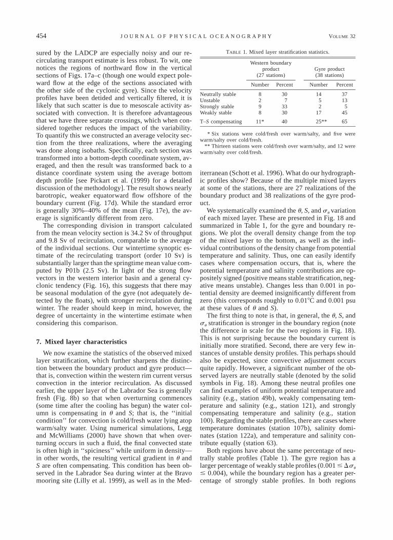
TABLE 1. Mixed layer stratification statistics.

Western boundaryproduct

(27 stations)

Number Percent

Gyre product(38 stations)

Number Percent

Neutrally stableUnstableStrongly stableWeakly stable

8298

307

3330

1452

17

3713

545

T–S compensating 11* 40 25** 65

* Six stations were cold/fresh over warm/salty, and five werewarm/salty over cold/fresh.

** Thirteen stations were cold/fresh over warm/salty, and 12 werewarm/salty over cold/fresh.

sured by the LADCP are especially noisy and our re-circulating transport estimate is less robust. To wit, onenotices the regions of northward flow in the verticalsections of Figs. 17a–c (though one would expect pole-ward flow at the edge of the sections associated withthe other side of the cyclonic gyre). Since the velocityprofiles have been detided and vertically filtered, it islikely that such scatter is due to mesoscale activity as-sociated with convection. It is therefore advantageousthat we have three separate crossings, which when con-sidered together reduces the impact of the variability.To quantify this we constructed an average velocity sec-tion from the three realizations, where the averagingwas done along isobaths. Specifically, each section wastransformed into a bottom-depth coordinate system, av-eraged, and then the result was transformed back to adistance coordinate system using the average bottomdepth profile [see Pickart et al. (1999) for a detaileddiscussion of the methodology]. The result shows nearlybarotropic, weaker equatorward flow offshore of theboundary current (Fig. 17d). While the standard erroris generally 30%–40% of the mean (Fig. 17e), the av-erage is significantly different from zero.

The corresponding division in transport calculatedfrom the mean velocity section is 34.2 Sv of throughputand 9.8 Sv of recirculation, comparable to the averageof the individual sections. Our wintertime synoptic es-timate of the recirculating transport (order 10 Sv) issubstantially larger than the springtime mean value com-puted by P01b (2.5 Sv). In light of the strong flowvectors in the western interior basin and a general cy-clonic tendency (Fig. 16), this suggests that there maybe seasonal modulation of the gyre (not adequately de-tected by the floats), with stronger recirculation duringwinter. The reader should keep in mind, however, thedegree of uncertainty in the wintertime estimate whenconsidering this comparison.

7. Mixed layer characteristics

We now examine the statistics of the observed mixedlayer stratification, which further sharpens the distinc-tion between the boundary product and gyre product—that is, convection within the western rim current versusconvection in the interior recirculation. As discussedearlier, the upper layer of the Labrador Sea is generallyfresh (Fig. 8b) so that when overturning commences(some time after the cooling has begun) the water col-umn is compensating in u and S; that is, the ‘‘initialcondition’’ for convection is cold/fresh water lying atopwarm/salty water. Using numerical simulations, Leggand McWilliams (2000) have shown that when over-turning occurs in such a fluid, the final convected stateis often high in ‘‘spiciness’’ while uniform in density—in other words, the resulting vertical gradient in u andS are often compensating. This condition has been ob-served in the Labrador Sea during winter at the Bravomooring site (Lilly et al. 1999), as well as in the Med-

iterranean (Schott et al. 1996). What do our hydrograph-ic profiles show? Because of the multiple mixed layersat some of the stations, there are 27 realizations of theboundary product and 38 realizations of the gyre prod-uct.

We systematically examined the u, S, and su variationof each mixed layer. These are presented in Fig. 18 andsummarized in Table 1, for the gyre and boundary re-gions. We plot the overall density change from the topof the mixed layer to the bottom, as well as the indi-vidual contributions of the density change from potentialtemperature and salinity. Thus, one can easily identifycases where compensation occurs, that is, where thepotential temperature and salinity contributions are op-positely signed (positive means stable stratification, neg-ative means unstable). Changes less than 0.001 in po-tential density are deemed insignificantly different fromzero (this corresponds roughly to 0.018C and 0.001 psuat these values of u and S).

The first thing to note is that, in general, the u, S, andsu stratification is stronger in the boundary region (notethe difference in scale for the two regions in Fig. 18).This is not surprising because the boundary current isinitially more stratified. Second, there are very few in-stances of unstable density profiles. This perhaps shouldalso be expected, since convective adjustment occursquite rapidly. However, a significant number of the ob-served layers are neutrally stable (denoted by the solidsymbols in Fig. 18). Among these neutral profiles onecan find examples of uniform potential temperature andsalinity (e.g., station 49b), weakly compensating tem-perature and salinity (e.g., station 121), and stronglycompensating temperature and salinity (e.g., station100). Regarding the stable profiles, there are cases wheretemperature dominates (station 107b), salinity domi-nates (station 122a), and temperature and salinity con-tribute equally (station 63).

Both regions have about the same percentage of neu-trally stable profiles (Table 1). The gyre region has alarger percentage of weakly stable profiles (0.001 # Dsu

# 0.004), while the boundary region has a greater per-centage of strongly stable profiles. In both regions


roughly half of the mixed layers are compensated in uand S, while the sense of this compensation is splitevenly between warm/salty over cold/fresh and cold/fresh over warm/salty—despite an initial condition ofthe latter. What are the distinguishing characteristics ofthe deepest mixed layers? Within the gyre region, thedeepest mixed layers are generally the most weaklystratified in density, temperature, and salinity. This isperhaps intuitive: the most intense overturning producesthe most weakly stratified product. However, the deepestmixed layers in the boundary region are the most strong-ly stratified in density. In particular, the temperaturestratification generally dominates, since there are salin-ity gradients of both signs. Hence the deepest productsin the two regions represent opposite extrema in termsof stratification—a result that was not anticipated, andshould be addressed in future work.

The reader should keep in mind that the above dis-cussion refers to the gross characteristics of the observedmixed layers. In essence this is equivalent to a coarselyresolved view of the water column, for example, similarto what a mooring with discrete instruments would mea-sure or a bottle station. The CTD has a 2-m samplingresolution, and as mentioned above there is substantialsmall-scale variability within the mixed layers. The typeof u/S compensation measured by the Bravo mooringand seen in Fig. 18 is of course governed by the mac-roscopic view. Detailed analysis of the smaller-scale sig-nals will be necessary to fully understand the nature ofthe overturning and ultimately enable us to parameterizeconvection in large-scale models. Toward this end, thehigh wavenumber part of the CTD data is the subjectof an ongoing study.

8. Summary

A wintertime hydrographic survey in February–March 1997 has provided the first broad-scale view ofthe Labrador Sea during the period of active convection.Overall, the winter of 1996/97 was moderate and wasnot typical of either the high or low NAO regime withrespect to atmospheric conditions or state of the sub-polar gyre. However, during the 5 week period of thecruise the atmospheric forcing was especially strong,characterized by cold air temperatures and strong west-erly winds. This resulted in overturning to nearly 1500m, since the sea was well preconditioned from precedingwinters.

A comparison of the WOCE AR7W section occupiedin March with that occupied the previous October re-vealed that familiar cold/fresh/dense classical LabradorSea Water (LSW) was formed in the western side of theinterior basin. The change in heat content in this regionimplies an average heat loss of ;200 W m22 over the4-month period, in line with that determined from thecalibrated, reanalyzed NCEP model fields of Renfrewet al. (2002). In the eastern Labrador Sea, overturning

did not occur because of a strong fresh cap extendingfrom the eastern rim current.

Deep convection was also observed on the westerncontinental slope, directly into the deep western bound-ary current. This formed a distinct water mass product,somewhat warmer, saltier, and lighter than the familiarinterior product. (It would, however, be difficult to dis-tinguish these two types of classical LSW large dis-tances from the Labrador Sea.) An occupation of theAR7W section the following May indicates that theboundary LSW product was either predominantlyflushed out of the Labrador Sea or quickly restratified.This is in contrast to the interior LSW product, whosepotential vorticity signature was prevalent in the spring-time section. This is likely due to the fact that the interiorconvection occurred within the cyclonic recirculationgyre recently measured by Lavender et al. (2000).Hence, the interior product was trapped to some degreein the western Labrador Sea. Deep overturning did notoccur farther north in the recirculating gyre because theambient water was more stratified, likely due to eddiesemanating from the eastern boundary.

The bulk stratification of the mixed layers furtherelucidates the difference between the boundary and in-terior classical LSW products. The deepest mixed layersin the interior region tend to be the most weakly strat-ified (weak in both temperature and salinity stratifica-tion), while the deepest mixed layers in the westernboundary current are generally the most strongly strat-ified (due mostly to the temperature stratification). Tem-perature/salinity compensation was observed in roughlyhalf of the mixed layers in each region, though it shouldbe remembered that the linear trends analyzed here giveonly a coarsely resolved view. Further analysis of thehigh wavenumber variability in the mixed layers willbe required to permit us to parameterize convection inmodels.

Acknowledgments. We are extremely indebted to Cap-tain A. D. Colburn and the crew of the Research VesselKnorr for their hard work and dedication in making thisfield program successful. From the moment we left thedock to the steam back home, the cruise was a constantseries of challenges. Each of these challenges was metwith professionalism, enthusiasm, and a strong desireto realize the scientific objectives. Whether it waspounding ice off the decks of the ship, navigatingthrough white-out conditions, or maintaining stationsnear the edge of the pack ice, the crew tackled eachtest, always maintaining the utmost safety and caution.This was one of the most difficult cruises ever under-taken by a Woods Hole Oceanographic Institution ves-sel. It was also a striking example of how the makeupof a vessel and the dedication of its crew can impactthe success of an experiment. Funding for the cruisewas provided by the Office of Naval Research throughContract N00014-97-1-0043. We are indebted to RussDavis for vocalizing the value of such a cruise, and to


Michael Van Woert for taking the risk and supportingit. We further acknowledge the assistance provided byDennis Conlon and Tom Curtin in the analysis phase ofthe experiment. The manuscript was greatly improvedas a result of comments from two anonymous reviewers.

REFERENCES

Belkin, I. M., S. Levitus, J. Antonov, and S.-A. Malmberg, 1998:‘‘Great Salinity Anomalies’’ in the North Atlantic. Progress inOceanography, Vol. 41, Pergamon, 1–68.

Clarke, R. A., and J. C. Gascard, 1983: The formation of LabradorSea Water. Part I: Large-scale processes. J. Phys. Oceanogr., 13,1764–1778.

——, and A. R. Coote, 1988: The formation of Labrador Sea water.Part III: The evolution of oxygen and nutrient concentration. J.Phys. Oceanogr., 18, 469–480.

Cuny, J., R. B. Rhines, P. P. Niiler, and S. Bacon, 2002: LabradorSea boundary currents and the fate of the Irminger Sea Water.J. Phys. Oceanogr., 32, 627–647.

Curry, R. G., and M. S. McCartney, 2001: Ocean gyre circulationchanges associated with the North Atlantic Oscillation. J. Phys.Oceanogr., 31, 3374–3400.

——, ——, and T. M. Joyce, 1998: Oceanic transport of subpolarclimate signals to mid-depth subtropical waters. Nature, 391,575–577.

Dickson, R. R., J. Meincke, S. A. Malmberg, and A. J. Lee, 1988:The ‘‘Great Salinity Anomaly’’ in the northern North Atlantic1968–1982. Progress in Oceanography, Vol. 20, Pergamon,103–151.

——, J. R. N. Lazier, J. Meincke, P. B. Rhines, and J. Swift, 1996:Long-term coordinated changes in the convective activity of theNorth Atlantic. Progress in Oceanography, Vol. 38, Pergamon,241–295.

Egbert, G. D., A. F. Bennett, and M. G. G. Foreman, 1994: TOPEX/POSEIDON tides estimated using a global inverse model. J.Geophys. Res., 99, 24 821–24 852.

Firing, E., and L. Gordon, 1990: Deep ocean acoustic doppler currentprofiling. Proc. IEEE Fourth Working Conf. on Current Mea-surements, Clinton, MD, Current Measurement TechnologyCommittee of the Ocean Engineering Society, 192–201.

Fischer, J., and M. Visbeck, 1993: Deep velocity profiling with selfcontained ADCPs. J. Atmos. Oceanic Technol., 10, 764–773.

Hurrell, J. W., 1995: Decadal trends in the North Atlantic Oscillationregional temperatures and precipitation. Science, 269, 676–679.

Lab Sea Group, 1998: The Labrador Sea Deep Convection Experi-ment. Bull. Amer. Meteor. Soc., 79, 2033–2058.

Lavender, K. L., R. E. Davis, and W. B. Owens, 2000: Mid-depthrecirculation observed in the interior Labrador and Irminger Seasby direct velocity measurements. Nature, 407, 66–69.

Lazier, J. R. N., 1973: The renewal of Labrador Sea water. Deep-SeaRes., 20, 341–353.

——, 1980: Oceanographic conditions at Ocean Weather Ship BRA-VO, 1964–1974. Atmos.–Ocean. 3, 227–238.

——, and D. G. Wright, 1993: Annual velocity variations in theLabrador Current. J. Phys. Oceanogr., 23, 559–678.

——, R. S. Pickart, and P. B. Rhines, 2001: Deep convection in theLabrador Sea. Ocean Circulation and Climate, G. Siedler, J.Church, and J. Gould, Eds., International Geophysics Series, Vol.77, Academic Press, 387–400.

Legg, S., and J. McWilliams, 2000: Temperature and salinity vari-ability in heterogenous convection. J. Phys. Oceanogr., 30,1188–1206.

Lilly, J. M., P. B. Rhines, M. Visbeck, R. Davis, J. R. N. Lazier, F.Schott, and D. Farmer, 1999: Observing deep convection in theLabrador Sea during winter 1994/95. J. Phys. Oceanogr., 29,2065–2098.

Lohmann, K., 1999: Gezeitenkorrektur von schiffsgestuetzten Stroe-

mungsmessungen. Diploma thesis, University of Kiel, Kiel, Ger-many, 86 pp.

McCartney, M. S., 1992: Recirculating components to the deepboundary current of the northern North Atlantic. Progress inOceanography, Vol. 29, Pergamon, 283–383.

Molinari, R. L., R. A. Fine, W. D. Wilson, R. G. Curry, J. Abell, andM. S. McCartney, 1998: The arrival of recently formed LabradorSea Water in the deep western boundary current at 26.5N. Geo-phys. Res. Lett., 25, 2249–2252.

Nielsen, J., 1928: The waters around Greenland. Greenland: TheDiscovery of Greenland, Exploration, and the Nature of theCountry, Vol. I, M. Vahl, Ed., C. A. Rietzel, 185–230.

Pickart, R. S., 1997: Adventure in the Labrador Sea: A wintertimecruise to the North Atlantic. Oceanus, 40 (1), 18–24.

——, P. Guest, F. Dobson, R. Anderson, K. Bumke, K. Uhlig, U.Karger, and H. Berndt, 1997a: KNORR 147 Leg V cruise sum-mary: Labrador Sea Convection Experiment. WHOI Unpub-lished Rep., 27 pp. [Available from Woods Hole OceanographicInstitution, Woods Hole, MA 02543.]

——, M. A. Spall, and J. R. N. Lazier, 1997b: Mid-depth ventilationin the western boundary current system of the sub-polar gyre.Deep-Sea Res., 44, 1025–1054.

——, T. K. McKee, D. J. Torres, and S. A. Harrington, 1999: Meanstructure and interannual variability of the slopewater systemsouth of Newfoundland. J. Phys. Oceanogr., 29, 2541–2558.

Prater, M. D., 2002: Eddies in the Labrador Sea as observed byprofiling RAFOS floats and remote sensing. J. Phys. Oceanogr.,32, 411–427.

Renfrew, I. A., G. W. K. Moore, P. S. Guest, and K. Bumke, 2002:A comparison of surface layer and surface turbulent flux ob-servations over the Labrador Sea with ECMWF analyses andNCEP reanalyses. J. Phys. Oceanogr., 32, 383–400.

Rhein, M., L. Stramma, and U. Send, 1995: The Atlantic deep westernboundary current: Water masses and transports near the equator.J. Geophys. Res., 100, 2441–2457.

Rhines, P. B., and J. R. N. Lazier, 1995: A 13-year record of con-vection and climate change in the deep Labrador Sea. AbstractReport of NOAA Principal Investigator’s Meeting, Miami, FL,NOAA, 50–55.

Rogers, J. C., 1990: Patterns of low-frequency monthly sea levelpressure variability (1899–1986) and associated wave cyclonefrequencies. J. Climate, 3, 1364–1379.

Ross, C. K., 1992: Moored current meter measurements across DavisStrait. Northwest Atlantic Fisheries Organization ScientificCouncil Doc. 92/70, 8 pp.

Schott, F., M. Visbeck, and J. Fischer, 1993: Observations of verticalcurrents and convection in the central Greenland Sea during thewinter of 1988–1989. J. Geophys. Res., 98, 14 401–14 421.

——, ——, U. Send, J. Fischer, L. Stramma, and Y. Desaubies, 1996:Observations of deep convection in the Gulf of Lions, northernMediterranean, during the winter of 1991/92. J. Phys. Oceanogr.,26, 505–524.

Smith, E. H., F. M. Soule, and O. Mosby, 1937: The Marion andGeneral Greene expeditions to Davis Strait and Labrador Sea.Scientific results, Part 2, physical oceanography. Bull. U.S. CoastGuard, 19, 1–259.

Steffen, E. L., and E. A. D’Asaro, 2002: Deep convection in theLabrador Sea as observed by Lagrangian floats. J. Phys. Ocean-ogr., 32, 475–492.

Straneo, F., and R. Pickart, 2001: Interannual variability in LabradorSea Water formation and export: How does it correlate to theatmospheric forcing? U.S. CLIVAR Meeting, June 2001, ex-tended abstract volume.

Sy, A., M. Rhein, J. R. N. Lazier, K. P. Koltermann, J. Meincke, A.Putzka, and M. Bersch, 1997: Surprisingly rapid spreading ofnewly formed intermediate waters across the North AtlanticOcean. Nature, 386, 675–679.

Talley, L. D., 2000: The shallow, intermediate and deep overturningcomponents of the global heat budget. Eos, Trans. Amer. Geo-phys. Union, 80, OS52.


——, and M. S. McCartney, 1982: Distribution and circulation ofLabrador Sea Water. J. Phys. Oceanogr., 12, 1189–1205.

Thompson, K. R., J. R. N. Lazier, and B. Taylor, 1986: Wind-forcedchanges in Labrador Current transport. J. Geophys. Res., 91,14 261–14 268.

Wallace, D. W. R., and J. R. N. Lazier, 1988: Anthropogenic Chlo-rofluorocarbons in newly-formed Labrador Sea Water. Nature,332, 61–63.

Yashayaev, I. M., R. A. Clarke, and J. R. N. Lazier, 2000: Recentdecline of the Labrador Sea Water. International Council for theExploration of the Sea, CM, 2000/L:18, 10 pp.

Zimmermann, S., T. K. McKee, R. S. Pickart, and W. M. Smethie Jr.,2000: KNORR 147 leg V hydrographic data report: Labrador SeaDeep Convection Experiment. Tech. Rep. WHOI-2000-05, WoodsHole Oceanographic Institution, Woods Hole, MA, 92 pp.

Hydrography of the Labrador Sea during Active Convection

Documents

Transcript of Hydrography of the Labrador Sea during Active Convection