HYDRATE GROWTH MODEL IN THE PRESENCE OF ...
336
HYDRATE GROWTH MODEL IN THE PRESENCE OF THERMODYNAMIC INHIBITORS OR PROMOTERS Ingrid Azevedo de Oliveira Tese de Doutorado apresentada ao Programa de Pós-graduação em Engenharia Química, COPPE, da Universidade Federal do Rio de Janeiro, como parte dos requisitos necessários à obtenção do título de Doutora em Engenharia Química. Orientadores: Frederico Wanderley Tavares, D. Sc. Amaro Gomes Barreto Jr., D. Sc. Rio de Janeiro Outubro de 2020
-
Upload
khangminh22 -
Category
Documents
-
view
2 -
download
0
Transcript of HYDRATE GROWTH MODEL IN THE PRESENCE OF ...
HYDRATE GROWTH MODEL IN THE PRESENCE OF THERMODYNAMIC
INHIBITORS OR PROMOTERS
Ingrid Azevedo de Oliveira
Tese de Doutorado apresentada ao Programa de
Pós-graduação em Engenharia Química, COPPE,
da Universidade Federal do Rio de Janeiro, como
parte dos requisitos necessários à obtenção do
título de Doutora em Engenharia Química.
Orientadores: Frederico Wanderley Tavares, D. Sc.
Amaro Gomes Barreto Jr., D. Sc.
Rio de Janeiro
Outubro de 2020

HYDRATE GROWTH MODEL IN THE PRESENCE OF THERMODYNAMIC
INHIBITORS OR PROMOTERS
Ingrid Azevedo de Oliveira
TESE SUBMETIDA AO CORPO DOCENTE DO INSTITUTO ALBERTO LUIZ
COIMBRA DE PÓS-GRADUAÇÃO E PESQUISA DE ENGENHARIA DA
UNIVERSIDADE FEDERAL DO RIO DE JANEIRO COMO PARTE DOS
REQUISITOS NECESSÁRIOS PARA A OBTENÇÃO DO GRAU DE DOUTOR EM
CIÊNCIAS EM ENGENHARIA QUÍMICA.
Orientadores: Frederico Wanderley Tavares
Amaro Gomes Barreto Jr.
Aprovada por: Prof. Frederico Wanderley Tavares
Prof. Amaro Gomes Barreto Jr.
Prof. Gabriel Gonçalves da Silva Ferreira
Prof. Pedro de Alcântara Pessôa Filho
Prof. Paulo Couto
Prof. Amadeu K. Sum
RIO DE JANEIRO, RJ - BRASIL
OUTUBRO DE 2020
iii
Oliveira, Ingrid Azevedo de
Hydrate growth model in the presence of thermodynamic
inhibitors or promoters / Ingrid Azevedo de Oliveira. – Rio de Janeiro:
UFRJ/COPPE, 2020.
XLIII, 337 p.: il.; 29,7cm.
Orientadores: Frederico Wanderley Tavares
Amaro Gomes Barreto Jr.
Tese (doutorado) – UFRJ/COPPE/Programa de Engenharia
Química, 2020.
Referências Bibliográficas: p. 134-161
1. Hidrato. 2. Crescimento. 3. Inibidores termodinâmicos.
4.Promotores termodinâmicos. 5. Termodinâmica de não-equilíbrio.
I. Tavares, Frederico Wanderley et al. II. Universidade Federal do Rio
de Janeiro, COPPE, Programa de Engenharia Química. III. Título.

iv
“É preciso que eu suporte duas ou três larvas
se quiser conhecer as borboletas...”
Antoine de Saint-Exupéry
v
Agradecimentos
Começo esses agradecimentos citando um trecho do livro O Pequeno Príncipe, de
Antoine de Saint-Exupéry: “Cada um que passa em nossa vida passa sozinho, mas não
vai só, nem nos deixa sós. Leva um pouco de nós mesmos, deixa um pouco de si mesmo.
Há os que levam muito; mas não há os que não levam nada. Há os que deixam muito; mas
não há os que não deixam nada.” Sem sombra de dúvidas todos que serão aqui citados
deixaram muito de si na minha vida nesses últimos quatro anos ou mais.
Agradeço a Deus, que na sua infinita bondade me permitiu chegar até aqui. Ele foi
o meu sustento, o meu refúgio e a minha força em todo esse tempo. Hoje afirmo que até
aqui me sustentou o Senhor e o seu Amor.
Agradeço aos meus país, Marcelo e Adriana, e à minha irmã, Iasmim; que foram
motivadores na minha vida mesmo quando eu não conseguia achar motivação; que
acreditaram em mim, quando eu mesma não consegui acreditar. Obrigada pelo amor que
me dedicaram, que não foi pouco, mas foi essencial para eu me tornar quem sou hoje.
Agradeço ao meu noivo, André; que todos os dias desses quatro anos me fez
lembrar que eu era capaz. Obrigada por sempre enxergar o melhor em mim. Te agradeço
imensamente pelo seu suporte, amor e amparo. Meus dias, tanto os ensolarados quanto os
nublados, são mais felizes desde que você chegou. Obrigada por sonhar junto comigo.
Agradeço, com muito carinho, a todos os meus amigos da vida. É muito bom cativar
e se deixar cativar. A vida é muito mais bela quando se tem amigos para compartilhá-la.
Agradeço aos meus orientadores, Professor Amaro e Professor Fred. Vocês me
ensinaram muito nesses anos. Passo a passo vocês me conduziram de uma caloura da
graduação, que nem sabia o que era fazer pesquisa, a uma Doutora. Obrigada por cada
oportunidade, cada reunião, cada correção e cada conselho. Obrigada por me
apresentarem o mundo da ciência e pela oportunidade que me deram de ser uma cientista.
Agradeço muito a toda a equipe do ATOMS. Se eu citar nomes sem dúvida
esquecerei algum, por isso vou me abster deles. Gostaria apenas de dizer que encontrei
nesse grupo muito mais que colegas de profissão, encontrei amigos. Encontrei ajuda,
solidariedade, carinho e respeito. No ATOMS encontrei cientistas que me motivaram e
motivam a seguir essa carreira tão desafiadora. Vocês são incríveis.
vi
Agradeço à UFRJ, ao PEQ, a todos os professores, pesquisadores e profissionais
dessa instituição. O trabalho que vejo sendo realizado me enche de orgulho e da certeza
de que escolhi a profissão certa. Mesmo com todos os desafios de fazer ciência no Brasil,
principalmente nos últimos tempos, vocês se superam diariamente. Todo o meu orgulho
e admiração pela ciência nacional.
Agradeço aos membros da banca, que prontamente aceitaram fazer parte deste
trabalho e contribuir para minha formação. Me sinto honrada de ter em minha banca
nomes tão valiosos para a ciência brasileira. Em especial, agradeço ao professor Amadeu
Sum, que me recebeu para um doutorado sanduíche em seu grupo no Colorado.
Agradeço à PETROBRÁS, ao CNPq e à CAPES pelo apoio financeiro a este
trabalho e à ciência brasileira.

vii
Resumo da Tese apresentada à COPPE/UFRJ como parte dos requisitos necessários
para a obtenção do grau de Doutor em Ciências (D.Sc.)
MODELO DE CRESCIMENTO DE HIDRATO NA PRESENÇA DE
INIBIDORES OU PROMOTORES TERMODINÂMICOS
Ingrid Azevedo de Oliveira
Outubro/2020
Orientadores: Frederico Wanderley Tavares
Amaro Gomes Barreto Jr.
Programa: Engenharia Química
Existem cenários em que a formação de hidrato é desejada, como na sua aplicação
tecnológica para armazenamento de gás ou em reservas naturais com potencial
energético. Existem outros cenários em que a formação desses sólidos é indesejada, como
na formação de hidratos em tubulações, dificultando a garantia de escoamento na
indústria de petróleo e gás. Em ambos os casos, a compreensão da termodinâmica e da
dinâmica de formação desses sólidos na presença de aditivos químicos é essencial. Neste
trabalho propõe-se aperfeiçoar o cálculo de equilíbrio de hidratos na presença de um
inibidor termodinâmico, etanol (EtOH), ou de um promotor termodinâmico,
tetrahidrofurano (THF). O conhecimento sobre o equilíbrio é usado para desenvolver um
modelo de crescimento capaz de contabilizar os efeitos desses aditivos, baseado na teoria
da termodinâmica de não-equilíbrio e usando a afinidade química como força motriz.
Como resultado, obteve-se adequada modelagem do hidrato duplo de CH4 com THF com
desvio máximo de 0.27% na temperatura de equilíbrio. Além disso, 15% em peso de
EtOH na fase líquida foi definido como o limite para sua aplicação apenas como um
inibidor, combinando resultados experimentais com cálculos de equilíbrio de fases. Os
efeitos de acoplamento entre difusão e reação no crescimento de hidrato de CH4 em água
pura se mostraram dependentes principalmente da pressão. O crescimento de hidrato de
CH4 na presença de EtOH, incluindo os efeitos de não-idealidade, permitiram descrever
o comportamento duplo desse álcool, normalmente observado na literatura, como inibidor
termodinâmico e como potencial inibidor cinético.

viii
Abstract of Thesis presented to COPPE/UFRJ as a partial fulfillment of the
requirements for the degree of Doctor of Science (D.Sc.)
HYDRATE GROWTH MODEL IN THE PRESENCE OF THERMODYNAMIC
INHIBITORS OR PROMOTERS
Ingrid Azevedo de Oliveira
October/2020
Advisors: Frederico Wanderley Tavares
Amaro Gomes Barreto Jr.
Department: Chemical Engineering
There are scenarios in which hydrate formation is desired, such as in its technological
application for gas storage or in natural reserves with potential sources of energy. There
are other scenarios in which these solids formation is undesirable, as hydrate precipitation
in pipelines causing flow assurance problems in the oil and gas industry. In both cases,
an understanding of the thermodynamics and dynamics of the hydrate formation in the
presence of chemical additives is essential. In this work, it is proposed to improve the
calculation of hydrate equilibrium in the presence of a thermodynamic inhibitor, ethanol
(EtOH), or a thermodynamic promoter, tetrahydrofuran (THF). The knowledge about
hydrate equilibria is used to develop a kinetic model of growth capable of accounting the
effects of additives, based on the non-equilibrium thermodynamics theory, and using
chemical affinity as a driving force. As a result, adequate modeling of the double
CH4/THF hydrate was obtained with a maximum deviation of 0.27% in the equilibrium
temperature. Besides, 15 wt% of EtOH in the liquid phase was defined as the limited for
its application only as an inhibitor by combining experimental results with equilibrium
calculations. The effects of coupling diffusion and reaction on the CH4 hydrate growth in
freshwater were mainly dependent on pressure. The kinetic model of CH4-hydrate growth
in the presence of EtOH, including the effects of non-ideality, can describe the behavior
of EtOH as a thermodynamic inhibitor and as a potential kinetic inhibitor, observed in the
literature.

ix
Summary
1.1 Background and relevance ............................................................................ 1
1.1.1 Gas hydrate ................................................................................................ 1
1.1.2 Gas hydrate as an issue, a resource or a potential technology ................... 3
1.1.3 Gas hydrate formation ................................................................................ 5
1.2 Motivation and objectives ............................................................................. 8
1.3 Thesis structure ........................................................................................... 10
2.1 Introduction ................................................................................................. 13
2.2 Thermodynamic modeling .......................................................................... 14
2.2.1 Equilibrium criteria and algorithms ......................................................... 15
2.2.2 Non-ideal liquid phase model .................................................................. 17
2.2.3 Hydrate phase model ................................................................................ 17
2.3 Parameter regression methodology ............................................................. 19
2.3.1 NRTL ....................................................................................................... 21
2.3.2 Kihara ....................................................................................................... 22
2.3.3 Optimization methodology ...................................................................... 23
2.4 Results and discussion ................................................................................ 23
2.4.1 Liquid-vapor equilibria of the THF/water system ................................... 24
Summary ........................................................................................................................ ix
List of Figures ............................................................................................................... xv
List of Tables ................................................................................................................ xlii
Chapter 1. Introduction ................................................................................................. 1
Chapter 2. Hydrate equilibria with promoter (THF) ............................................... 12
x
2.4.2 Infinite dilution activity coefficient of the THF/water system ................ 26
2.4.3 Solid-liquid equilibria of the THF/water system ..................................... 27
2.4.4 Thermodynamic prediction of promoted gas hydrate systems ................ 30
2.5 Partial conclusions ...................................................................................... 33
List of symbols .................................................................................................. 34
3.1 Introduction ................................................................................................. 37
3.2 Experimental section ................................................................................... 39
3.2.1 Materials ................................................................................................... 39
3.2.2 Experimental apparatus ............................................................................ 40
3.2.3 Experimental procedure ........................................................................... 40
3.3 Thermodynamic analysis and models ......................................................... 43
3.3.1 Thermodynamic consistency analysis ...................................................... 43
3.3.2 Prediction tool .......................................................................................... 45
3.3.2.1 Hu-Lee-Sum correlation ....................................................................... 45
3.3.2.2 Thermodynamic modeling .................................................................... 46
3.4 Results and discussion ................................................................................ 47
3.5 Partial conclusions ...................................................................................... 60
List of symbols .................................................................................................. 61
4.1 Introduction ................................................................................................. 64
4.2 Kinetic model .............................................................................................. 67
4.2.1 Driving force ............................................................................................ 68
4.2.2 Growth rate .............................................................................................. 70
4.2.3 System modeling ...................................................................................... 74
Chapter 3. Hydrate equilibria with inhibitor (EtOH) .............................................. 36
Chapter 4. Hydrate growth in freshwater .................................................................. 63
xi
4.3 Results and discussion ................................................................................ 79
4.3.1 Diffusion/reaction coupling effect ........................................................... 79
4.3.2 Effect of water activity on driving force .................................................. 86
4.3.3 Pressure effect .......................................................................................... 89
4.3.4 Temperature effect ................................................................................... 91
4.4 Partial conclusions ...................................................................................... 93
List of symbols .................................................................................................. 94
5.1 Introduction ................................................................................................. 97
5.2 Kinetic model .............................................................................................. 99
5.2.1 Growth Model ........................................................................................ 100
5.2.2 System modeling .................................................................................... 101
5.3 Results and discussion .............................................................................. 105
5.3.1 Hydrate growth with a thermodynamic hydrate inhibitor (EtOH) ......... 105
5.3.1.1 Thermodynamic hydrate inhibitor (EtOH) effect ............................... 105
5.3.1.2 Thermodynamic inhibitor (EtOH) concentration effect ...................... 110
5.3.2 The effect of water activity in the driving force in an inhibited system 114
5.3.2.1 Thermodynamic hydrate inhibitor (EtOH) effect ............................... 114
5.3.2.2 Thermodynamic inhibitor (EtOH) concentration effect ...................... 117
5.3.3 Pressure effect in an inhibited system .................................................... 122
5.3.4 Temperature effect in an inhibited system ............................................. 125
5.4 Partial conclusions .................................................................................... 128
List of symbols ................................................................................................ 129
6.1 Conclusions ............................................................................................... 131
Chapter 5. Hydrate growth in an inhibited system ................................................... 96
Chapter 6. Conclusion and future work suggestions .............................................. 131

xii
6.2 Future work suggestions ........................................................................... 132
S.1 Gas hydrate equilibrium model for systems containing ethanol. .............. 174
S.1.1 Liquid Phase .......................................................................................... 175
S.1.2 Vapor Phase ........................................................................................... 175
S.1.3 Hydrate Phase ........................................................................................ 176
S.2 Methodology of parameter estimation ...................................................... 178
S.3 Result of parameter estimation ................................................................. 180
S.3.1 Liquid-vapor equilibrium ....................................................................... 180
S.3.2 Infinite Dilution ..................................................................................... 182
S.3.3 Gas hydrate phase equilibria for pure water systems............................. 183
S.4 Excess Gibbs Free Energy Model (NRTL) ............................................... 188
S.5 Calculation of the equilibrium composition at the H-L interface ............. 189
S.6 Growth Kinetics ........................................................................................ 190
S.6.1 Liquid phase molar balance ................................................................... 190
S.6.2 Gas phase molar balance ........................................................................ 191
S.6.3 Solid phase molar balance ..................................................................... 191
S.6.4 Constitutive relations ............................................................................. 191
S.6.5 Volumes and Molar Densities of the Phases ......................................... 193
S.6.6 Population balance ................................................................................. 194
S.6.7 Numerical solution of dynamic .............................................................. 196
S.7 System property variable profiles ............................................................. 198
References ................................................................................................................... 134
Appendix 1. Supporting information for Chapter 2 ............................................... 161
Appendix 2. Supporting information for Chapter 3 ............................................... 166
Appendix 3. Supporting information for Chapter 4 ............................................... 188
xiii
S.7.1 System at 276 K and 70.9 bar with water activity in the driving force . 198
S.7.2 System at 276 K and 48.6 bar with water activity in the driving force . 202
S.7.3 System at 274 K and 76.0 bar with water activity in the driving force . 209
S.7.4 System at 276 K and 70.9 bar without water activity in the driving force
.................................................................................................................................. 216
S.8 System property derivative profiles .......................................................... 222
S.8.1 System at 276 K and 70.9 bar with water activity in the driving force . 222
S.8.2 System at 276 K and 48.6 bar with water activity in the driving force . 227
S.8.3 System at 274 K and 76.0 bar with water activity in the driving force . 232
S.8.4 System at 276 K and 70.9 bar without water activity in the driving force
.................................................................................................................................. 237
S.9 Correlation of the parameters in tG LA e GL
dk .................................................. 242
S.10 - Krichevsky e Kasarnovsey (1935) correlation ..................................... 244
S.11 - Fugacity correlation of the light gases hypothetical liquid phase at 101.32
Pa .............................................................................................................................. 245
S.12 - NRTL model adjustment with LVE and solubility experimental data of
the CH4 + H2O system .............................................................................................. 247
S.13 Excess Gibbs Free Energy Model (NRTL) ............................................. 250
S.14 Calculation of the equilibrium composition at the H-L interface ........... 252
S.15 Growth Kinetics ...................................................................................... 253
S.15.1 Liquid phase mole balance................................................................... 253
S.15.2 Gas-phase mole balance ....................................................................... 254
S.15.3 Solid-phase mole balance .................................................................... 254
S.15.4 Constitutive relations ........................................................................... 254
S.15.5 Volumes and Molar Densities of the Phases ....................................... 256
S.15.6 Numerical solution of dynamic ............................................................ 256
Appendix 4. Supporting information for Chapter 5 ............................................... 250

xiv
S.16 System property variable profiles ........................................................... 257
S.16.1 The system at 276 K and 70.9 bar with water activity in the driving force
for 0 and 5 wt% ........................................................................................................ 258
S.16.2 The system at 276 K and 70.9 bar with water activity in the driving force
for 5, 10 and 15 wt% ................................................................................................ 260
S.16.3 The system at 276 K and 70.9 bar without water activity in the driving
force for 0 and 5 wt% ............................................................................................... 262
S.16.4 The system at 276 K and 70.9 bar without water activity in the driving
force for 5, 10, and 15 wt% ...................................................................................... 264
S.16.5 The system at 276 K and 74.9 bar with water activity in the driving force
for 5, 10 and 15 wt% ................................................................................................ 266
S.16.6 The system at 274 K and 70.9 bar with water activity in the driving force
for 5, 10, and 15 wt% ............................................................................................... 269
S.17 System property derivative profiles ........................................................ 271
S.17.1 The system at 276 K and 70.9 bar with water activity in the driving force
for 0 and 5 wt% ........................................................................................................ 272
S.17.2 The system at 276 K and 70.9 bar with water activity in the driving force
for 5, 10, and 15 wt% ............................................................................................... 275
S.17.3 The system at 276 K and 70.9 bar without water activity in the driving
force for 0 and 5 wt% ............................................................................................... 278
S.17.4 The system at 276 K and 70.9 bar without water activity in the driving
force for 5, 10 and 15 wt% ....................................................................................... 281
S.17.5 The system at 276 K and 74.9 bar with water activity in the driving force
for 5, 10 and 15 wt% ................................................................................................ 284
S.17.6 The system at 274 K and 70.9 bar with water activity in the driving force
for 5, 10 and 15 wt% ................................................................................................ 287
S.18 Correlation of the parameters in tG LA e GL
dk ................................................ 290
S.19 NRTL model adjustment with LVE experimental data of the CH4 + EtOH
system ....................................................................................................................... 291
xv
List of Figures
Figure 1 - Block diagram of the parameters estimation methodology with the proposed
approach. All experimental data for estimation are in Appendix 1. ............................... 20
Figure 2 - Vapor-liquid equilibrium diagram for isobaric systems of THF/H2O.
Continuous curves represent modeling results at: ○, p=101.33/kPa [151]; ◊, p=93/kPa
[138]; □, p=80/kPa [138]; Δ, p=67/kPa [138]; ●, p=53.3/kPa [1]; ♦, p=40/kPa [138]. . 25
Figure 3 - Vapor-liquid equilibrium diagram for isothermal systems of THF/H2O.
Continuous curves represent modeling results at: □, T=343.15/K [149]; ○, T=323.15/K
[149]; Δ, T=298.15/K [150]. ........................................................................................... 26
Figure 4 - Coefficient of activity in infinite dilution for different temperatures at 101.33
kPa. The symbols represent the experimental data and the continuous curves represent
the values calculated by the NRTL model for: □, infinite dilution of THF in H2O (γTHF∞)
[152]; ○, infinite dilution of H2O in THF (γw∞) [153,154]. ............................................ 27
Figure 5 - Complete diagram for isobaric systems of THF/H2O at 101.33 kPa.
Continuous curves represent modeling results for: ◊, VLE [151]; ○, HLE [9,127,128,134–
137]; □, HILE [128]; Δ, ILE [128]. ................................................................................ 29
Figure 6 - Pressure, p, vs. temperature, T, diagram for the THF/H2O/CH4 system.
Continuous curves represent equilibrium temperature calculations with the proposed
approach for THF molar fractions of: ◊, x=0.0107 [119]; ○, x=0.03 [129]; □, x=0.05 [119];
Δ, x=0.06 [130]; ▲, x=0.1[119]. And p-T diagram for the THF/CH4 system, ■, x=0.0
[158]. .............................................................................................................................. 31
Figure 7 - Pressure, p, vs. temperature, T, diagram for the THF/H2O/CH4 system.
Continuous curves represent equilibrium temperature calculations with the proposed
approach for THF molar fractions of (literature data): ■, x=0.0 [158]; ◊, x=0.0107 [119];
□, x=0.05 [119]. Dashed curves represent equilibrium temperature calculations with the
proposed approach for THF molar fractions of: dotted line, x=0.2; dashed line, x=0.6;
dotted-dashed line, x=0.8, that do not present literature data. ........................................ 31
Figure 8 - Pressure, p, vs. temperature, T, diagram for the THF/H2O/CO2 system.
Continuous curves represent equilibrium temperature calculations with the proposed
approach for THF molar fractions of: □, x=0.012 [159]; ◊, x=0.016 [128]; ○, x=0.029
[128,159]; Δ, x=0.05 [159]. ............................................................................................ 32
Figure 9 - Pressure, p, vs. temperature, T, diagram for the THF/H2O/H2 system.

xvi
Continuous curves represent equilibrium temperature calculations with the proposed
approach for THF molar fractions of: □, x=0.01 [127,160]; ◊, x=0.0113[161]; ○, x=0.024
[160,161]; ■, x=0.0351 [161]; ●, x=0.05 [162]; Δ, x=0.13 [160]. .................................. 33
Figure 10 - Illustration of the experimental procedure for hydrate phase equilibrium
measurements with high ethanol concentration [168]. (a) Pressure vs. temperature trace
for hydrate formation and dissociation in the 40 wt% of ethanol system with the four steps
procedure. (1) Fast cooling step - black, (2) hydrate formation step - blue, (3) fast heating
step - red, (4) slow stepwise heating - green. The circled area shows the slope change of
the heating curve as the phase equilibrium point is reached. (b) Time traces for the
pressure (continuous black) and temperature (dashed red) during slow step-wise
temperature increase. Temperature steps are maintained for about 5 hours until the
pressure stabilizes. Circled area shows the reduction in the increase in pressure after
reaching the phase equilibrium point. ............................................................................ 42
Figure 11 - Methane (CH4) hydrate phase equilibrium data with ethanol. (a) x for 0 wt%
EtOH [158,180–186]. ■ for 5 wt% EtOH [52]. ● for 10 wt% EtOH [52]. ♦ for 13.2 wt%
EtOH [10]. (b) ■ for 15 wt% EtOH [169]. ● for 20 wt% EtOH [187]. ♦ for 26.2 wt%
EtOH [187]. ▲ for 30 wt% EtOH [10]. (c) ■ for 39.6 wt% EtOH [187]. ● for 44.6 wt%
EtOH [187]. ♦ for 52.3 wt% EtOH [10]. ▲ for 63 wt% EtOH [10]. The lines show the
predictive calculations of the models: continuous for the adapted model of Oliveira et al.
[123], dashed to PVTsim® software and dotted to Hu-Lee-Sum Correlation [176]. (d) The
relationship between ∆T/T0T and temperature T for methane hydrate systems with
ethanol. The lines correspond to the constant value of the best fit that represents the
constant value of the water activity for a small temperature range. ............................... 49
Figure 12 - Carbon dioxide (CO2) hydrate phase equilibrium data with ethanol. (a) x for
0 wt% EtOH [188]. ■ for 2 wt% EtOH [171]. ● for 5 wt% EtOH [52]. ♦ for 10 wt%
EtOH [52,170,172]. ▲ for 15 wt% EtOH [170,171]. for 20 wt% EtOH [172]. The lines
show the predictive calculations of the models: dashed-dotted for CO2 liquefy pressure
(PVTsim®), continuous for the adapted model of Oliveira et al. [123], dashed to PVTsim®
software and dotted to Hu-Lee-Sum Correlation [176]. (b) The relationship between
∆T/T0T and temperature T for carbon dioxide hydrate systems with ethanol. The lines
correspond to the constant value of the best fit that represents the constant value of the
water activity for a small temperature range. ................................................................. 51
Figure 13 - Propane (C3H8) hydrate phase equilibrium data with ethanol. (a) x for 0 wt%
EtOH [181,186,189–192]. ■ for 5 wt% EtOH [52,172]. ● for 10 wt% EtOH [52,172]. ♦

xvii
for 15 wt% EtOH [172]. The lines show the predictive calculations of the models: dashed-
dotted for C3H8 liquefy pressure (PVTsim®), continuous for the adapted model of Oliveira
et al. [123], dashed to PVTsim® software and dotted to Hu-Lee-Sum Correlation [176].
(b) The relationship between ∆T/T0T and temperature T for propane hydrate systems with
ethanol. The lines correspond to the constant value of the best fit that represents the
constant value of the water activity for a small temperature range. ............................... 53
Figure 14 - Ethane (C2H6) hydrate phase equilibrium conditions with ethanol. (a) x for 0
wt% EtOH [181,182,193]. for 5 wt% EtOH [52]. ► for 10 wt% EtOH [52]. ■ for 10
wt% EtOH (this work). ● for 26 wt% EtOH (this work). ♦ for 35 wt% EtOH (this work).
▲ for 40 wt% EtOH (this work). ▲ for 45 wt% EtOH (this work). The lines show the
predictive calculations of the models: dashed-dotted for C2H6 liquefy pressure
(PVTsim®), continuous for the adapted model of Oliveira et al. [123], dashed to PVTsim®
software and dotted to Hu-Lee-Sum Correlation [176]. (b) The relationship between
∆T/T0T and temperature T for propane hydrate systems with ethanol. The lines
correspond to the constant value of the best fit that represents the constant value of the
water activity for a small temperature range. ................................................................. 56
Figure 15 - Mixture of methane and ethane (73.8 mol%CH4/26.2 mol%C2H6) hydrate
phase equilibrium data with ethanol. (a) x for 0 wt% EtOH (this work). ■ for 9 wt% EtOH
(this work). ● for 25 wt% EtOH (this work). ♦ for 30 wt% EtOH (this work). ▲ for 40
wt% EtOH (this work). The lines show the predictive calculations of the models:
continuous for the adapted model of Oliveira et al. [123], dashed to PVTsim® software
and dotted to Hu-Lee-Sum Correlation [176]. (b) The relationship between ∆T/T0T and
temperature T for a mixture of methane and ethane (73.8 mol%CH4/26.2 mol%C2H6)
hydrate systems with ethanol. The lines correspond to the constant value of the best fit
that represents the constant value of the water activity for a small temperature range. . 58
Figure 16 - Illustrative image of the liquid film surrounding the hydrate solid surface. 71
Figure 17 - Block diagram of the hydrate growth dynamic modeling. The blocks
represent a set of models and equations, while the arrows represent the direction of the
input and output variables between these sets, like the growth rate, G, that is proportional
to the chemical affinity, A. The molar volume of the liquid phase, LV , of the vapor phase
VV ; the gas-liquid interface equilibrium, /G Leqx , the liquid-hydrate interface equilibrium,
H/Leqx , and the liquid bulk, L
ix , composition; the activity of the hydrate compounents

xviii
formers at the hydrate-liquid equilibrium, eqia and at the liquid bulk, b
ia ; and the order-
three moment, '3 . In this way we can see how the mass and population balances, the
growth rate and the thermodynamic models relate to each other. .................................. 75
Figure 18 - DR scale. Coupling scale between diffusion and reaction. A growth hydrate
profile limited by diffusion has a DR equal to 0.0, while a limited by reaction profile has
a DR equal to 1.0. A complete coupling profile between diffusion and reaction is
described by a DR equal to 0.5. ...................................................................................... 80
Figure 19 – The comparation of the methane molar consumption (ΔnG) over time at 276
K and 70.9 bar (a) between the limited by diffusion rate, equation (36), and the profile
using the diffusion-reaction coupling rate for a DR equal to 0.01, equation (35), (black
dotted line) and (b) between limited by reaction rate, equation (37), and the profile using
the diffusion-reaction coupling rate for a DR equal to 0.99, equation (35) (black dashed-
dotted line). The continuous gray line represents the 45 degree line expected for this
comparison. The insertion shows the temporal variation of the methane number of moles
in the gas phase (nG). The continuous line represented the profile with the adjusted DR
factor, while the dotted line represented the profile limited by diffusion and the dotted-
dashed line the profile limited by reaction. .................................................................... 81
Figure 20 - The hydrate number of moles (nH) temporal profile at 276 K and 70.9 bar.
The dotted line describes the limited by diffusion profile (DR=0.01), the continue line the
diffusion-reaction coupling profile (DR=0.5) and the dotted-dashed line, in the 2nd time
axis, the limited by reaction profile (DR=0.99). The insertion shows the hydrate growth
rate (G) temporal profile with a zoom in the limited by reaction profile also at 276 K and
70.9 bar. .......................................................................................................................... 82
Figure 21 - The methane number of moles in the bulk liquid phase (nL,CH4) temporal
profile at 276 K and 70.9 bar. The dotted line describes the limited by diffusion profile
(DR=0.01), the continue line the diffusion-reaction coupling profile (DR=0.5) and the
dotted-dashed line, in the 2nd time axis, the limited by reaction profile (DR=0.99). The
insertion on the left shows the methane in water saturation profile, the one in the bottom-
right shows the methane mole fraction (xL,CH4) profile in the bulk liquid phase (dark
lines), in the gas-liquid equilibria interface (gray continus line) and in the liquid-hydrate
equilibrium interface (gray dotted-dashed line) and the one in the top right shows the
water number of moles in the bulk liquid phase (nL,H2O). ............................................ 84
Figure 22 - The methane molar consumption (ΔnG) temporal profile at 276 K and 70.9

xix
bar. The insertion shows the temporal variation of the methane number of moles in the
gas phase (nG). The dotted line describes the limited by diffusion profile (DR=0.01), the
continue line the diffusion-reaction coupling profile (DR=0.5) and the dotted-dashed line,
in the 2nd time axis, the limited by reaction profile (DR=0.99). The black big circles are
the Englezos et al. [42] experimental data at 276 K and 70.9 bar. ................................ 85
Figure 23 - (a) The diffusion-reaction coupling temporal profile (DR=0.5) of the methane
number of moles in the bulk liquid phase (nL,CH4) at 276 K and 70.9 bar. The insertion
on the left shows the methane in the water saturation profile. In constrast, the insertion in
the top right shows the water number of moles in the bulk liquid phase (nL,H2O) and the
insertion in the bottom right shows the methane mole fraction (xL,CH4) profile in the bulk
liquid phase (dark lines), in the gas-liquid equilibria interface (gray continuous line) and
the liquid-hydrate equilibria interface (gray dotted-dashed line). (b) The hydrate number
of moles (nH) temporal profile. The insertion shows the hydrate growth rate (G) temporal
profile. The continuous line represents the profile with the water activity, while the dashed
line represents the profile without the water activity in the growth rate driving force. . 87
Figure 24 - (a) The diffusion-reaction coupling temporal profile (DR=0.5) of the product
reagents' activities weighted by their stoichiometric coefficients in the bulk phase variable
(Kb) and in the liquid-hydrate equilibrium interface variable (Keq) at 276 K and 70.9 bar.
The variable in the bulk liquid phase (Kb) are the ones with the the highest value, while
the variable in the liquid-hydrate equilibrium (Keq) are the ones constant. The insertion
on the right shows the methane mole fraction (xL,CH4) profile in the bulk liquid phase (dark
line), in the gas-liquid equilibria interface (gray line), and the liquid-hydrate equilibria
interface (gray dotted-dashed line). The continuous line represents the profile with the
water activity, while the dashed line represents the profile without the water activity in
the growth rate driving force. ......................................................................................... 88
Figure 25 - The diffusion-reaction coupling temporal profile of the methane molar
consumption (ΔnG). The insertion shows the temporal variation of the methane number
of moles in the gas phase (nG). The dark gray line is the calculated profile (DR = 0.5), and
the dark gray circles are the Englezos et al. [42] data at 276 K and 70.9 bar. The black
line is the calculated profile (DR = 0.1), and the black circles are the Englezos et al. [42]
data at 276 K and 48.6 bar. ............................................................................................. 90
Figure 26 - The diffusion-reaction coupling temporal profile of the methane molar
consumption (ΔnG). The insertion shows the temporal variation of the methane number
of moles in the gas phase (nG). The dark gray line is the calculated profile (DR = 0.5), and

xx
the dark gray circles are the Englezos et al. [42] data at 276 K and 70.9 bar. The light gray
line is the calculated profile (DR = 0.6), and the light gray circles are the Englezos et al.
[42] data at 274 K and 76.0 bar. ..................................................................................... 92
Figure 27 - Block diagram of the algebraic-differential equation system explaining the
variables that account for the effect of adding ethanol on hydrate growth. The molar
volume of the liquid phase, LV , the gas-liquid interface equilibrium, /G Leqx , and the hydrate-
liquid interface equilibrium, H/Leqx ; and activity of the hydrate compounents formers at the
hydrate-liquid equilibrium, eqia and at the bulk, b
ia . And also, the growth rate, G. and its
diving force the chemical affinity, A. ........................................................................... 105
Figure 28 - (a) The number of moles of methane (nL,CH4) and (b) the H2O (xL,H2O) and
EtOH (xL,EtOH, in gray) mass fractions in the bulk liquid phase temporal profiles at 276
K and 70.9 bar (DR = 0.5). The lines describe the time profiles for the following ethanol
compositions of the initial liquid phase: 0 wt% (dotted line) and 5 wt% (continuous line)
of EtOH. The insertion (a) in the left shows the methane in water saturation profile and
the one in the right shows the number of moles of water (nL,H2O) profile in the bulk
liquid phase. The insertion (b) in the left is a zoom in the H2O mass fraction temporal
profile for 0 wt% of EtOH, and the one in the right is the methane mass fraction (xL,CH4)
profile in the bulk liquid phase (continuous black lines), in the gas-liquid equilibrium
(GLE) interface (continuous gray line) and in the hydrate-liquid equilibrium (HLE)
interface (gray dotted-dashed line). .............................................................................. 107
Figure 29 - (a) The number of moles of hydrate (nH), (b) the hydrate growth rate (G), the
activity coefficient (γ) for (c) H2O and (d) CH4 temporal profile at 276 K and 70.9 bar
(DR = 0.5). The lines describe the time profiles for the following ethanol compositions of
the initial liquid phase: 0 wt% (dotted line) and 5 wt% (continuous line) of EtOH. The
insertion (a) in the right is the hydrate volume temporal profile (VH). The insertion (b)
shows the parameters of the product reagents' activities weighted by their stoichiometric
coefficients in the bulk phase (Kb) and in the hydrate-liquid equilibrium interface (Keq) at
0 wt% (1st axis) and 5 wt% (2nd axis). The gray lines represent the variable temporal
profiles at the hydrate-liquid equilibrium (eq) and the black ones at the bulk conditions (b).
...................................................................................................................................... 109
Figure 30 - (a) The number of moles of methane (nL,CH4) and (b) the EtOH (xL,EtOH)
and H2O (xL,H2O) mass fractions in the bulk liquid phase temporal profile at 276 K and
70.9 bar (DR = 0.5). The lines describe the time profiles for the following ethanol

xxi
compositions of the initial liquid phase: 5 wt% (continuous line), 10 wt% (dashed line)
and 15 wt% (dotted-dashed line) of EtOH. The insertion (a) in the left shows the methane
in the water saturation profile, and the one in the right shows the water number of moles
(nL,H2O) profile in the bulk liquid phase. The insertion (b) in the left is a zoom in the H2O
mass fraction temporal profile for 0 wt% of EtOH, and the one in the right is the methane
mass fraction (xL,CH4) profile in the bulk liquid phase (continuous black lines), in the
gas-liquid equilibrium (GLE) interface (continuous gray line) and the hydrate-liquid
equilibrium (HLE) interface (gray dotted-dashed line). ............................................... 111
Figure 31 – (a) The number of moles of hydrate (nH), (b) the hydrate growth rate (G), the
activity coefficient (γ) for (c) H2O and (d) CH4 temporal profiles at 276 K and 70.9 bar
(DR = 0.5). The lines describe the time profiles for the following ethanol compositions of
the initial liquid phase: 5 wt% (continuous line), 10 wt% (dashed line) and 15 wt%
(dotted-dashed line) of EtOH. The insertion (a) in the left is the hydrate volume temporal
profile (VH). The insertion (b) shows the parameters of the product reagents' activities
weighted by their stoichiometric coefficients in the bulk phase (Kb) and the hydrate-liquid
equilibrium interface (Keq) at 0 wt% for the one in the bottom, and at 10 wt% (1st axis)
and 15 wt% (2nd axis) for the one in the top. The gray lines represent the variable temporal
profiles at the hydrate-liquid equilibrium (eq) and the black ones at the bulk conditions (b).
...................................................................................................................................... 113
Figure 32 - (a) The number of moles of methane (nL,CH4) and (b) the H2O (xL,H2O) and
EtOH (xL,EtOH in gray and light yellow) mass fractions in the bulk liquid phase temporal
profiles at 276 K and 70.9 bar (DR = 0.5). The lines describe the time profiles for the
following ethanol compositions of the initial liquid phase: 0 wt% (dotted line) and 5 wt%
(continuous line) of EtOH, with (black or gray) and without (yellow or light yellow) water
activity in the driving force. The insertion (a) in the right shows the number of moles of
water (nL,H2O) profile in the bulk liquid phase. The insertion (b) in the left is a zoom in
the H2O mass fraction temporal profile for 0 wt% of EtOH, and the one in the right is the
methane mass fraction (xL,CH4) profile in the bulk liquid phase (black or yellow
continuous lines), in the gas-liquid equilibrium (GLE) interface (gray or light yellow
continuous lines) and in the hydrate-liquid equilibrium (HLE) interface (gray or light
yellow dotted-dashed lines). ......................................................................................... 115
Figure 33 - (a) The number of moles of hydrate (nH), (b) the hydrate growth rate (G), the
activity coefficient (γ) for (c) H2O and (d) CH4 temporal profiles at 276 K and 70.9 bar
(DR = 0.5). The lines describe the time profiles for the following ethanol compositions of
xxii
the initial liquid phase: 0 wt% (dotted line) and 5 wt% (continuous line) of EtOH, with
(black) and without (yellow) water activity in the driving force. The insertion (a) in the
right is the hydrate volume temporal profile (VH). The insertion (b) shows the parameters
of the product reagents' activities weighted by their stoichiometric coefficients in the bulk
phase (Kb) and in the hydrate-liquid equilibrium interface (Keq) at 0 wt% (1st axis) and 5
wt% (2nd axis). The gray and light yellow lines represent the variable temporal profiles at
the hydrate-liquid equilibrium (eq) and the black and yellow ones at the bulk conditions
(b). ................................................................................................................................. 117
Figure 34 - (a) The number of moles of methane (nL,CH4) and (b) the H2O (xL,H2O) and
EtOH (xL,EtOH, in gray and light yellow) mass fractions in the bulk liquid phase temporal
profiles at 276 K and 70.9 bar (DR = 0.5). The lines describe the time profiles for the
following ethanol compositions of the initial liquid phase: 5 wt% (continuous line), 10
wt% (dashed line) and 15 wt% (dotted-dashed line) of EtOH, with (black) and without
(yellow) water activity in the driving force. The insertion (a) in the right shows the
number of moles of water (nL,H2O) profile in the bulk liquid phase. The insertion (b) in
the right is the methane mass fraction (xL,CH4) profile in the bulk liquid phase (black and
yellow continuous lines), in the gas-liquid equilibrium (GLE) interface (gray and light
yellow continuous lines) and in the hydrate-liquid equilibrium (HLE) interface (gray and
light yellow dotted-dashed lines). ................................................................................. 119
Figure 35 - (a) The number of moles of hydrate (nH), (b) the hydrate growth rate (G), the
activity coefficient (γ) for (c) H2O and (d) CH4 temporal profiles at 276 K and 70.9 bar
(DR = 0.5). The lines describe the time profiles for the following ethanol compositions of
the initial liquid phase: 5 wt% (continuous line), 10 wt% (dashed line) and 15 wt%
(dotted-dashed line) of EtOH, with (black) and without (yellow) water activity in the
driving force. The insertion (a) in the left is the hydrate volume temporal profile (VH).
The insertion (b) shows the parameters of the product reagents' activities weighted by
their stoichiometric coefficients in the bulk phase (Kb) and in the hydrate-liquid
equilibrium interface (Keq) at 0 wt% for the one in the bottom, and at 10 wt% and 15 wt%
for the one in the top, without (1st axis) and with (2nd axis) water activity. The gray and
light yellow lines represent the variable temporal profiles at the hydrate-liquid
equilibrium (eq) and the black and yellow ones at the bulk conditions (b). .................. 121
Figure 36 - (a) The H2O (xL,H2O) and EtOH (xL,EtOH, in gray and light yellow) mass
fractions in the bulk liquid phase, (b) the number of moles of methane gas (nG), (c) the
number of moles of hydrate (nH) and (d) the hydrate growth rate (G) temporal profiles at
xxiii
276 K (DR = 0.5). The lines describe the time profiles for the following ethanol
compositions of the initial liquid phase: 5 wt% (continuous line), 10 wt% (dashed line)
and 15 wt% (dotted-dashed line) of EtOH, at 70.9 bar, θ = 72% (black and gray), and at
74.9 bar, θ = 75% (yellow and light yellow). The insertion (a) is the methane mass fraction
(xL,CH4) profile in the bulk liquid phase (black and continuous yellow lines), in the gas-
liquid equilibrium (GLE) interface (gray and light yellow continuous lines), and in the
hydrate-liquid equilibrium (HLE) interface (gray and light yellow dotted-dashed lines).
The insertion (d) shows the parameters of the product reagents' activities weighted by
their stoichiometric coefficients in the bulk phase (Kb) and in the hydrate-liquid
equilibrium interface (Keq) at 0 wt% for the one in the top-left, and at 10 wt% (1st axis)
and 15 wt% (2nd axis) for the one in the bottom-right. The gray and light yellow lines
represent the variable temporal profiles at the hydrate-liquid equilibrium (eq) and the black
and yellow ones at the bulk conditions (b). ................................................................... 124
Figure 37 - (a) The H2O (xL,H2O) and EtOH (xL,EtOH, in gray and light yellow) mass
fractions in the bulk liquid phase, (b) the number of moles of methane gas (nG), (c) the
number of moles of hydrate (nH) and (d) the hydrate growth rate (G) temporal profiles at
70.9 bar (DR = 0.5).The lines describe the time profiles for the following ethanol
compositions of the initial liquid phase: 5 wt% (continuous line), 10 wt% (dashed line),
and 15 wt% (dotted-dashed line) of EtOH, at 276 K, θ = 72% (black and gray), and at 274
K, θ = 68% (yellow and light yellow). The insertion (a) is the methane mass fraction
(xL,CH4) profile in the bulk liquid phase (black and continuous yellow lines), in the gas-
liquid equilibrium (GLE) interface (gray and light yellow continuous lines), and in the
hydrate- liquid equilibrium (HLE) interface (gray and light yellow dotted-dashed lines).
The insertion (d) shows the parameters of the product reagents' activities weighted by
their stoichiometric coefficients in the bulk phase (Kb) and the hydrate-liquid equilibrium
interface (Keq) at 0 wt% for the one in the top-left, and at 10 wt% (1st axis) and 15 wt%
(2nd axis) for the one in the bottom-right. The gray and light yellow lines represent the
variable temporal profiles at the hydrate- liquid equilibrium (eq) and the black and yellow
ones at the bulk conditions (b). ..................................................................................... 127
Figure S1 - Block diagram of the thermodynamic model used to calculate the LHV
equilibrium pressure of systems with additives [123]. ................................................. 174
Figure S2 - Isothermal curves of liquid-vapor equilibrium of H2O + Ethanol at: (a) 323.15
K, 328.15 K, 333.15 K and 343.15 K; (b) 298.15 K and 303.15 K; (c) 363.15 K. The
experimental data are represented by the squares for the dew point curves and circles for

xxiv
the bubble point curves [227–232]. The continuous curves represent the calculation with
the adjusted NRTL model. ........................................................................................... 181
Figure S3 - Isobaric equilibrium liquid-vapor equilibria of H2O + Ethanol. The
experimental data are represented by the squares for the dew point curves and circles for
the bubble point curves [227–232]. The continuous curves represent the calculation with
the adjusted NRTL model. ........................................................................................... 182
Figure S4 - Activity coefficient in the condition of infinite dilution of ethanol in H2O.
The squares represent the experimental data with their respective errors [152,157] and the
continuous curve is the model prediction. .................................................................... 183
Figure S5 - P vs. T hydrate phase equilibrium curve for the CH4 + H2O system. The
squares, ■, represent the experimental data [158,180–186]. The curve represents the
calculation of the hydrate dissociation pressure with the model [123]. ....................... 184
Figure S6 - P vs. T hydrate phase equilibrium curve for the CO2 + H2O system. The
squares, ■, represent the experimental data [188]. The curve represents the calculation of
the hydrate dissociation pressure with the model [123]. .............................................. 185
Figure S7 - P vs. T hydrate phase equilibrium curve for the C2H6 + H2O system. The
squares, ■, represent the experimental data [181,182,193]. The curve represents the
calculation of the hydrate dissociation pressure with the model [123]. ....................... 186
Figure S8 - P vs. T hydrate phase equilibrium curve for the C3H8 + H2O system. The
squares, ■, represent the experimental data [181,186,189–192]. The curve represents the
calculation of the hydrate dissociation pressure with the model [123]. ....................... 187
Figure S9 - The temporal profile of the liquid phase volume (VL). The insertion shows
the liquid density (ρL) profile with a zoom in the methane in water saturation (the first 2
hours). The dotted line describes the limited by diffusion profile (DR=0.01), the
continuous line the diffusion-reaction coupling profile (DR=0.5), and the dotted-dashed
line, in the 2nd time axis, the limited by reaction profile (DR=0.99). All profiles are at 276
K and 70.9 bar. ............................................................................................................. 198
Figure S10 - The temporal profile of the methane number of moles in the pure vapor
phase (nG). The insertion shows the vapor phase volume (VG) with the constant vapor
density (ρG) profile. The dotted line describes the limited by diffusion profile (DR=0.01),
the continue line the diffusion-reaction coupling profile (DR=0.5), and the dotted-dashed
line, in the 2nd time axis, the limited by reaction profile (DR=0.99). All profiles are at 276
K and 70.9 bar. ............................................................................................................. 199
Figure S11 - The temporal profile of the product reagents' activities weighted by their

xxv
stoichiometric coefficients in the bulk phase variable (Kb) and in the liquid-hydrate
equilibrium interface variable (Keq). The variable in the bulk liquid phase (Kb) is the one
with the the highest value, while the variable in the liquid-hydrate equilibrium interface
(Keq) is the one constant. The insertion shows the hydrate phase volume (VH). The dotted
line describes the limited by diffusion profile (DR=0.01), the continuous line the
diffusion-reaction coupling profile (DR=0.5), and the dotted-dashed line, in the 2nd time
axis, the limited by reaction profile (DR=0.99). All profiles are at 276 K and 70.9 bar.
...................................................................................................................................... 200
Figure S12 - (a) The temporal profile of the population balance moment of order zero,
number of particles per liquid volume (μ0), (b) moment of order one, particle diameter
per liquid volume (μ1), (c) moment of order two, particle surface area per liquid volume
(μ2) and (d) moment of order three, particle volume per liquid volume (μ3). The inserts
are a zoom in the limited by reaction profile. The dotted line describes the limited by
diffusion profile (DR=0.01), the continue line the diffusion-reaction coupling profile
(DR=0.5), and the dotted-dashed line, in the 2nd time axis, the limited by reaction profile
(DR=0.99). All profiles are at 276 K and 70.9 bar. ...................................................... 201
Figure S13 - The temporal profile of the methane number of moles in the bulk liquid
phase (nL,CH4). The insertion on the left shows the methane in water saturation profile,
the one in the bottom-right shows the methane mole fraction (xL,CH4) profile in the bulk
liquid phase (dark lines), in the gas-liquid equilibria interface (continuous gray line), and
the liquid-hydrate equilibrium interface (gray dotted-dashed line) and the one in the top
right shows the water number of moles in the bulk liquid phase (nL,H2O). The dotted line
describes the limited by diffusion profile (DR=0.01), the continuous line the diffusion-
reaction coupling profile (DR=0.1), and the dotted-dashed line, in the 2nd time axis, the
limited by reaction profile (DR=0.99). All profiles are at 276 K and 48.6 bar. ........... 202
Figure S14 - The temporal profile of the liquid phase volume (VL). The insertion shows
the liquid density (ρL) profile with a zoom in the methane in water saturation (the first 2
hours). The dotted line describes the limited by diffusion profile (DR=0.01), the continue
line the diffusion-reaction coupling profile (DR=0.1), and the dotted-dashed line, in the
2nd time axis, the limited by reaction profile (DR=0.99). All profiles are at 276 K and 48.6
bar. ................................................................................................................................ 203
Figure S15 - The temporal profile of the methane number of moles in the pure vapor
phase (nG). The insertion shows the vapor phase volume (VG) with the constant vapor

xxvi
density (ρG) profile. The dotted line describes the limited by diffusion profile (DR=0.01),
the continuous line the diffusion-reaction coupling profile (DR=0.1), and the dotted-
dashed line, in the 2nd time axis, the limited by reaction profile (DR=0.99). All profiles
are at 276 K and 48.6 bar. ............................................................................................. 204
Figure S16 - The temporal profile of the hydrate number of moles (nH). The insertion
shows the hydrate growth rate (G) temporal profile with a zoom in the limited by reaction
profile. The dotted line describes the limited by diffusion profile (DR=0.01), the
continuous line the diffusion-reaction coupling profile (DR=0.1), and the dotted-dashed
line, in the 2nd time axis, the limited by reaction profile (DR=0.99). All profiles are at 276
K and 48.6 bar. ............................................................................................................. 205
Figure S17 - The temporal profile of the product reagents' activities weighted by their
stoichiometric coefficients in the bulk phase variable (Kb) and in the liquid-hydrate
equilibrium interface variable (Keq). The variable in the bulk liquid phase (Kb) is the one
with the the highest value, while the variable in the liquid-hydrate equilibrium interface
(Keq) is the one constant. The insertion shows the hydrate phase volume (VH). The dotted
line describes the limited by diffusion profile (DR=0.01), the continuous line the
diffusion-reaction coupling profile (DR=0.1), and the dotted-dashed line, in the 2nd time
axis, the limited by reaction profile (DR=0.99). All profiles are at 276 K and 48.6 bar.
...................................................................................................................................... 206
Figure S18 - (a) The temporal profile of the population balance moment of order zero,
number of particles per liquid volume (μ0), (b) moment of order one, particle diameter
per liquid volume (μ1), (c) moment of order two, particle surface area per liquid volume
(μ2) and (d) moment of order three, particle volume per liquid volume (μ3). The inserts
are a zoom in the limited by reaction profile. The dotted line describes the limited by
diffusion profile (DR=0.01), the continuous line the diffusion-reaction coupling profile
(DR=0.1), and the dotted-dashed line, in the 2nd time axis, the limited by reaction profile
(DR=0.99). All profiles are at 276 K and 48.6 bar. ...................................................... 207
Figure S19 - The temporal profile of the methane molar consumption (ΔnG). The insertion
shows the temporal variation of the methane number of moles in the gas phase (nG). The
dotted line describes the limited by diffusion profile (DR=0.01), the continue line the
diffusion-reaction coupling profile (DR=0.1), and the dotted-dashed line, in the 2nd time
axis, the limited by reaction profile (DR=0.99). All profiles are at 276 K and 48.6 bar.
The black circles are the Englezos et al. [42] data also at 276 K and 48.6 bar. .......... 208

xxvii
Figure S20 - The temporal profile of the methane number of moles in the bulk liquid
phase (nL,CH4). The insertion on the left shows the methane in water saturation profile,
the one in the bottom-right shows the methane mole fraction (xL,CH4) profile in the bulk
liquid phase (dark lines), in the gas-liquid equilibria interface (gray continus line), and in
the liquid-hydrate equilibrium interface (gray dotted-dashed line) and the one in the top
right shows the water number of moles in the bulk liquid phase (nL,H2O). The dotted line
describes the limited by diffusion profile (DR=0.01), the continuous line the diffusion-
reaction coupling profile (DR=0.6), and the dotted-dashed line, in the 2nd time axis, the
limited by reaction profile (DR=0.99). All profiles are at 274 K and 76.0 bar. ........... 209
Figure S21 - The temporal profile of the liquid phase volume (VL). The insertion shows
the liquid density (ρL) profile with a zoom in the methane in water saturation (the first 2
hours). The dotted line describes the limited by diffusion profile (DR=0.01), the
continuous line the diffusion-reaction coupling profile (DR=0.6), and the dotted-dashed
line, in the 2nd time axis, the limited by reaction profile (DR=0.99). All profiles are at 274
K and 76.0 bar. ............................................................................................................. 210
Figure S22 - The temporal profile of the methane number of moles in the pure vapor
phase (nG). The insertion shows the vapor phase volume (VG) with the constant vapor
density (ρG) profile. The dotted line describes the limited by diffusion profile (DR=0.01),
the continuous line the diffusion-reaction coupling profile (DR=0.6), and the dotted-
dashed line, in the 2nd time axis, the limited by reaction profile (DR=0.99). All profiles
are at 274 K and 76.0 bar. ............................................................................................. 211
Figure S23 - The temporal profile of the hydrate number of moles (nH). The insertion
shows the hydrate growth rate (G) temporal profile with a zoom in the limited by reaction
profile. The dotted line describes the limited by diffusion profile (DR=0.01), the
continuous line the diffusion-reaction coupling profile (DR=0.6), and the dotted-dashed
line, in the 2nd time axis, the limited by reaction profile (DR=0.99). All profiles are at 274
K and 76.0 bar. ............................................................................................................. 212
Figure S24 - The temporal profile of the product reagents' activities weighted by their
stoichiometric coefficients in the bulk phase variable (Kb) and in the liquid-hydrate
equilibrium interface variable (Keq). The variable in the bulk liquid phase (Kb) is the one
with the the highest value, while the variable in the liquid-hydrate equilibrium interface
(Keq) is the one constant. The insertion shows the hydrate phase volume (VH). The dotted
line describes the limited by diffusion profile (DR=0.01), the continuous line the
diffusion-reaction coupling profile (DR=0.6), and the dotted-dashed line, in the 2nd time

xxviii
axis, the limited by reaction profile (DR=0.99). All profiles are at 274 K and 76.0 bar.
...................................................................................................................................... 213
Figure S25 - (a) The temporal profile of the population balance moment of order zero,
number of particles per liquid volume (μ0), (b) moment of order one, particle diameter
per liquid volume (μ1), (c) moment of order two, particle surface area per liquid volume
(μ2) and (d) moment of order three, particle volume per liquid volume (μ3). The inserts
are a zoom in the limited by reaction profile. The dotted line describes the limited by
diffusion profile (DR=0.01), the continuous line the diffusion-reaction coupling profile
(DR=0.6), and the dotted-dashed line, in the 2nd time axis, the limited by reaction profile
(DR=0.99). All profiles are at 274 K and 76.0 bar. ...................................................... 214
Figure S26 - The temporal profile of the methane molar consumption (ΔnG). The insertion
shows the temporal variation of the methane number of moles in the gas phase (nG). The
dotted line describes the limited by diffusion profile (DR=0.01), the continuous line the
diffusion-reaction coupling profile (DR=0.6), and the dotted-dashed line, in the 2nd time
axis, the limited by reaction profile (DR=0.99). All profiles are at 274 K and 76.0 bar.
The black circles are the Englezos et al. (1987) [42] data also at 274 K and 76.0 bar.215
Figure S27 - The diffusion-reaction coupling (DR=0.5) temporal profile of the methane
number of moles in the bulk liquid phase (nL,CH4). The insertion on the left shows the
methane in water saturation profile, the one in the bottom-right shows the methane mole
fraction (xL,CH4) profile in the bulk liquid phase (dark lines), in the gas-liquid equilibria
interface (gray continus line) and in the liquid-hydrate equilibrium interface (gray dotted-
dashed line) and the one in the top right shows the water number of moles in the bulk
liquid phase (nL,H2O). The continuous line represents the profile with the water activity,
while the dashed line represents the profile without the water activity in the growth rate
driving force. All profiles are at 276 K and 70.9 bar.................................................... 216
Figure S28 - The diffusion-reaction coupling (DR=0.5) temporal profile of the liquid
phase volume (VL). The insertion shows the liquid density (ρL) profile with a zoom in the
methane in water saturation (the first 2 hours). The continuous line represents the profile
with the water activity, while the dashed line represents the profile without the water
activity in the growth rate driving force. All profiles are at 276 K and 70.9 bar. ........ 217
Figure S29 - The diffusion-reaction coupling (DR=0.5) temporal profile of the methane
number of moles in the pure vapor phase (nG). The insertion shows the vapor phase
volume (VG) with the constant vapor density (ρG) profile. The continuous line represents
xxix
the profile with the water activity, while the dashed line represents the profile without the
water activity in the growth rate driving force. All profiles are at 276 K and 70.9 bar.
...................................................................................................................................... 218
Figure S30 - The diffusion-reaction coupling (DR=0.5) temporal profile of the hydrate
number of moles (nH). The insertion shows the hydrate growth rate (G) temporal profile
with a zoom in the limited by reaction profile. The continuous line represents the profile
with the water activity, while the dashed line represents the profile without the water
activity in the growth rate driving force. All profiles are at 276 K and 70.9 bar. ........ 219
Figure S31 - The diffusion-reaction coupling (DR=0.5) temporal profile of the product
reagents' activities weighted by their stoichiometric coefficients in the bulk phase variable
(Kb) and in the liquid-hydrate equilibrium interface variable (Keq). The variable in the
bulk liquid phase (Kb) is the one with the the highest value, while the variable in the
liquid-hydrate equilibrium interface (Keq) is the one constant. The insertion shows the
hydrate phase volume (VH). The continuous line represents the profile with the water
activity, while the dashed line represents the profile without the water activity in the
growth rate driving force. All profiles are at 276 K and 70.9 bar. ............................... 220
Figure S32 - (a) The diffusion-reaction coupling (DR=0.5) temporal profile of the
population balance moment of order zero, number of particles per liquid volume (μ0), (b)
moment of order one, particle diameter per liquid volume (μ1), (c) moment of order two,
particle surface area per liquid volume (μ2) and (d) moment of order three, particle volume
per liquid volume (μ3). The inserts are a zoom in the limited by reaction profile. The
continuous line represents the profile with the water activity, while the dashed line
represents the profile without the water activity in the growth rate driving force. All
profiles are at 276 K and 70.9 bar. ............................................................................... 221
Figure S33 - The differential profile of methane number of moles in the bulk liquid phase
(dnL,CH4). The insertion on the top-left shows a zoom in the limited by reaction profile,
while the one in the top-right shows the methane in water saturation profile (the first 2
hours). The insertion in the bottom-right shows the differential profile of the water
number of moles in the bulk liquid phase (dnL,H2O). The dotted line describes the limited
by diffusion profile (DR=0.01), the continuous line the diffusion-reaction coupling profile
(DR=0.5), and the dotted-dashed line, in the 2nd time axis, the limited by reaction profile
(DR=0.99). All profiles are at 276 K and 70.9 bar. ...................................................... 222
Figure S34 - The differential profile of the liquid phase volume (dVL). The insertion
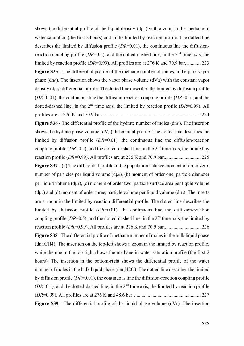
xxx
shows the differential profile of the liquid density (dρL) with a zoon in the methane in
water saturation (the first 2 hours) and in the limited by reaction profile. The dotted line
describes the limited by diffusion profile (DR=0.01), the continuous line the diffusion-
reaction coupling profile (DR=0.5), and the dotted-dashed line, in the 2nd time axis, the
limited by reaction profile (DR=0.99). All profiles are at 276 K and 70.9 bar. ........... 223
Figure S35 - The differential profile of the methane number of moles in the pure vapor
phase (dnG). The insertion shows the vapor phase volume (dVG) with the constant vapor
density (dρG) differential profile. The dotted line describes the limited by diffusion profile
(DR=0.01), the continuous line the diffusion-reaction coupling profile (DR=0.5), and the
dotted-dashed line, in the 2nd time axis, the limited by reaction profile (DR=0.99). All
profiles are at 276 K and 70.9 bar. ............................................................................... 224
Figure S36 - The differential profile of the hydrate number of moles (dnH). The insertion
shows the hydrate phase volume (dVH) differential profile. The dotted line describes the
limited by diffusion profile (DR=0.01), the continuous line the diffusion-reaction
coupling profile (DR=0.5), and the dotted-dashed line, in the 2nd time axis, the limited by
reaction profile (DR=0.99). All profiles are at 276 K and 70.9 bar.............................. 225
Figure S37 - (a) The differential profile of the population balance moment of order zero,
number of particles per liquid volume (dμ0), (b) moment of order one, particle diameter
per liquid volume (dμ1), (c) moment of order two, particle surface area per liquid volume
(dμ2) and (d) moment of order three, particle volume per liquid volume (dμ3). The inserts
are a zoom in the limited by reaction differential profile. The dotted line describes the
limited by diffusion profile (DR=0.01), the continuous line the diffusion-reaction
coupling profile (DR=0.5), and the dotted-dashed line, in the 2nd time axis, the limited by
reaction profile (DR=0.99). All profiles are at 276 K and 70.9 bar.............................. 226
Figure S38 - The differential profile of methane number of moles in the bulk liquid phase
(dnL,CH4). The insertion on the top-left shows a zoom in the limited by reaction profile,
while the one in the top-right shows the methane in water saturation profile (the first 2
hours). The insertion in the bottom-right shows the differential profile of the water
number of moles in the bulk liquid phase (dnL,H2O). The dotted line describes the limited
by diffusion profile (DR=0.01), the continuous line the diffusion-reaction coupling profile
(DR=0.1), and the dotted-dashed line, in the 2nd time axis, the limited by reaction profile
(DR=0.99). All profiles are at 276 K and 48.6 bar. ...................................................... 227
Figure S39 - The differential profile of the liquid phase volume (dVL). The insertion

xxxi
shows the differential profile of the liquid density (dρL) with a zoon in the methane in
water saturation (the first 2 hours) and in the limited by reaction profile. The dotted line
describes the limited by diffusion profile (DR=0.01), the continuous line the diffusion-
reaction coupling profile (DR=0.1), and the dotted-dashed line, in the 2nd time axis, the
limited by reaction profile (DR=0.99). All profiles are at 276 K and 48.6 bar. ........... 228
Figure S40 - The differential profile of the methane number of moles in the pure vapor
phase (dnG). The insertion shows the vapor phase volume (dVG) with the constant vapor
density (dρG) differential profile. The dotted line describes the limited by diffusion profile
(DR=0.01), the continuous line the diffusion-reaction coupling profile (DR=0.1), and the
dotted-dashed line, in the 2nd time axis, the limited by reaction profile (DR=0.99). All
profiles are at 276 K and 48.6 bar. ............................................................................... 229
Figure S41 - The differential profile of the hydrate number of moles (dnH). The insertion
shows the hydrate phase volume (dVH) differential profile. The dotted line describes the
limited by diffusion profile (DR=0.01), the continuous line the diffusion-reaction
coupling profile (DR=0.1), and the dotted-dashed line, in the 2nd time axis, the limited by
reaction profile (DR=0.99). All profiles are at 276 K and 48.6 bar.............................. 230
Figure S42 - (a) The differential profile of the population balance moment of order zero,
number of particles per liquid volume (dμ0), (b) moment of order one, particle diameter
per liquid volume (dμ1), (c) moment of order two, particle surface area per liquid volume
(dμ2) and (d) moment of order three, particle volume per liquid volume (dμ3). The inserts
are a zoom in the limited by reaction differential profile. The dotted line describes the
limited by diffusion profile (DR=0.01), the continuous line the diffusion-reaction
coupling profile (DR=0.1), and the dotted-dashed line, in the 2nd time axis, the limited by
reaction profile (DR=0.99). All profiles are at 276 K and 48.6 bar.............................. 231
Figure S43 - The differential profile of methane number of moles in the bulk liquid phase
(dnL,CH4). The insertion on the top-left shows a zoom in the limited by reaction profile,
while the one in the top-right shows the methane in water saturation profile (the first 2
hours). The insertion in the bottom-right shows the differential profile of the water
number of moles in the bulk liquid phase (dnL,H2O). The dotted line describes the limited
by diffusion profile (DR=0.01), the continuous line the diffusion-reaction coupling profile
(DR=0.6), and the dotted-dashed line, in the 2nd time axis, the limited by reaction profile
(DR=0.99). All profiles are at 274 K and 76.0 bar. ...................................................... 232
Figure S44 - The differential profile of the liquid phase volume (dVL). The insertion
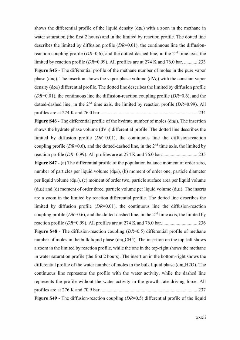
xxxii
shows the differential profile of the liquid density (dρL) with a zoon in the methane in
water saturation (the first 2 hours) and in the limited by reaction profile. The dotted line
describes the limited by diffusion profile (DR=0.01), the continuous line the diffusion-
reaction coupling profile (DR=0.6), and the dotted-dashed line, in the 2nd time axis, the
limited by reaction profile (DR=0.99). All profiles are at 274 K and 76.0 bar. ........... 233
Figure S45 - The differential profile of the methane number of moles in the pure vapor
phase (dnG). The insertion shows the vapor phase volume (dVG) with the constant vapor
density (dρG) differential profile. The dotted line describes the limited by diffusion profile
(DR=0.01), the continuous line the diffusion-reaction coupling profile (DR=0.6), and the
dotted-dashed line, in the 2nd time axis, the limited by reaction profile (DR=0.99). All
profiles are at 274 K and 76.0 bar. ............................................................................... 234
Figure S46 - The differential profile of the hydrate number of moles (dnH). The insertion
shows the hydrate phase volume (dVH) differential profile. The dotted line describes the
limited by diffusion profile (DR=0.01), the continuous line the diffusion-reaction
coupling profile (DR=0.6), and the dotted-dashed line, in the 2nd time axis, the limited by
reaction profile (DR=0.99). All profiles are at 274 K and 76.0 bar.............................. 235
Figure S47 - (a) The differential profile of the population balance moment of order zero,
number of particles per liquid volume (dμ0), (b) moment of order one, particle diameter
per liquid volume (dμ1), (c) moment of order two, particle surface area per liquid volume
(dμ2) and (d) moment of order three, particle volume per liquid volume (dμ3). The inserts
are a zoom in the limited by reaction differential profile. The dotted line describes the
limited by diffusion profile (DR=0.01), the continuous line the diffusion-reaction
coupling profile (DR=0.6), and the dotted-dashed line, in the 2nd time axis, the limited by
reaction profile (DR=0.99). All profiles are at 274 K and 76.0 bar.............................. 236
Figure S48 - The diffusion-reaction coupling (DR=0.5) differential profile of methane
number of moles in the bulk liquid phase (dnL,CH4). The insertion on the top-left shows
a zoom in the limited by reaction profile, while the one in the top-right shows the methane
in water saturation profile (the first 2 hours). The insertion in the bottom-right shows the
differential profile of the water number of moles in the bulk liquid phase (dnL,H2O). The
continuous line represents the profile with the water activity, while the dashed line
represents the profile without the water activity in the growth rate driving force. All
profiles are at 276 K and 70.9 bar. ............................................................................... 237
Figure S49 - The diffusion-reaction coupling (DR=0.5) differential profile of the liquid

xxxiii
phase volume (dVL). The insertion shows the differential profile of the liquid density
(dρL) with a zoom in the methane in water saturation (the first 2 hours) and in the limited
by reaction profile. The continuous line represents the profile with the water activity,
while the dashed line represents the profile without the water activity in the growth rate
driving force. All profiles are at 276 K and 70.9 bar.................................................... 238
Figure S50 - The diffusion-reaction coupling (DR=0.5) differential profile of the methane
number of moles in the pure vapor phase (dnG). The insertion shows the vapor phase
volume (dVG) with the constant vapor density (dρG) differential profile. The continuous
line represents the profile with the water activity, while the dashed line represents the
profile without the water activity in the growth rate driving force. All profiles are at 276
K and 70.9 bar. ............................................................................................................. 239
Figure S51 - The diffusion-reaction coupling (DR=0.5) differential profile of the hydrate
number of moles (dnH). The insertion shows the hydrate phase volume (dVH) differential
profile. The continuous line represents the profile with the water activity, while the dashed
line represents the profile without the water activity in the growth rate driving force. All
profiles are at 276 K and 70.9 bar. ............................................................................... 240
Figure S52 - (a) The diffusion-reaction coupling (DR=0.5) differential profile of the
population balance moment of order zero, number of particles per liquid volume (dμ0),
(b) moment of order one, particle diameter per liquid volume (dμ1), (c) moment of order
two, particle surface area per liquid volume (dμ2) and (d) moment of order three, particle
volume per liquid volume (dμ3). The inserts are a zoom in the limited by reaction
differential profile. The continuous line represents the profile with the water activity,
while the dashed line represents the profile without the water activity in the growth rate
driving force. All profiles are at 276 K and 70.9 bar.................................................... 241
Figure S53 - Fugacy profile of the hypothetical liquid phase for light gases by the
correlation of Prausnitz and Shair [244] with the temperature at 101.32 Pa. The points, ●,
represent the calculation of the correlation and the curve the calculation performed by the
function used in this work. ........................................................................................... 246
Figure S54 - H2O+CH4 liquid-vapor equilibrium isothermal curves. The experimental
data are represented by the filled circles for (a) the dew point and for (b) the bubble point
[234–236]. The empty circles represent the points calculated with the NRTL model. 248
Figure S55 - Isothermal curves of CH4 solubility in H2O. The experimental data is
represented by the filled circles [237–242]. The empty circles represent the points

xxxiv
calculated with the NRTL model.................................................................................. 248
Figure S56 - (a) The liquid phase volume (VL) and (b) the methane number of moles in
the pure vapor phase (nG) temporal profiles at 276 K and 70.9 bar (DR = 0.5). The
insertion (a) shows the liquid density (ρL) profile. The insertion (b) in the left is the gas
density (ρG) profile, and the one in the right is the vapor phase volume (VG). The lines
describe the time profiles for the following ethanol compositions of the initial liquid
phase: 0 wt% (dotted line) and 5 wt% (continuous line) of EtOH. .............................. 258
Figure S57 - (a) The temporal profile of the population balance moment of order zero,
number of particles per liquid volume (μ0), (b) moment of order one, particle diameter
per liquid volume (μ1), (c) moment of order two, particle surface area per liquid volume
(μ2) and (d) moment of order three, particle volume per liquid volume (μ3) at 276 K and
70.9 bar (DR = 0.5). The lines describe the time profiles for the following ethanol
compositions of the initial liquid phase: 0 wt% (dotted line) and 5 wt% (continuous line)
of EtOH. ....................................................................................................................... 259
Figure S58 - (a) The liquid phase volume (VL) and (b) the methane number of moles in
the pure vapor phase (nG) temporal profiles at 276 K and 70.9 bar (DR = 0.5). The
insertion (a) shows the liquid density (ρL) profile. The insertion (b) in the left is the gas
density (ρG) profile, and the one in the right is the vapor phase volume (VG). The lines
describe the time profiles for the following ethanol compositions of the initial liquid
phase: 5 wt% (continuous line), 10 wt% (dashed line) and 15 wt% (dotted-dashed line)
of EtOH. ....................................................................................................................... 260
Figure S59 - (a) The temporal profile of the population balance moment of order zero,
number of particles per liquid volume (μ0), (b) moment of order one, particle diameter
per liquid volume (μ1), (c) moment of order two, particle surface area per liquid volume
(μ2) and (d) moment of order three, particle volume per liquid volume (μ3) at 276 K and
70.9 bar (DR = 0.5). The lines describe the time profiles for the following ethanol
compositions of the initial liquid phase: 5 wt% (continuous line), 10 wt% (dashed line)
and 15 wt% (dotted-dashed line) of EtOH. .................................................................. 261
Figure S60 - (a) The liquid phase volume (VL) and (b) the methane number of moles in
the pure vapor phase (nG) temporal profiles at 276 K and 70.9 bar (DR = 0.5). The
insertion (a) shows the liquid density (ρL) profile. The insertion (b) in the left is the gas
density (ρG) profile, and the one in the right is the vapor phase volume (VG). The lines
describe the time profiles for the following ethanol compositions of the initial liquid

xxxv
phase: 0 wt% (dotted line) and 5 wt% (continuous line) of EtOH, with (black) and without
(yellow) water activity in the driving force. ................................................................. 262
Figure S61 - (a) The temporal profile of the population balance moment of order zero,
number of particles per liquid volume (μ0), (b) moment of order one, particle diameter
per liquid volume (μ1), (c) moment of order two, particle surface area per liquid volume
(μ2) and (d) moment of order three, particle volume per liquid volume (μ3) at 276 K and
70.9 bar (DR = 0.5). The lines describe the time profiles for the following ethanol
compositions of the initial liquid phase: 0 wt% (dotted line) and 5 wt% (continuous line)
of EtOH, with (black) and without (yellow) water activity in the driving force. ......... 263
Figure S62 - (a) The liquid phase volume (VL) and (b) the methane number of moles in
the pure vapor phase (nG) temporal profiles at 276 K and 70.9 bar (DR = 0.5). The
insertion (a) shows the liquid density (ρL) profile. The insertion (b) in the left is the gas
density (ρG) profile, and the one in the right is the vapor phase volume (VG). The lines
describe the time profiles for the following ethanol compositions of the initial liquid
phase: 5 wt% (continuous line), 10 wt% (dashed line) and 15 wt% (dotted-dashed line)
of EtOH, with (black) and without (yellow) water activity in the driving force. ......... 264
Figure S63 - (a) The temporal profile of the population balance moment of order zero,
number of particles per liquid volume (μ0), (b) moment of order one, particle diameter
per liquid volume (μ1), (c) moment of order two, particle surface area per liquid volume
(μ2) and (d) moment of order three, particle volume per liquid volume (μ3) at 276 K and
70.9 bar (DR = 0.5). The lines describe the time profiles for the following ethanol
compositions of the initial liquid phase: 5 wt% (continuous line), 10 wt% (dashed line)
and 15 wt% (dotted-dashed line) of EtOH, with (black) and without (yellow) water
activity in the driving force. ......................................................................................... 265
Figure S64 - (a) The number of moles of methane (nL,CH4) and (b) the liquid phase
volume (VL) temporal profiles at 276 K (DR = 0.5). The insertion (a) shows the number
of moles of water (nL,H2O) profile in the bulk liquid phase. The insertion (b) shows the
liquid density (ρL) profile. The lines describe the time profiles for the following ethanol
compositions of the initial liquid phase: 5 wt% (continuous line), 10 wt% (dashed line)
and 15 wt% (dotted-dashed line) of EtOH, at 70.9 bar, θ = 72% (black), and at 74.9 bar,
θ = 75% (yellow). ......................................................................................................... 266
Figure S65 - The activity coefficient (γ) for (a) H2O and (b) CH4, (c) the hydrate volume
temporal profile (VH) and (d) the vapor phase volume (VG) temporal profile at 276 K (DR
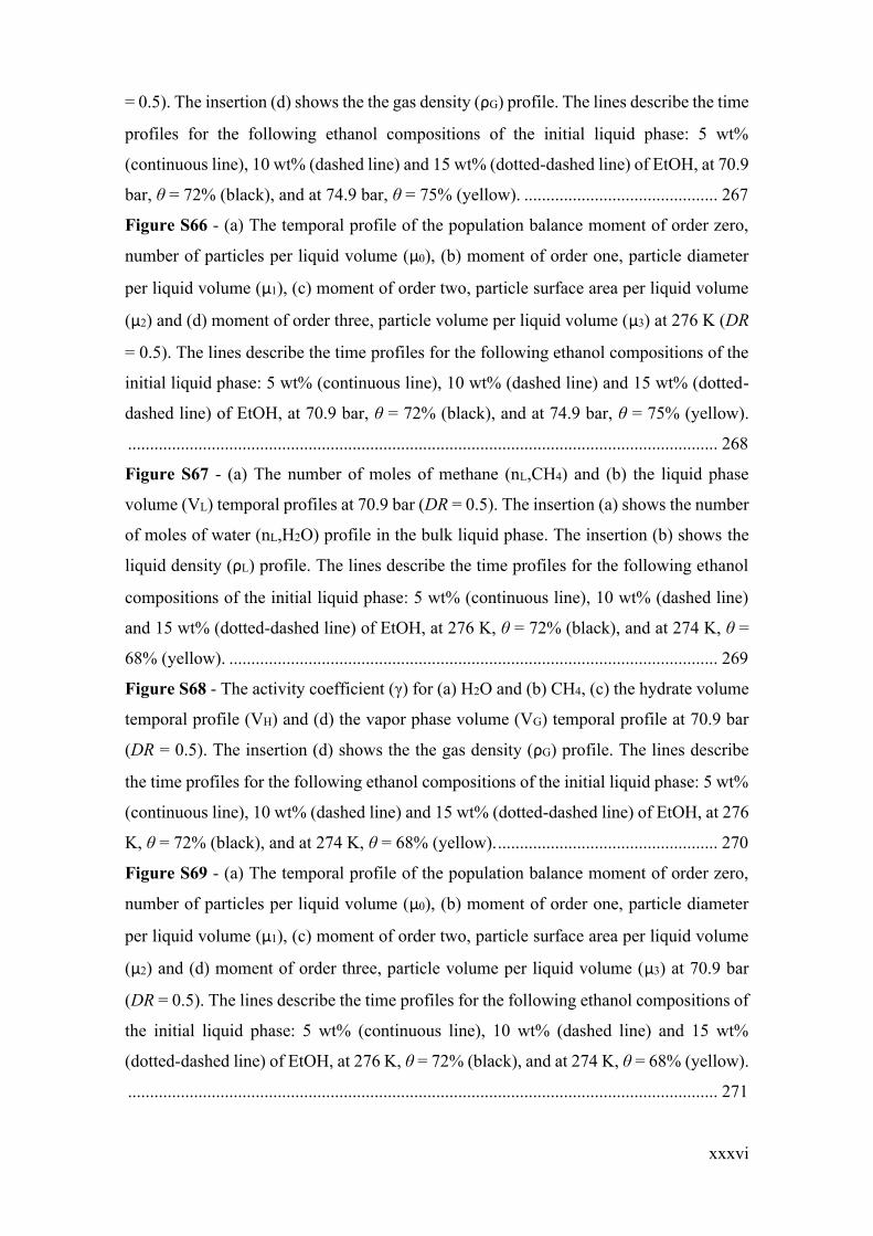
xxxvi
= 0.5). The insertion (d) shows the the gas density (ρG) profile. The lines describe the time
profiles for the following ethanol compositions of the initial liquid phase: 5 wt%
(continuous line), 10 wt% (dashed line) and 15 wt% (dotted-dashed line) of EtOH, at 70.9
bar, θ = 72% (black), and at 74.9 bar, θ = 75% (yellow). ............................................ 267
Figure S66 - (a) The temporal profile of the population balance moment of order zero,
number of particles per liquid volume (μ0), (b) moment of order one, particle diameter
per liquid volume (μ1), (c) moment of order two, particle surface area per liquid volume
(μ2) and (d) moment of order three, particle volume per liquid volume (μ3) at 276 K (DR
= 0.5). The lines describe the time profiles for the following ethanol compositions of the
initial liquid phase: 5 wt% (continuous line), 10 wt% (dashed line) and 15 wt% (dotted-
dashed line) of EtOH, at 70.9 bar, θ = 72% (black), and at 74.9 bar, θ = 75% (yellow).
...................................................................................................................................... 268
Figure S67 - (a) The number of moles of methane (nL,CH4) and (b) the liquid phase
volume (VL) temporal profiles at 70.9 bar (DR = 0.5). The insertion (a) shows the number
of moles of water (nL,H2O) profile in the bulk liquid phase. The insertion (b) shows the
liquid density (ρL) profile. The lines describe the time profiles for the following ethanol
compositions of the initial liquid phase: 5 wt% (continuous line), 10 wt% (dashed line)
and 15 wt% (dotted-dashed line) of EtOH, at 276 K, θ = 72% (black), and at 274 K, θ =
68% (yellow). ............................................................................................................... 269
Figure S68 - The activity coefficient (γ) for (a) H2O and (b) CH4, (c) the hydrate volume
temporal profile (VH) and (d) the vapor phase volume (VG) temporal profile at 70.9 bar
(DR = 0.5). The insertion (d) shows the the gas density (ρG) profile. The lines describe
the time profiles for the following ethanol compositions of the initial liquid phase: 5 wt%
(continuous line), 10 wt% (dashed line) and 15 wt% (dotted-dashed line) of EtOH, at 276
K, θ = 72% (black), and at 274 K, θ = 68% (yellow). .................................................. 270
Figure S69 - (a) The temporal profile of the population balance moment of order zero,
number of particles per liquid volume (μ0), (b) moment of order one, particle diameter
per liquid volume (μ1), (c) moment of order two, particle surface area per liquid volume
(μ2) and (d) moment of order three, particle volume per liquid volume (μ3) at 70.9 bar
(DR = 0.5). The lines describe the time profiles for the following ethanol compositions of
the initial liquid phase: 5 wt% (continuous line), 10 wt% (dashed line) and 15 wt%
(dotted-dashed line) of EtOH, at 276 K, θ = 72% (black), and at 274 K, θ = 68% (yellow).
...................................................................................................................................... 271

xxxvii
Figure S70 - The differential profile of (a) the methane number of moles in the bulk liquid
phase (dnL,CH4) and (b) the liquid phase volume (dVL) at 276 K and 70.9 bar (DR = 0.5).
The insertion (a) in the left shows the methane saturation profile and the one in the right
shows the water number of moles (nL,H2O) profile in the bulk liquid phase. The insertion
(b) shows the liquid density (ρL) profile with a zoom in the profile at 0 wt% of EtOH. The
lines describe the time profiles for the following ethanol compositions of the initial liquid
phase: 0 wt% (dotted line) and 5 wt% (continuous line) of EtOH. .............................. 272
Figure S71 - The differential profile of (a) the methane number of moles in the pure vapor
phase (dnG) and (b) the hydrate number of moles (dnH) at 276 K and 70.9 bar (DR = 0.5).
The insertion (a) shows the vapor phase volume (dVG) with the constant vapor density
(dρG) differential profile. The insertion (b) shows the hydrate phase volume (dVH)
differential profile. The lines describe the time profiles for the following ethanol
compositions of the initial liquid phase: 0 wt% (dotted line) and 5 wt% (continuous line)
of EtOH. ....................................................................................................................... 273
Figure S72 - (a) The differential profile of the population balance moment of order zero,
number of particles per liquid volume (dμ0), (b) moment of order one, particle diameter
per liquid volume (dμ1), (c) moment of order two, particle surface area per liquid volume
(dμ2) and (d) moment of order three, particle volume per liquid volume (dμ3) at 276 K
and 70.9 bar (DR = 0.5). The lines describe the time profiles for the following ethanol
compositions of the initial liquid phase: 0 wt% (dotted line, 2nd axis) and 5 wt%
(continuous line, 1st axis) of EtOH. .............................................................................. 274
Figure S73 - The differential profile of (a) the methane number of moles in the bulk liquid
phase (dnL,CH4) and (b) the liquid phase volume (dVL) at 276 K and 70.9 bar (DR = 0.5).
The insertion (a) in the left shows the methane saturation profile and the one in the right
shows the water number of moles (nL,H2O) profile in the bulk liquid phase. The insertion
(b) shows the liquid density (ρL) profile with a zoom in the methane saturation profile.
The lines describe the time profiles for the following ethanol compositions of the initial
liquid phase: 5 wt% (continuous line), 10 wt% (dashed line) and 15 wt% (dotted-dashed
line) of EtOH. ............................................................................................................... 275
Figure S74 - The differential profile of (a) the methane number of moles in the pure vapor
phase (dnG) and (b) the hydrate number of moles (dnH) at 276 K and 70.9 bar (DR = 0.5).
The insertion (a) shows the vapor phase volume (dVG) and the constant vapor density
(dρG) differential profile. The insertion (b) shows the hydrate phase volume (dVH)
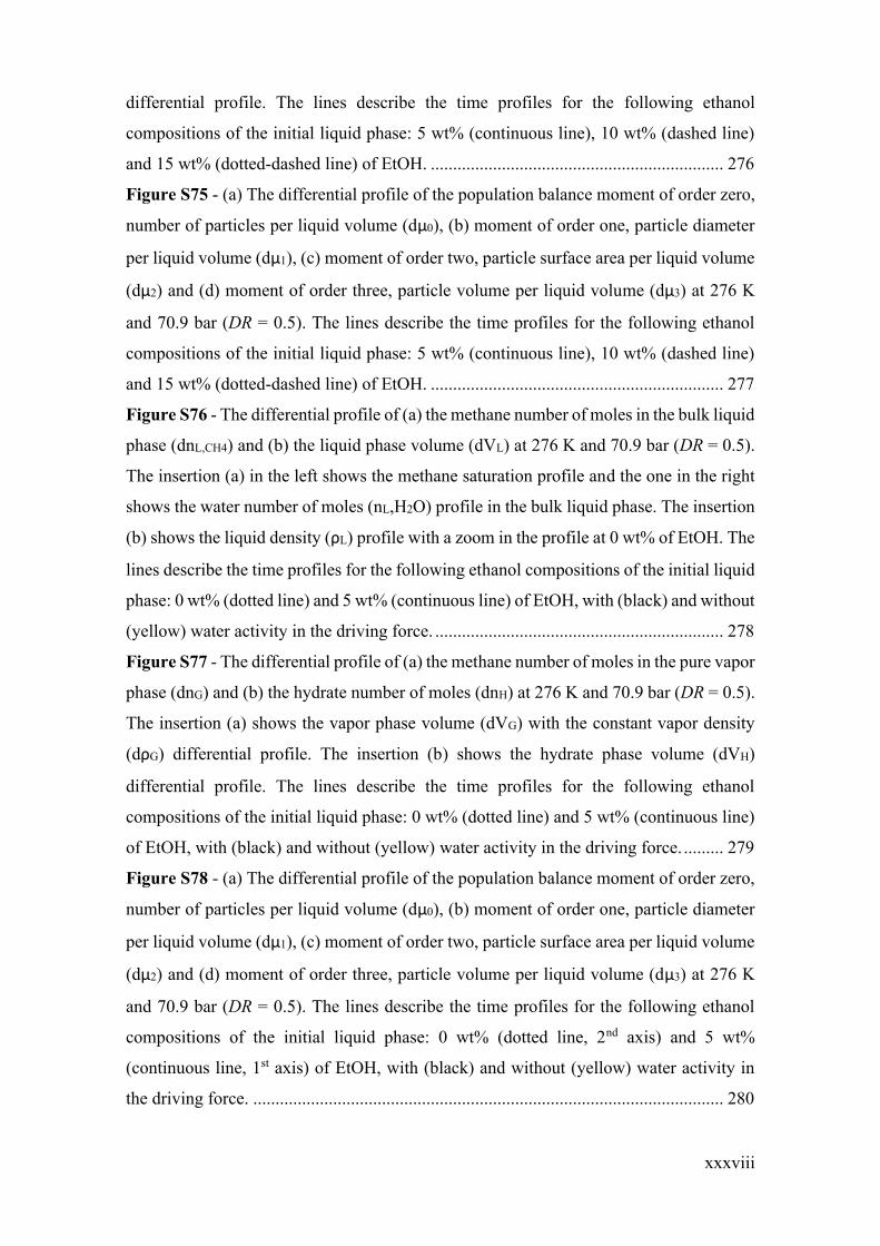
xxxviii
differential profile. The lines describe the time profiles for the following ethanol
compositions of the initial liquid phase: 5 wt% (continuous line), 10 wt% (dashed line)
and 15 wt% (dotted-dashed line) of EtOH. .................................................................. 276
Figure S75 - (a) The differential profile of the population balance moment of order zero,
number of particles per liquid volume (dμ0), (b) moment of order one, particle diameter
per liquid volume (dμ1), (c) moment of order two, particle surface area per liquid volume
(dμ2) and (d) moment of order three, particle volume per liquid volume (dμ3) at 276 K
and 70.9 bar (DR = 0.5). The lines describe the time profiles for the following ethanol
compositions of the initial liquid phase: 5 wt% (continuous line), 10 wt% (dashed line)
and 15 wt% (dotted-dashed line) of EtOH. .................................................................. 277
Figure S76 - The differential profile of (a) the methane number of moles in the bulk liquid
phase (dnL,CH4) and (b) the liquid phase volume (dVL) at 276 K and 70.9 bar (DR = 0.5).
The insertion (a) in the left shows the methane saturation profile and the one in the right
shows the water number of moles (nL,H2O) profile in the bulk liquid phase. The insertion
(b) shows the liquid density (ρL) profile with a zoom in the profile at 0 wt% of EtOH. The
lines describe the time profiles for the following ethanol compositions of the initial liquid
phase: 0 wt% (dotted line) and 5 wt% (continuous line) of EtOH, with (black) and without
(yellow) water activity in the driving force. ................................................................. 278
Figure S77 - The differential profile of (a) the methane number of moles in the pure vapor
phase (dnG) and (b) the hydrate number of moles (dnH) at 276 K and 70.9 bar (DR = 0.5).
The insertion (a) shows the vapor phase volume (dVG) with the constant vapor density
(dρG) differential profile. The insertion (b) shows the hydrate phase volume (dVH)
differential profile. The lines describe the time profiles for the following ethanol
compositions of the initial liquid phase: 0 wt% (dotted line) and 5 wt% (continuous line)
of EtOH, with (black) and without (yellow) water activity in the driving force. ......... 279
Figure S78 - (a) The differential profile of the population balance moment of order zero,
number of particles per liquid volume (dμ0), (b) moment of order one, particle diameter
per liquid volume (dμ1), (c) moment of order two, particle surface area per liquid volume
(dμ2) and (d) moment of order three, particle volume per liquid volume (dμ3) at 276 K
and 70.9 bar (DR = 0.5). The lines describe the time profiles for the following ethanol
compositions of the initial liquid phase: 0 wt% (dotted line, 2nd axis) and 5 wt%
(continuous line, 1st axis) of EtOH, with (black) and without (yellow) water activity in
the driving force. .......................................................................................................... 280

xxxix
Figure S79 - The differential profile of (a) the methane number of moles in the bulk liquid
phase (dnL,CH4) and (b) the liquid phase volume (dVL) at 276 K and 70.9 bar (DR = 0.5).
The insertion (a) in the left shows the methane saturation profile and the one in the right
shows the water number of moles (nL,H2O) profile in the bulk liquid phase. The insertion
(b) shows the liquid density (ρL) profile with a zoom in the methane saturation profile.
The lines describe the time profiles for the following ethanol compositions of the initial
liquid phase: 5 wt% (continuous line), 10 wt% (dashed line) and 15 wt% (dotted-dashed
line) of EtOH, with (black) and without (yellow) water activity in the driving force. . 281
Figure S80 - The differential profile of (a) the methane number of moles in the pure vapor
phase (dnG) and (b) the hydrate number of moles (dnH) at 276 K and 70.9 bar (DR = 0.5).
The insertion (a) shows the vapor phase volume (dVG) and the constant vapor density
(dρG) differential profile. The insertion (b) shows the hydrate phase volume (dVH)
differential profile. The lines describe the time profiles for the following ethanol
compositions of the initial liquid phase: 5 wt% (continuous line), 10 wt% (dashed line)
and 15 wt% (dotted-dashed line) of EtOH, with (black) and without (yellow) water
activity in the driving force. ......................................................................................... 282
Figure S81 - (a) The differential profile of the population balance moment of order zero,
number of particles per liquid volume (dμ0), (b) moment of order one, particle diameter
per liquid volume (dμ1), (c) moment of order two, particle surface area per liquid volume
(dμ2) and (d) moment of order three, particle volume per liquid volume (dμ3) at 276 K
and 70.9 bar (DR = 0.5). The lines describe the time profiles for the following ethanol
compositions of the initial liquid phase: 5 wt% (continuous line), 10 wt% (dashed line)
and 15 wt% (dotted-dashed line) of EtOH, with (black) and without (yellow) water
activity in the driving force. ......................................................................................... 283
Figure S82 - The differential profile of (a) the methane number of moles in the bulk liquid
phase (dnL,CH4) and (b) the liquid phase volume (dVL) at 276 K (DR = 0.5). The insertion
(a) in the left shows the methane saturation profile and the one in the right shows the
water number of moles (nL,H2O) profile in the bulk liquid phase. The insertion (b) shows
the liquid density (ρL) profile with a zoom in the methane saturation profile. The lines
describe the time profiles for the following ethanol compositions of the initial liquid
phase: 5 wt% (continuous line), 10 wt% (dashed line) and 15 wt% (dotted-dashed line)
of EtOH, at 70.9 bar, θ = 72% (black), and at 74.9 bar, θ = 75% (yellow). ................. 284
Figure S83 - The differential profile of (a) the methane number of moles in the pure vapor

xl
phase (dnG) and (b) the hydrate number of moles (dnH) at 276 K (DR = 0.5). The insertion
(a) shows the vapor phase volume (dVG) and the constant vapor density (dρG) differential
profile. The insertion (b) shows the hydrate phase volume (dVH) differential profile. The
lines describe the time profiles for the following ethanol compositions of the initial liquid
phase: 5 wt% (continuous line), 10 wt% (dashed line) and 15 wt% (dotted-dashed line)
of EtOH, at 70.9 bar, θ = 72% (black), and at 74.9 bar, θ = 75% (yellow). ................. 285
Figure S84- (a) The differential profile of the population balance moment of order zero,
number of particles per liquid volume (dμ0), (b) moment of order one, particle diameter
per liquid volume (dμ1), (c) moment of order two, particle surface area per liquid volume
(dμ2) and (d) moment of order three, particle volume per liquid volume (dμ3) at 276 (DR
= 0.5). The lines describe the time profiles for the following ethanol compositions of the
initial liquid phase: 5 wt% (continuous line), 10 wt% (dashed line) and 15 wt% (dotted-
dashed line) of EtOH, at 70.9 bar, θ = 72% (black), and at 74.9 bar, θ = 75% (yellow).
...................................................................................................................................... 286
Figure S85 - The differential profile of (a) the methane number of moles in the bulk liquid
phase (dnL,CH4) and (b) the liquid phase volume (dVL) at 70.9 bar (DR = 0.5). The insertion
(a) in the left shows the methane saturation profile and the one in the right shows the
water number of moles (nL,H2O) profile in the bulk liquid phase. The insertion (b) shows
the liquid density (ρL) profile with a zoom in the methane saturation profile. The lines
describe the time profiles for the following ethanol compositions of the initial liquid
phase: 5 wt% (continuous line), 10 wt% (dashed line) and 15 wt% (dotted-dashed line)
of EtOH, at 276 K, θ = 72% (black), and at 274 K, θ = 68% (yellow). ....................... 287
Figure S86 - The differential profile of (a) the methane number of moles in the pure vapor
phase (dnG) and (b) the hydrate number of moles (dnH) at 70.9 bar (DR = 0.5). The
insertion (a) shows the vapor phase volume (dVG) and the constant vapor density (dρG)
differential profile. The insertion (b) shows the hydrate phase volume (dVH) differential
profile. The lines describe the time profiles for the following ethanol compositions of the
initial liquid phase: 5 wt% (continuous line), 10 wt% (dashed line) and 15 wt% (dotted-
dashed line) of EtOH, at 276 K, θ = 72% (black), and at 274 K, θ = 68% (yellow). ... 288
Figure S87 - (a) The differential profile of the population balance moment of order zero,
number of particles per liquid volume (dμ0), (b) moment of order one, particle diameter
per liquid volume (dμ1), (c) moment of order two, particle surface area per liquid volume
(dμ2) and (d) moment of order three, particle volume per liquid volume (dμ3) at 70.9 bar

xli
(DR = 0.5). The lines describe the time profiles for the following ethanol compositions of
the initial liquid phase: 5 wt% (continuous line), 10 wt% (dashed line) and 15 wt%
(dotted-dashed line) of EtOH, at 276 K, θ = 72% (black), and at 274 K, θ = 68% (yellow).
...................................................................................................................................... 289
Figure S88- Comparison between experimental values, y-axis, and calculated values, x-
axis, in the estimation of NRTL model parameters using data reconciliation for the
CH4+EtOH system [165,253,254] and the matrix of the parameters correlation
coefficients. The input variables reconciled using the reported experimental errors were
(a) the methane composition in the liquid phase, xCH4, and (b) the equilibrium
temperature. The output variable calculated through the NRTL model in the estimation
process was (c) the pressure. ........................................................................................ 292
Figure S89 - CH4(2) + EtOH(3) liquid-vapor equilibrium isothermal curves. The
experimental data are represented by the filled circles for (a) 253.15 K, 263.15 K, 273.15
K, 298.15 K, and (b) 280.15 K, 313.4 K, and 333.4 K. The empty circles are calculated
with the NRTL model. .................................................................................................. 293
xlii
List of Tables
Table 1 - Relationship between the diameter of the molecule and the diameter of the
cavity. ............................................................................................................................... 2
Table 2 - NRTL model parameters, and their respective parameter errors, obtained by
adjusting the liquid-vapor equilibrium data and infinite dilution data of the
THF(1)/H2O(2) system. .................................................................................................. 24
Table 3 - Kihara potential cavity parameters for THF, and their respective parameter
errors, obtained by adjusting the hydrate-liquid equilibrium data of the THF/H2O system.
And the Kihara potential cavity parameters for CH4, CO2 e H2. .................................... 24
Table 4 - Purity and supplier of materials used in the experimental study. ................... 40
Table 5 - Input data for the calculation of isothermal-isobaric single hydrate (sI) growth
of the CH4 + H2O system. ............................................................................................... 76
Table 6 – Additional input data for the calculation of isothermal-isobaric single hydrate
(sI) growth of the CH4 + H2O + EtOH system. ............................................................ 102
Table S1 – Literature THF/H2O vapor-liquid equilibria experimental data..................161
Table S2 – Literature THF/H2O hydrate-liquid-vapor equilibria (HLE) experimental data.
...................................................................................................................................... 163
Table S3 - Calculated data properties from the liquid-hydrate-vapor equilibrium data for
H2O + EtOH + CH4 system. ......................................................................................... 166
Table S4 - The average absolute deviation (AAD) for the CH4 hydrate phase equilibria
data with ethanol for the three tested models. .............................................................. 167
Table S5 - Calculated data properties from the liquid-hydrate-vapor equilibria data for
H2O + EtOH + CO2 system. ......................................................................................... 168
Table S6 - The average absolute deviation (AAD) for the CO2 hydrate phase equilibria
data with ethanol for the three tested models. .............................................................. 169
Table S7 - Calculated data properties from the liquid-hydrate-vapor equilibria data for
H2O + EtOH + C3H8 system. ........................................................................................ 169
Table S8 - The average absolute deviation (AAD) for the C3H8 hydrate phase equilibria
data with ethanol for the three tested models. .............................................................. 170
Table S9 - Liquid-hydrate-vapor equilibrium data with ethanol of C2H6 gas. ............ 170
Table S10 - Calculated data properties from the liquid-hydrate-vapor equilibria data for
xliii
H2O + EtOH + C2H6 system. ........................................................................................ 171
Table S11 - The average absolute deviation (AAD) for the C2H6 hydrate phase equilibria
data with ethanol for the three tested models. .............................................................. 172
Table S12 - Liquid-hydrate-vapor equilibrium data with ethanol of the gas mixture of
73.8 wt.% CH4 and 26.2 wt.% C2H6. ............................................................................ 172
Table S13 - Calculated data properties from the liquid-hydrate-vapor equilibria data for
H2O + EtOH + CH4/C2H6 system. ................................................................................ 173
Table S14 - The average absolute deviation (AAD) for the gas mixture of 73.8 mol%
CH4 and 26.2 mol% C2H6 hydrate phase equilibria data with ethanol for the two tested
models. .......................................................................................................................... 173
Table S15 - Parameters of the NRTL model, and their respective errors, obtained by
adjusting the liquid-vapor equilibrium data and infinite dilution data of the Ethanol (1) +
H2O (2) system. ............................................................................................................ 180
Table S16 - Kihara parameters adjusted for the hydrate phase equilibrium data of the
Gas + H2O systems. ...................................................................................................... 184
Table S17 - Parameters of the NRTL model, and their respective errors, obtained by
adjusting the liquid-vapor equilibrium and solubility data of the system CH4 (1) + H2O
(2). ................................................................................................................................ 189
Table S18 - Correlation parameters of the hypothetical liquid phase for light gases at
101.32 Pa and their respective deviations. ................................................................... 245
Table S19 - Parameters of the ternary NRTL model for the system H2O(1) + CH4(2) +
EtOH(3), and their respective errors, obtained by adjusting experimental data from binary
systems. ........................................................................................................................ 251

1
Chapter 1. Introduction This chapter will pass through the background and contextualization of the
hydrate research field, focusing on the relevance of modeling the hydrate growth in non-
ideal systems using the literature thermodynamic knowledge. We will then present what
motivated this work and its objectives, and the structure, that compose this thesis.
1.1 Background and relevance
Gas hydrate formation and decomposition processes are critical in flow assurance
for the oil and gas industry [1], which boosted research to comprehend and avoid these
solids formation from 1930 until the present [2]. However, research on gas hydrates has
also progressed over the past several decades as a technology enabler for several
innovative applications in the areas of energy storage, energy transport, gas separation,
desalination, and others [3].
1.1.1 Gas hydrate
Hydrates are crystalline-solid structures formed by water and a guest molecule, an
organic light molecule, under high-pressure and low-temperature conditions [4]. The
hydrophobic effect causes the ordering of water molecules forming structured cavities
by hydrogen bonds interaction, while the guest is trapped inside the water-cavity
framework by van der Waals forces [2].
Hydrate crystals were characterized through X-ray methods, and the three main
crystalline structures of these solids were determined [5,6]. The structures I, II and H
are differentiated by the size of the cavities formed and by different amounts of
pentagonal and hexagonal faces with varied conformations and arrangements for each
type [4].
The main characteristics that distinguish these structures are:
a) The number of small and large cavities that a hydrate structure has per unit cell;
b) The type of cavity represented by the powers of 5 and 6 to describe the number
of pentagonal and hexagonal faces, respectively;
c) The average radius of each cavity, that is, the average distance between the
centers of the water molecules present in the edges that form the cavity; and

2
d) The coordination number, which is the quantity of water molecules on the
periphery of each cavity.
These characteristics of hydrate structures are specified for the three structures
mentioned in the paper Sloan Jr. [4].
The crystalline hydrate structure is defined mainly by the characteristics of the
guest molecule. Such definition is a function of two factors: a) the chemical nature of
the guest and b) its size and shape [2,4]. The ratio between the size of the guest and the
cavity-average radius is fundamental to determine the stability of the crystalline
structure. It is defined that the closer to one (between 0.75 and 1.00) is the relationship
between the guest molecule diameter and the cavity diameter, the more stable is the
structure [4].
With the literature information of the CH4 [4], tetrahydrofuran (THF) [7] and
ethanol (EtOH) [8], average radii, and the structures I and II average cavity radii [4], the
relationship between the guest molecule radius and the cavity radius are calculated,
Table 1, for the molecules of interest in this study.
Table 1 - Relationship between the diameter of the molecule and the diameter of the cavity.
Guest Molecule
The average
radius of the guest
molecule (Å)
Structure I Structure II
Small Large Small Large
Mean cavity radius (Å) 2.55a 2.93a 2.51a 3.33a
CH4 2.18c 0.855 0.744 0.869 0.655
THF 3.15d 1.235 1.075 1.255 0.946
EtOH 3.25e 1.275 1.109 1.295 0.976
a Cavity radius minus the water radius of 1.4 Å [4]. b Cavities occupied by a single guest. c [4] d [7] e[8]
However, the type of structure formed is not just a function of the guest molecule
size, but more specifically of a) the relationship between the molecule diameter and the
cavity diameter; b) the number of small and large cavities in a structure, and c) the
percentage of cavity occupation. It is important mention that organic additives such as
THF or EtOH are potential hydrate formers of structure II, with occupation of large
cavities. Some experimental studies reaffirm these characteristics [8–11].
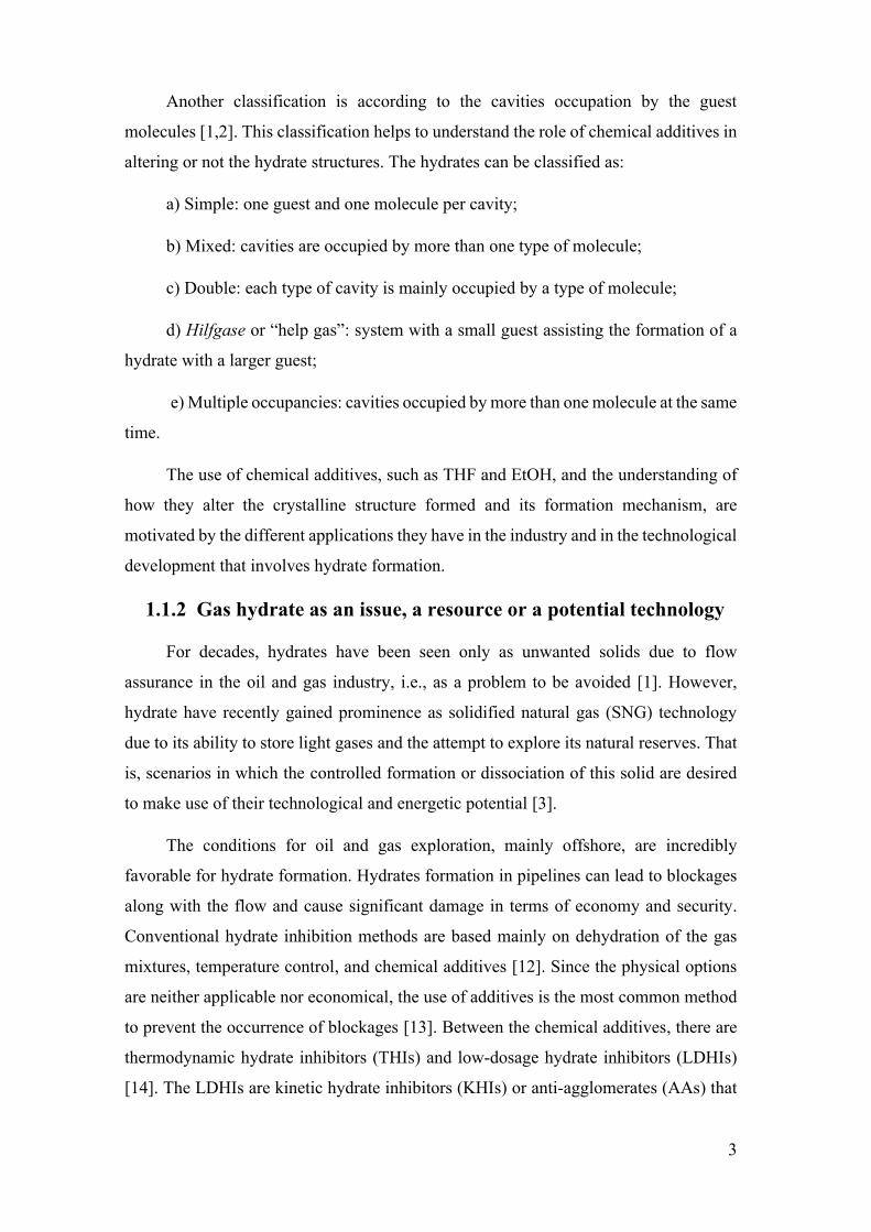
3
Another classification is according to the cavities occupation by the guest
molecules [1,2]. This classification helps to understand the role of chemical additives in
altering or not the hydrate structures. The hydrates can be classified as:
a) Simple: one guest and one molecule per cavity;
b) Mixed: cavities are occupied by more than one type of molecule;
c) Double: each type of cavity is mainly occupied by a type of molecule;
d) Hilfgase or “help gas”: system with a small guest assisting the formation of a
hydrate with a larger guest;
e) Multiple occupancies: cavities occupied by more than one molecule at the same
time.
The use of chemical additives, such as THF and EtOH, and the understanding of
how they alter the crystalline structure formed and its formation mechanism, are
motivated by the different applications they have in the industry and in the technological
development that involves hydrate formation.
1.1.2 Gas hydrate as an issue, a resource or a potential technology
For decades, hydrates have been seen only as unwanted solids due to flow
assurance in the oil and gas industry, i.e., as a problem to be avoided [1]. However,
hydrate have recently gained prominence as solidified natural gas (SNG) technology
due to its ability to store light gases and the attempt to explore its natural reserves. That
is, scenarios in which the controlled formation or dissociation of this solid are desired
to make use of their technological and energetic potential [3].
The conditions for oil and gas exploration, mainly offshore, are incredibly
favorable for hydrate formation. Hydrates formation in pipelines can lead to blockages
along with the flow and cause significant damage in terms of economy and security.
Conventional hydrate inhibition methods are based mainly on dehydration of the gas
mixtures, temperature control, and chemical additives [12]. Since the physical options
are neither applicable nor economical, the use of additives is the most common method
to prevent the occurrence of blockages [13]. Between the chemical additives, there are
thermodynamic hydrate inhibitors (THIs) and low-dosage hydrate inhibitors (LDHIs)
[14]. The LDHIs are kinetic hydrate inhibitors (KHIs) or anti-agglomerates (AAs) that
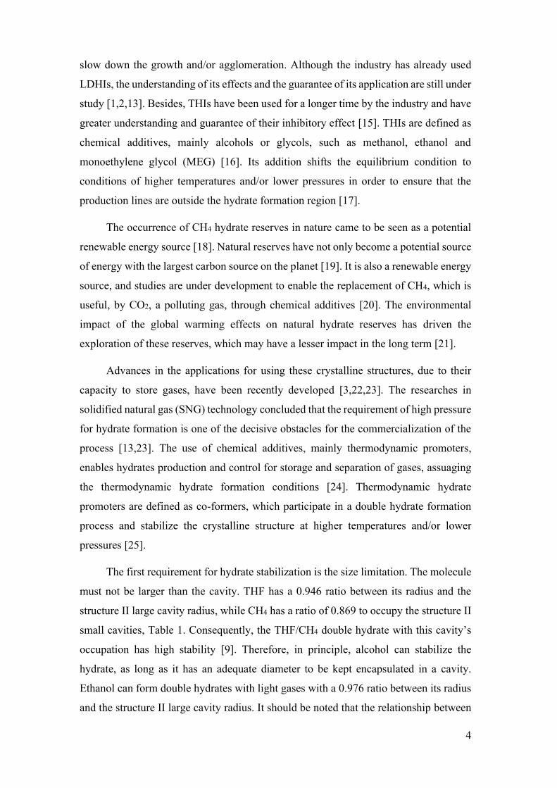
4
slow down the growth and/or agglomeration. Although the industry has already used
LDHIs, the understanding of its effects and the guarantee of its application are still under
study [1,2,13]. Besides, THIs have been used for a longer time by the industry and have
greater understanding and guarantee of their inhibitory effect [15]. THIs are defined as
chemical additives, mainly alcohols or glycols, such as methanol, ethanol and
monoethylene glycol (MEG) [16]. Its addition shifts the equilibrium condition to
conditions of higher temperatures and/or lower pressures in order to ensure that the
production lines are outside the hydrate formation region [17].
The occurrence of CH4 hydrate reserves in nature came to be seen as a potential
renewable energy source [18]. Natural reserves have not only become a potential source
of energy with the largest carbon source on the planet [19]. It is also a renewable energy
source, and studies are under development to enable the replacement of CH4, which is
useful, by CO2, a polluting gas, through chemical additives [20]. The environmental
impact of the global warming effects on natural hydrate reserves has driven the
exploration of these reserves, which may have a lesser impact in the long term [21].
Advances in the applications for using these crystalline structures, due to their
capacity to store gases, have been recently developed [3,22,23]. The researches in
solidified natural gas (SNG) technology concluded that the requirement of high pressure
for hydrate formation is one of the decisive obstacles for the commercialization of the
process [13,23]. The use of chemical additives, mainly thermodynamic promoters,
enables hydrates production and control for storage and separation of gases, assuaging
the thermodynamic hydrate formation conditions [24]. Thermodynamic hydrate
promoters are defined as co-formers, which participate in a double hydrate formation
process and stabilize the crystalline structure at higher temperatures and/or lower
pressures [25].
The first requirement for hydrate stabilization is the size limitation. The molecule
must not be larger than the cavity. THF has a 0.946 ratio between its radius and the
structure II large cavity radius, while CH4 has a ratio of 0.869 to occupy the structure II
small cavities, Table 1. Consequently, the THF/CH4 double hydrate with this cavity’s
occupation has high stability [9]. Therefore, in principle, alcohol can stabilize the
hydrate, as long as it has an adequate diameter to be kept encapsulated in a cavity.
Ethanol can form double hydrates with light gases with a 0.976 ratio between its radius
and the structure II large cavity radius. It should be noted that the relationship between
5
the size of the cavity and the diameter of the guest molecule does not determine whether
a compound can form hydrates or not [26], but it is a factor of significant influence.
However, more studies are still necessary to define under which temperature, pressure
or composition conditions the co-former effect predominates over the inhibitory effect
[8,27–29].
Chemical additives are required to prevent the formation of blockages in the oil
and gas industry, assist the exploration of natural hydrate reserves, or facilitate the SNG
technology. The formation of hydrates in mixtures containing water-soluble organic
compounds has ambiguous characteristics. Theoretically, some of THIs can stabilize the
hydrate structure under certain conditions [8,10,28,30]. Besides, hydrate-promoting
species can also alter water activity, changing the hydrate equilibrium condition
[9,26,31]. Because of the inhibitor/promoter present double behavior, it is necessary to
know and to model these effects to improve the use of this type of compound as a
blocking-prevention agent to assure flow, or hydrate promoting agent to enable a new
storage technology.
1.1.3 Gas hydrate formation
Water, light organic molecules, high pressure, and low temperature are considered
primary factors for the hydrate formation [4]. Although these factors are necessary to
guarantee formation, they are not decisive. Hydrate formation is a crystallization process
influenced by the dynamics that involve mainly two distinct stages: nucleation and
growth. These two hydrate formation stages must be understood to build a dynamic
model, and it is essential to establish considerations under the limitations imposed by
mass and/or energy transport [32]. Because the focus here is the hydrate growth kinetics,
only a summary of the nucleation theory is presented.
The stochastic nature of hydrate nucleation, confounding cause-effect relations,
and spatial-temporal scales has made it challenging to understand [33,34]. Because the
guest species is usually in the gas phase, the process starts with the dissolution into the
liquid phase. After that, supersaturation begins when the pressure and temperature are
thermodynamically favorable to hydrate formation. It occurs by forming light gases and
water pre-nuclei until the formation of critical-size hydrate nuclei. This reorganization
creates small gas-water clusters which form the sites for nucleation to begin.
Reorganization to create a new surface reduces the system entropy, leading to a positive

6
in the surface excess Gibbs free energy [11,35]. A critical nucleus of the hydrate phase
can be defined as the minimum amount of hydrate capable of existing independently
[34]. The time interval between the supersaturation establishment and critical nuclei
formation is called induction time [36]. Despite efforts to describe the hydrate
nucleation mechanism, the nucleation pathways themselves are still debated, and there
are opinions that nucleation is likely to occur through multiple competing pathways
[34,37,38]. Khurana, Yin, and Linga carried out a compilation of the main hydrate
nucleation mechanisms in the literature [34].
On the other side, the hydrate growth process involves hydrate core [32]. The
literature presents mechanisms on macroscopic, mesoscopic, and microscopic scales to
describe the hydrate growth phenomenon. While the macroscopic mechanisms are based
on the gas consumption profile [39], the mesoscopic and microscopic mechanisms are
mostly molecular and boundary layers [2].
The boundary layer theory, which is the fluid layer in the bounding surface, is
subject to diffusive effects, that is, the mass transfer of the guest from the bulk liquid
phase to the hydrate crystal interface [2,40]. Two regions are generally considered in
the hydrate growth mechanism: the region of stagnant film at the interface between the
crystal and the liquid phase, and the region corresponding to the adsorption layer [16].
Consequently, two driving forces can govern the phenomenon:
(1) the diffusion of the light organic gas dissolved in the solution to the liquid-
crystal interface through a laminar diffusion layer around the particle;
(2) the "reaction" at the crystal interface occurs when the gas molecules are
incorporated into the water structure, providing stability.
Hydrate growth models are based mainly on this two-steps mechanism and have
been in the literature since 1897 [41], including the model proposed by Englezos et al.
[42,43], which is the most notorious hydrate growth model in the past years, until the
most recent work by Bassani et al. [44–46].
From a microscopic point of view, Sloan and Koh [2] combined the conceptual
mechanism of Elwell and Sheel [47] for crystal growth with the Labile Cluster
Hypothesis (LCH) theory or the local structuring hypothesis (Local Structuring
Mechanism-LSM) [48,49] for nucleation and thus presented a molecular mechanism to

7
describe the phenomenon of hydrate crystal growth. As in the Elwell and Sheel
mechanism, the integration of the atoms in the crystal occurs more readily in the
crystalline surface faults.
Some molecular simulation studies use this mechanism conceptually [50,51].
However, unlike nucleation, growth, although also a stochastic process, has a high
probability of occurring and is an easier phenomenon to be experimentally measured.
For this reason, growth models developed more through boundary layer mechanisms
than through molecular mechanisms.
The literature has kinetic models that differ mainly in terms of the growth rate
driving force. According to Mohammadi et al. [52], the literature presents several
driving forces; however, the most common types are related to the equilibrium curve.
Hydrate growth models are classified by the literature [15,32] according to the
phenomena involved in growth and its driving force.
The empirical or semi-empirical kinetic growth models [53,54,63,64,55–62] are
based on mechanisms proposed to describe the hydration formation “reaction”,
considering the factors that favor these crystals formation. Among these factors are
subcooling, pressure, and solubility of the gas in the liquid phase, which can be
measured along with the growth process. Models based on subcooling [65–74], the
temperature difference between the system condition and the hydrate equilibrium
temperature, are typical because hydrate formation is an exothermic process. Models
limited by mass transfer [33,42,82–90,43,75–81] are basically divided into three
categories of driving force: in chemical potential or fugacity differences, in
concentration difference, and chemical affinity. Chemical affinity as a driving force is
recently proposed in the literature, and most models that use this approach tend to
simplify the driving force and be limited to describe systems without additives.
However, these simplifications are no longer valid when chemical additives are added,
as in the case of inhibited or promoted systems. Therefore, models based on chemical
affinity need improvements. Models combine driving forces, such as mass transfer and
chemical reaction [91–96], and subcooling and chemical reaction [40,97] are presented
in the literature, as well.
8
1.2 Motivation and objectives
Understanding the vital role of chemical additives in the hydrates field advances
and in what stage are the development of the hydrate growth models, this work proposes
a growth model with chemical affinity as a driving force capable of accounting for the
non-ideal effect of these systems. The objective is to incorporate the hydrate equilibrium
modeling knowledge in the growth kinetics, mainly for non-ideal systems.
The classical thermodynamic modeling of hydrate equilibrium in systems with
chemical additives is developed based on the theory of van der Waals and Platteeuw.
Van der Waals and Platteeuw [98] model is based on statistical thermodynamics. This
model expresses the water chemical potential difference between the hydrate phase and
the liquid phase, passing through the empty-hydrate hypothetical structure, as a function
of the cavity occupation fraction. The fraction of occupied cavities is obtained according
to the Langmuir theory of localized adsorption. Advances in the van der Waals and
Platteeuw model occur through the different models for the chemical potential of water
in the empty structure [99–102], and suitable models for calculating the Langmuir
constants [103–108].
The effects of chemical additives require consistent models for the fluid phases in
order to simultaneously describe the conditions of liquid-vapor (LVE), hydrate-liquid
(HLE) and hydrate-liquid-vapor (HLVE) equilibria. The equilibrium condition is
obtained directly by the equality between the water potentials in the liquid and solid
phases and indirectly by the criterion of fugacity equality between the fluid and the
hydrate phase for both gas and polar formers. Therefore, the literature presents, in
general, two approaches to calculate water activity and the hydrate former or co-former
fugacity. The first one consists of calculating the vapor and liquid phase fugacity of the
former and the co-former, and the water activity using an equation of state like CPA or
SAFT [109–113]. In the second approach, the water activity and the co-former fugacity
in the liquid phase are calculated by an excess Gibbs free energy model, like NRTL or
UNIQUAC, and the fugacity of the former in the vapor phase with a equation of state,
like Peng-Robinson [114–118].
However, the main difficulty in obtaining models capable of predicting the
complete diagram of systems containing hydrate inhibitors or promoters is to obtain
parameters that show good correlation of data and good transferability between the
9
different conditions involving LVE, HLE and HLVE. Most of the thermodynamic
models available in the literature are restricted to narrow ranges of system composition,
temperature, and pressure [13]. The first objective here is to improve the equilibria
understanding and modeling of promoted or inhibited systems. The development of a
growth model for these systems requires proper calculation for different equilibrium
conditions and thermodynamic properties over time.
The hydrate thermodynamic promoter studied here is tetrahydrofuran (THF). THF
is a well-known and used hydrate promoter in the literature [119]. Our objective in this
work is to provide a consistent thermodynamic modeling strategy capable of
representing the equilibrium of THF and water mixtures, and that also has the potential
for extrapolation to scenarios with light gases. The hydrate thermodynamic inhibitor
studied here is ethanol (ETOH). However, the literature presents limited equilibrium
data for EtOH, especially for high concentrated solutions [120]. Brazil is one of the
biggest producers of ethanol. Because of the price, it has become increasingly more
common in the Brazilian oil and gas industries. However, there are experimental data in
the literature showing that EtOH can work as a co-former for hydrates [8,27,28]. As
such, there is a need to understand the hydrate phase equilibrium with ethanol [8,27,28]
better. For the development of the equilibrium modeling, systems of different light gases
were studied, such as methane, ethane, carbon dioxide and others, most present in the
usually natural gas composition.
Exploring natural gas reserves, flow assurance, and the development of the SNG
technology require a predictive model for the formation of hydrates at non-ideal systems
to ensure the economic and safety requirements [13]. Therefore, the main objective here
is to develop a hydrate growth model to include thermodynamic knowledge. Non-
equilibrium thermodynamics [121,122] is the theoretical approach used in the model
development. A new driving force, based on the Prigogine Chemical Affinity [121], is
stablished to account for the effect of the thermodynamic factor in the kinetics and to be
able to describe the non-ideal systems adequately. With this model, we intend to
describe the growth considering the diffusion and reaction steps.
The developed model was first used to simulate the methane hydrate formation in
freshwater. We compared the CH4 hydrate growth system with and without the ethanol
addition. Even more, we evaluated the effect of increasing the ethanol concentration,
comparing systems with 5, 10 and 15 wt% of EtOH initial composition. The effect of
10
temperature and pressure, important properties for the hydrate formation, were also
studied. Because most of the hydrate growth models in the literature [15,33,84,85,93]
use only the guest properties in the driving force, we evaluated the effect of including
the water activity on the driving force with and without ethanol.
In summary, the objectives of this work are:
a) To provide consistent thermodynamic modeling for hydrate formation
systems with THF. The model can predict different equilibrium conditions
consistently, and that could be transferred to non-equilibrium conditions.
b) To obtain a better understanding of the EtOH effect as a hydrate inhibitor or
promoter, thus being able to distinguish this behavior and to better model the
hydrate equilibrium and kinetics in its presence.
c) To develop a hydrate growth model considering the thermodynamic
knowledge already well established in the literature and propose a driving
force that accounts for the chemical additives effect through the inclusion of
the thermodynamic factor.
d) To calculate the formation rate of methane hydrate in pure water and ethanol
inhibited systems, we tested the model quantitative and qualitative capacity
and the importance of including the thermodynamic factor for inhibited
systems.
1.3 Thesis structure
Besides the present chapter, this thesis is structured with five more chapters. Each
chapter, from 2 to 5, is prepared based on an article published or in preparation.
Chapter 2 corresponds to the proposed “Accurate thermodynamic description of
vapor-liquid and solid-liquid equilibria of THF, water and gas hydrates with a unique
set of parameters” [123]. In this chapter, the hydrate equilibrium modeling with THF is
discussed.
Chapter 3 presents the experimental study on “Phase Equilibria Data and
Thermodynamic Analysis for Liquid-Hydrate-Vapor (LHV) with High Ethanol
Concentrations” [124]. This chapter focus on the understanding and modeling of the
hydrate equilibrium with EtOH.

11
Chapter 4 present the “Hydrate growth model based on non-equilibrium
thermodynamics using Prigogine chemical affinity: Applied to CH4 hydrate in
freshwater”. The chapter presents the development of the proposed growth model and
its simulations for methane hydrate in fresh water. The corresponded article is in
preparation.
Chapter 5 corresponds to the study on the “Hydrate growth model based on non-
equilibrium thermodynamics using Prigogine chemical affinity: Applied to CH4 hydrate
in EtOH inhibited system”. This chapter presents the proposed model, and its
application to a hydrate inhibited system with simulated results for the methane hydrate
growth in the presence of ethanol. The corresponded article is in preparation.
Chapter 6 contains general conclusions and suggestions for future work.
In this document, there are additional and complementary information in terms of
Appendixes 1 to 4. Appendix 1 is the supporting information of the second chapter and
presented VLE and HLE experimental data of H2O+THF collected from the literature,
which were used to estimate parameters. Appendix 2 is the supporting information of
the third chapter. It presented the tables of the literature thermodynamic analysis for the
gas hydrate experimental data with ethanol. And also, the HLVE experimental data
obtained and the adjustments in the previously modeling for its application in hydrate
systems with ethanol.
Appendix 3 and Appendix 4 are the supporting information of the fourth and fifth
chapter, respectively. Appendixes 3 and 4 presented the thermodynamic models used,
the phase balances, the rates constitutive relationships, the interfaces equilibrium
compositions calculations, the numerical solution methods, and the parameters
adjustment necessary to describe the methane hydrate growth without and with ethanol,
respectively. The time profiles of the secondary variables for each simulated system are
also present in the Appendixes 3 and 4, as well as the time profiles of all derivatives
computed in the growth calculation, respectively.

12
Chapter 2. Hydrate equilibria with
promoter (THF) In the context of gas hydrates technology for gas storage and separation processes,
tetrahydrofuran (THF) has a recognized performance as a thermodynamic promoter.
The literature presents a large amount of phase equilibrium experimental data for the
THF hydrates systems. However, consistent thermodynamic modeling capable of
describing vapor-liquid, liquid-hydrate, and liquid-ice equilibria of THF and water is
still needed. To obtain this needed modeling, we propose a strategy for estimating a
unique set of parameters for suitable thermodynamic models for THF and water
mixtures in the conditions of vapor, liquid, and hydrate. We selected the NRTL model,
the Peng-Robinson equation of state, and the van der Waals and Platteeuw hydrate
model with the Kihara potential to correlate phase equilibrium calculations independent
properties. We regressed parameters for the NRTL and Kihara models in two sequential
steps using experimental data at conditions with pressure from 40 kPa to 101.33 kPa
and temperature from 272 K to 343.15 K. The first steps determine optimal parameters
for NRTL with, simultaneously, vapor-liquid equilibria and infinite dilution activity
coefficient data. The second determines optimal Kihara parameters with liquid-hydrate
equilibria data using a data reconciliation methodology. We verified the potential of the
model for extrapolation by accurately describing phase equilibria scenarios involving
liquid and vapor mixtures not included in the regression procedure, in addition to
scenarios involving conventional ice and hydrates of THF with some industrial gas or
natural gas components: H2, CO2 or CH4.
13
2.1 Introduction
Thermodynamics of hydrates is a matter of special relevance for some
technological applications involving industrial or natural gas components of interest. A
few of such are the storage of H2 and CH4 or the separation of CO2 from gas lines [125].
These exploit the nature of hydrates as solid phases with a molecular structure consisting
of a host lattice of water molecules and enculturated molecules of guest components [2].
According to Sun et al. [23], the requirement of high pressure for hydrate formation is
one of the decisive obstacles to the viability of such separation processes.
The thermodynamic stability of hydrates depends on the guest components. While
said components of interest form hydrate at relatively immoderate conditions of high
pressure and low temperature [2], tetrahydrofuran (THF) hydrate can form at
atmospheric pressure and temperature around 277 K [126]. Hydrates of THF occur in
structure II, where THF occupies the large cavities due to its relatively big molecular
size [9]. Moreover, in systems containing both THF and other component of interest,
double hydrates, where THF primarily occupies the large cavities while the smaller
component occupies the small cavity, form at conditions of higher temperature and
lower pressure than single hydrates would form whether only one of the guest
components was present. With that in mind, THF is a potential guest component that
has a recognized performance as a thermodynamic promoter [31,127–133].
At moderate conditions, THF is soluble in water. Increasing the concentration of
THF in the liquid phase contributes to hydrate stability in two opposite ways. It increases
its activity, which contribute to occupancy of hydrate cavities, and reduce chemical
potential of water there, thus stabilizing the hydrate phase, while at the same time
activity of water in the liquid phase decreases, granting more relative stability to the
liquid phase, in relation to the hydrate. At low concentration (up to 0.0556 mole fraction,
1 atm), the former contribution is dominant, and this component will show its promoter
effect on hydrate stability. On the other hand, at higher THF concentration, the water
activity effect becomes dominant and THF will show an inhibitor effect.
Literature presents a large amount of phase equilibrium experimental data for the
THF hydrates systems [9,126–128,134–137]. Most notably phase behavior of pure THF
and mixtures thereof with water at atmospheric pressure is summarized as follows: This
a volatile cyclic ether, with boiling point of 339 K and melting point of 164.8 K [138].

14
The solution of THF in water is highly non-ideal, with its vapor-liquid equilibria (VLE)
showing an azeotrope in the region of high THF concentration (around 0.82 mole
fraction). This solution’s solid-liquid equilibria shows a congruent melting point
hydrate-liquid-equilibria (HLE) at 277.55 K and 0.0556 mole fraction of THF [126],
and an eutectic point hydrate-ice-liquid-equilibria (HILE) at 272.0 K and 0.01 mole
fraction [127,128]. In order to be able to perform design and optimization of processes,
a thermodynamic model capable of representing these varying behaviors is of practical
importance. Moreover, descriptions of hydrate growth rate, adopting Gibbs energy
difference as driving force [139], further motivate the search for consistent description
of thermodynamic properties.
A few studies [111,140,141] have proposed modelings with varying combinations
of equations of states (EoS), excess Gibbs energy ( EG ) models and modifications of the
van der Waals and Platteeuw theory [98,101,106] to describes these behaviors of THF
and water mixtures. These were able to correlate properly only the hydrate phase
equilibria in the THF concentration range with promoter effect, while the modeling of
the inhibitory region has been neglected. Therefore, a consistent thermodynamic
modeling capable of describing all of vapor-liquid, liquid-hydrate in both concentration
ranges and liquid-ice equilibria of THF and water is still needed.
Our objective is to provide a consistent thermodynamic modeling capable of
representing both liquid-vapor and solid-liquid equilibria of THF and water mixtures,
while also having potential for extrapolation to different scenarios. For that purpose, we
select models of current engineering relevance. Then, we propose a strategy for the
estimation of a unique set of parameters to represent THF and water in the conditions
of vapor, liquid, hydrate and ice. We discuss the correlations obtained with the optimal
parameter set and, furthermore, verify the extrapolation potential by describing different
scenarios. We are able to describe phase equilibria involving ice and double hydrates
with all components of interest.
2.2 Thermodynamic modeling
In order to perform phase equilibrium calculations of broad applicability and with potential for extrapolations, we need consistent equilibrium criteria and well-known thermodynamic models. The underlying criteria basing the algorithms used here is the

15
classical thermodynamics condition for equilibrium: temperature (T ), pressure ( p ) and the chemical potential ( i ) of each component is the same for every present phase.
The phases of interest here are liquid (L) mixtures of water and THF, hydrates (H) of THF with or without H2, CO2 or CH4, vapor (V) mixtures of water and THF (for VLE scenarios), pure vapor of H2, CO2 or CH4 for (HLVE scenarios), and conventional ice (I). We implemented an algorithm for the specific scenario of VLE and expressed the equilibrium criteria for HLE in a way suited for fast iterative usage in the parameter estimation methodology.
2.2.1 Equilibrium criteria and algorithms
Our algorithm for VLE of water and THF is based on the equilibrium criteria
expressed from using fugacities if , equations (1).
L Vw wˆ ˆf f
(1)
L VTHF THFˆ ˆf f
Where, for the liquid phase, we choose an EG approach, thus expressing fugacities
in the mixture from the activity coefficients ( i ), as function of liquid phase composition
( x ), and the pure liquid fugacities ( Lif ), equation (2).
L Lˆ , , ,i i i if x T p x f T p (2)
Where Lif are calculated from pure VLE saturation pressure ( sat
ip ) and pure liquid
molar volume ( Liv ) correlations, equation (4).
LL sat sat ,
( ) expsati
pi
i i ip
v T pf p T T dp
RT
(3)
For THF, we were unable to find a correlation in literature, therefore using
experimental data of THF density at different temperatures [142,143], we fit an
empirical equation for the liquid molar volume of THF, ( )Li T , equation (4).
L 3 -1 10 2 7 4THF / m mol 7.0 10 ( / K ) 4.0 10 ( / K ) 10v T T (4)
While, for the vapor phase, we express fugacities from pressure and the fugacity
coefficients ( Vi ), equation (5).
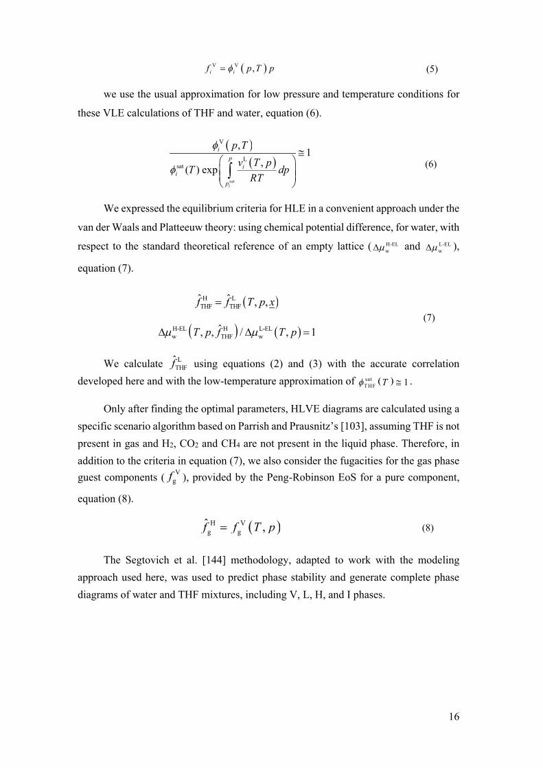
16
V V ,i if p T p (5)
we use the usual approximation for low pressure and temperature conditions for
these VLE calculations of THF and water, equation (6).
V
Lsat
,1
,( ) expsati
ip
ii
p
p Tv T pT dp
RT
(6)
We expressed the equilibrium criteria for HLE in a convenient approach under the
van der Waals and Platteeuw theory: using chemical potential difference, for water, with
respect to the standard theoretical reference of an empty lattice ( H-ELw and L-EL
w ),
equation (7).
H LTHF THFˆ ˆ , ,f f T p x
(7) H-EL H L-EL
w THF wˆ, , / , 1T p f T p
We calculate LTHFf using equations (2) and (3) with the accurate correlation
developed here and with the low-temperature approximation of satTHF 1T .
Only after finding the optimal parameters, HLVE diagrams are calculated using a specific scenario algorithm based on Parrish and Prausnitz’s [103], assuming THF is not present in gas and H2, CO2 and CH4 are not present in the liquid phase. Therefore, in addition to the criteria in equation (7), we also consider the fugacities for the gas phase guest components ( V
gf ), provided by the Peng-Robinson EoS for a pure component,
equation (8).
H Vg g
ˆ ,f f T p
(8)
The Segtovich et al. [144] methodology, adapted to work with the modeling approach used here, was used to predict phase stability and generate complete phase diagrams of water and THF mixtures, including V, L, H, and I phases.
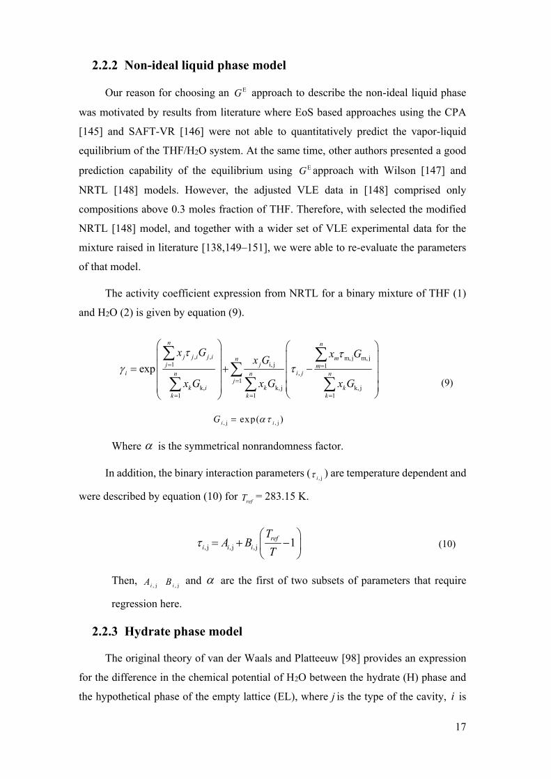
17
2.2.2 Non-ideal liquid phase model
Our reason for choosing an EG approach to describe the non-ideal liquid phase
was motivated by results from literature where EoS based approaches using the CPA
[145] and SAFT-VR [146] were not able to quantitatively predict the vapor-liquid
equilibrium of the THF/H2O system. At the same time, other authors presented a good
prediction capability of the equilibrium using EG approach with Wilson [147] and
NRTL [148] models. However, the adjusted VLE data in [148] comprised only
compositions above 0.3 moles fraction of THF. Therefore, with selected the modified
NRTL [148] model, and together with a wider set of VLE experimental data for the
mixture raised in literature [138,149–151], we were able to re-evaluate the parameters
of that model.
The activity coefficient expression from NRTL for a binary mixture of THF (1)
and H2O (2) is given by equation (9).
, , m, j m, j1 i, j 1
,1
k, k, j k, j1 1 1
exp
n n
j j i j i mnj j m
i i jn n nj
k i k kk k k
x G x Gx G
x G x G x G
(9)
, j , jexp( )i iG
Where is the symmetrical nonrandomness factor.
In addition, the binary interaction parameters ( , ji ) are temperature dependent and
were described by equation (10) for refT = 283.15 K.
, j , j , j 1refi i i
TA B
T
(10)
Then, , jiA , jiB and are the first of two subsets of parameters that require
regression here.
2.2.3 Hydrate phase model
The original theory of van der Waals and Platteeuw [98] provides an expression
for the difference in the chemical potential of H2O between the hydrate (H) phase and
the hypothetical phase of the empty lattice (EL), where j is the type of the cavity, i is
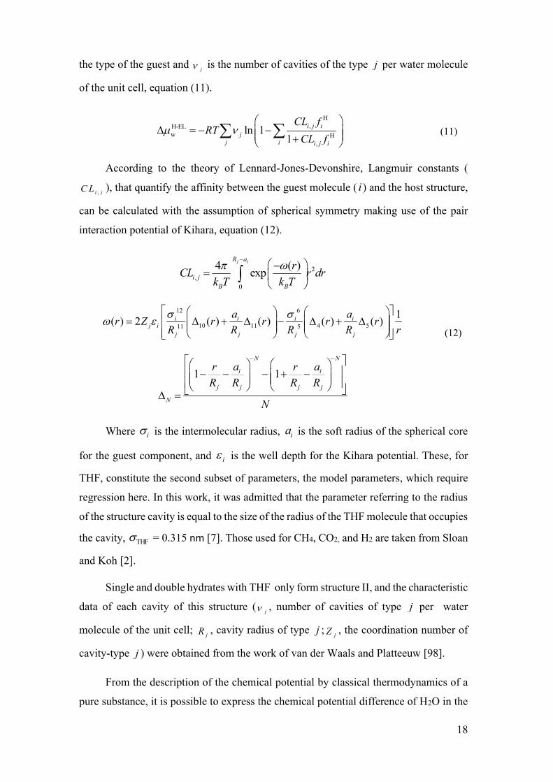
18
the type of the guest and j is the number of cavities of the type j per water molecule
of the unit cell, equation (11).
H,H-EL
w H,
ln 11
i j ij
j i i j i
CL fRT
CL f
(11)
According to the theory of Lennard-Jones-Devonshire, Langmuir constants (
,i jC L ), that quantify the affinity between the guest molecule ( i ) and the host structure,
can be calculated with the assumption of spherical symmetry making use of the pair
interaction potential of Kihara, equation (12).
2,
0
4 ( )expj iR a
i jB B
rCL r drk T k T
(12)
12 6
10 11 4 511 5
1( ) 2 ( ) ( ) ( ) ( )i i i ij i
j j j j
a ar Z r r r rR R R R r
1 1N N
i i
j j j j
N
a ar rR R R R
N
Where i is the intermolecular radius, ia is the soft radius of the spherical core
for the guest component, and i is the well depth for the Kihara potential. These, for
THF, constitute the second subset of parameters, the model parameters, which require
regression here. In this work, it was admitted that the parameter referring to the radius
of the structure cavity is equal to the size of the radius of the THF molecule that occupies
the cavity, THF = 0.315 nm [7]. Those used for CH4, CO2, and H2 are taken from Sloan
and Koh [2].
Single and double hydrates with THF only form structure II, and the characteristic
data of each cavity of this structure ( j , number of cavities of type j per water
molecule of the unit cell; jR , cavity radius of type j ; jZ , the coordination number of
cavity-type j ) were obtained from the work of van der Waals and Platteeuw [98].
From the description of the chemical potential by classical thermodynamics of a
pure substance, it is possible to express the chemical potential difference of H2O in the

19
empty lattice (EL) and the liquid phase coexisting with the hydrate phase. Where 0w
is the variation of the chemical potential of water in the reference conditions, -LwELh is
the enthalpy variation of water between phases, and -LwELv is the variation of the molar
volume of water between phases. Assuming that the difference of the molar volumes
constant and enthalpy calculated from specific heat depending linearly with
temperature, equation (13).
0 0
0w w w 0 w
w w0
L-EL L-EL L-EL
2
( ( (, ) , ) )pT
T p
h vdT dp lnRT RT RT
T p xRT
T p
(13) 0
L-EL L-EL L-EL0 w w0w 0 0,, ,
T
T
h h T p CT p T Tpp d
w wL-EL L-EL
0 0 0 1 0,,PC Cp T p a TT Tp
In this work, the reference pressure and temperature adopted were those of the
triple point of the water ( 0p = 612.62 Pa and 0T = 273.15 K), and the macroscopic
thermodynamic parameters of equation 13 were those presented in the work of John et
al. [105].
2.3 Parameter regression methodology
We seek a unique set of parameters for the NRTL and the Kihara models that is
able to correlate a wide range of data, provide reliable extrapolations and parameter
transferability. We make use of a parameter estimation framework to find the parameters
that best represent the available data. This consists on establishing a measure of the
distance between experimental data and predictions of the model and finding parameter
values that minimize this metric. The underlying metric used here is the maximum like
hood metric, in the absence of reported experimental uncertainties, we approximated it
to the least weighted squares function. Thus our matches the general weighted least
squares form below, for Ne experimental conditions indexed ( e ), in which Nc types of
variables were measured ( m ) such that we can calculate them ( c ), with our model, as a
function of parameters ( ), other measurements ( X ), and Nr types of reconciled
variables ( R ), equation (14).

20
2rc c m
, ,, , ,1
1 2r ,r ,m, , ,1
, ,,
e
e
Nce t e te t e t e ttNe
eNr t t
e r e r e rt
w Y X R YF R
w R R
(14)
For the goal depicted, we propose the parameter regression in two separate steps.
In the first step, we obtain optimal NRTL parameters using VLE and infinite dilution
activity coefficients ( i ) data. While in the second step, we extrapolate the NRTL
model and obtain optimal Kihara parameters using HLE data. The block diagram of
Figure 1 outlines the methodology proposed here.
Figure 1 - Block diagram of the parameters estimation methodology with the proposed
approach. All experimental data for estimation are in Appendix 1.
Previous works have taken varying strategies towards the parameterization of
thermodynamic models for water and THF systems. Our two-step-parameterization
strategy is similar to Herslund et al. [141], De Deugd et al. [119], Yoon [111], and
Strobel et al. [140], in that a model for liquid and a model for hydrate are parameterized
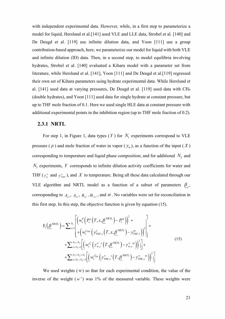
21
with independent experimental data. However, while, in a first step to parameterize a
model for liquid, Herslund et al.[141] used VLE and LLE data, Strobel et al. [140] and
De Deugd et al. [119] use infinite dilution data, and Yoon [111] use a group
contribution-based approach, here, we parameterize our model for liquid with both VLE
and infinite dilution (ID) data. Then, in a second step, to model equilibria involving
hydrates, Strobel et al. [140] evaluated a Kihara model with a parameter set from
literature, while Herslund et al. [141], Yoon [111] and De Deugd et al.[119] regressed
their own set of Kihara parameters using hydrate experimental data. While Herslund et
al. [141] used data at varying pressures, De Deugd et al. [119] used data with CH4
(double hydrates), and Yoon [111] used data for single hydrate at constant pressure, but
up to THF mole fraction of 0.1. Here we used single HLE data at constant pressure with
additional experimental points in the inhibition region (up to THF mole fraction of 0.2).
2.3.1 NRTL
For step 1, in Figure 1, data types (Y ) for 1N experiments correspond to VLE
pressure ( p ) and mole fraction of water in vapor ( wy ), as a function of the input ( X )
corresponding to temperature and liquid phase composition; and for additional 2N and
3N experiments, Y corresponds to infinite dilution activity coefficients for water and
THF ( w and THF ), and X to temperature. Being all these data calculated through our
VLE algorithm and NRTL model as a function of a subset of parameters 1
,
corresponding to 1,2A , 2,1A , 1,2B , 2 ,1B , and . No variables were set for reconciliation in
this first step. In this step, the objective function is given by equation (15).
1
THF
1 2 w
1
1 2 3 THF
1 2
2NRTLP c m
NRTL1 1 2
NRTLy c m, ,
2NRTLc m
w, w,1
2NRTLc m
THF, THF,1
, ,F
, ,
,
,
e e lN
e
e THF e THF l
N Ne e ee N
N N Ne e ee N N
w P T x P
w y T x y
w T
w T
(15)
We used weights ( w ) so that for each experimental condition, the value of the
inverse of the weight ( 1w ) was 1% of the measured variable. These weights were
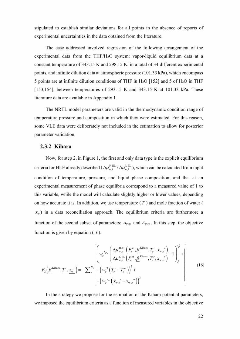
22
stipulated to establish similar deviations for all points in the absence of reports of
experimental uncertainties in the data obtained from the literature.
The case addressed involved regression of the following arrangement of the
experimental data from the THF/H2O system: vapor-liquid equilibrium data at a
constant temperature of 343.15 K and 298.15 K, in a total of 34 different experimental
points, and infinite dilution data at atmospheric pressure (101.33 kPa), which encompass
5 points are at infinite dilution conditions of THF in H2O [152] and 5 of H2O in THF
[153,154], between temperatures of 293.15 K and 343.15 K at 101.33 kPa. These
literature data are available in Appendix 1.
The NRTL model parameters are valid in the thermodynamic condition range of
temperature pressure and composition in which they were estimated. For this reason,
some VLE data were deliberately not included in the estimation to allow for posterior
parameter validation.
2.3.2 Kihara
Now, for step 2, in Figure 1, the first and only data type is the explicit equilibrium
criteria for HLE already described ( H-EL L-ELw, w,/l l ), which can be calculated from input
condition of temperature, pressure, and liquid phase composition; and that at an
experimental measurement of phase equilibria correspond to a measured value of 1 to
this variable, while the model will calculate slightly higher or lower values, depending
on how accurate it is. In addition, we use temperature (T ) and mole fraction of water (
wx ) in a data reconciliation approach. The equilibrium criteria are furthermore a
function of the second subset of parameters: THFa and THF . In this step, the objective
function is given by equation (16).
3
w
2KiharaH-EL m
w, w,
KiharaL-EL mw, w,
2Kihara T r2 w
2x rw, w,
, , ,1
, , ,
, ,
w
r re e e e
e r re e e e
Nr r me e ee
me e e
P T xw
P T x
F T x w T T
w x x
(16)
In the strategy we propose for the estimation of the Kihara potential parameters,
we imposed the equilibrium criteria as a function of measured variables in the objective

23
function, instead of using one of the measured variables itself as a function of another
by means of an algorithm. In this way we are saving the computational cost that would
be required by algorithm of the hydrate dissociation pressure at given temperature, by
iterative usage of the equilibrium criteria, such as Parrish and Prausnitz [103] algorithm,
also we are safe, through the regression methodology, from running the algorithm with
parameter such that there would be no solution for given input, the equilibrium criteria
will always yields some value to be compared with 1 in the objective function.
Moreover, the reason for reconciliation in this step, and the choice of value for weights
, w , was to obtain, empirically, a compromise between enforcing that the equilibrium
criteria is met with satisfactory tolerance while allowing for slightly variations of the
reconciled variables in relation to measurements in the absence of reports of
experimental uncertainties in the data obtained from the literature. We used the values
of 107 for the chemical potential difference ration term and the inverse of 0.001% of the
measured variable for the reconciliation terms.
We used experimental data of hydrate-liquid equilibrium of THF/H2O at 101.33
kPa [9,127,128,134–137] in the temperature range of 272 K to 280 K, with 69
experimental points up to the composition of 0.2 mole fraction of THF. These literature
data are in Appendix 1.
2.3.3 Optimization methodology
For conducting the minimization procedure, we use a particle swarm optimization
method [155] coupled to a Quasi-Newton [156] method, where the former provides a
global optimization characteristics while the latter provides improvement to the
precision of the final solution.
2.4 Results and discussion
Through the approach proposed here, we obtain, in the first step, optimal
parameter values and error analysis for NRTL ( ,i jA , ,i jB and ), these results are
summarized in Table 2.

24
Table 2 - NRTL model parameters, and their respective parameter errors, obtained by
adjusting the liquid-vapor equilibrium data and infinite dilution data of the THF(1)/H2O(2)
system.
NRTL parameters
1,2A 1.7545 ± 0.0009
2,1A 1.9684 ± 0.0009
1,2B 2.1355 ± 0.0062
2,1B -3.7664 ± 0.0098
0.4404 ± 0.0001 aThe standard error was calculated by making three times the standard deviation.
In the second step, we obtain the Kihara potential cavity parameters for THF (
THFa and THF ), Table 3 shows these values together with literature values for H2, CH4,
and CO2.
Table 3 - Kihara potential cavity parameters for THF, and their respective parameter errors,
obtained by adjusting the hydrate-liquid equilibrium data of the THF/H2O system. And the
Kihara potential cavity parameters for CH4, CO2 e H2.
Component Kihara potential cavity parameters
/ nma / nm KBk
Ref.
THF 0.0635 ± 0.0002a 0.315 (set) 320.16 ± 0.33a This work
CH4 0.0383 0.314 155.59 [2]
CO2 0.0681 0.298 175.40 [2]
H2 0.0353 0.314 127.43 [2] aThe standard error was calculated by making three times the standard deviation.
We compare the model results with the experimental data establishing the
Average Absolute Relative Deviation (AARD%) metric, equation (17). Where, Y
corresponds to either VLEp , w , T HF , or H-EL L-ELw w/ for each scenario under
consideration.
c m
m1
% 100
Ne e ee
e
Y YY
AARDNe
(17)
2.4.1 Liquid-vapor equilibria of the THF/water system
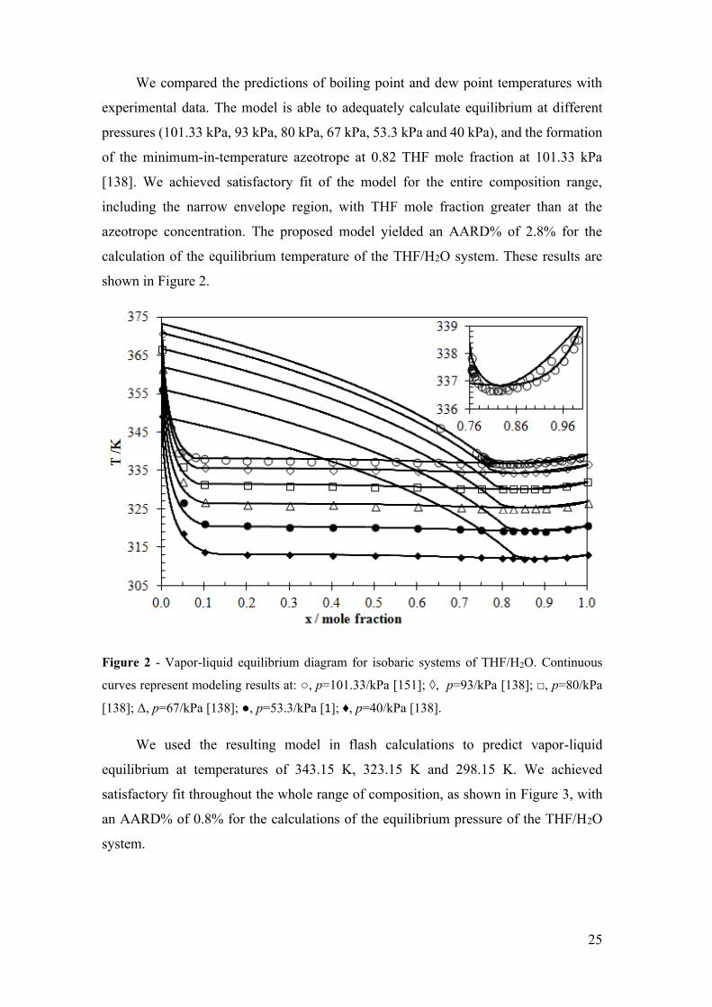
25
We compared the predictions of boiling point and dew point temperatures with
experimental data. The model is able to adequately calculate equilibrium at different
pressures (101.33 kPa, 93 kPa, 80 kPa, 67 kPa, 53.3 kPa and 40 kPa), and the formation
of the minimum-in-temperature azeotrope at 0.82 THF mole fraction at 101.33 kPa
[138]. We achieved satisfactory fit of the model for the entire composition range,
including the narrow envelope region, with THF mole fraction greater than at the
azeotrope concentration. The proposed model yielded an AARD% of 2.8% for the
calculation of the equilibrium temperature of the THF/H2O system. These results are
shown in Figure 2.
Figure 2 - Vapor-liquid equilibrium diagram for isobaric systems of THF/H2O. Continuous
curves represent modeling results at: ○, p=101.33/kPa [151]; ◊, p=93/kPa [138]; □, p=80/kPa
[138]; Δ, p=67/kPa [138]; ●, p=53.3/kPa [1]; ♦, p=40/kPa [138].
We used the resulting model in flash calculations to predict vapor-liquid
equilibrium at temperatures of 343.15 K, 323.15 K and 298.15 K. We achieved
satisfactory fit throughout the whole range of composition, as shown in Figure 3, with
an AARD% of 0.8% for the calculations of the equilibrium pressure of the THF/H2O
system.
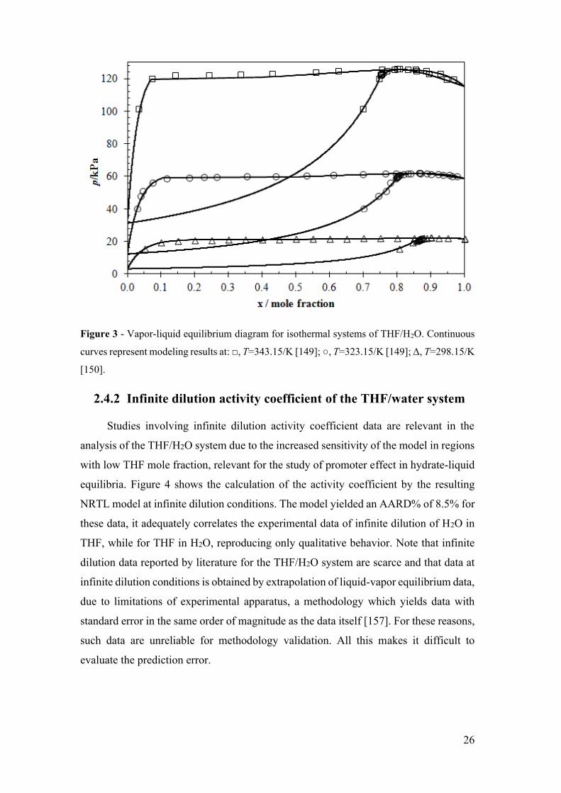
26
Figure 3 - Vapor-liquid equilibrium diagram for isothermal systems of THF/H2O. Continuous
curves represent modeling results at: □, T=343.15/K [149]; ○, T=323.15/K [149]; Δ, T=298.15/K
[150].
2.4.2 Infinite dilution activity coefficient of the THF/water system
Studies involving infinite dilution activity coefficient data are relevant in the
analysis of the THF/H2O system due to the increased sensitivity of the model in regions
with low THF mole fraction, relevant for the study of promoter effect in hydrate-liquid
equilibria. Figure 4 shows the calculation of the activity coefficient by the resulting
NRTL model at infinite dilution conditions. The model yielded an AARD% of 8.5% for
these data, it adequately correlates the experimental data of infinite dilution of H2O in
THF, while for THF in H2O, reproducing only qualitative behavior. Note that infinite
dilution data reported by literature for the THF/H2O system are scarce and that data at
infinite dilution conditions is obtained by extrapolation of liquid-vapor equilibrium data,
due to limitations of experimental apparatus, a methodology which yields data with
standard error in the same order of magnitude as the data itself [157]. For these reasons,
such data are unreliable for methodology validation. All this makes it difficult to
evaluate the prediction error.

27
Figure 4 - Coefficient of activity in infinite dilution for different temperatures at 101.33 kPa.
The symbols represent the experimental data and the continuous curves represent the values
calculated by the NRTL model for: □, infinite dilution of THF in H2O (γTHF∞) [152]; ○, infinite
dilution of H2O in THF (γw∞) [153,154].
2.4.3 Solid-liquid equilibria of the THF/water system
Using the optimal parameter set we were able to predict the solid-liquid diagram
for the THF/H2O system. This is shown in Figure 5. The model adequately correlates
the hydrate-liquid equilibrium with the experimental data throughout the evaluated
composition range, including points with higher than 0.1 mole fraction. The AARD%
was of 0.01%. We obtained prediction for the hydrate-ice-liquid equilibrium
temperature at 272.7 K, a result which is 0.5 K below the experimental data (272.0 ±
0.2 K, [128]). However, in the congruent melting composition, the experimental results
described are within a range of 0.8 K of variation, which is attributed to the fact that the
measurement of melting temperature of a THF hydrate is influenced by the presence of
air in the sample [126]. Note that our predictions are inside this range of experimental
uncertainty.
The ice-liquid equilibrium data [128] is reproduced within experimental error
range of 0.1 K. The eutectic at 0.01 THF mole fraction is also observed. In Figure 5, the

28
adequate simultaneous prediction of vapor-liquid equilibrium, hydrate-liquid
equilibrium, hydrate-ice-liquid equilibrium and ice-liquid equilibrium at pressure of
101.33 kPa and low THF compositions is observed. The model is able to predict
equilibria over the entire composition range; however, there is no experimental data on
solid-liquid equilibrium of THF/H2O above 0.2 mole fraction of THF.

29
Figure 5 - Complete diagram for isobaric systems of THF/H2O at 101.33 kPa. Continuous
curves represent modeling results for: ◊, VLE [151]; ○, HLE [9,127,128,134–137]; □, HILE
[128]; Δ, ILE [128].
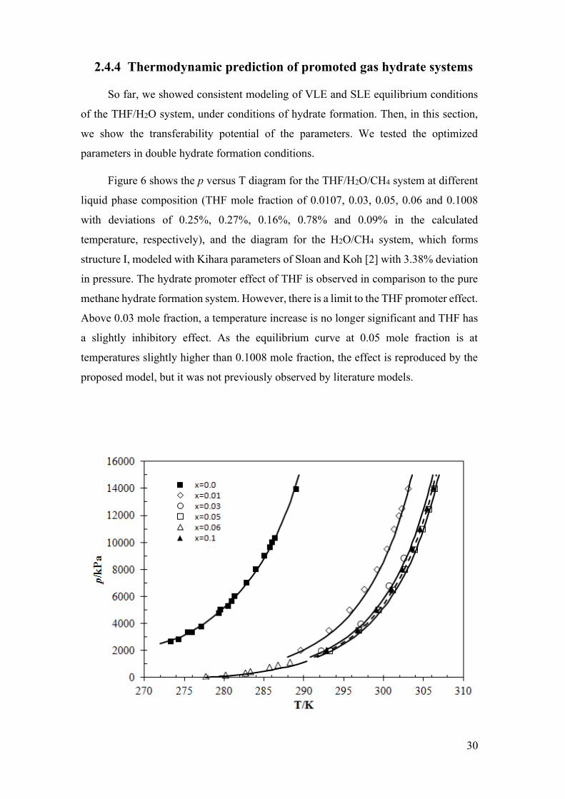
30
2.4.4 Thermodynamic prediction of promoted gas hydrate systems
So far, we showed consistent modeling of VLE and SLE equilibrium conditions
of the THF/H2O system, under conditions of hydrate formation. Then, in this section,
we show the transferability potential of the parameters. We tested the optimized
parameters in double hydrate formation conditions.
Figure 6 shows the p versus T diagram for the THF/H2O/CH4 system at different
liquid phase composition (THF mole fraction of 0.0107, 0.03, 0.05, 0.06 and 0.1008
with deviations of 0.25%, 0.27%, 0.16%, 0.78% and 0.09% in the calculated
temperature, respectively), and the diagram for the H2O/CH4 system, which forms
structure I, modeled with Kihara parameters of Sloan and Koh [2] with 3.38% deviation
in pressure. The hydrate promoter effect of THF is observed in comparison to the pure
methane hydrate formation system. However, there is a limit to the THF promoter effect.
Above 0.03 mole fraction, a temperature increase is no longer significant and THF has
a slightly inhibitory effect. As the equilibrium curve at 0.05 mole fraction is at
temperatures slightly higher than 0.1008 mole fraction, the effect is reproduced by the
proposed model, but it was not previously observed by literature models.

31
Figure 6 - Pressure, p, vs. temperature, T, diagram for the THF/H2O/CH4 system. Continuous
curves represent equilibrium temperature calculations with the proposed approach for THF
molar fractions of: ◊, x=0.0107 [119]; ○, x=0.03 [129]; □, x=0.05 [119]; Δ, x=0.06 [130]; ▲,
x=0.1[119]. And p-T diagram for the THF/CH4 system, ■, x=0.0 [158].
The observation of the hydrate inhibitory effect at high concentrations of THF,
reported by the solid-liquid diagram of the THF/H2O system (Figure 5), motivated
equilibrium calculations at high compositions of THF for double hydrates. We show, in
Figure 7, a smaller set of experimental data for the p versus T diagram of the
THF/H2O/CH4 system, together with calculations for higher THF concentrations. It is
noted that at 0.2 THF mole fraction, the curve is dislocated to temperatures less than
those for 0.05 mole fraction of THF, as well as at 0.6 mole fraction it presents a behavior
similar to the curve at 0.0107 mole fraction. At 0.8 mole fraction, the curve is closest to
the pure CH4 hydrate formation conditions. However, these equilibrium conditions lack
experimental data confirmation.
Figure 7 - Pressure, p, vs. temperature, T, diagram for the THF/H2O/CH4 system. Continuous
curves represent equilibrium temperature calculations with the proposed approach for THF
molar fractions of (literature data): ■, x=0.0 [158]; ◊, x=0.0107 [119]; □, x=0.05 [119]. Dashed
curves represent equilibrium temperature calculations with the proposed approach for THF
molar fractions of: dotted line, x=0.2; dashed line, x=0.6; dotted-dashed line, x=0.8, that do not
present literature data.

32
We also performed calculations for double hydrate with H2 or CO2. Figure 8
shows the p versus T diagram for the THF/H2O/CO2 system for different THF mole
fraction (0.012, 0.016, 0.029 and 0.05). The model adequately reproduced the
experimental data and the promoting effect of THF present in this composition range.
This diagram was reproduced only at low pressures.
Figure 8 - Pressure, p, vs. temperature, T, diagram for the THF/H2O/CO2 system. Continuous
curves represent equilibrium temperature calculations with the proposed approach for THF
molar fractions of: □, x=0.012 [159]; ◊, x=0.016 [128]; ○, x=0.029 [128,159]; Δ, x=0.05 [159].
Figure 9 shows the p versus T diagram for the THF/H2O/H2 system for different
THF mole fraction, x = (0.01, 0.0113, 0.024, 0.0351, 0.05 and 0.13) mole fraction. The
adjustment of the hydrate dissociation pressure of double hydrate of THF/H2, through
the proposed modeling, was adequate to the experimental data and the THF promoter
effect, from 0 to around 0.05 mole fraction was well predicted, the THF inhibitor effect
observed at 0.13 THF mole fraction was also predicted.
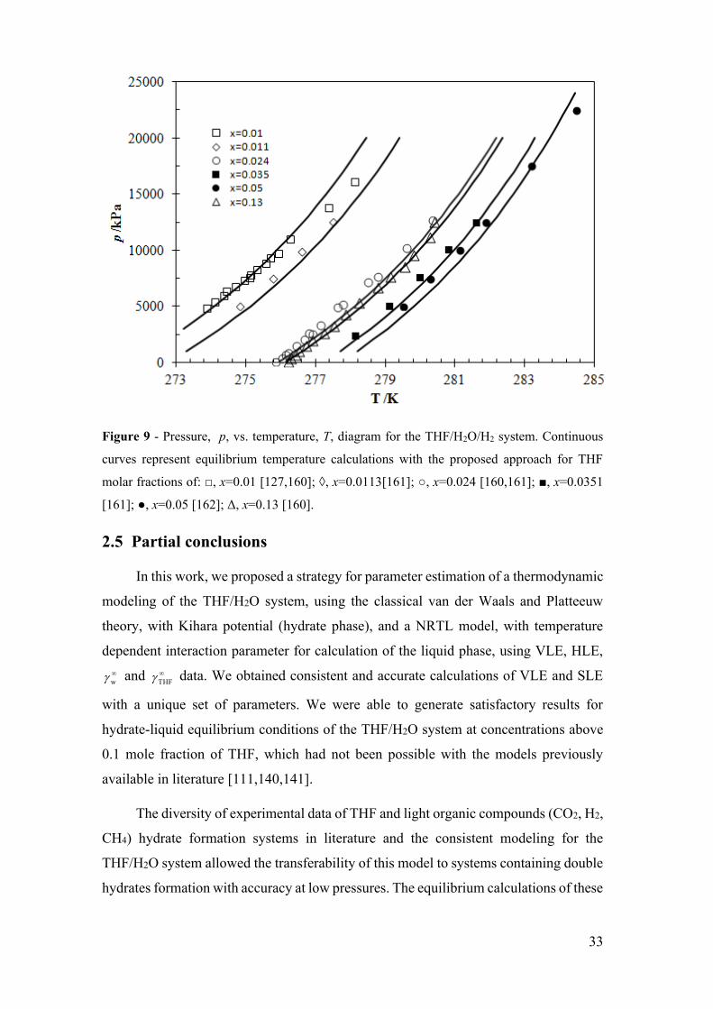
33
Figure 9 - Pressure, p, vs. temperature, T, diagram for the THF/H2O/H2 system. Continuous
curves represent equilibrium temperature calculations with the proposed approach for THF
molar fractions of: □, x=0.01 [127,160]; ◊, x=0.0113[161]; ○, x=0.024 [160,161]; ■, x=0.0351
[161]; ●, x=0.05 [162]; Δ, x=0.13 [160].
2.5 Partial conclusions
In this work, we proposed a strategy for parameter estimation of a thermodynamic
modeling of the THF/H2O system, using the classical van der Waals and Platteeuw
theory, with Kihara potential (hydrate phase), and a NRTL model, with temperature
dependent interaction parameter for calculation of the liquid phase, using VLE, HLE,
w and THF data. We obtained consistent and accurate calculations of VLE and SLE
with a unique set of parameters. We were able to generate satisfactory results for
hydrate-liquid equilibrium conditions of the THF/H2O system at concentrations above
0.1 mole fraction of THF, which had not been possible with the models previously
available in literature [111,140,141].
The diversity of experimental data of THF and light organic compounds (CO2, H2,
CH4) hydrate formation systems in literature and the consistent modeling for the
THF/H2O system allowed the transferability of this model to systems containing double
hydrates formation with accuracy at low pressures. The equilibrium calculations of these
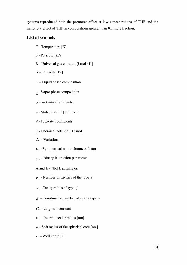
34
systems reproduced both the promoter effect at low concentrations of THF and the
inhibitory effect of THF in compositions greater than 0.1 mole fraction.
List of symbols
T - Temperature [K]
p - Pressure [kPa]
R - Universal gas constant [J mol / K]
f - Fugacity [Pa]
x - Liquid phase composition
y - Vapor phase composition
- Activity coefficients
v - Molar volume [m³ / mol]
- Fugacity coefficients
μ - Chemical potential [J / mol]
- Variation
- Symmetrical nonrandomness factor
, ji - Binary interaction parameter
A and B - NRTL parameters
j - Number of cavities of the type j
jR - Cavity radius of type j
jZ - Coordination number of cavity type j
CL- Langmuir constant
- Intermolecular radius [nm]
a - Soft radius of the spherical core [nm]
- Well depth [K]
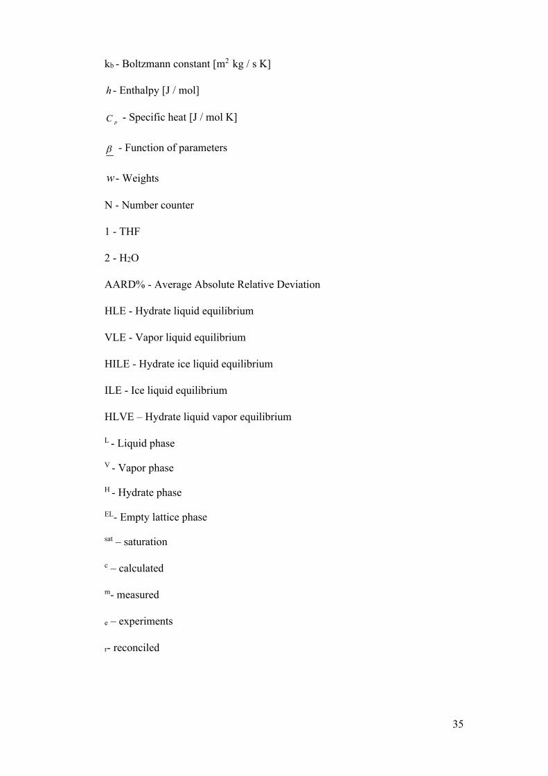
35
kb - Boltzmann constant [m2 kg / s K]
h - Enthalpy [J / mol]
pC - Specific heat [J / mol K]
- Function of parameters
w - Weights
N - Number counter
1 - THF
2 - H2O
AARD% - Average Absolute Relative Deviation
HLE - Hydrate liquid equilibrium
VLE - Vapor liquid equilibrium
HILE - Hydrate ice liquid equilibrium
ILE - Ice liquid equilibrium
HLVE – Hydrate liquid vapor equilibrium
L - Liquid phase
V - Vapor phase
H - Hydrate phase
EL- Empty lattice phase
sat – saturation
c – calculated
m- measured
e – experiments
r- reconciled

36
Chapter 3. Hydrate equilibria with inhibitor (EtOH)
Significant portions of the oil reserves in Brazil are located in deep or ultra-deep
waters. Oil production from these reservoirs implies a constant awareness of gas
hydrates formation. The petroleum industry uses thermodynamic inhibitors to reduce
the temperature/increase the pressure of hydrate formation to ensure hydrate-free
production. As ethanol is abundant in Brazil and works as a hydrate thermodynamic
inhibitor, its use is more common. However, experimental data of hydrate phase
equilibria (HPE) at high ethanol concentrations are scarce, and there is a limited
characterization of the existing data. This study reports LHV equilibrium data for C2H6
and a mixture of CH4/C2H6 at high ethanol concentrations and compiles the equilibrium
data with ethanol from the literature to evaluate their consistency hydrate inhibited
systems, as well as to present a comparison between predictive approaches for hydrates
with ethanol. We apply a consistency test with three criteria to characterize all HPE data
with ethanol in the literature data. The experimental data were measured up to 45 wt%
of ethanol. The used hydrate data, such as CH4, CO2, and C2H6, deviate from the average
behavior established by the criteria for 5 and 15 wt%, 2 and 5 wt%, and 5 wt%,
respectively. The C3H8 hydrate data from the literature obeys the average behavior of
the test criteria as well as the C2H6 and CH4/C2H6 data measured. In general, all
predictions were in agreement with the experimental data for ethanol concentrations up
to 15 wt%.

37
3.1 Introduction
Gas hydrates are crystalline compounds formed at low temperatures and high pressures
in systems with water and low molecular weight molecules, mainly light gases [2]. Such
conditions, typical of hydrate formation, are present in offshore oil and gas production.
In those systems, the occurrence of hydrates can lead to blockages along the flowline.
Among the conventional methods for hydrates inhibition, there is the prevention of the
occurrence of blockages by altering the thermodynamic equilibrium condition through
the addition of thermodynamic inhibitors [12]. Thermodynamic inhibitors of hydrates
are usually organic chemical additives, mainly alcohols and glycols. The presence of
inhibitors usually reduces the activity of water in the aqueous phase, which shifts
hydrate phase boundaries to higher pressures and lower temperatures without inclusion
in the hydrate crystalline structure [16].
Significant portions of the oil reserves in Brazil are located in deep or ultra-deep
waters, in which the oil production occurs at high pressures and low temperatures,
suitable conditions for the formation of hydrates. In this scenario, flow assurance actions
are crucial production factors, especially for large natural gas production scenarios such
as the exploration of the pre-salt layer [163]. Therefore, to ensure production is free of
hydrates in those scenarios, where the conditions are more favorable to hydrate
formation, i.e., the conditions of oil production are more rigorous, requirement larger
amounts of thermodynamic inhibitor to shift the hydrate equilibrium curve [17].
Desirable properties for a thermodynamic inhibitor include miscibility in water,
efficient recovery, stability, and low vapor pressure [164]. Based on these criteria, the
most common industrial thermodynamic inhibitors are methanol (MeOH), ethanol
(EtOH) and monoethylene glycol (MEG) [165]. Although many experimental data have
been reported for equilibrium conditions of gas hydrates in the presence of methanol,
information for hydrate equilibria in the presence of other alcohols, like ethanol, is
limited, especially for high concentrated solutions [166]. Brazil is one of the biggest
producers of ethanol, so its use is cheaper than the use of methanol or MEG for the
Brazilian oil and gas production scenarios. For this reason, the use of ethanol as a
thermodynamic inhibitor is increasingly more common. As such, there is a need to better
understand the hydrate phase equilibria for high concentrations of ethanol.

38
However, experimental studies on the thermodynamics of hydrate formation in
the presence of alcohols show that they may act as co-formers of double hydrate with
light gases [167]. The thermodynamically inhibited systems with ethanol have
characteristics of also promoting the formation of double hydrate with light gases, such
as methane [31]. The experimental studies to characterize the hydrate structure and
composition for those systems are challenging to perform, for this reason, the literature
presents only a few studies for the concentrations of 13.2 and 15 wt% of ethanol
[8,27,28]. In these studies, the participation of ethanol in the crystalline structure is
identified but with low occupation in the cavities. However, due to the methodological
difficulty of the execution of these experiments, it is not possible to affirm such
participation. We must evaluate this hypothesis. Therefore, more equilibrium data at
high ethanol concentration and better characterization are needed to define the
conditions at which this behavior occur [168].
The literature presents a few Liquid-Hydrate-Vapor (LHV) equilibrium data with
ethanol, mostly for single gas hydrate and even fewer data above 15 wt% of ethanol
[120]. Among the experimental data present in the literature, hydrates formed with CH4
for concentrations up to 63 wt% of ethanol [27,30,52,169], CO2 for concentrations up
to 20 wt% of ethanol [170–172], C2H6 for concentrations up to 10 wt% of ethanol [52],
and C3H8 for concentrations up to 15 wt% of ethanol [52,172]. As apparent from the
literature collected data, the availability of hydrate phase equilibrium data with high
concentrations of ethanol is limited.
In the petroleum industry, operating the production lines outside the hydrate zone
is a common practice to prevent the formation of hydrates. For this reason, proper
modeling of these systems for predicting the hydrate dissociation condition is essential
for the industry to ensure production is free of hydrates. Nevertheless, extra efforts are
needed before these models can reliably be applied for the cases when ethanol is present
at high concentrations [173].
The development of thermodynamic methods to calculate hydrate equilibrium
conditions requires accurate experimental data [171]. It is crucial to perform the
measurements considering that in systems with chemical additives at high
concentrations, the concentration of the solution is continuously changing during the
hydrate formation and dissociation processes [174]. We frequently apply this
consideration in the development of the methodologies present in the literature to obtain
39
experimental data at high concentrations of salts and thermodynamic inhibitors [168].
More than an adequately measured data at high ethanol concentration, the development
of a model to predict the hydrate zone needs consistent thermodynamic data with a
defined behavior of ethanol as an inhibitor or a potential hydrate co-former. Rigorous
thermodynamic analysis are rarely used to validate the data in the literature with
thermodynamic inhibitors at high concentrations [120,175].
This study reports hydrate phase equilibria data with ethanol, for C2H6 and a
mixture of CH4 and C2H6, at high ethanol concentrations, up to 45 wt% EtOH, applying
the methodology for an isochoric system and the thermodynamic consistency analysis
of the data. Here, we compile and apply the consistency test for inhibited systems
proposed by Sa et al. [175] to the hydrate phase equilibria data with ethanol. With this
test, it is possible to define a standard average established by the three criteria and define
which sets of experimental data deviate from the average behavior for each gas hydrate
system. We also tested a correlation based on the three thermodynamic criteria of the
consistency test, a thermodynamic model, and a commercial software to evaluate their
predictive reliability at high ethanol concentrations. All three approaches to describe
inhibited hydrate systems are used to determine the conditions that ethanol behaves
predominantly as a thermodynamic inhibitor. Moreover, we test whether the traditional
thermodynamic modeling is still applicable without including alcohol as a hydrate co-
former [123].
3.2 Experimental section
3.2.1 Materials
Table 4 presents the suppliers and purities of the chemicals used to obtain the
experimental data in this study. Appropriate amounts of the chemicals and distilled
water were weighed on an electronic balance with a resolution of 0.01 g and mixed
thoroughly at room temperature. Solutions up to 0.45 mass fraction of ethanol (45 wt%
EtOH) were prepared by keeping the cell cooled to prevent evaporation. The
uncertainties in the composition of the solutions were less than ± 0.001 on a mass
fraction basis of the balance.

40
Table 4 - Purity and supplier of materials used in the experimental study.
Chemical CAS Reg.
No. Source Purity (mass
fraction)
Analysis
method
Pure C2H6 74-84-0 Praxair 0.98 GCa
Mixture 73.8 mol% CH4 74-82-8 American
Gas Group
0.98 GCa
Balance C2H6 74-84-0 0.98 GCa
Ethanol 64-17-5 Greenfield ≥0.99 SGb
aGas chromatograph.
bSpecific gravity.
3.2.2 Experimental apparatus
The experimental setup used was a 275 mL stainless steel cylindrical cell. The
limit working condition of this cell is 50 bar for the pressure in the range of 258.15 K to
298.15 K for the temperature. The cell has a sapphire window which allows phase
transition observations and a mechanical stirrer used to maintain uniform and
homogenous conditions in the cell. The three temperature sensors are T-type
thermocouples (OMEGA®) with a precision of ± 0.1 K. They are used to measure the
temperature of the liquid phase inside the cell, the temperature of the cooling fluid in
the thermostatic bath, and the room temperature. The cell is immersed in a glycol-water
bath, in which the temperature is controlled by an external refrigeration unit. The
relative pressure measurements are made with a pressure transducer (WIKA®) sensor
with an uncertainty of ± 0.08 bar. A separate pressure transducer measures the absolute
pressure at the standard atmospheric pressure, with the precision of ± 0.001 bar.
3.2.3 Experimental procedure
It is essential to perform hydrate phase equilibria measurements, mainly at high
ethanol concentrations, considering that in systems with chemical additives, the
concentration of the solution is continuously changed during the hydrate formation and
dissociation processes. Therefore, for precise measurements, in the isochoric procedure
with the step-wise temperature increase methodology, with sufficient equilibration time
at every step, is used to ensure that the measurements of samples with a high
concentration of ethanol are properly equilibrated [168,174].

41
At first, before assembling the apparatus, the equilibrium cell is carefully cleaned.
The cell is loaded with 60 mL of the solution at ambient pressure and cooled, to be
around 2 K above the 10 K of the expected subcooling (predicted by the PVTsim®), to
prevent evaporation. With the cell cooled we cleaned the air inside. The air cleaning
process is doing filling the cell with the gas up to 2 bar and depressurizing slowly twice.
After that, we pressurized the cell up to 0.5 bar above the expected equilibrium pressure
(predicted by the PVTsim®). These procedures are previously done to prepare the cell
to begin the experimental process to obtain the phase equilibrium point [2], which
increases accuracy and speeds up the attainment of each experimental point.
Figure 10 shows an example of the experimental process utilized to obtain the
phase equilibrium points, which consists of four steps: (1) fast cooling step – linear line
of pressure-temperature data with no hydrate (around 10 degrees of subcooling); (2)
hydrate formation step – the amount of hydrate formation is controlled by increasing the
temperature after about 3 bars of large pressure decrease; (3) fast heating step – heating
up to 1 K below the expected equilibrium condition; and (4) slow stepwise heating –
the temperature is increased stepwise by 0.2 K in 1 hour and held for 5 hours so that
the system pressure stabilizes at each temperature. The five hours time per step ensures
complete equilibration at each step. The hydrate phase equilibrium point corresponds to
the inflection point, the intersection of the hydrate dissociation line and the
expansion/contraction line, as shown in Figure 10 (a), and at the same time the reduction
on the increasing rate of the pressure per step, as in Figure 10 (b).

42
Figure 10 - Illustration of the experimental procedure for hydrate phase equilibrium
measurements with high ethanol concentration [168]. (a) Pressure vs. temperature trace for
hydrate formation and dissociation in the 40 wt% of ethanol system with the four steps
procedure. (1) Fast cooling step - black, (2) hydrate formation step - blue, (3) fast heating step -
red, (4) slow stepwise heating - green. The circled area shows the slope change of the heating
curve as the phase equilibrium point is reached. (b) Time traces for the pressure (continuous
black) and temperature (dashed red) during slow step-wise temperature increase. Temperature
steps are maintained for about 5 hours until the pressure stabilizes. Circled area shows the
reduction in the increase in pressure after reaching the phase equilibrium point.

43
3.3 Thermodynamic analysis and models
3.3.1 Thermodynamic consistency analysis
Sa et al. [175] proposed a methodology to assess the thermodynamic consistency
of hydrate phase equilibrium data for inhibited systems. In this methodology,
thermodynamic relations are used to derive the criteria for assessment, including linear
regression of data according to the Clausius-Clapeyron equation, consistency of the
hydrate dissociation enthalpy, and water activity. The authors applied this methodology
for numerous cases of hydrate phase equilibria from the literature with salts.
Hu et al. [176] applied the same methodology to test the thermodynamic
consistency of hydrate phase equilibrium data from the literature with several salts
(NaCl, KCl, CaCl2, MgCl2, NH4Cl, NaBr, KBr, and CaBr2) and organic inhibitors
(methanol, monoethylene glycol, ethanol, glycerol, diethylene glycol and triethylene
glycol). However, the data with ethanol was only for CH4 hydrates up to 26.9 wt%.
This methodology consists in the application of three criteria. The first criterion
of thermodynamic consistency is to check how close the phase equilibrium data are to
the linear fitting regression equation given by the Clausius-Clapeyron equation. A
relation which adopts the hypothesis that the hydrate dissociation enthalpy and the gas
compressibility do not significantly change in a narrow temperature range of about 10-
20 K. The statistical parameter used to evaluate the linearity of phase equilibrium data
is the 1-R2 (R-squared) value. With this criterion, we can check if the hydrate structure
changes with the temperature and pressure condition for each concentration, because
the slope changes with a change in the hydrate structure.
The second criterion tests the consistency of the hydrate dissociation enthalpy,
which only depends on the hydrate structure and the guest species. The hydrate
dissociation enthalpy (∆Hdiss) values are relatively constant regardless of the type and
concentration of the thermodynamic hydrate inhibitor. The hydrate dissociation
enthalpy can be calculated through the linear slope of the phase equilibrium curves
plotted as log P vs. 1/T as expected by the Clausius-Clapeyron equation with the gas
compressibility (z) and the universal gas constant (R). We applied the relative standard
deviation (RSD) in ∆Hdiss for each ethanol concentration, which is defined as the
deviation of the ∆Hdiss at a concentration from the average ∆Hdiss of all concentrations
for each gas hydrate divided by the average ∆Hdiss. This criterion allows us to check if

44
the hydrate structure can change with the thermodynamic inhibitor concentration
because, with the change in the hydrate structure, the slope used to calculate the enthalpy
also changes. So, if the enthalpy varies significantly from one concentration to the other,
there is a possibility that the hydrate structure is changing with the thermodynamic
inhibitor concentration.
The last criterion is based on the suppression temperature (∆T = T0 – T), that is, at
a given concentration of a specific thermodynamic inhibitor, the activity of liquid water
does not significantly change over a relatively narrow temperature range (20-30 K). The
thermodynamic consistency of the water activity in the liquid phase is only determined
by the type and concentration of the thermodynamic inhibitor. So, if the concentration
of the thermodynamic inhibitor in the liquid phase does not change, i.e., the
thermodynamic inhibitor does not participate in the hydrate structure and/or do not
evaporate to the vapor phase, the water activity in the liquid phase will be constant.
The quantity ∆T/T0T is proportional to the water activity at each concentration and
independent of the temperature in the typical range of hydrate phase equilibrium data
and depends only on the thermodynamic hydrate inhibitor concentration. To quantify
the thermodynamic consistency in terms of water activity invariance, we also applied
the relative standard deviation (RSD) for ∆T/T0T – the sum, divided by the number of
data, of the difference between the ∆T/T0T for each data at the same concentration from
the average ∆T/T0T of that concentration divided by concentration average of ∆T/T0T.
The (= -nR/∆Hdiss) term depends on the hydrate structure, the guest species and
hydration number (n), and it can be also calculated through the suppression temperature
(∆T/T0T) and the hydrate dissociation enthalpy (∆Hdiss). This criterion evaluates if the
thermodynamic inhibitor concentration does not change with a small variation in
temperature. The parameter will be constant if the inhibitor is not participating in the
hydrate structure or evaporating.
In this work, those three criteria were applied for the literature data of CH4, CO2,
C2H6, and C3H8 hydrates with ethanol concentrations up to 63 wt%. Moreover, for the
measured data of C2H6 and the mixture of 73.8 mol% of CH4 and C2H6, with ethanol
concentrations up to 45 wt%.
We also used the classification proposed by Sa et al.[175] to evaluate the data
according to good (< 5%), acceptable (between 5% and 10%) and fail (> 10%) based on
45
the relative standard deviation (RSD). This classification allows us to evaluate in which
conditions hydrate equilibrium data with ethanol differs from the average that
characterizes all the data. That is, under which conditions inhibition and/or ethanol
inclusion into hydrate phase may cause changes in the water activity. Consequently, for
those conditions, experimental investigations for hydrate characterization are most
needed.
3.3.2 Prediction tool
PVTsim® is a commercial package for general phase equilibria calculation that is
also equipped with predictions for hydrate phase equilibria with and without inhibitors.
The software is distributed by Calsep A/S (Nova 4 version). For the hydrate calculations,
the Peng-Robinson equation of state, coupled with NRTL model and the Huron and
Vidal mixing rules[177,178]. PVTsim® is widely used in the oil and gas industry for
hydrate predictions.
3.3.2.1 Hu-Lee-Sum correlation
Hu et al. [120,176,179] developed a correlation based on the colligative properties
and thermodynamic consideration for the effect of inhibitors (salts and organic
inhibitors) in the hydrate phase equilibria. That correlation is based on the fundamental
principle of freezing point depression, which for hydrate is equivalent to the suppression
temperature from the uninhibited (fresh water) system.
The correlation considers that at the equilibrium hydrate dissociation, the fugacity
of water in the hydrate (solid) phase and the liquid phase have to be equal (isofugacity
condition). The assumptions for this condition are that the system pressure is constant;
the hydrate is a pure phase (the inhibitor is not part of the hydrate structure); the
composition of the hydrocarbon-rich vapor or liquid phase is constant; and the
composition of the hydrate is constant.
The correlation expresses the hydrate depression temperature in terms of the water
activity in the liquid phase, which is strongly dependent on the thermodynamic inhibitor
species and concentration. Based on published literature data, the regression of data
based on the effective mole fraction of inhibitors resulted in a general correlation for the
water activity. The correlation considers the water activity for salts and organic
inhibitors.
46
3.3.2.2 Thermodynamic modeling
Oliveira et al. [123] proposed a strategy for the estimation of a unique set of
parameters for suitable thermodynamic models for THF and water mixtures in the
conditions of LHV equilibrium. To perform phase equilibrium calculations, the authors
selected the NRTL EG model (for the liquid phase, L), the Peng-Robinson equation of
state (for the vapor phase, V), and the van der Waals and Platteeuw hydrate model with
the Kihara potential (for the hydrate phase, H) to correlate independent properties. They
regressed optimal parameters for the NRTL model with, simultaneously, vapor-liquid
equilibria and infinite dilution activity coefficient data, and determined optimal Kihara
parameters with liquid-hydrate equilibrium data, using data reconciliation. The method
used a strategy to obtain parameters through independent experiments.
Following a similar strategy, the NRTL parameters were estimated in this study
using infinite dilution and liquid-vapor equilibrium data of ethanol/water from the
literature to predict phase equilibria scenarios with ethanol involving liquid, hydrate,
and vapor mixtures (see Appendix 2).
The hydrate phase equilibria conditions evaluated were the ones with the
following natural gas components: CH4, CO2, C2H6, and C3H8, whose LHV equilibrium
data with ethanol are present in the literature [27,30,52,169–172]. In those conditions,
it was considered that the ethanol only act as a thermodynamic inhibitor and only change
the water activity in the bulk phase, i.e., it is not part of the hydrate structure. More
details about the NRTL parameters set and the methodology used to adapt the model for
the systems with ethanol instead of THF are in the Appendix 2.
Here, we used the average absolute deviation (AAD) to evaluate the accuracy of
each model. For the pressure, the absolute deviation accepted for the prediction is 2 bar,
and 0.5 K for the temperature. Since all three models were tested to calculate the
equilibrium condition for inhibited systems, we can use these results with the
consistency test to characterize the data.
If the same gas, water, and inhibitor system exhibit different behavior between
the data sets at different concentrations, this is an indication that the inhibitor may be
participating in the hydrate structure depending on the concentration. It is possible to
show, by applying the consistency analysis, that higher concentrations present higher
deviation from the average behavior, in separate data sets. With the analysis of the
47
deviation presented by the models, for the cases in which the ethanol only behaves as
an inhibitor (no inclusion in the hydrate), it is possible to define which of those
concentration sets are better adjusted by this hypothesis. In this way, we define the
conditions in which experimental characterization data, which are expensive and
challenging to perform, are still needed.
3.4 Results and discussion
Figure 11 shows the evaluation of the consistency analysis test for the methane
hydrate equilibrium data from the literature with ethanol concentrations up to 63 wt%.
The methane hydrate equilibrium data showed an excellent linear fit to the Clausius-
Clapeyron equation for all the concentrations. The statistical parameter (1-R2) are in
Table S3 of Appendix 2. For almost all the sets, (1-R2) is below 1%, with only two sets
having higher statistical parameters: 2.43% and 1.65% for 13.2 wt% and 44.6 wt%
EtOH, respectively. However, they are still adequate (< 5%), according to the criterion.
For the same concentration, the hydrate structure (sI) is the same for the temperature
and pressure ranges considered.
The second criterion is the independence of the hydrate dissociation enthalpy on
the type and concentration of the thermodynamic inhibitor. Using the Clausius-
Clapeyron equation and the linear slope of the experimental data of CH4 hydrate with
ethanol, the ∆Hdiss was calculated for each set of concentration (see Table S3 in
Appendix 2), as well as the relative standard deviation (RSD) of ∆Hdiss for each
concentration. Only the sets with 5 wt% and 15 wt% had RSD of ∆Hdiss higher than 10%
and were not in agreement with the average of the data. The data sets with 10 wt%, 20
wt%, 26.2 wt%, and 44.6 wt% showed an acceptable RSD of ∆Hdiss, however, higher
than 5%, which shows that they also have a deviation from the average behavior. The
other data sets had RSD lower than 5% and were characterized as the sets that follow
the average behavior.
Figure 11 (d) shows the thermodynamic consistency of the water activity in the
liquid phase (∆T/T0T) which is only determined by the type and concentration of the
thermodynamic inhibitor for the methane hydrate equilibrium data with ethanol. The
relative standard deviation (RSD) in ∆T/T0T for all the methane hydrate equilibrium data
(see Table S3 in Appendix 2), was acceptable, except for the case with 15 wt% EtOH.
However, in general, the data sets up to 20 wt% and the set with 52.3 wt% had an RSD
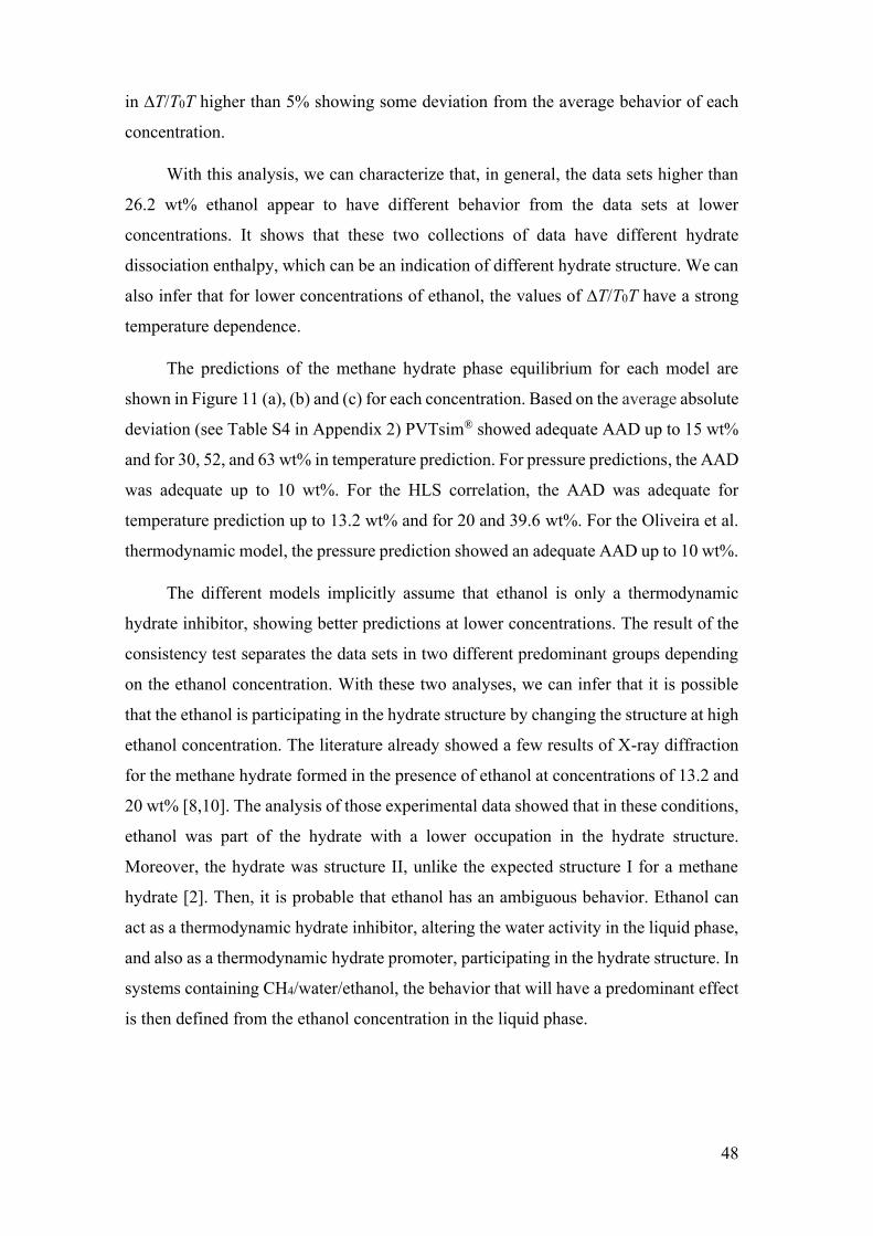
48
in ∆T/T0T higher than 5% showing some deviation from the average behavior of each
concentration.
With this analysis, we can characterize that, in general, the data sets higher than
26.2 wt% ethanol appear to have different behavior from the data sets at lower
concentrations. It shows that these two collections of data have different hydrate
dissociation enthalpy, which can be an indication of different hydrate structure. We can
also infer that for lower concentrations of ethanol, the values of ∆T/T0T have a strong
temperature dependence.
The predictions of the methane hydrate phase equilibrium for each model are
shown in Figure 11 (a), (b) and (c) for each concentration. Based on the average absolute
deviation (see Table S4 in Appendix 2) PVTsim® showed adequate AAD up to 15 wt%
and for 30, 52, and 63 wt% in temperature prediction. For pressure predictions, the AAD
was adequate up to 10 wt%. For the HLS correlation, the AAD was adequate for
temperature prediction up to 13.2 wt% and for 20 and 39.6 wt%. For the Oliveira et al.
thermodynamic model, the pressure prediction showed an adequate AAD up to 10 wt%.
The different models implicitly assume that ethanol is only a thermodynamic
hydrate inhibitor, showing better predictions at lower concentrations. The result of the
consistency test separates the data sets in two different predominant groups depending
on the ethanol concentration. With these two analyses, we can infer that it is possible
that the ethanol is participating in the hydrate structure by changing the structure at high
ethanol concentration. The literature already showed a few results of X-ray diffraction
for the methane hydrate formed in the presence of ethanol at concentrations of 13.2 and
20 wt% [8,10]. The analysis of those experimental data showed that in these conditions,
ethanol was part of the hydrate with a lower occupation in the hydrate structure.
Moreover, the hydrate was structure II, unlike the expected structure I for a methane
hydrate [2]. Then, it is probable that ethanol has an ambiguous behavior. Ethanol can
act as a thermodynamic hydrate inhibitor, altering the water activity in the liquid phase,
and also as a thermodynamic hydrate promoter, participating in the hydrate structure. In
systems containing CH4/water/ethanol, the behavior that will have a predominant effect
is then defined from the ethanol concentration in the liquid phase.
49
Figure 11 - Methane (CH4) hydrate phase equilibrium data with ethanol. (a) x for 0 wt% EtOH
[158,180–186]. ■ for 5 wt% EtOH [52]. ● for 10 wt% EtOH [52]. ♦ for 13.2 wt% EtOH [10].
(b) ■ for 15 wt% EtOH [169]. ● for 20 wt% EtOH [187]. ♦ for 26.2 wt% EtOH [187]. ▲ for 30
wt% EtOH [10]. (c) ■ for 39.6 wt% EtOH [187]. ● for 44.6 wt% EtOH [187]. ♦ for 52.3 wt%
EtOH [10]. ▲ for 63 wt% EtOH [10]. The lines show the predictive calculations of the models:
continuous for the adapted model of Oliveira et al. [123], dashed to PVTsim® software and
dotted to Hu-Lee-Sum Correlation [176]. (d) The relationship between ∆T/T0T and temperature
T for methane hydrate systems with ethanol. The lines correspond to the constant value of the
best fit that represents the constant value of the water activity for a small temperature range.
It is possible that the behavior observed for systems with methane also occur for
other gases. With the analysis presented here, we can identify conditions in which that
behavior is more likely to occur and will be worth to perform additional experimental
characterization since these data are expensive and challenging to perform [10].
Equilibrium data for carbon dioxide hydrate are shown in Figure 12 (a), including
a linear fit of the data to the Clausius-Clapeyron equation for all the concentrations. The
highest statistical parameters (1-R2) is 1.20% for the 10 wt% EtOH (see Table S5 in
Appendix 2). All of the CO2 hydrate phase equilibria data passed the first criterion. For
the temperature and pressure range, the hydrate structure does not change at each
concentration.

50
The hydrate dissociation enthalpy was calculated for each concentration of the
CO2 hydrate phase equilibria data (see Table S5 in Appendix 2). Here, the relative
standard deviation (RSD) of ∆Hdiss was calculated comparing each concentration with
the average ∆Hdiss. All of the CO2 hydrate phase equilibrium data have RSD of ∆Hdiss
lower than 5%, passing in the second criterion. This criterion confirms that the ∆Hdiss
are independent of the thermodynamic inhibitor type and concentration up to 20 wt%
EtOH having the same hydrate structure.
The evaluation of the third criterion for the CO2 data is shown in Figure 12 (b).
The relative standard deviation (RSD) in ∆T/T0T for those data at each concentration is
reported in Table S5 in Appendix 2. The CO2 data for concentrations higher than 5 wt%
were adequate according to the third criterion, with an RSD in ∆T/T0T lower than 10%.
So, for the data with 2 and 5 wt%, the ∆T/T0T shows higher sensibility in the temperature
range. However, for 10 wt% the RSD in ∆T/T0T is 6.27%, which is adequate according
to the criterion (< 10%) but still higher than the 5% observed for the other data sets. The
water activity in the liquid phase has a higher deviation from the average at lower
concentration.
The predictions with PVTsim® for the CO2 hydrate phase equilibria have an
adequate AAD in pressure for concentrations up to 15 wt%. The highest AAD is 2.45
bar for 20 wt% of EtOH. For the AAD in temperature, PVTsim® gives an adequate
prediction for all the concentrations except at 20 wt%, which has an AAD of 0.83 K,
higher than the accepted AAD for a good prediction. Similar to the result by PVTsim®
for temperature prediction, the HLS correlation has an AAD in temperature higher than
0.5 K only for the 20 wt% of EtOH, for which the AAD is 1.22 K. The Oliveira et al.
thermodynamic model showed an AAD higher than 2 bars only for the concentration of
20 wt% (AAD = 2.63 bar), similar to the PVTsim® result. Figure 12 (a) shows all the
calculations for each model for each concentration, with the AADs are reported in Table
S6 in Appendix 2.
The analysis showed that for the CO2 hydrate systems with ethanol up to 15 wt%
the inhibitor behavior is predominant. The literature reported experimental data
characterizing the CO2 hydrate as structure I for the system with 13.2 wt% EtOH [16].
However, the RSD of ∆Hdiss increases with the increase in the concentration, and the
modeling approach for inhibited hydrate systems shows large deviations for the highest
concentration (20 wt%). This can be an indication of the changing behavior of ethanol

51
from an inhibitor (altering only the water activity in the liquid phase) to a promoter
(participating in the hydrate phase). We can also notice that the ∆T/T0T for the carbon
dioxide hydrate data at lower ethanol concentration have higher variation for a narrow
temperature range. As such, there is a need for additional experimental characterization
of CO2 hydrate for ethanol concentrations higher than 15 wt% EtOH.
Figure 12 - Carbon dioxide (CO2) hydrate phase equilibrium data with ethanol. (a) x for 0 wt%
EtOH [188]. ■ for 2 wt% EtOH [171]. ● for 5 wt% EtOH [52]. ♦ for 10 wt% EtOH
[52,170,172]. ▲ for 15 wt% EtOH [170,171]. for 20 wt% EtOH [172]. The lines show the
predictive calculations of the models: dashed-dotted for CO2 liquefy pressure (PVTsim®),
continuous for the adapted model of Oliveira et al. [123], dashed to PVTsim® software and

52
dotted to Hu-Lee-Sum Correlation [176]. (b) The relationship between ∆T/T0T and temperature
T for carbon dioxide hydrate systems with ethanol. The lines correspond to the constant value
of the best fit that represents the constant value of the water activity for a small temperature
range.
The evaluation of the consistency of the propane hydrate equilibrium data as an
inhibited system is shown in Figure 13. Figure 13 (a) shows the linear fit of those data
to the Clausius-Clapeyron equation. The statistical parameter (1-R2) for the propane
hydrate phase equilibria showed a proper linear fitting, lower than 2%, as showed in
Table S7 in Appendix 2.
The second criterion of the consistency test for the C3H8 hydrate equilibrium data
is tested through the RSD of ∆Hdiss (see Table S7 in Appendix 2). The C3H8 hydrate
phase equilibria data up to 15 wt% EtOH presented good RSD of ∆Hdiss below 4%. So,
the hydrate structure (sII) is the same for all the three data sets. However, we only had
three concentration sets to evaluate the deviation from the average behavior. The third
criterion is evaluated through the RSD in ∆T/T0T for each concentration (Table S7
Appendix 2). All the C3H8 data presented good agreement, with the highest RSD in
∆T/T0T of 4.75% for the 10 wt% data, lower than 5%. Therefore, for all data, the water
activity in the liquid phase does not significantly change with temperature in the studied
range.
The calculation of the three models used in this work is also showed in Figure 13
(a). The AAD for each concentration and model are in Table S8 in Appendix 2. The
three models presented adequate AAD in pressure and temperature, besides the average
absolute deviation in temperature for the ethanol concentration of 15 wt%, that is 1.1 K,
obtained with the PVTsim® software.
Since the data passed the consistency test and the modeling approach for inhibited
systems showed adequate prediction, we can infer that for a propane hydrate system
with ethanol up to 15 wt%, the ethanol predominantly behaves as inhibitor. However,
propane is a gas that forms single gas hydrate of structure II [2]. For these systems, the
calculation already defines the same hydrate structure, in which the ethanol can occupy
the large cavity. Therefore, if the ethanol occupancy is lower for lower concentration in
the liquid phase, as the literature reported [8,16,27,28], the model approach will predict

53
better the equilibrium in those systems. Then, there is a need in the literature for more
propane hydrate equilibrium data with ethanol concentrations higher than 15 wt%.
Figure 13 - Propane (C3H8) hydrate phase equilibrium data with ethanol. (a) x for 0 wt% EtOH
[181,186,189–192]. ■ for 5 wt% EtOH [52,172]. ● for 10 wt% EtOH [52,172]. ♦ for 15 wt%
EtOH [172]. The lines show the predictive calculations of the models: dashed-dotted for C3H8
liquefy pressure (PVTsim®), continuous for the adapted model of Oliveira et al. [123], dashed
to PVTsim® software and dotted to Hu-Lee-Sum Correlation [176]. (b) The relationship between
∆T/T0T and temperature T for propane hydrate systems with ethanol. The lines correspond to
the constant value of the best fit that represents the constant value of the water activity for a
small temperature range.

54
The literature presents only two sets of ethane hydrate equilibrium data with
ethanol for concentrations of 5 and 10 wt% EtOH [52]. In this work, we increase the
ethane hydrate equilibrium data in the literature presenting data with concentrations up
to 45 wt% EtOH. These data are shown in Table S9 in Appendix 2. The C2H6 data was
tested for consistency as a hydrate inhibited system. Figure 14 (a) shows all those data
and present the linear fit as well as the predictive calculation of the three models.
The first criterion of the consistency test for the C2H6 data is evaluated through
the statistical parameter (1-R2), shown in Table S10 in Appendix 2. All the data from
the literature and the ones presented in this work showed adequate statistical parameter
below 0.4% and passed the first criterion. For each concentration, there is no higher
variation in the slope of the curve for that temperature and pressure range.
The second criterion to be evaluated is the consistency of the relative standard
deviation of ∆Hdiss, also shown in Table S10 in Appendix 2. The C2H6 hydrate phase
equilibria data were acceptable according to the criterion, presenting an RSD of ∆Hdiss
below 10%. However, the experimental data sets of 10, 35, 45 wt% of ethanol, from this
work, presented RSD of 9.36%, 5.52%, and 5.52%, respectively, higher than the good
classification of 5%. The ∆Hdiss is between 71.05 kJ/mol and 76.74 kJ/mol for the data
higher than 10 wt% and the set of 5 wt%, but for the set of 10 wt% the ∆Hdiss is 65.92
kJ/mol, having the highest RSD. The hydrate dissociation enthalpy at 10 wt% is the one
with the highest deviation from the average, which can be an indication of a different
hydrate structure (sII). This concentration will be the best condition for future
experimental hydrate characterization data.
Figure 14 (b) shows the independency of the water activity in the liquid phase
with the temperature range for C2H6 data. The RSD in ∆T/T0T for those data are shown
in Table S10 in Appendix 2. Except for the set of 5 wt% of ethanol, that showed an RSD
in ∆T/T0T of 10.38%, all the sets were accepted in the third criterion of the test.
However, the set of 10 wt% showed an RSD in ∆T/T0T of 5.28%, slightly higher than a
good deviation (< 5%). So, for the lower concentrations datasets, the water activity in
the liquid phase has higher sensitivity with the temperature. They show similar results
as for the hydrate-forming gases (CH4, CO2, C2H6) that formed single hydrate of
structure I1.
55
The accuracy of the models for the C2H6 data was evaluated through the average
absolute deviation (AAD) in Table S11 in Appendix 2. The Oliveira et al.
thermodynamic model had an AAD below 2 bars for the data sets up to 10 wt%. The
PVTsim® showed an adequate AAD in pressure up to 26 wt% and for 45 wt% EtOH.
For the AAD in temperature the PVTsim® had good AADs up to 10 wt% EtOH and for
45 wt% EtOH, below 0.5 K. For the HLS correlation, the AADs in temperature were
adequate up to 10 wt% and for 40 wt%. All the models showed a higher AAD for
concentrations from 26 wt% to 40 wt% EtOH. Using any approach to model inhibited
hydrate system, in general, the models show consistency with the data up to 10 wt% for
the C2H6 hydrate system with ethanol.
The predictive results and the consistency test showed that the ethane hydrate
equilibrium data with ethanol appears to have different behavior between the sets of 10
wt% or lower and 26 wt% or higher. This is an indication that a probable different
hydrate structure (i.e., sII) forms for concentrations larger than 26 wt%, giving further
evidence that ethanol can act as a hydrate co-former, changing the expecting single gas
hydrate of structure I to a double hydrate of structure II [10]. Therefore, more
experimental investigation is needed in these conditions to better understand the role of
ethanol.

56
Figure 14 - Ethane (C2H6) hydrate phase equilibrium conditions with ethanol. (a) x for 0 wt%
EtOH [181,182,193]. for 5 wt% EtOH [52]. ► for 10 wt% EtOH [52]. ■ for 10 wt% EtOH
(this work). ● for 26 wt% EtOH (this work). ♦ for 35 wt% EtOH (this work). ▲ for 40 wt%
EtOH (this work). ▲ for 45 wt% EtOH (this work). The lines show the predictive calculations
of the models: dashed-dotted for C2H6 liquefy pressure (PVTsim®), continuous for the adapted
model of Oliveira et al. [123], dashed to PVTsim® software and dotted to Hu-Lee-Sum
Correlation [176]. (b) The relationship between ∆T/T0T and temperature T for propane hydrate
systems with ethanol. The lines correspond to the constant value of the best fit that represents
the constant value of the water activity for a small temperature range.
57
Because there are no liquid-hydrate-vapor equilibria data with ethanol for a gas
mixture in the literature [194], this study presents the first set of hydrate equilibria data
with ethanol. Hydrate phase equilibria data were measured up to 40 wt% ethanol for a
gas mixture composed of 73.8 mol% of methane and 26.2 mol% of ethane, as given in
Table S12 in Appendix 2.
Figure 15 (a) shows the CH4/C2H6 hydrate phase equilibria data as well as their
linear fit and the equilibrium conditions predicted with two models (PVTsim® and HLS
correlation). The linear regression evaluated through the statistical parameter (1-R2) are
in Table S13 in Appendix 2 for the CH4/C2H6 hydrate data. The CH4/C2H6 data obtained
in this study passed the first criterion with a statistical parameter lower than 0.45%. For
each concentration, there is no variation in the slope for the temperature and pressure
ranges.
The relative standard deviation of ∆Hdiss for the CH4/C2H6 data are in Table S13
in Appendix 2. The CH4/C2H6 data were acceptable by the second criterion of the test.
However, the 9 wt% presented the highest RSD of ∆Hdiss of 7.82%, below the 10%
acceptable, but higher than a good deviation of less than 5%. For the sets from 25 wt%
up to 40 wt% EtOH, the value of the ∆Hdiss is between 57.72 kJ/mol and 58.46 kJ/mol,
which are in good agreement. However, the set at 9 wt% had a ∆Hdiss of 63.88 kJ/mol.
The ∆Hdiss is independent from the type and concentration of the thermodynamic
inhibitor for the same gas hydrate structure. Therefore, we can infer that the sets at 25
wt% or higher probably correspond to a hydrate structure with a different composition
from the structure of the set at 9 wt%, since the mixture CH4/C2H6 forms structure II.
Figure 15 (b) shows the evaluation of the average ∆T/T0T for the CH4/C2H6 data.
The RSD in ∆T/T0T was calculated for each concentration to analyze the third criterion,
with values given in Table S13 in Appendix 2. The CH4/C2H6 data obtained in this study
showed a good RSD in ∆T/T0T, below 4%, and passed the third criterion.
The prediction from the PVTsim® and the HLS correlation, shown in Figure 15
(a), were analyzed through the AAD from the CH4/C2H6 data and they are given in Table
S14 in Appendix 2. PVTsim® had an adequate AAD for the pressure, below 2 bar, and
for the temperature, below 0.5 K, for the sets up to 25 wt% EtOH, while the HLS
correlation had an AAD for the temperature below 0.5 K up to 30 wt% EtOH. These
two approaches assume that ethanol is only a hydrate inhibitor. The evaluation of the
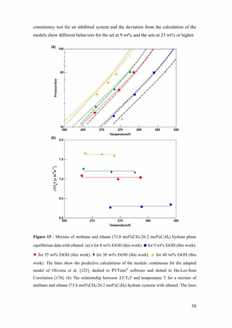
58
consistency test for an inhibited system and the deviation from the calculation of the
models show different behaviors for the set at 9 wt% and the sets at 25 wt% or higher.
Figure 15 - Mixture of methane and ethane (73.8 mol%CH4/26.2 mol%C2H6) hydrate phase
equilibrium data with ethanol. (a) x for 0 wt% EtOH (this work). ■ for 9 wt% EtOH (this work).
● for 25 wt% EtOH (this work). ♦ for 30 wt% EtOH (this work). ▲ for 40 wt% EtOH (this
work). The lines show the predictive calculations of the models: continuous for the adapted
model of Oliveira et al. [123], dashed to PVTsim® software and dotted to Hu-Lee-Sum
Correlation [176]. (b) The relationship between ∆T/T0T and temperature T for a mixture of
methane and ethane (73.8 mol%CH4/26.2 mol%C2H6) hydrate systems with ethanol. The lines

59
correspond to the constant value of the best fit that represents the constant value of the water
activity for a small temperature range.
We apply the three criteria of the consistency test proposed by Sa et al. [175] for
inhibited systems to all the hydrate equilibria data with ethanol. Applying this test, we
could verify the consistency of the data in the literature and also the data obtained in this
study to be characterized as a hydrate inhibited system. Since there is limited validation
to characterize the existing data with ethanol and there is an indication in the literature
that ethanol can have an ambiguous behavior as either a hydrate thermodynamic
inhibitor or promoter [8,27,28], this analysis has great importance to define conditions
in which hydrate experimental characterization data are needed.
For the set of CH4 hydrate phase equilibria with ethanol, only the 15 and 5 wt%
of ethanol fails the third criterion of the consistency test. Among the sets of CO2 hydrate
phase equilibria with ethanol, only the data of 2 and 5 wt% of ethanol fail the third
criterion. For all the other data of C3H8, C2H6, CH4/C2H6 hydrate phase equilibria, only
the C2H6 hydrate equilibria data of 5 wt% from the literature fails the third criterion of
the test. The hydrate structure for all of those systems is supposed to be a single hydrate
forming structure I. However, we could notice in the evaluation of the second criterion
that the hydrate dissociation enthalpy of those conditions showed higher deviation from
the other sets, giving some indication that the hydrate structure may be changed.
Coupling this information with the three predictive models for inhibited hydrate systems
and the literature reports that ethanol could behave as a hydrate thermodynamic
promoter, we can define experimental conditions in which more information about the
hydrate structure are needed. The definition of these experimental conditions is of high
relevance because the experimental data to characterize the hydrate structure are
expensive and challenging to perform [27].
For the sets of C3H8 and CH4/C2H6 hydrate phase equilibrium data, the hydrate is
already characterized as structure II [2]. So, the transformation that could occur on the
hydrate will not change the hydrate structure but include a competition between the
ethanol and the gases to occupy the large cavity of structure II. In these conditions, the
hydrate dissociation enthalpy will also change because of the changing hydrate
composition, as it was shown with the evaluation of the experimental CH4/C2H6 hydrate
phase equilibrium data.
60
The predictive potential of the three models was tested here, mainly for high
ethanol concentrations. In general, all the three models showed good predictions for
lower ethanol concentrations, up to 10 wt%, while for high concentrations the accuracy
varied. PVTsim® shows lower accuracy between 15 wt% and 44.6 wt%, with some
exceptions. The HLS correlation has an accuracy lower than 0.5 K for almost all the
data up to 30 wt% ethanol. The exceptions are for the 26 and 40 wt% for the C2H6, the
20 wt% for the CO2, and the 39.6 wt% for the CH4, that had the AAD above 0.5 K. The
thermodynamic model of Oliveira et al. [123] showed an AAD lower than 2 bar for all
the HPE data with ethanol for 10 wt% or lower. However, all three models were
developed with an approach to model a hydrate inhibitor system. As such, if ethanol is
a co-guest in the hydrate structure (solid phase), there may be structural change in some
system, and a different approach is needed to develop a model that will properly account
for the changes under the proper conditions. Between the three models presented here,
the thermodynamic model of Oliveira et al. [123] is the one that allows adaptation to
describe the equilibrium condition in systems where the chemical additive behaves both
as thermodynamic hydrate promoter and inhibitor. This modeling approach has already
been done to calculate the equilibrium condition of hydrate systems with THF [123].
3.5 Partial conclusions
Knowing that the hydrate phase equilibria data at high concentrations of ethanol
are scarce in the literature, this study presents a comprehensive summary of ethane
hydrate equilibrium data with ethanol, up to 45 wt% EtOH. Here we also show sets of
hydrate phase equilibrium data with ethanol, up to 40 wt%, for a gas mixture of 73.8
mol% methane and 26.2 mol% ethane, which was not available before in the literature.
In addition to experimental data for hydrate phase equilibria at high ethanol
concentrations, we tested the consistency of all the hydrate equilibria data with ethanol
as an inhibited hydrate system. The predictive potential to determine the gas hydrate
equilibrium temperature or pressure of three different modeling approaches were tested
for the systems, defined as inhibited hydrate systems, with ethanol. With this result and
the literature reports [8,27,28] that ethanol has ambiguous behavior, as a hydrate
thermodynamic inhibitor and promoter, we could infer the condition in which inhibitor
or promoter was predominant. For concentrations up to 10 wt%, ethanol is
predominantly a hydrate thermodynamic inhibitor, and for higher concentrations, the
61
promoter behavior begins to compete with the inhibitor behavior, reducing the
thermodynamic inhibition effect of ethanol, mainly for systems that in fresh water the
gas forms hydrate structure I (CH4, CO2 and C2H6). However, for systems that in fresh
water the gas forms structure II hydrate, we also see an indication that the ethanol could
participate as a hydrate co-former, as for the CH4/C2H6 data.
The hydrate phase equilibrium data with ethanol collected and measured here
contribute to increasing body of knowledge for hydrates with high ethanol
concentration. The methodology presented to evaluate the potential for ethanol to
behave as a hydrate thermodynamic inhibitor or promoter allowed to define conditions
at which a full experimental characterization of the hydrate structure and guest’s
occupancy are needed, which can be determined from x-ray diffraction and
spectroscopy measurements. Further improvements to predictive model will require
even more data with well-defined characterization of the hydrate structure and
composition.
List of symbols
T - Temperature [K]
P - Pressure [bar]
R - Universal gas constant [J mol / K]
wt% - massa fraction [g / g]
∆Hdiss - hydrate dissociation enthalpy [J / mol]
z - gas compressibility
RSD - relative standard deviation
∆T = T0 – T - suppression temperature
n - number of moles
T0 - equilibrium temperature without additive
LHVE - liquid hydrate vapor equiibrium
AAD - average absolute deviation
sI - Hydrate structure I
62
sII - Hydrate structure II
EtOH - Ethanol
63
Chapter 4. Hydrate growth in
freshwater Gas hydrates are crystalline solids formed in systems with water and light
components at low temperatures and high pressures. Those conditions are present in
natural gas offshore production, where it can lead to blockages. Although there are
consolidated operating procedures to avoid these blockages, there are also limitations to
their use. Similar conditions led to the formation of natural reserves of CH4 hydrate on
the seafloor, which came to be seen as a potential source of renewable energy.
Therefore, studies are under development to allow the exploration of the CH4 present in
those reserves. On the other hand, different applications for using these crystalline
structures are under development due to their capacity to store gases. Thus, a better
understanding of the growing phenomenon can allow the development of alternative
operational procedures to avoid blockages, adequately explore natural reserves, and
develop a new gas storage technology. The objective here is to develop a new model for
the hydrate growth kinetics with chemical affinity as a driving force. The use of the
Prigogine affinity allows the inclusion of the thermodynamic factor of all hydrate-
forming components in the growth model. This model is based on non-equilibrium
thermodynamics, which can clarify some conceptually relevant and rarely investigated
problems. Besides, it enables the inclusion of the thermodynamic behavior of hydrate
formation in the kinetics. Here, we evaluate the diffusion and reaction steps and their
limiting condition on the growth rate of CH4 hydrate in freshwater. The hydrate growth
model can describe the growth behavior quantitatively and qualitatively, showing good
agreement with the experimental data. Because the model considers both reaction and
diffusion, it shows that hydrate growth is governed by both mechanisms depending on
the pressure.

64
4.1 Introduction
Gas hydrates are crystalline solids formed in systems containing water and light-
guest molecules at low temperatures and high pressures [4]. The interactions between
the guest components and water molecules are controlled by the weak hydrogen bonds
[32]. These guest molecules are usually light gases, mainly natural gas components,
trapped inside the hydrogen-bond framework of water molecules [2]. Between natural
gas components, methane (CH4) is not only the gas usually in the highest concentration,
but also it is the most common gas in hydrate natural reserves. However, other gases
may also be included in hydrate structures, particularly in areas close to conventional
oil and gas reservoirs [195].
The conditions of hydrate formation are present in offshore oil and gas production.
In these systems, the formation of hydrates can lead to blockages along the flowline.
Conventional methods of hydrate preventions include physical and chemical
interventions. Limited physical options are available to prevent gas hydrate formation,
and, in most cases, the techniques are neither applicable nor economical [196]. The
conventional methods of chemical hydrate inhibition are the addition of thermodynamic
(THI) and low-dosage (LDHI) hydrate inhibitors [14]. However, the recent increase in
natural gas production started to require high volumes of THI [24]. As an alternative,
the use of LDHI, whether kinetic and/or anti-agglomerate, has become of greater interest
[196]. So, flow assurance requires an adequate predictive model for the formation of
solids to guarantee financial and safety requirements. Therefore, it is necessary to
understand the thermodynamic effects of hydrate formation in the presence of chemical
additives and the kinetic effect of the THIs and LDHIs on hydrate formation to guarantee
their use efficiency as hydrate blockage prevention methods [15].
The CH4 hydrate reserves in nature became a potential renewable energy source,
and studies are under development to explore these reserves [18]. According to the
review of Chong et al.[197], natural gas hydrates are one of the largest carbon sources on
earth and a potential source of clean carbon-based energy in the near future [195]. The
exploration of this solid in geological formations requires the hydrate formation and
dissociation dynamics knowledge [19] to guarantee an efficient and economically viable
gas production [198] without causing environmental impacts [21,199]. On the other
hand, there is a great interest in developing hydrate technology applications due to their

65
capacity to store gases. Among these applications are gas separation, energy storage,
energy transport, CO2 sequestration, and desalination [3]. However, the requirement of
high pressure is one of the decisive obstacles for the process commercialization [23].
The use of chemical additives eases the thermodynamic conditions and enables the
hydrate production for gas storage [200] and separation [196]. Therefore, developing a
model capable of describing hydrate growth will allow its process to be controlled,
making this new technology physically and economically viable [14].
Thermodynamic modeling for the phase equilibrium calculation with hydrate has
been in development since the 1960s with the van der Waals and Platteeuw model [98].
This model is based on statistical thermodynamics to describe the equilibrium between
hydrate, liquid, and vapor phases. The review of advances in modeling the phase
equilibrium with hydrate shows that this development occurred mainly around
improving the van der Waals and Platteeuw model. Although we still need some
improvements in the hydrate equilibrium calculations, this modeling is already
sufficiently consolidated for some systems such as the methane hydrate system [201].
Meanwhile, this solid-formation dynamic modeling still presents a large gap, as shown
in the literature [19].
The formation of gas hydrate is similar to the crystallization process and can be
described in three stages: nucleation, growth, and agglomeration [2]. Kinetic
experimentation and molecular simulation are used to understand the nucleation
mechanism [11,35]. However, due to the difficulty of obtaining nucleation direct
experimental evidence, molecular simulations have been preferred over experimental
studies [33,34]. The agglomeration is the stage with more evidence in the literature
studies because it is the main stage responsible for blocking oil and gas production lines
[19]. According to Yin et al. [15], that reviewed the gas hydrate growth kinetic models,
the gap still exists in understanding the controlling mechanism of gas hydrate growth,
which is further augmented by the dynamic behavior of multiphase fluids flow, the
thermodynamics of the hydrate-forming system, and the compounding interfacial
phenomena. Most of the hydrate growth models in the literature are based on the guest
molecule dynamics only and are unable to describe non-ideal systems [33,42–44,84–
87,95,96].
This work focuses on the hydrate growth kinetics, mainly because studies show
that, after the beginning of the appearance of the first crystals, the growth effect overlaps

66
the nucleation just as agglomeration overlaps the growth in the particle size scale.
However, it is possible to separate these effects in the time scale to understand those
mechanisms [44,202,203]. The models that include water or some additive effect do
not account for the host molecule effect or the interaction between those compounds
[80,83,204,205]. Therefore, there is still a need for a model capable of explaining the
effect of all components participating in the hydrate formation "reaction" and the non-
ideality effects of the systems. Here, we are proposing the use of the Prigogine affinity
as the driving force. Changes in thermodynamic potentials for chemical reactions
produce affinity [122]. The affinity allows evaluating all the components involved in
the hydrate formation and evaluates the growth accounting for non-ideal effects. The
affinity is already used in the literature [88–90]. However, as far as we know, all the
models that use affinity in the driving force adopted simplifications that did not take
into account the essential effects of the thermodynamic factor.
The reaction rate is the change in the extent of the reaction over time, and it can
be proved that, from non-equilibrium thermodynamics, the driving force and its
conjugated flow establish a linear relationship. More details on the thermodynamics of
non-equilibrium are on Demirel [121] and Lebon et al. [122].
The coupling of the diffusion effects from the gas-liquid interface to the bulk
phase, with the reaction effect, due to the host movement from the bulk phase to the
liquid-solid interface, is a mechanism widely used in the literature [33,41,42,86,206].
However, in ideal systems, the solubility of methane in water is low, and its diffusion
will be slower than the reaction to form the solid phase. Thus, a variety of models only
account for the diffusion effect for the hydrate growth in the literature [33,81,83–87].
Then, there are still questions about the competition between reaction and diffusion in
systems that deviate from this ideal scenario due to using an additive or systems at very
high pressures [93–96].
A better understanding of the dynamic hydrate growth behavior is necessary to
facilitate the exploration of natural gas hydrate reserves, develop the hydrate technology
to store or separate gases, and allow the safer use of KHI and LDHI. Therefore, this
work aimed to develop a hydrate growth model based on the non-equilibrium
thermodynamics and applied to CH4 hydrate in freshwater. With this model, we intend
to describe the growth considering the diffusion and reaction steps. To establish a new

67
driving force to account for the effect of the thermodynamic factor in the kinetic for
both water and guest molecule (CH4).
4.2 Kinetic model
Although hydrate formation does not involve breaking or forming new bonds
between the atoms involved, characterizing the transformation of molecules, the term
"reaction" is used to refer to the formation of hydrate [2]. The hydrate formation reaction
modeled here is the methane hydrate formation reaction in systems containing methane
and pure water. This reaction is shown in equation (35), where H is the symbol
representing the hydrate phase, with the molar composition of methane and of
water.
4 2 4 2CH H O H CH H O (18)
The stoichiometric coefficients of each component are defined depending on the
hydrate structure formed. For water, this is obtained by the number of water molecules
present in a unit cell, that is, it is the sum of the product between the number of cavities
per unit cell and the coordination number of each unit cell for large and small cavities.
Therefore, for structure I, 184 , and for structure II, 544 . The stoichiometric
coefficient of the guest is given by the sum of the number of large and small cavities per
unit cell of the structure. Then, for the methane hydrate unit, 8 , as it forms structure
I [2].
In order to describe the growth, some hypotheses were adopted. First, it is assumed
that growth occurs separately from nucleation. The growth process will take place at the
solid-liquid interface. Therefore, the mass and energy balances will be applied to the
liquid, vapor, and hydrate phases, given the following considerations:
(a) nucleation and growth occur sequentially, and, in this work, we will focus only
on the growth stage, so there is no nucleation after the beginning of the growth;
(b) the liquid phase consists of water and solubilized methane;
(c) the liquid provides water and methane for the hydrate growth process in the
solid-liquid interface;
(d) the vapor phase provides methane for the liquid phase;
(e) the amount of water present in the vapor phase is despised;
(f) in the vapor phase there is no hydrate growth;

68
(g) the gas-liquid interface is in local equilibrium.
4.2.1 Driving force
In this sense, for constant P and T systems, the mass balance for each phase, the
population balance to obtain properties of the solid phase, and the reaction rate with a
driving force that accounts for both water and hydrate forms’ activity are necessary. In
addition to this algebraic-differential equations system, thermodynamic models
proposed by Oliveira et al. [123,207] were structured and validated to calculate the
equilibrium conditions and thermodynamic properties (Appendix 3). The main equation
of the model will be presented in the following topics. The experimental hydrate
formation systems are a high-pressure reactor with a mechanical stirrer filled with pure
methane (CH4) gas, representing the gas phase, and pure water (H2O), representing the
liquid phase.
For chemical reactions, analysis in terms of Gibbs free energy is convenient. For
the constant temperature, T, and pressure, P, the variation of Gibbs' free energy, Gb, can
be related to the degree of extent of the reaction, , according to the Donder
thermodynamic theory of affinity. Then, the Prigogine's Affinity, A, defined by equation
(19), is introduced [121]. Where i is the stoichiometric coefficient and i is the
chemical potential of component i in the reaction.
,
bi i
iT P
dG Ad
(19)
Describing the chemical potential in terms of the activity, a, the affinity can be
obtained in terms of the activity of each component according to the equation (20).
0 0ln ln i
i i i i i ii i i
A RT a RT a
(20)
Because the Gibbs free energy is minimal at equilibrium 0dGd , the affinity
at equilibrium is zero. Applying the chemical equilibrium condition in equation (20)
leads to equation (21).
00 ln ieq eq eqi i i i i
i i i
A RT a
(21)

69
Substituting equation (21) into equation (20), affinity can be defined as the
distance from the equilibrium in terms of activity, according to equation (22).
'ln ln
'
i
i
eqi
eqi
ii
a KA RT RT
Ka
(22)
The chemical equilibrium constant is the geometric mean of the activities
weighted by the stoichiometric reaction coefficients, ' ieqeq i
i
K a
.
The calculation of affinity requires the description of each species’ activities in
the liquid and hydrate phases. For the proposed reaction, equation (35), the activity of
the components in the liquid phase is obtained by the excess Gibbs energy model, NRTL
[123], with the parameters estimated for the H2O and CH4 system (Appendix 3).
The literature does not contain consolidated models that describe the difference in
the chemical potential of the components in the hydrate phase-out of equilibrium.
However, with the hypothesis of the solid phase in equilibrium, the activity of the
components in the hydrate phase is only necessary to define the equilibrium curve of
the system, that can be obtained through the traditional modeling of van der Waals and
Platteeuw theory [98]. We used the modeling proposed by Oliveira et al. [207] to
describe the hydrate-liquid equilibrium conditions.
Adopting the hypothesis that the solid phase is in equilibrium, the activities in the
solid phase are the activities of the components in the equilibrium condition. Therefore,
the 'K is calculated according to equation (23) and 'eqK according to equation (24).
4 2
4 2
'H HCH H Oeq eq
L LCH H O
a aK
a a
(23)
4 2
4 2
'H HCH H Oeq eq
eq L LCH H Oeq eq
a aK
a a
(24)
The affinity is then described by equation (25), where K is the product of
activities, weighted by stoichiometric coefficients, in the liquid phase, out of the
equilibrium, and e qK is the same product but in equilibrium with the solid phase.
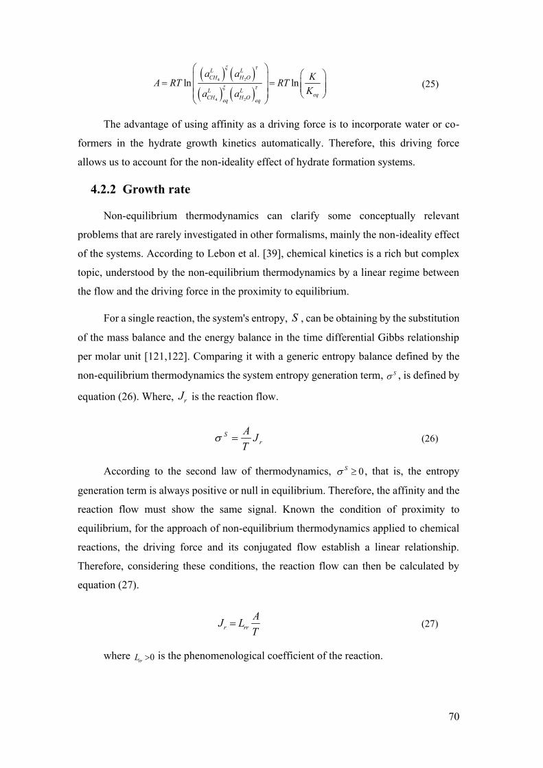
70
4 2
4 2
ln lnL LCH H O
L LeqCH H Oeq eq
a a KA RT RTKa a
(25)
The advantage of using affinity as a driving force is to incorporate water or co-
formers in the hydrate growth kinetics automatically. Therefore, this driving force
allows us to account for the non-ideality effect of hydrate formation systems.
4.2.2 Growth rate
Non-equilibrium thermodynamics can clarify some conceptually relevant
problems that are rarely investigated in other formalisms, mainly the non-ideality effect
of the systems. According to Lebon et al. [39], chemical kinetics is a rich but complex
topic, understood by the non-equilibrium thermodynamics by a linear regime between
the flow and the driving force in the proximity to equilibrium.
For a single reaction, the system's entropy, S , can be obtaining by the substitution
of the mass balance and the energy balance in the time differential Gibbs relationship
per molar unit [121,122]. Comparing it with a generic entropy balance defined by the
non-equilibrium thermodynamics the system entropy generation term, S , is defined by
equation (26). Where, rJ is the reaction flow.
Sr
A JT
(26)
According to the second law of thermodynamics, 0S , that is, the entropy
generation term is always positive or null in equilibrium. Therefore, the affinity and the
reaction flow must show the same signal. Known the condition of proximity to
equilibrium, for the approach of non-equilibrium thermodynamics applied to chemical
reactions, the driving force and its conjugated flow establish a linear relationship.
Therefore, considering these conditions, the reaction flow can then be calculated by
equation (27).
r rrAJ LT
(27)
where 0rrL is the phenomenological coefficient of the reaction.

71
Figure 16 outlines the hydrate growth phenomenon stages based on the hypothesis
of diffusion with reversible heterogeneous reaction. This approach is already used in
mathematical models found in the literature, such as the model by Englezos et al.
[42,43]. By the liquid film theory, the hydrate growth process is treated with
consideration of the following steps: a) diffusion of the solute from the bulk of the liquid
phase ( z ) to the solid surface ( 0z ), and b) hydrate formation reaction on the
surface ( 0z ).
Figure 16 - Illustrative image of the liquid film surrounding the hydrate solid surface.
For the description of the two stages, the following hypotheses are adopted: a) in
the liquid film, the system is in a steady state; b) absence of convection in the liquid
film; c) unidirectional transport; d) isothermal system, e) reversible heterogeneous
reaction, occurring only at the liquid-solid interface and f) there is no chemical reaction
in the liquid film. According to the considered hypotheses, the mass balance can be
represented by equation (28). The diffusive mass flow can be written in terms of each
component’s chemical potential, and the solution is linear with the z-axis, equation (28),
considering that the methane concentration slightly changes in the liquid film.
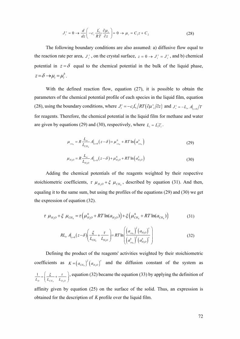
72
'
1 20 0z i ii i i
LdJ c C z Cdz RT z
(28)
The following boundary conditions are also assumed: a) diffusive flow equal to
the reaction rate per area, zrJ , on the crystal surface, 0 z z
i rz J J , and b) chemical
potential in z equal to the chemical potential in the bulk of the liquid phase, b
i iz .
With the defined reaction flow, equation (27), it is possible to obtain the
parameters of the chemical potential profile of each species in the liquid film, equation
(28), using the boundary conditions, where ' 'zi i i iJ c L RT z and
0zr rr z
J L A T
for reagents. Therefore, the chemical potential in the liquid film for methane and water
are given by equations (29) and (30), respectively, where 'i i iL L c .
4 4 4
4
00
lnCH CH CH
brrz
CH
LR A z RT aL
(29)
2 2 2
2
00
ln brrH O H O H Oz
H O
LR A z RT aL
(30)
Adding the chemical potentials of the reagents weighted by their respective
stoichiometric coefficients, 2 4H O CH , described by equation (31). And then,
equaling it to the same sum, but using the profiles of the equations (29) and (30) we get
the expression of equation (32).
2 4 2 2 4 4
0 0ln( ) ln( )H O CH H O H O CH CHRT a RT a
(31)
24
4 224
0ln CH
CH
H O
rr z b bCH H OH O
a aRL A z RT
L L a a
(32)
Defining the product of the reagents' activities weighted by their stoichiometric
coefficients as 4 2CH H OK a a
and the diffusion constant of the system as
4 2
1
D CH H OL L L
, equation (32) became the equation (33) by applying the definition of
affinity given by equation (25) on the surface of the solid. Thus, an expression is
obtained for the description of K profile over the liquid film.

73
We know from the Viges equation [208] that
2 4
4 2 4 2 2 4
0 0CH /H CH /H H /CH
H O CHn n
O O OL L L . As the system is mostly water, 2 4H O CHn n ,
4 2 4 2
0CH /H CH /HO OL L . So,
4CHL is basically the diffusion coefficient of methane in water
and can be described according to the relation 4 4
expCH CH aL c D E RT [87,209], where
4CHc is the methane average concentration in the liquid film, Ea is the activation energy
(J/mol) of the water diffusion process, R is the universal gases constant and D is a
parameter that depends on the molecule that is diffusing in the aqueous phase. Then, the
diffusion constant is 4D CHL L .
0
rr
D
LR zL
z
b eq
KKK K
(33)
As equation (33) is valid throughout the liquid film, it can be applied to the surface
of the solid to obtain 0zK
according to equation (34).
0
rr D
D rr D rr
RL LL RL L RL
eq bzK K K
(34)
The diffusion and reaction coefficients presented different dimensions, [ DL ] =
mol/m s and [ rrL ] = mol2 K/m² J s. However, the exponents D D rrL L RL or rr D rrRL L RL
are dimensionless. Therefore, a more accurate comparison is made between DL and
rrRL .
The equation (34) allows to evaluate the coupling between diffusion and reaction.
If D rrRL L the exponent of eqK tends to zero while the exponent of bK tends to one,
then 0 bzK K
. In other words, diffusion is the fast stage, reaction is the limiting stage
of the system and on the surface of the crystal the reagents are in the condition of the
bulk liquid phase. However, if rr DRL L , by the same analysis of the exponents,
0 eqzK K
. In this case, the reaction is the fast stage, diffusion is the limiting stage of
the system and the reagents are in equilibrium on the crystal surface. Then, the model is
capable to describe the coupling between diffusion and reaction, but also the limiting
conditions of the system where the growth is limited by reaction or limited by diffusion.
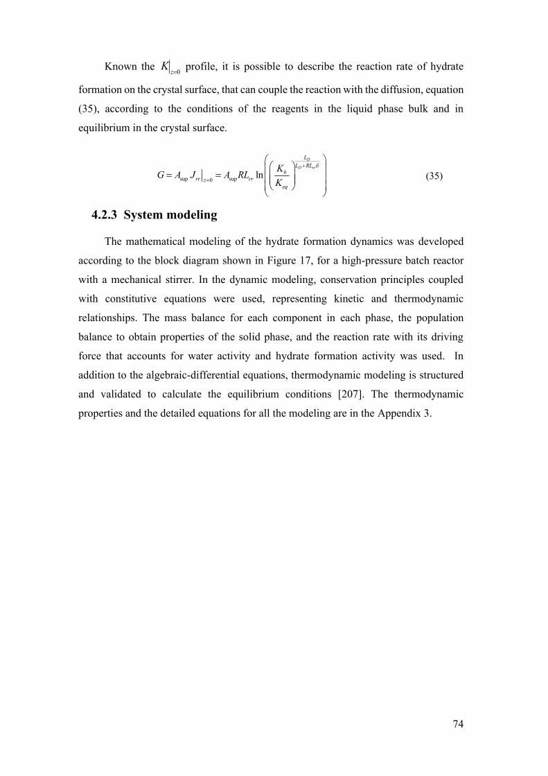
74
Known the 0zK
profile, it is possible to describe the reaction rate of hydrate
formation on the crystal surface, that can couple the reaction with the diffusion, equation
(35), according to the conditions of the reagents in the liquid phase bulk and in
equilibrium in the crystal surface.
sup sup0ln
D
D rr
LL RL
brr rrz
eq
KG A J A RLK
(35)
4.2.3 System modeling
The mathematical modeling of the hydrate formation dynamics was developed
according to the block diagram shown in Figure 17, for a high-pressure batch reactor
with a mechanical stirrer. In the dynamic modeling, conservation principles coupled
with constitutive equations were used, representing kinetic and thermodynamic
relationships. The mass balance for each component in each phase, the population
balance to obtain properties of the solid phase, and the reaction rate with its driving
force that accounts for water activity and hydrate formation activity was used. In
addition to the algebraic-differential equations, thermodynamic modeling is structured
and validated to calculate the equilibrium conditions [207]. The thermodynamic
properties and the detailed equations for all the modeling are in the Appendix 3.
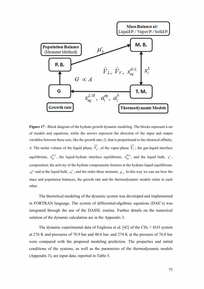
75
Figure 17 - Block diagram of the hydrate growth dynamic modeling. The blocks represent a set
of models and equations, while the arrows represent the direction of the input and output
variables between these sets, like the growth rate, G, that is proportional to the chemical affinity,
A. The molar volume of the liquid phase, LV , of the vapor phase VV ; the gas-liquid interface
equilibrium, /G Leqx , the liquid-hydrate interface equilibrium, H/L
eqx , and the liquid bulk, Lix ,
composition; the activity of the hydrate compounents formers at the hydrate-liquid equilibrium, eqia and at the liquid bulk, b
ia ; and the order-three moment, '3 . In this way we can see how the
mass and population balances, the growth rate and the thermodynamic models relate to each
other.
The theoretical modeling of the dynamic system was developed and implemented
in FORTRAN language. The system of differential-algebraic equations (DAE’s) was
integrated through the use of the DASSL routine. Further details on the numerical
solution of the dynamic calculation are in the Appendix 3.
The dynamic experimental data of Englezos et al. [42] of the CH4 + H2O system
at 276 K and pressures of 70.9 bar and 48.6 bar, and 274 K at the pressure of 76.0 bar
were compared with the proposed modeling prediction. The properties and initial
conditions of the systems, as well as the parameters of the thermodynamic models
(Appendix 3), are input data, reported in Table 5.

76
Table 5 - Input data for the calculation of isothermal-isobaric single hydrate (sI) growth of the
CH4 + H2O system.
Input data
Component and System Properties
Liquid Phase
Molar mass of component [g/mol]
H2O 18.015 [210]
CH4 16.043 [210]
Critical component temperature [K]
H2O 647.14 [210]
CH4 190.56 [210]
Critical component pressure [bar]
H2O 220.64 [210]
CH4 45.99 [210]
Critical component volume [cm³/mol]
H2O 55.95 [210]
CH4 98.60 [210]
Component dynamic viscosity [mol/m s]
H2O 2
2
310 578.918exp 3.7188137.546H O
H OMM T
Liquid Dynamic
Viscosity
(Vogel equation
by online
Dortmund Data
Bank) http://www.ddbst.com/
CH4 4
4
310 25392.0exp 25.5947969.306CH
CHMM T
Component density [kg/m³]
H2O 997.0 [210]
CH4 0.656 [210]
Solid Phase
Density [kg/m³] 917.8 [2,87]
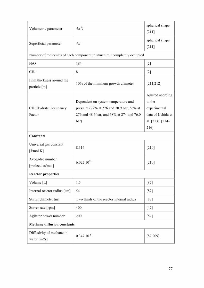
77
Volumetric parameter 4 3 spherical shape
[211]
Superficial parameter 4 spherical shape
[211]
Number of molecules of each component in structure I completely occupied
H2O 184 [2]
CH4 8 [2]
Film thickness around the
particle [m] 10% of the minimum growth diameter [211,212]
CH4 Hydrate Occupancy
Factor
Dependent on system temperature and
pressure (72% at 276 and 70.9 bar; 56% at
276 and 48.6 bar; and 68% at 274 and 76.0
bar)
Ajusted acording
to the
experimental
data of Uchida et
al. [213]. [214–
216]
Constants
Universal gas constant
[J/mol K] 8.314 [210]
Avogadro number
[molecules/mol] 6.022 1023 [210]
Reactor properties
Volume [L] 1.5 [87]
Internal reactor radius [cm] 54 [87]
Stirrer diameter [m] Two thirds of the reactor internal radius [87]
Stirrer rate [rpm] 400 [42]
Agitator power number 200 [87]
Methane diffusion constants
Diffusivity of methane in
water [m²/s] 0.347 10-5 [87,209]

78
Activation energy of the
methane diffusion process
in water [kJ/mol]
18.36 [87,209]
Initial Conditions
Liquid Phase
Number of moles
H2O 16.6 [42]
CH4 10-5
Minimum
amount to start
solubilization
without
numerical issues
Solid Phase
Relative hydrate fraction
(hydrate volume/water
volume)
0.0001% [24,79,87]
Average diameter of
hydrate crystals (d) [m] 10-6 [33,42,79]
Volume of a medium-sized
particle [m³] 34 3 2d
spherical shape
[211]
Surface area of a medium-
sized particle [m²] 34 2d
spherical shape
[211]
In order to predict the kinetic data obtained by Englezos et al. [42] with the
proposed model, the conditions used to obtain these data were used as input data. Some
extra information necessary to calculate the growth with the proposed model was
obtained mainly from the study proposed by Sampaio et al. [87], who described hydrate
growth using population balance.
It is important to note that the properties of the solid phase, Table 5, were imposed
to define the initial moments, based on spherical particles, for the calculation of the
population balance of the modeling (Appendix 3). We thus defined an average hydrate
crystal diameter based on the critical radius values used in nucleation models based on
the theory of primary homogeneous nucleation [11,34,42,87].

79
4.3 Results and discussion
Calculations of the simple methane hydrate growth with the proposed model and
conditions were performed. We evaluated the coupling effect between the diffusion and
reaction phenomena incorporated in the growth rate, the effect of the non-ideality that
the driving force incorporates to the hydrate growth, as well as the effect of adding the
water activity with the guest molecule activity of the hydrate phase in the driving force.
The effect of the pressure and temperature on the growth dynamics was also observed
here.
4.3.1 Diffusion/reaction coupling effect
The growth rate proposed in this work, equation (35), allows evaluating the
coupling effect between the solid phase growth reaction and the guest molecule
diffusion from the gas phase to the bulk liquid phase. For this evaluation, the DR factor
is defined as the degree of coupling between those two phenomena. The DR factor is
given by the ratio D D rrL L RL , which is the exponent of the growth rate driving force.
The DR factor represents a scale that goes from 0.0 to 1.0, Figure 18. DR equal to
0.0 describes a growth limited by diffusion only of the host molecule from the gas phase
to the bulk liquid phase. Meanwhile, DR factor equal to 1.0 describes a growth limited
by reaction only of the solid phase growth. The DR = 0.5 describes a growth with total
coupling between the diffusion and the reaction. Therefore, a DR = 0.1 describes a
growth where the diffusion is the slow stage and the reaction the quick stage; that is, the
diffusion rate corresponds to about 10% of the growth rate. For a DR = 0.6, the diffusion
is the quick stage, and the reaction is the slow stage, i.e., the diffusion rate corresponds
to about 60% of the growth rate.

80
Figure 18 - DR scale. Coupling scale between diffusion and reaction. A growth hydrate profile
limited by diffusion has a DR equal to 0.0, while a limited by reaction profile has a DR equal to
1.0. A complete coupling profile between diffusion and reaction is described by a DR equal to
0.5.
The imposition of these limit values for the DR factor in developing of the
proposed growth model generates two rates. The growth rate limited by diffusion,
equation (36), and the growth rate limited by reaction, equation (37).
In this work, we used to describe the limiting conditions with the factors of 0.01,
limited by diffusion, or 0.99, limited by reaction. Therefore, it is not necessary to impose
a rate to describe the system's limiting conditions. The proposed rate allows describing
systems in limit conditions or not from the adjustment of the DR factor. These factors
were sufficient to describe behavior similar to the profiles obtained from the limit rates
imposition. The comparisons between DR = 0 or 0.01 and equal to 1 or 0.99, close to
the limiting conditions, are shown in the Figure 19. Through this comparison it is noted
that is not necessary to impose a reaction rate in the limit condition, the proposed model
is able to describe through the DR adjustment whether or not the system is in the limit
condition. In addition, we observed that the limit condition does not occur by imposing
a DR = 0 or DR = 1 only, but in a range of DR that approaches that limit condition.
sup ln bD
eq
KLG AK
(36)
sup ln brr
eq
KG A RLK
(37)

81
Figure 19 – The comparation of the methane molar consumption (ΔnG) over time at 276 K and
70.9 bar (a) between the limited by diffusion rate, equation (36), and the profile using the
diffusion-reaction coupling rate for a DR equal to 0.01, equation (35), (black dotted line) and
(b) between limited by reaction rate, equation (37), and the profile using the diffusion-reaction
coupling rate for a DR equal to 0.99, equation (35) (black dashed-dotted line). The continuous
gray line represents the 45 degree line expected for this comparison. The insertion shows the
temporal variation of the methane number of moles in the gas phase (nG). The continuous line
represented the profile with the adjusted DR factor, while the dotted line represented the profile
limited by diffusion and the dotted-dashed line the profile limited by reaction.
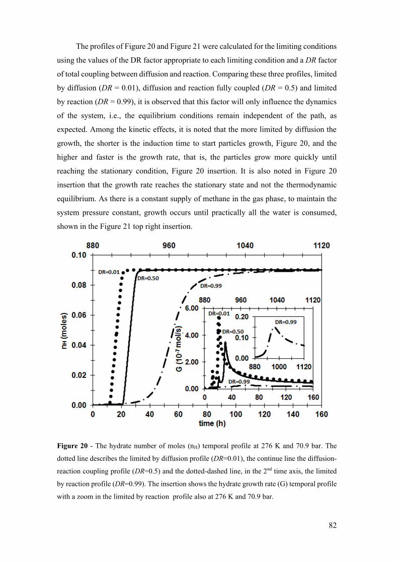
82
The profiles of Figure 20 and Figure 21 were calculated for the limiting conditions
using the values of the DR factor appropriate to each limiting condition and a DR factor
of total coupling between diffusion and reaction. Comparing these three profiles, limited
by diffusion (DR = 0.01), diffusion and reaction fully coupled (DR = 0.5) and limited
by reaction (DR = 0.99), it is observed that this factor will only influence the dynamics
of the system, i.e., the equilibrium conditions remain independent of the path, as
expected. Among the kinetic effects, it is noted that the more limited by diffusion the
growth, the shorter is the induction time to start particles growth, Figure 20, and the
higher and faster is the growth rate, that is, the particles grow more quickly until
reaching the stationary condition, Figure 20 insertion. It is also noted in Figure 20
insertion that the growth rate reaches the stationary state and not the thermodynamic
equilibrium. As there is a constant supply of methane in the gas phase, to maintain the
system pressure constant, growth occurs until practically all the water is consumed,
shown in the Figure 21 top right insertion.
Figure 20 - The hydrate number of moles (nH) temporal profile at 276 K and 70.9 bar. The
dotted line describes the limited by diffusion profile (DR=0.01), the continue line the diffusion-
reaction coupling profile (DR=0.5) and the dotted-dashed line, in the 2nd time axis, the limited
by reaction profile (DR=0.99). The insertion shows the hydrate growth rate (G) temporal profile
with a zoom in the limited by reaction profile also at 276 K and 70.9 bar.
83
The growth phenomenon described by the proposed model can be understood by
the behavior of the host molecule, CH4, mole fraction in the liquid phase, Figure 21. We
observed that the methane solubilization in water occurs in the first two hours, as seen
in the Figure 21 left insertion, and the gas saturates in the liquid phase after this time. It
is observed that the solubilization effect occurs more quickly than the growth, which
will only start hours after depending on the DR factor value and the initial conditions,
Table 5. The CH4 mole fraction profile in the liquid phase is limited by the gas-liquid
(G-L) and the liquid-hydrate (L-H) interfaces equilibrium conditions, as seen in the
Figure 21 bottom-right insertion. In 276 K and 70.9 bar conditions, methane
compositions in the interfaces G-L and L-H in equilibrium are 0.24% and 0.15%,
respectively.
Further details on the calculation of the equilibrium compositions are in the
Appendix 3. This limitation allowed us to adjust the methane occupation factor in the
hydrate phase. Some experimental works in the literature show possible occupancy
factors depending on temperature and pressure [213–216]. Within these ranges, we used
the maximum occupancy factor for which the methane mole fraction profile in the liquid
phase had the greatest possible variation limited by the equilibrium conditions. For the
system at 276 K and 70.9 bar, the occupancy factor was 72% given these criteria.
The methane number of moles profile, Figure 21, and water, Figure 21 bottom-
right insertion, in the liquid phase allows us to conclude that practically the entire liquid
phase converts to a solid phase in these systems. The number of moles of methane starts
in practically zero (10-5 moles), reaches the maximum solubility of methane in the liquid
phase, about 0.04 moles, and at the end of the growth, it returns to practically zero (10-
6 moles). In contrast, the water came from 16.6 moles (300 mL), a condition of the
Englezos et al. [42] experiments, to practically zero (5 10-4 moles). These values result
in similar initial, after the saturation, and final compositions. Note that the water is the
limiting factor for the system to reach steady-state because although the gas supply
remains, the amount of water is not enough to continue the hydrate structures growth.

84
Figure 21 - The methane number of moles in the bulk liquid phase (nL,CH4) temporal profile at
276 K and 70.9 bar. The dotted line describes the limited by diffusion profile (DR=0.01), the
continue line the diffusion-reaction coupling profile (DR=0.5) and the dotted-dashed line, in the
2nd time axis, the limited by reaction profile (DR=0.99). The insertion on the left shows the
methane in water saturation profile, the one in the bottom-right shows the methane mole fraction
(xL,CH4) profile in the bulk liquid phase (dark lines), in the gas-liquid equilibria interface (gray
continus line) and in the liquid-hydrate equilibrium interface (gray dotted-dashed line) and the
one in the top right shows the water number of moles in the bulk liquid phase (nL,H2O).
The methane molar consumption (ΔnG) from the gas phase during the hydrate
growth is the most accessible measurement variable in these experiments [2,15,39,217].
Therefore, the comparison and validation of the proposed model were performed using
this variable, as seen in Figure 22, for that we had to normalize the time scale.
Comparing the growth data given by Englezos et al. [42] with the model description, we
can understand how coupling is the diffusion and reaction. At 276 K, 70.9 bar, and the
initial conditions, Table 5, Figure 22 shows that the diffusion and reaction are coupled
and better described by a DR = 0.5.
The beginning of the growth (up to 0.2 hours in Figure 22) seems to be better
adjusted by the limited by diffusion profile; however, because our populational balance
does not include a nucleation model yet, this can be the primary nucleation effect, that
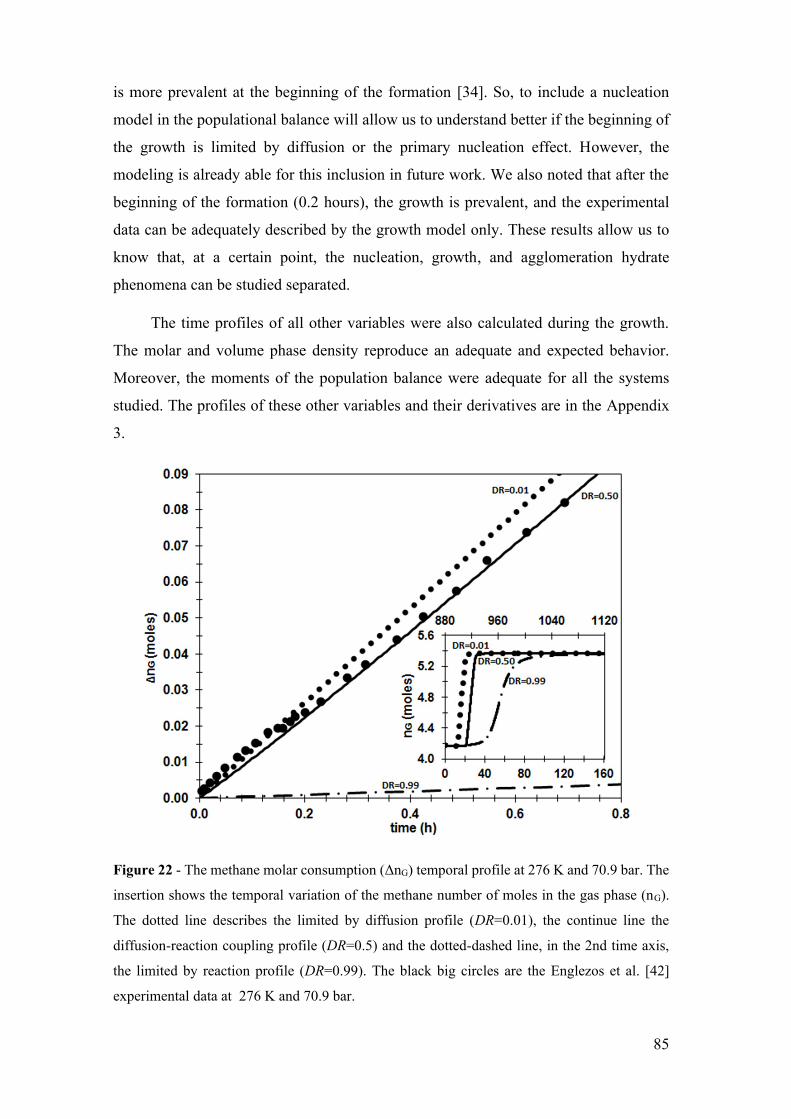
85
is more prevalent at the beginning of the formation [34]. So, to include a nucleation
model in the populational balance will allow us to understand better if the beginning of
the growth is limited by diffusion or the primary nucleation effect. However, the
modeling is already able for this inclusion in future work. We also noted that after the
beginning of the formation (0.2 hours), the growth is prevalent, and the experimental
data can be adequately described by the growth model only. These results allow us to
know that, at a certain point, the nucleation, growth, and agglomeration hydrate
phenomena can be studied separated.
The time profiles of all other variables were also calculated during the growth.
The molar and volume phase density reproduce an adequate and expected behavior.
Moreover, the moments of the population balance were adequate for all the systems
studied. The profiles of these other variables and their derivatives are in the Appendix
3.
Figure 22 - The methane molar consumption (ΔnG) temporal profile at 276 K and 70.9 bar. The
insertion shows the temporal variation of the methane number of moles in the gas phase (nG).
The dotted line describes the limited by diffusion profile (DR=0.01), the continue line the
diffusion-reaction coupling profile (DR=0.5) and the dotted-dashed line, in the 2nd time axis,
the limited by reaction profile (DR=0.99). The black big circles are the Englezos et al. [42]
experimental data at 276 K and 70.9 bar.
86
Therefore, in a broadway, we can describe and understand what occurs in a
hydrate growth experiment for the CH4 + H2O system at constant pressure and
temperature, given the initial conditions, Table 5. The experiment starts with the gas
solubilization in the aqueous phase until it reaches saturation because solubilization
occurs faster than growth. After the induction time, growth begins by consuming the
gas and water present in the liquid phase. As methane is consumed in the liquid phase,
the gas phase replaces this solubilized methane, as the system continues to be
pressurized by the addition of methane in the gas phase (constant pressure). This growth
occurs until the amount of water present in the liquid phase is no longer sufficient for
the hydrate crystalline structure formation, so the system reaches the stationary state if
it is given sufficient time. The induction time and the growth rate are related to the level
of coupling between diffusion and reaction (DR). The hydrate occupancy is likely to be
related to the difference between the equilibrium compositions at the G-L and L-H
interfaces.
4.3.2 Effect of water activity on driving force
Most of the literature hydrate growth models did not account for the water effect
in the growth [33,42–44,84–87,95,96], mainly because hydrate formation systems
without additives reproduce an ideal liquid phase because the guest molecule is usually
a gas with low solubility in water, such as CH4. However, this is an approximation, and
for systems with additives, it does not reproduce the reality, i.e., it is not possible to
extend the model for an inhibited or promoted hydrate system. Therefore, to better
understand this effect, we use the Prigogine Affinity that allows the non-ideal effect for
the guest, CH4, and the water in the liquid phase. With this approach, we can include
the non-ideal effect of all the hydrate formation compounds, given by the
thermodynamic modeling, in the kinect behavior.
Figure 23 shows the comparison for the model proposed included the water
activity in the driving force, continuous line, or without it (only with the methane
activity) in the driving force, dashed line. As expected, the equilibrium conditions do
not change; however, the driving force with water activity shifts the beginning of the
growth about 2 hours after.

87
Figure 23 - (a) The diffusion-reaction coupling temporal profile (DR=0.5) of the methane
number of moles in the bulk liquid phase (nL,CH4) at 276 K and 70.9 bar. The insertion on the
left shows the methane in the water saturation profile. In constrast, the insertion in the top right
shows the water number of moles in the bulk liquid phase (nL,H2O) and the insertion in the
bottom right shows the methane mole fraction (xL,CH4) profile in the bulk liquid phase (dark
lines), in the gas-liquid equilibria interface (gray continuous line) and the liquid-hydrate
equilibria interface (gray dotted-dashed line). (b) The hydrate number of moles (nH) temporal
profile. The insertion shows the hydrate growth rate (G) temporal profile. The continuous line
represents the profile with the water activity, while the dashed line represents the profile without
the water activity in the growth rate driving force.

88
To better understand why the addition of the water activity in the driving force for
a CH4 + H2O hydrate formation system changed the beginning of the growth in 2 hours,
we look at the Kb and the Keq variables the product of the compound activities weighted
by the stoichiometric coefficient.
Figure 24 compares Kb and Keq variables using the water activity, continuous line,
or not, dashed line. Since the equilibrium condition for the CH4 + H2O system does not
change with the growth, the Keq is constant with the growth and still basically the same
with the water activity or not. It is expected because, for the equilibrium condition in
water and gas systems, the literature modeling has considering the water an ideal liquid
phase because of the low solubility and describes adequate the equilibria using this
assumption. In the Kb profile the beginning of the growth is shifting in 2 hours after. It
occurs because, without the water activity in the driving force, 2
1.0LH Oa is imposed in
the calculation. While, with the water activity in the driving force, the thermodynamic
modeling is used to calculate the water activity, that is equal to 0.999. This difference is
the reason for the growth begging delay in 2 hours.
Figure 24 - (a) The diffusion-reaction coupling temporal profile (DR=0.5) of the product
reagents' activities weighted by their stoichiometric coefficients in the bulk phase variable (Kb)
and in the liquid-hydrate equilibrium interface variable (Keq) at 276 K and 70.9 bar. The variable
in the bulk liquid phase (Kb) are the ones with the the highest value, while the variable in the

89
liquid-hydrate equilibrium (Keq) are the ones constant. The insertion on the right shows the
methane mole fraction (xL,CH4) profile in the bulk liquid phase (dark line), in the gas-liquid
equilibria interface (gray line), and the liquid-hydrate equilibria interface (gray dotted-dashed
line). The continuous line represents the profile with the water activity, while the dashed line
represents the profile without the water activity in the growth rate driving force.
We can understand looking for that result that the assumption of the water as an
ideal phase in systems without additives is acceptable. However, we know that for
systems with addictive in water, as salts, hydrate inhibitors, or promoters, the growth
behavior could change, since the little change between the assumption of ideal liquid
phase or allows the modeling to calculate this proximity with an ideal liquid phase
already delayed the growth in 2 hours. Another interesting observation is that for this
system in proximity to the ideality, the K behavior is the same behavior of the CH4 liquid
mole fraction, as shown in the insertion in Figure 24. This justifies the use of the CH4
liquid mole fraction as a reasonable driving force for systems without additives, as we
can see being used in the literature [15,84,85,93,218].
4.3.3 Pressure effect
Because with the proposed model, we can evaluate how coupled is the diffusion
and reaction through the DR factor, we analyze the pressure and temperature effect in
the DR factor and the growth rate.
Figure 25 shows the methane temporal consumption (molar) for DR factor that
best adjusted both data sets (276 K) at 70.9 bar, dark gray, and 48.6 bar, black. Both
systems are at the same temperature so that we can infer the pressure effect with this
result. At the higher pressure, the model showed the best adjust for DR = 0.5, while for
the lower pressure, the best adjust is for DR = 0.1. The conclusion is that for lower
pressures, the system presents a behavior closer to the limited by diffusion behavior,
i.e., methane diffusion from the bulk liquid phase to the liquid-hydrate interface is the
slow growth stage. This behavior is justified because of the lower the pressure, the lower
the mobility of this gas, CH4, in the liquid phase, since it has low water solubility. The
equation of the diffusion coefficient, LD, described in the topic 2.2, does not depend on
the pressure, so this effect is given only by the growth rate. As shown in Figure 25, if
higher the pressure, higher the growth curve inclination.
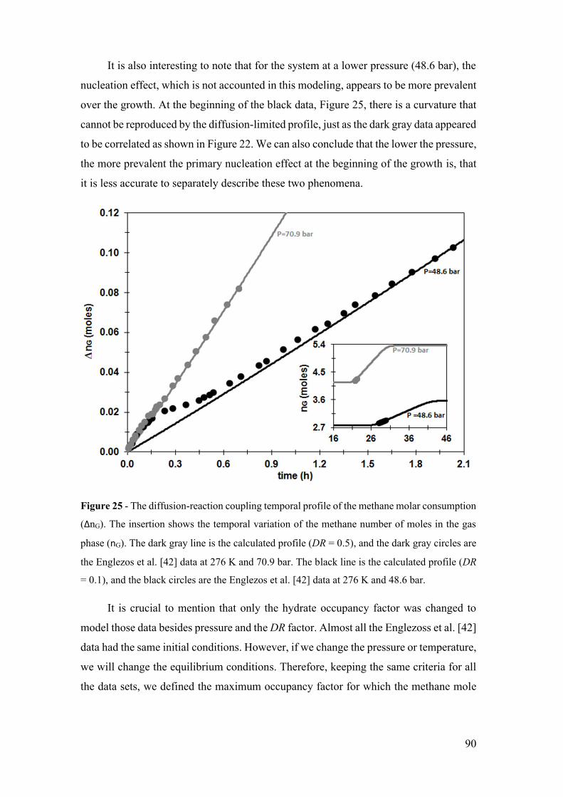
90
It is also interesting to note that for the system at a lower pressure (48.6 bar), the
nucleation effect, which is not accounted in this modeling, appears to be more prevalent
over the growth. At the beginning of the black data, Figure 25, there is a curvature that
cannot be reproduced by the diffusion-limited profile, just as the dark gray data appeared
to be correlated as shown in Figure 22. We can also conclude that the lower the pressure,
the more prevalent the primary nucleation effect at the beginning of the growth is, that
it is less accurate to separately describe these two phenomena.
Figure 25 - The diffusion-reaction coupling temporal profile of the methane molar consumption
(ΔnG). The insertion shows the temporal variation of the methane number of moles in the gas
phase (nG). The dark gray line is the calculated profile (DR = 0.5), and the dark gray circles are
the Englezos et al. [42] data at 276 K and 70.9 bar. The black line is the calculated profile (DR
= 0.1), and the black circles are the Englezos et al. [42] data at 276 K and 48.6 bar.
It is crucial to mention that only the hydrate occupancy factor was changed to
model those data besides pressure and the DR factor. Almost all the Englezoss et al. [42]
data had the same initial conditions. However, if we change the pressure or temperature,
we will change the equilibrium conditions. Therefore, keeping the same criteria for all
the data sets, we defined the maximum occupancy factor for which the methane mole
91
fraction in the bulk liquid phase uses the entire delta between the composition interfaces.
For 48.6 bar and 276 K it was 56%.
We can conclude that if we increase the pressure, we accelerated the hydrate
growth, changing the growth rate inclination and reducing the time to start the growth,
as seen in Figure 25 insertion. Then, less limited by diffusion is the growth, i.e., more
coupled are diffusion and reaction, and more separated can be modeled the nucleation
and growth phenomena.
4.3.4 Temperature effect
In the same way that we evaluated the effect of pressure, we evaluated the effect
of temperature on the DR factor and the possibility of modeling the nucleation and
growth phenomena separately. Among the data obtained by Englezos et al. (1987) [42]
we did not find data at the same pressure, so we compared two data sets at close
pressures (70.9 and 76 bar) and different temperatures (276 K and 274 K).
Figure 26 shows the temporal profile of the methane molar consumption for 276
K (70.9 bar), dark gray, and 274 K (76.0 bar), light gray. Considering that the increase
in the pressure increases the DR factor and accelerates the beginning of the growth, we
can say that the decrease of the temperature only slows down the beginning of the
growth. It slightly effects the DR factor or compensates part of the increase by the
pressure, as it changes little with the variation in the temperature. The DR factor adjusted
to get the best correlation between the experimental data and the model for the lower
temperature set is the same as the high-temperature data, DR =0.6, because the increase
of the pressure compensates the reduction of the temperature.
The decrease of the temperature slows down the growth beginning, and the same
logic can understand that the increase in pressure accelerates the growth beginning, as
seen in Figure 26 insertion. With the increase in the pressure, the arrival of methane
molecules at the liquid-hydrate interface accelerates. The reduction in temperature
makes it difficult for methane to reach the interface where the reaction occurs.
However, since the hydrate formation condition is favorable, the higher the
hydrate growth rate inclination, i.e., the faster this particle growth. The equation of the
diffusion coefficient, LD, described in the topic 2.2, depends on the temperature, but
when the DR factor is adjusted, the system will automatically calculate a new value of

92
the reaction constant, Lrr, for which its relation with this new LD follows the same
proportion.
At the beginning of the growth, the data set at 274 K and 76.0 bar also reproduce
the same behavior as the other sets showing some curvature, Figure 26. For this case,
data can be described by the limited by diffusion as the data set at 276 and 70.6 bar,
Figure 22. The limiting by diffusion profile for the system at 274 K and 76.0 bar is in
the Appendix 3. So, we can say that the temperature does not affect the possibility of
modeling the growth separately from the nucleation; however, we know that future
improvement, as the addition of a nucleation model in the DAE system proposed in this
work, could improve the adjustment of this growth beginning.
Figure 26 - The diffusion-reaction coupling temporal profile of the methane molar consumption
(ΔnG). The insertion shows the temporal variation of the methane number of moles in the gas
phase (nG). The dark gray line is the calculated profile (DR = 0.5), and the dark gray circles are
the Englezos et al. [42] data at 276 K and 70.9 bar. The light gray line is the calculated profile
(DR = 0.6), and the light gray circles are the Englezos et al. [42] data at 274 K and 76.0 bar.
To keep the same criteria, we defined the maximum occupancy factor as 68% for
76.0 bar and 274 K, for which the methane mole fraction in the bulk liquid phase used
the entire delta between the composition of the G-L and L-H interfaces. Note that is

93
higher than in the system at 276 K and 48.6 bar, but lower than in the system at 276 K
and 70.9 bar. It occurs because, even if the decrease in the temperature and increase in
the pressure facilitated the hydrate formation, the reduction in the temperature and
pressure also decrease the methane solubility in the liquid phase, so even more favorable
the 76.0 bar and 274 K system will contain a hydrate with less methane in the structure
than the system with 276 K and 70.9 bar.
We can conclude that the effect of temperature on the DR factor and the separation
of the nucleation and growth to model the formation is of little significance than the
pressure effect. Temperature basically only increases the start of the growth time, since
the temperature reduction slows down the molecules’ movement.
4.4 Partial conclusions
The model proposed in this work allows the evaluating the coupling between the
diffusion and reaction phenomena in the hydrate growth. The definition of a coupling
factor, DR, makes it unnecessary to estimate a constant reaction for each system as in
most growth models in the literature [33,42–44,84–87,95,96]. The DR factor has a scale
of 0.0 to 1.0 and can represent both conditions of limiting diffusion or limiting reaction
and the coupling between them using a single growth rate. Therefore, to adequately
describe different sets of experimental data, it is only necessary to adjust the DR factor
that best represents the data. We also note that this DR factor is mainly related to the
system pressure. The higher the system pressure, the lower the limiting diffusion effect,
and the more coupled is the diffusion and reaction. In contrast, the temperature has little
influence on DR factor. Besides, the pressure and temperature influence the time for the
beginning of the growth.
Another significant contribution here is in the terms of the driving force. It was
shown that for systems without chemical additives, with a liquid phase close to ideality,
there are driving forces in the literature that account for the host molecule effect, such
as CH4. However, these models cannot provide satisfactory results for non-ideal systems
and additive effects.
The proposed model can adequately model experimental hydrate formation data,
measuring methane consumption in the vapor phase at constant temperature and
pressure. Besides, the inclusion of the thermodynamic factor in the driving force and
thermodynamic modeling, which is already more consolidated than the dynamics in the

94
literature, allows us to understand how to describe more complete systems. Here, we
provide a growth model capable of describing simple systems (gas and water) at low
pressures, limited by diffusion, and more complex systems (gas, water, and chemical
additive) at high pressures, with diffusion and reaction coupled.
List of symbols
T - Temperature [K]
P - Pressure [bar]
R - Universal gas constant [J mol / K]
- Stoichiometric coefficient for CH4
- Stoichiometric coefficient for H2O
H - Hydrate
t - Time [h]
Gb - Free Gibbs energy [J / mol]
ԑ - Extent of reaction [mol]
ν - Stoichiometric coefficient
μ - Chemical potencial [J / mol]
A - Affinity
ɑ - Activity
- Density [mol / m³]
c - concentration [mol / m³]
M - Molar mass [g / mol]
S - Entropy [J / K]
S - Entropy generation [J / K s]
Jr - Reaction flow [mol / m² s]
G - Growth rate [mol/ s]
Asup - Surface area [m²]

95
δ - Liquid film thickness [m]
Nc - Number of compounds
Lrr - Reaction coefficient [mol2 K / m2 J s]
L’i - Diffusion coefficient for the component i [m² / s]
LD- Diffusion coefficient [mol / m s]
K - Activity product weighted by Stoichiometric coefficient
n - Number of moles [mol]
V - Volume [m³]
x - Mole fraction
μ’i - Moment of order i [mi / m3]
DR - Coupling factor
υ - Dynamic viscosity [mol / m s]
eq - Equilibrium condition
b - Bulk condition
L - Liquid phase
G - Gas phase
H - Hydrate phase
0- Reference
96
Chapter 5. Hydrate growth in an
inhibited system Gas hydrates can lead to blockages in natural gas offshore production. Among the
conventional methods for hydrates inhibition, there is the prevention of blockage
occurrence through thermodynamic hydrate inhibitors (THI). Although there are
consolidated operating procedures to avoid these blockages, its limitations are well-
known. As ethanol is abundant in Brazil and works as a THI, its use is becoming more
common. Besides the thermodynamic effect, it is experimentally known that the hydrate
inhibitor species alter the hydrate formation dynamics. Therefore, it is necessary to
understand such effects, to enable better usage of those chemicals. Here, we propose a
new model to simulate the hydrate growth kinetics with chemical affinity as a driving
force. The use of the Prigogine affinity allows the inclusion of the thermodynamic factor
in the growth. With this model based on non-equilibrium thermodynamics, we can better
understand the role of the THI on the hydrate growth. We evaluated the CH4 hydrate
growth with ethanol as a THI and concluded that the ethanol delays the hydrate growth
beginning, acting as a kinetic hydrate inhibitor, and reduces the amount of hydrate
formed, acting as a THI. The inclusion of the water activity in the driving force is key
to better understanding the kinetic inhibitor effect of ethanol.

97
5.1 Introduction
Gas hydrates are crystalline structures formed at low temperatures and high
pressures, in systems containing water and guest molecules [4]. These guest molecules
are usually light gases, mainly natural gas components, such as methane [219]. The
hydrophobic effect causes the ordering of water molecules forming structured cavities
by hydrogen bonds interaction, and the guest molecules are trapped inside the water
hydrogen-bond framework by van der Waals forces [2].
Offshore oil and gas productions present favorable conditions for hydrate
formation. In these systems, the formation of hydrates can lead to blockages along the
flowline. Conventional methods of hydrate preventions include physical and chemical
interventions. Limited physical options are available to prevent gas hydrate formation,
and, in most cases, the techniques are neither applicable nor economical [196]. The
conventional methods of chemical hydrate inhibition are the addition of thermodynamic
(THI) and low-dosage (LDHI) hydrate inhibitors [14]. Among the LDHI, there are the
kinetic hydrate inhibitors (KHI), that delay the formation of the crystals (increase the
hydrate induction time), and the anti-agglomerate (AA), which prevent blockages
formation through the formation of a suspension of the solid phase in the liquid phase
[1,2,13]. Therefore, it is necessary to understand the thermodynamic effects of hydrate
formation in the presence of chemical additives and the kinetic effect of the THIs and
LDHIs on hydrate formation to guarantee the efficiency of their use as hydrate blockage
prevention methods [15]. We focus on understanding the thermodynamic hydrate
inhibitors (THIs) in the hydrate growth in this work.
The chemicals, THIs, are usually organic additives, mainly alcohols and glycols.
The presence of inhibitors usually reduces water activity in the aqueous phase, which
shifts hydrate phase boundaries without participation in the hydrate crystalline structure
[16]. Significant portions of the oil reserves in Brazil are located in deep or ultra-deep
waters, in which the oil production occurs at high pressures and low temperatures,
suitable conditions for the formation of hydrates. In this scenario, flow assurance actions
are crucial production factors, especially for large natural gas production scenarios, such
as exploring the pre-salt layer [163]. Therefore, to ensure production is free of hydrates
in those scenarios, larger amounts of the thermodynamic inhibitors are required to shift
the hydrate equilibrium curve [17].

98
A thermodynamic hydrate inhibitor's desired properties include miscibility in
water, efficient recovery, and stability [164]. Based on these criteria, the most common
industrial THIs are methanol (MeOH), ethanol (EtOH), and monoethylene glycol
(MEG) [165]. Brazil is one of the largest ethanol producers, so its use is cheaper than
methanol or MEG for the Brazilian oil and gas production scenarios. For this reason,
the use of ethanol as a THI is increasingly more frequent. However, the literature
presents a few modeling hydrate equilibrium studies with ethanol [120] and even fewer
dynamic modeling and experimental studies for this system [196,220]. Thus, there is
still a lack of information to better understand the hydrate formation in ethanol systems
as THI. Mainly because experimental studies of the hydrate growth with ethanol have
showed that ethanol can also act as a kinetic hydrate inhibitor, that has not yet been
modeled [220].
The review of advances in modeling phase equilibrium with hydrates shows that
this development mainly improved details in the van der Waals and Platteeuw model
and is consolidated [98]. However, we still need improvements in the hydrate
equilibrium calculations, mainly for systems with additives [120]. Many experimental
data and proposed models have been reported for gas hydrates equilibrium conditions
in the presence of methanol, but for hydrate equilibria in other alcohols, like ethanol, it
is limited, especially for highly concentrated solutions [166]. Recently, we studied in
the work of Oliveira et al. [207] hydrate systems with ethanol as an inhibitor and we got
a set of experimental data in a broad range of ethanol concentration, up to 45 wt%. In
the same work, we proposed thermodynamic modeling that shown better accuracy for
the equilibrium condition for systems up to 15 wt% of EtOH [124]. The reduction in the
performance of the modeling at high ethanol concentrations can be understood because
ethanol can be a hydrate co-host trapped in the large cages of the hydrate structure II
with methane [8,27,124]. However, some questions still need to be answered for hydrate
systems with ethanol at high concentrations. Meanwhile, the dynamic modeling still
presents a large gap in the literature, even for low ethanol concentrations [19].
According to Yin et al. [15], who reviewed the gas hydrate growth kinetic models,
there is still a gap in the understanding of the gas hydrate growth control mechanism,
which is further augmented by the dynamic behavior of multiphase fluids flow, the
thermodynamics of the hydrate-forming system, and the compounding interfacial
phenomena. In the literature, most of the hydrate growth models are based on the guest

99
molecule behavior only and cannot describe non-ideal systems [33,42–44,84–87,95,96].
The ones that include water or some additive effect do not account for the interaction
between those compounds [80,83,204,205]. Nasir et al. [13], who reviewed
conventional and novel additives used to promote or inhibit hydrate formation in
different chemical processes, said that we still have challenges and need further
development to understand better the promoter/inhibitor hydrate role in the industry.
Therefore, there is still a need for a model capable of explaining the non-ideality effects
in the hydrate formation "reaction" for systems with additives is still required.
The Prigogine chemical affinity allows the evaluation of all the components
involved in the hydrate formation and evaluates the growth accounting for non-ideal
effects. The affinity is already used in the literature [88–90]. However, most models that
use this property adopted simplifications that result in the number of mols as the driving
force, without including the thermodynamic factor [89,90]. In our previous work
(Chapter 4), we proposed a model to describe the hydrate growth keeping the activity
of the components in the chemical affinity, i.e., including the thermodynamic factor in
the driving force in order to describe non-ideal systems.
The objective here is to apply the hydrate growth model based on the non-
equilibrium thermodynamics proposed previously to describe CH4 hydrate growth with
EtOH as an inhibitor. We compared the CH4 hydrate growth system with and without
the ethanol addition. Besides, the effect of increasing the concentration of ethanol
comparing systems with 5, 10, and 15 wt% of EtOH was also evaluated at different
temperatures and pressures. The effect of including the water activity on the growth
driving force and not only the guest molecule was studied [15,33,84,85,93].
5.2 Kinetic model
The dynamic model proposed previously (Chapter 4), used proper balances and
the reaction rate with the Prigogine chemical affinity driving force that accounts for the
non-ideal effect. In addition to the differential-algebraic equations, thermodynamic
models were used [124] to calculate the equilibrium conditions and thermodynamic
properties (Appendix 4). The simulated hydrate formation systems are based on the
experimental apparatus of the work of Englezos et al. [42]. It is a high-pressure reactor
with a mechanical stirrer contain methane (CH4), water (H2O), and ethanol (EtOH). The
gas phase is pure methane.
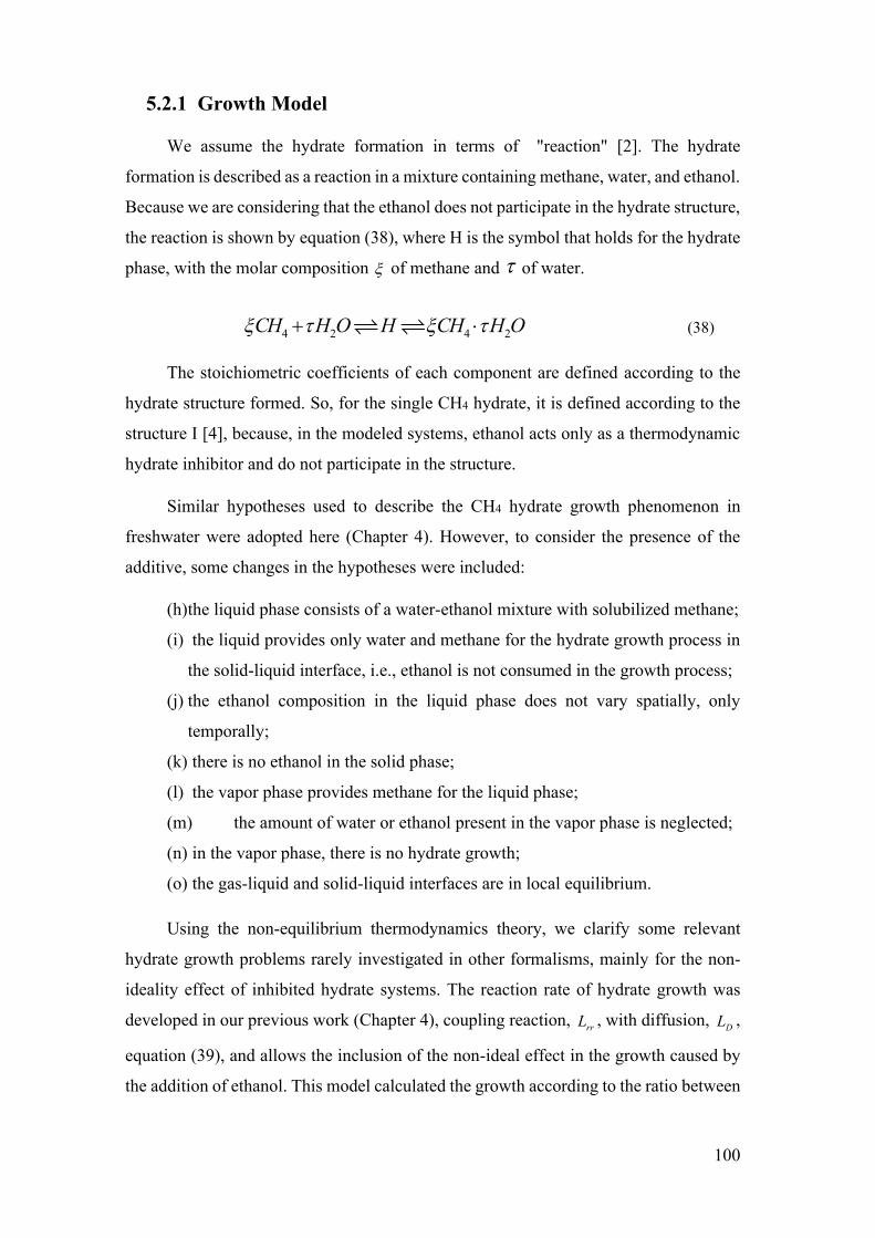
100
5.2.1 Growth Model
We assume the hydrate formation in terms of "reaction" [2]. The hydrate
formation is described as a reaction in a mixture containing methane, water, and ethanol.
Because we are considering that the ethanol does not participate in the hydrate structure,
the reaction is shown by equation (38), where H is the symbol that holds for the hydrate
phase, with the molar composition of methane and of water.
4 2 4 2CH H O H CH H O (38)
The stoichiometric coefficients of each component are defined according to the
hydrate structure formed. So, for the single CH4 hydrate, it is defined according to the
structure I [4], because, in the modeled systems, ethanol acts only as a thermodynamic
hydrate inhibitor and do not participate in the structure.
Similar hypotheses used to describe the CH4 hydrate growth phenomenon in
freshwater were adopted here (Chapter 4). However, to consider the presence of the
additive, some changes in the hypotheses were included:
(h) the liquid phase consists of a water-ethanol mixture with solubilized methane;
(i) the liquid provides only water and methane for the hydrate growth process in
the solid-liquid interface, i.e., ethanol is not consumed in the growth process;
(j) the ethanol composition in the liquid phase does not vary spatially, only
temporally;
(k) there is no ethanol in the solid phase;
(l) the vapor phase provides methane for the liquid phase;
(m) the amount of water or ethanol present in the vapor phase is neglected;
(n) in the vapor phase, there is no hydrate growth;
(o) the gas-liquid and solid-liquid interfaces are in local equilibrium.
Using the non-equilibrium thermodynamics theory, we clarify some relevant
hydrate growth problems rarely investigated in other formalisms, mainly for the non-
ideality effect of inhibited hydrate systems. The reaction rate of hydrate growth was
developed in our previous work (Chapter 4), coupling reaction, rrL , with diffusion, DL ,
equation (39), and allows the inclusion of the non-ideal effect in the growth caused by
the addition of ethanol. This model calculated the growth according to the ratio between
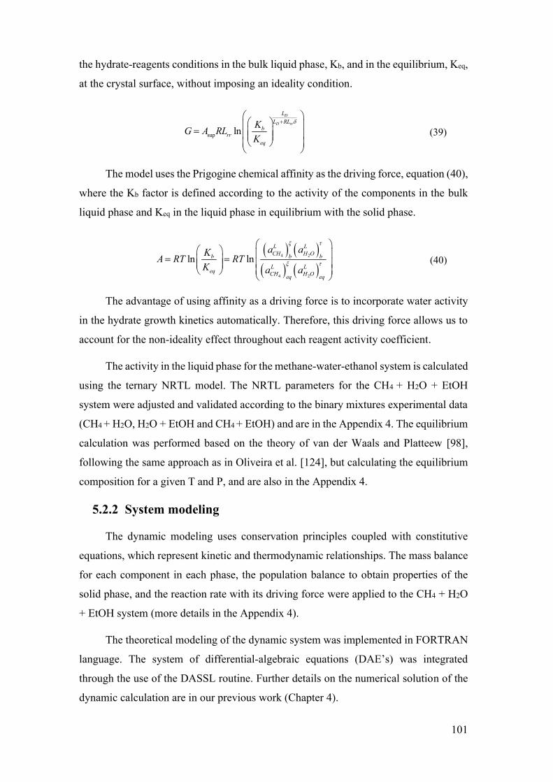
101
the hydrate-reagents conditions in the bulk liquid phase, Kb, and in the equilibrium, Keq,
at the crystal surface, without imposing an ideality condition.
sup ln
D
D rr
LL RL
brr
eq
KG A RLK
(39)
The model uses the Prigogine chemical affinity as the driving force, equation (40),
where the Kb factor is defined according to the activity of the components in the bulk
liquid phase and Keq in the liquid phase in equilibrium with the solid phase.
4 2
4 2
ln lnL LCH H Ob b b
L Leq CH H Oeq eq
a aKA RT RTK a a
(40)
The advantage of using affinity as a driving force is to incorporate water activity
in the hydrate growth kinetics automatically. Therefore, this driving force allows us to
account for the non-ideality effect throughout each reagent activity coefficient.
The activity in the liquid phase for the methane-water-ethanol system is calculated
using the ternary NRTL model. The NRTL parameters for the CH4 + H2O + EtOH
system were adjusted and validated according to the binary mixtures experimental data
(CH4 + H2O, H2O + EtOH and CH4 + EtOH) and are in the Appendix 4. The equilibrium
calculation was performed based on the theory of van der Waals and Platteew [98],
following the same approach as in Oliveira et al. [124], but calculating the equilibrium
composition for a given T and P, and are also in the Appendix 4.
5.2.2 System modeling
The dynamic modeling uses conservation principles coupled with constitutive
equations, which represent kinetic and thermodynamic relationships. The mass balance
for each component in each phase, the population balance to obtain properties of the
solid phase, and the reaction rate with its driving force were applied to the CH4 + H2O
+ EtOH system (more details in the Appendix 4).
The theoretical modeling of the dynamic system was implemented in FORTRAN
language. The system of differential-algebraic equations (DAE’s) was integrated
through the use of the DASSL routine. Further details on the numerical solution of the
dynamic calculation are in our previous work (Chapter 4).
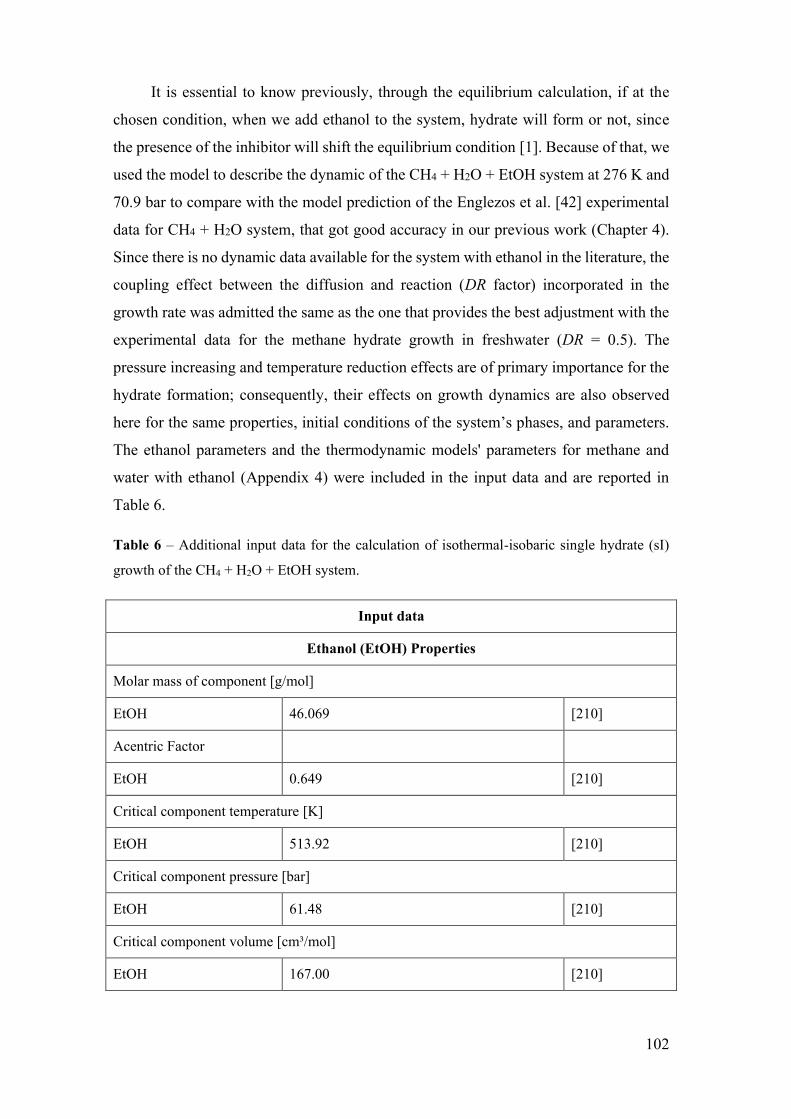
102
It is essential to know previously, through the equilibrium calculation, if at the
chosen condition, when we add ethanol to the system, hydrate will form or not, since
the presence of the inhibitor will shift the equilibrium condition [1]. Because of that, we
used the model to describe the dynamic of the CH4 + H2O + EtOH system at 276 K and
70.9 bar to compare with the model prediction of the Englezos et al. [42] experimental
data for CH4 + H2O system, that got good accuracy in our previous work (Chapter 4).
Since there is no dynamic data available for the system with ethanol in the literature, the
coupling effect between the diffusion and reaction (DR factor) incorporated in the
growth rate was admitted the same as the one that provides the best adjustment with the
experimental data for the methane hydrate growth in freshwater (DR = 0.5). The
pressure increasing and temperature reduction effects are of primary importance for the
hydrate formation; consequently, their effects on growth dynamics are also observed
here for the same properties, initial conditions of the system’s phases, and parameters.
The ethanol parameters and the thermodynamic models' parameters for methane and
water with ethanol (Appendix 4) were included in the input data and are reported in
Table 6.
Table 6 – Additional input data for the calculation of isothermal-isobaric single hydrate (sI)
growth of the CH4 + H2O + EtOH system.
Input data
Ethanol (EtOH) Properties
Molar mass of component [g/mol]
EtOH 46.069 [210]
Acentric Factor
EtOH 0.649 [210]
Critical component temperature [K]
EtOH 513.92 [210]
Critical component pressure [bar]
EtOH 61.48 [210]
Critical component volume [cm³/mol]
EtOH 167.00 [210]
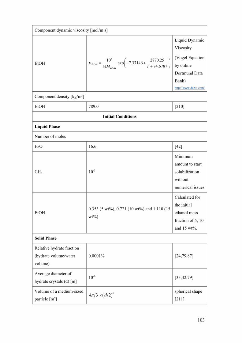
103
Component dynamic viscosity [mol/m s]
EtOH 310 2770.25exp 7.37146
74.6787EtOHEtOHMM T
Liquid Dynamic
Viscosity
(Vogel Equation
by online
Dortmund Data
Bank) http://www.ddbst.com/
Component density [kg/m³]
EtOH 789.0 [210]
Initial Conditions
Liquid Phase
Number of moles
H2O 16.6 [42]
CH4 10-5
Minimum
amount to start
solubilization
without
numerical issues
EtOH 0.353 (5 wt%), 0.721 (10 wt%) and 1.110 (15
wt%)
Calculated for
the initial
ethanol mass
fraction of 5, 10
and 15 wt%.
Solid Phase
Relative hydrate fraction
(hydrate volume/water
volume)
0.0001% [24,79,87]
Average diameter of
hydrate crystals (d) [m] 10-6 [33,42,79]
Volume of a medium-sized
particle [m³] 34 3 2d
spherical shape
[211]
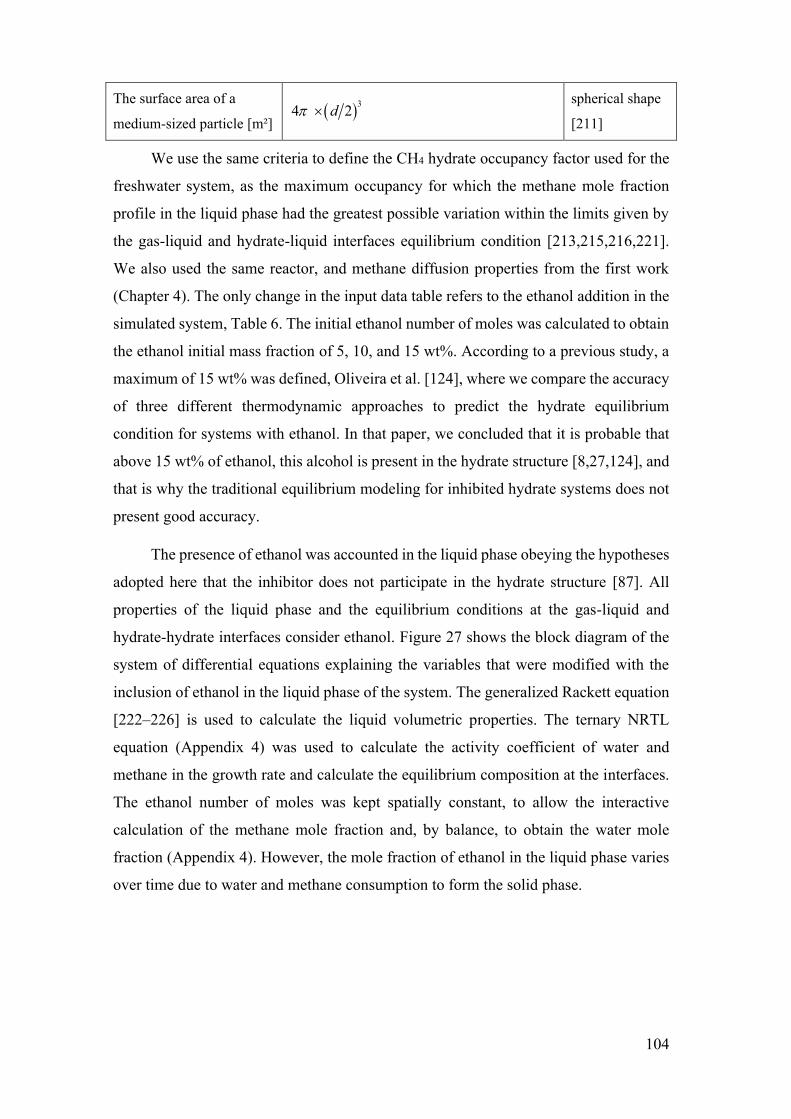
104
The surface area of a
medium-sized particle [m²] 34 2d
spherical shape
[211]
We use the same criteria to define the CH4 hydrate occupancy factor used for the
freshwater system, as the maximum occupancy for which the methane mole fraction
profile in the liquid phase had the greatest possible variation within the limits given by
the gas-liquid and hydrate-liquid interfaces equilibrium condition [213,215,216,221].
We also used the same reactor, and methane diffusion properties from the first work
(Chapter 4). The only change in the input data table refers to the ethanol addition in the
simulated system, Table 6. The initial ethanol number of moles was calculated to obtain
the ethanol initial mass fraction of 5, 10, and 15 wt%. According to a previous study, a
maximum of 15 wt% was defined, Oliveira et al. [124], where we compare the accuracy
of three different thermodynamic approaches to predict the hydrate equilibrium
condition for systems with ethanol. In that paper, we concluded that it is probable that
above 15 wt% of ethanol, this alcohol is present in the hydrate structure [8,27,124], and
that is why the traditional equilibrium modeling for inhibited hydrate systems does not
present good accuracy.
The presence of ethanol was accounted in the liquid phase obeying the hypotheses
adopted here that the inhibitor does not participate in the hydrate structure [87]. All
properties of the liquid phase and the equilibrium conditions at the gas-liquid and
hydrate-hydrate interfaces consider ethanol. Figure 27 shows the block diagram of the
system of differential equations explaining the variables that were modified with the
inclusion of ethanol in the liquid phase of the system. The generalized Rackett equation
[222–226] is used to calculate the liquid volumetric properties. The ternary NRTL
equation (Appendix 4) was used to calculate the activity coefficient of water and
methane in the growth rate and calculate the equilibrium composition at the interfaces.
The ethanol number of moles was kept spatially constant, to allow the interactive
calculation of the methane mole fraction and, by balance, to obtain the water mole
fraction (Appendix 4). However, the mole fraction of ethanol in the liquid phase varies
over time due to water and methane consumption to form the solid phase.
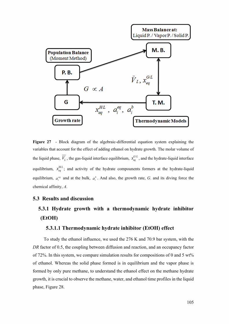
105
Figure 27 - Block diagram of the algebraic-differential equation system explaining the
variables that account for the effect of adding ethanol on hydrate growth. The molar volume of
the liquid phase, LV , the gas-liquid interface equilibrium, /G Leqx , and the hydrate-liquid interface
equilibrium, H/Leqx ; and activity of the hydrate compounents formers at the hydrate-liquid
equilibrium, eqia and at the bulk, b
ia . And also, the growth rate, G. and its diving force the
chemical affinity, A.
5.3 Results and discussion
5.3.1 Hydrate growth with a thermodynamic hydrate inhibitor
(EtOH)
5.3.1.1 Thermodynamic hydrate inhibitor (EtOH) effect
To study the ethanol influence, we used the 276 K and 70.9 bar system, with the
DR factor of 0.5, the coupling between diffusion and reaction, and an occupancy factor
of 72%. In this system, we compare simulation results for compositions of 0 and 5 wt%
of ethanol. Whereas the solid phase formed is in equilibrium and the vapor phase is
formed by only pure methane, to understand the ethanol effect on the methane hydrate
growth, it is crucial to observe the methane, water, and ethanol time profiles in the liquid
phase, Figure 28.

106
Figure 28 (a), the ethanol addition increases the methane solubilization in the
liquid phase in the first 2 hours. The CH4 composition in the liquid phase changes
slightly in the system without ethanol, from 0 wt% to the maximum of 0.214 wt% or
0.04 moles, Figure 28 (a) insertion on the left, as the CH4 has low solubility in water. In
the system with ethanol, the compositions change more along with the growth. The CH4
composition changes from 0 wt% to a maximum of 0.477 wt% during the first 2 hours,
related to the time for solubilization. It occurs because the CH4 solubility increases with
the addition of ethanol. We can also notice that the ethanol addition shifts the beginning
of the growth. Moreover, the growth finished when all water and almost all methane are
consumed for the system without ethanol as can be observed at 30h, approximately.
With ethanol, the growth finished nearly to 25h, before the hydrate reagents are
consumed.
Following the methane mass fraction (xL,CH4) profile, in Figure 28 (b) right
insertion, we can understand why the growth finished before the reagents ended in the
system with ethanol. During the growth, the methane mass fraction for the freshwater
system (dotted line) in the gas-liquid equilibrium interface and the hydrate-liquid
equilibrium interface are kept constant, Figure 28 (b) right insertion, so the growth keeps
going until all the water is consumed, Figure 28 (a) right insertion, because the methane
feed in the gas phase is maintained to keep the pressure constant. Meanwhile, for ethanol
systems (continuous line), the methane mass fraction in the gas-liquid and hydrate-
liquid equilibrium interfaces varies during the growth, Figure 28 (b) right insertion. It
occurs because, with the water, Figure 28 (a) right insertion, and methane consumption,
Figure 28 (a), for the solid-phase formation, the liquid phase becomes more concentrated
in ethanol, from 5 wt% to 22 wt% of EtOH, gray line in Figure 28 (b). Then, the bulk
liquid phase CH4 composition is changing until it matches the composition of the
hydrate-liquid equilibrium interface, Figure 28 (b) right insertion, changing with the
growth. So, the equilibrium condition of the system is achieved before the hydrate
reagents formers ended.

107
Figure 28 - (a) The number of moles of methane (nL,CH4) and (b) the H2O (xL,H2O) and EtOH
(xL,EtOH, in gray) mass fractions in the bulk liquid phase temporal profiles at 276 K and 70.9
bar (DR = 0.5). The lines describe the time profiles for the following ethanol compositions of
the initial liquid phase: 0 wt% (dotted line) and 5 wt% (continuous line) of EtOH. The insertion
(a) in the left shows the methane in water saturation profile and the one in the right shows the
number of moles of water (nL,H2O) profile in the bulk liquid phase. The insertion (b) in the left
is a zoom in the H2O mass fraction temporal profile for 0 wt% of EtOH, and the one in the right
is the methane mass fraction (xL,CH4) profile in the bulk liquid phase (continuous black lines),
in the gas-liquid equilibrium (GLE) interface (continuous gray line) and in the hydrate-liquid
equilibrium (HLE) interface (gray dotted-dashed line).
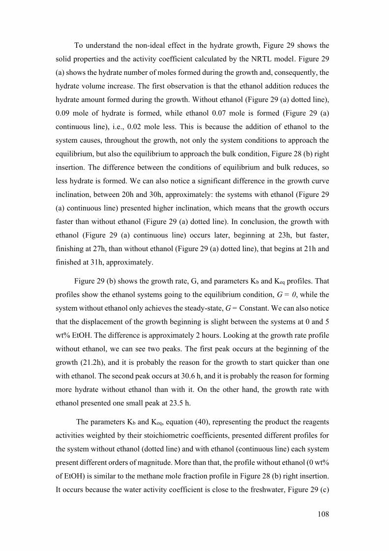
108
To understand the non-ideal effect in the hydrate growth, Figure 29 shows the
solid properties and the activity coefficient calculated by the NRTL model. Figure 29
(a) shows the hydrate number of moles formed during the growth and, consequently, the
hydrate volume increase. The first observation is that the ethanol addition reduces the
hydrate amount formed during the growth. Without ethanol (Figure 29 (a) dotted line),
0.09 mole of hydrate is formed, while ethanol 0.07 mole is formed (Figure 29 (a)
continuous line), i.e., 0.02 mole less. This is because the addition of ethanol to the
system causes, throughout the growth, not only the system conditions to approach the
equilibrium, but also the equilibrium to approach the bulk condition, Figure 28 (b) right
insertion. The difference between the conditions of equilibrium and bulk reduces, so
less hydrate is formed. We can also notice a significant difference in the growth curve
inclination, between 20h and 30h, approximately: the systems with ethanol (Figure 29
(a) continuous line) presented higher inclination, which means that the growth occurs
faster than without ethanol (Figure 29 (a) dotted line). In conclusion, the growth with
ethanol (Figure 29 (a) continuous line) occurs later, beginning at 23h, but faster,
finishing at 27h, than without ethanol (Figure 29 (a) dotted line), that begins at 21h and
finished at 31h, approximately.
Figure 29 (b) shows the growth rate, G, and parameters Kb and Keq profiles. That
profiles show the ethanol systems going to the equilibrium condition, G = 0, while the
system without ethanol only achieves the steady-state, G = Constant. We can also notice
that the displacement of the growth beginning is slight between the systems at 0 and 5
wt% EtOH. The difference is approximately 2 hours. Looking at the growth rate profile
without ethanol, we can see two peaks. The first peak occurs at the beginning of the
growth (21.2h), and it is probably the reason for the growth to start quicker than one
with ethanol. The second peak occurs at 30.6 h, and it is probably the reason for forming
more hydrate without ethanol than with it. On the other hand, the growth rate with
ethanol presented one small peak at 23.5 h.
The parameters Kb and Keq, equation (40), representing the product the reagents
activities weighted by their stoichiometric coefficients, presented different profiles for
the system without ethanol (dotted line) and with ethanol (continuous line) each system
present different orders of magnitude. More than that, the profile without ethanol (0 wt%
of EtOH) is similar to the methane mole fraction profile in Figure 28 (b) right insertion.
It occurs because the water activity coefficient is close to the freshwater, Figure 29 (c)
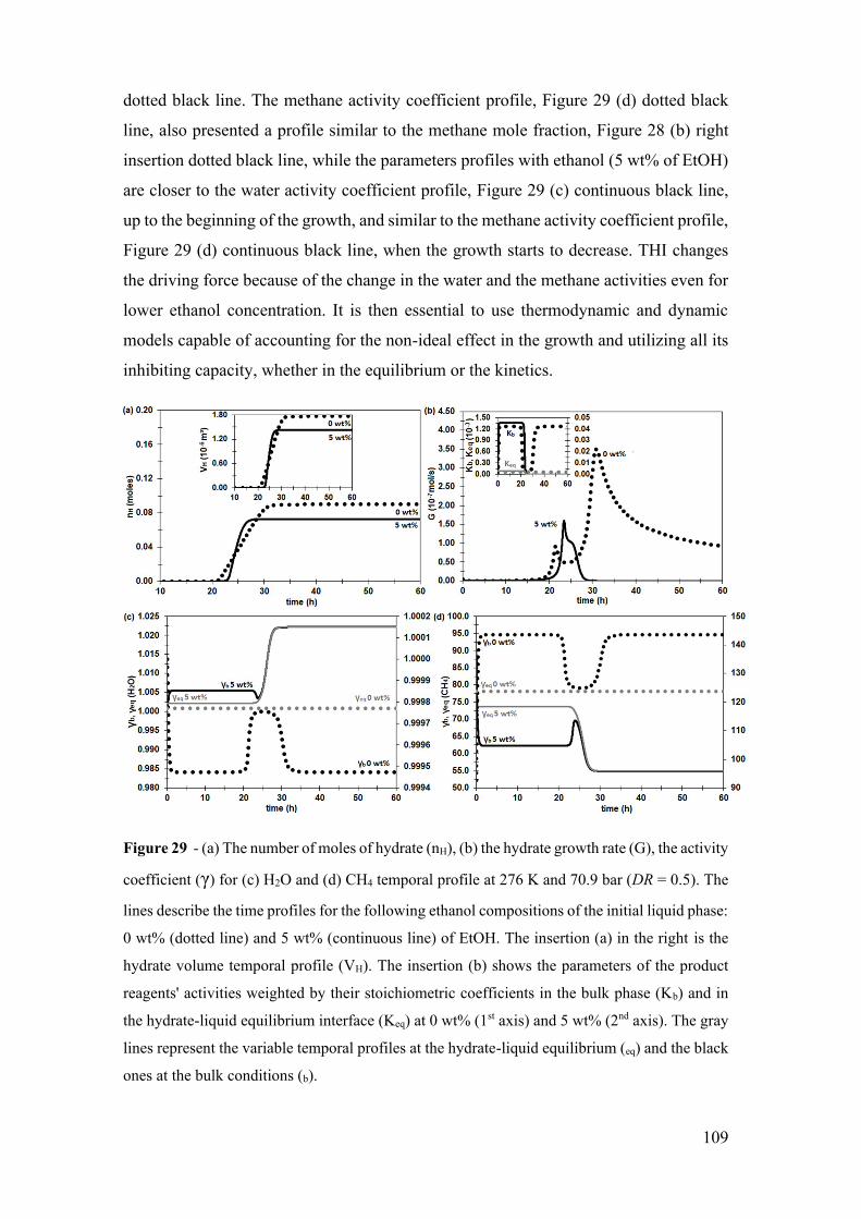
109
dotted black line. The methane activity coefficient profile, Figure 29 (d) dotted black
line, also presented a profile similar to the methane mole fraction, Figure 28 (b) right
insertion dotted black line, while the parameters profiles with ethanol (5 wt% of EtOH)
are closer to the water activity coefficient profile, Figure 29 (c) continuous black line,
up to the beginning of the growth, and similar to the methane activity coefficient profile,
Figure 29 (d) continuous black line, when the growth starts to decrease. THI changes
the driving force because of the change in the water and the methane activities even for
lower ethanol concentration. It is then essential to use thermodynamic and dynamic
models capable of accounting for the non-ideal effect in the growth and utilizing all its
inhibiting capacity, whether in the equilibrium or the kinetics.
Figure 29 - (a) The number of moles of hydrate (nH), (b) the hydrate growth rate (G), the activity
coefficient (γ) for (c) H2O and (d) CH4 temporal profile at 276 K and 70.9 bar (DR = 0.5). The
lines describe the time profiles for the following ethanol compositions of the initial liquid phase:
0 wt% (dotted line) and 5 wt% (continuous line) of EtOH. The insertion (a) in the right is the
hydrate volume temporal profile (VH). The insertion (b) shows the parameters of the product
reagents' activities weighted by their stoichiometric coefficients in the bulk phase (Kb) and in
the hydrate-liquid equilibrium interface (Keq) at 0 wt% (1st axis) and 5 wt% (2nd axis). The gray
lines represent the variable temporal profiles at the hydrate-liquid equilibrium (eq) and the black
ones at the bulk conditions (b).

110
This first evaluation allows us to understand that the THI effect in the hydrate
formation changes the equilibrium condition, but it also changes the growth dynamics.
More than that, the use of a THI will provide not only a thermodynamic inhibitor effect.
It can also act as a kinetic hydrate inhibitor, delaying the start of solid-phase growth, as
some experimental studies have shown [220]. This potential needs to be better
understood and explored to take advantage of the alcohol inhibiting capacity that has
already been used as additives in the oil and gas exploration systems with possible
hydrate formation [163].
5.3.1.2 Thermodynamic inhibitor (EtOH) concentration effect
In deep or ultra-deep waters, oil production presents even more favorable
conditions for the hydrate formation. In this scenario, flow assurance actions are crucial
production factors, especially for large natural gas production scenarios, such as the pre-
salt layer [163]. So, to ensure production is free of hydrates in those scenarios, a larger
amount of thermodynamic hydrate inhibitor is necessary to shift the hydrate equilibrium
curve [17]. An alternative is to use kinetic hydrate inhibitors (KHI). The KHI can delay
nucleation and/or reduce the growth rate [1]. Looking to the increases in THI volume
used to explore those reserves without hydrate blockages and the alternative that is the
use of KHI, we search for the ethanol capacity to act also as a KHI with the increase in
its concentration.
Figure 30 shows the methane, water, and ethanol liquid phase behavior with the
increase in the initial ethanol concentration. We can notice that the CH4 composition,
Figure 30 (a), changes from 0 wt% to a maximum of 0.477 wt%, 0.478 wt%, and 0.480
wt% (0.094, 0.099, 0.105 moles) for 5, 10, and 15 wt% of EtOH, respectively, in the
first 2 hours, that is the solubilization time. For higher ethanol concentration, slightly
more methane can be solubilized in the liquid phase. However, the ethanol composition
change with the water consumption from 5 wt%, 10 wt% or 15 wt% to 22 wt%, Figure
30 (b) grey line, that is the system equilibrium composition at 276 K and 70.9 bar (0.485
wt% of CH4 and 22 wt% of EtOH). Since the system conditions are kept the same, the
equilibrium condition will also be the same. The higher the initial concentration of
ethanol in the system, the faster the system reaches equilibrium because closer to the
equilibrium condition the system is, since the beginning. So, methane and water
consumption during hydrate growth is lower with the increase in the initial ethanol
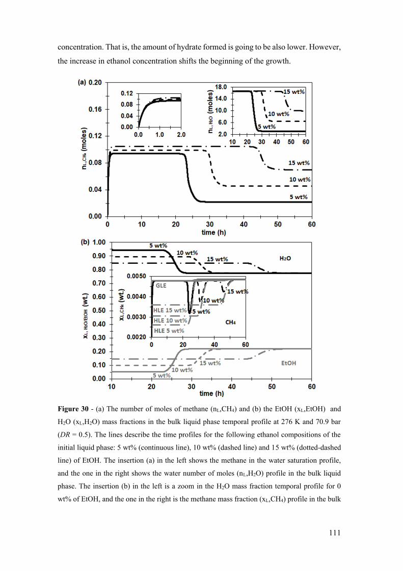
111
concentration. That is, the amount of hydrate formed is going to be also lower. However,
the increase in ethanol concentration shifts the beginning of the growth.
Figure 30 - (a) The number of moles of methane (nL,CH4) and (b) the EtOH (xL,EtOH) and
H2O (xL,H2O) mass fractions in the bulk liquid phase temporal profile at 276 K and 70.9 bar
(DR = 0.5). The lines describe the time profiles for the following ethanol compositions of the
initial liquid phase: 5 wt% (continuous line), 10 wt% (dashed line) and 15 wt% (dotted-dashed
line) of EtOH. The insertion (a) in the left shows the methane in the water saturation profile,
and the one in the right shows the water number of moles (nL,H2O) profile in the bulk liquid
phase. The insertion (b) in the left is a zoom in the H2O mass fraction temporal profile for 0
wt% of EtOH, and the one in the right is the methane mass fraction (xL,CH4) profile in the bulk

112
liquid phase (continuous black lines), in the gas-liquid equilibrium (GLE) interface (continuous
gray line) and the hydrate-liquid equilibrium (HLE) interface (gray dotted-dashed line).
Figure 31 shows the solid properties and the activity coefficient temporal profiles.
The amount of hydrate formed is reduced due to the increase in ethanol concentration,
shown in Figure 31 (a). In the mole base, the amount moles of hydrate formed are 0.07,
0.05, and 0.04 for 5, 10, and 15 wt% of EtOH, respectively, Figure 31 (a). It can also
be seen in the growth rate behavior, Figure 31 (b), the higher is the initial ethanol
concentration, the lower is the peak of growth rate. However, the longer it takes for the
growth to begin. The increase in the ethanol concentration increases the growth
beginning time in 8 and 22 hours, approximately 10 and 15 wt% of EtOH, comparing
the system without ethanol, Figure 31 (b). We can also notice that the higher the
concentration of ethanol, the more the time to start growing, and this increase is getting
bigger. In other words, the performance of ethanol as a kinetic hydrate inhibitor is
enhanced. Parameters Kb and Keq presented similar profiles for all the ethanol initial
concentration systems, but they present different orders of magnitude for each system,
decreasing ethanol concentration, Figure 31 (b) insertions. The same behavior is
observed for the water and methane activity temporal profile, Figure 31 (c), and (d).
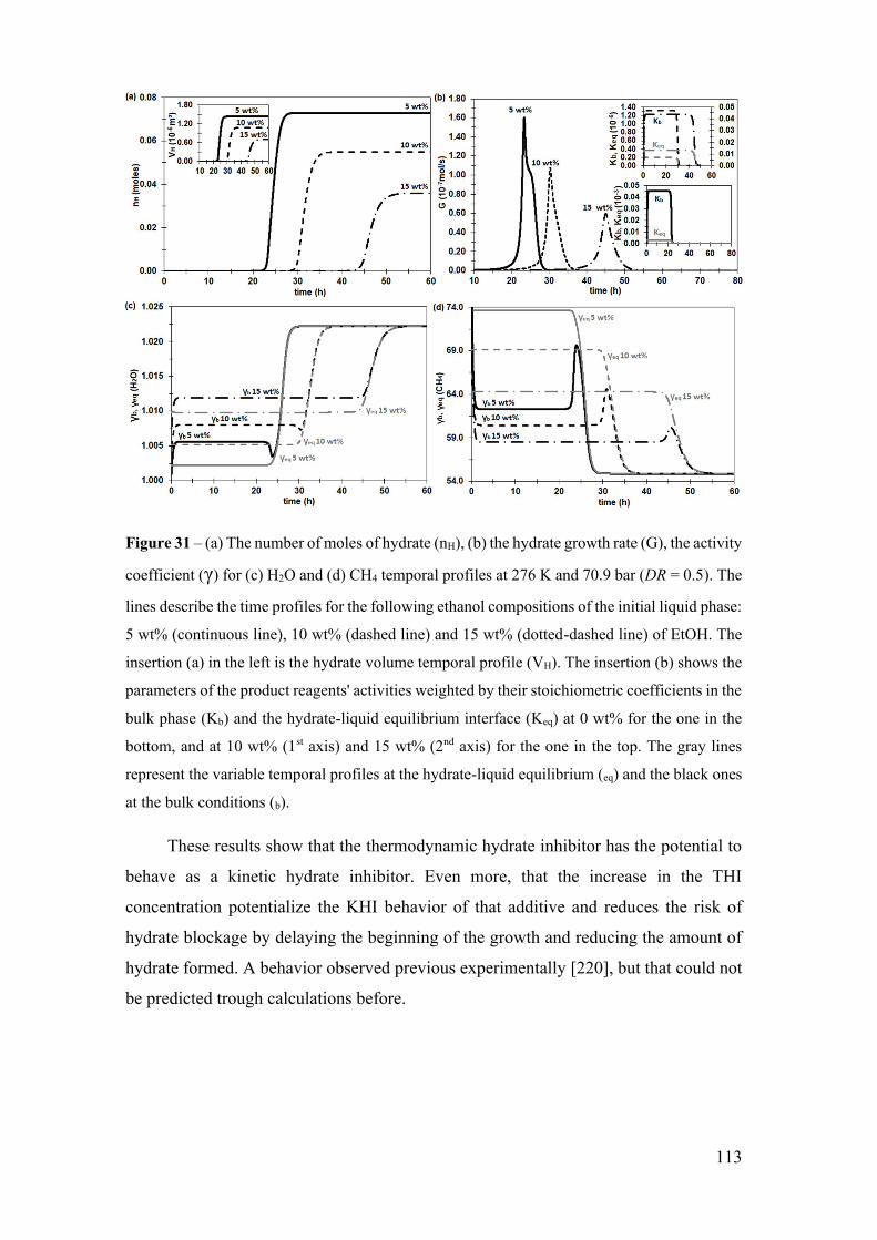
113
Figure 31 – (a) The number of moles of hydrate (nH), (b) the hydrate growth rate (G), the activity
coefficient (γ) for (c) H2O and (d) CH4 temporal profiles at 276 K and 70.9 bar (DR = 0.5). The
lines describe the time profiles for the following ethanol compositions of the initial liquid phase:
5 wt% (continuous line), 10 wt% (dashed line) and 15 wt% (dotted-dashed line) of EtOH. The
insertion (a) in the left is the hydrate volume temporal profile (VH). The insertion (b) shows the
parameters of the product reagents' activities weighted by their stoichiometric coefficients in the
bulk phase (Kb) and the hydrate-liquid equilibrium interface (Keq) at 0 wt% for the one in the
bottom, and at 10 wt% (1st axis) and 15 wt% (2nd axis) for the one in the top. The gray lines
represent the variable temporal profiles at the hydrate-liquid equilibrium (eq) and the black ones
at the bulk conditions (b).
These results show that the thermodynamic hydrate inhibitor has the potential to
behave as a kinetic hydrate inhibitor. Even more, that the increase in the THI
concentration potentialize the KHI behavior of that additive and reduces the risk of
hydrate blockage by delaying the beginning of the growth and reducing the amount of
hydrate formed. A behavior observed previous experimentally [220], but that could not
be predicted trough calculations before.

114
5.3.2 The effect of water activity in the driving force in an inhibited
system
Basically, all the hydrate growth models in the literature use a driving force that
only accounts for the guest molecule properties and does not account for the water effect
directly in the driving force [15]. This occurs because for systems without additives, the
water does not affect the growth rate, as we demonstrated in our previous work using
the proposed model (Chapter 4), because in this condition, the system is close to the
ideality and consequently the water activity is close to one. However, in systems with
additives, the inclusion of the water activity in the driving force affects the dynamics
because the system is no more ideal. Then here, we evaluate how the increasing in the
inhibitor concentration will further distance the system from the ideality.
5.3.2.1 Thermodynamic hydrate inhibitor (EtOH) effect
First, to understand the effect of adding the water activity in the driving force in
the system with ethanol, we compare systems with (black) and without (yellow) water
activity for the ethanol concentration of 0 wt% (dotted) and 5 wt% (continuous).
Figure 32 shows the same qualitative behavior of the system, in the liquid phase,
and the equilibrium conditions, with (black) and without (yellow) the water activity in
the driving force. However, the temporal behavior of the methane number of moles in
the liquid phase presents a displacement of 1.7 hours less in the system without ethanol,
difference between the curves of the methane consumption in the black and yellow
dotted lines, Figure 32 (a) from 21h to 31h, approximately, and 1.3 hours more in the
system with ethanol, difference between the curves of the methane consumption in the
black and yellow continuous lines, Figure 32 (a) from 22h to 30h, approximately. The
growth occurs before but slower in the system without ethanol than with ethanol.
Therefore, the inclusion of the water activity in the driving force changes the kinetic
rate, showing the effect of the THI in the kinetic.

115
Figure 32 - (a) The number of moles of methane (nL,CH4) and (b) the H2O (xL,H2O) and EtOH
(xL,EtOH in gray and light yellow) mass fractions in the bulk liquid phase temporal profiles at
276 K and 70.9 bar (DR = 0.5). The lines describe the time profiles for the following ethanol
compositions of the initial liquid phase: 0 wt% (dotted line) and 5 wt% (continuous line) of
EtOH, with (black or gray) and without (yellow or light yellow) water activity in the driving
force. The insertion (a) in the right shows the number of moles of water (nL,H2O) profile in the
bulk liquid phase. The insertion (b) in the left is a zoom in the H2O mass fraction temporal
profile for 0 wt% of EtOH, and the one in the right is the methane mass fraction (xL,CH4) profile
in the bulk liquid phase (black or yellow continuous lines), in the gas-liquid equilibrium (GLE)

116
interface (gray or light yellow continuous lines) and in the hydrate-liquid equilibrium (HLE)
interface (gray or light yellow dotted-dashed lines).
To better understand why the addition of the water activity in the growth driving
force presented an opposite temporal behavior without (dotted lines) and with ethanol
(continuous lines), Figure 33 shows the solid phase properties, like the growth rate. The
hydrate number of moles formed is kept the same, which means that the inclusion or not
of the water activity does not affect the equilibrium condition, as expected, Figure 33
(a). However, the systems presented the same temporal displacement that was shown
before. It is possible to understand why this displacement occurs, looking to the
parameters of the product reagents' activities weighted by their stoichiometric
coefficients in the bulk phase (Kb) and the hydrate-liquid equilibrium interface (Keq),
equation (40), Figure 33 (b) insertion. In Figure 33 (b), we can see that the growth rate
moves in time, and it happened mainly due to the behavior of parameters Kb and Keq.
As we have seen before, without the water activity in the driving force these parameters
reproduce the temporal behavior of the methane composition in the bulk liquid phase,
Figure 33 (a) right insertion. In contrast, with the water activity in the driving force,
these parameters present a temporal behavior similar to activity coefficients, Figure 33
(c), and (d).
However, if we look at the activity coefficient of water in Figure 33 (c) and (d),
we can see that the addition of ethanol in the liquid phase changes the water activity
coefficient. For the system without ethanol, dotted lines, the water activity coefficient
changes over time for values smaller than one. However, for systems with ethanol,
continuous lines, the water activity coefficient changes over time (slightly for 5 wt% of
ethanol), but values higher than 1.0 are observed. The increase in the water activity
coefficient due to the ethanol addition in the system is why the growth rate to start
decreases, Figure 33 (b). So, it is the non-ideal effect of the system that changes the
beginning of the growth. Moreover, the non-ideal effect of the system is critical to
understand ethanol as a kinetic inhibitor.

117
Figure 33 - (a) The number of moles of hydrate (nH), (b) the hydrate growth rate (G), the activity
coefficient (γ) for (c) H2O and (d) CH4 temporal profiles at 276 K and 70.9 bar (DR = 0.5). The
lines describe the time profiles for the following ethanol compositions of the initial liquid phase:
0 wt% (dotted line) and 5 wt% (continuous line) of EtOH, with (black) and without (yellow)
water activity in the driving force. The insertion (a) in the right is the hydrate volume temporal
profile (VH). The insertion (b) shows the parameters of the product reagents' activities weighted
by their stoichiometric coefficients in the bulk phase (Kb) and in the hydrate-liquid equilibrium
interface (Keq) at 0 wt% (1st axis) and 5 wt% (2nd axis). The gray and light yellow lines represent
the variable temporal profiles at the hydrate-liquid equilibrium (eq) and the black and yellow
ones at the bulk conditions (b).
The inclusion of the non-ideal effect in the driving force through the water activity
coefficient is the main factor in using the kinetic hydrate inhibitor potential of the
thermodynamic hydrate inhibitors.
5.3.2.2 Thermodynamic inhibitor (EtOH) concentration effect
Before that, we concluded that the ethanol kinetic inhibitor effect increases with
the increase in the initial ethanol concentration. Moreover, the addition of the water
activity in the driving force decreases the time to start the growth. To better understand

118
the contribution of water activity, we compare systems with 5, 10, and 15 wt% of EtOH
with and without the water activity in the driving force.
Figure 34 shows the properties of the components in the liquid phase behavior
with (black) and without (yellow) water activity in the driving force. It is shown that the
addition of water activity reduces the kinetic inhibitor behavior of ethanol. The
equilibrium conditions for all component’s concentrations are kept the same, Figure 34
(b); however, the time to start the growth changes for less 1.3 h, 2.1 h, and 3.8 h for 5,
10, and 15 wt%, respectively, Figure 34 (a). So, the increase in ethanol concentration
increases the displacement caused by adding water activity to the driving force. As the
ethanol concentration increases, the addition of the water activity in the driving force
became even more relevant because it reduces the kinetic inhibitor effect that the ethanol
can have in the hydrate growth.

119
Figure 34 - (a) The number of moles of methane (nL,CH4) and (b) the H2O (xL,H2O) and EtOH
(xL,EtOH, in gray and light yellow) mass fractions in the bulk liquid phase temporal profiles at
276 K and 70.9 bar (DR = 0.5). The lines describe the time profiles for the following ethanol
compositions of the initial liquid phase: 5 wt% (continuous line), 10 wt% (dashed line) and 15
wt% (dotted-dashed line) of EtOH, with (black) and without (yellow) water activity in the
driving force. The insertion (a) in the right shows the number of moles of water (nL,H2O) profile
in the bulk liquid phase. The insertion (b) in the right is the methane mass fraction (xL,CH4)
profile in the bulk liquid phase (black and yellow continuous lines), in the gas-liquid equilibrium
(GLE) interface (gray and light yellow continuous lines) and in the hydrate-liquid equilibrium
(HLE) interface (gray and light yellow dotted-dashed lines).
120
Figure 35 shows the solid phase properties and the activity coefficient behavior of
the hydrate reagents. We can understand why the water activity effect of reducing the
ethanol kinetic inhibitor behavior increases with the increase in ethanol concentration.
The hydrate number of moles, Figure 35 (a), and the growth rate, Figure 35 (b),
presented the same time displacement observed before, but the qualitative behavior and
equilibrium conditions are kept the same. It is also possible to see that the inclusion of
the water activity in the driving force changes the behavior of the product reagents'
activities weighted by their stoichiometric coefficients parameters, Kb and Keq, Figure
35 (b) insertions, equation (40). These parameters also reproduce the methane
composition behavior if we do not include the water activity for all the initial ethanol
concentration systems (yellow lines). However, the ethanol concentration increase
changes the water and methane activity coefficients, Figure 35 (c) and (d). We can see
that the increase in the ethanol concentration increases the water activity coefficient for
values each time more distant from the ideality condition, γH2O = 1.0, Figure 35 (c). So,
the water activity coefficient becomes greater with the increase in the system ethanol
concentration. This is the reason why the effect of reducing the ethanol kinetic inhibition
potential becomes more pronounced with the increase in concentration.
Therefore, there is probably an specific concentration point for a thermodynamic
inhibitor to reach its maximum kinetic inhibition effect, as ethanol also presents a
thermodynamic hydrate promoter behavior, participating in the solid structure, in
concentrations greater than 15 wt% [8,27]. In this system, 15 wt% is probably the
concentration with the highest kinetic/thermodynamic inhibition efficiency for the
ethanol without participation in the hydrate structure. However, other thermodynamic
inhibitors, like methanol, which do not have this characteristic, may have an even more
pronounced combined thermodynamic and kinetic inhibition effect at higher
concentrations. It is also worth mentioning that experimental investigations of the
ethanol behavior at higher concentrations are still necessary for better use of its potential
as a thermodynamic or kinetic promoter or inhibitor [8,27,28,124].
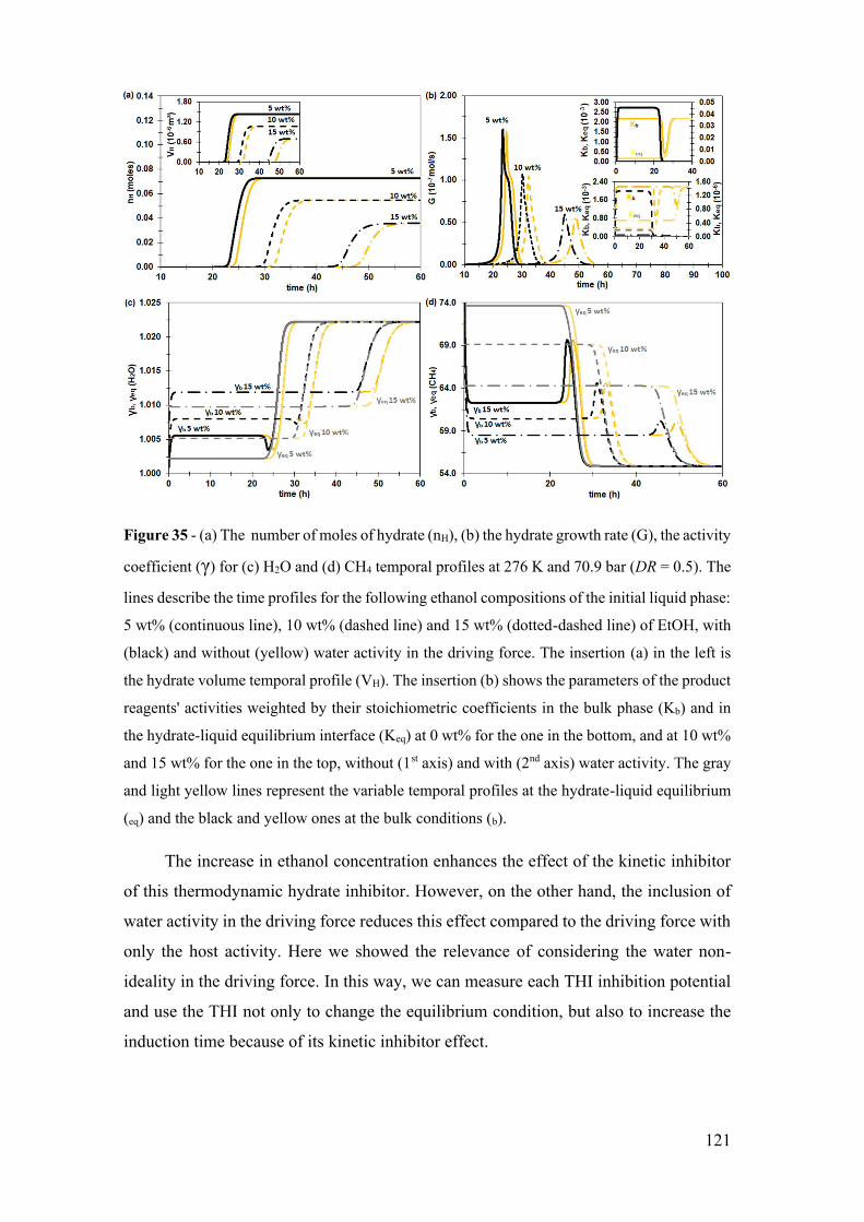
121
Figure 35 - (a) The number of moles of hydrate (nH), (b) the hydrate growth rate (G), the activity
coefficient (γ) for (c) H2O and (d) CH4 temporal profiles at 276 K and 70.9 bar (DR = 0.5). The
lines describe the time profiles for the following ethanol compositions of the initial liquid phase:
5 wt% (continuous line), 10 wt% (dashed line) and 15 wt% (dotted-dashed line) of EtOH, with
(black) and without (yellow) water activity in the driving force. The insertion (a) in the left is
the hydrate volume temporal profile (VH). The insertion (b) shows the parameters of the product
reagents' activities weighted by their stoichiometric coefficients in the bulk phase (Kb) and in
the hydrate-liquid equilibrium interface (Keq) at 0 wt% for the one in the bottom, and at 10 wt%
and 15 wt% for the one in the top, without (1st axis) and with (2nd axis) water activity. The gray
and light yellow lines represent the variable temporal profiles at the hydrate-liquid equilibrium
(eq) and the black and yellow ones at the bulk conditions (b).
The increase in ethanol concentration enhances the effect of the kinetic inhibitor
of this thermodynamic hydrate inhibitor. However, on the other hand, the inclusion of
water activity in the driving force reduces this effect compared to the driving force with
only the host activity. Here we showed the relevance of considering the water non-
ideality in the driving force. In this way, we can measure each THI inhibition potential
and use the THI not only to change the equilibrium condition, but also to increase the
induction time because of its kinetic inhibitor effect.

122
5.3.3 Pressure effect in an inhibited system
We studied a system similar to the one used by Englezos et al. [42] to obtain
hydrate growth experimental data and use the parameters, like the DR factor and the
hydrate occupancy factor adjusted to represent those data better. However, when we
simulate an experimental system adding a thermodynamic hydrate inhibitor, we have to
make sure that the system will form hydrate in that new condition because we know that
the THI will shift the hydrate formation curve to more severe conditions [2]. Because
of that, to make sure that the hydrate will form in all the ethanol concentration range
studied in this work, up to 15 wt%, to evaluate the pressure effect, we increase the
system pressure from 70.9 bar to 74.9 bar, to guarantee that we still are in a hydrate
formation region. For the evaluation, we kept the DR factor equal to 0.5. Furthermore,
we adjusted the hydrate occupancy factor, θ, using the same criteria used before: the
maximum occupancy factor for which the methane mole fraction profile in the liquid
phase had the greatest possible variation within limits given by the gas-liquid and
hydrate-liquid interfaces equilibrium condition [213]. The system at 276 K and 70.9 bar
was θ = 72%, while for the system at 276 K and 74.9 bar, it was 75%. We can see that
the increase in the pressure increases the hydrate occupancy factor, which is expected
and observed in experimental studies in the literature [213,215,216,221].
In Figure 36 it is shown the pressure effect in all the system phases: liquid phase,
gas phase, and solid phase, and also the growth rate behavior. As expected, the methane
equilibrium condition increases with the increase in the pressure, Figure 36 (a) insertion.
So, the equilibrium composition of 0.485 wt% of CH4 and 22.0 wt% of EtOH at 70.9
bar became 0.52 wt% of CH4 and 23.6 wt% of EtOH at 74.9 bar, Figure 36 (a). The
increase in the pressure also accelerates the hydrate formation. The increase of 4 bars
accelerate in 2.5, 4.2, and 8.8 hours the beginning of the growth for 5, 10, and 15 wt%,
respectively, Figure 36 (d). So, the equilibrium condition is increased with the pressure,
but the growth is accelerated. The higher the initial inhibitor concentration, the more the
growth beginning accelerates with an increase in the pressure.
Figure 36 (a) shows that the liquid phase components are consumed faster at 74.9
bar than at 70.9 bar. It is shown that the increase in the pressure increases the methane
solubilization in the liquid phase for all systems. That comes from an average of 0.478
wt% to 0.507 wt% of CH4 for the ethanol concentration range of 5 wt% to 15 wt%,
123
Figure 36 (a) insertion. We presented here the average values because the methane
solubilization slightly changes with the ethanol concentration. The methane saturation
is 0.477 wt%, 0.478 wt% and 0.480 wt% at 70.9 bar and 0.506 wt%, 0.507 wt% and
0.508 wt% at 74.9 bar for 5, 10 and 15 wt% of EtOH, respectively.
The addition of ethanol in the system, keeping the same amount of water, increases
the liquid phase volume. To achieve the same pressure, it is necessary less methane in
the gas phase: 5.07, 4.74, and 4.41 moles of CH4 for 5, 10, and 15 wt% of EtOH,
respectively at 70.9 bar, Figure 36 (b). The same occurs at 74.9 bar, where the number
of moles of methane in the gas phase is 5.38, 5.07, and 4.74 for 5, 10, and 15 wt% of
EtOH, respectively. Moreover, the number of moles in the gas phase increases with the
pressure increase. It increases around 0.33 mole with the 4 bars increase in the pressure
for each ethanol concentration system.
As it was shown before, the increase in the concentration reduces the amount of
hydrate formed because the initial condition became closer to the equilibrium condition.
So, the system achieves equilibrium quicker. In Figure 36 (c) this effect is shown, but it
is also shown that the increase in the pressure increases the amount of hydrate formed.
So, the hydrate number of moles at 70.9 bar is 0.073, 0.055, and 0.036 for 5, 10, and 15
wt% of EtOH, respectively, while at 74.9 bar the numbers are 0.074, 0.058 and 0.040
for 5, 10 and 15 wt% of EtOH, respectively. The 4 bars increase in the pressure increases
the number of hydrate moles in 0.001, 0.003 and 0.004 for 5, 10, and 15 wt% of EtOH,
respectively. This means that the increase in the pressure increases the amount of
hydrate formed and that this increase is more significant for the higher initial
concentration of ethanol in the system.
The growth behavior observed before can be understood throughout the growth
rate and its parameters, Figure 36 (d). The growth rate is accelerated and has its peak
increased with the increase in the pressure, which explains why the growth starts faster
and more hydrate is formed. The parameters order of magnitude decreases with the
increase in the ethanol concentration, but it is basically maintained with increased
pressure. Then, the increase in the growth rate peak occurs because the water activity
coefficient increases with the pressure as all the solid phase (in Appendix 4).
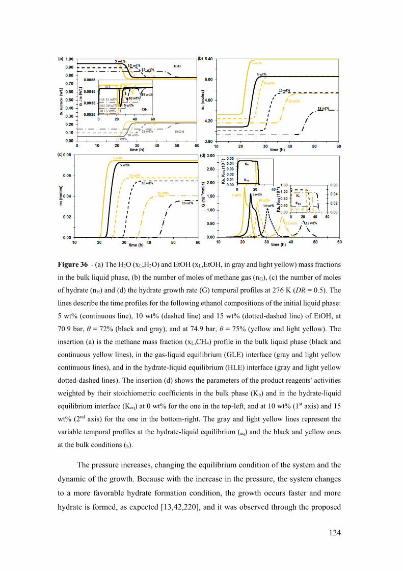
124
Figure 36 - (a) The H2O (xL,H2O) and EtOH (xL,EtOH, in gray and light yellow) mass fractions
in the bulk liquid phase, (b) the number of moles of methane gas (nG), (c) the number of moles
of hydrate (nH) and (d) the hydrate growth rate (G) temporal profiles at 276 K (DR = 0.5). The
lines describe the time profiles for the following ethanol compositions of the initial liquid phase:
5 wt% (continuous line), 10 wt% (dashed line) and 15 wt% (dotted-dashed line) of EtOH, at
70.9 bar, θ = 72% (black and gray), and at 74.9 bar, θ = 75% (yellow and light yellow). The
insertion (a) is the methane mass fraction (xL,CH4) profile in the bulk liquid phase (black and
continuous yellow lines), in the gas-liquid equilibrium (GLE) interface (gray and light yellow
continuous lines), and in the hydrate-liquid equilibrium (HLE) interface (gray and light yellow
dotted-dashed lines). The insertion (d) shows the parameters of the product reagents' activities
weighted by their stoichiometric coefficients in the bulk phase (Kb) and in the hydrate-liquid
equilibrium interface (Keq) at 0 wt% for the one in the top-left, and at 10 wt% (1st axis) and 15
wt% (2nd axis) for the one in the bottom-right. The gray and light yellow lines represent the
variable temporal profiles at the hydrate-liquid equilibrium (eq) and the black and yellow ones
at the bulk conditions (b).
The pressure increases, changing the equilibrium condition of the system and the
dynamic of the growth. Because with the increase in the pressure, the system changes
to a more favorable hydrate formation condition, the growth occurs faster and more
hydrate is formed, as expected [13,42,220], and it was observed through the proposed
125
model. The new observation that our model allowed is that the increase in the initial
ethanol concentration affects the amount of hydrate formed with the increase in the
pressure. Therefore, for inhibited systems, the greater the amount of inhibitor more
important it is to account for the non-ideal effect in the simulation to quantify the amount
of hydrate that will be formed and prevent blockages.
5.3.4 Temperature effect in an inhibited system
A system similar to the one used by Englezos et al. [42] to obtain hydrate growth
experimental data at 70.9 bar and 276 K or 274 K were simulated to evaluate the
temperature effect in hydrate inhibited systems, keeping the same DR factor of 0.5, and
the same hydrate occupancy factor, θ, adjusted to represent those data better. For the
system at 276 K and 70.9 bar it was θ = 72%. In comparison, for the system at 274 K
and 70.9 bar it was 68%, obeying the criterion of the maximum occupancy factor for
which the methane mole fraction profile in the liquid phase had the greatest possible
variation within limits given by the interfaces equilibrium condition at those temperature
and pressure [213]. We can see that the temperature decrease decreases the hydrate
occupancy factor, as it was observed experimentally in the literature [213,215,216,221].
Figure 37 shows the temperature effect in hydrate inhibited systems. The
temperature decrease puts the system in a more favorable hydrate formation condition,
accelerating the hydrate formation and increasing the methane and ethanol equilibrium
composition, Figure 37 (a). The equilibrium composition of 0.485 wt% of CH4 and 22.0
wt% of EtOH at 276 K became 0.54 wt% of CH4 and 27.8 wt% of EtOH at 274 K. The
decrease of 2 K accelerates in 5.7, 9.3, and 18.7 hours the beginning of the growth for
5, 10 and 15 wt%, respectively. It is noticed that the increase in ethanol concentration
accelerates, even more, the start of growth due to the temperature reduction.
The liquid phase behavior is shown in Figure 37 (a). The temperature reduction
increases the methane solubilization in the liquid phase, as expected. The methane
saturation is 0.477 wt%, 0.478 wt% and 0.480 wt% at 276 K and 0.544 wt%, 0.530 wt%
and 0.519 wt% at 274 K for 5, 10 and 15 wt% of EtOH, respectively. The cooling of the
system makes an increase in methane solubility. However, at a lower temperature, 274
K, the methane mass fraction in the liquid phase decreases with the ethanol
concentration increase. It occurs not because the methane solubility reduces, but because
the molecular weight of ethanol is greater than that of methane and, as both are

126
increasing, the methane mass fraction reduces. The amount of methane solubilized in
the liquid phase increases with increasing ethanol concentration at 274 K, 0.108, 0.110,
and 0.114 moles for 5, 10, and 15 wt% of EtOH, respectively (in Appendix 4).
When cooling the system, to reach the same pressure, it is necessary to increase
the amount of gas present in the gas phase; therefore, the methane number of moles in
the gas phase increases, as we can see in Figure 37 (b). The methane gas number of
moles goes from 5.07, 4.74 and 4.41 for 276 K to 5.18, 4.93 and 4.66 for 274 K at 5, 10
and 15 wt% of EtOH, respectively. So, the higher the ethanol initial concentration,
higher is the increase in the methane number of moles in the gas phase with cooling:
0.11, 0.19 and 0.25 moles at 5, 10 and 15 wt% of EtOH, respectively.
Figure 37 (c) shows that cooling the system increases the amount of hydrate
formed. The hydrate number of moles at 276 K come from 0.073, 0.055 and 0.036 to
0.078, 0.064 and 0.050 at 274 K for 5, 10 and 15 wt% of EtOH, respectively. The 2 K
cooling increases the hydrate number of moles in 0.005, 0.009 and 0.014 moles. This
means that the temperature decrease increases the amount of hydrate formed, and that
this increase is greater the higher is the initial ethanol concentration. We can see that
there is almost an increase of 0.005 in the hydrate number of moles for each system
ethanol initial concentration due to the cooling. It occurs because the temperature
reduction puts the system in an even more favorable hydrate formation condition. It
increases the distance between the bulk and equilibrium conditions, causing more
hydrate to form.
Cooling accelerates the growth rate and increases its peak, making growth start
faster and form more hydrate, Figure 37 (d). The order of magnitude of parameters Kb
and Keq decreases with the increase in the ethanol concentration and increases with the
temperature reduction, Figure 37 (d) insertions. The increase in the growth occurs
because the distance between the gas-liquid and hydrate-liquid interfaces equilibrium
conditions and the water activity coefficient (Appendix 4) increases with the cooling.
Therefore, the equilibrium condition and water activity change accelerate the growth
and increase the number of hydrates.

127
Figure 37 - (a) The H2O (xL,H2O) and EtOH (xL,EtOH, in gray and light yellow) mass fractions
in the bulk liquid phase, (b) the number of moles of methane gas (nG), (c) the number of moles
of hydrate (nH) and (d) the hydrate growth rate (G) temporal profiles at 70.9 bar (DR = 0.5).The
lines describe the time profiles for the following ethanol compositions of the initial liquid phase:
5 wt% (continuous line), 10 wt% (dashed line), and 15 wt% (dotted-dashed line) of EtOH, at
276 K, θ = 72% (black and gray), and at 274 K, θ = 68% (yellow and light yellow). The insertion
(a) is the methane mass fraction (xL,CH4) profile in the bulk liquid phase (black and continuous
yellow lines), in the gas-liquid equilibrium (GLE) interface (gray and light yellow continuous
lines), and in the hydrate- liquid equilibrium (HLE) interface (gray and light yellow dotted-
dashed lines). The insertion (d) shows the parameters of the product reagents' activities weighted
by their stoichiometric coefficients in the bulk phase (Kb) and the hydrate-liquid equilibrium
interface (Keq) at 0 wt% for the one in the top-left, and at 10 wt% (1st axis) and 15 wt% (2nd axis)
for the one in the bottom-right. The gray and light yellow lines represent the variable temporal
profiles at the hydrate- liquid equilibrium (eq) and the black and yellow ones at the bulk
conditions (b).
The higher the ethanol concentration and temperature, the greater the inhibitory
effect, thermodynamic and kinetic, of ethanol. A few experimental studies [220] have
already shown this result, but now with this model, we could simulate this kind of
system, predict and quantify the ethanol inhibitory capacity.

128
5.4 Partial conclusions
The proposed model is capable to adequately calculate the qualitative dynamic
behavior of the methane hydrate growth in systems [15,32,196] contain inhibitor. The
model was used to calculate the growth of methane hydrate in an ethanol-inhibited
system at different concentrations. We showed that the higher the ethanol concentration,
the slower it is for the growth to start. In other words, ethanol can act as a
thermodynamic hydrate inhibitor and as a kinetic inhibitor. Besides, when there is no
inhibitor, the system reaches a steady-state with the total consumption of water.
However, with the inhibitor, the system reaches equilibrium. The higher the initial
inhibitor concentration, the faster the equilibrium is achieved, as the system is closer to
the equilibrium concentration. The higher the inhibitor concentration, the slower the
growth starts, but when growth begins, the faster the system reaches equilibrium. The
thermodynamic hydrate inhibitor can then delay the beginning of the growth and reduce
the solid amount. At higher initial inhibitor concentration [220], these effects are more
pronounced. These results agree with experimental observation.
The inclusion of the water activity in the driving force is the key contribution to
the kinetic inhibitor behavior of ethanol better. The increase in ethanol concentration
enhances the kinetic inhibitor effect of this THI, but on the other hand, the inclusion of
water activity in the driving force reduces this effect concerning the driving force that
accounts only for the host activity. This evaluation shows the relevance of considering
the water non-ideality in the driving force to account for the real kinetic inhibition
potential. In this way, we can measure each THI's inhibition potential, use the ethanol
to change the equilibrium condition, delay the hydrate formation, and prevent
blockages.
The increase in the pressure and the temperature decrease presented similar
changes in the ethanol inhibited hydrate system. It occurs because the higher the
pressure and the lower the temperature, the more favorable is the hydrate formation, so
it is expected that the growth occurs faster and forms more hydrate [42,196,220].
Calculations of systems in more favorable conditions responded adequately, making the
beginning of growing faster and forming a more solid phase. However, 2 K cooling the
system pronounced more than the pressure increase by 4 bar. It is possible to conclude

129
that temperature has an even more pronounced kinetic and equilibrium effect in the
hydrate growth than pressure for inhibited systems.
The new model showed that the increases in the initial ethanol concentration affect
the amount of hydrate formed. So, for inhibited systems, the greater the amount of
inhibitor, the more important it is to account for the non-ideal effect in the simulation to
quantify the amount of hydrate that will be formed.
List of symbols
T - Temperature [K]
p - Pressure [bar]
R - Universal gas constant [J mol / K]
- Stoichiometric coefficient for CH4
- Stoichiometric coefficient for H2O
H - Hydrate
t - Time [h]
ν - Stoichiometric coefficient
A - Affinity
ɑ - Activity
- Density [mol / m³]
c - concentration [mol / m³]
M - Molar mass [g / mol]
Jrr - Reaction flow [mol / m2 s]
G - Growth rate [mol / s]
Asup - Surface area [m²]
δ - Liquid film thickness [m]
Nc - Number of compounds
Lrr - Reaction coefficient [mol2 K / m2 J s]
LD- Diffusion coefficient [mol / m s]

130
K - Activity product weighted by stoichiometric coefficient
n - Number of moles [mol]
V - Volume [m³]
x - Mole fraction
μi - Moment of order i [mi / m3]
DR - Coupling factor
Θ – Hydrate occupancy factor
υ - Dynamic viscosity [mol / m s]
eq - Equilibrium condition
b - Bulk condition
L - Liquid phase
G - Gas phase
H - Hydrate phase
0- Reference

131
Chapter 6. Conclusion and future work
suggestions 6.1 Conclusions
From the proper understanding of the gas hydrate equilibria in the presence of
promoters (THF) and inhibitors (EtOH), we define modeling with a broader application
range or with its applicability range well-established. The proper equilibrium calculation
of these systems allowed developing a hydrate growth model capable of including
thermodynamic effects in freshwater systems and systems with chemical additives
(EtOH).
The hydrate-liquid-vapor equilibria calculation with the proposed equilibrium
modeling is adequate for the systems of H2O+THF, H2O+Gas, and H2O+Gas+THF. The
parameter estimation strategy provides adequate and transferable parameters to be used
in different conditions. The traditional equilibrium modeling shows an adequate
deviation of up to 15 wt% of ethanol for the H2O+Gas+EtOH system. We obtained
thermodynamically consistent data of C2H6 and a mixture of C2H6/CH4 up to 45 wt% of
ethanol. Those measured data are valuable to test and improve hydrate prediction tools.
Besides, a qualitative assessment of the literature data with high ethanol concentration
was made to understand ethanol behavior as a THI better. However, a future
experimental investigation is still needed to better understand the ethanol concentration
limit as a thermodynamic hydrate inhibitor or a promoter. The presented methodology
allowed to define conditions at which a full experimental characterization data of the
hydrate structure is needed to hydrate formation with ethanol.
A driving force based on Prigogine’s affinity was proposed and applied to the new
hydrate growth model developed according to the non-equilibrium thermodynamic
fundamental theory. With the proposed hydrate growth model and adequate balances,
the growth system properties behavior was quantitatively and qualitatively reproduced
for the CH4 hydrate growth in freshwater and ethanol-inhibited systems. We could
conclude first that the hydrate growth phenomenon is governed by both stages: reaction
and diffusion. Second, at lower pressures, the growth behavior is close to the limiting
diffusion behavior, while at high pressures, the diffusion and the reaction compete to

132
drive the growth. Moreover, it is possible to describe the growth phenomenon separated
from the nucleation step. However, the lower the pressure, the greater the nucleation
effect on the growth. The addition of an inhibitor alters the induction time, the kinetic
rate, and the equilibrium condition. The simulations showed that THI presents a kinetic
inhibition potential. So, ethanol can be used to change the equilibrium condition and
delay the hydrate formation to prevent blockages. This effect can be simulated by adding
the H2O activity in the driving force, which is purely kinetic and increases with the
increase in the inhibitor concentration.
6.2 Future work suggestions
To expand and continue this study, we suggest the following subjects for future
work:
Experimental investigation on the gas hydrate formation at high ethanol
concentration. Hydrate-liquid-vapor equilibrium data, as well as the hydrate
crystalline structure data and hydrate occupancy factor data in the presence of
ethanol are still needed to better understand and model the ethanol behavior,
mainly at high concentrations.
Adaptation and application of the hydrate growth model to describe the growth
of the double hydrate promoted by THF, since the equilibrium is already
properly modeled. The proposed model can include the change in the water
activity due to the addition of THF, but it is also capable of including another
hydrate guest property in the driving force, through its activity, and account
both effects caused by the THF addition.
As hydrate formation is an exothermic reaction, it is important to include an
energy balance in growth modeling. Theoretical development of the hydrate
growth energy balance is already made. However, more experimental data on
the hydrate thermal properties is still needed to describe the system temperature
changes better. Previous studies [24,87] show that the spatial thermal variation
in a hydrate formation system can be neglected concerning the temporal
thermal variation. Therefore, an energy balance of the system can consider that
the thermal exchange between the phases occurs instantly, such that the
temperature of the entire system is the same spatially, although it varies
temporally.

133
An experimental study for the theoretical model validation, mainly for
application in systems with chemical additives, is critical. It will compare the
calculated temporal profiles with those measured and then obtain the model's
precision level. Besides, this experimental analysis can also be used to define
the induction time and the boundaries between the phenomena involved in the
hydrate formation process, so that the comparison is made in an adequate time
range. The initial conditions of the population balance moments by a particle
size distribution can also be obtained from experimental studies. These results
will allow the calculation of a more precise hydrate formation kinetic constant
by reconciling dynamic data to make the model more robust. It is the same
methodology that Clarke and Bishnoi [77] proposed for the Englezoss et
al.[42,43] model. It is interesting to note that this methodology will allow
detaching the model from the experimental apparatus.
The approach of using a population balance to describe the solid phase, even a
simple one, allows future inclusion of both the nucleation rate and the
aggregation/breakage rate. Thus, we can describe with even more precision all
stages of formation or dissociation of hydrates.

134
References [1] E.D. Sloan, C. Koh, K.A. Sum, Natural Gas Hydrates in Flow Assurance, 1st ed.,
Elsevier, 2011.
[2] E.D. Sloan, C.A. Koh, Clathrate Hydrates of Natural Gases, 3rd ed., CRC Press,
New York, 2008.
[3] H.P. Veluswamy, A. Kumar, Y. Seo, J.D. Lee, P. Linga, A review of solidified
natural gas (SNG) technology for gas storage via clathrate hydrates, Appl.
Energy. 216 (2018) 262–285. https://doi.org/10.1016/j.apenergy.2018.02.059.
[4] E.D. Sloan Jr, Fundamental principles and applications of natural gas hydrates,
Nature. 426 (2003) 353–359.
[5] V.M. V Stackelberg, Feste Gashydrate., Naturwissenschaften. 36 (1949) 359–
362.
[6] J.A. Ripmeester, J.S. Tse, C.I. Ratcliffe, B.M. Powell, A new clathrate hydrate
structure, Nature. 325 (1987) 135–136.
[7] J.Y. Lee, T.S. Yun, J.C. Santamarina, C. Ruppel, Observations related to
tetrahydrofuran and methane hydrates for laboratory studies of hydrate-bearing
sediments, Geochemistry, Geophys. Geosystems. 8 (2007) 1–10.
https://doi.org/10.1029/2006GC001531.
[8] K. Yasuda, S. Takeya, M. Sakashita, H. Yamawaki, R. Ohmura, Binary Ethanol
- Methane Clathrate Hydrate Formation in the System CH4 - C2H5OH - H2O :
Confirmation of Structure II Hydrate Formation, J.Phys. Chem. C. 113 (2009)
12598–12601.
[9] T. Makino, T. Sugahara, K. Ohgaki, Stability boundaries of tetrahydrofuran +
water system, J. Chem. Eng. Data. 50 (2005) 2058–2060.
https://doi.org/10.1021/je0502694.
[10] R. Anderson, A. Chapoy, H. Haghighi, B. Tohidi, Binary Ethanol−Methane
Clathrate Hydrate Formation in the System CH4-C2H5OH-H2O: Phase
Equilibria and Compositional Analyses, J. Phys. Chem. C. 113 (2009) 12602–
12607. https://doi.org/10.1021/jp9021536.

135
[11] S. Sun, X. Peng, Y. Zhang, J. Zhao, Y. Kong, Stochastic nature of nucleation and
growth kinetics of THF hydrate, J. Chem. Thermodyn. 107 (2017) 141–152.
https://doi.org/10.1016/j.jct.2016.12.026.
[12] Z. Vatani, G. Amini, M. Samadi, A.M. Fuladgar, Prediction of gas hydrate
formation in the presence of methanol, ethanol, (ethylene, diethylene and
triethylene) glycol thermodynamic inhibitors, Pet. Sci. Technol. 36 (2018) 1150–
1157. https://doi.org/10.1080/10916466.2018.1465960.
[13] Q. Nasir, H. Suleman, Y.A. Elsheikh, A review on the role and impact of various
additives as promoters/ inhibitors for gas hydrate formation, J. Nat. Gas Sci. Eng.
(2020) 103211. https://doi.org/10.1016/j.jngse.2020.103211.
[14] B. Lal, O. Nashed, Chemical Additives for Gas Hydrates, 1st ed., Springer, 2020.
[15] Z. Yin, M. Khurana, H.K. Tan, P. Linga, A review of gas hydrate growth kinetic
models, Chem. Eng. J. 342 (2018) 9–29.
https://doi.org/10.1016/j.cej.2018.01.120.
[16] T. Makiya, T. Murakami, S. Takeya, A.K. Sum, S. Alavi, R. Ohmura, Synthesis
and characterization of clathrate hydrates containing carbon dioxide and ethanol.,
Phys. Chem. Chem. Phys. 12 (2010) 9927–9932.
https://doi.org/10.1039/c002187c.
[17] H. Mozaffar, R. Anderson, B. Tohidi, Fluid Phase Equilibria Effect of alcohols
and diols on PVCap-induced hydrate crystal growth patterns in methane systems,
Fluid Phase Equilib. 425 (2016) 1–8. https://doi.org/10.1016/j.fluid.2016.05.005.
[18] X. Sen Li, C.G. Xu, Y. Zhang, X.K. Ruan, G. Li, Y. Wang, Investigation into gas
production from natural gas hydrate: A review, Appl. Energy. 172 (2016) 286–
322. https://doi.org/10.1016/j.apenergy.2016.03.101.
[19] Z. Yin, Z.R. Chong, H.K. Tan, P. Linga, Review of gas hydrate dissociation
kinetic models for energy recovery, J. Nat. Gas Sci. Eng. 35 (2016) 1362–1387.
https://doi.org/10.1016/j.jngse.2016.04.050.
[20] S. Horii, R. Ohmura, Continuous separation of CO2from a H2 + CO2gas mixture
using clathrate hydrate, Appl. Energy. 225 (2018) 78–84.
https://doi.org/10.1016/j.apenergy.2018.04.105.

136
[21] J. Zhao, Y. Song, X. Le Lim, W.H. Lam, Opportunities and challenges of gas
hydrate policies with consideration of environmental impacts, Renew. Sustain.
Energy Rev. 70 (2017) 875–885. https://doi.org/10.1016/j.rser.2016.11.269.
[22] J. Zheng, N.K. Loganathan, P. Linga, Natural gas storage via clathrate hydrate
formation: Effect of carbon dioxide and experimental conditions, Energy
Procedia. 158 (2019) 5535–5540. https://doi.org/10.1016/j.egypro.2019.01.590.
[23] C. Sun, W. Li, X. Yang, F. L i, Q. Yuan, L. Mu, J. Chen, B. Liu, G. Chen, Progress
in Research of Gas Hydrate, Chinese J. Chem. Eng. 19 (2011) 151–162.
https://doi.org/10.1016/S1004-9541(09)60192-0.
[24] C.P. Ribeiro, P.L.C. Lage, Modelling of hydrate formation kinetics: State-of-the-
art and future directions, Chem. Eng. Sci. 63 (2008) 2007–2034.
https://doi.org/10.1016/j.ces.2008.01.014.
[25] P.J. Herslund, N. Daraboina, K. Thomsen, J. Abildskov, N. Von Solms,
Measuring and modelling of the combined thermodynamic promoting effect of
tetrahydrofuran and cyclopentane on carbon dioxide hydrates, Fluid Phase
Equilib. 381 (2014) 20–27. https://doi.org/10.1016/j.fluid.2014.08.015.
[26] A. Chapoy, R. Anderson, H. Haghighi, T. Edwards, B. Tohidi, Can n-propanol
form hydrate?, Ind. Eng. Chem. Res. 47 (2008) 1689–1694.
https://doi.org/10.1021/ie071019e.
[27] R. Anderson, A. Chapoy, H. Haghighi, B. Tohidi, Binary Ethanol - Methane
Clathrate Hydrate Formation in the System CH4 -C2H5OH-H2O : Phase
Equilibria and Compositional Analyses, J.Phys. Chem. C. 113 (2009) 12602–
12607.
[28] K. Yasuda, R. Ohmura, A.K. Sum, Guest-guest and guest-host interactions in
ethanol, propan-1-ol, and propan-2-ol clathrate hydrate forming systems, New J.
Chem. 42 (2018) 7364–7370. https://doi.org/10.1039/c8nj00750k.
[29] J. Javanmardi, S. Babaee, A. Eslamimanesh, A.H. Mohammadi, Experimental
Measurements and Predictions of Gas Hydrate Dissociation Conditions in the
Presence of Methanol and Ethane-1,2-diol Aqueous Solutions, J. Chem. Eng.
Data. 57 (2012) 1474–1479.
137
[30] F. V Zhurko, A. Yu, V.I. Kosyakov, Formation of gas hydrates in the systems
methane – water – ROH (ROH = ethanol , n -propanol , i -propanol , i -butanol),
Chem. Eng. Sci. 65 (2010) 900–905. https://doi.org/10.1016/j.ces.2009.09.040.
[31] I.L. Moudrakovski, K.A. Udachin, S. Alavi, C.I. Ratcliffe, J.A. Ripmeester,
Facilitating guest transport in clathrate hydrates by tuning guest-host interactions,
J. Chem. Phys. 142 (2015) 074705-01-074705–10.
https://doi.org/10.1063/1.4907720.
[32] W. Ke, T.M. Svartaas, D. Chen, A review of gas hydrate nucleation theories and
growth models, J. Nat. Gas Sci. Eng. 61 (2019) 169–196.
https://doi.org/10.1016/j.jngse.2018.10.021.
[33] M.S. Khatami, A. Shahsavand, Application Of Population Balance Theory For
Dynamic Modeling Of Methane And Ethane Hydrate Formation Processes, 2018.
https://doi.org/10.1021/acs.energyfuels.8b01351.
[34] M. Khurana, Z. Yin, P. Linga, A review of clathrate hydrate nucleation, ACS
Sustain. Chem. Eng. 5 (2017) 11176–11203.
https://doi.org/10.1021/acssuschemeng.7b03238.
[35] P. Warrier, M.N. Khan, V. Srivastava, C.M. Maupin, C.A. Koh, Overview:
Nucleation of clathrate hydrates, J. Chem. Phys. 145 (2016) 211705.
https://doi.org/10.1063/1.4968590.
[36] J.W. Mullin, Crystallization, 4th ed., Butterworth-Heinemann, 2001.
https://doi.org/https://doi.org/10.1016/B978-0-7506-4833-2.X5000-1.
[37] Y. Bi, A. Porras, T. Li, Free energy landscape and molecular pathways of gas
hydrate nucleation, J. Chem. Phys. 145 (2016) 211909.
https://doi.org/10.1063/1.4961241.
[38] C. Moon, P.C. Taylor, P.M. Rodger, Molecular dynamics study of gas hydrate
formation, J. Am. Chem. Soc. 125 (2003) 4706–4707.
papers3://publication/uuid/D1804CE2-6160-461B-B684-215F438CC26D.
[39] J.P. Lederhos, J.P. Long, A. Sum, R.L. Christiansen, E.D. Sloan, Effective kinetic
inhibitors for natural gas hydrates, Chem. Eng. Sci. 51 (1996) 1221–1229.
https://doi.org/10.1016/0009-2509(95)00370-3.

138
[40] E.M. Freer, M.S. Selim, E.D. Sloan Jr, Methane hydrate film growth kinetics,
Fluid Phase Equilib. 185 (2001) 65–75.
[41] A.A. Noyes, W.R. Whitney, THE RATE OF SOLUTION OF SOLID
SUBSTANCES IN THEIR OWN SOLUTIONS, Solut. SOLID Subst. (1897)
930–934. https://doi.org/CMU/SEI-2006-TR-008 ESC-TR-2006-008.
[42] P. Englezos, N. Kalogerakis, P.D.D. Dholabhai, P.R.R. Bishnoi, Kinetics of
formation of methane and ethane gas hydrates, Chem. Eng. Sci. 42 (1987) 2647–
2658. https://doi.org/10.1016/0009-2509(87)87015-X.
[43] P. Englezos, N. Kalogerakis, P.D. Dholabhai, P.R. Bishnoi, Kinetics of gas
hydrate formation from mixtures of metane and ethane, Chem. Eng. Sci. 42
(1987) 2659–2666.
[44] C.L. Bassani, A.K. Sum, J. Herri, R.E.M. Morales, A. Cameira, A Multiscale
Approach for Gas Hydrates Considering Structure , Agglomeration , and
Transportability under Multiphase Flow Conditions : II . Growth Kinetic Model,
Ind. Eng. Chem. Res. 59 (2020) 2123–2144.
https://doi.org/10.1021/acs.iecr.9b04245.
[45] C.L. Bassani, C. Kakitani, J.-M. Herri, A.K. Sum, R.E.M. Morales, A. Cameirão,
A Multiscale Approach for Gas Hydrates Considering Structure, Agglomeration,
and Transportability under Multiphase Flow Conditions: III. Agglomeration
Model, Ind. Eng. Chem. Res. (2020). https://doi.org/10.1021/acs.iecr.0c02633.
[46] C.L. Bassani, A.M. Melchuna, A. Cameiraõ, J.M. Herri, R.E.M. Morales, A.K.
Sum, A multiscale approach for gas hydrates considering structure,
agglomeration, and transportability under multiphase flow conditions: I.
phenomenological model, Ind. Eng. Chem. Res. 58 (2019) 14446–14461.
https://doi.org/10.1021/acs.iecr.9b01841.
[47] D. Elwell, H.J. Sheel, Crystal Growth from High-Temperature Solutions,
Academic Press, New York, 1975.
[48] E.D. Sloan, F. Fleyfel, A Molecular Mechanism for Gas Hydrate Nucleation from
Ice, AIChE J. 37 (1991) 1281–1292.
[49] R.L. Christiansen, E.D. Sloan Jr., Mechanisms and Kinetics of Hydrate

139
Formation., 284 Ann. NEW YORK Acad. Sci. (1994) 283–305.
[50] L.A. Baez, P. Clancy, Computer simulation of the crystal growth and dissolution
of natural gas hydrates, Ann. N. Y. Acad. Sci. 715 (1994) 177–186.
https://doi.org/10.1111/j.1749-6632.1994.tb38833.x.
[51] M.R. Walsh, C.A. Koh, D.E. Sloan, A.K. Sum, D.T. Wu, Microsecond
Simulations of Spontaneous Methane Hydrate Nucleation and Growth, Science
(80-. ). 326 (2009) 1095–1098. https://doi.org/10.1126/science.1174010.
[52] A.H. Mohammadi, I. Kraouti, D. Richon, Experimental data and predictions of
dissociation conditions for methane, ethane, propane, and carbon dioxide simple
hydrates in the presence of glycerol aqueous solutions, Ind. Eng. Chem. Res. 47
(2008) 8492–8495. https://doi.org/10.1021/ie801018e.
[53] a. Vysniauskas, P.R. Bishnoi, A kinetic study of methane hydrate formation,
Chem. Eng. Scince. 38 (1983) 1061–1072. https://doi.org/10.1016/0009-
2509(83)80027-X.
[54] a. Vysniauskas, P.R. Bishnoi, Kinetics of ethane hydrate formation, Chem. Eng.
Sci. 40 (1985) 299–303. https://doi.org/10.1016/0009-2509(85)80070-1.
[55] D.R. Topham, THE MODELLING OF HYDROCARBON BUBBLE PLUMES
TO INCLUDE GAS HYDRATE FORMATION, Chem. Eng. Sci. 39 (1984)
1613–1622.
[56] D.R. Topham, The Formation of Gas Hydrates on Bubbles of Hydrocarbon Gases
Rising in Seawater, Chem. Eng. Sci. 39 (1984) 821–828.
[57] T. Elperin, A. Forminykh, MODEL OF GAS HYDRATE FORMATION ON
THE SURFACE OF A SLUG OF A PURE GAS, Int. Commun. Heat Mass
Transf. 22 (1995) 435–443.
[58] J. Boxall, S. Davies, C. Koh, E.D. Sloan, Predicting When and Where Hydrate
Plugs Form in Oil-Dominated Flowlines, SPE Proj. Facil. Constr. 4 (2009) 80–
86. https://doi.org/10.2118/129538-PA.
[59] T.B. Charlton, M. Di Lorenzo, L.E. Zerpa, C.A. Koh, M.L. Johns, E.F. May, Z.M.
Aman, Simulating Hydrate Growth and Transport Behaviour in Gas-Dominant
Flow, Energy & Fuels. 32 (2018) 1012–1023.
140
https://doi.org/10.1021/acs.energyfuels.7b02199.
[60] L.E. Zerpa, E.D. Sloan, A.K. Sum, C.A. Koh, Overview of CSMHyK: A transient
hydrate formation model, J. Pet. Sci. Eng. 98–99 (2012) 122–129.
https://doi.org/10.1016/j.petrol.2012.08.017.
[61] K. Lekvam, P. Ruoff, A Reaction Kinetic Mechanism for Methane Hydrate
Formation in Liquid Water, J. Am. Chem. Soc. 115 (1993) 8565–8569.
[62] K. Lekvam, P. Ruoff, Kinetics and mechanism of methane hydrate formation and
decomposition in liquid water description of hysteresis, J. Cryst. Growth. 179
(1997) 618–624.
[63] D. Yang, L.A. Le, R.J. Martinez, R.P. Currier, D.F. Spencer, Kinetics of CO2
hydrate formation in a continuous flow reactor, Chem. Eng. J. 172 (2011) 144–
157. https://doi.org/10.1016/j.cej.2011.05.082.
[64] E. Chaturvedi, K. Patidar, M. Srungavarapu, S. Laik, A. Mandal,
Thermodynamics and kinetics of methane hydrate formation and dissociation in
presence of calcium carbonate, Adv. Powder Technol. 29 (2018) 1025–1034.
https://doi.org/10.1016/j.apt.2018.01.021.
[65] D.N. Glew, M.L. Haggett, Kinetics of formation of ethylene oxide hydrate. Part
I. Experimental method and congruent solutions, Can. J. Chem. 46 (1968) 3857–
3865.
[66] D.N. Glew, M.L. Haggett, Kinetics of formation of ethylene oxide hydrate. Part
II. Incongruent solutions and discussion, Can. J. Chem. 46 (1968) 3867–3877.
https://doi.org/10.1139/v68-640.
[67] J.B. Pangborn, A.J. Barduhn, THE KINETICS OF METHYL BROMIDE
HYDRATE FORMATION, Dcsalinarion. 8 (1970) 35–68.
[68] T. Uchida, I.Y. Ikeda, S. Takeya, T. Ebinuma, J. Nagao, H. Narita, CO2 hydrate
film formation at the boundary between CO2 and water: Effects of temperature,
pressure and additives on the formation rate, J. Cryst. Growth. 237–239 (2002)
383–387. https://doi.org/10.1016/S0022-0248(01)01822-X.
[69] T. Uchida, T. Ebinuma, J. Kawabata, H. Narita, Microscopic observations of
formation processes of clathrate-hydrate films at an interface between water and
141
carbon dioxide, J. Cryst. Growth. 204 (1999) 348–356.
https://doi.org/10.1016/S0022-0248(99)00178-5.
[70] Y.H. Mori, Estimating the thickness of hydrate films from their lateral growth
rates: Application of a simplified heat transfer model, J. Cryst. Growth. 223
(2001) 206–212. https://doi.org/10.1016/S0022-0248(01)00614-5.
[71] T. Mochizuki, Y.H. Mori, Clathrate-hydrate film growth along water/hydrate-
former phase boundaries-numerical heat-transfer study, J. Cryst. Growth. 290
(2006) 642–652. https://doi.org/10.1016/j.jcrysgro.2006.01.036.
[72] B.Z. Peng, A. Dandekar, C.Y. Sun, H. Luo, Q.L. Ma, W.X. Pang, G.J. Chen,
Hydrate film growth on the surface of a gas bubble suspended in water, J. Phys.
Chem. B. 111 (2007) 12485–12493. https://doi.org/10.1021/jp074606m.
[73] R.-E. Meindinyo, T. Svartaas, Gas Hydrate Growth Kinetics: A Parametric
Study, Energies. 9 (2016) 1021. https://doi.org/10.3390/en9121021.
[74] R.T. Meindinyo, Gas Hydrate Growth Kinetics, Faculty of Science and
Technology, 2017.
[75] F. Chen, P.D. Yapa, Estimating hydrate formation and decomposition of gases
released in a deepwater ocean plume, J. Mar. Syst. 30 (2001) 21–32.
https://doi.org/10.1016/S0924-7963(01)00032-X.
[76] M.B. Malegaonkar, P.D. Dholabhai, P.R. Bishnoi, Kinetics of carbon dioxide and
methane hydrate formation, Can. J. Chem. Eng. 75 (1997) 1090–1099.
https://doi.org/10.1002/cjce.5450750612.
[77] M.A. Clarke, P.R. Bishnoi, Determination of the intrinsic kinetics of CO2gas
hydrate formation using in situ particle size analysis, Chem. Eng. Sci. 60 (2005)
695–709. https://doi.org/10.1016/j.ces.2004.08.040.
[78] F. Al-Otaibi, M. Clarke, B. Maini, P.R. Bishnoi, Kinetics of structure II gas
hydrate formation for propane and ethane using an in-situ particle size analyzer
and a Raman spectrometer, Chem. Eng. Sci. 66 (2011) 2468–2474.
https://doi.org/10.1016/j.ces.2011.03.012.
[79] F. Al-Otaibi, M. Clarke, B. Maini, P.R. Bishnoi, Formation kinetics of structure
I clathrates of methane and ethane using an in situ particle size analyzer, Energy

142
and Fuels. 24 (2010) 5012–5022. https://doi.org/10.1021/ef100560f.
[80] D. Kashchiev, A. Firoozabadi, Driving force for crystallization of gas hydrates,
J. Cryst. Growth. 241 (2002) 220–230. https://doi.org/10.1016/S0022-
0248(02)01134-X.
[81] Y.T. Luo, J.H. Zhu, S.S. Fan, G.J. Chen, Study on the kinetics of hydrate
formation in a bubble column, Chem. Eng. Sci. 62 (2007) 1000–1009.
https://doi.org/10.1016/j.ces.2006.11.004.
[82] N. Gnanendran, R. Amin, Modelling hydrate formation kinetics of a hydrate
promoter-water-natural gas system in a semi-batch spray reactor, Chem. Eng. Sci.
59 (2004) 3849–3863. https://doi.org/10.1016/j.ces.2004.06.009.
[83] A. V. Palodkar, S. Mandal, A.K. Jana, Modeling Growth Kinetics of Gas Hydrate
in Porous Media: Experimental Validation, Energy & Fuels. 30 (2016) 7656–
7665. https://doi.org/10.1021/acs.energyfuels.6b01397.
[84] P. Skovborg, P. Rasmussen, A Mass Transport Limited Model for the Growth of
Methane and Ethane Gas Hydrates, Chem. Eng. Prog. 49 (1993) 1131–1143.
[85] H. Zhou, C.I. Ferreira, Investigation Of Hydrate Growth Rate On The Interface
Between Liquid and Solid Film Investigation of hydrate growth rate on the
interface between liquid and solid film, in: 16 Th Int. Refrig. Air Cond. Conf.,
2016: pp. 1672 1–10.
http://docs.lib.purdue.edu/iracc%5Cnhttp://docs.lib.purdue.edu/iracc/1672.
[86] J.M. Herri, J.S. Pic, F. Gruy, M. Cournil, Methane Hydrate Crystallization
Mechanism from In- Situ Particle Sizing, AIChE J. 45 (1999) 590–602.
https://doi.org/10.1002/aic.690450316.
[87] T.P. Sampaio, F.W. Tavares, P.L.C. Lage, Non-isothermal population balance
model of the formation and dissociation of gas hydrates, Chem. Eng. Sci. 163
(2017) 234–254. https://doi.org/10.1016/j.ces.2016.12.012.
[88] B. Zarenezhad, F. Varaminian, A generalized macroscopic kinetic model for
description of gas hydrate formation processes in isothermal-isochoric systems,
Energy Convers. Manag. 57 (2012) 125–130.
https://doi.org/10.1016/j.enconman.2011.12.015.

143
[89] H. Roosta, S. Khosharay, F. Varaminian, Experimental and modeling
investigation on mixed carbon dioxide-tetrahydrofuran hydrate formation
kinetics in isothermal and isochoric systems, J. Mol. Liq. 211 (2015) 411–416.
https://doi.org/10.1016/j.molliq.2015.07.065.
[90] M. Gudala, S.K. Govindarajan, A. Mandal, CHEMICAL AFFINITY
MODELING OF METHANE HYDRATE FORMATION AND
DISSOCIATION IN PRESENCE OF SURFACTANTS, Energy & Fuels. 34
(2019) 319–331. https://doi.org/10.1021/acs.energyfuels.9b03777.
[91] Y. Shindo, P.C. Lund, Y. Fuhioka, H. Komiyama, KINETICS OF FORMATION
OF CO 2 HYDRATE Y., Energy Convers. Mgmt. 34 (1993) 1073–1079.
[92] H. Teng, C.M. Kinoshita, Hydrate Formation on the Surface of a CO2 Droplet in
High Pressure Low Temperature Wwater.pdf, Chem. Eng. Sci. 50 (1995) 559–
564.
[93] S. Hashemi, A. Macchi, P. Servio, Gas Hydrate Growth Model in a Semibatch
Stirred Tank Reactor, Ind. Eng. Chem. Res. 46 (2007) 5907–5912.
[94] S. Bergeron, P. Servio, Reaction rate constant of propane hydrate formation,
Fluid Phase Equilib. 265 (2008) 30–36.
https://doi.org/10.1016/j.fluid.2007.12.001.
[95] H. Tajima, T. Nagata, Y. Abe, A. Yamasaki, F. Kiyono, K. Yamagiwa, HFC-
134a hydrate formation kinetics during continuous gas hydrate formation with a
kenics static mixer for gas separation, Ind. Eng. Chem. Res. 49 (2010) 2525–
2532. https://doi.org/10.1021/ie901613h.
[96] S. Babaee, H. Hashemi, A.H. Mohammadi, P. Naidoo, D. Ramjugernath, Kinetic
study of hydrate formation for argon + TBAB + SDS aqueous solution system, J.
Chem. Thermodyn. 116 (2018) 121–129.
https://doi.org/10.1016/j.jct.2017.08.030.
[97] L. Mu, S. Li, Q.L. Ma, K. Zhang, C.Y. Sun, G.J. Chen, B. Liu, L.Y. Yang,
Experimental and modeling investigation of kinetics of methane gas hydrate
formation in water-in-oil emulsion, Fluid Phase Equilib. 362 (2014) 28–34.
https://doi.org/10.1016/j.fluid.2013.08.028.
144
[98] J.H. van der Waals, J.C. Platteeuw, Clathrate solutions, Adv. Chem. Phys. 2
(1959) 1–57. https://doi.org/10.1002/9780470143483.ch1.
[99] S. Saito, D.R. Marshall, R. Kobayashi, High Application of Statistical Mechanics
to the Study of the Hydrates of Methane , Argon , and Nitrogen, AIChE J. (1964)
734–740.
[100] E.D. Sloan, F.M. Khoury, R. Kobayashi, Water Content of Methane Gas in
Equilibrium with Hydrates, Ind. Eng. Chem., Fundam. 15 (1976) 318–323.
[101] G.D. Holder, G. Corbh, K.D. Papadopoulos, Prediction of high-pressure gas
solubilities in aqueous mixtures of electrolytes, Ind. Eng. Chem. Res. 19 (1980)
282–286. https://doi.org/10.1021/ie00057a019.
[102] J. Munck, S. Skjold-Jørgensen, P. Rasmussen, Computations of the formation of
gas hydrates, Chem. Eng. Sci. 43 (1988) 2661–2672.
https://doi.org/10.1016/0009-2509(88)80010-1.
[103] W.R. Parrishl, J.M. Prausnitz, Dissociation Pressures of Gas Hydrates Formed by
Gas Mixtures, Ind. Eng. Chem. Process Des. Dev. 11 (1972) 26–35.
[104] V.T. John, D. Holder, Contribution of Second and Subsequent Water Shells to
the Potential Energy of Guest-Host Interactions in Clathrate Hydrates, J. Phys.
Chem. 86 (1982) 455–459.
[105] V.T. John, K.D. Papadopoulos, G.D. Holder, A Generalized Model for Predicting
Equilibrium Conditions for Gas Hydrates, AIChE J. 31 (1985) 252–259.
https://doi.org/10.1002/aic.690310212.
[106] A.L. Ballard, E.D. Sloan Jr, The next generation of hydrate prediction I . Hydrate
standard states and incorporation of spectroscopy, Fluid Phase Equilib. 194–197
(2002) 371–383.
[107] J.B. Klauda, S.I. Sandler, Phase behavior of clathrate hydrates: A model for
single and multiple gas component hydrates, Chem. Eng. Sci. 58 (2003) 27–41.
https://doi.org/10.1016/S0009-2509(02)00435-9.
[108] A. Lakhlifi, P. Richard, S. Picaud, O. Mousis, A simple van ’ t Hoff law for
calculating Langmuir constants in clathrate hydrates, Chem. Phys. 448 (2015)
53–60. https://doi.org/10.1016/j.chemphys.2015.01.004.

145
[109] R. Burgass, A. Chapoy, X. Li, Gas hydrate equilibria in the presence of
monoethylene glycol, sodium chloride and sodium bromide at pressures up to
150 MPa, J. Chem. Thermodyn. 118 (2018) 193–197.
https://doi.org/10.1016/j.jct.2017.10.007.
[110] M.A. Mahabadian, A. Chapoy, R. Burgass, B. Tohidi, Fluid Phase Equilibria
Development of a multiphase fl ash in presence of hydrates : Experimental
measurements and validation with the CPA equation of state, Fluid Phase Equilib.
414 (2016) 117–132. https://doi.org/10.1016/j.fluid.2016.01.009.
[111] J.H. Yoon, A theoretical prediction of cage occupancy and heat of dissociation
of THF-CH4 hydrate, Korean J. Chem. Eng. 29 (2012) 1670–1673.
https://doi.org/10.1007/s11814-012-0137-6.
[112] X. Li, H. Wu, P. Englezos, Prediction of Gas Hydrate Formation Conditions in
the Presence of Methanol, Glycerol, Ethylene Glycol, and Triethylene Glycol
with the Statistical Associating Fluid Theory Equation of State, Ind. Eng. Chem.
Res. 45 (2006) 2131–2137.
[113] M. Abolala, M. Karamoddin, F. Varaminian, Fluid Phase Equilibria
Thermodynamic modeling of phase equilibrium for gas hydrate in single and
mixed refrigerants by using sPC-SAFT equation of state, Fluid Phase Equilib.
370 (2014) 69–74. https://doi.org/10.1016/j.fluid.2014.02.013.
[114] A.H.S. Dehaghani, B. Karami, A new predictive thermodynamic framework for
phase behavior of gas hydrate, Fuel. 216 (2018) 796–809.
https://doi.org/10.1016/j.fuel.2017.11.128.
[115] A. Beheshtimaal, A. Haghtalab, Thermodynamic modeling of hydrate formation
conditions using different activity coefficient models in the presence of
tetrahydrofuran (THF), Chem. Eng. Res. Des. 129 (2018) 150–159.
https://doi.org/10.1016/j.cherd.2017.11.015.
[116] G. Moradi, E. Khosravani, Fluid Phase Equilibria Modeling of hydrate formation
conditions for CH 4 , C 2 H 6 , C 3 H 8 , N 2 , CO 2 and their mixtures using the
PRSV2 equation of state and obtaining the Kihara potential parameters for these
components, Fluid Phase Equilib. 338 (2013) 179–187.
https://doi.org/10.1016/j.fluid.2012.11.010.

146
[117] G.D. Holder, N. Pradhan, P. Equilibria, T. Model, Phase Behavior in Systems
Containing Clathrate Hydrates, Rev. Chem. Eng. 5 (1988) 1–70.
[118] A. Saberi, A. Alamdari, A. Shariati, A.H. Mohammadi, Experimental
measurement and thermodynamic modeling of equilibrium condition for natural
gas hydrate in MEG aqueous solution, Fluid Phase Equilib. 459 (2018) 110–118.
https://doi.org/10.1016/j.fluid.2017.11.034.
[119] R.M. De Deugd, M.D. Jager, J. De Swaan Arons, Mixed Hydrates of Methane
and Water-Soluble Hydrocarbons Modeling of Empirical Results, AIChE J. 47
(2001) 693–704. https://doi.org/10.1002/aic.690470316.
[120] Y. Hu, J.H. Sa, B.R. Lee, A.K. Sum, Universal correlation for gas hydrates
suppression temperature of inhibited systems: III. salts and organic inhibitors,
AIChE J. 64 (2018) 4097–4109. https://doi.org/10.1002/aic.16369.
[121] Y. Demirel, Nonequilibrium Thermodynamics: Transport and Rate Processes in
Physical and Biological Systems, 2nd ed., Elsevier, Lincoln, 2014.
https://doi.org/10.1115/1.1579462.
[122] G. Lebon, D. Jou, J. Casas-Vazquez, Understanding Understanding Non-
equilibrium Thermodynamics, 1 ed, Springer, Catalonia, 2008.
[123] I.A. de Oliveira, I.S. V Segtovich, A.G. Barreto, F.W. Tavares, Accurate
thermodynamic description of vapor–liquid and solid–liquid equilibria of THF,
water and gas hydrates with a unique set of parameters, J. Chem. Thermodyn.
117 (2018) 60–67. https://doi.org/10.1016/j.jct.2017.08.003.
[124] I.A. De Oliveira, A.G. Barreto, F.W. Tavares, A.K. Sum, Phase Equilibria Data
and Thermodynamic Analysis for Liquid − Hydrate − Vapor ( LHV ) with High
Ethanol Concentrations, J. Chem. Eng. Data. 65 (2020) 349–359.
https://doi.org/10.1021/acs.jced.9b00691.
[125] A. Eslamimanesh, A.H. Mohammadi, D. Richon, P. Naidoo, D. Ramjugernath,
Application of gas hydrate formation in separation processes: A review of
experimental studies, J. Chem. Thermodyn. 46 (2012) 62–71.
https://doi.org/10.1016/j.jct.2011.10.006.
[126] S.R. Gough, D.W. Davidson, Composition of Tetrahydrofuran Hydrate and the

147
Effect of Pressure on the Decomposition, Can. J. Chem. 49 (1971) 2691–2699.
https://doi.org/10.1139/v71-447.
[127] R. Anderson, A. Chapoy, B. Tohidi, Phase Relations and Binary Clathrate
Hydrate Formation in the System H2 - THF - H2O, Langmuir. 23 (2007) 3440–
3444.
[128] A. Delahaye, L. Fournaison, S. Marinhas, I. Chatti, J.P. Petitet, D. Dalmazzone,
W. Fürst, Effect of THF on equilibrium pressure and dissociation enthalpy of
CO2 hydrates applied to secondary refrigeration, Ind. Eng. Chem. Res. 45 (2006)
391–397. https://doi.org/10.1021/ie050356p.
[129] Y.T. Seo, S.P. Kang, H. Lee, Experimental determination and thermodynamic
modeling of methane and nitrogen hydrates in the presence of THF, propylene
oxide, 1,4-dioxane and acetone, Fluid Phase Equilib. 189 (2001) 99–110.
https://doi.org/10.1016/S0378-3812(01)00580-5.
[130] Q. Zhang, G. Chen, Q. Huang, C. Sun, X. Guo, Q. Ma, Hydrate Formation
Conditions of a Hydrogen + Methane Gas Mixture in Tetrahydrofuran + Water,
J. Chem. Eng. Data. 50 (2005) 234–236.
[131] A.H. Mohammadi, D. Richon, Phase Equilibria of Clathrate Hydrates of
Tetrahydrofuran + Hydrogen Sulfide and Tetrahydrofuran + Methane, Ind. Eng.
Chem. Res. 48 (2009) 7838–7841.
[132] C. Sun, G. Chen, L. Zhang, Hydrate phase equilibrium and structure for ( methane
+ ethane + tetrahydrofuran + water ) system, J. Chem. Thermodyn. 42 (2010)
1173–1179. https://doi.org/10.1016/j.jct.2010.04.021.
[133] Q. Sun, X. Guo, W.G. Chapman, A. Liu, L. Yang, J. Zhang, Vapor–hydrate two-
phase and vapor–liquid–hydrate three-phase equilibrium calculation of
THF/CH4/N2 hydrates, Fluid Phase Equilib. 401 (2015) 70–76.
https://doi.org/10.1016/j.fluid.2015.05.024.
[134] K. Otake, T. Tsuji, I. Sato, T. Akiya, T. Sako, M. Hongo, A proposal of a new
technique for the density measurement of solids, Fluid Phase Equilib. 171 (2000)
175–179. https://doi.org/10.1016/S0378-3812(00)00358-7.
[135] H.J.M. Hanley, G.J. Meyers, J.W. White, E.D. Sloan, The melting curve of
148
tetrahydrofuran hydrate in D2O, Int. J. Thermophys. 10 (1989) 903–909.
https://doi.org/10.1007/BF00514485.
[136] D.G. Leaist, J.J. Murray, M.L. Post, D.W. Davidson, Enthalpies of
Decomposition and Heat Capacities of Ethylene Oxide and Tetrahydrofuran
Hydrate, J. Phys. Chem. 26 (1982) 4175–4178.
[137] Y.A. Dyadin, P.N. Kuznetsov, I.I. Yakovlev, A. V. Pyrinova, The system water-
tetrahydrofuran in the crystallization region at pressures up to 9 kbar., Dokl.
Chem. 208 (1973) 9–12.
[138] H. Matsuda., N. Kamihana, K. Kurihara, K. Tochigi, K. Yokayama,
Measurement of isobaric vapor-liquid equilibria for binary systems contining
tetrahydrofuran using an automatic apparatus, J. Chem. Eng. Jpn. 44 (2011) 131–
139.
[139] Q. Sun, Y.T. Kang, Experimental correlation for the formation rate of CO2
hydrate with THF (tetrahydrofuran) for cooling application, Energy. 91 (2015)
712–719. https://doi.org/10.1016/j.energy.2015.08.089.
[140] T.A. Strobel, C.A. Koh, E.D. Sloan, Thermodynamic predictions of various
tetrahydrofuran and hydrogen clathrate hydrates, Fluid Phase Equilib. 280 (2009)
61–67. https://doi.org/10.1016/j.fluid.2009.02.012.
[141] P.J. Herslund, K. Thomsen, J. Abildskov, N. Von Solms, Modelling of
tetrahydrofuran promoted gas hydrate systems for carbon dioxide capture
processes, Fluid Phase Equilib. 375 (2014) 45–65.
https://doi.org/10.1016/j.fluid.2014.04.031.
[142] T.M. Letcher, U. Domanska, The excess volumes of (tributylamine + an ether) at
the temperature 298.15 K, J. Chem. Thermodyn. 26 (1994) 1241–1247.
[143] R. Francesconi, F. Comelli, Excess Molar Volumes of Binary Mixtures
Containing Dimethyl Carbonate Linear and Cyclic Ethers, J. Chem. Eng. Data.
39 (1994) 106–107.
[144] I.S. V. Segtovich, A.G. Barreto Jr., F.W. Tavares, Simultaneous multiphase flash
and stability analysis calculations including hydrates, Fluid Phase Equilib. 413
(2016) 196–208. https://doi.org/10.1016/j.fluid.2015.10.030.
149
[145] P.J. Herslund, K. Thomsen, J. Abildskov, N. Von Solms, Application of the
cubic-plus-association ( CPA ) equation of state to model the fluid phase
behaviour of binary mixtures of water and tetrahydrofuran, Fluid Phase Equilib.
356 (2013) 209–222. https://doi.org/10.1016/j.fluid.2013.07.036.
[146] J.M. Míguez, M.M. Piñeiro, J. Algaba, B. Mendiboure, J.P. Torré, F.J. Blas,
Understanding the Phase Behavior of Tetrahydrofuran + Carbon Dioxide, +
Methane, and + Water Binary Mixtures from the SAFT-VR Approach, J. Phys.
Chem. B. 119 (2015) 14288–14302. https://doi.org/10.1021/acs.jpcb.5b07845.
[147] J. Lee, J. Cho, D.M. Kim, S. Park, Separation of tetrahydrofuran and water using
pressure swing distillation: Modeling and optimization, Korean J. Chem. Eng. 28
(2011) 591–596. https://doi.org/10.1007/s11814-010-0467-1.
[148] G.M. Bollas, P.I. Barton, A. Mitsos, Bilevel optimization formulation for
parameter estimation in vapor-liquid(-liquid) phase equilibrium problems, Chem.
Eng. Sci. 64 (2009) 1768–1783. https://doi.org/10.1016/j.ces.2009.01.003.
[149] J. Matouš, J.. Novák, J. Šobr, J. Pick, Phase equilibria in the system
tetrahydrofuran (1) + water (2), Collect. ’Czechoslov. Chem. Commun. 37 (1972)
2653–2663. https://doi.org/10.1007/s11669-014-0326-6.
[150] R. Signer, H. Arm, H. Daeniker, Dampfdrucke, Dichten, thermodynamische
Mischungsfunktionen und Brechungsindices der binaren Systeme Wasser-
Tetrahydrofuran und Wasser-Diathylather bei 25o, Helv. Chim. Acta. 52 (1969)
2347–2351.
[151] V.B. Kogan, Liquid-Vapor Equilibrium in the Systems Tetrahydrofuran-Water
and Tetrahydrofuran-Ethylene Glycol and a Method for Dehydration of
Tetrahydrofuran, J.Appl.Chem.USSR. 41 (1968) 1236–1242.
[152] K.A. Pividal, A. Birtigh, S.I. Sandler, Infinite Dilution Activity Coefficients for
Oxygenate Systems Determined Using a Differential Static Cell, J. Chem. Eng.
Data. 37 (1992) 484–487.
[153] D.L. Bergmann, C.A. Eckert, Measurement of limiting activity coefficients for
aqueous systems by differential ebulliometry, Fluid Phase Equilib. 63 (1991)
141–150.

150
[154] G.S. Shealy, S.I. Sandler, The Excess Gibbs Free Energy of Aqueous
Nonelectrolyte Solutions, AIChE J. 34 (1988) 1065–1074.
[155] M. Schwaab, J.C. Pinto, Análise de Dados Experimentais - Volume I
Fundamentos de Estatística, first ed., Rio de Janeiro, 2007.
[156] W.H. Press, S.A. Teukolsky, W.T. Vetterling, B.P. Flannery, Numerical Recipes
in Fortran, first ed., Cambidge University Press, New York, 1992.
[157] K. Kojima, S. Zhang, T. Hiaki, Measuring methods of infinite dilution activity
coefficients and a database for systems including water, Fluid Phase Equilib. 131
(1997) 145–179. https://doi.org/10.1016/S0378-3812(96)03210-4.
[158] J.L. De Roo, C.J. Peters, R.N. Lichtenthaler, G.A.M. Diepen, Occurrence of
Methane Hydrate in Saturated and Unsaturated Solutions of Sodium Chloride and
Water in Dependence of Temperature and Pressure, AIChE J. 29 (1983) 651–
657.
[159] K.M. Sabil, C.J. Peters, Phase equilibrium data of mixed carbon dioxide and
tetrahydrofuran clathrate hydrate in aqueous electrolyte solutions, in: 11th Int.
Conf. Prop. Phase Equilibria PPEPPD, Crete, Greece, 2007.
[160] S. Hashimoto, T. Sugahara, H. Sato, K. Ohgaki, Thermodynamic Stability of H2
+ Tetrahydrofuran Mixed Gas Hydrate in Nonstoichiometric Aqueous Solutions,
J. Chem. Eng. Data. 52 (2007) 517–520.
[161] L.J. Rovetto, J. Schoonman, C.J. Peters, Phase Behavior of Low-pressure
Hydrogen Clathrate Hydrate, in: 5th Int. Conf. Gas Hydrates, Trondheim,
Norway, 2005.
[162] L.J. Florusse, C.J. Peters, J. Schoonman, K.C. Hester, C.A. Koh, S.F. Dec, K.N.
Marsh, E.D. Sloan, Stable Low-Pressure Hydrogen Clusters Stored in a Binary
Clathrate Hydrate, Science (80-. ). 306 (2004) 469–471.
[163] C.M.M. Antunes, C. Kakitani, M.A.M. Neto, R.R.M. Morales, A.K. Sum, An
Examination of tge prediction of hydrate formation conditions in the presence of
thermodynamic inhibitors, Brazilian J. Chem. Eng. 35 (2018) 265–274.
[164] M. Dastanian, A.A. Izadpanah, M. Mofarahi, Phase Equilibria of Carbon Dioxide
Hydrates in the Presence of Methanol / Ethylene Glycol and KCl Aqueous

151
Solutions, J. Chem. Eng. Data. 62 (2017) 1701–1707.
https://doi.org/10.1021/acs.jced.7b00146.
[165] M.H. Kapateh, A. Chapoy, R. Burgass, B. Tohidi, Experimental Measurement
and Modeling of the Solubility of Methane in Methanol and Ethanol, J. Chem.
Eng. Data. 61 (2015) 666–673. https://doi.org/10.1021/acs.jced.5b00793.
[166] T. Maekawa, Equilibrium Conditions of Xenon Hydrates in the Presence of
Aqueous Solutions of Alcohols, Glycols, and Glycerol, J. Chem. Eng. Data. 61
(2016) 662–665. https://doi.org/10.1021/acs.jced.5b00791.
[167] A.D. Potts, D.W. Davidson, Ethanol Hydrate, J. Phys. Chem. 69 (1965) 996–
1000.
[168] Y. Hu, B.R. Lee, A.K. Sum, Insight into increased stability of methane hydrates
at high pressure from phase equilibrium data and molecular structure, Fluid Phase
Equilib. 450 (2017) 24–29. https://doi.org/10.1016/j.fluid.2017.07.003.
[169] R. Kobayashil, D.L. Katz, Vapor-Liquid Equilibria for Binary sn-water Systems,
Ind. Eng. Chem. 45 (1953) 440–446.
[170] P.F. Ferrari, A.Z. Guembaroski, M.A. Marcelino Neto, R.E.M. Morales, A.K.
Sum, Experimental measurements and modelling of carbon dioxide hydrate
phase equilibrium with and without ethanol, Fluid Phase Equilib. 413 (2015) 1–
8. https://doi.org/10.1016/j.fluid.2015.10.008.
[171] A.Z. Guembaroski, A.M. Neto, D. Bertoldi, R.E.M. Morales, Phase Behavior of
Carbon Dioxide Hydrates : A Comparison of Inhibition Between Sodium
Chloride and Ethanol, J. Chem. Eng. Data. 62 (2017) 3445–3451.
https://doi.org/10.1021/acs.jced.7b00463.
[172] T. Maekawa, Equilibrium Conditions of Propane Hydrates in Aqueous Solutions
of Alcohols , Glycols , and Glycerol, J. Chem. Eng. Data. 53 (2008) 2838–2843.
[173] A. Mohammadi, M. Manteghian, A.H. Mohammadi, Chemical Engineering
Research and Design Thermodynamic modeling of the dissociation conditions of
hydrogen sulfide clathrate hydrate in the presence of aqueous solution of inhibitor
( alcohol , salt or ethylene glycol ), Chem. Eng. Res. Des. 92 (2014) 2283–2293.
https://doi.org/10.1016/j.cherd.2014.01.010.
152
[174] M. Cha, Y. Hu, A.K. Sum, Methane Hydrate Phase Equilibria for Systems
Containing NaCl, KCl, and NH4Cl, Fluid Phase Equilib. 413 (2016) 2–9.
https://doi.org/10.1016/j.fluid.2015.08.010.
[175] J. Sa, Y. Hu, A.K. Sum, Assessing thermodynamic consistency of gas hydrates
phase equilibrium data for inhibited systems, Fluid Phase Equilib. 473 (2018)
294–299. https://doi.org/10.1016/j.fluid.2018.06.012.
[176] Y. Hu, J. Sa, B.R. Lee, A.K. Sum, Universal Correlation for Gas Hydrates
Suppression Temperature of Inhibited Systems: III. Salts and Organic Inhibitors,
AIChE J. 64 (2018) 4097–4109. https://doi.org/10.1002/aic.16369.
[177] M.-J. Huron, J. Vidal, New mixing rules in simple equations of state for
representing vapor-liquid equilibria of strongly non-ideal mixtures, Fluid Phase
Equilib. 3 (1979) 255–271. https://doi.org/https://doi.org/10.1016/0378-
3812(79)80001-1.
[178] J. Vidal, Mixing rules and excess properties in cubic equations of state, Chem.
Eng. Res. Des. 33 (1978) 787–791. https://doi.org/ttps://doi.org/10.1016/0009-
2509(78)80059-1.
[179] Y. Hu, B.R. Lee, A.K. Sum, Universal correlation for gas hydrates suppression
temperature of inhibited systems: II. Mixed salts and structure type, AIChE J. 64
(2018) 2240–2250. https://doi.org/10.1002/aic.16116.
[180] S. Adisasmito, R.J. Frank, E.D. Sloan, Hydrates of Carbon Dioxide and Methane
Mixtures, J. Chem. Eng. Data. 36 (1991) 68–71.
[181] W.M. Deaton, E.M.J. Frost, Gas Hydrates and Their Relation to the Operation of
Natural-Gas Pipe Lines, U.S. Bur. Mines Monogr. 8 (1946) 101.
[182] T.J. Galloway, W. Ruska, P.S. Chappelear, R. Kobayashi, Experimental
Measurement of Hydrate Numbers for Methane and Ethane and Comparison with
Theoretical Values, Ind. Eng. Chem., Fundam. 9 (1970) 237–243.
[183] J. Jhaveri, D.B. Robinson, Hydrates in the MethaneyNitrogen System, Can. J.
Chem. Eng. 4 (1980) 75–78.
[184] A.H. Mohammadi, B. Tohidi, A Novel Predictive Technique for Estimating the
Hydrate Inhibition Effects of Single and Mixed Thermodynamic Inhibitors, Can.

153
J. Chem. Eng. 83 (2005) 951–961.
[185] T. Nakamura, T. Makino, T. Sugahara, K. Ohgaki, Stability boundaries of gas
hydrates helped by methane — structure-H hydrates of methylcyclohexane and
cis -1 , 2-dimethylcyclohexane, Chem. Eng. Sci. 58 (2003) 269–273.
[186] J.L. Thakore, G.D. Holder, Solid-Vapor Azeotropes in Hydrate-Forming
Systems, (1987) 462–469.
[187] F. V. Zhurko, A.Y. Manakov, V.I. Kosyakov, Formation of gas hydrates in the
systems methane-water-ROH (ROH=ethanol, n-propanol, i-propanol, i-butanol),
Chem. Eng. Sci. 65 (2010) 900–905. https://doi.org/10.1016/j.ces.2009.09.040.
[188] S.D. Larson, Phase Studies of the Two-Component Carbon Dioxide-Water
System, Involving the Carbon Dioxide Hydrate, University of Illinois, 1955.
[189] D.B. Robinson, B.R. Mehta, Hydrate formation in systems containing methane,
hydrogen, sulphide, and carbon dioxide, J. Can. Pet. Technol. 10 (1940) 33.
[190] V.K. Verma, Gas Hydrates from Liquid Hydrocarbon–Water Systems,
University of Michigan, University Microfilms, 1974.
[191] H. Kubota, K. Shimizu, Y. Tanaka, T. Makita, Thermodynamic properties of R13
(CHF3), R152a (C2H4F2), and propane hydrates for desalination of sea water, J.
Chem. Eng. Japan. 17 (1984) 423–429.
[192] S.L. Patil, Measurements of Multiphase Gas Hydrates Phase Equilibria: Effect of
Inhibitors and Heavier Hydrocarbon Components, University of Alaska, 1987.
[193] G.D. Holder, G.C. Grigoriou, Hydrate dissociation pressures of ( methane +
ethane + water ) Existence of a locus of minimum pressures, J. Chem.
Thermodyn. A-150 (1980) 1093–1104.
[194] Y. Hu, B.R. Lee, A.K. Sum, Universal correlation for gas hydrates suppression
temperature of inhibited systems: I. Single salts, AIChE J. 63 (2017) 5111–5124.
https://doi.org/10.1002/aic.15846.
[195] C.D. Ruppel, Gas Hydrate in Nature, U.S. Geol. Surv. Fact Sheet (2018) 4.
https://doi.org/https://doi.org/10.3133/fs20173080.
[196] Q. Nasir, H. Suleman, Y.A. Elsheikh, A review on the role and impact of various
154
additives as promoters/ inhibitors for gas hydrate formation, J. Nat. Gas Sci. Eng.
(2020) 103211. https://doi.org/10.1016/j.jngse.2020.103211.
[197] Z.R. Chong, S. Hern, B. Yang, P. Babu, P. Linga, X. Li, Review of natural gas
hydrates as an energy resource : Prospects and challenges q, Appl. Energy. 162
(2016) 1633–1652. https://doi.org/10.1016/j.apenergy.2014.12.061.
[198] K. Yamamoto, X.X. Wang, M. Tamaki, K. Suzuki, The second o ff shore
production of methane hydrate in the Nankai Trough and gas production behavior
from a heterogeneous methane hydrate reservoir, R. Soc. Chem. 9 (2019) 25987–
26013. https://doi.org/10.1039/c9ra00755e.
[199] R. Braga, R.S. Iglesias, C. Romio, D. Praeg, D.J. Miller, A. Viana, J.M. Ketzer,
Modelling methane hydrate stability changes and gas release due to seasonal
oscillations in bottom water temperatures on the Rio Grande cone, offshore
southern Brazil, Mar. Pet. Geol. 112 (2019) 104071.
https://doi.org/10.1016/j.marpetgeo.2019.104071.
[200] C. Cheng, F. Wang, Y. Tian, X. Wu, J. Zheng, J. Zhang, L. Li, P. Yang, J. Zhao,
Review and prospects of hydrate cold storage technology, Renew. Sustain.
Energy Rev. 117 (2020) 109492. https://doi.org/10.1016/j.rser.2019.109492.
[201] M.N. Khan, P. Warrier, C.J. Peters, C.A. Koh, Advancements in hydrate phase
equilibria and modeling of gas hydrates systems, Fluid Phase Equilib. 463 (2018)
48–61. https://doi.org/10.1016/j.fluid.2018.01.014.
[202] C.L. Bassani, A.M. Melchuna, A. Cameira, J. Herri, R.E.M. Morales, A.K. Sum,
A Multiscale Approach for Gas Hydrates Considering Structure , Agglomeration
, and Transportability under Multiphase Flow Conditions : I . Phenomenological
Model, Ind. Eng. Chem. Res. 58 (2019) 14446−14461.
https://doi.org/10.1021/acs.iecr.9b01841.
[203] G. Song, Y. Li, W. Wang, K. Jiang, Z. Shi, S. Yao, Numerical simulation of
pipeline hydrate particle agglomeration based on population balance theory, J.
Nat. Gas Sci. Eng. 51 (2018) 251–261.
https://doi.org/10.1016/j.jngse.2018.01.009.
[204] Y. Sun, S. Jiang, S. Li, G. Zhang, W. Guo, Growth kinetics of hydrate formation
from water – hydrocarbon system, Chinese J. Chem. Eng. 27 (2019) 2164–2179.

155
https://doi.org/10.1016/j.cjche.2019.03.022.
[205] V.W.S. Lim, P.J. Metaxas, P.L. Stanwix, M.L. Johns, D. Crosby, Z.M. Aman,
E.F. May, Gas Hydrate Formation Probability and Growth Rate as a Function of
Kinetic Hydrate Inhibitor ( KHI ) Concentration, Chem. Eng. J. 388 (2020)
124177. https://doi.org/10.1016/j.cej.2020.124177.
[206] C.L. Bassani, A.K. Sum, J. Herri, R.E.M. Morales, A. Cameira, A Multiscale
Approach for Gas Hydrates Considering Structure , Agglomeration , and
Transportability under Multiphase Flow Conditions : II . Growth Kinetic Model,
Ind. Eng. Chem. Res. 59 (2020) 2123–2144.
https://doi.org/10.1021/acs.iecr.9b04245.
[207] I.A. De Oliveira, A.G. Barreto, F.W. Tavares, A.K. Sum, Phase Equilibria Data
and Thermodynamic Analysis for Liquid − Hydrate − Vapor ( LHV ) with High
Ethanol Concentrations, J. Chem. Eng. Data. (2019).
https://doi.org/10.1021/acs.jced.9b00691.
[208] A. Vignes, Diffusion in binary solutions: Variation of Diffusion Coefficient with
Composition, Ind. Eng. Chem. Fundam. 5 (1966) 189–199.
https://doi.org/10.1021/i160018a007.
[209] B.J. Jahne, G. Heinz, W. Dietrich, Measurment of the diffusion coefficients of
sparkling soluble gases in water, J. Geophys. Res. 92 (1987) 10767–10776.
https://doi.org/10.1029/JC092iC10p10767.
[210] B.E. Polling, J.M. Prausnitz, J.P. O’Connell, The properties of gases and liquids,
1st ed., McGRAW-HILL, New York, 2001.
[211] D. Ramkrishna, Population balances, 1st ed., Academic Press, Indiana, 2000.
https://doi.org/10.1016/B978-012576970-9/50000-X.
[212] B. V Balakin, A.C. Hoffmann, P. Kosinski, Population Balance Model for
Nucleation , Growth , Aggregation , and Breakage of Hydrate Particles in
Turbulent Flow, AIChE J. 56 (2010). https://doi.org/10.1002/aic.
[213] T. Uchida, T. Hirano, T. Ebinuma, H. Narita, K. Gohara, S. Mae, Raman
Spectroscopic Determination of Hydration Number of Methane Hydrates, AIChE
J. 45 (1999) 2641–2645.
156
[214] H. Henley, A. Lucia, Journal of Natural Gas Science and Engineering Constant
pressure Gibbs ensemble Monte Carlo simulations for the prediction of structure
I gas hydrate occupancy, J. Nat. Gas Sci. Eng. 26 (2015) 446–452.
https://doi.org/10.1016/j.jngse.2015.05.038.
[215] J. Qin, W.F. Kuhs, A. Kristallographie, Quantitative Analysis of Gas Hydrates
Using Raman Spectroscopy, 00 (2013). https://doi.org/10.1002/aic.
[216] W.F. Kuhs, B. Chazallon, A. Klapprothl, F. Pauer, Filling-Isotherms in Clathrate-
Hydrates, Rev. High Press. Sci. Technol. 7 (1998) 1147–1149.
[217] A.Y. Manakov, N. V Penkov, T. V Rodionova, A.N. Nesterov, E.E. Fesenko Jr,
Kinetics of formation and dissociation of gas hydrates, Russ. Chem. Rev. 86
(2017) 845–869. https://doi.org/10.1070/RCR4720.
[218] M.S. Khatami, A. Shahsavand, Application Of Population Balance Theory For
Dynamic Modeling Of Methane And Ethane Hydrate Formation Processes,
Energy & Fuels. 32 (2018) 8131–8144.
https://doi.org/10.1021/acs.energyfuels.8b01351.
[219] A.K. Sum, Gas Hydrates in Flow Assurance, in: Workshop, Curitiba - PR/Brazil,
2003.
[220] S. Renato, E. Vinicius, R. Castro, A. Teixeira, R. Rosa, T. Rodrigues, S. Renato,
Effects of ethanol on the performance of kinetic hydrate inhibitors, Fluid Phase
Equilib. 476 (2018) 112–117. https://doi.org/10.1016/j.fluid.2018.07.036.
[221] H. Henley, A. Lucia, Journal of Natural Gas Science and Engineering Constant
pressure Gibbs ensemble Monte Carlo simulations for the prediction of structure
I gas hydrate occupancy, J. Nat. Gas Sci. Eng. 26 (2015) 446–452.
https://doi.org/10.1016/j.jngse.2015.05.038.
[222] H.G. Rackett, Equation of State for Saturated Liquids, J. Chem. Eng. Data. 15
(1970) 514–517. https://doi.org/10.1021/je60047a012.
[223] F.S. Mjalli, K. Shahbaz, I.M. Alnashef, Thermochimica Acta Modi fi ed Rackett
equation for modelling the molar volume of deep eutectic solvents, Thermochim.
Acta. 614 (2015) 185–190. https://doi.org/10.1016/j.tca.2015.06.026.
[224] T. Yamada, R.D. Gunn, Saturated Liquid Molar Volumes . The Rackett Equation,
157
J. Chem. Eng. Data. 18 (1973) 234–236. https://doi.org/10.1021/je60057a006.
[225] O. Iulian, I. Nita, O. Ciocirlan, M. Catrinciuc, A. Fedeles, Property Prediction for
Binary and Ternary Systems with Water , 1 , 4-Dioxane , Ethyleneglycol and
Diethyleneglycol, REV. CHIM. 60 (2009) 7–10.
[226] J. Wang, V.N. Kabadi, Generalized Method for Prediction of Saturated Liquid
Volumes Using Van der Waals Volumes, AIChE J. 42 (1996) 595–598.
[227] H.J.E. Dobson, The partial pressures of aqueous ethyl alcohol, J. Chem. Soc.
Trans. 127 (1925) 2866–2873. https://doi.org/10.1039/ct9252702866.
[228] J. Gmehling, U. Onken, W. Arlt, P. Grenzheuser, U. Weidlich, B. Kolbe, J. Rarey,
VAPOR-LIQUID EQUILIBRIUM DATA COLLECTION, 1st ed., DECHEMA,
Chemische Technik und Biotechnologie, 1977.
[229] K. Kuriharaj, T. Minoura, K. Takedaj, Water, Methanol + Water, and Ethanol
Isothermal Vapor-Liquid Equilibria for Methanol + Ethanol + Water, J. Chem.
Eng. Data. 40 (1996) 679–684.
[230] D.F. Othmer, W.P. Moeller, S.W. Englund, R.G. Christopher, Composition of
Vapors from Boiling Binary Solutions - Recirculation-type Still and Equilibria
under Pressure for Ethyl Alcohol-Water System, Ind. Eng. Chem. 43 (1951) 707–
711. https://doi.org/10.1021/ie50495a038.
[231] R.C. Pemberton, C.J. Mash, Thermodynamic properties of aqueous mixtures II .
Vapour pressuresand excessGibbsenergies for water + ethanol at 303 . 15 to 363
. 15 K determined by an accurate static method, J. Chem. Thermodyn. 10 (1978)
867–888.
[232] R.C. Phutela, Z.S. Kooner, D. V Fenby, Vapour Pressure Study of Deuterium
Exchange Reactions in Water-Ethanol Systems : Equilibrium Constant
Determination, Aust. J. Chem. 32 (1979) 2353–2362.
[233] M. Schwaab, E.C. Biscaia, J.L. Monteiro, J.C. Pinto, Nonlinear parameter
estimation through particle swarm optimization, Chem. Eng. Sci. 63 (2008)
1542–1552. https://doi.org/10.1016/j.ces.2007.11.024.
[234] M. Frost, E. Karakatsani, N. Von Solms, D. Richon, G.M. Kontogeorgis, Vapor
− Liquid Equilibrium of Methane with Water and Methanol . Measurements and
158
Modeling, J. Chem. Eng. Data. 59 (2013) 961–967.
[235] S.O. Yang, S.H. Cho, H. Lee, C.S. Lee, Measurement and prediction of phase
equilibria for water + methane in hydrate forming conditions, Fluid Phase
Equilib. 185 (2001) 53–63.
[236] J. Qin, R.J. Rosenbauer, Z. Duan, Experimental Measurements of Vapor – Liquid
Equilibria of the H 2 O + CO 2 + CH 4 Ternary System, J. Chem. Eng. Data. 53
(2008) 1246–1249.
[237] A. Chapoy, C. Coquelet, D. Richon, Corrigendum to “ Revised solubility data
and modeling of water in the gas phase of the methane / water binary system at
temperatures from 283 . 08 to 318 . 12 K and pressures up to 34 . 5 MPa ” [ Fluid
Phase Equilibria 214 ( 2003 ) 101 – 117 ], Fluid Phase Equilib. 230 (2005) 210–
214. https://doi.org/10.1016/j.fluid.2004.07.005.
[238] A.H. Mohammadi, A. Chapoy, B. Tohidi, D. Richon, Gas Solubility : A Key to
Estimating the Water Content of Natural Gases, Ind. Eng. Chem. Res. 45 (2006)
4825–4829.
[239] O.L. Culberson, D. Co, J.J.M. Jr, Phase Equilibria In Hydrocarbon-Water
Systems IV - Vapor-Liquid Equilibrium Constants in the Methane-Water and
Ethane-Water Systems, Pet. Trans. AIME. 192 (1951) 297–300.
[240] Y.S. Kim, S.K. Ryu, S.O. Yang, C.S. Lee, Liquid Water - Hydrate Equilibrium
Measurements and Unified Predictions of Hydrate-Containing Phase Equilibria
for Methane , Ethane , Propane , and Their Mixtures, Ind. Eng. Chem. Res. 42
(2003) 2409–2414.
[241] J. Kiepe, S. Horstmann, K. Fischer, J. Gmehling, Experimental Determination
and Prediction of Gas Solubility Data for Methane + Water Solutions Containing
Different Monovalent, Ind. Eng. Chem. Res. 42 (2003) 5392–5398.
[242] W. Lu, I.M. Chou, R.C. Burruss, Determination of methane concentrations in
water in equilibrium with sI methane hydrate in the absence of a vapor phase by
in situ Raman spectroscopy, Geochim. Cosmochim. Acta. 72 (2008) 412–422.
https://doi.org/10.1016/j.gca.2007.11.006.
[243] J.M. Prausnitz, R.N. Lichtenthaler, E.G. De Azevedo, Molecular

159
thermodynamics of fluid-phase equilibria, 3rd ed., Prentice Hall PTR, New
Jersey, 1999. https://doi.org/10.1016/0021-9614(70)90078-9.
[244] J.M. Prausnitz, F.H. Shair, Thermodynamic Correlation of G as Solubilities,
AIChE J. 7 (1961) 682–687.
[245] R. Lemoine, B.I. Morsi, An algorithm for predicting the hydrodynamic and mass
transfer parameters in agitated reactors, Chem. Eng. J. 114 (2005) 9–31.
https://doi.org/10.1016/j.cej.2005.08.015.
[246] I.R. Krichevsky, J.S. Kasarnovsey, Thermodynamical Calculations of
Solubilities of Nitrogen and Hydrogen in Water at High Pressures, Contrib. from
D. I. Mendeleyeff Chem. Inst. (1935) 2168–2171.
[247] A. Chianese, H.J.. Kramer, Industrial Crystallization Process Monitoring and
Control, 1st ed., Wiley-VCH, Weinheim, 2012.
[248] L.R. Petzold, A description of DASSL : A Differential/Algebraic System Solver,
in: IMACS World Congr., Montreal, Canada, 1982.
[249] M. Mooney, THE VISCOSITY OF A CONCENTRATED SUSPENSION OF
SPHERICAL PARTICLES, J. Colloid Sci. 6 (1951) 162–170.
[250] A. Firoozabadi, H.J.J. Ramey, Surface-Tension of Water-Hydrocarbon Systems
at Reservoir Conditions, J. Can. Pet. Technol. 27 (1988) 41–48.
[251] S. Taniguchi, S. Kawaguchi, A. Kikuchi, Fluid flow and gas – liquid mass
transfer in gas-injected vessels, Appl. Math. Model. 26 (2002) 249–262.
[252] P.T. Spicer, S.E. Pratsinis, Coagulation and Fragmentation: Universal Steady-
State Particle-Size Distribution, AIChE J. 42 (1996) 1612–1620.
https://doi.org/10.1002/aic.690420612.
[253] T. Ukai, D. Kodama, J. Miyazaki, M. Kato, Solubility of methane in alcohols and
saturated density at 280.15 K, J. Chem. Eng. Data. 47 (2002) 1320–1323.
https://doi.org/10.1021/je020108p.
[254] K. Suzuki, H. Sue, M. Itou, R.L. Smith, H. Inomata, K. Arai, S. Saito, Isothermal
Vapor-Liquid Equilibrium Data for Binary Systems at High Pressures: Carbon
Dioxide-Methanol, Carbon Dioxide-Ethanol, Carbon Dioxide-1-Propanol,

160
Methane-Ethanol, Methane-1-Propanol, Ethane-Ethanol, and Ethane-1-Propanol
Systems, J. Chem. Eng. Data. 35 (1990) 63–66.
https://doi.org/10.1021/je00059a020.
[255] F.S. Mjalli, K. Shahbaz, I.M. Alnashef, Thermochimica Acta Modi fi ed Rackett
equation for modelling the molar volume of deep eutectic solvents, Thermochim.
Acta. 614 (2015) 185–190. https://doi.org/10.1016/j.tca.2015.06.026.

161
Appendix 1. Supporting information for
Chapter 2 Table S1 – Literature THF/H2O vapor-liquid equilibria experimental data.
Reference Experimental data of VLE of THF/H2O system
Matouš et al. [34]
T = 343.15/K
p/kPa THF mole fraction in liquid
phase, x
THF mole fraction in
vapor phase, y
102.05 0.032 0.697
120.59 0.072 0.745
122.71 0.141 0.749
122.66 0.241 0.75
123 0.335 0.751
123.35 0.429 0.754
124.32 0.558 0.758
125.26 0.625 0.768
126.22 0.754 0.79
126.44 0.8 0.805
126.06 0.854 0.83
125.26 0.886 0.855
123.39 0.928 0.893
120.1 0.966 0.945
Signer et al. [35]
T = 298.15/K
p/kPa THF mole fraction in liquid
phase, x
THF mole fraction in
vapor phase, y
15.47 0.05 0.805
19.32 0.1 0.847
20.34 0.15 0.856
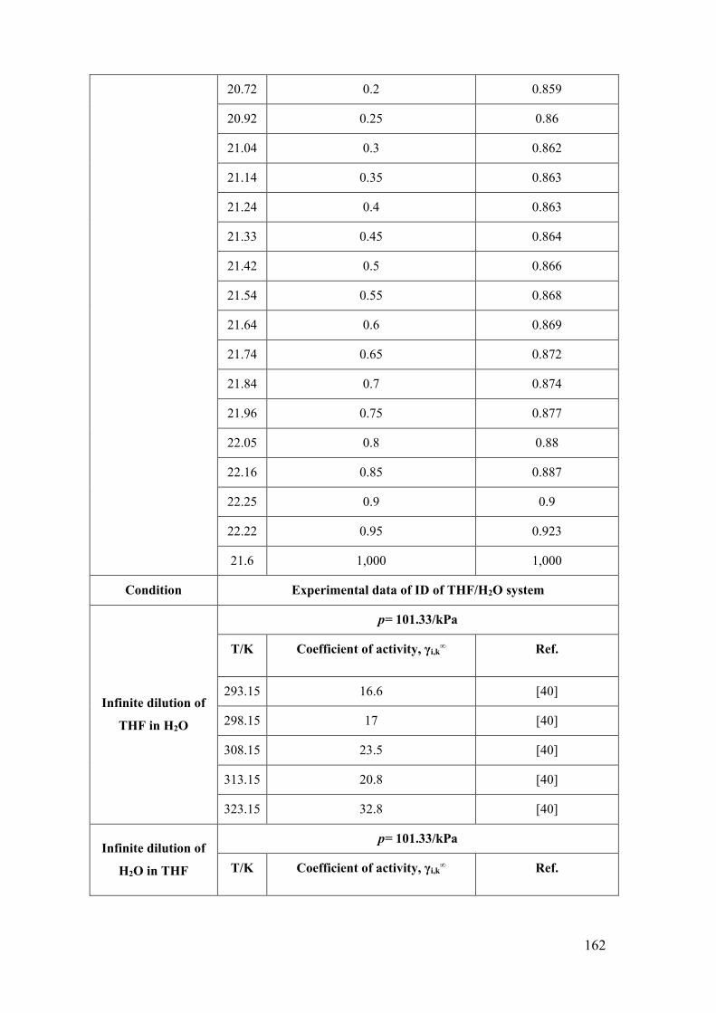
162
20.72 0.2 0.859
20.92 0.25 0.86
21.04 0.3 0.862
21.14 0.35 0.863
21.24 0.4 0.863
21.33 0.45 0.864
21.42 0.5 0.866
21.54 0.55 0.868
21.64 0.6 0.869
21.74 0.65 0.872
21.84 0.7 0.874
21.96 0.75 0.877
22.05 0.8 0.88
22.16 0.85 0.887
22.25 0.9 0.9
22.22 0.95 0.923
21.6 1,000 1,000
Condition Experimental data of ID of THF/H2O system
Infinite dilution of
THF in H2O
p= 101.33/kPa
T/K Coefficient of activity, γi,k∞ Ref.
293.15 16.6 [40]
298.15 17 [40]
308.15 23.5 [40]
313.15 20.8 [40]
323.15 32.8 [40]
Infinite dilution of
H2O in THF
p= 101.33/kPa
T/K Coefficient of activity, γi,k∞ Ref.

163
308.35 11.1 [41]
317.65 10.4 [41]
328.05 9.8 [41]
338.05 9.4 [41]
343.15 7.8 [42]
Table S2 – Literature THF/H2O hydrate-liquid-vapor equilibria (HLE) experimental data.
Experimental data of HLE of THF/H2O system
Reference p= 101.33/kPa
T/K THF mole fraction in liquid phase, x
Makino et al. [5]
272.27 0.011
275.73 0.024
277.26 0.045
277.45 0.056
277.37 0.065
276.9 0.09
276.21 0.13
275.14 0.18
275.02 0.188
Anderson et al.
[6]
272.4 0.01
274.1 0.015
276.8 0.027
277.6 0.035
278 0.043
278.2 0.056
278.1 0.059
Delahaye et al.
[7]
275.79 0.015
276.39 0.019

164
276.45 0.026
276.91 0.027
277.09 0.033
277.57 0.04
277.81 0.052
277.88 0.056
277.86 0.062
277.69 0.073
277.73 0.081
277.51 0.098
Otake et al. [14]
272.06 0.01
273.2 0.013
274.95 0.019
275.9 0.026
276.82 0.03
276.99 0.031
276.97 0.036
277.09 0.037
277.32 0.041
277.48 0.048
277.65 0.055
277.46 0.061
277.57 0.062
277.57 0.066
277.32 0.077
277.76 0.097
Hanley et al. [15] 273.69 0.017
276.49 0.03

165
278.1 0.066
276.99 0.129
Leaist et al. [16]
272.41 0.01
274.1 0.015
276.8 0.027
277.61 0.035
278 0.043
278.21 0.055
278.14 0.059
Dyadin et al. [17]
272.16 0.014
276.6 0.029
277.69 0.039
278.14 0.051
278.14 0.059
278.14 0.062
277.94 0.07
277.86 0.073
277.75 0.08
277.65 0.088
277.34 0.095
276.72 0.133
276.14 0.159
275.75 0.2
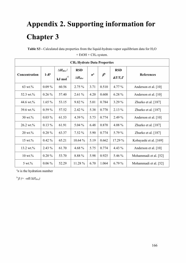
166
Appendix 2. Supporting information for
Chapter 3 Table S3 - Calculated data properties from the liquid-hydrate-vapor equilibrium data for H2O
+ EtOH + CH4 system.
CH4 Hydrate Data Properties
Concentration 1-R² ∆Hdiss /
kJ mol-1
RSD
∆Hdiss na βb
RSD
∆T/T0T References
63 wt.% 0.09 % 60.56 2.75 % 3.71 0.510 4.77 % Anderson et al. [10]
52.3 wt.% 0.26 % 57.40 2.61 % 4.20 0.608 6.28 % Anderson et al. [10]
44.6 wt.% 1.65 % 53.15 9.82 % 5.01 0.784 3.29 % Zhurko et al. [187]
39.6 wt.% 0.59 % 57.52 2.42 % 5.38 0.778 2.13 % Zhurko et al. [187]
30 wt.% 0.03 % 61.53 4.39 % 5.73 0.774 2.49 % Anderson et al. [10]
26.2 wt.% 0.13 % 61.91 5.04 % 6.48 0.870 4.08 % Zhurko et al. [187]
20 wt.% 0.28 % 63.37 7.52 % 5.90 0.774 5.79 % Zhurko et al. [187]
15 wt.% 0.42 % 65.21 10.64 % 5.19 0.662 17.29 % Kobayashi et al. [169]
13.2 wt.% 2.43 % 61.70 4.68 % 5.75 0.774 4.43 % Anderson et al. [10]
10 wt.% 0.20 % 53.70 8.88 % 5.98 0.925 5.46 % Mohammadi et al. [52]
5 wt.% 0.06 % 52.29 11.28 % 6.70 1.064 6.79 % Mohammadi et al. [52]
an is the hydration number
b β (= -nR/∆Hdiss)
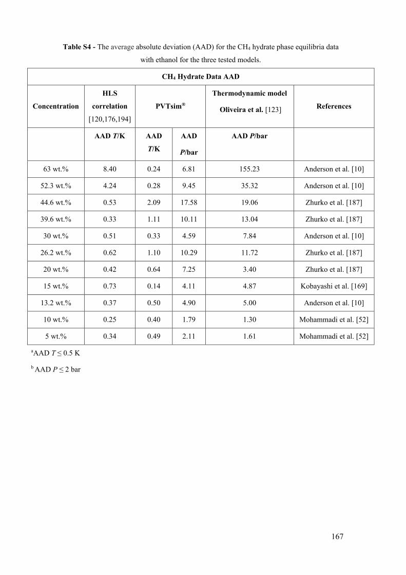
167
Table S4 - The average absolute deviation (AAD) for the CH4 hydrate phase equilibria data
with ethanol for the three tested models.
CH4 Hydrate Data AAD
Concentration
HLS
correlation
[120,176,194]
PVTsim®
Thermodynamic model
Oliveira et al. [123] References
AAD T/K AAD
T/K
AAD
P/bar
AAD P/bar
63 wt.% 8.40 0.24 6.81 155.23 Anderson et al. [10]
52.3 wt.% 4.24 0.28 9.45 35.32 Anderson et al. [10]
44.6 wt.% 0.53 2.09 17.58 19.06 Zhurko et al. [187]
39.6 wt.% 0.33 1.11 10.11 13.04 Zhurko et al. [187]
30 wt.% 0.51 0.33 4.59 7.84 Anderson et al. [10]
26.2 wt.% 0.62 1.10 10.29 11.72 Zhurko et al. [187]
20 wt.% 0.42 0.64 7.25 3.40 Zhurko et al. [187]
15 wt.% 0.73 0.14 4.11 4.87 Kobayashi et al. [169]
13.2 wt.% 0.37 0.50 4.90 5.00 Anderson et al. [10]
10 wt.% 0.25 0.40 1.79 1.30 Mohammadi et al. [52]
5 wt.% 0.34 0.49 2.11 1.61 Mohammadi et al. [52]
aAAD T ≤ 0.5 K
b AAD P ≤ 2 bar
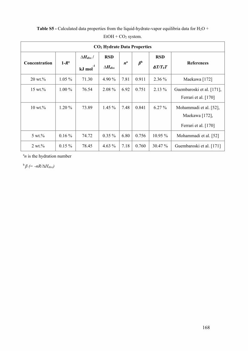
168
Table S5 - Calculated data properties from the liquid-hydrate-vapor equilibria data for H2O +
EtOH + CO2 system.
CO2 Hydrate Data Properties
Concentration 1-R² ∆Hdiss /
kJ mol-1
RSD
∆Hdiss na βb
RSD
∆T/T0T References
20 wt.% 1.05 % 71.30 4.90 % 7.81 0.911 2.36 % Maekawa [172]
15 wt.% 1.00 % 76.54 2.08 % 6.92 0.751 2.13 % Guembaroski et al. [171],
Ferrari et al. [170]
10 wt.% 1.20 % 73.89 1.45 % 7.48 0.841 6.27 % Mohammadi et al. [52],
Maekawa [172],
Ferrari et al. [170]
5 wt.% 0.16 % 74.72 0.35 % 6.80 0.756 10.95 % Mohammadi et al. [52]
2 wt.% 0.15 % 78.45 4.63 % 7.18 0.760 30.47 % Guembaroski et al. [171]
an is the hydration number
b β (= -nR/∆Hdiss)

169
Table S6 - The average absolute deviation (AAD) for the CO2 hydrate phase equilibria data
with ethanol for the three tested models.
CO2 Hydrate Data AAD
Concentration
HLS
correlation
[120,176,194]
PVTsim®
Thermodynamic model
Oliveira et al. [123] References
AAD T/K AAD
T/K
AAD
P/bar
AAD P/bar
20 wt.% 1.23 0.83 2.45 2.63 Maekawa [172]
15 wt.% 0.09 0.32 1.37 1.55 Guembaroski et al.
[171], Ferrari et al. [170]
10 wt.% 0.32 0.20 0.65 0.63 Mohammadi et al. [52],
Maekawa [172],
Ferrari et al. [170]
5 wt.% 0.14 0.15 0.56 0.64 Mohammadi et al. [52]
2 wt.% 0.16 0.15 0.41 0.41 Guembaroski et al. [171]
aAAD T ≤ 0.5 K
b AAD P ≤ 2 bar
Table S7 - Calculated data properties from the liquid-hydrate-vapor equilibria data for H2O +
EtOH + C3H8 system.
C3H8 Hydrate Data Properties
Concentration 1-R² ∆Hdiss /
kJ mol-1
RSD
∆Hdiss na βb
RSD
∆T/T0T References
15 wt.% 0.32 % 123.86 2.31 % 15.77 1.058 1.07 % Maekawa [172],
Mohammadi et al. [52]
10 wt.% 1.95 % 125.09 1.35 % 14.62 0.972 4.75 % Maekawa [172],
Mohammadi et al. [52]
5 wt.% 0.15 % 131.43 3.66 % 15.52 0.981 3.05 % Maekawa [172]
an is the hydration number
b β (= -nR/∆Hdiss)
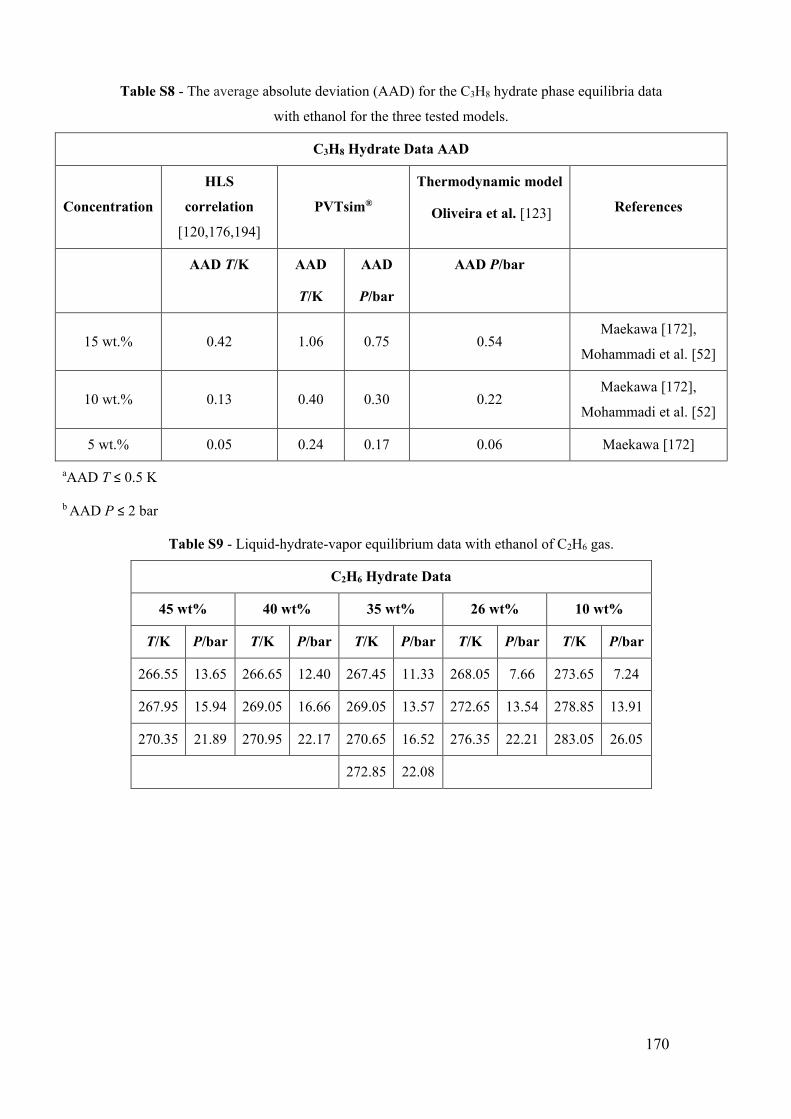
170
Table S8 - The average absolute deviation (AAD) for the C3H8 hydrate phase equilibria data
with ethanol for the three tested models.
C3H8 Hydrate Data AAD
Concentration
HLS
correlation
[120,176,194]
PVTsim®
Thermodynamic model
Oliveira et al. [123] References
AAD T/K AAD
T/K
AAD
P/bar
AAD P/bar
15 wt.% 0.42 1.06 0.75 0.54 Maekawa [172],
Mohammadi et al. [52]
10 wt.% 0.13 0.40 0.30 0.22 Maekawa [172],
Mohammadi et al. [52]
5 wt.% 0.05 0.24 0.17 0.06 Maekawa [172]
aAAD T ≤ 0.5 K
b AAD P ≤ 2 bar
Table S9 - Liquid-hydrate-vapor equilibrium data with ethanol of C2H6 gas.
C2H6 Hydrate Data
45 wt% 40 wt% 35 wt% 26 wt% 10 wt%
T/K P/bar T/K P/bar T/K P/bar T/K P/bar T/K P/bar
266.55 13.65 266.65 12.40 267.45 11.33 268.05 7.66 273.65 7.24
267.95 15.94 269.05 16.66 269.05 13.57 272.65 13.54 278.85 13.91
270.35 21.89 270.95 22.17 270.65 16.52 276.35 22.21 283.05 26.05
272.85 22.08
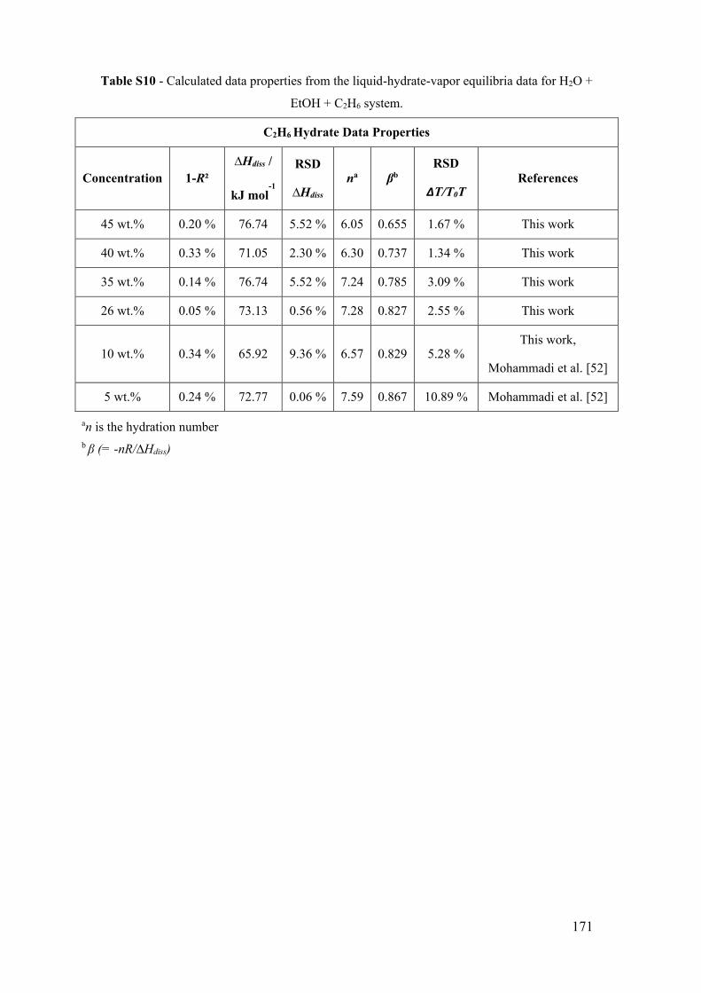
171
Table S10 - Calculated data properties from the liquid-hydrate-vapor equilibria data for H2O +
EtOH + C2H6 system.
C2H6 Hydrate Data Properties
Concentration 1-R² ∆Hdiss /
kJ mol-1
RSD
∆Hdiss na βb
RSD
∆T/T0T References
45 wt.% 0.20 % 76.74 5.52 % 6.05 0.655 1.67 % This work
40 wt.% 0.33 % 71.05 2.30 % 6.30 0.737 1.34 % This work
35 wt.% 0.14 % 76.74 5.52 % 7.24 0.785 3.09 % This work
26 wt.% 0.05 % 73.13 0.56 % 7.28 0.827 2.55 % This work
10 wt.% 0.34 % 65.92 9.36 % 6.57 0.829 5.28 % This work,
Mohammadi et al. [52]
5 wt.% 0.24 % 72.77 0.06 % 7.59 0.867 10.89 % Mohammadi et al. [52]
an is the hydration number b β (= -nR/∆Hdiss)
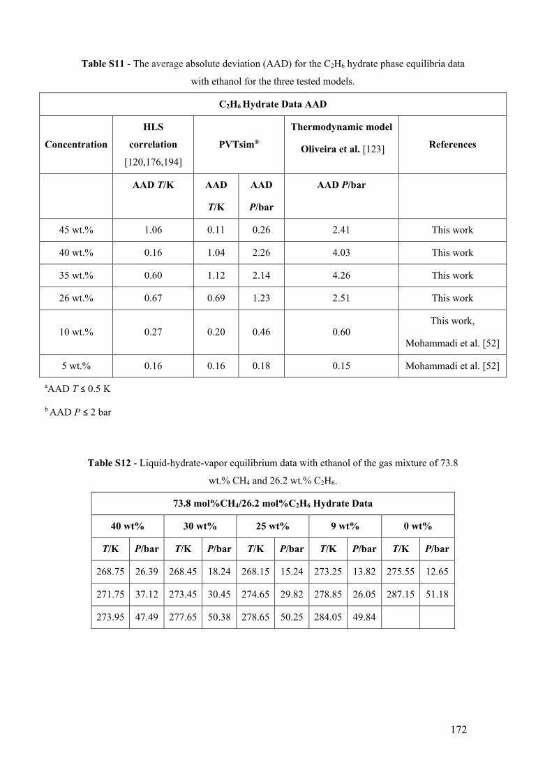
172
Table S11 - The average absolute deviation (AAD) for the C2H6 hydrate phase equilibria data
with ethanol for the three tested models.
C2H6 Hydrate Data AAD
Concentration
HLS
correlation
[120,176,194]
PVTsim®
Thermodynamic model
Oliveira et al. [123] References
AAD T/K AAD
T/K
AAD
P/bar
AAD P/bar
45 wt.% 1.06 0.11 0.26 2.41 This work
40 wt.% 0.16 1.04 2.26 4.03 This work
35 wt.% 0.60 1.12 2.14 4.26 This work
26 wt.% 0.67 0.69 1.23 2.51 This work
10 wt.% 0.27 0.20 0.46 0.60 This work,
Mohammadi et al. [52]
5 wt.% 0.16 0.16 0.18 0.15 Mohammadi et al. [52]
aAAD T ≤ 0.5 K
b AAD P ≤ 2 bar
Table S12 - Liquid-hydrate-vapor equilibrium data with ethanol of the gas mixture of 73.8
wt.% CH4 and 26.2 wt.% C2H6.
73.8 mol%CH4/26.2 mol%C2H6 Hydrate Data
40 wt% 30 wt% 25 wt% 9 wt% 0 wt%
T/K P/bar T/K P/bar T/K P/bar T/K P/bar T/K P/bar
268.75 26.39 268.45 18.24 268.15 15.24 273.25 13.82 275.55 12.65
271.75 37.12 273.45 30.45 274.65 29.82 278.85 26.05 287.15 51.18
273.95 47.49 277.65 50.38 278.65 50.25 284.05 49.84
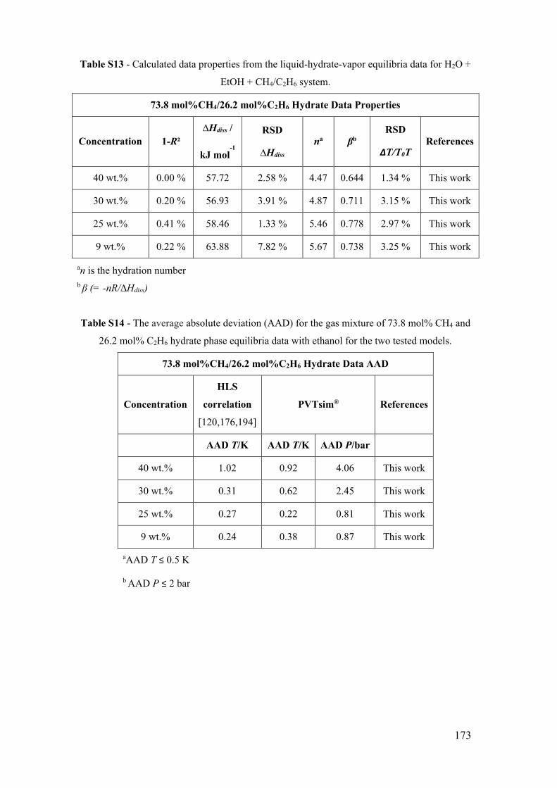
173
Table S13 - Calculated data properties from the liquid-hydrate-vapor equilibria data for H2O +
EtOH + CH4/C2H6 system.
73.8 mol%CH4/26.2 mol%C2H6 Hydrate Data Properties
Concentration 1-R² ∆Hdiss /
kJ mol-1
RSD
∆Hdiss na βb
RSD
∆T/T0T References
40 wt.% 0.00 % 57.72 2.58 % 4.47 0.644 1.34 % This work
30 wt.% 0.20 % 56.93 3.91 % 4.87 0.711 3.15 % This work
25 wt.% 0.41 % 58.46 1.33 % 5.46 0.778 2.97 % This work
9 wt.% 0.22 % 63.88 7.82 % 5.67 0.738 3.25 % This work
an is the hydration number b β (= -nR/∆Hdiss)
Table S14 - The average absolute deviation (AAD) for the gas mixture of 73.8 mol% CH4 and
26.2 mol% C2H6 hydrate phase equilibria data with ethanol for the two tested models.
73.8 mol%CH4/26.2 mol%C2H6 Hydrate Data AAD
Concentration
HLS
correlation
[120,176,194]
PVTsim® References
AAD T/K AAD T/K AAD P/bar
40 wt.% 1.02 0.92 4.06 This work
30 wt.% 0.31 0.62 2.45 This work
25 wt.% 0.27 0.22 0.81 This work
9 wt.% 0.24 0.38 0.87 This work
aAAD T ≤ 0.5 K
b AAD P ≤ 2 bar

174
S.1 Gas hydrate equilibrium model for systems containing
ethanol.
The model used here to calculate the equilibrium pressure of the gas hydrate
studied systems, with or without addictive, was based on Oliveira et al. [123].
In Figure S1, the thermodynamic model fitted to calculate the equilibrium pressure
of the Gas + H2O + Ethanol systems is shown in the block diagram. In this proposal will
be adopted the NRTL excess Gibbs energy model (liquid phase), the Peng-Robinson
equation of state (vapor phase) and the theory of van der Waals and Platteeuw [98] and
Holder et al.[101], with the Kihara potential (hydrate phase).
Figure S1 - Block diagram of the thermodynamic model used to calculate the LHV equilibrium
pressure of systems with additives [123].
The parameterization of this model for the systems Gas + H2O and Gas + H2O +
THF was carried out in the work of Oliveira et al [123] and the parameterization of the
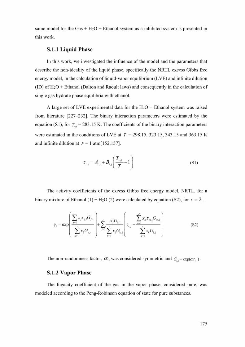
175
same model for the Gas + H2O + Ethanol system as a inhibited system is presented in
this work.
S.1.1 Liquid Phase
In this work, we investigated the influence of the model and the parameters that
describe the non-ideality of the liquid phase, specifically the NRTL excess Gibbs free
energy model, in the calculation of liquid-vapor equilibrium (LVE) and infinite dilution
(ID) of H2O + Ethanol (Dalton and Raoult laws) and consequently in the calculation of
single gas hydrate phase equilibria with ethanol.
A large set of LVE experimental data for the H2O + Ethanol system was raised
from literature [227–232]. The binary interaction parameters were estimated by the
equation (S1), for refT = 283.15 K. The coefficients of the binary interaction parameters
were estimated in the conditions of LVE at T = 298.15, 323.15, 343.15 and 363.15 K
and infinite dilution at P = 1 atm[152,157].
, j , j , j 1refi i i
TA B
T
(S1)
The activity coefficients of the excess Gibbs free energy model, NRTL, for a
binary mixture of Ethanol (1) + H2O (2) were calculated by equation (S2), for 2c .
, , m, j m, j1 i, j 1
,1
k, k, j k, j1 1 1
exp
c c
j j i j i mcj j m
i i jc c cj
k i k kk k k
x G x Gx G
x G x G x G (S2)
The non-randomness factor, , was considered symmetric and , j , jexp( )i iG .
S.1.2 Vapor Phase
The fugacity coefficient of the gas in the vapor phase, considered pure, was
modeled according to the Peng-Robinson equation of state for pure substances.
176
S.1.3 Hydrate Phase
The hydrate phase was modeled with the theory of van der Waals and Platteeuw
[98], which presents an expression for the difference in chemical potential of water
between the hydrate phase and the hypothetical phase of the empty hydrate lattice,
equation (S3). j is the number of cavities of type j per water molecule in the unit cell,
,i jCL is Langmuir constants of the guest molecule i in the cavity of type j , and Hif is the
fugacity of the guest molecule i in the hydrate phase.
2 i,
i,
ln 11
EL H HH O j i
j Hj i j i
CL fRT CL f
(S3)
The criterion of fugacity equality is adopted for the gas hydrate formers. It will be
adopted the hypothesis of gas present only in the vapor phase and ethanol present only
in the liquid phase. For the gaseous hydrate former, the fugacity equality will be
assumed between the hydrate phase and the vapor phase. Also, it is considered that
ethanol acts only as an inhibitor altering water activity, without participation in the
hydrate structure. This criterion appears embedded in the van der Waals and Platteeuw
[98] model.
Therefore, the fugacity of the gas in the hydrate phase is equal to the vapor phase,
as explained in the equilibrium criterion, and calculated by equation (S4), adopting the
hypothesis of the pure gas in the vapor phase, iy = 1,0.
^
, P , , P ,Vi i if T T P yy y (S4)
According to the Lennard-Jones-Devonshire theory, the Langmuir constants (
,i jCL ), which quantify the attractiveness between the guest molecule ( i ) and the host
structure, that can be calculated with spherical symmetry making use of the Kihara pair
interaction potential, equation (S5).
177
2,
0
12 6
10 11 4 511 5
4 ( )exp
1( ) 2 ( ) ( ) ( ) ( )
1 1
( ) 4, 5, 10 11.
j iR a
i jB B
i i i ij i
j j j j
N N
i i
j j j j
N
X rCL r drk T k T
a aX r Z r r r rR R R R r
a ar rR R R R
r N eN
(S5)
Where [Å] is the intermolecular radius of Kihara; a [Å] is the soft radius of
the spherical core for the guest component; and Bk [K] is the Kihara's maximum
attraction potential. The parameters of this model for the CH4, CO2, C2H6, C3H8 gases
were fitted directly to the hydrate-liquid-vapor equilibrium experimental data of the gas
and fresh water system [158,180,190–193,181–186,188,189].
The difference of the chemical potential of water in the empty hydrate lattice in
relation to the liquid phase can be obtained from the classical thermodynamic theory,
equation (S6). Assuming the differences of the constant molar volumes and taking into
account the classical thermodynamic theory of enthalpy dependence with the
temperature, equation (S7), in detriment of its constancy, and linear dependence of the
specific heat on temperature, equation (S8), we obtain the equation (S9):
0
2 2 2 2
2
0
22
00
0
(P )
() (
)EL L EL L EL LTH O H O H O
PH O L
H O H OL
T P
hdT dP ln
RT RT RT RTT
x
(S6)
2 2
0
2 0 0 0 0, PT
EL L ELH
L EL
TO H O O
LHP h T Cp dTPh (S7)
2 2 20 0 0 0,PEL L EL
HL EL
OL
O H H OCp Cp q T TP T (S8)
2 2 2 2 2
22 2 2
2 2
00 0 00
0 0 0
00 000 0
00
21 1 1 12
ln(
2ln )
H O H O H O H O H O
H OH O H O H O L LH O
EL L
H O
Cp TR T T R T T
q T TCp
h qR
T
T RT
q TRT
Px
RTRP
(S9)
Where 2
0H O is the chemical potential variation for water in the reference
conditions, 2H O
E L Lh the enthalpy change for water between the phases, 2H O
E L L the

178
variation of the molar volume for water between the phases and the term of non-ideality
of the liquid phase, considering the water activity, 2 2 2
L L LH O H O H Oa x , is obtained by the
NRTL model. Water activity was considered one for systems without additives.
In this work, the pressure and temperature of reference adopted were 0P = 612,61
Pa and 0T = 273.15 K, and the macroscopic thermodynamic parameters were those
presented in the work of John, Papadopoulos and Holder [105].
The hydrate-liquid-vapor balance criterion is described by the equality between
water potentials in both hydrate and liquid phases, given the intermediate phase of the
empty hydrate lattice structure (EL).
S.2 Methodology of parameter estimation
The equilibrium of the Gas + H2O + Ethanol system requires adjustment of the
parameters of the NRTL model to the H2O-Ethanol pair, which describes the non-
ideality of the liquid phase.
The objective function was minimized for the set of parameters of the NRTL
model using data of infinite dilution and liquid-vapor equilibrium of H2O + Ethanol,
similar to the work published for THF [123].
The parameters of the NRTL model were estimated by minimizing the sum of the
quadratic residuals of the output variables for each experiment ( l ), according to
equation (S10).
exp
2 2calc exp calc exp
obj1 2
calc exp1, 1,
l l l lN
l
l l
w P P w y yF
w
(S10)
For each type of experimental data, the implemented routine allows different
calculations with the NRTL model: for infinite dilution data, the activity coefficients are
calculated directly using the temperature as input variable; and for liquid-vapor
equilibrium data, the pressure and composition of the vapor phase at equilibrium are
calculated using as input variables the temperature and composition of the liquid phase.
is the set of parameters to be estimated. For the NRTL model, it was defined as:
179
1,2 2 ,1 1,2 2 ,1( , , B , B , ) A A . The inverse of the weights allowed for each output variable
was 0.01% of the measured variable. These weights were defined with the purpose of
establishing similar deviations for all points
The case involved regression of the following arrangement of the experimental
data of the H2O + Ethanol system: liquid-vapor equilibrium data at constant
temperatures of 298.15 K, 323.15 K, 343.15 K and 363.15 K, in a total of 142 different
experimental points, and infinite dilution data at atmospheric pressure (101.33 kPa),
which are 10 experimental points between 283.15 K and 373.15 K.
In the estimation strategy of the Kihara parameters the equilibrium criterion is
imposed in the objective function, equation (S11).
2
2
2exp exp exp
exp exp expobj
2
, , ,1
, , ,exp
EL HH O l l lEL LH O l l lN
l
P p T T x x
P p T T x xF
w
(S11)
where , ,Bka . These parameters were estimated from the hydrate-liquid-
vapor equilibrium experimental data set of the pure water and gas systems. The data
collected from the literature were used in the estimation of Kihara parameters for CH4
gases (273.2 K at 289.9 K and 26.50 bar at 158.37 bar), CO2 (271.8 K at 279.8 K and
10.48 bar at 27.30 bar), C2H6 (273.7 K 282.8 K and 5.03 bar at 16.66 bar) and C3H8
(273.4 K at 278.4 K and 1.72 bar and 5.42 bar). The inverse of the weight adopted,
empirically, for the difference between the potentials, in order to increase its accuracy,
was 10-10.
In this work we used the particle swarm optimization method [233] as the
stochastic method to obtain a good initial estimate to be submitted to a Quasi-Newton
algorithm, a deterministic method that makes use of techniques of differential
calculation.

180
S.3 Result of parameter estimation
S.3.1 Liquid-vapor equilibrium
The parameters of the NRTL model, Table S15, were estimated for liquid-vapor
equilibrium data of H2O (2) + Ethanol (1) at the temperatures of 298.15 K, 323.15 K,
343.15 K and 363.15 K and infinite dilution data at atmospheric pressure (101.33 kPa)
between 283.15 K and 373.15 K.
Table S15 - Parameters of the NRTL model, and their respective errors, obtained by adjusting
the liquid-vapor equilibrium data and infinite dilution data of the Ethanol (1) + H2O (2)
system.
A1,2 -1.57715 ± 0.06830
A2,1 3.07850 ± 0.07670
B1,2 7.19352 ± 0.16113
B2,1 -11.38690 ± 0..22354
0.0609696 ± 0.0019712
The calculated values for molar fraction and pressure were well adjusted and
showed absolute average deviations of 0.56% and 0.45%, respectively.
Figure S2 (a), (b) and (c) show the calculated diagrams within the temperature and
pressure conditions for which the parameters of the NRTL model were estimated,
including the data that were correlated (298.15 K, 323.15 K, 343.15 K and 363.15 K).
The correlation of the data used in the estimation was adequate and the model presented
satisfactory predictive capacity within the range of temperature and pressure studied.

181
Figure S2 - Isothermal curves of liquid-vapor equilibrium of H2O + Ethanol at: (a) 323.15 K,
328.15 K, 333.15 K and 343.15 K; (b) 298.15 K and 303.15 K; (c) 363.15 K. The experimental
data are represented by the squares for the dew point curves and circles for the bubble point
curves [227–232]. The continuous curves represent the calculation with the adjusted
NRTL model.
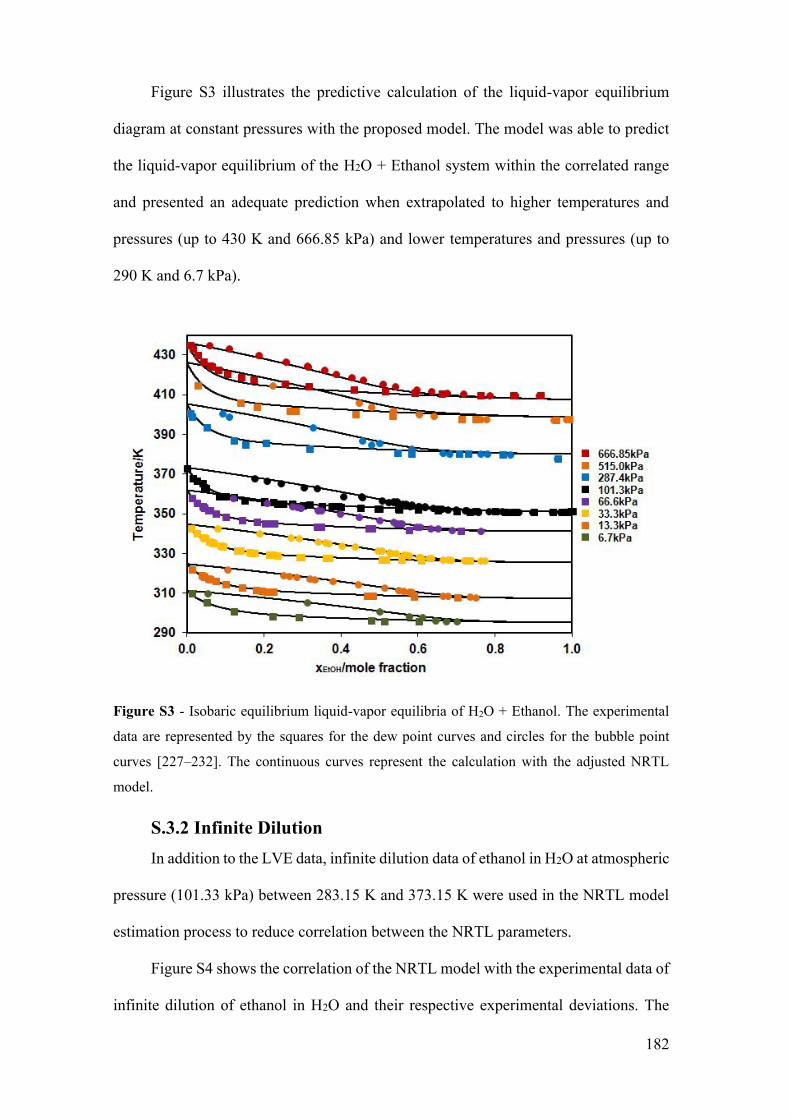
182
Figure S3 illustrates the predictive calculation of the liquid-vapor equilibrium
diagram at constant pressures with the proposed model. The model was able to predict
the liquid-vapor equilibrium of the H2O + Ethanol system within the correlated range
and presented an adequate prediction when extrapolated to higher temperatures and
pressures (up to 430 K and 666.85 kPa) and lower temperatures and pressures (up to
290 K and 6.7 kPa).
Figure S3 - Isobaric equilibrium liquid-vapor equilibria of H2O + Ethanol. The experimental
data are represented by the squares for the dew point curves and circles for the bubble point
curves [227–232]. The continuous curves represent the calculation with the adjusted NRTL
model.
S.3.2 Infinite Dilution In addition to the LVE data, infinite dilution data of ethanol in H2O at atmospheric
pressure (101.33 kPa) between 283.15 K and 373.15 K were used in the NRTL model
estimation process to reduce correlation between the NRTL parameters.
Figure S4 shows the correlation of the NRTL model with the experimental data of
infinite dilution of ethanol in H2O and their respective experimental deviations. The

183
calculation of the infinite dilution coefficient showed an absolute average deviation of
8.19%. This calculation had less precision than the LVE calculation, but it remained
within the experimental error of these data. Therefore, the model is able to correlate the
data within the presented experimental errors.
Figure S4 - Activity coefficient in the condition of infinite dilution of ethanol in H2O. The
squares represent the experimental data with their respective errors [152,157] and the continuous
curve is the model prediction.
S.3.3 Gas hydrate phase equilibria for pure water systems.
The Kihara parameters re-estimated for the gases studied in this work are
presented in Table S16 for pure water condition and were applied in this article in the
calculation of hydrate-liquid-vapor equilibrium with ethanol. With an error lower than
10-3 for the parameters [Å], which is the intermolecular radius of Kihara, and a [Å],
which is the soft radius of the spherical core for the guest component; and lower than
10-1 for Bk [K], which is the Kihara's maximum attraction potential.
3.0
3.5
4.0
4.5
5.0
5.5
6.0
6.5
7.0
270 290 310 330 350 370
γ EtO
H∞
Temperature/K

184
Table S16 - Kihara parameters adjusted for the hydrate phase equilibrium data of the Gas +
H2O systems.
[Å] a [Å] Bk
[K]
CH4 0.252 3.431 143.181
CO2 0.561 3.361 164.532
C2H6 1.351 2.762 224.999
C3H8 1.535 3.084 360.878
The Oliveira et al.[123] model adjustment for the hydrate phase equilibrium data
of the methane system with fresh water showed an absolute average deviation of 1.47%
and it is shown in Figure S5.
Figure S5 - P vs. T hydrate phase equilibrium curve for the CH4 + H2O system. The squares, ■,
represent the experimental data [158,180–186]. The curve represents the calculation of the
hydrate dissociation pressure with the model [123].
Figure S6 shows the fit of the model to the hydrate phase equilibrium data of the
system with CO2 and fresh water. The model presented an absolute average deviation
of 0.69% in relation to the literature data for this system.

185
Figure S6 - P vs. T hydrate phase equilibrium curve for the CO2 + H2O system. The squares, ■,
represent the experimental data [188]. The curve represents the calculation of the hydrate
dissociation pressure with the model [123].
For the hydrate phase equilibria experimental data of the system C2H6 in fresh
water the model presented absolute average deviation of 1.85% in relation to the
experimental data of the literature and the adjustment is presented in Figure S7.
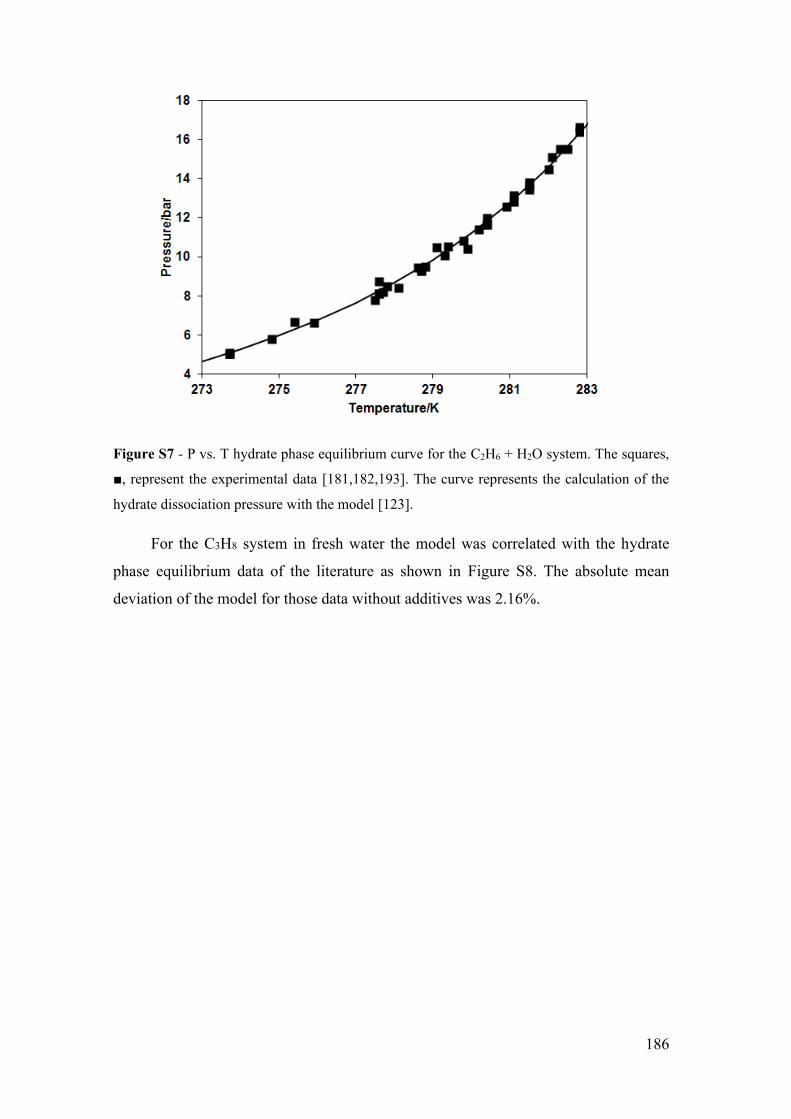
186
Figure S7 - P vs. T hydrate phase equilibrium curve for the C2H6 + H2O system. The squares,
■, represent the experimental data [181,182,193]. The curve represents the calculation of the
hydrate dissociation pressure with the model [123].
For the C3H8 system in fresh water the model was correlated with the hydrate
phase equilibrium data of the literature as shown in Figure S8. The absolute mean
deviation of the model for those data without additives was 2.16%.

187
Figure S8 - P vs. T hydrate phase equilibrium curve for the C3H8 + H2O system. The squares,
■, represent the experimental data [181,186,189–192]. The curve represents the calculation of
the hydrate dissociation pressure with the model [123].
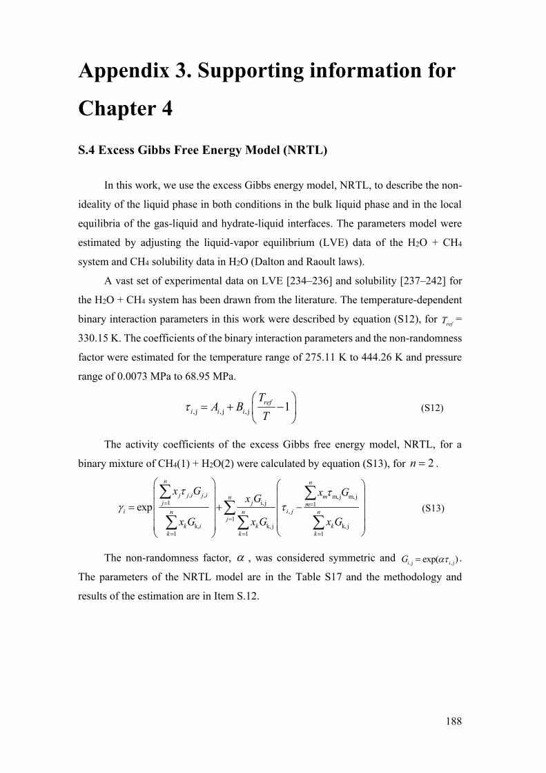
188
Appendix 3. Supporting information for
Chapter 4
S.4 Excess Gibbs Free Energy Model (NRTL)
In this work, we use the excess Gibbs energy model, NRTL, to describe the non-
ideality of the liquid phase in both conditions in the bulk liquid phase and in the local
equilibria of the gas-liquid and hydrate-liquid interfaces. The parameters model were
estimated by adjusting the liquid-vapor equilibrium (LVE) data of the H2O + CH4
system and CH4 solubility data in H2O (Dalton and Raoult laws).
A vast set of experimental data on LVE [234–236] and solubility [237–242] for
the H2O + CH4 system has been drawn from the literature. The temperature-dependent
binary interaction parameters in this work were described by equation (S12), for refT =
330.15 K. The coefficients of the binary interaction parameters and the non-randomness
factor were estimated for the temperature range of 275.11 K to 444.26 K and pressure
range of 0.0073 MPa to 68.95 MPa.
, j , j , j 1refi i i
TA B
T
(S12)
The activity coefficients of the excess Gibbs free energy model, NRTL, for a
binary mixture of CH4(1) + H2O(2) were calculated by equation (S13), for 2n .
, , m, j m, j1 i, j 1
,1
k, k, j k, j1 1 1
exp
n n
j j i j i mnj j m
i i jn n nj
k i k kk k k
x G x Gx G
x G x G x G
(S13)
The non-randomness factor, , was considered symmetric and , j , jexp( )i iG .
The parameters of the NRTL model are in the Table S17 and the methodology and
results of the estimation are in Item S.12.

189
Table S17 - Parameters of the NRTL model, and their respective errors, obtained by adjusting
the liquid-vapor equilibrium and solubility data of the system CH4 (1) + H2O (2).
NRTL Parameters
A1,2 879.302 ± 0.011
A2,1 -208.760 ± 0.007
B1,2 -430.631 ± 0.013
B2,1 -41.891 ± 0.006
0.00161 ± 0.00001
The calculation of the activity of the hydrate-forming components in the liquid
phase, both in the hydrate-liquid equilibrium and in the bulk liquid phase are obtained
by equation (S14) for the CH4+H2O system.
, P, , P,L Li ia T T xx x (S14)
S.5 Calculation of the equilibrium composition at the H-L interface
The work approach by Oliveira et al. [207], although adequate for the equilibrium
calculation, does not calculate the light organics fugacity, such as CH4, in the liquid
aqueous phase. Most hydrate equilibrium calculations in the literature assume that these
compounds are not present in the aqueous phase as they have low water solubility [2].
In this work, to calculate the equilibrium methane composition, at the hydrate-
liquid interface, we use the same approach as Oliveira et al. [207]. The minimization of
the water chemical potential difference between the liquid phase and the hydrate phase.
However, the iterative calculation was carried out at constant pressure and temperature,
varying the equilibrium composition at the hydrate-liquid interface (H-L), and we used
the bulk methane composition as the initial guess.
Therefore, it was necessary to describe the CH4 fugacity in the liquid phase, 4
LCHf
. For this, equation (S15) was used, incorporating non-ideality through the activity
coefficient obtained by the excess Gibbs free energy model, NRTL, Item S.4.
4 4 4
,0, ,L L L LCH CH CH purof T P x f T P (S15)
The fugacity of pure CH4 in the hypothetical liquid phase, 4
,0LCHf , was calculated
by the equation of Prausnitz, Lichtenthaler and Azevedo (1999) [243], where 0P =
101300 [Pa] and 4
LCH = 5.21 10-5 [m³ / mol], equation (S16).
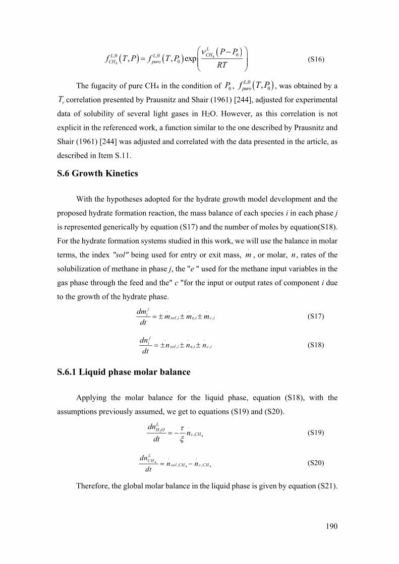
190
4
4
0,0 ,00, , exp
LCHL L
CH puro
P Pf T P f T P
RT
(S16)
The fugacity of pure CH4 in the condition of 0P , ,00,L
purof T P , was obtained by a
rT correlation presented by Prausnitz and Shair (1961) [244], adjusted for experimental
data of solubility of several light gases in H2O. However, as this correlation is not
explicit in the referenced work, a function similar to the one described by Prausnitz and
Shair (1961) [244] was adjusted and correlated with the data presented in the article, as
described in Item S.11.
S.6 Growth Kinetics
With the hypotheses adopted for the hydrate growth model development and the
proposed hydrate formation reaction, the mass balance of each species i in each phase j
is represented generically by equation (S17) and the number of moles by equation(S18).
For the hydrate formation systems studied in this work, we will use the balance in molar
terms, the index "sol" being used for entry or exit mass, .
m , or molar, .n , rates of the
solubilization of methane in phase j, the "e " used for the methane input variables in the
gas phase through the feed and the" c "for the input or output rates of component i due
to the growth of the hydrate phase. . . .
, e, ,
ji
sol i i c idm m m mdt
(S17)
. . .
, e, ,
ji
sol i i c idn n n ndt
(S18)
S.6.1 Liquid phase molar balance
Applying the molar balance for the liquid phase, equation (S18), with the
assumptions previously assumed, we get to equations (S19) and (S20).
24
.
,
LH O
c CHdn
ndt
(S19)
44 4
. .
, ,
LCH
sol CH c CHdn
n ndt
(S20)
Therefore, the global molar balance in the liquid phase is given by equation (S21).

191
2 44 4
. .
, ,1L LLH O CH
sol CH c CHdn dndn n n
dt dt dt
(S21)
Where, 4
.
,sol CHn is the methane solubilization rate in the liquid phase and 4
.
c,CHn is
the hydrate growth rate in terms of the methane moles, Item S.6.4.
S.6.2 Gas phase molar balance
Considering that there is no water evaporation for the gas phase, the mass balance
of the pure methane gas phase is described by equation (S22) in mole terms.
44 4
. .
, ,
GGCH
e CH sol CHdndn n n
dt dt (S22)
Where, 4
.
,e CHn is the methane molar rate entering the reactor and 4
.
,sol CHn is the
methane solubilization rate in the liquid phase according to Item S.6.4.
S.6.3 Solid phase molar balance
For the solid phase, with the hypotheses adopted, considering the hydrate crystal
a homogeneous solid, equation (S23) is given the mole balance.
4
. .
c,H c,CH1SS
Hdndn n ndt dt
(S23)
Where 4
.
c,CHn is the hydrate growth rate in terms of the methane moles, Item S.6.4
S.6.4 Constitutive relations
The methane solubilization molar rate (methane molar rate entering in the liquid
phase), 4
.
,sol CHn , is defined by the methane diffusion from the gas-liquid interface into
the liquid phase, equation (S24), as in Sampaio et al. [87] work, where int ²GLA m is the
gas-liquid interface area and /GLdk m s is the mass transfer coefficient at the gas-liquid
interface. Both parameters are obtained by correlations founded in the literature
[87,245], which are presented in Item S.9.
4 4 4
.int
, eq,
GL GLL Ld
sol CH CH CHL
A kn n nV
(S24)
Using the equilibrium hypothesis at the gas-liquid interface, the methane mole
fraction at the interface is obtained iteratively by the methane fugacity equality in the

192
phases, equation (S25). The Peng-Robinson equation of state is applied to obtain the
methane fugacity coefficient the CH4 pure vapor phase, 4
VCH , while for the methane
fugacity coefficient in the equilibrium liquid phase, 4
LCH , equation (S15) divided by
system pressure was used. For this iterative calculation, the Krichevsky and
Kasarnovsey [246] correlation, shown in Item S.10, is used as an initial guess.
4
4 4 4
4
^
^
,P,
,P,
VCHV L eq
CH CH CHL eqCH
Tf f x
T
y
x (S25)
Therefore, the methane number of moles solubilized in the liquid phase, 4eq,
LCHn , is
given by 4 4eq,
L eq LCH CHn x n , where L L L L
ii
n n V .
The methane molar rate consumed by the hydrate phase growth can be obtained
from the number of moles temporal variation in the particulate phase according to
equation (S26).
4
. .
, ,H
sH
c CH cdnn ndt
(S26)
The hydrate phase number of moles is equal to the product between the molar
density and the phase volume, equation (S27).
s H HHn V (S27)
The methane gas number of moles in the reactor is given by equation (S28), where
4
GCH is the molar density of the pure methane gas phase. The methane feed rate to
maintain the system pressure can be obtained from the vapor phase molar balance,
equation (S22). Applying the chain rule in Equation (S28), we arrive at equation (S29)
to describe the methane rate entering the reactor.
4 4 .
G G GCH CH sistn T V (S28)
4 4
4 4 44
. . .., sol, sol,.
G GGCH CH sistG G
e CH CH CHCH sist
dn d TdVn n T V ndt dt dt
(S29)

193
S.6.5 Volumes and Molar Densities of the Phases
The vapor phase molar density, G , is calculated with the Peng-Robinson EoS for
pure substances, adopting pure CH4 in the vapor phase. Meanwhile, the liquid phase
molar density, L , is calculated by the generalized Rackett equation [222–226]. In this
work, the hydrate phase molar density, H , is considered constant and is obtained by
the product between the hydrate phase mass density of Sloan and Koh [2] and the
hydrate phase molecular mass, HMM . It is obtained through the weighted sum of the
molecular masses of the components, by the number of water molecules and guests
present in the hydrate phase.
The gas volume inside the reactor can be obtained by the difference of the tank
volume, rV , and the volumes of the liquid, LV , and solid phases, SV , equation (S30).
G r L SV V V V (S30)
The liquid phase volume is obtained by defining the liquid phase number of moles,
the product between molar density and the phase volume, equation (S31).
..
( )( )
LL L L L
sist Lsist
nn T V VT
(S31)
Its size distribution characterizes the crystalline population that comes out of a
crystallizer. Because the hydrate phase is a crystalline phase, its properties can be
obtained through its size distribution. The density distribution function, ( , )n t l , refers to
the number, mass or volume of crystals per unit volume of liquid in a size range, whose
average size is l. The cumulative variable of the density distribution function expresses
the number, volume or mass of crystals per unit volume of liquid in a size range [247].
By definition, the third-order moment, 3 , is the cumulative variable of the
density distribution function that express the volume of crystals per unit volume of
liquid for the entire range of system particle size, according to the equation (S32).
Therefore, the third-order moment is proportional to the particulate solid phase volume
given a volumetric form factor, HVk , considered constant for the solid phase, if the liquid
phase volume is known, as shown in equation (S33) [247].
33
0
( , )l n t l dl
(S32)

194
3S L
HV k V (S33)
In this work, we assumed that the shape of the hydrate phase is spherical. The
calculation of the third-order moment of the particulate phase will be discussed below
in Item S.6.6.
S.6.6 Population balance
To understand the polydispersed systems growth kinetics and to compare the
modeling with experimental data, the use of a population balance equation, equation
(S34), is necessary to describe the hydrate particles temporal evolution. The population
balance equation is the conservation equation for the number of particles in a
polydispersed system. Mathematically, the distribution can be affected by external
variables, referring to the particle spatial location, and internal ones, referring to
particles’ intrinsic properties, such as mass and diameter.
In the problem addressed here, the distribution will be affected only by the internal
variable particle diameter l . The population balance equation to be used here is
presented in equation (S34). The deduction of that equation is not part of the scope of
this work, but can be found in [211,212].
( , ) ' ( , t)n l t G n l B Dt l
(S34)
In this equation, ( , t)n l is the function of particles numerical density distribution,
'G is the particle growth rate, B is the particle nucleation rate and D is the rate of
particle breakage and aggregation. That is, B - D is the net rate for particle birth and
death.
Considering that there is no nucleation and neither breaking nor aggregation, the
population balance is expressed by equation (S35).
( , ) ' ( , t) 0n l t G n lt l
(S35)
Here, the population balance objective is to calculate the growth molar rate, and
consequently, the hydrate former consumption molar rate, of the solid phase by
calculating the variation in the particulate phase volume obtained by the third-order
moment, equation (S33).

195
The equation that expresses the growth kinetics in this work is linear. For this
reason, the method chosen to solve the population balance was the most straightforward,
the method of moments, in order to simplify the modeling and make the calculation
faster. However, it is known that the method of moments does not allow the recovery of
the system particle distribution, just the computation of the moments.
Applying the moment operator to a function ( , )n t l , ( , ) jn t l l dl , in equation
(S35), we get to the equation (S36). The growth rate of the particles that will be proposed
in this work does not depend on the size of the particles, that is ' '( )G G t . The
definition of the moment of order j of the system particle distribution is given by
equation (S37).
0 0
( , ) ' ( , t) 0j jl n t l dl G n L l dlt l
(S36)
0
( , )jj l n t l dl
(S37)
As the integral of the first term of equation (S36) is defined, the partial derivative
becomes the total derivative. Replacing the definition of momentum, equation (S37),
we arrive at equation (S38). Integrating the second term of equation (S36) by parts make
it possible to obtain equation (S39).
0
' ( , t) 0j jG n L l dlt l
(S38)
1
00
' ( , ) ( , t) 0j j jG l n l t j n l l dlt
(S39)
Because it represents a probability function, the numerical density distribution
function of particles has the following properties: (0, t) 0n e0
( , t) 1n l dl
. From the
first property it is concluded that the function applied to the zero size particles is null. Using both properties we can conclude that lim ( , t) 0
ln l
, because the area under the
curve ( , )n t l is finite. This conclusion cancels the first term contained in the brackets of equation (S39).
Therefore, when applying the definition of momentum, equation (S37), equation
(S39) is now described by equation (S40).
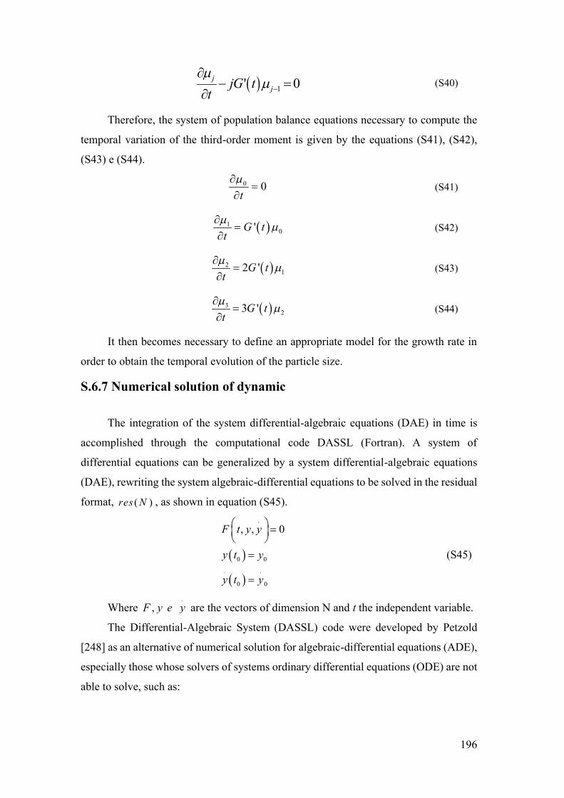
196
1' 0jjjG t
t
(S40)
Therefore, the system of population balance equations necessary to compute the
temporal variation of the third-order moment is given by the equations (S41), (S42),
(S43) e (S44).
0 0t
(S41)
10'G t
t
(S42)
212 'G t
t
(S43)
323 'G t
t
(S44)
It then becomes necessary to define an appropriate model for the growth rate in
order to obtain the temporal evolution of the particle size.
S.6.7 Numerical solution of dynamic
The integration of the system differential-algebraic equations (DAE) in time is
accomplished through the computational code DASSL (Fortran). A system of
differential equations can be generalized by a system differential-algebraic equations
(DAE), rewriting the system algebraic-differential equations to be solved in the residual
format, ( )res N , as shown in equation (S45).
.
0 0
. .
0 0
, , 0F t y y
y t y
y t y
(S45)
Where .
,F y e y are the vectors of dimension N and t the independent variable.
The Differential-Algebraic System (DASSL) code were developed by Petzold
[248] as an alternative of numerical solution for algebraic-differential equations (ADE),
especially those whose solvers of systems ordinary differential equations (ODE) are not
able to solve, such as:
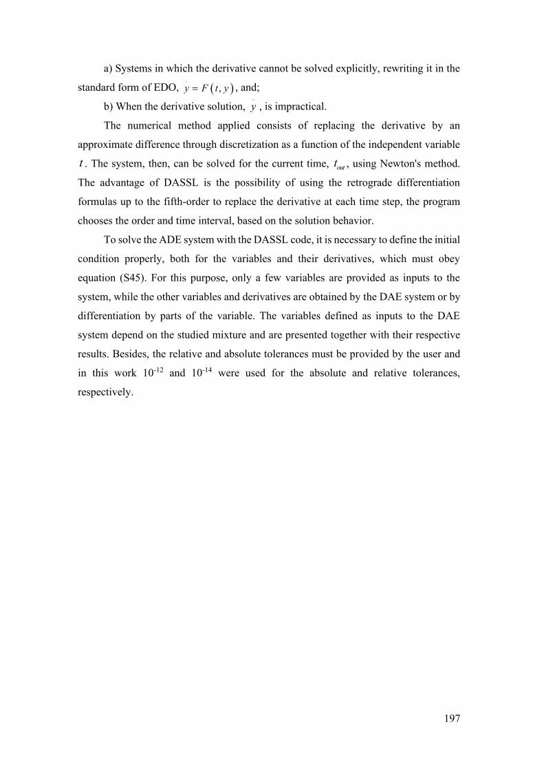
197
a) Systems in which the derivative cannot be solved explicitly, rewriting it in the
standard form of EDO, .
,y F t y , and;
b) When the derivative solution, .y , is impractical.
The numerical method applied consists of replacing the derivative by an
approximate difference through discretization as a function of the independent variable
t . The system, then, can be solved for the current time, outt , using Newton's method.
The advantage of DASSL is the possibility of using the retrograde differentiation
formulas up to the fifth-order to replace the derivative at each time step, the program
chooses the order and time interval, based on the solution behavior.
To solve the ADE system with the DASSL code, it is necessary to define the initial
condition properly, both for the variables and their derivatives, which must obey
equation (S45). For this purpose, only a few variables are provided as inputs to the
system, while the other variables and derivatives are obtained by the DAE system or by
differentiation by parts of the variable. The variables defined as inputs to the DAE
system depend on the studied mixture and are presented together with their respective
results. Besides, the relative and absolute tolerances must be provided by the user and
in this work 10-12 and 10-14 were used for the absolute and relative tolerances,
respectively.
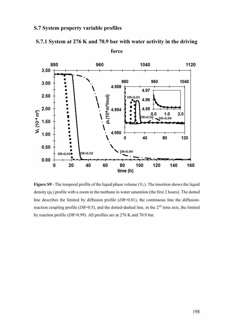
198
S.7 System property variable profiles
S.7.1 System at 276 K and 70.9 bar with water activity in the driving
force
Figure S9 - The temporal profile of the liquid phase volume (VL). The insertion shows the liquid
density (ρL) profile with a zoom in the methane in water saturation (the first 2 hours). The dotted
line describes the limited by diffusion profile (DR=0.01), the continuous line the diffusion-
reaction coupling profile (DR=0.5), and the dotted-dashed line, in the 2nd time axis, the limited
by reaction profile (DR=0.99). All profiles are at 276 K and 70.9 bar.
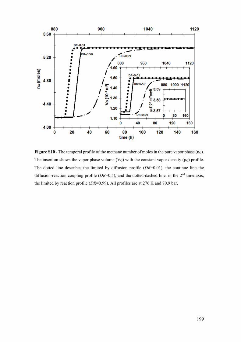
199
Figure S10 - The temporal profile of the methane number of moles in the pure vapor phase (nG).
The insertion shows the vapor phase volume (VG) with the constant vapor density (ρG) profile.
The dotted line describes the limited by diffusion profile (DR=0.01), the continue line the
diffusion-reaction coupling profile (DR=0.5), and the dotted-dashed line, in the 2nd time axis,
the limited by reaction profile (DR=0.99). All profiles are at 276 K and 70.9 bar.
200
Figure S11 - The temporal profile of the product reagents' activities weighted by their
stoichiometric coefficients in the bulk phase variable (Kb) and in the liquid-hydrate equilibrium
interface variable (Keq). The variable in the bulk liquid phase (Kb) is the one with the the highest
value, while the variable in the liquid-hydrate equilibrium interface (Keq) is the one constant.
The insertion shows the hydrate phase volume (VH). The dotted line describes the limited by
diffusion profile (DR=0.01), the continuous line the diffusion-reaction coupling profile
(DR=0.5), and the dotted-dashed line, in the 2nd time axis, the limited by reaction profile
(DR=0.99). All profiles are at 276 K and 70.9 bar.

201
Figure S12 - (a) The temporal profile of the population balance moment of order zero, number
of particles per liquid volume (μ0), (b) moment of order one, particle diameter per liquid volume
(μ1), (c) moment of order two, particle surface area per liquid volume (μ2) and (d) moment of
order three, particle volume per liquid volume (μ3). The inserts are a zoom in the limited by
reaction profile. The dotted line describes the limited by diffusion profile (DR=0.01), the
continue line the diffusion-reaction coupling profile (DR=0.5), and the dotted-dashed line, in
the 2nd time axis, the limited by reaction profile (DR=0.99). All profiles are at 276 K and 70.9
bar.
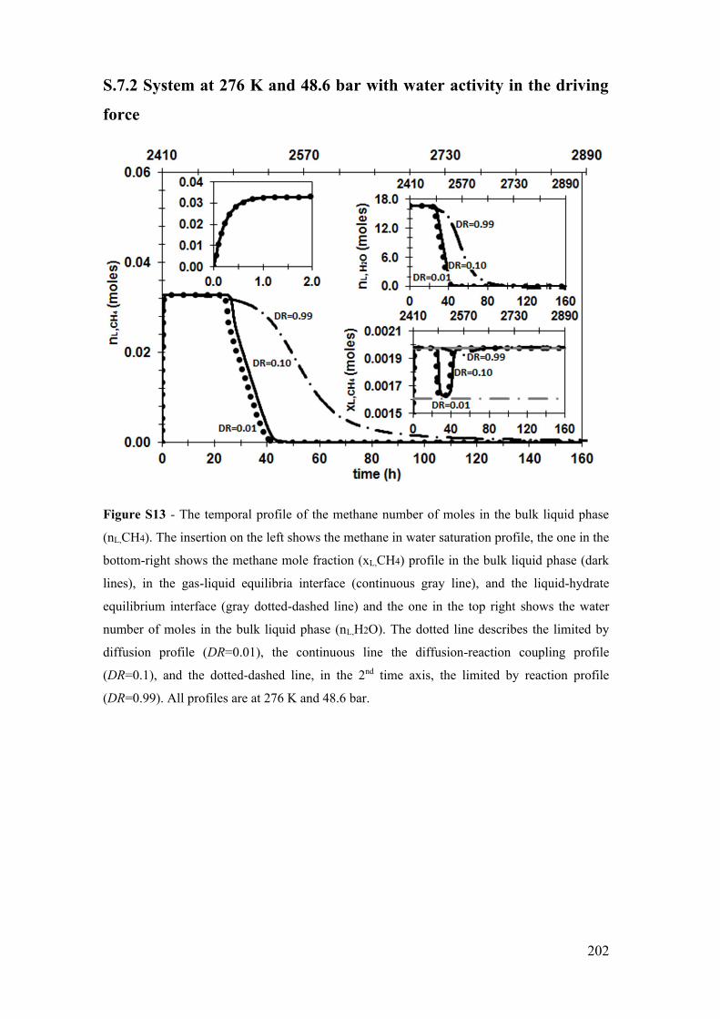
202
S.7.2 System at 276 K and 48.6 bar with water activity in the driving
force
Figure S13 - The temporal profile of the methane number of moles in the bulk liquid phase
(nL,CH4). The insertion on the left shows the methane in water saturation profile, the one in the
bottom-right shows the methane mole fraction (xL,CH4) profile in the bulk liquid phase (dark
lines), in the gas-liquid equilibria interface (continuous gray line), and the liquid-hydrate
equilibrium interface (gray dotted-dashed line) and the one in the top right shows the water
number of moles in the bulk liquid phase (nL,H2O). The dotted line describes the limited by
diffusion profile (DR=0.01), the continuous line the diffusion-reaction coupling profile
(DR=0.1), and the dotted-dashed line, in the 2nd time axis, the limited by reaction profile
(DR=0.99). All profiles are at 276 K and 48.6 bar.
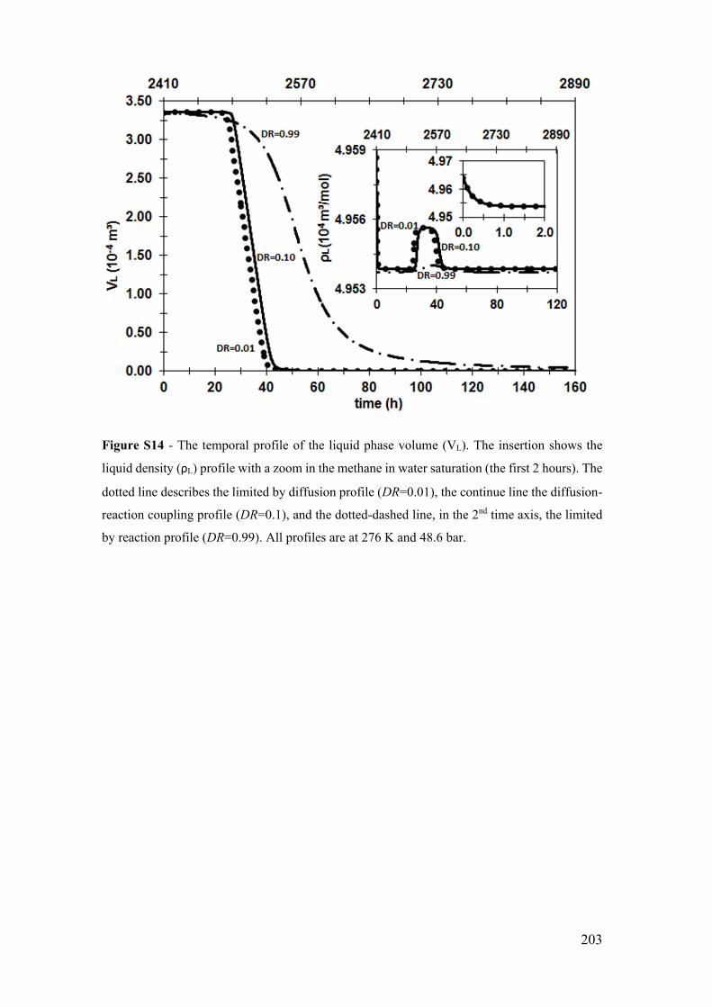
203
Figure S14 - The temporal profile of the liquid phase volume (VL). The insertion shows the
liquid density (ρL) profile with a zoom in the methane in water saturation (the first 2 hours). The
dotted line describes the limited by diffusion profile (DR=0.01), the continue line the diffusion-
reaction coupling profile (DR=0.1), and the dotted-dashed line, in the 2nd time axis, the limited
by reaction profile (DR=0.99). All profiles are at 276 K and 48.6 bar.
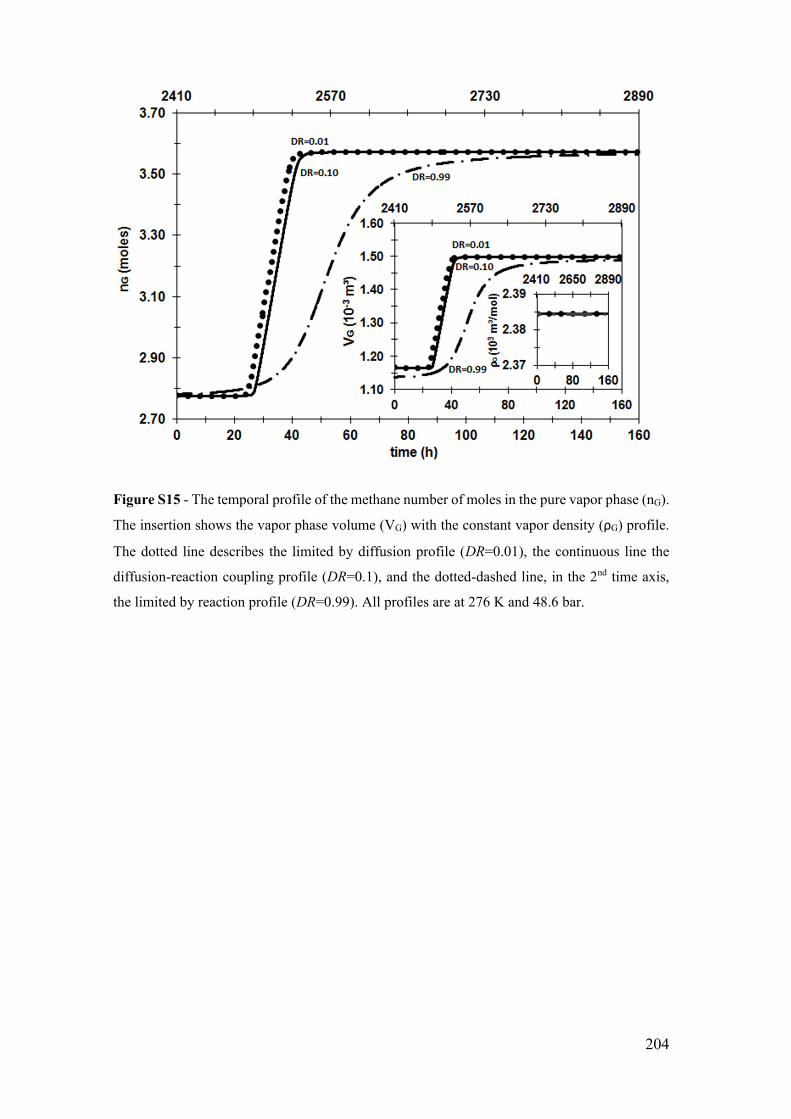
204
Figure S15 - The temporal profile of the methane number of moles in the pure vapor phase (nG).
The insertion shows the vapor phase volume (VG) with the constant vapor density (ρG) profile.
The dotted line describes the limited by diffusion profile (DR=0.01), the continuous line the
diffusion-reaction coupling profile (DR=0.1), and the dotted-dashed line, in the 2nd time axis,
the limited by reaction profile (DR=0.99). All profiles are at 276 K and 48.6 bar.
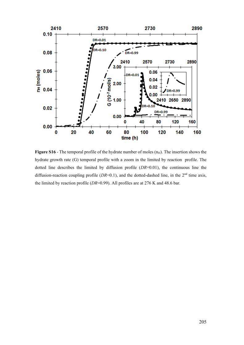
205
Figure S16 - The temporal profile of the hydrate number of moles (nH). The insertion shows the
hydrate growth rate (G) temporal profile with a zoom in the limited by reaction profile. The
dotted line describes the limited by diffusion profile (DR=0.01), the continuous line the
diffusion-reaction coupling profile (DR=0.1), and the dotted-dashed line, in the 2nd time axis,
the limited by reaction profile (DR=0.99). All profiles are at 276 K and 48.6 bar.
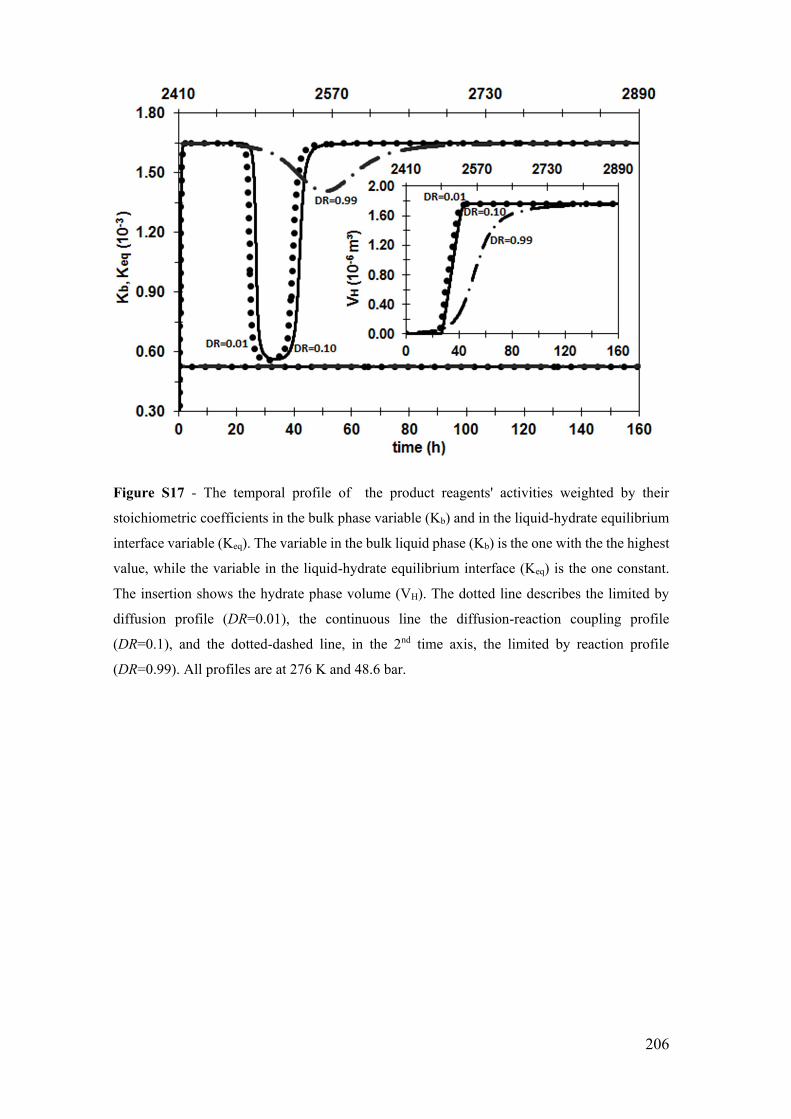
206
Figure S17 - The temporal profile of the product reagents' activities weighted by their
stoichiometric coefficients in the bulk phase variable (Kb) and in the liquid-hydrate equilibrium
interface variable (Keq). The variable in the bulk liquid phase (Kb) is the one with the the highest
value, while the variable in the liquid-hydrate equilibrium interface (Keq) is the one constant.
The insertion shows the hydrate phase volume (VH). The dotted line describes the limited by
diffusion profile (DR=0.01), the continuous line the diffusion-reaction coupling profile
(DR=0.1), and the dotted-dashed line, in the 2nd time axis, the limited by reaction profile
(DR=0.99). All profiles are at 276 K and 48.6 bar.

207
Figure S18 - (a) The temporal profile of the population balance moment of order zero, number
of particles per liquid volume (μ0), (b) moment of order one, particle diameter per liquid volume
(μ1), (c) moment of order two, particle surface area per liquid volume (μ2) and (d) moment of
order three, particle volume per liquid volume (μ3). The inserts are a zoom in the limited by
reaction profile. The dotted line describes the limited by diffusion profile (DR=0.01), the
continuous line the diffusion-reaction coupling profile (DR=0.1), and the dotted-dashed line, in
the 2nd time axis, the limited by reaction profile (DR=0.99). All profiles are at 276 K and 48.6
bar.

208
Figure S19 - The temporal profile of the methane molar consumption (ΔnG). The insertion
shows the temporal variation of the methane number of moles in the gas phase (nG). The dotted
line describes the limited by diffusion profile (DR=0.01), the continue line the diffusion-reaction
coupling profile (DR=0.1), and the dotted-dashed line, in the 2nd time axis, the limited by
reaction profile (DR=0.99). All profiles are at 276 K and 48.6 bar. The black circles are the
Englezos et al. [42] data also at 276 K and 48.6 bar.

209
S.7.3 System at 274 K and 76.0 bar with water activity in the driving
force
Figure S20 - The temporal profile of the methane number of moles in the bulk liquid phase
(nL,CH4). The insertion on the left shows the methane in water saturation profile, the one in the
bottom-right shows the methane mole fraction (xL,CH4) profile in the bulk liquid phase (dark
lines), in the gas-liquid equilibria interface (gray continus line), and in the liquid-hydrate
equilibrium interface (gray dotted-dashed line) and the one in the top right shows the water
number of moles in the bulk liquid phase (nL,H2O). The dotted line describes the limited by
diffusion profile (DR=0.01), the continuous line the diffusion-reaction coupling profile
(DR=0.6), and the dotted-dashed line, in the 2nd time axis, the limited by reaction profile
(DR=0.99). All profiles are at 274 K and 76.0 bar.

210
Figure S21 - The temporal profile of the liquid phase volume (VL). The insertion shows the
liquid density (ρL) profile with a zoom in the methane in water saturation (the first 2 hours). The
dotted line describes the limited by diffusion profile (DR=0.01), the continuous line the
diffusion-reaction coupling profile (DR=0.6), and the dotted-dashed line, in the 2nd time axis,
the limited by reaction profile (DR=0.99). All profiles are at 274 K and 76.0 bar.
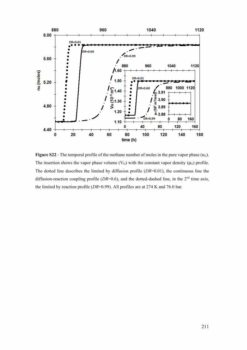
211
Figure S22 - The temporal profile of the methane number of moles in the pure vapor phase (nG).
The insertion shows the vapor phase volume (VG) with the constant vapor density (ρG) profile.
The dotted line describes the limited by diffusion profile (DR=0.01), the continuous line the
diffusion-reaction coupling profile (DR=0.6), and the dotted-dashed line, in the 2nd time axis,
the limited by reaction profile (DR=0.99). All profiles are at 274 K and 76.0 bar.
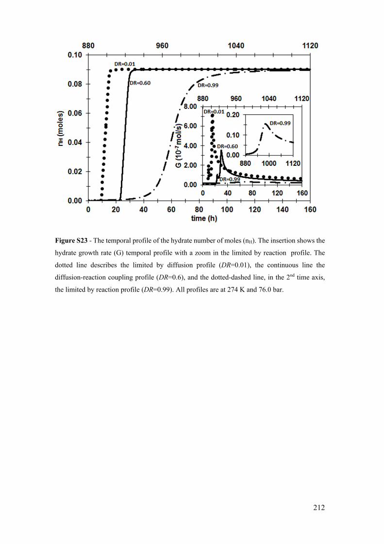
212
Figure S23 - The temporal profile of the hydrate number of moles (nH). The insertion shows the
hydrate growth rate (G) temporal profile with a zoom in the limited by reaction profile. The
dotted line describes the limited by diffusion profile (DR=0.01), the continuous line the
diffusion-reaction coupling profile (DR=0.6), and the dotted-dashed line, in the 2nd time axis,
the limited by reaction profile (DR=0.99). All profiles are at 274 K and 76.0 bar.

213
Figure S24 - The temporal profile of the product reagents' activities weighted by their
stoichiometric coefficients in the bulk phase variable (Kb) and in the liquid-hydrate equilibrium
interface variable (Keq). The variable in the bulk liquid phase (Kb) is the one with the the highest
value, while the variable in the liquid-hydrate equilibrium interface (Keq) is the one constant.
The insertion shows the hydrate phase volume (VH). The dotted line describes the limited by
diffusion profile (DR=0.01), the continuous line the diffusion-reaction coupling profile
(DR=0.6), and the dotted-dashed line, in the 2nd time axis, the limited by reaction profile
(DR=0.99). All profiles are at 274 K and 76.0 bar.
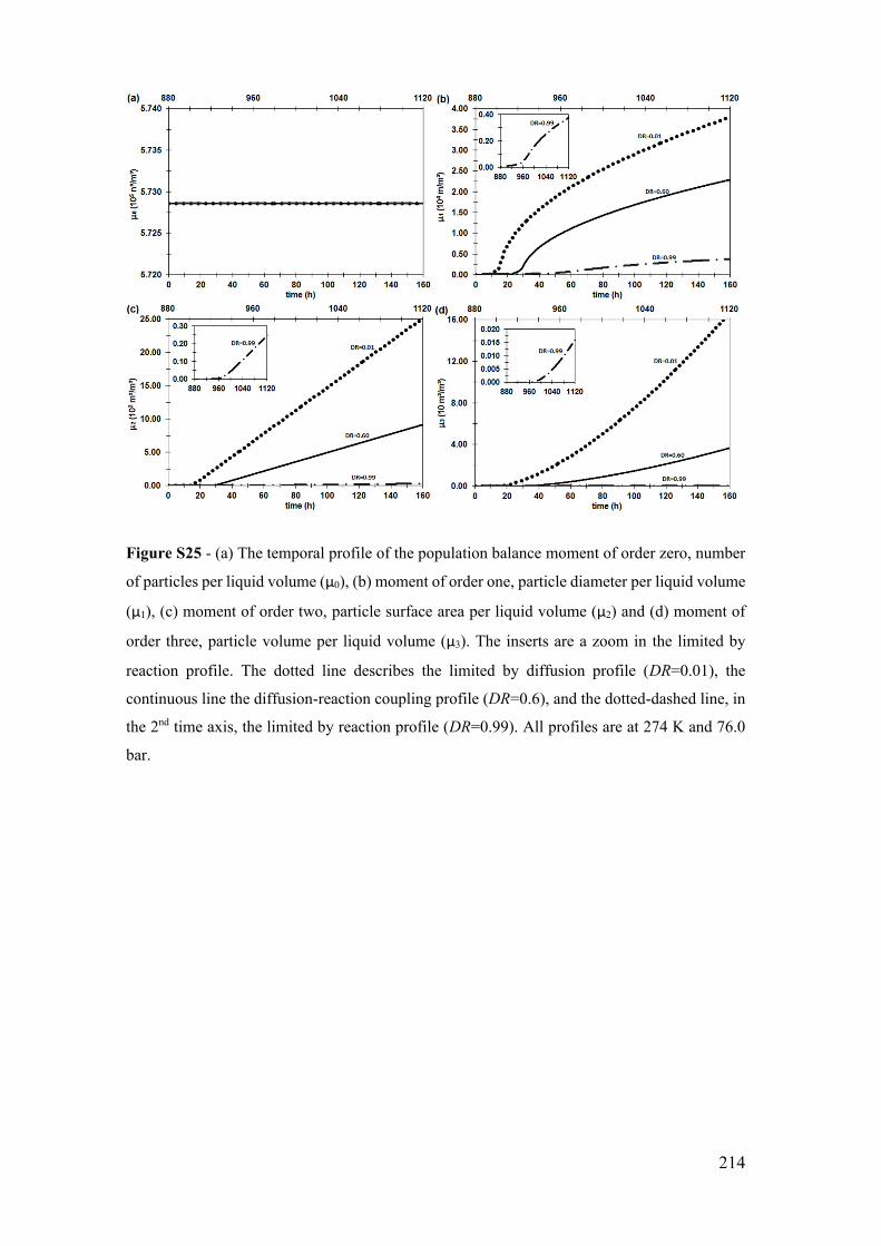
214
Figure S25 - (a) The temporal profile of the population balance moment of order zero, number
of particles per liquid volume (μ0), (b) moment of order one, particle diameter per liquid volume
(μ1), (c) moment of order two, particle surface area per liquid volume (μ2) and (d) moment of
order three, particle volume per liquid volume (μ3). The inserts are a zoom in the limited by
reaction profile. The dotted line describes the limited by diffusion profile (DR=0.01), the
continuous line the diffusion-reaction coupling profile (DR=0.6), and the dotted-dashed line, in
the 2nd time axis, the limited by reaction profile (DR=0.99). All profiles are at 274 K and 76.0
bar.

215
Figure S26 - The temporal profile of the methane molar consumption (ΔnG). The insertion
shows the temporal variation of the methane number of moles in the gas phase (nG). The dotted
line describes the limited by diffusion profile (DR=0.01), the continuous line the diffusion-
reaction coupling profile (DR=0.6), and the dotted-dashed line, in the 2nd time axis, the limited
by reaction profile (DR=0.99). All profiles are at 274 K and 76.0 bar. The black circles are the
Englezos et al. (1987) [42] data also at 274 K and 76.0 bar.

216
S.7.4 System at 276 K and 70.9 bar without water activity in the driving
force
Figure S27 - The diffusion-reaction coupling (DR=0.5) temporal profile of the methane number
of moles in the bulk liquid phase (nL,CH4). The insertion on the left shows the methane in water
saturation profile, the one in the bottom-right shows the methane mole fraction (xL,CH4) profile
in the bulk liquid phase (dark lines), in the gas-liquid equilibria interface (gray continus line)
and in the liquid-hydrate equilibrium interface (gray dotted-dashed line) and the one in the top
right shows the water number of moles in the bulk liquid phase (nL,H2O). The continuous line
represents the profile with the water activity, while the dashed line represents the profile without
the water activity in the growth rate driving force. All profiles are at 276 K and 70.9 bar.
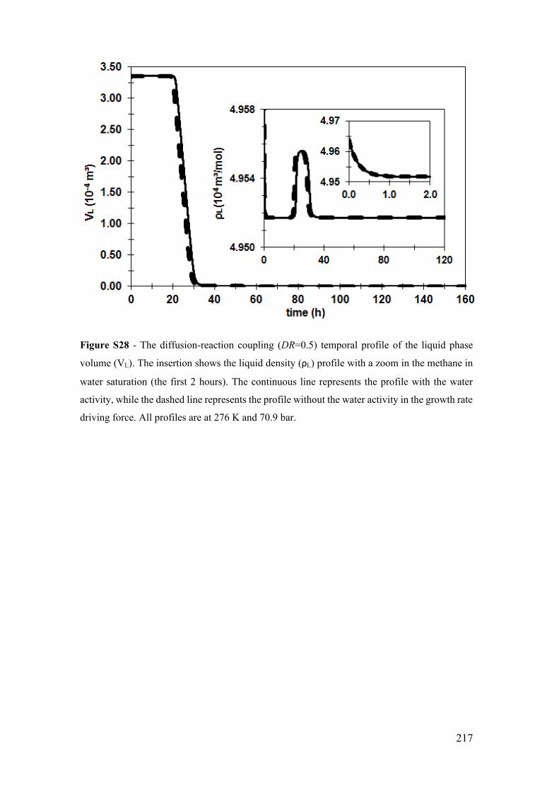
217
Figure S28 - The diffusion-reaction coupling (DR=0.5) temporal profile of the liquid phase
volume (VL). The insertion shows the liquid density (ρL) profile with a zoom in the methane in
water saturation (the first 2 hours). The continuous line represents the profile with the water
activity, while the dashed line represents the profile without the water activity in the growth rate
driving force. All profiles are at 276 K and 70.9 bar.

218
Figure S29 - The diffusion-reaction coupling (DR=0.5) temporal profile of the methane number
of moles in the pure vapor phase (nG). The insertion shows the vapor phase volume (VG) with
the constant vapor density (ρG) profile. The continuous line represents the profile with the water
activity, while the dashed line represents the profile without the water activity in the growth rate
driving force. All profiles are at 276 K and 70.9 bar.
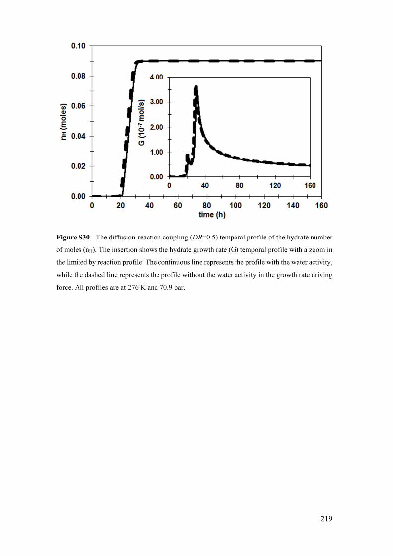
219
Figure S30 - The diffusion-reaction coupling (DR=0.5) temporal profile of the hydrate number
of moles (nH). The insertion shows the hydrate growth rate (G) temporal profile with a zoom in
the limited by reaction profile. The continuous line represents the profile with the water activity,
while the dashed line represents the profile without the water activity in the growth rate driving
force. All profiles are at 276 K and 70.9 bar.

220
Figure S31 - The diffusion-reaction coupling (DR=0.5) temporal profile of the product reagents'
activities weighted by their stoichiometric coefficients in the bulk phase variable (Kb) and in the
liquid-hydrate equilibrium interface variable (Keq). The variable in the bulk liquid phase (Kb) is
the one with the the highest value, while the variable in the liquid-hydrate equilibrium interface
(Keq) is the one constant. The insertion shows the hydrate phase volume (VH). The continuous
line represents the profile with the water activity, while the dashed line represents the profile
without the water activity in the growth rate driving force. All profiles are at 276 K and 70.9
bar.
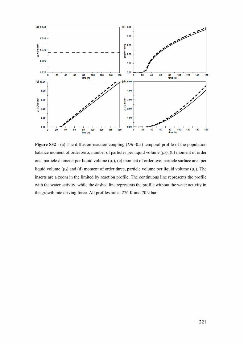
221
Figure S32 - (a) The diffusion-reaction coupling (DR=0.5) temporal profile of the population
balance moment of order zero, number of particles per liquid volume (μ0), (b) moment of order
one, particle diameter per liquid volume (μ1), (c) moment of order two, particle surface area per
liquid volume (μ2) and (d) moment of order three, particle volume per liquid volume (μ3). The
inserts are a zoom in the limited by reaction profile. The continuous line represents the profile
with the water activity, while the dashed line represents the profile without the water activity in
the growth rate driving force. All profiles are at 276 K and 70.9 bar.
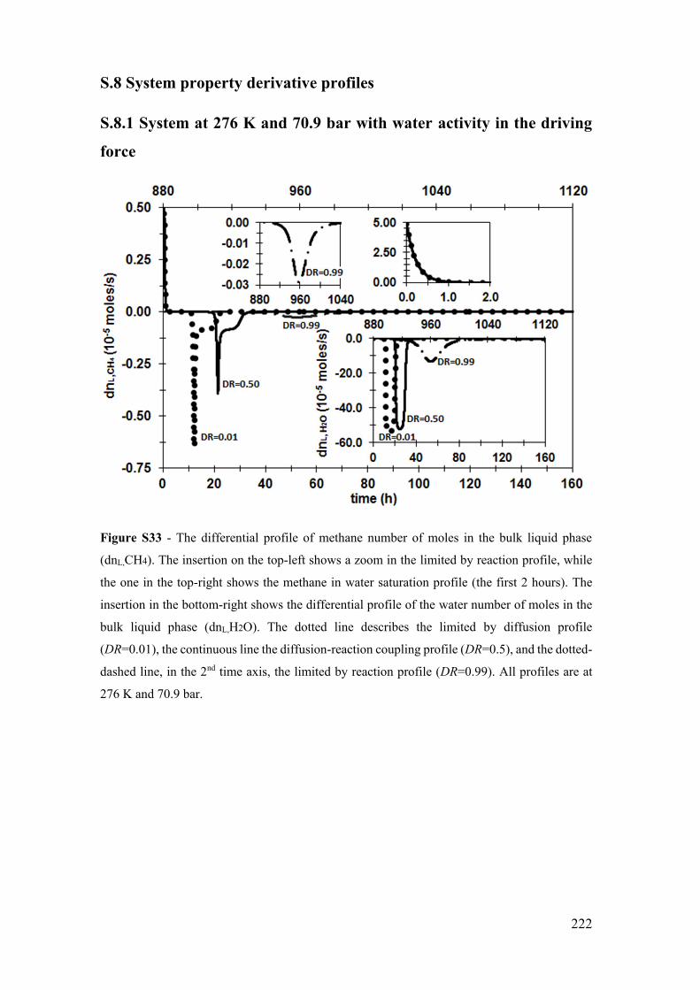
222
S.8 System property derivative profiles
S.8.1 System at 276 K and 70.9 bar with water activity in the driving
force
Figure S33 - The differential profile of methane number of moles in the bulk liquid phase
(dnL,CH4). The insertion on the top-left shows a zoom in the limited by reaction profile, while
the one in the top-right shows the methane in water saturation profile (the first 2 hours). The
insertion in the bottom-right shows the differential profile of the water number of moles in the
bulk liquid phase (dnL,H2O). The dotted line describes the limited by diffusion profile
(DR=0.01), the continuous line the diffusion-reaction coupling profile (DR=0.5), and the dotted-
dashed line, in the 2nd time axis, the limited by reaction profile (DR=0.99). All profiles are at
276 K and 70.9 bar.

223
Figure S34 - The differential profile of the liquid phase volume (dVL). The insertion shows the
differential profile of the liquid density (dρL) with a zoon in the methane in water saturation (the
first 2 hours) and in the limited by reaction profile. The dotted line describes the limited by
diffusion profile (DR=0.01), the continuous line the diffusion-reaction coupling profile
(DR=0.5), and the dotted-dashed line, in the 2nd time axis, the limited by reaction profile
(DR=0.99). All profiles are at 276 K and 70.9 bar.

224
Figure S35 - The differential profile of the methane number of moles in the pure vapor phase
(dnG). The insertion shows the vapor phase volume (dVG) with the constant vapor density (dρG)
differential profile. The dotted line describes the limited by diffusion profile (DR=0.01), the
continuous line the diffusion-reaction coupling profile (DR=0.5), and the dotted-dashed line, in
the 2nd time axis, the limited by reaction profile (DR=0.99). All profiles are at 276 K and 70.9
bar.

225
Figure S36 - The differential profile of the hydrate number of moles (dnH). The insertion shows
the hydrate phase volume (dVH) differential profile. The dotted line describes the limited by
diffusion profile (DR=0.01), the continuous line the diffusion-reaction coupling profile
(DR=0.5), and the dotted-dashed line, in the 2nd time axis, the limited by reaction profile
(DR=0.99). All profiles are at 276 K and 70.9 bar.

226
Figure S37 - (a) The differential profile of the population balance moment of order zero, number
of particles per liquid volume (dμ0), (b) moment of order one, particle diameter per liquid
volume (dμ1), (c) moment of order two, particle surface area per liquid volume (dμ2) and (d)
moment of order three, particle volume per liquid volume (dμ3). The inserts are a zoom in the
limited by reaction differential profile. The dotted line describes the limited by diffusion profile
(DR=0.01), the continuous line the diffusion-reaction coupling profile (DR=0.5), and the dotted-
dashed line, in the 2nd time axis, the limited by reaction profile (DR=0.99). All profiles are at
276 K and 70.9 bar.

227
S.8.2 System at 276 K and 48.6 bar with water activity in the driving
force
Figure S38 - The differential profile of methane number of moles in the bulk liquid phase
(dnL,CH4). The insertion on the top-left shows a zoom in the limited by reaction profile, while
the one in the top-right shows the methane in water saturation profile (the first 2 hours). The
insertion in the bottom-right shows the differential profile of the water number of moles in the
bulk liquid phase (dnL,H2O). The dotted line describes the limited by diffusion profile
(DR=0.01), the continuous line the diffusion-reaction coupling profile (DR=0.1), and the dotted-
dashed line, in the 2nd time axis, the limited by reaction profile (DR=0.99). All profiles are at
276 K and 48.6 bar.
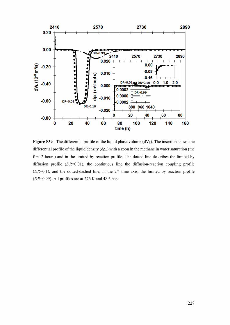
228
Figure S39 - The differential profile of the liquid phase volume (dVL). The insertion shows the
differential profile of the liquid density (dρL) with a zoon in the methane in water saturation (the
first 2 hours) and in the limited by reaction profile. The dotted line describes the limited by
diffusion profile (DR=0.01), the continuous line the diffusion-reaction coupling profile
(DR=0.1), and the dotted-dashed line, in the 2nd time axis, the limited by reaction profile
(DR=0.99). All profiles are at 276 K and 48.6 bar.
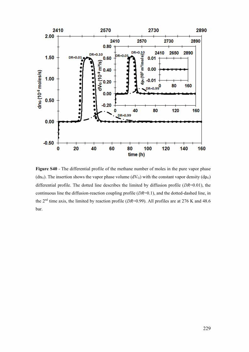
229
Figure S40 - The differential profile of the methane number of moles in the pure vapor phase
(dnG). The insertion shows the vapor phase volume (dVG) with the constant vapor density (dρG)
differential profile. The dotted line describes the limited by diffusion profile (DR=0.01), the
continuous line the diffusion-reaction coupling profile (DR=0.1), and the dotted-dashed line, in
the 2nd time axis, the limited by reaction profile (DR=0.99). All profiles are at 276 K and 48.6
bar.
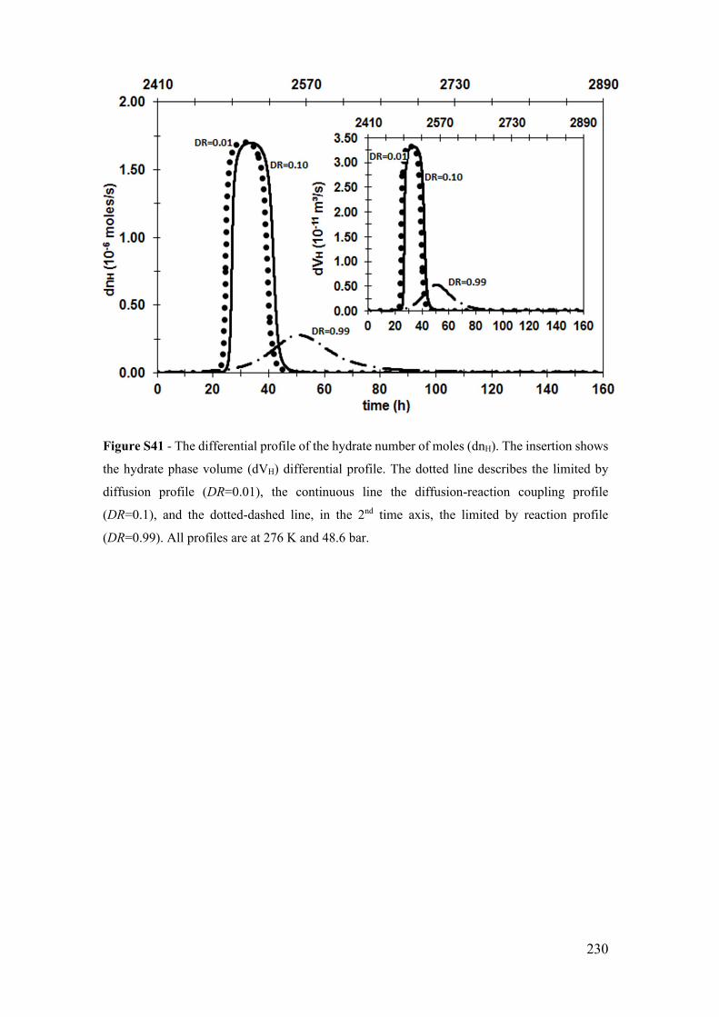
230
Figure S41 - The differential profile of the hydrate number of moles (dnH). The insertion shows
the hydrate phase volume (dVH) differential profile. The dotted line describes the limited by
diffusion profile (DR=0.01), the continuous line the diffusion-reaction coupling profile
(DR=0.1), and the dotted-dashed line, in the 2nd time axis, the limited by reaction profile
(DR=0.99). All profiles are at 276 K and 48.6 bar.
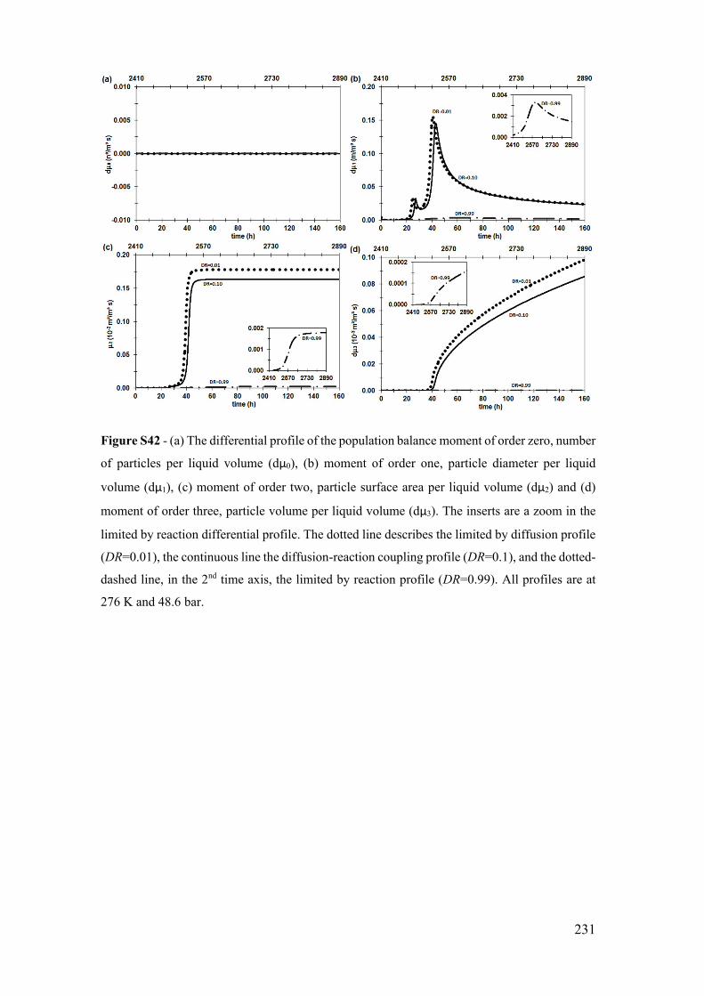
231
Figure S42 - (a) The differential profile of the population balance moment of order zero, number
of particles per liquid volume (dμ0), (b) moment of order one, particle diameter per liquid
volume (dμ1), (c) moment of order two, particle surface area per liquid volume (dμ2) and (d)
moment of order three, particle volume per liquid volume (dμ3). The inserts are a zoom in the
limited by reaction differential profile. The dotted line describes the limited by diffusion profile
(DR=0.01), the continuous line the diffusion-reaction coupling profile (DR=0.1), and the dotted-
dashed line, in the 2nd time axis, the limited by reaction profile (DR=0.99). All profiles are at
276 K and 48.6 bar.

232
S.8.3 System at 274 K and 76.0 bar with water activity in the driving
force
Figure S43 - The differential profile of methane number of moles in the bulk liquid phase
(dnL,CH4). The insertion on the top-left shows a zoom in the limited by reaction profile, while
the one in the top-right shows the methane in water saturation profile (the first 2 hours). The
insertion in the bottom-right shows the differential profile of the water number of moles in the
bulk liquid phase (dnL,H2O). The dotted line describes the limited by diffusion profile
(DR=0.01), the continuous line the diffusion-reaction coupling profile (DR=0.6), and the dotted-
dashed line, in the 2nd time axis, the limited by reaction profile (DR=0.99). All profiles are at
274 K and 76.0 bar.

233
Figure S44 - The differential profile of the liquid phase volume (dVL). The insertion shows the
differential profile of the liquid density (dρL) with a zoon in the methane in water saturation (the
first 2 hours) and in the limited by reaction profile. The dotted line describes the limited by
diffusion profile (DR=0.01), the continuous line the diffusion-reaction coupling profile
(DR=0.6), and the dotted-dashed line, in the 2nd time axis, the limited by reaction profile
(DR=0.99). All profiles are at 274 K and 76.0 bar.
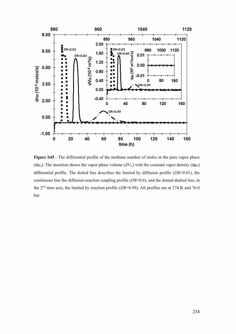
234
Figure S45 - The differential profile of the methane number of moles in the pure vapor phase
(dnG). The insertion shows the vapor phase volume (dVG) with the constant vapor density (dρG)
differential profile. The dotted line describes the limited by diffusion profile (DR=0.01), the
continuous line the diffusion-reaction coupling profile (DR=0.6), and the dotted-dashed line, in
the 2nd time axis, the limited by reaction profile (DR=0.99). All profiles are at 274 K and 76.0
bar.
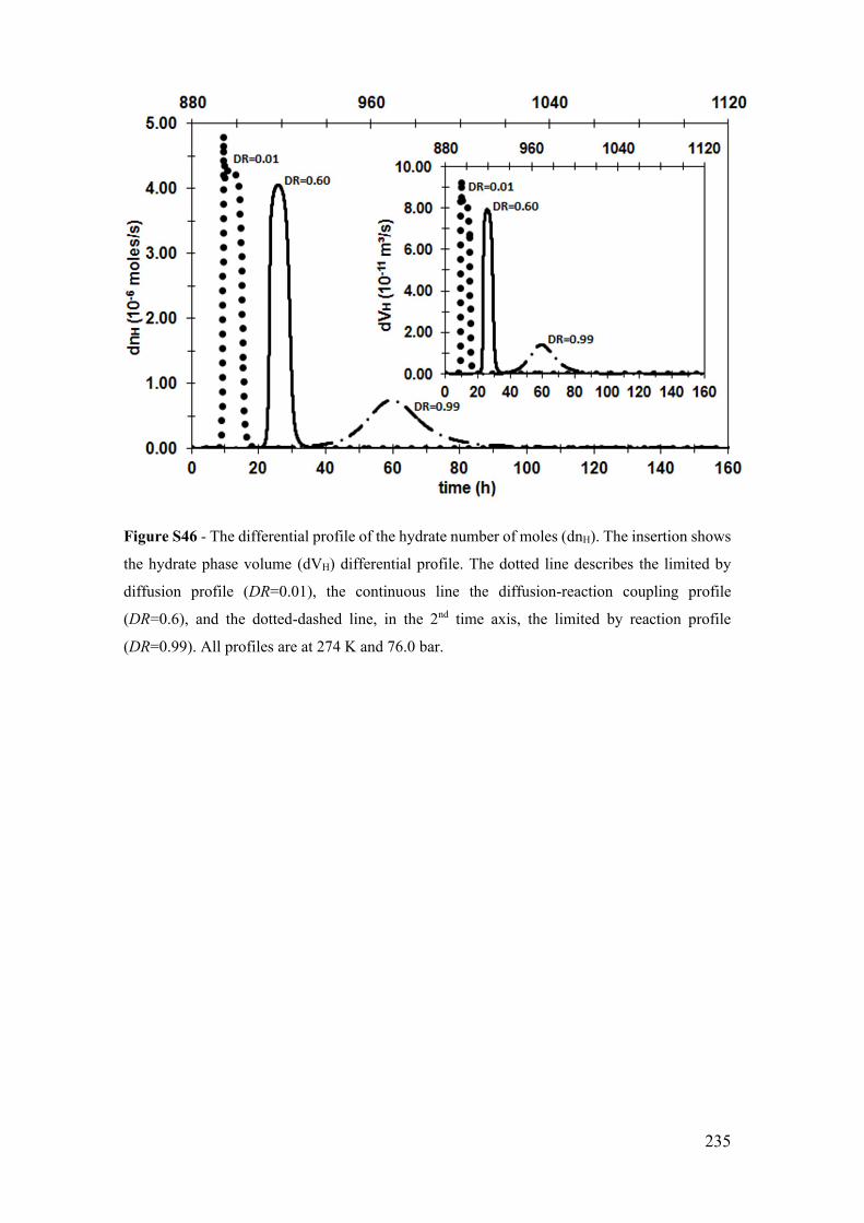
235
Figure S46 - The differential profile of the hydrate number of moles (dnH). The insertion shows
the hydrate phase volume (dVH) differential profile. The dotted line describes the limited by
diffusion profile (DR=0.01), the continuous line the diffusion-reaction coupling profile
(DR=0.6), and the dotted-dashed line, in the 2nd time axis, the limited by reaction profile
(DR=0.99). All profiles are at 274 K and 76.0 bar.

236
Figure S47 - (a) The differential profile of the population balance moment of order zero, number
of particles per liquid volume (dμ0), (b) moment of order one, particle diameter per liquid
volume (dμ1), (c) moment of order two, particle surface area per liquid volume (dμ2) and (d)
moment of order three, particle volume per liquid volume (dμ3). The inserts are a zoom in the
limited by reaction differential profile. The dotted line describes the limited by diffusion profile
(DR=0.01), the continuous line the diffusion-reaction coupling profile (DR=0.6), and the dotted-
dashed line, in the 2nd time axis, the limited by reaction profile (DR=0.99). All profiles are at
274 K and 76.0 bar.

237
S.8.4 System at 276 K and 70.9 bar without water activity in the driving
force
Figure S48 - The diffusion-reaction coupling (DR=0.5) differential profile of methane number
of moles in the bulk liquid phase (dnL,CH4). The insertion on the top-left shows a zoom in the
limited by reaction profile, while the one in the top-right shows the methane in water saturation
profile (the first 2 hours). The insertion in the bottom-right shows the differential profile of the
water number of moles in the bulk liquid phase (dnL,H2O). The continuous line represents the
profile with the water activity, while the dashed line represents the profile without the water
activity in the growth rate driving force. All profiles are at 276 K and 70.9 bar.

238
Figure S49 - The diffusion-reaction coupling (DR=0.5) differential profile of the liquid phase
volume (dVL). The insertion shows the differential profile of the liquid density (dρL) with a
zoom in the methane in water saturation (the first 2 hours) and in the limited by reaction profile.
The continuous line represents the profile with the water activity, while the dashed line
represents the profile without the water activity in the growth rate driving force. All profiles are
at 276 K and 70.9 bar.
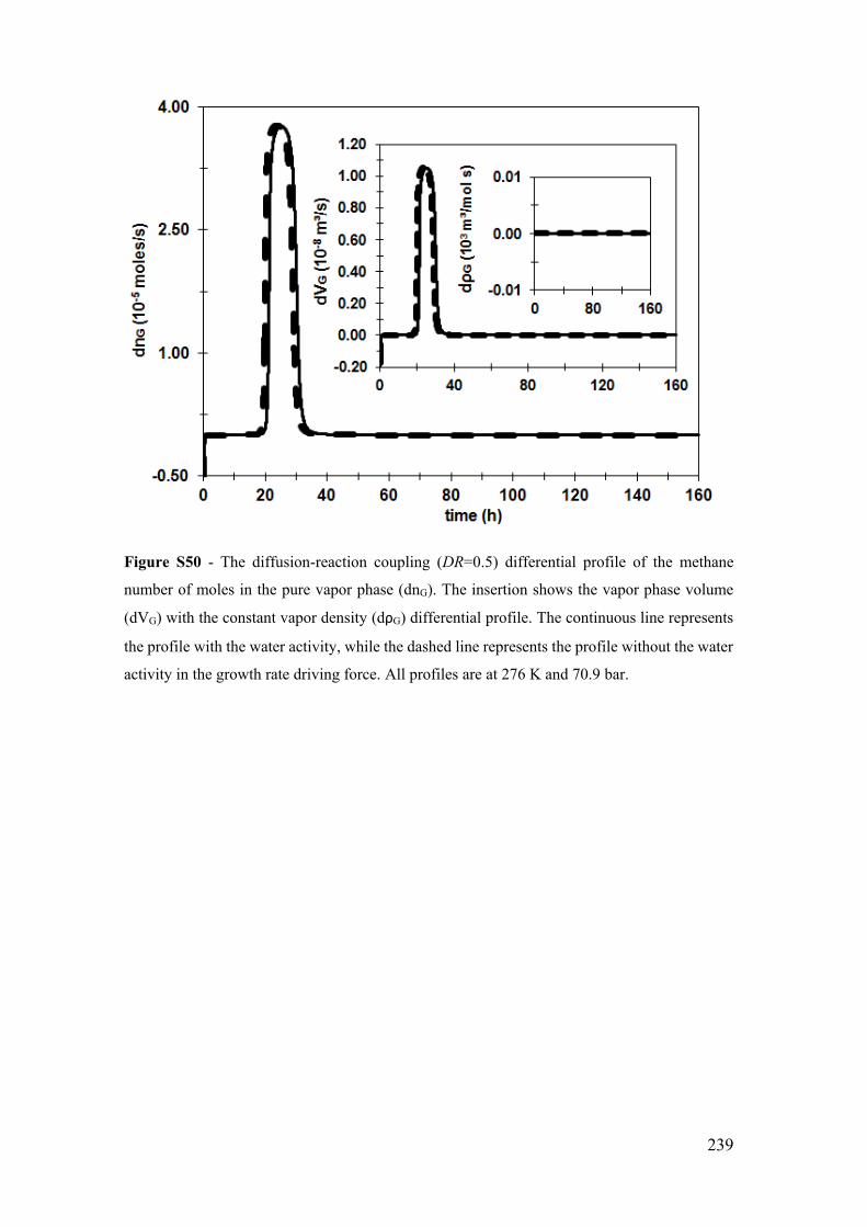
239
Figure S50 - The diffusion-reaction coupling (DR=0.5) differential profile of the methane
number of moles in the pure vapor phase (dnG). The insertion shows the vapor phase volume
(dVG) with the constant vapor density (dρG) differential profile. The continuous line represents
the profile with the water activity, while the dashed line represents the profile without the water
activity in the growth rate driving force. All profiles are at 276 K and 70.9 bar.

240
Figure S51 - The diffusion-reaction coupling (DR=0.5) differential profile of the hydrate
number of moles (dnH). The insertion shows the hydrate phase volume (dVH) differential profile.
The continuous line represents the profile with the water activity, while the dashed line
represents the profile without the water activity in the growth rate driving force. All profiles are
at 276 K and 70.9 bar.
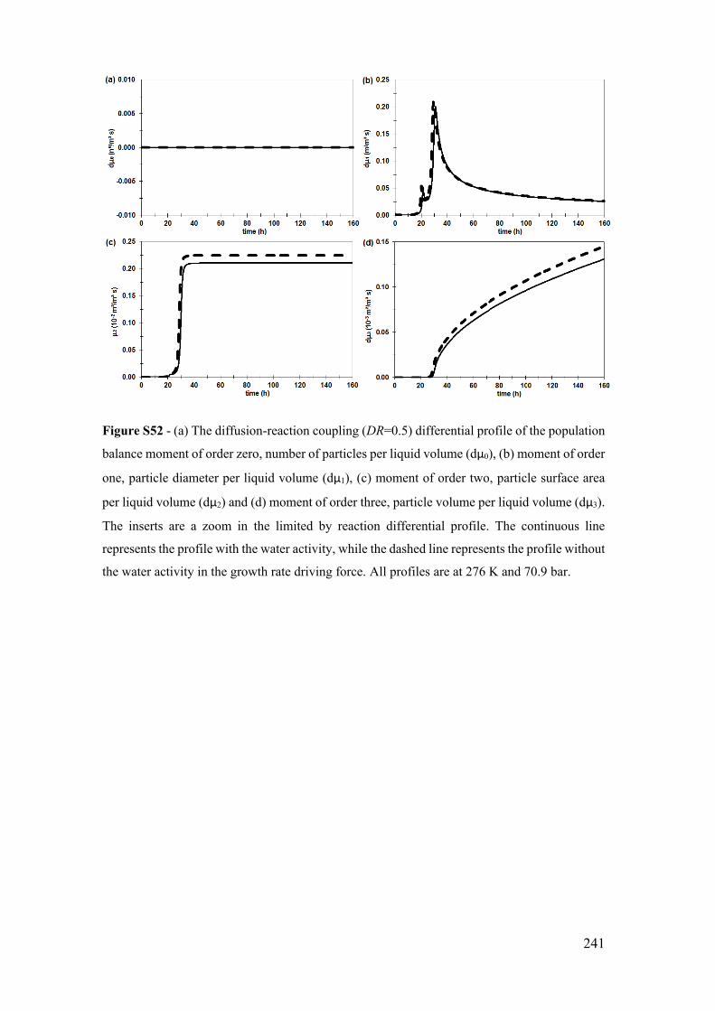
241
Figure S52 - (a) The diffusion-reaction coupling (DR=0.5) differential profile of the population
balance moment of order zero, number of particles per liquid volume (dμ0), (b) moment of order
one, particle diameter per liquid volume (dμ1), (c) moment of order two, particle surface area
per liquid volume (dμ2) and (d) moment of order three, particle volume per liquid volume (dμ3).
The inserts are a zoom in the limited by reaction differential profile. The continuous line
represents the profile with the water activity, while the dashed line represents the profile without
the water activity in the growth rate driving force. All profiles are at 276 K and 70.9 bar.
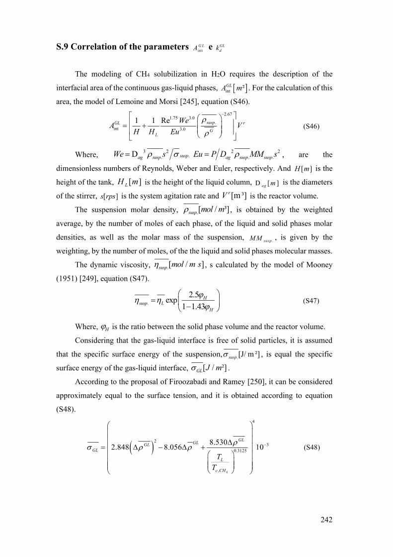
242
S.9 Correlation of the parameters in tG LA e GL
dk
The modeling of CH4 solubilization in H2O requires the description of the
interfacial area of the continuous gas-liquid phases, int ²GLA m . For the calculation of this
area, the model of Lemoine and Morsi [245], equation (S46).
2.671.75 3.0
.int 3.0
1 1 Re suspGL rG
L
WeA VH H Eu
(S46)
Where, 3 2..D suspag suspWe s 2 2
. .ag susp suspEu P D MM s , are the
dimensionless numbers of Reynolds, Weber and Euler, respectively. And [ ]H m is the
height of the tank, [ ]LH m is the height of the liquid column, D [ ]ag m is the diameters
of the stirrer, [ ]s rps is the system agitation rate and [m³]rV is the reactor volume.
The suspension molar density, .[ / ³]susp mol m , is obtained by the weighted
average, by the number of moles of each phase, of the liquid and solid phases molar
densities, as well as the molar mass of the suspension, .suspM M , is given by the
weighting, by the number of moles, of the the liquid and solid phases molecular masses.
The dynamic viscosity, .[ / ]susp mol m s , s calculated by the model of Mooney
(1951) [249], equation (S47).
.2.5exp
1 1.43H
susp LH
(S47)
Where, H is the ratio between the solid phase volume and the reactor volume.
Considering that the gas-liquid interface is free of solid particles, it is assumed
that the specific surface energy of the suspension, .[J/ m ²]susp , is equal the specific
surface energy of the gas-liquid interface, [ / ²]GL J m .
According to the proposal of Firoozabadi and Ramey [250], it can be considered
approximately equal to the surface tension, and it is obtained according to equation
(S48).
4
4
23
0.3125
,
8.5302.848 8.056 1 0GLGLGL
GL
L
c CH
TT
(S48)

243
where GL is the difference between the liquid and vapor phases molar
densities.
To determine the diffusion coefficient of methane, [ / ]GLdk m s , the penetration
model proposed by Taniguchi, Kawaguchi and Kikuchi [251] equation (S49) is used.
14
.
.
5 0. suspGLd
susp
k D
(S49)
Where [ ² / ]D m s is the diffusivity of the gas and [ ² / ³]m s is the average energy
input calculated according to the Spicer and Pratsinis [252] equation (S50).
3 5
OP agr
N s DV
(S50)
And OPN , [ ]s rps and [ ]agD m are the agitator power number, the agitator blade
diameter and the system agitation rate, respectively.
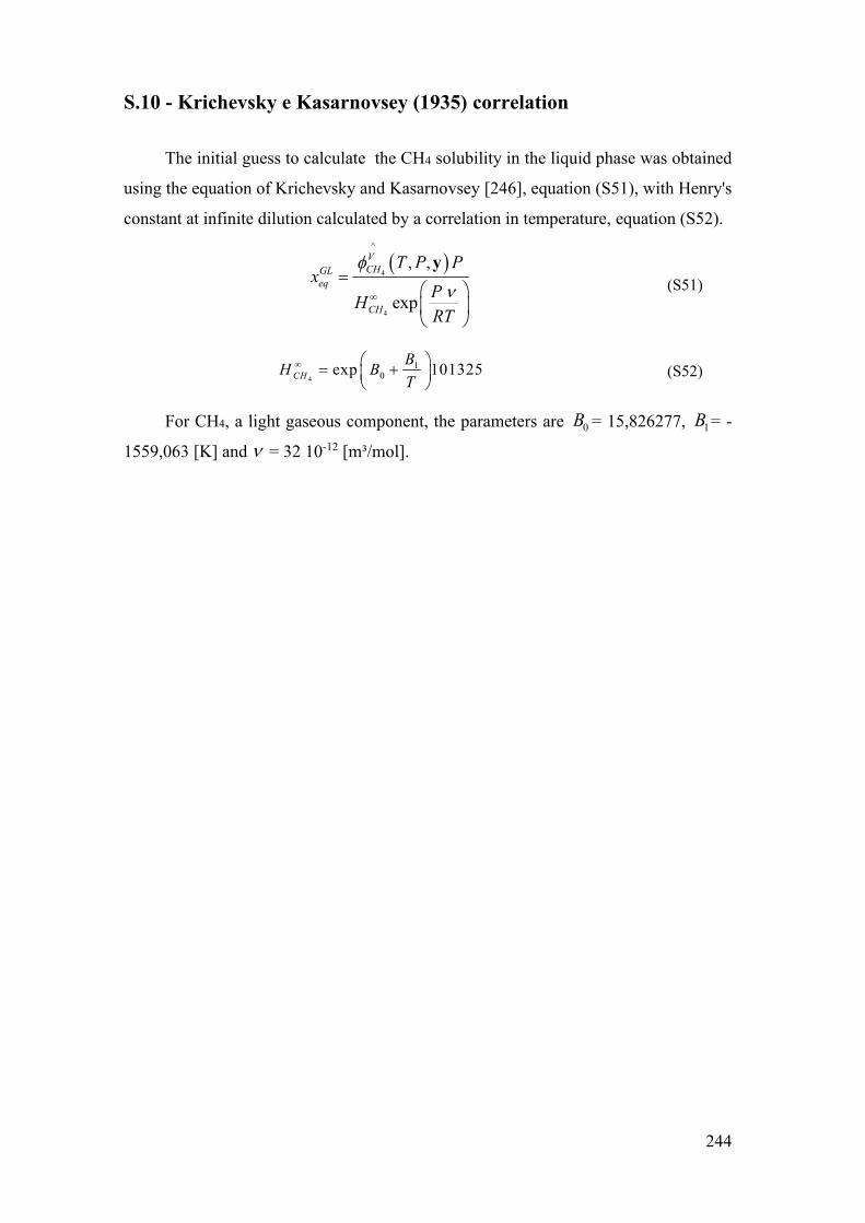
244
S.10 - Krichevsky e Kasarnovsey (1935) correlation
The initial guess to calculate the CH4 solubility in the liquid phase was obtained
using the equation of Krichevsky and Kasarnovsey [246], equation (S51), with Henry's
constant at infinite dilution calculated by a correlation in temperature, equation (S52).
4
4
^
, ,
exp
VCHGL
eq
CH
T P Px
PHRT
y (S51)
4
10exp 101325CH
BH BT
(S52)
For CH4, a light gaseous component, the parameters are 0B = 15,826277, 1B = -
1559,063 [K] and = 32 10-12 [m³/mol].

245
S.11 - Fugacity correlation of the light gases hypothetical liquid phase
at 101.32 Pa
According to Prausnitz and Shair [244] the volatility of the solute hypothetical
liquid phase at 101.32 Pa, being this a light gas, depends only on the temperature and
properties of the solute, that is, it is independent of the solvent properties. It is possible,
therefore, to apply the corresponding state theorem and show that the reduced fugacity
of the hypothetical liquid solute is a universal function of the reduced temperature.
Prausnitz and Shair [244] correlated data on light gas solubility using an
exponential function. However, as this function is not explicit in that work, the
calculation of the hypothetical liquid phase fugacity in this work was performed using
an exponential function, equation (S53), adjusted to the data obtained by the Prausnitz
and Shair [244] work.
The adjustment is shown in Figure S53 and the parameters obtained are in Table
S18.
,0 31 20 2, expL
puror r r
DD Df T PT T T
(S53)
Table S18 - Correlation parameters of the hypothetical liquid phase for light gases at 101.32
Pa and their respective deviations.
Correlation parameters
1D 2D 3D
44,490 ± 0,326 -1,445 ± 0,025 -2,688 ± 0,020

246
Figure S53 - Fugacy profile of the hypothetical liquid phase for light gases by the correlation
of Prausnitz and Shair [244] with the temperature at 101.32 Pa. The points, ●, represent the
calculation of the correlation and the curve the calculation performed by the function used in
this work.
Since the critical temperature of CH4 is 190.56 K and the occurrence of hydrate
formation in the range of 266.15 to 280.15 K, we work in the reduced temperature range
of 1.4 to 1.5, which was the range that showed the best agreement with the correlation
of Prausnitz and Shair [244].
0.1
1.0
10.0
0.4 0.8 1.2 1.6 2 2.4 2.8 3.2
fL,0
Pc
Tr

247
S.12 - NRTL model adjustment with LVE and solubility experimental
data of the CH4 + H2O system
The parameters of the NRTL model were estimated by minimizing the sum of the
quadratic residues of the output variables for each experiment (l), according to equation
(S54).
exp2 2
obj calc exp calc exp1
Nl l l ll
F w P P w y y (S54)
For each type of experimental data, the implemented routine allows different
calculations with the NRTL model: for solubility data, only the equilibrium pressure is
calculated; and for the liquid-vapor equilibrium data, the pressure and composition of
the vapor phase in equilibrium are calculated using the temperature and composition of
the liquid phase as input variables. is the set of parameters to be estimated. For the
NRTL model, it was defined as: 1,2 2 ,1 1,2 2 ,1( , , B , B )A A . The inverse of the admitted
weights for each output variable was 0.0001% of the measured variable. These weights
were defined in order to establish similar deviations for all points.
The NRTL model parameters, Table S15, were estimated for liquid-vapor balance
data of H2O (2) + CH4 (1) at the temperature of 283.89 K, 298.31 K, 313.11 K and
323.56 K, Figure S54, and solubility data between 275.11 K and 444.26 K, Figure S55,
covered a pressure range of 0.0073 MPa to 68.95 MPa.

248
Figure S54 - H2O+CH4 liquid-vapor equilibrium isothermal curves. The experimental data are
represented by the filled circles for (a) the dew point and for (b) the bubble point [234–236].
The empty circles represent the points calculated with the NRTL model.
Figure S55 - Isothermal curves of CH4 solubility in H2O. The experimental data is represented
by the filled circles [237–242]. The empty circles represent the points calculated with the NRTL
model.
Here, the particle swarm method - PSO [233] was used as the stochastic method
to achieve a good initial estimate to be provided to a Quasi-Newton type algorithm, a
deterministic method that uses differential calculus techniques.
Calculations of absolute average deviations, equation (S55), are used to analyze
the best adjustments.
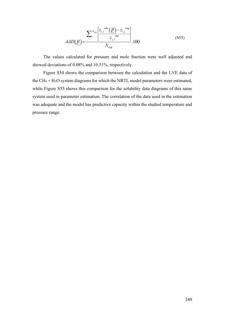
249
exp
calc exp, ,
exp,
exp
.100
N i j i j
ii j
z zz
AADN
(S55)
The values calculated for pressure and mole fraction were well adjusted and
showed deviations of 0.08% and 10.51%, respectively.
Figure S54 shows the comparison between the calculation and the LVE data of
the CH4 + H2O system diagrams for which the NRTL model parameters were estimated,
while Figure S55 shows this comparison for the solubility data diagrams of this same
system used in parameter estimation. The correlation of the data used in the estimation
was adequate and the model has predictive capacity within the studied temperature and
pressure range.

250
Appendix 4. Supporting information for
Chapter 5 S.13 Excess Gibbs Free Energy Model (NRTL)
In this work, we use the excess Gibbs energy model, NRTL, to describe the non-
ideality of the liquid phase in both conditions in the bulk liquid phase and in the local
equilibria of the gas-liquid and hydrate-liquid interfaces. The activity coefficients of the
excess Gibbs free energy model, NRTL, for the ternary mixture of H2O(1) + CH4(2) +
EtOH(3) were calculated by equation (S56), for 3n .
The NRTL model parameters were estimated by adjusting the binary systems
(H2O + CH4; H2O + EtOH; CH4 + EtOH) in equilibrium. In our previous work, Oliveira
et al. (2020, in submission process, Appendix 3) we used the liquid-vapor equilibrium
(LVE) and CH4 solubility in H2O data to estimate the NRTL parameters of the pair H2O
+ CH4 (Dalton and Raoult laws). For the pair H2O + EtOH the NRTL parameters were
estimated in Oliveira et al. [124] using the liquid-vapor equilibrium (LVE) and infinite
dilution of EtOH in H2O data. The NRTL parameters for CH4 + EtOH were estimated
here using liquid-vapor equilibrium (LVE) data. The conditions for estimating these
parameters were chosen according to the available experimental data from the respective
systems. However, with the objective of estimating parameters under conditions other
than hydrate formation conditions to obtain poorly correlated parameters of high
transferability.
A set of experimental data on LVE [165,253,254] for the CH4 + EtOH system has
been drawn from the literature. The temperature-dependent binary interaction
parameters in this work were described by equation (S57)(S1), for refT = 280.15 K. The
coefficients of the binary interaction parameters and the non-randomness factor were
estimated for the temperature range of 238.15 K to 333.40 K and pressure range of 0.33
MPa to 41.69 MPa.
, , m, j m, j1 i, j 1
,1
k, k, j k, j1 1 1
exp
n n
j j i j i mnj j m
i i jn n nj
k i k kk k k
x G x Gx G
x G x G x G
(S56)

251
, j , j , j 1refi i i
TA B
T
(S57)
The activity coefficients of the excess Gibbs free energy model, NRTL, for a
binary mixture of CH4(1) + EtOH(2) were calculated by equation (S56)(S2), for 2n .
The non-randomness factor, , was considered symmetric for each binary system
and , j , jexp( )i iG . The parameters of the NRTL model are in Table S19 and the
methodology and results of the estimation are in Item S.19.
Table S19 - Parameters of the ternary NRTL model for the system H2O(1) + CH4(2) +
EtOH(3), and their respective errors, obtained by adjusting experimental data from binary
systems.
Ternary NRTL Parameters
A1,2 -208.760 ±
0.007 A1,3
3.078 ±
0.077 A2,3
26.250 ±
0.019
A2,1 879.302 ±
0.011 A3,1
-1.577 ±
0.068 A3,2
-2.013 ±
0.003
B1,2 -41.891 ±
0.006 B1,3
-11.387 ±
0.223 B2,3
-146.893 ±
0.328
B2,1 -430.631 ±
0.013 B3,1
7.193 ±
0.161 B3,2
-16.337 ±
0.037
α1,2 = α2,1 0.00161 ±
0.00001 α1,3 = α3,1
0.06097 ±
0.00197 α2,3 = α3,2
0.08057 ±
0.00022
Tref 1,2 = Tref 2,1 330.15 K Tref 1,3 = Tref 3,1 283.15 K Tref 2,3 = Tref 3,2 280.15 K
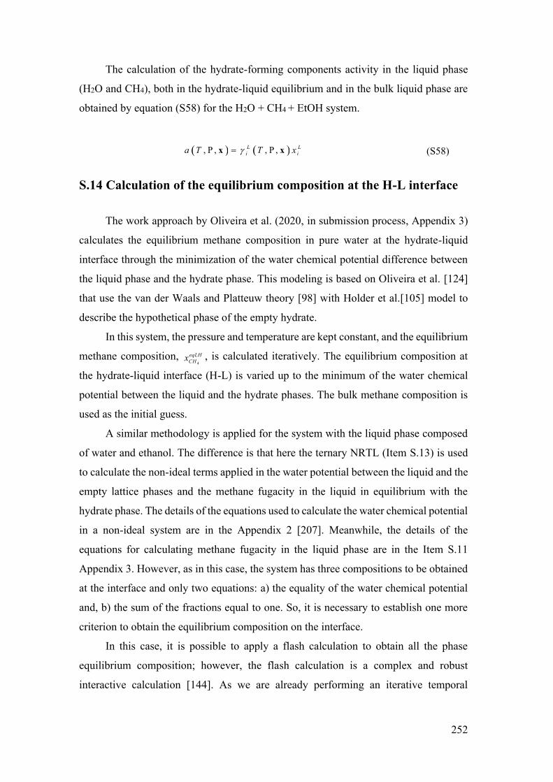
252
The calculation of the hydrate-forming components activity in the liquid phase
(H2O and CH4), both in the hydrate-liquid equilibrium and in the bulk liquid phase are
obtained by equation (S58) for the H2O + CH4 + EtOH system.
, P , , P ,L Li ia T T xx x (S58)
S.14 Calculation of the equilibrium composition at the H-L interface
The work approach by Oliveira et al. (2020, in submission process, Appendix 3)
calculates the equilibrium methane composition in pure water at the hydrate-liquid
interface through the minimization of the water chemical potential difference between
the liquid phase and the hydrate phase. This modeling is based on Oliveira et al. [124]
that use the van der Waals and Platteuw theory [98] with Holder et al.[105] model to
describe the hypothetical phase of the empty hydrate.
In this system, the pressure and temperature are kept constant, and the equilibrium
methane composition, 4
eqLHCHx , is calculated iteratively. The equilibrium composition at
the hydrate-liquid interface (H-L) is varied up to the minimum of the water chemical
potential between the liquid and the hydrate phases. The bulk methane composition is
used as the initial guess.
A similar methodology is applied for the system with the liquid phase composed
of water and ethanol. The difference is that here the ternary NRTL (Item S.13) is used
to calculate the non-ideal terms applied in the water potential between the liquid and the
empty lattice phases and the methane fugacity in the liquid in equilibrium with the
hydrate phase. The details of the equations used to calculate the water chemical potential
in a non-ideal system are in the Appendix 2 [207]. Meanwhile, the details of the
equations for calculating methane fugacity in the liquid phase are in the Item S.11
Appendix 3. However, as in this case, the system has three compositions to be obtained
at the interface and only two equations: a) the equality of the water chemical potential
and, b) the sum of the fractions equal to one. So, it is necessary to establish one more
criterion to obtain the equilibrium composition on the interface.
In this case, it is possible to apply a flash calculation to obtain all the phase
equilibrium composition; however, the flash calculation is a complex and robust
interactive calculation [144]. As we are already performing an iterative temporal

253
calculation of the system variables, this flash would have to be executed several times
for the temporal computation. Since the objective is to obtain a model capable of
describing the dynamic behavior in a quick and functional way, we then chose to use
one of the system hypotheses to define the methane composition at the H-L interface.
Considering that the ethanol is not consumed with hydrate growth is possible to
establish a third criterion. In this criterion, the ethanol number of moles in the liquid
phase does not suffer spatial or temporal variation. Ethanol has the same number of
moles at the interfaces and in bulk, and is preserved over time, with null time derivative.
Therefore, for each iterative calculation of the methane composition at the H-L
interface, an ethanol composition is defined. The number of moles of methane is equally
distributed in the liquid phase, i.e., the ethanol composition is constant spatially, but it
varies over time. Therefore, the methane and water are obtained from the water equal
chemical potential between the hydrate and liquid phases and the molar sum equal to 1,
receptively, while the amount of ethanol is kept constant.
Briefly, the calculation performed is the same as for the pure water system present
in Oliveira et al. (2020, in submission process), Item S.5 Appendix 3; however, using
the ternary NRTL to obtain the non-ideal properties of the liquid phase as activity and
activity coefficient of the systems.
S.15 Growth Kinetics
Similar modeling applied for the H2O+CH4 system (Item S.6 Appendix 3) is
applied for the H2O+CH4+EtOH system, including the ethanol in the balances. Here we
present only the equations that changed or are included in the differential equation
system due to the ethanol addition.
Using the hypotheses adopted to adapt the model to systems inhibited by ethanol,
changes, and inclusions of differential equations will be presented in this topic.
S.15.1 Liquid phase mole balance
Applying the mole balance for the liquid phase with the hypotheses previously
assumed, we get to equation (S59) for the ethanol. Given the considerations that ethanol
does not participate in the solid structure, and at low temperatures, it practically does
not evaporate into the gas phase, the ethanol molar derivative in the liquid phase will be
null. Because of this non-participation of ethanol in the solid and vapor phase, the water

254
and methane mole balance in the liquid phase was still the same in Item S.6 Appendix
3 for the system with fresh water.
0LEtOHdndt
(S59)
Therefore, the global mole balance in the liquid phase is given by equation (S60).
The same one for the freshwater system.
2 44 4
. .
, ,1L L LLH O CH EtOH
sol CH c CHdn dn dndn n n
dt dt dt dt
(S60)
Where, 4
.
,so l C Hn is the methane solubilization rate in the liquid phase and 4
.
c,CHn is
the hydrate growth rate in terms of the methane moles, Item S.15.40.
The index "sol" holds for entry or exit molar, .n , rates of the solubilization of
methane in phase j, o "e "used for the methane input variables in the gas phase through
the feed and the" c "for the input or output rates of component i due to the growth of the
hydrate phase.
S.15.2 Gas-phase mole balance
Considering that there is no water and ethanol evaporation for the gas phase, the
mass balance of the pure methane gas phase in molar terms does not modify by the
addition of ethanol, i.e., is the same as the freshwater.
S.15.3 Solid-phase mole balance
With the hypotheses adopted for the solid phase, the ethanol only acts as a
thermodynamic hydrate inhibiter. So, the hydrate crystal is a homogeneous solid without
the ethanol participation in the structure and the mole balance is kept the same one used
for freshwater.
S.15.4 Constitutive relations
The methane solubilization molar rate (methane molar rate entering in the liquid
phase), 4
.
,so l C Hn , is defined by the methane diffusion from the gas-liquid interface into
the liquid phase, equation (S61)(S24), as in Sampaio et al. [87] work, where in t ²G LA m
is the gas-liquid interface area and /GLdk m s is the mass transfer coefficient at the gas-

255
liquid interface. Both parameters are obtained by correlations founded in the literature
[87,245], presented in Item S.18.
4 4 4
.int
, eq,
GL GLL Ld
sol CH CH CHL
A kn n nV
(S61)
When using the equilibrium hypothesis at the gas-liquid interface, the methane
mole fraction at the interface is obtained iteratively by the methane fugacity equality in
the phases, equation (S62). The Peng-Robinson equation of state is applied to obtain the
methane fugacity coefficient the CH4 pure vapor phase4
VCH . For this iterative
calculation, the Krichevsky and Kasarnovsey [246] correlation is used as an initial
guess.
4
4 4 4
4
^
,0
,P,,P, ,
VCHV L eqGL
CH CH CH L LCH puro
T Pf f x
T f T P
yx
(S62)
The fugacity of pure CH4 in the hypothetical liquid phase, 4
,0LC Hf , was calculated
by the equation of Prausnitz, Lichtenthaler, and Azevedo [243], where 0P = 101300 [Pa]
and 4
LCH = 5.21 10-5 [m³ / mol]. The same methodology is used to calculate the methane
fugacity in the liquid phase in equilibrium with the hydrate phase4
eqLHCHx .
The fugacity of pure CH4 in the condition 0P ,00,L
purof T P was obtained by a rT
correlation presented by Prausnitz and Shair [244], adjusted for experimental data of
solubility of several light gases H2O. However, as this correlation is not explicit in the
referenced work, a function similar to the one described by Prausnitz and Shair [244]
was adjusted and correlated with the data presented in the article, as described in Item
S.11 of the Appendix 3 above.
Therefore, the methane number of moles solubilized in the liquid phase, 4eq,
LCHn , is
given by 4 4eq,
L eq LCH CHn x n , where
LL L Li
in n V .
The methane molar rate consumed by the hydrate phase growth is obtained from
the number of moles temporal variation in the particulate phase. The hydrate phase
number of moles is equal to the product between the molar density and the phase volume
in the same way as for the pure water system (Appendix 3).
The methane feed rate to maintain the system pressure can be obtained from the
vapor phase mole balance. The methane gas number of moles in the reactor is given by
the product between the molar density of the pure methane gas phase 4
GCH (Appendix
3).

256
S.15.5 Volumes and Molar Densities of the Phases
The vapor phase molar density, G , is calculated with the Peng-Robinson EoS for
pure substances, adopting pure CH4 in the vapor phase. Meanwhile, the liquid phase
molar density, L
, is calculated by the generalized Rackett equation [222,224–226,255].
Which in this case, includes the ethanol present in the liquid phase. In this work, the
hydrate phase molar density, H
, is considered constant and is obtained by the product
between the hydrate phase mass density of Sloan and Koh and the hydrate phase
molecular mass, HMM . It is obtained through the weighted sum of the component
molecular masses by the number of water molecules and guests present in the hydrate
phase.
The volumes of the gas, liquid, and solid are calculated in the same way as for the
pure water system 4
GCH (Appendix 3). The gas-phase volume, the difference of the tank
volume and the liquid, and solid volume phases. The liquid phase volume through the
product between the number of moles and the molar density. And finally, the solid phase
volume trough the characterization of the crystalline population size distribution
through the use of the population balance of solid-phase [87,247].
S.15.6 Numerical solution of dynamic
The same computational code DASSL (Fortran) as the integrator of the system
algebraic-differential equations (ADE) in time used previously for the freshwater
system is applied in this work (Supporting Information of Oliveira et al., 2020, in
submisson process). The Differential-Algebraic System (DASSL) code was developed
by Petzold [248] as an alternative to numerical solution for algebraic-differential
equations (ADE), especially those whose solvers of systems ordinary differential
equations (ODE) are not able to solve, such as systems in which the derivative cannot
be solved explicitly, and when the derivative solution is impractical. The numerical
method applied consists of replacing the derivative by an approximate difference
through discretization as a function of the independent variable. The system, then, can
be solved for the current time using Newton's method.
To solve the ADE system with the DASSL code, it is necessary to define the initial
condition properly, both for the variables and their derivatives. Only a few variables are
provided as inputs, while the other variables and derivatives are obtained by the DAE

257
system or by differentiation by parts of the variable. The variables defined as inputs to
the DAE system depend on the studied mixture and are presented together with their
respective results. The user must provide the relative and absolute tolerances, and 10-10
and 10-12 were used for the absolute and relative tolerances, respectively.
S.16 System property variable profiles
In this topic, we will present the secondary system variables at the different
temperature and pressure conditions, with or without the water activity in the driving
force and for the four initial ethanol compositions studied, 0, 5, 10, and 15 wt% of EtOH.
Among these variables are the volume and molar density of the liquid phase, the
number of moles, volume, and molar density of the gas phase. In addition to the
moments used to describe the solid phase. Moment of order 0, 1, 2, and 3, which are
proportional to the number of particles, particle diameter, the surface area of the
particles, and volume of the particles.
The temporal profile of the variables obtained by the simulations carried out with
the proposed model is following the expected behavior for each system and temperature,
pressure, and composition condition.
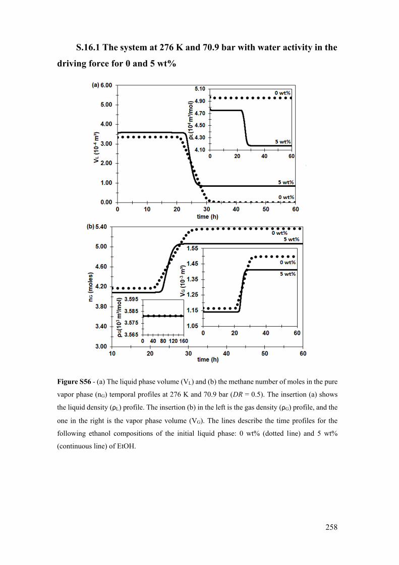
258
S.16.1 The system at 276 K and 70.9 bar with water activity in the
driving force for 0 and 5 wt%
Figure S56 - (a) The liquid phase volume (VL) and (b) the methane number of moles in the pure
vapor phase (nG) temporal profiles at 276 K and 70.9 bar (DR = 0.5). The insertion (a) shows
the liquid density (ρL) profile. The insertion (b) in the left is the gas density (ρG) profile, and the
one in the right is the vapor phase volume (VG). The lines describe the time profiles for the
following ethanol compositions of the initial liquid phase: 0 wt% (dotted line) and 5 wt%
(continuous line) of EtOH.

259
Figure S57 - (a) The temporal profile of the population balance moment of order zero, number
of particles per liquid volume (μ0), (b) moment of order one, particle diameter per liquid volume
(μ1), (c) moment of order two, particle surface area per liquid volume (μ2) and (d) moment of
order three, particle volume per liquid volume (μ3) at 276 K and 70.9 bar (DR = 0.5). The lines
describe the time profiles for the following ethanol compositions of the initial liquid phase: 0
wt% (dotted line) and 5 wt% (continuous line) of EtOH.
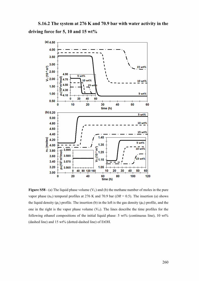
260
S.16.2 The system at 276 K and 70.9 bar with water activity in the
driving force for 5, 10 and 15 wt%
Figure S58 - (a) The liquid phase volume (VL) and (b) the methane number of moles in the pure
vapor phase (nG) temporal profiles at 276 K and 70.9 bar (DR = 0.5). The insertion (a) shows
the liquid density (ρL) profile. The insertion (b) in the left is the gas density (ρG) profile, and the
one in the right is the vapor phase volume (VG). The lines describe the time profiles for the
following ethanol compositions of the initial liquid phase: 5 wt% (continuous line), 10 wt%
(dashed line) and 15 wt% (dotted-dashed line) of EtOH.
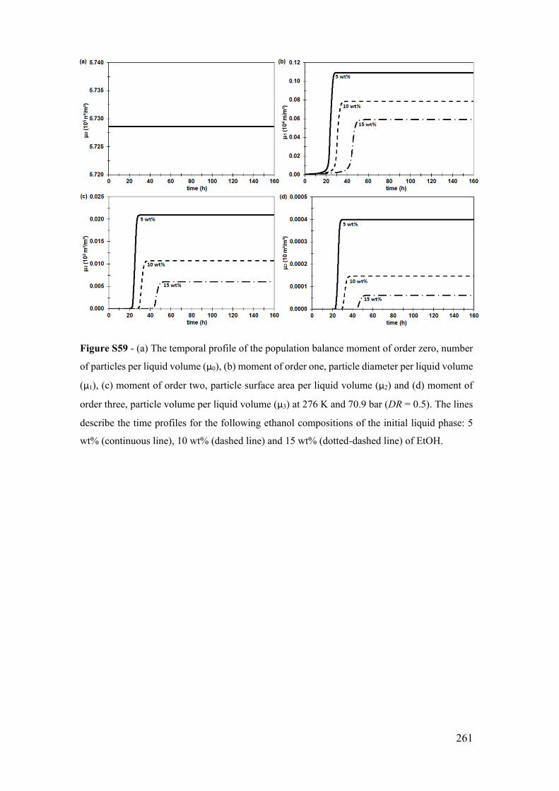
261
Figure S59 - (a) The temporal profile of the population balance moment of order zero, number
of particles per liquid volume (μ0), (b) moment of order one, particle diameter per liquid volume
(μ1), (c) moment of order two, particle surface area per liquid volume (μ2) and (d) moment of
order three, particle volume per liquid volume (μ3) at 276 K and 70.9 bar (DR = 0.5). The lines
describe the time profiles for the following ethanol compositions of the initial liquid phase: 5
wt% (continuous line), 10 wt% (dashed line) and 15 wt% (dotted-dashed line) of EtOH.
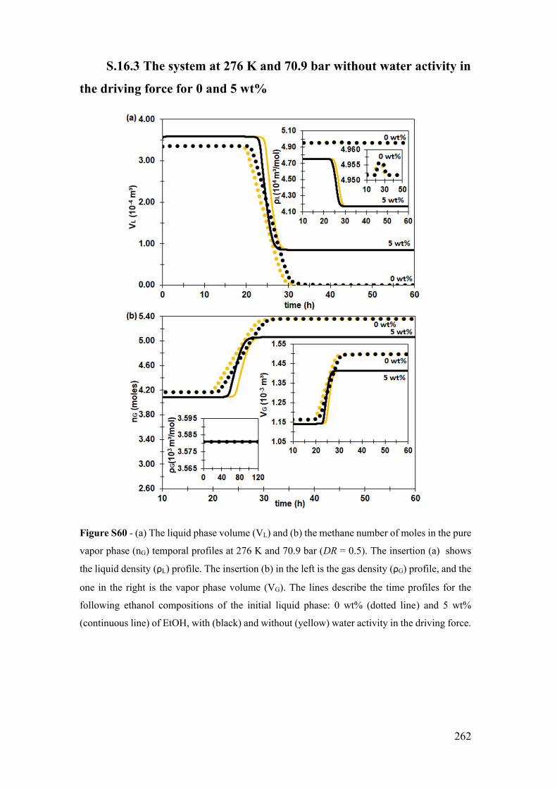
262
S.16.3 The system at 276 K and 70.9 bar without water activity in
the driving force for 0 and 5 wt%
Figure S60 - (a) The liquid phase volume (VL) and (b) the methane number of moles in the pure
vapor phase (nG) temporal profiles at 276 K and 70.9 bar (DR = 0.5). The insertion (a) shows
the liquid density (ρL) profile. The insertion (b) in the left is the gas density (ρG) profile, and the
one in the right is the vapor phase volume (VG). The lines describe the time profiles for the
following ethanol compositions of the initial liquid phase: 0 wt% (dotted line) and 5 wt%
(continuous line) of EtOH, with (black) and without (yellow) water activity in the driving force.

263
Figure S61 - (a) The temporal profile of the population balance moment of order zero, number
of particles per liquid volume (μ0), (b) moment of order one, particle diameter per liquid volume
(μ1), (c) moment of order two, particle surface area per liquid volume (μ2) and (d) moment of
order three, particle volume per liquid volume (μ3) at 276 K and 70.9 bar (DR = 0.5). The lines
describe the time profiles for the following ethanol compositions of the initial liquid phase: 0
wt% (dotted line) and 5 wt% (continuous line) of EtOH, with (black) and without (yellow) water
activity in the driving force.

264
S.16.4 The system at 276 K and 70.9 bar without water activity in
the driving force for 5, 10, and 15 wt%
Figure S62 - (a) The liquid phase volume (VL) and (b) the methane number of moles in the pure
vapor phase (nG) temporal profiles at 276 K and 70.9 bar (DR = 0.5). The insertion (a) shows
the liquid density (ρL) profile. The insertion (b) in the left is the gas density (ρG) profile, and the
one in the right is the vapor phase volume (VG). The lines describe the time profiles for the
following ethanol compositions of the initial liquid phase: 5 wt% (continuous line), 10 wt%
(dashed line) and 15 wt% (dotted-dashed line) of EtOH, with (black) and without (yellow) water
activity in the driving force.

265
Figure S63 - (a) The temporal profile of the population balance moment of order zero, number
of particles per liquid volume (μ0), (b) moment of order one, particle diameter per liquid volume
(μ1), (c) moment of order two, particle surface area per liquid volume (μ2) and (d) moment of
order three, particle volume per liquid volume (μ3) at 276 K and 70.9 bar (DR = 0.5). The lines
describe the time profiles for the following ethanol compositions of the initial liquid phase: 5
wt% (continuous line), 10 wt% (dashed line) and 15 wt% (dotted-dashed line) of EtOH, with
(black) and without (yellow) water activity in the driving force.
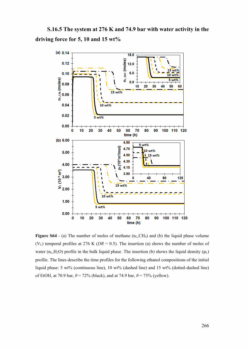
266
S.16.5 The system at 276 K and 74.9 bar with water activity in the
driving force for 5, 10 and 15 wt%
Figure S64 - (a) The number of moles of methane (nL,CH4) and (b) the liquid phase volume
(VL) temporal profiles at 276 K (DR = 0.5). The insertion (a) shows the number of moles of
water (nL,H2O) profile in the bulk liquid phase. The insertion (b) shows the liquid density (ρL)
profile. The lines describe the time profiles for the following ethanol compositions of the initial
liquid phase: 5 wt% (continuous line), 10 wt% (dashed line) and 15 wt% (dotted-dashed line)
of EtOH, at 70.9 bar, θ = 72% (black), and at 74.9 bar, θ = 75% (yellow).
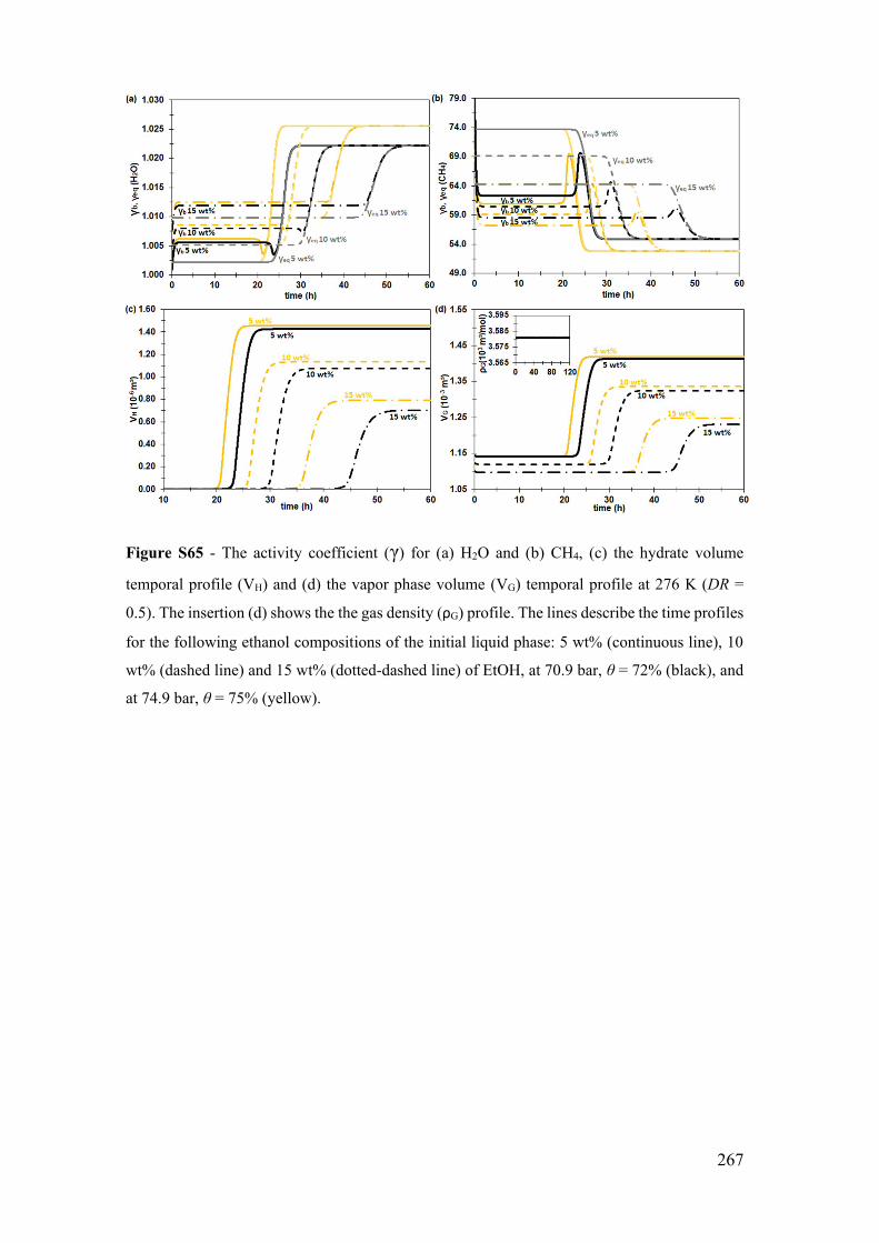
267
Figure S65 - The activity coefficient (γ) for (a) H2O and (b) CH4, (c) the hydrate volume
temporal profile (VH) and (d) the vapor phase volume (VG) temporal profile at 276 K (DR =
0.5). The insertion (d) shows the the gas density (ρG) profile. The lines describe the time profiles
for the following ethanol compositions of the initial liquid phase: 5 wt% (continuous line), 10
wt% (dashed line) and 15 wt% (dotted-dashed line) of EtOH, at 70.9 bar, θ = 72% (black), and
at 74.9 bar, θ = 75% (yellow).
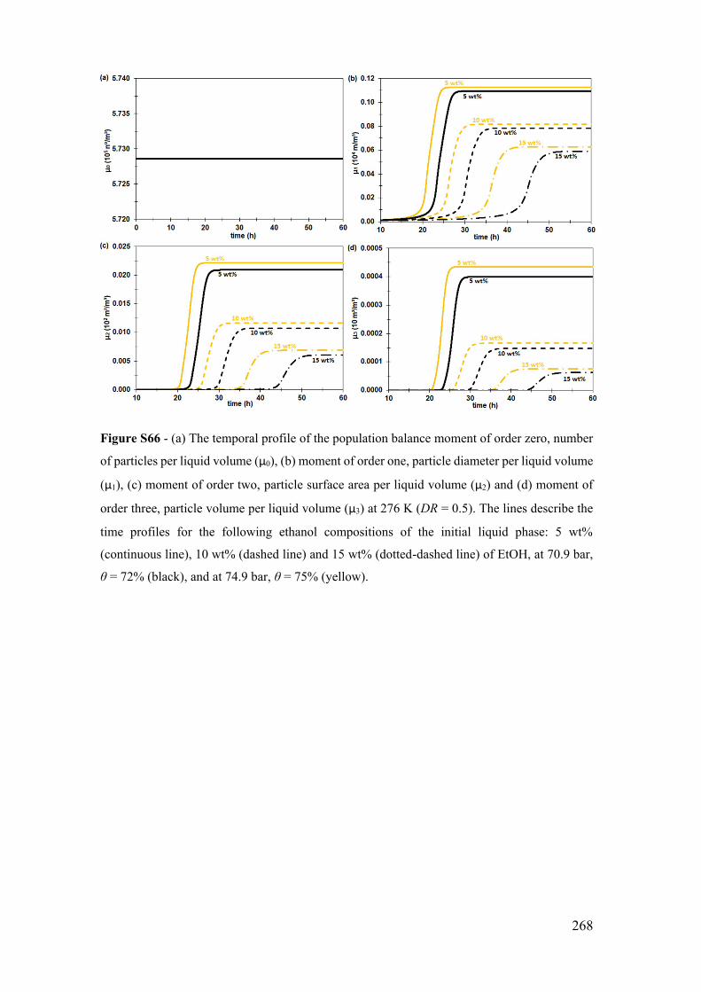
268
Figure S66 - (a) The temporal profile of the population balance moment of order zero, number
of particles per liquid volume (μ0), (b) moment of order one, particle diameter per liquid volume
(μ1), (c) moment of order two, particle surface area per liquid volume (μ2) and (d) moment of
order three, particle volume per liquid volume (μ3) at 276 K (DR = 0.5). The lines describe the
time profiles for the following ethanol compositions of the initial liquid phase: 5 wt%
(continuous line), 10 wt% (dashed line) and 15 wt% (dotted-dashed line) of EtOH, at 70.9 bar,
θ = 72% (black), and at 74.9 bar, θ = 75% (yellow).
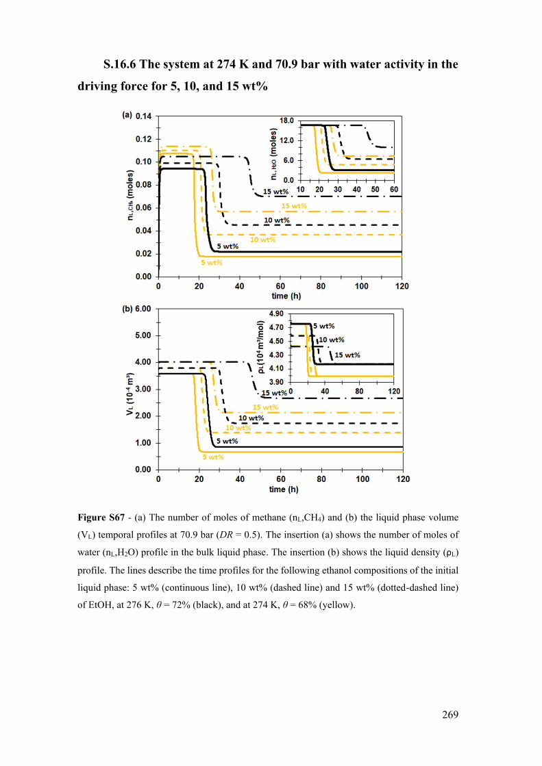
269
S.16.6 The system at 274 K and 70.9 bar with water activity in the
driving force for 5, 10, and 15 wt%
Figure S67 - (a) The number of moles of methane (nL,CH4) and (b) the liquid phase volume
(VL) temporal profiles at 70.9 bar (DR = 0.5). The insertion (a) shows the number of moles of
water (nL,H2O) profile in the bulk liquid phase. The insertion (b) shows the liquid density (ρL)
profile. The lines describe the time profiles for the following ethanol compositions of the initial
liquid phase: 5 wt% (continuous line), 10 wt% (dashed line) and 15 wt% (dotted-dashed line)
of EtOH, at 276 K, θ = 72% (black), and at 274 K, θ = 68% (yellow).
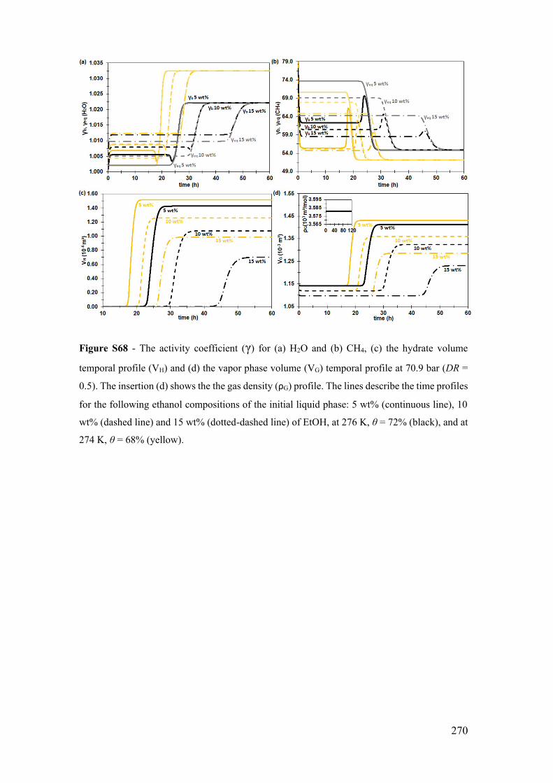
270
Figure S68 - The activity coefficient (γ) for (a) H2O and (b) CH4, (c) the hydrate volume
temporal profile (VH) and (d) the vapor phase volume (VG) temporal profile at 70.9 bar (DR =
0.5). The insertion (d) shows the the gas density (ρG) profile. The lines describe the time profiles
for the following ethanol compositions of the initial liquid phase: 5 wt% (continuous line), 10
wt% (dashed line) and 15 wt% (dotted-dashed line) of EtOH, at 276 K, θ = 72% (black), and at
274 K, θ = 68% (yellow).

271
Figure S69 - (a) The temporal profile of the population balance moment of order zero, number
of particles per liquid volume (μ0), (b) moment of order one, particle diameter per liquid volume
(μ1), (c) moment of order two, particle surface area per liquid volume (μ2) and (d) moment of
order three, particle volume per liquid volume (μ3) at 70.9 bar (DR = 0.5). The lines describe
the time profiles for the following ethanol compositions of the initial liquid phase: 5 wt%
(continuous line), 10 wt% (dashed line) and 15 wt% (dotted-dashed line) of EtOH, at 276 K, θ
= 72% (black), and at 274 K, θ = 68% (yellow).
S.17 System property derivative profiles
The profile of the time derivatives of all variables calculated by the proposed
model is presented in this topic. In all simulated conditions, of temperature, pressure,
and composition, the derivatives presented the expected temporal behavior for all phases
and components of the system.

272
S.17.1 The system at 276 K and 70.9 bar with water activity in the
driving force for 0 and 5 wt%
Figure S70 - The differential profile of (a) the methane number of moles in the bulk liquid phase
(dnL,CH4) and (b) the liquid phase volume (dVL) at 276 K and 70.9 bar (DR = 0.5). The insertion
(a) in the left shows the methane saturation profile and the one in the right shows the water
number of moles (nL,H2O) profile in the bulk liquid phase. The insertion (b) shows the liquid
density (ρL) profile with a zoom in the profile at 0 wt% of EtOH. The lines describe the time
profiles for the following ethanol compositions of the initial liquid phase: 0 wt% (dotted line)
and 5 wt% (continuous line) of EtOH.
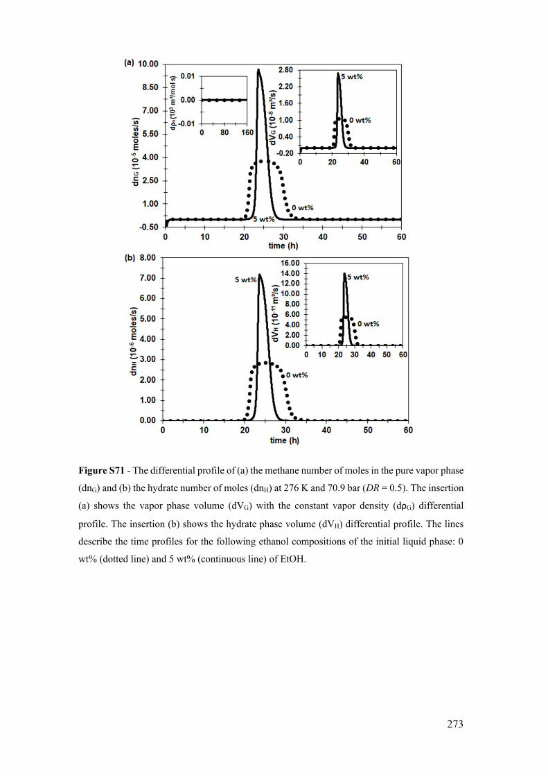
273
Figure S71 - The differential profile of (a) the methane number of moles in the pure vapor phase
(dnG) and (b) the hydrate number of moles (dnH) at 276 K and 70.9 bar (DR = 0.5). The insertion
(a) shows the vapor phase volume (dVG) with the constant vapor density (dρG) differential
profile. The insertion (b) shows the hydrate phase volume (dVH) differential profile. The lines
describe the time profiles for the following ethanol compositions of the initial liquid phase: 0
wt% (dotted line) and 5 wt% (continuous line) of EtOH.

274
Figure S72 - (a) The differential profile of the population balance moment of order zero, number
of particles per liquid volume (dμ0), (b) moment of order one, particle diameter per liquid
volume (dμ1), (c) moment of order two, particle surface area per liquid volume (dμ2) and (d)
moment of order three, particle volume per liquid volume (dμ3) at 276 K and 70.9 bar (DR =
0.5). The lines describe the time profiles for the following ethanol compositions of the initial
liquid phase: 0 wt% (dotted line, 2nd axis) and 5 wt% (continuous line, 1st axis) of EtOH.

275
S.17.2 The system at 276 K and 70.9 bar with water activity in the
driving force for 5, 10, and 15 wt%
Figure S73 - The differential profile of (a) the methane number of moles in the bulk liquid phase
(dnL,CH4) and (b) the liquid phase volume (dVL) at 276 K and 70.9 bar (DR = 0.5). The insertion
(a) in the left shows the methane saturation profile and the one in the right shows the water
number of moles (nL,H2O) profile in the bulk liquid phase. The insertion (b) shows the liquid
density (ρL) profile with a zoom in the methane saturation profile. The lines describe the time
profiles for the following ethanol compositions of the initial liquid phase: 5 wt% (continuous
line), 10 wt% (dashed line) and 15 wt% (dotted-dashed line) of EtOH.

276
Figure S74 - The differential profile of (a) the methane number of moles in the pure vapor phase
(dnG) and (b) the hydrate number of moles (dnH) at 276 K and 70.9 bar (DR = 0.5). The insertion
(a) shows the vapor phase volume (dVG) and the constant vapor density (dρG) differential profile.
The insertion (b) shows the hydrate phase volume (dVH) differential profile. The lines describe
the time profiles for the following ethanol compositions of the initial liquid phase: 5 wt%
(continuous line), 10 wt% (dashed line) and 15 wt% (dotted-dashed line) of EtOH.
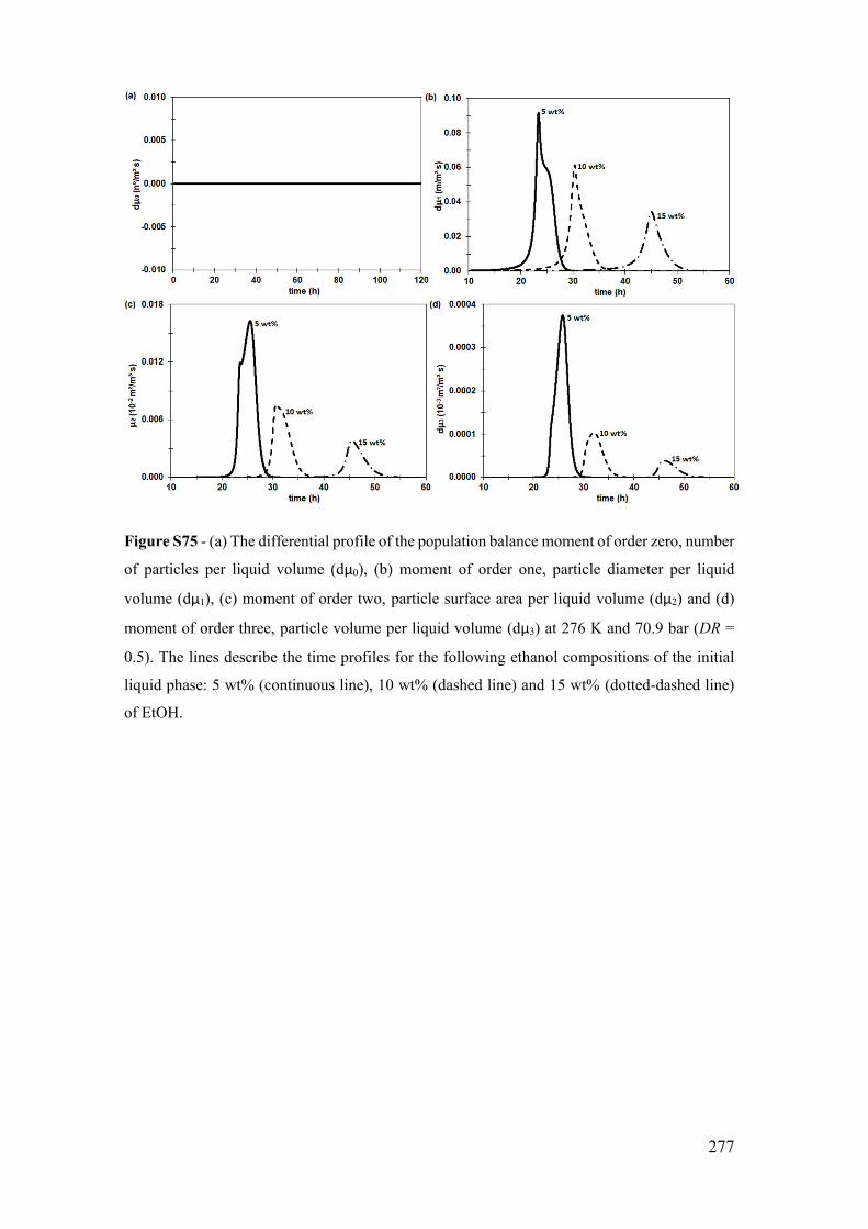
277
Figure S75 - (a) The differential profile of the population balance moment of order zero, number
of particles per liquid volume (dμ0), (b) moment of order one, particle diameter per liquid
volume (dμ1), (c) moment of order two, particle surface area per liquid volume (dμ2) and (d)
moment of order three, particle volume per liquid volume (dμ3) at 276 K and 70.9 bar (DR =
0.5). The lines describe the time profiles for the following ethanol compositions of the initial
liquid phase: 5 wt% (continuous line), 10 wt% (dashed line) and 15 wt% (dotted-dashed line)
of EtOH.

278
S.17.3 The system at 276 K and 70.9 bar without water activity in
the driving force for 0 and 5 wt%
Figure S76 - The differential profile of (a) the methane number of moles in the bulk liquid phase
(dnL,CH4) and (b) the liquid phase volume (dVL) at 276 K and 70.9 bar (DR = 0.5). The insertion
(a) in the left shows the methane saturation profile and the one in the right shows the water
number of moles (nL,H2O) profile in the bulk liquid phase. The insertion (b) shows the liquid
density (ρL) profile with a zoom in the profile at 0 wt% of EtOH. The lines describe the time
profiles for the following ethanol compositions of the initial liquid phase: 0 wt% (dotted line)
and 5 wt% (continuous line) of EtOH, with (black) and without (yellow) water activity in the
driving force.
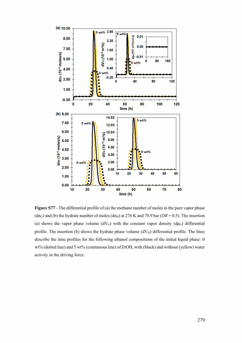
279
Figure S77 - The differential profile of (a) the methane number of moles in the pure vapor phase
(dnG) and (b) the hydrate number of moles (dnH) at 276 K and 70.9 bar (DR = 0.5). The insertion
(a) shows the vapor phase volume (dVG) with the constant vapor density (dρG) differential
profile. The insertion (b) shows the hydrate phase volume (dVH) differential profile. The lines
describe the time profiles for the following ethanol compositions of the initial liquid phase: 0
wt% (dotted line) and 5 wt% (continuous line) of EtOH, with (black) and without (yellow) water
activity in the driving force.

280
Figure S78 - (a) The differential profile of the population balance moment of order zero, number
of particles per liquid volume (dμ0), (b) moment of order one, particle diameter per liquid
volume (dμ1), (c) moment of order two, particle surface area per liquid volume (dμ2) and (d)
moment of order three, particle volume per liquid volume (dμ3) at 276 K and 70.9 bar (DR =
0.5). The lines describe the time profiles for the following ethanol compositions of the initial
liquid phase: 0 wt% (dotted line, 2nd axis) and 5 wt% (continuous line, 1st axis) of EtOH, with
(black) and without (yellow) water activity in the driving force.

281
S.17.4 The system at 276 K and 70.9 bar without water activity in
the driving force for 5, 10 and 15 wt%
Figure S79 - The differential profile of (a) the methane number of moles in the bulk liquid phase
(dnL,CH4) and (b) the liquid phase volume (dVL) at 276 K and 70.9 bar (DR = 0.5). The insertion
(a) in the left shows the methane saturation profile and the one in the right shows the water
number of moles (nL,H2O) profile in the bulk liquid phase. The insertion (b) shows the liquid
density (ρL) profile with a zoom in the methane saturation profile. The lines describe the time
profiles for the following ethanol compositions of the initial liquid phase: 5 wt% (continuous
line), 10 wt% (dashed line) and 15 wt% (dotted-dashed line) of EtOH, with (black) and without
(yellow) water activity in the driving force.
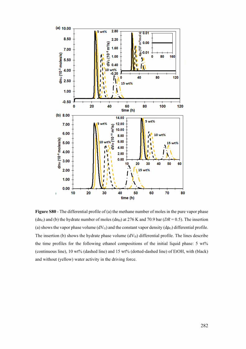
282
Figure S80 - The differential profile of (a) the methane number of moles in the pure vapor phase
(dnG) and (b) the hydrate number of moles (dnH) at 276 K and 70.9 bar (DR = 0.5). The insertion
(a) shows the vapor phase volume (dVG) and the constant vapor density (dρG) differential profile.
The insertion (b) shows the hydrate phase volume (dVH) differential profile. The lines describe
the time profiles for the following ethanol compositions of the initial liquid phase: 5 wt%
(continuous line), 10 wt% (dashed line) and 15 wt% (dotted-dashed line) of EtOH, with (black)
and without (yellow) water activity in the driving force.

283
Figure S81 - (a) The differential profile of the population balance moment of order zero, number
of particles per liquid volume (dμ0), (b) moment of order one, particle diameter per liquid
volume (dμ1), (c) moment of order two, particle surface area per liquid volume (dμ2) and (d)
moment of order three, particle volume per liquid volume (dμ3) at 276 K and 70.9 bar (DR =
0.5). The lines describe the time profiles for the following ethanol compositions of the initial
liquid phase: 5 wt% (continuous line), 10 wt% (dashed line) and 15 wt% (dotted-dashed line)
of EtOH, with (black) and without (yellow) water activity in the driving force.
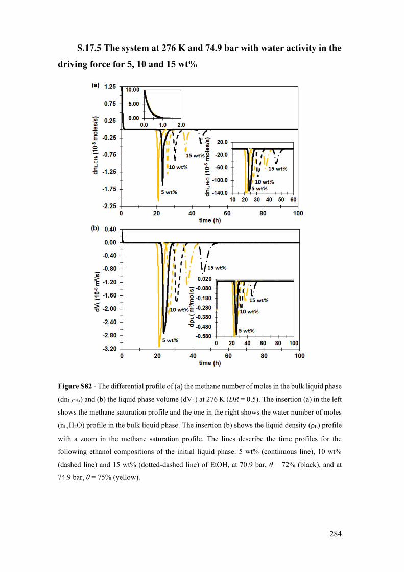
284
S.17.5 The system at 276 K and 74.9 bar with water activity in the
driving force for 5, 10 and 15 wt%
Figure S82 - The differential profile of (a) the methane number of moles in the bulk liquid phase
(dnL,CH4) and (b) the liquid phase volume (dVL) at 276 K (DR = 0.5). The insertion (a) in the left
shows the methane saturation profile and the one in the right shows the water number of moles
(nL,H2O) profile in the bulk liquid phase. The insertion (b) shows the liquid density (ρL) profile
with a zoom in the methane saturation profile. The lines describe the time profiles for the
following ethanol compositions of the initial liquid phase: 5 wt% (continuous line), 10 wt%
(dashed line) and 15 wt% (dotted-dashed line) of EtOH, at 70.9 bar, θ = 72% (black), and at
74.9 bar, θ = 75% (yellow).

285
Figure S83 - The differential profile of (a) the methane number of moles in the pure vapor phase
(dnG) and (b) the hydrate number of moles (dnH) at 276 K (DR = 0.5). The insertion (a) shows
the vapor phase volume (dVG) and the constant vapor density (dρG) differential profile. The
insertion (b) shows the hydrate phase volume (dVH) differential profile. The lines describe the
time profiles for the following ethanol compositions of the initial liquid phase: 5 wt%
(continuous line), 10 wt% (dashed line) and 15 wt% (dotted-dashed line) of EtOH, at 70.9 bar,
θ = 72% (black), and at 74.9 bar, θ = 75% (yellow).

286
Figure S84- (a) The differential profile of the population balance moment of order zero, number
of particles per liquid volume (dμ0), (b) moment of order one, particle diameter per liquid
volume (dμ1), (c) moment of order two, particle surface area per liquid volume (dμ2) and (d)
moment of order three, particle volume per liquid volume (dμ3) at 276 (DR = 0.5). The lines
describe the time profiles for the following ethanol compositions of the initial liquid phase: 5
wt% (continuous line), 10 wt% (dashed line) and 15 wt% (dotted-dashed line) of EtOH, at 70.9
bar, θ = 72% (black), and at 74.9 bar, θ = 75% (yellow).

287
S.17.6 The system at 274 K and 70.9 bar with water activity in the
driving force for 5, 10 and 15 wt%
Figure S85 - The differential profile of (a) the methane number of moles in the bulk liquid phase
(dnL,CH4) and (b) the liquid phase volume (dVL) at 70.9 bar (DR = 0.5). The insertion (a) in the
left shows the methane saturation profile and the one in the right shows the water number of
moles (nL,H2O) profile in the bulk liquid phase. The insertion (b) shows the liquid density (ρL)
profile with a zoom in the methane saturation profile. The lines describe the time profiles for
the following ethanol compositions of the initial liquid phase: 5 wt% (continuous line), 10 wt%
(dashed line) and 15 wt% (dotted-dashed line) of EtOH, at 276 K, θ = 72% (black), and at 274
K, θ = 68% (yellow).

288
Figure S86 - The differential profile of (a) the methane number of moles in the pure vapor phase
(dnG) and (b) the hydrate number of moles (dnH) at 70.9 bar (DR = 0.5). The insertion (a) shows
the vapor phase volume (dVG) and the constant vapor density (dρG) differential profile. The
insertion (b) shows the hydrate phase volume (dVH) differential profile. The lines describe the
time profiles for the following ethanol compositions of the initial liquid phase: 5 wt%
(continuous line), 10 wt% (dashed line) and 15 wt% (dotted-dashed line) of EtOH, at 276 K, θ
= 72% (black), and at 274 K, θ = 68% (yellow).
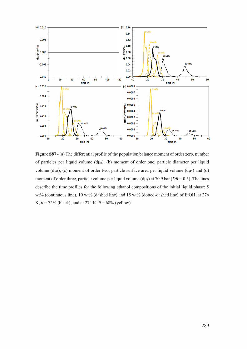
289
Figure S87 - (a) The differential profile of the population balance moment of order zero, number
of particles per liquid volume (dμ0), (b) moment of order one, particle diameter per liquid
volume (dμ1), (c) moment of order two, particle surface area per liquid volume (dμ2) and (d)
moment of order three, particle volume per liquid volume (dμ3) at 70.9 bar (DR = 0.5). The lines
describe the time profiles for the following ethanol compositions of the initial liquid phase: 5
wt% (continuous line), 10 wt% (dashed line) and 15 wt% (dotted-dashed line) of EtOH, at 276
K, θ = 72% (black), and at 274 K, θ = 68% (yellow).
290
S.18 Correlation of the parameters in tG LA e GL
dk
The modeling of CH4 solubilization in H2O with EtOH requires describing the
interfacial area of the continuous gas-liquid phases in t ²G LA m and the methane diffusion
coefficient [ / ]GLdk m s . For the calculation of this area, the same modeling used by
Sampaio et al. [87] and in our previous work Oliveira et a (2020, in submission process),
Item S.9 Appendix 3, is used.
Then, the suspension molar density, .[ / ³]susp mol m , the molar mass of the
suspension, .suspM M , the dynamic viscosity, .[ / ]susp mol m s , and the specific surface
energy of the suspension, .[J/ m ²]susp are given by models that pondered the properties
of the solid phase and the liquid phase (Item S.9 Appendix 3). Thus, in calculating the
properties of the liquid phase, which now has ethanol present, we now also include the
properties of ethanol weighted through its mole fraction at that time in the system.
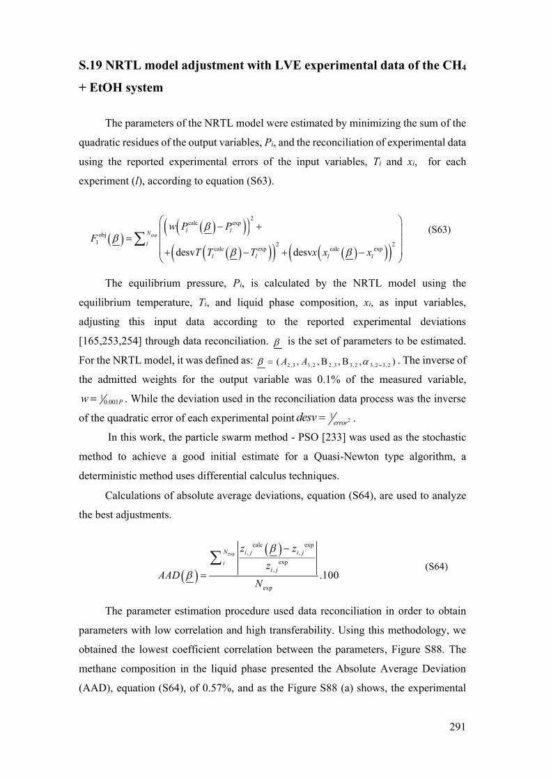
291
S.19 NRTL model adjustment with LVE experimental data of the CH4
+ EtOH system
The parameters of the NRTL model were estimated by minimizing the sum of the
quadratic residues of the output variables, Pi, and the reconciliation of experimental data
using the reported experimental errors of the input variables, Ti and xi, for each
experiment (l), according to equation (S63).
exp
2calc exp
obj1 2 2
calc exp calc expdesv desv
l lN
l
l l l l
w P PF
T T T x x x
(S63)
The equilibrium pressure, Pi, is calculated by the NRTL model using the
equilibrium temperature, Ti, and liquid phase composition, xi, as input variables,
adjusting this input data according to the reported experimental deviations
[165,253,254] through data reconciliation. is the set of parameters to be estimated.
For the NRTL model, it was defined as: 2 ,3 3,2 2 ,3 3,2 3,2 3,2( , , B , B , )A A . The inverse of
the admitted weights for the output variable was 0.1% of the measured variable,1
0.001Pw . While the deviation used in the reconciliation data process was the inverse
of the quadratic error of each experimental point 21
errordesv .
In this work, the particle swarm method - PSO [233] was used as the stochastic
method to achieve a good initial estimate for a Quasi-Newton type algorithm, a
deterministic method uses differential calculus techniques.
Calculations of absolute average deviations, equation (S64), are used to analyze
the best adjustments.
exp
calc exp, ,
exp,
exp
.100
N i j i j
ii j
z zz
AADN
(S64)
The parameter estimation procedure used data reconciliation in order to obtain
parameters with low correlation and high transferability. Using this methodology, we
obtained the lowest coefficient correlation between the parameters, Figure S88. The
methane composition in the liquid phase presented the Absolute Average Deviation
(AAD), equation (S64), of 0.57%, and as the Figure S88 (a) shows, the experimental

292
and the reconciliation data has total linearity with each other. On the other hand, the
reconciled temperature showed AAD of 2.59% and did not present total linearity with
the experimental data; however, the deviation was low, and the variation was within the
error range of 5 K, Figure S88 (b). Using the data reconciliation technique, the AAD of
the pressure calculated with the NRTL model was 0.0014% and showed total linearity
with the experimental pressure, Figure S88 (c). Then, as the pressure was calculated by
the model with high precision using data reconciliation despite the 5 K deviation in
temperature, the adjustment was considered adequate.
Figure S88- Comparison between experimental values, y-axis, and calculated values, x-axis, in
the estimation of NRTL model parameters using data reconciliation for the CH4+EtOH system
[165,253,254] and the matrix of the parameters correlation coefficients. The input variables
reconciled using the reported experimental errors were (a) the methane composition in the liquid
phase, xCH4, and (b) the equilibrium temperature. The output variable calculated through the
NRTL model in the estimation process was (c) the pressure.
The NRTL model parameters for the pair CH4(2) + EtOH(3), Table S19, were
estimated for liquid-vapor equilibrium data at the temperature of 253.15 K, 263.15 K,
273.15 K, 280.15 K, 298.15 K, 313.4 K, and 333.4 K, Figure S89, covered a pressure
range of 0.33 MPa to 41.69 MPa. The methane concentration range in the liquid phase
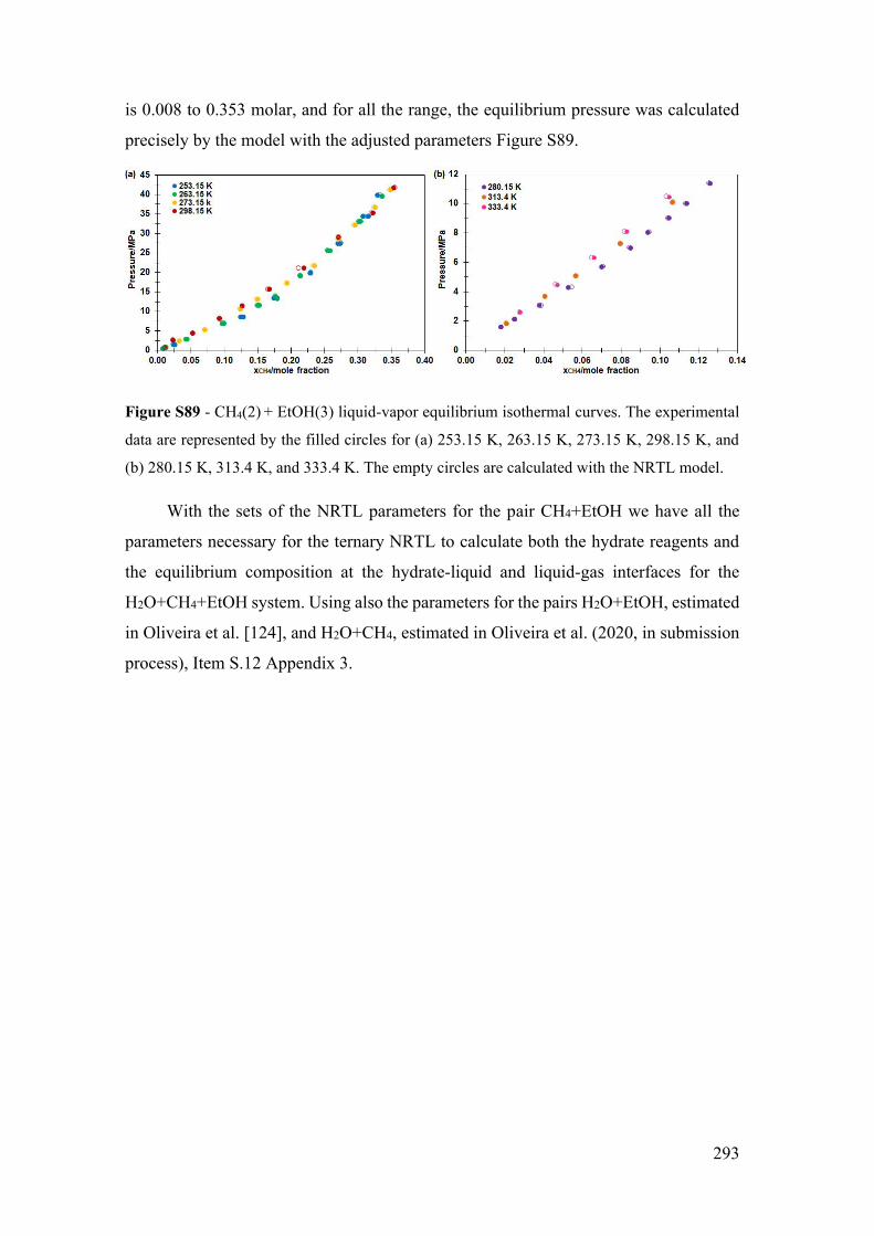
293
is 0.008 to 0.353 molar, and for all the range, the equilibrium pressure was calculated
precisely by the model with the adjusted parameters Figure S89.
Figure S89 - CH4(2) + EtOH(3) liquid-vapor equilibrium isothermal curves. The experimental
data are represented by the filled circles for (a) 253.15 K, 263.15 K, 273.15 K, 298.15 K, and
(b) 280.15 K, 313.4 K, and 333.4 K. The empty circles are calculated with the NRTL model.
With the sets of the NRTL parameters for the pair CH4+EtOH we have all the
parameters necessary for the ternary NRTL to calculate both the hydrate reagents and
the equilibrium composition at the hydrate-liquid and liquid-gas interfaces for the
H2O+CH4+EtOH system. Using also the parameters for the pairs H2O+EtOH, estimated
in Oliveira et al. [124], and H2O+CH4, estimated in Oliveira et al. (2020, in submission
process), Item S.12 Appendix 3.