HAL Id: tel-01128265https://tel.archives-ouvertes.fr/tel-01128265

Submitted on 9 Mar 2015

HAL is a multi-disciplinary open accessarchive for the deposit and dissemination of sci-entific research documents, whether they are pub-lished or not. The documents may come fromteaching and research institutions in France orabroad, or from public or private research centers.

L’archive ouverte pluridisciplinaire HAL, estdestinée au dépôt et à la diffusion de documentsscientifiques de niveau recherche, publiés ou non,émanant des établissements d’enseignement et derecherche français ou étrangers, des laboratoirespublics ou privés.

Hybrid modeling of hematopoiesis and blood diseasesNathalie Eymard

To cite this version:Nathalie Eymard. Hybrid modeling of hematopoiesis and blood diseases. General Mathematics[math.GM]. Université Claude Bernard - Lyon I, 2014. English. �NNT : 2014LYO10340�. �tel-01128265�

Universite Claude Bernard - Lyon 1

Institut Camille Jordan - CNRS UMR 5208

Ecole doctorale InfoMaths

Thesede l’universite de Lyon

pour obtenir le titre de

Docteur en Sciences

Mention : Mathematiques appliquees

presentee par

Nathalie Eymard

Modelisation hybride de l’hematopoıeseet de maladies sanguines

These dirigee par Vitaly Volpert

preparee a l’Universite Lyon 1

Jury :

Rapporteurs: Roeland Merks, Professor, University of LeidenRapporteurs: Pierre Magal, Professeur, Universite de Bordeaux

Jean Clairambault, Directeur de recherche, Inria Paris-RocquencourtMostafa Adimy, Directeur de Recherche, INRIA GrenobleIonel S. Ciuperca, Maıtre de Conferences, Universite Lyon

Jacques Demongeot, Professeur, Faculte de medecine, GrenobleVitaly Volpert, Directeur de recherche, CNRS Lyon

1

2

Resume :

Cette these est consacree au developpement de modeles mathematiques de l’hematopoıeseet de maladies du sang. Elle traite du developpement de modeles hybrides discrets continuset de leurs applications a la production de cellules sanguines (l’hematopoıese) et de maladiessanguines telles que le lymphome et le myelome.

La premiere partie de ce travail est consacree a la formation de cellules sanguines a partirdes cellules souches de la mœlle osseuse. Nous allons principalement etudier la productiondes globules rouges, les erythrocytes. Chez les mammiferes, l’erythropoıese se produit dansdes structures particulieres, les ılots erythroblastiques. Leur fonctionnement est regi par decomplexes regulations intra et extracellulaire mettant en jeux differents types de cellules,d’hormones et de facteurs de croissance. Les resultats ainsi obtenus sont compares avec desdonnees experimentales biologiques ou medicales chez l’humain et la souris.

Le propos de la deuxieme partie de cette these est de modeliser deux maladies du sang,le lymphome lymphoblastique a cellules T (T-LBL) et le myelome multiple (MM), ainsi queleur traitement. Le T-LBL se developpe dans le thymus et affecte la production des cellulesdu systeme immunitaire. Dans le MM, les cellules malignes envahissent la mœlle osseuseet detruisent les ılots erythroblastiques empechant l’erythropoıese. Nous developpons desmodeles multi-echelles de ces maladies prenant en compte la regulation intracellulaire, leniveau cellulaire et la regulation extracellulaire. La reponse au traitement depend descaracteristiques propres a chaque patient. Plusieurs scenarios de traitements efficaces, derechutes et une resistance au traitement sont consideres.

La derniere partie porte sur un modele d’equation de reaction diffusion qui peut etreutilise pour decrire l’evolution darwinnienne des cellules cancereuses. L’ existence de “pulsesolutions”, pouvant decrire localement les populations de cellules et leurs evolutions, estprouvee.

Mots clefs : modeles hybrides discret-continus, hematopoıese, maladies du sang, traite-ment, resistance.

3

Abstract :

The thesis is devoted to mathematical modeling of hematopoiesis and blood diseases. Itis based on the development of hybrid discrete continuous models and to their applicationsto investigate production of blood cell (hematopoiesis) and blood diseases such as lymphomaand myeloma.

The first part of the thesis concerns production of blood cells in the bone marrow. Wewill mainly study production of red blood cells, erythropoiesis. In mammals erythropoiesisoccurs in special structures, erythroblastic islands. Their functioning is determined by com-plex intracellular and extracellular regulations which include various cell types, hormonesand growth factors. The results of modeling are compared with biological and medical datafor humans and mice.

The purpose of the second part of the thesis is to model some blood diseases, T cellLymphoblastic lymphoma (T-LBL) and multiple myeloma (MM) and their treatment. T-LBL develops in the thymus and it affects the immune system. In MM malignant cellsinvade the bone marrow and destroy erythroblastic islands preventing normal functioningof erythropoiesis. We developed multi-scale models of these diseases in order to take intoaccount intracellular molecular regulation, cellular level and extracellular regulation. Theresponse to treatment depends on the individual characteristics of the patients. Variousscenarios are considered including successful treatment, relapse and development of theresistance to treatment.

The last part of the thesis is devoted to a reaction-diffusion model which can be usedto describe darwinian evolution of cancer cells. Existence of pulse solutions, which candescribe localized cell populations and their evolution, is proved.

Keywords: hybrid discrete-continuous models, hematopoiesis, blood diseases, treat-ment, resistance

4

5

Publications

1. N. Bessonov, N. Eymard, P. Kurbatova, V. Volpert. Mathematical Modelling of Ery-thropoiesis in vivo with Multiple Erythroblastic Islands. Applied Mathematics Letters,Volume 25, Issue 9, pp: 1217–1221, 2012.

2. P. Kurbatova, N. Eymard, V. Volpert. Hybrid model of erythropoiesis. Acta Biothe-oretica, Volume 61, Issue 3, pp: 305-315, 2013.

3. N. Eymard, N. Bessonov, O. Gandrillon, M.J. Koury, V. Volpert. The role of spatialorganization of cells in erythropoiesis. Journal of Mathematical Biology, Volume 70,issue 1, pp 71–97, 2015.

4. P. Kurbatova, N. Eymard, A. Tosenberger, V. Volpert, N. Bessonov. Application ofhybrid discrete-continuous models in cell population dynamics, in: BIOMAT 2011,World Sci. Publ., Hackensack, NJ, pp 1–10, 2012.

5. V. Volpert, N. Bessonov, N. Eymard, A. Tossenberger. Modele multi-echelle de ladynamique cellulaire, in: Le vivant discret et continu. Nicolas Glade et Angeliquestephanou, Editeurs: Editions Materiologiques, pp: 91–112, 2013.

6. P. Nony, P. Kurbatova, A. Bajard, S. Malik, C. Castellan, S. Chabaud, V. Volpert,N. Eymard, B. Kassai C. Cornu and The CRESim and Epi-CRESim study groups. Amethodological framework for drug development in rare diseases. Orphanet Journal ofRare Diseases, 9:164, 2014.

7. N. Eymard, P. Kurbatova. Hybrid models in hematopoiesis. (submitted 2014).

8. N.Eymard, N.Bessonov, V.Volpert, CRESim Group. Mathematical model of T-celllymphoblastic lymphoma: disease, treatment, cure or relapse of a virtual cohort ofpatients. (submitted 2014).

9. Awards. Best Poster Prize 8. 9th International Conference for Rare Diseases andOrphan Drugs (ICORD), October 7-9, 2014, The Netherlands.

6

Remerciements

Je remercie tous ceux, en particulier mon directeur de these V. Volpert, qui m’ont permisde mener jusqu’a son terme et de concretiser ce qui n’a longtemps ete qu’un projet. Je tiensegalement a remercier les rapporteurs et membres du jury de l’interet qu’ils ont porte amon travail.

7

Contents

1 Introduction 12

1.1 Biological background . . . . . . . . . . . . . . . . . . . . . . . . . . . . . . 13

1.1.1 Hematopoiesis . . . . . . . . . . . . . . . . . . . . . . . . . . . . . . 13

1.1.2 Blood diseases . . . . . . . . . . . . . . . . . . . . . . . . . . . . . . 16

1.2 Modeling approaches: multi-scale hybrid model . . . . . . . . . . . . . . . . 20

1.2.1 Modeling literature . . . . . . . . . . . . . . . . . . . . . . . . . . . . 20

1.2.2 Multi-scale hybrid discrete-continuous model . . . . . . . . . . . . . 22

1.3 Main results of the thesis . . . . . . . . . . . . . . . . . . . . . . . . . . . . 24

1.3.1 Methods of modeling . . . . . . . . . . . . . . . . . . . . . . . . . . . 24

1.3.2 Hematopoiesis . . . . . . . . . . . . . . . . . . . . . . . . . . . . . . 30

1.3.3 Blood diseases . . . . . . . . . . . . . . . . . . . . . . . . . . . . . . 32

1.3.4 Existence and dynamics of pulses . . . . . . . . . . . . . . . . . . . . 35

2 Hematopoiesis 40

2.1 Lineage choice . . . . . . . . . . . . . . . . . . . . . . . . . . . . . . . . . . 40

2.1.1 Introduction . . . . . . . . . . . . . . . . . . . . . . . . . . . . . . . 40

2.1.2 Intracellular regulation . . . . . . . . . . . . . . . . . . . . . . . . . . 41

2.1.3 Results . . . . . . . . . . . . . . . . . . . . . . . . . . . . . . . . . . 43

2.2 Erythropoiesis . . . . . . . . . . . . . . . . . . . . . . . . . . . . . . . . . . . 46

2.2.1 Introduction . . . . . . . . . . . . . . . . . . . . . . . . . . . . . . . 46

2.2.2 Regulation by proteins Erk and Fas . . . . . . . . . . . . . . . . . . 47

8

2.2.3 Regulation by proteins, glucocorticoids and transcriptions factors . . 51

2.2.4 Regulation by activated glucocorticosteroid receptor, activated BMPR4

receptor, transcription factor GATA-1 and activated caspases . . . . 58

2.2.5 Stability of multiple islands . . . . . . . . . . . . . . . . . . . . . . . 79

3 Blood diseases 85

3.1 Multiple Myeloma . . . . . . . . . . . . . . . . . . . . . . . . . . . . . . . . 85

3.1.1 Biological background . . . . . . . . . . . . . . . . . . . . . . . . . . 85

3.1.2 Mathematical model . . . . . . . . . . . . . . . . . . . . . . . . . . . 87

3.1.3 Partial differentiation of myeloma cells . . . . . . . . . . . . . . . . . 95

3.2 Lymphoma . . . . . . . . . . . . . . . . . . . . . . . . . . . . . . . . . . . . 97

3.2.1 Biological background . . . . . . . . . . . . . . . . . . . . . . . . . . 97

3.2.2 Mathematical model . . . . . . . . . . . . . . . . . . . . . . . . . . . 100

3.2.3 Lymphoma development and treatment . . . . . . . . . . . . . . . . 104

4 Pulses in reaction-diffusion equations 112

4.1 Introduction . . . . . . . . . . . . . . . . . . . . . . . . . . . . . . . . . . . . 112

4.2 Monotone solutions on the half-axis . . . . . . . . . . . . . . . . . . . . . . 119

4.2.1 Operators and spaces . . . . . . . . . . . . . . . . . . . . . . . . . . 119

4.2.2 Separation of monotone solutions . . . . . . . . . . . . . . . . . . . . 120

4.2.3 A priori estimates of monotone solutions . . . . . . . . . . . . . . . . 122

4.2.4 Model problem . . . . . . . . . . . . . . . . . . . . . . . . . . . . . . 125

4.2.5 Existence theorem . . . . . . . . . . . . . . . . . . . . . . . . . . . . 128

4.2.6 Examples . . . . . . . . . . . . . . . . . . . . . . . . . . . . . . . . . 130

4.3 Solutions on the half-axis without monotonicity condition . . . . . . . . . . 132

4.4 Existence of pulses in the case of global consumption . . . . . . . . . . . . . 134

4.5 Mathematical model of the development of the resistance to chemotherapy . 136

4.5.1 Model . . . . . . . . . . . . . . . . . . . . . . . . . . . . . . . . . . . 136

4.5.2 Stationary solution . . . . . . . . . . . . . . . . . . . . . . . . . . . . 137

9

4.5.3 Cell population with multiple survival gaps . . . . . . . . . . . . . . 139

4.5.4 Cancer treatment . . . . . . . . . . . . . . . . . . . . . . . . . . . . . 140

5 Conclusions 142

6 Appendix 164

6.1 Numerical implementation . . . . . . . . . . . . . . . . . . . . . . . . . . . . 164

6.1.1 Resolution of reaction-diffusion equations . . . . . . . . . . . . . . . 164

6.1.2 Implementation of numerical algorithms . . . . . . . . . . . . . . . . 166

6.2 Values of parameters for lineage choice . . . . . . . . . . . . . . . . . . . . . 168

6.3 Appendix 1. Intracellular regulation of erythroid progenitors . . . . . . . . 172

6.4 Appendix 2. Cell culture experiments . . . . . . . . . . . . . . . . . . . . . 175

6.5 Appendix 3 . . . . . . . . . . . . . . . . . . . . . . . . . . . . . . . . . . . . 176

6.6 Value of parameters of myeloma simulation . . . . . . . . . . . . . . . . . . 180

10

11

Chapter 1

Introduction

The thesis is devoted to the mathematical modeling of hematopoiesis and blood diseases.

We will begin this study with modeling of the lineage choice of megakaryocytic-erythroid

progenitors. These two lineages lead to the production of erythrocytes and platelets. We will

study in more detail the erythroid lineage of hematopoiesis. We will model erythroblastic

islands, main functional units of erythropoiesis, in normal and pathological situations. The

latter will be considered in the case of multiple myeloma. It is a hematological disorder where

malignant cells invade the bone marrow resulting in destruction of erythroblastic islands

and, as a consequence, to severe anemia. The methods developed for this modeling are

applicable to study other diseases. We will show their application to study T-cell lymphoma

where tumor develops in the thymus. One of the important aspects of these disorders is

that, similar to other cancers, malignant cells can adapt to treatment and develop resistant

clones. We will study this question in the case of lymphoma and in a more abstract setting.

In this introductory chapter, we will present a short biological background followed by the

discussion of the methods of modeling and by the presentation of the main results of this

work.

12

1.1 Biological background

1.1.1 Hematopoiesis

Hematopoiesis is a complex process which begins with hematopoietic stem cells (HSCs)

and results in production of red blood cells (erythrocytes), white blood cells (leucocytes)

and platelets. Erythrocytes participate in the transport of oxygen, white blood cells in the

immune response, platelets play an important role in blood coagulation. In adult humans

hematopoiesis occurs mainly in the bone marrow. Due to consecutive stages of maturation

and differentiation HSCs give rise to all lineages of blood cells. Various dysfunctions can

affect hematopoiesis and cause blood diseases.

Hematopoietic stem cells are located in specific area, called stem cell niche. In niche,

HSCs can be in a nondividing state or it can differentiate in order to keep a steady number

of blood cells. Hematopoiesis process has the ability to adapt to changes or to stress by

elevating the production rate of blood cells.

HSCs are pluripotent cells, they self-renew or differentiate into different lineages. This

first differentiation leads to the appearance of common myeloid progenitors (CMP) and

common lymphoid progenitors (CLP). Further differentiation of CMP and CLP give rise, in

case of CMP, among others cells, to megakaryocytes and erythrocytes and in case of CLP,

to lymphocytes. Secondary lymphoid organs such as thymus, spleen, liver and lymph nodes

also participate in final differentiations.

Lineage choice of pluripotent cells

Burst forming unit erythroid progenitors (BFU-E) and burst forming units-megakaryocytic

progenitors (BFU-MK) appear due to differentiation of megakaryocytic-erythroid progenitor

(MEP). BFU-MKs divide and differentiates and become thrombocytes. This process is

called the megakaryopoiesis. Similarly, BFU-Es becomes erythrocytes in the process of

erythropoiesis. The next stage of maturation of BFU-E is colony-forming unit-erythroid

(CFU-E).

13

Figure 1.1: All blood cells originate from the stem cell compartment on the left and arereleased in the blood stream on the right. The lymphoid branch, on top, releases T andB-lymphocytes. The myeloid branch consists of the red lineage (bottom), white lineage inblue and platelets in green.

The complex mechanism that determines commitment of MEP is not completely un-

derstood, but it is established that the proteins and transcription factors GATA-1, FLI-1,

EKLF play an important role in this process.

Figure 1.2: Pattern of differentiation of MEP.

Erythropoiesis

Every day, normal adult humans produce 3 · 109 new erythrocytes per Kg of body weight

[117], which is approximately 2.1·1011 new erythrocytes for the average 70 Kg person. These

new erythrocytes replace the same number of senescent erythrocytes that are removed daily

from the circulation. Bleeding or increased rates of erythrocyte destruction (hemolysis) de-

crease the number of circulating erythrocytes resulting in acute anemia. Acute anemia

14

causes hypoxia that induces stress erythropoiesis in which erythrocyte production is in-

creased until the recovery of normal numbers of circulating erythrocytes. The number of

red blood cells should be approximately constant which means that their production should

be able to adapt to stress or to diseases.

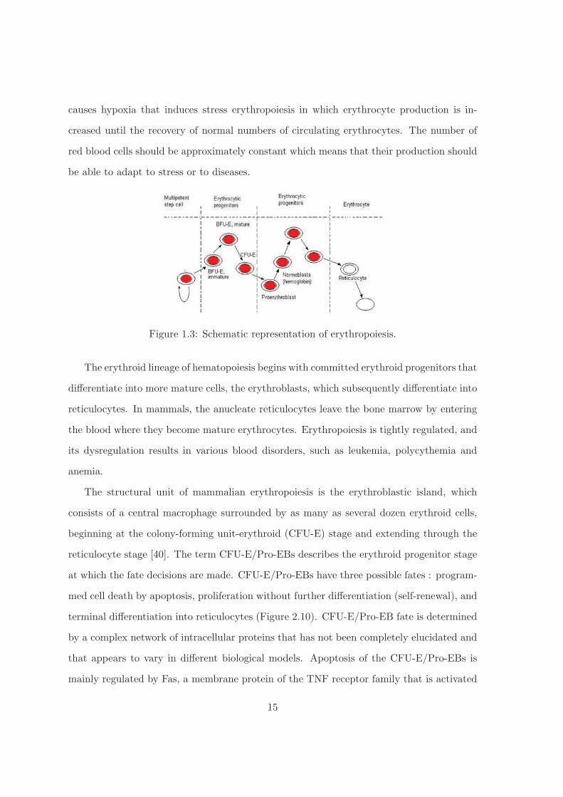
Figure 1.3: Schematic representation of erythropoiesis.

The erythroid lineage of hematopoiesis begins with committed erythroid progenitors that

differentiate into more mature cells, the erythroblasts, which subsequently differentiate into

reticulocytes. In mammals, the anucleate reticulocytes leave the bone marrow by entering

the blood where they become mature erythrocytes. Erythropoiesis is tightly regulated, and

its dysregulation results in various blood disorders, such as leukemia, polycythemia and

anemia.

The structural unit of mammalian erythropoiesis is the erythroblastic island, which

consists of a central macrophage surrounded by as many as several dozen erythroid cells,

beginning at the colony-forming unit-erythroid (CFU-E) stage and extending through the

reticulocyte stage [40]. The term CFU-E/Pro-EBs describes the erythroid progenitor stage

at which the fate decisions are made. CFU-E/Pro-EBs have three possible fates : program-

med cell death by apoptosis, proliferation without further differentiation (self-renewal), and

terminal differentiation into reticulocytes (Figure 2.10). CFU-E/Pro-EB fate is determined

by a complex network of intracellular proteins that has not been completely elucidated and

that appears to vary in different biological models. Apoptosis of the CFU-E/Pro-EBs is

mainly regulated by Fas, a membrane protein of the TNF receptor family that is activated

15

by Fas-ligand. An important difference between humans and mice is that, among erythroid

cells, mature late-stage erythroblasts produce the most Fas-ligand in humans [107], whereas

immature early-stage erythroblasts and some CFU-E/Pro-EB themselves, produce the most

Fas-ligand in mice [100].

1.1.2 Blood diseases

Two blood diseases, the lymphoma and the multiple myeloma, will be presented in more

detail since they will be studied in Chapter 3. These diseases are characterized by invasive

processes by tumors of different part of the body that block normal hematopoiesis. For lym-

phoma, respiratory symptoms shows the early stage of the disease. Symptoms of myeloma

are varied and often uncharacteristic.

Multiple Myeloma

Multiple Myeloma (MM) is a blood disease that affects especially elderly people, its fre-

quency increasing with age. This disease is exceptional before the age of forty years. Its

incidence is two time more prevalent in men than in women. Causes of the disease are

unknown.

Figure 1.4: Bone marrow. Courtesy of M. Koury.

Medical background. MM is a cancer of the bone marrow that destroys bone tissue,

by causing tumors formation inside bones, till the whole bone marrow is replaced by the

16

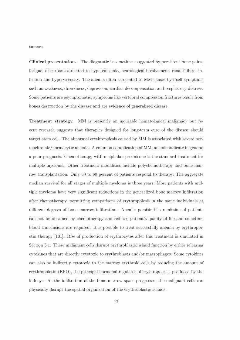
tumors.

Clinical presentation. The diagnostic is sometimes suggested by persistent bone pains,

fatigue, disturbances related to hypercalcemia, neurological involvement, renal failure, in-

fection and hyperviscosity. The anemia often associated to MM causes by itself symptoms

such as weakness, drowsiness, depression, cardiac decompensation and respiratory distress.

Some patients are asymptomatic, symptoms like vertebral compression fractures result from

bones destruction by the disease and are evidence of generalized disease.

Treatment strategy. MM is presently an incurable hematological malignacy but re-

cent research suggests that therapies designed for long-term cure of the disease should

target stem cell. The abnormal erythropoiesis caused by MM is associated with severe nor-

mochromic/normocytic anemia. A common complication of MM, anemia indicate in general

a poor prognosis. Chemotherapy with melphalan-prednisone is the standard treatment for

multiple myeloma. Other treatment modalities include polychemotherapy and bone mar-

row transplantation. Only 50 to 60 percent of patients respond to therapy. The aggregate

median survival for all stages of multiple myeloma is three years. Most patients with mul-

tiple myeloma have very significant reductions in the generalized bone marrow infiltration

after chemotherapy, permitting comparisons of erythropoiesis in the same individuals at

different degrees of bone marrow infiltration. Anemia persists if a remission of patients

can not be obtained by chemotherapy and reduces patient’s quality of life and sometime

blood transfusions are required. It is possible to treat successfully anemia by erythropoi-

etin therapy [101]. Rise of production of erythrocytes after this treatment is simulated in

Section 3.1. These malignant cells disrupt erythroblastic island function by either releasing

cytokines that are directly cytotoxic to erythroblasts and/or macrophages. Some cytokines

can also be indirectly cytotoxic to the marrow erythroid cells by reducing the amount of

erythropoietin (EPO), the principal hormonal regulator of erythropoiesis, produced by the

kidneys. As the infiltration of the bone marrow space progresses, the malignant cells can

physically disrupt the spatial organization of the erythroblastic islands.

17

T Lymphoblastic lymphoma

In industrialized countries, annual cancer incidence in children under than 15 years is esti-

mated to be 140 new cases per million and LBL annual incidence is also estimated between

0.3 to 0.5 case for 100000 children and adolescents, and 85 to 90% are T-cell-lymphoblastic

lymphoma [84, 32]. In the current WHO (World Health Organization) classification, T-LBL

and T-cell Acute Lymphoblastic Leukemia (T-ALL) are a biologic unit termed “precursor

lymphoma/leukemia”[149, 137].The distinction between T-LBL and T-ALL resides in an

arbitrary cut-off point of 25% BM infiltration: BM infiltration below 25% is considered

T-LBL and above, T-ALL [85]. Non-Hodgkin Lymphoma (NHL) is the third most common

form of childhood cancer. LBL represents about 30% of NHL cases in childhood and early

adolescence, and 85 to 90% of LBL are T-LBL [84]. Although T-LBL represents around

25% of all NHL in children, it is considered as a rare disease.

Medical background. Lymphoblastic lymphoma (LBL) is a neoplasm developing from

immature T- or B-precursor cells [137]. LBL are postulated to arise from precursor B in

the bone marrow (BM) or thymic T cells at varying stages of differentiation [52].

Most patients with T-LBL typically present with mediastinal tumor. Other manifes-

tations are lymphadenopathy, frequently with cervical and supraclavicular bulky disease.

Pleural or pericardial effusions are also common. The presence of a predominantly anterior

mediastinal mass can cause respiratory symptoms from coughing, stridor, dyspnea, edema,

elevated jugular venous pressure to acute respiratory distress. About 15–20% of patients

exhibit bone marrow infiltration. Less than 5% show CNS (Central Nervous System) in-

volvement [137]. The median age of diagnosis is 8.8 years, and T-LBL are 2.5 times more

often diagnosed in male patients [137, 33].

Prognostic factors. The probability of pEFS (probability of event-free survival) in LBL

is high, whereas survival in relapsed patients is very poor. As the 5-year EFS (event-free

survival) rates are acceptable, the possibility that patients with favorable risk profiles might

18

be “overtreated” is considered. However, there are currently no validated parameters for

use to identify patients with a favorable risk profile. It is of special importance to detect

the 10%–30% of patients with a high risk of relapse in order to adapt therapy regimen early.

Age older than 14 years [153], CNS involvement trial [1] and unresponse to therapy [155]

are identified as possible unfavorable prognostic factors, but this needs confirmation.

Treatment strategy. pEFS in pediatric T-LBLB is currently about 80% [29]. Based

on historical studies, the current treatment approach of LBL uses therapy similar to that

for childhood acute lymphoblastic leukemia [151], and EFS is actually more than 80% in

children and adolescent. Successive studies demonstrated the importance of initial intensive

treatment, secondary intensification of chemotherapy, prolonged maintenance therapy and

prophylaxis of CNS relapse. Although the development of therapy protocols meant a major

step toward curing pediatric patients from LBL, unanswered questions remain. Numerous

trials and protocols have been developed on the Berlin-Frankfurt-Muenster (BFM) or LSA2-

L2 (American group) backbone to increase event free survival as well as overall survival (OS)

and to reduce toxicity within the established therapy regimens [137]. Central nervous system

(CNS) prophylaxis is considered as an important element of all LBL protocols, including

prophylactic cranial irradiation and Methothrexate (MTX) (high-dose or intrathecal) [137].

Prophylactic irradiation was historically used in all protocols. Several recent trials showed

that it was not required any more to achieve an excellent treatment outcome [155, 33, 131].

More trials are needed to evaluate the role of high-dose MTX in pediatric LBL who do

not received prophylactic irradiation and an acceptable number of intrathecal MTX. The

therapy of LBL is rather long with its total duration of 24 months in most protocols including

induction, consolidation and maintenance therapy [137].

19

1.2 Modeling approaches: multi-scale hybrid model

1.2.1 Modeling literature

Hematopoiesis has been the topic of modeling works for decades. Dynamics of hematopoietic

stem cells have been described by Mackey’s early works [103, 104]. The author developed

hypothesis that aplastic anaemia (lower counts of all three blood cell types) and periodic

haematopoiesis in humans are probably due to irreversible cellular loss from the prolifer-

ating pluripotential stem cell population. A model for pluripotential stem cell population

is described by delay equations. In the later developed model, described by the first or-

der differential equations, a population dynamics of cells capable of both proliferation and

maturation was analysed [105]. In Bernard et al. [18] mathematical model was proposed

to explain the origin of oscillations of circulating blood neutrophil number. The authors

demonstrated that an increase in the rate of stem cell apoptosis can lead to long period

oscillations in the neutrophil count. In extension of the previous model Colijn and Mackey

in [51] applied mathematical model, described with system of delay differential equations,

to explain coupled oscillations of leukocytes, platelets and erythrocytes in cyclical neutrope-

nia. The platelet production process (thrombopoiesis) attracted less attention through years

[67, 163]. Cyclical platelet disease was a subject of mathematical modeling in Santillan et

al. [132] and was enriched in Apostu et al. [12]. The red blood cell production process

(erythropoiesis) has recently been the focus of modeling in hematopoiesis. Pioneering math-

ematical model which describes the regulation of erythropoiesis in mice and rats has been

developed by Wichmann, Loeffler and co-workers [164]. In this work, proposed models were

validated by comparing with experimental data. Analysis of the regulating mechanisms in

erythropoiesis was enriched in [168]. In 1995, Belair et al. proposed age-structured model

of erythropoiesis where erythropoietin (EPO) causes differentiation, without taking into

account erythropoietin control of apoptosis found out in 1990 by Koury and Bondurant in

[92]. In 1998 Mahaffy et al. [106] expanded this model by including the apoptosis possibility.

Age-stuctured model is detailed in [3] with assumption that decay rate of erythropoietin

20

depends on the number of precursor cells. In [57] Crauste et al. included in the model

the influence of EPO upon progenitors apoptosis and showed the importance of erythroid

progenitor self-renewing by confronting their model with experimental data on anaemia in

mice. A model of all hematopoietic cell lineages that has been proposed by Colijn and

Mackey [50, 51] includes dynamics of hematopoietic stem cells, white cell lineage, red blood

cell lineage and platelet lineage. A review of mathematical models and simulation studies,

applied to stem cell biology, with particular interest to the hematopoietic system is proposed

by Roeder[125].

In recent works a combination of different models is used in order to describe the process

of hematopoiesis in its complexity. A hybrid model is suggested in [95] where granulopoiesis

is described by ordinary differential equations and stem cell organization by an individual

based model.

In this work we consider another type of hybrid models coupling discrete and continuous

approaches at the level of each cell. The difference with the preceding works [36] is that ODE

are not used to describe cell concentrations of cells but concentrations of proteins inside

each individual cell. From this point of view this work can be related to the individual

based model in [95]. In our model, cell fate is determined by the combination of discrete

and continuous models. Global and local regulation acts at the level of individual cells and

not for the whole cell population.

All the previously mentioned approaches did not consider spatial aspects of hematopoiesis.

Cellular regulation by cell-cell interaction was neither considered in these models. Multi-

scale approaches include both cell population kinetics [24] or erythroid progenitor dynamics

[57, 55] and intracellular regulatory networks dynamics in the models [19] in order to give

insight in the mechanisms involved in erythropoiesis. Off-lattice discrete-continuous hybrid

models, applied to the erythropoiesis modeling, allow to take into account simultaneously

interactions at the cell population level, regulation at the intracellular and extracellular

levels and to study an importance of the spatial structure [98, 23]. The role of macrophage

in stabilizing of erythroblastic island is investigated in [70]. Indeed, macrophages produce

21

growth factors (GF) that influence the fate of cell. According to the distance between cells

and macrophage, the quantity of GF received by cells vary.

Multi-scale hybrid model consists in the coupling of two models, with different space and

time scales. Such discrete-continuous models are usually called hybrid models [24, 114, 118].

Hybrid discrete-continuous models are widely used in the investigation of dynamics of cell

populations in biological tissues and organisms that involve processes at different scales. In

this approach biological cells are considered as discrete objects described either by cellular

automata ([66], [78], [88], [108], [136], [145]) or by various on-lattice or off-lattice models

([64], [87], [120]) while intracellular and extracellular concentrations are described with

continuous models, ordinary or partial differential equations.

1.2.2 Multi-scale hybrid discrete-continuous model

Hybrid models can be based on cellular automata and other lattice models and off-lattice

models where cell position in space is not restricted to the nodes of a grid. In cellular

automaton model each individual cell can be represented as a single site of lattice, as several

connected lattice sites or the lattice site can be larger than an individual cell. A generalized

cellular automaton approach is presented by the cellular Potts models (CPM). The CPM is

a more sophisticated cellular automaton that describes individual cells, occupying multiple

lattice sites, as extended objects of variable shapes. These models take into account surface

energy of cell membrane. The CPM effective energy can control cell behaviors including cell

adhesion, signalling, volume and surface area or even chemotaxis, elongation and haptotaxis

[78], [136]. In each particular CA model, the rules which determine cell motion should

be specified. It can be influenced by the interaction of cells with the elements of their

immediate surrounding and by processes that involve cellular response to external signals

like chemotaxis. The numerous models with gradient fields of chemical concentrations that

govern motility of cells have been suggested. Cellular automaton have been used extensively

to model a wide range of problems. Different stages of tumor development from initial

avascular phase([66], [88]) to invasion ([11]) and angiogenesis ([108], [145]) are studied.

22

Off-lattice models are important to those biological situations in which the shape of

individual cells can influence the dynamics or geometry of the whole population of cells. In

off-lattice models, shape of cells can be explicitly modelled and response to local mechanical

forces, interaction with neighboring cells and environment can be investigated. Hybrid

off-lattice models, not limited in possible directions of cell motion, are widely applied to

the modeling of tumor growth and invasion where cell migration should be taken into

account ([87], [120]). Another type of off-lattice models, called fluid-based elastic cell model,

approach that takes into account cell elasticity, is also applied in tumor growth modeling

([11], [64]).

23

1.3 Main results of the thesis

The thesis is devoted to mathematical modeling of hematopoiesis and blood diseases. We

develop hybrid discrete-continuous models and apply them to study erythropoiesis and

lineage choice. We will also use them to model two diseases, lymphoma and myeloma.

The last chapter of the thesis is devoted to the analysis of solutions of reaction-diffusion

equations which describe Darwinian evolution of cancer cells.

1.3.1 Methods of modeling

A hybrid modeling approach with off-lattice cell dynamics is used in order to study hema-

topoiesis. Cells will be considered as discrete objects while intracellular and extracellular

concentrations will be described with ordinary and partial differential equations. This model

will be applied to study the lineage choice of megakaryocytic-erythroid bipotent progenitors,

functioning of erythroblastic islands in erythropoiesis and some blood diseases (lymphoma,

multiple myeloma).

Intracellular regulation

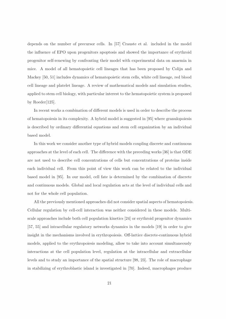
Cell fate is determined by specific cellular proteins P1, ..., Pk whose concentrations (or bio-

logic activities) are described by ordinary differential equations :

dPj

dt= Φj(P ), j = 1, ..., k, (1.3.1)

where Φj are the rates of their production or activation. These proteins will be specified

below for intracellular regulation of megakaryocytic-erythroid progenitors and of erythroid

progenitors.

Depending on the values of these intracellular proteins, the cell will self-renew, differ-

entiate or die by apoptosis. Precise conditions that determine cell fate will be specified

below for each particular application. It should be noted that cell fate depends also on the

extracellular regulation, that is on nutrients, hormones, growth factors in the extracellular

24

Figure 1.5: Schematic representation of hybrid models. Cells are considered as individualobjects. Circles of different colors correspond to different cell types. Intracellular con-centrations described by ordinary differential equations determine cell fate. Extracellularsubstances described by partial differential equations can influence the intracellular regula-tion. Cells can move due to mechanical forces acting from other cells or because of someother factors.

matrix. These substances can influence the intracellular regulation. Therefore instead of

equations (1.3.1) we should consider the equations

dPi(t)

dt= Φi(P (t), ν(xi, t)), j = 1, ..., k, (1.3.2)

where ν is a vector of extra-cellular concentrations taken at the center xi(t) of the cell.

Extracellular regulation

The concentrations of the species in the extra-cellular matrix are described by the reaction-

diffusion system of equations

∂ν

∂t= D Δν +G(ν, c), (1.3.3)

25

where c is the local cell density, G is the rate of consumption or production of these sub-

stances by cells. These species can be either nutrients coming from outside and consumed

by cells or some other bio-chemical products consumed or produced by cells. During ery-

thropoiesis, erythroid cells produce Fas-Ligand FL, which influences the surrounding cells

by increasing intracellular Fas activity. The Fas-ligand-producing erythroid cells are mainly

immature erythroblasts in murine erythropoiesis [100] and mainly the mature erythroblasts

in human erythropoiesis [107]. On the other hand, macrophages produce a growth factor

G, which stimulates erythroid cell proliferation. In mice, G is KL/SCF in normal erythro-

poiesis and BMP4 in stress erythropoiesis. The concentrations of Fas-ligand and of the

growth factor in the extracellular matrix are described by the reaction-diffusion equations :

∂FL

∂t= D1ΔFL +W1 − σ1FL, (1.3.4)

∂G

∂t= D2ΔG+W2 − σ2G. (1.3.5)

Here D1, D2 are diffusion coefficients and W1, W2 are the rates of production of the corre-

sponding factors. These functions are proportional to the concentrations of the correspond-

ing cells.

In numerical simulations, equations (1.3.4), (1.3.5) are solved by a finite difference

method with Thomas algorithm and alternative direction method. Neumann (no-flux)

boundary conditions are considered at the boundary of the rectangular domain. Constant

space and time steps are used.

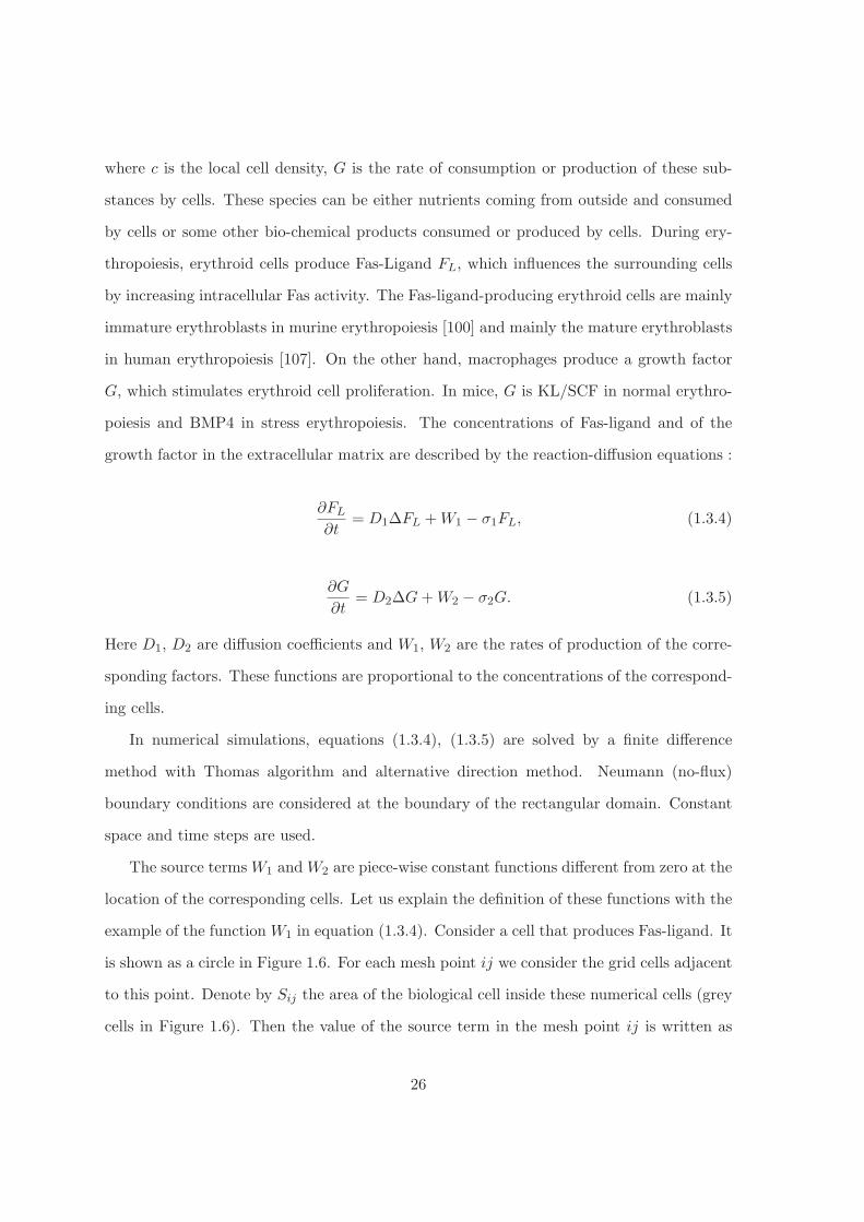
The source terms W1 and W2 are piece-wise constant functions different from zero at the

location of the corresponding cells. Let us explain the definition of these functions with the

example of the function W1 in equation (1.3.4). Consider a cell that produces Fas-ligand. It

is shown as a circle in Figure 1.6. For each mesh point ij we consider the grid cells adjacent

to this point. Denote by Sij the area of the biological cell inside these numerical cells (grey

cells in Figure 1.6). Then the value of the source term in the mesh point ij is written as

26

Figure 1.6: Schematic representation of a cell on the numerical grid.

follows: W ij1 = w0

1Sij/(4s), where w01 is a constant which measures the normalized intensity

of Fas-ligand production, s is the area of the numerical cell. For example, if the grid point ij

is inside the biological cell together with all four numerical cells around it, then W ij1 = w0

1.

When the concentrations of various substances in the extracellular matrix are found,

we can use them in the equations (1.3.2) for the intracellular concentrations. If cell size is

sufficiently small in the length scale determined by the gradients of extracellular concentra-

tions, then the variation of these concentration at the cell size is small. Therefore we use

the values of extracellular concentrations at the cell center. These values are found from

their values at the grid points by interpolation.

Movement of cells

Since cells divide and increase their number, they can push each other resulting in cell

displacement. In order to describe mechanical interaction between cells, we restrict ourselves

to the simplest model where cells are presented as elastic spheres. Consider two elastic

spheres with centers at the points x1 and x2 and with the radii, respectively, r1 and r2. If

27

the distance h12 between the center is less than the sum of the radii, r1 + r2, then there

is a repulsive force between them, f12, which depends on the difference between (r1 + r2)

and h12. If a particle with center at xi is surrounded by several other particles with centers

at the points xj , j = 1, ...k, then we consider the pairwise forces fij assuming that they

are independent of each other. This assumption corresponds to small deformation of the

particles. Hence, we find the total force Fi acting on the i-th particle from other particles,

Fi =∑

i fij . The motion of the particles can now be described as the motion of their centers

by Newton’s second law

mxi +mμxi −∑j �=i

fij = 0,

where m is the mass of the particle, the second term in the left-hand side describes the

friction by the surrounding medium, and the third term is the potential force between cells.

We consider the force between particles in the following form

fij =

⎧⎪⎨⎪⎩

Kh0−hij

hij−(h0−h1), h0 − hi < hij < h0

0 , hij ≥ h0

,

where hij is the distance between the particles i and j, h0 is the sum of cell radii, K is a

positive parameter, and h1 accounts for the incompressible part of each cell. This means

that the internal part of the cell is incompressible. It allows us to control compressibility of

the medium. The force between the particles tends to infinity when hij decreases to h0-h1.

When a cell center crosses the boundary of computational domain, it is removed from

the simulations. Under some conditions, cells can also be removed even if they are inside

the computational domain. In particular, in the case of cell death or, in the case of blood

cells in the bone marrow, if they leave bone marrow into the blood flow. When a new cell

appears, we prescribe it initial position and initial velocity.

28

Cell properties and division

Biological cells considered in hybrid models are characterized by certain parameters such

as their type, duration of cell cycle, initial radius and initial values of intracellular proteins.

These values are given to each cell at the moment of its birth. Some other cell properties

are variable and they can change during it life time. In particular, cell age, radius, position

and current values of intracellular proteins. These values are recalculated at every time

step.

Some of cell properties can be given as random variables. For example, duration of

cell cycle is considered as a random variable with a uniform distribution in the interval

[T − δT, T + δT ]. Initial protein concentrations can also be considered as random variables

in some given range.

Cell fate is determined at the end of cell cycle. At the first stage, they make a choice

between apoptosis and survival. If they survive and divide, they make a choice between

self-renewal and differentiation. In both cases, the choice is determined by the values of

intracellular proteins.

During cell cycle, cell radius grows linearly. It becomes twice the initial radius at the end

of cell cycle. Then mother cell is replaced by two daughter cells. Geometrically, two circles

with the initial radius are located inside the circle with twice larger radius. The direction

of cell division, that is the direction of the line connecting the centers of daughter cells,

is random. This is specific for cell division in hematopoiesis. In some other applications,

direction of cell division can be prescribed.

Let us also note, that cell volume in the model is not preserved after division. The

total volume of the daughter cells is twice less than the volume of the mother cell before its

division. Since cells in the bone marrow are sufficiently sparse, preservation of their volume

during division is not essential. It can be important in some other applications where cell

density is large and the forces acting between cells should be found more accurately.

29

1.3.2 Hematopoiesis

Hematopoiesis is a complex process that begins with hematopoietic stem cells and results in

production of erythrocytes, platelets and leucocytes. This process is controlled by numerous

local and global regulatory mechanisms. If some of them do not function properly, various

blood diseases can appear. In particular, excessive proliferation of immature cells can lead

to leukemia and other malignant diseases.

In this work we will study erythroid lineage of erythropoiesis beginning with lineage

choice and then its further progression till mature erythrocytes in the blood flow. We will

see that this process is tightly regulated by intracellular proteins, growth factors in the

extracellular matrix and hormones.

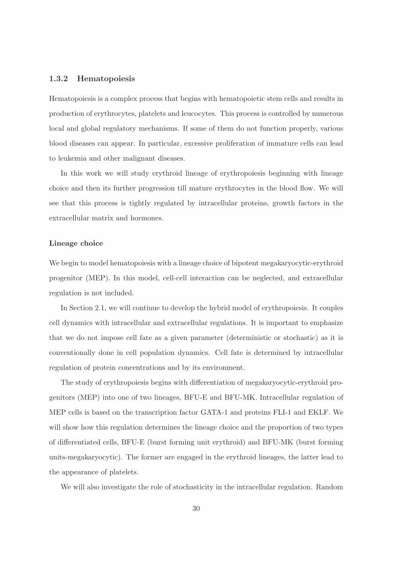
Lineage choice

We begin to model hematopoiesis with a lineage choice of bipotent megakaryocytic-erythroid

progenitor (MEP). In this model, cell-cell interaction can be neglected, and extracellular

regulation is not included.

In Section 2.1, we will continue to develop the hybrid model of erythropoiesis. It couples

cell dynamics with intracellular and extracellular regulations. It is important to emphasize

that we do not impose cell fate as a given parameter (deterministic or stochastic) as it is

conventionally done in cell population dynamics. Cell fate is determined by intracellular

regulation of protein concentrations and by its environment.

The study of erythropoiesis begins with differentiation of megakaryocytic-erythroid pro-

genitors (MEP) into one of two lineages, BFU-E and BFU-MK. Intracellular regulation of

MEP cells is based on the transcription factor GATA-1 and proteins FLI-1 and EKLF. We

will show how this regulation determines the lineage choice and the proportion of two types

of differentiated cells, BFU-E (burst forming unit erythroid) and BFU-MK (burst forming

units-megakaryocytic). The former are engaged in the erythroid lineages, the latter lead to

the appearance of platelets.

We will also investigate the role of stochasticity in the intracellular regulation. Random

30

variations in the initial intracellular concentrations of newly born cells will determine their

choice between self-renewal and differentiation. In the case of immature cells MEP, random

initial concentrations of intracellular proteins determine their further development and the

choice between two lineages. In the case of deterministic initial conditions all cells will have

the same fate, and lineage choice cannot be described.

Thus, in this section we have developed hybrid model of MEP cell choice between two lin-

eages, erythroid and megakaryocytic. We have shown how the intracellular regulation based

on GATA-1, FLI-1 and EKLF and random initial concentrations of intracellular proteins

determine cell fate and proportion of cells of two different lineages.

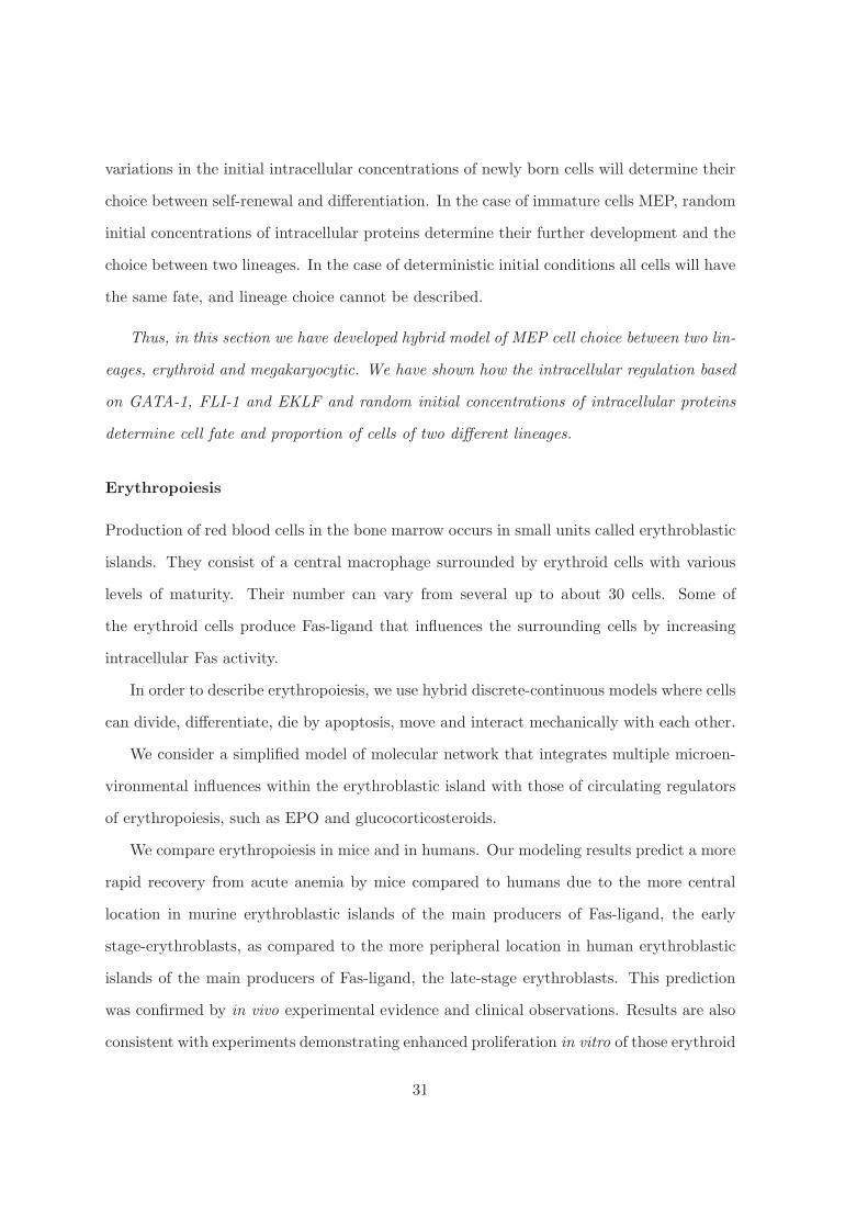
Erythropoiesis

Production of red blood cells in the bone marrow occurs in small units called erythroblastic

islands. They consist of a central macrophage surrounded by erythroid cells with various

levels of maturity. Their number can vary from several up to about 30 cells. Some of

the erythroid cells produce Fas-ligand that influences the surrounding cells by increasing

intracellular Fas activity.

In order to describe erythropoiesis, we use hybrid discrete-continuous models where cells

can divide, differentiate, die by apoptosis, move and interact mechanically with each other.

We consider a simplified model of molecular network that integrates multiple microen-

vironmental influences within the erythroblastic island with those of circulating regulators

of erythropoiesis, such as EPO and glucocorticosteroids.

We compare erythropoiesis in mice and in humans. Our modeling results predict a more

rapid recovery from acute anemia by mice compared to humans due to the more central

location in murine erythroblastic islands of the main producers of Fas-ligand, the early

stage-erythroblasts, as compared to the more peripheral location in human erythroblastic

islands of the main producers of Fas-ligand, the late-stage erythroblasts. This prediction

was confirmed by in vivo experimental evidence and clinical observations. Results are also

consistent with experiments demonstrating enhanced proliferation in vitro of those erythroid

31

(a) in mice (b) in human

Figure 1.7: Typical structure of an erythroblastic island in the simulations : Fas-ligand producedby early-stage erythroblasts (left) or by late-stage erythroblasts (right). The large cell in the centeris a macrophage, yellow cells - CFU-E/Pro-EBs and differentiating erythroblasts, blue - late-stagemature erythroblasts and reticulocytes, level of green - concentration of the growth factor (G)produced by the macrophage, level of red - concentration of Fas-ligand. Black circles inside cellsshow their incompressible parts.

cells that are most closely associated physically with central macrophages.

Thus, in this section we have developed hybrid model of erythropoiesis. We describe

its functioning in normal and stress (anemia) conditions. We obtain a good description of

experimental results and of clinical data. We also show that central macrophage is necessary

to stabilize erythroblastic islands. Multiple islands without macrophage are unstable and

cannot be stabilized by the hormone erythropoietin. On the other hand, erythroblastic islands

with macrophages show a stable and robust behavior in a wide range of parameters. Finally,

we modeled erythropoiesis in mice and in humans and explained the difference between them.

This difference shows that in some cases murine erythropoiesis cannot be used as a biological

model of human erythropoiesis.

1.3.3 Blood diseases

Myeloma

Multiple myeloma (MM) is a relatively common disease that is characterized by bone mar-

row infiltration with malignant plasma cells and, very frequently it leads to a malignancy-

32

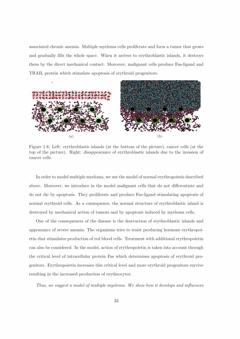
associated chronic anemia. Multiple myeloma cells proliferate and form a tumor that grows

and gradually fills the whole space. When it arrives to erythroblastic islands, it destroys

them by the direct mechanical contact. Moreover, malignant cells produce Fas-ligand and

TRAIL protein which stimulate apoptosis of erythroid progenitors.

(a) (b)

Figure 1.8: Left: erythroblastic islands (at the bottom of the picture), cancer cells (at thetop of the picture). Right: disappearance of erythroblastic islands due to the invasion ofcancer cells.

In order to model multiple myeloma, we use the model of normal erythropoiesis described

above. Moreover, we introduce in the model malignant cells that do not differentiate and

do not die by apoptosis. They proliferate and produce Fas-ligand stimulating apoptosis of

normal erythroid cells. As a consequence, the normal structure of erythroblastic island is

destroyed by mechanical action of tumors and by apoptosis induced by myeloma cells.

One of the consequences of the disease is the destruction of erythroblastic islands and

appearance of severe anemia. The organisms tries to resist producing hormone erythropoi-

etin that stimulates production of red blood cells. Treatment with additional erythropoietin

can also be considered. In the model, action of erythropoietin is taken into account through

the critical level of intracellular protein Fas which determines apoptosis of erythroid pro-

genitors. Erythropoietin increases this critical level and more erythroid progenitors survive

resulting in the increased production of erythrocytes.

Thus, we suggest a model of multiple myeloma. We show how it develops and influences

33

functioning of erythropoiesis. It leads to the development of anemia that can be partially

compensated by treatment with hormone erythropoietin.

Lymphoma

Lymphoma is a disease characterized by the appearance of tumor in the thymus, an or-

gan located in the thorax. The volume of the tumor increases and provokes important

respiratory difficulties. We study lymphoma development in children and its treatment by

chemotherapy. Patients are treated during two years, though according to some estimates,

patients can be over-treated. The purpose of this simulation is to study the number of re-

lapses as a function of the duration of treatment and of the doses of drugs, mainly purinethol

and methotrexate.

In order to study lymphoma, we begin with modeling of healthy thymus. The model is

based on the same approach as we used before to model normal erythropoiesis and multiple

myeloma. Cells are considered as individual objects. Their fate is determined by the

intracellular regulation and it is influenced by growth factors produced bo other cells.

In Section 3.2, we will model T cells formation in the thymus containing precursors,

double negative (DN), double positive (DP) and simple positive (SP) cells. After differ-

entiation, these cells give rise to T lymphocytes. The proportions of each kind of cells

remain approximately constant in a healthy individual. Thymus provide a constant T cells

production compensating apoptosis. In simulations, apoptosis is modeled by a probability

of remaining alive for each cell type. Nurse cells produce growth factor which promotes

self-renewal of thymocytes. The thymocytes located sufficiently far from the nurse cells will

differentiate else they will self renew.

A single mutated cell begins to proliferate and causes tumor. Malignant cells self-renew

at the end of each cell cycle with a given probability. They grow exponentially and invade

the thymus and push out normal cells.

The action of chemotherapy on thymus is simulated by intracellular drug concentration

given by physiologically based pharmacokinetic model (PBPK) in time, for various values of

34

parameters. If the intracellular drug concentration reaches some critical level at the end of

cell cycle, then the cell dies. Malignant cells are gradually eliminated, the tumor disappears,

precursors enter the thymus and recreate its normal structure.

We simulated maintenance treatment and analyzed the number of relapses as a function

of duration of treatment. The results of the simulations correspond to the database EuroLB.

They show that the duration of treatment can be reduced from 24 month, as it is the case

in clinical practice, to 12 month with the same proportion of relapses.

Resistance to treatment. We study the resistance to treatment in the case of lym-

phoma. Let us recall that malignant cells die if the intracellular concentration of drug

reaches some critical level pc. This value can be different in different cells. Hence different

cells have different sensibility to treatment. On the other hand, we assume that when lym-

phoma cells divide, daughter cells can have different values of pc in comparison with the

mother cell. Since cells with a larger value pc have a better probability to survive, then

more and more resistent cells will emerge in the process of treatment.

In the study of lymphoma, we have developed a hybrid model which describes normal

functioning of thymus and the development of the disease. We model treatment of lymphoma

and analyze the response of virtual patients to treatment. We show that the duration of

treatment can possibly be reduced with the same proportion of relapses. Finally, we model

the development of the resistance to treatment.

1.3.4 Existence and dynamics of pulses

Biological cells can be characterized by their genotype. Cells of the same type have a lo-

calized density distribution in the space of genotypes. This distribution can evolve under

the influence of various external factors. In particular cancer cells can adapt to chemother-

apy treatment resulting in appearance of resistant clones. This process is called Darwinian

evolution of cancer cells [27]. We studied above the emergence of resistance with hybrid

discrete-continuous models in the case of lymphoma treatment. In this chapter we analyze

35

this process with reaction-diffusion equations. We will consider the scalar reaction-diffusion

equation

∂u

∂t= D

∂2u

∂x2+ F (u, x), (1.3.6)

on the whole axis. The typical example of the nonlinearity is given by the function

F (u, x) = uk(1− u)− σ(x)u, (1.3.7)

where the first term describe the rate of cell birth and the second term the rate of their

death. Let us note that the space variable x here corresponds to cell genotype, u(x, t) is

the cell density which depends on x and on time t. The diffusion term describe variation

of genotype due to mutations, the mortality term depends on the space variable, that is on

cell genotype.

Monostable case

If k = 1 and σ(x) = const, then this equation does not have localized stationary solutions.

In order to describe cell populations with localized genotype which correspond to certain

cell type, we need to introduce space dependent mortality coefficients. This means that

cells can survive only in a certain range of genotypes (survival gap).

Consider now cell population dynamics if there are two survival gaps, that is two intervals

of genotype where cells can survive. We will consider the model with global consumption of

resources where all cells consume the same nutrients and their quantity is limited. In this

case, the function F in (2.2.20) is replaced by the functional

F (u, x, J(u)) = uk(1− J(u))− σ(x)u, J(u) =

∫ ∞

−∞u(y, t)dy.

Hence we consider a nonlocal reaction-diffusion equation.

Suppose that initially all cells are located in the first survival gap (Figure 1.9). If we

increase the mortality coefficient there, then this cell population disappears. Instead of

36

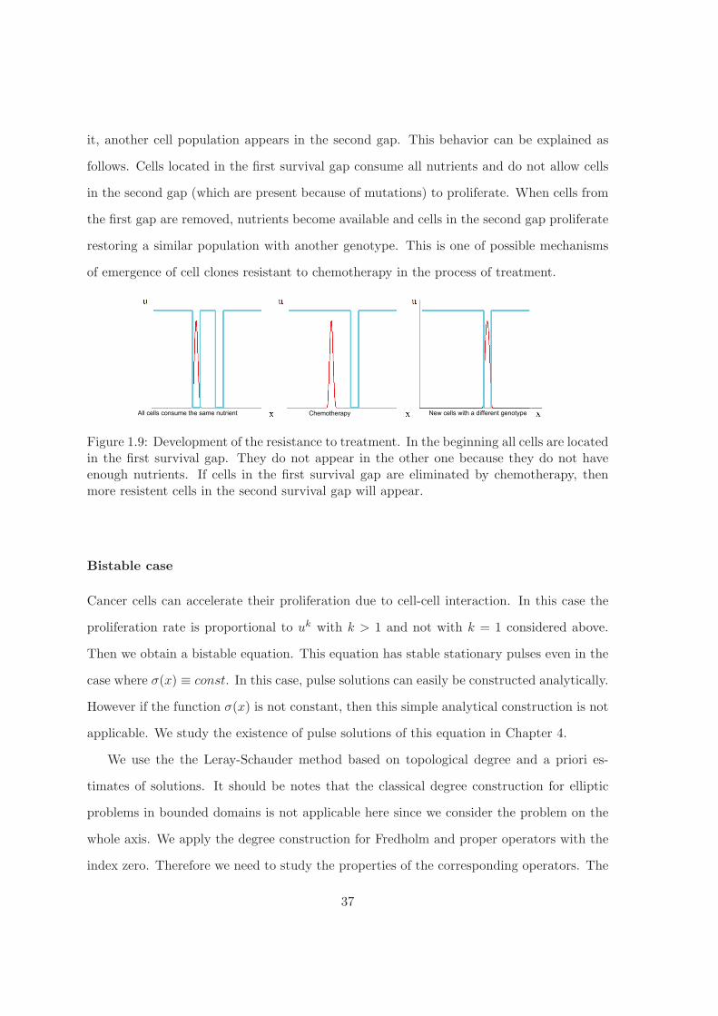
it, another cell population appears in the second gap. This behavior can be explained as

follows. Cells located in the first survival gap consume all nutrients and do not allow cells

in the second gap (which are present because of mutations) to proliferate. When cells from

the first gap are removed, nutrients become available and cells in the second gap proliferate

restoring a similar population with another genotype. This is one of possible mechanisms

of emergence of cell clones resistant to chemotherapy in the process of treatment.

All cells consume the same nutrient Chemotherapy New cells with a different genotype

Figure 1.9: Development of the resistance to treatment. In the beginning all cells are locatedin the first survival gap. They do not appear in the other one because they do not haveenough nutrients. If cells in the first survival gap are eliminated by chemotherapy, thenmore resistent cells in the second survival gap will appear.

Bistable case

Cancer cells can accelerate their proliferation due to cell-cell interaction. In this case the

proliferation rate is proportional to uk with k > 1 and not with k = 1 considered above.

Then we obtain a bistable equation. This equation has stable stationary pulses even in the

case where σ(x) ≡ const. In this case, pulse solutions can easily be constructed analytically.

However if the function σ(x) is not constant, then this simple analytical construction is not

applicable. We study the existence of pulse solutions of this equation in Chapter 4.

We use the the Leray-Schauder method based on topological degree and a priori es-

timates of solutions. It should be notes that the classical degree construction for elliptic

problems in bounded domains is not applicable here since we consider the problem on the

whole axis. We apply the degree construction for Fredholm and proper operators with the

index zero. Therefore we need to study the properties of the corresponding operators. The

37

main difficulty of the application of the Leray-Schauder method is related to a priori esti-

mates of solutions. We develop a special approach which allows us to obtain the estimates

in weighted Holder spaces which are introduced in order to define the degree. The following

theorem is proved.

Theorem. If the function F (w, x) satisfies conditions:

F (0, x) = 0, x ≥ 0;∂F (w, x)

∂x< 0, w > 0, x ≥ 0

F (w, x) < 0, ∀x ≥ 0, w > w+.

and the function F+(w) satisfies conditions:

F ′+(0) < 0, F+(w) < 0 for w > w+

∫ w0

0F+(u)du = 0,

∫ w

0F+(u)du �= 0 ∀w ∈ (0, w+), w �= w0.

then the problem

w′′ + F (w, x) = 0, w′(0) = 0

on the half-axis x > 0 has a positive monotonically decreasing solution vanishing at infinity.

It belongs to the weighted Holder space E1.

This theorem affirms the existence of solutions on the half-axis. The existence of pulse

solutions on the whole axis can be now obtained by symmetry. We also use this result

to prove the existence of pulse solutions for the corresponding nonlocal reaction-diffusion

equation.

In the case of time dependent problem, if the mortality rate depends on the genotype,

σ = σ(x), then the pulse will move in the direction where this function is less. In this

38

case we have a gradual change of cell genotype due to small mutations. This evolution will

also lead to the emergence of cell clones better adapted to treatment. Thus, there are two

different mechanisms of cell evolution. In one of them, cell genotype can have large changes,

jumps to other survival gaps (k = 1), in the other one these changes are continuous.

Analyzing the reaction-diffusion equations, we proved the existence of pulse solutions for

local and nonlocal reaction-diffusion equations. We suggested two possible mechanisms of

the resistance to treatment. These mechanisms are based on the evolution of cancer cells in

the space of genotypes and on survival of more adapted cells.

39

Chapter 2

Hematopoiesis

2.1 Lineage choice

2.1.1 Introduction

In this section, we discuss intracellular regulation of bipotent MEP (megakaryocytic-erythroid

progenitor) between thrombocytic and erythroid lineage. MEP can differentiate into BFU-E

(burst forming unit erythroid) progenitors or BFU-MK (burst forming units-megakaryocytic)

progenitors or self-renew in order to give rise to the two lineages of blood cells.

The ‘hybrid’ model that couples two relevant scales, intracellular protein regulation

with extracellular matrix is used to model lineage choice. An intracellular regulation of

progenitors allows to simulate this choice. Cell-cell interaction can be neglected, and the

model does not include extracellular regulation. Cell movement and their spatial position

play an important role in cell’s decision between self-renewal, differentiation and apoptosis

based on intracellular protein concentrations. We have performed numerical simulations

to model the behavior of MEP and we obtained all the expected behavior (appearance

of two lineages) concerning the commitment of progenitors by changing the parameters of

equations of an hybrid model.

40

2.1.2 Intracellular regulation

The complex mechanism that induces commitment of MEP is not completely understood

but the role of some growth factors and transcription factors has been established. Indeed,

the erythroid transcription factor (zinc finger factor) GATA-1 is required for the differenti-

ation and maturation of erythroid/megakaryocytic cells [38]. Endogenous EKLF (erythroid

Kruppel-like factor) promotes the erythroid lineage choice while FLI-1 (Friend Leukemia

Integration 1) overexpression inhibits erythroid differentiation [38]. Interactions between

FLI-1 and EKLF are also involved [38], EKLF represses FLI-1 [72, 30, 144].

We will take into account intracellular regulation of MEP with GATA-1 and transcrip-

tion factors FLI-1 and EKLF. We assumed that distribution of hormones Epo and Tpo

is uniform in the bone marrow. Moreover according to biological observations there is no

communication between these cells. Therefore extracellular regulation is not present in this

model.

Let u be the concentration of the transcription factor EKLF, v the concentration of

FLI-1 and w of GATA-1. FLI-1 can form complexes with the other two factors. We will

denote them by [uv] and [vw]. Then the intracellular regulation can be described as follows:

u+ wk+1←→

k−1

[uw], [uw]k2−→ n1u, v + w

k+3←→

k−3

[vw], [vw]k4−→ n2v.

Taking into account the mass balance w + [uw] + [vw] = w0, we obtain the system of

equations for these concentrations:

du

dt= −k+1 u(w0 − [uw]− [vw]) + (k−1 + n1k2)[uw], (2.1.1)

dv

dt= −k+3 v(w0 − [uw]− [vw]) + (k−3 + n2k4)[vw], (2.1.2)

d[uw]

dt= k+1 u(w0 − [uw]− [vw])− k−1 [uw], (2.1.3)

d[vw]

dt= k+3 v(w0 − [uw]− [vw])− k−3 [vw]. (2.1.4)

41

Intracellular regulation described by this system of equations should be completed by con-

ditions of self-renewal of the progenitors or their commitment to one of the two lineages.

We will suppose that if concentrations of FLI-1 and EKLF are less than some critical values

at the end of cell cycle, then differentiation does not hold and the cell self-renews. If at

least one of these two concentrations is greater than the critical level, then the cell differen-

tiates. In this case, it becomes BFU-MK if the concentration of FLI-1 is greater than the

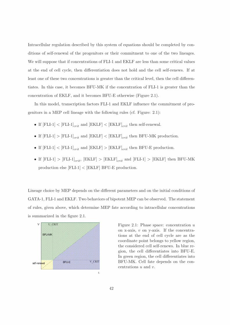
concentration of EKLF, and it becomes BFU-E otherwise (Figure 2.1).

In this model, transcription factors FLI-1 and EKLF influence the commitment of pro-

genitors in a MEP cell lineage with the following rules (cf. Figure: 2.1):

• If [FLI-1] < [FLI-1]crit and [EKLF] < [EKLF]crit then self-renewal.

• If [FLI-1] > [FLI-1]crit and [EKLF] < [EKLF]crit then BFU-MK production.

• If [FLI-1] < [FLI-1]crit and [EKLF] > [EKLF]crit then BFU-E production.

• If [FLI-1] > [FLI-1]crit, [EKLF] > [EKLF]crit and [FLI-1] > [EKLF] then BFU-MK

production else [FLI-1] < [EKLF] BFU-E production.

Lineage choice by MEP depends on the different parameters and on the initial conditions of

GATA-1, FLI-1 and EKLF. Two behaviors of bipotent MEP can be observed. The statement

of rules, given above, which determine MEP fate according to intracellular concentrations

is summarized in the figure 2.1.

Figure 2.1: Phase space: concentration uon x-axis, v on y-axis. If the concentra-tions at the end of cell cycle are as thecoordinate point belongs to yellow region,the considered cell self-renews. In blue re-gion, the cell differentiates into BFU-E.In green region, the cell differentiates intoBFU-MK. Cell fate depends on the con-centrations u and v.

42

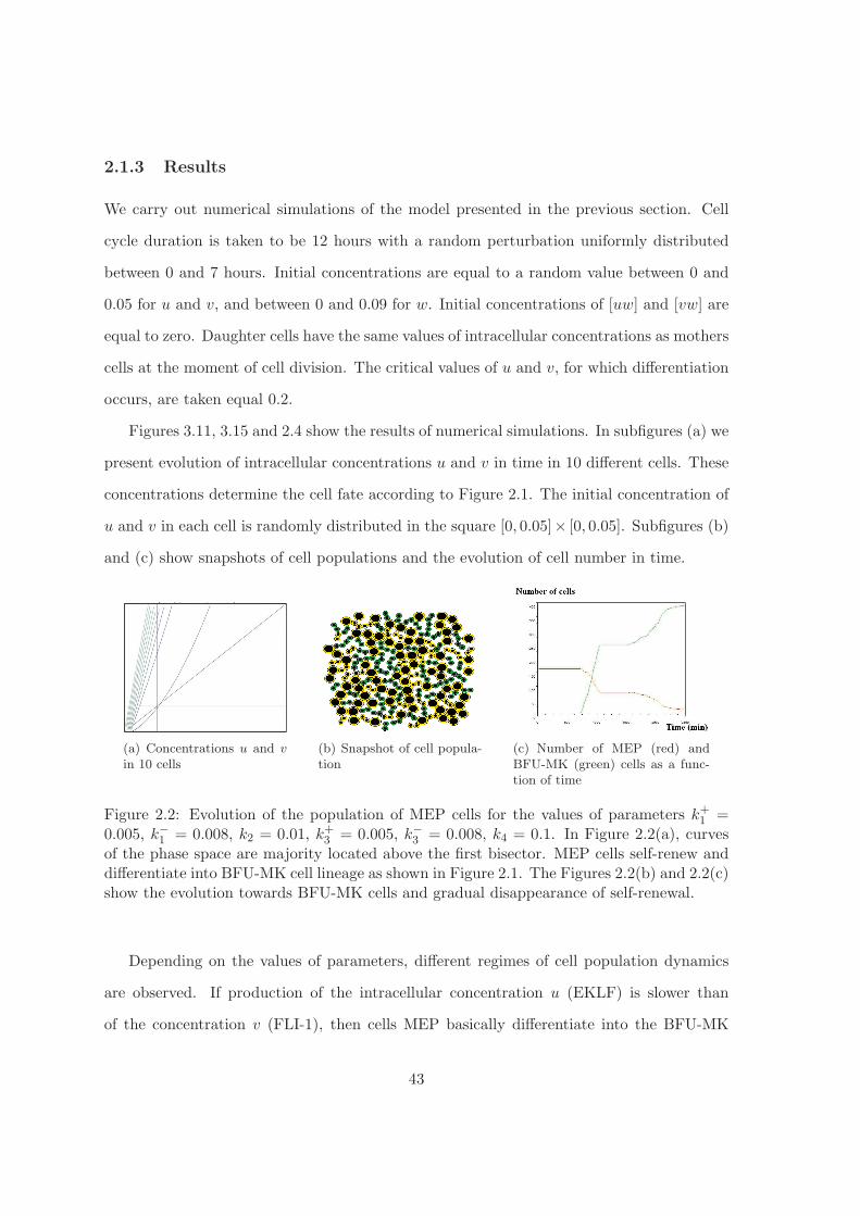
2.1.3 Results

We carry out numerical simulations of the model presented in the previous section. Cell

cycle duration is taken to be 12 hours with a random perturbation uniformly distributed

between 0 and 7 hours. Initial concentrations are equal to a random value between 0 and

0.05 for u and v, and between 0 and 0.09 for w. Initial concentrations of [uw] and [vw] are

equal to zero. Daughter cells have the same values of intracellular concentrations as mothers

cells at the moment of cell division. The critical values of u and v, for which differentiation

occurs, are taken equal 0.2.

Figures 3.11, 3.15 and 2.4 show the results of numerical simulations. In subfigures (a) we

present evolution of intracellular concentrations u and v in time in 10 different cells. These

concentrations determine the cell fate according to Figure 2.1. The initial concentration of

u and v in each cell is randomly distributed in the square [0, 0.05]× [0, 0.05]. Subfigures (b)

and (c) show snapshots of cell populations and the evolution of cell number in time.

(a) Concentrations u and v

in 10 cells(b) Snapshot of cell popula-tion

(c) Number of MEP (red) andBFU-MK (green) cells as a func-tion of time

Figure 2.2: Evolution of the population of MEP cells for the values of parameters k+1 =0.005, k−1 = 0.008, k2 = 0.01, k+3 = 0.005, k−3 = 0.008, k4 = 0.1. In Figure 2.2(a), curvesof the phase space are majority located above the first bisector. MEP cells self-renew anddifferentiate into BFU-MK cell lineage as shown in Figure 2.1. The Figures 2.2(b) and 2.2(c)show the evolution towards BFU-MK cells and gradual disappearance of self-renewal.

Depending on the values of parameters, different regimes of cell population dynamics

are observed. If production of the intracellular concentration u (EKLF) is slower than

of the concentration v (FLI-1), then cells MEP basically differentiate into the BFU-MK

43

(a) Concentrations u and v in10 cells

(b) Snapshot of cell popula-tion

(c) The same cell populationsome time later

Figure 2.3: Evolution of the population of MEP cells for the values of parameters k+1 =0.005, k−1 = 0.008, k2 = 0.1, k+3 = 0.005, k−3 = 0.008, k4 = 0.2. MEP cells self-renewand differentiate into BFU-E cell lineage. In Figure 2.3(a), curves of the phase space aremajority located bellow the first bisector, there is commitment into BFU-E lineage as shownin Figure 2.1. The Figures 2.3(b) and 2.3(c) show the evolution towards BFU-E cells andgradual disappearance of self-renewal.

(a) Concentrations u and v

in 10 cells(b) Snapshot of cell popula-tions

(c) Number of MEP cells(red), BFU-MK (green) andBFU-E (blue) as a functionof time

Figure 2.4: Evolution of the population of MEP cells for the values of parameters k+1 =0.002, k−1 = 0.003, k2 = 0.1, k+3 = 0.004, k−3 = 0.00329, k4 = 0.1. Both lineages ofdifferentiated cells BFU-E and BFU-MK are present. In Figure 2.4(a), curves of the phasespace are distributed around the first bissector, there is commitment into BFU-E and BFU-MK lineage as shown in Figure 2.1. The Figures 2.4(b) show the coexistence of the threetype of cells. Figure 2.4(c) show the evolution towards BFU-E and BFU-MK cells andgradual disappearance of self-renewal.

lineage. There is weak self-renewal observed for the values of parameters in Figure 3.11,

and after several cell cycles all cells differentiate. An opposite situation is shown in Figure

3.15 where MEP cells differentiate into BFU-E. As before, the self-renewing activity is weak

and after several cell cycles all cells differentiate. For the intermediate values of reaction

44

rates, both lineages of differentiated cells are present (Figure 3.16). If we decrease the

rate of production of the intracellular proteins EKLF and FLI-1, then some of the MEP

cells can remain undifferentiated and preserve their self-renewal capacity. Let us also note

that the distribution of initial protein concentrations can influence the dynamics of the cell

population.

Thus we show how intracellular regulation of MEP cells influence their differentiation

in one of the two lineages. The balance between them can be controlled by the hormones

EPO stimulating production of erythrocytes and TPO stimulating production of platelets.

Their concentrations influence the parameters of the intracellular regulation of the MEP

cells and can increase production of one of the two cell types decreasing production of the

other one.

45

2.2 Erythropoiesis

2.2.1 Introduction

The erythroid lineage of hematopoiesis begins with early erythroid progenitors that dif-

ferentiate into more mature cells, the erythroblasts, which subsequently differentiate into

reticulocytes. They leave the bone marrow and enter the bloodstream where they finish

their differentiation and become erythrocytes. Erythropoiesis occurs in the bone marrow

within small units, called erythroblastic islands. In vivo, erythroblastic islands consist of

a central macrophages surrounded by erythroid cells of different maturation stage. Pro-

genitor stage of colony-forming units-erythroid (CFU-Es) are situated close to macrophage

while reticulocytes are at the periphery of the island [40]. CFU-Es make a choice between

three possible fates. They can increase their number without differentiation, differentiate

into reticulocytes or die by apoptosis. Complex intracellular protein regulation determines

CFU-E fate.

We develop a multi-scale model of erythroblastic islands which takes into account in-

tracellular regulation, cell-cell interaction and extracellular regulation. The intracellular

regulation of erythroid progenitors describes the choice between self-renewal, differentiation

and apoptosis. Intracellular regulatory mechanisms involved in progenitor cell fate are nu-

merous and not completely known. This is an active area of biological research where new

data appear and where there is no clear understanding of the underlying biological mecha-

nisms. Therefore different approaches are possible in describing intracellular regulation.

Three models of intracellular regulation of erythroid progenitors are presented in this

chapter. The first model (Section 2.2.2) is suggested in [20]. It is based on the interaction of

two proteins: Erk (Extracellular signal-regulated kinases) and Fas. They inhibit each others

expression. ERK promotes self-renewal, while Fas controls differentiation and apoptosis.

The second model (Section 2.2.3) takes in count three proteins, Erk, BMP4 (Bone

Morphogenetic Protein 4) and Fas. These proteins control differentiation, self-renewal and

apoptosis of erythroid progenitors. This model can also be considered as a more general

46

example applicable in other situations where each of cell fates is controlled by some protein.

According to more recent data, the third model contains four proteins: activated glu-

cocorticosteroid receptor (GR), activated BMPR4 receptor (BMP-R), transcription factor

GATA-1 and activated caspases (Section 2.2.4). This model describes intracellular dynamics

represented by regulatory networks based on specific protein competition. This intracellular

dynamical level, represented by ordinary differential equations, is influenced by extracel-

lular substances represented by partial differential equations. The cell fate depends on its

environment, the extracellular regulation and on the intracellular regulation. Stochasticity

due to random events (cell cycle duration, orientation of the mitotic spindle at division)

and small population effects also plays an important role.

2.2.2 Regulation by proteins Erk and Fas

Intra- and extra- cellular regulation

Recent studies have proposed that there is competition between two key proteins: ERK,

which stimulates proliferation without differentiation, and Fas which stimulates differenti-

ation and apoptosis [128]. ERK is involved in a self-renewal loop, while Fas controls differ-

entiation and also triggers cell apoptosis. Fas is activated by extracellular Fas-ligand that is

produced by mature erythroblasts and reticulocytes [107]. This regulation demonstrates a

bistable behaviour that provides the choice between cell self-renewal and differentiation or

apoptosis [62, 55]. One of the most important regulator of erythropoiesis is erythropoietin

(EPO), a hormone released by the kidneys in quantities that are inversly proportional to

the number of erythrocytes in blood. EPO protects erythroid progenitors from apoptosis

through the binding to the erythropoietin receptor (EPO-R) [92].

Based on the current knowledge, in a first model (2.2.2), we decided to focus on a

simplified regulatory network based on two proteins, Erk and Fas, responsible respectively

for cell self-renewal and proliferation and cell differentiation and apoptosis [107, 128]. These

proteins are antagonists: they inhibit each other’s expression. They are also subject to

external regulation, through feedback loops.

47

One of these feedback loops is based upon the population of reticulocytes. They pro-

duce Fas-ligand which is fixed to their exterior cell membrane. Fas-ligand activates Fas,

a transmembrane protein and influences progenitor differentiation and apoptosis. Another

feedback control is related to mature erythrocytes in bloodstream. Their quantity deter-

mines the release of erythropoietin and other hormones, called growth factors. Erythro-

poietin is known to inhibit erythroid progenitor apoptosis [92] and to stimulate immature

erythroid progenitor self-renewal [61]. Other hormones, like glucocorticoids [62, 55], also

increase progenitor self-renewal by activating Erk.

The simplified system of Erk-Fas interactions considered as the main regulatory network

for erythroid progenitor fate is then [55]

dE

dt= (α(Epo,GF ) + βEk)(1− E)− aE − bEF, (2.2.5)

dF

dt= γ(FL)(1− F )− cEF − dF, (2.2.6)

where E and F denote intracellular normalized levels of Erk and Fas. Equation (2.2.5)

describes how Erk level evolves toward maximal value 1 by activation through hormones

(function α of erythropoeitin, denoted by Epo, and other growth factors, denoted by G)

and self-activation (parameters β and k). In the meantime, Erk is linearly degraded with a

rate a and is inhibited by Fas with a rate bF . Equation (2.2.6) is very similar, only there

is no proof for Fas self-activation. Fas is however activitated by Fas-ligand, denoted by

FL, through the function γ(FL), it is degraded with a rate d and it is inhibited by Erk

with a rate cE. Critical values of Erk and Fas, denoted by Ecr and Fcr, correspond to

self-renewal and apoptosis, respectively, when they are reached. If at the end of the cell

cycle intracellular concentrations of Erk and Fas do not reach their critical values, then cell

differentiates.

Reticulocytes and erythrocytes (differentiated cells) produce Fas-ligand.

∂FL

∂t= DFL

ΔFL +WFL− σFL

FL, (2.2.7)

48

where WFL= kFL

Cret is a source term depending on the number of reticulocytes, σFLis

degradation rate, and DFLis diffusion rate. If the diffusion coefficient DFL

is sufficiently

small, then Fas-ligand is concentrated in a small vicinity of reticulocytes. In this case,

Fas-ligand influences erythroid progenitors when they are sufficiently close to reticulocytes.

Results

The goal is to compare results of computations and experimental results. This experimental

data gives the increase in the size of the culture erythroid progenitors and the ratio of

reticulocytes and erythrocytes (differentiated cells) for six days (cf. experimental data in

Table 6.1 and value of parameters in Table 6.7 of Section 6.2).

Biology experience. Biological date were obtained under the following conditions: Nor-

mal bone marrow cells were prepared from 19 days old SPAFAS embryos and grown as

T2ECs in a medium consisting of α-modification of Eagle’s medium (α-MEM) containing

10% FBS (Gibco BRL); 1% normal chicken serum (NCS; Gibco BRL); 10−4 M betamercap-

toethanol (Sigma); 5 ng/ml TGF-α; 1 ng/ml TGF-β1; 10−6 M Dexamethasone and 1 % of

a 100 X antibiotics solution(penicillin plus streptomycin; Flow Laboratories) as previously

described [75]. T2ECs were induced to differentiate at 105 cells/ml by the concomitant

removal of TGF-α, TGF-β and Dex from the medium and the addition of 10 ng/ml insulin

and of 5% Anemic Chicken Serum (ACS). The differentiation level was assessed by acidic

benzidine staining for revealing hemoglobin-containing(mature) cells. The preparation of

ACS as well as the estimation of the level of differentiation by acidic benzidine staining

have been previously described [74].

Simulation of cells culture. The simulation begins with a culture of 98 progenitors (see

Figure 2.5). Behavior of the culture depends on the quantities of Erk and Fas in the cells.

At first, these progenitors have low random initial quantities. This small perturbation is

made to induce the appearance of the first reticulocytes. If the initial values of Erk and Fas

(E0 and F0) are equal to 0, only one choice can be observed (differentiation or self-renewal).

49

Figure 2.5: Growth of cells culture. Afterseveral divisions, progenitors (yellow) be-come reticulocytes (blue) which produce agrowth factor: Fas-ligand (red halo). Af-ter one cycle, reticulocytes become ery-throcytes (purple): cells do not divide inthis model.

Figure 2.6: Left: proportion of differentiated cells (reticulocytes, erythrocytes) to all cellsover time. Right: accumulation of total number of cells. Different curves correspond todifferent amplitude of stochastic variation of initial activities of ERK and Fas in newlyformed cells. Blue curve corresponds to the case where the initial activity of ERK isbetween 0 and 0.015, Fas between 0 and 0.01, with a uniform probability distribution. Red,black and green curves correspond to σ=0.15, 0.01, 0.007 respectively (see the explanationin the text). Normalized cell number: the ratio of the current cell number to the initialcell number. The initial cell number is 2.105 for the experiment and 98 for the numericalsimulations. Curves made with the mean of 3 simulations.

Reticulocytes produce a protein Fas-ligand which promotes differentiation and apoptosis.

Comparison between in vivo and in silico cells culture. The quantities of proteins

in the cells are given by the equations (2.2.5)-(2.2.6), so the behavior of the progenitors

depends on the parameter values of the system. The most significant are α and γ. For

exemple with α=0.000037 all the progenitors choose division, with α=0.000035 all the pro-

genitors choose differentiation after one cycle. To do some comparison between simulation

and experimental results, curves of cells number as a function of time are set out.

The evolution of the cells culture is similar in vitro experiment and in the calculation.

50

Almost all the progenitors no longer divide and become reticulocyte. After one cellular

cycle, reticulocytes all become erythrocyte.

The role of stochasticity in initial conditions. Curves of Figure 2.6 show the influ-

ence of initial conditions. In this simulation, initial quantities of Erk and Fas are randomly

distributed between between 0 and c. If c is less than 0.005, each division give only pro-

genitors. If c is between 0.005 and the threshold there is self-renewal and differentiation. If

the thresholds are exceeded, it is possible that some or all cells die during the first division.

In this case the next generation born of surviving cells was similar behavior to that shown

by the curves.

2.2.3 Regulation by proteins, glucocorticoids and transcriptions factors

Extracellular regulation

A population of cells is numerically simulated in a 2D computational domain which is a

rectangle. Each cell is a discrete object, an elastic ball, considered to be circular and

composed of two parts: a compressible part at the border and a hardly compressible part

at the center. All newborn cells have the same radius r0 and linearly increase in size until

the end of their cycle, when they reach twice the initial radius. When a cell divides, it gives

birth to two small cells side by side, the direction of division being chosen randomly. From

a biological point of view, cell cycle proceeds through G0/G1, S, G2 and M phases. We

assume the duration of G0/G1 phase is a random variable with a uniform distribution in

some given interval [79], other phase durations are supposed to be constant.

Several cell types are computed. Erythroblasts, which are immature erythroid cells, also

known as erythroid progenitors. They follow the growth rules explained above and their

fate is determined as described in Section 2.2. They either self-renew and give two cells of

the same type, or differentiate and give two reticulocytes, or die by apoptosis, depending

on their exposition to growth factors and Fas-ligand.

Reticulocytes, are almost mature red blood cells that leave the bone marrow and en-

51

ter the bloodstream after ejecting their nuclei. In this individual-based model, they are

differentiated cells which stay in the bone marrow a little while after being produced, and

leave the bone marrow (computational domain) at the end of one cell cycle. Contrarily to

erythroblasts, reticulocytes do not have a choice to make, they only express Fas-ligand on

their surfaces, thus influencing the development of surrounding erythroblasts.

Organization and modeling of erythropoiesis

Erythropoiesis represents a continuous process maintaining an optimal number of circulat-

ing red blood cells and tissue oxygen tension. It occurs mainly in the bone marrow where

erythroid progenitors, immature blood cells, which can proliferate and differentiate, un-

dergo a series of transformations to become erythroblasts (mature progenitors) and then

reticulocytes which subsequently enter the bloodstream and mature into erythrocytes. At

every step of this differentiation process, erythroid cells can die by apoptosis (programmed

cell death) or self-renew [73], [75]. Numerous external regulations control cell fate by mod-

ifying the activity of intracellular proteins. Erythropoietin (Epo) is a hormone synthesized

in the kidney in response of decrease in tissue oxygen level. Epo promotes survival of early

erythroblast subsets by negative regulation of their apoptosis through the action on the

death receptor Fas [92].

Glucocorticoids [73], [75] and some intracellular autocrine loops [75], [135] induce self-

renewal. Previously considered by the authors [55], [70], Erk (from the MAPK family)

promoting cell self-renewal inhibits Fas (a TNF family member) [128]. The cell fate depends

on the level of these proteins. In addition to global feedbacks, there is a local feedback

control through cell-cell interaction, during which Fas-ligand produced by mature cells binds

to the membrane protein Fas inducing both differentiation and death by apoptosis [107].

The process of erythroid maturation occurs in erythroblastic islands, the specialized

niches of bone marrow, in which erythroblasts surround a central macrophage which influ-

ences their proliferation and differentiation [40], [154]. However, erythropoiesis has been

mainly studied under the influence of Epo, which can induce differentiation and prolifera-

52

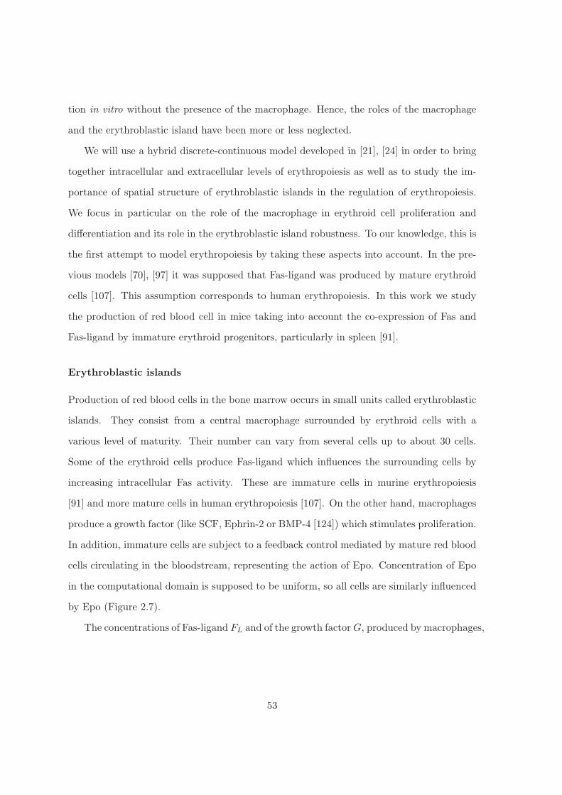
tion in vitro without the presence of the macrophage. Hence, the roles of the macrophage

and the erythroblastic island have been more or less neglected.

We will use a hybrid discrete-continuous model developed in [21], [24] in order to bring

together intracellular and extracellular levels of erythropoiesis as well as to study the im-

portance of spatial structure of erythroblastic islands in the regulation of erythropoiesis.

We focus in particular on the role of the macrophage in erythroid cell proliferation and

differentiation and its role in the erythroblastic island robustness. To our knowledge, this is

the first attempt to model erythropoiesis by taking these aspects into account. In the pre-

vious models [70], [97] it was supposed that Fas-ligand was produced by mature erythroid

cells [107]. This assumption corresponds to human erythropoiesis. In this work we study

the production of red blood cell in mice taking into account the co-expression of Fas and

Fas-ligand by immature erythroid progenitors, particularly in spleen [91].

Erythroblastic islands

Production of red blood cells in the bone marrow occurs in small units called erythroblastic

islands. They consist from a central macrophage surrounded by erythroid cells with a

various level of maturity. Their number can vary from several cells up to about 30 cells.

Some of the erythroid cells produce Fas-ligand which influences the surrounding cells by

increasing intracellular Fas activity. These are immature cells in murine erythropoiesis

[91] and more mature cells in human erythropoiesis [107]. On the other hand, macrophages

produce a growth factor (like SCF, Ephrin-2 or BMP-4 [124]) which stimulates proliferation.

In addition, immature cells are subject to a feedback control mediated by mature red blood

cells circulating in the bloodstream, representing the action of Epo. Concentration of Epo

in the computational domain is supposed to be uniform, so all cells are similarly influenced

by Epo (Figure 2.7).

The concentrations of Fas-ligand FL and of the growth factorG, produced by macrophages,

53

Figure 2.7: Intracellular and extracellular regulation that determine erythroid progenitorfate.

in the extracellular matrix are described by the reaction-diffusion equations:

∂FL

∂t= D1ΔF +W1 − σ1FL, (2.2.8)

∂G

∂t= D2ΔG+W2 − σ2G. (2.2.9)

where W1 and W2 are the constant source terms, the last terms in the right-hand sides of

these equations describe their degradation, D1 and D2 are diffusion coefficients.

Complete intracellular regulatory mechanisms involved in erythroid progenitor cell fate

are very complex and not yet elucidated. Based on the current knowledge, we consider

a simplified regulatory network with three groups of proteins and hormones. The first

group, denoted by u, consists of proteins and hormones, such as protein Erk, BMP4 and

glucocorticoids, involved into self-renewal. The second group, denoted by v is represented

by GATA-1 [5], promoting erythroid progenitor differentiation. The last group, denoted by

w, is represented by protein Fas inducing apoptosis. Moreover, self-renewal proteins inhibits

apoptotis and differentiation. Intracellular regulation in erythroid progenitors is described

by the ordinary differential equations:

54

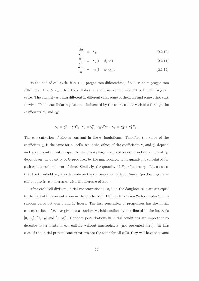
du

dt= γ1 (2.2.10)

dv

dt= γ2(1− β1uv) (2.2.11)

dw

dt= γ3(1− β2uw), (2.2.12)

At the end of cell cycle, if u < v, progenitors differentiate, if u > v, then progenitors

self-renew. If w > wcr, then the cell dies by apoptosis at any moment of time during cell

cycle. The quantity w being different in different cells, some of them die and some other cells

survive. The intracellular regulation is influenced by the extracellular variables through the

coefficients γ1 and γ3:

γ1 = γ01 + γ11G, γ2 = γ02 + γ12Epo, γ3 = γ03 + γ13FL.

The concentration of Epo is constant in these simulations. Therefore the value of the

coefficient γ2 is the same for all cells, while the values of the coefficients γ1 and γ3 depend

on the cell position with respect to the macrophage and to other erythroid cells. Indeed, γ1

depends on the quantity of G produced by the macrophage. This quantity is calculated for

each cell at each moment of time. Similarly, the quantity of FL influences γ3. Let us note,

that the threshold wcr also depends on the concentration of Epo. Since Epo downregulates

cell apoptosis, wcr increases with the increase of Epo.

After each cell division, initial concentrations u, v, w in the daughter cells are set equal

to the half of the concentration in the mother cell. Cell cycle is taken 24 hours plus/minus

random value between 0 and 12 hours. The first generation of progenitors has the initial

concentrations of u, v, w given as a random variable uniformly distributed in the intervals

[0, u0], [0, v0] and [0, w0]. Random perturbations in initial conditions are important to

describe experiments in cell culture without macrophages (not presented here). In this

case, if the initial protein concentrations are the same for all cells, they will have the same

55

fate. However the experiments show this fate can be different for different cells.

A typical structure of erythroblastic islands is shown in Figure 2.13. It consists of a

macrophage and two other types of cells, immature progenitors (yellow) and reticulocytes

(blue). Macrophage expresses a growth factor (green) driving nearby erythroblasts toward

self-renewal. In mice Fas-ligand (red) is produced by undifferentiated cells (Figure 2.13,

left), while in human by differentiated cells (Figure 2.13, right). We will consider below

only erythropoiesis in mice. The results of modeling will be compared with experiments in

the subsequent work. Model of human erythropoiesis can be found in [70].

With a suitable choice of extracellular and intracellular parameters, functioning of the

island is stable (Figure 2.8, left). It contains in average 25 erythroid progenitors and 5

reticulocytes. The influence of the most important parameters on the erythroblastic island

is estimated and shown in Figure 2.8 and 2.9. Periodic oscillations in the number of cells

are related to the cell cycle.

An important characteristic of erythroblastic islands is the rate of production of pro-

genitors and reticulocytes, which determine the number of erythrocytes in blood. We study

how this production depends on the parameters wcr, γ1 and γ02 . First, we will focus on

the global feedback control mediated by Epo. When wcr increases, the size of the island

also increases due to decreased apoptosis of immature progenitors. Consequently, there are

more cells at the perimeter of the island. They have a tendency to differentiate since they

are far from the macrophage which promotes self-renewal. Therefore, increasing of the Epo

level increases the production of reticulocytes (Figure 2.8, right).

Increase of γ1 promotes self-renewal and augments the number of immature progenitors.

Consequently, the number of reticulocytes also increases (Figure 2.9, left). When we in-

crease the value of γ02 , which influences the differentiation rate, the number of reticulocytes

decreases. For sufficiently large values of this parameter, the island disappears after several

cell cycles (Figure 2.9, right). Let us note that we split here the action of Epo on cell

differentiation from its action to downregulate apoptosis. In vivo, Epo acting on both of

them stimulates production of erythrocytes.

56

Figure 2.8: The number of progenitors (red curve) and reticulocytes (blue curve) in time(left). Average in time number of progenitors and reticulocytes for different values of theparameter wcr (right). Each curve is obtained as a mean value for 10 simulations.

Figure 2.9: Average in time number of progenitors and reticulocytes for different values ofγ1 (left) and γ02 (right) (mean values for 10 simulations).

Tis new model of erythropoiesis taking into account intracellular and extracellular reg-

ulations and cell-cell interaction. Competition between three groups of proteins that de-

termine the cell fate has been considered with continuous models (ordinary differential

equations) whereas cells have been studied as discrete objects. Extracellular regulatory

network are described by partial differential equations. The model suggests an important

role of macrophages in functioning of erythroblastic islands and production of mature red

blood cells. Without macrophages, erythroblastic islands quickly lose their stability and

either die out or abnormally proliferate [70]. Macrophages control the size of erythrob-

lastic islands which show their capacity to rapidly increase production of mature cells in

57

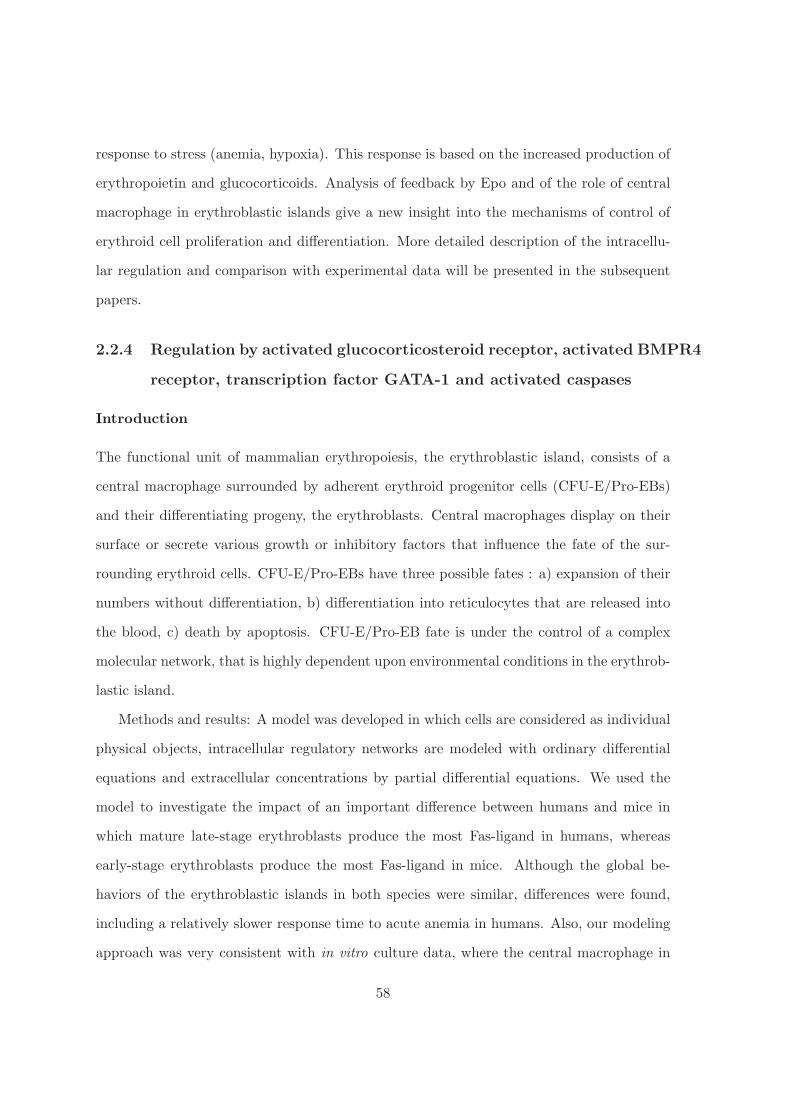
response to stress (anemia, hypoxia). This response is based on the increased production of

erythropoietin and glucocorticoids. Analysis of feedback by Epo and of the role of central

macrophage in erythroblastic islands give a new insight into the mechanisms of control of

erythroid cell proliferation and differentiation. More detailed description of the intracellu-

lar regulation and comparison with experimental data will be presented in the subsequent

papers.

2.2.4 Regulation by activated glucocorticosteroid receptor, activated BMPR4

receptor, transcription factor GATA-1 and activated caspases

Introduction

The functional unit of mammalian erythropoiesis, the erythroblastic island, consists of a

central macrophage surrounded by adherent erythroid progenitor cells (CFU-E/Pro-EBs)

and their differentiating progeny, the erythroblasts. Central macrophages display on their

surface or secrete various growth or inhibitory factors that influence the fate of the sur-

rounding erythroid cells. CFU-E/Pro-EBs have three possible fates : a) expansion of their

numbers without differentiation, b) differentiation into reticulocytes that are released into

the blood, c) death by apoptosis. CFU-E/Pro-EB fate is under the control of a complex

molecular network, that is highly dependent upon environmental conditions in the erythrob-

lastic island.

Methods and results: A model was developed in which cells are considered as individual

physical objects, intracellular regulatory networks are modeled with ordinary differential

equations and extracellular concentrations by partial differential equations. We used the

model to investigate the impact of an important difference between humans and mice in

which mature late-stage erythroblasts produce the most Fas-ligand in humans, whereas

early-stage erythroblasts produce the most Fas-ligand in mice. Although the global be-

haviors of the erythroblastic islands in both species were similar, differences were found,

including a relatively slower response time to acute anemia in humans. Also, our modeling

approach was very consistent with in vitro culture data, where the central macrophage in

58

reconstituted erythroblastic islands has a strong impact on the dynamics of red blood cell

production.

The specific spatial organization of erythroblastic islands is key to the normal, sta-

ble functioning of mammalian erythropoiesis, both in vitro and in vivo. Our model of a

simplified molecular network controlling cell decision provides a realistic functional unit of

mammalian erythropoiesis that integrates multiple microenvironmental influences within

the erythroblastic island with those of circulating regulators of erythropoiesis, such as EPO

and glucocorticosteroids, that are produced at remote sites.

Figure 2.10: Schematic representation of erythroid progenitor cell decision making. Largeyellow circles represent erythroid progenitors at the CFU-E/proerythroblast stage of differ-entiation. Their fate is determined by intracellular regulation which can be influenced byextracellular substances including Fas-ligand and EPO. This intracellular regulatory net-work is shown in greater detail in Figure 6.2. Erythroid progenitors have one of threepossible fates : die by apoptosis, proliferate without differentiation (self-renewal), or termi-nally differentiate.

Differentiation from hematopoietic stem cell (HSC) through the CFU-E/Pro-EB stage of

erythropoiesis requires the hematopoietic growth factor Kit ligand/stem cell factor (KL/SCF)

[58]. At the CFU-E/Pro-EB stage of differentiation, the KL/SCF requirement is lost, and a

59

dependency upon the hormone erythropoietin (EPO) to prevent apoptosis begins [92, 167].

This EPO-dependency persists throughout the period that the CFU-E/Pro-EBs make de-

cisions about their fate. EPO is produced by the kidneys in quantities that are inversely

and exponentially proportional to the number of erythrocytes in blood [93]. EPO gene

transcription is regulated by hypoxia-inducible factor (HIF), a transcription factor that

rapidly accumulates in the kidney EPO-producing cells when oxygen delivery to the kid-

neys is reduced [93]. Through specific receptors (EPO-R) on erythroid progenitors EPO

prevents their apoptosis via down-regulation of Fas and up-regulation of Bcl-xL, an anti-

apoptotic protein [107, 100, 81]. Thus, EPO is the major regulator of erythropoiesis that

directly links the tissue hypoxia caused by decreased circulating erythrocytes to the rates of

new erythrocyte production. Although increased EPO production and the other changes of

stress erythropoiesis are similar in humans and mice, one prominent difference is that during

hypoxic stress, mice have an extensive expansion of splenic erythropoiesis. This enhanced

murine splenic erythropoiesis during hypoxic stress is mediated by bone morphogenetic

protein 4 (BMP4), a protein produced by other hematopoietic and non-hematopoietic cells

[119]. This BMP4 expression in the spleen increases self-renewal of erythropoietic progeni-

tors including the CFU-E/Pro-EBs.

The differentiation of erythroid progenitors and erythroblasts depends upon multiple

transcription factors including, most prominently, GATA-1, the zinc finger-containing com-

ponent of transcription factor complexes that binds to the DNA sequence (A/T)GATA(A/G).

GATA-1 is required for the differentiation of HSCs to the erythroid-committed progenitor

stages and for the terminal differentiation of the CFU-E/Pro-EBs to reticulocytes [38]. The

complexity of erythroid differentiation related to species, organ, and stress conditions com-

plicates understanding of erythropoiesis and its mathematical modeling. In this report, we

develop mathematical models which will allow us to consider various hypotheses about the

organization of mammalian erythropoiesis.

60

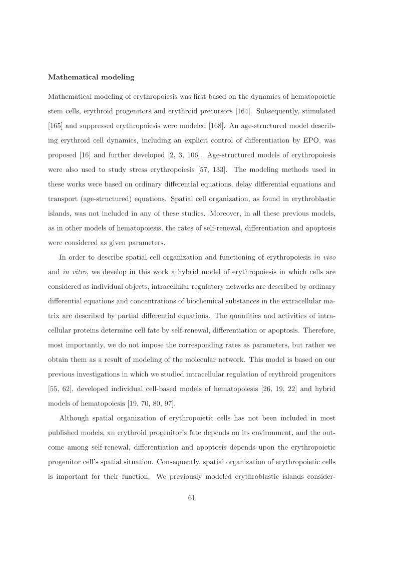
Mathematical modeling

Mathematical modeling of erythropoiesis was first based on the dynamics of hematopoietic

stem cells, erythroid progenitors and erythroid precursors [164]. Subsequently, stimulated

[165] and suppressed erythropoiesis were modeled [168]. An age-structured model describ-

ing erythroid cell dynamics, including an explicit control of differentiation by EPO, was

proposed [16] and further developed [2, 3, 106]. Age-structured models of erythropoiesis

were also used to study stress erythropoiesis [57, 133]. The modeling methods used in

these works were based on ordinary differential equations, delay differential equations and

transport (age-structured) equations. Spatial cell organization, as found in erythroblastic

islands, was not included in any of these studies. Moreover, in all these previous models,

as in other models of hematopoiesis, the rates of self-renewal, differentiation and apoptosis

were considered as given parameters.

In order to describe spatial cell organization and functioning of erythropoiesis in vivo

and in vitro, we develop in this work a hybrid model of erythropoiesis in which cells are

considered as individual objects, intracellular regulatory networks are described by ordinary

differential equations and concentrations of biochemical substances in the extracellular ma-

trix are described by partial differential equations. The quantities and activities of intra-

cellular proteins determine cell fate by self-renewal, differentiation or apoptosis. Therefore,

most importantly, we do not impose the corresponding rates as parameters, but rather we

obtain them as a result of modeling of the molecular network. This model is based on our

previous investigations in which we studied intracellular regulation of erythroid progenitors

[55, 62], developed individual cell-based models of hematopoiesis [26, 19, 22] and hybrid

models of hematopoiesis [19, 70, 80, 97].

Although spatial organization of erythropoietic cells has not been included in most

published models, an erythroid progenitor’s fate depends on its environment, and the out-

come among self-renewal, differentiation and apoptosis depends upon the erythropoietic

progenitor cell’s spatial situation. Consequently, spatial organization of erythropoietic cells

is important for their function. We previously modeled erythroblastic islands consider-

61

ing their specific structure: a macrophage at the center surrounded by closely associated

erythroid progenitors with the more mature erythroblasts and reticulocytes located at pro-

gressively peripheral locations from the central macrophage [70]. To study the role of the

central macrophage, we modeled erythroblastic islands without it, i.e., as foci of erythroid

progenitors surrounded by reticulocytes. Within the range of tested parameters, however,

these erythroblastic islands modeled without macrophages were very heterogeneous in de-

velopment. After several cell cycles, these islands without central macrophages diminished

and disappeared or, conversely, they expanded exponentially, with the difference between

these two fates depending on their initial size and stochastic perturbations. However, as-

suming that the central macrophage releases pro-survival cytokines, we demonstrated that

it induced a very significant stabilizing effect on the erythroblastic island [70].

In this work we continue the development of the hybrid model of erythropoiesis. Taking

into account recent biological data we will present a modified (in comparison with [70])

intracellular regulation. Moreover we will consider two different cases which correspond to

human and murine erythropoiesis. In the former, Fas-ligand, the secreted protein which

determines erythroid progenitor differentiation and apoptosis is produced by more mature

erythroid cells, while for the latter by early erythroblasts and erythroid progenitors them-

selves. We will demonstrate that although the quantitative behavior of the system in these

two cases is similar, there is some difference between them. In particular, hematocrit re-

covery in vivo after anemia is faster in mice than in humans.

Due to obvious limitations of in vivo investigation of erythropoiesis, especially in hu-

mans, detailed analysis of the structure and functioning of erythroblastic islands have not

been performed. In vitro experiments on CFU-E/Pro-EBs co-cultured with macrophages

were considered as a biological model of in vivo erythropoiesis, and such experiments showed

that erythroid cell properties strongly depend on their position with respect to adherence to

a central macrophage [124]. Mathematical modeling performed herein gives a good descrip-

tion of in vitro experimental results and confirms the importance of the spatial organization

of cells in erythroblastic islands. Moreover, numerical simulations show that erythropoiesis

62

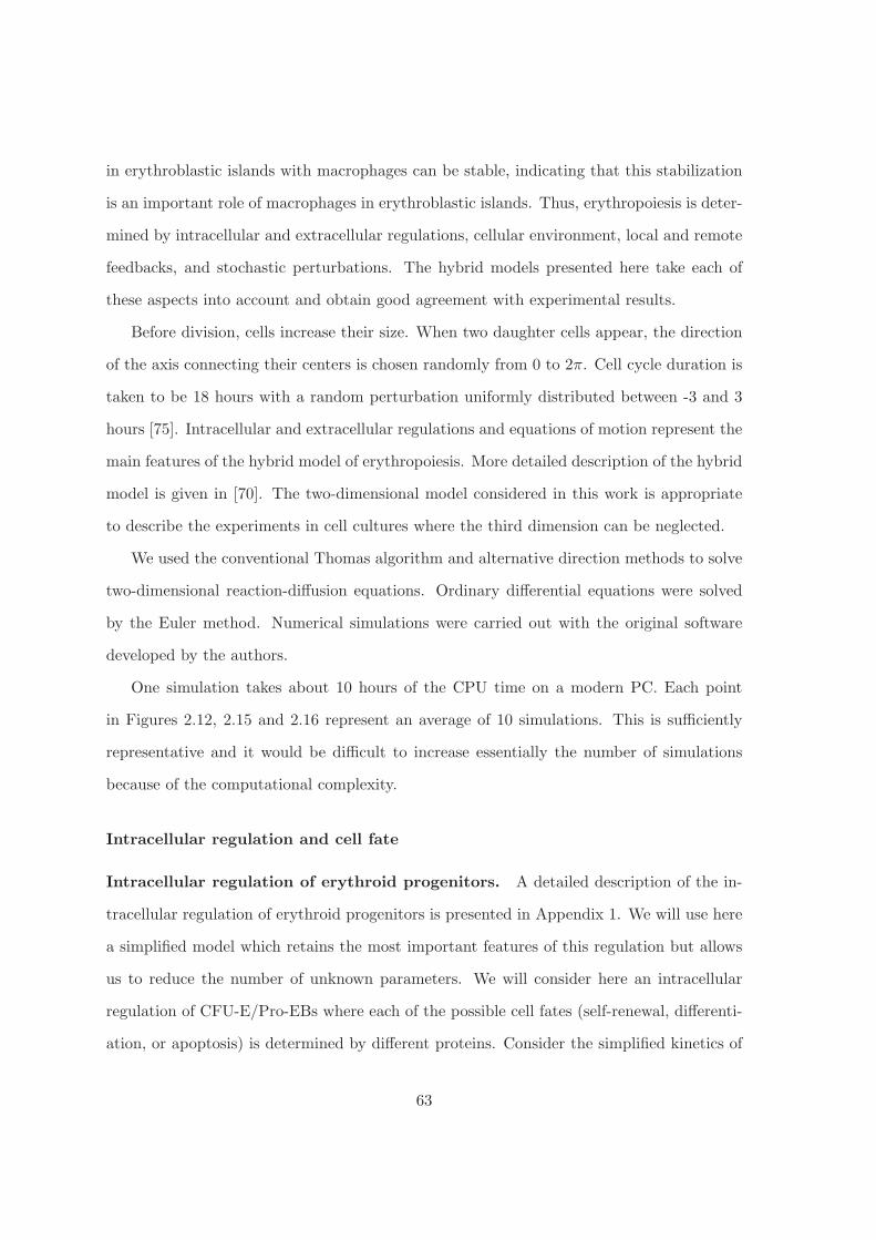
in erythroblastic islands with macrophages can be stable, indicating that this stabilization

is an important role of macrophages in erythroblastic islands. Thus, erythropoiesis is deter-

mined by intracellular and extracellular regulations, cellular environment, local and remote

feedbacks, and stochastic perturbations. The hybrid models presented here take each of

these aspects into account and obtain good agreement with experimental results.

Before division, cells increase their size. When two daughter cells appear, the direction

of the axis connecting their centers is chosen randomly from 0 to 2π. Cell cycle duration is

taken to be 18 hours with a random perturbation uniformly distributed between -3 and 3

hours [75]. Intracellular and extracellular regulations and equations of motion represent the

main features of the hybrid model of erythropoiesis. More detailed description of the hybrid

model is given in [70]. The two-dimensional model considered in this work is appropriate

to describe the experiments in cell cultures where the third dimension can be neglected.

We used the conventional Thomas algorithm and alternative direction methods to solve

two-dimensional reaction-diffusion equations. Ordinary differential equations were solved

by the Euler method. Numerical simulations were carried out with the original software

developed by the authors.

One simulation takes about 10 hours of the CPU time on a modern PC. Each point

in Figures 2.12, 2.15 and 2.16 represent an average of 10 simulations. This is sufficiently

representative and it would be difficult to increase essentially the number of simulations

because of the computational complexity.

Intracellular regulation and cell fate

Intracellular regulation of erythroid progenitors. A detailed description of the in-

tracellular regulation of erythroid progenitors is presented in Appendix 1. We will use here

a simplified model which retains the most important features of this regulation but allows

us to reduce the number of unknown parameters. We will consider here an intracellular

regulation of CFU-E/Pro-EBs where each of the possible cell fates (self-renewal, differenti-

ation, or apoptosis) is determined by different proteins. Consider the simplified kinetics of

63

Figure 2.11: Scheme for the modeling of erythropoietic fate based on simplification of thebiological scheme in Figure 6.2 (see Appendix 1). Four major variables that play a rolein the intracellular regulation of CFU-E/Pro-EBs and affect the fate decisions to undergoapoptosis, terminal differentiation, or self-renewal are retained from Figure 6.2. They in-clude : 1) the concentration of activated glucocorticosteroid receptor (z) that determinesthe rate of self-renewal in normal, steady-state erythropoiesis and in more limited hypoxiastates in which adjustments of EPO concentrations maintain a stable number of circulatingerythrocytes; 2) the concentration of activated BMP4 receptor (u) that determines the rateof expansion of the CFU-E/Pro-EB population in periods of hypoxic stress; 3) the con-centration of GATA-1 (v) that determines the rate of terminal differentiation; and 4) theconcentration of activated caspases (w) that determine the rate of apoptosis when elevatedand the rate of terminal differentiation when reduced. The major extracellular mediatorsthat affect the intracellular variables have been retained. These extracellular mediatorsinclude : 1) the concentration of glucocorticosteroid hormone (GC) that varies with de-gree of stress including that associated with hypoxia; 2) the expression of BMP4 by centralmacrophages that increases with hypoxia-induced stress; 3) the concentration of EPO whichvaries inversely with the degree of hypoxia; and 4) the expression of Fas by erythroid pro-genitor cells, which varies inversely with the EPO concentration and 5) Fas-ligand, whichis produced by other erythroid cells in the erythroblastic island, specifically by early stageerythroblasts in mice and late-stage mature erythroblasts in humans.

the intracellular regulation shown in Figure 2.11 :

dz

dt= a0, (2.2.13)

64

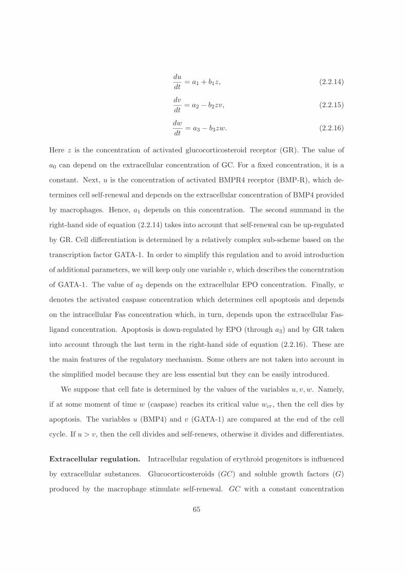
du

dt= a1 + b1z, (2.2.14)

dv

dt= a2 − b2zv, (2.2.15)

dw

dt= a3 − b3zw. (2.2.16)

Here z is the concentration of activated glucocorticosteroid receptor (GR). The value of

a0 can depend on the extracellular concentration of GC. For a fixed concentration, it is a

constant. Next, u is the concentration of activated BMPR4 receptor (BMP-R), which de-

termines cell self-renewal and depends on the extracellular concentration of BMP4 provided

by macrophages. Hence, a1 depends on this concentration. The second summand in the

right-hand side of equation (2.2.14) takes into account that self-renewal can be up-regulated

by GR. Cell differentiation is determined by a relatively complex sub-scheme based on the

transcription factor GATA-1. In order to simplify this regulation and to avoid introduction

of additional parameters, we will keep only one variable v, which describes the concentration

of GATA-1. The value of a2 depends on the extracellular EPO concentration. Finally, w

denotes the activated caspase concentration which determines cell apoptosis and depends

on the intracellular Fas concentration which, in turn, depends upon the extracellular Fas-

ligand concentration. Apoptosis is down-regulated by EPO (through a3) and by GR taken

into account through the last term in the right-hand side of equation (2.2.16). These are

the main features of the regulatory mechanism. Some others are not taken into account in

the simplified model because they are less essential but they can be easily introduced.

We suppose that cell fate is determined by the values of the variables u, v, w. Namely,

if at some moment of time w (caspase) reaches its critical value wcr, then the cell dies by

apoptosis. The variables u (BMP4) and v (GATA-1) are compared at the end of the cell

cycle. If u > v, then the cell divides and self-renews, otherwise it divides and differentiates.

Extracellular regulation. Intracellular regulation of erythroid progenitors is influenced

by extracellular substances. Glucocorticosteroids (GC) and soluble growth factors (G)

produced by the macrophage stimulate self-renewal. GC with a constant concentration

65

in the model, implicitly enters equation (2.2.13) through the right-hand side a0 (the first

relation in (3.1.5)) :

a0 = a00 + a10GC, a1 = a01 + a11G, a2 = a02 + a12E,

a3 = a03 + a13F. (2.2.17)

Growth factors enter equation (2.2.14) through a1. EPO and Fas-ligand influence differ-

entiation and apoptosis. They are taken into account in equations (2.2.15) and (2.2.16),

respectively, by means of the coefficients a2 and a3. All dependencies in (3.1.5) are taken to

be linear in order to simplify the model and to reduce the number of parameters. BMP4 at

the surface of macrophage acts through the surface receptor BMP4-R to decrease cell cycle

duration in those erythroid progenitors that are in contact with central macrophages.

Differentiated cells. Reticulocytes do not divide, but they stay in the bone marrow

before entering the blood. Human mature erythroblasts, which give rise to the reticulocytes,

are the major source of Fas-ligand that induces CFU-E/Pro-EB apoptosis by activating

intracellular caspases by binding to the specific membrane receptor, Fas. In mice, the

major source of Fas-ligand is the very early erythroblasts that are the immediate progeny

of CFU-E/Pro-EBs.

If the concentration of Fas-ligand is sufficiently high, then the CFU-E/Pro-EBs die by

apoptosis. In intermediate concentrations of Fas-ligand, the CFU-E/Pro-EBs differentiate

into reticulocytes after three divisions. In low concentrations of Fas-ligand, the erythrob-

last progenitors proliferate without differentiation, i.e., they self-renew. Thus, the fate of

erythroid progenitors is determined by the concentration of Fas-ligand or, in other words,

by their spatial location with respect to the immature erythroblasts in mice and the mature

erythroblasts in humans. Progenitors located close to Fas-ligand-producing erythroblasts

die by apoptosis, those at an intermediate distance differentiate, and those located furthest

from the Fas-ligand-producing erythroblasts proliferate without differentiation.

The numbers of differentiated cells and progenitors are strongly influenced by the values

66

Figure 2.12: Average number of CFU-E/Pro-EBs and differentiating erythroblasts (greencurves) and late-stage, pre-enucleation erythroblasts and reticulocytes (blue curves) in oneerythroblastic island as a function of a1 for different values of wcr equal to 0.7 (upper pair ofcurves), 0.6 (middle pair of curves) and 0.509 (lower pair of curves), respectively. Fas-ligandproduced by early stage erythroblasts. The average is taken with respect to time and withrespect to 10 simulations.

of multiple parameters, but the total number of erythroid cells increases with greater values

of wcr, the critical variable of Fas-ligand which determines apoptosis of progenitors (Figure

2.12). Increased wcr corresponds to greater values of EPO which stimulate survival of

progenitors under the action of reduced Fas-ligand. Similarly, the number of erythroid

cells also increases due to macrophages (parameter a1) that stimulate self-renewal of CFU-

E/Pro-EBs. In all cases, at steady state, CFU-E/Pro-EBs and differentiating erythroblasts

outnumber the mature cells.

Results

Structure and function of erythroblastic islands. In our erythroblastic island model,

macrophages produce various growth factors (G) including those, which stimulate prolifer-

ation without differentiation (self-renewal). Therefore, CFU-E/Pro-EBs located closest to

and interacting most with the central macrophage proliferate without differentiation, while

CFU-E/Pro-EBs located closest to Fas-ligand-producing erythroblasts die by Fas-mediated

apoptosis. CFU-E/Pro-EBs located at intermediate distances between macrophages and

67

Fas-ligand-producing erythroblasts differentiate and provide new reticulocytes that replace

those leaving the bone marrow by entering the circulating blood. Thus, normal CFU-E/Pro-

EBs that do not interact directly with and are sufficiently far from the central macrophage

will differentiate and cannot undergo unlimited proliferation. This organization of erythrob-

lastic islands in the presence of a central macrophage appears to be very stable [70], and

these erythroblastic islands can exist for an unlimited time with approximately constant

size and a constant rate of reticulocyte production. However, this steady-state rate of ery-

thropoiesis can be influenced by EPO, which downregulates apoptosis of CFU-E/Pro-EBs

allowing their enhanced proliferation and differentiation in response to anemia.

Figure 2.13: Typical structure of an erythroblastic island in the simulations : Fas-ligandproduced by early-stage erythroblasts (left) or by late-stage erythroblasts (right). Thelarge cell in the center is a macrophage, yellow cells - CFU-E/Pro-EBs and differentiatingerythroblasts, blue - late-stage mature erythroblasts and reticulocytes, level of green - con-centration of the growth factor (G) produced by the macrophage, level of red - concentrationof Fas-ligand. Black circles inside cells show their incompressible parts.

The major source of Fas-ligand produced by erythroid cells is the late-stage erythrob-

lasts in human [107] and the early-stage erythroblasts [100] in mice. Therefore, we con-

sidered models incorporating these two different sources of Fas-ligand and compared them.

Figure 2.13 shows erythroblastic islands in which Fas-ligand is produced by early-stage

erythroblasts (left) and by late-stage erythroblasts (right). If Fas-ligand is produced by

late erythroblasts, then progenitors located closest to them die by apoptosis, so that these

late erythroblasts are relatively isolated. If Fas-ligand is produced by early erythroblasts,

68

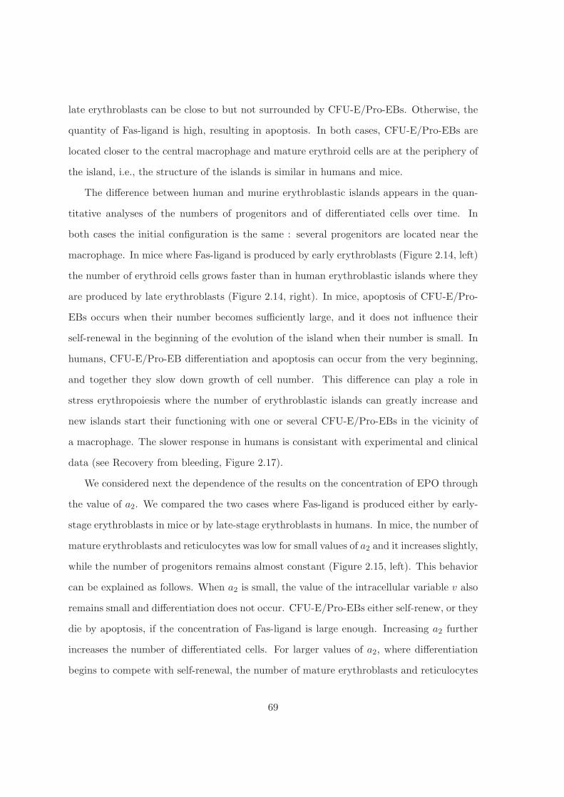
late erythroblasts can be close to but not surrounded by CFU-E/Pro-EBs. Otherwise, the

quantity of Fas-ligand is high, resulting in apoptosis. In both cases, CFU-E/Pro-EBs are

located closer to the central macrophage and mature erythroid cells are at the periphery of

the island, i.e., the structure of the islands is similar in humans and mice.

The difference between human and murine erythroblastic islands appears in the quan-

titative analyses of the numbers of progenitors and of differentiated cells over time. In

both cases the initial configuration is the same : several progenitors are located near the

macrophage. In mice where Fas-ligand is produced by early erythroblasts (Figure 2.14, left)

the number of erythroid cells grows faster than in human erythroblastic islands where they

are produced by late erythroblasts (Figure 2.14, right). In mice, apoptosis of CFU-E/Pro-

EBs occurs when their number becomes sufficiently large, and it does not influence their

self-renewal in the beginning of the evolution of the island when their number is small. In

humans, CFU-E/Pro-EB differentiation and apoptosis can occur from the very beginning,

and together they slow down growth of cell number. This difference can play a role in

stress erythropoiesis where the number of erythroblastic islands can greatly increase and

new islands start their functioning with one or several CFU-E/Pro-EBs in the vicinity of

a macrophage. The slower response in humans is consistant with experimental and clinical

data (see Recovery from bleeding, Figure 2.17).

We considered next the dependence of the results on the concentration of EPO through

the value of a2. We compared the two cases where Fas-ligand is produced either by early-

stage erythroblasts in mice or by late-stage erythroblasts in humans. In mice, the number of

mature erythroblasts and reticulocytes was low for small values of a2 and it increases slightly,

while the number of progenitors remains almost constant (Figure 2.15, left). This behavior

can be explained as follows. When a2 is small, the value of the intracellular variable v also

remains small and differentiation does not occur. CFU-E/Pro-EBs either self-renew, or they

die by apoptosis, if the concentration of Fas-ligand is large enough. Increasing a2 further

increases the number of differentiated cells. For larger values of a2, where differentiation

begins to compete with self-renewal, the number of mature erythroblasts and reticulocytes

69

Figure 2.14: Number of CFU-E/Pro-EBs and differentiating erythroblasts (green curves)and mature erythroblasts and reticulocytes (blue curves) in one erythroblastic island as afunction of time : Fas-ligand produced by early-stage erythroblasts (left) or by late-stageerythroblasts (right). Green and blue curves are mean values for 10 simulations. Blackand red curves show the 95% confidence intervals (mean ±1.96∗standard deviation/

√n

(n = 10)). For the parameter values used, see Tables 6.3 and 6.4.

still increases but there is a significant decrease in the number of progenitors. For even

larger values of a2 the number of mature of erythroblasts and reticulocytes also decreases

because of the decreased numbers of CFU-E/Pro-EBs.

This dependence is different in human erythroblastic islands where Fas-ligand is pro-

duced by late-stage erythroblasts (Figure 2.15, right). Surprisingly, increasing a2 decreased

the number of mature of erythroblasts and reticulocytes. Probably, this happened because

the number of self-renewing progenitors decreased and the number of apoptotic cells in-

creased. Since there were less progenitors, then the number of mature of erythroblasts and

reticulocytes also decreased. As noted previously, CFU-E and differentiating erythroblasts

outnumbered mature erythroblasts and reticulocytes, but the proportions remained about

the same as the numbers of both decreased.

These results in Figure 2.15 show that the action of EPO on GATA-1 does not by itself

increase the number of mature erythroid cells. EPO also acts on Fas receptors, downreg-

ulating apoptosis. Since we do not account explicitly for Fas receptors in the model, we

described the action of EPO on apoptosis through the critical value of Fas-ligand. Figure

2.16 shows the average number of cells in the erythroblastic island for different values of

wcr. The qualitative behavior of the curves was similar in the cases where Fas-ligand was

70

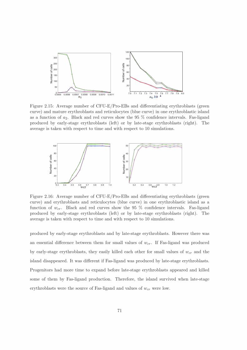
Figure 2.15: Average number of CFU-E/Pro-EBs and differentiating erythroblasts (greencurve) and mature erythroblasts and reticulocytes (blue curve) in one erythroblastic islandas a function of a2. Black and red curves show the 95 % confidence intervals. Fas-ligandproduced by early-stage erythroblasts (left) or by late-stage erythroblasts (right). Theaverage is taken with respect to time and with respect to 10 simulations.

Figure 2.16: Average number of CFU-E/Pro-EBs and differentiating erythroblasts (greencurve) and erythroblasts and reticulocytes (blue curve) in one erythroblastic island as afunction of wcr. Black and red curves show the 95 % confidence intervals. Fas-ligandproduced by early-stage erythroblasts (left) or by late-stage erythroblasts (right). Theaverage is taken with respect to time and with respect to 10 simulations.

produced by early-stage erythroblasts and by late-stage erythroblasts. However there was

an essential difference between them for small values of wcr. If Fas-ligand was produced

by early-stage erythroblasts, they easily killed each other for small values of wcr and the

island disappeared. It was different if Fas-ligand was produced by late-stage erythroblasts.

Progenitors had more time to expand before late-stage erythroblasts appeared and killed

some of them by Fas-ligand production. Therefore, the island survived when late-stage

erythroblasts were the source of Fas-ligand and values of wcr were low.

71

Comparison with experiments and clinical data

Figure 2.17: Recovery of hematocrits (Hct) after severe acute hemorrhage in mouse andhuman. In the upper panel, four healthy, adult mice were phlebotomized daily during thethree days prior to monitoring recovery of Hcts. Data are means +1 S.D. of Hcts. Thelast phlebotomy was on Day 0. Day 1, with the nadir Hct, is the first day of recovery. Forphlebotomy methods, see [92] and [124]. Shaded area shows the period of phlebotomies, andthe dashed line indicates the mean baseline Hct of the mice prior to phlebotomies. In thelower panel, Hct of a patient who refused transfusion of blood during recovery from bleedingcaused by anticoagulation administered during the 4-day period indicated by shading. Theanticoagulation was last administered on Day -1. Day 1, with the nadir Hct, is the first dayof recovery. The dashed line indicates the mean baseline Hct on Days -8 to -6, which wereprior to the administration of anticoagulation.

Recovery from experimental bleeding in mice and in the clinical setting. Simu-

lations of erythroblastic islands in Figure 2.14 predicted that mice with Fas-ligand provided

mainly by early stage erythroblasts will have a more rapid erythrocyte production during

stress erythropoiesis compared to humans with Fas-ligand provided mainly by late stage

progenitors. Direct comparison of erythroblastic islands in vivo between mice and humans

72

is not feasible, but respective responses, in terms of recovery of circulating erythrocytes

after severe blood loss, are shown in Figure 2.17. For this comparison, response to acute

hemorrhage is measured in hematocrit (Hct), the percentage of the blood volume that is

comprised of erythrocytes. Humans and mice have similar Hcts because mice have about

twice as many erythrocytes per volume of blood as humans, but a mouse erythrocyte is

about one-half the size of a human erythrocyte. In Figure 2.17, four normal mice are bled

on three consecutive days such that their Hcts are reduced from 47 ±1 % (mean ±1 S.D.)

to 24 ± 1 % on Day 1 of recovery, the day after the last bleeding. The human results are

from a patient who bled for 3 to 4 days following anticoagulation therapy. His mean Hct

of 33%, as measured on the 3 days prior to anticoagulation, decreased to a Hct of 17.5%

on Day 1 of recovery. Despite his severe anemia, the patient refused the blood transfusions

that would otherwise be given to a patient with such an acute anemia. The patient had

a slight baseline anemia from chronic arthritis, but he did not have renal failure, adrenal

failure or iron deficiency. When he refused blood transfusions, the patient received EPO

(darbepoetin), corticosteroids, and intravenous iron, and he was monitored with daily Hct

measurements.

In Figure 2.17, both the mice and the patient began their recovery after having lost

about one-half of their baseline erythrocyte volume. However, the mice recover completely

to their mean baseline Hct by Day 7 after bleeding, whereas the human patient, with a

Hct of 26% on Day 8, only recovered about one-half the total erythrocyte volume that he

had lost. During stress erythropoiesis, the size of individual islands increases because of

more intensive self-renewal and downregulation of apoptosis, but the number of islands also

grows. Thus, only a qualitative comparison is possible between the human data in Figure

2.17 and modeling in Figure 2.14 (right). In Figure 2.17, at some time between Day 9 and

17, when the patient had returned home and was not monitored daily, he recovered to his

baseline Hct, while the simulations in Figure 2.14 indicate that, indeed, about two weeks

is required for a human to return to a baseline Hct. The prolonged rate of recovery in the

human patient compared to the mice is consistent with the simulation results in Figure

73

2.14 that predict that mice will respond more quickly than humans to a similar degree of

acute blood loss. This prediction by our model indicates that the spatial constraints of

the erythroblastic island structure coupled with the differences in Fas regulation patterns

contribute to the prolonged recovery period after acute hemorrhage in humans compared

to mice.

In vitro experiments on cell cultures. Since we cannot directly compare our models

with erythroblastic island function in vivo, we also compared them with experimental results

from cell cultures, which can be considered as good in vitro approximations.

Figure 2.18: Comparison of in vitro experiments and numerical simulations with mousecells. Left figure : the total number of erythroid cells in co-cultures (upper curve). Thenumber erythroid cells in control cultures without macrophage (lower curve); black symbols- experiments, continuous curves - simulations. Three curves for each of the experimentsrepresent mean value and confidence intervals for 10 simulations. Right figure : the numberof cells adherent to macrophage in co-cultures (AC) - lower curve, nonadherent cells inco-cultures (NAC) - upper curve, and middle curve is control culture without macrophages.For a value of the parameters used, see Tables 3 and 4. Experimental data were originallyreported in reference [124].

New features of the in vitro systems were added in the model. Since the duration of

the cell cycle is different for erythroid cells adherent to macrophages (AC) in comparison

with nonadherent erythroid cells (NAC), we introduced different cell types in the model:

adherent progenitors and differentiated cells and nonadherent progenitors and differentiated

cells. In the model, a cell is considered as adherent if at the moment of its birth the distance

74

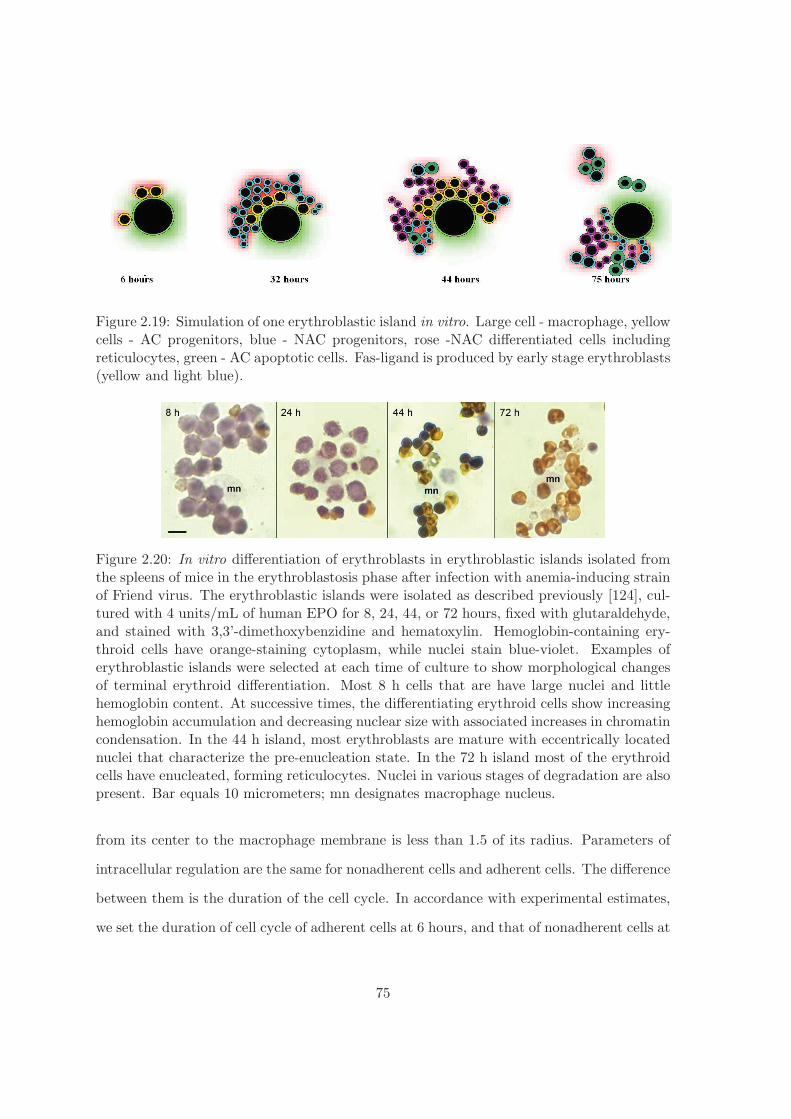
Figure 2.19: Simulation of one erythroblastic island in vitro. Large cell - macrophage, yellowcells - AC progenitors, blue - NAC progenitors, rose -NAC differentiated cells includingreticulocytes, green - AC apoptotic cells. Fas-ligand is produced by early stage erythroblasts(yellow and light blue).

Figure 2.20: In vitro differentiation of erythroblasts in erythroblastic islands isolated fromthe spleens of mice in the erythroblastosis phase after infection with anemia-inducing strainof Friend virus. The erythroblastic islands were isolated as described previously [124], cul-tured with 4 units/mL of human EPO for 8, 24, 44, or 72 hours, fixed with glutaraldehyde,and stained with 3,3’-dimethoxybenzidine and hematoxylin. Hemoglobin-containing ery-throid cells have orange-staining cytoplasm, while nuclei stain blue-violet. Examples oferythroblastic islands were selected at each time of culture to show morphological changesof terminal erythroid differentiation. Most 8 h cells that are have large nuclei and littlehemoglobin content. At successive times, the differentiating erythroid cells show increasinghemoglobin accumulation and decreasing nuclear size with associated increases in chromatincondensation. In the 44 h island, most erythroblasts are mature with eccentrically locatednuclei that characterize the pre-enucleation state. In the 72 h island most of the erythroidcells have enucleated, forming reticulocytes. Nuclei in various stages of degradation are alsopresent. Bar equals 10 micrometers; mn designates macrophage nucleus.

from its center to the macrophage membrane is less than 1.5 of its radius. Parameters of

intracellular regulation are the same for nonadherent cells and adherent cells. The difference

between them is the duration of the cell cycle. In accordance with experimental estimates,

we set the duration of cell cycle of adherent cells at 6 hours, and that of nonadherent cells at

75

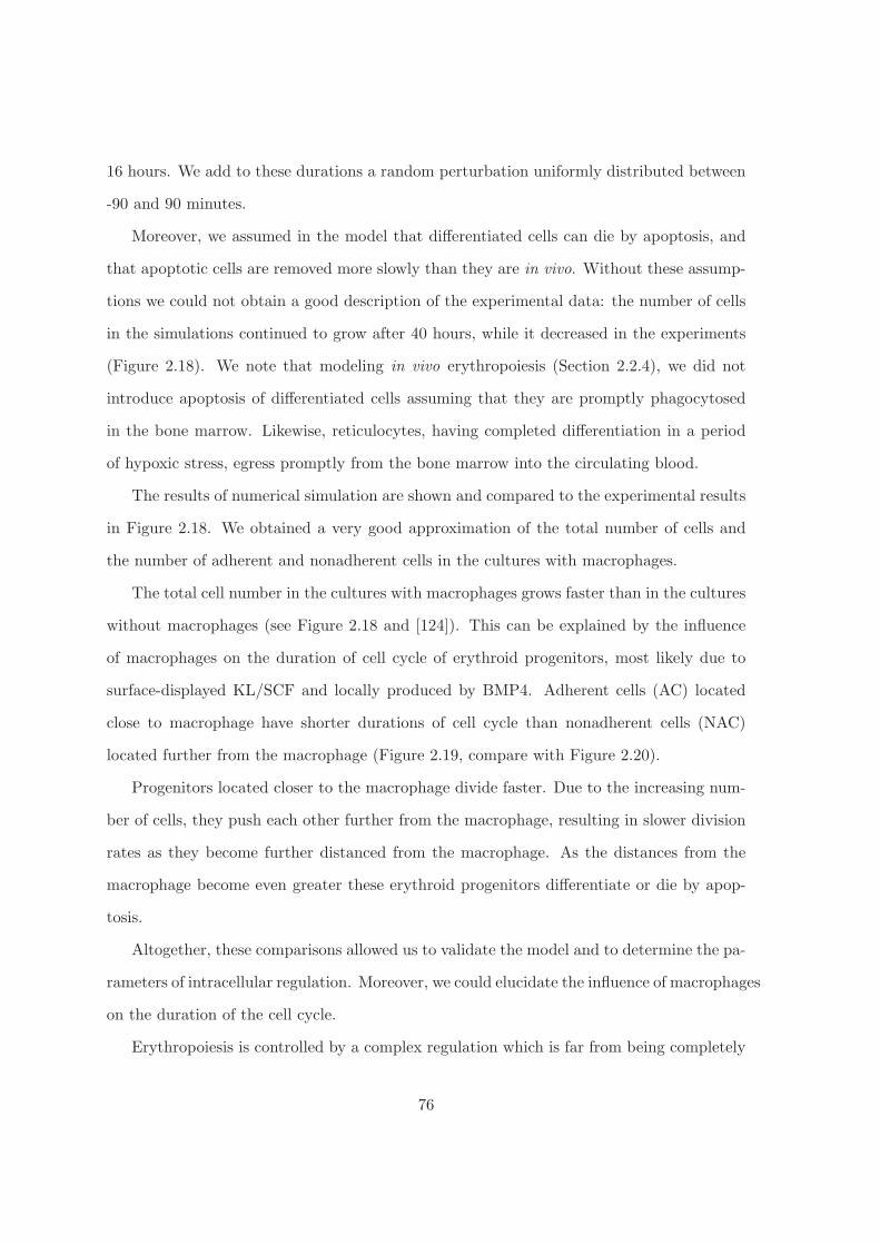
16 hours. We add to these durations a random perturbation uniformly distributed between

-90 and 90 minutes.

Moreover, we assumed in the model that differentiated cells can die by apoptosis, and

that apoptotic cells are removed more slowly than they are in vivo. Without these assump-

tions we could not obtain a good description of the experimental data: the number of cells

in the simulations continued to grow after 40 hours, while it decreased in the experiments

(Figure 2.18). We note that modeling in vivo erythropoiesis (Section 2.2.4), we did not

introduce apoptosis of differentiated cells assuming that they are promptly phagocytosed

in the bone marrow. Likewise, reticulocytes, having completed differentiation in a period

of hypoxic stress, egress promptly from the bone marrow into the circulating blood.

The results of numerical simulation are shown and compared to the experimental results

in Figure 2.18. We obtained a very good approximation of the total number of cells and

the number of adherent and nonadherent cells in the cultures with macrophages.

The total cell number in the cultures with macrophages grows faster than in the cultures

without macrophages (see Figure 2.18 and [124]). This can be explained by the influence

of macrophages on the duration of cell cycle of erythroid progenitors, most likely due to

surface-displayed KL/SCF and locally produced by BMP4. Adherent cells (AC) located

close to macrophage have shorter durations of cell cycle than nonadherent cells (NAC)

located further from the macrophage (Figure 2.19, compare with Figure 2.20).

Progenitors located closer to the macrophage divide faster. Due to the increasing num-

ber of cells, they push each other further from the macrophage, resulting in slower division

rates as they become further distanced from the macrophage. As the distances from the

macrophage become even greater these erythroid progenitors differentiate or die by apop-

tosis.

Altogether, these comparisons allowed us to validate the model and to determine the pa-

rameters of intracellular regulation. Moreover, we could elucidate the influence of macrophages

on the duration of the cell cycle.

Erythropoiesis is controlled by a complex regulation which is far from being completely

76

understood. The spatial organization of erythropoiesis in mammalian hematopoietic or-

gans, including the fetal liver and spleen as well as the bone marrow, is based on a specific

morphological structure, the erythroblastic island [40]. Our hybrid model is based on the

erythroblastic island as a stable, functional unit that integrates its multiple microenviron-

mental influences with those of circulating regulators of erythropoiesis, such as EPO and

glucocorticoids, that are produced at remote sites. As biological experiments incorporate

the microenvironmental influences of erythroblastic islands on erythropoiesis, we argue that

mathematical modeling should also incorporate them as well.

We have previously shown that one of the major roles of central macrophages was the

stabilization of cell numbers in erythroblastic islands [70]. Simulations showed that is-

lands without macrophages either grow exponentially or disappear after several cell cycles.

We demonstrate here that central macrophages are also needed for an adequate response

in stress situations, such as acute anemia, thereby reinforcing the need for proper spatial

description in modeling of erythropoiesis. Simpler models based on ordinary differential

equations, which implicitly assume a uniform cell distribution, cannot describe erythrob-

lastic islands whose size and production of mature cells are determined by interaction of

erythroid progenitors with reticulocytes and macrophages and, consequently, by their mu-

tual locations.

In our hybrid model of erythropoiesis, we do not impose cell fate as a given param-

eter (deterministic or stochastic), as is conventionally done in cell population dynamics,

but we describe the decision-making process at the cellular level as the function of its in-

tracellular network. Indeed, the rates of self-renewal, differentiation and apoptosis cannot

be considered as fixed parameters because they have strong variations for different cells

inside the same island. Although the molecular network controlling this process had to

be greatly simplified in Figure 2.11 compared to Figure 6.2, it nevertheless retained the

essential characteristics that would be expected from such a network, and proved to be

sufficient to derive the correct responses as a function of the cell’s environment. One key

issue is the parametrization of the model, since most parameters had to be fitted to obtain

77

the global expected behavior. A systematic parameter sweep was beyond the scope of the

present work, but it could be performed to assess critical parameters, that would have to

be measured.

Our modeling results were able to predict a more rapid recovery from acute anemia by

mice compared to humans due to the more central location in murine erythroblastic islands

of the main producers of Fas-ligand, the early stage-erythroblasts, as compared to the more

peripheral location in human erythroblastic islands of the main producers of Fas-ligand, the

late-stage erythroblasts. This prediction was confirmed by in vivo experimental evidence

and clinical observations. A testable prediction of our model is that engineered mice that

would express Fas-Ligand at later stages during the erythroid differentiation sequence would

display a much slower recovery than wild-type mice. Whether this accelerated recovery from

acute anemia by mice compared to humans might help explain the more rapid development

of murine CFU-E into erythroid colonies in vitro, 2-3 days in mice [146, 112] versus 6-8 days

in humans [134, 80], could also be addressed.

Furthermore, our results show that our model is consistent with experiments demonstrat-

ing enhanced proliferation in vitro of those erythroid cells that are most closely associated

physically with central macrophages. It is interesting to note that in order to model the

in vitro situation, two key assumptions had to be added: that differentiating cells can die

by apoptosis, and that apoptotic cells are more slowly removed in vitro than in vivo. Al-

though both assumptions stemmed as necessities for proper modeling, they were confirmed

by experimental evidence [124].

In sum, our work demonstrates that a proper modeling of erythropoiesis requires de-

parting from an average value for the decision-making rates, and to account for spatial

organization of the cells, both for modeling in vitro and in vivo experiments.

78

2.2.5 Stability of multiple islands

Introduction

The stability of erythroblastic islands is studied with a model containing an intra- regulation

by the two proteins Erk and Fas. It is known that macrophages influence surrounding cells in

erythroblastic islands in many different ways [40, 124]. In our previous works we conjectured

that one of its major roles can be to stabilize the island [24, 70]. Without a macrophage, a

single island will unlimitedly grow or shrink and disappear after several cell cycles. In vivo,

a big number of island interact with each other. So the question is whether this interaction

can result in a stable production of red blood cells. In this work, we investigate a system of

many islands. We begin with numerical simulations and then suggest and study a simplified

analytical model. The main conclusion of this work is that feedback by erythropoietin can

possibly stabilize a single island, but a system of many islands without macrophages is

unstable. Maintenance of a constant level of erythrocytes in blood seems to be impossible

to achieve with this model, and macrophages should be an important stabilizing factor.

Simulations of erythroblastic islands

Without feedback by erythropoietin. We first simulate a system of islands without

feedback by erythropoietin. This means that α in equation (2.2.5) is constant. Two neigh-

boring islands can interact mechanically (cells push each other) and biochemically through

Fas-ligand. Figure 2.21 shows an example of 2D numerical simulations with a hybrid model

for a system of nine islands. The initial configuration is shown in the left figure, and the

same islands after some time in the right figure. We see that the islands can grow, merge

or disappear. Their size and number change in time.

The number of erythroid progenitors in each island is shown in Figure 2.22 (left). During

about ten cycles the islands remain approximately constant in size. After that, some of them

exponentially grow (with time oscillations due to cell cycle), some other disappear.

Mature cells, reticulocytes leave the bone marrow into the blood and become erythro-

79

cytes. Figure 2.21 (left) shows the evolution of the number of erythrocytes in blood. It

constantly grows and does not stabilize to a constant value, as it should be in accordance

with biologically realistic behavior.

Figure 2.21: Simulation of erythroblastic islands. Initial configuration (left) and a snapshotof the islands after some time. Mature cells (reticulocytes) are shown in blue, immaturecells (erythroid progenitors) are yellow and Fas-ligand is the red halo.

Figure 2.22: Number of progenitors in each island. Without feedback (left), some islandsgrow, some other disappear. In the case with feedback (right), after some time all islandsdisappear.

With feedback by erythropoietin. In vivo, the number of erythrocytes in blood deter-

mines the quantity of erythropoietin produced in the kidney [140]. This hormone comes to

the bone marrow with blood flow and influences the fate of erythroid progenitors. On one

80

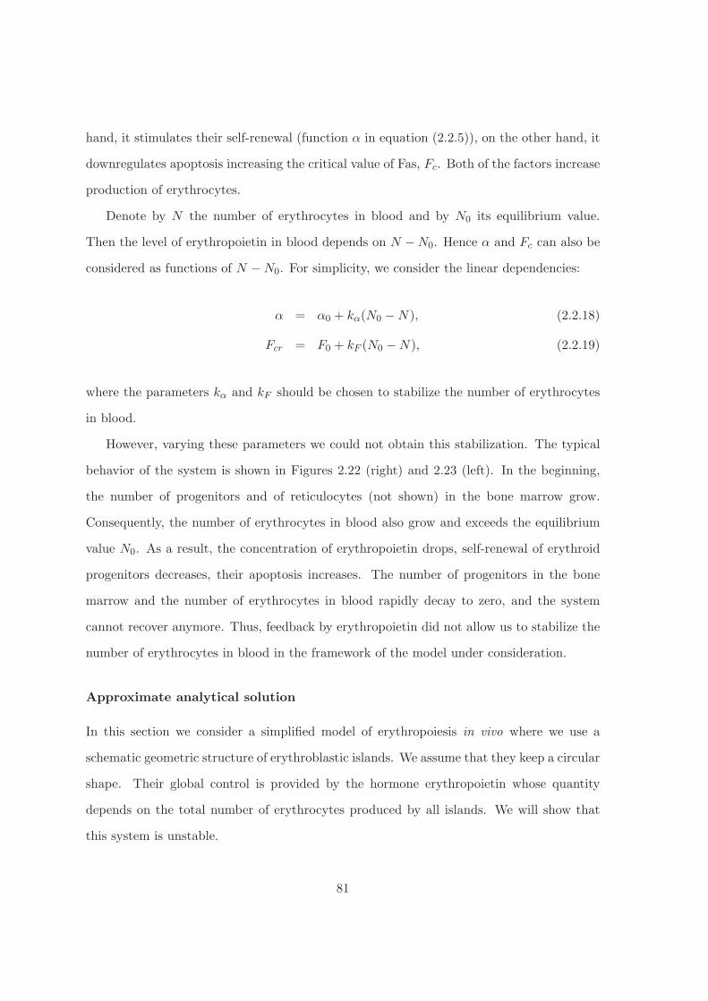
hand, it stimulates their self-renewal (function α in equation (2.2.5)), on the other hand, it

downregulates apoptosis increasing the critical value of Fas, Fc. Both of the factors increase

production of erythrocytes.

Denote by N the number of erythrocytes in blood and by N0 its equilibrium value.

Then the level of erythropoietin in blood depends on N −N0. Hence α and Fc can also be

considered as functions of N −N0. For simplicity, we consider the linear dependencies:

α = α0 + kα(N0 −N), (2.2.18)

Fcr = F0 + kF (N0 −N), (2.2.19)

where the parameters kα and kF should be chosen to stabilize the number of erythrocytes

in blood.

However, varying these parameters we could not obtain this stabilization. The typical

behavior of the system is shown in Figures 2.22 (right) and 2.23 (left). In the beginning,

the number of progenitors and of reticulocytes (not shown) in the bone marrow grow.

Consequently, the number of erythrocytes in blood also grow and exceeds the equilibrium

value N0. As a result, the concentration of erythropoietin drops, self-renewal of erythroid

progenitors decreases, their apoptosis increases. The number of progenitors in the bone

marrow and the number of erythrocytes in blood rapidly decay to zero, and the system

cannot recover anymore. Thus, feedback by erythropoietin did not allow us to stabilize the

number of erythrocytes in blood in the framework of the model under consideration.

Approximate analytical solution

In this section we consider a simplified model of erythropoiesis in vivo where we use a

schematic geometric structure of erythroblastic islands. We assume that they keep a circular

shape. Their global control is provided by the hormone erythropoietin whose quantity

depends on the total number of erythrocytes produced by all islands. We will show that

this system is unstable.

81

Figure 2.23: Left: number of erythrocytes in blood as a function of time for different valuesof feedback coefficients or without feedback (upper curve). Right: graphical solution ofequation 2.2.21.

Single island. Simplifying the structure of an erythroblastic island, we suppose that

erythroid progenitors fill a circle of radius R. Then the number n of progenitors in the

island is proportional to its area S = πR2: n = πR2

σ , where σ is the area of a single

progenitor cell. The rate of self-renewal of the progenitors is proportional to their number,

that is to the area S of the circle. Reticulocytes are located at the boundary of the circle.

Their number m is proportional to its length, m = 2πRd , where d is diameter of reticulocytes.

Since stimulation by Fas-ligand takes place at a small distance, we can suppose that

only the progenitors located near the boundary die by apoptosis. Hence the apoptosis rate

is proportional to 2πR. We can now write the equation for the number of progenitors:

dndt = k1n−k2m, where k1 is determined by the duration of cell cycle, k2 by the time during

which the intracellular concentration of Fas reaches the critical level necessary to kill the

cell. From the last equation we obtain:

dR

dt= aR− b, (2.2.20)

where a = k1/2, b = σk2/d. This equation has a stationary solution, R0 = b/a. It can be

easily verified that it is unstable. If R > R0, then the circle will indefinitely grow, if R < R0

it will shrink. Thus, a single island in this model is unstable.

82

Stabilization by the apoptosis rate. The apoptosis rate b depends on the concentration

of erythropoietin that depends, in its turn, on the number of erythrocytes N in blood. The

number of erythrocytes depends on the number of reticulocytes. For the sake of simplicity,

we suppose that this dependence is instantaneous, that is N is a function of m at the same

moment of time. Then b can be considered as a function of R. Hence instead of equation

(2.2.20) where b is a constant we obtain the equation

dR

dt= aR− b(R), (2.2.21)

where b(R) is some given function. According to its biological meaning, it is an increasing

function. Dependance of apoptosis on erythropoietin concentration is specified in [55] on

the basis of the data available in literature. Qualitatively, it has the S-shape shown in

Figure 3 (right). Its exact form is not essential for what follows.

Equation (2.2.21) can have one or several stationary solutions. In the example, in Figure

3, there are three solutions. Only one of them is stable, R = R2, since b′(R2) > a. Two

others are unstable. The solution of this equation with an initial condition R(0) = R0 will

converge to the stationary solution R = R2 if R1 < R0 < R3. If R0 < R1, the solution will

decrease, and if R(0) > R3, then it will grow.

System with more than one island. Let us return to a model similar to (2.2.21) when

there are n islands with radii R1, ..., Rn. Then we will have the system of equations

dRj

dt= aRj − b(S), j = 1, ..., n, (2.2.22)

where S = 1n(R

1 + ...+Rn). The last term in equation (2.2.22) implies that erythropoietin

production and apoptosis rate depend on the total (or average) erythrocyte concentration

which is proportional to S.

Each stationary solution R1, R2, R3 of equation (2.2.21) originates a stationary solution

of system (2.2.22): R1 = ... = Rn = Rk, k = 1, 2, 3. Let us show that solution R2, which

83

is stable for equation (2.2.21), becomes unstable for system (2.2.22). We note first of all

that taking a sum of all equations in (2.2.22) we obtain:

dS

dt= aS − b(S). (2.2.23)

As before, S = R2 is a stationary solution of this equation. Therefore, the solution S(t) of

this equation with the initial condition S(0) = R2 is identically equal to R2. Let us now

take initial conditions Rj(0) = Rj0, j = 1, ..., n of system (2.2.22) in such a way that

1n(R

10 + ... + Rn

0 ) = R2. Then S(t) ≡ 1n(R

1(t) + ... + Rn(t)) ≡ R2. Hence system (2.2.22)

can be written as

dRj

dt= aRj − b(R2), j = 1, ..., n. (2.2.24)

Hence all equations of this system are independent of each other. The functions Rj(t) with

the initial condition greater than R2 exponentially grow, with the initial conditions less

than R2 exponentially decay till they become equal to 0. Since the solution is exponentially

growing for a particular initial condition constructed above, then the matrix of the linearized

system has a positive eigenvalue. Hence the dimension of the stable manifold is less than

n. Therefore the solution with a generic initial condition, which does not belong to this

manifold, will not converge to the stationary solution. Thus we have proved that stationary

solutions of system (2.2.22) are unstable.

84

Chapter 3

Blood diseases

3.1 Multiple Myeloma

3.1.1 Biological background

Multiple myeloma (MM) is a relatively common disease that is characterized by bone

marrow infiltration with malignant plasma cells and, very frequently has a malignancy-

associated chronic anemia, i.e., a chronic decrease of circulating red blood cells. The degree

of anemia is correlated with the degree of marrow infiltration [15] and with the proliferative

rate of the myeloma cells, [71] both of which can be quantified before and after therapy.

Many patients treated for MM respond with improved or resolved anemia. Thus, the mar-

row infiltration by MM can be examined from its most prevalent stage at diagnosis to its

resolution or lowest degree of infiltration in those patients who respond to therapy, see

Figure 3.1.

Among human diseases, the progression of chronic infections or metastatic tumor growth

is variable, and infiltration of bone marrow by either process is rare when compared to

infiltration by hematologic diseases. Some hematologic diseases such as lymphomas and

leukemias often grow in the spleen as well as the bone marrow and, therefore, they can

confound determinations of bone marrow involvement because the spleen, which enlarges

and traps circulating cells will also reduce the numbers of circulating blood cells. Among the

85

various blood cell types, the red blood cells are the most accurate for determining decreased

counts because they have a relatively narrow normal range compared to leukocytes and

platelets, which can vary two-to-three fold and still remain in the normal range.

Erythropoiesis occurs in the bone marrow within small units of cells called erythroblastic

islands. Erythroblastic islands consist of a central macrophage surrounded by erythroid

cells beginning at the progenitor stage of colony-forming units-erythroid (CFU-Es) and

extending through reticulocytes [40], [128]. CFU-Es have three possible fates: expansion

of their numbers without differentiation, differentiation into reticulocytes, and death by

apoptosis. CFU-E fate is determined by a very complex network of intracellular proteins.

Malignant cells of MM disrupt erythroblastic island function. MM cells produce two

cytokines which be cytotoxic for erythroblasts: Fas-ligand (FL) and the tumor necrosis

factor-related apoptosis-inducing ligand (TRAIL). Differentiating erythroblasts have recep-

tors for both FL and TRAIL, and triggering the receptors activates apoptotic pathways

in erythroblasts. If receptors of FL and TRAIL are activated, they induce apoptosis of

erythroblasts. Abnormal up-regulation of apoptogenic receptors, including FL and TRAIL,

by highly malignant myeloma cells is involved in the pathogenesis of the ineffective erythro-

poiesis and chronic exhaustion of the erythroid matrix, see Figure 3.2.

In addition, GATA-1 (a survival factor for erythroid precursors) was remarkably down-

regulated in fresh erythroblasts from the severely anemic patients. These results indicate

that progressive destruction of the erythroid matrix in aggressive MM is due to cytotoxic

mechanisms based on the up-regulation in myeloma cells of FL, TRAIL, or both. It is con-

ceivable that the altered regulation of these receptors defines a peculiar cytotoxic phenotype

that drives the progression of aggressive MM [138].

Myeloma is treated with chemotherapies, which improves the patient’s condition but

does not heal the disease. Stem cell transplant are also used to try to cure patients. Anemia

associated with myeloma is treated with erythropoietin (EPO) injections. This treatment

rises patients life expectancy but, as chemotherapies, does not cure the disease.

In modeling of erythroblastic island function, immunoglobulin proteins produced by

86

Figure 3.1: Effects of MM infiltration of the bone marrow that can lead to chronic anemia.

multiple myeloma can reduce renal function and, thereby, indirectly inhibit erythropoiesis

via decreased EPO concentrations reaching the erythroblastic islands. Indeed, inappropri-

ately low serum EPO concentrations have been reported in patients with multiple myeloma,

and the degree of EPO deficiency is correlated with the amount of bone marrow infiltration

and the proliferation rate of the multiple myeloma cells [15] and [71]. However, EPO con-

centrations can be corrected by successful treatment of the myeloma and/or administration

of exogenous EPO. If the patients are successfully treated, the anemia resolves with the

clearance of myeloma from the bone marrow.

3.1.2 Mathematical model

In this section we will model development of multiple myeloma in the bone marrow. At the

first stage of this modeling, we will introduce erythroblastic islands in normal situation and

will describe their functioning similar to the modeling presented in Section 2.2. We take into

account here that some islands can extinct due to random perturbations in the dynamics

87

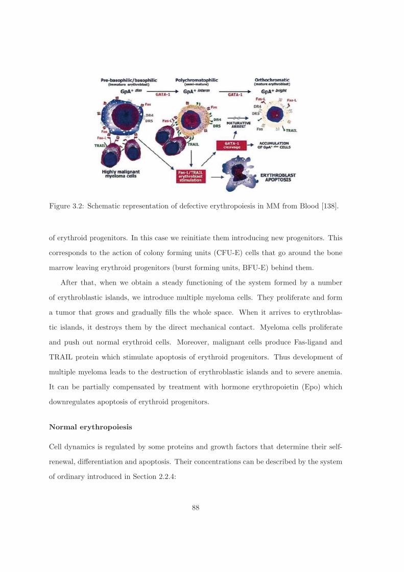
Figure 3.2: Schematic representation of defective erythropoiesis in MM from Blood [138].

of erythroid progenitors. In this case we reinitiate them introducing new progenitors. This

corresponds to the action of colony forming units (CFU-E) cells that go around the bone

marrow leaving erythroid progenitors (burst forming units, BFU-E) behind them.

After that, when we obtain a steady functioning of the system formed by a number

of erythroblastic islands, we introduce multiple myeloma cells. They proliferate and form

a tumor that grows and gradually fills the whole space. When it arrives to erythroblas-

tic islands, it destroys them by the direct mechanical contact. Myeloma cells proliferate

and push out normal erythroid cells. Moreover, malignant cells produce Fas-ligand and

TRAIL protein which stimulate apoptosis of erythroid progenitors. Thus development of

multiple myeloma leads to the destruction of erythroblastic islands and to severe anemia.

It can be partially compensated by treatment with hormone erythropoietin (Epo) which

downregulates apoptosis of erythroid progenitors.

Normal erythropoiesis

Cell dynamics is regulated by some proteins and growth factors that determine their self-

renewal, differentiation and apoptosis. Their concentrations can be described by the system

of ordinary introduced in Section 2.2.4:

88

dz

dt= a0, (3.1.1)

du

dt= a1 + b1z, (3.1.2)

dv

dt= a2 − b2zv, (3.1.3)

dw

dt= a3 − b3zw. (3.1.4)

Here u is the concentration of activated BMPR4 receptor (BMP-R), v is the concentration of

GATA-1, w is the concentration of the activated caspase, z is the concentration of activated

glucocorticosteroid receptor (GR). The parameters of the intracellular regulation depend

on the extracellular regulation:

a1 = a01 + a11G, a2 = a02 + a12E, a3 = a03 + a13F. (3.1.5)

Here G is the concentration of growth factor, E is the concentration of erythropoietin, F is

the concentration of Fas-ligand.

After some time, reticulocytes leave the bone marrow in the blood flow where they

become mature erythrocytes. In numerical simulation this time is taken equal one cell

cycle, after which they are removed from the computational domain. Reticulocytes produce

Fas-ligand. The distribution of its concentration is described by the equation:

∂F

∂t= DFΔF +WF − σFF, (3.1.6)

where the first term in the right-hand side of this equation describes diffusion of Fas-ligand in

the extracellular matrix, the second terms its production and the last terms its degradation.

We should specify that Fas-ligand is a transmembranian protein which acts by direct cell-

cell contact. Its description by the diffusion equation is a mathematical approximation. If

the diffusion coefficient is sufficiently small, then it will be localized around the Fas-ligand

89

producing cells and act only on the neighboring cells. This approach allows us to avoid the

detailed description of cell geometry. Let us also note that the production term is considered

as a step-wise constant function with the support located at the area of Fas-ligand producing

cells.

Let us recall that erythroblastic islands consist of erythroid progenitors and reticlocytes

around central macrophages. During the development of multiple myeloma, malignant

cells proliferate and push all other cells by the direct physical contact. This is one of

the mechanisms which act on erythroblastic islands. Erythroid progenitors are small cells

approximately of the same size as multiple myeloma cells.

Macrophages produce growth factor G which stimulated proliferation of erythroid pro-

genitors. Its concentration is described by the reaction-diffusion equation

∂G

∂t= DGΔG+WG − σGG (3.1.7)

which takes into account its diffusion, production and degradation.

Number of erythrocytes in blood. Anemia is one of the consequences of the disease,

characterized by the low levels of healthy red blood cells (RBCs) and less than normal level

of hemoglobin in blood.

Erythrocyte lifetime in blood for humans is 120 days. In order to accelerate the simula-

tions, we reduce it to 40 day (as it is for mice). New erythrocytes are added when they leave

the bone marrow (more precisely, reticulocytes become erythrocytes already in blood flow),

and they are removed when their age reaches 40 days. Erythroblastic islands are shown in

Figure 3.3 and the total number of erythrocytes produced by 8 islands in Figure 3.4. We

can see that after about 20 days, the total number of erythrocytes reaches its steady level.

Disease

There are two mechanisms by which multiple myeloma cells invade the bone marrow. Cells

of the tumor push out normal cells by pure mechanical interaction and cancer cells increase

90

Figure 3.3: Numerical modeling of normal erythropoiesis with 8 erythroblastic islands. Theinitial cell distribution is shown in the left image, the same islands 5 days later in the rightimage. In some of the islands, erythroid progenitors disappear. In this case, they are addedagain due to the presence of CFU-E cells in the bone marrow. Fas-ligand produced byreticulocytes is shown in red and growth factor produced by macrophages in green.

Figure 3.4: Total number of erythrocytes produced by 8 islands. After approximately 20days it reaches a steady state level with some oscillations around it due to cell cycle.

apoptosis of erythroid progenitors by Fas-ligand and other biochemical signals. A compar-

ative study of two cases of MM is conducted. We first studied MM with malignant cells

acting only mechanically and then with cancer cells producing Fas-ligand and TRAIL. In

both of them, the tumor does not spawn until the cells erythropoiesis reaches the stability

phase. The objective is to study the impact of Fas-ligand on the evolution of different pop-

ulations of cells. In other words, by comparing the populations of erythroid progenitors and

reticulocytes, we establish the role of Fas-ligand secretion in the development of multiple

myeloma.

Let us consider the case where malignant cells do not secrete Fas-ligand. We analyze

the erythroid progenitors and reticulocytes populations. We notice that while in the sta-

bility phase, the progenitors’ number is higher than the reticulocytes, the extinction of the

progenitors takes place faster. This can only be explained by the Fas-ligand effect of the

reticulocytes in the elimination of progenitors by triggering apoptosis. Nevertheless, be-

cause of the spatial organization and the location of macrophages, some of the progenitors

91

are surrounded by malignant cells. These cells are also pushed until they differentiate and

either die or leave the bone marrow.

The same behavior of the populations can also be observed in the case of MM cells

producing Fas-ligand. However, contrary to the case without Fas-ligand produced by MM

cells, the difference between the time of extinction of progenitors and reticulocytes is not as

important. In fact, if that difference is due to the Fas-ligand secreted by reticulocytes, the

Fas-ligand secreted by the tumor overshadow the effect of the Fas-ligand of reticulocytes in

the case of MM with Fas-ligand. This can be clearly noticed when analyzing qualitatively

the maximal values of Fas-ligand in both cases. The result is that the same fate which is

extinction is awaiting all cells whether they are progenitors or reticulocytes.

The first important effect of Fas-ligand does not take place until the few hours of the

simulation. In fact, we have seen that the cells that are near the tumor disappear at a

high rate when there is a secretion of Fas-ligand. While in the case of MM without Fas-

ligand, the elimination of cells is primarily due the physical pushing of reticulocytes by the

tumor against the progenitors. We have shown that while the difference in the apoptosis

of progenitors in the two cases is not that significant, the reticulocytes difference is wider

and clearer. In fact, the Fas-ligand protein is not only responsible of apoptosis, but also

of differentiation. This is why the extinction of reticulocytes in the case of MM with Fas-

ligand takes place earlier due to the early differentiation of a large number of progenitors.

The progenitors late extinction is explained by the compensation of the Fas-ligand of the

reticulocyte by the one of the MM.

Regulation by EPO

In the previous paragraph, we studied the development of multiple myeloma assuming that

the concentration of erythropoietin was constant. However the number of erythrocytes

in blood determines the quantity of erythropoietin produced in the kidney [140] and the

number of erythrocytes depends on the quantity of EPO. Indeed, a feedback loop regulates

the production of erythrocytes: if this number decreases, as in anemia, the amount of EPO

92

Figure 3.5: Left: appearance of the tumor (light blue cells in the top of the figure). Right:tumor invasion after 2 months.

(a) MM cells do not produce Fas-ligand andTRAIL

(b) MM cells produce Fas-ligand and TRAIL

Figure 3.6: We can see the declining number of progenitors and of mature cells duringthe growth of tumors. Left: with cancer cells acting by mechanical actions (yellow curve -progenitors, blue curve - reticulocytes). Right: with cancer cells producing Fas-ligand andTRAIL (blue curve - progenitors, red curve - reticulocytes).

produced increases in order to stimulate erythropoiesis.

In the model of normal erythropoiesis developed in Section 2.2.4, apoptosis of erythroid

progenitors is determined by the intracellular concentration of activated caspace (variable w

in equation (2.2.16)). If this concentration exceeds some critical level wcr, then the cell dies

by apoptosis. The hormone erythropoietin produced in the kidney downregulates apoptosis

of erythroid progenitors. In the model, we take this effect into account assuming that wcr

depends on the difference N − N0 of the current number N or erythrocytes in blood and

their number N0 in normal conditions:

wcr = wcr0 − k(N −N0) (3.1.8)

93

Figure 3.7 shows the number of erythroid progenitors in the bone marrow and the number

of erythrocytes in blood for fixed but different values of the critical value wcr.

Figure 3.7: Purple curve: wcr= 0.08, green curve: wcr= 0.09, red curve: wcr= 0.1, bluecurve: wcr= 0.11. Left: number of progenitors. Right: number of more mature cells, asfunctions of time.

The comparison of the both cases highlights the effect of EPO in regulating the popu-

lation of cells. In fact, by increasing and decreasing the apoptosis rate, EPO manages to

change the value to which the population converges.

Through these comparisons, we have shown that in the case of variable EPO, the pop-

ulation of normal cells takes a longer time to reach extinction than in the case of fixed

variable. This can only explained by the variation of the threshold wcr. Injection of EPO

are used to treat myeloma. Treatment by exogenous EPO can be presented as an increasing

of value of wcr.

wcr(t) =

⎧⎪⎨⎪⎩

wcr0 − k(N −N0), t ≤ T

wcr0 − k(N −N0) + wcr1 , t > T

(3.1.9)

where T is the time of injection and wcr1 describes the effect of exogenous EPO. In Figure

3.8, we can observe the increase of the number of erythrocytes, after an injection of EPO

the population extinct with a delay.

94

Figure 3.8: Blue curve: number of erythrocyte after injection of EPO. Red curve: numberof erythrocyte without exogenous EPO.

3.1.3 Partial differentiation of myeloma cells

In Chapter 2 we presented two models of erythropoiesis with two different schemes of intra-

cellular regulation. One of them was based on the interaction of Erk and Fas, another one

on a more complete regulation with BMP4, Fas, GATA-1 and activated caspases. Though

intracellular regulations are different, functioning of erythroblastic islands in these two cases

is similar. The results on the development of multiple myeloma presented above are ob-

tained for the second intracellular regulation (Section 2.2.4). We have also studied it in the

case of the first intracellular regulation. The results obtained in this case are very similar

to the other case, and we do not present them here.

We will study in this section how the rate of proliferation of multiple myeloma cells

influences the tumor growth and anemia which accompany this blood disorder. We will

consider this question in the case of the Erk-Fas intracellular regulation. We will suppose

that at each cell cycle, a cancer cell has a probability p to divide into two daughters cells

identical to the mother cell (self-renewal) and the probability 1 − p to divide into two

differentiated cancer cells that stop their division after one cell cycle.

If p = 1, then all myeloma cells divide giving similar cells. This means that their

number growth exponentially until they fill completely the whole computational domain

(Figure 3.9). At the same time, erythroid progenitors and reticulocytes in the bone marrow

rapidly disappear while the number of erythrocytes in blood gradually decay because their

production in the bone marrow is stopped. If p = 0.25, then multiple myeloma cells stop

95

Figure 3.9: Figure 3.9: Cell number in time during multiple myeloma development: ery-throcytes in blood (red), multiple myeloma cells (green), progenitors (yellow), mature cells(blue).

their proliferation after several cell cycles and erythropoiesis is almost normal. It is weakly

influenced by the presence of non-diving myeloma cell in the bone marrow. The number of

erythrocytes in blood for different values of p is shown in Figure 3.10. It rapidly decreases

for p > 0.5 and it tends to its normal value for p < 0.5.

Figure 3.10: Number of erythrocytes in blood as a function of time for different values ofthe parameter p.

96

3.2 Lymphoma

3.2.1 Biological background

Healthy functioning thymus

Given the clinical presentation of the disease, the modeling assumes a tumor arising in the

thymus. Therefore we begin by simulating the functioning of a healthy thymus. The thymus

is an important organ in the formation of the immune system in very young childrens. Its

action becomes negligible in adults. The thymus is composed of several lobules, containing

a cortex and a medulla separated by a cortico medullary jontion. The thymus is the site

of maturation, in particular the cortex [31], and education: selection process, of T lympho-

cytes. This area contains the three types of thymocytes studied: double negative (DN),

double positive (DP) and single positive (SP). This classification depends on the expression

of the receptors CD4 and CD8, DP: CD4+CD8+, DN: CD4−CD8−, SP: CD4+CD8− or

CD4−CD8+. Other thymic cells, such as nurse cells, cortical and medullary epithelial cells

are involved in proliferation, differentiation and apoptosis of thymocytes.

During education process of thymic cells, stem cells located in the bone marrow can

give rise to thymic precursors. Precursors will go through several stages of differentiation

and proliferation to give rise to all the T cells. Precursors enter the thymus through blood

vessels. During the early stages of T cell development precursors become DN1, which are

multipotent cells able to differentiate into T lymphocyte, NK (Natural Killer) lymphocyte

and dendritics cells. Pro T thymocytes (DN2) mature to become DP or NK. Finally, DP

become SP and exit the thymus through blood vessels [86] (see Figures 3.11 and 3.12).

Education of T cells. Cancer cells appear when cells proliferate rather than differentiate,

causing the emergence and development of a tumor. Control of maturation, migration,

proliferation and differentiation of T cells ligneage is due to their interactions with other

cells in the thymus, especially with epithelial cells, nurse cells and dendritic cells. For each

new stage of differentiation and maturation, a transcription factor of a T cell, activated by

97

Figure 3.11: Intrathymic migration of developing thymocytes. T lineage precursors enterthe thymus through post-capillary venules of the corticomedullary junction (CMJ) andthen migrate outward to the subcapsulary zone (SCZ) where they undergo TCR beta chainrearrangement and selection. At this time polarity of migration is reversed and CD4+CD8+(DP) thymocytes move back into the cortex for alpha chain rearrangement and for testingof nascent TCR through positive selection. Post-selected thymocytes are granted access tothe medulla where they are screened for self-reactivity through negative selection. Patternand legend from [166].

a signal from the microenvironment, is involved.

Selection. Each day 5.107 mature cells are produced but only 106 cells leave the thymus.

98% of the thymocytes die by apoptosis after three types of selections: β, positive and

negative selections. During their development, lymphocytes express several receptors which

allow cells to receive signals from their environment. Cells that fail to produce a functional

pre-TCR (T cell receptor) are eliminated by apoptosis. This is called the β-selection. In

positive selection, upon contact with cortical epithelial cells, lymphocytes DN receive a

signal of life or death. In negative selection, upon contact with epithelial cells of medulla,

surviving lymphocytes DP also receive this signal. More precisely, cells with a TCR (T cell

membrane receptor) with sufficient affinity for self MHC (major histocompatibility complex)

98

molecules of epithelial cells, survive. In summary, the cells with too high or too low affinity

with MHC die as a result of different selection processes.

Signal transmission. In the normal thymus, mature cells produce cytokines (soluble

substances cell signaling). Cytokines may be interleukins, growth factors or inhibitory

factors. They provide the biological support of proliferation, differentiation or death signal.

There is a balance between cytokines families with antagonist roles.

Proliferation and differentiation of thymocytes is a response to epythelial cells (Figure

3.13). It is suggested that intracellular signals through different MAP (Mitogen-activated

protein) kinase cascades selectively guide positive and negative selection of T lymphocytes

[85].

MAPK acts during the signaling cascade that induces proliferation or differentiation. It

is a regulator of the differentiation of immature thymocytes from double-negative to double-

positive cell, most probably acting as a transducer of pre-T cell receptor signaling[56].

Signals through ERK signaling cascade and through p38 signaling cascade are critically

involved in TCR signals inducing positive selection and negative selection, respectively [56].

Three proteins are mainly involved in the MAP cascade:

• ERK: activation of ERK by TCR promotes positive selection, differentiation of DN

to DP and proliferation,

• p38: activation blocks differentiation. Inhibition of p38 MAP is necessary for differ-

entiation and proliferation,

• JNK: activation of JNK is involved in negative selection.

Disease

Even if the disease begins in the thymus, it can also affect the bone marrow. The tumor

and the action of treatment are not limited to the thymus and can reach the whole body

through the blood vessels and also affect the bone marrow. The tumor appears due to the

99

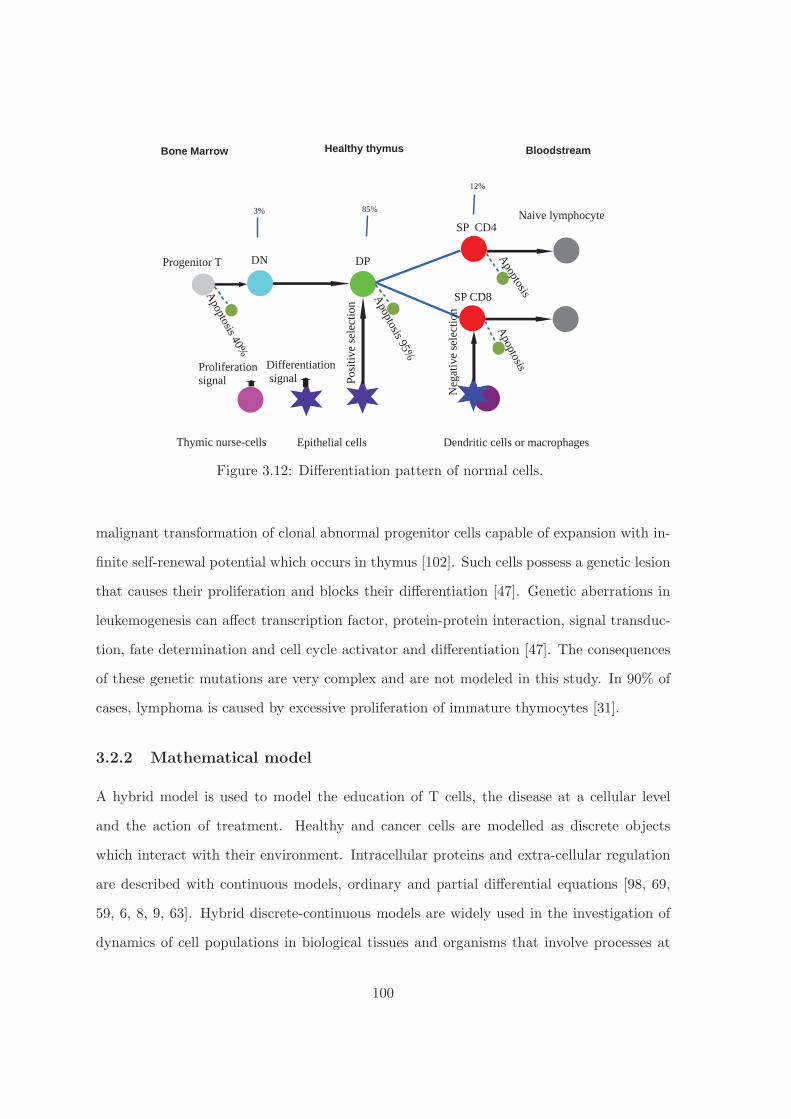
Figure 3.12: Differentiation pattern of normal cells.

malignant transformation of clonal abnormal progenitor cells capable of expansion with in-

finite self-renewal potential which occurs in thymus [102]. Such cells possess a genetic lesion

that causes their proliferation and blocks their differentiation [47]. Genetic aberrations in

leukemogenesis can affect transcription factor, protein-protein interaction, signal transduc-

tion, fate determination and cell cycle activator and differentiation [47]. The consequences

of these genetic mutations are very complex and are not modeled in this study. In 90% of

cases, lymphoma is caused by excessive proliferation of immature thymocytes [31].

3.2.2 Mathematical model

A hybrid model is used to model the education of T cells, the disease at a cellular level

and the action of treatment. Healthy and cancer cells are modelled as discrete objects

which interact with their environment. Intracellular proteins and extra-cellular regulation

are described with continuous models, ordinary and partial differential equations [98, 69,

59, 6, 8, 9, 63]. Hybrid discrete-continuous models are widely used in the investigation of

dynamics of cell populations in biological tissues and organisms that involve processes at

100

different scales.

Thymus modeling

The model of thymus considered in this work contains precursors, DN (3%), DP (85%)

and SP (12%) cells (these values are taken from [90]). The proportions of cells remain

approximately constant in a healthy individual. They provide a constant T cells production

compensating apoptosis. Precursors are supposed to be committed to the T lineage by

activation of their receptors Notch. Other lineages are not studied here. We only simulate

the transformation of DN1 cells into DP and after that into SP.

Cell cycle duration is taken in average T = 3 days plus/minus random variation in time

interval [T − δ, T + δ], with a uniform distribution. At the end of cell cycle, the cell divides.

Everywhere below we will set δ = 1. At the moment of cell division, its choice between self-

renewal, differentiation and apoptosis is specified. Early T cells are first located in a stromal

cell niche [28]. They are exposed to stromal factors [28] which determine their proliferation

and differentiation [56, 123]. Differentiation and self-renewal of T cells are controlled by

signals emitted by their microenvironnement. Intracellular regulation which determines cell

fate is described by ordinary differential equations (6.1.3), extracellular concentrations by

partial differential equations (2.2.9). Apoptosis is modeled by probability distribution (cf.

Paragraph “β-selection, negative and positive selections”).

When cells become SP, they leave the thymus. In order to maintain a constant number of

each type of cells, new cells are introduced in the computational domain by a periodic input

of precursors. New cells are added if there is some space available for them. Consequently,

if the number of lymphocytes in the thymus is sufficiently low, then new cells appear there.

If the number of cells is high, for example in the case of tumor growth, there are no new

cells. This is one of the reasons why during the progression of the disease, the thymus

cannot perform its function.

To model the individual behavior of cells and also that of patients, parameters are

assigned to each newly born cell. These parameters determine cell self-renewal capacity and

101

malignant potential. The parameters are the cell position, age, life expectancy, threshold

of sensitivity to treatment, threshold of sensitivity to the external environment. These

characteristics can be transmitted to daughter cells or they can be random variables.

Cell behavior depends on the intracellular and extracellular regulations described below.

It also depends on its spatial location and on various cell specific parameters such as duration

of cell cycle and sensitivity to treatment (Section 3.2).

Intracellular regulation

For each thymocyte we introduce an intracellular variable u which corresponds to the con-

centration of the proteins MAPK. Its evolution is described by the equation

du

dt= c0 + kG, (3.2.10)

where c0 is a positive constant and G is the concentration of extracellular growth factors. If

u exceeds some critical value ucrit at the end of cell cycle, then the cell self-renews, otherwise

it differentiates.

Extracellular regulation

Nurse cells produce growth factor G which promotes self-renewal of thymocytes. If they are

close to nurse cells, then the intracellular concentration u will grow due to the presence of

growth factor. It will reach the critical value and the cell will self-renew. The thymocytes

located sufficiently far from the nurse cells will differentiate. Concentration of the growth

factor G is described by the reaction-diffusion equation

∂G

∂t= DΔG+W − γG, (3.2.11)

where D is the diffusion coefficient, W is the production rate, γ is the degradation rate.

Nurse cells are considered as a constant source of growth factor. The last term in the

right-hand side of this equation describes its degradation.

102

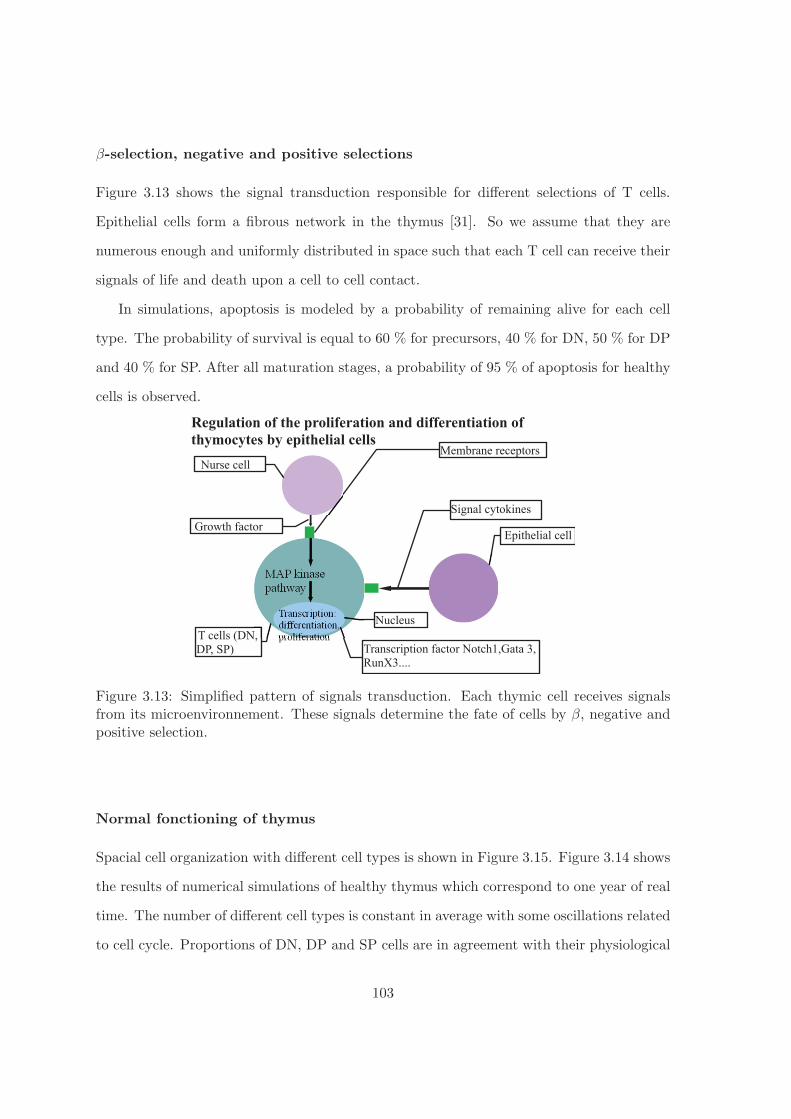
β-selection, negative and positive selections

Figure 3.13 shows the signal transduction responsible for different selections of T cells.

Epithelial cells form a fibrous network in the thymus [31]. So we assume that they are

numerous enough and uniformly distributed in space such that each T cell can receive their

signals of life and death upon a cell to cell contact.

In simulations, apoptosis is modeled by a probability of remaining alive for each cell

type. The probability of survival is equal to 60 % for precursors, 40 % for DN, 50 % for DP

and 40 % for SP. After all maturation stages, a probability of 95 % of apoptosis for healthy

cells is observed.

Figure 3.13: Simplified pattern of signals transduction. Each thymic cell receives signalsfrom its microenvironnement. These signals determine the fate of cells by β, negative andpositive selection.

Normal fonctioning of thymus

Spacial cell organization with different cell types is shown in Figure 3.15. Figure 3.14 shows

the results of numerical simulations of healthy thymus which correspond to one year of real

time. The number of different cell types is constant in average with some oscillations related

to cell cycle. Proportions of DN, DP and SP cells are in agreement with their physiological

103

values in humans.

Figure 3.14: Numerical simulations of healthy thymus: a part of thymic cortex. The numberof cells (DN (blue), DP (green), SP (red)) in a section of healthy thymus during one year.

3.2.3 Lymphoma development and treatment

Modeling of lymphoma

Appearance of tumor is caused by early thymocytes with excessive self-renewal and insuffi-

cient differentiation and apoptosis because of genetic mutations. In the model, we introduce

a single mutated cell which begins to proliferate. Malignant cells self-renew at the end of

each cell cycle with a given probability p. They have proliferating advantage compared to

normal cells. They multiply and increase the volume of thymus. Gradually, the whole thy-

mus is invaded by the tumor. Healthy cells can no longer develop normally. They disappear

being replaced by malignant cells.

Figure 3.15 shows the development of tumor. It invades the thymus and destroys the spa-

tial cell organization which is necessary for normal development of thymocytes. Therefore

their number decreases. On the other hand, there is no enough space for new immature cells

in the thymus. Therefore the influx of early thymocytes from the bone marrow (through

the blood flow) also decreases. Both factors result in the decrease of the number of normal

cells in the thymus (Figure 3.16).

104

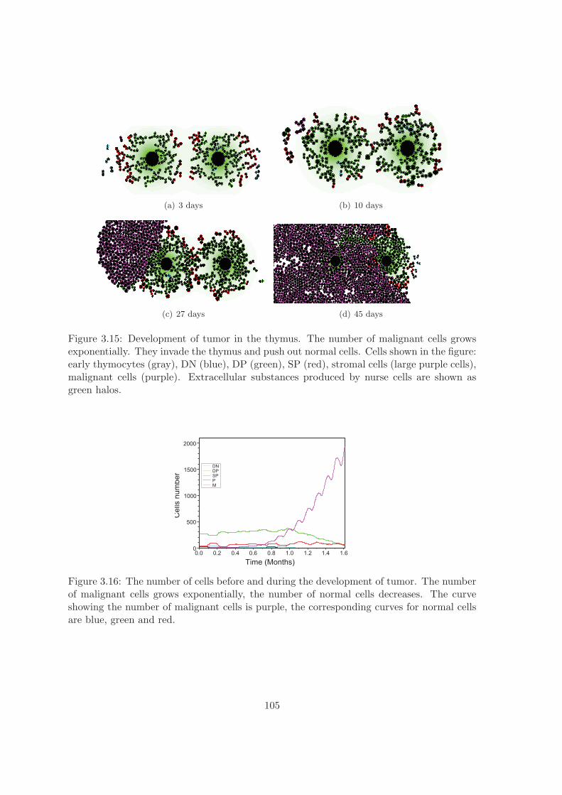
(a) 3 days (b) 10 days

(c) 27 days (d) 45 days

Figure 3.15: Development of tumor in the thymus. The number of malignant cells growsexponentially. They invade the thymus and push out normal cells. Cells shown in the figure:early thymocytes (gray), DN (blue), DP (green), SP (red), stromal cells (large purple cells),malignant cells (purple). Extracellular substances produced by nurse cells are shown asgreen halos.

Figure 3.16: The number of cells before and during the development of tumor. The numberof malignant cells grows exponentially, the number of normal cells decreases. The curveshowing the number of malignant cells is purple, the corresponding curves for normal cellsare blue, green and red.

105

Treatment

In this section we will study lymphoma treatment with chemotherapy. Medications used

in the treatment represent a combination of drugs, mainly methotrexate and purinethol.

Treatment consists of several phases: induction, consolidation, reinduction, maintenance

[155]. We will take into account two phases: treatment of acute phase (induction) with the

duration 1-1.5 months and maintenance treatment (up to 2 years after the beginning of of

induction) [155]. Treatment doses for Mercaptopurine (plurimethol) are 50 mg/m2 daily

and for Methotrexate (PO) 20 mg/m2 weekly.

The protocol of treatment is too complicated to be faithfully reproduced in the model.

However the frequency of drug injection is sufficient to consider that its concentrations in the

patient’s body is constant during the treatment. We assume that cancer cells are exposed to

the same quantity of treatment regardless of their location. Maintenance treatment begins

after the complete or partial disappearance of the tumor.

(a) 46 days (b) 48 days

(c) 65 days (d) 66 days

Figure 3.17: Simulations of lymphoma treatment by chemotherapy. When the tumor disap-pears, precursors enter the thymus and recreate its normal structure. Precursors (gray), DN(blue), DP (green), SP (red), stromal cells (large purple cells), epithelial cells (not shown,these cells form a fibrous network in the thymus), malignant cells (purple).

106

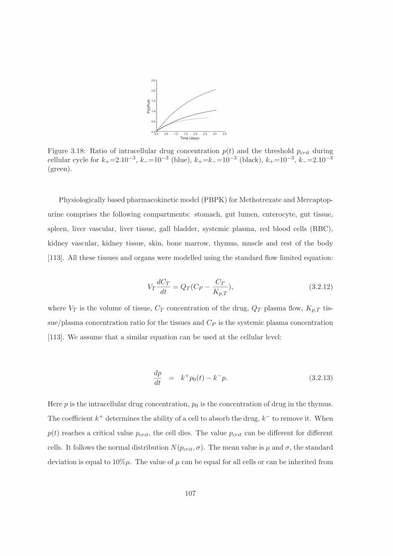
Figure 3.18: Ratio of intracellular drug concentration p(t) and the threshold pcrit duringcellular cycle for k+=2.10−3, k−=10−3 (blue), k+=k−=10−3 (black), k+=10−3, k−=2.10−3

(green).

Physiologically based pharmacokinetic model (PBPK) for Methotrexate and Mercaptop-

urine comprises the following compartments: stomach, gut lumen, enterocyte, gut tissue,

spleen, liver vascular, liver tissue, gall bladder, systemic plasma, red blood cells (RBC),

kidney vascular, kidney tissue, skin, bone marrow, thymus, muscle and rest of the body

[113]. All these tissues and organs were modelled using the standard flow limited equation:

VTdCT

dt= QT (CP − CT

Kp,T), (3.2.12)

where VT is the volume of tissue, CT concentration of the drug, QT plasma flow, Kp,T tis-

sue/plasma concentration ratio for the tissues and CP is the systemic plasma concentration

[113]. We assume that a similar equation can be used at the cellular level:

dp

dt= k+p0(t)− k−p. (3.2.13)

Here p is the intracellular drug concentration, p0 is the concentration of drug in the thymus.

The coefficient k+ determines the ability of a cell to absorb the drug, k− to remove it. When

p(t) reaches a critical value pcrit, the cell dies. The value pcrit can be different for different

cells. It follows the normal distribution N(pcrit, σ). The mean value is μ and σ, the standard

deviation is equal to 10%μ. The value of μ can be equal for all cells or can be inherited from

107

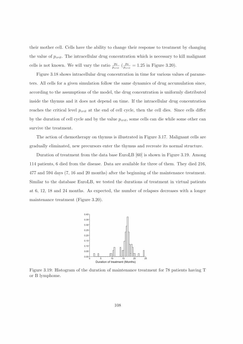
their mother cell. Cells have the ability to change their response to treatment by changing

the value of pcrit. The intracellular drug concentration which is necessary to kill malignant

cells is not known. We will vary the ratio p0pcrit

( p0pcrit

= 1.25 in Figure 3.20).

Figure 3.18 shows intracellular drug concentration in time for various values of parame-

ters. All cells for a given simulation follow the same dynamics of drug accumulation since,

according to the assumptions of the model, the drug concentration is uniformly distributed

inside the thymus and it does not depend on time. If the intracellular drug concentration

reaches the critical level pcrit at the end of cell cycle, then the cell dies. Since cells differ

by the duration of cell cycle and by the value pcrit, some cells can die while some other can

survive the treatment.

The action of chemotherapy on thymus is illustrated in Figure 3.17. Malignant cells are

gradually eliminated, new precursors enter the thymus and recreate its normal structure.

Duration of treatment from the data base EuroLB [60] is shown in Figure 3.19. Among

114 patients, 6 died from the disease. Data are available for three of them. They died 216,

477 and 594 days (7, 16 and 20 months) after the beginning of the maintenance treatment.

Similar to the database EuroLB, we tested the durations of treatment in virtual patients

at 6, 12, 18 and 24 months. As expected, the number of relapses decreases with a longer

maintenance treatment (Figure 3.20).

Figure 3.19: Histogram of the duration of maintenance treatment for 78 patients having Tor B lymphome.

108

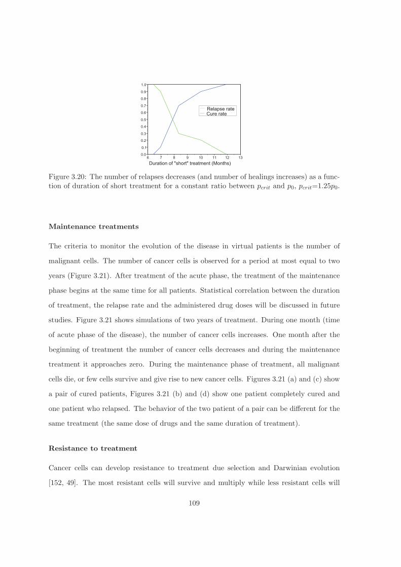
Figure 3.20: The number of relapses decreases (and number of healings increases) as a func-tion of duration of short treatment for a constant ratio between pcrit and p0, pcrit=1.25p0.

Maintenance treatments

The criteria to monitor the evolution of the disease in virtual patients is the number of

malignant cells. The number of cancer cells is observed for a period at most equal to two

years (Figure 3.21). After treatment of the acute phase, the treatment of the maintenance

phase begins at the same time for all patients. Statistical correlation between the duration

of treatment, the relapse rate and the administered drug doses will be discussed in future

studies. Figure 3.21 shows simulations of two years of treatment. During one month (time

of acute phase of the disease), the number of cancer cells increases. One month after the

beginning of treatment the number of cancer cells decreases and during the maintenance

treatment it approaches zero. During the maintenance phase of treatment, all malignant

cells die, or few cells survive and give rise to new cancer cells. Figures 3.21 (a) and (c) show

a pair of cured patients, Figures 3.21 (b) and (d) show one patient completely cured and

one patient who relapsed. The behavior of the two patient of a pair can be different for the

same treatment (the same dose of drugs and the same duration of treatment).

Resistance to treatment

Cancer cells can develop resistance to treatment due selection and Darwinian evolution

[152, 49]. The most resistant cells will survive and multiply while less resistant cells will

109

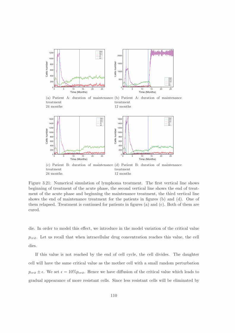
(a) Patient A: duration of maintenancetreatment24 months

(b) Patient A: duration of maintenancetreatment12 months

(c) Patient B: duration of maintenancetreatment24 months

(d) Patient B: duration of maintenancetreatment12 months

Figure 3.21: Numerical simulation of lymphoma treatment. The first vertical line showsbeginning of treatment of the acute phase, the second vertical line shows the end of treat-ment of the acute phase and beginning the maintenance treatment, the third vertical lineshows the end of maintenance treatment for the patients in figures (b) and (d). One ofthem relapsed. Treatment is continued for patients in figures (a) and (c). Both of them arecured.

die. In order to model this effect, we introduce in the model variation of the critical value

pcrit. Let us recall that when intracellular drug concentration reaches this value, the cell

dies.

If this value is not reached by the end of cell cycle, the cell divides. The daughter

cell will have the same critical value as the mother cell with a small random perturbation

pcrit ± ε. We set ε = 10%pcrit. Hence we have diffusion of the critical value which leads to

gradual appearance of more resistant cells. Since less resistant cells will be eliminated by

110

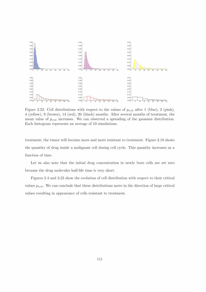
Figure 3.22: Cell distributions with respect to the values of pcrit after 1 (blue), 2 (pink),4 (yellow), 9 (brown), 14 (red), 20 (black) months. After several months of treatment, themean value of pcrit increases. We can observed a spreading of the gaussian distribution.Each histogram represents an average of 10 simulations.

treatment, the tumor will become more and more resistant to treatment. Figure 3.18 shows

the quantity of drug inside a malignant cell during cell cycle. This quantity increases as a

function of time.

Let us also note that the initial drug concentration in newly born cells are set zero

because the drug molecules half-life time is very short.

Figures 2.4 and 3.22 show the evolution of cell distribution with respect to their critical

values pcrit. We can conclude that these distributions move in the direction of large critical

values resulting in appearance of cells resistant to treatment.

111

Chapter 4

Pulses in reaction-diffusion

equations

4.1 Introduction

Biological cells can be characterized by their genotype. Cells of the same type have a lo-

calized density distribution in the space of genotypes. This distribution can evolve under

the influence of various external factors. In particular cancer cells can adapt to chemother-

apy treatment resulting in appearance of resistant clones. This process is called Darwinian

evolution of cancer cells [27]. We studied above the emergence of resistance with hybrid

discrete-continuous models in the case of lymphoma treatment. In this chapter we analyze

this process with reaction-diffusion equations. We will consider the scalar reaction-diffusion

equation

∂u

∂t= D

∂2u

∂x2+ F (u, x), (4.1.1)

on the whole axis. The typical example of the nonlinearity is given by the function

F (u, x) = uk(1− u)− σ(x)u, (4.1.2)

112

where the first term describe the rate of cell birth and the second term the rate of their

death. Let us note that the space variable x here corresponds to cell genotype, u(x, t) is

the cell density which depends on x and on time t. The diffusion term describe variation of

genotype due to mutations, the mortality term depends on the space variable, that is on cell

genotype. If k = 1 and σ(x) = const, then this equation does not have localized stationary

solutions. In order to describe cell populations with localized genotype which correspond

to certain cell type, we need to introduce space dependent mortality coefficients. This

means that cells can survive only in a certain range of genotypes (survival gap). We will

study the existence of stationary solutions of Equation 4.1.1 and will show that localized

solutions (pulses) can exist under certain conditions of the function σ(x). The method

of proof is based on topological degree for elliptic problems in unbounded domains and

on the Lerays-Schauder method. Consider now cell population dynamics if there are two

survival gaps, that is two intervals of genotype where cells can survive. We will consider

the model with global consumption of resources where all cells consume the same nutrients

and their quantity is limited. Suppose that initially all cells are located in the first survival

gap (Figure 4.2). If we increase the mortality coefficient there, then this cell population

disappears. Instead of it, another cell population appears in the second gap. This behavior

can be explained as follows. Cells located in the first survival gap consume all nutrients and

do not allow cells in the second gap (which are present because of mutations) to proliferate.

When cells from the first gap are removed, nutrients become available and cells in the

second gap proliferate restoring a similar population with another genotype. This is one of

possible mechanisms of emergence of cell clones resistant to chemotherapy in the process of

treatment.

Existence of solutions of the semilinear elliptic equation

Δw + F (w, x) = 0 (4.1.3)

in Rn, n ≥ 1 depends on the nonlinearity F (w, x). It is studied in detail for polynomial

113

functions F (w, x) = wp where existence of solutions is determined by the values of n and

p [37], [41], [42], [76], [77]. Another typical example is given by the nonlinearity F (w, x) =

−a(x)|w|p−2w+λb(x)|w|q−2w, where a(x) and b(x) are positive functions and λ is a positive

parameter. Under some additional conditions it is proved that there exists a value of λ for

which a nontrivial solution of this equation exists in the corresponding function space. In

some cases it can be proved that this solution is radial (n > 1) and non-negative. The

review of methods and results can be found in [7], [99].

In the second example considered above, the nonlinearity has variable sign and the

trivial solution w = 0 can be stable. In this case, nontrivial solutions, if they exist, do not

bifurcate from the trivial one. We can expect that they separate basins of attraction of the

trivial solution and of some other solution or infinity (blow up solution). These properties

can be clearly seen in the autonomous case, for example F (w, x) = −aw+bw2, where a and

b are some positive constants. In this case, equation (4.1.3) has a positive solution (pulse)

which vanish at infinity [17]. It is unstable as a stationary solution of the corresponding

parabolic equation. Solution of the Cauchy problem with a perturbed initial condition will

converge either to 0 or grow to infinity. Moreover, such pulse solutions exist for any values

of parameters a and b and not only for some values of parameters as in the example above.

In the one-dimensional case, they can be easily found analytically.

In this work we will study existence of pulse solutions for a nonautonomous nonlinearity.

We will consider the one-dimensional equation on the whole axis

w′′ + F (w, x) = 0 (4.1.4)

and we will look for its classical solutions with the limits

w(±∞) = 0. (4.1.5)

Similar to the example above, we will see that such solutions can separate basin of attraction

of the trivial solution and of some other solution. In fact, existence of solutions of problem

114

(4.1.4), (4.1.5) will be determined by the properties of travelling waves for the corresponding

autonomous equation with the limiting function F0(w) = lim|x|→∞ F (w, x). The typical

form of the function F considered in this work is given by the example from population

dynamics

F (w, x) = w2(1− w)− σ(x)w, (4.1.6)

where the first term in the right-hand side describes the reproduction of the population, the

second term its mortality. The mortality rate σ(x) is a positive function which depends on

the space variable. We can consider the nonlinearity in a more general form. The conditions

on it will be specified below.

We will use function (4.1.6) in order to explain the main features of this problem.

Consider first the case where σ(x) ≡ σ0 is a constant. Set

F0(w) = w2(1− w)− σ0w.

Suppose that 0 < σ0 < 1/4 and consider the zeros of this function, w0 = 0, w1 and w2 are

solutions of the equation w(1− w) = σ0, 0 < w1 < w2. If

∫ w2

0F0(w)dw > 0, (4.1.7)

then the equation

w′′ + F0(w) = 0 (4.1.8)

with the limits w(±∞) = 0 has two solutions. The trivial solution W0(x) ≡ 0 and a positive

solution W1(x) which can be easily found analytically. Its explicit form is not essential for

us. In the case of the inequality

∫ w2

0F0(w)dw < 0 (4.1.9)

115

there exists only trivial solution. Finally, if

∫ w2

0F0(w)dw = 0, (4.1.10)

then equation (4.1.8) does not have nontrivial solutions, which vanish at infinity, but there

is a solution with the limits

w(−∞) = w2, w(+∞) = 0. (4.1.11)

Let us note these three cases are related to the speed of travelling waves, that is solutions

of the equation

w′′ + cw′ + F0(w) = 0

with limits (4.1.11). Here c is the wave speed. Its sign can be determined multiplying the

equation by w′ and integrating from −∞ to +∞. If condition (4.1.7) is satisfied, then c > 0.

If the inequality is opposite, then c < 0. Finally, in the case (4.1.10), c = 0. We will see

that properties of solutions of problem (4.1.4), (4.1.5) depend on the sign of the wave speed.

Condition (4.1.7). In this case, the question about the existence of solution can be

formulated in the following way. If we change the function σ(x) by a continuous deformation

starting from the constant σ0, will the nontrivial solution persist? We will study this

question by a Leray-Schauder method which is based on topological degree and a priori

estimates of solutions. Topological degree in unbounded domains is defined in weighted

spaces, in the space without weight it may not exist. Therefore the estimates should also

be obtained in the weighted spaces. Usual estimates in Holder or Sobolev spaces are not

sufficient.

Let us explain in more detail what estimates we need in order to prove the existence of

solutions and how they can be obtained. Consider equation (4.1.4) with the function στ (x)

which depends on a parameter τ . Suppose that there exists a limit σ0 = limx→±∞ στ (x).

116

Let E = C2+αμ (R) be the weighted Holder space with the norm ‖u‖E = ‖uμ‖C2+α(R), where

μ(x) =√1 + x2. If the usual Holder norm ‖u‖E0

, E0 = C2+α(R) is bounded and the

solution decays exponentially at infinity, then the weighted Holder norm is also bounded.

The E0-norm of the solution can be estimated by the usual methods, exponential decay of

solution at infinity follows from the assumption F ′0(0) < 0. However this is not sufficient

for a uniform estimate in the weighted Holder space. Consider a family of solutions uτ

which depends on a parameter τ . If the weighted norm ‖u‖E tends to infinity as τ → τ0,

then it can be verified that equation (4.1.8) has a nonzero solution, and uτ converges to

this solution. Under some additional conditions, we will prove that this convergence cannot

occur and will obtain, by this, a priori estimates of solutions. We will use here monotonicity

of solutions on the half-axis.

Condition (4.1.9). The situation is different in the case of condition (4.1.9). Equation

(4.1.4) does not have nontrivial solutions vanishing at infinity. A nontrivial solution can

bifurcate from the trivial solution. Condition (4.1.9) will allow us to obtain a priori estimates

of nontrivial solutions in the weighted norm. Hence if the trivial solution becomes unstable,

then we will obtain the existence of a nontrivial solution. Let us note that for function

(4.1.6) the trivial solution becomes unstable if the function σ(x) is negative for some x.

This does not correspond to the biological meaning of this example. We consider this case

in view of other possible applications and more general functions F .

Thus, equality (4.1.10) separates two cases where we prove existence of solutions. In the

case where this equality is satisfied, the method to prove existence of solutions developed

in this work is not applicable.

Nonlocal equations. Besides equation (4.1.4) we will also study the nonocal equation

w′′ + F (w, x, I) = 0, I(w) =

∫ ∞

−∞w(x)dx (4.1.12)

with the typical example of nonlinearity

117

F (w, x, I) = w2(1− I)− σ(x)w. (4.1.13)

This case is quite similar to the previous one, and analysis of the existence of solutions is

based on the previous results. However, due to the integral term, the number of solutions

can change, and some of them can become stable [160]. Though we do not study stability

of solutions in this work, this is an important justification for the investigation of pulse

solutions.

Leray-Schauder method. Existence of solutions will be proved by the Leray-Schauder

method based on the topological degree for elliptic problems in unbounded domains. Let

us recall that the Leray-Schauder degree is not generally applicable in this case. It can

be used under some special conditions on the coefficients which allow the reduction of the

corresponding operator to the compact operator [99]. In our case this approach is not

applicable. We will use the degree construction for Fredholm and proper operators with

the zero index [159]. This construction requires the introduction of special weighted spaces.

Therefore a priori estimates of solutions required for the Leray-Schauder method should

also be obtained in the weighted spaces. This is a special type of estimates where the

boundedness of the solution and of its derivatives is not sufficient. These estimates will be

obtained for monotone solutions and will require separation of monotone and non-monotone

solutions (explained below). This approach is inspired by the method of proof of travelling

waves for monotone and locally monotone systems [158].

In the next section we will introduce function spaces and operators, we will obtain a

priori estimates of solutions and prove the main existence result (Theorem 2.7). It corre-

sponds to the case (4.1.7) in the example considered above. In Section 4.3 we will discuss

another possible case which correspond to inequality (4.1.10). Nonlocal equations will be

considered in Section 4.4.

118

4.2 Monotone solutions on the half-axis

We begin with the problem on the half-axis. We consider equation (4.1.4) for x > 0 with

the Neumann boundary condition and look for a solution decaying at infinity:

w′(0) = 0, w(+∞) = 0. (4.2.1)

This problem can be extended to the whole axis by symmetry. We will assume that

F (0, x) = 0, x ≥ 0;∂F (w, x)

∂x< 0, w > 0, x ≥ 0 (4.2.2)

and for some ε > 0

F ′w(0, x) ≤ −ε, ∀x ≥ 0. (4.2.3)

Moreover, there exists w+ > 0 such that

F (w, x) < 0, ∀x ≥ 0, w > w+. (4.2.4)

4.2.1 Operators and spaces

We will use the Leray-Schauder method to prove the existence of solutions. We need to

introduce the operators, function spaces, construct a continuous deformation of the operator

and obtain a priori estimates of solutions. Operators and spaces should be defined in such

a way that the topological degree exists for them. We suppose that the function F (w, x) is

sufficiently smooth with respect to both variables. We can assume for simplicity that it is

infinitely differentiable with all derivatives bounded. Consider the operator

A(w) = w′′ + F (w, x)

acting from the space

119

E1 = {u ∈ C2+αμ (R+), u′(0) = 0}

into the space E2 = Cαμ (R+). Here Ck+α

μ (R+) is a weighted Holder space with the norm

‖u‖Ck+αμ (R+) = ‖uμ‖Ck+α(R+),

where μ(x) is a weight function. We will set μ(x) =√1 + x2. Construction of the topological

degree for such spaces and operators can be found in [159].

4.2.2 Separation of monotone solutions

We will obtain a priori estimates of solutions for monotonically decreasing solutions. There-

fore we need to separate them from non-monotone solutions. We understand this separation

in the following sense. Consider a solution wτ (x) �≡ 0 which depends on parameter τ . The

dependence on τ is continuous in the norm C1(R+). Suppose that the solution wτ (x) is

monotonically decreasing for τ < τ0 and it is not monotonically decreasing for τ > τ0. We

will prove that this assumption leads to a contradiction.

We proceed by contradiction. Then there is a sequence τn → τ0 and the sequence of

solutions wn(x) = wτn(x) such that these functions are not monotone and the function

w0(x) = wτ0(x) is monotone. Therefore there exists a sequence xn such that w′n(xn) = 0.

Without loss of generality, we can suppose that xn → x0, where one of the following three

cases takes place: 0 < x0 < ∞, x0 = ∞, x0 = 0. We will show that all of them lead to

contradiction.

Finite value of x0. Consider first the case where 0 < x0 < ∞. Then w′0(x0) = 0 and

w′0(x) ≤ 0 for all x ≥ 0. Set u(x) = −w′

0(x). Differentiating equation (4.1.4), we get

u′′ + F ′w(w0, x)u− F ′

x(w0, x) = 0. (4.2.5)

120

Since u(x) ≥ 0 for all x ≥ 0, u(x0) = 0, F ′x < 0, then we obtain a contradiction in signs

in the last equation. If the inequality in (4.2.2) is not strict, that is F ′x ≤ 0, then the last

equation contradicts the maximum principle.

Let us consider one more generalization. We will suppose that

F (w, x) = 0 ⇒ F ′x(w, x) < 0, w > 0, x ≥ 0. (4.2.6)

Therefore the derivative F ′x is negative not everywhere as in condition (4.2.2) but only at

zero lines of the function F .

Since w′′0(x0) = 0, then F (w0(x0), x0) = 0. By virtue of condition (4.2.6), we have

F ′x(w0(x0), x0) < 0. Differentiating equation (4.1.4) and taking into account that w′

0(x0) =

0, we obtain

w′′′0 (x0) = −F ′

x(w0(x0), x0) > 0. (4.2.7)

Hence w′0(x) > 0 in some neighborhood of the point x0. This contradicts the assumption

that w′0(x) ≤ 0.

Infinite value of x0. We consider now the case where xn → ∞. Since wn(x) → w0(x)

in C1(R+) and w0(x) → 0 as x → ∞, then wn(xn) → 0 as n → ∞. If wn(xn) > 0, then

F (wn(xn), xn) < 0 and w′′n(xn) > 0. Hence any positive extremum of the functions wn(x)

is a minimum. Therefore they cannot converge to zero at infinity. Similarly, if wn(xn) < 0,

then it is a maximum and, as before, the function cannot converge to zero at infinity.

Finally, if wn(xn) = 0, then by virtue of condition (4.2.2) we have that F (wn(xn), xn) = 0,

w′′n(xn) = 0. Therefore wn(x) ≡ 0. This contradicts our assumption that all solutions wτ (x)

are nontrivial.

Zero value of x0. Let us consider the last case where xn → x0 = 0. We note that

F (w0(0), 0) > 0. Indeed, if F (w0(0), 0) < 0, then w′′0(0) > 0. Since w′

0(0) = 0, then this

function cannot be monotonically decreasing.

121

If F (w0(0), 0) = 0, then w′′0(0) = 0. The function u(x) = −w′

0(x) satisfies equation

(4.2.5) where F ′x < 0. Since u(x) ≥ 0 for all x ≥ 0, u(0) = 0 and u′(0) = 0, then we

obtain a contradiction with the Hopf lemma which affirms that u′(0) > 0. In the case of

the generalized condition (4.2.6), we get inequality (4.2.7). It contradicts the assumption

that the function w0(x) is decreasing.

Thus, we proved that F (w0(0), 0) > 0. Therefore the same inequality holds in some

neighborhood of x = 0. Since wn(x) converges uniformly to w0(x), then w′′n(x) < 0 in the

interval 0 < x < δ with some positive δ independent of n. This assertion contradicts the

assumption that w′n(xn) = 0 and xn → 0 as n→∞. We proved the following theorem.

Theorem 2.1 (Separation of monotone solutions.) There exists a positive number

r such that for any solution of problem (4.2.8), (4.2.9), which depends on a parameter τ ,

such that

‖wM − wN‖E1≥ r

for any monotone solution wM and any nonmonotone solution wN of this problem. This

estimate does not depend on τ .

4.2.3 A priori estimates of monotone solutions

We consider the equation

w′′ + Fτ (w, x) = 0 (4.2.8)

on the half-axis x > 0 with the Neumann boundary condition:

w′(0) = 0. (4.2.9)

We will look for its solution decaying at infinity, w(+∞) = 0. In order to simplify the

presentation, we suppose that the function Fτ (w, x) is infinitely differentiable with respect

122

to all variables w, x, τ ,

Fτ (0, x) = 0, x ≥ 0;∂Fτ (w, x)

∂x< 0, w > 0, x ≥ 0 (4.2.10)

and

∂Fτ (0, x)

∂w≤ −ε, x ≥ 0, τ ∈ [0, 1] (4.2.11)

for some ε > 0. Moreover, there exists w+ > 0 such that

Fτ (w, x) < 0, ∀w > w+, x ≥ 0, τ ∈ [0, 1] (4.2.12)

Let wτ (x) be positive solutions of problem (4.2.8), (4.2.9) decaying at infinity. From

condition (4.2.12) it follows that wτ (x) ≤ w+ for all x and τ . Indeed, since we consider

montonically decreasing solutions, it is sufficient to verify that wτ (0) ≤ w+. If the opposite

inequality holds, then, by virtue of the equation, w′′τ (0) > 0, and this function is not

decreasing.

Since the function Fτ (w, x) is sufficiently smooth with respect to w, x and τ , then

solutions are uniformly bounded in C2(R+) and the dependence on τ is continuous in

C1(R+). In order to prove that solutions are uniformly bounded in the weighted Holder

norm, it is sufficient to verify that the weighted norm

‖wτ‖μ = ‖wμ‖C(R+)

of these solutions is uniformly bounded. Here μ(x) =√1 + x2.

Let ε > 0 be sufficiently small such that Fτ (w, x) < 0 for 0 < w < ε and all x ≥ 0. Such

ε exists by virtue of condition (4.2.11). Since wτ (x) is a decreasing function and, obviously,

wτ (0) > ε (otherwise Fτ (wτ (0), 0) < 0 and w′′τ (0) > 0), then there exists a unique solution

of the equation wτ (x) = ε. Denote it by xτ .

The solutions wτ (x) admit a uniform exponential estimate for x > xτ . Therefore if xτ

123

is uniformly bounded, then we obtain a uniform estimate of the norm ‖wτ‖μ.Suppose that the values xτ are not uniformly bounded. Then there exists a sequence τn

for which xn = xτn →∞. Without loss of generality we can assume that τn → τ0 for some

τ0 ∈ [0, 1]. We will consider the corresponding sequence of solutions wn(x) = wτn(x). It has

a subsequence locally convergent to a solution w0(x) such that w′0(0) = 0 and w0(∞) > 0.

The latter follows from the equality wn(xn) = ε and convergence of the sequence xn to

infinity.

Let us also consider the sequence vn(x) = wn(x + xn) of shifted solutions. Obviously,

vn(0) = ε. It has a subsequence locally convergent to a monotone solution v0(x) of equation

v′′ + F+(v) = 0 (4.2.13)

defined on the whole axis and such that v0(+∞) = 0, v0(−∞) > ε. Here

F+(v) = limx→∞Fτ0(v, x).

This limit exists by virtue of the condition on the derivative in (4.2.10).

Set v− = v(−∞). Then F+(v−) = 0. Multiplying equation (4.2.13) by v′ and integrat-

ing, we obtain

∫ v−

0F+(u)du = 0.

Thus, the assumption that xτ is not uniformly bounded leads to the conclusion that there

exists a zero v− of the function F+ such that the previous equality holds.

Condition 2.2. For any v > 0, if F+(v) = 0, then∫ v0 F+(u)du �= 0.

If this condition is satisfied, then the values xτ are uniformly bounded. Hence the norm

‖wτ‖μ is also uniformly bounded.

124

4.2.4 Model problem

Consider the function F (w, x), which satisfies conditions (4.2.2)-(4.2.4), and the limit func-

tion

F+(w) = limx→+∞F (w, x).

We suppose that it satisfies the following conditions:

F ′+(0) < 0, F+(w) < 0 for w > w+ (4.2.14)

with some w+ > 0. Moreover there exists w0 ∈ (0, w+) such that F+(w0) �= 0,

∫ w0

0F+(u)du = 0,

∫ w

0F+(u)du �= 0 ∀w ∈ (0, w+), w �= w0. (4.2.15)

Then problem

w′′ + F+(w) = 0, w′(0) = 0, w(+∞) = 0

has a unique positive solution w0(x), and w0(0) = w0 is its maximal value. This solution

can be easily found analytically.

We will find the index of this solution, that is the value of the degree with respect to

small sphere around this solution. It is given by the following expression:

ind(w0) = (−1)ν ,

where ν is the number of positive eigenvalues (with their multiplicities) of the linearized

operator

Lu = u′′ + F ′+(w0(x))u

acting on functions C2(R+).

125

Lemma 2.5. The eigenvalue problem

u′′ + F ′+(w0(x))u = λu, u′(0) = 0, u(∞) = 0 (4.2.16)

does not have a zero eigenvalue.

Proof. Let us note first of all that the essential spectrum of this problem lies in the left-half

plane since F ′+(0) < 0. Suppose that the assertion of the lemma does not hold and problem

(4.2.16) has a nontrivial solution u0(x) for λ = 0. Then this solution cannot be positive for

all x. Indeed, if u0(x) > 0 for 0 ≤ x <∞, then the function v0(x) = u0(|x|) defined on the

whole axis is a positive solution of the equation

v′′ + F ′+(w1(x))v = 0, x ∈ R,

where the function w1(x) is an extension on the whole axis of the function w0(x) by sym-

metry. Since the function v0(x) is positive, then λ = 0 is the principal eigenvalue of the

operator

Lv = v′′ + F ′+(w1(x))v,

and this eigenvalue is simple [158]. On the other hand, v1(x) = w′1(x) is an eigenfunction

of this operator corresponding to the zero eigenvalue, and

v1(x) = −w′0(−x) > 0, −∞ < x < 0, v1(x) = w′

0(x) < 0, 0 < x <∞.

Hence this eigenfunction is not positive, and it is different from the eigenfunction v0(x). We

obtain a contradiction with simplicity of the principal eigenvalue.

Thus, the function u0(x) has variable sign. Since it is determined up to a factor, we can

assume that u0(0) < 0. Then it has positive values for some x > 0 and it decays at infinity

since F ′+(0) < 0.

Next, the function u1(x) = −w′0(x) is a solution of the problem

126

u′′ + F ′+(w0(x))u = 0, u(0) = 0, u(∞) = 0,

which differs from problem (4.2.16) considered for λ = 0 by the boundary condition. This

function is positive for all x > 0. We will use this function to prove that the solution u0(x)

cannot exist. Set ω(x) = tu1(x)−u0(x), where t is a positive number. This function satisfies

the equation

ω′′ + F ′+(w0(x))ω = 0. (4.2.17)

Let x0 be such that

F ′+(w0(x)) < 0, x0 ≤ x <∞.

Since u1(x) is a positive function, we can choose t for which ω(x0) > 0. We can verify that

ω(x) > 0, x0 ≤ x <∞. (4.2.18)

Indeed, if ω(x1) < 0 for some x1 > x0, then this function has a negative minimum since

it converges to 0 at infinity. We obtain a contradiction in signs in equation (4.2.17) at the

point of minimum. If ω(x1) = 0, then we get a contradiction with the maximum principle.

Indeed, since ω(x) ≥ 0 for x ≥ x0, then this function is either everywhere positive or

identically zero for such x. The latter contradicts the assumption that ω(x0) > 0.

Let us recall that u0(0) < 0. Therefore ω(0) > 0 for any t > 0. Moreover, (4.2.18) holds

for t large enough. Hence for t sufficiently large, the function ω(x) is positive for all x ≥ 0.

If t = 0, then it has negative values since u0(x) has positive values. Let t0 be the infimum

of all t for which ω(x) is positive for all x ≥ 0. Then there exists a value x2 ∈ [0, x0] for

which ω(x2) = 0. Indeed, if ω(x) is positive in this interval, then t can be decreased in

such a way that it remains positive there. Since ω(x0) > 0, then (4.2.18) holds, and ω(x) is

positive for all x. This contradicts the definition of t0.

Thus, ω(x) ≥ 0 for all x ≥ 0 and ω(x2) = 0. But this is not possible by virtue of the

127

maximum principle. Hence problem (4.2.16) cannot have nontrivial solution for λ = 0.

�

Remark 2.6. The principal eigenvalue λ0 of problem (4.2.16) is positive. Indeed, if it

is non-positive, then, since the corresponding eigenfunction is positive, we will obtain a

contradiction with the fact that the function −w′0(x) is a positive (for x > 0) solution of the

equation Lu = 0 (cf. the proof of the lemma). We proved in Lemma 2.5 that this problem

does not have a zero eigenvalue. We can verify that any real λ ∈ (0, λ0) is not an eigenvalue

of this problem. Indeed, suppose that there is an eigenvalue λ∗ ∈ (0, λ0). The corresponding

eigenfunction u∗(x) cannot be positive because only the principal eigenvalue has a positive

eigenfunction. As in the proof of the lemma, we introduce the function ω = tu1 − u∗. It

satisfies the equation

ω′′ + F ′+(w0(x))ω + φ(x) = λ∗ω,

where φ(x) = λ∗tu1. As above, we choose t > 0 in such a way that ω(x) ≥ 0 for all x and

ω(x2) = 0 for some x2 > 0. Since φ(x) > 0 for all x > 0, then we obtain a contradiction in

signs in the last equation at x = x2.

4.2.5 Existence theorem

We can now prove the main theorem of this section.

Theorem 2.7. If the function F (w, x) satisfies conditions (4.2.2)-(4.2.4) and the function

F+(w) satisfies conditions (4.2.14), (4.2.15), then problem

w′′ + F (w, x) = 0, (4.2.19)

w′(0) = 0 (4.2.20)

on the half-axis x > 0 has a positive monotonically decreasing solution vanishing at infinity.

128

It belongs to the weighted Holder space E1.

Proof. We will consider the homotopy

Fτ (w, x) = τF (w, x) + (1− τ)F+(w).

Let us recall Condition 2.2, which follows from (4.2.14), (4.2.15), and assumption that

solutions are uniformly bounded are used for a priori estimates of monotone solutions. The

latter can follow from the maximum principle or from the estimates. Conditions (4.2.14)

and (4.2.15) provide existence of solutions for the model problem; conditions (4.2.10) and

(4.2.11), which follow from (4.2.2)-(4.2.4) and the definition of the function Fτ (w, x), provide

separation of monotone solutions.

For τ = 0 this equation has a unique strictly decreasing solution w0(x). Let us find

its index, that is the degree with respect to a small ball which contains only this solution

and no other solutions. Such small ball exists because the operator linearized about this

solution is invertible (Lemma 2.5). By virtue of Lemma 2.5 and Remark 2.6

ind (w0) = (−1)ν = −1,

where ν is the number of positive eigenvalues of the operator linearized about this solution

together with their multiplicities [159].

Let us recall that the operator Aτ : E1 × [0, 1]→ E2,

Aτ (w) = w′′ + Fτ (w, x)

is proper on closed bounded sets. This means that for any compact set G ⊂ E2 and any

closed bounded set M ⊂ E1 × [0, 1], the set A−1τ (G) ∩M is compact. Therefore the set of

solutions of equation (4.2.8) for all τ ∈ [0, 1] is compact. By virtue of a priori estimates

of monotone solutions, there is a bounded ball B ⊂ E1 which contains all such solutions.

Next, because of the separation of monotone and non-monotone solutions, we can construct

129

a domain D ⊂ B such that it contains all monotone solutions, and it does not contain

non-monotone solutions.

Next, monotone solutions of problem (4.2.8) cannot approach the trivial solution w ≡ 0

in the norm of the function space. Indeed, if w(0) is sufficiently small, then w′′(0) =

−Fτ (w(0), 0) > 0 and the solution is not monotone since it grows for small x and vanishes

at infinity.

Thus, the domain D can be constructed in such a way that it does not contain the trivial

solution either. Therefore by virtue of homotopy invariance of the degree γ(Aτ , D) we get

γ(A1, D) = γ(A0, D) = −1.

Hence equation (4.2.8) has a positive decaying solution from the space E1 for τ = 1. The

theorem is proved.

�

Remark 2.8. If we consider equation (4.2.19) on the whole axis with a function F (w, x)

even with respect to x for each w, then we can use the result of Theorem 2.7 and extend

the solution from the half-axis to the whole axis by symmetry.

4.2.6 Examples

Example 2.9. Consider the function

F (w, x) = aw2(1− w)− σ(x)w,

where a > 0 is a constant, σ(x) is a positive bounded increasing function, σ+ = σ(+∞).

If problem (4.2.8), (4.2.9) has a positive solution, then the estimate supxw(x) ≤ 1 holds.

Indeed, otherwise at the point of maximum we obtain a contradiction in signs in the equa-

tion.

Let a > 4σ+. Then equation aw(1 − w) = σ+ has two positive solutions. Denote the

maximal of them by v−. If

130

v−

(1− 3

4v−

)>

3σ+2a

,

then∫ v

−

0 F+(u)du > 0, and Condition 2.2 is satisfied. In this case we can apply the result

on the existence of solutions. If the integral is negative, the solution may not exist since

condition (4.2.15) is not satisfied.

Example 2.10. Consider, next, the function

F (w, x) = aw2 − σ(x)w.

Condition 2.2 is obviously satisfied in this case. However we need to estimate the maximum

of the solution. It does not follow in this case from the maximum principle since the function

F (w, x) is not negative for large w. We multiply the equation

w′′ + aw2 − σ(x)w = 0

by w′ and integrate from 0 to ∞. Taking into account that w′(0) = 0 and w′(x) < 0 for all

x > 0, we get

a

3w3(0) = −

∫ ∞

0σ(x)ww′dx <

1

2σ+w

2(0).

Hence supxw(x) = w(0) < 3σ+/2a. Thus we can obtain a priori estimates and prove

existence of solutions by the Leray-Schauder method.

Remark about upper and lower functions. Let us consider as example the function

F given by equality (4.1.6). The condition (4.2.2) implies that σ′(x) > 0. Set

F−(w) = w2(1− w)− σ(0)w, F+(w) = w2(1− w)− σ(+∞)w.

Suppose that problems

131

w′′ + F±(w) = 0, w′(0) = 0, w(+∞) = 0

have solutions and denote them by w−(x) and w+(x), respectively. Their existence depends

on the values of σ(0) and σ(+∞), and it can be easily verified. Then w−(x) is an upper

function and w+(x) is a lower function. If w+(x) ≤ w−(x) for all x ≥ 0, then we can

use the method of upper and lower functions to prove the existence of solutions of the

problem under consideration. However, this inequality does not hold, and this method is

not applicable. The function w−(x) is positive. It can be considered as an upper function.

Then the corresponding solution will decay in time and uniformly converge to the trivial

solution w = 0 but not to the pulse solution.

4.3 Solutions on the half-axis without monotonicity condi-

tion

In the previous section we proved existence of monotone solutions on the half-axis using

separation of monotone and non-monotone solutions and a priori estimates of monotone

solutions. In this section we will study the case without separation of monotone and non-

monotone solutions. In this case we need to obtain a priori estimates of solutions which

may not be monotone. We consider problem (4.2.8), (4.2.9) on the half-axis assuming that

condition (4.2.11) is satisfied. We do not assume here condition (4.2.10).

We consider the equation

w′′ + Fτ (w, x) = 0 (4.3.1)

on the half-axis x > 0 with the boundary condition

w′(0) = 0. (4.3.2)

We will look for solutions decaying at infinity. Here

132

Fτ (w, x) = τF (w, x) + (1− τ)F+(w),

where

F+(w) = limx→∞F (w, x).

The function Fτ (w, x) depends on the parameter τ ∈ [0, 1]. We suppose that it is infinitely

differentiable with respect to the variables w, x, τ and

Fτ (0, x) = 0, Fτ (w, x) < 0, ∀w > w+, x ≥ 0, τ ∈ [0, 1]. (4.3.3)

We will also assume that

F+(0) = 0, F ′+(0) < 0 and

∫ w

0F+(u)du < 0, ∀w ∈ (0, w+). (4.3.4)

Proceeding as in Section 4.2.3, we estimate the values xτ . If they are not uniformly

bounded, then the equation

w′′ + F+(w) = 0 (4.3.5)

has a bounded solution w0(x) on the whole axis such that w0(+∞) = 0. Then 0 ≤ w0(x) ≤w0 for all x ∈ R. Moreover either w0(x) is a monotonically decreasing solution with some

limit w0 at −∞ or it is a pulse solution vanishing at ±∞ and some maximal value w0. In

both cases,∫ w0

0 F+(u)du = 0. We obtain a contradiction with inequality (4.3.4). Thus, we

can formulate the following theorem.

Theorem 3.1. If conditions (4.3.3) and (4.3.4) are satisfied, then solutions of problem

(4.3.1), (4.3.2) are uniformly bounded in the norm C2+αμ (R+).

If τ = 0, then equation (4.3.1) coincides with equation (4.3.5). It has only the trivial

solution. The value of the degree with respect to any bounded set in the space E1 equals

133

1. If F (0, x) ≡ 0 for all x, then problem (4.3.1), (4.3.2) also has the trivial solution. If a

simple real eigenvalue of the problem linearized about the trivial solution crosses the origin,

then this solution becomes unstable and nontrivial solutions bifurcate from it. This is not

only a local bifurcation. There is a continuous branch of solutions starting from the trivial

solution.

4.4 Existence of pulses in the case of global consumption

We consider the equation

w′′ + F (w, x, I(w)) = 0 (4.4.1)

on the whole axis. It describes evolution of biological species with global consumption of

resources [27], [160]. Here

F (w, x, I) = aw2(1− I(w))− σ(x)w, I(w) =

∫ ∞

−∞w(x)dx.

We look for a positive solution decaying at infinity. Set

c = 1− I(w) (4.4.2)

and w = u/(ac). Then we get the equation

u′′ + u2 − σ(x)u = 0 (4.4.3)

which we studied in Section 4.2.5. If σ(x) is a positive even function bounded and increasing

for x > 0, then it has a positive decaying at infinity solution (Example 2.10). Then from

(4.4.2)

c2 − c+1

aI(u) = 0. (4.4.4)

134

This equation has two real solutions if I(u) < a/4, one solution in the case of equality, and

no solutions if the inequality is opposite. Hence equation (4.4.1) has pulse solutions if the

reproduction rate coefficient a is sufficiently large.

Example 4.1. In the case when σ(x) = σ0 > 0 is a constant, assuming u′(0) = 0 we can

find the analytic solution:

u(x) =3σ0

2cosh2(√

σ0

2 x)

and the value of the integral I(u) = 6√σ0. Therefore, in the case of a > 24

√σ0 we have

the two pulse solutions given by the formula

w1,2(x) =3σ0

2ac1,2cosh2(√

σ0

2 x) , c1,2 =

1±√

1− 24a

√σ0

2.

When a = 24√σ0, there is a single pulse

w(x) =3σ0

acosh2(√

σ0

2 x) .

Finally, for 0 < a < 24√σ0, we have no real valued pulse solutions.

135

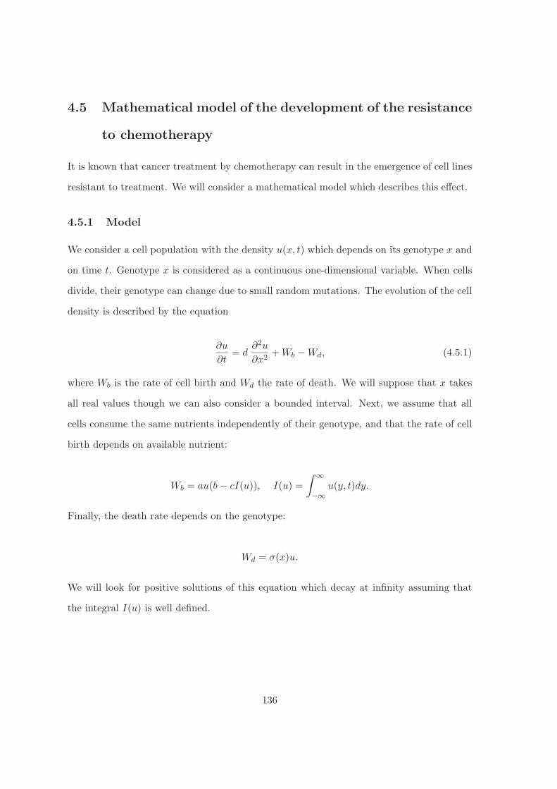
4.5 Mathematical model of the development of the resistance

to chemotherapy

It is known that cancer treatment by chemotherapy can result in the emergence of cell lines

resistant to treatment. We will consider a mathematical model which describes this effect.

4.5.1 Model

We consider a cell population with the density u(x, t) which depends on its genotype x and

on time t. Genotype x is considered as a continuous one-dimensional variable. When cells

divide, their genotype can change due to small random mutations. The evolution of the cell

density is described by the equation

∂u

∂t= d

∂2u

∂x2+Wb −Wd, (4.5.1)

where Wb is the rate of cell birth and Wd the rate of death. We will suppose that x takes

all real values though we can also consider a bounded interval. Next, we assume that all

cells consume the same nutrients independently of their genotype, and that the rate of cell

birth depends on available nutrient:

Wb = au(b− cI(u)), I(u) =

∫ ∞

−∞u(y, t)dy.

Finally, the death rate depends on the genotype:

Wd = σ(x)u.

We will look for positive solutions of this equation which decay at infinity assuming that

the integral I(u) is well defined.

136

4.5.2 Stationary solution

Existence of stationary solutions

Let us begin with the following example. If the mortality coefficient is constant σ(x) ≡const, then integrating equation (4.5.1), we obtain

I ′ = aI(b− cI). (4.5.1)

Hence I(t) converges exponentially to I(∞) = b/c. Though the integral of solution converges

to a positive constant, it can be proved that u(x, t) converges uniformly to zero. This, the

only stationary solution of equation (4.5.1) is the trivial solution u ≡ 0.

In order to get nontrivial solutions of this equation, we will consider the death rate

coefficient depending on genotype x. We will consider the following model example

σ(x) =

⎧⎪⎨⎪⎩

σ0 , |x| ≥ L

σ1 , |x| < L, (4.5.2)

where L is a positive constant. Without loss of generality we can set σ1 = 0. Otherwise we

can take it into account in the constant b. We will find a stationary solution of equation

(4.5.1) analytically. Put k = a(b− cI(u)). Then for |x| ≤ L we have the equation:

dw′′ + kw = 0

which we consider on the half-axis x > 0 with the boundary condition w′(0) = 0. Then

w(x) = c1 cos(λx),

where λ =√k/d, c1 is an arbitrary constant.

If x > 0, then the equation becomes

dw′′ + (k − σ0)w = 0.

137

Hence

w(x) = c2eμx ,

where μ =√(σ0 − k)/d, c2 is an arbitrary constant.

From the conditions

w(−L) = w(+L), w′(−L) = w′(L)

we get the equalities:

c1 cos(λL) = c2e−μL , −c1λ sin(λL) = −c2μe−μL .

This system has a nontrivial solution if the determinant equals zero. It gives the equation

tan(λL) =μ

λ.

It can be written as equation with respect to k:

tan

(√k

dL

)=

√σ0k− 1 . (4.5.3)

This equation has one or more solutions in the interval 0 < k < σ0. It is interesting to note

that this solution depends only on d, L and σ0 and it is independent of a, b and c, that is of

parameters which determine the rate of cell birth.

When we find the value of k, we can determine, next, the ratio

τ =c2c1

= cos(λL) eμL ,

the solution w(x) = c1w0(x), where

138

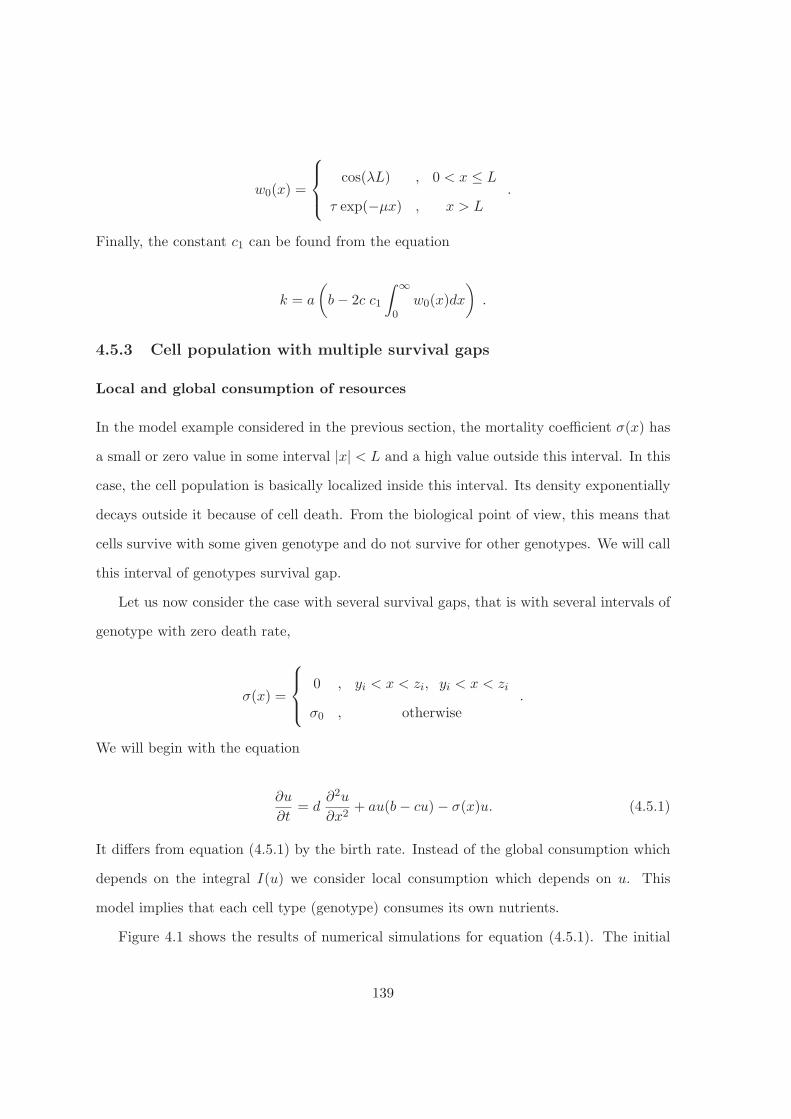
w0(x) =

⎧⎪⎨⎪⎩

cos(λL) , 0 < x ≤ L

τ exp(−μx) , x > L.

Finally, the constant c1 can be found from the equation

k = a

(b− 2c c1

∫ ∞

0w0(x)dx

).

4.5.3 Cell population with multiple survival gaps

Local and global consumption of resources

In the model example considered in the previous section, the mortality coefficient σ(x) has

a small or zero value in some interval |x| < L and a high value outside this interval. In this

case, the cell population is basically localized inside this interval. Its density exponentially

decays outside it because of cell death. From the biological point of view, this means that

cells survive with some given genotype and do not survive for other genotypes. We will call

this interval of genotypes survival gap.

Let us now consider the case with several survival gaps, that is with several intervals of

genotype with zero death rate,

σ(x) =

⎧⎪⎨⎪⎩

0 , yi < x < zi, yi < x < zi

σ0 , otherwise.

We will begin with the equation

∂u

∂t= d

∂2u

∂x2+ au(b− cu)− σ(x)u. (4.5.1)

It differs from equation (4.5.1) by the birth rate. Instead of the global consumption which

depends on the integral I(u) we consider local consumption which depends on u. This

model implies that each cell type (genotype) consumes its own nutrients.

Figure 4.1 shows the results of numerical simulations for equation (4.5.1). The initial

139

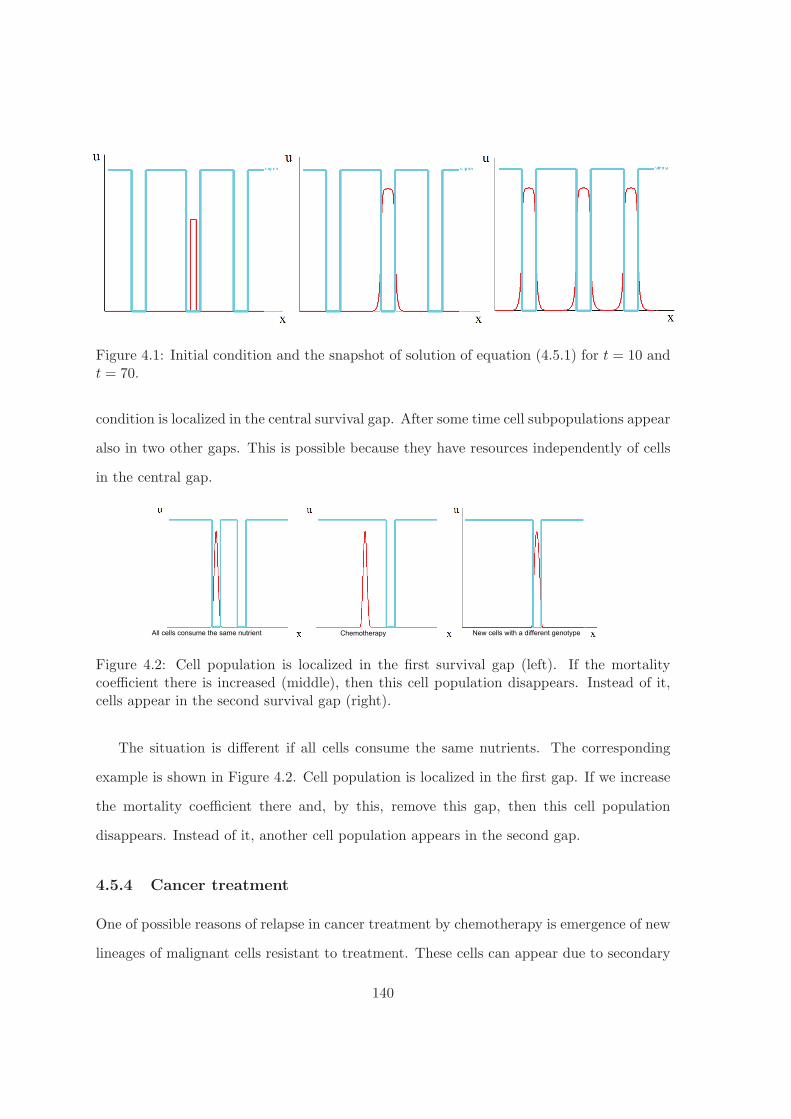
Figure 4.1: Initial condition and the snapshot of solution of equation (4.5.1) for t = 10 andt = 70.

condition is localized in the central survival gap. After some time cell subpopulations appear

also in two other gaps. This is possible because they have resources independently of cells

in the central gap.

All cells consume the same nutrient Chemotherapy New cells with a different genotype

Figure 4.2: Cell population is localized in the first survival gap (left). If the mortalitycoefficient there is increased (middle), then this cell population disappears. Instead of it,cells appear in the second survival gap (right).

The situation is different if all cells consume the same nutrients. The corresponding

example is shown in Figure 4.2. Cell population is localized in the first gap. If we increase

the mortality coefficient there and, by this, remove this gap, then this cell population

disappears. Instead of it, another cell population appears in the second gap.

4.5.4 Cancer treatment

One of possible reasons of relapse in cancer treatment by chemotherapy is emergence of new

lineages of malignant cells resistant to treatment. These cells can appear due to secondary

140

mutations from the existing malignant cells in the tumor. Some of them can get in another

survival gap. However they will not proliferate because they do not have enough nutrients.

If the original population of cancer cells is removed by chemotherapy, nutrients will be

available and these other cells will start proliferating.

The model presented above describes this process. It also allows us to estimate the

time of relapse. Let a cell population be located in the first survival gap, and l be the

distance from it to the second survival gap. Then from the stationary solution presented in

Section 3.1 we estimate the number of cells in the second survival gap as w(l) = c2 exp(−μl).When cells in the first survival gap are removed by chemotherapy, the integral I(u) rapidly

decreases and can be approximated by 0. From the equation we obtain the growth rate of

cell population in the second survival gap:

u(l, t) = w(l)eabt .

The product ab is determined by the duration of cell cycle and can be found experi-

mentally for each cell lineage. The value w(l) is the probability of cells in the first survival

gap to have mutation which will put them in the second survival gap. In fact, diffusion in

the space of genotypes should be understood in terms of such probabilities. If it can be

estimated, then we find how cell population grows in time.

Let us note that in this estimate, the first cell population is removed by treatment

instantaneously. More precise estimates can be obtained if we take into account its decay

rate.

141

Chapter 5

Conclusions

Cette these est consacree aux modeles hybrides discret-continus appliques a la modelisation

de l’hematopoıese et de maladies du sang, telles que le myelome multiple et le lymphome

lymphoblastique a cellules T, ainsi qu’a l’analyse des solutions d’equations de reaction-

diffusion permettant de decrire l’evolution darwinienne de cellules malignes.

Modeles hybrides. Les modeles hybrides permettent de decrire le comportement des

cellules sanguines (apoptose, proliferation et differenciation) en couplant l’aspect continu des

equations differentielles ordinaires pour la regulation intracellulaire ainsi que des equations

aux derivees partielles pour la regulation extracellulaire avec une representation discrete

des cellules considerees comme des spheres, auxquelles sont attribues des parametres.

Choix de lignage. Les modeles hybrides sont utilises pour simuler l’hematopoıese. Ils

permettent, en considerant uniquement une regulation intracellulaire de simuler le choix de

lignage du progeniteur MEP, l’une des premieres etapes de la cascade de differenciations

aboutissant a la formation des cellules sanguines.

Erythropoıese. Plusieurs regulations intracellulaires mettant en jeux la competition en-

tre plusieurs proteines auxquelles s’ajoute une regulation extracellulaire permettent de

simuler l’erythropoıese. En comparant les resultats obtenus avec des donnees biologiques,

142

nous constatons que le modele permet de reproduire assez fidelement les processus bi-

ologiques, en particulier les mecanismes permettant d’adapter le nombre de globules rouges

produits a un stress subi par l’organisme, par exemple dans le cas d’une hemorragie.

Myelome multiple. Ces modeles ont ete ensuite utilises pour simuler deux maladies du

sang. Le myelome multiple est une maladie invasive du sang, qui peut induire une grave

anemie. En effet, le developpement de tumeurs detruit la structure des ilots erythroblastiques

en les ecrasant et en produisant une substance cytotoxique: le Fas-ligand. La modelisation

de l’action mecanique et de la production de Fas-ligand ont permis de simuler l’apparition

de l’anemie.

Lymphome lymphoblastique a cellules T. Le lymphome lymphoblastique a cellules

T provoque l’apparition de tumeurs dans le thymus et est traite pendant deux ans. Les

resultats montrent qu’il semble possible de reduire la duree du traitement d’entretien sans

augmenter le nombre de rechute. Cette hypothese va etre testee sur une population virtuelle

creee avec ce modele, permettant de representer le thymus dans son fonctionnement normal

ou altere par la maladie. La variable permettant de suivre l’etat du malade, remission ou

rechute, est le nombre de cellules cancereuses.

Evolution darwinienne des cellules. La modelisation du traitement du lymphome a

egalement permis de simuler l’apparition d’une resistance aux medicaments utilises pen-

dant la chimiotherapie grace aux modeles hybrides. D’autres formes de modelisation sont

envisageables. Il est possible de modeliser l’apparition d’une resistance aux traitement en

considerant la distribution du phenotype des cellules malignes. Elle peut etre etudiee comme

etant la solution d’une equation de reaction-diffusion, dont les parametres dependent des

nutriments disponibles et consommes par les cellules malignes. La resistance est alors due

a une forme de selection et a l’evolution darwinnienne des cellules.

143

Bibliography

[1] M. Abromowitch, R. Sposto, S. Perkins, D. Zwick, S. Siegel, J. Finlay, M.S. Cairo.

Children’s Oncology Group. Shortened intensified multi-agent chemotherapy and non-

cross resistant maintenance therapy for advanced lymphoblastic lymphoma in children

and adolescents: report from the Children’s Oncology Group. Br J Haematol., 143 (2)

(2008), 261–7.

[2] A.S. Ackleh, K. Deng, C.E. Cole, H.T. Tran. Existence-uniqueness and monotone ap-

proximation for an erythropoiesis age-structured model. J Math Anal Appl., 289 (2004),

530–544.

[3] A.S. Ackleh, K. Deng, K. Ito, J. Thibodeaux. A structured erythropoiesis model with

nonlinear cell maturation velocity and hormone decay rate. Math Biosci., 204 (2006),

21–48.

[4] E. Afenya, S. Mundle. Hematologic disorders and bone marrow-peripheral blood dynam-

ics. Math. Model. Nat. Phenom., 5 no. 3 (2010), 15–27.

[5] G.R. Aispuru, M.V. Aguirre, J.A. Aquino-Esperanza, C.N. Lettieri, J.A. Juaristi, N.C.

Brandan. Erythroid expansion and survival in response to acute anemia stress: the role

of EPO receptor, GATA-1, Bcl-xL and caspase-3. Cell Biol. Int., 32 (8) (2008) 966–78.

[6] T. Alarcon, H.M. Byrneb, P.K. Mainia. A cellular automaton model for tumour growth

in inhomogeneous environment. J. Theor. Biol., 225 (2003), 257–274.

144

[7] A. Ambrosetti, A. Malchiodi. Nonlinear analysis and semilinear elliptic problems. Cam-

bridge Univ. Press, Cambridge, 2007.

[8] A.R.A. Anderson, M.A.J. Chaplain, K.A. Rejniak. The cellular Potts model and its

variants. Single-Cell-Based Models in Biology and Medicine, (2007).

[9] A.R.A. Anderson, M.A.J. Chaplain. Continuous and discrete mathematical models of

tumor-induced angiogenesis. Bull. Math. Biol., 60 (5) (1998), 857–99.

[10] A.R.A. Anderson, M. Chaplain, K.A. Rejniak. Single cell based models in biology and

medicine. Mathematics and Biosciences in Interaction, (2007).

[11] A.R.A. Anderson, K.A. Rejniaka, P. Gerleea, V. Quaranta. Modelling of Cancer

Growth, Evolution and Invasion: Bridging Scales and Models. Math. Model. Nat. Phe-

nom., 2 (3) (2007), 1–29.

[12] R. Apostu, M.C. Mackey. Understanding cyclical thrombocytopenia: A mathematical

modeling approach. J. Theor. Biol., 251 (2008), 297–316.

[13] S. Balea, A. Halanay, D. Jardan, M. Neamtu. Stability analysis of a feedback model

for the action of the immune system in leukemia. Math. Model. Nat. Phenom., 9 no. 1

(2014), 108–132.

[14] A. Bauer, F. Tronche, O. Wessely, C. Kellendonk, H.M. Reichardt, P. Steinlein, G.

Schutz, H. Beug. The glucocorticoid receptor is required for stress erythropoiesis. Genes

Dev., 13 no. 22 (1999), 2996–3002.

[15] Y. Beguin, M. Yerna, M. Loo, M. Weber, G. Fillet. Erythropoiesis in multiple myeloma:

defective red cell production due to inappropriate erythropoietin production. Br J

Haematol (1992), 82, 648-53.

[16] J. Belair, M.C. Mackey, J.M. Mahaffy. Age-structured and two-delay models for ery-

thropoiesis. Math Biosci., 128 (1995), 317–346.

145

[17] H. Berestycki, P.L. Lions, L.A. Peletier. An ODE approach to the existence of positive

solutions for semilinear problems in RN . Indiana Univ. Math. J., 30 (1981), no.1, 141–

157.

[18] S. Bernard , J. Belair, M.C. Mackey. Oscillations in cyclical neutropenia: New evidence

based on mathematical modeling. J. Theor. Biol., 223 (2003), 283–298.

[19] N. Bessonov, F. Crauste, I. Demin, V. Volpert. Dynamics of Erythroid Progenitors and

Erythroleukemia. Math Model Nat Phenom., 4 (2009) 210–232.

[20] N. Bessonov, F. Crauste, S. Fischer, P. Kurbatova, V. Volpert. Application of Hybrid

Models to Blood Cell Production in the Bone Marrow. In press Math. Model. Nat.

Phenom

[21] N. Bessonov, I. Demin, P. Kurbatova, L. Pujo-Menjouet, V.Volpert. Multi-agent sys-

tems and blood cell formation. In: Multi-Agent Systems - Modeling, Interactions, Simu-

lations and Case Studies, F. Alkhateeb, E. Al Maghayreh, I. A. Doush, Editors, (2011),

395–424.

[22] N. Bessonov, I. Demin, L. Pujo-Menjouet, V. Volpert. A multi-agent model describing

self-renewal of differentiation effects on the blood cell population. Mathematical and

computer modelling, 49 (2009), 2116–2127.

[23] N. Bessonov, N. Eymard, P. Kurbatova, V. Volpert. Mathematical modeling of ery-

thropoiesis in vivo with multiple erythroblastic islands. Applied Mathematics Letters,

25 (2012), 1217–1221.

[24] N. Bessonov, P. Kurbatova, V. Volpert. Particle dynamics modelling of cell populations.

Proc. Conf. JANO, Mohhamadia, 2008. Math. Model. Nat. Phenom., 5 7 (2010), 42–47.

[25] N. Bessonov, P. Kurbatova, V. Volpert. Pattern Formation in Hybrid Models of Cell

Populations. V. Capasso et al. (eds.), Pattern Formation in Morphogenesis, Springer

Proceedings in Mathematics 15, Springer-Verlag Berlin Heidelberg, (2013), 107–119.

146

[26] N. Bessonov, L. Pujo-Menjouet, V. Volpert. Cell modelling of hematopoiesis. Math.

Model. Nat. Phenom., 1 no. 2 (2006), 81–103.

[27] N. Bessonov, N. Reinberg, V. Volpert. Mathematics of Darwin’s diagram. Math. Model.

Nat. Phenom., 9 (2014), no. 3, in press.

[28] T. Boehm. Self-renewal of thymocytes in the absence of competitive precursor replen-

ishment. J. Exp. Med. Vol., 209 No. 8 (2012), 1397-1400.

[29] B.R. Bonn, M. Rohde, M. Zimmermann, D. Krieger, I. Oschlies, F. Niggli, G. Wrobel,

A. Attarbaschi, G. Escherich, W. Klapper, A. Reiter, B. Burkhardt. Incidence and

prognostic relevance of genetic variations in T-cell lymphoblastic lymphoma in child-

hood and adolescence. Blood, 121(16) (2013), 3153–60.

[30] F. Bouilloux, G. Juban, N. Cohet, D. Buet, B. Guyot, W. Vainchenker, F. Louache,

F. Morle. EKLF restricts megakaryocytic differentiation at the benefit of erythrocytic

differentiation. Blood, 1 112 (3) (2008), 576-84.

[31] N. Brousse Lymphome Lymphoblastique T enfant et adulte (2009).

[32] L. Brugieres, V. Minard, C. Patte. Lymphomas in children and adolescents. Rev Prat.,

62 (4) (2012), 453–8.

[33] B. Burkhardt, M. Zimmermann, I. Oschlies, F. Niggli, G. Mann, R. Parwaresch, H.

Riehm, M. Schrappe, A. Reiter, BFM Group. The impact of age and gender on biology,

clinical features and treatment outcome of non-Hodgkin lymphoma in childhood and

adolescence. Br J Haematol., 131 (1) (2005), 39–49.

[34] B. Burkhardt, W. Woessmann, M. Zimmermann, U. Kontny, J. Vormoor, W. Doerffel,

G. Mann, G. Henze, F. Niggli, W.D. Ludwig, D. Janssen, H. Riehm, M. Schrappe, A;

Reiter. Impact of cranial radiotherapy on central nervous system prophylaxis in children

and adolescents with central nervous system-negative stage III or IV lymphoblastic

lymphoma. J Clin Oncol., 20 24 (3) (2006), 491–9.

147

[35] M. Buyse, S. Michiels, D.J. Sargent, A. Grothey, A. Matheson, A. de Gramont. Inte-

grating biomarkers in clinical trials. Expert Rev Mol Diagn., 11 (2) (2011), 171–182.

[36] A.Q. Cai, K.A. Landman, B.D. Hughes, C.M. Witt. T cell development in the thymus:

from periodic seeding to constant output. J Theor Biol., 249 (2) (2007), 384–94.

[37] L.A. Caffarelli, B. Gidas, J. Spruck. Asymptotic symmetry and local behavior of semi-

linear elliptic equations with critical Sobolev growth. Comm. Pure Appl. Math., 42

(1989), no. 3, 271–297.

[38] A.B. Cantor, S.H. Orkin. Transcriptional regulation of erythropoiesis: an affair involv-

ing multiple partners. Oncogene, 21 (21) (2002), 3368–3376.

[39] S. Chari, S. Winandy Ikaros Regulates Notch Target Gene Expression in Developing

Thymocytes. The Journal of Immunology, 181 (2008), 6265–6274.

[40] J.A. Chasis, N. Mohandas. Erythroblastic islands: niches for erythropoiesis. Blood, 112

(2008).

[41] W.X. Chen, C. Li. Classification of solutions of some nonlinear elliptic equations. Duke

Math. J., 63 (1991), no. 3, 615–622.

[42] W.X. Chen, C. Li. Qualitative properties of solutions to some nonlinear elliptic equa-

tions in R2. Duke Math. J., 71 (1993), no. 2, 427–439.

[43] K. Chen, J. Liu, S. Heck, J.A. Chasis, X. An, N. Mohandas. Resolving the distinct stages

in erythroid differentiation based on dynamic changes in membrane protein expression

during erythropoiesis. Proc Natl Acad Sci U S A, 106 (2009), 17413–174138.

[44] R. Cheong, A. Bergmann, S.L. Werner, J. Regal, A. Hoffmann, A. Levchenko. Transient

IkappaB kinase activity mediates temporal NF-kappaB dynamics in response to a wide

range of tumor necrosis factor-alpha doses. J. Biol. Chem., 281 (2006), 2945–2950.

148

[45] R. Cheong, A. Bergmann, S.L. Werner, J. Regal, A. Hoffmann, A. Levchenko. Transient

IkappaB kinase activity mediates temporal NF-kappaB dynamics in response to a wide

range of tumor necrosis factor-alpha doses. J. Biol. Chem., 281 (2006), 2945–2950.

[46] S. Cherukuria, N. A. Tripoulasa, S. Nurkoc, P. L. Foxa. Anemia and impaired stress-

induced erythropoiesis in aceruloplasminemic mice. Blood Cells, Molecules, and Dis-

eases, Volume 33 (2004), 346–355.

[47] S. Chiaretti, R. Foa. T-cell acute lymphoblastic leukemia. Haematologica, 94 (2),

(2009).

[48] A. Chow, M. Huggins, J. Ahmed, D. Hashimoto, D. Lucas, Y. Kunisaki, S. Pinho, M.

Leboeuf, C. Noizat, N. van Rooijen, M. Tanaka, Z.J. Zhao, A. Bergman, M. Merad,

P.S. Frenette. CD169(+) macrophages provide a niche promoting erythropoiesis under

homeostasis and stress. Nat Med., 19 (2013), 429–436.

[49] J. Clairambault, P. Magal, V. Volpert. Cancer as evolutionary process. European Com-

munications in Mathematical and Theoretical Biology 2013, No. 16.

[50] C. Colijn, M.C. Mackey. A mathematical model of hematopoiesis – I. Periodic chronic

myelogenous leukemia. J. Theor. Biol., 237, (2005), 117–132.

[51] C. Colijn, M.C. Mackey. A mathematical model of hematopoiesis – II. Cyclical neu-

tropenia. J. Theor. Biol., 237 (2005), 133–146.

[52] S. Cortelazzo, M. Ponzoni, A.J. Ferreri, D. Hoelzer. Lymphoblastic lymphoma. Crit

Rev Oncol Hematol., 79 (3) (2011), 330–43.

[53] C. Cornu, B. Kassai, R. Fisch, C. Chiron, C. Alberti, R. Guerrini, A. Rosati, G. Pons,

H. Tiddens, S. Chabaud, D. Caudri, C. Ballot, P. Kurbatova, A. Castellan, A. Bajard,

P. Nony; CRESim & Epi-CRESim Project Groups. Experimental designs for small

randomised clinical trials: an algorithm for choice. Orphanet J Rare Dis., 8:48. doi:

10.1186/1750-1172-8-48. Review (2013).

149

[54] E. Coustan-Smith, M. Abromowitz, J.T. Sandlund, D. Campana. A novel approach for

minimal residual disease detection in childhood T-cell lymphoblastic lymphoma (T-LL):

a children s oncology group report. Blood (ASH Annual Meeting Abstracts), 110 3564,

(2007).

[55] F. Crauste, I. Demin, O. Gandrillon, V. Volpert. Mathematical study of feedback control

roles and relevance in stress erythropoiesis. J. Theor. Biology, 263 (2010), 303–316.

[56] T. Crompton, K.C. Gilmour, M.J. Owen. The MAP Kinase Pathway Controls Differ-

entiation from Double-Negative to Double-Positive Thymocyte. Cell, Volume 86, Issue

2, (1996), 243–251.

[57] F. Crauste, L. Pujo-Menjouet, S. Genieys, C. Molina, O.Gandrillon. Adding Self-

Renewal in Committed Erythroid Progenitors Improves the Biological Relevance of a

Mathematical Model of Erythropoiesis. J. Theor. Biology, Volume 250 (2008), 322–338.

[58] C.H. Dai, S.B. Krantz, K.M. Zsebo.Human burst-forming units-erythroid need direct

interaction with stem cell factor for further development. Blood, 78 (1991), 2493–4977.

[59] J.C. Dallon. Models with lattice-free center-based cells interacting with continuum en-

vironment variables. Single Cell Based Models in Biology and Medicine. Mathematics

and Biosciences in Interaction, III (2007), 197–219.

[60] Database EuroLB. Protocole Euro LB-02/LMT2004. Etude Europeenne de traite-

ment des Lymphomes Lymphoblastiques de l’enfant. Coordonnateur National : Yves

Bertrand (SFCE), Coordination Internationale : Alfred Reiter (Giessen). ClinInfo.

[61] S. Dazy, F. Damiola, N. Parisey, H. Beug, O. Gandrillon. The MEK-1/ERKs signaling

pathway is differentially involved in the self-renewal of early and late avian erythroid

progenitor cells. Oncogene, 22 (2003), 9205–9216.

[62] I. Demin, F. Crauste, O. Gandrillon, V. Volpert. A multi-scale model of erythropoiesis.

J Biol Dyn., 4 (2010), 59–70.

150

[63] A. Deutsch. Lattice-gas cellular automaton modeling of developing cell systems. Single-

Cell-Based Models in Biology and Medicine, Mathematics and Biosciences in Interac-

tion, (2007), 29–51.

[64] R. Dillon, M. Owen, K. Painter. A single-cell-based model of multicellular growth using

the immersed boundary method. AMS Contemp. Math., 466 (2008), 1–15.

[65] W.A. Dik, K. Pike-Overzet, F. Weerkamp, D. de Ridder, E.F.E. de Haas, M.R.M.

Baert, P. van der Spek, E.E.L. Koster, M.J.T. Reinders, J.J.M. van Dongen, A.W.

Langerak, F.J.T. Staal. New insights on human T cell development by quantitative T

cell receptor gene rearrangement studies and gene expression profiling. JEM. Vol., 201

No. 11 (2005), 1715–1723.

[66] S. Dormann, A. Deutsch. Modeling of self-organized avascular tumor growth with a

hybrid cellular automaton. In Silico Biol., (2002), 393–406,.

[67] J. Eller , I. Gyori, M. Zollei, F. Krizsa. Modelling Thrombopoiesis Regulation - I Model

description and simulation results. Comput. Math. Appli., 14 (1987), 841–848.

[68] N. Eymard, P. Kurbatova. Hybrid models in hematopoiesis. submitted.

[69] N. Eymard, N. Bessonov, O. Gandrillon, M.J. Koury, V. Volpert. The role of spatial

organisation of cells in erythropoiesis. Journal of Mathematical Biology, (2014).

[70] S. Fischer, P. Kurbatova, N. Bessonov, O. Gandrillon, V. Volpert, F. Crauste. Mod-

elling erythroblastic islands: using a hybrid model to assess the function of central

macrophage. Journal of Theoretical Biology, 298 (2012), 92–106.

[71] A. Fossa, D. Brandhorst, JH. Myklebust, S. Seeber, MR. Nowrousian. Relation between

S-phase fraction of myeloma cells and anemia in patients with multiple myeloma. Exp

Hematol, (1999), 27, 1621-6.

151

[72] P. Frontelo, D. Manwani, M. Galdass, H. Karsunky, F. Lohmann, P.G. Gallagher, J.J.

Bieker. Novel role for EKLF in megakaryocyte lineage commitment. Blood, 110 (12)

(2007), 3871–3880.

[73] O. Gandrillon. The v-erbA oncogene. Assessing its differentiation-blocking ability using

normal chicken erythrocytic progenitor cells. Methods Mol. Biol., 202 (2002), 91–107.

[74] O. Gandrillon, J. Samarut. Role of the different RAR isoforms in controlling the ery-

throcytic differentiation sequence. Interference with the v-erbA and p135gag-myb-ets

nuclear oncogenes. Oncogene, Volume 16 No. 5 (1998), 563–574.

[75] O. Gandrillon , U. Schmidt, H. Beug, J. Samarut. TGF-beta cooperates with TGF-alpha

to induce the self-renewal of normal erythrocytic progenitors: evidence for an autocrine

mechanism. Embo J., 18 (1999), 2764–2781.

[76] B. Gidas, J. Spruck. Global and local behavior of positive solutions of nonlinear elliptic

equations. Comm. Pure Appl. Math., 34 (1981), no. 4, 525–598.

[77] B. Gidas, J. Spruck. A priori bounds for positive solutions of nonlinear elliptic equa-

tions. Comm. Partial Differential Equations, 6 (1981), no. 8, 883–901.

[78] C. Giverso, M. Scianna, L. Preziosi, N. Lo Buono, A. Funaro. Individual Cell-Based

Model for In-Vitro Mesothelial Invasion of Ovarian Cancer, Math. Model. Nat. Phe-

nom., 5 (1) (2010), 203–223.

[79] A. Golubev. Random discrete competing events vs. dynamic bistable switches in cell

proliferation in differentiation. J. Theor. Biol., 267 (3) (2010), 341–354.

[80] C.J. Gregory, A.C. Eaves. Human marrow cells capable of erythropoietic differentiation

in vitro: definition of three erythroid colony responses. Blood, 49 (1977), 855–864.

[81] T. Gregory, C. Yu, A. Ma, S.H. Orkin, G.A. Blobel, M.J. Weiss. GATA-1 and ery-

thropoietin cooperate to promote erythroid cell survival by regulating bcl-xL expression.

Blood, 94 (1999), 87–96.

152

[82] A. Halanay. Periodic solutions in a mathematical model for the treatment of chronic

myelogenous leukemia. Math. Model. Nat. Phenom., 7 no. 1 (2012), 235–244.

[83] A. Halanay, D. Candea, I.R. Radulescu. Existence and stability of limit cycles in a

two-delays model of hematopoiesis including asymmetric division. Math. Model. Nat.

Phenom., 9 no. 1 (2014), 58–78.

[84] J. Hochberg, M.S. Cairo. Childhood and adolescent lymphoblastic lymphoma: end of

the beginning and future directions. Pediatr Blood Cancer, 53 (6) (2009), 917–9.

[85] D. Hoelzer, N. Gokbuget. T-cell lymphoblastic lymphoma and T-cell acute lymphoblas-

tic leukemia: a separate entity? Clin Lymphoma Myeloma, 9(Suppl. (3)) (2009), S214–

21.

[86] C.A. Janeway et Al. Immunobiology 6 th. edition Garland Science.

[87] J. Jeon, V. Quaranta, P.T. Cummings. An Off-Lattice Hybrid Discrete-Continuum

Model of Tumor Growth and Invasion. Biophys. J., 98 (1) (2010), 37–47.

[88] Y. Jiang, J. Pjesivac-Grbovic, C. Cantrell, J.P. Freyer. A Multiscale Model for Avas-

cular Tumor Growth. Biophys J., 289 (6) (2005), 3884–3894.

[89] M. Karttunen, I. Vattulainen, A.Lukkarinen. A novel methods in soft matter simula-

tions. Springer, Berlin, (2004).

[90] U. Koch, F. Radtke. Mechanisms of T Cell Development and Transformation Annu.

Rev. Cell Dev. Biol., 27 (2011), 539–62

[91] M. Koulnis, Y. Liu, K. Hallstrom, M. Socolovsky. Negative autoregulation by Fas sta-

bilizes adult erythropoiesis and accelerates its stress response. PLoS One, (2011).

[92] M.J. Koury, M.C. Bondurant. Erythropoietin retards DNA breakdown and prevents

programmed death in erythroid progenitor cells. Science, 248 (1990), 378–381.

153

[93] M.J. Koury. Erythropoietin: the story of hypoxia and a finely regulated hematopoietic

hormone. Exp Hematol., 33 (2005), 1263–1270.

[94] S.T. Koury, M.J. Koury, M.C. Bondurant, J. Caro, S.E. Graber. Quantitation of

erythropoietin-producing cells in kidneys of mice by in situ hybridization: correlation

with hematocrit, renal erythropoietin mRNA, and serum erythropoietin concentration.

Blood, Volume 74 No. 2 (1989), 645–651.

[95] A. Krinner, I. Roeder, M. Loeffler, M. Scholz. Merging concepts - coupling an agent-

based model of hematopoietic stem cells with an ODE model of granulopoiesis. BMC

Systems Biology, 7:117 (2013).

[96] P. Kurbatova. Modelisation hybride de l’erythropoıese et des maladies sanguines. [Hy-

brid modeling of erythropoiesis and blood diseases]. PhD thesis, University Lyon 1

(2011). French.

[97] P. Kurbatova, S. Bernard, N. Bessonov, F. Crauste, I. Demin, C. Dumontet, S. Fischer,

V. Volpert. Hybrid Model of Erythropoiesis and Leukemia Treatment with Cytosine

Arabinoside. 2011, SIAM J. Appl. Math, Volume 71, Issue 6 (2011), 2246–2268.

[98] P. Kurbatova, N. Eymard, V. Volpert. Hybrid model of erythropoiesis. Acta Biotheo-

retica, Volume 61, Issue 3 (2013), 305-315.

[99] I. Kuzin, S. Pohozaev. Entire solutions of semilinear elliptic equations. Birkhauser,

Basel, 1997.

[100] Y. Liu, R. Pop, C. Sadegh, C. Brugnara, V.H Haase, M. Socolovsky. Suppression

of Fas-FasL coexpression by erythropoietin mediates erythroblast expansion during the

erythropoietic stress response in vivo. Blood, 108 (2006), 123–133.

[101] H. Ludwig, E. Fritz, H. Kotzman, P.Hocker, H.Gisslinger, U. Barnas. Erythropoietin

treatment of anemia associted with multiple myeloma. The new england journal of

medecine, vol. 322,(1990) no. 24, 1693–9.

154

[102] F. Ma, A. Manabe, D. Wang, M. Ito, A. Kikuchi, M. Wada, M. Ito, A. Ohara, R.

Hosoya, S. Asano, K. Tsuji. Growth of human T cell acute lymphoblastic leukemia

lymphoblasts in NOD/SCID mouse fetal thymus organ culture. Leukemia, 16 (2002),

1541–1548.

[103] M.C. Mackey. Unified hypothesis of the origin of aplastic anaemia and periodic

hematopoıesis. Blood, 51 (1978), 941–956.

[104] M.C Mackey. Dynamic hematological disorders of stem cell origin. In: G. Vassileva-

Popova and E. V. Jensen, Editors. Biophysical and Biochemical Information Transfer

in Recognition, Plenum Press, New York, (1979), 373–409.

[105] M.C. Mackey, R. Rudnicki. A new criterion for the global stability of simultaneous

cell replication and maturation processes. J. Math. Biol., 38 (1999), 195–219.

[106] J.M. Mahaffy, J. Belair, M.C. Mackey. Hematopoietic model with moving boundary

condition and state dependent delay: applications in erythropoiesis. J. Theor. Biol.,

190 (1998), 135–146.

[107] R. De Maria, U. Testa, L. Luchetti, A. Zeuner, G. Stassi, E. Pelosi, R. Riccioni,

N. Felli, P. Samoggia, C. Peschle. Apoptotic Role of Fas/Fas Ligand System in the

Regulation of Erythropoiesis. Blood, 93 (1999), 796–803.

[108] S.R. McDougall, A.R.A. Anderson, M.A.J. Chaplain, J.A. Sherratt. Mathematical

modelling of flow through vascular networks: Implications for tumour-induced angio-

genesis and chemotherapy strategies. Bulletin of Mathematical Biology, 64 (4) (2002),

673–702.

[109] R. Mehr, A.S. Perelson, M. Fridkis-Hareli, A. Globerson. Feedback regulation of T cell

development in the thymus J Theor Biol., 181 (2) (1996), 157–67.

[110] S. Millot, V. Andrieu, P. Letteron, S. Lyoumi, M. Hurtado-Nedelec, Z. Karim, O.

Thibaudeau, S. Bennada, J.L. Charrier, S. Lasocki, C. Beaumont. Erythropoietin stim-

155

ulates spleen BMP4-dependent stress erythropoiesis and partially corrects anemia in a

mouse model of generalized inflammation. Blood, 116 (2010), 6072–6081.

[111] S.B. Murphy. Classification, staging and end results of treatment of childhood non-

Hodgkin’s lymphomas: dissimilarities from lymphomas in adults. Semin Oncol., 7

(1980), 332–339.

[112] W. Nijhof, P.K. Wierenga. Isolation and characterization of the erythroid progenitor

cell: CFU-E. J Cell Biol., 96 (1983), 386–392.

[113] K. Ogungbenro. Physiologically based pharmacokinetic modelling of methotrexate and

6-mercaptopurine in adults and children submitted.

[114] J.M. Osborne, A. Walter, S.K. Kershaw, G.R. Mirams, A.G. Fletcher, P. Path-

manathan, D. Gavaghan, O.E. Jensen, P.K. Maini, H.M. Byrne. A hybrid approach

to multi-scale modelling of cancer. Phil. Trans. R. Soc. A, 368 (2010), 5013–5028.

[115] H. Ozbay, C. Bonnet, H. Benjelloun, J. Clairambault. Stability analysis of cell dy-

namics in leukemia. Math. Model. Nat. Phenom., 7 (2012), no. 1, 203–234.

[116] B. Panzenbock, P. Bartunek, M.Y. Mapara, M. Zenke. Growth and differentiation

of human stem cell factor/erythropoietin-dependent erythroid progenitor cells in vitro.

Blood, 92 (1998), 3658–3668.

[117] T. Papayannopoulou, A.R. Migliaccio, J.L. Abkowitz, A.D. D’Andrea. Biology of ery-

thropoiesis, erythroid differentiation, and maturation. In Hematology: Basic Principles

and Practice, 5th Edition, (2009), 276-294, Hoffman R, Benz EJ Jr, Shattil SJ, Furie

B, Silberstein LE, McGlave P and Heslop HE, Editors, Churchill Livingstone, Elsevier,

Inc., Philadelphia.

[118] A.A. Patel, E.T. Gawlinsky, S.K. Lemieux, R.A. Gatenby. A Cellular Automaton

Model of Early Tumor Growth and Invasion: The Effects of Native Tissue Vascularity

and Increased Anaerobic Tumor Metabolism. J. Theor. Biol., 213 (2001), 315–331.

156

[119] R.F. Paulson, L. Shi, D.C. Wu. Stress erythropoiesis: new signals and new stress

progenitor cells. Curr Opin Hematol., 18 (2011), 139–145.

[120] I. Ramis-Conde, D. Drasdo, A.R.A. Anderson, M.A.J. Chaplain. Modeling the In-

fluence of the E-Cadherin-β-Catenin Pathway in Cancer Cell Invasion: A Multiscale

Approach. Biophys. J., 95 (1) (2008), 155–165.

[121] P. Ramos, C. Casu, S. Gardenghi, L. Breda, B.J. Crielaard, E. Guy, M.F. Marongiu,

R. Gupta, R.L. Levine, O. Abdel-Wahab, B.L. Ebert, N. Van Rooijen, S. Ghaffari,

R.W. Grady, P.J. Giardina, S. Rivella. Macrophages support pathological erythropoiesis

in polycythemia vera and β-thalassemia. Nat Med., 19 (2013), 437–445.

[122] M. Reth, T. Brummer. Feedback regulation of lymphocyte signalling. Nat Rev Im-

munol, (4) (2004), 269–77.

[123] M. Rincon, R.A. Flavell, R.J. Davis. Signal transduction by MAP kinases in T lym-

phocytes. Oncogene, Volume 20, Number 19, (2001), 2490–2497.

[124] M.M. Rhodes, P. Kopsombut, M.C. Bondurant, J.O. Price, M.J. Koury. Adherence to

macrophages in erythroblastic islands enhances erythroblast proliferation and increases

erythrocyte production by a different mechanism than erythropoietin. Blood, 111 (2008).

[125] I. Roeder. Quantitative stem cell biology: computational studies in the hematopoietic

system. Curr. Opin. Hematol., 13 (2006), 222–228.

[126] I. Roeder, I. Glauche. Towards an understanding of lineage specification in hematopoi-

etic stem cells: A mathematical model for the interaction of transcription factors

GATA-1 and PU.1. Journal of Theoretical Biology, 241 (2006), 852–865.

[127] E.V. Rothenberg, T. Taghon. Molecular genetics of T cell development. Annu. Rev.

Immunol., 23 (2005), 601–49.

157

[128] C. Rubiolo, D. Piazzolla, K. Meissl, H. Beug, J.C. Huber, A. Kolbus, M. Baccarini.

A balance between Raf-1 and Fas expression sets the pace of erythroid differentiation.

Blood, 108 (2006), 152–159.

[129] Y. Sadahira, H. Wada, T. Manabe, Y. Yawata. Immunohistochemical assessment of

human bone marrow macrophages in hematologic disorders. Pathology international,

(1999), 49, 626-32.

[130] Y. Sadahira, T. Yasuda, T. Yoshino, T. Manabe, T. Takeishi, Y. Kobayashi, Y. Ebe,

M. Naito. Impaired splenic erythropoiesis in phlebotomized mice injected with CL2MDP-

liposome: an experimental model for studying the role of stromal macrophages in ery-

thropoiesis. J Leukoc Biol., 68 (2000), 464–470.

[131] J.T. Sandlund, C.H. Pui, Y. Zhou, F.G. Behm, M. Onciu, B.I. Razzouk, N. Hijiya, D.

Campana, M.M. Hudson, R.C. Ribeiro. Effective treatment of advanced-stage childhood

lymphoblastic lymphoma without prophylactic cranial irradiation: results of St Jude

NHL13 study. Leukemia, 23(6) (2009), 1127–30.

[132] M. Santillan, J.M. Mahaffy, J. Belair, M.C. Mackey. Regulation of platelet production:

The normal response to perturbation and cyclical platelet disease. J. Theor. Biol., 206

(2000), 585–603.

[133] N.J. Savill, W. Chadwick, S.E. Reece. Quantitative analysis of mechanisms that gov-

ern red blood cell age structure and dynamics during an aemia. PLoS Comput Biol.,

(2009), 5:e1000416.

[134] K. Sawada, S.B. Krantz, J.S. Kans, E.N. Dessypris, S. Sawyer, A.D. Glick, C.I. Civin.

Purification of human erythroid colony-forming units and demonstration of specific

binding of erythropoietin. J Clin Invest. 80 (1987), 357–366.

[135] S.T. Sawyer, S.M. Jacobs-Helber. Unraveling distinct intracellular signals that pro-

mote survival and proliferation: study of erythropoietin, stem cell factor, and constitu-

tive signaling in leukemic cells. J. Hematother. Stem Cell Res. 9, (2000) 21–29.

158

[136] M. Scianna, R.M.H. Merks, L. Preziosi, E. Medico. Individual cell-based models of cell

scatter of ARO and MLP-29 cells in response to hepatocyte growth factor. J. Theor.

Biol., 260 (1) (2009), 151–160.

[137] E. Schmidt, B. Burkhardt. Lymphoblastic lymphoma in childhood and adolescence.

Pediatr Hematol Oncol., 30 (6) (2013), 484–508.

[138] F. Silvestris, P. Cafforio, M. Tucci, F. Dammacco. Negative regulation of erythroblast

maturation by Fas-L1/TRAIL1 highly malignant plasma cells: a major pathogenetic

mechanism of anemia in multiple myeloma. Blood, 99 (2002), no. 4, 1305–1313.

[139] R.V. Sionov, S. Kfir-Erenfeld, R. Spokoini, E. Yefenof. A Role for Bcl-2 in Notch1-

Dependent Transcription in Thymic Lymphoma Cells. Advances in Hematology. Article

ID 435241, (2012).

[140] M. Socolovsky. Molecular insights into stress erythropoiesis. Current opinion in hema-

tology, 14 (2007).

[141] M. Socolovsky, H. Nam, M.D. Fleming, V.H. Haase, C. Brugnara, H.F. Lodish. In-

effective erythropoiesis in Stat5a(-/-)5b(-/-) mice due to decreased survival of early

erythroblasts. Blood, 98 (2001), 3261–3273.

[142] F.J. Staal, F. Weerkamp, A.W. Langerak, R.W. Hendriks, H.C. Clevers. Transcrip-

tional control of T lymphocyte differentiation. Stem Cells, 19 (2001), 165–179.

[143] B. Stark, S. Avigad, D. Luria, S. Manor, T. Reshef-Ronen, G. Avrahami, I. Yaniv.

Bone marrow minimal disseminated disease (MDD) and minimal residual disease

(MRD) in childhood T-cell lymphoblastic lymphoma stage III, detected by flow cytom-

etry (FC) and real-time quantitative polymerase chain reaction (RQ-PCR). Pediatr

Blood Cancer, 52 (1) (2009), 20–5, .

[144] J. Starck, M. Weiss-Gayet, C. Gonnet, B. Guyot, J.M. Vicat, F. Morle. Inducible Fli-

1 gene deletion in adult mice modifies several myeloid lineage commitment decisions

159

and accelerates proliferation arrest and terminal erythrocytic differentiation. Blood,

116 (23) (2010), 4795–805.

[145] A. Stephanou, S.R. McDougall, A.R.A. Anderson, M.A.J. Chaplain. Mathematical

modelling of flow in 2D and 3D vascular networks: Applications to anti-angiogenic

and chemotherapeutic drug strategies. Mathematical and Computer Modelling, 41 (10)

(2005), 1137–1156.

[146] J.R.Stephenson, A.A. Axelrad, D.L. McLeod, M.M. Shreeve. Induction of colonies of

hemoglobin-synthesizing cells by erythropoietin in vitro. Proc Natl Acad Sci U S A, 68

(1971), 1542–1546.

[147] T. Stiehl, A. Marciniak-Czochra.Mathematical modeling of leukemogenesis and cancer

stem cell dynamics. Math. Model. Nat. Phenom., 7 (2012), no. 1, 166–202.

[148] T. Sugawara, T. Moriguchi, E. Nishida, Y. Takahama. Differential Roles of ERK

and p38 MAP Kinase Pathways in Positive and Negative Selection of T Lymphocytes.

Immunity, Vol. 9 (1998), 565–574.

[149] S.H. Swerdlow. Cancer IAFRO, World Health Organization. WHO Classification of

Tumours of Haematopoietic and Lymphoid Tissues. World Health Organization. 2008.

[150] M.R. Tallack, A.C. Perkins.Megakaryocyte-erythroid lineage promiscuity in EKLF null

mouse blood. Haematologica, 95 (1) (2010), 144–147.

[151] A.M. Termuhlem, L.M. Smith, S.L. Perkins, M. Lones, J.L. Finlay, H. Weinstein,

T.G. Gross, M. Abromowitch. Disseminated lymphoblastic lymphoma in children and

adolescents: results of the COG A5971 trial: a report from the Children’s Oncology

Group. Br J Haematol., 162 (6) (2013), 792–801.

[152] F. Thomas, D. Fisher, P. Fort, J-P Marie, S. Daoust, B. Roche, C. Grunau, C.

Cosseau, G. Mitta, S.Baghdiguian, F. Rousset, P. Lassus, E. Assenat, D. Gregoire, D.

Misse , A. Lorz, F. Billy, W. Vainchenker, F. Delhommeau, S. Koscielny, R. Itzykson,

160

R. Tang, F. Fava, A. Ballesta, T. Lepoutre, L. Krasinska, V. Dulic, P. Raynaud, P.

Blache, C. Quittau-Prevostel, E. Vignal, H. Trauchessec, B. Perthame, J. Clairambault,

V. Volpert, E. Solary, U. Hibner, M. E. Hochberg. Applying ecological and evolutionary

theory to cancer: a long and winding road. Evolutionary Applications, 6 (1), ISSN

1752-4571 (2013), 1–10.

[153] D.G. Tubergen, M.D. Krailo, A.T. Meadows, J. Rosenstock, M. Kadin, M. Morse, D.

King, P.G. Steinherz, J.H. Kersey. Comparison of treatment regimens for pediatric lym-

phoblastic non-Hodgkin’s lymphoma: a Childrens Cancer Group study. J Clin Oncol.,

13 (6) (1995), 1368–76.

[154] A.S. Tsiftsoglou, I.S. Vizirianakis, J. Strouboulis. Erythropoiesis: model systems,

molecular regulators, and developmental programs. IUBMB Life., 61 (8) (2009), 800–

830.

[155] A. Uyttebroeck, S. Suciu, G. Laureys, A. Robert, H. Pacquement, A. Ferster, G.

Marguerite, F. Mazingue, M. Renard, P. Lutz, X. Rialland, F. Mechinaud, H. Cave, L.

Baila, Y. Bertrand. Treatment of childhood T-cell lymphoblastic lymphoma according to

the strategy for acute lymphoblastic leukaemia, without radiotherapy: Long term results

of the EORTC CLG 58881 trial. Europeen journal of cancer, 44 (2008), 840–846.

[156] L. Varricchio, V. Tirelli, E. Masselli, B. Ghinassi, N. Saha, P. Besmer, A.R. Migli-

accio. The expression of the glucocorticoid receptor in human erythroblasts is uniquely

regulated by KIT ligand: implications for stress erythropoiesis. Stem Cells Dev., 21

(2012), 2852–2865.

[157] V. Volpert. Elliptic partial differential equations. Volume 2. Reaction-diffusion equa-

tions. Birkhauser, 2014.

[158] A.I. Volpert, V. Volpert, V.A. Volpert. Traveling wave solutions of parabolic systems.

Translation of Mathematical Monographs, Vol.140, AMS, Providence, 1994.

161

[159] V. Volpert. Elliptic partial differential equations. Volume 1. Fredholm theory of elliptic

problems in unbounded domains. Birkhauser, 2011.

[160] V. Volpert. Elliptic partial differential equations. Volume 2. Reaction-diffusion equa-

tions. Birkhauser, 2014.

[161] M. von Lindern, W. Zauner, G. Mellitzer, P. Steinlein, G. Fritsch, K. Huber, B.

Lowenberg, H. Beug. The glucocorticoid receptor cooperates with the erythropoietin

receptor and c-Kit to enhance and sustain proliferation of erythroid progenitors in vitro.

Blood, 94 (1999), 550–559.

[162] M. von Lindern, U. Schmidt, H. Beug. Control of erythropoiesis by erythropoietin

and stem cell factor: a novel role for Bruton’s tyrosine kinase. Cell Cycle, 3 (2004),

876–879.

[163] H.E. Wichmann, M.D. Gerhardts, H. SPechtmeyer, R. Gross. A mathematical model

of thrombopoiesis in rats. Cell Tissue Kinet., 12 (1979), 551–567.

[164] H.E. Wichmann, M. Loeffler. Mathematical Modeling of Cell Proliferation. Volume 1,

Model description, Irradiation, Erythropoietic Stimulation, (1985) Editor H. E Wich-

man CRC, Boca Raton, FLorida.

[165] H.E. Wichmann, M. Loeffler, K. Pantel, H. Wulff. A mathematical model of ery-

thropoiesis in mice and rats. Part 2: Stimulated erythropoiesis. Cell Tissue Kinet., 22

(1989), 31–49.

[166] C.M. Witt, E.A. Robey. Thymopoiesis in 4 dimensions. Seminars in Immunology. 17

(2005), 95–102.

[167] H. Wu, X. Liu, R. Jaenisch, H.F. Lodish. Generation of committed erythroid BFU-E

and CFU-E progenitors does not require erythropoietin or the erythropoietin receptor.

Cell, 83 (1995) 59–67.

162

[168] H. Wulff, H.E. Wichmann, K. Pantel, M. Loeffler. A mathematical model of erythro-

poiesis in mice and rats. Part 3: Suppressed erythropoiesis. Cell Tissue Kinet., 22

(1989), 51–61.

[169] J. Zhu, S.G. Emerson. Hematopoietic cytokines, transcription factors and lineage com-

mitment. Oncogene, 21 (2002), 3295–3313.

163

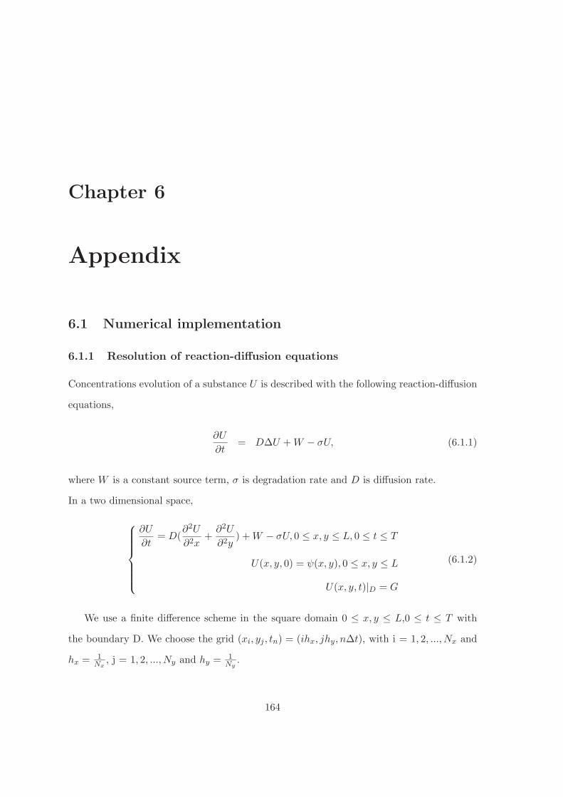
Chapter 6

Appendix

6.1 Numerical implementation

6.1.1 Resolution of reaction-diffusion equations

Concentrations evolution of a substance U is described with the following reaction-diffusion

equations,

∂U

∂t= DΔU +W − σU, (6.1.1)

where W is a constant source term, σ is degradation rate and D is diffusion rate.

In a two dimensional space,

⎧⎪⎪⎪⎪⎪⎨⎪⎪⎪⎪⎪⎩

∂U

∂t= D(

∂2U

∂2x+

∂2U

∂2y) +W − σU, 0 ≤ x, y ≤ L, 0 ≤ t ≤ T

U(x, y, 0) = ψ(x, y), 0 ≤ x, y ≤ L

U(x, y, t)|D = G

(6.1.2)

We use a finite difference scheme in the square domain 0 ≤ x, y ≤ L,0 ≤ t ≤ T with

the boundary D. We choose the grid (xi, yj , tn) = (ihx, jhy, nΔt), with i = 1, 2, ..., Nx and

hx = 1Nx

, j = 1, 2, ..., Ny and hy = 1Ny

.

164

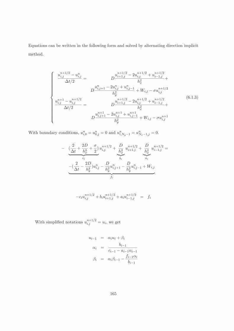
Equations can be written in the following form and solved by alternating direction implicit

method.

⎧⎪⎪⎪⎪⎪⎪⎪⎪⎪⎪⎪⎪⎪⎪⎨⎪⎪⎪⎪⎪⎪⎪⎪⎪⎪⎪⎪⎪⎪⎩

un+1/2i,j − uni,j

Δt/2= D

un+1/2i+1,j − 2u

n+1/2i,j + u

n+1/2i−1,j

h2x+

Duni,j+1 − 2uni,j + uni,j−1

h2y+Wi,j − σu

n+1/2i,j

un+1i,j − u

n+1/2i,j

Δt/2= D

un+1/2i+1,j − 2u

n+1/2i,j + u

n+1/2i−1,j

h2x+

Dun+1i,j+1 − 2un+1

i,j + un+1i,j−1

h2y+Wi,j − σun+1

i,j

(6.1.3)

With boundary conditions, uni,0 = un0,j = 0 and uni,Ny−1 = unNx−1,j = 0.

− (2

Δt+

2D

h2x+

σ

2)︸ ︷︷ ︸

ci

un+1/2i,j +

D

h2x︸︷︷︸bi

un+1/2i+1,j +

D

h2x︸︷︷︸ai

un+1/2i−1,j =

−( 2

Δt− 2D

h2y)uni,j −

D

h2yuni,j+1 −

D

h2yuni,j−1 +Wi,j︸ ︷︷ ︸

fi

−ciun+1/2i,j + biu

n+1/2i+1,j + aiu

n+1/2i−1,j = fi

With simplified notations un+1/2i,j = ui, we get

ui−1 = αiui + βi

αi =bi−1

ci−1 − ai−1αi−1

βi = αiβi−1 − fi−1αi

bi−1

165

− (2

Δt+

2D

h2y+

σ

2)︸ ︷︷ ︸

Cj

un+1i,j +

D

h2y︸︷︷︸Bj

un+1i,j+1 +

D

h2y︸︷︷︸Aj

un+1i,j−1 =

−( 2

Δt− 2D

h2x)u

n+1/2i,j − D

h2xun+1/2i+1,j −

D

h2xun+1/2i−1,j +Wi,j︸ ︷︷ ︸

Fj

−Ciun+1i,j +Biu

n+1i,j+1 +Aiu

n+1i,j−1 = Fi

With simplified notations un+1i,j = uj , we get

uj−1 = γjuj + κj

γj =Bj−1

Cj−1 −Aj−1γj−1

κj = γjκj−1 − Fj−1κjBj−1

The Thomas algorithm consists of calculating un+1/2i,j and uni,j (which approximate U(xi, yj , tn+1/2)

and U(xi, yj , tn)) with the previous recurrent formulas.

6.1.2 Implementation of numerical algorithms

The software used for the simulation of hematopoiesis is written in C++, with operating

system Ubuntu. The computations are carried out in dimensionless length units in such

a way that the initial cell diameter corresponds to one unit. The computation domain is

a square with the side equal 100 length units. In dimensional variables we consider cell

diameters to be 10 microns.

The structure of the software is as follow:

• Creation of a cell culture (list of cells) and of the computation domain. For each cell:

166

Figure 6.1: Simplification of the algorithm describing the fate of cells.

– Initialization of parameters. Birth of the healthy cells of a section of thymus and

of one cancer cell. Each cell has a duration of life, coordinates, and intracellular

concentrations.

– Forces between cells and coordinate of cells are calculated, movement is due to

Newton’s second law.

– Intracellular and extracellular concentrations are calculated.

• Application of the rules governing healthy cell divisions.

167

– Every time step, age of cell is evaluated. While the age of the cell is less than or

equal to the cell cycle, the cell grows.

– If a cell survives to the three selections, it self-renews or it differentiates according

to the intracellular concentration.

• Application of the rules governing cancer cell divisions

– If the age of a cancer cell is equal or exceeds cell cycle duration and if the quantity

of treatment is less than a threshold, the cell divides. Otherwise the cell dies.

• Treatment of the disease based of the date.

• Updated of the cell culture.

Parameters of intracellular regulation are not known from the experiments. We choose

them in such a way that: 1. the bistable dynamics is preserved, 2. the hybrid system shows

qualitatively correct and robust behavior with a correct proportion of cells of different types,

3. the results of the simulations fit the experimental curves. The values of parameters are

given in the following tables.

6.2 Values of parameters for lineage choice

day 0 day 2 day 3 day 4 day 6

number of cells 2105 6.6105 11.9105 16.5105

ratio of differentiated cells (%) 0 40 80 97

Table 6.1: Biological data for Section 2.2.2.

168

Parameter Value Unit

Cell cycle length 720 minCell cycle variation 420 min

α 0.000358 h−1

β 0.05 h−1.NU−1

a 0.0041 h−1

b 0.0139 h−1.NU−1

c 0.00139 h−1

d 0.00011 h−1

kg 0.0002 h−1.NU−2

Ecr 0.8 NUFcr 0.19 NU

E0 Value of initial quantity E 0.015 NUF0 Value of initial quantity F 0.01 NU

Table 6.2: Intracellular parameters. Data for Section 2.2.2.

Parameter Value Unit

Cells cycle length T 18 hCells cycle variation 3 h

a00 0.001a10 0a11 0.0001a01 0.0000005a12 0a02 0.00077a13 0.0001a03 0.000001b1 0.0004b2 0.0045b3 0.43wcr 0.09 NU

Table 6.3: Values of intracellular parameters. figure 2.14 (right).

169

Parameter Value Unit

Cells cycle length T 18 hCells cycle variation 3 h

a00 0.001a10 0a11 0.00025a01 0.0000005a12 0a02 0.000825a13 0.0001a03 0.000001b1 0.0004b2 0.0045b3 0.51wcr 0.509 NU

Table 6.4: Values of intracellular parameters. figure 2.14 (left).

Parameter Value Unit

AC Cells cycle length 6.5 hCells cycle variation 0.5 h

a00 0.001a10 0a11 0.000035a01 0.000035a12 0a02 0.00035a13 0.0001a03 0.000001b1 0.0004b2 0.0045b3 0.4wcr 0.5 NU

Table 6.5: Values of intracellular parameters for AC. figure 2.18.

170

Parameter Value Unit

NAC Cells cycle length 16 hCells cycle variation 0.5 h

a00 0.001a10 0a11 0.00003a01 0.0000005a12 0a02 0.00044a13 0.0001a03 0.000001b1 0.0004b2 0.0045b3 0.4wcr 0.485 NU

Table 6.6: Values of intracellular parameters for NAC. figure 2.18.

Parameter Value Unit

Cell cycle length 720 minCell cycle variation 420 min

α 0.000358 h−1

β 0.05 h−1.NU−1

a 0.0041 h−1

b 0.0139 h−1.NU−1

c 0.00139 h−1

d 0.00011 h−1

kg 0.0002 h−1.NU−2

Ecr 0.8 NUFcr 0.19 NU

E0 Value of initial quantity E 0.015 NUF0 Value of initial quantity F 0.01 NU

Table 6.7: Intracellular parameters (Section 2.2.2).

171

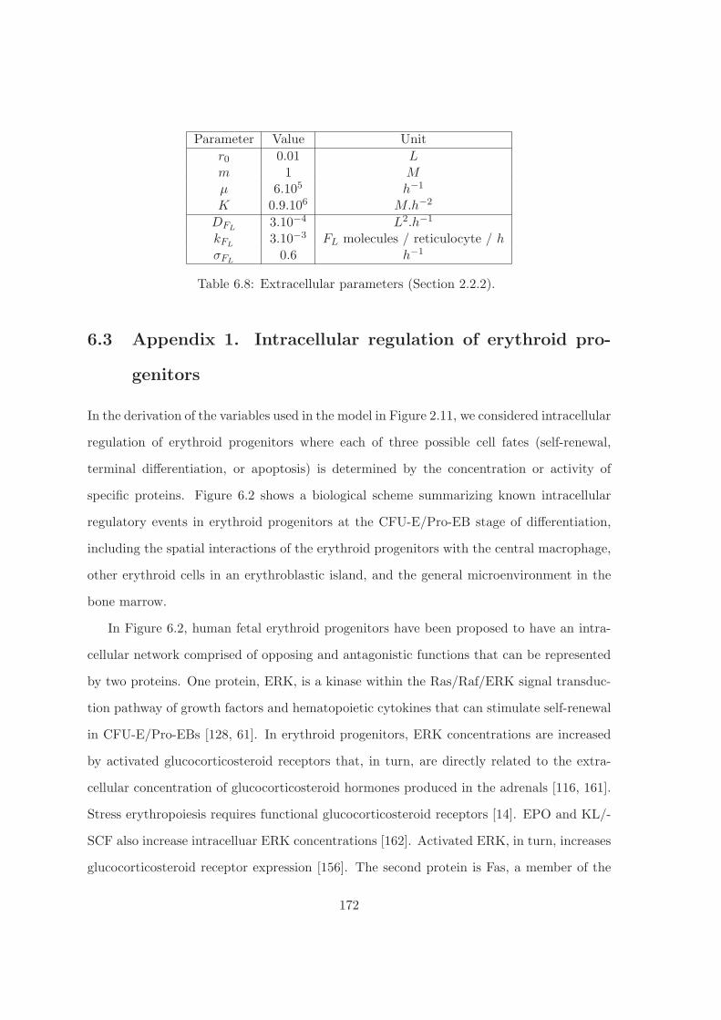
Parameter Value Unit

r0 0.01 Lm 1 Mμ 6.105 h−1

K 0.9.106 M.h−2

DFL3.10−4 L2.h−1

kFL3.10−3 FL molecules / reticulocyte / h

σFL0.6 h−1

Table 6.8: Extracellular parameters (Section 2.2.2).

6.3 Appendix 1. Intracellular regulation of erythroid pro-

genitors

In the derivation of the variables used in the model in Figure 2.11, we considered intracellular

regulation of erythroid progenitors where each of three possible cell fates (self-renewal,

terminal differentiation, or apoptosis) is determined by the concentration or activity of

specific proteins. Figure 6.2 shows a biological scheme summarizing known intracellular

regulatory events in erythroid progenitors at the CFU-E/Pro-EB stage of differentiation,

including the spatial interactions of the erythroid progenitors with the central macrophage,

other erythroid cells in an erythroblastic island, and the general microenvironment in the

bone marrow.

In Figure 6.2, human fetal erythroid progenitors have been proposed to have an intra-

cellular network comprised of opposing and antagonistic functions that can be represented

by two proteins. One protein, ERK, is a kinase within the Ras/Raf/ERK signal transduc-

tion pathway of growth factors and hematopoietic cytokines that can stimulate self-renewal

in CFU-E/Pro-EBs [128, 61]. In erythroid progenitors, ERK concentrations are increased

by activated glucocorticosteroid receptors that, in turn, are directly related to the extra-

cellular concentration of glucocorticosteroid hormones produced in the adrenals [116, 161].

Stress erythropoiesis requires functional glucocorticosteroid receptors [14]. EPO and KL/-

SCF also increase intracelluar ERK concentrations [162]. Activated ERK, in turn, increases

glucocorticosteroid receptor expression [156]. The second protein is Fas, a member of the

172

tumor necrosis factor receptor family that can activate specific caspases, a series of intra-

cellular proteolytic enzymes that promote apoptosis [128]. At high levels of activation, Fas

stimulates erythroid progenitor apoptosis [107, 100], while at lower activities it promotes

terminal erythroid differentiation [128] that is mediated through the activity of the tran-

scription factor GATA-1 on the expression of many erythroid-specific genes. Activated Fas

concentrations are directly related to extracellular Fas-ligand concentrations, which in hu-

man hematopoietic tissues are produced mainly by the most mature erythroblasts [107] and

in mouse hematopoietic tissues are produced mainly by early stage erythroblasts [100].

The intracellular concentration of activated Fas is a key factor in the decisions made

by the erythroid progenitor in Figure 2.10. When a specific threshold of intracellular Fas-

mediated caspase activity is present, the erythroid progenitor dies by apoptosis. If the

intracellular concentration of activated Fas is not sufficient to reach the apoptosis threshold,

then the erythroid progenitor makes the second decision based on a competition between

ERK-mediated self-renewal and Fas-mediated terminal differentiation [128]. The major

regulator of Fas activity is the concentration of EPO in the bone marrow microenvironment.

Under normal conditions, the EPO concentrations in the blood and the marrow are relatively

low, and the Fas expression on the CFU-E/Pro-EBs is sufficiently high that the resultant

level of caspase activity causes most of them undergo apoptosis [93]. The relatively low

concentrations of glucocorticoid hormone present under normal conditions results in only

a few CFU-E/Pro-EBs undergoing self-renewal. Therefore, of those CFU-E/Pro-EBs that

do not undergo apoptosis, most will have sufficient Fas and limited ERK so that they will

terminally differentiate, thereby supplying the 2 · 1011 new erythrocytes required each day

to replace those erythrocytes lost to senescent removal.

The normal steady-state erythropoiesis can respond rapidly to changes in EPO concen-

trations [93]. In kidney disease, anemia develops as less EPO is produced, and more than

normal numbers of CFU-E/Pro-EBs undergo apoptosis from the resulting increases in Fas

and caspase activities. Exogenous EPO administration or recovery from the kidney disease

will lower the Fas and caspase activities, thereby decreasing the apoptosis rate to normal,

173

and the anemia will resolve. EPO levels increase slightly or moderately with limited bleed-

ing, hemolysis, lung disease, or ascent to high altitude because normal kidneys will produce

more EPO in response to slight or moderate hypoxia. The increased EPO will decrease

Fas activity and increase the Bcl-xL concentration, thereby reducing the intracellular cas-

pase activities. The decreased apoptosis resulting from the reduced caspase activities is

accompanied by an EPO-mediated increase in GATA-1 such that terminal differentiation is

increased relative to self-renewal.

Although EPO can increase ERK activity, its effect alone on self-renewal is less than

its effect on preventing apoptosis and promoting terminal differentiation. With acute hy-

poxia due to large amounts of bleeding or hemolysis, the resultant stress erythropoiesis is

characterized by large increases in EPO, but the ability of the erythroid progenitor cells

that supply the steady-state erythrocyte production to respond to the increased EPO has

a maximal limit. Very high EPO concentrations eliminate almost all apoptosis, and EPO-

mediated increases in GATA-1 promote terminal differentiation.

Although the total response to very high concentrations of EPO is limited by the num-

ber of available CFU-E/Pro-EBs, the erythropoietic response to hypoxic stress is amplified

by an increased self-renewal that provides more CFU-E/Pro-EBs. Increased concentrations

of glucocorticosteroids and EPO in stress erythropoiesis can raise ERK levels and pro-

mote CFU-E/Pro-EB self-renewal, but a major factor in the expansion of CFU-E/proery-

throblasts numbers during stress erythropoiesis in mouse spleens is BMP4, a member of the

transforming growth factor-family of cytokines, with receptors that signal through the Smad

pathway [119]. Splenic macrophages with the same immunophenotype (F4/80 positive) as

those that include the central macrophages of erythroblastic islands appear to be the source

of BMP4 in murine stress erythropoiesis [110]. Erythroid cells that are directly in contact

with central macrophages have a decreased duration of cell cycle that increases their pro-

liferation rate [124], and macrophage function in vivo is required for recovery from anemia

due to bleeding or hemolysis [130, 48, 121]. The generation of increased CFU-E/Pro-EBs

during hypoxic stress requires not only hypoxia but c-Kit and EPO as well as priming by

174

the cytokine Hedgehog [119]. The source of the BMP4-inducible erythroid progenitors that

give rise to an expanded CFU-E/Pro-EB population in the spleen is not certain. They

appear to be a separate population of erythroid progenitors that are closely related to,

if not the same as, the CFU-E/Pro-EBs of normal steady-state erythropoiesis. However,

once they develop to the CFU-E/Pro-EB stage, these BMP-derived progenitors appear to

have all of the characteristics of the CFU-E/Pro-EBs present during normal, steady-state

erythropoiesis [119].

Figure 6.2: Schematic representation of intracellular and extracellular regulation of mam-malian erythropoiesis at the stage of the CFU-E/Pro-EB in an erythroblastic island. Thescheme uses data from studies of both human and mouse. Macrophages through BMP4, andthe microenvironment through KL/SCF and glucocorticosteroids stimulate CFU-E/Pro-EBself-renewal. EPO stimulates CFU-E/Pro-EB survival and differentiation through its down-regulation of Fas and up-regulation of GATA-1. Very early stage erythroblasts in mouse andlate stage erythroblasts in human promote apoptosis through their production of Fas-ligand.See text for a detailed description of the scheme.

6.4 Appendix 2. Cell culture experiments

In previously reported studies [124], erythroblastic islands isolated from the spleens of mice

in the acute erythroblastosis phase of anemia-inducing Friend virus (FVA)-infection pro-

vided the macrophages for experiments that reconstituted erythroblastic islands in vitro.

175

Because EPO levels are low in FVA-infected mice [92], most erythroid progenitors do not

survive beyond the CFU- E/Pro-EB stages in vivo, and a majority of erythroblastic islands

in the spleen are populated mainly with CFU-E/Pro-EB. However, when these isolated

splenic erythroblastic islands are cultured for 72 hours in vitro with EPO under conditions

that promote differentiation, the erythroid cells terminally differentiate. Although some

erythroblasts lose adherence to macrophages in culture, others remain in the cultured ery-

throblastic islands. In Figure 2.20, islands at various times of culture were selected to show

the stages of erythroid differentiation within the islands in vitro.

In order to compare the proliferation and differentiation of the same population of devel-

opmentally homogeneous CFU-E/Pro-EBs cultured in erythroblastic islands and cultured

without central macrophages, a series of experiments used reconstituted erythroblastic is-

lands [124]. In these experiments, isolated splenic erythroblastic islands were cultured for

6 hours so that their central macrophages bound to the tissue culture plates. Then, after

removal of adherent erythroid cells, the macrophages were cultured for another day before

CFU-E/Pro-EBs purified from the spleen of another FVA-infected mouse were added in

co-cultures for 6 h. Excess unbound erythroid progenitors were then removed, and the

co-cultures were continued. Proliferation and differentiation of co-cultured CFU-E/Pro-

EBs over the ensuing 3 days were compared to aliquots of the same CFU-E/Pro-EBs that

were cultured alone and, thereby, served as controls. In the co-cultures some erythroblasts

lost their macrophage adherence. Comparisons of erythroid cells that remained adherent

to the macrophages with non-adherent erythroid cells of co-cultures or the control cells

cultured without macrophages demonstrated that central macrophage adherence promoted

more rapid cell proliferation due to shortened G1 phase of cell cycle [124].

6.5 Appendix 3

In the models considered in this work, some parameters are known : cell size, cell number,

duration of cell cycle [75], diffusion coefficient [45]. Some other parameters, especially

176

reaction constants in intracellular regulation are not known. Such parameters were varied

in a large range in order to see how the results depends on them. In the description of the

experiments, unknown parameters were fitted.

Initial quantities for the systeme (2.2.13)-(2.2.16) are as follows: z = 1, u = 0.5, v = 0.5,

w = 0.25 (mice); z = 1, u = 0.5, v = 0.5, w = 0.5 (human). At the moment of cell division,

the two daughter cells inherit half of quantities z, u, v, w of the mother cell.

Parameter Value Unit

Cells cycle length T 18 hCells cycle variation 3 hspace variable x NUtime variable h

a00 0.001 h−1

a10 0 h−1

a11 0.0001 h−1

a01 0.0000005 h−1

a12 0 h−1

a02 0.00077 h−1

a13 0.0001 h−1

a03 0.000001 h−1

b1 0.0004 h−1

b2 0.0045 h−1

b3 0.43 h−1

wcr 0.09 NU

Table 6.9: Values of intracellular parameters used in Figure 2.14 (right). NU denotesnondimensional unit

177

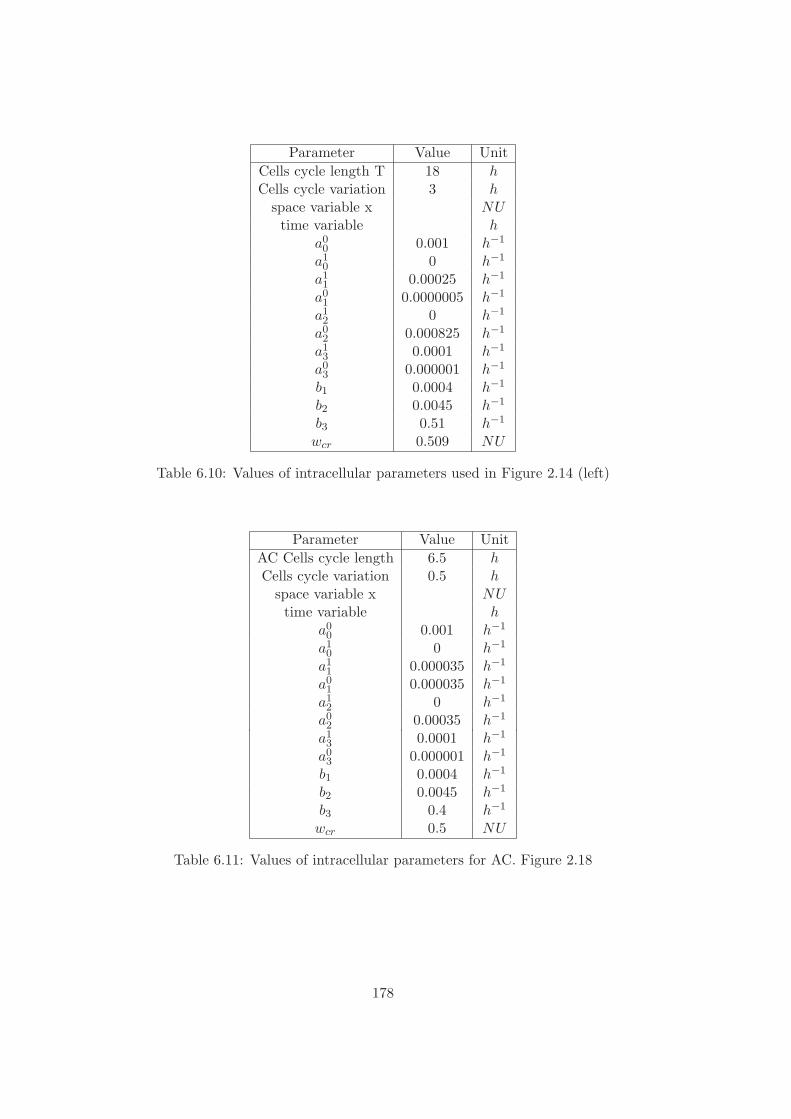
Parameter Value Unit

Cells cycle length T 18 hCells cycle variation 3 hspace variable x NUtime variable h

a00 0.001 h−1

a10 0 h−1

a11 0.00025 h−1

a01 0.0000005 h−1

a12 0 h−1

a02 0.000825 h−1

a13 0.0001 h−1

a03 0.000001 h−1

b1 0.0004 h−1

b2 0.0045 h−1

b3 0.51 h−1

wcr 0.509 NU

Table 6.10: Values of intracellular parameters used in Figure 2.14 (left)

Parameter Value Unit

AC Cells cycle length 6.5 hCells cycle variation 0.5 hspace variable x NUtime variable h

a00 0.001 h−1

a10 0 h−1

a11 0.000035 h−1

a01 0.000035 h−1

a12 0 h−1

a02 0.00035 h−1

a13 0.0001 h−1

a03 0.000001 h−1

b1 0.0004 h−1

b2 0.0045 h−1

b3 0.4 h−1

wcr 0.5 NU

Table 6.11: Values of intracellular parameters for AC. Figure 2.18

178

Parameter Value Unit

NAC Cells cycle length 16 hCells cycle variation 0.5 hspace variable x NUtime variable h

a00 0.001 h−1

a10 0 h−1

a11 0.00003 h−1

a01 0.0000005 h−1

a12 0 h−1

a02 0.00044 h−1

a13 0.0001 h−1

a03 0.000001 h−1

b1 0.0004 h−1

b2 0.0045 h−1

b3 0.4 h−1

wcr 0.485 NU

Table 6.12: Values of intracellular parameters for NAC. Figure 2.18

Parameter Value Unit

σ1 0.01 h−1

D1 0.25e-5 L2.h−1

w1 0.00005 molecules.L−2.h−1

σ2 0.005 h−1

D2 0.05e-4 L2.h−1

w2 0.0005 molecules.L−2.h−1

Table 6.13: Values of extracellular parameters. L is an arbitrary length unit

179

6.6 Value of parameters of myeloma simulation

Parameter Value Unit

Cell cycle length 720 minCell cycle variation 180 min

α 0.026 h−1

β 1 h−1.NU−1

a 0.265 h−1

b 0.03 h−1.NU−1

c 0.05 h−1

d 0.025 h−1

Ecr 0.3 NUFcr 0.6 NU

E0 Value of initial quantity E 0.3 NUF0 Value of initial quantity F 0.3 NU

Table 6.14: Value of parameters without macrophage

Parameter Value Unit

Cell cycle length 1440 minCell cycle variation 360 min

α 0.01 h−1

β 2 h−1.NU−1

kalpha 0.1 h−1/GFmoleculesa 0.53 h−1

b 0.06 h−1.NU−1

c 0.1 h−1

d 0.05 h−1

kg 0.03 h−1.NU−2

Ecr 0.55 NUFcr 0.48 NU

E0 Value of initial quantity E 0.3 NUF0 Value of initial quantity F 0.3 NU

Table 6.15: Value of parameters with macrophages, Figure 3.9.

180

Parameter Value Unit

Cell cycle length 720 minCell cycle variation 180 min

Table 6.16: Value of parameters without macrophage

Parameter Value Unit

Cell cycle length 1440 minCell cycle variation 360 min

Table 6.17: Value of parameters with macrophages, Figure 3.9.

181