How Weather-Proof is the Construction Sector? Empirical Evidence from Germany
41
Discussion Paper No. 08-105 How Weather-Proof is the Construction Sector? Empirical Evidence from Germany Melanie Arntz and Ralf A. Wilke
Transcript of How Weather-Proof is the Construction Sector? Empirical Evidence from Germany

Dis cus si on Paper No. 08-105
How Weather-Proof is the Construction Sector?
Empirical Evidence from Germany
Melanie Arntz and Ralf A. Wilke

Dis cus si on Paper No. 08-105
How Weather-Proof is the Construction Sector?
Empirical Evidence from Germany
Melanie Arntz and Ralf A. Wilke
Die Dis cus si on Pape rs die nen einer mög lichst schnel len Ver brei tung von neue ren For schungs arbei ten des ZEW. Die Bei trä ge lie gen in allei ni ger Ver ant wor tung
der Auto ren und stel len nicht not wen di ger wei se die Mei nung des ZEW dar.
Dis cus si on Papers are inten ded to make results of ZEW research prompt ly avai la ble to other eco no mists in order to encou ra ge dis cus si on and sug gesti ons for revi si ons. The aut hors are sole ly
respon si ble for the con tents which do not neces sa ri ly repre sent the opi ni on of the ZEW.
Download this ZEW Discussion Paper from our ftp server:
ftp://ftp.zew.de/pub/zew-docs/dp/dp08105.pdf

Das Wichtigste in Kurze
Saisonale Entlassungen im Baugewerbe fuhren in der Winterzeit regelmassig zu einem Anstieg
der Arbeitslosigkeit. Aus diesem Grund gibt es in verschiedenen europaischen Landern institu-
tionelle Regelungen, die entweder eine Winterbautaigkeit fordern sollen oder Arbeitgeber und
Arbeitnehmer fur den Ausfall an Arbeitsstunden kompensieren. In Deutschland wurden diese
Regelungen in den 1990er Jahren mehrfach uberarbeitet und das zum großen Teil durch die Bun-
desagentur fur Arbeit finanzierte Schlechtwettergeld durch Regelungen abgelost, bei der Arbeit-
szeitkonten einen Teil der Ausfallstunden abfangen. Diese institutionellen Reformen erlauben
es, die Effektivitat zweier in Europa weit verbreiteten Ansatze der Forderung im Bausektor
im Hinblick auf die Vermeidung saisonaler Arbeitslosigkeit zu vergleichen. Insbesondere soll-
ten Maßnahmen, welche aus der Sicht der Arbeitgeber die Entlassungskosten relativ zu den
Weiterbeschaftigungskosten im Falle von Ausfallstunden reduzieren, das Risiko einer Entlassung
senken.
In diesem Artikel untersuchen wir empirisch die Bestimmungsgrunde von Entlassungen im
deutschen Baugewerbe. Dabei analysieren wir insbesondere den Einfluss der institutionellen Rah-
menbedingungen, berucksichtigen aber zusatzlich auch den Einfluss der Wetterbedingungen sowie
der konjunkturellen Bedingungen. Fur unsere Analysen konnen wir auf tagesgenaue Individual-
daten uber einen Zeitraum von mehr als zwanzig Jahre zuruckgreifen. Die Datenbasis kombinieren
wir mit regionalen Wetter- und Konjunkturdaten um den Beitrag der institutionellen Regelun-
gen auf das individuelle Arbeitslosigkeitsrisiko zu isolieren. Unsere Ergebnisse bestatigen die
okonomische Theorie insoweit, als dass Entlassungen aufgrund von schlechten Witterungs- und
Konjunkturbedingungen sowie im Zuge sinkender Entlassungskosten zunehmen. Insbesondere
zeigt sich, dass das Schlechtwettergeld im Vergleich zu einer Regelung mit Arbeitszeitkonten zu
einem hoheren Arbeitslosigkeitsrisiko fuhrt. Der Einfluss der Witterungsbedingungen sowie der
institutionellen Regelungen ist jedoch schwacher als allgemein vermutet, da Entlassungen haufig
an festen Kalendertagen (Vorweihnachtszeit, Wochen- und Monatsende) erfolgen.

Non-technical summary
Adverse weather conditions that hamper outdoor construction work have been the prime justifi-
cation for promoting all-season employment in the construction sector in many European countries.
The aim is to reduce seasonal layoffs and thereby reduce spending on unemployment compensation
by reducing some of the risk that a weather-induced shortfall of work means to both employers
and workers. In Germany, recent years have seen a major shift from a system based on mainly
publicly funding a weather allowance to a system that promotes the use of working hours accounts
to compensate for seasonal fluctuations in the workload. For two of the main employment pro-
motion schemes that can be found across Europe, the regime shifts in Germany thus constitute a
prime opportunity for comparing the effectiveness of such measures in preventing seasonal layoffs.
In particular, we would expect measures that lower a firm’s layoff costs relative to the costs of
maintaining an employment relationship during a seasonal labour shortfall to reduce transition
rates to unemployment.
This paper therefore empirically investigates the determinants of individual layoff probabilities
in the German construction sector. Based on daily data of more than twenty subsequent years,
our analysis explores the impact of the institutional changes that occurred during the 1990s while
taking account of other factors such as weather conditions, the business cycle, and individual
level characteristics. We are thus able to disentangle the relevance of each of these factors as
a determinant of seasonal unemployment. Our results generally confirm the effects suggested
by economic theory, i. e. a higher inflow into unemployment during periods of adverse weather
conditions, unfavourable business conditions as well as reduced layoff costs. In particular, the
longstanding bad weather allowance that is financed mainly by both the unemployment insurance
fund and by employers turns out to significantly increase layoffs compared to the introduction of
a winter allowance in addition to the use of working hours accounts. Our results also suggest,
however, that actual weather conditions and the legal setup are less relevant than thought by the
public as most of the layoffs simply take place at fixed calender times.
2
How weather-proof is the construction sector?
Empirical evidence from Germany. ∗
Melanie Arntz†
Ralf A. Wilke‡
December 2008
Abstract
With the purpose to reduce winter unemployment and to promote all-season employment
in the constructions sector, Germany maintains an extensive bad weather allowance system.
Since the mid 1990s, these regulations have been subject to several reforms that resemble
the range of approaches for employment promotion which can be found in other European
countries. We analyse the effect of these reforms on individual unemployment risks using
large individual administrative data merged with information about local weather conditions
and the business cycle. We find a weaker direct link between seasonal layoffs and actual
weather than broadly assumed, since most of the layoffs take place at fixed dates. The
reforms under consideration have economically plausible effects; Regulations that limit an
employer’s financial burden reduce transitions to unemployment and render it less weather-
dependent.
Keywords: panel data, temporary layoffs, employment stability
JEL: J38, J48, J68
∗We thank Julian Link for research assistance and the ZEW Mannheim for financial support through the grant
”A microeconometric evaluation of seasonal unemployment in Germany”. We use a sample drawn from the IAB
employment sample 2004 - R04 of the Institute of Employment Research (IAB).†ZEW Mannheim, E–mail: [email protected].‡University of Nottingham, E–mail: [email protected]

1 Introduction
During periods of adverse weather conditions that hamper outdoor construction work firms have
incentives to temporarily lay off parts of their workforce. Countries with unfavourable conditions
for winter construction work thus tend to experience seasonal unemployment patterns. However,
the degree of seasonality strongly varies across countries. According to Grady and Kapsalis (2002)
there is empirical evidence for considerable seasonal employment and unemployment patterns in
Canada, Finland and Sweden, while other countries with similar climate conditions such as Nor-
way, Denmark and Iceland experience much less seasonal labour market variations. In contrast,
Germany has a distinct seasonal unemployment pattern as shown in Figure 1 in spite of having
a significantly milder climate than the Nordic countries. Depending on the year, up to 50% of
all unemployment spells in agriculture and the construction sector end by reemployment with the
former employer (Wilke, 2005). Moreover, while there is a considerable decline in seasonal unem-
ployment patterns over the past decades in the Nordic countries, probably driven by technological
and climate change, this cannot be observed for Germany.
Figure 1: Monthly unemployment rate in Germany. Note: West-Germany only for years 1991 and
later. Source: Federal Employment Agency.
0.0
2.0
4.0
6.0
8.0
10.0
12.0
14.0
Jan-81 Jan-84 Jan-87 Jan-90 Jan-93 Jan-96 Jan-99 Jan-02
Unemployment rate in %
4

The link between weather conditions and seasonal unemployment thus varies across countries.1
To some extent, this likely reflects the different approaches that can be found across countries in
fighting seasonal unemployment. See Bosch and Philips (2003) as well as RKW (2003) for an
overview. In particular, one can distinguish three main approaches to the promotion of all-season
employment: (i) financial incentives for winter construction work, (ii) a financial compensation
for weather-induced shortfall hours and (iii) the use of flexible working hour accounts to cushion
seasonal shortfall hours. While the first approach can be found in many European countries
including the Nordic countries, weather allowances have been used in the Netherlands, Belgium,
Austria, Switzerland, and France. In addition, the latter three countries also promote flexible
working hours. These employment promotion schemes have either been financed by an industry-
specific levy system or by special government programs. The motivation to spend public money to
this end is both political and financial. First of all, high unemployment is politically undesirable
even if it is only of a temporary nature. Secondly, seasonal unemployment puts a financial stress
on the unemployment insurance funds and can result in a cross subsidy of firms and employees
subject to seasonal unemployment. Thirdly, seasonal fluctuations have been associated with a
low-quality construction sector that is dominated by small firms with limited fixed capital and
unskilled and often low-paid workers (Bosch and Philips, 2003). All these aspects may to some
extent justify the use of public funds for fighting seasonal unemployment. However, the benefits
and costs of public spending on such regulations have to be contrasted. The German Federal
Employment Agency, for example, usually spends several hundred million Euros each year to
prevent seasonal unemployment in the construction sector, while such extensive policies do not
exist in the Nordic countries. There thus exist a wide range of approaches to promote all-season
employment in Europe, but, to the best of our knowledge, none of these programs have been
analysed with respect to its effectiveness in reducing layoffs.
This paper exploits a number of recent reforms in the German construction sector to provide a
first comparison of different approaches to the promotion of all-season employment. In particular,
Germany has seen a major shift from a system based on mainly publicly funding a weather al-
lowance to a system that promotes the use of flexible working hours accounts. For an overview of
these changes see also Bosch and Zuhlke-Robinet (2003) or Deutscher Bundestag (2002). For two
1To some extent, cross-country differences in seasonal unemployment patterns may also stem from differences
in defining individuals who are temporary laid off as unemployed or not.
5

of the main approaches of promoting all-season employment in the European construction sector,
the regime shifts in Germany thus constitute a prime opportunity for comparing the effective-
ness of such measures in preventing seasonal layoffs. Following Feldstein (1976), we would expect
lower transition rates to unemployment if an employment promotion scheme reduces a firm’s lay-
off costs relative to the costs of maintaining an employment relationship during a seasonal labour
shortfall.2 This paper therefore empirically investigates the determinants of individual layoff prob-
abilities in the construction sector. Based on daily data of more than twenty subsequent years,
our analysis explores the impact of the institutional changes that occurred during the 1990s condi-
tional on other observable variables such as weather conditions, the business cycle, and individual
level characteristics. Apart from carrying out a first microeconometric assessment of employment
promotion measures and thus providing new insights for both national and international policy
advisors in this field, we believe this paper to contribute to the literature for two more reasons.
First, the microeconometric analysis of seasonal unemployment in this paper is distinct from
the previous contributions as it analyses individual layoff probabilities and not the duration un-
til re-employment. Our research focus thus complements a number of empirical studies on the
duration of unemployment (Mavromaras and Rudolph, 1995; Roed and Nordberg, 2003). Roed
and Nordberg (2003), for example, analyse the effect of firms’ pay liability during the periods
of temporary dismissals on the length of unemployment in Norway. They show that the length
of unemployment spells until a worker is recalled by an employer is highly sensitive to financial
incentives for firms.
Secondly, our microeconometric panel analysis combines comprehensive individual level ad-
ministrative panel data from the Federal Employment Agency with information on the business
cycle as well as detailed information on local weather conditions. The combination of these types
of data is rather unique. Most studies concerning temporary lay-offs or work interruptions are
either based only on individual level information (Plassmann, 2002; Wilke, 2005) or only combine
individual and firm level information (Mavromaras and Rudolph, 1995; Mavromaras and Rudolph,
1998; Mavromaras and Orme, 2004). On the other extreme, effects of weather conditions on the
business cycle have been analysed on a macro level. Solomou and Wu (1997) find that weather
conditions have an effect on aggregate output in the construction sector in the UK. Combining
2This need not reduce the unemployment rate if firms not only reduce layoffs but also hire less frequently in
anticipation of the higher layoff costs (Burdett and Wright, 1989).
6

information on institutional changes, weather conditions, the business cycle, and individual level
characteristics, thus helps us in disentangling the relevance of each of these factors as a determi-
nant of seasonal unemployment. In particular, it allows for assessing to what extent the changes in
the institutional setup during the 1990s had an effect on employment stability in the construction
sector.
Our results generally confirm the effects suggested by economic theory, i. e. a higher inflow into
unemployment during periods of adverse weather conditions, unfavourable business conditions as
well as reduced layoff costs. However, they also suggest that actual weather conditions and the
legal setup are less relevant than thought by the public as most of the layoffs simply take place at
fixed calender times. The paper is structured as follows. The following section describes the main
features of the institutional setup for seasonal employment in Germany. We describe our data in
section three and the econometric framework in section four. The empirical results are presented
and discussed in section five before we conclude in section six.
2 Institutional setup for seasonal employment in Germany
Before the labour market in the German construction industry became heavily regulated in the
1950s, employment in the construction sector had been highly insecure due to the cyclical and sea-
sonal nature of construction work. Adverse weather conditions during the winter often combined
with seasonally empty order books raised the firm’s cost of maintaining employment during the
winter period. As a consequence, employment relationships were often ended before Christmas
and workers were hired again in early spring. Many construction workers left the industry due to
these unattractive working conditions which resulted in an increasing labour shortage. For an ex-
tensive review of the institutional setup in the German construction industry see Zuhlke-Robinet
(1997) and Bosch and Zuhlke-Robinet (2000, 2003).
In order to promote employment during the winter period and thus improve working conditions
in the construction sector, an employment promotion act was implemented in 1959. At the core of
this regulation was a bad weather allowance, the Schlechtwettergeld (SWG), that aimed at reduc-
ing the financial risk that shortfall hours had previously meant to both employers and employees.3
3Working conditions in the construction sectors also improved due to introducing a supplementary pension
fund (Zusatzversorgungskasse) and a vacation and wage compensation fund for vacation pay between 24 and 31
7
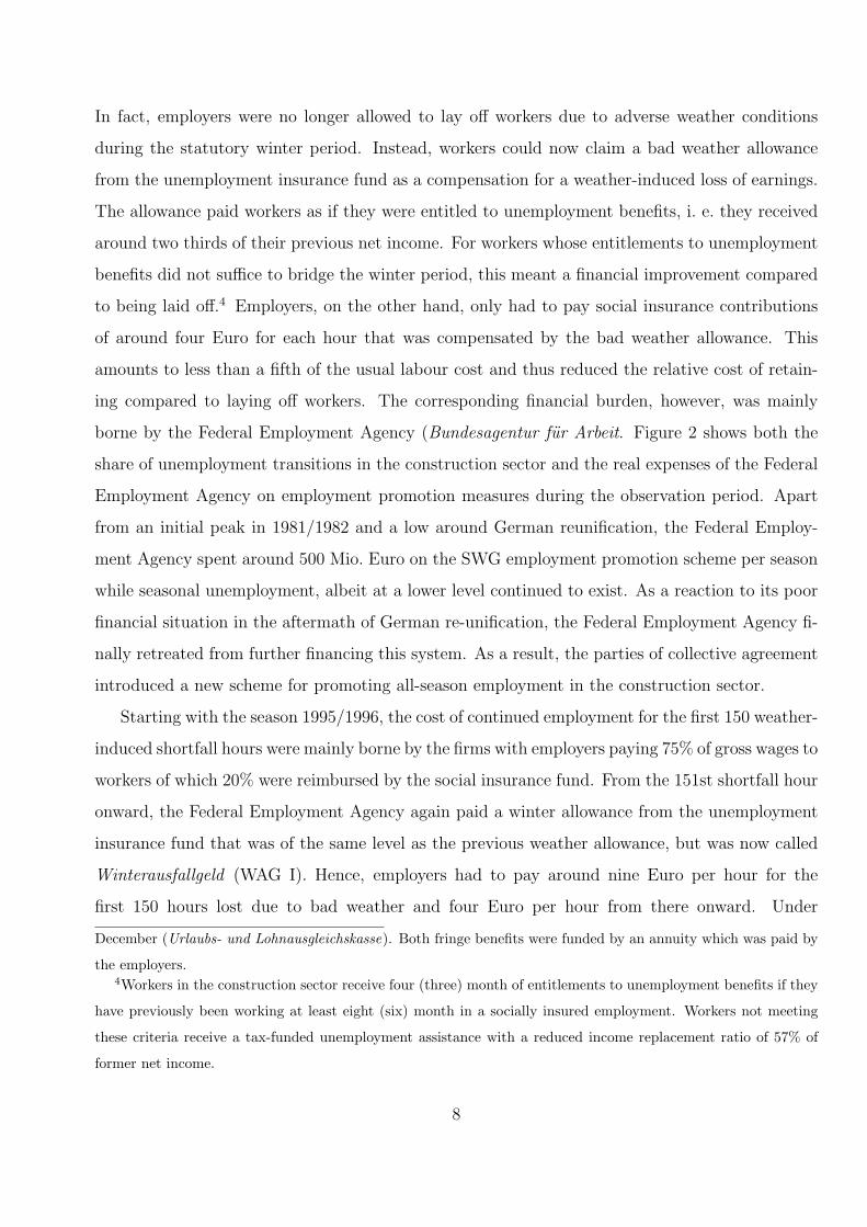
In fact, employers were no longer allowed to lay off workers due to adverse weather conditions
during the statutory winter period. Instead, workers could now claim a bad weather allowance
from the unemployment insurance fund as a compensation for a weather-induced loss of earnings.
The allowance paid workers as if they were entitled to unemployment benefits, i. e. they received
around two thirds of their previous net income. For workers whose entitlements to unemployment
benefits did not suffice to bridge the winter period, this meant a financial improvement compared
to being laid off.4 Employers, on the other hand, only had to pay social insurance contributions
of around four Euro for each hour that was compensated by the bad weather allowance. This
amounts to less than a fifth of the usual labour cost and thus reduced the relative cost of retain-
ing compared to laying off workers. The corresponding financial burden, however, was mainly
borne by the Federal Employment Agency (Bundesagentur fur Arbeit. Figure 2 shows both the
share of unemployment transitions in the construction sector and the real expenses of the Federal
Employment Agency on employment promotion measures during the observation period. Apart
from an initial peak in 1981/1982 and a low around German reunification, the Federal Employ-
ment Agency spent around 500 Mio. Euro on the SWG employment promotion scheme per season
while seasonal unemployment, albeit at a lower level continued to exist. As a reaction to its poor
financial situation in the aftermath of German re-unification, the Federal Employment Agency fi-
nally retreated from further financing this system. As a result, the parties of collective agreement
introduced a new scheme for promoting all-season employment in the construction sector.
Starting with the season 1995/1996, the cost of continued employment for the first 150 weather-
induced shortfall hours were mainly borne by the firms with employers paying 75% of gross wages to
workers of which 20% were reimbursed by the social insurance fund. From the 151st shortfall hour
onward, the Federal Employment Agency again paid a winter allowance from the unemployment
insurance fund that was of the same level as the previous weather allowance, but was now called
Winterausfallgeld (WAG I). Hence, employers had to pay around nine Euro per hour for the
first 150 hours lost due to bad weather and four Euro per hour from there onward. Under
December (Urlaubs- und Lohnausgleichskasse). Both fringe benefits were funded by an annuity which was paid by
the employers.4Workers in the construction sector receive four (three) month of entitlements to unemployment benefits if they
have previously been working at least eight (six) month in a socially insured employment. Workers not meeting
these criteria receive a tax-funded unemployment assistance with a reduced income replacement ratio of 57% of
former net income.
8

this new regime, spending by the Federal Employment Agency on employment promotion in the
construction sector fell sharply, while unemployment risk among construction workers doubled
during the winter seasons of 1995/1996 and 1996/1997 compared to the early 1990s as shown in
Figure 2. However, unemployment transitions were similarly prevalent during the 1980s. In fact,
the increase in winter unemployment compared to the preceding summer period was particularly
pronounced for two winter seasons: 1987/88 and 1995/96. This suggests that it may be too
simplistic to exclusively ascribe the latter increase in unemployment risks to the introduction of
WAG I.
In order to find a remedy for the high seasonal unemployment after the introduction of WAG I,
a new regulation, the Winterausfallgeld II (WAG II), came into force in the season of 1997/1998.
It shifted most of the financial burden from the employer to the worker by introducing an accu-
mulation of overtime during spring and summer that had to be used to compensate for a shortfall
of work during the winter period. Firms could choose between a small working time flexibility
(WAG IIa) and a large working time flexibility (WAG IIb). In case a firm opted for the large
working time flexibility (WAG IIb), the first 120 shortfall hours had to be compensated by a work-
ing hours account and were thus cost-neutral for an employer while workers lost any additional
financial compensation.5 In case of the small working time flexibility (WAG IIa), only the first
fifty hours had to be compensated by overtime. After the 50th shortfall hour, workers received
the usual winter allowance of around two thirds of their previous net income. During the 51st and
the 120th shortfall hour, this allowance and a 50% deduction of an employer’s social insurance
contributions was financed by a statutory winter levy of 1.7% of a firm’s gross wage bill. Under
both flexibilisation regimes, the unemployment insurance fund paid the winter allowance from the
121st shortfall hour onward with employers paying the full social insurance contribution. Hence,
the Federal Employment Agency again took a higher financial risk compared to WAG I, but a re-
duced burden compared to SWG. Furthermore, the financial burden of the employer was reduced
compared to the SWG regime irrespective of whether a firm chose the small or large working hour
flexibility. The risk of seasonal layoffs thus seemed reduced compared to both WAG I and SWG.
However, Figure 2 suggests that unemployment transitions remained at a high level under
5A worker with overtime would previously receive the overtime pay including the premium and in addition
receive the bad weather allowance. In the new setting, the worker only receives the overtime pay including the
premium.
9

Figure 2: Unemployment transitions in the construction sector and expenses of the Federal Em-
ployment Agency on promoting all-season employment.
(top) Share of individuals that is laid off during winter and summer periods. Source: IABS 2004
0
0.02
0.04
0.06
0.08
0.1
0.12
1981 1983 1985 1987 1989 1991 1993 1995 1997 1999 2001 2003
Winter period (starting in year…) Summer period
SWG WAG I WAG II WAG III
(bottom) Real expenses of Federal Employment Agency on employment promotion in Mio Euro (in
2004 prices). Source: Federal Employment Agency
0 €
200 €
400 €
600 €
800 €
1,000 €
1,200 €
1,400 €
1,600 €
1981
/2
1982
/3
1983
/4
1984
/5
1985
/6
1986
/7
1987
/8
1988
/9
1989
/0
1990
/1
1991
/2
1992
/3
1993
/4
1994
/5
1995
/6
1996
/7
1997
/8
1998
/9
1999
/0
2000
/1
2001
/2
2002
/3
2003
/4
2004
/5
10
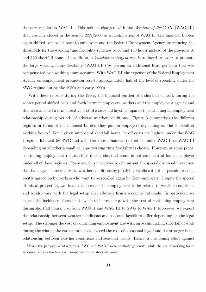
the new regulation WAG II. This neither changed with the Winterausfallgeld III (WAG III)
that was introduced in the season 1999/2000 as a modification of WAG II. The financial burden
again shifted somewhat back to employers and the Federal Employment Agency by reducing the
thresholds for the working time flexibility schemes to 30 and 100 hours instead of the previous 50
and 120 shortfall hours. In addition, a Zuschusswintergeld was introduced in order to promote
the large working hours flexibility (WAG IIIb) by paying an additional Euro per hour that was
compensated by a working hours account. With WAG III, the expenses of the Federal Employment
Agency on employment promotion rose to approximately half of the level of spending under the
SWG regime during the 1980s and early 1990s.
With these reforms during the 1990s, the financial burden of a shortfall of work during the
winter period shifted back and forth between employers, workers and the employment agency and
thus also affected a firm’s relative cost of a seasonal layoff compared to continuing an employment
relationship during periods of adverse weather conditions. Figure 3 summarises the different
regimes in terms of the financial burden they put on employers depending on the shortfall of
working hours.6 For a given number of shortfall hours, layoff costs are highest under the WAG
I regime, followed by SWG and with the lowest financial risk either under WAG II or WAG III
depending on whether a small or large working time flexibility is chosen. However, at some point,
continuing employment relationships during shortfall hours is not cost-neutral for an employer
under all of these regimes. There are thus incentives to circumvent the special dismissal protection
that bans layoffs due to adverse weather conditions by justifying layoffs with other pseudo reasons,
tacitly agreed on by workers who want to be recalled again by their employers. Despite the special
dismissal protection, we thus expect seasonal unemployment to be related to weather conditions
and to also vary with the legal setup that affects a firm’s economic rationale. In particular, we
expect the incidence of seasonal layoffs to increase c.p. with the cost of continuing employment
during shortfall hours, i. e. from WAG II and WAG III to SWG to WAG I. Moreover, we expect
the relationship between weather conditions and seasonal layoffs to differ depending on the legal
setup. The stronger the cost of continuing employment rise with an accumulating shortfall of work
during the winter, the earlier total costs exceed the cost of a seasonal layoff and the stronger is the
relationship between weather conditions and seasonal layoffs. Hence, a cushioning effect against
6From the perspective of a worker, SWG and WAG I were similarly generous, while the use of working hours
accounts reduces the financial compensation for shortfall hours.
11

bad weather conditions may be especially weak for WAG I while it may be relatively strong for
WAG II and WAG III.
Figure 3: Total firm costs of a shortfall in working hours under different employment promotion
regimes - SWG (upper left), WAG I (upper right), WAG II (lower left) and WAG III (lower right),
1959-2004
0
250
500
750
1000
1250
1500
0 20 40 60 80 100 120 140 160 180
shortfall of work in hours
Eu
ro
0
250
500
750
1000
1250
1500
0 20 40 60 80 100 120 140 160 180
shortfall of work in hours
Eu
ro
0
250
500
750
1000
1250
1500
0 20 40 60 80 100 120 140 160 180
shortfall of work in hours
Eu
ro
WAG IIa WAG IIb
0
250
500
750
1000
1250
1500
0 20 40 60 80 100 120 140 160 180
shortfall of work in hours
Eu
ro
WAG IIIa WAG IIIb
In addition, observed seasonal layoffs as shown in Figure 2 likely result not only from the
combined effect of the regulation of the labour market and the severity of weather conditions in a
particular year, but also result from business cycle conditions. In periods of empty order books,
firms are more likely to lay off workers. Moreover, it is always cheaper for firms to lay off redundant
workers than keeping them if the expected length of the redundancy and the corresponding total
costs of continued employment is long enough such that hiring costs become negligible. For this
reason, fixed calender times ahead of less productive time intervals or company holidays could
also increase layoffs. In order to assess the effectiveness of the four regimes in preventing seasonal
unemployment and making the construction sector weather-proof, the empirical analysis thus
needs to disentangle the impact of weather conditions, the business environment, the relevance
12

of certain fixed calender times as well as the legal setup. Unfortunately, we cannot evaluate
the legal regimes relative to a state without any all-season employment promotion because our
period of analysis is restricted to 1981 until 2004. Instead, we compare the relative effectiveness
of the four regimes in reducing seasonal layoffs. From the perspective of the Federal Employment
Agency, a legal setup that minimises seasonal unemployment with a minimum of public spending
on employment promotion should be preferable.
Apart from institutional changes with respect to the promotion of all-season employment,
the construction sector has also undergone further changes that need to be kept in mind for the
following empirical analysis. In particular, the previously domestic construction industry has
experienced an increasing transnationalisation (Bosch and Zuhlke-Robinet, 2003). While foreign
workers until the early 1990s were employed at the same pay and working conditions than domestic
workers, this territorial principle no longer applies within the EU member states. Foreign workers,
especially from central and eastern European countries, could now be posted from their company
to work in Germany on the terms that apply in their home country. Despite bilateral agreements
on quotas for these posted workers and recommended minimum wages, officially posted workers
in Germany reached an all time high in 1992 (see Figure 4, top). The Posted Workers Act in 1996
meant the introduction of binding minimum wages for all legal workers in Germany including
posted workers from abroad. However, illegal employment continues to provide opportunities for
considerably reducing labour costs. According to Bosch and Zuhlke-Robinet (2003: 65), ”con-
siderable numbers of German construction workers have been made redundant and replaced by
contract or illegal workers”. This crowding out of domestic employment may also explain why
revenues per (legal) head have been increasing during the 1990s. As Figure 4 (bottom) shows,
real revenues have generally been declining since the 1980s despite a significant boom around the
German re-unification. The employment level, however, declined even more to about 50% of its
initial level. This led to an upward shift in revenues per employee since the end of the 1980s that
may at least partly reflect the crowding out of domestic workers. Since we were not able to obtain
data on the amount of illegal employment from official sources, we cannot evaluate the effects of
these accompanying policy reforms. However, we assume that the inflow of non-domestic workers
is not correlated with the four policy regimes and we control for cyclical patterns by using year
dummies. Moreover, we use individual level indicators for possible effects of binding minimum
wages in different parts of the construction sector which were introduced between 1996 and 1999.
13

Figure 4: Annual macroeconomic indicators for the German construction sector.
(top) number of officially posted non EU construction workers
0
10000
20000
30000
40000
50000
60000
70000
80000
1982 1984 1986 1988 1990 1992 1994 1996 1998 2000 2002 2004
Number of posted non EU workers Source: Federal Employment Agency
1994: Tighter quotas for work permits 1996: Posted Workers Act
(bottom) employment and real revenue level.
40.0
50.0
60.0
70.0
80.0
90.0
100.0
110.0
120.0
1981 1983 1985 1987 1989 1991 1993 1995 1997 1999 2001 2003
Revenue EmploymentIndex: 1994 = 100
West-Germany only
1988: Facilitation of temporary work
permits for non EU nationals
1996: Introduction of minimum work
standards and minimum wages
Source: Federal Statistical Office
The identification of the policy effects can also be hampered by improvements in the production
technology in presence of severe weather conditions over time. This could result in a reduced
weather-dependency of layoffs in later years. Since we are not aware of any data about production
14

technology in the construction sector, we are not able to control for it. In order to identify changes
in response to the policy reforms, we have to assume that such trends are of minor importance or
not correlated with the policy reforms.
Finally, we want to point out that we are not able to analyse possible effects of the intro-
duction of the Saisonkurzarbeitergeld in 2006 since our individual data does not cover the period
after 2004. As we also do not have information about the receipt of the bad weather allowance
(Schlechtwettergeld) or the winter allowance (Winterausfallgeld) on an individual level so that
we cannot analyse the determinants for claiming these allowances. Moreover, due to the lack of
this information we cannot assess the overall changes in compensation transfers in reaction to the
policy reforms.
3 Data
Our analysis is based on comprehensive administrative individual data from Germany which is
merged with several regional indicators about the business cycle and weather conditions.
Individual data. We use the IAB employment sample 1975-2004 - regional file (IABS-R04)
which is described in detail by Drews (2008). This administrative data set contains information
on a 2 % sample of the population working in jobs that are subject to social insurance payments. In
particular, we have daily information on employment periods and periods for which the individual
received unemployment compensation from the Federal Employment Agency. Due to data quality
problems in the early years of the data set, we restrict our sample to information between 1981
and 2004. Moreover, we do not include information from Eastern Germany as information is not
available before 1991.7 We further restrict our sample to individuals working in the construction
sector.8
From a descriptive analysis of the daily information it became evident that there are mass
points in the distribution of unemployment inflows at the end of each month, year and on each
Friday. Moreover, there are major peaks at the last two Fridays before Christmas. Since these
7For the period after 1991, estimates both ex- and including the eastern German counties did yield robust
findings.8In order to receive a consistent time series of employment relationships, we further exclude so called minor
employment relationships that are included in the data since March 1999 only.
15
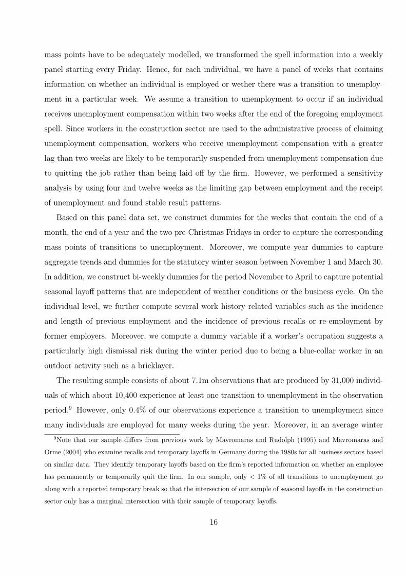
mass points have to be adequately modelled, we transformed the spell information into a weekly
panel starting every Friday. Hence, for each individual, we have a panel of weeks that contains
information on whether an individual is employed or wether there was a transition to unemploy-
ment in a particular week. We assume a transition to unemployment to occur if an individual
receives unemployment compensation within two weeks after the end of the foregoing employment
spell. Since workers in the construction sector are used to the administrative process of claiming
unemployment compensation, workers who receive unemployment compensation with a greater
lag than two weeks are likely to be temporarily suspended from unemployment compensation due
to quitting the job rather than being laid off by the firm. However, we performed a sensitivity
analysis by using four and twelve weeks as the limiting gap between employment and the receipt
of unemployment and found stable result patterns.
Based on this panel data set, we construct dummies for the weeks that contain the end of a
month, the end of a year and the two pre-Christmas Fridays in order to capture the corresponding
mass points of transitions to unemployment. Moreover, we compute year dummies to capture
aggregate trends and dummies for the statutory winter season between November 1 and March 30.
In addition, we construct bi-weekly dummies for the period November to April to capture potential
seasonal layoff patterns that are independent of weather conditions or the business cycle. On the
individual level, we further compute several work history related variables such as the incidence
and length of previous employment and the incidence of previous recalls or re-employment by
former employers. Moreover, we compute a dummy variable if a worker’s occupation suggests a
particularly high dismissal risk during the winter period due to being a blue-collar worker in an
outdoor activity such as a bricklayer.
The resulting sample consists of about 7.1m observations that are produced by 31,000 individ-
uals of which about 10,400 experience at least one transition to unemployment in the observation
period.9 However, only 0.4% of our observations experience a transition to unemployment since
many individuals are employed for many weeks during the year. Moreover, in an average winter
9Note that our sample differs from previous work by Mavromaras and Rudolph (1995) and Mavromaras and
Orme (2004) who examine recalls and temporary layoffs in Germany during the 1980s for all business sectors based
on similar data. They identify temporary layoffs based on the firm’s reported information on whether an employee
has permanently or temporarily quit the firm. In our sample, only < 1% of all transitions to unemployment go
along with a reported temporary break so that the intersection of our sample of seasonal layoffs in the construction
sector only has a marginal intersection with their sample of temporary layoffs.
16

season, 7.5% of all individuals working in the construction sector become unemployed of which
only 1% experience a transition to unemployment twice. This indicates that individuals tend to
be laid off once for the whole winter period instead of switching back and forth between em-
ployment and unemployment. Even though this suggests that the effect of weather conditions on
the employment status may be limited, it does not preclude that the actual layoff time depends
on current weather conditions or cumulative weather conditions in the current winter season as
discussed in the previous section. Summary statistics of the sample can be found in Appendix A.
Regional data. Since the IABS provides county level information about the workplace location,
we can merge regional data about weather conditions and the business cycle. The business cycle
information on yearly revenues in the construction sector as plotted in Figure 4 is also available
for the sixteen German states. In order to avoid a scaling problem due to the different sizes of
states, we generate for each state an index of real revenues. We thus merge the state level index on
real revenues. Moreover, we merge information on the annual percentage change of real revenues
compared to the previous year to capture a changing business environment in the construction
sector.
The weather data is obtained from the German meteorological service (Deutscher Wetterdienst,
DWD) and comprises information about daily temperature intervals, the amount of snow, rain
and the wind speed for a sample of 35 weather stations throughout Germany.10 These stations
were chosen by the DWD based on the criterium that weather conditions measured at these
stations are representative for the densely populated areas of the surrounding county. Hence,
weather stations that capture local or extreme weather conditions (e.g. hilltops) were excluded.
Moreover, for many counties, the meteorologists at DWD could not identify a weather station
with representative weather conditions for its surrounding county. Owing to these limitations,
our sample of workers in the construction sector is limited to 35 German counties which may not
be fully representative for Germany as a whole. On the other hand, the sample includes a broad
mixture of rural and urban counties spread throughout Germany (see Figure 8 in the Appendix).
As an alternative to including weather indicators such as temperature, precipitation or wind
in our analysis, we decided to define days with severe weather conditions that hamper outdoor
10The data is available for academic use from the DWD by paying a low administrative fee. We thank the DWD
for its scientific advice and support.
17

construction work, in short DSW, according to the official DWD definition. We reconstruct DSW
as precise as possible based on the available weather information on temperature and precipita-
tion. In order to make the data compatible to our weekly panel data, we define weekly weather
conditions. In particular, we consider a week to have severe weather conditions, in short WSW, if
at least three days fulfil the DSW criterium. While for the individual data, a weekly information
reflects the employment status in the week following a Friday, the weather information merged for
this week reflects weather conditions between the last Monday and the next Sunday, thus taking
account of short-term expectations concerning the weather on the weekend. We tested alternative
specifications but found this one to yield the sharpest estimates. In addition to the indicator con-
cerning weather conditions in the current week, we also compute the cumulative number of DSW
in a winter season in order to capture the varying severity of the winter that is likely to affect
layoffs. Figure 5 reports the smallest and the largest number of DSW in any region in addition
to the overall average during the winter seasons from 1981 until 2003. The figure thus illustrates
that we are able to exploit substantial annual and regional variation during an interval of more
than 20 years.
Aggregate time series Figure 6 summarises some of the previously shown time series and
marks the different institutional regimes. Note that we observe the SWG regime during both
prosperous and declining business conditions while the subsequent WAG regulations were imple-
mented in mainly declining market environments. Including the less prosperous early 1980s in our
analysis is thus important to observe the different legal regimes under similar business conditions.
Moreover, the figure suggests some relation between unemployment transitions in the winter and
the business cycle. In fact, the correlation between revenues and unemployment transitions in
the winter is ρ = −0.6. We also find some positive relationship between unemployment transi-
tions and the average number of days with severe weather conditions (ρ = 0.4). However, the
transition probability to unemployment increased after the abolition of the SWG regulations and
remained on a higher level since then. To what extent the latest regimes thus have been successful
in preventing seasonal layoffs compared to the previous SWG regime is an open question that we
can answer only by disentangling the impact of institutional regimes, weather conditions and the
business cycle. For this purpose, we can exploit a higher degree of regional and time variation in
our data than Figure 6 suggests: yearly state level data on business cycle conditions as well as
18

Figure 5: Number of days with severe weather conditions (DSW) per winter season: min, mean
and max taken over weather stations. Source: German meteorological service
0
20
40
60
80
100
120
140
160
1981/2 1983/4 1985/6 1987/8 1989/0 1991/2 1993/4 1995/6 1997/8 1999/0 2001/2 2003/4
Minimum regions
Average regions
Maximum regions
weekly county level information on local weather conditions.
4 Econometric Model
As discussed before, layoffs tend to take place only once per winter season with almost no multiple
transitions between the two labour market states. We therefore consider a framework in which
an employed individual i = 1, . . . , N can either continue employment or experience a transition
to unemployment at period t = 1, . . . , T . Thus, unemployment risk is examined as a binary
outcome with yit = 1 if there is a transition to unemployment and yit = 0 otherwise. Using
this transition indicator, we explore the determinants of experiencing a layoff by modelling the
transition probability as a function of k = 1, . . . , K explanatory variables xkit. In particular, we
assume
Pr[yit = 1|xit] = F (β0 + x′itβ)
19

Figure 6: Macro developments and institutional regimes. Sources: Federal Employment Agency,
DWD, IABS 2004.
0.0
50.0
100.0
150.0
200.0
250.0
1981
1982
1983
1984
1985
1986
1987
1988
1989
1990
1991
1992
1993
1994
1995
1996
1997
1998
1999
2000
2001
2002
2003
2004
transitions to unemployment revenues in the construction sector average SWT days
SWG WAG I WAG II WAG III
Index: 1994 = 100
with F is a monotone function ranging from 0 to 1, β0 is an unknown coefficient, β is a K × 1
vector of unknown coefficients, and xit is a K × 1 vector. In most applications and textbooks,
F is the cumulative logistic or normal distribution function and the models are referred to as
logit and probit, respectively. We follow this literature by assuming that the true function F
is logistic. The explanatory variables are a combination of individual, regional information and
calender time dummies. Note that xit does not include a common constant. In our empirical
analysis we estimate the β coefficients by means of different methods and model specifications
using STATA. In particular, we apply pooled and fixed effects methods.
Pooled Model. Pooled estimation of the logit model is mainly attractive because of its con-
venience. Moreover, it delivers an estimate for the constant β0 and for time invariant regressors
such as gender. A detailed review of this model can be found in Wooldridge (2002). The pooled
model does not exploit the panel data structure. In this model, standard statistics are not valid
and need to be corrected due to serial correlation of the individual specific errors over time. While
20
this does not affect consistency, potential correlation between the regressors and unobserved indi-
vidual specific effects (such as ability or motivation) does. Moreover, panel attrition may lead to
inconsistency if the reasons for attrition are correlated with the regressors of interest. Due to these
disadvantages, we do not present full estimation results in our empirical part. However, since this
model provides interesting insights on the effects of time constant individual specific explanatory
variables, we briefly list them in a table in the Appendix. Our specific model setup faces the
additional problem of rare event data (King and Zheng, 2001). Rare event data is characterised
by a huge amount of zeros (no transition) and just very few ones (transitions) in the dependent
variable. This can lead to a systematic finite sample bias of the estimated coefficients and to an
underreporting of estimated probabilities. Even though we have about 7m observations in our
pooled sample, we checked these potential issues by using the STATA code of King and Zheng
(relogit). As the corrections resulted in very minor changes only, we concluded that our sample is
indeed not small.
Fixed Effects Model. There are competing model specifications such as random effects (RE)
and fixed effects (FE) models which have preferable properties in presence of unobserved individual
effects. Fixed effect estimation gains its popularity from the fact that it produces consistent
estimates even if the individual time constant effect has a non zero population covariance with
the observed regressors. The logit FE panel estimator gains its convenience mainly from its
computational convenience as it is a conditional maximum likelihood estimator. In contrast to
the linear FE panel estimator it uses period data from individuals only, for which the value of
the dependent variable switches between two periods. For the observations generated by these
individuals, it is essentially a pooled logit estimator with period changes of regressors (Baltagi,
2005). Therefore, similar to the linear FE model, it does not yield estimates for time constant
variables such as gender and it does not reveal any information about the individual fixed effect.
In contrast to the linear FE model and pooled logit model, it is not possible to compute changes in
conditional probabilities as the constant and the fixed effects are unknown. Given this limitation
for interpretation, we also considered a linear FE model as an alternative specification. As up to
20% of the fitted values of this model do not fall in the unit interval we decided not to pursue in this
direction and results are therefore not reported. Moreover, we also considered the estimation of a
RE panel model. As the RE model is characterised by a substantially higher computational effort,
21

we were not able to obtain results in a reasonable amount of time and estimated the fixed effects
approach instead. This is possible as our main coefficients of interest are time varying (policies,
weather, business cycle). In our application we therefore mainly report results and statistics for
the FE logit model. Our main empirical findings are, however, robust with respect to the choice
of the econometric method (pooled logit, linear FE model). Moreover, as estimated asymptotic
standard errors and robust standard errors are very similar in our application, we do not report
the latter.
Choice of regressors. In our empirical exercise we use different sets of regressors to explore
and determine the effect of weather conditions and the legal setup on unemployment risks in the
construction sector. We do not include region dummies and most of the individual level regressors
since the use of fixed effects requires time varying regressors. However, in Table 4 (Appendix) we
summarise the pooled logit estimates for the individual level covariates. These include a low wage
variable to explore the effect of minimum wages in the construction sector which was introduced in
the late 1990s. Moreover, we use age group dummies for older unemployed to capture the effects
of different early retirement regulations during the 1980s and 1990s. As some of these variables are
time varying, we also included them in the FE logit model but as the main results were unsensitive
we decided to omit them in the panel analysis.
22

Table 1: Regressor sets in models A B and C.
variable description in model
end year, end month, pre Xmas,
bi-weekly dummies during win-
ter, year dummies
calender time dummies A B C
season81 - season04 winter season dummies A
SWG, WAG I - WAG III dummies for the policy regime in the statutory winter
period
B C
revenue revenue in the construction sector (index, state level) B C
change revenue annual % change in revenue, winter period only (state
level)
B C
WSW ≥ 3 days with severe weather conditions in current
winter week (dummy, county level)
B C
WSWw1 - WSWw4 WSW in current week and total number of DSW dur-
ing the current winter period amounts to 1, 2, 3 or ≥4
weeks (dummies, county level)
B
SWG, WAG I - WAG III X
WSWw1 - WSWw4
WSWw1 - WSWw4 interacted with each policy regime
SWG, WAG I, WAG II and WAG III
C
All indicators are dummy variables except for revenue and change revenue.
DSW: days with severe weather conditions; WSW: weeks with severe weather conditions
To analyse the effect of the policy changes on unemployment risks we will report results for
three models (A, B and C) which are summarised in Table 1. All models contain year dummies
and several calender time dummies, such as the end of month, end of year, pre-Christmas period
and bi-weekly dummies during the whole winter period. These dummies capture the effects due
to the calender time only and help in disentangling the effects of severe weather conditions and
calender time. Model A is a simple approach to illustrate the main variation in layoff risks
during the observation period. Estimates for year and winter dummy coefficients can be related
to the descriptive results in Figure 2, but differ from the pure descriptive findings by controlling
for a changing composition among construction workers across time. Model B does not contain
23

winter dummies. Instead it controls for weather conditions, the changes in the business cycle and
allows for different effects of the four policy regimes (SWG, WAG I, WAG II, WAG III). It is
therefore a first attempt to disentangle the effect of weather conditions and policy regimes while
controlling for the business cycle (real revenue, change in revenue, year dummies). In order to
capture both short-term and long-term effects of the local weather conditions, model B includes
both a dummy variable on whether the current week had severe weather conditions as well as four
dummy variables for the number of DSW during the current winter season. Model C contains
interactions between weather conditions and policy regimes to allow for heterogeneous treatment
patterns depending on the regime, the current weather conditions and the cumulative bad weather
period during a season.
5 Empirical Results
Table 2 shows estimates for the three specifications of the fixed effects logit model as described in
the previous section. Year and winter season dummies are not reported to ease the reading of the
table. Instead, Figure 7 shows the corresponding odds ratios for model A which resemble the purely
descriptive evidence from Figure 2 in many but not all respects. In particular, unemployment
risks during the summer period have been constantly increasing since the early 1980s according
to Figure 7. Moreover, unemployment risks during the winter period have always exceeded those
during the summer, but the difference temporarily vanishes during the boom period after German
reunification. The largest increase of unemployment transitions compared to the summer level
can be found during the mid 1980s, mid 1990s and the last three years, thus spanning all major
policy regimes. Without taking account of weather and business cycle conditions, there is thus no
clear prediction as to the effectiveness of the policy regimes in reducing layoffs. Note that we do
not report year dummy estimates for models B and C because year dummy coefficients are similar
across the three specifications and have already been shown in Figure 7.
24
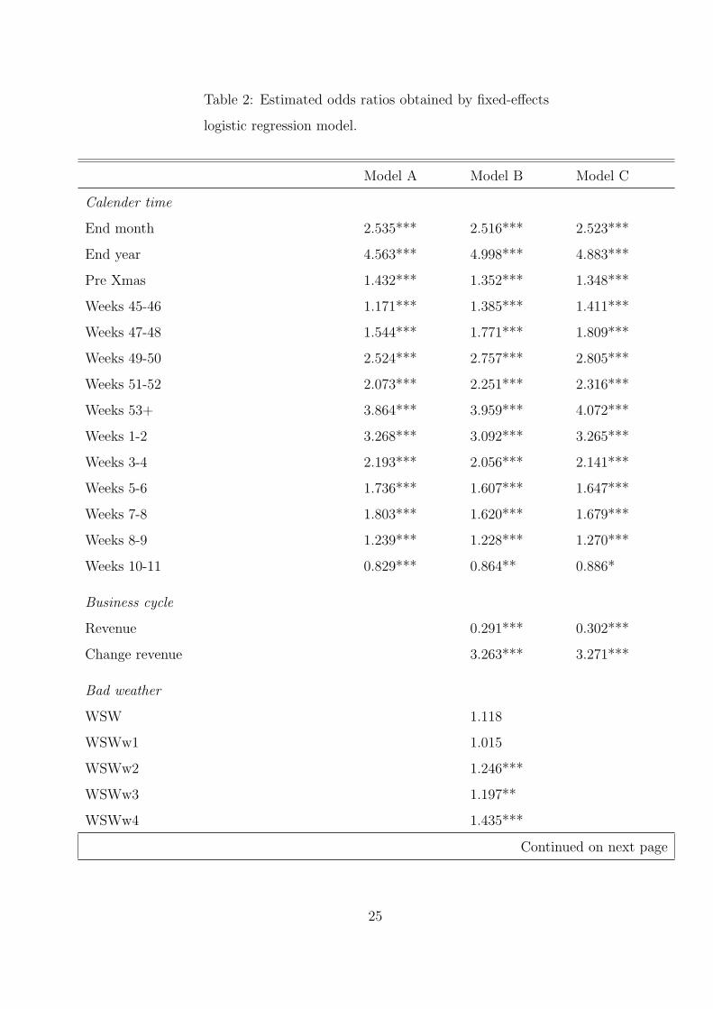
Table 2: Estimated odds ratios obtained by fixed-effects
logistic regression model.
Model A Model B Model C
Calender time
End month 2.535*** 2.516*** 2.523***
End year 4.563*** 4.998*** 4.883***
Pre Xmas 1.432*** 1.352*** 1.348***
Weeks 45-46 1.171*** 1.385*** 1.411***
Weeks 47-48 1.544*** 1.771*** 1.809***
Weeks 49-50 2.524*** 2.757*** 2.805***
Weeks 51-52 2.073*** 2.251*** 2.316***
Weeks 53+ 3.864*** 3.959*** 4.072***
Weeks 1-2 3.268*** 3.092*** 3.265***
Weeks 3-4 2.193*** 2.056*** 2.141***
Weeks 5-6 1.736*** 1.607*** 1.647***
Weeks 7-8 1.803*** 1.620*** 1.679***
Weeks 8-9 1.239*** 1.228*** 1.270***
Weeks 10-11 0.829*** 0.864** 0.886*
Business cycle
Revenue 0.291*** 0.302***
Change revenue 3.263*** 3.271***
Bad weather
WSW 1.118
WSWw1 1.015
WSWw2 1.246***
WSWw3 1.197**
WSWw4 1.435***
Continued on next page
25

Table 2 – continued from previous page
Model A Model B Model C
Policy regime base effect
SWG 1.618*** 1.575***
WAG I 1.703*** 1.728***
WAG II 1.486*** 1.330***
WAG III 1.382*** 1.411***
Interaction of policy regime and bad weather
SWG × WSW 1.096
WAG I × WSW 0.607
WAG II × WSW 1.052
WAG III × WSW 1.301**
SWG and ...
WSWw1 1.013
WSWw2 1.238**
WSWw3 1.241**
WSWw4 1.454***
WAG I and ...
WSWw1 1.709
WSWw2 1.965
WSWw3 1.741
WSWw4 2.277*
WAG II and ...
WSWw1 1.183
WSWw2 1.757**
WSWw3 1.325
WSWw4 2.288***
WAG III and ...
WSWw1 0.874
Continued on next page
26

Table 2 – continued from previous page
Model A Model B Model C
WSWw2 0.854
WSWw3 0.866
WSWw4 1.015
Number of obs = 2,750,395
Number of groups = 10,426
Obs per group: min = 2, avg = 263.8, max = 1,251
Log Likelihood -74,850 -74,887 -74,879
Significance levels: ***: 1% **: 5% *: 10%
Note: results for year dummies not reported (all models)
results for season dummies shown in Figure 7 (model A)
Model A also suggests another interesting finding. The odds of experiencing a transition to
unemployment is much higher at fixed calender times such as the end of a month or week as
well as the one to two weeks prior to Christmas. We also find a strong bi-weekly pattern of
unemployment inflows during the winter period. Of course these patterns could to some extent
reflect the effects of weather conditions, which are not accounted for in model A. However, theses
strong result patterns with regard to these fixed calender times remain robust when including
the relevant indicators (as done in models B and C). Therefore, consistent with our hypothesis in
section 2, we find strong evidence for layoffs being strongly determined by fixed calender times.
In the public debate, weather conditions have been considered as a major determinant of
seasonal unemployment. In fact, adverse weather conditions are the prime justification for the peak
in the unemployment rate during the winter period as shown in Figure 1 and the introduction of
all-season employment promotion measures. Model B is therefore a first attempt to disentangle the
impact of weather conditions, the business cycle and the legal setup by simultaneously controlling
for all these factors.
The estimation results for model B suggest that adverse weather conditions significantly in-
crease unemployment risks only if there have been more than two weeks of such conditions in the
27

Figure 7: Estimated odds ratio of experiencing a transition to unemployment (Model A). Reference
level is the summer period in 2001.
0.0000
0.5000
1.0000
1.5000
2.0000
2.5000
3.0000
3.5000
1981
1982
1983
1984
1985
1986
1987
1988
1989
1990
1991
1992
1993
1994
1995
1996
1997
1998
1999
2000
2001
2002
2003
2004
Od
ds R
atio
Summer period Winter period
current winter season. Moreover, the odds of experiencing a transition to unemployment further
increases with an extended period of four or more weeks of adverse weather conditions. Neverthe-
less, the impact of weather conditions appears minor compared to most calender times, a finding
that is robust with respect to other model specifications which we do not present. However, this
may partly reflect that the employment promotion during the statutory winter period has to some
extent already made the construction sector weather-proof (e.g. stronger dismissal protection in
presence of bad weather). The impact of weather conditions might have been stronger in absence
of employment promotion measures prior to our observation period. As an additional explana-
tion, the impact of weather conditions may have been partly exaggerated and confused with other
factors such as empty order books. In fact, unemployment risks strongly decline with increasing
revenue levels in the construction sector (keeping the percentage change constant). Moreover, the
partial effect of an annual percentage change in revenues is not significant during the summer (and
has therefore not been included in the model) while it is significantly positive during the winter.
In years of increasing revenues (given the same revenue level), firms thus seem to hire additional
28

workers that do not belong to the core personnel and that are laid off in the subsequent winter
period. Thus, we do find a strong and plausible impact of the business cycle on the inflow into
unemployment.
In reference to the summer period, unemployment risks are significantly higher during the
statutory winter period as captured by the four regimes of employment promotion in model B.
Note that we do not observe a time period prior to the introduction of employment promotion
regimes so that we can only compare the relative effectiveness of the four regimes in reducing
individual layoffs. In particular, compared to SWG and WAG I unemployment risks appear lower
during winter periods in which flexible working time approaches have been implemented (WAG
II and WAG III). Furthermore, differences between SWG and WAG III and WAG I and WAG II/
WAG III are highly significant, indicating that the last two regimes may have been more effective
in cushioning the impact of adverse work conditions during the winter period. This ranking of
employment promotion regimes is in line with the hypothesis in section 2 since WAG II and WAG
III relieve firms of some of the financial risk of a shortfall of work compared to SWG and especially
WAG I.
As a major limitation, model B does not yield any insights on the effect of the employment
regimes depending on weather conditions. According to the discussion in section 2, the cushion-
ing effect of certain regimes may wear off at a varying speed with accumulating adverse weather
conditions during a winter season. In particular, the cushioning effect should wear off faster, the
faster a firm’s total cost of maintaining an employment relationship increase with accumulating
shortfall hours due to adverse weather conditions. Model C thus extends the previous specification
by interacting the four legal regimes with weather conditions in the current week and cumulative
weather conditions in the present season. Findings for the other covariates are mainly unaffected
by this extension so that we concentrate on the interpretation of these interaction effects. Table
3 eases this interpretation by not only showing the odds ratio of the SWG regime and its inter-
actions with weather conditions, but by also displaying the corresponding differences to the three
alternative regimes and their significance levels.
29
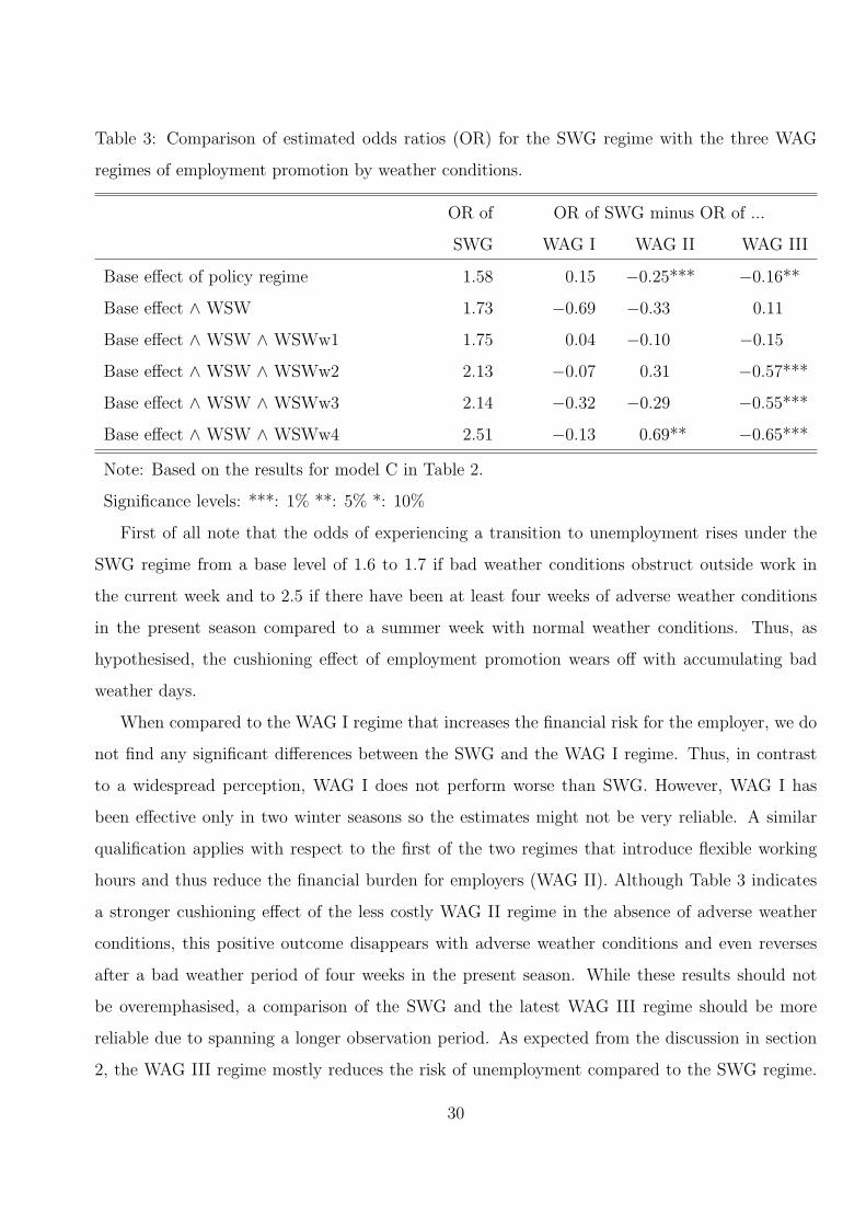
Table 3: Comparison of estimated odds ratios (OR) for the SWG regime with the three WAG
regimes of employment promotion by weather conditions.
OR of OR of SWG minus OR of ...
SWG WAG I WAG II WAG III
Base effect of policy regime 1.58 0.15 −0.25*** −0.16**
Base effect ∧ WSW 1.73 −0.69 −0.33 0.11
Base effect ∧ WSW ∧ WSWw1 1.75 0.04 −0.10 −0.15
Base effect ∧ WSW ∧ WSWw2 2.13 −0.07 0.31 −0.57***
Base effect ∧ WSW ∧ WSWw3 2.14 −0.32 −0.29 −0.55***
Base effect ∧ WSW ∧ WSWw4 2.51 −0.13 0.69** −0.65***
Note: Based on the results for model C in Table 2.
Significance levels: ***: 1% **: 5% *: 10%
First of all note that the odds of experiencing a transition to unemployment rises under the
SWG regime from a base level of 1.6 to 1.7 if bad weather conditions obstruct outside work in
the current week and to 2.5 if there have been at least four weeks of adverse weather conditions
in the present season compared to a summer week with normal weather conditions. Thus, as
hypothesised, the cushioning effect of employment promotion wears off with accumulating bad
weather days.
When compared to the WAG I regime that increases the financial risk for the employer, we do
not find any significant differences between the SWG and the WAG I regime. Thus, in contrast
to a widespread perception, WAG I does not perform worse than SWG. However, WAG I has
been effective only in two winter seasons so the estimates might not be very reliable. A similar
qualification applies with respect to the first of the two regimes that introduce flexible working
hours and thus reduce the financial burden for employers (WAG II). Although Table 3 indicates
a stronger cushioning effect of the less costly WAG II regime in the absence of adverse weather
conditions, this positive outcome disappears with adverse weather conditions and even reverses
after a bad weather period of four weeks in the present season. While these results should not
be overemphasised, a comparison of the SWG and the latest WAG III regime should be more
reliable due to spanning a longer observation period. As expected from the discussion in section
2, the WAG III regime mostly reduces the risk of unemployment compared to the SWG regime.
30

In particular, we have a significantly lower unemployment risk under the WAG III regime in the
absence of adverse weather conditions. Somewhat cautiously, one might interpret this as some
evidence that the expectation of possible shortfalls of work in the winter period triggers less
anticipating layoffs under the flexible working time regime WAG III than under the bad weather
allowance scheme SWG. With incipient bad weather conditions, however, differences between
WAG III and SWG at first turn insignificant, but strongly increase with a prolonged period of
adverse weather conditions. If adverse weather conditions prevail for at least two weeks in a present
winter season, the odds ratio under the WAG III regime is significantly lower by around −0.6.
These estimates have a causal interpretation if there are no relevant trends other than the business
cycle which affect the probability of lay-off. For this reason, we have also estimated a model with
a linear time trend to proxy for technological change. While this trend had a significantly positive
effect, our main results remained unchanged. Although it is difficult to verify that trends are not
correlated with the policy regime periods under investigation, we do not find evidence that our
results are seriously biased.
Our estimation results therefore suggest that the flexibilisation of working hours by means of
working hours accounts and the corresponding reduction of the fiscal burden a shortfall of work
means to employers has been effective in reducing weather-induced seasonal layoffs compared to
the long-standing SWG regime. In fact, our results indicate that seasonal unemployment has
become less dependent on weather conditions under the most favourable regime WAG III. Layoff
probabilities no longer significantly increase with prolonged periods of adverse weather conditions
as suggested by the corresponding interaction effects in Table 2. The construction sector under the
WAG III regime has thus turned largely weather-proof. The increasing seasonal unemployment
during the last observed years can thus not be attributed to a failure of the legal regime, but
seems to be dominated by macro developments with regard to the declining business environment
and a possible crowding out of domestic workers by mainly illegal foreign workers. Most of the
increase in unemployment transitions thus seems captured by the year dummies for 2002 to 2004
that are much higher than in the previous years (see Figure 7).
Furthermore, note that even under the most effective regime WAG III, the odds of experiencing
a layoff during the winter period is significantly higher than during the summer period (base effect
of 1.4). This suggests that a substantial share of seasonal layoffs is unrelated to either weather
conditions or the business cycle. One explanation for this finding could be that employers prefer to
31

permanently layoff workers (e.g. due to retirement) during the winter period as another adjustment
mechanism to the seasonal character of construction work. This could also explain the mass
points of layoffs at fixed calender times during the winter period and would indicate that a certain
level of seasonal unemployment is unlikely to disappear even with the most effective employment
promotion measure. We created a variable indicating a very hard winter by comparing cumulative
bad weather days to the average number over the whole observation period. Surprisingly we found
that unemployment risks are not systematically higher during extremely adverse winter periods.
This is further evidence for a planned capacity reduction by firms. We also estimated a model
where we interacted fixed calender times with the regimes. As several weather and regime related
coefficients in this model loose significance, we concluded that such a specification is too flexible
so that we do not report results here.
We finish this section by briefly summarising the main findings for the individual level variables
from the pooled estimation (see Table 4, Appendix). Since all variables are dummy variables, it is
possible to relate them directly. Having had a previous unemployment period strongly increases
the incidence of unemployment. In addition, having already had a recall in the past weakens the
effect in the summer while it strongly increases the effect during the winter. Interestingly, there
is some evidence for discrimination against foreign nationals. Information on the citizenship is
sometimes missing in the data even after imputing previous or future values from the individ-
ual employment biographies. For this reason we create a dummy for unknown citizenship. The
coefficient on this variable is highly positive but more research on data quality is necessary to un-
derstand the composition of this group (German/non German). We observe a significant increase
in unemployment risk for older employees with longer entitlement lengths for unemployment ben-
efits after the late 1980s. We do not obtain evidence that the 1997 reform of the unemployment
benefit system was able to offset these developments. Unemployment risk decreases if tenure is
more than one year and strongly increases if the worker’s wage is in the lowest quintile of the pop-
ulation wage distribution. The situation for low wage workers became even worse during the late
1990s. With the introduction of the Posted Worker Act, the German government has introduced
minimum wages in several sub sectors of the construction sector such as electrical installation,
roofing etc. Since the minimum wage regulations treat only parts of the workforce during specific
periods of time, they can be analysed with a difference in differences setup (see also Konig and
Moller, 2008). Unfortunately, we only have access to highly aggregated business sector level in-
32

formation and therefore cannot distinguish between the relevant business sub sector on firm level.
However, we interacted the sub sector minimum wage regulation periods by the profession of the
workers (roofer, painter,...) to proxy for the specific business sub sectors. Our resulting difference
in differences estimates are mainly insignificant. Therefore, similar to Konig and Moller (2008)
we do not obtain empirical evidence for strong effects of the introduction of minimum wages on
employment stability. The increase in unemployment risks for low paid workers therefore has to
be explained by other reasons such as a shift of low paid employment subject to social security
contributions towards other forms of employment. However, more detailed analysis using less
aggregated data would be required to analyse this question in greater detail.
6 Conclusion
Avoiding seasonal unemployment and the corresponding unemployment compensation payments is
desirable both from a fiscal as well as a political perspective. A number of European countries have
thus adopted some form of all-season employment promotion in the construction sector. However,
to the best of our knowledge, there has been no attempt to assess the effectiveness of such measures
in preventing seasonal layoffs so far. In Germany, recent years have seen several reforms that shifted
the financial burden of a seasonal labour slack back and forth between employers, workers and the
unemployment insurance fund. In particular, there has been a major shift from a system based
on mainly publicly funding a weather allowance to a system that promotes the additional use of
working hours accounts. For two of the main approaches of promoting all-season employment in the
European construction sector, the regime shifts in Germany thus constitute a prime opportunity
for comparing the effectiveness of such measures in preventing seasonal layoffs. Based on an
extensive daily panel of individual employment histories, this paper examined the impact of the
changing legal setup on individual layoff probabilities conditional on rich information concerning
the regional business cycle as well as local weather conditions. Our analysis thus disentangled the
main determinants of a seasonal layoff that due to a lack of profound microeconometric research
have often been confused in the public debate. Our analysis suggests the following main findings:
• The inflow into unemployment is lower in case of a favourable business environment measured
by revenues in the construction sector. However, layoff risks are higher during winters that
33

follow a boom year with increasing revenues, thus indicating the previous hiring of additional
workers that do not belong to the core personnel.
• The impact of weather conditions is significant, but less strong than expected. Adverse
weather conditions significantly increase seasonal unemployment, but do so only if adverse
weather conditions accumulate for at least two weeks during the winter season. This suggests
that all employment promotion regimes during the observation period reduce seasonal layoffs
due to a stronger dismissal protection in presence of bad weather as well as some financial
compensation.
• A large fraction of layoffs takes place at fixed calender times during the winter period even
when controlling for weather conditions and the business cycle. Moreover, the impact of
weather conditions is much weaker compared to the impact of fixed calender times.
• The different regimes of promoting all-season employment are heterogeneously effective in
reducing individual unemployment risks. In particular, the longstanding bad weather al-
lowance (SWG) that is financed mainly by both the unemployment insurance fund and
by employers turns out to significantly increase layoffs compared to the introduction of a
winter allowance in addition to the use of working hours accounts (WAG III). Moreover,
WAG III reduces unemployment risks in the absence as well as presence of (prolonged) ad-
verse weather conditions. In fact, WAG III appears to make the construction sector less
weather-dependent since prolonged periods of adverse weather conditions no longer affect
unemployment transitions under this legal regime.
At the same time, the fiscal burden on the part of the Federal Employment Agency of promoting
all-season employment has been lower under the WAG III than under the SWG regime. The
combination of working hours accounts for the first shortfall hours with a winter allowance that is
paid by the employer and the unemployment insurance after the shortfall of working hours exceeds
some threshold thus is an improvement in many respects: lower seasonal unemployment and more
stable employment relationships at lower public expenditures.
These outcomes can be achieved because some of the financial burden of a weather-induced
shortfall of work is now borne by the workers. With declining labour demand conditions since
the late 1990s, workers were apparently willing to accept these cutbacks in exchange for stable
34

employment. However, high ability workers may not be willing to accept these deals and may thus
leave the construction sector permanently. This may also be one of the reasons why - despite our
positive assessment - WAG III was abolished in 2006 and replaced by the Saisonkurzarbeitergeld,
a legal setup that is even more generous in publicly compensating for shortfall hours than the
long-standing weather allowance, but that tries to promote the use of flexible working hours by
additional economic incentives. Since we do not have access to post 2006 data, we are not able to
evaluate the most recent reform. This is left to future research as well as an attempt to evaluate
the cost efficiency of all year employment promotion programs. For this purpose, it would be
advantageous to observe a comparable winter period without any all year employment promoting
policy. Unfortunately, this is not provided in the case of Germany and therefore our analysis cannot
shed light on this. Moreover, our analysis could be complemented by looking at the effect of the
institutional setup on hires in the construction sector. If employers anticipate high costs during
the winter, they may adjust their hiring practices by extending or shrinking their core personnel.
In addition, future research should look at the length of seasonal unemployment periods under
the different regimes since a reduction in the incidence of unemployment may be balanced out by
an increase in the duration. Our findings, however, indicate that layoffs tend to occur only once
per season so that a reduced layoff probability is likely to be a major indicator of the effectiveness
of an all-season employment promotion program in reducing the seasonal unemployment.
Given these open questions, we would like to encourage scholars from countries with equivalent
policy schemes to perform a similar analysis. It would be interesting to explore whether the effect of
local weather on seasonal layoffs is more important in Nordic countries, the Netherlands, Canada
or other German speaking countries. Moreover, it would be interesting to perform a detailed
empirical analysis to compare a situation in absence of any employment promoting policy with
the outcome in a more regulated labour market.
35

References
[1] Baltagi, B.H. (2005), Econometric Analysis of Panel Data, 3rd Edition, Wiley.
[2] Bosch, G. and Philips, P. (Eds.) (2003), Building Chaos. An International Comparison of
Deregulation in the Construction Industry, Routledge, London/New York.
[3] Bosch, G. and Zuhlke-Robinet, K. (2000), Der Bauarbeitsmarkt. Soziologie und konomie einer
Branche, Campus Verlag, Frankfurt.
[4] Bosch, G. and Zuhlke-Robinet, K. (2003), The Labor Market in the German Construction
Industry, in: Bosch, G. and Philips, P. (Eds.), Building Chaos. An International Comparison
of Deregulation in the Construction Industry, Routledge, London/New York.
[5] Burdett, K. and Wright, R. (1989), Optimal Firm Size, Taxes and Unemployment, Journal of
Public Economics, Vol. 39, 275–287.
[6] Deutscher Bundestag (2002), Unterrichtung durch die Bundesregierung: Bericht der Bun-
desregierung ber die Umsetzung des Gesetzes zur Neuregelung der Frderung der ganzjhrigen
Beschaftigung in der Bauwirtschaft, Deutscher Bundestag Drucksache 14/8477, Berlin, Ger-
many.
[7] Drews, N. (2008), Das Regionalfile der IAB-Beschaftigtenstichprobe 1975-2004, FDZ Metho-
denreport No. 02/2008, IAB Nurnberg.
[8] Feldstein, M. (1976), Temporary Layoffs in the Theory of Unemployment. The Journal of
Political Economy, Vol. 84, 937–957.
[9] Grady, P. and Kapsalis, C. (2002), The Approach to Seasonal Unemployment in the Nordic
Countries: A Comparison with Canada, MPRA Paper No. 2991, Munchen, Germany.
[10] King, G. and Zheng, L. (2001), Logistic Regression in Rare Events Data. Political Analysis,
Vol. 9(2), 137–63.
[11] Konig, M. and Moller, J. (2008), Mindestlohneffekte des Entsendegesetzes? - Eine Mikro-
datenanalyse fur die Deutsche Bauwirtschaft. Zeitschrift fur Arbeitsmarktforschung Vol. 41(2),
327–346.
36

[12] Mavromaras, K. and Orme, C.D. (2004), Temporary Layoff Unemployment: A Split Popula-
tion Model, Journal of Applied Econometrics, Vol. 19, 49–67.
[13] Mavromaras, K. and Rudolph, H. (1995), Recalls - Wiederbeschaftigung im alten Betrieb
(Recalls - re-employment in the same firm), Mitteilungen aus der Arbeitsmarkt und Berufs-
forschung. Vol. 28, 171–194.
[14] Mavromaras, K. and Rudolph, H. (1998), Temporary Separations and Firm Size in the Ger-
man Labour Market, Oxford Bulletin of Economics and Statistics. Vol. 60 (2), 215–225.
[15] Plaßmann, G. (2002), Der Einfluss der Arbeitslosenversicherung auf die Arbeitslosigkeit in
Deutschland. Beitrage zur Arbeitsmarkt- und Berufsforschung, 255, Institut fur Arbeitsmarkt-
und Berufsforschung der Bundesanstalt fur Arbeit (IAB), Nurnberg, Germany.
[16] RKW (2003), Development of a catalog of intruments and measures for achieving the even
utilization of construction capacities on the basis of experiences from Germany and selected
European countries, final report, Rationalisierungs- und Innovationszentrum der Deutschen
Wirtschaft e.V., Eschborn, Germany.
[17] Roed, K. and Nordberg, M. (2003), Temporary Layoffs and the duration of unemployment,
Labour Economics, Vol. 10, 381–398.
[18] Solomou, S. and Wu, W. (1997), The Impact of Weather on the Construction Sector Output
Variations, 1955-1989, DAE Working Papers No. 9722, University of Cambridge, Cambridge,
UK.
[19] Wilke, R.A. (2005), New Estimates of the Duration and Risk of Unemployment for West-
Germany, Schmollers Jahrbuch, Vol. 128(2), 207–237.
[20] Wooldridge, J. (2002), Econometric Analysis of Cross Section and Panel Data, MIT Press.
[21] Zuhlke-Robinet, K. (1998), Von der Schlechtwettergeld-Regelung zu Arbeitszeitkonten im
Bauhauptgewerbe, Discussion Paper Institut Arbeit und Technik, Gelsenkirchen, Germany.
37

Appendix
Table 4: Effect of individual level variables on unemployment risks in the west German constructionsector. Symbolic results derived from pooled logistic regression with 7,089,948 observations.
variable name effect variable name effectfemale - aged <26 +aged 51-55 0 aged >55 -aged 51-55 & >24 months employment - aged >55 & >24 months employment -ext UIB entitlements for aged 51-55 in1987-1997
0 ext UIB entitlements for aged >55 in1987-1997
+
ext UIB entitlements for aged 51-55 af-ter 1997
+ ext UIB entitlements for aged >55 after1997
+
previous unemployment ++ previous unemployment and winter 0same employer before previous unem-ployment
– same employer before previous unem-ployment and winter
++
foreign citizen + unknown citizenship ++blue collar + blue collar and winter +previous employment 6-12 months 0 previous employment >12 months –low wage ++ low wage after 1997 +construction worker after 1997 + roofer after 1997 0electrician after 1997 - painter after 2003 +min wage construction 0 min wage roofer 0min wage electrician 0 min wage painter -
Legend: ++ strong positive effect, + positive effect, 0 negligible effect, - negative effect, −− strongnegative effect
38

Figure 8: Map of German counties - 28 western and 7 eastern German counties for which repre-sentative weather information is available are mapped in dark grey.
39


![48216 Baack Final Proof [FM]](https://static.fdokumen.com/doc/165x107/631bfe5b3e8acd997705b218/48216-baack-final-proof-fm.jpg)