How Good is Phase-Shift Keying for Peak-Limited Rayleigh Fading Channels in the Low-SNR Regime

arX

iv:c

s/05

0812

1v1

[cs.

IT]

27 A

ug 2

005

1

How Good is Phase-Shift Keying for Peak-Limited

Rayleigh Fading Channels in the Low-SNR Regime?

Wenyi Zhang,Student Member, IEEE, and J. Nicholas Laneman,Member, IEEE

Abstract

This paper investigates the achievable information rate ofphase-shift keying (PSK) over frequency

non-selective Rayleigh fading channels without channel state information (CSI). The fading process

exhibits general temporal correlation characterized by its spectral density function. We consider both

discrete-time and continuous-time channels, and find theirasymptotics at low signal-to-noise ratio (SNR).

Compared to known capacity upper bounds under peak constraints, these asymptotics usually lead to

negligible rate loss in the low-SNR regime for slowly time-varying fading channels. We further specialize

to case studies of Gauss-Markov and Clarke’s fading models.

I. INTRODUCTION

For Rayleigh fading channels without channel state information (CSI) at low signal-to-noise

ratio (SNR), the capacity-achieving input gradually tendsto bursts of “on” intervals sporadically

inserted into the “off” background, even under vanishing peak power constraints [1]. This highly

unbalanced input usually imposes implementation challenges. For example, it is difficult to

maintain carrier frequency and symbol timing during the long “off” periods. Furthermore, the

unbalanced input is incompatible with linear codes, unlessappropriate symbol mapping (e.g.,

M-ary orthogonal modulation with appropriately chosen constellation sizeM) is employed to

match the input distribution.

This work has been supported in part by the State of Indiana through the 21st Century Research Fund, by the National Science

Foundation through contract ECS03-29766, and by the Fellowship of the Center for Applied Mathematics of the Universityof

Notre Dame. Some preliminary results in this work were presented in part at the IEEE International Workshop on Signal

Processing Advances for Wireless Communication (SPAWC), New York, 2005.

The authors are with Department of Electrical Engineering,University of Notre Dame. Email:wzhang1,[email protected]

January 9, 2014 DRAFT

http://arxiv.org/abs/cs/0508121v1

2

This paper investigates the achievable information rate ofphase-shift keying (PSK). PSK is

appealing because it has constant envelope and is amenable to linear codes without additional

symbol mappings. Focusing on low signal-to-noise ratio (SNR) asymptotics, we utilize a recursive

training scheme to convert the original fading channel without CSI into a series of parallel

sub-channels, each with estimated CSI but additional noisethat remains circular complex white

Gaussian. The central results in this paper are as follows. First, for a discrete-time channel whose

unit-variance fading processhd[k] : −∞ < k < ∞ has a spectral density functionShd(ejΩ)

for −π ≤ Ω ≤ π, the achievable rate is(1/2) ·[

(1/2π) · ∫ π−π S2

hd(ejΩ)dΩ − 1

]

· ρ2 + o(ρ2) nats

per symbol, as the average channel SNRρ → 0. This achievable rate is at most(1/2) · ρ2 +

o(ρ2) away from the channel capacity under peak SNR constraintρ. Second, for a continuous-

time channel whose unit-variance fading processhc(t) : −∞ < t < ∞ has a spectral density

function Shc(jω) for −∞ < ω < ∞, the achievable rate as the input symbol durationT → 0 is

[

1 − (1/2πP ) · ∫∞−∞ log (1 + P · Shc(jω)) dω

]

·P nats per unit time, whereP > 0 is the envelope

power. This achievable rate exactly coincides with the channel capacity under peak envelopeP .

We further apply the above results to specific case studies ofGauss-Markov fading models (both

discrete-time and continuous-time) as well as a continuous-time Clarke’s fading model. For

discrete-time Gauss-Markov fading processes with innovation rateǫ ≪ 1, the quadratic behavior

of the achievable rate becomes dominant only forρ ≪ ǫ. Our results, combined with previous

results for the high-SNR asymptotics, suggest that coherent communication can essentially be

realized forǫ ≤ ρ ≤ 1/ǫ. For Clarke’s model, we find that the achievable rate scales sub-linearly,

but super-quadratically, asO (log(1/P ) · P 2) nats per unit time asP → 0.

The remainder of this paper is organized as follows. SectionII describes the channel model

and the recursive training scheme. Section III deals with the discrete-time channel model, and

Section IV the continuous-time channel model. Finally Section V provides some concluding

remarks. Throughout the paper, random variables are in boldfont. All the logarithms are to base

e, and information units measured in nats.


3

II. CHANNEL MODEL, RECURSIVE TRAINING SCHEME, AND EFFECTIVE SNR

We consider a scalar time-selective, frequency non-selective Rayleigh fading channel, written in

baseband-equivalent continuous-time form as

x(t) = hc(t) · s(t) + z(t), for −∞ < t < ∞, (1)

where s(t) ∈ C and x(t) ∈ C denote the channel input and the corresponding output at time

instant t, respectively. The additive noisez(t) : −∞ < t < ∞ is modeled as a zero-mean

circular complex Gaussian white noise process withEz(s)z†(t) = δ(s−t). The fading process

hc(t) : −∞ < t < ∞ is modeled as a wide-sense stationary and ergodic zero-meancircular

complex Gaussian process with unit varianceEhc(t)h†c(t) = 1 and with spectral density

functionShc(jω) for −∞ < ω < ∞. Additionally, we impose a technical condition thathc(t) :

−∞ < t < ∞ is mean-square continuous, so that its autocorrelation function Khc(τ) =

Ehc(t + τ)h†c(t) is continuous forτ ∈ (−∞,∞).

Throughout the paper, we restrict our attention to PSK over the continuous-time channel (1).

For technical convenience, we let the channel inputs(t) have constant envelopeP > 0 and

piecewise constant phase,i.e.,

s(t) = s[k] =√

P · ejθ[k], if kT ≤ t < (k + 1)T,

for −∞ < k < ∞1. The symbol durationT > 0 is determined by the reciprocal of the channel

input bandwidth2.

Applying the above channel input to the continuous-time channel (1), and processing the channel

output through a matched filter3, we obtain a discrete-time channel

x[k] =√

ρ · hd[k] · s[k] + z[k], for −∞ < k < ∞. (2)

1Here we note a slight abuse of notation in this paper, that a symbol (e.g., s) can be either continuous-time or discrete-time.

The two cases are distinguished by·(t) for continuous-time and·[k] for discrete-time.

2For multipath fading channels,T should also be substantially greater than the delay spread [2], otherwise the frequency

non-selective channel model (1) may not be valid. Throughout the paper we assume that this requirement is met.

3A matched filter suffers no information loss for white Gaussian channels [3]. For the fading channel (1), it is no longer

optimal in general [4]. However, in this paper we still focuson the matched filter, which is common in most practical systems.


4

The channel equations (1) and (2) are related through

s[k] = ejθ[k]

x[k] =1√T

∫ (k+1)T

kTx(t)dt

z[k] =1√T

∫ (k+1)T

kTz(t)dt

hd[k] =1

√∫ T0

∫ T0 Khc

(s − t)dsdt

∫ (k+1)T

kThc(t)dt.

For the discrete-time channel (2) we can verify that

• The additive noisez[k] : −∞ < k < ∞ is circular complex Gaussian with zero mean

and unit variance,i.e., z[k] ∼ CN (0, 1), and is independent, identically distributed (i.i.d.)

for different k.

• The fading processhd[k] : −∞ < k < ∞ is wide-sense stationary and ergodic zero-mean

circular complex Gaussian, withhd[k] being marginallyCN (0, 1). We further notice that

hd[k] : −∞ < k < ∞ is obtained through sampling the output of the matched filter,

hence its spectral density function is

Shd(ejΩ) =

1√∫ T0

∫ T0 Khc

(s − t)dsdt·

∞∑

k=−∞Shc

(

jΩ − 2kπ

T

)

· sinc2(Ω − 2kπ)

for −π ≤ Ω ≤ π.

• The channel inputs[k] : −∞ < k < ∞ is always on the unit circle. In the sequel, we

will further restrict it to be complex proper [5],i.e., Es2[k] = [Es[k]]2. The simplest

such input is quadrature phase-shift keying (QPSK); by contrast, binary phase-shift keying

(BPSK) is not complex proper.

• The average channel SNR is given by

ρ =P

T·(∫ T

0

∫ T

0Khc

(s − t)dsdt

)

> 0. (3)

Throughout the paper, we assume that the realization of the fading processhc(t) : −∞ < t <

∞ is not directly available to the transmitter or the receiver, but its statistical characterization

in terms ofShc(jω) is precisely known at both the transmitter and the receiver.

We employ a recursive training scheme to communicate over the discrete-time channel (2). By

interleaving the transmitted symbols as illustrated in Figure 1 (cf. [6]), the recursive training


5

... ... ......

0 1

L L + 1

L − 1

2L − 1

2L 3L − 1

(K − 1)L .........

......

......

......

2L + 1

KL − 1......

. . . . . .

. . . . . .

. . . . . .

......

......

......

PSC0 PSC1 PSCL−1

L parallel sub-channels (PSC)

len

gth

-Kco

din

gb

lock

s

Fig. 1. Illustration of the interleaving scheme. Input symbols are encoded/decoded column-wise, and transmitted/received

row-wise.

scheme effectively converts the original non-coherent channel into a series of parallel sub-

channels, each with estimated receive CSI but additional noise that remains i.i.d. circular complex

Gaussian. The interleaving scheme decomposes the channel into L parallel sub-channels (PSC).

The lth (l = 0, 1, . . . , L − 1) PSC sees all the inputss[k · L + l] of (2) for k = 0, 1, . . . , K − 1.

TheseL PSCs suffer correlated fading, and this correlation is exactly what we seek to exploit

using recursive training. Although some residual correlation remains within each PSC among its

K symbols, due to the ergodicity of the channel (2), this correlation vanishes as the interleaving

depthL → ∞. In practical systems with finiteL, if necessary, we may utilize an additional

interleaver for each PSC to make it essentially memoryless.

We make a slight abuse of notation in the sequel. Since all thePSCs are viewed as memoryless,

when describing a PSC we can simply suppress the internal index k among itsK coding

symbols, and only indicate the PSC indexl without loss of generality. For example,hd[l] actually

corresponds to anyhd[k · L + l], for k = 0, 1, . . . , K − 1.

The recursive training scheme performs channel estimationand demodulation/decoding in an

alternating manner. To initialize transmission, PSC 0, thefirst parallel sub-channel, transmits

pilots rather than information symbols to the receiver. Based upon the received pilots in PSC

0, the receiver predictshd[1], the fading coefficient of PSC 1, and proceeds to demodulate and


6

decode the transmitted symbols in PSC 1 coherently. If the rate of PSC 1 does not exceed

the corresponding channel mutual information, then information theory ensures that, as the

coding block lengthK → ∞, there always exist codes that have arbitrarily small decoding

error probability. Hence the receiver can, at least in principle, form an error-free reconstruction

of the transmitted symbols in PSC 1, which then effectively become “fresh” pilots to facilitate

the prediction ofhd[2] and subsequent coherent demodulation/decoding of PSC 2. Alternating

the estimation-demodulation/decoding procedure repeatedly, all the PSCs are reliably decoded

one after another.

Remark: A major drawback of the recursive training scheme is that itsinterleaved structure

typically leads to a large delay. The coding block lengthK should be large enough such that the

decoding error probability is small enough to prevent catastrophic error propagation along the

PSCs. Furthermore, the number of PSCsL should also be large enough such that the prediction

of the fading process essentially converges to its steady-state limit. Only after receiving all the

K · L symbols in the interleaved block can the receiver perform the alternating estimation-

demodulation/decoding procedure. However, we note that this may not be the case for wideband

channels. In wideband channels with frequency-decorrelated fading processes, we can employ

multi-carrier techniques,e.g., orthogonal frequency-division multiplexing (OFDM), to decompose

the original wide bandwidth into a large number of sub-bands, suffering essentially independent

frequency non-selective fading processes. In this case, each row in Figure 1 corresponds to

a sub-band, and the coding block length (i.e., the number of sub-bands)K increases as the

bandwidth grows. For each PSC, itsK coding symbols occur simultaneously in physical time,

hence the receiver need not wait until receiving all theK ·L symbols to perform the alternating

estimation-demodulation/decoding procedure.

By induction, let us consider PSCl, assuming that the inputss[i] : i = 0, 1, . . . , l − 1 of the

previous PSCs have all been successfully reconstructed at the receiver. Since the channel inputs

are always on the unit circle, the receiver can compensate for their phases in the channel outputs,

and the resulting observations become

e−jθ[i] · x[i]︸︷︷︸

x′[i]

=√

ρ · hd[i] + e−jθ[i] · z[i]︸︷︷︸

z′[i]

for i = 0, 1, . . . , l − 1.

Since zero-mean circular complex Gaussian distributions are invariant under rotation, the rotated


7

noisez′[i] is still i.i.d. zero-mean unit-variance circular complex Gaussian. Then we can utilize

standard linear prediction theory (e.g., [7]) to obtain the one-step minimum mean-square error

(MMSE) prediction ofhd[l] defined as

hd[l] = E hd[l] | x′[i] : i = 0, 1, . . . , l − 1 . (4)

The estimatehd[l] and the estimation errorhd[l] = hd[l] − hd[l] are jointly circular complex

Gaussian distributed asCN (0, 1 − σ2[l]) andCN (0, σ2[l]), respectively, and are uncorrelated and

further independent. Hereσ2[l] denotes the mean-square prediction error. The channel equation

of PSCl can then be written as

x[l] =√

ρ · hd[l] · s[l] + z[l]

=√

ρ · hd[l] · s[l] +√

ρ · hd[l] · s[l] + z[l]︸︷︷︸

z[l]

, (5)

where the effective noisez[l] is circular complex Gaussian, and is independent of both the

channel inputs[l] and the estimated fading coefficienthd[l]. Thus, the channel (5) becomes a

coherent Gaussian channel with fading and receive CSIhd[l], with effective SNR

ρ[l] =1 − σ2[l]

σ2[l] · ρ + 1· ρ. (6)

In the paper we mainly focus on the ultimate performance limit without delay constraints, which

is achieved as the interleaving depthL → ∞. Under mild technical conditions, the one-step

MMSE prediction error sequenceσ2[l] : l = 0, 1, . . . converges to the limit [8, Chap. XII, Sec.

4]

σ2∞

def= lim

l→∞σ2[l] =

1

ρ·

exp

1

2π

∫ π

−πlog

(

1 + ρ · Shd(ejΩ)

)

dΩ

− 1

. (7)

Consequently the effective SNR (6) sequenceρ[l] : l = 0, 1, . . . converges to

ρ∞def= lim

l→∞ρ[l] =

1 − σ2∞

σ2∞ · ρ + 1

· ρ. (8)

We are mainly interested in evaluating the mutual information of the induced channel (5) at the

limiting effective SNRρ∞ as the actual channel SNRρ → 0. This low-SNR channel analysis

is facilitated by the explicit second-order expansion formulas of the channel mutual information


8

at low SNR [9]. Applying [9, Theorem 3] to the induced channel4 (5) at ρ∞, we have

Rdef= lim

l→∞I(

s[l];x[l] | hd[l])

= ρ∞ − ρ2∞ + o(ρ2) as ρ → 0. (9)

III. A SYMPTOTIC CHANNEL MUTUAL INFORMATION AT LOW SNR

As shown in (9), the asymptotic channel mutual information depends on the limiting effective

SNR (8), which further relates to the limiting one-step MMSEprediction error (7). The following

theorem evaluates the asymptotic behavior of the channel mutual information (9).

Theorem 3.1: For the discrete-time channel (2), asρ → 0, its induced channel (5) achieves the

rate

R =1

2

[1

2π

∫ π

−πS2

hd(ejΩ)dΩ − 1

]

· ρ2 + o(ρ2), (10)

if the integral(1/2π) · ∫ π−π S2

hd(ejΩ)dΩ exists.

Proof: We will prove that

σ2∞ = 1 − 1

2

[1

2π

∫ π

−πS2

hd(ejΩ)dΩ − 1

]

· ρ + o(ρ), (11)

which together with (8) leads to

ρ∞ =1

2

[1

2π

∫ π

−πS2

hd(ejΩ)dΩ − 1

]

· ρ2 + o(ρ2).

Then (10) immediately follows from (9).

For simplicity let us denote byg(ρ) the integral(1/2π) · ∫ π−π log

(

1 + ρ · Shd(ejΩ)

)

dΩ, hence

limρ→0

g(ρ) =1

2π

∫ π

−πlog 1dΩ = 0

limρ→0

dg(ρ)

dρ=

1

2π

∫ π

−πShd

(ejΩ)dΩ = 1

limρ→0

dg2(ρ)

d2ρ= − 1

2π

∫ π

−πS2

hd(ejΩ)dΩ.

4Note that [9, Theorem 3] is only applicable to complex properchannel inputs, as we have assumed in the channel model.


9

To prove (11), we apply l’Hospital’s rule in (7) to evaluate

limρ→0

σ2∞ = lim

ρ→0

eg(ρ) − 1

ρ

= limρ→0

eg(ρ) · dg(ρ)

dρ= 1;

limρ→0

d(σ2∞)

dρ= lim

ρ→0

[

eg(ρ)

ρ· dg(ρ)

dρ− eg(ρ) − 1

ρ2

]

= limρ→0

eg(ρ) ·(

dg(ρ)

dρ

)2

+ eg(ρ) · dg2(ρ)

d2ρ− eg(ρ)

2ρ· dg(ρ)

dρ

=1

2limρ→0

eg(ρ) ·(

dg(ρ)

dρ

)2

+ eg(ρ) · dg2(ρ)

d2ρ

= −1

2

[1

2π

∫ π

−πS2

hd(ejΩ)dΩ − 1

]

.

Substituting the above quantities into the first-order Taylor expansion ofσ2∞, we then obtain

(11). Q.E.D.

Theorem 3.1 states that for PSK at low SNR, the achievable channel mutual information vanishes

quadratically with SNR. This is consistent with [10] [11]. Furthermore, it is of particular interest

to compare the asymptotic expansion (10) with several previous results.

A. Comparison with a Capacity Upper Bound

For the discrete-time channel (2), PSK with constant SNRρ is a particular peak-limited channel

input. The capacity per unit energy of channel (2) under a peak SNR constraintρ is [1]

C = 1 − 1

2πρ·∫ π

−πlog

(

1 + ρ · Shd(ejΩ)

)

dΩ, (12)

achieved by on-off keying (OOK) in which each “on” or “off” symbol corresponds to an infinite

number of channel uses, and the probability of choosing “on”symbols vanishes. Such “bursty”

channel inputs are in sharp contrast to PSK. From (12), an upper bound to the channel capacity

can be derived as [1]

C ≤ U(ρ)def=

1

2· 1

2π

∫ π

−πS2

hd(ejΩ)dΩ · ρ2. (13)

Comparing (10) and (13), we notice that the penalty of using PSK instead of the bursty capacity-

achieving channel input is at most(1/2) · ρ2 + o(ρ2). For fast time-varying fading processes,


10

this penalty can be relatively significant. For instance, ifthe fading process is memoryless,i.e.,

Shd(ejΩ) = 1 for −π ≤ Ω ≤ π, then (1/2π) · ∫ π

−π S2hd

(ejΩ)dΩ − 1 = 0, implying that no

information can be transmitted using PSK over a memoryless fading channel. Fortunately, for

slowly time-varying fading processes, the integral(1/2π) · ∫ π−π S2

hd(ejΩ)dΩ is typically much

greater than1, as we will illustrate in the sequel.

B. Comparison with the High-SNR Channel Behavior

From (10) and (13), it can be said that(1/2π) · ∫ π−π S2

hd(ejΩ)dΩ is a fundamental quantity

associated with a fading process at low SNR. This is in contrast to the high-SNR regime, where

a fundamental quantity is [12]

σ2pred

def= exp

1

2π

∫ π

−πlog Shd

(ejΩ)dΩ

.

The quantityσ2pred is the one-step MMSE prediction error ofhd[0] given its entire noiseless past

hd[−1],hd[−2], . . .. Whenσ2pred > 0 the process is said to be regular; and whenσ2

pred = 0 it is

said to be deterministic, that is, the entire futurehd[0],hd[1], . . . can be exactly reconstructed

(in the mean-square sense) by linearly combining the entirepasthd[−1],hd[−2], . . .. It has

been established in [12] [13] that, for regular fading processes,

C = log log ρ − 1 − γ + log1

σ2pred

+ o(1) as ρ → ∞, (14)

whereγ = 0.5772 . . . is Euler’s constant, and for deterministic fading processes,

C

log ρ→ 1

2π· µ(

Ω : Shd(ejΩ) = 0

)

as ρ → ∞, (15)

whereµ(·) denotes the Lebesgue measure on the interval[−π, π].

It is then an interesting issue to investigate the connection between(1/2π) · ∫ π−π S2

hd(ejΩ)dΩ and

σ2pred. However, as the following two examples reveal, there is no explicit relationship between

these two quantities.

1) Example 1: Even a deterministic fading process can lead to poor low-SNR performance:

Consider the following class of spectral density functionsShd(ejΩ) as illustrated in Figure 2:

Shd(ejΩ) =

nn−1

if |Ω| ≤ π − πn

0 if π − πn

< |Ω| ≤ π, n = 2, 3, . . .


11

00

1

π −π π − π/n −π + π/n

n/(n − 1)

Ω

Sh

d(e

jΩ)

Fig. 2. Spectral density function of a deterministic fadingprocess that leads to poor low-SNR performance. The narrow

notches on the spectrum make the process deterministic, while the remaining almost unit spectrum makes it behave as if nearly

memoryless in the low-SNR regime for largen.

SinceShd(ejΩ) = 0 for certain intervals with non-zero measure, the corresponding fading process

is deterministic withσ2pred = 0 [8]. However, this class ofShd

(ejΩ) leads to

1

2π

∫ π

−πS2

hd(ejΩ)dΩ =

n

n − 1→ 1 as n → ∞,

resulting in vanishing values of the quadratic coefficient in (10).

2) Example 2: Even an almost memoryless fading process can lead to good low-SNR perfor-

mance: Consider the following class of spectral density functionsShd(ejΩ) as illustrated in

Figure 3:

Shd(ejΩ) =

n if |Ω| ≤ πn√

n√n−1√

n−1/nif π

n√

n< |Ω| ≤ π

, n = 2, 3, . . .

For largen the fading process becomes almost memoryless since

σ2pred = exp

log n

n√

n+ log

√n − 1√

n − 1/n· (1 − 1

n√

n)

→ 1 as n → ∞.

However, this class ofShd(ejΩ) also leads to

1

2π

∫ π

−πS2

hd(ejΩ)dΩ =

√n + (1 − 1

n√

n) ·( √

n − 1√n − 1/n

)2

→ ∞

asn → ∞.


12

001

n

(n1/2 − 1)/(n1/2 − 1/n)

−π π Ω = π/(n3/2) Ω

Sh

d(e

jΩ)

Fig. 3. Spectral density function of an almost memoryless fading process that leads to good low-SNR performance. The almost

unit spectrum makes the process nearly memoryless, while the narrow impulse-like spectrum peak significantly contributes to

the integral(1/2π) ·∫ π

−πS2

hd(ejΩ)dΩ, leading to good low-SNR performance for largen.

C. Case Study: Discrete-Time Gauss-Markov Fading Processes

In this subsection, we apply Theorem 3.1 to analyze a specificclass of discrete-time fading

processes, namely, the discrete-time Gauss-Markov fadingprocesses. The fading process in the

channel model can be described by a first-order auto-regressive (AR) evolution equation of the

form

hd[k + 1] =√

1 − ǫ · hd[k] +√

ǫ · v[k + 1], (16)

where the innovation sequencev[k] : −∞ < k < ∞ consists of i.i.d.CN (0, 1) random

variables, andv[k + 1] is independent ofhd[i] : −∞ < i ≤ k. The innovation rateǫ satisfies

0 < ǫ ≤ 1.

The spectral density functionShd(ejΩ) for such a process is

Shd(ejΩ) =

ǫ

(2 − ǫ) − 2√

1 − ǫ · cos Ω, −π ≤ Ω ≤ π. (17)

Hence

1

2π

∫ π

−πS2

hd(ejΩ)dΩ =

ǫ2

2π

∫ π

−π

1(

(2 − ǫ) − 2√

1 − ǫ · cos Ω)2dΩ =

2

ǫ− 1.


13

Applying Theorem 3.1, we find that for the discrete-time Gauss-Markov fading model,

R =(

1

ǫ− 1

)

· ρ2 + o(ρ2) as ρ → 0. (18)

For practical systems in which the fading processes are underspread [2], the innovation rateǫ

typically ranges from1.8× 10−2 to 3× 10−7 [14]. So the(1/2) · ρ2 + o(ρ2) rate penalty of PSK

with respect to optimal, peak-limited signaling may well beessentially negligible at low SNR.

Due to the simplicity of the discrete-time Gauss-Markov fading model, we are able to carry out

a non-asymptotic analysis to gain more insight. Applying (17) to (7), the steady-state limiting

channel prediction error is

σ2∞ =

(ρ − 1) · ǫ +√

(ρ − 1)2 · ǫ2 + 4ρǫ

2ρ. (19)

Further applying (19) to (8), we can identify the following three qualitatively distinct operating

regimes of the induced channel (5) for smallǫ ≪ 1:

• The quadratic regime: Forρ ≪ ǫ, σ2∞ ≈ 1 − ρ/ǫ, ρ∞ ≈ ρ2/ǫ;

• The linear regime: Forǫ ≪ ρ ≪ 1/ǫ, σ2∞ ≈

√

ǫ/ρ, ρ∞ ≈ ρ;

• The saturation regime: For1/ǫ ≪ ρ, σ2∞ ≈ ǫ, ρ∞ ≈ 1/ǫ.

Figure 4 illustrates these three regimes forǫ = 10−4. The different slopes ofρ∞ on the log-log

plot are clearly visible for the three regimes. The linear regime covers roughly80 dB, from−40

dB to +40 dB, in this particular example.

An interesting observation is that the two SNR thresholds dividing the three regimes are deter-

mined by a single parameterǫ, which happens to be the one-step MMSE prediction errorσ2pred

for the discrete-time Gauss-Markov fading process. The1/ǫ threshold dividing the linear and the

saturation regimes coincides with that obtained in [14], where it is obtained for circular complex

Gaussian inputs with nearest-neighbor decoding. In this paper we investigate PSK, which results

in a penalty in the achievable rate at high SNR. More specifically, it can be shown that the

achievable rate forρ ≫ 0 behaves like(1/2) · log minρ, 1/ǫ + O(1) [15].

A further observation relevant to low-SNR system design is that, theǫ threshold dividing the

quadratic and the linear regimes clearly indicates when thelow-SNR asymptotic channel behavior

becomes dominant. Since the innovation rateǫ for underspread fading processes is typically small,


14

−60 −40 −20 0 20 40 60−100

−50

0

50

the quadraticregime

the saturationregime

the linear regime

the linear regime

ρ (dB)

ρ∞

(dB

)

Fig. 4. Case study of the discrete-time Gauss-Markov fadingmodel: Illustration of the three operating regimes,ǫ = 10−4.

we essentially have a low-SNR channel with perfect receive CSI aboveρ = ǫ. This suggests

that there may be an “optimal” SNR at which the low-SNR capacity limit is the most closely

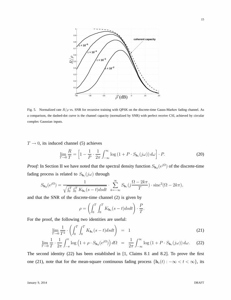
approached. Figure 5 plots the normalized achievable rateR/ρ vs. SNR, in which the achievable

rateR is numerically evaluated for the induced channel (5) using QPSK. Although all the curves

vanish rapidly below the thresholdρ = ǫ, for certainρ > ǫ, the normalized achievable rate can

be reasonably close to1. For example, takingǫ = 10−4, the “optimal” SNR isρ ≈ −15 dB, and

the corresponding normalized achievable rate is above0.9, i.e., more than90% of the low-SNR

capacity limit is achieved.

IV. FILLING THE GAP TO CAPACITY BY WIDENING THE INPUT BANDWIDTH

In Section III we have investigated the achievable information rate of the discrete-time channel

(2), which is obtained from the continuous-time channel (1)as described in Section II. The

symbol durationT there is a fixed system parameter. In this section we will showthat, if we are

allowed to reduceT , i.e., widen the input bandwidth, then the recursive training scheme using

PSK achieves an information rate that is asymptotically consistent with the channel capacity

under peak envelopeP . More specifically, we have the following theorem.

Theorem 4.1: For the continuous-time channel (1) with envelopeP > 0, as the symbol duration


15

−40 −30 −20 −10 0 10 200

0.1

0.2

0.3

0.4

0.5

0.6

0.7

0.8

0.9

1

ε = 10−2

ε = 10−3

ε = 10−4

ε = 10−5

coherent capacity

ρ (dB)

R/ρ

Fig. 5. Normalized rateR/ρ vs. SNR for recursive training with QPSK on the discrete-time Gauss-Markov fading channel. As

a comparison, the dashed-dot curve is the channel capacity (normalized by SNR) with perfect receive CSI, achieved by circular

complex Gaussian inputs.

T → 0, its induced channel (5) achieves

limT→0

R

T=[

1 − 1

P· 1

2π

∫ ∞

−∞log (1 + P · Shc

(jω)) dω]

· P. (20)

Proof: In Section II we have noted that the spectral density function Shd(ejΩ) of the discrete-time

fading process is related toShc(jω) through

Shd(ejΩ) =

1√∫ T0

∫ T0 Khc

(s − t)dsdt·

∞∑

k=−∞Shc

(jΩ − 2kπ

T) · sinc2(Ω − 2kπ),

and that the SNR of the discrete-time channel (2) is given by

ρ =

(∫ T

0

∫ T

0Khc

(s − t)dsdt

)

· P

T.

For the proof, the following two identities are useful:

limT→0

1

T 2·(∫ T

0

∫ T

0Khc

(s − t)dsdt

)

= 1 (21)

limT→0

1

T· 1

2π

∫ π

−πlog

(

1 + ρ · Shd(ejΩ)

)

dΩ =1

2π

∫ ∞

−∞log (1 + P · Shc

(jω))dω. (22)

The second identity (22) has been established in [1, Claims 8.1 and 8.2]. To prove the first

one (21), note that for the mean-square continuous fading processhc(t) : −∞ < t < ∞, its


16

autocorrelation functionKhc(τ) = Ehc(t+τ)h†

c(t) is continuous for all−∞ < τ < ∞. Hence

for any T > 0, there existsT ∗ ∈ [0, T ] such that∫ T

0

∫ T

0Khc

(s − t)dsdt = Khc(T ∗) · T 2

→ Khc(0) · T 2 = T 2 as T → 0.

Now substituting (21) and (22) into (7), we have

σ2∞ =

1

ρ·

exp

1

2π

∫ π

−πlog

(

1 + ρ · Shd(ejΩ)

)

dΩ

− 1

=1

ρ·

exp

1

2π

∫ ∞

−∞log (1 + P · Shc

(jω)) dω · T + o(T )

− 1

=1

ρ·[

1

2π

∫ ∞

−∞log (1 + P · Shc

(jω))dω · T + o(T )]

=1

P· 1

2π

∫ ∞

−∞log (1 + P · Shc

(jω)) dω + o(1) as T → 0.

That is,

limT→0

σ2∞ =

1

P· 1

2π

∫ ∞

−∞log (1 + P · Shc

(jω)) dω. (23)

Then substituting (21) and (23) into (8), we have

limT→0

ρ∞T

= limT→0

(1 − σ2∞) · ρ

(σ2∞ · ρ + 1) · T

=[

1 − 1

P· 1

2π

∫ ∞

−∞log (1 + P · Shc

(jω)) dω]

· P. (24)

Finally Theorem 4.1 immediately follows from substituting(24) into (9).Q.E.D.

Again we compare the asymptotic achievable rate (20) to a capacity upper bound based upon

the capacity per unit energy. For the continuous-time channel (1), the capacity per unit energy

under a peak envelope constraintP > 0 is [1]

C = 1 − 1

2πP·∫ ∞

−∞log (1 + P · Shc

(jω)) dω, (25)

and the related capacity upper bound (measured per unit time) is [1]

C ≤ U(P )def=

[

1 − 1

2πP·∫ ∞

−∞log (1 + P · Shc

(jω))dω]

· P. (26)

Comparing (20) and (26), it is surprising to notice that these two quantities coincide. Recalling

that in Section III we have noticed a(1/2) · ρ2 + o(ρ2) rate penalty in discrete-time channels,


17

we conclude that widening the input bandwidth eliminates this penalty and essentially results in

an asymptotically capacity-achieving scheme in the wideband regime5.

The channel capacity of continuous-time peak-limited wideband fading channels (20) was origi-

nally obtained in [16]. However, in [16] the capacity is achieved by frequency-shift keying (FSK),

which is bursty in frequency. In our Theorem 4.1, we show thatthe capacity is also achievable

if we employ recursive training and PSK, which is bursty in neither time nor frequency.

After some manipulations of (20), we further have that

• As P → 0,

limT→0(R/T )

P 2→ 1

2· 1

2π

∫ ∞

−∞S2

hc(jω)dω, (27)

if the above integral exists.

• As P → ∞,

limT→0(R/T )

P→ 1. (28)

In the sequel we will see that (27) and (28) are useful for asymptotic analysis.

A. An Intuitive Explanation of Theorem 4.1

In our proof of Theorem 4.1, we have utilized identities (21)and (22) to conveniently relate the

continuous-time channel (1) to the discrete-time channel (2). However, these identities also have

concealed much of the intuition contained in the derivation. To further illustrate the underlying

mechanism in Theorem 4.1, here we give an alternative argument. Although the following

reasoning is not mathematically rigorous, it does provide an intuitive way to understand the

channel behavior as the symbol durationT → 0.

In Section II, we have described the conversion from the continuous-time channel (1) to the

discrete-time channel (2). Strictly speaking, the discrete-time fading coefficienthd[k] is thekth

sample of the matched-filtered, continuous-time fading process. The matched-filtering effect can

5Again, the same caveat as in footnote 2 applies.


18

be viewed as averaginghc(t) within a symbol interval of lengthT . Since we have assumed

that the continuous-time fading processhc(t) : −∞ < t < ∞ is mean-square continuous in

t, roughly speaking, asT → 0, the discrete-time fading coefficienthd[k] ≈ hc(kT ), and the

SNR per symbolρ ≈ P · T . Furthermore, compared to sufficiently smallT , the fading process

hc(t) : −∞ < t < ∞ can be viewed as essentially band-limited. So the discrete-time fading

processhd[k] : −∞ < k < ∞ is approximately the sampled continuous-time fading process

hc(t) : −∞ < t < ∞ with sampling rate well beyond its Nyquist rate, and we may write

Shd(ejΩ) ≈ (1/T ) · Shc

(jΩ/T ) for −π ≤ Ω ≤ π.

Now let us apply the above approximations to (7) to evaluateσ2∞ for small T :

σ2∞ =

1

ρ·

exp

1

2π

∫ π

−πlog

(

1 + ρ · Shd(ejΩ)

)

dΩ

− 1

≈ 1

P · T ·

exp

1

2π

∫ π

−πlog

(

1 + P · Shc(j

Ω

T))

dΩ

− 1

=1

P · T ·

exp

1

2π

∫ π/T

−π/Tlog (1 + P · Shc

(jΩ)) dΩ · T

− 1

≈ 1

P · T ·

exp

1

2π

∫ ∞

−∞log (1 + P · Shc

(jω)) dω · T

− 1

≈ 1

P · T · 1

2π

∫ ∞

−∞log (1 + P · Shc

(jω)) dω · T =1

P· 1

2π

∫ ∞

−∞log (1 + P · Shc

(jω)) dω,

which is the same as (23) in our proof.

B. Case Study: The Continuous-Time Gauss-Markov Fading Model

In this subsection, we apply Theorem 4.1 to analyze the continuous-time Gauss-Markov fading

processes. Such a process has autocorrelation function

Khc(τ) = (1 − ǫc)

|τ |/2,

where the parameter0 < ǫc ≤ 1 characterizes the channel variation, analogously toǫ for the

discrete-time case in Section III. The spectral density function of the process is

Shc(jω) =

| log(1 − ǫc)|ω2 + (log(1 − ǫc))

2 /4.


19

−40 −30 −20 −10 0 10 20 30 4010

−8

10−6

10−4

10−2

100

102

104

P (dB)

lim

T→

0(R

/T)

Fig. 6. The asymptotic achievable ratelimT→0(R/T ) vs. the envelopeP , for recursive training with complex proper PSK on

the continuous-time Gauss-Markov fading channel with innovation rateǫc = 0.9. The dashed-dot curves indicate the limiting

behaviors for small and largeP .

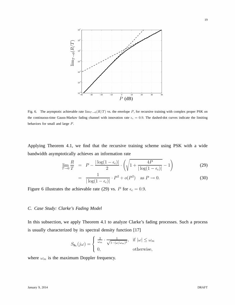
Applying Theorem 4.1, we find that the recursive training scheme using PSK with a wide

bandwidth asymptotically achieves an information rate

limT→0

R

T= P − | log(1 − ǫc)|

2·(√

1 +4P

| log(1 − ǫc)|− 1

)

(29)

=1

| log(1 − ǫc)|· P 2 + o(P 2) as P → 0. (30)

Figure 6 illustrates the achievable rate (29) vs.P for ǫc = 0.9.

C. Case Study: Clarke’s Fading Model

In this subsection, we apply Theorem 4.1 to analyze Clarke’sfading processes. Such a process

is usually characterized by its spectral density function [17]

Shc(jω) =

2ωm

· 1√1−(ω/ωm)2

, if |ω| ≤ ωm

0, otherwise,

whereωm is the maximum Doppler frequency.


20

−40 −30 −20 −10 0 10 20 30 4010

−10

10−8

10−6

10−4

10−2

100

102

104

P (dB)

lim

T→

0(R

/T)

Fig. 7. The asymptotic achievable ratelimT→0(R/T ) vs. the envelopeP , for recursive training with complex proper PSK on

Clarke’s fading channel with maximum Doppler frequencyωm = 100. The dashed-dot curves indicate the limiting behaviors

for small and largeP .

Applying Theorem 4.1, we find that

limT→0

R

T=

ωm

π·

log ωm

P−√

1 − (2P/ωm)2 · logωm·[

1+√

1−(2P/ωm)2]

2P

, if P ≤ ωm/2

ωm

π·

log ωm

P+√

(2P/ωm)2 − 1 · arctan√

(2P/ωm)2 − 1

, if P > ωm/2.

(31)

For largeP , the asymptotic behavior of (31) is consistent with (28). For small P , however, the

integral in (27) diverges, hence the asymptotic behavior of(31) scales super-quadratically with

P . After some manipulations of (31), we find that

limT→0

R

T=

2

πωm· log

1

P· P 2 + O(P 2) as P → 0. (32)

Figure 7 illustrates the achievable rate (31) vs.P for ωm = 100. We notice that, for smallP ,

the asymptotic expansion (32) is accurate.

V. CONCLUDING REMARKS

For fading channels that exhibit temporal correlation, a key to enhancing communication per-

formance is efficiently exploiting the implicit CSI embedded in the fading processes. From the

preceding developments in this paper, we see that a recursive training scheme, which performs


21

channel estimation and demodulation/decoding in an alternating manner, accomplishes this job

reasonably well, especially when the channel fading variesslowly. The main idea of recursive

training is to repeatedly use decisions of previous information symbols as pilots, and to ensure

the reliability of these decisions by coding over sufficiently long blocks.

Throughout this paper, we restrict the channel inputs to complex proper PSK, which is not

optimal in general for Rayleigh fading channels without CSI. There are two main motivations

for this choice. First, compared to other channel inputs such as circular complex Gaussian,

PSK leads to a significant simplification of the analytical developments. As we saw, recursive

training with PSK converts the original fading channel without CSI into a series of parallel sub-

channels, each with estimated receive CSI but additional noise that remains circular complex

white Gaussian. In this paper we mainly investigate the steady-state limiting channel behavior;

however, it may worth mentioning that, using the induced channel model presented in Section II,

exact evaluation of the transient channel behavior is straightforward, with the aid of numerical

methods.

Second, PSK inputs perform reasonably well in the moderate to low SNR regime. This is due to

the fact that, for fading channels with perfect receive CSI,as SNR vanishes, channel capacity can

be asymptotically achieved by rather general complex proper inputs besides circular complex

Gaussian [9]. The main contribution of our work is that it clearly separates the effect of an

input peak-power constraint and the effect of replacing optimal peak-limited inputs with PSK,

which is non-bursty in both time and frequency. It is shown that, for slowly time-varying fading

processes, the rate loss from PSK inputs is essentially negligible. Furthermore, as revealed by

the non-asymptotic analysis for discrete-time Gauss-Markov fading processes, there appear to

be non-vanishing SNRs at which near-coherent performance is attainable with recursive training

and PSK.

ACKNOWLEDGMENT

The authors are grateful to Shlomo Shamai (Shitz) for bringing to attention reference [16], and

for providing useful comments on this work.


22

REFERENCES

[1] V. Sethuraman and B. Hajek, “Capacity per Unit Energy of Fading Channels with a Peak Constraint,”IEEE Trans. Inform.

Theory, vol. 51, no. 9, pp. 3102–3120, Sept. 2005.

[2] E. Biglieri, J. Proakis, and S. Shamai (Shitz), “Fading Channels: Information-Theoretic and Communications Aspects,”

IEEE Trans. Inform. Theory, vol. 44, no. 6, pp. 2619–2692, Oct. 1998.

[3] J. G. Proakis,Digital Communications, McGraw-Hill, Inc., New York, third edition, 1995.

[4] T. Kailath, “Correlation Detection of Signals Perturbed by a Random Channel,”IEEE Trans. Inform. Theory, vol. 6, no.

3, pp. 361–366, June 1960.

[5] F. Neeser and J. L. Massey, “Proper Complex Random Processes with Applications to Information Theory,”IEEE Trans.

Inform. Theory, vol. 39, no. 4, pp. 1293–1302, July 1993.

[6] A. J. Goldsmith and P. P. Varaiya, “Capacity, Mutual Information, and Coding for Finite-State Markov Channels,”IEEE

Trans. Inform. Theory, vol. 42, no. 3, pp. 868–886, May 1996.

[7] T. Kailath, Lectures on Wiener and Kalman Filtering, Springer-Verlag, New York, 1981.

[8] J. L. Doob, Stochastic Processes, John Wiley & Sons, Inc., New York, 1953.

[9] V. V. Prelov and S. Verdu, “Second-Order Asymptotics of Mutual Information,” IEEE Trans. Inform. Theory, vol. 50, no.

8, pp. 1567–1580, Aug. 2004.

[10] M. Medard and R. G. Gallager, “Bandwidth Scaling for Fading Multipath Channels,”IEEE Trans. Inform. Theory, vol.

48, no. 4, pp. 840–852, Apr. 2002.

[11] B. Hajek and V. G. Subramanian, “Capacity and Reliability Function for Small Peak Signal Constraints,”IEEE Trans.

Inform. Theory, vol. 48, no. 4, pp. 828–839, Apr. 2002.

[12] A. Lapidoth, “On the Asymptotic Capacity of StationaryGaussian Fading Channels,”IEEE Trans. Inform. Theory, vol.

51, no. 2, pp. 437–446, Feb. 2005.

[13] A. Lapidoth and S. M. Moser, “Capacity Bounds via Duality with Applications to Multiple-Antenna Systems on Flat

Fading Channels,”IEEE Trans. Inform. Theory, vol. 49, no. 10, pp. 2426–2567, Oct. 2003.

[14] R. Etkin and D. N. C. Tse, “Degrees of Freedom in Underspread MIMO Fading Channels,”IEEE Trans. Inform. Theory,

May 2003, submitted; available athttp://www.eecs.berkeley.edu/∼dtse/raul hisnr.pdf.

[15] A. D. Wyner, “Bounds on Communication with Polyphase Coding,” Bell Sys. Tech. J., vol. 45, pp. 523–559, Apr. 1966.

[16] A. J. Viterbi, “Performance of an M-ary Orthogonal Communication System Using Stationary Stochastic Signals,”IEEE

Trans. Inform. Theory, vol. 13, no. 3, pp. 414–422, July 1967.

[17] W. C. Jakes and D. C. Cox, Eds.,Microwave Mobile Communications, IEEE Press, New York, 1994.


How Good is Phase-Shift Keying for Peak-Limited Rayleigh Fading Channels in the Low-SNR Regime

Documents

Transcript of How Good is Phase-Shift Keying for Peak-Limited Rayleigh Fading Channels in the Low-SNR Regime