Distributed Fading Memory for Stimulus Properties in the Primary Visual Cortex

Distributed Fading Memory for Stimulus Properties inthe Primary Visual CortexDanko Nikolic1,2.*, Stefan Hausler3., Wolf Singer1,2, Wolfgang Maass2,3

1 Department of Neurophysiology, Max-Planck-Institute for Brain Research, Frankfurt, Germany, 2 Frankfurt Institute for Advanced Studies (FIAS), Johann Wolfgang

Goethe University, Frankfurt, Germany, 3 Institute for Theoretical Computer Science, Graz University of Technology, Graz, Austria

Abstract

It is currently not known how distributed neuronal responses in early visual areas carry stimulus-related information. Wemade multielectrode recordings from cat primary visual cortex and applied methods from machine learning in order toanalyze the temporal evolution of stimulus-related information in the spiking activity of large ensembles of around 100neurons. We used sequences of up to three different visual stimuli (letters of the alphabet) presented for 100 ms and withintervals of 100 ms or larger. Most of the information about visual stimuli extractable by sophisticated methods of machinelearning, i.e., support vector machines with nonlinear kernel functions, was also extractable by simple linear classificationsuch as can be achieved by individual neurons. New stimuli did not erase information about previous stimuli. The responsesto the most recent stimulus contained about equal amounts of information about both this and the preceding stimulus.This information was encoded both in the discharge rates (response amplitudes) of the ensemble of neurons and, whenusing short time constants for integration (e.g., 20 ms), in the precise timing of individual spikes (#,20 ms), and persistedfor several 100 ms beyond the offset of stimuli. The results indicate that the network from which we recorded is endowedwith fading memory and is capable of performing online computations utilizing information about temporally sequentialstimuli. This result challenges models assuming frame-by-frame analyses of sequential inputs.

Citation: Nikolic D, Hausler S, Singer W, Maass W (2009) Distributed Fading Memory for Stimulus Properties in the Primary Visual Cortex. PLoS Biol 7(12):e1000260. doi:10.1371/journal.pbio.1000260

Academic Editor: Jonathan D. Victor, Weill Cornell Medical College, United States of America

Received June 22, 2009; Accepted November 10, 2009; Published December 22, 2009

Copyright: � 2009 Nikolic et al. This is an open-access article distributed under the terms of the Creative Commons Attribution License, which permitsunrestricted use, distribution, and reproduction in any medium, provided the original author and source are credited.

Funding: This work was supported by a grant from Deutsche Forschungsgemeinschaft (NI 708/2-1), by the German Federal Ministry of Education and Research(BMBF) within the ‘‘Bernstein Focus: Neurotechnology’’, through research grant 01GQ0840, Alexander von Humboldt Stiftung, and Hertie Stiftung. Additionalpartial support was obtained also from the Austrian Science Fund FWF # S9102-N13 and project # FP6-015879 (FACETS), project # FP7-216593 (SECO), andproject # FP7-506778 (PASCAL2) of the European Union. The funders had no role in study design, data collection and analysis, decision to publish, or preparationof the manuscript.

Competing Interests: The authors have declared that no competing interests exist.

Abbreviations: AUC, area under receiver-operating characteristics; I&F, integrate-and-fire; ISI, interspike interval; IT, inferotemporal; Mfr, mean firing rate; PSTH,peristimulus time histogram; RBF, radial basis function; RF, receptive field; SD, standard deviation; SVM, support vector machine; XOR, exclusive OR

* E-mail: [email protected]

. These authors contributed equally to this work.

Introduction

A number of analysis methods have been designed to investigate

how neuronal spiking activity correlates to sensory stimulation or

behavior and, as expected, many relations have been found. All of

the following variables—firing rates [1–4] and the synchronization

[4–7] and the differential timing of spiking activity [8–10]—have

been reported to correlate, one way or another, with stimuli and/

or with behavior. Most of the efforts to distinguish between

relevant and epiphenomenal variables face the problem that they

have to rely on correlative rather than causal evidence. In the

absence of direct access to the information of causal nature, one

way to begin addressing this issue is to complement the highly

specialized statistical methods that have been developed to detect

specific stimulus-related changes in responses [9,11–18] with

analyses that make minimal assumptions about putative codes

[19–21], and examine how much information can be extracted by

a single cortical neuron from the joint responses of its presynaptic

neurons and then find out which variables were carrying the

relevant information [22,23]. To adjust to the conditions under

which these cortical ‘‘readout’’ neurons are likely to operate, the

data must be presented to the readout units in parallel, i.e., the

responses of the putative feeding neurons must be recorded

simultaneously. Also, analysis and classification of data should

correspond to that conducted in real time. Thus, the results

should be available with short delays. Hence, the analysis method

should be allowed no more time for accumulating evidence than is

available for cortical neurons to accomplish their task. To fulfill

these requirements, readout neurons need to be simulated on a

computer and fed with data obtained in parallel recordings from

a large number of cortical neurons, the assumption being that a

certain fraction of these neurons provides input to neuronal

classification.

The present study was designed to fulfill these premises.

Applying multielectrode technology, we recorded simultaneously

from a large number of neurons in area 17 of lightly anesthetized

cats and evoked responses with brief sequences of different,

stationary flashed stimuli (letters of the alphabet). These responses

were then fed as inputs to artificial readout neurons simulated on a

computer (also referred to as classifiers). We first trained the

artificial neurons to classify the visual stimuli that have generated

the responses, and once the classification had reached criterion, we

PLoS Biology | www.plosbiology.org 1 December 2009 | Volume 7 | Issue 12 | e1000260

investigated which of the information-carrying variables were used

by these artificial—but neuron-inspired—readout systems. A

recent study provided evidence that an artificial readout system

can extract stimulus-specific information from the spiking activity

of neurons that were sequentially recorded from macaque

inferotemporal (IT) cortex [23]. However, in this study, responses

of different neurons that were supplied in parallel to the readout

system had been obtained by recording sequentially from the

different cells. This approach eliminates temporal relations

between neuronal responses that are not time locked to the

stimulus, but established by internal interactions (referred to also

as ‘‘noise correlation’’ [24]). Thus, it was not possible to determine

whether stimulus-specific information is encoded by internal

adjustment of spike timing, as this information cannot be retrieved

unless responses are recorded simultaneously.

In addition to the identification of response variables containing

stimulus-specific information, we were particularly interested in

determining the duration over which this information was

retrievable after the stimuli have disappeared. In case there was

evidence for ‘‘fading memory’’ already in primary visual cortex,

the data would allow for inferences on the mechanisms underlying

perceptual phenomena such as visual persistence and iconic

storage [25–29]. Moreover, the lack of evidence for fading

memory would provide an important constraint for hypotheses

on processing modes implemented in primary visual cortex.

Computer simulations of sparsely connected recurrent circuits of

neuron-like processing units [30–33] as well as theoretical analyses

of related circuits with simpler (linear) processing units [34,35]

have shown that systems with fading memory exhibit powerful

computational capabilities because they permit integration of

stimulus information over time. Negative evidence of fading

memory would render such models unlikely and support more

classical views that emphasize sequential step-by-step processing of

single frames resulting from a pipelined organization of the circuits

[36,37].

In order to distinguish between processing with or without

fading memory, we presented sequences of different stimuli and

investigated whether information about preceding stimuli was

erased by the presentation of subsequent stimuli or whether it

persisted. The latter case would provide strong evidence for the

existence of fading memory, whereas the former would be

supportive of models favoring frame-by-frame analysis of succes-

sive stimuli.

Results

MethodsWe used silicon-based multielectrodes (Michigan probes, see

Materials and Methods) to obtain highly parallel recordings from up

to 124 randomly selected neurons in the primary visual cortex (area

17) of lightly anesthetized cats. These neurons, most of which had

overlapping receptive fields (RFs), were activated by presenting

stationary flashed (100 ms) uppercase letters (A, B, C, D, and E). The

letters were always shown with maximal contrast and were either

presented singly, one per trial, or in a sequence of two or three (e.g.,

ABC; and a 100-ms blank interval between letters in most

experiments) (see Table S1 for experiments made on each cat).

The times at which letters were presented are indicated in all graphs

by gray rectangles. Each stimulation condition was presented 50 to

300 times in a randomized order.

To emulate classification processes realized with leaky integrate-

and-fire (I&F) readout neurons (but without reset or a refractory

period), the time stamps of discharge sequences were first convolved

with an exponentially decaying kernel (if not specified otherwise,

time constant, t = 20 ms) that mimicked the time course of

excitatory postsynaptic potentials (EPSPs) [38,39] (see Materials

and Methods). The continuous convolved signal was fed to the

classifier system, as illustrated in Figure 1C. If not specified

otherwise, the classification was made by a single I&F readout

whose activation, at a time point, t, was computed as the weighted

sum of the input signals at that time. The classifier ‘‘fired’’ (i.e.,

detected the stimulus) if its activation crossed a threshold. The

optimal weights and the firing thresholds of the classifiers were found

(learned) by applying support vector machines (SVM) with linear

kernels. All reported results were obtained from test datasets derived

from trials that were not part of the training datasets, only the latter

being used to adjust the input weights for the readout neurons (see

Materials and Methods for a 10-fold cross-validation scheme).

In a few additional analyses (reported later in ‘‘Superposition of

Information about Different Stimuli’’), we used also SVMs with

polynomial and radial basis function kernels to investigate whether

classification performance improved with these more sophisticated,

nonlinear transformations of the input variables. If not specified

otherwise, the results are reported for classifiers trained only on a

single instance in time, t, which were the values of the continuous

signal resulting from the convolution of the spike trains by the

exponential kernel (Figure 1C). The total number of values used to

train each classifier depended on the number of trials (see Table S2).

Thus, for most analyses, different classifiers were trained for each

time point along the trial, each classifier having its own unique set of

weights. These classifiers are denoted as Rt and should be

distinguished from Rint classifiers, which were trained to generalize

by using only one set of weights to classify neuronal responses over

longer periods of time (e.g., 100-ms or 300-ms long). In general, Rt

classifiers have better performance than Rint classifiers because a

single Rint classifier uses only one set of weights to accomplish

a number of different classification tasks, each taking place at a

different time point. A corresponding collection of Rt classifiers

approaches this problem by sharing the workload—each classifier

having its own set of weights optimized for the unique properties of

the responses at that time point, t. Consequently, the recent history

affecting the activity at time t imposes fewer constraints on the

Author Summary

Researchers usually assume that neuronal responses carryprimarily information about the stimulus that evoked theseresponses. We show here that, when multiple images areshown in a fast sequence, the response to an imagecontains as much information about the preceding imageas about the current one. Importantly, this memory capacityextends only to the most recent stimulus in the sequence.The effect can be explained only partly by adaptation ofneuronal responses. These discoveries were made with thehelp of novel methods for analyzing high-dimensional dataobtained by recording the responses of many neurons (e.g.,100) in parallel. The methods enabled us to study theinformation contents of neural activity as accessible toneurons in the cortex, i.e., by collecting information onlyover short time intervals. This one-back memory hasproperties similar to the iconic storage of visual informa-tion—which is a detailed image of the visual scene thatstays for a short while (,1 s) when we close our eyes. Thus,one-back memory may be the neural foundation of iconicmemory. Our results are consistent with recent detailedcomputer simulations of local cortical networks of neurons(‘‘generic cortical microcircuits’’), which suggested thatintegration of information over time is a fundamentalcomputational operation of these networks.

Distributed Fading Memory


Rt than on the Rint classifier, the latter having to accommodate

variability of response properties over an entire time interval. All

classifications were made as binary choices among two stimuli (such

as A and D), the chance level for correct classification being 50%. In

all graphs, the classification performance of Rt (Rint) readouts is

shown as percentage correct classifications of the presented stimulus

(see Materials and Methods for more details on experimental and

analysis procedures).

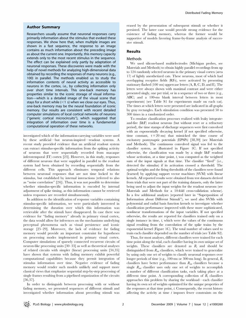
Figure 1. Experimental setup and illustration of the analysis method. (A) An example of a visual stimulus in relation to the constellation ofreceptive fields (rectangles) from one Michigan probe. (B) Upper part: spike times recorded from one neuron across 50 stimulus presentations and fortwo stimulus sequences (ABC and DBC). In this and in all other figures, the gray boxes indicate the periods during which the letter stimuli were visibleon the screen. Lower part: peristimulus time histogram (PSTH) for the responses of this neuron (5-ms bin size). (C) Left: spike trains obtainedsimultaneously from 66 neurons in one stimulation trial. Blue: the neuron for which all 50 trials are shown in (B). Right: for the classification analysis,each spike train is convolved with an exponential kernel (i.e., low-pass filtered). The spike trains for only six example neurons are shown. Red: examplevalues of the convolved trace that are used as inputs to the classifier (far right).doi:10.1371/journal.pbio.1000260.g001



High-Classification Performance and Fading MemoryHigh-classification performance. Figure 2 shows an

example for the classification performance when a single letter

is presented at a time. The classifiers achieved near perfect

performance in some experiments (in Figure 2A, close to 100%

correct at t = ,200–250 ms), in others, the performance stayed

reliably above chance level (Figure 2B). This high-classification

performance was achieved despite the high trial-to-trial variability

of the responses (see Materials and Methods). The main factor

influencing performance was the total number of spikes available

for the analysis. Classification was almost always better for datasets

with larger numbers of spikes. The classification shown in

Figure 2A was based on an average of 1,729 spikes per second

(62 units recorded simultaneously), whereas the classification in

Figure 2B had to be performed with only 874 spikes per second (49

units) (see Text S1 for more details on predictors of overall

classification performance).

This dependence of classification performance on spike counts

also held for stimulus-specific changes in firing rate. High rate

responses were associated with better classification performance

than weak responses. For the cases shown in Figure 2, best

classification performance was achieved at the times at which the

mean firing rates (Mfrs) had also the highest values. This

relationship is most clearly seen in Figure 2A, where the Mfr

shows a strong biphasic modulation in response to the on- and

offset of the stimulus. The initial increase in discharge rate at

,50 ms is associated with an increase in classification perfor-

mance, and the second, much larger increase in Mfr that peaks at

about 200–250 ms is associated with the highest level of

classification performance (approaching 100%). This correlation

between classification performance and Mfr is clearly expressed by

a positive value of Pearson’s coefficient of correlation (r = 0.91)

between Mfr and classification. Here, one needs to consider that

cortical neurons respond with latencies of 30–60 ms to light stimuli

[40]. Therefore, the stimulus-induced changes in Mfrs and the

corresponding changes of the classification performance are

always delayed relative to the stimuli (which are indicated by

gray rectangles in the figures).

In Figure 2B, the biphasic changes in rate responses are much

less pronounced than in Figure 2A. Consequently, the changes in

classification performance are also less pronounced, the correla-

tion between classification and Mfr remaining positive (r = 0.63).

The overall correlation for all investigated responses was 0.65.

Similar results were obtained for the Rint classifiers (see Figure S1).

Long-lasting persistence of information. A remarkable

finding was that information about stimulus identity did not

disappear quickly after the removal of the stimulus but was often

available for an extended period of time. In some cases, the

performance stayed above chance level for the entire duration of

our trials for which we initially recorded neuronal responses (i.e.,

700 ms after stimulus onset for the experiment shown in

Figure 2A). The results from the experiment summarized in

Figure 2B are similar. Although the classification performance

dropped considerably at about 400 ms in this experiment, the

performance nevertheless stayed above chance level for a large

part of the remaining duration of the trial. Therefore, the

information about the nature of stimuli appears to be available as

long as the neuronal firing rates stay elevated. Similar long-lasting

off-responses in area 17 and under anesthesia have been reported

previously ([41], pp. 108–109, 116). These results indicate clearly

that the information about stimuli persists long beyond the

disappearance of the stimuli, which allows us to investigate the

interactions with new stimuli presented after the offset of the first

stimulus.

To investigate whether these long-lasting responses were en-

trained (learned) during the stimulation procedure, we compared the

Figure 2. The ability of a linear classifier to determine the identity of the presented letters, A or D. The classification performance isshown (solid line) as a function of time passed from the presentation of the stimulus (at 0 ms) until the moment at which a sample of neuronalactivity was taken for training/testing the Rt classifier (the stimulus was removed at 100 ms). Dash-dotted line: the mean firing rate across the entirepopulation of investigated neurons. Dotted line: expected performance at chance level (50% correct). The shaded horizontal stripe around the dottedline covers the region of statistically nonsignificant deviations from the chance level (p.0.05), estimated by a label-shuffling test. In this and all otherfigures, the color of the stripe matches the color of the performance curve for which the statistical test was performed. (A and B) Two differentexperiments on different cats.doi:10.1371/journal.pbio.1000260.g002



peristimulus time histograms (PSTHs) to the sequences of flashed

letters early in the stimulation protocol (e.g., first 10 or 50 trials) with

those occurring late (e.g., last 10 or 50 trials). The Mfrs were similar

across all subsets of trials and always at least two times larger than

spontaneous activity, even 700 ms after stimulus onset (in the case of

cat 4, only 300 ms after stimulus onset), indicating that there was no

entrainment of these long-lasting responses. Moreover, the duration

of the elevated Mfrs in the off-responses were not specific to flashed

stimuli, as we observed a similar duration also for off-responses to

classical sinusoidal grating stimuli (Figure S2).

Sequences of StimuliResponses to a second letter in a sequence. In most of our

experiments, we presented not one but a series of three letters.

This made it possible to investigate whether new stimuli erase the

information about the preceding ones—akin to the masking effect

in iconic memory [26,27,29,42]—or alternatively, whether the

information about the new stimuli can coexist with and is

superimposed on the information about the preceding stimuli.

In all experiments, the classifiers could retrieve the information

about the first stimulus in the sequence, not only in the on- or off-

responses to that stimulus (i.e., up to 200 ms after its onset), but

also in the responses to a later stimulus in the sequence (i.e., from

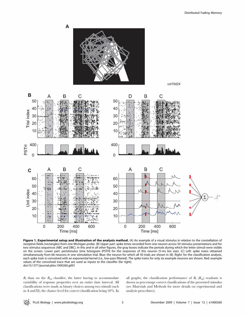
,250 ms onward). In some cases, even classification based on the

off-responses to the second stimulus approached 100% accuracy

for the identification of the first stimulus (Figure 3A, at ,380 ms).

See Figure 4D for classification performance over all experiments

made. Thus, when a novel letter was presented, the information

about the previously presented letter was not erased but was still

present in the responses to the novel stimulus and could be

extracted reliably by a linear I&F classifier. This suggests that the

second letter in a sequence produces none or only weak masking

effects on the information about the first letter.

As with the presentation of single letters, there was again a

strong positive correlation between classification performance and

Mfr. For the case exemplified in Figure 3A–3C, r-values were 0.45,

0.68, and 0.66, respectively (explained variance: 20%–46%;

analysis window: 800 ms). Thus, the best classification perfor-

mance coincided with maximal Mfr. Importantly, however, in the

present analysis, the elevated Mfr was evoked, not by the stimulus

that was classified, but by another stimulus that was presented

later. This suggests that elevated firing rates (i.e., the total spike

count) are more important for the readout than the identity of the

stimulus that has caused the elevated rates or than the time elapsed

since the presentation of the target stimulus. In a control experi-

ment, we could show that the first letter could be classified well

Figure 3. Availability of information about a stimulus presented as a part of a sequence. Classifiers Rt were trained to identify the firstletter in the sequences, i.e., ABC versus DBC in one experiment (cat 1) and ABE versus CBE in the other two experiments (cats 2 and 3). (A–C) Threedifferent experiments on different cats. Notations are the same as described in Figure 2.doi:10.1371/journal.pbio.1000260.g003



even if, as the second stimulus, we presented a blank white screen

instead of a letter (Figure S3). Thus, it did not matter whether the

Mfr was increased by a structured or by an unstructured stimulus.

The role of various factors for coding information in these elevated

Mfrs, such as rate responses over longer periods of time (e.g.,

100 ms) and temporal structure of action potentials on a shorter

time scale (e.g., #,20 ms), is investigated explicitly in ‘‘Analyses

of Information-Carrying Variables.’’

Suppressive role of the second stimulus. A comparison

between responses to one- and three-letter stimuli (i.e., Figures 2

and 3; for a direct comparison, see Figure S4) suggested that the

second stimulus had strong suppressive effects on the off-responses

to the first stimulus. This was confirmed by a control experiment

in which we manipulated systematically the interval between the

first and second stimulus (see Figure S3), where the second

stimulus interacted with the dynamics of the off-responses to the

first stimulus: The on-response to the second stimulus did not

simply sum up with the off-response to the first stimulus. Instead,

when presented in temporal proximity (e.g., interspike interval

[ISI] = 100–300 ms), the second stimulus clearly produced a

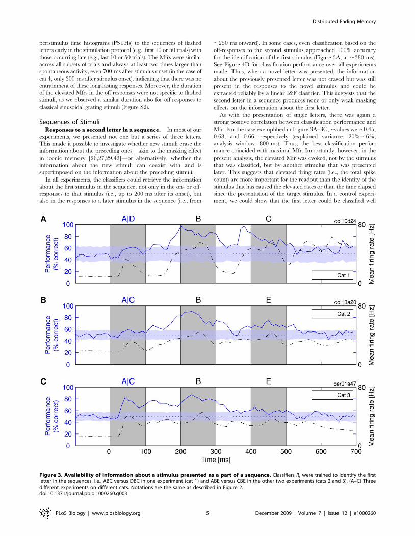
Figure 4. Simultaneous availability of information about multiple stimuli in a sequence. (A) Performance of time-specialized classifiers Rt

trained on individual time points to identify the second letter in the sequences of three letters (i.e., ABC vs. ADC). The results should be compared toFigure 3A. (B and C) Simultaneous availability of information about two different letters of a sequence. The following four sequences were presented:ABE, CBE, ADE, and CDE, and two classifiers identified each the presentation of either the first (blue line) or the second letter (green line). Shadedstripe and dotted lines are as described in Figure 2. (D and E) Rt classification performance for 16 different recordings made across four cats. Due tothe sparseness of responses, the results are given as average classification performance within 100-ms windows. Thick black curve: gross averageacross all datasets. Vertical lines: standard error of the mean across all datasets of all cats. Asterisk: the datasets chosen for further analysis.doi:10.1371/journal.pbio.1000260.g004



suppressive effect on the otherwise strong and sustained off-

responses to the first stimulus (i.e., with ISI = 500 ms). Likewise,

the properties of the preceding stimulus affected the on-responses

to the second stimulus, an effect that was obviously sufficiently

specific to classify accurately the first stimulus. Interestingly, we

found only very limited evidence that this one-back memory

mechanism occurs due to the adaptation of neuronal responses

(see Figure S5). Also, the control experiment in Figure S3 was

designed to avoid repetitive presentation of stimuli with a single

ISI, unlike the other experiments. Thus, this experiment provides

additional evidence that the long-lasting off-responses cannot be

explained by an entrainment (learning) process that would develop

expectancies for a specific ISI (i.e., the rhythm of stimulation).

Responses to a third letter in a sequence. The responses

to the third stimulus in the sequence (C or E in Figure 3; from

,450 ms onward) contained much less information about the first

stimulus than the responses to the second stimulus. This did not

appear to be due to a simple decay of information over time. In one

experiment, we were able to compare directly the responses of the

same neurons to a single stimulus and to triplets of stimuli (cat 1 in

Figures 2A and 3A; direct comparison in Figure S4). With a single

stimulus, classification performance was still high at delays as long as

450 ms, but had dropped to chance level at the same time point

when sequences of three stimuli were presented. Similar results were

obtained in other experiments (Figure 3B and 3C). In contrast to the

presentation of one or two letters, information about the first letter

was always considerably reduced when a third letter was presented.

Also, in the experiment with varying interstimulus interval in Figure

S3, the on-responses to the distant second stimulus (300 ms)

contained much more information about the first stimulus than any

other on-responses to equally distant third stimuli in Figure 3.

Furthermore, the reduction in classification performance in third

stimulus responses was not due to a reduction of Mfrs. This indicates

that the third stimulus in the sequence actually acted as a mask and

erased the information about the identity of the first stimulus. Thus,

the system has nearly unimpaired memory for one-back but not for

two-back stimuli.

Another remarkable finding was that off-responses often

returned temporarily to the level of spontaneous activity before

again assuming high levels of Mfr (e.g., 100–150 ms and ,350 ms

in Figure 3A; see also Figure S3). This rebound was strongest if the

screen was left blank, and hence, no suppression was induced by

the presentation of subsequent stimuli. Therefore, the changes in

the system responsible for the memory effect have persisted across

intervals during which the activity of the neurons used for

classification was low and carried little or no information about the

stimulus.

Superposition of Information about Different StimuliResponses that carry the information about past stimuli should

also carry information about the most recent stimuli, i.e., about

those that evoked the responses. The results of the following

analyses indicate that this is the case. In Figure 4A, a readout is fed

with inputs from the same set of neurons as in Figure 3A (and in

Figure 2A), but this time, the readout is trained to classify the

second stimulus in the sequence of three letters (letter B vs. D). The

classification performance was high (,80%) despite the high

degree of similarity of the shapes. Consistent with our previous

findings, classification performance correlated positively with Mfr

(r = 0.39 for the entire period of 800 ms).

In Figure 4B and 4C, we show results for cats 2 and 3 in which

both the first and second letter in the sequence were varied at the

same time, allowing us to estimate whether information was

available to classify simultaneously both the first and the second

stimulus in the sequence. We found that such sequence-specific

information was available in the on- and off-responses to the

second stimulus. During this period, the classification performance

for the first stimulus was not lower than the performance for the

recent stimulus that evoked the response (e.g., around 70% correct

in both cases for cat 3). We could also show that readouts could be

trained to perform nonlinear exclusive OR (XOR) classification,

i.e., fire if either a sequence AB_ or CD_ was presented, but not if

sequences AD_ or CB_ were presented (for details, see ‘‘Nonlinear

superposition of information’’ in Text S1).

In Figure 4D and 4E, we show that these findings generalized

across all the cats and, as a rule, also across different recordings

made from the same cat. For the classification of the first letter, the

gross average maximum performance across the total of all 16

recordings peaked at ,80% correct during the presentation of the

second letter (Figure 4D), and similarly, the classification of the

second letter peaked at ,75% correct during the presentation of

the third letter (Figure 4E). In Figure 4D and 4E, one can also see

one more remarkable result: classification performance is typically

better for off- than for on-responses (e.g., in Figure 4D, the

performance is overall higher at 250 ms than at 150 ms). This

result can also be seen in Figures 2A, 3A, and 3B (i.e., for cats 1

and 2). The results indicate that successful stimulus classification is

a ubiquitous phenomenon and that off-responses contain substan-

tial information about the stimuli even when interacting with on-

responses to stimuli presented next in the sequence.

Analyses of Information-Carrying VariablesThe information extracted by the classifier could be encoded

either by slow changes in firing rates (slow-rate code; e.g.,

,100 ms) or by precise timing of neuronal spiking events (i.e., fine

temporal code; e.g., #,20 ms) or both. Our next step was to

investigate the contribution of information encoded at these two

different time scales.

Information carried by spike timing. An analysis of

classification performance with t varying between 1 and 100 ms

indicated that, at the points of peak performance, the classification

with t= 20 ms was about as good as with any other larger value of

t, although longer integration constants always led to equivalent or

better performances (Figure 5A). At other time points, larger

values of t were required for maximum performance, but these

values increased monotonically with the distance from the points

of peak performance (the right-skew–shaped intensity plots in

Figure 5C–5E). This suggested that an important role of long t’swas to reach sufficiently far into the past in order to ‘‘carry over’’

the responses from the time when they were most informative

about the stimulus.

We next investigated the role of precise spike timing for

achieving such high-classification performance with t= 20 ms. To

this end, we perturbed the fine temporal structure of the spike

trains. The times of action potentials were jittered by moving each

spike by a random time drawn from a Gaussian distribution with

the mean of zero and a prespecified standard deviation (SD) (x-axis

in all plots in Figure 6; both training and test trials were jittered).

We then investigated the ability of readouts to learn to classify the

first letter in the sequence based on such jittered datasets (see

Materials and Methods for details). Jitter had strong detrimental

effects on classification performance as it reduced the performance

in all analyses. In Figure 6A, changes in classification performance

are shown as a function of the amount of jitter. For this purpose,

we selected three time points that exhibited the highest

classification performances prior to the application of the jitter

and were thus most relevant for such analyses (see Figure S6 for

analyses of all other time points and other values of t). Jitters with



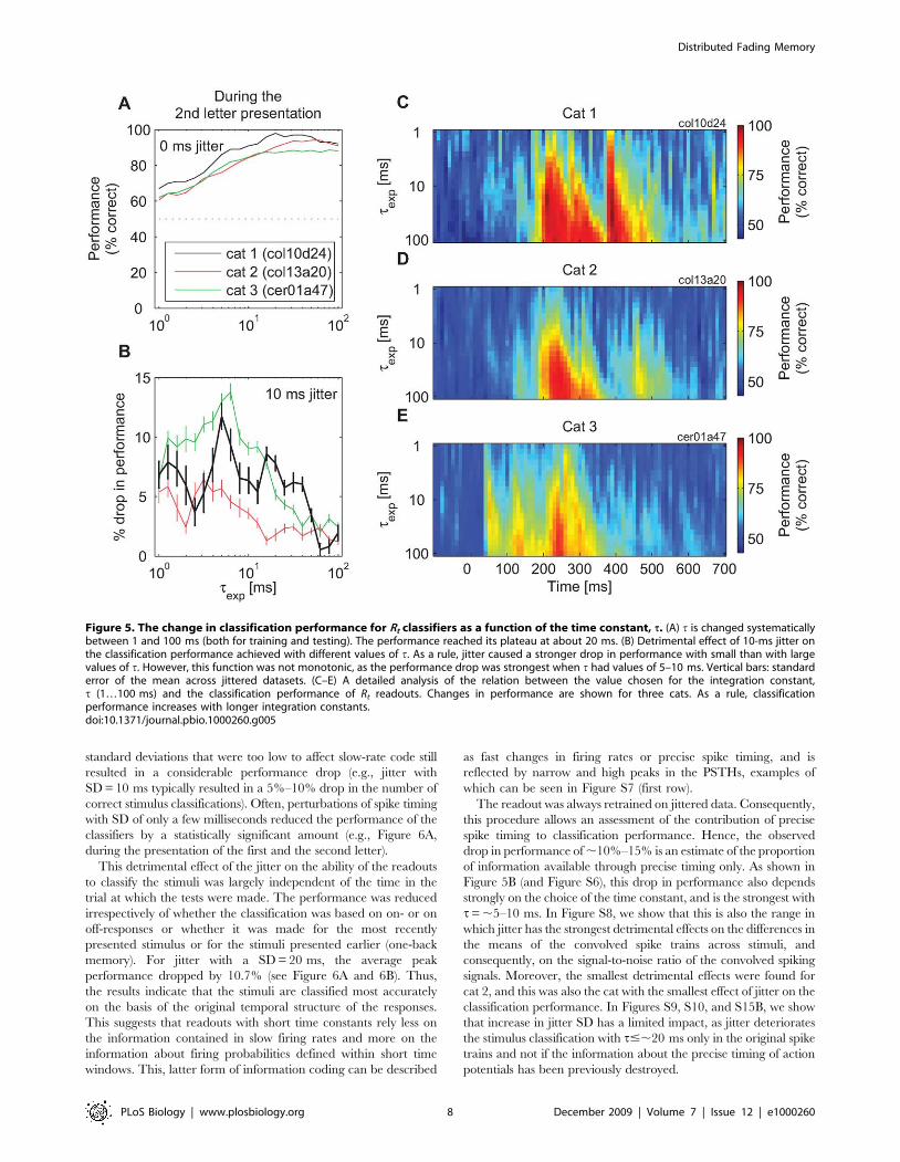
standard deviations that were too low to affect slow-rate code still

resulted in a considerable performance drop (e.g., jitter with

SD = 10 ms typically resulted in a 5%–10% drop in the number of

correct stimulus classifications). Often, perturbations of spike timing

with SD of only a few milliseconds reduced the performance of the

classifiers by a statistically significant amount (e.g., Figure 6A,

during the presentation of the first and the second letter).

This detrimental effect of the jitter on the ability of the readouts

to classify the stimuli was largely independent of the time in the

trial at which the tests were made. The performance was reduced

irrespectively of whether the classification was based on on- or on

off-responses or whether it was made for the most recently

presented stimulus or for the stimuli presented earlier (one-back

memory). For jitter with a SD = 20 ms, the average peak

performance dropped by 10.7% (see Figure 6A and 6B). Thus,

the results indicate that the stimuli are classified most accurately

on the basis of the original temporal structure of the responses.

This suggests that readouts with short time constants rely less on

the information contained in slow firing rates and more on the

information about firing probabilities defined within short time

windows. This, latter form of information coding can be described

as fast changes in firing rates or precise spike timing, and is

reflected by narrow and high peaks in the PSTHs, examples of

which can be seen in Figure S7 (first row).

The readout was always retrained on jittered data. Consequently,

this procedure allows an assessment of the contribution of precise

spike timing to classification performance. Hence, the observed

drop in performance of ,10%–15% is an estimate of the proportion

of information available through precise timing only. As shown in

Figure 5B (and Figure S6), this drop in performance also depends

strongly on the choice of the time constant, and is the strongest with

t= ,5–10 ms. In Figure S8, we show that this is also the range in

which jitter has the strongest detrimental effects on the differences in

the means of the convolved spike trains across stimuli, and

consequently, on the signal-to-noise ratio of the convolved spiking

signals. Moreover, the smallest detrimental effects were found for

cat 2, and this was also the cat with the smallest effect of jitter on the

classification performance. In Figures S9, S10, and S15B, we show

that increase in jitter SD has a limited impact, as jitter deteriorates

the stimulus classification with t#,20 ms only in the original spike

trains and not if the information about the precise timing of action

potentials has been previously destroyed.

Figure 5. The change in classification performance for Rt classifiers as a function of the time constant, t. (A) t is changed systematicallybetween 1 and 100 ms (both for training and testing). The performance reached its plateau at about 20 ms. (B) Detrimental effect of 10-ms jitter onthe classification performance achieved with different values of t. As a rule, jitter caused a stronger drop in performance with small than with largevalues of t. However, this function was not monotonic, as the performance drop was strongest when t had values of 5–10 ms. Vertical bars: standarderror of the mean across jittered datasets. (C–E) A detailed analysis of the relation between the value chosen for the integration constant,t (1…100 ms) and the classification performance of Rt readouts. Changes in performance are shown for three cats. As a rule, classificationperformance increases with longer integration constants.doi:10.1371/journal.pbio.1000260.g005



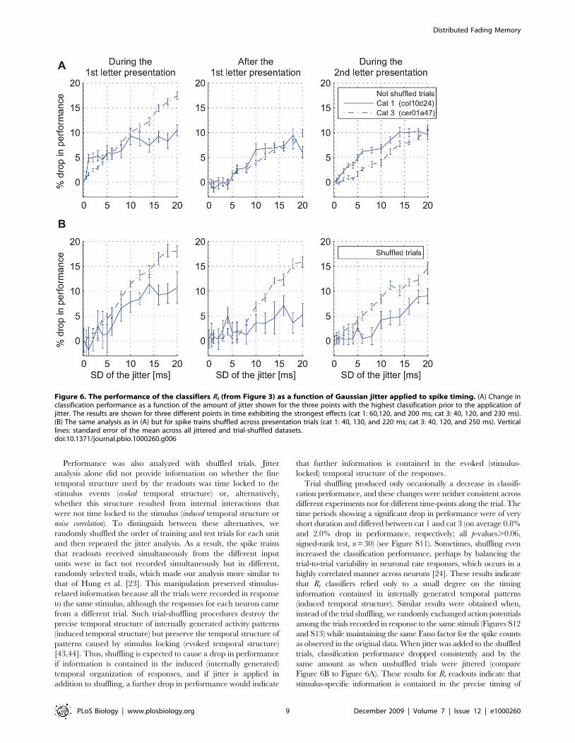
Performance was also analyzed with shuffled trials. Jitter

analysis alone did not provide information on whether the fine

temporal structure used by the readouts was time locked to the

stimulus events (evoked temporal structure) or, alternatively,

whether this structure resulted from internal interactions that

were not time locked to the stimulus (induced temporal structure or

noise correlation). To distinguish between these alternatives, we

randomly shuffled the order of training and test trials for each unit

and then repeated the jitter analysis. As a result, the spike trains

that readouts received simultaneously from the different input

units were in fact not recorded simultaneously but in different,

randomly selected trails, which made our analysis more similar to

that of Hung et al. [23]. This manipulation preserved stimulus-

related information because all the trials were recorded in response

to the same stimulus, although the responses for each neuron came

from a different trial. Such trial-shuffling procedures destroy the

precise temporal structure of internally generated activity patterns

(induced temporal structure) but preserve the temporal structure of

patterns caused by stimulus locking (evoked temporal structure)

[43,44]. Thus, shuffling is expected to cause a drop in performance

if information is contained in the induced (internally generated)

temporal organization of responses, and if jitter is applied in

addition to shuffling, a further drop in performance would indicate

that further information is contained in the evoked (stimulus-

locked) temporal structure of the responses.

Trial shuffling produced only occasionally a decrease in classifi-

cation performance, and these changes were neither consistent across

different experiments nor for different time-points along the trial. The

time periods showing a significant drop in performance were of very

short duration and differed between cat 1 and cat 3 (on average 0.8%

and 2.0% drop in performance, respectively; all p-values.0.06,

signed-rank test, n = 30) (see Figure S11). Sometimes, shuffling even

increased the classification performance, perhaps by balancing the

trial-to-trial variability in neuronal rate responses, which occurs in a

highly correlated manner across neurons [24]. These results indicate

that Rt classifiers relied only to a small degree on the timing

information contained in internally generated temporal patterns

(induced temporal structure). Similar results were obtained when,

instead of the trial shuffling, we randomly exchanged action potentials

among the trials recorded in response to the same stimuli (Figures S12

and S13) while maintaining the same Fano factor for the spike counts

as observed in the original data. When jitter was added to the shuffled

trials, classification performance dropped consistently and by the

same amount as when unshuffled trials were jittered (compare

Figure 6B to Figure 6A). These results for Rt readouts indicate that

stimulus-specific information is contained in the precise timing of

Figure 6. The performance of the classifiers Rt (from Figure 3) as a function of Gaussian jitter applied to spike timing. (A) Change inclassification performance as a function of the amount of jitter shown for the three points with the highest classification prior to the application ofjitter. The results are shown for three different points in time exhibiting the strongest effects (cat 1: 60,120, and 200 ms; cat 3: 40, 120, and 230 ms).(B) The same analysis as in (A) but for spike trains shuffled across presentation trials (cat 1: 40, 130, and 220 ms; cat 3: 40, 120, and 250 ms). Verticallines: standard error of the mean across all jittered and trial-shuffled datasets.doi:10.1371/journal.pbio.1000260.g006



individual spikes and that the relevant temporal structure of the

spike trains results from stimulus locking and not from internally

generated temporal patterning that would be independent of the

temporal structure of stimuli.

Generalized information contents across longer stretches

of signals. In all the analyses presented so far, the weights of a

linear classifier were trained—and the classification performance

was tested—on convolved neuronal activity extracted from one

specific time point, t. As a result, classifiers trained at different time

points had different sets of ‘‘synaptic’’ weights, each set being

optimized for stimulus classification at exactly one point in time.

An analysis of the weight distributions revealed that these weights

were highly dissimilar for different time points. The values of

weights changed quickly along the trial and even flipped their signs

as often as every 50–100 ms. Thus, the optimal set of weights for

good stimulus identification differs substantially across different

time points.

We also investigated the degree to which our readout systems

could achieve good classification performance when trained on

longer time intervals. Hence, readouts were trained on all time

points within a time interval of either 100-ms or 300-ms duration,

and their performance was tested on each time point, t. For both

training and test, the integration constant remained unchanged, i.e.,

t= 20 ms. These readouts were denoted as Rint classifiers or time-

invariant classifiers (to distinguish them from time-specialized, Rt,

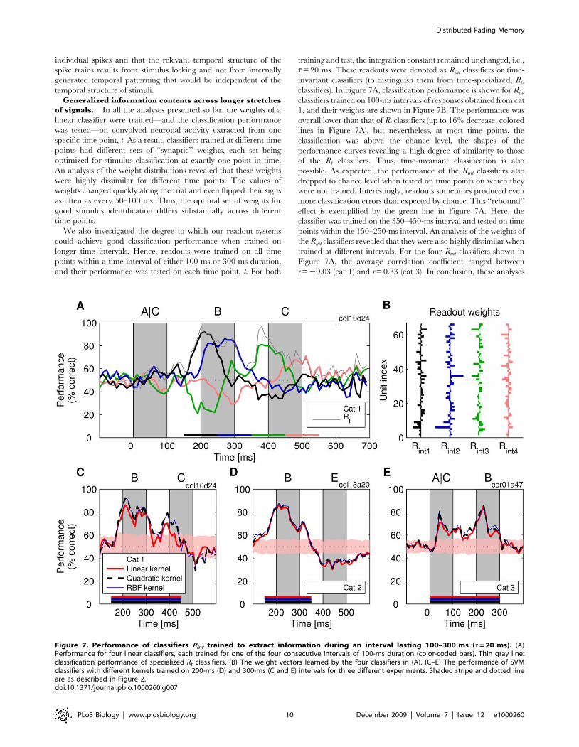
classifiers). In Figure 7A, classification performance is shown for Rint

classifiers trained on 100-ms intervals of responses obtained from cat

1, and their weights are shown in Figure 7B. The performance was

overall lower than that of Rt classifiers (up to 16% decrease; colored

lines in Figure 7A), but nevertheless, at most time points, the

classification was above the chance level, the shapes of the

performance curves revealing a high degree of similarity to those

of the Rt classifiers. Thus, time-invariant classification is also

possible. As expected, the performance of the Rint classifiers also

dropped to chance level when tested on time points on which they

were not trained. Interestingly, readouts sometimes produced even

more classification errors than expected by chance. This ‘‘rebound’’

effect is exemplified by the green line in Figure 7A. Here, the

classifier was trained on the 350–450-ms interval and tested on time

points within the 150–250-ms interval. An analysis of the weights of

the Rint classifiers revealed that they were also highly dissimilar when

trained at different intervals. For the four Rint classifiers shown in

Figure 7A, the average correlation coefficient ranged between

r = 20.03 (cat 1) and r = 0.33 (cat 3). In conclusion, these analyses

Figure 7. Performance of classifiers Rint trained to extract information during an interval lasting 100–300 ms (t = 20 ms). (A)Performance for four linear classifiers, each trained for one of the four consecutive intervals of 100-ms duration (color-coded bars). Thin gray line:classification performance of specialized Rt classifiers. (B) The weight vectors learned by the four classifiers in (A). (C–E) The performance of SVMclassifiers with different kernels trained on 200-ms (D) and 300-ms (C and E) intervals for three different experiments. Shaded stripe and dotted lineare as described in Figure 2.doi:10.1371/journal.pbio.1000260.g007



indicate that training and testing have to be performed on exactly

the same time intervals to achieve good performance irrespective of

whether Rint or Rt classifiers are used.

Less critical was the duration of the interval for which Rint

classifiers were trained. Even with time intervals longer than

100 ms, good classification performance could be achieved. In

Figure 7C to 7E (cats 1 to 3), we show results for analyses with

200- or 300-ms-long training intervals. The performance did drop

relative to the Rt classifiers (thin gray line in Figure 7A) but stayed

nevertheless high above the chance level. As was the case with Rt

classifiers, performance of the Rint classifiers was best when Mfrs

had high levels. This suggests that the performance of Rint

classifiers can increase further and perhaps approach the ceiling of

100% accuracy if the total number of spikes can be increased by

recording simultaneously from even more neurons.

In Rint classifiers, the decrease in performance, in comparison to

Rt classifiers, was traded off with an increased resistance to jitter.

The performance of Rint classifiers was not affected by small jitter

(SD = 10 ms). The maximum performance of Rint classifiers

dropped by 1% and 3% for cat 1 and cat 3, respectively, and

these changes were not significant. Also, the effect of jitter has

decreased with the size of the generalization interval, approaching

the region of zero effects at interval lengths of about 100 ms

(Figure S14). Apparently, as the Rint classifier must generalize over

the long period of time, unlike the Rt classifier, it cannot benefit

from precise stimulus-locked events that occur at unique time

points along the trial. Thus, forcing a classifier with short

integration constants to use the same set of weights over the

entire duration of the trial prevents these classifiers from relying on

precise stimulus-locked information (see Figure S8 for an account

of this phenomenon based on signal-to-noise ratios).

The notion that Rint classifiers learned to decode information

differently than Rts is suggested also by the finding that shuffling of

trials led to a drop of performance of Rint classifiers. With

int = 300 ms, the drop in classification performance was highly

consistent across different experiments and along the trials, and

amounted up to 14% (on average, 4.5% and 6.5% for cats 1 and 3,

respectively; all p-values,0.0001, signed-rank test, n = 30). In no

case did shuffling improve performance as observed with Rt

classifiers in cats 1 and 3 (Figure S15). As the performance of Rint

classifiers did not depend on jitter, this result suggests that these

classifiers take advantage of correlations that occur on longer time

scales (i.e., covariation in slow-rate responses).

Nonlinear readouts and the important role of second-order

correlations. Finally, we investigated whether classification

performance could be enhanced when the classifiers performed

nonlinear operations on the input signals. To this end, we applied

SVMs with quadratic kernels or with kernels such as radial basis

functions (RBF) that provide high flexibility in implementing

nonlinear transformations. Classification performance of these

nonlinear classifiers was investigated separately for Rt and Rint

readouts and compared to that of linear readouts.

We found no evidence that nonlinear classification improved

readout performance of Rt classifiers. Performance improvement

never exceeded 2% and never reached the level of statistical

significance. Thus, consistent with the report by Hung et al. [23],

linear classification was as good as nonlinear classification. This

was also true for Rint classifiers if these were tested on responses to

single, isolated stimuli, as those shown in Figure 2 (Figure S1).

In contrast, nonlinear Rint classifiers (int = 150–450 ms) achieved

better performance than linear Rint when applied for the

identification of one-back stimuli. Already with quadratic transfor-

mations, the ability to identify a previously presented stimulus

increased the maximum performance by ,6% in cat 1 and by 10%

in cat 3, but not in cat 2, which was an exception to that result

(Figure 7C–7E). On average, performance increased by 5.3% and

2% for cats 1 and 3, respectively, and these changes were significant

(two sample t-tests, n = 10, all p-values,0.01). Quadratic transfor-

mations use information stored in second-order correlations

between the variables more efficiently than linear classifiers, as

quadratic operations involve multiplicative operations between the

weighted contributions of the inputs (as opposed to simple, weighted

summation in a linear system). This form of nonlinearity only takes

into account pairwise correlations. Classifiers based on RBFs—by

contrast—take into account also higher-order correlations. Re-

markably, application of RBFs did not improve performance above

the level attained with quadratic classifiers (Figure 7C–7E) (for more

detailed analysis, see Figure S16). This indicates that most of the

stimulus-specific information used by the nonlinear Rint readout

could be extracted already from second-order correlations.

Previous studies examining synchronization among neuron

populations [45,46] found that second-order correlations can

account for almost all the correlation patterns observed in certain

natural neuronal networks, and thus, higher-order correlations are

unlikely to convey additional information. However, the nonlinear

Rint classifiers, being robust to jitter, could not have evaluated

precise timing relations between spikes. Instead, they could have

relied on slow stimulus-locked changes in firing rates, which may

carry information at the level of second-order correlations. To

investigate this possibility, for the four input units that made the

largest contribution to the performance of the quadratic Rint

classifier, we calculated the Mfrs and areas under receiver-

operating characteristics (AUC) for all units individually and for

the products of the Mfrs for all possible pairs of these units

(Figure 8) (see also Figure S17). This revealed that the products

differ strongly for different stimuli, leading to high AUC values.

Moreover, maximum differentiation between the stimuli occurs

often at different time points for products of Mfrs and for

individual Mfrs. These results indicate that second-order correla-

tions of neuronal firing rates are informative of stimulus properties

and, in principle, can be used by classifiers.

There is one more potential source of correlations that may

be picked up by nonlinear Rint classifiers. Averbeck et al. [24]

have shown that slow covariations in overall firing rates

(responsiveness of neurons) can boost classification performance.

In Figure S18, we show that, indeed, firing rates vary along

the experiment in a manner that is highly correlated across

units. Thus, slow covariations in rate responses may benefit

Rint classification when second-order correlations are considered.

However, the scope of their contribution is, at best, limited

because even if these correlations are removed by shuffling

the trials and only stimulus-locked correlations are maintained

[43], a polynomial Rint is more efficient than a linear one. Under

these conditions, we found a 5.6% and 7.2% increase in the peak

performance for cats 1 and 3, respectively. The mean performance

along the trial also increased for these two cats by 5.0% and 2.8%,

respectively (signed-rank tests, all p-values,0.0001, all n’s = 30).

In conclusion, these results indicate that time-invariant

classification is in principle possible and can attain a very high

level of performance if the responses of a sufficient number of

neurons can be evaluated. This evaluation can be achieved by

linear classifiers similar to I&F neurons. As indicated by the

shuffling test, unlike Rt classifiers, the linear Rint classifiers rely to a

substantial extent on information that can only be extracted from

temporal patterns in the joint activity of the recorded neurons. In

addition, nonlinear Rint classifiers, also in contrast to Rts, can

enhance classification performance by using information about

correlations, which may come from different sources.



Discussion

Our results demonstrate that the distributed activity of neurons

in cat primary visual cortex (area 17) contains information about

previously shown images and that this information is available for

a prolonged period of time. The information can be extracted by

simple computer-simulated readout neurons and is available for as

long as the firing rates stay elevated. These findings are related to

the results obtained in macaque IT cortex [23], but there are also

a number of differences. First, we show that information required

for stimulus classification can be extracted easily from neurons at

early processing stages that represent detailed and feature-based

information, and under anesthesia. The results are similar to those

obtained from neurons in IT that represent categorical informa-

tion. Second, stimulus-specific information is readily extractable

also from responses evoked by the offset of the stimulus (off-

responses). This suggests that off-responses play an important

role in cortical functions, and hence, should be studied more

thoroughly than is usually the case. Third, by presenting sequences

of stimuli, we show that the system has reliable memory for one

stimulus back. Fourth, we were able to identify the response

variables (neuronal code) that carry the stimulus-related informa-

tion. The classifiers relied on information carried both by neuronal

firing rates and by precise timing of neuronal spiking events locked

to the stimulus. As the classification was based on an estimate

of integration time constants of cortical pyramidal neurons

(t= 20 ms), the results suggest that upstream projection neurons

in the cortex—those that receive information from early visual

areas—should also be able to use this information. In other words,

the results suggest that precise timing of action potentials

complements the information available in neuronal firing rates

and thus that both types of information can in principle be used as

a neuronal code.

The finding that most of the timing information used by Rt

readouts was contained in the stimulus-locked timing of action

potentials (evoked temporal structure) and that the internally

generated timing information (induced temporal structure; noise

correlation) supported only Rint classification is probably due to the

prominent temporal structure of the rapidly repeating stimuli (5-

Hz stimulation rhythm due to 200-ms period between stimulus

presentations). Rager and Singer [47] have shown that when a

stimulus is flickered with a similar frequency, cortical responses

exhibit resonance phenomena to the periodic nature of the

stimulus. As a consequence, higher frequencies (.20 Hz) are

strongly suppressed. Therefore, for the present stimuli, most of

the classification performance based on precise spike timing can be

Figure 8. Information contents of neuronal firing rates and their second-order correlations. (A) Left y-axis: the average firing rates (Mfrs)in response to two different stimuli for the four most informative units in the analysis of time invariant classification with int = 150–450 ms, cat 1.Right y-axis: area under receiver-operating characteristic (AUC), related to the probability of correct classification. (B) Pairwise correlations in rateresponses, expressed as a product between Mfrs in (A) and the corresponding AUC values obtained from these products.doi:10.1371/journal.pbio.1000260.g008



accounted for by inhomogeneous Poisson processes with fast

fluctuating rates (#,20 ms), whose timing is locked to the

stimulus onset. This suggests that neuronal synchrony driven by

internally generated rhythms does not play an important role for

these stimuli and is in agreement with the finding that if Rt

readouts were endowed with polynomial kernels, optimal for

detection of pairwise correlations, classification results did not

improve. The present results do not allow us to identify the type of

information used by real readout systems in the brain. Some

cortical neurons may operate with longer time scales (e.g.,

,100 ms) and may rely predominantly on slow changes in rate

responses. As our results suggest, these neurons can also achieve

good classification performance.

The present results were surprisingly consistent across the range

of classifiers used. We obtained similar classification performance

irrespective of the type of kernel applied to SVM, for a wide range

of the time constants used for convolution of the spike trains, and

across different cats. The robustness of these findings is all the

more surprising if one considers the high level of trial-to-trial

variability, which is a typical property of neuronal rate responses

[40,48–53], and was also found in the present data (see Materials

and Methods). Future experiments should investigate the level of

robustness achievable for more difficult classification decisions

than the binary ones made in the present study.

Because the responses fed to the classifier had been recorded

simultaneously, we were also able to examine whether additional

information was encoded in non–stimulus-locked correlations

between the responses of different neurons. Applying nonlinear

readouts revealed that this was indeed the case for Rint

classification that takes advantage only of slow-rate covariation.

Performance improved over the linear readouts, but importantly,

this improvement was limited to pairwise correlations (quadratic

kernels). One possibility is that similar to precise neuronal

synchrony, no additional information is contained in correlations

of higher order also for slow covariation in rate responses. This

would be consistent with the report that pairwise synchronizations

account for most or all of the entropy within the system [45,46].

Therefore, the claim that higher-order correlations contain no

additional information appears to be generalizable to slower time

scales.

As Rt readouts operate, by design, with less input information

than Rints, we cannot rule out the possibility that the effects of the

second-order correlations (but also those of trial shuffling) would

not become significant with a larger dataset—i.e., if more

statistical power was available. However, irrespective of this

significance, the absolute magnitudes of these effects were always

smaller for Rt than for Rint classifiers, whereas on the other hand,

Rts were overall more accurate than Rints. Thus, a principal

difference in the nature of information exploited by the two

classification strategies remains and needs to be dealt with. In the

present study, we deciphered only partly the characteristics of the

two approaches to decoding information. Further efforts, possibly

relying heavily on theoretical analyses, will also be needed in order

to understand fully the respective implications and (dis-)advantages

of the two strategies. Thus, not only the time span of integration

(as investigated here), but also the time span (possibly longer)

appropriate for generalization, may need to be considered in

future studies. These considerations may be relevant for settling

the long-standing disputes over the principles by which informa-

tion is encoded and extracted in the brain (e.g., [31,54]).

Early visual areas are likely candidates for the implementation

of visual persistence and iconic memory [27], because of their

retinotopic organization and their noncategorical, feature-based

responses [1]. Iconic memory is believed to operate on the basis of

automatic (preattentive) processes and it is possible, therefore, that

the respective mechanisms also remain operational under

anesthesia. Considering that iconic memory declines with similar

time constants as the retrievability of stimulus-specific information

in the present experiment and is sensitive to masks [26,27,29,42],

it is conceivable that we studied a related mechanism. The

discovered one-back memory may be responsible for both the

integration process in iconic memory and masking effects. The

particular outcome would then depend on whether the two

subsequent component images (i.e., the ‘‘icons’’) are meaningful

only when isolated (masking) or only when integrated.

Our results suggest that the mechanisms responsible for the

temporary storage of stimulus-specific information involve mod-

ifications that are often not directly detectable in population rate

responses due to the suppression induced by subsequently

presented stimuli. Nevertheless, through this suppression process-

es, the activity from the past affects also the responses to the most

recent stimuli. As a consequence, it is possible to identify

accurately the past stimuli from the responses evoked by the

present. The suppression of sustained activity is likely to involve

active inhibition but possibly also more complex mechanisms.

Information about the nature of the first stimulus could be

contained in the patterning of inhibitory influences, which could

then shape the subsequent excitatory responses, but the process

may also involve reentry loops from higher cortical areas. Other

possibilities are mechanisms of short-term plasticity such as use-

dependent transient changes of transmitter release [55], receptor

sensitivity [56], and postsynaptic excitability [57]. Although we did

not find evidence that adaptation of neuronal responses [58] is

responsible for one-back memory, we cannot completely rule out

the possibility that these mechanisms play at least some role. It is

currently unclear whether and under which circumstances similar

long-lasting responses also occur in the awake state and in other

brain areas. In some studies, stimuli presented in IT cortex

produced short off-responses [23,59], but in others, the responses

are as long as in the present study [60]. One possibility is that the

duration of responses depends on the deployment of selective

attention, which is necessarily involved in the working memory

tasks applied in such studies [61]. Attention may produce

suppressive effects similar to those achieved by a second stimulus

under anesthesia. Studies on iconic memory suggest this possibility

as focusing attention on one subset of items impedes retrieval of

the remaining items from that storage [25].

An important factor for temporal integration of information

based on fading memory is that the information about a preceding

stimulus is not simply superimposed linearly on that of the most

recent stimulus. Rather, these effects should be nonlinear, as

revealed by the successful XOR classification. Such superposition

of information is also a prediction by computer simulations of

generic cortical microcircuits [31]. These results indicate that

cortical networks are not confined to operating as a serial

processing pipeline, where a sequence of precisely structured

processing steps is applied sequentially to each input frame but

can, in principle, involve kernel-like processors that fuse

information from different time slices in such a way that a simple

linear classifier (i.e., the readout) can extract information about the

stimulus. The important advantage of processes based on fading

memory is that novel complex computations can be implemented

if only the readout learns by adjusting the weights of its synapses,

as emulated in the present study, whereas the remaining part of

the system can stay unchanged. The main prerequisite for the

implementation of such functions is that nonlinear interactions are

combined with fading memory for recent inputs. As suggested by

the present study, these are exactly the properties of responses in



early visual areas. Thus, cortical neurons at later processing stages

have access to signals that have already been subjected to temporal

integration.

In conclusion, our data provide support for the existence of fading

memory and nonlinear integration between past and present input

already at the level of V1. This suggests that the brain exploits the

computational advantages of such processes as predicted by

computer simulations of generic cortical microcircuits [31,62], not

only for high-level computations, but with all likelihood at all levels

of cortical processing. Another, potentially important implication of

this finding is that relatively simple readout devices can be used to

evaluate complex trajectories of time-varying neuronal activity

patterns. This feature can be exploited for the construction of

prosthetic devices controlled by neuronal activity.

The present study leaves several questions unanswered. To

determine the boundary conditions for the present phenomena,

stimulus presentation times need also to be changed systematically.

Experiments with larger numbers of electrodes are required in

order to examine whether the present findings still hold when the

number of simultaneously recorded neurons approaches more

closely the number of presynaptic inputs to a typical cortical

neuron. Further, psychophysical experiments will be needed to

validate our proposal that the present memory effects are closely

related to iconic memory. Finally, one would like to obtain direct

evidence that cortical neurons actually use the information in the

same way as our artificial readouts. However, at present, it is

unclear how this could be achieved.

Concluding RemarksOlshausen and Field [63] have argued recently that fundamen-

tal aspects of visual cortex functions are still unknown. The present

results support this notion in that they force us to extend classical

theories on visual processing. These are based on the notion that

the main functions of the visual processing hierarchy consist of the

extraction and recombination of elementary visual features in

divergent–convergent and hierarchically organized feedforward

architectures (e.g., [37]). In this case, scene analysis is essentially

based on frame-by-frame computations in which each new input is

processed independently of the previous one. Hence, there is no

memory for the past, and such memory is even considered

disturbing rather than useful. In contrast, we find evidence for

fading memory in combination with nonlinear temporal interac-

tions, at least in early visual areas. Processes supporting both

perception and action may benefit from such memory mechanisms

because these offer a much wider spectrum of (time-dependent)

computations than feedforward architectures. As our data suggest,

precise timing of action potentials plays an important role in these

processes, suggesting that, besides firing rates, cortical processing

also exploits time and temporal relations as coding space.

Materials and Methods

Experimental ProceduresAll the experiments were conducted according to the guidelines

of the Society for Neuroscience and the German law for the

protection of animals, approved by the local government’s ethical

committee, and overseen by a veterinarian. In five cats, anesthesia

was induced with ketamine and maintained with a mixture of 70%

N2O and 30% O2 and with halothane (0.4%–0.6%). The cats

were paralyzed with pancuronium bromide applied intravenously

(Pancuronium, Organon, 0.15 mg kg21 h21). Multiunit activity

(MUA) was recorded from area 17 with multiple silicon-based

16-channel probes (organized in a 464 spatial matrix), which were

supplied by the Center for Neural Communication Technology at

the University of Michigan (Michigan probes). The intercontact

distances were 200 mm (0.3–0.5 MV impedance at 1,000 Hz).

Signals were amplified 1,0006 and, to extract unit activity, were

filtered between 500 Hz and 3.5 kHz. Digital sampling was made

with 32 kHz frequency, and the waveforms of threshold-detected

action potentials were stored for an off-line spike sorting

procedure. The probes were inserted approximately perpendicular

to the surface of the cortex, allowing us to record simultaneously

from neurons at different cortical layers and at different columns.

Up to three probes were inserted simultaneously, allowing for

recordings from up to 48 electrode contacts (channels) in parallel,

each providing a signal with multiunit activity. This arrangement

produced a cluster of overlapping receptive fields (RFs), all RFs

being covered by the stimuli (Figure 1A in the main text). Results

for one cat were obtained from the same preparation as in [9] and

for another cat from [4]. These studies also describe further details

on recording techniques.

Stimuli were presented binocularly on a CRT monitor (210,

HITACHI CM813ET) with 100-Hz refresh rate and by using

the software for visual stimulation ActiveSTIM (http://www.

ActiveSTIM.com). After mapping the borders of the respective

RFs, binocular fusion of the two eyes was achieved by aligning the

optical axes with an adjustable prism placed in front of one eye.

The stimuli consisted of single white letters that spanned

approximately 5u of visual angle and that were composed of

elementary features suitable for evoking strong responses in area

17. The stimuli were presented with maximal brightness on a black

background (thus, also with the maximal contrast) and were placed

such that they stimulated the cluster of RFs near optimally. For

presentation of single letters, we used letters A and D, each

presented for 100 ms. Stimulus sequences of three letters consisted

of letters A, B, C, D, and E and were either presented as sequences

ABC, DBC, and ADC (cat 1) or sequences ABE, CBE, ADE, and

CDE (cats 2 and 3). Each member of a sequence was presented for

100 ms, and the blank period separating the presentation of letters

also lasted, in most cases, 100 ms. For each stimulation condition

(single letter or a sequence), 50 (cat 1), 100 (cat 4), or 150 (cats 2, 3,

and 5) repetitions were made. In a control experiment, we varied

the blank period between two stimuli presented in a sequence, the

periods having the values 100, 200, 300, and 500 ms. In this

experiment, the first stimulus in the sequence was always a letter

(A or C), whereas as the second stimulus, we randomly exchanged

a letter (B) with a white blank screen that had the same luminance

as the letter stimuli. This control experiment was made on a

separate cat, which ensured that we fully avoided repetitive

presentations of identical blank periods, which were made in other

cats. The block randomization of the presentation order ensured

that no more than two blank periods of identical duration

occurred in a row. Sinusoidal gratings were presented with full

contrast, spanned 18u of visual angle, had spatial frequency of 2.6

cycles/degree, and drifted with the speed of 2.0u/s, thereby being

suitable for evoking strong responses in area 17. For an overview

of experiments performed on each cat, see Table S1.

Data AnalysisOff-line spike-sorting procedures. To extract single units,

extracellularly recorded spike waveforms of each channel were

subjected first to principal component analysis and then to clustering

procedures whereby the waveforms of similar shapes were assumed

to be generated by the same neuron [64]. In some cases, separation

of single units was not possible due to undistinguishable shapes of

waveforms, usually of small amplitude. In this case, multiple single

units were pooled into a larger multiunit. Also, it was not possible to

treat clearly distinguishable single units as separate entries if these



units had too low firing rates. Units with low firing rates have very

sparse high-dimensional data representations that can produce

weak generalization capabilities of trained readouts (the overfitting

problem). Thus, we pooled low-rate units (,,10 Hz) into a larger

multiunit. As a result, we combined on average 2.30 units per

recording channel (range one to five units), with about 50% of them

being multiunits. In the five recording sessions from the five cats we

used, 66, 78, 52, 124, and for one analysis, 25 units of

simultaneously recorded activity for training and testing

classification (for cat 5, only 13 electrode channels were

responding). There was no selection of units for further analyses.

Further pooling of units always reduced the peak classification

performance. In three cats for which we investigated the effect of

pooling beyond the removal of low-rate units (cats 1, 2, and 3), on

average, the additional pooling reduced the peak classification

performance by 8.8% as compared to the datasets actually used for

the analyses (standard deviation across all comparisons was 6.1%).

Only for cat 2, this decrease in performance was not statistically

significant, and its magnitude was smaller than 1%.

Variability of responses. All responses showed a con-

siderable level of trial-to-trial variability. The Fano-factors were

computed according to Fano [65] for the total spike counts

obtained per recording electrode and across individual stimulation

trials within the time interval of 1.2 s, beginning 500 ms before the

stimulus onset. The obtained values were on average about 8 and

ranged between 1 and 60, and these values were consistent with

previous reports for comparable window sizes [66].

Classification. The decay time constant t (20 ms in most

analyses) was used for convolving the spike times, which means

that without further inputs, the ‘‘depolarization’’ of the artificial

integrate-and-fire (I&F) neurons (which did not implement a reset

or a refractory period) drops within this period with the time

course exp(2t/t) to 37% of its initial value (hence the name ‘‘leaky

I&F’’). This convolution endowed the readout neurons with

memory for the history of activation (inputs), the duration of the

memory being determined by the constant, t. Thus, the resulting

activation at any time, t, was a function of the current activation

and the activation from the recent past, as determined by the

speed of the depolarization leak. There were no other mechanisms

for the interaction with past inputs. Hence, the dimensionality of

the inputs to SVMs learning Rt classification equaled always the

number of units (neurons) that participated in the analysis. Note

that our implementation of readouts is different from that used by

Hung et al. [23], who simply counted the number of spikes that

were fired by each neuron within a time bin of 50 ms. We opted

for leaky integration because this approach, although resulting in

low-pass filtering, nevertheless preserves much information about

precise temporal relations between action potentials (time delays).

This approach also approximates more accurately the conditions

under which real cortical (readout) systems should operate.

Nevertheless, we also made analyses with spike counts similar to

those reported by Hung et al., and the results remained similar

(Figure S19). The spike count yielded roughly the same

information as low-pass filtering when the time constant of the

filtering corresponded to the time bin used for the spike count. The

time constant t can be thought of representing the temporal

properties of the membrane and of the synaptic receptors. No

additional time constants were used to mimic decays in synaptic

currents, and hence, these inputs were modeled as Dirac delta

functions. Although classification was based on the linear

combinations constructed from input intensities and ‘‘synaptic’’

weights, the final classification also involved one nonlinear step

due to the threshold for generation of a ‘‘spike’’ (with exception of

the analysis of XOR classification function). The threshold was

necessary to make the binary decisions for the presented letters

(e.g., letter A or B). The value of this threshold was optimized for

maximum performance and determined by the same training

procedures as those used to optimize the synaptic weights. All the

calculations for spike-timing convolutions were made in steps of

10 ms. In all analyses, the testing was made with the same value

for t as the training. Note that the present analyses do not

investigate information that may be stored in ISIs.

Support vector machine. A support vector machine (SVM)

is a supervised learning method for binary classification problems.

The training samples are first mapped into a N-dimensional

feature space, and classification is performed in this feature space

by constructing a hyperplane that optimally separates the data into

two classes. The constraint is that the shortest distance from a

training sample to the hyperplane (i.e., geometric margin) must be

maximized. Consequently, SVMs are not based on iterative

procedures. The main advantage of SVMs is that even if the

training samples are not linearly separable in the input space, they

might become linearly separable in the feature space after an

application of a nonlinear feature mapping procedure. Another

important property of SVMs is that this nonlinear mapping into

the feature space does not need to be defined explicitly provided

that the dot product in the feature space can be replaced by a so-

called kernel function. In case of kernels based on RBFs, N is even

infinite dimensional. We used the LIBSVM library for support

vector machines [67]. The classifiers were trained with linear-

kernel SVMs, and overfitting was controlled by choosing the

parameter C to be 10 in case of 50 repetitions per stimulus

condition, and 50 in case of 150 repetitions per condition. The

parameter C was optimized prior to the analysis on an

independent validation set that was not used later either for

training or testing. This parameter sets the tradeoff between

minimizing the number of training samples located on the wrong

side of the margin on the one hand, and maximizing the geometric

margin between correctly classified samples and the classification

hyperplane on the other hand [68,69]. In case of RBF kernels, the

variance of the Gaussian kernel was set to 0.5. The classification

performance was estimated with 10-fold cross-validation in which

we balanced the number of examples for the training and for the

test class: For each of the 10 tests, a different set of 1/10 of the data

was chosen for testing under the constraint that all 10 test sets were

disjoint. For example, for 50 trials, each test was made on another

set of five trials, the remaining 45 trials being always used for

training. Ten-fold cross-validation was repeated 10 times with

different data points in different splits (results represent average

values), except for the results reported in Figure 5C–5E and Figure

S16, for which, due to the computational time constraints, only a

single cross-validation run was carried out. All the reported

performance results are averages for the test data. For the number

of data points in each analysis, see Table S2. To assess the

significance of classification performance, we obtained the H0

distribution for classification performance by randomizing the

information about the identity of the stimuli inducing the

responses and repeating this randomization procedure 100 times

(i.e., a label-shuffling procedure). The sets of four units with best

classification were found by determining exhaustively the

performance for all possible four-unit combinations. Rint

classifiers were trained and classified on all time points of the

same 100-ms or 300-ms intervals, classification performance being

tested at each 10-ms time point. The significance in the Figure S16

was estimated by performing a two-sample t-test of the hypothesis

that the two sets of cross-validation errors obtained for the Rt and

the Rint classifier come from distributions with equal means (critical

p-value = 0.05). The significance levels for trial-shuffling experi-



ments was assessed by applying a sign-rank test to the readout

decoding accuracies pooled from all 30 time points within the

specified time interval. The comparisons were made either between

trial-shuffled and not trial-shuffled data or between linear and

polynomial readouts trained on trial-shuffled data. To ensure the

statistical independence of the differences in performance, at each of

the 30 time points, different trial-shuffled datasets were used for

training and for testing.

It is important to note that differences in the absolute values of the

classification performance (% correct) cannot be used as a direct

indicator of the reliability of the reported findings or of the general

ability of the readout neurons to extract information. This is because

classification performance depends on a number of factors such as the

total number of units recorded simultaneously and the total number

of action potentials recorded. The performance is necessarily low with

fewer electrodes (fewer action potentials), and if the number of units

recorded can be increased further (e.g., .100 recording channels),

the performance is likely to saturate at 100% correct.

Mutual information. We performed also an alternative data

analysis based on an information-theoretic approach. Thus,

instead of percentage correct classification, we calculated the

mutual information between the stimulus properties and the

responses of readout neurons. These analyses yielded identical

results to those reported for performance correct (for an example

of such analysis, see Figure S20).

Total firing rates. The average level of activity for the

investigated units is shown in all figures as mean firing rate (Mfr).

Mfr provides information very similar to that of peristimulus time

histograms (PSTHs) (shown only in Figure 1B), but instead of

simple spike counts, we show the averaged spike trains after the

convolution with the exponentially decaying kernel. Thus, the

plots provide the information that is most relevant for the present

analyses. The two datasets with lowest classification performance

in Figure 4D (purple lines) had weakest responses to visual

stimulation, the signal-to-noise ratio of rate responses being #1.9.

For all other recordings, this ratio ranged between 4 and 12.

Jitter analysis. Spike times were always jittered 100 times by

adding a value drawn from a Gaussian distribution with a mean of

zero and the specified standard deviation (SD). The performance

for shuffled and nonshuffled trials was compared for the time

points at which the performance was maximal prior to the jitter

analysis. Note that these time points were not necessarily identical

and were shifted by up to 20 ms (Figure 6). In these analyses, both

training and testing were made on jittered spike trains. The results

were similar for all three cats, but the performance difference

between linear and nonlinear Rint readouts was somewhat smaller

for cat 2 (3%–7%) than for other cats.

Nonlinear superposition of information. To investigate

nonlinear superposition of information in brain responses, we

removed the nonlinear component of the classification process,

i.e., the activation threshold determining whether classifiers fired

or not. For more detail, see Text S1 and Figure S21.

Supporting Information

Figure S1 Single letters classification by time-invariantreadouts. Analysis similar to that in Figure 2 of the main text,

but instead of using time-specialized classifiers (R,), the classifica-

tion was made on the basis of time-invariant classifiers (Rint) trained

on all time points within an interval that had the duration of either

500 ms (cat 1) or 400 ms (cat 4). This analysis was made with three

types of SVM classifiers that had either linear or polynomial

kernels or kernels based on radial basis functions.

Found at: doi:10.1371/journal.pbio.1000260.s001 (0.05 MB EPS)

Figure S2 Long off-responses are not unique to flashedstimuli. Comparison of mean firing rates (Mfrs) in off-responses

observed after removing either the last stimulus in the sequence

(blue line) or a sinusoidal grating presented previously for 4 s (red

line). The time at which the stimuli were removed is indicated on

the abscissa by 0 ms. The duration of the off-responses is similar

for the two types of stimuli.


Figure S3 Variation of the interstimulus interval.Classification performance in a control experiment in which

interstimulus interval was varied (100, 200, 300, and 500 ms), and

as the second stimulus, either a letter B was presented (blue solid

line) or the screen was blank, i.e., white (w.s. stands for white screen)

during this short period of time (green solid line). If good

classification performance was evoked only by structured letter

stimuli and not by a white screen, the result would have suggested

that classification relied on stimulus-specific processing occurring

only within this brain area. However, the results indicate that good

classification performance was obtained also from rate responses

evoked by a white screen. Thus, readout neurons identify efficiently

the past stimuli irrespective of the mechanism by which the Mfrs are

elevated and are able to take advantage of any type of interaction

that occurs between past and present stimuli.


Figure S4 Direct comparison between one- and three-letter sequences. The results from Figures 2 and 3 obtained

from the same cat are shown here together to facilitate direct

comparison. The plot indicates the suppressive effects of the

subsequent stimuli in the sequence.


Figure S5 Adaptation of neuronal responses plays littleor no role in the one-back memory for stimulationsequences. If adaptation plays an important role in the one-back

memory phenomenon, it is expected to find negative correlations

between the weights of Rt readouts trained to classify the first

stimulus early and late in the trials. Also, the rate responses to later

stimuli should be reduced if they were high in response to earlier

stimuli. (A–C) Cross-correlation matrices of the weight vectors

assigned to Rt units for the classification of the first stimulus when all

three stimuli are shown. The correlations indicate the vectors’

similarities/differences across time. Periods with high-classification

performance tend to be correlated positively. The strongest negative

correlations were found for the periods in which the classification

performance was low ($,400 ms) and in the cat that had overall

lowest performance (cat 2). Very similar plots were obtained when,

instead of vector similarities, we plotted the classification perfor-

mance at one time based on the vectors trained at another time

(unpublished data). The autocorrelations along the diagonal are set

to zero (green color). (D and E) A test of adaptation based on a

comparison of rate responses within and between letter-sequences.

To make comparisons between sequences, quotients of rate

responses, Q, to two different stimulation sequences (ABC or DBC

[D], and ABC or ADC [E]) are computed for each unit and across

different time intervals during which either the first (0–100 ms),

the second (200–300 ms), or the third (400–500 ms) letter was

presented. In (D), Q (0–100 ms) = spike count (ABC)/spike count (DBC),

during the interval 0–100 ms and Q (200–300 ms) = spike count

(ABC)/spike count (DBC), during the interval 200–300 ms. Similarly, in

(E), Q (200–300 ms) = spike count (ABC)/spike count (ADC), for the

period 200–300 ms and Q (400–500 ms) = spike count (ABC)/spike

count (ADC), for the period 400–500 ms. Values .1.0 indicate that

the responses were higher in the first than in the second sequence. To

make comparisons within sequences (at different times), the quotients



are presented in a scatter plot. In case of adaptation, one would

expect a negative correlation between the values of Q early and late

in the trial (e.g., in response to the first and second letter). The scatter

plot diagrams indicate in most cases lack of such negative

correlations between the quotients (the values of Pearson’s

correlation coefficients, r, are not significantly different from zero)

with the exception of the classification of the second letter for cat 2

and cat 3 with r = 20.55 and r = 20.31, respectively. Thus, if a unit

is activated more strongly by A than by D early in the trial, this does

not predict that the response to letter B, presented later in the same

trial, will necessarily be weaker when preceded with A than when

preceded with D. The quotients are computed for each unit and are

averaged across all presentation trials.


Figure S6 A detailed analysis of the effect of jitter on theclassification performance. The effect of jitter was calculated

along the entire trial and for three different values of the

integration constant, t: 5, 20, and 80 ms. Color code: the amount

of jitter (0–20 ms). Jitter always exhibited strongest detrimental

effects with t= 5 ms.


Figure S7 The effect of jitter on PSTHs. Precise temporal

information was removed from the spike trains by jittering the

spike timing with varying standard deviations (SD = 0–50 ms). (A

and B) Example PSTHs that gradually lose their fine temporal

structure (i.e., become smoother) calculated for one unit in

response to two different stimulation sequences (ABC and DBC).


Figure S8 Analysis of the signal-to-noise ratio in theconvolved signals that serve as inputs to classifiers. (A)

Detailed analysis of the two factors that determine the signal-to-

noise ratio is shown for cat 1. First row: standard deviation (SD)

across all the convolved values that entered the analysis (both

training and testing). For Rt classifiers (left column), one SD was

computed for each time t, which were then averaged across all

times t that entered the analysis (the same intervals are used as for

Rint analysis). In contrast, for Rint classifiers, only one SD value was

computed across the entire investigated interval (the same intervals

are used as in Figure 7). Second row: absolute mean difference in

the rate responses (|D Mean|) for the two stimuli that needed to be

classified. The values |D Mean| were computed first for each time

point t, and subsequently averaged across all times points that

entered the analysis. (B–D) Signal-to-noise ratio (SNR) defined as

SNR = |D Mean|/SD and shown separately for three different

cats. All estimates were made for different integration constants, t(5–160 ms; x-axis) and different amounts of Gaussian jitter

(standard deviations: 0–80 ms; color coded). Increase in t reduces

both SD and |D Mean|, resulting in relatively small changes in

SNR. These effects of t are similar on the input statistics for Rt and

Rint classifiers. In contrast, jitter affects strongly only |D Mean| of

the input statistics, but not SD, and only for Rt classifiers. Also, the

effects are strongest for the smallest values of t. Consequently, the

effect of jitter on SNR is restricted to Rt classifiers, which are

affected most strongly when t is small. Vertical lines: standard

error of the mean across electrodes and time points.


Figure S9 The classification performance of readoutsapplied to jittered spike trains (SD = 50 ms) as shown inFigure S7. (A–C) Classification performance in three different

experiments (blue solid line). The performance is lower than that for

nonjittered spike trains in Figure 3 of the main text (here shown

again by gray solid lines). Nevertheless, the classification perfor-

mance exceeds the chance level. Dash-dotted line: the mean firing

rate across the entire population of investigated neurons before

jittering the spike trains.


Figure S10 No information is encoded in the precisespike timing of previously jittered spike trains. (A and B)

The effect of additional jitter and change in t for the classification

performance estimated for the spike trains previously jittered with

SD = 50 ms as in Figure S7. (A) Accuracy for classifying the first

letter in the sequence as a function of the time constant, t. The

performance for t#,20 ms is considerably lower than for the trains

without the previous jitter, shown in Figure 5. (B) Further

application of a small jitter (SD = 10 ms) does not affect the

classification performance for any value of t. This is in contrast to

previously nonjittered spike trains shown in Figure 5B. (C) Analysis

identical to that in Figure 6A in the main text but applied to the

spike trains with the same jittered spike trains as in (A and B).

Vertical lines: standard error of the mean across jittered datasets.


Figure S11 Classification performance for Rt readoutsafter the application of trial shuffling. (A and B) Results for

cats 1 and 3, respectively.


Figure S12 Performance of classifiers trained on surro-gate data. Classification performance computed on a set of

surrogate data created by using a different procedure for removing

information from spike trains than that used in Figure S10. Here,

we randomly exchanged the spikes of the same unit across

different presentation trials of the same stimulus, while maintain-

ing for each unit the Fano factors for the spike counts. Unlike

the jitter, this procedure preserves each spike’s latency but removes

the associations to the original trials, which in turn removes the

dependencies between different spike trains generated by the

internal, not stimulus-locked, timing mechanisms (similarly to

the trial-shuffling procedure presented in Figure 6B in the main

text). After the application of the present procedure, the spike

trains correspond to inhomogeneous Poisson processes, which, in

the same time, retain the rate profiles of the original PSTHs. (A to

C) Classification performance in three different experiments (red

solid line). Blue solid line: the classification performance without

exchanging the spikes, shown originally in Figure 3 in the main

text. Dash-dotted line: the mean firing rate across the entire

population of investigated neurons. Vertical lines: standard errors

of the mean across surrogate datasets.


Figure S13 Jitter analysis for surrogate data. Jitter-based

analysis of the spike trains with randomly exchanged spikes across

trials as shown in Figure S12. (A) The effect of a small jitter (up to

20 ms) on the classification performance was tested by using a

procedure identical to that shown in Figure 6A in the main text

(e.g., t= 20 ms). Small jitter reduced the classification perfor-

mance in a manner similar to that observed in the original data,

supporting the conclusion that most of the fine temporal

information used by the readouts was time locked to the stimulus

onset (or offset). (B) The effect of small jitter after the fine stimulus-

locked temporal structure was first destroyed in the spike trains by

applying a large jitter of SD = 50 ms (as in Figures S7, S9, and

S10). Vertical lines: standard error of the mean across jittered

surrogate datasets.


Figure S14 Jitter affects only the performance of Rt

classifiers. Analysis of the drop in classification performance



induced by a jitter (SD = 20 ms) shown as a function of the time

interval over which the readout was trained. With a time

interval = 0 ms, the analysis corresponds to Rt readouts. Other-

wise, we refer to Rint readouts. Thin lines: estimates made for 16

time points along the trial that had the highest classification

performance. Thick line: the average across all estimates. Vertical

lines: standard error of the mean across jittered datasets. (A–C)

Estimates made separately for three different cats.


Figure S15 Performance of polynomial Rint classifierstrained on trial shuffled data. Classification performance

after trial shuffling as in Figure S11 but for time-invariant

polynomial Rint classification with an interval of 300 ms. (A and B)

Results for cats 1 and 3, respectively.


Figure S16 Dependence of the performance of Rint

classifiers on the length of the time interval andperformance improvement of polynomial classifiers.Classification performance for linear Rint readouts (left column)

and the improvement in performance when changing the kernel

functions from linear to polynomial (right column), shown for

different locations of the generalization interval (its endpoint) within

the trial (x-axis), and as a function of the size of the interval (y-axis).

Time interval = 0 ms corresponds to the Rt classifier. Only

significant differences are plotted in the right column, significance

being determined on the basis of cross-validation errors (see

Materials and Methods). White stars: parameter values for the

analyses shown in Figure 7C–7E in the main text. The performance

of Rint classifiers with intervals $,200 ms is consistently facilitated

in all cats by the use of polynomial functions.


Figure S17 Differences in firing rates correlate with theclassification performance. The time course of classifier

performance from Figure 3 of the main text shown together with

the difference in the mean firing rates between two stimulation

conditions (8-fold magnified; dashed lines in red) in addition to the

mean firing rates (dash-dotted lines in black).


Figure S18 Temporal stability of the recordings. Analysis

of the changes in the neuronal firing rates along the experiment for

three cats. Left column: time course of the changes in neural

responsiveness along the experiments. Each of the ten trial blocks is

an average of 260 (cat 1) or 120 (cats 2 and 3) consecutive trials.

Each color indicates one electrode. Right column: correlations in

the changes of the overall firing rate responses across the electrodes.

Positive correlations predominate (red colors). Cat 2 also exhibits a

considerable number of negative correlations (blue colors).


Figure S19 Comparison of classifiers trained on spikecounts. Our main classification method, based on convolved

spike trains, is compared to a method based on simple spike

counts. At each time point, a time-specialized linear classifier (Rt)

was trained, either on convolved spike trains with an exponential

decay (time constant, t= 20 ms), or on the basis of spike counts

obtained for intervals of 5, 20, 50, and 100 ms. When similar time

constants are used, spike count produces similar classification

performance to the exponential convolution.


Figure S20 Mutual information. Performance for the same

classification task as in Figure 3A of the main text but this time

expressed as the mutual information between the stimulus identity

and the responses of the readout (blue solid line).


Figure S21 XOR classification. Readouts were trained to

make a nonlinear XOR-type detection, e.g., fire if either a

sequence AB_ or CD_ has been presented but not if sequences

AD_ or CB_ have been presented. Here, the performance was

assessed by the point-biserial coefficient of correlation between

stimulus identity (binary code) and readout ‘‘depolarization’’ (a

continuous variable).


Table S1 Overview of the experiments made on differ-ent cats. Columns: types of experiments/analyses. Rows: cats.

Vertical line (|) indicates the stimuli that were altered (and

classified) at the give position in the sequence. X indicates a

control experiment in which a white blank screen was presented as

the second stimulus. s.g., sinusoidal gratings.

Found at: doi:10.1371/journal.pbio.1000260.s022 (0.03 MB

DOC)

Table S2 The amount of training data available for eachanalysis. Indicated are the numbers of data points in the training

set (number of trials6number of time points). For Rt classifiers, number of

time points = 1. Columns: figure numbers. (A) Figures in the main

text. (B) Supplementary figures.


DOC)

Text S1 Nonlinear superposition of information andsupplementary theorem.


DOC)

Acknowledgments

The authors would like to thank Julia Biederlack, Shan Yu, Martha N.

Havenith, N. C. Chen, Sergio Neuenschwander, Hanka Klon-Lipok,

Mathias Munk, and Ralf Galuske for their assistance during data

acquisition and conditioning, and Sergiu Pasca during manuscript

preparation.

Author Contributions

The author(s) have made the following declarations about their

contributions: Conceived and designed the experiments: DN WS WM.

Performed the experiments: DN. Analyzed the data: SH. Wrote the paper:

DN SH WS WM.

References

1. Hubel DH, Wiesel TN (1962) Receptive fields, binocular interaction andfunctional architecture in the cat’s visual cortex. J Physiol 160: 106–154.

2. Britten KH, Newsome WT, Shadlen MN, Celebrini S, Movshon JA (1996) A

relationship between behavioral choice and the visual responses of neurons in

macaque MT. Vis Neurosci 13: 87–100.

3. McAdams CJ, Maunsell JHR (1999) Effects of attention on orientation-tuningfunctions of single neurons in macaque cortical area V4. J Neurosci 19: 431–441.

4. Biederlack J, Castelo-Branco M, Neuenschwander S, Wheeler DW, Singer W,

et al. (2006) Brightness induction: rate enhancement and neuronal synchroni-

zation as complementary codes. Neuron 52: 1073–1083.

5. Singer W (1999) Neuronal synchrony: a versatile code for the definition ofrelations? Neuron 24: 49–65.

6. Samonds JM, Allison JD, Brown HA, Bonds AB (2004) Cooperative

synchronized assemblies enhance orientation discrimination. Proc Natl Acad

Sci U S A 101: 6722–6727.

7. Fries P (2005) A mechanism for cognitive dynamics: neuronal communicationthrough neuronal coherence. Trends Cog Sci 9: 474–480.

8. Van Rullen R, Thorpe SJ (2001) Rate coding versus temporal order coding:

what the retinal ganglion cells tell the visual cortex? Neural Comput 13:

1255–1283.



9. Nikolic D (2007) Non-parametric detection of temporal order across pairwise

measurements of time delays. J Comput Neurosci 22: 5–19.

10. Fries P, Nikolic D, Singer W (2007) The gamma cycle. Trends Neurosc 30:

309–316.

11. Grun S, Diesmann M, Aertsen A (2002) Unitary events in multiple singleneuron

activity. I. Detection and significance. Neural Comp 14: 43–80.

12. Fries P, Roelfsema PR, Engel AK, Konig P, Singer W (1997) Synchronization of

oscillatory responses in visual cortex correlates with perception in interocular

rivalry. Proc Natl Acad Sci U S A 94: 12699–12704.

13. Johnson DH, Gruner CM, Baggerly K, Seshagiri C (2001) Information-theoretic

analysis of neural coding. J Comput Neurosci 10: 47–69.

14. Pipa G, Wheeler DW, Singer W, Nikolic D (2008) NeuroXidence: a non-

parametric test on excess or deficiency of joint-spike events. J Comput Neurosci,

25: 64–88.

15. Schneider G, Nikolic D (2006) Detection and assessment of near-zero delays in

neuronal spiking activity. J Neurosci Methods 152: 97–106.

16. Schneider G, Havenith MN, Nikolic D (2006) Spatiotemporal structure in large

neuronal networks detected from cross-correlation. Neural Comput 18:

2387–2413.

17. Optican LM, Richmond BJ (1987) Temporal encoding of two-dimensional

patterns by single units in primate inferior temporal cortex. III. Information

theoretic analysis. J Neurophysiol 57: 162–178.

18. Tovee MJ, Rolls ET, Treves A, Bellis RP (1993) Information encoding and the

responses of single neurons in the primate temporal visual-cortex. J Neurophysiol

70: 640–654.

19. Bialek W, Rieke F, de Ruyter van Steveninck RR, Warland D (1991) Reading a

neural code. Science 252: 1854–1857.

20. Bialek W, Rieke F (1992) Reliability and information transmission in spiking

neurons. Trends Neurosci 15: 428–434.

21. Heller J, Hertz JA, Kjær TW, Richmond BJ (1995) Information flow and

temporal coding in primate pattern vision. J Comput Neurosci 2: 175–193.

22. Meyers EM, Freedman DJ, Kreiman GK, Miller EK, Poggio T (2008) Dynamic

population coding of category information in inferior temporal and prefrontal

cortex. J Neurophysiol 100: 1407–1419.

23. Hung CP, Kreiman G, Poggio T, DiCarlo JJ (2005) Fast readout of object

identity from macaque inferior temporal cortex. Science 310: 863–866.

24. Averbeck BB, Latham PE, Pouget A (2006) Neural correlations, population

coding and computation. Nat Rev Neurosci 7: 358–366.

25. Sperling G (1960) The information available in brief visual presentations.

Psychol Monogr 74: 1–29.

26. Phillips WA, Baddeley AD (1971) Reaction time and short-term visual memory.

Psychon Sci 22: 73–74.

27. Phillips WA (1974) On the distinction between sensory storage and short-term

visual memory. Percept Psychophys 16: 283–290.

28. di Lollo V (1977) Temporal characteristics of iconic memory. Nature 267:

241–243.

29. Smithson H, Mollon J (2006) Do masks terminate the icon? The Quarterly

Journal of Experimental Psychology 59: 150–160.

30. Buonomano DV, Merzenich MM (1995) Temporal information transformed

into a spatial code by a neural network with realistic properties. Science 267:

1028–1030.

31. Maass W, Natschlager T, Markram H (2002) Real-time computing without

stable states: a new framework for neural computation based on perturbations.

Neural Comput 14: 2531–2560.

32. Jager H (2002) Short term memory in echo state networks. GMD Report 152,

German National Research Center for Information Technology. Available at:

http://www.faculty.iu-bremen.de/hjaeger/pubs/STMEchoStatesTechRep.pdf

Accessed: January 1, 2006.

33. Wyss R, Konig P, Verschure PF (2003) Invariant representations of visual

patterns in a temporal population code. Proc Natl Acad Sci U S A 100: 324–329.

34. White OL, Lee DD, Sompolinsky H (2004) Short-term memory in orthogonal

neural networks. Phys Rev Lett 92: 148102.

35. Jager H, Haas H (2004) Harnessing nonlinearity: predicting chaotic systems and

saving energy in wireless communication. Science 304: 78–80.

36. Riesenhuber M, Poggio T (2000) Models of object recognition. Nature Neurosci

3: 1199–1204.

37. Serre T, Kouh M, Cadieu C, Knoblich U, Kreiman G, et al. (2005) A theory of

object recognition: computations and circuits in the feedforward path of the

ventral stream in primate visual cortex. Cambridge (Massachusetts): Massachu-

setts Institutes of Technology, AI Memo 2005-036 (CBCL Memo 259).

38. Spruston N, Johnston D (1992) Perforated patch-clamp analysis of the passive

membrane properties of three classes of hippocampal neurons. J Neurophysiol

67: 508–529.

39. Kasper EM, Larkman AU, Lubke J, Blakemore C (1994) Pyramidal neurons in

layer 5 of the rat visual cortex. II. Development of electrophysiologicalproperties. J Comp Neurol 339: 475–494.

40. Fries P, Neuenschwander S, Engel AK, Goebel R, Singer W (2001) Rapid

feature selective neuronal synchronization through correlated latency shifting.Nat Neurosci 4: 194–200.

41. Orban GA (1984) Neuronal operations in the visual cortex. Berlin (Germany):Springer-Verlag. 367 p.

42. Uttal WR (1969) Masking of alphabetic character recognition by dynamic visual

noise (DVN). Percept Psychophys 6: 121–128.43. Gerstein GL, Perkel DH (1972) Mutual temporal relationships among neuronal

spike trains. Statistical techniques for display and analysis. Biophys J 12:453–473.

44. Tallon-Baudry C, Bertrand O, Delpuech C, Pernier J (1997) Oscillatory c-band(30–70 Hz) activity induced by a visual search task in humans. J Neurosc 17:

722–734.

45. Schneidman E, Berry MJ, Segev R, Bialek W (2006) Weak pairwise correlationsimply strongly correlated network states in a neural population. Nature 440:

1007–1012.46. Yu S, Huang D, Singer W, Nikolic D (2008) A small world of neuronal

synchrony. Cereb Cortex 18: 2891–2901.

47. Rager G, Singer W (1998) The response of cat visual cortex to flicker stimuli ofvariable frequency. Eur J Neurosci 10: 1856–77.

48. Softky WR, Koch C (1993) The highly irregular firing of cortical cells isinconsistent with temporal integration of random EPSPs. J Neurosci 13:

334–350.49. Tomko GJ, Crapper DR (1974) Neuronal variability: non-stationary responses

to identical visual stimuli. Brain Res 79: 405–418.

50. Shadlen MN, Newsome WT (1994) Noise, neural codes and corticalorganization. Curr Opin Neurobiol 4: 569–579.

51. Shadlen MN, Newsome WT (1995) Is there a signal in the noise? Curr OpinNeurobiol 5: 248–250.

52. Shadlen MN, Newsome WT (1998) The variable discharge of cortical neurons:

implications for connectivity, computation, and information coding. J Neurosci18: 3870–3896.

53. Carandini M (2004) Amplification of trial-to-trial response variability by neuronsin visual cortex. PLoS Biol 2: e264. doi:10.1371/journal.pbio.0020264.

54. Konig P, Engel AK, Singer W (1996) Integrator or coincidence detector? Therole of the cortical neuron revisited. Trends Neurosci 19: 130–137.

55. Zucker RS, Regehr WG (2002) Short-term synaptic plasticity. Annu Rev Physiol

64: 355–405.56. Kennedy MB, Bennett MK, Bulleit RF, Erondu NE, Jennings VR, et al. (1990)

Structure and regulation of type II calcium/calmodulin-dependent proteinkinase in central nervous system neurons. Cold Spring Harb Symp Quant Biol

55: 101–110.

57. Markram R, Segal M (1992) The inositol 1,4,5-triphospate pathway mediatescholinergic potentiation of rat hippocampal neuronal responses to NMDA.

J Physiol 447: 513–533.58. Kohn A (2007) Visual adaptation: physiology, mechanisms and functional

benefits. J Neurophysiol 97: 3155–3164.59. Bisley JW, Zaksas D, Droll JA, Paternak T (2004) Activity of neurons in cortical

area MT during a memory for motion task. J Neurophysiol 91: 286–300.

60. Fuster JM, Jervey JP (1982) Neuronal firing in the inferotemporal cortex of themonkey in a visual memory task. J Neurosci 2: 361–375.

61. Wheeler ME, Treisman AM (2002) Binding in short-term visual memory. J ExpPsych Gen 131: 48–64.

62. Natschlager T, Maass W (2005) Dynamics of information and emergent

computation in generic neural microcircuit models. Neural Netw 18:1301–1308.

63. Olshausen BA, Field DJ (2006) What is the other 85% of V1 doing? In:Sejnowski TJ, van Hemmen L, eds. Problems in systems neuroscience. Oxford

(United Kingdom): Oxford University Press. pp 182–211.

64. Lewicki M (1998) A review of methods for spike sorting: the detection andclassification of neural action potentials. Network 9: R53–R78.

65. Fano U (1947) Ionization yield of radiations. II. The fluctuations of the numberof ions. Phys Rev 72: 26–29.

66. Baddeley R, Abbott LF, Booth MCA, Sengpiel F, Freeman T, et al. (1997)Responses of neurons in primary and inferior temporal visual cortices to natural

scenes. Proc Biol Sci 264: 1775–1783.

67. Chih-Chung C, Chih-Jen L (2001) LIBSVM: a library for support vectormachines. Available at: http://www.csie.ntu.edu.tw/,cjlin/libsvm. Accessed

January 1, 2006.68. Vapnik VN (1998) Statistical learning theory. New York (New York): Wiley.736 p.

69. Scholkopf B, Smola AJ (2002) Learning with kernels. Cambridge (Massachu-

setts): MIT Press. 644 p.



Distributed Fading Memory for Stimulus Properties in the Primary Visual Cortex

Documents

Transcript of Distributed Fading Memory for Stimulus Properties in the Primary Visual Cortex