Capacity of η-μ fading channels under different adaptive transmission techniques

Capacity of η-µ fading channels under

different adaptive transmission techniques

Kostas P. Peppas

Abstract

In this paper, an analysis for the Shannon channel capacity of digital receivers operating over η-µ

fading channels is presented under four adaptive policies: constant power with optimal rate adaptation,

optimal power and rate adaptation, channel inversion with fixed rate and truncated channel inversion with

fixed rate. In this context, useful formulae for the average channel capacity for maximal-ratio combining

(MRC) receivers with not necessarily identically distributed branches are derived. The analysis also

includes the performance of single-branch receivers. These expressions provide an effective tool to

assess the spectral efficiency of the aforementioned adaptive transmission techniques over practical

fading channels. Our newly derived expressions include several special cases that arise from the η-

µ distribution, namely the Nakagami-m and the Hoyt distribution. Extensive numerical and computer

simulation results are also presented that illustrate the proposed mathematical analysis.

Index Terms

Channel Capacity, η-µ fading, Maximal Ratio Combining.

I. INTRODUCTION

The propagation of electromagnetic waves in a mobile radio environment is commonly mod-

eled as a mixture of multi-path fading and shadowing. The long-term signal variation follows a

log-normal distribution whereas the short term signal variation may be described by distributions

such as Rayleigh, Rice, Nakagami-m, Hoyt and Weibull. Although, in general, it has been found

that the short term fading statistics of the wireless channel may well be characterized by the

K. P. Peppas is with the Laboratory of Mobile Communications, Institute of Informatics and Telecommunications, National

Centre for Scientific Research–“Demokritos,” Patriarhou Grigoriou and Neapoleos, Agia Paraskevi, 15310, Athens, Greece (e-

mail: [email protected]).

November 4, 2009 DRAFT

1

previously mentioned distributions, in some specific situations none of the above distributions

seem to adequately fit experimental data. Interestingly enough, in some researches the use of

the Nakagami-m distribution has been questioned because its tail does not seem to yield a good

fitting to experimental data [1].

Recently, the so-called η-µ fading distribution has been proposed as an alternative model for

practical fading radio channels [2]. The η-µ distribution is quite general as it includes the Hoyt

and the Nakagami-m distributions as special cases and has recently gained interest in the field of

digital communications over fading channels [3]–[5]. Besides, it fits well to experimental data and

can accurately approximate the sum of independent non-identical Hoyt envelopes having arbitrary

mean powers and arbitrary fading degrees [6]. Given the appropriateness of this distribution for

characterizing real-world wireless communication links, it is appealing to investigate the capacity

of these channels.

Various works available in the open technical literature study the spectral efficiency of adaptive

transmission techniques over fading channels. Representative past works can be found in [7]–

[9]. For example in [7], an extensive analysis of the Shannon capacity of adaptive transmission

techniques in conjunction with diversity combining over Rayleigh fading channels has been

presented. Moreover in [8], by assuming maximum ratio combining diversity (MRC) reception

under correlated Rayleigh fading, closed-form expressions for the single-user capacity were

presented. Finally, in [9] the capacity of generalized-K fading channels under different adaptive

transmission techniques was studied in detail.

In this paper we provide a thorough analysis of the capacity of η-µ channels under different

adaptive transmission techniques. Both single-antenna and MRC diversity systems with not

necessarily identically distributed (n.i.d.) branches are considered. Moreover, we show that when

the shaping parameters of the η-µ probability density function (PDF) take certain special values,

closed form expressions for the capacity may be obtained. The adaptive transmission schemes

under consideration are optimal simultaneous power and rate adaptation (OPRA), optimal rate

adaptation with constant transmit power (ORA), channel inversion with fixed rate (CIFR) and

truncated channel inversion with fixed rate (TCIFR) [10]–[12]. The ORA scheme achieves the

ergodic capacity by using variable-rate transmission relative to the channel conditions while the

transmit power remains constant. The OPRA scheme also achieves the ergodic capacity of the

system by varying the rate and power relative to the channel conditions, which, however, may


2

not be appropriate for applications requiring a fixed rate. Finally, the CIFR and TCIFR schemes

achieve the outage capacity of the system, defined as the maximum constant transmission rate

that can be supported under all channel conditions with some outage probability [11], [12]. It

is noted that the formulation presented herein is general and exact and comprises all of the

other special cases that arise from the η-µ distribution, namely the Nakagami-m and the Hoyt

distributions.

The remainder of this paper is structured as follows: In Section II the channel model is

described in detail. Section III presents the derivation of analytical expressions for the channel

capacity in the case of ORA scheme for both single antenna and MRC systems. The case of

OPRA scheme is dealt with in Section IV. Section V and VI discuss the cases of the CIFR and

TCIFR schemes, respectively. Numerical and computer simulation results are given in Section

VII while the paper concludes with a summary given in Section VIII.

II. SYSTEM AND CHANNEL MODEL

We consider an L-branch MRC receiver operating in an η-µ fading environment. Assuming that

signals are transmitted through independently distributed branches, the instantaneous signal-to-

noise ratio (SNR) of the combiner output is given by γ =∑L

i=1 γi where γi is the instantaneous

SNR of the i-th branch. The PDF of γi may be expressed in two formats. In Format 1,the

parameter 0 < η < ∞ denotes the ratio between the in-phase and quadrature components of the

fading signal within each cluster,which are assumed to be independent from each other and to

have different powers. In Format 2, −1 < η < 1 denotes the correlation between the powers

of the in-phase and quadrature scattered waves in each multi-path cluster. In both formats, the

parameter µ > 0 denotes the number of multi-path clusters.

The PDF of γi can be expressed as [3, Eq.(3)]:

fγi(γi) =

2√

πµµi+

12

i hµi

i

Γ(µi)Hµi− 1

2i

γµi− 1

2i

γµi+

12

i

exp

(−2µiγihi

γi

)Iµi− 1

2

(2µiHiγi

γi

)(1)

where Γ[·] is the Gamma function [13, Eq. 8.310], Iν [·] is the modified Bessel function of the

first kind and arbitrary order ν [13, Eq.(8.406.1)], γi = E〈γi〉 is the average SNR with E〈·〉denoting expectation. In Format 1, hi = (2 + η−1

i + ηi)/4 and Hi = (η−1i − ηi)/4 whereas in

Format 2, hi = 1/(1 − η2i ) and Hi = ηi/(1 − η2

i ). For µi = 0.5, (1) is reduced to the Hoyt

distribution whereas for η → 0, η →∞, η → ±1 it is reduced to the Nakagami-m distribution.


3

The moment generating function (MGF) of γ, defined as Mγ(s) = E〈exp(−sγ)〉, with the

help of [5, Eq. (6)] can be expressed as :

Mγ(s) =L∏

i=1

∫ ∞

0

exp(−sγi)fγi(γi)dγi =

L∏i=1

(2µi

γi

)2µi

hµi

i (s + Ai)−µi(s + Bi)

−µi (2)

where Ai = 2µi(hi−Hi)γi

and Bi = 2µi(hi+Hi)γi

, i = 1 · · ·L. The PDF of γ can be obtained from its

corresponding MGF using the inverse Laplace transform, i.e. fγ (γ) = L−1 {Mγ(s); γ} where

L−1 {·} denotes inverse Laplace transformation. Under the assumption of integer-valued µi,

fγ (γ) can be evaluated by performing partial fraction decomposition of Mγ(s) and then taking

the inverse Laplace transform, as follows:

fγ (γ) =L∑

k=1

µk∑j=1

Ckj

(j − 1)!γj−1e−Akγ +

L∑

k=1

µk∑j=1

Dkj

(j − 1)!γj−1e−Bkγ (3)

where Ckj , Dkj are the residues of Mγ(s) to the poles −Ak and −Bk, respectively, with

multiplicity j. The residues Ckj , Dkj can be calculated as

Ckj =1

(µk − j)!

L∏i=1

(2µi

γi

)2µi

hµi

i

L∏i=1i6=k

(s + Ai)−µi

[L∏

i=1

(s + Bi)−µi

]

(µk−j)∣∣∣∣∣∣∣∣s=−Ak

(4)

Dkj =1

(µk − j)!

L∏i=1

(2µi

γi

)2µi

hµi

i

[L∏

i=1

(s + Ai)−µi

]

L∏i=1i 6=k

(s + Bi)−µi

(µk−j)∣∣∣∣∣∣∣∣s=−Bk

. (5)

It is also noted that for independent and identically distributed (i.i.d.) η-µ channels with

arbitrary fading parameters, the PDF of γ is an η-µ distribution with parameters η, Lµ and Lγ

[14].

III. OPTIMAL RATE ADAPTATION WITH CONSTANT TRANSMIT POWER

Under the ORA policy, the capacity is known to be given by [7]

〈C〉ORA =1

ln 2

∫ ∞

0

fγ(γ) ln(1 + γ)dγ (6)

It is noted that 〈C〉ORA was introduced by Lee in [15] as the average channel capacity of a

flat-fading channel, since it is obtained by averaging the capacity of an AWGN channel Cawgn =

log2(1 + γ) over the distribution of the received SNR γ.


4

A. No diversity-MRC diversity with i.i.d. branches

For arbitrary η and µ, infinite series representations of the capacity have been presented in [3,

Eq. (4)]. This result is given in terms of the well-known Meijer-G functions [13, Eq. (9.301)]

which are available as standard built-in functions in the most commercial mathematical software

packages such as Maple or Mathematica. We will prove that a closed form expression for the

capacity may be obtained for integer values of the parameter µ. Using [13, Eq. (8.467)], (1) can

be expressed as:

fγ (γ) =

(µh

Hγ

)µγµ−1

Γ(µ)e−

2µhγγ

[e

2µHγγ

µ−1∑

k=0

(−1)k(µ + k − 1)!

k!(µ− k − 1)!

(4µHγ

γ

)−k

+ (−1)µe−2µHγ

γ

µ−1∑

k=0

(µ + k − 1)!

k!(µ− k − 1)!

(4µHγ

γ

)−k] (7)

One may easily observe that (7) may readily be obtained from (3) by setting L = 1 and with

the help of (4) and (5). In order to obtain a closed form for the capacity, integrals of the form

In(x) =

∫ ∞

0

tn−1 ln(1 + t)e−xtdt (8)

where x > 0 and n integer, need to be evaluated. Using [7, Appendix B], the above integral can

be solved in closed form as

In(x) = (n− 1)!ex

n∑j=1

Γ(−n + j, x)

xj(9)

where Γ(·, ·) is the incomplete gamma function [13, Eq. (8.350.2)]. Using (9), the capacity can

be expressed as

〈C〉ORA =1

Γ(µ) ln 2

(µh

Hγ

)µ[

µ−1∑

k=0

(−1)k(µ + k − 1)!

k!(µ− k − 1)!

(4µH

γ

)−k

Iµ−k

(2µ(h−H)

γ

)

+ (−1)µ

µ−1∑

k=0

(µ + k − 1)!

k!(µ− k − 1)!

(4µH

γ

)−k

Iµ−k

(2µ(h + H)

γ

)] (10)

B. MRC diversity with n.i.d. branches

For integer values of µ`, ` = 1, · · · , L using (3) as well as (9) the capacity may be expressed

in closed form as:

〈C〉ORA =1

ln 2

L∑

k=1

µk∑j=1

Ckj

(j − 1)!Ij(Ak) +

1

ln 2

L∑

k=1

µk∑j=1

Dkj

(j − 1)!Ij(Bk) (11)


5

IV. OPTIMAL SIMULTANEOUS POWER AND RATE ADAPTATION

For optimal power and rate adaptation (OPRA), the capacity is known to be given by [7, Eq.

(7)]

〈C〉OPRA =

∫ ∞

γ0

log2

(γ

γ0

)fγ (γ) dγ (12)

where γ0 is the optimal cutoff SNR level below which data transmission is suspended. This

optimal cutoff SNR must satisfy the equation [7, Eq. (8)]∫ ∞

γ0

(1

γ0

− 1

γ

)fγ (γ) dγ = 1 (13)

Since no data is sent when γ < γ0, the optimal policy suffers a probability of outage Pout, equal

to the probability of no transmission, given by

Pout = 1−∫ ∞

γ0

fγ (γ) dγ (14)


In order to obtain an analytical expression for the capacity with arbitrary values of η and µ,

we first make use of the infinite series representations of the modified Bessel function of the

second kind [13, Eq. (8.445)]. Then, by expressing the exponential and the logarithm in terms

of Meijer-G functions [16, Eq. (8.4.3.1)], [16, Eq. (8.4.6.2)] and applying the result given in

[16, Eq. (2.24.1.1)], the following expression for the capacity may be obtained:

〈C〉OPRA =

√π

Γ(µ) ln 2

∞∑

k=0

H2k

k!Γ(µ + 1

2+ k

)22µ+2k−1hµ+2k

G 0,33,2

[γ

2µhγ0

∣∣1, 1, 1−2µ−2k0, 0

](15)

where G m,np,q [·] is the Meijer-G function. The optimal cutoff SNR γ0 may be obtained from (13)

by using an infinite series representation of the modified Bessel function and the definition of

the incomplete gamma function as the solution of the equation

2√

πhµ

Γ(µ)

∞∑

k=0

H2k

k!Γ(µ + 1

2+ k

)(

µ

γ

)2µ+2k

×F

(2µ + 2k, 2µh

γ, γ0

)

γ0

−F(

2µ + 2k − 1,2µh

γ, γ0

) = 1

(16)

where the function F(·, ·, x) is defined as

F(A,B, x) , Γ(A,Bx)

BA(17)

It is noted that (16) may be numerically solved with the help of any commercial software

mathematical package, such as Maple or Mathematica.


6


In the following analysis, we assume integer values for µ`. Substituting (3) into (12), and by

performing the change of variables γγ0

= t, integrals of the form

Jn(x) =

∫ ∞

1

tn−1 ln te−xtdt (18)

where x > 0 and n positive integer, need to be evaluated. Using [7, Appendix A], the above

integral can be solved in closed form as

Jn(x) =(n− 1)!

xn

n−1∑j=0

Γ(j, x)

j!(19)

Using (19), the capacity may be obtained in closed form as:

〈C〉OPRA =1

ln 2

L∑

k=1

µk∑j=1

Ckjγj0

(j − 1)!Jj(Akγ0) +

1

ln 2

L∑

k=1

µk∑j=1

Dkjγj0

(j − 1)!Jj(Bkγ0) (20)

The optimal cutoff SNR, γ0, may be obtained by substituting (3) into (13) and with the help

of the definition of the incomplete gamma function as the solution of the equationL∑

k=1

µk∑j=1

Ckj

(j − 1)!

[Γ(j, γ0Ak)

γ0Ajk

− Γ(j − 1, γ0Ak)

Aj−1k

]

+L∑

k=1

µk∑j=1

Dkj

(j − 1)!

[Γ(j, γ0Bk)

γ0Bjk

− Γ(j − 1, γ0Bk)

Bj−1k

]= 1

(21)

Similarly to the previous case, (21) may be easily numerically solved by means of any

commercial software mathematical package.

V. CHANNEL INVERSION WITH FIXED RATE

Channel inversion with fixed rate is the least complex technique to implement, assuming

good channel estimates are available at the transmitter and receiver. This technique uses fixed-

rate modulation and a fixed code design, since the channel after channel inversion appears as a

time-invariant AWGN channel. The channel capacity is given by

〈C〉CIFR =1

ln 2ln

[1 +

1∫∞0

γ−1fγ (γ) dγ

](22)


7


By substituting (1) to (22), the following integral needs to be evaluated, for arbitrary values

of µ and η:

K(µ, η) =2√

πµµ+ 12 hµ

Γ(µ)Hµ− 12 γµ+ 1

2

∫ ∞

0

exp

(−2µhγ

γ

)γµ− 3

2 Iµ− 12

(2µHγ

γ

)dγ (23)

By observing that K(µ, η) is expressed as a Laplace transform and with the use of [17, Eq.

(3.15.1.2)], K(µ, η) can be solved in closed form as follows:

K(µ, η) =2µh−µ+1

γ(2µ− 1)2F1

(µ, µ− 1

2; µ +

1

2;H2

h2

)(24)

where 2F1(·, ·; ·; x) is the Gauss hypergeometric function [13, Eq. (9.100)]. Hence, the capacity

can be evaluated in closed form as

〈C〉CIFR =1

ln 2ln

[1 +

1

K(µ, η)

](25)

For the special case of Rayleigh fading channels (µ = 1, η → 0, η →∞ for Format 1, η → ±1

for Format 2) we will prove that the capacity is zero. Using the identity [16, Eq. (7.3.2.83)]

2F1

(1,

1

2;3

2, z

)=

1

2√

zln

(1 +

√z

1−√z

)(26)

we observe that:

• For Format 1,√

H2/h2 = |(1− η)/(1 + η)|. Thus, for η → 0 or η →∞, |H/h| → 1 and

K(µ, η) →∞. Therefore 〈C〉CIFR = 0

• For Format 2,√

H2/h2 = |η|. Thus, for η → ±1, |H/h| → 1 and K(µ, η) →∞. Therefore

〈C〉CIFR = 0

This result is in agreement with the result presented in [7] for the case of CIFR policy.


Similarly to the previous section, integer values for µ` are assumed. Substituting (3) into (22),

the integral N (µ, η) ,∫∞0

γ−1fγ (γ) dγ appearing in (22) may be evaluated as:

N (µ, η) =

∫ ∞

0

γ−1fγ (γ) dγ =L∑

k=1

µk∑j=2

Ckj

(j − 1)Aj−1k

+L∑

k=1

µk∑j=2

Dkj

(j − 1)Bj−1k

+ limγ→0

L∑

k=1

Ck1E1(Akγ) + limγ→0

L∑

k=1

Dk1E1(Bkγ)

(27)


8

where E1(·) is the exponential integral defined as [18, Eq. (5.1.1)] E1(z) ,∫∞

ze−t

tdt, z > 0.

Using the Taylor series expansion for E1(z) at z = 0 given by [18, Eq. (5.1.10)]

E1(z) = −C − ln z −∞∑

k=1

(−1)kzk

k k!(28)

where C is the Euler−Mascheroni constant [18, Eq. (6.1.3)], as well as the fact that∑L

k=1 (Ck1 + Dk1) =

0, N (µ, η) may be evaluated as follows:

N (µ, η) =

∫ ∞

0

γ−1fγ (γ) dγ =L∑

k=1

µk∑j=2

Ckj

(j − 1)Aj−1k

+L∑

k=1

µk∑j=2

Dkj

(j − 1)Bj−1k

−L∑

k=1

[Ck1 ln(Ak) + Dk1 ln(Bk)]

(29)

VI. TRUNCATED CHANNEL INVERSION WITH FIXED RATE

The CIFR policy suffers a large capacity penalty relative to the other techniques, since a large

amount of the transmitted power is required to compensate for the deep channel fades. A better

approach is to use a modified inversion policy which inverts the channel fading only above a

fixed cutoff fade depth γ0, which we shall refer to as TCIFR. The capacity with this truncated

channel inversion and fixed rate policy is given by

〈C〉TCIFR =1

ln 2ln

[1 +

1∫∞γ0

γ−1fγ (γ) dγ

](1− Pout(γ0)) (30)

where Pout is the outage probability given by (14).


For arbitrary values of η and µ, the outage probability may be obtained with the help of (14)

by using an infinite series representation for the modified Bessel function and the definition of

the incomplete gamma function as

Pout(γ0) = 1−√

π

Γ(µ)

∞∑

k=0

H2k

k!Γ(k + µ + 1

2

)22µ+2k−1hµ+2k

Γ

(2µ + 2k,

2µhγ0

γ

)(31)

Using a similar methodology, the integral P(η, µ) ,∫∞

γ0γ−1fγ (γ) dγ appearing in (30) may

be evaluated as:

P(η, µ) =µ√

π

Γ(µ)γ

∞∑

k=0

H2k

k!Γ(k + µ + 1

2

)22µ+2k−2hµ+2k−1

Γ

(2µ + 2k − 1,

2µhγ0

γ

)(32)

and therefore an analytical expression for 〈C〉TCIFR may be obtained.


9


Under the assumption of integer values for µ`, using (3) and the definition of the incomplete

gamma function, the integral P(η, µ) may be evaluated in closed form as follows:

P(η, µ) =L∑

k=1

µk∑j=1

Ckj

(j − 1)!Aj−1k

Γ(j − 1, γ0Ak) +L∑

k=1

µk∑j=1

Dkj

(j − 1)!Bj−1k

Γ(j − 1, γ0Bk) (33)

and therefore a closed-form expression for 〈C〉TCIFR may be obtained. The corresponding outage

probability may easily be obtained from (3) as

Pout(γ0) = 1−L∑

k=1

µk∑j=1

Ckj

(j − 1)!Ajk

Γ(j, γ0Ak)−L∑

k=1

µk∑j=1

Dkj

(j − 1)!Bjk

Γ(j, γ0Bk) (34)

VII. NUMERICAL AND COMPUTER SIMULATION RESULTS

In this section, numerical and computer simulation results for the capacity of an η−µ channel

with ORA, OPRA, CIFR and TCIFR policies are presented. Both single antenna and MRC

diversity combining techniques are considered. Also, an exponential power decay profile (PDP)

γ` = γ1 exp[−δ (`− 1)], ` = 1, · · · , L with power decaying factor δ = 0.1 is assumed.

With the aid of Eq. (10) and Eq. (11), in Fig. 1, 〈C〉ORA is plotted as a function of γ1

for η = 2, and µ = 1, 2 As expected, 〈C〉ORA improves with an increase of γ(1) and/or or a

decrease of µ. Furthermore, as it is evident, the incorporation of MRC diversity reception schemes

significantly enhances the capacity of the considered system. In the same figure, equivalent

computer simulation results obtained via monte carlo simulations are also included and as it can

be observed, an excellent match with the analytically obtained results is obtained, thus verifying

the correctness of our analysis.

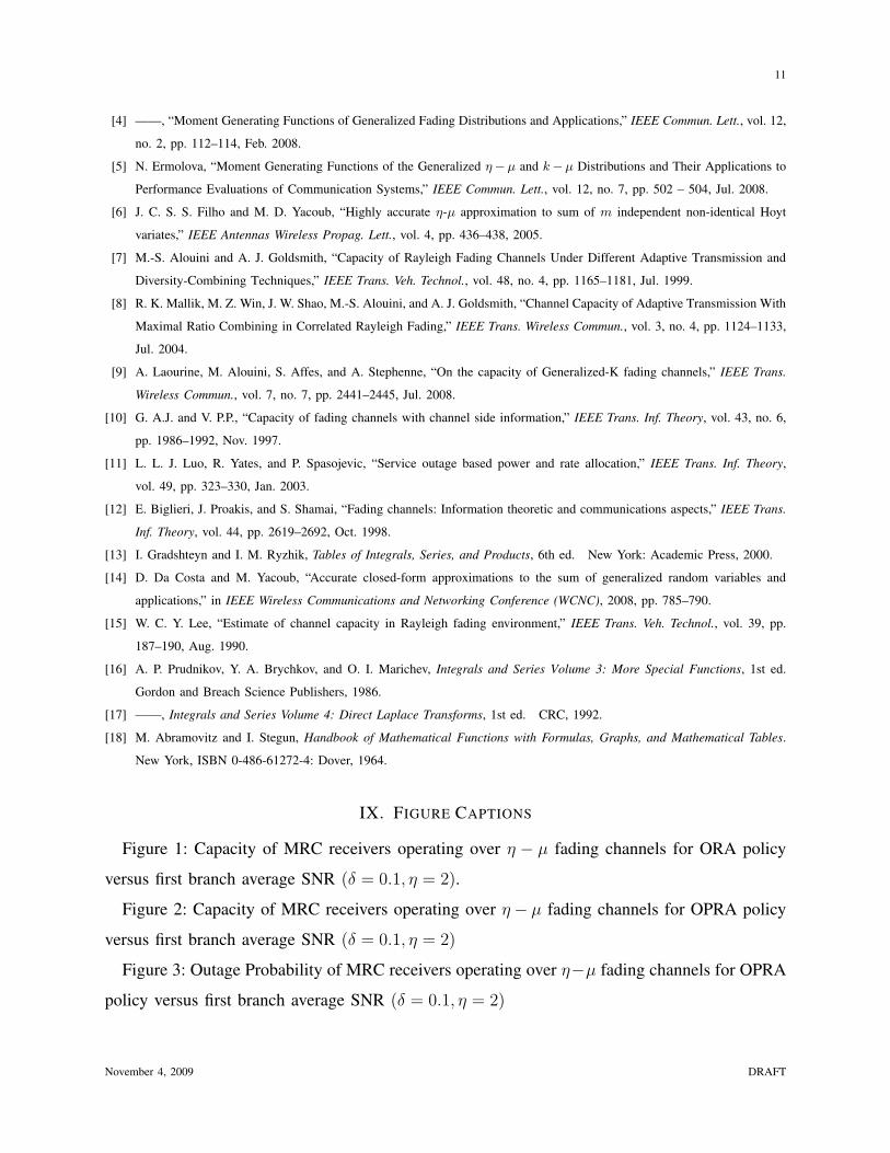
Fig. 2 depicts the channel capacity as a function of γ1 for the OPRA scheme with MRC

diversity for η = 2, and µ = 1, 2. As it can be observed, the OPRA scheme yields a small

increase in capacity over just rate adaptation, and this small increase in capacity diminishes as

γ1 increases. The corresponding outage probability evaluated for the optimal cutoff SNR given

by (16) and (21) is also presented in Fig. 3. Moreover, it can be observed that as the number of

combining branches increases the capacity difference between optimal power and rate adaptation

versus optimal rate adaptation alone becomes negligible for all values of γ1. As in the case of

the OPRA scheme, computer simulation results are included and an excellent match with the

analytically obtained results is observed. Moreover, for the case of single-antenna systems, the


10

infinite series appearing in (15) and (16) converge rapidly and steadily requiring only a few

terms to obtain a desired accuracy. For example, in order to obtain an accuracy equal to the

sixth significant digit, ten terms are required.

In Fig. 4 the channel capacity as a function of γ1 for total channel inversion and MRC diversity

for η = 2, µ = 1, 2 is depicted. As it can be observed, the capacity with total channel inversion

and two-branch MRC exceeds that of a single-branch system with OPRA scheme. Therefore,

given the fact that channel inversion is the least complex technique, a tradeoff of complexity and

capacity for the various adaptation methods and diversity-combining techniques exists. Finally,

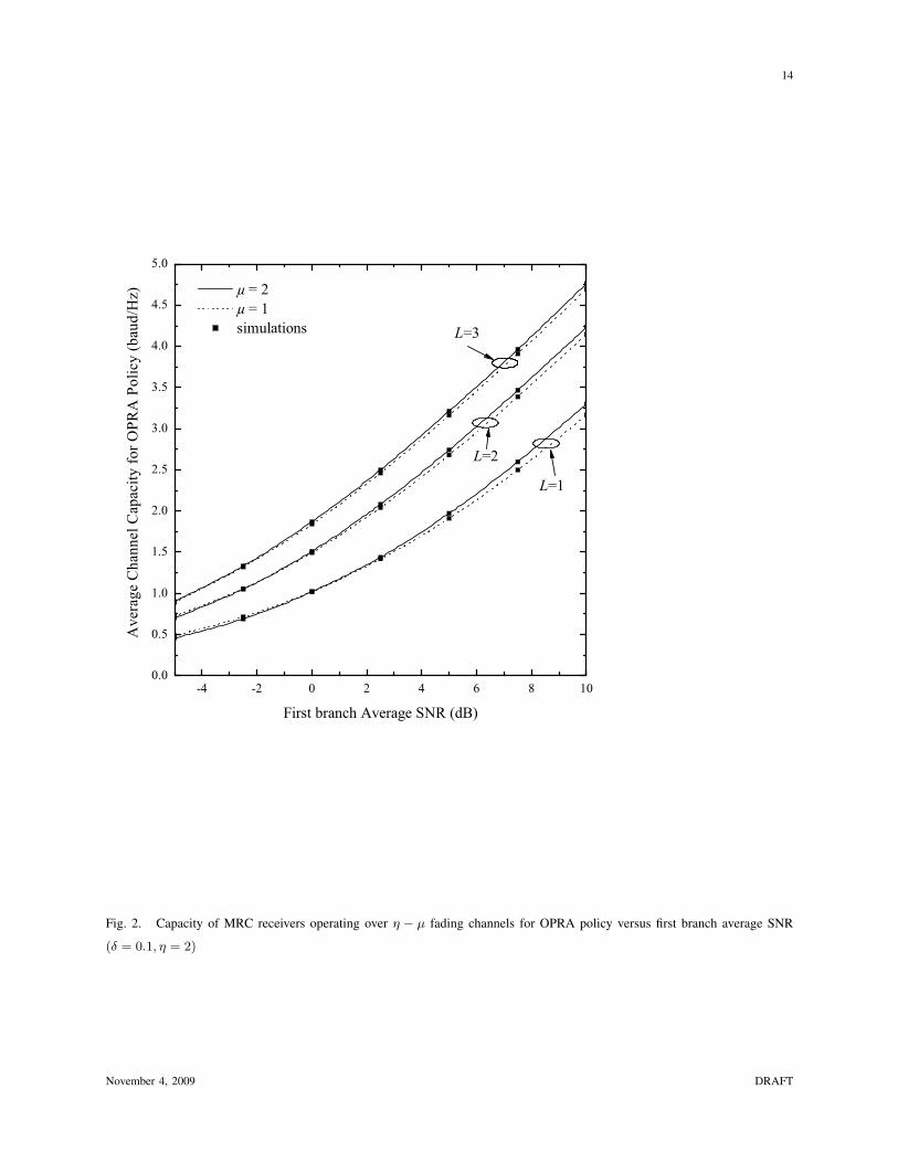
in Figs 5 and 6 the capacity of single and dual-branch MRC receivers as a function of the cutoff

SNR per symbol and for different values of γ1 is illustrated, respectively. As it can be observed,

the cutoff SNR that maximizes the capacity increases as γ1 increases. In all the previously

mentioned test cases, the analytical results are accompanied by monte carlo simulations and an

excellent match with the analytically obtained results is observed. Moreover, the infinite series

appearing in (31) and (32) converge rapidly requiring only a few terms to achieve a given

accuracy. For example, in order to obtain an accuracy equal to the sixth significant digit, eight

terms are required.

VIII. CONCLUSIONS

In this paper, we have examined the single-user capacity of both single-antenna and MRC

systems in an η − µ fading environment. Four adaptive transmission schemes were considered,

namely ORA, OPRA, CIFR and TCIFR. In all cases, we derived analytical expressions in

terms of well-known tabulated functions (the incomplete gamma, the Meijer-G and the Gauss

hypergeometric functions). The mathematical analysis has been illustrated by extensive numerical

and computer simulation results, studying the impact of diversity and comparing the capacity

under different adaptive transmission strategies.

REFERENCES

[1] S. Stein, “Fading channel issues in system engineering,” IEEE J. Sel. Areas Commun., vol. 5, no. 2, pp. 68 – 69, Feb.

1987.

[2] M. D. Yacoub, “The κ-µ and the η-µ distribution,” IEEE Antennas Propag. Mag., vol. 49, no. 1, pp. 68–81, Feb. 2007.

[3] D. B. da Costa and M. D. Yacoub, “Average Channel Capacity for Generalized Fading Scenarios,” IEEE Commun. Lett.,

vol. 11, no. 12, pp. 949–951, Dec. 2007.


11

[4] ——, “Moment Generating Functions of Generalized Fading Distributions and Applications,” IEEE Commun. Lett., vol. 12,

no. 2, pp. 112–114, Feb. 2008.

[5] N. Ermolova, “Moment Generating Functions of the Generalized η−µ and k−µ Distributions and Their Applications to

Performance Evaluations of Communication Systems,” IEEE Commun. Lett., vol. 12, no. 7, pp. 502 – 504, Jul. 2008.

[6] J. C. S. S. Filho and M. D. Yacoub, “Highly accurate η-µ approximation to sum of m independent non-identical Hoyt

variates,” IEEE Antennas Wireless Propag. Lett., vol. 4, pp. 436–438, 2005.

[7] M.-S. Alouini and A. J. Goldsmith, “Capacity of Rayleigh Fading Channels Under Different Adaptive Transmission and

Diversity-Combining Techniques,” IEEE Trans. Veh. Technol., vol. 48, no. 4, pp. 1165–1181, Jul. 1999.

[8] R. K. Mallik, M. Z. Win, J. W. Shao, M.-S. Alouini, and A. J. Goldsmith, “Channel Capacity of Adaptive Transmission With

Maximal Ratio Combining in Correlated Rayleigh Fading,” IEEE Trans. Wireless Commun., vol. 3, no. 4, pp. 1124–1133,

Jul. 2004.

[9] A. Laourine, M. Alouini, S. Affes, and A. Stephenne, “On the capacity of Generalized-K fading channels,” IEEE Trans.

Wireless Commun., vol. 7, no. 7, pp. 2441–2445, Jul. 2008.

[10] G. A.J. and V. P.P., “Capacity of fading channels with channel side information,” IEEE Trans. Inf. Theory, vol. 43, no. 6,

pp. 1986–1992, Nov. 1997.

[11] L. L. J. Luo, R. Yates, and P. Spasojevic, “Service outage based power and rate allocation,” IEEE Trans. Inf. Theory,

vol. 49, pp. 323–330, Jan. 2003.

[12] E. Biglieri, J. Proakis, and S. Shamai, “Fading channels: Information theoretic and communications aspects,” IEEE Trans.

Inf. Theory, vol. 44, pp. 2619–2692, Oct. 1998.

[13] I. Gradshteyn and I. M. Ryzhik, Tables of Integrals, Series, and Products, 6th ed. New York: Academic Press, 2000.

[14] D. Da Costa and M. Yacoub, “Accurate closed-form approximations to the sum of generalized random variables and

applications,” in IEEE Wireless Communications and Networking Conference (WCNC), 2008, pp. 785–790.

[15] W. C. Y. Lee, “Estimate of channel capacity in Rayleigh fading environment,” IEEE Trans. Veh. Technol., vol. 39, pp.

187–190, Aug. 1990.

[16] A. P. Prudnikov, Y. A. Brychkov, and O. I. Marichev, Integrals and Series Volume 3: More Special Functions, 1st ed.

Gordon and Breach Science Publishers, 1986.

[17] ——, Integrals and Series Volume 4: Direct Laplace Transforms, 1st ed. CRC, 1992.

[18] M. Abramovitz and I. Stegun, Handbook of Mathematical Functions with Formulas, Graphs, and Mathematical Tables.

New York, ISBN 0-486-61272-4: Dover, 1964.

IX. FIGURE CAPTIONS

Figure 1: Capacity of MRC receivers operating over η − µ fading channels for ORA policy

versus first branch average SNR (δ = 0.1, η = 2).

Figure 2: Capacity of MRC receivers operating over η − µ fading channels for OPRA policy

versus first branch average SNR (δ = 0.1, η = 2)

Figure 3: Outage Probability of MRC receivers operating over η−µ fading channels for OPRA

policy versus first branch average SNR (δ = 0.1, η = 2)


12

Figure 4: Capacity of MRC receivers operating over η − µ fading channels for CIFR policy

versus first branch average SNR (δ = 0.1, η = 2)

Figure 5: Capacity of single antenna receivers operating over η−µ fading channels for TCIFR

policy versus cutoff SNR and for different values of average SNR(µ = 2, η = 2)

Figure 6: Capacity of dual-branch MRC receivers (L = 2) operating over η − µ fading

channels for TCIFR policy versus cutoff SNR and for different values of first branch average

SNR (δ = 0.1, µ = 2, η = 2)


13

-5.0 -2.5 0.0 2.5 5.0 7.5 10.00.0

0.5

1.0

1.5

2.0

2.5

3.0

3.5

4.0

4.5

5.0

L=3

L=2

Ave

rage

Cha

nnel

Cap

acity

For

OR

A P

olic

y (b

aud/

Hz)

First branch Average SNR (dB)

= 2 = 1 simulations

L=1

Fig. 1. Capacity of MRC receivers operating over η − µ fading channels for ORA policy versus first branch average SNR

(δ = 0.1, η = 2)


14

-4 -2 0 2 4 6 8 100.0

0.5

1.0

1.5

2.0

2.5

3.0

3.5

4.0

4.5

5.0

L=1

L=2

L=3

= 2 = 1 simulations

Ave

rage

Cha

nnel

Cap

acity

for O

PRA

Pol

icy

(bau

d/H

z)


Fig. 2. Capacity of MRC receivers operating over η − µ fading channels for OPRA policy versus first branch average SNR

(δ = 0.1, η = 2)


15

-4 -2 0 2 4 6 8 1010-6

10-5

10-4

10-3

10-2

10-1

100

L=1

L=2

L=3

= 2 = 1 simulations

Out

age

Prob

abili

ty fo

r OPR

A P

olic

y (b

aud/

Hz)


Fig. 3. Outage Probability of MRC receivers operating over η−µ fading channels for OPRA policy versus first branch average

SNR (δ = 0.1, η = 2)


16

-5.0 -2.5 0.0 2.5 5.0 7.5 10.00.0

0.5

1.0

1.5

2.0

2.5

3.0

3.5

4.0

4.5

5.0

= 2 = 1 simulations

L=3

L=2

Ave

rage

Cha

nnel

Cap

acity

w

ith C

hann

el In

vers

ion

(bau

d/H

z)

First Branch Average SNR (dB)

L=1

Fig. 4. Capacity of MRC receivers operating over η − µ fading channels for CIFR policy versus first branch average SNR

(δ = 0.1, η = 2)


17

-10 -5 0 5 10 15 20 250

1

2

3

4

5

6

7

= 20dB

= 10dB

= 5dB

simulations

Ave

rage

Cha

nnel

Cap

acity

w

ith T

runc

ated

Cha

nnel

Inve

rsio

n (b

aud/

Hz)

Cutoff SNR per Symbol (dB)

= 0dB

Fig. 5. Capacity of single antenna receivers operating over η − µ fading channels for TCIFR policy versus cutoff SNR and

for different values of average SNR(µ = 2, η = 2)


18

-10 -5 0 5 10 15 20 250

1

2

3

4

5

6

7

8

1= 20dB

1= 10dB

1= 5dB

simulations

Ave

rage

Cha

nnel

Cap

acity

w

ith T

runc

ated

Cha

nnel

Inve

rsio

n (b

aud/

Hz)

Cutoff SNR per Symbol (dB)

1= 0dB

Fig. 6. Capacity of dual-branch MRC receivers (L = 2) operating over η− µ fading channels for TCIFR policy versus cutoff

SNR and for different values of first branch average SNR (δ = 0.1, µ = 2, η = 2)


Capacity of η-μ fading channels under different adaptive transmission techniques

Documents

Transcript of Capacity of η-μ fading channels under different adaptive transmission techniques