How Does Spatial Extent of fMRI Datasets AffectIndependent Component Analysis Decomposition?

Adriana Aragri,1* Tommaso Scarabino,2 Erich Seifritz,3 Silvia Comani,4,5

Sossio Cirillo,6 Gioacchino Tedeschi,1 Fabrizio Esposito,1,6,7 andFrancesco Di Salle7,8

1Second Division of Neurology, Second University of Naples, Naples, Italy2Department of Neuroradiology, Scientific Institute Casa Sollievo della Sofferenza, S. Giovanni

Rotondo, Foggia, Italy3University Hospital of Clinical Psychiatry, University of Bern, Bern, Switzerland

4Department of Clinical Sciences and Bio-imaging, University Foundation, Chieti University, Chieti, Italy5ITAB-Institute of Advanced Biomedical Technologies, University Foundation, Chieti University,

Chieti, Italy6Department of Neuroradiology, Second University of Naples, Naples, Italy

7Department of Neurological Sciences, University of Naples Federico II, Naples, Italy8Department of Neurological Sciences, University of Pisa, Pisa, Italy

� �

Abstract: Spatial independent component analysis (sICA) of functional magnetic resonance imaging (fMRI)time series can generate meaningful activation maps and associated descriptive signals, which are useful toevaluate datasets of the entire brain or selected portions of it. Besides computational implications, variationsin the input dataset combined with the multivariate nature of ICA may lead to different spatial or temporalreadouts of brain activation phenomena. By reducing and increasing a volume of interest (VOI), we appliedsICA to different datasets from real activation experiments with multislice acquisition and single or multiplesensory-motor task-induced blood oxygenation level-dependent (BOLD) signal sources with different spatialand temporal structure. Using receiver operating characteristics (ROC) methodology for accuracy evaluationand multiple regression analysis as benchmark, we compared sICA decompositions of reduced and increasedVOI fMRI time-series containing auditory, motor and hemifield visual activation occurring separately orsimultaneously in time. Both approaches yielded valid results; however, the results of the increased VOIapproach were spatially more accurate compared to the results of the decreased VOI approach. This isconsistent with the capability of sICA to take advantage of extended samples of statistical observations andsuggests that sICA is more powerful with extended rather than reduced VOI datasets to delineate brainactivity. Hum Brain Mapp 27:736–746, 2006. © 2006 Wiley-Liss, Inc.

Key words: functional magnetic resonance imaging; exploratory data-driven analysis; independent com-ponent analysis; information maximization; data reduction; dataset spatial extent; receiveroperating characteristics; fixed point approach

� �

INTRODUCTION

In functional magnetic resonance imaging (fMRI), univar-iate and multivariate statistics are used to read out differentblood oxygenation level-dependent (BOLD) signals from theacquired time series. Univariate methods, both hypothesis-driven [Bandettini et al., 1993; Friston, 1996] and data-driven[Baumgartner et al., 2000], enable detection and signal char-acterization through an estimation procedure that is re-peated identically at each individual volume element(voxel). The spatial accuracy of the results from univariatemethods is not affected by the selection of the region of

Contract grant sponsor: Swiss National Science Foundation; Con-tract grant number: PP00B-103012.*Correspondence to: Adriana Aragri, Department of NeurologicalSciences, University of Naples Federico II, II Policlinico (NuovoPoliclinico) Padiglione 13, Via S. Pansini 5, 80131 Naples, Italy.E-mail: adrianaaragri@libero.itReceived for publication 22 December 2004; Accepted 8 August 2005DOI: 10.1002/hbm.20215Published online 30 January 2006 in Wiley InterScience (www.interscience.wiley.com).

� Human Brain Mapping 27:736–746(2006) �

© 2006 Wiley-Liss, Inc.

analysis (ROI); univariate approaches, testing each singlebrain voxel independently, neither exploit at all nor fullycharacterize the co-activation phenomena within the sameneurophysiological pattern. This lack of consideration ofspatial interactions inspired the utilization of multivariatemethods for detection and estimation of spatial activationand temporal dynamics of the brain. Multivariate techniqueshave been verified and adopted for functional connectivitypattern analysis of distributed regions in the brain duringcognitive tasks, such as human memory [Fletcher et al.,1996] and resting state [Van de Ven et al., 2004]. This task isaccomplished by estimating suitable second- or higher-orderstatistical entities on the relationships among subsets ofbrain voxels or time points.

Multivariate methods try to aggregate the voxels in spa-tiotemporal patterns of activity based on a common timecourse and a common spatial distribution of a given effect.In general, the relationships between voxel time courses areestimated in the spatial covariance of the measured signals,whose processing reveals the modes of signal variability.

Independent component analysis (ICA) is a popular andhighly studied technique of multivariate (data-driven) anal-ysis of multidimensional datasets. It transforms the mea-sured time series into components that are as statisticallyindependent from each other as possible [Comon, 1994]: theindependent components (ICs).

Statistical independence can be considered a plausibleassumption in many neuroimaging applications, becauseneuronal responses that have distinct causes are likely togenerate regionally specific effects on the measured signalsand it is plausible that these effects do not overlap system-atically, which gives rise to approximately statistically inde-pendent observations [Brown et al., 2001]. So far, the appli-cation of the ICA model to data from different neuroimagingmodalities has provided important insights about funda-mental spatiotemporal dynamics of the human visual[Makeig et al., 2002] and auditory systems [Seifritz et al.,2002].

ICA can be applied to fMRI data in two different ways,namely spatial ICA [McKeown et al., 1998b] and temporalICA [Biswal and Ulmer, 1999]. In spatial ICA (sICA), statis-tical independence is assumed for the distribution in spaceof the extracted sources of signal change: the signal sourcesare independent in their spatial locations rather than in theirtime profile that can exhibit high mutual correlations. Intemporal ICA (tICA), the sources are assumed to be inde-pendent across time. These two variants are described andcompared in Calhoun et al. [2001a].

Considering a typical 3D fMRI dataset, the spatial andtemporal dimensions of the statistical samples suggest theuse of the sICA for 3-D pattern generation, whereas tICA canreveal the presence of multiple dynamics in an anatomicallyor functionally selected region of interest [ROI; Calhoun etal., 2001a; Seifritz et al., 2002]. From the perspective ofstatistical power, sICA has the best potential for a robustrepresentation of whole-brain fMRI datasets because of thesample sizes achievable. The statistical power of sICA can be

as high as to enable useful sICA decomposition even usingfew time points of a single slice fMRI time-series [Esposito etal., 2003].

In multislice 3-D fMRI experiments, the data matrix isfilled by a suitable vectorization of all voxels from all slices.The selection of voxels in sICA may affect the outcome of thedecomposition in two opposite ways: statistical and infor-mative. From the statistical point of view increasing thenumber of voxels increases the power of the sICA analysis asa method that exploits spatial statistics. From the informa-tive point of view, excluding or including a region in thedata selection step may crucially change the actual numberof neurologically relevant signal sources or their statisticalcharacterization. These two situations are thought to pro-duce antithetic effects on ICA decompositions. The purposeof this study is to evaluate and compare two different ap-proaches of selecting raw data before the computationalstage: reduced versus increased volumes of interest (VOI).

To achieve this purpose and to keep the analysis as closeas possible to the real case of a common fMRI experiment,the slice of acquisition was preferentially chosen as theelementary degree of freedom that is available to the user todefine the VOI; besides, in a separate moment, an anatom-ically and functionally guided selection of the volume wasapplied along the three spatial dimensions. In this sense,selecting a volume of just one slice at a time could involvebetter performances because of the reduced influence of“extra-slice” sources of signal change (whose foci of influ-ence are located in a different slice) on the “intra-slice”sources (whose foci of influence are located in that slice). Inother words, given the same number of time points, themixtures are “simpler.” Selecting a bigger volume of data (soincreasing the computational load), however, gathers addi-tional statistical observations even for the intra-slice sources,which helps ICA to extract the corresponding component.Of course, more sources will have the chance to be estimatedin this enlarged domain but the temporal dimensionality ofthe dataset is not changed.

This fundamental trade-off makes the choice of a dataselection approach non-trivial and justifies an analytical in-vestigation of the true extent to which the performancescould be affected by the spatial configuration of the dataset.After having investigated in a previous study the effect ofthe temporal dimension on the ICA output [Esposito et al.,2003], we thus focused here on the spatial extent.

SUBJECTS AND METHODS

Data Acquisition

Imaging parameters

In this study, informed consent was obtained from threeright-handed healthy volunteers (all female; age range24–34 years) who participated in three sessions of a domi-nant hand finger-tapping, visual, and auditory fMRI exper-iment. Whole-brain images were acquired on a 3 Tesla su-perconducting SIGNA MR scanner (General Electric

� Spatial Extent in ICA �

� 737 �

Medical Systems, S. Giovanni Rotondo, Foggia, Italy) usinga standard circularly polarized head coil. After localizerscans, we acquired T1-weighted structural volumes consist-ing of 184 sagittal slices covering the entire brain (field ofview 250 � 250 mm2, matrix 256 � 256 pixels, and slicethickness 1 mm). For fMRI, we used conventional single-shot echo-planar image sequence (volume repetition time1,000 ms, interslice time 71 ms, field of view 240 � 240 mm2;matrix 64 � 64 pixels, and slice thickness 7 mm). A func-tional slab consisted of 14 contiguous slices, which werepositioned parallel to the bi-commissural plane and coveredthe primary motor, supplementary motor, and occipital cor-tex areas. In total, 180 fMRI volumes (180 s) were acquiredthree times during one experimental session. Twentydummy (discarded acquisitions) scans were carried out atthe beginning to allow for longitudinal equilibrium, afterwhich the paradigm was automatically triggered to start bythe scanner.

Experimental paradigms

As shown in Figure 1, visual and auditory stimuli werepresented alternating across the three experimental runs.Stimuli were separated by a nonstimulation interval rangingbetween 10 and 20 s using the stimulation software packagePresentation (http://www.neuro-bs.com; Version 0.91). Awhite cross on a black background was visible during theexperiment (not only during the visual interstimulus inter-vals). The imaging series consisted of an alternating 20-s restepoch (no auditory stimulation) with a 20-s auditory activa-tion epoch repeated 12 times in total for all the sessions. Theacoustic stimulus consisted of a train of 20 bursts of 3.4 kHz,which lasted 20 s and alternated every 20 s. There were threedifferent auditory conditions (Fig. 1): the stand-alone audi-tory one (pattern A) and the other two, which were auditorystimuli with a distracting visual stimulus that lasted 10 s,starting 5 s after the auditory stimulus onset. The visualstimuli consisted of a flickering checkerboard at a fixedluminance contrast level, which was in one case on the leftside of the screen (pattern B) and in the other on the rightside (pattern C). The participants looked into a mirror to seea screen subtending approximately 25 degrees of visual fieldin which the figures were back-projected. The subject had topress a fiberoptically-monitored button panel when he/shelistened to the acoustic stimuli. The button was controlled bythe index finger of the right hand. We recorded reactiontimes for each item for all the participants to get a feedbackof the answers and a measure of accuracy of response.

Data Models

Reduced and increased sample data selectionmethods

The selection of the voxels included in the analysis istypically carried out based on intensity histograms of themean signal or using anatomically relevant segmentation ofthe data [cortex-based ICA; Formisano et al., 2004].

We investigated the effects of reducing or increasing thespatial extent of the dataset (increased VOI [iVOI]; reducedVOI [rVOI]) by including or excluding an adequate sam-pling of multiple concurrent hemodynamic sources in thedata matrix. Two different approaches to vary the spatialextent of the sample were used. In the first approach, thesingle slice of acquisition was chosen as the unitary step andthe VOI was increased or reduced slice by slice along thez-axis. In the second approach, an anatomically and func-tionally guided selection of the region of interest was madealong a 3D volume, based on the inspection of a skilled fMRIneuroradiologist and on data by previous fMRI experi-ments.

In this sense, the problem has a close connection with thenatural choice posed to an MR experimenter of including orexcluding single or multiple slices during the acquisitionand analysis steps. This choice has both technical and meth-odological relevance and helps the experimenter in makingdecision about critical slice-based sampling of the brain aswell as post-hoc evaluations of ICA outcomes.

For this study, an illustrative multislice whole-brain ac-quisition has been designed during a mixed visual, auditory,and motor experimental paradigm with slices encompassingvisual, auditory, and motor cortices. For the analyses weselected a reduced dataset (rVOI) by covering an area ex-pected to comprise only one of the three analyzed systems.This allowed us to observe preferentially one of four foci(left visual, right visual, auditory, and motor) of BOLDactivity resulting in one main source of signal change in thedata. Alternatively, by selecting a bigger spatial volume forthe same ICA run, more spatial observations were evidentfor the sources and more than two sources had to be sepa-rated. The goal of this experimental paradigm was to testspatial ICA on whole-brain functional MRI time series con-taining multiple sources of consistently task-related in ana-tomically disparate and well-separated regions such as thevisual areas, the auditory areas and the motor areas. Thisframework aims at investigating the conditions of reducingthe volume of interest of the ICA analysis in a way thatexcludes from the data matrix both one independent source(leaving at least another independent source), as in the caseof the visual and the audio-motor source, and a spatiallyseparated part of the same independent source. This wasmade possible by using temporally overlapping auditoryand motor sources.

Models and methods of sICA

The basic goal of ICA is to solve the blind source separa-tion (BSS) problem by expressing a set of random vectorialobservations as linear combinations of statistically indepen-dent latent source scalar variables. In the field of fMRI, ICAhas been applied since the publication of two seminal arti-cles [Calhoun et al., 2001a; McKeown et al., 1998b]. It pur-sues maximally independent components by maximizingthe joint entropy of suitably transformed component mapsso that the mutual information between different compo-nents is minimized, finally reducing the redundancy be-

� Aragri et al. �

� 738 �

tween the distributions of map values for different compo-nents.

The raw data from each participant was arranged into a (P� T) matrix with P voxels measured at T different timepoints and entered into a spatial ICA analysis. Principal

component analysis (PCA) was employed as a data reduc-tion step before the estimation of N�T components. Thisstep is usually carried out heuristically or analytically withthe attempt of limiting the under-decomposition or over-reduction (thus excluding important signal contribution to

Figure 1.Schematic presentation of the sequential epoch stimulation. Vari-ously combined, AM, LV, and RV represent auditory-motor, leftvisual, and right visual, respectively. Given that there is no signif-icant confounding effect on each other, three main patterns (A–C)of behavioral-related activation can be considered. In this example,pattern A through pattern C can be utilized as a model function forgeneral linear model analysis to detect the areas of activationcorresponding to auditory-motor predictor in general (A), leftvisual predictor (B), and right visual predictor (C). Representative

multiple regression analysis using patterns A, B, and C modelfunctions within the whole brain are shown below. White graphsindicate representative time series of active voxels (P-corrected� 0.001) BOLD signal. The activation areas are subsequentlyidentified as the primary motor cortex and primary auditorycortex for the pattern A, and lateralized primary visual areas (V1)for patterns B and C. [Color figure can be viewed in the onlineissue, which is available at www.interscience.wiley.com.]

� Spatial Extent in ICA �

� 739 �

the measured variance) and the over-fitting of the data(causing clusters of voxels belonging to the same generativesource to be fragmented into multiple different spatialmaps). Different methods for estimating the optimal numberof components to be extracted have been already proposed[e.g., see Beckmann and Smith, 2004; Calhoun et al., 2001a].We applied the PPCA method [Beckmann and Smith, 2004]and found out an optimal choice at n � 34 ICs (on average).

The component maps were automatically inspected basedon their spatial [Formisano et al., 2002] and anatomical [Vande Ven et al., 2004] structure and identified as left visual (LV;Cleft visual, j), right visual (RV; Cright visual, j), and auditory-motor (AM; Cauditory-motor, j), for each jth participant forevery spatial configuration from rVOI to iVOI.

Models and methods of general linear model(multiple regression analysis)

The general linear model (GLM), first introduced in ana-lyzing brain imaging data by Friston et al. [1990], is theconventional analysis method for most study designs [Lau-rienti et al., 2003]. In the GLM (also known as multipleregression analysis), a linear combination of several regres-sor variables (predictor or explanatory variables) are used to“predict” the variation of an observed signal time course.GLM analysis is carried out independently for the timecourse at each individual voxel, and the results of GLManalysis for a voxel time course are the estimates for theregression coefficients (estimated by the least squaresmethod [LSM] to minimize error values) that make thepredicted values as close as possible to the measured values.

Data Analysis

To define suitable benchmark maps for a receiver operatorcharacteristic (ROC)-based comparison [Skudlarski et al.,1999] of rVOIs and iVOIs in ICA, each dataset was firstanalyzed with the GLM analysis tool with Brain Voyager2000 (Brain Innovation, Maastricht, The Netherlands; onlineat http://www.brainvoyager.com).

Preprocessing

Whole-brain images were first corrected for timing differ-ences between the slices using sinc interpolation to reducepotential misinterpretable effects due to the sequential scan-ning of slices [van de Moortele et al., 1997] and then weremotion corrected to compensate for head movement. Imageswere spatially normalized to Talairach and Tournoux space[1988] after warping different subject anatomies onto thesame template. Data were temporally smoothed by applyinga linear trend removal (slow-frequency drift removal) and ahigh-pass filter for three cycles (to remove nonlinear drifts).This filter converts the time series at each voxel in thefrequency domain and then removes low frequencies. Thefrequency domain representation is then converted back inthe time domains, which looks then as before except thatlow-frequency drifts are no longer visible. Finally, data werespatially smoothed by applying a Gaussian kernel of 2 mm

full-width at half maximum to each acquired slice; the effectof this step is to reduce high-frequency spatial fluctuationsin the images.

General linear model

Data from each participant was entered into GLM sin-gle-subject analysis framework using Brain Voyager 2000.The conventional multiple regression analysis was carriedout on each voxel of every subject separately using BrainVoyager 2000 with one regressor for each of the fourconditions, each consisting of a box-car convolved by thestandard Brain Voyager 2000 canonical hemodynamic re-sponse function (HRF), which consists of a gamma func-tion. Furthermore, voxels lying outside the brain wereremoved by limiting to 500 the image intensity threshold-ing of every subject.

Independent component analysis

To avoid any potential influence of the preprocessingsteps on data quality and intrinsic spatiotemporal corre-spondence, the preprocessing steps in ICA as well as in theGLM analysis were limited to the intensity thresholding andthe gaussian spatial smoothing. ICA runs based on the fixed-point algorithm in deflation mode [Hyvarinen, 1999a and2001] were started from Brain Voyager 2000 using the cortex-based ICA module, without specifying any mask (i.e., vol-ume-based ICA). Instead, the performance evaluation pro-cedures were implemented in MATLAB, using the output ofBrain Voyager 2000.

The fixed-point algorithm aims at solving the ICA prob-lem through a linear transformation that minimizes the mu-tual information of the components by finding the directionsof maximum negentropy. In this algorithm, suitable approx-imations of the negentropy introduced in [Hyvarinen, 1998]are used to derive objective functions for the optimization[Hyvarinen, 1999b].

Selecting ICs that contain cortical or subcortical func-tional units is often a problem in the interpretation offMRI-ICA results, as many components also representartifacts (e.g., scanner and echo-planar imaging (EPI)-related noise, subject movement, breathing, and arterypulsation). Previous applications of ICA could identifyrelevant ICs by post-hoc correlation of the IC time coursesto the event or epoch timing [Calhoun et al., 2001a; Gu,2001; McKeown, 2000], selecting them according to theirspatial and temporal nature [Calhoun et al., 2002] or bypredicting that functionally corresponding areas in differ-ent subjects should have temporally correlated activitytime courses as identical stimuli activate same regions inthe same way across subjects [Bartels and Zeki, 2004]. Inthis study, we found that each selected IC had always anassociated time course that was well correlated to theBOLD signal of the most significant voxels (i.e., maximalvoxel time course), r(AM) � 0.896 � 0.095, r(LV) � 0.902� 0.074, r(RV) � 0.882 � 0.089 across subjects and VOIs.The ICs thus could be selected both according to thecorrelation of their time courses with the GLM regressors

� Aragri et al. �

� 740 �

and according to the anatomical correspondence of theirmost significant voxels with the GLM maps. The IC timecourses are normally provided by ICA decompositions ascolumns of the mixing matrix, in turn reconstructed bypseudo-inversion of the estimated unmixing matrices.Apart from difference in the sign of the activity, howmuch these waveforms visually describe the time coursesof the regions of activity depends also on the distributionof values in the spatial map and may be often poorlycorrelated with the data even in the highest voxels in theIC maps. For these reasons, it is sometimes reported theregion-of-activity (ROA) time course instead of the ICtime course [see also Duann et al., 2002].

In both the rVOI and the iVOI approach, the selectionand assignment of components with similar sources forthe identification was unambiguous and straightforwardin all areas because the individual maps proved to behighly correlated with the GLM (for separate subjects) aspresented in Figure 1 (P corrected � 0.05), even if in theapproach with increased volumes we found out that ei-

ther multiple or single foci could be present in a singleextracted component map.

Quantification and comparison of the approaches’performance

We used the ROC method to compare the efficacy of thetwo approaches in estimating the activation map from asingle subject. ROC is based on the optimization of thetrue-positive ratio (portion of correctly detected activationsto all added activations) to the false-positive ratio (portion ofpixels that were incorrectly recognized as active in all pixelswithout added activation). We evaluated specificity and sen-sibility of the two sICA approaches in estimating the spatiallayout of the task-related effects using multiple regressionanalysis maps as benchmarks.

To distinguish significantly contributing voxels, ICAmaps were scaled to the spatial z-scores, computed as thenumber of standard deviations from the map mean [McKe-own et al., 1998b]. These parameters are useful for descrip-

Figure 2.Consistently task-related components. ICA decomposition of eachsession produced a component to which the activated voxels timecourse well resembled the task block structure (r[a] � 0.66� 0.09 and r[b] � 0.61 � 0.06). ICA component map activevoxels (posterior probability images thresholded at 0.5) are dis-played in the original 2D image matrix (fMRI images) for Subject 1by selecting five different VOI configurations. More spatial obser-vations (iVOI) improve the spatial accuracy of the extracted com-

ponents (with respect to the GLM benchmark). A: Result for theright visual task. The ICA maps look like much performing to GLMmaps already when we build up a VOI of seven slices. B: Com-parison of consistently task-related component maps for auditory-motor task. The ICA maps get the top performing to GLM mapsonly when we build up a complete VOI. [Color figure can beviewed in the online issue, which is available at www.interscience.wiley.com.]

� Spatial Extent in ICA �

� 741 �

tive purposes only and do not provide intrinsic confidencelevels for statistical thresholding. For the figures, we thuschose the threshold of the z-maps using a gaussian mixturemodel (GMM) of the histograms [see Beckmann and Smith,2004], accepting as active voxels with an estimated posteriorprobability of activation exceeding a value of 0.5.

Following the ROC procedure, a curve is traced by findingthe corresponding false-positive fraction (FPF) and the false-negative fraction (FNF) at varying thresholds for the se-lected ICA z-map (i.e., z-map threshold varying 0–10). Inthis way, the results of our analysis will be independent ofthe z-threshold, which is not a rigorous statistical concept byitself [see Beckmann and Smith, 2004]. To produce a singlequantitative figure of merit for each ROC curve, we used themean of the ROC curve over the limited range of false-positive ratio between 0 and 0.1 [Skudlarski et al., 1999]. Thesomewhat arbitrary threshold 0.1 was chosen in relation toan empirical working regime of fMRI data analysis: stayingwithin the value of 0.1 ensures that the ratio of false activa-tions is much smaller than the ratio of true activations [seeFadili et al., 2000].

RESULTS AND DISCUSSION

For each dataset or each run and session, the carried outanalysis provided results that were highly consistent acrosssubjects, suggesting an adequate level of generality of theoutcomes. ICA revealed the same activity patterns as theGLM analysis did carried out with Brain Voyager 2000 in theoccipital lobe (visual component) and in the auditory andmotor cortices (auditory-motor component). This shows thatICA can segregate regions that are activated by stimulusepochs occurring both simultaneously and asynchronously.Each of these ICs had a time course that closely matched theBOLD signal time course of the active voxels revealed byGLM in the corresponding region. Results were well repro-ducible across subjects, in that the IC time courses were wellcorrelated to GLM predictors: r(AM) � 0.730 � 0.179, r(LV)� 0.763 � 0.179, and r(RV) � 0.684 � 0.173, across subjectsand VOIs.

The rVOI and iVOI approaches exhibited different resultsfor the components associated with the auditory-motorsources (multiple sources activated) and similar results forthe visual components (single sources activated).

Specifically, as expected based on the timing of the sen-sory stimulation, separate task-related maps contained therelative hemi-visual sources. Furthermore, audio-motortask-related maps contained task-related single foci (only“auditory” or only “motor” component) in the rVOI andmultiple foci of brain activity (“auditory-motor” compo-nents) in the iVOI datasets. Including or not including aregion of interest in ICA data selection (by selecting biggeror smaller volumes of data) may crucially affect the extrac-tion of targeted source signals. The auditory-motor sourcewas best estimated on the maximal iVOI whereas a spatiallyreduced dataset that comprised only the auditory slices wasless accurate in estimating the same auditory components.This suggests that when the observations of the fMRI mix-

tures are drawn from a native auditory-motor (multiple foci)source, the iVOI approach actually takes advantage of someform of signal interaction between the multiple foci of ac-tivity in the conceptually unique component that is notexploited in the rVOI (Fig. 2B). Additional slices in the motorcortex globally improve the estimate of the auditory-motorcomponents but do not affect the estimate of the visualcomponents (Fig. 2A; Fig. 3). Despite the improved spatio-temporal accuracy, because of the highly similar regionaltime courses the iVOI decompositions exhibited a substan-tially poor functional segregation, providing a single-com-ponent instead of a two-component model of the observedfunctional connectivity in the two spatially separate sys-tems. In general, ICA provides a better functional segrega-tion in event-related designs [see Calhoun et al., 2001b;Formisano et al., 2004] where the measured interregionaldifferences in the time-courses are more systematic.

The visual inspection of the components generated bysICA decompositions confirmed the ROC measures andrevealed the different technical quality of iVOI and rVOImaps. Both rVOI and iVOI ICA as well as GLM mapsclearly show clusters of cortical activity corresponding tothe main areas expected to be activated by the auditory-motor, left visual, and right visual tasks. For the purposeof a reliable selection of the task-related ICs, the ROI-based selection criterion [Van de Ven et al., 2004] wasused and the output was confirmed by the temporal ref-

Figure 3.The panels show the correlation values of IC time courses vs. timecourses of IC maximal voxel and vs. GLM regressors time courses,across VOIs, averaged on subjects.

� Aragri et al. �

� 742 �

erences. The auditory-motor pattern (Fig. 1, see A) re-sulted in an wide network of activations that included avery large cluster in the primary motor cortex spanningthe left pre- (supplementary motor area; SMA), medial-(premotor cortex), middle- (prefrontal cortex), and post-central (pre-SMA) gyrus (Brodmann area [BA] 4, 6, 46, 2,respectively) and an extended region of activation in theinsula (basal ganglia; BA 13). The peak of activation wasfound in BA 42 (superior temporal gyrus; STG) consistentwith the activation of the auditory area in primary audi-tory cortex (Heschl’s convolutions). In the left visual pat-tern (Fig. 1, see B) the activated regions were the inferior(BA 17) and middle occipital gyrus (BA 18), the fusiformgyrus (BA 19), and the cuneus (BA 17), consistent withactivation of the primary visual cortex (V1). Finally in the

right visual pattern (Fig. 1, see C), the activated regionswere similar to the pattern (B) and included the lingualgyrus (BA 18).

McKeown et al. [1998b] compared sICA with other data-driven methods and showed that sICA performs best inisolating voxels whose activity time courses correlate withdistinct task conditions or with artifacts. We observed thatfor every subject, the Cleft visual, j and Cright visual, j are com-ponents more easily extracted than are Cauditory-motor, j (Fig.3); in fact, they fit better to the multiple regression analysismaps.

The GLM analysis and ICA decomposition exhibitedclearly different behavior with respect to the changes of thethreshold. In fact, threshold proved to be a critical parameterfor the ROC power evaluation, particularly related to filter-

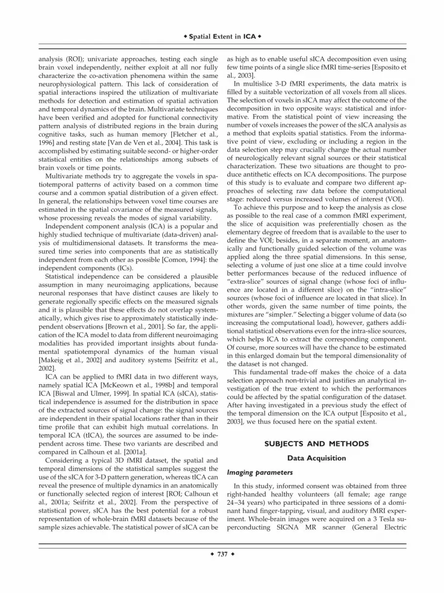
Figure 4.The left panels present the mean measure of the ROC curve as afunction of the selected increasing VOI (from slice 1 to 14 for theslice-based approach in the upper panel and five functional-basedVOIs in the lower panel), for the three main functional activities(auditory-motor [AM], left visual [LV], and right visual [RV]). Thecurves were obtained from the whole ROC curve using only 0–0.1false positive ratio regions as used in this article. We used threedifferent imaging sessions and the results are reported for the threesessions averaged out. The measures of spatial accuracy revealed thatthe iVOI approach can ensure superior performances in terms ofROC power than the rVOI one can: by increasing the number ofvoxels, the extracted independent components perform better tomultiple regression analysis benchmarks. We noticed that for theC

auditory-motor, jin the slice-based approach, including additional spatial

volumes with new sources causes a transitory slow down in the meanROC value, which rises again by including further extra spatial vol-

umes, useful for the auditory-motor component. Specifically, this falloccurs when including the extra auditory area (slice 7) until whenincluding the motor area (slice 11). The graphs on the right representthe mean number of iterations necessary for extracting the repre-sentative independent components as function of the selected in-creasing VOI for the three main functional activities (AM, LV, RV).The number of iterations for extracting the best ROC power task-related extracted components in the iVOI approach is on the averagelower than that in the rVOI approach. Furthermore, in the slice-basedapproach, including additional spatial volumes with new sourcescauses a transitory rise in the number of iterations, which goes againdown by including further extra spatial volumes, useful for the audi-tory-motor component Cauditory-motor, j. The number of iterationsseems to be affected by the structure of the sample used in spatialICA in a way that the more information about the sources affectingthe data, the faster (and more accurate) the estimation is.

� Spatial Extent in ICA �

� 743 �

ing properties of ICA not present in standard multiple re-gression analysis. We found an acceptable threshold trade-off between statistical significance and the accuracy ofactivation patterns in using a corrected significance of P� 0.01 for the GLM, but in the ROC analysis a pixel isconsidered active only when a certain number of its closestneighbors (20) are active as well. In this approach, pixels onthe border of activated regions are not treated as activatedeven for an extremely low threshold level. In such circum-stances, the true-positive ratio is always significantly smallerthan one. This may offset the high efficiency of such a filterin the more interesting regime of a more realistic and higherthreshold. Despite the obvious suboptimality of multipleregression analysis as a benchmark, we have used it toachieve a simple standardization of the results.

The measures of spatial accuracy revealed that the iVOIapproach can ensure superior performances in terms of ROCpower than the rVOI one can. Figure 4 and Tables I and IIshow ROC results on auditory-motor and visual activationdata averaged across subjects and sessions. Those results

indicate that by increasing the number of voxels westrengthen sICA power to identify clusters of activation, orat least, if more spatial observations are available for covari-ant sources the decomposition will produce more accuratecomponents (Fig. 2A,B).

Furthermore, we noticed that the number of iterations forextracting the best ROC power task-related components inthe iVOI approach was on average lower than that in therVOI approach (Fig. 4; Tables III and IV). This indicates thatselecting a bigger spatial volume of data and making morestatistical observations available for source estimation mayrender the ICA extraction easier from the algorithmic pointof view. Moreover, we noticed that incrementally addingsubvolumes of data with new active sources altered thenumber of iterations as a function of the actual spatial cov-erage of the new sources. More in detail, a transient rise inthe number of iterations was observed when including theauditory area or the motor area in the iVOI audiomotorcomponent. The number of iterations thus seems to be af-fected by the structure of the sample used in sICA in a waythat the more information about the sources affecting thedata we use, the faster (and more accurate) the estimation is.More spatial observations available for both single and mul-tiple sources produce an average decrease in the number ofiterations, provided that these additional observations actu-ally enforced the statistical ICA efficiency in the extraction ofthose sources (i.e., voxels that fit those sources in terms oftheir multivariate spatiotemporal profiles). When additionalobservations only increase the complexity of the mixturerather than “enforcing” the structure of “already” extract-able components or allowing the identification of new com-ponents, these act as noisy, confounding observations andthe unmixing process of ICA is less effective and accurate.

These considerations imply important consequences forthe practical application of ICA to protocols in which syn-chronous spatially independent multiple sources are inves-

TABLE I. Mean ROC scores for VOI along z for three subjects

Slices

1st Session 2nd Session 3rd Session All 3 Sessions

CLV CRV CAM CLV CRV CAM CLV CRV CAM CLV CRV CAM

1 0.085 0.000 0.356 0.120 0.000 0.390 0.196 0.000 0.378 0.134 0.000 0.3752 0.491 0.505 0.438 0.464 0.539 0.352 0.434 0.596 0.469 0.463 0.547 0.4203 0.784 0.758 0.434 0.724 0.733 0.377 0.763 0.710 0.404 0.757 0.733 0.4054 0.758 0.731 0.454 0.799 0.688 0.455 0.805 0.759 0.443 0.787 0.726 0.4515 0.843 0.745 0.514 0.839 0.692 0.516 0.843 0.772 0.510 0.842 0.737 0.5136 0.881 0.749 0.327 0.846 0.723 0.508 0.854 0.753 0.419 0.860 0.742 0.4187 0.892 0.766 0.353 0.866 0.719 0.422 0.849 0.770 0.421 0.869 0.752 0.3998 0.886 0.764 0.434 0.875 0.509 0.397 0.857 0.777 0.442 0.873 0.683 0.4249 0.904 0.780 0.363 0.883 0.736 0.516 0.857 0.759 0.466 0.881 0.758 0.448

10 0.878 0.764 0.407 0.893 0.705 0.403 0.859 0.758 0.447 0.877 0.743 0.41911 0.882 0.761 0.300 0.889 0.719 0.388 0.858 0.758 0.459 0.877 0.746 0.38212 0.856 0.771 0.501 0.890 0.715 0.429 0.865 0.758 0.464 0.870 0.748 0.46413 0.888 0.773 0.583 0.895 0.729 0.545 0.868 0.749 0.580 0.884 0.750 0.56914 0.896 0.841 0.605 0.912 0.803 0.573 0.879 0.770 0.555 0.896 0.805 0.578

All subjects mean ROC measures as a function of the selected increasing VOI (from 1 to 14 slices), for the three main related extractedcomponents (Cleft visual [CLV]; Cright visual [CRV]; Cauditory-motor [CAM]) along a mean of all sessions, by using only 0–0.1 false-positive ratioregions.

TABLE II. Mean ROC scores for VOI along xyz forthree subjects for all three sessions

VOI CLV CRV CAM

1 0.537 0.491 0.3682 0.693 0.658 0.5073 0.891 0.666 0.5924 0.900 0.727 0.6465 0.896 0.805 0.578

All subjects mean ROC measures as a function of the selectedincreasing VOI: an anatomically and functionally informed selectionof the region of interest that is made variable along all the threespatial dimensions, for the three main related extracted components(Cleft visual [CLV]; Cright visual [CRV]; Cauditory-motor [CAM]) along amean of all sessions using only 0–0.1 false positive ratio regions.

� Aragri et al. �

� 744 �

tigated with respect to how the computational load and theaccuracy of the layout are affected. This aspect becomescrucial in a real-time ICA [Esposito et al., 2003], in which thetrade-off of space and time source sampling is at its extremegrade.

CONCLUSIONS

The aim of this article was to explore the performance ofmultiple ways to select the data sample for sICA in multi-condition experimental designs, to provide quantitative in-formation concerning their impact in the processing of fMRIdata, and to suggest their choice based on specific applica-tion problems. We have experimentally compared twomethods for voxel selection when constructing the ICA ob-servation matrix from the acquired slice time-series andcompared the rVOI and the iVOI for sICA decompositions.Estimation and accuracy performances in extracting task-related activation maps from multiple condition block-de-sign fMRI datasets were considered within a multiconditionexperimental framework. The performances of the iVOI ap-proach were almost always better compared to that of therVOI. Although the rVOI approach was faster in extracting

the individual sources because of the reduced size of theinput data matrix, the iVOI approach was more powerful interms of appropriate separation and estimation of multiplesources in a single decomposition.

The spatial extent of a dataset is a major issue for off-lineand real-time ICA applications in relation to the experimen-tal design. In fact, especially with a temporally reducedobservation window, it is essential to predict how the spatialstructure of the sample will be affected by the number ofsources and their spread across space. In our off-line appli-cation, even when both types of data selection worked prop-erly, the iVOI approach also exhibited a specific superiorityin the efficacy of ICA component extraction, a relevant pointfor further work in the context of real-time ICA.

REFERENCES

Bandettini PA, Jesmanowicz AJ, Wong EC, Hyde JS (1993): Process-ing strategies for time-course data sets in functional MRI of thehuman brain. Magn Reson Med 30:161–173.

Bartels A, Zeki S (2004): The chronoarchitecture of the humanbrain—natural viewing conditions reveal a time-based anatomyof the brain. Neuroimage 22:419–433.

Baumgartner R, Somorjai R, Summers R, Richter W, Ryner L (2000):Novelty indices: identifiers of potentially interesting time-courses in functional MRI data. Magn Reson Imaging 18:845–850.

Beckmann CF, Smith SM (2004): Probabilistic independent compo-nent analysis for functional magnetic resonance imaging. IEEETrans Med Imaging 23:137–152.

Biswal BB, Ulmer JL (1999): Blind source separation of multiplesignal sources of fMRI data sets using independent componentanalysis. J Comput Assist Tomogr 23:265–271.

Brown GD, Yamada S, Sejnowski TJ (2001): Independent componentanalysis at the neural cocktail party. Trends Neurosci 24:54–63.

Calhoun VD, Pekar JJ, McGinty VB, Adali T, Watson TD, PearlsonGD (2002): Different activation dynamics in multiple neuralsystems during simulated driving. Hum Brain Mapp 16:158–167.

TABLE III. Mean number of iterations for VOI along z

Slices

1st Session 2nd Session 3rd Session All 3 Sessions

CLV CRV CAM CLV CRV CAM CLV CRV CAM CLV CRV CAM

1 0.00 0.00 99.00 0.00 0.00 85.67 0.00 0.00 89.50 0.00 0.00 91.392 36.33 0.00 212.67 49.33 37.67 128.67 20.33 0.00 111.67 35.33 12.56 1513 11.33 42.67 37.00 14.67 25.67 55.67 23.00 44.33 37.33 16.33 37.56 43.334 41.33 49.33 43.33 15.67 29.33 111.33 23.00 36.33 49.33 26.67 38.33 68.005 22.67 26.67 37.33 15.67 20.00 23.33 18.67 26.67 52.00 19.00 24.44 37.566 46.00 19.67 51.00 20.00 70.67 95.00 53.67 33.00 137.67 39.89 41.11 94.567 25.67 24.00 69.67 17.00 37.33 33.00 15.67 33.67 57.00 19.44 31.67 53.228 25.00 31.33 46.67 17.67 79.33 46.67 14.00 24.33 123.67 18.89 45.00 72.339 23.33 29.67 35.33 39.67 52.00 50.00 32.33 40.33 91.00 32.11 40.67 58.78

10 19.67 73.67 34.67 23.00 56.67 76.00 23.67 27.67 92.67 23.33 52.67 67.7811 36.00 24.00 53.33 48.67 56.00 51.00 29.67 30.67 53.00 32.67 36.89 52.4412 32.22 31.00 59.00 31.33 52.33 34.33 29.33 29.33 48.00 32.22 37.56 47.1113 21.33 35.33 101.33 23.67 54.67 93.00 20.33 40.33 40.67 21.33 43.44 78.3314 48.78 23.00 54.33 36.67 52.00 50.00 85.67 26.67 36.67 48.78 33.89 47.00

All subjects mean number of iterations as a function of the selected increasing VOI (from 1 to 14s), for the three main related extractedcomponents (Cleft visual [CLV]; Cright visual [CRV]; Cauditory-motor [CAM]) along distinct sessions and showing a mean of all sessions.

TABLE IV. Mean number of iterations for VOI alongxyz for three subjects for all three sessions

VOI CLV CRV CAM

1 72.00 56.33 84.002 40.00 67.00 58.003 25.00 33.00 34.004 128.00 55.00 47.005 48.78 33.89 47.00

All subjects mean number of iterations as a function of the selectedincreasing VOI along all the three spatial dimensions, for the threemain related extracted components (Cleft visual [CLV]; Cright visual

[CRV]; Cauditory-motor [CAM]) along a mean of all sessions.

� Spatial Extent in ICA �

� 745 �

Calhoun VD, Adali T, McGinty VB, Pekar JJ, Watson TD, PearlsonGD (2001b): fMRI activation in a visual-perception task: networkof areas detected using the general linear model and indepen-dent components analysis. Neuroimage 14:1080–1088.

Calhoun VD, Adali T, Pearlson GD, Pekar JJ (2001a): Spatial andtemporal independent component analysis of functional MRIdata containing a pair of task-related waveforms. Hum BrainMapp 13:43–53.

Comon P (1994): Independent component analysis, a new concept?Signal Process 36:287–314.

Duann JR, Jung TP, Kuo WJ, Yeh TC, Makeig S, Hsieh JC, SejnowskiTJ (2002): Single-trial variability in event-related BOLD signals.Neuroimage 15:823–835.

Esposito F, Seifritz E, Formisano E, Morrone R, Scarabino T, Tede-schi G, Cirillo S, Goebel R, Di Salle F (2003): Real-time indepen-dent component analysis of fMRI time-series. Neuroimage 20:2209–2224.

Fadili MJ, Ruan S, Bloyet D, Mazoyer B (2000): A multistep unsu-pervised fuzzy clustering analysis of fMRI time series. HumBrain Mapp 10:160–178.

Fletcher PC, Dolan RJ, Shallice T, Frith CD, Frackowiak RS, FristonKJ (1996): Is multivariate analysis of PET data more revealingthan the univariate approach? Evidence from a study of episodicmemory retrieval. Neuroimage 3:209–215.

Formisano E, Esposito F, Di Salle F, Goebel R (2004): Cortex-basedindependent component analysis of fMRI time-series. Magn Re-son Imaging 22:1493–1504.

Formisano E, Esposito F, Kriegerskorte N, Tedeschi G, Di Salle F,Goebel R (2002): Spatial independent component analysis offunctional MRI time-series: characterization of the cortical com-ponents. Neurocomputing 49:241–254.

Friston KJ, Frith CD, Liddle PF, Dolan RJ, Lammertsma AA, Frack-owiak RS (1990): The relationship between global and localchanges in PET scans. J Cereb Blood Flow Metab 10:458–466.

Friston KJ (1996): Statistical parametric mapping and other analysesof functional imaging data. In: Toga AW, Mazziotta JC, editors.Brain mapping: the methods. San Diego: Academic Press. p363–396.

Gu H, Engelien W, Feng H, Silbersweig DA, Stern E, Yang Y (2001):Mapping transient, randomly occurring neuropsychologicalevents using independent component analysis. Neuroimage 14:1432–1443.

Hyvarinen A, Karhunen J, Oja E (2001): Independent componentanalysis. New York: Wiley.

Hyvarinen A, Pajunen P (1999): Nonlinear independent componentanalysis: Existence and uniqueness results. Neural Netw 12:429–439.

Hyvarinen A (1999b): Sparse code shrinkage: denoising of nongaus-sian data by maximum likelihood estimation. Neural Comput11:1739–1768.

Hyvarinen A (1999a): Fast and robust Fixed-Point algorithms forindependent component analysis. IEEE Trans Neural Networks10:626–634.

Hyvarinen A (1998): New approximations of differential entropy forindependent component analysis and projection pursuit. In: Jor-dan MI, Kearns MJ, Solla SA, editors. Advances in Neural Infor-mation Processing Systems 10. Cambridge, MA: MIT Press. p273–279.

Lange N (1996): Statistical procedures for functional MRI. In:Moonen CT, Bandettini PA, editors. Functional MRI. New York:Springer. p 301–335.

Laurienti PJ, Burdette JH, Maldjian JA (2003): Separating neuralprocesses using mixed event-related and epoch-based fMRI par-adigms. J Neurosci Methods 131:41–50.

Makeig S, Westerfield M, Jung TP, Enghoff S, Townsend J,Courchesne E, Sejnowski TJ (2002): Dynamic brain sources ofvisual evoked responses. Science 295:690–694.

McKeown MJ (2000): Detection of consistently task-related activa-tions in fMRI data with hybrid independent component analysis.Neuroimage 11:24–35.

McKeown MJ, Makeig S, Brown GG, Jung TP, Kindermann SS, BellAJ, Sejnowski TJ (1998b): Analysis of fMRI data by blind sepa-ration into independent spatial components. Hum Brain Mapp6:160–188.

McKeown MJ, Jung TP, Makeig S, Brown G, Kindermann SS, LeeTW, Sejnowski TJ (1998a): Spatially independent activity pat-terns in functional MRI data during the stroop color-namingtask. Proc Natl Acad Sci USA 95:803–810.

Seifritz E, Esposito F, Hennel F, Mustovic H, Neuhoff JG, Bilecen D,Tedeschi G, Scheffler K, Di Salle F (2002): Spatiotemporal patternof neural processing in the human auditory cortex. Science 297:1706–1708.

Skudlarski P, Constable RT, Gore JC (1999): ROC analysis of statis-tical methods used in functional MRI: individual subjects. Neu-roimage 9:311–329.

Talairach J, Tournoux P (1988): Co-Planar Stereotaxic Atlas of theHuman Brain. New York: Thieme.

Van de Moortele PF, Cerf B, Lobel E, Paradis AL, Faurion A, LeBihan D (1997): Latencies in fMRI time-series: effect of sliceacquisition order and perception. NMR Biomed 10:230–236.

Van de Ven VG, Formisano E, Prvulovic D, Roeder CH, Linden DE(2004): Functional connectivity as revealed by spatial indepen-dent component analysis of fMRI measurements during rest.Hum Brain Mapp 22:165–178.

� Aragri et al. �

� 746 �