High Performance Optical Force Sensing
152
High Performance Optical Force Sensing - Design, Characterization and Integration in Robotic Minimally Invasive Surgery by Amir Hossein Hadi Hosseinabadi B.Sc. Mechanical Engineering, Sharif University of Technology, 2011 M.A.Sc. Mechanical Engineering, University of British Columbia, 2014 A THESIS SUBMITTED IN PARTIAL FULFILLMENT OF THE REQUIREMENTS FOR THE DEGREE OF Doctor of Philosophy in THE FACULTY OF GRADUATE AND POSTDOCTORAL STUDIES (Electrical and Computer Engineering) The University of British Columbia (Vancouver) August 2021 © Amir Hossein Hadi Hosseinabadi, 2021
-
Upload
khangminh22 -
Category
Documents
-
view
0 -
download
0
Transcript of High Performance Optical Force Sensing
High Performance Optical Force Sensing - Design, Characterization andIntegration in Robotic Minimally Invasive Surgery
by
Amir Hossein Hadi Hosseinabadi
B.Sc. Mechanical Engineering, Sharif University of Technology, 2011
M.A.Sc. Mechanical Engineering, University of British Columbia, 2014
A THESIS SUBMITTED IN PARTIAL FULFILLMENT
OF THE REQUIREMENTS FOR THE DEGREE OF
Doctor of Philosophy
in
THE FACULTY OF GRADUATE AND POSTDOCTORAL STUDIES
(Electrical and Computer Engineering)
The University of British Columbia
(Vancouver)
August 2021
© Amir Hossein Hadi Hosseinabadi, 2021

The following individuals certify that they have read, and recommend to the Faculty of Graduate andPostdoctoral Studies for acceptance, the dissertation entitled:
High Performance Optical Force Sensing - Design, Characterization and Integration inRobotic Minimally Invasive Surgery
submitted by Amir Hossein Hadi Hosseinabadi in partial fulfillment of the requirements for the degreeof Doctor of Philosophy in Electrical and Computer Engineering.
Examining Committee:
Septimiu E. Salcudean, Electrical and Computer Engineering, UBCSupervisor
Yusuf Altintas, Mechanical Engineering, UBCSupervisory Committee Member
Robert Rohling, Electrical and Computer Engineering, UBCSupervisory Committee Member
Edmond Cretu, Electrical and Computer Engineering, UBCSupervisory Committee Member
Shahriar Mirabbasi, Electrical and Computer Engineering, UBCUniversity Examiner
Ryozo Nagamune, Mechanical Engineering, UBCUniversity Examiner
Rajni Patel, Electrical and Computer Engineering, Western UniversityExternal Examiner
ii
Abstract
In this thesis, we researched design developments for multi-axis force sensing at the surgeon and the
patient consoles of the da Vinci® classic system. A systematic survey on the force sensing literature in
Minimally Invasive Surgery (MIS), was conducted. It summarizes the design requirements, compares
different technologies, and lists the pros and cons of different locations for sensor integration.
While more than 100 articles were published on MIS force sensing, no prior work that addresses
force sensing at the surgeon console, without limiting its dexterity, was found. We propose modifications
in the wrist’s yaw link of the da Vinci’s Master Tool Manipulator (MTM) for integration of a commercial
6-axis force-torque sensor. The new design does not change the original manipulator’s kinematics and
its dexterity. Two example applications of the MTM’s impedance control and joystick control of the
Patient Side Manipulator (PSM) were presented to demonstrate the successful integration of the force
sensor into the MTM.
The mechanical design, electronics hardware, and firmware and software architectures of a novel
6-axis optical force sensor are discussed. The mechatronic design features simple integration, no over-
load, low-noise, wide dynamic range opto-electronics, and signal conditioning, coupled with co-located
digital electronics based on a Field Programmable Gate Array (FPGA) that samples all sensing chan-
nels synchronously, enabling very low noise displacement sensing with a resolution of 1.62 nm, low
measurement signal latency of 100 µs, high measurement bandwidth of 500 Hz, and high data transfer
rates over 11.5 kHz for transmission of six-axis transducer data to a host computer. The transducer’s
resolution is better than 0.0001% of the full-scale.
The optical force sensor was used for measuring the forces applied to the distal end of a da Vinci® En-
doWrist® instrument by mounting it onto its proximal shaft. A new cannula design comprising an inner
tube and an outer tube was proposed. A mathematical model of the sensing principle was developed
and used for model-based calibration. A data-driven calibration based on a shallow neural network ar-
chitecture is discussed. The proposed force-sensing requires no modification of the instrument itself;
therefore, it is adaptable to different instruments.
iii
Lay Summary
In Robotic Minimally Invasive Surgery (RMIS), the surgeon’s hand motions are captured by one ma-
nipulator and copied by another manipulator at the surgical site to perform delicate tasks. Compared
to open surgery, access to the surgical site is through small incisions. The isolation via two manipu-
lators removes the sense of touch that is traditionally a rich source of information for the surgeons to
locate veins, nerves, and abnormalities, and regulate forces to avoid tissue damage. It has been shown
that presenting the interaction force data to the surgeon can significantly improve the sense of telep-
resence, enhance task efficiency, and accuracy. Due to the involved challenges in sensor design, safety
concerns, and cost, no clinical system yet has force sensing and display capabilities. In this thesis, we
research modifications to the da Vinci telesurgical system, the most widely used RMIS platform, to
cost-effectively provide force-sensing capability at the surgeon and the patient consoles.
iv
Preface
This thesis is written based on several published manuscripts resulting from the work done by the author
and in collaboration with multiple researchers. The material from the publications has been modified to
make the thesis coherent.
A modified version of Chapter 1 has been submitted for publication as:
• A. H. Hadi Hosseinabadi and S. E. Salcudean, “Force Sensing in Robot-assisted Keyhole En-
doscopy: A Systematic Survey”, accepted for publication with minor revisions, International
Journal of Robotics Research, 2020 (IJR-20-3943).
The author’s contribution to the paper above was finding the relevant literature in different scholarly
repositories; screening and selection of the records based on the PRISMA guidelines to identify those to
be included in the survey; detailed review of the selected articles to extract the key information related
to the sensing technologies and design requirements; categorize the extracted info; write the paper, and
be the corresponding author for the paper submission.
A modified version of Chapter 2 has been published as:
• D. G. Black, A. H. Hadi Hosseinabadi* and S. E. Salcudean, “6-DOF Force Sensing for the Mas-
ter Tool Manipulator of the da Vinci Surgical System,” in International Conference on Robotics
and Automation (ICRA), 2020, Conference Presentation.
• D. G. Black, A. H. Hadi Hosseinabadi* and S. E. Salcudean, “6-DOF Force Sensing for the
Master Tool Manipulator of the da Vinci Surgical System,” in IEEE Robotics and Automation
Letters, vol. 5, no. 2, pp. 2264-2271, April 2020, doi: 10.1109/LRA.2020.2970944.
The first two authors share the first authorship in the publications above. The author’s contribution
was defining the project objectives and supervising the summer student, David G. Black, throughout
the project execution; brainstorm and review the design ideas; integrating the system in terms of both
software and hardware components, assembly, and debugging; designing lab experiments; review and
analyze the test results; review and edit the paper, and be the corresponding author for the paper sub-
mission.
A modified version of Chapter 3 and Chapter 4 have been accepted for publication as:
*Co-first author
v
• A. H. Hadi Hosseinabadi and S. E. Salcudean, “Optical Force Sensor”, Patent Cooperation
Treaty (PCT) Number: PCT/CA2019/051276, 2019
• A. H. Hadi Hosseinabadi and S. E. Salcudean, “Ultra Low Noise, High Bandwidth, Low Latency,
No Overload 6-Axis Optical Force Sensor”, in IEEE/ASME Transactions on Mechatronics, 2020,
doi: 10.1109/TMECH.2020.3043346.
• A. H. Hadi Hosseinabadi and S. E. Salcudean, “Ultra Low Noise, High Bandwidth, Low La-
tency, No Overload 6-Axis Optical Force Sensor”, in IEEE/ASME International Conference on
Advanced Intelligent Mechatronics, July 2021. Conference Presentation.
• A. H. Hadi Hosseinabadi, D. G. Black and S. E. Salcudean, “Ultra Low-Noise FPGA-Based 6-
Axis Optical Force-Torque Sensor: Hardware and Software,” in IEEE Transactions on Industrial
Electronics, vol. 68, no. 10, pp. 10207-10217, Oct. 2021, doi: 10.1109/TIE.2020.3021648.
The author’s contribution in the work resulting into the above articles was: developing the electro-optical
and continuum mechanics model of the sensor; prototyping for conceptual evaluation of the sensing ap-
proach; mechanical design of the 6-axis optical force sensor and generate fabrication drawings; work
closely with a local machine shop on parts fabrication, quality inspection, and repair; collaborate with
the project’s consultant, Gerald F. Cummings, on the sensor’s electronics design development in com-
ponents selection, testing, and performance verification; development of the FPGA’s IP cores, hardware
configuration, and the Nios firmware; design and build lab experiments for sensor performance evalu-
ation; supervise the software development by the summer student, David G. Black; write the invention
disclosure and generate required visualizations, collaborate with the UBC’s University-Industry Liaison
Office (UILO) on market exploration and the provisional and PCT patent application; write the papers
and be the corresponding author for the papers submissions.
A modified version of Chapter 5 has been submitted for publication as:
• A. H. Hadi Hosseinabadi, M. Honarvar and S. E. Salcudean, “Optical Force Sensing In Min-
imally Invasive Robotic Surgery”, 2019 International Conference on Robotics and Automation
(ICRA), Montreal, QC, Canada, 2019, pp. 4033-4039, doi: 10.1109/ICRA.2019.8793589.
• A. H. Hadi Hosseinabadi and S. E. Salcudean, “Multi-Axis Force Sensing for Endoscopic
Surgery; Design and Calibration”, submitted for review to a journal.
The author’s contribution to the papers above was developing the model that captures the bending be-
havior of the instrument shaft for the varying boundary condition at the cannula; mechanical design of
the compliant cannula and generate fabrication drawings; work closely with a local machine shop on
parts fabrication, quality inspection, and repair; integrating the system in terms of both hardware and
software; design, build, and integration of the calibration setup; build and design lab experiments; anal-
ysis of the test results; documentation and writing the paper, and be the corresponding author for the
paper submission.
vi

Table of Contents
Abstract . . . . . . . . . . . . . . . . . . . . . . . . . . . . . . . . . . . . . . . . . . . . . . . iii
Lay Summary . . . . . . . . . . . . . . . . . . . . . . . . . . . . . . . . . . . . . . . . . . . iv
Preface . . . . . . . . . . . . . . . . . . . . . . . . . . . . . . . . . . . . . . . . . . . . . . . v
Table of Contents . . . . . . . . . . . . . . . . . . . . . . . . . . . . . . . . . . . . . . . . . vii
List of Tables . . . . . . . . . . . . . . . . . . . . . . . . . . . . . . . . . . . . . . . . . . . . x
List of Figures . . . . . . . . . . . . . . . . . . . . . . . . . . . . . . . . . . . . . . . . . . . xi
Glossary . . . . . . . . . . . . . . . . . . . . . . . . . . . . . . . . . . . . . . . . . . . . . . xiii
Acronyms . . . . . . . . . . . . . . . . . . . . . . . . . . . . . . . . . . . . . . . . . . . . . . xviii
Acknowledgments . . . . . . . . . . . . . . . . . . . . . . . . . . . . . . . . . . . . . . . . . xxiv
Dedication . . . . . . . . . . . . . . . . . . . . . . . . . . . . . . . . . . . . . . . . . . . . . xxv
1 Introduction and Literature Review . . . . . . . . . . . . . . . . . . . . . . . . . . . . . 11.1 MIS and RMIS . . . . . . . . . . . . . . . . . . . . . . . . . . . . . . . . . . . . . . 1
1.2 Teleoperation and Haptic Feedback . . . . . . . . . . . . . . . . . . . . . . . . . . . . 2
1.2.1 Teleoperation System Types . . . . . . . . . . . . . . . . . . . . . . . . . . . 3
1.2.2 Transparency and Stability . . . . . . . . . . . . . . . . . . . . . . . . . . . . 3
1.3 Literature Survey . . . . . . . . . . . . . . . . . . . . . . . . . . . . . . . . . . . . . 5
1.4 Methodology . . . . . . . . . . . . . . . . . . . . . . . . . . . . . . . . . . . . . . . 6
1.5 Design Requirements . . . . . . . . . . . . . . . . . . . . . . . . . . . . . . . . . . . 6
1.5.1 DoF, Range, Resolution, Accuracy, Bandwidth and Sampling Rate . . . . . . . 6
1.5.2 Size, Mass, and Packaging . . . . . . . . . . . . . . . . . . . . . . . . . . . . 8
1.5.3 Sterilizability . . . . . . . . . . . . . . . . . . . . . . . . . . . . . . . . . . . 9
1.5.4 Biocompatibility . . . . . . . . . . . . . . . . . . . . . . . . . . . . . . . . . 9
1.5.5 Adaptability and Cost . . . . . . . . . . . . . . . . . . . . . . . . . . . . . . 9
vii
1.6 Location . . . . . . . . . . . . . . . . . . . . . . . . . . . . . . . . . . . . . . . . . . 9
1.7 Sensing Technologies . . . . . . . . . . . . . . . . . . . . . . . . . . . . . . . . . . . 10
1.7.1 Sensorless . . . . . . . . . . . . . . . . . . . . . . . . . . . . . . . . . . . . . 10
1.7.2 Strain Gauge . . . . . . . . . . . . . . . . . . . . . . . . . . . . . . . . . . . 17
1.7.3 Optical . . . . . . . . . . . . . . . . . . . . . . . . . . . . . . . . . . . . . . 21
1.7.4 Capacitive . . . . . . . . . . . . . . . . . . . . . . . . . . . . . . . . . . . . . 23
1.7.5 Micro ElectroMechanical (MEM) . . . . . . . . . . . . . . . . . . . . . . . . 25
1.7.6 Other Technologies . . . . . . . . . . . . . . . . . . . . . . . . . . . . . . . . 26
1.8 Discussion and Conclusion . . . . . . . . . . . . . . . . . . . . . . . . . . . . . . . . 28
1.9 Thesis Objectives . . . . . . . . . . . . . . . . . . . . . . . . . . . . . . . . . . . . . 30
1.10 Thesis Outline . . . . . . . . . . . . . . . . . . . . . . . . . . . . . . . . . . . . . . . 31
2 6-DOF Force Sensing for the MTM of the da Vinci® Surgical System . . . . . . . . . . 332.1 Introduction . . . . . . . . . . . . . . . . . . . . . . . . . . . . . . . . . . . . . . . . 33
2.2 System Design Objectives . . . . . . . . . . . . . . . . . . . . . . . . . . . . . . . . 33
2.3 Mechanical Design . . . . . . . . . . . . . . . . . . . . . . . . . . . . . . . . . . . . 34
2.4 Calibration and Analysis . . . . . . . . . . . . . . . . . . . . . . . . . . . . . . . . . 37
2.5 Electrical Design . . . . . . . . . . . . . . . . . . . . . . . . . . . . . . . . . . . . . 40
2.6 Software Development . . . . . . . . . . . . . . . . . . . . . . . . . . . . . . . . . . 41
2.7 Applications . . . . . . . . . . . . . . . . . . . . . . . . . . . . . . . . . . . . . . . . 42
2.7.1 Force-Controlled Joystick . . . . . . . . . . . . . . . . . . . . . . . . . . . . 42
2.7.2 Impedance Control . . . . . . . . . . . . . . . . . . . . . . . . . . . . . . . . 43
2.8 Conclusion . . . . . . . . . . . . . . . . . . . . . . . . . . . . . . . . . . . . . . . . 44
3 6-Axis Optical Force Sensor: Design Development and Performance Evaluation . . . . 463.1 Introduction . . . . . . . . . . . . . . . . . . . . . . . . . . . . . . . . . . . . . . . . 46
3.2 Sensor Design . . . . . . . . . . . . . . . . . . . . . . . . . . . . . . . . . . . . . . . 48
3.3 Modeling . . . . . . . . . . . . . . . . . . . . . . . . . . . . . . . . . . . . . . . . . 50
3.3.1 Noise Model . . . . . . . . . . . . . . . . . . . . . . . . . . . . . . . . . . . 50
3.3.2 Sensor Model . . . . . . . . . . . . . . . . . . . . . . . . . . . . . . . . . . . 50
3.4 Numerical Evaluation . . . . . . . . . . . . . . . . . . . . . . . . . . . . . . . . . . . 52
3.5 Calibration . . . . . . . . . . . . . . . . . . . . . . . . . . . . . . . . . . . . . . . . 54
3.6 Performance Evaluation . . . . . . . . . . . . . . . . . . . . . . . . . . . . . . . . . . 55
3.6.1 Noise Performance . . . . . . . . . . . . . . . . . . . . . . . . . . . . . . . . 55
3.6.2 Modeling Verification . . . . . . . . . . . . . . . . . . . . . . . . . . . . . . 56
3.6.3 Calibration . . . . . . . . . . . . . . . . . . . . . . . . . . . . . . . . . . . . 59
3.6.4 Temperature Performance and Compensation . . . . . . . . . . . . . . . . . . 63
3.7 Conclusion . . . . . . . . . . . . . . . . . . . . . . . . . . . . . . . . . . . . . . . . 65
4 6-Axis Optical Force Sensor: Hardware and Software . . . . . . . . . . . . . . . . . . . 67
viii
4.1 Introduction . . . . . . . . . . . . . . . . . . . . . . . . . . . . . . . . . . . . . . . . 67
4.2 Electronics Design . . . . . . . . . . . . . . . . . . . . . . . . . . . . . . . . . . . . 69
4.2.1 Bicell board . . . . . . . . . . . . . . . . . . . . . . . . . . . . . . . . . . . . 69
4.2.2 Power and communication board . . . . . . . . . . . . . . . . . . . . . . . . . 71
4.2.3 Interconnect flex . . . . . . . . . . . . . . . . . . . . . . . . . . . . . . . . . 72
4.3 Hardware Configuration and Firmware . . . . . . . . . . . . . . . . . . . . . . . . . . 73
4.4 Software . . . . . . . . . . . . . . . . . . . . . . . . . . . . . . . . . . . . . . . . . . 76
4.5 Performance Evaluation . . . . . . . . . . . . . . . . . . . . . . . . . . . . . . . . . . 77
4.5.1 Latency . . . . . . . . . . . . . . . . . . . . . . . . . . . . . . . . . . . . . . 77
4.5.2 Noise and Resolution . . . . . . . . . . . . . . . . . . . . . . . . . . . . . . . 81
4.6 Conclusion . . . . . . . . . . . . . . . . . . . . . . . . . . . . . . . . . . . . . . . . 83
5 Multi-Axis Force Sensing in RMIS With No Instrument Modification . . . . . . . . . . 845.1 Introduction . . . . . . . . . . . . . . . . . . . . . . . . . . . . . . . . . . . . . . . . 84
5.2 Sensing Approach . . . . . . . . . . . . . . . . . . . . . . . . . . . . . . . . . . . . . 84
5.3 Modeling . . . . . . . . . . . . . . . . . . . . . . . . . . . . . . . . . . . . . . . . . 86
5.4 Calibration . . . . . . . . . . . . . . . . . . . . . . . . . . . . . . . . . . . . . . . . 89
5.4.1 Model-based . . . . . . . . . . . . . . . . . . . . . . . . . . . . . . . . . . . 89
5.4.2 Data-driven . . . . . . . . . . . . . . . . . . . . . . . . . . . . . . . . . . . . 92
5.5 Design Evaluation . . . . . . . . . . . . . . . . . . . . . . . . . . . . . . . . . . . . . 95
5.5.1 Overcoat Test . . . . . . . . . . . . . . . . . . . . . . . . . . . . . . . . . . . 95
5.5.2 Wrist Maneuver Test . . . . . . . . . . . . . . . . . . . . . . . . . . . . . . . 95
5.6 Conclusion . . . . . . . . . . . . . . . . . . . . . . . . . . . . . . . . . . . . . . . . 97
6 Conclusion and Future Work . . . . . . . . . . . . . . . . . . . . . . . . . . . . . . . . . 996.1 Conclusion . . . . . . . . . . . . . . . . . . . . . . . . . . . . . . . . . . . . . . . . 99
6.2 Future Work . . . . . . . . . . . . . . . . . . . . . . . . . . . . . . . . . . . . . . . . 101
Bibliography . . . . . . . . . . . . . . . . . . . . . . . . . . . . . . . . . . . . . . . . . . . . 103
A Electro-Optical Conversion . . . . . . . . . . . . . . . . . . . . . . . . . . . . . . . . . . 122A.1 Source . . . . . . . . . . . . . . . . . . . . . . . . . . . . . . . . . . . . . . . . . . . 122
A.2 Detector . . . . . . . . . . . . . . . . . . . . . . . . . . . . . . . . . . . . . . . . . . 122
B Bending Model of the Surgical Instrument . . . . . . . . . . . . . . . . . . . . . . . . . 125
ix
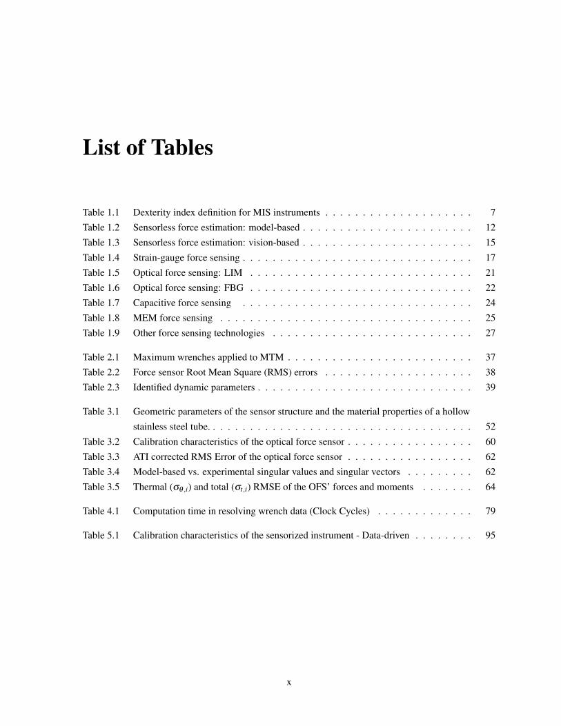
List of Tables
Table 1.1 Dexterity index definition for MIS instruments . . . . . . . . . . . . . . . . . . . . 7
Table 1.2 Sensorless force estimation: model-based . . . . . . . . . . . . . . . . . . . . . . . 12
Table 1.3 Sensorless force estimation: vision-based . . . . . . . . . . . . . . . . . . . . . . . 15
Table 1.4 Strain-gauge force sensing . . . . . . . . . . . . . . . . . . . . . . . . . . . . . . . 17
Table 1.5 Optical force sensing: LIM . . . . . . . . . . . . . . . . . . . . . . . . . . . . . . 21
Table 1.6 Optical force sensing: FBG . . . . . . . . . . . . . . . . . . . . . . . . . . . . . . 22
Table 1.7 Capacitive force sensing . . . . . . . . . . . . . . . . . . . . . . . . . . . . . . . 24
Table 1.8 MEM force sensing . . . . . . . . . . . . . . . . . . . . . . . . . . . . . . . . . . 25
Table 1.9 Other force sensing technologies . . . . . . . . . . . . . . . . . . . . . . . . . . . 27
Table 2.1 Maximum wrenches applied to MTM . . . . . . . . . . . . . . . . . . . . . . . . . 37
Table 2.2 Force sensor Root Mean Square (RMS) errors . . . . . . . . . . . . . . . . . . . . 38
Table 2.3 Identified dynamic parameters . . . . . . . . . . . . . . . . . . . . . . . . . . . . . 39
Table 3.1 Geometric parameters of the sensor structure and the material properties of a hollow
stainless steel tube. . . . . . . . . . . . . . . . . . . . . . . . . . . . . . . . . . . . 52
Table 3.2 Calibration characteristics of the optical force sensor . . . . . . . . . . . . . . . . . 60
Table 3.3 ATI corrected RMS Error of the optical force sensor . . . . . . . . . . . . . . . . . 62
Table 3.4 Model-based vs. experimental singular values and singular vectors . . . . . . . . . 62
Table 3.5 Thermal (σθ ,i) and total (σt,i) RMSE of the OFS’ forces and moments . . . . . . . 64
Table 4.1 Computation time in resolving wrench data (Clock Cycles) . . . . . . . . . . . . . 79
Table 5.1 Calibration characteristics of the sensorized instrument - Data-driven . . . . . . . . 95
x
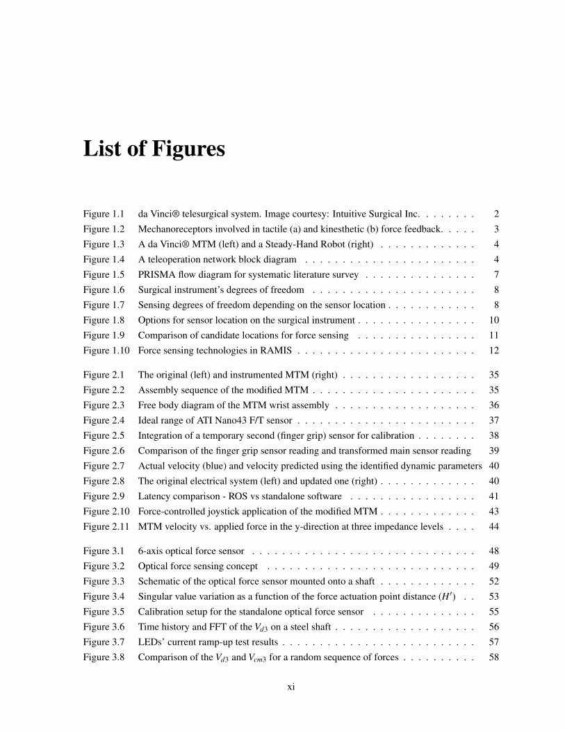
List of Figures
Figure 1.1 da Vinci® telesurgical system. Image courtesy: Intuitive Surgical Inc. . . . . . . . 2
Figure 1.2 Mechanoreceptors involved in tactile (a) and kinesthetic (b) force feedback. . . . . 3
Figure 1.3 A da Vinci® MTM (left) and a Steady-Hand Robot (right) . . . . . . . . . . . . . 4
Figure 1.4 A teleoperation network block diagram . . . . . . . . . . . . . . . . . . . . . . . 4
Figure 1.5 PRISMA flow diagram for systematic literature survey . . . . . . . . . . . . . . . 7
Figure 1.6 Surgical instrument’s degrees of freedom . . . . . . . . . . . . . . . . . . . . . . 8
Figure 1.7 Sensing degrees of freedom depending on the sensor location . . . . . . . . . . . . 8
Figure 1.8 Options for sensor location on the surgical instrument . . . . . . . . . . . . . . . . 10
Figure 1.9 Comparison of candidate locations for force sensing . . . . . . . . . . . . . . . . 11
Figure 1.10 Force sensing technologies in RAMIS . . . . . . . . . . . . . . . . . . . . . . . . 12
Figure 2.1 The original (left) and instrumented MTM (right) . . . . . . . . . . . . . . . . . . 35
Figure 2.2 Assembly sequence of the modified MTM . . . . . . . . . . . . . . . . . . . . . . 35
Figure 2.3 Free body diagram of the MTM wrist assembly . . . . . . . . . . . . . . . . . . . 36
Figure 2.4 Ideal range of ATI Nano43 F/T sensor . . . . . . . . . . . . . . . . . . . . . . . . 37
Figure 2.5 Integration of a temporary second (finger grip) sensor for calibration . . . . . . . . 38
Figure 2.6 Comparison of the finger grip sensor reading and transformed main sensor reading 39
Figure 2.7 Actual velocity (blue) and velocity predicted using the identified dynamic parameters 40
Figure 2.8 The original electrical system (left) and updated one (right) . . . . . . . . . . . . . 40
Figure 2.9 Latency comparison - ROS vs standalone software . . . . . . . . . . . . . . . . . 41
Figure 2.10 Force-controlled joystick application of the modified MTM . . . . . . . . . . . . . 43
Figure 2.11 MTM velocity vs. applied force in the y-direction at three impedance levels . . . . 44
Figure 3.1 6-axis optical force sensor . . . . . . . . . . . . . . . . . . . . . . . . . . . . . . 48
Figure 3.2 Optical force sensing concept . . . . . . . . . . . . . . . . . . . . . . . . . . . . 49
Figure 3.3 Schematic of the optical force sensor mounted onto a shaft . . . . . . . . . . . . . 52
Figure 3.4 Singular value variation as a function of the force actuation point distance (H ′) . . 53
Figure 3.5 Calibration setup for the standalone optical force sensor . . . . . . . . . . . . . . 55
Figure 3.6 Time history and FFT of the Vd3 on a steel shaft . . . . . . . . . . . . . . . . . . . 56
Figure 3.7 LEDs’ current ramp-up test results . . . . . . . . . . . . . . . . . . . . . . . . . . 57
Figure 3.8 Comparison of the Vd3 and Vcm3 for a random sequence of forces . . . . . . . . . . 58
xi
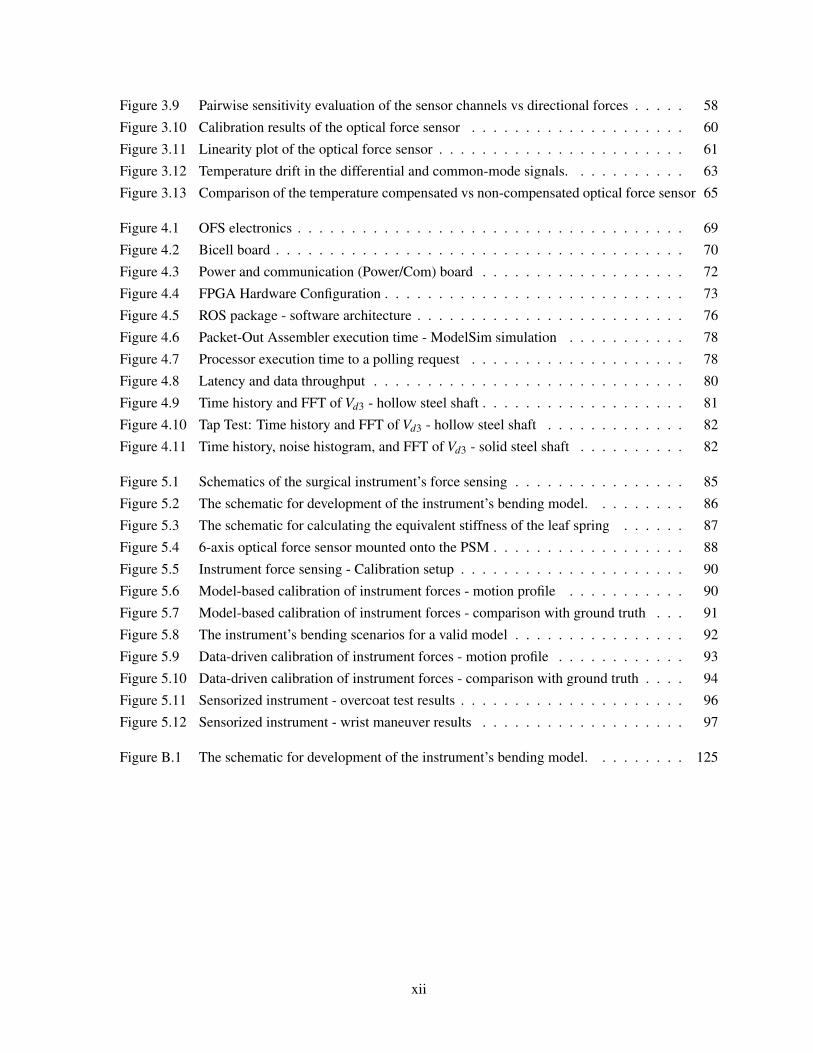
Figure 3.9 Pairwise sensitivity evaluation of the sensor channels vs directional forces . . . . . 58
Figure 3.10 Calibration results of the optical force sensor . . . . . . . . . . . . . . . . . . . . 60
Figure 3.11 Linearity plot of the optical force sensor . . . . . . . . . . . . . . . . . . . . . . . 61
Figure 3.12 Temperature drift in the differential and common-mode signals. . . . . . . . . . . 63
Figure 3.13 Comparison of the temperature compensated vs non-compensated optical force sensor 65
Figure 4.1 OFS electronics . . . . . . . . . . . . . . . . . . . . . . . . . . . . . . . . . . . . 69
Figure 4.2 Bicell board . . . . . . . . . . . . . . . . . . . . . . . . . . . . . . . . . . . . . . 70
Figure 4.3 Power and communication (Power/Com) board . . . . . . . . . . . . . . . . . . . 72
Figure 4.4 FPGA Hardware Configuration . . . . . . . . . . . . . . . . . . . . . . . . . . . . 73
Figure 4.5 ROS package - software architecture . . . . . . . . . . . . . . . . . . . . . . . . . 76
Figure 4.6 Packet-Out Assembler execution time - ModelSim simulation . . . . . . . . . . . 78
Figure 4.7 Processor execution time to a polling request . . . . . . . . . . . . . . . . . . . . 78
Figure 4.8 Latency and data throughput . . . . . . . . . . . . . . . . . . . . . . . . . . . . . 80
Figure 4.9 Time history and FFT of Vd3 - hollow steel shaft . . . . . . . . . . . . . . . . . . . 81
Figure 4.10 Tap Test: Time history and FFT of Vd3 - hollow steel shaft . . . . . . . . . . . . . 82
Figure 4.11 Time history, noise histogram, and FFT of Vd3 - solid steel shaft . . . . . . . . . . 82
Figure 5.1 Schematics of the surgical instrument’s force sensing . . . . . . . . . . . . . . . . 85
Figure 5.2 The schematic for development of the instrument’s bending model. . . . . . . . . 86
Figure 5.3 The schematic for calculating the equivalent stiffness of the leaf spring . . . . . . 87
Figure 5.4 6-axis optical force sensor mounted onto the PSM . . . . . . . . . . . . . . . . . . 88
Figure 5.5 Instrument force sensing - Calibration setup . . . . . . . . . . . . . . . . . . . . . 90
Figure 5.6 Model-based calibration of instrument forces - motion profile . . . . . . . . . . . 90
Figure 5.7 Model-based calibration of instrument forces - comparison with ground truth . . . 91
Figure 5.8 The instrument’s bending scenarios for a valid model . . . . . . . . . . . . . . . . 92
Figure 5.9 Data-driven calibration of instrument forces - motion profile . . . . . . . . . . . . 93
Figure 5.10 Data-driven calibration of instrument forces - comparison with ground truth . . . . 94
Figure 5.11 Sensorized instrument - overcoat test results . . . . . . . . . . . . . . . . . . . . . 96
Figure 5.12 Sensorized instrument - wrist maneuver results . . . . . . . . . . . . . . . . . . . 97
Figure B.1 The schematic for development of the instrument’s bending model. . . . . . . . . 125
xii

Glossary
The listings in this section are also defined in the text.
B Viscous damping coefficient.
C calibration matrix.
Ce Experimental conversion matrix from ~wP to~n.
Cm Model-based conversion matrix from ~wP to~n.
CAT I Calibration matrix of the ATI force sensor.
Ctot Calibration matrix from strain gauge voltage signals to the finger grip’s wrench vector.
E Young’s modulus of elasticity in 3.3.2, Error matrix between the reference and the OFS-resolved F/T
data in Section 3.5.
Es Young’s modulus of elasticity of the spring-steel sheet of the leaf spring in the modified cannula.
F Matrix of reference F/T measurements.
G Shear modulus of elasticity.
H Distance between the clamping point of the active and the passive components of the OFS.
H ′ Distance between the force application point and the clamping point of the OFS’ passive component.
HG Geometric transformation matrix from the displacement and orientation at the clamping point of
the OFS’ passive component to ~δ .
Hc Load transformation matrix from ~wt to the ~wc.
Hw Load transformation matrix from ~wP to the displacements and orientations at the clamping point of
the OFS’ passive component.
Hi j The i, j element of Hw or Hc.
I Moment of inertia.
xiii

I1, I2 Photocurrent generated in the the cells 1 and 2 of the bicell.
IF Forward current of the LED.
Is Bending moment of inertia of the leaf spring arms in the modified cannula.
IFt Test forward current of the LED.
Ixx, Iyy Principal moments of inertia about the x and y principal axes.
J Cost function used for solving the calibration minimization problem.
Ji Directional cost function used for solving the calibration minimization problem.
Jzz Polar moment of inertia about the z axis.
N 6×m matrix of~n for m samples.
Pet LED’s light output power at IFt .
R Feedback resistor in the transimpedance amplifier of the bicell’s signal conditioning circuit..
Rλ bicell’s responsivity.
S Matrix of MTM’s wrist F/T sensor measurements.
Vd Differential voltage of the two cells of the bicell.
Ve Velocity of the environment in a teleoperation system.
Vh Velocity of the operator’s hand in a teleoperation system.
Vcm,n Nominal common-mode voltage of the bicells in each sensing module.
Vcm Common-mode voltage between the two cells of the bicell.
Vd,n Nominal differential voltage of the bicells in each sensing module.
Vd,tc Temperature compensated differential voltage of the bicells in each sensing module.
Wr 6×m matrix of ~wP for m samples.
Ze Impedance of the environment.
Zto Impedence transferred to the operator.
∆Σ Delta-Sigma.
Vcm,e Electrical temperature drift in the common-mode voltage of the bicells in each sensing module.
Vcm,m Mechanical temperature drift in the common-mode voltage of the bicells in each sensing module.
xiv

Vcm Temperature drift in the common-mode voltage of the bicells in each sensing module.
Vd,e Electrical temperature drift in the differential voltage of the bicells in each sensing module.
Vd,m Mechanical temperature drift in the differential voltage of the bicells in each sensing module.
Vd Temeprature drift in the differential voltage of the bicells in each sensing module.
c Nominal width of the light beam on each cell of the bicell.
ds LED’s diameter.
dz Vertical distance from the clamping point of the OFS’ passive component to its slits’ center point.
e Error between Ce and Cm.
f+c Coulomb friction in the positive direction.
f−c Coulomb friction in the negative direction.
fe Force applied to the environment in a teleoperation system.
fl Lateral force.
fn Gripper normal force.
fp Gripper pull force.
fs Gripper shear force.
fx Force component in the x-axis.
fy Force component in the y-axis.
fz Force component in the z-axis.
fni Normalized directional force/moment data.
g Width of the gap between the two cells of the bicell.
h Height of the cells of the bicells.
kl Stiffness of the leaf spring’s arms in the modified cannula.
ks Equivalent stiffness at the tip of the modified cannula’s inner tube.
l Length of the surgical instrument’s shaft.
lc Distance between .
le Effective length of the leaf spring’s arms in the modified cannula.
xv
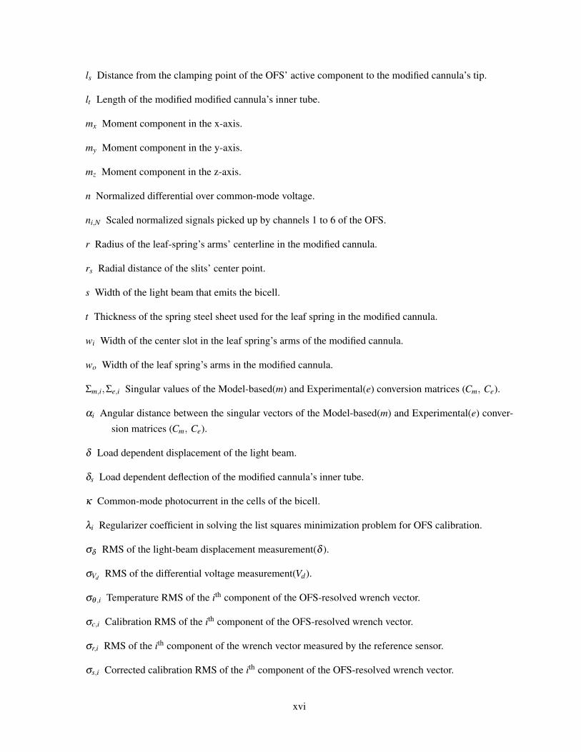
ls Distance from the clamping point of the OFS’ active component to the modified cannula’s tip.
lt Length of the modified modified cannula’s inner tube.
mx Moment component in the x-axis.
my Moment component in the y-axis.
mz Moment component in the z-axis.
n Normalized differential over common-mode voltage.
ni,N Scaled normalized signals picked up by channels 1 to 6 of the OFS.
r Radius of the leaf-spring’s arms’ centerline in the modified cannula.
rs Radial distance of the slits’ center point.
s Width of the light beam that emits the bicell.
t Thickness of the spring steel sheet used for the leaf spring in the modified cannula.
wi Width of the center slot in the leaf spring’s arms of the modified cannula.
wo Width of the leaf spring’s arms in the modified cannula.
Σm,i,Σe,i Singular values of the Model-based(m) and Experimental(e) conversion matrices (Cm, Ce).
αi Angular distance between the singular vectors of the Model-based(m) and Experimental(e) conver-
sion matrices (Cm, Ce).
δ Load dependent displacement of the light beam.
δs Load dependent deflection of the modified cannula’s inner tube.
κ Common-mode photocurrent in the cells of the bicell.
λi Regularizer coefficient in solving the list squares minimization problem for OFS calibration.
σδ RMS of the light-beam displacement measurement(δ ).
σVd RMS of the differential voltage measurement(Vd).
σθ ,i Temperature RMS of the ith component of the OFS-resolved wrench vector.
σc,i Calibration RMS of the ith component of the OFS-resolved wrench vector.
σr,i RMS of the ith component of the wrench vector measured by the reference sensor.
σs,i Corrected calibration RMS of the ith component of the OFS-resolved wrench vector.
xvi

σt,i Total sensing RMS of the ith component of the OFS-resolved wrench vector.
θ The OFS temperature measured by at the Power/Com board.
~δ = [δ1,δ2, · · · ,δ6]T Vector of the OFS’ slits displacement in ei direction.
~θC = [θCx,θCy,θCz]T Orientation vector at the clamping point of the OFS’ passive component.
~dC = [dCx,dCy,dCz]T Displacement vector at the clamping point of the OFS’ passive component.
~di = [dix,diy,diz]T Displacement vector at the ith slit of the OFS’ passive component.
~ei Unit vector in the direction that is inplane-normal to the ith slit of the OFS.
~li Vector from the clamping point of the OFS’ passive component to the center of its ith slit.
~n = [n1,n2, · · · ,n6]T Vector of the normalized signals (n) of the OFS’ sensing modules.
~wP = [ fPx, fPy, fPz,mPx,mPy,mPz]T Wrench vector applied to the OFS.
~wc = [ fcx, fcy, fcz,mcx,mcy,mcz]T Wrench vector at clamping point of the OFS’ passive component.
~wp = [ fpx, fpy, fpz,mpx,mpy,mpz]T Wrench vector applied to the MTM’s finger grip.
~ws = [ fsx, fsy, fsz,msx,msy,msz]T Wrench vector measured by the MTM’s wrist F/T sensor.
~wt = [ fx, fy, fz,mx,my,mz]T Wrench vector applied to the distal end of the surgical instrument.
xvii

Acronyms
The acronyms listed in this section are also defined in the text.
ACC Accuracy.
ADC Analog to Digital Converter.
AFM Atomic Force Microscopy.
ARMA Auto Regressive Moving Average.
ASIC Application-Specific Integrated Circuit.
CD Custom Developed.
CDC Capacitance to Digital Converter.
CFM Configuration Flash Memory.
CLKIN Input Clock.
CNC Computer Numerically Controlled.
Comedilib It is a user-space library that provides a developer-friendly interface to Comedi devices.
COMM Common-Mode.
CRAM Configuration RAM.
CRC Cyclic Redundancy Check.
CS Coordinate System.
DAC Digital to Analog Converter.
DAQ Data Acquisition.
DI Dexterity Index.
DIFF Difference.
xviii
DMA Direct Memory Access.
DoF Degrees of Freedom.
DRIE Deep Reactive Ion Etching.
DSP Digital Signal Processing.
dVRK da Vinci Research Kit.
EDM Electric Discharge Machining.
EEPROM Electrically Erasable Programmable Read-Only Memory.
EMI ElectroMagnetic Interference.
ERR Maximum Absolute Error.
F/T Force Torque.
FBG Fiber Bragg Grating.
FF Force Feedback.
FFT Fast Fourier Transform.
FIFO First In First Out.
FPC Flexible Printed Circuit.
FPGA Field Programmable Gate Array.
FSO Full Scale Output.
FSR Force Sensitive Resistors.
FTDI Future Technology Devices International.
GA Genetic Algorithm.
GPR Gaussian Process Regression.
GPU Graphic Processing Unit.
GRNN Generalized Regression Neural Network.
I2C Inter-Integrated Circuit.
IC Integrated Circuit.
xix

ID Inner Diameter.
IMU Inertial Measurement Unit.
IO Input/Output.
IP Intellectual Property.
IR InfraRed.
ISO International Standard Organization.
JND Just-Noticeable Difference.
JST JST connectors are electrical connectors manufactured to the design standards originally devel-
oped by J.S.T. Mfg. Co. (Japan Solderless Terminal).
JTAG Joint Test Action Group - An industry standard for verifying designs and testing printed circuit
boards after manufacture.
LB Logic Block.
LED Light-Emitting Diode.
LIFO Last In First Out.
LIM Light Intensity Modulation.
LPF Low Pass Filter.
LSTM Long Short Term Memory.
LUT Look Up Table.
LVDS Low-voltage Differential Signaling.
MAE Mean Absolute Error.
MAF Moving Average Filter.
Mbps Megabits per second.
MCU Micro Controller Unit.
MEM Micro Electro Mechanical.
MIRS Minimally Invasive Robotic Surgery.
MIS Minimally Invasive Surgery.
xx

MISO Master Input Slave Output.
MOSI Master Output Slave Input.
MRI Magnetic Resonance Imaging.
MSE Mean Squared Error.
MTM Master Tool Manipulator.
MUX Multiplexer.
NN Neural Network.
NRMSD Normalized Root Mean Square Deviation.
NRMSE Normalized Root Mean Square Error.
OCT Optical Coherence Tomography.
OD Outer Diameter.
OFS Optical Force Sensor.
OS Operation System.
PAM Pneumatic Actuation Muscles.
PCB Printed Circuit Board.
PCI Peripheral Component Interconnect.
PCMEMS Printed-Circuit MEMS.
PCT Patent Cooperation Treaty.
PGA Programmable Gain Amplifier.
PLA PolyLactic Acid.
Power/Com Power and Communication.
PPCA Probabilistic Principal Component Analysis.
PRISMA Preferred Reporting Items for Systematic reviews and Meta-Analyses.
PSM Patient Side Manipulator.
PSO-BPNN Particle Swarm Optimization Back Propagation Neural Network.
xxi

PV Peak-to-Valley.
QTC Quantum Tunneling Composite.
RAMIS Robot Assisted Minimally Invasive Surgery.
RAS Robot Assisted Surgery.
RCL Robotics and Controls Laboratory.
RES Resolution.
RMIS Robotic Minimally Invasive Surgery.
RMS Root Mean Square.
RMSE Root Mean Square Error.
RNG Range.
RNN Recurrent Neural Network.
ROS Robot Operating System.
RRTO Robust Reaction Torque Observer.
SAN Scanner-Adapter Network.
SAR Successive Approximation Register.
SDK Software Development Kit.
SENS Sensitivity.
SLM Selective Laser Melting.
SMA Shape Memory Alloy.
SMCSPO Sliding Mode Control with SPO.
SNR Signal to Noise Ratio.
SoPC System on Programmable Chip.
SPI Serial Peripheral Interface.
SPO Sliding Perturbation Observer.
SS Sensory Substitution.
xxii
SVD Singular Value Decomposition.
TCA Trans-Conductance Amplifier.
TMP Temperature.
TPS Thin-Plate Splines.
TZA Transimpedance Amplifier.
UART Universal Asynchronous Receiver-Transmitter.
UILO University-Industry Liaison Office.
UKF Unscented Kalman Filter.
USB Universal Serial Bus.
VHDL A hardware description language (HDL) that can model the behavior and structure of digital
systems.
WSN Wireless Sensor Network.
xxiii

Acknowledgments
My deep gratitude goes to my supervisor Dr. Septimiu E. Salcudean for his support, guidance, and
patience throughout my doctoral studies, and the freedom to shape my research in a way that aligns the
best with my professional aspirations.
My appreciation extends to my supervisory committee members Dr. Yusuf Altintas (also my mas-
ters’ supervisor), Dr. Edmund Cretu, and Dr. Robert Rohling for their insightful feedback and com-
ments. I appreciate help from the project’s electronics consultant, Gerald F. Cummings, the summer
student, David G. Black and all the members of the Robotics and Controls Laboratory (RCL), in partic-
ular, Dr. Mohammad Honarvar for his support in the early years of my doctoral studies.
I acknowledge scholarship support from the Natural Sciences and Engineering Research Council of
Canada (NSERC) Graduate Scholarship, the funding support from the Charles Laszlo Chair in Biomed-
ical Engineering, and the infrastructure support from Canada Foundation for Innovation (CFI).
Last but not least, I would like to thank my beloved family and friends for continuous support and
always being there for me.
xxiv

Dedication
I dedicate this work to my parents, Mohammad Reza Hadi and Fatemeh Sadat Taheri, and my siblings,
Alireza, Ahmadreza, and Negin for their endless love, support and encouragement.
xxv
Chapter 1
Introduction and Literature Review
1.1 MIS and RMISIn Minimally Invasive Surgery (MIS), surgical access is provided through small incisions or natural ori-
fices in the body. A surgical instrument is operated by the surgeon for tissue manipulation. Compared
to open surgery, MIS provides less tissue trauma, postoperative pain, patient discomfort, wound com-
plications and immunological response stress [1], lower risk of infection [2] and blood loss [3], shorter
hospital stay [4], faster recovery [5], and improved cosmetics [6] all of which lead to improved thera-
peutic outcome and efficiency [7] and lower morbidity and mortality [8] making MIS cost-effective [9].
Nonetheless, the ergonomically cumbersome posture increases surgeon fatigue. The limited instrument
dexterity and visual perception of the scene [10, 11], and the non-intuitive hand-eye coordination due
to fulcrum motion reversal decrease accuracy and contribute to surgeon fatigue [12]. The high level of
psychomotor skills needed increases the operation time and require a longer learning curve [13]. The
sense of touch is reduced by friction in the access port and instrument mechanism.
In Robotic Minimally Invasive Surgery (RMIS), the surgical instrument is controlled by a robotic
manipulator and operated by a remote surgeon. The robotic operation restores hand–eye coordination
[14], and innovations in tool design improve dexterity leading to improved ergonomics that reduce
surgeon fatigue [4, 15]. The enhanced 3D surgical vision, automatic movement transformations, fine
motions, filtering of physiological hand tremor and motion scaling lead to improved surgery precision
[16]. However, the surgeon is isolated from the surgical site by robotic manipulators that do not provide
the haptic perception [17]. This deprives the surgeon of a rich source of information. Thus, many studies
are targeted towards the reconstruction and evaluation of haptic feedback.
da Vinci® robots manufactured by Intuitive Surgical Inc. (see Figure 1.1) are the most popular RMIS
systems in clinical use with close to 6,000 da Vinci® systems installed worldwide and more than 8.5
million procedures performed by the end of 2020 [18]. The da Vinci® system has two main components:
1) A surgeon console with two Master Tool Manipulators (MTMs) and a display, 2) A patient-side cart
with usually three Patient Side Manipulators (PSMs) and an additional arm that controls an endoscopic
camera. The surgical instruments are mounted onto the PSMs and access the surgical site through small
1
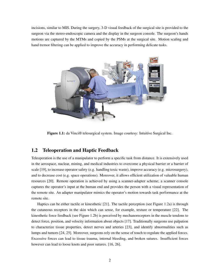
incisions, similar to MIS. During the surgery, 3-D visual feedback of the surgical site is provided to the
surgeon via the stereo-endoscopic camera and the display in the surgeon console. The surgeon’s hands
motions are captured by the MTMs and copied by the PSMs at the surgical site. Motion scaling and
hand tremor filtering can be applied to improve the accuracy in performing delicate tasks.
Figure 1.1: da Vinci® telesurgical system. Image courtesy: Intuitive Surgical Inc.
1.2 Teleoperation and Haptic FeedbackTeleoperation is the use of a manipulator to perform a specific task from distance. It is extensively used
in the aerospace, nuclear, mining, and medical industries to overcome a physical barrier or a barrier of
scale [19], to increase operator safety (e.g. handling toxic waste), improve accuracy (e.g. microsurgery),
and to decrease cost (e.g. space operations). Moreover, it allows efficient utilization of valuable human
resources [20]. Remote operation is achieved by using a scanner-adapter scheme; a scanner console
captures the operator’s input at the human end and provides the person with a visual representation of
the remote site. An adapter manipulator mimics the operator’s motion towards task performance at the
remote site.
Haptics can be either tactile or kinesthetic [21]. The tactile perception (see Figure 1.2a) is through
the cutaneous receptors in the skin which can sense, for example, texture or temperature [22]. The
kinesthetic force feedback (see Figure 1.2b) is perceived by mechanoreceptors in the muscle tendons to
detect force, position, and velocity information about objects [17]. Traditionally surgeons use palpation
to characterize tissue properties, detect nerves and arteries [23], and identify abnormalities such as
lumps and tumors [24, 25]. Moreover, surgeons rely on the sense of touch to regulate the applied forces.
Excessive forces can lead to tissue trauma, internal bleeding, and broken sutures. Insufficient forces
however can lead to loose knots and poor sutures. [16, 26].
2
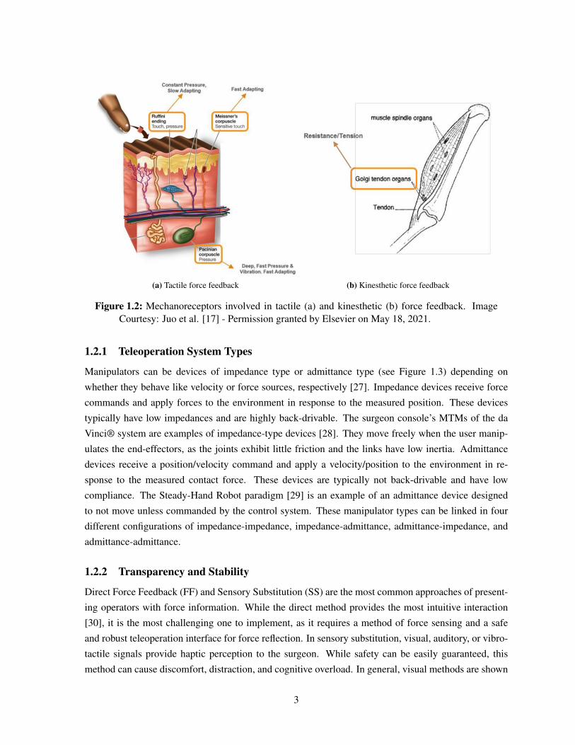
(a) Tactile force feedback (b) Kinesthetic force feedback
Figure 1.2: Mechanoreceptors involved in tactile (a) and kinesthetic (b) force feedback. ImageCourtesy: Juo et al. [17] - Permission granted by Elsevier on May 18, 2021.
1.2.1 Teleoperation System Types
Manipulators can be devices of impedance type or admittance type (see Figure 1.3) depending on
whether they behave like velocity or force sources, respectively [27]. Impedance devices receive force
commands and apply forces to the environment in response to the measured position. These devices
typically have low impedances and are highly back-drivable. The surgeon console’s MTMs of the da
Vinci® system are examples of impedance-type devices [28]. They move freely when the user manip-
ulates the end-effectors, as the joints exhibit little friction and the links have low inertia. Admittance
devices receive a position/velocity command and apply a velocity/position to the environment in re-
sponse to the measured contact force. These devices are typically not back-drivable and have low
compliance. The Steady-Hand Robot paradigm [29] is an example of an admittance device designed
to not move unless commanded by the control system. These manipulator types can be linked in four
different configurations of impedance-impedance, impedance-admittance, admittance-impedance, and
admittance-admittance.
1.2.2 Transparency and Stability
Direct Force Feedback (FF) and Sensory Substitution (SS) are the most common approaches of present-
ing operators with force information. While the direct method provides the most intuitive interaction
[30], it is the most challenging one to implement, as it requires a method of force sensing and a safe
and robust teleoperation interface for force reflection. In sensory substitution, visual, auditory, or vibro-
tactile signals provide haptic perception to the surgeon. While safety can be easily guaranteed, this
method can cause discomfort, distraction, and cognitive overload. In general, visual methods are shown
3
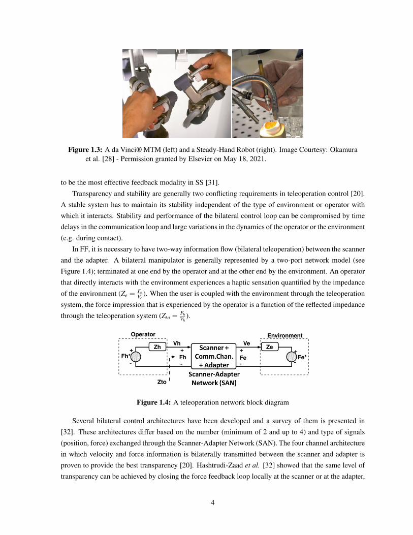
Figure 1.3: A da Vinci® MTM (left) and a Steady-Hand Robot (right). Image Courtesy: Okamuraet al. [28] - Permission granted by Elsevier on May 18, 2021.
to be the most effective feedback modality in SS [31].
Transparency and stability are generally two conflicting requirements in teleoperation control [20].
A stable system has to maintain its stability independent of the type of environment or operator with
which it interacts. Stability and performance of the bilateral control loop can be compromised by time
delays in the communication loop and large variations in the dynamics of the operator or the environment
(e.g. during contact).
In FF, it is necessary to have two-way information flow (bilateral teleoperation) between the scanner
and the adapter. A bilateral manipulator is generally represented by a two-port network model (see
Figure 1.4); terminated at one end by the operator and at the other end by the environment. An operator
that directly interacts with the environment experiences a haptic sensation quantified by the impedance
of the environment (Ze =FeVe
). When the user is coupled with the environment through the teleoperation
system, the force impression that is experienced by the operator is a function of the reflected impedance
through the teleoperation system (Zto =FhVh
).
Figure 1.4: A teleoperation network block diagram
Several bilateral control architectures have been developed and a survey of them is presented in
[32]. These architectures differ based on the number (minimum of 2 and up to 4) and type of signals
(position, force) exchanged through the Scanner-Adapter Network (SAN). The four channel architecture
in which velocity and force information is bilaterally transmitted between the scanner and adapter is
proven to provide the best transparency [20]. Hashtrudi-Zaad et al. [32] showed that the same level of
transparency can be achieved by closing the force feedback loop locally at the scanner or at the adapter,
4
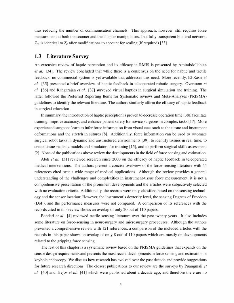
thus reducing the number of communication channels. This approach, however, still requires force
measurement at both the scanner and the adapter manipulators. In a fully transparent bilateral network,
Zto is identical to Ze after modifications to account for scaling (if required) [33].
1.3 Literature SurveyAn extensive review of haptic perception and its efficacy in RMIS is presented by Amirabdollahian
et al. [34]. The review concluded that while there is a consensus on the need for haptic and tactile
feedback, no commercial system is yet available that addresses this need. More recently, El-Rassi et
al. [35] presented a brief overview of haptic feedback in teleoperated robotic surgery. Overtoom et
al. [36] and Rangarajan et al. [37] surveyed virtual haptics in surgical simulation and training. The
latter followed the Preferred Reporting Items for Systematic reviews and Meta-Analyses (PRISMA)
guidelines to identify the relevant literature. The authors similarly affirm the efficacy of haptic feedback
in surgical education.
In summary, the introduction of haptic perception is proven to decrease operation time [38], facilitate
training, improve accuracy, and enhance patient safety for novice surgeons in complex tasks [17]. More
experienced surgeons learn to infer force information from visual cues such as the tissue and instrument
deformations and the stretch in sutures [8]. Additionally, force information can be used to automate
surgical robot tasks in dynamic and unstructured environments [39], to identify tissues in real time, to
create tissue-realistic models and simulators for training [15], and to perform surgical skills assessment
[2]. None of the publications above review the developments in the field of force sensing and estimation.
Abdi et al. [31] reviewed research since 2000 on the efficacy of haptic feedback in teleoperated
medical interventions. The authors present a concise overview of the force-sensing literature with 44
references cited over a wide range of medical applications. Although the review provides a general
understanding of the challenges and complexities in instrument-tissue force measurement, it is not a
comprehensive presentation of the prominent developments and the articles were subjectively selected
with no evaluation criteria. Additionally, the records were only classified based on the sensing technol-
ogy and the sensor location; However, the instrument’s dexterity level, the sensing Degrees of Freedom
(DoF), and the performance measures were not compared. A comparison of its references with the
records cited in this review shows an overlap of only 20 out of 110 papers.
Bandari et al. [4] reviewed tactile sensing literature over the past twenty years. It also includes
some literature on force-sensing in neurosurgery and microsurgery procedures. Although the authors
presented a comprehensive review with 121 references, a comparison of the included articles with the
records in this paper shows an overlap of only 8 out of 110 papers which are mostly on developments
related to the gripping force sensing.
The rest of this chapter is a systematic review based on the PRISMA guidelines that expands on the
sensor design requirements and presents the most recent developments in force sensing and estimation in
keyhole endoscopy. We discuss how research has evolved over the past decade and provide suggestions
for future research directions. The closest publications to our review are the surveys by Puangmali et
al. [40] and Trejos et al. [41] which were published about a decade ago, and therefore there are no
5
overlapping papers with those reviews.
1.4 MethodologyA systematic survey was conducted by following the PRISMA guidelines (see Figure 1.5) and it was
based on Google Scholar, Web-of-Science, PubMed, and IEEE Xplore Digital Library repositories. The
period for the review is from January 2011 until May 2020. The following keywords were used for
identification: Force sensing, Kinesthetic, Tactile, Haptics, MIS, Minimally Invasive Robotic Surgery
(MIRS), RMIS, Robot Assisted Surgery (RAS), Robot Assisted Minimally Invasive Surgery (RAMIS),
Laparoscopy, and Endoscopy. For every year, the first 20 pages of search results in Google Scholar were
surveyed (total of 2000 records). The same approach was used for the identification of records through
the other repositories (PubMed: 213, Web-of-Science: 42, and IEEEXplore: 40). For screening, the
duplicates were removed and the identified records were skimmed through to mark the ones that are
relevant to keyhole endoscopy. The articles that refer to force sensing in microsurgery, neurosurgery,
and needle insertion were excluded because they involve a different set of requirements and challenges.
Specifically, microsurgical instruments such as those used in neurosurgery and retinal surgery [42] have
a much smaller diameter (less than 2 mm) and do not require an articulated wrist, which complicates
the actuation system and sensors’ power and signals routing. Moreover, Bandari et al. [4] briefly
discussed the force-sensing literature in microsurgery, neurosurgery, and needle insertion. 114 articles
were found eligible for a complete review. Throughout the review, the references of the selected papers
were surveyed and the relevant articles that were not initially identified were added, thus increasing the
total number of eligible records to 129. The work progressions and duplicate publications were removed
to lead to the 110 articles included in this survey.
The included articles are tabulated for an easier comparison of the method, the sensor location, the
sensing DoFs, the dexterity of the instrument under study, and the results. The Dexterity Index (DI)
for different instruments is defined according to the Table 1.1 and Figure 1.6. Depending on the sensor
location, the sensing DoFs are defined as instrument or wrist tri-axial forces ( fx, fy, fz) and moments
(mx, my, mz), and the gripper normal ( fn), shear ( fs), and pull ( fp) forces as depicted in Figure 1.7.
In summarizing the results, the following acronyms were used: Accuracy (ACC), Maximum Absolute
Error (ERR), Mean Absolute Error (MAE), Normalized Root Mean Square Error (NRMSE), Resolution
(RES),Root Mean Square Error (RMSE), Range (RNG), and Sensitivity (SENS).
1.5 Design Requirements
1.5.1 DoF, Range, Resolution, Accuracy, Bandwidth and Sampling Rate
The grasping force, the instrument lateral and axial forces, and the axial torque are the most relevant
DoFs to improve accuracy and provide an effective haptic experience in MIS applications [2, 4, 43].
Deformations in the sensor structure or displacements in its components are the physical surrogates that
are monitored for force estimation. Thus, there are always trade-offs between the sensor’s structural
6
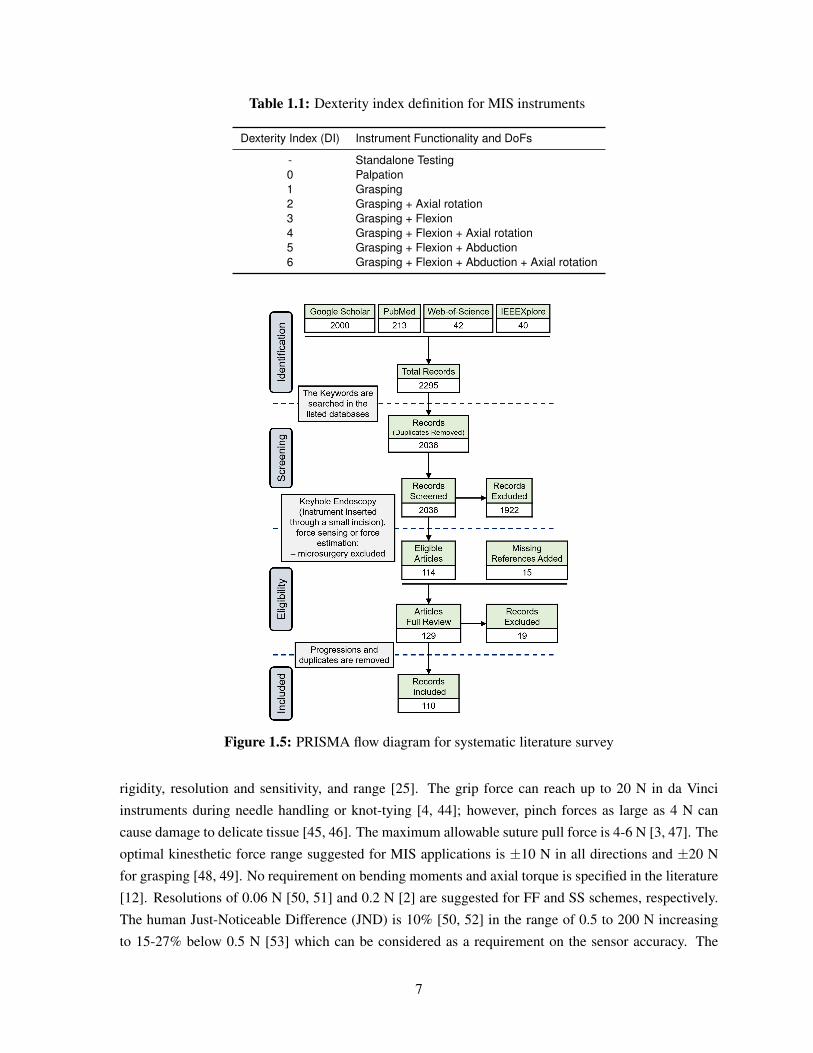
Table 1.1: Dexterity index definition for MIS instruments
Dexterity Index (DI) Instrument Functionality and DoFs
- Standalone Testing0 Palpation1 Grasping2 Grasping + Axial rotation3 Grasping + Flexion4 Grasping + Flexion + Axial rotation5 Grasping + Flexion + Abduction6 Grasping + Flexion + Abduction + Axial rotation
Figure 1.5: PRISMA flow diagram for systematic literature survey
rigidity, resolution and sensitivity, and range [25]. The grip force can reach up to 20 N in da Vinci
instruments during needle handling or knot-tying [4, 44]; however, pinch forces as large as 4 N can
cause damage to delicate tissue [45, 46]. The maximum allowable suture pull force is 4-6 N [3, 47]. The
optimal kinesthetic force range suggested for MIS applications is ±10 N in all directions and ±20 N
for grasping [48, 49]. No requirement on bending moments and axial torque is specified in the literature
[12]. Resolutions of 0.06 N [50, 51] and 0.2 N [2] are suggested for FF and SS schemes, respectively.
The human Just-Noticeable Difference (JND) is 10% [50, 52] in the range of 0.5 to 200 N increasing
to 15-27% below 0.5 N [53] which can be considered as a requirement on the sensor accuracy. The
7
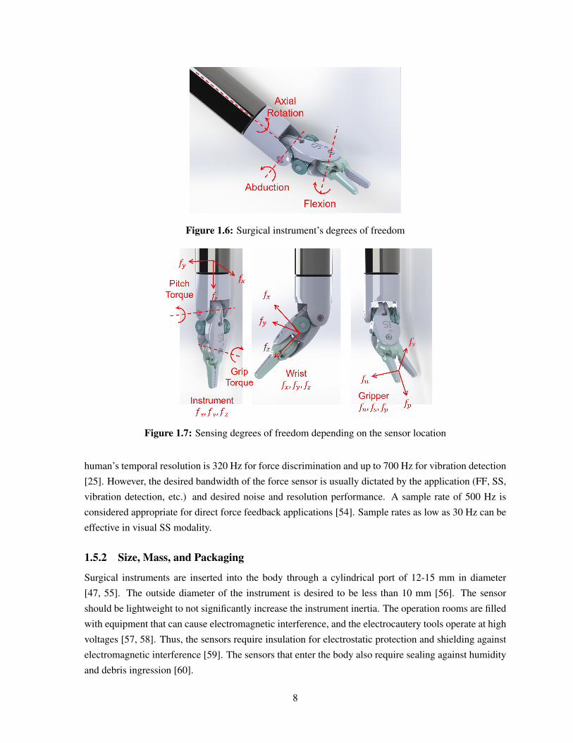
Figure 1.6: Surgical instrument’s degrees of freedom
Figure 1.7: Sensing degrees of freedom depending on the sensor location
human’s temporal resolution is 320 Hz for force discrimination and up to 700 Hz for vibration detection
[25]. However, the desired bandwidth of the force sensor is usually dictated by the application (FF, SS,
vibration detection, etc.) and desired noise and resolution performance. A sample rate of 500 Hz is
considered appropriate for direct force feedback applications [54]. Sample rates as low as 30 Hz can be
effective in visual SS modality.
1.5.2 Size, Mass, and Packaging
Surgical instruments are inserted into the body through a cylindrical port of 12-15 mm in diameter
[47, 55]. The outside diameter of the instrument is desired to be less than 10 mm [56]. The sensor
should be lightweight to not significantly increase the instrument inertia. The operation rooms are filled
with equipment that can cause electromagnetic interference, and the electrocautery tools operate at high
voltages [57, 58]. Thus, the sensors require insulation for electrostatic protection and shielding against
electromagnetic interference [59]. The sensors that enter the body also require sealing against humidity
and debris ingression [60].
8
1.5.3 Sterilizability
Surgical instruments are cleaned and sterilized for reuse; the former refers to removing debris from the
device and the latter is the elimination of microorganisms that can cause disease [60]. The common
sterilization methods are plasma and gamma radiation, the use of chemicals (alcohol, ethylene oxide or
formaldehyde), and steam sterilizations [61]. Steam sterilization is the fastest and the most preferred
method [2] which is performed in an autoclave at 120-135°C, 207 kPa and 100% humidity for 15-30
minutes [47, 62]. This harsh environment can be destructive to many transducers, signal conditioning
electronics, wire insulations, bondings, and coatings.
1.5.4 Biocompatibility
The sensors for use in MIS must abide by ISO10993 which entails a series of standards for evaluating
the biocompatibility of medical devices [60]. For biocompatibility electrical components often require
coatings that interfere with sterilizability [47].
1.5.5 Adaptability and Cost
Instruments are disposed after 10 to 15 uses due to accelerated cable fatigue [63–65]. The EndoWrist
instruments retail at $2k-$5k [47]. If the sensor is integrated into the instrument and is to be disposed, it
should not increase the instrument price significantly. An adaptable solution that can be easily used on
different instruments is desirable.
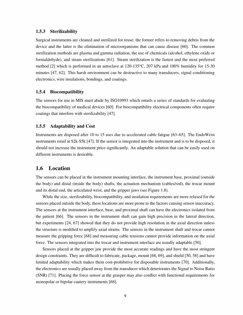
1.6 LocationThe sensors can be placed in the instrument mounting interface, the instrument base, proximal (outside
the body) and distal (inside the body) shafts, the actuation mechanism (cables/rod), the trocar mount
and its distal end, the articulated wrist, and the gripper jaws (see Figure 1.8).
While the size, sterilizability, biocompatibility, and insulation requirements are more relaxed for the
sensors placed outside the body, these locations are more prone to the factors causing sensor inaccuracy.
The sensors at the instrument interface, base, and proximal shaft can have the electronics isolated from
the patient [66]. The sensors in the instrument shaft can gain high precision in the lateral direction,
but experiments [24, 67] showed that they do not provide high resolution in the axial direction unless
the structure is modified to amplify axial strains. The sensors in the instrument shaft and trocar cannot
measure the gripping force [68] and measuring cable tensions cannot provide information on the axial
force. The sensors integrated into the trocar and instrument interface are usually adaptable [50].
Sensors placed at the gripper jaw provide the most accurate readings and have the most stringent
design constraints. They are difficult to fabricate, package, mount [68, 69], and shield [50, 58] and have
limited adaptability which makes them cost-prohibitive for disposable instruments [70]. Additionally,
the electronics are usually placed away from the transducer which deteriorates the Signal to Noise Ratio
(SNR) [71]. Placing the force sensor at the grasper may also conflict with functional requirements for
monopolar or bipolar cautery instruments [68].
9
Figure 1.8: Options for sensor location on the surgical instrument
Figure 1.9 summarizes the severity level of different sources that contribute to the sensing inaccuracy
as a function of the sensor location (scale of 1 to 3; 1 is minimum, 3 is maximum and 8 is no effect).
It also compares how stringent the listed design requirements are for each sensor location (scale of 1
to 3; 1 is the least, 3 is the most and 8 refers to not a requirement). The distribution of the records
included in this survey as a function of the sensor locations and the sensing technologies are shown in
the same figure. It is evident that the sensorless techniques have the majority of publications over the
past ten years. Additionally, the Micro Electro Mechanical (MEM) and Fiber Bragg Grating (FBG)
technologies have been widely adopted in the fabrication of miniature transducers that can be integrated
into the gripper jaws. An overview of different transduction technologies is presented in the next section.
1.7 Sensing TechnologiesSensing technologies and the corresponding number of articles in this survey is shown in Figure 1.10.
1.7.1 Sensorless
Sensorless refers to the case where the sensors used for force estimation are already inherent in the
surgical robot [15]. In model-based approaches, the sensors are the encoders and the motor current
measurements. In the vision-based techniques, the sensor is the visual feedback of the surgical site
through mono or stereo cameras.
10
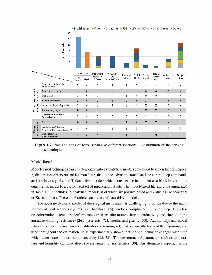
Figure 1.9: Pros and cons of force sensing at different locations + Distribution of the sensingtechnologies
Model-Based
Model-based techniques can be categorized into 1) analytical models developed based on first principles,
2) disturbance observers and Kalman filters that utilize a dynamic model and the control loop commands
and feedback signals, and 3) data-driven models which consider the instrument as a black-box and fit a
quantitative model to a customized set of inputs and outputs. The model-based literature is summarized
in Table 1.2. It includes 15 analytical models, 8 of which are physics-based and 7 studies use observers
or Kalman filters. There are 6 articles on the use of data-driven models.
The accurate dynamic model of the surgical instruments is challenging to obtain due to the many
sources of nonlinearities e.g. friction, backlash [16], tendons compliance [63] and creep [10], elas-
tic deformations, actuators performance variations (the motors’ brush conductivity and change in the
armature winding resistance) [26], hysteresis [72], inertia, and gravity [50]. Additionally, any model
relies on a set of measurements (calibration or training set) that are usually taken at the beginning and
used throughout the estimation. It is experimentally shown that the tool behavior changes with time
which deteriorates the estimation accuracy [12, 73]. The environmental parameters such as tempera-
ture and humidity can also affect the instrument characteristics [30]. An alternative approach is the
11
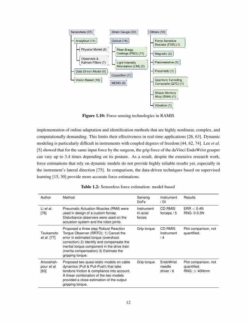
Figure 1.10: Force sensing technologies in RAMIS
implementation of online adaptation and identification methods that are highly nonlinear, complex, and
computationally demanding. This limits their effectiveness in real-time applications [26, 63]. Dynamic
modeling is particularly difficult in instruments with coupled degrees of freedom [44, 62, 74]. Lee et al.
[5] showed that for the same input force by the surgeon, the grip force of the daVinci EndoWrist grasper
can vary up to 3.4 times depending on its posture. As a result, despite the extensive research work,
force estimations that rely on dynamic models do not provide highly reliable results yet, especially in
the instrument’s lateral direction [75]. In comparison, the data-driven techniques based on supervised
learning [15, 30] provide more accurate force estimations.
Table 1.2: Sensorless force estimation: model-based
Author Method SensingDoFs
Instrument/ DI
Results
Li et al.[76]
Pneumatic Actuation Muscles (PAM) wereused in design of a custom forcep.Disturbance observers were used on theactuation system and the robot joints.
Instrumenttri-axialforces
CD RMISforceps / 5
ERR < 0.4NRNG: 0-3.5N
Tsukamotoet al. [77]
Proposed a three step Robust ReactionTorque Observer (RRTO): 1) Cancel theerror in estimated torque (overshootcorrection) 2) Identify and compensate theinertial torque component in the drive train(inertia compensation) 3) Estimate thegripping torque.
Grip torque CD RMISinstrument/ 4
Plot comparison, notquantified.
Anooshah-pour et al.[63]
Proposed two quasi-static models on cabledynamics (Pull & Pull-Push) that taketendons friction & compliance into account.A linear combination of the two modelsprovided a close estimation of the outputgripping torque.
Grip torque EndoWristneedledriver / 6
Plot comparison, notquantified.RNG: ± 40Nmm
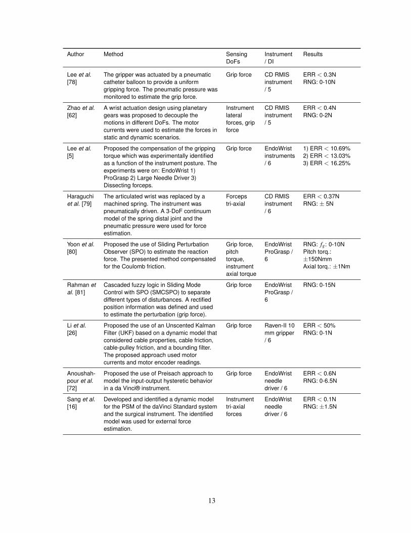
12
Author Method SensingDoFs
Instrument/ DI
Results
Lee et al.[78]
The gripper was actuated by a pneumaticcatheter balloon to provide a uniformgripping force. The pneumatic pressure wasmonitored to estimate the grip force.
Grip force CD RMISinstrument/ 5
ERR < 0.3NRNG: 0-10N
Zhao et al.[62]
A wrist actuation design using planetarygears was proposed to decouple themotions in different DoFs. The motorcurrents were used to estimate the forces instatic and dynamic scenarios.
Instrumentlateralforces, gripforce
CD RMISinstrument/ 5
ERR < 0.4NRNG: 0-2N
Lee et al.[5]
Proposed the compensation of the grippingtorque which was experimentally identifiedas a function of the instrument posture. Theexperiments were on: EndoWrist 1)ProGrasp 2) Large Needle Driver 3)Dissecting forceps.
Grip force EndoWristinstruments/ 6
1) ERR < 10.69%2) ERR < 13.03%3) ERR < 16.25%
Haraguchiet al. [79]
The articulated wrist was replaced by amachined spring. The instrument waspneumatically driven. A 3-DoF continuummodel of the spring distal joint and thepneumatic pressure were used for forceestimation.
Forcepstri-axial
CD RMISinstrument/ 6
ERR < 0.37NRNG: ± 5N
Yoon et al.[80]
Proposed the use of Sliding PerturbationObserver (SPO) to estimate the reactionforce. The presented method compensatedfor the Coulomb friction.
Grip force,pitchtorque,instrumentaxial torque
EndoWristProGrasp /6
RNG: fg: 0-10NPitch torq.:±150NmmAxial torq.: ±1Nm
Rahman etal. [81]
Cascaded fuzzy logic in Sliding ModeControl with SPO (SMCSPO) to separatedifferent types of disturbances. A rectifiedposition information was defined and usedto estimate the perturbation (grip force).
Grip force EndoWristProGrasp /6
RNG: 0-15N
Li et al.[26]
Proposed the use of an Unscented KalmanFilter (UKF) based on a dynamic model thatconsidered cable properties, cable friction,cable-pulley friction, and a bounding filter.The proposed approach used motorcurrents and motor encoder readings.
Grip force Raven-II 10mm gripper/ 6
ERR < 50%RNG: 0-1N
Anoushah-pour et al.[72]
Proposed the use of Preisach approach tomodel the input-output hysteretic behaviorin a da Vinci® instrument.
Grip force EndoWristneedledriver / 6
ERR < 0.6NRNG: 0-6.5N
Sang et al.[16]
Developed and identified a dynamic modelfor the PSM of the daVinci Standard systemand the surgical instrument. The identifiedmodel was used for external forceestimation.
Instrumenttri-axialforces
EndoWristneedledriver / 6
ERR < 0.1NRNG: ±1.5N
13
Author Method SensingDoFs
Instrument/ DI
Results
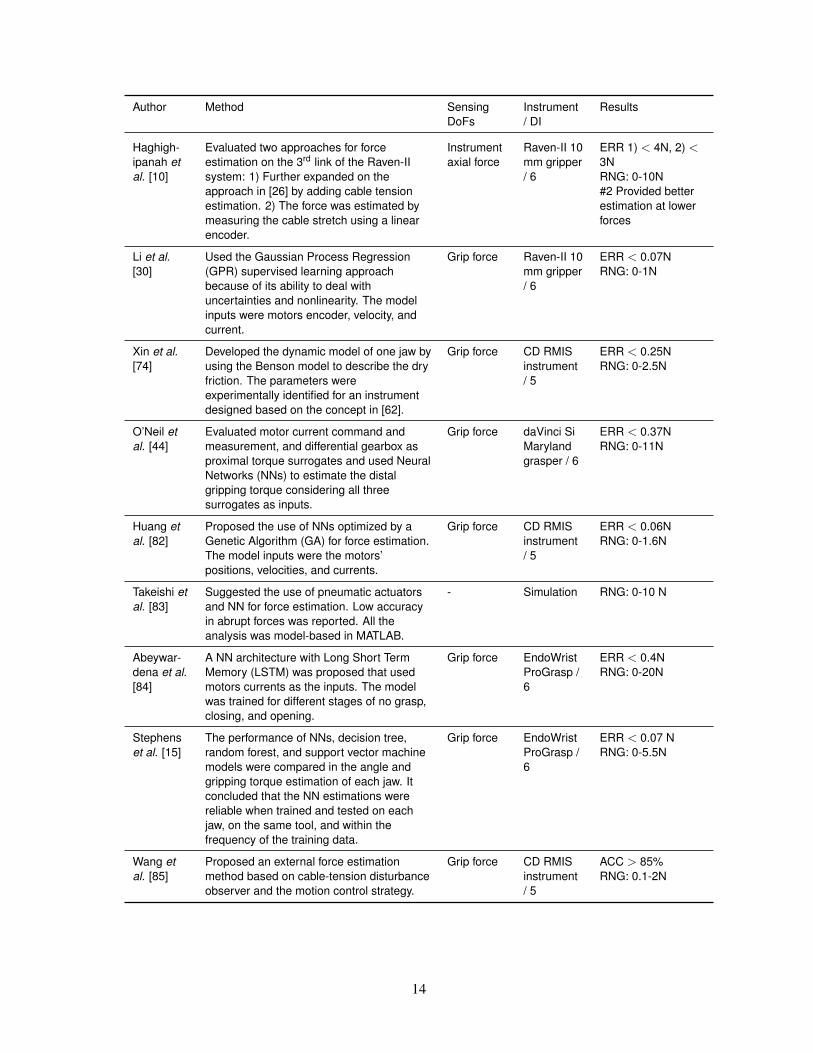
Haghigh-ipanah etal. [10]
Evaluated two approaches for forceestimation on the 3rd link of the Raven-IIsystem: 1) Further expanded on theapproach in [26] by adding cable tensionestimation. 2) The force was estimated bymeasuring the cable stretch using a linearencoder.
Instrumentaxial force
Raven-II 10mm gripper/ 6
ERR 1) < 4N, 2) <3NRNG: 0-10N#2 Provided betterestimation at lowerforces
Li et al.[30]
Used the Gaussian Process Regression(GPR) supervised learning approachbecause of its ability to deal withuncertainties and nonlinearity. The modelinputs were motors encoder, velocity, andcurrent.
Grip force Raven-II 10mm gripper/ 6
ERR < 0.07NRNG: 0-1N
Xin et al.[74]
Developed the dynamic model of one jaw byusing the Benson model to describe the dryfriction. The parameters wereexperimentally identified for an instrumentdesigned based on the concept in [62].
Grip force CD RMISinstrument/ 5
ERR < 0.25NRNG: 0-2.5N
O’Neil etal. [44]
Evaluated motor current command andmeasurement, and differential gearbox asproximal torque surrogates and used NeuralNetworks (NNs) to estimate the distalgripping torque considering all threesurrogates as inputs.
Grip force daVinci SiMarylandgrasper / 6
ERR < 0.37NRNG: 0-11N
Huang etal. [82]
Proposed the use of NNs optimized by aGenetic Algorithm (GA) for force estimation.The model inputs were the motors’positions, velocities, and currents.
Grip force CD RMISinstrument/ 5
ERR < 0.06NRNG: 0-1.6N
Takeishi etal. [83]
Suggested the use of pneumatic actuatorsand NN for force estimation. Low accuracyin abrupt forces was reported. All theanalysis was model-based in MATLAB.
- Simulation RNG: 0-10 N
Abeywar-dena et al.[84]
A NN architecture with Long Short TermMemory (LSTM) was proposed that usedmotors currents as the inputs. The modelwas trained for different stages of no grasp,closing, and opening.
Grip force EndoWristProGrasp /6
ERR < 0.4NRNG: 0-20N
Stephenset al. [15]
The performance of NNs, decision tree,random forest, and support vector machinemodels were compared in the angle andgripping torque estimation of each jaw. Itconcluded that the NN estimations werereliable when trained and tested on eachjaw, on the same tool, and within thefrequency of the training data.
Grip force EndoWristProGrasp /6
ERR < 0.07 NRNG: 0-5.5N
Wang etal. [85]
Proposed an external force estimationmethod based on cable-tension disturbanceobserver and the motion control strategy.
Grip force CD RMISinstrument/ 5
ACC > 85%RNG: 0.1-2N
14
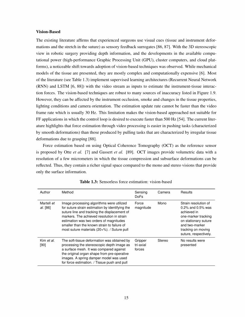
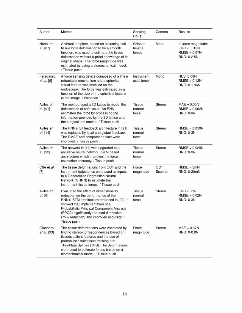
Vision-Based
The existing literature affirms that experienced surgeons use visual cues (tissue and instrument defor-
mations and the stretch in the suture) as sensory feedback surrogates [86, 87]. With the 3D stereoscopic
view in robotic surgery providing depth information, and the developments in the available compu-
tational power (high-performance Graphic Processing Unit (GPU), cluster computers, and cloud plat-
forms), a noticeable shift towards adoption of vision-based techniques was observed. While mechanical
models of the tissue are presented, they are mostly complex and computationally expensive [6]. Most
of the literature (see Table 1.3) implement supervised learning architectures (Recurrent Neural Network
(RNN) and LSTM [6, 88]) with the video stream as inputs to estimate the instrument-tissue interac-
tion forces. The vision-based techniques are robust to many sources of inaccuracy listed in Figure 1.9.
However, they can be affected by the instrument occlusion, smoke and changes in the tissue properties,
lighting conditions and camera orientation. The estimation update rate cannot be faster than the video
frame rate which is usually 30 Hz. This limitation makes the vision-based approached not suitable for
FF applications in which the control loop is desired to execute faster than 500 Hz [54]. The current liter-
ature highlights that force estimation through video processing is easier in pushing tasks (characterized
by smooth deformations) than those produced by pulling tasks that are characterized by irregular tissue
deformations due to grasping [88].
Force estimation based on using Optical Coherence Tomography (OCT) as the reference sensor
is proposed by Otte et al. [7] and Gassert et al. [89]. OCT images provide volumetric data with a
resolution of a few micrometers in which the tissue compression and subsurface deformations can be
reflected. Thus, they contain a richer signal space compared to the mono and stereo visions that provide
only the surface information.
Table 1.3: Sensorless force estimation: vision-based
Author Method SensingDoFs
Camera Results
Martell etal. [86]
Image processing algorithms were utilizedfor suture strain estimation by identifying thesuture line and tracking the displacement ofmarkers. The achieved resolution in strainestimation was two orders of magnitudessmaller than the known strain to failure ofmost suture materials (20+%). / Suture pull
Forcemagnitude
Mono Strain resolution of0.2% and 0.5% wasachieved inone-marker trackingon stationary sutureand two-markertracking on movingsuture, respectively.
Kim et al.[90]
The soft-tissue deformation was obtained byprocessing the stereoscopic depth image asa surface mesh. It was compared againstthe original organ shape from pre-operativeimages. A spring damper model was usedfor force estimation. / Tissue push and pull
Grippertri-axialforces
Stereo No results werepresented
15
Author Method SensingDoFs
Camera Results
Noohi etal. [87]
A virtual template, based on assuming softtissue local deformation to be a smoothfunction, was used to estimate the tissuedeformation without a-priori knowledge of itsoriginal shape. The force magnitude wasestimated by using a biomechanical model./ Tissue push
Grippertri-axialforces
Mono In force magnitude:ERR < 0.12NRMSE = 0.07NRNG: 0-2.5N
Faragassoet al. [9]
A force sensing device composed of a linearretractable mechanism and a sphericalvisual feature was installed on theendoscope. The force was estimated as afunction of the size of the spherical featurein the image. / Palpation
Instrumentaxial force
Mono RES: 0.08NRMSE = 0.13NRNG: 0-1.96N
Aviles etal. [91]
The method used a 3D lattice to model thedeformation of soft tissue. An RNNestimated the force by processing theinformation provided by the 3D lattice andthe surgical tool motion. / Tissue push
Tissuenormalforce
Stereo MAE = 0.05NRMSE = 0.062NRNG: 0-3N
Aviles etal. [14]
The RNN’s full feedback architecture in [91]was replaced by local and global feedback.The RMSE and computation time wereimproved. / Tissue push
Tissuenormalforce
Stereo RMSE = 0.059NRNG: 0-3N
Aviles etal. [92]
The network in [14] was upgraded to arecursive neural network LSTM basedarchitecture which improves the forceestimation accuracy. / Tissue push
Tissuenormalforce
Stereo RMSE = 0.029NRNG: 0-3N
Otte et al.[7]
The tissue deformations from OCT and theinstrument trajectories were used as inputsto a Generalized Regression NeuralNetwork (GRNN) to estimate theinstrument-tissue forces. / Tissue push
Forcemagnitude
OCTScanner
RMSE = 3mNRNG: 0-20mN
Aviles etal. [6]
Evaluated the effect of dimensionalityreduction on the performance of theRNN+LSTM architecture proposed in [92]. Itshowed that implementation of aProbabilistic Principal Component Analysis(PPCA) significantly reduced dimension(75% reduction) and improved accuracy. /Tissue push
Tissuenormalforce
Stereo ERR < 2%RMSE = 0.02NRNG: 0-3N
Giannarouet al. [93]
The tissue deformations were estimated byfinding stereo-correspondences based ontissues salient features and the use ofprobabilistic soft tissue tracking andThin-Plate Splines (TPS). The deformationswere used to estimate forces based on abiomechanical model. / Tissue push
Forcemagnitude
Stereo MAE = 0.07NRNG: 0-0.8N
16
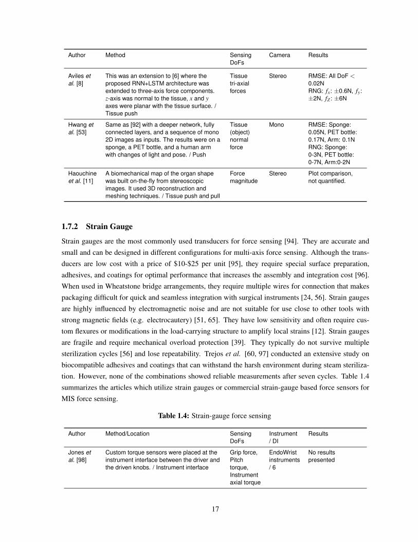
Author Method SensingDoFs
Camera Results
Aviles etal. [8]
This was an extension to [6] where theproposed RNN+LSTM architecture wasextended to three-axis force components.z-axis was normal to the tissue, x and yaxes were planar with the tissue surface. /Tissue push
Tissuetri-axialforces
Stereo RMSE: All DoF <0.02NRNG: fx: ±0.6N, fy:±2N, fZ : ±6N
Hwang etal. [53]
Same as [92] with a deeper network, fullyconnected layers, and a sequence of mono2D images as inputs. The results were on asponge, a PET bottle, and a human armwith changes of light and pose. / Push
Tissue(object)normalforce
Mono RMSE: Sponge:0.05N, PET bottle:0.17N, Arm: 0.1NRNG: Sponge:0-3N, PET bottle:0-7N, Arm:0-2N
Haouchineet al. [11]
A biomechanical map of the organ shapewas built on-the-fly from stereoscopicimages. It used 3D reconstruction andmeshing techniques. / Tissue push and pull
Forcemagnitude
Stereo Plot comparison,not quantified.
1.7.2 Strain Gauge
Strain gauges are the most commonly used transducers for force sensing [94]. They are accurate and
small and can be designed in different configurations for multi-axis force sensing. Although the trans-
ducers are low cost with a price of $10-$25 per unit [95], they require special surface preparation,
adhesives, and coatings for optimal performance that increases the assembly and integration cost [96].
When used in Wheatstone bridge arrangements, they require multiple wires for connection that makes
packaging difficult for quick and seamless integration with surgical instruments [24, 56]. Strain gauges
are highly influenced by electromagnetic noise and are not suitable for use close to other tools with
strong magnetic fields (e.g. electrocautery) [51, 65]. They have low sensitivity and often require cus-
tom flexures or modifications in the load-carrying structure to amplify local strains [12]. Strain gauges
are fragile and require mechanical overload protection [39]. They typically do not survive multiple
sterilization cycles [56] and lose repeatability. Trejos et al. [60, 97] conducted an extensive study on
biocompatible adhesives and coatings that can withstand the harsh environment during steam steriliza-
tion. However, none of the combinations showed reliable measurements after seven cycles. Table 1.4
summarizes the articles which utilize strain gauges or commercial strain-gauge based force sensors for
MIS force sensing.
Table 1.4: Strain-gauge force sensing
Author Method/Location SensingDoFs
Instrument/ DI
Results
Jones etal. [98]
Custom torque sensors were placed at theinstrument interface between the driver andthe driven knobs. / Instrument interface
Grip force,Pitchtorque,Instrumentaxial torque
EndoWristinstruments/ 6
No resultspresented
17
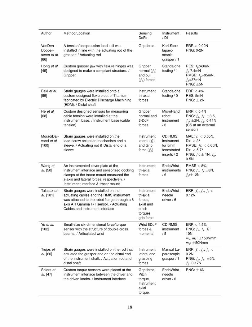
Author Method/Location SensingDoFs
Instrument/ DI
Results
VanDen-Dobbel-steen et al.[66]
A tension/compression load cell wasinstalled in line with the actuating rod of thegrasper. / Actuating rod
Grip force Karl-Storzlaparo-scopicgrasper / 1
ERR < 0.09NRNG: 0-2N
Hong et al.[45]
Custom grasper jaw with flexure hinges wasdesigned to make a compliant structure. /Gripper
Grippernormal ( fn)and pull( fp) forces
Standalonetesting / 1
RES: fp:43mN,fn:7.4mNRMSE: fp=95mN,fn=37mNRNG: ±5N
Baki et al.[99]
Strain gauges were installed onto acustom-designed flexure out of Titaniumfabricated by Electric Discharge Machining(EDM). / Distal shaft
Instrumenttri-axialforces
Standalonetesting / 0
ERR < 4%RES: 5mNRNG: ± 2N
He et al.[68]
Custom designed sensors for measuringcable tension were installed at theinstrument base. / Instrument base (cabletension)
Grippernormal and3-DoFforces
MicroHandrobotinstrument/ 6
ERR < 0.4NRNG: fx, fy: ±3.5,fz: ±2N, fg: 0-11N(CS at an externalsensor)
MoradiDal-vand et al.[100]
Strain gauges were installed on thelead-screw actuation mechanism and asleeve. / Actuating rod & Distal end of asleeve
Instrumentlateral ( fl)and Gripforce ( fg)
CD RMISinstrumentfor 5mmfenestratedinserts / 2
MAE: fl < 0.05N,Dir. < 3°RMSE: fl : < 0.05N,Dir. < 5.7°RNG: fl : ± 1N, fg:0-5N
Wang etal. [50]
An instrumented cover plate at theinstrument interface and sensorized dockingclamps at the trocar mount measured thez-axis and lateral forces, respectively. /Instrument interface & trocar mount
Instrumenttri-axialforces
EndoWristinstruments/ 6
RMSE < 8%RNG: fx, fy:±8N,fz:±12N
Talasaz etal. [101]
Strain gauges were installed on theactuating cables and the RMIS instrumentwas attached to the robot flange through a 6axis ATI Gamma F/T sensor. / ActuatingCables and instrument interface
Instrumenttri-axialforces,axial andpinchtorques,grip force
EndoWristneedledriver / 6
ERR: fx, fy, fz <0.12N
Yu et al.[102]
Small-size six-dimensional force/torquesensor with the structure of double crossbeams. / Articulated wrist
Wrist 6DoFforces &moments
CD RMISinstrument/ 5
ERR < 4.5%RNG: fx, fy, fz:10N,mx, my: ±150Nmm,mz: ±50Nmm
Trejos etal. [60]
Strain gauges were installed on the rod thatactuated the grasper and on the distal endof the instrument shaft. / Actuation rod anddistal shaft
Instrumentlateral andgraspingforces
Manual La-paroscopicgrasper / 1
ERR: fx, fy, fg <0.2NRNG: fx, fy: ±5N,fg: 0-17N
Spiers etal. [47]
Custom torque sensors were placed at theinstrument interface between the driver andthe driven knobs. / Instrument interface
Grip force,Pitchtorque,Instrumentaxialtorque,
EndoWristneedledriver / 6
RNG: ± 6N
18
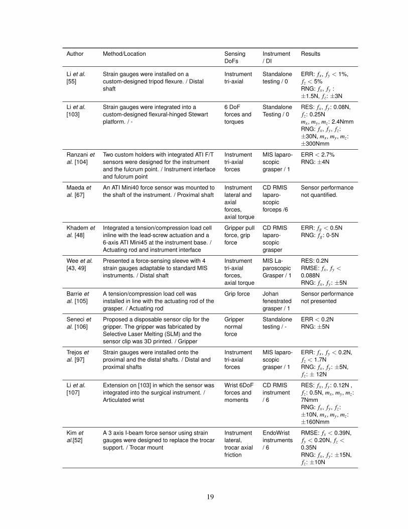
Author Method/Location SensingDoFs
Instrument/ DI
Results
Li et al.[55]
Strain gauges were installed on acustom-designed tripod flexure. / Distalshaft
Instrumenttri-axial
Standalonetesting / 0
ERR: fx, fy < 1%,fz < 5%RNG: fx, fy :±1.5N, fz: ±3N
Li et al.[103]
Strain gauges were integrated into acustom-designed flexural-hinged Stewartplatform. / -
6 DoFforces andtorques
StandaloneTesting / 0
RES: fx, fy: 0.08N,fz: 0.25Nmx, my, mz: 2.4NmmRNG: fx, fy, fz:±30N, mx, my, mz:±300Nmm
Ranzani etal. [104]
Two custom holders with integrated ATI F/Tsensors were designed for the instrumentand the fulcrum point. / Instrument interfaceand fulcrum point
Instrumenttri-axialforces
MIS laparo-scopicgrasper / 1
ERR < 2.7%RNG: ±4N
Maeda etal. [67]
An ATI Mini40 force sensor was mounted tothe shaft of the instrument. / Proximal shaft
Instrumentlateral andaxialforces,axial torque
CD RMISlaparo-scopicforceps /6
Sensor performancenot quantified.
Khadem etal. [48]
Integrated a tension/compression load cellinline with the lead-screw actuation and a6-axis ATI Mini45 at the instrument base. /Actuating rod and instrument interface
Gripper pullforce, gripforce
CD RMISlaparo-scopicgrasper
ERR: fg < 0.5NRNG: fg: 0-5N
Wee et al.[43, 49]
Presented a force-sensing sleeve with 4strain gauges adaptable to standard MISinstruments. / Distal shaft
Instrumenttri-axialforces,axial torque
MIS La-paroscopicGrasper / 1
RES: 0.2NRMSE: fx, fy <0.088NRNG: fx, fy: ±5N
Barrie etal. [105]
A tension/compression load cell wasinstalled in line with the actuating rod of thegrasper. / Actuating rod
Grip force Johanfenestratedgrasper / 1
Sensor performancenot presented
Seneci etal. [106]
Proposed a disposable sensor clip for thegripper. The gripper was fabricated bySelective Laser Melting (SLM) and thesensor clip was 3D printed. / Gripper
Grippernormalforce
Standalonetesting / -
ERR < 0.2NRNG: ±5N
Trejos etal. [97]
Strain gauges were installed onto theproximal and the distal shafts. / Distal andproximal shafts
Instrumenttri-axialforces
MIS laparo-scopicgrasper / 1
ERR: fx, fy < 0.2N,fz < 1.7NRNG: fx, fy: ±5N,fz: ± 12N
Li et al.[107]
Extension on [103] in which the sensor wasintegrated into the surgical instrument. /Articulated wrist
Wrist 6DoFforces andmoments
CD RMISinstrument/ 6
RES: fx, fy: 0.12N ,fz: 0.5N, mx, my, mz:7NmmRNG: fx, fy, fz:±10N, mx, my, mz:±160Nmm
Kim etal.[52]
A 3 axis I-beam force sensor using straingauges were designed to replace the trocarsupport. / Trocar mount
Instrumentlateral,trocar axialfriction
EndoWristinstruments/ 6
RMSE: fx < 0.39N,fy < 0.20N, fz <0.35NRNG: fx, fy: ±15N,fz: ±10N
19
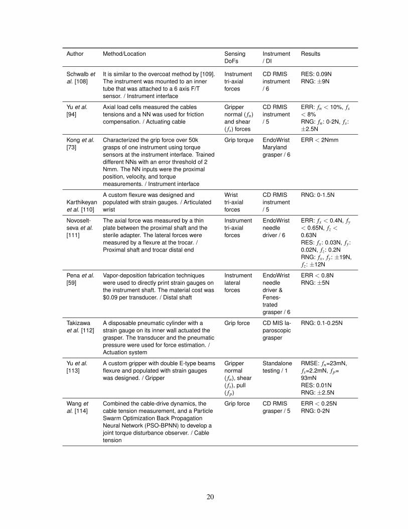
Author Method/Location SensingDoFs
Instrument/ DI
Results
Schwalb etal. [108]
It is similar to the overcoat method by [109].The instrument was mounted to an innertube that was attached to a 6 axis F/Tsensor. / Instrument interface
Instrumenttri-axialforces
CD RMISinstrument/ 6
RES: 0.09NRNG: ±9N
Yu et al.[94]
Axial load cells measured the cablestensions and a NN was used for frictioncompensation. / Actuating cable
Grippernormal ( fn)and shear( fs) forces
CD RMISinstrument/ 5
ERR: fn < 10%, fs< 8%RNG: fn: 0-2N, fs:±2.5N
Kong et al.[73]
Characterized the grip force over 50kgrasps of one instrument using torquesensors at the instrument interface. Traineddifferent NNs with an error threshold of 2Nmm. The NN inputs were the proximalposition, velocity, and torquemeasurements. / Instrument interface
Grip torque EndoWristMarylandgrasper / 6
ERR < 2Nmm
Karthikeyanet al. [110]
A custom flexure was designed andpopulated with strain gauges. / Articulatedwrist
Wristtri-axialforces
CD RMISinstrument/ 5
RNG: 0-1.5N
Novoselt-seva et al.[111]
The axial force was measured by a thinplate between the proximal shaft and thesterile adapter. The lateral forces weremeasured by a flexure at the trocar. /Proximal shaft and trocar distal end
Instrumenttri-axialforces
EndoWristneedledriver / 6
ERR: fx < 0.4N, fy< 0.65N, fz <0.63NRES: fx: 0.03N, fy:0.02N, fz: 0.2NRNG: fx, fy: ±19N,fz: ±12N
Pena et al.[59]
Vapor-deposition fabrication techniqueswere used to directly print strain gauges onthe instrument shaft. The material cost was$0.09 per transducer. / Distal shaft
Instrumentlateralforces
EndoWristneedledriver &Fenes-tratedgrasper / 6
ERR < 0.8NRNG: ±5N
Takizawaet al. [112]
A disposable pneumatic cylinder with astrain gauge on its inner wall actuated thegrasper. The transducer and the pneumaticpressure were used for force estimation. /Actuation system
Grip force CD MIS la-paroscopicgrasper
RNG: 0.1-0.25N
Yu et al.[113]
A custom gripper with double E-type beamsflexure and populated with strain gaugeswas designed. / Gripper
Grippernormal( fn), shear( fs), pull( fp)
Standalonetesting / 1
RMSE: fn=23mN,fs=2.2mN, fp=93mNRES: 0.01NRNG: ±2.5N
Wang etal. [114]
Combined the cable-drive dynamics, thecable tension measurement, and a ParticleSwarm Optimization Back PropagationNeural Network (PSO-BPNN) to develop ajoint torque disturbance observer. / Cabletension
Grip force CD RMISgrasper / 5
ERR < 0.25NRNG: 0-2N
20
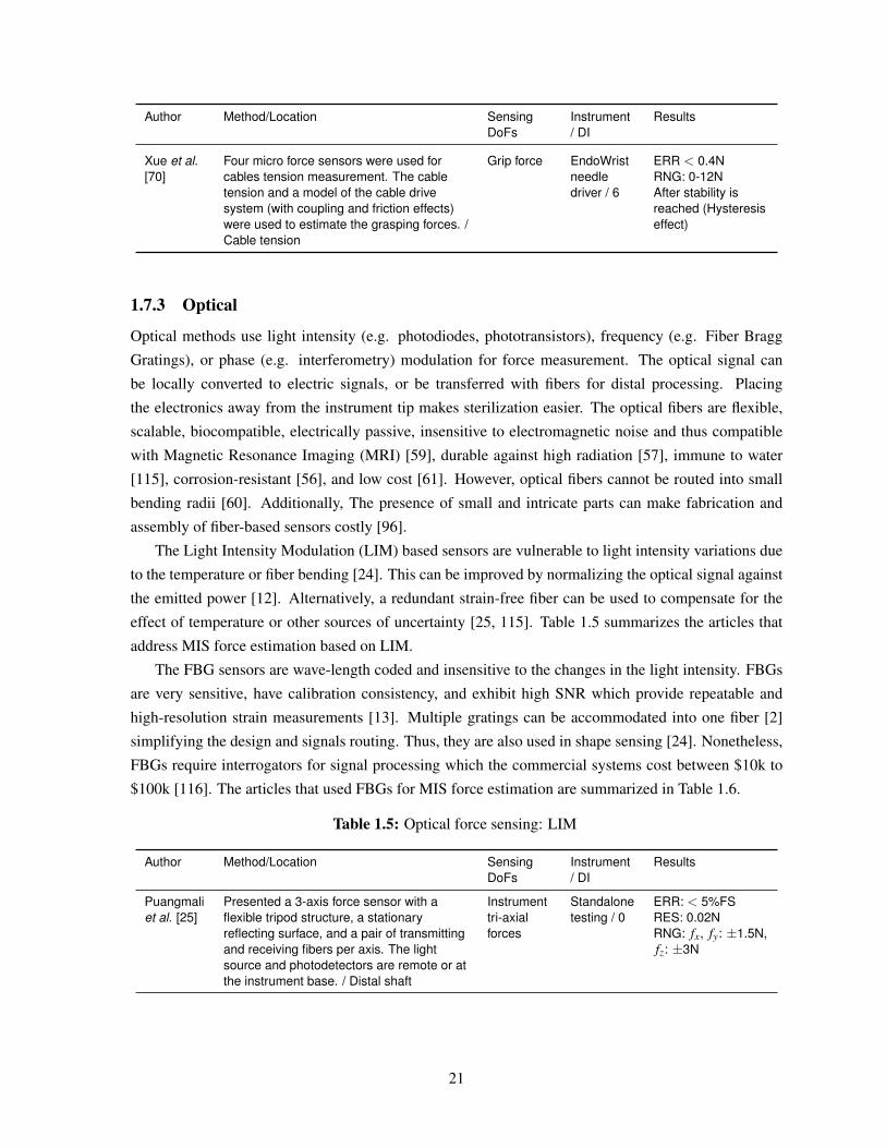
Author Method/Location SensingDoFs
Instrument/ DI
Results
Xue et al.[70]
Four micro force sensors were used forcables tension measurement. The cabletension and a model of the cable drivesystem (with coupling and friction effects)were used to estimate the grasping forces. /Cable tension
Grip force EndoWristneedledriver / 6
ERR < 0.4NRNG: 0-12NAfter stability isreached (Hysteresiseffect)
1.7.3 Optical
Optical methods use light intensity (e.g. photodiodes, phototransistors), frequency (e.g. Fiber Bragg
Gratings), or phase (e.g. interferometry) modulation for force measurement. The optical signal can
be locally converted to electric signals, or be transferred with fibers for distal processing. Placing
the electronics away from the instrument tip makes sterilization easier. The optical fibers are flexible,
scalable, biocompatible, electrically passive, insensitive to electromagnetic noise and thus compatible
with Magnetic Resonance Imaging (MRI) [59], durable against high radiation [57], immune to water
[115], corrosion-resistant [56], and low cost [61]. However, optical fibers cannot be routed into small
bending radii [60]. Additionally, The presence of small and intricate parts can make fabrication and
assembly of fiber-based sensors costly [96].
The Light Intensity Modulation (LIM) based sensors are vulnerable to light intensity variations due
to the temperature or fiber bending [24]. This can be improved by normalizing the optical signal against
the emitted power [12]. Alternatively, a redundant strain-free fiber can be used to compensate for the
effect of temperature or other sources of uncertainty [25, 115]. Table 1.5 summarizes the articles that
address MIS force estimation based on LIM.
The FBG sensors are wave-length coded and insensitive to the changes in the light intensity. FBGs
are very sensitive, have calibration consistency, and exhibit high SNR which provide repeatable and
high-resolution strain measurements [13]. Multiple gratings can be accommodated into one fiber [2]
simplifying the design and signals routing. Thus, they are also used in shape sensing [24]. Nonetheless,
FBGs require interrogators for signal processing which the commercial systems cost between $10k to
$100k [116]. The articles that used FBGs for MIS force estimation are summarized in Table 1.6.
Table 1.5: Optical force sensing: LIM
Author Method/Location SensingDoFs
Instrument/ DI
Results
Puangmaliet al. [25]
Presented a 3-axis force sensor with aflexible tripod structure, a stationaryreflecting surface, and a pair of transmittingand receiving fibers per axis. The lightsource and photodetectors are remote or atthe instrument base. / Distal shaft
Instrumenttri-axialforces
Standalonetesting / 0
ERR: < 5%FSRES: 0.02NRNG: fx, fy: ±1.5N,fz: ±3N
21
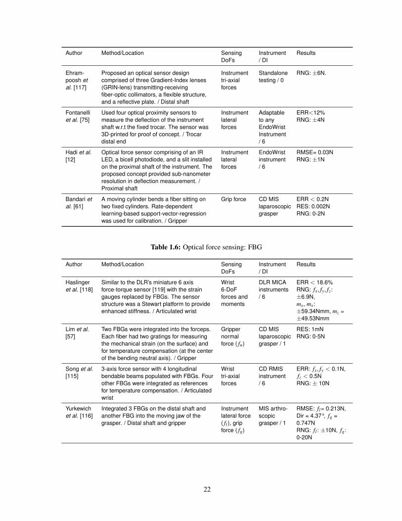
Author Method/Location SensingDoFs
Instrument/ DI
Results
Ehram-poosh etal. [117]
Proposed an optical sensor designcomprised of three Gradient-Index lenses(GRIN-lens) transmitting-receivingfiber-optic collimators, a flexible structure,and a reflective plate. / Distal shaft
Instrumenttri-axialforces
Standalonetesting / 0
RNG: ±6N.
Fontanelliet al. [75]
Used four optical proximity sensors tomeasure the deflection of the instrumentshaft w.r.t the fixed trocar. The sensor was3D-printed for proof of concept. / Trocardistal end
Instrumentlateralforces
Adaptableto anyEndoWristInstrument/ 6
ERR<12%RNG: ±4N
Hadi et al.[12]
Optical force sensor comprising of an IRLED, a bicell photodiode, and a slit installedon the proximal shaft of the instrument. Theproposed concept provided sub-nanometerresolution in deflection measurement. /Proximal shaft
Instrumentlateralforces
EndoWristinstrument/ 6
RMSE= 0.03NRNG: ±1N
Bandari etal. [61]
A moving cylinder bends a fiber sitting ontwo fixed cylinders. Rate-dependentlearning-based support-vector-regressionwas used for calibration. / Gripper
Grip force CD MISlaparoscopicgrasper
ERR < 0.2NRES: 0.002NRNG: 0-2N
Table 1.6: Optical force sensing: FBG
Author Method/Location SensingDoFs
Instrument/ DI
Results
Haslingeret al. [118]
Similar to the DLR’s miniature 6 axisforce-torque sensor [119] with the straingauges replaced by FBGs. The sensorstructure was a Stewart platform to provideenhanced stiffness. / Articulated wrist
Wrist6-DoFforces andmoments
DLR MICAinstruments/ 6
ERR < 18.6%RNG: fx, fy, fz:±6.9N,mx, mx:±59.34Nmm, mz =±49.53Nmm
Lim et al.[57]
Two FBGs were integrated into the forceps.Each fiber had two gratings for measuringthe mechanical strain (on the surface) andfor temperature compensation (at the centerof the bending neutral axis). / Gripper
Grippernormalforce ( fn)
CD MISlaparoscopicgrasper / 1
RES: 1mNRNG: 0-5N
Song et al.[115]
3-axis force sensor with 4 longitudinalbendable beams populated with FBGs. Fourother FBGs were integrated as referencesfor temperature compensation. / Articulatedwrist
Wristtri-axialforces
CD RMISinstrument/ 6
ERR: fx, fy < 0.1N,fz < 0.5NRNG: ± 10N
Yurkewichet al. [116]
Integrated 3 FBGs on the distal shaft andanother FBG into the moving jaw of thegrasper. / Distal shaft and gripper
Instrumentlateral force( fl), gripforce ( fg)
MIS arthro-scopicgrasper / 1
RMSE: fl= 0.213N,Dir = 4.37°, fg =0.747NRNG: fl : ±10N, fg:0-20N
22
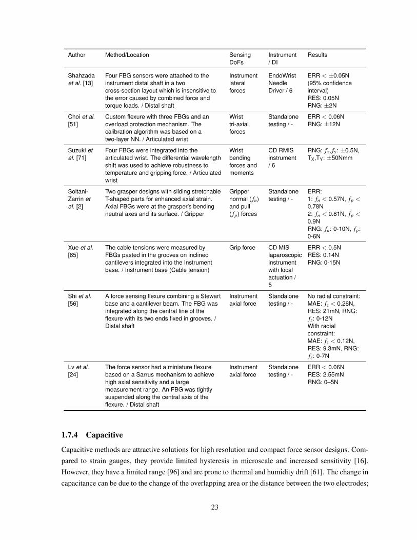
Author Method/Location SensingDoFs
Instrument/ DI
Results
Shahzadaet al. [13]
Four FBG sensors were attached to theinstrument distal shaft in a twocross-section layout which is insensitive tothe error caused by combined force andtorque loads. / Distal shaft
Instrumentlateralforces
EndoWristNeedleDriver / 6
ERR < ±0.05N(95% confidenceinterval)RES: 0.05NRNG: ±2N
Choi et al.[51]
Custom flexure with three FBGs and anoverload protection mechanism. Thecalibration algorithm was based on atwo-layer NN. / Articulated wrist
Wristtri-axialforces
Standalonetesting / -
ERR < 0.06NRNG: ±12N
Suzuki etal. [71]
Four FBGs were integrated into thearticulated wrist. The differential wavelengthshift was used to achieve robustness totemperature and gripping force. / Articulatedwrist
Wristbendingforces andmoments
CD RMISinstrument/ 6
RNG: fx, fy: ±0.5N,TX,TY: ±50Nmm
Soltani-Zarrin etal. [2]
Two grasper designs with sliding stretchableT-shaped parts for enhanced axial strain.Axial FBGs were at the grasper’s bendingneutral axes and its surface. / Gripper
Grippernormal ( fn)and pull( fp) forces
Standalonetesting / -
ERR:1: fn < 0.57N, fp <0.78N2: fn < 0.81N, fp <0.9NRNG: fn: 0-10N, fp:0-6N
Xue et al.[65]
The cable tensions were measured byFBGs pasted in the grooves on inclinedcantilevers integrated into the Instrumentbase. / Instrument base (Cable tension)
Grip force CD MISlaparoscopicinstrumentwith localactuation /5
ERR < 0.5NRES: 0.14NRNG: 0-15N
Shi et al.[56]
A force sensing flexure combining a Stewartbase and a cantilever beam. The FBG wasintegrated along the central line of theflexure with its two ends fixed in grooves. /Distal shaft
Instrumentaxial force
Standalonetesting / -
No radial constraint:MAE: fz < 0.26N,RES: 21mN, RNG:fz: 0-12NWith radialconstraint:MAE: fz < 0.12N,RES: 9.3mN, RNG:fz: 0-7N
Lv et al.[24]
The force sensor had a miniature flexurebased on a Sarrus mechanism to achievehigh axial sensitivity and a largemeasurement range. An FBG was tightlysuspended along the central axis of theflexure. / Distal shaft
Instrumentaxial force
Standalonetesting / -
ERR < 0.06NRES: 2.55mNRNG: 0–5N
1.7.4 Capacitive
Capacitive methods are attractive solutions for high resolution and compact force sensor designs. Com-
pared to strain gauges, they provide limited hysteresis in microscale and increased sensitivity [16].
However, they have a limited range [96] and are prone to thermal and humidity drift [61]. The change in
capacitance can be due to the change of the overlapping area or the distance between the two electrodes;
23
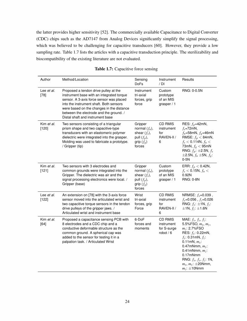
the latter provides higher sensitivity [52]. The commercially available Capacitance to Digital Converter
(CDC) chips such as the AD7147 from Analog Devices significantly simplify the signal processing,
which was believed to be challenging for capacitive transducers [60]. However, they provide a low
sampling rate. Table 1.7 lists the articles with a capacitive transduction principle. The sterilizability and
biocompatibility of the existing literature are not evaluated.
Table 1.7: Capacitive force sensing
Author Method/Location SensingDoFs
Instrument/ DI
Results
Lee et al.[78]
Proposed a tendon drive pulley at theinstrument base with an integrated torquesensor. A 3-axis force sensor was placedinto the instrument shaft. Both sensorswere based on the changes in the distancebetween the electrode and the ground. /Distal shaft and instrument base
Instrumenttri-axialforces, gripforce
Customprototypeof an MISgrasper / 1
RNG: 0-0.5N
Kim et al.[120]
Two sensors consisting of a triangularprism shape and two capacitive-typetransducers with an elastomeric polymerdielectric were integrated into the grasper.Molding was used to fabricate a prototype./ Gripper (tip)
Grippernormal ( fn),shear ( fs),pull ( fp),grip ( fg)forces
CD RMISinstrumentforRAVEN-II /6
RES: fp=42mN,fs=72mN,fn=58mN, fg=46mNRMSE: fp < 84mN,fs < 0.114N, fn <73mN, fg < 95mNRNG: fp: ±2.5N, fs±2.5N, fn ±5N, fg:0-5N
Kim et al.[121]
Two sensors with 3 electrodes andcommon grounds were integrated into theGripper. The dielectric was air and thesignal processing electronics were local. /Gripper (base)
Grippernormal ( fn),shear ( fs),pull ( fp),grip ( fg)forces
Customprototypeof an MISgrasper / 1
ERR: fp < 0.42N,fs < 0.15N, fn <0.92NRNG: 0-8N
Lee et al.[122]
An extension on [78] with the 3-axis forcesensor moved into the articulated wrist andtwo capacitive torque sensors in the tendondrive pulleys of the gripper jaws. /Articulated wrist and instrument base
Wristtri-axialforces, gripForce
CD RMISinstrumentforRAVEN-II /6
NRMSE: fx=0.039 ,fy=0.056 , fz=0.026RNG: fx: ±1N, fy:±1N, fz: ±1.6N
Kim et al.[64]
Proposed a capacitance sensing PCB with8 electrodes and a CDC chip and aconductive deformable structure as thecommon ground. A spherical cap wasadded to the sensor for testing it in apalpation task. / Articulated Wrist
6-DoFforces andmoments
CD RMISinstrumentfor S-surgerobot / 6
MAE: fx, fy, fz:5.5%FSO, mx, my,mz: 2.7%FSORES: fx: 0.22mN,fy: 0.31mN, fz:0.11mN, mx:0.47mNmm, my:0.41mNmm, mz:0.17mNmmRNG: fx, fy, fz: 1N,mx, my: ±20Nmm,mz: ±10Nmm
24
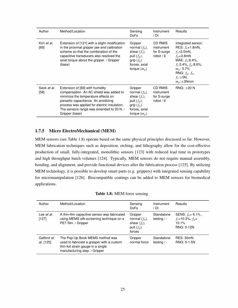
Author Method/Location SensingDoFs
Instrument/ DI
Results
Kim et al.[69]
Extension of [121] with a slight modificationin the proximal gripper jaw and calibrationscheme so that the combination of thecapacitive transducers also resolved theaxial torque about the gripper. / Gripper(base)
Grippernormal ( fn),shear ( fs),pull ( fp),grip ( fg)forces, axialtorque (mp)
CD RMISinstrumentfor S-surgerobot / 6
Integrated sensor:RES: fn=1.8mN,fs=2.0mN,fp=3.8mNMAE: fn:6.4%,fs:3.4%, fp:8.6%,mp: 5.7%RNG: fp, fn,fs:±5N,mp:±3Nmm
Seok et al.[58]
Extension of [69] with humiditycompensation. An AC shield was added tominimize the temperature effects onparasitic capacitance. An anodizingprocess was applied for electric insulation.The sensors range was extended to 20 N. /Gripper (base)
Grippernormal ( fn),shear ( fs),pull ( fp),grip ( fg)forces, axialtorque (mp)
CD RMISinstrumentfor S-surgerobot / 6
RNG: ±20 N
1.7.5 Micro ElectroMechanical (MEM)
MEM sensors (see Table 1.8) operate based on the same physical principles discussed so far. However,
MEM fabrication techniques such as deposition, etching, and lithography allow for the cost-effective
production of small, fully-integrated, monolithic sensors [123] with reduced lead time in prototypes
and high throughput batch volumes [124]. Typically, MEM sensors do not require manual assembly,
bonding, and alignment, and provide functional devices after the fabrication process [125]. By utilizing
MEM technology, it is possible to develop smart parts (e.g. grippers) with integrated sensing capability
for micromanipulation [126]. Biocompatible coatings can be added to MEM sensors for biomedical
applications.
Table 1.8: MEM force sensing
Author Method/Location SensingDoFs
Instrument/ DI
Results
Lee et al.[127]
A thin-film capacitive sensor was fabricatedusing MEMS silk-screening technique on aPET film. / Gripper
Grippernormal ( fn),shear ( fs),pull ( fp)forces
Standalonetesting / -
SENS: fn= 6.1% ,fs=10.3%, fp=10.1%RNG: 0-12N
Gafford etal. [125]
The Pop-Up Book MEMS method wasused to fabricate a grasper with a customthin-foil strain gauge in a singlemanufacturing step. / Gripper
Grippernormal force
Standalonetesting / -
RES: 30mNRNG: 0-1.5N
25
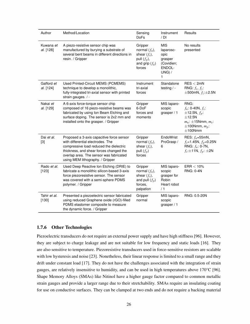
Author Method/Location SensingDoFs
Instrument/ DI
Results
Kuwana etal. [128]
A piezo-resistive sensor chip wasmanufactured by burying a substrate ofseveral bent beams in different directions inresin. / Gripper
Grippernormal ( fn),shear ( fs),pull ( fp),and grip ( fg)forces
MISlaparosc-opicgrasper(Covidien;ENDOL-UNG) /1
No resultspresented
Gafford etal. [124]
Used Printed-Circuit MEMS (PCMEMS)technique to develop a monolithic,fully-integrated tri-axial sensor with printedstrain gauges. / -
Instrumenttri-axialforces
Standalonetesting / -
RES < 2mNRNG: fx, fy:±500mN, fz:±2.5N
Nakai etal. [129]
A 6-axis force-torque sensor chipcomposed of 16 piezo-resistive beams wasfabricated by using Ion Beam Etching andsurface doping. The sensor is 2x2 mm andinstalled onto the grasper. / Gripper
Gripper6-DoFforces andmoments
MIS laparo-scopicgrasper / 1
RNG:fn: 0-40N, fs:±12.5N, fp:±12.5Nmn: ±15Nmm, ms:±100Nmm, mp:±100Nmm
Dai et al.[3]
Proposed a 3-axis capacitive force sensorwith differential electrodes. Thecompressive load reduced the dielectricthickness, and shear forces changed theoverlap area. The sensor was fabricatedusing MEM lithography. / Gripper
Grippernormal ( fn),shear ( fs),pull ( fp)forces
EndoWristProGrasp /6
RES: fn=55mN,fs=1.45N, fp=0.25NRNG: fn: 0-7N,fs:±11N, fp: ±2N
Rado et al.[123]
Used Deep Reactive Ion Etching (DRIE) tofabricate a monolithic silicon-based 3-axisforce piezoresistive sensor. The sensorwas covered with a semi-sphere PDMSpolymer. / Gripper
Grippernormal ( fn),shear ( fs),and pull ( fp)forces,palpation
MIS laparo-scopicgrasper forRobinHeart robot/ 1
ERR < 10%RNG: 0-4N
Tahir et al.[130]
Presented a piezoelectric sensor fabricatedusing reduced Graphene oxide (rGO)-filledPDMS elastomer composite to measurethe dynamic force. / Gripper
Grippernormal
MIS laparo-scopicgrasper / 1
RNG: 0.5-20N
1.7.6 Other Technologies
Piezoelectric transducers do not require an external power supply and have high stiffness [96]. However,
they are subject to charge leakage and are not suitable for low frequency and static loads [16]. They
are also sensitive to temperature. Piezoresistive transducers used in force-sensitive resistors are scalable
with low hysteresis and noise [23]. Nonetheless, their linear response is limited to a small range and they
drift under constant load [17]. They do not have the challenges associated with the integration of strain
gauges, are relatively insensitive to humidity, and can be used in high temperatures above 170°C [96].
Shape Memory Alloys (SMAs) like Nitinol have a higher gauge factor compared to common metallic
strain gauges and provide a larger range due to their stretchability. SMAs require an insulating coating
for use on conductive surfaces. They can be clamped at two ends and do not require a backing material
26
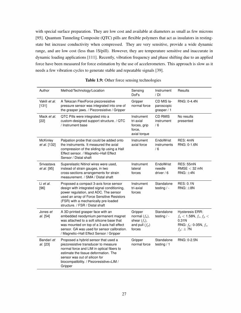
with special surface preparation. They are low cost and available at diameters as small as few microns
[95]. Quantum Tunneling Composite (QTC) pills are flexible polymers that act as insulators in resting-
state but increase conductivity when compressed. They are very sensitive, provide a wide dynamic
range, and are low cost (less than 1$/pill). However, they are temperature sensitive and inaccurate in
dynamic loading applications [111]. Recently, vibration frequency and phase shifting due to an applied
force have been measured for force estimation by the use of accelerometers. This approach is slow as it
needs a few vibration cycles to generate stable and repeatable signals [39].
Table 1.9: Other force sensing technologies
Author Method/Technology/Location SensingDoFs
Instrument/ DI
Results
Vakili et al.[131]
A Tekscan FlexiForce piezoresistivepressure sensor was integrated into one ofthe grasper jaws. / Piezoresistive / Gripper
Grippernormal force
CD MIS la-paroscopicgrasper / 1
RNG: 0-4.4N
Mack et al.[22]
QTC Pills were integrated into acustom-designed support structure. / QTC/ Instrument base
Instrumenttri-axialforces, gripforce,axial torque
CD RMISinstrument/ 6
No resultspresented
McKinleyet al. [132]
Palpation probe that could be added ontothe instruments. It measured the axialcompression of the sliding tip using a HallEffect sensor. / Magnetic–Hall EffectSensor / Distal shaft
Instrumentaxial force
EndoWristinstruments/ 6
RES: 4mNRNG: 0-1.6N
Srivastavaet al. [95]
Superelastic Nitinol wires were used,instead of strain gauges, in twocross-sections arrangements for strainmeasurement. / SMA / Distal shaft
Instrumentlateralforces
EndoWristneedledriver / 6
RES: 55mNRMSE < 32 mNRNG: ±4N
Li et al.[96]
Proposed a compact 3-axis force sensordesign with integrated signal conditioning,power regulation, and ADC. The sensorused an array of Force Sensitive Resistors(FSR) with a mechanically pre-loadedstructure. / FSR / Distal shaft
Instrumenttri-axialforces
Standalonetesting / -
RES: 0.1NRNG: ±8N
Jones etal. [54]
A 3D-printed grasper face with anembedded neodymium permanent magnetwas attached to a soft silicone base thatwas mounted on top of a 3-axis hall effectsensor. GA was used for sensor calibration./ Magnetic–Hall Effect Sensor / Gripper
Grippernormal ( fn),shear ( fs),and pull ( fp)forces
Standalonetesting / -
Hysteresis ERR:fn < 1.58N, fs, fp <0.31NRNG: fn: 0-35N, fs,fp: ± 7N
Bandari etal. [23]
Proposed a hybrid sensor that used apiezoresistive transducer to measurenormal force and LIM in optical fibers toestimate the tissue deformation. Thesensor was out of silicon forbiocompatibility. / Piezoresistive+LIM /Gripper
Grippernormal force
Standalonetesting / 1
RNG: 0-2.5N
27
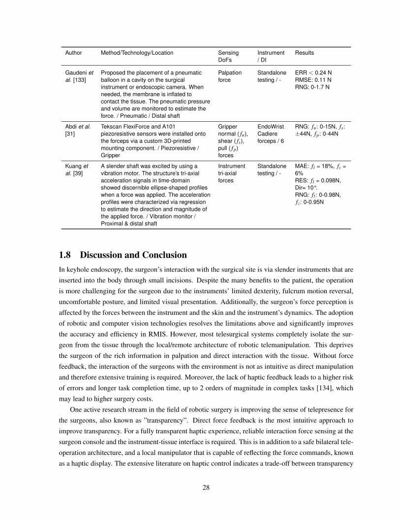
Author Method/Technology/Location SensingDoFs
Instrument/ DI
Results
Gaudeni etal. [133]
Proposed the placement of a pneumaticballoon in a cavity on the surgicalinstrument or endoscopic camera. Whenneeded, the membrane is inflated tocontact the tissue. The pneumatic pressureand volume are monitored to estimate theforce. / Pneumatic / Distal shaft
Palpationforce
Standalonetesting / -
ERR < 0.24 NRMSE: 0.11 NRNG: 0-1.7 N
Abdi et al.[31]
Tekscan FlexiForce and A101piezoresistive sensors were installed ontothe forceps via a custom 3D-printedmounting component. / Piezoresistive /Gripper
Grippernormal ( fn),shear ( fs),pull ( fp)forces
EndoWristCadiereforceps / 6
RNG: fn: 0-15N, fs:±44N, fp: 0-44N
Kuang etal. [39]
A slender shaft was excited by using avibration motor. The structure’s tri-axialacceleration signals in time-domainshowed discernible ellipse-shaped profileswhen a force was applied. The accelerationprofiles were characterized via regressionto estimate the direction and magnitude ofthe applied force. / Vibration monitor /Proximal & distal shaft
Instrumenttri-axialforces
Standalonetesting / -
MAE: fl = 18%, fz =6%RES: fl = 0.098N,Dir= 10°.RNG: fl : 0-0.98N,fz: 0-0.95N
1.8 Discussion and ConclusionIn keyhole endoscopy, the surgeon’s interaction with the surgical site is via slender instruments that are
inserted into the body through small incisions. Despite the many benefits to the patient, the operation
is more challenging for the surgeon due to the instruments’ limited dexterity, fulcrum motion reversal,
uncomfortable posture, and limited visual presentation. Additionally, the surgeon’s force perception is
affected by the forces between the instrument and the skin and the instrument’s dynamics. The adoption
of robotic and computer vision technologies resolves the limitations above and significantly improves
the accuracy and efficiency in RMIS. However, most telesurgical systems completely isolate the sur-
geon from the tissue through the local/remote architecture of robotic telemanipulation. This deprives
the surgeon of the rich information in palpation and direct interaction with the tissue. Without force
feedback, the interaction of the surgeons with the environment is not as intuitive as direct manipulation
and therefore extensive training is required. Moreover, the lack of haptic feedback leads to a higher risk
of errors and longer task completion time, up to 2 orders of magnitude in complex tasks [134], which
may lead to higher surgery costs.
One active research stream in the field of robotic surgery is improving the sense of telepresence for
the surgeons, also known as ”transparency”. Direct force feedback is the most intuitive approach to
improve transparency. For a fully transparent haptic experience, reliable interaction force sensing at the
surgeon console and the instrument-tissue interface is required. This is in addition to a safe bilateral tele-
operation architecture, and a local manipulator that is capable of reflecting the force commands, known
as a haptic display. The extensive literature on haptic control indicates a trade-off between transparency
28
and stability [27]. Alternatively, sensory substitution was proposed instead of haptic feedback, in the
form of visual, auditory, or vibrotactile cues of force information. Although the safety can be easily
guaranteed in systems with SS, it is not intuitive and can cause cognitive overload for the surgeon. The
SS methods can also be used in MIS systems because no robotic manipulator is required for force reflec-
tion. The efficacy of different haptic feedback modalities in improving the surgical training and surgeon
performance metrics has been studied extensively [31, 34, 36, 37]. It is shown that a transparent haptic
experience and visual feedback of force information improve the performance metrics and shorten the
training time for novice surgeons in complex tasks. Apart from haptic feedback, the instrument-tissue
interaction forces can be used for tissue damage monitoring, surgical skills assessment, development of
surgical training guidelines, and to automate tasks.
Extensive research has been conducted to estimate or sense the instrument-tissue interaction forces.
The functional requirements depend on the application. While it is not necessary to estimate the tissue
forces precisely to provide an appropriate haptic experience [98], the bandwidth and sampling rate are
important requirements to ensure low latency and smooth interaction with the remote environment. The
sampling rate and bandwidth are less critical in SS.
Sensorless approaches utilize the information that is already available in the robotic manipulator;
the axes positions and velocities, motors currents, and visual display of the surgical theatre. With the
exponential growth, over the past decade, in the available computational power to researchers, data-
driven approaches based on supervised learning [8, 30] have been widely adopted. Among them, neural
networks have shown promising results when trained and used on one particular instrument. How-
ever, they require a long and computationally-expensive training phase that is yet clinically-prohibitive.
The training is based on a set of measurements at the beginning of the surgery that is used afterward
for force estimation throughout the entire surgery. Proposed approaches that have an instrument’s op-
erational parameters as inputs, do not consider the variations between instruments and the change of
instruments behavior throughout its use [73]. Considering how the research direction has evolved over
the past decade, experimentation with different model architectures, development of efficient training,
and identification methods that can be automatically performed at the system start-up [47], improving
the computation time, and incorporation of online adaptation techniques are attractive research areas to
be further investigated. Moreover, all the existing literature uses the information at the patient manipu-
lator for force estimation, but the inclusion of the operating parameters at the surgeon console may also
improve the quality of force estimation.
The sensor design is another avenue towards collecting force data at the instrument tip. The sen-
sor can be located inside or outside the body. The closer the sensor is to the instrument tip the more
accurate the measurements are. However, the size, biocompatibility, sterilizability, insulation, and seal-
ing requirements are more stringent when such an approach is followed. Design proposals for sensor
integration into the instrument tip have limited adaptability because the instruments for different types
of surgery have different shapes at the tip (e.g. EndoWrist cautery forceps, graspers, dissectors, needle
drivers, etc.). Therefore, a custom sensor needs to be designed for every instrument, which increases
the development, fabrication, and maintenance costs.
29
A variety of transduction principles, including resistive, capacitive, optical, piezoelectric, and mag-
netic have been used in the development of sensing solutions for minimally invasive procedures. While
strain gauges are still the most commonly used transducers, the study by Trejos et al. [97] showed
that biocompatible adhesives and coatings can only survive a maximum of 6 steam sterilization cycles.
Considering that the instruments are typically used 10 times before disposed, this would lead to a 40%
increase in the cost of the instruments with integrated strain gauges. Additionally, the installation of
strain gauges is labor-intensive that contributes to an increased cost.
A comparison of the publications summarized in this article with the surveys by Puangmali et al.
[40] and Trejos et al. [41] indicates a noticeable shift towards utilizing FBG and MEM technologies for
the development of gripper integrated miniature sensors (Figure 1.9). FBGs are compact, sterilizable,
biocompatible, electrically passive, and immune to electromagnetic noise. They provide high sensitivity
with sub-micron resolution and can have multiple gratings embedded in one fiber which simplifies opti-
cal signal management. While the commercial interrogators are expensive, there are signal conditioning
solutions proposed to decrease the electronics cost [116]. The developments in MEM technology have
overcome the barrier of scale and cost in the fabrication of delicate miniature sensors. Additionally,
MEM sensors typically do not need manual assembly and can be integrated into the desired application
after production.
Another observable trend is the utilization of data-driven regression approaches for sensor calibra-
tion. Models based on neural networks and other supervised learning methods such as GPR have shown
unprecedented performance in handling nonlinearities and uncertainties in sensor calibration. Compared
to the surgical instruments, the transducers show a more consistent response and do not need regular
calibration unless removed and reintegrated. Efficient calibration approaches that can be quickly and
automatically performed without operator intervention (e.g based on payload estimation) would benefit
the RMIS systems.
1.9 Thesis ObjectivesAs discussed in Section 1.2, the maximum transparency in a teleoperation system is achievable via a
four-channel bilateral network with force and position sensing at the scanner and the adapter manip-
ulators. To the best of our knowledge, no da Vinci® MTM is instrumented with a force sensor that
allows the measurement of the surgeon forces without limiting the dexterity of the MTM’s wrist gim-
bal. Extensive research is reported in literature on the force estimation and force sensing at the surgical
site. However, no tele-surgical system, which is clinically in use, yet provides this capability in a safe,
reliable, and robust manner. In this thesis, we are set to research the upgrades to the da Vinci® classic
system that allow the development of a highly transparent teleoperation framework by instrumenting the
MTM and the PSM of the da Vinci® classic system to allow force sensing at the surgeon console and at
the surgical site. For this purpose, we
1. research a design modification of the MTM in the da Vinci® classic system to integrate a com-
mercial 6-axis force sensor without modifying its kinematic chain and the interface to the surgeon.
30
2. research a force sensing approach for the da Vinci® instruments used in multi-port keyhole en-
doscopy that 1) can measure the multi-axis forces and moments applied to the instrument, 2)
does not require instrument modifications and is therefore adaptable to different surgical tools,
and 3) provides high resolution and low latency force data that is usable in high transparency
tele-operation control frameworks.
1.10 Thesis OutlineChapter 2 explains the integration of a force/torque sensor into the wrist of the MTM of the da Vinci® clas-
sic surgical system. The added sensor can be used to monitor the surgeon interaction forces and to
improve the haptic experience. The proposed mechanical design is expected to have little effect on the
surgeon’s operative experience and is simple and inexpensive to implement. The complete mechanical
and electrical modifications, as well as the software packages are discussed. Two example applica-
tions of impedance control at the MTM and joystick control of the PSM are presented to demonstrate
the successful integration of the sensor into the MTM and the interface to the da Vinci Research Kit
(dVRK).
In Chapter 3, a novel 6-axis Optical Force Sensor (OFS) is discussed, It employs pairs of Light-
Emitting Diodes (LEDs) and bicell photodetectors, and corresponding slits that modulate the projected
LED light onto the photodetectors in response to external forces. The sensor can be clamped on and
off a structure and relies upon the compliance of the structure for force estimation; it has no flexible
components and therefore it is robust to overload. A sensor model is derived and validated that can
be used to explore design trade-offs. A calibration approach based on an external reference sensor and
an approach to temperature compensation are presented and validated. It was shown that the sensing
concept provides nanometer resolution in displacement measurement.
Chapter 4 details the novel hardware and software architecture of the OFS. The proposed config-
urable, modular, and compact electronics lead to performance characteristics that cannot be reached by
currently available sensors: ultra-low noise with average noise power spectral density of 15 nV/√
Hz
over a signal bandwidth of 500 Hz, a resolution of 0.0001% full-scale at a 95% confidence level, and
a hardware latency of less than 100 µs. Performance is achieved by local synchronized over-sampling
of the sensor’s optical transducers, and parallel hardware processing of the sensor data using a Field
Programmable Gate Array (FPGA). The FPGA’s reconfigurability provides for easy customization and
updates; for example, by increasing the FPGA system clock rate to a maximum of 160 MHz, latency
can be decreased to 50 µs, limited by the current Analog to Digital Converter (ADC). Furthermore, the
approach is generic and could be duplicated with other types of transducers. An Inertial Measurement
Unit (IMU) and a temperature sensor are integrated into the sensor electronics for gravity, inertia, and
temperature compensation. Two Software Development Kits (SDKs) that allow for the use of the sensor
and its integration into the Robot Operating System (ROS) are discussed.
Chapter 5 presents the integration of the OFS in the PSM of the da Vinci® classic system with
no modification to the surgical instrument. Thus, it is adaptable to different surgical instruments. The
sensor is mounted onto the proximal shaft of a da Vinci® EndoWrist instrument. A new cannula design
31
comprising an inner tube and an outer tube is proposed. The inner tube is attached to the cannula’s
interface to the robot base through a compliant leaf spring with adjustable stiffness. It allows bending
of the instrument shaft due to the tip forces. The outer tube mechanically filters out the body forces
from affecting the instrument’s bending behavior. A mathematical model of the sensing principle is
developed and used for model-based calibration. A data-driven calibration based on a shallow neural
network architecture comprising a single 5-nodes hidden layer and a 5×1 output layer is discussed.
Extensive testing was conducted to validate that the sensor can successfully measure the lateral forces
and moments and the axial torque applied to the instrument’s distal end within the desired resolution,
accuracy, and range requirements.
The final chapter of this thesis provides an overview of the work presented. The long term goals and
limitations of the work are also discussed. Finally, the future of the work and possible improvements
are considered.
32
Chapter 2
6-DOF Force Sensing for the MTM of theda Vinci® Surgical System
2.1 IntroductionInstrumenting the manipulator is the preferred method to develop a three or four channel [135] [32] tele-
operation system. Additionally, force sensing at the surgeon console will enable novel studies in teleop-
eration, including but not limited to improved teleoperation transparency, surgical skills assessment by
monitoring operator interaction forces [136], learning from demonstration, improving the human-robot
interface, simplified gravity compensation, and comparison of force sensing vs. estimation.
While work has been reported on force sensing at the surgical site (Section 1.3), and four channel
teleoperation in palpation and knot-tying tasks [137], a four channel teleoperation interface has not been
developed on a da Vinci® system where the articulated wrist assemblies at the surgeon and patient side
manipulators allow for dexterous tasks to be completed. Kamikawa et al. [138] presented a 3-DOF,
force-controlled, tactile sensory substitution device at the finger grip of the MTM. The proposed design
has a 3-axis force sensor at its base; however, its size significantly limits the motion envelope of the
wrist assembly, reducing its maneuverability to perform dexterous tasks.
The MTM instrumentation presents its own technical challenges, as described in this chapter. Size
and workspace restrictions are severely limiting, and the accurate capture of all 6-axes of force and
torque, electrical and software integration, and increased inertia and friction are all important consider-
ations. At the same time, the modifications to the original wrist design should be minimal in order to
provide an interface as similar as possible to the original da Vinci® system.
2.2 System Design ObjectivesThe goal with the installation of a force sensor into the MTM is to accurately measure the forces and
torques being applied by the surgeon, in all 6-axes, in real-time, and without affecting the normal oper-
ation of the robot. In order to achieve this, there are a number of design requirements:
Sensor location:
33
• The sensor should be located as close as possible to the the finger grips to (1) minimize the effect
of manipulator dynamics and (2) avoid large lever arms, which can saturate or break the sensor.
• The sensor must be installed in the load path, so it measures the applied forces and torques.
• The finger grips’ position should remain unchanged. They are at the intersection of the wrist axes
so moving them will introduce moment-arms, increase inertia, and change the surgeon’s feel.
Mechanical:
• No parts should protrude into the workspace or affect the range of motion or operative experience.
This is challenging because of the limited workspace and relatively large size of a force sensor
with suitable range.
• The sensor and modified wrist should not add significant inertia or friction to the arm.
Electrical and Software:
• MTM sensors and motors should all function exactly as before.
• The software should be integrated into ROS for real-time control with the dVRK.
2.3 Mechanical DesignThe ideal position for the sensor is at the finger grips, closest to the surgeon interaction point. However,
this would shift the position of the gripping location, cause interference issues, and/or force an alteration
of the MTM kinematics. We therefore investigated different ATI force sensors, all of which provide
resolutions higher than the human force perception threshold [139][140][141], to find one that satisfies
the load and geometric constraints described later in this section (see Figure 2.4 and Table 2.1).
An ATI Force Torque (F/T) Nano43 sensor was chosen and integrated into the wrist yaw link as
shown in Figure 2.1. The wrist yaw link was broken into two components (A,B in Figure 2.2.I) with
connection interfaces (C) for the two faces of the ATI F/T sensor (D). The sensor does not increase the
yaw link’s length since the motor (E) and electrical connections pass through its centre hole (F). Thus,
the finger grips (G) stay in exactly the same location as before, and the feel of the MTM is affected only
by the small additional inertia. The sensor’s orientation makes for an easy translation between sensor
readings and actual user inputs. Proximal placement of the sensor to the finger grips keeps the lever
arms short to avoid measurement saturation (see Figure 2.4).
The design was made with a focus on ease of manufacture. The designed parts that construct the
wrist yaw link were 3D printed in PolyLactic Acid (PLA). These parts are thicker than the original metal
yaw link and have reinforcements to maintain rigidity. While the PLA 3D printing process is sufficient
for research purposes, the manufacturing process could easily be changed (i.e. to molding, Computer
Numerically Controlled (CNC) machining, etc.) for production-quality components.
In designing the sensor interfaces, it was important to consider the transfer of wrenches (forces
and torques) to the sensor. In the proposed design, five of the 6-DoFs are directly captured, and the
34
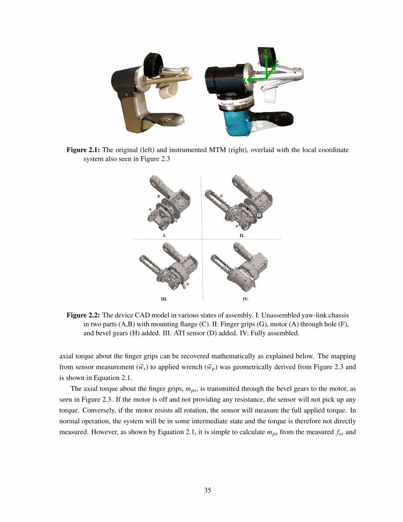
Figure 2.1: The original (left) and instrumented MTM (right), overlaid with the local coordinatesystem also seen in Figure 2.3
I. II.
III. IV.
A
B
CH
G
D
F
A
Figure 2.2: The device CAD model in various states of assembly. I: Unassembled yaw-link chassisin two parts (A,B) with mounting flange (C). II: Finger grips (G), motor (A) through hole (F),and bevel gears (H) added. III: ATI sensor (D) added. IV: Fully assembled.
axial torque about the finger grips can be recovered mathematically as explained below. The mapping
from sensor measurement (~ws) to applied wrench (~wp) was geometrically derived from Figure 2.3 and
is shown in Equation 2.1.
The axial torque about the finger grips, mpx, is transmitted through the bevel gears to the motor, as
seen in Figure 2.3. If the motor is off and not providing any resistance, the sensor will not pick up any
torque. Conversely, if the motor resists all rotation, the sensor will measure the full applied torque. In
normal operation, the system will be in some intermediate state and the torque is therefore not directly
measured. However, as shown by Equation 2.1, it is simple to calculate mpx from the measured fsx and
35
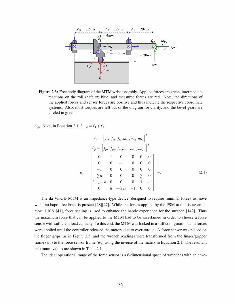
Figure 2.3: Free body diagram of the MTM wrist assembly. Applied forces are green, intermediatereactions on the roll shaft are blue, and measured forces are red. Note, the directions ofthe applied forces and sensor forces are positive and thus indicate the respective coordinatesystems. Also, most torques are left out of the diagram for clarity, and the bevel gears arecircled in green.
msy. Note, in Equation 2.1, `1+2 = `1 + `2.
~ws =[
fsx, fsy, fsz,msx,msy,msz
]T
~wp =[
fpx, fpy, fpz,mpx,mpy,mpz
]T
~wp =
0 1 0 0 0 0
0 0 −1 0 0 0
−1 0 0 0 0 0r2r1
h 0 0 0 r2r1
0
`1+2 +h 0 0 0 1 −1
0 h −`1+2 −1 0 0
·~ws (2.1)
The da Vinci® MTM is an impedance-type device, designed to require minimal forces to move
when no haptic feedback is present [28][27]. While the forces applied by the PSM at the tissue are at
most ±10N [41], force scaling is used to enhance the haptic experience for the surgeon [142]. Thus
the maximum force that can be applied to the MTM had to be ascertained in order to choose a force
sensor with sufficient load capacity. To this end, the MTM was locked in a stiff configuration, and forces
were applied until the controller released the motors due to over-torque. A force sensor was placed on
the finger grips, as in Figure 2.5, and the wrench readings were transformed from the finger/gripper
frame (~wp) to the force sensor frame (~ws) using the inverse of the matrix in Equation 2.1. The resultant
maximum values are shown in Table 2.1.
The ideal operational range of the force sensor is a 6-dimensional space of wrenches with an enve-
36
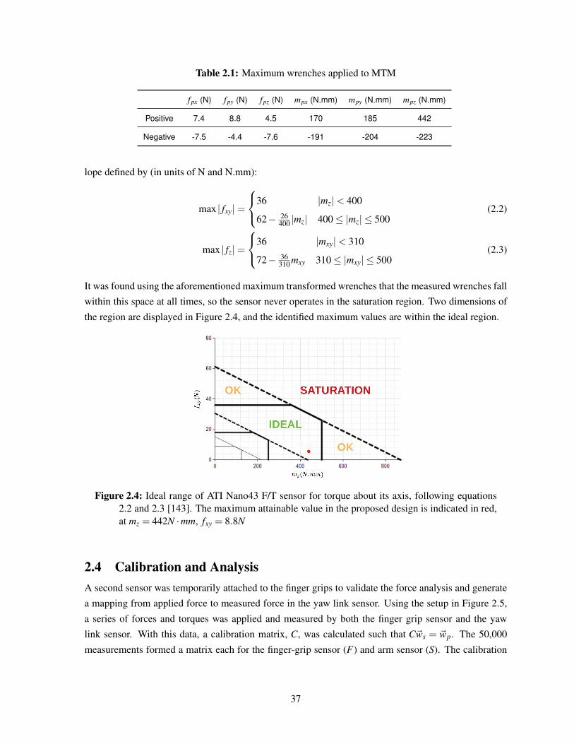
Table 2.1: Maximum wrenches applied to MTM
fpx (N) fpy (N) fpz (N) mpx (N.mm) mpy (N.mm) mpz (N.mm)
Positive 7.4 8.8 4.5 170 185 442
Negative -7.5 -4.4 -7.6 -191 -204 -223
lope defined by (in units of N and N.mm):
max | fxy|=
36 |mz|< 400
62− 26400 |mz| 400≤ |mz| ≤ 500
(2.2)
max | fz|=
36 |mxy|< 310
72− 36310 mxy 310≤ |mxy| ≤ 500
(2.3)
It was found using the aforementioned maximum transformed wrenches that the measured wrenches fall
within this space at all times, so the sensor never operates in the saturation region. Two dimensions of
the region are displayed in Figure 2.4, and the identified maximum values are within the ideal region.
Figure 2.4: Ideal range of ATI Nano43 F/T sensor for torque about its axis, following equations2.2 and 2.3 [143]. The maximum attainable value in the proposed design is indicated in red,at mz = 442N ·mm, fxy = 8.8N
2.4 Calibration and AnalysisA second sensor was temporarily attached to the finger grips to validate the force analysis and generate
a mapping from applied force to measured force in the yaw link sensor. Using the setup in Figure 2.5,
a series of forces and torques was applied and measured by both the finger grip sensor and the yaw
link sensor. With this data, a calibration matrix, C, was calculated such that C~ws = ~wp. The 50,000
measurements formed a matrix each for the finger-grip sensor (F) and arm sensor (S). The calibration
37
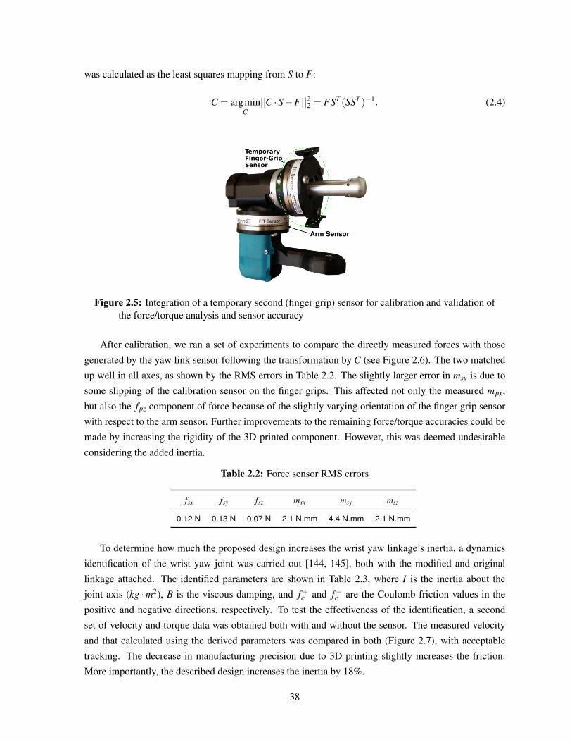
was calculated as the least squares mapping from S to F :
C = argminC||C ·S−F ||22 = FST (SST )−1. (2.4)
Figure 2.5: Integration of a temporary second (finger grip) sensor for calibration and validation ofthe force/torque analysis and sensor accuracy
After calibration, we ran a set of experiments to compare the directly measured forces with those
generated by the yaw link sensor following the transformation by C (see Figure 2.6). The two matched
up well in all axes, as shown by the RMS errors in Table 2.2. The slightly larger error in msy is due to
some slipping of the calibration sensor on the finger grips. This affected not only the measured mpx,
but also the fpz component of force because of the slightly varying orientation of the finger grip sensor
with respect to the arm sensor. Further improvements to the remaining force/torque accuracies could be
made by increasing the rigidity of the 3D-printed component. However, this was deemed undesirable
considering the added inertia.
Table 2.2: Force sensor RMS errors
fsx fsy fsz msx msy msz
0.12 N 0.13 N 0.07 N 2.1 N.mm 4.4 N.mm 2.1 N.mm
To determine how much the proposed design increases the wrist yaw linkage’s inertia, a dynamics
identification of the wrist yaw joint was carried out [144, 145], both with the modified and original
linkage attached. The identified parameters are shown in Table 2.3, where I is the inertia about the
joint axis (kg ·m2), B is the viscous damping, and f+c and f−c are the Coulomb friction values in the
positive and negative directions, respectively. To test the effectiveness of the identification, a second
set of velocity and torque data was obtained both with and without the sensor. The measured velocity
and that calculated using the derived parameters was compared in both (Figure 2.7), with acceptable
tracking. The decrease in manufacturing precision due to 3D printing slightly increases the friction.
More importantly, the described design increases the inertia by 18%.
38
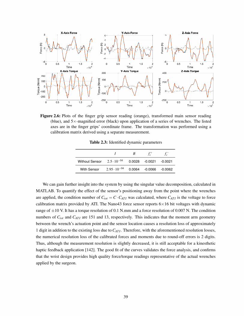
Figure 2.6: Plots of the finger grip sensor reading (orange), transformed main sensor reading(blue), and 5×-magnified error (black) upon application of a series of wrenches. The listedaxes are in the finger grips’ coordinate frame. The transformation was performed using acalibration matrix derived using a separate measurement.
Table 2.3: Identified dynamic parameters
I B f+c f−c
Without Sensor 2.5 ·10−04 0.0028 -0.0021 -0.0021
With Sensor 2.95 ·10−04 0.0064 -0.0066 -0.0062
We can gain further insight into the system by using the singular value decomposition, calculated in
MATLAB. To quantify the effect of the sensor’s positioning away from the point where the wrenches
are applied, the condition number of Ctot = C ·CAT I was calculated, where CAT I is the voltage to force
calibration matrix provided by ATI. The Nano43 force sensor reports 6×16 bit voltages with dynamic
range of ±10 V. It has a torque resolution of 0.1 N.mm and a force resolution of 0.007 N. The condition
numbers of Ctot and CAT I are 151 and 13, respectively. This indicates that the moment arm geometry
between the wrench’s actuation point and the sensor location causes a resolution loss of approximately
1 digit in addition to the existing loss due to CAT I . Therefore, with the aforementioned resolution losses,
the numerical resolution loss of the calibrated forces and moments due to round-off errors is 2 digits.
Thus, although the measurement resolution is slightly decreased, it is still acceptable for a kinesthetic
haptic feedback application [142]. The good fit of the curves validates the force analysis, and confirms
that the wrist design provides high quality force/torque readings representative of the actual wrenches
applied by the surgeon.
39
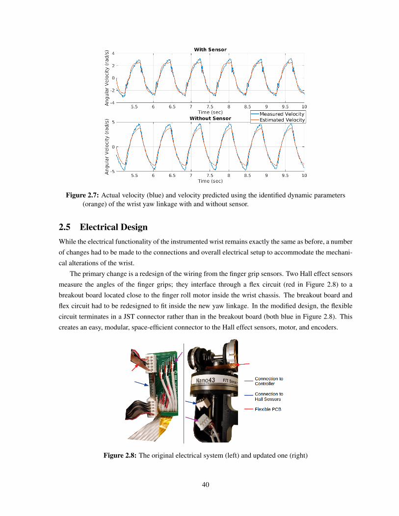
Figure 2.7: Actual velocity (blue) and velocity predicted using the identified dynamic parameters(orange) of the wrist yaw linkage with and without sensor.
2.5 Electrical DesignWhile the electrical functionality of the instrumented wrist remains exactly the same as before, a number
of changes had to be made to the connections and overall electrical setup to accommodate the mechani-
cal alterations of the wrist.
The primary change is a redesign of the wiring from the finger grip sensors. Two Hall effect sensors
measure the angles of the finger grips; they interface through a flex circuit (red in Figure 2.8) to a
breakout board located close to the finger roll motor inside the wrist chassis. The breakout board and
flex circuit had to be redesigned to fit inside the new yaw linkage. In the modified design, the flexible
circuit terminates in a JST connector rather than in the breakout board (both blue in Figure 2.8). This
creates an easy, modular, space-efficient connector to the Hall effect sensors, motor, and encoders.
Figure 2.8: The original electrical system (left) and updated one (right)
40
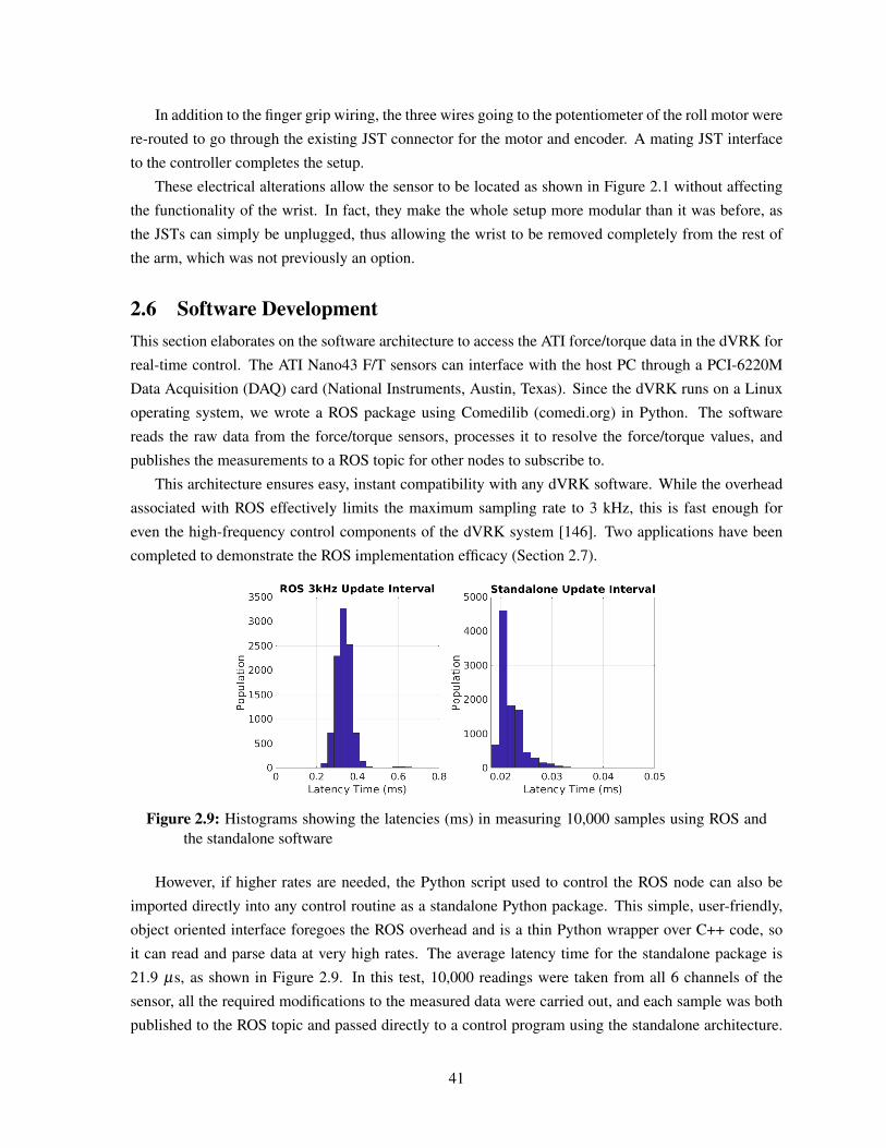
In addition to the finger grip wiring, the three wires going to the potentiometer of the roll motor were
re-routed to go through the existing JST connector for the motor and encoder. A mating JST interface
to the controller completes the setup.
These electrical alterations allow the sensor to be located as shown in Figure 2.1 without affecting
the functionality of the wrist. In fact, they make the whole setup more modular than it was before, as
the JSTs can simply be unplugged, thus allowing the wrist to be removed completely from the rest of
the arm, which was not previously an option.
2.6 Software DevelopmentThis section elaborates on the software architecture to access the ATI force/torque data in the dVRK for
real-time control. The ATI Nano43 F/T sensors can interface with the host PC through a PCI-6220M
Data Acquisition (DAQ) card (National Instruments, Austin, Texas). Since the dVRK runs on a Linux
operating system, we wrote a ROS package using Comedilib (comedi.org) in Python. The software
reads the raw data from the force/torque sensors, processes it to resolve the force/torque values, and
publishes the measurements to a ROS topic for other nodes to subscribe to.
This architecture ensures easy, instant compatibility with any dVRK software. While the overhead
associated with ROS effectively limits the maximum sampling rate to 3 kHz, this is fast enough for
even the high-frequency control components of the dVRK system [146]. Two applications have been
completed to demonstrate the ROS implementation efficacy (Section 2.7).
Figure 2.9: Histograms showing the latencies (ms) in measuring 10,000 samples using ROS andthe standalone software
However, if higher rates are needed, the Python script used to control the ROS node can also be
imported directly into any control routine as a standalone Python package. This simple, user-friendly,
object oriented interface foregoes the ROS overhead and is a thin Python wrapper over C++ code, so
it can read and parse data at very high rates. The average latency time for the standalone package is
21.9 µs, as shown in Figure 2.9. In this test, 10,000 readings were taken from all 6 channels of the
sensor, all the required modifications to the measured data were carried out, and each sample was both
published to the ROS topic and passed directly to a control program using the standalone architecture.
41
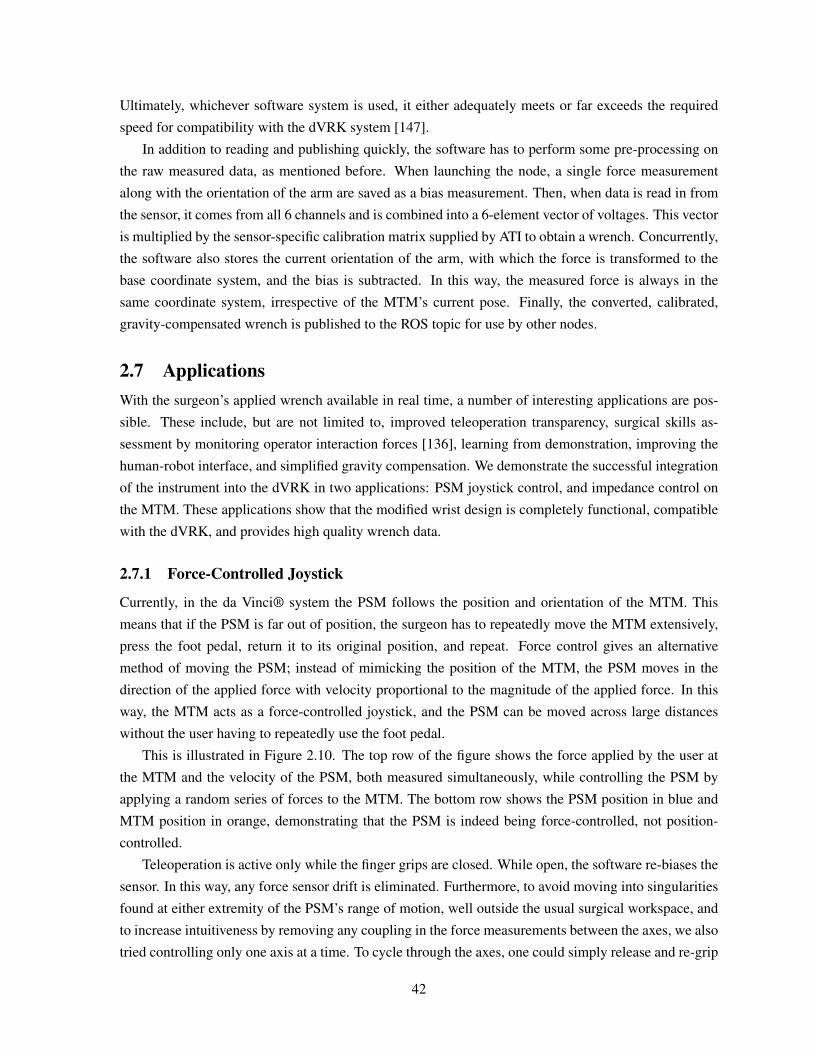
Ultimately, whichever software system is used, it either adequately meets or far exceeds the required
speed for compatibility with the dVRK system [147].
In addition to reading and publishing quickly, the software has to perform some pre-processing on
the raw measured data, as mentioned before. When launching the node, a single force measurement
along with the orientation of the arm are saved as a bias measurement. Then, when data is read in from
the sensor, it comes from all 6 channels and is combined into a 6-element vector of voltages. This vector
is multiplied by the sensor-specific calibration matrix supplied by ATI to obtain a wrench. Concurrently,
the software also stores the current orientation of the arm, with which the force is transformed to the
base coordinate system, and the bias is subtracted. In this way, the measured force is always in the
same coordinate system, irrespective of the MTM’s current pose. Finally, the converted, calibrated,
gravity-compensated wrench is published to the ROS topic for use by other nodes.
2.7 ApplicationsWith the surgeon’s applied wrench available in real time, a number of interesting applications are pos-
sible. These include, but are not limited to, improved teleoperation transparency, surgical skills as-
sessment by monitoring operator interaction forces [136], learning from demonstration, improving the
human-robot interface, and simplified gravity compensation. We demonstrate the successful integration
of the instrument into the dVRK in two applications: PSM joystick control, and impedance control on
the MTM. These applications show that the modified wrist design is completely functional, compatible
with the dVRK, and provides high quality wrench data.
2.7.1 Force-Controlled Joystick
Currently, in the da Vinci® system the PSM follows the position and orientation of the MTM. This
means that if the PSM is far out of position, the surgeon has to repeatedly move the MTM extensively,
press the foot pedal, return it to its original position, and repeat. Force control gives an alternative
method of moving the PSM; instead of mimicking the position of the MTM, the PSM moves in the
direction of the applied force with velocity proportional to the magnitude of the applied force. In this
way, the MTM acts as a force-controlled joystick, and the PSM can be moved across large distances
without the user having to repeatedly use the foot pedal.
This is illustrated in Figure 2.10. The top row of the figure shows the force applied by the user at
the MTM and the velocity of the PSM, both measured simultaneously, while controlling the PSM by
applying a random series of forces to the MTM. The bottom row shows the PSM position in blue and
MTM position in orange, demonstrating that the PSM is indeed being force-controlled, not position-
controlled.
Teleoperation is active only while the finger grips are closed. While open, the software re-biases the
sensor. In this way, any force sensor drift is eliminated. Furthermore, to avoid moving into singularities
found at either extremity of the PSM’s range of motion, well outside the usual surgical workspace, and
to increase intuitiveness by removing any coupling in the force measurements between the axes, we also
tried controlling only one axis at a time. To cycle through the axes, one could simply release and re-grip
42
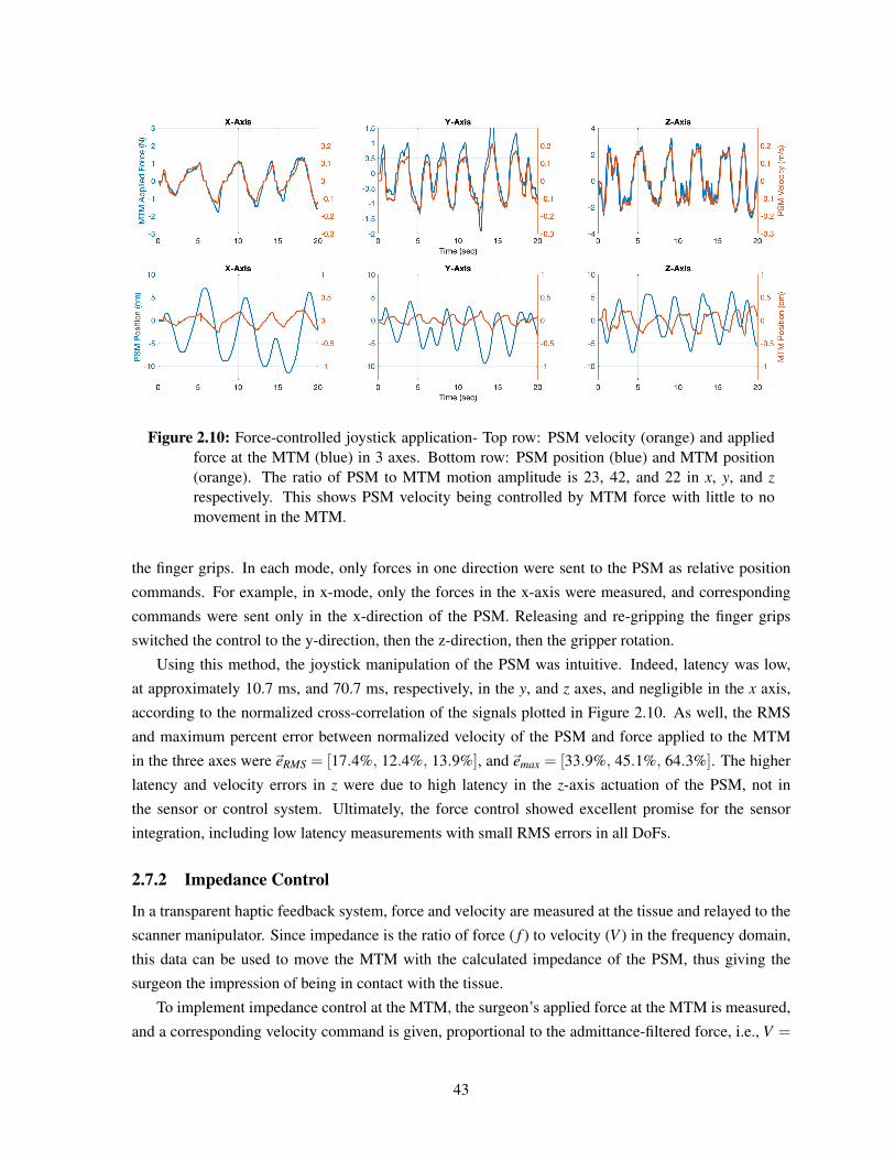
Figure 2.10: Force-controlled joystick application- Top row: PSM velocity (orange) and appliedforce at the MTM (blue) in 3 axes. Bottom row: PSM position (blue) and MTM position(orange). The ratio of PSM to MTM motion amplitude is 23, 42, and 22 in x, y, and zrespectively. This shows PSM velocity being controlled by MTM force with little to nomovement in the MTM.
the finger grips. In each mode, only forces in one direction were sent to the PSM as relative position
commands. For example, in x-mode, only the forces in the x-axis were measured, and corresponding
commands were sent only in the x-direction of the PSM. Releasing and re-gripping the finger grips
switched the control to the y-direction, then the z-direction, then the gripper rotation.
Using this method, the joystick manipulation of the PSM was intuitive. Indeed, latency was low,
at approximately 10.7 ms, and 70.7 ms, respectively, in the y, and z axes, and negligible in the x axis,
according to the normalized cross-correlation of the signals plotted in Figure 2.10. As well, the RMS
and maximum percent error between normalized velocity of the PSM and force applied to the MTM
in the three axes were~eRMS = [17.4%, 12.4%, 13.9%], and~emax = [33.9%, 45.1%, 64.3%]. The higher
latency and velocity errors in z were due to high latency in the z-axis actuation of the PSM, not in
the sensor or control system. Ultimately, the force control showed excellent promise for the sensor
integration, including low latency measurements with small RMS errors in all DoFs.
2.7.2 Impedance Control
In a transparent haptic feedback system, force and velocity are measured at the tissue and relayed to the
scanner manipulator. Since impedance is the ratio of force ( f ) to velocity (V ) in the frequency domain,
this data can be used to move the MTM with the calculated impedance of the PSM, thus giving the
surgeon the impression of being in contact with the tissue.
To implement impedance control at the MTM, the surgeon’s applied force at the MTM is measured,
and a corresponding velocity command is given, proportional to the admittance-filtered force, i.e., V =
43
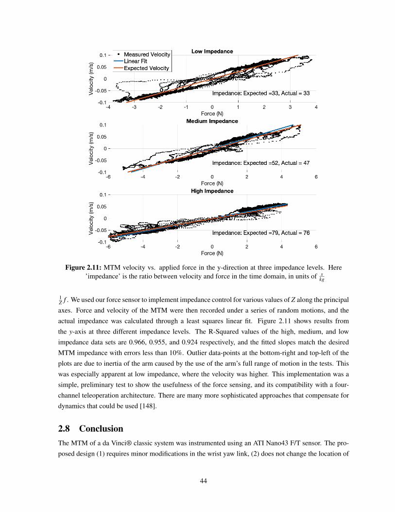
Figure 2.11: MTM velocity vs. applied force in the y-direction at three impedance levels. Here’impedance’ is the ratio between velocity and force in the time domain, in units of s
kg
1Z f . We used our force sensor to implement impedance control for various values of Z along the principal
axes. Force and velocity of the MTM were then recorded under a series of random motions, and the
actual impedance was calculated through a least squares linear fit. Figure 2.11 shows results from
the y-axis at three different impedance levels. The R-Squared values of the high, medium, and low
impedance data sets are 0.966, 0.955, and 0.924 respectively, and the fitted slopes match the desired
MTM impedance with errors less than 10%. Outlier data-points at the bottom-right and top-left of the
plots are due to inertia of the arm caused by the use of the arm’s full range of motion in the tests. This
was especially apparent at low impedance, where the velocity was higher. This implementation was a
simple, preliminary test to show the usefulness of the force sensing, and its compatibility with a four-
channel teleoperation architecture. There are many more sophisticated approaches that compensate for
dynamics that could be used [148].
2.8 ConclusionThe MTM of a da Vinci® classic system was instrumented using an ATI Nano43 F/T sensor. The pro-
posed design (1) requires minor modifications in the wrist yaw link, (2) does not change the location of
44
the finger grips, (3) adds little inertia to the wrist yaw and pitch axes, and (4) does not limit the available
wrist manipulation envelope. It is therefore expected that the sensor will not significantly change the
surgeon’s feel of interacting with the original MTM. A software interface was developed to provide user
force/torque measurements to the dVRK control functions in real time, and with low latency. Finally,
example applications of the sensed forces were presented to showcase successful integration of the in-
strumented MTM into the dVRK. The high-fidelity tracking in the force control application, as well as
the accurate impedance control, demonstrate that the sensor has been fully integrated into the dVRK
and is ready to be used in a four channel teleoperation interface. The developments can potentially also
be used in surgical skills assessment and research work on learning from demonstration.
45
Chapter 3
6-Axis Optical Force Sensor: DesignDevelopment and Performance Evaluation
3.1 IntroductionSix-axis force-torque (F/T) sensors are widely used in robotic applications including manipulation, re-
mote operation, robot-assisted or human-guided task performance, and cell-biology and biomechanical
characterization [54, 149]. Resistive [126], capacitive [52], piezoelectric [150], MEM [151], pneumatic
[152], and optical methods have been used for multi-axis force sensing. Strain gauges are the most pop-
ular transducers due to their accuracy and small size. However, they are susceptible to noise and require
surface preparation, special adhesives and coatings, mechanical overload protection, and delicate wiring
[153, 154] which contribute to their increased fabrication and assembly costs.
Optical sensors have recently gained attraction because of their high accuracy in small form factors
[155, 156]. FBGs are used in force [82, 157] and shape sensing without hysteresis [158]. These trans-
ducers are wave-length encoded making them robust to the light source intensity variations. They do
not generate leakage currents and are immune to electromagnetic interference [159]. However, FBGs
require complex and therefore expensive equipment for data acquisition and signal conditioning [160].
Additionally, the optical fibers cannot be bent to small radii of curvature and therefore require special
interfaces with other system components [56].
Optical transducers in reflective [161] and direct [162] configurations using emitter and receiver
pairs have been integrated to develop compact and accurate force sensors [163]. In these sensors, ex-
ternal loads change the intensity of the light incident on the receiver, thereby varying the sensor output
[164]. The intensity-based designs that utilize a single photodiode or phototransistor [165] per DoF are
sensitive to variations in the light source’s intensity due to temperature or aging. The proposed sensing
mechanisms often require delicate assembly processes due to the limited linearity range of the transduc-
ers, eventually increasing the fabrication and overall sensor cost [166]. Furthermore, electronic noise
and ambient light distort the outputs of the emitter and receiver and necessitate external disturbance
compensation [167].
46
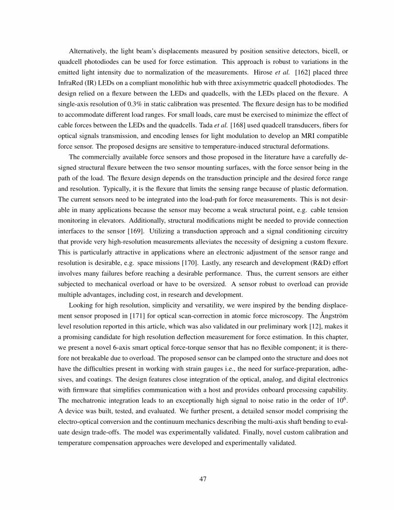
Alternatively, the light beam’s displacements measured by position sensitive detectors, bicell, or
quadcell photodiodes can be used for force estimation. This approach is robust to variations in the
emitted light intensity due to normalization of the measurements. Hirose et al. [162] placed three
InfraRed (IR) LEDs on a compliant monolithic hub with three axisymmetric quadcell photodiodes. The
design relied on a flexure between the LEDs and quadcells, with the LEDs placed on the flexure. A
single-axis resolution of 0.3% in static calibration was presented. The flexure design has to be modified
to accommodate different load ranges. For small loads, care must be exercised to minimize the effect of
cable forces between the LEDs and the quadcells. Tada et al. [168] used quadcell transducers, fibers for
optical signals transmission, and encoding lenses for light modulation to develop an MRI compatible
force sensor. The proposed designs are sensitive to temperature-induced structural deformations.
The commercially available force sensors and those proposed in the literature have a carefully de-
signed structural flexure between the two sensor mounting surfaces, with the force sensor being in the
path of the load. The flexure design depends on the transduction principle and the desired force range
and resolution. Typically, it is the flexure that limits the sensing range because of plastic deformation.
The current sensors need to be integrated into the load-path for force measurements. This is not desir-
able in many applications because the sensor may become a weak structural point, e.g. cable tension
monitoring in elevators. Additionally, structural modifications might be needed to provide connection
interfaces to the sensor [169]. Utilizing a transduction approach and a signal conditioning circuitry
that provide very high-resolution measurements alleviates the necessity of designing a custom flexure.
This is particularly attractive in applications where an electronic adjustment of the sensor range and
resolution is desirable, e.g. space missions [170]. Lastly, any research and development (R&D) effort
involves many failures before reaching a desirable performance. Thus, the current sensors are either
subjected to mechanical overload or have to be oversized. A sensor robust to overload can provide
multiple advantages, including cost, in research and development.
Looking for high resolution, simplicity and versatility, we were inspired by the bending displace-
ment sensor proposed in [171] for optical scan-correction in atomic force microscopy. The Angstrom
level resolution reported in this article, which was also validated in our preliminary work [12], makes it
a promising candidate for high resolution deflection measurement for force estimation. In this chapter,
we present a novel 6-axis smart optical force-torque sensor that has no flexible component; it is there-
fore not breakable due to overload. The proposed sensor can be clamped onto the structure and does not
have the difficulties present in working with strain gauges i.e., the need for surface-preparation, adhe-
sives, and coatings. The design features close integration of the optical, analog, and digital electronics
with firmware that simplifies communication with a host and provides onboard processing capability.
The mechatronic integration leads to an exceptionally high signal to noise ratio in the order of 106.
A device was built, tested, and evaluated. We further present, a detailed sensor model comprising the
electro-optical conversion and the continuum mechanics describing the multi-axis shaft bending to eval-
uate design trade-offs. The model was experimentally validated. Finally, novel custom calibration and
temperature compensation approaches were developed and experimentally validated.
47
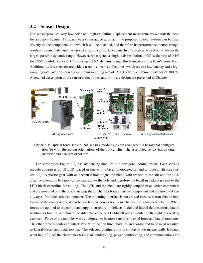
3.2 Sensor DesignOur sensor provides very low-noise and high-resolution displacement measurements without the need
for a custom flexure. Thus, unlike a strain gauge approach, the proposed optical system can be used
directly on the component onto which it will be installed, and therefore its performance metrics (range,
resolution, sensitivity, and hysteresis) are application dependent. In this chapter, we set out to obtain the
largest possible dynamic range. However, we targeted a single-axis resolution to full-scale ratio of 0.1%
for a 95% confidence level. Considering a±5 V dynamic range, this translates into a 10 mV noise floor.
Additionally, force sensors are widely used in control applications, which require low-latency and a high
sampling rate. We considered a minimum sampling rate of 1500 Hz with a maximum latency of 300 µs.
A detailed description of the sensor’s electronics and firmware design are presented in Chapter 4.
(a) Exploded view (b) Active and passivecomponents
(c) Fully assembled sensor
Figure 3.1: Optical force sensor - Six sensing modules (a) are arranged in a hexagonal configura-tion (b) with alternating orientations of the optical slits. The assembled sensor has an outerdiameter and a height of 50 mm.
The sensor (see Figure 3.1) has six sensing modules in a hexagonal configuration. Each sensing
module comprises an IR LED placed in-line with a bicell photodetector, and an optical slit (see Fig-
ure 3.2). A plastic gear with an eccentric hole aligns the bicell with respect to the slit and the LED
after the assembly. Rotation of the gear moves the hole and therefore the bicell in a plane normal to the
LED-bicell centerline for nulling. The LED and the bicell are rigidly coupled in an active component
and are mounted onto the load-carrying shaft. The slits form a passive component and are mounted axi-
ally apart from the active component. The mounting interface is not critical because it transfers no load
to any of the components; it can be a set-screw connection, a mechanical, or a magnetic clamp. When
forces are applied to the compliant support structure, it deflects (axial and lateral deformations, lateral
bending, or torsion) and moves the slits relative to the LED-bicell pairs modulating the light received by
each cell. Three of the modules were configured to be most sensitive to axial force and lateral moments.
The other three modules are interleaved with the first three modules and configured to be most sensitive
to lateral forces and axial torsion. The selected configuration is similar to the magnetically levitated
wrist in [172]. All the electronics for signal conditioning, power conditioning, and communications are
48
parts of the active component. We hypothesize that each sensing module can function similarly to a
strain gauge without the challenges discussed above; by populating a load-carrying element with mul-
tiple LED-bicell pairs in an engineered configuration, it is possible to measure forces/moments applied
to the element in multiple DoFs.
Figure 3.2: Optical force sensing concept. The LED is aligned with and fixed relative to the bicell.The motion of the optical slit with respect to the LED-bicell pair modulates the light on thebicell active areas.
The photocurrents I1, I2 generated in each active area of the bicell are related to the load-dependent
displacement (δ ) of the projected beam relative to its nominal position (see Appendix A):
I1 = In
(1+
δ
c
)c =
s−g2
I2 = In
(1− δ
c
)In =
2π
h(s−g)d2
s
PetRλ
IFtIF , (3.1)
where the geometric parameters s, g are shown in Figure 3.2 and c is 0.45 mm in the current design.
IF is the IR LED forward current, Pet is the light output power for a test current IFt , Rλ is the bicell’s
responsivity, and ds is the LED’s diameter. The photocurrents are conditioned to differential (Vd) and
common-mode (Vcm) voltages. By normalizing the differential voltage Vd over the common-mode volt-
age Vcm, the centroid position of the light beam can be calculated as:
δ =c2
n, n =Vd
Vcm,
Vd =−2c InRδ
Vcm =−InR(3.2)
where R is the gain of the matched trans-impedance amplifiers in the signal conditioning circuit. The
normalization above minimizes the effect of possible electronics drift that can affect the feedback resis-
tors, nominal photocurrent (In), and LED’s forward current.
49
3.3 Modeling
3.3.1 Noise Model
This section evaluates the theoretical limitation of the optical sensing concept in displacement measure-
ment of the optical slit. The photocurrent generated within each cell (I1, I2) is shot-noise limited [171].
Hence, the uncertainty in the photo-currents (σI1 ,σI2) can be formulated as:
σI1 = σI2 =√
2qIn∆ f (3.3)
where q is the electron charge, and ∆ f is the measurement bandwidth. With the assumption that noises
are uncorrelated, one can determine that σI1−I2 = 2√
qIn∆ f . From Equation 3.1, d(I1−I2)dδ
= 2Inc . Thus:
σδ = σI1−I2×dδ
d(I1− I2)= c
√q∆ fIn
. (3.4)
The signal conditioning circuit (see Chapter 4) was designed for a maximum photo-current of In =
200 µA, and a bandwidth of 500 Hz. Therefore, considering Equation 3.4, the uncertainty in displace-
ment estimation (σδ ) due to the shot-noise limited photo-currents (σI) is 0.28 nm for the current design;
the optical transducer cannot resolve displacements smaller than 0.28 nm and this is a lower bound on
the resolution in the displacement measurement of the optical slit. The estimated performance is close
to the analysis by Barret and Quate [171] that claimed 6.1 Angstrom RMS.
The presented analysis gives the theoretical limitation; in practice, other sources of noise in the
signal conditioning circuitry (electronics components, signals routing and ElectroMagnetic Interference
(EMI), etc.) can increase the lower bound in the measurement resolution. Instead, the uncertainty in the
slit’s displacement measurement can be formulated as a function of the differential (Vd) and common-
mode (Vcm) voltages. Considering Equation 3.2 and the derivations in Appendix A, σδ can be computed
as:
σδ =c2
(1
Vcm− Vd
2V 2cm
)σVd (3.5)
where σVd is the RMS noise in the conditioned differential signal.
3.3.2 Sensor Model
A schematic of the sensor is shown in Figure 3.3. The active and passive components are clamped to
the support structure (black shaft) at points B and C. The vectors (~e1) to (~e6) are the unit vectors normal
to the directions of the slits.
The wrench applied at point P causes deflection in the support structure and consequently relative
displacements (~di =[dx,dy,dz
]T
i) between the slits and the LED-bicell centerlines:
~di = ~dC + ~θC×~li i ∈ {1,2, . . . ,6} , (3.6)
50

where ~dC =[dCx,dCy,dCz
]Tand ~θC =
[θCx,θCy,θCz
]Tare the deflection and orientation vectors at point
C, and~li are the vectors from point C to the slits’ center points. The displacement of the slits (δi) along
the unit vectors (~ei) are:
δi = Proj~di~ei= ~di ·~ei i ∈ {1,2, . . . ,6} (3.7)
Equation 3.6 and Equation 3.7 can be combined in a matrix form as:
~δ =
0 1 0 dz 0 rs
0 0 1√
32 rs −1
2 rs 0
−√
32 −1
2 0 −12 dz
√3
2 dz rs
0 0 1 0 rs 0√
32 −1
2 0 −12 dz −
√3
2 dz rs
0 0 1 −√
32 rs −1
2 rs 0
︸ ︷︷ ︸
HG
[~dc
~θc
](3.8)
where ~δ =[δ1, . . . ,δ6
]are the slit displacements and rs, H, H ′ and dz are shown in Figure 3.3. By
using continuum mechanics principles, the transformation from the wrench vector at point P ( ~wP =[fPx, fPy, fPz,mPx,mPy,mPz
]T) to the translation and orientation at point C can be derived as:
[~dc
~θc
]=
H11 0 0 0 H2
2EIyy0
0 H22 0 − H2
2EIxx0 0
0 0 HAE 0 0 0
0 H42 0 HEIxx
0 0
H51 0 0 0 HEIyy
0
0 0 0 0 0 HGJzz
︸ ︷︷ ︸
Hw
~wP
{H11 =
H3
3EIyy+ H ′H2
2EIyyH22 =
H3
3EIxx+ H ′H2
2EIxx
H42 =− H2
2EIxx− H ′H
EIxxH51 =
H2
2EIyy+ H ′H
EIyy,
(3.9)
where E and G are the tensile and shear moduli of elasticity of the shaft, A is the area, Ixx and Iyy are
the area moments of inertia, and Jzz is the polar moment of inertia of the cross-section of the shaft
about its principal axes. With the electro-optical conversion in Equation 3.2 and the geometric trans-
formation in Equation 3.8, the transformation from ~wP to the vector of normalized transducers signals
(~n =[n1, . . . ,n6
]T) can be derived as:
~n =Cm ~wP, Cm =2c
HGHw. (3.10)
51
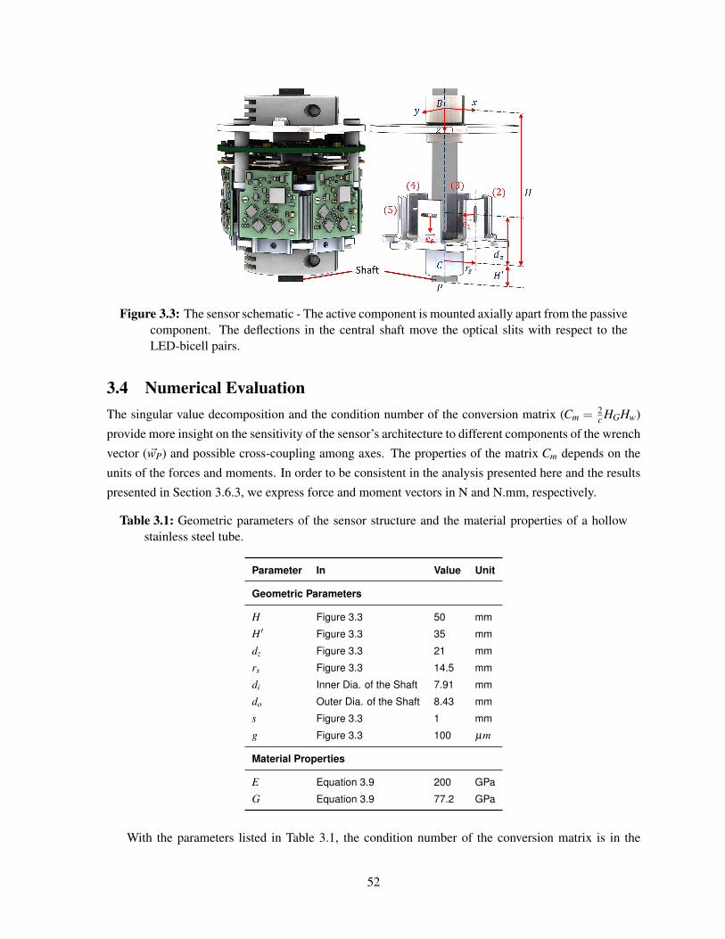
Figure 3.3: The sensor schematic - The active component is mounted axially apart from the passivecomponent. The deflections in the central shaft move the optical slits with respect to theLED-bicell pairs.
3.4 Numerical EvaluationThe singular value decomposition and the condition number of the conversion matrix (Cm = 2
c HGHw)
provide more insight on the sensitivity of the sensor’s architecture to different components of the wrench
vector ( ~wP) and possible cross-coupling among axes. The properties of the matrix Cm depends on the
units of the forces and moments. In order to be consistent in the analysis presented here and the results
presented in Section 3.6.3, we express force and moment vectors in N and N.mm, respectively.
Table 3.1: Geometric parameters of the sensor structure and the material properties of a hollowstainless steel tube.
Parameter In Value Unit
Geometric Parameters
H Figure 3.3 50 mm
H ′ Figure 3.3 35 mm
dz Figure 3.3 21 mm
rs Figure 3.3 14.5 mm
di Inner Dia. of the Shaft 7.91 mm
do Outer Dia. of the Shaft 8.43 mm
s Figure 3.3 1 mm
g Figure 3.3 100 µm
Material Properties
E Equation 3.9 200 GPa
G Equation 3.9 77.2 GPa
With the parameters listed in Table 3.1, the condition number of the conversion matrix is in the
52
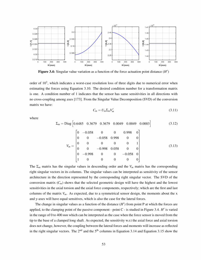
Figure 3.4: Singular value variation as a function of the force actuation point distance (H ′)
order of 103, which indicates a worst-case resolution loss of three digits due to numerical error when
estimating the forces using Equation 3.10. The desired condition number for a transformation matrix
is one. A condition number of 1 indicates that the sensor has same sensitivities in all directions with
no cross-coupling among axes [173]. From the Singular Value Decomposition (SVD) of the conversion
matrix we have:
Cm =UmΣmV ′m (3.11)
where
Σm = Diag[0.6485 0.3679 0.3679 0.0049 0.0049 0.0003
](3.12)
Vm =
0 −0.058 0 0 0.998 0
0 0 −0.058 0.998 0 0
0 0 0 0 0 1
0 0 −0.998 0.058 0 0
0 −0.998 0 0 −0.058 0
1 0 0 0 0 0
(3.13)
The Σm matrix has the singular values in descending order and the Vm matrix has the corresponding
right singular vectors in its columns. The singular values can be interpreted as sensitivity of the sensor
architecture in the direction represented by the corresponding right singular vector. The SVD of the
conversion matrix (Cm) shows that the selected geometric design will have the highest and the lowest
sensitivities in the axial torsion and the axial force components, respectively; which are the first and last
columns of the matrix Vm. As expected, due to a symmetrical sensor design, the moments about the x
and y-axes will have equal sensitives, which is also the case for the lateral forces.
The change in singular values as a function of the distance (H ′) from point P at which the forces are
applied, to the clamping point of the passive component - point C - is studied in Figure 3.4. H ′ is varied
in the range of 0 to 400 mm which can be interpreted as the case when the force sensor is moved from the
tip to the base of a clamped long shaft. As expected, the sensitivity w.r.t the axial force and axial torsion
does not change, however, the coupling between the lateral forces and moments will increase as reflected
in the right singular vectors. The 2nd and the 5th columns in Equation 3.14 and Equation 3.15 show the
53
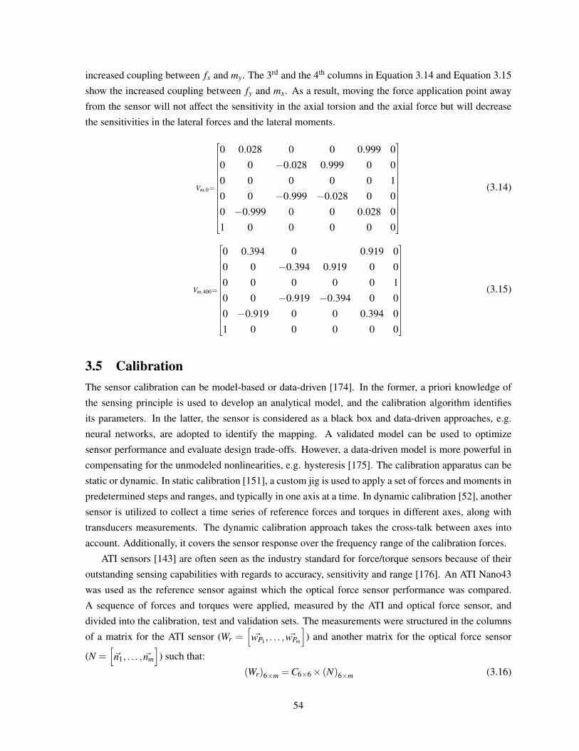
increased coupling between fx and my. The 3rd and the 4th columns in Equation 3.14 and Equation 3.15
show the increased coupling between fy and mx. As a result, moving the force application point away
from the sensor will not affect the sensitivity in the axial torsion and the axial force but will decrease
the sensitivities in the lateral forces and the lateral moments.
Vm,0=
0 0.028 0 0 0.999 0
0 0 −0.028 0.999 0 0
0 0 0 0 0 1
0 0 −0.999 −0.028 0 0
0 −0.999 0 0 0.028 0
1 0 0 0 0 0
(3.14)
Vm,400=
0 0.394 0 0.919 0
0 0 −0.394 0.919 0 0
0 0 0 0 0 1
0 0 −0.919 −0.394 0 0
0 −0.919 0 0 0.394 0
1 0 0 0 0 0
(3.15)
3.5 CalibrationThe sensor calibration can be model-based or data-driven [174]. In the former, a priori knowledge of
the sensing principle is used to develop an analytical model, and the calibration algorithm identifies
its parameters. In the latter, the sensor is considered as a black box and data-driven approaches, e.g.
neural networks, are adopted to identify the mapping. A validated model can be used to optimize
sensor performance and evaluate design trade-offs. However, a data-driven model is more powerful in
compensating for the unmodeled nonlinearities, e.g. hysteresis [175]. The calibration apparatus can be
static or dynamic. In static calibration [151], a custom jig is used to apply a set of forces and moments in
predetermined steps and ranges, and typically in one axis at a time. In dynamic calibration [52], another
sensor is utilized to collect a time series of reference forces and torques in different axes, along with
transducers measurements. The dynamic calibration approach takes the cross-talk between axes into
account. Additionally, it covers the sensor response over the frequency range of the calibration forces.
ATI sensors [143] are often seen as the industry standard for force/torque sensors because of their
outstanding sensing capabilities with regards to accuracy, sensitivity and range [176]. An ATI Nano43
was used as the reference sensor against which the optical force sensor performance was compared.
A sequence of forces and torques were applied, measured by the ATI and optical force sensor, and
divided into the calibration, test and validation sets. The measurements were structured in the columns
of a matrix for the ATI sensor (Wr =[~wP1 , . . . , ~wPm
]) and another matrix for the optical force sensor
(N =[~n1, . . . , ~nm
]) such that:
(Wr)6×m =C6×6× (N)6×m (3.16)
54
A regularized least squares cost function was defined as given in Equation 3.17 where E =CN−Wr
is the error matrix. The regularizer coefficients λi are tuned by comparing the value of the cost function
J for the calibration and test data sets and minimizing the overfit to the calibration data, where the cost
J is given by:
J =6
∑i=1
Ji, Ji =1
2m‖E(i, :)‖2 +
12
λi ‖C(i, :)‖2 . (3.17)
Each row C(i, :)T of the calibration matrix C was calculated by minimizing the corresponding cost
function Ji as:
argminC(i,:)T
Ji = (NNT +λiI6×6)−1N (Wr(i, :))
T (3.18)
3.6 Performance EvaluationA prototype of the sensor, mountable on a 8.4 mm shaft, was built (see Figure 3.5). A Nano43 ATI
F/T sensor, aligned with the design coordinate system in Figure 3.3, was clamped onto the shaft for
calibration as described in Section 3.5. The applied forces on the handle are transferred through the ATI
sensor to the shaft.
Figure 3.5: Calibration setup - The optical force sensor is mounted onto a stainless steel tube. AnATI Nano43 F/T sensor is used as the reference for calibration.
3.6.1 Noise Performance
To minimize the effect of the structural vibrations on the channel output and develop a more accurate
estimation of the noise floor, the sensor was first mounted onto a solid stainless steel rod. The differential
Vd and common-mode Vcm voltages of all the channels were recorded for 20 seconds during which no
wrench was applied to the sensor.
The recorded data on all the tangential channels were similar in peak-to-valley and RMS. The same
55
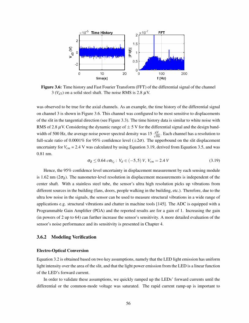
Figure 3.6: Time history and Fast Fourier Transform (FFT) of the differential signal of the channel3 (Vd3) on a solid steel shaft. The noise RMS is 2.8 µV.
was observed to be true for the axial channels. As an example, the time history of the differential signal
on channel 3 is shown in Figure 3.6. This channel was configured to be most sensitive to displacements
of the slit in the tangential direction (see Figure 3.3). The time history data is similar to white noise with
RMS of 2.8 µV. Considering the dynamic range of± 5 V for the differential signal and the design band-
width of 500 Hz, the average noise power spectral density was 15 nV√Hz
. Each channel has a resolution to
full-scale ratio of 0.0001% for 95% confidence level (±2σ ). The upperbound on the slit displacement
uncertainty for Vcm = 2.4 V was calculated by using Equation 3.19, derived from Equation 3.5, and was
0.81 nm.
σδ ≤ 0.64 cσVd : Vd ∈ (−5,5) V, Vcm = 2.4 V (3.19)
Hence, the 95% confidence level uncertainty in displacement measurement by each sensing module
is 1.62 nm (2σδ ). The nanometer-level resolution in displacement measurements is independent of the
center shaft. With a stainless steel tube, the sensor’s ultra high resolution picks up vibrations from
different sources in the building (fans, doors, people walking in the building, etc.). Therefore, due to the
ultra low noise in the signals, the sensor can be used to measure structural vibrations in a wide range of
applications e.g. structural vibrations and chatter in machine tools [145]. The ADC is equipped with a
Programmable Gain Amplifier (PGA) and the reported results are for a gain of 1. Increasing the gain
(in powers of 2 up to 64) can further increase the sensor’s sensitivity. A more detailed evaluation of the
sensor’s noise performance and its sensitivity is presented in Chapter 4.
3.6.2 Modeling Verification
Electro-Optical Conversion
Equation 3.2 is obtained based on two key assumptions, namely that the LED light emission has uniform
light intensity over the area of the slit, and that the light power emission from the LED is a linear function
of the LED’s forward current.
In order to validate these assumptions, we quickly ramped up the LEDs’ forward currents until the
differential or the common-mode voltage was saturated. The rapid current ramp-up is important to
56
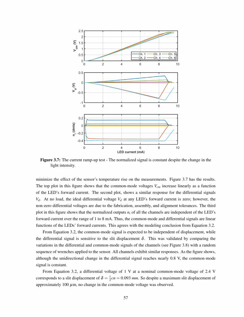
Figure 3.7: The current ramp-up test - The normalized signal is constant despite the change in thelight intensity.
minimize the effect of the sensor’s temperature rise on the measurements. Figure 3.7 has the results.
The top plot in this figure shows that the common-mode voltages Vcm increase linearly as a function
of the LED’s forward current. The second plot, shows a similar response for the differential signals
Vd . At no load, the ideal differential voltage Vd at any LED’s forward current is zero; however, the
non-zero differential voltages are due to the fabrication, assembly, and alignment tolerances. The third
plot in this figure shows that the normalized outputs ni of all the channels are independent of the LED’s
forward current over the range of 1 to 8 mA. Thus, the common-mode and differential signals are linear
functions of the LEDs’ forward currents. This agrees with the modeling conclusion from Equation 3.2.
From Equation 3.2, the common-mode signal is expected to be independent of displacement, while
the differential signal is sensitive to the slit displacement δ . This was validated by comparing the
variations in the differential and common-mode signals of the channels (see Figure 3.8) with a random
sequence of wrenches applied to the sensor. All channels exhibit similar responses. As the figure shows,
although the unidirectional change in the differential signal reaches nearly 0.8 V, the common-mode
signal is constant.
From Equation 3.2, a differential voltage of 1 V at a nominal common-mode voltage of 2.4 V
corresponds to a slit displacement of δ = 12 cn = 0.093 mm. So despite a maximum slit displacement of
approximately 100 µm, no change in the common-mode voltage was observed.
57
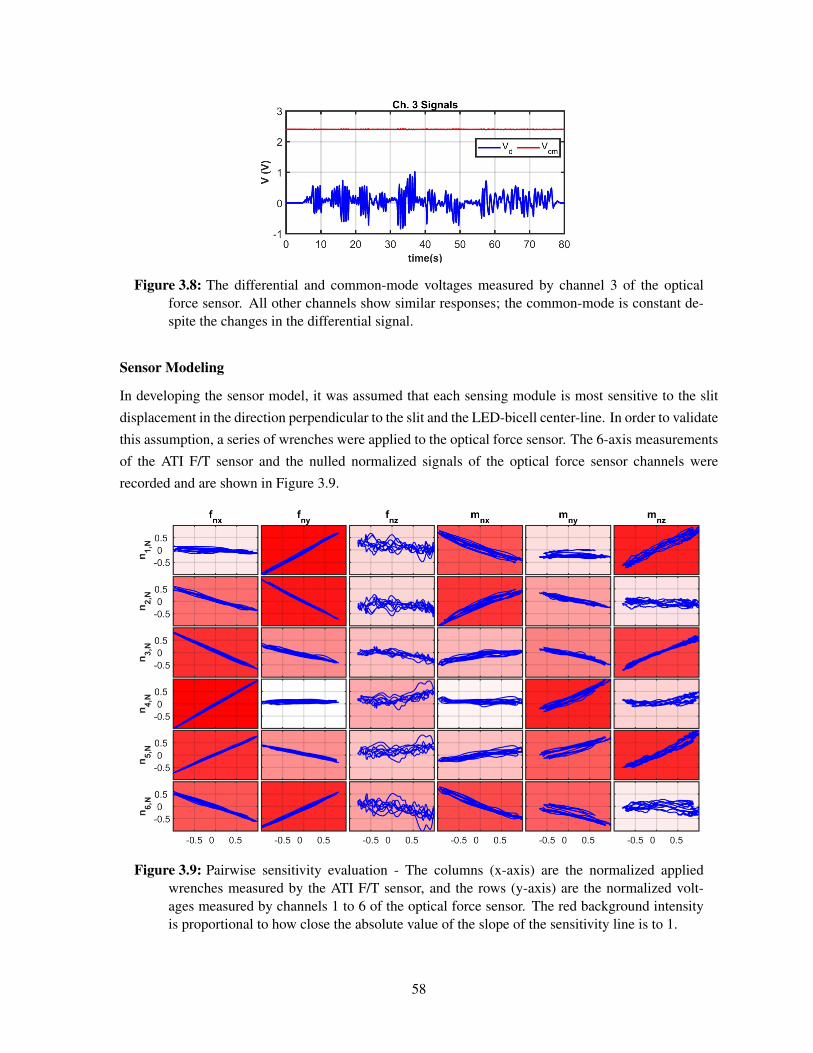
Figure 3.8: The differential and common-mode voltages measured by channel 3 of the opticalforce sensor. All other channels show similar responses; the common-mode is constant de-spite the changes in the differential signal.
Sensor Modeling
In developing the sensor model, it was assumed that each sensing module is most sensitive to the slit
displacement in the direction perpendicular to the slit and the LED-bicell center-line. In order to validate
this assumption, a series of wrenches were applied to the optical force sensor. The 6-axis measurements
of the ATI F/T sensor and the nulled normalized signals of the optical force sensor channels were
recorded and are shown in Figure 3.9.
Figure 3.9: Pairwise sensitivity evaluation - The columns (x-axis) are the normalized appliedwrenches measured by the ATI F/T sensor, and the rows (y-axis) are the normalized volt-ages measured by channels 1 to 6 of the optical force sensor. The red background intensityis proportional to how close the absolute value of the slope of the sensitivity line is to 1.
58
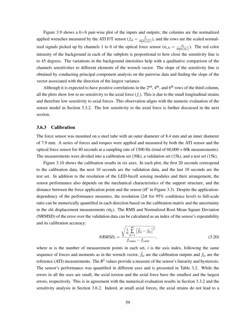
Figure 3.9 shows a 6×6 pair-wise plot of the inputs and outputs; the columns are the normalized
applied wrenches measured by the ATI F/T sensor ( fni =fi
maxi(| fi|) ), and the rows are the scaled normal-
ized signals picked up by channels 1 to 6 of the optical force sensor (ni,N = nimax
i(|ni|) ). The red color
intensity of the background in each of the subplots is proportional to how close the sensitivity line is
to 45 degrees. The variations in the background intensities help with a qualitative comparison of the
channels sensitivities to different elements of the wrench vector. The slope of the sensitivity line is
obtained by conducting principal component analysis on the pairwise data and finding the slope of the
vector associated with the direction of the largest variance.
Although it is expected to have positive correlations in the 2nd, 4th, and 6th rows of the third column,
all the plots show low to no sensitivity to the axial force ( fz). This is due to the small longitudinal strains
and therefore low sensitivity to axial forces. This observation aligns with the numeric evaluation of the
sensor model in Section 3.3.2. The low sensitivity to the axial force is further discussed in the next
section.
3.6.3 Calibration
The force sensor was mounted on a steel tube with an outer diameter of 8.4 mm and an inner diameter
of 7.9 mm. A series of forces and torques were applied and measured by both the ATI sensor and the
optical force sensor for 40 seconds at a sampling rate of 1500 Hz (total of 60,000 = 60k measurements).
The measurements were divided into a calibration set (30k), a validation set (15k), and a test set (15k).
Figure 3.10 shows the calibration results in six axes. In each plot, the first 20 seconds correspond
to the calibration data, the next 10 seconds are the validation data, and the last 10 seconds are the
test set. In addition to the resolution of the LED-bicell sensing modules and their arrangement, the
sensor performance also depends on the mechanical characteristics of the support structure, and the
distance between the force application point and the sensor (H ′ in Figure 3.3). Despite the application-
dependency of the performance measures, the resolution (2σ for 95% confidence level) to full-scale
ratio can be numerically quantified in each direction based on the calibration matrix and the uncertainty
in the slit displacement measurements (σδ ). The RMS and Normalized Root Mean Square Deviation
(NRMSD) of the error over the validation data can be calculated as an index of the sensor’s repeatability
and its calibration accuracy:
NRMSDi =
√1m
m∑
k=1
[fki− fki
]2fi,max− fi,min
, (3.20)
where m is the number of measurement points in each set, i is the axis index, following the same
sequence of forces and moments as in the wrench vector, fki are the calibration outputs and fki are the
reference (ATI) measurements. The R2 values provide a measure of the sensor’s linearity and hysteresis.
The sensor’s performance was quantified in different axes and is presented in Table 3.2. While the
errors in all the axes are small, the axial torsion and the axial force have the smallest and the largest
errors, respectively. This is in agreement with the numerical evaluation results in Section 3.3.2 and the
sensitivity analysis in Section 3.6.2. Indeed, at small axial forces, the axial strains do not lead to a
59
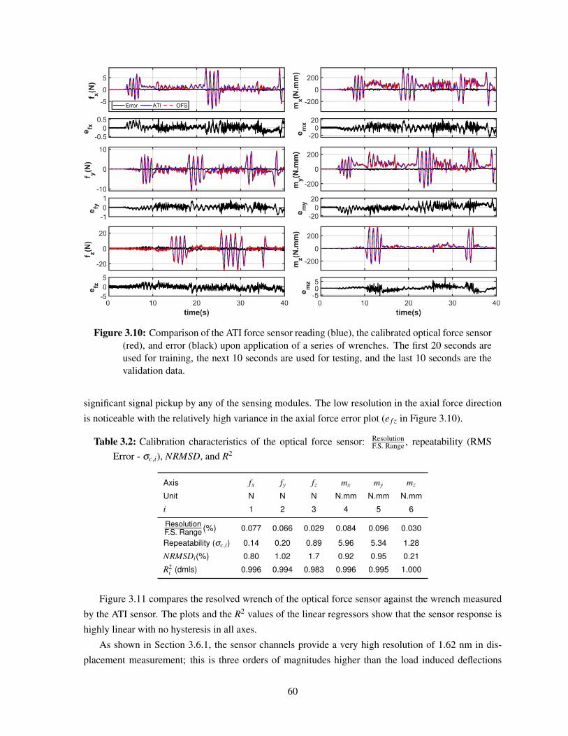
Figure 3.10: Comparison of the ATI force sensor reading (blue), the calibrated optical force sensor(red), and error (black) upon application of a series of wrenches. The first 20 seconds areused for training, the next 10 seconds are used for testing, and the last 10 seconds are thevalidation data.
significant signal pickup by any of the sensing modules. The low resolution in the axial force direction
is noticeable with the relatively high variance in the axial force error plot (e f z in Figure 3.10).
Table 3.2: Calibration characteristics of the optical force sensor: ResolutionF.S. Range , repeatability (RMS
Error - σc,i), NRMSD, and R2
Axis fx fy fz mx my mz
Unit N N N N.mm N.mm N.mm
i 1 2 3 4 5 6
ResolutionF.S. Range (%) 0.077 0.066 0.029 0.084 0.096 0.030
Repeatability (σc,i) 0.14 0.20 0.89 5.96 5.34 1.28
NRMSDi(%) 0.80 1.02 1.7 0.92 0.95 0.21
R2i (dmls) 0.996 0.994 0.983 0.996 0.995 1.000
Figure 3.11 compares the resolved wrench of the optical force sensor against the wrench measured
by the ATI sensor. The plots and the R2 values of the linear regressors show that the sensor response is
highly linear with no hysteresis in all axes.
As shown in Section 3.6.1, the sensor channels provide a very high resolution of 1.62 nm in dis-
placement measurement; this is three orders of magnitudes higher than the load induced deflections
60
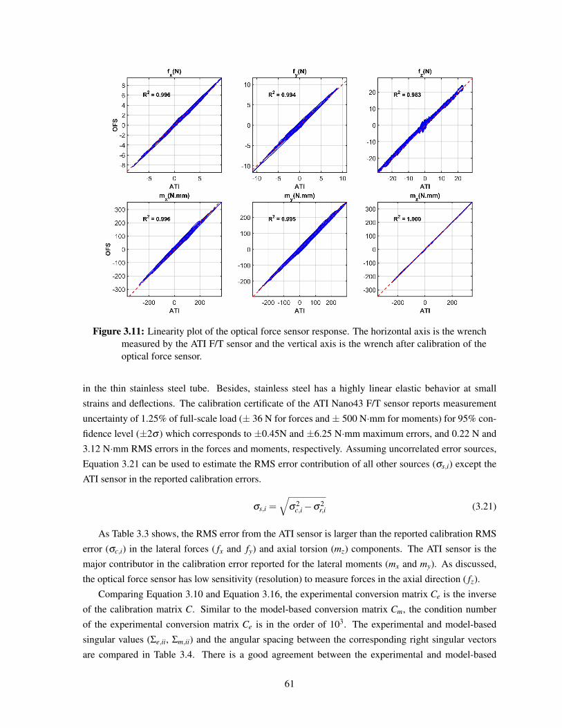
Figure 3.11: Linearity plot of the optical force sensor response. The horizontal axis is the wrenchmeasured by the ATI F/T sensor and the vertical axis is the wrench after calibration of theoptical force sensor.
in the thin stainless steel tube. Besides, stainless steel has a highly linear elastic behavior at small
strains and deflections. The calibration certificate of the ATI Nano43 F/T sensor reports measurement
uncertainty of 1.25% of full-scale load (± 36 N for forces and± 500 N·mm for moments) for 95% con-
fidence level (±2σ ) which corresponds to ±0.45N and ±6.25 N·mm maximum errors, and 0.22 N and
3.12 N·mm RMS errors in the forces and moments, respectively. Assuming uncorrelated error sources,
Equation 3.21 can be used to estimate the RMS error contribution of all other sources (σs,i) except the
ATI sensor in the reported calibration errors.
σs,i =√
σ2c,i−σ2
r,i (3.21)
As Table 3.3 shows, the RMS error from the ATI sensor is larger than the reported calibration RMS
error (σc,i) in the lateral forces ( fx and fy) and axial torsion (mz) components. The ATI sensor is the
major contributor in the calibration error reported for the lateral moments (mx and my). As discussed,
the optical force sensor has low sensitivity (resolution) to measure forces in the axial direction ( fz).
Comparing Equation 3.10 and Equation 3.16, the experimental conversion matrix Ce is the inverse
of the calibration matrix C. Similar to the model-based conversion matrix Cm, the condition number
of the experimental conversion matrix Ce is in the order of 103. The experimental and model-based
singular values (Σe,ii, Σm,ii) and the angular spacing between the corresponding right singular vectors
are compared in Table 3.4. There is a good agreement between the experimental and model-based
61
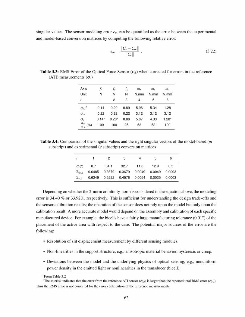
singular values. The sensor modeling error em can be quantified as the error between the experimental
and model-based conversion matrices by computing the following relative error:
em =‖Ce−Cm‖‖Ce‖
. (3.22)
Table 3.3: RMS Error of the Optical Force Sensor (σS) when corrected for errors in the reference(ATI) measurements (σr)
Axis fx fy fz mx my mz
Unit N N N N.mm N.mm N.mm
i 1 2 3 4 5 6
σc,i† 0.14 0.20 0.89 5.96 5.34 1.28
σr,i 0.22 0.22 0.22 3.12 3.12 3.12
σs,i 0.14* 0.20* 0.86 5.07 4.33 1.28*
σr,iσc,i
(%) 100 100 25 53 58 100
Table 3.4: Comparison of the singular values and the right singular vectors of the model-based (msubscript) and experimental (e subscript) conversion matrices
i 1 2 3 4 5 6
αi(°) 8.7 34.1 32.7 11.6 12.9 0.5
Σm,ii 0.6485 0.3679 0.3679 0.0049 0.0049 0.0003
Σe,ii 0.6249 0.5222 0.4576 0.0054 0.0035 0.0003
Depending on whether the 2-norm or infinity-norm is considered in the equation above, the modeling
error is 34.40 % or 33.92%, respectively. This is sufficient for understanding the design trade-offs and
the sensor calibration results; the operation of the sensor does not rely upon the model but only upon the
calibration result. A more accurate model would depend on the assembly and calibration of each specific
manufactured device. For example, the bicells have a fairly large manufacturing tolerance (0.01′′) of the
placement of the active area with respect to the case. The potential major sources of the error are the
following:
• Resolution of slit displacement measurement by different sensing modules.
• Non-linearities in the support structure, e.g., anisotropic material behavior, hysteresis or creep.
• Deviations between the model and the underlying physics of optical sensing, e.g., nonuniform
power density in the emitted light or nonlinearities in the transducer (bicell).
†From Table 3.2*The asterisk indicates that the error from the reference ATI sensor (σr,i) is larger than the reported total RMS error (σc,i).
Thus the RMS error is not corrected for the error contribution of the reference measurements
62
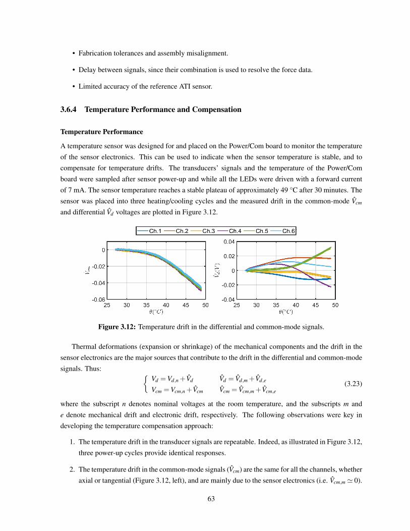
• Fabrication tolerances and assembly misalignment.
• Delay between signals, since their combination is used to resolve the force data.
• Limited accuracy of the reference ATI sensor.
3.6.4 Temperature Performance and Compensation
Temperature Performance
A temperature sensor was designed for and placed on the Power/Com board to monitor the temperature
of the sensor electronics. This can be used to indicate when the sensor temperature is stable, and to
compensate for temperature drifts. The transducers’ signals and the temperature of the Power/Com
board were sampled after sensor power-up and while all the LEDs were driven with a forward current
of 7 mA. The sensor temperature reaches a stable plateau of approximately 49 °C after 30 minutes. The
sensor was placed into three heating/cooling cycles and the measured drift in the common-mode Vcm
and differential Vd voltages are plotted in Figure 3.12.
Figure 3.12: Temperature drift in the differential and common-mode signals.
Thermal deformations (expansion or shrinkage) of the mechanical components and the drift in the
sensor electronics are the major sources that contribute to the drift in the differential and common-mode
signals. Thus: {Vd =Vd,n +Vd Vd = Vd,m +Vd,e
Vcm =Vcm,n +Vcm Vcm = Vcm,m +Vcm,e(3.23)
where the subscript n denotes nominal voltages at the room temperature, and the subscripts m and
e denote mechanical drift and electronic drift, respectively. The following observations were key in
developing the temperature compensation approach:
1. The temperature drift in the transducer signals are repeatable. Indeed, as illustrated in Figure 3.12,
three power-up cycles provide identical responses.
2. The temperature drift in the common-mode signals (Vcm) are the same for all the channels, whether
axial or tangential (Figure 3.12, left), and are mainly due to the sensor electronics (i.e. Vcm,m ' 0).
63
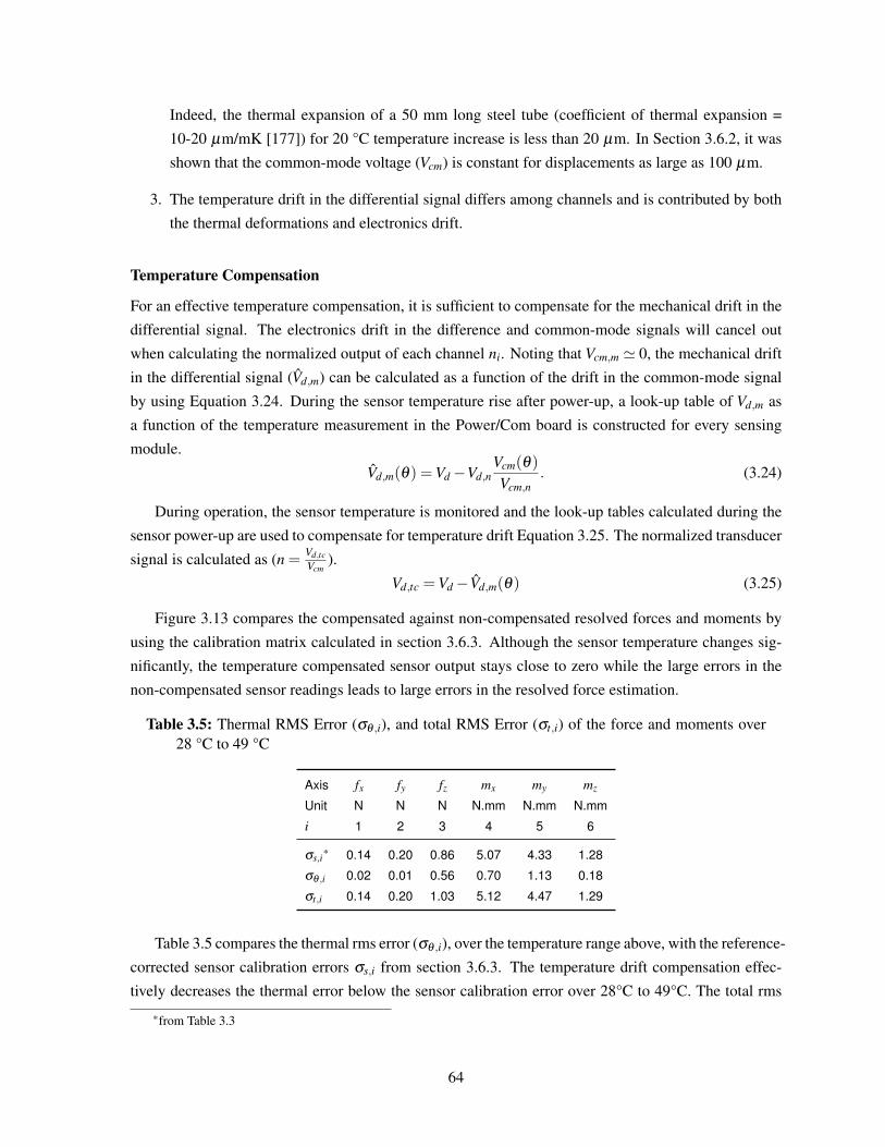
Indeed, the thermal expansion of a 50 mm long steel tube (coefficient of thermal expansion =
10-20 µm/mK [177]) for 20 °C temperature increase is less than 20 µm. In Section 3.6.2, it was
shown that the common-mode voltage (Vcm) is constant for displacements as large as 100 µm.
3. The temperature drift in the differential signal differs among channels and is contributed by both
the thermal deformations and electronics drift.
Temperature Compensation
For an effective temperature compensation, it is sufficient to compensate for the mechanical drift in the
differential signal. The electronics drift in the difference and common-mode signals will cancel out
when calculating the normalized output of each channel ni. Noting that Vcm,m ' 0, the mechanical drift
in the differential signal (Vd,m) can be calculated as a function of the drift in the common-mode signal
by using Equation 3.24. During the sensor temperature rise after power-up, a look-up table of Vd,m as
a function of the temperature measurement in the Power/Com board is constructed for every sensing
module.
Vd,m(θ) =Vd−Vd,nVcm(θ)
Vcm,n. (3.24)
During operation, the sensor temperature is monitored and the look-up tables calculated during the
sensor power-up are used to compensate for temperature drift Equation 3.25. The normalized transducer
signal is calculated as (n =Vd,tcVcm
).
Vd,tc =Vd−Vd,m(θ) (3.25)
Figure 3.13 compares the compensated against non-compensated resolved forces and moments by
using the calibration matrix calculated in section 3.6.3. Although the sensor temperature changes sig-
nificantly, the temperature compensated sensor output stays close to zero while the large errors in the
non-compensated sensor readings leads to large errors in the resolved force estimation.
Table 3.5: Thermal RMS Error (σθ ,i), and total RMS Error (σt,i) of the force and moments over28 °C to 49 °C
Axis fx fy fz mx my mz
Unit N N N N.mm N.mm N.mm
i 1 2 3 4 5 6
σs,i* 0.14 0.20 0.86 5.07 4.33 1.28
σθ ,i 0.02 0.01 0.56 0.70 1.13 0.18
σt,i 0.14 0.20 1.03 5.12 4.47 1.29
Table 3.5 compares the thermal rms error (σθ ,i), over the temperature range above, with the reference-
corrected sensor calibration errors σs,i from section 3.6.3. The temperature drift compensation effec-
tively decreases the thermal error below the sensor calibration error over 28°C to 49°C. The total rms
*from Table 3.3
64
Figure 3.13: Comparison of resolved force and moments measurement by the sensor in tempera-ture compensated vs. non-compensated scenarios.
error of the optical force sensor (σt,i) can be calculated as the root-sum-squared of the thermal and
reference-corrected sensor errors.
σt,i =√
σ2s,i +σ2
θ ,i (3.26)
3.7 ConclusionThis chapter presented the mechanical design and the performance evaluation of the first FPGA-based
smart F/T sensor in a compact form-factor. We presented an analytical model of the sensor and per-
formed extensive tests to validate it. The model can be used for design optimization. The proposed
design comprises six sensing modules that can provide a resolution of 0.0001% FS. The resolved force-
torque values on a steel tube and without a custom flexure have standard deviations between 0.03% to
0.1% in dynamic single-axis loading which is one-third of the 0.3% reported by Hirose et al. [162]
for static single-axis performance. The sensor’s components do not require special provisions to be
mounted onto the structure because their connection interface is not in the load path. Although we
proposed a hexagonal configuration, the sensing modules can have alternate arrangements to minimize
the coupling in different directions and further improve the sensing resolution and accuracy. Besides, a
higher number of sensing modules could be used for redundancy and error correction.
65

The sensor has no structural flexure; therefore, it does not break due to overload. In extreme cases
of plastic deformation of the load-carrying structure, the sensor just needs to be re-calibrated. Thus, it
is suitable for applications where the force sensor is not easily integrated into the load-path, keeping the
design simple and without adding a structural weak point. For example, sensing forces in an elevator
shaft or in the limbs of a robot is always challenging as the supporting structure has to be modified. The
sensor is also suitable for R&D projects that may face many failures before a final design is selected. A
sensing module can be used like a strain gauge that does not break. The modular design provides ease
of maintenance and customization.
The sensor is equipped with an IMU chip and a temperature sensor. The IMU can be used for gravity
and inertia compensation. It is particularly useful in applications where the sensor is integrated into a
long kinematic chain and the acceleration and orientation estimations based on the position sensing of
the links are not accurate. The temperature sensor was used to compensate for the temperature drift and
its effectiveness over a range of 20 °C was experimentally validated.
66
Chapter 4
6-Axis Optical Force Sensor: Hardwareand Software
4.1 IntroductionMulti-axis F/T sensors show growing use in industry [178] where an actuator interacts with an un-
structured environment (e.g. gripping) independently or via remote operation, where sensing of both
the environment and operator forces is needed to achieve a “transparent” system [179, 180]. In ap-
plications where sensed forces are used for real-time control, the force sensor must provide reliable
measurements at low latency and high data throughput [181]. A significant lag in the feedback signal
degrades the controller performance and can destabilize the control loop [182]. The specific sample rate
is application-dependent; for stable and smooth feedback control, a rule of thumb supported by analysis
suggests that the sampling frequency should be more than ten times the desired control loop bandwidth
[183]. To meet these requirements, a large amount of data must be processed and transmitted in a short
time.
The minimum number of physical transducers in a multi-axis F/T sensor is equal to the number of
DoFs it measures. A redundant sensor design with more transducers than the minimum can reduce noise
and/or add valuable information for fault detection. In resolving the force data, a processor needs to read
signals from all the transducers. Therefore, its latency is affected by the number of transducers, their
resolution, sampling rate, and communication interface. Other factors that contribute to the sensor’s
latency and data throughput are the level of signal pre-processing (analog and digital) required and the
available processing power.
SNR is an important characteristic of a sensor. Prior approaches used to improve a sensor’s noise
performance are local analog to digital conversion [184], low pass filtering, Kalman filtering [185, 186]
or other model-based observers [187], and oversampling [188]. A careful sensor design (mechanical
and electronics) minimizes the need for additional digital signal processing to meet the noise perfor-
mance requirement, thus reducing latency and improving the bandwidth of the feedback control system
employing the sensor.
67
Traditionally, Application-Specific Integrated Circuits (ASICs) were used for local processing and
to interface with transducers. These processors only work for the specific application they are de-
signed for and their customized building blocks require specific design and manufacture. They execute
firmware instructions sequentially with limited parallelization depending on the hardware design. Thus,
the system performance limits are imposed by the available resources in a processor. With the fabricated
hardware, each of the Integrated Circuit (IC)’s pins has a preconfigured set of functionalities; therefore,
once integrated into a PCB, the board may not be usable in a different application.
With the technological developments over the past two decades, FPGAs have found their way into
the development of smart sensors and high-performance control systems [189, 190]. State-of-the-art
FPGAs have Logic Blocks (LBs) and Look Up Tables (LUTs), an Interconnection network, config-
urable Input/Outputs (IOs), memory blocks, hardwired Digital Signal Processing (DSP) blocks, clock
managers, and communication blocks [191] that can be arbitrarily configured for specific applications.
There are multiple microcontroller cores that are available for FPGA implementation. Furthermore, spe-
cific hardware blocks can be cost-effectively prototyped and configured to meet stringent performance
requirements, such as real-time performance with a sub-millisecond latency requirement [192]. The
custom hardware configuration allows for parallel processing for performance optimization, and clock
gating to optimize power consumption in a targeted application. Simultaneous sampling and parallel
processing of the transducers can improve a sensor’s dynamic performance.
The sensor nodes in Wireless Sensor Networks (WSNs) use FPGAs due to their efficient hardware
processing and low power consumption [190]. Zhiyong et al. [193] used an FPGA and Micro Controller
Unit (MCU) System on Programmable Chip (SoPC) architecture to build a wireless vision sensor node.
Won et al. [194] used FPGAs in the development of a vision-based proximity sensor for mobile devices.
Nikolic et al. [195] utilized the FPGA’s processing power to build a compact visual-inertial sensor
system. Chen et al. [196] prototyped the hardware architecture of a smart temperature sensor using an
FPGA. Ahola et al. [197] used an FPGA to develop a wireless wearable sensor whose hardware can be
arbitrarily configured for different applications. Oballe-Peinado et al. [181] used the parallel processing
ability of FPGAs to scan and preprocess the tactile data from a sensor suite of an artificial hand.
This chapter presents:
1. A novel electronics design for a smart force-torque sensor that offers unparalleled performance.
The sensor electronics are reconfigurable, modular, and compact (Outer Diameter (OD) = 50 mm,
height = 35 mm) to provide ultra-low signal noise (5.6 µV) over a wide dynamic range (±5 V),
high signal bandwidth of 500 Hz, low latency of 100 µs, and data throughput of 11.5 kHz for the
transmission of 6-axis (3d force and torque vectors) transducer data, IMU, and temperature data.
2. A novel FPGA architecture and firmware for the synchronized sampling and parallel processing
of all the transducers, the IMU, and the temperature sensor.
3. A software package for easy integration of the sensor into the widely used ROS framework. The
proposed architecture allows for reading data in polling and streaming-modes with low latency at
publishing rates up to 3 kHz.
68
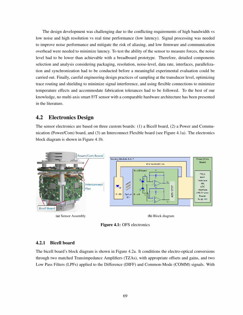
The design development was challenging due to the conflicting requirements of high bandwidth vs
low noise and high resolution vs real time performance (low latency). Signal processing was needed
to improve noise performance and mitigate the risk of aliasing, and low firmware and communication
overhead were needed to minimize latency. To test the ability of the sensor to measure forces, the noise
level had to be lower than achievable with a breadboard prototype. Therefore, detailed components
selection and analysis considering packaging, resolution, noise-level, data rate, interfaces, paralleliza-
tion and synchronization had to be conducted before a meaningful experimental evaluation could be
carried out. Finally, careful engineering design practices of sampling at the transducer level, optimizing
trace routing and shielding to minimize signal interference, and using flexible connections to minimize
temperature effects and accommodate fabrication tolerances had to be followed. To the best of our
knowledge, no multi-axis smart F/T sensor with a comparable hardware architecture has been presented
in the literature.
4.2 Electronics DesignThe sensor electronics are based on three custom boards: (1) a Bicell board, (2) a Power and Commu-
nication (Power/Com) board, and (3) an Interconnect Flexible board (see Figure 4.1a). The electronics
block diagram is shown in Figure 4.1b.
(a) Sensor Assembly (b) Block diagram
Figure 4.1: OFS electronics
4.2.1 Bicell board
The bicell board’s block diagram is shown in Figure 4.2a. It conditions the electro-optical conversions
through two matched Transimpedance Amplifiers (TZAs), with appropriate offsets and gains, and two
Low Pass Filters (LPFs) applied to the Difference (DIFF) and Common-Mode (COMM) signals. With
69
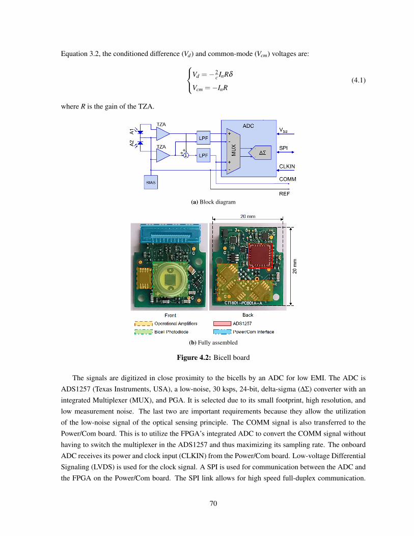
Equation 3.2, the conditioned difference (Vd) and common-mode (Vcm) voltages are:Vd =−2c InRδ
Vcm =−InR(4.1)
where R is the gain of the TZA.
(a) Block diagram
(b) Fully assembled
Figure 4.2: Bicell board
The signals are digitized in close proximity to the bicells by an ADC for low EMI. The ADC is
ADS1257 (Texas Instruments, USA), a low-noise, 30 ksps, 24-bit, delta-sigma (∆Σ) converter with an
integrated Multiplexer (MUX), and PGA. It is selected due to its small footprint, high resolution, and
low measurement noise. The last two are important requirements because they allow the utilization
of the low-noise signal of the optical sensing principle. The COMM signal is also transferred to the
Power/Com board. This is to utilize the FPGA’s integrated ADC to convert the COMM signal without
having to switch the multiplexer in the ADS1257 and thus maximizing its sampling rate. The onboard
ADC receives its power and clock input (CLKIN) from the Power/Com board. Low-voltage Differential
Signaling (LVDS) is used for the clock signal. A SPI is used for communication between the ADC and
the FPGA on the Power/Com board. The SPI link allows for high speed full-duplex communication.
70
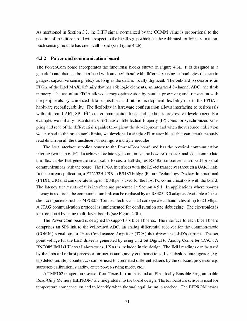
As mentioned in Section 3.2, the DIFF signal normalized by the COMM value is proportional to the
position of the slit centroid with respect to the bicell’s gap which can be calibrated for force estimation.
Each sensing module has one bicell board (see Figure 4.2b).
4.2.2 Power and communication board
The Power/Com board incorporates the functional blocks shown in Figure 4.3a. It is designed as a
generic board that can be interfaced with any peripheral with different sensing technologies (i.e. strain
gauges, capacitive sensing, etc.), as long as the data is locally digitized. The onboard processor is an
FPGA of the Intel MAX10 family that has 16k logic elements, an integrated 8-channel ADC, and flash
memory. The use of an FPGA allows latency optimization by parallel processing and transaction with
the peripherals, synchronized data acquisition, and future development flexibility due to the FPGA’s
hardware reconfigurability. The flexibility in hardware configuration allows interfacing to peripherals
with different UART, SPI, I2C, etc. communication links, and facilitates progressive development. For
example, we initially instantiated 6 SPI master Intellectual Property (IP) cores for synchronized sam-
pling and read of the differential signals; throughout the development and when the resource utilization
was pushed to the processor’s limits, we developed a single SPI master block that can simultaneously
read data from all the transducers or configure multiple modules.
The host interface supplies power to the Power/Com board and has the physical communication
interface with a host PC. To achieve low latency, to minimize the Power/Com size, and to accommodate
thin flex cables that generate small cable forces, a half-duplex RS485 transceiver is utilized for serial
communications with the board. The FPGA interfaces with the RS485 transceiver through a UART link.
In the current application, a FT2232H USB to RS485 bridge (Future Technology Devices International
(FTDI), UK) that can operate at up to 10 Mbps is used for the host PC communications with the board.
The latency test results of this interface are presented in Section 4.5.1. In applications where shorter
latency is required, the communication link can be replaced by an RS485 PCI adapter. Available off-the-
shelf components such as MPG003 (ConnectTech, Canada) can operate at baud rates of up to 20 Mbps.
A JTAG communication protocol is implemented for configuration and debugging. The electronics is
kept compact by using multi-layer boards (see Figure 4.3b).
The Power/Com board is designed to support six bicell boards. The interface to each bicell board
comprises an SPI-link to the collocated ADC, an analog differential receiver for the common-mode
(COMM) signal, and a Trans-Conductance Amplifier (TCA) that drives the LED’s current. The set
point voltage for the LED driver is generated by using a 12-bit Digital to Analog Converter (DAC). A
BNO085 IMU (Hillcrest Laboratories, USA) is included in the design. The IMU readings can be used
by the onboard or host processor for inertia and gravity compensations. Its embedded intelligence (e.g.
tap detection, step counter, ...) can be used to command different actions by the onboard processor e.g.
start/stop calibration, standby, enter power-saving mode, etc..
A TMP102 temperature sensor from Texas Instruments and an Electrically Erasable Programmable
Read-Only Memory (EEPROM) are integrated into the board design. The temperature sensor is used for
temperature compensation and to identify when thermal equilibrium is reached. The EEPROM stores
71
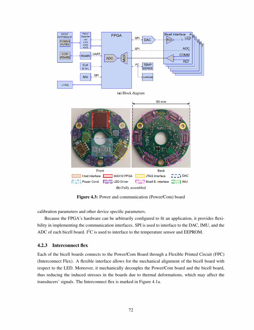
(a) Block diagram
(b) Fully assembled
Figure 4.3: Power and communication (Power/Com) board
calibration parameters and other device specific parameters.
Because the FPGA’s hardware can be arbitrarily configured to fit an application, it provides flexi-
bility in implementing the communication interfaces. SPI is used to interface to the DAC, IMU, and the
ADC of each bicell board. I2C is used to interface to the temperature sensor and EEPROM.
4.2.3 Interconnect flex
Each of the bicell boards connects to the Power/Com Board through a Flexible Printed Circuit (FPC)
(Interconnect Flex). A flexible interface allows for the mechanical alignment of the bicell board with
respect to the LED. Moreover, it mechanically decouples the Power/Com board and the bicell board,
thus reducing the induced stresses in the boards due to thermal deformations, which may affect the
transducers’ signals. The Interconnect flex is marked in Figure 4.1a.
72
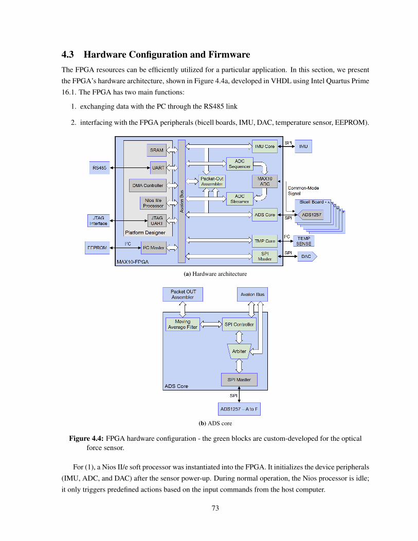
4.3 Hardware Configuration and FirmwareThe FPGA resources can be efficiently utilized for a particular application. In this section, we present
the FPGA’s hardware architecture, shown in Figure 4.4a, developed in VHDL using Intel Quartus Prime
16.1. The FPGA has two main functions:
1. exchanging data with the PC through the RS485 link
2. interfacing with the FPGA peripherals (bicell boards, IMU, DAC, temperature sensor, EEPROM).
(a) Hardware architecture
(b) ADS core
Figure 4.4: FPGA hardware configuration - the green blocks are custom-developed for the opticalforce sensor.
For (1), a Nios II/e soft processor was instantiated into the FPGA. It initializes the device peripherals
(IMU, ADC, and DAC) after the sensor power-up. During normal operation, the Nios processor is idle;
it only triggers predefined actions based on the input commands from the host computer.
73
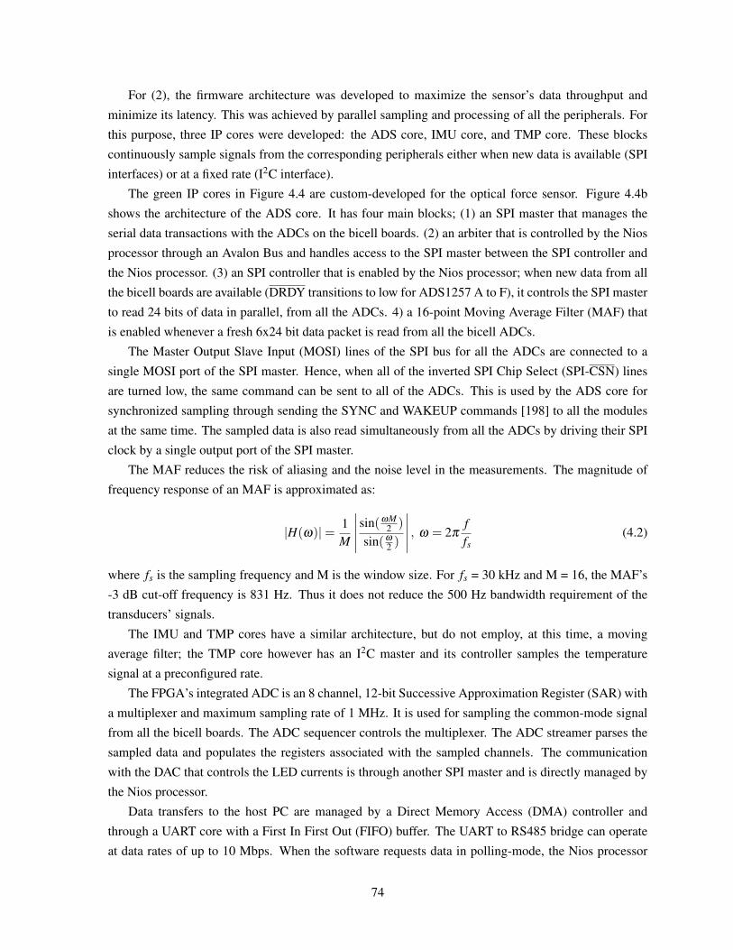
For (2), the firmware architecture was developed to maximize the sensor’s data throughput and
minimize its latency. This was achieved by parallel sampling and processing of all the peripherals. For
this purpose, three IP cores were developed: the ADS core, IMU core, and TMP core. These blocks
continuously sample signals from the corresponding peripherals either when new data is available (SPI
interfaces) or at a fixed rate (I2C interface).
The green IP cores in Figure 4.4 are custom-developed for the optical force sensor. Figure 4.4b
shows the architecture of the ADS core. It has four main blocks; (1) an SPI master that manages the
serial data transactions with the ADCs on the bicell boards. (2) an arbiter that is controlled by the Nios
processor through an Avalon Bus and handles access to the SPI master between the SPI controller and
the Nios processor. (3) an SPI controller that is enabled by the Nios processor; when new data from all
the bicell boards are available (DRDY transitions to low for ADS1257 A to F), it controls the SPI master
to read 24 bits of data in parallel, from all the ADCs. 4) a 16-point Moving Average Filter (MAF) that
is enabled whenever a fresh 6x24 bit data packet is read from all the bicell ADCs.
The Master Output Slave Input (MOSI) lines of the SPI bus for all the ADCs are connected to a
single MOSI port of the SPI master. Hence, when all of the inverted SPI Chip Select (SPI-CSN) lines
are turned low, the same command can be sent to all of the ADCs. This is used by the ADS core for
synchronized sampling through sending the SYNC and WAKEUP commands [198] to all the modules
at the same time. The sampled data is also read simultaneously from all the ADCs by driving their SPI
clock by a single output port of the SPI master.
The MAF reduces the risk of aliasing and the noise level in the measurements. The magnitude of
frequency response of an MAF is approximated as:
|H(ω)|= 1M
∣∣∣∣∣sin(ωM2 )
sin(ω
2 )
∣∣∣∣∣ , ω = 2πffs
(4.2)
where fs is the sampling frequency and M is the window size. For fs = 30 kHz and M = 16, the MAF’s
-3 dB cut-off frequency is 831 Hz. Thus it does not reduce the 500 Hz bandwidth requirement of the
transducers’ signals.
The IMU and TMP cores have a similar architecture, but do not employ, at this time, a moving
average filter; the TMP core however has an I2C master and its controller samples the temperature
signal at a preconfigured rate.
The FPGA’s integrated ADC is an 8 channel, 12-bit Successive Approximation Register (SAR) with
a multiplexer and maximum sampling rate of 1 MHz. It is used for sampling the common-mode signal
from all the bicell boards. The ADC sequencer controls the multiplexer. The ADC streamer parses the
sampled data and populates the registers associated with the sampled channels. The communication
with the DAC that controls the LED currents is through another SPI master and is directly managed by
the Nios processor.
Data transfers to the host PC are managed by a Direct Memory Access (DMA) controller and
through a UART core with a First In First Out (FIFO) buffer. The UART to RS485 bridge can operate
at data rates of up to 10 Mbps. When the software requests data in polling-mode, the Nios processor
74
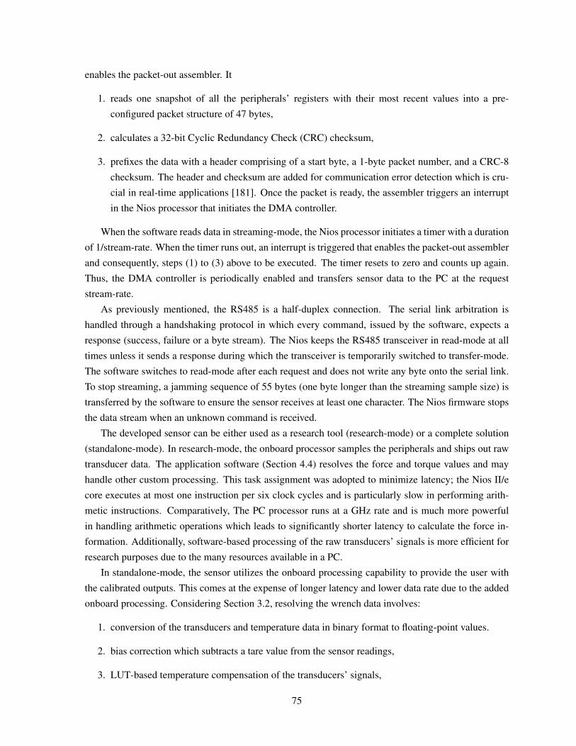
enables the packet-out assembler. It
1. reads one snapshot of all the peripherals’ registers with their most recent values into a pre-
configured packet structure of 47 bytes,
2. calculates a 32-bit Cyclic Redundancy Check (CRC) checksum,
3. prefixes the data with a header comprising of a start byte, a 1-byte packet number, and a CRC-8
checksum. The header and checksum are added for communication error detection which is cru-
cial in real-time applications [181]. Once the packet is ready, the assembler triggers an interrupt
in the Nios processor that initiates the DMA controller.
When the software reads data in streaming-mode, the Nios processor initiates a timer with a duration
of 1/stream-rate. When the timer runs out, an interrupt is triggered that enables the packet-out assembler
and consequently, steps (1) to (3) above to be executed. The timer resets to zero and counts up again.
Thus, the DMA controller is periodically enabled and transfers sensor data to the PC at the request
stream-rate.
As previously mentioned, the RS485 is a half-duplex connection. The serial link arbitration is
handled through a handshaking protocol in which every command, issued by the software, expects a
response (success, failure or a byte stream). The Nios keeps the RS485 transceiver in read-mode at all
times unless it sends a response during which the transceiver is temporarily switched to transfer-mode.
The software switches to read-mode after each request and does not write any byte onto the serial link.
To stop streaming, a jamming sequence of 55 bytes (one byte longer than the streaming sample size) is
transferred by the software to ensure the sensor receives at least one character. The Nios firmware stops
the data stream when an unknown command is received.
The developed sensor can be either used as a research tool (research-mode) or a complete solution
(standalone-mode). In research-mode, the onboard processor samples the peripherals and ships out raw
transducer data. The application software (Section 4.4) resolves the force and torque values and may
handle other custom processing. This task assignment was adopted to minimize latency; the Nios II/e
core executes at most one instruction per six clock cycles and is particularly slow in performing arith-
metic instructions. Comparatively, The PC processor runs at a GHz rate and is much more powerful
in handling arithmetic operations which leads to significantly shorter latency to calculate the force in-
formation. Additionally, software-based processing of the raw transducers’ signals is more efficient for
research purposes due to the many resources available in a PC.
In standalone-mode, the sensor utilizes the onboard processing capability to provide the user with
the calibrated outputs. This comes at the expense of longer latency and lower data rate due to the added
onboard processing. Considering Section 3.2, resolving the wrench data involves:
1. conversion of the transducers and temperature data in binary format to floating-point values.
2. bias correction which subtracts a tare value from the sensor readings,
3. LUT-based temperature compensation of the transducers’ signals,
75
4. calculation of the normalized signal (di) for each module,
5. application of the calibration matrix (Equation 3.16) to obtain the force and torque values.
The added latency due to the onboard calculation of the force values is addressed in Section 4.5.1.
The desired operation mode can be selected at the sensor power-up. The FPGA chip has two Con-
figuration Flash Memories (CFM) that can be used to store two different configuration images. On
power-up, the internal programmer loads the selected image into the Configuration RAM (CRAM) de-
pending on the status of a configuration pin (CONFIG SEL). In the standalone mode, the Nios firmware
reads the calibration matrix from the EEPROM. If needed, the software can be used to overwrite the
calibration parameters.
4.4 SoftwareTwo software packages were developed: (1) a standalone library in Python (sensor.py), (2) a package
for sensor integration into ROS. Both packages use libftdi, an open source C/C++ FTDI driver library,
as the hardware-abstraction layer for transactions with the USB-RS485 bridge.
Figure 4.5: ROS package - software architecture
In the Python library, the main thread relays user commands to the sensor. A separate thread con-
stantly reads from the input buffer, parses the data, resolves the force/torque, IMU, and temperature
76
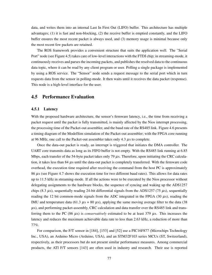
data, and writes them into an internal Last In First Out (LIFO) buffer. This architecture has multiple
advantages; (1) it is fast and non-blocking, (2) the receive buffer is emptied constantly, and the LIFO
buffer ensures the most recent packet is always used, and (3) memory usage is minimal because only
the most recent few packets are retained.
The ROS framework provides a convenient structure that suits the application well. The ”Serial
Port” node (see Figure 4.5) takes care of low-level interactions with the FTDI chip; in streaming-mode, it
continuously receives and parses the incoming packets, and publishes the resolved data to the continuous
data topic, where it can be read by any client program or user. Polling a single package is implemented
by using a ROS service. The “Sensor” node sends a request message to the serial port which in turn
requests data from the sensor in polling-mode. It then waits until it receives the data packet (response).
This node is a high-level interface for the user.
4.5 Performance Evaluation
4.5.1 Latency
With the proposed hardware architecture, the sensor’s firmware latency, i.e., the time from receiving a
packet request until the packet is fully transmitted, is mainly affected by the Nios interrupt processing,
the processing time of the Packet-out assembler, and the baud rate of the RS485 link. Figure 4.6 presents
a timing diagram of the ModelSim simulation of the Packet-out assembler; with the FPGA core running
at 96 MHz, one call to the Packet-out assembler takes only 4.3 µs to complete.
Once the data-out packet is ready, an interrupt is triggered that initiates the DMA controller. The
UART core transmits data as long as its FIFO buffer is not empty. With the RS485 link running at 6.85
Mbps, each transfer of the 54-byte packet takes only 79 µs. Therefore, upon initiating the CRC calcula-
tion, it takes less than 84 µs until the data-out packet is completely transferred. With the firmware code
overhead, the execution time required after receiving the command from the host PC is approximately
86 µs (see Figure 4.7 shows the execution time for two different baud rates). This allows for data rates
up to 11.5 kHz in streaming-mode. If all the actions were to be executed by the Nios processor without
delegating assignments to the hardware blocks, the sequence of syncing and waking up the ADS1257
chips (8.3 µs), sequentially reading 24-bit differential signals from the ADS1257 (75 µs), sequentially
reading the 12 bit common-mode signals from the ADC integrated in the FPGA (30 µs), reading the
IMU and temperature data (61.3 µs + 80 µs), applying the same moving average filter to the data (38
µs), and performing packet-assembly, CRC calculation and data transfer over the RS485 link and trans-
ferring them to the PC (86 µs) is conservatively estimated to be at least 379 µs. This increases the
latency and reduces the maximum achievable data rate to less than 2.63 kHz, a reduction of more than
77%.
For comparison, the F/T sensor in [184], [153] and [52] use a PIC16F877 (Microchips Technology
Inc., USA), an Arduino Micro (Arduino, USA), and an STM32F103 series MCUs (ST, Switzerland),
respectively, as their processors but do not present similar performance measures. Among commercial
products, the ATI F/T sensors [143] are often used in industry and research. Their use is reported
77
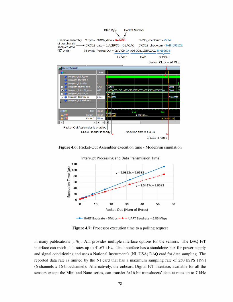
Figure 4.6: Packet-Out Assembler execution time - ModelSim simulation
Figure 4.7: Processor execution time to a polling request
in many publications [176]. ATI provides multiple interface options for the sensors. The DAQ F/T
interface can reach data rates up to 41.67 kHz. This interface has a standalone box for power supply
and signal conditioning and uses a National Instrument’s (NI, USA) DAQ card for data sampling. The
reported data rate is limited by the NI card that has a maximum sampling rate of 250 kSPS [199]
(6-channels x 16 bits/channel). Alternatively, the onboard Digital F/T interface, available for all the
sensors except the Mini and Nano series, can transfer 6x16-bit transducers’ data at rates up to 7 kHz
78
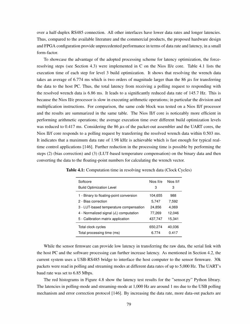
over a half-duplex RS485 connection. All other interfaces have lower data rates and longer latencies.
Thus, compared to the available literature and the commercial products, the proposed hardware design
and FPGA configuration provide unprecedented performance in terms of data rate and latency, in a small
form-factor.
To showcase the advantage of the adopted processing scheme for latency optimization, the force-
resolving steps (see Section 4.3) were implemented in C on the Nios II/e core. Table 4.1 lists the
execution time of each step for level 3 build optimization. It shows that resolving the wrench data
takes an average of 6.774 ms which is two orders of magnitude larger than the 86 µs for transferring
the data to the host PC. Thus, the total latency from receiving a polling request to responding with
the resolved wrench data is 6.86 ms. It leads to a significantly reduced data rate of 145.7 Hz. This is
because the Nios II/e processor is slow in executing arithmetic operations; in particular the division and
multiplication instructions. For comparison, the same code block was tested on a Nios II/f processor
and the results are summarized in the same table. The Nios II/f core is noticeably more efficient in
performing arithmetic operations; the average execution time over different build optimization levels
was reduced to 0.417 ms. Considering the 86 µs of the packet-out assembler and the UART cores, the
Nios II/f core responds to a polling request by transferring the resolved wrench data within 0.503 ms.
It indicates that a maximum data rate of 1.98 kHz is achievable which is fast enough for typical real-
time control applications [146]. Further reduction in the processing time is possible by performing the
steps (2) (bias correction) and (3) (LUT-based temperature compensation) on the binary data and then
converting the data to the floating-point numbers for calculating the wrench vector.
Table 4.1: Computation time in resolving wrench data (Clock Cycles)
Softcore Nios II/e Nios II/f
Build Optimization Level 3 3
1 - Binary to floating-point conversion 104,655 988
2 - Bias correction 5,747 7,592
3 - LUT-based temperature compensation 24,856 4,069
4 - Normalized signal (di) computation 77,269 12,046
5 - Calibration matrix application 437,747 15,341
Total clock cycles 650,274 40,036
Total processing time (ms) 6.774 0.417
While the sensor firmware can provide low latency in transferring the raw data, the serial link with
the host PC and the software processing can further increase latency. As mentioned in Section 4.2, the
current system uses a USB-RS485 bridge to interface the host computer to the sensor firmware. 30k
packets were read in polling and streaming modes at different data rates of up to 5,000 Hz. The UART’s
baud rate was set to 6.85 Mbps.
The red histograms in Figure 4.8 show the latency test results for the ”sensor.py” Python library.
The latencies in polling-mode and streaming-mode at 1,000 Hz are around 1 ms due to the USB polling
mechanism and error correction protocol [146]. By increasing the data rate, more data-out packets are
79
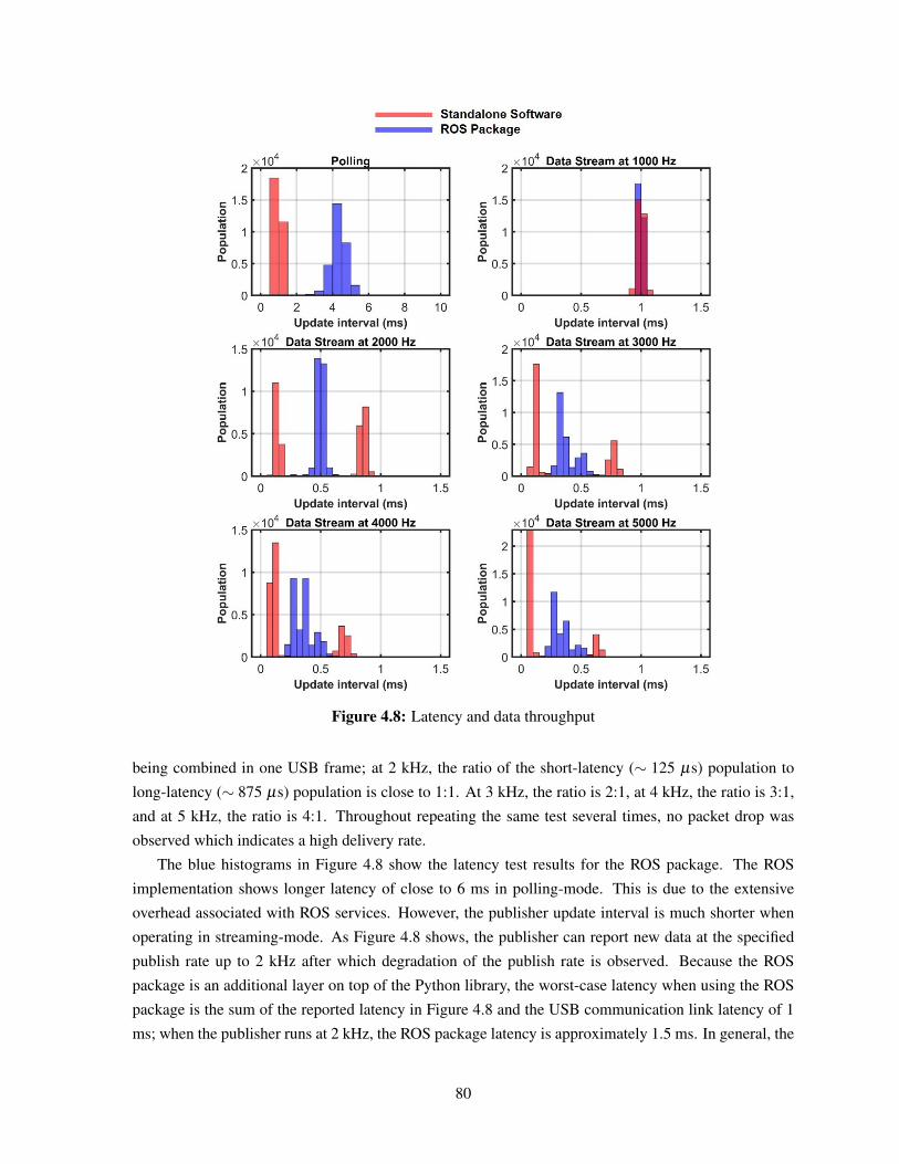
Figure 4.8: Latency and data throughput
being combined in one USB frame; at 2 kHz, the ratio of the short-latency (∼ 125 µs) population to
long-latency (∼ 875 µs) population is close to 1:1. At 3 kHz, the ratio is 2:1, at 4 kHz, the ratio is 3:1,
and at 5 kHz, the ratio is 4:1. Throughout repeating the same test several times, no packet drop was
observed which indicates a high delivery rate.
The blue histograms in Figure 4.8 show the latency test results for the ROS package. The ROS
implementation shows longer latency of close to 6 ms in polling-mode. This is due to the extensive
overhead associated with ROS services. However, the publisher update interval is much shorter when
operating in streaming-mode. As Figure 4.8 shows, the publisher can report new data at the specified
publish rate up to 2 kHz after which degradation of the publish rate is observed. Because the ROS
package is an additional layer on top of the Python library, the worst-case latency when using the ROS
package is the sum of the reported latency in Figure 4.8 and the USB communication link latency of 1
ms; when the publisher runs at 2 kHz, the ROS package latency is approximately 1.5 ms. In general, the
80
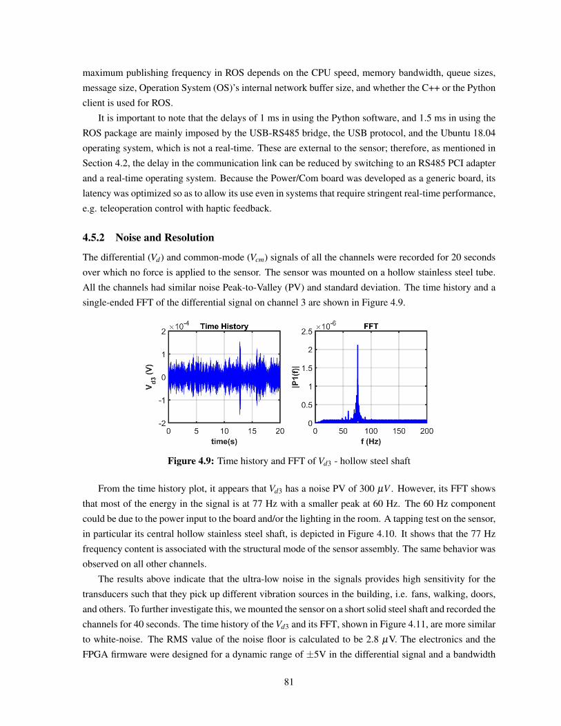
maximum publishing frequency in ROS depends on the CPU speed, memory bandwidth, queue sizes,
message size, Operation System (OS)’s internal network buffer size, and whether the C++ or the Python
client is used for ROS.
It is important to note that the delays of 1 ms in using the Python software, and 1.5 ms in using the
ROS package are mainly imposed by the USB-RS485 bridge, the USB protocol, and the Ubuntu 18.04
operating system, which is not a real-time. These are external to the sensor; therefore, as mentioned in
Section 4.2, the delay in the communication link can be reduced by switching to an RS485 PCI adapter
and a real-time operating system. Because the Power/Com board was developed as a generic board, its
latency was optimized so as to allow its use even in systems that require stringent real-time performance,
e.g. teleoperation control with haptic feedback.
4.5.2 Noise and Resolution
The differential (Vd) and common-mode (Vcm) signals of all the channels were recorded for 20 seconds
over which no force is applied to the sensor. The sensor was mounted on a hollow stainless steel tube.
All the channels had similar noise Peak-to-Valley (PV) and standard deviation. The time history and a
single-ended FFT of the differential signal on channel 3 are shown in Figure 4.9.
Figure 4.9: Time history and FFT of Vd3 - hollow steel shaft
From the time history plot, it appears that Vd3 has a noise PV of 300 µV . However, its FFT shows
that most of the energy in the signal is at 77 Hz with a smaller peak at 60 Hz. The 60 Hz component
could be due to the power input to the board and/or the lighting in the room. A tapping test on the sensor,
in particular its central hollow stainless steel shaft, is depicted in Figure 4.10. It shows that the 77 Hz
frequency content is associated with the structural mode of the sensor assembly. The same behavior was
observed on all other channels.
The results above indicate that the ultra-low noise in the signals provides high sensitivity for the
transducers such that they pick up different vibration sources in the building, i.e. fans, walking, doors,
and others. To further investigate this, we mounted the sensor on a short solid steel shaft and recorded the
channels for 40 seconds. The time history of the Vd3 and its FFT, shown in Figure 4.11, are more similar
to white-noise. The RMS value of the noise floor is calculated to be 2.8 µV. The electronics and the
FPGA firmware were designed for a dynamic range of ±5V in the differential signal and a bandwidth
81
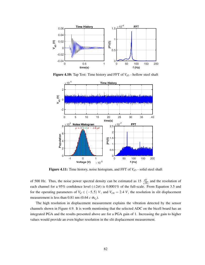
Figure 4.10: Tap Test: Time history and FFT of Vd3 - hollow steel shaft
Figure 4.11: Time history, noise histogram, and FFT of Vd3 - solid steel shaft
of 500 Hz. Thus, the noise power spectral density can be estimated as 15 nV√Hz
and the resolution of
each channel for a 95% confidence level (±2σ ) is 0.0001% of the full-scale. From Equation 3.5 and
for the operating parameters of Vd ∈ (−5,5) V , and Vcm = 2.4 V , the resolution in slit displacement
measurement is less than 0.81 nm (0.64 c σVd ).
The high resolution in displacement measurement explains the vibration detected by the sensor
channels shown in Figure 4.9. It is worth mentioning that the selected ADC on the bicell board has an
integrated PGA and the results presented above are for a PGA gain of 1. Increasing the gain to higher
values would provide an even higher resolution in the slit displacement measurement.
82
4.6 ConclusionWe presented the hardware and firmware design of a novel FPGA-based smart optical force-torque
sensor. The sensor electronics are compact, configurable, and modular. They provide ultra-low noise
signal performance with average power spectral density of 15 nV√Hz
over signal bandwidth of 500 Hz, and
a resolution of 0.0001% full-scale. The digital electronics utilizes an FPGA as the onboard processor
with a novel hardware architecture for synchronized sampling and parallel hardware processing of all
the transducers data. The FPGA’s hardware and its softcore’s firmware were developed to provide
operations in research-mode and standalone-mode. The sensor provides a latency of less than 100
µs and can stream at the maximum data rate of 11.5 kHz in research-mode in which it transfers the
transducers’ raw data to a host PC for further processing. The sensor provides a latency of 503 µs and
can stream at the maximum data rate of 1.98 kHz in standalone-mode in which it outputs the calibrated
wrench vector. The sensor electronics integrates an inertial measurement unit and a temperature sensor
for gravity, inertia, and temperature compensations.
A standalone Python library was developed for easy integration of the force sensor into different
applications. When the software is interfaced to the sensor through a USB-RS485 bridge, it provided a
short latency of 1 ms limited by the error correction and polling mechanism in the USB communication
protocol. A shorter latency can be achieved by using an RS485 PCI card. A ROS package for sensor
integration into the ROS framework was developed and tested. The ROS package delivered a latency of
6 ms in polling-mode and 1.5 ms in streaming-mode.
83
Chapter 5
Multi-Axis Force Sensing in RMIS WithNo Instrument Modification
5.1 IntroductionA comprehensive introduction and literature survey on force sensing and haptic feedback in MIS and
RMIS was presented in Chapter 1.
The focus of our research was developing a multi-axis force sensor that does not require modifica-
tions to the surgical instrument and is adaptable to different surgical tools. The literature suggests that
the lateral forces should be the primary focus for an effective haptic experience, and the axial force and
torsion are secondary [47]. The human JND is 10% in the range of 0.5 to 200 N increasing to 15-27%
below 0.5 N, which can be considered as a requirement on the sensor accuracy [52]. A resolution of
0.2 N over a range of ±10 N was assumed for the lateral forces [97]. To the best of our knowledge, no
requirements for the other DoFs have been specified. The closer the sensor is to the instrument tip, the
more accurate the force sensing will be; however, the requirements on sterilizability and biocompatibil-
ity are more stringent.
This chapter expands on the use of the optical force sensor explained in Chapter 3 and Chapter 4 to
5-axis force sensing (lateral forces and moments and the axial torsion) at the instrument’s distal end, in
the da Vinci® classic systems. Additionally, it presents a novel cannula design for mechanically filtering
the body forces.
5.2 Sensing ApproachThe optical force sensor was mounted onto the proximal shaft of the instrument via screw-type mechan-
ical clamps as shown in Figure 5.1. The mounting interface is not critical because it transfers no load to
any of the components; therefore, it can be a set-screw connection, a mechanical, or a magnetic clamp.
As explained in Chapter 1, force sensing at the proximal shaft can be affected by the forces between
the cannula and the patient’s body. To mitigate this, we modified the design of the cannula in the da
Vinci® classic system such that an outer tube with an outer diameter of 14.5 mm and a wall thickness
84
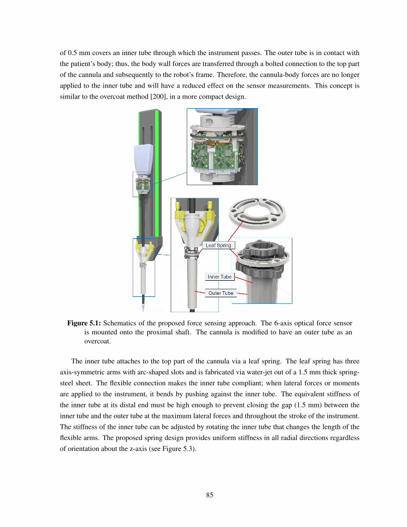
of 0.5 mm covers an inner tube through which the instrument passes. The outer tube is in contact with
the patient’s body; thus, the body wall forces are transferred through a bolted connection to the top part
of the cannula and subsequently to the robot’s frame. Therefore, the cannula-body forces are no longer
applied to the inner tube and will have a reduced effect on the sensor measurements. This concept is
similar to the overcoat method [200], in a more compact design.
Figure 5.1: Schematics of the proposed force sensing approach. The 6-axis optical force sensoris mounted onto the proximal shaft. The cannula is modified to have an outer tube as anovercoat.
The inner tube attaches to the top part of the cannula via a leaf spring. The leaf spring has three
axis-symmetric arms with arc-shaped slots and is fabricated via water-jet out of a 1.5 mm thick spring-
steel sheet. The flexible connection makes the inner tube compliant; when lateral forces or moments
are applied to the instrument, it bends by pushing against the inner tube. The equivalent stiffness of
the inner tube at its distal end must be high enough to prevent closing the gap (1.5 mm) between the
inner tube and the outer tube at the maximum lateral forces and throughout the stroke of the instrument.
The stiffness of the inner tube can be adjusted by rotating the inner tube that changes the length of the
flexible arms. The proposed spring design provides uniform stiffness in all radial directions regardless
of orientation about the z-axis (see Figure 5.3).
85

5.3 ModelingA mathematical model from the forces and moments at the distal end of the instrument shaft (point
t in Figure 5.2) to the normalized transducers signals of the optical force sensor was developed. The
mechanical constraints of the instrument shaft, which affect its bending behavior, vary as a function
of the instrument’s insertion into the cannula. The model was developed in two steps to decouple the
sensor behavior from the changes in the boundary condition. The first part (see Equation 5.1) explains
the sensor response to the forces applied at the clamping point of the passive component (point c). The
second part (see Equation 5.2 to Equation 5.4) focuses on the reflected wrench vector at the shaft’s
cross-section at point c as a function of the wrenches applied at the point t considering the change in the
instrument’s insertion into the cannula (ls).
Figure 5.2: The schematic for development of the instrument’s bending model.
From geometric algebra, the principles of continuum mechanics, and the electro-optical conversion
(see Equation 3.1) the transformation from the wrench vector at point c (~wc =[
fcx, fcy, fcz,mcx,mcy,mcz
]T)
to the vector of normalized transducers signals (~n =[n1, . . . ,n6
]T) is (see Section 3.3.2):
~n =Cm~wc, Cm =2c
HGHw, (5.1)
where HG is a geometric transformation matrix from the tri-axial displacement and rotation vector at
point c to the normal and in-plane slits displacements. HG relates to the hexagonal sensor configuration.
Hw is a transformation matrix from the wrenches applied at point c to its tri-axial displacements and
86
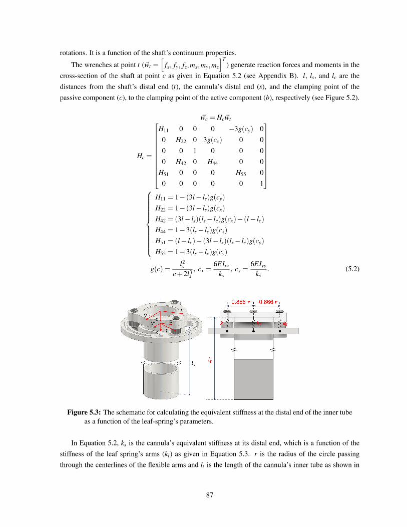
rotations. It is a function of the shaft’s continuum properties.
The wrenches at point t (~wt =[
fx, fy, fz,mx,my,mz
]T) generate reaction forces and moments in the
cross-section of the shaft at point c as given in Equation 5.2 (see Appendix B). l, ls, and lc are the
distances from the shaft’s distal end (t), the cannula’s distal end (s), and the clamping point of the
passive component (c), to the clamping point of the active component (b), respectively (see Figure 5.2).
~wc = Hc~wt
Hc =
H11 0 0 0 −3g(cy) 0
0 H22 0 3g(cx) 0 0
0 0 1 0 0 0
0 H42 0 H44 0 0
H51 0 0 0 H55 0
0 0 0 0 0 1
H11 = 1− (3l− ls)g(cy)
H22 = 1− (3l− ls)g(cx)
H42 = (3l− ls)(ls− lc)g(cx)− (l− lc)
H44 = 1−3(ls− lc)g(cx)
H51 = (l− lc)− (3l− ls)(ls− lc)g(cy)
H55 = 1−3(ls− lc)g(cy)
g(c) =l2s
c+2l3s, cx =
6EIxx
ks, cy =
6EIyy
ks. (5.2)
Figure 5.3: The schematic for calculating the equivalent stiffness at the distal end of the inner tubeas a function of the leaf-spring’s parameters.
In Equation 5.2, ks is the cannula’s equivalent stiffness at its distal end, which is a function of the
stiffness of the leaf spring’s arms (kl) as given in Equation 5.3. r is the radius of the circle passing
through the centerlines of the flexible arms and lt is the length of the cannula’s inner tube as shown in
87
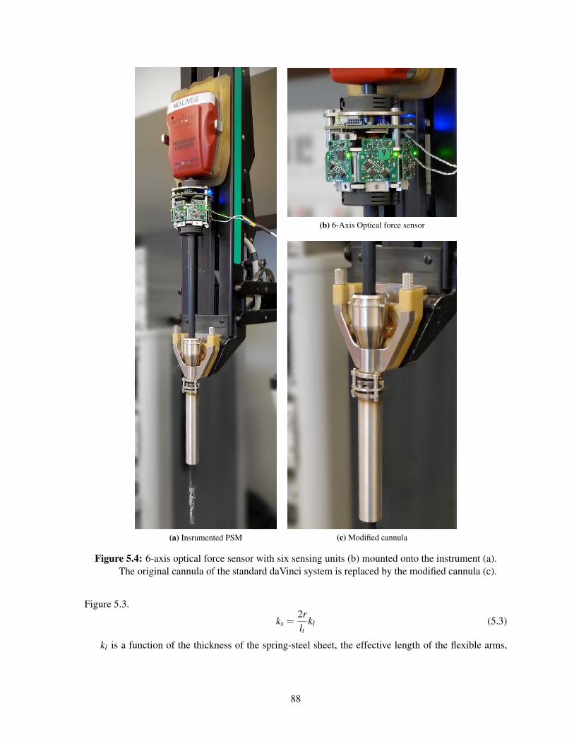
(a) Insrumented PSM
(b) 6-Axis Optical force sensor
(c) Modified cannula
Figure 5.4: 6-axis optical force sensor with six sensing units (b) mounted onto the instrument (a).The original cannula of the standard daVinci system is replaced by the modified cannula (c).
Figure 5.3.
ks =2rlt
kl (5.3)
kl is a function of the thickness of the spring-steel sheet, the effective length of the flexible arms,
88
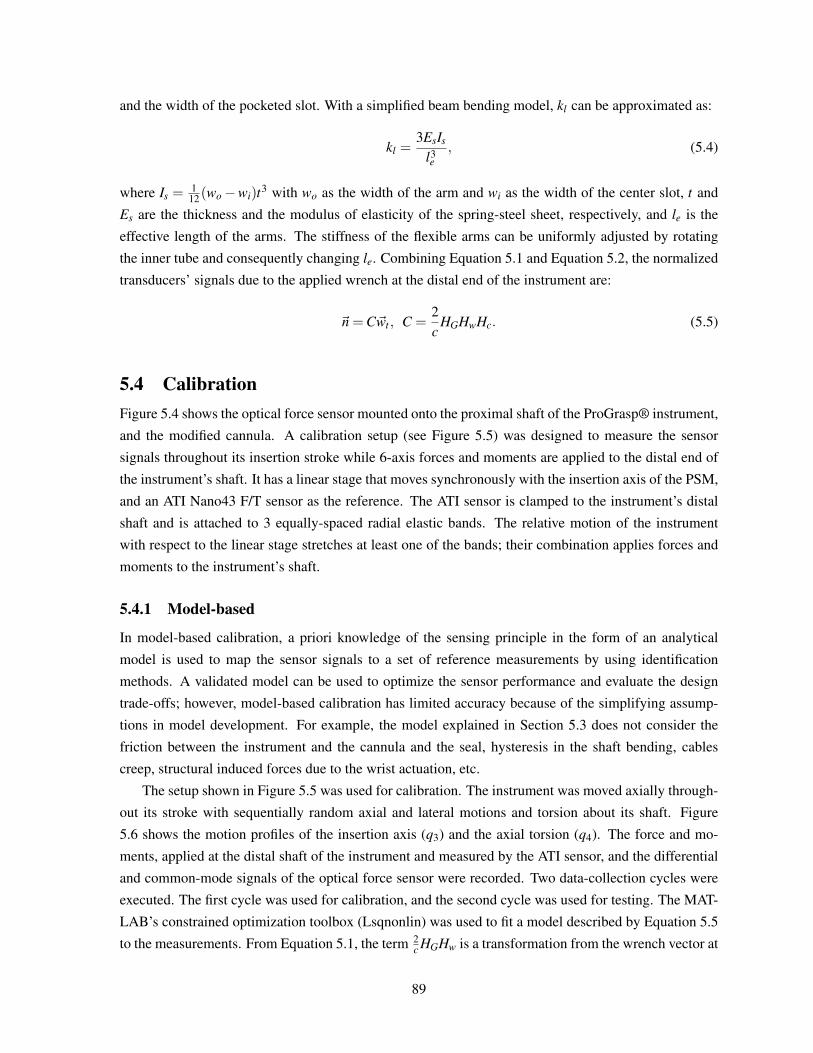
and the width of the pocketed slot. With a simplified beam bending model, kl can be approximated as:
kl =3EsIs
l3e
, (5.4)
where Is =1
12(wo−wi)t3 with wo as the width of the arm and wi as the width of the center slot, t and
Es are the thickness and the modulus of elasticity of the spring-steel sheet, respectively, and le is the
effective length of the arms. The stiffness of the flexible arms can be uniformly adjusted by rotating
the inner tube and consequently changing le. Combining Equation 5.1 and Equation 5.2, the normalized
transducers’ signals due to the applied wrench at the distal end of the instrument are:
~n =C~wt , C =2c
HGHwHc. (5.5)
5.4 CalibrationFigure 5.4 shows the optical force sensor mounted onto the proximal shaft of the ProGrasp® instrument,
and the modified cannula. A calibration setup (see Figure 5.5) was designed to measure the sensor
signals throughout its insertion stroke while 6-axis forces and moments are applied to the distal end of
the instrument’s shaft. It has a linear stage that moves synchronously with the insertion axis of the PSM,
and an ATI Nano43 F/T sensor as the reference. The ATI sensor is clamped to the instrument’s distal
shaft and is attached to 3 equally-spaced radial elastic bands. The relative motion of the instrument
with respect to the linear stage stretches at least one of the bands; their combination applies forces and
moments to the instrument’s shaft.
5.4.1 Model-based
In model-based calibration, a priori knowledge of the sensing principle in the form of an analytical
model is used to map the sensor signals to a set of reference measurements by using identification
methods. A validated model can be used to optimize the sensor performance and evaluate the design
trade-offs; however, model-based calibration has limited accuracy because of the simplifying assump-
tions in model development. For example, the model explained in Section 5.3 does not consider the
friction between the instrument and the cannula and the seal, hysteresis in the shaft bending, cables
creep, structural induced forces due to the wrist actuation, etc.
The setup shown in Figure 5.5 was used for calibration. The instrument was moved axially through-
out its stroke with sequentially random axial and lateral motions and torsion about its shaft. Figure
5.6 shows the motion profiles of the insertion axis (q3) and the axial torsion (q4). The force and mo-
ments, applied at the distal shaft of the instrument and measured by the ATI sensor, and the differential
and common-mode signals of the optical force sensor were recorded. Two data-collection cycles were
executed. The first cycle was used for calibration, and the second cycle was used for testing. The MAT-
LAB’s constrained optimization toolbox (Lsqnonlin) was used to fit a model described by Equation 5.5
to the measurements. From Equation 5.1, the term 2c HGHw is a transformation from the wrench vector at
89
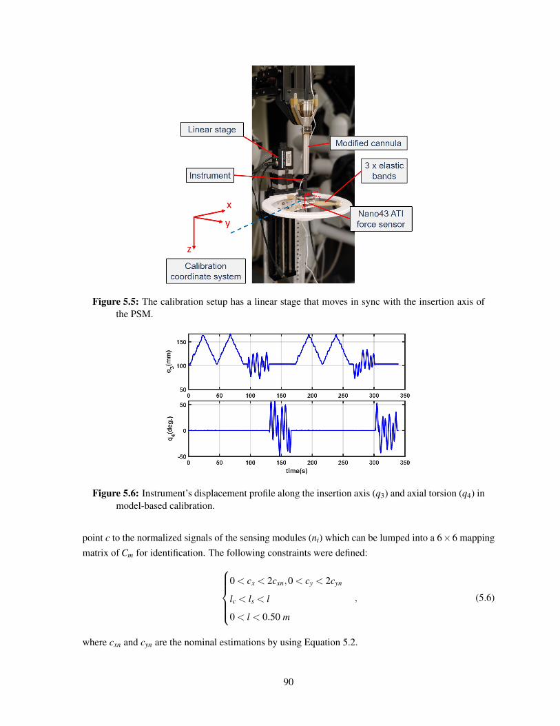
Figure 5.5: The calibration setup has a linear stage that moves in sync with the insertion axis ofthe PSM.
Figure 5.6: Instrument’s displacement profile along the insertion axis (q3) and axial torsion (q4) inmodel-based calibration.
point c to the normalized signals of the sensing modules (ni) which can be lumped into a 6×6 mapping
matrix of Cm for identification. The following constraints were defined:0 < cx < 2cxn,0 < cy < 2cyn
lc < ls < l
0 < l < 0.50 m
, (5.6)
where cxn and cyn are the nominal estimations by using Equation 5.2.
90
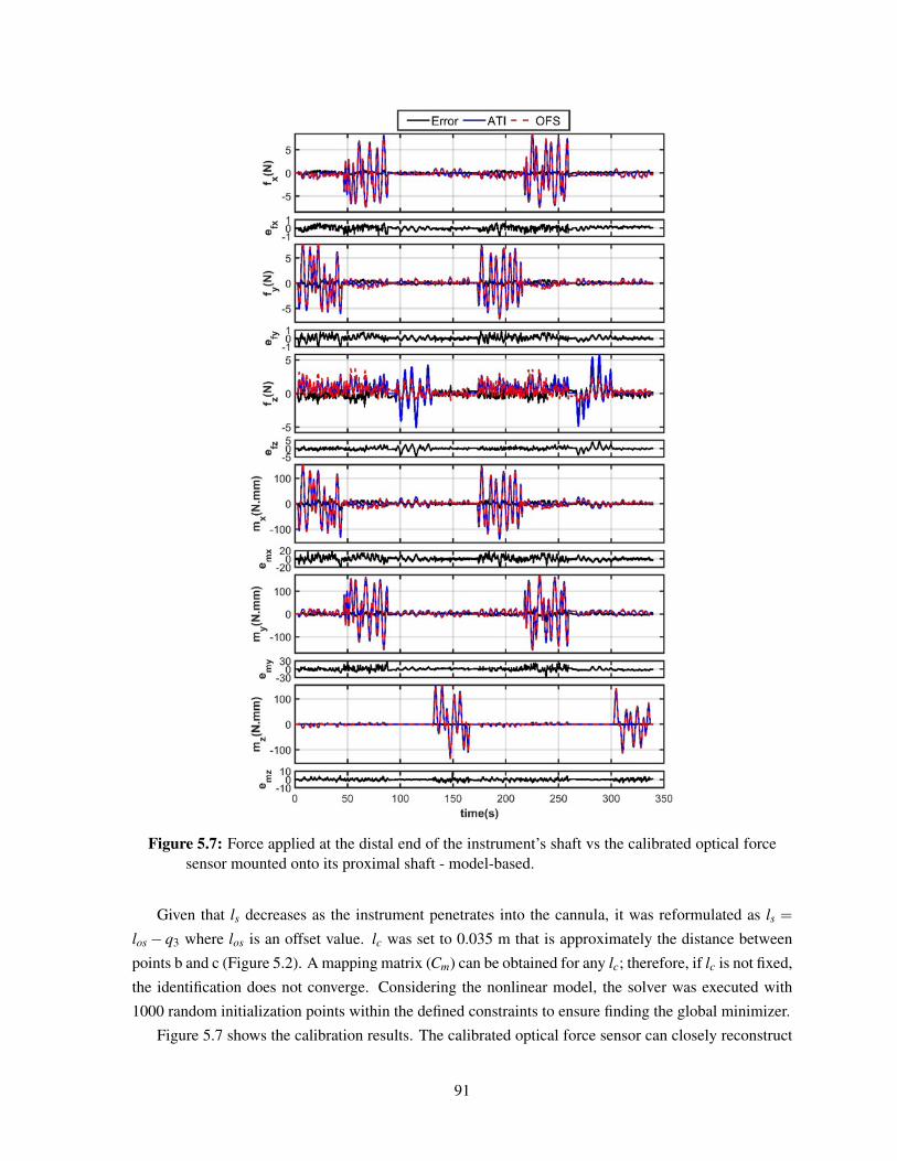
Figure 5.7: Force applied at the distal end of the instrument’s shaft vs the calibrated optical forcesensor mounted onto its proximal shaft - model-based.
Given that ls decreases as the instrument penetrates into the cannula, it was reformulated as ls =
los− q3 where los is an offset value. lc was set to 0.035 m that is approximately the distance between
points b and c (Figure 5.2). A mapping matrix (Cm) can be obtained for any lc; therefore, if lc is not fixed,
the identification does not converge. Considering the nonlinear model, the solver was executed with
1000 random initialization points within the defined constraints to ensure finding the global minimizer.
Figure 5.7 shows the calibration results. The calibrated optical force sensor can closely reconstruct
91
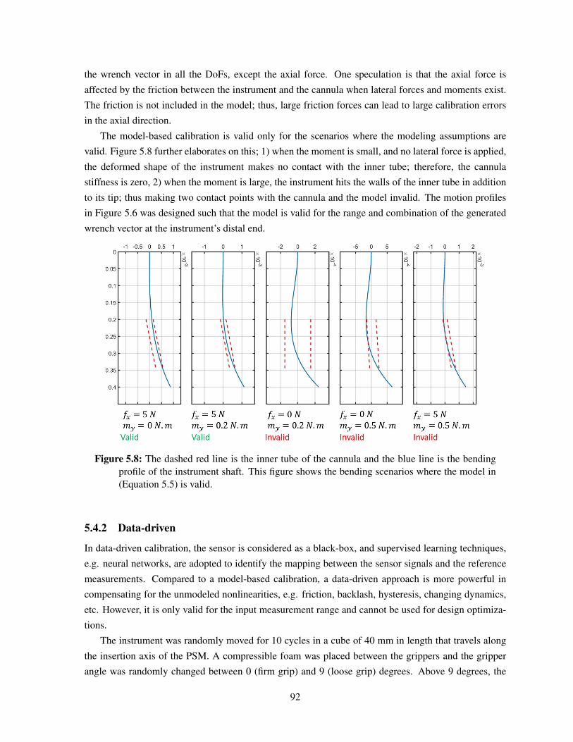
the wrench vector in all the DoFs, except the axial force. One speculation is that the axial force is
affected by the friction between the instrument and the cannula when lateral forces and moments exist.
The friction is not included in the model; thus, large friction forces can lead to large calibration errors
in the axial direction.
The model-based calibration is valid only for the scenarios where the modeling assumptions are
valid. Figure 5.8 further elaborates on this; 1) when the moment is small, and no lateral force is applied,
the deformed shape of the instrument makes no contact with the inner tube; therefore, the cannula
stiffness is zero, 2) when the moment is large, the instrument hits the walls of the inner tube in addition
to its tip; thus making two contact points with the cannula and the model invalid. The motion profiles
in Figure 5.6 was designed such that the model is valid for the range and combination of the generated
wrench vector at the instrument’s distal end.
Figure 5.8: The dashed red line is the inner tube of the cannula and the blue line is the bendingprofile of the instrument shaft. This figure shows the bending scenarios where the model in(Equation 5.5) is valid.
5.4.2 Data-driven
In data-driven calibration, the sensor is considered as a black-box, and supervised learning techniques,
e.g. neural networks, are adopted to identify the mapping between the sensor signals and the reference
measurements. Compared to a model-based calibration, a data-driven approach is more powerful in
compensating for the unmodeled nonlinearities, e.g. friction, backlash, hysteresis, changing dynamics,
etc. However, it is only valid for the input measurement range and cannot be used for design optimiza-
tions.
The instrument was randomly moved for 10 cycles in a cube of 40 mm in length that travels along
the insertion axis of the PSM. A compressible foam was placed between the grippers and the gripper
angle was randomly changed between 0 (firm grip) and 9 (loose grip) degrees. Above 9 degrees, the
92
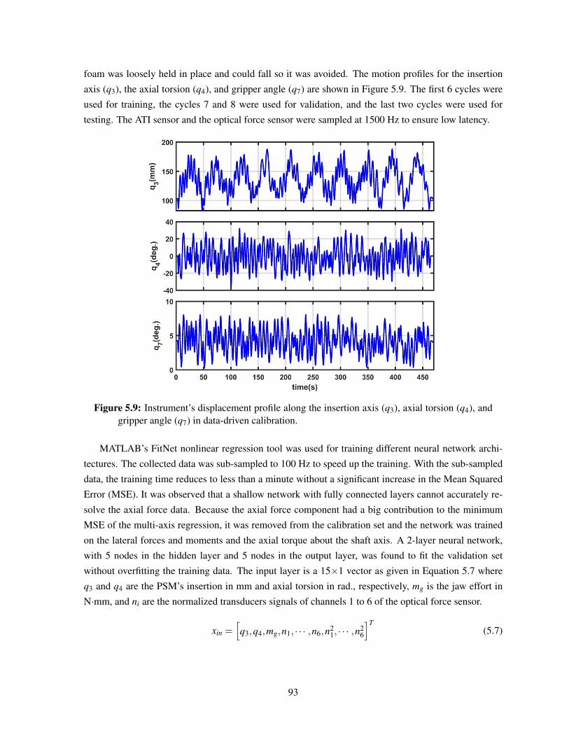
foam was loosely held in place and could fall so it was avoided. The motion profiles for the insertion
axis (q3), the axial torsion (q4), and gripper angle (q7) are shown in Figure 5.9. The first 6 cycles were
used for training, the cycles 7 and 8 were used for validation, and the last two cycles were used for
testing. The ATI sensor and the optical force sensor were sampled at 1500 Hz to ensure low latency.
Figure 5.9: Instrument’s displacement profile along the insertion axis (q3), axial torsion (q4), andgripper angle (q7) in data-driven calibration.
MATLAB’s FitNet nonlinear regression tool was used for training different neural network archi-
tectures. The collected data was sub-sampled to 100 Hz to speed up the training. With the sub-sampled
data, the training time reduces to less than a minute without a significant increase in the Mean Squared
Error (MSE). It was observed that a shallow network with fully connected layers cannot accurately re-
solve the axial force data. Because the axial force component had a big contribution to the minimum
MSE of the multi-axis regression, it was removed from the calibration set and the network was trained
on the lateral forces and moments and the axial torque about the shaft axis. A 2-layer neural network,
with 5 nodes in the hidden layer and 5 nodes in the output layer, was found to fit the validation set
without overfitting the training data. The input layer is a 15×1 vector as given in Equation 5.7 where
q3 and q4 are the PSM’s insertion in mm and axial torsion in rad., respectively, mg is the jaw effort in
N·mm, and ni are the normalized transducers signals of channels 1 to 6 of the optical force sensor.
xin =[q3,q4,mg,n1, · · · ,n6,n2
1, · · · ,n26
]T(5.7)
93
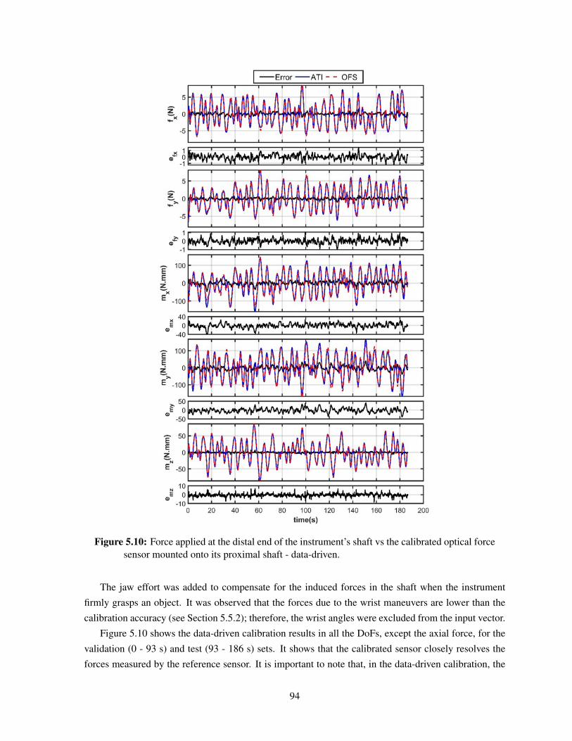
Figure 5.10: Force applied at the distal end of the instrument’s shaft vs the calibrated optical forcesensor mounted onto its proximal shaft - data-driven.
The jaw effort was added to compensate for the induced forces in the shaft when the instrument
firmly grasps an object. It was observed that the forces due to the wrist maneuvers are lower than the
calibration accuracy (see Section 5.5.2); therefore, the wrist angles were excluded from the input vector.
Figure 5.10 shows the data-driven calibration results in all the DoFs, except the axial force, for the
validation (0 - 93 s) and test (93 - 186 s) sets. It shows that the calibrated sensor closely resolves the
forces measured by the reference sensor. It is important to note that, in the data-driven calibration, the
94
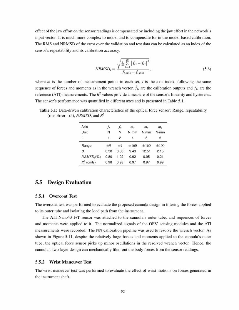
effect of the jaw effort on the sensor readings is compensated by including the jaw effort in the network’s
input vector. It is much more complex to model and to compensate for in the model-based calibration.
The RMS and NRMSD of the error over the validation and test data can be calculated as an index of the
sensor’s repeatability and its calibration accuracy:
NRMSDi =
√1m
m∑
k=1
[fki− fki
]2fi,max− fi,min
, (5.8)
where m is the number of measurement points in each set, i is the axis index, following the same
sequence of forces and moments as in the wrench vector, fki are the calibration outputs and fki are the
reference (ATI) measurements. The R2 values provide a measure of the sensor’s linearity and hysteresis.
The sensor’s performance was quantified in different axes and is presented in Table 5.1.
Table 5.1: Data-driven calibration characteristics of the optical force sensor: Range, repeatability(rms Error - σi), NRMSD, and R2
Axis fx fy mx my mz
Unit N N N·mm N·mm N·mm
i 1 2 4 5 6
Range ±9 ±9 ±160 ±160 ±100σi 0.38 0.30 9.43 12.51 2.15
NRMSDi(%) 0.80 1.02 0.92 0.95 0.21
R2i (dmls) 0.98 0.98 0.97 0.97 0.99
5.5 Design Evaluation
5.5.1 Overcoat Test
The overcoat test was performed to evaluate the proposed cannula design in filtering the forces applied
to its outer tube and isolating the load path from the instrument.
The ATI Nano43 F/T sensor was attached to the cannula’s outer tube, and sequences of forces
and moments were applied to it. The normalized signals of the OFS’ sensing modules and the ATI
measurements were recorded. The NN calibration pipeline was used to resolve the wrench vector. As
shown in Figure 5.11, despite the relatively large forces and moments applied to the cannula’s outer
tube, the optical force sensor picks up minor oscillations in the resolved wrench vector. Hence, the
cannula’s two-layer design can mechanically filter out the body forces from the sensor readings.
5.5.2 Wrist Maneuver Test
The wrist maneuver test was performed to evaluate the effect of wrist motions on forces generated in
the instrument shaft.
95
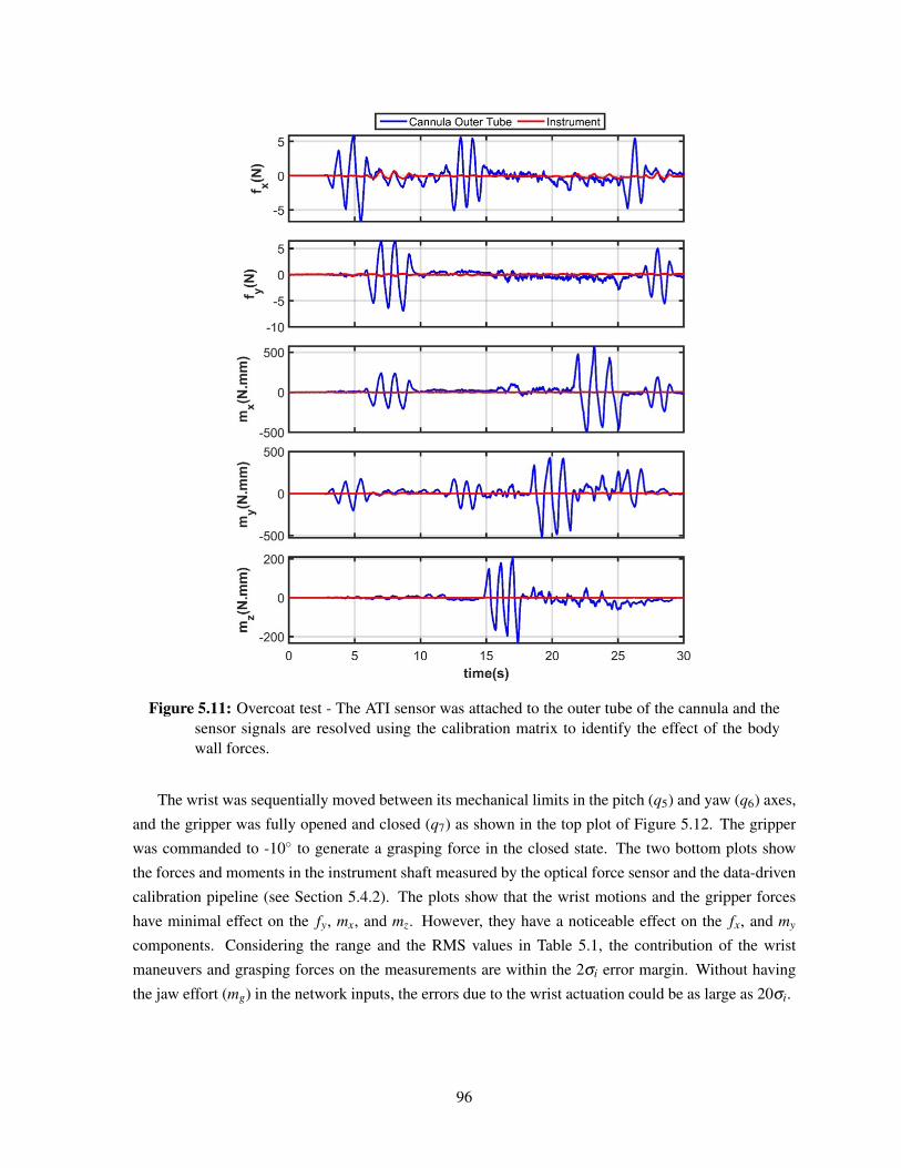
Figure 5.11: Overcoat test - The ATI sensor was attached to the outer tube of the cannula and thesensor signals are resolved using the calibration matrix to identify the effect of the bodywall forces.
The wrist was sequentially moved between its mechanical limits in the pitch (q5) and yaw (q6) axes,
and the gripper was fully opened and closed (q7) as shown in the top plot of Figure 5.12. The gripper
was commanded to -10◦ to generate a grasping force in the closed state. The two bottom plots show
the forces and moments in the instrument shaft measured by the optical force sensor and the data-driven
calibration pipeline (see Section 5.4.2). The plots show that the wrist motions and the gripper forces
have minimal effect on the fy, mx, and mz. However, they have a noticeable effect on the fx, and my
components. Considering the range and the RMS values in Table 5.1, the contribution of the wrist
maneuvers and grasping forces on the measurements are within the 2σi error margin. Without having
the jaw effort (mg) in the network inputs, the errors due to the wrist actuation could be as large as 20σi.
96
Figure 5.12: Wrist maneuver test - The instrument’s wrist was moved within its mechanical rangeand the induced forces in the instrument shaft were estimated using the data-driven calibra-tion pipeline.
5.6 ConclusionIn this chapter, we proposed a novel 6-axis optical force sensor mounted onto the proximal shaft of a da
Vinci® EndoWrist® instrument for measuring the wrench vector applied to its distal end. The optical
force sensor has an active and a passive component. The active component has the power conditioning
and digital electronics and six sensing modules. Each sensing module has a LED and a bicell placed
inline, and a collocated signal conditioning board. The passive component has the slits in alternating
orientations, aligned with the gap between the two active areas of the bicells, for light modulation. The
careful electronics design provides a very high-resolution slit displacement measurement.
The first prototype is compact and fits in a cube of 50 mm in length. It weighs approximately 150
grams, which is close to the weight of the ProGrasp instrument. A balancing slider with dummy weights
is used in the parallelogram mechanism design of the da Vinci® classic system for gravity compensation
of the drive train and the instrument. The weights were adjusted to avoid the instrument dropping when
the sensor is mounted and the drives are off. With the improvements in the next prototypes, the sensor’s
weight and size can be further reduced.
The sensor has no structural flexure making it not breakable due to overload. The sensor’s compo-
nents are not in the load path, and they do not require special provisions for mounting onto the structure.
Therefore, it allows easy integration into RAMIS systems. A higher number of sensing modules can
be used for redundancy and error detection. Additionally, they can be placed in alternate configurations
97
for improved accuracy and resolution. The signal conditioning electronics has a high-resolution ADC
with a built-in programmable gain amplifier that can be used for dynamic adjustment of the transducer’s
range and resolution. The low latency and high data-rate reported in Section Chapter 4 make the sensor
a good fit for control applications. With the onboard processor, only four wires (two for power and two
for RS485 half-duplex communication link) are needed to interface with the sensor, which makes the
wiring management simple and minimizes the cable loads in arm maneuvers. Lastly, the signal condi-
tioning circuit has a high bandwidth of 500 Hz that allows using the sensor for vibration detection [145],
and vibrotactile haptic perception, as proposed by Kuchenbecker et al. [201].
In addition to the force sensor, a modified cannula design was presented. The new design has two
tubes. The outer tube isolates the load path from the instrument. The inner tube is attached through
a 3-arm leaf spring to the base of the cannula to allow instrument bending due to forces at its distal
end. The effective stiffness at the tip of the cannula’s inner tube can be adjusted by rotating the inner
tube and consequently changing the arm of the leaf springs. It is to avoid the closing of the 1.5 mm
gap between the inner and the outer tube at the maximum lateral forces and moments. The proposed
concept increased the OD of the cannula by 3 mm. This idea can be easily applied to the standard da
Vinci® cannula’s currently used in clinical systems as well as the AirSeal® access ports from CONMED
[202] for reduced friction.
A mathematical model was developed to capture the changes in the instrument’s bending behavior
as it penetrates into the cannula. It was used for a model-based calibration, and the results showed
that the model captures the dynamics of the varying boundary condition. The model combined with
the validated sensor model presented in Chapter 3 can be used for evaluating the design trade-offs and
optimizations. The limitations of the model-based calibration were discussed. It was compared with
a data-driven approach comprising a shallow neural network of one hidden layer and one output layer.
In particular, the data-driven calibration covers the scenarios in which the developed model is not valid
(see Figure 5.8), and it can compensate for the effect of the grasping force on the measurements that is
complex to model.
A shallow NN architecture was used to avoid overfitting to the training data and minimize the com-
putation cost. The data-driven calibration results showed an accuracy of close to 10% in the lateral
forces, which is the human’s JND over the range of 0.5-200 N as explained in Chapter 1 and Sec-
tion 5.1. As expected, the best accuracy (∼6%) was obtained in the axial torque. It is because the sensor
configuration is most sensitive to the axial torque (see Chapter 3) and it is not affected by the changes in
the instrument support (see Equation 5.1 and Equation 5.2). Despite the high-resolution displacement
measurement that the sensor provides, it failed to closely resolve the axial force.
The overcoat test and the wrist maneuver test were conducted to further evaluate the proposed sens-
ing approach. The former showed that the modified cannula can properly filter the body wall forces
from the measurements. The latter verified that the grasping forces have a more dominant effect on the
measurement accuracy compared to the wrist actuation in the pitch and yaw axes.
98
Chapter 6
Conclusion and Future Work
6.1 ConclusionWith the rapid developments in the fields of robotics, computer vision, and data-driven learning, RAMIS
has been showing exponential popularity over the past decade [18]. In addition to the benefits of a min-
imally invasive procedure such as less tissue trauma, blood loss, and faster recovery, RAMIS provides
improved ergonomic factors, reducing surgeon fatigue, 3D surgical vision, automatic movement trans-
formations, fine motions, hand tremor filtering, motion scaling, and improved instrument dexterity all
of which lead to higher surgery precision [4, 8].
Despite the recent advancements, the clinical RAMIS systems do not provide haptic perception [38].
This deprives the surgeon of the rich information embedded in palpating the tissue and direct interaction
with surgical tools. Traditionally, surgeons use palpation to characterize tissue properties, detect nerves
and arteries, and identify abnormalities such as lumps and tumors [45]. Moreover, the surgeons rely on
the sense of touch to regulate the applied forces. Excessive forces can lead to tissue trauma, internal
bleeding, and broken sutures. However, insufficient forces can lead to loose knots and poor sutures.
Thus, many studies are targeted towards the reconstruction and evaluation of haptic feedback [12].
Several surveys on haptic feedback and its efficacy in teleoperated robotic surgery [34, 35], simula-
tion, and training [36, 37] have been published in recent years. In summary, the introduction of haptic
perception is proven to decrease operation time, facilitate training, improve accuracy, and enhance pa-
tient safety in complex tasks. Additionally, force information can be used to automate robotic tasks
in unstructured environments, to identify tissues in real-time, to create tissue-realistic models and sim-
ulators for training, and to perform surgical skills assessment [4, 31]. A transparent haptic interface
requires a method of force estimation or force sensing.
In this thesis, we aimed to research the developments that add the force-sensing capability to the
scanner and adapter manipulators of the da Vinci® classics system without modifying the interface to
the surgeon and the surgical instruments.
Chapter 1 presented a comprehensive review of the articles, published over the past decade, focused
on estimation or measurement of the instrument-tissue interaction forces. The design requirements of a
99
sensor that can be deployed into clinical use was discussed. The pros and cons of different transduction
technologies at different locations along the instrument were compared. It concluded that a noticeable
shift towards using the FBGs and MEM transducers for sensing, and data-driven methods for calibration
and estimation can be observed. While many studies are published on the instrument-tissue forces
measurement, the surgeon interaction forces with the scanner manipulator in the surgeon console is not
studied extensively.
Chapter 2 proposed a novel design for the wrist’s yaw link of the MTM in the da Vinci® classic
system that allows the integration of an ATI Nano43 F/T sensor without changing the arm’s kinematics.
The mechanical design and the modifications in the electrical wiring of the finger roll motor and the
finger grip’s hall-effect sensor were explained. The new design does not limit the original wrist’s enve-
lope and its dexterity. The dynamic identification of the wrist’s yaw link showed close to 18% increase
in its moment of inertia and a minor increase in its friction. Two software packages were developed
for the standalone use of the sensor, and to integrate it into the ROS framework and dVRK. Two exam-
ple applications of impedance control of the MTM and joystick control of the PSM were presented to
demonstrate the successful integration of the sensor into the MTM and its interface to the dVRK.
In Chapter 3, the transduction principle and the mechanical design of a novel 6-axis optical force
sensor was presented. The proposed sensor comprises of six sensing modules in alternating orientations.
Each module has an IR LED inline with a bicell photodiode. An optical slit aligned with the gap
between the two active areas of the bicell modulates the light incident on each cell. It was shown that
the multi-cell photodiodes can provide a very high resolution displacement measurement in the order
of a few nanometers. A mathematical model of the sensor based on the electro-optical conversion and
the principles of continuum mechanics was developed. Extensive testing was conducted to validate
the sensor model. A least squares calibration was presented to resolve the wrench vector applied to
the sensor from the transducers signals. It was shown that the error between the theoretical and the
experimental calibration matrices is less than 35%, which is sufficient for design development. A novel
temperature compensation approach was developed and validated.
The OFS has no flexible components, which makes it robust to overload. In fact, it relies on the
compliance of the support structure and its high resolution displacement measurement for force sensing.
An external reference sensor is required for calibration where the active and passive components are
installed onto a load carrying structure. Alternatively, the sensor can be supplied with different calibrated
center shafts for different force ranges and resolutions.
Chapter 4 presented the electronics hardware, the firmware design, and the software packages to
interface with the OFS. The sensor electronics has three custom boards. The bicell board has the sig-
nal conditioning circuitry and a co-located high resolution ADC. Each sensing module has one bicell
board. The Power/Com board has the power conditioning and management circuitry, an onboard FPGA
processor, the LED current drivers, an IMU, and a temperature sensor. An FPC is used to route the
signals between the bicell boards and the Power/Com board to accommodate fabrication tolerances and
avoid stressing the boards due to temperature changes. The FPGA is configured for parallel processing
and synchronized sampling of all the peripherals to achieve low latency and high data throughput. A
100
standalone software and a ROS package was developed for easy integration of the sensor into the robotic
applications. Extensive testing was reported to quantify the noise level, latency, and data throughput. It
was shown that sensor design provides ultra-low noise with an average noise power spectral density of
15 nV/√
Hz over a signal bandwidth of 500 Hz, a resolution of 0.0001% full-scale at a 95% confidence
level, and a hardware latency of less than 100 µs. The features above make the sensor a cost-effective
candidate in many robotic and mechatronic applications.
In Chapter 5, the integration of the OFS into the da Vinci® classic system for measuring the forces
applied to the distal end of an EndoWrist® instrument (ProGrasp®) was discussed. The sensor was
mounted onto the proximal shaft of the instrument. A modified cannula design with an inner tube and
an outer tube was proposed. The outer tube mechanically filters out the cannula forces at the access
hole and the inner tube is compliant to allow the instrument deflection. The presented approach requires
no modification to the instrument and is therefore adaptable to different endoscopic instruments with
a slender shaft. A mathematical model that explains the bending behavior of the instrument’s shaft as
a function of its penetration into the cannula was developed. A model-based calibration and a data-
driven calibration using a shallow neural network were compared. The results showed that a data-driven
calibration can more accurately capture the non-linearities that are difficult to model. The current design
sensor cannot be mounted onto the instrument before the instrument is attached to the classic, S, and
SI da Vinci® robots. It is because in the above series, the instrument clips onto a sterile adapter that
intersects with the sensor’s envelope. However, this is not a limitation in the X, and XI series because
the mounting interface is different.
6.2 Future WorkConsidering the research and developments presented in this thesis, the followings can be considered as
the future work and improvements:
Modified MTM:
• During assembly, we noticed that although the JST connector provides a modular interface to
the hall-effect sensors and the potentiometer, its connections to the ribbon wires are fragile and
not robust. In the future, we will replace the JST connectors with a breakout board and a FPC
connection to the hall-effect sensor.
• One potential application of using the MTM as a joystick is in positioning the endoscopic camera
without losing the registration between the MTMs and the PSMs.
OFS - Design and Calibration:
• It is of interest to modify the sensor design for easy installation onto support structures with
different shapes, not necessarily limited to cylindrical shafts of a particular diameter.
• Redundant transducers can be used for noise improvement and fault detection.
• The design of the sensing modules can be simplified to eliminate the eccentric gear for nulling.
101

• The fabrication cost of the current prototype is comparable to the ATI Nano43 and its DAQ box,
which retail at 6.3k USD. Design improvements and mass production can reduce the sensor cost.
OFS - Electronics and Firmware:
• Individual temperature sensors can be integrated on the bicell boards for improved temperature
compensation.
• A wireless adapter can be integrated into the Power/Com board to allow remote use of the sensor
when operated off a battery. One example application is mounting the sensor onto the spindle or
tool-holder of a CNC machine for 6-axis force sensing, chatter detection, and/or vibration control.
• The sensor electronics can be more compact by using surface mount LEDs and photodiodes.
• We consider replacing the moving average filter with an Auto Regressive Moving Average (ARMA)
model for customized low-pass, high-pass, band-pass, notch, or a combination of multiple filters.
• The Python library will also be developed further to provide more extensive functionality (e.g.
calibration, programming filters, etc.).
PSM Instrumentation:
• The sensing approach failed to closely resolve the axial force component. Design improvements
such as using the AirSeal® access port, and adding a Teflon coating or bronze bushings at the tip
of the cannula’s inner tube can improve the sensor performance in the axial direction by reducing
the friction.
• Other supervised learning methods can be investigated to reconstruct the axial force component
without degrading the sensor performance in the other DoFs.
• Mechanical references can be added for a more accurate positioning and repeatable sensor instal-
lation, which could eliminate the need for re-calibration after every installation onto the PSM.
• One limitation of the current sensor is the need for another reference sensor and the calibration
setup in Section 5.4 for calibration. In future work, other calibration methods that do not rely
upon an external sensor can be explored, e.g., using the IMU and the inertial parameters of a
known payload, or by payload estimation in robotic applications.
In addition to the above, the modified MTM’s wrist discussed in Chapter 2 and the new multi-axis optical
force sensor discussed in the subsequent chapters upgrade the da Vinci® classic system to provide
force sensing at the surgeon and the patient consoles. This enhancement allows for a diverse range
of research opportunities as developing a transparency optimized telesurgical framework by adding
haptic feedback, surgical tasks automation by using the force information, surgical skills assessment,
developing simulators for training, and learning from demonstration.
102

Bibliography
[1] C.R. Wottawa, B. Genovese, B.N. Nowroozi, J.W. Bisley, W.S. Grundfest, and E.P. Dutson.Evaluating Tactile Feedback in Robotic Surgery for Potential Clinical Application Using anAnimal Model. Surgical Endoscopy, 30:3198–3209, 2016.doi:https://doi.org/10.1007/s00464-015-4602-2. → page 1
[2] Pouya Soltani-Zarrin, Abelardo Escoto, Ran Xu, Rajni V. Patel, Michael D. Naish, andAna Luisa Trejos. Development of a 2-DOF Sensorized Surgical Grasper for Grasping andAxial Force Measurements. IEEE Sensors Journal, 18(7):2816–2826, April 2018.doi:10.1109/JSEN.2018.2805327. → pages 1, 5, 6, 7, 9, 21, 23
[3] Yuan Dai, Ahmad Abiri, Siyuan Liu, Omeed Paydar, Hyunmin Sohn, Eric P. Dutson, Warren S.Grundfest, and R. N. Candler. Grasper Integrated Tri-axial Force sensor System for RoboticMinimally Invasive Surgery. In 2017 Proceedings of the Annual International Conference of theIEEE Engineering in Medicine and Biology Society, EMBS, pages 3936–3939, September 2017.doi:10.1109/EMBC.2017.8037717. → pages 1, 7, 26
[4] N. Bandari, J. Dargahi, and M. Packirisamy. Tactile Sensors for Minimally Invasive Surgery: AReview of the State-of-the-Art, Applications, and Perspectives. IEEE Access, 8:7682–7708,2020. doi:10.1109/ACCESS.2019.2962636. → pages 1, 5, 6, 7, 99
[5] Chiwon Lee, Yong Hyun Park, Chiyul Yoon, Seungwoo Noh, Choonghee Lee, Youdan Kim,Hee Chan Kim, Hyeon Hoe Kim, and Sungwan Kim. A Grip Force Model for the da VinciEnd-effector to Predict a Compensation Force. Medical and Biological Engineering andComputing, 53(3):253–261, November 2015. doi:10.1007/s11517-014-1230-2. → pages1, 12, 13
[6] Angelica I. Aviles, Samar Alsaleh, Pilar Sobrevilla, and Alicia Casals. Exploring the Effects ofDimensionality Reduction in Deep Networks for Force Estimation in Robotic-Assisted Surgery.In 2016 Medical Imaging 2016: Image-Guided Procedures, Robotic Interventions, andModeling, volume 9786, pages 585–592, 2016. doi:10.1117/12.2217000. → pages 1, 15, 16, 17
[7] Christoph Otte, Jens Beringhoff, Sarah Latus, Sven Thomas Antoni, Omer Rajput, andAlexander Schlaefer. Towards Force Sensing Based on Instrument-Tissue Interaction. In 2016IEEE International Conference on Multisensor Fusion and Integration for Intelligent Systems,pages 180–185, September 2016. doi:10.1109/MFI.2016.7849486. → pages 1, 15, 16
[8] Angelica I. Aviles, Samar M. Alsaleh, James K. Hahn, and Alicia Casals. Towards RetrievingForce Feedback in Robotic-Assisted Surgery: A Supervised Neuro-Recurrent-Vision Approach.IEEE Transactions on Haptics, 10(3):431–443, July 2017. doi:10.1109/TOH.2016.2640289. →pages 1, 5, 17, 29, 99
103
[9] A. Faragasso, J. Bimbo, Y. Noh, A. Jiang, S. Sareh, H. Liu, T. Nanayakkara, H. A. Wurdemann,and K. Althoefer. Novel Uniaxial Force Sensor Based on Visual Information for MinimallyInvasive Surgery. In 2014 Proceedings - IEEE International Conference on Robotics andAutomation, pages 1405–1410, September 2014. doi:10.1109/ICRA.2014.6907036. → pages1, 16
[10] Mohammad Haghighipanah, Muneaki Miyasaka, and Blake Hannaford. Utilizing Elasticity ofCable-Driven Surgical Robot to Estimate Cable Tension and External Force. IEEE Robotics andAutomation Letters, 2(3):1593–1600, July 2017. doi:10.1109/LRA.2017.2676347. → pages1, 11, 14
[11] Nazim Haouchine, Winnie Kuang, Stephane Cotin, and Michael Yip. Vision-Based ForceFeedback Estimation for Robot-Assisted Surgery Using Instrument-Constrained BiomechanicalThree-Dimensional Maps. IEEE Robotics and Automation Letters, 3(3):2160–2165, July 2018.doi:10.1109/LRA.2018.2810948. → pages 1, 17
[12] A. H. Hadi Hosseinabadi, M. Honarvar, and S. E. Salcudean. Optical Force Sensing InMinimally Invasive Robotic Surgery. In 2019 International Conference on Robotics andAutomation (ICRA), pages 4033–4039, May 2019. doi:10.1109/ICRA.2019.8793589. → pages1, 7, 11, 17, 21, 22, 47, 99
[13] Kaspar S. Shahzada, Aaron Yurkewich, Ran Xu, and Rajni V. Patel. Sensorization of a SurgicalRobotic Instrument for Force Sensing. In 2016 Optical Fibers and Sensors for MedicalDiagnostics and Treatment Applications XVI, volume 9702, pages 153–162, 2016.doi:10.1117/12.2213385. → pages 1, 21, 23
[14] Angelica I. Aviles, Samar Alsaleh, Pilar Sobrevilla, and Alicia Casals. Sensorless ForceEstimation Using a Neuro-Vision-Based Approach for Robotic-Assisted Surgery. In 2015International IEEE/EMBS Conference on Neural Engineering, NER, pages 86–89, April 2015.doi:10.1109/NER.2015.7146566. → pages 1, 16
[15] Trevor K Stephens, John J O’neill, Nathan J Kong, Mark V Mazzeo, Jack E Norfleet, Robert MSweet, and Timothy M Kowalewski. Conditions for Reliable Grip Force and Jaw AngleEstimation of da Vinci Surgical Tools. International Journal of Computer Assisted Radiologyand Surgery, 14:117–127, 2019. doi:10.1007/s11548-018-1866-8. → pages 1, 5, 10, 12, 14
[16] Hongqiang Sang, Jintian Yun, Reza Monfaredi, Emmanuel Wilson, Hadi Fooladi, and KevinCleary. External Force Estimation and Implementation in Robotically Assisted MinimallyInvasive Surgery. The International Journal of Medical Robotics and Computer AssistedSurgery, 13(2):e1824:1–15, 2017. doi:10.1002/rcs.1824. → pages 1, 2, 11, 13, 23, 26
[17] Yen-Yi Juo, Ahmad Abiri, Jake Pensa, Songping Sun, Anna Tao, James Bisley, WarrenGrundfest, and Erik Dutson. Center for Advanced Surgical and Interventional TechnologyMultimodal Haptic Feedback for Robotic Surgery. In Handbook of Robotic and Image-GuidedSurgery, pages 285–301. Elsevier, January 2020. doi:10.1016/B978-0-12-814245-5.00017-7.→ pages 1, 2, 3, 5, 26
[18] Intuitive Surgical Inc. Intuitive Surgical Inc. - J.P. Morgan Healthcare Conference 2021.https://isrg.intuitive.com/, 2021. Accessed March 10, 2021. → pages 1, 99
104

[19] Peter F. Hokayem and Mark W. Spong. Bilateral teleoperation: An historical survey.Automatica, 42(12):2035–2057, 2006. doi:https://doi.org/10.1016/j.automatica.2006.06.027.URL https://www.sciencedirect.com/science/article/pii/S0005109806002871. → page 2
[20] D. A. Lawrence. Stability and Transparency in Bilateral Teleoperation. IEEE Transactions onRobotics and Automation, 9(5):624–637, 1993. doi:10.1109/70.258054. → pages 2, 4
[21] Allison M Okamura. Haptic Feedback in Robot-Assisted Minimally Invasive Surgery. CurrentOpinion in Urology, 19(1):102–107, January 2009. doi:10.1097/MOU.0b013e32831a478c. →page 2
[22] Ian Mack, Stuart Ferguson, Karen Rafferty, Stephen Potts, and Alistair Dick. InteractiveForce-Sensing Feedback System for Remote Robotic Laparoscopic Surgery. Transactions of theInstitute of Measurement and Control, 34(4):376–387, June 2012.doi:10.1177/0142331210382943. → pages 2, 27
[23] Naghmeh M. Bandari, Roozbeh Ahmadi, Amir Hooshiar, Javad Dargahi, and MuthukumaranPackirisamy. Hybrid Piezoresistive-Optical Tactile Sensor for Simultaneous Measurement ofTissue Stiffness and Detection of Tissue Discontinuity in Robot-Assisted Minimally InvasiveSurgery. Journal of Biomedical Optics, 22(7):077002:1–10, July 2017.doi:10.1117/1.jbo.22.7.077002. → pages 2, 26, 27
[24] Changhu Lv, Shuxin Wang, and Chaoyang Shi. A High-Precision and Miniature Fiber BraggGrating-Based Force Sensor for Tissue Palpation During Minimally Invasive Surgery. Annals ofBiomedical Engineering, 48(2):669–681, February 2020. doi:10.1007/s10439-019-02388-w.→ pages 2, 9, 17, 21, 23
[25] Pinyo Puangmali, Hongbin Liu, Lakmal D. Seneviratne, Prokar Dasgupta, and KasparAlthoefer. Miniature 3-axis Distal Force Sensor for Minimally Invasive Surgical Palpation.IEEE/ASME Transactions on Mechatronics, 17(4):646–656, August 2012.doi:10.1109/TMECH.2011.2116033. → pages 2, 7, 8, 21
[26] Yangming Li, Muneaki Miyasaka, Mohammad Haghighipanah, Lei Cheng, and BlakeHannaford. Dynamic Modeling of Cable Driven Elongated Surgical Instruments for SensorlessGrip Force Estimation. In 2016 Proceedings - IEEE International Conference on Robotics andAutomation, pages 4128–4134, May 2016. doi:10.1109/ICRA.2016.7487605. → pages2, 11, 12, 13, 14
[27] Keyvan Hashtrudi-Zaad and Septimiu E. Salcudean. Analysis of Control Architectures forTeleoperation Systems with Impedance/Admittance Master and Slave Manipulators.International Journal of Robotics Research, 20(6):419–445, June 2001.doi:10.1177/02783640122067471. → pages 3, 29, 36
[28] Allison M. Okamura, Lawton N. Verner, Tomonori Yamamoto, James C. Gwilliam, and Paul G.Griffiths. Force Feedback and Sensory Substitution for Robot-Assisted Surgery, pages 419–448.Springer US, Boston, MA, 2011. ISBN 978-1-4419-1126-1.doi:10.1007/978-1-4419-1126-1 18. → pages 3, 4, 36
[29] Russell Taylor, Pat Jensen, Louis Whitcomb, Aaron Barnes, Rajesh Kumar, Dan Stoianovici,Puneet Gupta, Zhengxian Wang, Eugene Dejuan, and Louis Kavoussi. A Steady-Hand RoboticSystem for Microsurgical Augmentation. The International Journal of Robotics Research, 18(12):1201–1210, 1999. doi:10.1177/02783649922067807. → page 3
105
[30] Yangming Li and Blake Hannaford. Gaussian Process Regression for Sensorless Grip ForceEstimation of Cable-Driven Elongated Surgical Instruments. IEEE Robotics and AutomationLetters, 2(3):1312–1319, July 2017. doi:10.1109/LRA.2017.2666420. → pages 3, 11, 12, 14, 29
[31] Elahe Abdi, Dana Kulic, and Elizabeth Croft. Haptics in Teleoperated Medical Interventions:Force Measurement, Haptic Interfaces and Their Influence on Users Performance. IEEETransactions on Biomedical Engineering, April 2020. doi:10.1109/tbme.2020.2987603. →pages 4, 5, 28, 29, 99
[32] K. Hastrudi-Zaad and S. E. Salcudean. On the use of local force feedback for transparentteleoperation. In Proceedings 1999 IEEE International Conference on Robotics and Automation,volume 3, pages 1863–1869 vol.3, 1999. doi:10.1109/ROBOT.1999.770380. → pages 4, 33
[33] J. E. Colgate. Robust Impedance Shaping Telemanipulation. IEEE Transactions on Roboticsand Automation, 9(4):374–384, 1993. doi:10.1109/70.246049. → page 5
[34] Farshid Amirabdollahian, Salvatore Livatino, Behrad Vahedi, Radhika Gudipati, Patrick Sheen,Shan Gawrie-Mohan, and Nikhil Vasdev. Prevalence of Haptic Feedback in Robot-MediatedSurgery: A Systematic Review of Literature. Journal of Robotic Surgery, 12(1):11–25, March2018. doi:10.1007/s11701-017-0763-4. → pages 5, 29, 99
[35] Issam El Rassi and Jean Michel El Rassi. A review of Haptic Feedback in Tele-OperatedRobotic Surgery. Journal of medical engineering & technology, pages 1–8, June 2020.doi:10.1080/03091902.2020.1772391. → pages 5, 99
[36] Evelien M. Overtoom, Tim Horeman, Frank Willem Jansen, Jenny Dankelman, and Henk W.R.Schreuder. Haptic Feedback, Force Feedback, and Force-Sensing in Simulation Training forLaparoscopy: A Systematic Overview. Journal of Surgical Education, 76(1):242–261, January2019. doi:10.1016/j.jsurg.2018.06.008. → pages 5, 29, 99
[37] Karan Rangarajan, Heather Davis, and Philip H. Pucher. Systematic Review of Virtual Hapticsin Surgical Simulation: A Valid Educational Tool? Journal of Surgical Education, 77(2):337–347, March 2020. doi:10.1016/j.jsurg.2019.09.006. → pages 5, 29, 99
[38] Ahmad Abiri, Anna Tao, Meg LaRocca, Xingmin Guan, Syed J. Askari, James W. Bisley, Erik P.Dutson, and Warren S. Grundfest. Visual–Perceptual Mismatch in Robotic Surgery. SurgicalEndoscopy, 31(8):3271–3278, August 2017. doi:10.1007/s00464-016-5358-z. → pages 5, 99
[39] Winnie Kuang, Michael Yip, and Jun Zhang. Vibration-Based Multi-Axis Force Sensing:Design, Characterization, and Modeling. IEEE Robotics and Automation Letters, 5(2):3082–3089, April 2020. doi:10.1109/LRA.2020.2975726. → pages 5, 17, 27, 28
[40] Pinyo Puangmali, Kaspar Althoefer, Lakmal D. Seneviratne, Declan Murphy, and ProkarDasgupta. State-of-the-Art in Force and Tactile Sensing for Minimally Invasive Surgery. IEEESensors Journal, 8(4):371–380, April 2008. doi:10.1109/JSEN.2008.917481. → pages 5, 30
[41] A L Trejos, R V Patel, and M D Naish. Force Sensing and Its Application in Minimally InvasiveSurgery and Therapy: A Survey. 2010 Proceedings of the Institution of Mechanical Engineers,Part C: Journal of Mechanical Engineering Science, 224(7):1435–1454, January 2010.doi:10.1243/09544062JMES1917. → pages 5, 30, 36
106
[42] B. Gonenc, A. Chamani, J. Handa, P. Gehlbach, R. H. Taylor, and I. Iordachita. 3-DOFForce-Sensing Motorized Micro-Forceps for Robot-Assisted Vitreoretinal Surgery. IEEESensors Journal, 17(11):3526–3541, 2017. → page 6
[43] Justin Wee, Robert J. Brooks, Thomas Looi, Georges Azzie, James Drake, and J. Ted Gerstle.Force-Sensing Sleeve for Laparoscopic Surgery. Journal of Medical Devices, 10(3):030946:1–2, August 2016. doi:10.1115/1.4033810. → pages 6, 19
[44] John J. O’Neill, Trevor K. Stephens, and Timothy M. Kowalewski. Evaluation of TorqueMeasurement Surrogates as Applied to Grip Torque and Jaw Angle Estimation of RoboticSurgical Tools. IEEE Robotics and Automation Letters, 3(4):3027–3034, October 2018.doi:10.1109/LRA.2018.2849862. → pages 7, 12, 14
[45] Man Bok Hong and Yung Ho Jo. Design and evaluation of 2-DOF compliant forceps withforce-sensing capability for minimally invasive robot surgery. IEEE Transactions on Robotics,28(4):932–941, 2012. doi:10.1109/TRO.2012.2194889. → pages 7, 18, 99
[46] Ahmad Abiri, Jake Pensa, Anna Tao, Ji Ma, Yen-Yi Juo, Syed J. Askari, James Bisley, JacobRosen, Erik P. Dutson, and Warren S. Grundfest. Multi-Modal Haptic Feedback for Grip ForceReduction in Robotic Surgery. Scientific Reports, 9(1):5016:1–10, December 2019.doi:10.1038/s41598-019-40821-1. → page 7
[47] Adam J. Spiers, Harry J. Thompson, and Anthony G. Pipe. Investigating Remote SensorPlacement for Practical Haptic Sensing with EndoWrist Surgical Tools. In 2015 IEEE WorldHaptics Conference, pages 152–157, June 2015. doi:10.1109/WHC.2015.7177706. → pages7, 8, 9, 18, 29, 84
[48] Seyed Mohsen Khadem, Saeed Behzadipour, Alireza Mirbagheri, and Farzam Farahmand. AModular Force-Controlled Robotic Instrument for Minimally Invasive Surgery - Efficacy forBeing Used in Autonomous Grasping Against a Variable Pull Force. The International Journalof Medical Robotics and Computer Assisted Surgery, 12(4):620–633, December 2016.doi:10.1002/rcs.1727. → pages 7, 19
[49] J. Wee, M. Kang, P. Francis, R. Brooks, L. Masotti, D. Villavicencio, T. Looi, G. Azzie, J. Drake,and J. T. Gerstle. Novel Force-sensing System for Minimally Invasive Surgical Instruments. In2017 39th Annual International Conference of the IEEE Engineering in Medicine and BiologySociety (EMBC), pages 4447–4450, 2017. doi:10.1109/EMBC.2017.8037843. → pages 7, 19
[50] Hyuk Wang, Buwon Kang, and Doo Yong Lee. Design of a Slave Arm of a Surgical RobotSystem to Estimate the Contact Force at the Tip of the Employed Instruments. AdvancedRobotics, 28(19):1305–1320, October 2014. doi:10.1080/01691864.2014.933128. → pages7, 9, 11, 18
[51] Hyundo Choi, Yoan Lim, and Junhyung Kim. Three-axis Force Sensor With Fiber BraggGrating. In 2017 Proceedings of the Annual International Conference of the IEEE Engineeringin Medicine and Biology Society, EMBS, pages 3940–3943, September 2017.doi:10.1109/EMBC.2017.8037718. → pages 7, 17, 23
[52] Suyong Kim, Cheongjun Kim, Suhwan Park, and Doo Yong Lee. A 3-DOF Sensor to Estimatethe Force Applied to the Tip of a Surgical Instrument. In 2017 18th International Conference onAdvanced Robotics, ICAR 2017, pages 143–148, August 2017.doi:10.1109/ICAR.2017.8023509. → pages 7, 19, 24, 46, 54, 77, 84
107
[53] Wonjun Hwang and Soo Chul Lim. Inferring Interaction Force from Visual Information withoutUsing Physical Force Sensors. Sensors (Switzerland), 17(11), November 2017.doi:10.3390/s17112455. → pages 7, 17
[54] Dominic Jones, Hongbo Wang, Ali Alazmani, and Peter R. Culmer. A Soft Multi-Axial ForceSensor to Assess Tissue Properties in Real-Time. In 2017 IEEE International Conference onIntelligent Robots and Systems, pages 5738–5743, December 2017.doi:10.1109/IROS.2017.8206464. → pages 8, 15, 27, 46
[55] Kun Li, Bo Pan, Juncheng Zhan, Wenpeng Gao, Yili Fu, and Shuguo Wang. Design andPerformance Evaluation of a 3-Axis Force Sensor for MIS Palpation. Sensor Review, 35(2):219–228, March 2015. doi:10.1108/SR-04-2014-632. → pages 8, 19
[56] Chaoyang Shi, Ming Li, Changhu Lv, Jianmin Li, and Shuxin Wang. High-Sensitivity FiberBragg Grating-Based Distal Force Sensor for Laparoscopic Surgery. IEEE Sensors Journal,pages 2467–2475, November 2019. doi:10.1109/jsen.2019.2951782. → pages 8, 17, 21, 23, 46
[57] Soo Chul Lim, Hyung Kew Lee, and Joonah Park. Grip Force Measurement of Forceps withFibre Bragg Grating Sensors. Electronics Letters, 50(10):733–735, May 2014.doi:10.1049/el.2013.4182. → pages 8, 21, 22
[58] Dong Yeop Seok, Yong Bum Kim, Uikyum Kim, Seung Yeon Lee, and Hyouk Ryeol Choi.Compensation of Environmental Influences on Sensorized-Forceps for Practical Surgical Tasks.IEEE Robotics and Automation Letters, 4(2):2031–2037, April 2019.doi:10.1109/LRA.2019.2899217. → pages 8, 9, 25
[59] R. Pena, M. J. Smith, N. P. Ontiveros, F. L. Hammond, and R. J. Wood. Printing Strain Gaugeson Intuitive Surgical da Vinci Robot End Effectors. In 2018 IEEE International Conference onIntelligent Robots and Systems, pages 806–812, December 2018.doi:10.1109/IROS.2018.8594517. → pages 8, 20, 21
[60] A.L. Trejos, A. Escoto, D. Hughes, M.D. Naish, and R.V. Patel. A Sterilizable Force-SensingInstrument for Laparoscopic Surgery. In 2014 Proceedings of the IEEE RAS and EMBSInternational Conference on Biomedical Robotics and Biomechatronics, pages 157–162, August2014. doi:10.1109/BIOROB.2014.6913769. → pages 8, 9, 17, 18, 21, 24
[61] Naghmeh Bandari, Javad Dargahi, and Muthukumaran Packirisamy. Miniaturized Optical ForceSensor for Minimally Invasive Surgery with Learning-Based Nonlinear Calibration. IEEESensors Journal, 20(7):3579–3592, April 2020. doi:10.1109/JSEN.2019.2959269. → pages9, 21, 22, 23
[62] Baoliang Zhao and Carl A. Nelson. Sensorless Force Sensing for Minimally Invasive Surgery.Journal of Medical Devices, 9(4), 10 2015. doi:10.1115/1.4031282. → pages 9, 12, 13, 14
[63] Farshad Anooshahpour, Ilia G. Polushin, and Rajni V. Patel. Quasi-Static Modeling of the daVinci Instrument. In 2014 IEEE International Conference on Intelligent Robots and Systems,pages 1308–1313, September 2014. doi:10.1109/IROS.2014.6942726. → pages 9, 11, 12
[64] Uikyum Kim, Yong Bum Kim, Dong Yeop Seok, Jinho So, and Hyouk Ryeol Choi. A SurgicalPalpation Probe with 6-Axis Force/Torque Sensing Capability for Minimally Invasive Surgery.IEEE Transactions on Industrial Electronics, 65(3):2755–2765, March 2018.doi:10.1109/TIE.2017.2739681. → page 24
108
[65] Renfeng Xue, Bingyin Ren, Jiaqing Huang, Zhiyuan Yan, and Zhijiang Du. Design andEvaluation of FBG-Based Tension Sensor in Laparoscope Surgical Robots. Sensors, 18(7):2067:1–18, June 2018. doi:10.3390/s18072067. → pages 9, 17, 23
[66] John J. Van Den Dobbelsteen, Ruben A. Lee, Maarten Van Noorden, and Jenny Dankelman.Indirect Measurement of Pinch and Pull Forces at the Shaft of Laparoscopic Graspers. Medicaland Biological Engineering and Computing, 50(3):215–221, March 2012.doi:10.1007/s11517-012-0862-3. → pages 9, 18
[67] S Maeda, K Oiwa, and C Ishii. Scaling Method for Force Feedback of Forceps ManipulatorBased on Beam Theory. International Journal of Pharma Medicine and Biological Sciences, 5(1), 2016. doi:10.18178/ijpmbs.5.1.23-30. → pages 9, 19
[68] Chao He, Shuxin Wang, Hongqiang Sang, Jinhua Li, and Linan Zhang. Force Sensing ofMultiple-DOF Cable-Driven Instruments for Minimally Invasive Robotic Surgery. TheInternational Journal of Medical Robotics and Computer Assisted Surgery, 10(3):314–324,2014. doi:10.1002/rcs.1532. → pages 9, 18
[69] Uikyum Kim, Yong Bum Kim, Jinho So, Dong Yeop Seok, and Hyouk Ryeol Choi. SensorizedSurgical Forceps for Robotic-Assisted Minimally Invasive Surgery. IEEE Transactions onIndustrial Electronics, 65(12):9604–9613, December 2018. doi:10.1109/TIE.2018.2821626. →pages 9, 25
[70] Renfeng Xue, Zhijiang Du, Zhiyuan Yan, and Bingyin Ren. An Estimation Method of GraspingForce for Laparoscope Surgical Robot Based on the Model of a Cable-Pulley System.Mechanism and Machine Theory, 134:440–454, April 2019.doi:10.1016/j.mechmachtheory.2018.12.032. → pages 9, 21
[71] Hiroyuki Suzuki, Hiromasa Masuda, Kazuo Hongo, Ryuta Horie, Shunsuke Yajima, YukiItotani, Masahiro Fujita, and Kenichiro Nagasaka. Development and Testing of Force-SensingForceps Using FBG for Bilateral Micro-Operation System. IEEE Robotics and AutomationLetters, 3(4):4281–4288, October 2018. doi:10.1109/LRA.2018.2864771. → pages 9, 23
[72] Farshad Anooshahpour, Ilia G. Polushin, and Rajni V. Patel. Classical Preisach Model ofHysteretic Behavior in a da Vinci Instrument. In 2016 IEEE/ASME International Conference onAdvanced Intelligent Mechatronics, AIM, pages 1392–1397, September 2016.doi:10.1109/AIM.2016.7576965. → pages 11, 13
[73] N. J. Kong, T. K. Stephens, and T. M. Kowalewski. Da Vinci Tool Torque Mapping Over 50,000Grasps and Its Implications on Grip Force Estimation Accuracy. In 2018 InternationalSymposium on Medical Robotics (ISMR), pages 1–6, March 2018.doi:10.1109/ISMR.2018.8333292. → pages 11, 20, 29
[74] Xiaoxiao Xin, Xu Chen, Shoubin Liu, Baoliang Zhao, Peng Gao, Ying Hu, and Guoqing Lv.Model-Based Grasp Force Estimation for Minimally Invasive Surgery. In 2017 IEEEInternational Conference on Information and Automation, ICIA 2017, pages 489–493, October2017. doi:10.1109/ICInfA.2017.8078957. → pages 12, 14
[75] G A Fontanelli, L Buonocore, F Ficuciello, L Villani, and B Siciliano. A novel force sensingintegrated into the trocar for minimally invasive robotic surgery. In 2017 IEEE/RSJInternational Conference on Intelligent Robots and Systems (IROS), pages 131–136, 2017. →pages 12, 22
109

[76] Hongbing Li, Kenji Kawashima, Kotaro Tadano, Shameek Ganguly, and Sumire Nakano.Achieving Haptic Perception in Forceps Manipulator Using Pneumatic Artificial Muscle.IEEE/ASME Transactions on Mechatronics, 18(1):74–85, 2013.doi:10.1109/TMECH.2011.2163415. → page 12
[77] Yusuke Tsukamoto and Chiharu Ishii. Estimation of the Grasping Torque of Robotic ForcepsUsing the Robust Reaction Torque Observer. In 2014 IEEE International Conference onRobotics and Biomimetics, IEEE ROBIO 2014, pages 1650–1655, April 2014.doi:10.1109/ROBIO.2014.7090571. → page 12
[78] Chiwon Lee, Woo Jung Park, Myungjoon Kim, Seungwoo Noh, Chiyul Yoon, Choonghee Lee,Youdan Kim, Hyeon Hoe Kim, Hee Chan Kim, and Sungwan Kim. Pneumatic-Type SurgicalRobot End-Effector for Laparoscopic Surgical-Operation-by-Wire. BioMedical EngineeringOnline, 13(1), September 2014. doi:10.1186/1475-925X-13-130. → pages 13, 24
[79] Daisuke Haraguchi, Takahiro Kanno, Kotaro Tadano, and Kenji Kawashima. A PneumaticallyDriven Surgical Manipulator with a Flexible Distal Joint Capable of Force Sensing. IEEE/ASMETransactions on Mechatronics, 20(6):2950–2961, December 2015.doi:10.1109/TMECH.2015.2415838. → page 13
[80] Sung Min Yoon, Min Cheol Lee, and Chi Yen Kim. Sliding Perturbation Observer BasedReaction Force Estimation Method of Surgical Robot Instrument for Haptic Realization.International Journal of Humanoid Robotics, 12(2), June 2015.doi:10.1142/S0219843615500139. → page 13
[81] Nahian Rahman and Min Cheol Lee. Actual Reaction Force Separation Method of Surgical Toolby Fuzzy Logic Based SMCSPO. International Journal of Control, Automation and Systems, 13(2):379–389, April 2015. doi:10.1007/s12555-014-0100-x. → page 13
[82] Jiaqing Huang, Zhiyuan Yan, and Renfeng Xue. Grip Force Estimation of Laparoscope SurgicalRobot Based on Neural Network Optimized by Genetic Algorithm. In ICRCA ’18: Proceedingsof the 3rd International Conference on Robotics, Control and Automation, page 95–100.Association for Computing Machinery, 2018. ISBN 9781450365307.doi:10.1145/3265639.3265660. → pages 14, 46
[83] Hisami Takeishi, Renann G. Baldovino, Nilo T. Bugtai, and Elmer P. Dadios. A ForceSensing-Based Pneumatics for Robotic Surgery Using Neural Network. In 2018 IEEE 10thInternational Conference on Humanoid, Nanotechnology, Information Technology,Communication and Control, Environment and Management, HNICEM 2018, March 2019.doi:10.1109/HNICEM.2018.8666235. → page 14
[84] Sajeeva Abeywardena, Qiaodi Yuan, Antonia Tzemanaki, Efi Psomopoulou, Leonidas Droukas,Chris Melhuish, and Sanja Dogramadzi. Estimation of Tool-Tissue Forces in Robot-AssistedMinimally Invasive Surgery Using Neural Networks. Frontiers in Robotics and AI, 6:56, July2019. doi:10.3389/frobt.2019.00056. → page 14
[85] Zhengyu Wang, Bin Zi, Daoming Wang, Jun Qian, Wei You, and Lingtao Yu. External ForceSelf-Sensing based on Cable-Tension Disturbance Observer for Surgical Robot End-Effector.IEEE Sensors Journal, 19(13):5274–5284, July 2019. doi:10.1109/JSEN.2019.2903776. →page 14
110

[86] John Martell, Thomas Elmer, Nachappa Gopalsami, and Young Soo Park. Visual Measurementof Suture Strain for Robotic Surgery. Computational and Mathematical Methods in Medicine,2011, 2011. doi:10.1155/2011/879086. → page 15
[87] Ehsan Noohi, Sina Parastegari, and Milos Zefran. Using Monocular Images to EstimateInteraction Forces During Minimally Invasive Surgery. In 2014 IEEE International Conferenceon Intelligent Robots and Systems, pages 4297–4302, October 2014.doi:10.1109/IROS.2014.6943169. → pages 15, 16
[88] Arturo Marban, Vignesh Srinivasan, Wojciech Samek, Josep Fernandez, and Alicia Casals. ARecurrent Convolutional Neural Network Approach for Sensorless Force Estimation in RoboticSurgery. Biomedical Signal Processing and Control, 50:134–150, April 2019.doi:10.1016/j.bspc.2019.01.011. → page 15
[89] Nils Gessert, Jens Beringhoff, Christoph Otte, and Alexander Schlaefer. Force estimation fromOCT volumes using 3D CNNs. International Journal of Computer Assisted Radiology andSurgery, 13(7):1073–1082, July 2018. doi:10.1007/s11548-018-1777-8. → page 15
[90] Wooyoung Kim, Sungmin Seung, Hongseok Choi, Sukho Park, Seong Young Ko, and Jong OhPark. Image-Based Force Estimation of Deformable Tissue Using Depth Map for Single-PortSurgical Robot. In 2012 International Conference on Control, Automation and Systems, pages1716–1719, 2012. → page 15
[91] Angelica I. Aviles, Arturo Marban, Pilar Sobrevilla, Josep Fernandez, and Alicia Casals. ARecurrent Neural Network Approach for 3D Vision-Based Force Estimation. In 2014 4thInternational Conference on Image Processing Theory, Tools and Applications, IPTA 2014,January 2014. doi:10.1109/IPTA.2014.7001941. → page 16
[92] Angelica I. Aviles, Samar M. Alsaleh, Pilar Sobrevilla, and Alicia Casals. Force-FeedbackSensory Substitution Using Supervised Recurrent Learning for Robotic-Assisted Surgery. In2015 Proceedings of the Annual International Conference of the IEEE Engineering in Medicineand Biology Society, EMBS, pages 1–4, November 2015. doi:10.1109/EMBC.2015.7318246. →pages 16, 17
[93] Stamatia Giannarou, Menglong Ye, Gauthier Gras, Konrad Leibrandt, Hani J. Marcus, andGuang Zhong Yang. Vision-based Deformation Recovery for Intraoperative Force Estimation ofTool–Tissue Interaction for Neurosurgery. International Journal of Computer AssistedRadiology and Surgery, 11(6):929–936, June 2016. doi:10.1007/s11548-016-1361-z. → page16
[94] Lingtao Yu, Wenjie Wang, and Fengfeng Zhang. External Force Sensing Based on CableTension Changes in Minimally Invasive Surgical Micromanipulators. IEEE Access, 6:5362–5373, January 2018. doi:10.1109/ACCESS.2017.2788498. → pages 17, 20
[95] Amit Srivastava, Ran Xu, Abelardo Escoto, Christopher Ward, and Rajni V. Patel. Design of anUltra Thin Strain Sensor Using Superelastic Nitinol for Applications in Minimally InvasiveSurgery. In 2016 IEEE/ASME International Conference on Advanced Intelligent Mechatronics,AIM, pages 794–799, July 2016. doi:10.1109/AIM.2016.7576865. → pages 17, 27
[96] Lu Li, Bocheng Yu, Chen Yang, Prasad Vagdargi, Rangaprasad Arun Srivatsan, and HowieChoset. Development of an Inexpensive Tri-Axial Force Sensor for Minimally Invasive Surgery.
111

In 2017 IEEE International Conference on Intelligent Robots and Systems, pages 906–913,December 2017. doi:10.1109/IROS.2017.8202253. → pages 17, 21, 23, 26, 27
[97] Ana Luisa Trejos, Abelardo Escoto, Michael D. Naish, and Rajni V. Patel. Design andEvaluation of a Sterilizable Force Sensing Instrument for Minimally Invasive Surgery. IEEESensors Journal, 17(13):3983–3993, July 2017. doi:10.1109/JSEN.2017.2703883. → pages17, 19, 30, 84
[98] Daniel Jones, Andrew Lewis, and Gregory S. Fischer. Development of a Standalone SurgicalHaptic Arm. In 2011 Proceedings of the Annual International Conference of the IEEEEngineering in Medicine and Biology Society, EMBS, pages 2136–2139, August 2011.doi:10.1109/IEMBS.2011.6090399. → pages 17, 29
[99] Peter Baki, Gabor Szekely, and Gabor Kosa. Miniature Tri-Axial Force Sensor for Feedback inMinimally Invasive Surgery. In 2012 Proceedings of the IEEE RAS and EMBS InternationalConference on Biomedical Robotics and Biomechatronics, pages 805–810, 2012.doi:10.1109/BioRob.2012.6290770. → page 18
[100] Mohsen Moradi Dalvand, Bijan Shirinzadeh, Amir Hossein Shamdani, Julian Smith, andYongmin Zhong. An Actuated Force Feedback-Enabled Laparoscopic Instrument forRobotic-Assisted Surgery. The International Journal of Medical Robotics and ComputerAssisted Surgery, 10(1):11–21, March 2014. doi:10.1002/rcs.1503. → page 18
[101] Ali Talasaz, Ana Luisa Trejos, Simon Perreault, Harmanpreet Bassan, and Rajni V. Patel. ADual-Arm 7-Degrees-of-Freedom Haptics-Enabled Teleoperation Test Bed for MinimallyInvasive Surgery. Journal of Medical Devices, 8(4):041004–1:15, August 2014.doi:10.1115/1.4026984. → page 18
[102] Hailong Yu, Jun Jiang, Le Xie, Lin Liu, Yunyong Shi, and Ping Cai. Design and StaticCalibration of a Six-Dimensional Force/Torque Sensor for Minimally Invasive Surgery.Minimally Invasive Therapy & Allied Technologies, 23(3):136–143, June 2014.doi:10.3109/13645706.2013.873469. → page 18
[103] Kun Li, Bo An, Wen peng Ao, Hai bo Eng, Yi li U, and Shu guo Ang. Miniature 6-axisForce/Torque Sensor for Force Feedback in Robot-Assisted Minimally Invasive Surgery.Journal of Central South University, 22(12):4566–4577, December 2015.doi:10.1007/s11771-015-3007-7. → page 19
[104] Tommaso Ranzani, Gastone Ciuti, Giuseppe Tortora, Alberto Arezzo, Simone Arolfo, MarioMorino, and Arianna Menciassi. A Novel Device for Measuring Forces in EndoluminalProcedures. International Journal of Advanced Robotic Systems, 12(8):116, August 2015.doi:10.5772/60832. → page 19
[105] Jenifer Barrie, David G Jayne, Anne Neville, Louise Hunter, Adrian J Hood, and Peter RCulmer. Real-Time Measurement of the Tool-Tissue Interaction in Minimally InvasiveAbdominal Surgery: The First Step to Developing the Next Generation of Smart LaparoscopicInstruments. Surgical innovation, 23(5):463–468, October 2016.doi:10.1177/1553350616646475. → page 19
[106] C. A Seneci, S Anastasova, and Guang Zhong Yang. Disposable Force Sensing Clip for RoboticSurgical Instruments. In 2017 Hamlyn Symposium on Medical Robotics, pages 31–32, 2017.doi:10.31256/hsmr2017.16. → page 19
112

[107] Kun Li, Bo Pan, Fuhai Zhang, Wenpeng Gao, Yili Fu, and Shuguo Wang. A novel 4-DOFSurgical Instrument with Modular Joints and 6-Axis Force Sensing Capability. TheInternational Journal of Medical Robotics and Computer Assisted Surgery, 13(1):e1751:1–14,March 2017. doi:10.1002/rcs.1751. → page 19
[108] W. Schwalb, B. Shirinzadeh, and J. Smith. A Force-Sensing Surgical Tool with a ProximallyLocated Force/Torque Sensor. International Journal of Medical Robotics and ComputerAssisted Surgery, 13(1), March 2017. doi:10.1002/rcs.1737. → page 20
[109] S. Shimachi, Y. Hakozaki, T. Tada, and Y. Fujiwara. Measurement of Force Acting on SurgicalInstrument for Force-feedback to Master Robot Console. International Congress Series, 1256(C):538–546, 2003. doi:10.1016/S0531-5131(03)00356-X. → page 20
[110] K. B. Karthikeyan and V. Nithya. Implementation of Surgical Robot Instrument with a ForceFeedback. In 2017 5th IEEE Region 10 Humanitarian Technology Conference 2017, R10-HTC2017, pages 101–104, February 2018. doi:10.1109/R10-HTC.2017.8288916. → page 20
[111] Anna Novoseltseva. Force Feedback for the Patient Side Manipulator of the daVinci ResearchKit. Master’s thesis, Worcester Polytechnic Institute, April 2018. → pages 20, 27
[112] Takashi Takizawa, Takahiro Kanno, Ryoken Miyazaki, Kotaro Tadano, and Kenji Kawashima.Grasping Force Estimation in Robotic Forceps Using a Soft Pneumatic Actuator with a Built-inSensor. Sensors and Actuators, A: Physical, 271:124–130, March 2018.doi:10.1016/j.sna.2018.01.007. → page 20
[113] Lingtao Yu, Yusheng Yan, Xiaoyan Yu, and Yongqiang Xia. Design and Realization of Forcepswith 3-D Force Sensing Capability for Robot-Assisted Surgical System. IEEE Sensors Journal,18(21):8924–8932, November 2018. doi:10.1109/JSEN.2018.2867838. → page 20
[114] Zhengyu Wang, Daoming Wang, Bing Chen, Lingtao Yu, Jun Qian, and Bin Zi. A ClampingForce Estimation Method Based on a Joint Torque Disturbance Observer Using PSO-BPNN forCable-Driven Surgical Robot End-Effectors. Sensors (Switzerland), 19(23), December 2019.doi:10.3390/s19235291. → page 20
[115] Ho Seok Song, Ju Won Jeong, and Jung Ju Lee. Optical Fiber Bragg Grating (FBG) ForceReflection Sensing System of Surgical Tool for Minimally Invasive Surgery. In 2014Proceedings of the 9th IEEE Conference on Industrial Electronics and Applications, ICIEA2014, pages 478–482, October 2014. doi:10.1109/ICIEA.2014.6931211. → pages 21, 22
[116] Daniel S. Yurkewich, Abelardo Escoto, Ana Luisa Trejos, Marie Eve Le Bel, Rajni V. Patel, andMichael D. Naish. Low-Cost Force-Sensing Arthroscopic Tool Using Threaded Fiber BraggGrating Sensors. Proceedings of the IEEE RAS and EMBS International Conference onBiomedical Robotics and Biomechatronics, pages 28–33, 2014.doi:10.1109/biorob.2014.6913747. → pages 21, 22, 30
[117] Shervin Ehrampoosh, Mohit Dave, Michael A. Kia, Corneliu Rablau, and Mehrdad H. Zadeh.Providing Haptic Feedback in Robot-Assisted Minimally Invasive Surgery: A Direct OpticalForce-Sensing Solution for Haptic Rendering of Deformable Bodies. Computer Aided Surgery,18(5-6):129–141, September 2013. doi:10.3109/10929088.2013.839744. → page 22
[118] R. Haslinger, P. Leyendecker, and U. Seibold. A Fiberoptic Force-Torque Sensor for MinimallyInvasive Robotic Surgery. In 2013 IEEE International Conference on Robotics and Automation,pages 4390–4395, May 2013. doi:10.1109/ICRA.2013.6631199. → page 22
113
[119] U. Seibold, B. Kubler, and G. Hirzinger. Prototype of Instrument for Minimally InvasiveSurgery with 6-Axis Force Sensing Capability. In Proceedings of the 2005 IEEE InternationalConference on Robotics and Automation, pages 496–501, April 2005.doi:10.1109/ROBOT.2005.1570167. → page 22
[120] Uikyum Kim, Dong Hyuk Lee, Woon Jong Yoon, Blake Hannaford, and Hyouk Ryeol Choi.Force Sensor Integrated Surgical Forceps for Minimally Invasive Robotic Surgery. IEEETransactions on Robotics, 31(5):1214–1224, October 2015. doi:10.1109/TRO.2015.2473515.→ page 24
[121] Uikyum Kim, Yong Bum Kim, Dong Yeop Seok, Jinho So, and Hyouk Ryeol Choi.Development of Surgical Forceps Integrated with a Multi-axial Force Sensor for MinimallyInvasive Robotic Surgery. In IEEE International Conference on Intelligent Robots and Systems,pages 3684–3689, November 2016. doi:10.1109/IROS.2016.7759543. → pages 24, 25
[122] Dong Hyuk Lee, Uikyum Kim, Tauseef Gulrez, Woon Jong Yoon, Blake Hannaford, andHyouk Ryeol Choi. A Laparoscopic Grasping Tool with Force Sensing Capability. IEEE/ASMETransactions on Mechatronics, 21(1):130–141, February 2016.doi:10.1109/TMECH.2015.2442591. → page 24
[123] Janos Rado, Csaba Ducso, Peter Foldesy, Gabor Szebenyi, Zbigniew Nawrat, Kamil Rohr, andPeter Furjes. 3D Force Sensors for Laparoscopic Surgery Tool. Microsystem Technologies, 24(1):519–525, January 2018. doi:10.1007/s00542-017-3443-4. → pages 25, 26
[124] Joshua B. Gafford, Samuel B. Kesner, Alperen Degirmenci, Robert J. Wood, Robert D. Howe,and Conor J. Walsh. A monolithic Approach to Fabricating Low-Cost, Millimeter-ScaleMulti-Axis Force Sensors for Minimally-Invasive Surgery. In 2014 IEEE InternationalConference on Robotics and Automation, pages 1419–1425, September 2014.doi:10.1109/ICRA.2014.6907038. → pages 25, 26
[125] Joshua B. Gafford, Samuel B. Kesner, Robert J. Wood, and Conor J. Walsh. Force-SensingSurgical Grasper Enabled by Pop-up Book MEMS. In 2013 IEEE International Conference onIntelligent Robots and Systems, pages 2552–2558, 2013. doi:10.1109/IROS.2013.6696716. →page 25
[126] H. J. Pandya, Hyun Tae Kim, Rajarshi Roy, and Jaydev P. Desai. MEMS Based Low CostPiezoresistive Microcantilever Force Sensor and Sensor Module. Materials Science inSemiconductor Processing, 19(1):163–173, March 2014. doi:10.1016/j.mssp.2013.12.016. →pages 25, 46
[127] Dong Hyuk Lee, Uikyum Kim, Hyungpil Moon, Ja Choon Koo, Woon Jong Yoon, andHyouk Ryeol Choi. Preliminary Design of Multi-Axial Contact Force Sensor for MinimallyInvasive Robotic Surgery Grasper. In 2013 IEEE International Conference on Robotics andAutomation, pages 1019–1024, 2013. doi:10.1109/ICRA.2013.6630698. → page 25
[128] K. Kuwana, A. Nakai, K. Masamune, and T. Dohi. A Grasping Forceps with a Triaxial MEMSTactile Sensor for Quantification of Stresses on Organs. 2013 International Conference of theIEEE Engineering in Medicine and Biology Society, EMBS, pages 4490–4493, 2013.doi:10.1109/EMBC.2013.6610544. → page 26
114

[129] Akihito Nakai, Kenta Kuwana, Kai Saito, Takeyoshi Dohi, Ami Kumagai, and Isao Shimoyama.MEMS 6-axis Force-Torque Sensor Attached to the Tip of Grasping Forceps for Identification ofTumor in Thoracoscopic Surgery. In 2017 IEEE International Conference on Micro ElectroMechanical Systems (MEMS), pages 546–548. Institute of Electrical and Electronics EngineersInc., February 2017. doi:10.1109/MEMSYS.2017.7863464. → page 26
[130] Anas Tahir, Julien Abinahed, Nikhil Navkar, Kishor Kumar Sadasivuni, Abdulla Al-Ansari, andJohn John Cabibihan. Experimental Characterization of a Tactile Sensor for SurgicalApplications. In 2018 IEEE International Conference on Innovative Research and Development,ICIRD 2018, pages 1–4, June 2018. doi:10.1109/ICIRD.2018.8376322. → page 26
[131] Khashayar Vakili, Mattias S Flander, Toomas R Sepp, Manuel Corral, Juan D Diaz, AlexanderSlocum, and Grace Sl Teo. Design and Testing of a Pressure Sensing Laparoscopic Grasper. InDesign of Medical Devices, 2011. → page 27
[132] Stephen McKinley, Animesh Garg, Siddarth Sen, Rishi Kapadia, Adithyavairavan Murali, KirkNichols, Susan Lim, Sachin Patil, Pieter Abbeel, Allison M. Okamura, and Ken Goldberg. ASingle-Use Haptic Palpation Probe for Locating Subcutaneous Blood Vessels in Robot-AssistedMinimally Invasive Surgery. In 2015 IEEE International Conference on Automation Science andEngineering, pages 1151–1158, October 2015. doi:10.1109/CoASE.2015.7294253. → page 27
[133] Chiara Gaudeni, Leonardo Meli, and Domenico Prattichizzo. A Novel Pneumatic Force Sensorfor Robot-Assisted Surgery. In Lecture Notes in Computer Science (including subseries LectureNotes in Artificial Intelligence and Lecture Notes in Bioinformatics), volume 10894 LNCS,pages 587–599, June 2018. doi:10.1007/978-3-319-93399-3 50. → page 28
[134] B. Hannaford, L. Wood, D. A. McAffee, and H. Zak. Performance Evaluation of a Six-AxisGeneralized Force-Reflecting Teleoperator. IEEE Transactions on Systems, Man, andCybernetics, 21(3):620–633, 1991. → page 28
[135] A. Albakri, C. Liu, and P. Poignet. Stability and Performance Analysis of Three-channelTeleoperation Control Architectures for Medical Applications. In 2013 IEEE/RSJ InternationalConference on Intelligent Robots and Systems, pages 456–462, 2013.doi:10.1109/IROS.2013.6696391. → page 33
[136] A. L. Trejos, R. V. Patel, M. D. Naish, and C. M. Schlachta. Design of a sensorized instrumentfor skills assessment and training in minimally invasive surgery. In 2008 2nd IEEE RAS EMBSInternational Conference on Biomedical Robotics and Biomechatronics, pages 965–970, 2008.doi:10.1109/BIOROB.2008.4762804. → pages 33, 42
[137] M. Tavakoli, R. V. Patel, and M. Moallem. Robotic Suturing Forces in the Presence of HapticFeedback and Sensory Substitution. In Proceedings of 2005 IEEE Conference on ControlApplications, pages 1–6, 2005. doi:10.1109/CCA.2005.1507091. → page 33
[138] Y. Kamikawa, N. Enayati, and A. M. Okamura. Magnified Force Sensory Substitution forTelemanipulation via Force-Controlled Skin Deformation. In 2018 IEEE InternationalConference on Robotics and Automation (ICRA), pages 4142–4148, 2018.doi:10.1109/ICRA.2018.8460810. → page 33
[139] Elizabeth Mesa-Munera, Juan F. Ramirez-Salazar, Pierre. Boulanger, Walter F. Bischof, andJohn William Branch Bedoya. Estimation of vibration and Force Stimulus Thresholds for HapticGuidance in MIS Training. Revista Ingenierıa Biomedica, 5(10):17–22, 2011. → page 34
115
[140] Bing Wu, Roberta Klatzky, Randy Lee, Vikas Shivaprabhu, John Galeotti, Mel Siegel, Joel S.Schuman, Ralph Hollis, and George Stetten. Psychophysical Evaluation of Haptic PerceptionUnder Augmentation by a Handheld Device. Human Factors, 57(3):523–537, 2015.doi:10.1177/0018720814551414. → page 34
[141] Mi Zhou, J. Perreault, S. D. Schwaitzberg, and C. G. L. Cao. Force Perception Threshold VariesWith Experience in Minimally Invasive Surgery. In 2007 IEEE International Conference onSystems, Man and Cybernetics, pages 2228–2232, 2007. doi:10.1109/ICSMC.2007.4413671. →page 34
[142] Leonardo Meli, Claudio Pacchierotti, and Domenico Prattichizzo. Experimental Evaluation ofMagnified Haptic Feedback for Robot-Assisted Needle Insertion and Palpation. TheInternational Journal of Medical Robotics and Computer Assisted Surgery, 13(4):e1809, 2017.doi:https://doi.org/10.1002/rcs.1809. → pages 36, 39
[143] ATI Industrial Automation. Multi-axis Force/Torque Sensors.https://www.ati-ia.com/products/ft/sensors.aspx, 2021. Accessed March. 23, 2021. → pages37, 54, 77
[144] Kaan Erkorkmaz and Yusuf Altintas. High speed CNC system design. Part II: modeling andidentification of feed drives. International Journal of Machine Tools and Manufacture, 41(10):1487–1509, 2001. ISSN 0890-6955. doi:https://doi.org/10.1016/S0890-6955(01)00003-7. →page 38
[145] A.H. Hadi Hosseinabadi and Y. Altintas. Modeling and Active Damping of Structural Vibrationsin Machine Tools. CIRP Journal of Manufacturing Science and Technology, 7(3):246–257,2014. doi:https://doi.org/10.1016/j.cirpj.2014.05.001. → pages 38, 56, 98
[146] Z. Chen, A. Deguet, R. H. Taylor, and P. Kazanzides. Software Architecture of the Da VinciResearch Kit. In 2017 First IEEE International Conference on Robotic Computing (IRC), pages180–187, 2017. doi:10.1109/IRC.2017.69. → pages 41, 79
[147] P. Kazanzides, Z. Chen, A. Deguet, G. S. Fischer, R. H. Taylor, and S. P. DiMaio. Anopen-source research kit for the da Vinci® Surgical System. In 2014 IEEE InternationalConference on Robotics and Automation (ICRA), pages 6434–6439, 2014.doi:10.1109/ICRA.2014.6907809. → page 42
[148] Adnan Munawar and Gregory Fischer. A Surgical Robot Teleoperation Framework forProviding Haptic Feedback Incorporating Virtual Environment-Based Guidance. Frontiers inRobotics and AI, 3:47, 2016. doi:10.3389/frobt.2016.00047. → page 44
[149] C. Jacq, B. Luthi, Th. Maeder, O. Lambercy, R. Gassert, and P. Ryser. Thick-film multi-DOFforce/torque sensor for wrist rehabilitation. Sensors and Actuators A: Physical, 162(2):361–366,2010. ISSN 0924-4247. doi:https://doi.org/10.1016/j.sna.2010.01.014. → page 46
[150] Ying-Jun Li, Jun Zhang, Zhen-Yuan Jia, Min Qian, and Hanguang Li. Research onForce-sensing Element’s Spatial Arrangement of Piezoelectric Six-component Force/TorqueSensor. Mechanical Systems and Signal Processing, 23(8):2687–2698, 2009. ISSN 0888-3270.doi:10.1016/j.ymssp.2009.05.014. → page 46
[151] F. Beyeler, S. Muntwyler, and B. J. Nelson. A Six-Axis MEMS Force–Torque Sensor WithMicro-Newton and Nano-Newtonmeter Resolution. Journal of Microelectromechanical
116
Systems, 18(2):433–441, April 2009. ISSN 1941-0158. doi:10.1109/JMEMS.2009.2013387. →pages 46, 54
[152] H. Choi and K. Kong. A Soft Three-Axis Force Sensor Based on Radially SymmetricPneumatic Chambers. IEEE Sensors Journal, 19(13):5229–5238, July 2019. ISSN 2379-9153.doi:10.1109/JSEN.2019.2904606. → page 46
[153] J. W. Guggenheim, L. P. Jentoft, Y. Tenzer, and R. D. Howe. Robust and Inexpensive Six-AxisForce–Torque Sensors Using MEMS Barometers. IEEE/ASME Transactions on Mechatronics,22(2):838–844, April 2017. doi:10.1109/TMECH.2017.2654446. → pages 46, 77
[154] C. Ren, Y. Gong, F. Jia, and X. Wang. Theoretical Analysis of a Six-Axis Force/Torque Sensorwith Overload Protection for Polishing Robot. In 2016 23rd International Conference onMechatronics and Machine Vision in Practice (M2VIP), pages 1–6, November 2016.doi:10.1109/M2VIP.2016.7827338. → page 46
[155] P. Polygerinos, D. Zbyszewski, T. Schaeffter, R. Razavi, L. D. Seneviratne, and K. Althoefer.MRI-Compatible Fiber-Optic Force Sensors for Catheterization Procedures. IEEE SensorsJournal, 10(10):1598–1608, October 2010. doi:10.1109/JSEN.2010.2043732. → page 46
[156] H. Su, I. I. Iordachita, J. Tokuda, N. Hata, X. Liu, R. Seifabadi, S. Xu, B. Wood, and G. S.Fischer. Fiber-Optic Force Sensors for MRI-Guided Interventions and Rehabilitation: AReview. IEEE Sensors Journal, 17(7):1952–1963, April 2017.doi:10.1109/JSEN.2017.2654489. → page 46
[157] L. Xiong, G. Jiang, Y. Guo, and H. Liu. A Three-Dimensional Fiber Bragg Grating ForceSensor for Robot. IEEE Sensors Journal, 18(9):3632–3639, May 2018. ISSN 2379-9153.doi:10.1109/JSEN.2018.2812820. → page 46
[158] R. J. Roesthuis, M. Kemp, J. J. van den Dobbelsteen, and S. Misra. Three-Dimensional NeedleShape Reconstruction Using an Array of Fiber Bragg Grating Sensors. IEEE/ASMETransactions on Mechatronics, 19(4):1115–1126, August 2014. ISSN 1941-014X.doi:10.1109/TMECH.2013.2269836. → page 46
[159] O. Al-Mai, M. Ahmadi, and J. Albert. Design, Development and Calibration of a Lightweight,Compliant Six-Axis Optical Force/Torque Sensor. IEEE Sensors Journal, 18(17):7005–7014,September 2018. ISSN 2379-9153. doi:10.1109/JSEN.2018.2856098. → page 46
[160] Q. Liang, K. Zou, J. Long, J. Jin, D. Zhang, G. Coppola, W. Sun, Y. Wang, and Y. Ge.Multi-component FBG-based force sensing systems by comparison with other sensingtechnologies: A review. IEEE Sensors Journal, 18(18):7345–7357, September 2018. ISSN2379-9153. doi:10.1109/JSEN.2018.2861014. → page 46
[161] G. Palli, L. Moriello, U. Scarcia, and C. Melchiorri. Development of an Optoelectronic 6-axisForce/Torque Sensor for Robotic Applications. Sensors and Actuators A: Physical, 220:333–346, 2014. doi:10.1016/j.sna.2014.09.023. → page 46
[162] S. Hirose and K. Yoneda. Development of optical six-axial force sensor and its signalcalibration considering nonlinear interference. In Proceedings., IEEE International Conferenceon Robotics and Automation, volume 1, pages 46–53, May 1990.doi:10.1109/ROBOT.1990.125944. → pages 46, 47, 65
117
[163] Yohan Noh, Joao Bimbo, Sina Sareh, Helge Wurdemann, Jan Fras, Damith Suresh Chathuranga,Hongbin Liu, James Housden, Kaspar Althoefer, and Kawal Rhode. Multi-Axis Force/TorqueSensor Based on Simply-Supported Beam and Optoelectronics. Sensors, 16(11), 2016.doi:10.3390/s16111936. → page 46
[164] R. Gassert, D. Chapuis, H. Bleuler, and E. Burdet. Sensors for Applications in MagneticResonance Environments. IEEE/ASME Transactions on Mechatronics, 13(3):335–344, June2008. ISSN 1941-014X. doi:10.1109/TMECH.2008.924113. → page 46
[165] G. Palli, M. Hosseini, and C. Melchiorri. A Simple and Easy-to-Build Optoelectronics ForceSensor Based on Light Fork: Design Comparison and Experimental Evaluation. Sensors andActuators A: Physical, 269:369–381, 2018. doi:10.1016/j.sna.2017.04.054. → page 46
[166] S. Jeong, Y. Chitalia, and J. P. Desai. Miniature Force Sensor Based on Dual-PhotointerrupterWith High Linearity and Disturbance Compensation. IEEE Sensors Journal, 20(11):5855–5864,June 2020. ISSN 1558-1748. doi:10.1109/JSEN.2020.2975024. → page 46
[167] Akshay Anand Potdar, Simon Fletcher, and Andrew P. Longstaff. Performance Characterisationof a New Photo-Microsensor Based Sensing Head for Displacement Measurement. Sensors andActuators A: Physical, 238:60–70, 2016. ISSN 0924-4247.doi:https://doi.org/10.1016/j.sna.2015.12.007. → page 46
[168] M. Tada, S. Sasaki, and T. Ogasawara. Development of an Optical 2-axis Force Sensor Usablein MRI Environments. In SENSORS, 2002 IEEE, volume 2, pages 984–989, June 2002.doi:10.1109/ICSENS.2002.1037244. → page 47
[169] S. B. Kesner and R. D. Howe. Design Principles for Rapid Prototyping Forces Sensors Using3-D Printing. IEEE/ASME Transactions on Mechatronics, 16(5):866–870, October 2011. ISSN1941-014X. doi:10.1109/TMECH.2011.2160353. → page 47
[170] D. Chen, A. Song, and A. Li. Design and Calibration of a Six-axis Force/torque Sensor withLarge Measurement Range Used for the Space Manipulator. Procedia Engineering, 99:1164–1170, 2015. doi:10.1016/j.proeng.2014.12.699. → page 47
[171] R. C. Barrett and C. F. Quate. Optical Scan-correction System Applied to Atomic ForceMicroscopy. Review of Scientific Instruments, 62(6):1393–1399, 1991. doi:10.1063/1.1142506.→ pages 47, 50
[172] R. L. Hollis, S. E. Salcudean, and A. P. Allan. A Six Degree-of-Freedom Magnetically LevitatedVariable Compliance Fine-motion Wrist: Design, Modeling, and Control. IEEE Transactions onRobotics and Automation, 7(3):320–332, June 1991. ISSN 2374-958X. doi:10.1109/70.88141.→ page 48
[173] Masaru Uchiyama, Yoshihiro Nakamura, and Kyojiro Hakomori. Evaluation of the Robot ForceSensor Structure using Singular Value Decomposition. Advanced Robotics, 5(1):39–52, 1990.doi:10.1163/156855391X00052. → page 53
[174] K. Xu, C. Li, and Z. Zhu. Dynamic Modeling and Compensation of Robot Six-Axis WristForce/Torque Sensor. IEEE Transactions on Instrumentation and Measurement, 56(5):2094–2100, October 2007. doi:10.1109/TIM.2007.904553. → page 54
118
[175] H. S. Oh, U. Kim, G. Kang, J. K. Seo, and H. R. Choi. Multi-Axial Force/Torque SensorCalibration Method Based on Deep-Learning. IEEE Sensors Journal, 18(13):5485–5496, July2018. doi:10.1109/JSEN.2018.2834727. → page 54
[176] D. G. Black, A. H. Hadi Hosseinabadi, and S. E. Salcudean. 6-DOF Force Sensing for theMaster Tool Manipulator of the da Vinci Surgical System. IEEE Robotics and AutomationLetters, 5(2):2264–2271, April 2020. ISSN 2377-3766. doi:10.1109/LRA.2020.2970944. →pages 54, 78
[177] B.D. Dunn. Materials and Processes. Springer International Publishing Switzerland, 2016. →page 64
[178] G. De Maria, C. Natale, and S. Pirozzi. Force/Tactile Sensor for Robotic Applications. Sensorsand Actuators A: Physical, 175:60–72, March 2012. doi:10.1016/j.sna.2011.12.042. → page 67
[179] E. Ishii, H. Nishi, and K. Ohnishi. Improvement of Performances in Bilateral Teleoperation byUsing FPGA. IEEE Transactions on Industrial Electronics, 54(4):1876–1884, August 2007.ISSN 1557-9948. doi:10.1109/TIE.2007.898295. → page 67
[180] A. Song and L. Fu. Multi-dimensional Force Sensor for Haptic Interaction: A Review. VirtualReality & Intelligent Hardware, 1(2):121–135, April 2019.doi:10.3724/SP.J.2096-5796.2019.0016. → page 67
[181] O. Oballe-Peinado, J. A. Hidalgo-Lopez, J. Castellanos-Ramos, J. A. Sanchez-Duran,R. Navas-Gonzalez, J. Herran, and F. Vidal-Verdu. FPGA-based Tactile Sensor Suite Electronicsfor Real-Time Embedded Processing. IEEE Transactions on Industrial Electronics, 64(12):9657–9665, December 2017. ISSN 1557-9948. doi:10.1109/TIE.2017.2714137. → pages67, 68, 75
[182] S. Katsura, Y. Matsumoto, and K. Ohnishi. Analysis and Experimental Validation of ForceBandwidth for Force Control. IEEE Transactions on Industrial Electronics, 53(3):922–928,June 2006. ISSN 1557-9948. doi:10.1109/TIE.2006.874262. → page 67
[183] B. Ward-Cherrier, L. Cramphorn, and N. F. Lepora. Tactile Manipulation With a TacThumbIntegrated on the Open-Hand M2 Gripper. IEEE Robotics and Automation Letters, 1(1):169–175, January 2016. ISSN 2377-3766. doi:10.1109/LRA.2016.2514420. → page 67
[184] C. Kang. Performance Improvement of a 6-Axis Force-torque Sensor via Novel Electronics andCross-shaped Double-hole Structure. International Journal of Control Automation and Systems,3:469–476, 2005. → pages 67, 77
[185] C. Mitsantisuk, K. Ohishi, and S. Katsura. Estimation of Action/Reaction Forces for theBilateral Control Using Kalman Filter. IEEE Transactions on Industrial Electronics, 59(11):4383–4393, November 2012. doi:10.1109/TIE.2011.2173092. → page 67
[186] J. R. Millan-Almaraz, I. Torres-Pacheco, C. Duarte-Galvan, R. G. Guevara-Gonzalez, L. M.Contreras-Medina, R. J. Romero-Troncoso, and J. R. Rivera-Guillen. FPGA-based WirelessSmart Sensor for Real-time Photosynthesis Monitoring. Computers and Electronics inAgriculture, 95:58–69, July 2013. doi:10.1016/j.compag.2013.04.009. → page 67
[187] T. T. Phuong, K. Ohishi, Y. Yokokura, and C. Mitsantisuk. FPGA-based High-PerformanceForce Control System With Friction-Free and Noise-Free Force Observation. IEEE Transactions
119

on Industrial Electronics, 61(2):994–1008, February 2014. ISSN 1557-9948.doi:10.1109/TIE.2013.2266081. → page 67
[188] B. Weber, K. Wiedmann, and A. Mertens. Increased Signal-to-Noise Ratio of SensorlessControl Using Current Oversampling. In 9th International Conference on Power Electronicsand ECCE Asia, pages 1129–1134, June 2015. doi:10.1109/ICPE.2015.7167922. → page 67
[189] G.J. Garcia, C.A. Jara, J. Pomares, A. Alabdo, and F. Torres. A Survey on FPGA-based SensorSystems: Towards Intelligent and Reconfigurable Low-Power Sensors for Computer Vision,Control and Signal Processing. Sensors, 14(4):6247–6278, March 2014.doi:10.3390/s140406247. → page 68
[190] A. De la Piedra, A. Braeken, and A. Touhafi. Sensor Systems Based on FPGAs and TheirApplications: A Survey. Sensors, 12(9):12235–12264, September 2012.doi:10.3390/s120912235. → page 68
[191] J. J. Rodriguez-Andina, M. D. Valdes-Pena, and M. J. Moure. Advanced Features and IndustrialApplications of FPGAs - A Review. IEEE Transactions on Industrial Informatics, 11(4):853–864, August 2015. ISSN 1941-0050. doi:10.1109/TII.2015.2431223. → page 68
[192] E. Monmasson and M. N. Cirstea. FPGA Design Methodology for Industrial Control Systems-AReview. IEEE Transactions on Industrial Electronics, 54(4):1824–1842, August 2007. ISSN1557-9948. doi:10.1109/TIE.2007.898281. → page 68
[193] C. H. Zhiyong, L. Y. Pan, Z. Zeng, and M. Q. . Meng. A novel FPGA-based wireless visionsensor node. In IEEE International Conference on Automation and Logistics, pages 841–846,August 2009. doi:10.1109/ICAL.2009.5262805. → page 68
[194] J. Won, H. Ryu, T. Delbruck, J. H. Lee, and J. Hu. Proximity Sensing Based on a DynamicVision Sensor for Mobile Devices. IEEE Transactions on Industrial Electronics, 62(1):536–544,January 2015. ISSN 1557-9948. doi:10.1109/TIE.2014.2334667. → page 68
[195] J. Nikolic, J. Rehder, M. Burri, P. Gohl, S. Leutenegger, P. T. Furgale, and R. Siegwart. ASynchronized Visual-Inertial Sensor System with FPGA Pre-processing for Accurate Real-timeSLAM. In IEEE International Conference on Robotics and Automation, pages 431–437, May2014. doi:10.1109/ICRA.2014.6906892. → page 68
[196] P. Chen, M. Shie, Z. Zheng, Z. Zheng, and C. Chu. A Fully Digital Time-domain SmartTemperature Sensor Realized With 140 FPGA Logic Elements. IEEE Transactions on Circuitsand Systems I: Regular Papers, 54(12):2661–2668, December 2007. ISSN 1558-0806.doi:10.1109/TCSI.2007.906073. → page 68
[197] T. Ahola, P. Korpinen, J. Rakkola, T. Ramo, J. Salminen, and J. Savolainen. Wearable FPGABased Wireless Sensor Platform. In 29th Annual International Conference of the IEEEEngineering in Medicine and Biology Society, pages 2288–2291, August 2007.doi:10.1109/IEMBS.2007.4352782. → page 68
[198] Texas Instruments. Data sheet for ADS1257 30-kSPS, 4-Channel, 24-Bit ADC with PGA in5-mm × 5-mm VQFN Package. https://www.ti.com/product/ADS1257, 2021. Accessed June. 26,2020. → page 74
[199] National Instruments. Device Specifications, NI 6320, X Series Data Acquisition.https://http://www.ni.com/pdf/manuals/374459d.pdf, 2021. Accessed June. 26, 2020. → page 78
120

[200] Shigeyuki Shimachi, Surakij Hirunyanitiwatna, Yasunori Fujiwara, Akira Hashimoto, andYoshinori Hakozaki. Adapter for Contact Force Sensing of the da Vinci® Robot. TheInternational Journal of Medical Robotics and Computer Assisted Surgery, 4(2):121–130, 2008.doi:10.1002/rcs.187. → page 85
[201] Katherine J. Kuchenbecker, Jamie Gewirtz, William McMahan, Dorsey Standish, Paul Martin,Jonathan Bohren, Pierre J. Mendoza, and David I. Lee. Verrotouch: High-frequencyacceleration feedback for telerobotic surgery. In Astrid M. L. Kappers, Jan B. F. van Erp,Wouter M. Bergmann Tiest, and Frans C. T. van der Helm, editors, Haptics: Generating andPerceiving Tangible Sensations, pages 189–196, Berlin, Heidelberg, 2010. Springer BerlinHeidelberg. → page 98
[202] CONMED. AirSeal® Access Ports, CONMED - Laparoscopic, Robotic, and Open Surgery.https://www.conmed.com/en/medical-specialties/laparoscopic-robotic-and-open-surgery/general-and-bariatric-surgery/access/airseal-system/airseal-products/airseal-access-ports,2020. Accessed March 10, 2021. → page 98
121

Appendix A
Electro-Optical Conversion
A.1 SourceA collimated infrared LED source (Hamamatsu P/N L11913) was used in each of the OFS’ sensing
module. The source will have a full-width-half-max beam width Ds with steep sidewalls. It is assumed
that optical power will be uniformly distributed over a beam area of:
As ≈ π
(Ds
2
)2
. (A.1)
Specified light output at forward test current IFt is Pet . Optical power is approximately linear with
current so a constant slope efficiency (ηδ ) is assumed:
ηλ ≈Pet
IFt. (A.2)
Radiant exitance (Me) is then directly proportional to forward current:
Me ≈ηλ
AsIF . (A.3)
A.2 DetectorThe detector used in each of the OFS’ sensing module was a bi-cell photodiode Opto-Diode P/N ODD-
3W-2. The nominal projected beam width (c) incident on each side of the bi-cell will be defined as:
c =s−g
2, (A.4)
with s and g shown in Figure 3.2. For simplicity it is assumed the beam profile, slit, and bi-cell geometry
are all ideal. The centroid of the projected beam relative to the centroid of the bi-cell active areas will
be expressed as:
∆ = ∆n +δ , (A.5)
122

where ∆n is an offset of nominal projected beam position due to alignment error of the bi-cell with
respect to the slit, and δ is load-dependent displacement of the projected beam relative to its nominal
position. The nominal projected beam position is limited to |∆n| ≤ ∆n,lim and load-dependent displace-
ment is limited to |δ | ≤ δlim.
The projected areas on the two halves of the bi-cell are:
A1 = h(c+(∆n +δ )) ,
A2 = h(c+(∆n−δ )) , (A.6)
where h is the effective height of the cells in the bicell. When x = 0, the projected areas are equal and
have a nominal value of:
An = hc. (A.7)
For ∆ 6= 0, the projected areas can be expressed in terms of the nominal value as:
A1 =
(1+
∆
c
)An,
A2 =
(1− ∆
c
)An, (A.8)
Irradiance at the bi-cell is assumed to be equal to radiant exitance at the source. Nominal power
incident on the photodiodes is:
Pn = MeAn = Mehc (A.9)
The two cells of the bicell have incident power as:
P1 =
(1+
∆
c
)Pn,
P2 =
(1− ∆
c
)Pn (A.10)
The bi-cell has responsivity Rλ at source wavelength λ , and it is assumed to be uniform over the
active area. The nominal photo-current (In) due to the incident power is then:
In = Rλ Pn =2π
h(s−g)d2
s
PetRλ
IFtIF . (A.11)
Photo-currents corresponding to the two halves of the bi-cell are:
I1 =
(1+
∆
c
)In,
I2 =
(1− ∆
c
)In (A.12)
The trans-impedance amplifier circuit in Figure 4.1 conditions the photo-currents (I1 and I2) to
123

photo-voltages (V1 and V2) as
V1 =−I1R,
V2 =−I2R. (A.13)
The differential (Vd) and common-mode (Vcm) voltages are:
Vd =V1−V2 =−2c
InR∆,
Vcm =V1 +V2
2=−InR. (A.14)
Ignoring the nominal alignment error (∆n = 0), we have:
δ =c2
n, n =Vd
Vcm, (A.15)
The uncertainty in displacement calculation based on the differential and common-mode photo-
voltages (σδ ) is:
σδ =c2
σn, (A.16)
where:
σn =1
VcmσVd −
Vd
V 2cm
σVcm , (A.17)
considering Equation A.14, we can derive σVcm =σVd
2 , and thus:
σδ =c2
(1
Vcm− Vd
2Vcm2
)σVd (A.18)
124
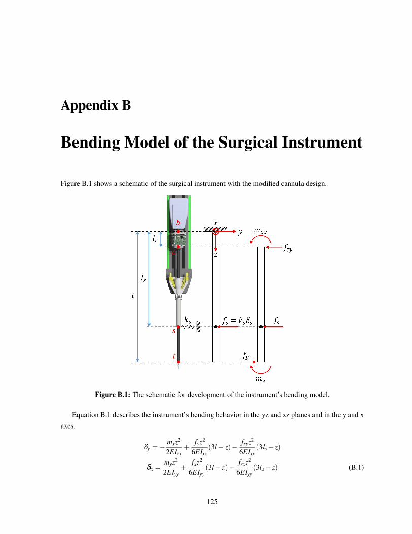
Appendix B
Bending Model of the Surgical Instrument
Figure B.1 shows a schematic of the surgical instrument with the modified cannula design.
Figure B.1: The schematic for development of the instrument’s bending model.
Equation B.1 describes the instrument’s bending behavior in the yz and xz planes and in the y and x
axes.
δy =−mxz2
2EIxx+
fyz2
6EIxx(3l− z)−
fsyz2
6EIxx(3ls− z)
δx =myz2
2EIyy+
fxz2
6EIyy(3l− z)− fsxz2
6EIyy(3ls− z) (B.1)
125

At z = ls:
δsy =−mxl2
s
2EIxx+
fyl2s
6EIxx(3l− ls)−
ksδsyl3s
3EIxx
δsx =myl2
s
2EIyy+
fxl2s
6EIyy(3l− ls)−
ksδsxl3s
3EIyy(B.2)
thus, the lateral deflection of the compliant cannula in the x and y directions (δsx and δsy) are:
δsy =l2s
6EIxx +2ksl3s(−3mx + fy(3l− ls))
δsx =l2s
6EIyy +2ksl3s(3my + fx(3l− ls)) . (B.3)
From the equations of stability for the instrument shaft, in the xz and yz planes, we can write:
fy− fsy− fcy = 0→ fcy = fy− ksδsy
−mcx +mx + fsy(ls− lc)− fy(l− lc) = 0→ mcx = mx + ksδsy(ls− lc)− fy(l− lc)
fx− fsx− fcx = 0→ fcx = fx− ksδsx
−mcy +my + fsx(ls− lc)− fx(l− lc) = 0→ mcy = my− ksδsx(ls− lc)+ fx(l− lc). (B.4)
By replacing the δsx amd δsy from Equation B.3 into Equation B.4, the reaction forces and moments
at the cross-section of the sensor’s clamping point onto the instrument’s shaft (c) are:
fcy =
(1− ksl2
s (3l− ls)6EIxx +2ksl3
s
)fy +
(3ksl2
s
6EIxx +2ksl3s
)mx
fcx =
(1− ksl2
s (3l− ls)6EIyy +2ksl3
s
)fx−
(3ksl2
s
6EIyy +2ksl3s
)my
mcy =
(1− 3ksl2
s (ls− lc)6EIyy +2ksl3
s
)my +
((l− lc)−
ksl2s (3l− ls)
6EIyy +2ksl3s
)fx
mcx =
(1− 3ksl2
s (ls− lc)6EIxx +2ksl3
s
)mx−
((l− lc)−
ksl2s (3l− ls)
6EIxx +2ksl3s
)fy. (B.5)
The instrument’s material and structural properties (E, Ixx, and Iyy) as well as the cannula’s equivalent
stiffness at its distal end can be lumped into two directional parameter (cx and cy) as:
cx =6EIxx
ks
cy =6EIyy
ks. (B.6)
An auxiliary function g(c) was defined to simplify Equation B.5 as:
g(c) =l2s
c+2l3s
(B.7)
126
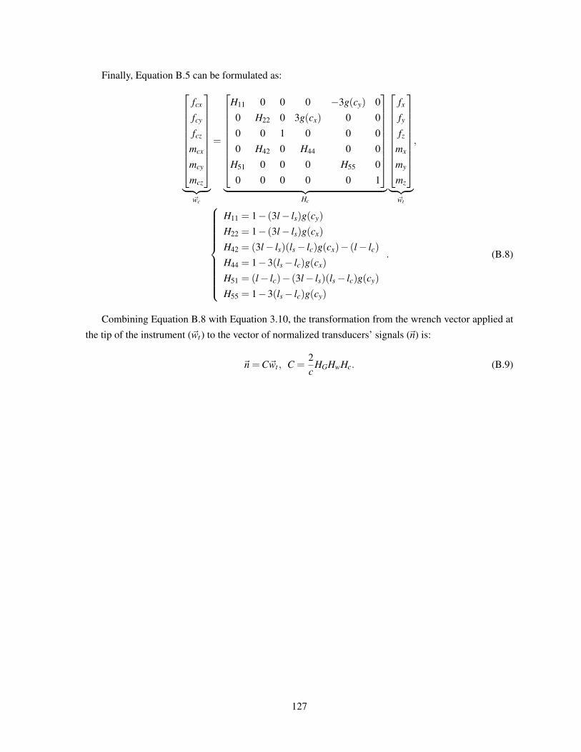
Finally, Equation B.5 can be formulated as:
fcx
fcy
fcz
mcx
mcy
mcz
︸ ︷︷ ︸
~wc
=
H11 0 0 0 −3g(cy) 0
0 H22 0 3g(cx) 0 0
0 0 1 0 0 0
0 H42 0 H44 0 0
H51 0 0 0 H55 0
0 0 0 0 0 1
︸ ︷︷ ︸
Hc
fx
fy
fz
mx
my
mz
︸ ︷︷ ︸
~wt
,
H11 = 1− (3l− ls)g(cy)
H22 = 1− (3l− ls)g(cx)
H42 = (3l− ls)(ls− lc)g(cx)− (l− lc)
H44 = 1−3(ls− lc)g(cx)
H51 = (l− lc)− (3l− ls)(ls− lc)g(cy)
H55 = 1−3(ls− lc)g(cy)
. (B.8)
Combining Equation B.8 with Equation 3.10, the transformation from the wrench vector applied at
the tip of the instrument (~wt) to the vector of normalized transducers’ signals (~n) is:
~n =C~wt , C =2c
HGHwHc. (B.9)
127