High field MREIT: setup and tissue phantom imaging at 11 T

Rosalind Sadleir1, Samuel Grant2, Sung Uk Zhang1, Suk Hoon Oh3, Byung Il Lee3, and EungJe Woo3

1 Department of Biomedical Engineering, University of Florida, USA

2 Department of Neuroscience, University of Florida, USA

3 College of Electronics and Information, Kyung Hee University, Korea

AbstractMagnetic resonance electrical impedance tomography (MREIT) has the potential to provideconductivity and current density images with high spatial resolution and accuracy. Recentexperimental studies at a field strength of 3 T showed that the spatial resolution of conductivity andcurrent density images may be similar to that of conventional MR images as long as enough currentis injected, at least 20 mA when the object being imaged has a size similar to the human head. Toapply the MREIT technique to image small conductivity changes using less injection current, weperformed MREIT studies at 11 T field strength, where noise levels in measured magnetic flux densitydata are significantly lower. In this paper we present the experimental results of imaging biologicaltissues with different conductivity values using MREIT at 11 T. We describe technical difficultiesencountered in using high-field MREIT systems and possible solutions. High-field MREIT issuggested as a research tool for obtaining accurate conductivity data from tissue samples and animalsubjects.

KeywordsMREIT; conductivity; high magnetic field

1. IntroductionMagnetic resonance electrical impedance tomography (MREIT) is a potentially high-resolution conductivity imaging method (Zhang 1992, Woo et al 1994, 2005, Ider and Birgul1998, Joy 2004). It proceeds from MRI measurements of internal magnetic flux densitiescaused by externally applied currents (Scott et al 1991, 1992). Experimental MREIT studiesat 3 T field strength showed that the spatial resolution of both conductivity and current densityimages is comparable to that of MR magnitude images created from the same data set if enoughcurrent is injected. For example, an object having the size of the human head can be imagedat MRI resolution if a current of 20–40 mA is applied (Oh et al 2003, 2004, 2005).

When injecting current into tissue through pairs of surface electrodes, local conductivitychanges caused by, for example, neural activity or pathological changes in the tissue will distortthe original internal current density distributions (Holder 2005). When current flows, amagnetic flux density distribution is formed following the Biot–Savart law. These conductivitychanges will alter the magnetic flux density distribution (Lee et al 2003a). In order to detectsmall conductivity changes from measured magnetic flux density data, it is essential tominimize noise in the measured data.

E-mail: ejwoo@khu.ac.kr.

NIH Public AccessAuthor ManuscriptPhysiol Meas. Author manuscript; available in PMC 2008 June 3.

Published in final edited form as:Physiol Meas. 2006 May ; 27(5): S261–S270.

NIH

-PA Author Manuscript

NIH

-PA Author Manuscript

NIH

-PA Author Manuscript

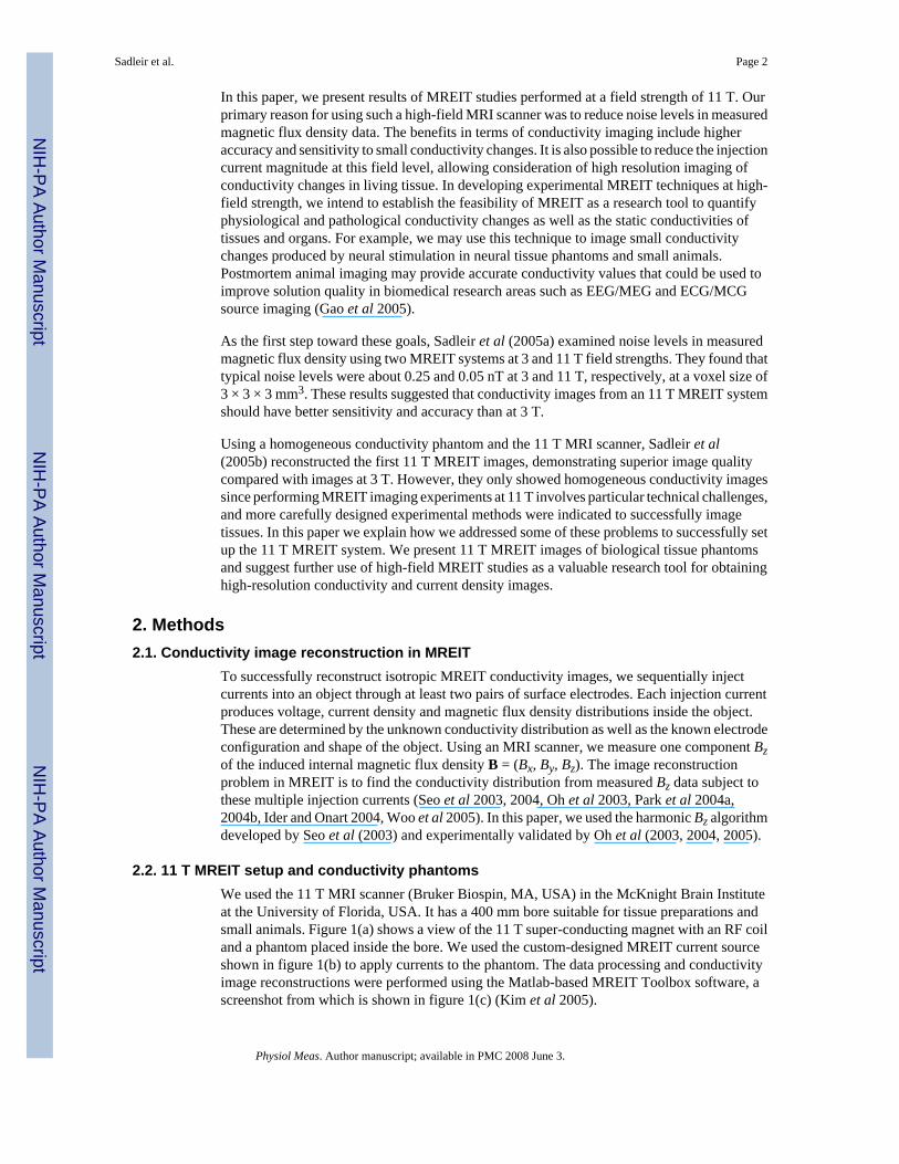
In this paper, we present results of MREIT studies performed at a field strength of 11 T. Ourprimary reason for using such a high-field MRI scanner was to reduce noise levels in measuredmagnetic flux density data. The benefits in terms of conductivity imaging include higheraccuracy and sensitivity to small conductivity changes. It is also possible to reduce the injectioncurrent magnitude at this field level, allowing consideration of high resolution imaging ofconductivity changes in living tissue. In developing experimental MREIT techniques at high-field strength, we intend to establish the feasibility of MREIT as a research tool to quantifyphysiological and pathological conductivity changes as well as the static conductivities oftissues and organs. For example, we may use this technique to image small conductivitychanges produced by neural stimulation in neural tissue phantoms and small animals.Postmortem animal imaging may provide accurate conductivity values that could be used toimprove solution quality in biomedical research areas such as EEG/MEG and ECG/MCGsource imaging (Gao et al 2005).

As the first step toward these goals, Sadleir et al (2005a) examined noise levels in measuredmagnetic flux density using two MREIT systems at 3 and 11 T field strengths. They found thattypical noise levels were about 0.25 and 0.05 nT at 3 and 11 T, respectively, at a voxel size of3 × 3 × 3 mm3. These results suggested that conductivity images from an 11 T MREIT systemshould have better sensitivity and accuracy than at 3 T.

Using a homogeneous conductivity phantom and the 11 T MRI scanner, Sadleir et al(2005b) reconstructed the first 11 T MREIT images, demonstrating superior image qualitycompared with images at 3 T. However, they only showed homogeneous conductivity imagessince performing MREIT imaging experiments at 11 T involves particular technical challenges,and more carefully designed experimental methods were indicated to successfully imagetissues. In this paper we explain how we addressed some of these problems to successfully setup the 11 T MREIT system. We present 11 T MREIT images of biological tissue phantomsand suggest further use of high-field MREIT studies as a valuable research tool for obtaininghigh-resolution conductivity and current density images.

2. Methods2.1. Conductivity image reconstruction in MREIT

To successfully reconstruct isotropic MREIT conductivity images, we sequentially injectcurrents into an object through at least two pairs of surface electrodes. Each injection currentproduces voltage, current density and magnetic flux density distributions inside the object.These are determined by the unknown conductivity distribution as well as the known electrodeconfiguration and shape of the object. Using an MRI scanner, we measure one component Bzof the induced internal magnetic flux density B = (Bx, By, Bz). The image reconstructionproblem in MREIT is to find the conductivity distribution from measured Bz data subject tothese multiple injection currents (Seo et al 2003, 2004, Oh et al 2003, Park et al 2004a,2004b, Ider and Onart 2004, Woo et al 2005). In this paper, we used the harmonic Bz algorithmdeveloped by Seo et al (2003) and experimentally validated by Oh et al (2003, 2004, 2005).

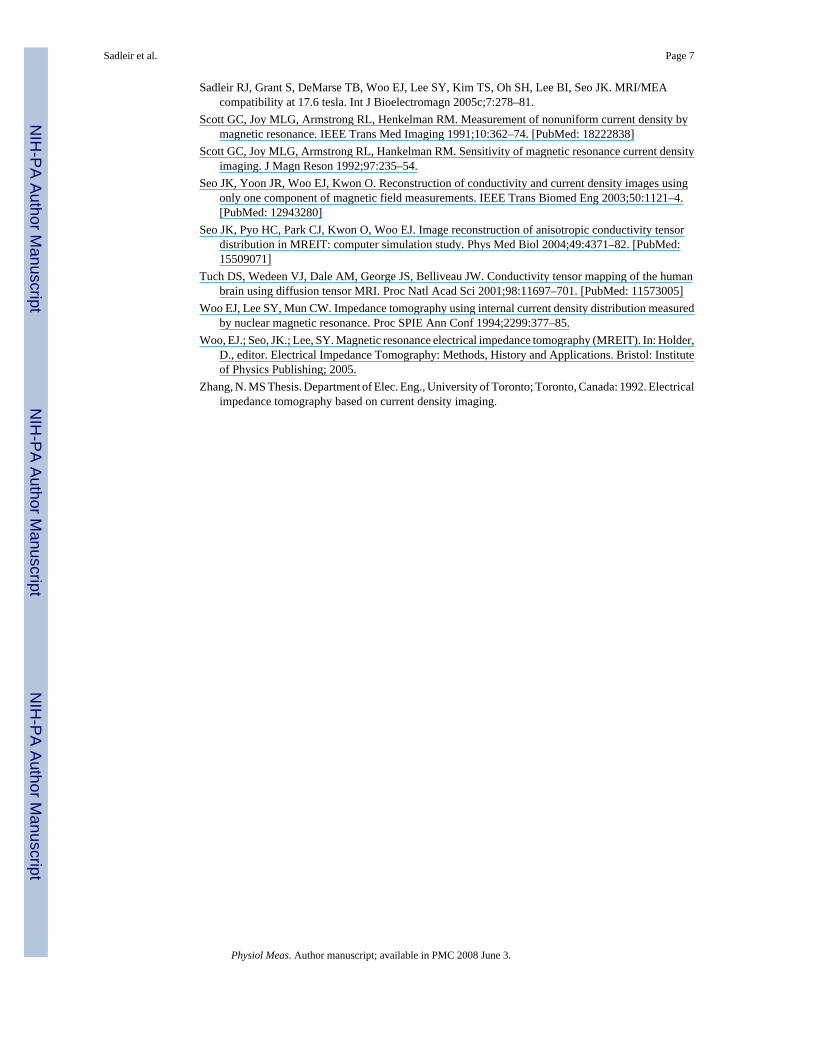
2.2. 11 T MREIT setup and conductivity phantomsWe used the 11 T MRI scanner (Bruker Biospin, MA, USA) in the McKnight Brain Instituteat the University of Florida, USA. It has a 400 mm bore suitable for tissue preparations andsmall animals. Figure 1(a) shows a view of the 11 T super-conducting magnet with an RF coiland a phantom placed inside the bore. We used the custom-designed MREIT current sourceshown in figure 1(b) to apply currents to the phantom. The data processing and conductivityimage reconstructions were performed using the Matlab-based MREIT Toolbox software, ascreenshot from which is shown in figure 1(c) (Kim et al 2005).

Sadleir et al. Page 2

Physiol Meas. Author manuscript; available in PMC 2008 June 3.

NIH

-PA Author Manuscript

NIH

-PA Author Manuscript

NIH

-PA Author Manuscript

We prepared imaging phantoms constructed of acrylic plastic. They typically contained saline,agar or animal hide gelatine with incorporated biological tissues. Figure 2 shows a conductivityphantom having both diameter and height of either 60 mm or 40 mm. In this paper, we referto these phantoms as either the ‘60 mm phantom’ or ‘40 mm phantom’. Recessed electrodeassemblies, through which current was injected into the phantom, were attached on four sidesof the octagonal column. By using recessed electrodes we avoided RF shielding problems andconsequent Bz artifacts caused by having metal electrodes directly in contact with the objectsurface (Lee et al 2003b,Oh et al 2003). The sizes of each recessed electrode assembly were7.55 × 7.55 × 10 and 6 × 6 × 10 mm3 for the ‘60 mm phantom’ and ‘40 mm phantom’,respectively. The copper electrodes each had a size of 5 × 7.55 or 5 × 6 mm2, respectively.

2.3. MREIT experimentsAfter one of the phantoms was placed inside the 11 T machine, we injected a current I1 betweenan opposing pair of electrodes, synchronous with the MRI pulse sequence. The pulse sequencesshown in figure 3 were used with either of two multi-slice imaging techniques (Scott et al1991): the spin echo (SE) pulse sequence shown in figure 3(a) or the gradient echo (GE) pulsesequences shown in figure 3(b). The injection current magnitude I was chosen at levels between5 and 20 mA, with a pulse width Tc between 9 and 18 ms depending on the chosen echo time(TE). The slice thicknesses used were 1 or 2 mm, with no slice gap. Data from eight axial sliceswere gathered in each scan, therefore the total region imaged spanned a region with thicknessbetween 8 and 16 mm, centered on the electrode plane. After acquiring eight slices for I1,denoted as , another current I2, with the same magnitude as I1, was injected through the otherpair of electrodes to obtain the image set. The image matrix size used in each case was 128× 128. The field-of-view (FOV) was between 80 × 80 and 128 × 128 mm2, therefore the pixelsize was between 0.625 × 0.625 and 1 × 1 mm2.

3. ResultsFigure 4 shows experimental results using phantoms filled with homogeneous saline. Figures4(a) and (b) are MR magnitude images and the one-dimensional profiles of the 60 mm phantomusing SE and GE pulse sequences, respectively. Figure 4(c) is the magnitude image and profileof the 40 mm phantom using the SE pulse sequence. For better comparison, we normalized theimages in figures 4(a), (b) and (c) so that the maximal pixel value in each image becomes 1.The signal-to-noise ratios (SNR) were estimated as 76, 151 and 182 in the central region offigures 4(a), (b) and (c), respectively. Figures 4(d), (e) and (f) show magnetic flux density( ) images corresponding to magnitude images in (a), (b) and (c), respectively.

The images in figure 4 illustrate possible technical problems that may be encountered in high-field MREIT experiments. In figure 4(a), we observed the signal intensity gradually decreasingtowards the outer boundary of the phantom. This corresponded with a gradually increasingnoise level in the image, as shown in figure 4(d). Standing wave effects at the short RFwavelength of 11 T (450 MHz) are believed to cause this characteristic (Beck et al 2004). Inthe GE data shown in figure 4(b), we observed ripple artifacts as well as signal attenuation inthe magnitude data related to the main magnetic field inhomogeneity. These appeared as similarartifacts in the corresponding image shown in figure 4(e). In order to avoid these artifacts,it was essential to shim the magnet as well as possible. It was necessary to keep the object sizesmall, and to pay close attention to tuning imaging parameters including RF gain andbandwidth, as well as considering the appropriate settings of TR/TE and number of averages(NEX). Figures 4(c) and (f) show images of the homogeneous 40 mm phantom with muchsmaller noise and artifact after careful parameter adjustment.

Sadleir et al. Page 3

Physiol Meas. Author manuscript; available in PMC 2008 June 3.

NIH

-PA Author Manuscript

NIH

-PA Author Manuscript

NIH

-PA Author Manuscript

Figure 5(a) shows the MR magnitude image of a 40 mm tissue phantom. The backgroundmaterial was an agar gel with a conductivity of 1.4 S m−1. Inside the phantom, we placed twodifferent muscle samples (porcine muscle and turkey breast) packed closely together. Theaverage SNR in the magnitude image were 380, 140 and 107 inside the agar, turkey and pork,respectively. Figures 5(b) and (c) show the reconstructed conductivity images using 10 and 20mA injection currents, respectively, with a SE pulse sequence. Average conductivity valuesfor the pork and turkey tissues were found to be 0.78 and 1.05 S m−1, respectively. Note thatthe two different tissues can be distinguished in the conductivity images better than in themagnitude image.

Figure 6(a) shows a 60 mm phantom containing the lower body of a rat. The phantombackground was filled with an animal hide gelatine (AHG) with a conductivity of 0.6 S m−1.We used a multi-slice SE imaging method with fat suppression. Figures 6(b) and (c) are themagnitude image at the middle imaging slice and its one-dimensional profile along the dottedline, respectively. Inside the regions marked as ‘A’ and ‘B’ in figure 6(b), average SNRs were232 and 114, respectively. Figure 7(a) is the measured magnetic flux density image of atthe same imaging slice using 18 mA injection current. Figures 7(b) and (c) are the reconstructedconductivity image and its profile along the same dotted line marked in figure 6(b),respectively.

Figure 8(a) shows the MR magnitude image of a 40 mm phantom with a backgroundconductivity of gelatin at 0.6 S m−1. Inside the phantom, we placed two small pieces of differentmuscle tissues (chicken breast and bovine muscle). Figures 8(b) and (c) are one magnetic fluxdensity and the reconstructed conductivity image, respectively, using a 5 mA injection current.These images qualitatively show the effect of reducing injection current.

4. DiscussionSince MREIT relies on MR phase signals, it requires a high degree of main magnetic fieldhomogeneity and gradient linearity. Even though the large main magnetic field of 11 T enablesus to reduce intrinsic phase noise levels, we may fail to take advantage of such a high fieldwithout properly adapting low-field MREIT experiments. As illustrated in figure 4, manyproblems such as signal loss or attenuation and artifacts can be amended by better shimmingof the magnet and tuning of imaging parameters. For most experiments described in this paper,SE pulse sequences were used as we found that SE usually produces better results with fewerartifacts compared with GE.

When imaging biological tissues, we recommend longer TR times to obtain more signalstrength, at the expense of prolonged scan times. The current injection pulse width Tc shouldbe chosen so that it is slightly shorter than TE. Thus, increasing TE allows us to choose a widerTc to reduce noise level in magnetic flux density signals. However, using a longer TE decreasesMR signal strength and leads to lower magnitude image SNR. Therefore, before commencingMREIT scanning, we recommend trying at least two different TR/TE values to evaluate noiselevels and SNRs using the method described in Scott et al (1991 and 1992) and Sadleir et al(2005) to find proper values of TR/TE for a given sample configuration.

Any chosen RF coil must be tuned carefully for each subject or phantom. At high fields of 11T and above, the long metal wires connected to electrodes have a large effect on RF coil tuningcharacteristics. Use of carbon fiber wires has been found to improve image quality (Sadleir etal 2005c) as long as the current source has enough voltage compliance to overcome theincreased load resistance.

Sadleir et al. Page 4

Physiol Meas. Author manuscript; available in PMC 2008 June 3.

NIH

-PA Author Manuscript

NIH

-PA Author Manuscript

NIH

-PA Author Manuscript

We found that the 11 T system produced images with much larger geometrical distortion thanat 3 T, especially in the outer regions of larger objects. This distortion is believed to be due toinhomogeneity in the main magnetic field and gradient field nonlinearity. The distortion issignificantly worse without correct shimming (Sadleir et al 2005b). At 11 T, standing waveeffects also limit the size of imaged objects (Beck et al 2004). For these reasons, we found thateven though the 11 T MRI scanner has a 400 mm bore, the useful MREIT imaging area wasless than 100 mm about its central axis.

The images and profiles shown in figure 5 illustrate that MREIT images can distinguish tissuesbetter than conventional MR images when there exist enough conductivity differences amongtissues and not much contrast in conventional MR images. Compared with experimental resultsusing 3 T published in Oh et al (2005), high-field MREIT shows a similar ability to distinguishdifferent tissues with small conductivity contrasts, but using significantly smaller injectedcurrents. In both figures 5(b) and (c), reconstructed conductivity images show a slightly darkerarea to the left of the tissue samples. We speculate that this could have been caused by artifactsalong the phase encoding direction, unless the agar gel was actually inhomogeneous due toimproper mixing. Further studies are needed to investigate artifacts and noise effects inreconstructed conductivity images.

When the imaged object contains a complex mixture of many different tissues, as in figure 6,it seems to be difficult to quantitatively measure or visualize the internal conductivitydistribution in its absolute values using other methods such as electrical impedance tomography(EIT) (Holder 2005) or diffusion tensor imaging (DTI) (Tuch et al 2001). The image in figure7(b) illustrates the capability of MREIT to measure the spatially varying conductivitydistribution of a mixture of tissues in its absolute values. In future studies, we plan MREITimaging of animals by attaching electrodes directly to their skin. It would also be veryinteresting to compare reconstructed conductivity images obtained by using differenttechniques including MREIT, EIT and DTI.

Figure 8 shows the first MREIT image using injection currents as low as 5 mA. Even thoughthe image quality is low compared with the results at 10 or 20 mA, we can observe theconductivity contrast both in the magnetic flux density and reconstructed conductivity images.This shows the benefit of the high-field system compared to the 3 T results described in Oh etal (2003,2004,2005). One of the reasons for the noisy conductivity image inside the tissuesshown in figure 8(c) could be the relatively short TR. Improvements in image quality andfurther reduction in injection current amplitude are being pursued in studies planned for thenear future, incorporating improved pulse sequences and RF coils, better (probably hybrid)algorithms and efficient denoising techniques (Lee et al 2005). Theoretical analysis and furtherexperimental work are also needed to find a more concrete relationship between image qualityand noise level.

5. ConclusionWe present results of MREIT experiments performed at 11 T field strength. Although noiselevels in the measured magnetic flux density data are smaller using the 11 T system, we foundwe had to resolve problems related to systematic artifacts. Amongst many factors, propershimming of the magnet is most important. We found that the object size must be selected withreference to the system’s field uniformity and gradient linearity, and not just by the bore size.

These 11 T MREIT experiments suggest that we may reduce the injection current to 5 mA infuture studies. We plan to further improve our experimental MREIT techniques at 11 T andhigher field strengths. Our primary goal is to image small conductivity changes associated with

Sadleir et al. Page 5

Physiol Meas. Author manuscript; available in PMC 2008 June 3.

NIH

-PA Author Manuscript

NIH

-PA Author Manuscript

NIH

-PA Author Manuscript

physiological and pathological changes. We will undertake high-field MREIT experimentalstudies using neural tissue preparations and small animals in the near future.

Acknowledgements

This work was supported by the Advanced Magnetic Resonance Imaging and Spectroscopy (AMRIS) facility at theMcKnight Brain Institute, University of Florida, USA and grants R11-2002-103/M60501000035-05A0100-03510from the Korea Science and Engineering Foundation (KOSEF) in Korea.

ReferencesBeck BL, Jenkins K, Caserta J, Padgett K, Fitzsimmons J, Blackband SJ. Observation of significant signal

voids in images of large biological samples at 11.1 T. Magn Reson Med 2004;51:1103–7. [PubMed:15170828]

Gao G, Zhu SA, He B. Estimation of electrical conductivity distribution within the human head frommagnetic flux density measurement. Phys Med Biol 2005;50:2675–87. [PubMed: 15901962]

Holder, D., editor. Electrical Impedance Tomography: Methods, History and Applications. Bristol:Institute of Physics Publishing; 2005 .

Ider YZ, Birgul O. Use of the magnetic field generated by the internal distribution of injected currentsfor electrical impedance tomography (MR-EIT). Elektrik 1998;6:215–25.

Ider YZ, Onart S. Algebraic reconstruction for 3D MR-EIT using one component of magnetic flux density.Physiol Meas 2004;25:281–94. [PubMed: 15005322]

Joy, ML. MR current density and conductivity imaging: the state of the art. Proc. 26th Ann. Int. Conf.IEEE EMBS; San Francisco CA, USA. 2004. p. 5315-9.

Kim TS, Lee BI, Park C, Lee SH, Tak SH, Seo JK, Kwon O, Woo EJ. A Matlab toolbox for magneticresonance electrical impedance tomography (MREIT): MREIT toolbox. Int J Bioelectromagn2005;7:352–5.

Lee BI, Oh SH, Woo EJ, Lee SY, Cho MH, Kwon O, Seo JK, Lee JY, Baek WS. Three-dimensionalforward solver and its performance analysis in magnetic resonance electrical impedance tomography(MREIT) using recessed electrodes. Phys Med Biol 2003a;48:1971–86. [PubMed: 12884929]

Lee BI, Oh SH, Woo EJ, Lee SY, Cho MH, Kwon O, Seo JK, Baek WS. Static resistivity image of acubic saline phantom in magnetic resonance electrical impedance tomography (MREIT). Physiol Meas2003b;24:579–89. [PubMed: 12812440]

Lee BI, Lee SH, Kim TS, Kwon O, Woo EJ, Seo JK. Harmonic decomposition in PDE-based denoisingtechnique for magnetic resonance electrical impedance tomography. IEEE Trans Biomed Eng2005;52:1912–20. [PubMed: 16285395]

Oh SH, Lee BI, Woo EJ, Lee SY, Cho MH, Kwon O, Seo JK. Conductivity and current density imagereconstruction using harmonic Bz algorithm in magnetic resonance electrical impedance tomography.Phys Med Biol 2003;48:3101–16. [PubMed: 14579854]

Oh SH, Lee BI, Park TS, Lee SY, Woo EJ, Cho MH, Kwon O, Seo JK. Magnetic resonance electricalimpedance tomography at 3 tesla field strength. Mag Reson Med 2004;51:1292–6.

Oh SH, Lee BI, Woo EJ, Lee SY, Kim TS, Kwon O, Seo JK. Electrical conductivity images of biologicaltissue phantoms in MREIT. Physiol Meas 2005;26:S279–88. [PubMed: 15798241]

Park C, Park EJ, Woo EJ, Kwon O, Seo JK. Static conductivity imaging using variational gradient Bzalgorithm in magnetic resonance electrical impedance tomography. Physiol Meas 2004a;25:257–69.[PubMed: 15005320]

Park C, Kwon O, Woo EJ, Seo JK. Electrical conductivity imaging using gradient Bz decompositionalgorithm in magnetic resonance electrical impedance tomography (MREIT). IEEE Trans MedImaging 2004b;23:388–94. [PubMed: 15027531]

Sadleir R, et al. Noise analysis in MREIT at 3 and 11 tesla field strength. Physiol Meas 2005a;26:875–84. [PubMed: 16088075]

Sadleir RJ, Grant S, Silver X, Zhang SU, Woo EJ, Lee SY, Kim TS, Oh SH, Lee BI, Seo JK. Magneticresonance electrical impedance tomography (MREIT) at 11 tesla field strength: preliminaryexperimental study. Int J Bioelectromagn 2005b;7:340–3.

Sadleir et al. Page 6

Physiol Meas. Author manuscript; available in PMC 2008 June 3.

NIH

-PA Author Manuscript

NIH

-PA Author Manuscript

NIH

-PA Author Manuscript

Sadleir RJ, Grant S, DeMarse TB, Woo EJ, Lee SY, Kim TS, Oh SH, Lee BI, Seo JK. MRI/MEAcompatibility at 17.6 tesla. Int J Bioelectromagn 2005c;7:278–81.

Scott GC, Joy MLG, Armstrong RL, Henkelman RM. Measurement of nonuniform current density bymagnetic resonance. IEEE Trans Med Imaging 1991;10:362–74. [PubMed: 18222838]

Scott GC, Joy MLG, Armstrong RL, Hankelman RM. Sensitivity of magnetic resonance current densityimaging. J Magn Reson 1992;97:235–54.

Seo JK, Yoon JR, Woo EJ, Kwon O. Reconstruction of conductivity and current density images usingonly one component of magnetic field measurements. IEEE Trans Biomed Eng 2003;50:1121–4.[PubMed: 12943280]

Seo JK, Pyo HC, Park CJ, Kwon O, Woo EJ. Image reconstruction of anisotropic conductivity tensordistribution in MREIT: computer simulation study. Phys Med Biol 2004;49:4371–82. [PubMed:15509071]

Tuch DS, Wedeen VJ, Dale AM, George JS, Belliveau JW. Conductivity tensor mapping of the humanbrain using diffusion tensor MRI. Proc Natl Acad Sci 2001;98:11697–701. [PubMed: 11573005]

Woo EJ, Lee SY, Mun CW. Impedance tomography using internal current density distribution measuredby nuclear magnetic resonance. Proc SPIE Ann Conf 1994;2299:377–85.

Woo, EJ.; Seo, JK.; Lee, SY. Magnetic resonance electrical impedance tomography (MREIT). In: Holder,D., editor. Electrical Impedance Tomography: Methods, History and Applications. Bristol: Instituteof Physics Publishing; 2005.

Zhang, N. MS Thesis. Department of Elec. Eng., University of Toronto; Toronto, Canada: 1992. Electricalimpedance tomography based on current density imaging.

Sadleir et al. Page 7

Physiol Meas. Author manuscript; available in PMC 2008 June 3.

NIH

-PA Author Manuscript

NIH

-PA Author Manuscript

NIH

-PA Author Manuscript

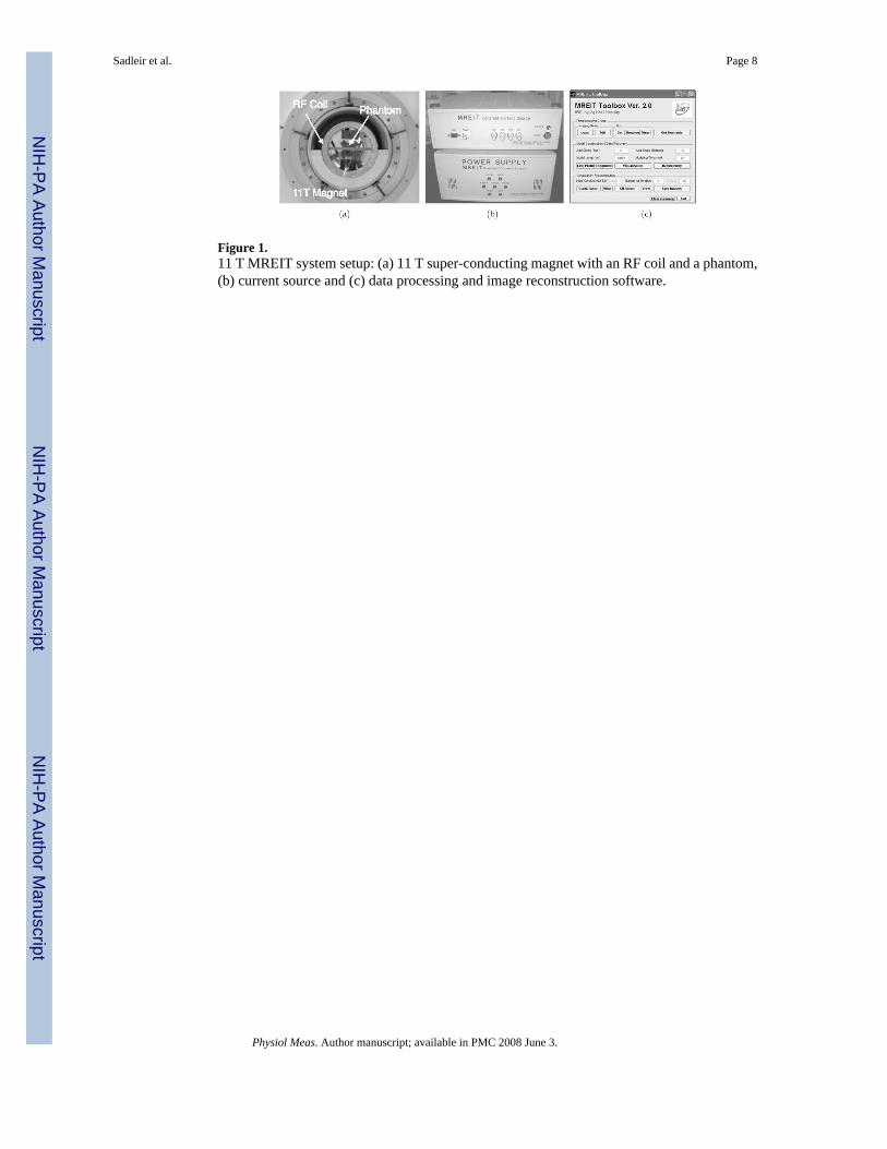
Figure 1.11 T MREIT system setup: (a) 11 T super-conducting magnet with an RF coil and a phantom,(b) current source and (c) data processing and image reconstruction software.

Sadleir et al. Page 8

Physiol Meas. Author manuscript; available in PMC 2008 June 3.

NIH

-PA Author Manuscript

NIH

-PA Author Manuscript

NIH

-PA Author Manuscript

Figure 2.Phantom design: (a) front view, (b) top view and (c) oblique view. The z-direction denotes theorientation of the main magnetic field B0.

Sadleir et al. Page 9

Physiol Meas. Author manuscript; available in PMC 2008 June 3.

NIH

-PA Author Manuscript

NIH

-PA Author Manuscript

NIH

-PA Author Manuscript

Figure 3.MREIT pulse sequences: (a) spin echo (SE) and (b) gradient echo (GE) pulse sequences withsynchronized injection current pulses (Scott et al 1991). The positive and negative currentpulses with an amplitude of I and width of Tc are shown as the solid and dotted lines,respectively.

Sadleir et al. Page 10

Physiol Meas. Author manuscript; available in PMC 2008 June 3.

NIH

-PA Author Manuscript

NIH

-PA Author Manuscript

NIH

-PA Author Manuscript

Figure 4.Effects of different pulse sequences using homogeneous saline phantoms. Normalizedmagnitude images and their profiles in the 60 mm phantom using (a) SE and (b) GE pulsesequence. For (a) and (b), pixel size was 0.625 × 0.625 mm2. (c) Normalized magnitude imageand its profile in the 40 mm phantom using the SE pulse sequence with 1 × 1 mm2 pixel size.One-dimensional profiles are shown below corresponding to the dotted lines in magnitudeimages. (d) and (e) images of the 60 mm phantom corresponding to (a) and (b), respectively.(f) image of the 40 mm phantom corresponding to (c).

Sadleir et al. Page 11

Physiol Meas. Author manuscript; available in PMC 2008 June 3.

NIH

-PA Author Manuscript

NIH

-PA Author Manuscript

NIH

-PA Author Manuscript

Figure 5.(a) MR magnitude image of a 40 mm tissue phantom containing samples of preserved porcinemuscle and turkey breast. (b) and (c) are conductivity images using 10 and 20 mA injectioncurrent, respectively. We used the same scale bar for both (b) and (c). Note that the image in(b) has more noise. A SE pulse sequence was used with TR/TE = 800/20 ms and Tc = 18 ms.Number of slices (NS) was eight, NEX was 8, slice thickness was 1 mm, FOV was 128 × 128mm2, image matrix size was 128 × 128 and pixel size was 1 × 1 mm2.

Sadleir et al. Page 12

Physiol Meas. Author manuscript; available in PMC 2008 June 3.

NIH

-PA Author Manuscript

NIH

-PA Author Manuscript

NIH

-PA Author Manuscript

Figure 6.(a) 60 mm phantom containing the lower body of a rat. The background was filled with ananimal hide gelatine (AHG) at 0.6 S m−1, (b) MR magnitude image and (c) its profile alongthe dotted line. A SE pulse sequence was used with TR/TE = 700/10 ms, I = 18 mA and Tc =9 ms. Eight slices were imaged with 2 mm slice thickness, NEX was 16, FOV was 100 × 100mm2, image matrix size was 128 × 128 and pixel size was 0.78 × 0.78 mm2.

Sadleir et al. Page 13

Physiol Meas. Author manuscript; available in PMC 2008 June 3.

NIH

-PA Author Manuscript

NIH

-PA Author Manuscript

NIH

-PA Author Manuscript

Figure 7.(a) Measured magnetic flux density images, of the 60 mm phantom shown in figure 6. (b)and (c) are reconstructed conductivity image and its profile along the dotted line, respectively.

Sadleir et al. Page 14

Physiol Meas. Author manuscript; available in PMC 2008 June 3.

NIH

-PA Author Manuscript

NIH

-PA Author Manuscript

NIH

-PA Author Manuscript

Figure 8.MREIT experiment at 5 mA injection current. (a) MR magnitude image of a 40 mm tissuephantom containing pieces of chicken breast and bovine muscle. (b) Magnetic flux densityimage. (c) Reconstructed conductivity image. A SE pulse sequence was used with TR/TE =600/10 ms, I = 5 mA and Tc = 9 ms. Eight slices were imaged with 1 mm slice thickness, NEXwas 16, FOV was 80 × 80 mm2, image matrix size was 128 × 128 and pixel size was 0.625 ×0.625 mm2.

Sadleir et al. Page 15

Physiol Meas. Author manuscript; available in PMC 2008 June 3.

NIH

-PA Author Manuscript

NIH

-PA Author Manuscript

NIH

-PA Author Manuscript