arX

iv:0

801.

2544

v1 [

hep-

ph]

16

Jan

2008

IFUM-911-FTEdinburgh 2008/1

CERN-PH-TH/2008-009

Higgs production via gluon-gluon fusionwith finite top mass beyond next-to-leading order

Simone Marzani,a, Richard D. Ball,a,b Vittorio Del Duca,c1

Stefano Forted and Alessandro Vicinid

aSchool of Physics, University of Edinburgh,

Edinburgh EH9 3JZ, Scotland, UK

bCERN, Physics Department, Theory Division,

CH-1211 Geneve 23, Switzerland

cINFN, Laboratori Nazionali di Frascati,

Via E. Fermi 40, I-00044 Frascati, Italy

dDipartimento di Fisica, Universita di Milano and INFN, Sezione di Milano,

Via Celoria 16, I-20133 Milano, Italy

Abstract

We present a computation of the cross section for inclusive Higgs production in gluon–gluonfusion for finite values of the top mass in perturbative QCD to all orders in the limit of highpartonic center–of–mass energy. We show that at NLO the high energy contribution accountsfor most of the difference between the result found with finite top mass and that obtained inthe limit mt → ∞. We use our result to improve the known NNLO order result obtained atmt → ∞. We estimate the effect of the high energy NNLO mt dependence on the K factor tobe of the order of a few per cent.

CERN-PH-TH/2008-009January 2008

1On leave from INFN, Sezione di Torino, Italy

1 The cross section in the soft limit and in the hard limit

The determination of higher–order corrections to collider processes [1], and specifically Higgsproduction [2] in perturbative QCD is becoming increasingly important in view of forthcomingphenomenology at the LHC. The dominant Higgs production mechanism in the standard modelis inclusive gluon–gluon fusion (gg → H + X) through a top loop. The next–to–leading ordercorrections to this process were computed several years ago [3, 4] and turn out to be very large(of order 100%). The bulk of this large correction comes from the radiation of soft and collineargluons [5], which give the leading contribution in the soft limit in which the partonic center-of-mass energy s tends to the Higgs mass m2

H , and which at LHC energies turns out to dominatethe hadronic cross section after convolution with the parton distributions.

This dominant contribution does not resolve the effective gluon-gluon-higgs (ggH) couplinginduced by the top loop. As a consequence, the NLO correction can be calculated [6, 7] quiteaccurately in the limit mt → ∞, where it simplifies considerably because the ggH couplingbecomes pointlike and the corresponding Feynman diagrams have one less loop. Recently, theNNLO corrections to this process have been computed in the mt → ∞ limit [8]. The NNLOresult appears to be perturbatively quite stable, and this stability is confirmed upon inclusion [9]of terms in the next few orders which are logarithmically enhanced as s → mH , which can bedetermined [10] using soft resummation methods. This suggests that also at NNLO the largemt approximation should provide a good approximation to the yet unknown exact result.

However, this is only true for the total inclusive cross section: for example, if one looks at theproduction of Higgs plus jets, if the transverse momentum is large the infinite mt approximationfails [11]. Indeed, even though the mt–independent contribution from soft and collinear radiationturns out to dominate the cross section at the hadronic level, it does not necessarily provide agood approximation to the partonic cross section in a fixed kinematical region. In particular,the infinite mt approximation, which becomes exact in the soft limit, fails in the opposite (hard)limit of large center–of–mass energy. This is due to the fact that the ggH vertex is pointlikein the infinite mt limit, whereas for finite mt the quark loop provides a form factor (as weshall see explicitly below). Clearly, a point–like interaction has a completely different highenergy behaviour than a resolved interaction which is softened by a form factor: in fact one canshow [12] that a point–like interaction at n–th perturbative order has double energy logs whilea resolved interaction has only single logs.

This means that as s → ∞ the gg → H + X partonic cross section σ behaves as

σ ∼s→∞

∑∞k=1 αk

s ln2k−1(

sm2

H

)

pointlike: mt → ∞

∑∞k=1 αk

s lnk−1(

sm2

H

)

resolved: finite mt

(1)

Hence, as the center-of-mass energy grows, eventually mt → ∞ ceases to be a good approxi-mation to the exact result. It is clear from eq. (1) that this high energy deviation between theexact and approximate behaviour is stronger at higher orders, so one might expect the relativeaccuracy of the infinite mt approximation to the k–th order perturbative contribution to thecross section to become worse as the perturbative order increases. Conversely, this suggests that

1

it might be worth determining the high energy behaviour of the exact cross section and use theresult to improve the infinite mt result, which is much less difficult to determine. Eventually, afull resummation of these contributions might also become relevant.

The leading high energy contributions to this process in the infinite mt limit have in factbeen computed some time ago in Ref. [13]: this amounts to a determination of the coefficient ofthe double logs eq. (1), in the pointlike case. In this paper, we compute the coefficients of thesingle logs eq. (1) in the resolved (exact) case. Our result takes the form of a double integral,whose numerical evaluation order by order in a Taylor expansion gives the coefficient of the logseq. (1) (at the lowest perturbative order the integral can be computed in closed form). Afterchecking our result against the known full NLO result of Ref. [3, 4], we will discuss the wayknowledge of the exact high energy behaviour of the cross section at a given order can be usedto improve the infinite mt result, using the NLO case, where everything is known, as a testingground. We will show that in fact, at NLO the different high energy behaviour eq. (1) accountsfor most of the difference between the exact and infinite mt cross sections. We will then repeatthis analysis in the NNLO case, where only the infinite mt result is currently known. We willshow that in fact at this order the contribution of the logarithmically enhanced terms whichdominate the partonic cross section at high energy is substantial even for moderate values of thepartonic center-of-mass energy, such as s ∼ 2m2

H .The calculation of the leading high energy logs is presented in section 2, while in section 3

we discuss its use to improve the NLO and NNLO results. The appendix collects the explicitexpressions of the form factors which parametrize the amplitude for the process gg → H withtwo off–shell gluons, which is required for the calculation of sect. 2.

2 Determination of the leading high energy logarithms

2.1 Definitions, kinematics and computational procedure

We compute the total inclusive partonic cross section σ(gg → H + X) in an expansion in powerof αs, as a function of the partonic center-of-mass energy s:

σ(gg → H + X) = σgg

(

αs; τ ; yt, m2H

)

, (2)

where the dimensionless variables τ and yt parametrize respectively the partonic center-of-massenergy and the dependence on the top mass:

τ ≡ m2H

s(3)

yt ≡ m2t

m2H

. (4)

2

The corresponding contribution to the hadronic cross section σ can be obtained by convolutionwith the gluon-gluon parton luminosity L:

σgg(τh; yt, m2H) =

∫ 1

τh

dw σgg

(

αs;τh

w; yt, m

2H

)

L(w) (5)

L(w) ≡∫ 1

w

dx2

x2

gh1

(

w

x2

, m2H

)

gh2

(

x2, m2H

)

, (6)

where ghi(xi, Q

2) is the gluon distribution in the i-th incoming hadron and in eq. (5) the dimen-sionless variables τh parametrizes the hadronic center-of-mass energy s

τh ≡ m2H

s. (7)

Note that 0 ≤ τh ≤ τ ≤ 1, and that if yt < 14

then the intermediate tt pair produced by thegluon-gluon fusion can go on shell.

It is convenient to define a dimensionless hard coefficient function C(αs(m2H); τ, yt)

σgg

(

αs; τ ; yt, m2H

)

= σ0(yt)C(αs(m2H), τ, yt) (8)

C(αs(m2H), τ, yt) = δ(1 − τ) +

αs(m2H)

πC(1)(τ, yt) +

(

αs(m2H)

π

)2

C(2)(τ, yt), (9)

where σ0δ(1 − τ) is the leading order cross section, determined long ago in ref. [14]:

σ0(yt) =α2

sGF

√2

256π

∣

∣

∣

∣

4yt

(

1 − 1

4(1 − 4yt)s

20(yt)

)∣

∣

∣

∣

2

, (10)

where

s0(yt) =

ln(

1−√

1−4yt

1+√

1−4yt

)

+ π i if yt < 14

2 i tan−1(√

14yt−1

)

= 2 i sin−1(√

14yt

)

if yt ≥ 14.

(11)

We also define the Mellin transform

C(αs(m2H), N, yt) =

∫ 1

0

dτ τN−1C(αs(m2H), τ, yt), (12)

denoted with the same symbol by slight abuse of notation.We are interested in the determination of the leading high energy contributions to the partonic

cross section σ(gg → H + X), namely, the leading contributions to C(αs(m2H), τ, yt) as τ → 0

to all orders in αs(m2H). Order by order in αs(m

2H), these correspond to the highest rightmost

pole in N in the expansion in powers of αs(m2H) of C(αs(m

2H), N, yt). The leading singular

contributions to the partonic cross section σ(gg → H + X) to all orders can be extracted [12]from the computation of the cross section for a slightly different process, namely, the crosssection σoff(gg → H) computed at leading order, but with incoming off-shell gluons, a suitablechoice of kinematics and a suitable prescription for the sum over polarizations.

The procedure used for this determination is based on the so-called high energy (or kt)factorization [12], and consists of the following steps.

3

• One computes the matrix element Mµνab (k1, k2) for the leading-order process gg → H at

leading order with two incoming off-shell gluons with polarization indices µ, ν and colorindices a, b. The momenta k1, k2 of the gluons in the center-of-mass frame of the hadroniccollision admit the Sudakov decomposition at high energy

ki = zipi + ki, (13)

where pi are lightlike vectors such that p1 · p2 6= 0, and ki are transverse vectors, ki · pj = 0for all i, j. The gluons have virtualities

k2i = k2

i = −|ki|2. (14)

The cross section σoff(gg → H) is computed averaging over incoming and summing overoutgoing spin and color:

σoff =1

J

1

256Mµν

abM∗µ′ν′

ba

∑

λ1

ελ1

µ (k1)ε∗λ1

µ′ (k1)∑

λ2

ελ2

ν (k2)ε∗λ2

ν′ (k2) dP, (15)

where the flux factorJ = 2(k1 · k2 − k1 · k2) (16)

is determined on the surface orthogonal to p1, p2 eq. (13), and the phase space is

dP =2π

m2H

δ

(

1

z− 1 − |k1 + k2|2

m2H

)

. (17)

Note that the kinematics for a 2 → 1 process is fixed, so eq. (15) gives the total crosssection and no phase–space integration is needed.

The sums over gluon polarizations are given by

∑

λi

ελi

µ (ki)ε∗λi

ν (ki) = 2k

µi k

νi

|k2

i| ; i = 1, 2. (18)

Here, the virtualities will be parametrized through the dimensionless variables

ξi ≡|ki|2m2

H

. (19)

The reduced cross section σ, obtained extracting an overall factor m2H ,

m2Hσoff(gg → H) ≡ σ(yt; ξ1, ξ2, ϕ, z), (20)

is then a dimensionless function σ(yt; ξ1, ξ2, ϕ, z) of the parameter yt eq. (4) and of thekinematic variables ξ1, ξ2, the relative angle ϕ of the two transverse momenta

ϕ = cos−1

(

k1 · k2

|k1||k2|

)

, (21)

and

z ≡ m2H

2z1z2p1 · p2

=m2

H

2 (k1 · k2 − k1 · k2). (22)

Note that, in the collinear limit k1, k2 → 0, z eq. (22) reduces to τ eq. (3).

4

• The reduced cross section is averaged over ϕ, and its dependence on z eq. (22) is Mellin-transformed:

σ(N, ξ1, ξ2) =

∫ 1

0

dz zN−1

∫ 2π

0

dϕ

2πσ(yt; ξ1, ξ2, ϕ, z). (23)

• The dependence on ξi is also Mellin-transformed, and the coefficient of the collinear polein M1, M2 is extracted:

h(N, M1, M2) = M1M2

∫ ∞

0

dξ1

∫ ∞

0

dξ2 ξM1−11 ξM2−1

2 σ(N, ξ1, ξ2). (24)

Note that the integral in eq. (24) has a simple pole in both M1 = 0 and M2 = 0. The residueof this pole is the usual hard coefficient function as determined in collinear factorization,which is thus C(N) = h(N, 0, 0).

• The leading singularities of the hard coefficient function eq. (12) are obtained by expandingin powers of αs at fixed αs/N the function obtained when M1 and M2 in eq. (24) areidentified with the leading singularities of the largest eigenvalue of the singlet anomalousdimension matrix, namely

m2Hσ0(yt)C(αs(m

2H), N, yt) = h

(

N, γs

(αs

N

)

, γs

(αs

N

))

[1 + O (αs)] . (25)

Here, γs is the leading order term in the expansion of the large eigenvalue γ+ of the singletanomalous dimension matrix in powers of αs at fixed αs/N :

γ+(αs, N) = γs

(αs

N

)

+ γss

(αs

N

)

+ . . . , (26)

with [15]

γs

(αs

N

)

=∞

∑

n=1

cn

(

CAαs

πN

)n

; cn = 1, 0, 0, 2ζ(3), . . . , (27)

where CA = 3.So far, this procedure has been used to determine the leading nontrivial singularities to the

hard coefficients for a small number of processes: heavy quark photo– and electro–production [12],deep–inelastic scattering [16], heavy quark hadroproduction [17,18], and Higgs production in theinfinite mt limit [13].

2.2 Cross section for Higgs production from two off-shell gluons

The leading–order amplitude for the production of a Higgs in the fusion of two off–shell gluonswith momenta k1 and k2 and color a,b is given by the single triangle diagram, and it is equal to

Mµνab = 4i δab g2

sm2t

v

[

kµ2kν

1

m2H

A1(ξ1, ξ2; yt) − gµνA2(ξ1, ξ2; yt)

+

(

k1 · k2

m2H

A1(ξ1, ξ2; yt) − A2(ξ1, ξ2; yt)

)

k1 · k2kµ1kν

2 − k21k

µ2 kν

2 − k22k

µ1 kν

1

k21k

22

]

, (28)

5

where the strong coupling is αs = g2s

4πand the top Yukawa coupling is given by ht = mt

vin

terms of the Higgs vacuum-expectation value v, related to the Fermi coupling by GF = 1√2v2

.

The dimensionless form factors A1(ξ1, ξ2; yt) and A2(ξ1, ξ2; yt) have been computed in ref. [11];their explicit expression is given in the appendix. They were subsequently rederived in Ref. [19],where an expression for the Higgs production cross section from the fusion of two off-shell gluonswas also determined, but was not used to obtain the high energy corrections to perturbativecoefficient functions.

The spin- and colour-averaged reduced cross section eq. (20) is then found using eq. (15),with the phase space eq. (17). We get

σ(yt; ξ1, ξ2, ϕ, z) = 8√

2π3α2sGF m2

H

y2t

ξ1ξ2

∣

∣

∣

∣

1

2zA1 − A2

∣

∣

∣

∣

2

δ

(

1

z− 1 − ξ1 − ξ2 −

√

ξ1ξ2 cos ϕ

)

. (29)

Because of the momentum–conserving delta, the Mellin transform with respect to z is trivial,and the reduced cross section eq. (23) is given by

σ(N, ξ1, ξ2) = 8√

2π3α2sGF m2

Hy2t

∫ 2π

0

dϕ

2π

1

(1 + ξ1 + ξ2)N

1

(1 +√

α cos ϕ)N(30)

[

(

|A1|2 cos2 ϕ + ξ1ξ2|A3|2)

+1√ξ1ξ2

[

|A1|2(1 + ξ1 + ξ2) − (A∗1A2 + A1A

∗2)

]

cos ϕ

]

,

where we have defined the dimensionless variable

α ≡ 4ξ1ξ2

(1 + ξ1 + ξ2)2. (31)

The three form factors Ai are independent of ϕ, so all the angular integrals can be performedin terms of hypergeometric functions, with the result

σ(N, ξ1, ξ2) = 8√

2π3α2sGFm2

Hy2t

1

(1 + ξ1 + ξ2)N

{

|A1|22

(

2F1(N

2,N + 1

2, 2, α)

+α

4N(N + 1)2F1(

N + 2

2,N + 3

2, 3, α)

)

+ ξ1ξ2|A3|22F1(N

2,N + 1

2, 1, α)

−N[

|A1|2(1 + ξ1 + ξ2) − (A∗1A2 + A1A

∗2)

] 1

1 + ξ1 + ξ22F1(

N + 1

2,N + 2

2, 2, α)

}

. (32)

In the limit mt → ∞, using the behaviour of the form factors eq. (60) the term in squarebrackets in eq. (32) as well as the term proportional to A3 are seen to vanish. The remainingterms, proportional to A1, give the result in the pointlike limit. The reduced cross section inthis limit was already derived in ref. [13] (see eq. (9) of that reference): our result differs fromthat of ref. [13], though the disagreement is by terms of relative O(N), hence it is immaterialfor the subsequent determination of the leading singularities of the hard coefficient function.

6

2.3 High energy behaviour

The leading singularities of the coefficient function can now be determined from the Mellintransform h(N, M1, M2) eq. (24) of the reduced cross section eq. (32), letting M1 = M2 =γs(αs/N) according to eq. (25), and expanding in powers of αs (i.e. effectively in powers ofM1, M2) and then in powers of N about N = 0. In the pointlike case (mt → ∞) the Mellinintegral eq. (24) diverges for all M1, M2 when N = 0, and it only has a region of convergencewhen N > 0. As a consequence, the function h(N, M1, M2) eq. (24) has singularities in the Mplane whose location depends on the value of N , namely, simple poles of the form 1

N−M1−M2

: theexpansion in powers of Mi has finite radius of convergence Mi < N , leading to an expansion inpowers of Mi

Nand thus double poles when Mi = γs.

In the resolved case (finite mt) we expect the Mellin integral to converge when N = 0 at leastfor 0 < Mi < M0, for some real positive M0. We can then set N = 0, and obtain the leadingsingularities of the coefficient function from the expansion in powers of M of h(0, M, M), lettingM = γs. This turns out to be indeed the case: when N = 0, σ(N, ξ1, ξ2) only depends on ξ1, ξ2

through the form factors, and the combination of form factors which appear in σ eq. (32) isregular when ξ1, ξ2 → 0 (see eq. (63)), while it vanishes when ξ1, ξ2 → ∞ (see eq. (64)). Hence,we can let N = 0 in σ, and get

h(0, M1, M2) = 8√

2π3α2sGFm2

Hy2t

×M1M2

∫ +∞

0

dξ1ξM1−11

∫ +∞

0

dξ2ξM2−12

[

1

2|A1|2 + ξ1ξ2|A3|2

]

. (33)

Because the term in square brackets in eq. (33) tends to a constant as ξ1, ξ2 → 0, theintegrals in eq. (33) have an isolated simple pole in M1 and M2, and thus the Taylor expansionof h(N, M1, M2) has a finite radius of convergence. We can then determine the Taylor coefficientsby expanding the integrand of eq. (33) and integrating term by term. It follows from eqs. (25-27)that knowledge of the coefficients up to k-th order in both M1 and M2 is necessary and sufficientto determine the leading singularity of the coefficient function up to order αk

s .Let us now determine the leading singularities of first three coefficients of the expansion of

the coefficient function eq. (8). The constant term determines the leading–order result σ0 eq. (8):

m2Hσ0(yt) = h(0, 0, 0). (34)

Using the on-shell limit of the form factors (see eq. (63) of the appendix) in eq. (33) we reproducethe well-known result eq. (10).

The next-to-leading order term C(1)(N, yt) is determined by noting that

h(0, M, 0) = 4√

2π3α2sGFm2

Hy2t M

∫ +∞

0

dξ ξM−1|A1(ξ, 0)|2

= h(0, 0, 0) − 8√

2π3α2sGF m2

Hy2t M

∫ +∞

0

dξ ln ξd|A1(ξ, 0)|2

dξ+ O(M2) . (35)

7

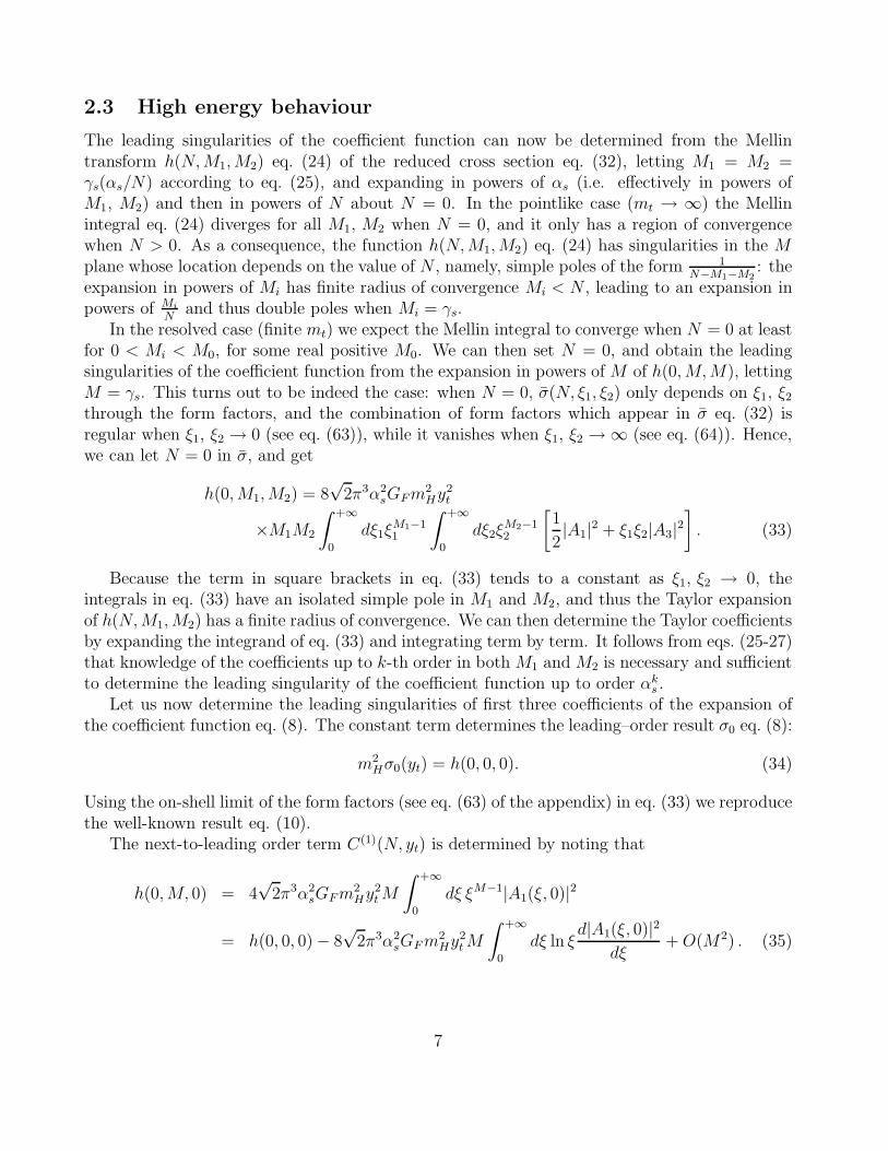
mH C(1)(yt) C(2)(yt)110 5.0447 16.2570120 4.6873 14.5133130 4.3568 13.0155140 4.0490 11.7196150 3.7607 10.5919160 3.4890 9.6058170 3.2318 8.7406180 2.9872 7.9794190 2.7536 7.3085200 2.5296 6.7166210 2.3140 6.1946220 2.1057 5.7346230 1.9037 5.3303240 1.7072 4.9761250 1.5151 4.6677260 1.3267 4.4013270 1.1409 4.1738280 0.9568 3.9828290 0.7731 3.8268300 0.5884 3.7049

Table 1: Values of the coefficients eq. (36) and eq. (38) of the O(αs/N) and O((αs/N)2) of theleading singularities of the coefficient function C(αs(m

2H); N, yt) eq. (12).

Equations (25-27) then immediately imply that

C(1)(N, yt) = C(1)(yt)CA

N[1 + O(N)] ,

C(1) = − 2(8π2)2

∣

∣

(

1 − 14(1 − 4yt)s0(yt)2

)∣

∣

2

∫ +∞

0

dξ ln ξd|A1(ξ, 0)|2

dξ. (36)

The value of the coefficient C(1), determined from a numerical evaluation of the integral ineq. (36), is tabulated in table 1 as a function of the Higgs mass. Upon inverse Mellin transfor-mation, one finds that

limτ→0

C(1)(τ, yt) = CAC(1)(yt). (37)

The values given in table 1 are indeed found to be in perfect agreement with a numericalevaluation of the small τ limit of the full NLO coefficient function C(1)(τ, yt) [4], for which wehave used the form given in ref. [20].

Turning finally to the determination of the hitherto unknown NNLO leading singularity, we

8

evaluate the O(M2) terms in the expansion eq. (35): by using again eqs. (25-27) we find

C(2)(N, yt) = C(2)(yt)C2

A

N2[1 + O(N)]

C(2)(yt) = − (8π2)2

∣

∣

(

1 − 14(1 − 4yt)s0(yt)2

)∣

∣

2

{∫ +∞

0

dξ ln2 ξd|A1(ξ, 0)|2

dξ(38)

−∫ +∞

0

dξ1

∫ +∞

0

dξ2

[

ln ξ1 ln ξ2∂2|A1(ξ1, ξ2)|2

∂ξ1∂ξ2

+ 2|A3(ξ1, ξ2)|2]}

.

The value of the NNLO coefficient C(2)(yt) obtained from numerical evaluation of the integralsin eq. (38) is also tabulated in table 1. This is the main result of the present paper.

3 Improvement of the NLO and NNLO cross sections

Knowledge of the leading small τ behaviour of the exact coefficient function C(αs(m2H); τ, yt)

eq. (8) can be used to improve its determination. Indeed, as discussed in section 1, we expectthe pointlike (mt → ∞) approximation to be quite accurate at large τ , whereas we know thatit must break down as τ → 0. Specifically, the small τ behaviour of the coefficient function isdominated by the highest rightmost singularity in C(αs(m

2H); N, yt) eq. (12), which for the exact

result is a k-th order pole but becomes a 2k-th order pole in the pointlike approximation. Hencethe pointlike approximation displays a spurious stronger growth eq. (1) at small enough τ .

Having determined the exact small τ behaviour up to NNLO, we can improve the approximatepointlike determination of the coefficient function by subtracting its spurious small τ growth andreplacing it with the exact behaviour. We discuss first the NLO case, where the full exact resultis known, and then turn to the NNLO where only the mt → ∞ result is available.

3.1 NLO results

At NLO the small τ behaviour of the coefficient function in the pointlike approximation isdominated by a double pole, whereas it is given by the simple pole eq. (36) in the exact case.This corresponds to an exact NLO contribution C(1)(τ, yt) which tends to a constant at small τ ,whereas the pointlike approximation to it grows as ln τ :

C(1)(τ,∞) = d(1)point(τ) + O (τ) ; d

(1)point(τ) = c1

2 ln τ + c11 (39)

C(1)(τ, yt) = d(1)ex (τ, yt) + O (τ) ; d(1)

ex (τ, yt) = 3C(1)(yt), (40)

where C(1)(yt) is tabulated in table 1, while from Refs. [4, 6, 7] we get

c12 = −6; c1

1 = −11

2. (41)

The NLO term C(1)(τ, yt) eq. (8) is plotted as a function of τ in fig. 1, both in the pointlike(mt → ∞) approximation, and in its exact form computed with increasing values of the Higgs

9

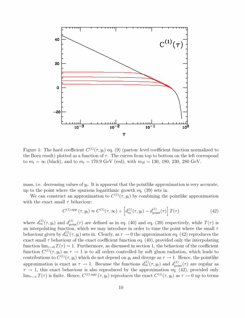
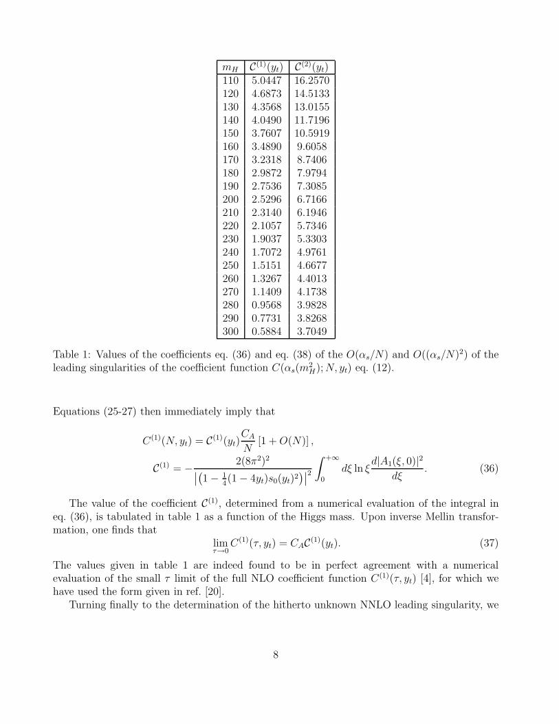
Figure 1: The hard coefficient C(1)(τ, yt) eq. (9) (parton–level coefficient function normalized tothe Born result) plotted as a function of τ . The curves from top to bottom on the left correspondto mt = ∞ (black), and to mt = 170.9 GeV (red), with mH = 130, 180, 230, 280 GeV.

mass, i.e. decreasing values of yt. It is apparent that the pointlike approximation is very accurate,up to the point where the spurious logarithmic growth eq. (39) sets in.

We can construct an approximation to C(1)(τ, yt) by combining the pointlike approximationwith the exact small τ behaviour:

C(1),app.(τ, yt) ≈ C(1)(τ,∞) +[

d(1)ex (τ, yt) − d

(1)point(τ)

]

T (τ) (42)

where d(1)ex (τ, yt) and d

(1)point(τ) are defined as in eq. (40) and eq. (39) respectively, while T (τ) is

an interpolating function, which we may introduce in order to tune the point where the small τbehaviour given by d

(1)ex (τ, yt) sets in. Clearly, as τ → 0 the approximation eq. (42) reproduces the

exact small τ behaviour of the exact coefficient function eq. (40), provided only the interpolatingfunction limτ→0 T (τ) = 1. Furthermore, as discussed in section 1, the behaviour of the coefficientfunction C(1)(τ, yt) as τ → 1 is to all orders controlled by soft gluon radiation, which leads tocontributions to C(1)(τ, yt) which do not depend on yt and diverge as τ → 1. Hence, the pointlike

approximation is exact as τ → 1. Because the functions d(1)ex (τ, yt) and d

(1)point(τ) are regular as

τ → 1, this exact behaviour is also reproduced by the approximation eq. (42), provided onlylimτ→1 T (τ) is finite. Hence, C(1),app.(τ, yt) reproduces the exact C(1)(τ, yt) as τ → 0 up to terms

10

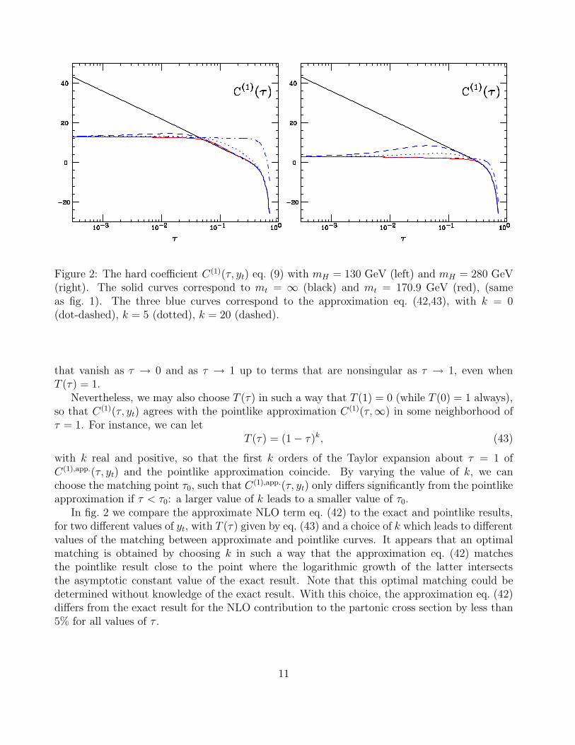
Figure 2: The hard coefficient C(1)(τ, yt) eq. (9) with mH = 130 GeV (left) and mH = 280 GeV(right). The solid curves correspond to mt = ∞ (black) and mt = 170.9 GeV (red), (sameas fig. 1). The three blue curves correspond to the approximation eq. (42,43), with k = 0(dot-dashed), k = 5 (dotted), k = 20 (dashed).

that vanish as τ → 0 and as τ → 1 up to terms that are nonsingular as τ → 1, even whenT (τ) = 1.

Nevertheless, we may also choose T (τ) in such a way that T (1) = 0 (while T (0) = 1 always),so that C(1)(τ, yt) agrees with the pointlike approximation C(1)(τ,∞) in some neighborhood ofτ = 1. For instance, we can let

T (τ) = (1 − τ)k, (43)

with k real and positive, so that the first k orders of the Taylor expansion about τ = 1 ofC(1),app.(τ, yt) and the pointlike approximation coincide. By varying the value of k, we canchoose the matching point τ0, such that C(1),app.(τ, yt) only differs significantly from the pointlikeapproximation if τ < τ0: a larger value of k leads to a smaller value of τ0.

In fig. 2 we compare the approximate NLO term eq. (42) to the exact and pointlike results,for two different values of yt, with T (τ) given by eq. (43) and a choice of k which leads to differentvalues of the matching between approximate and pointlike curves. It appears that an optimalmatching is obtained by choosing k in such a way that the approximation eq. (42) matchesthe pointlike result close to the point where the logarithmic growth of the latter intersectsthe asymptotic constant value of the exact result. Note that this optimal matching could bedetermined without knowledge of the exact result. With this choice, the approximation eq. (42)differs from the exact result for the NLO contribution to the partonic cross section by less than5% for all values of τ .

11

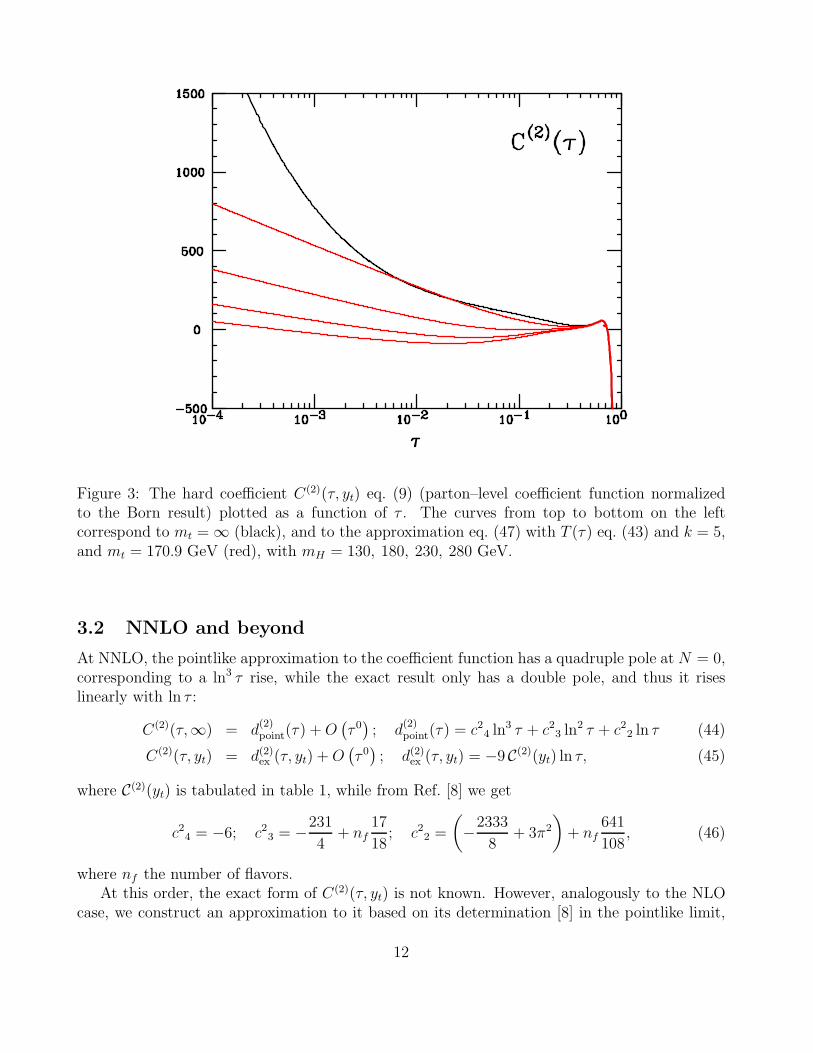
Figure 3: The hard coefficient C(2)(τ, yt) eq. (9) (parton–level coefficient function normalizedto the Born result) plotted as a function of τ . The curves from top to bottom on the leftcorrespond to mt = ∞ (black), and to the approximation eq. (47) with T (τ) eq. (43) and k = 5,and mt = 170.9 GeV (red), with mH = 130, 180, 230, 280 GeV.

3.2 NNLO and beyond

At NNLO, the pointlike approximation to the coefficient function has a quadruple pole at N = 0,corresponding to a ln3 τ rise, while the exact result only has a double pole, and thus it riseslinearly with ln τ :

C(2)(τ,∞) = d(2)point(τ) + O

(

τ 0)

; d(2)point(τ) = c2

4 ln3 τ + c23 ln2 τ + c2

2 ln τ (44)

C(2)(τ, yt) = d(2)ex (τ, yt) + O

(

τ 0)

; d(2)ex (τ, yt) = −9 C(2)(yt) ln τ, (45)

where C(2)(yt) is tabulated in table 1, while from Ref. [8] we get

c24 = −6; c2

3 = −231

4+ nf

17

18; c2

2 =

(

−2333

8+ 3π2

)

+ nf

641

108, (46)

where nf the number of flavors.At this order, the exact form of C(2)(τ, yt) is not known. However, analogously to the NLO

case, we construct an approximation to it based on its determination [8] in the pointlike limit,

12

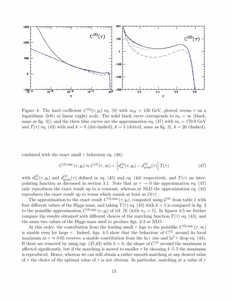
Figure 4: The hard coefficient C(2)(τ, yt) eq. (9) with mH = 130 GeV, plotted versus τ on alogarithmic (left) or linear (right) scale. The solid black curve corresponds to mt = ∞ (black,same as fig. 3)), and the three blue curves are the approximation eq. (47) with mt = 170.9 GeVand T (τ) eq. (43) with and k = 0 (dot-dashed), k = 5 (dotted, same as fig. 3), k = 20 (dashed).

combined with the exact small τ behaviour eq. (38):

C(2),app.(τ, yt) ≈ C(2)(τ,∞) +[

d(2)ex (τ, yt) − d

(2)point(τ)

]

T (τ) (47)

with d(2)ex (τ, yt) and d

(2)point(τ) defined in eq. (45) and eq. (44) respectively, and T (τ) an inter-

polating function as discussed in section 3.1. Note that as τ → 0 the approximation eq. (47)only reproduces the exact result up to a constant, whereas at NLO the approximation eq. (42)reproduces the exact result up to terms which vanish at least as O(τ) .

The approximation to the exact result C(2),app.(τ, yt), computed using C(2) from table 1 withfour different values of the Higgs mass, and taking T (τ) eq. (43) with k = 5 is compared in fig. 3to the pointlike approximation C(2),app.(τ, yt) of ref. [8] (with nf = 5). In figures 4-5 we furthercompare the results obtained with different choices of the matching function T (τ) eq. (43), andthe same two values of the Higgs mass used to produce figs. 2-3 at NLO.

At this order, the contribution from the leading small τ logs to the pointlike C(2),app.(τ,∞)is sizable even for large τ . Indeed, figs. 4-5 show that the behaviour of C(2) around its localmaximum at τ ≈ 0.65 receives a sizable contribution from the ln τ rise and ln2 τ drop eq. (44).If these are removed by using eqs. (47,43) with k = 0, the shape of C(2) around the maximum isaffected significantly, but if the matching is moved to smaller τ by choosing k >∼ 5 the maximumis reproduced. Hence, whereas we can still obtain a rather smooth matching at any desired valueof τ the choice of the optimal value of τ is not obvious. In particular, matching at a value of τ

13

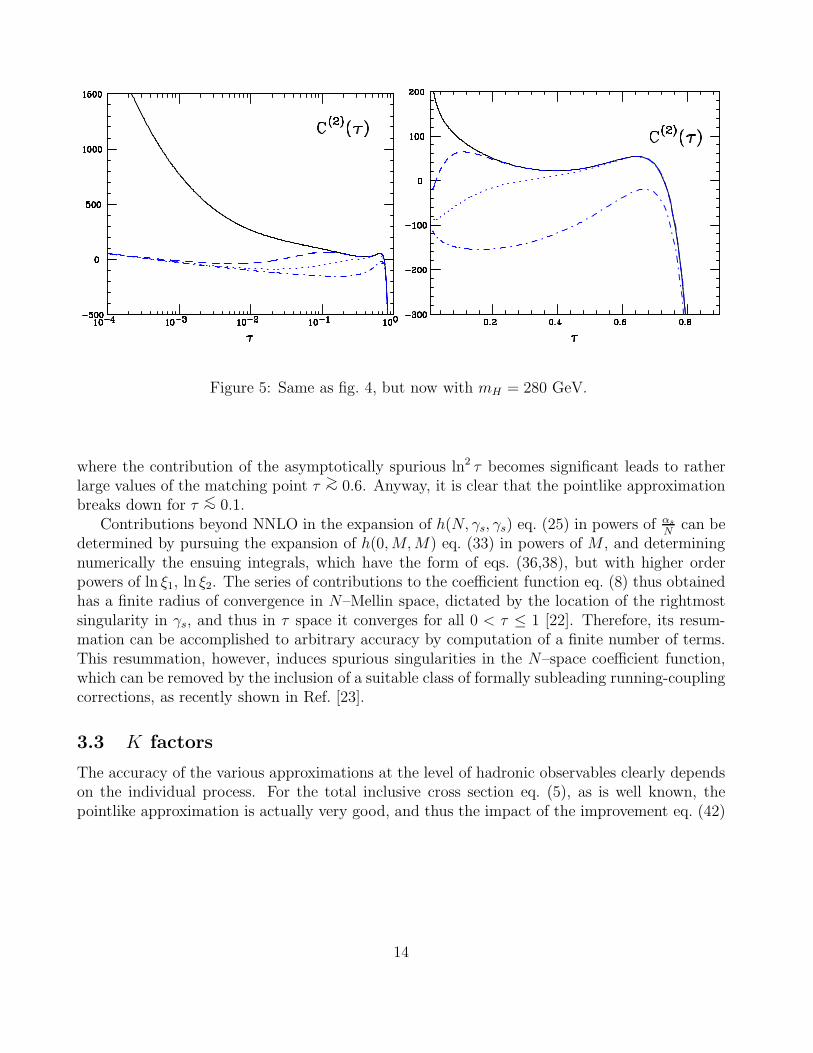
Figure 5: Same as fig. 4, but now with mH = 280 GeV.

where the contribution of the asymptotically spurious ln2 τ becomes significant leads to ratherlarge values of the matching point τ >∼ 0.6. Anyway, it is clear that the pointlike approximationbreaks down for τ <∼ 0.1.

Contributions beyond NNLO in the expansion of h(N, γs, γs) eq. (25) in powers of αs

Ncan be

determined by pursuing the expansion of h(0, M, M) eq. (33) in powers of M , and determiningnumerically the ensuing integrals, which have the form of eqs. (36,38), but with higher orderpowers of ln ξ1, ln ξ2. The series of contributions to the coefficient function eq. (8) thus obtainedhas a finite radius of convergence in N–Mellin space, dictated by the location of the rightmostsingularity in γs, and thus in τ space it converges for all 0 < τ ≤ 1 [22]. Therefore, its resum-mation can be accomplished to arbitrary accuracy by computation of a finite number of terms.This resummation, however, induces spurious singularities in the N–space coefficient function,which can be removed by the inclusion of a suitable class of formally subleading running-couplingcorrections, as recently shown in Ref. [23].

3.3 K factors

The accuracy of the various approximations at the level of hadronic observables clearly dependson the individual process. For the total inclusive cross section eq. (5), as is well known, thepointlike approximation is actually very good, and thus the impact of the improvement eq. (42)

14

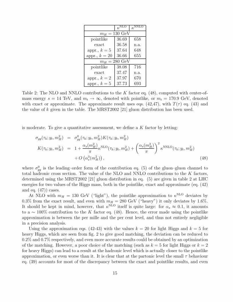
κNLO κNNLO

mH = 130 GeVpointlike 36.69 658

exact 36.58 n.a.appr., k = 5 37.64 648appr., k = 20 36.66 655

mH = 280 GeVpointlike 38.08 716

exact 37.47 n.a.appr., k = 2 37.97 670appr., k = 5 37.73 693

Table 2: The NLO and NNLO contributions to the K factor eq. (48), computed with center-of-mass energy s = 14 TeV, and mt → ∞, denoted with pointlike, or mt = 170.9 GeV, denotedwith exact or approximate. The approximate result uses eqs. (42,47), with T (τ) eq. (43) andthe value of k given in the table. The MRST2002 [21] gluon distribution has been used.

is moderate. To give a quantitative assessment, we define a K factor by letting:

σgg(τh; yt, m2H) = σ0

gg(τh; yt, m2H)K(τh; yt, m

2H)

K(τh; yt, m2H) = 1 +

αs(m2H)

πκNLO(τh; yt, m

2H) +

(

αs(m2H)

π

)2

κNNLO(τh; yt, m2H)

+ O(

α3s(m

2H)

)

, (48)

where σ0gg is the leading–order form of the contribution eq. (5) of the gluon–gluon channel to

total hadronic cross section. The value of the NLO and NNLO contributions to the K factors,determined using the MRST2002 [21] gluon distribution in eq. (5) are given in table 2 at LHCenergies for two values of the Higgs mass, both in the pointlike, exact and approximate (eq. (42)and eq. (47)) cases.

At NLO with mH = 130 GeV (“light”), the pointlike approximation to κNLO deviates by0.3% from the exact result, and even with mH = 280 GeV (“heavy”) it only deviates by 1.6%.It should be kept in mind, however, that κNLO itself is quite large: for αs ≈ 0.1, it amountsto a ∼ 100% contribution to the K factor eq. (48). Hence, the error made using the pointlikeapproximation is between the per mille and the per cent level, and thus not entirely negligiblein a precision analysis.

Using the approximation eqs. (42-43) with the values k = 20 for light Higgs and k = 5 forheavy Higgs, which are seen from fig. 2 to give good matching, the deviation can be reduced to0.2% and 0.7% respectively, and even more accurate results could be obtained by an optimizationof the matching. However, a poor choice of the matching (such as k = 5 for light Higgs or k = 2for heavy Higgs) can lead to a result at the hadronic level which is actually closer to the pointlikeapproximation, or even worse than it. It is clear that at the partonic level the small τ behavioureq. (39) accounts for most of the discrepancy between the exact and pointlike results, and even

15

the determination of a hadronic observable which depends very little on the parton-level smallτ behaviour can be improved very substantially for values of τH relevant for LHC by using theapproximation eq. (42).

The NNLO contribution κNNLO is not known. Its values computed in the pointlike approxi-mation, or with the approximation eqs. (47,43) and different choices of k are shown in table 2.Even at the inclusive hadronic level, now the size of the NNLO contribution can change upto about 5 − 10% if the matching is performed at large τ . Furthermore, κNNLO is also quitelarge: with αs ≈ 0.1, it amounts to a ∼ 50% correction to the leading order, and thus to afurther ∼ 25% correction to the K factor. Therefore, the impact of the pointlike approximationat NNLO is up to several per cent of the total K factor, rather larger that the impact of thepointlike approximation at NLO, and comparable to uncertainties which are currently discussedin precision studies at NNLO.

4 Outlook

In this paper we have determined the leading high energy (i.e. small τ =m2

H

s) singularities of the

cross section for Higgs production in gluon–gluon fusion to all orders in the strong coupling, byproviding an expression (eq. (33)) whence the coefficients of these singularities can be obtained byTaylor expanding and computing a double integral. We have given explicit numerical expressionsfor these coefficients up to NNLO.

The high energy behaviour of this cross section is different according to whether it is deter-mined with finite mt or with mt → ∞ (pointlike approximation). It turns out that at NLO thisdifferent high energy behaviour is responsible for most of the discrepancy between the pointlikeapproximation and the exact result. As a consequence, an accurate approximation to the exactresult can be constructed by combining the pointlike approximation at large τ with the exactsmall τ behaviour. Some care must be taken in matching, but very accurate results can beobtained by simply choosing the matching point as that where the spurious small τ behaviourof the pointlike behaviour sets in.

At NNLO, where the exact result is not known, the impact of the high energy behaviourturns out to be large even for moderate values of τ ∼ 0.5. Hence, an approximation constructedanalogously to that which is successful at NLO, namely matching the pointlike limit to theasymptotic exact behaviour at the point where the asymptotically spurious terms become signif-icant, leads to an approximate result which differs significantly from the pointlike approximationfor most values of the partonic center-of-mass energy.

The effect of these high energy terms on the total inclusive hadronic cross section remainsquite small, because the latter is dominated by the region of low partonic center–of–mass energy,partly due to shape of the gluon parton distributions, which are peaked in the region where thegluons carry a small fraction of the incoming nucleon’s energy, and partly because the partoniccross section is peaked in the threshold τ ≈ 1 region. Even so, the pointlike determination ofthe NNLO contribution to the total hadronic cross section can be off by almost 5-10% due tothis spurious high energy behaviour, especially for relatively large values of mH

>∼ 200 GeV.Because the NLO and NNLO corrections to the cross section are quite large, the overall effect of

16

these terms on the cross section is at the per cent level, and in particular their effect at NNLOis rather larger than at NLO.

A study of the phenomenological implications of these results is thus relevant for a precisiondetermination of the Higgs production cross section.

Acknowledgements: We thank Thomas Binoth and Fabio Maltoni for discussions, andGuido Altarelli for a critical reading of the manuscript. This work was partly supported bythe Marie Curie Research and Training network HEPTOOLS under contract MRTN-CT-2006-035505 and by a PRIN2006 grant (Italy). The work of S. Marzani and R.D. Ball was done withthe support of the Scottish Universities’ Physics Alliance.

A Form factors

The form factors in eq. (28) are given by

A1(ξ1, ξ2, yt) = C0(ξ1, ξ2, yt)

[

4yt

∆3(1 + ξ1 + ξ2) − 1 − 4ξ1ξ2

∆3+ 12

ξ1ξ2

∆23

(1 + ξ1 + ξ2)

]

− [B0(−ξ2) − B0(1)]

[

−2ξ2

∆3+ 12

ξ1ξ2

∆23

(1 + ξ1 − ξ2)

]

− [B0(−ξ1) − B0(1)]

[

−2ξ1

∆3

+ 12ξ1ξ2

∆23

(1 − ξ1 + ξ2)

]

+2

∆3

1

(4π)2(1 + ξ1 + ξ2) , (49)

A2(ξ1, ξ2, yt) = C0(ξ1, ξ2, yt)

[

2yt −1

2(1 + ξ1 + ξ2) +

2ξ1ξ2

∆3

]

+ [B0(−ξ2) − B0(1)]

[

ξ2

∆3

(1 − ξ1 + ξ2)

]

+ [B0(−ξ1) − B0(1)]

[

ξ1

∆3(1 + ξ1 − ξ2)

]

+1

(4π)2, (50)

with∆3 = 1 + ξ2

1 + ξ22 − 2ξ1ξ2 + 2(ξ1 + ξ2) = (1 + ξ1 + ξ2)

2 − 4ξ1ξ2 . (51)

It is also convenient to define the form factor

A3(ξ1, ξ2, yt) ≡1

ξ1ξ2

[

1 + ξ1 + ξ2

2A1 − A2

]

. (52)

The scalar integrals B0 and C0 are

B0(ρ) = − 1

8π2

√

4yt − ρ

ρtan−1

√

ρ

4yt − ρ, if 0 < ρ < 4yt ;

B0(ρ) = − 1

16π2

√

ρ − 4yt

ρln

1 +√

ρ

ρ−4yt

1 −√

ρ

ρ−4yt

, if ρ < 0 or ρ > 4yt ; (53)

17

C0(ξ1, ξ2) ≡ 1

16π2

1√∆3

{

ln(1 − y−) ln

(

1 − y−δ+1

1 − y−δ−1

)

+ ln(1 − x−) ln

(

1 − x−δ+2

1 − x−δ−2

)

+ ln(1 − z−) ln

(

1 − z−δ+3

1 − z−δ−3

)

+Li2(y+δ+1 ) + Li2(y−δ+

1 ) − Li2(y+δ−1 ) − Li2(y−δ−1 )

+Li2(x+δ+2 ) + Li2(x−δ+

2 ) − Li2(x+δ−2 ) − Li2(x−δ−2 )

+Li2(z+δ+3 ) + Li2(z−δ+

3 ) − Li2(z+δ−3 ) − Li2(z−δ−3 )}

, (54)

where

δ1 ≡−ξ1 + ξ2 − 1√

∆3

, δ2 ≡ξ1 − ξ2 − 1√

∆3

, δ3 ≡ξ1 + ξ2 + 1√

∆3

, (55)

δ±i ≡ 1 ± δi

2, (56)

and

x± ≡ − ξ2

2yt

(

1 ±√

1 +4yt

ξ2

)

,

y± ≡ − ξ1

2yt

(

1 ±√

1 +4yt

ξ1

)

,

z± ≡ 1

2yt

(

1 ± i√

4yt − 1)

. (57)

In the infinite top mass limit the scalar integrals become

limyt→∞

B0(ρ) =1

16π2

(

−2 +ρ

6yt

)

+ O

(

1

y2t

)

, (58)

limyt→∞

C0(ξ1, ξ2) = − 1

32π2yt

(

1 +1 − ξ1 − ξ2

12yt

)

+ O

(

1

y3t

)

, (59)

so that the form factors reduce to

limmt→∞

m2t A1 = m2

H

1

48π2; lim

mt→∞4m2

t A2 = m2H

αs

48π2

1 + ξ1 + ξ2

2. (60)

These limits also imply thatlim

mt→∞m2

tA3 = 0. (61)

In the on-shell limit the scalar integrals are

limξi→0

B0(ξi) = − 1

8π2,

limξ1→0

C0(ξ1, ξ2, yt) =1

32π2

1

1 + ξ2

(

ln2 −z−z+

− ln2 −x−

x+

)

, (62)

limξ1,ξ2→0

C0(ξ1, ξ2, yt) =1

32π2

(

ln2 −z−z+

)

,

18

so that

A1(0, 0) =1

8π2+

1

32π2

(

ln2 −z−z+

)

(4yt − 1)

A2(0, 0) =1

16π2+

1

32π2

(

ln2 −z−z+

) (

2yt −1

2

)

(63)

The high energy limit of the form factors is trivially determined when ξ1 → ∞, ξ2 → ∞ withξ1 6= ξ2:

limξ1→∞, ξ2→∞

A1(ξ1, ξ2, yt) = 0; limξ1→∞, ξ2→∞

A3(ξ1, ξ2, yt) = 0; limξ1→∞, ξ2→∞

A2(ξ1, ξ2, yt) =1

(4π)2.

(64)If ξ1 → ∞, ξ2 → ∞ with ξ1 = ξ2 the limit is more subtle. In this case we get

limξ→∞

A1(ξ, ξ, yt) = limξ→∞

C0(ξ, ξ, yt)

4

√

ξ − 1

16π2

[

1

2ln

yt

ξ− 1 +

√

4yt − 1 tan−1

√

1

4yt − 1

]

+O

(

1√ξ

)

, (65)

where we have definedC0(ξ1, ξ2, yt) ≡ C0(ξ1, ξ2, yt)

√∆3. (66)

However, it turns out that

limξ→∞

C0(ξ, ξ, yt) =1

16π2√

ξ

[

2 lnyt

ξ− 4 + 4

√

4yt − 1 tan−1

√

1

4yt − 1

]

+ O

(

1

ξ

)

, (67)

hence we conclude that eq. (64) holds also when ξ1 = ξ2.

References

[1] G. P. Salam, Int. J. Mod. Phys. A 21 (2006) 1778.

[2] R. Harlander, Acta Phys. Polon. B 38 (2007) 693.

[3] D. Graudenz, M. Spira and P. M. Zerwas, Phys. Rev. Lett. 70 (1993) 1372.

[4] M. Spira, A. Djouadi, D. Graudenz and P. M. Zerwas, Nucl. Phys. B 453 (1995) 17.

[5] M. Kramer, E. Laenen and M. Spira, Nucl. Phys. B 511 (1998) 523.

[6] A. Djouadi, M. Spira and P. M. Zerwas, Phys. Lett. B 264 (1991) 440.

[7] S. Dawson, Nucl. Phys. B 359 (1991) 283.

19

[8] C. Anastasiou and K. Melnikov, Nucl. Phys. B 646 (2002) 220; R. V. Harlander andW. B. Kilgore, Phys. Rev. Lett. 88 (2002) 201801; V. Ravindran, J. Smith and W. L. vanNeerven, Nucl. Phys. B 665 (2003) 325.

[9] S. Moch and A. Vogt, Phys. Lett. B 631 (2005) 48.

[10] S. Catani, D. de Florian, M. Grazzini and P. Nason, JHEP 0307 (2003) 028.

[11] V. Del Duca, W. Kilgore, C. Oleari, C. Schmidt and D. Zeppenfeld, Nucl. Phys. B 616

(2001) 367.

[12] S. Catani, M. Ciafaloni and F. Hautmann, Phys. Lett. B 242 (1990) 97; S. Catani,M. Ciafaloni and F. Hautmann, Nucl. Phys. B 366 (1991) 135.

[13] F. Hautmann, Phys. Lett. B 535 (2002) 159.

[14] J. R. Ellis, M. K. Gaillard and D. V. Nanopoulos, Nucl. Phys. B 106 (1976) 292; M. A. Shif-man, A. I. Vainshtein, M. B. Voloshin and V. I. Zakharov, Sov. J. Nucl. Phys. 30 (1979)711 [Yad. Fiz. 30 (1979) 1368].

[15] T. Jaroszewicz, Phys. Lett. B 116 (1982) 291.

[16] S. Catani and F. Hautmann, Nucl. Phys. B 427 (1994) 475.

[17] R. D. Ball and R. K. Ellis, JHEP 0105 (2001) 053.

[18] G. Camici and M. Ciafaloni, Nucl. Phys. B 496 (1997) 305 [Erratum-ibid. B 607 (2001)431].

[19] R. S. Pasechnik, O. V. Teryaev and A. Szczurek, Eur. Phys. J. C 47 (2006) 429.

[20] R. Bonciani, G. Degrassi and A. Vicini, JHEP 0711 (2007) 095.

[21] A. D. Martin, R. G. Roberts, W. J. Stirling and R. S. Thorne, Eur. Phys. J. C 28 (2003)455.

[22] R. D. Ball and S. Forte, Phys. Lett. B 351 (1995) 313.

[23] R. D. Ball, arXiv:0708.1277 [hep-ph].

20