Stopping distance for high energy jets in weakly coupled quark-gluon plasmas
Upload
khangminh22Category
view
3download
0
SE9900237
ISBN 91-628-3636-6LUNFD6/(NFFL-7168) 1999
Different Methods for Ouark/Gluon Jet Classificationon Real Data from the DELPHI Detector
Thesis Submitted for the Degree ofDoctor of Philosophy in Physics
by
Goran TranstromerDepartment of Particle Physics
Lund UniversityProfessorsgatan 1
Box 118S-221 00 Lund
Sweden
3 0 - 2 9

Elegie
J'ouvre la premiere porte.C'est une grande chambre inondee de soleil.Une lourde voiture passe dans la rueet fait trembler la porcelaine.
J'ouvre la porte numero deux.Amis! Vous avez bu de l'ombrepour vous rendre visibles.
Porte numero trois. Une chambre d'hotel etroite.Avec vue sur une ruelle.Une laterne qui etincelle sur l'asphalte.Belles scories de l'experience.
Tomas Transtromer

Abstract
Different methods to separate quark jets from gluon jets have been investigated and testedon data from the DELPHI experiment. A test sample of gluon jets was selected from bbgthreejet events where the two b-jets had been identified using a lifetime tag and a quarkjet sample was obtained from qqi events where the photon was required to have a highenergy and to be well separated from the two jets.
Three types of tests were made.Firstly, the jetenergy, which is the variable most frequently used for quark/gluon jet
separation, was compared with methods based on the differences in the fragmentation ofquark and gluon jets. It was found that the fragmentation based classification providessignificantly better identification than the jet energy only in events where the jets allhave approximately the same energy. In Monte Carlo generated symmetric e+e~ —» qqgthreejet events, where the jet energy does not provide any identification at all, the gluonjet was correctly assigned in 58% of the events. More importantly, however, is thatthe identification has been divided into two independent parts, the energy part and thefragmentation part.
Secondly, two different sets of fragmentation sensitive variables were tested. It wasfound that a slightly better identification could be achieved using information from allthe particles of the jet rather than using only the leading ones.
Thirdly, three types of statistical discrimination methods were compared:
• a cut on a single fragmentation variable;
• a cut on the Fisher statistical discriminant calculated from one set of variables;
• a cut on the output from an Artificial Neural Networks (ANN) trained on differentsets of variables.
The three types of classifiers gave about the same performance and one conclusionfrom this study was that the use of ANNs or Fisher statistical discrimination do not seemto improve the results significantly in quark/gluon jet separation on a jet to jet basis.
VLl

Contents
1 Introduction 2
2 Theory 52.1 One hundred years of Particles Physics 5
2.1.1 Only three particles 52.1.2 Hundreds of particles 62.1.3 A subatomic periodic table 6
2.2 The Standard Model , 82.2.1 Quantum Chromodynamics 9
2.3 Grouping of particles 122.3.1 Matter constituents 122.3.2 Force carriers 13
2.4 The fragmentation process 142.5 The Z° decay into b-quarks 172.6 B-particles 172.7 Simulated events 18
2.7.1 Monte Carlo generation 182.7.2 Pertubative QCD 182.7.3 Non Pertubative QCD 19
2.8 Tuning of fragmentation variables 20
3 LEP and the DELPHI experiment 223.1 Why so large dimensions? 22
3.1.1 Radiation losses at LEP 223.2 The accelerator complex 24
3.2.1 LEP, the Large Electron-Positron collider 243.2.2 LEP and LEP2 30
3.3 The DELPHI Detector 303.3.1 Tracking detectors 313.3.2 Calorimeters 33
3.4 DAS, the data acquisition system 343.4.1 DSTANA 343.4.2 DELANA 343.4.3 DELSIM 343.4.4 SKELANA 34
vni

4 Multi-variable discriminant analysis 424.1 Linear discrimination analysis 424.2 Non-linear discrimination analysis 45
4.2.1 Artificial Neural Network models 464.2.2 Feed-Forward Neural Networks 474.2.3 Implementation or the learning phase 50
5 Overview of the Main Analysis 52
6 Event selection and jet reconstruction 556.1 Data selection 556.2 Particle selection 556.3 Event selection 566.4 Selection of threejet events 566.5 Jet reconstruction 566.6 Jet algorithms 57
7 B-tagging 607.1 LeptonTag 607.2 Lifetime Tag 617.3 The tagging method used in the analysis 65
7.3.1 The event tagging 657.3.2 The individual tagging of the jets in the event 65
8 Quark/Gluon jet samples 688.1 Association of quarks/gluons to jets in qqg MC events 688.2 Differencies between the true quark/gluon jet samples 728.3 Selection of quark jets in qqj events 738.4 Selection of gluon jets in bbg events 75
9 Jet classification using the jet energy 869.1 Definition of efficiency and purity 869.2 Efficiency and purity on a jet to jet basis 889.3 Efficiency/purity on an event basis 88
10 Fragmentation variables 9210.1 Fragmentation sensitive variables for gluon and quark jets 92
10.1.1 Variables based on leading particles 9210.1.2 The Fodor moments 94
10.2 The energy dependence of the fragmentation variables 97
11 Jet classification using fragmentation 10211.1 Using the Fisher discrimination method 10311.2 Using only one fragmentation variable 10511.3 Using artificial neural networks 105
11.3.1 The training of an ANN 108

11.3.2 JETNET 10911.3.3 Description of the different ANNs used 110
11.4 Comparison of Monte Carlo data with real data I l l11.5 Performance of the classifiers used on Monte Carlo data 112
11.5.1 Purity on a jet to jet basis 11511.5.2 Purity on an event basis 118
11.6 The classifiers used on experimental data 120
12 Applications of jet identification 13012.1 Investigation of the splitting of quark and gluon jets 13012.2 Measurement of the triple gluon vertex 132
12.3 Scale dependence of the multiplicity 135
13 Conclusions 138
A Geometry for Classification Purposes 144
B The energy dependence of the longitudinal momenta 147
C The energy dependence of the transverse momenta 150
D The energy dependence of the Fodor momenta 153

Chapter 1
Introduction
The theory of Quantum Chromo Dynamics, QCD, contains two fundamental types ofparticles, quarks and gluons. Quarks carry a single colour while gluons carry two coloursand therefore quarks and gluons differ in their coupling strength to another gluon. Quarksand gluons themselves are not visible but after an interaction they hadronize into a jetof particles. Jets originating from quarks and gluons are expected to differ in energyspectrum, multiplicity and angular distributions and many previous studies [1], [2], [3],have confirmed that gluon jets have a softer energy spectrum, a higher multiplicity anda wider angular distribution than a quark jet. The energy spectra can be calculated tohigh precision from the matrix elements in pertubative QCD. The differences betweenthe energy spectra of quark jets and gluon jets can essentially be explained by the factthat gluons are normally produced in an additional bremsstrahlung-like radiative processfrom a quark or another gluon and thus fragmentation differences are due to the differentcolour charge of the gluons compared to the quarks. Because the fragmentation takesplace at a low energy scale, pertubative QCD is not applicable and the process must bestudied with phenomenological models.
At LEP, the simplest topology involving a gluon jet occurs when a (hard) gluon isradiated from one of the quarks in a qq pair produced in a Z° decay. Hard here meansenergetic enough to create a shower of hadrons, a jet which is separated in space from thetwo jets created by the quarks. It is, in principle, possible to see if the original parton wasa quark or a gluon. Quark jets and gluon jets are distinguishable, at least on a statisticalbasis, from differences in their energy spectra and their fragmentation properties and theproblem studied in this work is how to best separate these two types of jets. If one candistinguish between quark jets and gluon jets the predictions of QCD can be tested andthe fragmentation features can be better understood. A more specific example is five jetevents at LEP2 coming from a WW-pair that have radiated a hard gluon. If the gluonjet could be identified the possibility to combine jets to the correct W-particles would beenhanced and the mass determination would be better.
Most of the interesting events at hadron colliders, for instance the Tevatron, are dom-inated by quark jets and the gluon jets are a background to these events. For instancett —> W W bb where the W-particles both decay by W —>• qq. The reverse is also true,i.e. if the elusive Higg's particle will be produced, its decay rate to two gluon jets (via atop loop) could, at least in principle, be seen if the overwhelming "background" of b-jets

could be overcome. The determination of the parton distribution of the proton would alsobe improved if the different jets could be well separated.
Normally, the jet energy provides a high degree of separation between quark jetsand gluon jets. The intention in this thesis is to demonstrate how the quark/gluon jetseparation using only the fragmentation (so far mostly studied at Monte Carlo level)performs on real data, collected during the period 1992-1994 by the DELPHI experimentat LEP. The quark/gluon jet separation using the fragmentation is a statistical problemwhich may be solved by using methods such as Fisher statistical discrimination or ArtificialNeural Networks (ANNs). In this theses ANNs trained on different types of fragmentationvariables and with different training methods are compared. For completeness, the Fisherstatistical discrimination as well as the discriminative power of the single best inputvariable are compared with ANNs.
A short historical background, leading to QCD, is given in chapter 2. Some sixtyyears ago there was a simple picture with only three fundamental particles. Then "chaos"broke out with hundreds of elementary particles, some 40 years ago, but soon order wasrestored by the quark hypothesis and the invention of the Standard Model (SM) with itsthree families.
The accelerator LEP and the DELPHI detector, presented in chapter 3, are intimatelyconnected, LEP provides an extremely clean initial condition and the full solid anglecoverage of the DELPHI detector makes it possible to fully use the powerful constraint ofenergy-momentum conservation.
A short introduction to multi-dimensional methods, such as the Fisher statisticalmethod and Artificial Neural Networks is given in chapter 4. An overview of the mainanalysis is given in chapter 5.
The event selection, which is more or less the same for all DELPHI analysis, is discussedin chapter 6. In the same chapter, different jet algorithms are presented. The LUCLUSalgorithm was mainly used to reconstruct the threejet events for this analysis.
The different methods to identify or tag specific events are given in chapter 7. Withthe silicon vertex detectors, now installed in every LEP experiment, there is a possibilityto select special events with a high purity as well as high efficiency. This will be used tofind a pure sample of tagged b-quark jets that will be used to produce a sample of cleangluon jets from real data.
The different ways of obtaining, from the hadronic events, a quark sample as well asa gluon sample from the Monte Carlo is the content of chapter 8. It also reviews theanti-tagging method, which will be used to obtain the sample of real gluon jets from bbgevents. The quark jet sample has been obtained from qq'y events. The same types ofsamples have been used in other studies measuring the multiplicity and particle contentsof quark jets and gluon jets [1, 2, 3].
The must powerful variable to use when considering a quark/gluon jet classifier forthe bulk of the events is the jet energy and it is discussed and evaluated in chapter 9.The performances of the various analysis methods can be compared to the correspondingsamples obtained from detector simulated Monte Carlo data. Here is also a discussion onhow to adequately present the performance of the classifiers in different jet topologies.
The intention of the thesis is to demonstrate how the quark/gluon jet separationusing only the fragmentation performs on real data without using the jet energy which is

4 CHAPTER 1. INTRODUCTION
particular relevant for the subset of events which have similar jet energies. A discussionof the most suitable ways of doing this is discussed in chapter 10 and the different sets offragmentation variables used as input are also presented in this chapter.
The selected fragmentation variables are then used in chapter 11 as input to theFisher statistical discrimination method as well as to Artificial Neural Networks andtheir performances as quark/gluon jet classifier are evaluated. The traditional methodof averaging over the entire jet sample is compared with the more useful measure ofperformance associated with a specific event type. Here is also a presentation of theresults on the sample of DELPHI quark jets.
A brief account is given in chapter 12 of results of recently performed DELPHI analy-ses, where quark and gluon jets have been selected and identified in ways similar to thosedescribed in this thesis.
In the last chapter, conclusions are drawn of this study of jet identification.

Chapter 2
Theory
2.1 One hundred years of Particles Physics
Human knowledge is said to depend on our faculty to receive some raw material from theoutside world and on our faculty to organise this material by means of certain concepts.Using this definition our knowledge of basic elementary particle physics has changedseveral times during the last century.
2.1.1 Only three particlesWhen Thompson discovered the negatively charged electron and its elementary natureabout a hundred years ago, it became clear that the atom was not elementary. He alsofound the weight of the electrons to be about 2000 times less than the smallest atom, thatof hydrogen. The discovery of the electron was reported to the British Royal Institutionon 30 April 1897, so this date can be considered as the birthday of particle physics.
In the beginning of this century, Rutherford performed his scattering experiment witha-particles bombarding a very thin gold foil. The heavy, positively charged a-particles,which had been discovered some decade earlier by Becquerel and the Curie couple, pene-trated the foil easily in most cases. Occasionally, however, they scattered into large angles,or even bounced backwards1, which could be interpreted as if the mass and the charge ofthe atom was concentrated to a very small space in the centre, called the nucleus, about10000 smaller then the size of the atom (~ 10~10 m).
In 1919, Rutherford returned to Cambridge to become director of the Cavendish lab-oratory where he had previously done his graduate work under J.J. Thomson. Here hediscovered the proton from a-particle bombardment (from Po2U) on nitrogen, by observ-ing the first nuclear reaction, iV14(a,p)O17.
When Chadwick, in 1932, found the neutron, the picture of particle physics was veryclean. All ordinary matter is made of atoms, which are built by a nucleus of protonsand neutrons (nucleons) surrounded by as many electrons as there are protons in order tomake the atom neutral. For a while these particles were considered to be truly elementary,i.e. the number of elementary particles, at this time, was only three.
*At a rate of one in eight thousand. "As if you fired a 15-inch naval shell at a piece of tissue paperand the shell came right back and hit you" was Rutherford classical comment.

6 CHAPTER 2. THEORY
2.1.2 Hundreds of particlesPhysicists knew that nuclei axe difficult to break up, so what held the protons and theneutrons, i.e. the nucleons, together? In 1935, considering the size of nuclei, about 1Fermi, Yukawa predicted a particle, which he called meson (meson = middle), whichought to be heavier than the electron (me = 9,109 • 10~31 kg) but lighter than the1836 times heavier proton. The particle should be responsible for the strong nuclearforce. Yukava drew a parallel with the well known electromagnetic force between chargedparticles. This force could be interpreted in such a way that one of the particles isemitting radiation which is absorbed by the other. According to the quantum theorythis radiation is quantised and the force is originating from the exchange of photons.They cannot detach themselves from the charges, so they are said to be virtual. Photonsare force carriers and are characterized by integer spin (in units of %). Such particles arecalled bosons. Since the strong nuclear force is acting at a very short range, approximately10~15 m, the energy (and therefore its mass) of the strong force carriers could be estimatedaccording to Heisenberg's uncertainty principle, to be around 140 MeV (M = 106,1 eV =1.6021 • 10~19 J).
Anderson, who in 1933 also discovered the first antiparticle, the positron, found in 1937yet another new particle in the cosmic rays, the muon or fi, which was first mistakinglyidentified with the Yukawa particle. It was, however, a puzzle that this new particleinteracted "weakly". The real Yukawa particle, the pion, ft, was discovered in 1947 inballoon flight carrying emulsion from the interaction of cosmic protons with the upperatmosphere producing pions which sub-sequentially were observed to decay to Anderson'smuon.
In the fifties an explosion of discoveries of new particles followed. Some of these werecalled strange particles, for example K, A, S and E, because they were produced in pairsand decayed very slowly, in about 10~10 seconds and sometimes even longer. In orderto explain why these particles lived so long, Gell-Mann proposed that they carried afundamental property that he called strangeness, which had to be conserved in strongdecays. Therefore the strange particles had to decay via the weak nuclear force, in whichstrangeness was not conserved and so managed to live longer. The clean particle physicspicture from 1930 was now a "zoo" of particles, and the situation was very much likethe one in chemistry, before the table of elements (the periodic system) was presented byMendeleyev in 1869.
2.1.3 A subatomic periodic tableGell-Mann and Neeman constructed in 1961, the first successful subatomic periodic tableby grouping the particles in families of specific geometrical patterns. These familiescontained sometimes eight and sometimes ten members. In 1962, Gell-Mann predicted anew particle, £2", as a missing member in a group of ten. The question was whether thetheory would be able to explain the truth underneath the geometrical patterns. Zweigand Gell-Mann showed that this classification was a natural fact if there were three basicconstituents, later named quarks. Gell-Mann called them up, down and strange or justu, d and s. They must all have fractional charges, the up quark should have a charge of

2.1. ONE HUNDRED YEARS OF PARTICLES PHYSICS
+2e/3 and the down quark and the strange quark, a charge of —e/3. JVactional chargeswas a concept many physicists refused to accept. However, simple quark algorithms orrules could form all known hadrons (hadron = heavy, heavier than the proton), all baryonsby putting three quarks together and aU mesons by combining a quark and its antiquark.The proton was, for example, easily constructed of two up-quarks and one down-quark,giving the proton a positive "elementary" charge. The neutron was equally easy to builtof one up-quark and two down-quarks, in that way being neutral. The quarks were atfirst- accepted as some sort of a mathematical tool rather than real constituents.
A real problem appeared when the SV", was discovered at Brookhaven's bubble cham-ber in 1963, see figure 2.1, since the model to construct the Q~ violated a fundamentallaw of physics, the Pauli principle. The same argument applies to the particle A++, con-sisting of three u-quarks and A", consisting of three d-quarks. This principle excludes
Figure 2.1: Production and decay of a negative omega particle, fir, when a K~ has hit aproton, in the CERN two-metre liquid hydrogen bubble chamber.
the possibility that the three, identical, s-quarks, needed to construct the Or, could bein the same state (i.e. have the same set of quantum numbers}. It can be shown thatthe particle (having J—3/2 and L=0) must have the spins of three quarks aligned in thesame direction and therefore could not exist inside the Q~ simultaneously if they wereidentical, since a symmetric wave function could not possibly describe a fermion. ThePauli exclusion principle of quantum mechanics required an antisymmetric wave function.W. Greenberg solved this puzzle by introducing three distinguishable colours which re-stored the antisymmetry. Colour turned out to be the key to explaining how the quarkmodel could be true. Now also the precise value of the anomalous magnetic moment ofthe proton and the neutron found an explanation ia terms of the quark model with threecolours. This had been a puzzle since the discovery in the beginning of the 1930s.
In order to bring some experimental proof into the quark idea, a rerun, of Rutherford'sclassical experiment was performed at the Stanford Linear Accelerator Center (SLAC)in 1967, with its three kilometres long accelerator. In the SLAC-MIT experiment highenergy electrons scattered inelastically against the nucleon. The results showed a much

8 CHAPTER 2. THEORY
higher rate of wide angle scattering than expected from previous models for the nucleon,revealing tiny charged bodies inside the nucleon. The first experimental evidence for thesubstructure of the nucleons required high momentum transfers. According to Bjorkenand Feynman, the result of the experiment could be explained by assuming that the protonconsisted of a few hard, pointlike scattering centres. In 1968 R. Feynman called those newobjects partons, not yet ready to call them quarks. B.J. Bjorken worked out the detailedconsequences of the quark-parton model for both electron and neutrino scattering.
In 1974, a neutrino beam experiment at Cern, when compared to the electron scat-tering experiment, showed that the main features of the data could be explained by theexistence of the three valence quarks of the nucleon.
The very same year, 1974, a group at Stanford led by Richter and another group atBrookhaven led by Ting simultaneously discovered a new, heavy and long lived, totallyunexpected, particle. The two research groups agreed about all details describing theparticle except for the name. Therefore we are stuck with the name J /* . Is was agreedthat the fourth quark charm, or c, had been found in the J/\I/ particle. Since the particlewas a quark-antiquark conglomerate the charm was hidden.
By 1974, the world of particle physics looked in a remarkably good shape, with fourleptons (lepton = light), the electron, e~, the electron neutrino, ve, the muon, fj,~ and themuon neutrino, v^, together with the four quarks up, down, strange and charm.
But one year later, the number of leptons suddenly jumped to six, because an evenheavier brother than the muon to the electron, called tau, r, was found, also at SLAC.Since electrons and muons had separated neutrino partners, a tau neutrino, vT must alsoexist, although it has not yet been directly observed. To restore the equilibrium predictedfor the sum of the electric charges for the leptons and quarks two extra quarks were needed.The fifth quark, bottom, or b, was found by Lederman at Fennilab in 1977. The particle,named upsilon, T, is a quark-antiquark conglomerate, the bottom quark was hidden,as was the case for the charm quark. In early LEP data there were strong, indirect,indications that the sixth quark, top, t, existed. The discovery was made at Fermilab in1995 confirming the LEP estimate of the top mass (175 GeV). This completed the zoo ofelementary building blocks of nature as we know it now!
2.2 The Standard Model
The theoretical picture that describes how the elementary particles are organised and howthey interact with one another via the forces is called the Standard Model. This describesthe quantum field theory that includes the theory of strong interactions (quantum chro-modynamics or QCD) and the unified theory of weak and electromagnetic interactions(electroweak). The underlying principle, the spontaneously broken local gauge symme-tries SU(3)CXSU(2)LXU(1)Y is nice and "simple". The model enables us to calculate, to ahigh precision, variables that can be observed and measured, like cross sections, branchingratios and lifetimes. Gravity 2 is, however, not incorporated in the model although it is
2Much of the problem is connected with the tensor nature of its predicted mediator of the gravitationalforce, the graviton, G, which is supposed to be a spin 2 particle. Since the gravitational force is very-small compared to all other forces at present energies, it has a negligible effect on the measured data.

2.2. THE STANDARD MODEL 9
one of the fundamental interactions. The standard model accommodates all the quarks,leptons and bosons (except G); the gluons, the W+, the W~, the Z° and the photon. Toproduce massive particles the Higg's mechanism is needed, and at least one Higg's particleis predicted to be observable. (An event, where a Higg's particle and a Z° are produced,could look like the decay of a W+W~--pa,ir in figure 3.4). The standard model leaves somequestions unanswered, e.g. the concept of charge and spin. Two of the most importantpuzzles are the questions of how to calculate the spectrum of masses and why there existthree generations of particles.
2.2.1 Quantum ChromodynamicsThe strong nuclear force is due to colour exchange. The colour force is another exampleof a gauge theory, a theory using relativistic quantum mechanics and the principles ofsymmetry to summarise how the particles will interact. The theory, describing the inter-action by gluons, postulates that each quark carries one of three types of colour charge,for convenience often called red, green and blue. If a red quark and an antired antiquark
' are combined, the resulting object, a meson, is colourless and the same result is obtainedif a red, blue and green quark are combined giving a baryon. The deep inelastic scatteringexperiment at SLAC revealed that only half of the momentum of the nucleon was carriedby the charged quarks. The rest must be due to the strong force carriers.
In SU(3)c, a nonabelean, local, three-dimensional symmetry group, the quark colourforce is transmitted by the eight possible types of bicolour charge carriers called gluons.Just as electrically charged particles interact by exchanging photons, in strong interactionscolour-charged particles exchange colour-charged gluons. Since gluons have colour theyinteract among themselves, which is not the case with the electromagnetic force carrier,
• the photon. (Leptons, photons, and W and Z bosons have no colour charges, so they haveI no strong interaction.) One has experimentally found that one cannot isolate the colourI charge. Therefore, quarks and gluons are confined into colour-neutral hadrons i.e. mesons
or baryons. This confinement (binding) results from multiple exchanges of gluons amongI the colour-charged objects.', A great step forward came in 1973 when the concept of asymptotic freedom was worked• out by D. Politzer, D. Gross and F. Wilczek. In high energy collisions, quarks and gluons! are more or less independent particles, what is called asymptotic freedom and it also! means that the colour coupling "constant" as decreases with increasing energy, as is; said to be running. Prom then on a real calculable theory of strong interaction could be
formulated. Asymptotic freedom allows pertubative calculation.QCD predicts gluon emission by one of the quarks (bremsstrahlung) analogous to the
photon emission by electrons in QED. The proposition was that the gluons should manifest'. themselves as jets not very different from these of quarks and that three-jet topologies
should be observed. This was showed in PETRA experiments in 1979. Figure 2.2 shows: a nice picture from DELPHI of a threejet event including a gluon jet. The correspondingi Feynman diagram is seen in figure 2.3. Inside the hadron at long inter-quark distances,
the strong force is reasonably. When the quarks are further separated, the potential. energy is increasing linearly with distance and it is clear that it would take an infinite
amount of (kinetic) energy to remove a quark from the hadron. Eventually, before that

10 CHAPTER 2. THEORY
DELPHI interactive Analysis•= «•* *•/ gun. 2 6 1 5 1
-.^.-^-l,,, Evt:567 25:35:55SCM:17-M>-1M2
Figure 2.2: Z° decay into two quark jets and one gluon jet in the Delphi detector.
happens, the energy is converted into additional quark-antiquark pairs, see figure 2.4. Theobjects, finally emerging as a jet of particles, are colour-neutral combinations of baryonsand mesons, see table 2.3 and table 2.4, respectively.
The as, depends on the energy transfer scale Q2, where the different processes, in-cluding the self coupling of gluons and loop diagrams have to be considered, giving us thefollowing "running" coupling constant,
as(Q2) =
127T
- 2Nf)
where:
• Nf is the number of fermion families (i.e. three);
• Nc is the number of colours (i.e. three);
• A is the mass scale, the only free parameter of the theory.

2.2. THE STANDARD MODEL 11
VYYYYYY g
Figure 2.3: A Feynman diagram of a Z° decay into two quark jets and one gluon jet.
Figure 2.4: The qq string pulled far enough apart can create a new qq pair.
A is the reference energy that we choose depending on our energy scale. A measuredQs{Q2) at some Q2, will define the value of A, which can only be determined from exper-iment. A typical value for A ~ 200MeV is well suited for the hadronic world. At largeQ2, the strong coupling constant is sufficiently small to treat the quarks and gluons asalmost free particles but at smaller values of Q2 this is not the case and it is obvious fromequation 2.2.1 that when Q2 is close to A2, as(Q
2) will approach infinity i.e. as diverges.This is called infrared slavery and believed to be the origin of the confinement of colour-less hadrons. Therefore perturbation theory fails at energies ~ 1 GeV where interactionsbecome very strong and some other calculation technique, not based on perturbationexpansion, is required.

12 CHAPTER 2. THEORY
2.3 Grouping of particles
The particles to be found in the Particle Data Tables are grouped according to the intrinsicspin, parity and charge conjugation. Fermions have half-integer spin and bosons haveinteger spin. They obey different statistics, Fermi-Dirac- and Bose-Einstein-statistics,respectively.
2.3.1 Matter constituents
The building blocks of matter are fermions, i.e. particles with half-integer spin. There aretwo classes of such particles, namely quarks and leptons. One of the first aims of the LEPexperiments was to determine the total number of elementary fermions by studying themass and the width of the Z° particle, the mediator of the weak force, with high precisionfrom a scan at five accurately known beam energies around the peak. The width of the Z°allows a determination of the number of light (i.e. with a mass, mv < 45GeV) neutrinosto three, see figure 2.5. Since the shape is fully determined by quantum field theory, bycalculating the width of the Z°, Yz and using
and getting Yz from
12TT Ti+j- • T/i
the result will be
^ - - 5.957
and denning
JL ift/t)
measuring the fraction
= 1.991 ± 0.001
will give as the best fit the value of the number of light neutrinos
Nv = 2.992 ± 0.011
This makes it very plausible that the number of quark families is not more than three,hence there are probably six leptons, see table 2.1, and six quarks, see table 2.2.
Hadrons are made up of quarks bound together by gluons. The particles with threequark constituents form all the baryons, or antibaryons, see table 2.3 for some examples.Baryons range from the lightest states, i.e. proton and neutron, which are constituents

2.3. GROUPING OF PARTICLES 13
30
25
20
15
10
5
: N=2
: N=3 /
; N=4 / /
/ \ DELPHI
A\
\
i . . . , i • . . , i . . , . i . , , , i
88 89 90 91 92 93 94 95Energy, GeV
Figure 2.5: The width of the Z° allows a determination of the number of (light) neutrinos.
leptonselectron neutrinoelectronmuon neutrinomuontau neutrinotau
symbolv&
e
vT
T
charge, e0-10-10-1
mass, GeV/c^< 5•10~a
0.000511< 0.000170.105658< 0.018
1.777
Table 2.1: The leptons.
of the atomic nucleus, to the ever-growing families of "hyperons" and other baxyonic"resonances" at higher energies, exited particle states. The particles with quark-antiquarkconstituents form all the mesons, (or anti-mesons), see table 2.4 for some examples.
2.3.2 Force carriersAll the force carriers are bosons. In some respect these particles are even more funda-mental than the matter constituents, e.g. the gluons could by themselves form matter.However, nature did not chose this option. See table 2.5 for a specification of the forcecarriers.

14 CHAPTER 2. THEORY
quark flavourdownupstrangecharmbottomtop
symboludscbt
charge, e-1/3+2/3-1/3+2/3-1/3+2/3
mass, GeV/c2
0.0015-0.0050.003-0.0090.060-0.170
1.1-1.44.1-4.4
173.8±5.2
Table 2.2: The quark flavours.
baryonproton, pantiproton, pneutron, n
S°E~A + +
Q-
Ag
quark contentuuduududduusudsddsuuuussdsssssudb
charge, e+1-10
+10-1+20-1-10
spin, h1/21/21/21/21/21/23/21/21/23/21/2
mass, GeV/c2
0.9380.9380.9401.1891.1931.1971.2321.3151.3211.6725.641
Table 2.3: Some baryons.
2.4 The fragmentation process
The fragmentation (or hadronization) is the process in which quarks and gluons transforminto observable hadrons. A phenomenological model for the fragmentation process can beseen in figure 2.6. The example is from LEP running as a Z°-factory.
Phase 1 (10-19 m)The e+e~ pair produces a Z° at the resonance, where the contribution from thephoton exchange channel can be neglected. Before the annihilation, the electronand the positron can have initial state radiation (ISR). The process is well describedby the electroweak theory. When the Z° decays hadronically, a qq pair is created.
Phase 2 (10"17 m)The qq pair can radiate gluons (primary branching) often called hard gluonbremsstrahlung. In the next branching a gluon can split into two gluons as wellas into a qq pair according to QCD. This prediction of QCD, that gluons coupleto themselves, have been proven experimentally in fourjet events and therefore thenature of QCD is non Abelian. These first steps of the whole process can be de-scribed by pertubative QCD, either based on exact matrix elements calculations to

2.4. THE FRAGMENTATION PROCESS 15
phase 1 phase 2 phase 3 phase 4
Figure 2.6: The hadronization process.

16 CHAPTER 2. THEORY
mesons7T+
7T~
K+K°K°K~D°D°D+D~DtDs3/VQ.S)
quark contentududusdssdusuccudccdsccscc
charge, e+1-1+100-100
+1-1+1-10
spin, h0000000000001
mass, GeV/c2
0.1400.1400.4940.4980.4980.4941.8651.8651.8691.8691.9691.9693.097
Table 2.4: Some mesons.
forcestrongelec. magn.weakgravity
force carrierg7
W+, W~, Z°G
charge, e00
±1,00
spin, %1112
mass, GeV/c2
00
80.33 91.1870
Table 2.5: The force carriers.
some order or parton shower models which are based on leading log approximations.Parton showers are describing how a single initial parton gives a bunch of partonsin the final state and the process can be treated in a pertubative way, which hasbeen showed above in equation 2.2.1. When Q2 is less than A2, the shower is nolonger developing.
Phase 3 (10-15 m)As said above, when Q2 is less than A2, it is no longer possible to treat the processby pertubative QCD and therefore phenomenological models have to be used. Inthe fragmentation models, the partons now regroup into confined colour neutralhadrons, forming jets of hadrons.
Phase 4 (> 10~15 m)In this last phase unstable hadrons, i.e. short lived resonances, will decay intorelatively stable particles that will finally be seen by the various detectors.

2.5. THE Z° DECAY INTO B-QUARKS 17
2.5 The Z° decay into b-quarks
According to the standard model the Z° created in the e+e~ annihilation rapidly decaysinto a fermion-antifermion pair with the following branching ratios:
• Z° -» ee w 3.367 ± 0.0009 %
• Z° - » p / i » 3.367 ± 0.0013 %
• Z ° - » r f « 3.367 ± 0.0015 %
• Z° -+ vv (i.e. i/ei7e and v^Vy. and i/Tz/T) « 20.01 ± 0.16 %
• Z° -* hadrons « 69.90 ± 0.15 %
In this study the interest is mainly focused on b-quarks and to some extent c-quarksand therefore it is interesting to know the fraction of the hadronic decays that will decayinto these particles.
• Z° ~>cc& 11.9 ± 1.4 %
• Z° -+ bb « 15.45 ± 0.21 %
2.6 B-particles
The b-quark has a running mass, depending on the production mechanism. The valueobtained from T-decay is around 4.1-4.4 GeV and is therefore more than twice as heavyas the c-quark and four times heavier than the familiar proton, see table 2.2. As wehave seen in chapter 2, the b-quark can form B-mesons, together with lighter quarks.These particles will therefore have heavy masses and also long lifetimes, of the order ofpicoseconds 3. A selection of B-mesons can be found in table 2.6.
B-mesonsB+B~B°B°B°sB°s
quark contentububbdbdsbbs
charge, e+1-10000
spin, h000000
mass, GeV/c?5.27895.27895.27925.27925.36935.3693
Table 2.6: Some B-mesons.
3 A picosecond, 10"12 seconds, seems like a very short time, but the time scale of strong interaction,in which the B-mesons are formed, is some 10~23 seconds.

18 CHAPTER 2. THEORY
2.7 Simulated eventsSimulated events exist at three levels:
• generator level;
• detector level;
• reconstructed level.
The events are produced in an event generator, normally the JETSET program, givingevents as detailed as could be observed by a perfect detector. The events are sent to adetector-simulator where all effects of the detector are taken into account. The outputof the detector simulation should give the electrical signals as produced by the detector.In the next step the events are put into the same reconstruction program as for the realevents.
2.7.1 Monte Carlo generationA typical hadronic final state from a Z° decay contains about thirty stable particles,i.e. some twenty charged particles, mainly pions, and about ten neutral hadrons, mainly7r°'s, decaying into photons. Monte Carlo event generator programs, e.g. [7] have beendeveloped providing accurate detailed descriptions of complete hadronic events. The aimof the Monte Carlo is to simulate the physics built on a theory and the response of thephysical event of the experiment. In order to use this type of simulation for physicsanalysis the reconstructed Monte Carlo events must include detector simulation in orderto make a perfect "copy" of the detector in the computer. Usually it is difficult toincorporate all detector faults and inefficiencies in one step. If the Monte Carlo wascompletely correct, any distribution of experimental data compared to the correspondingMonte Carlo data, would be identical within statistical fluctuations.
2.7.2 Pertubative QCDThere exist two attempts within the framework of pertubative QCD in order to constructthe final states of the originating partons.
• Matrix Elements (ME)
• Parton Shower (PS)
In both of these models one starts with a system of partons generated according topertubative QCD.In the Matrix Element model the pertubative state hadronizes directly according tothe Lund string fragmentation model and the calculations are completely determinedanalytically and exact up to second order pertubative QCD.The parton shower development is based on that the initial quark-antiquark pair evolvesinto a system of quarks and gluons according to the leading log (LL) approximationwhich will allow more than four partons in the final state (using the Altarelli-Parisi

2.7. SIMULATED EVENTS 19
formula). Successive branching of the type q —> qg, g —*• gg and g —> qq are repeateduntil the invariant mass off the resulting partons falls below a specified cut-off value ofthe order of w 1 GeV. The final conversion of partons into colour neutral hadrons issimulated using the string fragmentation scheme.
2.7.3 Non Pertubative QCDSeveral schemes have been developed to describe the quark and gluon fragmentation. Themost important are:
• independent fragmentation;
• cluster fragmentation;
• string fragmentation.
The independent fragmentation approach of the hadronization process is almost synony-mous with the work of Field and Feynman. This fragmentation model assumes that anysystem of partons can be described by a non coherent sum of individually fragmentingpartons and the fragmentation axis of the jet is given by the direction of the originatingparton. The best known Monte Carlo generator using independent fragmentation isthe "colour blind" CO JETS where the fast particles in the jet are used which will givean isotropic string fragmentation with a diquark-antidiquark. Typically a large cut-offvalue, Qo « 3 GeV, is used which will result in a final state with only a few partons.COJETS uses fewer parameters than HERWIG (see next section) or JETSET but gives,on the other hand, a poorer fit when comparing Monte Carlo data with experimental data.
The best known Monte Carlo generator using cluster fragmentation is HERWIGwhich, in the final state will produce only quarks. Therefore the gluons remaining at thecut-off QQ are forced to split into (light) qq pairs. Then neighbouring quark-antiquarkpairs form colour singlets with an effective mass. The fragmentation will allow a smallestmass mg ^ 0.7 GeV for the gluons, and mq ~ 0.3 GeV for the quarks clusters.
The physics generator mostly used in this work is the Parton Shower MC JETSET7.4 [7], the Lund Monte Carlo, specially suitable for e+e~ physics. The fragmentationis the Lund string scheme. The Lund fragmentation model is described in detail in [8],where the basic ideas are presented. A more modern approach is in [9] and reviews offragmentation models can be found in [10] and [11]. In the string picture a production ofqq pairs are causally disconnected but the gluon field between the quarks forms a string.A convenient way of describing the linear confinement is to use the picture of a masslessrelativistic string with a string constant k of the order of the appropriate energy scale vs.the transverse dimension of the string i.e. k ~ iGeV ~ Ifm.As described above, when the quarks are separated, the field energy will increase linearlywith distance, neglecting a short-range 'Coulomb' term, and the string will break, whenthe energy density along the string is greater than the string value, thus converting

20 CHAPTER 2. THEORY
the energy into an additional quark-antiquark pair, see figure 2.4. The model alsoadmits solutions that include localized energy-momentum carrying 'kinks' which havesuccessfully been identified with gluons. In this way the geometry of the string can beseen as two string pieces attached to the gluon and the open ends to the quark, q, andthe anti-quark,g, respectively. This process will continue until all systems are so smallthat they are all leading to hadronic states. In the simplest case this will lead to a systemwith two "cones" of particles, each of them forming a jet. In describing the the stringbreaking, there is no preference for where along the string the fragmentation processstarts. The fragmentation function will, since the fragmentation process should look thesame from the q-side as well as from the g-side, therefore have a left/right symmetry.This leads to the "Lund symmetric fragmentation function", which is very suitable fordescribing light quarks, u-, d- and s-quarks.
/ ( z ) ~ ^ ( l - z ) a e x p .
where mr is the transverse mass of q and q and
_ {E + PL)hadr<mZ~ {E + pL)quark
The fragmentation function will be retained by a hadron after the breakup of the stringand can be modelled in many ways to suit different situations. Heavy quark fragmentationfunction has to be modified in comparison with the one for light quark. If for instancethe string breaks very close to a heavy quark and therefore receiving a very small amountof mass, giving the result that not many particles can be created and therefore whendescribing c- and b-quarks the most popular choice for the fragmentation function, is thePeterson parameterisation [12],
*V> K Z{1 - I - M.)*
where
2.8 Tuning of fragmentation variables
The fragmentation variables used in the Monte Carlo in DELPHI are modified shghtlyfrom the default values in the Jetset 7.4 Monte Carlo, see table 2.7, in order to bestdescribe the hadronic decay of a Z°. There are many possible choices for the fragmentationparameters, depending on the Monte Carlo one prefers to use.
• Parton Shower (PS) + String Fragmentation (SF)
• PS + SF + Peterson
• Ariadne (AR) + SF

2.8. TUNING OF FRAGMENTATION VARIABLES 21
• AR + SF + Peterson
• NN (NUjet 2.0) + SF
• Herwig (HW) + SF(decays in Jetset)
• Matrix Element (ME) + SF + Peterson
• ME + Independent Fragmentation (IF) + Peterson
• PS + IF + Peterson
The slightly modified JETSET version used in our case is PPSPEl, that is PARTONSHOWER + STRING FRAGMENTATION + PETERSON, and it is best in describingthe fragmentation function for heavy quarks, which will be used in this analysis. Aselection of the most important parameter settings in this DELPHI MC compared to thedefault values in JETSET 7.4 are shown in table 2.7.
ParameterLight flavours
Max flavour numberTransverse momentum aq
Lund aLund b
Peterson eo
Peterson %A value
Cut value on rriminMass of Z°
Width of Z°sin2(6w)
Parameter nameMSTJ(ll)MSTJ(45)PARJ(21)PARJ(41)PARJ(42)PARJ(54)PARJ(55)PARJ(81)PARJ(82)PARJ(123)PARJ(124)PARU(107)
DELPHI MC36
0.395 GeV0.20
0.385 GeV~2
-0.0474-0.005
0.30 GeV1.74 GeV
91.25 GeV2.5 GeV
0.22
JETSET 7.445
0.36 GeV0.30
0.58 GeV~2
-0.05-0.005
0.29 GeV1.0 GeV
91.187 GeV2.489 GeV
0.232
Table 2.7: DELPHI tuned parameters, compared to default values in JETSET 7.4.

Chapter 3
LEP and the DELPHI experiment
3.1 Why so large dimensions?
The high energy accelerator enables the investigation of smaller and smaller distances,i.e. small compared to the dimensions of the proton. The famous formula of de Broglie,A = h/p, gives the answer to the question why higher energy (or momentum) is neededto see small objects, so physicists use accelerators of higher and higher energies to probedeeper and deeper inside the particles and to create larger and larger masses.
When accelerated particles collide at a speed close to the speed of light, they createan energy density as high as that of the early stages of the big bang (some trillionths of asecond old). For a symmetric collider, like LEP, the available energy in the center-of-masssystem, Ecms, for creating new particles, is
Earns — 2 • Eteam
This available energy, Ecms goes into a virtual force mediator, which subsequently decaysand yields e.g. jets of particles.
To observe and record the created particles, physicists axe using sophisticateddetectors and powerful computers to sort through and analyse the enormous amount ofdata, collected from these experiments. The search for new particles and phenomena cantest the predictions from the theories supplied by theoretical physicists.
3.1.1 Radiation losses at LEPInside LEP, the electron and positron beams are tuned to produce Z° particles. Tuned,means that the energy has been selected for creating the the Z° boson which has a restmass of 91.2 GeV.
The particles are being accelerated with the help of a large number of powerful RF-cavities, and magnets so that they bend correctly. Due to the opposite charge of electronsand positrons, they move in the opposite direction in the same vacuum chamber, and arebrought to collide at four points along the circumference.
The problem with circular colliders (such as LEP) is, that when electrons are accel-erated, they will radiate energy. The maximum electron energy that can be reached is
22

3.1. WHY SO LARGE DIMENSIONS? 23
therefore limited by the available accelerating power that can be provided to compen-sate for the synchrotron radiation. The energy loss per turn, — Als^m, by synchrotronradiation, is given as,
11—L » 8.85 • 10-8 • 22E_ eV
where:
• r is the radius of curvature (in meter);
• v is the velocity of the electron;
• Ebeam is the energy of the beam (in MeV).
and the natural constants are:
• j » 1.602 177• 10-19 As;
• e0 « 8.854 188 • lO"12 As/Vm.
The synchrotron radiation at LEP with E^m ~ 45 GeV and a radius of curvaturer ~ 3096 m gives an energy loss of 120 MeV/turn. This gives a loss of power of 1.6MW (The ohmic losses are 14 MW &t y/s = E^s = 100 GeV) which for LEP2 with anenergy twice that of LEP is 16 times larger and the synchrotron radiation at LEP2 is ~2 GeV/turn. These losses have to be compensated by RF cavities along the LEP ring.
At LEP each beam contained 8 bunches of particles in a so called Pretzels scheme, andmeasured (150 x 10 x 10000)/xm, along the bending radius, perpendicular to the bendingplane and along the beam direction, respectively, during 1994. Each bunch contains~ 2 • 10u particles and traverses LEP approximately every 89 ^s, giving a luminousvolume at the interaction point every 11 fis. The bunches are kept apart outside theinstrumented interaction points by electrostatic separators. Typically, it took 30 minutesto 'fill' LEP with electrons and positrons, 30 minutes to 'ramp' the beams up to fullenergy and 'squeeze' to produce good luminosity and 15 minutes to correct orbits, curebackgrounds and produce stable colliding beams. Once set-up with high current beamsthe luminosity is dominated by beam-beam interference effects and careful tuning ofthe machine parameters can result in ~ 15 hours of data taking by the experiments atluminosities1 of ~ 1.8 • 1031cm~2s~1. When the beam energies are tuned to the Z° massthe hadronic (quarks) and visible leptonic (electrons, muons or taus) cross-sections are 30nb2 and 4.5 nb respectively, giving ~ 15000 hadronic and ~ 2250 leptonic events a day.
luminosity, L, is the product of the incident beam flux (particles/unit time) with mean targetdensity (particles/unit area). If the cross section for a special event is a, the product L • a, gives thecorresponding event rate.
2The prefix n = 10"9, 1 barn = 10"24 cm2

24 CHAPTER 3. LEP AND THE DELPHI EXPERIMENT
3.2 The accelerator complex
Studies of the design of the LEP machine started at CERN in 1976 and the first practicaldesign was published in 1978. This machine had a cost-optimized energy of 70 GeVper beam and measured 22 km in circumference. Later a cheaper design for the mainmagnet system was developed and also a more economical system for the RF acceleratingsystem using a storage cavity scheme. The accelerator complex at Cem is shown infigure 3.1, where the LEP ring is the last accelerator in a chain of five, each of whichhandles the same electrons and positrons generated on every pulse by the electron gunand the positron converter. The LEP injectors consist of two linacs of 200 MeV and600 MeV followed by a 600 MeV Electron-Positron Accumulator (EPA), which injectsinto the CERN Proton Synchrotron (PS) operating as a 3.5 GeV e+e~ synchrotron. ThePS then injects into the CERN Super Proton Synchrotron (SPS), which operates as a20 GeV electron-positron injector for LEP. The decision to use the two already existingCERN proton synchrotrons (the SPS and the PS) and all the infrastructure associatedwith them, resulted in significant economies both in cost and in time.
3.2.1 LEP, the Large Electron-Positron colliderPhysics goals of LEP
The first aim was the production of the Z° at an energy of 90 GeV. Since these bosons canbe produced singly, the LEP energy is initially about 45 GeV per beam, giving 90 GeVin the centre of mass system. The second aim was the production of pairs of the chargedintermediate boson pairs (W+W~, each with a rest energy of about 80 GeV) at an energyof about 160 GeV. To explore the Z° region, only a part of the RF accelerating cavitiesand their power amplifiers were needed in the machine. To reach the LEP2 energy stageone had to install super-conducting cavities while all the other components of the LEPmachine were designed for this higher energy.
LEP construction
Between 1983 and 1988 LEP was the largest civil-engineering undertaking in Europe. The26.67 km main ring tunnel formed the most impressive part of this work, even though itrepresented less than half of the 1.4 million m3 of material which had to be excavated forthe project. The remainder of the underground work consisted of the four experimentalcaverns, 18 pits, 3 km of secondary tunnel, and some 60 chambers and alcoves. After anextensive campaign of test borings in and around the area proposed for the LEP tunnelit was decided to incline the plane of the tunnel by 1.4 degrees. This decision was madeso as to ensure that all underground caverns and the main part of the tunnel would belocated in solid rock while and, at the same time, limiting the maximum depth of any ofthe shaft to less than 150 m. The guidance of the tunnelling machines on their desiredtrajectory to a precision of about 1 cm and the alignment of the collider componentswithin the LEP tunnel to a required short-range relative precision of less than about 0.1mm on the scale of many kilometres is impressive. The basic reference for this work wasprovided by a geodesic network between the hills surrounding the site. The base lines of

3.2. THE ACCELERATOR COMPLEX 25
up to 13 km length were measured with precisions of 10~7 by the use of a two-wavelengthlaser interferometer (Terrameter). Recently these measurements have been verified withexcellent agreement by satellite observations using the NAVSAT satellite system. Thefirst precise measurements with beams indicated that the LEP circumference was in factmore than twice as precise as predicted: better than 1 cm in 26.67 km.
Beam elements
The electromagnetic guide field system of LEP consists of dipoles, quadrupoles, sex-tupoles, horizontal and vertical dipole correctors, rotated quadrupoles, and finally elec-trostatic dipole deflectors. About 3/4 of the LEP circumference is occupied by 'standardcells'. Each of the eight arcs contains 31 of these standard cells, which are comprised ofmagnets in the following order:
• a defocusing quadrupole;
• a vertical orbit corrector;
• a group of six bending dipoles;
• a focusing sextupole;
• a focusing quadrupole;
• a horizontal orbit corrector;
• a second group of six bending dipoles;
• a defocusing sextupole.
The length of a standard cell is 79.11 m. The electrons and positrons are bent in a piece-wise circular trajectory by the strength of the dipole magnets. As previously indicated,the bending field of these dipoles has been made unusually low (about 0.1 T) so as toincrease the bending radius and thereby reduce the amount of synchrotron radiation. Thelow bending field allowed a novel design of the dipole magnet cores, with the 4 mm gapsbetween the steel laminations (1.5 mm thick) filled by mortar. Compared with classicalsteel cores, this produced a cost saving of around 40%. The quadrupole magnets, whichproduce fields linear to the transverse direction, act as magnetic lenses and focus the beamto be comfortably contained within the vacuum chamber. The alternating polarity of thequadrupoles in the standard cells produces alternating-gradient focusing or 'strong' focus-ing. The cell sextupoles produce a field which is quadratic in transverse displacement, andthey are used to compensate the dependence of the focusing strength on the beam energy('chromaticity'). The small horizontal and vertical correctors are individually powered soas to allow 'steering' of the beam through the centre of the LEP aperture.
Each experimental collision point in LEP is surrounded by a large solenoid magnet usedfor particle identification. The bunches of each beam must be tightly focused ('squeezed')to very small dimensions in the centre of these detectors in order to increase the luminosityor particle production rate. This is accomplished by a set of superconducting quadrupoles

26 CHAPTER 3. LEP AND THE DELPHI EXPERIMENT
with very strong field gradients that focus the transverse beam dimensions to about 10fim. and 150 fim in the vertical and horizontal planes respectively. The solenoid detectormagnets produce another effect, since they cause the horizontal oscillations to be 'coupled'into the vertical plane and if this were uncompensated it would greatly increase the verticalbeam size and cause a reduction in the luminosity. For this reason, rotated quadrupoles areinstalled around each solenoid to compensate this magnetic coupling. These quadrupolesare similar to conventional quadrupoles but rotated about their axis by 45°.
For the main dipole and quadrupole supplies, absolute accuracies down to 2 parts in105 have been achieved with a resolution typically three times better. Each magnet hasits own cooling circuit. For the majority, the cooling is provided by demineralized watercircuits, which are connected to a total of 10 cooling towers with a capacity of 10 MWeach. Some of the small correcting magnets axe cooled by air, while the superconductingquadrupoles and the superconducting experimental solenoids are cooled by liquid heliumat 4.2 K from the cryogenics installation.
The RF acceleration system consists of 128 four-cell copper cavities powered by sixteen1 MW klystrons via a complex of waveguides. Each accelerating cavity is coupled to aspherical low-loss storage cavity in such a way that the electromagnetic power continuouslyoscillates between the two sets of cavities. The coupling is arranged so that the power is atits peak in the acceleration cavities at the instant of the passage of the beam bunches. Inthis way, the bunches receive the maximum possible accelerating gradient, but the powerloss due to heating of the copper cavity walls is greatly reduced since the electromagneticpower spends half of its time in the very-low-loss storage cavities. The operating frequencyis 352.21 MHz, which corresponds to 31320 times the revolution frequency of a beamcirculating in LEP. The sinusoidal electric field that is generated in each accelerating cavitycell produces a 'potential well', inside which each particle of each bunch can perform stableoscillations with respect to the particle at the centre of the bunch, i.e. the synchronousparticle. These oscillations are around the energy of the synchronous particle and, inazimuthal distance, ahead of or behind this particle. When represented in a phase-planeplot of normalized energy as a function of normalized distance, the trajectories form circlesfor the case of small oscillation amplitudes while the maximum stable oscillation possibleinside the potential well forms a closed contour which, in accelerator jargon, is called anRF bucket.
The vacuum system
The two main components of the vacuum system are the vacuum chamber itself andthe pumping system. Of the 27 km of LEP vacuum chamber, a length of about 22 kmpasses through the dipole and quadrupole magnets, and is subjected to the heating due tosynchrotron radiation. Although this heating represents a mere 100 W/m at LEP, it risesto more than 2000 W/m at LEP2. Therefore the chambers need water-cooling channelsand are constructed from aluminium because of its good thermal conductivity.
However, only about half the radiated power would be absorbed by the aluminiumand the remainder would normally escape into the tunnel and produce such a high radia-tion dose that organic materials such as gaskets, cables or electronic components, wouldrapidly be destroyed. In addition, severe damage could result from the formation of ozone

3.2. THE ACCELERATOR COMPLEX 27
and nitric oxides, which produce highly corrosive nitric acid in the presence of humid air.For these reasons, the aluminium chamber is covered with a lead cladding of a thick-ness varying between 3 and 8 mm, which greatly reduces the radiation that escapes intothe tunnel during operation. These chambers are interconnected by bolted flanges withaluminium gaskets and stainless-steel bellows, which allow for minor misalignments dur-ing installation and thermal expansion during machine operation and high-temperature'baking' of the chambers. Other types of chambers are used in special regions such asthe injection, RF, electrostatic separators, and the detector regions. For the main partthese are made of stainless steel except for the detector regions where, for reasons oftransparency to particles, they are fabricated from beryllium or carbon-fibre composites.
In previous electron storage rings, the ultra high vacuum was normally producedby linear sputter-ion pumps operating in the field of the bending magnets. However,this proved impossible in LEP since the bending field strength is below the thresholdfor efficient operation of such pumps. Consequently, a novel type of ultra high-vacuumpumping system was required for the LEP storage ring. The solution adopted, for thefirst time in an accelerator, was the use of non-evaporating getter (NEG) strips, installedin pumping channels running parallel to the beam channel with pumping holes betweenthe two. The NEG strip is 3 cm wide, and extends over 22 km. It is fabricated bycoating constantan with a zirconium-aluminium alloy. The NEG material forms stablechemical compounds with the majority of the active gases and consequently the residualgas molecules inside the pumping channel simply 'stick' to the NEG ribbon. During longperiods of pumping, the getter surface becomes progressively saturated and loses some ofits pumping capacity. An essential operation is therefore reconditioning, which consistsof heating the getter up to 400° C for about 15 minutes and results in the diffusion of0 2 and AT2 from the saturated surface layer into the bulk of the material. The verylow static pressure of less than 10"11 torr requires initially very clean internal surfaces.This was achieved by careful chemical cleaning of all chambers, followed by storage underchemically inert conditions. After installation in the tunnel all chambers were 'baked out'at 150° C for 24 hours. The bake outs were performed by pumping super heated waterat 150° C and at a pressure of 5 • 105 Pa into the cooling channels of the aluminium-leadchambers. Sputter-ion pumps, valves, gauges, all stainless steel chambers, and specialequipment such as the electrostatic separators and the feedback system, were baked outby electrical heating elements and jackets.
Beam diagnostics
The LEP beam instrumentation system is used to observe the position, shape, or otherrelevant properties (such as polarization or electrical current) of the beam. The beamelectrical current is measured in LEP as in other accelerators by current transformersplaced around the vacuum chamber. These transformers are capable of measuring thecurrent of a single injection or of a steady circulating beam. In the latter case the beamlifetime can be evaluated by accurate measurement of the current as a function of time.In order to position the beam accurately in the middle of the vacuum aperture, it isessential to measure the transverse beam positions at many azimuthal locations on thecircumference.

28 CHAPTER 3. LEP AND THE DELPHI EXPERIMENT
In the case of LEP this 'closed orbit' is measured by 504 monitors fairly evenly dis-tributed around the circumference. Each monitor consists of four electrostatic pick-up'buttons' and these are positioned in housings, which are connected directly to the endfaces of the quadrupole magnets. The electromagnetic field of the bunches induces volt-ages on each of the four buttons and when properly analysed, these can give an accuratemeasurement of the horizontal and vertical beam positions relative to the centre of themonitor. This system has been designed to be capable of measuring the positions of alleight individual bunches during more than 1,000 revolutions to an accuracy of better thana millimetre.
The betatron-tune value is defined as the number of transverse oscillations, aroundthe closed orbit, made by the beam per revolution. The measurement and correctionof this parameter is of paramount importance for the stability of a beam in a storagering. Owing to non-linear resonances driven by magnetic imperfections in the guide field,there are many undesirable values for the horizontal and vertical betatron tunes as well asundesirable combinations of the two. In LEP the betatron-tune values (or the Q values)are measured by two Q meters, one for each plane. The Q-meter system consists of amagnetic beam 'shaker', which excites the beam, and of dedicated electrostatic pickups,which measure the phase and amplitude of the induced transverse oscillations as a functionof the excitation frequency. Since the beam acts as a resonator of high quality, theamplitude of the response is at a maximum when the excitation frequency equals thenatural resonant frequency of the beam, which gives the betatron-tune value.
Synchrotron radiation
As previously described, when charged particles are bent in a circular trajectory theyradiate photons. Consequently, the beams can be 'seen' by measuring this flux in the UVfrequency range. Four UV monitors are used in LEP to measure the transverse dimensionsof both beams at two different locations. The UV range is preferred because it produces asharper image on the digital TV camera. The images are transmitted to the control roomto give a real-time view of the beam, while the digital signals are processed to providenumerical values for the beam sizes. The UV synchrotron radiation monitors cannot givethe absolute beam dimensions, instead for calibration a wire scanner monitor is used,which is a 37 /xm diameter carbon fibre that traverses the beam at 0.5 m/s and therebycreates photons which are detected outside the vacuum chamber. The beam profile isgiven by the density of the detected photons, plotted as a function of the position of theflying wire, which can be measured to an accuracy of 10 jum. The synchrotron light signalcan also be used to measure the length of the bunch with a precision of a picosecond.
The synchrotron radiation results in another problem since it gives a backgroundoriginating from the high energy spectrum of the photon emissions. In order to reducethis background, collimators are installed around each experimental point. Each of thecollimators consists of movable jaws of tungsten and copper, which can intercept andabsorb the high-energy photons very close to the beam. The system of collimators hasproved invaluable in LEP and has resulted in low background conditions in the detectors.

3.2. THE ACCELERATOR COMPLEX 29
Colliding beams
Under certain circumstances it is essential that the beams of electrons and positrons donot collide. This is particularly true at injection energy, where the electromagnetic fieldsassociated with each bunch would destroy the opposing bunch long before a sufficientnumber of particles could be accumulated. If electrons and positrons, travelling in oppositedirections are subjected to the same transverse electrostatic field, they will be displacedin opposite directions, thereby avoiding collisions and greatly reducing the beam-beameffect. In LEP this has been achieved by equipping each of the eight possible collisionpoints (four bunches could make eight collision points) with four electrostatic separators,each of which is 4 m long and produces a vertical electric field of 2.5 MV/m between theplates, which are separated by 11 cm. This produces a separation between the bunchesof electrons and positrons of more than 40 standard deviations of the vertical beamsize. The separators are powered in all eight possible collision points during injection,accumulation, and energy ramping. Some time before physics data taking starts theseparators in the experimental points are switched off to allow collisions. At higherenergies in LEP however, the bunches may not necessarily collide perfectly 'head-on',even if the separators are off. For this reason the separators have been equipped with avernier adjustment, which allows vertical steering of the beam positions in the collisionpoints.
The duration of a typical operation to fill LEP with particles for a physics run is 12hours. During this time each of the 1012 particles in the beams will have traversed thecomplete 26.67 km of the LEP vacuum chamber about 500 million times. In order tominimize particle losses due to collisions with residual gas molecules, the whole vacuumchamber must be pumped down to very low pressures. The achieved static pressure forLEP is 8 • 10~10 torr whereas in the presence of beam the pressure rises to about 10~9
torr. This pressure rise is due to gas desorption from the inner vacuum-chamber wall,provoked by the synchrotron radiation of the circulating beam, and has had a profoundinfluence on the design of the LEP vacuum system.
Controlling LEP
Almost every single LEP component and piece of equipment must be remotely controllablefrom the main control room by means of the LEP computer control system, which consistsof more than 160 computers and microprocessors distributed over 24 underground areasand 24 surface buildings. Communication between the computers and microprocessors isprovided by a data network and a synchronization timing system. Many of the designchoices for this system have been dictated by the size and topology of the project. Forexample, the prohibitive cost of laying many dedicated cables around the 27 km circum-ference led to the decision to replace cables by a Time -Division Multiplex (TDM) system,which allows many communication channels on a single cable. The network is composedof two logical levels. The upper level consists of the central consoles and servers, whichare situated in the control room, and the lower level consists of local consoles and processcomputers. This network is based on the Token Passing Ring principle using TCP/IPas the high level protocol. The synchronization of control and data taking is a very im-portant aspect of accelerator control. Two important examples of this are the energy

30 CHAPTER 3. LEP AND THE DELPHI EXPERIMENT
ramping process, where all 750 power converters and the RF system must be controlledin perfect synchronization and the acquisition, on the same machine revolution, of theclosed-orbit data coming from the electrostatic pick-ups.
3.2.2 LEP and LEP2From August 1989 till the end of 1995, LEP provided each LEP experiment with about 6million i?°-decays. This gave about 4.3 million multihadronic Z°-decays with an averageof 21 charged tracks and 21 photons per event. Figure 3.3 shows the integrated luminosityduring the years 1992-1995, which summed over the whole period 1989-1995 gave a totalintegrated luminosity of 170 pb~x.
Since the end of 1995, LEP has moved on from the Z° and entered its second phase. Itsenergy is being doubled to allow the study of the W+, W~ pairs, the charged counterpartsof the Z°, thus opening a new domain of investigations and tests of the standard model, thesearch for new particles, particularly the Higgs boson and/or super symmetric particles.The first pair of W particles, produced by LEP2, was detected by the DELPHI experiment,on July 10, 1996, see figure 3.4.
The steps in energy taken so far are:
• 130-136 GeV operation in November 1995 (6 pb'1 3 ; of data taken)
• 161 GeV operation in July and August 1996 (10 pb~l of data taken);
• 172 GeV operation in October and November 1996 (10 pb~l of data taken);
• 183 GeV in 1997 (54 pb~l of data taken);
• 188 GeV in 1998 (150.5 pb~l of data taken);
• 200 GeV is scheduled for the year 1999.
To provide these higher energies, 288 super conducting cavities with a designed gradientof 6 MV/m, are to be installed. A drawing of one of the superconducting cavities can beseen in figure 3.5 and a picture of the same cavity in figure 3.6. As mentioned beforethe energy loss due to the synchrotron radiation, at LEP2 is about 2.0 GeV/turn. If onewants to increase the energy even more, this value will increase rapidly with energy andbrings a limit to how high in energy it is meaningful to go. For 1999/2000 additionalcooling will be provided to push the LEP's cavities to 7 MV/m (more than 16% that theywere designed for) which will allow the energy of the colliding beams to approach, andmaybe go beyond, 200 GeV.
3.3 The DELPHI DetectorDELPHI is a DEtector with Lepton Photon and Hadron Identification. It is one of fourmain detectors at LEP. DELPHI was designed as a general purpose detector with emphasis
4The unit pb 1 is a way of expressing the integrated luminosity, £, which is ftL-dt where t is theaccumulated time of the measurement of data taking.

3.3. THE DELPHI DETECTOR 31
on particle identification. The general features of the detector can be seen in figure 3.7.DELPHI is a large structure consisting of several detectors and each of them are specifiedto perform a special task, such as energy measurement, particle trajectory measurementsor being a trigger for other measurements. Some of the detectors are specialized to detecta certain kind of particles while the identification of others rely on the combined resultsof more than one detector.
DELPHI consists of one cylindrical section and two end-caps, with an overall lengthof 10 meters and a diameter of the same size. The total weight is around 3500 tons.
The collisions between electrons and positrons, going in opposite directions, take placeinside the beampipe, which is made of beryllium-carbon inside the detector. The productsfrom this annihilation fly almost isotropically, and if they are charged they will be guidedby the strong magnetic field and their trajectories will be bent so their momentum can bemeasured. The magnetic field of 1.23 T is produced by a huge super conducting solenoid(once the largest in the world). DELPHI has high precision and 'granularity' over almostthe full solid angle and it has the specific ability, using the Ring Imaging CHerenkovtechnique, to differentiate between all the various secondary charged particles. Design andconstruction of the DELPHI detector took some seven years. The present collaborationconsists of about 550 physicists from 56 participating universities and institutes in 22countries. Data have been taken for the last 8 years.
In the following, the subdetectors that are interesting for the following analysis are pre-sented in some detail. For a more complete treatment of all the subdetectors in DELPHI,see [13].
3.3.1 Tracking detectorsThere are several tracking detectors throughout DELPHI that will provide measurementsof the coordinates of charged particles in the r^-plane, transverse to the beam direction,as well as the z-coordinate, along the beam direction. These are the vertex detector (VD),the inner detector (ID), the time projection chamber (TPC) and the outer detector (OD).
The vertex detector, VD
The vertex detector consists of three concentric and overlapping layers of silicon microstripdetectors which allows a very precise tracking, principally in order to detect very shortlived, charmed and beauty particles, by extrapolating the tracks back towards the inter-action point. The precision in the np-pl&ne is about 8 /im. The drawing of the vertexdetector is seen in figure 3.8 and a picture of the same detector is seen in figure 3.9.
The inner detector, ID
The inner detector is a cylindrical jet chamber providing 24 coordinates in the r^-plane.The outer cylinder consist of five layers of multiwire proportional chambers (MWPC),each equipped with 192 anode wires parallel to the beam axis and 192 cathode stripsforming full circles at constant z thus giving both the z and the r^-coordinates. Theresolution is of the order of 60 fan. in r<f> and about 1.5 mrad in the ^-angle.

32 CHAPTER 3. LEP AND THE DELPHI EXPERIMENT
The time projection chamber, TPC
The TPC detector is the principal tracking device for momentum measurements andworks as a drift chamber. In an ordinary proportional chamber anode wires are stringedup between two cathode planes. The space is filled with a gas that is ionized when ahigh energetic incident particle enters the tube. The electrons from the ionization driftstowards the anode, and in the high field close to the anode wires they ionize a largenumber of atoms leading to an avalanche of electrons. The number of electrons in theavalanche is proportional to the number of primary ion pairs. Measurement of the time ittakes for the primary ionization to drift to the wires where the avalanche is created givesa precise measurement of the location of the particle. This requires a reference trigger intime in order to know when the particle entered the chamber. The TPC is of a somewhatdifferent type, see figure 3.12. The electric field is in the same direction as the primarybeam axis, and the anode wires are placed in the two end caps. These are divided into 6sectors each with 16 circular pad rows in the cathode plane to give the coordinate alongthe wire. A sector is seen in figure 3.11.
In this way the TPC provides a three dimensional picture of the ionization patternof the primary charged particle. In the TPC the electrons have drift distances of overone meter which means that the bunches of electrons would have long time to spreadout by diffusion. This would be true if it was not for the magnetic field that is alignedwith the electric field, holding the electrons together in curly-paths. The first meter ofthe track (except for the very first part covered by the ID and the VD) can in this waybe detected and described by means of 16 points in the endcap of the TPC. Combinedwith the drift time, that gives the position along the beam axis, this gives a full three-dimensional information of the track, see figure 3.12. The TPC also measure dE/dx, theenergy loss of the particle by pulse height measurements which combined with the particlemomentum, given by the bending of the track, can be used to calculate the particle mass.
The TPC is a cylinder of 2x1.3 m, see figure 3.12, situated between the radii 0.29 m and1.22 m. The two drift volumes are separated by a HT (20 kV) plate producing an electricfield of 15 kV/m. A charged particle crossing the TPC produces by ionisation around 70electrons per cm of gaz (80% Ar 20% CH4). Under the action of the electric field theseprimary electrons drift in the direction of the proportional chambers (6 at each end ofthe TPC). Each of 12 TPC sectors have 16 rows of pads, allowing the reconstruction of16 space points per track (for a non looping track). In each sectors there is 1680 pads. Infront of the pads plates there is 3 grid levels and the one closest to the pad (the anode ata HV of 1430 V) contains 192 sensitive wires, separated by 4 mm per sector, performingthe dE/dx (ionisation) measurement. There are 22464 electronic channels of the TPC,2304 for the wires and 20160 for the pads. The precision of the measurement of the rcj>coordinate is 250 [im and the accuracy of the z measurement is 900 (i.m..
The outer detector, OD
The outer detector is completing the tracking in the barrel region. It is composed of 24planks of 5 layers x 32 columns of 4.7 meters long drift tubes operating in the limitedstreamer mode (section 1.65x1.65 cm2). The electrons produced by a charged particlecrossing a tube drift toward the wire (HT of 4.4 kV) and give a signal with short rise time

3.3. THE DELPHI DETECTOR 33
and high amplitude (typically 3 ns and 80 mV). Situated at 2 meters from the beam axis,it improves the precision of the momenta of charged particles measured by the TPC.
The precision over the measure of the r<$> coordinate is 100 //m per track and theaccuracy of the z-measurement is of the order of 4.4 cm.
3.3.2 CalorimetersCalorimeters are used to measure the energy and the position of of the particles by totalabsorption. The calorimeter is different from most other detectors in that it can detectboth neutral and charged particles. The neutrals are detected by detection of the sec-ondary charged particles they produce when they are observed. Calorimeters are basicallyof two sorts, electromagnetic and hadronic. At Delphi the electromagnetic calorimeter isaccomplished in the barrel region by the high density projection chamber.
The high density projection chamber, HPC
The high density projection chamber is the barrel electromagnetic calorimeter of 18 radi-ation lengths with a dynamical range from MIPs to a 50 GeV shower and it is installed asa cylindrical layer outside the outer detector and mounted on the inside of the solenoid. Itconsists of 144 independent modules, arranged in 6 rings of 24 modules each, and coversthe polar angles 9 from 40° to 140°. Each HPC module is a box filled with 41 layers of leadseparated by 8 mm gas gaps (filled with 80% Ar and 20% methane). It is a gas samplingcalorimeter and uses the time projection principle to measure the three dimensional dis-tribution of charges induced by electromagnetic showers in the lead and the ionization ofthe gas. The charges drift to one end, where they are collected by a proportional chamberwith pad readout (like in a TPC). The granularity of the HPC is 1° in <j) and 4 mm in z.
The hadron calorimeter HCAL
The hadron calorimeter is a sampling gas detector incorporated in the magnet yoke, thebarrel part covering polar angles between 42.6° — 137.4° and two end-caps between polarangles of 11.2° -48.5° and 131.5° - 168.8°. The barrel, is constructed of 24 modules with20 layers of limited streamer tubes inserted into 18 mm slots between 50 mm iron platesin each module. The modularity of the end-caps is similar to the barrel with a samplingdepth of 19 layers.
The detectors are wire chambers which consist of a plastic cathode forming 8 cells of0.9 cm x 0.9 cm with one anode wire (80^ni Cu-Be) in each. The inner surface of thecathode cells is coated with a poorly conductive graphite varnish. The copper clad readoutboards are segmented into pads which pick up the streamer charges. Pads are shaped toform protective towers pointing to the intersection point. In the barrel 5 adjacent pads inthe radial direction are combined into a tower. Each tower covers an angular region of A<f>= 3.75° and A0 = 2.96° in the barrel, and A0 = 2.62° in the end-caps. The dimensionsof a typical tower in the barrel are 25x25x35 cm and there are 19008 towers in the hadroncalorimeter.
The hadron calorimeter contains by far the largest volume of gas in DELPHI, andoperates with relatively low iso-butane content: Ar/CC^/iso-butane 10/60/30%. With

34 CHAPTER 3. LEP AND THE DELPHI EXPERIMENT
this gas mixture an average charge of 10 pC is induced on external readout boards withan HV of 4kV.
3.4 DAS, the data acquisition systemAll DELPHI data are written in a format which allows the members of the collaborationto transport data from one computing architecture to another without having to convertthe data from one format to another. The DELPHI data sets produced by the programDSTANA for use in the analysis is called short DST data, which is a compact data set,allowing faster analysis and it is mainly used by the hadronic analysis teams in DELPHI.
3.4.1 DSTANADSTANA stands for DST ANAlysis and is the main DELPHI software program for rawdata event processing of real events collected by the DELPHI online system or simulatedevents produced by DELSIM. It is the code used for the short DST production and also thecode needed to perform a physical analysis. The DSTANA library includes, for example,the following packages:
• track extrapolation, track refit and vertex fit;
• jet reconstruction packages;
• tagging of B-events and B-jets.
3.4.2 DELANAThe main DELPHI software for event reconstruction.
3.4.3 DELSIMThe simulated data were generated by a Monte Carlo program with full DELPHI detectorresponse simulation called DELSIM which is the standard DELPHI simulation softwarepackage into which different event generator can be plugged. Each detector group providesits individual code to coexist with the entire DELPHI Detector set up. The DELPHI De-tector Description and Calibration Database is needed to track through detector modulesand to guarantee that events are reconstructed like real events. The output of the rawdata structure from simulation events can be either with a perfect detector or with runconditions as for real data.
3.4.4 SKELANAThere exists a user friendly analysis program called SKELANA, [14]. SKELANA is aprogram for physics analysis. When working in the SKELANA frame work the DSTANAsoftware can be considered as a black box with the physics information being availablewithout having to take care of the technical details. SKELANA can run part of the

3.4. DAS, THE DATA ACQUISITION SYSTEM 35
DSTANA software (e. g. to perform particle identification or btagging). The interfacebetween the user and SKELANA is done through flags asking SKELANA to provide agiven kind of information and SKELANA gives access to the data through the flags setby the user. The program reads the data and tracks and fills the common blocks whichcontains the required physics information thereby making them accessible for the analysis.The results of the analysis are typically stored in a HBOOK [15] file and visualised inhistograms, accessed through the program Physics Analysis Workshop, or PAW [16]. Tomake a further analysis of the data, the results are sometimes stored in ntuples. Thentuple is an array of several variables, making it possible to handle the data in a veryinteractive way by plotting various histograms with different cuts on the chosen variablesand much of the analysis is done in this way.

36 CHAPTER 3. LEP AND THE DELPHI EXPERIMENT
CERN Accelerators
ALEPH OPAL
Pbions
South Area
LEP: Large Electron Positron colliderSPS: Super Proton SynchrotronAAC: Antiproton Accumulator Complex
LPLLepPre-InjectorEPA: Electron Positron AccumulatorLIL: Lep Injector Linac
ISOLDE: Isotope Separator OnLine DEvice LINAC: LINear AcceleratorPSB: Proton Synchrotron BoosterPS: Proton Synchrotron
LEAR: Low Energy Antiproton Ring
Rudolf LEY, PS Division, CERN, 02.09.96
Figure 3.1: The different accelerators at CERN.

3.4. DAS, THE DATA ACQUISITION SYSTEM 37
Figure 3.2: The LEP accelerator at CERN in an aerial view.
2so
Bays
Figure 3.3: The integrated luminosity during 1992-1995.

38 CHAPTER 3. LEP AND THE DELPHI EXPERIMENT
i -
til
Figure 3-4: The first pair of P/+ , W~ particles, produced byDELPHI experiment on July 10, 1996.
. was detected by the
Figure 3.5: A drawing of one of tlie m ;nctmg cavities.

3.4. DAS, THE DATA ACQUISITION SYSTEM 39
Figure .3.8: A cavity for LEP2 in preparation.
ufrei MO<MI Chambers
/ BasruJ l
Figure 3.7: The Delphi detector.

CHAPTER 3. LEP AND THE DELPHI EXPERIMENT
; SSL?. *;5:T2X zrrsrrs..
Figure 3.9: The vertex de-tector.
Figure 3.8: A drawing of the vertex detector.
Figure 3.10: AH event seen by the inner detector.

3.4. DAS, THE DATA ACQUISITION SYSTEM 41
Figure 3.11: A TPC sector with some of the 192 sense wires indicated.
Figure 3.12: The TPC detector.

Chapter 4
Multi-variable discriminant analysis
Multi-variable data analysis has been used in high energy physics for more then twentyyears. The principle is to analyse the events in the multi-space, spanned by the relevantobservables, and to maximize the use of the given information. In the multi-space, thatmay be of a large dimension, the hope is that events coming from different elementaryprocesses will populate different regions in space with none or little overlap between them.This separation clearly depends on the choice of the set of variables describing the space.A linear method, Fisher's Linear Discriminant, [17], is used to project d-dimensionaldata onto an appropriate line, thereby reducing the data to a single measurement. Thisis one version of a problem in multiple discriminant analysis where data are projectedfrom Rd into Rq, where typically q « d. After the discussion about linear methods,non-linear methods, using artificial neural network (ANN) are presented with examplestaken from [18], since ANNs are suitable in analysis of specific physics processes like eventclassification which depend upon a very large number of variables. These discriminationanalyses will be used later for an application on the gluon/quark classification problem.
4.1 Linear discrimination analysis
An often used linear discrimination analysis method is called the Fisher statistical dis-crimination method and it is used in natural and social sciences. Originally it was usedon taxonomic problems of statistical nature. The technique is illustrated with a modifiedexample from [19]. Consider a scatter plot of the variable x\, considered to be the sig-nal and the variable x2, considered to be the background. A hypothetical distribution isshown in figure 4.1. The individual distributions, X\ and X2 overlap and do not provide avery efficient discrimination. However, a variable F{x\,x2) can be constructed through alinear combination, F(xi, x2) = / i • £i + /2 • x2. It is evident from the figure that the twoparameters /i and /2 can be determined in such a way that the two classes (signal andbackground) are entirely separated, in this ideal situation, by a cut on F(xi,x2). Thescale of the variables is very important. For instance by compressing the axis for of onevariable (i.e. xi) the distribution of the two variables will approach one another, thuslosing discrimination power. The best result is obtained by using variables renormalized
42

4.1. LINEAR DISCRIMINATION ANALYSIS 43
FISHER VARIABLE AXIS
SIGNAL EVENTS
BACKGROUND EVENTS
Figure 4.1: An example of signal/background classification using Fisher statistical dis-crimination. The two variables X\ and x-i do not individually provide a good separationbetween the two classes, whereas in the Fisher variable (F(xi, x2) = / i • xi + /b • £2) theclasses are entirely separated.

44 CHAPTER 4. MULTI-VARIABLE DISCRIMINANT ANALYSIS
to their variances, <ra, for the variable Xi,
and similarly for X2- The described two-dimensional linear transformation can be showedto be valid in a more rigorous mathematical approach and this is treated in appendix Aand it can be generalised to an arbitrary number of dimensions. The variable F(x) =F(xi,X2,—,xn) is called the Fisher variable. A systematic procedure to calculate theoptimal values of the parameters / i , /2,..., /„ is provided by the Fisher method.
The Fisher approach is based on the projection of d-dimensional data onto a line. Theobject of the method is to find the direction of this line to make these projections wellseparated by class. The output of the analysis is a probability that an event belongsto a class and the probability is calculated using a measure between the events and theaverage value of the class. Generalising the method outlined in the sections above andrealising that the problem has only two classes, the following discrimination variables canbe defined in the R™ space:
*, is the signal variable;
• x\g, is the background variable.
Where the choice of the set, xf9mU, i = 1, n , is one of the most crucial decisions to makefor the analysis.
The covariant matrix A^9™1 for the signal class, is defined as
^signal
A*ignal = j / J V ^ . £ (3***- < Xi > s i^a i) • {xf9™1- < Xj >sil>nal)
where:
• Nsignai is the number of signal events;
• < Xi >si9naX is the average value of the signal variable.
The covariant matrix A^ for the background class, is created in a similar way.
A* = 1/Nbg • £ ( : # - < Xi >*) • (xf- < xs >bs)
where:
• Nbg is the number of background events;
• < Xi >b9 is the average value of the background variable.
The matrix Ay is constructed with the help the matrices A*??naX and J4*|, defined above
ASignal ,

4.2. NON-LINEAR DISCRIMINATION ANALYSIS 45
The inverse of the matrix Aij is written A~^ and it fulfils the matrix multiplicationrules,
Aij • Atj = A^ • A\j = /
where I is the identity matrix. Following the scheme, the inverse of the matrix Ay isneeded in order to form the Fisher coefficients.
The Fisher coefficients, /,, are created in the following way
where:
• i is the number of the discriminating variable, i = 1,2, ...,n, where n is the dimensionof the multi-variable space, RJ1;
• N is the number of events.
The last coefficient /o (the offset from the origin) is defined as1 n
JO — ^ 2_, h \Xj xj )lj=\
The Fisher variable is formed by
F{x) = fo + fi-x1 + f2-x2 +... + fn-xn
where finally, the the projection of n-dimensional data has been reduced to a scalar number
4.2 Non-linear discrimination analysis
For many centuries, man has developed machines to perform all cumbersome and tedioustasks so that we can enjoy a better life. The era of machine started with the discoveryof simple machines such as the wheel and today scientists and engineers are trying todevelop intelligent machines. Artificial Neural Networks are examples of such machineshaving a great potential to improve in suitable areas of problems. The human brain is,for example, excellent in fast recognising a photograph as one describing Albert Einsteinbut usually poorer in adding up the square roots of a million numbers. So only when verysimple arithmetic operations are required, will the computer out match the human brain.The human brain is composed of some 20 billion nerve cells (there is in fact a gender1
difference) called neurons, with about 106 inputs and around 1014 connections.
•'Danish researchers say that they have found that men, on average, have about 4 billion more braincells than women. But they have not figured out what men do with them. A Copenhagen MunicipalHospital neurologist (Bente Pakkenberg) leader of the research project, has told Danish radio that theconclusions came from an examination of the brains in 94 cadavers of people aged 20 to 90. The averagenumber of brain cells in males was 23 billion, while the female average was about 19 billion. Asked whatthe males might be doing with the surplus, Pakkenberg said: "Right now it is a mystery. The knowledgewe already have shows men are not smarter than women." Copenhagen, Denmark (AP).

46 CHAPTER 4. MULTI-VARIABLE DISCRIMINANT ANALYSIS
The first mathematical model of a human brain neuron was introduced by McCullochand Pitts, in 1943, see figure 4.2. This Artificial Neuron is a non-linear threshold devicewith many degrees of freedom in the input. The transfer (threshold) function, g{o), seetable 4.1, is a step-function, and 6 is the threshold value. First, the weighted input ofthe signals are summed in S and the sum is passed on to the threshold function (activityfunction) g that will give an output if the sum is greater than the threshold value 0otherwise will give zero output.
Figure 4.2: The McCulloch-Pitts neuron.
Even if this neuron model is very simple it has a substantial potential and if it is provided
a < 90 1
Table 4.1: The threshold function, g(cr).
with appropriate weights and thresholds it can perform basic logic operations.
4.2.1 Artificial Neural Network modelsArtificial Neural Networks (ANNs) are mathematical models that are inspired by thefunctioning of the neurons and their connections in biological systems. They have givenrise to a branch of research called neural computing, being used or tried out in manydisciplines. The basic concept is based on two simple concepts:
• the topology of nodes and connections between them;
• and the transfer functions relating input and output of each node.
An ANN consists of neurons and connectors. To the connectors are associated weightswhich constitute the internal representation (the memory) of the ANN. The task of anode is to map nonlinearly (using a transfer /activation function), the weighted totaloutput from the preceding layer and output the result to the neurons in the next layer.

4.2. NON-LINEAR DISCRIMINATION ANALYSIS 47
An optimization procedure, based on the minimization of an error function will changethe weights.
A node receives input data through its input connections, performs a very simpleoperation on these (doing a weighted sum and then using a threshold function), thenpasses the result on to its output connections, to be used in the next coming nodes or asa final output.
If the threshold function is a step function, a feed-forward network of more than onelayer performs multiple piecewise linear transformations and the decision boundaries willbe hyperplanes. However, for more complex threshold (transfer/activation)-functions,sigmoid functions, the interpretation is more complicated.
ANNs are often used as a way of optimizing a classification procedure or patternrecognition. ANNs also usually have more input than output nodes and they may inthat way be considered to perform a dimensionality reduction on input data, in a moregeneral way than principal component analysis. A further possibility of interpretation ofthe outputs of the ANNs is that of probabilities.
4.2.2 Feed-Forward Neural NetworksThis class of ANN have their units organized in layers with the following characteristics:
• a hierarchical scheme;
• no connections between the nodes belonging to the same layer. The nodes can onlybe activated with a node from an immediate subsequent layer;
• an output layer can have more than one node;
• the activating function is continuously differentiable (typically a sigmoid);
• the learning is supervised.
To understand how it works one can start with the simplest Feed-Forward Neural Net-works, the perceptron. The perceptron, was constructed in 1969, and can perform logicoperations like AND, NOT and OR. This perceptron in figure 4.3 acts as an AND function
Figure 4.3: A simple perceptron.
with (for example) the following settings:

48 CHAPTER 4. MULTI-VARIABLE DISCRIMINANT ANALYSIS
• wi = 3/4;
• u>2 = 3/4;
• 0 = 1.
However, the XOR function was not possible to construct with a perceptron and forquite some time artificial neural network were out. The renaissance for ANN came in theend of the 1980s, when help was to be found in the hidden layers forming a multi-layerperceptron, MLP.
The XOR function, that was impossible to construct with a single perceptron, is easilyconstructed with the help of the simplest possible hidden layer, see for example figure 4.4,with the following settings:
• wi = 2;
• CJ2 = 3/4;
• w3 = 3/4;
• Ui = 2;
• u>5 = - 4 ;
• 6 = 1.
CT=XOR(S,,S2)
Figure 4.4: An XOR with one hidden "layer" (only one node).
MLPs with one hidden layer behaves essentially like a conventional discriminant analy-sis method, which projects the data on a subspace in R11 so as to optimise some criterion. Itcan be showed that a MLP with one hidden layer and linear units trained with a quadraticcost function, performs a discriminant analysis in its first layer of weight, having providedthe number of hidden units equals the dimensions of the discriminant analysis space, soone can not do better than a MLP in such a case. A typical ANN, with one hidden layer,is shown in figure 4.5.
The learning rule mostly used for a MLP is called the back-propagating algorithm andit was suggested in 1986 [20]. From an arbitrary starting point, this rule allows one tofind a set of weights via the following iterative process:

4.2. NON-LINEAR DISCRIMINATION ANALYSIS 49
ANN inputvariable 1
ANN inputvariable 2
ANN inputvariable 3
ANN inputvariable 4
ANN inputvariable 5
ANN outputvariable 1
ANN outputvariable 1
ANN outputvariable 1
Figure 4.5: An ANN with five input nodes, one hidden layer with ten nodes and threeoutput nodes.
• calculate the error between the desired output and the actual output from a nodein the output layer;
• change each weight belonging to that node in proportion with the partial derivativeof the error for that node in respect to that weight;
• use the updated weights in the output layer to update the weights in the layer closestto the output layer;
• continue to update the weights, layer by layer, going backwards through the net.
In the chosen structure, the node makes a weighted sum of the output values from allnodes in the previous layer using the sigmoid function as a temperature T. The output o*is therefore
where the sum is taken over all nodes in the previous layer. In the training procedure thevalues of the weights are fixed by looking at the difference in the error function E
between the obtained output calculated by the neural network Xj from neuron i and thedesired (true) target value o* from output neuron i for the same input pattern.

50 CHAPTER 4. MULTI-VARIABLE DISCRIMINANT ANALYSIS
The function is minimized by updating the weights by an amount computed from theerror function by the gradient descent method [20].
. . . dEany-
where the gradient is used to update the changes of the weights in order to reach a
minimum for E. The method is controlled by:
• the "learning strength parameter" 77;
• the "momentum" a.
The artificial neural network program, JETNET [21], has been used throughout thisanalysis. The Lund JETNET program version 3.0, is a Fortran implementation of thestandard gradient descent back-propagating algorithm for the updating of the weights asdescribed earlier, which was used for the neural network simulations. More details aboutJETNET and the meaning of the parameters 77 and a can be found in [21].
4.2.3 Implementation or the learning phaseMany classification and pattern recognition problems can be expressed in terms of ANNs.One of their important properties is that they can be trained, i.e. they can be giventraining samples of events of different classes, and by learning algorithms, adjust theweights associated to all input connections until some overall function is maximized whichcharacterizes the quality of the decision mechanism.
Impressive results can be achieved on classification problems of a small size, for in-stance, character recognition, where ANNs can learn to a good performance level withoutmore input than the training samples. An optimization of the choice of input data and ofthe network topology is usually left to trial and error. Since the input data should ideallydescribe the event exhaustively, this might be interpreted as to use all possible variablesas input as long as they have any relevance to the problem. However, too large andsometimes inadequate neural networks can be avoided by trying to reduce and transformthe variables of the training sample into a fewer number or into new variables, beforesubmitting them to a ANN training algorithm.
A trial-and-error approach is often used as the initial choice of weights in order tobe able to start the learning process. The solidity is demonstrated by showing thatdifferent starting values are converging towards the similar results. Training can also bea continuous process, were the network weights are updated regularly by new trainingsamples. This could be the case, for example if the training samples are not availablefrom the start, so the network has to learn from the data.
The learning of an ANN is a minimization process in which the weights are changedso that the output of the neural network for a given input is as close as possible to thetarget output. The training sample consists of a relatively large set of input sequencestogether with their associated target output. The learning process of a real problem couldlook like this:
1. generate a training sample;

4.2. NON-LINEAR DISCRIMINATION ANALYSIS 51
2. decide on a network architecture;
3. replace the step-function by a sigmoid function;
4. Adjust the weights and make the networks to learn the training sample.
The Heavy-side step-function is therefore replaced by a smoother function, sigmoidfunction, gr, which has finite derivatives, see figure 4.6 where the T parameter, can beinterpreted as a "temperature", deciding the "steepness" of the function.
0.8
0.6
0.4
0.2
o_
r
~T
~r
0
1
0.75
0.5
0.25
E-
E-
E-E-
0
1
0.75
0.5
0.25
°--
-
0
. , 1 . ,- 5
I . . . . I , .0 5
1/(exp(-x/8.0)+1.0)
y- 5
s
/
//
, , I i i , • I , i
0 5
1/(exp(-x/2.0)+1.0)
- 5
f//J\,.., i,,
0 5
1/(exp(-x/0.5)+1.0)
1
0.75
0.5
0.25
o u-
r
T
T
0
1
0.75
0.5
0.25
10 0
1
0.75
0.5
0.25
:_
r
0
- 5 0 5 10
1/(exp(-x/4.0)+1.0)
1 ~V- 5
I/(.XP
- 5
/
/
/, , 1 , ,
0
(-x/1.0
/
, )\ . .0
y
, , I , , , ,5 10
)+1.0)
5 10
1/(exp(-x/0.25)+1)
Figure 4.6: A sigmoid function, gr{x) = I + ! t ,T , for six different values (8.0, 4.0, 2.0,1.0, 0.5 and 0.25) of T.

Chapter 5
Overview of the Main Analysis
The purpose of the work described in this thesis is to test different types of quark/gluonjet classifiers based on either the jet energy or fragmentation differences. A flow-chart ofthe analysis is shown in figure 5.1.
In the main analysis the quark/gluon jet classifiers are tested on samples of gluon andquark jets. In order to obtain these gluon and quark jet samples, which are the inputsfor the analysis, some quality cuts are applied in the event selection. These selectioncriteria, which differ slightly for charged and neutral particles are discussed in chapter 6,where the cuts on hadronic events and the selection of threejet events are also discussed.In the same chapter, different jet algorithms are described. The LUCLUS algorithm hasmostly been used but other algorithms are used when the performances of the differentquark/gluon jet classifiers are studied.
Vertex detectors makes it possible to identify, or tag, bb events with high purity andhigh efficiency. Different b-tagging methods are presented and discussed in chapter 7.
In chapter 8, the selection of the three different jet samples is presented and thesesamples are:
• Hadronic events from Monte Carlo simulations where the jets of have been associatedto quark or gluon jets using the simulation history
• Hadronic events from Monte Carlo where
— the quark jets have been taken from qqy events
— the gluon jets have been anti-tagged as the remaining non b-jet in bbg events
• Hadronic events from real DELPHI data where
— the quark jets have been taken from qqy events— the gluon jets have been anti-tagged as the remaining jet in bbg events
In the first selection of these threejet event samples, associations of quarks and gluonsto jets in qqg Monte Carlo events are made. By using the simulation history in hadronicthreejet events it is in principle an easy task to identify quark and gluon jets. The detaileddescription of this procedure is a part of chapter 8.
52

53
Event selection and jet reconstruction
VAssociation ofquarks andgluons to jetsin qqg MC events
V
B—tagging
Selection of quarkjets by_ photonidentification inqqy events
MCgluon samplequark sample
vMCquarksample
^Selection of gluonjets by lifetimetag in bbg events
DATAquarksample
vDATAgluonsample
Fragmentationwith single variable'
How to measureperformanceDependence onevent topology
Identification capability(Quality of the classifier)
MCgluonsample
Test ofquark,selectionprocedure
TEST OFQUARK/GLUON JET
CLASSIFIER
Fragmentation
V
Test oflifetimetagpurityandefficiency
JET ENERGY
Figure 5.1: The main analysis.

54 . CHAPTER 5. OVERVIEW OF THE MAIN ANALYSIS
Pure quark jet samples in DELPHI data are easy to obtain since twojet events containonly quark jets. These are, however, not suitable for the present analysis since these quarkjets are mono-energetic and it is impossible to obtain gluon jets of a comparable energy.One way of getting quark jets at lower energy is to study quark jets in qqj events and theselection of such a sample is described in chapter 8. The Monte Carlo quark jet sample,selected in the same way as the real data sample, is used to measure the purity and theefficiency of the method of the quark jet selection.
The selection of gluon jets by lifetime tag in bbg events is used to produce the thirdevent sample. One of the ways of tagging events, described in chapter 7, is the b-lifetimetagging, which is used to identify b-quark jets. They are then used to produce a sampleof anti-tagged gluon jets. Similarly selected samples have been used in other DELPHIstudies measuring the multiplicity and particle contents of gluon jets, see [1, 2, 3]. AMonte Carlo gluon jet sample, produced with the same selection criteria as the real datasample, is used to measure the purity and the efficiency of the gluon selection and this isalso presented in chapter 8.
The most powerful variable to use as a quark/gluon jet classifier is the jet energy andthis is discussed and evaluated in chapter 9. Here is also a discussion on how to correctlypresent the performance of the classifier for different jet topologies.
Since one of the main objectives in this work is to separate the classification done byjet energy from that of fragmentation, a discussion of the most suitable ways of doingthis, is found in chapter 10, where the different sets of fragmentation variables used asinput to the quark/gluon jet classifiers are also presented.
The two training samples used as an input for the quark/gluon jet classifier are takenfrom the associated quark and gluon jet samples in chapter 8. These selected sets of frag-mentation variables are then used as input to three different quarks/gluon classificationmethods:
• Fisher statistical discrimination method;
• A single variable discrimination method;
• Artificial Neural Networks.
Chapter 11 is dedicated to the problem of measuring the performances of thequark/gluon jet classifiers. There is also a section in which the Monte Carlo samplesare used to estimate the purity of the classifiers using the traditional method of averagingover the entire jet sample. This is then compared to a more useful measure of performancewhich is associated with a specific event type. The chapter ends with a presentation ofthe results of the classifiers when tested on experimental DELPHI data.

Chapter 6
Event selection and jetreconstruction
6.1 Data selection
The data used was collected by the DELPHI detector in 1992-19941 around the Z° res-onance which gave some 2.7 million hadronic events from e+e~ annihilations. After theDELPHI standard hadronic cuts and the cuts on threejet events in table 6.2, a total of741548 threejet events were selected in the Delphi data.
A slightly larger sample of events has been generated with the Lund Parton showerMonte Carlo JETSET 7.4 program [7], with parameters taken from the DELPHI tun-ing [22]. In total 793009 threejet events in Monte Carlo data were left after the cuts.
The jets were clustered using the LUCLUS jet-algorithm, but two other jet-algorithms,JADE and DURHAM, will be used in a later chapter and for convenience they are alldescribed below.
6.2 Particle selection
The charged particles are measured in the barrel region by the set of cylindrical trackingdetectors (VD, ID, TPC and OD) in the solenoid magnetic field of 1.23 T. In the re-construction, a track is only accepted if the impact parameter at closest approach in ther<£-plane is less than 5 cm-rad and less than 10 cm in the z-plane (the beam direction).A minimum track length of 0.50 m in the TPC, which is the main tracking device, wasalso required.
Charged particles are required to have a momenta between 0.1 GeV and 45 GeV andneutral particles between 0.5 GeV and 45 GeV. Only particles within the angular range25° < 6 < 155° (where 9 is the angle to the beam direction) are used.
*More specificly the real data events were taken from the short DST-tapes: short94J>2, short93.cl andshort92^d2 and the simulated events from sh.qqps-k94-21.bl, sh.qqps.b93.lgjc! and sh.qqps.b92Jg.d2.
55

56 CHAPTER 6. EVENT SELECTION AND JET RECONSTRUCTION
6.3 Event selection
The standard Delphi cuts were used to select hadronic events. An event was accepted ifthe total visible energy was larger than 15 GeV and a minimum value of 3 GeV of visibleenergy deposited in each of the hemispheres, E^em i.e. cos# > 0 and E^em, i.e. cos# < 0was also demanded. Furthermore, for all events, the polar angle of the thrust axis had tobe in the interval 40° to 140° and the event was required to contain a particle multiplicityNcharged + ^neutral > 8.
6.4 Selection of threejet events
The selection criteria for individual jets in threejet events are given in table 6.1. Because
Cuts on individual jetsmultiplicity in jets
measured energy in jetsNcharged + Nneutrai > 4Ejet > 5 • GeV
Table 6.1: Selection criteria for individual jets.
of momentum conservation, threejet events are coplanar. In order to enhance the contri-butions of three well denned jets, cuts are imposed on the angular sum of the three anglesand a cut on the minimum angle between every pair of jets as summarised in table 6.2.
Cuts on three jet eventsplanar events
minimum jet to jet angle012 + 013 + #23 > 357°
i2,gi3,023) > 35°
Table 6.2: Cuts on three jet events.
6.5 Jet reconstruction
A particle jet is a cluster of particles with correlated directions which form a "cone". Thedifferent jet algorithms used in the data analysis are based on different ways of combiningparticles to jets. The algorithms used in e+e~ experiment are clustering algorithms.A typical jet algorithm, e.g. JADE or DURHAM, distributes particles in sets of aninvariant mass smaller than a given cut off parameter, y^t (~ mass or ~ energy), whichis chosen in advance. It is required that a particle belongs to one jet only and that noother particle can be added to a given jet without exceeding this parameter. One usuallyintroduces a dimensionless parameter yiiy

6.6. JET ALGORITHMS 57
that measures "the distance" between two particles, where:
• Mij is ~ mass or ~ energy of the particle pair (ij);
• Ems is the visible (measured) centre-of-mass energy (i.e. s).
The particle pair (i,j) having the smallest yy are combined to a pseudo-particle with indexk, {i, j) —* k iiyij > ymt- In every step, the pseudo-particle gets the properties given by thesum of the properties of the two pseudo-particles that have been joined together. This isiterated until all particle pairs satisfy y^ > ycut- Depending upon how the cut parameteris chosen, the algorithm gives a number of jets as as result. If a higher y^t is chosenit will mean that particles with a greater distance in phase space are joined together,giving a smaller number of jets as a result. The smaller the resolution parameter ytj, thesmaller the mass of the jet. If the jet mass is large, fluctuations in the jet evolution (likeemission of soft or collinear gluons) will not affect its structure. On the other hand, smallfluctuations for a light jet, can easily change its structure and the overall jet multiplicity.
6.6 Jet algorithms
From the discussion in the previous section, it is clear that even within the same algorithmthe definition of a jet is not fixed. It therefore exist many different algorithms, which suitdifferent analysis purposes and which are favoured by different people.
In e+e~ -* qqg threejet events it is in principle possible to calculate the jet energiesfrom the jet-jet angles given the kinematic constraints imposed by energy and momentumconservation. Assuming massless kinematics, the calculated jet energy, i?faic, for jetnumber i, can be expressed as,
where:
Ecalc = singjfc n
1 sinOij + sindik + sinB
is the angle between jet number j and jet number k;
h d f• s is the squared centre of mass energy;
• i, j and k are cyclic.
It is well known that the calculated jet energy corresponds better to the original partonenergy than the measured jet energy, see for instance [23]. However, the latter is moregeneral (i.e. not bound to a specific topology) and in the case of jets initiated by b-quarks,corrections have to be made due to the mass effect and therefore the measured energyhas been used in this study.
As the main jet finder, the LUCLUS algorithm provided in JETSET, [7] with theseparation parameter djom set to 3.5 GeV/c (LUCLUS 3.5) has been used. To check thesensitivity of the quark/gluon jet classification with respect to jet-clustering, the followingalgorithms and separation cuts have also been tried,

58 CHAPTER 6. EVENT SELECTION AND JET RECONSTRUCTION
LUCLUS with djoin = 5.0 GeV/c, (LUCLUS 5.0)
JADE with ymt = 0.015
DURHAM with y^ = 0.015
A common feature of the jet algorithms are that they order the jets according to theirenergy. It is therefore always true in this analysis that
> EjET2 >
LUCLUSThe LUCLUS algorithm is based on the momentum of the particle. At the start of thealgorithm, every particle in the final state is considered to be one cluster. The distancemeasure between two clusters, dy, is defined as,
4 = —where:
• &ij is the angle between particle i and particle j ;
• pi is the momentum vector of particle i;
• p~j is the momentum vector of particle j .
The algorithm uses binary joining, which means that the two nearest clusters are joinedinto one cluster, if their distance, dy, is smaller than a preset value, djoin- If the twoparticles or jets are merged, new jet axes are calculated and the particles are reassignedto the nearest jet. Then the new configuration of clusters is investigated and again thetwo nearest clusters are joined into one cluster if the joining condition is fulfilled, untilall clusters are separated by a distance larger than d ^ . The now remaining clusters areforming the jets. In this approach every single particle belongs to one, and only one, jet.The jet reconstruction depends on one single parameter with a definite physical meaningof a transverse momentum. If well separated jets is needed, a rather large djoin should bechosen, while a small value of dJOTn would allow the separation of jets very close to eachother. The default value of djoin is 2.5 GeV/c, which is good for lower energies but forLEP energies, a higher value is often required. Therefore the selection of Z° —> bbg eventsused a djoint of 3.5 GeV/c.
JADEIn the JADE algorithm, the jet resolution parameter, j/y, is the measure of closeness forall pairs of particles in the events and it is defined as,
_ 2-Ei-Ej-(l-cos6ij)y*j 7712
^visible
where:

6.6. JET ALGORITHMS 59
• 6ij is the angle between particle i and particle j ;
• Ei is the energy of particle i;
• Ej is the energy of particle j ;
• Edible is the sum of the energies of all the particles of the event, seen by the differentdetectors.
The closest particles, i.e. the particle pair with the smallest 7/y is replaced by a pseudo-particle with four-momentum equal to the sum of the four-momenta of the two particlesi and j , if j/y is smaller than a pre-chosen cut-off value y ^ . This is repeated until alldistances y^ are larger than the preset cut value.
DURHAMThe DURHAM algorithm is very similar to the JADE algorithm, but the jet resolutionparameter, t/y, is defined for all pairs of particles in the events as,
2-min(E?,E?)-{l-cos6ij)
^visible
where:
• 6ij is the angle between particle i and particle j ;
• Ei is the energy of particle i;
• Ej is the energy of particle j ;
• Emsibie is the sum of the visible energies of all particles in the event.
The pairing of the particles is identical to the JADE algorithm.

Chapter 7
B-tagging
There exists in principle two different possibilities to identify or to tag an event containingheavy B-particles, lepton tag or lifetime tag. After tagging, a jet is most likely emanatingfrom quarks and thus "known" and it will be used in the analysis to anti-tag the gluon jetby identifying the two quark jets in threejet events. The lifetime tag is the only one usedin this analysis and the semileptonic tagging is only presented for reasons of reference.
7.1 Lepton Tag
One possibility to separate events with heavy quarks, like b and c, from event with lightquarks s, d and u, is the decay of the heavy quarks into a lepton, e.g. an electron or amuon. This semileptonic decay, see figure 7.1, provides a mean to tag B-events. However,only about 20% of the b-quarks decay to leptons so even if this tagging method is effectiveit will have limitations. By using energy and momentum conservation one can show that
W"
Figure 7.1: The semileptonic decay b —> c e~ ve mediated by a W~
the transverse momentum, pr, of the lepton, i.e. the momentum component perpendicularto the direction of the jet, must fulfil pr < 0.5 • mq, see [24], where mq is the mass of thedecaying quark. Since the lepton is very difficult to detect inside a jet, it is often separatedby a cut, thus making it isolated, by requiring the lepton to have an angle greater thanan angle, 8min, with respect to the jet axis. The decay of a heavy quark will in generalgive leptons with large transverse momenta. For example, a decaying c-quark with a mass
60

7.2. LIFETIME TAG 61
of ~ 1.5 GeV/c2, from a semileptonic decay would give leptons with a maximum pr of0.75 GeV/c while a decaying b-quark with a mass of ~ 4.5 GeV/c2, would give leptonswith a maximum pj- of 2.3 GeV/c. Hence, by requiring some lower cut on the pT, e.g.1.0 GeV/c, one can enhance a sample of B-events. An estimation of the purity achievedby using this tagging of semileptonic decays is about 80% with an tag efficiency of about60% for electrons and 80% for muons, for details see [25].
7.2 Lifetime TagThe B-hadrons have a lifetime of about a picosecond. The B°, for example, has a measuredlifetime of 1.56 picoseconds. Its rest mass, mB is about 5 GeV/c2, so if the B° gets atotal energy, EB of the order of 20 GeV, the particle will travel at a speed close to that oflight, with a 7-factor = EB/E%, of about four. Average 7-factor distributions for differenttypes of jets, taken from threejet events in 1994 simulated data, are shown in figure 7.2.Moving at this velocity and with the given lifetime, the B° will cover a distance of c • r= 468 nm in the particle's rest frame, before the particle decays, something that willbe measured as a distance of a few millimetres, in the Delphi detector. The productionvertex (the primary vertex), will therefore be well separated from the decay vertex (thesecondary vertex) and easily separated in experiments equipped with vertex detectors.These detectors, see figure 3.9, (earlier discussed in section 3.3.1), can measure tracks in
gluons i?O.03
|o.02
0-01
0
uds—quarks
- / \
- / \
b-quarks
5 10SAMtUFACTSR
5 10OUCMAFACTOR
Figure 7.2: The normalized 7-factor distribution for jets emanating from gluons, lightquarks, c-quarks and b-quarks, respectively.
the silicon micro strips with an accuracy of a few pan. An event with a secondary vertexis shown in figure 7.3.
The lifetime signed impact parameter, d, is defined as the shortest distance between

62 CHAPTER 7. B-TAGGING
DELPHI26024 /
DELPHI26024 / 1730
2.0 c
Figure 7.3: The decay of a Z° into B-mesons giving clearly identified secondary vertices.
the track in an event and the primary vertex, PV. This distance can be parametrised byan angle a between the direction of the impact parameter and the jetaxis and if a falls inthe interval 0-90 degrees, the signed impact parameter is positive (see figure 7.4) and ifa falls in the interval 90-180 degrees, the signed impact parameter is negative (see figure7.5). There will, of course, be an uncertainty in the impact parameter, due to the finiteresolution of the detectors. To create a dimensionless variable, the impact parameter isdivided by its standard error, o&, and this new variable is called the significance, S. Trackswith negative significance (or negative impact parameter since the standard error is alwayspositive) are either badly reconstructed (do not belong to the jet in question) or emergesdirectly from the primary vertex. These tracks have an equal chance of being assigned anegative or a positive significance, depending on which side of the origin the extrapolatedtrack pass. Tracks with S < 0 will therefore describe the background distribution of thetagging technique built on a secondary vertex, since they essentially reflects the resolutionof the vertex detectors, see figure 7.6. Since the position of the primary vertex is crucialfor a correct measurement of the impact parameters, it is of great importance that theprimary vertex is reconstructed correctly. To improve this, and the reconstruction of thesecondary vertex, many different constrains are used and a lot of different approachestried.
The tagging technique in DELPHI assumes a symmetrically distributed functionaldependence on the significance, f(S), around S equals zero for non B-events. Ideallythe negative significance distribution should have a Gaussian shape, but typically, f(S)

7.2. LIFETIME TAG 63
PV
Track
Figure 7.4: The signed impact parameter ispositive, d > 0.
Track
PV Jetaxis
Figure 7.5: The signed impact parameter isnegative, d < 0.
will have a maximum at S=0 and decrease rapidly for large values of S. There is a non-Gaussian tail, due to tracks measured wrongly by the tracking detectors and from particlesfrom secondary decays and interactions. This part of the distribution can be changed bydifferent cuts.
The negative significance distribution is used to define the track probability function,P(5o). B-events with their large positive impact parameters and therefore large signifi-cance values add an excess of large positive values of S compared to the background fromthe negative S distribution and the difference will increase for larger S values. If f(S) isproperly normalized it can be integrated from minus infinity up to a value So to be usedas an interpretation of probability. With the following definition of P(5<j) it is clear thatP(So) is almost one for small So values and close to zero for large So values.
/ / So < 0, P(SQ) = / f(S)dSJS<SoJS<S0
If 5 0>0, P(SQ) = P(-So)
A convenient interpretation is now that P(S0) gives the probability that a track fromthe primary vertex will have S > So- Since tracks from a B-decay will have large positivesignificance values for S, say 5B , the probability, P(5B)> that these tracks originate fromthe primary vertex will be small. By choosing a small enough value of P ( S B ) (i.e. make acut on P(SB)) the chances of finding tracks from a B-decay will increase. Using this trackprobability function and the value of the significance, the probability for each track in the

64 CHAPTER 7. B-TAGGING
Impact parameter significance
0 dataMC uds
— MCudsc /— MCaD *
DELPHI
Figure 7.6: The impact parameter significance for light quarks, light+c-quarks and allquarks, showing the obvious enhancement for b-quarks.
event can be calculated. Using this track probability interpretation an even better taggingvariable, the N-track probability, PN, can be constructed, taking all track probabilities inthe event into consideration.
}=0
Nwhere
»=oThe variable PN gives the probability that a group of N tracks, with individual valuesP(Si) are all coming from the primary vertex, [26]. A fiat distribution of PN is expected ifthe N tracks are coming from the primary vertex and their significance are uncorrelated.If, however, some of the tracks are coming from a secondary vertex, the distribution willhave high values for small values of PN- Therefore the distribution will be approximatelyflat for the light quarks, u, d, s and have high values when PN is close to zero for theheavier c-quark and very high values for the even heavier b-quark, see figure 7.7. There isa slight excess at low PN even for light quarks, due to residual tracks from neutral particleslike K° or A, decaying into a charged pah- outside the detector or from interactions in thedetector material, but PN is still significantly lower than for the heavy quarks.

7.3. THE TAGGING METHOD USED IN THE ANALYSIS 65
7.3 The tagging method used in the analysis
The standard program package used in Delphi for b-tagging [26] is based on the algorithmproposed by D.Brown and M.Frank [27] and it is implemented in the package AABTAG byG.Borisov [28]. Only the routines used in the analysis are briefly discussed here. They usethe impact parameters of the tracks, which have large positive values in events containingb-quarks due to the long lifetime of the B-hadrons for tagging. The probability can beused to tag the whole event, but also for the tagging of individual jets.
7.3.1 The event taggingThe main routine for b-tagging of the event, BTAGAA, is reconstructing the jets and theprimary vertex. Using all the tracks, it calculates the probability that all well-measuredtracks belonging to the event are originating from this vertex. The output parametersaxe:
PROBN, the probability computed with the tracks with negative impact parameters;
PROBP, the probability computed with the tracks with positive impact parameters;
PROBS, the event probability computed for all tracks.
The variable PROBP is used for the actual tagging of B-events, using the fact that thevalue of PROBP is much smaller for b-quark events than for event coming from lightquarks or c-quarks, see figure 7.7. The B-sample can be selected with a desired degree ofpurity (taking the corresponding efficiency into consideration) by a cut on the PROBP.The cut PROBP < 0.01, for example, selects B-events with a purity of around 90%and an efficiency of around 50%, for 94 data. A typical efficiency-purity diagram for theb-tagging in the DELPHI detector can be seen in figure 7.8.
7.3.2 The individual tagging of the jets in the eventThe main routine for the b-tagging of the individual jets, AAJPRB, is computing theprobabilities with signs of the impact parameters for one or several jets in the event.Input information to the algorithm is the number of jets, the direction of the jets, thenumber of tracks and to which jet number in the event the tracks belongs. This can beused for tagging the individual jet by calculating the probability for each jet separately,that all well-measured tracks belonging to the jet are originating from the primary vertex.The output parameters of AAJPRB are:
PROBJN, the probability computed for the given group of tracks with negative impactparameters;
PROBJP, the probability computed for the given group of tracks with positive impactparameters;
PROBJS, the probability computed for the given group of all tracks.

66 CHAPTER 7. B-TAGGING
0.6 O.S 1
EVENT PROBABILITY
0.2 0.4 0.6 0.8 1
EVENT PROBABILITY
0.8 1EVENT PROBABILITY
Figure 7.7: The normalized event probability for uds-, c- and b-quarks in simulated 1994data.
The variable PROBJP is used for the actual tagging of individual jets, see figure 7.9.The tagged gluon sample, used in the following analysis, is obtained by first using
an event cut in order not to collect too many non B-events, before the jet-algorithm,searching for threejet events, is applied. Then individual jets are tagged and the ideais to select among all threejet events, the events containing exactly two jets satisfyingthe experimental signature for being initiated by b-quarks. The remaining jet is thenassumed to be the gluon jet. This procedure is described in some detail in section 8.4where different settings of the tagging parameters are also discussed, since this affect thepurity of the tagging method.

7.3. THE TAGGING METHOD USED IN THE ANALYSIS 67
™
:
: : :: : :: : :
^ r j i
ism
: :
i i
• •
• •
! 1! i: :: :; ;: ;• •
i I\ •
i ij !
N
: j *: : :1 1 1
\\
V
A
0.82 0.84 0.86 0.88 0.9 0.92 0.94 0.96 0.98 1b Purity
Figure 7.8: A typical efficiency-purity diagram for b-tagging in DELPHI.
b—quarksc-quorksuds-quarks
JETPftOSABUTT
Figure 7.9: The normalized jet probability for b-, c- and uds-quarks in 1994 simulateddata.

Chapter 8
Quark/Gluon jet samples
The basic idea in the method of collecting quark jet and gluon jet samples in threejetevents, is that pairs of quark jets are identified, where the third jet must then come froma gluon. To obtain jet samples, quality cuts are applied in the particle selection as well asthe standard DELPHI cuts in the hadronic event selection and finally the cuts to selectthreejet events. These criteria were all previously discussed in chapter 5.
8.1 Association of quarks/gluons to jets in qqg MCevents
If Monte Carlo events are used, the flavour of the quarks in the event is in principle known.After the hadronization it is, however, not obvious which particle belongs to which jet andto which parton. If the quarks are heavy b- or c-quarks one can use the simulation historyof the decaying heavy hadrons to associate a jet to a specific quark and this method isdescribed in this section. A flow cart of the method used is seen in figure 8.1.
The simulated data was produced by using Jetset 7.4 with the CMS energy equal tothe Z° mass in order to generate the decay chain of Z° —> qqg events.
Since the event description is known in detail in the simulation, the whole event canbe reconstructed and all the necessary values of the jet parameters can be calculated.This makes it possible to follow the history of the original quark pair, via the breaking ofthe string and the decay of the unstable particles until only stable, detectable particlesremain and are seen in the DELPHI detector. This is done by starting with a gf-partonpair of a selected flavour, by choosing the corresponding flavour code in Jetset (for acomplete description of the Jetset variables see [7]) and then follow the evolution until allhadrons are hanging on a string. Finally all particles are decayed until only stable particlesremain in the jets. These are the phases of the hadronization process discussed earlier,see figure 2.6. Events starting with a uu~, dd- or a ss-parton pair, the light quarks, aregrouped together and separated from the heavy cc-parton pair and the heaviest tfr-partonpair, which are forming their own groups.
Two tests with different selections of particles were done. One used all detected par-ticles and the second only the charged particles. One of the reasons for this investigationwas to see if any of these samples would introduce a bias in the performance of the jet
68

5.2. ASSOCIATION OF QUARKS/GLUONS TO JETS IN QQG MC EVENTS 69
Simulation ofqqg events
Parton flavourselecting criteria Flavour selection
bbg ccg uug.dd g,ss g
Particle selection
Clusteringparameter
All particles | Charged particles
Jet clustering tofind threejet events
Flavour-jetassociationcriteria
Quark
V
Not threejetevents
Association offlavour—jets
Not quark jets
True quarkjet sample
True gluonjet sample
Figure 8.1: How to obtain the pure quark sample and the pure gluon sample.
reconstruction and in the association procedure.The reconstruction of jets has been made by using the LUCLUS jet algorithm, de-
scribed in section 6.6, with a djoint value of 3.5 GeV/c. The LUCLUS jet algorithmwas used because it was considered the best algorithm for reconstructing jets from heavyquarks.
To illustrate how the association procedure works, a typical Z° —» bbg Monte Carloevent has been chosen. The particles produced in this event are shown in figure 8.6. Theresult, after the LUCLUS algorithm was applied to the selected three jet event, is shownin figure 8.2. More precise information about the same event is given in the followingboxes,
The energy of JET 1 is 40.2 GeV and its mass is 7.5 GeV/c2.It consists of the following 14 stable particles:3 7r+, 3 7T~ and 8 7

70 CHAPTER 8. QUARK/GLUON JET SAMPLES
P2 = 34.9 GeV/cN, = 23
•^23
012=164.8O P, = 39.5 GeV/cN, = 14
0,,= 122.5°
P3 = 1 0.9 GeV/cN3 = 14
Figure 8.2: The selected threejet event with all the relevant information.
The energy of JET 2 is 36.0 GeV and its mass is 8.8 GeV/c2.It consists of the following 23 stable particles:5 7T+, 4 7T-, 10 7, 1 K+, 1 K-, 1 e~and Pe (not used in the jet finding process)
The energy of JET 3 is 13.3 GeV and its mass is 7.6 GeV/c2.It consists of the following 14 stable particles:2 7r+, 2 71-, 2 n°, 2 n° and 6 7
In order to be able to compare the values for this selected event, with other Z° —> bbgevents, the distribution of the average number of particles in a jet, the average valuesof the angles 612, ©13 and 623, and the average energy distribution for the three jetsin threejets events for the 1994 simulated data, are shown in figures 8.3, 8.4 and 8.5,respectively.
There are several possibilities to identify the quark jets and hence the gluon jet insimulated threejet events. One obvious method to use the start with a heavy parton pairand to use the simulation history of the decaying B/C-hadrons and identify the jet thatcontains every decay products of the B/C-hadron as being the B/C-jet.
The event in figure 8.6, which is used as an example, contains two heavy B-hadrons(i.e. B-mesons, see table 2.6), a B% and a B~.
The decay products of the neutral B*, consists of the following17 stable particles (including the undetected Pe) :4 7T+, 2 7r~, 1 K~, 1 e~, 1 ve and 8 7
The decay products of the charged B , consists of the following11 stable particles:2 7T+, 3 7T~, 6 7
In this event, all 17 particles (with 16 detected) from the decaying neutral B-hadronare all in JET2, so this jet can easily be identified as a B-jet and all 11 particles from thecharged B-hadron are all in JET1, so this jet can also be interpreted as a B-jet.

8.1. ASSOCIATION OF QUARKS/GLUONS TO JETS IN QQG MC EVENTS 71
-
-
r-
.J-.J
\, .—
nJ 1 %
_.. JET1
JET2
i
j '••- - t
20 30NUMBER OF PARTICLES
Figure 8.3: The normalized distribution of the number of particles of the jet in simulatedthreejet events.
A crucial question for this jet association method is if this is the case every time,i.e. are all the decay products of the B-hadrons always contained in one jet or axe someparticles from the decay chain sometimes found in another jet?
To investigate this, a variable, bfrac, was introduced in order to measure if the decay-ing B-hadrons were fully contained in the two B-jets or if there were some "cross-talk"between the B-jets and the non B-jet (the third jet). The bfrac variable was defined as:
bfrac=Number of B — hadron decay products in the non B — jet
Number of all B — hadrons decay productsThe decay of the lighter c-quark was also investigated by the construction of a similarcfrac variable. Figures 8.7 and 8.8, show the variable bfrac/cfrac as a function of theminimum separating jet angle (angmin), to the relevant B/C-jet.
The conclusion from the study was clear. The association of the jet to a heavy B-particle works well since most decay products of the B-hadrons are fully contained in thetwo B-jets as long as the angle between the jets are not too small. This is even more truewith the lighter C-hadrons since their decay is more "pencil like" due to their lower mass.
Another method, which also uses the decay chain, was utilized to identify the lightquark jets. The natural choice is then to measure "the distance" between the momentumvectors of the original partons with the momentum vectors of the three jets and associatethe "closest" of the two jet directions to the parton directions as the quarkjet directions.

72 CHAPTER 8. QUARK/GLUON JET SAMPLES
I
i0.06
-
\ \
-
\ f "1. f
1 -.
r s! 1 J '-••
\=s...
•
U
'-.
JET1JET2JET3
eoENERGY IN GeV
Figure 8.4: The normalized distribution of the energy of the jet in simulated threejetevents.
The angle between the jets can be used as a measure of closeness.In a previous section it was shown that most likely all particles from the decay of a
heavy B-hadron are found in the same jet. Even at the smallest allowed angle betweenthe jets, the cross-talk between the jets is completely negligible and do not in any wayjeopardize the associated procedure where the jet that contains the majority of the decayproducts of the B-hadron is identified as the B-jet. Thus, since two jets will have quarkorigin, they are considered to be quark jets.
Using the two quark jet associations described above, it is obvious to assign the re-maining jet, in a three jet event, as the gluon jet.
8.2 Differencies between the true quark/gluon jetsamples
Differencies between the quark and gluon samples can be studied on a statistical basis. Ifthe quarkjets are subdivided into light quarks, c-quarks and b-quarks, studies can be madeconcerning their energy jet distributions, their jet masses or their particle multiplicitiesof the jet, see figures 8.9, 8.10 and 8.11. In table, 8.1 are summarized the average valuesof the energy, the jet mass, the number of particles and the 7-factors of the jet. It is clearthat there is a significant differences between the gluon jet and the different quark jets

8.3. SELECTION OF QUARK JETS IN QQ-y EVENTS 73
NTS
i O
F E
VE
"0.08
i
0.06
0.04
0.02
°C
ANGLE
..... ANGLE
ANGLE
-
j
V
) 50
between
between
between
JET1
JET1
JET2
"r *';:-*~
——i100
and
and
and
--
JET2 p.
JET3 j
JET3 T
s \ '•• 1150
ANGLE BETWEEN JETS
Figure 8.5: The distribution of the angles between the jets in simulated threejet events.
and it is this difference that will be used in the forthcoming analysis.
Jets fromgluonslight quarksc-quarksb-quarks
Energy (GeV)14.330.828.828.4
Jet mass (GeV/c2)5.37.47.07.5
Multiplicity9.611.811.812.9
7-factor2.84.44.34.0
Table 8.1: Average energies, jet masses, jet multiplicities and 7-factors for the differentjets in 1994 simulated data.
One often measured quantity in LEP experiment, is the ratio of the number of particlesin a quarkjet compared to the number of particles in a gluonjet, see for instance, [1], [2]or [3]. Gluonjets contain more particles than a quarkjet of the same energy. This can beseen in figure 8.12 which shows the number of particles as a function of the jetenergy.
8.3 Selection of quark jets in qq^y events
In this analysis not only gluon jets but also jets from light quarks are needed. Using theDELPHI data, it is easy to obtain a completely pure sample of quark jets from twojet

74 CHAPTER 8. QUARK/GLUON JET SAMPLES
events like e+e~ —* qq. Such a sample is of limited use, however, because the jetenergy isrestricted to £ t e m and these two quark jets will, in general, be at a higher energy thanthe energy of the gluon jets. Quark jets of lower energies can instead be obtained fromevents where one of the quarks has radiated a hard photon. Such a qqj event seen inthe DELPHI detector is depicted in figure 8.14. These events are, however, quite rare,especially if a high Ey (i.e. a low quark jet energy) is required.
The flow chart in figure 8.13, describes the quark jet selection procedure. The realdata from the DELPHI detector, collected between 1992-1994, has to pass the standardquality cut presented in section6.2. The simulated data was produced by using Jetset 7.4,with the CMS energy equal to the Z° mass. The Monte Carlo data had to pass the samecut as the real data.
The selection of qqy events has been made by using the LUCLUS jet algorithm witha djoint value of 3.5 GeV/c. There exists a possibility to test the selection by removingthe 7-particle from the event and then apply LUCLUS on the remaining particles. If thenumber of jets is still three after this procedure, this will indicate that the 7-particle wasprobably coming from the fragmentation process, instead of being a final state radiation(FSR) 7-particle, as desired. Events with two jets and an isolated particle (classified hereas a threejet event) are quite rare (of the order of some hundred events a year), if thephoton energy is large.
Isolated particle identified as a photon.After finding a jet with one single particle in threejet events, requirements are made onthis particle. It is necessary to distinguish a neutral hadron, which gives a signal inthe hadron calorimeter, from a 7-particle, which gives a signal in the electromagneticcalorimeter, while a TT° (an unresolved gamma pair, TT° —» 77) and a 7-particle can bedistinguished because of the cluster separation done in the HPC.
Therefore, Monte Carlo events with a final state radiation 7 have been investigated,i.e. Z° —> qq"f events and the suitable cuts for this type of events have been investigated.These events, with a single particle in one of the jets, should of course, like all otherthreejet event, be lying in the same plane, due to momentum conservation. The sumof the angles between the jets should therefore add up to 360°, see figure 8.16. A cuton the sum of the three angles is obviously very useful and it was decided that the sum612 + #i7 + #27 should be > 357° in order to enhance the final state radiation sample. Thetwo remaining hadronic jets have to pass the normal jet selection cuts and are thereforerequired to contain at least 4 particles and the jet energy must be > 5 GeV for each ofthe jets.
For the 7-particle, a cut on the minimum 7-energy and a cut on the angle betweenthe 7-particle and the nearest jet was chosen by looking at figure 8.15, which shows theenergy spectrum for the 7-particles in ^7-events from 1993 simulated data. The numberof isolated photons as a sensitive function of the energy and thus the lowest allowed 7-energy has to be selected with extra care and the 7-particle energy was finally requiredto be > 3 GeV and it was decided the that the angle between the photon and the nearestjet direction.should be > 15°, thus clearly separating it from the quark jet. The taggedquark jet sample was obtain by simply taking the jets without an identified single photon

8.4. SELECTION OF GLUON JETS IN BBG EVENTS 75
giving an almost completely pure tagged quark jets sample. The purity of the quark jetsample has been estimated to be on average 92% using Monte Carlo data. In total 3211quark jets with Ejet < 35 GeV were tagged in DELPHI data from 1992-1994.
8.4 Selection of gluon jets in bbg events
As had already been pointed out, the improved vertex detector technology together witha high statistics of heavy quark events at LEP, has made it possible to collect a gluonjet sample with a broad energy spectrum and low quark contamination. The idea isto select among all reconstructed threejet events the events which contain exactly twojets satisfying the experimental signature for being initiated by b-quarks. In each of theselected threejet event the remaining jet, i.e. the jet which has not been tagged (i.e. anti-tagged) as being initiated by a b-quark, is associated to the gluon jet. See the flow chart infigure 8.17 for a description of the procedure in detail. The lifetime tag has been describedin a previous sections where jets originating from heavy quarks were recognizable througha secondary vertex, see 7.2.
First, real data from the DELPHI detector, collected between 1992-1994, have to passthe standard quality cuts, as well as the hadronic cuts, presented in sections 6.2 and 6.1.
Before applying the jet clustering algorithm, events which are not B-events are removedand the Monte Carlo events are used to test the purity of this B-event tagging. Aftersome studies the event cut PROBP < 0.032 was chosen in order to achieve a high purityof B-events with a reasonable efficiency.
The reconstruction of jets in bbg events has been made by using the LUCLUS jetalgorithm with a dj^nt value of 3.5 GeV/c.
The lifetime tag has been described previously. The following requirements was con-sidered for what will be referred to as the hard btagging in order to obtain a very puresample of quark jets:
• two of the three jets in the event are required to have a probability of less than 1%not to contain decay products from long lived hadrons;
• the third jet is required to have a probability greater than 10% to contain no decayproducts from long lived hadrons.
This is obtained with the following cuts the variable PROBJP for the individual jettagging:
• PROBJP < 0.01, in order to tag one of the jets as a quark jet;
• PROBJP < 0.01, in order to tag one of the two remaining jets as a quark jet;
• PROBJP > 0.1, in order to anti-tag the gluon jet.
The purity of the gluon jet sample with this hard b-tagging is estimated by using theMonte Carlo simulated data in the DELPHI detector and the result is plotted in figure8.18, as a function of the jet energy. As can be seen, the gluon purity for low jet energiesis above 95%, falling to around 87% for jet energies above 30 GeV. A softer tagging

76 CHAPTER 8. QUARK/GLUON JET SAMPLES
procedure was also tested in order to achieve higher statistics. The following cuts on thevariable PROBJP were used:
• PROBJP < 0.1, in order to tag one of the jets as the quark jet;
• PROBJP < 0.1, in order to tag one of the two remaining jets as a quark jet;
• PROBJP > 0.1, in order to anti-tag the gluon jet.
The purity of the gluon jet sample with this soft b-tagging is also estimated by usingthe Monte Carlo simulated data. The gluon purity for low jet energies is just under 90%falling to about 73% for jet energies around 30 GeV.
Finally, the hard tagging was chosen because the required purity in this analysis neededto be high over the full energy spectrum. The softer tagging can, however, be used inspecial topologies, e.g. Mercedes events (where all the jets have approximately the sameenergy).

8.4. SELECTION OF GLUON JETS IN BBG EVENTS 77
(*»)
7
K~
7
7
77
77
(K°s)IT
7
X
J
E
T
2
J
E
T
3
J
E
T
1
Figure 8.6: A string cascading into a threejet event.

78 CHAPTER 8. QUARK/GLUON JET SAMPLES
Figure 8.7: The variable bfrac as a function of the small-est angle, angmin, to a jet. The lower points are theresult of using all particles, the upper the result of usingonly the charged particles.
io.os
0.07
0.06
0.05
0.04
0.03
0.02
0.01
0, i
20
* %
1•40
• *%[;%60 SO
j100 120
ANGMIN
Figure 8.8: The variable cfrac as a function of the small-est angle, angmin, to a jet. The lower points are theresult of using all particles, the upper the result of usingonly the charged particles.

8.4. SELECTION OF GLUON JETS IN BBG EVENTS 79
gluons S £
50ENERGY IN GeV
0.02
0.01
n
ud</
/
5—quarks
\
50ENERGY IN GeV
|o.O2
c-quarks b-quarks
50ENERGY IN GeV
50ENERGY IN GeV
Figure 8.9: The normalized energy distribution of jetsemanating from gluons, light quarks, c-quarks and b-quarks, respectively.
ABER
OF
JE
TSo
o
b
b
0.02
0.01
NU
MB
ER
OF
JE
TSo
c
b
cto
t»
0.01
_ . gluons
7 \7 V
(BE
R0F
JET
S
sNU
k
0.01
) 10 20 " CJET MASS IN GeV/c*
A , c-quarks
'I V
NU
MB
ER
OF
JE
TSo
o
b
b
0.01
) 10 20 " (JET MASS IN GeV/c'
jjds—quarks
/ \
J , V) 10 20
JET MASS IN GeV/c'
b—quarks
- A7 \) 10 20
JET MASS IN GeV/c1
Figure 8.10: The normalized mass distribution of jetsemanating from gluons, light quarks, c-quarks and b-quarks, respectively.

80 CHAPTER 8. QUARK/GLUON JET SAMPLES
3FJE
TS
E 0.1
I0.05
p-. gluons
-
0 20NUMBER OF PARTICLES
ar| . O 7 5
z
0.05
0.025
ru c-quarks
- J \7 V
" 0 20NUMBER OF PARTICLES
!^ 0.1
1-075
0.05
0.025
°(
g.075
Z0.05
0.025
°(
uds—quarks
: / \
) 20NUMBER OF PARTICLES
mb-quarks
7 \) 20
NUMBER OF PARTICLES
Figure 8.11: The normalized multiplicity of particles injets emanating from gluons, light quarks, c-quarks andb-quarks, respectively.
9
fe 15
gluonsb—quarksc-quarksuds—quarks
30ENERGY IN GeV
Figure 8.12: The number of particles as a function ofthe jetenergy in jets emanating from gluons, b-quarks,c-quarks and light quarks.

8.4. SELECTION OF GLUON JETS IN BBG EVENTS 81
Clusteringparameter
Finding one of thethree jets withonly one particle
Cuts on the twohadronic jets
y—jet taggingcriteria
Test of y—jettagging on MC
Cuts on y-jeievents
Real data or MC dataafter full detector simulation
Particle selection
Jet clustering tofind threejet events
Threejet events
Finding two jets andone isolated particle
Not three-jet event
Not twojetsand isofatedparticle
Two jets andisolated particle event
Isolated particleidentified as a photon
Events withoutidentifiedsingle photon
Two quarkjets withidentified single photon
Tagged Quarkjet Sample
Figure 8.13: How to obtain the tagged quaxk sample.

82 CHAPTER 8. QUARK/GLUON JET SAMPLES
DELPHI Interactive analysis5.!«v Run- 47011 BS:H-HW-I»M
22:30:2&scar.: 6-Ju.i-lSK
Oi ; *; • f-y • • - ; » : • ( 0 ) r t- :
uFigure 8.14: A Z° -»• gfr event, seen in the DELPHI detector. Thisevent has two well collimated jets at a polar angle of about 45 oand a hard 7 of ~ 15 QeV is seen in the HPC.
0 2 4rtUn . iflr^lK . Jl
10 12 14 16 18 20ENPIGY OT THE PHOTON IN GeV
Figure 8.15: The energy spectrum of the 7in gg7-events from 1993 simulated data.

8.4. SELECTION OF GLUON JETS IN BBG EVENTS 83
310 315 320 325 330 335 340 345 350 355 360
Figure 8.16: The sum of the three angles in the <7<37-events from 1993 simulated data.

84 CHAPTER 8. QUARK/GLUON JET SAMPLES
B-eventtagging criteria
Test of B—eventog on MC
Clusteringparameter
(dioin)
B—jet taggingcriteria
Test of B-jettagging on MC
Estimate purity ofgluon samplefrom MC
Real data or MC dataafter full detector simulation
Particle selection
B-event tagging NotB-events
B-events
Jet clustering tofind threejet events
vThreejet events
B—jet tagging
Not threejetevents
B-jets
Gluonjets
Tagged Gluonjet Sample
Figure 8.17: How to obtain the tagged gluon sample.

8.4. SELECTION OF GLUON JETS IN BBG EVENTS 85
0.95 -
0.9 -
0.85
1
I
1 1 I
EJET
Figure 8.18: The purity of the hard tagged gluon jet sample, as a function of the measuredjetenergy. The tagging corresponds to the cuts given in the text.

Chapter 9
Jet classification using the jet energy
The jet energy is by far the most discriminant variable in quark/gluon jet classificationbecause the gluon jets are normally produced in a bremsstrahlung like process and hencemore likely to have lower energy than the radiating parton (which can be a quark oranother gluon). The gluon jet energy spectrum is therefore much softer than the quarkjet energy spectrum. The jet energy, thus, provides a good separation between quark jetsand gluon jets as can be seen from figure 9.1, which shows the energy spectrum of quarkjets and gluon jets in e+e~ —* qqg events.
Since the strategy of this analysis is to divide the quark/gluon jet identification intoone part based on the jet energy and another part based on the fragmentation, thesetwo parts will be discussed separately. This chapter is devoted to the quark/gluon jetclassification based on the energy.
First, the definitions of efficiency and purity will be discussed. The study of thejet energy based classification itself is based on data simulated using the second orderQCD matrix element option in the JETSET 7.4 [7] Monte Carlo without any detectorsimulation.
9.1 Definition of efficiency and purity
Given the jet energy spectrums fq(Ejet) for quark jets and fg(Ejet) for gluon jets, theefficiency (e) for a specific jet energy cut Eaa, is the fraction of the jets passing the cut.Formally, it is defined as
for gluon jets and
&q\*~fcut) —
for quark jets.The purity (n), i.e. the relative number of correctly identified jets (either as a gluon
jet or a quark jet) of all the jets accepted by the cut E^t, is formally defined as
86

9.1. DEFINITION OF EFFICIENCY AND PURITY 87
0.05
Gluon Jets = full line Quark Jets - dashed line
35EJETlnGeV
Figure 9.1: The quark jet and gluon jet energy spectrums. (The integral is normalized toone).
J0E"*fg(E)dE
for gluon jets and
for quark jets.In order to account for the actual number of quark jets and gluon jets in the
test sample, it is assumed that JJ° fg(E)dE = Ng (the number of quark jets) andfg{E) dE = Ng (the number of gluon jets) in these formulas.
The definitions above may sometimes be a bit confusing. The Ecut does not haveto be the same for quark jets and gluon jets but it should of course be chosen so that
When the two cuts are equal, sg + eg = 1, which means that a jet is always identified,

88 CHAPTER 9. JET CLASSIFICATION USING THE JET ENERGY
either as a quark jet or a gluon jet and consequently the classifier works with a 100%efficiency. However, the individual efficiencies sg and eq are always less than 100%.
The lowest limit of identification, the random limit, is equal to the total fraction ofjets in each class, i.e. Ng/(Ng + Ng) for gluon jets and Nq/(Ng + Nq) for quark jets, andit will be indicated for all result in the following. With an equal number of gluon jetsand quark jets, the random limit is 50% and a method giving a purity of 50% has notprovided any identification at all.
9.2 Efficiency and purity on a jet to jet basis
With the fg and fg functions normalised to one, the calculated efficiency /purity referof course to a sample of equal number of quark jets and gluon jets. The calculatedefficiency and purity therefore depend on whether the functions have been normaUsed ornot. Table 9.1 summarises the corresponding efficiency-purity diagrams before and afterthe actual proportion of quark jets and gluon jets is taken into account.
Event type
3-jet3-jet Q:G=1:1
Eg =
91.695.9
= 10%±0.3±0.3
Sg =
80.692.4
(%)30%
±0.2±0.2
Sg =
63.184.4
= 50%±0.2±0.2
*" ( % )
3350
Table 9.1: Quark/gluon separation using the jet energy. Gluon purities (7r9) are calculatedfor the natural proportion of quarks and gluons is shown on the first line. The second lineshows the purities calculated from normalised fg and fg which corresponds to an equalproportion (1:1) of quark jets and gluon jets. The corresponding random limits (nrl) areindicated in the rightmost column. The errors are statistical.
9.3 Efficiency/purity on an event basis
If the number of quark and gluon jets are known in an event it is reasonable to use thisinformation in the jet classification. A typical example is the e+e~ —* qqg threejet eventwhich always contains exactly one gluon jet and two quark jets. Assigning the jet withthe lowest energy in a threejet event as the gluon jet gives an overall purity of 78%.The efficiency is obviously 100% since there is always a lowest energetic jet in an event.Figure 9.2 shows how the probability of correctly assigning the lowest energetic jet as thegluon jet in threejet events as a function of the jet energy of the lowest energetic jet.
Evidently the probability for correctly assigning the lowest energetic jet as the gluondecreases as the jet energy approaches the energy of the other jets in the event. In highlynon symmetric e+e~ —> qqg threejet events the probability exceeds 90% for correctly as-signing the lowest energetic jet as gluon whereas in twofold symmetric "Y"-events (see

9.3. EFFICIENCY/PURITY ON AN EVENT BASIS 89
figure 9.3) or threefold symmetric "Mercedes"-events (see figure 9.4) where the corre-sponding probability is close to the limit value 7rrZ, the assignment is completely random.The purity may be increased at the expense of a lower efficiency if a cut on the lowest jetenergy is introduced. There are then two choices, either an event is accepted wheneverthere is at least one jet which fulfil the jet energy cut or an event is accepted wheneverthere is exactly one jet which fulfil the cut. In the first case a 100% efficiency is achievedwhen the cut is set to Etot/3 whereas in the second case a 100% efficiency is not reachable.For instance, with Eaa = Etot/3 all three jets fulfil Ejet < E^. Note that a hard cut onthe lowest jet energy implies a bias towards asymmetric threejet topologies.
The overall conclusion is that jet energy is effective in identifying gluon jets in as-symetric three jet events but to improve the gluon identification for symmetric threejetevents one clearly needs to make use of the fragmentation differences between quarks andgluons, e.g. use the variables defined in a following chapter.

90 CHAPTER 9. JET CLASSIFICATION USING THE JET ENERGY
JTY
PR
OB
AB
I
0.8
0.6
0.4
0.2
-
-
"0.05 0.1, , I , ,
0.15 0.2
X
, , 1 , ,
0.25 0.3 0.35
EMIN/ETOT
Figure 9.2: The probability of correctly assigning the lowest energetic jet as a gluon jetin e+e~ —> qqg threejet events, versus the scaled energy of the lowest energetic jet. At
T — 0-33, the probability is 1/3 and the assignment is completely random.

9.3. EFFICIENCY/PURITY ON AN EVENT BASIS 91
/-< DELPHI/• Jj B«om' i & - D*S: W-
• ^ * ' * " ;
Run:
-Oe 1 - W2tO7il3
53578PrSc
oc:on:
Ev : 122392S-Sep-B963D-Sflp-l»6
Tfli.*l>ST
H » ) t " M O )(
Figure 9.3: An Y-event, where JET2 and JET3 haveabout the same energy.
Figure 9.4: A "Mercedes-event" whereall three jets have about the same en-ergy.

Chapter 10
Fragmentation variables
Many of the expected differences between gluon jets and quark jets are due to then-different colour charge, which leads to differencies in the way that they hadronize. Thegluons are expected to give rise to broader jets with a larger number of particles with asofter momentum spectrum than the quarks of the same energy. While the jet energyspectrum can be calculated with pertubative QCD only phenomenological models likethe Lund string model are available for the fragmentation studies. For this reason acomparison between Monte Carlo and real data is of vital importance. Described earlieris the selection of samples of jets. In this chapter different variables sensitive to thefragmentation will be described.
10.1 Fragmentation sensitive variables for gluon andquark jets
Fragmentation differencies may be seen already from the four-momentum of the mostenergetic particle, the leading particle of the jet, see [29]. A rather natural choice istherefore to chose a set of variables based on the four-momentum of the most energeticparticles of the jet and study their energy dependence.
A set of more complex variables can improve, at least in theory, the identification bycombining the four-momentum of several particles in different groups. These groups arediscussed in section 10.1.2.
Finally, the two sets of fragmentation sensitive variables have been tested for jet en-ergies from 5 GeV (which is the low cut on the jet energy) up to 35 GeV. (This energyinterval is hereafter referred to as the full energy range).
10.1.1 Variables based on leading particles
The first set of fragmentation sensitive variables that was tried consisted of:
Q2M, the square of the invariant jetmass;
Pn, the longitudinal momentum of the i:th particle of the jet relative to the jet axis;
92

10.1. FRAGMENTATION SENSITIVE VARIABLES FOR GLUONAND QUARK JETS93
I.17S
0.15
0.125
0.1
0.075
0.05
0.025
0
•
/
sV \
...'••'""
\
*l«k*4MllWlh»
^v^, ._03W ov«r lh« full «n«rgy ren9«
Figure 10.1: The distributions of the fragmentation variable Q2M, for gluon jets and quark
jets over the full energy range.
PTi, the transverse momentum of the i:th particle of the jet relative to the jet axis.
The same set of variables has been used by Fodor et al. [30]. The invariant mass ofthe jet, Q2
M, which is a collective (since it is composed of all particles of the jet) scalarvariable, is defined as,
where:
• EjeU is the total energy of all the particles of the jet;
• pjet, is the total momentum of all the particles of the jet.
Figure 10.1 shows the Q2M distribution for gluon jets and quark jets over the full energy
range. The difference between quarks and gluons is significant but the distributions areto a large extend overlapping.
The longitudinal momentum of the particle in the jet has not the same identificationpower as the transverse momentum when classifying B-events, see section 7.1. Figure 10.2shows the normalized longitudinal momentum of the i:th particle, PulPjeu for the sixleading particles of the jet, i.e. i=l, 2, 3, 4, 5 and 6. Not only the number of particlesused were restricted but also the minimum momentum, since a cut was applied such thatonly particles of the jet with a total momentum, piy fulfilling
Pi > 0.05 -pjet
were considered.The identification power of Pu/Pjet as a quark/gluon jet separation variable is illus-
trated in figure 10.2. There seem to be little difference between quarks and gluons for the

94 CHAPTER 10. FRAGMENTATION VARIABLES
Figure 10.2: The distributions of the normalized longitudinal momentum of the i:th par-ticle, Pn/Pjet, for gluon jets and quark jets over the full energy range for the six leadingparticles of the jet.
most leading particles, but the difference seems to increase for the less energetic particles.
The transverse momentum is an important quantity forming the base for one of theB-tagging methods described earlier in chapter 7. The transverse momentum of theleading particles, pxi is expected to be of use also in quark/gluon separation. Figure 10.3shows the normalized transverse momentum of the i:th particle, Pn/Pjet, for gluon jetsand quark jets over the full energy range, for the six leading particles of the jet. Thesame momentum cut, as was used for the longitudinal momentum, was applied. Thesensitivity of the transverse momentum to the fragmentation differencies (compared tothe longitudinal momentum) seems to be much more higher, something that was alsofound in [31].
10.1.2 The Fodor momentsThe second set of fragmentation variables consists of a type of moments, proposed byFodor et al. [32]. These moments, Fodor moments, Mnm, are based on the same jetvariables as above but are assumed to be more sensitive to the fragmentation differences.They are defined as,
2_s J
where the sum is taken over all particles, Njet, of the jet and where:
n is the transverse momentum of the i:th particle of the jet;

10.1. FRAGMENTATION SENSITIVE VARIABLES FOR GLUON AND QUARK JETS95
0.2 0.2SPTJ over the fuD energy rerqe
0.035 0.05 0.075 0.1 0.135;r tha full •nergy rangt
0.025 0.05 0.075 0,1full entrgy range
Figure 10.3: The distributions of the normalized transverse momentum of the i:th particle,Pn/Pjet, for gluon jets and quark jets over the full energy range for the six leading particlesof the jet.
• j]i the pseudo rapidity of the i:th particle of the jet;
• Ejet is the total jet energy.
The pseudo rapidity, rjj, of a particle is defined as,
where:
2 (Ei - pLi)
• Ei is the energy of the i:th particle;
• pn is the longitudinal momentum of the i:th particle of the jet.
After a study of the 10 x 10 first Mmn the following eight, Mio, Mn, Mu, Mi5, M16)
M25, M26 and M27, were seen to show the largest difference between quark jets and gluonjets, [33] and were therefore chosen for the analysis.
Negative signed PL
Using LUCLUS (and for that matter any jet algorithm) does not imply that all pn forthe particles of the jet are positive and the Fodor moments can occasionally be negativeif pn < 0 . One way of avoiding this is to reassign all particles with negative pn to thejetaxis to which it has the greatest pr,- The jetaxis itself can not be changed, because,if the problem is solved for one particle, this can cause similar problems for anotherparticle when changing the axis, so this is unfortunately not a recipe that will work inevery situation. Especially in events with two hadronic jets and a final state photon, the

96 CHAPTER 10. FRAGMENTATION VARIABLES
Figure 10.4: The distribution of the 748 particles in the 1994 simulated data with aPL<0-
probability of having particles with PL < 0 is not zero, although these particles often havesmall pL and thus contribute little to the Fodor moments.
In 295 721 threejet events, the number of particles with a pL < 0 was 748 (in the1994 simulated data) and in addition the pz.-values were rather low, see figure 10.4, so inthe end, it was decided to simply exclude these particles in the calculation of the Fodormoments.
Normalization of the Fodor moments
The Fodor moments generally depend on the jet energy and it is convenient to have theFodor moments scaled to a similar size (~ 1), that is to normalize them to the averageof all jets of the same energy, < Mnm(Ejet) >. This quantity will also permit an easieruse in the multivariable discrimination methods that will be applied later in the analysis.These normalized Fodor moments, Fnm, are defined as
Fnm{Ejet) —Mnm(Ejet)Mnm(Ejet)
Here the normalization is calculated from the jet sample itself and one could thereforeexpect that some of the model dependence on the absolute value of the Fodor moments isdivided out. The residual energy dependence in Fmn(Ejet) which is apparent in the upperplot in figure 10.5 could in principle have been avoided if the scale factor (< Mmn(Ejet) >)had been calculated with an equal amount of gluon jets and quark jets, rather than takingall jets in each energy bin. The advantage with the rescaling used, is that it can be appliedto both real data as well as to Monte Carlo generated data.
The following eight normalized Fodor moments, Fi0, Fn, Fu, Fi5, F16, F25, F2& andF27 were chosen as input for the future analysis. Figures 10.6 and 10.7 show the difference

10.2. THE ENERGY DEPENDENCE OF THE FRAGMENTATION VARIABLES 97
IB
30
ts
10
L _---**•... "j
.-•-Z^—~——*
_ G
0
Figure 10.5: The upper plot shows the average value of M\$ versus the jet energy fordetector simulated data. Gluon jets = full line, quark jets = dashed line. The dottedline represents the scale factor (< M15 >) which is calculated as an average over all jetsin each of the energy bins. The lower plot shows the rescaled average Fodor momentFi5 = Mi5/ < Mis > for quark and gluon jets. Gluon jets = full line, quark jets = dashedline.
in the fragmentation variables of these eight selected normalized Fodor moments for gluonjets and quark jets over the full energy range. It is obvious from these figures, that theidentification power is very different for different moments and Fi5 is for example muchmore powerful than F25. What is not clear from these figures is the correlation betweenthe variables. As a cross check the multivariable analysis described later was thereforecompared to an analysis using only one variable (Fa).
10.2 The energy dependence of the fragmentationvariables
The dominating role played by the jet energy in the classification of gluon jets and quarkjets has already been demonstrated. Therefore the energy spectrum was divided up in anumber of bins. Six bins were used, each with a width of 5 GeV, i.e. 5-10 GeV, 10-15GeV, 15-20 GeV, 20-25 GeV, 25-30 GeV and 30-35 GeV were the selected energy intervals.In the following, they will be referred to as the six energy bins. The obvious next thingto study is the distribution of the fragmentation variables for gluon jets and quark jets inthese six energy bins.
Figure 10.8 shows the fragmentation variable Q2M, (defined in section 10.2) for gluon
jets and quark jets in the six energy bins. The identification power of Q2M seems to
increase with increasing jet energy.Figure 10.9 shows the difference between the gluon jet and the quark jet distributions

98 CHAPTER 10. FRAGMENTATION VARIABLES
4.5
4
3.5
3
2.5
2
1.51
03a
• y \: A \1- / / 'i \
/ / \ I" / / ''" \-1/ , vV
50.05
SO.04
^0.03
0.02
0.01
a
Fll over
7 /j /
the full energy range
\ \
\ \
the full energy rung* F15 over the full energy range
Figure 10.6: The distributions of the fragmentation variables, the normalized Fodor mo-ments, F10, Fl l , F14 and F15 for gluon jets and quark jets, respectively, over the fullenergy range.
1)
D.O18
g.016
SK»4§.<,,*
*0.O10.00s
O.O06
0.004
0.002
A4 \• A• / \
; / \
Jl iwiMIni
VMrk.riMttedln*
\
A
- A
F16 over
h5 1
the (uP energy range
I 0.3
I-0.15
0.1
0.05
0
F25 over the full e
fkergy range
F26 over the f uR energy range v the full energy range
Figure 10.7: The distributions of the fragmentation variables, the normalized Fodor mo-ments, F16, F25, F26 and F27 for gluon jets and quark jets, respectively, over the fullenergy range.

10.2. THE ENERGY DEPENDENCE OF THE FRAGMENTATION VARIABLES 99
02M in the energy bin 05-10 CeV O3M in the energy Wn 10-15 CeV
Q2U In the energy bin 15-20 CeV O2M in the energy bin 20-25 CeV
O2M in the energy bfc 25-30 C«V Q2U in tne energy bin 30-35 CeV
Figure 10.8: The distributions of the invariant jetmass, Q,2M, for gluon jets and quark jetsin the six energy bins.
of the normalized longitudinal momentum (pLi/Pjet) for the leading particle of the jet inthe six energy bins. The differencies between gluon jets and quark jets, that were smallalready over the full energy range, are still there but it is clear that the most energeticparticles are the most important, since the differencies for the second to the sixth leadingparticle of the jet are steadily decreasing and are hardly significant, see appendix B.
The normalized transverse momentum distributions (pn/Pjet) for the leading particleof the jet are given in figure 10.10. The differencies between gluon jets and quark jets,that were quite large over the full energy range are clearly observable in all bins and thesame is true for the other leading particles of the jet, see appendix C.
Figures 10.11 and 10.12 show the normalised Fodor moments F15 and F25 for gluonjets and quark jets in the six energy bins. It is noticeable that the identification powerseems to be much higher for F15 than F25 and indeed all moments with the pr/Ejet-factoTsquared, results in moments with a smaller difference between quarks and gluons. Seeappendix D for all the other Fodor moments.
The Fodor moments seem to have a similar power as quark/gluon jet classificationvariables in all energy bins.

100 CHAPTER 10. FRAGMENTATION VARIABLES
0.2 0.4 0.6 0.8 1T m th« enorgy bin 10- T5 G«V
DJ D.+ 0.6 0.8 1I /WET * the energy Wn 20-25 G«V
0.2 0.4 D.6 0.8 l g 0.2 0 . ' O.C 0 J ?PL1 in tha ann^y bin 25-30 C*V PL1/PJCT 'm tha srw^y btfi 30-35 GeV
Figure 10.9: The distributions of the normalized longitudinal momentum, PLi/Pjet, forthe leading particle of the jet for gluon jets and quark jets, in the six energy bins.
• . . t • . • TT^T-'Wtet0.05 0.1 0.15 0.2 0-2$
J C T t h b J O S I O C V
0.05 0.1 0.15 0.2 0 -2§ 0.05 0.1 0.15 0.2 075PT1/PJET in the energy Wn 15-20 CW PT1/PJET in the wwgy bin 20-25 C«V
f l ..0.OS 0.1
PT1/PJET in t>» engD.15 0.2 O J |
gy Wo 25-30 C«VM 5 0.1 0.15 OJ 0.25
PT1/PJCT m the mrgy bm 30-35 CV
Figure 10.10: The distributions of the normalized transverse momentum, Vri/Vjet for theleading particle of the jet for gluon jets and quark jets, in the six energy bins.

10.2. THE ENERGY DEPENDENCE OF THE FRAGMENTATION VARIABLES 101
0 10 20 30 40 0 10 20 30 40r iS fc the energy «r> 05-10CeV FI5 in the energy U'n 10-15 C«V
0 10 2 O 3 0 4 C 0 10 2 0 3 0 4 0F15 in the energy bin 15-20 CeV F15 Wi the energy bin 20-25 GeV
£o.oe
0 10 20 30 4C 0 10 20 30 40F15 in the energy bin 25-30 CfeV F1S in tha energy bin X-3S GeV
Figure 10.11: The distributions of the nonnalised Fodor moment, F15, for gluon jets andquark jets in the six energy bins.
" 0 0.3 1 0 0.5 :RZS rf. tfw energy bin 05-TO CeV rZ5 in the energy bin TO- IS CeV
I15 3
0.5 1 0 0.5 1S in the energy bin 1S-20 CeV F25 in the energy bin 20-35 CeV
0 0.5 I 0 0.5 1FS5 in the energy bin 25-30 5«V F35 in lha energy bin 30-35 CeV
Figure 10.12: The distributions of the normalised Fodor moment, F25, for gluon jets andquark jets in the six energy bins.

Chapter 11
Jet classification using fragmentation
As can be seen in the overview flow-chart of the analysis in figure 5.1, it is at this stepof the analysis that the major part of the study, i.e. the test of the fragmentation asa quark/gluon jet separator, will take place. Both linear and nonlinear multivariableanalysis (see chapter 4) has now been described and the selection of jets and events hasbeen made (see chapter 6). The quark/gluon jet separation using jet energy has beenstudied (see chapter 9) and the fragmentation variables has furthermore been presented(see chapter 10). What remains to be done is to demonstrate how the quark/gluon jetclassifier performs on real data without using the jet energy. In contrast to the jet energy, itis not expected that all the fragmentation properties can be contained in a single variable,although M. A. Graham et al. [34, 35] did some attempts to do so. The quark/gluon jetclassification using the fragmentation is a multidimensional statistical problem which maybe solved by using methods such as Fisher statistical discrimination or Artificial NeuralNetworks. The effect of adding fragmentation variables to a classification based only onenergy is often marginal in most experimental situations since the jet energy providessuch a high degree of separation between quark and gluon jets. It is therefore better touse fragmentation variables at colliders (e.g. LEP) for symmetric threejet events wherethe quark jets and gluon jets have almost the same energy. Fodor et al. [30] showed thatwhat had been achieved in [29] by using an ANN, could be a obtained with a single cuton the jet energy. Naturally, a combination of a cut on the jet energy together with anANN, trained to see fragmentation differences has been exploited, [30], as well as an ANN,trained on both jet energy and fragmentation at the same time [29].
In an attempt to use only fragmentation differencies, the jet energy has been hiddenduring the training of the ANNs. This was made possible by using training samplescontaining equal numbers of quark jets and gluon jets at each jet energy, which is also theapproach in [30, 33]. Threejet events are mostly asymmetric since the gluon jet often hasa lower energy than the gluon jets and a large training sample and a long learning time isneeded for the ANN to perform well on symmetric events. It is also difficult to hide theEjet information in order to avoid that the ANN "discovers" correlations between the jetsin the event and consequently the jets are always presented one at a time to the ANN.In the training of the ANN to identify jets from the fragmentation differencies, a specialEjet-balanced training sample was produced. This sample consisted of an equal amount(i.e. 500) of quark jets and gluon jets at each jet energy (in bins of 5 GeV) and in this
102

11.1. USING THE FISHER DISCRIMINATION METHOD 103
way the jet energy was hidden from the ANN.
11.1 Using the Fisher discrimination methodThe linear statistical discrimination method i.e. the Fisher discrimination analysis,earlier described in section, 4.1, have been used to classify jets. Since the purpose ofapplying the method is to separate gluon jets from quark jets the following arbitrarychoice was made:
• the quark jet is the signal;
• the gluon jet is the background.
Using the results presented earlier (see section 10.1.2), the following eight fragmentationsensitive discrimination variables, M10, Mil, M14, M15, M16, M25, M26 and M27 wereused in the Fisher analysis.The quark jet variables xf are associated with the Fodor moment (using only quark jets)as input variables:
• x? = M10Q;
• xf = Mil0;
• xf = MUQ;
• xi = M15Q;
• xf = M16Q;
• xf = M25Q;
• xf = M26Q;
• xf = M27<?.
In table 11.1 typical values and their rms values are shown for the Fodor moments forquark jets, in the six energy bins.In the same way the gluon jet variables xf are associated with the Fodor moment (using
only gluon jets) as input variables:
• xf = M10G;
xG = M14G;
xG = M15G;
xf = M16G;

104 CHAPTER 11. JET CLASSIFICATION USING FRAGMENTATION
<MQ>M10MilM14M15M16M25M26M27
5-10.246.4134.7713.239.4.4481.173.26
GeV(.113)(.100)(1-75)(7.22)(29.8)(.232)(.732)(2.45)
10-15 GeV.202 (.093).380 (.099)5.66 (1.61)16.7 (7.39)52.8 (32.8).433 (.216)1.23 (.718)3.67 (2.58)
15-20 GeV.172.3516.2919.463.7.4051.213.79
(.076)(.094)(1.39)(7.07)(33.6)(.194)(.662)(2.46)
20-25 GeV.153.3306.6821.372.0.3821.183.84
(.065)(.089)(1.22)(6.76)(33.9)(.181)(.634)(2.42)
25-30 GeV.140.3126.7022.879.2.3621.163.89
(.058)(.085)(1.10)(6.50)(34.1)(.174)(.619)(2.41)
30-35 GeV.129 (.052).296 (.080)7.21 (.976)24.2 (6.18)85.7 (33.8).350 (.171)1.15 (.615)3.97 (2.41)
Table 11.1: The average values and the rms value (in parentheses) of the Fodor momentsfor quark jets in the six energy bins, 5-10 GeV, 10-15 GeV, 15-20 GeV, 20-25 GeV, 25-30GeV and 30-35 GeV.
<MG>M10MilM14M15M16M25M26M27
5-10.306.4613.769.3925.5.393.9282.36
GeV(.115)(.085)(1.63)(6.00)(22.6)(.219)(.653)(2.08)
10-15 GeV.251.4274.8013.038.1.385.9992.77
(.099)(.090)(1.59)(6.58)(27.1)(.204)(.651)(2.22)
15-20 GeV.211.3955.5616.049.3.3721.033.05
(.084)(.091)(1.47)(6.75)(29.9)(.191)(.636)(2.28)
20-25 GeV.187.3706.0518.158.3.3561.043.23
(.073)(.089)(1.34)(6.72)(31.7)(.187)(.649)(2.41)
25-30 GeV.174.3556.3419.564.0.3341.013.22
(.064)(.085)(1.19)(6.41)(31.6)(.181)(.637)(2.40)
30-35 GeV.162.3396.5820.870.5.3211.013.32
(.057)(.082)(1.06)(6.22)(32.8)(.184)(.663)(2.36)
Table 11.2: The average values and the nns value (in parenthesis) of the Fodor momentsfor gluon jets in the six energy bins, 5-10 GeV, 10-15 GeV, 15-20 GeV, 20-25 GeV, 25-30GeV and 30-35 GeV.
• x% = M25G;
• x^ = M26G;
• af = M27G.
In table 11.2 typical values and the rms value are shown for the Fodor moments for quarkjets, in the six energy bins.
Using the technique described in section 4.1, the Fisher coefficients are calculated andthey are presented in table 11.3 for the six energy bins.
The Fisher function, F, using the Fisher coefficients above, is finally constructed from
F = fO + fl- M10 + /2 • Mi l + / 3 • M14 + /4 • M15 +
/ 5 • M16 + /6 • M25 + /7 • M26 + / 8 • M27Typical outputs of the normalised distributions of the Fisher function, F, for simulatedgluon jets and quark jets in the six energy bins, are shown in figure 11.1. The overall

11.2. USING ONLY ONE FRAGMENTATION VARIABLE 105
Fcoefficientflf2f3f4f5f6f7f8fO
5-10 GeV-4.987-5.8680.2917
0.075270.02048
2.0780.58490.1708
-0.4796
10-15 GeV-5.867-5.5680.3151
0.072390.01816
2.1360.56640.1556
-0.5005
15-20 GeV-6.211-5.0130.3151
0.065160.01526
1.9700.50320.1327
-0.4536
20-25 GeV-6.057-4.3710.2970
0.056130.01244
1.6400.40930.1048-0.370
25-30 GeV-7.863-5.2850.3821
0.067320.01433
1.8480.45720.1153
-0.4102
30-35 GeV-8.774-5.5500.4243
0.069390.01417
1.7270.42350.1052
-0.3832
Table 11.3: The normalised Fisher coefficients in the six energy bins.
impression from these plots is that although the shape of the Fisher function distributionvaries with energy, the separation between the quark and gluon distributions remainsmore or less the same in all bins. The quark and gluon distributions are also to a largeextent overlapping and one can only expect a modest performance of the method. Theactual purity and efficiencies that can be obtained with this method will be presentedlater in this chapter together with the result from ANNs and an analysis using only onevariable.
11.2 Using only one fragmentation variable
In the Fisher discrimination method, eight variables was used in order to separate gluonjets from quark jets. Obviously one tries to avoid multi dimensional analysis in favourof simple one dimensional cuts when possible and indeed, in [35] it was found that a cuton an appropriately chosen single variable gave almost the same separation as an ANN,using several input variables and that conclusion also will be tested in this analysis. One-dimensional cuts on highly overlapping distributions can, however, become very inefficient.
It has already been pointed out that some Fodor moments appear to have a betterdiscrimination power than others. A test with the best Fodor moment was made and F14was chosen for this purpose. The normalised distributions for the single variable F14, forgluon jets and quark jets, in the six energy bins are shown in figure 11.2. The separationbetween the gluon and quark distributions does not seem be much worse than what wasobtained after constructing the Fisher function distributions shown in figure 11.1.
11.3 Using artificial neural networks
In order to hide the jet energy, two different methods were used. In the first method, thejet energy interval was divided into bins and an individual ANN was trained in each binas proposed in [30]. This method was applied to both sets of input variables, describedin section 10.1. The jet energy interval (5-35 GeV) was divided into six bins of 5 GeV.For each Ejet bin an ANN was trained on a sample containing an equal number of quark

106 CHAPTER 11. JET CLASSIFICATION USING FRAGMENTATION
gluon = full Dmquark = dashed line
in 0-2S£0.15o£ o.iCO| o . O 5
-10 0 10 20 -10 0 10 20Fisher value in the energy bin 05-10 GeV Fisher value in the energy bin 10-15 GeV
0.15
i=0.05
- 1 0
n 0.2
^0.15
I 0.1D
io.05
20 - 1 0 20Fisher value in the energy bin 15—20 GeV Fisher value in the energy bin 20-25 GeV
co 0.2UJ
£0.15o£ o.i
=0.05
n 0.2
0.15
| o . O 5
-10 0 10 20 -10 0 10 20Fisher volue in the energy bin 25—30 GeV Fisher value in the energy bin 30—35 GeV
Figure 11.1: The normalised Fisher output distributions for simulated gluon jets andquark jets in the six energy bins.
jets and gluon jets (the sizes of the training samples varied between 2000 and 5000 jet ofeach kind).
From an experimental point of view there is a disadvantage with having individualANNs in each energy bin since most likely the output from two or more independentANNs must be compared with each other in a multi-jet event and there is no guaranteethat the gluon output distribution for one ANN does not entirely overlap the quark outputdistribution from another ANN. Thus, it is in general not possible to apply the principleof ordering the jets according to their distance to the gluon and quark target values andassign the most "gluon-like" as gluons etc. Instead each one of the jets must be classifiedusing some predetermined cut in the output characteristics for the specific ANN used. Theprobability of correctly identifying all the jets in the event will therefore be equal to theproduct of the individual jet identification probabilities. In practice such an identificationmethod is not very efficient for events containing more than two jets. A typical outputfrom the ANN can be seen in figure 11.3. After the training when the back propagatingalgorithm has given the variation of the weights of the network, which are then fixed, thenetwork is used for a test on both real and simulated data.

11.3. USING ARTIFICIAL NEURAL NETWORKS 107
2 4 6 8 10F14 volue in the energy bin 05-10 GeV F14 value in the energy bin 10-15 GeV
••""v.
0.5
0.4
0.3
0.2
0.1
° 0 2 4 6 8 10F14 volue in the energy bin 15-20 GeV
v, 0.5§0.4° 0.3| 0.2§ o.i
02 4 5 8 10
F14 value In the energy bin 20-25 GeV
0.5
0.4
0.3
0.2
0.1
° 0 2 4 6 8 10F14 value in the energy bin 25-30 GeV
0 2 4 6F14 value in the energy bin 30
Figure 11.2: The normalised distributions for the single variable F14, for gluon jets andquark jets, in the six energy bins.
The second training method has been described in [33]. It has the advantage thatthe classifier consists of only one ANN. At the expense of slightly decreased performanceon individual jets, a single ANN was trained over the whole energy range but with thetraining sample still containing an equal number (500) of jets at each jet energy (within 5GeV bins). In this way the ANN was presented to quark jets and gluon jets with a "flat"energy spectrum.
This method was applied only to the set of input variables which consisted of thevariables Fmn. In order to help the ANN to correct for the the residual energy dependence(see figure 10.5) the jet energy was added as an extra input variable. The jet energy itselfcould not be used by the ANN since the training sample contained an equal amount ofjets in each energy bin and hence the fact that gluon jets have lower energy, on average,than quark jets was hidden from the ANN. With other words, the jet energy differencebetween quarks and gluons was not seen by the ANN but the energy dependence of theFmn variables could be used by the ANN.

108 CHAPTER 11. JET CLASSIFICATION USING FRAGMENTATION
0.8
0.6
0.4
0.2
0 I I . I L.,1...200 400 600 800
Purity, troning somple
200 400 600 800
Purity, test somple
0 0.2 0.4 0.6 0.8 1 0 0.2 0.4 0.5 0.8 1
G output, traning sample
100
75
50
25
n
Q output,
j-
I- M
-IkTV , I , , , I
troning sample
\
0 0.2 0.4 0.6 0.8 1 0 0.2 0.4 0.6 0.8 1
G output, test sample Q output, test sample
Figure 11.3: The output of the PLPTBIN(10-15) network during the training and testingperiod.
11.3.1 The training of an ANNTwo types of ANNs have mainly been used in earner quark/gluon jet identification studies:
• feed forward multi-layered perceptron (MLP) with gradient descent back-propagation learning rule were used in [29, 36, 35, 33];
• learning vector quantization (LVQ) was used by Fodor et al. [30].
There are no strong arguments for the preference of one type over the other. It seems thatthe MLP type has become the most popular among experimental physicists [37, 38,39, 40]and it will also be used in this study.
To train the ability of the ANN to distinguish gluon jets from quark jets a MonteCarlo program was used to generate a sample of both jets. The output of the MonteCarlo was a set of variables which were used for the discrimination. These variables werepreviously defined in section 10.1. The separation of gluon jets and quark jets in any ofthese variables is modest even though the differencies in the distributions are quite clear.These variables were the input to a multi-layer perceptron with one hidden layer and

11.3. USING ARTIFICIAL NEURAL NETWORKS 109
one single output. The network was then trained with a back propagating network usingsome hundreds of gluon jets and about the same amount of quark jets. In order to avoidthat the ANN "discovers" correlations between the jets in the event, the jets are alwayspresented one at a time.
In a naturally distributed training sample, threejet events are mostly asymmetric,i.e. the gluon jets are low energetic and a large training sample and long learning is neededfor the ANN to perform well on symmetric events. It is furthermore difficult to hidethe Ejet information. As mentioned earlier, a special .Ejet-balanced training sample hadtherefore to be produced when trying to train an ANN to identify jets only from theirfragmentation. The artificial £jet-balanced training sample was composed of an equalamount (500) of quark and gluon jets in each jet energy (in bins of 5 GeV).
It is possible that the ANN introduces a bias in the subsequent analysis due to theclassification done by the ANN since the quark/gluon jet separation is normally onlyone of the steps in an analysis. Consider, for example, an analysis where the differencein particle multiplicity between quark and gluon jets is to be measured. If the quarkjets and gluon jets are identified with an ANN and one of the ANN input variables iscorrelated with the multiplicity of particles in the jet there is a risk for a bias in themeasurement towards a higher value. The reason for this bias is of course that the ANNduring the training has learned to identify jets with a high/low multiplicity of particles,as gluon/quark jets.
11.3.2 JETNET
The artificial neural network program, the Lund JETNET program (version 3.0), hasbeen used throughout the analysis. The architecture is a feed-forward ANN with a For-tran implementation of the standard gradient descent back propagating algorithm for theweights. The program package has been used with the following settings:
• initial learning rate, r\ = 0.01, (this parameter was dynamically decreased duringthe learning phase);
• momentum term for stabilisation of the learning, a = 0.5;
• the weights were randomly initialized in [—0.5,0.5];
• number of patterns per update = 10;
• normal gradient descent back-propagation with summed square error measure;
• the length of the training phase was 400 epochs.
More details about JETNET and the meaning of the above parameters can be foundin [21].
Background (gluons) and signal (quarks) were presented in equal proportion. In orderto obtain an universal quark gluon jet classifier, the ANNs are trained on individual jets.This was the approach also in the previous studies [29, 36, 30, 35, 33]. However, whenusing the ANN in a specific analysis it is clear that as much as possible of the event

110 CHAPTER 11. JET CLASSIFICATION USING FRAGMENTATION
information should be used in order to improve the performance. An example of suchinformation could be that there is exactly one gluon jet in a e+e~ —• qqg threejet eventand hence one should normally assign the gluon jet as the one giving the ANN outputclosest to the gluon target value. Another example is the jet energy. In e+e~ experiments,where often the total jet energy (£&*) adds up close to the center of mass energy (ECMS),
it is normally sufficient to give the jet energy as an input variable to the ANN, whereasin experiments where this is not the case (e.g. hadron colliders), the scaled jet energy
is normally better.
11.3.3 Description of the different ANNs usedTo distinguish between the three different types of ANNs in the subsequent sections thefollowing notation will be used. For all ANNs, the output target values were chosen to be"1" for the signal (quark jets) and "0" for the background (gluon jets).
Definition of the PLPTBIN ANN
PLPTBIN consists of six different ANNs trained in each Eiet bin on the input variableset
Q%[, PLl/PjeU PTl/Pjet, PLl/Pjet, Pm/PjeU PLi/Pjet,
PlA/Pjet,PTi/Pjet, PLslPjet, PT5/Pjet, PLe/Pj
The layout of the PLPTBIN ANN was 13 input, 26 hidden and one single output node,see figure 11.4. Figure 11.5 shows typical output distributions from the PLPTBIN ANNfor gluon jets and quark jets in the six energy bins.
Definition of the FMBIN ANN
FMBIN consists of six different ANNs trained in each Ejet bin on the input variable set
Ejet, -flO, -^11, Fli, Fi5, Fi6, F25, F 2 6 , F27.
The layout of the FMBIN ANN had 9 input, 18 hidden and one single output node, seefigure 11.6. Figure 11.7 shows typical output distributions from the FMBIN ANN forgluon jets and quark jets in the six energy bins.
Definition of the FMONE ANN
FMONE consists of one single ANN trained over the entire Ejet interval, with the samenumber of quark jets and gluon jets (in each energy bin) on the input variable set
•Sjet, Fw, Fn, Fu, Fi5, Fie, F25, F2e, F27-
The layout of the FMONE ANN had 9 input, 18 hidden and one single output node andlooks like the FMBIN ANN, see figure 11.6. Figure 11.8, shows typical output distributionsfrom the FMONE ANN for gluon jets and quark jets in the six energy bins.

11.4. COMPARISON OF MONTE CARLO DATA WITH REAL DATA 111
Quarkjet=1Gluonjet=0
Figure 11.4: The layout of the PLPTBIN ANN with 13 input, 26 hidden and one singleoutput node, with the target values, quark jet=l and gluon jet=O.
11.4 Comparison of Monte Carlo data with real data
Despite the significant theoretical efforts to prove the functionality of quark/gluon jetseparation using ANNs, very few experimental paper on the methods have been published.One reason for this low experimental interest is the lack of clean samples of gluon andquark jets samples to test the method, i.e. the method relies heavily on the assumptionthat the Monte Carlo simulation used to train the ANNs describes the data perfectly.A test on clean quark jets and gluon jets is therefore essential in order to verify if thisassumption is correct. This is important because the calculations performed by the ANNare rather complex since it explores any non linear correlations and anti-correlations foundin the input training sample (normally consisting of simulated data).
Therefore, before the presentation of the efficiencies and purities achieved with thesefragmentation based quark/gluon jet classifiers, it will be checked that the ANNs behavesimilarly on real and Monte Carlo data. Samples of gluon jets and quark jets fromDELPHI have been collected using the methods described in chapter 8. In total, 28625lifetime tagged gluon jets were collected and used as input to the ANNs. The resultingANN output distributions for the lifetime tagged gluon jets in the data together with thetagged and "true" (from the simulation history) gluon jets from PLPTBIN, FMBIN andFMONE in the Monte Carlo are shown in figures 11.9, 11.10 and 11.11, respectively.
The ANN outputs for the lifetime tagged gluon jets in real data follow closely thesimulated gluon jets for all three ANNs. The quark jet contamination, of the order of10% in the high energy bins of the lifetime tagged gluon jets, is manifested as a slightdeviation towards the quark jet target value (=1). Figures 11.12, 11.13 and 11.14 shows

112 CHAPTER 11. JET CLASSIFICATION USING FRAGMENTATION
5-10 GoV gluon = lull linequark = dashed line
0.5 1NNW OUTPUT
OS 1NNW OUTPUT
0.5 1NNWOUTPUT
0.5 1NNW OUTPUT
0.5 1NNW OUTPUT
0.5 1NNW OUTPUT
Figure 11.5: Typical output distributions of the PLPTBIN ANN, for an equal number ofdetector simulated quark jets and gluon jets, in the six energy bins.
the output distributions for the ANN output distributions from the PLPTBIN, FMBINand FMONE classifiers, respectively, when the tagged quark jets from experimental dataand the Monte Carlo were used as input (in the six energy bins). The overall conclusionfrom this comparison of data with Monte Carlo samples is that the simulated events givea very good description of the data even after the ANNs have been applied. This is offundamental importance for the analysis.
11.5 Performance of the classifiers used on MonteCarlo data
Since the output distributions from the ANNs tested on data and Monte Carlo are verysimilar it is meaningful to continue the analysis with an estimation of the efficiency andthe purity that the methods can achieve. Given the samples of gluon jets and quark jetstagged according to the method explained earlier in section 8.1, the measurement of thepurity was firstly done on Monte Carlo generated jets. This was done for five classifiers,i.e., Fisher, cuts on F14, ANNs trained in each bin with both Fodor moments as input(FMBIN) and the momentum of the leading particles as inputs (PLPTBIN) and an ANNtrained with a "fiat" energy spectrum with the Fodor moments as input (FMONE).

11.5. PERFORMANCE OF THE CLASSIFIERS USED ON MONTE CARLO DATA113
10
F15
F,6
25
F.26
27
Quarkjet=1Gluonjet=0
Figure 11.6: The layout of the FMBIN (and FMONE) ANN with 9 input, 18 hidden andone single output node, with the target values, quark jet=l and gluon jet=O.

114 CHAPTER 11. JET CLASSIFICATION USING FRAGMENTATION
2.5
5-10 GeV gluon = full linequark = dashed line
0.5 1NNW OUTPUT
0.5 1NNW OUTPUT
OS 1NNW OUTPUT
0.5 1NNW OUTPUT
0.5 1NNW OUTPUT
0.5 1NNW OUTPUT
Figure 11.7: Typical output distributions of the FMBIN ANN for an equal number ofdetector simulated quark jets and gluon jets, in the six energy bins.

11.5. PERFORMANCE OF THE CLASSIFIERS USED ON MONTE CARLO DATA115
5-10 CieV
2.5
gluon = full linequark = dashed line
03 1 0NNW OUTPUT
0.5 1NNW OUTPUT
OS 1 0NNW OUTPUT
0.5 1NNW OUTPUT
NNW OUTPUT NNW OUTPUT
Figure 11.8: Typical output distributions of the FMONE ANN for an equal number ofdetector simulated quark jets and gluon jets, in the six energy bins.
11.5.1 Purity on a jet to jet basis
The discriminative power of a quark/gluon jet classifier based on the fragmentation isbest measured on a sample of jets with similar energy. The jet energy interval 5-35 GeVwas divided into six 5 GeV-bins (same binning as in the training). In each jet energy binthe normalised output distributions (fg and fg) for quark jets and gluon jets were usedto calculate the purity (the limit for random assignment is 50%). The purities presentedhere refer to 100% jet identification efficiency, i.e. each jet was always classified eitheras a quark jet or a gluon jet (eq + eg = 1). The cut on the discrimination variable (e.g.the ANN output) was therefore the same for quark jets and gluon jets. In addition, itwas chosen such as to give about equal efficiency for quark jets and gluon jets in theMonte Carlo data (eg 0.5). The same cut will later be used on the jets fromthe experimental data (in the following section 11.6). Figure 11.15 show the results forthe three different ANNs for the detector simulated Monte Carlo data. The purity isplotted versus the jet energy. It can be seen in this figure that the FMBIN classifiergave the best separation between quark jets and gluon jets. This may not be surprisingsince this classifier had access to most information. The PLPTBIN classifier was providedwith information from only the six leading particles in the jet and can thus achieve thesame separation as FMBIN only for low-multiplicity (< 6 particles in the jet) jets. TheFMONE classifier was provided with fewer jets in the individual energy bins during the
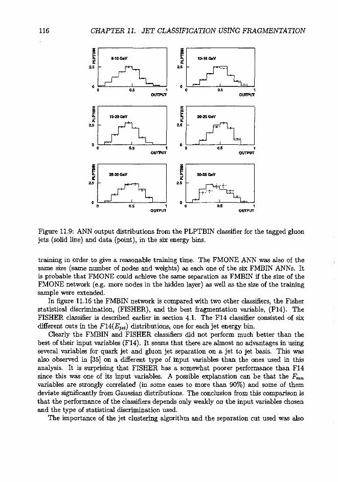
116 CHAPTER 11. JET CLASSIFICATION USING FRAGMENTATION
OUTPUT'L
PTB
IN
2.5
fl
15-20 GeV
* I*0.5
OUTPUT OUTPUT
0.5 0.5OUTPUT
Figure 11.9: ANN output distributions from the PLPTBIN classifier for the tagged gluonjets (solid line) and data (point), in the six energy bins.
training in order to give a reasonable training time. The FMONE ANN was also of thesame size (same number of nodes and weights) as each one of the six FMBIN ANNs. Itis probable that FMONE could achieve the same separation as FMBIN if the size of theFMONE network (e.g. more nodes in the hidden layer) as well as the size of the trainingsample were extended.
In figure 11.16 the FMBIN network is compared with two other classifiers, the Fisherstatistical discrimination, (FISHER), and the best fragmentation variable, (F14). TheFISHER classifier is described earlier in section 4.1. The F14 classifier consisted of sixdifferent cuts in the F14(Ejet) distributions, one for each jet energy bin.
Clearly the FMBIN and FISHER classifiers did not perform much better than thebest of their input variables (F14). It seems that there are almost no advantages in usingseveral variables for quark jet and gluon jet separation on a jet to jet basis. This wasalso observed in [35] on a different type of input variables than the ones used in thisanalysis. It is surprising that FISHER has a somewhat poorer performance than F14since this was one of its input variables. A possible explanation can be that the Fmn
variables are strongly correlated (in some cases to more than 90%) and some of themdeviate significantly from Gaussian distributions. The conclusion from this comparison isthat the performance of the classifiers depends only weakly on the input variables chosenand the type of statistical discrimination used.
The importance of the jet clustering algorithm and the separation cut used was also

11.5. PERFORMANCE OF THE CLASSIFIERS USED ON MONTE CARLO DATAU7
0.5OUTPUT OUTPUT
0.5 0.5OUTPUT
Figure 11.10: ANN output distributions from the FMBIN classifier for the tagged gluonjets (solid line) and data (point) in the six energy bins.
investigated. The five classifiers described above were all trained on jets clustered with theLUCLUS [7] algorithm using the separation parameter djoin = 3.5GeV/c. Figure 11.17shows the test of the FMBIN classifier on test samples of jets which were clustered differ-ently from the jets in the training sample.
The following jet algorithms, which were discussed in section 6.5, were tested:
• DURHAM with jfc* = 0.015;
• JADE with you = 0.015;
• LUCLUS with djoin = 5.0 GeV/c.
The classifier seems to have a better performance on jets clustered with these threedifferent algorithms than with the one that was used for the training sample. This isexplained by the comparably low djoin = 3.5 GeV/c which was used for the clustering ofthe jets in the training sample. In each of the three new test samples the jet separationwas higher which resulted in fewer but more separated jets (from the other jets in theevent), compared to the jets in the training sample. The JADE clustering gave the bestperformance of all the algorithms.

118 CHAPTER 11. JET CLASSIFICATION USING FRAGMENTATION
0.5OUTPUT OUTPUT
0.5OUTPUT OUTPUT
Figure 11.11: ANN output distributions from the FMONE classifier for the tagged gluonjets (solid line) and data (point), in the six energy bins.
11.5.2 Purity on an event basisThe event based identification presented in section 9.3 can also be applied to fragmen-tation based classifiers. For each of the five classifiers the jets in a e+e~ —* qqg threejetevent were ordered in the output variable and the jet which was closest to the gluontarget value was assigned as the gluon jet. The efficiency is then 100% and the randomlimit for the purity is 33%. Figure 11.18 shows the purity for each of the five classifiersversus the energy of the lowest energetic jet (Emin) in the event. In this type of plotthe fragmentation based classifiers can be directly compared with the jet energy basedclassifier (denoted JETS in the figure), bearing in mind that a common feature of the jetalgorithms are that they order the jets according to their energy, see section 6.5. Thefollowing observations can be made:
the fragmentation based classifiers can only compete with JET3 in events where> 25 GeV;
• for the fragmentation based classifiers the purity is nearly the same in highly asym-metric events (low Emin) as in "Mercedes" events and this shows that the jet energywas not used in the classification;
• the "bin"-trained classifiers {FMBIN, PLPTBIN, FISHER and F14) show a peculiar

11.5. PERFORMANCE OF THE CLASSIFIERS USED ON MONTE CARLO DATAU9
OUTPUT OUTPUT
OUTPUT OUTPUT
OUTPUT OUTPUT
Figure 11.12: ANN output distributions from the PLPTBIN classifier for the tagged quarkjets (solid line) and data (point) in the six energy bins.
jagged behaviour which becomes flatter with increasing Emin and only the FMONEclassifier seems to be more or less independent of Emin.
The jagged behaviour of the bin-trained classifiers come about because the output fromdifferent ANNs (or Fisher statistical discriminators) were compared when ordering thejets. Consider for instance a threejet event where the three jet energies were 8, 24 and35 GeV1. The first jet was then fed into the ANN (or Fisher discriminator) for the jetenergy bin 5-10 GeV, the second jet into the 25-30 GeV ANN and the third jet into the30-35 GeV ANN. Thus, the output from three different ANNs were used in the ordering.Numerical differences between the ANN output distributions are inevitable and this mayspoil the gluon jet identification based on ANN output ordering. Because the jet energybins must be of finite size (5 GeV in this analysis) the distribution of quark jet and gluonjet energies within each training sample were not totally uniform. This can be seen infigure 11.19 which shows the jet energy distribution in each bin. The variation of theenergy within a bin explains why the purity is always peaked at the low energy edge ofthe bin. The effect is most pronounced in the first bin (5 - 10 GeV).
The jagged behaviour disappeared only in symmetric threejet events (high Eja) whereall three jets are in the same energy bin, i.e. were fed into the same ANN. These are
1The jet energies seldom add up to the center-of-mass energy (91.2 GeV) because of the limitedacceptance and energy-momentum resolution of the detector.

120 CHAPTER 11. JET CLASSIFICATION USING FRAGMENTATION
2.5 -
OUTPUT OUTPUT
Figure 11.13: ANN output distributions from the FMBIN classifier for the tagged quarkjets (solid line) and data (point), in the six energy bins.
normally the most interesting topologies in which to use fragmentation based quark/gluonjet separation since in other topologies the jet energy (JETS) provides a much strongerdiscrimination.
11.6 The classifiers used on experimental data
Given the samples of gluon and quark jets tagged in the DELPHI data according to themethod explained in section 8.1, the same tests of the purity on a jet to jet basis for eachof the five classifiers which were done for Monte Carlo generated jets, can also be donewith real data. This may reveal differences between experimental data and the MonteCarlo data which was used to train the classifiers. It is also a test of the stability of theclassifiers with respect to the input data.
Although the output distributions in figures 11.9, 11.10 and 11.11 showed that there isa good agreement between data and the simulated Monte Carlo sample of gluons, as wellas the figures 11.12,11.13 and 11.14 indicated that there is a good agreement between dataand the simulated Monte Carlo sample of quarks, it is interesting to get it quantified interms of efficiency and purity. Deviations which are larger than the statistical errors in anyof these two quantities must be accounted for as systematic errors for the correspondingclassifier. The results for the three ANN classifiers (FMBIN, PLPTBIN and FMONE) on

11.6. THE CLASSIFIERS USED ON EXPERIMENTAL DATA 121
2.5 -
OUTPUT
Figure 11.14: ANN output distributions from the FMONE classifier for the tagged quarkjets (solid line) and data (point), in the six energy bins.
jets from the real data (showing the resulting purity versus energy for the whole energyrange) are presented in figure 11.20 where the purities were calculated using the samecuts in the output distributions as in figure 11.15. In a similar way the results for theother three classifiers (FMBIN, FISHER and F14) are presented in figure 11.21.
From the tests on real data the systematic errors on the efficiency and purity forthe different classifiers were estimated. The same tagging techniques for collecting thereal gluon jet and quark jet samples were applied to the Monte Carlo data and themaximum deviation of the central values from the corresponding values in figure 11.15and figure 11.16 was taken as the systematic error.
The imperfection of the Monte Carlo model for the fragmentation was also estimatedfrom the difference in the results with the tagged gluon jets and quark jets in the realdata and the Monte Carlo data and again the maximum deviation for each classifier istaken as the systematic error.
Table 11.4 summarises the results for each of the five classifiers tested on data andMonte Carlo for quark jets and gluon jets, in the energy range 25-30 GeV. The cuts inthe classifier output distributions (cf. E^ in chapter 9 were chosen to give about 50%efficiency {eq « eg « 0.5) on the Monte Carlo data. Since the same cuts were also usedin the tests on the experimental data any systematic global displacement of the outputdistributions compared to the tests on Monte Carlo data will result in efficiencies which

122 CHAPTER 11. JET CLASSIFICATION USING FRAGMENTATION
0.75
0.7 -
0.65 -
0.6 -
a)A
D
O
FMBIN
FMONE
PLPTBIN
A
1
—A- '
*' . * . - • * • "
110 20 30 40
EJET
0.7
0.65
0.6
-
i
A
D
O
FMBIN
FMONE
PLPTBIN
4^:4- *i i
10 20 30 40
EJET
Figure 11.15: Performance (on Monte Carlo data) of the fragmentation based quark/gluonjet classifiers presented in this paper. The purity is measured with a 100% efficiency (ajet is always identified, either as a quark jet or a gluon jet). The random limit is at 50%.
deviate from 50%. An example of such global displacement could be a badly tuned MonteCarlo which in average gives higher average multiplicity for both quark jets and gluon jets.Comparing the two rightmost columns in table 11.4 gives an idea of how well the MonteCarlo model describes data. PLPTBIN is clearly the best classifier in this respect, FMBINand FMONE are the worst and FISHER and F14 falls in between. Simple input variableslike pi and pr of the leading particles in the jet gives, as expected, less model dependencethan the rather complex Fmn variables. A further observation, though less significant,is that non-linear discriminators like artificial neural networks (FMBIN and FMONE)are more model dependent than linear discriminators like Fisher statistical discrimination{FISHER) or a cut on a single variable (F14).
For completeness the results on Monte Carlo data with the JADE clustering algorithm(Vcut — 0.015) are given in table 11.4. Among the four different clustering methodsand cuts in the jet distance measures (see section 6.5) which were tested, JADE withVent = 0.015 was found to give the best performance compared with the default LUCLUSwith djoin — 3.5 GeV/c. Note that the JADE results are better (higher purity) thanthe LUCLUS ones. This was also the case for the other two clustering choices. The

11.6. THE CLASSIFIERS USED ON EXPERIMENTAL DATA 123
Classifier
FMBIN
FMONE
PLPTBIN
FISHER
F14
Simulated£g = 50.4 ± 0.2•Kg = 62.2 ± 0.1eq = 49.6 ± 0.27rq = 62.4 ± 0.2eg = 49.3 ± 0.2-Kg = 61.8 ± 0.1eq = 50.7 ± 0.2TT, = 61.4 ±0.2£g = 50.3 ± 0.2Kg = 60.4 ± 0.1£, = 49.7 ±0.2•Kq = 60.5 ± 0.2eg = 49.8 ±0.1•Kg = 62.1 ± 0 . 1eq = 50.2 ± 0.1irq = 62.0 ± 0.2£s = 48.6 ±0 .1TTg = 62.1 ±0 .1eg = 51.4 ±0.1•Kq = 61.5 ± 0.2
25 < Ejet
Simulated+JADE49.5 ± 0.366.3 ± 0.250.5 ± 0.366.0 ± 0.449.7 ±0.365.6 ± 0.250.3 ± 0.365.4 ± 0.450.6 ± 0.364.1 ± 0.249.4 ± 0.364.5 ± 0.449.0 ± 0.366.4 ± 0.251.0 ±0.365.7 ± 0.449.8 ± 0.365.8 ±0.250.2 ± 0.365.7 ±0.4
< 30 GeVSimulated+tagging
55 ± 164 ± 145 ± 167 ± 154 ± 164 ± 146 ± 166 ± 154 ± 161 ± 146 ± 163 ± 151 ±164 ±149 ±164 ±151 ±163 ±149 ±164 ± 1
Data+tagging49 ± 166 ± 151 ± 165 ± 148 ± 167 ± 152 ± 165 ± 155 ± 161 ± 145 ± 163 ± 148 ± 166 ± 152 ± 165 ± 147 ± 166 ± 153 ± 164 ± 1
Table 11.4: Jet to jet classification with the five classifiers in the jet energy bin 25 <Ejet < 30 GeV. The purities and efficiencies are given in percent. The first column showsthe results on simulated quark jets and gluon jets. The second column shows the results onsimulated quark jets and gluon jets which have been clustered using the JADE algorithmwith ycut — 0.015. The third and fourth column shows the results on gluon jets and quarkjets tagged according to the method described in the section 8.1 for Monte Carlo andexperimental data.

124 CHAPTER 11. JET CLASSIFICATION USING FRAGMENTATION
0.75
3O.
0.7 -
0.65 -
0.6 -
c) A
•*
u
FMBIN
FISHER
F14
1
-A- ^
I
0.75
a 0.7
0.65
0.6
d)
10 20
A FMBIN
O FISHER
0 F14
10 20
30 40EJET
30 40EJET
Figure 11.16: Performance (on Monte Carlo data) of the fragmentation based quark/gluonjet classifiers presented in this analysis. The purity is measured with a 100% efficiencysince a jet is always identified, either as a quark jet or a gluon jet. The random limit isat 50%.
efficiency-purity results obtained with default choice of LUCLUS 3.5 represents the worst
case.

11.6. THE CLASSIFIERS USED ON EXPERIMENTAL DATA 125
0.75
0.7 -
0.65 -
0.6 -
•*
A
* *•e-
i
JADE
DURHAM
LUCLUS 5.0
LUCLUS 3.5
• *
..m --ra-'.'. -m JJP- •
- A - *—•
1
* i~"--a
' * • " > • *
- ; : : . * ' < - ^
^ ^
i
10 20 30 40EJET
0.75
0.7 -
0.65 -
0.6 -
-
4, *-
n.. —-~H--
1
D*
A
JADE
DURHAM
LUCLUS 5.0
LUCLUS 3.5
•••••. +
—A *
1
•-::^rS
10 20 30 40EJET
Figure 11.17: The dependence of the FMBIN performance on the jet clustering. The clas-sifier was trained using jets clustered with the LUCLUS algorithm and diOin = 3.5 GeV/c.After the training it was tested on samples of jets with similar clustering (LUCLUS 3.5)as well as three different ones: LUCLUS with djoin = 5.0 GeV/c (LUCLUS 5.0), JADEwith y^ = 0.015 (JADE) and DURHAM with y^t = 0.015 (DURHAM). The upper plotshows the gluon purity and the lower plot the quark purity. The random limit is 50%.

126 CHAPTER 11. JET CLASSIFICATION USING FRAGMENTATION
0.95
0.64 -
0.33
0.75
0.5
-
i"U-, i"i
-D '-••••U ' " : J . . " ' " } - T
i i
FMONPFMBIN
. . PLPTBIN
; i i
10 20 30 40 50EMIN
0.6 -
0.4 - J •
I I I
-
r-i
FHQNEFISHER
F14
I
10 20 30 40 50
EMIN
Figure 11.18: The identification of the gluon jet in e+e —» qqg threejet events. Inthe upper plot, the jet energy based identification JETS is compared with the FMONEclassifier. The middle plot shows the three ANN based classifiers. In the lower plot,FMONE is compared with the single variable classifier, F14 and the Fisher statisticaldiscrimination classifier, FISHER. The lower limit of the y-axis in all plots is set to therandom limit, i.e. 0.33.

11.6. THE CLASSIFIERS USED ON EXPERIMENTAL DATA 127
Gluon jets = full lineQuark jets = dashed line
10EJETinGeV
15EJETinGeV
20EJETinGeV
25EJET in GeV
30EJETinGeV
35EJETinGeV
Figure 11.19: The quark jet and gluon jet energy spectrums with the integral normalisedto one in the six energy bins.

128 CHAPTER 11. JET CLASSIFICATION USING FRAGMENTATION
0.75
0.7
0.65
0.6
A FMB1N
O FMONE
« PLPTBIN
10 20 30 40EJET
u./o
0.7
0.65
0.6
b)
-
1
;-
A
D
*
i
FMBIN
FMONE
PLPTBIN
i
-t f \H
10 20 30 40EJET
Figure 11.20: Performance of the different fragmentation based classifiers on quark jetsand gluon jets from experimental data. The purities were calculated with the same cutson the output distributions as were used in figure 11.15. The upper plot shows the gluonpurity and the lower plot the quark purity. The random limit is 0.5.

11.6. THE CLASSIFIERS USED ON EXPERIMENTAL DATA 129
0.75
O 0.7
0.65
0.6
C)A FMBIN
D FISHER
O F14
10 20 30 40EJET
0.7
0.65
0.6
d) A
D
*
I
FMBIN
FISHER
F14
V'"*a
i i '10 20 30 40
EJET
Figure 11.21: Performance of the different fragmentation based classifiers on quark jetsand gluon jets from experimental data. The purities were calculated with the same cutson the output distributions as were used in figure 11.16. The upper plot shows the gluonpurity and the lower plot the quark purity. The random limit is 0.5.

Chapter 12
Applications of jet identification
The motivation for the study of jet identification, presented in the previous chapters, wasto find new and unbiased methods that could be applied to various DELPHI analysis. Inthis chapter three physics studies in which jet identification is necessary are presented.All three analyses use heavy quark lifetime tagging as described previously.
12.1 Investigation of the splitting of quark and gluonjets
The aim of this analysis, [43], is to investigate if the initial splittings into quark and gluonjets are in agreement with QCD expectation and to study the jet evolution in order toexplain the small measured value of the ratio of the number of particles in gluon andquark jets, 2 a . The relative strength of quark and gluon jet splittings are determined bythe colour factors (or the Casimir factors). The colour factors CF, CA and TF determinethe coupling strength of a gluon radiating from a quark, two gluons radiating from agluon and a gluon splitting into a quark/antiquark pair, see figures 12.1 - 12.3. These
a C, a C. a T,
Figure 12.1: CF. Figure 12.2: CA. Figure 12.3: 7>.
coupling constants are determined within the SU(3) group and their predicted values areCF = 4/3, (7^ = 3 and TF = 1/2 which has to be weighted with the number of activequark flavours nF. According to QCD, more splittings are therefore expected in gluonjets than in quark jets, since ^ = | , and gluon initiated jets should consequently bedifferent from quark jets. In particular, one expect the ratio j*a to be approximately §A
and this is confirmed by even more detailed calculations.
130

12.1. INVESTIGATION OF THE SPLITTING OF QUARK AND GLUON JETS 131
The experimental situation is, however, completely different. Prom threejet eventsin e+e~ annihilation at Z° energies, recorded by DELPHI, this fraction is measured tobe only about f, but an increase of this value with the energy has been observed. Theanalysis has two aims, firstly to establish that the initial splitting in quark and gluon jetsare consistent with QCD and secondly to follow the jet evolution in order to understandthe observed differencies in particle multiplicities. To achieve this, two types of observablesare used, the scale dependence of the scaled energy distributions of stable hadrons whichis related to the longitudinal part of the jet evolution and the subjet splittings, which isproportional to the transverse part of the jet evolution.
A detailed comparison of quark and gluon jet properties needs samples of quark andgluon jets with nearly the same kinematics for a direct match of their properties undersimilar circumstances. To fulfil this condition two different event topologies have beenused. Threejet events from the decay of the Z°, collected in the DELPHI detector during1991-1994, are selected. After a standard hadronic event selection, similar to the oneused in this thesis, the Durham jet algorithm, see section 6.6, is used to find the threejetevents. With this algorithm, the minimum transverse momentum between two jets whichhave been resolved at a scale defined by y^t, is approximately given by k^m ~ E^sy/Voit-Prom these events only the events with Y and Mercedes topologies, see figures 9.3 and9.4, are used. The jet axes is projected into the event plane and the energy of eachjet is calculated using the measured angles between the jets, see equation 6.6. In orderto enhance events with three well defined jets, the following condition, a planar cut, isrequired:
Oij + 9ik + 9jk > 355°.
A gluon jets sample is obtained from threejet events which originate from the Z°decaying to bbg. The event is identified by using an event lifetime tag and the gluon jet istagged indirectly by identifying the two other jets as b-quark jets using a jet lifetime tag.Events with a b-quark signature were selected by requiring that the event probability, seesection 7.3.1, is PN < 10~15 = 0.032, which is the same requirement as used in the thesis.The tracks corresponding to each of the reconstructed jets are then used to determine thejet probability, PJ, see section 7.3.2.
For the Y and the Mercedes events two different selection strategies are used. For theY events, the most energetic jet is always chosen to be a quark jet. For this sample, thisis correct in about 98 % of all cases. For the two remaining jets, Pj is compared withthe cut 0.1 and if for one of them we have Pj < 0.1 and for the second one Pj > 0.1 weconsider them as quarks respectively gluon jets. For the Mercedes events, two of the jetsare demanded to fulfil the condition Pj < 0.1 to be consider quark jets assuming that thethird jet fulfils Pj > 0.1.
The efficiency and purity calculations have been made using events, generated bythe JETSET Monte Carlo, tuned to DELPHI data, which have passed through the fullsimulation program of the DELPHI detector, DELSIM and the standard DELPHI datareconstruction chain. The assignment of parton flavours to the jets is not unique, not evenin simulated events. Therefore two independent ways of identifying the the gluon jets areused. The jet that makes the largest angle to the direction of the hadrons containing theheavy quarks or contains the fewest decay particles from the heavy quarks, is consideredto be the gluon jet. These two ways are called the angle assignment and the history

132 CHAPTER 12. APPLICATIONS OF JET IDENTIFICATION
assignment. The methods give very similar results and the purities are therefore estimated-with small systematic uncertainties. Gluon jet purities of (79.6 ± 2.0)% for Y events andof (74.5 ± 2.5)% for Mercedes events are obtained with the tagging procedure described.
The splitting of jets can be studied by investigating the distribution of energy in theprocess. The study is related to the analysis of the scale dependence (scaling violation) ofthe fragmentation function D"(xE, s) of a parton p into a hadron H described by theory,where XE = Ehadron}Ejet (and s = Ecms). For values XB > 0.5 it can be shown thatthe splitting process g —> qq is disfavoured with respect to g —> gg. The fragmentationfunctions for quarks and gluons can be used to compare the relative size of the observedscaling violation. The following ratio, TS{XE), which can be predicted by solving theevolution equations, measures the relative changes in the fragmentation functions
g dins
The scaling violations in the quark and gluon jets can thus be measured by computingthe relative change, 7-5, in the fragmentation function and it is found to be:
7-5(0.23 < xE < 0.75) = 2.8 ± 0.8 db 0.6.
This can be compared to the QCD expectation
rs(xE -> 1) = CA/CF = 9/4
indicating that the ratio of quark and gluon splitting can indeed be explained by thecolour factors.
Conclusion
The splitting processes are investigated in quark and gluon jets that are identified by theuse of longitudinal and transverse observables from symmetric threejet events in DELPHI.The longitudinal part of the jet evolution is the main contributor to the scale dependencyof the energy distribution of stable hadrons. The scaling violation in gluon jets are iden-tified for the first time in this study. The scale energy dependence of the fragmentationfunction for gluons is found to be twice larger than of the fragmentation function forquark jets, something that is consistent with the QCD expectation of CA/CF-
12.2 Measurement of the triple gluon vertexIn this study, [44], fourjet events collected during 1992-1994 by the DELPHI experimentare analysed to determine the contribution from the triple-gluon vertex process. Diagramsshowing the different four-parton final states contributions are shown in figures 12.2 -12.6.Two of the four jets are tagged as heavy quarks (b or c), using a lifetime tag and lepton
transverse momentum information.The jets were reconstructed by the LUCLUS jet algorithm, see section 6.6, with the
jet resolution parameter djnn set to the value of 4 GeV/c. To check the influence of the

12.2. MEASUREMENT OF THE TRIPLE GLUON VERTEX 133
Figure 12.4: Double gluon bremsstrahlung.
Figure 12.5: Secondary qq production.
cluster algorithm, the JADE jet algorithm was also used, with the jet resolution parametery set to the value of 0.02, but no systematic effects were observed.
The generalized Nachmann-Reiter angle, Q*NR is the angle between the vectors pi—p^andp3-p4 and it distinguishes between the triple-gluon vertex contribution and secondarygg-production and the angle 0:34 is the angle between the two jets of lowest energy in afourjet event, and it distinguishes between the triple-gluon vertex contribution and thedouble-bremsstrahlung, see figure 12.7.
The triple-gluon vertex contribution can therefore be determined from the from thetwo-dimensional distribution in these two variables. These distribution in fourjet eventsfrom double gluon bremsstrahlung, secondary quark/antiquark pair and triple gluon ver-tex are significantly different and they are used to fit CA/CF, the ratio of the couplingstrength of the triple gluon vertex to that of the gluon bremsstrahlung, and the ratio ofthe number of quark colours to the number of gluons, NC/NA-
In a previous analysis of fourjet events, energy ordering of the jets was used to dis-tinguish between jets coming from primary and secondary partons. However, in the new
Figure 12.6: Triple gluon vertex.

134 CHAPTER 12. APPLICATIONS OF JET IDENTIFICATION
P, - P ,
Figure 12.7: Figure showing how the generalized Nachmann-Reiter angle, Q*NR, and theangle 0:34 are defined.
analysis, the primary jets were tagged as b-quark jets using a lifetime tag as well as inthe semileptonic decay, see 7.1, in order to make the tagging as effective as possible thesemethods were combined using a neural network. The ANN has 13 input variables, theevent lifetime probability, the lifetime probability of each jet, the transverse momentumof the electron in each jet and the transverse momentum of the muon in each jet. Thenetwork had one hidden layer and four output nodes, one for each jet. Since node one cor-responds to the highest energy and so on, energy ordering was also included. The outputswere normalized to be in the interval zero to one and a jet is tagged as a primary quarkjet if the associated output value is below 0.5 and the event was only accepted if exactlytwo of the four jets were tagged as primary quark jets. This happened in 15.6 ± 0.2%of the MC event sample and 15.6 ± 0.2% of the DELPHI data. Figure 12.8 shows theoutputs from the four nodes and the good agreement between data and simulated events.This improved tagging led to larger differencies between the shapes of the distributionsof the observables for gluon bremsstrahlung, the triple gluon vertex and secondary quarkproduction and hence increasing the method's sensitivity. The efficiency of the taggingwas increased by 50 % compared to the standard b-tagging which is less efficient in thecase of many jets and the purity was 70%.
Conclusion
The results of the measurements were
CAJCF = 2.51 ± 0.25(stot.) ± 0.11(frag.) ± 0.25(6 - tagging)
TRJCF = 1.91 ± 0.M(stat.) ± 0.25(frag.) ± 0.03(6 - tagging)

12.3. SCALE DEPENDENCE OF THE MULTIPLICITY 135
— r • •
T~~ - *
;
- ~.j L 4 -
r 1 r r. . i . . . i . . . i .
-i—1
7~T
P . . . I . • . ; • • • -U t4 OJ
Figure 12.8: Output of the four different nodes of the neural network using DELPHI data(filled boxes) and simulation (open boxes). Nodes 1-4 correspond to jets 1-4 numberedin order of decreasing energy. A jet with output below 0.5 was classified as a quark jet.Only events with exactly two jets classed as quark jets were used in the analysis.
where TR = nfTF. Since TF/CF = NC/NA and nf = 5 one obtains CA/CF = 2.51 ±0.30 and NC/NA = 0.38 ± 0.10 in agreement with the QCD predictions.
12.3 Scale dependence of the multiplicity
The third analysis [45] uses three jet events selected similarly as in first study [43], wherethe scaling violation in jets were identified for the first time, to determine the relativecoupling of the participating elementary fields and thereby making a direct test of QCD.
The data set used here was collected with the DELPHI detector at Z° energies duringthe years 1992-1995. The cuts were applied in order to select hadronic Z°-decays of theqqg and qq~") type and they are very similar to the ones used in the thesis. The gluonpurities vary from 95% for low energy gluons to 46% for the highest gluon jet energies. Thejets in these threejet events were clustered using the Durham jet algorithm. In additionit was required that the angle 9^ was in the interval 100° < #12 < 170° and the sameconditions were imposed on the angle 013, in order to obtain the requested type of events.The leading jet was not used in the analysis and events were considered to be symmetricif 612 was equal to #13, within some tolerance (chosen to be 6°).
The jets were identified by the anti-tagging process of the the gluon jet using the heavyquark jets from ggg-events enhanced by b-quark events by the use of the impact parametertechnique. In the simulation, quark and gluon jets were of course also clustered with theDurham algorithm and the jets were identified at "parton level". For each parton jet thenumber of quarks (weight +1) and antiquarks (weight -1) were summed and the jets withthe sum equal to +1 (-1) were assigned to be quark (antiquark)jets. The jets with thesum equal to 0 were assigned to be gluon jets. The small amount of events where theexpected pattern (+1, -1, 0) did not appear were rejected. It was also demanded that theangle between the original parton direction and the hadron jet did not exceed a maximum

136 CHAPTER 12. APPLICATIONS OF JET IDENTIFICATION
angle.As the successive bremsstrahhmg processes axe directly proportional to the ratio of
the radiated gluon multiplicity from a gluon and a quark source, it will asymptoticallyapproach the ratio CA/CF of the colour factors. The increased radiation from gluonsshould manifest itself in a higher multiplicity and a stronger scaling violation of the gluonfragmentation function. Already in the first study, it was shown that this prediction isinfluenced by the fact that the primary parton is a quark or a gluon, due to the differenciesin their fragmentation functions. These differencies must be present because quarks arevalence particles of the hadron whereas gluons are not. This is evident from the behaviourof the gluon fragmentation function to charged hadrons at large scaled momentum, whereit is suppressed by about one order of magnitude compared to the quark fragmentationfunction. At low momentum, soft radiation and the production of low energy hadrons isfurther suppressed which is due to a reduction of the primary splitting of gluons comparedto expectation and thus responsible for the observed small hadron multiplicity ratio aswas shown in the first analysis. Due to the high number of particles from the decayof a primary heavy particle this multiplicity ratio is further reduced, if heavy quarksare included. Furthermore the jet algorithms that combine hadrons to jets are likely toassign low energy particles at large angles with respect to the original parton directionto a different jet, which for gluon jets, initially broader than quark jets, will lead to areduction of the multiplicity for gluon jets hence a corresponding enhancement of themultiplicity of the quark jets.
These effects, which will lower the ratio of the charged hadron multiplicities for gluonand quark jets, have earner been neglected, but this study shows that they are importantand a good test of the prediction that the radiated gluon to quark multiplicity ratio isequal to the colour factor ratio.
The more rapid increase of the gluon jet multiplicity with a relevant energy scale,compared to that of the quark jets have been demonstrated. The intuitive energy scale,the jet energy, has been confirmed to be valid and recently, the scale has been extendedinto a transverse momentum scale. This dependence of the scale on the mean hadronmultiplicities in gluon and quark jets can be used for a precision determination of thecolour factor ratio CA/CF, by an estimation of the differencies of the contribution to themultiplicities of gluon and quark jets.
The relevant scales can be determined from the jet properties and the event topologyand studies of the hadron production show that the characteristics of the parton cascadedepend mainly on the hardness, K, of the process producing the jet,
where Ejet is the jet energy and 9 is the angle to the closest jet.This energy is related to the transverse momentum of the jet as well as to the y/y as it
is used in the jet algorithm, K is used as the relevant scale measure, see figures 12.9. Thischoice of scale parameter is used to determine the charged hadron multiplicity in gluonand quark jets as a function of this scale and the colour factor ratio CA/CF is directlyobserved to depend on the increase of multiplicities with this scale. The discrepancyin the multiplicity ratio between gluon jets and quark jets is explained by the differenthadronization schemes.

12.3. SCALE DEPENDENCE OF THE MULTIPLICITY 137
S 7 I » 10K[GeV]
Figure 12.9: a) Average charged particle multiplicity for light quark and gluon jets as afitted function of K. b) Ratio of the gluon to quark jet multiplicity.
ConclusionAfter taking the dependence of the charged multiplicity on the opening angle between thetwo jets with the smallest energies in symmetric threejet events into account the colourfactor ratio, CA/CF, is measured to be = 2.12 ± 0.10, which is in good agreement withthe QCD expectation.

Chapter 13
Conclusions
Different methods for separating quark jets and gluon jets using their fragmentation differ-ences have been tested on both Monte Carlo data and data from the DELPHI experiment.Both linear and non-linear multivariable analysis methods have been tried.
Two different types of variables were used to measure the fragmentation properties.The conclusions from this study are:
• The purity that can be obtained by using the fragmentation differences betweenquark jets and gluon jets is limited.
• Different input variables gives similar results.
• Artificial neural networks and Fisher statistical discrimination gives similar results.
• A multivariable discrimination is not necessary. A cut on the best single variablegives almost the same discrimination as a multivariable analysis.
• Comparisons between data and Monte Carlo showed that the output distributionsof the different classifiers were in good agreement. A detailed study of the efficiencyand purity obtained showed:
- negligible model dependence for the classifier with the simplest input variables(PL and pr of the six leading particles).
- significant model dependence for classifiers with complicated input variableswhich were calculated using all particles in the jet.
- slightly more model dependence for non-linear discriminators (artificial neuralnetworks) compared to linear ones (Fisher statistical discrimination and cutson a single variable).
The purities obtained in this analysis were all around 60% which appears very low com-pared to most other studies where the purities often are claimed to be ~ 95%. However,it must be stressed that high purities can easily be achieved with any method using thejet energy as an input. One of the major goals of this study was to remove the jet energyand all dependencies on it from the input and to find out how much the fragmentationinformation by itself could contribute to the identification.
138

Acknowledgements
Firstly I would like to thank all members of the DELPHI and the LEP collaboration.It has been a privilege to work in such a successful experimental enterprise and to haveaccess to a supplier delivering high quality data.
My deepest gratitude goes to Professor Derek Imrie for having invited me to BruneiUniversity and there arousing my interest in participating in a LEP experiment, by invit-ing me to be a research fellow at Cern. This contact was possible thanks to Professor PerCarlson, who also was a benevolent landlord during my initial period at Cern.
In the autumn 1993 I was awarded a grant from the Royal Institute of Technologywith 60% work reduction as lecturer for two years 1993/95 and also a grant from theInternational Foundation, for a stay at CERN 1995/96, for which I am deeply grateful.
It was, also in August 1993, during an examination for Professor Cecilia Jarlskog, thatthe PhD plans really took off. Thanks to her kindness and personal interest even in herperipheral students, I shortly afterwards found myself being a student at Lund Universityand supplied with a very clever and competent supervisor on the Cern site, Olof Barring,as well as a very understanding main supervisor in Lund, Professor Goran Jarlskog, whohas supported me during all these years, whatever the difficulties. My sincere thanks goesto them both.
Vincent Hedberg has been another very important person with the same qualities.Without his help and untiring and self-sacrificing work, I would certainly not have reachedthe finishing line. My feelings of gratitude towards him are very profound.
Being a member of the TPC-group at DELPHI, it is impossible not to thank somecolleagues of this group: Jeanne Mas, Marilisa Turluer-Faccini, Pierre Antilogus, GerardCosme, Patrick Roudeau, Patrick Jarry and Patrice Siegrist, who have all helped me andshared laughs and problems during shifts.
A very warm thanks to "lunchgruppen" at Cern: Hans Danielsson, Elisabeth Falk-Harris, Kristina Gunne, Magnus Hansen and Per Jonsson, with whom I have experiencedmany good moments and from whom I have also received a lot of help and information.
Another group of very personal friends at Cern, which has played an equally importantrole during my stay, consists of Per Grafstrom, Mats Lindroos, Thomas Pettersson, PerWerner and Mats Wilhelmsson. Bengt Sagnell, a Cern guide colleague, is a also a memberof this group. I especially want to thank him for the LEP information he supplied mewith, which has been a great help when being a Cern guide and when writing a part ofchapter 3.
Furthermore, I have the privilege of having a friend whom I personally consider theGuru of Physics, Torbjorn Sjostrand, who, for a very long time has answered my questionswith a lot of patience and also in a way to make me understand the answers.
139

140 CHAPTER 13. CONCLUSIONS
Persons that I consider belonging to my "family" have played a decisive role especiallyin difficult times. When feeling down, I could always count on the positive attitude andsupport from Gunn Carlsdotter and Folke Johansson. The same soothing influence alsocame from an old friend from CTH, Margareta Lagerkvist-Briggs. Encouraging emailsand wise words from Gunnar Overgaard have also played a major part in my well-being.From my brother Tomas' poem "Elegie", attached on the wall in my office, I obtained adaily inspiration. I interpret his memorable words "Amis! Vous avez bu de l'ombre pourvous rendre visibles." as a way for particles to be seen in a detector.
Last but not least, more than thanks to my wonderful wife Helene, who has been thecentre of my universe during a fantastic time with many difficulties but with far morehappy moments. She has always been standing by my side and without her positiveattitude and willingness for a change of milieu, I would not even have reached first base.

Bibliography
[1] DELPHI Collaboration, Zeit. Phys. C 70, 179 (1996).
[2] ALEPH Collaboration, Phys. Lett. B346, 163 (1995).
[3] OPAL Collaboration, Zeit. Phys. C68, 179 (1995).
[4] DELPHI Collaboration, Eur. Phys. J C4, 1 (1998).
[5] DELPHI Collaboration, Phys. Lett. B414, 401 (1997).
[6] DELPHI Collaboration, Phys. Lett. B449, 383 (1999).
[7] T.Sjostrand, Phys. Comm. 39, 346 (1986).
[8] B. Andersson, G. Gustafson, G. Ingelman and T. Sjostrand, Phys. Rep. 97, 31 (1983).
[9] T. Sjostrand, Nucl. Phys. B248, 469 (1984).
[10] T. Sjostrand, Int. J. Mod. Phys. A3, 751 (1988).
[11] T. Sjostrand et al. eds. G. Altarelli, R. Kleiss and C. Verzegnassi, Z physics at LEP1, CERN 89-08 3, 143 (1989).
[12] C. Peterson, D. Schlatter, I. Schmitt and P. Zerwas, Phys. Rev. D27, 105 (1983).
[13] DELPHI Collaboration Nucl. Instr. Meth. A378, 57 (1996).
[14] Ts. Spassov, N. Smirnov, Skelana Users Guide.
[15] CERN Program Library Long Writeup Y250 HBOOK Reference Manual.
[16] CERN Program Library Long Writeup Q121 PAW The Complete Reference.
[17] R. A. Fisher, The Use of Multiple Measurements in Taxonomic Problems, Contribu-tions to Mathematical Statistics (reprinted) John Wiley&Sons, New York, (1950).
[18] F. James, Introduction to neural networks, Cern lectures, (1994).
[19] A. Cherubini and R. Odorico, in Neural Networks: from biology to high energyphysics, EIPC, Elba (Italy), edited by O. Benhar, C. Bosio, P. Del Giudice andE. Tabet (ETS EDITRICE, piazza Torricelli 4, Pisa, Italy, 1991), pp. 515-549.
141

142 BIBLIOGRAPHY
[20] D. E. Rummelhart, G. E. Hilton and R. J. Williams, Learning Internal Represen-tation by Error Propagation, Parallel Distributed Processing: Explorations in theMicrostructure of Cognition, Vol.1, MIT Press, (1986).
[21] L. Lonnblad and C. Peterson and T. Rognvaldsson, Comput. Phys. Comm. 81 , 185(1994).
[22] DELPHI Collaboration, PROG 130, CERN DELPHI 89-15.
[23] DELPHI Collaboration, Zeit. Phys. C70, 179 (1996).
[24] V. Barger, R. Phillips, Collider Physics, Addison-Wesley, (1997).
[25] DELPHI CoUaboration, Zeit.Phys C 66, 323 (1995).
[26] DELPHI CoUaboration, Zeit. Phys. C65, 555 (1995).
[27] ALEPH Collaboration, Phys. Lett. B313, 535 (1993).
[28] G.V. Borisov, Lifetime Tag of events Z° -+ bb with the DELPHI detector. AABTAGprogram, DELPHI 94-125.
[29] L. Lonnblad and C. Peterson and T. Rognvaldsson, Phys. Rev. Lett. 65, 1321 (1990).
[30] I. Csabai and F. Czako and Z. Fodor, Nucl.Phys. B374, 288 (1992).
[31] J. Pumplin, How to tell Quark Jets from Gluon Jets, MSUTH 91/3, (1991).
[32] I. Csabai and F. Czako and Z. Fodor, Phys.Rev. D44, 1905 (1991).
[33] T. Akesson, O. Barring and V. Hedberg, in Application and Science of ArtificialNeural Networks, SPIE, The International Society for Optical Engineering, editedby Steven K.Rogers, Dennis W. Ruck (SPIE, P.O.Box 10, Bellingham, Washington98227-0010 USA, 1995), Vol. 2492, pp. 1121-1131.
[34] M. A. Graham and L. M. Jones and S. Herbin, Phys. Rev. D51 , 4789 (1995).
[35] M. A. Graham, L. M. Jones and P. R. Daumerie, Phys. Rev. D46, 222 (1992).
[36] L. Lonnblad and C. Peterson and T. Rognvaldsson, Nucl.Phys. B349, 675 (1991).
[37] DELPHI Collaboration, Phys. Lett. B295, 383 (1992).
[38] ALEPH Collaboration, Phys.Lett. B313, 549 (1993).
[39] D. Bertrand, V. Lefebure, in Application and Science of Artificial Neural Networks,SPIE, The International Society for Optical Engineering, edited by Steven K.Rogers,Dennis W. Ruck (SPIE, P.O.Box 10, Bellingham, Washington 98227-0010 USA,1995), Vol. 2492, pp. 1098-1108.
[40] DELPHI CoUaboration, Nucl.Phys. B421, 3 (1994).

BIBLIOGRAPHY 143
[41] C. Caso et al, The European Physical Journal C3, 1 (1998).
[42] R. J. Scalkoff, Pattern Recognition: Statistical, Structural and Neural Approaches,John Wiley&Sons, New York (1992).
[43] DELPHI Collaboration, Eur. Phys. C4, 1 (1998).
[44] DELPHI Collaboration, Phys. Lett. B414, 401 (1997).
[45] DELPHI Collaboration, Phys. Lett. B449, 383 (1999).

Appendix A
Geometry for Classification Purposes
For a complete treatment of pattern recognition, see [42]. In 3-D or (xi,x^,X3)-space aplane through the origin is determined by three parameters (wi,cJ ,c< ) via
| = 0
or simply
QT • x = 0
This equation indicates that Q and x are orthogonal. C3 is therefore the normal to theplane. A plane through any other point Xd, represented by position vector x"d, may bewritten
uJT -(x-xa) = 0
or
where d = CJT • x"d
This reformation is equivalent to a coordinate system transformation, where the origin isshifted to xd and therefore measure vectorsX = X - Xd
Notice that Q is orthogonal to any vector, lying in the plane.
QT • x - d = 0
can be used to determine the "distance" of H from the origin and for a given vector x,which "side" of H in B? that x is on and the distance of x from H.If Q is normalised by dividing it with its norm, giving the vector uf,
144

145
The vector xd can then be written
Xi = a-uj
where
||x*d|| = a
Since xd represents a point on H
so
uFIMI
This means that a can be written as,
\\£
So any point x represented by a vector x may be written,
x — xd + x" '
and if ||a^|| = k, the vector x"n can be written
IMiand therefore
OF • x = UJT • {xd + xp + xti) = uF • Xn + uF -Xd — k • \\uj\\ + a • \\u\\
Let, for simplicity a = 0 (i.e. a plane through the origin). Since x"n = k • Qj the quantity~*T -^ i II —»nUJ • X = K- \\U}\\
tells which side of the line H, x is on.
If uF -x> 0 =*> k > 0 => xis on the "positive" side
If CF • x < 0 => k <0 => xis on the "negative" side
If uF • x = 0 => k = 0 =» xis in H
For an figure illustrating this discussion, see figure A.I. Notice that the plane H (givenby ) partitions R2 (in general R?) into two mutually exclusive regions, denoted i?1 andR".
Following this mathematical outline and by looking at the figure A.I, the aim is tomake the intuitive description of the linear discrimination method, outlined in section 4.1a bit more trustworthy.
The assignment of a vector x to the "positive" or "negative" side, or along H can beimplemented by using the expression uF • x — d in the following way,

146 APPENDIX A. GEOMETRY FOR CLASSIFICATION PURPOSES
co (unnormalised)
line, locu^of points x,where© (x-xd)=0
Negative side Rn \Positive side R
• * X ,
Figure A.I: The assignment of a vector f to the positive or negative side of (or along)the line H.
• t3T • x - d > Oifze Rp
• uF • x - d = 0 ifx € H
• uF • x - d < 0 ifx € Rn
This suggests a linear discriminant function F(x) to implement the classification of theassignment above, as
F{x) = Gf • x - d (A.1)
Examination of equation A.I and figure A.I indicates that the linear discriminants func-tion that yields H and is used to partition R2 into two regions has the following charac-teristics
• The orientation of H is determined by Q
• The location of H is determined by d
Extension to Rd is straightforward for the linear classification of d-dimensional featurevectors x. The surface H is, in this context, referred to as a hyperplane.

Appendix B
The energy dependence of thelongitudinal momenta
Figures B.1-B.5 show the differences in the input variable, the normalized longitudinalmomentum, relative to the jet axis, PtlPjei for the second to the sixth particle of the jet.
0.1 0.2 0.3 0.4PL2/PJET in the energy bin 05-10 C«V
0.1 0.2 0.3 0.4 0.5PL2/PJET in the energy bin 10-15 CeV
: 0.1 0.2 0.3PL2/PJET in the energy bin 15-20GeV
>.1 0.2 0.3 0.4 0.5PU/PJET in the energy bin 20-25 GeV
0.2 0.3 0.4 0.PL2/PJH"m the energy bin 25-30 GeV
0.1 0.2 0.3 0.4 0.5PU/PJET in the energy bin 30-35 OeV
Figure B.I: The distributions of the fragmentation variable, the normalized longitudinalmomentum, relative to the jet axis, PhlPjet for the second particle of the jet for gluonjetsand quarkjets, in the six energy bins.
147

U8APPENDLX B. THE ENERGY DEPENDENCE OF THE LONGITUDINAL MOMENTA
•• 0.1 0.2 0.3§ 0.1 0.2 0.3Pl3/PJETin the energy bin 05-lOCeV PL3/PJET in the energy bin 10-15 G«V
0.1 0.2 0 .3 | 0.1 0.2 0.3PU/PJtT in the energy bin 15-20 CeV PU/PJET in the energy bin 20-25 GeV
0.1 0.2 O J i 0.1 0.2 0.3PL3/PJET in the energy bin 25-30 OeV PL3/PJCT !n the energy bin 30-35 CeV
Figure B.2: The distributions of the fragmentation variable, the normalized longitudinalmomentum, relative to the jet axis, PLIVJSI for the third particle of the jet for gluonjetsand quarkjets, in the six energy bins.
0.05 0.1 0.15 0.2PM/PJCT in the energy bin 25-30 GeV
0.05 0.1 0.15 0.2ir> the energy bin 30-35 GeV
Figure B.3: The distributions of the fragmentation variable, the normalized longitudinalmomentum, relative to the jet axis, p^Pjet for the fourth particle of the jet for gluonjetsand quarkjets, in the six energy bins.

149
In Oi. energy bin 05-10 G«V PL5/PJET in the energy bin 10-1S GeV
0.05 0.1 0.15PL5/PJCT in the energy bin 25-30 G«v
0.05 0.1 0.15PL5/PJET in the energy bin 30-35 GeV
Figure B.4: The distributions of the fragmentation variable, the normalized longitudinalmomentum, relative to the jet axis, pz/Pjet for the fifth particle of the jet for gluonjetsand quarkjets, in the six energy bins.
0.05PL6/PJETinthee.
0.1 0.1% 0.05 0.1 0.15y bin 05-10 C«V PL6/PJET in th« energy bin 10-15 CeV
0.05 0.1 O.lg 0.05 0.1 0.15PL6/PJET in the energy bin 15-20 GeV PU/PJET in the energy bin 20-25 GcV
0.05 0.1 O.ig 0.05 0.1 0.15PL6/PXT in the energy bin 25-30 GeV PL6/PJET n the energy bin 30-35 GeV
Figure B.5: The distributions of the fragmentation variable, the normalized longitudinalmomentum, relative to the jet axis, pi/pjet for the sixth particle of the jet for gluonjetsand quarkjets, in the six energy bins.

Appendix C
The energy dependence of thetransverse momenta
Figures C.1-C.5 show the differencies in the input variable, the normalized transversemomentum, relative to the jet axis, Pr/Pjet for the second to the sixth particle of the jet.
" 0.05 0.1 0.15 0.2 0.2g " 0.05 0.1 0.15 0.2 0.25PT2/PJE7 in the energy bin 05-10 G.V PT2/PJET In the energy bin 10-15 CeV
0.05 0.1 0.15 0.2 0.2? " 0.05 0.1 0.15 0.2 0.25PT2/PJEI in the enenjy bin 15-20 GeV PT2/PJET in the energy bin 20-25 GtV
0.05 0.1 0.15 0.2 0,PT2/PJEJ in the enenjy bin 25-30 GeV
0.05 0.1 0.15 0.2 0.25PT2/PJET 'in the energy bin 30-35 GeV
Figure C.I: The distributions of the fragmentation variable, the normalized transversemomentum, relative to the jet axis, pr/Pjet for the second particle of the jet for gluonjetsand quarkjets, in the six energy bins.
150

i5 20
0.05 0.1 0.1 g 0.05 0.1 0.15PT3/PJET in the energy bin 05-10 GeV PT3/PJET in the energy bin 10-15 CeV
fe 20
PT3/PJET in the energy bin 15-20 CeV P13/PJET in the energy bin 20-25 OeV
0.05 0.1 0.15J 0.05 0.1 0.15PT3/PJET in Ihe energy bin 25-30 GeV PT3/PJET in the energy bin 30-35 GeV
151
Figure C.2: The distributions of the fragmentation variable, the normalized transversemomentum, relative to the jet axis, Pr/Vjet for the third particle of the jet for gluonjetsand quarkjets, in the six energy bins.
quark »dM(M4lln»
0.05 0.1 O.1 |PT4/PJCT " Ihe energy bin 05-10 GeV
0.05 0.1 0.15PT4/PJET in Ihe energy birt 10-15 C«V
PT4/PJET in the energy bin 15-20 GeV0.05 0.1 0.15
PT4/PJEI in the energy bin 20-25 CeV
0.05 0.1 O.15J 0.05 0.1 0.15PT4/PJEI in the energy bin 25-30 OeV PT4/PJET!n the enersy bin 30-35 OeV
Figure C.3: The distributions of the fragmentation variable, the normalized transversemomentum, relative to the jet axis, Pr/Pjet for the fourth particle of the jet for gluonjetsand quarkjets, in the six energy bins.

152APPENDDC C. THE ENERGY DEPENDENCE OF THE TRANSVERSE MOMENTA
0.025 0.05 0.075 0.1 O,125g " 0.025 0.05 0.075 0.1 0.125PT5/PJETintheefiergybin05-10CeV PT5/PJET !n the energy bin 10-15GeV
0.025 0.05 0.075 0.1 0.1255 " ° ' 0 2 5 °-0 5 ° - 0 7 5 °-1 ° - 1 2 5
PT5/PJET in the energy bin 15-20 GeV PTS/PJET in the energy bin 20-25 GeV
O.025 0.05 0.075 0.1 0.125^ 0.025 0.05 0.075 0.1 0.125PT5/PJET in the energy bin 25-30 <SeV PT5/PJET in the energy bin 30-35 GeV
Figure C.4: The distributions of the fragmentation variable, the normalized transversemomentum, relative to the jet axis, Pr/Pjet for the fifth particle of the jet for gluonjetsand quarkjets, in the six energy bins.
«jMrfc-daatNdrkN
O.025 0.05 0.075 0.1 j " 0.025 0.05 0.075 0.1PT6/PJET in lh« energy bin 05-10 GeV PT6/PJET in the energy bin 10-15 GeV
0.025 0.05 0.075 0.1 | 0.025 0.05 0.075 0.1PT6/PJET in the energy bin 15-20 GeV PT6/PJET in the energy bTn 20-25 CeV
0.025 0.05 0.075 0.1PT6/PJET in th« energy bin 25-30 GeV
0.025 0.05 0.075 0.1PT6/PJET In the energy bin 30-35 GeV
Figure C.5: The distributions of the fragmentation variable, the normalized transversemomentum, relative to the jet axis, pr/Pjet for the sixth particle of the jet, for gluonjetsand quarkjets in the six energy bins.

Appendix D
The energy dependence of the Fodormomenta
Figures D.1-D.6 show the differencies in the input vaxiables, the normalized Fodor mo-menta, for gluon jets and quark jets in the full energy range.
0.2 0.4 0.6FIDin theenergy bin 10-15 CeV
0 0.2 0.4 0.6FIO in (he energy bin 75-20 CeV
0.2 0.4 0.6F10 In the energy bin 20-25 CeV
0 0.2 0.4 0.6F10 in the energy bin 25-30 GeV
' 0 0.2 0.4 0.6F10 In the energy bin 30-35 CeV
Figure D.I: The distributions of the normalised Fodor moment F10, for gluon jets andquaxk jets in the six energy bins.
153

154 APPENDIX D. THE ENERGY DEPENDENCE OF THE FODOR MOMENTA
0 0.2 0.4 0.6 0 0.2 0.4 0.6F11 in the energy bin 05-10 GeV F11 in the energy bin 10-15 CeV
i» 6
S 4
-si,,0 0.2 0.4 0.6 0 0.2 0,4 0-6
F11 in the energy bin 15-20 GeV F11 in the energy bin 20-25 GeV
0 0.2 0A 0.6Fl 1 in the energy bin 25-30 GeV
0.2 0.4 0.6F11 in the energy bin 30-35 OeV
Figure D.2: The distributions of the normalised Fodor moment, F l l , for gluon jets andquark jets in the six energy bins.
quark. dMlMd In*
0 2 4 6 8 10F14 in the energy bin 05-10 CeV
0 2 4 6 8 10F14 in the energy bin 10-15 CeV
1 2 4 6 8 10FI4 in the energy bin 15-200eV
10.1
0 2 4 6 S 10F14 in the energy bin 25-30 GeV
0 2 4 6 8 10F14 in the energy bin 30-35 GeV
Figure D.3: The distributions of the normalised Fodor moment, F14, for gluon jets andquark jets in the six energy bins.

155
CO.03
0 50 100 150 200F16 in the energy bin 10-15 CeV
0 50 100 150 200F16 In the energy bin 20-25 GeV
0 50 100 150 200F1 $ in the energy bin 25-30 GeV
50 100 150 200F16 in the energy bin 30-35 GeV
Figure D.4: The distributions of the normalised Fodor moment, F16, for gluon jets andquark jets in the six energy bins.
gluon-fnilM ; d
F26 In the energy bin 10-15 CeV
0 1 2 3 *F26 in Die energy bin 20-25 CeV
0 1 2 3 •6 in the energy bin 25-30 GeV
0 1 2 3 4F26 in the energy bin 30-35 OeV
Figure D.5: The distributions of the normalised Fodor moment, F26, for gluon jets andquark jets, in the six energy bins.

156 APPENDIX D. THE ENERGY DEPENDENCE OF THE FODOR MOMENTA
0 5 10 15F27 in the entrgy bin 05-10 CeV F27 in the energy bin 10-15 G»V
0 5 10F27 in the energy bTn 15-20 GeV
10 15bin 25-30 CeV
5 10 15F27 in the energy bin 20-25 GeV
0 5 10 15F27 V. the energy bin 30-35 GeV
Figure D.6: The distributions of the normalised Fodor moment, F27, for gluon jets andquark jets in the six energy bins.
Copyright © 2022 FDOKUMEN