arX

iv:0

912.

3862

v2 [

hep-

ph]

22

Dec

200

9

Stopping distance for high energy jets in weakly-coupled

quark-gluon plasmas

Peter Arnold, Sean Cantrell,∗ and Wei Xiao

Department of Physics, University of Virginia,

Box 400714, Charlottesville, Virginia 22904, USA

(Dated: December 22, 2009)

AbstractWe derive a simple formula for the stopping distance for a high-energy quark traveling through a

weakly-coupled quark gluon plasma. The result is given to next-to-leading-order in an expansion in

inverse logarithms ln(E/T ), where T is the temperature of the plasma. We also define a stopping

distance for gluons and give a leading-log result. Discussion of stopping distance has a theoretical

advantage over discussion of energy loss rates in that stopping distances can be generalized to the

case of strong coupling, where one may not speak of individual partons.

∗ Current address: Department of Physics & Astronomy, Johns Hopkins University, 3400 N. Charles St.,

Baltimore, MD 21218

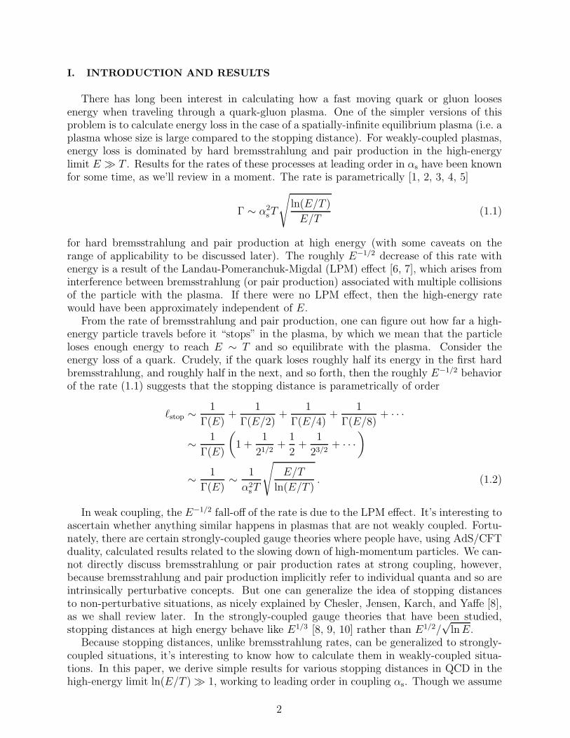
I. INTRODUCTION AND RESULTS

There has long been interest in calculating how a fast moving quark or gluon loosesenergy when traveling through a quark-gluon plasma. One of the simpler versions of thisproblem is to calculate energy loss in the case of a spatially-infinite equilibrium plasma (i.e. aplasma whose size is large compared to the stopping distance). For weakly-coupled plasmas,energy loss is dominated by hard bremsstrahlung and pair production in the high-energylimit E ≫ T . Results for the rates of these processes at leading order in αs have been knownfor some time, as we’ll review in a moment. The rate is parametrically [1, 2, 3, 4, 5]

Γ ∼ α2sT

√

ln(E/T )

E/T(1.1)

for hard bremsstrahlung and pair production at high energy (with some caveats on therange of applicability to be discussed later). The roughly E−1/2 decrease of this rate withenergy is a result of the Landau-Pomeranchuk-Migdal (LPM) effect [6, 7], which arises frominterference between bremsstrahlung (or pair production) associated with multiple collisionsof the particle with the plasma. If there were no LPM effect, then the high-energy ratewould have been approximately independent of E.

From the rate of bremsstrahlung and pair production, one can figure out how far a high-energy particle travels before it “stops” in the plasma, by which we mean that the particleloses enough energy to reach E ∼ T and so equilibrate with the plasma. Consider theenergy loss of a quark. Crudely, if the quark loses roughly half its energy in the first hardbremsstrahlung, and roughly half in the next, and so forth, then the roughly E−1/2 behaviorof the rate (1.1) suggests that the stopping distance is parametrically of order

ℓstop ∼ 1

Γ(E)+

1

Γ(E/2)+

1

Γ(E/4)+

1

Γ(E/8)+ · · ·

∼ 1

Γ(E)

(

1 +1

21/2+

1

2+

1

23/2+ · · ·

)

∼ 1

Γ(E)∼ 1

α2sT

√

E/T

ln(E/T ). (1.2)

In weak coupling, the E−1/2 fall-off of the rate is due to the LPM effect. It’s interesting toascertain whether anything similar happens in plasmas that are not weakly coupled. Fortu-nately, there are certain strongly-coupled gauge theories where people have, using AdS/CFTduality, calculated results related to the slowing down of high-momentum particles. We can-not directly discuss bremsstrahlung or pair production rates at strong coupling, however,because bremsstrahlung and pair production implicitly refer to individual quanta and so areintrinsically perturbative concepts. But one can generalize the idea of stopping distancesto non-perturbative situations, as nicely explained by Chesler, Jensen, Karch, and Yaffe [8],as we shall review later. In the strongly-coupled gauge theories that have been studied,stopping distances at high energy behave like E1/3 [8, 9, 10] rather than E1/2/

√ln E.

Because stopping distances, unlike bremsstrahlung rates, can be generalized to strongly-coupled situations, it’s interesting to know how to calculate them in weakly-coupled situa-tions. In this paper, we derive simple results for various stopping distances in QCD in thehigh-energy limit ln(E/T ) ≫ 1, working to leading order in coupling αs. Though we assume

2

Nf a b c a(e)g a

(e)q

QCD 0 — — 0.736866 5.26606 —

2 2.06480 0.092141 0.432769 5.98760 3.61355

3 2.23024 0.105282 0.345885 6.27235 3.87544

4 2.38423 0.115487 0.280721 6.52525 4.11632

5 2.52886 0.123314 0.230039 6.75427 4.34031

6 2.66565 0.129246 0.189492 6.96480 4.55038

QED 1 0.30216 3.16393 -0.175423 0.11121 0.12072

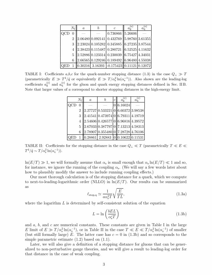
TABLE I: Coefficients a,b,c for the quark-number stopping distance (1.3) in the case Q⊥ ≫ T

(parametrically E ≫ T 4/q or equivalently E ≫ T/α2s ln(α−1

s )). Also shown are the leading-log

coefficients a(e)g and a

(e)q for the gluon and quark energy stopping distances defined in Sec. II B.

Note that larger values of a correspond to shorter stopping distances in the high-energy limit.

Nf a b c a(e)g a

(e)q

QCD 0 — — 0 6.16024 —

2 2.27727 0.533221 0 6.60372 3.98538

3 2.41541 0.473974 0 6.79311 4.19719

4 2.54606 0.426577 0 6.96816 4.39572

5 2.67033 0.387797 0 7.13213 4.58313

6 2.78907 0.355480 0 7.28728 4.76106

QED 1 0.28861 2.92883 0 0.10622 0.11531

TABLE II: Coefficients for the stopping distance in the case Q⊥ ≪ T (parametrically T ≪ E ≪T 4/q ∼ T/α2

s ln(α−1s )).

ln(E/T ) ≫ 1, we will formally assume that αs is small enough that αs ln(E/T ) ≪ 1 and so,for instance, we ignore the running of the coupling αs. (We will say a few words later abouthow to plausibly modify the answer to include running coupling effects.)

Our most thorough calculation is of the stopping distance for a quark, which we computeto next-to-leading-logarithmic order (NLLO) in ln(E/T ). Our results can be summarizedas

ℓstop,q ≃ 1

aα2sT

√

E

TL, (1.3a)

where the logarithm L is determined by self-consistent solution of the equation

L = ln

(

bEL

αcsT

)

(1.3b)

and a, b, and c are numerical constants. These constants are given in Table I in the largeE limit of E ≫ T/α2

s ln(α−1s ), or in Table II in the case T ≪ E ≪ T/α2

s ln(α−1s ) of smaller

(but still formally large) E. The latter case has c = 0 in (1.3b) and so corresponds to thesimple parametric estimate (1.2) based on (1.1).

Later, we will also give a definition of a stopping distance for gluons that can be gener-alized to non-perturbative gauge theories, and we will give a result to leading-log order forthat distance in the case of weak coupling.

3

At the moment, we do not have a precise weakly-coupled result for the types of super-symmetric gauge theories in which the strongly-coupled limit has been studied. The answerwill be in the form (1.3) for weak coupling, but we leave the calculation of the coefficientsa, b, and c in this case for future work.

Throughout this paper, we will assume that the baryon chemical potential of the quark-gluon plasma is negligible compared to its temperature.

In section II, we review Chesler et al.’s definition of a stopping distance for quarks, whichwe call the quark number stopping distance, and then we discuss a natural generalization fordiscussing gluons, which introduces what we will call the quark and gluon energy stoppingdistances. Section III derives results for these various stopping distances to leading-logorder, which is enough to determine the coefficients a and c in our result (1.3). Section IVthen continues to next-to-leading log order for the quark number stopping distance, givingthe remaining coefficient b. As a test of our NLLO result, we compare it in section Vto numerical simulations of energy loss that make no approximation regarding the size ofln(E/T ) but instead use full weak-coupling results for the bremsstrahlung rate. We verifythat our NLLO result (1.3) correctly reproduces the large E behavior. Finally, in sectionVI, we discuss how one might modify our result to account for running of αs.

II. DEFINING STOPPING DISTANCES

A. Quark Number Stopping

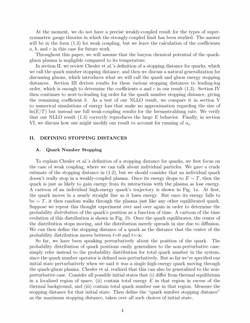
To explain Chesler et al.’s definition of a stopping distance for quarks, we first focus onthe case of weak coupling, where we can talk about individual particles. We gave a crudeestimate of the stopping distance in (1.2), but we should consider that an individual quarkdoesn’t really stop in a weakly-coupled plasma. Once its energy drops to E ∼ T , then thequark is just as likely to gain energy from its interactions with the plasma as lose energy.A cartoon of an individual high-energy quark’s trajectory is shown in Fig. 1a. At first,the quark moves in a nearly straight line as it loses energy. But once its energy falls tobe ∼ T , it then random walks through the plasma just like any other equilibrated quark.Suppose we repeat this thought experiment over and over again in order to determine theprobability distribution of the quark’s position as a function of time. A cartoon of the timeevolution of this distribution is shown in Fig. 1b. Once the quark equilibrates, the center ofthe distribution stops moving, and the distribution merely spreads in size due to diffusion.We can then define the stopping distance of a quark as the distance that the center of theprobability distribution moves between t=0 and t=∞.

So far, we have been speaking perturbatively about the position of the quark. Theprobability distribution of quark positions easily generalizes to the non-perturbative case:simply refer instead to the probability distribution for total quark number in the system,since the quark number operator is defined non-perturbatively. But so far we’ve specified ourinitial state perturbatively when we said it was a single high-energy quark moving throughthe quark-gluon plasma. Chesler et al. realized that this can also be generalized to the non-perturbative case. Consider all possible initial states that (i) differ from thermal equilibriumin a localized region of space, (ii) contain total energy E in that region in excess of thethermal background, and (iii) contain total quark number one in that region. Measure thestopping distance for that initial state. Then define the “quark number stopping distance”as the maximum stopping distance, taken over all such choices of initial state.

4

stopping distance

(b)

(a)

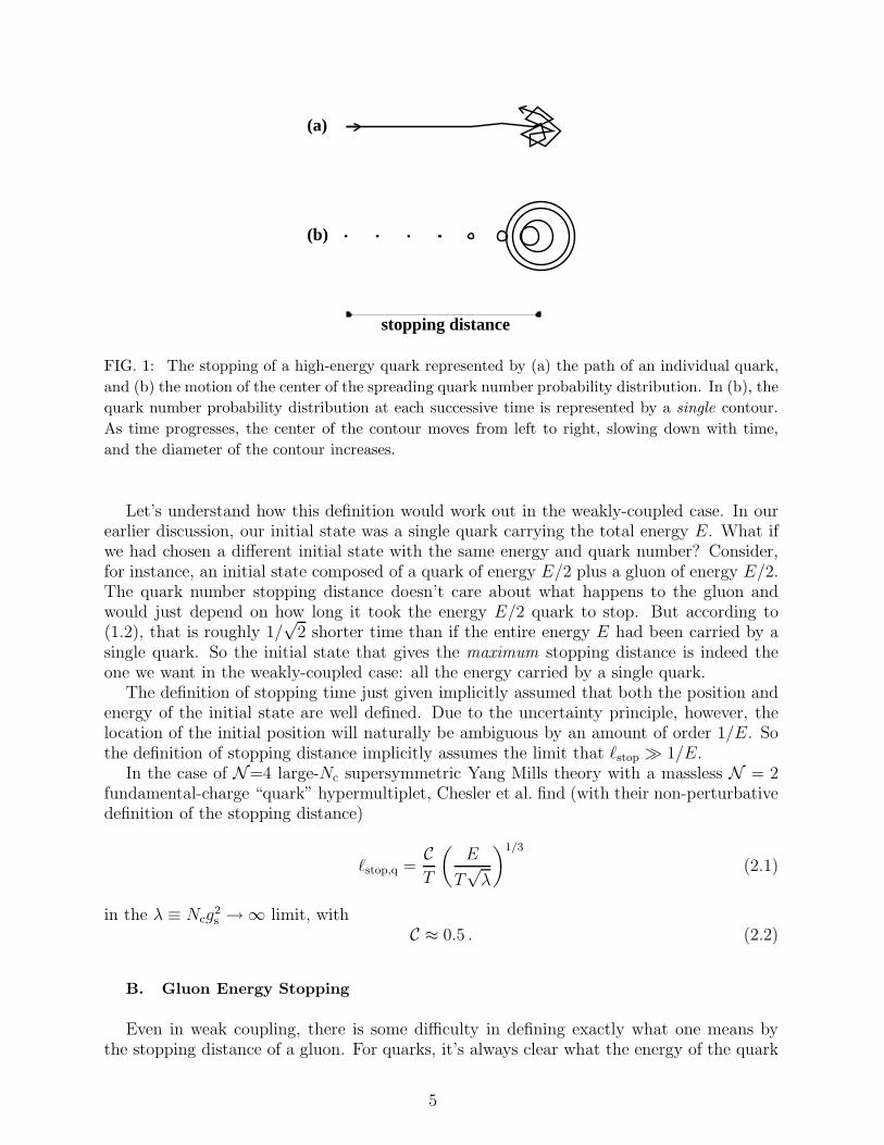
FIG. 1: The stopping of a high-energy quark represented by (a) the path of an individual quark,

and (b) the motion of the center of the spreading quark number probability distribution. In (b), the

quark number probability distribution at each successive time is represented by a single contour.

As time progresses, the center of the contour moves from left to right, slowing down with time,

and the diameter of the contour increases.

Let’s understand how this definition would work out in the weakly-coupled case. In ourearlier discussion, our initial state was a single quark carrying the total energy E. What ifwe had chosen a different initial state with the same energy and quark number? Consider,for instance, an initial state composed of a quark of energy E/2 plus a gluon of energy E/2.The quark number stopping distance doesn’t care about what happens to the gluon andwould just depend on how long it took the energy E/2 quark to stop. But according to(1.2), that is roughly 1/

√2 shorter time than if the entire energy E had been carried by a

single quark. So the initial state that gives the maximum stopping distance is indeed theone we want in the weakly-coupled case: all the energy carried by a single quark.

The definition of stopping time just given implicitly assumed that both the position andenergy of the initial state are well defined. Due to the uncertainty principle, however, thelocation of the initial position will naturally be ambiguous by an amount of order 1/E. Sothe definition of stopping distance implicitly assumes the limit that ℓstop ≫ 1/E.

In the case of N=4 large-Nc supersymmetric Yang Mills theory with a massless N = 2fundamental-charge “quark” hypermultiplet, Chesler et al. find (with their non-perturbativedefinition of the stopping distance)

ℓstop,q =CT

(

E

T√

λ

)1/3

(2.1)

in the λ ≡ Ncg2s → ∞ limit, with

C ≈ 0.5 . (2.2)

B. Gluon Energy Stopping

Even in weak coupling, there is some difficulty in defining exactly what one means bythe stopping distance of a gluon. For quarks, it’s always clear what the energy of the quark

5

is after a q → qg splitting process. For gluons, we can have g → gg or g → qq, and wehave to decide which particle to follow. One possibility would be to follow, at each splitting,the final particle that has the highest energy. This definition does not have any obviousgeneralization to strong coupling. But we can instead use a definition like the previous onefor quark number stopping distance. For the initial state, we now require quark numberzero. Then, for the stopping distance, we measure the distance traveled before the center ofthe probability distribution for energy in excess of equilibrium (rather than quark number)stops. We will call this the “gluon energy stopping distance.”

For a gluon in a weakly-coupled plasma, this definition can be translated as follows.Consider the splitting of an initial high-energy gluon, moving in the z direction, whichcascades through splitting into N particles, which are “stopped” at positions z1, z2, ..., zN

relative to the initial position of the initial gluon. Here stopped means that the individualenergies Ei are of order T . The gluon energy stopping distance is the energy-weightedaverage of these stopping positions:

ℓ(energy)stop,g ≃

∑

i Eizi

E. (2.3)

This simple translation is fuzzy when it comes to deciding exactly when a final parton haslow enough energy to be considered “stopped.” Is it Ei ≤ T or Ei ≤ 2T or ...? However,because the time scale (α2T )−1 for particles with energy of order T to significantly interactis so much faster than the time scale (1.2) for the initial gluon to lose significant energy,this ambiguity only involves corrections to the calculation of the stopping distance that aresuppressed by a factor of

√

T/E (up to logarithms). We can ignore these corrections if weare just interested in E ≫ T . Note that, when Ei ∼ T , we should also be thinking aboutcollisional energy loss, which is then competitive with bremsstrahlung and pair production.But the effects of collisional loss on the stopping distance will similarly be suppressed by afactor of

√

T/E.

III. LEADING LOG

A. Quark Number Stopping: General Analysis

We’ll begin with a leading-log calculation of the quark number stopping distance, whichis fairly simple. To motivate the approximation, consider the crude, heuristic estimate madein (1.2). At leading-log order, we can ignore the difference between a ln(E/T ) appearingin Γ(E), a ln(E/2T ) appearing in Γ(E/2), and a ln(E/4T ) appearing in Γ(E/4). Since theseries in (1.2) converges sufficiently rapidly (i.e. geometrically), it is sufficient at leading-logorder to replace the logarithm in the bremsstrahlung rate (1.1) by a constant:

Γ(E) ∼ α2sT

√

ln(E0/T )

E/T(3.1)

where E0 is the initial energy of the quark. In this approximation, the E dependence ofΓ(E) is simply E−1/2, without any logarithm. That simplification will be the key to a simplesolution for the stopping distance in what follows.

In more detail, the bremsstrahlung rate is a function of the momentum fraction x = ω/Eof the emitted gluon of frequency ω. (For hard bremsstrahlung in the large E limit, we can

6

ignore the thermal mass of the gluon.) In the leading-log approximation, we can write

dΓ(E)

dx≃

(

E0

E

)1/2dΓ(E0)

dx≡ E−1/2 dΓ

dx, (3.2)

where there is an implicit logarithmic dependence of dΓ/dx on E0. We will review thespecific leading-log formula for q → gq bremsstrahlung later. But for now we can proceedwith the analysis in a general way, based simply on the scaling (3.2).

Let ℓq(E) be the quark number stopping distance as a function of E. We can formallywrite the following self-consistent equation for ℓq:

ℓq(E) =1

Γq→gq(E)+

∫ 1

0

dxdΓq→gq(E, x)/dx

Γq→gq(E)ℓq

(

(1 − x)E)

. (3.3)

The first term on the right-hand side is the average distance before the first bremsstrahlung.That first bremsstrahlung splits the quark into a nearly-collinear gluon with energy xEand quark with energy (1 − x)E. The second term on the right-hand side of (3.3) is theremainder of the stopping distance after the first bremsstrahlung. This is just ℓq((1 − x)E)weighted by the probability (dΓ/dx)/Γ that the first bremsstrahlung had gluon momentumfraction x. To find the stopping distance, we just need to solve this equation in leading-logapproximation.

Note that (3.3) ignores what happens to the radiated gluons. Suppose a bremsstrahlunggluon later splits into a qq pair with the new quark carrying more energy than the newanti-quark. The subsequent cascading of that pair will then affect the distribution of quarkcharge at the end of the cascade process, and so will affect where the center of the total quarknumber distribution stops. However, it’s just as likely that the gluon would have insteadsplit into a qq pair in which the new anti-quark carries more energy, and this will produce anopposite effect on the location of the center of the final quark number distribution. Becauseof charge symmetry, we can ignore what happens to the gluons when calculating the quarknumber stopping distance. We dwell on this point because the situation will be differentwhen we later compute the gluon energy stopping distance.

The reason we referred to (3.3) as “formal” is that the total bremsstrahlung rate

Γq→gq(E) =

∫ 1

0

dxdΓq→gq(E, x)

dx(3.4)

is infrared (x→0) divergent in leading-log approximation. You can imagine temporarilyimposing some sort of infrared regulator. But it is easy to manipulate (3.3) to remove theneed for such a regulator by multiplying both sides by Γq→gq(E) and rearranging terms torewrite the equation as

∫ 1

0

dxdΓq→gq(E, x)

dx

[

ℓq(E) − ℓq

(

(1 − x)E)]

= 1. (3.5)

The fact that the factor in brackets vanishes as x → 0 turns out to be sufficient to make thex integration in (3.5) infrared convergent.

Now make the leading-log approximation by substituting (3.2) into (3.5) to get

E−1/2

∫ 1

0

dxdΓq→gq(x)

dx

[

ℓq(E) − ℓq

(

(1 − x)E)]

= 1. (3.6)

7

We can solve this equation by writing

ℓq(E) =E1/2

Aq, (3.7)

where Aq is a constant. Then the factors of E drop out of (3.6), leaving

Aq =

∫ 1

0

dxdΓq→gq(x)

dx

[

1 − (1 − x)1/2]

. (3.8)

It only remains to plug in the detailed leading-log formula for dΓq→gq/dx in leading-logapproximation. We’ll leave that to Sec. IIIC.

B. Gluon Energy Stopping: General Analysis

For the gluon energy stopping distance ℓ(e)g (E) given in weak coupling (and high energy)

by (2.3), we can write down an equation similar to (3.3). One difference is that we now haveto account for both of the high-energy particles present after the first splitting, because theyboth carry energy. To warm up, first consider pure Yang Mills gauge theory with no quarks.Then the only relevant splitting process would be g → gg, and the equation for the gluonenergy stopping distance would be

ℓ(e)g (E) =

1

Γg→gg(E)+

1

2

∫ 1

0

dxdΓg→gg(E, x)/dx

Γg→gg(E)

[

x ℓ(e)g (xE) + (1 − x) ℓ(e)

g

(

(1 − x)E)]

. (3.9)

The new feature to this equation is that the energy stopping distances ℓ(e)g (xE) and ℓ

(e)g

(

(1−x)E

)

of the two gluons after the first splitting are averaged, weighted by their energies, asrequired by (2.3). (An energy-weighted average of the energy stopping distances of thesetwo gluons is the same thing as an energy-weighted average of the positions of all theirstopped descendants.) The overall factor of 1

2in front of the integral in (3.9) is to avoid

double counting states of the final two, identical gluons.Once quarks are introduced, there is the added complication that the energy carried by

a gluon could be converted into energy carried by quarks via g → qq. To find the gluon

energy stopping distance ℓ(e)g (E), we will therefore need to also introduce the quark energy

stopping distance ℓ(e)q (E), which is given in weak coupling by (2.3) but in the case where the

initial particle is a quark (or anti-quark). The basic equation (3.9) for ℓ(e)g now becomes

ℓ(e)g (E) =

1

Γg(E)+

∫ 1

0

dx

{

1

2

dΓg→gg(E, x)/dx

Γg(E)

[

x ℓ(e)g (xE) + (1 − x) ℓ(e)

g

(

(1 − x)E)]

+dΓg→qq(E, x)/dx

Γg(E)

[

x ℓ(e)q (xE) + (1 − x) ℓ(e)

q

(

(1 − x)E)]

}

, (3.10)

where

Γg ≡ Γg→gg + Γg→qq =1

2

∫ 1

0

dxdΓg→gg

dx+

∫ 1

0

dxdΓg→qq

dx(3.11)

8

is the total rate for a gluon to split by either bremsstrahlung or pair production. We nowneed the corresponding equation for the quark energy stopping distance:

ℓ(e)q (E) =

1

Γq→gq(E)+

∫ 1

0

dxdΓq→gq(E, x)/dx

Γq→gq(E)

[

x ℓ(e)g (xE) + (1 − x) ℓ(e)

q

(

(1 − x)E)]

. (3.12)

To solve this coupled system of equations, we proceed as before. First eliminate the issueof infrared divergences by rewriting them as

∫ 1

0

dx

{

1

2

dΓg→gg(E, x)

dx

[

ℓ(e)g (E) − x ℓ(e)

g (xE) − (1 − x) ℓ(e)g

(

(1 − x)E)]

+dΓg→qq(E, x)

dx

[

ℓ(e)g (E) − x ℓ(e)

q (xE) − (1 − x) ℓ(e)q

(

(1 − x)E)]

}

= 1, (3.13)

∫ 1

0

dxdΓq→gq(E, x)

dx

[

ℓ(e)q (E) − x ℓ(e)

g (xE) − (1 − x) ℓ(e)q

(

(1 − x)E)]

= 1. (3.14)

Then we make the leading-log approximation (3.2) and write

ℓ(e)g (E) =

E1/2

A(e)g

, ℓ(e)q (E) =

E1/2

A(e)q

, (3.15)

to obtain coupled algebraic equations for 1/A(e)g and 1/A

(e)q . The solution is

A(e)g =

MggMqq − MgqMqg

Mqq − Mgq, A(e)

q =MggMqq − MgqMqg

Mgg − Mqg, (3.16a)

where

Mgg =

∫ 1

0

dx

{

1

2

dΓg→gg(x)

dx

[

1 − x3/2 − (1 − x)3/2]

+dΓg→qq(E, x)

dx

}

, (3.16b)

Mgq =

∫ 1

0

dxdΓg→qq(x)

dx

[

−x3/2 − (1 − x)3/2]

, (3.16c)

Mqg =

∫ 1

0

dxdΓq→gq(x)

dx

[

−x3/2]

, (3.16d)

Mqq =

∫ 1

0

dxdΓq→gq(x)

dx

[

1 − (1 − x)3/2]

. (3.16e)

C. Leading Log Details

1. Bremsstrahlung and pair production rates

Following notation similar to Ref. [12], the leading-log splitting rates are

dΓa→bc

dx=

α µ2a→bc Pa→b(x)

4π√

2x(1 − x)E(3.17)

9

where, at leading-log order,

µ2a→bc ≃

{

4x(1 − x)E[

(−Ca + Cb + Cc) + (Ca − Cb + Cc)x2

+ (Ca + Cb − Cc)(1 − x)2]

ˆq(Q⊥0)}1/2

. (3.18)

Here ˆq(Λ) is proportional to the average squared transverse momentum Q2⊥ that a high-

energy particle picks up per unit length while traveling through the plasma. We’ll discuss theformula shortly. In the present context, the definition of ˆq(Λ) is UV-regulated by imposingan ultra-violet cut-off Λ imposed on the momentum transfers from individual collisions.Q⊥0 ∼ (qE)1/4 is any rough estimate of the total transverse momentum transfer during onebremsstrahlung formation time,1 and ambiguities in that guess of O(1) factors only affectthe answer beyond leading-log order. Cs is the quadratic Casimir associated with the colorrepresentation of particle s. For QCD,

Cq = CF = 43, Cg = CA = 3. (3.19)

The Pa→b are the usual Dokshitzer-Gribov-Lipatov-Alterelli-Parisi (DGLAP) splitting func-tions

Pq→g(x) = CF[1 + (1 − x)2]

x, (3.20)

Pg→g(x) = CA[1 + x4 + (1 − x)4]

x(1 − x), (3.21)

Pg→q(x) = NftF[x2 + (1 − x)2], (3.22)

where Nf is the number of quark flavors and ts is the trace normalization of color generatorsT a defined by tr(T a

s T bs ) = ts δab, with

tF = 12, tA = CA , (3.23)

The UV-regulated ˆq(Λ) discussed above is given in weak coupling by

qs(Λ) ≡ Cs ˆq(Λ) =

∫

q⊥<Λ

d2q⊥dΓel,s

d2q⊥q2⊥, (3.24)

where Γel is the rate of elastic 2→2 scattering of a high-energy particle of type s off of theplasma, and q⊥ is the transverse momentum transfer in an individual such collision. Theonly dependence on the type of high-energy particle is a factor of Cs, which we have factoredout of the definition of ˆq.

1 Here is a lightning review. By the uncertainty principle, the formation time tf is of order 1/∆E, where ∆E

is the amount by which energy would be violated if an on-shell high-energy particle split by bremsstrahlung

(or pair production) in isolation. For hard bremsstrahlung, ∆E ∼ Q2

⊥/E in the high-energy limit, where

Q⊥ is the transverse momentum of the final particles, and so tf ∼ E/Q2

⊥. The Q⊥ must be supplied by

collisions with the plasma. By definition of q, the amount of Q⊥ picked up in one formation time is given

by Q2

⊥∼ qtf . Putting the last two equations together gives tf ∼ (E/q)1/2 and Q⊥ ∼ (qE)1/4. (For a

review, see, for example, Sec. 3.2 of Ref. [13] together with Ref. [14].)

10

The weak-coupling result for ˆq(Λ) is slightly different depending on the precise range ofΛ. At leading-log order in coupling,2

ˆq(Λ) ≃ αTm2D ln

(

T 2

m2D

)

+ 4πα2N ln

(

Λ2

T 2

)

(3.25)

if Λ & T , where the second term dominates in the limit of large Λ; and

ˆq(Λ) ≃ αTm2D ln

(

Λ2

m2D

)

(3.26)

if mD ≪ Λ . T . Here mD is the Debye mass, given by

m2D = 1

3(tA + NftF)g2T 2 = (1 + 1

6Nf)g

2T 2, (3.27)

and N is the plasma particle density weighted by group factors, given by

N = 13(tA + 3

2NftF)

ζ(3)

ζ(2)T 3 = (1 + 1

4Nf)

ζ(3)

ζ(2)T 3, (3.28)

where ζ(s) is the Riemann zeta function.

2. Leading log stopping distances

Substituting the leading-log bremsstrahlung and pair production rates into the generalleading-log formulas (3.8) and (3.16) gives us leading-log stopping distances. For the quarknumber stopping distance (3.8),

Aq =α

2π√

2[ˆq(Q⊥0)]

1/2

∫ 1

0

dx Pq→g(x)

[

CA + (2CF − CA)x2 + CA(1 − x)2

x(1 − x)

]1/2

×[

1 − (1 − x)1/2]

, (3.29)

Now take Q⊥0 ∼ (qE)1/4 ∼ (α2T 3E)1/4. If Q⊥0 ≪ T , then (3.26) gives

ˆq(Q⊥0) ≃ αTm2D ln

(

Q2⊥0

m2D

)

≃ 12αTm2

D ln

(

α2T 3E

m4D

)

≃ 12αTm2

D ln

(

E

T

)

(3.30)

at leading-log order. Note that the factors of coupling cancel out in the logarithm. IfQ⊥0 ≫ T , and if we keep track of logarithms of coupling as well as logarithms of energy,then

ˆq(Q⊥0) ≃ αTm2D ln

(

T 2

m2D

)

+ 4πα2N ln

(

Q2⊥0

T 2

)

≃ 4πα2N[

ln

(

Q2⊥0

m2D

)

+c

2ln

(

T 2

m2D

)]

≃ 2πα2N[

ln

(

E

T

)

+ c ln

(

1

α

)]

≃ 2πα2N ln

(

E

αcT

)

(3.31)

2 For a discussion of the perturbative result for q(Λ) using this notation, see Ref. [12].

11

with

c = 2

[

Tm2D

4παN − 1

]

. (3.32)

In what follows, it will be convenient to define the dimensionless numbers

m2D ≡ m2

D

αT 2=

4π

3(tA + NftF), (3.33)

N ≡ 4πNT 3

=4π

3(tA + 3

2NftF)

ζ(3)

ζ(2). (3.34)

We can now summarize the leading-log result as being given by (1.3) with

a =Q1/2

4π

∫ 1

0

dx Pq→g(x)

[

CA + (2CF − CA)x2 + CA(1 − x)2

x(1 − x)

]1/2[

1 − (1 − x)1/2]

, (3.35)

Q ≡{

N , Q⊥ ≫ T ;

m2D, Q⊥ ≪ T,

(3.36)

and

c =

{

2(

m2

D

N− 1

)

, Q⊥ ≫ T ;

0, Q⊥ ≪ T.(3.37)

Plugging in QCD group factors and doing the integral (3.35) numerically gives the resultsfor a and c in Tables I and II with

a = 0.55634 Q1/2 (3.38)

The result listed for one-flavor QED corresponds to setting CA = tA = 0 and CF = tF = 1.A similar analysis of the energy stopping distances of (3.15) gives

ℓ(e)s ≃ 1

a(e)s α2

sT

√

E

TL(3.39)

where, at leading-log order,

L ≃ ln

(

E

αcsT

)

(3.40)

as before, with the same value (3.37) of c. The coefficients a(e)s , however, are given by

a(e)g =

Q1/2

4π

(mggmqq − mgqmqg)

mqq − mgq, a(e)

q =Q1/2

4π

(mggmqq − mgqmqg)

mgg − mqg, (3.41)

12

where

mgg =

∫ 1

0

dx

{

12Pg→g(x)

[

CA + CAx2 + CA(1 − x)2

x(1 − x)

]1/2[

1 − x3/2 − (1 − x)3/2]

+ Pg→q(x)

[

(2CF − CA) + CAx2 + CA(1 − x)2

x(1 − x)

]1/2}

, (3.42)

mgq =

∫ 1

0

dx Pg→q(x)

[

(2CF − CA) + CAx2 + CA(1 − x)2

x(1 − x)

]1/2[

−x3/2 − (1 − x)3/2]

, (3.43)

mqg =

∫ 1

0

dx Pq→g(x)

[

CA + (2CF − CA)x2 + CA(1 − x)2

x(1 − x)

]1/2[

−x3/2]

, (3.44)

mqq =

∫ 1

0

dx Pq→g(x)

[

CA + (2CF − CA)x2 + CA(1 − x)2

x(1 − x)

]1/2[

1 − (1 − x)3/2]

. (3.45)

Results are displayed in Tables I and II.

D. Quark mass thresholds

In this paper, Nf is the number of effectively massless quark species. Here we commenton what counts as a massless quark for the purposes of our analysis. Parametrically, thecondition to ignore the mass of a high-energy quark in a splitting process q → qg or g → qqis3

M ≪ Q⊥ ∼ (qE)1/4. (3.46)

So we can use our formulas to describe the quark number stopping time of such a quark, orwe can compute energy stopping times provided we take Nf in the DGLAP splitting function(3.22) to be the number of quark species that satisfy (3.46). All other factors of Nf in thispaper refer to the number of quark species in the plasma, which should be taken as thenumber satisfying M ≪ T . The specific results in tables I and II are given for the case thatthese two Nf values are the same.

IV. NLLO ANALYSIS OF QUARK NUMBER STOPPING

Now we extend the analysis of the previous section to next-to-leading logarithmic orderfor the case of the quark number stopping distance. Our goal is to determine the coefficientb in (1.3).

3 See footnote 1. For hard bremsstrahlung, the quark mass will give a contribution of order M2/E to

∆E ∼ Q2

⊥/E. This effect of the mass is negligible when M ≪ Q⊥. Plugging in the massless result

Q⊥ ∼ (qE)1/4 makes this condition (3.46).

13

A. NLLO splitting rates

The NLLO result for splitting rates was computed in Refs. [11, 12] and corresponds tothe leading-log result (3.17),

dΓa→bc

dx=

α µ2a→bc Pa→b(x)

4π√

2x(1 − x)E, (4.1a)

with the formula (3.18) for µ2a→bc replaced by

µ2a→bc ≃

{

4x(1 − x)E

[

(−Ca + Cb + Cc) ˆq(

ξ1/2µa→bc

)

+ (Ca − Cb + Cc)x2 ˆq

(

ξ1/2µa→bc

x

)

+ (Ca + Cb − Cc)(1 − x)2 ˆq

(

ξ1/2µa→bc

1 − x

)]}1/2

, (4.1b)

whereξ ≡ exp(2 − γE + π

4). (4.2)

Numerically, equation (4.1b) may be solved self-consistently for µa→bc. Alternatively, onemay solve it iteratively starting from an initial guess µa→bc = Q⊥0 ∼ (qE)1/4 on the right-hand side, then using the result as a refined guess, and so forth. This generates an explicitexpansion of the solution in inverse powers of logarithms. In either case, the final result forthe rate dΓ/dx is only correct to NLLO. For the quark-number stopping distance, we onlycare about the q → gq splitting rate.

The explicit expansion of the rate (4.1a) in powers of inverse logarithms has the form

dΓ

dx= α2T

(

T

E

)1/2

A(x) ln1/2(κE)

[

1 +12ln[ln(κE)] + B(x)

ln(κE)+ · · ·

]

, (4.3)

where κ is an arbitrary constant with dimensions of inverse energy. B(x) and higher-ordercoefficients in the expansion implicitly depend on κ in such a way that the rate is formallyindependent of the choice of κ — that is, the dependence on κ at any fixed order in theexpansion is always a higher-order effect. However, in practice κ should be chosen to beparametrically of order 1/αcT . (We will make a much more specific choice of κ later on.)

A(x) simply gives the leading-log term, which we will find notationally convenient towrite as (specializing to q → gq)

A(x) =[λ(x)]1/2

4πx(1 − x)Pq→g(x) (4.4)

withλ(x) ≡ Qx(1 − x)

[

CA + (2CF − CA)x2 + CA(1 − x)2]

. (4.5)

For NLLO, we need better than the leading-log result (3.25) for ˆq(Λ). Complete resultsto leading order in powers of coupling are presented in Refs. [12, 15].4 For the case Λ ≫ T ,

ˆq(Λ) ≃ α2T 3

[

m2D ln

ξ′T 2

m2D

+ N lnΛ2

ξ′T 2− 16

π(tAσ+ + 2NftFσ−)

]

(4.6)

4 Ref. [15] also calculated the next-order correction in powers of the coupling g, which is quite significant

for any value of αs of possible interest to experiment.

14

whereξ′ ≡ 4 exp (1 − 2γE) , (4.7)

and

σ+ ≡∞

∑

k=1

1

k3ln[(k − 1)!] ≃ 0.3860438 , (4.8)

σ− ≡∞

∑

k=1

(−)k−1

k3ln[(k − 1)!] ≃ 0.0112168 . (4.9)

For the case Λ ≪ T , the leading-order answer for ˆq is in fact the same as (3.26)

ˆq(Λ) ≃ αTm2D ln

(

Λ2

m2D

)

. (4.10)

Combining these expressions for ˆq(Λ) with (4.1) and (4.3) gives

B(x) = 12ln

(

1

αcTκ

)

+ B1(x) + B2(x), (4.11)

with

B1(x) = 12ln[2 λ(x)] − 2

[(2CF − CA)x2 ln x + CA(1 − x)2 ln(1 − x)]

[CA + (2CF − CA)x2 + CA(1 − x)2], (4.12a)

B2(x) =

ln ξξ′

+ 1N

[

m2D ln ξ′

m2

D

− 16π

(tAσ+ + 2NftFσ−)]

, Q⊥ ≫ T ;

ln ξm2

D

, Q⊥ ≪ T.(4.12b)

B. NLLO stopping distance

Corresponding to the expansion (4.3) of the rate, one may now look for a solution to thequark number stopping distance equation (3.5) in the form

ℓq(E) =E1/2

A ln1/2(κE)

[

1 −12ln[ln(κE)] + B

ln(κE)+ · · ·

]

. (4.13)

The internal minus sign in this formula compared to (4.3) arises because the length is relatedto the inverse of the rate. Plugging the ansatz (4.13) and the NLLO rate (4.3) into (3.5)determines the same A = aα2T 3/2 as in the leading-log calculation, with

a =

∫ 1

0

dx A(x)[

1 − (1 − x)1/2]

. (4.14)

It also determines

B =1

a

∫ 1

0

dx A(x){

B(x)[

1 − (1 − x)1/2]

+ 12(1 − x)1/2 ln(1 − x)

}

= −12ln(αcTκ) + 1

2β (4.15)

15

with

β ≡ 1

a

∫ 1

0

dx A(x){

2[B1(x) + B2(x)][

1 − (1 − x)1/2]

+ (1 − x)1/2 ln(1 − x)}

. (4.16)

As mentioned earlier, the precise choice of κ is formally arbitrary, and the effect ofchanging κ by a multiplicative factor of order one does not affect the NLLO result except bycorrections that are yet higher order in inverse logarithms. However, as a practical matter,it is useful to have some definite prescription for choosing a sensible value for κ. We willuse the fastest apparent convergence (FAC) prescription, which in this context is to chooseκ such that the NLLO correction in (4.13) vanishes:

12ln[ln(κE)] − 1

2ln(αcTκ) + 1

2β = 0, (4.17)

and so

ln(κE) = ln

(

eβE ln(κE)

αcT

)

. (4.18)

This corresponds to (1.3b) with the identification L = ln(κE) and

b = eβ . (4.19)

The combination of equations (4.12), (4.16), and (4.19) is our final result for the NLLOcoefficient b in (1.3). Evaluating the integrals numerically gives the tabulated results for bin Tables I and II.

V. A NUMERICAL TEST OF THE RESULT

In this paper, we have derived a simple NLLO formula (1.3) for the quark number stop-ping distance of a high-energy particle. This result relies on an expansion in powers ofinverse logarithms, which parametrically requires ln(E/T ) ≫ 1, and one may wonder justhow large E has to be before this assumption becomes reasonable. As an alternative, onecould imagine dropping the assumption that logarithms are large and instead computingthe stopping distance using the full weak-coupling result for the bremsstrahlung rate, atleading order in αs [16, 17, 18, 19]. The disadvantage is that one must then do (somewhatcomplicated) numerics—we know of no simple formula for the stopping distance unless oneassumes ln(E/T ) ≫ 1. In this section, we perform such a numerical analysis simply as acheck that our result (1.3) is indeed correct at sufficiently large E.

The numerics consist of Monte Carlo evolution of a large sample of quarks with energyE, using the full weak-coupling result5 for the bremsstrahlung rate dΓ/dx to randomly de-termine whether each quark loses energy xE in each small time step ∆t. We will focuson the case E ≫ T and so may (for simplicity) ignore other mechanisms of energy loss,such as collisional energy loss. For the same reason, we only consider energy loss and will

5 Specifically, we take dΓa→bc/dx = (2π)3γa→bc/Eνa where the γa→bc are the splitting functions of Refs.

[17, 18] and the number νa of spin+color degrees of freedom is 6 for a quark or anti-quark and 16 for a

gluon. We do not include any final-state Bose enhancement or Fermi blocking factors for the final-state

particles b and c: In the limit that their energies are large compared to T , no such factors are necessary.

16

ignore processes which can increase the quark energy (such as inverse bremsstrahlung).Also for the sake of simplicity, we will formally focus on the Q⊥ ≪ T case (parametricallyE ≪ T/α2

s ln(α−1s )), which is the approximation implicitly used in previous numerical cal-

culations of the bremsstrahlung rate for weak coupling.6 In the numerics, we will call aquark “stopped” when its energy drops below T , since our approximations no longer makesense then and since a real quark would equilibrate once its energy dropped to be of orderT . Whether one defines “stopped” as E < T or E < T/2 or E < 2T will only affect

the stopping distance by a relative correction that is parametrically of order√

T/E (up tologarithms) and so is unimportant when E ≫ T .

In each time step, we let each quark bremsstrahlung with probability Γ ∆t. Whenbremsstrahlung occurs, we randomly choose the momentum fraction of the bremsstrahlunggluon according to the probability distribution Γ−1 dΓ/dx. This is not completely straight-forward because the total bremsstrahlung rate Γ has a small x divergence. Radiation ofsmall x gluons is inefficient for energy loss, and so the final result for the stopping distanceshould not be sensitive to this divergence. In our numerics, we simply sidestep such diver-gences by restricting the range of x values to ǫ1 ≤ x ≤ 1− ǫ2, where ǫ1 and ǫ2 are small, andthen we check that our numerical results converge as we make ǫ1 and ǫ2 (and ∆t) smallerand smaller.

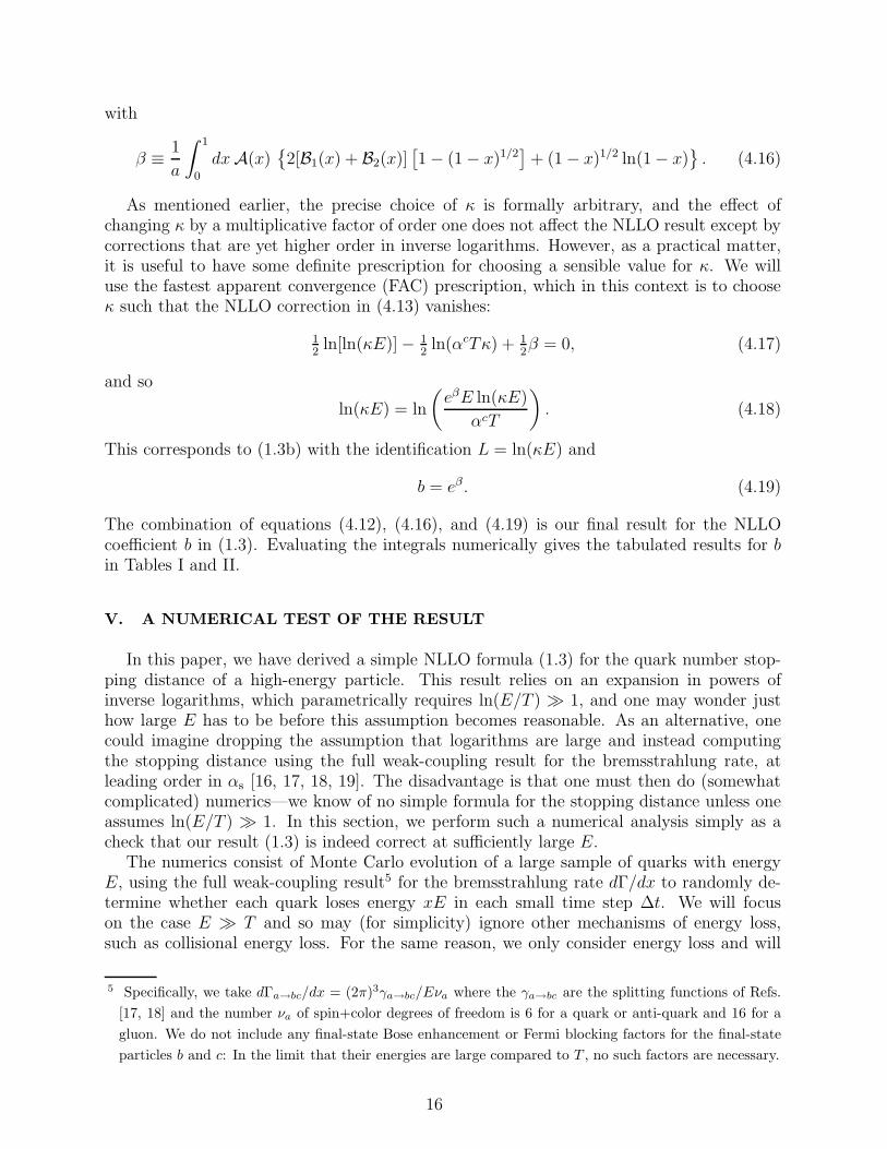
A comparison of the full numeric result with the NLLO approximation (1.3) is shownin Fig. 2 as a function of E/T for 3-flavor QCD. The plot shows the size of the relativeerror ǫ ≡ 1 − tNLLO/tnumeric that the NLLO approximation makes compared to the numericsimulation. The plot extends to absurdly large values of E/T because the purpose of thisplot is to check our NLLO analysis. We can see that the NLLO result indeed approaches thefull weak-coupling result at very large E. Moreover, it does not do too badly even at smallervalues of E/T that are only moderately large: The difference is . 30% for E & 6T . Oneshould not take this too seriously, however, since at E ∼ 6T the various approximations wemade earlier in this section are in doubt. We do not show any comparison for even smallerE/T simply because the NLLO result (1.3), which implements the FAC prescription, ceasesto exist: There is no solution to (1.3b) for L when E/T ≤ αc

se/b, which in the present caseis E/T ≤ 5.74. At exactly E/T = αc

se/b, the logarithm L becomes 1, and so the idea of alarge-logarithm approximation has certainly broken down then.

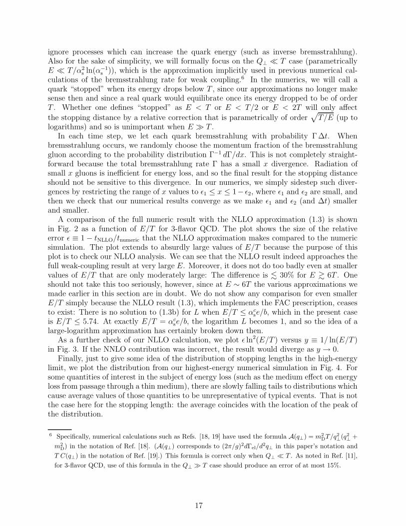
As a further check of our NLLO calculation, we plot ǫ ln2(E/T ) versus y ≡ 1/ ln(E/T )in Fig. 3. If the NNLO contribution was incorrect, the result would diverge as y → 0.

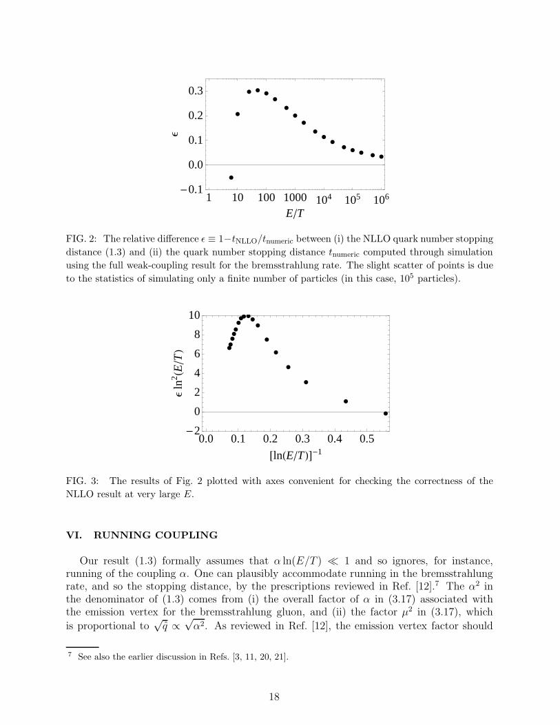
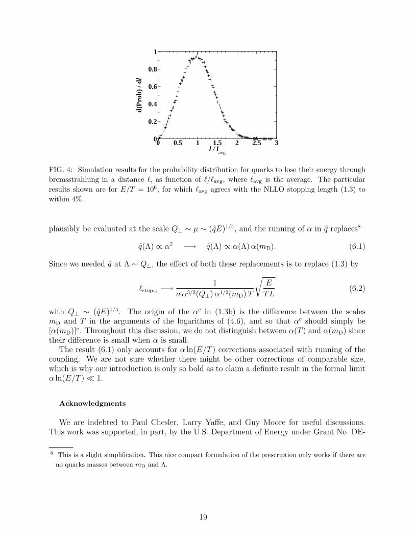
Finally, just to give some idea of the distribution of stopping lengths in the high-energylimit, we plot the distribution from our highest-energy numerical simulation in Fig. 4. Forsome quantities of interest in the subject of energy loss (such as the medium effect on energyloss from passage through a thin medium), there are slowly falling tails to distributions whichcause average values of those quantities to be unrepresentative of typical events. That is notthe case here for the stopping length: the average coincides with the location of the peak ofthe distribution.

6 Specifically, numerical calculations such as Refs. [18, 19] have used the formula A(q⊥) = m2

DT/q2

⊥(q2

⊥+

m2

D) in the notation of Ref. [18]. (A(q⊥) corresponds to (2π/g)2dΓel/d2q⊥ in this paper’s notation and

T C(q⊥) in the notation of Ref. [19].) This formula is correct only when Q⊥ ≪ T . As noted in Ref. [11],

for 3-flavor QCD, use of this formula in the Q⊥ ≫ T case should produce an error of at most 15%.

17

æææ

ææ

ææ

æ

æ

æ

æ

æ

æææ

æ

æ

1 10 100 1000 104 105 106-0.1

0.0

0.1

0.2

0.3

E�T

Ε

FIG. 2: The relative difference ǫ ≡ 1−tNLLO/tnumeric between (i) the NLLO quark number stopping

distance (1.3) and (ii) the quark number stopping distance tnumeric computed through simulation

using the full weak-coupling result for the bremsstrahlung rate. The slight scatter of points is due

to the statistics of simulating only a finite number of particles (in this case, 105 particles).

ææ

æææ

æææææ

æ

æ

æ

æ

æ

æ

æ

0.0 0.1 0.2 0.3 0.4 0.5-2

0

2

4

6

8

10

@lnHE�TLD-1

Εln

2 HE�TL

FIG. 3: The results of Fig. 2 plotted with axes convenient for checking the correctness of the

NLLO result at very large E.

VI. RUNNING COUPLING

Our result (1.3) formally assumes that α ln(E/T ) ≪ 1 and so ignores, for instance,running of the coupling α. One can plausibly accommodate running in the bremsstrahlungrate, and so the stopping distance, by the prescriptions reviewed in Ref. [12].7 The α2 inthe denominator of (1.3) comes from (i) the overall factor of α in (3.17) associated withthe emission vertex for the bremsstrahlung gluon, and (ii) the factor µ2 in (3.17), which

is proportional to√

q ∝√

α2. As reviewed in Ref. [12], the emission vertex factor should

7 See also the earlier discussion in Refs. [3, 11, 20, 21].

18

0 0.5 1 1.5 2 2.5 3l / l

avg

0

0.2

0.4

0.6

0.8

1

d(P

rob)

/ dl

FIG. 4: Simulation results for the probability distribution for quarks to lose their energy through

bremsstrahlung in a distance ℓ, as function of ℓ/ℓavg, where ℓavg is the average. The particular

results shown are for E/T = 106, for which ℓavg agrees with the NLLO stopping length (1.3) to

within 4%.

plausibly be evaluated at the scale Q⊥ ∼ µ ∼ (qE)1/4, and the running of α in q replaces8

q(Λ) ∝ α2 −→ q(Λ) ∝ α(Λ) α(mD). (6.1)

Since we needed q at Λ ∼ Q⊥, the effect of both these replacements is to replace (1.3) by

ℓstop,q −→ 1

a α3/2(Q⊥) α1/2(mD) T

√

E

TL(6.2)

with Q⊥ ∼ (qE)1/4. The origin of the αc in (1.3b) is the difference between the scalesmD and T in the arguments of the logarithms of (4.6), and so that αc should simply be[α(mD)]c. Throughout this discussion, we do not distinguish between α(T ) and α(mD) sincetheir difference is small when α is small.

The result (6.1) only accounts for α ln(E/T ) corrections associated with running of thecoupling. We are not sure whether there might be other corrections of comparable size,which is why our introduction is only so bold as to claim a definite result in the formal limitα ln(E/T ) ≪ 1.

Acknowledgments

We are indebted to Paul Chesler, Larry Yaffe, and Guy Moore for useful discussions.This work was supported, in part, by the U.S. Department of Energy under Grant No. DE-

8 This is a slight simplification. This nice compact formulation of the prescription only works if there are

no quarks masses between mD and Λ.

19

FG02-97ER41027.

[1] R. Baier, Y. L. Dokshitzer, A. H. Mueller, S. Peigne and D. Schiff, Nucl. Phys. B 478, 577

(1996) [arXiv:hep-ph/9604327];

[2] R. Baier, Y. L. Dokshitzer, A. H. Mueller, S. Peigne and D. Schiff, Nucl. Phys. B 483, 291

(1997) [arXiv:hep-ph/9607355];

[3] R. Baier, Y. L. Dokshitzer, A. H. Mueller, S. Peigne and D. Schiff, Nucl. Phys. B 484, 265

(1997) [arXiv:hep-ph/9608322].

[4] B. G. Zakharov, JETP Lett. 63, 952 (1996) [arXiv:hep-ph/9607440].

[5] B. G. Zakharov, JETP Lett. 65, 615 (1997) [arXiv:hep-ph/9704255].

[6] L. D. Landau and I. Pomeranchuk, Dokl. Akad. Nauk Ser. Fiz. 92 (1953) 535; ibid. 735. These

two papers are also available in English in L. Landau, The Collected Papers of L.D. Landau

(Pergamon Press, New York, 1965).

[7] A. B. Migdal, Phys. Rev. 103, 1811 (1956);

[8] P. M. Chesler, K. Jensen, A. Karch and L. G. Yaffe, Phys. Rev. D 79, 125015 (2009)

[arXiv:0810.1985 [hep-th]].

[9] S. S. Gubser, D. R. Gulotta, S. S. Pufu and F. D. Rocha, JHEP 0810, 052 (2008)

[arXiv:0803.1470 [hep-th]].

[10] Y. Hatta, E. Iancu and A. H. Mueller, JHEP 0805, 037 (2008) [arXiv:0803.2481 [hep-th]].

[11] P. Arnold and C. Dogan, Phys. Rev. D 78, 065008 (2008) [arXiv:0804.3359 [hep-ph]].

[12] P. Arnold and W. Xiao, Phys. Rev. D 78, 125008 (2008) [arXiv:0810.1026 [hep-ph]].

[13] R. Baier, D. Schiff and B. G. Zakharov, Ann. Rev. Nucl. Part. Sci. 50, 37 (2000)

[arXiv:hep-ph/0002198].

[14] R. Baier, Nucl. Phys. A 715, 209 (2003) [arXiv:hep-ph/0209038].

[15] S. Caron-Huot, Phys. Rev. D 79, 065039 (2009) [arXiv:0811.1603 [hep-ph]].

[16] P. Arnold, G. D. Moore and L. G. Yaffe, JHEP 0206, 030 (2002) [arXiv:hep-ph/0204343];

[17] P. Arnold, G. D. Moore and L. G. Yaffe, JHEP 0301, 030 (2003) [arXiv:hep-ph/0209353];

[18] P. Arnold, G. D. Moore and L. G. Yaffe, JHEP 0305, 051 (2003) [arXiv:hep-ph/0302165].

[19] S. Jeon and G. D. Moore, Phys. Rev. C 71, 034901 (2005) [arXiv:hep-ph/0309332].

[20] A. Peshier, J. Phys. G 35, 044028 (2008).

[21] P. Arnold, Phys. Rev. D 79, 065025 (2009) [arXiv:0808.2767 [hep-ph]].

20