This article appeared in a journal published by Elsevier. The attachedcopy is furnished to the author for internal non-commercial researchand education use, including for instruction at the authors institution

and sharing with colleagues.

Other uses, including reproduction and distribution, or selling orlicensing copies, or posting to personal, institutional or third party

websites are prohibited.

In most cases authors are permitted to post their version of thearticle (e.g. in Word or Tex form) to their personal website orinstitutional repository. Authors requiring further information

regarding Elsevier’s archiving and manuscript policies areencouraged to visit:

http://www.elsevier.com/copyright

Author's personal copy

Computational Statistics and Data Analysis 55 (2011) 1736–1747

Contents lists available at ScienceDirect

Computational Statistics and Data Analysis

journal homepage: www.elsevier.com/locate/csda

Hierarchical Bayes multivariate estimation of poverty rates based onincreasing thresholds for small domainsEnrico Fabrizi a, Maria Rosaria Ferrante b, Silvia Pacei b,∗, Carlo Trivisano b

a DISES, Università Cattolica, Piacenza, Italyb Dipartimento di Scienze Statistiche ‘P. Fortunati’, Università di Bologna, Italy

a r t i c l e i n f o

Article history:Received 28 October 2009Received in revised form 14 September2010Accepted 5 November 2010Available online 21 November 2010

Keywords:Fay–Herriot modelBeta distributionHierarchical Bayes modeling

a b s t r a c t

A model-based small area method for calculating estimates of poverty rates based ondifferent thresholds for subsets of the Italian population is proposed. The subsets areobtained by cross-classifying by household type and administrative region. The suggestedestimators satisfy the following coherence properties: (i) within a given area, ratesassociatedwith increasing thresholds aremonotonically increasing; (ii) interval estimatorshave lower and upper bounds within the interval (0, 1); (iii) when a large domain-specificsample is available the small area estimate is close to the one obtained using standarddesign-basedmethods; (iv) estimates of poverty rates should also be produced for domainsfor which there is no sample or when no poor households are included in the sample.A hierarchical Bayesian approach to estimation is adopted. Posterior distributions areapproximated by means of MCMC computation methods. Empirical analysis is based ondata from the 2005 wave of the EU-SILC survey.

© 2010 Elsevier B.V. All rights reserved.

1. Introduction

Poverty and social exclusion are unevenly distributed both geographically and across social groups. This is particularlytrue for Italy, a country characterized by a low degree of regional cohesion (European Commission, 2005) and where thedisparities between household types interact with those between the different regions.

We focus on the estimation of three different poverty rates for domains (sub-populations) obtained by cross-classifyingthe Italian population by household type and Administrative Region. Estimates will be based on data collected by the‘European Union-Statistics on Income and Living Conditions’ survey (EU–SILC — 2nd wave, year 2005). The three povertyrates make reference to increasing poverty thresholds that are all defined as fractions of the national median of theequivalized disposable income. As a consequence the three rates are in ascending order and they are respectively aimed atmeasuring the portion of very poor people, of poor people and of people who are either poor or risk becoming poor (ISTAT,2007).

The EU–SILC survey is designed to provide reliable estimates of the main parameters of interest for sub-populations thatare much bigger than those we target. Moreover our domains are not planned (they are not survey design strata or unionsof strata), so nominimum sample size in these domains is guaranteed. The number of units sampled from a large number ofthe domains we consider is too low. Calibration estimators calculated following the samemethodology as that employed bythe National Institute of Statistics (ISTAT) for larger domains, are easily shown to be too imprecise. To improve this ‘directestimation’ strategy, a small area method is advisable.

∗ Corresponding address: Dipartimento di Scienze Statitiche ‘P. Fortunati’, Università di Bologna, via Belle Arti 41, 40126 Bologna, Italy. Tel.: +39 0512098229; fax: +39 051 232153.

E-mail address: silvia.pacei@unibo.it (S. Pacei).

0167-9473/$ – see front matter© 2010 Elsevier B.V. All rights reserved.doi:10.1016/j.csda.2010.11.001

Author's personal copy

E. Fabrizi et al. / Computational Statistics and Data Analysis 55 (2011) 1736–1747 1737

Among the many small area methods proposed in the literature, we refer to model-based small area estimators relyingon area-level models (see Rao (2003), section 5.4.1). In our application multivariate models are advisable, since we havethree poverty rates for each area and their estimators are of course correlated. Given the nature of the target parameters,we require that small area estimators of the poverty rates satisfy the following coherence properties: (i) within a givenarea, rates associated with increasing thresholds should also be monotonically increasing; (ii) interval estimators shouldhave lower and upper bounds within the interval (0, 1); (iii) when a large domain-specific sample is available the smallarea estimate should be reasonably close to the direct estimate; (iv) estimates of poverty rates should also be produced fordomains for which we have no sample or when no poor households are included in the sample.

Properties (i) and (ii) are not satisfied by popular multivariate small area models relying on the assumption of normality(see Ghosh et al. (1996) and Datta et al. (1998)). To obtain estimators satisfying these properties, we propose a modelassuming that, within each area, the differences between successive poverty rates are conditionally beta distributed andexchangeable. This modelling of differences is justified by the fact that the direct estimators of rates based on increasingthresholds are not independent, while differences between successive poverty rates estimators have a much lower,practically negligible, correlation. This assumption avoids the complicated generalization of the beta to the multivariatecase and allows for an unrestricted correlation structure between rate estimators.

We then propose a multivariate logistic-normal model for the expected values of the Beta distributions, thus obtaininga hierarchical two-stage model. The coherence property (iii) requires the inclusion of sampling weights into the estimationprocess, and this is what we do using the calibration estimators as input for our models; in this respect our approachdiffers from that of Molina et al. (2007). The estimators in question also meet the coherency requirement (iv). Our proposalrepresents an alternative to other solutions to the problem of estimating small area proportions recently presented in theliterature (Gonzàlez-Manteiga et al., 2002; Liu et al., 2007; Lohr and Rao, 2009; Longford, 2010).

As far as estimation is concerned, we adopt a hierarchical Bayesian approach implemented by means of a MCMCcomputationalmethod. The results obtained allow us to compare the incidence of poverty by household type in the differentItalian administrative regions. The suggested method could be extended to the estimation of other indicators and could beused with data collected by the EU–SILC in other countries.

The paper is organized as follows. In Section 2 we briefly review the EU–SILC survey, while in Section 3, domains andtarget parameters are defined. Direct estimators and the estimation of their variance are discussed in Section 4. Section 5introduces the suggested small area models while Section 6 is devoted to model checking and sensitivity analyses. Theevaluation of the performance of the associated small area estimators is discussed in Section 7. Conclusions and possiblefuture developments are outlined in the final Section 8.

2. The data

The EU–SILC survey (European Parliament and Council, 2003; Eurostat, 2005) survey has the aim of collecting timelyand comparable cross-sectional and longitudinal microdata on income, poverty, social exclusion and living conditions. Thesampling design is a rotating panel based on consistent methodology and definitions across most member states of theEuropean Union (EU). The survey is conducted in each country by the relevant national institute of statistics (in Italy, byISTAT) and coordinated by Eurostat, the Statistical Bureau of the EU. In Italy, the first wave of the EU–SILC survey waslaunched in 2004. In this paper we analyse data from the 2005 wave. The income reference period is 2004.

Survey units (households) are sampled according to a stratified two-stage sampling design. First-stage units are givenby municipalities, stratified according to administrative region and demographic size. Of the municipalities those withat least 30,000 inhabitants are considered self-representative and form a take-all stratum. Secondary sampling units aregiven by households. The effective sample of the 2005 wave of the survey contains 22,032 households and a total of 56,105individuals. In Italy, the survey is designed to obtain reliable estimates at the administrative region level. For more detailson the EU–SILC survey see also ISTAT (2007). As far as the domains of interest to us are concerned, the number of householdsranges from a minimum of 4 to a maximum of 600; 25th, 50th and 75th percentiles are respectively 45, 97 and 165. Notethat the domains of interest, that will be described in detail in the next section, are not planned, i.e. they cut across strata,so a minimum sample size in these domains is guaranteed.

3. Definition of the domains and of the target parameters

We identify 180 domains of interest, obtained by cross-classifying the population of the 20 Italian administrative regionsby the 9 household types considered in the EU–SILC survey. These types are defined by simultaneously considering thehousehold size, the presence of children and the age of household members. They are defined as follows: 1. one-personhouseholds; 2. two adults, no dependent children, both adults under 65 years of age; 3. two adults, no dependent children,at least one adult 65 years or more years old; 4. other households without dependent children; 5. single parent households,one or more dependent children; 6. two adults, one dependent child; 7. two adults, two dependent children; 8. two adults,three or more dependent children; 9. other households with dependent children. Dependent children comprise all personsbelow the age of 16 and persons aged 16–24 who are living in the household with at least one of their parents and who areeconomically inactive.

Author's personal copy

1738 E. Fabrizi et al. / Computational Statistics and Data Analysis 55 (2011) 1736–1747

Table 1Summary of of the coefficient of variationestimated for the direct estimates.

PR80 PR PR120

min[CV (θijk)] 0.097 0.072 0.060mean[CV (θijk)] 0.466 0.337 0.248max[CV (θijk)] 1.786 1.405 1.420

For each domain of interest we target the following poverty rates: (i) The ‘severe poverty rate’ (PR80) for which thethreshold is fixed at the 80% of the standard poverty threshold (ii) the ‘poverty rate’ (PR) i.e. the share of persons withan equivalent disposable income below the 60% of the national median of personal equivalent income (standard povertythreshold) and (iii) the ‘expanded poverty rate’ (PR120) characterized by a threshold equal to the 120% of the standardpoverty threshold.

Personal equivalent disposable income is obtained by dividing total disposable household income (see Appendix A fordetails) by the equivalent household size calculated according to the modified OECD scale commonly used by Eurostat. Thisformula gives a weight of 1.0 to the first adult, of 0.5 to other persons aged 14 or over in the household and of 0.3 to childrenunder the age of 14. The same equivalent disposable income is assigned to each person in the household.

4. Direct estimators and the estimation of their variances

Published estimates of population descriptive quantities are based on calibration estimators (ISTAT, 2007). The weightsused in these estimators are obtained by a double calibration correction of basic weights which are defined as the inverseof inclusion probabilities. The first step adjusts basic weights for non-response and panel attrition, while the second stepmodifies these intermediate weights to calibrate them to known totals as suggested in the EUROSTAT guidelines for theEU–SILC survey. In particular the distribution of population by gender, age class and geographical region is considered.

As we focus on domains that are not planned, we re-calculate calibration estimators using a different set of weights thatcalibrate on the totals of the Italian population by administrative region and household type. Accurate estimates of thesetotals have kindly beenprovided to us by ISTAT and are based on the quarterly Labour Force Survey of 2005.More specifically,starting from the survey’s intermediate weights, we propose an alternative second step, calibrating to the populations ofadministrative regions classified by household type and to the same regional populations classified by gender and five ageclasses. In the calculation of the calibration weights, the log distance, leading to raking-ratio weights is used (Deville andSärndal, 1992).

Estimating the variances of the direct estimators is a complicated task in our problem, as (i) the considered poverty ratesare non-linear functions of data; (ii) the underlying design is complex; (iii) theweights used in their computation incorporatetwo stages of calibration corrections, as described above. In keeping with other works in this field (Verma and Betti, 2005),we opt for a solution based on resampling algorithms and specifically we propose a bootstrap estimation strategy.

Bootstrap algorithms for complex samples are based on the resampling of primary units within strata under theassumptions that the number of strata is large and that few primary units (but at least two) are sampled from each stratum,so that the sampling fraction at the first stage is negligible (Rao, 1999). This latter assumption is not satisfied in our case asthere is a take-all stratum of primary units.

In point of fact, the sample we analyse may be represented as the union of two sub-samples. The first is taken with astratified, single-stage design from the population of households residing in self-representative municipalities; the secondis drawn with a stratified two-stage design from the rest of the population. Exploiting this representation, we propose abootstrap algorithm inwhich any bootstrap sample is the union of two sub-samples, one taken by resampling the populationin the self-representative municipalites and the other drawn from the rest using the quoted algorithms for bootstrap inmulti-stage designs. After it has been drawn, each bootstrap sample undergoes the same calibration process of adjustmentof weights to known totals applied to the original sample. The algorithm was tested by means of simulation exercises andfound to provide estimates close to those obtained using the linearization method for simpler parameters (i.e. averages) forwhich this latter method may be applied.

Let θijk be the direct estimator of poverty rate θijk in the i, j-th domain, i indexing the administrative region (i =

1, . . . ,m = 20) and j the household type (j = 1, . . . , J = 9); let k = 1, . . . , K = 3 index the increasing poverty thresholds.As regards the reliability of direct estimators, the coefficients of variation are, on average, too high to consider the direct

estimators to be sufficiently reliable, even the case of PR120 for which the average is about 25% (see Table 1). This motivatesthe need for a small area estimation strategy. As anticipated in Section 1, the model in the next section is specified interms of differences between poverty rates based on successive increasing poverty thresholds. Let δijk = θijk − θij,k−1,assuming θij0 = 0. Variances of δijk can be estimated using the results of the bootstrap algorithm as varBOOT (δijk) =

varBOOT (θijk)+varBOOT (θij,k−1)−2covBOOT (θijk, θij,k−1); covariances between poverty rates estimators can be easily obtainedusing the bootstrap algorithm. Likewise, we can use the bootstrap output to calculate covBOOT (δijk, δijl), k = l; in all caseswe find that these figures are close to 0 and 0 is always included in the 95% bootstrap probability intervals, even if at the

Author's personal copy

E. Fabrizi et al. / Computational Statistics and Data Analysis 55 (2011) 1736–1747 1739

population level they are not zero. If we denote δij4 the probability of an income above the highest of the three thresholds,we have that

∑4k=1 δijk = 1.Wemay expect them to be small as δij4 is in all cases far larger than δijk, k ≤ 3. In fact, on average

with respect to the areas, the estimated correlations are equal to −0.07, −0.08 and −0.09.We propose smoothing the estimated variances using a Generalized Variance Function approach in order to reduce the

effect of the bootstrap estimate’s sampling error; moreover this solution enables us to obtain an estimate of the variance forthe domains in which there is no poor or, as far as the the differences are concerned, δijk = 0 as in Ferrante and Trivisano(2010). Consider the identity

VAR(δijk) =δijk(1 − δijk)

mijIFijk

where VAR denotes the actual sampling variance (var indicates its estimator); mij is the number of sampled householdswithin the i, j-th domain, IFijk a variance inflation factor with respect to simple random sampling. The smoothing is based onthe assumption that the inflation factor varies with the rate being considered, but not with the area (that is, with the indicesi, j). This leads to the specification of the following smoothing equation where we replace VAR(δijk) with varBOOT (δijk) andδijk with δijk:

δijk(1 − δijk)

varBOOT (δijk)= ψkmij + ϵijk (1)

where ϵijk are zero-mean and homoskedastic residuals and the parameters ψk can be interpreted as the inverse of thevariance inflation factor. The model is estimated, separately for each rate k using ordinary least squares, excluding the caseswith δijk = 0. The fit of the smoothing model for all rates is satisfactory. Linear smoothing models of this kind are popularin the literature; see for instance O’ Malley and Zaslasvsky (2005). Anyway, we considered also linear models for the log ofthe right-hand side of (1), but they did not fit as well. The estimates ψk are equal respectively to 0.872, 0.771, 0.839, so wemay observe than the direct estimators have a design effect greater than, but not far from 1; these estimated parametersare used to obtain smoothed variance estimates (also for cases where δijk = 0) and are used as input in the models of nextsections. The smoothed bootstrap variances of poverty rates are defined as

varS−BOOT (θijk) =

k−l=1

δijl(1 − δijl)

mij

1

ψl. (2)

Consistently with what we observed about covBOOT (δijk, δijl), in (2) we overlooked the covariance terms. In the rest of thepaper, these smoothed variances are used whenever a reference is made to variance of direct estimators.

5. The model

An ‘area level’ model consists of two parts, a ‘samplingmodel’ formalizing the assumptions on direct estimators and theirrelationships with underlying area parameters, and a ‘linking model’ that relates these parameters to area-specific auxiliaryinformation. Note that, in the ‘samplingmodel’, data (i.e. sampling observations) enter only through the summaries providedby direct estimates and their associated estimate of the variance-covariance matrix.

To specify the ‘sampling model’ we use the fact that the three increasing poverty thresholds divide the domain ofdisposable income into four mutually exclusive intervals. We assume that the estimated probabilities of falling into oneof these intervals (which can be seen as the difference between poverty rates based on successive thresholds) are betadistributed conditionally on the hyperparameters, and that these betas are independent.

A multinomial likelihood may be considered as an alternative as done in Molina et al. (2007), but this model is based onthe assumption of simple random sampling, while we want to model direct estimators, thus including sampling weightsthat correct for unequal inclusion probabilities, non-response and attrition. We assume:

δijk|δijk,mij, ψkind∼ Beta(δijk(mijψk − 1), (1 − δijk)(mijψk − 1)) (3)

implying E(δijk|δijk,mij, ψk) = δijk, V (δijk|δijk,mij, ψk) =δijk(1−δijk)

mijψk. Since the parameters of the beta must be positive, the

conditionmijψk > 1 should be satisfied. This represents amild restriction and it is satisfied by our data. This parametrizationis also used in Liu et al. (2007) to model the estimated rates in a univariate problem.

The choice of the beta as a ‘sampling model’ is logically consistent with the fact that δijk ≥ 0; moreover given that thebeta is the posterior distribution of the success rate characterizing a binomial model, its parameters may be interpreted asthe number of successes and the number of failures in the binomial experiment (augmented by the prior information), sothe factormijψk may be read as the number of ‘equivalent observations’ under simple random sampling.

The specification of the ‘linking model’ is as follows: let δijk = exp(ζijk)/[1 +∑

k exp(ζijk)]. We assume

ζij ∼ MVN(µij,Σ) (4)

Author's personal copy

1740 E. Fabrizi et al. / Computational Statistics and Data Analysis 55 (2011) 1736–1747

where ζij = (ζijk), µij = (µijk)k = 1, . . . , K = 3, Σ is a positive definite K × K matrix. Assuming (4) implies that the δijk aredistributed according to a logistic-normal distribution. The use of a logistic-normal distribution for themodelling of variatesin the K -variate simplex is discussed in Aitchinson and Shen (1980). Even though the Dirichlet is sometimes regarded asthe reference distribution in this context because of its nice mathematical properties, the logistic-normal is more flexible(having a richer parameterization), can approximate the Dirichlet very well, and the moments of its log-transformation canbe very easily modelled.

The logit model has been considered in the small area estimation literature (see for instance Farrell et al. (1997) and Liuet al. (2007)), but only in univariate models. Note that, the solution we propose avoids modelling the target variable at themicro-level as in unit-level models employed by, among others Elbers et al. (2003) in their poverty mapping exercise. Theadvantage is that it is not necessary that auxiliary variables be known for each unit in the population outside the sample as isthe case in all non-linear unit-levelmodels. As the sampling and linkingmodels cannot be combined into a single expression,we say that this model is unmatched in the sense of Yu and Rao (2002).

As usual in area level small areamodel, in order to improve the estimation of area-specific poverty rates, we use auxiliaryinformation, that is information on the domains of interest accurately known from sources independent of the EU–SILCsurvey, such as censuses or administrative archives. We assume

µijk = αjk + xiβjk (5)

whereαjk,βjk are household type and rate specific slope and intercepts; xi is the per-capita GDP of the administrative region i.Note that many area level models use auxiliary information at the domain-of-interest level, but auxiliary information

at an higher level of aggregation may also be used. In our case it is not easy to obtain reliable information on theItalian population cross-classified by administrative region and household type. Here we considered auxiliary informationat the administrative region level of aggregation using the regional section of the National System of Accounts andother administrative archives as data sources. A number of variables were considered as candidate covariates: per-capitaconsumption of the household sector, per-capita GDP, per-capita employee income, per-capita expenditure for leisure andculture, per-capita taxable income, share of workers/value added in the manufacturing industry, school abandonment rate,annual average unemployment rate. The selection of per-capita GDP as the only regressor was based on the followingprocedure. First, we approximated the unobservable ζijk with ζijk = log(δijk) − log(1 −

∑3k=1 δijk); then, separately for

each k we selected the best subset of regressors among the mentioned set of covariates, using standard linear regressionand using the minimization of AIC as the model selection criterion. The model with per-capita GDP as the only regressorturned out to be the best solution in all cases. As usual in MCMC analyses, to improve the mixing of chains, we standardizethe covariate. Note that in (5), although xi is constant for all household types within the same region, slopes and interceptsare type specific. The choice of this specification was driven by evidence that the relationships between ζijk and per-capitaGDP are different for different household types.

As regards the prior specification needed to complete the Bayesian specification of the model we assume αjk ∼ N(0, Aij),βjk ∼ N(0, Bjk), Σ−1

∼ Wishart(I3, 3). The prior variances Ajk, Bjk are set equal to 100, that is they are very ‘high’ withrespect to the order of magnitude of the parameters. This choice implies diffuse, mildly informative but proper and nicelybehaving from an MCMC point of view, prior distributions. The same criteria (approximation of non-informativeness andsimplification of MCMC computation) drives the choice of the Wishart prior for the variance matrix.

Estimates of the poverty rates are obtained by summarizing the posterior distributions of θijk =∑k

l=1 δijl; these posteriordistributions are easily approximated using the output of the MCMC algorithms. Assuming quadratic loss, we adopted aspoint predictors the posterior means, i.e. θBijk = E(θijk|data). Even if we did not meet the problem in this application, wenote that estimates for non-sample areas may be obtained from the predictive distribution conditionally to known auxiliaryinformation. This can be easily done using the output of MCMC algorithms.

To implement MCMC calculations we used the OpenBugs software (Thomas et al., 2006; Spiegelhalter et al., 2003) whichis very widely used in applied hierarchical modelling. More specifically, we ran three parallel chains of R = 25, 000 drawseach, whose starting point was taken from an over-dispersed distribution to verify the independence of the chain behaviourfrom the starting point. The convergence of the the chains involved in our model, monitored by visual inspection of thechain plots and the Gelman and Rubin statistics (Gelman and Rubin, 1992) is achieved within hundreds of iterations. Weconservatively discarded the first 5000 iterations from each chain. The autocorrelation diagrams have been analysed toassess the quality of mixing, and they confirm the good behaviour of the chains. The BUGS codemay be found in Appendix C.

6. Model checking and discussion

We do not present a formal model selection exercise. The arguments leading to our model choice may summarizedas follows. Normal sampling models were ruled out since the sampling distribution of the direct estimator is likelyto be positively skewed and they may yield posterior probability intervals with a negative lower bound; univariatesampling models for the poverty rates (implicitly assuming independence between the direct estimators of rates basedon different thresholds for the same area) are based on an untenable assumption and turned out to be severely inadequate.Multivariate normal linking models do not guarantee that estimates of poverty rates associated with increasing thresholdsare monotonically non-decreasing; univariate linking models suffer from the same limitation. In our model we allow the

Author's personal copy

E. Fabrizi et al. / Computational Statistics and Data Analysis 55 (2011) 1736–1747 1741

0.0 0.2 0.4 0.6

Direct estimates

0.6

0.4

0.2

0.0

Mod

el b

ased

est

imat

es

Fig. 1. Direct versus model based estimates of the Poverty Rate.

ζijk to be correlated within the same area. Posterior summaries of the entries of the Σ matrix reported in Appendix B showthat the off-the-diagonal elements have a high probability of being positive (posterior means of the correlation range from0.21 to 0.46); as a consequence a model with independent ζijk provides a worse fit, as is confirmed from the calculation ofthe DIC statistic (Spiegelhalter et al., 2002).

We tried to assess the impact of prior parameters choices analysing the impact of various choices for hyperparametersAij, Bij on the posterior distributions, without finding any appreciable impact. More specifically, comparing the posteriordistributions of θijk obtained with Aij = 100 and Bij = 100 with those obtained with Aij = 10 and Bij = 10 we found that theaverages of the ratios of posterior means are 1.0022, 1.0002 and 0.9992 for the three rates respectively, while for posteriorstandard deviation these average ratios are equal to 1.0072, 1.0042 and 0.9984. As for theWishart prior on Σ−1, it is knownthat setting its first parameter to I3 as we did, may cause over-shrinkage of the estimates toward the hypothesized a prioriindependence. From the analyses of the simulation results, that will be discussed in Section 7.2 this seems not to be the casein our application. An alternative guess of the structure of Σ−1 may be obtained calculating the average precision matrix ofthe ζij using the output of the bootstrap algorithm illustrated in Section 4. This has not an appreciable impact on posteriordistribution of the θijk; moreover it may judged questionable as it entails the use of data in the prior specification process.

Turning to model checking, as in most Bayesian literature we checked the fit of the model discussed in the previoussection following the posterior predictive approach: new observations are generated according to the posterior distributionof the given model; if the fit is adequate, then the generated observations should be similar to the observed data. Thediscrepancy may be summarized by some suitable measures. The first we considered is the popular omnibus discrepancymeasure (see Gelman et al. (1995, p. 172) or within small area literature, Datta et al. (1999)):

d(y, θ) =

K−k=1

m−i=1

J−j=1

(yijk − θBijk)2

V (yijk|θijk)(6)

where θ = (θijk)i=1,...,m; j=1,...,J; k=1,...,K , y is defined analogously with yijk given by either θijk or θ ⋆ijk; θ⋆ijk is a draw from the

posterior predictive distribution p(θijk|data). On the basis of this discrepancymeasurewe can obtain the posterior predictivep-values as the probability that the discrepancy measure calculated for the generated new data is larger than that obtainedfor the observed data, given the observed data. The posterior predictive p-value, is expected to be far from 0 and 1 if themodel adequately fits the data. Posterior predictive p-values can easily be calculated from the output of MCMC softwares.For our data the posterior p-value based on d is equal to 0.56; if we remove the sum in k from (6) and look at distinct p-valuesfor each rate we find that the three figures range from 0.31 to 0.70. Since the p-values are far from 0 and 1, we can concludethat no model failures are detected by the omnibus discrepancy measure.

Following Yu and Rao (2002), to assess the model fit at the individual ‘area’ level (that is for each region by type cell) weintroduced the following discrepancy measure:

rijk = Prob(θijk < θ ⋆ijk). (7)

About 95% of the rijk lie in the interval (0.14, 0.87) with a median of 0.48 and symmetric distribution, thus indicating nosystematic overestimation or underestimation for the vast majority of these areas.

Fig. 1 shows the plot of direct versusmodel-based estimates of the poverty rate (central threshold). There is a strong linearrelation between the two sets of estimates (their correlation is 0.954). With respect to the y = x line represented in the plotwe note that direct estimates at the right extreme of the distribution have shrunk to smaller values. This is in part due to thecorrection of instability of direct estimates based on few observations, but also reflects the impact of the auxiliary variableused in the estimation process. In the calculation of per-capita GDP, the National Institute of Statistics corrects for the effect

Author's personal copy

1742 E. Fabrizi et al. / Computational Statistics and Data Analysis 55 (2011) 1736–1747

Table 2Performances of the small area estima-tors in terms of average reduction in co-efficient of variation and width of inter-val estimators.

PR80 PR PR120

ACVR 35.54 38.57 33.32AWIR 32.65 34.49 28.12

of the informal economy, which is not distributed evenly across the country (being more concentrated in the south), thusobtaining a less pronounced picture of the north-south divide than the one emerging from income data measured by theEU–SILC survey. Consequently, disagreement between direct and model-based estimates of poverty rates for the poorestareas should be expected and makes sense from an economic point of view. Similar plots for the ‘severe poverty rate’ andthe ‘expanded poverty rate’ are not reported for brevity.We can thus conclude that there is no evidence against the adequacyof the proposed model for our data.

7. Performance of small area estimators

Small area estimators are introduced primarily to improve the precision of the estimators of parameters describingsub-populations. To evaluate the performance of the estimators we propose either a comparison with direct estimators(Section 7.1) and a design-based simulation study (Section 7.2).

7.1. Comparisons with direct estimators

We base the comparison on: (i) the average percentage reduction of the coefficient of variation of small area estimatorsversus the direct ones; (ii) the average percentage reduction in the width of posterior probability intervals with respect tobootstrap probability intervals associated to direct estimators.

The average reduction of the coefficient of variation is defined as

ACVRk = 1001 −

ACV Bk

ACVDk

where the average coefficient of variation of θBijk is defined as a function of posterior variances: ACV B

k = (mJ)−1∑mi=1∑J

j=1

√V (θijk|data)

θijk; as regards direct estimators, coefficients of variation are calculated using smoothed bootstrap variances

defined in (2) ACVDk = (mJ)−1∑m

i=1∑J

j=1

√varS−BOOT (θijk)

θijkThe average reduction in the width of interval estimators is defined analogously as

AWIRk = 1001 −

AWIBkAWIDk

where AWIBk = (mJ)−1∑m

i=1∑J

j=1 WCI(θBijk) and WCI(θBijk) is the difference between the upper and lower bounds ofposterior 0.95 probability intervals estimated using posterior quantiles calculated from theMCMC sample; similarlyAWIDk =

(mJ)−1∑mi=1∑J

j=1 WCI(θijk) where WCI(θijk) is the width of the 0.95 bootstrap interval estimator calculated for the directestimator.

The results are summarized in Table 2; it is clear that small area estimators considerably reduce the variability of directestimators. The performances of the estimators for the ‘severe poverty rate’ and the ‘poverty rate’ are fairly close while forthe ‘expanded poverty rate’ they are a littleworse; this depends on the fact that this latter rate can be less precisely predictedby the auxiliary information.

The consideration of average reduction in coefficients of variation and width of interval estimators masks the fact thatthese reductions are bigger for domains of smaller size. For instance, if we restrict our attention to household type 8 (twoadults, three or more dependent children), which is a small subset of the households in all administrative regions and ischaracterized in Italy by very high poverty rates, the average reduction in the coefficient of variation and the width ofinterval estimators for PR are respectively 53.1 and 48.3. The inverse relationship between the sample size (in terms ofhouseholds) and the effectiveness of the small area estimator in reducing the coefficient of variation, for PR, is displayed inFig. 2.

In the introductionwementioned that a desirable property of small area estimates is that of being close to direct estimatesfor domains for which a large sample is available. Fay and Herriot (1979), in their seminal paper on the subject, recommendthat small area estimates should be within one standard deviation of the direct estimator; in our case this condition issatisfied in the 93.6% of the cases and in all cases if we consider only the first 50% of the domains in terms of sample size.

Author's personal copy

E. Fabrizi et al. / Computational Statistics and Data Analysis 55 (2011) 1736–1747 1743

020

4060

8010

0

0 100 200 300 400 500 600

Sample size

Red

uctio

n in

CV

Fig. 2. Number of households in the sample vs reduction in coefficient of variation for estimation of the poverty rate.

Table 3Relative bias of the small area estimatorswith respect to the randomization distribu-tion.

k Mean Min Max

1 0.00197 −0.05181 0.055782 −0.00205 −0.11845 0.097833 −0.00077 −0.10261 0.10853

7.2. Simulation study

To evaluate the properties of model-based small area predictors that we proposed with respect to the randomizationdistribution induced by the design, we use the same bootstrap exercise introduced in Section 4. On the one hand, in thisway we do not need to make assumptions about whether underlying area specific parameters obey our model or not. Onthe other hand, the synthetic population reproduces the same characteristics of the direct estimates. This means that forareas characterized by few sample units in the original sample and estimate in sharp contrast with our model, we mayexpect a model based estimator to remain biased to some extent. Anyway, the simulation may be useful to assess whethermodel predictors have nice randomization properties on most of the areas and meet essential requirements such as designconsistency and asymptotic unbiasedness.

For each of the bootstrap samples, themodel based estimators have been recalculated using the sameprocedure illustratein Sections 4 and 5, with the only exception that the coefficients of the variance smoothing function introduced in (1) areassumed known and equal to those estimated in the analysis of the original sample.

In the first place we consider the average relative bias:

ARBk = (Rm)−1R−

r=1

m−i=1

θBr,ijk − θijk

θijk

where θBr,ijk = E(θijk|datar), i.e. the posterior expected value of θijk conditional on the r-th replicated dataset, θijk is the directestimate we obtained for rate k and area ij using our original sample. The average relative bias evaluated with respect to θijkis an approximation of the actual average relative bias with respect to the underlying θijk, as θijk is design nearly unbiased,i.e. E(θijk) ∼= θijk.

In Table 3 we present the minimum and the maximum relative bias along with the mean defined above.We may then conclude that the average relative bias is really small, while in individual areas it very seldom crosses the

threshold of±10%. To understand the distribution of relative bias in individual areaswe plot it against the number of samplehouseholds (see Fig. 3). We also present the same plot for the absolute bias of model predictors.

From the analysis of the distribution of bias in individual areas we have that both absolute and relative biases are rapidlydecreasing as the area-specific sample sizes get large. This confirms our claim that model predictors are design consistentand asymptotically design unbiased. For areas with a small mij (number of area-specific sample households) small areaestimators are biased by construction; indeed they aim at reducing overall MSE using the principle of ’’borrowing strength’’from a model assumption. This will markedly reduce variance at the price of some bias inflation. So a moderate bias whenmij is small is expected.

Author's personal copy

1744 E. Fabrizi et al. / Computational Statistics and Data Analysis 55 (2011) 1736–1747

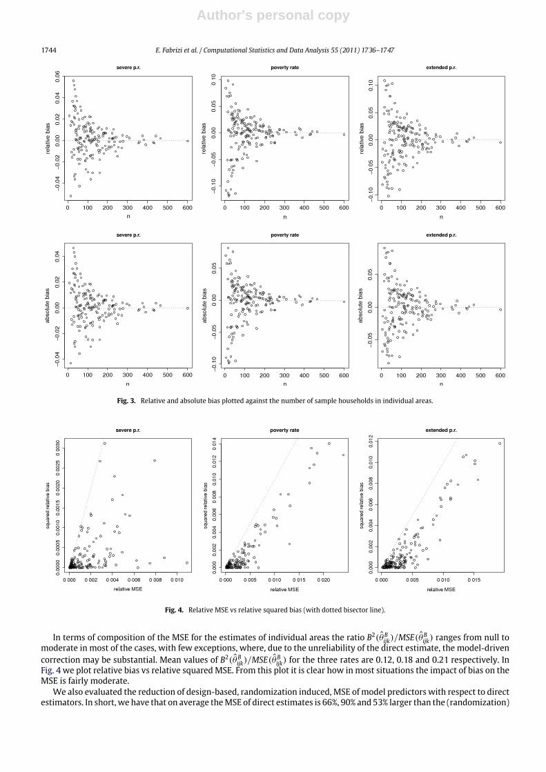
Fig. 3. Relative and absolute bias plotted against the number of sample households in individual areas.

Fig. 4. Relative MSE vs relative squared bias (with dotted bisector line).

In terms of composition of the MSE for the estimates of individual areas the ratio B2(θBijk)/MSE(θBijk) ranges from null tomoderate in most of the cases, with few exceptions, where, due to the unreliability of the direct estimate, the model-drivencorrection may be substantial. Mean values of B2(θBijk)/MSE(θBijk) for the three rates are 0.12, 0.18 and 0.21 respectively. InFig. 4 we plot relative bias vs relative squared MSE. From this plot it is clear how in most situations the impact of bias on theMSE is fairly moderate.

We also evaluated the reduction of design-based, randomization induced, MSE of model predictors with respect to directestimators. In short, we have that on average theMSE of direct estimates is 66%, 90% and 53% larger than the (randomization)

Author's personal copy

E. Fabrizi et al. / Computational Statistics and Data Analysis 55 (2011) 1736–1747 1745

Fig. 5. Comparisons betweenMSE(θijk) and

MSE(θBijk).

MSE of model predictors. This is line with the results of Section 7.1. More specifically, in Fig. 5, we plot, separately for each

rate, theMSE(θijk) vs

MSE(θBijk). In the same plot we also present the ratio

MSE(θijk)÷

MSE(θBijk).

Next, let us consider the frequentist coverage of the probability intervals based on quantiles of the posterior distributions.More specifically, we try to assess the coverage rate of the intervals defined using the 0.025 and 0.975 quantiles of theposteriors (as approximated by means of MCMC methods), that is the proportion of such intervals including the ‘true’reference value. On the averagewith respect to all the areas, this coverage rate is equal to 0.925, 0.949 and 0.951 respectivelyfor the three poverty rates.

Eventually,we calculated the design-based correlationmatrix (averaged over the areas) of θBij = {θBijk}k=1,...,K and compare

it to that of θij defined analogously. The element-wise absolute differences are always lower than0.06.Wemay conclude that,despite the simplification represented by assuming independence among the δijk, model predictors are able to reproduce acorrelation structure similar to that of direct estimators. The two matrices are shown below

Rθ =

1 0.66 0.501 0.74

1

, RθB =

1 0.72 0.551 0.72

1

.

8. Conclusions and future work

We presented a small area strategy for estimating a set of related poverty parameters for a set of non-planned domains.This latter fact required the modification of published sampling weights when obtaining direct estimators while the formerled us to the specification of a area-levelmultivariate normal-logistic ‘linkingmodel’. The analysiswere driven by the need ofsatisfying some coherence properties important to final users of small area estimates: (i) within a given area, rates associatedwith increasing thresholds should also be monotonically increasing; (ii) interval estimators should have lower and upperbounds within the interval (0, 1); (iii) when a large domain-specific sample is available the small area estimate should bereasonably close to the one obtained using standard design-based methods; (iv) estimates of poverty rates should also beproduced for domains forwhichwehave no sample orwhennopoor households are included in the sample. Other coherence

Author's personal copy

1746 E. Fabrizi et al. / Computational Statistics and Data Analysis 55 (2011) 1736–1747

properties may also be considered; for instance (v) formal benchmarking, that is the exact agreement of weighted (usingpopulation counts) averages of the poverty rates with direct estimates for administrative regions and household types; (vi)adequate representation of the between-area variability of the underlying area-level parameters, that is avoiding over orunder-shrinkage. We leave these further analyses for future work.

Wenote thatmultivariatemodelsmayplay an important rolewhen including into the small area estimationprocess otherpoverty parameters such as gaps or the quintile ratio: for these parameters it is more difficult to find good predictors, soexploiting their correlationwith other parameters, such as the poverty rates, may be a goodway to obtain reliable estimates.

Appendix A. Definition of total disposable household income in the EU–SILC survey

Total disposable household income can be computed as follow.The sum for all household members of gross personal income components (gross employee cash or near cash in-

come; gross non-cash employee income; employers‘ social insurance contributions; gross cash benefits or losses fromself-employment (including royalties); value of goods produced for own consumption; unemployment benefits; old-agebenefits; survivor’ benefits, sickness benefits; disability benefits and education-related allowances plus gross income com-ponents at household level (imputed rent); income from rental of a property or land; family/children related allowances;social exclusion not elsewhere classified; housing allowances; regular inter-household cash transfers received; interests,dividends, profit from capital investments in unincorporated business; income received by people aged under 16 minusemployer’s social insurance contributions; interest paid on mortgage; regular taxes on wealth; regular inter-householdcash transfer paid; tax on income and social insurance contributions).

Appendix B. Posterior summaries of Σ

E(Σ|data) =

0.255 0.055 0.0850.055 0.131 0.0480.085 0.048 0.311

q0.025(Σ|data) =

0.165 −0.009 0.002−0.009 0.075 −0.0200.002 −0.020 0.201

q0.975(Σ|data) =

0.373 0.132 0.1810.132 0.209 0.1290.181 0.129 0.456

Appendix C. BUGS code

model{

for(i in 1:n){

# model specificationP.bar[i,1]< −exp(v[i,1])/(1+exp(v[i,1])+exp(v[i,2])+exp(v[i,3]))P.bar[i,2]< −exp(v[i,2])/(1+exp(v[i,1])+exp(v[i,2])+exp(v[i,3]))P.bar[i,3]< −exp(v[i,3])/(1+exp(v[i,1])+exp(v[i,2])+exp(v[i,3]))P[i,1]< −P.bar[i,1]P[i,2]< −P.bar[i,1]+P.bar[i,2]P[i,3]< −P.bar[i,1]+P.bar[i,2]+P.bar[i,3]for(j in 1:3){

p.bar[i,j]∼ dbeta(A[i,j],B[i,j])A[i,j]< −P.bar[i,j]*(phi[i,j]-1)B[i,j]< −(1-P.bar[i,j])*(phi[i,j]-1)prec[i,j]< −phi[i,j]/(P.bar[i,j]*(1-P.bar[i,j]))mu[i,j]< −alpha[j]+alpha1[(tipof[i]-4),j]+beta[(tipof[i]-4),j]*x[i]}

# posterior predictive checksfor(j in 1:3){

P.bar.pred[i,j]∼ dbeta(A[i,j],B[i,j])d.obs[i,j]< −pow((p[i,j]-P[i,j]),2)/((P[i,j]*(1-P[i,j]))/(phi[i,j]+1))d.pred[i,j]< −pow((P.pred[i,j]-P[i,j]),2)/((P[i,j]*(1-P[i,j]))/(phi[i,j]+1))p.area.val[i,j]< −step(d.pred[i,j]-d.obs[i,j])step.div[i,j]< −step(P.pred[i,j]-p[i,j]) }

Author's personal copy

E. Fabrizi et al. / Computational Statistics and Data Analysis 55 (2011) 1736–1747 1747

P.pred[i,1]< −P.bar.pred[i,1]P.pred[i,2]< −P.bar.pred[i,1]+P.bar.pred[i,2]P.pred[i,3]< −P.bar.pred[i,1]+P.bar.pred[i,2]+P.bar.pred[i,3]p[i,1]< −p.bar[i,1]p[i,2]< −p.bar[i,1]+p.bar[i,2]p[i,3]< −p.bar[i,1]+p.bar[i,2]+p.bar[i,3]

v[i,1:3]∼ dmnorm(mu[i,1:3],prec.P[1:3,1:3])d1.obs[i]< −sum(d.obs[i,])d1.pred[i]< −sum(d.pred[i,])p1.area.val[i]< −step(d1.pred[i]-d1.obs[i])} d1.obs.glob< −sum(d.obs[,])d1.pred.glob< −sum(d.pred[,])p1.value< −step(d1.pred.glob-d1.obs.glob)for(j in 1:3){

d.obs.glob[j]< −sum(d.obs[,j])d.pred.glob[j]< −sum(d.pred[,j])p.value[j]< −step(d.pred.glob[j]-d.obs.glob[j])pvalue.divstep.rs[j]< −sum(step.div[,j])}

pvalue.divstep< −mean(step.div[,])prec.P[1:3,1:3]∼ dwish(R[,],3)sigma.P[1:3,1:3]< −inverse(prec.P[1:3,1:3])# prior specificationfor(j in 1:3){

alpha[j]∼ dnorm(0,A)for(k in 1:9){

beta[k,j]∼ dnorm(0,B)alpha11[k,j]∼ dnorm(0,A)alpha1[k,j]< −alpha11[k,j]-mean(alpha11[,j])}}

}

References

Aitchinson, J., Shen, M., 1980. Logistic-normal distribution: some properties and uses. Biometrika 67, 261–272.Datta, G.S., Day, B., Maiti, T., 1998. Multivariate Bayesian small area estimation: an application to survey and satellite data. Sankhya, A 60, 1–19.Datta, G.S., Lahiri, P., Maiti, T., Lu, T., 1999. Hierarchical Bayes estimation of unemployment rates for the states of the US. Journal of the American Statistical

Association 94, 1074–1082.Deville, J.C., Särndal, C.E., 1992. Calibration estimators in survey sampling. Journal of the American Statistical Association 87, 376–382.European Commission, 2005. Regional Indicators to Reflect Social Exclusion and Poverty. Report prepared for Employment and Social Affairs DG.Elbers, C., Lanjouw, J.O., Lanjouw, P., 2003. Micro-level estimation of poverty and inequality. Econometrica 71, 355–364.European Parliament and Council, 2003. Regulation (EC) No 1177/2003 of June 16, 2003 concerning Community statistics on income and living conditions

(EU–SILC) Official Journal of the European Union 3.7.2003 L 165/1.Eurostat, 2005. Income, Poverty and Social Exclusion in the EU25. Statistics in Focus — Population and Social Conditions, 13, 2005.Farrell, P.J., MacGibbon, B., Tomberlin, T.J., 1997. Empirical Bayes estimators of small area proportions in multistage design. Statistica Sinica 7, 1065–1083.Fay, R., Herriot, R., 1979. Estimates of income for small places: an application of James–Stein procedures to census data. Journal of the American Statistical

Association 74, 269–277.Ferrante, M.R., Trivisano, C., 2010. Estimating firms labour demand forecasts using small area models for count data. Survey Methodology 36 (2), 171–180.Gelman, A., Carlin, J., Stern, H., Rubin, D.B., 1995. Bayesian Data Analysis. Chapman and Hall, New York.Gelman, A., Rubin, D.B., 1992. Inference from iterative simulation using multiple sequences. Statistical Science 7, 457–472.Ghosh, M., Nangia, N., Kim, D., 1996. Estimation of median income of four-persons families: a Bayesian time series approach. Journal of the American

Statistical Association 91, 1423–1431.Gonzàlez-Manteiga,W., Lombardìa, M.J., Molina, I., Morales, D., Santamarìa, L., 2002. Estimation of themean squared error of predictors of small area linear

parameters under a logistic mixed model. Computational Statistics and Data Analysis 51, 2720–2733.ISTAT, 2007. La povertà relativa in Italia nel 2006. Statistiche in breve (in Italian).Liu, B., Lahiri, P., Kalton, G., 2007. Hierarchical Bayesmodeling of surveyweighted small area proportions. In: ASA Proceedings on Survey ResearchMethods,

Alexandria, VA.Lohr, S.L., Rao, J.N.K., 2009. Jackknife estimation of mean squared error of small area predictors in nonlinear mixed models. Biometrika 96, 457–468.Longford, T., 2010. Small area estimation with spatial similarity. Computational Statistics and Data Analysis 54, 1151–1166.Molina, I., Saei, A., Lombardia, J.M., 2007. Small area estimates of labour force participation under a multinomial logit mixed model. Journal of the Royal

Statistical Society, A 170, 975–1000.O’ Malley, A.J., Zaslasvsky, A.M., 2005. Variance-covariance functions for domains means of ordinal survey items. Survey Methodology 31, 169–182.Rao, J.N.K., 2003. Small Area Estimation. John Wiley and sons, New York.Rao, J.N.K., 1999. Some current trends in sample survey theory and methods. Sankhya, B 1–57.Spiegelhalter, D.J., Best, N.G., Carlin, B.P., Van der Linde, A., 2002. Bayesian measure of model complexity and fit (with discussion). Journal of the Royal

Statistical Society, B 64, 583–616.Spiegelhalter, D.J., Thomas, A., Best, N.G., Lunn, D., 2003. WinBUGS User Manual Version 1.4. dowloadable at http://www.mrc-bsu.cam.ac.uk/bugs.Thomas, A., O’Hara, B., Ligges, U., Sturz, S., 2006. Making BUGS open. R News 6, 12–17.Verma, V., Betti, G., 2005. Sampling errors for measures of inequality and poverty. In: Classification and Data Analysis (CLADAG) Book of Short Papers.

pp. 175–178.Yu, Y., Rao, J.N.K., 2002. Small area estimation using unmatched sampling and linking models. Canadian Journal of Statistics 30, 3–15.